Minimal Markov Models

MINIMAL MARKOV MODELS ∗

By Jesus E. Garcıa†,‡ and Veronica A. Gonzalez-Lopez†,‡

Universidade Estadual de Campinas ‡

In this work we introduce a new and richer class of finiteorder Markov chain models and address the following modelselection problem: find the Markov model with the minimal setof parameters (minimal Markov model) which is necessary torepresent a source as a Markov chain of finite order. Let us callM the order of the chain and A the finite alphabet, to determinethe minimal Markov model, we define an equivalence relation onthe state space AM , such that all the sequences of size M withthe same transition probabilities are put in the same category.In this way we have one set of (|A| − 1) transition probabilitiesfor each category, obtaining a model with a minimal number ofparameters. We show that the model can be selected consistentlyusing the Bayesian information criterion.

1. Introduction. In this work we consider discrete stationary processes over a finitealphabet A. Markov chains of finite order are widely used to model stationary processeswith finite memory. A problem with full Markov chains models of finite order M is thatthe number of parameters (|A|M(|A| − 1)) grows exponentially with the order M, where |A|denotes the cardinal of the alphabet A. Another characteristic is that the class of full Markovchains is not very rich, fixed the alphabet A there is just one model for each order M andin practical situations could be necessary a more flexible structure in terms of number ofparameters. For an extensive discussion of those two problems se Buhlmann P. and WynerA. [1]. A richer class of finite order Markov models introduced by Rissanen J. [6] andBuhlmann P. and Wyner A. [1] are the variable length Markov chain models (VLMC) whichare mentioned in section 2.3. In the VLMC class, each model is identified by a prefix tree Tcalled context tree. For a given model with a context tree T , the final number of parametersfor the model is |T |(|A| − 1) and depending on the tree, this produce a parsimonious model.In Csiszar, I. and Talata, Z. [4] is proved that the bayesian information criterion (BIC) canbe used to consistently choose the VLMC model in an efficient way using the context treeweighting (CTW) algorithm.

In this paper we introduce a larger class of finite order Markov models, and we addressthe problem of model selection inside this class, showing that the model can be selectedconsistently using the BIC criterion. In our class, each model is determined by choosing apartition of the state space, our class of models include the full Markov chain models and

∗This work is partially supported by PRONEX/FAPESP Project Stochastic behavior, critical phenomenaand rhythmic pattern identification in natural languages (grant number 03/09930-9) and by CNPq EditalUniversal (2007), project: “Padroes rıtmicos, domınios prosodicos e modelagem probabilıstica em corpora doportugues”.†Departamento de Estatıstica. Intituto de Matematica Estatıstica e Computacao Cientıfica.AMS 2000 subject classifications: Primary 62M05; secondary 60J10Keywords and phrases: Bayesian Information criterion (BIC), Markov chain, consistent estimation

1

arX

iv:1

002.

0729

v1 [

mat

h.ST

] 3

Feb

201

0

2 J. E. GARCIA AND V. A. GONZALEZ-LOPEZ

the VLMC models because a context tree can be seen as a particular partition of the statespace (see for illustration the example 2.1).

In Section 2, we define the minimal Markov models and show that this models can beselected in a consistently in theorems 2.1 and 2.2. In Section 3 we show two algorithms thatuse the results in Section 2 to choose consistently a minimal Markov model for a sample andsome simulations. Section 4 have the conclusions and Section 5 have the proofs.

2. Minimal Markov models.

2.1. Notation. Let (Xt) be a discrete time order M Markov chain on a finite alphabetA. Let us call S = AM the state space. Denote the string amam+1 . . . an by anm, whereai ∈ A, m ≤ i ≤ n.

Let L = {L1, L2, . . . , LK} be a partition of S,

P (L, a) =∑s∈L

Prob(X t−1t−M = s,Xt = a), a ∈ A, L ∈ L;(1)

P (L) =∑s∈L

Prob(X t−1t−M = s), L ∈ L.(2)

Let xn1 be a sample of the process(Xt

), s ∈ S, a ∈ A and n > M. We denote by Nn(s, a)

the number of occurrences of the string s followed by a in the sample xn1 ,

Nn(s, a) =∣∣∣{t : M < t ≤ n, xt−1t−M = s, xt = a}

∣∣∣,(3)

the number of occurrences of s in the sample xn1 is denoted by Nn(s) and

Nn(s) =∣∣∣{t : M < t ≤ n, xt−1t−M = s}

∣∣∣.(4)

The number of occurrences of elements into L followed by a is given by,

NLn (L, a) =∑s∈L

Nn(s, a), L ∈ L;(5)

the accumulated number of Nn(s) for s in L is denoted by,

NLn (L) =∑s∈L

Nn(s), L ∈ L.(6)

2.2. Good partitions of S.

Definition 2.1. Let (Xt) be a discrete time order M Markov chain on a finite alphabetA, S = AM the state space. A partition L = {L1, L2, . . . , LK} of S is a good partition of Sif for each s, s′ ∈ L, L ∈ L,

P rob(Xt = . |X t−1t−M = s) = Prob(Xt = . |X t−1

t−M = s′).

Remark 2.1. For a discrete time order M Markov chain on a finite alphabet A withS = AM the state space, L = S is a good partition of S.

MINIMAL MARKOV MODELS 3

If L is a good partition of S, we define for each category L ∈ L

P (a|L) = Prob(Xt = a|X t−1t−M = s) ∀a ∈ A,(7)

where s is some element into L. As a consequence, if we write P (xn1 ) = Prob(Xn1 = xn1 ), we

obtain

P (xn1 ) = P (xM1 )∏

L∈L,a∈AP (a|L)N

Ln (L,a).(8)

In the same way that Csiszar, I. and Talata, Z. [4] we will define our BIC criterion using amodified maximum likelihood. We will call maximum likelihood to the maximization of thesecond term in the equation (8) for the given observation. For the sequence xn1 , will be

ML(L, xn1 ) =∏

L∈L,a∈A

(rn(L, a)

rn(L)

)NLn (L,a)

,(9)

where

rn(L, a

)=NLn (L, a)

n, a ∈ A, L ∈ L and rn

(L)

=NLn (L)

n, L ∈ L.(10)

The BIC is given by the next definition

Definition 2.2. Given a sample xn1 , of the process (Xt), a discrete time order M Markovchain on a finite alphabet A with S = AM the state space and L a good partition of S. TheBIC of the model (9) is given by

BIC(L, xn1 ) = ln (ML(L, xn1 ))− (|A| − 1)|L|2

ln(n).

2.3. Good partitions and context trees.Let (Xt) be a finite order Markov chain taking values on A and T a set of sequences of

symbols from A such that no string in T is a suffix of another string in T , for each s ∈ T ,d(T ) = max

(l(s), s ∈ T

)where l(s) denote the length of the string s, with l(∅) = 0 if the

string is the empty string.

Definition 2.3. T is a context tree for the process (Xt) if for any sequence of symbolsin A, xn1 sample of the process with n ≥ d(T ), there exist s ∈ T such that

Prob(Xn+1 = a|Xn1 = xn1 ) = Prob(Xn+1 = a|Xn

n−l(s)+1 = s)

d(T ) is the depth of the tree.The context tree is the minimal state space of the variable length Markov chain (VLMC),Buhlmann P. and Wyner A. [1]. The context tree for a VLMC with finite depth M definea good partition on the space S = AM as illustrated by the next example.

Example 2.1. Let be a VLMC over the alphabet A = {0, 1} with depth M = 3 andcontexts,

{0}, {01}, {011}, {111}This context tree correspond to the good partition {L1, L2, L3, L4} whereL1 = {{000}, {100}, {010}, {110}}, L2 = {{001}, {101}}, L3 = {011} and L4 = {111}.


2.4. Smaller good partitions.

Definition 2.4. Let Lij denote the partition

Lij = {L1, . . . , Li−1, Lij, Li+1, . . . , Lj−1, Lj+1, . . . , LK},

where L = {L1, . . . , LK} is a good partition of S, and for 1 ≤ i < j ≤ K with Lij = Li ∪Lj.

Now we adapt the notation established for the partition L to the new partition Lij.

Notation 2.1. for a ∈ A we write,

P (Lij, a) = P (Li, a) + P (Lj, a);

P (Lij) = P (Li) + P (Lj).

NLij

n (Lij, a) = NLn (Li, a) +NLn (Lj, a);(11)

NLij

n (Lij) = NLn (Li) +NLn (Lj);(12)

If P (.|Li) = P (.|Lj) then Lij is a good partition and (7) remains valid for Lij, just isnecessary to change L by Lij in equations (8), (9) and definition (2.2).In the following theorem, we show that the BIC criterion provides a consistent way of de-tecting smaller good partition.

Theorem 2.1. Let (Xt) be a Markov chain with order M over a finite alphabet A, S =AM the state space. If L = {L1, L2, . . . , LK} is a good partition of S and Li 6= Lj, Li, Lj ∈ L.Then, eventually almost surely as n→∞,

I{BIC(Lij ,xn1 )>BIC(L,xn1 )} = 1

if, and only ifP (a|Li) = P (a|Lj) ∀a ∈ A.

Where IA is the indicator function of A, and the Lij partition is defined under L by equation(2.4).

Next we extract from the previous theorem the relation that we use in the next section,in practice to find smaller good partitions.

Definition 2.5. Let be (Xt) a Markov chain of order M, with finite alphabet A and statespace S = AM , xn1 a sample of the process and let L = {L1, L2, . . . , LK} be a good partitionof S,

dL(i, j) =1

ln(n)

∑a∈A

{NLn (Li, a) ln

(Nn(Li, a)

Nn(Li)

)+NLn (Lj, a) ln

(Nn(Lj, a)

Nn(Lj)

)

−NLijn (Lij, a) ln

(Nn(Lij, a)

Nn(Lij)

)}(13)


Corollary 2.1. Under the assumptions of theorem 2.1,

BIC(L, xn1 )−BIC(Lij, xn1 ) < 0 ⇐⇒ dL(i, j) <(|A| − 1)

2.

Proof. From equation (14) we have the validity of the result.

Remark 2.2. The results will remain valid if we replace the constant (|A|−1)2

for somearbitrary constant, positive and finite value v, into the definition (2.2).

Remark 2.3. Under the assumptions of theorem 2.1, if P (a|Li) 6= P (a|Lj) for somea ∈ A, then eventually almost surely as n → ∞, BIC(L, xn1 ) > BIC(Lij, xn1 ) where Lijverified the definition (2.4).

2.5. Minimal good partition.We want to find the smaller good partition into the universe of all possible good partitions

of S. This special good partition could be defined as follows and it allows the definition ofthe most parsimonious model into the class considered in this paper.

Definition 2.6. Let (Xt) be a discrete time order M Markov chain on a finite alphabetA, S = AM the state space. A partition L = {L1, L2, . . . , LK} of S is the minimal goodpartition of S if, ∀L ∈ L,

s, s′ ∈ L if, and only if Prob(Xt = . |X t−1t−M = s) = Prob(Xt = . |X t−1

t−M = s′).

Remark 2.4. For a discrete time order M Markov chain on a finite alphabet A withS = AM the state space, ∃! minimal good partition of S.

In the next example we emphasize the difference between good partitions and the minimalgood partition,

The next theorem shows that for n large enough we achive the partition L∗ which is theminimal good partition.

Theorem 2.2. Let (Xt) be a Markov chain with order M over a finite alphabet A,S = AM the state space and let P be the set of all the partitions of S. Define,

L∗n = argmaxL∈P{BIC(L, xn1 )}

then, eventually almost surely as n→∞,

L∗ = L∗n

3. Minimal good partition estimation algorithm.

Algorithm 3.1. (MMM algorithm for good partitions)Consider xn1 a sample of the Markov process (Xt), with order M over a finite alphabet A,S = AM the state space.Let be L = {L1, L2, . . . , LK} a good partition of S, for each s ∈ S,


1 for i = 1, 2, · · · , K − 1,

for j = i+ 1, 2, · · · , K,Calculate dL(i, j)

Ri,jn = I{dL(i,j)< (|A|−1)

2}

2 If Ri,jn = 1, define Lij = Li ∪ Lj and L = Lij . Else i = i+ 1, Return to step 1

The algorithm allows to define the next relation based on the sample xn1 ,

Definition 3.1. for r, s ∈ S; r ∼n s ⇐⇒ Ra(r),a(s)n = 1.

For n large enough, the algorithm return the minimal good partition.

Corollary 3.1. Let {Xt, t = 0, 1, 2, . . .} be a Markov chain with order M over a finitealphabet A, S = AM and xn1 a sample of the Markov process. Ln, given by the algorithm(3.1) converges almost surely eventually to L∗, where L∗ is the minimal good partition of S.

Proof. Because K < ∞, for n large enough, the algorithm return the minimal goodpartition.

Remark 3.1. In the worst case, which correspond to an initial good partition equal to

S, we need to calculate the term(NLn (L,a)NLn (L)

)NLn (L,a)for each s ∈ S plus K(K − 1)/2 divisions

to implement the algorithm (3.1).

The next algorithm is a variation of the first. In this case the partitions are grow selectingthe pair of elements with the minimal value of {dL(i, j), the algorithm stop when there isnot {dL(i, j) lower than (|A| − 1)/2.

Algorithm 3.2. Consider xn1 a sample of the Markov process (Xt), with order M overa finite alphabet A, S = AM the state space.Let L = {L1, L2, . . . , LK} be a good partition of S

1 Calculate(i∗, j∗) = arg min

i,j|1≤i<j≤K{dL(i,j)}

2 If dL(i,j) <|A|−1

2then L = Li∗j∗, K = K − 1 and return to 1.

Else end.

This algorithm is consistent and always return a partition but have a greater computationalcost. Taking in consideration that the cost depend on K and that for a Markov chain of orderM we consider samples of size n such that log(n) > M . The two algorithms 3.1 and 3.2 havea computational cost that is linear in n (the sample size).


3.1. Dendrograms and MMM algorithm . In practice, when the sample size is not largeenough and the algorithm 3.1 has not converged, it is possible that the algorithm will notreturn a partition of S, independent of the value used in v. In that case, a better approachcan be to use for each r, s ∈ S the function dn(r, s) as a similarity measure between r ands. Then dn(r, s) can be used to produce a dendrogram and then use the partition defined bythe dendrogram as the partition estimator.

Also in practice it is possible that the maximum number of free parameters in our modelis limited by a number K. In that case, the logic choice will be to find a value of d in thedendrogram such that the size of the partition obtained cutting the dendrogram in d is lessor equal to K, the chosen model will be the one defined by that partition.

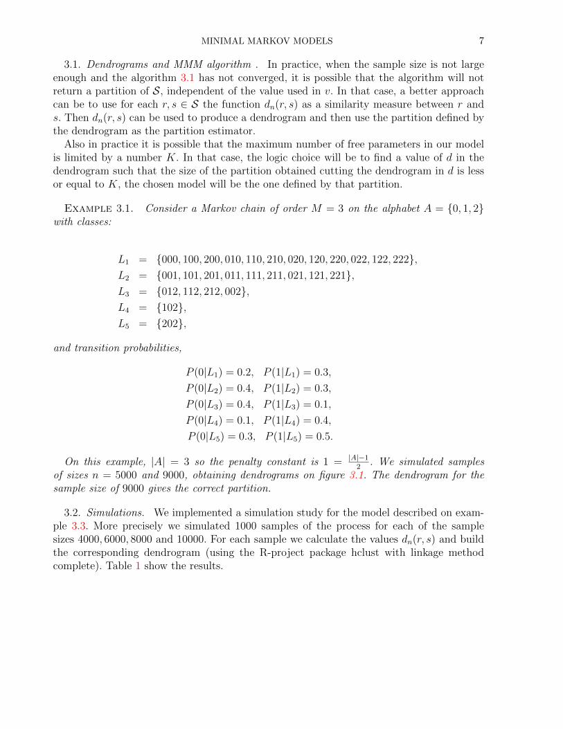
Example 3.1. Consider a Markov chain of order M = 3 on the alphabet A = {0, 1, 2}with classes:

L1 = {000, 100, 200, 010, 110, 210, 020, 120, 220, 022, 122, 222},L2 = {001, 101, 201, 011, 111, 211, 021, 121, 221},L3 = {012, 112, 212, 002},L4 = {102},L5 = {202},

and transition probabilities,

P (0|L1) = 0.2, P (1|L1) = 0.3,

P (0|L2) = 0.4, P (1|L2) = 0.3,

P (0|L3) = 0.4, P (1|L3) = 0.1,

P (0|L4) = 0.1, P (1|L4) = 0.4,

P (0|L5) = 0.3, P (1|L5) = 0.5.

On this example, |A| = 3 so the penalty constant is 1 = |A|−12

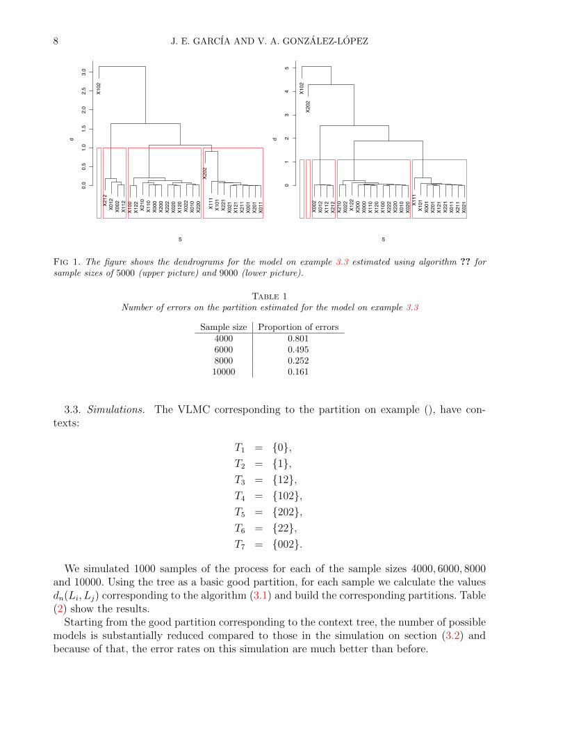
. We simulated samplesof sizes n = 5000 and 9000, obtaining dendrograms on figure 3.1. The dendrogram for thesample size of 9000 gives the correct partition.

3.2. Simulations. We implemented a simulation study for the model described on exam-ple 3.3. More precisely we simulated 1000 samples of the process for each of the samplesizes 4000, 6000, 8000 and 10000. For each sample we calculate the values dn(r, s) and buildthe corresponding dendrogram (using the R-project package hclust with linkage methodcomplete). Table 1 show the results.


X102

X212

X012

X002

X112

X100

X122

X210

X110

X000

X200

X222

X020

X120

X022

X010

X220

X202

X111

X101

X221

X021

X121

X211

X001

X201

X011

0.0

0.5

1.0

1.5

2.0

2.5

3.0

S

d

X102

X202

X002

X012

X112

X212

X210

X022

X122

X200

X000

X110

X120

X100

X222

X220

X010

X020 X1

11X101

X001

X201

X121

X221

X011

X211

X021

01

23

45

S

d

Fig 1. The figure shows the dendrograms for the model on example 3.3 estimated using algorithm ?? forsample sizes of 5000 (upper picture) and 9000 (lower picture).

Table 1Number of errors on the partition estimated for the model on example 3.3

Sample size Proportion of errors4000 0.8016000 0.4958000 0.25210000 0.161

3.3. Simulations. The VLMC corresponding to the partition on example (), have con-texts:

T1 = {0},T2 = {1},T3 = {12},T4 = {102},T5 = {202},T6 = {22},T7 = {002}.

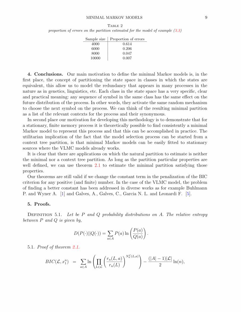
We simulated 1000 samples of the process for each of the sample sizes 4000, 6000, 8000and 10000. Using the tree as a basic good partition, for each sample we calculate the valuesdn(Li, Lj) corresponding to the algorithm (3.1) and build the corresponding partitions. Table(2) show the results.

Starting from the good partition corresponding to the context tree, the number of possiblemodels is substantially reduced compared to those in the simulation on section (3.2) andbecause of that, the error rates on this simulation are much better than before.


Table 2proportion of errors on the partition estimated for the model of example (3.3)

Sample size Proportion of errors4000 0.6146000 0.2068000 0.04710000 0.007

4. Conclusions. Our main motivation to define the minimal Markov models is, in thefirst place, the concept of partitioning the state space in classes in which the states areequivalent, this allow us to model the redundancy that appears in many processes in thenature as in genetics, linguistics, etc. Each class in the state space has a very specific, clearand practical meaning: any sequence of symbol in the same class has the same effect on thefuture distribution of the process. In other words, they activate the same random mechanismto choose the next symbol on the process. We can think of the resulting minimal partitionas a list of the relevant contexts for the process and their synonymous.

In second place our motivation for developing this methodology is to demonstrate that fora stationary, finite memory process it is theoretically possible to find consistently a minimalMarkov model to represent this process and that this can be accomplished in practice. Theutilitarian implication of the fact that the model selection process can be started from acontext tree partition, is that minimal Markov models can be easily fitted to stationarysources where the VLMC models already works.

It is clear that there are applications on which the natural partition to estimate is neitherthe minimal nor a context tree partition. As long as the partition particular properties arewell defined, we can use theorem 2.1 to estimate the minimal partition satisfying thoseproperties.

Our theorems are still valid if we change the constant term in the penalization of the BICcriterion for any positive (and finite) number. In the case of the VLMC model, the problemof finding a better constant has been addressed in diverse works as for example BuhlmannP. and Wyner A. [1] and Galves, A., Galves, C., Garcia N. L. and Leonardi F. [5].

5. Proofs.

Definition 5.1. Let be P and Q probability distributions on A. The relative entropybetween P and Q is given by,

D(P (·)||Q(·)) =∑a∈A

P (a) ln

(P (a)

Q(a)

).

5.1. Proof of theorem 2.1.

BIC(L, xn1 ) =∑a∈A

ln

∏L∈L

(rn(L, a)

rn(L)

)NLn (L,a)− (|A| − 1)|L|

2ln(n),


as consequence,

BIC(L, xn1 )−BIC(Lij, xn1 ) =∑a∈A

{NLn (Li, a) ln

(rn(Li, a)

rn(Li)

)

+NLn (Lj, a) ln

(rn(Lj, a)

rn(Lj)

)

− NLijn (Lij, a) ln

(rn(Lij, a)

rn(Lij)

)}− (|A| − 1)

2ln(n).(14)

We note that, the condition I{BIC(Lij ,xn1 )>BIC(L,xn1 )} = 1 is true if, and only if

∑a∈A

{rn(Li, a) ln

(rn(Li, a)

rn(Li)

)+ rn(Lj, a) ln

(rn(Lj, a)

rn(Lj)

)

−rn(Lij, a) ln

(rn(Lij, a)

rn(Lij)

)}<

(|A| − 1) ln(n)

2n.(15)

Because rn(L, a) and rn(L) are non-negative, using Jensen we have that,

rn(Li, a) ln

(rn(Li, a)

rn(Li)

)+ rn(Lj, a) ln

(rn(Lj, a)

rn(Lj)

)≥

(rn(Li, a) + rn(Lj, a)) ln

(rn(Li, a) + rn(Lj, a)

rn(Li) + rn(Lj)

)

or equivalently,

(16) rn(Li, a) ln

(rn(Li, a)

rn(Li)

)+ rn(Lj, a) ln

(rn(Lj, a)

rn(Lj)

)≥ rn(Lij, a) ln

(rn(Lij, a)

rn(Lij)

),

with equality if and only if rn(Li,a)rn(Li)

= rn(Lj ,a)

rn(Lj), ∀a ∈ A.

As consequence, equation (16) ⇒

∑a∈A

{rn(Li, a) ln

(rn(Li, a)

rn(Li)

)+ rn(Lj, a) ln

(rn(Lj, a)

rn(Lj)

)

−rn(Lij, a) ln

(rn(Lij, a)

rn(Lij)

)}≥ 0,(17)

with equality if and only if rn(Li,a)rn(Li)

= rn(Lj ,a)

rn(Lj)∀a ∈ A.

Considering that (|A|−1) ln(n)2n

→ 0, as n→∞ and from the equation (15), we have that iflimn→∞ I{BIC(Lij ,xn1 )>BIC(L,xn1 )} = 1, then

limn→∞

∑a∈A

{rn(Li, a) ln

(rn(Li, a)

rn(Li)

)+ rn(Lj, a) ln

(rn(Lj, a)

rn(Lj)

)

−rn(Lij, a) ln

(rn(Lij, a)

rn(Lij)

)}≤ 0,


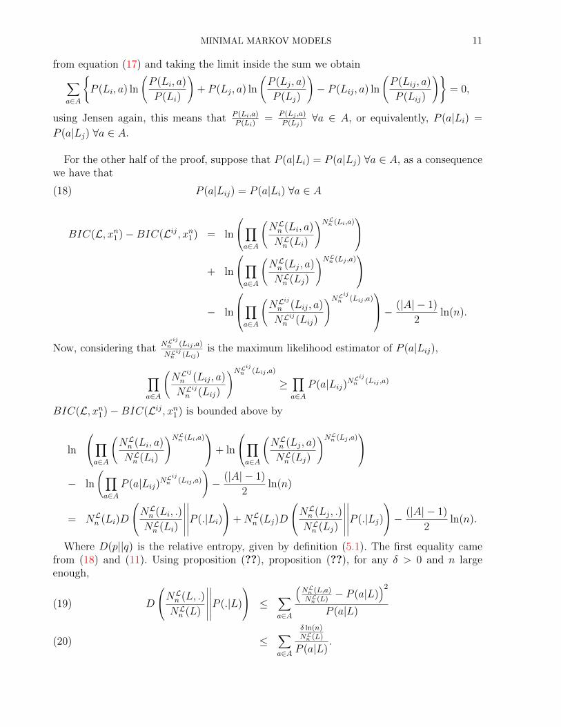
from equation (17) and taking the limit inside the sum we obtain∑a∈A

{P (Li, a) ln

(P (Li, a)

P (Li)

)+ P (Lj, a) ln

(P (Lj, a)

P (Lj)

)− P (Lij, a) ln

(P (Lij, a)

P (Lij)

)}= 0,

using Jensen again, this means that P (Li,a)P (Li)

= P (Lj ,a)

P (Lj)∀a ∈ A, or equivalently, P (a|Li) =

P (a|Lj) ∀a ∈ A.

For the other half of the proof, suppose that P (a|Li) = P (a|Lj) ∀a ∈ A, as a consequencewe have that

P (a|Lij) = P (a|Li) ∀a ∈ A(18)

BIC(L, xn1 )−BIC(Lij, xn1 ) = ln

∏a∈A

(NLn (Li, a)

NLn (Li)

)NLn (Li,a)

+ ln

∏a∈A

(NLn (Lj, a)

NLn (Lj)

)NLn (Lj ,a)

− ln

∏a∈A

(NL

ij

n (Lij, a)

NLijn (Lij)

)NLijn (Lij ,a)− (|A| − 1)

2ln(n).

Now, considering that NLij

n (Lij ,a)

NLijn (Lij)is the maximum likelihood estimator of P (a|Lij),

∏a∈A

(NL

ij

n (Lij, a)

NLijn (Lij)

)NLijn (Lij ,a)

≥∏a∈A

P (a|Lij)NLijn (Lij ,a)

BIC(L, xn1 )−BIC(Lij, xn1 ) is bounded above by

ln

∏a∈A

(NLn (Li, a)

NLn (Li)

)NLn (Li,a)+ ln

∏a∈A

(NLn (Lj, a)

NLn (Lj)

)NLn (Lj ,a)

− ln

(∏a∈A

P (a|Lij)NLijn (Lij ,a)

)− (|A| − 1)

2ln(n)

= NLn (Li)D

NLn (Li, .)

NLn (Li)

∣∣∣∣∣∣∣∣∣∣∣∣P (.|Li)

+NLn (Lj)D

NLn (Lj, .)

NLn (Lj)

∣∣∣∣∣∣∣∣∣∣∣∣P (.|Lj)

− (|A| − 1)

2ln(n).

Where D(p||q) is the relative entropy, given by definition (5.1). The first equality camefrom (18) and (11). Using proposition (??), proposition (??), for any δ > 0 and n largeenough,

D

NLn (L, .)

NLn (L)

∣∣∣∣∣∣∣∣∣∣∣∣P (.|L)

≤∑a∈A

(NLn (L,a)NLn (L)

− P (a|L))2

P (a|L)(19)

≤∑a∈A

δ ln(n)NLn (L)

P (a|L).(20)


Then for any δ > 0 and n large enough,

BIC(L, xn1 )−BIC(Lij, xn1 ) ≤ 2δ|A|p

ln(n)− (|A| − 1)

2ln(n)

= ln(n)

(2δ|A|p− (|A| − 1)

2

)

where p = min{P (a|L) : a ∈ A,L ∈ {Li, Lj}}.In particular, taking δ < p(|A|−1)

4|A| , for n large enough,

BIC(L, xn1 )−BIC(Lij, xn1 ) < 0.

Acknowledgements. We thank Antonio Galves, Nancy Garcia, Charlotte Galves andFlorencia Leonardi for their useful comments and discussions.

References.

[1] Buhlmann P. and Wyner A. (1999). Variable length Markov chains. Ann. Statist. 27 480–513.[2] Csiszar, I. and Shields, P. C. (2000).The consistency of the BIC Markov order estimator. Ann.

Statist. 28 1601–1619.[3] Csiszar, I. (2002). Large-scale typicality of Markov sample paths and consistency of MDL order

estimators. IEEE Trans. Inform. Theory 48 1616–1628.[4] Csiszar, I. and Talata, Z. (2006). Context tree estimation for not necessarily finite memory processes,

via BIC and MDL. IEEE Trans. Inform. Theory 52 1007–1016.[5] Galves et al. (2009). Context tree selection and linguistic rhythm retrieval from written texts.

arXiv:0902.3619.[6] Rissanen J. (1983). A universal data compression system, IEEE Trans. Inform. Theory 29(5) 656 –

664.

Departamento de EstatısticaInstituto de Matematica Estatıstica e Computacao CientıficaUniversidade Estadual de CampinasRua Sergio Buarque de Holanda,651Cidade Universitaria-Barao GeraldoCaixa Postal: 606513083-859 Campinas, SP, BrazilE-mail: [email protected]

[email protected]

mailto:[email protected]

mailto:[email protected]

Documents

Minimal Markov Models