Automatica 38 (2002) 655–669www.elsevier.com/locate/automatica

Minimal partial realization from generalized orthonormal basisfunction expansions�

Thomas J. de Hooga, Zolt*an Szab*ob, Peter S.C. Heubergera, Paul M.J. Van den Hof a ; ∗;1,J*ozsef Bokorb

aSignals, Systems and Control Group, Department of Applied Physics, Delft University of Technology, Lorentzweg 1,2628 CJ Delft, The Netherlands

bComputer and Automation Research Institute, Hungarian Academy of Sciences, Budapest, Hungary

Received 3 April 2000; received in revised form 12 January 2001; accepted 4 October 2001

Abstract

A solution is presented for the problem of realizing a discrete-time LTI state-space model of minimal McMillan degree suchthat its :rst N expansion coe;cients in terms of generalized orthonormal basis match a given sequence. The basis considered, alsoknown as the Hambo basis, can be viewed as a generalization of the more familiar Laguerre and two-parameter Kautz constructions,allowing general dynamic information to be incorporated in the basis. For the solution of the problem use is made of the propertiesof the Hambo operator transform theory that underlies the basis function expansion. As corollary results compact expressions arefound by which the Hambo transform and its inverse can be computed e;ciently. The resulting realization algorithms can beapplied in an approximative sense, for instance, for computing a low-order model from a large basis function expansion that isobtained in an identi:cation experiment. ? 2002 Elsevier Science Ltd. All rights reserved.

Keywords: Realization theory; Partial expansions; Algorithms; State-space realization; Transforms; All-pass :lters; Interpolation; Systemidenti:cation; Model approximation

1. Introduction

The idea of decomposing a system in terms of ba-sis functions is widely applied in system theory andrelated problems such as system approximation andidenti:cation. It is, for instance, common to representa stable discrete-time system G(z) in the form of its

� This paper was not presented at any IFAC meeting. This paperwas recommended for publication in revised form by Associate EditorBrett Ninness under the direction of Editor Torsten SAoderstrAom. Thiswork is :nancially supported by the Dutch Science and TechnologyFoundation (STW) under Contract 55.3618.

∗ Corresponding author. Tel.: +31-15-2784509/2782473; fax: +31-15-2784263.E-mail address: p.m.j.vandenhof@tnw.tudelft.nl (P.M.J. Van den

Hof ).1 This work is part of the research program of the ‘Stichting voor

Fundamenteel Onderzoek der Materie (FOM)’, which is :nanciallysupported by the ‘Nederlandse Organisatie voor WetenschappelijkOnderzoek (NWO)’.

Laurent expansion as

G(z)=∞∑k=1

gkz−k ; (1)

where the functions {z−k} form an orthonormal basis forthe space of functions (1) with

∑∞k=1 |gk |2 ¡∞, denoted

as H2 in the following. The associated expansion coe;-cients gk , also known as the Markov parameters, play animportant role in systems theory, realization theory, sys-tem approximation and identi:cation. The representationof a system in terms of a :nite set of Markov parametersis known as :nite impulse response (FIR) modeling. Inspite of its apparent simplicity the FIR model is widelyapplied, e.g. in :lter synthesis problems in signal process-ing (Roberts &Mullis, 1987), adaptive :ltering problems(Haykin, 1996), and in the context of :nite horizon opti-mal control problems (Richalet, Rault, Testud, & Papon,1978; Furuta & Wongsaisuwan, 1995).Generalized orthonormal basis constructions have been

proposed that oNer the Oexibility to tune them so as to

0005-1098/02/$ - see front matter ? 2002 Elsevier Science Ltd. All rights reserved.PII: S 0005-1098(01)00247-3

656 T.J. de Hoog et al. / Automatica 38 (2002) 655–669

perform better than the FIR models in particular situa-tions. These are the expansions of the general form

G(z)=∞∑k=1

ckfk(z); (2)

in which the functions fk(z) represent general orthonor-mal basis functions while ck ∈R are the correspond-ing expansion coe;cients. Examples of such basisfunction expansions are the well-known Laguerre andtwo-parameter Kautz basis constructions (Lee, 1960;Kautz, 1954, Wahlberg, 1991, 1994). Further general-izations were proposed in Heuberger (1991), Heuberger,Van den Hof, and Bosgra (1995) and Ninness andGustafsson (1997). Their general form is given by

fk(z)=

√1− |�k |2z − �k

k−1∏i=1

1− �∗i zz − �i

; (3)

where {�i}i=1; :::; k is a collection of poles to be chosenby the user. The origin of these constructions lies in thetheory on rational orthonormal bases as developed byTakenaka and Malmquist in the 1920s (Walsh, 1956).The functions constitute a complete orthonormal set inH2

provided that∑∞

k=1(1− |�k |)=∞. Typically, the rate ofconvergence of the series expansion (2) is higher whenthe pre-chosen poles �i are closer to the poles of the un-derlying system. The application of these functions in theareas of model reduction and model approximation is an-alyzed in MAakilAa (1990), Wahlberg and MAakilAa (1996)and Schipp and Bokor (1997). This paper will considerthe basis construction that was proposed in Heubergeret al. (1995), sometimes denoted as the Hambo basis,which in terms of (3) is equivalent to a :nite pole selec-tion {�i}; i=1; : : : ; nb which is repeated periodically, i.e.�k+nb = �k ;∀k.

The problem considered is as follows: given a par-tial expansion {ck}k=1; :::;N , :nd a minimal state-spacerealization (A; B; C;D) of a system G(z)=D + C(zI −A)−1B of smallest order such that G(z)=

∑∞k=1 ckfk(z)

and ck = ck ; k=1; : : : ; N . This problem can be viewed asa generalization of the classical minimal partial realiza-tion problem that was solved in Ho and Kalman (1966)and Tether (1970). In the case of Laguerre function ex-pansions, the problem has been solved in Nurges (1987).For the Hambo basis case, the realization problem was:rst considered in Szab*o and Bokor (1997) and Szab*o,Heuberger, Bokor, and Van den Hof (2000), wherethe problem was solved for the full-information case(N → ∞). However, in order to provide an algorithm,that is able to deal with :nite N , a diNerent approach hasto be followed.In this paper, it will be shown that a solution for this

latter case can be constructed by exploiting the so-calledHambo transform theory. This transform theory hasalso been used to analyze the statistical properties of

identi:cation algorithms, estimating series expansion co-e;cients (see Van den Hof, Heuberger, & Bokor, 1995).As a result this paper has two main contributions:

• the development of an algorithm that solves the min-imal partial realization problem for generalized basisfunctions, and

• the further development and analysis of the under-lying Hambo transform theory, by deriving explicit(state-space) expressions for the transform and itsinverse.

The presented results will be limited to scalar transferfunctions. The generalization to multivariable systemspresents no great di;culties.Besides being interesting from a system theoretic point

of view, the analysis in this paper :nds its motivationin the application of these bases in system identi:ca-tion (Van den Hof et al., 1995; Szab*o, Bokor, & Schipp,1999). Owing to the linear parameterization (ck appearslinearly in G(z)) attractive computational properties re-sult, e.g. in least-squares algorithms, which enables thehandling of large-scale problems. However, it is commonto estimate a high-order basis function model that is sub-sequently reduced to a low-order state-space model bymeans of model reduction. It seems appropriate to replacethis model reduction step by an (approximate) realizationprocedure. When using model reduction the extension toin:nity of the estimated expansion is simply set to zero,while approximate realization tries to infer the unknownextension from the dynamics that reveals itself in the par-tial expansion.The outline of the paper is as follows. First, some pre-

liminaries about the Hambo basis and Hambo transformtheory are recalled in Section 2. In Section 3, some prop-erties of the Hambo operator transform are establishedthat are instrumental for the solution of the realizationproblem. In Section 4, the Hankel operator frameworkis presented in which the realization problem is solvedfor the case where one has knowledge of the full expan-sion. In Sections 5 and 6, this approach is combined withresults from Hambo basis theory to derive the main re-sults. The connection with a related interpolation prob-lem is analyzed in Section 7, while in Section 8 appli-cation of the results in the context of system identi:ca-tion is discussed, which is illustrated with an example inSection 9. The proofs of all results are collected in theappendix.

NotationAT; A∗ transpose, respectively, complex conjugate

transpose, of matrix ALp×m2 Hilbert space of complex matrix functions of

dimension p × m that are square integrable onthe unit circle. The superscript p × m will besuppressed if p=m=1

T.J. de Hoog et al. / Automatica 38 (2002) 655–669 657

Hp×m2 Hardy space of complex matrix functions of

dimension p×m which are analytic in the ex-terior of the unit disc such that

limr→1

12�

∫ 2�

0Trace(f(rei!)∗f(rei!)) d!¡∞

and f(∞)=0.2 The superscript p×m will besuppressed if p=m=1

RH2 subspace of rational (strictly proper) transferfunctions of H2

〈X; Y 〉M matrix “inner” product between X ∈Lp×12

and Y ∈Lm×12 de:ned as 〈X; Y 〉M = 1

2�∫ 2�0 X (ei!)Y (ei!)∗ d!. For p=m=1 thesubscript M will be suppressed

H⊥2 the orthogonal complement of H2 in L23

Hp×m2;0 the same as Hp×m

2 , without the restriction thatthe functions must be zero at in:nity

RHp×m2;0 subspace of rational (proper) transfer func-

tions of Hp×m2;0

PX orthogonal projection onto the subspace XN0 N extended with zero‘n2(J ) the space of square summable vector

sequences, of vector dimension n, where Jdenotes the index set of the sequence. Thesuperscript n will be omitted if n=1

ei the ith canonical Euclidean basis (column) vec-tor.

diag{xi}i=1; :::; n diagonal matrix with diagonal elementsxi; : : : ; xn.

At various instances in this paper use is made ofSylvester equations of the form

AXB+ C=X:

Existence and uniqueness of the solution matrix X willbe everywhere guaranteed by the fact that—whereverused—the matrices A and B both have eigenvalues withmodulus strictly smaller than 1.In this paper, we assume that all transfer functions and

state-space realizations have real-valued coe;cients, i.e.poles of transfer functions appear in complex conjugatepole pairs.

2. Preliminaries

2.1. Orthogonal basis functions—Hambo basis

One way to construct the Hambo basis functions(Heuberger et al., 1995) is by considering a :nite set of

2Here, H2 is identi:ed with the subspace of L2 withvanishing non-positive Fourier-coe;cients. More precisely, forf∈H2; f(z)=f1z−1 + f2z−2 + · · ·, and ∑∞

k=1 |fk |2 ¡∞.3For f∈H⊥

2 ; f(z)=∑∞

k=0 fkzk ; and∑∞

k=0 |fk |2 ¡∞.

poles {�i}i=1; :::; nb that are stable, i.e. |�i|¡ 1, generatingan all-pass transfer function

Gb(z)=nb∏i=1

(1− �∗i z)(z − �i)

having a minimal balanced realization (Ab; Bb; Cb; Db)that satis:es[Ab Bb

Cb Db

]T [Ab Bb

Cb Db

]= I: (4)

Due to these properties the input-to-states transfer func-tions of Gb:

!i(z) := eTi (zI − Ab)−1Bb; i=1; : : : ; nb;

form an orthonormal set. An orthogonal basis for H2 iscreated by introducing

!i;k(z)=!i(z)Gb(z)k−1; k=1; : : : ;∞:

In order to facilitate analysis, we also denote: Vk =[!1; k !2; k : : : !nb ;k]

T, leading to V1(z)= (zI − Ab)−1Bb

and the basis function vectors

Vk(z)=V1(z)Gb(z)k−1: (5)

Since the functions {!i;k}i=1; :::; nb;k=1;:::;∞ form an orthonor-mal basis, any element G of H2 can be written as

G(z)=∞∑k=1

nb∑i=1

li; k!i; k(z) with li; k = 〈G;!i;k〉 (6)

with li; k being the expansion coe;cients. Equality hereshould be interpreted in the two-norm sense. Through-out this paper, it will be assumed that all state-space re-alizations and expansion coe;cients li; k are real-valued.Similar to (6) we can write

G(z)=∞∑k=1

LTk Vk(z) (7)

with LTk := [l1; k l2; k : : : lnb ;k]= 〈G;Vk〉M . The all-pass

function Gb(z) also generates a basis for the H⊥2 space(and thereby for the entire L2 space) by repeatedly mul-tiplying V1(z) with Gb(z)−1 =Gb(1=z).

Lemma 1. De:ning U0(1=z) :=V1(z)Gb(1=z); it holdsthat

U0(1=z)=∞∑l=0

ATblCT

b zl =(1=z)((1=z)I − AT

b )−1CT

b : (8)

Clearly, U0(1=z) is an element of Hnb2⊥ and Gb(1=z)

is an element of H⊥2 . This implies that all the functionsUk(1=z) de:ned as

Uk(1=z)=U0(1=z)Gb(1=z)k (9)

658 T.J. de Hoog et al. / Automatica 38 (2002) 655–669

for k ∈N0 lie in Hnb2⊥. In fact the functions eTi Uk , with

16 i6 nb, and k ∈N0 constitute an orthonormal basis ofH⊥2 , as is shown, e.g. in Szab*o et al. (1999).

2.2. Signal and operator transforms

By the isomorphic property of the z-transform thereexist equivalent time-domain representations of !i;k thatform an orthonormal basis of the signal space ‘2(N).They are written as !i;k(t), or Vk(t) for the vectors, wherethe index t ∈N denotes time.The Hambo signal transform (Heuberger & Van den

Hof, 1996) of a signal x in ‘2(N) is then de:ned by

X(')=∞∑k=1

X(k)'−k with X(k)= 〈Vk; x〉M

and ' a complex indeterminate.This signal transform gives rise to a transform opera-

tion on a dynamical system, as formulated next.

Proposition 2. Suppose that u∈ ‘2(N); G ∈RH2;0 andlet y(z)=G(z)u(z). Let Y and U denote the Hambosignal transform of y; respectively u. Then;

Y(m)=m∑

j=1

Mm−jU(j) (10)

with the Markov parameters Mk given by

Mk = 〈V1(z); V1(z)Gb(1=z)kG(z)〉M= 〈V1(z)Gb(z)k ; V1(z)G(z)〉M : (11)

The resulting dynamical system G ∈RHnb×nb2;0 determined

by

G(')=∞∑k=0

Mk'−k ; (12)

is referred to as the Hambo operator transform of G.

It follows from this proposition that the Hambo oper-ator transform of the scalar system G is a causal, lineartime-invariant nb × nb system. Several properties of thistransform have been derived (Heuberger & Van den Hof,1996):

• G(') is obtained by a simple variable substitution ap-plied to the transfer function G(z). It holds that

G(')=∞∑k=0

gkN (')k (13)

with gk the Markov parameters ofG as in (1) and N (')a transfer matrix that has the state-space realization(Db; Cb; Bb; Ab).

• The transform of Gb is a simple shift, i.e.

Gb(')= '−1Inb : (14)

• G(') and G(z) have the same McMillan degree.

In Section 5, it will be shown how the analysis involvedin solving the realization problem produces a means fordirectly computing a minimal state-space realization ofG(') on the basis of a minimal state-space realization ofG(z) and vice versa.

3. Transformation of expansion coe�cients

As stated in the previous section, one can expand anyG(z)∈RH2 in terms of the Hambo basis function vectorsas in (7). We will now recall from Szab*o et al. (2000)the connection that exists between the coe;cient vectorsequence {Lk} and the sequence of Markov parameters{Mk} of the Hambo operator transform G('). The rela-tion will prove to be essential for the solution of the gen-eralized realization problems.

Proposition 3. LetG ∈H2 have a generalized expansionas in (6). Then;(a) the Markov parameters Mk of the Hambo opera-

tor transform G(') satisfy

Mk =

nb∑i=1

li; k+1PTi + li; kQT

i ; k¿ 1;

nb∑i=1

li;1PTi ; k=0:

(15)

(b) zG(z)(')=∑∞

k=1 M←k '−k with

M←k = LTk+1Bb · I +

nb∑i=1

{LTk+1Ab}iPT

i

+ {LTk Ab}iQT

i ; k¿ 1; (16)

where {·}i denotes the ith element of the correspondingvector.The matrices Pi and Qi are obtained as unique solu-

tions to the following Sylvester equations:

AbPiATb + BbeTi A

Tb =Pi; (17)

ATbQiAb + CT

b eTi =Qi: (18)

A proof of this proposition can be found in Szab*o et al.(2000), except for Eq. (18), which is proven in de Hoog,(2001).The expression for the Hambo transform of the shifted

system zG(z) will turn out to be useful when construct-ing the realization algorithm in the sequel. The main im-plication of part (a) of Proposition 3 is that the Markov

T.J. de Hoog et al. / Automatica 38 (2002) 655–669 659

parameters of G(') can be derived directly from the ex-pansion coe;cients. More precisely, Mk solely dependson the coe;cient vectors Lk and Lk+1. In the next section,this fact is used to solve the realization problem.

4. Realization on the basis of the in nite expansion

The solution to the classical minimal realization prob-lem, due to Ho and Kalman (1966), is based on the rep-resentation of a system G(z)=

∑∞k=1 gkz−k in the Hankel

operator form, reOecting the mapping from past input sig-nals u∈ ‘2(−∞; 0] to future output signals y∈ ‘2[1;∞).This operator is represented by an in:nite Hankel matrixH that operates on the in:nite vectors u and y, as in

y=

y(1)y(2)y(3)...

=g1 g2 g3 · · ·g2 g3 g4g3 g4 g5...

. . .

u(0)u(−1)u(−2)

...

=Hu:

(19)

The Ho–Kalman realization algorithm employs the prop-erty that any full-rank decomposition of H correspondsto a minimal realization (A; B; C):

H=-.=

CCA

CA2

...

[B AB A2B · · · ]: (20)

Hence, the B and C matrices of a minimal realization areobtained by extracting the :rst column of . and the :rstrow of -, respectively, while the A matrix is obtained bysolving the equation

H←=-A.; (21)

where H← is the Hankel matrix that is obtained by re-moving the :rst column of H or equivalently by shiftingthe columns of H one place to the left. Note that the ma-trix H← can be viewed as the Hankel matrix associatedwith the system zG(z). This algorithm yields an exact re-alization provided that an underlying :nite dimensionalsystem exists.In our situation, the problem is to :nd this system not

on the basis of {gk}, but by starting with {Lk}. To this end,it is expedient to formulate the Hankel operator of system(19) in terms of a matrix representation that considersthe signals to be decomposed in terms of the generalizedbasis functions chosen. We then de:ne the vectors y and ucontaining the expansion coe;cient sequences accordingto

y=[Y(1)T Y(2)T · · · ]T and

u=[U(0)T U(−1)T · · · ]T (22)

Since the coe;cients satisfy Y(k)= 〈Vk; y〉M andU(−k)= 〈Uk; u〉M one can express the vectors y and u as

y=

v1v2...

y=T1y and u=

u0u1...

u=T2u; (23)

where vk and uk are given by

vk =[Vk(1) Vk(2) · · · ] and

uk =[Uk(0) Uk(−1) · · · ]: (24)

The matrices T1 and T2 consist of inverse z-transforms ofthe orthonormal basis functions Vk(z) and Uk(z). Hence,they are unitary (orthogonal) matrices: TT

1T1 =TT2T2 = I .

From Eqs. (19) and (23), it then follows that one canwrite

y=T1HTT2 u= Hu: (25)

The matrix H is the Hankel operator representation asso-ciated with expansions of signals in terms of the Hambobasis functions.

Proposition 4. With y and u as de:ned in Eq. (22) itholds that y= Hu with H given by

H=

M1 M2 M3 · · ·M2 M3 M4

M3 M4 M5

.... . .

; (26)

where Mk are the Markov parameters of the Hambooperator transform of G(z) as de:ned by Eq. (11).

It follows that the matrix H coincides with the blockHankel matrix that is associated with system G('), theHambo operator transform ofG(z). This matrix can hencebe constructed from the expansion coe;cients Lk usingthe result of Proposition 3.The construction of a minimal realization (A; B; C) ac-

cording to (20) and (21) requires a full-rank decomposi-tion of H and the availability of H←.A full-rank decomposition of H is obtained by any

full-rank decomposition of H= -., because since (25) itfollows that H=TT

1 - · .T2 is a full-rank decomposition.The shifted Hankel matrix H← is obtained by observ-

ing that it is the Hankel matrix related to the shifted sys-tem zG(z), satisfying H←=TT

1 H←T2, where H

←is the

Hankel matrix related to zG(z). The Markov parametersof this latter system are speci:ed by Proposition 3(b),and so H

←can be constructed.

We can now formulate a realization algorithm for com-putation of a minimal realization of system G from thecoe;cient vectors Lk . This algorithm is essentially thesame as the minimal realization algorithm in Szab*o et al.(2000).

660 T.J. de Hoog et al. / Automatica 38 (2002) 655–669

Algorithm 1. Let Lk for k=1; : : : ;∞ be the expansioncoe@cient vectors of a system G ∈RH2. A minimalstate-space realization (A; B; C) of G is obtained asfollows:

(1) Compute the Markov parametersMk andM←k fromthe expansion coe@cient Lk vectors according toformulas (15) and (16); and build the correspondingblock Hankel matrices H and H

←(as in Eq. (26));

(2) calculate a full-rank decomposition H= -.;(3) obtain B and C as the :rst column of .T2 and

the :rst row of TT1 -; respectively; and A accord-

ing to A= -†H←.†; with (·)† denoting the pseudo-

inverse.

While Algorithm 1 gives insight into the method ofsolving the realization problem, it has limited practicalvalue as it requires knowledge of the expansion coe;-cients of G up to in:nity. The situation of a given :niteexpansion is considered next.

5. Minimal realization on the basis of a nite expansion

For the classical basis, it is well known that whena :nite sequence {gk}k=1; :::;N is given, the Ho–Kalmanalgorithm can be applied to a :nite submatrix HN1 ; N2 ofthe full matrixH (with N1+N2 =N ), leading to an exactrealization of the underlying system if N is su;cientlylarge. The Ho–Kalman algorithm in this case is equal tothe one sketched at the beginning of Section 4 with themodi:cation that now the Hankel matrices involved areof :nite dimension, containing only the parameters thatone actually knows.In this section, we treat the (intermediate) problem that

a :nite number of expansion coe;cients {Lk}k=1; :::;N isgiven of a system G ∈RH2 with known McMillan degreen. The results obtained here will be instrumental in solv-ing the partial realization problem in the next section,where the McMillan degree of the underlying system isnot assumed to be known.When given a :nite number of expansion coe;cients

{Lk}k=1; :::;N of a system G ∈RH2, this information canbe translated to a :nite number of Markov parameters{Mk}k=0; :::;N−1 of G according to (15). If N is su;cientlylarge, allowing the construction of a :nite matrix HN1 ; N2

with N1 + N2 =N − 1 that has the same rank as H, astandard Ho–Kalman algorithm can be applied to arriveat a minimal realization (A; B; C; D) of G.

If we would be able to apply an inverse Hambo trans-form to this realization (A; B; C; D) this would solve ourproblem; however, such a direct inverse relation main-taining state-space dimension is not yet available. Actu-ally the realization algorithm that is developed here isgoing to provide us with such an inverse relation.

For constructing a realization of G we need to haveknowledge of H and H

←. The realization (A; B; C; D)

characterizes H completely. Next, it is shown that it alsocontains all information to construct H

←.

Lemma 5. Given a realization (A; B; C; D) of theHambo transform of a system G(z). Then realizationsof the proper part of the system zG(z)(') are given by

(1)

[A1 B1

C1 D1

]=

[A B

ATb C + CT

b XCA ATb D+ CT

b XCB

]

with XC the solution to DTbXCA+ BT

b C=XC .

(2)

[A2 B2

C2 D2

]=

[A BAT

b + AXBBTb

C DATb + CXBBT

b

]

with XB the solution to AXBDTb + BCT

b =XB.

The state-spacematrices associated with zG(z)(') bearthe necessary information to construct the in:nite Hankelmatrix H

←. Note that this implies that once a state-space

realization of G(') is known, one does not need to com-pute the parameters M←k according to (16), because therealizations of Lemma 5 can be used to derive them.One can now write down factorizations of the matri-

ces H and H←

in terms of extended controllability andobservability matrices. De:ne for instance the matrices- and -1 to represent the extended observability matri-ces associated with the pairs (A; C) and (A1; C1), respec-tively. Similarly, de:ne the extended controllability ma-trices . and .1 on the basis of (A; B) and (A1; B1). It thenholds that H= -. and H

←= -1.1. Note that .1 = ..

According to Algorithm 1, one can now obtain a real-ization (A; B; C) of the system G(z) according to

B= .T2e1; C= eT1TT1 -; (27)

A= -†-1.1.

†= -

†-1: (28)

Because of the particular structure of T1 and T2, thestate space matrices can be calculated by taking ma-trix inner products between known stable, strictly propertransfer functions, which can be formulated in terms ofSylvester equations.One can interpret Eqs. (27) and (28) as expressions to

recover a minimal state-space representation (A; B; C) forG(z) from the state-space matrices (A; B; C) represent-ing the strictly proper part of G(z). In other words, theyrepresent the inverse Hambo transform operation. Hence,the following proposition.

Proposition 6 (Inverse Hambo transform). Given a mini-mal state-space realization (A; B; C) of the strictly-proper part of a Hambo transform G(') of a system

T.J. de Hoog et al. / Automatica 38 (2002) 655–669 661

G ∈RH2; then aminimal state-space realization (A; B; C)of G(z) is given by

A= X−1o X o

A ; B=XB; C=XC; (29)

where X o is the observability Gramian of the pair (A; C)and XB, XC and XA are the solutions to the following setof equations:

AXBDTb + BCT

b =XB; (30)

DTbXCA+ BT

b C=XC; (31)

ATX o

A A+ CT(AT

b C + CTb XCA)=X o

A : (32)

Note that the expression for A in (29) simpli:es to A=X oA

if the system (A; B; C) is in output balanced form, i.e.when X o = I . Also, note that the matrices A and A havethe same dimension, which is consistent with the fact thatMcMillan degree is invariant under the Hambo transfor-mation.It should be mentioned that the particular form of

expressions (29) and (32) depends on the factorizationH←= -1.1 used in the derivation. If the factorization

H←= -2.2 were to be used, representing the observabil-

ity and controllability matrices associated with the secondrealization in Lemma 5, one would have found an alter-native expression for the matrix A. In that case, it holdsthat A=X c

AX−1c with X c the controllability Gramian of

the pair (A; B) and X cA the solution to

AX cAA

T+ (BAT

b + AXBBTb )B

T=X c

A : (33)

The expression for A simpli:es to A=X cA if (A; B; C) is

in input balanced form.It now is easy to formulate the following minimal re-

alization algorithm for :nite expansions.

Algorithm 2. Let Lk for k=1; : : : ; N be the :rst N ex-pansion coe@cient vectors of a system G in RH2 havingMcMillan degree n. A minimal state-space realization(A; B; C) of G is obtained as follows:

(1) Compute the Markov parameters Mk for k=1; : : : ; N−1 from the corresponding expansion coef-:cient vectors Lk according to formula (15).

(2) Check whether rank(HN1 ; N2)= n with N1 + N2 =N − 1. If not then the algorithm fails.

(3) Compute from HN1 ; N2 a minimal realization(A; B; C); of McMillan degree n; by applying aHo–Kalman algorithm.

(4) Compute (A; B; C) from (A; B; C) by applying theinverse Hambo transform using (29)–(32).

It is interesting to note how the solution of the min-imal realization problem has produced a set of expres-

sions to compute the Hambo inverse transform. Alongsimilar lines of reasoning, a dual set of equations canbe derived to compute a minimal state-space realizationof the Hambo transform G(') on the basis of a minimalstate-space realization of G(z).

Proposition 7 (Hambo transform). For a system G ∈RH2; with minimal state-space realization (A; B; C); aminimal state-space realization of its Hambo transformis given by

A=X−1o X oA ; B=XB; C=XC; D=XD; (34)

where Xo is the observability Gramian of the pair (A;C)and XB; XC ; XA and XD are the solutions to the followingset of equations:

AXBAb + BCb =XB; (35)

AbXCA+ BbC=XC; (36)

AbXDATb + (BbD+ AbXCB)B

Tb =XD; (37)

ATX oA A+ CT(DbC + CbXCA)=X o

A : (38)

As before the expressions for the matrix A can alter-natively be written as A=X c

AX−1c , with Xc the controlla-

bility Gramian of the pair (A; B) and X cAthe solution to

AX cAA

T + (BDb + AXBBb)BT =X cA : (39)

Also, the expressions for A again simplify when (A; B; C)is in input or output balanced form.An interesting corollary result of Proposition 7 is as

follows.

Corollary 8. Given a system G(z)∈RH2 with minimalstate-space realization (A; B; C); its expansion coe@-cients satisfy

Lk = CAk−1

B; (40)

with A and C as given by Eq. (34).

This result might suggest that a realization of G can beobtained through application of a Ho–Kalman algorithmto the sequence {Lk} followed by application of formu-las (30) and (32). The problem, however, is that thepair (A; B) is not reachable, for a large class of systems.Hence, application of a Ho–Kalman algorithm to the se-quence {Lk} might produce a matrix A that has a dimen-sion smaller than the McMillan degree of G. However,as shown in the next section, Corollary 8 turns out to bea key result in the solution of the minimal partial realiza-tion problem.The formulas for computing the Hambo transform and

its inverse, as given in Propositions 7 and 6 are useful

662 T.J. de Hoog et al. / Automatica 38 (2002) 655–669

spinoN results of the analysis involved in solving the re-alization problem, for the case where a :nite number ofexpansion coe;cients are given. They provide us withcompact expressions to compute the transforms directlyin terms of the state-space matrices of minimal realiza-tions, in an e;cient and reliable manner. Previously, sim-ple formulas were available only for the Laguerre trans-form and its inverse (Nurges, 1987; Heuberger, 1991;Fischer & Medvedev, 1998) while the computation ofthe Hambo transform, and especially its inverse, still re-quired quite elaborate computations (Heuberger & Vanden Hof, 1996).

6. Minimal partial realization

In this section, an algorithm is given that provides asolution to the minimal partial realization problem forexpansions in the Hambo bases as formulated in the in-troduction. A solution to this problem is called a minimalpartial realization of the sequence {Lk}k=1; :::;N . In Tether(1970), it was shown that a unique solution (modulo sim-ilarity transformation) to the classical minimal partial re-alization problem is obtained through application of theHo–Kalman algorithm, provided that a certain rank con-dition is satis:ed by the sequence of Markov parameters{gk}k=1; :::;N .A similar result can be derived for the general-

ized problem. Given the expansion coe;cients Lk fork=1; : : : ; N one can calculate the Markov parametersMk for k=0; : : : ; N − 1 as described in Section 3. Thiswould perhaps suggest that the problem can be solvedby means of Algorithm 2 under condition that the se-quence {Mk}k=1; :::;N−1 satis:es the realizability conditiongiven by Tether (1970). This condition is, however,not su;cient to guarantee that the resulting realization(A; B; C;M0) constitutes a valid Hambo transform. Werequire a realizability criterion that is speci:cally tunedto our problem.The key to :nd such a realizability condition is pro-

vided by Corollary 8. This result shows that for a sys-tem G ∈RH2 the sequences {Lk} and {Mk} are realizedby state-space realizations that share the state transitionmatrix A. This leads us to consider the sequence of con-catenated matrices

Kk =[Mk |Lk |Lk+1] (41)

for k=1; : : : ; N − 1. Parameter Lk+1 is included in viewof the fact that parameter Mk is obtained on the basis ofLk and Lk+1.The following lemma provides the conditions under

which the minimal partial realization problem can besolved.

Lemma 9. Let {Lk}k=1; :::;N be an arbitrary sequence ofnb × 1 vectors and let Mk and Kk for k=1; : : : ; N − 1 be

derived from Lk via relations (15) and (41). Then; thereexists a unique minimal realization (modulo similaritytransformation) (A; B; C) with McMillan degree n; andan n× 1 vector B such that

(a) Mk = CAk−1

B for k=1; : : : ; N − 1; andLk = CA

k−1B for k=1; : : : ; N;

(b) the in:nite sequences [Mk Lk] := CAk−1

[B B] satisfyrelation (15) for all k ∈N;

if and only if there exist positive N1; N2 such that N1 +N2 =N − 1 and

rank HN1 ; N2 = rank HN1+1;N2 = rank HN1 ; N2+1 = n; (42)

where Hi; j is the Hankel matrix built from the matrices{Kk} with block-dimensions i × j.

Note that condition (42) is in fact equal to the con-dition given by Tether (1970) applied to the sequence{Kk}k=1; :::;N−1. Also, note that it can only be checked forN ¿ 2. On the basis of Lemma 9 and its proof we can for-mulate the following proposition that also provides an al-gorithm to solve the minimal partial realization problem,i.e. given a sequence of expansion coe;cients, when doesthere exist a system with minimal degree that matchesthese coe;cients.

Proposition 10. Let {Lk}k=1; :::;N be an arbitrary se-quence of nb × 1 vectors; then there exists a minimalrealization (A; B; C) of McMillan degree n; such that{Lk}k=1; :::;N are the :rst N expansion coe@cients ofG(z)=C[zI − A]−1B; if

(1) there exist positive N1; N2 such that N1+N2 =N −1and condition (42) of Lemma 9 holds;

(2) the minimal realization (A; [B X2 X3]; C; D); result-ing from application of the Ho–Kalman algorithmto the sequence {Kk}k=1; :::;N−1; is stable.

Furthermore; the matrices A; B; C are derived by appli-cation of the inverse Hambo transform to the realization(A; B; C; D) using Eqs. (29)–(32).

Remark 11. The requirement that A is stable assures thatthe Ho–Kalman algorithm yields a valid Hambo trans-form of a stable system. It should be mentioned that it ispossible to give a formal de:nition of the Hambo oper-ator transform that applies to rational transfer functionsthat are in L2, and which therefore may be unstable. Sucha setup lies beyond the scope of this paper.However, it is straightforward to extend the algorithm

provided by Proposition 10 to the case where A has nopoles on the unit circle. If G has unstable poles, it has tobe separated in a stable and unstable part. The unstablepart is transformed by mirroring it to a stable functionand after transformation, mirroring the transform back

T.J. de Hoog et al. / Automatica 38 (2002) 655–669 663

to an unstable function. Hence, the only situation whichis actually not covered by this algorithm is when A haspoles on the unit circle, if A has poles that are reciprokesof poles of Gb, the resulting system may be non-causal.

If condition (42) is not ful:lled one can—as in theclassical case—investigate the set of all minimal realiza-tions that matches the given sequence of the Markov pa-rameters and choose a component of this set to proceed.The problem of parameterizing these extensions will bethe subject of future research.

7. The underlying interpolation problem

It is well known that the classical problem of minimalpartial realization from the :rst N Markov parameters isequivalent to the problem of constructing a stable strictlyproper real-rational transfer function of minimal degreethat interpolates to the :rst N − 1 derivatives of G(z)evaluated at in:nity (Anderson & Antoulas, 1990). Sim-ilarly, the least-squares approximation of a stable trans-fer function G(z) in terms of a :nite set of rational ba-sis functions interpolates to the function G(z) and=or itsderivatives in the points 1=�i with �i being the poles ofthe basis functions involved (Walsh, 1956).In the basis construction considered in this paper the

error function of an N th order approximation G(z) takeson the form

E(z)=∞∑

k=N+1

LTk Vk(z)=GN

b (z)∞∑k=1

LTN+kV1(z)Gb(z)k−1:

Due to the repetition of the all-pass function Gb(z) inVk , the error E(z) will have as a factor the functionGN

b (z). This means that E(z) has zeros of order N ateach of the points 1=�i and subsequently G(z) interpo-lates to (dk−1G)=(dzk−1) in z=1=�i for k=1; : : : ; N andi=1; : : : ; nb. This interpolation property in fact holds truefor any model of which the :rst N expansion coe;-cient vectors match those of the system, in particular, fora model found by solving the partial realization prob-lem.In view of the interpolating property of the basis

function expansion it is not surprising that there ex-ists a one-to-one correspondence between the expan-sion coe;cient vector sequence {Lk}k=1; :::;N and theinterpolation data {(dk−1G)=(dzk−1)(1=�i)}k=1; :::;N . Anexplicit expression for this relation can be derivedby exploiting the linear transformation that links theset of basis function vectors Vk and the set of vec-tors that consists of single-pole transfer functions asgiven by

STk (z)=

[1

(z − �1)k; : : : ;

1(z − �nb)k

]T;

with �i the poles of the basis generating function Gb(z).If the poles �i are assumed to be distinct one can writeV1(z)V2(z)...

=T11 0 · · ·T21 T22

.... . .

S1(z)S2(z)...

with Tkl ∈Rnb×nb . The coe;cient vectors Lk are obtainedaccording to (7) as

Lk =12�i

∮Vk(1=z)G(z)

dzz:

When substituting Vk(1=z)=∑k

l=1 TklSl(1=z) and apply-ing Cauchy’s integral formula one :nds the followingexpression for the coe;cients Lk :

Lk =k∑

l=1

Tkl diag{ −1(−�i)l

}i=1; :::; nb

l−1∑m=0

(l− 1m

)1m![

dmGdzm

(1=�1) · · · dmGdzm

(1=�nb)]T

:

In matrix=vector notation, the relation between the inter-polation data and expansion coe;cients can be expressedasL1

L2

...

=T11 0 · · ·T21 T22

.... . .

5

F0

F1

...

with

FTm =

1(m)!

[1�m1

dmGdzm

(1=�1); : : : ;1�mnb

dmGdzm

(1=�nb)]T

;

and 5 a matrix that is given by

5=

7−1 0 · · ·0 −7−2

.... . .

( 00

)I 0 · · ·( 1

0

)I( 11

)I

.... . .

(43)

with 7−k =diag {1=�ki }i=1; :::; nb . Since 1=�i exists only for

�i �=0, we must make the additional assumption that�i �=0; ∀i. Actually, the corresponding elements in 5simplify considerably when �i =0 for some i but we willnot consider that situation here. Eq. (43) shows that thereexists a direct correspondence between the :rst N coef-:cient vectors Lk and the :rst N vectors Fk that containthe data (dk−1G)=(dzk−1) for k=1; : : : ; N evaluated atthe points 1=�i.

A similar relation can be derived that shows the cor-respondence between the generalized Markov param-eter sequence {Mk−1}k=1; :::;N and the interpolation data

664 T.J. de Hoog et al. / Automatica 38 (2002) 655–669

{(dk−1G)=(dzk−1)}k=1; :::;N , e.g. starting from Eq. (11).Another option is to use expression (15) to compute theMarkov parameters {Mk−1} from the coe;cients {Lk},for k=1; : : : ; N . One can hence solve the following inter-polation problem, by means of the algorithm of Proposi-tion 10.

Problem 12 (Interpolation problem). Given the interpo-lation conditions

dk−1Gdzk−1

(1=�i)= ci; k ; ci; k ∈C

for i=1; : : : ; nb and k=1; : : : ; N; with �i �=0 distinctpoints inside the unit disc; :nd the RH2 transfer functionof least possible degree that interpolates these points.

The problem is solved for N ¿ 2 by construct-ing an all-pass function Gb with balanced realization(Ab; Bb; Cb; Db) such that the eigenvalues of Ab are �i.From this all-pass function one can then obtain all theparameters that are necessary to compute the set ofMarkov parameters Mk that correspond to the interpola-tion data. Proposition 10 gives the desired transfer func-tion, provided that the necessary conditions are satisi:ed.Note that the �i should come in conjugate pairs to en-sure that the resulting transfer function has real-valuedcoe;cients.The relation between the Markov parameters Mk and

the derivatives of G(z) evaluated at 1=�i has been treatedin a similar context in Audley and Rugh (1973) on therepresentation of systems in the so-called H -matrix form.The H -matrix is not to be mistaken for the Hankel op-erator discussed earlier but it is closely connected to it.It takes on a Toeplitz instead of a Hankel matrix formbut the basic elements of the H -matrix for the basis con-sidered in this paper are still the Markov parameters Mk .Audley and Rugh provided an algorithm to realize a trans-fer function of minimal degree from a :nite dimensionalH -matrix representation by directly solving the underly-ing interpolation problem.

8. Approximate realization

The classical partial realization algorithm can be ap-plied as a system identi:cation method, as in e.g. Zeigerand McEwen (1974) and Kung (1978), building a Hankelmatrix with (possibly noise corrupted) expansion coe;-cients and by applying rank reduction through singularvalue truncation. This approach can be applied similarlyto the generalized situation using Algorithm 2. In Sec-tion 9, an example is given in which this method is com-pared with the classical approximate realization method.Aside from this identi:cation context, the approximaterealization procedure can also be applied as a modelreduction method.

In comparison with the classical case, approximate re-alization in the generalized case has one additional dif-:culty. It is due to the fact that not every system inRHnb×nb

2;0 is the Hambo transform of a system in H2. Anecessary condition 4 is that it commutes with the trans-fer matrix N ('). This follows directly from the variablesubstitution property of the Hambo transform accordingto (13). Naturally, this commutative property of Hambotransforms is not true for general approximate realiza-tions {A; B; C} obtained with Algorithm 2, respectivelyrealizations (A; [X1|X2|X3]; C) obtained through the algo-rithm of Proposition 10. Although formulas (29)–(32)for the inverse transform still can be applied, the resultingsystem will not have a one-to-one correspondence withthe approximate realization. In the exact realization set-ting, this problem does not arise. The full implications ofthis phenomenon, such as the topological properties ofthe approximation, are not fully understood yet and willbe the subject of further research. The problem can becircumvented, however, by using the approximate real-ization (A; X2; C) for {Lk} resulting from the algorithmof Proposition 10 and considering the approximation

G(z)=∞∑k=1

(CAk−1

X2)TVk(z)

which (under the condition that A is stable) is :nitedimensional with McMillan degree smaller or equal tonb dim(A). A minimal realization for G(z) can subse-quently be obtained by application of Algorithm 2. Forthe example in the next section the :rst approach andAlgorithm 2 are used.The formulas for the inverse Hambo transformation

(Eqs. (29)–(32)) make it possible to transfer not onlythe realization problem to the transform domain but alsothe whole identi:cation procedure itself. This idea hasbeen applied before for the Laguerre and two-parameterKautz case in Fischer and Medvedev (1998) and Diaz,Fischer, andMedvedev (1998), where a subspace identi:-cation method is used for the extraction of the state-spacematrices of the transformed system from expansions ofthe measured data in terms of these basis functions. Astate-space representation in the time domain is then ob-tained by applying inversion formulas. This idea canstraightforwardly be extended to the general case usingthe formulas provided in this paper. It should be noted,however, as explained above, that in general the out-come of the identi:cation procedure does not immedi-ately result in a valid operator transform, not even in theLaguerre case. Therefore, care should be taken whenthe inverse transformation formulas are applied in sucha context.

4 It can be shown that for Hambo transforms of systems in RH2;0this is even a necessary and su;cient condition.

T.J. de Hoog et al. / Automatica 38 (2002) 655–669 665

9. Example

In this example, we compare the application of thegeneralized approximate realization method suggestedin Section 8 with the classical approximate realizationmethod of Kung (1978). We consider a sixth order SISOtransfer function G(z), given by

G(z)=10−3

−0:564z5+43:9z4−21:7z3−1:04z2−95:7z+75:2z6−3:35z5+4:84z4−4:44z3+3:11z2−1:48z+0:318

:

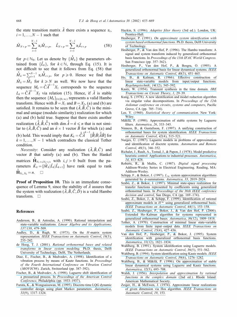
The impulse response of G(z), as shown in Fig. 1, re-veals that the system incorporates a mix of fast and slowdynamics.Ten simulations are carried out in which the response

of the system G(z) to a Gaussian white-noise input withunit standard deviation is determined. An independentGaussian noise disturbance with standard deviation 0:05is added to the output. This amounts to a signal-to-noiseratio (in terms of RMS values) of about 17 dB. The lengthof the input and output data signals is taken to be 1000samples. For each of the ten data sets two basis functionmodels of the form

G(z)=N∑

k=1

LTk Vk(z); (44)

are estimated using the least-squares method describedin Van den Hof et al. (1995). The :rst model is a 40thorder FIR model. Hence, in this case Vk(z)= z−k andN =40. The second model uses a generalized basis that isgenerated by a second-order all-pass function with poles0.5 and 0.9. For this model 20 coe;cient vectors areestimated. Hence, the number of estimated coe;cients isequal for both models.We now apply the approximate realization method us-

ing the estimated expansion coe;cients of both models,for all ten simulations. In either case a sixth order modelis computed, through truncation of the SVD of the :niteHankel matrix. In Fig. 2, step response plots of the re-sulting models are shown. It is seen that approximate re-alization using the standard basis results in a model that:ts only the :rst samples of the response. This is a known

0 5 10 15 20 25 30 35 40 45 50_0.05

0

0.05

0.1

0.15

0.2

Fig. 1. Impulse response of the example system.

Fig. 2. Step responses of the example system (solid) and the modelsobtained in ten simulations with approximate realization using thestandard basis (dash-dotted) and the generalized basis (dashed).

drawback of this method. Employing the generalized ba-sis, with poles 0.5 and 0.9 results in models that bet-ter capture the transient behavior. Apparently, a sensiblechoice of basis can considerably improve the performanceof the Kung algorithm.

10. Conclusions

In this paper, an algorithm is derived that solves theminimal partial realization problem for expansions interms of generalized orthonormal basis functions, gener-ated according to the Hambo basis construction. The re-alization problem is solved by linking it to the classicalrealization problem formulated in the Hambo operatortransform domain. As corollary results expressions areobtained for directly computing the operator transformand its inverse in terms of minimal state-space represen-tations. The presented algorithm yields an original solu-tion to a general minimal rational interpolation problem,and can also be used in an approximate sense, e.g. for thepurpose of model reduction or in a system identi:cationsetting.

Appendix

Proof of Lemma 1.

Gb(1=z)V T1 (z)=

∞∑l=0

gbl zl∞∑k=1

BTb A

Tk−1

b z−k :

Put the term for l=0 aside for a moment. Making use ofthe fact that AbAT

b +BbBTb = I (this follows from (4)) the

remainder of the sums can be written as

∞∑l=1

∞∑k=1

CbAl−1b ATk−1

b zl−k −∞∑l=1

∞∑k=1

CbAlb A

Tk

b zl−k :

666 T.J. de Hoog et al. / Automatica 38 (2002) 655–669

It is obvious that most terms in this expression cancelout. It can be simpli:ed to∞∑l=0

CbAlbz

l +∞∑k=1

Cb ATk

b z−k :

With CbATb =−DbBT

b (this follows from (4)) this becomes∞∑l=0

CbAlbz

l −∞∑k=1

DbBb ATk−1

b z−k :

The last term is exactly equal to minus the term forl=0 which we set aside. So we end up with the desiredresult.

Proof of Proposition 2. Because y=Gu, it follows from(7) that

Y(m) = 〈Vm;Gu〉M =

⟨Vm;G

∞∑j=1

UT(j)Vj

⟩M

=∞∑j=1

〈Vm; VjG〉MU(j):

Using the shift structure in the basis this can be written as

Y(m)=∞∑j=1

〈V1Gm−1b ; V1G

j−1b G〉MU(j): (45)

The adjoint of the transfer function Gb(z) is equal toGT

b (1=z), which by the all-pass property is also equal tothe inverse of Gb(z). By these facts the last equation canbe expressed as

Y(m)=∞∑j=1

〈V1(z); V1(z)Gj−mb (z)G(z)〉MU(j): (46)

The outcome of the inner product term is equal to zerofor j¿m. This follows directly from the fact that the ele-ments of V1(z) are orthogonal to the space spanned by thefunctions Vk for k ¿ 1 which is equal to the shift-invariantsubspace Gb(z)H2.

Proof of Proposition 4. We partition the matrix H intoblocks of dimension nb × nb with the i; jth block denotedas H(i; j). It holds that H(i; j) = viHu

Tj−1. The vector Hu

Tj−1

corresponds to the output of the system G in responseto the input Uj−1 ∈ ‘nb

2 (−∞; 0], restricted to the space offuture signals ‘nb

2 [1;∞). This output can be expressed as

PHnb2G(z)Uj−1(1=z)T =PH

nb2G(z)G−j

b V1(z)T: (47)

The last equality follows from Eqs. (9) and (8). We thenhave that

H(i; j) = 〈Vi(z);PHnb2−G(z)Gb(z)−j V1(z)〉M

= 〈Gb(z)i−1V1(z); G(z)Gb(z)−j V1(z)〉M :

Because Gb(z) is inner this expression simpli:es to

H(i; j) = 〈Gb(z)i+j−1 V1(z); G(z)V1(z)〉M ; (48)

which is equal to Mi+j−1 as was established earlier, seeProposition 2.

Proof of Lemma 5. Using the variable substitution prop-erty of the Hambo operator transform, reOected in expres-sion (13), it follows that the system zG(z) has a Hambotransform that is equal to N T(1=')G('), or equivalentlyG(')N T(1='). These two forms lead to two diNerent re-

alizations for the proper part of zG(z)('). The :rst one,N T(1=')G(') can be written as∞∑t=0

∞∑k=0

nTk gt'k−t ; (49)

where nk and gt represent the kth and tth pulse responseparameters of the transfer matrices N (') and G('), re-

spectively. To evaluate the proper part of zG(z)(') wemake an orthogonal projection of (49) onto the spaceHnb×nb

2;0 . We then :nd

PH2; 0NT(1=')G(')=

∞∑t=0

t∑k=0

nTk gt'k−t

=∞∑k=0

∞∑t=k

nTk gt'k−t :=

∞∑t′=0

∞∑k=0

nTk gt′+k'−t′

with t′= t − k. This is equal to( ∞∑k=0

nTk gk

)+∞∑t′=1

( ∞∑k=0

nTk CAk)

At−1

B'−t′ : (50)

Clearly, this system has realization (A1; B1; C1; D1) withA1 = A, B1 = B, C1 =

∑∞k=0 n

Tk CA

kand D1 =

∑∞k=0 n

Tk gk .

The result now follows by observing that∞∑k=0

nTk CAk= AT

b C +∞∑k=1

CTb DTk−1

b BTb CA

k

= ATb C + CT

b XCA (51)

and∞∑k=0

nTk gk = ATb D+

∞∑k=1

CTb DTk−1

b BTb CA

k−1B

= ATb D+ CT

b XCB (52)

with XC the solution to DTbXCA+ BT

b C=XC: The second

realization for the proper part of zG(z)(') follows simi-larly when starting from the form G(')N T(1=').

Proof of Proposition 6. Because (A; B; C) is minimalit follows that a left-inverse of - is given by X

−1o -

T.

T.J. de Hoog et al. / Automatica 38 (2002) 655–669 667

Hence, it follows from (28) that A= X−1o -

T-1. The prod-

uct -T-1 is equal to the solution of Eq. (32). From (27)

we have B= .T2e1 and C= eT1TT1 -. The form of T1 and

T2 implies that

eTi TT1 = [BT

b BTbDb BT

bD2b · · · ]; (53)

eTi TT2 = [Cb CbDb CbD2

b · · · ]: (54)

It is then seen that .T2e1 is equal to the solution of (30)and eT1T

T1 - is equal to the solution of (31).

Proof of Proposition 7. The derivation of this result iscompletely dual to the derivation of the equations in al-gorithm 2, except for the D term. That is, in this case weuse that H=T1HT

T2 . A full-rank decomposition of H can

then be obtained from a full-rank decomposition of H:

H=-. → H=(T1-)(.TT2 )= -.:

The B and C matrices can be extracted as the :rstblock-row and block-column (with block dimension nb)of - and ., respectively. It then follows that

C= 〈V1(z); (zI − AT)−1CT〉M ;

B= 〈(zI − A)−1B; z−1U0(z)〉M ;

which corresponds to the Sylvester equations (35) and(36). A is obtained through A=-†H

Gb.†, where HGb

is the matrix H with its :rst block-column removed.To compute A we need to know the standard basisequivalent of H

Gb which is denoted by HGb . Then with

T1HGbTT2 = H

Gb and -†=-†TT

1 and .†=T2.† it fol-

lows that

A=-†HGb.†:

Formally, HGb is the Hankel matrix associated with the

transfer function 'G('). By Eq. (14) we know that thiscorresponds, in the z-domain, to the strictly proper part of(Gb(z))−1G(z)=Gb(1=z)G(z) (hence the notation H

Gb).Similar to the derivation of the realizations in Lemma 5we can derive, on the basis of a state-space realization(A; B; C;D) of G(z) the following possible realizations ofthe proper part of Gb(1=z)G(z).

(1) (A; B; DbC + CbXCA; DbD+ CbXCB),(2) (A; BDb + AXBBb; C; DDb + CXBBb)

with XB and XC de:ned as in Proposition 7. This thengives us implicit full-rank decompositions of HGb . Moreprecisely, with -1, .1, -2 and .2 de:ned in the obviousmanner, as in the derivation of Algorithm 2, we then havethat

A=-†-1.1.†=-†-1 =X−1o -T-1; (55)

A=-†-2.2.†=.2.†=.2.TX−1c ; (56)

with Xo and Xc the observability and controllabilitymatrices associated with (A; B; C). It is straightforwardto see that -T-1 =X o

Aand .2.T =X c

A, with X o

Aand

X cAthe solutions to the given Sylvester equations. For

the derivation of D we observe that it follows directlyfrom Eq. (13) that D=

∑∞k=0 gkAk

b =DI +∑∞

k=1 gkAkb.

Pre-multiplication with Ab and post-multiplication withATb , and using that AbAT

b = I − BbBTb (follows from (4))

yields

Ab(D −DI)ATb = D −DI − Ab

∑k=1

Ak−1b BbCAk−1BBT

b ;

which is equal to D − DI − AbXCBBTb . Note that a dual

expression involving XB can be derived in the same man-ner. Also, note that the expressions for A and D havea remarkable symmetry. In fact, with (A; B; C) mini-mal, the Sylvester equation for A can also be written asA=

∑∞k=0 gbk A

k , where gbk represent the pulse responseparameters of Gb(z).

Proof of Corollary 8. Since Lk = 〈Vk(z); G(z)〉M we canalso write

L1

L2

L3...

=T1

CCA

CA2

...

B=T1-B= -B=

C

CA

CA2

...

B

with -; - and (A; C) as de:ned in (the proof of) Propo-sition 7.

Proof of Lemma 9. Su@ciency: Suppose that N ¿ 2and that condition (42) is satis:ed for some n. Then theclassical minimal partial realization criterion of Tetherimplies that application of the Ho–Kalman algorithm toHN1 ; N2 yields the unique (modulo similarity transforma-tion) minimal realization (A; [X1|X2|X3]; C) with McMil-

lan degree n, such that [Mk |Lk |Lk+1]= CAk−1

[X1|X2|X3]for k=1; : : : ; N − 1. It therefore holds that

-N−2AX2 = -N−2X3 (57)

with -k de:ned as -k =[CT

ATC · · · C

TATk−1

]T. Byconstruction, -N1 is a full-rank factor of HN1 ; N−2. Be-cause N16N − 2 it follows that -N−2 is full columnrank. Hence (57) implies that AX2 =X3. Consequently,it holds that Lk = CA

k−1X2 for k=1; : : : ; N . We now

show that the sequence M k = CAk−1

X1; k ∈N corre-sponds to the coe;cient sequence Lk = CA

k−1X2; k ∈N

through Eq. (15). We know that this is true by construc-tion for k=1; : : : ; N − 1. Because {M k} and {Lk} share

668 T.J. de Hoog et al. / Automatica 38 (2002) 655–669

the state transition matrix A there exists a sequence 8i,i=1; : : : ; N − 1 such that

MN+p =N−1∑i=1

8iM i+p; LN+p =N−1∑i=1

8iLi+p (58)

for p∈N0. Let us denote by { ˆMk} the parameters ob-tained from {Lk}, for k ∈N, through Eq. (15). It isnot di;cult to see that it follows from Eq. (58) thatˆMk =

∑N−1i=1 8i

ˆMi+p, for p¿ 0. Hence we :nd that

M k =ˆMk for k¿N as well. We now have that the

sequence Mk = CAk−1

X1 corresponds to the sequenceLk = CA

k−1X2 via relation (15). Hence, if A is stable

then the sequence {Mk}k∈[0;∞) represents a valid Hambotransform. Hence with B=X1 and B=X2, (a) and (b) aresatis:ed. It remains to be seen that (A; B; C) is the mini-mal and unique (modulo similarity) realization for which(a) and (b) hold true. Suppose that there exists another

realization ( ˆA; ˆB; ˆC) with dim ˆA= n6 n that is not simi-lar to (A; B; C) and an n × 1 vector B for which (a) and

(b) hold. This would imply that Kk =ˆC ˆA

k−1[ ˆB|B| ˆAB] for

k=1; : : : ; N − 1 which contradicts the classical Tethercondition.Necessity: Consider any realization (A; B; C) and

vector B that satisfy (a) and (b). Then the Hankel

matrices ˆHN1+i;N2+j, with i; j¿ 0 built from the pa-rameters Kk =[M k |Lk |Lk+1] have rank equal to rankˆHN1 ; N2 = n.

Proof of Proposition 10. This is an immediate conse-quence of Lemma 9, since the stability of A assures thatthe system with realization (A; B; C; D) is a valid Hambotransform.

References

Anderson, B., & Antoulas, A. (1990). Rational interpolation andstate-variable realizations. Linear Algebra and its Applications,137=138, 479–509.

Audley, D., & Rugh, W. (1973). On the H -matrix systemrepresentation. IEEE Transactions on Automatic Control, 18(3),235–242.

de Hoog, T. J. (2001). Rational orthonormal bases and relatedtransforms in linear system modeling. Ph.D. thesis, DelftUniversity of Technology, Delft, The Netherlands.

Diaz, E., Fischer, B., & Medvedev, A. (1998). Identi:cation of avibration process by means of Kautz functions. In Proceedingsof the Fourth International Conference on Vibration Control(MOVIC98). Zurich, Switzerland (pp. 387–392).

Fischer, B., & Medvedev, A. (1998). Laguerre shift identi:cation ofa pressurized process. In Proceedings of the American ControlConference, Philadelphia (pp. 1933–1937).

Furuta, K., & Wongsaisuwan, M. (1995). Discrete-time LQG dynamiccontroller design using plant Markov parameters. Automatica,31(9), 1317–1324.

Haykin, S. (1996). Adaptive :lter theory (3rd ed.). London, UK:Prentice-Hall.

Heuberger, P. (1991). On approximate system identi:cation withsystem based orthonormal functions. Ph.D. thesis, Delft Universityof Technology.

Heuberger, P., & Van den Hof, P. (1996). The Hambo transform: Asignal and system transform induced by generalized orthonormalbasis functions. In Proceedings of the 13th IFACWorld Congress.San Francisco (pp. 357–362).

Heuberger, P., Van den Hof, P., & Bosgra, O. (1995). Ageneralized orthonormal basis for linear dynamical systems. IEEETransactions on Automatic Control, 40(3), 451–465.

Ho, B., & Kalman, R. (1966). ENective construction oflinear state-variable models from input=output functions.Regelungstechnik, 14(12), 545–592.

Kautz, W. (1954). Transient synthesis in the time domain. IRETransactions on Circuit Theory, 1, 29–39.

Kung, S. (1978). A new identi:cation and model reduction algorithmvia singular value decompositions. In Proceedings of the 12thAsilomar conference on circuits, systems and computers, Paci:cGrove, CA (pp. 705–714).

Lee, Y. (1960). Statistical theory of communication. New York:Wiley.

MAakilAa, P. (1990). Approximation of stable systems by Laguerre:lters. Automatica, 26, 333–345.

Ninness, B., & Gustafsson, F. (1997). A unifying construction oforthonormal bases for system identi:cation. IEEE Transactionson Automatic Control, 42(4), 515–521.

Nurges, AU. (1987). Laguerre models in problems of approximationand identi:cation of discrete systems. Automation and RemoteControl, 48(3), 346–352.

Richalet, J., Rault, A., Testud, J., & Papon, J. (1978). Model predictiveheuristic control: Applications to industrial processes. Automatica,14, 413–428.

Roberts, R., & Mullis, C. (1987). Digital signal processingAddison-Wesley Series in Electrical Engineering. Reading, MA:Addison-Wesley.

Schipp, F., & Bokor, J. (1997). L∞ system approximation algorithmsgenerated by !-summations. Automatica, 33, 2019–2024.

Szab*o, Z., & Bokor, J. (1997). Minimal state-space realization fortransfer functions represented by coe;cients using generalizedorthonormal basis. In Proceedings of the 36th IEEE conferencedecision and control, San Diego, CA (pp. 169–174).

Szab*o, Z., Bokor, J., & Schipp, F. (1999). Identi:cation of rationalapproximate models in H∞ using generalized orthonormal basis.IEEE Transactions on Automatic Control, 44(1), 153–158.

Szab*o, Z., Heuberger, P., Bokor, J., & Van den Hof, P. (2000).Extended Ho–Kalman algorithm for systems represented ingeneralized orthonormal bases. Automatica, 36(12), 1809–1818.

Tether, A. (1970). Construction of minimal linear state-variablemodels from :nite input–output data. IEEE Transactions onAutomatic Control, 15(4), 427–436.

Van den Hof, P., Heuberger, P., & Bokor, J. (1995). Systemidenti:cation with generalized orthonormal basis functions.Automatica, 31(12), 1821–1834.

Wahlberg, B. (1991). System identi:cation using Laguerre models.IEEE Transactions on Automatic Control, 36(5), 551–562.

Wahlberg, B. (1994). System identi:cation using Kautz models. IEEETransactions on Automatic Control, 39(6), 1276–1282.

Wahlberg, B., & MAakilAa, P. (1996). On approximation of stablelinear dynamical systems using Laguerre and Kautz functions.Automatica, 32(5), 693–708.

Walsh, J. (1956). Interpolation and approximation by rationalfunctions in the complex domain (2nd ed.). Rhode Island:American Mathematical Society.

Zeiger, H., & McEwen, J. (1974). Approximate linear realizationsof given dimension via Hos algorithm. IEEE Transactions onAutomatic Control, 19, 153.

T.J. de Hoog et al. / Automatica 38 (2002) 655–669 669

Jozsef Bokor received the Dr.Univ. andPh.D. degrees from the EE Departmentof Technical University Budapest in1977 and 1983, respectively, and theD.Sc. degree in control from the Hun-garian Academy of Sciences in 1990.He has been a research fellow withthe Computer and Automation Institute,Hungarian Academy of Sciences andheld visiting positions in the ImperialCollege of Science and Technology,London, UK, System and Control Group,

Delft University, NL and MIT LIDS, Cambridge, MA. Presently heis the head of Systems and Control Laboratory of the Computer andAutomation Institute and also the Professor and Head of the Automa-tion Department, Faculty of Transportation Engineering, TechnicalUniversity Budapest. His research interests include multivariable sys-tems and robust control, system identi:cation, fault detection withapplications in power systems safety operations and also in controlof mechanical and vehicle structures.

Thomas de Hoog received the M.Sc.and Ph.D. degrees from Delft Univer-sity of Technology, the Netherlands,in 1996 and 2001, respectively. HisPh.D. research topic was on the use ofgeneralized orthonormal basis functionsfor system modeling, with emphasis ontransform theory aspects. In 2001 hehas joined the Philips Research Labo-ratories in Eindhoven, the Netherlands,where he is working in the area of op-tical recording. His research interests

include system modeling with generalized orthonormal basis func-tions, repetitive and learning control, servo and signal processingaspects of optical recording.

Peter Heuberger was born in Maas-tricht, The Netherlands, in 1957. Heobtained the M.Sc. degree in Mathemat-ics from the Groningen State Universityin 1983, and the Ph.D. degree from theMechanical Engineering Department ofthe Delft University of Technology in1991. Since 1991 he is with the DutchNational Institute for Public Healthand the Environment (RIVM). Since

1996 he also holds a parttime post-doc position at the DelftUniversity of Technology, currently in the Signals, Systemsand Control Group of the Department of Applied Physics. Hisresearch interests are in issues of system identi:cation, opti-mization, uncertainty, model reduction and in the theory andapplication of orthogonal basis functions.

Zoltan Szabo was born in Nagyvarad,Roumania, in 1966. He obtained theM.Sc. degree in Computer Sciencefrom the Eotvos Lorand UniversityBudapest in 1993, and he is prepar-ing to obtain the Ph.D. degree at thesame university. Since 1996 he hasbeen a research fellow with the Sys-tems and Control Laboratory of theComputer and Automation Institute. Hisresearch interests are in issues of ap-proximation theory, system identi:cation,

and in the theory and application of orthogonal basis functions.

Paul Van den Hof was born in 1957 inMaastricht, The Netherlands. He receivedthe M.Sc. and Ph.D. degrees both fromthe Department of Electrical Engineering,Eindhoven University of Technology, TheNetherlands in 1982 and 1989, respec-tively. From 1986 to 1999 he was an as-sistant and associate professor in the Me-chanical Engineering Systems and Con-trol Group of Delft University of Tech-nology, The Netherlands. In 1992 he helda short-term visiting position at the Cen-

tre for Industrial Control Science, The University of Newcastle, NSW,Australia. Since 1999 he is a full-time professor in the Signals,Systems and Control Group of the Department of Applied Physics atDelft University of Technology. He is acting as IPC=NOC chairmanof the 13th IFAC Symposium on System Identi:cation, to be held inthe Netherlands in 2003. Paul Van den Hof’s research interests are inthe issues of system identi:cation, parametrization, signal processingand (robust) control design, with applications in mechanical servosystems, physical measurement systems, and industrial process controlsystems. He is a member of the IFAC Council and Automatica Editorfor Rapid Publications.