Embed Size (px)
Citation preview
Projection Pursuit Indices Based On
Orthonormal Function Expansions
Dianne Cook
yz
, Andreas Buja
y
, Javier Cabrera
z
y Bellcore, 445 South St,Morristown, NJ 07962-1910
z Dept of Statistics, Hill Cntr, Busch Campus, Rutgers University, New Brunswick, NJ 08904
Abstract
Projection pursuit describes a procedure for searching high dimensional data for \inter-
esting" low dimensional projections, via the optimization of a criterion function called the
projection pursuit index. By empirically examining the optimization process for several
projection pursuit indices we observed di�erences in the types of structure that maximized
each index. We were especially curious about di�erences between two indices based on
expansions in terms of orthogonal polynomials, the Legendre index (Friedman, 1987) and
the Hermite index (Hall, 1989). Being fast to compute these indices are ideally suited for
dynamic graphics implementations.
Both Legendre and Hermite indices are weighted L
2
-distances between the density of the
projected data and a standard normal density. A general form for this type of index is
introduced, which encompasses both of these. The form clari�es the e�ects of the weight
function on the index's sensitivity to di�erences from normality, highlighting some concep-
tual problems with the Legendre and Hermite indices. A new index, called the Natural
Hermite index, which alleviates some of these problems, is introduced.
As proposed by Friedman (1987) and also used by Hall (1989), a polynomial expansion
of the data density reduces the form of the index to a sum of squares of the coe�cients used
in the expansion. This drew our attention to examining these coe�cients as indices in their
own right. We found that the �rst two coe�cients and the lowest order indices produced
by them are the most useful ones for practical data exploration since they respond to
structure that can be analytically identi�ed, and because they have \long-sighted" vision
which enables them to \see" large structure from a distance. Complementing this low order
behaviour the higher order indices are \short-sighted". They are able to \see" intricate
structure but only when close to it.
We also show some practical use of projection pursuit using the polynomial indices,
including a discovery of previously unseen structure in a set of telephone usage data, and
two cautionary examples which illustrate that structure found is not always meaningful.
1
1 Introduction
The term \projection pursuit" was coined by Friedman and Tukey (1974) to de-
scribe a procedure for searching high (p) dimensional data for \interesting" low (k = 1
or 2 usually, maybe 3) dimensional projections. The procedure, originally suggested
by Kruskal (1969), involves de�ning a criterion function, or index, which measures
the \interestingness" of each k-dimensional projection of p-dimensional data. This
criterion function is optimized over the space of all k-dimensional projections of p-
space, searching for both global and local maxima. The resulting solutions hopefully
reveal low dimensional structure in the data not necessarily found by methods such
as principal component analysis.
Searching for interesting projections can be equated to searching for the most
non-normal projections. One reason is that for many high dimensional data sets
most projections look approximately Gaussian, so to �nd the unusual projections one
should search for non-normality (see Andrews et al (1971) and Diaconis and Freed-
man (1984) for further discussion). Huber (1985) equates interesting to structured or
non-randomness and discusses entropy (measured by
R
f(x) log f(x)dx, for example)
as a measure of randomness: the lower the value of entropy indicates more random-
ness. Notably, this also suggests searching away from normality because entropy, as
de�ned above with �xed scale, is minimized by the Gaussian distribution.
Using normality as the null model is highlighted in indices proposed by Jones
(1983, e.g. moment index) and Huber (1985, e.g., negative Shannon entropy, Fisher
information). This approach also suggests discarding structure such as location, scale
and covariance, which are found reasonably well with more conventional multivariate
methods, by sphering the data before beginning projection pursuit. Consequently we
have a framework for considering a family of projection pursuit indices based on a
description of the data in terms of an IR
p
-valued random vector, Z, satisfying EZ = 0
and CovZ = I
p
.
We want to construct a k-dimensional projection pursuit index, that is a real valued
function on the set of all k-dimensional projections of IR
p
. For simplicity, let k = 1,
so we consider all 1-dimensional projections of Z,
Z �! X = �
0
Z 2 IR (� 2 S
p�1
);
where S
p�1
is a unit (p � 1)-sphere in IR
p
, and X is a real-valued random variable.
(We use � 2 S
p�1
because only direction is important and we search over all possible
directions in IR
p
.) In the null case if Z
dis
� N (0; I
p
) then X
dis
� N (0; 1). Let the random
variable X have distribution function F (x) and density f(x). An index, I, can be
constructed by measuring the distance of f(x) from the standard normal density.
A practical index of this kind was proposed by Friedman (1987), although he de-
toured from the above route, by �rst mapping X into the bounded interval [�1; 1] by
the transformation Y = 2�(X)�1, where � is the distribution function of a standard
normal. By doing this he hoped to concentrate attention on di�erences in the center,
2
producing an index robust to tail uctuations. In the null case if X
dis
� N (0; 1) then
Y
dis
� U [�1; 1]. In general, let Y have distribution function G(y) and density g(y).
Friedman's proposed index is an L
2
-distance of g(y) from the density of U [�1; 1]:
I
L
=
Z
1
�1
fg(y)�
1
2
g
2
dy
We call this the Legendre index because g(y) will later be expanded in terms of the
natural polynomial basis with respect to U [�1; 1], namely the Legendre polynomials.
This is the starting point for the work presented in this paper, but before we
continue we note two basic details about the use of an index, I, in projection pursuit:
1: I is a functional of f (in Friedman's case I
L
is a functional of g).
2: f (or g) depends on the projection vector, �, so that projection pursuit
entails the search for local maxima of I over all possible �.
2 Transformation Approach
Friedman's detour can be generalized by considering an arbitrary strictly monotone
and smooth transformation T : IR! IR on the random variableX so that Y = T (X).
Then if X has distribution function F (x) and density f(x), let Y have distribution
function G(y) and density g(y). Given that the null version of the density, f(x), is
�(x) we denote the null version of the density g(y) to be (y). A general family of
indices is now de�ned by
I =
Z
IR
fg(y)� (y)g
2
(y)dy (1)
which specializes to
1
2
I
L
for T (X) = 2�(X)�1. (Note that we integrate with respect
to (y)dy, which becomes
1
2
dy for the Legendre index, I
L
.) This family of indices
incorporates the idea of a distance computation between \observed" f(x) or g(y) and
\null" �(x) or (y) under the assumption of the null distribution. The transformation,
T , can be considered to transform the index into a form suitable for estimation by
an alternative orthonormal basis (see below), and to adjust the index's sensitivities
to particular structures.
In somewhat reverse logic, now start with I, de�ned in its transformed state, and
map it back through the inverse transformation:
I =
Z
IR
(
f(x)
T
0
(x)
�
�(x)
T
0
(x)
)
2
�(x)dx
=
Z
IR
ff(x)� �(x)g
2
�(x)
T
0
(x)
2
dx (2)
This form clearly shows that the index is a weighted distance between f(x) and a
standard normal density, with weighting function �(x)=T
0
(x)
2
.
3
Using this formulation the Legendre index, I
L
, proposed by Friedman (1987) be-
comes:
I
L
=
Z
IR
ff(x)� �(x)g
2
1
2�(x)
dx; (3)
since T (X) = 2�(X) � 1 ) T
0
(X) = 2�(X). Ironically the mapping proposed by
Friedman to reduce the in uence of tail uctuations does exactly the opposite. The
term 1=�(x) e�ectively upweights tail observations, leaving the Legendre index very
sensitive to di�erences from normality in the tails of f(x). This is more a conceptual
stumbling block than a practical de�ciency because the problem is somewhat moot
for �nite function expansions. Just the same, equation (3) illustrates an unintended
e�ect of an otherwise innocuous-looking data transformation.
Through di�erent considerations Hall (1989) also observed the same phenomenon
of upweighted tails in the Legendre index. It motivated him to propose an alternative
index that measures the L
2
-distance between f(x) and the standard normal density
with respect to Lebesgue measure:
I
H
=
Z
IR
ff(x)� �(x)g
2
dx
Interestingly, this index is also a member of the family of indices (1) as it can be
obtained through a suitable transformation. Equating the implicit weight 1 with
�(x)=T
0
(x)
2
in 2 we �nd T
0
(x)
2
= �(x), or T
0
(x) =
q
�(x) and hence T (X) /
�
�=
p
2
(X) . Such a transformation seems unnatural at �rst, and may not contribute
any additional insight beyond the obvious one that I
H
gives equal weight to all
di�erences along IR. Aside from this, Hall's motivation for the design of the index is
from an established approach in density estimation.
We return then to Friedman's original idea of giving more weight to di�erences in
the center. Going a step beyond Hall's approach, we propose to use T (X) = X, the
identity transformation, giving:
I
N
=
Z
IR
ff(x)� �(x)g
2
�(x)dx (4)
We call this index the \Natural Hermite" index, and Hall's index the \Hermite" index
because both use Hermite polynomials in the expansion of f(x), but I
N
is \natural"
because the distance from the normal density is taken with respect to Normal measure.
The class of T that we have allowed is exibly broad, to entertain various construc-
tions which may not be entirely sensible for practical purposes. We make use only of
the following one-parameter family of transformations,
T
�
(X) =
p
2��(�
�
(X)� 1=2)
which allows us to see the three indices in a natural order. The elements of the family
are scaled to achieve T
0
�
(0) = 1, for all � > 0. The limit for �!1 is T
�!1
(X) = X.
4
For T
�=1
we get essentially the Legendre index, I
L
, for T
�=
p
2
we have an index
proportional to the Hermite, I
H
, and for T
1
we get the Natural Hermite index, I
N
.
The proper way to interpret these transformations is according to their ability to thin
out the tail weight for increasing �. The smaller �, the more the tail weight is in ated
and allowed to exert in uence on the projection pursuit index.
As mentioned above, the problem of tail weight is more conceptual than practical.
The upshot of this section then is conceptual consistency in a framework that allowed
us to devise a new index which is simple and more radical in its treatment of tail
weight. In the following sections, we will mostly work with our new index and give
cursory attention to the Legendre and Hermite indices when appropriate.
3 Density Estimation
For the purposes of projection pursuit index estimation, the empirical data distri-
bution needs to be mapped into a density estimate to which the de�nition of an index
can be applied. A natural approach in this context is polynomial expansion (Fried-
man, 1987). Density estimates obtained in this way are usually not very pleasing
for graphical purposes since the non-negativity constraint is impossible to enforce.
However, in the present context no graphical presentation of such estimates is in-
tended. In addition, considerable analytical simplicity and computational e�ciency
is achieved by this approach.
In each of the indices described above, the density f(x) (or g(y) in the transformed
version) is expanded using orthonormal functions:
f(x) =
1
X
i=0
a
i
p
i
(x)
In the Natural Hermite index, fp
i
(x); i = 0; 1; : : :g is the set of standardized Hermite
polynomials orthonormal with respect to (on. wrt) �(x). (Note that �(x) is also
called the weight function of the polynomial basis. In the notation of Thisted (1988),
p
i
(x) = (i!)
�
1
2
H
e
i
(x); p
0
(x) = 1; p
1
(x) = x; p
2
(x) = x
2
� 1. The subscript \e" is a
convention used to distinguish this Hermite polynomial basis from the basis on. wrt
�
2
(x).)
In addition, to estimate I
N
, �(x) is expanded as
P
1
i=0
b
i
p
i
(x). Inserting both ex-
pansions into I
N
(4) gives:
I
N
=
Z
IR
(
1
X
i=0
a
i
p
i
(x)�
1
X
i=0
b
i
p
i
(x)
)
2
�(x)dx
=
Z
IR
(
1
X
i=0
(a
i
� b
i
)p
i
(x)
)
2
�(x)dx
=
1
X
i=0
(a
i
� b
i
)
2
5
since the p
i
's are on. wrt �(x).
The Fourier coe�cients of the expansion, a
i
and b
i
, are as follows:
a
i
=
Z
IR
f(x)p
i
(x)�(x)dx =
Z
IR
p
i
(x)�(x)dF (x)
b
i
=
Z
IR
�(x)p
i
(x)�(x)dx
The coe�cients, b
i
, can be analytically calculated from Abramowitz and Stegun (1972,
22.5.18, 22.5.19):
b
2i
=
(�1)
i
p
�
((2i)!)
1
2
i!
1
2
2i+1
; b
2i+1
= 0; i = 0; 1; 2; : : :
Because of its dependence on f , the coe�cient a
i
is unknown and must be estimated
in order to estimate I
N
. Reinterpreting a
i
as an expectation,
a
i
= E
F
fp
i
(X)�(X)g
leads to the obvious sample estimate:
a
i
=
1
n
n
X
j=1
p
i
(x
j
)�(x
j
)
The index I
N
is estimated by using a
i
and truncating the sum at M terms,
^
I
N
M
=
M
X
i=0
(a
i
� b
i
)
2
:
The asymptotic theory for the choice of M as a function of sample size for I
L
and I
H
is the subject of Hall's (1989) paper. Using Hall's approach we �nd that the choice of
M for I
N
is the same as that for I
H
. Note also, that the truncation at M constitutes
a smoothing of the true index, I
N
.
The approximations in both Legendre and Hermite indices are similarly constructed.
In the Legendre index, the expansion is made on g(y), after X is transformed from
IR to [�1; 1] by Y = 2�(X) � 1, with fp
i
(y); i = 0; 1; : : :g being the set of stan-
dardized Legendre polynomials (Friedman, 1987). The Hermite index uses Hermite
polynomials on. wrt �
2
(x) (Hall, 1989).
4 Structure Detection
Our interest in the structure sensitivity of the indices stems from implementing
projection pursuit dynamically (Cook et al, 1991) in XGobi, which is dynamic graph-
ics software being developed by Swayne et al (1991). Included in the implementation
are controls for steepest ascent optimization of a variety of 2-dimensional projection
6
pursuit indices. The main feature is that the procedure is visualized by sequential
plotting of the projected data as the optimization ensues, and the interactive nature
of the implementation enables the optimization to be readily started from multiple
points.
For many long but interesting hours we watched projections of various types of
data as they were steered into local maxima of di�erent projection pursuit indices.
In the course we found that indices truncated as low as M = 0 or M = 1 were
the most interesting and also useful. This ies in the face of the natural idea that
M should be chosen as large as possible, within limits dictated by the sample size.
The usefulness of these low order indices arises from a \long-sighted" quality which
enables them to see large structure, such as clusters, from a distance. Speci�cally, we
found that low order Hermite and Natural Hermite indices often �nd projections with
a \hole" in the center, whilst the low order Legendre index tends to �nd projections
containing skewness. Higher (4, 5, : : : ) indices lose the long-sightedness and become
\short-sighted". They are receptive to �ner detail in the projected data although they
need starting points much closer to the structure to �nd it. The intrigue induced by
observing these behaviours led to the qualitative results in the next few sections.
5 One-dimensional Index
For simplicity we begin with the 1-dimensional index, using the Natural Hermite
as an example and then extending the results to both the Legendre and Hermite
indices. We are interested in maxima of I
N
0
= (a
0
� b
0
)
2
, I
N
1
= (a
0
� b
0
)
2
+ (a
1
� b
1
)
2
and its second term (a
1
� b
1
)
2
. Because each (a
i
� b
i
)
2
involves a quadratic in a
i
it
is maximized by minimizing or maximizing a
i
. Write a
i
as E
F
fp
i
(X)�(X)g and the
problem reduces to �nding the types of distribution functions, F (x), which minimize
or maximize this expectation.
Now F (x) needs to be absolutely continuous for the integral form (4) of the index,
I
N
, to exist but once the expansion is truncated this restriction may be dropped and
F (x) may be discrete. In the execution of projection pursuit, F (x) is restricted to
the set of distribution functions of all 1-dimensional projections of Z:
F (x) 2 F
Z
= fF (x):X = �
0
Z;� 2 S
p�1
g
and EZ = 0 and CovZ = I
p
are assumed as usual. However, to understand the
general types of distributions to which a
i
responds, consider F (x) belonging to the
expanded set:
F = fF (x): E
F
X = 0;E
F
X
2
= 1g
Now F is convex, but it is not closed in the weak topology. In order to consider
minimizing or maximizing a
i
over F we need to consider all F (x) in the weak closure
of F ,
�
F , which happens to be:
7
�
F = fF (x): E
F
X = 0;Var
F
X � 1g (�)
This set is furthermore weakly compact (��). (Proofs of these two statements and
Lemma 5.1, Propositions 5.2 and 5.3 are left to the Appendix.) Since
�
F is also convex,
this is a natural domain for optimizing the projection pursuit coe�cients, a
i
. They
are weakly continuous linear functionals, and their extrema in
�
F are taken on at the
extremal elements:
Lemma 5.1: The extremal elements of
�
F are the union of:
(i) the 3-point masses, F , satisfying E
F
X = 0, E
F
X
2
= 1;
(ii) the 2-point masses, F , satisfying E
F
X = 0, E
F
X
2
� 1;
(iii) the 1-point mass F = �
0
.
(where �
x
denotes a unit point mass at x.)
Thus, the set of extremals is not very expressive, but it is su�cient to give insight
into the behaviours of the lower order coe�cients, a
0
and a
1
. While it is true that
a
i
takes on its extrema on these elements for all i = 0; 1; 2; 3; : : :, none of its ability
to respond to high frequency structure in F is revealed by studying this extremal
behaviour for larger orders of i.
5.1 Truncation at First Term - I
N
0
Consider the simplest but, in our experience, most useful index I
N
0
= (a
0
� b
0
)
2
,
where
a
0
=
Z
IR
�(x)dF (x) since p
0
(x) � 1
b
0
=
1
2
p
�
(= a
0
when f � �)
so that I
N
0
= (a
0
� 1=(2
p
�))
2
: As mentioned earlier, we should expect two types of
(local) maxima for I
N
0
; one for a minimum of a
0
and one for a maximum.
Proposition 5.2:
(i) a
0
is minimized, with a value 1=
p
2�e, by a distribution with
equal masses of weight 0:5 at �1. (Call this distribution type CH,
or a \central hole".)
(ii) a
0
is maximized with a value 1=
p
2�, by a point mass at 0. This
distribution actually maximizes I
N
0
with a value of (1�1=
p
2)
2
=2�.
(Call this distribution type CM, or a \central mass" concentration.)
8
0.0 0.2 0.4 0.6 0.8 1.0
0.0
0.00
50.
010
0.01
5
γ
I0N
Central Mass
Central Hole
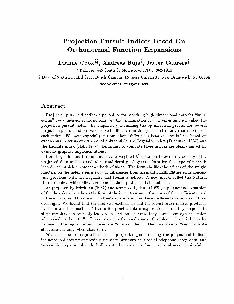
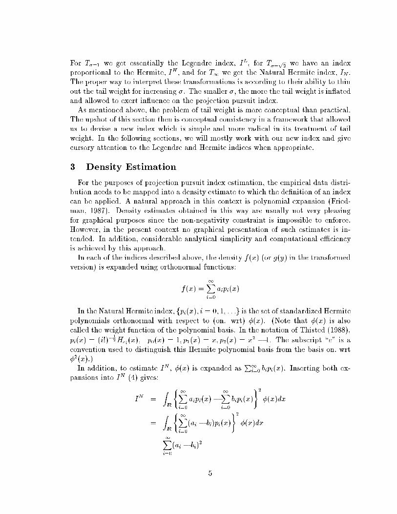
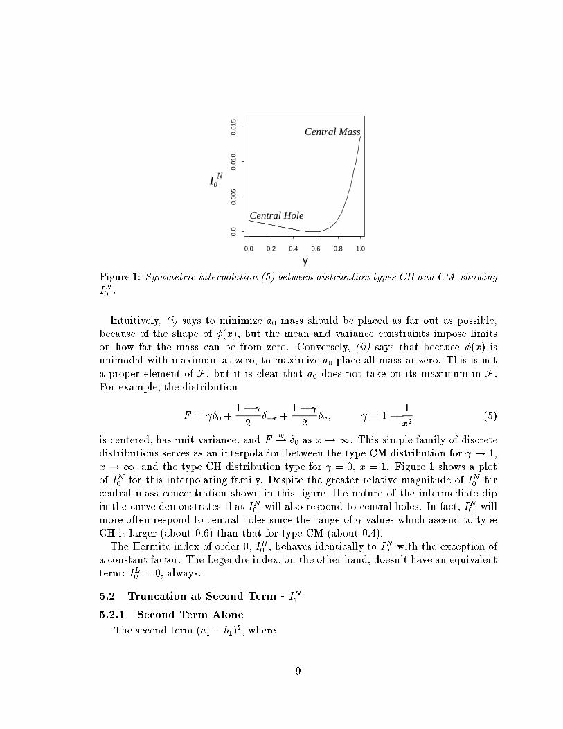
Figure 1: Symmetric interpolation (5) between distribution types CH and CM, showing
I
N
0
.
Intuitively, (i) says to minimize a
0
mass should be placed as far out as possible,
because of the shape of �(x), but the mean and variance constraints impose limits
on how far the mass can be from zero. Conversely, (ii) says that because �(x) is
unimodal with maximum at zero, to maximize a
0
place all mass at zero. This is not
a proper element of F , but it is clear that a
0
does not take on its maximum in F .
For example, the distribution
F = �
0
+
1�
2
�
�x
+
1 �
2
�
x
; = 1�
1
x
2
(5)
is centered, has unit variance, and F
w
! �
0
as x!1. This simple family of discrete
distributions serves as an interpolation between the type CM distribution for ! 1,
x! 1, and the type CH distribution type for = 0, x = 1. Figure 1 shows a plot
of I
N
0
for this interpolating family. Despite the greater relative magnitude of I
N
0
for
central mass concentration shown in this �gure, the nature of the intermediate dip
in the curve demonstrates that I
N
0
will also respond to central holes. In fact, I
N
0
will
more often respond to central holes since the range of -values which ascend to type
CH is larger (about 0.6) than that for type CM (about 0.4).
The Hermite index of order 0, I
H
0
, behaves identically to I
N
0
with the exception of
a constant factor. The Legendre index, on the other hand, doesn't have an equivalent
term: I
L
0
= 0, always.
5.2 Truncation at Second Term - I
N
1
5.2.1 Second Term Alone
The second term (a
1
� b
1
)
2
, where
9
a
1
=
Z
IR
x�(x)dF (x) since p
1
(x) � x
b
1
= 0 (= a
1
when f � �)
reduces to a
2
1
. For this quantity we need only consider maximizing a
1
, because the
skew symmetry of a
1
about x = 0 implies that the minimal value of a
1
will be equal
in magnitude to its maximal value, and obtained by a re ection through x = 0 of the
maximal distribution.
Proposition 5.3:
The second coe�cient, a
1
, is maximized by the two point distribu-
tion with mass ; (1� ) at
q
(1 � )= ;�
q
=(1 � ), respectively,
where is found by maximizing
q
(1 � )(�e
�(1� )=
+ e
=(1� )
).
( approximately equals 0.838.)
The maximum value of I
N
1
, is achieved equally by this right-skewed distribution and
the left-skewed distribution produced by its re ection through x = 0. Call these
distributions type SK. As above, it is useful to embed the distributions of interest in
a one-parameter family:
F = (1� )�
x
+ �
y
; x = �
q
=(1 � ); y =
q
(1� )= (6)
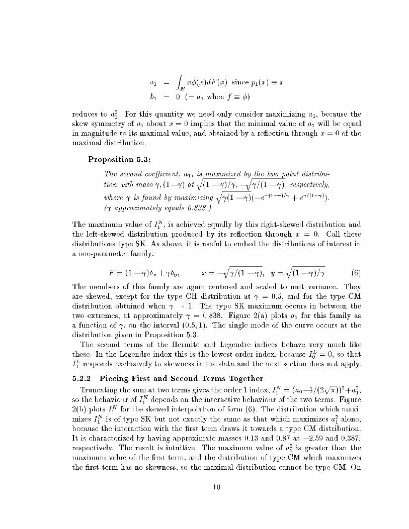
The members of this family are again centered and scaled to unit variance. They
are skewed, except for the type CH distribution at = 0:5, and for the type CM
distribution obtained when ! 1. The type SK maximum occurs in between the
two extremes, at approximately = 0:838. Figure 2(a) plots a
1
for this family as
a function of , on the interval (0:5; 1). The single mode of the curve occurs at the
distribution given in Proposition 5.3.
The second terms of the Hermite and Legendre indices behave very much like
these. In the Legendre index this is the lowest order index, because I
L
0
= 0, so that
I
L
1
responds exclusively to skewness in the data and the next section does not apply.
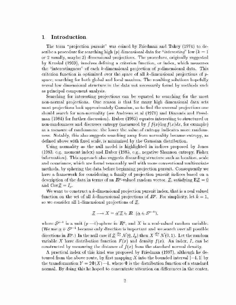
5.2.2 Piecing First and Second Terms Together
Truncating the sum at two terms gives the order 1 index, I
N
1
= (a
0
�1=(2
p
�))
2
+a
2
1
,
so the behaviour of I
N
1
depends on the interactive behaviour of the two terms. Figure
2(b) plots I
N
1
for the skewed interpolation of form (6). The distribution which maxi-
mizes I
N
1
is of type SK but not exactly the same as that which maximizes a
2
1
alone,
because the interaction with the �rst term draws it towards a type CM distribution.
It is characterized by having approximate masses 0:13 and 0:87 at �2:59 and 0:387,
respectively. The result is intuitive. The maximum value of a
2
1
is greater than the
maximum value of the �rst term, and the distribution of type CM which maximizes
the �rst term has no skewness, so the maximal distribution cannot be type CM. On
10
0.5 0.6 0.7 0.8 0.9 1.0
0.0
0.00
50.
010
0.01
5
(a)
γ
a1
CMCH
0.5 0.6 0.7 0.8 0.9 1.0
0.0
0.00
50.
010
0.01
5
(b)
γ
I1N
CM
CH
Figure 2: Skewed interpolation (6) between distribution types CH and CM, showing
(a) a
1
and (b) I
N
1
.
the other hand the SK type distributions that are \close" to maximizing a
2
1
also get
a contribution from the �rst term which favours all mass at 0.
Clearly the behaviour of I
N
1
is to respond to skewness when it is present. This
behaviour is also seen in the Hermite index, I
H
1
.
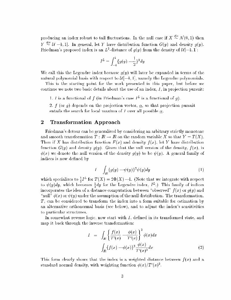
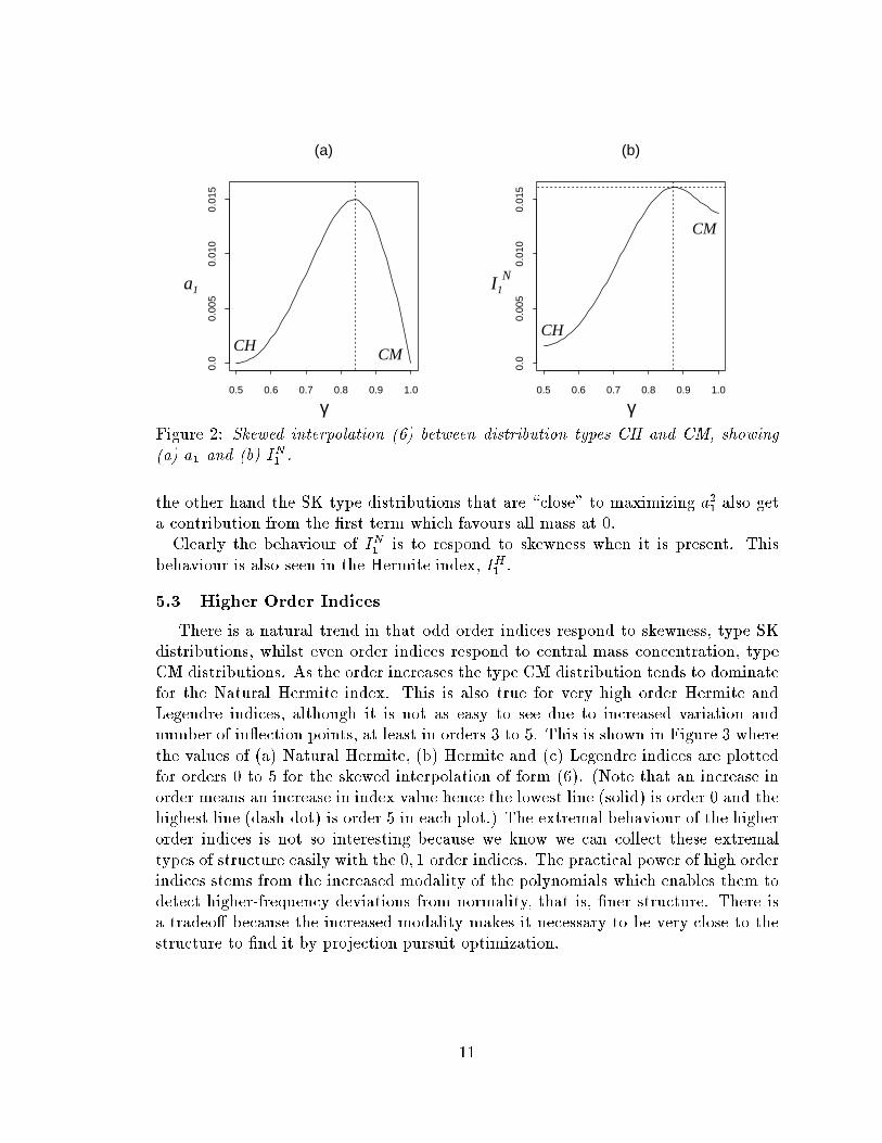
5.3 Higher Order Indices
There is a natural trend in that odd order indices respond to skewness, type SK
distributions, whilst even order indices respond to central mass concentration, type
CM distributions. As the order increases the type CM distribution tends to dominate
for the Natural Hermite index. This is also true for very high order Hermite and
Legendre indices, although it is not as easy to see due to increased variation and
number of in ection points, at least in orders 3 to 5. This is shown in Figure 3 where
the values of (a) Natural Hermite, (b) Hermite and (c) Legendre indices are plotted
for orders 0 to 5 for the skewed interpolation of form (6). (Note that an increase in
order means an increase in index value hence the lowest line (solid) is order 0 and the
highest line (dash-dot) is order 5 in each plot.) The extremal behaviour of the higher
order indices is not so interesting because we know we can collect these extremal
types of structure easily with the 0; 1 order indices. The practical power of high order
indices stems from the increased modality of the polynomials which enables them to
detect higher-frequency deviations from normality, that is, �ner structure. There is
a tradeo� because the increased modality makes it necessary to be very close to the
structure to �nd it by projection pursuit optimization.
11
0.5 0.7 0.9
0.0
0.02
0.04
0.06
0.08
Natural Hermite
γ
IkN
0
1
2
3
4
5
0.5 0.7 0.9
0.0
0.1
0.2
0.3
0.4
0.5
Hermite
γ
IkH
0
1
2
3
4
5
0.5 0.7 0.9
0.0
0.2
0.4
0.6
0.8
1.0
1.2
1.4
Legendre
γ
IkL
1
2
3
4
5
Figure 3: Skewed interpolation (6) for indices of orders k = 0; 1; : : : ; 5 (a) Natural
Hermite, (b) Hermite, (c) Legendre.
6 Illustrations of 1-dimensional Projection Pursuit
6.1 Low Order Indices
Now that we have examined some aspects of the behaviour of the polynomial indices
over the ideal expanded set,
�
F , we would like to examine their behaviour, in practice,
that is, over the set, F
Z
, of distributions of 1-dimensional projections of Z. For most
dimensions, p, of Z this is not possible, but it is practical for the simple case of p = 2.
The following type of plot has been used by Huber (1990): project a two-dimensional
distribution onto lines parametrized by angles of unit vectors in the plane,
�
�
= (cos �; sin �); � = 0
o
; 1
o
; : : : ; 179
o
and calculate
^
I
N
0
for each �, and display its values radially as a function of �.
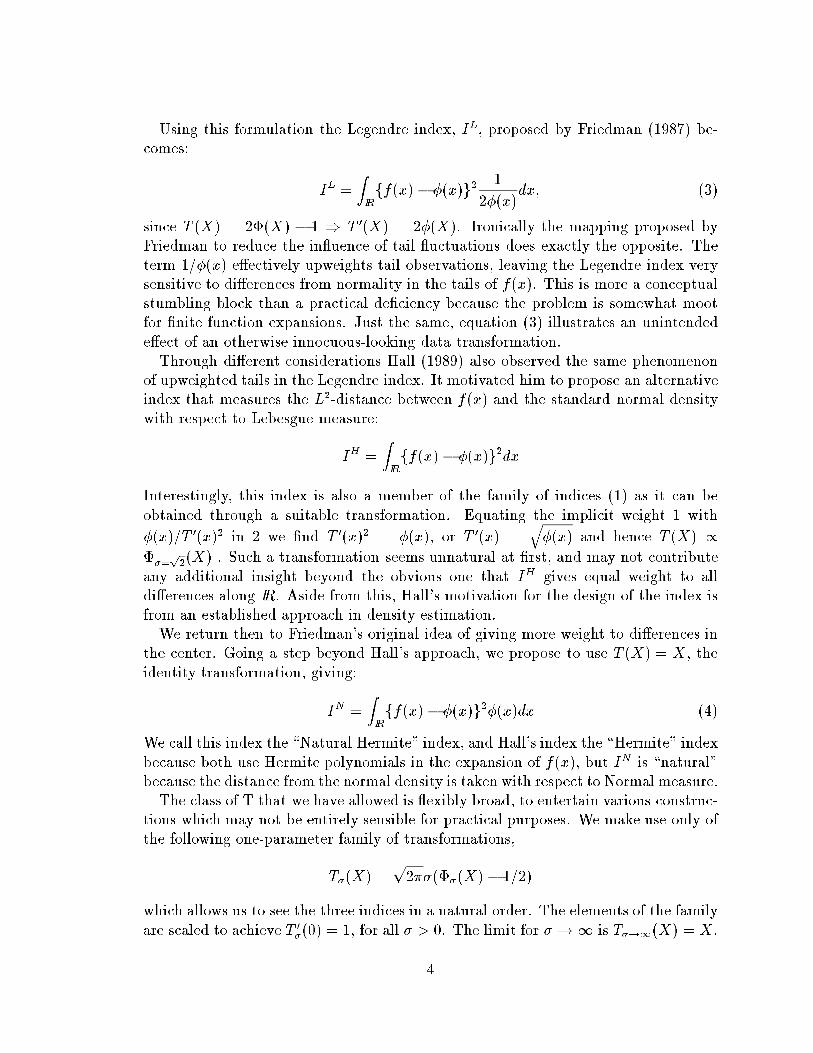
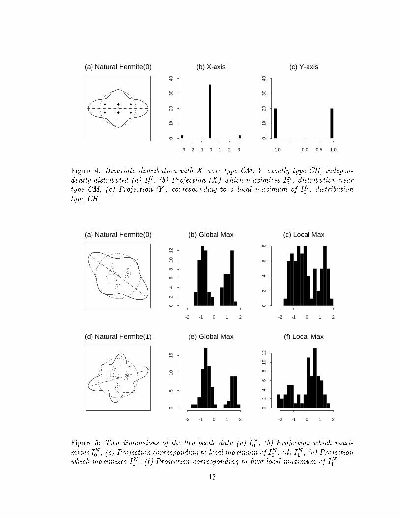
Figure 4(a) shows an example of this for a bivariate distribution whose X and Y
variables are independent and distributed according to a near type CM and an exact
type CH distribution, respectively. The data points (diamonds) are plotted in the
center of the �gure. (Note that overplotting obscures the relative frequency at each
12
+
(a) Natural Hermite(0)
-3 -2 -1 0 1 2 3
010
2030
40
(b) X-axis
-1.0 0.0 0.5 1.0
010
2030
40
(c) Y-axis
Figure 4: Bivariate distribution with X near type CM, Y exactly type CH, indepen-
dently distributed (a) I
N
0
, (b) Projection (X) which maximizes I
N
0
, distribution near
type CM, (c) Projection (Y ) corresponding to a local maximum of I
N
0
, distribution
type CH.
. ... .... ...
....
..
.. ..
.............. ...
..
...
.
...
....
.
.....
.. ..
..
. .
...
... ... +
(a) Natural Hermite(0)
-2 -1 0 1 2
02
46
810
12
(b) Global Max
-2 -1 0 1 2
02
46
8
(c) Local Max
.... .... ...
......
.. ..
.............. ..... ...
.
...
....
.
.....
.. ..
..
. ...
.
... ... +
(d) Natural Hermite(1)
-2 -1 0 1 2
05
1015
(e) Global Max
-2 -1 0 1 2
02
46
810
12
(f) Local Max
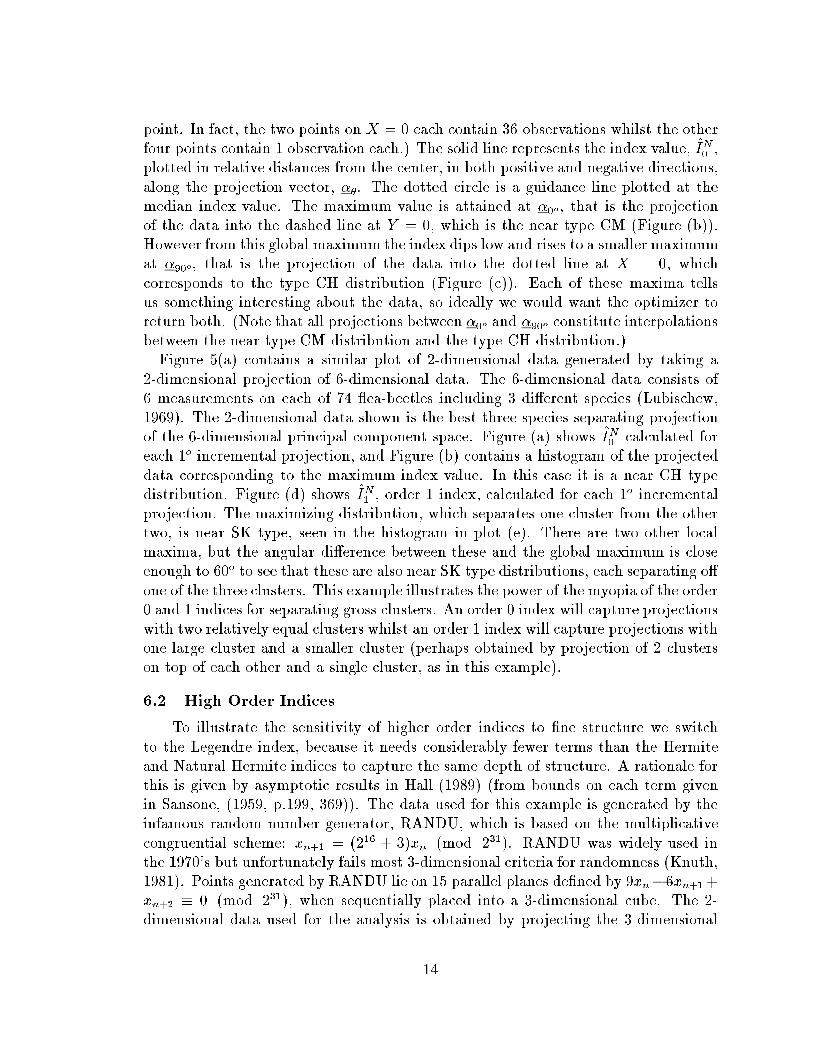
Figure 5: Two dimensions of the ea beetle data (a) I
N
0
, (b) Projection which maxi-
mizes I
N
0
, (c) Projection corresponding to local maximum of I
N
0
, (d) I
N
1
, (e) Projection
which maximizes I
N
1
, (f) Projection corresponding to �rst local maximum of I
N
1
.
13
point. In fact, the two points on X = 0 each contain 36 observations whilst the other
four points contain 1 observation each.) The solid line represents the index value,
^
I
N
0
,
plotted in relative distances from the center, in both positive and negative directions,
along the projection vector, �
�
. The dotted circle is a guidance line plotted at the
median index value. The maximum value is attained at �
0
o, that is the projection
of the data into the dashed line at Y = 0, which is the near type CM (Figure (b)).
However from this global maximum the index dips low and rises to a smaller maximum
at �
90
o, that is the projection of the data into the dotted line at X = 0, which
corresponds to the type CH distribution (Figure (c)). Each of these maxima tells
us something interesting about the data, so ideally we would want the optimizer to
return both. (Note that all projections between �
0
oand �
90
oconstitute interpolations
between the near type CM distribution and the type CH distribution.)
Figure 5(a) contains a similar plot of 2-dimensional data generated by taking a
2-dimensional projection of 6-dimensional data. The 6-dimensional data consists of
6 measurements on each of 74 ea-beetles including 3 di�erent species (Lubischew,
1969). The 2-dimensional data shown is the best three species separating projection
of the 6-dimensional principal component space. Figure (a) shows
^
I
N
0
calculated for
each 1
o
incremental projection, and Figure (b) contains a histogram of the projected
data corresponding to the maximum index value. In this case it is a near CH type
distribution. Figure (d) shows
^
I
N
1
, order 1 index, calculated for each 1
o
incremental
projection. The maximizing distribution, which separates one cluster from the other
two, is near SK type, seen in the histogram in plot (e). There are two other local
maxima, but the angular di�erence between these and the global maximum is close
enough to 60
o
to see that these are also near SK type distributions, each separating o�
one of the three clusters. This example illustrates the power of the myopia of the order
0 and 1 indices for separating gross clusters. An order 0 index will capture projections
with two relatively equal clusters whilst an order 1 index will capture projections with
one large cluster and a smaller cluster (perhaps obtained by projection of 2 clusters
on top of each other and a single cluster, as in this example).
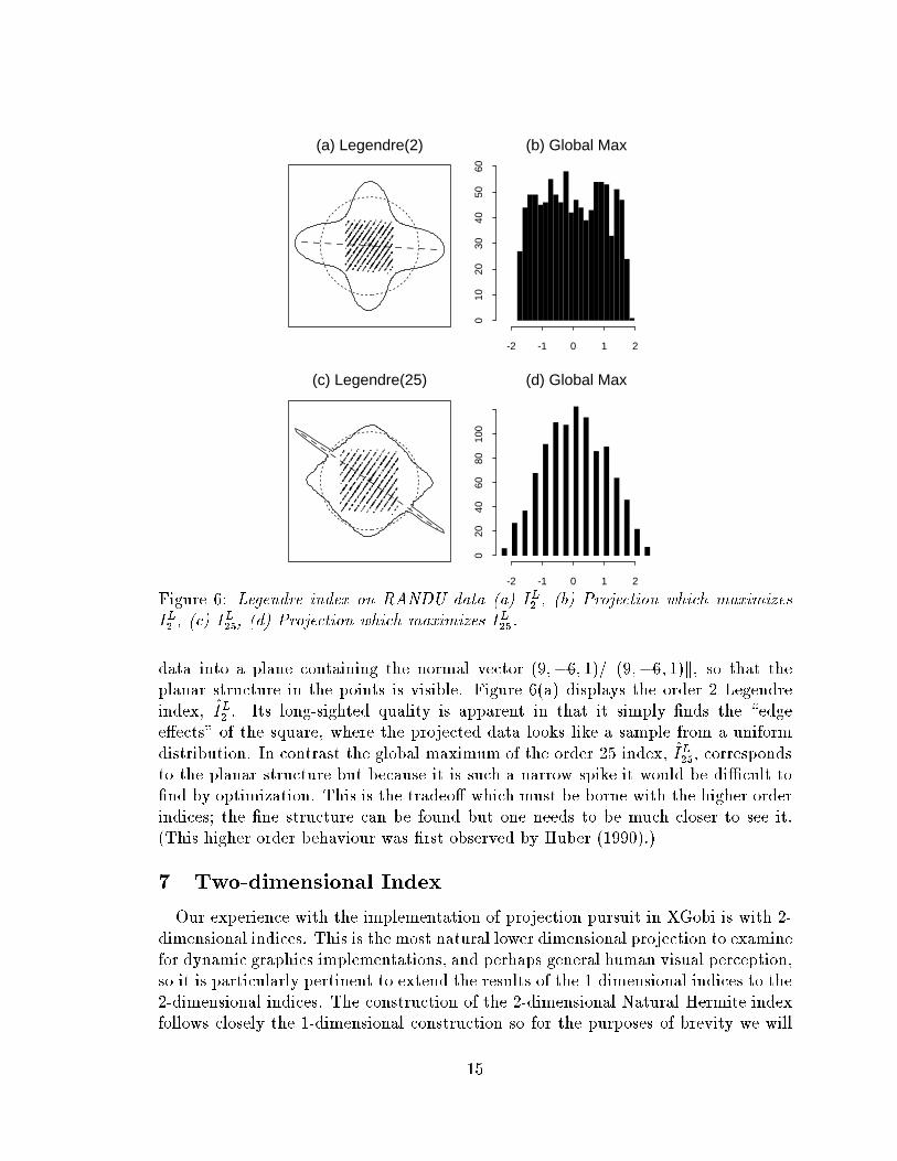
6.2 High Order Indices
To illustrate the sensitivity of higher order indices to �ne structure we switch
to the Legendre index, because it needs considerably fewer terms than the Hermite
and Natural Hermite indices to capture the same depth of structure. A rationale for
this is given by asymptotic results in Hall (1989) (from bounds on each term given
in Sansone, (1959, p.199, 369)). The data used for this example is generated by the
infamous random number generator, RANDU, which is based on the multiplicative
congruential scheme: x
n+1
= (2
16
+ 3)x
n
(mod 2
31
). RANDU was widely used in
the 1970's but unfortunately fails most 3-dimensional criteria for randomness (Knuth,
1981). Points generated by RANDU lie on 15 parallel planes de�ned by 9x
n
�6x
n+1
+
x
n+2
� 0 (mod 2
31
), when sequentially placed into a 3-dimensional cube. The 2-
dimensional data used for the analysis is obtained by projecting the 3-dimensional
14
..
..
.
..
.....
.
..
..
.
.
..
..
..
.
.
..
.
.
. ..
.
...
.
.
. ...
.
.
. . ..
...
.. .
.
.
.. .
... ..
.
.
...
. .
.
.
.
.
.
....
..
.
.
.
..
..
.
..
. ..
.
.
... .
.
..
. ..
. .
. ..
..
.
..
....
.
.
. ...
.
..
.
.
.
. .
.
.
.
.
. ..
.
.
.
. ...
.
.
. . .
..
.
.
..
.
. .
..
..
.
.
.
.
.
.
.
.
.
..
.
.
..
.
...
.
.
.
. .
.
.
.
.
.
.
....
. .
.
..
.
.. ..
.
..
.
..
.
.
.
..
.
..
..
.
.
.
.
..
.
. ..
.
.
..
..
..
.
.
....
. .
.
.
.
.
..
.
..
..
..
..
. ...
... .
..
.
. . .
..
.
.
.
..
..
.
.
.
.
.. ...
...
.
.
.
.
.
. ...
.
.
.
...
.
.
.. .
.
.
...
.
.
. ...
...
.
.
.
.
.
. ..
. ..
..
... ..
.
.. ..
...
. .
. .
.
.
..
. .
..
. ...
. .
.
..
....
.
.. ..
..
.
.
..
.
...
..
..
....
.
..
.
. ..
.
..
...
.
.
.
.
...
..
..
..
..
..
.
...
...
..
.. .
.
..
.
. .
.
..
.
.
.
.
..
.
. . ...
..
.
.
.
...
.
.
.
..
....
..
..
.
.
.
.. .
.
.
.
.
..
.
.. ..
.
.
..
.
.
.
.
.
.
..
..
..
.
. ..
.
... .
.
...
.
..
..
..
.. .
. ..
. ..
.
. .....
.
.
.
. ..
..
.
.
..
.
.
.
..
...
..
.
.. .
..
. .
. . ....
.
..
.
...
.
.
...
.
.
...
..
. .
...
.
.
..
..
..
.
.
. .
.... .
..
. .
..
..
..
..
.
.
.. .
.
.
..
..
.
..
.
..
.
.. ..
....
...
. .
. ..
...
.
.
.
.
.
..
.
.
.
.
.
. .
..
.
..
.
.
.
.
.
..
.
.
.. ..
.
...
..
. .
.
..
. ..
.
..
.
.
.
.
.
.
.
..
.
.
.
.. .
.
.
.
..
.
...
..
..
.
..
.
..
..
..
.
.
.
.
..
.
..
.
..
.
.
..
.
... .
...
..
.
.. .. ..
.
..
.
.
..
..
.
.
..
.
.
.
.
... .
.
.
.
. .
..
..
..
.
...
.
.. .
.
.
.
. .. .
...
.
.
.
.
.
.
..
.
.
.
.
...
...
...
.
.
.
.
.
. ...
..
.
..
. ..
..
...
..
.. .
.
..
..
.
...
.
.
.
.
.
.
..
.
..
..
.
..
.
. .
.
.
.
..
.
.
.
.
.
...
.
.
..
.
.
..
.
..
.
. .
.
.
.
.
..
. . .
. .
.
..
.
..
..
. ..
...
. ..
.
.
.
.
...
+
(a) Legendre(2)
-2 -1 0 1 2
010
2030
4050
60
(b) Global Max
..
.
.
.
..
.....
.
..
..
.
.
.
.
..
..
.
.
.
.
.
.
. .
.
.
...
.
.
. ...
.
.
.. .
..
.
.
..
.
.
.
.. .
... ..
.
.
...
. .
.
.
.
.
.
....
..
.
.
.
..
.
.
.
..
. ..
.
.
...
.
.
..
..
.. .
. ..
.
.
.
..
...
.
.
.
. .
..
.
..
.
.
.
. .
.
.
.
.
. .
..
.
.
. ..
..
.
. . .
..
.
.
.
.
.
. .
..
.
.
.
.
.
.
.
.
.
.
.
..
.
.
..
.
...
.
.
.
. .
.
.
.
.
.
.
....
..
.
..
.
.. .
..
..
.
..
.
.
.
..
.
..
..
.
.
.
.
.
.
.
. ..
.
.
.
.
..
..
.
.
...
.
..
.
.
.
.
.
.
.
..
..
.
.
..
. ..
.
... .
..
.
. ..
..
.
.
.
..
..
.
.
.
.
.. ...
...
.
.
.
.
.
. ...
.
.
.
..
.
.
.
.
. ..
.
..
.
.
.
. ...
.
.
..
.
.
.
.
..
.
. .
..
.
... ..
.
...
..
..
. .
. .
.
.
..
. .
..
. ...
..
.
..
....
.
.. . .
..
.
.
.
.
.
.
...
.
..
....
.
..
.
...
.
.
.
...
.
.
.
.
..
.
..
..
..
..
.
.
.
.
....
.
.
..
..
.
.
.
.
. .
.
..
.
.
.
.
..
.
. . ...
..
.
.
.
...
.
.
.
..
.
..
.
..
..
.
.
.
.. ..
.
.
.
..
.
.
. .
.
.
.
..
.
.
.
.
.
.
..
.
.
..
.
. ..
.
... .
.
.
.....
..
.
.
.. .
. .
.. .
.
.
. .....
.
.
.
. ..
..
.
.
.
..
.
.
..
...
..
.
.. .
..
. .
.. .
...
.
..
.
...
.
.
...
.
...
.
..
. .
...
.
.
..
.
.
..
.
.
. .
.
... .
..
. .
.
.
..
..
..
.
.
.. .
.
.
..
..
.
..
.
..
.
.. ..
....
...
. .
. ..
...
.
.
.
.
.
..
.
.
.
.
.
. .
..
.
..
.
.
.
.
.
..
.
.
.. ..
.
..
...
. .
.
..
..
..
..
.
.
.
.
.
.
.
..
.
.
.
.
. .
.
.
.
..
.
...
. .
..
.
..
.
.
...
..
.
.
.
.
..
.
..
.
..
.
.
..
.
... .
.
..
..
.
.. ..
.
.
.
..
.
.
..
..
.
.
..
.
.
.
.
... .
.
.
.
. .
..
..
.
.
.
...
.
..
..
.
.
..
. .
...
.
.
.
.
.
.
..
.
.
.
.
...
...
...
.
.
.
.
.
. ..
.
..
.
..
..
.
..
...
..
...
.
..
.
.
.
...
.
.
.
.
.
.
..
.
..
..
.
..
.
. .
.
.
.
.
.
.
.
.
.
.
...
.
.
..
.
.
..
.
..
.
..
.
.
.
.
..
..
.
. .
.
..
.
..
..
. ..
..
.
..
.
.
.
.
.
...
+
(c) Legendre(25)
-2 -1 0 1 2
020
4060
8010
0
(d) Global Max
Figure 6: Legendre index on RANDU data (a) I
L
2
, (b) Projection which maximizes
I
L
2
, (c) I
L
25
, (d) Projection which maximizes I
L
25
.
data into a plane containing the normal vector (9;�6; 1)=k(9;�6; 1)k, so that the
planar structure in the points is visible. Figure 6(a) displays the order 2 Legendre
index,
^
I
L
2
. Its long-sighted quality is apparent in that it simply �nds the \edge
e�ects" of the square, where the projected data looks like a sample from a uniform
distribution. In contrast the global maximum of the order 25 index,
^
I
L
25
, corresponds
to the planar structure but because it is such a narrow spike it would be di�cult to
�nd by optimization. This is the tradeo� which must be borne with the higher order
indices; the �ne structure can be found but one needs to be much closer to see it.
(This higher order behaviour was �rst observed by Huber (1990).)
7 Two-dimensional Index
Our experience with the implementation of projection pursuit in XGobi is with 2-
dimensional indices. This is the most natural lower dimensional projection to examine
for dynamic graphics implementations, and perhaps general human visual perception,
so it is particularly pertinent to extend the results of the 1-dimensional indices to the
2-dimensional indices. The construction of the 2-dimensional Natural Hermite index
follows closely the 1-dimensional construction so for the purposes of brevity we will
15
only point to the di�erences and refer the reader back to Sections 1-3 for complete
treatment.
Consider a bivariate projection of Z,
Z �! (X;Y ) = (�
0
Z; �
0
Z) 2 IR
2
(�; � 2 S
p�1
; �
0
� = 0)
then the Natural Hermite index has the following form:
I
N
=
Z
IR
2
ff(x; y)� �(x; y)g
2
�(x; y)dxdy
Bivariate Hermite polynomials that are orthonormal with respect to �(x; y) (Jackson,
1936) are used to expand f(x; y) and �(x; y) giving:
I
N
=
Z
IR
2
8
<
:
1
X
i;j=0
(a
ij
� b
ij
)p
i
(x)p
j
(y)
9
=
;
2
�(x; y)dxdy
=
1
X
i;j=0
(a
ij
� b
ij
)
2
since p
i
, p
j
's are on. wrt �(x; y)
where p's are as previously de�ned, and a
ij
; b
ij
are the usual Fourier coe�cients for
the expansion. (Note that a
ij
depends on f and consequently is unknown whilst
b
ij
= b
i
b
j
where b
i
, b
j
are de�ned as in the univariate index.)
Estimating the index involves estimating a
ij
and truncating the expansion. The
natural sample estimate of a
ij
is the sample average, a
ij
=
1
n
P
n
k=1
p
i
(x
k
)p
j
(y
k
) �
�(x
k
; y
k
). Truncating the sum is a little more complicated than in the 1-dimensional
case. To maintain a�ne invariance in the estimation the summation needs to be done
on a triangle as follows:
^
I
N
M
=
X
i;j�0;i+j�M
(a
ij
� b
ij
)
2
This ensures that
^
I
N
M
is the same for all 2-dimensional rotations (cos � �X + sin � � Y ,
� sin � �X+cos � �Y ) of (X;Y ). (This property is lacking in Friedman's 2-dimensional
version of the Legendre index.) Projection pursuit entails the optimization of the
index over all 2-dimensional projections of Z but in order to understand the possible
behaviour of the index we consider elements of the closure of the set of all possible
2-dimensional distribution functions with zero mean and identity covariance.
7.1 Truncation at M = 0: I
N
0
Again to understand the index we begin with the simplest case, the 0 order
index, I
N
0
= (a
00
� b
00
)
2
, where
a
00
=
Z
IR
2
�(x; y)dF (x; y) since p
0
(x) = 1, p
0
(y) = 1
b
00
=
1
4�
(= a
00
when f � �)
16
so I
N
0
= (a
00
� 1=(4�))
2
.
Convexity and Jensen's Inequality can be used to show that a
00
is minimized by
any distribution with all mass placed on a unit circle. This constitutes the bivariate
generalization of CH type distribution and examples are:
(1) Uniform on a unit circle, or
(2) 2 replications of a Bernouilli experiment, in which X and Y have an
equal chance of being �1=
p
2, that is, equal mass at the vertices of a square.
The value of a
00
for any distribution of CH type is 1=(2�e) leading to I
N
0
= (1=(2�e)�
1=(4�))
2
. Conversely to maximize a
00
, all mass needs to be at 0. This distribution,
bivariate \central mass", maximizes I
N
0
, since a
00
= 1=(2�) and then I
N
0
= (1=(2�)�
1=(4�))
2
. While this constitutes the global maximum of I
N
0
, another local maximum
is produced by the bivariate \central hole" distribution, so in doing projection pursuit
with
^
I
N
0
it is likely to �nd both types of deviations from normality.
The bivariate Hermite index, I
H
0
, has similar properties but the Legendre index,
I
L
0
= 0, for all F .
7.2 Truncation at M = 1: I
N
1
An index of order 1 contains three sums of squares, I
N
1
= (a
00
� b
00
)
2
+ (a
01
�
b
01
)
2
+ (a
10
� b
10
)
2
, where b
01
= b
10
= 0. The contribution a
2
01
+ a
2
10
to I
N
1
forms a
rotation-invariant index in its own right. It is tailored to respond to skewness at any
rotation in the projection plane. Similar to its 1-dimensional analog, I
N
1
has a mixed
response pattern, with skewness dominating, but bivariate \central hole" and \central
mass" distributions also throw in their weight through the presence of (a
00
� b
00
)
2
.
The Hermite index, I
H
1
, responds similarly and the Legendre index, I
L
1
, responds
only to skewness.
7.3 Higher Order Indices
Except that each increment in order will add (order+1) extra terms into the sum-
mation, the same sorts of principles as the 1-dimensional higher order indices apply.
The global maximal behaviour of the indices is not as interesting as their ability to
respond to �ne structure.
8 Illustrations of 2-dimensional Projection Pursuit
8.1 Low Order Indices
Although for most dimensions, p, of Z it is not possible to visualize the entire
2-dimensional projection pursuit function, to a limited extent we can visualize 2-
dimensional projection pursuit on 4-dimensional data by constraining the 2-planes to
a manageable 2-parameter family. Given a 4-dimensional space, consider the family
f(�; �) : �
0
= (cos �; 0; sin �; 0); �
0
= (0; cos �; 0; sin�); �; � 2 (��=2; �=2)g. Each
17
-1.5 -0.5 0.5 1.5-1
.5-0
.50.
51.
5
(a) Natural Hermite(0)
(1,2)
(3,4)
(b)
-1.5 -0.5 0.5 1.5
-1.5
-0.5
0.5
1.5
(c) Natural Hermite(1)
(3,2)
(1,4)
(d)
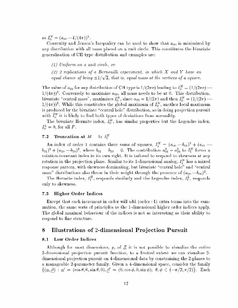
Figure 7: Two-dimensional indices in four dimensions of the ea beetle data: (a)
Contour of I
N
0
, (b) Perspective plot of I
N
0
, (c) Contour of I
N
1
, (d) Perspective plot of
I
N
1
.
1
2
3
4
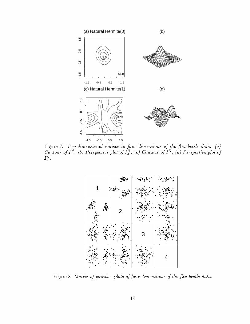
Figure 8: Matrix of pairwise plots of four dimensions of the ea beetle data.
18
-1.5 -0.5 0.5 1.5
-1.5
-0.5
0.5
1.5
(a) Legendre(2)
(1,2)
(3,2) (3,4)
(1,4)
(b)
-1.5 -0.5 0.5 1.5
-1.5
-0.5
0.5
1.5
(c) Legendre(15) (d)
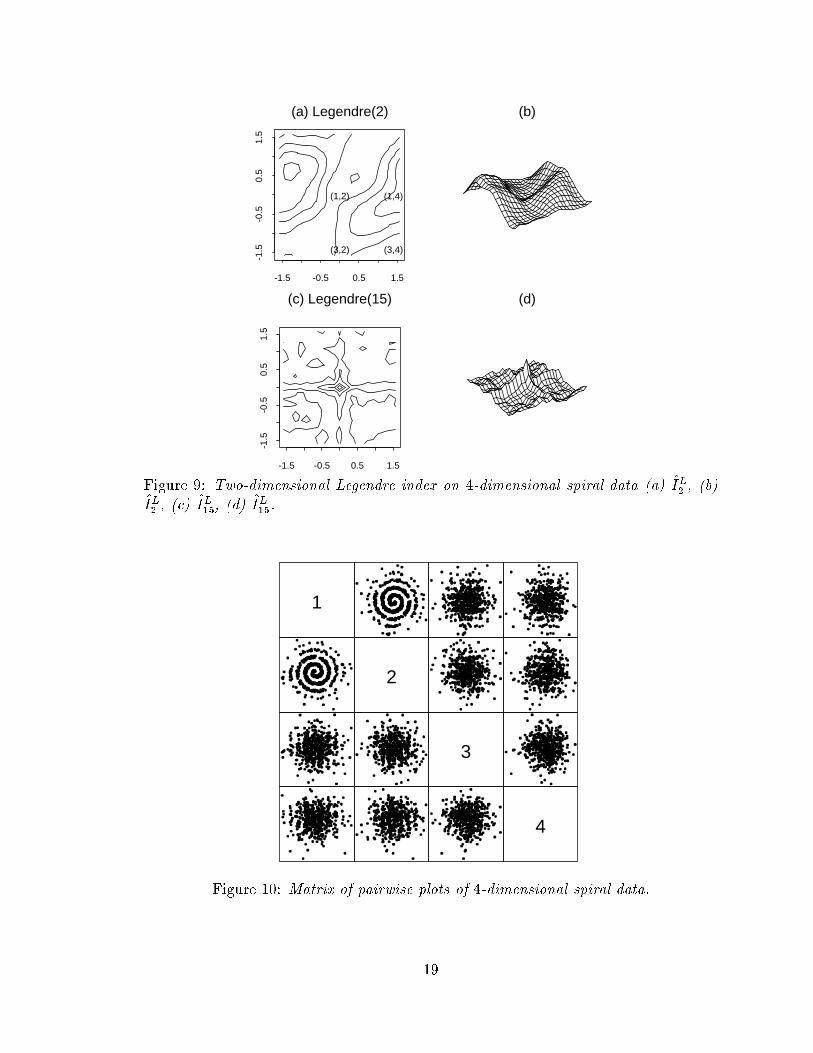
Figure 9: Two-dimensional Legendre index on 4-dimensional spiral data (a)
^
I
L
2
, (b)
^
I
L
2
, (c)
^
I
L
15
, (d)
^
I
L
15
.
1
2
3
4
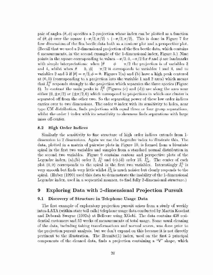
Figure 10: Matrix of pairwise plots of 4-dimensional spiral data.
19
pair of angles (�; �) speci�es a 2-projection whose index can be plotted as a function
of (�; �) over the square (��=2; �=2) � (��=2; �=2). This is done in Figure 7 for
four dimensions of the ea beetle data both as a contour plot and a perspective plot.
(Recall that we used a 2-dimensional projection of the ea beetle data, which contains
6 measurements, in the second example of the 1-dimensional index, Figure 5.) Nine
points in the square corresponding to values ��=2; 0;+�=2 for � and � are landmarks
with simple interpretations: when j�j = j�j = �=2 the projection is of variables 3
and 4, whilst when � = 0; j�j = �=2 it corresponds to variables 1 and 4, and to
variables 2 and 3 if j�j = �=2; � = 0. Figures 7(a) and (b) have a high peak centered
at (0; 0) (corresponding to a projection into the variable 1 and 2 axes) which means
that
^
I
N
0
responds strongly to the projection which separates the three species (Figure
8). In contrast the main peaks in
^
I
N
1
(Figures (c) and (d)) are along the axes near
either (0;��=2) or (��=2; 0) which correspond to projections in which one cluster is
separated o� from the other two. So the separating power of these low order indices
carries over to two dimensions. The order 0 index with its sensitivity to holes, near
type CM distribution, �nds projections with equal three or four group separations,
whilst the order 1 index with its sensitivity to skewness �nds separations with large
mass o�-center.
8.2 High Order Indices
Similarly the sensitivity to �ne structure of high order indices extends from 1-
dimension to 2-dimensions. Again we use the Legendre index to illustrate this. The
data, plotted in a matrix of pairwise plots in Figure 10, is formed from a bivariate
spiral in the �rst two variables and samples from a standard normal distribution in
the second two variables. Figure 9 contains contour and perspective plots of the
Legendre index, (a),(b) order 2,
^
I
L
2
and (c),(d) order 15,
^
I
L
15
. The center of each
plot (0; 0) corresponds to the spiral in the �rst two variables. Interestingly
^
I
L
2
is
very smooth but �nds very little whilst
^
I
L
15
is much noisier but clearly responds to the
spiral. (Huber (1990) used this data to demonstrate the inability of the 1-dimensional
Legendre index, used in a sequential manner, to �nd fully 2-dimensional structure.)
9 Exploring Data with 2-dimensional Projection Pursuit
9.1 Discovery of Structure in Telephone Usage Data
The �rst example of exploratory projection pursuit arises from a study of weekly
intra-LATA (within-state toll calls) telephone usage data conducted byMartin Koschat
and Deborah Swayne (1992a) at Bellcore using XGobi. The data contains 438 resi-
dential customers and 52 weeks of measurements of total usage. Some usual cleaning
of the data, including taking transformations and normal scores, was done prior to
the projection pursuit analysis, but we don't expand on this because it is not directly
pertinent to the illustration. The Hermite(1) index, used on the �rst 5 principal
components of the cleaned data, �nds a projection containing a \V" shape, which
20
x xx
x
x
xxxx
x
xx
x xx
x
x
x
x
x
x
x
x
x
xx
x
x xxx
xx
x x
xx
xx x
x
x
x
x
x
xx
xx
xx
xxx
x
x x
x
x
xx
x
x
x
xx
x xx
x
x
x
x
x
x
x
x
x x
xx
xxx
x
xx
x
x
x
x
x
x
x
xx
xx
x
x
x
x
x
x
x
x
x
x
x
x
xx
x
xx
xx
x
x x
x
x
x
xx
x
x
x
x
x
x
x
x
x
x
x
x
x
x
x
x
x
x
x
x x
xx
x
x
x
x x
x
xx
xx
x
x
x
x
x
x
x
x
x
x
x
x
x
x
x
x x
x
x
x
x
x
x
x
x
x
x
x
x
xxx
x
x
x
xxx x
xxx
x
x x
x
x
x
x
x
x
x
xx
x
x
x
x
xx
x
x
x
x
-3 -2 -1 0 1 2 3
-10
12
34
o
o
o
o
o
o
o
o
oo
o
o
o
oo
o
o
o
oo
oo
o
o
o
o
o
o
o
o
oo
oo
o
o
o
o
oo
o o
ooo
oo
o
o
o
o
o
o
o
o
o
o
o
o
o
o
o
o
oo
o
oo
oo
o
o
o
oo
o
o
o
o
o
o
o o
o
o
o
oo
o
o
o
oo
o
o
o
o
oo o
o
o
o
o
o
oo
o
o
o
o
o
oo oo
o
o
oo
o
oo
o
o
o
o
o
o
o
oo
o
o
o
o
o
o
oo
o
o
o
o
ooo
oo
o
o
o
o
o
o
o
o
o
oo
o
o
o
o
o
o
oo o
o
oo
o
oo
o
oo
oo
o
oo
o
oo
o
o
o
o
o
o
o
o
o
oo
ooo
o
o
o
o
o
o
o
o
o
oo
o
o
oo
o
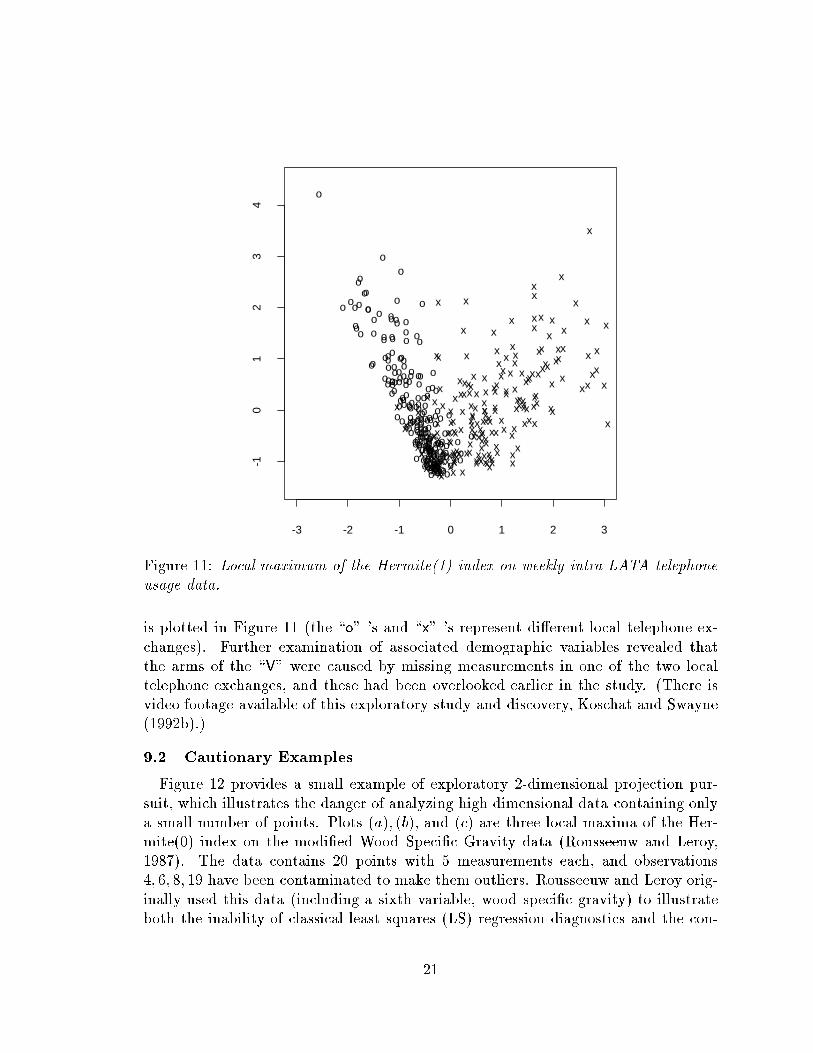
Figure 11: Local maximum of the Hermite(1) index on weekly intra-LATA telephone
usage data.
is plotted in Figure 11 (the \o" 's and \x" 's represent di�erent local telephone ex-
changes). Further examination of associated demographic variables revealed that
the arms of the \V" were caused by missing measurements in one of the two local
telephone exchanges, and these had been overlooked earlier in the study. (There is
video footage available of this exploratory study and discovery, Koschat and Swayne
(1992b).)
9.2 Cautionary Examples
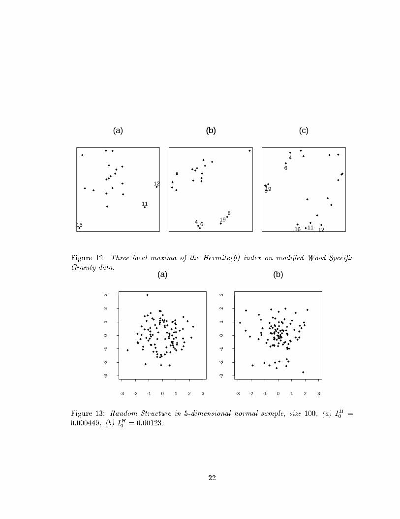
Figure 12 provides a small example of exploratory 2-dimensional projection pur-
suit, which illustrates the danger of analyzing high dimensional data containing only
a small number of points. Plots (a); (b), and (c) are three local maxima of the Her-
mite(0) index on the modi�ed Wood Speci�c Gravity data (Rousseeuw and Leroy,
1987). The data contains 20 points with 5 measurements each, and observations
4; 6; 8; 19 have been contaminated to make them outliers. Rousseeuw and Leroy orig-
inally used this data (including a sixth variable, wood speci�c gravity) to illustrate
both the inability of classical least squares (LS) regression diagnostics and the con-
21
11
12
16
(a)
6
819
(b)
4
(b)
4
6
8
11 1216
19
(c)
Figure 12: Three local maxima of the Hermite(0) index on modi�ed Wood Speci�c
Gravity data.
-3 -2 -1 0 1 2 3
-3-2
-10
12
3
(a)
-3 -2 -1 0 1 2 3
-3-2
-10
12
3
(b)
Figure 13: Random Structure in 5-dimensional normal sample, size 100, (a) I
H
0
=
0:000449, (b) I
H
0
= 0:00123.
22
trasting capabilities of resistant Least Median Squares (LMS) regression diagnostics
in �nding the arti�cial outliers. In their analysis the LMS diagnostics reveal the
expected outliers, 4; 6; 8; 19, whereas the LS diagnostics suggest other points, for ex-
ample 11; 12; 16, are outlying. From the projection pursuit solutions (a); (b), it is
evident that all of these points may be in uential outliers. In fact plot (c) shows that
all points lie near a convex shell leaving an \empty center". (The authors have since
acknowledged the shortcomings of using this data to illustrate resistant methods.)
To further illustrate the danger of putting too much emphasis on structures found in
sparse high dimensional data Figure 13 displays two local maxima of the Hermite(0)
index on a sample of size 100 from a 5-dimensional standard normal distribution.
The projection in plot (a) contains a very small central hole, and plot (b) shows a
central mass concentration (plus a small separated cluster!). Looking at the index
values, 0:000449 and 0:00123, we see the values are quite small compared to the
absolute maximum that can be achieved (0:00556 for type CH, and 0:0796 for type
CM). So we issue a word of warning: exploratory projection pursuit will always �nd
structure, albeit weak, but care must be taken when emphasizing the signi�cance
of this structure (see Sun (1991) for a discussion of p-values for the 1-dimensional
Legendre index).
10 Discussion
There are a few matters related to our analysis that warrant attention.
The �rst is the signi�cance of the individual terms of the expansion as indices in
themselves. Notably each is minimized by the Normal distribution and is sensitive to
particular di�erences. We saw this in looking separately at the �rst and second terms.
They could be considered to be \template"-type indices because of their particular
sensitivity, and this leads to another approach in constructing projection pursuit
indices: construct a measure for a particular type of structure. An example of this
would be to reformat the �rst term of the Hermite indices by dropping the square
and simply using the negative coe�cient. This measure would speci�cally respond to
\central holes". Also recent developments with using wavelets as a tool for density
estimation may lead to even better tailoring for speci�c structure.
The other matters concern related work. Gnanadesikan (1977, p. 142-3), proposes
a 1-parameter family of methods for �nding directions of non-normality in multi-
variate data. Opposite ends of the parameter scale correspond to methods sensitive
to outlying observations and inlying clusters, respectively. Jee (1985) conducts an
empirical comparison of projection pursuit indices based on non-normality measures
such as Information and Entropy using histogram density estimation. Morton (1989)
in her work on modifying projection pursuit to trade accuracy for interpretability
adapts the bivariate Legendre index by transformations into a Fourier index. This
uses both Laguerre polynomials and trigonometric functions to expand the bivariate
data density. We suspect that it behaves like the bivariate Hermite indices.
23
Appendix
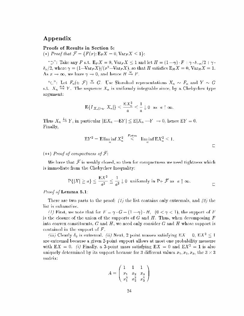
Proofs of Results in Section 5:
(�) Proof that
�
F = fF (x): E
F
X = 0;Var
F
X � 1g:
\�": Take any F s.t. E
F
X = 0, Var
F
X � 1 and let H = (1� ) �F + � �
�x
=2+ �
�
x
=2, where = (1�Var
F
X)=(x
2
�Var
F
X), so thatH satis�es E
H
X = 0, Var
H
X = 1.
As x!1, we have ! 0, and hence H
w
! F .
\�": Let F
n
(2 F)
w
! G. Use Skorohod representations X
n
� F
n
and Y � G
s.t. X
n
a:s:
! Y . The sequence X
n
is uniformly integrable since, by a Chebychev-type
argument:
EfI
jX
n
j�a
:jX
n
jg �
EX
2
n
a
�
1
a
# 0 as a " 1:
Thus X
n
L
1
! Y , in particular jEX
n
� EY j � EjX
n
� Y j ! 0, hence EY = 0.
Finally,
EY
2
= E lim inf
n
X
2
n
Fatou
� lim inf
n
EX
2
n
� 1:
2
(��) Proof of compactness of
�
F :
We have that
�
F is weakly closed, so then for compactness we need tightness which
is immediate from the Chebychev Inequality:
PfjXj � ag �
EX
2
a
2
�
1
a
2
# 0 uniformly in P2
�
F as a " 1:
2
Proof of Lemma 5.1:
There are two parts to the proof: (1) the list contains only extremals, and (2) the
list is exhaustive.
(1) First, we note that for F = �G+ (1� ) �H; (0 < < 1), the support of F
is the closure of the union of the supports of G and H. Thus, when decomposing F
into convex constituents, G and H, we need only consider G and H whose support is
contained in the support of F .
(iii) Clearly �
0
is extremal. (ii) Next, 2-point masses satisfying EX = 0, EX
2
� 1
are extremal because a given 2-point support allows at most one probability measure
with EX = 0. (i) Finally, a 3-point mass satisfying EX = 0 and EX
2
= 1 is also
uniquely determined by its support because for 3 di�erent values x
1
; x
2
; x
3
, the 3� 3
matrix:
A =
0
B
@
1 1 1
x
1
x
2
x
3
x
2
1
x
2
2
x
2
3
1
C
A
24
is of the Vandermonde type, hence has maximal rank and allows only one solution
= (
1
;
2
;
3
)
0
of A = (1; 0; 1)
0
.
(2) We show that (i) a convex mixture F of 4 linearly independent components
cannot be extremal if E
F
X = 0 and E
F
X
2
= 1, (ii) a convex mixture F of 3 linearly
independent components cannot be extremal if E
F
X = 0 and 0 <E
F
X
2
< 1, while
case (iii) is trivial: E
F
X = 0, E
F
X
2
= 0) F = �
0
.
(i) Let F =
P
4
1
i
G
i
, E
F
X = 0, E
F
X
2
= 1.
The set A = f(
1
;
2
;
3
;
4
):
i
� 0;
P
4
1
i
= 1g is a 3-dimensional simplex whose
faces are described by one of
i
= 0. The subset of A satisfying
P
4
1
i
E
G
i
X = 0 and
P
4
1
i
E
G
i
X
2
= 1 forms at least a 1-dimensional segment through A which intersects
with a face on both ends. This implies that F is not extremal, unless it already lies
on a face
i
= 0, that is, it is really a 3-component mixture.
(ii) This case is solved by considering linearly independent 3-component mixtures
F satisfying E
F
X = 0, E
F
X
2
< 1. The set A = f(
1
;
2
;
3
):
i
� 0;
P
3
1
i
= 1g is
a 2-dimensional simplex with faces
i
= 0, and also
P
3
1
i
E
G
i
X
2
= 1. The condition
P
3
1
i
E
G
i
X = 0 traces a segment out of A which intersects with a face
i
= 0 or
P
3
1
i
E
G
i
X
2
= 1. Thus, for F to be extremal it would have to be at
i
= 0, that is, a
2-component mixture, or F would have to satisfy the unit variance constraint, which
is excluded by assumption.
2
Proof of Proposition 5.2:
(i) Let F 2
�
F be arbitrary and G = �
1
=2 + �
�1
=2:
a
0
(F ) =
1
p
2�
E
F
e
�
1
2
X
2
�
1
p
2�
e
�
1
2
E
F
X
2
by Jensen's inequality
�
1
p
2�
e
�
1
2
since E
F
X
2
� 1
=
1
p
2�
E
G
e
�
1
2
X
2
= a
0
(G)
(ii) Let F 2
�
F be arbitrary and G = �
0
:
a
0
(F ) = E
F
�(X) � �(0) = E
G
�(X) = a
0
(G)
2
Proof of Proposition 5.3:
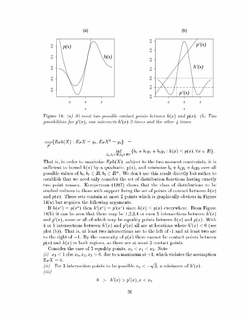
Let h(x) = x�(x); p(x) = b
0
+ b
1
x + b
2
x
2
where b
0
; b
1
; b
2
are arbitrary constants,
and let y
1
= 0; y
2
= 1, then by a result in Kemperman (1987) (originally from an
article in German by Richter, 1957):
25
x
-2 0 2
-0.2
-0.1
0.0
0.1
0.2
(a)
h(x)
p(x)
x
-2 0 2
-0.2
-0.1
0.0
0.1
0.2
0.3
0.4
(b)
h’(x)
p’(x)
p’(x)
Figure 14: (a) At most two possible contact points between h(x) and p(x). (b) Two
possibilities for p
0
(x), one intersects h
0
(x) 3 times and the other 4 times.
sup
F
fE
F
h(X) : E
F
X = y
1
; E
F
X
2
= y
2
g =
inf
b
0
;b
1
2IR;b
2
2IR
+
fb
0
+ b
1
y
1
+ b
2
y
2
: h(x) � p(x);8x 2 IRg:
That is, in order to maximize E
F
h(X), subject to the two moment constraints, it is
su�cient to bound h(x) by a quadratic, p(x), and minimize b
0
+ b
1
y
1
+ b
2
y
2
over all
possible values of b
0
; b
1
2 IR; b
2
2 IR
+
. We don't use this result directly but rather to
establish that we need only consider the set of distribution functions having exactly
two point masses. Kemperman (1987) shows that the class of distributions to be
studied reduces to those with support being the set of points of contact between h(x)
and p(x). These sets contain at most 2 points which is graphically obvious in Figure
14(a) but requires the following arguments.
If h(x
�
) = p(x
�
) then h
0
(x
�
) = p
0
(x
�
) since h(x) � p(x) everywhere. From Figure
14(b) it can be seen that there may be 1,2,3,4 or even 5 intersections between h
0
(x)
and p
0
(x), some or all of which may be equality points between h(x) and p(x). With
4 or 5 intersections between h
0
(x) and p
0
(x) all are at locations where h
0
(x) < 0 (see
plot (b)). That is, at least two intersections are to the left of -1 and at least two are
to the right of +1. By the convexity of p(x) there cannot be contact points between
p(x) and h(x) in both regions, so there are at most 3 contact points.
Consider the case of 3 equality points, x
0
< x
1
< x
2
. Note
(i) x
2
< 1 else x
0
; x
1
; x
2
> 0, due to a maximum at +1, which violates the assumption
E
F
X = 0.
(ii) For 3 intersection points to be possible x
0
< �
p
3, a minimum of h
0
(x).
(iii)
0 > h
0
(x) > p
0
(x); x < x
0
26
h
0
(x) < p
0
(x); x
0
< x < x
1
(7)
h
0
(x) > p
0
(x); x
1
< x < x
2
h
0
(x) < p
0
(x); x > x
2
Assume that x
0
is a contact point, that is, h(x
0
) = p(x
0
), and write h(x
1
) = h(x
0
) +
R
x
1
x
0
h
0
(x)dx and p(x
1
) = p(x
0
) +
R
x
1
x
0
p
0
(x)dx. Then h(x
1
) � p(x
1
) =
R
x
1
x
0
(h
0
(x) �
p
0
(x))dx < 0 by (7). Therefore h(x
1
) 6= p(x
1
) ) there are at most three contact
points.
The set of all two point mass distributions can be completely characterized by one
unknown parameter, which we call , because of the mean and variance constraints.
2
Acknowledgements
We would like to thank our colleagues at Bellcore and Rutgers, particularly Martin
Maechler, Diane Du�y, David Tyler and Cunhui Zhang, Jop Kemperman and Andrew
McDougall, for many useful and informative discussions. In addition we appreciate
the comments of three anonymous referees.
We are very grateful to Martin Koschat and Deborah Swayne for allowing us to
use their telephone usage data and for providing us with an example of projection
pursuit being responsible for a practical discovery.
References
Abramowitz, M. and Stegun, I. A. (1972). Handbook of Mathematical Functions.
Dover, New York.
Andrews, D. F., Gnanadesikan, R., and Warner, J. L. (1971). Transformations of
Multivariate Data. Biometrics, 27:825{840.
Cook, D., Buja, A., and Cabrera, J. (1991). Direction and Motion Control in the
Grand Tour. In Keramidas, E., editor, Proc. of the 23rd Symp. on the Interface
between Comput. Sci. and Statist., Seattle, WA. Interface Foundation of North
America.
Friedman, J. H. (1987). Exploratory Projection Pursuit. J. Amer. Statist. Assoc.,
82:249{266.
Friedman, J. H. and Tukey, J. W. (1974). A Projection Pursuit Algorithm for Ex-
ploratory Data Analysis. IEEE Trans. Comput. C, 23:881{889.
Gnandesikan, R. (1977). Methods for Statistical Data Analysis of Multivariate Ob-
servations. Wiley, New York.
27
Hall, P. (1989). Polynomial Projection Pursuit. Ann. Statist., 17:589{605.
Huber, P. J. (1985). Projection Pursuit (with discussion). Ann. Statist., 13:435{525.
Huber, P. J. (1990). Data Analysis and Projection Pursuit. Technical Report PJH-
90-1, M.I.T.
Jackson, D. (1936). Formal Properties of Orthogonal Polynomials in Two Variables.
Ann. Math., 37:423{434.
Jee, J. R. (1985). A Study of Projection Pursuit Methods. Technical Report TR
776-311-4-85, Rice University.
Jones, M. C. (1983). The Projection Pursuit Algorithm for Exploratory Data Analysis.
PhD thesis, Univerity of Bath.
Jones, M. C. and Sibson, R. (1987). What is Projection Pursuit? (with discussion).
J. Roy. Statist. Soc. Ser. A, 150:1{36.
Kemperman, J. H. B. (1987). Geometry of the Moment Problem. In Landau, H. J.,
editor, Proc. of the Symp. in App. Math., San Antonio, TX. A.M.S.
Knuth, D. E. (1981). The Art of Computer Programming. Vol. 2: Seminumerical
Algorithms. Addison-Wesley, Reading, Mass.
Koschat, M. A. and Swayne, D. F. (1992a). Visualizing Panel Data. Technical
Memorandum, Bellcore, Morristown, N.J.
Koschat, M. A. and Swayne, D. F. (1992b). Visualizing Panel Data. Video available
by request to [email protected].
Kruskal, J. B. (1969). Toward a practical method which helps uncover the structure
of a set of observations by �nding the line transformation which optimizes a new
\index of condensation". In Milton, R. C. and Nelder, J. A., editors, Statistical
Computation, pages 427{440. Academic Press, New York.
Lubischew, A. A. (1962). On the Use of Discriminant Functions in Taxonomy. Bio-
metrics, 18:455{477.
Morton, S. C. (1989). Interpretable Projection Pursuit. Technical Report 106, Lab.
for Computat. Statist., Stanford Univ.
Rousseeuw, P. J. and Leroy, A. M. (1987). Robust Regression and Outlier Detection.
Wiley, New York.
Sansone, G. (1959). Orthogonal Functions. Interscience Publ. Inc., New York.
28
Sun, J. (1991). Signi�cance Levels in Exploratory Projection Pursuit. Biometrika,
78(4):759{769.
Swayne, D. F., Cook, D., and Buja, A. (1991). XGobi: Interactive Dynamic Graphics
in the X Window System with a Link to S. In ASA Proc. of the Section on
Statistical Graphics, pages 1{8.
Thisted, R. A. (1988). Elements of Statistical Computing. Chapman and Hall, New
York.
Upensky, J. V. (1927). On the Development of Arbitrary Functions in Series of
Hermite and Laguerre's Polynomials. Ann. Math., 28:593{619.
29


