Minimax Optimal Bayesian Aggregation

Yun Yang and David Dunson

Abstract

It is generally believed that ensemble approaches, which combine multiple algorithms or

models, can outperform any single algorithm at machine learning tasks, such as prediction.

In this paper, we propose Bayesian convex and linear aggregation approaches motivated by

regression applications. We show that the proposed approach is minimax optimal when the

true data-generating model is a convex or linear combination of models in the list. Moreover,

the method can adapt to sparsity structure in which certain models should receive zero weights,

and the method is tuning parameter free unlike competitors. More generally, under an M-

open view when the truth falls outside the space of all convex/linear combinations, our theory

suggests that the posterior measure tends to concentrate on the best approximation of the

truth at the minimax rate. We illustrate the method through simulation studies and several

applications.

Key words: Dirichlet aggregation; Ensemble learning; Minimax risk; Misspecification;

Model averaging; Shrinkage prior.

1. Introduction

In many applications, it is not at all clear how to pick one most suitable method out of a list

of possible models or learning algorithms M = M1, . . . ,MM. Each model/algorithm has its

own set of implicit or explicit assumptions under which that approach will obtain at or near

optimal performance. However, in practice verifying which if any of these assumptions hold for

a real application is problematic. Hence, it is of substantial practical importance to have an

aggregating mechanism that can automatically combine the estimators f1, . . . , fM obtained from

the M different approaches M1, . . . ,MM , with the aggregated estimator potentially better than

any single one.

Towards this goal, three main aggregation strategies receive most attention in the literature:

model selection aggregation (MSA), convex aggregation (CA) and linear aggregation (LA), as

first stated by Nemirovski (2000). MSA aims at selecting the optimal single estimator from

the list; CA considers searching for the optimal convex combination of the estimators; and LA

focuses on selecting the optimal linear combination. Although there is an extensive literature

(Juditsky and Nemirovski, 2000; Tsybakov, 2003; Wegkamp, 2003; Yang, 2000, 2001, 2004; Bunea

1

and Nobel, 2008; Bunea and Tsybakov, 2007; Guedj and Alquier, 2013; van der Laan et al., 2007)

on aggregation, there has been limited consideration of Bayesian approaches.

In this paper, we study Bayesian aggregation procedures and their performance in regression.

Consider the regression model

Yi = f(Xi) + εi, i = 1, . . . , n, (1.1)

where Yi is the response variable, f : X → R is an unknown regression function, X is the feature

space, Xi’s are the fixed- or random-designed elements in X and the errors are iid Gaussian.

Aggregation procedures typically start with randomly dividing the sample Dn = (X1, Y1),

. . . , (Xn, Yn) into a training set for constructing estimators f1, . . . , fM , and a learning set for

constructing f . Our primary interest is in the aggregation step, so we adopt the convention

(Bunea and Tsybakov, 2007) of fixing the training set and treating the estimators f1, . . . , fM

as fixed functions f1, . . . , fM . Our results can also be translated to the context where the fixed

functions f1, . . . , fM are considered as a functional basis (Juditsky and Nemirovski, 2000), either

orthonormal or overcomplete, or as “weak learners” (van der Laan et al., 2007). For example,

high-dimensional linear regression is a special case of LA where fj maps an M -dimensional vector

into its jth component.

Bayesian model averaging (BMA) (Hoeting et al., 1999) provides an approach for aggregation,

placing a prior over the ensemble and then updating using available data to obtain posterior model

probabilities. For BMA, f can be constructed as a convex combination of estimates f1, . . . , fM

obtained under each model, with weights corresponding to the posterior model probabilities. If

the true data generating model f0 is one of the models in the pre-specified list (“M-closed” view),

then as the sample size increases the weight on f0 will typically converge to one. With a uniform

prior over M in the regression setting with Gaussian noise, f coincides with the exponentially

weighted aggregates (Tsybakov, 2003). However, BMA relies on the assumption thatM contains

the true model. If this assumption is violated (“M-open”), then f tends to converge to the

single model in M that is closest to the true model in Kullback-Leibler (KL) divergence. For

example, when f0 is a weighted average of f1 and f2, under our regression setting f will converge

to f ∈ f1, f2 that minimizes ||f − f0||2n = n−1∑n

i=1 |f(Xi) − f0(Xi)|2 under fixed design or

||f − f0||2Q = EQ|f(X) − f0(X)|2 under random design where X ∼ Q. Henceforth, we use the

notation || · || to denote || · ||n or || · ||Q depending on the context.

In this paper, we primarily focus on Bayesian procedures for CA and LA. Let

FH =fλ =

M∑j=1

λjfj : λ = (λ1, . . . , λM ) ∈ H

be the space of all aggregated estimators for f0 with index set H. For CA, H takes the form of

Λ = (λ1, . . . , λM ) : λj ≥ 0, j = 1, . . . ,M,∑M

j=1 λj = 1 and for LA, H = Ω = (λ1, . . . , λM ) :

2

λj ∈ R, j = 1, . . . ,M,∑M

j=1 |λj | ≤ L, where L > 0 can be unknown but is finite. In addition,

for both CA and LA we consider sparse aggregation with FHs , where an extra sparsity structure

||λ||0 = s is imposed on the weight λ ∈ Hs = λ ∈ H : ||λ||0 = s. Here, for a vector θ ∈ RM , we

use ||θ||p = (∑M

j=1 |θj |p)1/p to denotes its lp-norm for 0 ≤ p ≤ ∞. In particular, ||θ||0 is the number

of nonzero components of θ. The sparsity level s is allowed to be unknown and expected to be

learned from data. In the sequel, we use the notation fλ∗ to denote the best || · ||-approximation

of f0 in FH . Note that if f0 ∈ FH , then f0 = fλ∗ .

One primary contribution of this work is to propose a new class of priors, called Dirichlet

aggregation (DA) priors, for Bayesian aggregation. Bayesian approaches with DA priors are shown

to lead to the minimax optimal posterior convergence rate over FH for CA and LA, respectively.

More interestingly, DA is able to achieve the minimax rate of sparse aggregation (see Section

1.1), which improves the minimax rate of aggregation by utilizing the extra sparsity structure

on λ∗. This suggests that DA is able to automatically adapt to the unknown sparsity structure

when it exists but also has optimal performance in the absence of sparsity. Such sparsity adaptive

properties have also been observed in Bunea and Tsybakov (2007) for penalized optimization

methods. However, in order to achieve minimax optimality, the penalty term, which depends on

either the true sparsity level s or a function of λ∗, needs to be tuned properly. In contrast, the

DA does not require any prior knowledge on λ∗ and is tuning free.

Secondly, we also consider an “M-open” view for CA and LA, where the truth f0 can not only

fall outside the listM, but also outside the space of all convex/linear combinations of the models

in M. Under the “M-open” view, our theory suggests that the posterior measure tends to put

all its mass into a ball around the best approximation fλ∗ of f0 with a radius proportional to

the minimax rate. The metric that defines that ball will be made clear later. This is practically

important because the true model in reality is seldom correctly specified and a convergence to

fλ∗ is the best one can hope for. Bayesian asymptotic theory for misspecified models is under

developed, with most existing results assuming that the model class is either known or is an

element of a known list. One key step is to construct appropriate statistical tests discriminating

fλ∗ from other elements in FH . Our tests borrow some results from Kleijn and van der Vaart

(2006) and rely on concentration inequalities.

The proposed prior on λ induces a novel shrinkage structure, which is of independent interest.

There is a rich literature on theoretically optimal models based on discrete (point mass mix-

ture) priors (Ishwaran and Rao, 2005; Castillo and van der Vaart, 2012) that are supported on a

combinatorial model space, leading to heavy computational burden. However, continuous shrink-

age priors avoid stochastic search variable selection algorithms (George and McCulloch, 1997) to

sample from the combinatorial model space and can potentially improve computational efficiency.

Furthermore, our results include a rigorous investigation on M -dimensional symmetric Dirichlet

3

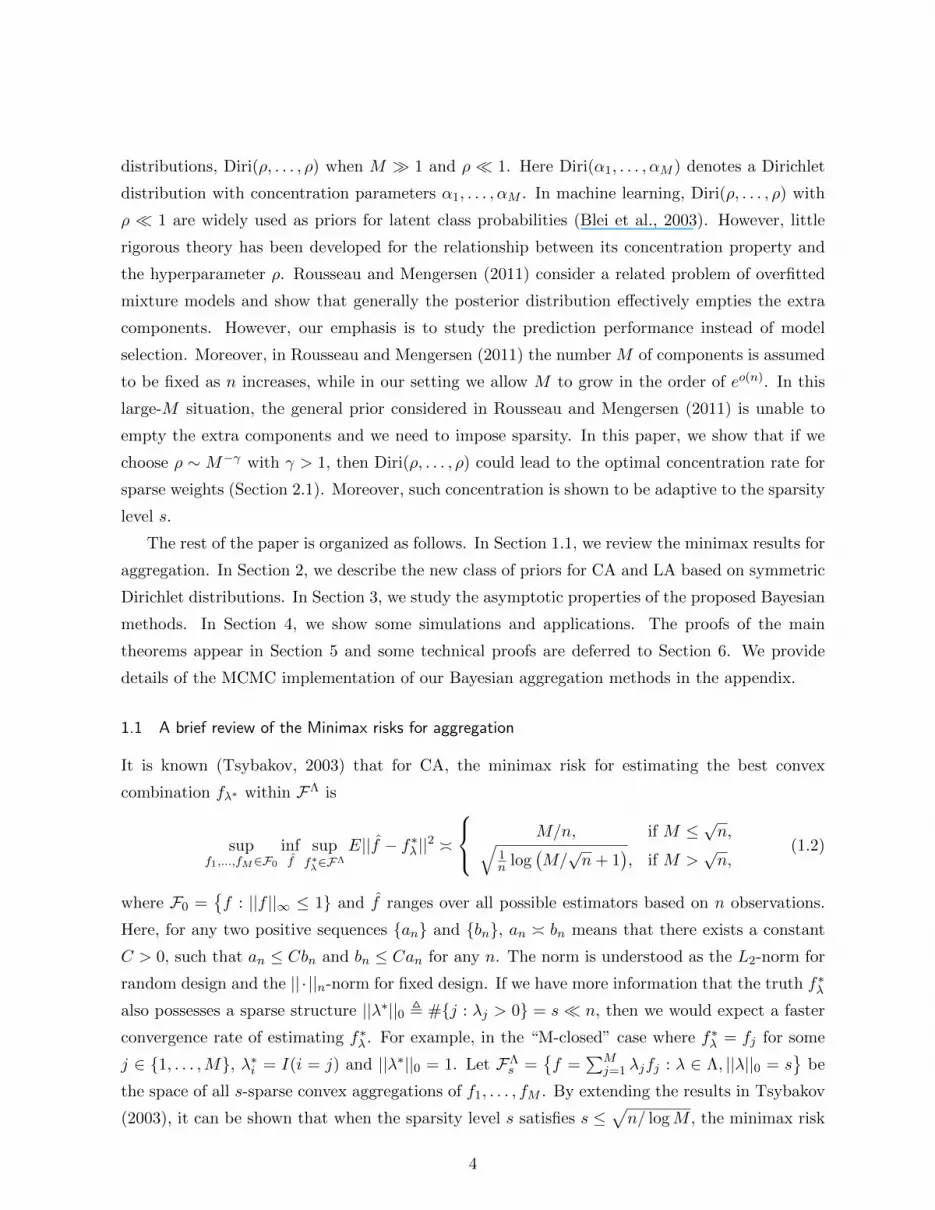
distributions, Diri(ρ, . . . , ρ) when M 1 and ρ 1. Here Diri(α1, . . . , αM ) denotes a Dirichlet

distribution with concentration parameters α1, . . . , αM . In machine learning, Diri(ρ, . . . , ρ) with

ρ 1 are widely used as priors for latent class probabilities (Blei et al., 2003). However, little

rigorous theory has been developed for the relationship between its concentration property and

the hyperparameter ρ. Rousseau and Mengersen (2011) consider a related problem of overfitted

mixture models and show that generally the posterior distribution effectively empties the extra

components. However, our emphasis is to study the prediction performance instead of model

selection. Moreover, in Rousseau and Mengersen (2011) the number M of components is assumed

to be fixed as n increases, while in our setting we allow M to grow in the order of eo(n). In this

large-M situation, the general prior considered in Rousseau and Mengersen (2011) is unable to

empty the extra components and we need to impose sparsity. In this paper, we show that if we

choose ρ ∼ M−γ with γ > 1, then Diri(ρ, . . . , ρ) could lead to the optimal concentration rate for

sparse weights (Section 2.1). Moreover, such concentration is shown to be adaptive to the sparsity

level s.

The rest of the paper is organized as follows. In Section 1.1, we review the minimax results for

aggregation. In Section 2, we describe the new class of priors for CA and LA based on symmetric

Dirichlet distributions. In Section 3, we study the asymptotic properties of the proposed Bayesian

methods. In Section 4, we show some simulations and applications. The proofs of the main

theorems appear in Section 5 and some technical proofs are deferred to Section 6. We provide

details of the MCMC implementation of our Bayesian aggregation methods in the appendix.

1.1 A brief review of the Minimax risks for aggregation

It is known (Tsybakov, 2003) that for CA, the minimax risk for estimating the best convex

combination fλ∗ within FΛ is

supf1,...,fM∈F0

inff

supf∗λ∈FΛ

E||f − f∗λ ||2

M/n, if M ≤√n,√

1n log

(M/√n+ 1

), if M >

√n,

(1.2)

where F0 =f : ||f ||∞ ≤ 1 and f ranges over all possible estimators based on n observations.

Here, for any two positive sequences an and bn, an bn means that there exists a constant

C > 0, such that an ≤ Cbn and bn ≤ Can for any n. The norm is understood as the L2-norm for

random design and the || · ||n-norm for fixed design. If we have more information that the truth f∗λ

also possesses a sparse structure ||λ∗||0 , #j : λj > 0 = s n, then we would expect a faster

convergence rate of estimating f∗λ . For example, in the “M-closed” case where f∗λ = fj for some

j ∈ 1, . . . ,M, λ∗i = I(i = j) and ||λ∗||0 = 1. Let FΛs =

f =

∑Mj=1 λjfj : λ ∈ Λ, ||λ||0 = s

be

the space of all s-sparse convex aggregations of f1, . . . , fM . By extending the results in Tsybakov

(2003), it can be shown that when the sparsity level s satisfies s ≤√n/ logM , the minimax risk

4

of estimating an element in FΛs is given by

supf1,...,fM∈F0

inff

supf∗λ∈FΛ

s

E||f − f∗λ ||2 s

nlog

(M

s

). (1.3)

From the preceding results,√n/ logM serves as the sparsity/non-spasrsity boundary of the weight

λ∗ as there is no gain in the estimation efficiency if s >√n/ logM .

From Tsybakov (2003), the minimax risk for LA with H = RM is

supf1,...,fM∈F0

inff

supf∗λ∈FRM

E||f − f∗λ ||2 M/n.

As a result, general LA is only meaningful when M/n → 0, as n → ∞. Similarly, the above

minimax risk can be extended to s-sparse LA FRMs =

f =

∑Mj=1 λjfj : λ ∈ RM , ||λ||0 = s

for

s ∈ 1, . . . ,M as

supf1,...,fM∈F0

inff

supf∗λ∈FRM

s

E||f − f∗λ ||2 s

nlog

(M

s

).

Note that for sparse LA, the sparsity level s can be arbitrary. A simple explanation is that the

constraint ||λ∗||1 = 1 ensures that every element in FΛ can be approximated with error at most√1n log

(M/√n+ 1

)by some

√n/ logM -sparse element in FΛ (see Lemma 6.1). However, if we

further assume that ||λ∗|| ≤ A and restrict fλ∗ ∈ FΩ, then by extending Tsybakov (2003), it can

be shown that the minimax risks of LA of FRMA is the same as those of convex aggregation under

a non-sparse structure as (1.2) and a sparse structure as (1.3).

2. Bayesian approaches for aggregation

2.1 Concentration properties of high dimensional symmetric Dirichlet distributions

Consider an M -dimensional symmetric Dirichlet distribution Diri(ρ, . . . , ρ) indexed by a concen-

tration parameter ρ > 0, whose pdf at λ ∈ Λ is given by Γ(Mρ)Γ(ρ)−M∏Mj=1 λ

ρ−1j , where Γ(·)

is the Gamma function. M -dimensional Dirichlet distributions are commonly used in Bayesian

procedures as priors over the M − 1-simplex. For example, Dirichlet distributions can be used

as priors for probability vectors for latent class allocation. In this subsection, we investigate the

concentration properties of Diri(ρ, . . . , ρ) when M 1 and ρ 1. Fig. 2.1 displays typical

patterns for 3-dimensional Dirichlet distributions Diri(ρ, ρ, ρ) with ρ changing from moderate to

small. As can be seen, the Dirichlet distribution tends to concentrate on the boundaries for small

ρ, which is suitable for capturing sparsity structures.

To study the concentration of Diri(ρ, . . . , ρ), we need to characterize the space of sparse weight

vectors. Since Dirichlet distributions are absolutely continuous, the probability of generating an

5

ρ=1

(a) ρ = 1.

ρ=0.1

(b) ρ = 0.1.

ρ=0.01

(c) ρ = 0.01.

Figure 1: Symmetric Dirichlet distributions with different values for the concentration parameter.

Each plot displays 100 independent draws from Diri(ρ, ρ, ρ).

exactly s-sparse vector is zero for any s < M . Therefore, we need to relax the definition of

s-sparsity. Consider the following set indexed by a tolerance level ε > 0 and a sparsity level

s ∈ 1, . . . ,M: FΛs,ε = λ ∈ Λ :

∑Mj=s+1 λ(j) ≤ ε, where λ(1) ≥ λ(2) ≥ · · · ≥ λ(M) is the ordered

sequence of λ1, . . . , λM . FΛs,ε consists of all vectors that can be approximated by s-sparse vectors

with l1-error at most ε. The following theorem shows the concentration property of the symmetric

Dirichlet distribution Diri(ρ, . . . , ρ) with ρ = α/Mγ . This theorem is a easy consequence of Lemma

5.1 and Lemma 5.4 in Section 5.

Theorem 2.1. Assume that λ ∼ Diri(ρ, . . . , ρ) with ρ = α/Mγ and γ > 1. Let λ∗ ∈ Λs be any

s-sparse vector in the M − 1-dimensional simplex Λ. Then for any ε ∈ (0, 1) and some C > 0,

P (||λ− λ∗||2 ≤ ε) & exp

− Cγs log

M

ε

, (2.1)

P (λ /∈ FΛs,ε) . exp

− C(γ − 1)s log

M

ε

. (2.2)

The proof of (2.2) utilizes the stick-breaking representation of Dirichlet processes (Sethuraman,

1994) and the fact that Diri(ρ, . . . , ρ) can be viewed as the joint distribution of(G([0, 1/M)), . . . ,

G([(M − 1)/M, 1)))

where G ∼ Dirichlet process DP((Mρ)U) with U the uniform distribution

on [0, 1]. The condition γ > 1 in Theorem 2.1 reflects the fact that the concentration parameter

Mρ = αM−(γ−1) should decrease to 0 as M → ∞ in order for DP((Mρ)U) to favor sparsity.

(2.2) validates our observations in Fig. 2.1 and (2.1) suggests that the prior mass around every

sparse vector is uniformly large since the total number of s-sparse patterns (locations of nonzero

components) in Λ is of order expCs log(M/s). In fact, both (2.1) and (2.2) play crucial roles

in the proofs in Section 5.1 on characterizing the posterior convergence rate εn for the Bayesian

method below for CA (also true for more general Bayesian methods), where εn is a sequence

satisfying P (||λ − λ∗||2 ≤ εn) & exp(−nε2n) and P (λ /∈ FΛs,ε) . exp(−nε2n). Assume the best

approximation fλ∗ of the truth f0 to be s-sparse. (2.2) implies that the posterior distribution of

6

λ tends to put almost all its mass in FΛs,ε and (2.1) is required for the posterior distribution to be

able to concentrate around λ∗ at the desired minimax rate given by (1.2).

2.2 Using Dirichlet priors for Convex Aggregation

In this subsection, we assume Xi to be random with distribution Q and f0 ∈ L2(Q). Here, for a

probability measure Q on a space X , we use the notation || · ||Q to denote the norm associated

with the square integrable function space L2(Q) = f :∫X |f(x)|2dQ(x) ≤ ∞. We assume

the random design for theoretical convenience and the procedure and theory for CA can also be

generalized to fixed design problems. Assume the M functions f1, . . . , fM also belong to L2(Q).

Consider combining these M functions into an aggregated estimator f =∑M

j=1 λjfj , which tries

to estimate f0 by elements in the space FΛ =f =

∑Mj=1 λjfj : λj ≥ 0,

∑Mj=1 λj = 1

of all

convex combinations of f1, . . . , fM . The assumption that f1, . . . , fM are fixed is reasonable as

long as different subsets of samples are used for producing f1, . . . , fM and for aggregation. For

example, we can divide the data into two parts and use the first part for estimating f1, . . . , fM

and the second part for aggregation.

We propose the following Dirichlet aggregation (DA) prior:

(DA) f =

M∑j=1

λjfj , (λ1, . . . , λM ) ∼ Diri

(α

Mγ, . . . ,

α

Mγ

),

where (γ, α) are two positive hyperparameters. As Theorem 2.1 and the results in Section 5

suggest, such a symmetric Dirichlet distribution is favorable since Diri(α1, . . . , αM ) with equally

small parameters α1 = . . . = αM = α/Mγ for γ > 1 has nice concentration properties under both

sparse and nonsparse L1 type conditions, leading to near minimax optimal posterior contraction

rate under both scenarios.

We also mention a related paper (Bhattacharya et al., 2013) that uses Dirichlet distributions in

high dimensional shrinkage priors, where they considered normal mean estimating problems. They

proposed a new class of Dirichlet Laplace priors for sparse problems, with the Dirichlet placed on

scaling parameters of Laplace priors for the normal means. Our prior is fundamentally different

in using the Dirichlet directly for the weights λ, including a power γ for M . This is natural for

aggregation problems, and we show that the proposed prior is simultaneously minimax optimal

under both sparse and nonsparse conditions on the weight vector λ as long as γ > 1.

2.3 Using Dirichlet priors for Linear Aggregation

For LA, we consider a fixed design for Xi ∈ Rd and write (1.1) into vector form as Y = F0 + ε,

ε ∼ N(0, σ2In), where Y = (Y1, . . . , yn) is the n× 1 response vector, F0 = (f0(X1), . . . , f0(Xn))T

is the n × 1 vector representing the expectation of Y and In is the n × n identity matrix. Let

7

F = (Fij) = (fj(Xx)) be the n ×M prediction matrix, where the jth column of F consists of

all values of fj evaluated at the training predictors X1, . . . , Xn. LA estimates F0 as Fλ with

λ = (λ1, . . . , λM )T ∈ RM the p × 1 the coefficient vector. Use the notation Fj to denote the

jth column of F and F (i) the ith row. Notice that this framework of linear aggregation includes

(high-dimensional) linear models as a special case where d = M and fj(Xi) = Xij .

Let A = ||λ||1 =∑M

j=1 |λj |, µ = (µ1, . . . , µM ) ∈ Λ with µj = |λj |/A, z = (z1, . . . , zM ) ∈−1, 1M with zj = sgn(λj). This new parametrization is identifiable and (A,µ, z) uniquely

determines λ. Therefore, there exists a one-to-one correspondence between the prior on (A,µ, z)

and the prior on λ. Under this parametrization, the geometric properties of λ transfer to those

of µ. For example, a prior on µ that induces sparsity will produce a sparse prior for λ. With this

in mind, we propose the following double Dirichlet Gamma (DDG) prior for λ or (A,µ, z):

(DDG1) A ∼ Ga(a0, b0), µ ∼ Diri

(α

Mγ, . . . ,

α

Mγ

), z1, . . . , zM iid with P (zi = 1) =

1

2.

Since µ follows a Dirichlet distribution, it can be equivalently represented as(T1∑pj=1 Tj

, . . . ,TM∑pj=1 Tj

), with Tj

iid∼ Ga

(α

Mγ, 1

).

Let η = (η1, . . . , ηM ) with ηj = zjλj . By marginalizing out the z, the prior for µ can be equiva-

lently represented as(T1∑M

j=1 |Tj |, . . . ,

TM∑Mj=1 |Tj |

), with Tj

iid∼ DG

(α

Mγ, 1

). (2.3)

where DG(a, b) denotes the double Gamma distribution with shape parameter a, rate parameter

b and pdf 2Γ(a)−1ba|t|a−1e−b|t| (t ∈ R), where Γ(·) is the Gamma function. More generally, we

call a distribution as the double Dirichlet distribution with parameter (a1, . . . , aM ), denoted by

DD(a1, . . . , aM ), if it can be represented by (2.3) with Tj ∼DG(aj , 1). Then, the DDG prior for

λ has an alternative form as

(DDG2) λ = Aη, A ∼ Ga(a0, b0), η ∼ DD

(α

Mγ, . . . ,

α

Mγ

).

We will use the form (DDG2) for studying the theoretical properties of the DDG prior and focus

on the form (DDG1) for posterior computation.

3. Theoretical properties

In this section, we study the prediction efficiency of the proposed Bayesian aggregation procedures

for CA and LA in terms of convergence rate of posterior prediction.

8

We say that a Bayesian model F = Pθ : θ ∈ Θ, with a prior distribution Π over the

parameter space Θ, has a posterior convergence rate at least εn if

Π(d(θ, θ∗) ≥ Dεn

∣∣X1, . . . , Xn

) Pθ0−→ 0, (3.1)

with a limit θ∗ ∈ Θ, where d is a metric on Θ and D is a sufficiently large positive constant.

For example, to characterize prediction accuracy, we use d(λ, λ′) = ||fλ− fλ′ ||Q and ||n−1/2F (λ−λ′)||2 for CA and LA, respectively. Let P0 = Pθ0 be the truth under which the iid observations

X1, . . . , Xn are generated. If θ0 ∈ Θ, then the model is well-specified and under mild conditions,

θ∗ = θ0. If θ0 /∈ Θ, then the limit θ∗ is usually the point in Θ so that Pθ has the minimal

Kullback-Leibler (KL) divergence to Pθ0 . (3.1) suggests that the posterior probability measure

puts almost all its mass over a sequence of d-balls whose radii shrink towards θ∗ at a rate εn. In

the following, we make the assumption that σ is known, which is a standard assumption adopted

in Bayesian asymptotic proofs to avoid long and tedious arguments. de Jonge and van Zanten

(2013) studies the asymptotic behavior of the error standard deviation in regression when a prior

is specified for σ. Their proofs can also be used to justify our setup when σ is unknown. In the

rest of the paper, we will frequently use C to denote a constant, whose meaning might change

from line to line.

3.1 Posterior convergence rate of Bayesian convex aggregation

Let Σ = (EQ[fi(X)fj(X)])M×M be the second order moment matrix of (f1(X), . . . , fM (X)),

where X ∼ Q. Let f∗ =∑M

j=1 λ∗jfj be the best L2(Q)-approximation of f0 in the space FΛ =

f =∑M

j=1 λjfj : λj ≥ 0,∑M

j=1 λj = 1

of all convex combinations of f1, . . . , fM , i.e. λ∗ =

arg minλ∈Λ ||fλ − f0||2Q. This misspecified framework also includes the well-specified situation as

a special case where f0 = f∗ ∈ FΛ. Denote the jth column of Σ by Σj .

We make the following assumptions:

(A1) There exists a constant 0 < κ <∞ such that sup1≤j≤M |Σjj | ≤ κ.

(A2) (Sparsity) There exists an integer s > 0, such that ||λ∗||0 = s < n.

(A3) There exists a constant 0 < κ <∞ such that sup1≤j≤M supx∈X |fj(x)| ≤ κ.

• If EQ[fj(X)] = 0 for each j, then Σ is the variance covariance matrix. (A1) assumes the

second moment Σjj of fj(X) to be uniformly bounded. By applying Cauchy’s inequality,

the off-diagonal elements of Σ can also be uniformly bounded by the same κ.

• (A3) implies (A1). This uniformly bounded condition is only used in Lemma 5.5 part a.

As illustrated by Birge (2004), such a condition is necessary for studying the L2(Q) loss of

9

Gaussian regression with random design, since under this condition the Hellinger distance

between two Gaussian regression models is equivalent to the L2(Q) distance between their

mean functions.

• Since λ∗ ∈ Λ, the l1 norm of λ∗ is always equal to one, which means that λ∗ is always l1-

summable. (A2) imposes an additional sparse structure on λ∗. We will study separately the

convergence rates with and without (A2). It turns out that the additional sparse structure

improves the rate if and only if s√

nlogM .

The following theorem suggests that the posterior of fλ concentrates on an || · ||Q-ball around

the best approximation f∗ with a radius proportional to the minimax rate of CA. In the special

case when f∗ = f0, the theorem suggests that the proposed Bayesian procedure is minimax

optimal.

Theorem 3.1. Assume (A3). Let (X1, Y1), . . . , (Xn, Yn) be n iid copies of (X,Y ) sampled from

X ∼ Q, Y |X ∼ N(f0(X), σ2). If f∗ =∑M

j=1 λ∗jfj is the minimizer of f 7→ ||f − f0||Q on FΛ,

then under the prior (DA), for some D > 0, as n→∞,

E0,QΠ

(||f − f∗||Q ≥ Dmin

√M

n,

4

√log(M/

√n+ 1)

n

∣∣∣∣X1, Y1, . . . , Xn, Yn

)→ 0.

Moreover, if (A2) is also satisfied, then as n→∞,

E0,QΠ

(||f − f∗||Q ≥ D

√s log(M/s)

n

∣∣∣∣X1, Y1, . . . , Xn, Yn

)→ 0.

3.2 Posterior convergence rate of Bayesian linear aggregation

Let λ∗ = (λ∗1, . . . , λ∗M ) be the coefficient such that Fλ∗ best approximates F0 in || · ||2 norm,

i.e. λ∗ = arg minλ∈RM ||Fλ − F0||22. Similar to the CA case, such a misspecified framework also

includes the well-specified situation as a special case where F0 = Fλ∗ ∈ FRM . It is possible

that there exists more than one such a minimizer and then we can choose λ∗ with minimal

nonzero components. This non-uniqueness will not affect our theorem quantifying the prediction

performance of LA since any minimizers of ||Fλ − F0||22 will give the same prediction Fλ. Our

choice of λ∗, which minimizes ||λ∗||0, can lead to the fastest posterior convergence rate.

We make the following assumptions:

(B1) There exists a constant 0 < κ <∞ such that 1√n

sup1≤j≤M ||Fj ||2 ≤ κ.

(B2a) (Sparsity) There exists an integer s > 0, such that ||λ∗||0 = s < n.

(B2b) (l1-summability) There exists a constant A0 > 0, such that A∗ = ||λ∗||1 < A0.

10

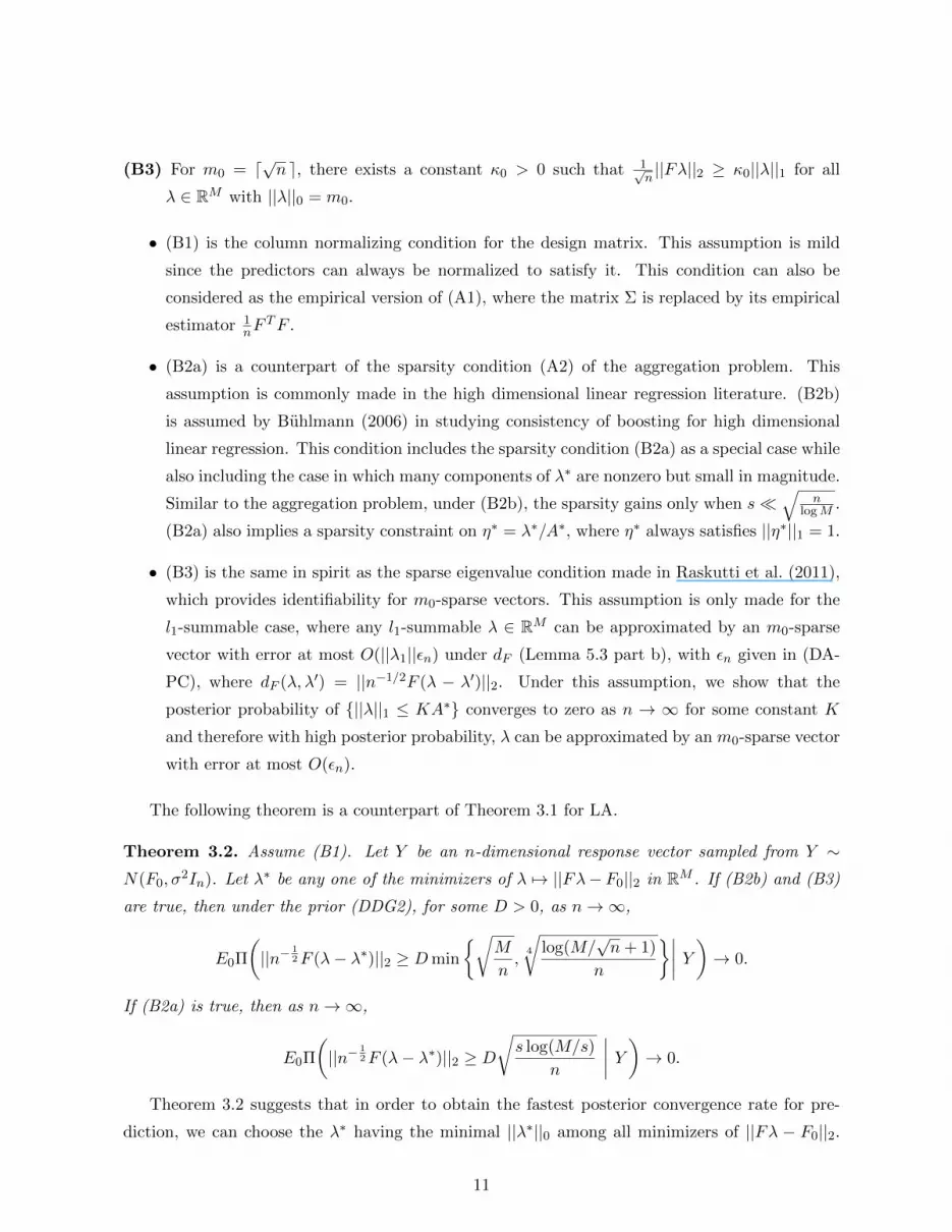
(B3) For m0 = d√n e, there exists a constant κ0 > 0 such that 1√

n||Fλ||2 ≥ κ0||λ||1 for all

λ ∈ RM with ||λ||0 = m0.

• (B1) is the column normalizing condition for the design matrix. This assumption is mild

since the predictors can always be normalized to satisfy it. This condition can also be

considered as the empirical version of (A1), where the matrix Σ is replaced by its empirical

estimator 1nF

TF .

• (B2a) is a counterpart of the sparsity condition (A2) of the aggregation problem. This

assumption is commonly made in the high dimensional linear regression literature. (B2b)

is assumed by Buhlmann (2006) in studying consistency of boosting for high dimensional

linear regression. This condition includes the sparsity condition (B2a) as a special case while

also including the case in which many components of λ∗ are nonzero but small in magnitude.

Similar to the aggregation problem, under (B2b), the sparsity gains only when s√

nlogM .

(B2a) also implies a sparsity constraint on η∗ = λ∗/A∗, where η∗ always satisfies ||η∗||1 = 1.

• (B3) is the same in spirit as the sparse eigenvalue condition made in Raskutti et al. (2011),

which provides identifiability for m0-sparse vectors. This assumption is only made for the

l1-summable case, where any l1-summable λ ∈ RM can be approximated by an m0-sparse

vector with error at most O(||λ1||εn) under dF (Lemma 5.3 part b), with εn given in (DA-

PC), where dF (λ, λ′) = ||n−1/2F (λ − λ′)||2. Under this assumption, we show that the

posterior probability of ||λ||1 ≤ KA∗ converges to zero as n → ∞ for some constant K

and therefore with high posterior probability, λ can be approximated by an m0-sparse vector

with error at most O(εn).

The following theorem is a counterpart of Theorem 3.1 for LA.

Theorem 3.2. Assume (B1). Let Y be an n-dimensional response vector sampled from Y ∼N(F0, σ

2In). Let λ∗ be any one of the minimizers of λ 7→ ||Fλ− F0||2 in RM . If (B2b) and (B3)

are true, then under the prior (DDG2), for some D > 0, as n→∞,

E0Π

(||n−

12F (λ− λ∗)||2 ≥ Dmin

√M

n,

4

√log(M/

√n+ 1)

n

∣∣∣∣ Y )→ 0.

If (B2a) is true, then as n→∞,

E0Π

(||n−

12F (λ− λ∗)||2 ≥ D

√s log(M/s)

n

∣∣∣∣ Y )→ 0.

Theorem 3.2 suggests that in order to obtain the fastest posterior convergence rate for pre-

diction, we can choose the λ∗ having the minimal ||λ∗||0 among all minimizers of ||Fλ − F0||2.

11

This suggests that the posterior measure tends to concentrate on the sparsest λ∗ that achieves

the same prediction accuracy, which explains the sparse adaptivity. The non-uniqueness happens

when M > n.

4. Experiments

As suggested by Yang (2001), the estimator fn depends on the order of the observations and one

can randomly permute the order a number of times and average the corresponding estimators. In

addition, one can add a third step of estimating f1, . . . , fM with the full dataset as f1, . . . , fM and

setting the final estimator as f =∑M

j=1 λj fj . We will adopt this strategy and our splitting and

aggregation scheme can be summarized as follows. First, we randomly divide the entire n samples

into two subsets S1 and S2 with |S1| = n1 and |S2| = n2. As a default, we set n1 = 0.75n and

n2 = 0.25n. Using S1 as a training set, we obtain M base learners f(n1)1 , . . . , f

(n1)M . Second, we

apply the above MCMC algorithms to aggregate these learners into f (n1) =∑M

j=1 λj f(n1)j based on

the n2 aggregating samples. Finally, we use the whole dataset to train these base learners, which

gives us f(n)j , and the final estimator is f (n) =

∑Mj=1 λj f

(n)j . Therefore, one basic requirement

on the base learners is that they should be stable in the sense that f(n)j can not be dramatically

different from f(n1)j (e.g. CART might not be a suitable choice for the base learner).

4.1 Bayesian linear aggregation

In this subsection, we apply the Bayesian LA methods to the linear regression Y = Xλ+ ε, with

X ∈ RM and ε ∼ N(0, σ2In). Since every linear aggregation problem can be reformed as a linear

regression problem, this is a simple canonical setting for testing our approach. We consider two

scenarios: 1. the sparse case where the number of nonzero components in the regression coefficient

λ is smaller than M and the sample size n; 2. the non-sparse case where λ can have many nonzero

components, but the l1 norm ||λ||1 =∑M

j=1 |λj | remains constant as M changes. We vary model

dimensionality by letting M = 5, 20, 100 and 500.

We compare the Bayesian LA methods with lasso, ridge regression and horseshoe. Lasso

(Tibshirani, 1996) is widely used for linear models, especially when λ is believed to be sparse. In

addition, due to the use of l1 penalty, the lasso is also minimax optimal when λ is l1-summable

(Raskutti et al., 2011). Ridge regression (Hoerl and Kennard, 1970) is a well-known shrinkage

estimator for non-sparse settings. Horseshoe (Carvalho et al., 2010) is a Bayesian continuous

shrinkage prior for sparse regression from the family of global-local mixtures of Gaussians (Polson

and Scott, 2010). Horseshoe is well-known for its robustness and excellent empirical performance

for sparse regression, but there is a lack of theoretical justification. n training samples are used to

fit the models and N − n testing samples are used to calculate the prediction root mean squared

12

error (RMSE)

(N − n)−1∑N

i=n+1(yi − yi)21/2

, where yi denotes the prediction of yi.

The MCMC algorithm for the Bayesian LA method is run for 2,000 iterations, with the first

1,000 iterations as the burn-in period. We set α = 1, γ = 2, a0 = 0.01 and b0 = 0.01 for the

hyperparameters. The tuning parameters in the MH steps are chosen so that the acceptance rates

are around 40%. The lasso is implemented by the glmnet package in R, the ridge is implemented

by the lm.ridge function in R and horseshoe is implemented by the monomvn package in R. The

iterations for horseshoe is set as the default 1,000. The regularization parameters in Lasso and

ridge are selected via cross-validation.

4.1.1 Sparse case

In the sparse case, we choose the number of non-zero coefficients to be 5. The simulation data

are generated from the following model:

(S) y = −0.5x1 + x2 + 0.4x3 − x4 + 0.6x5 + ε, ε ∼ N(0, 0.52),

with M covariates x1, . . . , xM ∼ i.i.d N(0, 1). The training size is set to be n = 100 and testing

size N−n = 1000. As a result, (S) with M = 5 and 20 can be considered as moderate dimensional,

while M = 100 and M = 500 are relatively high dimensional.

M 5 20 100 500

LA.511 .513 .529 .576

(0.016) (0.016) (0.020) (0.023)

Lasso.514 .536 .574 .613

(0.017) (0.020) (0.039) (0.042)

Ridge.514 .565 1.23 2.23

(0.017) (0.019) (0.139) (0.146)

Horseshoe.512 .519 .525 .590

(0.016) (0.014) (0.019) (0.022)

Table 1: RMSE for the sparse linear model (S). The numbers in the parentheses indicate the

standard deviations. All results are based on 100 replicates.

From Table 1, all the methods are comparable when there is no nuisance predictor (M = 5).

However, as more nuisance predictors are included, the Bayesian LA method and horseshoe have

noticeably better performance than the other two methods. For example, for M = 100, the

Bayesian LA method has 8% and 53% improvements over lasso and ridge, respectively. In addition,

as expected, ridge deteriorates more dramatically than the other two as M grows. It appears that

13

Bayesian LA is more computationally efficient than horseshoe. For example, under m = 100 it

takes horseshoe 50 seconds to draw 1,000 iterations but only takes LA about 1 second to draw

2,000 iterations.

0 200 600 1000

−1.

3−

1.1

−0.

9

(a)

Iterations

0 200 600 1000−2e

−06

0e+

002e

−06

(b)

Iterations

Figure 2: Traceplots for a non-zero regression coefficient and a zero coefficient.

Fig. 2 displays the traceplots after the burn-in for a typical non-zero and a typical zero

regression coefficient respectively under M = 100. The non-zero coefficient mixes pretty well

according to its traceplot. Although the traceplot of the zero coefficient exhibits some small

fluctuations, their magnitudes are still negligible compared to the non-zero ones. We observe that

these fluctuant traceplots like Fig. 2(b) only happens for those λj ’s whose posterior magnitudes are

extremely small. The typical orders of the posterior means of those λj ’s in LA that correspond to

unimportant predictors range from 10−17 to 10−2. However, the posterior medians of unimportant

predictors are less than 10−4 (see Fig. 3). This suggests that although the coefficients are not

exactly to zero, the estimated regression coefficients with zero true values are still negligible

compared to the estimators of the nonzero coefficients. In addition, for LA the posterior median

appears to be a better and more robust estimator for sparse regression than the posterior mean.

14

0 20 40 60 80 100

−1.

00.

01.

0

j

lam

bda'

s

Figure 3: 95% posterior credible intervals for λ1, . . . , λ100 in sparse regresion. The solid dots are

the corresponding posterior medians.

0 20 40 60 80 100

−0.

20.

00.

10.

2

j

lam

bda'

s

Figure 4: 95% posterior credible intervals for λ1, . . . , λ100 in non-sparse regression. The solid dots

are the corresponding posterior medians.

15

4.1.2 Non-sparse case

In the non-sparse case, we use the following two models as the truth:

(NS1) y =M∑j=1

3(−1)j

j2xj + ε, ε ∼ N(0, 0.12),

(NS2) y =

bM/2c∑j=1

5

bM/2cxj + ε, ε ∼ N(0, 0.12),

with M covariates x1, . . . , xM ∼ i.i.d N(0, 1). In (NS1), all the predictors affect the response and

the impact of predictor xj decreases quadratically in j. Moreover, λ satisfies the l1-summability

since limp→∞ ||λ||1 = π2/3 ≈ 4.9. In (NS2), half of the predictors have the same influence on the

response with ||λ||1 = 5. The training size is set to be n = 200 and testing size N − n = 1000 in

the following simulations.

M 5 20 100 500

NS1

LA.101 .112 .116 .129

(0.002) (0.003) (0.005) (0.007)

Lasso.105 .110 .116 .155

(0.006) (0.005) (0.005) (0.006)

Ridge.102 .107 .146 2.42

(0.003) (0.004) (0.008) (0.053)

Horseshoe.102 .111 .114 .136

(0.003) (0.003) (0.004) (0.005)

NS2

LA.101 .104 .121 .326

(0.002) (0.003) (0.005) (0.008)

Lasso.111 .106 .131 .323

(0.006) (0.003) (0.007) (0.008)

Ridge.103 .107 .140 .274

(0.003) (0.003) (0.008) (0.010)

Horseshoe.102 .104 .124 .308

(0.003) (0.003) (0.004) (0.007)

Table 2: RMSE for the non-sparse linear models (NS1) and (NS2). All results are based on 100

replicates.

From Table 2, all the methods have comparable performance when M is moderate (i.e 5 or 20)

in both non-sparse settings. In the non-sparse settings, horseshoe also exhibits excellent prediction

16

performance. In most cases, LA, lasso and horseshoe have similar performance. As M increases

to an order comparable to the sample size, LA and horseshoe tend to be more robust than lasso

and ridge. As M becomes much greater than n, LA, lasso and horseshoe remain good in (NS1)

while breaking down in (NS2); ridge breaks down in (NS1) while becoming the best in (NS2). It

might be because in (NS1), although all λj ’s are nonzero, the first several predictors still dominate

the impact on y. In contrast, in (NS2), half of λj ’s are nonzero and equally small. Fig. 4 plots

95% posterior credible intervals for λ1, . . . , λ100 of (NS2) under M = 100. According to Section

1.1, the spasrse/non-sparse boundary for (NS2) under M = 100 is√

200/ log 100 ≈ 3 50.

Therefore, the results displayed in Fig. 4 can be classified into the non-sparse regime. A simple

variable selection based on these credible intervals correctly identifies all 50 nonzero components.

4.1.3 Robustness against the hyperparameters

Since changing the hyperparameter α in the Dirichlet prior is equivalent to changing the hyper-

parameter γ, we perform a sensitivity analysis for γ in the above two regression settings with

M = 100.

0 1 2 3 4 5

0.4

0.6

0.8

1.0

1.2

1.4

1.6

γ

RM

SE

S

0 1 2 3 4 5

0.10

0.14

0.18

0.22

γ

RM

SE

NS1NS2

Figure 5: Robustness of the Bayesian LA methods against the hyperparameter γ. The results are

based on 100 replicates.

From Figure 5, the Bayesian LA method tends to be robust against the change in γ at a

wide range. As expected, the Bayesian LA method starts to deteriorate as γ becomes too small.

In particular, when γ is zero, the Dirichlet prior no longer favors sparse weights and the RMSE

becomes large (especially for the sparse model) in all three settings. However, the Bayesian LA

methods tend to be robust against increase in γ. As a result, we would recommend choosing

γ = 2 in practice.

17

4.2 Bayesian convex aggregation

In this subsection, we conduct experiments for the Bayesian convex aggregation method.

4.2.1 Simulations

The following regression model is used as the truth in our simulations:

y = x1 + x2 + 3x23 − 2e−x4 + ε, ε ∼ N(0, 0.5), (4.1)

with p covariates x1, . . . , xd ∼ i.i.d N(0, 1). The training size is set to be n = 500 and testing size

N − n = 1000 in the following simulations.

In the first simulation, we choose M = 6 base learners: CART, random forest (RF), lasso,

SVM, ridge regression (Ridge) and neural network (NN). The Bayesian aggregation (BA) is com-

pared with the super learner (SL). SL is implemented by the SuperLearner package in R. The

implementations of the base learners are described in Table 3. The MCMC algorithm for the

Bayesian CA method is run for 2,000 iterations, with the first 1,000 iterations as the burn-in

period. We set α = 1, γ = 2 for the hyperparameters. The simulation results are summarized in

Table 4, where square roots of mean squared errors (RMSE) of prediction based on 100 replicates

are reported.

Base learner CART RF Lasso

R package rpart randomForest glmnet

SVM Ridge NN GAM

e1071 MASS nnet gam

Table 3: Descriptions of the base learners.

d CART RF Lasso SVM Ridge NN SL BA

53.31 3.33 5.12 2.71 5.12 3.89 2.66 2.60

(0.41) (0.42) (0.33) (0.49) (0.33) (0.90) (0.48) (0.48)

203.32 3.11 5.18 4.10 5.23 5.10 3.13 3.00

(0.41) (0.49) (0.37) (0.46) (0.38) (1.57) (0.54) (0.48)

1003.33 3.17 5.17 5.48 5.64 7.12 3.19 3.03

(0.38) (0.45) (0.32) (0.35) (0.33) (1.31) (0.45) (0.45)

Table 4: RMSE for the first simulation. All results are based on 100 replicates.

In the second simulation, we consider the case when M is moderately large. We consider

M = 26, 56 and 106 by introducing (M − 6) new base learners in the following way. In each

18

simulation, for j = 1, . . . ,M−6, we first randomly select a subset Sj of the covariates x1, . . . , xdwith size p = bminn1/2, d/3c. Then the jth base learner fj is fitted by the general additive

model (GAM) with the response y and covariates in Sj as predictors. This choice of new learners is

motivated by the fact that the truth is sparse when M is large and brutally throwing all covariates

into the GAM tends to have a poor performance. Therefore, we expect that a base learner based

on GAM that uses a small subset of the covariates containing the important predictors x1, x2

x3 and x4 tends to have better performance than the full model. In addition, with a large M

and moderate p, the probability that one of the randomly selected (M − 6) models contains the

truth is high. In this simulation, we compare BA with SL and a voting method using the average

prediction across all base learners. For illustration, the best prediction performance among the

(M − 6) random-subset base learners is also reported. Table 5 summarizes the results.

d M Best Voting SL BA

20

263.14 4.63 3.40 2.78

(0.82) (0.48) (0.60) (0.52)

562.86 4.98 3.33 2.79

(1.57) (0.71) (0.86) (0.78)

1062.79 4.95 3.23 2.73

(0.62) (0.60) (0.70) (0.61)

100

263.14 4.72 3.09 2.78

(0.71) (0.44) (0.50) (0.45)

562.95 4.93 3.07 2.78

(0.46) (0.45) (0.50) (0.47)

1062.84 4.90 2.98 2.69

(0.45) (0.47) (0.55) (0.51)

500

265.21 5.75 3.77 3.19

(0.75) (0.50) (0.650) (0.59)

564.86 5.92 4.02 3.18

(0.78) (0.59) (0.73) (0.70)

1064.65 5.98 4.18 3.13

(0.69) (0.45) (0.52) (0.49)

Table 5: RMSE for the second simulation study. All results are based on 100 replicates.

19

4.2.2 Applications

We apply BA to four datasets from the UCI repository. Table 6 provides a brief description of

those datasets. We use CART, random forest, lasso, support vector machine, ridge regression

and neural networks as the base learners. We run 40,000 iterations for the MCMC for the BA

for each dataset and discard the first half as the burn-in. Table 7 displays the results. As we can

see, for 3 datasets (auto-mpg, concrete and forest), the aggregated models perform the best. In

particular, for the auto-mpg dataset, BA has 3% improvement over the best base learner. Even

for the slump dataset, aggregations still have comparable performance to the best base learner.

The two aggregation methods SL and BA have similar performance for all the datasets.

dataset sample size # of predictors response variable

auto-mpg 392 8 mpg

concrete 1030 8 CCS∗

slump 103 7 slump

forest 517 12 log(1+area)

Table 6: Descriptions of the four datasets from the UCI repository. CCS: concrete compressive

strength.

dataset Cart RF Lasso SVM Ridge NN GAM SL BA

auto-mpg 3.42 2.69 3.38 2.68 3.40 7.79 2.71 2.61 2.61

concrete 9.40 5.35 10.51 6.65 10.50 16.64 7.95 5.31 5.33

slump 7.60 6.69 7.71 7.05 8.67 7.11 6.99 7.17 7.03

forest .670 .628 .612 .612 .620 .613 .622 .606 .604

Table 7: RMSE of aggregations for real data applications. All results are based on 10-fold cross-

validations.

5. Proofs of the main results

Let K(P,Q) =∫

log(dP/dQ)dP be the KL divergence between two probability distributions P

and Q, and V (P,Q) =∫| log(dP/dQ)−K(P,Q)|2dP be a discrepancy measure.

5.1 Concentration properties of Dirichlet distribution and double Dirichlet distribution

According to the posterior asymptotic theory developed in Ghosal et al. (2000) (for iid observa-

tions, e.g. regression with random design, such as the aggregation problem in section 2.2), to

20

ensure a posterior convergence rate of at least εn, the prior has to put enough mass around θ∗ in

the sense that

(PC1) Π(B(θ∗, εn)) ≥ e−nε2nC , with

B(θ∗, ε) =θ ∈ Θ : K(Pθ∗ , Pθ) ≤ ε2, V (Pθ∗ , Pθ) ≤ ε2,

for some C > 0. For independent but non-identically distributed (noniid) observations (e.g.

regression with fixed design, such as the linear regression problem in section 2.3), where the likeli-

hood takes a product form P(n)θ (Y1, . . . , Yn) =

∏ni=1 Pθ,i(Yi), the corresponding prior concentration

condition becomes (Ghosal and van der Vaart, 2007)

(PC2) Π(Bn(θ∗, εn)) ≥ e−nε2nC , with

Bn(θ∗, ε) =

θ ∈ Θ :

1

n

n∑i=1

K(Pθ∗,i, Pθ,i) ≤ ε2,1

n

n∑i=1

V (Pθ∗,i, Pθ,i) ≤ ε2.

If a (semi-)metric dn, which might depend on n, dominates KL and V on Θ, then (PC) is implied

by Π(dn(θ, θ∗) ≤ cεn) ≥ e−nε2nC for some c > 0. In the aggregation problem with a random design

and parameter θ = λ, we have K(Pθ∗ , Pθ) = V (Pθ∗ , Pθ) = 12σ2 ||

∑Mj=1(λj − λ∗j )fj ||2Q = 1

2σ2 (λ −λ∗)TΣ(λ− λ∗). Therefore, we can choose dn(θ, θ∗) as dΣ(λ, λ∗) = ||Σ1/2(λ− λ∗)||2. In the linear

aggregation problem with a fixed design and θ = λ,∑n

j=1K(Pθ∗,i, Pθ,i) =∑n

j=1 V (Pθ∗,i, Pθ,i) =1

2σ2 ||F (λ− λ∗)||2, where Pθ,i(Y ) = Pλ(Y |F (i)). Therefore, we can choose dn(θ, θ∗) as dF (λ, λ∗) =

|| 1√nF (λ− λ∗)||2.

For CA and LA, the concentration probabilities can be characterized by those of λ∗ ∈ Λ and

η∗ ∈ DM−1 = η ∈ RM , ||η||1 = 1. Therefore, it is important to investigate the concentration

properties of the Dirichlet distribution and the double Dirichlet distribution as priors over Λ and

DM−1. The concentration probabilities Π(dΣ(λ, λ∗) ≤ cε) and Π(dF (η, η∗) ≤ cε) depend on the

location of the centers λ∗ and η∗, which are characterized by their geometrical properties, such

as sparsity and l1-summability. The next lemma characterizes these concentration probabilities

and is of independent interest.

Lemma 5.1. Assume (A1) and (B1).

a. Assume (A2). Under the prior (DA), for any γ ≥ 1,

Π(dΣ(λ, λ∗) ≤ ε) ≥ exp

− Cγs log

M

ε

, for some C > 0.

b. Under the prior (DA), for any m > 0, any λ ∈ Λ and any γ ≥ 1,

Π

(dΣ(λ, λ∗) ≤ ε+

C√m

)≥ exp

− Cγm log

M

ε

,

Π(dΣ(λ, λ∗) ≤ ε) ≥ exp

− CγM log

M

ε

, for some C > 0.

21

c. Assume (B2a). Under the prior for η in (DDG2), for any γ ≥ 1,

Π(dF (η, η∗) ≤ ε) ≥ exp

− Cγs log

M

ε

, for some C > 0.

d. Under the prior for η in (DDG2), for any m > 0, any η ∈ DM−1 and any γ ≥ 1,

Π

(dF (η, η∗) ≤ ε+

C√m

)≥ exp

− Cγm log

M

ε

,

Π(dF (η, η∗) ≤ ε) ≥ exp

− CγM log

M

ε

, for some C > 0.

• The lower bound exp−Cγs log(M/ε) in Lemma 5.1 can be decomposed into two parts:

exp−Cγs logM and expCs log ε. The first part has the same order as 1/(Ms

), one over

the total number of ways to choose s indices from 1, . . . ,M. The second part is of the

same order as εs, the volume of an ε-cube in Rs. Since usually which s components are

nonzero and where the vector composed of these s nonzero components locates in Rs are

unknown, this prior lower bound cannot be improved.

• The priors (DA) and (DDG2) do not depend on the sparsity level s. As a result, Lemma 5.1

suggests that the prior concentration properties hold simultaneously for all λ∗ or η∗ with

different s and thus these priors can adapt to an unknown sparsity level.

By the first two parts of Lemma 5.1, the following is satisfied for the prior (DA) with D large

enough,

(DA-PC) Π(dΣ(λ, λ∗) ≤ εn) ≥ e−nε2nC , with εn =

D

√s log(M/s)

n , if ||λ∗||0 = s;

D√

Mn , if M ≤

√n;

D4

√log(M/

√n+1)

n , if M >√n.

This prior concentration property will play a key role in characterizing the posterior convergence

rate of the prior (DA) for Bayesian aggregation.

Based on the prior concentration property of the double Dirichlet distribution provided in

Lemma 5.1 part c and part d, we have the corresponding property for the prior (DDG2) by

taking into account the prior distribution of A = ||λ||1.

Corollary 5.2. Assume (B1).

a. Assume (B2a). Under the prior (DDG2), for any γ ≥ 1,

Π(dF (λ, λ∗) ≤ ε) ≥ exp

− Cγs log

M

ε

, for some C > 0.

22

b. Assume (B2b). Under the prior (DDG2), for any m > 0, any η ∈ DM−1 and any γ ≥ 1,

Π

(dF (λ, λ∗) ≤ ε+

C√m

)≥ exp

− Cγm log

M

ε

,

Π(dF (λ, λ∗) ≤ ε) ≥ exp

− CγM log

M

ε

, for some C > 0.

Based on the above corollary, we have a similar prior concentration property for the prior

(DDG2):

(DDG2-PC) Π(dF (θ, θ∗) ≤ cεn) ≥ e−nε2nC , with the same εn in (DA-PC).

5.2 Supports of the Dirichlet distribution and the double Dirichlet distribution

By Ghosal et al. (2000), a second condition to ensure the posterior convergence rate of θ∗ ∈ Θ at

least εn is that the prior Π should put almost all its mass in a sequence of subsets of Θ that are

not too complex. More precisely, one needs to show that there exists a sieve sequence Fn such

that θ∗ ∈ Fn ⊂ Θ, Π(Fcn) ≤ e−nε2nC and logN(εn,Fn, dn) ≤ nε2n for each n, where for a metric

space F associated with a (semi-)metric d, N(ε,F , d) denotes the minimal number of d-balls with

radii ε that are needed to cover F .

For the priors (DA) and (DDG2), the probability of the space of all s-sparse vectors is zero.

We consider the approximate s-sparse vector space FΛs,ε defined in Section 2.1 for CA. For LA,

we define FDB,s,ε = θ = Aη : η ∈ DM−1,∑M

j=s+1 |η(j)| ≤ B−1ε; 0 ≤ A ≤ B, where |η(1)| ≥ · · · ≥|η(M)| is the ordered sequence of η1, . . . , ηM according to their absolute values.

The following lemma characterizes the complexity of Λ, DBM−1 = Aη : η ∈ DM−1; 0 ≤ A ≤

B, FΛs,ε and FDB,s,ε in terms of their covering numbers.

Lemma 5.3. Assume (A1) and (B1).

a. For any ε ∈ (0, 1), integer s > 0 and B > 0, we have

logN(ε,FΛs,ε, dΣ) . s log

M

ε,

logN(ε,FDB,s,ε, dF ) . s logM

ε+ s logB.

b. For any ε ∈ (0, 1) and integer m > 0, we have

logN(C/√m,Λ, dΣ) . m logM,

logN(ε,Λ, dΣ) .M logM

ε,

logN(CB/√m,BDM−1, dF ) . m logM,

logN(Bε,BDM−1, dF ) .M logM

ε.

23

The next lemma provides upper bounds to the complementary prior probabilities of FΛs,ε and

FDB,s,ε. The proof utilizes the connection between the Dirichlet distribution and the stick-breaking

representation of the Dirichlet processes (Sethuraman, 1994).

Lemma 5.4. a. For any ε ∈ (0, 1), under the prior (DA) with γ > 1, we have

Π(λ /∈ FΛs,ε) . exp

− Cs(γ − 1) log

M

ε

.

b. For any ε ∈ (0, 1), under the prior (DDG2) with γ > 1, we have

Π(θ /∈ FDB,s,ε) . exp

− Cs(γ − 1) log

M

ε− Cs logB

+ exp−CB.

5.3 Test construction

For CA, we use the notation Pλ,Q to denote the joint distribution of (X,Y ), whenever X ∼ Q and

Y |X ∼ N(∑M

j=1 λjfj(X), σ2) for any λ ∈ Λ and Eλ,Q the expectation with respect to Pλ,Q. Use

P(n)λ,Q to denote the n-fold convolution of Pλ,Q. Let Xn = (X1, . . . , Xn) and Y n = (Y1, . . . , Xn) be

n copies of X and Y . Recall that f0 is the true regression function that generates the data. We

use P0,Q to denote the corresponding true distribution of Y . For LA, we use Pλ to denote the

distribution of Y , whenever Y ∼ N(Fλ, σ2In) and Eλ the expectation with respect to Pλ.

For both aggregation problems, we use the “M-open” view where f0 might not necessarily

belong to FΛ or FRM . We apply the result in Kleijn and van der Vaart (2006) to construct

a test under misspecification for CA with random design and explicitly construct a test under

misspecification for LA with fixed design. Note that the results in Kleijn and van der Vaart (2006)

only apply for random-designed models. For LA with fixed design, we construct a test based on

concentration inequalities for Gaussian random variables.

Lemma 5.5. Assume (A3).

a. Assume that f∗ =∑M

j=1 λ∗jfj satisfies EQ(f − f∗)(f∗ − f0) = 0 for every f ∈ FΛ. Then

there exist C > 0 and a measurable function φn of Xn and Y n, such that for any other

vector λ2 ∈ Λ,

P(n)0,Qφn(Xn, Y n) ≤ exp

− Cnd2

Σ(λ2, λ∗)

supλ∈Λ: dΣ(λ,λ2)< 1

4dF (λ∗,λ2)

P(n)λ,Q(1− φn(Xn, Y n)) ≤ exp

− Cnd2

Σ(λ2, λ∗).

b. Assume that λ∗ ∈ Rd satisfies F T (Fλ∗ − F0) = 0 for every λ ∈ Rd. Then there exists a

measurable function φn of Y and some C > 0, such that for any other λ2 ∈ Rd,

P0φn(Y ) ≤ exp− Cnd2

F (λ2, λ∗)

supλ∈RM : dF (λ,λ2)< 1

4dF (λ∗,λ2)

Pλ(1− φn(Y )) ≤ exp− Cnd2

X(λ2, λ∗).

24

• As we discussed in the remark in section 3.1, in order to apply Kleijn and van der Vaart

(2006) for Gaussian regression with random design, we need the mean function to be uni-

formly bounded. For the convex aggregation space FΛ, this uniformly bounded condition

is implied by (A3). For the linear regression with fixed design, we do not need the uni-

formly bounded condition. This property ensures that the type I and type II errors in b

do not deteriorate as ||λ2||1 grows, which plays a critical role in showing that the posterior

probability of A > CA∗ converges to zero in probability for C sufficiently large, where

A = ||λ||1 and A∗ = ||λ∗||1. Similarly, if we consider CA with a fixed design, then only an

assumption like (B1) on the design points is needed.

• The assumption on f∗ in CA is equivalent to that f∗ is the minimizer over f ∈ FΛ of

||f − f0||2Q, which is proportional to the expectation of the KL divergence between two

normal distributions with mean functions f0(X) and f(X) with X ∼ Q. Therefore, f∗ is

the best L2(Q)-approximation of f0 within the aggregation space FΛ and the lemma suggests

that the likelihood function under f∗ tends to be exponentially larger than other functions

in FΛ. Similarly, the condition on λ∗ in LA is equivalent to that λ∗ is the minimizer over

λ ∈ Rd of ||Fλ−F0||22, which is proportional to the KL divergence between two multivariate

normal distributions with mean vectors Fλ and F0.

5.4 Proof of Theorem 3.1

The proof follows similar steps as the proof of Theorem 2.1 in Ghosal et al. (2000). The difference

is that we consider the misspecified framework where the asymptotic limit of the posterior distri-

bution of f is f∗ instead of the true underlying regression function f0. As a result, we need to

apply the test condition in Lemma 5.5 part a in the model misspecified framework. We provide

a sketched proof as follows.

Let εn be given by (DA-PC) and ΠB(λ) = Π(λ|B(λ∗, εn)

)with B(λ∗, εn) defined in (PC1).

By Jensen’s inequality applied to the logarithm,

log

∫B(λ∗,εn)

n∏i=1

Pλ,QP0,Q

(Xi, Yi)dΠB(λ) ≥n∑i=1

∫B(λ∗,εn)

logPλ,QP0,Q

(Xi, Yi)dΠB(λ).

By the definition of B(λ∗, εn) and an application of Chebyshev’s inequality, we have that for any

25

C > 0,

P0

n∑i=1

∫B(λ∗,εn)

(log

Pλ,QP0,Q

(Xi, Yi) +K(Pλ0,Q, Pλ,Q)

)dΠB(λ)

≤ −(1 + C)nε2n + n

∫B(λ∗,εn)

K(Pλ0,Q, Pλ,Q)dΠB(λ)

≤ P0

n∑i=1

∫B(λ∗,εn)

(log

Pλ,QP0,Q

(Xi, Yi) +K(Pλ0,Q, Pλ,Q)

)dΠB(λ) ≤ −Cnε2n

≤n∫B(λ∗,εn) V (Pλ0,Q, Pλ,Q)dΠB(λ)

(Cnε2n)2≤ 1

C2nε2n→ 0, as n→∞.

Combining the above two yields that on some set An with P0-probability converging to one,∫B(λ∗,εn)

n∏i=1

Pλ,QP0,Q

(Xi, Yi)dΠ(λ) ≥ exp(−(1 + C)nε2n)Π(B(λ∗, εn)) ≥ exp(−C0nε2n), (5.1)

for some C0 > 0, where we have used the fact that Π(B(λ∗, εn)) ≥ Π(dΣ(λ, λ∗) ≤ Cεn) ≥exp(−Cnε2n) for some C > 0.

Let Fn = Fλas,εn for some a > 0 if (A2) holds and otherwise Fn = Λ. Then by Lemma 5.3 part

a and Lemma 5.4 part a, for some constants C1 > 0 and C2 > 0,

logN(εn,Fn, dΣ) ≤ C1nε2n, Π(λ /∈ Fn) ≤ exp(−C2nε

2n). (5.2)

Because C2 is increasing with the a in the definition of Fn, we can assume C2 > C0 +1 by properly

selecting an a.

For some D0 > 0 sufficiently large, let λ∗1, . . . , λ∗J ∈ Fn − λ : dΣ(λ, λ∗) ≤ 4D0εn with

|J | ≤ exp(C1nε2n) be J points that form an D0εn-covering net of Fn − λ : dΣ(λ, λ∗) ≤ 4D0εn.

Let φj,n be the corresponding test function provided by Lemma 5.5 part a with λ2 = λ∗j for

j = 1, . . . , J . Set φn = maxj φj,n. Since dΣ(λ∗j , λ∗) ≥ 4D0εn for any j, we obtain

P(n)0,Qφn ≤

J∑j=1

P(n)0,Qφj,n ≤ |J | exp(−C16D2

0nε2n) ≤ exp(−C3nε

2n), (5.3)

where C3 = 16CD20 − 1 > 0 for D0 large enough. For any λ ∈ Fn − λ : dΣ(λ, λ∗) ≤ 4D0εn, by

the design, there exists a j0 such that dΣ(λ∗j0 , λ) ≤ D0εn. This implies that dΣ(λ∗j0 , λ∗) ≥ 4D0εn ≥

4dΣ(λ∗j0 , λ), therefore

supλ∈Fn: dΣ(λ,λ∗)≥4D0εn

P(n)λ,Qφn

≤ minj

supλ∈Λ: dΣ(λ,λ∗j )< 1

4dΣ(λ∗,λ∗j )

P(n)λ,Q(1− φn) ≤ exp

− C4nε

2n

, (5.4)

26

with C4 = 16CD20 > C0 + 1 with D0 sufficiently large. With D = 4D0, we have

E0,QΠ(dΣ(λ, λ∗) ≥ Dεn|X1, Y1, . . . , Xn, Yn)I(An)

≤ P(n)0,Qφn + E0,QΠ(dΣ(λ, λ∗) ≥ Dεn|X1, Y1, . . . , Xn, Yn)I(An)(1− φn). (5.5)

By (5.1), (5.2) and (5.4), we have

E0,QΠ(dΣ(λ, λ∗) ≥ Dεn|X1, Y1, . . . , Xn, Yn)I(An)(1− φn)

≤ P(n)0,Q(1− φn)I(An)

∫λ∈Fn:dΣ(λ,λ∗)≥Dεn

∏ni=1

Pλ,QP0,Q

(Xi, Yi)dΠ(λ)∫B(λ∗,εn)

∏ni=1

Pλ,QP0,Q

(Xi, Yi)dΠ(λ)

+ P(n)0,QI(An)

∫λ/∈Fn

∏ni=1

Pλ,QP0,Q

(Xi, Yi)dΠ(λ)∫B(λ∗,εn)

∏ni=1

Pλ,QP0,Q

(Xi, Yi)dΠ(λ)

≤ exp(C0nε2n) sup

λ∈Fn: dΣ(λ,λ∗)≥4D0εn

P(n)λ,Qφn + exp(C0nε

2n)Π(λ /∈ Fn) ≤ 2 exp(−nε2n). (5.6)

Combining the above with (5.3), (5.5), and the fact that E0,QI(Acn)→ 0 as n→∞, Theorem 3.1

can be proved.

5.5 Proof of Theorem 3.2

For the sparse case where (B2a) is satisfied, we construct the sieve by Fn = FDbnε2n,as,εn with the

εn given in (DDG2-PC), where a > 0, b > 0 are sufficiently large constants. Then by Lemma 5.3

part a and Lemma 5.4 part b, we have

logN(εn,Fn, dF ) ≤ C1nε2n, Π(λ /∈ Fn) ≤Π(−C2nε

2n), (5.7)

where C2 is increasing with a and b. The rest of the proof is similar to the proof of Theorem 3.1

with the help of (5.7), Corollary 5.1 part b and Lemma 5.5 part b.

Next, we consider the dense case where (B2b) and (B3) are satisfied. By the second half of

Lemma 5.3 part b, the approximation accuracy of BDM−1 degrades linearly in B. Therefore, in

order to construct a sieve such that (5.7) is satisfied with the εn given in (DDG2-PC), we need to

show that E0Π(A ≤ KA∗|Y ) → 0 as n → ∞ with some constant K > 0. Then by conditioning

on the event A ≤ KA∗, we can choose Fn = BDM−1 with B = KA∗, which does not increase

with n, and 5.7 will be satisfied. As long as 5.7 is true, the rest of the proof will be similar to the

sparse case.

We only prove that E0Π(A ≤ KA∗|Y ) → 0 as n → ∞ here. By (B1) and (B3), for any

η ∈ DM−1 and A > 0, dF (Aη,A∗η∗) ≥ κ0A− κA∗. As a result, we can choose K large enough so

that dF (Aη,A∗η∗) ≥ 4 for all A ≥ KA∗ and all η ∈ DM−1. Therefore, by Lemma 5.5 part b, for

27

any λ2 = A2η2 with A2 > KA∗ and η2 ∈ DM−1, there exists a test φn such that

Pλ∗φn(Y ) ≤ exp− Cn

sup

λ∈RM : dF (λ,λ2)< 14dF (λ∗,λ2)

Pλ(1− φn(Y )) ≤ exp− Cn

.

By choosing K large enough, we can assume that κ0KA∗/8 > κ + κA∗/4. For any λ = Aη

satisfying dF (η, η2) ≤ κ0/8 and |A−A2| ≤ 1, by (B1) and A2 > KA∗ we have

dF (λ, λ2) ≤ dF (Aη,A2η) + dF (A2η,A2η2) ≤ κ+1

8κ0A2

≤1

4(κ0A2 − κA∗) ≤

1

4dF (λ∗, λ2).

Combining the above, we have that for any λ2 = A2η2 with A2 > KA∗ and η2 ∈ DM−1,

Pλ∗φn(Y ) ≤ exp− Cn

sup

|A−A2|≤1,dF (η,η2)≤κ0/8Pλ(1− φn(Y )) ≤ exp

− Cn

.

Let A∗1, . . . , A∗J1

be a 1-covering net of the interval [KA∗, Cnε2n] with J1 ≤ Cnε2n and η∗1, . . . , η∗J2

be a κ0/8-covering net of DM−1 with log J2 ≤ Cnε2n (by Lemma 5.3 part b with B = 1). Let

φj (j = 1, . . . , J1J2) be the corresponding tests associated with each combination of (A∗s, η∗t ) for

s = 1, . . . , J1 and t = 1, . . . , J2. Let φn = maxj φj . Then for n large enough,

Pλ∗φn(Y ) ≤ exp

log(nε2n) + Cnε2n − Cn≤ exp

− Cn

supλ=Aη:A∈[KA∗,Cnε2n],η∈DM−1

Pλ(1− φn(Y )) ≤ exp− Cn

.

(5.8)

Moreover, because A ∼ Ga(a0, b0), we have

Π(λ /∈ Cnε2nDM−1) ≤ Π(A > Cnε2n) ≤ exp−Cnε2n. (5.9)

Combining (5.8) and (5.9), we can prove that E0Π(A ≤ KA∗|Y ) → 0 as n → ∞ by the same

arguments as in (5.6).

6. Technical Proofs

6.1 Proof of Lemma 5.1

The following lemma suggests that for any m > 0, each point in Λ or DM−1 can be approximated

by an m-sparse point in the same space with error at most√

2κ/m.

Lemma 6.1. Fix an integer m ≥ 1. Assume (A1) and (B1).

a. For any λ∗ ∈ Λ, there exists a λ ∈ Λ, such that ||λ||0 ≤ m and dΣ(λ, λ∗) ≤√

2κm .

28

b. For any η∗ ∈ DM−1, there exists an η ∈ DM−1, such that ||η||0 ≤ m and dF (η, η∗) ≤√

2κm .

Proof. (Proof of a) Consider a random variable J ∈ 1, . . . ,M with probability distribution

P (J = j) = λ∗j , j = 1, . . . ,M . Let J1, . . . , Jm be m iid copies of J and nj be the number of

i ∈ 1, . . . , n such that (Ji = j). Then (n1, . . . , nM ) ∼ MN(m, (λ∗1, . . . , λ∗M ), where MN denotes

the multinomial distribution. Let V = (n1/m, . . . , nM/m) ∈ Λ. Then the expectation E[V ] of

the vector V is λ∗. Therefore, we have

Ed2Σ(V, λ∗) =

M∑j,k=1

ΣjkE

(njm− λ∗j

)(nkm− λ∗k

)

=1

m

M∑j=1

Σjjλ∗j (1− λ∗j )−

2

m

∑1≤j<k≤M

Σjkλ∗jλ∗k

≤ κ

m

M∑j=1

λ∗j (1− λ∗j ) +2κ

m

∑1≤j<k≤M

λ∗jλ∗k ≤

2κ

m,

where we have used (A1), the fact that |Σjk| ≤ Σ1/2jj Σ

1/2kk and

∑Mj=1 λ

∗j = 1. Since the expectation

of d2Σ(V, λ∗) is less than or equal to 2κ/m, there always exists a λ ∈ Λ such that dΣ(λ, λ∗) ≤√

2κ/m.

(Proof of b) The proof is similar to that of a. Now we define J ∈ 1, . . . ,M as a random

variable with probability distribution P (J = j) = |η∗j |, j = 1, . . . ,M and let V = (sgn(η∗1)n1/m,

. . ., sgn(η∗M )nM/m) ∈ DM−1. The rest follows the same line as part a. under assumption (B1).

Now, we can proceed to prove Lemma 5.1.

(Proof of a) Without loss of generality, we may assume that the index set of all nonzero

components of λ∗ is S0 = 1, 2, . . . , s− 1,M. Since supj Σjj ≤ κ and |Σjk| ≤ Σ1/2jj Σ

1/2kk ≤ κ,

dΣ(λ, λ∗) =

M∑j,k=1

Σjk(λj − λ∗j )(λk − λ∗k) ≤ κ||λ− λ∗||21.

Therefore, for any ε > 0, ||λ−λ∗||1 ≤ κ−1/2ε ⊂ dΣ(λ, λ∗) ≤ ε. Since |λM−λ∗M | ≤∑M−1

j=1 |λj−λ∗j |, for δ1 = κ−1/2ε/(4M − 4s) and δ0 = κ−1/2ε/(4s), we have

Λε =λ ∈ Λ : λj ∈ (0, δ1], j ∈ Sc0; |λj − λ∗j | ≤ δ0, j ∈ S0 − M

⊂ ||λ− λ∗||1 ≤ κ−1/2ε.

Combining the above conclusions yields

Π(dΣ(λ, λ∗) ≤ ε) ≥ Π(Λε)

=

∫Λε

Γ(α/Mγ−1)

ΓM (α/Mγ)

M−1∏j=1

λα/Mγ−1j

(1−

M−1∑j=1

λj

)α/Mγ−1

dλ1 · · · dλM−1,

29

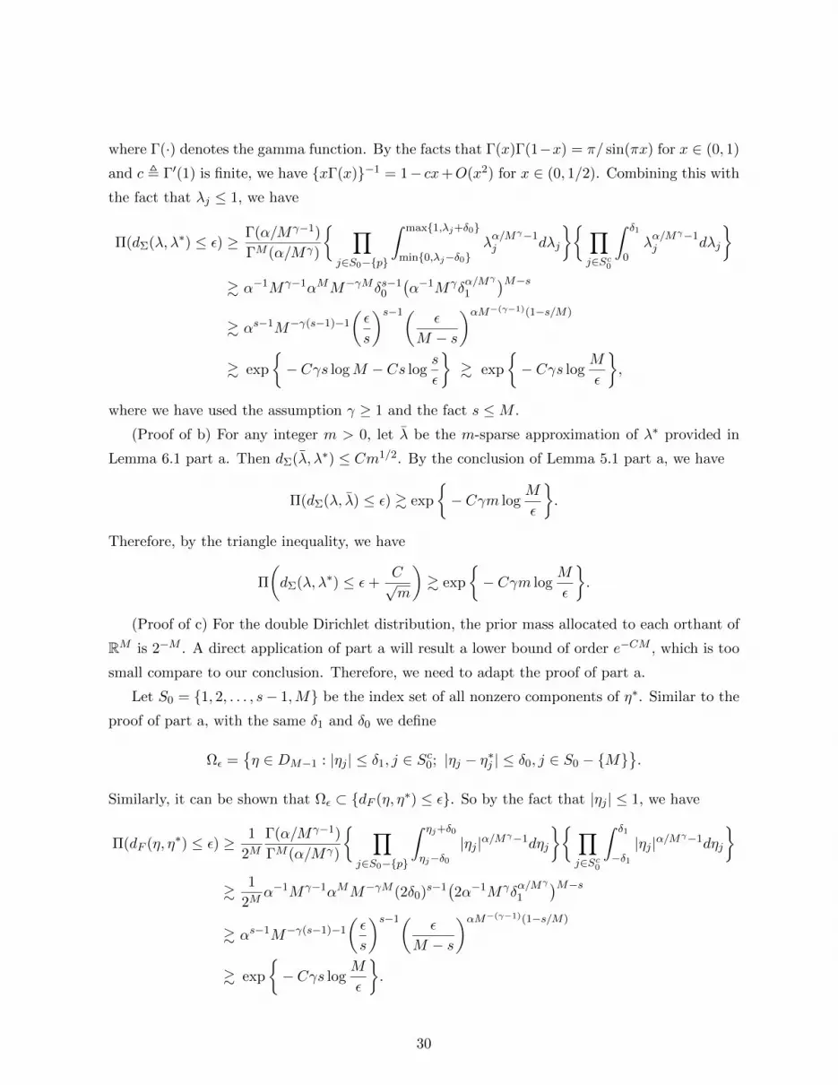
where Γ(·) denotes the gamma function. By the facts that Γ(x)Γ(1−x) = π/ sin(πx) for x ∈ (0, 1)

and c , Γ′(1) is finite, we have xΓ(x)−1 = 1− cx+O(x2) for x ∈ (0, 1/2). Combining this with

the fact that λj ≤ 1, we have

Π(dΣ(λ, λ∗) ≤ ε) ≥ Γ(α/Mγ−1)

ΓM (α/Mγ)

∏j∈S0−p

∫ max1,λj+δ0

min0,λj−δ0λα/Mγ−1j dλj

∏j∈Sc0

∫ δ1

0λα/Mγ−1j dλj

& α−1Mγ−1αMM−γMδs−1

0

(α−1Mγδ

α/Mγ

1

)M−s& αs−1M−γ(s−1)−1

(ε

s

)s−1( ε

M − s

)αM−(γ−1)(1−s/M)

& exp

− Cγs logM − Cs log

s

ε

& exp

− Cγs log

M

ε

,

where we have used the assumption γ ≥ 1 and the fact s ≤M .

(Proof of b) For any integer m > 0, let λ be the m-sparse approximation of λ∗ provided in

Lemma 6.1 part a. Then dΣ(λ, λ∗) ≤ Cm1/2. By the conclusion of Lemma 5.1 part a, we have

Π(dΣ(λ, λ) ≤ ε) & exp

− Cγm log

M

ε

.

Therefore, by the triangle inequality, we have

Π

(dΣ(λ, λ∗) ≤ ε+

C√m

)& exp

− Cγm log

M

ε

.

(Proof of c) For the double Dirichlet distribution, the prior mass allocated to each orthant of

RM is 2−M . A direct application of part a will result a lower bound of order e−CM , which is too

small compare to our conclusion. Therefore, we need to adapt the proof of part a.

Let S0 = 1, 2, . . . , s− 1,M be the index set of all nonzero components of η∗. Similar to the

proof of part a, with the same δ1 and δ0 we define

Ωε =η ∈ DM−1 : |ηj | ≤ δ1, j ∈ Sc0; |ηj − η∗j | ≤ δ0, j ∈ S0 − M

.

Similarly, it can be shown that Ωε ⊂ dF (η, η∗) ≤ ε. So by the fact that |ηj | ≤ 1, we have

Π(dF (η, η∗) ≤ ε) ≥ 1

2MΓ(α/Mγ−1)

ΓM (α/Mγ)

∏j∈S0−p

∫ ηj+δ0

ηj−δ0|ηj |α/M

γ−1dηj

∏j∈Sc0

∫ δ1

−δ1|ηj |α/M

γ−1dηj

&

1

2Mα−1Mγ−1αMM−γM (2δ0)s−1

(2α−1Mγδ

α/Mγ

1

)M−s& αs−1M−γ(s−1)−1

(ε

s

)s−1( ε

M − s

)αM−(γ−1)(1−s/M)

& exp

− Cγs log

M

ε

.

30

As we can seen, now each ηj contributes an additional factor of 2 to the prior concentration

probability comparing to that of λj in the proof of part a. This additional factor compensates for

the 2−M factor in the normalizing constant of the double Dirichlet distribution.

(Proof of d) The proof is similar to that of part b by instead combining the proof of part c

and Lemma 6.1 part b. Therefore, we omit the proof here.

6.2 Proof of Corollary 5.2

By the triangle inequality and assumption (B1), we have

dF (λ, λ∗) ≤ dF (Aη,A∗η) + dF (A∗η,A∗η∗) ≤ κ|A−A∗|+A∗dF (η, η∗).

As a result, |A−A∗| ≤ κ−1ε; dF (η, η∗) ≤ (A∗)−1ε ⊂ dF (λ, λ∗) ≤ 2ε and

Π(dF (λ, λ∗) ≤ ε) ≥ Π(|A−A∗| ≤ Cε) ·Π(dF (η, η∗) ≤ Cε).

Since log Π(|A− A∗| ≤ Cε) log ε, the conclusions can be proved by applying part c and part d

in Lemma 5.1.

6.3 Proof of Lemma 5.3

(Proof of a) For any λ ∈ FΛs,ε, let S(λ) be the index set of the s largest λj ’s. For any λ ∈ FΛ

s,ε,

if λ′ ∈ Λ satisfies λ′j = 0, for j ∈ Sc(λ) and |λ′j − λj | ≤ ε/s, for j ∈ S(λ), then dΣ(λ, λ′) ≤κ||λ′ − λ||1 ≤ 2κε. Therefore, for a fixed index set S ⊂ 1, . . . ,M with size s, the set of all grid

points in [0, 1]s with mesh size ε/s forms an 2κε-covering set for all λ such that S(λ) = S. Since

there are at most(Ms

)such an S, the minimal 2κε-covering set for FΛ

s,ε has at most(Ms

)×(sε

)selements, which implies that

logN(2κε,FΛs,ε, || · ||1) ≤ log

(M

s

)+ s log

s

ε. s log

M

ε.

This proves the first conclusion.

For any η ∈ FηB,s,ε, let S(η) be the index set of the s largest |ηj |’s. Similarly, for any λ =

Aη ∈ FηB,s,ε, if η′ ∈ DM−1 satisfies η′j = 0, for j ∈ Sc(η) and |η′j − ηj | ≤ ε/(Bs), for j ∈ S(η), and

A′ ≤ B satisfies |A′−A| ≤ ε, then dF (A′η′, Aη) ≤ κ||A′η′−Aη||1 ≤ κ|A−A′|+Bκ||η′−η||1 ≤ 3κε.

Similar to the arguments for FΛs,ε, we have

logN(3κε,FηB,s,ε, || · ||1) ≤ log

(M

s

)+ s log

Bs

ε+ log

B

ε. s log

M

ε+ s logB.

(Proof of b) By Lemma 6.1, any λ ∈ Λ and η ∈ BDM−1 can be approximated by an m-sparse

vector in the same space with error Cm−1/2 and CBm−1/2 respectively. Moreover, by the proof of

31

Lemma 6.1, all components of such m-sparse vectors are multiples of 1/m. Therefore, a minimal

C/√m-covering set of Λ has at most

(M+m−1m−1

)elements, which is the total number of nonnegative

integer solutions (n1, . . . , nM ) of the equation: n1 + · · ·+ nM = m. Therefore,

logN(C/√m,Λ, dΣ) ≤ log

(M +m− 1

m− 1

). m logM,

logN(CB/√m,Λ, dΣ) ≤ log

(M +m− 1

m− 1

)+ log

B

B/√m

. m logM.

6.4 Proof of Lemma 5.4

(Proof of a) Consider a random probability P drawn from the Dirichlet process (DP)DP((α/Mγ−1)U

)with concentration parameter α/Mγ−1 and the uniform distribution U on the unit interval [0, 1].

Then by the relationship between the DP and the Dirichlet distribution, we have

(λ1, . . . , λM ) ∼(P (A1), . . . , P (AM )

),

with Ak = [(k − 1)/M, k/M) for k = 1, . . . ,M . The stick-breaking representation for DP (Sethu-

raman, 1994) gives Q =∑∞

k=1wkδξk , a.s. where ξkiid∼ U and

wk = w′k

k−1∏i=1

(1− w′i), with w′kiid∼ Beta(1, α/Mγ−1).

For each k, let i(k) be the unique index such that ξk ∈ Ai(k). Let λ(1) ≥ · · · ≥ λ(M) be an ordering

of λ1, . . . , λM , then

s∑j=1

λ(j) ≥ Q( s⋃j=1

Ai(j)

)=

∑k:ξk∈

⋃sj=1 Ai(j)

wk ≥s∑

k=1

wk.

Combining the above with the definition of wk provides

M∑j=s+1

λ(j) ≤ 1−s∑

k=1

w′k

k−1∏i=1

(1− w′i) =

s∏k=1

(1− w′k) ,s∏

k=1

vk,

where vk = 1−w′kiid∼ Beta(α/Mγ−1, 1). Since vk ∈ (0, 1), we have (FΛ

s,ε)c =

∑Mj=s+1 λ(j) ≥ ε

⊂∏s

k=1 vk ≥ ε

. Because

Evsk =

∫ 1

0

α

Mγ−1tα/M

γ−1+s−1dt =α

α+Mγ−1s≤ αM−(γ−1)s−1,

an application of Markov’s inequality yields

Π

s∏k=1

vk ≥ ε≤ ε−s

s∏k=1

Evsk .M−s(γ−1)s−sε−s.

32

As a result,

Π(λ /∈ Fλs,ε) ≤ Π

s∏k=1

vk ≥ ε≤ exp

(− Cs(γ − 1) log

M

ε

).

(Proof of b) The proof is similar to that of a since (|η1|, . . . , |ηM |) ∼ (λ1, . . . , λM ) and Π(A >

B) ≤ e−CB for A ∼ Ga(a0, b0).

6.5 Proof of Lemma 5.5

(Proof of a) Under (A3), the conclusion can be proved by applying Lemma 2.1 and Lemma 4.1

in Kleijn and van der Vaart (2006) by noticing the fact that ||∑M

j=1 λjfj − f∗||Q = dΣ(λ, λ∗).

(Proof of b) Let ψ(λ, Y ) = 12σ2 ||Y −Fλ||22. We construct the test function as φn(Y ) = I(ψ(λ∗, Y )−

ψ(λ2, Y ) ≥ 0). By the choice of λ∗, under P0 we can decomposition the response Y as Y =

Fλ∗ + ζ + ε, where ε ∼ N(0, σ2In) and ζ = F0 − Fλ∗ ∈ Rd satisfying F T ζ = 0. By Markov’s

inequality, for any t < 0, we have

Pλ∗φn(Y ) = Pλ∗(etψ(λ∗,Y )−ψ(λ2,Y ) ≥ 1)

≤ Eλ∗ exp

t

2σ2

(||ζ + ε||22 − ||F (λ∗ − λ2) + ζ + ε||22

)= Eλ∗ exp

t

σ2(λ2 − λ∗)TF T ε

exp

− t

2σ2nd2

F (λ2, λ∗)

= exp

− t(2σ2)−1nd2

F (λ2, λ∗) + t2σ−2nd2

F (λ2, λ∗),

= exp− (16σ2)−1nd2

F (λ2, λ∗), (6.1)

with t = 14 > 0, where we have used the fact that ε ∼ N(0, σ2In) under Pλ∗ and F T ζ = 0.

Similarly, for any λ ∈ RM , under Pλ we have Y = Fλ+ ε with ε ∼ N(0, σ2In). Therefore, for any

t > 0 we have

Pλ(1− φn(Y )) = Pλ(etψ(λ2,Y )−ψ(λ∗,Y ) ≥ 1)

≤ Eλ exp

t

2σ2

(||ε− F (λ2 − λ)||22 − ||ε− F (λ∗ − λ)||22

)= Eλ exp

− t

σ2(λ2 − λ∗)TF T ε

exp

− t

2σ2n(d2

F (λ, λ∗)− d2F (λ, λ2))

= exp

− t(2σ2)−1n

(d2F (λ, λ∗)− d2

F (λ, λ2))

+ t2σ−2nd2F (λ2, λ

∗),

= exp

− (16σ2)−1n

(d2F (λ, λ∗)− d2

F (λ, λ2))2

d2F (λ2, λ∗)

, (6.2)

with t = 14

(d2F (λ, λ∗)− d2

F (λ, λ2))/d2

F (λ2, λ∗) > 0 if dF (λ, λ∗) > dF (λ, λ2).

33

Combining (6.1) and (6.2) yields

Pλ∗φn(Y ) ≤ exp− (16σ2)−1nd2

F (λ2, λ∗)

supλ∈RM : dF (λ,λ2)< 1

4dF (λ∗,λ2)

Pλ(1− φn(Y )) ≤ exp− (64σ2)−1nd2

F (λ2, λ∗).

Acknowledgments

This research was supported by grant R01ES020619 from the National Institute of Environmental

Health Sciences (NIEHS) of the National Institutes of Health (NIH).

APPENDIX

In the appendix, we provide details of the MCMC implementation for CA and LA. The key

idea is to augment the weight vector λ = (λ1, . . . , λM ) ∼ Diri(ρ, . . . , ρ) by λj = Tj/(T1 + · · ·+TM )

with Tjiid∼ Ga(ρ, 1) for j = 1, . . . ,M and conduct Metropolis Hastings updating for log Tj ’s.

Recall that F = (Fj(Xi)) is the n×M prediction matrix.

A.1 Convex aggregation

By augmenting the Dirichlet distribution in the prior for CA, we have the following Bayesian

convex aggregation model:

Yi =M∑j=1

λjFij + εi, εi ∼ N(0, 1/φ),

λj =Tj

T1 + · · ·+ TM, Tj ∼ Ga(ρ, 1), φ ∼ Ga(a0, b0).

We apply a block MCMC algorithm that iteratively sweeps through the following steps, where

superscripts “O”, “P” and “N” stand for “old”, “proposal” and “new” respectively:

1. Gibbs updating for φ: Updating φ by sampling from [φ|−] ∼ Ga(an, bn) with

an = a0 +n

2, bn = b0 +

1

2

n∑i=1

(Yi −

M∑j=1

λjFij

)2

.

2. MH updating for T (λ): For j = 1 to M , propose TPj = TOj eβUj , where Uj ∼ U(−0.5, 0.5).

34

Calculate λPj = TPj /(∑M

j=1 TPj ) and the log acceptance ratio

logR =φ

2

n∑i=1

(Yi −

M∑j=1

λPj Fij

)2

− φ

2

n∑i=1

(Yi −

M∑j=1

λOj Fij

)2

(log-likelihood)

+

M∑j=1

((ρ− 1) log TPj − TPj

)−

M∑j=1

((ρ− 1) log TOj − TOj

)(log-prior)

+M∑j=1

log TPj −M∑j=1

log TOj (log-transition probability).

With probability min1, R, set TNj = TPj , j = 1, . . . ,M and with probability 1−min1, R,set TNj = TOj , j = 1, . . . ,M . Set λNj = TNj /(

∑Mj=1 T

Nj ), j = 1, . . . ,M .

In the above algorithm, β serves as a tuning parameter to make the acceptance rate of T around

40%.

A.2 Linear aggregation

By augmenting the double Dirichlet distribution in the prior for LA, we have the following

Bayesian linear aggregation model:

Yi =

M∑j=1

θjFij + εi, εi ∼ N(0, 1/φ), θj = Azjλj , λj =Tj

T1 + · · ·+ TM,

A ∼Ga(c0, d0), zj ∼ Bernoulli(0.5), Tj ∼ Ga(ρ, 1), φ ∼ Ga(a0, b0).

The MCMC updating of T (or equivalently λ) and φ is the similar as those in the convex

aggregation. In each iteration of the block MCMC algorithm, we add two additional steps for

updating z and A:

3. MH updating for A: Propose AP = AOeβU , where Uj ∼ U(−0.5, 0.5). Calculate λPj =

λOj eβU and the log acceptance ratio

logR =φ

2

n∑i=1

(Yi −

M∑j=1

λPj Fij

)2

− φ

2

n∑i=1

(Yi −

M∑j=1

λOj Fij

)2

(log-likelihood)

+((c1 − 1) logAP − d1A

P)−((c1 − 1) logAO − d1A

O)

(log-prior)

+ logAP − logAO (log-transition probability).

With probability min1, R, set AN = AP and with probability 1−min1, R, set AN = AO.

Set λNj = λOj AN/AO, j = 1, . . . ,M .

35

4. MH updating for z: For j = 1 to M , propose zPj = zOj Vj , where P (Vj = ±1) = 0.5.

Calculate λPj = λOj Vj and the log acceptance ratio

logR =φ

2

n∑i=1

(Yi −

M∑j=1

λPj Fij

)2

− φ

2

n∑i=1

(Yi −

M∑j=1

λOj Fij

)2

(log-likelihood).

With probability min1, R, set zNj = zPj , j = 1, . . . ,M and with probability 1−min1, R,set zNj = zOj , j = 1, . . . ,M . Set λNj = λOj z

Pj /z

Oj , j = 1, . . . ,M .

References

Bhattacharya, A., D. Pati, N. S. Pillai, and D. B. Dunson (2013). Bayesian shrinkage.

arXiv:1212.6088 .

Birge, L. (2004). Model selection for Guassian regression with random design. Bernoulli 10,

1039–1151.

Blei, D. M., A. Y. Ng, and M. I. Jordan (2003). Latent Dirichlet allocation. Journal of Machine

Learning Research 3, 993–1022.

Buhlmann, P. (2006). Boosting for high-dimensional linear models. Ann. Statist. 34, 559–583.

Bunea, F. and A. Nobel (2008). Sequential procedures for aggregating arbitrary estimators of a

conditional mean. IEEE Transactions on Information Theory 54, 1725–1735.

Bunea, F. and Tsybakov (2007). Aggregation for Gaussian regression. Ann. Statist. 35, 1674–1697.

Carvalho, C. M., N. G. Polson, and J. G. Scott (2010). The horseshoe estimator for sparse signals.

Biometrika 97, 465–480.

Castillo, I. and A. W. van der Vaart (2012). Needles and straw in a haystack: Posterior concen-

tration for possibly sparse sequences. Ann. Statist. 40, 2069–2101.

de Jonge, R. and H. van Zanten (2013). Semiparametric bernsteincvon mises for the error standard

deviation. Electronic Journal of Statistics 7, 217–243.

George, E. I. and R. E. McCulloch (1997). Approaches for Bayesain variable selection. Statistica

Sinica 7, 339–373.

Ghosal, S., J. K. Ghosh, and A. W. Van Der Vaart (2000). Convergence rates of posterior

distributions. Ann. Statist. 28, 500–531.

36

Ghosal, S. and A. W. van der Vaart (2007). Convergence rates of posterior distributions for noniid

observations. Ann. Statist. 35, 192–223.

Guedj, B. and P. Alquier (2013). PAC-Bayesian estimation and prediction in sparse additive

models. Electronic Journal of Statistics 7, 264–291.

Hoerl, A. and R. Kennard (1970). Ridge regression: Biased estimation for nonorthogonal prob-

lems. Technometrics 12, 69–82.

Hoeting, J. A., D. Madigan, A. E. Raftery, and C. T. Volinsky (1999). Bayesian model averaging:

A tutorial. Statistical Science 14, 382–417.

Ishwaran, H. and J. S. Rao (2005). Spike and slab variable selection: Frequentist and Bayesian

strategies. Ann. Statist. 33, 730–773.

Juditsky, A. and A. Nemirovski (2000). Functional aggregation for nonparametric regression.

Ann. Statist. 28, 681–712.

Kleijn, B. J. K. and A. W. van der Vaart (2006). Misspecification in infinite-dimensional Bayesian

statistics. Ann. Statist. 34, 837–877.

Nemirovski, A. (2000). Topics in non-parametric statistics. Lectures on Probability Theory and

Statistics (Saint-Flour, 1998). ecture Notes in Math. 1738. Springer, Berlin.

Polson, N. G. and J. G. Scott (2010). Shrink globally, act locally: Sparse Bayesian regularization

aand prediction. Bayesian Statistics 9 (J.M. Bernardo, M.J. Bayarri, J.O. Berger, A.P. Dawid,

D. Heckerman, A.F.M. Smith and M. West, eds.). Oxford University Press, New York.

Raskutti, G., M. Wainwright, and B. Yu (2011). Minimax rates of estimation for high-dimensional

linear regression over lq-balls. IEEE transactions on information theory 57, 6976–6994.

Rousseau, J. and K. Mengersen (2011). Asymptotic behaviour of the posterior distribution in

overfitted mixture models. J. R. Statist. Soc. B 73, 689–710.

Sethuraman, J. (1994). A constructive definition of Dirichlet priors. Statistica Sinica 4, 639–650.

Tibshirani, R. (1996). Regression shrinkage and selection via the lasso. Journal of the Royal

Statistical Association 58, 267–288.

Tsybakov, A. (2003). Optimal rates of aggregation. Learning Theory and Kernel Machines,

Lecture Notes in Computer Science, 2777, 303–313.

van der Laan, M. J., E. C. Polley, and A. E. Hubbard (2007). Super learner. Genetics and

Molecular Biology 6.

37

Wegkamp, M. (2003). Model selection in nonparametric regression. Ann. Statist. 31, 252–273.

Yang, Y. (2000). Combining different procedures for adaptive regression. J. Multivariate Anal. 74,

135–161.

Yang, Y. (2001). Adaptive regression by mixing. J. Amer. Statist. Assoc. 96, 574–588.

Yang, Y. (2004). Aggregating regression procedures to improve performance. Bernoulli 10, 25–47.

38