The Bayesian Occupation Filter

The Bayesian occupation filter

M.K Tay1, K. Mekhnacha2, M. Yguel1, C. Coué1, C. Pradalier3, C. Laugier1

Th. Fraichard1 and P. Bessière4

1 INRIA Rhône-Alpes2 PROBAYES3 CSIRO ICT Centre, Queensland Centre for Advanced technologies (QCAT)4 CNRS - Grenoble Université

1 Introduction

Perception of and reasoning about dynamic environments is pertinent for mo-bile robotics and still constitutes one of the major challenges. To work inthese environments, the mobile robot must perceive the environment withsensors; measurements are uncertain and normally treated within the esti-mation framework. Such an approach enables the mobile robot to model thedynamic environment and follow the evolution of its environment. With aninternal representation of the environment, the robot is thus able to performreasoning and make predictions to accomplish its tasks successfully. Systemsfor tracking the evolution of the environment have traditionally been a majorcomponent in robotics. Industries are now beginning to express interest insuch technologies. One particular example is the application within the au-tomotive industry for adaptive cruise control [Coué et al., 2002], where thechallenge is to reduce road accidents by using better collision detection sys-tems. The major requirement of such a system is a robust tracking system.Most of the existing target-tracking algorithms use an object-based represen-tation of the environment. However, these existing techniques must explicitlyconsider data association and occlusion. In view of these problems, a grid-based framework, the Bayesian occupancy filter (BOF) [Coué et al., 2002,2003], has been proposed.

1.1 Motivation

In classical tracking methodology [Bar-Shalom and Fortman, 1988], the prob-lem of data association and state estimation are major problems to be ad-dressed. The two problems are highly coupled, and an error in either com-ponent leads to erroneous outputs. The BOF makes it possible to decomposethis highly coupled relationship by avoiding the data association problem, inthe sense that the data association is handled at a higher level of abstraction.

inria

-002

9508

4, v

ersi

on 1

- 11

Jul

200

8Author manuscript, published in "Probabilistic Reasoning and Decision Making in Sensory-Motor Systems, Bessière, P. and Laugier,

C. and Siegwart, R. (Ed.) (2008)"

http://hal.inria.fr/inria-00295084/fr/

http://hal.archives-ouvertes.fr

80 M.K Tay , K. Mekhnacha, M. Yguel, C. Coué, C. Pradalier, et al.

In the BOF model, concepts such as objects or tracks do not exist; theyare replaced by more useful properties such as occupancy or risk, which aredirectly estimated for each cell of the grid using both sensor observations andsome prior knowledge.

It might seem strange to have no object representations when objects obvi-ously exist in real life environments. However, an object-based representationis not required for all applications. Where object-based representations arenot pertinent, we argue that it is more useful to work with a more descriptive,richer sensory representation rather than constructing object-based represen-tations with their complications in data association. For example, to calculatethe risk of collision for a mobile robot, the only properties required are theprobability distribution on occupancy and velocities for each cell in the grid.Variables such as the number of objects are inconsequential in this respect.

This model is especially useful when there is a need to fuse informationfrom several sensors. In standard methods for sensor fusion in tracking ap-plications, the problem of track-to-track association arises where each sensorcontains its own local information. Under the standard tracking frameworkwith multiple sensors, the problem of data association will be further compli-cated: as well as the data association between two consecutive time instancesfrom the same sensor, the association of tracks (or targets) between the dif-ferent sensors must be taken into account as well.

In contrast, the grid-based BOF will not encounter such a problem. A grid-based representation provides a conducive framework for performing sensorfusion [Moravec, 1988]. Different sensor models can be specified to match thedifferent characteristics of the different sensors, facilitating efficient fusion inthe grids. The absence of an object-based representation allows easier fusingof low-level descriptive sensory information onto the grids without requiringdata association.

Uncertainty characteristics of the different sensors are specified in the sen-sor models. This uncertainty is explicitly represented in the BOF grids inthe form of occupancy probabilities. Various approaches using the probabilis-tic reasoning paradigm, which is becoming a key paradigm in robotics, havealready been successfully used to address several robotic problems, such asCAD modelling [Mekhnacha et al., 2001] and simultaneous map building andlocalization (SLAM) [Thrun, 1998, Kaelbling et al., 1998, Arras et al., 2001].

In modelling the environment with BOF grids, the object model problem isnonexistent because there are only cells representing the state of the environ-ment at a certain position and time, and each sensor measurement changesthe state of each cell. Different kinds of objects produce different kinds ofmeasures, but this is handled naturally by the cell space discretization.

Another advantage of BOF grids is their rich representation of dynamicenvironments. This information includes the description of occupied and hid-den areas (i.e. areas of the environment that are temporarily hidden to thesensors by an obstacle). The dynamics of the environment and its robustnessrelative to object occlusions are addressed using a novel two-step mechanism

inria

-002

9508

4, v

ersi

on 1

- 11

Jul

200

8

The Bayesian occupation filter 81

that permits taking the sensor observation history and the temporal consis-tency of the scene into account. This mechanism estimates, at each time step,the state of the occupancy grid by combining a prediction step (history) andan estimation step (incorporating new measurements). This approach is de-rived from the Bayesian filter approach [Jazwinsky, 1970], which explains whythe filter is called the Bayesian occupancy filter (BOF).

The five main motivations in the proposed BOF approach are as follows.

• Taking uncertainty into account explicitly, which is inherent in any modelof a real phenomenon. The uncertainty is represented explicitly in theoccupancy grids.

• Avoiding the “data association problem” in the sense that data associationis to be handled at a higher level of abstraction. The data associationproblem is to associate an object ot at time t with ot+1 at time t+1. Currentmethods for resolving this problem often do not perform satisfactorilyunder complex scenarios, i.e. scenarios involving numerous appearances,disappearances and occlusions of several rapidly manoeuvring targets. Theconcept of objects is nonexistent in the BOF and hence avoids the problemof data association from the classical tracking point of view.

• Avoiding the object model problem, that is, avoiding the need to makeassumptions about the shape or size of the object. It is complex to definewhat the sensor could measure without a good representation of the object.In particular, a big object may give multiple detections whereas a smallobject may give just one. In both cases, there is only one object, and thatlack of coherence causes multiple-target tracking systems, in most cases,to work properly with only one kind of target.

• An Increased robustness of the system relative to object occlusions, appear-ances and disappearances by exploiting at any instant all relevant informa-tion on the environment perceived by the mobile robot. This informationincludes the description of occupied and hidden areas (i.e. areas of theenvironment that are temporarily hidden to the sensors by an obstacle).

• A method that could be implemented later on dedicated hardware, to obtainboth high performance and decreased cost of the final system.

1.2 Objectives of the BOF

We claim that in the BOF approach, the five previous objectives are met asfollows.

• Uncertainty is taken into account explicitly, thanks to the probabilisticreasoning paradigm, which is becoming a key paradigm in robotics.

• The data association problem is postponed by reasoning on a probabilisticgrid representation of the dynamic environment. In such a model, conceptssuch as objects or tracks are not needed.

• The object model problem is nonexistent because there are only cells in theenvironment state, and each sensor measurement changes the state of each

inria

-002

9508

4, v

ersi

on 1

- 11

Jul

200

8


cell. The different kinds of measures produced by different kinds of objectare handled naturally by the cell space discretization.

• The dynamics of the environment and its robustness relative to object oc-clusions are addressed using a novel two-step mechanism that permitstaking the sensor observation history and the temporal consistency of thescene into account.

• The Bayesian occupancy filter has been designed to be highly parallelized. Ahardware implementation on a dedicated chip is possible, which will leadto an efficient representation of the environment of a mobile robot.

This chapter presents the concepts behind BOF and its mathematical for-mulation, and shows some of its applications.

• Section 2 introduces the basic concepts behind the BOF.• Section 2.1 introduces Bayesian filtering in the 4D occupancy grid frame-

work [Coué et al., 2006].• Section 2.2 describes an alternative formulation for filtering in the 2D

occupancy grid framework [Tay et al., 2007].• Section 3 shows several applications of the BOF.• Section 4 concludes this chapter.

2 Bayesian occupation filtering

The consideration of sensor observation history enables robust estimations inchanging environments (i.e. it allows processing of temporary objects, occlu-sions and detection problems). Our approach for solving this problem is tomake use of an appropriate Bayesian filtering technique called the Bayesianoccupancy filter (BOF).

Bayesian filters Jazwinsky [1970] address the general problem of estimatingthe state sequence xk, k ∈ N of a system given by:

xk = fk(xk−1, uk−1, wk), (1)

where fk is a possibly nonlinear transition function, uk−1 is a “control” vari-able (e.g. speed or acceleration) for the sensor that allows it to estimate itsown movement between time k − 1 and time k, and wk is the process noise.This equation describes a Markov process of order one.

Let zk be the sensor observation of the system at time k. The objective ofthe filtering is to estimate recursively xk from the sensor measurements:

zk = hk(xk, vk) (2)

where hk is a possibly nonlinear function and vk is the measurement noise.This function models the uncertainty of the measurement zk of the system’sstate xk.

inria

-002

9508

4, v

ersi

on 1

- 11

Jul

200

8


In other words, the goal of the filtering is to estimate recursively the proba-bility distribution P (Xk | Zk), known as the posterior distribution. In general,this estimation is done in two stages: prediction and estimation. The goal ofthe prediction stage is to compute an a priori estimate of the target’s stateknown as the prior distribution. The goal of the estimation stage is to com-pute the posterior distribution, using this a priori estimate and the currentmeasurement of the sensor.

Exact solutions to this recursive propagation of the posterior density doexist in a restrictive set of cases. In particular, the Kalman filter [Kalman,1960, Welch and Bishop] is an optimal solution when the functions fk and hk

are linear and the noise values wk and vk are Gaussian. In general, however, so-lutions cannot be determined analytically, and an approximate solution mustbe computed.

Prediction

Estimation

6 ? ?

Z

Fig. 1. Bayesian occupancy filter as a recursive loop.

In this case, the state of the system is given by the occupancy state of eachcell of the grid, and the required conditions for being able to apply an exactsolution such as the Kalman filter are not always verified. Moreover, the par-ticular structure of the model (occupancy grid) and the real-time constraintimposed on most robotic applications lead to the development of the conceptof the Bayesian occupancy filter. This filter estimates the occupancy state intwo steps, as depicted in Fig. 1.

In this section, two different formulations of the BOF will be introduced.The first represents the state space by a 4-dimensional grid, in which the oc-cupancy of each cell represents the joint space of 2D position and 2D velocity.The estimation of occupancy and velocity in this 4D space are described inSection 2.1.

The second formulation of the BOF represents the state space by a 2-dimensional occupancy grid. Each cell of the grid is associated with a prob-ability distribution on the velocity of the occupancy associated with the cell.The differences between the two formulations are subtle. Essentially, the 4Dformulation permits overlapping objects with different velocities whereas the

inria

-002

9508

4, v

ersi

on 1

- 11

Jul

200

8


2D formulation does not allow for overlapping objects. The estimation onvelocity and occupancy in this 2D grid are described in Section 2.2.

2.1 The 4D Bayesian occupation filter

The 4-dimensional BOF takes the form of a gridded histogram with two di-mensions representing positions in 2D Cartesian coordinates and the othertwo dimensions representing the orthogonal components of the 2-dimensionalvelocities of the cells. As explained previously in Section 2, the BOF consistsof a prediction step and an estimation step in the spirit of Bayesian filtering.

Based on this approach, the evolution of the BOF at time k occurs in twosteps:

1. the prediction step makes use of both the result of the estimation step attime k−1 and a dynamic model to compute an a priori estimate of thegrid; and

2. the estimation step makes use of both this prediction result and the sensorobservations at time k to compute the grid values.

The next two subsections will explain the prediction and estimation stepsof the 4D BOF respectively.

Estimation in the 4D BOF

The estimation step consists of estimating the occupancy probability of eachcell of the grid, using the last set of sensor observations. These observationsrepresent preprocessed information given by a sensor. At each time step, thesensor is able to return a list of detected objects, along with their associatedpositions and velocities in the sensor reference frame. In practice, this set ofobservations could also contain two types of false measurements: false alarms(i.e. when the sensor detects a nonexistent object) and missed detections (i.e.when the sensor does not detect an existing object).

Solving the static estimation problem can be done by building a Bayesianprogram. The relevant variables and decomposition are as follows.

• Ck: The cell itself at time k; this variable is 4-dimensional and representsa position and a speed relative to the vehicle.

• EkC : The state of the cell C at time k; whether it is occupied.

• Z: The sensor observation set; one observation is denoted by Zs, and thenumber of observation is denoted by S; each variable Zs is 4-dimensional.

• M : The “matching” variable; it specifies which observation of the sensor iscurrently used to estimate the state of a cell.

The decomposition of the joint distribution of these variables can be expressedas:

inria

-002

9508

4, v

ersi

on 1

- 11

Jul

200

8


P (Ck EkC Z M) = P (Ck)P (Ek

C | Ck)P (M) ×S∏

s=1

P (Zs | Ck EkC M)

Parametric forms can be assigned to each term of the joint probabilitydecomposition.

• P (Ck) represents the information on the cell itself. As we always know thecell for which we are currently estimating the state, this distribution maybe left unspecified.

• P (EkC | C) represents the a priori information on the occupancy of the

cell. The prior distribution may be obtained from the estimation of theprevious time step.

• P (M) is chosen uniformly. It specifies which observation of the sensor isused to estimate the state of a cell.

• The shape of P (Zs |Ck EkC M) depends on the value of the matching vari-

able.– If M 6= s, the observation is not taken from the cell C. Consequently,

we cannot say anything about this observation. P (Zs |Ck EkC M) is

defined by a uniform distribution.– If M = s, the form of P (Zs |Ck Ek

C M) is given by the sensor model.Its goal is to model the sensor response knowing the cell state. Detailson this model can be found in Elfes [1989].

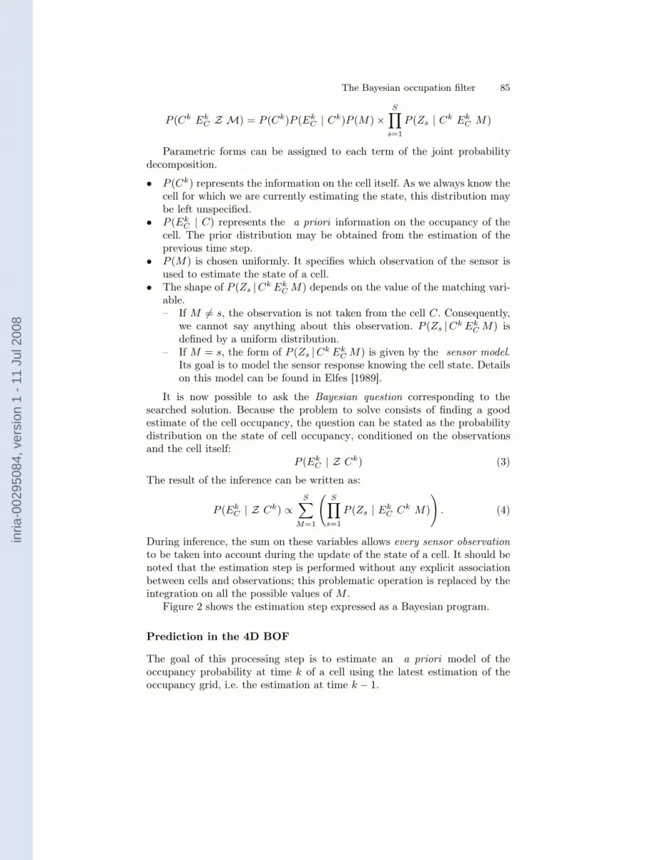
It is now possible to ask the Bayesian question corresponding to thesearched solution. Because the problem to solve consists of finding a goodestimate of the cell occupancy, the question can be stated as the probabilitydistribution on the state of cell occupancy, conditioned on the observationsand the cell itself:

P (EkC | Z Ck) (3)

The result of the inference can be written as:

P (EkC | Z Ck) ∝

S∑

M=1

(S∏

s=1

P (Zs | EkC Ck M)

). (4)

During inference, the sum on these variables allows every sensor observationto be taken into account during the update of the state of a cell. It should benoted that the estimation step is performed without any explicit associationbetween cells and observations; this problematic operation is replaced by theintegration on all the possible values of M .

Figure 2 shows the estimation step expressed as a Bayesian program.

Prediction in the 4D BOF

The goal of this processing step is to estimate an a priori model of theoccupancy probability at time k of a cell using the latest estimation of theoccupancy grid, i.e. the estimation at time k − 1.

inria

-002

9508

4, v

ersi

on 1

- 11

Jul

200

8


Pro

gra

m

8

>>>>>>>>>>>>>>>>>>>>>>>>>>>>>>>>>>>>>>>>><

>>>>>>>>>>>>>>>>>>>>>>>>>>>>>>>>>>>>>>>>>:

Des

crip

tion

8

>>>>>>>>>>>>>>>>>>>>>>>>>>>>>>>>>>>>><

>>>>>>>>>>>>>>>>>>>>>>>>>>>>>>>>>>>>>:

Spec

ifica

tion

8

>>>>>>>>>>>>>>>>>>>>>>>>>>>>>>>>><

>>>>>>>>>>>>>>>>>>>>>>>>>>>>>>>>>:

Relevant Variables:Ck T he cell itself at time k; this variable is 4-dimensional and

represents a position and a speed relative to the vehicle.Ek

C The state of the cell C, occupied or not.Z The sensor observation set: one observation is denoted Zs;

the number of observation is denoted S;each variable Zs is 4-dimensional.

M The “matching” variable; its goal is to specify whichobservation of the sensor is currently used to estimate thestate of a cell.

Decomposition:P (Ck Ek

C Z M) =

P (Ck)P (EkC | Ck)P (M) ×

SQ

s=1

P (Zs | Ck EkC M)

Parametric Forms:P (Ck): uniform;P (ECk | Ck): from the prediction;P (M): uniform;P (Zs | Ck Ek

C M): sensor model;Identification:None

Question:P (Ek

C | Z C‖)

Fig. 2. Occupancy Probability Static Estimation

Similarly, the prediction step can be expressed as a Bayesian program.The relevant variable specifications are the same as those of the estimationstage except for the variable Uk−1, which represents the “control” input ofthe CyCab at time k − 1. For example, it could be a measurement of itsinstantaneous velocity at time k − 1.

The decomposition of the joint distribution can therefore be expressed asfollows.

P (Ck EkCCk−1 Ek−1

C Uk−1)

= P (Ck−1) × P (Uk−1) × P (Ek−1C | Ck−1)

×P (Ck | Ck−1 Uk−1) × P (EkC | Ek−1

C Ck−1 Ck)

The parametric forms for each of the decomposition terms are as follows.

• P (Ck−1) and P (Uk−1) are chosen as uniform distributions.• P (Ek−1

C |Ck−1) is given by the result of the estimation step at time k− 1.• P (Ck | Ck−1 Uk−1) is given by the dynamic model. It represents the

probability that an object has moved from cell Ck−1 to cell Ck. Thismovement is because of the object itself and the robot’s movement between

inria

-002

9508

4, v

ersi

on 1

- 11

Jul

200

8


times k − 1 and k. To define this model, we suppose a constant velocitymodel subject to zero-mean Gaussian errors for the moving objects.

• P (EkC |Ek−1

C Ck−1 Ck) represents the probability that an existing objectat time k − 1 (i.e. [Ek−1

C = 1] still exists at time k (i.e. [EkC = 1]). As

we consider that objects cannot disappear, Dirac functions are chosen forthese distributions.

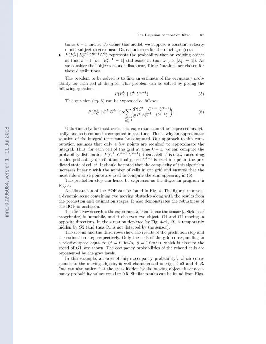
The problem to be solved is to find an estimate of the occupancy prob-ability for each cell of the grid. This problem can be solved by posing thefollowing question.

P (EkC | Ck Uk−1) (5)

This question (eq. 5) can be expressed as follows.

P (EkC | Ck Uk−1)∝

∑

Ck−1

Ek−1C

(P (Ck | Ck−1 Uk−1)

×P (Ek−1C | Ck−1)

). (6)

Unfortunately, for most cases, this expression cannot be expressed analyt-ically, and so it cannot be computed in real time. This is why an approximatesolution of the integral term must be computed. Our approach to this com-putation assumes that only a few points are required to approximate theintegral. Thus, for each cell of the grid at time k − 1, we can compute theprobability distribution P (Ck |Ck−1 Uk−1); then a cell ck is drawn accordingto this probability distribution; finally, cell Ck−1 is used to update the pre-dicted state of cell ck. It should be noted that the complexity of this algorithmincreases linearly with the number of cells in our grid and ensures that themost informative points are used to compute the sum appearing in (6).

The prediction step can hence be expressed as the Bayesian program inFig. 3.

An illustration of the BOF can be found in Fig. 4. The figures representa dynamic scene containing two moving obstacles along with the results fromthe prediction and estimation stages. It also demonstrates the robustness ofthe BOF in occlusion.

The first row describes the experimental conditions: the sensor (a Sick laserrangefinder) is immobile, and it observes two objects O1 and O2 moving inopposite directions. In the situation depicted by Fig. 4-c1, O1 is temporarilyhidden by O2 (and thus O1 is not detected by the sensor).

The second and the third rows show the results of the prediction step andthe estimation step respectively. Only the cells of the grid corresponding toa relative speed equal to (x = 0.0m/s, y = 1.0m/s), which is close to thespeed of O1, are shown. The occupancy probabilities of the related cells arerepresented by the grey levels.

In this example, an area of “high occupancy probability”, which corre-sponds to the moving objects, is well characterized in Figs. 4-a2 and 4-a3.One can also notice that the areas hidden by the moving objects have occu-pancy probability values equal to 0.5. Similar results can be found from Figs.

inria

-002

9508

4, v

ersi

on 1

- 11

Jul

200

8


Pro

gra

m

8

>>>>>>>>>>>>>>>>>>>>>>>>>>>>>>>>>>>>>>><

>>>>>>>>>>>>>>>>>>>>>>>>>>>>>>>>>>>>>>>:

Des

crip

tion

8

>>>>>>>>>>>>>>>>>>>>>>>>>>>>>>>>>>><

>>>>>>>>>>>>>>>>>>>>>>>>>>>>>>>>>>>:

Spec

ifica

tion

8

>>>>>>>>>>>>>>>>>>>>>>>>>>>>>>><

>>>>>>>>>>>>>>>>>>>>>>>>>>>>>>>:

Relevant Variables:Ck Cell C considered at time K

EkC State of cell C at time K

Ck−1 Cell C at time k − 1

Ek−1C State of cell C at time k − 1

Uk−1 “control” input of the CyCab at time k − 1. Forexample, it could be a measurement of its instantaneousvelocity at time k − 1.

Decomposition:P (Ck Ek

C Ck−1 Ek−1C Uk−1) =

P (Ck−1) × P (Uk−1) × P (Ek−1C | Ck−1)

×P (Ck | Ck−1 Uk−1) × P (EkC | Ek−1

C Ck−1 Ck)Parametric Forms:P (Ck−1): uniform;P (Uk−1): uniform;P (Ek−1

C | Ck−1): estimation at time k-1;P (Ck | Ck−1 Uk−1): dynamic model;P (Ek

C | Ek−1C Ck−1 Ck): dirac;

Identification:None

Question:P (Ek

C | Ck Uk−1)

Fig. 3. Prediction Step at time k

4-b2 and 4-b3. Figure 4-c2 shows the result of the prediction step, based onthe grid of Fig. 4-b3 and on the dynamic model used. This prediction showsthat an object is probably located in the area hidden by O2 (i.e. an area ofhigh occupancy probability is found in Fig. 4-c3). Of course, the confidence inthe presence of a hidden object (i.e. the values of the occupancy probabilityin the grid) progressively decreases when this object is not observed by thesensor during the following time steps. In the example depicted by Fig. 4-d3,the object is no longer hidden by O2; it is detected by the laser, and therelated occupancy probability values increase.

2.2 The 2D Bayesian occupancy filter

An alternative formulation presents the BOF as 2D grids instead of the pre-vious formulation of 4D grids. This model of the dynamic grid is differentfrom the approach adopted in the original BOF formulation by Coué et al.[2006]. Their grid model is in 4-dimensional space whereas the 2D BOF [Tayet al., 2007] models the grid in 2-dimensional space. A subtle difference is thatthe 4D BOF allows the representation of overlapping objects but the 2D BOFdoes not. A more obvious difference is the ability to infer velocity distributions

inria

-002

9508

4, v

ersi

on 1

- 11

Jul

200

8


a.1. b.1. c.1. d.1.

0 0.2 0.4 0.6 0.8 1

0

2

4

6

8

10

-4 -2 0 2 4

0 0.2 0.4 0.6 0.8 1

0

2

4

6

8

10

-4 -2 0 2 4

0 0.2 0.4 0.6 0.8 1

0

2

4

6

8

10

-4 -2 0 2 4

0.1

0.2

0.3

0.4

0.5

0.6

0 0.2 0.4 0.6 0.8 1

0

2

4

6

8

10

-4 -2 0 2 4

a.2. b.2. c.2. d.2.

0 0.2 0.4 0.6 0.8 1

0

2

4

6

8

10

-4 -2 0 2 4

0 0.2 0.4 0.6 0.8 1

0

2

4

6

8

10

-4 -2 0 2 4

0 0.2 0.4 0.6 0.8 1

0

2

4

6

8

10

-4 -2 0 2 4

0.1

0.2

0.3

0.4

0.5

0.6

0 0.2 0.4 0.6 0.8 1

0

2

4

6

8

10

-4 -2 0 2 4

a.3. b.3. c.3. d.3.

Fig. 4. A short sequence of a dynamic scene. The first row describes the situation:a moving object is temporarily hidden by a second object. The second row showsthe predicted occupancy grids, and the third row shows the result of the estimationstep. The grids show P ([Ek

C = 1] | x y [x = 0.0] [y = 1.0])

in the 2D BOF model, which is absent in the 4D BOF model as it requiresthe specification of the dynamics of the cells.

The 2D BOF can also be expressed as a Bayesian program. In the spiritof Bayesian programming, we start by defining the relevant variables.

• C is an index that identifies each 2D cell of the grid.• A is an index that identifies each possible antecedent of the cell c over all

the cells in the 2D grid.• Zt ∈ Z where Zt is the random variable of the sensor measurement relative

to the cell c.• V ∈ V = {v1, . . . , vn} where V is the random variable of the velocities for

the cell c and its possible values are discretized into n cases.

inria

-002

9508

4, v

ersi

on 1

- 11

Jul

200

8


• O, O−1 ∈ O ≡ {occ, emp} where O represents the random variable of thestate of c being either “occupied” or “empty”. O−1 represents the randomvariable of the state of an antecedent cell of c through the possible motionthrough c. For a given velocity vk = (vx, vy) and a given time step δt, it ispossible to define an antecedent for c = (x, y) as c−k = (x−vxδt, y−vyδt).

The following expression gives the decomposition of the joint distributionof the relevant variables according to Bayes’ rule and dependency assumptions.

P (C, A, Z, O, O−1, V )

= P (A)P (V |A)P (C|V, A)P (O−1|A)P (O|O−1)P (Z|O, V, C) (7)

The parametric form and semantics of each component of the joint decom-position are as follows.

• P (A) is the distribution over all the possible antecedents of the cell c. Itis chosen to be uniform because the cell is considered reachable from allthe antecedents with equal probability.

• P (V |A) is the distribution over all the possible velocities of a certain an-tecedent of the cell c; its parametric form is a histogram.

• P (C|V, A) is a distribution that explains whether c is reachable from [A =a] with the velocity [V = v]. In discrete spaces, this distribution is a Diracwith value equal to one if and only if cx = ax + vxδt and cy = ay + vyδt,which follows a dynamic model of constant velocity.

• P (O−1|A) is the conditional distribution over the occupancy of the an-tecedents. It gives the probability of the possible previous step of the cur-rent cell.

• P (O|O−1) is the conditional distribution over the occupancy of the currentcell, which depends on the occupancy state of the previous cell. It is defined

as a transition matrix: T =

[1 − ǫ ǫ

ǫ 1 − ǫ

], which allows the system to use

the null acceleration hypothesis as an approximation; in this matrix, ǫ is aparameter representing the probability that the object in c does not followthe null acceleration model.

• P (Z|O, V, C) is the conditional distribution over the sensor measurementvalues. It depends of the state of the cell, the velocity of the cell andobviously the position of the cell.

In the 2D BOF, the Bayesian question will be the probability distributionon the occupation and velocity for each cell of the grid.

P (O | Z C)

P (V | Z C)

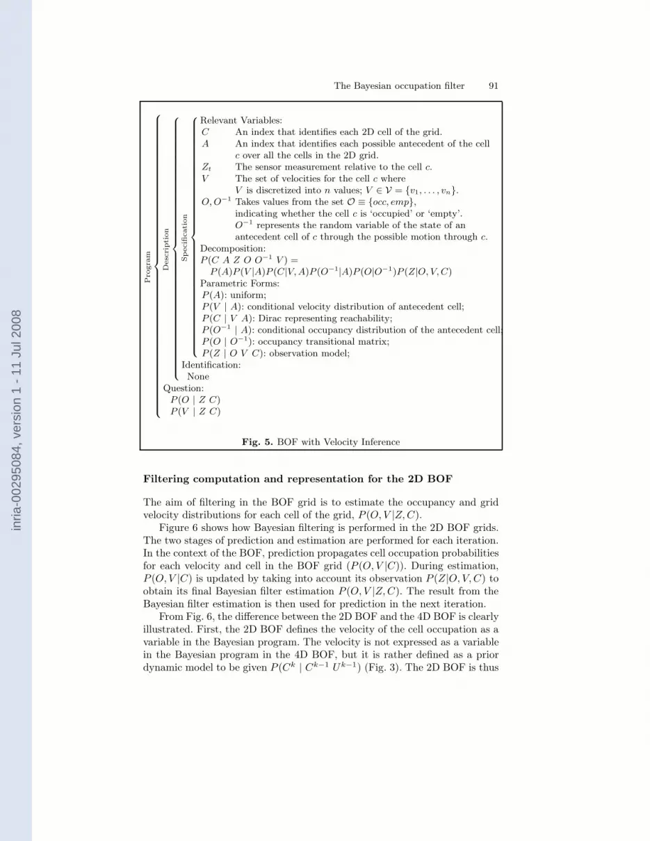
The 2D BOF can be formulated as the Bayesian program in Figure 5.

inria

-002

9508

4, v

ersi

on 1

- 11

Jul

200

8


Pro

gra

m

8

>>>>>>>>>>>>>>>>>>>>>>>>>>>>>>>>>>>>>>>>>>>>>>><

>>>>>>>>>>>>>>>>>>>>>>>>>>>>>>>>>>>>>>>>>>>>>>>:

Des

crip

tion

8

>>>>>>>>>>>>>>>>>>>>>>>>>>>>>>>>>>>>>>>><

>>>>>>>>>>>>>>>>>>>>>>>>>>>>>>>>>>>>>>>>:

Spec

ifica

tion

8

>>>>>>>>>>>>>>>>>>>>>>>>>>>>>>>>>>>><

>>>>>>>>>>>>>>>>>>>>>>>>>>>>>>>>>>>>:

Relevant Variables:C An index that identifies each 2D cell of the grid.A An index that identifies each possible antecedent of the cell

c over all the cells in the 2D grid.Zt The sensor measurement relative to the cell c.V The set of velocities for the cell c where

V is discretized into n values; V ∈ V = {v1, . . . , vn}.O, O−1 Takes values from the set O ≡ {occ, emp},

indicating whether the cell c is ‘occupied’ or ‘empty’.O−1 represents the random variable of the state of anantecedent cell of c through the possible motion through c.

Decomposition:P (C A Z O O−1 V ) =

P (A)P (V |A)P (C|V, A)P (O−1|A)P (O|O−1)P (Z|O, V, C)Parametric Forms:P (A): uniform;P (V | A): conditional velocity distribution of antecedent cell;P (C | V A): Dirac representing reachability;P (O−1 | A): conditional occupancy distribution of the antecedent cell;P (O | O−1): occupancy transitional matrix;P (Z | O V C): observation model;

Identification:None

Question:P (O | Z C)P (V | Z C)

Fig. 5. BOF with Velocity Inference

Filtering computation and representation for the 2D BOF

The aim of filtering in the BOF grid is to estimate the occupancy and gridvelocity distributions for each cell of the grid, P (O, V |Z, C).

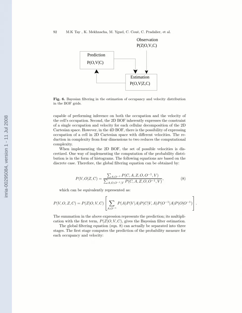
Figure 6 shows how Bayesian filtering is performed in the 2D BOF grids.The two stages of prediction and estimation are performed for each iteration.In the context of the BOF, prediction propagates cell occupation probabilitiesfor each velocity and cell in the BOF grid (P (O, V |C)). During estimation,P (O, V |C) is updated by taking into account its observation P (Z|O, V, C) toobtain its final Bayesian filter estimation P (O, V |Z, C). The result from theBayesian filter estimation is then used for prediction in the next iteration.

From Fig. 6, the difference between the 2D BOF and the 4D BOF is clearlyillustrated. First, the 2D BOF defines the velocity of the cell occupation as avariable in the Bayesian program. The velocity is not expressed as a variablein the Bayesian program in the 4D BOF, but it is rather defined as a priordynamic model to be given P (Ck | Ck−1 Uk−1) (Fig. 3). The 2D BOF is thus

inria

-002

9508

4, v

ersi

on 1

- 11

Jul

200

8


Estimation

P(O,V|Z,C)

P(Z|O,V,C)Observation

Prediction

P(O,V|C)

Fig. 6. Bayesian filtering in the estimation of occupancy and velocity distributionin the BOF grids.

capable of performing inference on both the occupation and the velocity ofthe cell’s occupation. Second, the 2D BOF inherently expresses the constraintof a single occupation and velocity for each cellular decomposition of the 2DCartesian space. However, in the 4D BOF, there is the possibility of expressingoccupation of a cell in 2D Cartesian space with different velocities. The re-duction in complexity from four dimensions to two reduces the computationalcomplexity.

When implementing the 2D BOF, the set of possible velocities is dis-cretized. One way of implementing the computation of the probability distri-bution is in the form of histograms. The following equations are based on thediscrete case. Therefore, the global filtering equation can be obtained by:

P (V, O|Z, C) =

∑A,O−1 P (C, A, Z, O, O−1, V )

∑A,O,O−1,V P (C, A, Z, O, O−1, V )

, (8)

which can be equivalently represented as:

P (V, O, Z, C) = P (Z|O, V, C)

∑

A,O−1

P (A)P (V |A)P (C|V, A)P (O−1|A)P (O|O−1)

.

The summation in the above expression represents the prediction; its multipli-cation with the first term, P (Z|O, V, C), gives the Bayesian filter estimation.

The global filtering equation (eqn. 8) can actually be separated into threestages. The first stage computes the prediction of the probability measure foreach occupancy and velocity:

inria

-002

9508

4, v

ersi

on 1

- 11

Jul

200

8


α(occ, vk) =∑

A,O−1

P (A)P (vk|A)P (C|V, A)P (O−1|A)P (occ|O−1),

α(emp, vk) =∑

A,O−1

P (A)P (vk|A)P (C|V, A)P (O−1|A)P (emp|O−1).

(9)

Equation 9 is performed for each cell in the grid and for each velocity.Prediction for each cell is calculated by taking into account the velocity prob-ability and occupation probability of the set of antecedent cells, which are thecells with a velocity that will propagate itself in a certain time step to thecurrent cell.

With the prediction of the grid occupancy and its velocities, the secondstage consists of multiplying by the observation sensor model, which gives theunnormalized Bayesian filter estimation on occupation and velocity distribu-tion:

β(occ, vk) = P (Z|occ, vk)α(occ, vk),

β(emp, vk) = P (Z|emp, vk)α(emp, vk).

Similarly to the prediction stage, these equations are performed for eachcell occupancy and each velocity. The marginalization over the occupancyvalues gives the likelihood of a certain velocity:

l(vk) = β(occ, vk) + β(emp, vk).

Finally, the normalized Bayesian filter estimation on the probability ofoccupancy for a cell C with a velocity vk is obtained by:

P (occ, vk|Z, C) =β(occ, vk)∑

vkl(vk)

. (10)

The occupancy distribution in a cell can be obtained by the marginaliza-tion over the velocities and the velocity distribution by the marginalizationover the occupancy values:

P (O|Z, C) =∑

V

P (V, O|Z, C), (11)

P (V |Z, C) =∑

O

P (V, O|Z, C). (12)

3 Applications

The goal of this section is to show some examples of applications using BOF5.Two different experiments are shown. The first is on estimating collision dan-5 Different videos of these applications may be found at the follow-

ing URLs: http://www.bayesian-programming.org/spip.php?article143,

inria

-002

9508

4, v

ersi

on 1

- 11

Jul

200

8


ger, which is in turn used for collision avoidance. The 4D BOF was used forthe first experiment. The second is on object-level human tracking using acamera and was based on the 2D BOF.

3.1 Estimating danger

The experiments on danger estimation and collision avoidance were conductedusing the robotic platform CyCab. CyCab is an autonomous robot fashionedfrom a golf cab. The aim of this experiment is to calculate the danger ofcollision with dynamic objects estimated by the BOF, followed by a collisionavoidance manoeuvre.

The cell state can be used to encode some relevant properties of the robotenvironment (e.g. occupancy, observability and reachability). In the previoussections, only the occupancy characteristic was stored; in this application, thedanger property is encoded as well. This will lead to vehicle control by takingoccupancy and danger into account.

0

2

4

6

8

10

-4-2 0 2 4

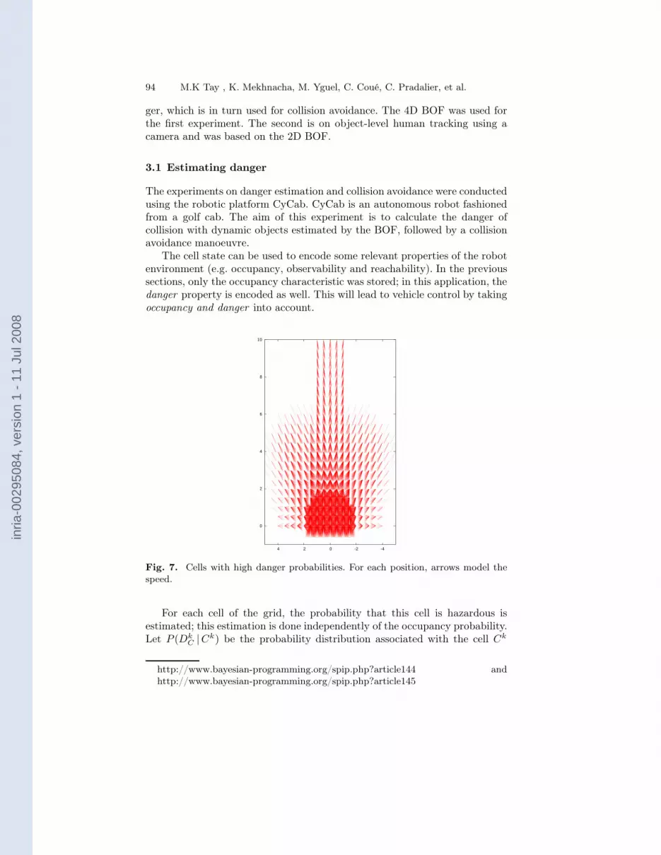
Fig. 7. Cells with high danger probabilities. For each position, arrows model thespeed.

For each cell of the grid, the probability that this cell is hazardous isestimated; this estimation is done independently of the occupancy probability.Let P (Dk

C |Ck) be the probability distribution associated with the cell Ck

http://www.bayesian-programming.org/spip.php?article144 andhttp://www.bayesian-programming.org/spip.php?article145

inria

-002

9508

4, v

ersi

on 1

- 11

Jul

200

8


Cycab

pedestrian

parked car

Fig. 8. Scenario description: the pedestrian is temporarily hidden by a parked car.

of the vehicle environment, where DkX is a boolean variable that indicates

whether this cell is hazardous or not.

Fig. 9. Snapshots of the experimental pedestrian avoidance scenario (see Exten-sion 1 for the video).

Basically, both “time to collision” and “safe travelling distance” may beseen as two complementary relevant criteria to be used for estimating thedanger to associate with a given cell. In our current implementation, we areusing the following related criteria, which can easily be computed: (1) theclosest point of approach (CPA), which defines the relative positions of the

inria

-002

9508

4, v

ersi

on 1

- 11

Jul

200

8


pair (vehicle, obstacle) corresponding to the “closest admissible distance” (i.e.safe distance); (2) the time to the closest point of approach (TCPA), which isthe time required to reach the CPA; and (3) the distance at the closest pointof approach (DCPA), which is the distance separating the vehicle and theobstacle when the CPA has been reached. In some sense, these criteria givean assessment of the future relative trajectories of any pair of environmentcomponents of the types (vehicle, potential obstacle).

These criteria are evaluated for each cell at each time step k, by takinginto account the dynamic characteristics of both the vehicle and the poten-tial obstacles. In practice, both TCPA and DCPA are estimated under thehypothesis that the related velocities at time k remain constant; this compu-tation can easily be done using some classical geometrical algorithms (see forinstance: http://softsurfer.com/algorithms.htm).

The goal is to estimate the “danger probability” associated with each cellof the grid (or in other terms, the probability for each cell Ck that a collisionwill occur in the near future between the CyCab and a potential obstacle inCk). Because each cell Ck represents a pair (position, velocity) defined relativeto the CyCab, it is easy to compute the TCPA and DCPA factors, and in asecond step to estimate the associated danger probability using given intuitiveuser knowledge. In the current implementation, this knowledge roughly statesthat when the DCPA and the TCPA decrease, the related probability ofcollision increases. In future versions of the system, such knowledge can beacquired with a learning phase.

Figure 7 shows the cells for which the danger probability is greater than0.7 in our CyCab application; in the figure, each cell is represented by anarrow: its tail indicates the position, and its length and direction indicatethe associated relative speed. This figure exhibits quite reasonable data: cellslocated near the front of the CyCab are considered as having a high dangerprobability for any relative velocity (the arrows are pointing in all directions);the other cells having a high “oriented” danger probability are those having arelative speed vector oriented towards the CyCab. Because we only considerrelative speeds when constructing the danger grid, the content of this griddoes not depend on the actual CyCab velocity.

3.2 Collision avoidance behaviours

This section describes the control of the longitudinal speed of the autonomousvehicle (the CyCab), for avoiding partially observed moving obstacles havinga high probability of collision with the vehicle. The implemented behaviourconsists of braking or accelerating to adapt the velocity of the vehicle to thelevel of risk estimated by the system.

As mentioned earlier, this behaviour derives from the combination of twocriteria defined on the grid: the danger probability associated with each cellCk of the grid (characterized by the distribution P (Dk

C |Ck)), and the oc-cupancy probability of this cell (characterized by the posterior distribution

inria

-002

9508

4, v

ersi

on 1

- 11

Jul

200

8


P (EkC | Zk Ck)). In practice, the most hazardous cell that is considered as

probably occupied is searched for; this can be done using the following equa-tion:

maxCk

{P (DkC | Ck), with P (Ek

C | Ck) > 0.5}.

Then the longitudinal acceleration/deceleration to apply to the CyCab con-troller can be decided according to the estimated level of danger and to theactual velocity of the CyCab.

Figure 8 depicts the scenario used for experimentally validating the previ-ous collision avoidance behaviour on the CyCab. In this scenario, the CyCabis moving forward, the pedestrian is moving from right to left, and for a smallperiod of time, the pedestrian is temporarily hidden by a parked car.

Figure 9 shows some snapshots of the experiment (see also Extension 1,which shows the entire video): the CyCab brakes to avoid the pedestrian, thenit accelerates as soon as the pedestrian has crossed the road.

0

0.5

1

1.5

2

0 2 4 6 8 10 12 14

Vco

nsig

ne (

m/s

-1)

time (s)

Fig. 10. Velocity of the CyCab during the experiment involving a pedestrianocclusion.

Figure 10 shows the velocity of the CyCab during this experiment. Fromt = 0 s to t = 7 s, the CyCab accelerates, up to 2 m/s. At t = 7 s, thepedestrian is detected; as a collision could possibly occur, the CyCab deceler-ates. From t = 8.2 s to t = 9.4 s, the pedestrian is hidden by the parked car;thanks to the BOF results, the hazardous cells of the grid are still consid-ered as probably occupied; in consequence the CyCab still brakes. When thepedestrian reappears at t = 9.4 s, there is no longer a risk of collision, andthe CyCab can accelerate.

3.3 Object-level tracking

Experiments were conducted based on video sequence data from the Europeanproject CAVIAR. The selected video sequence presented in this paper is takenfrom the interior of a shopping centre in Portugal. An example is shown inthe first column of Fig. 11. The data sequence from CAVIAR, which is freelyavailable from the Web6, gives annotated ground truths for the detection of

6 http://groups.inf.ed.ac.uk/vision/CAVIAR/CAVIARDATA1/

inria

-002

9508

4, v

ersi

on 1

- 11

Jul

200

8


the pedestrians. Another data set is also available, taken from the entry hallof INRIA Rhône Alpes.

Based on the given data, the uncertainties, false positives and occlusionshave been simulated. The simulated data are then used as observations forthe BOF. The BOF is a representation of the planar ground of the shoppingcentre within the field of view of the camera. With the noise and occlusionby simulated bounding boxes that represent human detections, a Gaussiansensor model is used, which gives a Gaussian occupation uncertainty (in theBOF grids) of the lower edge of the image bounding box after being projectedonto the ground plane.

Recalling that there is no notion of objects in the BOF, object hypothesesare obtained from clustering, and these object hypotheses are used as obser-vations on a standard tracking module based on the joint probabilistic dataassociation (JPDA).

Previous experiments based on the 4D BOF technique (Section 3.1) reliedon the assumption of a given constant velocity, as the problem of velocity es-timation in this context has not been addressed. In particular, the assumptionthat there could only be one object with one velocity in each cell was not partof the previous model. In this current experiment, experiments were conductedbased on the 2D BOF model, which gives both the probability distributionon the occupation and the probability distribution on the velocity.

The tracker is implemented in the C++ programming language withoutoptimizations. Experiments were performed on a laptop computer with anIntel Centrino processor with a clock speed of 1.6 GHz. It currently trackswith an average frame rate of 9.27 frames/s. The computation time requiredfor the BOF, with a grid resolution of 80 cells by 80 cells, takes an averageof 0.05 s. The BOF represents the ground plane of the image sequence takenfrom a stationary camera and represents a dimension of 30 m by 20 m.

The results in Fig. 11 are shown in time sequence. The first column ofthe figures shows the input image with the bounding boxes, each indicatingthe detection of a human after the simulation of uncertainties and occlusions.The second column shows the corresponding visualization of the Bayesianoccupancy filter. The colour intensity of the cells represents the occupationprobability of the cell. The little arrows in each cell give the average velocitycalculated from the velocity distribution of the cell. The third column givesthe tracker output given by a JPDA tracker. The numbers in the diagramsindicate the track numbers. The sensor model used is a 2D planar Gaussianmodel projected onto the ground. The mean is given by the centre of the loweredge of the bounding box.

The characteristics of the BOF can be seen from Fig. 11. The diminishedoccupancy of a person further away from the camera is seen from the data inFigs. 11(b) and 11(e). This is caused by the occasional instability in humandetection. The occupancy in the BOF grids for the missed detection dimin-ishes gradually over time rather than disappearing immediately as it does

inria

-002

9508

4, v

ersi

on 1

- 11

Jul

200

8


(a) (b) (c)

(d) (e) (f)

(g) (h) (i)

(j) (k) (l)

(m) (n) (o)

Fig. 11. Data sequence from project CAVIAR with simulated inputs. The firstcolumn displays camera image input with human detection, the second column dis-plays the BOF grid output, and the third column displays tracking output. Numbersindicate track numbers.

inria

-002

9508

4, v

ersi

on 1

- 11

Jul

200

8


with classical occupation grids. This mechanism provides a form of temporalsmoothing to handle unstable detection.

A more challenging occlusion sequence is shown in the last three rowsof Fig. 11. Because of a relatively longer period of occlusion, the occupancyprobability of the occluded person becomes weak. However, with an appro-priately designed tracker, such problems can be handled at the object trackerlevel. The tracker manages to track the occlusion at the object tracker levelas shown in Fig. 11(i)(l)(o).

4 Conclusion

In this chapter, we introduced the Bayesian occupation filter, its differentformulations and several applications.

• The BOF is based on a gridded decomposition of the environment. Twovariants were described, a 4D BOF in which each grid cell represents theoccupation probability distribution at a certain position with a certainvelocity, and a 2D BOF in which the grid represents the occupation prob-ability distribution and each grid is associated with a velocity probabilitydistribution of the cell occupancy.

• The estimation of cell occupancy and velocity values is based on theBayesian filtering framework. Bayesian filtering consists of two main steps,the prediction step and the estimation step.

• The 4D BOF allows representation of several “objects”, each with a distinctvelocity. There is also no inference on the velocity for the 4D BOF. Incontrast, the 2D BOF implicitly imposes constraints in having only a single“object” occupying a cell, and there is inference on velocities for the 2DBOF framework. Another advantage of the 2D BOF framework over the4D BOF is the reduction in computational complexity as a consequenceof the reduction in dimension.

• There is no concept of objects in the BOF. A key advantage of this is“avoiding” the data association problem by resolving it as late as possiblein the pipeline. Furthermore, the concept of objects is not obligatory inall applications.

• However, in applications that require object-based representation, objecthypotheses can be extracted from the BOF grids using methods such asclustering.

• A grid-based representation of the environment imposes no model on theobjects found in the environment, and sensor fusion in the grid frameworkcan be conveniently and easily performed.

We would like to acknowledge the European project carsense: IST-1999-12224 “Sensing of Car Environment at Low Speed Driving”, Carsense [January2000–December 2002] for the work on the 4D BOF [Coué et al., 2006].

inria

-002

9508

4, v

ersi

on 1

- 11

Jul

200

8


References

K. Arras, N. Tomatis, and R. Siegwart. Multisensor on-the-fly localization: precision and reliability for applications. Robotics and Autonomous Sys-tems, 44:131–143, 2001.

Y. Bar-Shalom and T. Fortman. Tracking and Data Association. AcademicPress, 1988.

C. Coué, T. Fraichard, P. Bessière, and E. Mazer. Multi-sensor data fusionusing bayesian programming: an automotive application. In Proc. of theIEEE-RSJ Int. Conf. on Intelligent Robots and Systems, Lausanne, (CH),Octobre 2002.

C. Coué, T. Fraichard, P. Bessière, and E. Mazer. Using bayesian program-ming for multi-sensor multi-target tracking in automotive applications. InProceedings of IEEE International Conference on Robotics and Automation,Taipei (TW), septembre 2003.

C. Coué, C. Pradalier, C. Laugier, T. Fraichard, and P. Bessière. Bayesianoccupancy filtering for multitarget tracking: an automotive application. Int.Journal of Robotics Research, 25(1):19–30, January 2006.

A. Elfes. Using occupancy grids for mobile robot perception and navigation.IEEE Computer, Special Issue on Autonomous Intelligent Machines, Juin1989.

A. H. Jazwinsky. Stochastic Processes and Filtering Theory. New York :Academic Press, 1970. ISBN 0-12381-5509.

L. Kaelbling, M. Littman, and A. Cassandra. Planning and acting in partiallyobservable stochastic domains. Artificial Intelligence, 101, 1998.

R. Kalman. A new approach to linear filtering and prediction problems. Jour-nal of basic Engineering, 35, Mars 1960.

K. Mekhnacha, E. Mazer, and P. Bessière. The design and implementationof a bayesian CAD modeler for robotic applications. Advanced Robotics, 15(1):45–70, 2001.

H. Moravec. Sensor fusion in certainty grids for mobile robots. AI Magazine,9(2), 1988.

C. Tay, K. Mekhnacha, C. Chen, M. Yguel, and C. Laugier. An efficientformulation of the bayesian occupation filter for target tracking in dynamicenvironments. International Journal Of Autonomous Vehicles, To AppearSpring, 2007. (Accepted) To be published.

S. Thrun. Learning metric-topological maps for indoor mobile robot naviga-tion. Artificial Intelligence, 99(1), 1998.

G. Welch and G. Bishop. An introduction to the Kalman filter. available athttp://www.cs.unc.edu/ welch/kalman/index.html.

inria

-002

9508

4, v

ersi

on 1

- 11

Jul

200

8

Documents

The Bayesian Occupation Filter