Minotor: Monitoring Timing and Behavioral Propertiesfor Dependable Distributed Systems

Olivier Baldellon∗‡, Jean-Charles Fabre∗‡, Matthieu Roy∗†∗ CNRS, LAAS, 7 avenue du colonel Roche, F-31400 Toulouse, France

† Univ de Toulouse, LAAS, F-31400 Toulouse, France‡ Univ de Toulouse, INP, LAAS, F-31400 Toulouse, France

Abstract—Assessing the correct behavior of a givensystem at run-time can be achieved by monitoring itsexecution, and is complementary to off-line analysissuch as static verification.In this work, we focus on run-time monitoring of

system properties that include both causality and tim-ing constraints, in distributed and time-constrainedsystems. Based on a description of a property thatincludes events and temporal constraints, expressedas a timed-arc Petri net, we show how to automati-cally transform it into a an executable and distributedmonitoring engine.To that aim, we introduce a modification of the

semantics of Petri nets to be able to execute it onlineon partial executions and distributed observationenvironments. We show how to use this formal frame-work to provide Minotor, a model-driven distributedmonitoring system, describe its implementation andshow its applicability on a transportation use-case.

Keywords-Distributed Systems; Time-constrainedSystems; Online Monitoring; Fault-tolerant Systems;Petri nets.

IntroductionSupervising or monitoring applications states is a requi-site to detect a possible violation of system specificationand envisage a recovery action. Alas, on-line monitoringof complex, distributed and real-time systems is a highlycomplex task that, to our knowledge, has not yet beenfully tackled. On-line monitoring of applications, be themdistributed or not, in a centralized way is an activeresearch domain (see, e.g., [MR10], [JRR94], [BLS06],[RFR08], [ZSLL09]), but, as we will see in Section I, thesesolutions do not provide a distributed implementation ofmonitors that can handle both distributed and real-timespecifications.Most formalisms available to express event-based

behavioral properties are inherently centralized, partlybecause they were developed to model check the systembefore its deployment, a step that does not require adistribution of the verification process. In our approach,we want to verify an application in operation, and thusdistributing the monitoring process is a crucial issue.

This work has been partially supported by ANR French nationalprogram MURPHY (grant #ANR-10-BLAN-0306).

The first step towards the distribution of monitoring isto use a formalism in which the state of the system isdistributed.Following this reasoning, timed-arc Petri nets are

good candidates for modeling a distributed embeddedsystem with timing constraints, since this formalism isdecentralized by nature, and allows to express local timingconstraints. The dual nature of the formalism thus allowsto reason both on temporal and behavioral propertiesthat may be distributed among a set of nodes.

In this paper, we focus on the run-time monitoring ofsystem properties expressed as timed-arc Petri nets. Moreprecisely, the monitoring system uses timed events totrigger transitions in a Petri net that describes behavioraland temporal properties of the system. We assume aglobal clock enables events to be time-stamped.

The structure our approach is schematized in Figure 1.Intuitively, the system under supervision raises timedevents — i.e., couples (ei, τi) meaning that event eihappened at time τi — which are then captured by themonitor system that triggers the firing of transitionsin the Petri net that models behavioral and temporalproperties of the system.

System Monitor Alarm handler

(e1, τ1)

(e2, τ2)

(e3, τ3)

Figure 1. General approach

We aim at detecting violation of system properties:1) events not generated by the actual distributed

system in operation (missing events);2) wrong order of raised event (event e2 appears before

e1 whereas e2 should have happened after e1);3) deadline missed by some event.The detection of the above properties should be

performed as soon as possible, for obvious detectionlatency reasons, without requiring a perfect observation:due to the distribution of generated events, and thetime required to dispatch events to the monitoring

system, events may be received in an order that does notcorrespond to their real-time occurrence.

We assume that the specification (i.e., correct behavior)of the monitored application is provided as a Petri net.In a classical weak Petri net semantics [BR08], the firingof a given transition results in the removal of tokens ininput places and the creation of others in output places.Thus, a transition is fireable if and only if the tokens arealready present in the input places.Intuitively, we propose to fire a transition as soon as

the corresponding system event is received, no matter iftokens are present in input places or not. We introducethe concept of negative tokens to mark the fact that atransition was fired, independently from the marking ofinput places. Allowing negative tokens permits us to firea transition associated to an event as soon as the eventis captured without blocking the execution of the model.

The main benefit of this approach is that transitionscan be fired independently as soon as the correspondingsystem event appears. This has two major interests: firstly,it allows to perform most of computation locally, reducingrequired communication and synchronization betweenprocesses. Secondly, it allows to completely distributethe monitoring process and to optimize it based on systemtopology, enabling a better resources utilization.

Summary of contributions.: In this paper, we de-scribe in details a monitoring strategy that was brieflypresented in [BFR12]. Based on a modification of Petrinet semantics, we provide algorithms that implement ef-ficiently this strategy, and develop a thorough analysis oftiming hypotheses required to implement our monitoringframework. We provide measurements on automaticallygenerated patterns to test the scalability of the approach,and model, for proof-of-concept, a simplified automatedrailway transportation scenario.In a first part, we compare our approach with other

related techniques of on-line monitoring. Section II brieflypresents the formalism used, and in particular the exten-sion of Petri nets to include negative tokens. Section IIIdescribes a protocol to distribute the monitoring engine,based both on the Petri net and on physical mappingconsiderations. Section IV describes our implementation.Section V exemplifies the applicability of the approach.

I. State of the artMost previous works on monitoring of real-time prop-

erties are based on centralized monitoring of propertiesexpressed using Linear Temporal Logic (ltl) formulasor Timed Automata [MR10], [BLS06], [RFR08]. Unfor-tunately, both logic formulas and timed automata areinherently centralized and cannot be easily adaptedfor distributed monitoring. Usually, an ltl formula ismapped to its corresponding timed automata equivalentfor run-time evaluation. A timed automata has an

instantaneous state that has no natural decompositionin sub-states and thus cannot be easily distributed.Other approaches explicitly target the distribution

of the monitoring process [ZSLL09], [JRR94]. [JRR94]allows a distributed monitoring of properties that areexpressed as conjunction of simple logic properties, while[ZSLL09] proposes, in some cases, the distribution ofproperties expressed in the temporal logic based MEDLspecification language. Yet, in both approaches, theformalism proposed is not as expressive as timed-arc Petrinets, that can express complex and, more importantly,distributed behaviors.Centralized monitoring of asynchronous [FBHJ05] or

real-time [CJ05] distributed systems using Petri netshas also been studied. In the above works, the mainchallenge solved consists in finding, from an observedevents sequence, a corresponding Petri net execution to“explain” the observation. The aim we are pursuing here isdifferent: to simplify the event/transition correspondence,we require that an event corresponds to exactly onetransition. Moreover, we are interested in distributedmonitoring of systems, and thus we need to accommodatewith delayed observations, missing events and faultybehaviors.In the distributable nets approach [Hop91], one ex-

ecutes a Petri net in a distributed network, followinga location function such that if a place is an input ofa transition, then this place and this transition mustbe on the same node — that means that the decisionof firing a transition can be done locally. Althoughdistributable nets are not directly related to the workpresented here, we adapted the location function conceptwhile overcoming the “same node” requirement, in orderto be able to fire transitions as soon as events are caught.

II. Petri Nets For System PropertiesAs mentioned in the introduction, our monitor tool,

Minotor, is a distributed service that executes a modelof the system expressing temporal and behavioral prop-erties on reception of timed events from the system, cf.Figure 1. In this section, we first recall some classicaldefinitions on timed-arc Petri nets, before describinginformally its new semantics. Finally, the generalizationof timed events is presented and discussed.

A. Timed-Arc Petri NetsA timed-arc Petri net is a tuple (P , T , •(·), (·)•, M0,

I), where P is a finite set of places, T is a finite set oftransitions, M0 is the initial marking (a function thatassociates to each place a set of tokens), •(·) (respectively(·)•) is the backward (resp. forward) incidence functionthat associates to each transition the set of places fromwhich the transition starts (resp. to which the transitionends), and I a time constraint function that associates

a time interval to every arc from a place to a transition.We say that there is an arc from a place p to a transitiont if p ∈ •t.

We assume there is a bijection between transitions andevents generated by the system. Thus a timed event(ei, τi) can always be written (ti, τi) where ti is thetransition associated to ei.

B. Petri Net ExecutionAs explained in the previous part, the properties on

system events that need to be monitored are expressedusing the timed-arc Petri net formalism. Our approachconsists in executing a Petri net on-the-fly to detectfailures. The monitoring tool takes as an input a sequenceof events, i.e., a sequence of couples (t, τ) where trepresents the transition associated to an event and τthe date of the event. The monitoring tool executes themodel using such events sequence, and possibly raises analarm when it detects an incorrect behavior.

A simple execution: Let us take as an examplethe simple Petri net depicted in Figure 2: if the mon-itor receives, in this order, the sequence of events(t1, 10); (t2, 15); (t3, 21), it will first fire t1 and rememberthat this firing was done at time 10. When the eventcorresponding to t2 is received, the transition t2 is firedbecause τ2 − τ1 = 15 − 10 ∈ [3, 6]. The reception of(t3, 21) will raise an error because the event occurredtoo late; the token stayed in the place of •t3 six unitsof time (τ3 − τ2 = 21 − 15 = 6), which is out of thespecified interval [0, 5]. However, as the correspondingevent happened, the transition t3 will still be fired toenable the execution of the Petri net model to continue,and an error will be reported.

t1[0,∞]t2[3, 6]

t3[0, 5]

Figure 2. A simple Petri net

In this scenario, notice that the minimal amountof information to detect a failure is (t2, 15); (t3, 21):whatever the occurrence time of t1, t3 happened toolate with respect to t2. If the monitor only receives(t2, 15); (t3, 21) but (t1, 10) is not yet received, the usualsemantics of Petri nets forbids to fire the transitionst2 and t3; in other words, to fire t2 and consequentlyt3, the transition t1 needs to have been already fired.This crucial issue can be solved using negative tokens, asshown below.

An execution with negative tokens: Our approachconsists in firing a transition t as soon as it is receivedand anticipating the removal of tokens in places of •t by“adding” negative tokens in these places. Figure 3 shows

the result of firing t2, with a negative token representedas a black circle, a positive token as a black disk.

p0 t1[0,∞]p1 t2[3, 6]

p2 t3[0, 5]p3

Figure 3. After the firing of t2

The firing of t3 will add one negative token in p2and one positive token in p3, as shown in Figure 4.The removal of a positive token always depends onthe presence of its negative counterpart. To know howlong the positive token stayed in the place p2, we needto compare the date of the event that created thenegative token with the date of the event that created thepositive one. If the difference is not in the time intervalI(p2, t3) = [0, 5], then an error is raised. In all cases, bothtokens are removed.

p0 t1 p1 t2 p2 t3 p3

Figure 4. After the firing of t3

In summary, the main difference between our approachand classical semantics is that, in the classical one, atransition is allowed to be fired only if it all requiredtokens are present. In our approach, transitions are alwaysfired speculatively, and the fireability property is checkeda posteriori.

C. TagsAs classical Petri nets tokens are extended to include

both positive and negative tokens, this implies that themonitoring system has to add information to be able toknow unambiguously to which negative token a positiveone may be associated to. In particular, the problemof having to distinguish between tokens may appearwhen a given transition is fired several times in the sameexecution, at different dates, within a cycle.As an example, let us consider the Petri net of

Figure 5(a) and the following execution (t1, τ1); (t2, τ2);(t1, τ3); (t2, τ4) in which the token moves to p2, goes backto p1, moves again to p2 and finally returns in p1. Let ussuppose that events (t2, τ2) and (t1, τ3) were not received.The observed execution is then (t1, τ1); (t2, τ4) and theresulting Petri net state is the one of Figure 5(b).The missing event (t2, τ2) would have created a neg-

ative token in p2, corresponding to the positive onegenerated by (t1, τ1). Similarly, the missing event (t1, τ3)would have created a positive token corresponding tothe negative one generated by (t2, τ4). Consequently, thepositive and negative tokens present in place p2 do not

match: the positive token was produced by (t1, τ1) whilethe negative one was created by (t2, τ4).

p1

t1p2

t2

(a) Beginning of Execution

p1

t1p2

t2

(b) With missing events

Figure 5. Token and tags

To give a more concrete example, let us suppose that t1corresponds to the beginning of an action and t2 to its end.The value τ2 − τ1 corresponds to the time taken by thefirst occurrence of this action and τ4−τ3 is the time takenby the second occurrence execution; however, the valueτ4−τ1 represents the time taken by two occurrences, andthus does not correspond to timing constraints expressedin the specification.

The issue to answer is “given a positive and a negativetoken, do those two tokens match?”. To address thisissue, we introduce the notion of tags. A tag is a uniqueidentifier added to tokens. A positive and a negativetokens are related if and only if they have the same tags(cf. Figure 6). The main difference with colored tokensis the following: colored tokens are used to extent theexpressivity of a Petri net while tagged tokens are onlyused to allows an out-of-order execution of a given Petrinet.

1 2

Figure 6. Two tokens that cannot match

As a consequence, two nodes of the monitor in chargeof generating tokens for a same place need to agree ontag generation for the tokens of the place. If agreement isnot possible, then it is impossible to monitor propertiesin presence of missing events without false negatives, i.e.,undetected errors may occur. One can easily notice thatbeing able to compute the running time of a task requiresto unambiguously associate the two events correspondingto its beginning and its end.

D. EventsUntil now, events were described as couples (t, τ) where

t is a transition and τ a date. Now we need to refine thisdefinition to take into account tags.Since tags are added at event generation, a tagged

event is a tuple (t, τ, f) where t is a transition, τ a dateand f the tag function defined on •t ∪ t•. The functionf associates to each place of •t ∪ t• a tag. Then, at the

reception of the event (t, τ, f), a positive token, taggedf(p), is added in every place p of t• and a negative token,tagged f(p), is added in every place p of •t.

On the example of Figure 5, a simple implementationof f is to tag each token by the occurrence number ofthe corresponding action (i.e., the first firing of t1 andt2 is tagged 1, the second occurrence is tagged 2, etc.)

III. Monitoring with Negative TokensThe first part of this section describes the protocol

main ideas, and provides a relatively straightforwardtranscription of the execution semantics described pre-viously with negative tokens. A second part deals withthe timing aspects of the monitoring engine: given a fullysynchronous communication system, we show how tocompute the timeouts for handling deadline misses andmissing events. Then, we dig into the physical mappingof the monitoring engine on a distributed set of nodes.

A. Protocol descriptionThe protocol assigns a monitoring thread to each place

and each transition of the Petri net. When the systemgenerates an event, this event is sent to the threadassociated to the corresponding transition. In return,transition threads send tokens to threads associated toplaces when they receive events and fire transitions.The transition thread for transition t is described in

Algorithm 1; notation “p ! msg” means that messagemsg is sent to the thread associated to place p, and Preand Post variables refer to the two sets •t and t•.

Algorithm 1 Thread associated to transition t1: procedure Transition(Pre,Post)2: When an event e = (t, τ, f) is received do3: for p ∈ Pre do p ! (−, t, τ, f(p))4: end for5: for p ∈ Post do p ! (+, t, τ, f(p))6: end for7: done8: end procedure

The place thread is described in Algorithm 2. When athread associated to a place receives a token, it checksif it already received the negative version of this token(same tag, but opposite sign). In this case, the placethread needs to compute the difference between thetwo dates and to compare it with the correspondingtiming interval given by the I function before deletingthe two corresponding tokens. The detection of theviolation of temporal properties is partially done duringthis comparison: the comparison of the two dates mayraise an error if timing assumptions are violated.If no opposite sign token has been received before,

the token is stored and a new timer is started, to beable to detect a deadline miss of the opposite sign

token. The timer is required in addition to the differenceand comparison mechanism described above: if theopposite counterpart of a token is never received, thenthe comparison mechanism will not be triggered. Tobe able to trigger an alarm for a missing event, thistimeout mechanism is implemented in the timer functiondescribed in Section III-B. Interestingly, this mechanismallows also for the detection of deadline misses as soonas they are detectable.

The main goal of the SetTimer function is to detectthe fact that an event did not arrive on time. The exactcomputation of the value of the timeout is described inthe next section. The timer runs in a separate threadthat sends to the place a message timeout(token) whenthe timer expires. If a place receives such message whenthe corresponding token is still in memory, tokens areerased, and a timing error is raised up.

Algorithm 2 Place thread associated to p1: procedure Place(I)2: When token = (sign, t, τ, tag) is received do3: if ∃token′ = (−sign, t′, τ ′, tag) ∈ Mem then4: Mem ← Mem−token′

5: CancelTimer(token′)6: if sign = +7: then ok =

((τ ′ − τ) ∈ I(p, t′)

)8: else ok =

((τ − τ ′) ∈ I(p, t)

)9: end10: if ¬ok then raise(timing failure)11: else12: Mem ← Mem+token13: SetTimer(token,t,p)14: end if15: done

16: When timeout(token) is received do17: Mem ← Mem−token18: raise(timing failure)19: done20: end procedure

B. TimersThe very existence of timeouts is conditioned by the

ability to bound both message transfer delays and reac-tion delays. In this part, we explore timer computationin an optimistic fashion —we want a timer to expire onlywhen there is for sure a timing error in the system—, sincemost timing verifications will be handled by the differenceand comparison mechanism (lines 7–8 of Algorithm 2).For this purpose, we need to introduce additional

assumptions on the communication layer, both for theactual system in operation and for the monitoring system.Notice that the existence of such bounds seems natural inany system that implements real-time mechanisms withtimeouts in the specification, which is the core target ofour approach.

We assume that there are bounds on message transferdelays in the whole system. More precisely, we assumethat a message sent by a thread th at time τ will bereceived by time τ+∆th,th’ by thread th′. We also assumethe existence of a second function δ that gives, for anytransition, the delay needed for an event to be received bythe thread associated to a transition. If an event happensin the system at time τ , then the corresponding transitiont will receive this event before time τ + δ(t).

The existence of those two functions ∆ and δ impliesthat all links in the system are synchronous. Indeed,∆ and δ exactly represent the time needed to routea message between the different participants of themonitoring system.Now we dig into timers computations; when a token

is received by a place thread in Algorithm 2, and nocorresponding opposite signed token exists, a timer isset (line 13) and, would the timer expire, it would raisea timing failure. Notice that all computations here areoptimistic, i.e., we want a timer to expire only when thereis for sure a timing error in the system.

Let us consider a place p in which a transition t1 createsa positive token at time τ1, and t2 produces its negatedversion at time τ2 (for example, Figure 5 with place p2).Now if the arc to the transition t2 is time constrained byI(p, t2) = [a, b], then by definition of the semantics,

a ≤ τ2 − τ1 ≤ b (∗)

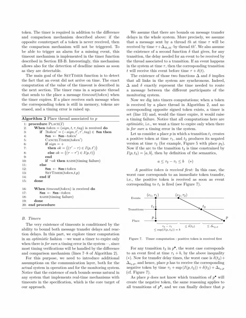
A positive token is received first: In this case, theworst case corresponds to an immediate token transfer,i.e., the positive token is received as soon as eventcorresponding to t1 is fired (see Figure 7).

Events

Transitions

Place

(e1, τ1)

t1

p

(e2, τ2)

t2

p

τ2 − τ1≤ sup(I(p, t2)) = b

≤ δ(t2) ≤ ∆t2,p

Figure 7. Timer computation : positive token is received first

For any transition t2 in p•, the worst case correspondsto an event fired at time τ1 + b, by the above inequality(∗). Now for transfer delay times, the worst case is δ(t2)+∆t2,p, and hence, place p has to receive the correspondingnegative token by time τ1 + sup (I(p, t2)) + δ(t2) + ∆t2,p

(cf. Figure 7).As place p does not know which transition of p• will

create the negative token, the same reasoning applies toall transitions of p•, and we can finally deduce that p

needs to wait until τ1 + T+(p) with:

T+(p) = maxt∈p•{∆t,p + δ(t) + sup (I(p, t))} (1)

A negative token is received first: As in the previouscase, the worst case corresponds to an immediate tokentransfer, i.e., the negative token is received as soon asthe event corresponding to t2 is fired (see Figure 8).

Events

Transitions

Place

(e1, τ1) (e2, τ2)

t1 t2

p p

τ2 − τ1 ≥inf(I(p, t2)) = a

≤ δ(t1) ≤ ∆t1,p

Figure 8. Timer computation: negative token is received first

Using inequality (∗), it is easy to check that (e1, τ1)happens at most at time τ2 − inf(I(p, t2)) = τ2 − a.Now, considering worst case communication delays, preceives the token associated to e1 at most at timeτ2− inf (I(p, t2)) + δ(t1) + ∆t1,p (cf. Figure 8). Contrarilyto the previous case, here p knows which transition ofp• to wait for, and hence p arms a timer that expires atτ2 + T−(p, t2) with:

T−(p, t2) = maxt∈•p{∆t,p + δ(t)} − inf (I(p, t2)) (2)

The description of the SetTimer algorithm used bythe place thread of Algorithm 2 to arm watchdogs whenwaiting events is described in Algorithm 3.

Algorithm 3 SetTimer procedure1: procedure SetTimer(token,t0,p)2: if token.sign > 0 then3: T = maxt∈p•{∆t,p + δt + sup(Ip,t)}4: else5: T = maxt∈•p{∆t,p + δt} − inf(Ip,t0 )6: end if7: wait T8: p ! timeout(token)9: end procedure

C. Physical mappingAn important question that needs to be addressed

now concerns the physical mapping of the threads ofthe protocol. Intuitively, an adequate placement strategywould locate the transition thread as close as possible tothe node where the corresponding event is generated.

In the case a transition thread is located on the nodethat generates the event of its transition, the failure of

the node will result in the failure of the place thread.This case is not problematic: the failure of the transitionthread tht will result in a timeout for associated tokens inplace threads that depends on transition t. Such timeoutswill raise timing failures (see Algorithm 2) : the failurewill be detected.

Contrarily, if a place thread is collocated to transitionthreads it depends on, the crash of the node will notbe detected, since only place threads may raise errors.Indeed, the optimal placement of place threads is theresult of a trade-off between low detection latency andfault tolerance.In order to attain a low latency detection while

preserving fault tolerance properties, and mitigate theabove mentioned trade-off, we use a classical replicationmechanism. In this strategy, place threads are duplicatedon several node, and events are sent to the set of replicasusing a uniform reliable broadcast service. Let us supposethat the thread associated to a place p is replicated onk nodes. To maintain consistency between replicas, wewant the k replicas receive the same set of tokens. Noticethat, since our approach allows out-of-order reception oftokens, the required service is a simple Uniform ReliableBroadcast [Ray10], thus does not require costly consensus-based Atomic Broadcast.

IV. Implementation

We have developed Minotor1, an implementation of theapproach in the Erlang language. The implementationheavily uses multithreading, assigning one lightweightthread per place and one per transition. Indeed, theimplementation has proved to be very scalable, since wewere able to run series of tests on Petri nets of size upto 220 (more than one million) transitions and places.

A. Timing hypotheses

We assumed we have an upper bound D of ∆t,p + δ(t)for every place p and transition t. Intuitively, this meansthan when an event occurs in the system at time τ , thecorresponding tokens will be received by the places beforeτ +D. Equations 1 and 2 of Section III-B become:

T+(p) ≤ D + maxt∈p• {sup (I(p, t))}T−(p, t2) ≤ D − inf(I(p, t2))

To compute the two above values to set timers, placep needs to know the intervals I(p, t) for transitions t ofp•. Thanks to this simplification, in the implementationa place p needs to be aware of transitions in p• only, butnot of the ones in •p.

1http://www.olivier.baldellon.eu/documents/minotor-prdc.tar.gz

B. Petri net deploymentTo create an arc, a message is sent to the target

transition thread. When the arc concerns an inputplace, for instance {arc, "p1", "t1", 0, infinity},the transition thread t1 sends to the place thread p1the interval [0,+∞]. The processing of this message willbe described in the next section, when explaining thetransition thread code. When the arc concerns an outputplace, as {arc, "t1", "p2" }, no message needs to besent to places t•, due to the simplification explainedabove.The deployment philosophy is to be as dynamic as

possible: places, transitions and arcs can be added at anytime to be able to update the model at runtime.

C. Transition thread in actionThe code of the transition thread, presented in List-

ing 1, is a direct transcription of the algorithm describedin Section III, with some additional machinery requiredto create and deploy dynamically the Petri net.

1 −module( t r a n s i t i o n ) .23 loop (Name, Pre , Post ) −>4 receive5 {event , Tags , Time} −>6 send_token (Pre , minus , Tags , Time ,Name) ,7 send_token ( Post , plus , Tags , Time ,Name) ,8 loop (Name, Pre , Post ) ;9 {new_arc , Place , Pid} −>10 loop (Name, Pre , [ {Place , Pid} | Post ] ) ;11 {new_arc , Place , Pid ,Min ,Max}−>12 Pid ! {new_arc ,Name,Min ,Max} ,13 loop (Name, [ {Place , Pid} | Pre ] , Post )14 end .

Listing 1. Code for transitions

In brief, the function loop has three parameters: thetransition name and two lists, one representing the inputplaces set called Pre, and the other one representing theoutput places set called Post. When the function is firstlaunched, the two sets are initialized to the empty list.The loop function waits for the reception of messages,does some action and calls itself again with updatedparameters. This is the common way of implementingthreads in Erlang, definitely recursive.Three types of messages can be received: an “event”

message and two “new arc” messages. “Event” messagescorrespond to monitoring messages, while “new arc”messages correspond to deployment operations.

Deployment: When a transition t is asked to create anew arc with a place, it just needs to call recursively theloop function with updated parameters Pre and Post. Forexample, line 10 (loop(Name,Pre,[Place,Pid|Post]))corresponds to the creation of a new arc between placePlace and the current transition. The Post set is updatedwith a couple containing both the name Place and theaddress Pid of the place. In the case of a new place in t•,

then the value of the interval I(p, t) is sent to the placeusing the Pid value: Pid ! new_arc,Name,Min,Max (line12).

Monitoring: When an event is received, tokensmust be sent to the two sets Pre and Post. Negativetokens are sent to Pre by means of the statement:send_token(Pre,minus,Tags,Time,Name), line 6. Pos-itive tokens are sent to Post by means of the state-ment: send_token(Post,plus,Tags,Time,Name), line 7.Finally, the loop function is called back with the sameparameters: loop(Name,Pre,Post) at line 8.

1s t a r t (Timeout , Pid , {plus , Tag ,Tp} ) −>2receive3{token , {minus , Tag ,Tm} ,{Min ,Max}} −>4case t imer : now_diff (Tm,Tp) of5D when D > Max −>6Pid ! { too_late , Tag ,D} ;7D when D < Min −>8Pid ! { too_early , Tag ,D} ;9D −>10Pid ! {ok , Tag ,D}11end12after Timeout −>13Pid ! {plus_timeout , Tag}14end .15s t a r t (Timeout , Pid , {minus , Tag ,Tm} ,{Min ,Max} ) −>16receive17{token , {plus , Tag ,Tp} } −>18case t imer : now_diff (Tm,Tp) of19D when D > Max −>20Pid ! { too_late , Tag ,D} ;21D when D < Min −>22Pid ! { too_early , Tag ,D} ;23D −> Pid ! {ok , Tag ,D}24end25after Timeout −>26Pid ! {minus_timeout , Tag}27end .

Listing 2. Code for timers

D. Places and timersWe do not give in this paper the full implementation

of place thread, but rather focus on timing constraintverification. In Listing 2, we show the current imple-mentation of the verification of timing constraints usingtimers threads.When a positive token is received by a place p,

the place starts a new timer with the parametersstart(Timeout,PlaceId,plus,Tag,Tp). The first pa-rameter, Timeout corresponds to the value T+(p), thesecond one corresponds to the address of p and the lastone corresponds to the token with the sign (here plus),the Tag and the creation date Tp. The timer threadwaits for the reception of the negative token within thecorresponding timing interval [Min, Max].

Depending on the value Tm− Tp, i.e. the time spent bythe token in the place (line 4), the timer will inform theplace of the result. It can be either ok (line 10), too_late(line 6) or too_early (line 8). If the negative token isnot received before the timer expires, then the place is

informed by a message PlaceId ! plus_timeout,Tag(line 13).

Similarly, the handling of timers for negative tokens isdescribed lines 15–27.

E. Performance and scalabilityTo test the scalability of our approach, we conducted

tests on a simple square Petri net described in Figure 9.This Petri net consists of n concurrent sub Petri nets(n “lines”), every one being a sequence of n actions. Wegenerated the associated Petri nets for n = 2k withk = 0..10 and conducted the experiments on a 8-coreHP machine running Debian GNU/Linux (2.89 GHzwith 8 GB of memory). The monitor was controlledfrom an other computer where events were generated.Notice that for k = 10 there are 1 048 576 places and1 049 600 transitions and thus about 2.1 million threads.The memory footprint was measured with Erlang VMrunning on a single core.

p1,1 ∆. . .

p1,n∆

. . .pn,1

∆ . . .

pn,n∆

Figure 9. Test Petri net

The table in Figure 10 shows the memory footprintwith respect to the value of n. We show that for bigenough values of n there is a proportional relationbetween the number of threads and the payload. Thepayload corresponds to the difference between the VMmemory footprint after the creation and deployment ofthe Petri net with the initial VM footprint.

n 1 . . . 32 64 128 256 512 1024Mem. (MB) 410 417 435 746 1731 5664

Payload (MB) 0 7 25 336 1321 5254#Threads/Payload - - - 390 397 399(2n+ 1)n/Payload

Figure 10. Memory footprint for large Petri nets (table)

For small Petri nets, memory footprint is always 410MB. This value corresponds to the size of the virtualmachine. This value is relatively big because the virtualmachine was configured for all tests to be able to runlarge Petri nets (more than 2 millions of threads), Inpractice, for small Petri net (n = 16, i.e. 496 transitionsor places), a virtual machine of 30MB has proved to besufficient.Finally, in term of CPU time, the deployment of the

Petri net is a costly operation (about 40s to generate the2 millions thread Petri net). However, the execution, i.e.the processing of received events, is negligible on eachnode.

0 250 500 750 10000

1000

2000

3000

4000

5000

6000Memory footprint (MB)

Total footprintPayload×

Patternsize (n)

Figure 11. Memory footprint for large Petri nets (graph)

To conclude, the Erlang implementation was a success-ful proof of concept in terms of feasibility and perfor-mance. A more significant implementation of Minotorin the Xenomai real-time system as a kernel driver isbeing developed (work in progress)

V. Deriving Models from a Concrete ExampleThe monitoring system presented in this paper needs,

as an input, a description of the time- and event-basedspecification of correct behaviors in terms of an timed-arcPetri net. This step has not been fully addressed yet, and,indeed, devising a correct specification as a Petri net isusually not considered to be an easy task.Fortunately, when considering critical systems, most

designers provide clear specification of interactions withinthe system, in order to run unit tests, and to useas an input for model-checking interactions betweencomponents. Such specifications may be provided aslinear temporal logic formulas, timed automata, statecharts, etc. Then, one can use one of the possibleautomated translations from a given formalism to a Petrinet, e.g., [Srb05], [RPC02].Hence, we assume that we can reuse a description

that has already been provided to developers as early asduring the testing phase of the system.

To motivate our approach, we here consider a railwaytransportation supervision system, and show how a modelof its behavior can be developed incrementally from itssimplest form up to a complex model that encompassesadvanced techniques such as nominal and degraded modesof operation.

A. Railway supervision system: overviewIn the introduction of this paper we advocated that

our approach was able to detect the violation of systemproperties without blocking despite wrong order of eventsand deadline misses by some events. In real systems,detection is not enough and thus we assume that thenominal behavior of a given system is complemented

station station

sensor

Network PC

section

PC

(a) A fully-automated train supervision system

[0, D]

[0, D] [0, D]

[0, D]p1 t1 p2 t2 p3

t3 p4 t4

tw

p5

[0, d]

]d,∞]q1 q2

r1

r2

q3

q4

(b) Handling warning states and missing events

Figure 12. Railway supervision system

by at least one alternative behavior, targeting possiblyseveral degraded modes of operation.In this last part, we briefly illustrate this problem by

means of an example. We consider a fully-automatedtrain control system made up of a network of lines,each composed of a set of railway track sections, asdepicted in Figure 12(a). Control of a train is supervisedfrom a central command and control system but thetrains have some autonomic behavior, i.e. automatictrain driving is carried out simply by assigning eachtrain a “target station”. In other words, each train startsfrom an initial station and has a target destination,with several intermediate stations in between. Betweeneach station the tracks are divided into sections, eachequipped with sensors reporting the passing of the train.In a nutshell, each train has to pass through severalcheckpoints between stations. The first objective of ourdistributed monitor is to check that the trains do obeysome timing properties, the violation of them leading topossible catastrophic failure. The distributed monitorsare located on computers (PC) at each station.In this scenario, signals for abnormal behaviors are

classified in two different classes: a warning signal corre-sponds to a violation of the specification that may notlead to a catastrophic failure and can be recovered, whilea error signal corresponds to the system entering a statewhere a drastic action has to be taken to ensure safetyof passengers.

On the monitoring side, the detection of a timing faultcan be i) a warning (timing overhead on a single givensection) that is part of the specification and does notrequire the monitoring system to raise an alarm, or ii) areal error signal that may lead to a catastrophic failure.

On the system operational side, a warning is handledby triggering a degraded mode of operation of the system(e.g. alternate route, skip of intermediate stations, etc.).The error leads the system to start a recovery action thatwill put it in a safety state, e.g., stopping the train onan alternate track.Errors are raised by the monitor when detected.

Additionally, if a warning was detected and the traindoes not use the degraded mode of operation, then anerror must also be raised. However, the train may usethe degraded mode even if neither warning nor error was

detected.

B. Timing constraintsThe monitoring system must signal an error if the

train stays more than D units of time in a section, anda warning if it stays more than d time units in the firstsection; in this case, the degraded mode corresponds toa shorter path to try to recover with the time table.As our monitoring tools deals with missing events, if

the property “the train stayed more than d time units inthe first section” does not hold, then an error will haveto be raised if the degraded mode is not used.

C. Railway supervision system: Petri net modelingStations and sections are represented by places. The

initial station is represented by p1, the four sectionsare represented by p2, p3, p4 and pw and the finalstation by p5. Sensors detecting the entrance in a sectionare represented by transitions t1, . . . , t4, tw. In otherwords, each time a sensor is activated, the correspondingtransition will receive an event.The nominal mode is represented in green and red

in Figure 12(b). There are two paths: the long pathp1, p2, p3, p4, p5 is the nominal one, in green, while theshort one p1, p2, pw, p5 is the degraded one, in red. Thelabel [0, D] between places and transitions indicates thata train cannot stay more than D units of time in anyof the sections; if such a constraint were to be violated,then an error would have to be raised by the monitor.

D. Dealing with warning statesThe last part of the Petri net, represented in blue in

Figure 12(b), takes into account warnings. This blue partmust be interpreted with a slightly different semantics:the firing of transitions must not be triggered by thereception of an event, but by the monitoring systemas soon as they are fireable. We call these transitionswith different semantics logical transitions, to distinguishthem from event transitions. Notice that such transitionsrepresent classical Petri nets transitions, i.e., they are notevent-triggered, and thus their firing is straightforwardand not described in this paper.To detect if the long path can be taken by the train,

the monitoring system needs to receive both eventscorresponding to t1 and t2. Indeed, if one of these two

events is missing, the monitor will ensure the train usesthe short path, otherwise the monitoring system will raisean error.

We briefly show below how logical transitions allow toincrease the expressiveness of the approach.

Let us assume that t1 and t2 were fired at time τ1 andτ2 respectively (with τ2 > τ1). As soon as both eventsare received by the monitor, one of the two transitions,r1 or r2 is fireable. Notice that the token in place q1 haswaited τ2 − τ1 time units since its creation at the firingof t1. Thus, either r1 or r2 can be fired, but not both dueto the disjoint timing constraints on arcs. Since none ofthese transitions are associated to an event, the monitorwill fire the correct transition at time τ2 (before τ2, notoken was present in place q2).To sum up, the monitoring system verifies that the

system is in one of the two mutual excluding executionbranches:− if the train stayed less than d time units in the

first section, then r2 will be fired and tokens willappear in place q3 and q4, allowing the train to useits nominal path,

− if the train stayed more than d time units in thefirst section, transition r1 is fired and blocks anyfiring of t3 or t4: the train is forced to run in thedegraded mode (or fast path).

VI. ConclusionMinotor is a contribution towards the on-line mon-

itoring of distributed systems. Minotor improves thedetection coverage of timing faults thanks to a model ofthe correct behaviors of the system that is animated atruntime through system events.We impose the specification to be described as an

timed-arc Petri net, a powerful formalism to expressboth distributed and timed behaviors.

Differently of static analysis, Minotor receives systemevents on the fly, and possibly out-of-order. To cope withthis problem, we introduce the notion of signed token,i.e. we execute every transition associated to an event assoon as this event is caught by the monitoring system,no matter the current state of the Petri net. The actualmonitoring of timing constraints and events ordering isperformed a posteriori by checking respective dates ofsigned tokens.The decoupling of transitions firing and timing con-

straints monitoring allows us to completely distributethe monitoring, as we show in the article. Our strategyis to associate to each transition, and each place in thePetri net a conceptual thread, in charge of executing anatomic sub part of the Petri net and verifying locallythat timing constraints are valid.

In our experiments, complexity is manageable, in termsof memory footprint, but also in terms of execution time.

The definition of the model remains a complex issue. Insome cases, such event-based specification may alreadybe available to system developers, as it is one of theformalisms used for model checking, or static analysis ofprograms. This means that, Even for a complex physicalsystem, the complexity of the model can be limited,abstracting all implementation details, while providingearly detection mechanisms.

References[BFR12] O. Baldellon, J-C. Fabre, and M. Roy. Distributed

monitoring of temporal system properties usingpetri nets. In SRDS, 2012.

[BLS06] A. Bauer, M. Leucker, and C. Schallhart. Monitor-ing of real-time properties. FSTTCS, 2006.

[BR08] M. Boyer and O. H. Roux. On the comparedexpressiveness of arc, place and transition timePetri nets. Fundamenta Informaticae, 2008.

[CJ05] T. Chatain and C. Jard. Time supervision ofconcurrent systems using symbolic unfoldings oftime petri nets. Formal Modeling and Analysis ofTimed Systems, pages 196–210, 2005.

[FBHJ05] E. Fabre, A. Benveniste, S. Haar, and C. Jard.Distributed monitoring of concurrent and asyn-chronous systems. Discrete Event Dynamic Sys-tems, 15(1):33–84, 2005.

[Hop91] R. Hopkins. Distributable nets. Advances in PetriNets 1991, pages 161–187, 1991.

[JRR94] F. Jahanian, R. Rajkumar, and S.C.V. Raju. Run-time Monitoring of Timing Constraints in Dis-tributed Real-Time Systems. Real-Time Systems,7(3):247–273, 1994.

[MR10] P. Meredith and G. Roşu. Runtime Verificationwith the RV system. In Proceedings of the Firstinternational conference on Runtime verification,pages 136–152. Springer-Verlag, 2010.

[Ray10] M. Raynal. Communication and Agreement Ab-stractions For Fault Tolerant Distributed Systems.Morgan & Claypool, 2010.

[RFR08] T. Robert, J.C. Fabre, and M. Roy. On-linemonitoring of real time applications for early errordetection. In PRDC, pages 24–31. IEEE, 2008.

[RPC02] V. Ruiz, J. Pardo, and F. Cuartero. Translatingtpal specifications into timed-arc petri nets. InICATPN’02, pages 414–433. Springer-Verlag, 2002.

[Srb05] J. Srba. Timed-arc petri nets vs. networks of timedautomata. In ICATPN, pages 385–402, 2005.

[ZSLL09] W. Zhou, O. Sokolsky, B. T. Loo, and I. Lee.DMaC: Distributed Monitoring and Checking. Lec-ture Notes in Computer Science, 5779:184, 2009.