Embed Size (px)
Citation preview

Mixing AutoMetrics with MARS: A
study of psychological sequelae of
Chornobyl
Robert Alan Yaffee1, RoseMary Perez Foster2, Thomas B. Borak3,Remi Frazier3, Mariya Burdina4, Victor Chtenguelov6,
and Gleb Prib5
1Silver School of Social Work, New York University, New York, N.Y.2Natural Hazards Center, University of Colorado, Boulder, Colorado
3Environmental and Radiological Health Sciences,Colorado State University, Fort Collins, Colorado
4Department of Economics and International Business,University of Central Oklahoma, Edmund, Oklahoma
6Department of Applied Psychology, Academy of LaborSocial Relations, Kiev, Ukraine
5Ukrainian Institute on Public Health Policy, Kiev, Ukraine
OxMetrics Users Group ConferenceCass Business school
London City University,106 Bunhill Row
London, U.K.
3-4 September 2012
1

Contents
1 Acknowledgements 2
2 Introduction 2
3 Nomenclature 4
4 Data collection and sampling 5
5 Research instruments and measures 65.1 Outcome measures . . . . . . . . . . . . . . . . . . . . . . . . . . 6
5.1.1 Physical health . . . . . . . . . . . . . . . . . . . . . . . . 65.2 Outcome measures . . . . . . . . . . . . . . . . . . . . . . . . . . 7
5.2.1 Mental health . . . . . . . . . . . . . . . . . . . . . . . . . 75.2.2 Predictors . . . . . . . . . . . . . . . . . . . . . . . . . . . 8
6 Objectives 9
7 Historical highlights in the development of MARS 12
8 MARS algorithm 148.1 How MARS works . . . . . . . . . . . . . . . . . . . . . . . . . . 148.2 basis function generatioon . . . . . . . . . . . . . . . . . . . . . . 17
9 Dose reconstruction of exposure to 137 CS 22
10 Application of MARS and AutoMetrics to variable selectionand model building 2610.1 BSI positive symptoms models . . . . . . . . . . . . . . . . . . . 26
10.1.1 Female positive symptoms models . . . . . . . . . . . . . 2610.1.2 Female positive symptoms model using AutoMetrics alone 2610.1.3 Female model using AutoMetrics and MARS . . . . . . . 27
10.2 Male Models for BSI Positive symptoms . . . . . . . . . . . . . . 2810.2.1 Male model with AutoMetrics Alone . . . . . . . . . . . . 2910.2.2 Male model for Positive symptoms using AutoMetrics +
MARS . . . . . . . . . . . . . . . . . . . . . . . . . . . . . 3010.3 PTSD models . . . . . . . . . . . . . . . . . . . . . . . . . . . . . 3110.4 Male PTSD models . . . . . . . . . . . . . . . . . . . . . . . . . . 32
10.4.1 Male PTSD model using AutoMetrics alone . . . . . . . . 3510.4.2 Male PTSD model using AutoMetrics + MARS . . . . . . 36
10.5 Male PTSD model with AutoMetrics + MARS- cont’d . . . . . . 3710.6 Female PTSD models using AutoMetrics alone . . . . . . . . . . 42
10.6.1 Female PTSD model using AutoMetrics and MARS . . . 48

11 Conclusion 5211.1 Exploration of new dimensions . . . . . . . . . . . . . . . . . . . 5211.2 Are MARS models well-behaved? . . . . . . . . . . . . . . . . . . 5311.3 Can MARS capture nonlinear relationships ? . . . . . . . . . . . 5311.4 Content validity Tables . . . . . . . . . . . . . . . . . . . . . . . 5411.5 Advantages of MARS . . . . . . . . . . . . . . . . . . . . . . . . 5711.6 Disadvantages of MARS . . . . . . . . . . . . . . . . . . . . . . . 5811.7 Caveats . . . . . . . . . . . . . . . . . . . . . . . . . . . . . . . . 59
1 Acknowledgements
The project was funded by the National Science Foundation, Division of Deci-sion, Risk and Uncertainty (082-6983); and conducted in cooperation with theMinistry of Health of Ukraine. HSD grant 08262983 and we are very gratefulfor their support. We would also like to thank the Ministry of Health in theUkraine for their cooperation in this study. We are grateful to the developers ofStata in College Station, Texas, Salford Systems, Inc. in San Diego, California,and all of the AutoMetrics developers in Oxford, London for the software theyhave developed and which have used for variable selection and model buildingon this project.
2 Introduction
The current study conducted a random population sampling of Ukrainian resi-dents in the Kiev and Zhytomir oblasts of that country, with the aim of develop-ing long-term models of human nuclear disaster risk. Living in relatively closeproximity to the Chornobyl Nuclear station in Ukraine, residents were exposedto the largest industrial radiological accident to date in 1986. A survey method-ology was used to assess the complex bio-psycho-social pathways that contributeto long-term population outcomes after a significant radiological event. Datacollection was conducted from 2008-2011.
In the effort to understand the long-term burden of nuclear accident expo-sure on a general population, investigators primary foci of interest included: thepopulations reconstructed cumulative dose exposure to 137 Caesium (radiationsource term for the Chornobyl event), cognitive perception of risk to health andenvironment, mental health status (standardized instruments), medical diag-noses (ICD-9), psychosocial functioning, health behavior, reproductive patterns,nutritional practices, Chornobyl accident information sources, and social com-munication networks. These domains were assessed in the population for theircurrent status, and retrospectively for three earlier time periods from 1986 tothe time of the survey interview. The current presentation describes preliminarystatistical exploration of covariates influencing: 1) health-related behaviors asmeasured by the Nottingham Health Profile, 2) general mental health dysfunc-tion as measured by the Brief Symptom Inventory , and 3) Chornobyl-related
2

post traumatic stress syndrome as measured by the Revised Civilian PTSDScale.
Research of protracted, low dose radiation exposures from nuclear plantaccidents, show relatively low impacts on population health risk [22]. Con-versely, population perceptions of risk from radiological events remain activeup to several years post-event [1, 3, 5, 14]. Toxic accidents (radiological, chem-ical, biologic agents) appear to drive a unique spectrum of psychosocial andbehavioral responses in affected populations. These responses are distinct fromevent-related physical injury. They include depression, anxiety, traumatic re-sponse, increased medical services utilization, phobic nutritional behavior andchanges in reproductive patterns [2, 3, 5, 6, 7].
3

3 Nomenclature
Multivariate adaptive regression splines (MARS)
• MARS is a method of using regression splines
called basis functions to model local slope and
intercept changes in relationships.
• It is similar to a piecewise regression model in
that it combines basis functions to approximate
the global nonlinear form of the relationship
being modeled.
• MARS endeavors to improve the fit of the model
and can identify interactions among the vari-
ables selected. To avoid overfitting, it uses a
backward stepwise algorithm to trim the model
to what it deems the essentials.
4

4 Data collection and sampling
• A sampling of 702 participants
• Randomized selection of phone numbers
• household sample of the Kiev and Zhytomir
oblasts (states) of Ukraine
• Informed and consenting respondents were in-
terviewered
• Responses were entered in interviewers hand-
held computers,
• uploaded for storage to a website constructed
for the study (Vovici Corporation, USA).
• Participants ranged in age from 28-84.
5

5 Research instruments and measures
5.1 Outcome measures
5.1.1 Physical health
• ICD-9 Medical Diagnosis. Diagnostic informa-
tion from the Ukraine Ministry of Health database
of annual standardized dispensary exams.
• Randomized selection of phone numbers
• Nottingham Health Profile. Standardized scale
of self-reported health and its impact on multi-
domain behavioral functioning [11]
• Reliability/validity on Russian language form
tested in pilot study [12].
6

5.2 Outcome measures
5.2.1 Mental health
• Brief Symptom Inventory [13] Standardized scale
measuring patterns of psychological distress:
depression, anxiety, somatization, obsessive-compulsiveness,
hostility, paranoia, psychoticism , global dis-
tress, positive symptom score. Russian form
pilot tested [12].
• Revised Civilian PTSD Scale. Russian version
anchored in Chornobyl event and restandard-
ized [14]. Assesses post traumatic stress and
distress clusters related to Chornobyl. Relia-
bilities computed in pilot study of this sam-
ple [12].
• of Psychosocial/Health Behavior: factors asso-
ciated with toxic accident behavioral outcomes
and are integrated within the research ques-
tionnaire, including medical services utilization,
phobic behavior, substance use , eating habits,
abortions and contraceptive use.
7

5.2.2 Predictors
• demographics,
• perception of radiation risk and nuclear atti-
tudes, Chornobyl cognitions [1, 8],
• Chornobyl information sources, accident char-
acteristics (distance, relocation, etc.),
• general hazards perception,
• negative life events and buffers,
• coping style [7].
• cumulative external radiation exposure to 137Caesium
was estimated for each participant (see below)
8

6 Objectives
Primary research objectives
• To explore the psychological sequelae of the
Chornobyl disaster with respect to its effect on
the part Ukrainian residents in the area.
• To analyze dose - mental health effect on sur-
vivors and residents of the general area.
• To analyze perceived risk of exposure effect on
survivors and residents of the general vicinity
of such a nuclear event.
9

Primary methodological objectives
• Although we use AutoMetrics for variable se-
lection, we want to ascertain whether MARS
can add value to this process.
• To answer two questions concerning the value
added to our AutoMetrics analysis by MARS.
Does MARS help us explore dimensions of
our data which we might have ignored?
Does MARS aid in providing a well-behaved
model for our investigation of the subject of
choice?
Could MARS help us capture the nonlinear
relationships between variables?
10

Secondary objectives
• To use general-to-specific (GETS) approach to
minimize omitted variable bias [10].
• To assure ourselves of not having overlooked
important relevant variables.
• To be able to search, identify, and model non-
linear functional relationships as painlessly as
possible (while avoiding the curses of multidi-
mensionality and multi- collinearity.
• We had a large number of variables– some of
our datasets have approximately 3000 variables
but we only have 339 males and 363 females in
it.
• We could have more variables than observa-
tions in some cases and this is a problem Au-
toMetrics was designed to solve.
• To optimize construct validity– capturing all of
the relevant and important dimensions
• To discover what disadvantages this usage en-
tailed, if any.
11

7 Historical highlights in the development of MARS
• Automatic Interaction Detection: AID was de-
veloped by Morgan and Sonquist in1963 in JASA
to identify interaction terms by testing relative
reduction in sse. But there was a bias in the
variable selection as the splits contained less
observations.
• CHi-square Automatic Interaction Detection (CHAID)
proposed by Gordon Kass in his doctoral dis-
sertation in 1980 with bonferroni corrections
for multiple tests.
• CART used regression and classification (Clas-
sification and regression trees) were later devel-
oped (Brieman, Freedman, Olshen and Stone,
1984) to combine categorical and continuous
variables in the same tree output.
• Hastie, T. and Tibshirani, R. (1990) develop
the generalized additive model which combines
parametric and nonparametric estimation.
• Jerry Freedman developed MARS in 1993 as a
method of automatic regression models– using
basis functions and interactions between them.
12
Our situation
• Large dasets with more than 2900 variables in
them.
• Sample size 363 women and 339 men
• Most analysis wrt socio-medical research is per-
formed with gender-specific models.
• We want to developing optimal models to ex-
plain psychological phenomena experienced and
reported by residents in the Oblasts near Chornobyl
• We have variables that exhibit a latency period
before exhibiting a relationship
• We have variables that exhibit a delay mani-
festing a relationship.
• We depend on the multipath misspecification
testing of AutoMetrics to show guide our anal-
ysis.
13

8 MARS algorithm
8.1 How MARS works
MARs automates variable selection. It transforms
variables into truncated regression splines to ac-
commodate nonlinear functional forms. It checks
for potential interactions with predictors. It drops
irrelevant variables to minimize overfitting [23, 2].
MARS models nonlinear components with a vari-
ation of piecewise spline regression models. It uses
a recursive partitioning algorithm for the regres-
sion problem, which emerged in a program for clas-
sification and regression trees, dubbed CART (
Brieman, L., Friedman, J., Olshen, R. and Stone,
C., 1984).
Originally MARS recursively partitioned the do-
main into disjoint subregions, within each of which
it split the domain into two left and right offspring
regions. The regression components would reside
either within the left or the right daughter domain.
Basis functions have the general form of
f (x) = β0 +
S∑j=1
h(m)B(m) (1)
14

where B(x) = I(x ∈ Rj) with I being an indic-
tor function with a value of 1 if x is a condition is
true or 0, otherwise. The indicator function then
becomes part of a product of a series of step func-
tions, in turn indicating membership of the subre-
gion, formulated as
H [η] = 1, if η ≥ 0, (2)
= 0, otherwise.
such that they could be incorporated as follows
[19]
B5(x) = H [x1 − 0] ∗H [1− x2] ∗H [x2 − 0] ∗H [1− x1],(3)
which would delineate region 5 as a unit square
within the larger region R. But as Stevens and
Lewis point out these functions were step func-
tions in disjointed areas. The disjoint requirement
precluded MARS from finding linear additive mod-
els. Friedman replaced the univariate step func-
tions with truncated regression splines.
15

A regression spline:
• If x = 2 4 6 8 10 12 14 16 18 20
• Spline formulation (x−5)+ = 0, 0, 0, 0, 0, 12, 14, 16, 18, 20
• This spline may appear to be a shortened hockey
stick with a value of zero until the 6th value is
reached, upon the spline contains the values of
x.
He formulated these in pairs, consisting of a pri-
mary basis function and a mirror image of it as
C = {(Xj − kt)+, (kt −Xj)+} (4)
where kt = represented the knots (joints) connect-
ing the regression splines. The plus indicates that
only the positive portion is used, so that the oth-
erwise negative values are coded as zeros. This
usually gives the basis function of the left-hand
component with the parenthesis of Equation 5 the
appearance of a hockey-stick. In effect, these func-
tions entail recentering the variable around a knot.
The effect of the transformation can take a variable
that has a hockey - stick- like shape and linearize
it, as shown in Figure 1.
16

8.2 basis function generatioon
• a stepwise algorithm. MARS begins with a
constant and then searches each variable,
• and for each variable, tests all possible knots.
• The variable-knot combination that reduces the
sum of squared errors the most or increases the
sum of squared errors the least is selected.
17

Basis function transformation
• basis functions can transform hockey-stick like
variables into more linear variables.
• For each primary transformation a mirror im-
age is generated as well. For example if vari-
able x is to be transformed, the basis function
transformation might be max(0, 30 - x) and its
mirror image would be max (0, x - 30).
18

/Users/robertyaffee/Documents/data/H4figs/mptsdanx.pdf
Figure 1: Comparison of PTSD anxiety relationship before and after basis func-tion transformation
What kinds of variables are amenable to such transformations?
• delayed responses or
• variables containing threshold conditions for a
response to appear
• One example is the relationship between PTSD
and anxiety shown in the left panel Figure 1,
where a nonlinear variable is linearized by a
basis function transformation. Each basis func-
tion can handle one sharp bend in the function.
If more than one slope change is identified, sev-
eral basis functions or an interaction may be
required for their modeling.
The linearization renders the variable amenable
to linear regression analysis, whereas the nonlinear
form might be overlooked in a variable selection
process.
The resulting linear combination of basis func-
tions is then used in lieu of a nonlinear regression
19

analysis. These functions are added to the lin-
ear combination of basis functions that constitutes
the MARS model. For example, when PTSD in
wave three is run against average cumulative recon-
structed external dose of the respondent to 137CS
for women in Figure 1 or men in Figure 2, we can
observe that the relationships are nonlinear.
MARS generates sets of pairs of truncated spline
transformations for each possible position on the
domain of the regressor.They are generated in re-
flected pairs, always representing the positive part
of the domain. These plots often appear as hockey
sticks of various dimensions. But just as our pat-
terns of male PTSD against cumulative external
dose of 137Cesium reveal piecewise patterns, these
hockey stick transformations can serve to linearize
delayed, latent, or threshold responses to exoge-
nous variables. For these reasons, relationships
that have such a shape may be linearized by MARS
and made more amenable to linear OLS regression
analysis than otherwise might be the case. Because
this is the first empirical examination of this sub-
ject, we are partly in an exploratory mode. There-
fore, we want to be sure that we explore as many
aspects of the relationships that might exist that
20

we can. In situations such as these MARS may
provide an invaluable investigative tool to plumb
the depths of relationships that could exist within
our dataset.
After generating many of these regression splines
from the radial basis functions, the pair that di-
minished the sum of squared errors the most was
the pair that was incorporated into the model.[17,
287].
To guard against overfitting by the forward step-
wise algorithm, backward pruning was also incor-
porated into the system, while the model under-
goes a 10-fold cross-validation test. Alternatively,
the user may opt for a testing segment to be re-
served, and then a training segment to preclude
that overfitting.
The nonparametric selection of basis function
provided a different driver for the model building
process that could be modulated at a later stage.
It is that last stage where AutoMetrics is brought
into the process.
9 Dose reconstruction of exposure to 137 CS
21

It is helpful to know that the 137 CS in the
Ukraine was not in general very large. Natural
background radiation is about 2.4 mSv/year. De-
pending upon where people were and what they
ate, and the extent to which they were outdoors,
the amount of radiation to which they were ex-
posed may well have been below the level of normal
biological reactivity.
However, that was not always the case. Infant
children under the age of 2-5, when their thyroids
absorb more iodine from the air, were more af-
fected than older youth whose physical growth had
slowed down. When natural iodine uptake from
the air had considerably subsided on the part of
the youth of five or older, as it does in the natu-
ral life cycle, the danger subsided. Moreover, the
farther away they were from the accident site, the
less their health was threatened, unless the winds
shifted direction and carried the radioactive plume
to them. For some time, there was considerable
uncertainty as to who and how much the health of
some people were threatened. In the Ukraine the
in area we sampled, the situation can be described
by Figure 2.
Because our sample was a random one, many of
22

/Users/robertyaffee/Documents/data/H4figs/CS137ukr.pdf
Figure 2: Cumulative 137CS dose in the Ukraine in microGrays
Table 1: Deposition of 137CS
Measure of 137CS µGrays
minimum: 44maximum: 26,600mode: 800median: 715mean: 838standard deviation: 1695geometric mean: 550geometric standard deviation: 2.4
our respondents lived beyond the reach of the ex-
clusion zone, an area of approximately 30 km from
Chornobyl. Consequently, the mean effective dose
sustained by this sample may not reflect the condi-
tion of those who were seriously and substantially
exposed.
We hope to test this hypothesis with the best
possible regression model. What does that mean?
We have to have the optimal covariates in the
model to assure that the general unrestricted model
( GUM ) is congruent. We wish to minimize the
possibility of specification error by increasing the
chance of including relevant covariates in our model.
23

We use MARS to point out potential relationships
that we might have missed by automatically and
systematically finding relationships in the data by
recentering and transforming our variables.
24

10 Application of MARS and AutoMetrics tovariable selection and model building
10.1 BSI positive symptoms models
10.1.1 Female positive symptoms models
10.1.2 Female positive symptoms model using AutoMetrics alone
Table 2 Modelling BSIposymp by OLS-CSThe dataset is: gals.in7The estimation sample is: 1 - 363Dropped 3 observation(s) with missing values from the sample
Coefficient Std.Error HACSE t-HACSE t-prob Part.R^2Constant 36.1449 7.460 6.939 5.21 0.0000 0.0741age 0.567945 0.1656 0.1737 3.27 0.0012 0.0306edu3 8.27144 2.726 3.183 2.60 0.0098 0.0195edu4 -1.86104 5.139 4.521 -0.412 0.6809 0.0005marrw13 3.87829 3.807 4.073 0.952 0.3416 0.0027marrw16 -4.68635 11.63 7.866 -0.596 0.5517 0.0010marrw24 32.7286 23.94 6.326 5.17 0.0000 0.0732childw1 -2.08219 2.009 2.003 -1.04 0.2993 0.0032emplw16 10.1987 3.583 3.277 3.11 0.0020 0.0278emplw23 2.59385 4.633 4.253 0.610 0.5423 0.0011emplw24 2.61391 24.74 7.494 0.349 0.7275 0.0004depagw2 0.237815 0.07052 0.06819 3.49 0.0006 0.0346anxagw1 0.146863 0.03891 0.04042 3.63 0.0003 0.0375radfmw1 0.0553968 0.08792 0.07394 0.749 0.4542 0.0017radhlw1 -0.180692 0.09119 0.08640 -2.09 0.0372 0.0127radhlw3 0.234851 0.04998 0.05035 4.66 0.0000 0.0603inc4w1 9.02537 5.808 6.853 1.32 0.1887 0.0051inc1w3 10.2430 3.593 4.756 2.15 0.0320 0.0135avgcumdosew1 U 4.72494 4.655 4.306 1.10 0.2733 0.0035avgcumdosew2 U 4.50510 5.896 5.738 0.785 0.4329 0.0018avgcumdosew3 U -3.55804 4.255 3.947 -0.901 0.3680 0.0024
sigma 23.0765 RSS 180526.366R^2 0.365256 F(20,339) = 9.754 [0.000]**Adj.R^2 0.327808 log-likelihood -1629.97no. of observations 360 no. of parameters 21mean(BSIposymp) 86.6667 se(BSIposymp) 28.1465When the log-likelihood constant is NOT included:AIC 6.33419 SC 6.56088HQ 6.42433 FPE 563.590When the log-likelihood constant is included:AIC 9.17207 SC 9.39876HQ 9.26221 FPE 9625.82
Normality test: Chi^2(2) = 58.204 [0.0000]**Hetero test: F(28,329) = 1.1833 [0.2433]Hetero-X test: F(73,284) = 0.87766 [0.7442]RESET23 test: F(2,337) = 1.9412 [0.1451]
25

10.1.3 Female model using AutoMetrics and MARS
Table 3 Modelling BSIposymp by OLS-CSThe dataset is: gals.dtaThe estimation sample is: 1 - 363
Coefficient Std.Error HACSE t-HACSE t-prob Part.R^2BFps2f 1.77871 0.1518 0.2158 8.24 0.0000 0.1629BFps3f 3.64609 0.07497 0.09200 39.6 0.0000 0.8182BFps3 -3.44030 0.1022 0.1302 -26.4 0.0000 0.6667BFps4 3.53564 0.07835 0.1000 35.3 0.0000 0.7816BFps8w2 -0.638613 0.1687 0.1754 -3.64 0.0003 0.0366BFps9 -1.70877 0.09559 0.1195 -14.3 0.0000 0.3692BFps10 2.40125 0.1976 0.2177 11.0 0.0000 0.2585BFps11 -1.96492 0.1354 0.1634 -12.0 0.0000 0.2930BFps12 0.155755 0.04992 0.06037 2.58 0.0103 0.0187BFps22aw1 -0.346626 0.2059 0.1572 -2.20 0.0281 0.0137BFps28w2 -4.59650 2.512 1.921 -2.39 0.0173 0.0161avgcumdosew1 U 0.188333 1.400 1.189 0.158 0.8742 0.0001avgcumdosew2 U 1.86420 1.758 1.550 1.20 0.2300 0.0041avgcumdosew3 U -1.23718 1.263 1.287 -0.961 0.3371 0.0026
sigma 6.94119 RSS 16814.877R^2 0.941297 F(13,349) = 430.5 [0.000]**Adj.R^2 0.939111 log-likelihood -1211.24no. of observations 363 no. of parameters 14mean(BSIposymp) 86.5069 se(BSIposymp) 28.1296When the log-likelihood constant is NOT included:AIC 3.91275 SC 4.06295HQ 3.97245 FPE 50.0384When the log-likelihood constant is included:AIC 6.75063 SC 6.90083HQ 6.81033 FPE 854.628B
// basis function legend//----------------------// 0 bf4m = max(0, 32 - BSIsoma)// 1 BFps2f = max(0, phobanx - 2.03628e-00*)// 2 BFps3f = max(0, WHPer + 3.14933e-007)// 3 BFps3 = max(0, WHPer - 33.7)// 4 BFps4 = max(0, 33.7 - WHPer)// 5 BFps8w2 = max(0, 5 - depagw2)// 6 BFps9 = max(0, 3.852327e-007)// 7 BFps10= max(0, BSIpsyc - 4)// 8 BFps11 = max(0, 17- BSIpar)// 9 BFps12 = max(0, MiPTSD-44)// 10 BFps22aw1= max(0, 3-pillw1)// 11 BFps28w2 = max(0, sepaw2 + 5.41039e-010)
Normality test: Chi^2(2) = 18.105 [0.0001]**Hetero test: F(25,337) = 1.8159 [0.0108]*Hetero-X test: F(97,265) = 2.0224 [0.0000]**RESET23 test: F(2,347) = 1.5619 [0.2112]
26

10.2 Male Models for BSI Positive symptoms
Particular problems plague these men during wave
two with significant effects. They include air and
water pollution in both waves one and two (airw1
and airw2), and self-reported wave two depres-
sion and Chornobyl related health threat to oneself
(radhlw2). However, the only dose-positive symp-
tom impact is evident at wave one. The model as
measured by adjusted R2=0.458 is a respectable.
But even more important is that only one of the
model assumptions is in violation.
27

10.2.1 Male model with AutoMetrics Alone
Table 4: EQ(13) Modelling BSIposymp by OLS-CSThe dataset is: guys.dtaThe estimation sample is: 1 - 340
Coefficient Std.Error HACSE t-HACSE t-prob Part.R^2Constant 76.0152 4.446 4.030 18.9 0.0000 0.5328educ4 10.5398 4.830 5.188 2.03 0.0431 0.0131educ7 -13.1150 9.002 4.358 -3.01 0.0028 0.0282marrw12 -15.9041 7.535 3.753 -4.24 0.0000 0.0544marrw21 -12.1409 2.996 3.263 -3.72 0.0002 0.0425marrw24 -19.2302 10.39 4.196 -4.58 0.0000 0.0631marrw33 -6.72192 2.293 2.648 -2.54 0.0116 0.0202childw2 -3.42953 1.581 1.863 -1.84 0.0666 0.0107emplw25 -14.6481 4.954 4.564 -3.21 0.0015 0.0320occ6w1 -14.7849 8.032 5.540 -2.67 0.0080 0.0223occ8w1 -3.04011 2.796 3.050 -0.997 0.3196 0.0032occ7w3 9.52459 2.796 3.381 2.82 0.0052 0.0248inc1w1 4.51683 3.031 2.836 1.59 0.1122 0.0081inc3w2 -2.83038 2.105 2.050 -1.38 0.1684 0.0061inc4w2 -10.3680 6.052 5.953 -1.74 0.0826 0.0096inc1w3 -1.23529 3.226 3.836 -0.322 0.7476 0.0003inc4w3 11.6291 5.642 4.657 2.50 0.0130 0.0196airw1 -0.0538877 0.03236 0.03894 -1.38 0.1674 0.0061airw2 -0.108320 0.04605 0.04958 -2.18 0.0296 0.0151airw3 0.0562605 0.04006 0.04158 1.35 0.1770 0.0058radchw3 -0.0375368 0.03117 0.02909 -1.29 0.1979 0.0053radhlw2 0.224384 0.03387 0.04215 5.32 0.0000 0.0833illw3 6.08420 1.103 1.337 4.55 0.0000 0.0623depagw1 0.0908117 0.04081 0.06095 1.49 0.1372 0.0071depagw2 0.269824 0.07069 0.1049 2.57 0.0106 0.0208avgcumdosew1 U 1.18106 1.284 0.5961 1.98 0.0484 0.0124avgcumdosew2 U -1.43189 4.240 2.289 -0.626 0.5320 0.0013avgcumdosew3 U 0.560894 3.831 2.229 0.252 0.8015 0.0002
sigma 17.0257 RSS 90441.298R^2 0.501136 F(27,312) = 11.61 [0.000]**Adj.R^2 0.457965 log-likelihood -1431.64no. of observations 340 no. of parameters 28mean(BSIposymp) 74.9618 se(BSIposymp) 23.1256When the log-likelihood constant is NOT included:AIC 5.74822 SC 6.06354HQ 5.87386 FPE 313.748When the log-likelihood constant is included:AIC 8.58609 SC 8.90142HQ 8.71174 FPE 5358.65
Normality test: Chi^2(2) = 35.773 [0.0000]**Hetero test: F(39,300) = 1.3885 [0.0694]RESET23 test: F(2,310) = 0.55927 [0.5722]
28

10.2.2 Male model for Positive symptoms using AutoMetrics + MARS
Table 5 Modelling BSIposymp by OLS-CSThe dataset is guys.in7The estimation sample is: 1 - 340
Coefficient Std.Error HACSE t-HACSE t-prob Part.R^2depagw1 0.0422038 0.01124 0.01496 2.82 0.0051 0.0245BFps1f 1.01014 0.3436 0.5369 1.88 0.0608 0.0110BFps2f 3.77415 0.4887 1.001 3.77 0.0002 0.0429BFps4 0.800758 0.09437 0.1582 5.06 0.0000 0.0748BFps14b 3.54876 0.5376 1.033 3.44 0.0007 0.0359BFbsidep11 -0.0370855 0.01675 0.01997 -1.86 0.0643 0.0108BFbsidep12 1.66140 0.1198 0.1356 12.3 0.0000 0.3214BFbsidep13 2.09106 0.1552 0.2106 9.93 0.0000 0.2373BFbsidep14 2.30043 0.1575 0.1948 11.8 0.0000 0.3055BFptsd2a 0.0397467 0.01259 0.01901 2.09 0.0373 0.0136BF5sociso3 -2.24763 0.3732 0.5600 -4.01 0.0001 0.0484BFdepx1 0.776016 0.08013 0.1486 5.22 0.0000 0.0792emplw11 22.1433 4.671 10.71 2.07 0.0395 0.0133emplw12 16.3055 3.151 8.316 1.96 0.0508 0.0120emplw13 16.7090 3.211 8.284 2.02 0.0445 0.0127emplw16 16.9370 3.194 8.240 2.06 0.0407 0.0132emplw22 1.71709 0.6972 0.6371 2.70 0.0074 0.0224occ5w2 2.15340 1.128 1.186 1.82 0.0704 0.0103occ4w3 1.41793 0.8934 0.6351 2.23 0.0263 0.0155I:180 -35.9714 5.501 3.896 -9.23 0.0000 0.2120avgcumdosew1 U -0.678928 0.3604 0.3830 -1.77 0.0772 0.0098avgcumdosew2 U 0.552981 1.172 1.380 0.401 0.6889 0.0005avgcumdosew3 U -0.0585932 1.055 1.196 -0.0490 0.9609 0.0000
sigma 4.85845 RSS 7482.62731log-likelihood -1007.98no. of observations 340 no. of parameters 23mean(BSIposymp) 74.9618 se(BSIposymp) 23.1256When the log-likelihood constant is NOT included:AIC 3.22669 SC 3.48570HQ 3.32989 FPE 25.2013When the log-likelihood constant is included:AIC 6.06456 SC 6.32358HQ 6.16777 FPE 430.424
//-------------------------------------------------------------------------------// Basis function legend for positive symptom analysis//0 bf4m = max(0, 32 - BSIsoma)//1 BFps1f = max(0, bf4m - 1.19546e-007)//2 BFps2f = max(0, phobanx - 2.03628e-008)//3 BFps4 = max(0, 33.7 - WHPer)//4 BFbsidep11 = max(0, 65.06 - WHPsleep)//5 BFbsidep12 = max(0, BSIoc - 5)//6 BFbsidep13 = max(0, BSIanx - 5)//7 BFbsidep14 = max(0, BSIips - 4)//8 BFps14b = max(0, 11-BSIphanx)//10 BFptsd2a = max(0, fdferw2 - 7.17707e-007)//11 BF5sociso3 = max(0, 25-BSIsoma)//12 BFdepx1 = max(0, WHPer + 3.14933e-007)
Normality test: Chi^2(2) = 18.319 [0.0001]**Hetero test: F(37,301) = 6.5782 [0.0000]**RESET23 test: F(2,315) = 20.030 [0.0000]**
29

When we add basis functions to the model, we
observe the results in Table 5. We find no evidence
to support a dose-mental health relationship. We
observe a tendency of the radial basis functions to
dominate the output, with 47.8% of the variables
selected are now basis functions. Because we now
need variable labels to be able to facilitate an inter-
pretation of the output, we provide a basis function
index at the base of the model output.
The assumption violation rate increases again
from 33.3% to 100%.
Many other factors appear to be related to gen-
eral mental health on the part of the males, includ-
ing depression in 1986 (depagw1 and BF5sociso3),
somaticism (BFps1f), lack of sleep (BFbsidep11),
anxiety (BFbsidep13 and BFbsi14b), interpersonal
sensitivity (BFbsidep14), emotional reaction (BFps4
and BFdepx1), with some obsessive-compulsiveness
(BSIdep12) included.
10.3 PTSD models
To test the hypothesis that cumulative dose pre-
dicts PTSD among men and women, we examine
the addition of truncated regression splines does to
the model of dose-PTSD relationship.
30

First we want to graphically examine the rela-
tionship in Figure 3. Not only do we see that the
relationship changes over time, but that at first it is
characterized by an abrupt turn downward in wave
one. In later waves, it more or less straightens out
but retains a slight upward slope.
First we run our baseline model before adding
the truncated spline transformations. Unlike our
previous findings, we find that dose effect relation-
ship seem to be associated with PTSD on the part
of the male respondents. This association remains
through all three waves.
We find comfort in believing that AutoMetrics
has kept those covariates which were significantly
related to the endogenous variable and which there-
fore provide us with the good control against spec-
ification error, at least insofar as the Ramsay reset
test would have us believe. However, two of the
regression assumptions are not fulfilled.
10.4 Male PTSD models
Socioeconomic status appears to play a significant
role in PTSD for males. Being employed full-time
during wave one (emplw12) is positively associ-
ated with PTSD. But part-time employment dur-
31

/Users/robertyaffee/Documents/data/h6figs/CMalePTSDvDose3wvs-eps-converted-to.pdf
Figure 3: Male PTSD against Cumulative Effective Dose of 137CS overthree waves
ing wave three (emplw33) is significantly negatively
associated with PTSD. For some reason, home-
making and caregiving becomes positively associ-
ated with male PTSD in wave three.
Many of these men have experienced some kind
of catastrophe in wave three (cataw3) and they re-
port illnesses in waves one and three (illw1 and
illw3). There is a significant yet inverse relation-
ship between their belief in the proportion of pol-
lution due to Chornobyl (radchw3) in wave three.
They are aware of the hazardous effects of radia-
tion (efradw2) and remain fearful of eating radioac-
tively contaminated food in wave three (fdferw3).
These are men who exhibit significant emotional
reactions (WHPer), somaticism (BSIsoma), para-
noia (BSIpar), and in wave two they report anx-
iety (anxagw2). For some reason the direction of
significant dose-PTSD relationship switches from
inverse to direct and then fades into relative sta-
32

tistical non-significance in wave three (p=0.074).
33

10.4.1 Male PTSD model using AutoMetrics alone
Table 6 EQ(20) Modelling MiPTSD by OLS-CSThe dataset is:/guys.dtaThe estimation sample is: 1 - 340Dropped 1 observation(s) with missing values from the sample
Coefficient Std.Error HACSE t-HACSE t-prob Part.R^2emplw12 1.74095 0.8400 0.7437 2.34 0.0199 0.0170emplw25 9.57283 3.406 6.409 1.49 0.1363 0.0070emplw33 -7.60494 1.677 1.891 -4.02 0.0001 0.0487occ7w2 -8.96825 3.580 6.720 -1.33 0.1830 0.0056occ7w3 5.29819 1.689 1.802 2.94 0.0035 0.0266cataw3 15.0846 3.670 5.033 3.00 0.0029 0.0276illw1 2.82366 0.9845 1.149 2.46 0.0145 0.0188illw3 1.56530 0.4444 0.4377 3.58 0.0004 0.0389shfamw1 -0.00984147 0.009452 0.009251 -1.06 0.2882 0.0036suchrw3 0.0144091 0.009844 0.009279 1.55 0.1214 0.0076fdferw3 0.133797 0.01621 0.01669 8.02 0.0000 0.1690efradw2 0.0607720 0.01242 0.01325 4.59 0.0000 0.0624radchw1 0.0134653 0.01282 0.01344 1.00 0.3170 0.0032radchw3 -0.0395825 0.01386 0.01374 -2.88 0.0042 0.0256WHPer 0.112901 0.03244 0.03768 3.00 0.0029 0.0276lBSItotal 7.31530 0.4480 0.4154 17.6 0.0000 0.4954BSIsoma 0.502610 0.09646 0.1127 4.46 0.0000 0.0592BSIips -0.337637 0.2135 0.1954 -1.73 0.0850 0.0094BSIpar 0.393373 0.1629 0.1462 2.69 0.0075 0.0224anxagw2 0.0638708 0.02325 0.02468 2.59 0.0101 0.0207avgcumdosew1 U -1.03625 0.4535 0.3685 -2.81 0.0052 0.0244avgcumdosew2 U 3.53115 1.577 1.736 2.03 0.0427 0.0129avgcumdosew3 U -2.80259 1.423 1.566 -1.79 0.0744 0.0100
sigma 6.1492 RSS 11948.787log-likelihood -1084.84no. of observations 339 no. of parameters 23mean(MiPTSD) 47.174 se(MiPTSD) 11.9189When the log-likelihood constant is NOT included:AIC 3.69808 SC 3.95766HQ 3.80152 FPE 40.3781When the log-likelihood constant is included:AIC 6.53596 SC 6.79554HQ 6.63940 FPE 689.636
Normality test: Chi^2(2) = 7.3566 [0.0253]*Hetero test: F(40,298) = 1.6234 [0.0133]*RESET23 test: F(2,314) = 1.0049 [0.3673]
34

10.4.2 Male PTSD model using AutoMetrics + MARS
By adding basis functions, the model becomes con-
siderably less parsimonious. In fact, the number
of parameters increases to 65, although there is a
huge decline in the residual sums of squares from
11948.787 to 6783.70162. The Schwartz criterion
is used as an arbiter, this actually rises from 3.958
to about 4.16 with the addition of the new vari-
ables. The only basis function that was added in
this case was a linear combination of the depen-
dent variable, which we subsequently deleted from
the variable candidate pool.
35

10.5 Male PTSDmodel with AutoMetrics +MARS- cont’d
Table 7 EQ(25) Modelling MiPTSD by OLS-CSThe dataset is: guys.dtaThe estimation sample is: 1 - 340Dropped 9 observation(s) with missing values from the sample
Coefficient Std.Error HACSE t-HACSE t-prob Part.R^2emplw12 7.69107 2.819 2.420 3.18 0.0017 0.0366occ7w2 -5.04297 1.831 1.736 -2.91 0.0040 0.0308occ7w3 10.3099 2.226 2.254 4.57 0.0000 0.0729cataw3 8.28971 4.078 2.440 3.40 0.0008 0.0416illw1 5.17788 0.9376 0.9342 5.54 0.0000 0.1035fdferw3 0.0302069 0.03236 0.03779 0.799 0.4248 0.0024efradw2 0.0238300 0.01675 0.01587 1.50 0.1343 0.0084radchw1 0.0169080 0.01422 0.01504 1.12 0.2619 0.0047radchw3 -0.0567978 0.01438 0.01427 -3.98 0.0001 0.0562lBSItotal 4.20572 1.033 0.9615 4.37 0.0000 0.0671BSIips -0.911879 0.2381 0.2334 -3.91 0.0001 0.0543anxagw2 0.0497071 0.02337 0.02327 2.14 0.0336 0.0169emplw13 5.89476 2.982 2.564 2.30 0.0223 0.0195emplw16 6.08702 2.940 2.568 2.37 0.0185 0.0207occ1w1 -2.59177 1.095 0.9997 -2.59 0.0101 0.0246occ2w2 -3.66632 1.256 1.134 -3.23 0.0014 0.0378occ3w2 -3.72039 1.623 1.487 -2.50 0.0129 0.0230occ4w2 -3.96241 1.373 1.072 -3.70 0.0003 0.0489occ8w2 -2.27052 1.193 1.002 -2.27 0.0243 0.0189occ1w3 10.7594 2.171 2.255 4.77 0.0000 0.0788occ2w3 11.5444 2.323 2.244 5.14 0.0000 0.0905occ3w3 10.5016 2.460 2.383 4.41 0.0000 0.0680occ4w3 9.37193 2.393 2.131 4.40 0.0000 0.0678occ5w3 11.9117 2.347 2.450 4.86 0.0000 0.0816occ6w3 6.08384 3.680 5.175 1.18 0.2408 0.0052inc2w3 -2.02479 0.9227 0.9335 -2.17 0.0310 0.0174inc3w3 -2.38019 0.9749 1.008 -2.36 0.0189 0.0205cataw1 -1.43900 0.9247 0.8904 -1.62 0.1072 0.0097cataw2 7.34793 3.360 2.425 3.03 0.0027 0.0334dvcew3 -2.54128 1.302 1.335 -1.90 0.0581 0.0134illw2 1.16389 0.5908 0.5776 2.02 0.0449 0.0150movew2 4.36285 0.8182 0.6689 6.52 0.0000 0.1379shjobw1 0.0436225 0.01294 0.01375 3.17 0.0017 0.0365shjobw2 -0.0396988 0.01321 0.01286 -3.09 0.0022 0.0346
36

Table 7 -- continued...Coefficient Std.Error HACSE t-HACSE t-prob Part.R^2
shhlw2 0.0223050 0.01419 0.01356 1.65 0.1011 0.0101shfincw2 -0.0219229 0.01411 0.01400 -1.57 0.1187 0.0091shfincw3 0.0136628 0.01356 0.01175 1.16 0.2459 0.0051shhousw1 -0.0436495 0.01381 0.01440 -3.03 0.0027 0.0334shhousw3 0.0403242 0.01213 0.01228 3.28 0.0012 0.0389shrelaw2 0.0375747 0.01576 0.01483 2.53 0.0119 0.0236shrelaw3 -0.0429053 0.01358 0.01398 -3.07 0.0024 0.0342suprtw3 0.00665292 0.008794 0.008390 0.793 0.4285 0.0024sufamw1 0.0500712 0.01839 0.02032 2.46 0.0144 0.0223suchrw2 -0.0200943 0.008790 0.009018 -2.23 0.0267 0.0183fdferw2 0.0793413 0.03196 0.04034 1.97 0.0502 0.0143kmacc 0.0823621 0.01387 0.02051 4.02 0.0001 0.0572injothr 1.59261 0.7767 0.8111 1.96 0.0506 0.0143kmwork -0.0861868 0.01378 0.02045 -4.21 0.0000 0.0626polprw3 0.0358676 0.01554 0.01554 2.31 0.0217 0.0196airw2 -0.0413224 0.01281 0.01355 -3.05 0.0025 0.0338radw1 0.0322737 0.01101 0.01106 2.92 0.0038 0.0310radhlw1 -0.0385425 0.01545 0.01560 -2.47 0.0141 0.0224radhlw3 0.0455350 0.01831 0.01870 2.44 0.0155 0.0218healthef 0.0176544 0.01307 0.01555 1.14 0.2572 0.0048icdxcnt -0.395851 0.2306 0.2331 -1.70 0.0906 0.0107HP2work 1.58433 0.8974 0.7985 1.98 0.0483 0.0146HP2hmcare -2.48808 0.9763 0.8842 -2.81 0.0053 0.0289HP2pbfhm 1.92806 1.379 1.448 1.33 0.1842 0.0066BSIposymp 0.382404 0.05583 0.05262 7.27 0.0000 0.1656BSIdep -0.617556 0.1875 0.1736 -3.56 0.0004 0.0454BSIphanx -1.03931 0.2448 0.2323 -4.47 0.0000 0.0700BSIhos -0.425587 0.1974 0.1798 -2.37 0.0186 0.0206avgcumdosew1 U 0.730692 0.7812 0.5074 1.44 0.1510 0.0077avgcumdosew2 U -3.98866 2.462 1.707 -2.34 0.0202 0.0201avgcumdosew3 U 2.47899 1.851 1.423 1.74 0.0827 0.0113
sigma 5.05001 RSS 6783.70162log-likelihood -969.505no. of observations 331 no. of parameters 65mean(MiPTSD) 47.0242 se(MiPTSD) 11.7831When the log-likelihood constant is NOT included:AIC 3.41291 SC 4.15955HQ 3.71070 FPE 30.5107When the log-likelihood constant is included:AIC 6.25079 SC 6.99743HQ 6.54858 FPE 521.107
Normality test: Chi^2(2) = 0.97273 [0.6149]Hetero test: F(104,226)= 1.1353 [0.2170]RESET23 test: F(2,264) = 12.918 [0.0000]**
With this model, the hypothesis that dose pre-
dicts PTSD is not supported by the data for males
at wave one and three The only apparent statis-
tically significant association appears during wave
37
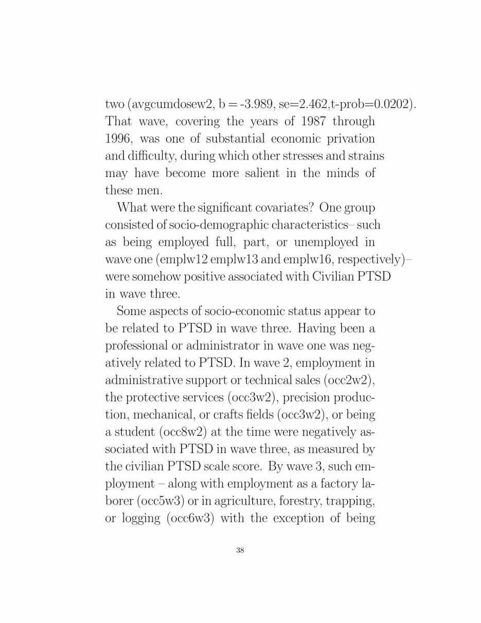
two (avgcumdosew2, b = -3.989, se=2.462,t-prob=0.0202).
That wave, covering the years of 1987 through
1996, was one of substantial economic privation
and difficulty, during which other stresses and strains
may have become more salient in the minds of
these men.
What were the significant covariates? One group
consisted of socio-demographic characteristics– such
as being employed full, part, or unemployed in
wave one (emplw12 emplw13 and emplw16, respectively)–
were somehow positive associated with Civilian PTSD
in wave three.
Some aspects of socio-economic status appear to
be related to PTSD in wave three. Having been a
professional or administrator in wave one was neg-
atively related to PTSD. In wave 2, employment in
administrative support or technical sales (occ2w2),
the protective services (occ3w2), precision produc-
tion, mechanical, or crafts fields (occ3w2), or being
a student (occ8w2) at the time were negatively as-
sociated with PTSD in wave three, as measured by
the civilian PTSD scale score. By wave 3, such em-
ployment – along with employment as a factory la-
borer (occ5w3) or in agriculture, forestry, trapping,
or logging (occ6w3) with the exception of being
38

a student, were positively associated with PTSD.
Income sufficiency with resources enough to meet
basic necessities plus a little left over (inc3w3) is
negatively associated with PTSD. It appears as if
socio-economic adequacy may be important.
Environmental factors may have played a role as
well. Males suffering from PTSD were concerned
about the distance of their residence and work-
place from the scene of the accident (kmacc and
kmwork). By wave two, their concerns about air
and water pollution (airw2) were inversely associ-
ated with PTSD. The farther the distance from
the accident site the less the PTSD. They were
concerned about the Chornobyl related threats to
their own health (radhlw3) in wave three, whereas
at first any concern they had was inversely asso-
ciated with PTSD (radhlw1). They were people
whose reported illnesses count in waves one (illw1)
and two (illw2) were significantly associated with
PTSD. Their fear of eating radioactively contami-
nated food was of borderline statistical significance
in wave two (fdferw2 p=0.0502), which became
statistically nonsignificant later.
PTSD appears to be positively related to having
observed a catastrophic event in wave two or three
39

(cataw2 or cataw3). A belief in the proportion of
radioactively contaminated area is directly related
to PTSD. Stresses and hassles from job related
matters were in wave one directly associated with
PTSD but switched to a significant inverse related
relationship in wave two (shjobw1 and shjobw2).
Stresses and hassles due to housing matters were
inversely related in wave one but directly related
in wave three (shhousw1 and shhousw3). Stresses
and hassles relating to relationships went from sig-
nificantly positive to significantly negative in waves
two and three (shrelaw2 and shrelaw3).
Forms of support were occasionally related to
PTSD in wave3. Family support was significant
only in wave one (sufamw1). Chornobyl survivor
support was negatively related to PTSD in wave
two (suchrw2).
These were individuals who exhibited general
mental health dysfunctionality (BSIposymp) whose
health problems impacted their work (HP2work).
Both of these traits were significantly positively
related to PTSD in wave three. There was a sig-
nificant positive association with PTSD between
the log of total BSI. There was a borderline signif-
icance in the relationship of having injured others
40

and PTSD (p=0.0506). Their reported anxiety in
wave two was statistically significant with PTSD
in wave three (anxagw2,b = .049, p = 0.034).
They also exhibited a number of significant in-
verse relationships between psychological symptoma-
tology and PTSD. These included depression (BSIdep),
phobic anxiety (BSIphanx), hostility (BSIhos), in-
terpersonal sensitivity (BSIips), and the impact of
health issues on home care cooking, and repairs
(HP2hmcare). It is possible that the economic dif-
ficulties exacerbated the PTSD problems in wave
two so that there appeared to be a dose-PTSD
male relationship at that time.
10.6 Female PTSD models using AutoMetrics alone
Before turning to the female PTSD models, it be-
hooves us to graph the relationships observed be-
tween PTSD and average cumulative dose over the
three waves, shown in Figure 4.
/Users/robertyaffee/Documents/data/h6figs/CfemalePTSDvDose3wvs-eps-converted-to.pdf
Figure 4: Female PTSD over three waves
Wave one appears to be less linear in functional
41

form than the others, so we may have more need of
basis functions there, but the other two relation-
ships appear to be fairly linear and without the
need of transformation.
We can examine the female baseline model ex-
plaining PTSD, for our hypothesis test of stres-
sors, and then of buffers relating to the PTSD.
In the baseline model, we observe no statistically
significant relationship between cumulative exter-
nal dose as measured by avgcumdose in waves one
through three, and PTSD for women, measured by
the Civilian PTSD scale score.
For the women, the baseline model has 55 pa-
rameters. Two-thirds of the first page of output
consist in socio-economic attributes. How does
socio-economic status relate to PTSD? Some of
the largest coefficients indicate salient aspects of
socio-economic status related to PTSD. Being sin-
gle (marrw21) in wave two 2 can be positively re-
lated to it. Income insufficiency (inc1w3) or almost
having such insufficiency (inc2w3) in wave 3 are
significantly related to the PTSD. Having a child
in wave one is significantly inversely related to it.
With respect to occupational status, working out-
doors (occ6w1) is significantly related to PTSD in
42

wave two (farming, logging, trapping, etc).
Other stressors are salient. Accidents (accdw1)
in wave1are significantly positively related to fe-
male PTSD in wave three. Stresses and hassles
from relationships (shrelaw1) during wave one are
significantly positively related to PTSD. Catastro-
phes in wave three are positive related to PTSD for
women. General mental dysfunctionality as mea-
sured by the BSI positive symptom scale is signif-
icantly positively related to PTSD. Self-reported
depression (depagw1 and depagw2) and anxiety
(anxagw1 and anxagw2) may be statistically re-
lated as well. They seem to be significantly related
but the signs of their parameter estimate change
in opposite directions as we move from wave one
to wave two. Health problem interference with
interests and hobbies (HP2inthob) is significantly
positively associated with PTSD on the part of
the female respondents. Consumption of pain pills
(pillw2) in wave two seems to be statistically re-
lated to PTSD. The geodesic distance of the resi-
dence from the accident site (havmil) is also found
to be statistically significantly related to PTSD.
Also, the stresses and hassles from the job and
from relationships appears to be significantly pos-
43
itively related to female PTSD.
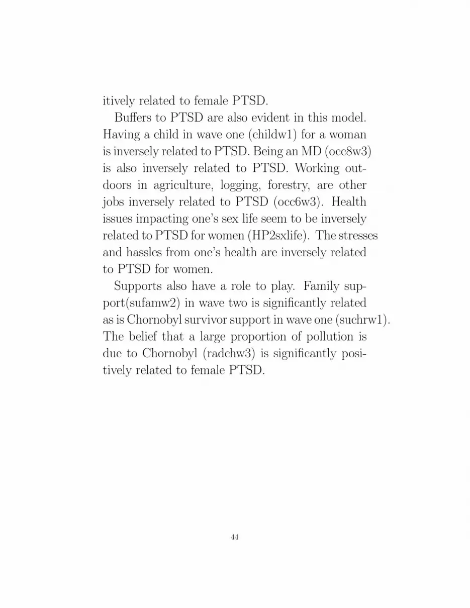
Buffers to PTSD are also evident in this model.
Having a child in wave one (childw1) for a woman
is inversely related to PTSD. Being an MD (occ8w3)
is also inversely related to PTSD. Working out-
doors in agriculture, logging, forestry, are other
jobs inversely related to PTSD (occ6w3). Health
issues impacting one’s sex life seem to be inversely
related to PTSD for women (HP2sxlife). The stresses
and hassles from one’s health are inversely related
to PTSD for women.
Supports also have a role to play. Family sup-
port(sufamw2) in wave two is significantly related
as is Chornobyl survivor support in wave one (suchrw1).
The belief that a large proportion of pollution is
due to Chornobyl (radchw3) is significantly posi-
tively related to female PTSD.
44

Table 8 EQ(29) Modelling MiPTSD by OLS-CSThe dataset is: gals.dtaThe estimation sample is: 1 - 363Dropped 7 observation(s) with missing values from the sample
Coefficient Std.Error HACSE t-HACSE t-prob Part.R^2marrw12 8.24237 4.931 4.806 1.72 0.0873 0.0096marrw21 12.3299 1.805 1.792 6.88 0.0000 0.1355marrw22 8.47335 3.703 2.766 3.06 0.0024 0.0301marrw23 6.23052 1.614 1.725 3.61 0.0004 0.0414childw1 -1.26565 0.8791 0.7999 -1.58 0.1146 0.0082childw2 2.55125 0.9794 0.8653 2.95 0.0034 0.0280emplw13 2.94446 2.047 1.774 1.66 0.0980 0.0090emplw32 3.52670 1.876 2.169 1.63 0.1050 0.0087emplw33 4.18612 7.971 1.777 2.36 0.0191 0.0180occ2w1 2.77946 1.582 1.613 1.72 0.0860 0.0097occ4w1 -0.606786 2.170 1.844 -0.329 0.7424 0.0004occ6w1 13.1978 4.550 2.815 4.69 0.0000 0.0678occ6w2 -9.92894 4.473 2.773 -3.58 0.0004 0.0407occ8w2 -5.30301 2.045 2.187 -2.42 0.0159 0.0191occ8w3 -9.21187 8.387 2.808 -3.28 0.0012 0.0344inc1w3 8.22857 1.680 1.812 4.54 0.0000 0.0639inc2w3 8.85438 1.391 1.337 6.62 0.0000 0.1267inc3w3 7.71199 1.413 1.372 5.62 0.0000 0.0947deaw1 1.16721 0.5685 0.6472 1.80 0.0723 0.0107deaw2 -0.631489 0.5636 0.5662 -1.12 0.2656 0.0041dvcew3 -5.08077 1.884 1.790 -2.84 0.0048 0.0260sepaw2 -5.42709 3.268 2.621 -2.07 0.0392 0.0140sepaw3 7.34660 2.257 2.257 3.26 0.0013 0.0339accdw1 8.14050 2.308 1.849 4.40 0.0000 0.0603accdw3 4.52347 1.349 1.181 3.83 0.0002 0.0463cataw1 -2.97149 1.501 1.410 -2.11 0.0359 0.0145cataw3 9.48043 5.937 5.320 1.78 0.0757 0.0104shjobw1 0.0459037 0.01897 0.02220 2.07 0.0395 0.0140shfamw2 0.0173869 0.02005 0.02067 0.841 0.4010 0.0023shhlw1 -0.0632661 0.01947 0.02554 -2.48 0.0138 0.0199shhlw3 0.0113486 0.01642 0.01671 0.679 0.4976 0.0015shfincw2 -0.0151884 0.02226 0.02365 -0.642 0.5212 0.0014shfincw3 -0.0204790 0.01681 0.01948 -1.05 0.2941 0.0036shrelaw1 0.0579751 0.01556 0.01523 3.81 0.0002 0.0458sufamw3 0.0354931 0.01329 0.01453 2.44 0.0151 0.0194suchrw1 0.0885848 0.04288 0.04238 2.09 0.0374 0.0143pillw2 0.246420 0.1558 0.1249 1.97 0.0493 0.0127pillw3 -0.132645 0.09234 0.09077 -1.46 0.1450 0.0070injselfr 1.48063 1.100 1.147 1.29 0.1978 0.0055
45

Table 8 - continued...
explanatory var Coefficient Std.Error HACSE t-HACSE t-prob Part.R^2
radchw1 -0.00608758 0.01568 0.01719 -0.354 0.7234 0.0004radchw3 0.0455101 0.01787 0.01961 2.32 0.0210 0.0175WHPer 0.0124274 0.03620 0.04239 0.293 0.7696 0.0003HP2pbfhm -2.00175 1.695 1.999 -1.00 0.3176 0.0033HP2sxlife -5.74679 1.371 1.523 -3.77 0.0002 0.0450HP2inthob 7.84715 1.583 2.314 3.39 0.0008 0.0367BSIposymp 0.292820 0.02081 0.02386 12.3 0.0000 0.3328havmil 0.00610682 0.001950 0.002717 2.25 0.0253 0.0165depagw1 -0.0666916 0.02328 0.02283 -2.92 0.0037 0.0275depagw2 0.109470 0.03546 0.03460 3.16 0.0017 0.0321anxagw1 0.0455276 0.01835 0.01819 2.50 0.0128 0.0203anxagw2 -0.0720609 0.02882 0.03571 -2.02 0.0445 0.0133avgcumdosew1 U 3.03671 1.669 1.928 1.57 0.1164 0.0081avgcumdosew2 U 2.25711 2.073 2.156 1.05 0.2960 0.0036avgcumdosew3 U -2.93719 1.507 1.815 -1.62 0.1067 0.0086
sigma 7.70878 RSS 17946.4376log-likelihood -1202.94no. of observations 356 no. of parameters 54mean(MiPTSD) 49.6208 se(MiPTSD) 12.0886When the log-likelihood constant is NOT included:AIC 4.22359 SC 4.81136HQ 4.45739 FPE 68.4392When the log-likelihood constant is included:AIC 7.06146 SC 7.64923HQ 7.29527 FPE 1168.91
Normality test: Chi^2(2) = 4.9117 [0.0858]Hetero test: F(81,272) = 1.1388 [0.2219]RESET23 test: F(2,300) = 37.383 [0.0000]**
46

10.6.1 Female PTSD model using AutoMetrics and MARS
When we mix AutoMetrics with MARS to test
the female PTSD hypothesis, we get an elaborate
rather than a parsimonious model. The hypothesis
that dose is directly associated with PTSD mea-
sured by the Civilian Mississippi scale is consistent
with parameter estimates for cumulative dose of 137
CS in mGys (avgcumdosew1 and avgcumdosew3,
both of which are statistically significant at the
0.05 level).
Table 9 EQ(32) Modelling MiPTSD by OLS-CSThe dataset is:gals.dtaThe estimation sample is: 1 - 363Dropped 5 observation(s) with missing values from the sample
Coefficient Std.Error HACSE t-HACSE t-prob Part.R^2marrw10 2.40743 3.127 2.103 1.14 0.2533 0.0044marrw12 8.70104 3.872 4.456 1.95 0.0518 0.0126marrw13 3.79369 1.166 1.149 3.30 0.0011 0.0351marrw21 3.82439 1.410 1.323 2.89 0.0041 0.0272marrw25 7.03501 3.217 2.954 2.38 0.0179 0.0186marrw32 -4.37927 2.753 1.800 -2.43 0.0155 0.0194marrw35 -5.37582 1.928 2.308 -2.33 0.0205 0.0178childw1 -0.595462 0.5982 0.7546 -0.789 0.4307 0.0021emplw13 3.04047 1.861 1.736 1.75 0.0810 0.0102emplw15 5.87467 3.790 2.599 2.26 0.0245 0.0168emplw22 2.45999 1.227 1.047 2.35 0.0194 0.0181emplw25 -3.04349 2.065 2.118 -1.44 0.1518 0.0069emplw33 8.96577 7.031 2.166 4.14 0.0000 0.0542occ3w1 -5.70773 1.423 1.598 -3.57 0.0004 0.0409occ6w1 5.11728 2.547 2.332 2.19 0.0290 0.0159occ2w2 2.73149 1.220 1.465 1.86 0.0632 0.0115occ7w2 5.13912 1.805 1.523 3.38 0.0008 0.0367occ8w2 -3.99304 1.859 1.748 -2.28 0.0231 0.0172occ8w3 -7.08976 6.967 1.908 -3.72 0.0002 0.0442inc1w3 2.59772 1.277 1.311 1.98 0.0485 0.0130inc2w3 2.52167 0.9265 0.9327 2.70 0.0073 0.0239deaw2 -0.776765 0.5023 0.5270 -1.47 0.1416 0.0072dvcew1 3.21334 5.055 2.772 1.16 0.2473 0.0045dvcew2 -6.65500 2.146 1.942 -3.43 0.0007 0.0378
Continued on the next page...
47
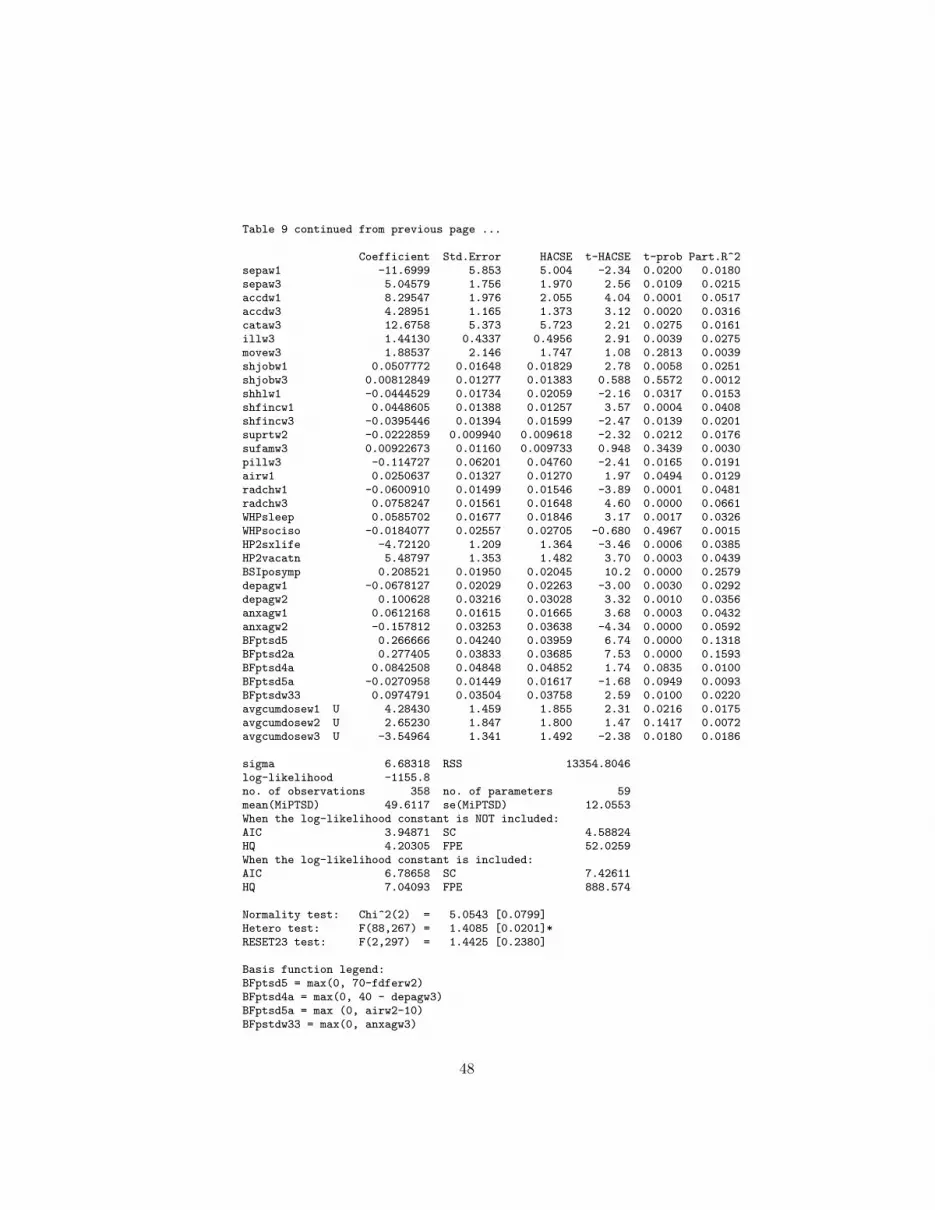
Table 9 continued from previous page ...
Coefficient Std.Error HACSE t-HACSE t-prob Part.R^2sepaw1 -11.6999 5.853 5.004 -2.34 0.0200 0.0180sepaw3 5.04579 1.756 1.970 2.56 0.0109 0.0215accdw1 8.29547 1.976 2.055 4.04 0.0001 0.0517accdw3 4.28951 1.165 1.373 3.12 0.0020 0.0316cataw3 12.6758 5.373 5.723 2.21 0.0275 0.0161illw3 1.44130 0.4337 0.4956 2.91 0.0039 0.0275movew3 1.88537 2.146 1.747 1.08 0.2813 0.0039shjobw1 0.0507772 0.01648 0.01829 2.78 0.0058 0.0251shjobw3 0.00812849 0.01277 0.01383 0.588 0.5572 0.0012shhlw1 -0.0444529 0.01734 0.02059 -2.16 0.0317 0.0153shfincw1 0.0448605 0.01388 0.01257 3.57 0.0004 0.0408shfincw3 -0.0395446 0.01394 0.01599 -2.47 0.0139 0.0201suprtw2 -0.0222859 0.009940 0.009618 -2.32 0.0212 0.0176sufamw3 0.00922673 0.01160 0.009733 0.948 0.3439 0.0030pillw3 -0.114727 0.06201 0.04760 -2.41 0.0165 0.0191airw1 0.0250637 0.01327 0.01270 1.97 0.0494 0.0129radchw1 -0.0600910 0.01499 0.01546 -3.89 0.0001 0.0481radchw3 0.0758247 0.01561 0.01648 4.60 0.0000 0.0661WHPsleep 0.0585702 0.01677 0.01846 3.17 0.0017 0.0326WHPsociso -0.0184077 0.02557 0.02705 -0.680 0.4967 0.0015HP2sxlife -4.72120 1.209 1.364 -3.46 0.0006 0.0385HP2vacatn 5.48797 1.353 1.482 3.70 0.0003 0.0439BSIposymp 0.208521 0.01950 0.02045 10.2 0.0000 0.2579depagw1 -0.0678127 0.02029 0.02263 -3.00 0.0030 0.0292depagw2 0.100628 0.03216 0.03028 3.32 0.0010 0.0356anxagw1 0.0612168 0.01615 0.01665 3.68 0.0003 0.0432anxagw2 -0.157812 0.03253 0.03638 -4.34 0.0000 0.0592BFptsd5 0.266666 0.04240 0.03959 6.74 0.0000 0.1318BFptsd2a 0.277405 0.03833 0.03685 7.53 0.0000 0.1593BFptsd4a 0.0842508 0.04848 0.04852 1.74 0.0835 0.0100BFptsd5a -0.0270958 0.01449 0.01617 -1.68 0.0949 0.0093BFptsdw33 0.0974791 0.03504 0.03758 2.59 0.0100 0.0220avgcumdosew1 U 4.28430 1.459 1.855 2.31 0.0216 0.0175avgcumdosew2 U 2.65230 1.847 1.800 1.47 0.1417 0.0072avgcumdosew3 U -3.54964 1.341 1.492 -2.38 0.0180 0.0186
sigma 6.68318 RSS 13354.8046log-likelihood -1155.8no. of observations 358 no. of parameters 59mean(MiPTSD) 49.6117 se(MiPTSD) 12.0553When the log-likelihood constant is NOT included:AIC 3.94871 SC 4.58824HQ 4.20305 FPE 52.0259When the log-likelihood constant is included:AIC 6.78658 SC 7.42611HQ 7.04093 FPE 888.574
Normality test: Chi^2(2) = 5.0543 [0.0799]Hetero test: F(88,267) = 1.4085 [0.0201]*RESET23 test: F(2,297) = 1.4425 [0.2380]
Basis function legend:BFptsd5 = max(0, 70-fdferw2)BFptsd4a = max(0, 40 - depagw3)BFptsd5a = max (0, airw2-10)BFpstdw33 = max(0, anxagw3)
48

To summarize the female analysis, we will note
some salient significant stressors and buffers for
PTSD among women in several domains–that of
socio- economic status (SES), that of major nega-
tive life events, that of daily stresses and hassles,
environmental factors, and psychological sequelae.
Using the partial R2 as a form of beta weight, we
see that within the domain of SES, being mar-
ried in wave 1 (marrw13), being divorced in wave
2 (marrw25), unemployed in wave 3 (emplw35),
and having a Ph.D. in wave 2(occ7w2) are major
stressors relating to PTSD. Other SES stressors
are income insufficiency for basic needs or border-
line income sufficiency for basic needs in wave three
(inc1w3 and inc2w3).
Prominent socio-economic status buffers are be-
ing retired in waves 2 and 3 (emplw25 and em-
plw35) and being a medical doctor in waves two
and three (occ8w2 and occ8w3).
Among the major negative life events, several
salient stressors appear. Some of the worst are
getting separated in wave one (sepaw1) and get-
ting a divorce in wave two, that time of economic
tribulation (dvcew2). However, accidents in wave
one (accdw1) and three (accdw3) also emerge as
49

substantial stressors.
Within the domain of daily stresses and hassles,
financial ones in wave 1 are significantly positively
related to PTSD. The reception of Chornobyl sup-
port in wave 2 and the consumption of pain pills
in wave three (pillw3) not surprisingly appear to
work as buffers.
As for environmental or contextual effects, in
wave 1 the percent belief air and water pollution
(airw1) is dangerous is related to PTSD, as is the
proportion of pollution due to Chornobyl is high in
wave 3 (radchw3) appears to be significantly nega-
tively related to PTSD, although there was a belief
that the air and water pollution was dangerous in
wave 1 (airw1) and wave 2 (BFptsd5a), whereas
by wave three the direction of this relationship re-
versed itself, so that it became a significantly pos-
itive in wave 3.
Fears of eating contaminated food appear to be
significantly positively related to PTSD in wave 2
(BFptsd5).
Psychological symptoms appeared in depression
and anxiety in waves one and two (depagw1 and
depage2), where they went from inverse to direct
over those two waves. However, anxiety went from
50

positive to negative as people became used to the
situation from wave one to wave two (anxagw1
and anxagw2). The basis functions reveal that de-
pression and anxiety in wave three were related to
PTSD as well.
These effects impacted the sleep, sex life, and
vacation plans of the female respondents such that
even general mental dysfunction became signifi-
cantly positively related to PTSD. When the na-
ture of the situation is considered, these women
may not seem so unreasonable, after all.
11 Conclusion
11.1 Exploration of new dimensions
Does MARS help us explore dimensions we might
otherwise have ignored? Sometimes it does and
sometimes it does not. For the men, the propor-
tion of variance explained tends to increase, but
for the females it does not. In our study of the
BSI positive symptom response, males exhibit an
increase in the number of factors extracted, but
females do not. Females, to the contrary, exhibit
a slight decline in the number of factors extracted.
In our PTSD models, the same pattern appears.
51

The result may vary with the nature of the data.
11.2 Are MARS models well-behaved?
MARS models tend to violate more assumptions
than AutoMetrics built models and MARS ba-
sis function generation supervised by AutoMetrics
does not guarantee well-behaved residuals. Some-
times MARS generated basis functions if selected
by AutoMetrics proliferate assumption violations
and sometimes they do not. The results at this
juncture are not conclusive, although there is ten-
tative evidence that MARS is motivated by opti-
mizing fit and not fulfilling regression assumptions.
Therefore the user must be careful about his use
of MARS.
MARS interaction generation fails to include all
component parts of of the interaction and actually
may prune some of them out if it improves the
overall fit. The resulting model may be misspeci-
fied according to conventional statistical theory.
11.3 Can MARS capture nonlinear relationships ?
MARS can by adding basis functions approximate
a nonlinear relationship between the dependent
52

variable and the other variables in the model. How-
ever, it may try to do this by building one of its in-
complete and unbalanced interaction vectors. This
may not be what the user wants so he must be
careful about such developments.
11.4 Content validity Tables
Does MARS improve content validty? The answer
is sometimes and not always. If the dimensional-
ity of the explanatory variables increases, then the
content validity increases. But the use of MARS
may actually decrease the dimensionality of the
model, as shown among women with respect to
their Positive symptom scale scores and their Chornobyl
PTSD scores in Tables 2 and 3 below. For male
respondents the application of MARS appeared to
increase dimnsionality but did not necessarily im-
prove fit.
Did MARS always improve the fit? If we ex-
amine in table 2 immediately above the propor-
tion of common variance explained we find that
among male BSI positive symptoms, it did. How-
ever, among females, the proportion of common
variance explained declined. As for the PTSD, the
application of MARS as a front end generator of
53

Table 2: Construct validity assessment of BSI positive symptom models
AutoMetrics alone MARS + AutoMetrics
Malemodelnfactors 4 6Number of singletons 0 0% common variance explained: 87 94number of regression predictors 28 23Number of regression assumption violations 1 2Femalemodel
nfactors 3 2Number of singletons 0 0% common variance explained 92 87Number of regression assumption violations 0 0number of regression predictors 21 14Number of regression assumption violations 1 2
basis functions did improve proportion of variance
explained among men but not in women. If the di-
mensionality of the predictor variable set actually
decline slightly among women. Further research
needs to be done to be sure, but if these few ex-
amples can serve as a guide, the value added by
MARS is mostly to capture nonlinearities in rele-
vant relationships.
54

Table 3: Construct validity assessment of PTSD models
AutoMetrics MARS+AutoMetrics
Malemodelnfactors 4 15Number of singletons 0 0% common variance explained: 85 88number of regression predictors 23 65number of regression assumption violations 1 3
Femalemodel
nfactors 10 9Number of singletons 0 0% common variance explained 86 84number of regression predictors 54 59number of regression assumption violations 1 1
55

11.5 Advantages of MARS
• automated
• fast
• builds additive model for you
56

11.6 Disadvantages of MARS
• adding them together to get a function
• no prima facie clear translation available some-
times
• you will need a translation table
• only emphasizes goodness of fit
• does not test regression assumptions
• interaction terms are not conventional
57

11.7 Caveats
• MARS may provide an optimal fit at the ex-
pense of violating the assumptions of regression
analysis
• does not test regression assumptions
• interaction terms are not conventional in that
they do not include the component terms con-
ventionally required for proper interaction spec-
ification.
References
[1] Havenaar, J.M, de Wilde, E.J., Van Den Bout,
J., Drottz-Sjoberg, B.M. and Van Den Brink,
W. (2003) Perception of risk and subjective
health among victims of the Chernobyl disaster
Social Science and Medicine, 569-572.
[2] Slovic, P. (2000) The Perception of Risk Lon-
don:Earthscan Publications Ltd.
[3] Bromet, E. J. and Litcher, L. (2002) Psy-
chological response of mothers of young chil-
dren to the Three Mile Island and Chernobyl
58

Nuclear Plant accidents one decade later in
In J.M. Havenaar, J. Cwikel and E.J. Bromet
(Eds.) Toxic Turmoil: Psychological and So-
cietal Consequences of Ecological Disasters
NY:Kluwer Academic/Plenum Publishers.
[4] Dew, M.A., Bromet, E.J., Schulburg, H.C.,
Dunn, L.O. and Parkinson, D.K. (1987) Mental
health effects of the Three Mile Island nuclear
reactor restart American Journal of Psychia-
try, 144, 1074-1077.
[5] Page, W.G., Babyleva, A.E., Naboka, M.V.
and Shestopalov, M.V. (1995) Environmental
health policies in Ukraine after the Chernobyl
accident Policy Studies Journal, 23, 141-151.
[6] Michal, F., Grigor, K.M. Negro-Vilar, A. and
Skakkebaek, N.E. (1993) Impact of environ-
ment on reproductive health Environmental
Health Perspectives, 101 (Suppl. 2) 159-167.
[7] Amirkhan, J.H. and Auyeung, B. (2007) Cop-
ing with stress across the life-span: Absolute
versus relative changes in strategy Journal of
Applied Developmental Psychology, 28, 298-
317.
[8] Purvis-Roberts, K.L., Werner, C.A., and
59

Frank, I. (2007) Perceived risks from radiation
and nuclear testing near Semipalatinsk, Kaza-
khstan: A comparison between physicians, sci-
entists and the public. Risk Analysis, 291-302.
[9] Hendry, Sir D.F. and Richard, J-F. (1983)
The econometric analysis of economic time se-
ries (with discussion). International Statistical
Review, 51, 111-163.
[10] Hendry, Sir D.F., and Krolzig, H-M. (2001)
Automatic Econometric Model Selection using
Pc-GETS London, UK: Timberlake Consul-
tants, Ltd..
[11] Hunt, S.M., McEwen, J. and McKenna, S.P.
(1985) Measuring health status: A new tool
for clinicians and epidemiologists Journal of the
Royal College of General Practitioners, 35, 185-
188.
[12] Perez Foster, R., Yaffee, R.A., Borak, T., and
Tierney, K. (2010) Modeling nuclear disas-
ter risk Poster presented at the National Sci-
ence Foundation, Human and Social Dynamics
Grantees Conference, Sept. 26-27, 2010, Arling-
ton.
60

[13] Derogatis, L.R. (1993) Brief Symptom Inven-
tory: Procedures Manual. MN:National Com-
puters Systems.
[14] Perez Foster, R. and Goldstein, M.F. (2007)
Chernobyl disaster sequelae in recent immi-
grants to the US from the former Soviet union
Journal of Immigrant Health, 9, 115-124.
[15] Castle, J.L., Doornik, J.A., and Hendry, D.F.
2011 Evaluating Automatic Model Selection
Journal of Time Series Econometrics, Vol.3,
1, 1-31.
[16] Friedman, Jerome H. 1990 Multivariate Adap-
tive Regression Splines Stanford Linear Accel-
erator Center Publication 4960-Rev.
[17] Hastie, T., Tibsharani, R. and Friedman, J.
2001 The Elements of Statistical Learning
New York, N.Y.: Springer, 115-163.
[18] Harrell, Jr., Frank 2001 Regression Modeling
Strategies New York, N.Y.: Springer, 18-24.
[19] Lewis, P.A.W. and Stevens, J. G. 1991 Non-
linear Modeling of Iime Series Using Multivari-
ate Adaptive Regression Splines Journal of
61

the American Statistical Association, Vol.86,
No.416, 864-877.
[20] Alina V. Brenner, Mykola D. Tronko, Mau-
reen Hatch, Tetyana I. Bogdanova, Valery A.
Oliynik, Jay H. Lubin, Lydia B. Zablotska,
Valery P. Tereschenko, Robert J. McConnell,
Galina A. Zamotaeva, Patrick OKane, An-
dre C. Bouville, Ludmila V. Chaykovskaya,
Ellen Greenebaum, Ihor P. Paster, Victor
M. Shpak, Elaine Ron (2007) I-131 Dose
Response for Incident Thyroid Cancers in
Ukraine Related to the Chornobyl Accident
http://ehp03.niehs.nih.gov/article/info:doi/10.1289/ehp.1002674.
[21] Marsh, L.C.and Cormier, David R. 2001
Spline Regression Models Sage Publications
[22] Chernobyl Forum (2003-2005) (2–5) Cher-
nobyl Legacy: Health, Environmental and
Socio-Economic Impacts: Recommendations to
the Governments of Belarus, Russian Federation
and Ukraine, Second Revised Edition.
[23] MARS User Guide (2001) San Diego, Ca:
Salford Systems, Ince., 2, 15.
[24] Selvin, Steve (2011) Statistical tools for Epi-
62

demiological Research New York: Oxford Uni-
versity Press, 257-309.
63


