Block 3

PRODUCTION AND COST ANALYSIS

Unit 7: Production Function 135

Unit 8: Short Run Cost Analysis 166

Unit 9: Long Run Cost Analysis 193

MMPC - 010Managerial Economics

Indira Gandhi

National Open University

School of Management Studies

BLOCK 3 PRODUCTION AND COST

ANALYSIS

Block 3 introduces production and cost analysis and the estimation of production

and cost functions. Production is the process of combining inputs to create output

which the firm sells in the market. The relationship between the production

function and the cost function is analyzed in this block and the implication for

managerial decisions is examined. In Unit 7, the production function and its

building blocks are analyzed from a managerial perspective. The difference

between short run and long run is explained from an economist’s perspective. It

is discussed that a profit-maximizing firm will choose an optimal combination

of inputs based on input prices. Estimation of production function and its

managerial uses are also elaborated in this unit. Unit 8 and 9 examines cost

analysis in the short and long run. Cost is related to production because if the

production function exhibits increasing returns to scale, the unit cost of production

falls, while if the production function exhibits decreasing returns to scale the

unit cost will rise and so on. Different types of costs including accounting costs

& opportunity costs and short run cost function are defined in Unit 8. Further,

certain applications of short run cost function like break-even analysis and

operating leverage are also explained. In Unit 9, long run cost function, economies

of scale & scope are explained. Finally, estimation of cost function is presented

using the tools of regression analysis that were developed in Blocks 1 and 2.

135

Production Function UNIT 7 PRODUCTION FUNCTION

Objectives

After going through this unit, you should be able to:

familiarize with the concepts and rules relevant for production decision

analysis;

understand the economics of production;

understand the set of conditions required for efficient production.

Structure

7.1 Introduction

7.2 Production Function

7.3 Production Function with one Variable inputs

7.4 Production Function with two Variable inputs

7.5 The Optimal Combination of inputs

7.6 Returns to Scale

7.7 Functional Forms of Production Function

7.8 Managerial Uses of Production Function

7.9 Summary

7.10 Self - Assessment Questions

7.11 Further Readings

7.1 INTRODUCTION

Production process involves the transformation of inputs into output. The

inputs could be land, labour, capital, entrepreneurship etc. and the output

could be goods or services. In a production process managers take four types

of decisions: (a) whether to produce or not, (b) how much output to produce,

(c) what input combination to use, and (d) what type of technology to use.

This Unit deals with the analysis of managers’ decision rules concerning (c)

and (d) above. The analysis of the other two decisions will be covered in

Units 8 and Unit 9 of this block.

In this unit, we shall begin with a general discussion of the concept of

production function. The analysis of this unit mainly focuses on the firms that

produce a single product. Analysis on decisions related to multiproduct firms

is also given briefly. The nature of production when there is only one variable

input is taken up first. We then move on to the problem of finding optimum

136

Production and Cost

Analysis combination of inputs for producing a particular level of output when there

are two or more variable inputs. You will also learn about the production

decisions in case of product mix of multiproduct firms. The unit concludes

with various functional forms of production frequently used by economists

and their empirical estimation.

7.2 PRODUCTION FUNCTION

Suppose we want to produce apples. We need land, seedlings, fertilizer,

water, labour, and some machinery. These are called inputs or factors of

production. The output is apples. In general a given output can be produced

with different combinations of inputs. A production function is the functional

relationship between inputs and output. It shows the maximum output which

can be obtained for a given combination of inputs. It expresses the

technological relationship between inputs and output of a product.

In general, we can represent the production function for a firm as:

Q = f (x1, x2, ….,xn)

Where Q is the maximum quantity of output, x1, x2, ….,xn are the quantities

of various inputs, and f stands for functional relationship between inputs and

output. For the sake of clarity, let us restrict our attention to only one product

produced using either one input or two inputs. If there are only two inputs,

capital (K) and labour (L), we write the production function as:

Q = f (L, K)

This function defines the maximum rate of output (Q) obtainable for a given

rate of capital and labour input. It may be noted here that outputs may be

tangible like computers, television sets, etc., or it may be intangible like

education, medical care, etc. Similarly, the inputs may be other than capital

and labour. Also, the principles discussed in this unit apply to situations with

more than two inputs as well.

Economic Efficiency and Technical Efficiency

We say that a firm is technically efficient when it obtains maximum level of

output from any given combination of inputs. The production function

incorporates the technically efficient method of production. A producer

cannot decrease one input and at the same time maintain the output at the

same level without increasing one or more inputs. When economists use

production functions, they assume that the maximum output is obtained from

any given combination of inputs. That is, they assume that production is

technically efficient.

On the other hand, we say a firm is economically efficient, when it produces a

given amount of output at the lowest possible cost for a combination of inputs

137

Production Function provided that the prices of inputs are given. Therefore, when only input

combinations are given, we deal with the problem of technical efficiency;

that is, how to produce maximum output. On the other hand, when input

prices are also given in addition to the combination of inputs, we deal with

the problem of economic efficiency; that is, how to produce a given amount

of output at the lowest possible cost.

One has to be careful while interpreting whether a production process is

efficient or inefficient. Certainly a production process can be called efficient

if another process produces the same level of output using one or more

inputs, other things remaining constant. However, if a production process

uses less of some inputs and more of others, the economically efficient

method of producing a given level of output depends on the prices of inputs.

Even when two production processes are technically efficient, one process

may be economically efficient under one set of input prices, while the other

production process may be economically efficient at other input prices.

Let us take an example to differentiate between technical efficiency and

economic efficiency. An ABC company is producing readymade garments

using cotton fabric in a certain production process. It is found that 10 percent

of fabric is wasted in that process. An engineer suggested that the wastage of

fabric can be eliminated by modifying the present production process. To this

suggestion, an economist reacted differently saying that if the cost of wasted

fabric is less than that of modifying production process then it may not be

economically efficient to modify the production process.

Short Run and Long Run

All inputs can be divided into two categories; i) fixed inputs and ii) variable

inputs. A fixed input is one whose quantity cannot be varied during the time

under consideration. The time period will vary depending on the

circumstances. Although any input may be varied no matter how short the

time interval, the cost involved in augmenting the amount of certain inputs is

enormous; so as to make quick variation impractical. Such inputs are

classified as fixed and include plant and equipment of the firm.

On the other hand, a variable input is one whose amount can be changed

during the relevant period. For example, in the construction business the

number of workers can be increased or decreased on short notice. Many

‘builder’ firms employ workers on a daily wage basis and frequent change in

the number of workers is made depending upon the need. The amount of milk

that goes in the production of butter can be altered quickly and easily and is

thus classified as a variable input in the production process.

Whether or not an input is fixed or variable depends upon the time period

involved. The longer the length of the time period under consideration, the

more likely it is that the input will be variable and not fixed. Economists find

it convenient to distinguish between the short run and the long run. The short

138

Production and Cost

Analysis run is defined to be that period of time when some of the firm’s inputs are

fixed. Since it is most difficult to change plant and equipment among all

inputs, the short run is generally accepted as the time interval over which the

firm’s plant and equipment remain fixed. In contrast, the long run is that

period over which all the firms’ inputs are variable. In other words, the firm

has the flexibility to adjust or change its environment.

Production processes of firms generally permit a variation in the proportion

in which inputs are used. In the long run, input proportions can be varied

considerably. For example, at Maruti Udyog Limited, an automobile dye can

be made on conventional machine tools with more labour and less expensive

equipment, or it can be made on numerically controlled machine tools with

less labour and more expensive equipment i.e. the amount of labour and

amount of equipment used can be varied. Later in this unit, this aspect is

considered in more detail. On the other hand, there are very few production

processes in which inputs have to be combined in fixed proportions.

Consider, Ranbaxy or Smith-Kline-Beecham or any other pharmaceutical

firm. In order to produce a drug, the firm may have to use a fixed amount of

aspirin per 10 gm of the drug. Even in this case a certain (although small)

amount of variation in the proportion of aspirin may be permissible. If, on the

other hand, no flexibility in the ratio of inputs is possible, the technology is

described as fixed proportion type. We refer to this extreme case later in this

unit, but as should be apparent, it is extremely rare in practice.

Activity 1

1. What is a production function? How does a long run production

function differ from a short run production function?

…………………………………………………………………………

…………………………………………………………………………

…………………………………………………………………………

…………………………………………………………………………

…………………………………………………………………………

…………………………………………………………………………

2. When can we say that a firm is: (a) technically efficient, (b)

economically efficient? Is it necessary that a technically efficient firm

is also economically efficient?

…………………………………………………………………………

…………………………………………………………………………

…………………………………………………………………………

…………………………………………………………………………

…………………………………………………………………………

…………………………………………………………………………

139

Production Function 7.3 PRODUCTION FUNCTION WITH ONE

VARIABLE INPUT

Consider the simplest two input production process - where one input with a

fixed quantity and the other input with its variable quantity. Suppose that the

fixed input is the service of machine tools, the variable input is labour, and

the output is a metal part. The production function in this case can be

represented as:

Q = f (K, L)

Where Q is output of metal parts, K is service of five machine tools (fixed

input), and L is labour (variable input). The variable input can be combined

with the fixed input to produce different levels of output.

Total, Average, and Marginal Products

The production function given above shows us the maximum total product

(TP) that can be obtained using different combinations of quantities of inputs.

Suppose the metal parts company decides to know the output level for

different input levels of labour using fixed five machine tools. Table 7.1

explains the total output for different levels of variable input. In this

example, the TP rises with increase in labour up to a point (six workers),

becomes constant between sixth and seventh workers, and then declines.

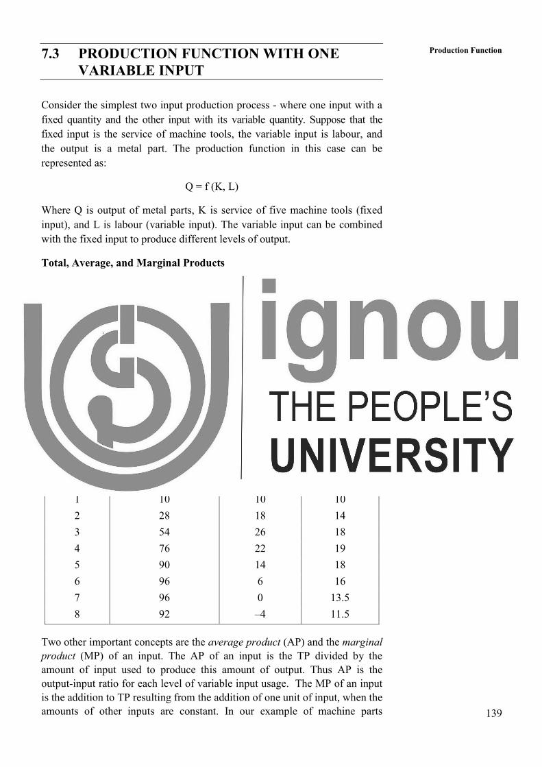
Table 7.1: Total, Average and Marginal Products of labour

(with fixed capital at five machine tools)

Two other important concepts are the average product (AP) and the marginal

product (MP) of an input. The AP of an input is the TP divided by the

amount of input used to produce this amount of output. Thus AP is the

output-input ratio for each level of variable input usage. The MP of an input

is the addition to TP resulting from the addition of one unit of input, when the

amounts of other inputs are constant. In our example of machine parts

Number of

workers (L)

Total output (TP)

(thousands per year) (Q)

Marginal product

(MPL = ∆Q/∆L)

Average product

(APL = Q/L)

0 0 — —

1 10 10 10

2 28 18 14

3 54 26 18

4 76 22 19

5 90 14 18

6 96 6 16

7 96 0 13.5

8 92 –4 11.5

140

Production and Cost

Analysis production process, the AP of labour is the TP divided by the number of

workers.

APL = Q/L

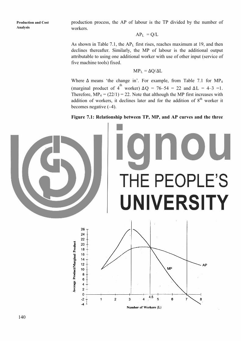
As shown in Table 7.1, the APL first rises, reaches maximum at 19, and then

declines thereafter. Similarly, the MP of labour is the additional output

attributable to using one additional worker with use of other input (service of

five machine tools) fixed.

MPL = ∆Q/∆L

Where ∆ means ‘the change in’. For example, from Table 7.1 for MP4

(marginal product of 4th

worker) ∆Q = 76–54 = 22 and ∆L = 4–3 =1.

Therefore, MP4 = (22/1) = 22. Note that although the MP first increases with

addition of workers, it declines later and for the addition of 8th worker it

becomes negative (–4).

Figure 7.1: Relationship between TP, MP, and AP curves and the three

stages of production

141

Production Function The graphical presentation of total, average, and marginal products for our

example of machine parts production process is shown in Figure 7.1.

Relationship between TP, MP and AP Curves

Examine Table 7.1 and its graphical presentation in Figure 7.1. We can

establish the following relationship between TP, MP, and AP curves.

1a) If MP > 0, TP will be rising as L increases. The TP curve begins at the

origin, increases at an increasing rate over the range 0 to 3, and then

increases at a decreasing rate. The MP reaches a maximum at 3, which

corresponds to an inflection point (x) on the TP curve. At the inflection

point, the TP curve changes from increasing at an increasing rate to

increasing at decreasing rate.

b) If MP = 0, TP will be constant as L increases. The TP is constant

between workers 6 and 7.

c) If MP < 0, TP will be declining as L increases. The TP declines beyond

7. Also, the TP curve reaches a maximum when MP = 0 and then starts

declining when MP < 0.

2. MP intersects AP (MP = AP) at the maximum point on the AP curve.

This occurs at labour input rate 4.5. Also, observe that whenever MP

>AP, the AP is rising (upto number of workers 4.5) — it makes no

difference whether MP is rising or falling. When MP < AP (from

number of workers 4.5), the AP is falling. Therefore, the intersection

must occur at the maximum point of AP. It is important to understand

why. The key is that AP increases as long as the MP is greater than AP.

And AP decreases as long as MP is less than AP. Since AP is positively

or negatively sloped depending on whether MP is above or below AP, it

follows that MP=AP at the highest point on the AP curve.

This relationship between MP and AP is not unique to economics. Consider a

cricket batsman, say Sachin Tendulkar, who is averaging 50 runs in 10

innings. In his next innings he scores a 100. His marginal score is 100 and his

average will now be above 50. More precisely, it is 54 i.e. (50 * 10 + 100)/

(10+1) = 600/11. This means when the marginal score is above the average,

the average must increase. In case he had scored zero, his marginal score

would be below the average, and his average would fall to 45.5 i.e. 500/11

is 45.45. Only if he had scored 50 would the average remain constant, and

the marginal score would be equal to the average.

The Law of Diminishing Marginal Returns

The slope of the MP curve in Figure 7.1 illustrates an important principle, the

law of diminishing marginal returns. As the number of units of the variable

input increases, the other inputs held constant (fixed), there exists a point

beyond which the MP of the variable input declines. Table 7.1 illustrates this

law. Observe that MP was increasing up to the addition of 4th worker (input);

142

Production and Cost

Analysis beyond this the MP decreases. What this law says is that MP may rise or stay

constant for some time, but as we keep increasing the units of variable input,

MP should start falling. It may keep falling and turn negative, or may stay

positive all the time. Consider another example for clarity. Single application

of fertilizers may increase the output by 50%, a second application by another

30% and the third by 20% and so on. However, if you were to apply fertilizer

five to six times in a year, the output may drop to zero.

Three things should be noted concerning the law of diminishing marginal

returns.

1. This law is an empirical generalization, not a deduction from physical

or biological laws.

2. It is assumed that technology remains fixed. The law of diminishing

marginal returns cannot predict the effect of an additional unit of

input when technology is allowed to change.

3. It is assumed that there is at least one input whose quantity is being

held constant (fixed). In other words, the law of diminishing marginal

returns does not apply to cases where all inputs are variable.

Stages of Production

Based on the behaviour of MP and AP, economists have classified production

into three stages:

Stage 1: MP > 0, AP rising. Thus, MP > AP.

Stage 2: MP > 0, but AP is falling. MP < AP but TP is increasing (because

MP >0).

Stage 3: MP < 0. In this case TP is falling.

These results are illustrated in Figure 7.1. No profit-maximizing producer

would produce in stages I or III. In stage I, by adding one more unit of

labour, the producer can increase the AP of all units. Thus, it would be

unwise on the part of the producer to stop the production in this stage. As for

stage III, it does not pay the producer to be in this region because by reducing

the labour input the total output can be increased and the cost of a unit of

labour can be saved

Thus, the economically meaningful range is given by stage II. In Figure 7.1

at the point of inflection (x), we saw earlier that MP is maximized. At point y,

since AP is maximized, we have AP = MP. At point z, TP reaches a

maximum. Thus, MP = 0 at this point. If the variable input is free then the

optimum level of output is at point z where TP is maximized. However, in

practice no input will be freely available. The producer has to pay a price for

it. Suppose the producer pays Rs. 200 per worker per day and the price of a

143

Production Function unit of output (say one apple) is Rs. 10. In this case the producer will keep on

hiring additional workers as long as

(Price of a unit of output) * (marginal product of labour) > (price of a unit of

labour)

That is, marginal revenue of product (MRP) of labour >PL

On a similar analogy,

(price of a unit of output) * (marginal product of capital) > (price of a unit of

capital)

That is, marginal revenue of product (MRP) of capital > PK

The left side denotes the increase in revenue and the right side denotes the

increase in the cost of adding one more unit of labour. As long as the

increment to revenues exceeds the increment to costs, the profit of the

producer will increase. As we increase the units of labour, we see that MP

diminishes. We assume that the prices of inputs and output do not change. In

this case, as MP declines, revenues will start falling, and a point will come

when the increase in revenue equals the increase in cost. At this point the

producer will stop adding more units of input. With further addition, since

MP declines, the additional revenues would be less than the additional costs,

and the profit of the producer would decline.

Thus, profit maximization implies that a producer with no control over prices

will increase the use of an input until—

Value of marginal product (MP) = Price of a unit of variable input

Activity 2

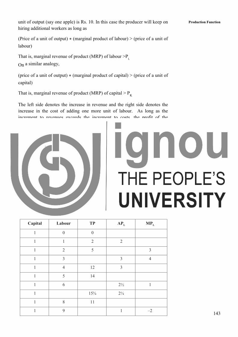
1. Fill in the blanks of the following Table

Capital Labour TP APL

MPL

1 0 0

1 1 2 2

1 2 5 3

1 3 3 4

1 4 12 3

1 5 14

1 6 2½ 1

1 15¾ 2¼

1 8 11

1 9 1 –2

144

Production and Cost

Analysis 2. State clearly the relation between APLand MPL.

.............................................................................................................

.............................................................................................................

.............................................................................................................

.............................................................................................................

.............................................................................................................

.............................................................................................................

.............................................................................................................

3. Why is the marginal product of labour likely to increase and then decline

in the short-run?

.............................................................................................................

.............................................................................................................

.............................................................................................................

.............................................................................................................

.............................................................................................................

.............................................................................................................

.............................................................................................................

4. Faced with constantly changing conditions, why would a firm ever keep

any factors fixed? What determines whether a factor is fixed or variable?

.............................................................................................................

.............................................................................................................

.............................................................................................................

.............................................................................................................

.............................................................................................................

.............................................................................................................

.............................................................................................................

5. Suppose a chair manufacturer is producing in the short run where

equipment is fixed. The manufacturer knows that as the number of

labourers used in the production process increases from 1 to 7, the

number of chairs produced changes as follows: 10, 17, 22, 25, 26, 25, and

23.

a) Calculate the marginal and average product of labour for this

production function.

b) Does this production function exhibit increasing returns to labour or

decreasing returns to labour or both? Explain.

145

Production Function c) Explain intuitively what might cause the marginal product of labour

to become negative?

.............................................................................................................

.............................................................................................................

.............................................................................................................

.............................................................................................................

.............................................................................................................

.............................................................................................................

.............................................................................................................

6. Why a profit-maximizing producer would produce in stage-II and not in

stage-I or III? Explain.

...................................................................................................................

...................................................................................................................

...................................................................................................................

...................................................................................................................

...................................................................................................................

...................................................................................................................

...................................................................................................................

7.4 PRODUCTION FUNCTION WITH TWO

VARIABLE INPUTS

Now we turn to the case of production where two inputs (say capital and labour)

are variable. Although, we restrict our analysis to two variable inputs, all of

the results hold for more than two also. We are restricting our analysis to two

variable inputs because it simply allows us the scope for graphical analysis.

When analyzing production with more than one variable input, we cannot simply

use sets of AP and MP curves like those discussed in section 7.3, because these

curves were derived holding the use of all other inputs fixed and letting the use

of only one input vary. If we change the level of fixed input, the TP, AP and MP

curves would shift. In the case of two variable inputs, changing the use of one

input would cause a shift in the MP and AP curves of the other input. For

example, an increase in capital would probably result in an increase in the MP of

labour over a wide range of labour use.

Production Isoquants

In Greek the word ‘iso’ means ‘equal’ or ‘same’. A production isoquant (equal

output curve) is the locus of all those combinations of two inputs which yields a

given level of output. With two variable inputs, capital and labour, the isoquant

gives the different combinations of capital and labour, that produces the same

level of output. For example, 5 units of output can be produced using either 15

units of capital (K) or 2 units of labour (L) or K=10 and L=3 or K=5 and L=5 or

146

Production and Cost

Analysis K=3 and L=7. These four combinations of capital and labour are four points on

the isoquant associated with 5 units of output as shown in Figure 7.2. And if we

assume that capital and labour are continuously divisible, there would be many

more combinations on this isoquant.

Now let us assume that capital, labour, and output are continuously divisible in

order to set forth the typically assumed characteristics of isoquants. Figure 7.3

illustrates three such isoquants. Isoquant I shows all the combinations of capital

and labour that will produce 10 units of output. According to this isoquant, it is

possible to obtain this output if K0 units of capital and L0 units of

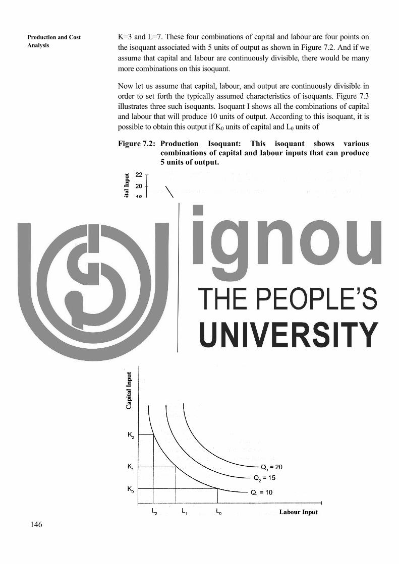
Figure 7.2: Production Isoquant: This isoquant shows various

combinations of capital and labour inputs that can produce

5 units of output.

Figure 7.3: Isoquant Map: These isoquants shows various combinations

of capital and labour inputs that can produce 10, 15, and 20

units of output.

147

Production Function labour inputs are used. Alternately, this output can also be obtained if K1

units of capital and L1 units of labour inputs or K2 units of capital and L2

units of labour are used. Similarly, isoquant II shows the various

combinations of capital and labour that can be used to produce 15 units of

output. Isoquant III shows all combinations that can produce 20 units of

output. Each capital- labour combination can be on only one isoquant. That

is, isoquants cannot intersect. These isoquants are only three of an infinite

number of isoquants that could be drawn. A group of isoquants is called an

isoquant map. In an isoquant map, all isoquants lying above and to the right

of a given isoquant indicate higher levels of output. Thus, in Figure 7.3

isoquant II indicates a higher level of output than isoquant I, and isoquant III

indicates a higher level of output than isoquant II.

In general, isoquants are determined in the following way. First, a rate of

output, say Q0, is specified. Hence the production function can be written as

Q0 = f (K,L)

Those combinations of K and L that satisfy this equation define the isoquant

for output rate Q0.

Marginal Rate of Technical Substitution

As we have seen above, generally there are a number of ways (combinations

of inputs) that a particular output can be produced. The rate, at which one

input can be substituted for another input, if output remains constant, is called

the marginal rate of technical substitution (MRTS). It is defined in case of

two inputs, capital and labour, as the amount of capital that can be replaced

by an extra unit of labour, without affecting total output.

MRTSL for K = ∆�∆�

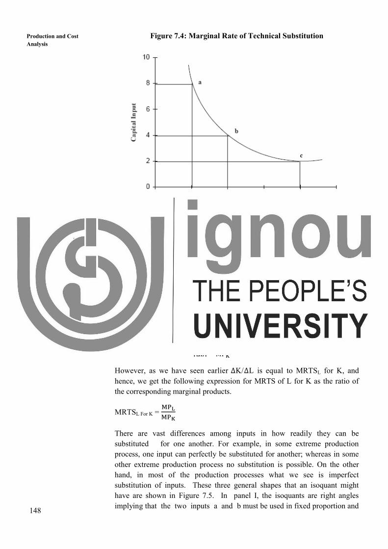
It is customary to define the MRTS as a positive number, since ∆K/∆L, the

slope of the isoquant, is negative. Over the relevant range of production the

MRTS diminishes. That is, more and more labour is substituted for capital

while holding output constant, the absolute value of ∆K/∆L decreases. For

example, let us assume that 10 pairs of shoes can be produced using either 8

units of capital and 2 units of labour or 4 units each of capital and of labour

or 2 units of capital and 8 units of labour. From Figure 7.4 the MRTS of

labour for capital between points a and b is equal to ∆K/∆L= (4–8) / (4–2) =

–4/2 = –2 or | 2 |. Between points b and c, the MRTS is equal to –2/4 = –½ or

| ½ |. The MRTS has decreased because capital and labour are not perfect

substitutes for each other. Therefore, as more of labour is added, less of

capital can be used (in exchange for another unit of labour) while keeping the

output level constant.

148

Production and Cost

Analysis Figure 7.4: Marginal Rate of Technical Substitution

There is a simple relationship between MRTS of labour for capital and the

marginal product MPK and MPL of capital and labour respectively. Since

along an isoquant, the level of output remains the same, if ∆L units of labour

are substituted for ∆K units of capital, the increase in output due to ∆L units

of labour (namely, ∆L* MPL) should match the decrease in output due to a

decrease of ∆K units of capital (namely, ∆K * MPk). In other words, along an

isoquant,

∆ L * MPL = ∆ K * MPK

Which is equal to

�∆�∆�� =

������

However, as we have seen earlier ∆K/∆L is equal to MRTSL for K, and

hence, we get the following expression for MRTS of L for K as the ratio of

the corresponding marginal products.

MRTSL For K = ������

There are vast differences among inputs in how readily they can be

substituted for one another. For example, in some extreme production

process, one input can perfectly be substituted for another; whereas in some

other extreme production process no substitution is possible. On the other

hand, in most of the production processes what we see is imperfect

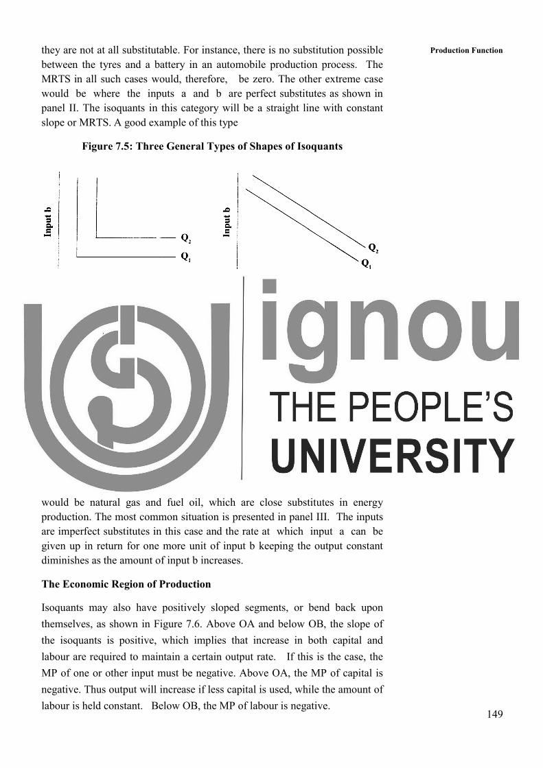
substitution of inputs. These three general shapes that an isoquant might

have are shown in Figure 7.5. In panel I, the isoquants are right angles

implying that the two inputs a and b must be used in fixed proportion and

149

Production Function they are not at all substitutable. For instance, there is no substitution possible

between the tyres and a battery in an automobile production process. The

MRTS in all such cases would, therefore, be zero. The other extreme case

would be where the inputs a and b are perfect substitutes as shown in

panel II. The isoquants in this category will be a straight line with constant

slope or MRTS. A good example of this type

Figure 7.5: Three General Types of Shapes of Isoquants

would be natural gas and fuel oil, which are close substitutes in energy

production. The most common situation is presented in panel III. The inputs

are imperfect substitutes in this case and the rate at which input a can be

given up in return for one more unit of input b keeping the output constant

diminishes as the amount of input b increases.

The Economic Region of Production

Isoquants may also have positively sloped segments, or bend back upon

themselves, as shown in Figure 7.6. Above OA and below OB, the slope of

the isoquants is positive, which implies that increase in both capital and

labour are required to maintain a certain output rate. If this is the case, the

MP of one or other input must be negative. Above OA, the MP of capital is

negative. Thus output will increase if less capital is used, while the amount of

labour is held constant. Below OB, the MP of labour is negative.

150

Production and Cost

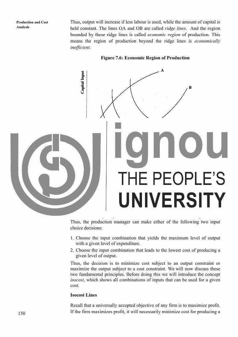
Analysis Thus, output will increase if less labour is used, while the amount of capital is

held constant. The lines OA and OB are called ridge lines. And the region

bounded by these ridge lines is called economic region of production. This

means the region of production beyond the ridge lines is economically

inefficient.

Figure 7.6: Economic Region of Production

7.5 THE OPTIMAL COMBINATION OF INPUTS

In the above section you have learned that any desired level of output can be

produced using a number of different combinations of inputs. As said earlier

in the introduction of this unit one of the decision problems that concerns a

production process manager is, which input combination to use. That is, what

is the optimal input combination? While all the input combinations are

technically efficient, the final decision to employ a particular input

combination is purely an economic decision and rests on cost (expenditure).

Thus, the production manager can make either of the following two input

choice decisions:

1. Choose the input combination that yields the maximum level of output

with a given level of expenditure.

2. Choose the input combination that leads to the lowest cost of producing a

given level of output.

Thus, the decision is to minimize cost subject to an output constraint or

maximize the output subject to a cost constraint. We will now discuss these

two fundamental principles. Before doing this we will introduce the concept

isocost, which shows all combinations of inputs that can be used for a given

cost.

Isocost Lines

Recall that a universally accepted objective of any firm is to maximize profit.

If the firm maximizes profit, it will necessarily minimize cost for producing a

151

Production Function given level of output or maximize output for a given level of cost. Suppose

there are 2 inputs: capital (K) and labour (L) that are variable in the relevant

time period. What combination of (K,L) should the firm choose in order to

maximize output for a given level of cost?

If there are 2 inputs, K,L, then given the price of capital (Pk) and the price of

labour (PL), it is possible to determine the alternative combinations of (K,L)

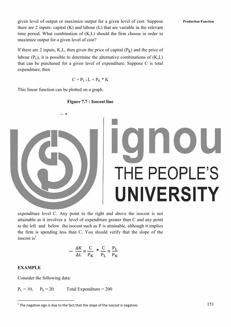
that can be purchased for a given level of expenditure. Suppose C is total

expenditure, then

C = PL * L + PK * K

This linear function can be plotted on a graph.

Figure 7.7 : Isocost line

If only capital is purchased, then the maximum amount that can be bought is

C/Pk shown by point A in figure 7.7. If only labour is purchased, then the

maximum amount of labour that can be purchased is C/PL shown by point B

in the figure. The 2 points A and B can be joined by a straight line. This

straight line is called the isocost line or equal cost line. It shows the

alternative combinations of (K,L) that can be purchased for the given

expenditure level C. Any point to the right and above the isocost is not

attainable as it involves a level of expenditure greater than C and any point

to the left and below the isocost such as P is attainable, although it implies

the firm is spending less than C. You should verify that the slope of the

isocost is1

�����

= ���

* ���

= ����

EXAMPLE

Consider the following data:

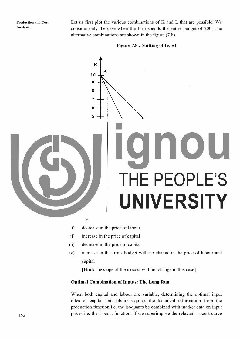
PL = 10, Pk = 20 Total Expenditure = 200

1 The negative sign is due to the fact that the slope of the isocost is negative.

152

Production and Cost

Analysis Let us first plot the various combinations of K and L that are possible. We

consider only the case when the firm spends the entire budget of 200. The

alternative combinations are shown in the figure (7.8).

Figure 7.8 : Shifting of Iscost

The slope of this isocost is –½. What will happen if labour becomes more

expensive say PL increases to 20? Obviously with the same budget the firm

can now purchase lesser units of labour. The isocost still meets the Y–axis at

point A (because the price of capital is unchanged), but shifts inwards in the

direction of the arrow to meet the X-axis at point C. The slope therefore

changes to –1. You should work out the effect on the isocost curve on the

following:

i) decrease in the price of labour

ii) increase in the price of capital

iii) decrease in the price of capital

iv) increase in the firms budget with no change in the price of labour and

capital

[Hint:The slope of the isocost will not change in this case]

Optimal Combination of Inputs: The Long Run

When both capital and labour are variable, determining the optimal input

rates of capital and labour requires the technical information from the

production function i.e. the isoquants be combined with market data on input

prices i.e. the isocost function. If we superimpose the relevant isocost curve

153

Production Function on the firm’s isoquant map, we can readily determine graphically as to which

combination of inputs maximize the output for a given level of expenditure.

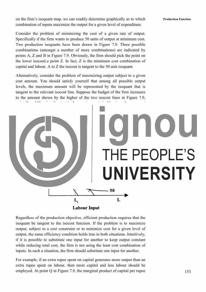
Consider the problem of minimizing the cost of a given rate of output.

Specifically if the firm wants to produce 50 units of output at minimum cost.

Two production isoquants have been drawn in Figure 7.9. Three possible

combinations (amongst a number of more combinations) are indicated by

points A, Z and B in Figure 7.9. Obviously, the firm should pick the point on

the lower isocosti.e point Z. In fact, Z is the minimum cost combination of

capital and labour. A to Z the isocost is tangent to the 50 unit isoquant.

Alternatively, consider the problem of maximizing output subject to a given

cost amount. You should satisfy yourself that among all possible output

levels, the maximum amount will be represented by the isoquant that is

tangent to the relevant isocost line. Suppose the budget of the firm increases

to the amount shown by the higher of the two isocost lines in Figure 7.9,

point Q or 100 units of output is the maximum attainable given the new cost

constraint in Figure7.9.

Figure 7.9: Optimal combination of inputs

Regardless of the production objective, efficient production requires that the

isoquant be tangent to the isocost function. If the problem is to maximize

output, subject to a cost constraint or to minimize cost for a given level of

output, the same efficiency condition holds true in both situations. Intuitively,

if it is possible to substitute one input for another to keep output constant

while reducing total cost, the firm is not using the least cost combination of

inputs. In such a situation, the firm should substitute one input for another.

For example, if an extra rupee spent on capital generates more output than an

extra rupee spent on labour, then more capital and less labour should be

employed. At point Q in Figure 7.9, the marginal product of capital per rupee

154

Production and Cost

Analysis spent on capital is equal to the marginal product of labour per rupee spent on

labour. Mathematically this can be shown as

��L��

= ��K��

………………………….....….1

Or equivalently,

��L��K

= �L�K

…………………………....…...2

Whenever the 2 sides of the above equation are not equal, there are

Possibilities that input substitutions will reduce costs. Let us work with

numbers. Suppose PL = 10, Pk = 20,

MPL = 50 and MPk = 40. Thus, we have

����

> ����

This cannot be an efficient input combination, because the firm is getting

more output per rupee spent on labour than on capital. If one unit of capital

is sold to obtain 2 units of labour (Pk = 20, PL = 10), net increase in output

will be 160.3 Thus the substitution of labour for capital would result in a net

increase in output at no additional cost. The inefficient combination

corresponds to a point such as A in Figure 7.9. At that point two much

capital is employed. The firm, in order to maximize profits will move down

the isocost line by substituting labour for capital until it reaches point Q.

Conversely, at a point such as B in figure7.9 the reverse is true-there is too

much labour and the in equality

�����

< �����

will hold

21

Recall that ������

is the slope of the isoquant and it is also the MRTS while ����

is the slope of

the isocost line, Since for optimum, the isocost must be tangent to the isoquant, the result

follows. Many text books denote PL which is the price of labour as w or the wage rate and

PK which is the price of capital as r or the rental. The equilibrium condition can thus also be

written as

������

= ��

2 Since the MPL = 50, 2 units of labour produce 100 units, while reducing capital by 1 unit

decreases output by 40 units (MPk = 40). Therefore, net increase is 60 units. This, of

course, assumes that MPL and MPk remain constant in the relevant range. We know that as

more labour is employed in place of capital, MPL will decline and MPK will increase (this

follows from the law of diminishing returns)and thus equation (2) will be satisfied.

155

Production Function

L

This means that the firm generates more output per rupee spent on capital

than from rupees spent on labour. Thus a profit maximizing firm should

substitute capital for labour.

Suppose the firm was operating at point B in Figure 7.9. If the problem is to

minimize cost for a given level of output (B is on the isoquant that

corresponds to 50 units of output), the firm should move from B to Z along

the 50-unit isoquant thereby reducing cost, while maintaining output at 50.

Alternatively, if the firm wants to maximize output for given cost, it should

move from B to Q, where the isocost is tangent to the 100-unit isoquant. In

this case output will increase from 50 to 100 at no additional cost. Thus both

the following decisions

(a) the input combination that yields the maximum level of output with a

given level of expenditure, and

(b) the input combination that leads to the lowest cost of producing a

given level of output are satisfied at point Q in Figure7.9.

You should be satisfied that this is indeed the case.

The isocost-isoquant framework described above lends itself to various

applications. It demonstrates, simply and elegantly, when relative prices of

inputs change, managers will respond by substituting the input that has

become relatively less expensive for the input that has become relatively

more expensive. On average, we know that compared to developed countries

like the US, UK, Japan and Germany, labour in India is less expensive. It is

not surprising therefore to find production techniques that on average, use

more labour per unit of capital in India than in the developed world. For

example, in construction activity you see around you in your city, inexpensive

workers do the job that in developed countries is performed by machines.

One application of the isocost-isoquant framework frequently cited is the

response of industry to the rapidly rising prices of energy products in the

1970s. (Remember the oil price shock of 1973 and again of 1979). Most

prices of petrol and petroleum products increased across the world, and as our

analysis suggests, firms responded by conserving energy by substituting other

inputs for energy.

Activity 3

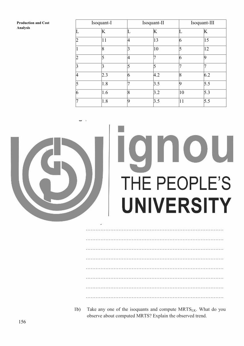
1. Draw an isoquant map using the information available in the following

Table.

156

Production and Cost

Analysis Isoquant-I Isoquant-II Isoquant-III

L K L K L K

2 11 4 13 6 15

1 8 3 10 5 12

2 5 4 7 6 9

3 3 5 5 7 7

4 2.3 6 4.2 8 6.2

5 1.8 7 3.5 9 5.5

6 1.6 8 3.2 10 5.3

7 1.8 9 3.5 11 5.5

1a) Which one of the isoquants provides you with highest level of output

and why?

…………………………………………………………………………

…………………………………………………………………………

…………………………………………………………………………

…………………………………………………………………………

…………………………………………………………………………

…………………………………………………………………………

…………………………………………………………………………

…………………………………………………………………………

1b) Take any one of the isoquants and compute MRTSLK. What do you

observe about computed MRTS? Explain the observed trend.

157

Production Function Isoquant..........

L K MRTSLK

2. The marginal product of labour in the production of computer chips

is 50 chips per hour. The marginal rate of technical substitution of

hours of labour for hours of machine-capital is ¼. What is the

marginal product of capital?

………………………………………………………………………

………………………………………………………………………

………………………………………………………………………

………………………………………………………………………

………………………………………………………………………

………………………………………………………………………

3. What would the isoquants look like if all inputs were nearly

perfect substitutes in a production process? What if there was

near-zero substitutability between inputs?

………………………………………………………………………

………………………………………………………………………

………………………………………………………………………

………………………………………………………………………

………………………………………………………………………

………………………………………………………………………

7.6 RETURNS TO SCALE

Another important attribute of production function is how output responds in

the long run to changes in the scale of the firm i.e. when all inputs are

increased in the same proportion (by say 10%), how does output change.

Clearly, there are 3 possibilities. If output increases by more than an increase

in inputs (i.e. by more than 10%), then the situation is one of increasing

returns to scale (IRS). If output increases by less than the increase in inputs,

158

Production and Cost

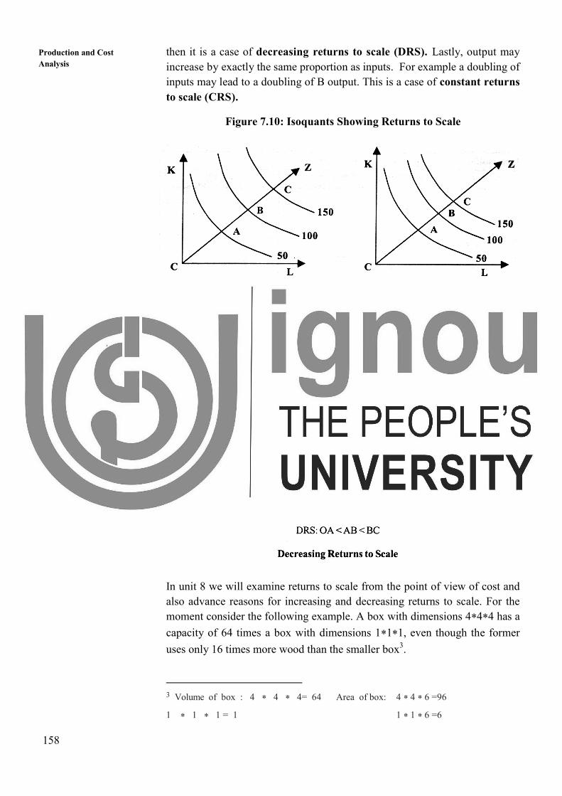
Analysis then it is a case of decreasing returns to scale (DRS). Lastly, output may

increase by exactly the same proportion as inputs. For example a doubling of

inputs may lead to a doubling of B output. This is a case of constant returns

to scale (CRS).

Figure 7.10: Isoquants Showing Returns to Scale

In unit 8 we will examine returns to scale from the point of view of cost and

also advance reasons for increasing and decreasing returns to scale. For the

moment consider the following example. A box with dimensions 4*4*4 has a

capacity of 64 times a box with dimensions 1*1*1, even though the former

uses only 16 times more wood than the smaller box3.4.

3 Volume of box : 4 * 4 * 4= 64 Area of box: 4 * 4 * 6 =96

1 * 1 * 1 = 1 1 * 1 * 6 =6

159

Production Function Isoquants can also be used to depict returns to scale (Figure 7.10)

Panel A shows constant returns to scale. Three isoquants with output levels

50,100 and 150 are drawn. In the figure, successive isoquants are equidistant

from one another along the ray CZ. Panel B shows increasing returns to scale,

where the distance between 2 isoquants becomes less and less i.e. in order to

double output from 50 to 100, input increase is less than double. The

explanation for panel C, which exhibits decreasing returns to scale, is

analogous.

There is no universal answer to which industries will show what kind of

returns to scale. Some industries like public utilities (Telecom and Electricity

generation) show increasing returns over large ranges of output, whereas

other industries exhibit constant or even decreasing returns to scale over the

relevant output range. Therefore, whether an industry has constant, increasing

or decreasing returns to scale is largely an empirical issue.

7.7 FUNCTIONAL FORMS OF PRODUCTION

FUNCTION

The production function can be estimated by regression techniques (refer to

MMPC-005, course on “Quantitative Analysis for Managerial Applications”

to know about regression techniques) using historical data (either time-series

data, or cross-section data, or engineering data). For this, one of the first tasks

is to select a functional form, that is, the specific relationship among the

relevant economic variables. We know that the general form of production

function is,

Q = f (K,L)

Where, Q = output, K = capital and L = labour.

Although, a variety of functional forms have been used to describe

production relationships, only the Cobb-Douglas production function is

discussed here. The general form of Cobb-Douglas function is expressed as:

Q = �����

where A, α, and β are the constants that, when estimated, describe the

quantitative relationship between the inputs (K and L) and output (Q).

The marginal products of capital and labour and the rates of the capital and

labour inputs are functions of the constants A, α, and β and. That is,

MPK = ����

AK-1 L�

MPL = ����

� �AK L���

160

Production and Cost

Analysis The sum of the constants (� +�) can be used to determine returns to scale.

That is,

(� +�) > 1 increasing returns to scale,

(� +�) = 1 constant returns to scale, and

(� +�) < 1 decreasing returns to scale.

Having numerical estimates for the constants of the production function

provides significant information about the production system under study.

The marginal products for each input and returns to scale can all be

determined from the estimated function.

The Cobb-Douglas function does not lend itself directly to estimation by the

regression methods because it is a nonlinear relationship. Technically, an

equation must be a linear function of the parameters in order to use the

ordinary least-squares regression method of estimation. However, a linear

equation can be derived by taking the logarithm of each term. That is,

log Q = log A+�log K+�log L

A linear relationship can be seen by setting,

Y = log Q, A* =log A, X1 =log K, X2 = log L and

Re writing the function as

Y = A* + � X1 + � X2

This function can be estimated directly by the least-squares regression

technique and the estimated parameters used to determine all the important

production relationships. Then the antilogarithm of both sides can be taken,

which transforms the estimated function back to its conventional

multiplicative form. We will not be studying here the details of computing

production function since there are a number of computer programs available

for this purpose.

Types of Statistical Analyses

Once a functional form of a production function is chosen the next step is to

select the type of statistical analysis to be used in its estimation. Generally,

there are three types of statistical analyses used for estimation of a production

function. These are:(a) time series analysis,(b)cross-section analysis and(c)

engineering analysis.

a) Time series analysis: The amount of various inputs used in various

periods in the past and the amount of output produced in each period

is called time series data. For example, we may obtain data

concerning the amount of labour, the amount of capital, and the

161

Production Function amount of various raw materials used in the steel industry during each

year from 1970 to 2000. On the basis of such data and information

concerning the annual output of steel during 1970 to 2000, we may

estimate the relationship between the amounts of the inputs and the

resulting output, using regression techniques.

Analysis of time series data is appropriate for a single firm that has

not undergone significant changes in technology during the time span

analyzed. That is, we cannot use time series data for estimating the

production function of a firm that has gone through significant

technological changes. There are even more problems associated with

the estimation a production function for an industry using time series

data. For example, even if all firms have operated over the same time

span, changes in capacity, inputs and outputs may have proceeded at

a different pace for each firm. Thus, cross section data may be more

appropriate.

b) Cross-section analysis: The amount of inputs used and output

produced in various firms or sectors of the industry at a given time is

called cross- section data. For example, we may obtain data

concerning the amount of labour, the amount of capital, and the

amount of various raw materials used in various firms in the steel

industry in the year 2020. On the basis of such data and information

concerning the year 2020, output of each firm, we may use regression

techniques to estimate the relationship between the amounts of the

inputs and the resulting output.

c) Engineering analysis: In this analysis we use technical information

supplied by the engineer or the agricultural scientist. This analysis is

undertaken when the above two types do not suffice. The data in this

analysis is collected by experiment or from experience with day-to-

day working of the technical process. There are advantages to be

gained from approaching the measurement of the production function

from this angle. Because the range of applicability of the data is

known, and, unlike time- series and cross-section studies, we are not

restricted to the narrow range of actual observations.

Limitations of Different Types of Statistical Analysis

Each of the methods discussed above has certain limitations.

1. Both time-series and cross-section analysis are restricted to a

relatively narrow range of observed values. Extrapolation of the

production function outside that range may be seriously misleading.

For example, in a given case, marginal productivity might decrease

162

Production and Cost

Analysis rapidly above 85% capacity utilization; the production function

derived for values in the 70%-85% capacity utilization range would

not show this.

2. Another limitation of time series analysis is the assumption that all

observed values of the variables pertains to one and the same

production function. In other words, a constant technology is

assumed. In reality, most firms or industries, however, find better,

faster, and/or cheaper ways of producing their output. As their

technology changes, they are actually creating new production

functions. One way of coping with such technological changes is to

make it one of the independent variables.

3. Theoretically, the production function includes only efficient (least-

cost) combinations of inputs. If measurements were to conform to

this concept, any year in which the production was less than nominal

would have to be excluded from the data. It is very difficult to find a

time-series data, which satisfy technical efficiency criteria as a

normal case.

4. Engineering data may overcome the limitations of time series data but

mostly they concentrate on manufacturing activities. Engineering data

do not tell us anything about the firm’s marketing or financial

activities, even though these activities may directly affect production.

5. In addition, there are both conceptual and statistical problems in

measuring data on inputs and outputs.

It may be possible to measure output directly in physical units such as tons of

coal, steel etc. In case more than one product is being produced, one may

compute the weighted average of output, the weights being given by the cost

of manufacturing these products. In a highly diversified manufacturing unit,

there may be no alternative but to use the series of output values, corrected

for changes in the price of products. One has also to choose between

‘gross value’ and ‘net value’. It seems better to use “net value added”

concept instead of output concept in estimating production function,

particularly where raw-material intensity is high.

The data on labour is mostly available in the form of “number of workers

employed” or “hours of labour employed”. The ‘number of workers’ data

should not be used because, it may not reflect underemployment of labour,

and they may be occupied, but not productively employed. Even if we use

‘man hours’ data, it should be adjusted for efficiency factor. It is also not

advisable that labour should be measured in monetary terms as given by

expenditure on wages, bonus, etc.

The data on capital input has always posed serious problems. Net investment

i.e. a change in the value of capital stock, is considered most appropriate.

163

Production Function Nevertheless, there are problems of measuring depreciation in fixed capital,

changes in quality of fixed capital, changes in inventory valuation, changes in

composition and productivity of working capital, etc.

Finally, when one attempts an econometric estimate of a production function,

one has to overcome the standard problem of multi-collinearity among inputs,

autocorrelation, homoscadasticity, etc.

7.8 MANAGERIAL USES OF PRODUCTION

FUNCTION

There are several managerial uses of the production function. It can be used

to compute the least-cost combination of inputs for a given output or to

choose the input combination that yields the maximum level of output with

a given level of cost. There are several feasible combinations of input factors

and it is highly useful for decision-makers to find out the most appropriate

among them. The production function is useful in deciding on the additional

value of employing a variable input in the production process. So long as

the marginal revenue productivity of a variable factor exceeds it price, it may

be worthwhile to increase its use. The additional use of an input factor should

be stopped when its marginal revenue productivity just equals its price.

Production functions also aid long-run decision-making. If returns to scale

are increasing, it will be worthwhile to increase production through a

proportionate increase in all factors of production, provided, there is enough

demand for the product. On the other hand, if returns to scale are decreasing,

it may not be worthwhile to increase the production through a proportionate

increase in all factors of production, even if there is enough demand for the

product. However, it may in the discretion of the producer to increase or

decrease production in the presence of constant returns to scale, if there is

enough demand for the product.

Activity 2

1. Can you list some more managerial uses of production function other

than those given in section 7.8?

…………………………………………………………………………

…………………………………………………………………………

…………………………………………………………………………

…………………………………………………………………………

…………………………………………………………………………

…………………………………………………………………………

…………………………………………………………………………

…………………………………………………………………………

…………………………………………………………………………

164

Production and Cost

Analysis 7.9 SUMMARY

A production function specifies the maximum output that can be produced

with a given set of inputs. In order to achieve maximum profits the

production manager has to use optimum input-output combination for a

given cost. In this unit, we have shown how a production manager

minimizes the cost for a given output in order to maximize the profit.

Also, we have shown how to maximize the output at a given level of cost.

The law of diminishing marginal returns states that as equal increments of

variable input are added to fixed input, a point will eventually be reached

where corresponding increments to output begin to decline. We have also

seen the relations between the marginal product, average product, and total

product. There are three stages of production. Stage I is characterized by

MP>0 and MP>AP. Stage II is characterized by MP>0 and MP<AP. Stage

III is characterized by MP<0. The economically meaningful range is Stage

II. The production manager maximizes the profit at a point where the

value of marginal product equals the price of the output.

A production isoquant consists of all the combinations of two inputs that

will yield the same maximum output. The marginal rate of technical

substitution is ∆K/∆L, holding output constant. The law of diminishing

marginal rate of substitution implies the rate at which one input can be

substituted for another input, if output remains constant. An isocost line

consists of all the combinations of inputs which have the same total cost.

The absolute slope of the isocost line is the input price ratio. Returns to

scale, a long run concept, involves the effect on output of changing all

inputs by same proportion and in the same direction. Although, there are

many different forms of production function we have discussed here only

Cobb-Douglas production function.

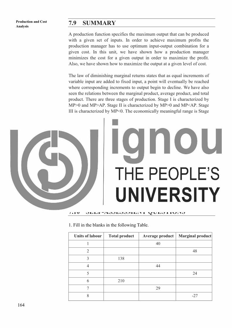
7.10 SELF-ASSESSMENT QUESTIONS

1. Fill in the blanks in the following Table.

Units of labour Total product Average product Marginal product

1 40

2 48

3 138

4 44

5 24

6 210

7 29

8 -27

165

Production Function 2. The marginal product of labour is known to be greater than the average

product of labour at a given level of employment. Is the average

product increasing or decreasing? Explain.

3. Explain the law of diminishing marginal returns and provide an

example of the phenomenon.

4. Explain why a profit maximizing firm using only one variable input

will produce in stage-II.

5. Explain why an A P curve and the corresponding MP curve must

intersect at the maximum point on the A P curve

6. Explain why MP is greater than (less than ) AP when AP is rising

(falling).

7. Suppose a firm is currently using 500 labourers and 325 units of capital

to produce its product. The wage rate is `25,and price of capital is

`130. The last labourer adds 25 units of total output, while the last unit

of capital adds 65 units to total output. Is the manager of this firm

making the optimal input choice? Why or why not? If not, what should

the manager do?

7.11 FURTHER READINGS

Adhikary, M. (1987). Managerial Economics (3rd

ed.).Khosla Publishers,

Delhi.

Maddala, G. S., & Miller, E. M. (1989). Micro Economics: Theory and

Applications. McGraw-Hill, NewYork.

Maurice, S.C., Smithson, C.W., & Thomas, C. R.(2001). Managerial

Economics: Applied Microeconomics for Decision Making. McGraw-Hill

Publishing.

Mote, V. L., Paul, S., & Gupta, G. S. (2016). Managerial Economics:

Concepts and Cases. Tata McGraw-Hill, New Delhi.

Dholakia, R., & Oza, A. N. (1996). Microeconomics for Management

Students. Oxford University Press, Delhi.

166

Production and Cost

Analysis UNIT 8 SHORT RUN COST ANALYSIS

Objectives

After going through this unit, you should be able to:

understand some of the cost concepts that are frequently used in the

managerial decision-making process

understand short run cost function

understand applications of short run cost function in managerial decision

making

Structure

8.1 Introduction

8.2 Actual Costs and Opportunity Costs

8.3 Explicit and Implicit Costs

8.4 Accounting Costs and Economic Costs

8.5 Direct Costs and Indirect Costs

8.6 Total Cost, Average Cost and Marginal Cost

8.7 Fixed and Variable Costs

8.8 Short-Run and Long-Run Costs

8.9 Short Run Cost Function

8.10 Applications of Short Run Cost Analysis

8.11 Summary

8.12 Self-Assessment Questions

8.13 Further Readings

8.1 INTRODUCTION

The analysis of cost is important in the study of managerial economics

because it provides a basis for two important decisions made by managers:

(a) whether to produce or not and (b) how much to produce when a decision

is taken to produce. There are two types of cost analysis: short run cost

analysis & long run cost analysis.

In this Unit, we shall discuss some important cost concepts that are relevant

for managerial decisions. We analyze the basic differences between these cost

concepts and also, examine how accountants and economists differ on

treating different cost concepts. We shall discuss short run cost function and

its applications in managerial decision making. The short run cost estimates a

helpful to managers in arriving at the optimal mix of inputs to achieve a

particular output target of a firm.

167

Short Run Cost

Analysis 8.2 ACTUAL COSTS AND OPPORTUNITY

COSTS

Actual costs are those costs, which a firm incurs while producing or

acquiring a good or service like raw materials, labour, rent, etc. Suppose, we

pay ` 150 per day to a worker whom we employ for 10 days, then the cost of

labour is ` 1500. The economists called this cost as accounting costs because

traditionally accountants have been primarily connected with collection of

historical data (that is the costs actually incurred) in reporting a firm’s

financial position and in calculating its taxes. Sometimes the actual costs are

also called acquisition costs or outlay costs.

On the other hand, opportunity cost is defined as the value of a resource in

its next best use. For example, Mr. Ram is currently working with a firm and

earning ` 5 lakhs per year. He decides to quit his job and start his own small

business. Although, the accounting cost of Mr. Ram’s labour to his own

business is 0, the opportunity cost is ` 5 lakhs per year. Therefore, the

opportunity cost is the earnings he foregoes by working for his own firm.

One may ask you that whether this opportunity cost is really meaningful in

the decision-making process. Opportunity cost can be similarly defined for

other factors of production. For example, consider a firm that owns a building

and therefore do not pay rent for office space. If the building was rented to

others, the firm could have earned rent. The foregone rent is an opportunity

cost of utilizing the office space and should be included as part of the cost of

doing business. Sometimes these opportunity costs are called as alternative

costs.

8.3 EXPLICIT AND IMPLICIT COSTS

Explicit costs are those costs that involve an actual payment to other parties.

Therefore, an explicit cost is the monetary payment made by a firm for use of

an input owned or controlled by others. Explicit costs are also referred to as

accounting costs. For example, a firm pays ` 100 per day to a worker and

engages 15 workers for 10 days, the explicit cost will be ` 15,000 incurred by

the firm. Other types of explicit costs include purchase of raw materials,

renting a building, amount spent on advertising etc.

On the other hand, implicit costs represent the value of foregone

opportunities but do not involve an actual cash payment. Therefore, an

implicit cost is the opportunity cost of using resources that are owned or

controlled by the owners of the firm. Implicit costs are just as important as

explicit costs but are sometimes neglected because they are not as obvious.

The implicit cost is the foregone return, the owner of the firm could have

received had they used their own resources in their best alternative use rather

than using the resources for their own firm’s production. For example, a

manager who runs his own business foregoes the salary that could have been

earned working for someone else as we have seen in our earlier example.

168

Production and Cost

Analysis This implicit cost generally is not reflected in accounting statements, but

rational decision-making requires that it be considered.

8.4 ACCONTING COSTS AND ECONOMIC

COSTS

For a long time, there has been a considerable disagreement among

economists and accountants on how costs should be treated. The reason for

the difference of opinion is that the two groups want to use the cost data for

dissimilar purposes. Accountants always have been concerned with firms’

financial statements. Accountants tend to take a retrospective look at firm’s

finances because they keep trace of assets and liabilities and evaluate past

performance. The accounting costs are useful for managing taxation needs as

well as to calculate profit or loss of the firm. On the other hand, economists

take forward-looking view of the firm. They are concerned with what cost

is expected to be in the future and how the firm might be able to rearrange its

resources to lower its costs and improve its profitability. They must therefore

be concerned with opportunity cost. Since the only cost that matters for

business decisions are the future costs, it is the economic costs that are used

for decision-making. Accountants and economists both include explicit costs

in their calculations. For accountants, explicit costs are important because

they involve direct payments made by a firm. These explicit costs are also

important for economists as well because the cost of wages and materials

represent money that could be useful elsewhere.

Accountants and economists use the term ‘profits’ differently. Accounting

profits are the firm’s total revenue less its explicit costs. But economists

define profits differently. Economic profits are total revenue less all costs

(explicit and implicit costs). The economist takes into account the implicit

costs (including a normal profit) in addition to explicit costs in order to retain

resources in a given line of production. Therefore, when an economist says

that a firm is just covering its costs, it is meant that all explicit and implicit

costs are being met, and that, the entrepreneur is receiving a return just large

enough to retain his/her talents in the present line of production. If a firm’s

total receipts exceed all its economic costs, the residual accruing to the

entrepreneur is called an economic profit, or pure profit.

Example of Economic Profit and Accounting Profit

Mr. Raj is a small storeowner. He has invested ` 2 lakhs as equity in the

store and inventory. His annual turnover is ` 8 lakhs, from which he must

deduct the cost of goods sold, salaries of hired staff, and depreciation of

equipment and building to arrive at annual profit of the store. He asked help

of a friend who is an accountant by profession to prepare annual income

statement. The accountant reported the profit to be ` 1.5 lakhs. Mr. Raj

could not believe this and asked the help of another friend who is an

economist by profession. The economist told him that the actual profit was

169

Short Run Cost

Analysis only ` 75,000 and not ` 1.5 lakhs. The economist found that the accountant

had underestimated the costs by not including the implicit costs of time spent

as Manager by Mr. Raj in the business and interest on owner’s equity. The

two income statements are shown below:

Income statement prepared by accountant Income statement prepared by economist

` ` ` `

Sales 8,00,000 Sales 8,00,000

Explicit costs Explicit costs

Cost of goods sold 6,00,000 Cost of goods sold 6,00,000

Salaries 40,000 Salaries 40,000

Depreciation 10,000 6,50,000 Depreciation 10,000 6,50,000

Implicit costs

Salary to owner

Manager

50,000

Interest on owners’

equity

25,000 75,000

Accounting profit 1,50,000 Economic profit 75,000

Controllable and Non-Controllable costs

Controllable costs are those which are capable of being controlled or

regulated by executive vigilance and, therefore, can be used for assessing

executive efficiency. Non-controllable costs are those, which cannot be

subjected to administrative control and supervision. Most of the costs are

controllable, except, of course, those due to obsolescence and depreciation.

The level at which such control can be exercised, however, differs: some

costs (like, capital costs) are not controllable at factory’s shop level, but

inventory costs can be controlled at the shop level.

Out-of-pocket costs and Book costs

Out of pocket costs are those costs that improve current cash payments to

outsiders. For example, wages and salaries paid to the employees are out-of-

pocket costs. Other examples of out-of-pocket costs are payment of rent,

interest, transport charges, etc. On the other hand, book costs are those

business costs, which do not involve any cash payments but for them a

provision is made in the books of account to include them in profit and loss

accounts and take tax advantages. For example, salary of owner manager, if

not paid, is a book cost. The interest cost of owner’s own fund and

depreciation cost are other examples of book cost. The out-of-pocket costs

are also called explicit costs and correspondingly book costs are called

implicit or imputed costs.

170

Production and Cost

Analysis Past and Future costs

Past costs are actual costs incurred in the past and they are always contained

in the income statements. Their measurement is essentially a record keeping

activity. These costs can only be observed and evaluated in retrospect. If they

are regarded as excessive, management can indulge in post-mortem checks to

find out the factors responsible for the excessive costs, if any and take

corrective actions for future. Past costs serve as the basis for projecting future

costs.

Future costs are those costs that are likely to be incurred in future periods.

Since the future is uncertain, these costs have to be estimated and cannot be

expected to be absolutely correct figures. In periods of inflation and deflation,

the two cost concepts differ significantly. Managerial decisions are forward

looking and therefore they require estimates of future costs. Unlike past costs,

future costs are subject to management control and they can be planned or

avoided. Management needs to estimate future costs for a variety of reasons

such as expense control pricing, projecting future profits and capital

budgeting decisions. When historical costs are used instead of explicit

projections, the assumption is made that future costs will be the same as past

costs. In periods of significant price variations, such an assumption may lead

to wrong managerial decisions.

Historical and Replacement costs

The historical cost of an asset is the actual cost incurred at the time; the asset

was originally acquired. In contrast to this, replacement cost is the cost,

which will have to be incurred if that asset is purchased now. The difference

between the historical and replacement costs results from price changes over

time. Suppose a machine was acquired for `50,000 in the year 2015 and the

same machine can be acquired for ` 1,20,000 in the year 2021.Here ` 50,000

is the historical or original cost of the machine and ` 1,20,000 is its

replacement cost. The difference of `70,000 between the two costs has

resulted because of the price change of the machine during the period. In the

conventional financial accounts, the value of assets is shown at their

historical costs. But for decision-making, firms should try to adjust historical

costs to reflect price level changes. If the price of the asset does not change

over time, the historical cost will be the same as the replacement cost. If the

price raises the replacement cost will exceed historical cost and vice versa.

During periods of substantial price variations, historical costs are poor

indicators of actual costs.

Private Costs and Social Costs

A further distinction that is useful to make - especially in the public sector - is

between private and social costs. Private costs are those that accrue directly

to the individuals or firms engaged in relevant activity. Social costs, on the

171

Short Run Cost

Analysis other hand, are passed on to persons not involved in the activity in any direct

way (i.e., they are passed on to society at large). Consider the case of a

manufacturer located on the bank of a river who dumps the waste into water

rather than disposing it of in some other manner. While the private cost to the

firm of dumping is zero, it is definitely harmful to the society. It affects

adversely the people located down current and incur higher costs in terms of

treating the water for their use, or having to travel a great deal to fetch

potable water. If these external costs were included in the production costs of

a producing firm, a true picture of real or social costs of the output would be

obtained. Ignoring external costs may lead to an inefficient and undesirable

allocation of resources in society.

Relevant Costs and Irrelevant Costs

The relevant costs for decision-making purposes are those costs, which are

incurred as a result of the decision under consideration. The relevant costs are

also referred to as the incremental costs. Costs that have been incurred

already and costs that will be incurred in the future, regardless of the present

decision are irrelevant costs as far as the current decision problem is

concerned.

There are three main categories of relevant or incremental costs. These are

the present-period explicit costs, the opportunity costs implicitly involved in

the decision, and the future cost implications that flow from the decision. For

example, direct labour and material costs, and changes in the variable

overhead costs are the natural consequences of a decision to increase the

output level.

Also, if there is any expenditure on capital equipments incurred as a result of

such a decision, it should be included in full, notwithstanding that the

equipment may have a useful life remaining after the present decision has

been carried out. Thus, the incremental costs of a decision to increase output

level will include all present-period explicit costs, which will be incurred as a

consequence of this decision. It will exclude any present-period explicit cost

that will be incurred regardless of the present decision.

The opportunity cost of a resource under use, as discussed earlier, becomes a

relevant cost while arriving at the economic profit of the firm. Many

decisions will have implications for future costs, both explicit and implicit. If

a firm expects to incur some costs in future as a consequence of the present

analysis, such future costs should be included in the present value terms if

known for certain.

Sunk Costs and Incremental Costs

Sunk costs are expenditures that have been made in the past or must be paid

in the future as part of contractual agreement or previous decision. For

example, the money already paid for machinery, equipment, inventory and

future rental payments on a warehouse that must be paid as part of long-term

lease agreement are sunk costs. In general, sunk costs are not relevant to

172

Production and Cost

Analysis economic decisions. For example, the purchase of specialized equipment

designed to order for a plant. We assume that the equipment can be used to

do only what it was originally designed for and cannot be converted for

alternative use. The expenditure on this equipment is a sunk cost. Also,

because this equipment has no alternative use its opportunity cost is zero and,

hence, sunk costs are not relevant to economic decisions. Sometimes the sunk

costs are also called as non-avoidable or non-escapable costs.

On the other hand, incremental cost refers to total additional cost of

implementing a managerial decision. Change in product line, change in

output level, adding or replacing a machine, changing distribution channels

etc. are examples of incremental costs. Sometimes incremental costs are also

called as avoidable or escapable costs. Moreover, since incremental costs

may also be regarded as the difference in total costs resulting from a

contemplated change, they are also called differential costs.

As stated earlier sunk costs are irrelevant for decision making, as they do not

vary with the changes contemplated for future by the management. It is the

incremental costs, which are important for decision-making purpose.

Activity 1

1. A graduate from a business school decides to open business and devote

his full time to its management. What cost would you assign to his time?

Is this implicit or explicit?

……………………………………………………………………………

……………………………………………………………………………

……………………………………………………………………………

……………………………………………………………………………

……………………………………………………………………………

2. Why is the historic cost of inventory or capital equipment irrelevant for

managerial decision making?

……………………………………………………………………………

……………………………………………………………………………

……………………………………………………………………………

……………………………………………………………………………

……………………………………………………………………………

3. Comment on the nature of costs involved in depreciation from both

economic and accounting approaches.

……………………………………………………………………………

……………………………………………………………………………

……………………………………………………………………………

……………………………………………………………………………

……………………………………………………………………………

173

Short Run Cost

Analysis 8.5 DIRECT COSTS AND INDIRECT COSTS

There are some costs, which can be directly attributed to production of a

given product. The use of raw material, labour input, and machine time

involved in the production of each unit can usually be determined. On the

other hand, there are certain costs like stationery and other office and

administrative expenses, electricity charges, depreciation of plant and

buildings, and other such expenses that cannot easily and accurately be

separated and attributed to individual units of production, except on arbitrary

basis. When referring to the separable costs of first category accountants call

them the direct, or prime costs per unit. The accountants refer to the joint

costs of the second category as indirect or overhead costs. Direct and

indirect costs are not exactly synonymous to what economists refer to as

variable costs and fixed costs. The criterion used by the economist to divide

cost into either fixed or variable is whether or not the cost varies with the

level of output, whereas the accountant divides the cost on the basis of

whether or not the cost is separable with respect to the production of

individual output units. The accounting statements often divide overhead

expenses into ‘variable overhead’ and ‘fixed overhead’ categories. If the

variable overhead expenses per unit are added to the direct cost per unit, we

arrive at what economists call as average variable cost.

Separable Costs and Common Costs

Costs can also be classified on the basis of their traceability. The costs that

can be easily attributed to a product, a division, or a process are called

separable costs. On the other hand, common costs are those, which cannot

be traced to any one unit of operation. For example, in a multiple product

firm the cost of raw material may be separable (traceable) product-wise but

electricity charges may not be separable product-wise. In a University the

salary of a Vice-Chancellor is not separable department-wise but the salary of

teachers can be separable department-wise. The separable and common costs

are also referred to as direct and indirect costs respectively. The distinction

between direct and indirect costs is of particular significance in a multi-

product firm for setting up economic prices for different products.

8.6 TOTAL COST, AVERAGE COST &

MARGINAL COST

Total cost (TC) of a firm is the sum-total of all the explicit and implicit

expenditures incurred for producing a given level of output. It represents the

money value of the total resources required for production of goods and

services. For example, a shoe-maker’s total cost will include the amount s/he

spends on leather, thread, rent for her/his workshop, interest on borrowed

capital, wages and salaries of employees, etc., and the amount s/he charges

174

Production and Cost

Analysis for her/his services and funds invested in the business. The total cost concept

is useful in break-even analysis and finding out whether a firm is making

profit or not.

Average cost (AC) is the cost per unit of output. That is, average cost equals

the total cost divided by the number of units produced (N).If TC =`500 and

N = 50 then AC = `10.The average cost concept is significant for calculating

the per unit profit.

Marginal cost (MC) refers to the change in total cost associated with a one-

unit change in output. Marginal cost (MC) is the extra cost of producing one

additional unit. At a given level of output, one examines the additional costs

being incurred in producing one extra unit and this yields the marginal cost.

For example, if TC of producing 100 units is `10,000 and the TC of

producing 101 units is `10,050, then MC at N = 101 equals `50.This cost

concept is significant to short-term decisions about profit maximizing rates of

output. For example, in an automobile manufacturing plant, the marginal cost

of making one additional car per production period would be the labour,

material, and energy costs directly associated with that extra car. Marginal

cost is that sub category of incremental cost in the sense that incremental cost

may include both fixed costs and marginal costs.

However, when production is not conceived in small units, management will

be interested in incremental cost instead of marginal cost. For example, if a

firm produces 5000 units of TV sets, it may not be possible to determine the

change in cost involved in producing 5001 units of TV sets. This difficulty

can be resolved by taking units to significant size. For example, if the TV sets

produced is measured to hundreds of units and total cost (TC) of producing

the current level of three hundred TV sets is `15,00,000 and the firm decides

to increase the production to four hundred TV sets and estimates the TC as

`18, 00,000, then the incremental cost of producing one hundred TV sets

(above the present production level of three hundred units) is `3, 00,000.

The marginal and incremental cost concepts are needed in deciding

whether a firm needs to expand its production or not. In fact, the relevant

costs to be considered will depend upon the situation or production problem

faced by the manager.

8.7 FIXED COSTS AND VARIABLE COSTS

Fixed costs are that part of the total cost of the firm which does not change

with output. Expenditures on depreciation, rent of land and buildings,

property taxes, and interest payment on bonds are examples of fixed costs.

Given a capacity, fixed costs remain the same irrespective of actual output.

Variable costs, on the other hand, change with changes in output. Examples

of variable costs are wages and expenses on raw material.

175

Short Run Cost

Analysis However, it is not very easy to classify all costs into fixed and variable. There

are some costs, which fall between these extremes. They are called semi-

variable costs. They are neither perfectly variable nor absolutely fixed in

relation to changes in output. For example, part of the depreciation charges is

fixed and part variable. However, it is very difficult to determine how much

of depreciation cost is due to the technical obsolescence of assets and hence

fixed cost, and how much is due to the use of equipments and hence variable

cost. Nevertheless, it does not mean that it is not useful to classify costs in to

fixed and variable. This distinction is of great value in break-even analysis

and pricing decisions. For decision-making purposes, in general, it is the

variable cost, which is relevant and not the fixed cost.

To an economist the fixed costs are overhead costs and to an accountant these

are indirect costs. When the output goes up, the fixed cost per unit of output

comes down, as the total fixed cost is divided between larger units of output.

8.8 SHORT RUN AND LONG RUN COSTS

The short run is defined as a period in which the supply of at least one

element of the inputs cannot be changed. To illustrate, certain inputs like

machinery, buildings, etc., cannot be changed by the firm whenever it so

desires. It takes time to replace, add or dismantle them. Short-run costs are

the costs that can vary with the degree of utilization of plant and other fixed

factors. In other words, these costs relate to the variation in output, given

plant capacity. Short-run costs are, therefore, of two types: fixed costs and

variable costs. In the short-run, fixed costs remain unchanged while variable

costs fluctuate with output.

Long run, on the other hand, is defined as a period in which all inputs are

changed with changes in output. In other words, it is that time-span in which

all adjustments and changes are possible to realize. Long-run costs are costs

that can vary with the size of plant and with other facilities normally regarded

as fixed in the short-run. In fact, in the long-run there are no fixed inputs and

therefore no fixed costs, i.e., all costs are variable. Thus, in the short run,

some inputs are fixed (like installed capacity) while others are variable (like

the level of capacity utilization); but in the long run all inputs, including the

size of the plant, are variable.

Both short-run and long-run costs are useful in decision-making. Short-run

cost is relevant when a firm has to decide whether or not to produce and if a

decision is taken to produce then how much more or less to produce with a

given plant size. If the firm is considering an increase in plant size, it must

examine the long-run cost of expansion. Long-run cost analysis is useful in

investment decisions.

Activity 2

1. Classify different cost concepts into:

176

Production and Cost

Analysis a. useful for decision making

……………………………………………………………………………

……………………………………………………………………………

……………………………………………………………………………

……………………………………………………………………………

…………………………………………………………………………....

b. Not useful for decision making

……………………………………………………………………………

……………………………………………………………………………

……………………………………………………………………………

……………………………………………………………………………

……………………………………………………………………………

2. Give specific example of:

a. Direct costs:……………………………...…………………………….

b. Indirect costs: ………………………………………………………….

c. Sunk costs: …………………………………………………………….

d. Traceable costs: ……………………………………………………….

e. Common costs : ……………………………………………………….

f. Implicit costs: …………………………………………………………

g. Social costs: ……………..…………………………………………….

h. Non-controllable costs : ……………...………………………………..

3. Give examples to distinguish between ‘fixed overheads’ and ‘variable

overheads’.

…………………………………………………………………………………

…………………………………………………………………………………

…………………………………………………………………………………

…………………………………………………………………………………

…………………………………………………………………………………

4. Can all ‘direct costs’ be treated as ‘variable costs’ Explain?

…………………………………………………………………………………

…………………………………………………………………………………

…………………………………………………………………………………

…………………………………………………………………………………

…………………………………………………………………………………

177

Short Run Cost

Analysis 8.9 SHORT RUN COST FUNCTIONS

In above sections, we have distinguished between the short run and the long

run. We also distinguished between fixed costs and variable costs. The

distinction between fixed and variable costs is of great significance to the

business manager. Variable costs are those costs, which the business manager

can control or alter in the short run by changing levels of production. On the

other hand, fixed costs are clearly beyond business manager’s control, such

costs are incurred in the short run and must be paid regardless of output.

Total Costs

Three concepts of total cost in the short run must be considered: total fixed

cost (TFC), total variable cost (TVC), and total cost (TC).Total fixed costs

are the total costs per period of time incurred by the firm for fixed inputs.

Since the amount of the fixed inputs is fixed, the total fixed cost will be the

same regardless of the firm’s output rate. Table 8.1 shows the costs of a firm

in the short run. According to this table, the firm’s total fixed costs are `100.

The firm’s total fixed cost function is shown graphically in Figure 8.1.

Table 8.1: A Firm’s Short Run Costs (in `)

Q TFC TVC TC MC AFC AVC ATC

0 100 0 100

1 100 50 150 50 100.0 50 150

2 100 90 190 40 50.0 45 95.0

3 100 120 220 30 33.3 40 73.3

4 100 140 240 20 25.0 35 60.0

5 100 150 250 10 20.0 30 50.0

6 100 156 256 6 16.7 26 42.7

7 100 175 275 19 14.3 25 39.3

8 100 208 308 33 12.5 26 38.5

9 100 270 370 62 11.1 30 41.1

10 100 350 450 80 10.0 35 45.0

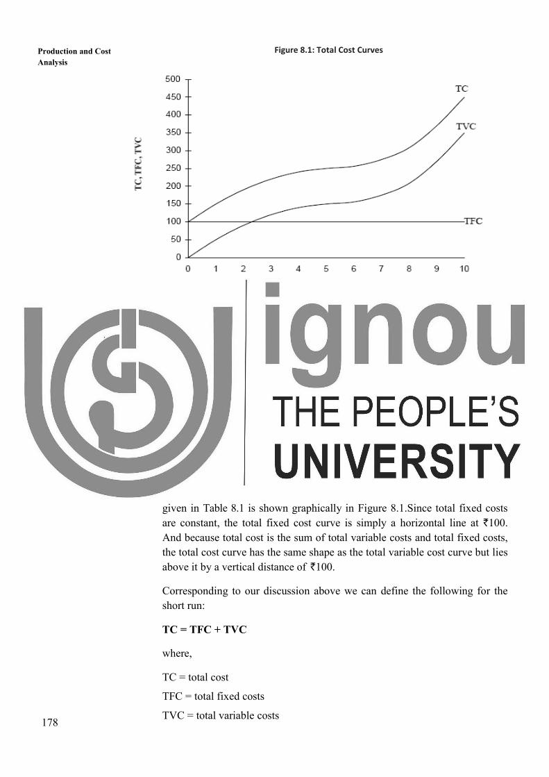
178

Production and Cost

Analysis Figure 8.1: Total Cost Curves

Total variable costs are the total costs incurred by the firm for variable inputs.

To obtain total variable cost we must know the price of the variable inputs.

Suppose if we have two variable inputs viz. labour (V1) and raw material (V2)

and the corresponding prices of these inputs are P1 and P2, then the total

variable cost (TVC) = P1 × V1 + P2 × V2. They go up as the firm’s output

rises, since higher output rates require higher variable input rates, which

mean bigger variable costs. The firm’s total variable cost function

corresponding to the data given in Table 8.1 is shown graphically in Figure

8.1.

Finally, total costs are the sum of total fixed costs and total variable costs. To

derive the total cost column inTable 8.1, add total fixed cost and total variable

cost at each output. The firm’s total cost function corresponding to the data

given in Table 8.1 is shown graphically in Figure 8.1.Since total fixed costs

are constant, the total fixed cost curve is simply a horizontal line at `100.

And because total cost is the sum of total variable costs and total fixed costs,

the total cost curve has the same shape as the total variable cost curve but lies

above it by a vertical distance of `100.

Corresponding to our discussion above we can define the following for the

short run:

TC = TFC + TVC

where,

TC = total cost

TFC = total fixed costs

TVC = total variable costs

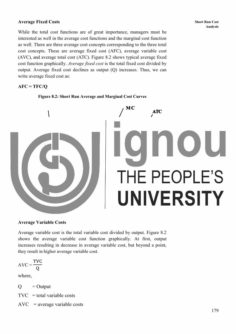
179

Short Run Cost

Analysis Average Fixed Costs

While the total cost functions are of great importance, managers must be

interested as well in the average cost functions and the marginal cost function

as well. There are three average cost concepts corresponding to the three total

cost concepts. These are average fixed cost (AFC), average variable cost

(AVC), and average total cost (ATC). Figure 8.2 shows typical average fixed

cost function graphically. Average fixed cost is the total fixed cost divided by

output. Average fixed cost declines as output (Q) increases. Thus, we can

write average fixed cost as:

AFC = TFC/Q

Figure 8.2: Short Run Average and Marginal Cost Curves

Average Variable Costs

Average variable cost is the total variable cost divided by output. Figure 8.2

shows the average variable cost function graphically. At first, output

increases resulting in decrease in average variable cost, but beyond a point,

they result in higher average variable cost.

AVC = ����

where,

Q = Output

TVC = total variable costs

AVC = average variable costs

180

Production and Cost

Analysis Average Total Cost

Average total cost (ATC) is the sum of the average fixed cost and average

variable cost. In other words, ATC is total cost divided by output. Thus,

ATC = AFC + AVC = ���

Figure 8.2 shows the average total cost function graphically. Since ATC is

sum of the AFC and AVC, ATC curve always exceeds AVC curve. Also,

since AFC falls as output increases, AVC and ATC get closer as output rises.

Note that ATC curve is nearer the AFC curve at initial levels of output, but is

nearer the AVC curve at later levels of output. This indicates that at lower

levels of output fixed costs are more important part of the total cost, while at

higher levels of output the variable element of cost becomes more important.

Marginal Cost

Marginal cost (MC) is the addition to either total cost or total variable cost

resulting from the addition of one unit of output. Thus,

MC = ∆��∆�

� ∆���∆�

where,

MC = marginal cost

Δ�= change in output

ΔTC= change in total cost due to change in output

ΔTVC= change in total variable cost due to change in output

The two definitions are the same because, when output increases, total cost

increases by the same amount as the increase in total variable cost (since

fixed cost remains constant). Figure 8.2 shows the marginal cost function

graphically. At low output levels, marginal cost may decrease with increase

in output, but after reaching a minimum, it goes up with further increase in

output. The reason for this behavior is found in diminishing marginal returns.

The marginal cost concept is very crucial from the manager’s point of view.

Marginal cost is a strategic concept because it designates those costs over

which the firm has the most direct control. More specifically, MC indicates

those costs which are incurred in the production of the last unit of output and

therefore, also the cost which can be “saved” by reducing total output by the

last unit. Average cost figures do not provide this information. A firm’s

decisions as to what output level to produce is largely influenced by its

marginal cost. When coupled with marginal revenue, which indicates the

change in revenue from one more or one less unit of output, marginal cost

allows a firm to determine whether it is profitable to expand or contract its

level of production.

181

Short Run Cost

Analysis Relationship between Marginal Cost and Average Costs

The relationships between the various average and marginal cost curves are

illustrated in Figure 8.2. The figure shows typical AFC, AVC, ATC, and MC

curves but is not drawn to scale for the data given in Table 8.1. The MC cuts

both AVC and ATC at their minimum. When both the MC and AVC are

falling, AVC will fall at a slower rate. When both the MC and AVC are

rising, MC will rise at a faster rate. As a result, MC will attain its minimum

before the AVC. In other words, when MC is less than AVC, the AVC will

fall, and when MC exceeds AVC, AVC will rise. This means that as long as

MC lies below AVC, the latter will fall and where MC is above AVC, AVC

will rise.

Therefore, at the point of intersection where MC = AVC, AVC has just

ceased to fall and attained its minimum, but has not yet begun to rise.

Similarly, the MC curve cuts the ATC curve at the latter’s minimum point.

This is because MC can be defined as the addition either to TC or TVC

resulting from one more unit of output. However, no such relationship exists

between MC and AFC, because the two are not related; MC by definition

includes only those costs which change with output, and FC by definition is

independent of output.

Relationship between Average Product and Marginal Product, and

Average Variable Cost and Marginal Cost

There is a straightforward relationship between factor productivity and output

costs. To see this, let us consider a single variable factor L say labour. All

other inputs are fixed. AP and MP will denote the average and marginal

products of labour, respectively. If W is the wage rate and L is the quantity of

labour, then

TVC = W * L

Hence, if Q is the output,

AVC = ����

= W ����

Consequently, since Q/L is the average product (AP), AVC = W/AP

Also, ΔTVC = W * ΔL (W does not change and is assumed to be given.).

Dividing by ΔQ we get

MC = ∆���∆�

= W �∆�∆��

But, marginal product (MP) = Δ� / Δ�. Hence, MC = W/MP

Figure 8.3 shows the relationship between average product and marginal

product, and average variable cost and marginal cost. The relationship AVC

= W/AP shows that AVC is at a minimum when AP is at maximum.

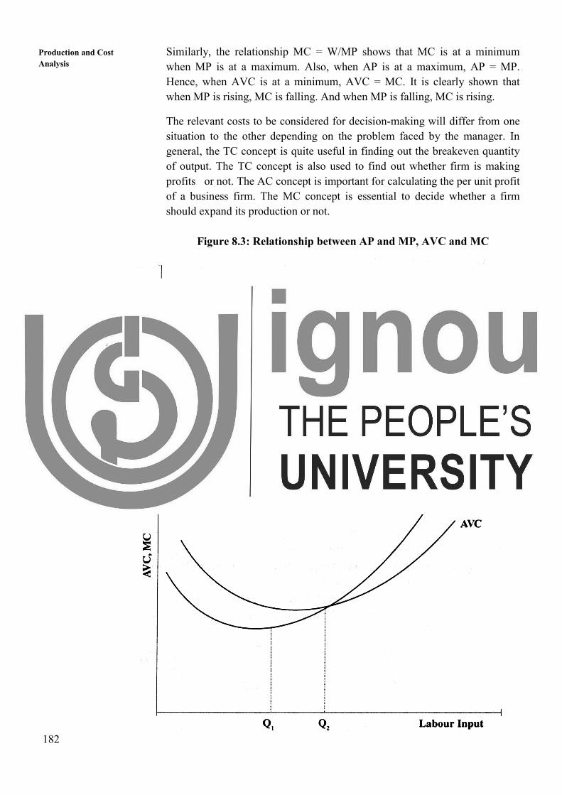
182

Production and Cost

Analysis Similarly, the relationship MC = W/MP shows that MC is at a minimum

when MP is at a maximum. Also, when AP is at a maximum, AP = MP.

Hence, when AVC is at a minimum, AVC = MC. It is clearly shown that

when MP is rising, MC is falling. And when MP is falling, MC is rising.

The relevant costs to be considered for decision-making will differ from one

situation to the other depending on the problem faced by the manager. In

general, the TC concept is quite useful in finding out the breakeven quantity

of output. The TC concept is also used to find out whether firm is making

profits or not. The AC concept is important for calculating the per unit profit

of a business firm. The MC concept is essential to decide whether a firm

should expand its production or not.

Figure 8.3: Relationship between AP and MP, AVC and MC

183

Short Run Cost

Analysis Activity 3

1. Fill in the blanks in the Table below:

Q TFC TVC TC AFC AVC ATC MC

1. 50 55

2. 50 8 25

3. 50 60.5

4. 13

5. 50 65

6. 50 18 3 11.3 3

7. 50 72.5

8. 50 28

9. 86

10 50 45 5 9.5 9

11. 50 54.5 4.5 9.5 9.5

12. 50 65.2

13. 50 130

14. 50 99.1

15. 50 174.75

16. 50 162

17. 50 259.25

18. 269.5

19. 50 399

20. 50 450 2.5 22.5 25 101

Note: Output Q is measured in ’000 units

All costs are measured in ` ’000

2. Suppose that a firm is currently employing 20 workers, the only variable

input, at wage rate of ` 60. The average product of labour is 30, the last

worker added 12 units to total output, and total fixed cost is ` 3600.

a. What is the marginal cost?

……………………………………………………………….

b. What is the average variable cost?

……………………………………………………….

c. How much output is being produced?

……………………………………………………

d. What is the average total cost?

……………………………………………………………

184

Production and Cost

Analysis e. Is average variable cost increasing, constant, or decreasing? What about

average total cost?

………………………………………………………………………………

3. Suppose average variable cost is constant over a range of output. What is

marginal cost over this range? What is happening to average total cost

over this range?

………………………………………………………………………………

………………………………………………………………………………

………………………………………………………………………………

………………………………………………………………………………

………………………………………………………………………………

8.10 APPLICATION OF SHORT RUN COST

ANALYSIS

In the previous sections of this unit, we discussed total, marginal, and average

cost curves for short run. The relationships between these cost curves have a

very wide range of applications for managerial use. Here we will discuss a

few applications of these concepts.

Determining Optimum Output Level

Earlier we have seen that the optimum output level is the point where average

cost is minimum. In other words, the optimum output level is the point where

average cost equals marginal cost. Consider the following example.

TC = 128 + 6Q + 2Q2

This is a short run total cost function since there is a fixed cost (TFC = 128).

AC = (TC/Q) = ����

+ 6 + 2Q

�������

= - ����� + 2 = 0

2 Q2

= 128

Q2

= 64

Q = 8

or

MC = �������

= 6 + 4Q = 0

Setting AC = MC

����

+ 6 + 2Q = 6 + 4Q

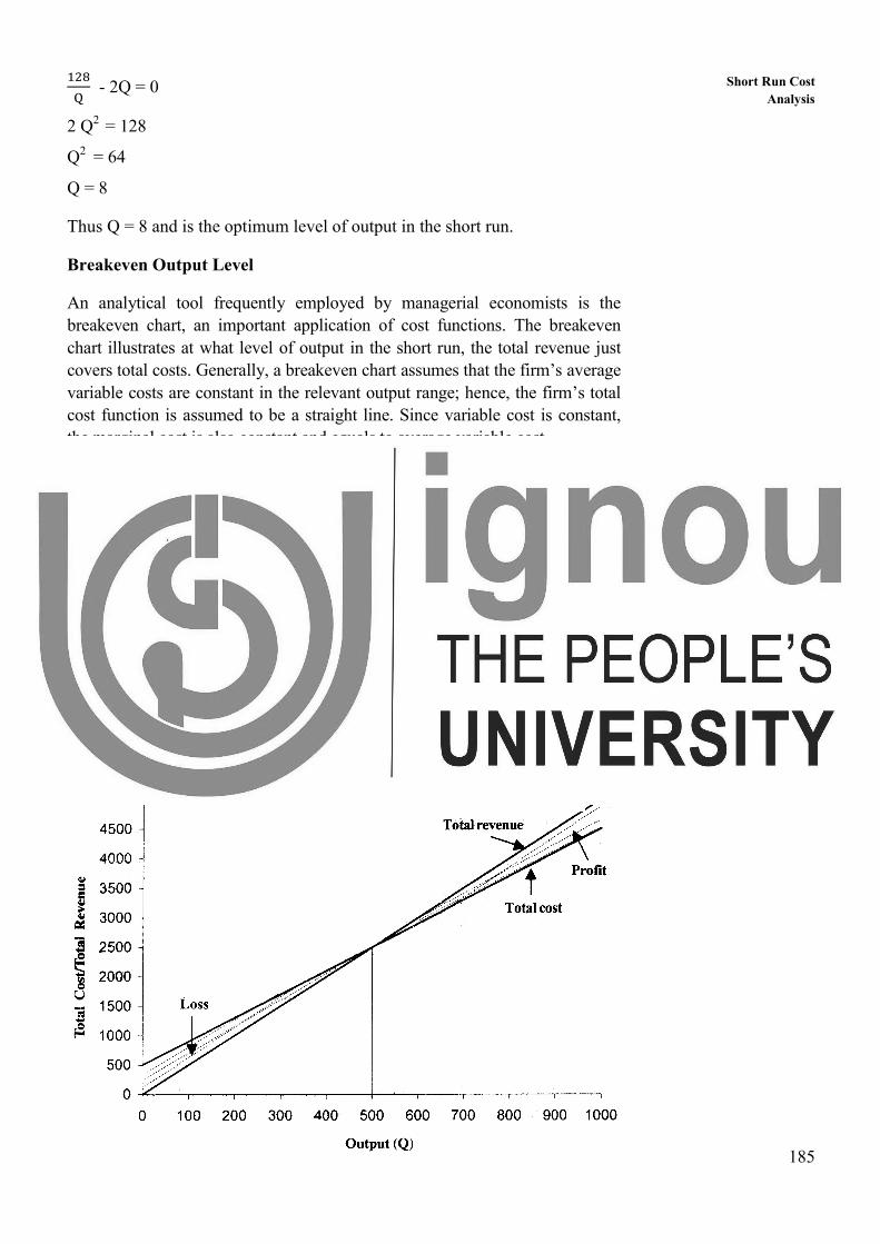
185

Short Run Cost

Analysis

����

- 2Q = 0

2 Q2

= 128

Q2

= 64

Q = 8

Thus Q = 8 and is the optimum level of output in the short run.

Breakeven Output Level

An analytical tool frequently employed by managerial economists is the

breakeven chart, an important application of cost functions. The breakeven

chart illustrates at what level of output in the short run, the total revenue just

covers total costs. Generally, a breakeven chart assumes that the firm’s average

variable costs are constant in the relevant output range; hence, the firm’s total

cost function is assumed to be a straight line. Since variable cost is constant,

the marginal cost is also constant and equals to average variable cost.

Figure 8.4 shows the breakeven chart of a firm. Here, it is assumed that the

price of the product will not be affected by the quantity of sales. Therefore,

the total revenue is proportional to output. Consequently, the total revenue

curve is a straight line through the origin. The firm’s fixed cost is `500,

variable cost per unit is `4 and the unit sales price of output is `5. The break

even chart, which combines the total cost function and the total revenue

curve, shows profit or loss resulting from each sales level. For example,

Figure 8.4 shows that if the firm sells 200 units of output it will make a loss

of `300. The chart also shows the breakeven point, the output level that must

be reached if the firm is to avoid losses. It can be seen from the figure; the

breakeven point is 500 units of output. Beyond 500 units of output the firm

makes profit.

Figure 8.4 Breakeven Chart

186

Production and Cost

Analysis Breakeven charts are used extensively for managerial decision process.

Under right conditions, breakeven charts can produce useful projections of

the effect of the output rate on costs, revenue and profits. For example, a firm

may use breakeven chart to determine the effect of projected decline in sales

or profits. On the other hand, the firm may use it to determine how many

units of a particular product it must sell in order to breakeven or to make a

particular level of profit. However, breakeven charts must be used with

caution, since the assumptions underlying them, sometimes, may not be

appropriate. If the product price is highly variable or if costs are difficult to

predict, the estimated total cost function and revenue curves may be subject

to these errors.

We can analyze the breakeven output with familiar algebraic equations.

TR = P * Q

TC = TFC + AVC ×Q �AVC � ����

so, TVC � AVC ∗ Q�

At breakeven point, TR = TC

P * Q = TFC + (AVC *Q)

Q �TFC

P � AVC�

TotalFixedcostPrice � Variablecostperunit

Here Q stands for breakeven volume of output. Multiplying Q with price (P)

we get the breakeven value of output. In the case of our example given in

Figure 8.4, TFC = `500, P = `5 and AVC = `4. Consequently,

Q �5005 � 4

� 5001

� 500

Therefore, the breakeven output (Q) will be 500 units. Similarly, the

breakeven output value will be `2500 (P × Q = `5 × 500).

Profit Contribution Analysis

In making short run decisions, firms often find it useful to carry out profit

contribution analysis. The profit contribution is the difference between price

and average variable cost (P – AVC).That is, revenue on the sale of a unit of

output after variable costs are covered represents a contribution towards

profit. In our example since price is `5 and average variable cost is `4, the

profit contribution per unit of output will be `1 (`5 – `4).At low rates of

output the firm may be losing money because fixed costs have not yet been

covered by the profit contribution. Thus, at these low rates of output, profit

contribution is used to cover fixed costs. After fixed costs are covered, the

firm will be earning a profit.

A manager wants to know the output rate necessary to cover all fixed costs

and to earn a ‘required’ profit (πR). Assume that both price and AVC are

187

Short Run Cost

Analysis constant. Profit is equal to revenue less the sum of total variable costs and

fixed costs. Thus

πR = TR – TC

πR = (P * Q) – �TFC � �AVC ∗ Q��

Solving this equation for Q gives a relation that can be used to determine the

rate of output necessary to generate a specified rate of profit. Thus

πR + TFC = (P * Q) - (AVC *Q)

πR + TFC = Q (P - AVC)

Q � �����������

To illustrate how profit contribution analysis can be used, suppose that the

firm in our example (where TFC = ` 500, P = `5 and AVC = `4) wants to

determine how many units of output it will have to produce and sell to earn a

profit of `10, 000. To generate this profit, an output rate of 10,500 units is

required; that is,

Q = ��,�����

��� = 10500

Operating Leverage

Managers must make comparisons among alternative systems of production.

Should one type of plant be replaced by another? Breakeven analysis can be

extended to help make such comparisons more effective. Consider the degree

of operating leverage (�� ), which is defined as the percentage change in

profit resulting from a 1% change in the number of units of product sold.

Thus,

E π = %��������������

%������������������

= �∆�/��∆�

∆�/� =

�∆�

* ���

or ���

∗ ���

If the price of output is constant regardless of the rate of output, the change in

degree of operating leverage depends on three variables: the rate of output,

the level of fixed costs, and variable cost per unit of output. This can be seen

by substituting the above equation for profit with

π � TR � �TVC � TFC�

� � � ∗ � � ���� ∗ �� � ���

and change in profit ∆� � � ∗ ∆� � �AVC� ∗ ∆�

Therefore, the degree of operating leverage will be

E�= ��∗∆�������∗∆��/��∗�������∗������∆�/�

188

Production and Cost

Analysis On Simplification,

E� � �������������������

Example: Consider three firms I, II and III having the following fixed costs,

average variable costs and price of the product.

Firm-I has more fixed cost than firm-II, and firm-III. However, Firm-I has

less average costs than firm-II, and firm-III. Essentially, firm-I has

substituted capital (fixed costs) for labour and materials (variable costs) with

the introduction of more mechanized machines. On the other hand, firm-III

has less fixed costs and more average variable costs when compared to other

two plants because firm-III has less mechanized machines. The firm-II

occupies middle position in terms of fixed costs and average variable costs.

In comparing these plants, we use the degree of operating leverage. Suppose

for all the three plants Q=40,000.

For firm – I, Eπ = ����������

����������������� = 6

For firm – II, Eπ = ����������

���������������� = 4

For firm – III, Eπ = �����������������������,���

= 3

Thus, a 1% increase in sales volume results in a 6% increase in profit at firm-

I, a 4% profit at firm-II, and 3% profit at firm-III. This means firm-I’s profits

are more sensitive to changes in sales volume than firm-II and firm-III and

firm-II’s profits are more sensitive to changes in sales volume than firm-III.

Activity 4

1. Speed-Marine Co. builds motorboat engines. They recently estimated

their total costs and total revenue as:

TC = 80,000 – 600Q + 2Q2 TR = 400Q - Q

2

Where TC is total cost, TR is total revenue, and Q is the number of

engines produced each year.

Where TC is total cost, TR is total revenue, and Q is the number of

engines produced each year.

Firm Fixed Cost (`) Average variable

Cost (`)

Price of the product

(`)

Firm-I 1,00,000 2 5

Firm-II 60,000 3 5

Firm-III 26,650 4 5

189

Short Run Cost

Analysis a. At what level of production will the company breakeven? How many

engines should be produced to maximize profit?

............................................................................................................

............................................................................................................

............................................................................................................

............................................................................................................

2. Give TC=6Q + 2Q2 – Q

3, find out the optimum level of output, Q.

...................................................................................................................

...................................................................................................................

...................................................................................................................

...................................................................................................................

3. During the last period, the sum of average profit and fixed costs for a

firm totaled ` 1, 00,000. Unit sales were 10,000. If variable cost per

unit was ` 4, what was the selling price of a unit of output? How much

would profit change if the firm produced and sold 11,000 units of

output? (Assume average variable cost remains at ` 4 per unit).

...................................................................................................................

...................................................................................................................

...................................................................................................................

...................................................................................................................

8.11 SUMMARY

Cost concepts are important for decision-making but neither the accounting

approach nor the economic approach is completely acceptable when decision-

making is involved. Costs must be considered in various ways, depending on

the decision at hand. Both traditional economists and traditional accountants

have tended to be fairly dogmatic in their definitions of costs. On the other

hand, managerial economists want a flexible approach. All the cost concepts

need to be considered in such a way so as to help make sound decisions. The

decision maker should try to discover the “relevant” costs by asking what

costs are relevant to a particular decision at hand, and the decision maker is

not necessarily bound by traditional concepts constructed for other purposes.

In short run, the total cost consists of fixed and variable costs. A firm’s

marginal cost is the additional variable cost associated with each additional

unit of output. The average variable cost is the total variable cost divided by

the number of units of output. When there is a single variable input, the

190

Production and Cost

Analysis presence of diminishing returns determines the shape of cost curves. In

particular, there is an inverse relationship between the marginal product of

the variable input and the marginal cost of production. The average variable

cost and average total cost curves are U-shaped. The short run marginal cost

curve increases beyond a certain point, and cuts both average total cost curve

and average variable cost curve from below at their minimum points.

These cost concepts and analysis have a lot of applications in real world

decision-making process such as optimum output, break even output, profit

contribution, operating leverage, etc.

8.12 SELF ASSESSMENT QUESTIONS

1. Differentiate between accounting costs and economic costs?

2. Take a firm you are working with or know its nature. Make a list of

relevant cost concepts from the standpoint of an (a) accountant and (b)

economist.

3. What is the significance of opportunity cost in managerial decision-

making?

4. What is short run cost analysis? For what type of decisions is it useful?

5. What are marginal costs and incremental costs? What is the difference

between these two cost concepts?

6. A pharmaceutical company has spent ₹5 crores on developing and

testing a new antibiotic drug. The head of the marketing department now

estimates that it will cost ₹3 crores in advertising to launch this new

product. Total revenue from all future sales is estimated at ₹6crores, and

therefore, total costs will exceed revenue by ₹2 crores. He recommends

that this product be dropped from the firm’s product offerings. What is

your reaction to this recommendation? The head of the accounting

department now indicates that ₹3.5 crores of corporate overhead

expenses also will be assigned to this product if it is marketed. Does this

new information affect your decision? Explain.

7. When Mr. Kapoor’s father gave him a new Truck costing ₹30 lakhs.

Recently Mr. Kapoor was boasting to some of his friends that his

revenues were typically ₹150,000 per month, while his operating costs

(fuel, maintenance, and depreciation) amounted to only ₹1,20,000 per

month. A truck identical to Mr. Kapoor’s Truck is available on a

monthly rent of ₹35000. If Mr. Kapoor was driving trucks for someone

else, he would earn ₹5000 per month.

a. How much are Mr. Kapoor’s explicit costs per month? How much

are his implicit costs per month?

b. What is the amount of the opportunity cost of the resources used by

Mr. Kapoor each month?

191

Short Run Cost

Analysis c. Mr. Kapoor is proud of the fact that he is generating a net cash flow

of ₹30000 (=₹1, 50,000 – ₹1, 20,000) per month, since he would

only be earning ₹5000 per month if he were working for some else.

What advice would you give Mr. Kapoor?

9. The following table pertains to Savitha Company. Fill in the blanks below:

Output Total

Cost

Total

Fixed

Cost

Total

Variable

Cost

Average

Total

Cost

Average

Fixed

Cost

Average

Variable

Cost

Marginal

Cost

100 260 60

200

0.30

300

0.50

400

1.05

500

360

600

3.00

700

1.60

800 2040

10. Suppose that a local metal fabricator has estimated its short run total cost

function and total revenue function as

TC = 1600 +100Q + 25Q2

TR = 500Q

What is the breakeven amount of output? How might the company go

about reducing the break even rate if it does not feel that it can sell the

estimated amount in the market place?

11. A TV company sells color TV sets at ₹15,000 each. Its fixed costs are

₹ 30,000, and its average variable costs are ₹ 10,000 per unit. Draw its

breakeven graph, and then determine its breakeven rate of production.

12. The Bright Electronics is producing small electronic calculators. It wants

to determine how many calculators it must sell in order to earn a profit of

₹10,000 per month. The price of each calculator is ₹300, the fixed costs

are ₹ 5,000 per month, and the average variable cost is ₹ 100.

a. What is the required sales volume?

192

Production and Cost

Analysis b. If the firm were to sell each calculator at a price of ₹350 rather than

₹ 300, what would be the required sales volume?

c. If the price is ₹ 350, and if average variable cost is ₹ 85 rather than

₹100, what would be the required sales volume?

8.13 FURTHERS READINGS

Adhikary, M. (1987). Managerial Economics (3rd

ed.).Khosla Publishers,

Delhi.

Maddala, G. S., & Miller, E. M. (1989). Micro Economics: Theory and

Applications. McGraw-Hill, NewYork.

Mote, V. L., Paul, S., & Gupta, G. S. (2016). Managerial Economics:

Concepts and Cases. Tata McGraw-Hill, New Delhi.

Mehta, P.L.(2016) Managerial Economics: Analysis, Problems and Cases.

Sultan Chand & Sons, New Delhi.

Dholakia, R., & Oza, A. N. (1996). Microeconomics for Management

Students. Oxford University Press, Delhi.

193

Long Run Cost

Analysis UNIT 9 LONG RUN COST ANALYSIS

Objectives

After studying this unit, you should be able to:

analyze the behavior of costs in long run;

comprehend the different sources of economies of scale;

explain various functional forms of production and costs;

understand empirical determination of these theoretical functions;

identify managerial uses of such empirical estimates.

Structure

9.1 Introduction

9.2 Long-run Cost Functions

9.3 Economies and Diseconomies of Scale

9.4 Learning Curve

9.5 Economies of Scope

9.6 Cost Function and its Determinants

9.7 Estimation of Cost Function

9.8 Empirical Estimates of Cost Function

9.9 Managerial Uses of Cost Function

9.10 Summary

9.11 Self-Assessment Questions

9.12 Further Readings

9.1 INTRODUCTION

In unit 8, you have learnt about different cost concepts used by managers in

decision- making process, the relationship between these concepts, and the

distinction between accounting costs and economic costs, and short run cost

analysis and its applications in managerial decision making. We will continue

the analysis of costs in this unit also, long term cost analysis will be

discussed.

In the process of decision-making, a manager should understand clearly the

relationship between the inputs and output on one hand and output and costs

on the other. Estimation of cost curves will help production manager in

understanding the nature and shape of cost curves and taking useful

decisions. Both short run cost function and the long run cost function must

be estimated, since both sets of information will be required for some vital

decisions. Knowledge of the short run cost functions allows the decision

makers to judge the optimality of present output levels and to solve decision

problems of production manager. Knowledge of long run cost functions is

important when considering the expansion or contraction of plant size, and

194

Production and Cost

Analysis for confirming that the present plant size is optimal for the output level that is

being produced. In the present Unit, we will discuss different approaches to

examination of cost functions, analysis of some empirical estimates of these

functions, and managerial uses of the estimated functions.

9.2 LONG-RUN COST FUNCTIONS

In the long run, all inputs are variable, and a firm can have a number of

alternative plant sizes and levels of output that it wants. There are no fixed

cost functions (total or average) in the long run, since no inputs are fixed. A

useful way of looking at the long run is to consider it a planning horizon. The

long run cost curve is also called planning curve because it helps the firm in

future decision-making process.

Figure 9.1: Short-Run and Long Run Average Cost Curves

The long run cost output relationship can be shown with the help of a long

run cost curve. The long run average cost curve (LRAC) is derived from

short run average cost curves (SRAC). Let us illustrate this with the help of a

simple example. A firm faces a choice of production with three different

plant sizes viz. plant size-1 (small size), plant size-2 (medium size), plant

size-3 (large size), and plant size-4 (very large size). The short run average

cost functions shown in Figure 9.1 (SRAC1, SRAC2, SRAC3, and SRAC4) are

associated with each of these plants discrete scale of operation. The long run

average cost function for this firm is defined by the minimum average cost of

each level of output. For example, output rate Q1 could be produced by the

plant size-1 at an average cost of C1 or by plant size-2 at a cost of C2.

Clearly, the average cost is lower for plant size-1, and thus point a is one

point on the long run average cost curve. By repeating this process for various

rates of output, the long run average cost is determined. For output rates of

zero to Q2 plant size-1is the most efficient and that part of SRAC1 is part of

the long run cost function. For output rates of Q2 to Q3 plant size-2 is the

most efficient, and for output rates Q3 to Q4, plant size-3 is the most

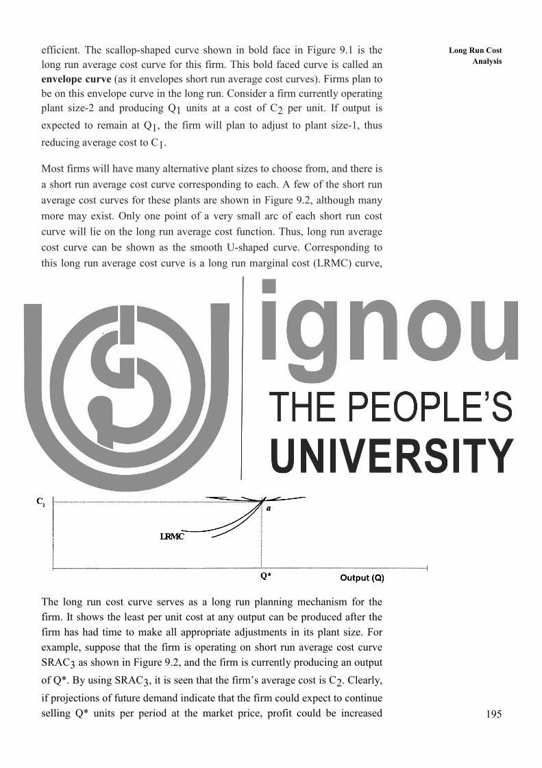
195

Long Run Cost

Analysis efficient. The scallop-shaped curve shown in bold face in Figure 9.1 is the

long run average cost curve for this firm. This bold faced curve is called an

envelope curve (as it envelopes short run average cost curves). Firms plan to

be on this envelope curve in the long run. Consider a firm currently operating

plant size-2 and producing Q1 units at a cost of C2 per unit. If output is

expected to remain at Q1, the firm will plan to adjust to plant size-1, thus

reducing average cost to C1.

Most firms will have many alternative plant sizes to choose from, and there is

a short run average cost curve corresponding to each. A few of the short run

average cost curves for these plants are shown in Figure 9.2, although many

more may exist. Only one point of a very small arc of each short run cost

curve will lie on the long run average cost function. Thus, long run average

cost curve can be shown as the smooth U-shaped curve. Corresponding to

this long run average cost curve is a long run marginal cost (LRMC) curve,

which intersects LRAC at its minimum point a, which is also the minimum

point of short run average cost curve 4 (SRAC4). Thus, at a point a and only

at a point a, the following unique result occurs:

SRAC = SRMC when LRAC = LRMC

Figure 9.2 : Short – Run and Long – Run Average Cost and Marginal

Cost Curves

The long run cost curve serves as a long run planning mechanism for the

firm. It shows the least per unit cost at any output can be produced after the

firm has had time to make all appropriate adjustments in its plant size. For

example, suppose that the firm is operating on short run average cost curve

SRAC3 as shown in Figure 9.2, and the firm is currently producing an output

of Q*. By using SRAC3, it is seen that the firm’s average cost is C2. Clearly,

if projections of future demand indicate that the firm could expect to continue

selling Q* units per period at the market price, profit could be increased

LRAC

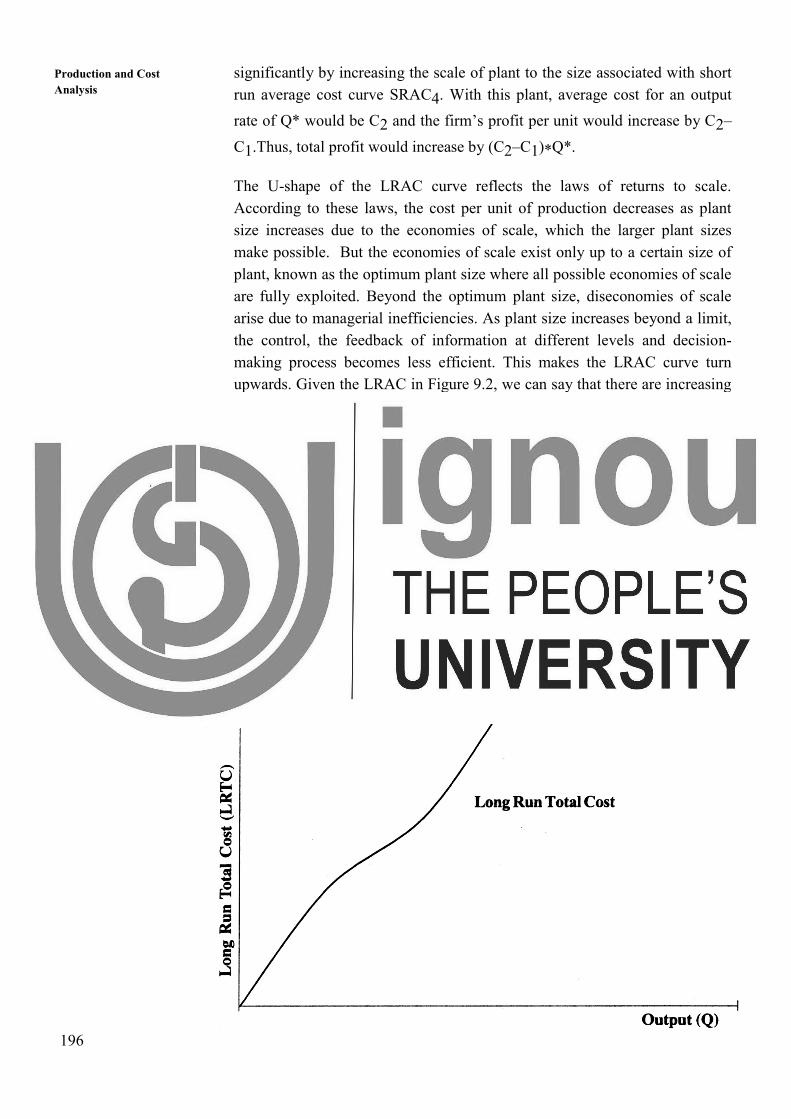
196

Production and Cost

Analysis significantly by increasing the scale of plant to the size associated with short

run average cost curve SRAC4. With this plant, average cost for an output

rate of Q* would be C2 and the firm’s profit per unit would increase by C2–

C1.Thus, total profit would increase by (C2–C1)*Q*.

The U-shape of the LRAC curve reflects the laws of returns to scale.

According to these laws, the cost per unit of production decreases as plant

size increases due to the economies of scale, which the larger plant sizes

make possible. But the economies of scale exist only up to a certain size of

plant, known as the optimum plant size where all possible economies of scale

are fully exploited. Beyond the optimum plant size, diseconomies of scale

arise due to managerial inefficiencies. As plant size increases beyond a limit,

the control, the feedback of information at different levels and decision-

making process becomes less efficient. This makes the LRAC curve turn

upwards. Given the LRAC in Figure 9.2, we can say that there are increasing

returns to scale up to Q* and decreasing returns to scale beyond Q*.

Therefore, the point Q* is the point of optimum output and the corresponding

plant size-4 is the optimum plant size. If you have long run average cost of

producing a given output, you can readily derive the long run total cost

(LRTC) of the output, since the long run total cost is simply the product of

long run average cost and output. Thus, LRTC = LRAC *Q.

Figure 9.3 shows the relationship between long run total cost and output.

Given the long run total cost function you can readily derive the long run

marginal cost function, which shows the relationship between output and the

cost resulting from the production of the last unit of output, if the firm has

time to make the optimal changes in the quantities of all inputs used.

Figure 9.3 : Long Run Total Cost Function

197

Long Run Cost

Analysis Activity 1

1. Explain why short run marginal cost is greater than long run marginal

cost beyond the point at which they are equal?

…………………………………………………………………………

…………………………………………………………………………

…………………………………………………………………………

…………………………………………………………………………

…………………………………………………………………………

2. Explain why short run average cost can never be less than long run

average cost?

…………………………………………………………………………

…………………………………………………………………………

…………………………………………………………………………

…………………………………………………………………………

…………………………………………………………………………

3. Why are all costs variable in the long run?

…………………………………………………………………………

…………………………………………………………………………

…………………………………………………………………………

…………………………………………………………………………

…………………………………………………………………………

4. Why is the long run average cost curve called an “envelope curve”?

Why cannot the long run marginal cost curve be an envelope as well?

…………………………………………………………………………

…………………………………………………………………………

…………………………………………………………………………

…………………………………………………………………………

…………………………………………………………………………

5. What do you understand by “cost-efficiency”? Draw a long run cost

diagram and explain.

…………………………………………………………………………

…………………………………………………………………………

…………………………………………………………………………

…………………………………………………………………………

…………………………………………………………………………

198

Production and Cost

Analysis 6. Economists frequently say that the firm plans in the long run and

operates in the short run. Explain.

…………………………………………………………………………

…………………………………………………………………………

…………………………………………………………………………

…………………………………………………………………………

…………………………………………………………………………

…………………………………………………………………………

………………………………

9.3 ECONOMIES AND DISECONOMIES OF

SCALE

We have seen in the preceding section that larger plant will lead to lower

average cost in the long run. However, beyond some point, successively

larger plants will mean higher average costs. Exactly, why is the long run

average cost (LRAC) curve U-shaped? What determines the shape of LRAC

curve? This point needs further explanation.

It must be emphasized here that the law of diminishing returns is not

applicable in the long run as all inputs are variable. Also, we assume that

resource prices are constant. What then, is our explanation? The U-shaped

LRAC curve is explainable in terms of what economists call economies of

scale and diseconomies of scale.

Economies and diseconomies of scale are concerned with behaviour of

average cost curve as the plant size is increased. If LRAC declines as output

increases, then we say that the firm enjoys economies of scale. If, instead, the

LRAC increases as output increases, then we have diseconomies of scale.

Finally, if LRAC is constant as output increases, then we have constant

returns to scale implying we have neither economies of scale nor

diseconomies of scale. Economies of scale explain the down sloping part of

the LRAC curve. As the size of the plant increases, LRAC typically declines

over some range of output for a number of reasons. The most important is

that, as the scale of output is expanded, there is greater potential for

specialization of productive factors. This is most notable with regard to

labour but may apply to other factors as well. Other factors contributing to

declining LRAC include ability to use more advanced technologies and more

efficient capital equipment; managerial specialization; opportunity to take

advantage of lower costs (discounts) for some inputs by purchasing larger

quantities; effective utilization of by products, etc.

But, after sometime, expansion of a firm’s output may give rise to

diseconomies, and therefore, higher average costs. Further expansion of

output beyond a reasonable level may lead to problems of overcrowding of

labour, managerial in efficiencies, etc., pushing up the average costs.

199

Long Run Cost

Analysis The economies of scale and diseconomies of scale are sometimes called as

internal economies of scale and internal diseconomies of scale

respectively. This is because the changes in long run average costs result

solely from the individual firm’s adjustment of its output. On the other hand,

there may exist external economies of scale. The external economies also

help in cutting down production costs. With the expansion of an industry,

certain specialized firms also come up for working up the by-products and

waste materials. Similarly, with the expansion of the industry, certain

specialized units may come up for supplying raw material, tools, etc., to the

firms in the industry. Moreover, they can combine together to undertake

research etc., whose benefit will accrue to all firms in the industry. Thus, a

firm benefits from expansion of the industry as a whole. These benefits are

external to the firm, in the sense that these have arisen not because of any

effort on the part of the firm but have accrued to it due to expansion of

industry as a whole. All these external economies help in reducing production

costs.

Economies of scale are often measured in terms of cost- output elasticity,

Ec.

Ec is the percentage change in the average cost of production resulting from a

one percent increase in output:

�� � �∆TC/TC) / (∆�/�) = �∆TC/∆�� / (TC/Q) = MC/AC

Clearly, Ec is equal to one when marginal and average costs are equal. This

means costs increase proportionately with output, and there are neither

economies nor diseconomies of scale. When there are economies of scale MC

will be less than AC (both are declining) and Ec is less than one. Finally,

when there are diseconomies of scale, MC is greater than AC, and Ec is

greater than one.

ECONOMIES OF SCALE

Internal economies

Real and Pecuniary are two types of internal economies. When quantity of

inputs used decrease for a particular level of output, it gives rise to real

economies. When large quantities of input are bought and large quantities of

output are sold, there are savings in the cost of inputs and distribution costs

due to bulk buying and selling, these savings are known as pecuniary

economies.

A) REAL ECONOMIES OF SCALE

1. Production economies

Production economies arise from different factors of production such

as :-

200

Production and Cost

Analysis

201

Long Run Cost

Analysis Labour Economies

Large scale of production leads to division of labour and specialization,

leading to reduction in costs and time. Due to large scale production,

technical personnel acquire significant experience and this ‘cumulative

volume’ has positive effect on production and costs, leading to high

productivity and lower costs for large level of outputs.

Technical Economies

Technical economies are related to fixed capital which includes machinery

and equipments. Specialization and indivisibility of machines and equipments

leads to reduction in per unit costs. Machines have a property of indivisibility

so, when large production (maximum capacity of machine) is achieved,

machine cost is divided between large units.

In large size firms, there are large machines which perform different

continuous automatic processes which saves time and cost of labour as

different machines for different steps are not required. And with increase in

scale, general purpose machinery is left to set up more which reduces its set

up costs.

Inventory economies

The main aim of inventories is to meet random fluctuations in supply and

demand of inputs & output respectively. When size of firm increases, these

fluctuations are eased out due to large quantity of resources.

2) Marketing economies

With increase in output, advertising, R&D (such as developing new models

and designs) expenditures etc. are spread over and expenditure per unit

decreases considerably.

3) Managerial economies

Managerial economies arise due to various reasons, most important of them

are specialization, decentralization, team work experience and modern

managerial techniques. When scale of operations rises, division of managerial

tasks (production, sales, finance etc.) is done and this leads to specialization

as same task is performed again and again. Team work experience helps in

improving decision making ability of managers and with decentralization

decision making becomes faster leading to managerial efficiency.

4) Transport and storage economies

Storage costs decrease with increase in the size of output. But transportation

costs keep falling for some extent and then they become constant, making a L

shaped curve.

B) PECUNIARY ECONOMIES OF SCALE

These economies include all the savings and discounts obtained by firm

because of its large size. Few examples of these are:

Raw material prices become competitive when there is bulk buying.

202

Production and Cost

Analysis Banks offer lower rates of interest to large firms, ultimately it comes

down to lower cost of capital.

Large firms have need of large-scale advertising, they are offered

better prices.

Transportation costs turn out lower for bulk transportation.

Labour costs can be saved by large firms, if they attain a position,

which gives them monopsony power due to large size or prestige in

market.

EXTERNAL ECONOMIES

External economies are those which are not particular to one particular firm

rather these are shared by all firms operating in a particular industry. These

are external to the firm as they do not arise due to efforts of any one

particular firm, they arise when whole industry expands. These can be

economies of information, economies of concentration, economies of

disintegration etc. These external economies also help in reduction of

production costs just like internal economies.

DISECONOMIES OF SCALE

Diseconomies of scale occur, at a level of output where one unit increase in

output leads to increase in marginal costs. At this level, diminishing returns

are there and economies of scale are ruled out by diseconomies of scale.

Diseconomies of scale generally arise due to human and behavioural

problems instead of technical factors.

There are several reasons for diseconomies of scale, some of them have been

listed below:

Morale and motivation problems

When the size of firm increases more and more employees join the

organization which reduces personal connection with owners and

management which leads to reduction in motivation among employees.

Reduction in motivation leads to reduction in productivity as well.

Communication problems

Effective and properly defined communication channels are very important in

any business organization. When a firm increases its size, there are increased

layers of command, it may create problems in communication and a message

can be distorted or lost. So, the formal communication of objectives and

goals will also suffer in this scenario which will lead to reduction in

productivity.

In short, it can be concluded that diseconomies of scale will come into picture

when with increase in size, management faces tough challenges in regards to

communication, motivation & morale of employees etc. and they are not able

to overcome those challenges.

203

Long Run Cost

Analysis Activity 2

1. Distinguish between internal and external economies of scale. Give

examples.

…………………………………………………………………………

…………………………………………………………………………

…………………………………………………………………………

…………………………………………………………………………

…………………………………………………………………………

2. Distinguish between real and pecuniary economies of scale.

…………………………………………………………………………

…………………………………………………………………………

…………………………………………………………………………

…………………………………………………………………………

…………………………………………………………………………

3. Explain the reasons of diseconomies of scale with examples.

…………………………………………………………………………

…………………………………………………………………………

…………………………………………………………………………

…………………………………………………………………………

…………………………………………………………………………

9.4 LEARNING CURVE

Learning curve denotes the relationship between labour cost and additional units of

output. It basically revolves around the concept that, with practice workers improve

and ultimately, cost per unit of producing one more units of output decreases.

Learning curve effect is this reduction in cost due to learning process of employees

over a period of time.

9.5 ECONOMIES OF SCOPE

According to the concept of economies of scale, cost advantages follow the

increase in volume of production or what is called the scale of output. On the

other hand, according to the concept of economies of scope, such cost

advantages may follow from a variety of output. For example, many firms

produce more than one product and the products are closely related to one

another — an automobile company produces scooters and cars, and a

university produces teaching and research. A firm is likely to enjoy

production or cost advantages when it produces two or more products. These

advantages could result from the joint use of inputs or production facilities,

joint marketing programs, or possibly the cost savings of a common

204

Production and Cost

Analysis administration. Examples of joint products are mutton and wool, eggs and

chicken, fertilizer, etc.

Therefore, economies of scope exist when the cost of producing two (or

more) products jointly is less than the cost of producing a single product. To

measure the degree to which there are economies of scope, we should know

what percentage of the cost of production is saved when two (or more)

products are produced jointly rather than individually. The following

equation gives the degree of economies of scope (SC) that measures the

savings in cost:

�� � ����� � ����� � ���� � ���

���� � ���

Here, C (Q1) represents the cost of producing output Q1, C (Q2) the cost of

producing output Q2, and C (Q1, Q2) the joint cost of producing both outputs

(Q1 +Q2).

For example, a firm produces 10000 TV sets and 5000 Radio sets per year at

a cost of Rs.8.40 crores, and another firm produces 10000 TV sets only, then

the cost would be Rs.10.00 crores, and if it produced 5000 Radio sets only,

then the cost would be Rs. 0.50 crores. In this case, the cost of producing

both the TV and Radio sets is less than the total cost of producing each

separately. Thus, there are economies of scope. Thus,

�� � 10.00 � 0.50 � 8.40

8.40� 0.25

Which means that there is a 25% saving of cost by going for joint

production.

With economies of scope, the joint cost is less than the sum of the individual

costs, so that SC is greater than 0. With diseconomies of scope, SC is

negative. In general, the larger the value of SC, the greater is the economies

of scope.

Activity 3

1. Distinguish between economies of scale and economies of scope using

examples.

…………………………………………………………………………………

…………………………………………………………………………………

…………………………………………………………………………………

…………………………………………………………………………………

…………………………………………………………………………………

9.6 COST FUNCTION AND ITS DETERMINANTS

Cost function expresses the relationship between cost and its determinants

such as the size of plant, level of output, input prices, technology, managerial

efficiency, etc. In a mathematical form, it can be expressed as,

205

Long Run Cost

Analysis C = f (S, O, P, T, E….)

Where, C = cost (it can be unit cost or total cost)

S = plant size

O = output level

P = prices of inputs used in production

T = nature of technology

E = managerial efficiency

Determinants of Cost Function

The cost of production depends on many factors and these factors vary from

one firm to another firm in the same industry or from one industry to another

industry. The main determinants of a cost function are:

a) plant size

b) output level

c) prices of inputs used in production,

d) nature of technology

e) managerial efficiency

We will discuss briefly the influence of each of these factors on cost.

a) Plant size: Plant size is an important variable in determining cost.

The scale of operations or plant size and the unit cost are inversely

related in the sense that as the former increases, unit cost decreases,

and vice versa. Such a relationship gives downward slope of cost

function depending upon the different sizes of plants taken into

account. Such a cost function gives primarily engineering estimates of

cost.

b) Output level: Output level and total cost are positively related, as the

total cost increases with increase in output and total cost decreases

with decrease in output. This is because increased production requires

increased use of raw materials, labour, etc., and if the increase is

substantial, even fixed inputs like plant and equipment, and

managerial staff may have to be increased.

c) Price of inputs: Changes in input prices also influence cost,

depending on the relative usage of the inputs and relative changes in

their prices. This is because more money will have to be paid to those

inputs whose prices have increased and there will be no simultaneous

reduction in the costs from any other source. Therefore, the cost of

production varies directly with the prices of production.

206

Production and Cost

Analysis d) Technology: Technology is a significant factor in determining cost.

By definition, improvement in technology increases production

leading to increase in productivity and decrease in production cost.

Therefore, cost varies inversely with technological progress.

Technology is often quantified as capital-output ratio. Improved

technology is generally found to have higher capital-output ratio.

e) Managerial efficiency: This is another factor influencing the cost of

production. More the managerial efficiency less the cost of

production. It is difficult to measure managerial efficiency

quantitatively. However, a change in cost at two points of time may

explain how organizational or managerial changes within the firm

have brought about cost efficiency, provided it is possible to exclude

the effect of other factors

9.7 ESTIMATION OF COST FUNCTION

Several methods exist for the measurement of the actual cost-output relation

for a particular firm or a group of firms, but the three broad approaches -

accounting, engineering and econometric – are the most important and

commonly used.

Accounting Method

This method is used by the cost accountants. In this method, the cost-output

relationship is estimated by classifying the total cost into fixed, variable and

semi-variable costs. These components are then estimated separately. The

average variable cost, the semi-variable cost which is fixed over a certain

range of output, and fixed costs are determined on the basis of inspection and

experience. The total cost, the average cost and the marginal cost for each

level of output can then be obtained through a simple arithmetic procedure.

Although, the accounting method appears to be quite simple, it is a bit

cumbersome as one has to maintain a detailed breakdown of costs over a

period to arrive at good estimates of actual cost-output relationship. One must

have experience with a wide range of fluctuations in output rate to come up

with accurate estimates.

Engineering Method

The engineering method of cost estimation is based directly on the physical

relationship of inputs to output, and uses the price of inputs to determine

costs. This method of estimating real world cost function rests clearly on the

knowledge that the shape of any cost function is dependent on: (a) the

production function and (b) the price of inputs.

We have seen earlier in Unit – 7 while discussing the estimation of

production function that for a given the production function and input prices,

207

Long Run Cost

Analysis the optimum input combination for a given output level can be determined.

The resultant cost curve can then be formulated by multiplying each input in

the least cost combination by its price, to develop the cost function. This

method is called engineering method as the estimates of least cost

combinations are provided by engineers.

The assumption made while using this method is that both the technology and

factor prices are constant. This method may not always give the correct

estimate of costs as the technology and factor prices do change substantially

over a period of time. Therefore, this method is more relevant for the short

run. Also, this method may be useful if good historical data is difficult to

obtain. But this method requires a sound understanding of engineering and a

detailed sampling of the different processes under controlled conditions,

which may not always be possible.

Econometric Method

This method is also sometimes called statistical method and is widely used

for estimating cost functions. Under this method, the historical data on cost

and output are used to estimate the cost-output relationship. The basic

technique of regression is used for this purpose. The data could be a time

series data of a firm in the industry or of all firms in the industry or a cross-

section data for a particular year from various firms in the industry.

Depending on the kind of data used, we can estimate short run or long run

cost functions. For instance, if time series data of a firm whose output

capacity has not changed much during the sample period is used, the cost

function will be short run. On the other hand, if cross-section data of many

firms with varying sizes, or the time series data of the industry as a whole is

used, the estimated cost function will be the long run one.

The procedure for estimation of cost function involves three steps. First, the

determinants of cost are identified. Second, the functional form of the cost

function is specified. Third, the functional form is chosen and then the basic

technique of regression is applied to estimate the chosen functional form.

Functional Forms of Cost Function

The following are the three common functional forms of cost function in

terms of total cost function (TC).

Linear cost function: TC = a1 +b1Q

Quadratic cost function: TC = a2 + b2Q + c2Q2

Cubic cost function: TC = a3 + b3Q + c3Q2 +d3Q

3

where, a1, a2, a3, b1, b2, b3, c2, c3, d3 are constants.

When all the determinants of cost are chosen and the data collection is

complete, the alternative functional forms can be estimated by using

208

Production and Cost

Analysis regression software package on a computer. The most appropriate form of the

cost function for decision-making is then chosen on the basis of the principles

of economic theory and statistical inference.

Once the constants in the total cost function are estimated using regression

technique, the average cost (AC) and marginal cost (MC) functions for

chosen forms of cost function will be calculated. The TC, AC and MC cost

functions for different functional forms of total cost function and their typical

graphical presentation and interpretation are explained below.

A. Linear cost function

TC = a1 + b1Q

AC=(TC)/Q= (a1/Q) +b1

MC = �������

= b1

The typical TC, AC, and MC curves that are based on a linear cost function

are shown in Figure 9.4. These cost functions have the following properties:

TC is a linear function, where AC declines initially and then becomes quite

flat approaching the value of MC as output increases and MC is constant at

b1.

B. Quadratic cost function

TC = a2 + b2Q + c2Q2

AC = (TC/Q) = (a2/Q)+ b2 + c2Q

MC = �������

= b2+ 2c2Q

The typical TC, AC, and MC curves that are based on a quadratic cost

function are shown in Figure 9.5.These cost functions have the following

properties: TC increases at an increasing rate; MC is a linearly increasing

function of output; and AC is a U-shaped curve.

C. Cubic cost function

TC = a3 + b3Q + c3Q2 +d3Q

3

AC = (TC/Q) = (a3/Q) +b3+c3 Q+d3Q2

MC = = �������

= b3+ 2c3Q + 3d3 Q2

The typical TC, AC, and MC curves that are based on a cubic cost function

are shown in Figure 9.6. These cost functions have the following properties:

TC first increases at a decreasing rate up to output rate Q1 in the Figure 9.6

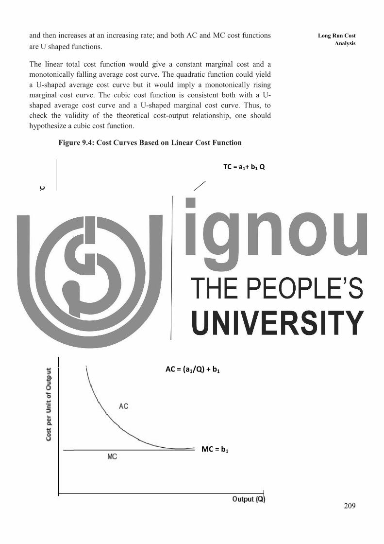
209

Long Run Cost

Analysis and then increases at an increasing rate; and both AC and MC cost functions

are U shaped functions.

The linear total cost function would give a constant marginal cost and a

monotonically falling average cost curve. The quadratic function could yield

a U-shaped average cost curve but it would imply a monotonically rising

marginal cost curve. The cubic cost function is consistent both with a U-

shaped average cost curve and a U-shaped marginal cost curve. Thus, to

check the validity of the theoretical cost-output relationship, one should

hypothesize a cubic cost function.

Figure 9.4: Cost Curves Based on Linear Cost Function

TC

Output (Q)

TC = a1+ b1 Q

AC = (a1/Q) + b1

MC = b1

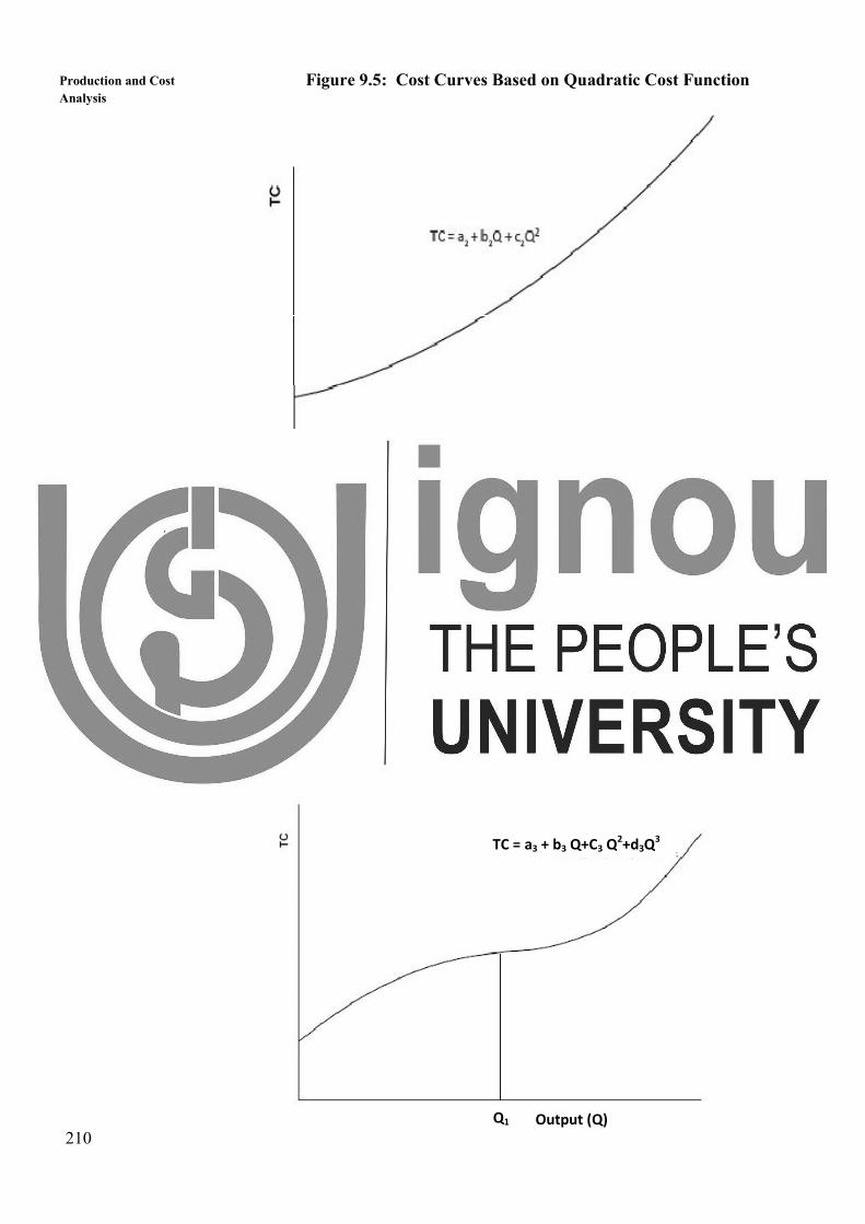
210

Production and Cost

Analysis Figure 9.5: Cost Curves Based on Quadratic Cost Function

Figure 9.6 : Cost curves Based on Cubic Cost Function

Output (Q)

Output (Q)

Output (Q) Q1

TC = a3 + b3 Q+C3 Q2+d3Q3

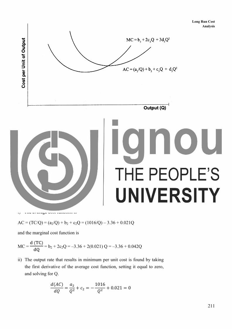
211

Long Run Cost

Analysis

An example of using estimated cost function:

Using the output-cost data of a chemical firm, the following total cost

function was estimated using quadratic function:

TC = 1016 – 3.36Q + 0.021Q2

a) Determine average and marginal cost functions.

b) Determine the output rate that will minimize average cost and the per unit

cost at that rate of output.

c) The firm proposed a new plant to produce nitrogen. The current market

price of this fertilizer is Rs 5.50 per unit of output and is expected to

remain at that level for the foreseeable future. Should the plant be built?

i) The average cost function is

AC = (TC/Q) = (a2/Q) + b2 + c2Q = (1016/Q) – 3.36 + 0.021Q

and the marginal cost function is

MC = �������

= b2 + 2c2Q = –3.36 + 2(0.021) Q = –3.36 + 0.042Q

ii) The output rate that results in minimum per unit cost is found by taking

the first derivative of the average cost function, setting it equal to zero,

and solving for Q.

�������

����� � �� � �

1016�� � 0.021 � 0

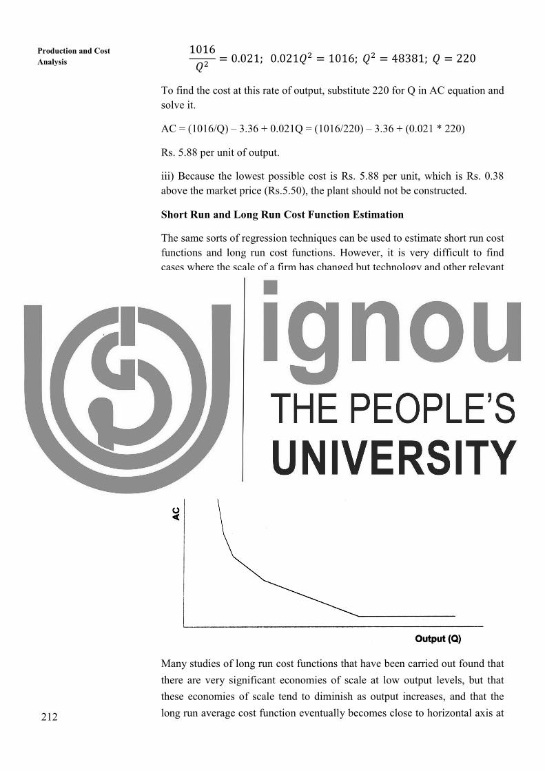
212

Production and Cost

Analysis 1016�� � 0.021; 0.021�� � 1016;�� � 48381; � � 220

To find the cost at this rate of output, substitute 220 for Q in AC equation and

solve it.

AC = (1016/Q) – 3.36 + 0.021Q = (1016/220) – 3.36 + (0.021 * 220)

Rs. 5.88 per unit of output.

iii) Because the lowest possible cost is Rs. 5.88 per unit, which is Rs. 0.38

above the market price (Rs.5.50), the plant should not be constructed.

Short Run and Long Run Cost Function Estimation

The same sorts of regression techniques can be used to estimate short run cost

functions and long run cost functions. However, it is very difficult to find

cases where the scale of a firm has changed but technology and other relevant

factors have remained constant. Thus, it is hard to use time series data to

estimate long run cost functions. Generally, regression analysis based on

cross section data has been used instead. Specially, a sample of firms of

various sizes is chosen, and a firm’s TC is regressed on its output, as well as

other independent variables, such as regional differences in wage rates or

other input prices.

Figure 9.7: Typical Long Run Average Cost Curve

Many studies of long run cost functions that have been carried out found that

there are very significant economies of scale at low output levels, but that

these economies of scale tend to diminish as output increases, and that the

long run average cost function eventually becomes close to horizontal axis at

213

Long Run Cost

Analysis high output levels. Therefore, in contrast to the U-shaped curve in Figure 9.1,

which is often postulated in micro economic theory, the long run average

cost curve tends to be L-shaped, as shown in Figure 9.7.

Problems in Estimation of Cost Function

We confront certain problems while attempting to derive empirical cost

functions from economic data. Some of these problems are briefly discussed

below.

1. In collecting cost and output data we must be certain that they are

properly paired. That is, the cost data applicable to the corresponding

data on output.

2. We must also try to obtain data on cost and output during a time

period when the output has been produced at relatively even rate.

If for example, a month is chosen as the relevant time period over

which the variables are measured, it would not be desirable to have

wide weekly fluctuations in the rate of output. The monthly data in

such a case would represent an average output rate that could

disguise the true cost- output relationship. Not only should the

output rate be uniform, but it also should be a rate to which the firm

is fully adjusted. Furthermore, there should be no disruptions in the

output due to external factors such as power failures, delays in

receiving necessary supplies, etc. To generate the data necessary for

a meaningful statistical analysis, the observations must include a wide

range of rates of output. Observing cost-output data for the last 24

months, when the rate of output was the same each month, would

provide little information concerning the appropriate cost function.

3. The cost data is normally collected and recorded by accountants for

their own purposes and in a manner that it makes the information

less than perfect from the perspective of economic analysis. While

collecting historical data on cost, care must be taken to ensure that all

explicit as well as implicit costs have been properly taken into

account, and that all the costs are properly identified by time period in

which they were incurred.

4. For situations in which more than one product is being produced with

given productive factors, it may not be possible to separate costs

according to output in a meaningful way. One simple approach of

allocating costs among various products is based on the relative

proportion of each product in the total output. However, this may not

always accurately reflect the cost appropriate to each output.

214

Production and Cost

Analysis 5. Since prices change over time, any money value cost would therefore

relate partly to output changes and partly to price changes. In order to

estimate the cost-output relationship, the impact of price change on

cost needs to be eliminated by deflating the cost data by price indices.

Wages and equipment price indices are readily available and

frequently used to ‘deflate’ the money cost.

6. Finally, there is a problem of choosing the functional form of equation

or curve that would fit the data best. The usefulness of any cost

function for practical application depends, to a large extent, on

appropriateness of the functional form chosen. There are three

functional forms of cost functions, which are popular, viz., linear,

quadratic and cubic. The choice of a particular function depends upon

the correspondence of the economic properties of the data to the

mathematical properties of the alternative hypotheses of total cost

function.

The accounting and engineering methods are more appropriate than the

econometric method for estimating the cost function at the firm level, while

the econometric method is more suitable for estimating the cost function at

the industry or national level. There has been a growing application of the

econometric method at the macro level and there are good prospects for its

use even at the micro level. However, it must be understood that the three

approaches discussed above are not competitive, but are rather

complementary to each other. They supplement each other. The choice of a

method therefore depends upon the purpose of study, time and expense

considerations.

9.8 EMPIRICAL ESTIMATES OF COST

FUNCTION

A number of studies using time series and cross-section data have been

conducted to estimate short run and long run cost behavior of various

industries. Table 9.1 lists a number of well-known studies estimating short

run average and marginal cost curves. These and many other studies point

one conclusion: in the short run a linear total variable cost function with

constant marginal cost is the relationship that appears to describe best the

actual cost conditions over the “normal” range of production. U-shaped

average cost (AC) and marginal cost (MC) curves have been found, but are

less prevalent than one might expect.

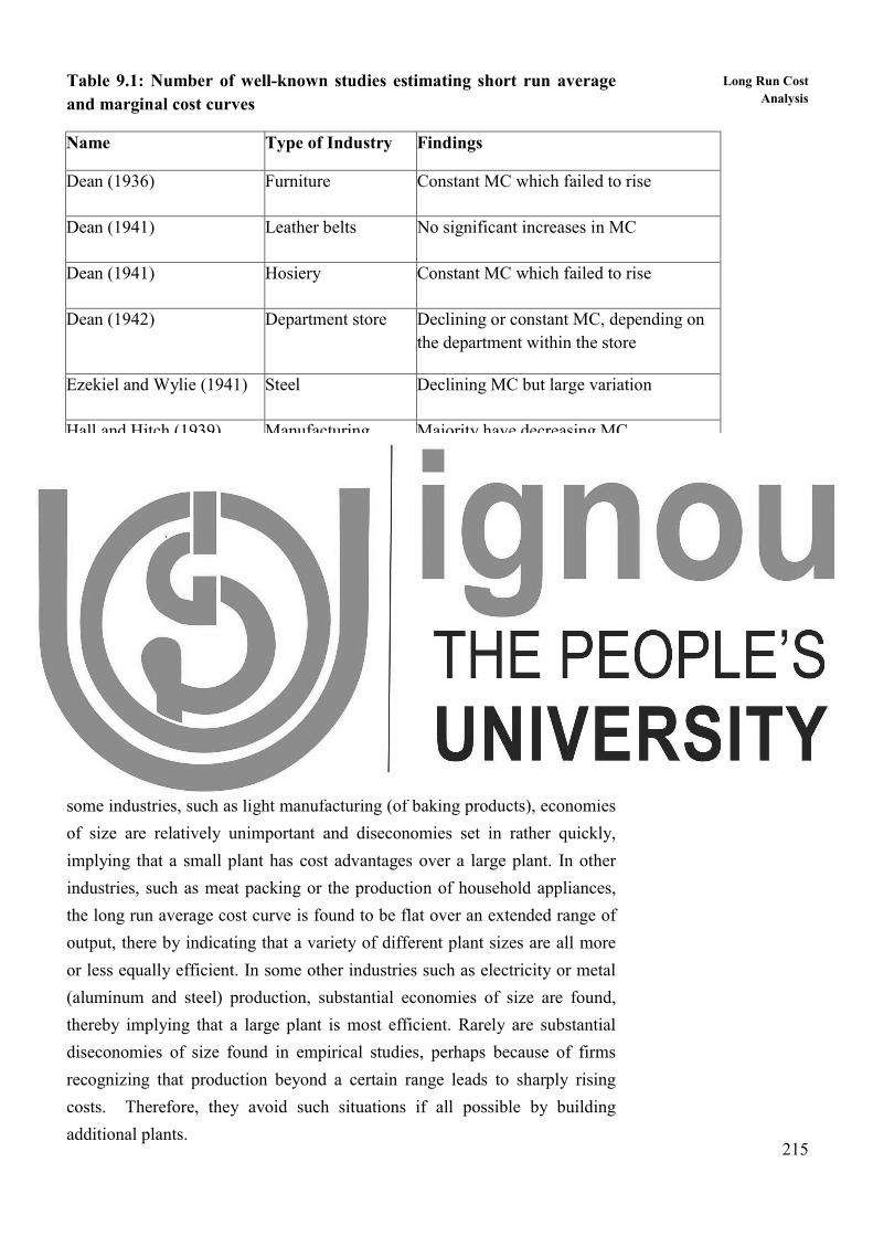
215

Long Run Cost

Analysis Table 9.1: Number of well-known studies estimating short run average

and marginal cost curves

Name Type of Industry Findings

Dean (1936) Furniture Constant MC which failed to rise

Dean (1941) Leather belts No significant increases in MC

Dean (1941) Hosiery Constant MC which failed to rise

Dean (1942) Department store Declining or constant MC, depending on

the department within the store

Ezekiel and Wylie (1941) Steel Declining MC but large variation

Hall and Hitch (1939) Manufacturing Majority have decreasing MC

Johnston (1960) Electricity, multi

product function

food processing

“Direct” cost is a linear function of output,

and MC is constant

Johnston (1960) Electricity Average total cost falls, then flattens,

tending toward constant MC up to

capacity

Mansfield and Wein (1958) Railways Constant MC

Yntema (1940) Steel Constant MC

Source: A.A. Walters, “Production and Cost Functions: An Econometric Survey”, Econometrica, January-

February 1963, PP.49-54

Table 9.2 lists a number of well known, long run average cost studies. In

some industries, such as light manufacturing (of baking products), economies

of size are relatively unimportant and diseconomies set in rather quickly,

implying that a small plant has cost advantages over a large plant. In other

industries, such as meat packing or the production of household appliances,

the long run average cost curve is found to be flat over an extended range of

output, there by indicating that a variety of different plant sizes are all more

or less equally efficient. In some other industries such as electricity or metal

(aluminum and steel) production, substantial economies of size are found,

thereby implying that a large plant is most efficient. Rarely are substantial

diseconomies of size found in empirical studies, perhaps because of firms

recognizing that production beyond a certain range leads to sharply rising

costs. Therefore, they avoid such situations if all possible by building

additional plants.

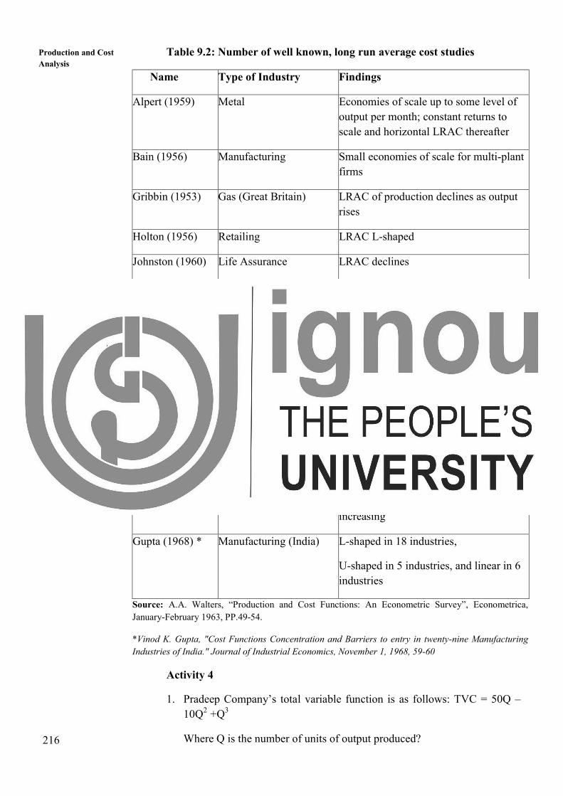
216

Production and Cost

Analysis Table 9.2: Number of well known, long run average cost studies

Name Type of Industry Findings

Alpert (1959) Metal Economies of scale up to some level of

output per month; constant returns to

scale and horizontal LRAC thereafter

Bain (1956) Manufacturing Small economies of scale for multi-plant

firms

Gribbin (1953) Gas (Great Britain) LRAC of production declines as output

rises

Holton (1956) Retailing LRAC L-shaped

Johnston (1960) Life Assurance LRAC declines

Johnston (1960) Road passenger transport

(Great Britain)

LRAC either falling or constant

Johnston (1960) Electricity (Great Britain) LRAC of production declines as output

rises

Lomax (1951) Gas (Great Britain) LRAC of production declines as output

rises

Lomax (1952) Electricity (Great Britain) LRAC of production declines as output

rises

Moore (1959) Manufacturing Economies of scale prevail quite

generally

Nerlove (1961) Electricity (U.S.) LRAC (excluding transmission costs)

declines and then shows signs of

increasing

Gupta (1968) * Manufacturing (India) L-shaped in 18 industries,

U-shaped in 5 industries, and linear in 6

industries

Source: A.A. Walters, “Production and Cost Functions: An Econometric Survey”, Econometrica,

January-February 1963, PP.49-54.

*Vinod K. Gupta, "Cost Functions Concentration and Barriers to entry in twenty-nine Manufacturing

Industries of India." Journal of Industrial Economics, November 1, 1968, 59-60

Activity 4

1. Pradeep Company’s total variable function is as follows: TVC = 50Q –

10Q2 +Q

3

Where Q is the number of units of output produced?

217

Long Run Cost

Analysis a) What is the output level where marginal cost is a minimum?

b) What is the output level where average variable cost is a minimum?

c) What is the value of average variable cost and marginal cost at the

output specified in the answer to part (b)?

……………………………………………………………………………

……………………………………………………………………………

……………………………………………………………………………

……………………………………………………………………………

……………………………………………………………………………

2. How would you reconcile the findings of Yntena with those of Ezekiel and

Wylie?

……………………………………………………………………………

……………………………………………………………………………

……………………………………………………………………………

……………………………………………………………………………

……………………………………………………………………………

3. How would you explain the findings of Johnston (Electricity) in short run

and long run?

……………………………………………………………………………

……………………………………………………………………………

……………………………………………………………………………

……………………………………………………………………………

……………………………………………………………………………

4. Production is related to costs. In fact, cost function can be derived from

estimated production function. In view of empirical determination of

production function, can you think of some limitations of statistical

analysis relating to cost function?

……………………………………………………………………………

……………………………………………………………………………

……………………………………………………………………………

……………………………………………………………………………

……………………………………………………………………………

5. Despite the above limitations listed by you, an estimated cost function is

useful to a manager. Can you think of some points to support this

contention?

218

Production and Cost

Analysis ……………………………………………………………………………

……………………………………………………………………………

……………………………………………………………………………

……………………………………………………………………………

……………………………………………………………………………

6. Some empirical studies have suggested that the marginal cost function is

approximately horizontal, but conventional cost theory suggests that the

marginal cost curve is U-shaped. Provide an explanation for this apparent

inconsistency.

……………………………………………………………………………

……………………………………………………………………………

……………………………………………………………………………

……………………………………………………………………………

……………………………………………………………………………

7. The ABC Manufacturing Company’s short-run average cost function in

the year 2000 is AC=3+4Q

Where AC is the firm’s average cost (in Rs. per unit of the product), and Q is

the output rate.

a) Obtain the firm's short-run total cost function.

b) Does the firm have any fixed costs? Explain.

c) If the price of the firm’s product is Rs. 3 per unit, is the firm making

profits or losses? Explain.

d) Derive the firm's marginal cost function.

………………………………………………………………………………

………………………………………………………………………………

………………………………………………………………………………

………………………………………………………………………………

………………………………………………………………………………

9.9 MANAGERIAL USES OF COST FUNCTION

The estimated cost function can help managers to take meaningful decisions

with regard to:

1. determination of optimum plant size,

2. determination of optimum output for a given plant, and

219

Long Run Cost

Analysis 3. determination of a firm’s supply curve.

The optimum plant size, as discussed earlier, is defined in terms of minimum

costs per unit of output. In other words, an optimum plant is given by that

value of K (plant size) for which the average cost is minimum. If the long

run total cost curve is a cubic function, the resultant long run average cost

curve will be a conventional U-shaped curve. The plant level at which the

long run average cost is minimum will be of optimum size.

For a given plant, the optimum output level will be achieved at a point where

the average cost is the least. This condition can be easily verified from the

short run total cost function.

The level of output that a firm would like to supply to the market will depend

on the price that can charge for its product. In other words, a firm’s supply is

a positive function of the product price. To get the firm’s supply schedule,

one needs to know the firm's cost function and its objectives.

Activity 5

1. Can you list some more managerial uses of cost function other than given

in section 9.9?

………………………………………………………………………………

………………………………………………………………………………

………………………………………………………………………………

………………………………………………………………………………

………………………………………………………………………………

9.10 SUMMARY

In the long run, all inputs to the production process are variable. Thus, in the

long run, total costs are identical to variable costs. The long run average cost

function shows the minimum cost for each output level when a desired scale

of plant can be built. The long run average cost curve is important to

managers because it shows the extent to which larger plants have cost

advantages over smaller ones. Economies or diseconomies of scale arise

either due to the internal factors pertaining to the expansion of output by a

firm, or due to the external factors such as industry expansion. In contrast,

economies of scope result from product diversification. Thus, the scale-

economies have reference to an increase in volume of production, whereas

the scope-economies have reference to an improvement in the variety of

products from the existing plant and equipment.

We have also discussed three forms of cost functions viz. linear cost function,

quadratic cost function, and cubic cost function and their empirical estimates.

Though, empirical estimates of both production functions and cost functions

220

Production and Cost

Analysis have a lot of use for managerial decision making. There are conceptual and

statistical problems in estimating such functions. But we understand that it

will be sufficient for the manager if he knows how to interpret the estimates

based on empirical research in her/his decision-making process.

9.11 SELF ASSESSMENT QUESTIONS

1. Explain the various economies of scale?

2. Explain the determinants of cost function?

3. Explain the econometric method of estimating cost function? Why is this

method more popular than the other two methods (accounting and

engineering) estimation costs?

4. What are the common problems you encounter while attempting to derive

empirical cost functions from economic data?

5. The total cost function for a manufacturing firm is estimated as

C=128+6Q+2Q2

Determine the optimum level of output Q to be produced?

6. Suppose that for a XYZ corporation’s total cost function is as follows

TC=300+3Q+0.02Q2

Where TC is the total cost, Q is the output.

a. What is the corresponding fixed cost function, average fixed cost

function, and variable cost function, average variable cost function?

b. Calculate the average total cost function and marginal cost function.

7. Based on a consulting economist’s report, the total and marginal cost

functions for an ABC company are

TC = 200 + 5Q – 0.04Q2 + 0.001Q

3

MC = 5 – 0.08Q + 0.003Q2

The president of the company decides that knowing only these equations

is inadequate for decision making. You have been directed to do the

following.

a. Determine the level of fixed cost (if any) and equations for average

total cost, average variable cost, and average fixed cost.

b. Determine the rate of output that results in minimum average variable

cost.

c. If fixed costs increase to ` 500, what output rate will result in

minimum average variable cost?

8. Given the total cost function for Laxmi Enterprises Co.

TC = 100Q – 3Q2 + 0.1Q

3

221

Long Run Cost

Analysis a. Determine the average cost function and the rate of output that will

minimize average cost.

9. Determine the marginal cost function and the rate of output that will

minimize marginal cost.

9.12 FURTHER READINGS

Adhikary, M. (1987). Managerial Economics (3rd

ed.).Khosla Publishers,

Delhi.

Maddala, G. S., & Miller, E. M. (1989). Micro Economics: Theory and

Applications. McGraw-Hill, NewYork.

Maurice, S. C., Smithson, C. W., & Thomas, C. R.(2001). Managerial

Economics: Applied Microeconomics for Decision Making. McGraw- Hill

Publishing.

Mote, V. L., Paul, S., & Gupta, G. S. (2016). Managerial Economics:

Concepts and Cases. Tata McGraw-Hill, New Delhi.

Dholakia, R., & Oza, A. N. (1996). Microeconomics for Management

Students. Oxford University Press, Delhi.

Lewis, W.C., Jain, S. K., & Peterson, H. C. (2005). Managerial Economics

(4th

ed.). Pearson.