Embed Size (px)
Citation preview

Model Identification
with Application to Building Control and Fault Detection
by
- Peter Ross Armstrong
B.S. Engineering Design and Economic EvaluationUniversity of Colorado (1974)
M.S. Mechanical EngineeringColorado State University (1980)
Submitted to the Department of Architecturein partial fulfillment of the requirements for the degree of
Doctor of Philosophy in Architecture: Building Technology
at the
Massachusetts Institute of Technology MASSACHUSETTS INS7MTUTOF TECHNOLOGY
September 2004
OCT 2 0 20040 2004 Massachusetts Institute of Technology
All rights reserved LIBRARIES
ROTCH1)Signature of Author...,-, ....... ....................
Department *of*ArchitectureJune 1, 2004
C ertified by ......... .... ..... ...........................................
Leslie K. NorfordProfessor of Building Technology, Department of Architecture
Thesis Supervisor
C ertified by.... ......................................
Steven B. LeebAssociate Professor of Electrical Engineering and Computer Science
Thesis Supervisor
A ccepted by..... .......................................
Stanford AndersonChairman, Committee on Graduate Students
Head, Department of Architecture

THESIS COMMITTEE
Leslie K. Norford, Professor of Building Technology, Department of Architecture
Steven B. Leeb, Associate Professor of Electrical Engineering and Computer Science
James L. Kirtley, Professor of Electrical Engineering and Computer Science

Model Identification with Application to Building Control and Fault Detectionby
Peter Ross Armstrong
Submitted to the Department of Architecture on June 1, 2004, in partial fulfillment of therequirements for the degree of Doctor of Philosophy in Architecture: Building Technology
Abstract:Motivated by the high speed of real-time data acquisition, computational power, and low cost ofgeneric PCs and embedded-PCs running Linux, this thesis addresses new methods and approaches tofault detection, model identification, and control.
Fault detection. A series of faults was introduced into a 3-Ton roof-top air-conditioning unit (RTU).Supply and condenser fan imbalance were detected by changes in amplitude spectrum of real powerresulting from the interaction of impeller rotation and the dominant chassis vibration mode. Ingestionof liquid refrigerant by the compressor was identified by detecting power and reactive powertransients during compressor starts. An adaptive ARX(5) model was used to detect ingestion duringsteady compressor operation. Compressor valve or seal leakage were detected by a change in theleakage parameter of a simple evaporator-compressor-condenser model that explains the rise incompressor load from 0.25 to .5 seconds after compressor start, i.e. as shaft speed rises from about50% to 90% of synchronous speed. Refrigerant undercharge was also detected by changes in starttransient shape. Overcharge was detected by steady state compressor power and reduced evaporatorand condenser air flow were detected by steady state power draw of the respective fan motors.
Model Identification. On-line models are useful for control as well as fault detection. Model-basedcontrol of building loads requires a valid plant model and identification of such a model for a specificbuilding or zone is a non-trivial inverse problem. The thesis develops three advances in the thermaldiffusion inverse problem. Two involve thermodynamic constraints. The problem is first reformu-lated in such a way that the constraint on temperature coefficients becomes implicit and the problemmay still be solved as an unconstrained linear least squares problem. To enforce the constraint onsystem eigenvalues, the problem is formulated as an unconstrained mixed (linear and non-linear)least-squares problem, which is easier to solve than the corresponding problem with linear objectivefunction and non-linear constraints. The (usually unfounded) assumption on which the normalequations are based-that observations of the independent variables are error free-is relaxed at thecost of one more non-linear term. The resulting model coefficients are valid for predicting heat rategiven zone temperature as well as for predicting zone temperature given heat rate.
Control. Three important control applications involving transient zone thermal response are HVACcurtailment, optimal start, and night precooling. A general framework for model-based control ofzone and whole-building operation is developed. Optimal precooling under time-of-use rates isformulated to solve the optimal fan operation sequence using a one-day control horizon with hourlytime steps. Energy and demand cost savings are presented.
Thesis Supervisors:Leslie K. Norford, Professor of Building Technology, Department of ArchitectureSteven B. Leeb, Associate Professor of Electrical Engineering and Computer Science

Acknowledgements
This research was sponsored by the California Energy Commission under contract number 400-99-011 with additional support from The Grainger Foundation, the U.S. Navy's ONR Control Challenge,National Science Foundation, and Talking Lights, LLC.
I am ever indebted for the unwavering support and confidence of my co-advisors, Les Norford andSteve Leeb. Professor James Kirtley patiently provided useful input as reader in this last year.
Without site support a field monitoring project can't even get off the ground. This was provided forthe RTU fault detection testing by Jim Braun, Haoron Li, and Frank Lee of Purdue Ray HerrickLaboratory, and in the East Los Angeles County test buildings, with incredible patience anddedication, by Ron Mohr of Internal Services Division, Energy Group. It is a pleasure to thank againmy Russian collaborator, Boris Nekrasov, and his staff Denis Tishchenko and Rashid Muxharlamov.
MIT project colleagues, Kwanduk Lee, Rogelio Palomera, and Rob Cox were always available to talkshop; Chris Laughmen packed in (and unpacked... and repacked) tools, equipment and computers forcountably infinite field trips with gay abandon...and introduced me to glass lab.
My fellow Building Technology students have provided exceptional camaraderie; among the manywho have acted as sounding boards I especially thank Henry Spindler.
For stress relief, Dwight, John, Bill, Bob, Cory, Sean, Bashar, Mike and Fran of the sailing program.
For encouraging this mid-career venture I thank PNNL colleagues Michael Kintner-Meyer, MikeBrambley, Srinivas Katipamula, Rob Pratt, John Schmelzer and Sriram Somasundaram. SteveShankle has, in addition, provided the invaluable conduit to computing resources and administrativesupport and maintained continuity with the mothership throughout my educational leave from PNNL.
For being mentors: Robert Bushnell, Byron Winn, Frank deWinter, John Seem and Bill Currie.
For financial and moral support Joan Sandgren Bridges and Art Smith, Mother and Dad.
For additional moral support, Liz, Martha, Rob and Marcia, and my far-flung nieces and nephews.
For their patience and love, Abigail, Ford and Jack
To all those I have forgotten to thank in these last minutes of writing.. .and
To all those who didn't interfere.

Contents
Chapter 1I Introduction ........................................................................................................................... 7
1.1 Industry Trends/M otivation....................................................................................................... 7
1.2 Technical Background................................................................................................................. 7
1.3 O rganization ..............................................................................................................................-- 9
Chapter 2 Fault D etection in H VA C Plants ....................................................................................... 10
2.1 Previous Research...................................................................................................................... 11
2.2 Fault D etection Tests ................................................................................................................. 11
2.3 Im plem entation and A pplication ........................................................................................... 34
2.4 Sum m ary and D iscussion ...................................................................................................... 36
Chapter 3 Identification of Building Therm al Response .................................................................. 41
3.1 M otivation .......................................................................-....... -------................................. 41
3.2 Previous W ork ........................................................................................................................... 42
3.3 M odel Synthesis ........................................................................................................................ 46
3.4 Test Room Results..................................................................................................................... 53
3.5 ISD and ECC Test Results......................................................................................................... 68
3.6 Zubkova Test Results ................................................................................................................ 73
3.7 Sum m ary.................................................................................... . ---- .. . ---.................. 79
Chapter 4 O ptim al U se of Building Therm al Capacitance ............................................................... 80
4.1 Control Function D escriptions................................................................................................ 80
4.2 Previous W ork ........................................................................................................................... 85
4.3 Experim ental D em onstration of Peak Shifting Potential....................................................... 86
4.4 Sim ulation.................................................................................................................................. 96
4.5 Results for ISD Building Driven by LA TM Y .......................................................................... 99
4.6 Sum m ary ........... ....................................................................................... ....... 103
Chapter 5 Conclusion......................................................................................................................... 104
5.1 Thesis A ccom plishm ents ......................................................................................................... 104
5.2 Future Research ..................................................................-----..... . -... ---------------.................... 106
References ............... .................................................................................................. 104

AppendicesA ppendix A : M otor D ata....................................................................................................................118A ppendix B . Test Sum m ary ............................................................................................................... 119Appendix C. Bypass Valve Flow-Pressure Test................................................................................. 121Appendix D. Transient Evaporator-Compressor-Condenser Model.................................................. 122Appendix E. LEES Test Zones: Materials, Construction.................................................................. 125Appendix F. ISD Building D escription .............................................................................................. 126Appendix G. Zubkova Building: Materials, Construction, and Thermal Properties......................... 132A ppendix H . M odel Canonical Form s...............................................................................................135Appendix I. Script for Model Identification with Constrained Roots ............................................... 136Appendix J. Model Identification by Ordinary and Hybrid Least Squares ....................................... 138Appendix K. Fragment of data LEES oct.txt for input to aggLEES9.m .......................................... 143Appendix L. "Why It Works" and Relation of Hybrid Method to TLS............................................ 144

Chapter 1 Introduction
Building costs are generally broken down into the broad areas of operation and maintenance (O&M),
capital cost (amortized principal plus interest), and taxes. Operational costs include utilities and
operations labor. Maintenance costs include labor, parts and materials. Operation and maintenance
costs are usually lumped together because the building owner has some measure of control such as
investing in efficiency or replacing old equipment. For most buildings, O&M represents the largest
share of ownership costs.
1.1 Industry Trends/MotivationBecause of the owner's special interest in O&M costs and associated investment opportunities, the
industry-wide trends in O&M bear further scrutiny.
First, the costs of gas and electricity, despite the optimistic predictions of deregulation proponents,have not on average and in terms of constant dollars, come down. Meanwhile volatility has definitely
gone up. Moreover, there is an increasing recognition that one's energy bill is not the complete
picture and that there are significant external costs of waste disposal, resource depletion, land use,pollution and climate change associated with energy use.
Second, in the maintenance arena the trend to outsource maintenance services seems to be following
an inexorable asymptotic path to 100% outsourcing. This means that the maintenance provider is
motivated to minimize downtime and complaints and keep maintenance costs low but has little or no
incentive to maintain or improve energy efficiency. In addition, there is often little or no staff
continuity in HIVAC maintenance for a given building. A given mechanic's responsibility is a
constantly changing pool of buildings. It is ironic that efforts to allocate mechanics optimally among
buildings may actually increase costs in the long-term because needed maintenance is forgotten,faults are misdiagnosed, the knowledge of each building's quirks is lost, and unnecessary repairs are
made while necessary repairs are overlooked.
Third, there is a trend toward ubiquitous computing and digital communication in both the operations
and maintenance arenas that are associated, again, with peculiar ironies. Operators and building
mechanics now have computers to "help" with their work but often the computer applications simply
translate the former pneumatic, analog, or paper and pencil systems to software without any real
improvement in efficiency. Too alarmingly often there are substantial reductions in understanding
and sense of ownership. Fortunately, the recognition that "computers should do the things that
computers do well" is slowly emerging. In the context of this thesis, these things are: fast
communication, continuous monitoring, sophisticated analysis, optimization, acquisition and use of
vast data records and, when necessary, convenient access by humans to that data.
1.2 Technical BackgroundThe first two trends are clearly adverse. The third seems to be a mixed blessing which might, if
properly applied, give some relief from the first two. Our goal then is to address two O&M problems
that really can benefit from sophisticated on-line analysis. These are Fault Detection and Diagnosis
(FDD) and control of HVAC peak loads.

There are many O&M tasks that can be made more efficient and less tedious by application of oneform or another of computer technology. The transition generally benefits from standardization andthoughtful software engineering but does not require great sophistication (such concepts as artificialintelligence or self-configuration) in most cases. Two exceptions that have held much of the buildingresearch community's interest in recent years are optimal control of transient thermal conditions andon-line fault detection and diagnosis (FDD).
Control and FDD have more in common than first (computer-centricity) meets the eye. In eachactivity there are important roles to be played by plant-specific models.
Model-based FDD and model-based control can take many forms. For example, fault detection canstart by comparing the response given by the detailed simulation of a system (driven by the measuredexcitations that also drive the real system) with the measured response of the real system. Variousresponses may be closely or remotely related to various faults. Detection may involve little or muchuncertainty. The control application raises similar questions of model type. The detailed, physics-based simulation is one extreme. At the other extreme, the model may be completely non-physical,e.g. ANN or statistics-based, or somewhere in between.
To be plant-specific often means to be adaptive and autonomous. And it often means a model that isidentified or updated on-line. There may or may not be human initiation or intervention, e.g. as in thebuilding commissioning process.
Thus our two applications of interest, FDD and control of HVAC peak loads, are bound by twocommon requirements: the need for powerful, standardized, low cost computing resources, the needfor large amounts of data, and the need for reliable, plant-specific models.
The computing resources are at hand. The presumed platform is the ubiquitous PC because it has theright hardware (powerful CPU, mass storage, DMA, Ethernet and various other 10) , software (Linuxand Octave), and is incredibly cheap ($200 single-board computer).
The need for large amounts of data is partly answered by the computer/network resources. However,obtaining sufficiently detailed data in a useful form can be a daunting task. One recent and highlymotivating advance is the non-intrusive load monitor (NILM).
A non-intrusive load monitor (NILM) identifies individual loads by sampling voltage and current athigh rates and reducing the resulting start transients or harmonic content to concise "signatures"(Leeb 1992, Shaw et al 1998, Laughman et al 2003). The NILM's traditional role of end-usemetering in buildings is needed by the HVAC peak control application because room temperaturesrespond to specific electrical loads (i.e. the light and plug loads of the room in question) as well as toweather and heating and cooling stream inputs. But, almost incidentally, the NILM is also extremelywell suited to the tasks of measuring and analyzing electrical signals with high information contentthat may be useful in fault detection. Use of the NILM for fault detection and diagnosis (FDD) isimportant because 1) it complements other FDD schemes that are based on thermo-fluid sensors andanalyses and 2) it is minimally intrusive (one measuring point in the relatively protected confines ofthe control panel) and therefore inherently reliable.

1.3 OrganizationGiven the computing and data collection resources of the existing NILM platform, there are three
pieces left to the puzzle and they are addressed in Chapters 2, 3 and 4 of this thesis.
Chapter 2 addressesfault detection. A series of faults was introduced into a 3-Ton roof-top air-conditioning unit (RTU). The NILM was used to record start transients and the power signals during
steady operation. Chapter 2 presents the results analyzing these signals to detect supply and
condenser fan imbalance, ingestion of liquid refrigerant by the compressor, compressor valve or sealleakage, refrigerant overcharge, and reduced evaporator and condenser air flow.
The compressor valve or seal leakage fault is detected by a change in the leakage parameter of a
simple evaporator-compressor-condenser model that explains the rise in compressor load. The
detection of liquid ingestion during steady operation is accomplished by a weighted-mean of k-step
ahead innovations generated at each time step. The k-step-ahead forecasts are generated by a new
transient event detector (TED) based on a recursively updated, exponentially-weighted ARX model.
Model Identification is the subject of Chapter 3 and parts of Chapter 2. The aggregate load process
model, described in Chapter 2, is continuosly updated on line for optimal transient detection
sensitivity. A refrigeration loop transient model, also developed in Chapter 2, explains start transient
innovations for the vapor bybass fault. The need for such a plant-specific refrigeration loop model in
the RTU FDD application is not especially onerous because RTU's are mass produced and the
appropriate model would be loaded into flash-RAM at the factory and whenever a field upgrade is
made. For control of HVAC peak loads, however, a room or building thermal response model is
needed. Because very few of our buildings are mass produced, every model is different, if not in
form, at least in the parmeter values.
Identification of such a model for a specific building or zone is a non-trivial inverse problem.
Chapter 3 develops three advances in the thermal diffusion inverse problem. Two involve
thermodynamic constraints. The inverse problem is formulated in such a way that the constraint on
temperature coefficients becomes implicit and the problem may still be solved as an unconstrained
linear least squares problem. Solution of this linear problem provides good initial guesses for the
subsequent non-linear formulations. To enforce the constraint on system eigenvalues, the problem is
formulated as an unconstrained mixed (linear and non-linear) least-squares problem, which is easier
to solve than the corresponding linear least squares problem with non-linear constraints. The (usually
unfounded) assumption on which the normal equations are based-that observations of theindependent variables are error free-is relaxed at the cost of one more non-linear term. The
resulting model coefficients are valid for predicting heat rate given zone temperature as well as for
predicting zone temperature given heat rate.
Control is addressed in Chapter 4. Three important control applications involving transient zone
thermal response are HVAC curtailment, optimal start, and night precooling. A general framework
for model-based control of zone and whole-building operation is developed. Curtailment and optimal
start problems are cast as one- or two-variable problems with a final state constraint. Optimal
precooling under time-of-use rates with allowance for zone temperature swings is formulated to solve
for the optimal discrete-time zone temperature sequence. This generally results in 24 variables for a
one-day control horizon with hourly time steps. A suboptimal control in which fan power for night
free cooling has a single gain parameter for each 24-hour horizon is also developed and evaluated.
A literature review is presented at the beginning, and a summary of results at the end, of each chapter.
Overarching conclusions and suggested future research are presented in Chapter 5.

Chapter 2 Fault Detection in HVAC Plants
Hardware and control failures result in aggregate repair costs that are a large fraction of total U.S.HVAC operational costs (Katipamula 2003). Comfort and consequent productivity loss mayrepresent significant additional costs. Unitary equipment appears to be just as susceptible toperformance degradation as built-up systems (Breuker 1998a). Many roof-top unit (RTU) faults goundetected by occupants and maintenance staff. A "wait for complaints" strategy is often taken inspite of its many well known negative side effects. There are two generally accepted paths tocorrecting this situation:
1) test-and-measurement-based preventive maintenance' and2) automated on-line fault detection.
The key to cost-effective on-line fault detection and diagnosis (FDD) is finding the right mix ofsensors and automated analysis for a given target system. Much attention has focused ontemperature-measurement-based fault detection because of low sensor cost (Rossi 1997). However,temperature sensor location is critical; sensors must be installed in specific locations regardless of theresulting susceptibility to harsh environments or damage during inspection and service activities.Consequently, more expensive but less intrusive sensor types, such as pressure and power, may bejustified by improved reliability.
The non-intrusive load monitor (NILM) was developed to identify individual loads by samplingvoltage and current at high rates and reducing the resulting start transients or harmonic content toconcise "signatures" (Leeb 1992, Shaw et al 1998, Laughman et al 2003). In this thesis, loadidentification plays only a small role2. However, because the NILM is extremely well suited to thetasks of measuring and analyzing electrical signals with high information content it provides a veryuseful platform for fault detection. Changes in these signatures can be used to detect, and possiblydiagnose, equipment and component faults associated with roof-top cooling units. Use of the NILM'spower signature analysis (PSA) capabilities for fault detection and diagnosis (FDD) is importantbecause 1) it complements other FDD schemes that are based on thermo-fluid sensors and analysesand 2) it is minimally intrusive (one measuring point in the relatively protected confines of the controlpanel) and therefore inherently reliable.
Results of field tests reported in this chapter show that some RTU thermo-fluid faults can be detectedby PSA alone. Certain mechanical (compressor and fan) faults and most electrical (supply, controls,motor) faults can also be detected. In this chapter, previous research is reviewed and the ways inwhich electrical loads respond to faults (artificially introduced in an operating unit) are characterized.New methods of detecting bypass leakage, fan imbalance, and liquid ingestion faults are describedand fault detection implementation issues are discussed. The methods developed in this chapter canbe extended to other HVAC equipment configurations. In central plant applications a PSA platformwill be installed at each motor control center as a standalone device or, possibly in conjunction withthe model-based control implementations developed in chapters 3 and 4, as part of the control system.
Including such concepts as re-commissioning or continuous commissioning2 In Chapter 3, model identification requires disaggregation of total building power into exterior, interior, andHVAC loads and, in some cases, further disaggregation of HVAC loads into fan, punp and compressor loads.

2.1 Previous ResearchThe frequency of faults in unitary cooling equipment has been assessed from substantial insuranceclaim and service record data bases by Stouppe and Lau (1989) and Breuker and Braun (1998a).Stouppe and Lau (1989) compiled 15,716 failure records and attribute 76% of faults to electricalcomponents, 19% to mechanical and 5% to refrigerant circuit components. Of the electrical failures87% were motor winding failures from deterioration of insulation (vibration, overheating) unbalancedoperation and short cycling (overheating). The reported numbers refer to events; costs of repair werenot published. Rossi and Braun (1993) reviewed various detection and diagnostic methods and later(1997) developed effective rule-based methods.
Rossi (1997) and Breuker and Braun (1997, 1998a, 1998b) applied detection, diagnosis andevaluation methods and performed statistical analyses of detection sensitivity at specific fault levels.Two prototype systems, designated the low-cost system (2 temperature inputs, 5 outputs) and thehigh-performance system (3 inputs, 7 outputs), were developed and fault detection (without excessivefalse alarm rates) was generally found to be effective when capacity and COP dropped by 10 to 20%for five common mechanical faults:
Refrigerant leakage, undercharge or overcharge;Liquid line restriction;Loss of volumetric efficiency (leaky valves, seals);Fouled condenser coil;Dirty supply air filter.
2.2 Fault Detection TestsOf the five faults examined by Rossi and Breuker, NILM detection was attempted for all but theliquid line restriction fault. Purely electrical faults were not tested. Contact erosion and bounce havealready been successfully tested (Shaw 2000). Detection of an unbalanced three-phase voltagecondition (failure of any phase to maintain a preset threshold voltage for a preset number of cycleswhile the other two hold up) is completely straightforward. Three new mechanical faults, rotorimbalance and flooded start and liquid ingestion, were therefore selected for testing. The test unit ispictured in Figure 2.1
Figure 2.1 RTU compartments, from left, for controls, supply fan, compressor/condenser.

The RTU has two fans and a compressor as shown in Figure 2.2. The fans are connected across linesA and C; the compressor is wired as a 3-phase delta load. Nameplate data and stator resistancemeasured in the field are summarized in Figure 2.2Appendix A. Observation of start transients underfault conditions requires a special procedure for each type of fault. Baseline start transients werecollected by starting each motor, letting it run for -5 seconds, and waiting for it to stop spinning aftershutdown. This process was repeated 5 times while the NILM wrote the data to a single file.
Compressor
Supply Condenser
4FFanl FanThermostatic Expansion
Valve '(TXV)
Figure 2.2 Schematic of direct expansion air conditioner.
Evaporator and condenser blockage were artificially introduced by inserting strips of cardboardagainst the heat exchanger inlet face. This achieves a quasi-uniform flow distribution of knownblockage factor. Refrigerant over- and undercharge conditions were achieved by evacuating, thenadding a known mass of refrigerant to obtain the desired level of charge. Leaky valves or seals weremimicked by opening the hot bypass valve a specific amount and making repeated compressor starts.Fan imbalance was artificially introduced by adding small weights of known mass near the rotor tip atone point on the circumference. For the supply fan, binder clips were fastened to a vane from insidethe squirrel cage. For the condenser, a known mass was affixed at the tip of one blade.To detect small changes in an electrical load signal it is essential to suppress the 120Hz componentand consider only the "dc" components of power (P1) and reactive power (Q 1). This is accomplishedby a special digital filter implemented in the NILM software (Leeb 1992, Shaw 2004).
In subsequent sections we show plots of the start trajectories of P1 or QI for each motor load. Repeat-ability of these transients is important to the FDD application. The trajectories are time-shifted andsuperimposed to highlight similarities or differences between repeated transient shapes. Additionalstart transients, recorded after fault introduction, are plotted to show any change. Appendix Bprovides a summary of all the tests performed on the unit.
2.2.1 Short Cycling
Compressor start transients with no pressure relief between starts are shown in Figure 2.3. Starts withpressure relief between are shown in Figure 2.4. Fans were off in both these tests. The compressorcycling frequency of about three starts per minute used during the test is much higher than theshortest cycling frequency of normal operation and is therefore representative of a short-cycling fault.Note that each unit on the time (horizontal ) axis is a 60-Hz half cycle, that is, 1/120 s = 8.333 ms.This time scale, which corresponds to the sampling rate most used in NILM and PSA signal

processing, appears throughout the thesis and consistently denoted by "time index (sampled at120Hz)."
8000,
7000
6000
5000
4000
3000
2000
1000
time (sampled at 120 H-z)
0 20 40 60 80 100 120 140 160 180 200Figure 2.3 Five compressor starts with no pressure relief. The main difference between start traces isthat the final value of P1 (time index >50) increases with successive starts.
8000
7000
6000
5000
4000
3000
2000
1000
time (sampled at 120 Hz)-10001 - ' '
0 20 40 60 80 100 120 140 160 180 200Figure 2.4. Five compressor starts with pressure relief (zero initial head).
2.2.2 Refrigerant Charge
Evaporator and condenser capacity are adversely affected by incorrect refrigerant charge. The system
can be overcharged or undercharged. In either case, excessive portions of the evaporator or
condenser are relegated to sensible, rather than boiling or condensing, modes of heat transfer. With
undercharge there is too much vapor being superheated in the evaporator and desuperheated in the
condenser. With overcharge too much liquid collects in the condenser3 . The TXV can maintain
capacity only at the expense of increased volumetric flow, in the case of undercharge, and increased
pressure rise in both cases. Thus increased compressor power is a symptom of both under- and over-
3 There is also increased danger of liquid ingestion.

charge. In some cases suction pressure will be too high for the TXV to maintain capacity and loss ofcapacity will be an additional symptom, albeit not observable by the PSA.
The increase in compressor power is illustrated in Figure 2.5 for overcharge. With undercharge,however, power does not quickly settle to a steady value. Two start transients representative ofundercharge are compared to the normal start transients in Figure 2.6. Figure 2.7 shows the mean Ptransient for each fault level on one plot and Figure 2.8 shows the phase angle, A, for each of thethree conditions.
7000
6000
5000
4000
3000
2000
1000
0time index (sampled at 120Hz)
-1000 II
0 20 40 60 80 100 120 140 160 180 200Figure 2.5 Compressor start transients: lower traces normal, upper with 20% overcharge.
7000
6000
5000a-c> 4000
3000
. 2000
'ti 1000
0
0 20 40 60 80 100 120 140 160 180 200Figure 2.6 Start transients: lower seven traces normal, upper two traces 20% undercharge. For clarity,only two of the four undercharge traces are shown.

8000
6000-
4000-
2000-
0 --time index (sampled at 120Hz)
0 20 40 60 80 100 120 140 160 180 200Figure 2.7 Real power start transients, mean of repetitions for each fault level: normal charge (solid),20% undercharge (dotted), and 20% overcharge (dashed).
1.6-
1.4
Icet
0.8 ---
0.6-
time index (sampled at 120Hz)0.4 1 1 1 1 I
0 20 40 60 80 100 120 140 160 180 200Figure 2.8 Phase angle start transients, mean of repetitions for each fault level: normal charge (solid),20% undercharge (dotted), and 20% overcharge (dashed).
Detection sensitivity and false alarm rate can be estimated from the small field test samples of meanP1 and Q1. Detection can be based on P, Q, or one of the derived parameters, R = (P2 + Q 2 ), orphase angle, A= tan'(P,Q). The sample mean and variance are listed for each parameter (P, Q, R, A)and each condition (80%, 100% and 120% of normal charge) in Table 2.1. Two of the parameters,power (P) and phase (A), are useful for detection. The estimated population distributions for P and A,both assumed to be Gaussian, are plotted in Figure 2.9 and Figure 2.10.
Sample size is an important factor in detection. One advantage of on-line fault detection is that the
parameters for the no-fault condition can be established with relatively high confidence because, in a
new RTU, there will usually be a large number of observations, n, before a fault occurs and
uncertainty is proportional to n-2. The vertical dashed line in each plot indicates the sample mean for
the no-fault condition. If this mean value were confirmed after many fault-free observations, the
probability that the new mean indicated for one of the fault conditions (based on the indicated number
of post-fault observations) is truly different from the fault-free mean is given by the area under the

distribution minus the area of the tail on the other side of the vertical line. The NILM can beprogrammed to implement standard tests (Wild 2000) for change of sample mean given actual samplesizes for the fault-free and post-fault observations that have accumulated at any given time.
We did not assess in these tests the variation of steady-state compressor power that occurs withoperating conditions. The observed changes in compressor power alone cannot, therefore, beattributed to a particular fault (overcharge versus undercharge) or distinguished from normalvariations in capacity. Discharge-suction pressure difference or condensing and evaporatingtemperatures could be used to normalize for conditions.
Table 2.1 Detection sensitivity for refrigerant undercharge (80%) and overcharge (120%).Charge= 80% 100% 120%
N= 4 7 7Avg(Pss)= 3891 2542 3009sdev(Pss)= 203 97.5 219Avg(Qss)= 2675 2585 2583sdev(Qss)= 24 16.3 22.8Avg(Rss)= 4723 3626 3967sdev(Rss)= 177 74.1 177Avg(Phss)= 0.6033 0.7941 0.7107sdev(Phs)= 0.0219 0.0181 0.0327
4-
03--0
1500 2000 2500 3000 3500 4000 4500 5000P(W)
Figure 2.9 Estimated distributions of steady-state power. Because only a small portion of the tail ofthe 20% overcharge envelope (centered at 3009W) crosses the no-blockage mean (2542W), detectionat 20% overcharge will be almost immediate (~10 starts) once the normal-charge mean has been wellestablished.

25 r
20
15
10-
5-
0.5 0.55 0.6 0.65 0.7 0.75 0.8 0.85 0.9A(rad)
Figure 2.10 Estimated distributions of steady-state phase. Because only a small portion of the tail ofthe 20% overcharge envelope (centered at 0.711 radians) crosses the no-blockage mean (0.794radians), detection at 20% overcharge will be almost immediate (-10 starts) once the normal-chargemean has been well established.
2.2.3 Vapor Bypass (Back-Leakage) Fault
Start transients were recorded (4 repetitions) for the compressor/condenser fan with the vapor bypassvalve closed and two more start transients were recorded with the bypass valve turn open as shownin Figure 2.11. The transients with no bypass are the top two. The amplitude difference when themotor is developing peak torque (0.2-0.5s from initial contact) is much greater than the steady-stateamplitude difference and, moreover, the shapes of the faulty and fault-free start transients aredistinctly different. In contrast, the reactive power shows no such distinct change in response to the
fault. The bypass valve characteristic is documented in Appendix C.
5000
4000
3000
2000
1000-
0-time index (sampled at 120Hz)
-1000 -0 50 100 150 200 250
Figure 2.11 Compressor/condenser active power with bypass leakage (bottom four traces) andwithout (top two traces).
The mechanism for a behavior that is distinctive during the start transient, yet results in little (or no)
change in steady state compressor power, is not obvious. However, it turns out that a simple model,in which evaporator and condenser vapor masses are the only state variables, explains the observed
behavior.

We assume that evaporator and condenser vapor volumes are constant, that leak rate follows a powerlaw', and that the compressor flow rate is smooth, not pulsing, with zero clearance volume. Underthese assumptions, the rate of change in evaporator vapor mass is the rate of evaporation plus theback leakage minus the compressor suction rate, hence the following mass balance equation:
dM ATue-" * + pepC(P-Pe)"-PV
where
V is the effective compressor displacement, in 3 ,o is the compressor shaft speed, rad/s,
Pe = MIVe is the evaporator (suction) vapor density, kg/m3,Pc = Ma/V is the condenser (discharge) vapor density, kg/m3,Pe = Pat(pe), Te = Tat(Pe) are the evaporator pressure and temperature, Pa, OK,Pe = Par(pe), T, = T,.a(Pe) are the condenser pressure and temperature, Pa, *K,AT, = Ta - T is the supply air - refrigerant temperature difference, *K,u, is the effective evaporator conductance, W/m 2_oK,
C,n are the leak parameters with leakage flow modeled as a power law, m3s1 Pa~",ifg(T) = heat of vaporization as a function of temperature, kJ/kg, and.Pa,(p, Tsa(P) are the other saturation properties, Pa, *K.
The corresponding condenser mass balance is
dM CO ATuC = peV _ . "P "C -ppC(P - P)dt 2r ijg(Ta(P))
where
ATc = Tamonb - Tc is the ambient air - refrigerant temperature difference, andu, is the effective condenser conductance.
Compressor power (averaged over one shaft turn) is given by the energy balance'C dM" C(pp P AT uc dMe P ATu,
dt p Pc cC ici) g(T,a,(P)) dt pe ig(Twa(Pe))
Simulated power transients with two different leak levels are shown in Figure 2.126. The MatLabcode for the simulation is listed inFigure 1. Flow-pressure data for bypass valve of type used inback-leakage tests.
4Several flow modes are possible; use of the simple power law is based on Appendix K empirical results.5Energy dissipated by the leak is assumed to add to discharge superheat, which is recognized, but notexplicitly modeled; the ideal gas work is given by: ik _= k _ I _ - Vp (T- = T)21r k- -1 21c
6 The simulated power in both cases is much lower than the measured power because superheating, flow losses,and mechanical losses are not modeled.

Appendix D. With a leak fault, condenser pressure builds more slowly until the vapor reaches the
saturated condition. Evaporator vapor is already saturated so pressure is initially almost constant,thus initial suction density and flow rate are the same for both cases. With similar mass flow rates,less head translates to lower power initially. At steady state, suction flow rate is higher for the faulty
case due to higher evaporator pressure. Despite loss of capacity, with higher flow rate and lower head
there is little change in steady state compressor input power.
10000-
8000-
6000-
S4000-
52000-time index (sampled at 120Hz)
00 50 100 150 200 250
Figure 2.12 Simulated transient compressor power with leak fault (dashed) and no fault.
2.2.4 Flow BlockageOn the air side, reduced flow (blockage or restriction) is one of the main faults of interest. Condenser
fan start transients were measured at three levels of blockage: 0%, 14% and 39% of coil face area.
The compressor was locked out and six to eight repetitions were made at each fault level. Figure 2.13
shows the P1 ,Ql transients for the no-fault case. Figure 2.14 shows the mean P transient for each
fault level on one plot and Figure 2.15 shows the phase angle, A, for each fault level. Figure 2.16
gives the mean static pressure transient for each fault level.
Condenser fan power is a good fault detection criterion because it is normally quite constant. Use of
temperature-rise-based detection, on the other hand, is problematic for the condenser fan blockage
fault. Both inlet and outlet sensors are exposed to the elements. The inlet (ambient) temperature
sensor in particular is susceptible to radiation, icing, and wet-bulb bias type errors.

0 50Condenser fan
100 150 200 250 300 350 400start transients with no blockage, P is larger than Q, 6 reps.
900
800 -
700 -
600 -
500-
400
300 I
200
100
0 1 1 1 1 1
0 50 100 150 200 250 300 350 400Figure 2.14 Condenser fan real power start transients, mean of repetitions for each fault level: 0%blockage (solid), 14% blockage (dotted), and 39% blockage (dashed).
0.8
0.75
0.7
2 0.65to
0.6(D
* 0.550.
0.5
0.45
0.4150 200 250 300 350
1000
800
600
400
200
Figure 2.13
- -
time index (sampled at 120Hz)
time index (sampled at 120Hz)
0 50 100 400

Figure 2.15 Condenser fan phase during start transients, mean of repetitions for each fault level: 0%blockage (solid), 14% blockage (dotted), and 39% blockage (dashed).
The sample mean and variance are listed for each parameter (P, Q, R, A) and each condition (0%,14%, and 39% blockage) in Table 2.2. Only one of the parameters, P, is useful for detecting blockagebecause the other variances are large relative to their change in mean with fault level. The estimatedpopulation distributions for P, assumed to be Gaussian, are plotted in Figure 2.17.

0.5
0.4
0.3
0.2
0.1
0-time index (sampled at 120Hz)
-0 .1111110 50 100 150 200 250 300 350 400
Figure 2.16 Condenser fan pressure start transients, mean of repetitions for each fault level: 0%blockage (solid), 14% blockage (dotted), and 39% blockage (dashed).
Table 2.2 Detection sensitivity for condenser fan blockage.BlockageN=avg(Pss)
sdev(Pss)avg(Qss)
sdev(Qss)avg(Rss)
sdev(Rss)avg(Phss)sdev(Phs)
0% 14%6
3533.17
198.21.39
404.83.15
0.51170.00361
8361.4
2.692001.62
413.12.64
0.50550.00414
39%7
393.72.24
209.21.88
445.81.99
0.48850.00481
0.2
0.15
0.1
0.05
0'340 350 360 370 380 390 400 410
P1(W)Figure 2.17 Estimated distributions of steady-state power. Because only a small portion of the tailof the 14% blockage envelope (centered at 361W) crosses the no-blockage mean, 353W, detection at14% blockage will be almost immediate (-10 starts) once the no-blockage mean has been established.
7 - - --- -- -----

Supply fan start transients were measured with four levels of blockage: 0%, 10%, 50% and 100% ofcoil face area. Six to eight repetitions were made at each fault level. Figure 2.18 and Figure 2.19show one the P1 and Q 1 transient responses for all three fault levels.
2000-
1500-
1000
500-
0-0
Figure 2.18(solid), 10%
1800
1600 -
1400
1200-
1000-
800-
600-
400-
200-
time index (sampled at 120Hz)
50 100 150 200 250 300 350 400Supply fan real power start transients, mean of repetitions for each blockage level: 0%(---), 50% (--), and 100% blockage (- -).
LIIII~ IIIU~A ~~IIIF.JI~LI OL I~~.JI IL)
0 H , , I'"""_ " RUCA k01ICz I L IIU IVI-f
0 50 100 150 200 250 300 350 4Figure 2.19 Supply fan reactive power start transients, mean of repetitions fo0% (solid), 10% (-- ), 50% (--), and 100% blockage (--).
00r each blockage level:
The steady-state sample mean and variance are listed for each parameter (P, Q, R, A) and eachcondition (0%, 10%, 50%, and 100% blockage) in Table 2.3. Two of the parameters, R and A, arenot useful for detecting improper charge because their variances are large relative to the change inmean of R and A with fault level. The other two parameters, P and Q, are useful. The estimatedpopulation distributions for P and Q are plotted in Figure 2.20 and Figure 2.21.
Note that, in contrast to the condenser fan response, supply fan power and reactive power bothdecrease with increasing blockage. This is a consequence of differences in fan curves and the points
on those curves that correspond to the respective no-blockage conditions. Moreover, in the case of

the supply fan, detection of a blockage is best accomplished by testing the hypothesis that both thereactive and real components of steady-state electrical load have deviated from the established no-fault mean values.
Table 2.3 Detection sensitivity for supply fan blockage.BlockageN=
avg(Pss)=sdev(Pss)=avg(Qss)=sdev(Qss)=avg(Rss)=sdev(Rss)=avg(Phss)=sdev(Phs)=
0.06
CO
? 0.04
0 .
0.02
0%8
6626.14374.47936.7
0.5840.0045
10%6
6545.6
4283.27825.6
0.5810.0037
50%6
6006.4
4252.17356.2
0.6170.0035
100%8
4447.5
4232.1
6134.5
0.7630.0104
I I
0 11I400 450 500 550 600 650 700
P1(W)Figure 2.20 Estimated distributions of steddy-state power. Because the 10% blockage envelope,centered at 654W, overlaps the no-blockage mean (662W), it would take several hundred starttransient observations before a 10% blockage could be reliably detected based on P1 alone.
.2
0.15
0.05
/ jI /\ III
I /
/ II /
/ / I
/~/ //
405 410 415 420 425 430 435 440 445 450Q1(VAR)
Figure 2.21 Estimated distributions of steady-state reactive power. Because only a bit of the 10%blockage envelope (centered at 428VAR) crosses the no-blockage mean, 437VAR, detection at 10%blockage will be almost immediate (-10 starts) once the no-blockage mean has been established.
0
From the test results it appears that a 10% blockage can be readily detected. However, variations insystem resistance resulting from air density changes (Armstrong 1983) upstream or downstream ofthe fan and changing damper settings may result in substantial uncertainty in the no-fault means.Further work is needed to understand if the supply fan blockage fault is truly amenable to detectionby power signature analysis alone in the face of such ubiquitous system disturbances.
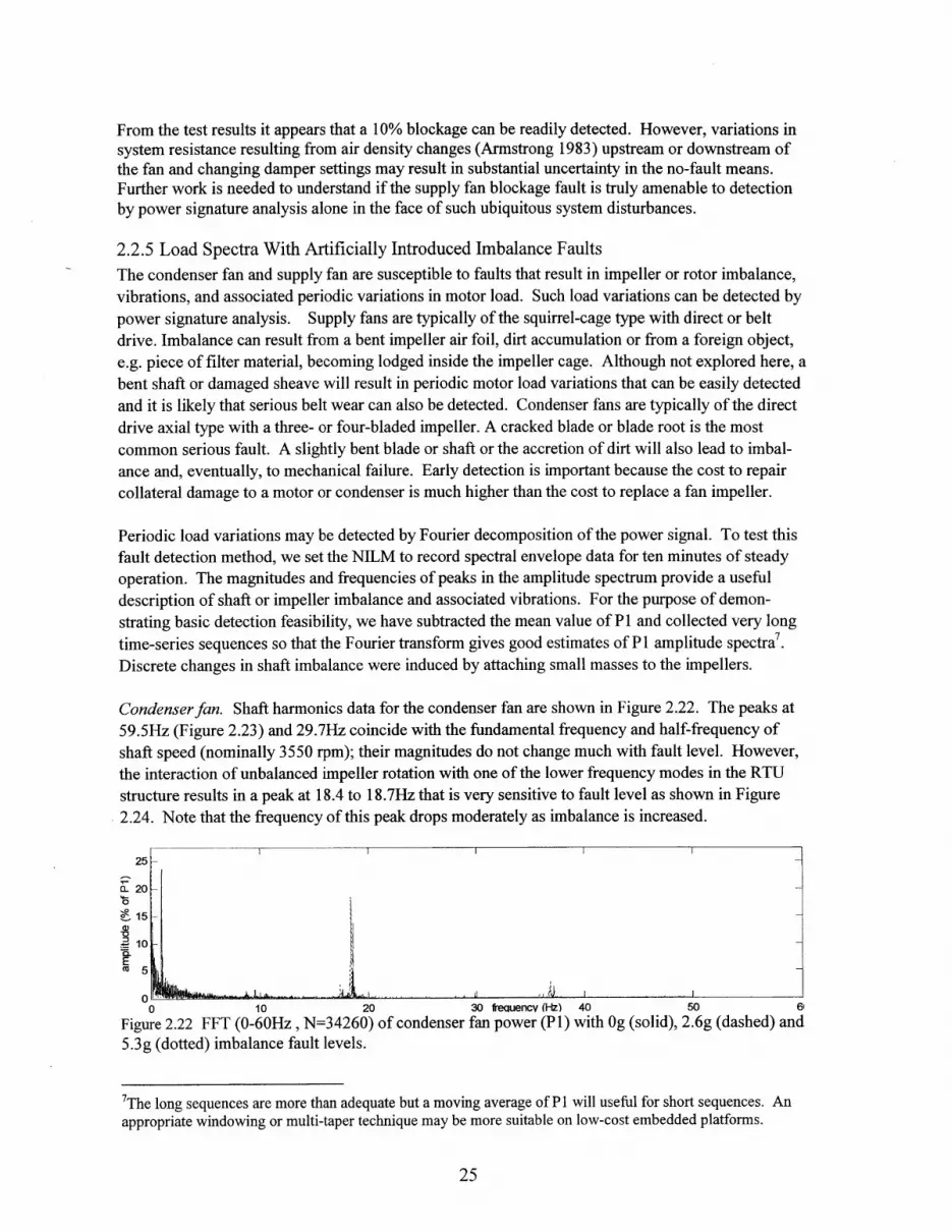
2.2.5 Load Spectra With Artificially Introduced Imbalance Faults
The condenser fan and supply fan are susceptible to faults that result in impeller or rotor imbalance,vibrations, and associated periodic variations in motor load. Such load variations can be detected bypower signature analysis. Supply fans are typically of the squirrel-cage type with direct or beltdrive. Imbalance can result from a bent impeller air foil, dirt accumulation or from a foreign object,e.g. piece of filter material, becoming lodged inside the impeller cage. Although not explored here, abent shaft or damaged sheave will result in periodic motor load variations that can be easily detectedand it is likely that serious belt wear can also be detected. Condenser fans are typically of the directdrive axial type with a three- or four-bladed impeller. A cracked blade or blade root is the mostcommon serious fault. A slightly bent blade or shaft or the accretion of dirt will also lead to imbal-ance and, eventually, to mechanical failure. Early detection is important because the cost to repaircollateral damage to a motor or condenser is much higher than the cost to replace a fan impeller.
Periodic load variations may be detected by Fourier decomposition of the power signal. To test thisfault detection method, we set the NILM to record spectral envelope data for ten minutes of steadyoperation. The magnitudes and frequencies of peaks in the amplitude spectrum provide a usefuldescription of shaft or impeller imbalance and associated vibrations. For the purpose of demon-strating basic detection feasibility, we have subtracted the mean value of P1 and collected very longtime-series sequences so that the Fourier transform gives good estimates of P1 amplitude spectra7.Discrete changes in shaft imbalance were induced by attaching small masses to the impellers.
Condenserfan. Shaft harmonics data for the condenser fan are shown in Figure 2.22. The peaks at59.5Hz (Figure 2.23) and 29.7Hz coincide with the fundamental frequency and half-frequency ofshaft speed (nominally 3550 rpm); their magnitudes do not change much with fault level. However,the interaction of unbalanced impeller rotation with one of the lower frequency modes in the RTUstructure results in a peak at 18.4 to 18.7Hz that is very sensitive to fault level as shown in Figure2.24. Note that the frequency of this peak drops moderately as imbalance is increased.
25-
a. 20-
10 -
5
0 """""60 10 20 30 frecuencv (Hz) 40 50 6
Figure 2.22 FFT (0-60Hz , N=34260) of condenser fan power (P1) with Og (solid), 2.6g (dashed) and5.3g (dotted) imbalance fault levels.
7The long sequences are more than adequate but a moving average of P1 will useful for short sequences. Anappropriate windowing or multi-taper technique may be more suitable on low-cost embedded platforms.

0.0
0.
0.0
59 59.1
Figure 2.23 Detail(dashed) and 5.3g
a.
59.2 59.3 59.4 59.5 f((Hz) 59.6
of the FFT (59-60Hz band) of condenser fan power(dotted) imbalance fault levels.
59.7 59.8 59.9
(P1) with Og (solid), 2.6g
18 18.1 18.2 18.3 18.4
Figure 2.24 Detail of the FFT (18-19Hz band)(dashed) and 5.3g (dotted) imbalance fault lev
18.5 f (Hz) 18.6 18.7 18.8 18.9of condenser fan power (P1I) with Og (solid), 2.6g
Supplyfan. The supply fan motor and impeller are pictured in Figure 2.25.
Figure 2.25 Supply fan accelerometer (PCB on angle bracket) and binder clip impeller weights.
25 -
02-
15
01I x
20 1
10-
5 --
0 L

Shaft harmonics data for the supply fan are shown in Figure 2.26. The peaks at 59.6 Hz and 29.8 Hzcoincide with the fundamental frequency and second harmonic8 of shaft speed (nominally 1770 rpm).As with the condenser fan, the interaction of unbalanced impeller rotation with one of the lowerfrequency modes in the RTU structure results in a peak that is very sensitive to fault level. Figure2.27 shows the peak for fault-free operation at around 19Hz; the frequency of the peak drops to below18.9Hz, and its magnitude increases many times, as fault level is increased.
The results for both fans show that the existence and relative level of imbalance faults can be inferredfrom signals measured by the standard NILM platform. Appropriate scaling factors for reportingactual fault levels can be determined for a given RTU design by the simple tests performed here.
70---
60-
50-
30-
a20 -
10
0 10 20 30 frequency (Hz) 40 50Figure 2.26 FFT (0-60Hz, N=37300) of supply fan power (P1) with Og (solid), 8g (dashed) and(dotted) imbalance fault levels.
25-
16g
20
15-
10 -
5-
f0iJ'18.4 18.5 18.6 18.7 18.8 18.9 freu (Hz) 19 19.1
Figure 2.27 Detail of the FFT (18.4-19.4Hz band) of supply fan power (P1)(dashed) and 16g (dotted) imbalance fault levels.
19.2 19.3with Og (solid), 8g
2.2.6 Compressor Liquid Ingestion
Compressor damage by liquid ingestion is likely to be preceded by one or more incidents in whichsmall, relatively inconsequential, amounts of liquid9 enter the machine. The ability to detect floodedstarts and liquid slugging by power signature analysis was tested. Initial tests were performed in thefield by condensing high-side refrigerant in reservoirs (the two sight glass fixtures pictured in
Figure 2.28) and releasing the liquid to the suction line as the compressor was started. Because theliquid is not conveyed directly to the scroll inlet, it falls to the bottom of the can and the onlynoticeable effect is increased mass flow rate during the first few seconds of operation as the liquid
rapidly evaporates in the can. Figure 2.29 shows the corresponding compressor power increases,followed by small abrupt drops in power when evaporation is complete.
8 "a component...twice the rotational speed is generally linked with rotor anisotropy" Genta (1998) p. 4 10.9 An amount of liquid that fills the clearance volume, about 2% of displacement, can cause damage.
-1

Figure 2.28 Liquid ingestion apparatus. Inset shows method of "filling" the sight glass.
0 100 200 300 400 500 600 700 80CFigure 2.29 Compressor start transients with 10cc liquid ingestion, 8 repetitions.
To introduce liquid in a manner that properly simulates the flooded start condition, it was necessary toperform additional tests in the lab using a small semi-hermetic compressor. The nameplate data forthis unit are documented in Table 2.4.
For the flooded start fault, pairs of successive starts were monitored. Liquid was injected in the firststart of each pair and not in the second. By alternating between wet and dry starts certain confound-ing effects, such as change in stator temperature and build-up of liquid residue on the valves, areminimized. A series of five pairs of wet-dry starts was observed with 1.0 cc oil injected above theintake valve ports immediately before each wet start. Dichloromethane (R-30) was injected afterabout 4s and the compressor was run another 10-20s to clear oil out of the head and valve assemblies.
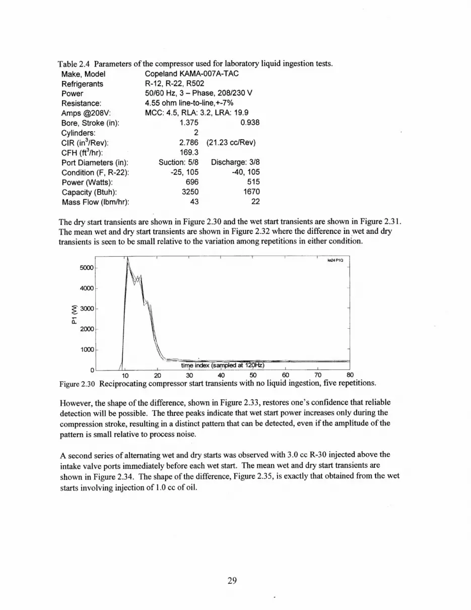
Table 2.4 ParametersMake, ModelRefrigerantsPowerResistance:Amps @208V:Bore, Stroke (in):Cylinders:CIR (in3/Rev):CFH (ft/hr):Port Diameters (in):Condition (F, R-22):Power (Watts):Capacity (Btuh):Mass Flow (Ibm/hr):
of the compressor used for laboratory liquid ingestion tests.Copeland KAMA-007A-TACR-12, R-22, R50250/60 Hz, 3 - Phase, 208/230 V4.55 ohm line-to-line,+-7%MCC: 4.5, RLA: 3.2, LRA: 19.9
1.375 0.9382
2.786169.3
Suction: 5/8-25, 105
6963250
43
(21.23 cc/Rev)
Discharge: 3/8-40, 105
5151670
22
The dry start transients are shown in Figure 2.30 and the wet start transients are shown in Figure 2.31.The mean wet and dry start transients are shown in Figure 2.32 where the difference in *wet and drytransients is seen to be small relative to the variation among repetitions in either condition.
Io24 PlO
5000
4000
2000--
1000 -
0 tirme index (sampled at 12 Hz)
10 20 30 40 50 60 70 80Figure 2.30 Reciprocating compressor start transients with no liquid ingestion, five repetitions.
However, the shape of the difference, shown in Figure 2.33, restores one's confidence that reliabledetection will be possible. The three peaks indicate that wet start power increases only during thecompression stroke, resulting in a distinct pattern that can be detected, even if the amplitude of thepattern is small relative to process noise.
A second series of alternating wet and dry starts was observed with 3.0 cc R-30 injected above the
intake valve ports immediately before each wet start. The mean wet and dry start transients are
shown in Figure 2.34. The shape of the difference, Figure 2.35, is exactly that obtained from the wet
starts involving injection of 1.0 cc of oil.

3000
01~ /hI I -. f..
10 20 30 40Figure 2.31 Compressor start transients with 1.0 cc
5000-
4000
P 3000-
C
D 2000-
1000-
time index (sampled
10 20 30 40Figure 2.32 Mean of repetitions with no fault (solid)
250[-
50 60 70liquid ingestion, five repetitions.
50 60 70 80and 1.0 cc liquid ingestion (dotted).
200-
150-
100-
\JI
10 20Figure 2.33 Mean deviation of P1
time index (sampled at 120Hz)
30 40 50 60for starts with 1.0 cc liquid from P1 for
70 80fault free starts.
I I I

4500-
4000-
3500 -
a30000)
o 2500-C0 2000-E-1500-C-
1000
500time index (sampled at 120Hz)
5 10 15 20 25 30 35 40 45 50 55 60Figure 2.34 Mean of repetitions with no fault (solid) and 3.0 cc liquid ingestion (dotted).
200-
150 --C0
to 100-0CCS50-
--- -- ---0
time index (sampled at 120Hz)
-505 10 15 20 25 30 35 40 45 50 55 60
Figure 2.35 Mean deviation of Pl for starts with 3.0 cc liquid from P1 for fault-free starts.
Another liquid ingestion fault, called liquid slugging, involves liquid entering the compressor during
steady operation. This might be caused by an intermittent TXV fault. To observe this effect, equal
doses of oil were injected, at the rate of about one injection every 20s, during steady operation. Aseries of five events was observed with 1.0 cc oil injected at the suction port for each event. The P1
transients observed in the test are plotted (superimposed) in Figure 2.36. Compressor power
increases briefly (by about 15W (2.5%) for 300ms) and then returns gradually to normal. Note that a
reciprocating compressor presents a cyclic load component corresponding to shaft speed because
more torque is required during suction and compression than when the crank is taking the pistons
through their top and bottom positions. The shaft speed cycle interacts with line frequency to produce
strong beats, evident in Figure 2.36 at 3.6Hz. At higher time resolution, Figure 2.37, the amplitude
of the shaft cycle power (P1) fluctuations is seen to increase substantially when liquid is injected.
The corresponding QI traces show little or no sign of the disturbance.
As in the flooded start case, the effect on P1 of ingesting non-damaging amounts (<5cc) of liquid is
small, making reliable detection difficult. There are three aspects of the difficulty: 1) the small

6901.18 p
680-
670-
660-
F 640
630-
620
610-time index (sampled at 120H-z)
600 -0 100 200 300 400 500 600 700
Figure 2.36 Real power during steady run liquid ingestion, five repetitions.
700 1ka18 P1Q680- -
660-
620-
600-
580- time index (sampled at 120Hz)
560- 1 1 1 1 1 10 20 40 60 80 100 120 140 160 180 200
Figure 2.37 Detail showing increase in amplitude of shaft-speed cycle.
magnitude of the change relative to normal variations in P1, 2) the lack of abrupt transient features,and 3) lack of a distinct repeatable transient shape. There is the further difficulty, not apparent in the1-1 Os time frames plotted above, that the dc component of P1 varies gradually with refrigeration load,ambient temperature, and stator temperature.
To address these difficulties, we have modeled the time-series of P1 produced in steady operation as aslowly varying autoregressive process (Seem 1991, Ljung 1999). That is, the process that gives riseto y(t)=P 1 is modeled as:
y(t)= '?(q)y(t) + A + n(t)where
'P(q) is an nt'-order polynomial in the back-shift operator, q, F(q) = 1 + 1q-1 + (92 -2+.+ nq -"
A is the detrending parameter, andn(t) is observation noise
The model coefficients are assumed to vary slowly with time. In vector notation, letx(t) = [y(t-1) y(t-2) .. y(t-n) 1] and
b [1 92 *** (nq A]T, thusy(t) = O(q)y(t) + A + n(t) = x(t)b + n(t)
The model coefficients are estimated recursively by exponentially weighted least squares:b = b-1 + A-IxT(t)(y(t) - x(t)bt. 1), whereA = At. + xT(t)X(t)
The efficient recursive least-squares algorithm that avoids matrix inversion (A-1) at every time step,based on the work of Kalman and Bierman, is given accessible presentation in, e.g., Ljung (1999) and

Wunsch (1993), and the various methods for obtaining initial values of b and A (e.g. A=I) are alsoreviewed. An ARX(5,1) model was used with forgetting factor X = 0.995 and the exogenous inputwas set to unity so that the corresponding model coefficient is a slowly varying (i.e., exponentially-weighted moving average) of the "dc" component of P1. The first 14 k-step-ahead forecast errors(P1(k)-P1) are plotted for the first ingestion event in Figure 2.38.
The adaptive model provides not only k-step-ahead predictions, but also estimates of the variances ofprediction errors. Together these numbers may be used to reduce detection to an adaptive scalarthreshold test based on the norm of 1/variance-weighted squared innovations:
J(tm,kH) = nTRin,
where n is the vector of innovations for the time-tm model over a prediction horizon (tm+1: tm+ kH), Ris the diagonal matrix of mean-square-error (Figure 2.39) for recent k-step-ahead predictions, k=1:kH,and kH is the prediction horizon.
200-
150-
100 120 140 160 180 200 220 240 260 280
Figure 2.38 k-step-ahead prediction errors from recursive ARX(5,1), k=0.995, k=1:14.
II I I I
5-
4-
3-
20 20 40 60 80 100 120
Figure 2.39 Sqrt(variance) for k-step-ahead prediction errors of the ARX(5,1) model during 10seconds (n=1 200) of steady operation. The dashed line is the variance about the mean.
The time evolution of this norm, obtained from the k-step-ahead predictions of Figure 2.38 andadditional predictions out to kH = 128, are shown in Figure 2.40. The smoothness of J is the result of
ensemble averaging. Because transients vary in duration, and may or may not be associated with a
change of mean, it will be usefull to evaluate J over several prediction horizons, e.g. kH=32, 64, 128,
256 half cycles. In this case, the duration of the transient vastly exceeds the useful prediction horizon
and the predictor reduces to the most recent trend line after about 25 time steps. In cases of small,
10 The duration of the horizon that gives maximal J is an indication of transient duration that can be of furtheruse in identifying the load associated with the transient. The recursive ARX-based TED is ideal (and sorelyneeded) for detection of off-transients because only very short prediction horizons are needed.

short transient events however, this detector is about three times more sensitive than a simpleadaptive trend line and it is the optimal detector for transients of any magnitude, duration, and shape,provided the background process is reasonably linear and quasi-stationary. A transient event detector(TED) based on the given vector norm has, moreover, the desirable statistical properties of properlyweighted ensemble sampling while retaining the simplicity of a scalar test. The adaptive processmodel, in addition to detecting a new transient event, has the further important function of isolatingthe detected transient from the background signal that is the sum of all loads that are active when thenew load is switched on. This improves the confidence interval for finding a match with a starttransient in the database of known loads.
x 10
2-
1.5-
01260 1280 1300 1320 1340 1360 1380 1400 1420
Figure 2.40 Transient event detection by norm of ARX(5, 1) k-step-ahead prediction errors, k=1:128.
A diagnosis of liquid slugging could be made with utmost reliability by applying the foregoing filterto suction and discharge pressure signals of similar or moderately lower time resolution. Thecontemporaneous detection of anomalous power and pressure transients during otherwise steadyoperation is a sure indication of liquid slugging.
2.3 Implementation and Application
2.3.1 Hardware Implementation.
The NILM or other PSA platform requires only current and voltage sensors at the RTU feed, alllocated safely in the electrical box. A single-phase platform requires one current sensor and onevoltage sensor, while a three-phase platform requires two of each sensor. There may be a niche for aPSA-based FDD device with one current and three voltage sensors so that phase imbalance or phaseloss can be immediately detected. The single-phase PSA device can be implemented in a low cost150 MHz PC-on-a-chip with a two channel A/D converter. The incremental RTU manufacturing costcould be as low as $200. Integration with RTU controls is a natural extension which reduces theincremental cost of FDD capability and may be especially attractive for high SEER designs withvariable-speed fans or compressors.
2.3.2 Fault Detection Architecture.
PSA-based fault detection uses five generic detection methods.
A change in mean power (P1) or reactive power (QI) was the only method of load identificationimplemented in the original NILM (Hart 1992). A change of mean is measured in four steps. Firstthe current mean aggregate load is established recursively by a running, moving, or exponentiallyweighted moving average. Second, when an appliance switches on or off, a transient event detector

(TED) freezes the current means, logs the time, and tracks aggregate load until the transient conditionhas settled. Third, after the transient has settled, accumulation of the new mean aggregate load
begins. After a new mean aggregate load has been established (typically 10-100s) the change of mean
is computed. Once the change in mean has been estimated it is compared to the values established for
known loads. Each known load is characterized by its first four odd power harmonics (Pn,Qn) and a
confidence ellipsoid in (Pn,Qn) space. If a match is found the nominal as well as measured loadparameters (Pn,Qn), transition type (on or off) and timestamp are logged to a tag file. If a match is
not found the closest (in a weighted Euclidean norm sense) can be identified and additional tests (e.g.start transient shape) may be applied in succession until the appliance most likely to be the source of
the start or stop transient and associated change of mean is identified. If the appliance so identified is
one for which simple faults have been established, the type and level of fault are determined based ondeviations of the measured change of mean from the expected values.
The amplitude spectrum of P1 is computed based on a fixed sample size. The calculation is a fast-
Fourier transform on 2" points of P1 where n is on the order of 12 to 16 and P1 is sampled at 120Hz.
When the newly computed spectrum falls outside the confidence region of the baseline spectrum, the
PSA enters test mode. New spectra are accumulated until a rigorous statistical test is satisfied or the
predetermined maximum test sample size is exceeded. The baseline can include amplitude spectra for
two fans operating together as well as spectra for the individual fans. When imbalance is detected
with two fans running, the spectrum must be decomposed to determine which fan is at fault. An
alternative approach is to track gradual shifting in amplitude and frequency of the peaks identified
with imbalance faults by Kalman filter.
Start transients are identified by pattern matching. The process is initiated by a transient event
detector (TED) which responds to deviations from k-step-ahead predictions generated by adaptive
(Pn,Qn) ARX forecasts. The first step is to identify which motor has started or stopped. The next
step is to determine if the pattern is within the confidence limits of the established fault-free pattern
and if not, what type and level of fault is present. If a motor start transient cannot be identified the
event is considered an anomalous transient.
The TED will detect fault-induced transients as well as those associated with individual loads starting
or stopping. These transients will, in general, not match any of the established transients. For the
RTU, two such anomalous transients are liquid slugging and intermittent contacts. The estimatedchange of mean will be close to zero in both cases. For the intermittent contact fault the time average
of (P1,Q1) during the transient will not differ significantly from the mean before or after the
transient. Also note that although the contact fault may occur on only one phase of a delta-connected
load, the transient will appear on all three phases in such a way that the faulty phase contact can be
identified. For liquid slugging the time average of some elements (P1 ,Q 1) will be significantly
greater than the mean before or after the transient.
Phase (current or voltage) imbalance results in elevated motor temperature which increases the
likelihood of early stator insulation failure. Loss of phase causes very rapid overheating and quickly
leads to catastrophic failure of three-phase induction motors. A 3-phase PSA-FDD device or a device
that monitors one phase of current but all three phase voltages can respond instantly to loss of phase.
This eliminates the need for a dedicated loss-of-phase detector and provides the necessary remote
diagnosis to reduce service cost while expediting repair.

2.3.3 Application to larger equipment.
The observations reported here are from a small package rooftop unit. Larger units typically have abelt-driven supply fan, multiple condenser fans, and multiple compressors. A number of changes willbe needed for application to larger units. The maximum order of the TED AR(n) process modelwould be expected to grow (n=3+2m where m is the number of motors). A larger number, m, of startexemplars must be maintained. The possibility of simultaneous motor starts (although normally notallowed by the control sequence) and simultaneous motor stops (not disallowed) should be addressed.The amplitude spectra generated during steady run periods must be disaggregated before a growth inpower (integrated under selected peaks) can be reliably attributed to a particular motor.
Large package DX split systems are much like large rooftop packages except that supply fans,condenser fans and compressors may be on separate circuits. The PSA-FDD device would beinstalled at the appropriate HVAC subpanel or motor control center. Refrigeration racks present asimilar application scenario.
In small central plants, one typically finds a rack of semi-hermetic reciprocating compressors, chilledwater and condenser water pumps, and one or more (often 2-speed) cooling tower fans. Large centralplant chillers often have dedicated controls that also provide FDD capability based on compressorcurrent and several temperature measurements that may include oil and stator winding temperatures.However a NILM or PSA-FDD device installed at the HVAC subpanel to provide balance-of-system(pumps, fans) diagnostics would collect additional useful information about root causes of chiller tripevents as well as diagnosing the auxiliary equipment itself.
2.4 Summary and DiscussionWe have demonstrated that PSA can detect a variety of important faults in a rooftop air conditioner.The methods for detecting these faults are summarized below and a preliminary assessment of thevalue of fault detection follows.
2.4.1 Detection Method by Fault TypeAir-side blockage faults can be detected by a shift in steady state (P1,QI) and, to some extent, bychanges in start transient shape. However the change magnitudes and directions are related toblockage magnitude via the interaction of fan curve, air-side flow-pressure curve, motor torque curveand no-fault operating point. Thus diagnosis requires more information than that needed for detection,e.g. addition of static pressure. Flow transitions clearly evident in the pressure start transient are alsoevident in P and Q start transients. Detectable flow transitions may be useful in acquiring veryreliable and complete diagnoses.
Short cycling can be detected in the obvious way, by logging time between start transients. Theadvantage over detection by a temperature-sensor-based FDD system is that very short-evenincomplete-start transients are detected. This is important because just a few inrush current eventsin quick succession will raise stator winding temperature to the point of insulation damage. Thesecond method of short cycling detection relies on the shape of individual start transients beingsensitive to residual head. The two methods should be implemented together because they arecomplementary. A time-stamp and the thermal conditions at the time of each short-cycle occurrencecan be saved to aid in diagnosing a root cause.

Refrigerant charge faults result in elevated head pressures which translate to higher steady statecompressor loads. Detection of overcharge requires normalizing compressor load over the range ofthermal operating conditions. Detection of undercharge is possible based only on the distinct shapeof its start transient. The refrigerant vapor bypass fault has a distinct effect on the start transientshape: the change of magnitude in the latter half of the transient is two to five times the change insteady state power.
Liquid ingestion results in transients that PSA can detect in two ways. The change in start transientshape is small in magnitude but has distinct compression stroke features. The shapes of liquidingestion transients during steady operation are not repeatable in the usual sense but they alwaysresult increased power of 0.1-Is duration that appears clearly as positive deviations from k-step-aheadforecasts. Thus any positive power transient that fails to match a known start transient, and thatexceeds the adaptive model innovation norm threshold, probably indicates liquid ingestion.Conditions recorded at the time of occurrence can be saved to aid in diagnosing a root cause.
Shaft harmonics observed with no fault indicate that direct drive fan harmonics are not as obvious asbelt driven shaft harmonics (Lee 2004) but still potentially useful for load identification. The resultsof tests using small weights to unbalance the impeller indicate that PSA can identify degradation ofimpeller balance well before the added repair costs of a catastrophic failure are incurred.
PSA-based fault detection uses five generic detection methods. Current and voltage imbalance (orcomplete loss of phase) are detected by simple ratio and threshold tests. A change-of-mean resultsfrom a change in steady state mechanical load that is detected as a change in electrical power, P1,with corresponding changes in reactive and apparent power and a corresponding change in powerfactor. The amplitude spectrum of power, P1, is used to detect shaft, coupling, rotor, impeller, andbelt-drive faults. Start transients are identified by pattern matching. The motor associated with ameasured transient is first identified using a generous confidence interval and a tighter confidenceinterval is then applied to detect a possible fault. Anomalous transients are detected by an adaptivelinear filter and may arise from faults that do not produce repeatable patterns; the list of such knownfaults is necessarily incomplete.
Event sequence analysis is a PSA capability per se (it can use load state sequences detected in anynumber of means) but is a fault detection method that is important to implement in the PSA-baseddevice. An event sequence analysis compares the timing and sequence of motor state (on, off)changes to the sequences expected in response to given controller commands. The PSA platform'svery high time resolution of motor start and stop detection and ability to log the sequences forplayback by a technician are put to good use here.
The suite of faults that are best detected by PSA complements, to large extent, the faults that are best
detected by temperature-based FDD systems. Faults that are primarily electrical or electro-
mechanical are difficult to detect by thermal measurements but can be detected by PSA using the
methods indicated in Table 2.5. PSA can also play a role in detecting many of the more interestingnon-electrical faults as summarized in Table 2.6. A comprehensive FDD system could employ an
extension of the models developed by Rossi (1997) and Breuker (1998), which currently use return
air and ambient air conditions as inputs, by adding compressor power as an input.

Table 2.5 Summary of electrical and electro-mechanical RTU faults detectable by PSA alone.
Fault NILM MethodLoss of phase Current and VoltageLocked rotor Start transientSlow starting motor Start transientUnbalanced voltage VoltageShort cycling Event sequenceMotor disconnect/failure to start Event sequenceIncorrect control sequence Event sequenceContactor (improper contact closure) Phase current interruption transientFan rotor faults that result in imbalance Amplitude spectrum in steady operationCompressor mechanical faults (not tested) Amplitude spectrum in steady operation
Table 2.6 Summary of non-electrical faults. Some of these can only be detected by the thermalmeasurements and some can only be detected by PSA, but detection of most can benefit by havingboth types of measurements.
Fault PSA Method 7T[l] 10T[l]1 Refrigerant leakage, undercharge, or overcharge Change of mean 4 42 Liquid line restriction 4 43 Loss of volumetric efficiency (leaky valves, seals) Start transient [2] 44 Fouled condenser coil Change of mean 4 45 Dirty supply air filter Change of mean [3] 4 46 Liquid ingestion Anomalous transient7 Vapor line restriction [4]8 Non-condensable gas [4]9 COP degradation (root cause: 1, 2, 3, 4, 5, 7 or 8) [5] [6] [6][1] 7T FDD measures Twb, Tamb, Tevp, Tsh, Thg, Tcnd, and Tsc; lOT FDD also measures Tra, ATcndair, and ATevpair (Breuker 1998).[2] low sensitivity[3] system flow-pressure-temperature model may be needed for reliable detection[4] not tested[5] with addition of refrigerant flow (or comnpressor map) and head pressure[6] with addition of air-side flow and RH
2.4.2 Value Assessment
We can now make a preliminary assessment of the value of fault detection. The very useful results ofBreuker's large sample" analysis are summarized in Figure 2.41* and Table 2.7. Value is realized inseveral areas such as reduced down time, better efficiency, avoidance of consequential damage, andthe efficient dispatch of repair staff and replacement parts. The data needed to assess current costs ineach of these areas apparently do not exist. However, it is safe to say that these costs are, inaggregate, at least equal to the current aggregate cost of repair. Indeed, it is often the case that onlyconsequential damage is repaired in the first service call and the failure recurs one or more timesbefore the root cause is actually identified and corrected. The information recorded at the first sign ofa fault, and additional data recorded about any consequential failures, is therefore of great value inreducing callbacks.
" "a statistically representative subset of the data" drawn from "over 6000 separate fault cases"

Compressor 24%
Miscellaneous 21%
Evc
Electrical 7% Air Handler 51Controls 10%
Figure 2.41 Cost of Repair by affected component or subsystem (Breuker 1998a).
Condenser 9%
aporator 6%
Let's consider the fraction of total repair costs associated with faults that PSA can detect assuming,based on the foregoing discussion, that the value of detection is "on the order" of the cost to repair.Breuker's compilation helps us to do just that. The first column of Table 2.7 lists repair cost aspercent of total based on Breuker's Table 2; the second and third give cost fraction as a percentage ofcolumn 1 based on Breuker's Tables 3-8 (1998a). Assignment of faults to columns 2 and 3 representthe author's assessment, based on the test results reported in Section 2.3, of PSA-based FDD potentialfor the fault subcategories as tabulated by Breuker.
Table 2.7 Cost breakdown for repair of faults.Detection by PSA Certain Detection by PSA Probable
Compressor 24 short, open, locked rotor 66 broken internals, vapor bypass 11Condenser 9 motor, belt failure, cycle control 51 fouling, coil leak 36Evaporator 6 0 fouling, leak, loss of capacity 75
ir Handler 5 motor, impeller, belt, electrical2 67 damper motor, duct leaks 20Controls 10 compressor interlocks, fan sequence 37 0Electrical 7 Contactor, loose connection 44 fuse/breaker, short/open 27Miscellany 21 water loop/pump, fan belt 29 refrigerant leak, installation/startup 42Other 18 n.a. n.a.
Repair of all PSA detectable faults Faults likely to be detected by PSATotal % 100 (sum of products with column .1) 37 (sum of products with column 1) 22
The PSA-detectable faults represent at least 37% of all repair costs and an additional 22% ofrepair costs are attributed to faults PSA is likely to detect. Together this indicates apossibility of detecting faults associated with 59% of all repair costs or 72% (59/(1-. 18)) ofattributed repair costs. The fault category that represents the largest repair cost, 16%, iscompressor short, open, or locked rotor. (Compressor replacement is typically the singlemost expensive repair to an RTU.) The database analyzed by Breuker does not provide rootcause analysis of these or any other of the reported failures, but likely root causes include
12 Note that Breuker (1998a) associates motor and beltfailure faults with the air handler rather than with theevaporator, presumably because the air handler and evaporator are treated as separate components whereas thecondenser (motor, fan, belt (if present), and heat exchanger) is treated as a single component.

internal damage (e.g. from liquid ingestion), overheating from condenser or evaporatorfouling, fan failure, or bypass leakage, and the standard electrical faults such as loss of phase,contactor faults, and short cycling. All of these root causes would be detected by PSA beforeserious compressor damage ensued for an immediate reduction in total repair costs of at least10%.

Chapter 3 Identification of Building Thermal Response
This chapter derives a general transient thermal response model for on-line identification that can beapplied to walls, zones, and whole building envelopes. Several important aspects of building HVACoperation-FDD, curtailment, verification, model-based control and commissioning-can beimproved by use of accurate building-specific plant13 models. The aggregate potential savings, aswill be shown in Chapter 4, is substantial. But such control applications will be economically usefulonly if the process of identification can be reliably automated. The models and identificationmethods developed in this chapter are tested using time series data obtained in a test room, at theInternal Services Division (ISD) office building in East Los Angeles County, and at the 60-unitZubkova apartment building in Ryazan, Russia.
The chapter has seven main sections: Motivation, Previous Work, Model Synthesis, Test RoomResults, ISD Test Results, Zubkova Test Results and Summary. The materials and geometries aredocumented for the test room in Appendix E, for the ISD Building in Appendix F, and for theZubkova Building in Appendix G. describes a general canonical form for the discrete-time transfer
function model of an arbitrary thermal system. Appendix I documents the model identification code
with constrained time constants. Appendix J documents the model identification code by a newmethod related to total least squares. A representative fragment of the data file input to the identifi-cation codes appears in Appendix K.
3.1 MotivationIdentification of building thermal response models is motivated by three broad areas of application:
Peak shifting (includes curtailment and verification of demand savings),Model-based control, andFault detection and diagnosis (FDD).
Additional narrow areas of application include commissioning, planning (e.g. for efficiency retrofits)and verification of energy and demand savings 4 . Load shedding and peak shifting strategies areconstrained by building and HVAC plant characteristics as well as climate, utility rate structure andbuilding occupancy requirements. The analytical framework for dealing with different climates, ratestructures and occupancies is well established (Armstrong 2002, Braun 1990, Kintner-Meyer 1995,Morris 1994, Norford 1985, Xing 2004). Reliable one-day-ahead weather forecasts can bedownloaded daily or hourly. Internal gains, predominantly light and plug loads, can be disaggregatedby a NILM from the building total (Leeb 1992, Laughman 2003) and future loads can be similarlyextrapolated from the accumulated history (Seem and Braun 1991).
13 Here the "plant" refers to the building envelope, a distributed R-C system with some mildly non-linear R's.14 Note that demand and energy savings, while related, are often treated differently because transient responseusually has little effect on energy savings but is a dominant factor in demand savings.

However, thermal response to weather, internal loads and HVAC inputs is unique to each buildingand difficult to characterize empirically (Braun and Chaturvedi 2002, Norford 1985, Pryor 1982, Rabland Norford 1991). The development of a general model and model identification proceduresufficiently robust to be automated is therefore a central and challenging prerequisite to theimplementation of useful curtailment or peak-shifting (CEC, Stoecker 1981), precooling (Keeney1997), and optimal start (Seem 1989) control strategies. Verification of curtailment for allocatingincentives would, ideally, be based on the same model that is used for control.
Model-based control, particularly of zone temperature control loops, can be used to improve comfortand reduce the frequency and amplitude of control variable excursions. The plant model provides arational way to handle some or all of the easily measured system excitations (sunshine, outsidetemperature or sol-air temperature, light and plug loads) that are normally treated as "disturbances" intraditional PID control of a plant. Model-based control also addresses problems that often occurwhen control loops are cascaded. Even if O&M providers resist giving up SISO control loops, aproperly identified model can be very useful in the accurate tuning and cascading of such loops.Tuning of control loops is a significant (costly and error prone) element of the HVAC commissioningand re-commissioning processes.
Finally, on-line identification of zone and building thermal response models is essential to detectionand diagnosis of HVAC faults that affect comfort and overall HVAC system efficiency (Rossi andBraun 1993). Fault detection can be as simple as checking that zone temperatures respond to HVACcontrol modes (economizer operation, including control of openings for natural cooling, changes inflow rate or supply temperature, etc.) as predicted by a properly identified model.
We expand on certain aspects of the control application in Chapter 4. However, the key elementcommon to all of the foregoing control, verification, FDD, and commissioning applications is anaccurate building-specific plant model. In some cases the required level of accuracy may only beachievable by an adaptive model. Such models, whether adaptive or not, will be economically usefulonly if the process of identification can be reliably automated. Models and identification methodsthat have been proposed for on-line identification of building thermal response are reviewed in thePrevious Work section. The model structure found to be most generally useful and the newidentification methods developed for this thesis are presented in the Technical Approach section.
3.2 Previous WorkIn the area of thermal response modeling we have seen one-node models used by a number ofinvestigators (Dexter 1981, Klein 1994, Richardson 1981, Saunders 1987, Horn 1982, Subbarao1985) to approximate the dynamics. However, most general purpose building simulation programsuse a response factor (DOE 2.1) or transfer function (TRNSYS, BLAST, TARP, EnergyPlus) modelof each envelope component. Walton (1983), Klein (1996), and Clark (1985) describe simulationalgorithms used in all aspects envelope modeling.
Simple design methods based on the results of building simulations have been developed. Transferfunctions did not become part of a recommended design procedure (ASHRAE 1997, Rudoy 1975,Sowell 1985) until recently (ASHRAE 2001). The RTS method is based on conduction transferfunctions and can be implemented in a spreadsheet but is too tedious for hand calculation.

The approximations inherent in transfer function models are satisfactory for most buildingcharacteristics and for most model fidelity requirements (Mitalas 1968). Indeed, lower-order modelsare desirable in many situations. Techniques have been developed for deriving reduced-order modelsgiven a detailed thermo-physical description of the building (Balcomb 1983, Richardson 1981, Seem
1989). These techniques invoke certain criteria for minimizing model errors such as reproducingexact response to a limited set of driving functions. Balcomb's criterion is response at 0, 0.2 and 1.0cycles per day. Seem has examined two different criteria: reduced-order models based on the
system's dominant roots and reduced-order models based on the Pade' approximation (Sinha 1983).
Analysis of building test data is another topic germane to the question of reference model-basedcontrol. Most of the work in this area has been applied to the "generalization problem." One suchquestion is how to estimate general building parameters, such as UA product or "effective thermal
capacitance," from measurements obtained under transient conditions (Armstrong 2000). Another
generalization involves estimation of annual energy use in response to a standard weather series suchas one of the widely used TMY tapes. Model validation (Judkoff 1999, Spitler 2002) is yet anotherarea for which generalization of short-term test data may be useful. Work in the area of short-termtesting and analysis has been reported by Barakat (1987), Bushnell (1978), Kahwaji (1986), McCabe(1983), Duffy (1987), Pryor (1982), Sonderegger (1978), Subbarao (1985) and Wilson (1984). Anextensive review of these techniques has been presented by Rabl'(1988).
There is some pertinent literature on optimal start/stop control, however Park points out that thedetails of the algorithms used in commercial products are not generally made public. The schemesthat have been reported vary with respect to complexity of the underlying building model that isassumed (Hittle 1981, Seem 1989).
The foregoing is an overview of the literature. Specific topics germane to model identification, modelorder reduction and other research germane to the applications of interest are reported below.
Recovery Response. E.G. Smith developed a method for determining recovery time in 1940 (Smith,1940a, 1940b, 1942). He neglects the thermal capacitance of room air and assumes that all envelope
walls and contents are initially in a steady-state condition. He further assumes that the heat flux at the
surface of each wall and at the surface of each object contained in the conditioned space is constantduring the recovery period and that all walls and contents are of homogeneous composition. With
these assumptions Smith was able to derive an exact but tedious solution for recovery time. The
solution is tedious in that tables of thermal "absorbance," a function of recovery time, film resistancesand material properties and thickness, had to be computed by hand in 1940 for each wall constructionand for each type of furnishing contained within the conditioned space.
Peak Cooling Load Models. The thermal storage effect has long been considered an essential factor
in the calculation of peak cooling loads due in part to the relatively high incremental cost of installed
capacity and in part to the highly transient nature of cooling loads. The temperature recoveryproblem raises similar concerns. It is therefore not surprising that the literature on cooling load
analysis is rich in techniques that are potentially applicable to the model identification and peak
shifting problems.
The ASHRAE hand-calculation procedures (Rudoy, 1975) are based on the results of hour-by-hour
simulations using transfer function models to account for thermal storage. It has been found that the
storage effect for many different kinds of constructions can be adequately accounted for by
categorizing these constructions as light, medium or heavy. (Barakat, 1987, has added an extra-light
category for framed residences.) Recent efforts to more accurately account for the storage effects
(Sowell, 1985a,b and Chiles 1985) have still used the transfer function as the underlying model.

The ASHIRAE thermal response factors method was developed for computing cooling loads and roomtemperature trajectories under transient conditions (Stephenson 1967). The room temperature wasoriginally assumed to be constant for the cooling load calculations. When the cooling load exceededplant capacity a separate set of response factors called "response factors for variation of room airtemperature" was required. These factors were used to compute the deviation from the coolingsetpoint and the method was later extended to include continuously varying room temperatures foundin intermittently occupied rooms and rooms in which capacity is proportional to temperature over athrottling range (Mitalas 1969). The companion to Stephenson's paper (Mitalas 1967) derives thehomogeneous slab response factors (Appendix A) and the room thermal response factors (AppendixB), but the response factors for variation in room air temperature are never derived. Ceylan andMeyers (1980,1985) developed a general transfer function method that can be used to obtain arelationship between the room temperature and net sensible heating or cooling of the room in a formsimilar to that envisioned by Stephenson and Mitalas. The method of Pawelski (1979) is similar tothat of Ceylan and Meyers in starting with a finite element model; Pawelski's use of statisticaltechniques results in a parsimonious but not necessarily robust model. More recently Seem(1987,1988) has developed a method specifically for the whole room problem that yields particularlyrobust and parsimonious whole room transfer functions.
One-node Models. One-node models have been used extensively to account for thermal storageeffects in the dynamic response of buildings. Sonderegger (1978) and Duffy and Saunders (1987) forexample, have used one-node models to generalize the results of short-term building tests. One-nodemodels have been used in hour-by-hour simulation programs, e.g. TRNSYS (Klein 1983).
Richardson and Berman (1981) used Fourier decomposition to determine optimal one-node modelparameters. Several alternate methods of estimating one-node wall model parameters were developedby Horn (1982). Horn also reviews the DHC method (Balcomb,1980) and the thermal admittancemethod (Davies, 1973 and Milbank, 1974) and presents a very thorough analysis of the simulationerrors that result when the various one-node wall models are used. Horn recommends furtherinvestigation of two-mode models.
Model Order Reduction. Pawelski et al (1984) used correlation to find the ARMA coefficients for acomplex roof-attic structure. He used a finite difference model of the structure driven by two weeksof hour-by-hour weather data and imposes the constraint sum(b)/sum(d) = UA, where b is thecoefficient vector associated with outdoor temperature, d is the coefficient vector associated with atticenvelope heat load, and UA is from a steady-state solution of the finite difference model. Balcomb(1983) and Seem (1987,1988) have developed the more sophisticated model-order reductiontechniques described previously.
Modelsfrom short-term testing. Quentzel (1974) and Bushnell (1978) have used linear correlation toestimate parameters affecting daily energy use in buildings. Quentzel correlates daily furnace runtime with daily degree days. Bushnell correlates energy use, inferred from daily utility meterreadings, with daily mean solar irradiation, outside temperature and wind speed. Neither investigatorchose to model thermal storage effects even though the monitored building used night setbackschedules. As a result standard errors for the correlations were on the order of the daily heat loss thatwould result from a 5F temperature difference across the heated envelope.
Sonderegger (1978) used a one-capacitor, two-resistor model to obtain "equivalent thermalparameters" of a light frame townhouse. The parameters were evaluated by linear regression usingfour days of measured data during which the room temperatures were allowed to float and internalgains were relatively constant. The principal time-varying heat input was due to solar irradiation ofthe interior envelope surfaces.

Pryor et al (1980) used a two-capacitor R-C network to model a passive solar residence with water-wall storage. The one- and two- capacitance models are simple enough to be expressed as finitedifference equations with unknown parameters. Kahwaji develops a method of finding the thermalparameters of homogeneous layered walls from transient measurements based on the exact solution ofthe conduction equation. To model higher order systems that are more complex than a homogeneouswall, e.g. a room or zone, it is desirable to use transfer functions or variations (e.g. ARMAX models)thereof. These models are especially appropriate for distributed parameter systems because the stateof a finite order model used to approximate such a system is not physically meaningful. Theinput/output relationship is the thing of interest.
McCabe et al (1982) and Seem and Hancock (1985) estimated transfer function parameters by linearleast squares to characterize the performance of a solar mass wall component. Forrester and Wepfer(1984) estimated DARMA time series model parameters to identify a load predictor for a large officebuilding. The goal in the forgoing investigations was to find models that were good predictors, notnecessarily to find physically meaningful parameters. Subbarao (1985) has estimated transferfunction parameters and analyzed the resulting models in an effort to obtain physically meaningfulthermal parameters of monitored buildings. Taylor and Pratt (1988) use a finite differenceformulation of a fixed-topology, two-node R-C model to estimate equivalent thermal parameters ofELCAP buildings.
Hittle and Bishop (1983) show that a thermal delay line (1-dimensional conduction through a multi-layer slab) has time constants of alternating magnitude and that the largest temperature response timeconstant is always greater than the largest heat flux response time constant. Harrison, et al (1981)develop a superimposable room transfer function to model short-term transient response.
Peavy, et al (1973) use data from a simple masonry test building to validate NBSLD and performsimilar NBSLD validation work using data from a carefully monitored 4-bedroom townhouse (1975).Bushnell (1978) fits a model with solar, wind, auxiliary heat and indoor and outdoor temperatureterms to data from four buildings. An adequate 0 th -order model is obtained using one-day timesteps.
Summary. The three most common models for envelope model identification are steady-state models,difference models derived for a specific topology, and transfer function models. Frequency domainmethods have been used mainly for network reduction.
Steady state models have been successfully used to estimate wall U-values, and to estimate effectivesolar aperture, UA, and a linear infiltration coefficient at the zone- or building-level. No informationcan be obtained about thermal capacitance or transient response.
Topology-specific difference equations can usually be constrained to return thermodynamicallyfeasible models in a straightforward manner, e.g., by constraining the coefficients to be positive.However, the method is limited in practice to 2nd-order models and the 2nd-order topologies that canbe handled are too simple for most buildings.
Time-domain transfer function models are the most general linear models that have been used andtheir coefficients can be easily estimated by ordinary least squares. However the relations betweenthe model coefficients and the buildings physical parameters is complex. If these relationships are
ignored (as is usual when taking a purely statistical approach, e.g., applying a multi-input ARMAXmodel) the resulting model is likely to violate conservation of energy, to exhibit resonant behavior, orto be unstable or non-causal.
In this chapter, constraints that ensure physically realistic behavior are described and identificationmethods that impose those constraints are developed. These developments allow the practitioner to
take advantage of the generality and model-order flexibility of transfer function models withoutgetting into trouble.

3.3 Model SynthesisRoom air temperature, T,., responds to weather, internal gains and thermal energy delivered by theHVAC system as shown schematically in Figure 3.1. "Weather" includes the effects of sun, wind andoutdoor temperature on all exterior surfaces, as well as direct gains through windows. Internal loads,QL&p, are usually dominated by office equipment and lighting, i.e. "light and plug" loads. Heating orcooling effects, QHVAC, may be delivered by forced air, natural ventilation, or various types ofhydronic terminal equipment.
Weather
QL&P Zone Tzone1 Thermal
QHVAC , Response
Figure 3.1 Thermal response model.
The response to a given input is determined by the physical parameters and geometry of the buildingenvelope, internal partitions, furniture, and other contents. The thermal capacitance or "mass" as wellas the thermal transmission properties of the building fabric determine these response relationships.The engineering data needed to predict how a given building will respond are complex and subject tosubstantial uncertainty and variation over time. However the response function illustrated in Figure3.1, if it can be properly identified, is just the sort of crystal ball that is needed for improved control,commissioning and fault detection.
For each application discussed in the Problem Statement section, there is an objective function orcontrol law that has a thermal response model embedded in it. It is critical that the thermal responsemodel represent not the intended design but, rather, the building as built and currently used. Theproblem of producing such a model, with minimal fuss, has been addressed in this research project bynew robust identification methods. These methods enable one to reliably obtain models based onmeasured excitations and the corresponding response. The required thermal excitation and responsetime-series data may include data obtained by state-of-the art devices (wireless, roving, NILMsinstalled at the service entrance and HVAC subpanel) as well as time-series data routinely monitoredby existing HVAC control systems.
The technical approaches for characterizing envelope thermal response and for assessing theapplication of such models to control, commissioning, and FDD are developed followed by briefsummary of test zone instrumentation. Results of application are presented in the Results sectionwhich follows Model Synthesis.
3.3.1 Thermal Response ModelThe previously described control and fault detection applications have one very basic thing incommon: the need to predict building- or zone-specific thermal response. The ideal properties of athermal response model are that it should be simple yet give accurate predictions over the expected

range of operating conditions, including extremes and abnormal conditions. A model based on thephysics of the problem, if sufficiently simple, is often best. A model that is generally applicable tolinear and weakly nonlinear thermal systems and some of its key properties are derived below.
Heat transfer and storage in the building structure and contents is governed (Carslaw and Jeager1959) by the diffusion (Fourier's) equation:
PCT =kV2T (3-D)atP T = 2T (1)pc - k(1-D)P at aX
where k-conductivity (assumed isotropic) and pc,=thermal capacitance are the local materialproperties of interest. In steady-state, (1) reduces to Laplace's equation:
kV2T = 0 (3-D)
027 (2a)k - 0 (1-D)
8x2
to which boundary conditions are applied after integration to obtain heat flux (W/m 2 or Btuhft2 ):
q = -kVT (3-D)
dT (2b)q, = -k (1-D)
dxApplied to a wall (or an enveloping surface) in steady state:
Q2 = u(T, - TZ) (3)
where T, is a uniform exogenous temperature15, T, is zone16 temperature (Seem 1987), and Q, is netheat input (flux integrated over area, W or Btuh) to the zone and u = EUA (W/K or Btuh/0F) is theparallel conductance of all sub-areas defined on the envelope.
With multiple walls:W
QZ = L u,(T, - TZ ) (4A)W=1
An important constraint implicit in (4) will become apparent momentarily. Consider the discrete-time, linear, time-invariant dynamic system with one wall. We have used the symbol t for continuoustime (1) but t is now, and hereafter, defined as the discrete time index. It can be shown via a state-space formulation and the state-transition matrix of the resulting diagonalized system that the 1 -Dcase of (1) corresponds to the following discrete time expression:
B""($ ,Qz)+B""(0,, T,)-B"(Oz, T) =0 (5)
where the coefficient vectors each have n+1 elements:
$z= [$2o #, --' #zn]Oz = [ Oz 0 Oz,1 ---. Oz n]
Ow= [Qwo O,1 --- Own],the time-varying condition and response vectors have corresponding elements:
1 Several exterior surface or sol-air temperatures may be included as forcing functions16 Seem's linearized star model approximates the weighted mean of air and mean-radiant temperatures

Qz = Qz (t) Qz (t -1) --- Q z(t-n)]ITz =[Tz (t) Tz (t -1) --- T z(t-n)]
T,= [ Tw(t) T,(t-1) --- T ,(t-n)],
and each backshift polynomial term in (5) expands to a sum, as follows:n
Bn (x, y) = I Xky(t - k)-k=O
It is convenient, when disassociating the 0-lag terms of (5), to use a more general form of thebackshift polynomial notation in which the index of summation starts not at 0 but at i:
n
B"(xy) = YXky(t - k)-k=i
Note that one coefficient in (5) can be assigned arbitrarily; by convention (Stephenson 1971, Walton1983) #2= -1 so that (5) becomes:
Q2 = B'"(#z, 92)+B B4" (0,, T,)- B "n(Oz,, T,) (6a)
for one wall and, for multiple walls (Seem 1987) we have:
Q, = B"#EQ,+ B ",T,- B ",z )(6b)w=1
This form is the sought-after (Figure 3.1) response function that predicts heating or sensible coolingload, Qz, given zone temperature, T, and several exogenous sol-air temperatures, T.
To satisfy the steady-state response model (4) the coefficients must satisfy the following constraint:W n n
I Z wk z,k Ww=1 k=O k=O (7a)
k=O k=0
equivalently:W n n
SZ wk +Z z,k =0 (7b)w=1 k=O k=0
In the steady-state formulations (3, 4) the sum of temperature coefficients equals zero by definitionbut in the discrete time (DT) formulation (5, 6) constraint (7b) must be consciously enforced. Thisconstraint appears to have been overlooked in the thermo-fluid identification literature where modelsin the form of (6,8) have been used.
The DT model (5) can be evaluated recursively for Qz as in (6), or for Tz as follows:
Oz,o~z = BO"#2 Q + BO"(O,, T,) - BI"02 Tz (8)or, equivalently, Tz = RHS expression divided by Ozo.
An expression for Qz like (6) is known as a comprehensive room transfer function, or CRTF (Seem1987). We will call the corresponding expression for T (8) the inverted CRTF or iCRTF.Expressions (6) and (8) are the two basic forms of desired "crystal ball" postulated in Figure 3.1.
There are additional conditions (constraints) the coefficients must satisfy for the CRTF (6,8) modelsto be physically (thermodynamically) plausible. To see this one must start with the fact that the

system can be represented by 1 +W transfer functions for zone thermal load response, Q, and 1 + Wtransfer functions for zone temperature response, T, where W is the number of walls exposed todifferent driving temperatures or sol-air conditions. In the time (z-transform) domain we have:
Q Bo(9z) T B(#z )GQi(Z) - z - (9) GT,(z) =- (10)Tz BO # Q, BO S
nzBo (Ow) T no (OW)G r(z) - (11) GTzT(z)= -= (12)T, Bn (#2) T, B"(Oz )
Note that the CRTF is given by
Qz(z) = GQ/Tz(z)Tz(z) + G QTw(z)Tw(z)
and the iCRTF is
Tz(z) = GTzIQ(z)Qz(z) + GTIr(z)Tw(z).
The roots of the denominators correspond to the eigenvalues, 2 k, and thus to the time constants,rk = -Il/k, of any system (CRTF or ICRTF) of interest as follows:
M{ - = AkAt (13)
equivalently
(rk ) = At (14)
The polynomial form may be reconstructed from its roots by Pascal's triangle to satisfy:
n 1k11(r- B) = 0 xBk=1 Xn k=O
where
(15)17
[xk] = 92 for the CRTF, and
[xk] = 0z for the iCRTF.
For diffusion processes, the characteristic frequencies, or poles, Ak, must be real and negative,corresponding to time constants, rk, that are real and positive. Note that the roots of x (62 or #z) aremonotonic in both r and A. It has been shown (Hittle and Bishop 1983) that zone flux and zonetemperature response function pole locations must alternate along the real axis. That is, if the roots of0z, [2a], and the roots of #, [24], are each presented as ordered sets, then together they satisfy:
A01 < A < 2 < A2 <-- -< A < (16)
Unless the coefficients of the transfer function denominators are somehow constrained, the parameterestimation process is likely to return one or more thermodynamically infeasible poles. With someadditional manipulation of (16), as will be shown in 3.3.2, a bounded nonlinear search algorithm,such as Matlab's flninbndo, can be made to handle this constraint set.
n n
"Multiplying through by x, gives x, (rk - B) = xkBk , which has cross terms but is more useful ink=1 k=O
practice; note that the vector (6) and scalar backshift operators are related by B kk(x,y) -= xkBk(y) = xky(t-k)

3.3.2 Model Identification and Application.There are several ways to estimate the parameters of (6) and (8) given noisy data. There are a numberof different ways, in terms of problem formulation, to account for observational noise and modelconstraints (Golub 1980, Wunsch 2004). Three formulations relevant to zone thermal response(CRTF and iCRTF) modeling are developed below.
Model Identification with U-value Constraints. The discrete-time, linear, time-invariant simulationmodel (5) can, in principle, be obtained from observations of thermal response under a range of (zoneheat rate and sol-air temperature) excitations by applying linear least squares.
However, unconstrained least-squares analysis minimizes the model-observation deviations withoutregard for the thermodynamic constraints previously noted. Moreover, the inverted model typically isvery inaccurate under certain transients and it would be desirable not to have to maintain twoincompatible models.
We therefore normalize temperatures by subtracting current zone temperature or one of the sol-airtemperatures from all other current and lagged temperatures. This eliminates the current zone (or sol-air) temperature term, reduces the order of the least squares problem by one, and results in a solutionthat satisfies the U-value constraint (Armstrong 2000).
Model Identification with Constrained Poles. The constraints represented by eqns (14-16) cannot beimplemented in such a simple manner. However, a formulation that fits a standard bounded non-linear search model is possible. From eqns 14 and 16 one can write the constraint as
r1>rp> ro>r--...>r>r (17)
We can now define a new search vector, x, each element of which has simple bounds, 0 <x < 1 fromwhich the roots can be evaluated recursively:
r0i=xiroa 0<x ,1<Jrpxp roi 0<x2<1r9 =xorg, 0 < x 92 < (18)rp2x02ro 0<x2<1
ronxxaronI 0 < x,<1
rex, pr 0 <xO< 1where
ran = exp(At/ro..
There are two useful properties-besides reducing the multi-variable constraints (16) to a set ofsimple bounds on individual variables (1 8)-that arise from this formulation. First, note that x,91corresponds to the largest time constant and a reasonable upper limit, r,., on this time constant canalmost always be easily estimated. Second, minimum spacing of time constants can be imposed byusing a lower bound that is greater than zero or an upper bound that is less than one.

Implementation of the foregoing model identification formulation, coded as a Matlab script and afunction called by Matlab's built-in bounded, nonlinear least squares routine, lsqnonlin, are presentedin Appendix I.
Without pole constraints, least squares identification will typically return parameters that correspondto an unstable model (simulation grows without bound), complex or imaginary eigenvalues(resonance) or negative time constants (noncausality). None of these three properties is possible in adiffusion system.
Model Identification with Uncertainty. Evaluation of thermal response is needed in both of the twomodes, (6) and (8). Ordinary least squares (OLS) analysis minimizes the Euclidean norm ofobservation residuals. Thus if OLS is applied to heat rate observations in order to identify a CRTFmodel (6), temperatures forecast by the corresponding ICRTF model (8) are likely to have a relativelylarge error norm. Conversely, if OLS is applied to zone temperature observations in order to identifyan ICRTF model, heat rates forecast by the corresponding CRTF model are likely to have a relativelylarge error norm. Total least squares (Golub 1980) may provide the better model parameter estimatesif reasonable estimates of the uncertainties are available for all the variables.
The exogenous temperature errors are of less concern than the zone temperature and heat rate errorsbecause we are not using the models to estimate or forecast the exogenous temperatures. Thissuggests an alternate formulation:
Qz + 0 Tz = B + B B Z (19)
in which the objective function for m observations (t =1:m) is
Jg =IIn[1:m] = IIQ[1:m]+ Oz,oTz[1:m] -xg[i1:m]bg|| (20)where
xg(t) = [Q(t-k, k=1:n) Tz(t-k, k=1:n) Ti(t-k, k=1:n) T2(t-k, k=o:n) --- Tw(t-k, k=o:n)]bg = [#(1:n) Oz(1:n) 0i( 1:n) 02(o:n),---, 0,(0:n)].
In this formulation the zero-lag zone temperature coefficient, Oz,o, is estimated by non-linear leastsquares. The LHS observation vector is then generated and the remaining coefficients are estimated
at each iteration by OLS. Matlab code is listed in Appendix J. The foregoing objective function(20), in combination with the non-linear formulation that constrains poles, is another approach to betested.
3.3.3 Model Application.Now we are in a position to fill in some of the Figure 3.1 details. Evaluation of thermal response isneeded in both of the two modes described by eqns 9-12. For example, model-based control typicallytreats T as a given trajectory (Kintner-Meyer 1994) and simulated Q is added to the command givenby a local loop controller. Conversely, for optimal start, a Q trajectory is given and the response ofinterest is temperature as start of occupancy approaches. For curtailment, both modes are important.In deciding whether a given level of curtailment is feasible a Q trajectory (corresponding to thereduction in chiller power called for by the ISO) is given and the response of interest is comfort, i.e.,the zone temperature trajectory. Once committed to curtailment the verification of demand reduction

can be based on the original CRTF model which tells us how much heating or cooling would havebeen required if room temperature had been maintained.
The heat rate response mode of model application is illustrated in Figure 3.2. Inputs include all of theexogenous conditions of weather (temperature, solar gains on the main opaque and Window surfacesof the envelope) and building operation (light and plug and certain other-mostly non-HVAC-electrical gains, metabolic gains). Zone temperature is an input and heat rate is the output of interest.The transfer functions of eqns 9 and 11 give this response by superposition.
The temperature response mode of model application is illustrated in Figure 3.3. Inputs include thesame exogenous conditions of weather and building operation. Net heat rate is an input and MRT orzone air temperature" is the output of interest. The transfer functions of eqns 10 and 12 give thisresponse by superposition.
Weather
QL&P
Tzone
QHVAC
Figure 3.2 Building thermal response modeled as a comprehensive room transfer function (CRTF)
Weather
QL&P
QHVAC
TZone
Figure 3.3 Building thermal response modeled as an inverted CRTF
Training and cross validation data collected from three very different buildings are used in the nextthree sections to demonstrate the identification methods. The building characteristics,instrumentation and test conditions are documented. The resulting thermal response models aredescribed and characterized in terms of model order, equivalent thermal parameters, parameterconfidence intervals, and residual analysis.
18 Any of several response temperatures may be defmed, including star temperature [Davies, Seem 1987],operational temperature, Top=(MRT+Ti)/2, or other measures of perceived temperature.
CRTF:
GQ/Tw+ GQ/Tz
ICRTF:
GT/Tw+ GT/Q

3.4 Test Room ResultsTwo large rooms, shown in Figure 3.4, were instrumented to provide training and testing data withwhich the model and identification methods can be evaluated.
3.4.1 Room Description.
The thermal regime in a room is complex. Surface temperatures are constantly changing under theinfluence of conduction (most strongly in windows and exterior walls) convection and radiation.Convection may at times be dominated by buoyant forces, fan-induced, or virtually nonexistent.Boundary layer flows develop in response to surface-to-bulk-air temperature differences. The bulkair may be stratified (stagnant or in a simple, stable mode, such as displacement ventilation), turbulent(mixed), or even divided into two regime-layers, one mixed and one stratified.
Temperature sensors generally respond to the radiant field as well as to local air temperature and thesplit depends strongly on local air velocity and on sensor size and emissivity. The most troublesomemeasurements for advanced control are therefore often the temperatures of room air and the MRTfields. For control applications, we need a single estimate of zone air temperature and/or of occupant-
Figure 3.4 Main lab floor plan showing monitored zones in lower right. Room 047 is the shop androom 087 is the prototyping lab. Columns are 46"x 46" concrete.

perceived temperature. Also note that the air stream heat rate is directly proportional to the differencebetween supply and exhaust temperature. The latter is often difficult to measure in the case ofplenum air returns where interior and perimeter air returning at different temperatures will mix.
To obtain reliable spatial average zone temperatures, as well as indications of local variations, sevento eight temperature loggers were deployed in each of the two test zones.
A two-foot diameter axial fan draws air from the main lab areas (4850 ft2 to north and west) via atwo-foot diameter supply duct, and distributes supply air to the shop (740 ft2), to the proto lab (650ft2), or to both simultaneously. Zone air is allowed to return to the main lab through one or both setsof double doors.
Figure 3.5. View of shop with supply air tube (left photo); supply air fan (right photo)
The lighting load (ten 60W fixtures) presents a connected load, measured by the Fluke 39, of 590W =2013 Btuh. It is the completely dominant source of internal gain in the shop. The proto-lab hascomputers and bench meters that add about 900 W to the 530 W connected load of lighting. Thesupply air fan flow rate was measured and the corresponding thermal capacitance rate calculated to be1620 Btuh/*F (855 W/K). Wall, floor, and ceiling construction are documented in Appendix E.
Temperature loggers were deployed as indicated in Table 3.1 to assess spatial variations. Additionalloggers monitored supply and exit air stream temperatures. The loggers sample at 2Hz, record sampleaverages at 5-minute intervals, and are accurate to +/-0.1 F in the room temperature (65-80'F) range.
3.4.2 Test Protocol.The existing HVAC fan coil unit serving the zones was turned off at the start of monitoring. Internalgain variations were effected by turning the lights on and off. Envelope loads resulted primarily fromdiurnal temperature excursions in the main lab and outside. Selected temperature trajectories logged6 September through 10 October, 2003, are plotted in Figure 3.6. Figure 3.7 shows the sametrajectories for the identification training and testing periods.

Table 3.1. Temperature logger locationsLogger Location Moved GroupSerial# Code Room planLoc elevation 20030909 Average
C 678777 Sh-E-1 shop East Floor ShopD 678778 Sh-N-3 shop North Hat ShopE 678779 PI-C-2 protoLab center Table protoLabF 678780 Sh-N-1 shop North Floor ShopG 678781 Fan-In-1 faninlet Floor ShopH 678782 PI-E-3 protoLab East Hat protoLabI 678783 Fan-In-2 faninlet 26"AFFJ 678784 Sh-N-2 shop North Table shopOutK 678785 Sh-E-3 shop East Hat ShopL 678786 PI-W-3 protoLab West Hat protoLabM 678787 Sh-S-3 shop south Hat ShopN 678788 8788 shop ShopO 678789 Pt-W-1 protoLab West Floor protoLabP 678790 Sh-S-2 shop south Table protOutQ 678791 Sh-E-2 shop East Table protinR 678792 Sh-S-1 shop south Floor ShopS 678793 P-S-1 protoLab south Floor protoLabT 678794 Pl-N-1 protoLab North Floor protoLabU 678795 PI-S-3 protoLab south Hat protoLabV 678796 Fan-out duct
76 < dInfini ntEES testial 678x.x s Tfan sep-1I:t
74 20
70 12
68 ------ - - protoLab 8-- shop
66 - - --- - -- -_ -4
64-
0 000
Time (00:00 EST)
Figure 3.6 Temperatures measured in September and early October, 2003. Temperature differencesare shown only during periods of fan operation. In the 12-15 September test air is delivered to the
proto-lab and exits to the shop by the connecting door (dTprot). Air exits the shop by its west door
(dTshop). In the 26-29 September test the connecting door is shut and air is delivered directly to the
shop, leaving again by the west door.

74 - - -1-- - - - - - - - - - - - - - - - - 2 0W
45
70 .12
-...- protoLab - -shop
68 ---------fan-out -fan-in - -- - -8
dTshop
64 -0
60 -8----o 0 a 0 0 00 0 0 0 0 0 0 0 0 0 0 0 0 0 0 0 0 0o oD N0 0 ( 0 0 0 0 0 D 0 0 0 0 0 0 0 0 00 0 0D 01 c 0 (0 0
Time (from 20030926 00:00 EST)
Figure 3.7. Temperatures measured in the test zones from 25 September to 1 October 2003.
3.4.3 Zone Thermal Conditions.
One of the main challenges to practical model identification is the accurate measurement ofexcitations and responses. For building thermal response, the spatial variation of temperature is aparticular concern. Consider the conditions monitored during the period from which training andtesting data sets have been drawn, specifically the six days beginning 10:00 am, 25 September.
The test zone temperature trajectories can be explained, at least qualitatively, in terms of threeexogenous conditions: ambient temperature, fan operation, and the internal gains of lighting and otherelectrical loads.
Ambient temperature. The shop is strongly driven by temperatures in the main lab because thethermal resistance of the large windowed partitions is low. The prototyping lab, with its large eastwindow exposure to the outside, is more strongly driven by outside temperature and is driven,additionally, by diffuse solar gains. The partition between the two zones means that each is driven tosome extent by the temperature in the other. Thus the proto-lab has four significant exogenous inputs(three temperature and solar radiation) while the shop has only two temperature inputs.
Internal gains. Proto-lab internal gains consist of lighting and computers. The heat from computersgenerally rises in a plume and diffuses across the ceiling. This, and the fact of additional heat fromlighting fixtures in the ceiling, promotes thermal stratification. Weak lateral circulation occurs, evenin the absence of fan operation, to place a limit on the degree of thermal stratification that candevelop. The shop is dominated by gains from lighting in the suspended ceiling and behavessimilarly.
Fan operation. Zone air is generally mixed when the fans are operating.

Against this background of generally expected behavior one can begin to understand the observationsfrom individual temperature loggers deployed in the shop.
Individual logger temperatures are plotted against their average in Figure 3.8. Local temperature isseen to vary in a somewhat systematic way from the average. However, the biases are quite large(right hand band of points with average temperature in the 73.7-74.8'F range) and more variablewhen the fan is off.
78
+678777 Floor- 678780 Floor
77 . s, 678792 Floorx 678790 Workplane* 678791 Workplane* 678778 Hat Level
76 - - 678787 Hat Level+ 678785 Hat Level
C-75+
0+
.j 73-
71
FAN OFF FAN OFF70III
71 72 73 74 75Tshop-avg(67777,78,80,86,87,90,91,92) (F)
Figure 3.8. Temperatures recorded by eight spatially distributed loggers are plotted againsttemperature averaged across the loggers. With the fan on, local temperatures deviate in a fairlysystematic way from the average. However, the biases are quite large (right hand band of points withaverage temperature in the 73.7-74.8'F range) and more variable when the fan is off.

The exhaust temperature is plotted against the average of logger temperatures in Figure 3.9. Exhausttemperature provides a well correlated, but biased, estimate of average zone temperature during fanoperation. The bias in a real building with plenum return will generally be a function of lightingpower. For the particular exhaust path arrangement present during these tests, the exhausttemperature is very poorly correlated with average room temperature when the fan is off.
76ddnfiNILMWaIIBcxis TlshopOut 200 31117
75 - J_______
+
0 + x
+
x + o2-eX04
EX
0 XE X
73 7 7 7E 72 X __ _ ___1_ _
ui 7 27 47
Tshop=avg(678777,78,80,8,87,90,91,92) ("F)
Figure 3.9. Exhaust stream temperature plotted against the average of eight spatially distributedlogger temperatures. The fan is on (+) from 26-Sep 20:40 to 29-Sep 06:15 and then remains off(x)until 1-Oct 11:35.
One can imagine an ideal air temperature sensor that would return a spatial average of the bulk airtemperature in the occupied region, i.e. to about 2 m above the floor. An ideal MRT sensor wouldreturn the temperature of a black, spherical receiver that is unaffected by air temperature and hasunobstructed view from a central location 9 of floor, ceiling, and perimeter wall surfaces. In occupiedbuildings one is generally constrained to sensors mounted on the ceiling (i.e., at the highest stratum)or along perimeter walls (i.e. in the boundary layer flows) and further constrained by current practicalsensor technologies to a temperature that is some weighted average of the local air and MRT. Thecostly practice of averaging over multiple temperature sensors remains, for the foreseeable future, theonly practical approach to acquiring representative continuous time-series data. One can only seek tominimize the number of sensors by judicious selection of sensor locations.
19 i.e., a typical occupant location

3.4.4 Model Identification Results.
Here the discrete-time, linear models developed in the Model Synthesis section are identified and usedto simulate the dynamic thermal responses of one of the two test rooms. The parameters for eachmodel are determined by least-squares fit using each of the three response models: CRTF, ICRTF andhybrid. The models have identical terms but different objective functions; the identified coefficientscan therefore be quite different. Each model is used to simulate, in turn, the two responses of interest:zone temperature and zone heat rate. The results are assessed by residual analysis and cross-valida-tion. In all time series plots of Q and Tz, the forecast response is solid and the observed is dashed.
In all three model identification cases, the exogenous temperatures and time-shifted zone temperatureare converted to temperature differences by subtracting any unlagged exogenous temperature seriesfrom the other (current and lagged) temperature series. This eliminates the selected unlaggedreference series term, reduces the order of the least squares problem by one, and results in a solutionthat satisfies the constraint on sums of temperature coefficients (7).
The first model identified for the shop is in the form of a CRTF (6) with two thermal capacitances and15-minute time steps:
Q, = Bn"($,,5Qz)+ Bn"(0,,5 T,) - B"(0,, T,) (6 )
With #zo equal minus one, the least squares solution is given in Table 2 where T is in "F and Q is inBtuh. The building load coefficient (UA) corresponding to the estimated model coefficients is 15634Btuh/*F. The normalized width of each coefficient's confidence interval (CI) is given in Table 3.2.
Table 3.2. Coefficients, confidence intervals, and time constants from CRTF identification.Term Coefficient Icoefi/CI Root Tau(hr)Qk-o -1.0000 9.6Qk-J 1.2024 11.3 1.0205 n.a.Qk-2 -0.1856 1.4 0.1819 0.34Txkl -1383 1.2Txk2 210 0.3T k -1351 0.7 1.3351 n.a.T k2 2371 0.7 0.4196 0.66Tx2,k-o -757 0.4T,2,k-I 1163 0.2Tx2,-2 -2227 0.3
Shop temperature responses produced by the second-order models are compared to the measuredresponses in Figure 10. Cross-validation was performed by dividing the data set into a training set(27 Sep 03:30 to 28 Sep 06:30) and a testing set (28 Sep 06:30 to 29 Sep 09:30), shown on the leftand right sides of Figure 3.10. Simulated heat input trajectories are compared to the measuredtrajectory in Figure 3.11. The training and testing sets are again shown on, respectively, the left andright sides. Residual norms are se(Q, T,)nain=186, 0.138 and se(Q, T)Te,=445, 0.330. The residuals
corresponding to Figure 3.10 are plotted in Figure 3.12 where large errors are apparent duringtransient operation (the residuals corresponding to Figure 3.11 differ only by a scale factor). Furtherevidence that the transient errors are excessive is provided by the tails of the cumulative distributions,Figure 3.13. Note also that the model predictions over the test set (dashed) are significantly biased.

I I
- I'
8 12 16 20 24 8 12 16 20 24 4 8Time (hr) from 00:00 09/29/03(trainSet); 09/30/03(testSet)
Forecast (solid) of temperature by inversion of identified CRTF model
2000
1000
0
-1000
-2000
-3000
-4000
-5000
4 8 12 16 20 24 8 12 16 20 24 4Time (hr) from 00:00 09/29/03(trainSet); 09/30/03(testSet)
Figure 3.11. Forecast of heat rate by identified CRTF model
2
1.5
1
0.5
0
-0.5
-1
-1.5
-2
4
Figure 3.10.
7-
~ ~ ~
I I I I I I I I
8 12
r I I i i i i i i i i i i i i
------------------ -------- V-
I I I I I I

2.5
2
1.5
1
0.5
0
-0.5
-1
4 8 12 16 20 24
Figure 3.12.1 F
8 12 16 20 24 4 8 12Time (hr) from 00:00 09/29/03(trainSet); 09/30/03(testSet)
Deviation of predicted response from observed over training set (left) and test set (right).
-1 -0.5 0 0.5 1 1.5 2Tz.obs-Tz.model(F)
Cumulative distributions of prediction error over training set (solid) and test set (dashed).
The second model identified for the shop is in the form of an ICRTF (8) with two thermalcapacitances and 15-minute time steps:
Oz'ofz = B"#, Q,+ BO"0, , - B,", Tz) (8)
With $z,o equal minus one, the least squares solution is given in Table 3.3 where T is in 'F and Q is inBtuh. The zone load coefficient (UA) corresponding to these estimated model coefficients is 8317
Btuh/0 F.
61
I I I I I I
----- - -- -- -/ ILIL
0.9
0.8
0.7
0.6
0.5
0.4
0.3
0.2
0.1
0
Figure 3.13.
----------------
\I-,-- -'_1 -A/-\,-----------------

Simulated shop temperature responses produced by the second-order models are compared to themeasured responses in Figure 3.14. Simulated heat input trajectories are compared to the measuredtrajectories in Figure 3.15. The training and testing sets are shown on, respectively, the left and rightsides; se(Q, T)rin=11650, 0.043; se(Q, T)rin=6328, 0.023. The residuals corresponding to Figure3.14 are plotted in Figure 3.16 where large errors are apparent during transient operation (theresiduals corresponding to Figure 3.15 differ only by a scale factor). Further evidence that thetransient errors are excessive is provided by the tails of the cumulative distributions, Figure 3.17.Note also that the model predictions over the test set (dashed) are again significantly biased.
Table 3.3. Coefficients, confidence intervals, and time constants; iCRTF identification.Term Coefficient |coef|/CI Root Tau(hr)
Q'k o -1.0000 0.7Qk 5.9271 2.7 4.5104 n.a.
Q k2 -6.3899 3.5 1.4167 n.a.T ,kJ -139580 14.7
Tx 2 46230 5.2Tz ,k -272720 52.5 0.8887 4.88Tz,k-2 405790 20.6 0.5992 1.12
Tx2,k- -145230 7.5Tx2,k-1 -9180 0.1Tx2,k-2 -4580 0.0
2 -
1.5
1
0.5-
4 8 12 16 20 24 8 12 16 20 24 4Time (hr) from 00:00 09/29/03(trainSet); 09/30/03(testSet)
Figure 3.14. Forecast of temperature by identified ICRTF model
8 12
I I I I I
I I I i I I I

----y--- -1------------- -- - --C
-2-
-3-
I I I I I I I I I I i _ _ _ j4 8 12 16 20 24 8 12 16 20 24 4 8 12
Time (hr) from 00:00 09/29/03(trainSet); 09/30/03(testSet)
Figure 3.15. Forecast of heat rate by inversion of identified ICRTF model (multiply by 1000)
0.05
0
-0.05
4 8 12 16 20 24 8 12 16 20 24 4 8 12Time (hr) from 00:00 09/29/03(trainSet); 09/30/03(testSet)
Figure 3.16. Deviation of ICRTF-predicted response from observed over training (left) and test set(right).

-0.08 -0.06 -0.04 -0.02 0 0.02 0.04Tz.obs-Tz.model(F)
0.06 0.08 0.1
Figure 3.17.(dashed).
Cumulative distributions of ICRTF prediction errors over training (solid) and test set
The third model identified for the shop is in the hybrid form (17) with two thermal capacitances and15-minute time steps:
Qz+ 0,0 T, B "($2,Q2)+ B "(0,,, T) - B "(02, T) (17)
With $,o equal minus one, the least squares solution is given in Table 3.4 where T is in *F and Q is inBtuh. The zone load coefficient (UA) corresponding to these estimated model coefficients is 4980Btuh/*F.
Table 3.4. Coefficients, confidence intervals, and time constants from hybrid identification.Term Coefficient |coefi/CI Root Tau(hr)
Qko -1 8.5 0.9374 8.90
Qk-J 1.3697 12.2 0.4323 0.69
Qk 2 -0.4052 2.9TkJ -6274 8.5Txk-2 1839 2.7 0.9636 15.52T ,kJ -10956 n.a. 0.556 0.98Tzk2 16650 10.8Tx2,ko -5870 3.9Tx2k-J 797 0.1Tx2,k2 -2310 0.2
0.9-
0.8-
0.7
0.6
0.515~
50.4Eo 0.3
0.2
0.1 k
-
-
-
-
---------------------- ---- --

Simulated shop temperature responses produced by the 2nd-order models are compared to themeasured responses in Figure 3.18. Simulated heat input trajectories are compared to the measuredtrajectories in Figure 3.19. The training and testing sets are shown on, respectively, the left and rightsides. Training residuals norms are se(Q, T)= 346, 0.0316; testing residual norms are se(Q, T)= 498,0.0455. The residuals corresponding to Figure 3.18 are plotted in Figure 3.20 where large errors areapparent during transient operation (the residuals corresponding to Figure 3.19 differ only by a scalefactor). Further evidence that the transient errors are excessive is provided by the tails of thecumulative distributions, Figure 3.21. Note that the model predictions over the test set (dashed) areless biased than the predictions by the CRTF and ICRTF models..
I I I I | | |
2-
1.5- ~ A v
1-1
0.5
0-
4 8 12Time
16 20 24 8 12 16 20 24 4(hr) from 00:00 09/29/03(trainSet); 09/30/03(testSet)
8 12
Figure 3.18. Temperature by model identified using weighted sum of zero-lag observations.
4 8 12 16 20 24 8 12 16 20 24 4 8 12Time (hr) from 00:00 09/29/03(trainSet); 09/30/03(testSet)
Figure 3.19. Heat rate by model identified using weighted sum of zero-lag response observations.

0.3 - -
0.2 - -
u..T>0 .1 -------- --- ---------- ------------------------------------------
0
-01 ----- - -- - - -- --
-0.2 ----------------- -- -------
4 8 12 16 20 24 8 12 16 20 24 4 8 12Time (hr) from 00:00 09/29/03(trainSet); 09/30/03(testSet)
Figure 3.20. Deviation of hybrid-predicted response from observed over training (left) and test set(right).
0.9-
0.8
0.7
0.6
0 .5 --------------- ---- ------ ----- -- --- -- ------------------------------
0.4
, 0.3
0.2
0.1
-0.2 -0.15 -0.1 -0.05 0 0.05 0.1 0.15 0.2 0.25 0.3Tz.obs-Tz.model(F)
Figure 3.21. Cumulative distributions of prediction errors over training (solid) and test set (dashed).
3.4.5 Results Summary.
Three ways of estimating the parameters of a general model were assessed. The residual analysisindicates that the hybrid model identification procedure reduces bad behavior of inverted modelsidentified with heat rate on the one hand, or zone temperature, on the other, as the response whoseprediction error is to be minimized. The hybrid approach uses a linear combination of heat rate andzone temperature which results in a model that is a good compromise for both prediction jobs. Thebias of predictions over the testing set was also somewhat smaller with the hybrid procedure. The

behavior of the three fitting procedures can be viewed in terms of the equivalent thermal parametersas well as in terms of observation-prediction residuals.
Residual norms. The deviation of predicted from observed heat rate with CRTF model identificationis on the order of 10% of rms heat rates measured during training and testing periods. The norms are186 Btuh for training and 445 Btuh for testing. When zone temperature is treated as the response thenorms are 0. 14F for testing and 0.33 'F for training. These error norms are quite reasonable but thelarge deviations seen in Figure 3.10 and Figure 3.12 during transients are unacceptable.
The deviation of predicted from observed zone temperature with iCRTF model identification is on theorder of 5% of the rms temperature variations measured during training and testing periods. Thenorms are 0.02'F for training and 0.04*F for testing. When heat rate is simulated by the invertedmodel, the norms are unacceptably large: 6328 Btuh for testing and 11650 Btuh for training.
Hybrid identification gives the best of both worlds in terms of overall error norms (0.03'F and 346Btuh for training; 0.05'F and 498 Btuh for testing) and deviations during transients (Figures 14-15).
UA. The zone load coefficients inferred from the three identification procedures are 15634 Btuh/*Ffor the CRTF, 8317 Btuh/'F for the iCRTF, and 4980 Btuh/'F for the hybrid formulation. Thecalculated UA is only about 2000 Btuh/*F. This is partly explained by the large return air openingthat provides a bi-directional free-convection path when the fan is off.
Time constants. Two of the four time constants obtained by CRTF identification violate diffusionsystem constraints. A similar result is obtained with iCRTF identification. In both cases the resultingmodels are unstable. The hybrid identification returns time constants that are all positive real and,furthermore, obey the alternating magnitude constraint derived by Hittle and Bishop (1983).

- IU II
3.5 ISD and ECC Test ResultsThe results obtained in the test zones are promising, but application to real buildings is essential todemonstrate the feasibility of model-based control and similar applications. Here we consider twotest buildings, ISD and ECC, that were monitored under the CEC PIER project. The two buildingsare of particular interest because night precooling tests performed in 2003 showed, at leastqualitatively, that precooling is feasible in terms of existing thermal storage capacity. Thesebuildings were not monitored continuously for long periods but fairly complete (electrical internalgains, heating and cooling capacities, weather data, and room temperatures) data sets of about onecontinuous month for each building were collected. The building footprints and orientations areindicated in the aerial view of Figure 3.22.
Figure 3.22. Aerial view of monitored buildings on the LA County Eastern Avenue Campus: ISD(left at 34.051N, 118,174W), ECC (top at 34.058N, 118.166W), and the building hosting a weatherstation (bottom at 34.049N, 118.170W). I-10 and 1-7 10 intersect at the upper right and Eastern Ave.snakes north-south just west of ISD. The top edge of the photo faces north exactly.

Dimensions and aggregate areas of the ISD and ECC envelope elements are described in Appendix F.First-order models were obtained for both buildings. The ECC Building did not yield a very usefulmodel because some of the important inputs-internal gains and incident solar radiation--could notbe properly measured or estimated" and the room temperature sample was small; the statisticalsignificance of several coefficients are marginal in the first-order model. In Chapter 4's demonstra-tion of precooling potential, therefore, we will use ISD and Zubkova models, but no ECC model.Instrumentation used to obtain training data and model identification results are described below.
3.5.1 Instrumentation.
Two NILM installations were made in each building, one to track HVAC (chillers, fans, pumps), theother to track whole building (lighting, plugs, other non-HVAC) loads. Each NILM, except at theECC service entrance, is shadowed by a K20-6 (traditional end-use metering) logger with one-minuteintegration intervals.
The K20-6 loggers serve to monitor the non-power variables needed to properly control loadshedding activity and analyze the effectiveness and comfort impacts of such actions21 as well as toverify NILM end-use disaggregation. One K20-6 logger can monitor 16 end-use circuits, 16 status orpulse channels, and 15 analog channels. The electrical end-use channels are documented inAppendices A and B.
Return air temperature and humidity are measured in each building to provide an estimate of averagezone conditions. The return temperature is typically a biased estimate22 of average zone temperaturewhen zone air returns through ceiling plenums because most of the heat from lights is added to the airas or after it enters the ceiling plenum.
Room temperatures in selected zones (Table 3.5 and Table 3.6) are monitored by unobtrusive battery-powered microloggers. The loggers sample temperature at 2 Hz and the sample averages arerecorded at 5-minute intervals. Data storage capacity is 24 days; data are retrieved as needed tocharacterize envelope response and assess test results.
Coil air-side temperature rise is measured in the ISD hot and cold decks and net air-handlertemperature rise is measured in ECC. (Installation at the ECC chilled water coil was impracticalbecause of the very large size (-12' x 36') of the coil face).
Air-side temperature differences, measured by a thermopile with multiple upstream and downstreamjunctions distributed over the projected coil face area, determine sensible cooling capacity . Thethermopile puts out a very low level signal (about 50 uV per Kelvin per pair ofjunctions) that isamplified by an auto-zeroing op-amp configured for the appropriate gain (200 to 2000 depending onthe number of junction pairs in the thermopile and the maximum temperature difference expected).The op-amp output is connected to a K20-6 analog input channel. (K20-6 input range is fixed at 0 to5V).
20 The east wing of ECC casts a time-varying shadow on the large east-facing window area and a parking garagecasts a time-varying shadow on the large west-facing window area of the north wing. The parking garage andexterior lighting represent an unknown, but probably substantial, part of the measured electrical load21 The variables needed for control, including end-use loads output by a NILM, would normally be monitoredby the control system. Prototype NILMs may be interfaced to control systems in one or more of the projectsites after the effectiveness of load shedding has been demonstrated. However, for the initial tests control andmonitoring of load shedding actions and responses will be implemented independently.2 The ideal sensor measures what the occupant perceives, Toce, which is a weighted average from head to toe atwhatever location the occupant chooses to occupy at a given time. A single fixed sensor can only provide anestimate, Tsese, of occupant-perceived temperature. In the most general linear model To0 c = Cox + Dou andTsense = Cx + Dsu. These relations show that there is at least the possibility of obtaining a better estimate of Toccfrom Tsense via a state observer.

Table 3.5. ISD zone temperature micro-logger locations:Floor Wing Side Dept. Room Serial No Comment0 S Core 522639 Mid open office; lost after 2003.01.241 N Core 332632 Mid open office1 S Core 495219 Mid open office, Ron's cubicle2 N E 332635 Private office2 N Core 495190 On T-stat outside west private office2 S W 495213 Private office, Susan Lopez2 S Core 522646 Mid open office3 S Core 522644 Mid open office, replaced 2002.06.26
_ _500862
Table 3.6. ECC zone temperature micro-logger locations:Floor Wing Side Dept. Room Serial No CommentG N core 0101 332630 sheriff (reception and open office)L N core 495205 large open office2 N W 2700 495199 large open office near phone closet T2N42 E N 332268 large private office (Jo Schiff)3 E core 406 332633 court room converted to arts & crafts3 N core 3511 5224614 E S 400C 522645 four-person office (Angela Smith)4 N core 417 522637 courtroom5 E core 421 522640 courtroom (Judge John L.Henning)5 C S Hall 522638 on T-stat near copy machine & stairwell5 N core 424 332631 courtroom6 N 522643 three-person office and reception
(Lisa Romero/Ann Fragraso)
Boiler run times at each firing stage are monitored by installing relays in parallel with the boiler gasvalves. The relays provide contact closure inputs to the K20-6 loggers that monitor thermal loads ineach building. Note that boiler run time is the primary measure of heat supply in buildings withreheat coils (ECC) and is a redundant measure in buildings with central heating coils (ISD).
The temperature and relative humidity (RH) of return, mixed and supply air are monitored by RTDsand HyCal RH sensors in the ECC.Weather is monitored at the Communications building. Outdoor temperature is measured by an RTDmounted in a radiation shield and solar radiation is measured by a LiCor pyranometer mounted on thewind cross-arm. Wind is measured by a 3-cup anemometer and an active (op-amp-based) rectifier toconvert the AM signal to dc. Barometric pressure is measured by a Setra 207. Direct and diffusecomponents of solar radiation are determined by a shadowband pyranometer employing a LiCormodel PY-200 detector and controlled by a Campbell Scientific CR10 logger.
3.5.2 Model Identification.
The parameters for each model are again determined by least-squares fit to the monitored conditionsand thermal responses of each building. The data sets for these buildings are somewhat limited (3weeks) and the zone temperature observations (2 loggers per floor) were not sufficient to obtain avery accurate estimate of mean zone temperature. The analysis for these buildings is therefore oflimited value in validating the identification process and only basic parameters and error bands arereported here.

As in the case of the test zones, sol-air temperatures and time-shifted zone temperatures are convertedto temperature differences by subtracting current zone temperature from the other (current andlagged) temperatures. This eliminates the current zone temperature term and reduces the order of theleast squares problem by one, and results in a solution that satisfies the constraint on sums oftemperature coefficients.
The model identified for ISD is in the form of (8) with one thermal capacitance and an hour timestep:
(8)
With $zo equal minus one, the least squares solution is
Qz,k = Qzk-l + 19 4 .4Tzk - 198.1Tz k1 + 0.2249Tk + 3.456T,kJi
where T is in 'F and Q is in kW. The building load coefficient (UA) corresponding to these estimatedmodel coefficients is 16367 Btuh/*F. The time constant for Q is 3.93h and the time constant for Tz is53.0h. The normalized width of each coefficient's confidence interval (CI) is given in Table 3.7.
Table 3.7. ISD model coefficients and confidence intervalsTerm Coefficient CI/|coefi
Qkl 0.7751 212.5Tx, ko -0.2249 0.745T,,- -3.456 11.3To 194.4 109.3Tk- -198.1 109.3
The response produced by the model for ISD is compared to the measured response in Figure 3.23.
1000 1 1 1 1 1
Net Direct Aggregate Zone Heat Gain (kBtuh)
800 - Blue - MeasuredRed - Simulated
600-
400
200
0
-200
-400
-600-
-8000 48 96 144 192 240 288 336
Time (hr from 20020907 07:00 GMT)
Figure 3.23. Measured and simulated trajectories of ISD net zone heat gainsolar radiation and electrical loads.
384 432 480
from HVAC air streams,
~#z,o Qz = BI"$,Qz+ BO"6, - Be"6, Tz)

The model identified for the ECC is in the form of (7) with two thermal capacitances and hour timesteps:
Oz,0 z = B" ($, ,Qz) + B" (0,,T,) - B" (0,T
With 0,o equal one, the least squares solution is
Tz , = .88 73Tz,k- + .0991Tzk-2 + .2580Tx,k -. 032 3T,k_1 + .0201Tx,k-2 + .00160Q
where T is in 'F and Q is in kW. The building load coefficient (UA) corresponding to these estimatedmodel coefficients is 29004 Btuh/*F. This is about twice the UA of ISD, which is reasonable for amuch larger, albeit better insulated, building. The normalized width of each coefficient's confidenceinterval (CI) is given in Table 3.8.
Table 3.8. ECC model coefficients and confidence intervalsCoefficient CI/Jcoefl
TermT,k-I 0.8873 10.8T,k-2 0.0991 1.2T ,k-I -0.0323 1.0T,k-2 0.0201 1.0Q 0.0160 3.4
The response produced by the model for ECC is compared to measured response in Figure 3.24. Themagnitude of the root-mean-square of the residual, 0.33*F, is comparable to the observationuncertainty but it is visually obvious the the residual is not random. One of the weaknesses of leastsquares is that it does not penalize structure within the residual time series, only its 2-norm.
0 100 200 300 400 500 600 700Time (h) from 200212.26 04:00 GMT
Figure 3.24. Measured and simulated trajectories of ECC indoor-outdoor temperature difference(note Toa = Tx).
3.5.3 Results Summary.Attempts to identify physically plausible second-order models of ISD and ECC buildingsfailed. This failure can be at least partly attributed to the lack of a good spatial average zonetemperature. The possibility that the system parameters change significantly with fanoperation may also have a role. Finally, in the case of ECC, the diurnal variation in shadingpatterns. While the objective of identifying useful second- or third-order models was notachieved, the first-order models are reasonably good predictors of response.

3.6 Zubkova Test ResultsA 60-unit, 5-story apartment building located at 22-1 Zubkova St., Ryazan, Russia serves as thefourth test case for model identification. This building was instrumented with 24 high-resolutiontemperature loggers carefully and uniformly distributed among the five floors and four cardinalexposures. All building utilities, including cooking gas, domestics hot water, cold service water, andwaste water enthalpy flows, as well as space heating water and electricity were monitored. A weatherstation on the roof measured wind speed, solar radiation, and outdoor temperature. Thus we have avery complete and accurate set of data for model identification. Another reason for selecting thisbuilding is its construction type of precast panels for partitions as well as exterior walls and floordecks (see Appendix G). The concrete floor slabs of each intermediate story are relatively wellcoupled to occupied spaces both above and below. The resulting large surface-to-floor area ratio fordirectly exposed concrete slab sections of 10-15cm thickness is ideal for the performance of chillercurtailment strategies as well as the precooling strategies assessed in the next chapter. The south wall,which actually faces 17.5* west of south, and east gable end are pictured in Figure 3.25.
Figure 3.25 South facade of test building at 22-1 Zubkova, Ryazan (54.62N, 39.72E).
3.6.1 Test Conditions.In Ryazan apartment buildings, the cold water enthalpy stream is typically larger in magnitude thanthe heat input by electric power. The reason for this surprising fact is that cold water, entering at 3 to5*C in winter, is mainly used in the toilets and thus has a long residence time in the flush tanks. Wastewater typically leaves at temperatures close to room temperature. The seasonal average values of allthe heat inputs are tabulated in Table 3.9. The average, maximum and minimum values of the dailymean outdoor temperature time series for 4 December 1996 to 16 April 1997 were -4.9, 10.9, and -27.5"C. Horizontal solar radiation averaged 63.2 W/m2, and wind speed averaged 3.8 m/s (BNW1997). Daily average values of zone temperature and utility enthalpy rates appear in Figure 3.26.

390 - 22
360 20
330 12
1508
300--27016 Q
2700
b14~240----H
210 Tepeatr 12 .
> Gas Stvs W313
He180a SystemkW 71.88
~150 0
120-0
60 T m r 48 .
0 ~ 0
Figure 3.26. Average daily enthalpy rates for 221 Zubkova utilities from 1996.12.04 to 1997.04.16
Table 3.9. 1996.12.04 to 1997.04.16 average of zone temperature and utility thermal inputs_____________ Units Zubkova 22-1
Indoor Temperature muchbelo 17.1Gas Stoves kW 31.34
3 lectrical kW 9.93Heating System kW 71.88
i ot Tapwater kW 33.78Cold Tapwater kW -10.07
T HW Recirculation kW 11.7Net Thermal Power kW 148.831
When district heat supply temperatures were below the values established by the district heatingoutdoor temperature reset schedule, the room temperatures dropped to as low as 14fC. Tenants copedas best they could by drawing less cold tap water, drawing more hot water, and using their kitchenstoves to stay warm. Gas use more than doubles during periods of heat deficit-that is, at times whenindoor temperatures are much below 1 80C.
3.6.2 Model Identification.
The parameters of 2 d- and 3rdorder models were determined by least squares. Results are presentedin Table 3. 10 for the 3 rd-order model and inTable 3.11 for the 2nd~order model. The Q time constants and UA parameters of the building inferredfrom the two models are similar. The TZ time constants for the 2 nd,.order model are more in line withour expectations than the corresponding time constants of the 3rd order model and, furthermore, theinterleaving constraint on Q,Tz time constants is satisfied by the 2"d-order model but not by the 3rd.
The auxiliary terms are xxl=constant, xx2=solar on horizontal, and xx3=windspeed*dT product.

Table 3.10 Model coefficients and confidence intervals (CI) for 3rd order model with 2-hour timestep2 hour time step; merge221c(,,,2,2)Term coeff CI Icoeff|/CIQ1 1.0413 0.054 19.2764Q2 -0.2657 0.0733 '3.6228Q3 0.004 0.0507 0.0791
TzO -50.8952 8.5922 5.9234Tz1 69.3284 2.8871 5.3797Tz2 -7.6737 3.1546 0.5833Tz3 -12.2181 8.4002 1.4545Tx1 -0.2401 1.0225 0.2348Tx2 3.8853 1.0091 3.8504Tx3 -3.2555 0.5602 5.8112Xxi -3.355 3.1904 1.0516Xx2 0.016 0.0122 1.3175Xx3 -0.0016 0.0191 0.0828
----- residual trend f(ki)------coeff CI Icoeffi/Cl
T 20.1908 14.2465 1.4173tA2 -64.3678 44.1274 1.4587tA3 44.8002 32.6226 1.3733
-----time constants (tau/At)----Tz tau/dt: 8.386268 4.716192 0.098969Q tau/dt: 2.158929 1.07939 0.242199
UA(w)=6.619817Se(Q,Tz)= 16.978106 8.592161
Table 3.11. Model coefficients and confidence intTerm Coeff Cl Icoeff|/CIQ1 1.0676 0.0553 19.3107Q2 -0.2773 0.0487 5.6914TzO -48.4847 8.6212 5.6239Tzl 72.474 12.7778 5.6719Tz2 -25.4102 8.4852 2.9947Tx1 2.5783 0.9387 2.7467Tx2 -0.9994 0.5864 1.7044Xxi -1.2471 3.2696 0.3814Xx2 -0.0059 0.0116 0.5102Xx3 -0.0011 0.0199 0.0529
S----residual trend f(ki)-----coeff Cl Icoeff|/Cl
T 26.2203 14.8004 1.7716TA2 -78.7943 45.8432 1.7188TA3 51.828 33.8911 1.5293
----- time constants (tau/At)---Tz tau/dt: 14.4539 1.733363Q tau/dt: 2.100208 1.239904UA(w)=6.774821Se(Q,Tz)= 17.671588 8.621222
ervals for 2"d-order model with 2-hour timestep

The tabulated results nevertheless show the distinct possibility of a meaningful 3rd order model. Theauxiliary heat rate terms, when statistically significant, satisfy physical expectations and the first two(xxI and xx2) are at least statistically marginal. To further explore the 3rd-order model, one might tryfitting 1-hour timestep data with a model that has assumed time constants of 16.37, 9.43, 1.73 for Tand 4.32, 2.16, 1.24 for Q
400
300
200
100
S 0
-100
time index (from 1996.12.04 0:00 GMT, dt=2h)-200 1 1 1 1 1 1
0 200 400 600 800 1000 1200 1400 1600Figure 3.27. Observed (dots) and predicted (solid) net enthalpy rate of utilities plus direct solar gains.Residual is the solid trace centered on zero.
Figure 3.28.
time index from 1996.12.04 00:00GMT, dt=2h1 - 1 1 1 1 1
200 400 600 800 1000 1200 1400Residuals points shown on an expanded scale and trend (dashed line).
160(
The trend in the residuals is small but significant and probably results from the model's use of totalsolar radiation on the horizontal. The ratios of 1) radiation incident on vertical surfaces and 2) directgains through windows to radiation incident on the horizontal vary systematically and substantiallyover the diurnal cycle and through the monitored part (December to April) of the heating season.
The distribution of residuals (observations - predictions) is shown in the cumulative frequency plot,Figure 3.29, where the deviation from a normal distribution (dotted) is seen to be small except in thetails, Figure 3.30. One of the extreme values coincides with interruption of district heat service on 5

January 1997; others may be bad data, non-linear physics, or other model error. The autocorrelation,Figure 3.31, shows a strong diurnal peak. This can be partly (perhaps mostly) attributed to the modelusing total solar radiation on the horizontal for both direct gain (windows) and sol-air temperature(exterior envelope) terms. The manual operation of windows (exhaust rates were monitored but datawas collected from the loggers only sporadically) and treatment of cold service water heating load asinstantaneous may also contribute to the problem.
-100
3.29.
-80 -60 -40 -20 0 20 40 60residual
An almost perfect match of residuals (solid) with the normal distribution (dash)
10 2 1 1 1 1 1 1-120 -100 -80 -60 -40 -20 0 20 40 60 80
residualFigure 3.30. Semi-log plot showing large deviations from the fitted normal distribution for the ~15 ofthe 1620 residuals; these are, of course, the residuals of greatest magnitude.
Figure
100
C
10-2E0
CUE -4
ES 104
E

0.8
a 0.60
Cu
o 0.4-
0.2-
0
0 5 10 15 20 25 30lags
Figure 3.31. Excessive correlation of residuals separated by 24 hours (12 lags)
3.6.3 Results Summary
The Zubkova data set consistently produces physically valid 2"d-order models with only the sum-of-T-coefficients constraint imposed. The distributions of residuals are Gaussian except for about 1%which may be considered outliers. The UA inferred by the models ranges within 10% of thecalculated UA and the value does not change much with model order. The inferred dominant timeconstants are shorter than the calculated value by factors of 4 to 8 but the interleaving of zonetemperature and heat rate time constants is generally correct. The autocorrelation indicates a diurnalcycle in the residuals. This may be attributed to the use of solar radiation on the horizontal as aninput when in fact the system is driven mainly by beam and diffuse radiation incident on the northand south walls. Other data limitations are the lack of an albedo measurement and lack of kitchentemperature measurements. Kitchen temperatures are important because the kitchen generally getswarmer than other rooms during cooking and cooking generally occurs on a diurnal schedule. Otheroccupant behaviors, such as window opening, may also be significant.

3.7 SummaryA general building thermal response model and three thermodynamic constraints have beenidentified. The constraints are crucial to on-line identification for the model-based controlapplication because the observations used for model identification are inevitably noisy andoften incomplete or biased as well. Without the constraints, a physically implausible modelthat behaves badly under certain conditions (e.g., fast transients or temperature extremes)will often be accepted as the "best" model implied by the data.
Formulations were developed for enforcing the constraints using the simple optimizationtools of ordinary least squares and bounded-search nonlinear least squares. The steady-stateconductance constraint is handled algebraically. This approach eliminates one unknown but,more importantly, has the invaluable advantage of leaving the problem in unconstrainedordinary least squares form. The constraint on time constants is a non-linear constraint. Toavoid the difficulties traditionally associated with non-linear constraints, a way was found topresent the problem as a nonlinear least squares problem. A further modification wasdevised to enforce the constraint of alternating roots by imposing simple bounds on thetransformed unknowns. However there are still some unresolved numerical problems thatprevented application of the time constant constraints to our test buildings.
The problem of identifying coefficients for predicting both (Q and Tz) responses of interestusing the CRTF form for heat load, Q, and its inverse, the ICRTF, for zone temperature, Tz,has been addressed. The "errors in variables" (aka total least squares) approach was triedwith poor results. An alternative approach was developed by defining a new response that isthe sum of the zero lag terms for Q and Tz. This approach has the advantage of greatsimplicity but the disadvantage of making the estimation problem nonlinear in one unknown,the ratio of Q and Tz zero-lag coefficients. In the case of the test room, which exhibited badbehavior when its conventionally identified models were inverted, the new procedure gavevery satisfactory results.
Second-order models were identified for the test cases that had spatially averaged zonetemperature observations. For the two LA buildings where the number of zone temperatureloggers was relatively small for the magnitude of expected spatial variations it was possibleto identify only first-order models. The massive building came close to giving a third-ordermodel and it is likely that better observations of excitations, particularly the solar gains,would result in reliable identification of valid third-order models.
There are only a few really useful evaluations of reduced-order models in the literature (Horn1982, Seem 1989), and they do not fully answer the question of the minimum model orderneeded for model-based control and other applications. The question should probably bemore thoroughly explored using simulation before further effort is expended on real data.

Chapter 4 Optimal Use of Building Thermal Capacitance
This chapter puts the general transient thermal response model of Chapter 3 to use as the kernel of anon-line controller. Several strategies are used to shift peak cooling loads by reducing zonetemperatures before the time of peak load when outside air and lower electric rates can be used toadvantage.
4.1 Control Function DescriptionsThe three main control functions that require a plant model are precooling and curtailment (bothforms of peak shifting), optimal start, and set-point control under large disturbances (model-basedcontrol). Precooling is the most challenging of these with its variety of possible implementationsinvolving various approaches to optimal or heuristic control as well as variations predicated by thecooling air distribution system (CV, VAV, dual deck, etc.) Here we describe some important detailsof the more important variations and define useful nomenclature along the way.
4.1.1 . Curtailment and Peak-shifting Strategies
Peak electrical demand may be reduced by1) reducing non-HVAC loads (lighting and plug loads), and/or2) reducing HVAC cooling capacity (fans, chillers, pumps and cooling tower).
Reduction of base load is the first measure that should be considered because energy savings accruefor all hours of operation, are not subject to occupant, operator, or controller behaviors, and generallyresult in additional cooling plant and distribution system load reductions. Lighting and officeequipment are significant base loads in many buildings. Improvements in heating and cooling plantand air distribution efficiency are also classified as base-load reduction measures.
Curtailment. Short-term reductions in plug and lighting loads are generally the second most desirablemeasure because they produce additional cooling capacity reductions without occupant discomfort.The bonus, of course, is that curtailment of lighting and plug loads yields an immediate reduction incooling load which the control system will sense and automatically respond to by effecting just thecapacity reduction needed to maintain room conditions near setpoint. Dispatchable loads may includesuch equipment as copiers and printers, two-level lighting, general lighting (if task lighting orcentrally controlled dimmable ballasts (LBNL 2003) are available) or even task lighting (if sufficientdaylighting is available), and may be extended to workstations of users who are able to indulge innon-computer-related work without undue disruption of their productivity. Many of these additionalreductions would be controlled manually. Occupants could be notified by email, phone broadcast, orover a public address system. Some advance training and periodic "fire drills" will be necessary inmost situations to implement this sort of curtailment strategy effectively. An ability to predict andconfirm responses to such occupant-implemented load curtailment is key to its effectiveness.
A more aggressive curtailment measure that can be implemented involves further reduction in coolingcapacity, either by direct control or by raising room temperature (and humidity, if implemented) setpoints. The setpoint changes can be abrupt or gradual, depending on the curtailment responsedesired. The occupants will experience loss of comfort in either case, and the amount of additional

capacity reduction, and its duration, will be limited by occupants' tolerances for elevated temperatureand humidity levels.
The last, most difficult, but potentially most efficient and least disruptive, curtailment measurerequires control functions that anticipate curtailment by anywhere from one to sixteen hours andincrease cooling capacity modestly during this pre-curtailment period so that zone conditions are ascold and dry as can be tolerated immediately before the curtailment period and the thermal masses ofbuilding structure and contents are at or even below this minimum tolerable temperature. With such afavorable initial state, the reduction in cooling capacity and its duration can be made significantlylarger-i.e., the amount of cooling capacity that can be shed during the curtailment event issignificantly increased.
There are at least three distinct schemes for implementing precooling as a retrofit:1) Short period of reduced setpoint before the anticipated load shedding time.2) Extended period of reduced setpoint (starting the day with a lower setpoint or ramping it
down gradually during the pre-curtailment period)3) Night cooling (outside air with or without chiller operation)
The last two schemes are generally referred to as peak-shifting rather than curtailment.
Peak Shifting. Curtailment is a short-term mechanism to prevent a utility's aggregate load fromexceeding its available generation capacity. Curtailment programs usually provide no direct incentive
for efficient operation. Utilities have used (extensively in the last two decades) demand- and time-of-
use- (TOU) based rate structures, on the other hand, to encourage longer-term reduction of peak
loads23 . Peak-shifting is a customer response that typically benefits both the utility and the customerunder a time-of-use- or simple demand-based rate structure24 . The incentive to improve energy
efficiency, although often ignored by cream-skimming measures, does exist under TOU rates.
Night cooling is a peak shifting strategy that is well suited to office buildings and similar air-
conditioned buildings in climates where cool nights and significant daytime cooling loads coincide
through much of the year. Night cooling can save energy by using ambient conditions (cool night air)
to remove heat from the building structure and contents or by using forms of mechanical cooling that
are particularly efficient under night cooling (low lift, small load) conditions. The maximum usable
cooling capacity stored on a given day is proportional to the normal zone cooling setpoint minus the
thermal capacitance weighted average of contents and structure temperatures at the start of
occupancy. The actual capacity is roughly (but not exactly, because the envelope temperature field is
affected by outdoor, as well as indoor, conditions) proportional to the change in the thermal-
capacitance-weighted average of contents and structure temperatures between start and end of
occupancy.
23 for which a utility typically incurs higher generation cost, T&D loss, and risk of service interruption.24 "Real-time" pricing with 24 hour advance rate notification is another effective rate structure that has beentested, and appears to have an assured future, in electric utility markets.

Stored capacity is limited in four ways: total thermal capacitance, rate of charge/discharge, nighttemperature, and comfort constraints. Within the framework of these basic limitations, however,there are a number of control strategies that can be used to implement night cooling.
Constant volume(CV) precooling. The simplest strategy is to cool the building at night wheneveroutdoor temperature is below return air temperature and to modulate the cooling rate to just maintainthe minimum comfortable temperature (MCT) until occupancy. On warm nights there may be nocooling, on mild nights the minimum comfortable temperature may not be reached.
This strategy is suboptimal for two reasons: no part of the mass can ever be cooled below the MCTand the cost of fan energy has not been considered.
CV delayed start. The simple strategy can be improved by running the fan fewer hours at night. Theobjective in this strategy is to reach the MCT not too long before occupancy and, on days with littlecooling load, to not reach MCT. Implementation is relatively simple because there is only onevariable, start time, to be determined each night.
CVsubcooling/tempering. Delayed start is still not optimal because the potential to cool part of themass below MCT is not exploited. A third CV strategy, therefore, add another variable, the temperingtime. With this strategy the optimal night cooling start and stop times are determined each day.
Constant volume objectivefunction. The foregoing strategies have been described in terms of massstate at start of occupancy. However this state is not observable and, in any case, is only indirectlyrelated to the objectives of minimizing plant demand and energy costs. An objective function thatrepresents daily electricity cost will therefore be used. For the most elaborate CV strategy, daily costcan be minimized by enumerating all possible start and tempering times and comparing total dailycost for each".
Variable volume precooling. The fan energy required on any given day can be further reduced bymodulating fan speed during the night cooling phase. This is a much more difficult optimizationproblem because any sense in which daily cost is monotonic with fan speed in a given hour is lost.Two approaches will be used to make the problem tractable: discretization of fan speed andapplication of a fan modulating function in which gain is determined daily by optimizationsanalogous to the CV-delayed-start and CV-tempering strategies.
4.1.2 . Recovery/Optimal Start
Temperature recovery refers to the restoration of comfort conditions just prior to the start of eachoccupied period. In heating mode, maximum energy savings are usually achieved by startingrecovery at the last possible moment. Controls that approach or accomplish this are often referred toas optimal start.
25 In practice, a one hour time step is convenient and reasonable in terms of control resolution. Also, completeenumeration is found to be unnecessary. One starts with the earliest start time and shortest (zero) temperingtime. Tempering time is increased until daily cost stops decreasing. The process is repeated with progressivelylater start times until the daily cost stops decreasing with lateness of start time.

Equipment (plant, distribution or terminal unit) capacity, envelope thermal characteristics, andconditions (initial zone and outside temperatures, internal gains, daytime setpoint) determine howlong it will take for controlled zones to recover from night setback. It is generally desirable, forenergy efficiency reasons, to set zone temperatures back during unoccupied periods. Yet, becausefirst-cost and part-load-efficiency penalize over-sizing, equipment specified on the basis of steady-state design load may not have sufficient excess capacity to effect timely recovery of zonetemperature on the coldest or hottest mornings of the year. Additionally, the potential for heating andcooling recovery problems has been compounded in recent decades as buildings have become tighter,better insulated, and better designed with respect to undesirable solar gains.
The engineer must reconcile these conflicting design and operation objectives by providing sufficientexcess capacity under design load conditions to recover from a given setback temperature within areasonable recovery time.
The dimensionless response of room temperature to a step change in zone heat input rate, Q, isdefined as:
T(t) = T,(t) - T,(0) , whereT,(x0) -T, (0)
Tr(t) = room temperature at t, time from start of recovery,Tr(O) = initial room temperature at t = 0, and
Tr(oo)= limit to which room temperature tends as t-*c under given boundary conditions.
Recovery time is the time, t, that satisfiesT(t) =Td (day setpoint) whenT(O)=T, (night setpoint).
The design load is given byQs, = UA(T, - Tde,), where
Tde, is the design ambient temperature, and the limiting temperature isT,(oo) = Tde, + Q/(UA) , where
Q, is the total plant capacity, and
Qp - Qdes (excess plant capacity) is the step excitation that results in the response Vf(t).
The room temperature trajectory during recovery, T(t), depends on conditions (initial roomtemperature, outside temperature, heating capacity and internal gains). The dimensionless response,T(t), on the other hand, is determined completely and uniquely by the thermal parameters of thebuilding envelope and its contents (Armstrong 1992). Dimensionless response has a form consistentwith (8):
y(t) = 1 - (yiexp(2,t) + y2exp(2t) + + yexp(2nt))
where /, are the eigenvalues (13-16) of the system or a reduced-order approximation of the system.
The step response is a reasonable basis (always conservative, albeit moderately so in most practical
cases) for sizing plant and distribution equipment. However, it is too conservative, in most cases, as a
basis for optimal start control (Seem 1989). An on-line model is ideal because it safely allows the
latest possible plant start times on mornings when temperature recovery is needed.
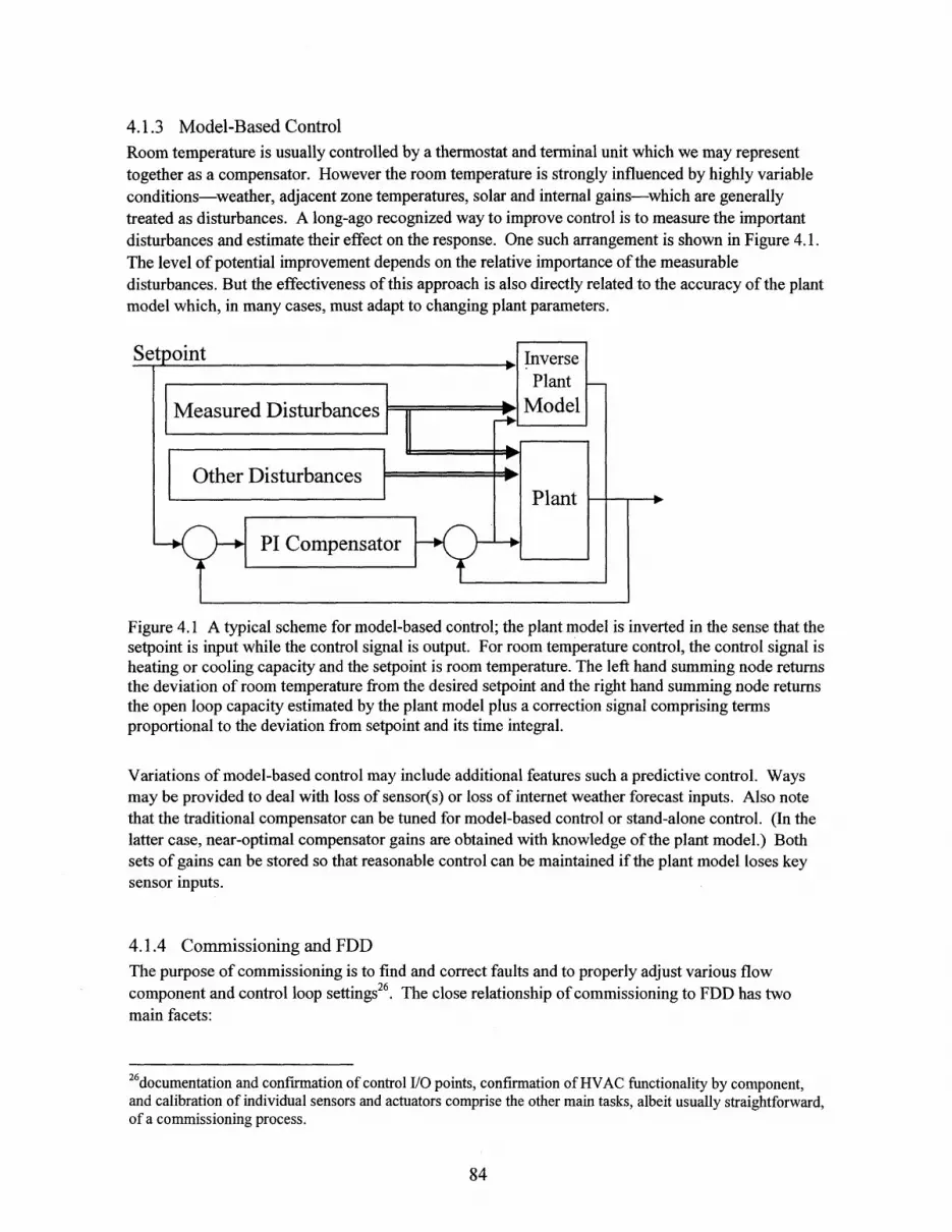
4.1.3 Model-Based Control
Room temperature is usually controlled by a thermostat and terminal unit which we may representtogether as a compensator. However the room temperature is strongly influenced by highly variableconditions-weather, adjacent zone temperatures, solar and internal gains-which are generallytreated as disturbances. A long-ago recognized way to improve control is to measure the importantdisturbances and estimate their effect on the response. One such arrangement is shown in Figure 4.1.The level of potential improvement depends on the relative importance of the measurabledisturbances. But the effectiveness of this approach is also directly related to the accuracy of the plantmodel which, in many cases, must adapt to changing plant parameters.
Setpoint , InversePlant-
Measured DisturbancesT1 Model
Other DisturbancesPlant-- +
PI Compensator
Figure 4.1 A typical scheme for model-based control; the plant model is inverted in the sense that thesetpoint is input while the control signal is output. For room temperature control, the control signal isheating or cooling capacity and the setpoint is room temperature. The left hand summing node returnsthe deviation of room temperature from the desired setpoint and the right hand summing node returnsthe open loop capacity estimated by the plant model plus a correction signal comprising termsproportional to the deviation from setpoint and its time integral.
Variations of model-based control may include additional features such a predictive control. Waysmay be provided to deal with loss of sensor(s) or loss of internet weather forecast inputs. Also notethat the traditional compensator can be tuned for model-based control or stand-alone control. (In thelatter case, near-optimal compensator gains are obtained with knowledge of the plant model.) Bothsets of gains can be stored so that reasonable control can be maintained if the plant model loses keysensor inputs.
4.1.4 Conmissioning and FDD
The purpose of commissioning is to find and correct faults and to properly adjust various flowcomponent and control loop settings2 6. The close relationship of commissioning to FDD has twomain facets:
2 6documentation and confirmation of control I/O points, confirmation of HVAC functionality by component,and calibration of individual sensors and actuators comprise the other main tasks, albeit usually straightforward,of a commissioning process.

1) fault detection tasks that are feasible without apriori knowledge of as-built behaviors, can andshould be automated and made part of the commissioning process;
2) properly identified models of HVAC and other building subsystems2 7 are essential to serve as abaseline for continuous fault detection and continuous commissioning. It is most reasonable toidentify such baseline models during the commissioning process when there is a high confidencethat each subsystem modeled is operating correctly.
In this chapter the precooling application will be explored.
4.2 Previous WorkThe analytical framework for dealing with different climates, rate structures and occupancies is wellestablished (Braun 1990, Kintner-Meyer 1995, Morris1994, Norford 1985, Rabl 1991, Xing 2004).Reliable one-day-ahead weather forecasts can be downloaded daily or hourly. Internal gains,predominantly light and plug loads, can be disaggregated by a NILM from the building total (Leeb1992, Laughman 2003) and future loads can be similarly extrapolated from the accumulated history(Seem and Braun 1991, Forrester 1984).
However, thermal response to weather, internal loads and HVAC inputs is unique to each buildingand difficult to characterize empirically (Braun and Chaturvedi 2002, Norford 1985, Pryor 1982, Rabland Norford 1991). The development of a general model and model identification proceduresufficiently robust to be automated is therefore a central and challenging prerequisite to theimplementation of useful curtailment or peak-shifting (Kintner-Meyer 2003, Stoecker 1981),precooling (Keeney 1997), and optimal start (Seem 1989, Armstrong 1992) control strategies.Verification of curtailment for allocating incentives would, ideally, be based on the same model thatis used for control (Goldman 2002).
The literature dealing with optimal control of discrete storage (e.g. a tank of ice or cold water) isdominated by the very thorough work of Henze and Krarti (1995, 1997) and Kintner-Meyer (1994,1995). Of particular interest to both discrete storage control and building mass control is anassessment of the impact of forecast uncertainties (Henze 1999).
The literature dealing with precooling of building mass is richer and more varied in part because ofthe uncertainties in building thermal response and in part because of the severe capacity and storagelimitation constraints (Andresen 1992, Brandemuehl 1990, Braun 1990, Braun and Chaturvedi 2002,Coniff 1991, Eto 1984, Keeney 1996 and 1997, Morris 1994, Rabl 1991, Ruud 1990). Nightprecooling studies have used simplified analyses, as well as simulation, to show annual savings inmechanical cooling energy input of up to 50%. Unfortunately there has been only one successfuldemonstration of significant precooling benefits in a real building (Keeney 1997). Control of nightprecooling involves the same building-specific thermal response model that is used for curtailment.
Reducing peak cooling loads, the usual basis for curtailment, is addressed in a number of papersQuestions of incentives and dispatch have dominated the discussion; building transient thermalresponse has not been handled very rigorously except in the simulation studies (Haves 2001,Goldman 2002, Kintner-Meyer 2003, Stoecker 1981).
27Possibly including whole-building performance models

Optimal start requires some kind of thermal response model. HVAC controls have traditionally usedvery simplistic models (Hittle) More reliable control can be obtained with more realistic models butthe economic benefit with respect to the best simplified models appears not to be very great (Seem1989, Armstrong 1992).
4.3 Experimental Demonstration of Peak Shifting PotentialThe transient thermal responses of the LA test buildings (ECC and ISD) to manually introducedcontrol changes were observed in a series of field tests. Field tests included summer afternoon loadshedding (curtailment) sequences and summer and winter pre-cooling sequences in both buildings.The test protocols and observed responses are documented in this section.
4.3.1 Curtailment Test Protocol
A summer load shedding protocol proposed by Haves (2001) provides a number of load sheddingscenarios. All scenarios require heat to be completely shut off to eliminate the inadvertent heat gains(poorly insulated pipes, stuck valves, etc.) that inevitably exist in real world distribution systems. Theideal method of cooling plant modulation is to raise all zone setpoints gradually by the same amount.The practical approximation given by Haves is to raise all setpoints abruptly by the same amount.This will cause chillers to shut down for 30-60 minutes in most buildings. Since the L.A. testbuilding control systems do not provide a way to raise zone setpoints simultaneously, we simply shutdown the chillers. This has the same effect up until the time when one or more zones reaches its newsetpoint. An alternative approach for ISD is to shut down one or more compressors or, for ECC, toreduce chiller capacity by modulating the inlet vanes. Such capacity modulation actions let us tradeoff load reduction against duration.
The most extreme action given by the Haves protocol is by no means the most extreme electric loadshedding scenario possible nor does it represent the most extreme thermal excitation possible.Rather, the protocol aims to provide significant load reduction with modest comfort impact over short(1- to 4-hour) time frames. In the case of ECC, the test was implemented by disabling HVACequipment in the sequence indicated below:
1) supply fan speed frozen at current setting (32Hz)
2) return fan speed frozen at current setting (25Hz)
3) hot water pumps to OFF
4) chilled water pumps to OFF
5) chiller and tower pumps and fans turn off automatically after step 4.ISD cooling load was shed, as at ECC, by turning off hot and chilled water pumps. The chillers andcooling towers go down automatically upon loss of chilled water flow.
A log of load shedding activities is correlated with NILM measurements to quantitatively assess theimpacts in terms of both load reduction and loss of comfort for occupants.
The NILMs monitor electric load changes effected by occupants and plant operators duringcurtailment events and the K20-6s and microloggers monitor weather and zone comfort conditions aswell as coil loads.
Data obtained during load shedding are analyzed to determine the following:
Reductions, from baseload, achieved by curtailment of lighting and plug loads;
Reduction, from model-predicted HVAC load, achieved by the combination oflighting and plug load curtailment, and

further reduction in cooling capacity;
Disaggregation of HVAC load reduction by the two above-mentioned actions;
4.3.2 Night Precooling Test Protocol.
A constant volume precooling strategy was tested in ISD and a variable volume strategiy was testedin ECC. Since model-based optimal control could not be implemented on the existing controlsystems the tests were performed manually by an MIT research assistant and site contact as operators.
For ISD, the CVSubcooling/Tempering strategy was implemented in the conventional way, with bothsupply and return fans operating, and in a low fan energy mode with windows opened and only thereturn fan operating.
For ECC, the Variable Volume cooling strategy is not practical as a manually implemented strategy.A suboptimal variant was tested instead in which the fans are operated at a reduced but fixed staticpressure and the terminal boxes are allowed to modulate air flow to each zone.
In both tests, the economizer dampers were held open manually until outside air exceeded return airenthalpy on the constant comfort line and the chillers were held off until average or least comfortablezone conditions reached a corresponding predetermined comfort limit.
4.3.3 ECC Load-Shedding Test Results
Load curtailment tests followed the main elements of the Haves protocol, described earlier. The 25June 2002 test was effected by simply turning off the chilled-water and hot-water pumps at the motorcontrol panel (MCP). The chiller (immediately) and cooling tower (within one minute) then shutdown automatically. The averages of pre-curtailment temperatures shown in Figure 4.2 were 72.05'Ffor zones and 72.16'F for return air; both were very steady (standard deviation <0.1 F) over the 100minutes preceding the test.
80
75 - --- i- --------- -- -- - - - - -
70
C 65-IUI
60 .----- T-
--- Tmix50 - - -Tsa _________ _____
E- -- - -CTowerFan1 - - --------------j 45 - HWpump7
10: -4-- -CndWpump3 4
N - RetumFan1 2 t ---0 35. -- - -ChWpump1 2
C.- Hfpump5 6E 30- SupplyFani
no ------- --------. SupplyFan2 --.---- --- ------ Chmer125- MCP feed
Y 20 . ... Chilledi
15""
E 10'
F 4.2. - - - - - - -dn Ea~ 0O 0 0) 0 0r 0 0O 0 O 07
CD4 (4 (D
Figure 4.2. Temperatures and HVAC motor loads during EGG load shedding test.
1200
1050
900 0
Ca
750 L
600C
450 E
300
150

It is not surprising that the return air is warmer than the average temperature across zones becausereturn air is taken from the ceiling level and usually picks up some heat from ceiling lights as it leavesa room. Both temperatures begin to rise almost from the instant-indicated in Figure 4.2 by the 400A(330kVA) drop in MCP load at 16:48-that the plant was shut down. Both rise along similarlyshaped trajectories after the chiller stops but the return air temperature rises more rapidly. This, too,is not surprising because the zone temperature sensors were placed on file or desktop cabinets or onwall thermostats where the proximate slower responding surface temperatures affect themeasurements by radiant coupling. The zone sensors are indicating something close to "operativetemperature" defined [ASHRAE 2001] as the average of air temperature and mean radianttemperature (MRT). The zone average and return air temperatures after 53 minutes without coolingwere 74.65 and 76.89'F. When the chiller is turned back on, the return air temperature againresponds more quickly than the zone sensors and we see that it approaches within 0.1 'F of the pre-testtemperature 50 minutes later. At this point the return temperature is 0.8'F below the sluggishlyresponding average zone temperature. The return air temperature drops below the pre-test value(overshoots in the direction of initial response) after the chiller is restarted--a direct result of slowzone thermostat response. Fan power rises gradually during curtailment as air flow increases tosatisfy terminal units demand for more cooling and static pressure is maintained. The pressuresetpoint could be reduced to prevent this.
Zone temperatures (transient behavior and dispersion among zones) observed during the June 2002site visit were analyzed to assess the consistency of zone thermal conditions. The zone temperatures,their average, and the standard deviation across zones, are plotted in Figure 4.3 and Figure 4.4. Notethat loggers resided together in a bag prior to deployment (2002.06.21 15:00-16:30 PDT), thus thedata taken prior to deployment is only useful for showing that the loggers track each other quite well.
86
84
82
80
78
76
74
72
70
68
66
64
62
60
oa 0 0. 0 0 0 0 0L0 i 0 0
oN 0 0 0 0 0 0 0 0 0 0 0 0 0M
N N - N N - N N - NN 0a N N N 0 N 0 N 0 N
0 0 0 0a0* N 0 N M l N 6 D N C
Time (PDT)
Figure 4.3. Children's Court micro-logger data from launch time (2002.06.19 13:00 PDT) throughfirst download/lrelaunch (2002.06.26 16:00-16:45 PDT).
-- 332630 -- 332631- 332633 -- 495199-495205 -522637-- 522638 - 522640
522641 522643522645 - 522646
-avg - stDev

78 495205 -522637522638 522640522641 522643
76 522645 -522646
avg - stDev
72 - _______________
70
68 4
- -- 925---522637rehhmi~T' "' C~C~ \
4.. *S avg ---sheddnv eteutTimeN (hUm PT
ISD cooling equipment was shut down, as at ECC, by turning off hot and chilled water pumps. Thechiller and cooling tower shut down automatically. Prior to shut down, return air and average zonetemperatures were 74.8 and 72.0 ±0.1 0F, as shown in Figure 4.5. The higher return-air temperaturemay be partly caused by air leaking from the hot deck. Also note in Figure 4.5 that the return airtemperature is less responsive to the step change than the average zone temperature. Supply ductleaks alone could only account for this if they were on the order of 50% of supplied air; thermalcoupling to the underside of the floor decks also contributes to attenuation of rapid changes in returnair temperature. Over half the total building load (600 - 350 =250kVA) was cut during the test. Afurther 12% was cut when the fans were shut off at 5:30 pm. The average zone temperature rose5.5 CF in the first 40 minutes (fans on) and 0.50F in the next 40 minutes (fans off). The zonetemperature responded quickly after the test, in part because the hot deck was not restored until muchlater; return air temperature responds slowly. It is not clear why, with the large zone temperature rise,the chillers did not return to high capacity at the end of the test.

1200
110 1100
100 1000
0 9000
L 80 -..... .... . 800 0--------------------------------------------- ....
70 _ avgTzone H 700<070 - -Tmixed>- TcoldDeck
0 IV -% I wThotDeck ___600___ __ __ __ __
E 60 Ch Water Pumps 600- Cnd Water Pumps
50 ~ - - HWPumps5+6 500- - - - MCAB -
--- Retumn Fan
2 40 --- Supply Fan 400 C- - -- ---- Chiller 1A+2AB 40ILL -- Chiller 1B+2B t
30 -HVACtotal "300- Main total -
0 -- 200
-- , o o o----o---o-o - o-<10 11k .. ... 100
o - 0 -- -- - - - - 0 0-- - - 0 0 0 0I0 (CD 0 ( C) C) CD 0D a~
L- o Co t- _ CO o o 0o CoCI 4 (N (N (N 0N (NJ 04 (J CIA CV
p C 0 0 0 0 0D 0I 0
(N4 C4 (N (N (N 04 04NII C
Figure 4.5. Temperatures and HVAC motor loads during ISD load shedding test.
4.3.5 Children's Court Precooling Test Results
A second ECC precooling test was completed 23 January 2003 in a week of mixed weather andbuilding occupancy. Monday, 20 January, was sunny, Tuesday hazy, Wednesday and Thursdaymoderately overcast. Temperatures were typical for January except Wednesday morning was about5*F below normal. The building was closed to the public on Monday for Martin Luther King Day.
The chiller was turned off 17:00 PST on Wednesday afternoon and the supply fan static pressure (SP)setpoint was reduced from 2.2 to 0.5 inches (water gauge) at 01:00 early Thursday morning. Thesetpoint was restored to 2.2 inches at 07:00 and the chiller was restored at 10:15. The HVAC andbuilding electrical loads are shown in Figure 4.6 and the temperature trajectories are plotted in Figure4.7.
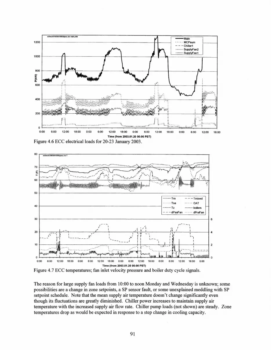
1200
1000
800
600
400--
200
0:00 6:00 12:00 18:00 0:00
Figure 4.6 ECC electrical loads
6:00 12:00 18:00 0:00 6:00 12:00 18:00 0:00 6:00 12:00 18:00
Time (from 2003.01.20 00:00 PST)
for 20-23 January 2003.
30 6
20 14A - -4
10 li 240
0:00 6:00 12:00 18:00 0:00 6:00 12:00 18:00 0:00 6:00 12:00 18:00 0:00 6:00 12:00 18:00 0:00
Time (from 2003.01.20 00:00 PST)
Figure 4.7 ECC temperatures; fan inlet velocity pressure and boiler duty cycle signals.
The reason for large supply fan loads from 10:00 to noon Monday and Wednesday is unknown; somepossibilities are a change in zone setpoints, a SP sensor fault, or some unexplained meddling with SPsetpoint schedule. Note that the mean supply air temperature doesn't change significantly eventhough its fluctuations are greatly diminished. Chiller power increases to maintain supply airtemperature with the increased supply air flow rate. Chiller pump loads (not shown) are steady. Zonetemperatures drop as would be expected in response to a step change in cooling capacity.

Also note that the supply air temperature control loop is poorly tuned for part-load operation. Theresult is oscillation of the coil control valve, reflected in chiller power, at about 2.2 cycles per hour.The amplitude of these oscillations decreases during times of high cooling load (high supply air flowrate). The daily mean conditions, loads, and room temperatures averaged across 12 zones aresummarized in Table 4.1.
Table 4.1 24-Hour average conditions at Children's Court for 20-23 January 2003
CtowerFan (CT1)CndWpump (P3)ReturnFan (R1,R2)SupplyFans (S 1,S2)HWpumps (P5,P6)ChWpump (P1)ChillerlMCP feedC-H mainTraTmixedTsaRhraRhmixedRhsaTz (Hobos)Tamb (outside)S (plain LiCor)Total (unshaded)Diffuse1 (shaded)Prt'l (partly shaded)
kWkWkWkWkWkWkWkWkW*FOFOF
OFF
W/m2W/m2W/m2W/m2
Monday1.8
28.20.3
100.43.8
23.6236.7394.8415.2
67.565.255.849.944.870.871.060.1
154.1154.127.7
136.1
Tuesday1.3
28.30.3
90.63.8
23.7222.1370.0465.7
67.363.855.852.851.474.371.458.5
114.2114.455.9
101.8
Wednesday1.3
25.60.3
81.53.5
22.0203.5337.6462.4
68.664.656.651.645.073.271.557.275.975.955.369.8
Thursday1.5
10.35.3
74.91.99.1
99.6202.7306.569.263.959.750.340.865.271.761.977.177.762.373.1
Because the chiller operates inefficiently at part load, there is little variation in average chiller powerexcept on the day of the precooling test, when it was completely shut off for 16 hours. The chilleraverage power Thursday was thus reduced from over 200 kW to 100 kW. The associated averagecooling tower and chilled water pump loads were also reduced substantially from 49 to 21 kW.Supply fan power is about 16kW (4 kW daily average) during the precooling phase and about 112 kWduring the day. Baseline chiller and pump power are very high Monday through Wednesday becauseno unoccupied periods were scheduled on the control system. The baseline daily average would havebeen about 150 kW for the chiller and 30 kW for pumps under a normal night lockout schedule.Estimated savings from this reduced baseline are, nonetheless, a considerable 45% which representsabout $50k/year. The extra fan energy (compared to a fan-off-at-night baseline) is only about 10% ofchiller and pump savings thanks to the reduced static pressure during precooling.

4.3.6 ISD Building Precooling Test Results
The test was completed Wednesday, 22 January. In contrast to Children's Court, the ISD Buildingwas partly occupied on the preceding Monday, 20 January 2003. Temperature trajectories are plottedin Figure 4.8 and HVAC and building electrical loads are plotted in Figure 4.9.
80
S60
ILi=' 40 -
0:00 8:00 16:00 0:00 8:00 16:00 0:00 8:00 16:00 0:00 8:00 16:00 0:00 8:00 16:Time (from 2003.01.19 0:00 PSI)
Figure 4.8 ISD temperatures and electric loads during week of the precooling test.
120
80
40
00 0:00 8:00
- - Sfan -Ch12B- - - ChWP - - CndWP
-- Ch1A2A - Rfan- -HWP - CT
hvac - main
fl1 hii 'A i hA A i ~A~~AAAAI1A AAAAAAfIAAAAA10
II~ ~ ~ ~~I n ii su ii uiiiiuiii 1 11 1 I I I I ISIIIi 11 EI4 IUV. V nYU v!V VV 1:Ji I;.
- -- 60
20 40
10 20
0 09:10 9-20 9:30 9:40 9:50 10:00 10:10 10:20 10:30 10:40 10:50 11:00 11:10 11:20 11:30 11:40 11:50 12:00 12:10 12:20 12:30 12:40 12:50 13:00 13:10
Time (2003.01.21 PSI)
Figure 4.9 Short segment of Figure 4.8 showing compressor cycles (Im-average loads)
For this precooling test the chiller was turned off 18:00 PST on Tuesday afternoon and restored at13:50 the following day. The windows were opened at 21:30 Tuesday and the return fan was started.Return temperature dropped from 73.2 to 69.0*F and average room temperature dropped from 73.5 to64.3 F during the precooling period, which ended at 05:30 Wednesday morning with closing of thewindows. The supply fan started at 05:40 per its normal schedule. The exhaust damper was closed
.y V V ~Ii
0 4--
nawo-1%Nf"3-nannumann1unaoa

and the return damper opened from 07:00 to 8:45 allowing the occupied space temperature to risefrom 67.9 to 71.7*F. The space was thus effectively in a tempering mode from 05:30 to 08:45. Thisamount of tempering is more than was necessary; tempering would have ended at 07:20 when thezone reached 70'F, had the controls been properly automated.
Average zone temperature reached 744F at 11:45am. The chiller remained locked out until 13:50, bywhich time the zone temperature had reached 75.1*F. The return fan remained on through 24 Januarybut the windows were not opened that night. This resulted in limited precooling Thursday morningby outside air being drawn through the hot and cold deck systems even though the supply fan was off.Note that return temperature approaches room temperature progressively more closely from Monday(after the previous week and weekend in which there was no precooling) to Thursday. Several daysof precooling are needed to cool the building's floor deck structures from their under (ceiling plenum)sides. It is fair to conclude that 1) a one-day test is not sufficient to demonstrate the full potential and2) precooling on Saturday, as well as Sunday, night may be cost effective.
Chiller cycling is apparent in Figure 4.8. Details of this cyclic behavior are shown to better advantageon the expanded time scale of Figure 4.9. One may conclude that the cycling could be largelyeliminated by modifying the compressor sequencing logic so that compressors come on one by one,rather than in pairs. The response to precooling is presented on an expanded time scale in Figure 4.10where the cycling tendency, even under the heavy zone temperature pull-down load that existed whenthe chillers were finally started at -14:00, can be clearly seen.
The daily mean conditions, loads, and room temperatures averaged across six zones are summarizedin Table 4.2. The ISD chillers, in contrast to the Children's Court chiller, operate more efficiently atpart load (in spite of the cycling). The average chiller input is therefore significantly lower on coolerand partial occupancy days. Average chiller power on the day of the precooling test is, nevertheless,less than half of the average power used on the other three days. Fan power, on the other hand,changes little from day to day except that average return fan power is higher Tuesday throughThursday because it was run during certain unoccupied hours on all three of those days.
On the day of precooling, average chiller power was reduced from ~22 to 8.3 kW. Associatedaverage cooling tower and chilled water pump loads also dropped substantially from -8 to 3.7 kW.Average return fan power increases from -7 to almost 13 kW. Net average savings are thereforeabout 12 kW from a baseline of 58 kW representing about $15,000/year. Precooling by the supplyfan would reduce savings by roughly half these amounts.
120- t*I3I3d-swAX-- -Tra -.-.--.-. OAT
Thot - - - Tcold
100 -- avgTz - Sfan-- Ch1B8 -Ch1A2A
-Rfan ---- main
8 0 - 8
20 - - -- 40
0 ~ ------------- ...... . . . ..--.- . -..- -.. . -..-... . -. ...- 0
40 ~ 8
18:00 21:00 0:00 3:00 6:00 9:00 12:00 15:00 18:00Time (from 2003.01.21 18:00 PST)
Figure 4.10 One-day segment of Figure 4.8 showing precooling test details.
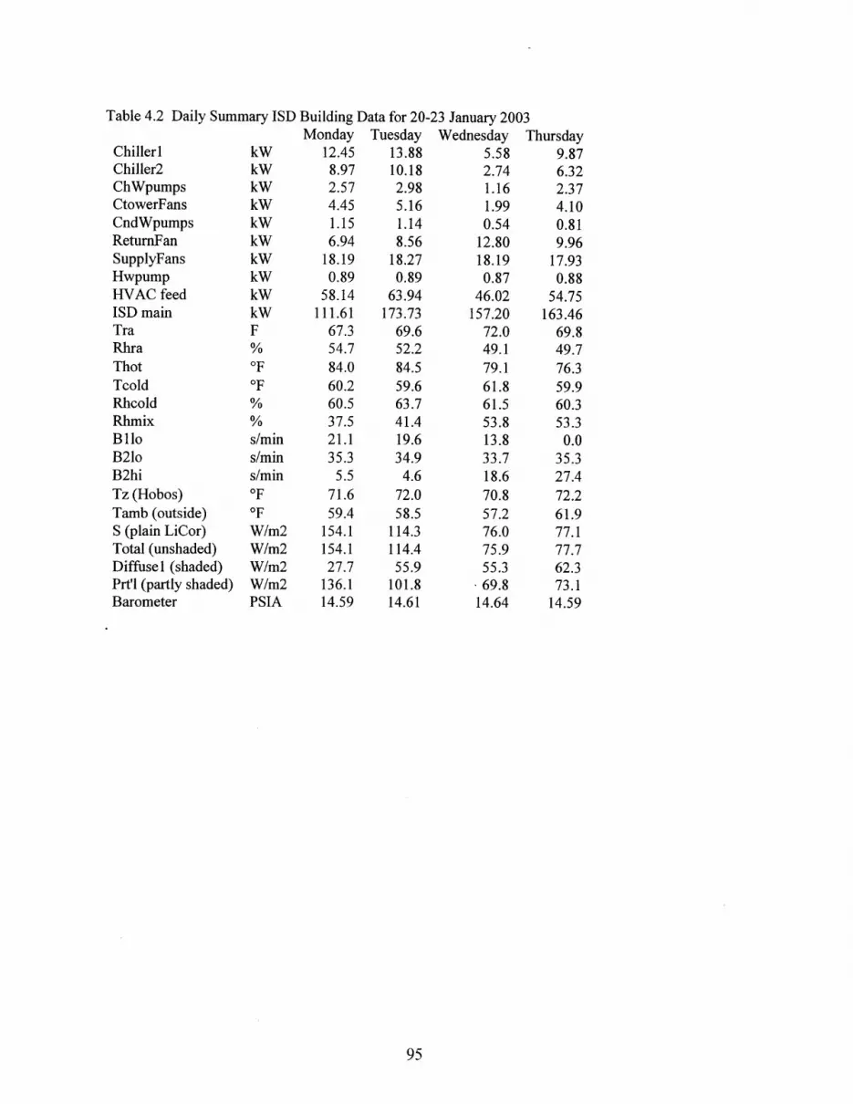
Table 4.2 Daily Summary ISD Building Data for 20-23 January 2003
ChillerlChiller2ChWpumpsCtowerFansCndWpumpsReturnFanSupplyFansHwpumpHIVAC feedISD mainTra,RhraThotTcoldRhcoldRhmixBlloB21oB2hiTz (Hobos)Tamb (outside)S (plain LiCor)Total (unshaded)Diffusel (shaded)Prt'l (partly shaded)Barometer
kWkWkWkWkWkWkWkWkWkWF
OFOF
s/mins/mins/min*F*FW/m2W/m2W/m2W/m2PSIA
Monday12.45
8.972.574.451.156.94
18.190.89
58.14111.61
67.354.784.060.260.537.521.135.35.5
71.659.4
154.1154.127.7
136.114.59
Tuesday13.8810.182.985.161.148.56
18.270.89
63.94173.73
69.652.284.559.663.741.419.634.9
4.672.058.5
114.3114.4
55.9101.814.61
Wednesday5.582.741.161.990.54
12.8018.190.87
46.02157.20
72.049.179.161.861.553.813.833.718.670.857.276.075.955.369.8
14.64
Thursday9.876.322.374.100.819.96
17.930.88
54.75163.46
69.849.776.359.960.353.3
0.035.327.472.261.977.177.762.373.1
14.59

4.4 SimulationTo compare cooling control strategies we must estimate annual energy use and cost for each strategywhile all other aspects of building operation are held constant. These "constants" include fan andchiller performance curves; fan, chiller, and auxiliary equipment control sequences; weekly andholiday schedules that describe internal gains, minimum outside air and fan static pressure; zonetemperature setpoint schedule and related control parameters; utility rate schedule, and weather.
The information flow and main functional elements of the simulation are shown in Figure 4.11. Thethermal response model of chapter 3 is integrated with economizer operation as described in 4.4.1.This model is of of general form and is made building-specific by plugging in the model order,number of walls, and coefficients. The chiller and internal gain models are described in sections 4.4.2and 4.4.3.
Occupancy Control Optimizer .Schedule
!T
Weather 0.Fan Energy
Sun - Envelope Power Utility __-andAngles (CRTF )hle Rate Demand
Internal (economizer) CiLle -- + ct CostsGain Power Stu.Schedule
Figure 4.11 Simulation block diagram showing main functions, structures and information flow
4.4.1 CRTF for Simulation
Recall from the Model Synthesis subsection (3.3) that the discrete-time model (5) can be evaluatedrecursively for Qz or T:
for Qz: -# 0 =B"(#2,2)+B"(0,,T,)-B"(,,T,) (6a,b)
fo T:Oz0Iz= 0_(z,Qz )+ Bo I0,, , O T (8a)
With qz= -1 eqn (6) becomes:
Q, B," (# G + B"0,,, - B0" (zT)
When the zone heat balance involves exchange of outside air with mass flow rate F, the foregoingexpression for Qz becomes:
Qz = Fc,(Tz - Toa) - Qsrar, where Qsrar = Qh/c + Qsotrad+ Qg, the expression for T becomes:
Fc,~~ +Qe B"#,+(0z ,T,)-Bn"(Oz, TzT = Fc oh,+1+Bn(w w I z(8b)0z,0 + Fc,
and it is easy to see that with F = 0, (8b) reduces to (8a).

4.4.2 Chiller Performance
ISD coil loads were monitored for two weeks, 29 August - 9 September, 2002, a period whichincluded very hot weather. The total coil load is computed from its sensible, Fcp(Toid - Tmix) andlatent, Fhfg(wmix - wcold), air-side components. The measured 5-minute average sensible and total coilload are plotted in Figure E- 1 against chiller power. Note that the latent fraction increases moderatelywith load, as expected for an essentially constant air-side flow rate. Chiller-specific power, expressedas chiller power per unit coil load (kW/Ton) increases with load. This is also expected. Thecondenser and evaporator areas are fixed so the approach temperatures increase with load resulting inthe lift temperature increasing even faster than the condenser-chilled water temperature difference.Only one chiller was operated during this period. There are four compressors per chiller and theresulting performance in each of four operational stages, clearly evident in the plot, is summarized inTable 4.3.
Table 4.3 ISD chiller performance summary for 29 August - 9 September 2002
For discrete-time simulation it is inconvenient and unnecessary to emulate the cycling between stagesthat occurs with periods less than the simulation timestep. A power law, shown in Figure 4.12, istherefore used to represent chiller performance in the simulation. Control parameters determinemaximum capacity and at what load the second chiller starts.
1400 1 1
Qsens(kBtuh) vs. Pch(kBtuh)1200
100 -)(~C()()
800
00600600- C)
40061 (C)) )
200
0 0
-2001I0 0 100 150 200 250 300 350 400 450
Qtot Qtot Qlat/Qtot Pch/Qtot(kBtuh) (RefTon) (-) (kW/RT)770 64 0.28 0.521270 106 0.31 0.651500 125 0.30 0.811700 142 0.31 0.93

Figure 4.12 Power law used to simulate ISD part-load chiller performance.
4.4.3 Internal Gain Schedule
The measured internal gains are shown in Appendix P???. Weekday and weekend profiles aredistinct and repeatable. The ISD building is supposed to be operated in weekend mode on Fridays butsome people do work and the resulting lighting and plug loads are variable. The 24-hour weekdayand weekend profiles shown in Figure 4.13 were obtained by averaging the observed kW numbers.
550
500
450-
400-
350-
300-
250-
200
Figure 4.13 Occupied and unoccupied internal gain schedules used for ISD simulations (kW).
4.4.4 Control of Fan and Outside Air
The following truth table summarizes the control structures used in the simulation in a form that canbe readily ported to an EMCS for a demonstration. The logical input columns (1-6) have entries of1-true, 0=false and *=either. The zone temperature setpoint relation TzITe refers to the economizerset point, Te, which may be different in occupied and unoccupied periods. For example Tz<Tegenerally turns the fan off in unoccupied periods and reduces outside airflow to the minimumrequired for ventilation in occupied periods. The output columns (7-8) refer to fan and damperoperation. Fnom is the nominal (maximum) supply fan mass flow rate and %F/Fom is the fraction ofFnom expressed as a percent.
() )
(C)
00
0 C
fg ure(3); Flot(1 +n d( 1:477 ,2), x(:, ),bo'); ( main-Phvac-P ba
()n (_0C()-(Co(57)C )C0 ))0 c))o
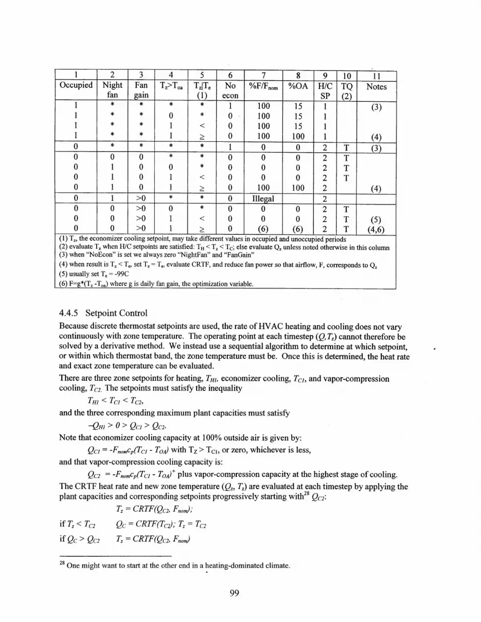
1 2 3 4 5 6 7 8 9 10 11Occupied Night Fan Tz>Toa TzTe No %F/Fnom %OA H/C TQ Notes
fan gain (1) econ SP (2)1 * * * * 1 100 15 1 (3)1 * * 0 * 0 100 15 11 * * 1 < 0 100 15 11 * * 1 > 0 100 100 1 (4)0 * * * * 1 0 0 2 T (3)0 0 0 * * 0 0 0 2 T0 1 0 0 * 0 0 0 2 T0 1 0 1 < 0 0 0 2 T0 1 0 1 > 0 100 100 2 (4)
0 1 >0 * * 0 Illegal 2
0 0 >0 0 * 0 0 0 2 T0 0 >0 1 < 0 0 0 2 T (5)0 0 >0 1 > 0 (6) (6) 2 T (4,6)
(1) Tz, the economizer cooling setpoint, may take different values in occupied and unoccupied periods(2) evaluate T2 when H/C setpoints are satisfied: TH< Tz < Tc; else evaluate Qz unless noted otherwise in this column(3) when "NoEcon" is set we always zero "NightFan" and "FanGain"(4) when result is T2 < Te, set Tz = Te, evaluate CRTF, and reduce fan power so that airflow, F, corresponds to Qz(5) usually set Te = -99C
(6) F=g*(Tz -Toa) where g is daily fan gain, the optimization variable.
4.4.5 Setpoint Control
Because discrete thermostat setpoints are used, the rate of HVAC heating and cooling does not varycontinuously with zone temperature. The operating point at each timestep (Q, T) cannot therefore besolved by a derivative method. We instead use a sequential algorithm to determine at which setpoint,or within which thermostat band, the zone temperature must be. Once this is determined, the heat rateand exact zone temperature can be evaluated.
There are three zone setpoints for heating, THI, economizer cooling, Tc1, and vapor-compressioncooling, T 2 . The setpoints must satisfy the inequality
THI T IC2,and the three corresponding maximum plant capacities must satisfy
-QHi > 0 > Qci > Qc2.Note that economizer cooling capacity at 100% outside air is given by:
Qci = -For,.c,(Tcj - T0 with Tz> Tci, or zero, whichever is less,and that vapor-compression cooling capacity is:
QC2 = -Fo,,cp(TCi - T0f plus vapor-compression capacity at the highest stage of cooling.
The CRTF heat rate and new zone temperature (Qz, T) are evaluated at each timestep by applying theplant capacities and corresponding setpoints progressively starting with28 Qc2:
Tz= CRTF(Qc 2, Fno,,);
if T < Tc2 Qc = CRTF(Tc'); T = Tc2
if Qc > Qc2 T CRTF(Qc2, Fn,,)
28 One might want to start at the other end in a heating-dominated climate.

Qc = CRTF(Tc); F=FnI*QC/QC2
if Qc > Qci Tz = CRTF(Qci, Fnom)
if TZ <Tci Qc = CRTF(Tcj); F=Fn0 , *Qc/Qc,
if Qc > 0 Tz = CR TF(0, Fmn)
if Tz < THi QH = -CRTF(THI); F=Fnon *QH/QHI,
if QH> QHJ Tz = CRTF(-QH, Fmin)
As soon as the bracketing setpoints have been found, the progression can be terminated and the heatbalance solved for QH/c:
QCRTF + QH/C + QIG + QDSG = 0
where
QCRTF = OxoTx - OoTz + Qp., and
QDSG = rate of direct solar gain,QH= QH/c, QC = 0, when QH/c > 0, and
QH= 0, Qc = QH/c, when QH/c < 0.
The final evaluation of zone temperature is then given by:
Tz = ((Fc, + Oxo)Tx + QP + QH + QC + QIG + QSR)/(Fc, + zo)
4.5 Results for ISD Building Driven by LA TMYHere the annual performance of night precooling control strategies is evaluated by using TMY2 LosAngeles weather data to drive the ISD thermal response model. The cooling capacities provided bythe chiller plant and by outside air are separately integrated over the year for each case simulated.These numbers and the annual electricity (energy and demand) costs together provide a completepicture of the alternative control strategies described in Section 4.1.1.
The base case, no night cooling with the economizer setpoint equal to the mechanical cooling setpoint(74.5'F), is shown in Figure 4.14. Mechanical cooling represents almost 60% of the total annualload. As the economizer setpoint is reduced, the total cooling load is increased but the annualmechanical cooling share is reduced to about 50% of the total with the most extreme economizersetpoint of 68'F. The cooling shares are not very sensitive to economizer setpoint because there islittle daytime economizer cooling potential on days when there would be significant chiller loadwithout economizer cooling.
With economizer cooling enabled at night (fan runs whenever zone temperature is above theeconomizer setpoint and outdoor temperature is below zone temperature) mechanical cooling isimmediately reduced by 30% for case 6 (economizer setpoint = mechanical cooling setpoint =74.5'F) simply by eliminating morning pull down loads. Total annual cooling is immediatelyincreased by 20% in response to lower zone temperatures on many nights. Note, furthermore, that themechanical share drops significantly (an additional 30%) and total load increases significantly(another 17%) as the economizer setpoint is lowered. These results are shown in Figure 4.15.
With optimal nightly delayed-start times, the annual fan energy (hours of fan operation) is greatlyreduced, the amount of economizer cooling is moderately reduced, and the amount of mechanicalcooling is increased slightly as shown in Figure 4.16. Total annual cooling numbers are 10-15%lower. However, as shown in Figure 4.17, there is very little cost savings because off-peak energyrates are relatively low.
100
i f Tz <: Tci

4000
3500-
3000
. 2500 -
200 -
1500-
1000-
500-
0-74.5 74
E
Figure 4.14 No night cooling, cases 1-5.4000.
SeconomizerErmechanical
3500
3000-
. 2500 -
cCD
5 2000-0
C 1500-
1000 -
500-
0
72 70 68conomizer Setpoint (F)
74.5 74 72 70 68Economizer Setpoint (F)
Figure 4.15 All night cooling, cases 6-10.
101

4000
3500
E economizerU mechanical
3000 -
. 2500
0 ZU02"2000
0
1500-
1000-
500
74 72
Economizer Setpoint (F)Figure 4.16. Delayed-start night cooling, cases 11-15.
200000 ,
70 6874.5
11
1111l. 111111_1 II1 2 3 4 5 6 7 8 9 10 11 12 13 14 15
* RatchetEOn-Peak kWM Mid-Peak kWN Off-Peak kWOOn-Peak kWhI Mid-Peak kWhfOff-Peak kWh
Case#
Figure 4.17. Annual electricity costs (building total) by time of use, energy, and demand
102
180000
160000
140000
1200000
0
g 800004
60000
40000
20000
0

4.6 SummaryIn Chapter 4 a simulation environment was developed for the study of optimal and suboptimal controlstrategies involving building thermal transient response. Chiller performance curves, utility ratestructures, and building thermal response models can be plugged in to enable building-specificanalysis.
A precooling control strategy with variable subcooling time and variable tempering time wasdeveloped. The strategy results in significant reduction of mechanical cooling using typical LosAngeles weather, utility rate structure and office occupancy schedules. Sensitivity of annual savingsto building mass and mean annual outdoor temperature was characterized.
In the base case, no night cooling with the economizer setpoint equal to the mechanical coolingsetpoint, mechanical cooling represents 60% of the total annual load. This was reduced to 50% withthe economizer setpoint reduced by 6*F.
With economizer cooling enabled at night mechanical cooling is reduced another 30% by eliminatingmorning pull down loads and yet another 30% when the economizer setpoint is reduced by 6*F.With optimal nightly delayed-start times, total annual cooling numbers are 10-15% lower and there isa small cost savings from reduced fan hours.
Because it is primarily a controls measure, and because it does not involve utility coordination2 9 , theimplementation cost for night cooling is potentially quite low. However, packaging is again a keyissue. The control package must provide reliable, autonomous identification of the plant's thermalresponse.
29 Verification becomes a matter of internal evaluation, rather than being a contractual issue.
103

Chapter 5 ConclusionThe related themes of fault detection, diagnostics, and control are bound by the important role that aplant-specific model plays in each application.
Model-based FDD and model-based control can take many forms. For example, fault detection canstart by comparing the response given by the detailed simulation of a system (driven by the measuredexcitations that also drive the real system) with the measured response of the real system. Variousresponses may be closely or remotely related to various faults. Detection may involve little or muchuncertainty. The control application raises similar questions of model type. The detailed, physics-based simulation is one extreme. At the other extreme, the model may be completely non-physical,e.g. ANN- or statistics-based, or somewhere in between.
To be plant-specific often means to be adaptive and autonomous. And it often means a model that isidentified or updated on-line. There may or may not be human initiation or intervention, e.g. as in thebuilding commissioning process.
Consequently, the type of model is a key issue. There exists a white-box to black-box continuum inwhich the white-box model is based entirely on process physics and the black box model is basedentirely on any sort of generic pattern matching that has no physical interpretation. It is rarelydesirable to settle on either extreme. Even a model that can have a purely physical interpretation, e.g.the CRTF, can often also have a statistical interpretation, e.g., in the case of the CRTF, an ARMAXinterpretation, and it would be rare for a plant to behave as a perfect CRTF so we must always beprepared to interpret model identification results statistically as well as physically.
White-box models typically present parameter estimation difficulties. If overcome the white- or grey-box model is typically better suited, for extrapolation, than a black-box model identified from thesame training set. The discrepancy between the testing set prediction error norm and the training setprediction error norm is likely to be less for a light-grey-box than for a dark-grey-box model. Theseconcerns are especially germane to building applications where identification data often lack richnessor reflect a low signal-to-noise ratio. Thus this thesis has been largely concerned with identificationand application of grey box models of the lighter sort and finding a good balance between reliabilityof identification and accuracy in application.
5.1 Thesis AccomplishmentsSignificant advances have been made in both direct and model-based fault detection, in zone- andbuilding-level model identification, and in precooling control and design.
Chapter 2 shows how the NILM's signal acquisition and PSA capability can be used to detect faults,prefault behavior, and performance degradation. A recursive ARX-based filter for detection ofnormal and anomalous transients was developed. The consistent association of anomalous transientswith liquid slugging, a dangerous condition that leads to compressor failure, was demonstrated bycompressor bench tests. Liquid ingestion during steady operation results a transient power increase of0.1-1s duration that appears clearly as positive deviations from k-step-ahead forecasts made by anadaptive ARX(5) model. Any positive power transient that fails to match a known start transient andthat exceeds the adaptive model innovation norm threshold indicates liquid ingestion.
104

The following additional fault detection capabilities were demonstrated.
* Air-side blockage faults were detected by a shift in steady state (P1,Q 1).
* Short cycling can be detected by PSA in the obvious way, by logging time between starttransients. The advantage over detection by a refrigerant-temperature-based FDD system is thatvery short-even incomplete-start transients that promote severe overheating are detected. Asecond method of short cycling detection relies on the shape of individual start transients beingsensitive to residual head.
" Refrigerant charge faults result in elevated head pressures which translate to higher steady statecompressor loads. Undercharge can also be detected from the start transient shape.
e The refrigerant vapor bypass fault had a distinct effect on the start transient shape: the change ofmagnitude in the latter half of the transient was two to five times the change in steady statepower.
* Flooded starts were detected by a distinctive change in start transient shape.
* PSA's ability to identify degradation of impeller balance well before the added repair costs of acatastrophic failure are incurred was demonstrated by spectral analysis.
The value of FDD is realized in several areas such as reduced down time, better efficiency, avoidanceof consequential damage, and the efficient dispatch of repair staff and replacement parts. Theavailable data, summarized in Table 5.1, are not sufficient to make precise statements about FDDsavings without making some assumptions about costs avoided through detection of incipient faultsor about the logistical savings achieved by remote FDD. For example, if we assume that earlydetection and repair of faults leading to compressor short, open, or locked rotor failures is 100%effective at preventing ultimate compressor failure, the savings are (.24)*(.66)=10% of all repair costsfor this one class of faults alone.
Table 5.1 Breakdown of repair cost by fault from Breuker; columns 2 and 3 are percents of column 1.Detection by PSA Certain Detection by PSA Probable
Compressor 24 short, open, locked rotor 66 broken internals, vapor bypass 11Condenser 9 Motor, belt failure, cycle control 51 fouling, coil leak 36Evaporator 6 0 fouling, leak, loss of capacity 75Air Handler 5 motor, impeller, belt, electrical 67 damper motor, duct leaks 20Controls 10 compressor interlocks, fan sequence 37 0Electrical 7 Contactor, loose connection 44 fuse/breaker, short/open 27Miscellany 21 water loop/pump, fan belt 29 refrigerant leak, installation/startup 42
bther 18 n.a. n.a.
Total % 100 Repair of all PSA-detectable faults 37 Faults likely to be detected by PSA 22__ (sumfof products with column1) (sum of productsawithcolumn1)
A very general model of wall, zone and whole-building thermal response was developed in Chapter 3.Three thermodynamic constraints were also identified. The constraints are crucial to on-lineidentification for the model-based control application because the observations used for modelidentification are inevitably noisy and often incomplete or biased as well. Without the constraints, aphysically implausible model that behaves badly under certain conditions (e.g., fast transients ortemperature extremes) will often be accepted as the "best" model implied by the data.
105

Formulations were developed for enforcing the constraints using the simple optimization tools ofordinary least squares and bounded-search nonlinear least squares. The steady-state conductanceconstraint is handled algebraically. This approach eliminates one unknown but, more importantly,has the invaluable advantage of leaving the problem in unconstrained ordinary least squares form.The constraint on time constants is a non-linear constraint. To avoid the difficulties traditionallyassociated with non-linear constraints, a way was found to reformulate the problem as anunconstrained nonlinear least squares problem. A further modification was devised to enforce theconstraint of alternating roots by imposing simple bounds on the transformed unknowns.
The problem of identifying coefficients for predicting both (Q and Tz) responses of interest using theCRTF form for heat load, Q, and its inverse, the ICRTF, for zone temperature, Tz, has beenaddressed. The "errors in variables" (aka total least squares) approach was tried with poor results.An alternative approach was developed by defining a new response that is the sum of the zero lagterms for Q and Tz. This approach has the advantage of great simplicity but the disadvantage ofmaking the estimation problem nonlinear in one unknown, the ratio of Q and Tz zero-lag coefficients.In the case of the test room, which exhibited bad behavior when its conventionally identified modelswere inverted, the new procedure gave very satisfactory results.
Second-order models were identified for the test cases (test room and Zubkova building) that hadspatially averaged zone temperature observations. For the two LA buildings where the number ofzone temperature loggers was relatively small for the magnitude of expected spatial variations, it waspossible to identify only first-order models. The massive Zubkova building came close to giving athird-order model and it is likely that better observations of excitations, particularly the solar gains,would result in reliable identification of valid third-order models for such buildings.
In Chapter 4 a simulation environment was developed for the study of optimal and suboptimal controlstrategies involving building thermal transient response. Chiller performance curves, utility ratestructures, and building thermal response models can be plugged in to enable building-specificanalysis.
A precooling control strategy with variable subcooling time and variable tempering time wasdeveloped. The strategy results in significant reduction of mechanical cooling using typical LosAngeles weather, utility rate structure and office occupancy schedules. Sensitivity of annual savingsto building mass and mean annual outdoor temperature was characterized.
Past research has focused on the savings potential of various precooling strategies in buildings oftypical design. The question of how best to distribute building mass and how to estimate savingspotential in early design phases based on mass distribution and the important parameters of lightingand equipment gains (over which designer and owner may have some discretion) is addressed for thefirst time in this thesis. A simple bin method based on step response is proposed for designers.
5.2 Future ResearchA number of directions and tasks of various sizes could be beneficially pursued further.
All of the detection schemes discussed in Chapter 2 operate on 60Hz spectral envelopes (Leeb 1992).In single-phase applications this greatly simplifies the process of matching start transients. However,
106

in 3-phase applications a preprocessor that computes 3-phase power and reactive power does notreally need to implement the spectral envelope filter, In fact, eliminating the filter will allow possiblyuseful high frequency signals pass. An immediately apparent benefit is a much higher resolutiondetermination of contact closure. This in turn gives higher resolution, and more repeatable transientshapes, more reliable identification of start transients, and better detection of faults that result inchanges to those shapes.
Detection of the flooded-start fault, in particular, would benefit. This benefit should be quantifiedand the impact on detection of other faults explored. Fitting the adaptive ARX directly to theunfiltered, high-sampling-rate P,Q signals provides an alternate transient event detector. This wouldhelp detect very short transients and small fault-induced innovations with significant signal powerabove 60Hz based on transients in admittance (Z), P, and Q generated without spectral envelopes
Availability raw 3-phase P and Q signals opens the possibility of estimating aggregate windingtemperature (a function of locked-rotor30 3-phase input-terminal admittance) from inrush power, P,and the simultaneous V and Q signals. Temperature is a concern during heavy load conditions, whenthe off cycles are short. Although the temperature will only be estimated during the first few ms ofexcitation (when shaft power is insignificant) and the exact source of overheating (stator or rotor) willbe indeterminate, any indication of overheating is useful because so many failures ultimately are theresult of overheating. Moreover, if the rate of temperature rise can be estimated during the first fewmilliseconds, the presence of partly shorted windings or hot spots might be immediately detected.
The success of fan imbalance fault detection raises the possibility of detecting other similarmechanical faults. One likely candidate in this class of faults is motor support failures such asdisintegration of a rubber bushing or fatigue failure of a support strut. This capability could bequickly tested at the Purdue RTU.
A vapor-compression testbed with small interchangeable reciprocating and scroll compressors shouldbe established in the lab. One important liquid slugging detection question involves use ofcompressor suction and discharge pressures sampled at high (>=60Hz) rates to explore the lower limitof liquid slug mass ingestion detectable in otherwise steady operation. Other PSA-based faultdetection areas that might benefit from pressure data should also be further tested. These includevapor bypass and over- and under-charge faults. In another testbed activity, the feasibility of a COPdiagnostician based on compressor power and suction and discharge pressures should be exploredusing either a compressor map or a liquid line flow meter to track refrigeration capacity.
Finally, after accumulating sufficient laboratory and attended field testing experience, and refiningand automating the detection algorithms, a large-scale deployment of PSA-based RTU FDDprototypes should be made. (A central plant demonstration would also be useful.) This would servethe dual purpose of a very thorough testing of PSA hardware, software, and application details and ofcollecting data about the frequency and nature of real faults that occur during the deployment.
There are still some unresolved numerical problems that prevented application in Chapter 3 of thetime-constant-constrained models to our test buildings. Alternate ways to implement the constraint
30 Locked rotor here denotes any negligible shaft load condition, e.g. near-zero torque or near-zero shaft speed.
107

should be explored. One possible method is the superposition of first order models fit to the originalsignal and the successively generated residual vectors. The successive models could have the sametime step or start with a time step appropriate for the longest expected time constant and moveprogressively to a timestep corresponding to the raw sampling rate the latter approach addressesnumerical problems typically associated with stiff systems, of which the Zubkova Building is a goodexample. Synthetic data sets and simple data sets, such as the time series of interior and exteriorsurface heat fluxes and temperatures taken during U-value testing may be useful test cases.
Time invariant model is almost always preferred from both the identification and simulation points ofview. However fan operation makes the assumption untenable in some cases. One possible approachin these cases is to define auxiliary inputs related to fan operation that allow a more elaborate, buttime invariant model to predict response over a complete data set as well as two simpler models, onefor fan on and one for fan off operation, can perform on the disaggregated data.
It is still difficult to obtain data of acceptable quality (accuracy and completeness) for model identifi-cation. Data sets that include zone pressures and possibly intake and exhaust rates are needed wheninfiltration loads are significant. Separate observations of beam, diffuse, and ground-reflectedradiation are needed when solar gains, incident-angle dependent transmission, snow cover, andseasonally or diurnally varying shading are significant. Finally, accurate and spatially well-resolvedobservations of room and plenum temperatures are critical to the model applications addressed here.
The Chapter 3 models pertain only to sensible heating and cooling loads. The transient latent coolingload response of the building envelope and its contents to changes in zone humidity conditions maybe important for the curtailment application (Fairey 1983). The mass diffusion process may be toononlinear for the successful application of approximate linear models of transient response. Futureresearch should assess the importance of latent load to the curtailment control application and, iffound to be important, should seek ways to implement the model-based control autonomously andreliably.
Chapter 4 results are based on thermal response of the occupied space. An alternative form ofprecooling could move cool air through a building's ceiling plenums. To explore this it is necessaryto use separate plenum and conditioned-space thermal response models. Further research shoulddetermine the benefits of :
1) subcooling the plenum at night2) maintaining an optimal daytime plenum setpoint schedule (Coniff 1991).
Chapter 4 focused on precooling. Curtailment and optimal start are both simpler, but equallyimportant, applications of model-based control. It will be important to develop, simulate, and fieldtest optimal start and optimal curtailment control strategies based on the identified building thermalresponse models. It is critical for practitioner acceptance to test the precooling, optimal start, andcurtailment strategies in real buildings
Once optimal mass placement and optimal control of plenum, as well as occupied space temperaturecontrol has been developed to the point of routine application it will be possible to assess the nationalpotential for savings by precooling and optimal start. The assessment should look at retrofit in
108

existing buildings as well as the potential in properly designed new buildings. The potentialcurtailment resource should be assessed in a similar manner.
The potential benefit of night precooling raises some policy questions. Standards (ASHRAE 90.1)are based on equipment and envelope specifications that result in least-life-cycle-cost buildingperformance. Advanced control strategies have generally been avoided because they are so easily(and often are) abandoned soon after occupancy. However it may be argued that, in the case ofcontrol strategies that make use of building thermal mass, such standards effectively discourageadoption of advanced controls. A buyer of an existing building who wants to implement suchcontrols is faced with the prospect of poor performance or of high initial cost to add mass that isn'talready there. The policy research question then is "should buildings be required to be precoolingready?" and a corollary is "(how) should a performance-based standard trade mass for other envelopeproperties?"
109

ReferencesAndresen I., M J. Brandemuehl, 1992. Heat storage in building thermal mass - a parametric study,
ASHRAE Transactions 98(1) AN-92-8-3, 910-918
Armstrong, P.R., 1983. Instrumentation of solar heating and cooling systems at CSU, invited paper,Proc. 2nd Workshop on Performance Monitoring, FSEC, Cape Canaveral.
Armstrong, P.R., C.E. Hancock and J.E. Seem, 1992. Commercial building temperature recovery:design procedure based on step response model, ASHRAE Transactions, 93(1)
Armstrong, P.R., et al, 2004. Fault detection based on motor start transients and shaft harmonicsmeasured at the RTU electrical service, Int'l Refrigeration andAir Conditioning Conf at Purdue.
Armstrong, P.R., J.A.Dirks, R.W.Reilly, J.W.Currie, R.J.Nesse, B. Nekrasov, O.V. Komarov., 2000.Russian apartment building thermal response models for retrofit selection and verification, ACEEESummer Study on Energy Efficiency in Buildings.
ASHRAE. 2001. Handbook of Fundamentals, Atlanta
Balcomb, J.D. 1981. Heat storage duration, Proc. 6th National Passive Solar Conf, Portland, OR.LA-UR-81-2186.
Balcomb, J.D. 1983. Thermal network reduction, Proc. Annual ASES Conf, Minneapolis, MN. LA-UR-83-869; also in LA-9694-MS
Barakat, S.A., 1987. Experimental determination of the z-transfer function coefficients for houses,ASHRAE Transactions, 93 (1) 3022.
Brambley, M.R., R.G. Pratt, D.P. Chassin, S. Katipamula, 1998. Automated diagnostics for outdoorair ventilation and economizers. ASHRAE J. 40(10).
Brandemuehl M.J., M.J. Lepoer, J.F. Kreider, 1990. Modeling and testing the interaction ofconditioned air with building thermal mass, ASHRAE Transactions 96(2) SL-90-16-1, 871-875.
Braun J E., 1990. Reducing energy costs and peak electrical demand through optimal control ofbuilding thermal storage, ASHRAE Transactions, 96(2) SL-90-16-2, 876-888.
Braun J E., Klein S A., Mitchell J W., Beckman W A., 1989. Applications of optimal control tochilled water systems without storage, ASHRAE Transactions, 95(1), 663-675.
Braun, J.E. and Nitin Chaturvedi, 2002. An inverse grey-box model for transient building loadprediction, Int ' J. HVAC&R Research, 8(1) pp.73 -99 .
Breuker, M.S. and J.E. Braun, 1998a. Common faults and their impacts for rooftop air conditioners,Int'l J HVAC&R Research, 4(3) pp.3 03-318.
Breuker, M.S. and J.E. Braun. 1998b. Evaluating the performance of a fault detection and diagnosticsystem for vapor compression equipment. Int'l J. HVAC&R Research, 4(4) 401-425.
Bushnell, R.H., 1978. The measured heat loss coefficient of solar heated buildings, ASES, Proc.Annual Conf , Denver.
Carslaw, H.S. and J.C. Jeager, 1959. Conduction of Heat in Solids, Oxford University Press.
Ceylan, H.T., and G.E. Myers. 1980. Long-time solutions to heat conduction transients with time-dependent inputs. ASME J. Heat Transfer 102(1) pp. 115-120.
Ceylan, H.T., and G.E. Myers. 1985. Application of response-coefficient method to heat-conductiontransients. ASHRAE Transactions 91(1 A).
110

Coniff, J.P., 1991. , ASHRAE Trans., 96(2) 910-9.
Davies, M.G. 1973. The thermal admittance of layered walls. Building Science 8, 207-220
Dexter, A.L. Self-tuning Optimum Start Control of Heating Plant, Automatica, V.17, No.3 (1981)
Ehrich, F, and D. Childs, 1984. Self-excited vibration in high performance turbomachinery,Mechanical Engineering, May.
Eto, J.H., et al, 2002. Innovative Developments in Load as a Reliability Resource, LBNL-50968
Eto, J.H., 1984. Coolung strategies based on indicators of thermal storage in commercial buildingmass, Annual Symp. On Improving Building Energy Efficiency in Hot and Humid Climates, ESL,Texas A&M.
Forrester, J.R. and W.J. Wepfer, Formulation of a load prediction algorithm for a large commercialbuilding, ASHRAE Transactions, V.90, pt.2B (1984).
Genta, G., 1998. Vibration ofStructures and Machines-Practical Aspects, 3rd ed. Springer-Verlag.
Golub, G.H. and C.F. Van Loan, 1980. An analysis of the total least squares problem, SIAMJ.Numerical Analysis, 17(6).
Gordon, J.M, and K.C. Ng, 2000. Cool Thermodynamics, Cambridge International SciencePublishing ISBN 1898326 908.
Harrison, H.L., W.S. Hansen, and R.E. Zelenski, 1981. Development of a room transfer functionmodel for use in the study of short-term transient response. ASHRAE Trans. 87(1): 461-472.
Hart, G.W., 1992. Nonintrusive appliance load monitoring, Proc. IEEE, 80(12) pp.187 0- 189 1.
Haves P, Norford L K, DeSimone M., 1998. A standard simulation test bed for the evaluation ofcontrol algorithms and strategies, ASHRAE Transactions, 104(1) #4140 (RP-825), 460-473
Haves, P., and F. Smothers, 2002. Guidelines for Emergency Energy Reduction in Commercial .Office Buildings (LBNL Report)
Haves, P., and L. Gu, 2001. Guidelines for Operation of Demand Responsive HVAC Systems(LBNL Report)
Henze G P, Dodier R H, Krarti M., 1997. Development of a predictive optima confroller for thermalenergy storage systems. International Journal of HVAC&R Research, vol.3, no. 3.
Henze G P, Krarti M., 1999. The impact of forecasting uncertainty on performance of a predictiveoptimal controller for thermal energy storage systems. ASHRAE Trans., 105(1) SE-99-02-02, 553-561.
Hittle, D.C. and R. Bishop, 1983. An improved root-finding procedure for use in calculating transientheat flow through multilayered slabs, Int'l JHeat Mass Transfer, 26(11) 1685-1693.
Horn J.C., 1982. Investigation of various thermal capacitance models; M.S. Thesis, M.E. Dept,University of Wisconsin, Madison, WI.
Kahwaji, G., P. Burns and C.B. Winn, Flux, Heat Storage, and Effective Thermal Properties From inSitu Temperature Measurements in Passive Solar Components, ASME J. Solar Energy Engineering(Jan. 1986) New York, NY.
Katipamula S., R.G. Pratt, D.P. Chassin, Z.T. Taylor, K. Gowri, M.R.Brambley, 1998. Automatedfault detection and diagnostics for outdoor air ventilation systems and economizers: methodologyand results from field testing, ASHRAE Transactions. 105(1).
111

Katipamula, S. and S. Gaines, 2003. Characterization of Building Controls and Energy EfficiencyOptions Using Commercial Building Energy Consumption Survey, PNWD-3247.
Katipamula, S., 1989. A Study of the Transient Behavior During Start-up of Residential Heat Pumps,Ph.D. Thesis, Mechanical Engineering, Texas A&M
Katipamula, S., O'Neal, D. L., 1991. Performance Degradation During On-Off Cycling of Single-Speed Air Conditioners and Heat Pumps: Model Development and Analysis, ASHRAE Trans,97(2) 316 - 323.
Keeney K R., Braun J E., 1997. Application of building precooling to reduce peak coolingrequirements, ASHRAE Trans., 103(1) PH-97-4-1, 463-469
Keeney K., Braun J., 1996. A simplified method for determining optimal cooling control strategiesfor thermal storage in building mass, IJ HVAC&R Research, 2(1) 59-78.
Kintner-Meyer M. and A.F.Emery, 1995. Cost optimal analysis and load shifting potentials of coldstorage equipment, ASHRAE Trans., Vol.101, Part 2, #3929, 539-548
Kintner-Meyer, M., 1994. An Investigation of Optimal Sizing and Control of Air-ConditioningSystems in Commercial Buildings, PhD Thesis, M.E., U. Washington.
Kintner-Meyer, M., C. Goldman, 0. Sezgen, and D. Pratt, 2003. Dividends with Demand Response,LBNL-52980
Kintner-Meyer, M., et al, 2003. How and Why Customers Respond to Electricity Price Variability: AStudy of NYISO and NYSERDA 2002 PRL Program Performance, LBNL, PNNL, NeenanAssociates.
Kusuda, T., 1969. Thermal response factors for multilayer structures of various heat conductionsystem, ASHRAE Transactions, Vol 75, p. 246.
Laughman, C.R., et al, 2003. Power Signature Analysis, IEEE Power and Energy, March 2003.
Lawton, L., M. Sullivan, K. Van Liere, A. Katz, and J. Eto, 2003. A Framework and Review ofCustomer Outage Costs: Integration and Analysis of Electric Utility Outage Cost Surveys, LBNL-54365
LBNL. http://eetd.lbl.gov/ea/EMS/EMSpubs.html
LBNL. http://www.lbl.gov/Science-Articles/Archive/sb-EETD-internet-controls.html, November2003.
Lee, D.K. 2003. Electric Load Information System Based on Non-Intrusive Power Monitoring, Ph.D.thesis, Massachusetts Institute of Technology.
Leeb, S. B. 1992. A Conjoint Pattern Recognition Approach to Non-Intrusive Load Monitoring.Ph.D. thesis, Massachusetts Institute of Technology.
Leeb, S. B. and J. L. Kirtley, A Transient Event Detector for Nonintrusive Load Monitoring.U.S.Patent Number 5,483,153, Issued January 1996.
Leeb, S. B., S. R. Shaw, and J. L. Kirtley, Transient event detection in spectral envelope estimates fornonintrusive load monitoring, IEEE Transactions on Power Delivery, vol. 7, pp. 1200-1210, July1995.
Leeb, S.B. and S.R. Shaw, 1994. Harmonic estimates for transient event detection, IEEE UPEC.
Li, Haorong, and J.E. Braun, 2002. On-line models for use in automated fault detection and diagnosisof HVAC&R equipment, Proc. ACEEE Buildings Conference, Monterey.
112

Liu, Zheji and W Soedel, 1994. An investigation of compressor slugging problems, Int'l CompressorEngineering Conf. at Purdue.
Ljung, L., 1999. System Identification: Theory for the User, Prentice Hall.
Luo D., L. K. Norford, S. R. Shaw, and S. B. Leeb. 2001. Monitoring HVAC loads from a centralizedlocation--method and field test results. ASHRAE Trans. Vol. 107.
Luo, Dong. 2001. Detection and Diagnosis of Faults and Energy Monitoring of HVAC Systems withLeast-Intrusive Power Analysis. MIT PhD Thesis.
Mannion, Sean, 2004, private communication, United Refrigeration, 1 March 2004, Somerville, MA.
Mitalas, G.P. and D.G. Stephenson, Room Thermal Response Factors, ASHRAE Transactions, V.73,Pt.I (Jan. 1967).
Mitalas, G.P., An Assessment of Common Assumptions in Estimating Cooling Loads and SpaceTemperatures, ASHRAE Transactions, 71, Pt.II (1965).
Mitalas, G.P., Calculation of Transient Heat Flow Through Walls and Roofs, ASHRAE Transactions,74, 182-188 (1968).
Morris F B., Braun J E., Treado S J., 1994. Experimental and simulated performance of optimalcontrol of building thermal performance, ASHRAE Trans., 100(1) 3776, 402-414.
Mouen, E.D., Equivalent Thermal Properties of Hollow Elements Found via the Thermal ResponseFactor Method, ASHRAE Transactions, V.81, Pt. 1 (1975).
Norford L K., Rabl A., Socolow R H., Persily A K., 1985. Measurement of thermal characteristics ofoffice buildings, Proc. BTECC III Conf., ASHRAE SP 49, 272-288.
Norford, L. K. and R. D. Little. 1993. Fault detection and load monitoring in ventilation systems.ASHRAE Transactions, Vol. 99, Part 1, pp. 590-602.
Norford, L. K. and S. B. Leeb. 1996. Nonintrusive electrical load monitoring in commercial buildingsbased on steady-state and transient load-detection algorithms. Energy and Buildings 24, pp.5 1-64.
Norford, L. K., J. A. Wright, R. A. Buswell, and D. Luo. 2000. Demonstration of fault detection anddiagnosis methods in a real building. Final Report, ASHRAE 1020-RP.
Pawelski, M.J., Mitchell, J.W., and Beckman, W.A., Transfer Functions for Combined Walls andPitched Roofs, ASHRAE Transactions, V.85, Part 2 (1979).
Peavy, B.A., D.M.Burch, F.J.Powell and C.M.Hunt, 1975. Comparison of Measured and Computer-Predicted Thermal Performance of a Four-Bedroom Wood-Frame Townhouse, NBS BSS 57.
Peavy, B.A., F.J.Powell and D.M.Burch, 1973. Dynamic Thermal Performance of an ExperimentalMasonry Building, NBS BSS 45.
Pedersen, C.O. and G.H. Youker An Experimental Study of Equivalent Thermal Properties of a WallSection With Air Cavities, Paper AT-76-6 #5, RP 102, ASHRAE Transactions.
Percival, D.B. and A.T. Walden, 1993. Spectral Analysis for Physical Applications, Cambridge U.Press.
Pipes, L.A., 1957. Matrix analysis of heat transfer problems, Franklin Inst. J., 263(3).
Press, W.H., et al, 1992. Numerical Recipes in Fortran 77: The Art of Scientific Computing,Cambridge U. Press, Cambridge.
Pryor, D.V. and C. Byron Winn, A Sequential Filter Used for Parameter Estimation in a Passive SolarSystem, Solar Energy, V.28, No. 1, pp. 65-73 (1982).
113

Rabl A. Parameter estimation in buildings: methods for dynamic analysis of measured energy use;ASME J. Solar Energy Engineering, 1988, Vol 110.
Rabl, A. and L.K. Norford, 1991. Peak load reduction by preconditioning buildings at night, Int'l JEnergy Res., 15(781-798).
Reddy T.A., 1989. Application of dynamic building inverse models to three occupied residencesmonitored non-intrusively; BTECC-IV, Proceedings of the ASHRAE/DOE/BTECC/CIBSEConference, Orlando, Florida. 654-663. ISBN 0-910110-66-2.
Reilly, R.W., P.R. Armstrong, and L.A. Klevgard, 1997. Post-Retrofit Energy Consumption-Ryazan Demonstration, Enterprise Housing Divestiture Project Report, Battelle Northwest Lab.
Richardson, R.W. and S.M.Berman, Optimum lumped parameters for modeling building thermalperformance, Construction Press (1981).
Rossi T.M. and Braun J.E., 1993. Classification of fault detection and diagnostic methods; in IEAAnnex 25, edited by Hyvarinen and Kohonen.
Rossi, T.M. and J.E. Braun, 1993. Classification of fault detection and diagnostic methods, BuildingOptimization and Fault Diagnosis Concepts, Int'l Energy Agency Annex 25
Rossi, T.M. and J.E. Braun. 1997. A statistical, rule-based fault detection and diagnostic method forvapor compression air conditioners. HVAC&R Research 3(1), pp. 19 -3 7.
Ruud, M.D., J.W. Mitchell, S.A. Klein, 1990. Use of building thermal mass to offset cooling loads,ASHRAE Transactions 96(2) SL-90-14-2, 820-829.
Seem J.E., Klein S.A., Beckman W.A., Mitchell J.W., 1989. Model reduction of transfer functions bythe dominant root method; ASME J. Heat Transfer.
Seem, J.E., J. M. House, and R. H. Monroe. 1999. On-line monitoring and fault detection. ASHRAEJournal, July 1999, Vol.41, pp. 21-26.
Seem, J.E. and C.E. Hancock, A Method for Characterizing the Performance of a Thermal StorageWall from Measured Data, Thermal Performance of the Exterior Envelopes of Buildings III,ASHRAE/DOE/BTECC, (1985) Clearwater Beach, FL.
Seem, J.E. and J.E. Braun, 1991. Adaptive methods for real-time forecasting of building electricaldemand, ASHRAE Trans. 1991, vol.97, Part 1, paper# NY-910-10-3, 710-721.
Seem, J.E., 1987. Modeling of Heat Transfer in Buildings, PhD Thesis, UW, Madison.
Seem, J.E., P.R. Armstrong and C.E. Hancock, 1989. Algorithms for Predicting Recovery Time fromNight Setback, ASHRAE Transactions 90(1) Atlanta, GA.
Shaw, S. R., C. B. Abler, R. F. Lepard, D. Luo, S. B. Leeb, and L. K. Norford, 1998. Instrumentationfor high performance nonintrusive electrical load monitoring, ASME JSolar Energy Engineering,vol. 120, pp. 224-229.
Shaw, S.R. and C.R. Laughman, 2004. A Kalman-filter spectral envelope preprocessor, IEEE Trans.Instrumentation and Measurement (in review).
Shaw, S.R., 2000. System Identification Techniques and Modeling for Nonintrusive LoadDiagnostics, Ph.D. thesis, Massachusetts Institute of Technology.
Shaw, S.R., and S.B. Leeb, 1999. Identification of Induction Motor Parameters from Transient StatorCurrent Measurements, IEEE Trans. Industrial Electronics, 46(1) pp. 13 9- 149 .
Smith, E.G., A Method of Compiling Tables For Intermittent Heating, Heating, Piping and AirConditioning, V.14, No.6 (June 1942).
114

Smith, E.G., A Simple and Rigorous Method for the Determination of the Heat Requirements ofSimple Intermittently Heated Exterior Walls, Journal ofApplied Physics, V.12 (August 1941).
Smith, E.G., The Heat Requirements of Simple Intermittently Heated Interior Walls and Furniture,Journal of Applied Physics, V.12 (August 1941).
Sonderegger, Robert C., Diagnostic Tests for Determining The Thermal Response of a House,ASHR AE Transactions, AT-78-4 No. 4.
Stephenson, D.G. and Mitalas, G.P., Calculation of Heat Conduction Transfer Functions for Multi-layer Slabs, ASHRAE Transactions V.77, Part II, (1971).
Stephenson, D.G. and Mitalas, G.P., Cooling Load Calculations by Thermal Response FactorMethod, ASHRAE Transactions, V.73, Part I, (1967).
Stoecker, W.F., R.R. Crawford, S. Ikeda, W.H. Dolan, D.J. Leverenz, 1981. Reducing the peak ofinternal air-conditioning loads by use of thermal swings, ASHRAE Transactions 87(2) 599-608.
Stouppe, D.E. and T.Y Lau, 1989. Air conditioning and refrigeration equipment failures, NationalEngineer, 9/89.
Subbarao, K. and J.V. Anderson, Graphical Method for Passive Building Energy Analysis, ASMEJSEE V. 105, pp. 134-141 (May 1983).
Subbarao, K., Thermal Parameters for Single and Multizone Buildings and Their Determination fromPerformance Data, Solar Energy Research Institute Report SERI/TR-253-2617 (Jan. 1985).
Taylor Z T, Pratt R G. The effect of model simplifications on equivalent thermal parameterscalculated form hourly building performance data; Proc 1988 ACEEE SS Energy Efficiency inBuildings, Vol 10, 268-278.
Tomczyk, J.,1995. Troubleshooting and Servicing Modern Air Conditioning and RefrigerationSystems, BNP.
Van Huffel, S. and J. Vandewalle, 1991. The Total Least Squares Problem: Computational Aspectsand Analysis, SIAM
Walton G N. Thermal analysis research program (TARP). NBSIR 83-2655, March 1983.
Wild, C.J. and G.A.F.Seber, 2000. Chance Encounters: A First Course in Data Analysis andInference, Wiley.
Wilson,N.W., W.G.Colborne and R.Ganesh, "Determination of Thermal Parameters for an OccupiedHouse," KC-84-01, No.3, ASHRAE Transactions V.90, Pt.2 (1984)
Wunsch, C, 2004. Discrete Inverse and State Estimation Problems With Geophysical FluidApplications, draft revision of The Ocean Circulation Inverse Problem, 1996, Cambridge U. Press.
Wunsch, C.I., 2003. Discrete Inverse and State Estimation Problems with Fluid Flow Applications. 3April 2003 draft, revised chapters 1 and 2; originally published 1996 as The Ocean CirculationInverse Problem, Cambridge U. Press, Cambridge.
115

Appendix A: Motor Data
RTU model No: D1EE06OA25C, s/n NEHMOJ9328; Manufacturer: York..
Compressor: compliant scroll type; hermetic. The suction line ID is 7/8" and the discharge is'/2". Note that stator resistances are for the given winding in parallel with the seriescombination of the other two. Thus R ~ 1.1700 for individual windings.
Supply Fan: 10"W x 12"dia; 2-sided inlet; inlets are 10" diameter at throat; direct drive.
Condenser Fan: 22" diameter axial, 3-bladed.
Note that all three motors are mounted with their shafts vertical. This may be the cause ofbeats observed in the shaft harmonics data obtained with two or more motors running at thesame time.
Supply condensercompressor fan fan
Brand CopelandZR57K3-
Model TF5-250HP 4.75 1 0.5LRA 123RLA 18 6.6 2.3RPM 3500 1750 3550RAB 0.775RBC 0.784RCA 0.781 4.44 11.64RSTART 16.63 45.2
116

Appendix B. Test Summary
The parameters for each raw data file collected in April and October, 2003, are tabulatedbelow in Tables B-I and B-2. All files were created by the following NILM/Linux commandline:
prep /dev/pcI1710 Ichansift |prune >fnam
Each plot in the body of the thesis was produced from data contained in one of these files.The first column contains the start time (hh:mm) to the nearest minute and the filename islisted in the second column. The potential connection used during a given test is listed incolumn 3; potentials were measured from phase A to neutral (AN) phase A to phase B (AB)or phase A to phase C (AC). The type of test-"V" for transient start training or "S" forshaft harmonics sampling-is listed in column 4. The number of repetitions is listed, for "V"tests, in column 5 and the duration, for "S" tests, in column 6. The load that is active duringa given test is listed in column 7.
April 22, 2003file
fantest1fantest1ifantest2fantest2
hotplatelhotplate2fantest3fantest3shaftfilelshaftfilelshaftfile2shaftfile2compfilelcompfile2compfile3shaftfile3shaftfile4shaftfile5shaftfile6
cfanblockfilelsfanblockfilelhotbypass1hotbypass1
Test SummaryPT Test repsAN V 5AN V 5AB V 5AB V 5AN 1AC 1AC V 5AC V 5AC SAC SAN SAN SAN V 5AN V 5AN V 5AN SAN SAN SAN SAN V 5AN V 5AN V 4AN V 2
duration Loadsupply fancondenser fansupply fancondenser fanreference load: hotplatereference load: hotplatesupply fancondenser fan
180 supply fan180 condenser fan180 supply fan180 condenser fan
compressor, no pressure relief betweenpressure relief between starts fans off.compressor/condenser fan, relief between
20 condenser fan with 13g imbalance.40 condenser fan with 22x2" tape.100 supply fan with 2.45g imbalance60 supply fan with 6.05g imbalance
condenser fan with 3/8 of coil face areasupply fan with return blocked and OA 70%compressor/condenser fan with hot bypasscompressor/condenser fan with bypass
117
Table B-1.CDT10:20
10:31
10:5210:5611:08
11:16
11:24
11:2911:3511:4612:0012:1912:2712:3613:5514:0615:03

Table B-2. October 29-31, 2003 Test Summary
File Nameparftial-fill-1pf0laparftial-fill-2parftial-fill-3parftial-fill-4parftial-fill-5parftial-fill-6parftial-fill-7parftial-fill-8
liquid-slugging-IA
liquid-slugging-2Aliquid-slugging-3Aliquid-slugging-4Ablocked-supply-fan-Iblocked-supply-fan-2blocked-supply-fan-3blocked-supply-fan-4blocked-supply-fan-5blocked-supply-fan-6blocked-supply-fan-7blocked-supply-fan-8blocked-condenser-fan-1blocked-condenser-fan-2blocked-condenser-fan-3liquid-slugging-5Asupply-fan-test-9supply-fan-test-1 0supply-fan-test-1 Isupply-fan-test-12supply-fan-test-1 3supply-fan-test-14supply-fan-test-1 5supply-fan-test-16supply-fan-test-17liquid-slugging-6ACondenser-fan-test-8Condenser-fan-test-9Condenser-fan-test-1 0Condenser-fan-test-1 ICondenser-fan-test-1 2Condenser-fan-test-1 3Condenser-fan-test-I 4Condenser-fan-test-1 5Condenser-fan-test-I 6
Date10/2910/2910/2910/3010/3010/3010/3010/3010/30
time16:4816:4817:3311:1611:1612:0612:1713:2513:35
Duration/reps5reps5reps5reps5reps5reps5reps5reps5reps5reps
VA-NA-NA-NA-NA-NA-NA-NA-NA-N
condition20% undercharged20% undercharged20% underchargednormal chargenormal charge20% overcharged20% overcharged1/8 turn bypass1/2 turn bypass
10/30 13:53 5reps A-N 5cc (20%oc)
10/3010/3010/3010/3010/3010/3010/3010/3010/3010/3110/3110/3110/3110/3110/3110/3110/3110/3110/3110/3110/3110/3110/3110/3110/3110/3110/3110/3110/3110/3110/3110/3110/3110/31
13:5614:2016:4818:0418:1218:1518:2718:3018:3319:2519:3020:05.20:0920:118:549:309:409:529:549:569:57
10:0910:1210:1310:5211:2911:3211:3211:5011:5211:5412:0212:0512:10
4r + 5r4r + 5r8reps
3reps30slOm5repsSreps30s10m5reps30s10m
5reps30slOm5reps30slOm5reps30s3m
A-NA-NA-NA-NA-NA-NA-CA-CA-CA-CA-CA-CA-CA-CA-NA-CA-CA-CA-CA-CA-CA-CA-CA-CA-NA-CA-CA-CA-CA-CA-CA-CA-CA-C
5cc (20%oc)5cc (20%oc)10cc (20%oc)
0% blockage50% blockage100% blockage10% blockage; no dP10% blockage; with dP35/82=39% blockage13.7% blockage0% blockage10cc w/cold cmprOgOgOg8g8g8g16g16g16g10cc w/cold cmprOgOgOg7.78g7.78g7.78g15.56g15.56g15.56g
notes
20% overchrg.20% overchrg.practicesession4r w/high valveopen; 5r w/highvalve closed
1-5v==0-2"wc1-5v==0-2"wc1-5v==0-2"wc1-5v==0-2"wc1-5v==0-2"wc1-5v==0-2"wc1-5v==0-2"wc1-5v==0-2"wc1-5v==0-1 "wc1-5v==0-1"wc1-5v==0-1 "wc20% overchrg.
20% overchrg.
118

Appendix C. Bypass Valve Flow-Pressure Test
Compressor back leakage faults were simulated by a bypass valve connected between thedischarge and suction lines. A rough estimate of refrigerant flow rate through the valve wasobtained by testing an identical valve. The test apparatus consisted of a nitrogen cylinder,pressure regulator, the valve under test, and a rotameter, connected in series, with therotameter outlet discharging to the atmosphere. Flow-pressure data were obtained at each ofseveral valve positions: /16 turn open, 1/8 turn open, and 1/4 turn open.At each position, the valve inlet pressure was varied from 0 to 200 psig in 40 psi incrementsand the flow rate indicated by the rotameter was recorded at each pressure.The results are plotted in Figure 1.
500
450
c 400(D0.0(n 350E
30000
$ 250to
: 200
- 150
L- 100
0 20 40 60 80 100P (psig)
Figure 1. Flow-pressure data for bypass valve of type used in back-leakage tests.
120
119

Appendix D. Transient Evaporator-Compressor-Condenser Modelfunction simCmpr3(tf)%2004.01.23pra simulate A/C start transient: x(1:2)=condenser,evaporator vapor mass%future:x(3)=rotor speed (inertia); x(4:5)=cnd,evp wetted fractions; x(5:7)=Tcwall,Tewallif 1;%modified US engineering units
b.T2Psat =[0.0049165 0.32174 87.582 2963.2]';%se= 503, rmsy=1.63e+005, cv=0.00308b.rho2Psat =[2.2967 -233.46 7788 -730.25]';%se= 457, rmsy=1.63e+005, cv=0.0028b.T2ifgsat =[-1.3517e-6 -0.00053832 0.015297 214.01]';%se=0.562,rmsy= 495,cv=0.00113
else;%SI (kPa) unitsb.T2Psat =[0.0014 0.1232 10.6315 2 99.7518]';%se=24.1, rmsy=7.81e+003, cv=0.00308b.rho2Psat =[0.0000 -0.0434 23.2536 -34.9874]';%se=21.9, rmsy-=7.81e+003, cv=0.0028b.T2ifgsat =[-0.0000 -0.0013 0.0177 101.1145]';%se=0.312, rmsy= 222, cv"=0.00141
end; b.T2ifgsatp.R = 0.08; %R134 J/kgKp.gamn=0.191; %R/cp = (cp-cv)/cpp.k = 1.25; %cp/cv%p.Psuc =.4; %R134 0.5kPa at 5C, 0.3kPa at ICp.Tsuc = 86; %F NOT USEDp.Psuc = polyval(b.T2Psat,p.Tsuc)%psf NOT USEDp.rhosuc=poly2x(b.rho2Psat,p.Pauc,150);%NOT USEDp.Tdschg=212; %F NOT USED%CONDENSER & EVAPORATOR STUFFp.Tca = 70; %Fp.Tea = 70; %Fp.PsaTca=polyval(b.T2Psat,p.Tca);p.PsaTea=polyval(b.T2Psat,p.Tea);p.rhosaTca=poly2x(b.rho2Psat,p.PsaTca,300);p.rhosaTea=poly2x(b.rho2Psat,p.PsaTea,300);p.Vc = 0.016;%.066; %ft3 volume of condenser & upstream to cmpr discharge portp.Ve = 0.016;%.066; %ft3 volume of evaporator & downstream to cmpr suction portp.UAc= 0.25;%.25; %Btu/s/F (1750Btuh/F)p.UAe= 0.25;%.25; %Btu/s/F (175OBtuh/F)%COMPRESSOR STUFFp.cratio=20; %compression ratiop.Vs= 0.0020;%.0017; %ft3 cmprVolume/revolutionp.w = 60; %rev/s cmpr shaft speedp.Vdot=p.Vs*p.w/(2*pi) ;%NOT USEDp.Cleak=0.00001;%.0001;%cfs/psf power law coefficientp.xleak=0.5; %power law exponentMO=[p.Vc*p.rhosaTca p.Ve*p.rhosaTea]'fprintf (1,' Mc rho Pc Tsat dMdt dMcompr dMcondns dMleak Qrej (W)Leak(W) dMass(W)\n');% TEST
opts=odeset('reltol',.0001);[t,x]=ode45('cmprODE2',[0 tf] ,MO,opts,b,p);figure(1); plot(t,x,'r:'); xlabel('time (s)'); ylabel('Me,Mc(lbm)');for i=1:length(t); y=cmprResim2(t(i),x(i,:),[],b,p); z(i,:)=y;endfigure(2); plot(120*t,z(:,6),'r:');xlabel ( ' time index (half-cycles) ' ) ; ylabel ('Compressor Power (W) ');figure(3); plot(120*t,z(:,7),'r:');xlabel ('time index (half-cycles)'); ylabel ('Compressor I. G. Power (W)');figure(4); hold on; plot(120*t,z(:,8),'r:');plot(120*t,z(:,9),'r:');xlabel('time index (half-cycles)'); ylabel('Pc,Pe (psia)');fprintf (1,' Mc rho Pc Tsat dMdt dMcompr dMcondns dMleak
Qrej (W) Leak (W) dMass (W) \n');p.Cleak=0.000001;%.00005[t,x]=ode45('cmprODE2',t,MO,opts,b,p);figure(1); hold on; plot(t,x,'b-')for i=1:length(t); y=cmprResim2(t(i),x(i,:),[],b,p);z(i,:)=y;endfigure(2); hold on; plot(120*t,z(:,6),'b-1);figure(3); hold on; plot(120*t,z(:,7),'b-1);figure(4); hold on; plot(120*t,z(:,8),'b-');plot(120*t,z(:,9),'b-');
return
function [x]=poly2x(b,y,x)bd=polyder(b); e=y-polyval(b,x);while abs(e)/y>0.000001
e=y-polyval(b,x);dy=polyval(bd,x);x=x+e/dy;
end
120

function [y]=cmprResim2(t,x,flag,b,p)revs=p.w/(2*pi);%compressor shaft rps = rpm/60Mc=x(1); %vapor resident in condenser & upstream to cmpr discharge portMe=x(2); %vapor resident in evaporator & downstream to cmpr suction portrhoc=Mc/p.Vc; %condenser density=mass*volumerhoe=Me/p.Ve; %condenser density=mass*volumePc=polyval(b.rho2Psat,rhoc);%condenser pressurePe=polyval(b.rho2Psat,rhoe);%condenser pressureif Pc<p.PsaTca;Pc=rhoc*p.R*p.Tca; if Pc>p.PsaTca; 'ERROR';end; endif Pe>p.PsaTea;Pc=rhoc*p.R*p.Tea; if Pc<p.PsaTea; 'ERROR';end; endTcsat = poly2x(b.T2Psat,Pc,80); %saturation temperatureTesat = poly2x(b.T2Psat,Pe,80); %saturation temperaturedTc= max(Tcsat-p.Tca,O); %dT<O has same effect as dT=O: no heat rejectiondTe= min(Tesat-p.Tea,0); %dT<0 has same effect as dT=0: no heat rejectionifgc = polyval(b.T2ifgsat,Tcsat);%enthalpy of vaporization, Btu/lbmifge = polyval(b.T2ifgsat,Tesat);%enthalpy of vaporization, Btu/lbmrhoms= sqrt(rhoe*rhoc); %mean densitydp = max(Pc - Pe,O);ml=rhoe*p.Vs*revs;m2=dTc*p.UAc/ifgc;m3=rhoms*p .Cleak*dp^p .xleak;%mdot = compressorFlow - condnstnRate - leakRatey(l)=rhoe*p.Vs*revs - dTc*p.UAc/ifgc - rhoms*p.Cleak*dpAp.xleak;y(2)=-rhoe*p.Vs*revs - dTe*p.UAe/ifge + rhoms*p.Cleak*dp~p.xleak;y(3) = dTc*p.UAc*1055;% HEAT REJECTION RATE (W)y(4) = dTe*p.UAe*1055;% HEAT REJECTION RATE (W)%y(5) = ((Pc/p.Psuc)^p.gam - 1) *p.Psuc*p.Vs*revs/p.gam*1.355;%underest P(W)745/550J/ft-lby(5) = -y(3)-y(4)-(Pc*m3/rhoc/p.gam)*((pe/pc)Ap.gam - 1)*1.355; %add LEAK PWR DISSIPATIONy(6) = y(5)+(y(1)*Pc/rhoc+y(2)*Pe/rhoe)*1.355;%(W) add WORK associated w/net chg in masskk=(p.k-1)/p.k;y(7) = p.Vs*revs*Pe/kk*( (Pc/Pe)^kk-1)*1.355;%(W)y(7)=imax(y(7) ,0);y(8)=Pc/144; y(9)=Pe/144;fprintf(1,'%7.3f %8.2f %9.Of %9.lf %8.3f%8.3f%8.0f%8.0f',Mc,rhoc,Pc,Tcsat,y(1),m,m2,m3)fprintf (1, '\n')return
function [f]=cmprODE2(t,x,flag,b,p)f=x;revs=p.w/(2*pi);%compressor shaft rps = rpm/60Mc=x(1); %vapor resident in condenser & upstream to cmpr dMe=x(2); %vapor resident in evaporator & downstream to cmprhoc=abs (Mc) /p . Vc; %condenser density=mass*volumerhoe=abs (Me) /p .Ve; %condenser density=mass*volumePc=polyval(b.rho2Psat,rhoc);%condenser pressurePe=polyval(b.rho2Psat,rhoe);%condenser pressureif Pc<p.PsaTca;Pc=rhoc*p.R*p.Tca; if Pc>p.PsaTca; 'ERROR';end; endif Pe>p.PsaTea;Pc=rhoc*p.R*p.Tea; if Pc<p.PsaTea; 'ERROR';end; endTosat = poly2x(b.T2Psat,Pc,80); %saturation temperatureTesat = poly2x(b.T2Psat,Pe,80); %saturation temperaturedTc= max(Tcsat-p.Tca,0); %dT<0 has same effect as dT=0: no heat r4dTe= min(Tesat-p.Tea,0); %dT<0 has same effect as dT=Q: no heat rifgc = polyval(b.T2ifgsat,Tcsat);%enthalpy of vaporization, Btu/1ifge = polyval(b.T2ifgsat,Tesat);%enthalpy of vaporization, Btu/1rhoms= sqrt(rhoe*rhoc); %mean densitydp = max(Pc - Pe,0);ml=rhoe*p.Vs*revs;m2=dTc*p.UAc/ifgc;m3=rhoms*p . Cleak*dp^p .xleak;%mdot = compressorFlow - condnstnRate - leakRatef(1)=rhoe*p.Vs*revs - dTc*p.UAc/ifgc - rhoms*p.Cleak*dp^p.xleak;f(2)=-rhoe*p.Vs*revs - dTe*p.UAe/ifge + rhoms*p.Cleak*dpAp.xleak;return
ischarge portr suction port
ejectionejectionbmbm
121

function PVcurves%R134 T(C), P(kPa)T=[-100 -90 -80 -70 -60 -30 -20 -10 0 10 20 30 40 50 60 70 8090 100 101.06]';P=[.56 1.52 3.67 7.98 15.91 84.38 132.73 200.6 292.8 414.6 571.7 770.2 1016.6 1318 1682 21172633 3244 3972 4059]';T3 = -103.3; P3=.39; Tc=101.06;title('R134');%plot(log(T-T3) ,log(P)); ylabel('log(P[kPa])'); xlabel('log(T-T3[K])');plot((T-T3),log(P)); ylabel('log(P[kPa])'); xlabel('T-T3[K]');%b=fitPv(log(P-P3),log(T-T3));b=fitPv(log(P-P3),(T-T3));
function b=fitPv(P,T)x(:,1)=0*T+1;x(:,2)=T;%x(:,2)=T.*T;x(:,3)=sqrt(T);[b,bi,r,ri,stats]=regress(P,x);hold on; plot(T,x*b,'r')
return
122

Appendix E. LEES Test Zones: Materials, Construction.The floor is concrete cast in place on grade, thickness unknown, finished in asphalt tile (12" squares).
The shop has a floor area of 740 ft2 . The north and west walls are light partitions of standard hollow-core concrete/masonry units (CMU; 4" nominal, 3.5" actual thickness) to 56" above finished floor(AFF) and glass to 104" AFF. The shop is entered by a 60 x 84" double door on its west wall.
The dividing wall between the two zones is CMU (4" nominal, 3.5" actual thickness) extending fromfloor to top of ceiling plenum (124"AFF). A 60 x 84" double door provides access between the tworooms. The 46" square columns at either end of the east wall extend 42" into the proto-lab space andare flush with the partition on the shop side.
The proto-lab has a floor area of 650 ft2 . The north wall is CMU (4" nominal, 3.5" actual thickness)extending from floor to ceiling (104"AFF) with a72 x 90" double door leading to the main lab. Theeast wall is 8" CMU to 56" AFF and metal frame windows, facing a parking lot, to the ceiling. Thewindow units are 64 x 88" in 16" deep concrete mullions. The top mullion is 12" high and thecolumns between windows are 16" wide. The 46" square columns at either end of the east wallextend 29" into the space and 16" to the outside.
The south wall of both rooms appears to be of 8" CMU; same for the shop pantry wall. The pantry isentered by a 36x 90" door.
The shop ceiling is suspended acoustic tile (SAT) in a standard 24" grid, suspended 104" AFF. Theproto-lab ceiling is suspended acoustic tile (SAT) in a standard 24" grid, suspended 94.5" AFF.
The UA of the dividing wall and double doors, assuming no airflow through gaps and other leaks, canbe estimated. The controlling uncertainty in this estimate is film resistance. We have used acombined convection radiation coefficient for vertical interior walls of xxx. The R-value of a 4"hollow-core CMU wall is taken to be 1.51 ft2F/Btuh. The R-value of a solid-core wooden door istaken to be 1.41 ft2F/Btuh.
The UA of the portion of the proto-lab wall exposed to the main lab can be estimated as follows. Wehave used a combined convection radiation coefficient for vertical exterior walls of yyy. The R-valuefor the window units is taken to be 0.02 + 1/xxx + 1/yyy ft2F/Btuh.
The UA of the portion of shop wall exposed to the main lab can be estimated based on the R-value of the fixed glass being zzz ft2F/Btuh.
123

Appendix F. ISD Building Description
The ISD Building is a 70,000 ft2 structure built in 1973 with a constant volume dual duct HVACsystem. The plant consists of two boilers and two four-stage reciprocating chillers. Two NILMs havebeen installed, one at the service entrance and one at the central fan/chiller motor control panel.Thermal instrumentation includes temperature and humidity of return-, mixed-, hot-deck and cold-deck air. Fan inlet pressure taps measure flow rates at the supply and return fans while thermalanemometers measure "mass velocity" (labeled "rhoV" in the plots) to determine the damper-controlled division of supply air between hot- and cold-decks.
Table F-1. ISD Building HVAC Electrical Loads.Circuit & Motor Ratings
Name Function Ckt Amps HP rpmP1 Chilled water pump 1 30 7.5P2 Chilled water pump 2 30 7.5P3 Condenser water pump 1 30 10P4 Condenser water pump 2 30 10P5 Hot water pump 1 15 1.5P6 Hot water pump 2 15 1.5CP1 Circulation pump 1 0.5SF Supply fan 200 60RF Return fan 60 20C1.1 Chiller stage 1 compressorsC1.2 Chiller stage 2 compressorsC1.3 Chiller stage 3 compressorsC1.4 Chiller stage 4 compressors 300TF1A Toilet fan 1ATF1B Toilet fan 1BTF2 Toilet fan 2EF1 Exhaust fan 1 0.5EF2 Exhaust fan 2 0.5EF3 Exhaust fan 3EF4 Exhaust fan 4 0.33EF5 Exhaust fan 5 0.25EF6 Exhaust fan 6 0.75
CACI Control air compressor 1 1CAC2 Control air compressor 2 1
Strip heater, 13kW
Internal Services Department (ISD) BuildingBIS#7022; LACO#5863 Completion date: 1 May 19731100 N Eastern Avenue Lighting retrofit: 29 November 1996Los Angeles, CA 90063 Floor area net/gross (ft2): 58,826/45,646Function: Offices Operating hours: 11 (Monday-Thursday)Heat: two 1.1 Mbtuh (input) gas-fired hot water boilersCooling: two 2-stage reciprocating chillersDistribution: Dual-duct constant volume system; built-up AHUElectric Utility: SCE, 1-6 (interruptible) rateContact: Ron Mohr
124

Table F-2. ISD Building K20 Channel Assignments (a l are A-phase currents).K20 Circuit & Motor Ratings CT FSChannel Name Function Ckt Amps HP amps2 P1 Chilled water pump 1 30 7.5 252 P2 Chilled water pump 2 30 7.53 P3 Condenser water pump 1 30 10 503 P4 Condenser water pump 2 30 107 P5 Hot water pump 1 15 1.5 107 P6 Hot water pump 2 15 1.56 CP1 Circulation pump 1 0.5
0 SF Supply fan 200 60 1505 RF Return fan 60 20 50
1 C1B+2B Chiller stages 3&4 (both chillers) 3004 ClA+2A Chiller stages 1&2 (both chillers)
6 TF1A Toilet fan 1A 106 TF1B Toilet fan IB6 TF2 Toilet fan 26 EFI Exhaust fan 1 0.56 EF2 Exhaust fan 2 0.56 EF3 Exhaust fan 36 EF4 Exhaust fan 4 0.336 EF5 Exhaust fan 5 0.256 EF6 Exhaust fan 6 0.75
6 CACI Control air compressor 1 16 CAC2 Control air compressor 2 16 Strip heater, 13kW8 LAC G,1,2 floor lighting (w/retrofit) 1509 DSA General plug loads 30010 MCAB Penthouse HVAC loads (CT) 10011 Liftl+2 Hydraulic elevators 15012 DEA Emergency loads 15013 LAG 3rd floor lighting (no retrofit) 5014 Main Service entrance (5A piggy back CT) 150015 MCA Main HVAC loads 600
125

NILM Load Data.HVAC loads were cycled on and off, one load at a time, while recording at 120Hz the power, P, andreactive power, Q, fed to the MCC. Second and higher harmonic spectral envelopes were notrecorded during these training tests. When interpreting the recorded signals it is important to keep inmind that the spectral envelope is not an instantaneous signal but rather a one-cycle moving averageof the selected harmonic (in this case the 60Hz fundamental) of the power signal.
Each pump was turned on, allowed to run for about 10 seconds, turned off, and left off for about 10seconds. This standard on/off sequence was repeated five times for each pump. The supply andreturn fans were operated longer because they have longer start transients. The chillers also producedlong on cycles because they have a programmed multi-stage sequence control that requires operationat a given stage for a minimum time before switching to the next higher stage.
V-sections were fit to all start and stop transients by the interactive Matlab program vtrain. Theprogram locates events and allows the user to define the section boundaries and averaging weightsused to aggregate points taken from all (or a subset) of the observed transients.
The mean values of P and Q and their standard deviations, computed for data points recorded aftereach load had reached steady state, are presented in Table F-3. The steady-state means and standarddeviations serve two purposes. The real (P) and reactive (Q) components are used to identify offtransitions and the real component is used to estimate energy used by a given load during each of itsoperating periods. Standard deviations are generally 1% of average load. However, the standarddeviations for the two small pumps (P5 and P6) are about 3% of average load. These numberssuggest a simple "base-value-plus-percent-of-signal" noise model. Note that two sets of lead-lagpumps have significantly different steady-state loads: P1,P2 (chilled water) and P5,P6 (heatingwater).
Table F-3. Loads recorded during ISD NILM training (mult ply P and Q values by 20).Circuit & Motor Ratings P (W) Q (VAR) Change
Name Function Ckt Amps HP Rpm Average s.d. Average s.d. PF P(W) Q(VAR) PFP1 ChW 30 7.5 287.7 2.9 -344.9 2.5 0.64P2 ChW 30 7.5 268.1 2.7 -202.5 2.3 0.80P3 CndW 30 10 488.7 4.3 -336.7 2.6 0.82P4 CndW 30 10 465.3 5.0 -332.8 2.8 0.81
P5 HW 15 1.5 69.7 2.3 -87.3 2.2 0.62P6 HW 15 1.5 77.8 2.1 -98.8 2.2 0.62
S+R Fans 1869 42 -1456 13 0.79SF fan 200 60 1460 35 -1092 7 0.80 409 -364 0.75RF Fan 60 20 476 28 -391 10 0.77
Fans 2002 40 -1420 26 0.82C1.1 Chiller 2775 45 -2115 26 0.80 773 -695 0.74C1.2 Chiller 4162 47 -3470 23 0.77 1387 -1354 0.72C1.3 Chiller 5581 55 -5023 22 0.74 1419 -1553 0.67C1.4 Chiller 300 6762 48 -6475 17 0.72 1181 -1453 0.63
126

ISD Floor, Wall and Window AreasThe ISD is built on a 24'x24' structural grid 10 bays wide (the long side running almost east to west;the "south" wall normal actually points -30 degrees east of south) and 4 bays deep (the short side).The main footprint is thus a bit over 240'x 96'~ 23,000 ft2 . The basement is only 3 bays deep (floors1 and 2 extend 1 bay further north) giving it a -240'x 72'~ 17,300 ft2 footprint. The basement isessentially windowless. Windows on the main floors (1 and 2) are placed every 4 feet to fit the 24-foot grid and the floor-to-floor height is 14 feet. The windows are operable but usually remainclosed. The third floor (penthouse) has no windows except on the 50-foot east wall, looking on to arooftop terrace, which is essentially all glass with a 20" (clear) transom strip of fixed glazings abovean 80" (clear) main span of sliding doors and fixed glazings.
There are roof doors at the tops of both stairwells, one at the north-east corner (north-most point) andone near the center of the west end of the building (just west of and adjacent to the elevators).
Window types are described in Table F-3 and their aggregate surface areas are summarized bylocation in Tables F-4 and F-5.
Table F-4. ISD Window Types
Dimensions (H x W, in.) Clear Mullion
Type Finished Clear Area (ft2) Area (ft2)
A (single casement) 66.0 x 36.5 61.5 x 31.25 13.35 3.38
B (narrow fixed) 108.0 x 17.0 64.7 x 13.5 9.44 3.31
36.0 x 13.5
C (wide fixed) 108.0 x 99.0 64.7 x 95.5 66.78 7.47
36.0 x 95.5
D (door) 83.5 x 36.0 66.7 x 24.8 11.35 9.53
E (narrow transom) 24.0 x 72.0 20.0 x 70.5 9.79 2.21
G (double casement) 66.0 x 22.5 61.5x18.3 7.82 2.50
I (sliding door) 83 x 36 80 x 33 18.33 2.42
J (door-height, fixed) 83 x 40 80 x 37 20.56 2.50
K (transom) 23 x 40 20 x 37 5.14 1.25
127

Table F-5. ISD Window Inventory
Floor Wall Type Qty Clear (ft2) Mullion (ft2)
1 N A (single casement) 54 720.7 182.5
1 N B (narrow fixed) 2 18.9 6.6
1 N C (wide fixed) 1 66.8 7.5
1 N D (door) 4 45.4 38.1
1 N E (narrow transom) 2 19.8 4.4
1 S A (single casement) 60 800.8 202.8
1 W H (double casement) 5 78.2 25.0
2 N A (single casement) 60 800.8 202.8
2 S A (single casement) 60 800.8 202.8
2 W H (double casement) 5 78.2 25.0
3 E I (sliding door) 2 36.66 4.8
3 E J (door-height, fixed) 12 246.7 30.0
3 E K (transom) 14 72.0 17.5
Table F-6. ISD Window and Wall Areas
Wall Dimensions (ft) Gross(ft2) Clear(ft2) Mullion(ft2)
N 2x240x14 +110xll 7,930 1672.3 441.9
E 2x96x14+72x14+50x11 4,246 355.4 52.3
S 3x240x14 +110xll 11,290 1601.6 405.6
W 2x96x14+72x14+50xll 4,246 156.4 50.0
Roof 240x96 23,040
ground 240x(96+12) 25,920
Condition of HVAC Equipment. The air-side instrumentation was designed to measure air-sidezone sensible heat balance within 10% (3% repeatability) for a properly functioning CV system.However the CV system is not in great condition as outlined below.
1) air distribution. Some access doors have been found open and there are probably leaks in hot andcold decks as well. The condition of zone control dampers is not known; damper leakage at full shutposition should be less than 2% of design flow to ensure reasonable efficiency. The cooling coilcondensate pan has rusted through so that water puddles on, and re-evaporates from, the floor of themixed air plenum changing the latent/sensible load ratio at the coil. This affects system performanceand performance measurement but the effects are difficult to quantify.
2) Zone thermostats and controls dampers do not communicate with the EMCS. There is therefore noway to monitor or change zone temperatures and damper positions remotely. In particular, supervisor
31 CV system serving ISD is inherently inefficient but this in itself does not affect model identification
128

must be able to such that Controls that could reduce simultaneous heating and cooling by resetting hotand cold deck temperatures are therefore not possible with the existing control hardware. The chilledwater temperature and hot water temperature control loops have a similar configuration that will notsupport more efficient control and coordination of supply air and water temperatures.
3) Upgrade central plant equipment. Install 2-speed chilled water pumps or replace with VSD pumps.Install 2-speed condenser water pumps or replace with VSD pumps. Install 2-speed cooling towerfans or replace with VSD fans.
4) Upgrade central plant controls. Replace zone temperature control loops so that setpoints can becentrally controlled and local loop temperature and damper positioning commands are available to thesupervisory control system. Replace pneumatic hot and cold control loops with DDC. Replace boilertemperature controls with DDC so that boiler temperature can be reset. Replace chilled watertemperature control loop with DDC so that it can be reset by the supervisor. Reprogram (or replacewith appropriately programmable) compressor sequence controls so that supervisor can select localloop control on chilled water or cold deck temperature or over-ride for modes such as optimal start orcurtailment; compressors should come on one at a time alternating between the north and south chillerunits and commissioning should check that when one chiller is off line for service, the appropriatenumber of compressors come on in the other chiller. Install DDC local loop controls to make chilledwater, condenser water, and tower air flow rates approximately proportional to chiller load when infail-safe mode but program supervisor to control operation for maximum whole plant efficiency innormal operating mode. Cooling tower air and water-side discharge temperatures and cooling coilair- and water-side inlet and outlet temperatures must be available to the supervisor.
5) Economizer control is currently based on a mixed air temperature control loop and a minimumoutdoor temperature set point. The latter is set up to command minimum outside air when outside airis above 65F regardless of return air temperature. There is no provision to go to 0% outside airduring morning warmup in winter. It appears that an enthalpy control loop based pneumatic sensorswas in operation when the building was new.
6) There is no provision to shut off the hot deck coil in warm weather or to shut off the cold deck coilin very cold weather.
7) The air distribution system should be re-balanced to provide uniform supply air flow overconditioned floor area, correct building pressure, and correct ventilation air to each zone.
If a VAV retrofit is pursued, the supervisor must be able to reset hot and cold deck temperatures suchthat simultaneous heating and cooling are minimized or, alternatively, total cost of central plantoperation is minimized. In addition, supply air static pressure reset control and demand ventilationcontrol should be provided so that fan power can be controlled by the supervisor in conjunction withoptimal operation of other central plant.
129

Appendix G. Zubkova Building: Materials, Construction, and Thermal Properties.
Russian apartment buildings of precast panel construction typically have 35-cm-thick exteriorwalls. A standard 1.5-m-high by 2-m-wide window unit contains two double-glazed operable sashpanels of nominal 1.0 x 0.5 and 0.5 x 0.5m size and a 1.5m square fixed sash. Small bedrooms andkitchens sometimes use a smaller (1.5 x 1.5 m) standard window. Panels are attached by weldingmetal tabs that protrude at standard locations along their edges. After welding, the panel joints arefilled with grout, which is sometimes covered with mastic or a similar sealant. A floor deck typicallycomprises an array of 150-mm precast concrete panels. Over this is an air gap formed by 15-25mmfurring strips covered with ~20mm wood planks or particle board and linoleum.
Each apartment typically has a balcony accessed from the main room by a partly or fully double-glazed door. The main room has an additional window in rare cases. All other rooms, including thekitchen have a single standard window unit. The bathroom is an exception (bathrooms are neversituated on an exterior wall). There is a hot water radiator under each window. Attics are of twotypes: "cold" and "warm"-the latter type is heated by apartment exhaust air passing through on itsway to a roof stack.
Except for the double-glazing of windows and the reported use of light aggregates in exterior panels,most Russian building envelopes are uninsulated. A one-room apartment has a kitchen, bathroom,and one main room and a floor area of 30 to 35 m2; a two-room apartment has one additional roomand a floor area of 48 to 54 m2; and a three-room apartment adds yet another room for a floor area of67 to 73 m2. Heat, service, and wastewater risers are exposed in apartments as they traverse thevertical extent of a building. Electrical risers, on the other hand, pass through a chase and thetreatment of floor penetrations varies. Doors and windows, passive ventilation channels, smokecontrol channels, electrical chases, and stair and elevator shafts are the main paths available for airmovement into, out of, and through the building.
Thermal parameters of the 60-unit apartment at 221 Zubkova, Ryazan, are summarized below.
The front wall faces 17.5' E of North (NNE) and is 74m long.The gable ends are 1 Im long and are mostly opaque with just one balcony window/door unit per floorThe balance of window area is about equally distributed between front and back walls.
Envelope areas and U-values by component are from building plans, a field audit, and U-value tests:kitchen windows 1.8m 2 *50 = 90 M2
large windows 2.8m2 100 = 280 m2
balcony window/door units of 3.72m2 40 = 148.8 m2
common space windows of 1.85m 2 32 = 59.2 m2
window U-value (double glazed 1.5cm air gap) assumed to be 3.06 Wm 2K'.Two-thirds of balconies assumed to be covered U-value of 2.16 Wm 2K-.Common space windows are assigned a higher U-value of 3.69 Wm 2 K1.Window Total 578m 2 UA=1716.7WK 1.
Perimeter: 176.5m; height: 2.55*5; net wall area: 2250 - 578 = 1672 M2
Median wall U-value (Armstrong 2002): 2.424 Wm-2 K1, giving a wall UA of 4052 WK 1 .
Attic floor/basement ceiling median U-value (Armstrong 2002): 2.651 Wm-2K-; area: 81 m 2. Attic
130

and basement buffer spaces are heated by ventilation exhaust and hot water pipe losses. Assumedbuffer-space temperature differences as fraction of total temperature difference are 0.1 for interior toattic and 0.5 for interior to basement. Based on these assumptions:
effective attic UA: 301 WK-1effective basement UA: 1075 WK.
Total envelope conductance is the sumWindow area = 578m 2
Wall area: 2250 - 578 = 1672 M2 ;
Attic (effective UA)Basement (effective UA)Total envelope conductance:
as recapitulated below:UA = 1717WK'UA = 4052 WK-1
UA = 301 WK~1
UA = 1075 WK-'UA = 7145 WK-'
Partitions are precast concrete, thickness 10cm (4in). The wall between apartment blocks is assumedequivalent to a gable end wall. Each block has 4 transverse partitions and 2.5 longitudinal partitions.The volume per floor per block is therefore about 86m 3. With 4 blocks and 5 floors the total volumeis 1725 M3 and the corresponding participating mass is about 3,320,000 kg. The building UA is 7-12kW/K giving a maximum time constant of 60-11 Ohr.
131
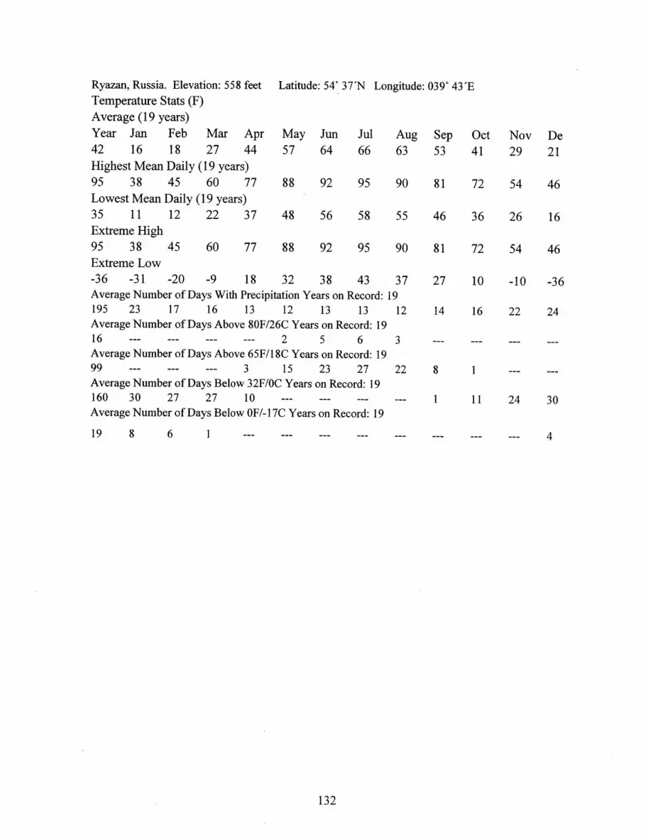
Ryazan, Russia. Elevation: 558 feetTemperature Stats (F)
Latitude: 54' 37'N Longitude: 039' 43'E
Average (19 years)Year Jan Feb Mar Apr May Jun Jul42 16 18 27 44 57 64 66Highest Mean Daily (19 years)95 38 45 60 77 88 92 95Lowest Mean Daily (19 years)35 11 12 22 37 48 56 58Extreme High95 38 45 60 77 88 92 95Extreme Low-36 -31 -20 -9 18 32 38 43Average Number of Days With Precipitation Years on Record:195 23 17 16 13 12 13 13Average Number of Days Above 80F/26C Years on Record: 1916 --- --- --- --- 2 5 6Average Number of Days Above 65F/i 8C Years on Record: 1999 --- --- --- 3 15 23 27Average Number of Days Below 32F/OC Years on Record: 19160 30 27 27 10 --- ---Average Number of Days Below OF/- 1 7C Years on Record: 19
19 8 6 1 --- --- ---
132
Nov29
54
26
54
-10
22
De21
46
16
46
-36
24
Aug Sep63 53
90 81
55 46
90 81
37 27912 14
22 8
1
Oct41
72
36
72
10
16
1
11
4
3
1

Appendix H. Model Canonical Forms.
Inversion, i.e., transformation between the CRTF (6) and iCRTF (8) models is a frequent andsometimes confusing operation (see simulation code listings in Appendices I and J). A set of fourcanonical forms have been found to be useful. The coefficient index notation (i:n) indicates the rangeof a coefficient vector's association with past samples. Thus, for example:
$,z(o:n)= [$,o $,1 -- #zn] $2(1:n) = [# $22 -. ' #n]z(o:n)= [Oz o Oz,j --- Ozn] Oz(1:n) = [0,1z 2 --- Oz,n]
0,(o:n) = [ O o Ow, -... ] 0,(1:n) = [O, i O,2 --- Own]The range of lags may also be expressed in operator notation by the backshift operator with the rangeexpression appended as a superscript:
B"(#)= [#i #i.; --. #n]
B"(0) = [ i Ai On]B n(q) = [ q(t-i) q(t-i-1) --- q(t-n)]B n(7) = [T(t-i) T(t-i-J) --- T(t-n)]
Equations (6) and (8) were developed for the simplest case involving just one exogenous temperature,e.g. a wall model. Here we extend the subscript used with temperature coefficients to indicate whichtemperature is meant: z refers to the inside wall surface or zone temperature and w = 1:W refers toexogenous temperatures or sol-air temperatures 1 through W.
Note that the zero-lag term of the first exogenous temperature is absent from all of the forms. Itsvalue is given by the u-value constraint (7).
CRTF formxe = [Q(t-k, k=1:n) Tz(t-k, k=o:n) Ti(t-k, k=1:n) T2(t-k, k=o:n) --- Tw(t-k, k=o:n)]be = [#(1:n) Oz(o:n) 01(1:n) 02(o:n) --- 0,(o:n)] with $(0) = -1 implicitQ = xe be
iCRTF formxi = [Q(t-k, k=o:n) T(t-k, k=1:n) Ti(t-k, k=1:n) T2(t-k, k=o:n) - Tw(t-k, k=o:n)]bi= [#(o:n) Oz(1:n) 01( 1:n) 62(o:n),-, O(o:n)] with O2(o)= -1 implicitTz = xi bi
Un-normalized complete formxn = [Q(t-k, k=o:n) Tz(t-k, k=o:n) Ti(t-k, k=1:n) T2(t-k, k=o:n) --- Tw(t-k, k=o:n)]bn = [#(o:n) O(o:n) O( 1:n) 02(o:n),-, O,(o:n)] with no particular scaling imposed0 = xn bn
Q-normalized complete formx,= [Q(t-k, k=o:n) Tz(t-k, k=o:n) Ti(t-k, k=1:n) T2(t-k, k=o:n) --- Tw(t-k, k=o:n)]bn = [#(o:n) 92(o:n) 0(1:n) 2(:n),---, 04(o:n)] with #(o) = -1 explicit.0 = xn bn
It is apparent that a T-normalized form can also be immediately defined. However, one is morelikely, in practice, to use an iCRTF form obtained, on the fly, from the CRTF form or from either oneof the complete forms.
Note: we insert the t-ratio from the residual error norm when converting from CRTF or iCRTFcanonical form to either of the complete forms (see function rootstu(bs,n)).
133

Appendix I. Script for Model Identification with Constrained RootsS2003.06.07 Hittle- ishop constraint: via 0<x<1; xbx
%is serch vector, rbr becomes an intermediate vector in resimctfxbx()%test 2003.06.06 2-step search at each increment of model order%testctf6.m 2003.01.,12 fit. progressivelv higher order modelsif 1;%---generate sine responses by qctf () and tctf () top p.14-----bb=[.53355063E-4 .013730926 .064549573 .037668124 .33696494E-2 .38707349E-4];cc=[5.9708847 -10.761687 5.967169 -1.1142596 .057851433 -. 54859184E-3];dd=[1.0 -1.2165741 .38310083 -. 029577257 .37410267E-3 -. 43038736E-61;crrx=sum(bb)/sum(cc); cc=crrx*cc;cof=[bb;-cc;dd];np=length(bb);n=np-1; nnp=n+np;m=4*12;%30;tz=[1:m]'; tz=0*tz; tz(1:m/2)=1+tz(1:m/2);tx=[tz(1+m/4:m);tz(1:m/4)];qstart=0*tz(1:n);tx=[qstart;tx];tz=[qstart;tz];q=qctf(cof,qstart,tx,tz);figure(1); plot(tx);hold on;plot(tz,'g');plot(q,'r');plot([0;length(tx)],[0;0],'k');[be,ce,de,se]=lsqctf(5,q,tx,tz);fprintf (1, 'norr(bb-be)=%11.4g\nI,norm(bb-be'))disp(bb);disp(be')fprintf(1,'normn(cc--ce)=%11.4e\n',norm(cc-ce'))disp(cc);disp(ce')f print f(1, 'norm (dd-de)=%1 ~'norm (dd- [1,-de')disp(dd);disp([1,-de'])
endif 1;% t manipulation of C(TF coelFfi cients and roots bo4- pnp=length(bb);n=np-1;b=[-cof(3,2:np),cof(l,:),-cof(2,:)]';dbcof=[roots(cof(3,:));cof(l,:)';roots(cof(2,:))];disp(l./log(l./roots(cof(3,:))'));%tau/timestep q (dd)disp(1./log(1./roots(cof(2,:))'));%tau/timestep Tz (cc)disprbr (dbcof)phi=poly(dbcof(1:n));bb=dbcof(np:n+np)';thz=poly(dbcof(np+np:n+n+np));thz=(sum(bb)/sum(thz))*thz;newb=[-phi(2:np),bb,thz]';disp('Inewb-b..l=');disp(norm(newb-b))
endx=zeros(m,3*np);for i=l:np
x(:,i)= q(1+np-i:m+np-i);x(:,np+i)=tx(+np-i:m+np-i);x(:,np+np+i)=tz(1+np-i:m+np-i);
end;y=x(:,1);hold offxx=x(:,2:3*np); fig=l
% error norm given by the correctfigure(2);rbr=dbcof;xbx=rbr;%xbz( )=rbr(1)xbx(nnp+l)=rbr(nnp+1);xbx(l)=rbr(l)/rbr(nnp+l);for i=2:n;
xbx(nnp+i)=rbr(nnp+i)/rbr(i-1);xbx(i)=rbr(i)/rbr(nnp+i);
endfig=.99if 1
f=resimctfxbx(xbx,xbx,xx,y); plot(f); hold on; disp('xbxnorm');norm(f)opti=optimset('m,axfune',8000*length(dbcof), 'maxiter',4000, 'tolfun',le-11, 'tolx',le-
11,'diffmin',le-9);xbx=fig*xbx; xbx(nnp+l)=xbx(nnp+l)*1.005/figb = 1. + 0*xbx; lb=.l*b; ub=.9*b;lb(np:nnp)=deal(0);ub(nnp+l)=xbx(nnp+l);
134

[xbx,sse,e]=lsqnonlin('resimctfxbx',xbx,lb,ub,opti,xbx,xx,y+.2*randn(length(y),l));figure(3);plot(e)disp([norm(rbr-dbcof),sse,e'*e,sqrt(sse/length(e))])rbk=xbx;' rbk!(1)=xbx(1) DELETE THIS STUFFrbk(l)=xbx(l)*rbk(nnp+l);for i=2:n;rbk(nnp+i)=xbx(nnp+i)*rbk(i-1);rbk(i)=xbx(i)*rbk(nnp+i);enddisprbr(rbk)e=resimctfxbx(xbx,xbx,xx,y);disp('rbr-dbcofI,sse,sse,rms=')disp([norm(rbr-dbcof),sse,e'*e,sqrt(sse/length(e))])alle=e;figure(4);plot(e)
endreturn
function f=resimctfxbx(xbxr,xbx,x,y)uth uses past predicted y~ye also try wi th past valules of v data
% f--resCTFrbr (rbr, y) returns mt residuals given parm estimate,b= roots (ph:i) thx; roots (thz I , and data x (mxl en (b) y mxI
% Columns of corres-pond to [ph i' , t hhx' , t ehz '] elemnts. See testctf3np=(length(x(l,:))+l)/3; n=np-1; nnp=n+np;if length(xbx)==length(xbxr);%for 2-step t-consts search when incrementing node' order
xbx=xbxr;else
xbx(n-l:n)=xbxr(1:2);xbx(np:n+np)=xbxr(3:2+np);nr=length(xbxr);xbx(n+np+n-l:n+np+n)=xbxr(nr-l:nr);
endrbr=xbx; rbr(1 )xbx 1)rbr(l)=xbx(l)*rbr(nnp+l);for i=2:n;
rbr(nnp+i)=xbx(nnp+i)*rbr(i-1);rbr(i)=xbx(i)*rbr(nnp+i);
enddbc=[rbr;O];p=poly(rbr(l:n));dbc(l:n)=-p(2:np)';p=poly(rbr(l+np+n:n+np+n));dbc(l+np+n:np+np+n)=p'*sum(rbr(np:np+n))/sum(p);ye=O*y; ye(l)=x(l,:)*dbc;for k=2:length(y);
x(k,2:n)=x(k-1,1:n-1);x(k,1)=ye(k-1);
exk1=y k-1)ye(k)=x(k, :)*dbc;
endf=y-ye;
135

Appendix J. Model Identification by Ordinary and Hybrid Least Squares>>agglees9('leesloct',1,2000,890,919,1210,600,[2],[3]);function b=aggLEES9(fnam,fLtg,mcp,jhead,jtail,khead,ktail,nlist,malist);%train/test sets from fnam between head and tail line#s;%fit model orders in nlist, e.g. [0 1 2 3] and%time-aggregations in malist, e.g. [1 2 3 6]%fLtg, mcp for problem specific heat rate calcs%aggLEES9.m 20031218pra use canonical order within x,bdata=load([fnam '.txt']); size(data);%1:8 lotusdate TfanInl TfanIn2 TfanOut Tprot Tshop dTube dTshop (degF)time.nXTicks=15; time=timecalc(data,jhead,khead,time);for ma=malist;
%----------problem specific heat rate calcs---------q=data(:,1)>=37890.86806 & data(:,1)<37892.26389; %ltgoff & fanOn%g=2390*(1-data(:,))+2581*data(: ,1) .*data(:,8); %Qltg+G*dTshopQltg=fLtg*590*3600/1055;%fLtg*[W]*[W2Btuh]=fLtg*2013Btuhq=Qltg*(1-q)+mcp*q.*data(:,8); %Qltg+G*dTshop%---------end problem-specific heat rate calcs---------
[jq,jz,jx,jx2,jn]=laggedTs([q data(:,6) data(:,3) data(:,5)],ma,jhead,jtail,nlist);[kq,kz,kx,kx2,kn]=laggedTs([q data(:,6) data(:,3) data(:,5)],ma,khead,ktail,nlist);time=timacalc(ma,jn,kn,time);plotqtzi([1,2],jq,jz,jn,kq,kz,kn,time,'iCRTFid')plotqtzi([3,4],jq,jz,jn,kq,kz,kn,time,'CRTFid')plotqtzi([5,6],jq,jz,jn,kq,kz,kn,time,'QTzid')uscale=1.for n=nlist;%model order (number of poles)
np=n+1xj=[jq(:,1:np) jz(:,1:np) jx(:,2:np) jx2(:,1:np)];xk=[kq(:,1:np) kz(:,1:np) kx(:,2:np) kx2(:,1:np)];
y=jz(:,1);x=[uscale*jq(:,1:np) jz(:,2:np) jx(:,2:np) jx2(:,1:np)];%Tz-response
disp('iCRTF LScovWgt')alph2=0;Rbb=alph2*eye(length(x(1,:))) ;Rnn=eye(length(x(:,1)));[b,bse]=lscovwgt(x,Rbb,y,Rnn);bs=bi2bns(b,bse,n,x,y)bs2str(bs,n);u=rootstu(bs(:,1) ,bs(:,2) ,n)seqtz=plotcrtf([1,2],xj,n,bs,O);seqtz=plotcrtf([1,2],xk,n,bs,jn);
if 0disp('iCRTF lscov')[b,bse]=lscov(x,jz(:,1),eye(length(x(:,1))));bs=bi2bns(b,bse,n,x,jz(:,1))%bs=[b bse abs(b./bse)];bs2str(bs,n);u=rootstu(bs(:,1),bs(:,2),n)
disp('iCRTF LSVDcovy)[b,bse]=lsvdcov(x,jz(:,1),eye(length(x(:,1))));bs=bi2bns(b,bse,n,x,jz(:,1))bs2str(bs,n);u=rootstu(bs(:,1),bs(:,2),n)end
y=uscale*jq(:,1);x=[uscale*jq(:,2:np) jz(:,1:np) jx(:,2:np) jx2(:,1:np)];%q-responsedisp('CRTF LScovWgt')alph2=0;Rbb=alph2*eye(length(x(1,:)));Rnn=eye(length(x(:,1)));[b,bse]=lscovwgt(x,Rbb,y,Rnn);bs=bc2bns(b,bse,n,x,y)bs2str(bs,n);u=rootstu(bs(:,1),bs(:,2),n)seqtz=plotcrtf([3,4],xj,n,bs,0);
136

seqtz=plotcrtf([3,4],xk,n,bs,jn);bz=-bs (np+1)if bz<200; bz=1000; end
xx=[jq(:,2:np) jz(:,2:np) jx(:,2:np) jx2(:,1:np)];bz=fminbnd('lsqz',bz,50*bz,[],xx,y,jz(:,1))[b,bse]=lscov(xx,y+bz*jz(:,1),eye(length(y)));%b s/b unchngdb=[b(1:n);-bz;b(np:length(b))];bse=[bse(1:n);O;bse(np:length(bse))];bs=bc2bns(b,bse,n,x,y)bs2str(bs,n);u=rootstu(bs(:,1),bs(:,2),n)seqtz=plotcrtf([5,6],xj,n,bs,O);seqtz=plotcrtf([5,6],xk,n,bs,jn);
end;%nend; %mafor i=1:6;figure(i);v=axy(.5); plot([jn jn],[v(3),v(4)]);hold off;endreturn;%--------------------------------------------------------------
function v=axy (f)vi=axis; axis('tight');v=axis;vi=(l-f)*v+f*vi; %tighter y limitsv=[v(1) v(2) vi(3) vi(4)]; %x-fullyTight; y-partlyTightaxis (v); %applyre tu rn ;% -- --- --- -- ---- ----- ----- --- -------- --- ---- ----- -- ---- -- ----- --function e=lsqz (bz,x,yq,yz)%cost fcn name passed to fminbnd('lsqz',bzl,bzu,options,x,y,kz(:,l))%x is the CRTF data matrix with Tzone column removed%ygrqzone is the vector observations; u=thetaQ associated with yz=Tzoney=yq+bz*yz; cov=eye (length (y)); one=diag (cov);rmsq=norm (yq-mean (yq) *one);rms z=norm(yz-mean (yz) *one);b=lscov(x,y,cov)ye=x*b;e=norm (yq-ye+bz*yz) /rmsq +norm (yz- (ye-yq) /bz) /rmsz;return;%----function [kq,kz,kx,kx2,kn]=laggedTs (data,ma,khead,ktail,nlist)%function [kq,kx,kz,kx2]=laggedTs(data,clist,ma,khead,ktail,nlist)nn=max(nlist);m=f ix((length(data(:,1))-khead-ktail-ma*nn)/ma)mm~-m*mak=khead+l; kf=khead+mm+ma*nn;q=decima (data (k: kf, 1) ,ma); %Qltg+G*dTshoptz=decima(data(khead+1:khead+mm+ma*nn, 2) ,ma);fprintf(1,'%21s Tshop staircase\n',datestr(now));wp=length(data(1,:)); %future multiple exogenous temperaturestx=decima(data(khead+1:khead+mm+ma*nn, 3),ma); %Tmain=TfanIn2tx2=decima(data(khead+l:khead+mm+ma*nn, 4) ,ma); %Tprot%NOTE len(tx,tz,q) = len(kx,kz,kq)+nnkq= q(l+nn:m+nn);kx=tx(1+nn:m+nn) ; kxO=kx;kz=tz (l+nn:m+nn) -kxO;kx2=tx2 (1+nn:m+nn) -kxO;kn=length (kq);for n=l:nn
k=nn-n;kg=[kq q(1+k:m+k)];kz=[kz tz(l+k:m+k)-kxO];kx=[kx tx(l+k:m+k)-kx0];kx2=[kx2 tx2(1+k:m+k)-kxO];
endreturn;%---function t=timecalc(data,jhead,khead,t);t.StepHr=[ 2 3 4 6 8 12 18 24 36 48];%allow these axis increments%following round-off correction works only if 1/t.StepHr is an integert.StepHr=1.0/round(/(24*(data(2,1)-data(1,l))));t.Startj=data(jhead,l)+1900*365.25-13;%convert from lotusdate to a.d.t.StartjRem=t.Startj-floor(t.Startj);t.Startk=data(khead,l)+1900*365.25-13;%convert from lotusdate to a.d.t.StartkRem=t.Startk-floor(t.Startk);%tickStartH r=ceil (24*t. StartRem)
137
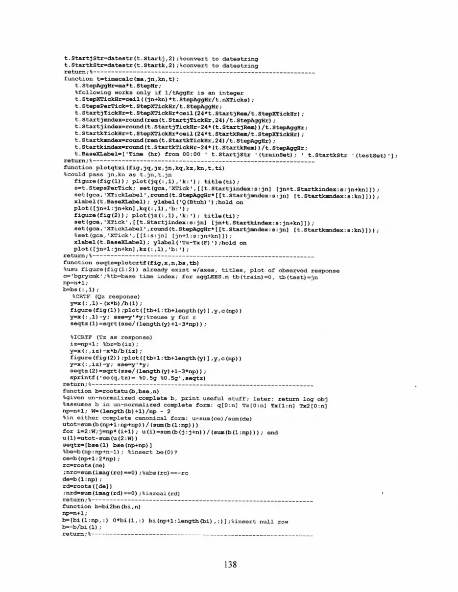
t.StartjStr=datestr(t.Startj,2);%convert to datestringt.StartkStr=datestr(t.Startk,2);%convert to datestringreturn;% --------------------------------------------------------------function t=timacalc(ma,jn,kn,t);
t. StepAggHr=ma*t. StepHr;%following works only if 1/tAggHr is an integert.StepXTickHr=ceil ( (jn+kn)*t.StepAggHr/t.nXTicks);t. StepsPerTick=t. StepXTickHr/t . StepAggHr;t.StartjTickHr=t.StepXTickHr*ceil(24*t.StartjRem/t.StepXTickHr);t.Startjmndex=round(rem(t.StartjTickHr,24)/t.StepAggHr);t.Startjindex=round(t.StartjTickHr-24*(t.StartjRem))/t.StepAggHr;t. StartkTickHr=t. StepXTickHr*ceil (24*t. StartkRem/t. StepXTickHr);t. Startkmndex=round (rem(t. StartkTickHr, 24) /t. StepAggHr);t.Startkindex=round(t.StartkTickHr-24*(t.StartkRem))/t.StepAggHr;t.BaseXLabel=['Time (hr) from 00:00 ' t.StartjStr '(trainSet); ' t.StartkStr '(testSet)'];
return;%--------------------------------------------------------------function plotqtzi(fig,jq,jz,jn,kq,kz,kn,t,ti)%could pass jn,kn as t.jn,t.jn
figure(fig(1)); plot(jg(:,1),'k:'); title(ti);s=t.StepsPerTick; set(gca,'XTick',[[t.Startjindex:s:jn] [jn+t.Startkindex:s:jn+kn]]);set(gca, TXTickLabel' ,round(t.StepAggHr*[ [t.Startjmndex:s:jn] [t.Startkmndex:s:kn]]));xlabel(t.BaseXLabel); ylabel('Q(Btuh)');hold onplot([jn+:jn+kn],kq(:,l),b:');figure(fig(2)); plot(jz(:,1),'k:'); title(ti);set(gca,'XTick',[[t.Startjindex:s:jn] [jn+t.Startkindex:s:jn+kn]]);set (gca, 'XTickLabel' ,round(t.StepAggHr*[ [t.Startjmndex:s:jn] [t.Startkmndex:s:kn] ]));%set(gca,'XTick',([1:s:jn] [jn+l:s:jn+kn]]);xlabel(t.BaseXLabel); ylabel('Tz-Tx(F)');hold onplot([jn+1:jn+kn],kz(:,1),'b:');
return;%----------------------------------------------function seqtz=plotcrtf(fig,x,n,bs,tb)%usu figure(fig(l:2)) already exist w/axes, titles, plot of observed responsec='bgrycmk' ;%tb=base time index; for aggLEES.m tb(train)=0, tb(test)=jnnp=n+1;b=bs(:,l);
%CRTF (Qz response)y=x(: ,1)-(x*b)/b(1)figure(fig(l));plot([tb+l:tb+length(y)],y,c(np))y=x(:,1)-y; sse=y'*y;%reuse y for rseqtz(1)=sqrt(sse/(length(y)+1-3*np));
%ICRTF (Tz as response)iz=np+1; %bz=b(iz) ;y--x(:,i~z)-x*b/b(iz);figure(fig(2));plot([tb+l:tb+length(y)],y,c(np))y=x(:,iz)-y; sse=y'*y;seqtz(2)=sqrt(sse/(length(y)+1-3*np));sprintf('se(q,tz)= %0.5g %0.5g',seqtz)
return;% -----------------------------------------function b=rootstu(b,bse,n)%given un-normalized complete b, print useful stuff; later: return log obj%assumes b in un-normalized complete form: q[0:n] Tz[0:n] Tx[l:n] Tx2[0:n]np=n+l; W=(length(b)+1)/np - 2%in either complete canonical form: u=sum(ce)/sum(de)utot=sum(b (np+l:np+np) ) / (sum(b (1:np)))for i=2:W; j=np*(i+l); u(i)=sum(b(j:j+n))/(sum(b(1:np))); endu(1)-utot-sum(u(2:W))seqtz=[bse(l) bse(np+np)]%be=b(np:np+n-l); %insert be(O)?ce=b(np+1:2*np);rc=roots(ce);nrc=sum(imag(rc)==0);%abs(rc)==-rcde=b(l:np);rd=roots([de]);nrd=sum(imag(rd)==0);%isreal(rd)return;%-----------------------------------function b=bi2bn(bi,n)np=n+1;b=[bi(1:np,:) 0*bi(l,:) bi(np+l:length(bi),:)];%insert null rowb=-b/bi(1);return;%-
138

function bs=bc2bns(b,be,n,x,y)np=n+1;%[b,bse] convert CRTF model id result to normalized canonical formr=y-x*b; %compute std error of fitse=sqrt((r'*r)/(length(y)-length(b)));
%move observation [coeff,se] to RHSbs(:,l)=[-l; b(l:np+n); b(np+np:length(b))];bs(:,2)=[sqrt((r'*r)/(y'*y)); be(l:np+n); be(np+np:length(b))];%be(l:np+n); se; be(np+np:length(b))];
%normalize%bs=-bs/b(l);%compute t-ratios%bs(:,3)=abs(bs(:,1)./bs(:,2))return;%--------------------------------------------------------------
function bs=bi2bns(b,be,n,x,y)np=n+l;%[b,bse] convert iCRTF model id result to normalized canonical formr=y-x*b; %compute std error of fitse=sqrt((r'*r)/(length(y)-length(b)));%THIS IS se(data); NEED TO CONVERT TO se(coeff) using expression for CV?
%move observation [coeff,se] to RHSbs(:,l)=[b(l:np); -1; b(np+l:length(b))];bs(:,2)=[be(1:np); sqrt((r'*r)/(y'*y)); be(np+l:length(b))]; %s/b se(coeff)!%be(1:np); se; be(np+1:length(b))J;
%normalizebs=-bs/b(l);%compute t-ratios%bs(:,3 )=abs(bs(:,1)./bs(:,2))return;%--------------------------------------------------------------
function bstr=bs2str(bs,n)np=n+1;%pretty-print the (complete) model [coeff,se] vectors and t-ratios%scale by u-value?t=abs(bs(:,l)./bs(:,2))xt=[np+l:length(t) ];
if 0;blanco=char([Q*t+32]);bstr=[num2str(bs(: ,l)) ,blanco,num2str(bs(:,2)) ,blanco,num2str(t)];
elsedisp([bs(1:np,:),t(1:np)])disp([bs(xt,:), t(xt)])
endreturnblanco=char([0*t(1:np)+32]);bstr=[num2str(bs(l:np,l)) ,blanco,num2str(bs(l:np,2)) ,blanco,num2str(t(1:np))]xt=[np+l:length(t) ];blanco=char([Q*t(xt)+32]);bstr=[[num2str(bs(xt,l)) ,blanco,num2str(bs(xt,2)) ,blanco,num2str(t(xt))]];return;%---------------------------------------------------------------
function [b,be]=lsvdcov(x,y,cov)%Numercal Recipes Ftn (1992) 15.4.3-5 and 15.4.18-19%corrected per Wunsch,C.I., Ch 2.5, 2003 rev of The Ocean Circulation Inverse Problem (1996)m=length(x(1,:))yb=cov\y;%yb=y/diag(cov);%for diagonal cov%[u,w,v=svd(cov\x,0);%svd([x(i,j)/sig(i)D);for diag[u,w,v]=svd(x,O);%sd([x(i,j)/sig(i)]);for diags=diag(w);b=0*x(1,:)';be=b; k=0; tol=sqrt(m)*s(1)*4e-15while s(k+1)>tol;
k=k+1;if k==m;
break;end
end%below tol tests c/b avoided by using k as upper summation limitfor i=l:m;
139

if s(i)>tol; b=b+(u(:,i)'*yb)*v(:,i)/s(i); endfor j=1:m;
if s(j)>tol; be(i)=be(i)+(v(i,j)/s(j))^2;endendbe(i)=sqrt(be(i));
endreturn;%--------------------------------------------------------------function [b,be]=lsvdw(x,y)%Wunsch,C.I., Ch 2.5, 2003 rev of The Ocean Circulation Inverse Problem (1996)m=length(x(l,:))yb=y;[u,w,v]=sd(x,O);%sd([x(i,j)/sig(i)]);for diags=diag(w);overs=1./sb=0*x(l,:)';be=b; ey=0*yb; p=0*eye(m); k=O; tol=sqrt(m)*s(l)*4e-15while s(k+1)>tol; k=k+1; if k==m; break; end; endfor i=1:k;
b=b+overs(i)*(u(:,i)'*yb*v(:,i));%(5.77) w/o bias partey=ey+(u(:,i)'*yb)*u(:,i);; %(5.78)p =p +overs(i)*overs(i)*(v(:,i)*v(:,i)');%(5.83) w/o bias part
endey=ey-yb;p=diag (p)length(yb)-mbe=sqrt ( ( (ey' *ey) / (length (yb) -m)) *p);return;%--------------------------------------------------------------function [b,be]=lscovwgt(E,Pbb,y,Rnn)%Wunsch,C.I., Ch 2.5, 2003 rev of The Ocean Circulation Inverse Problem (1996)%eqns 2.7.19-21 with provision for Rbb=0Rnn=inv(Rnn);m=length(E (1,:))if rank(Ebb)-==m; p=inv(inv(Rbb)+E'*Rnn*E);else; p=inv(E'*Rnn*E);endb=p*E'*Rnn*y;ey=y-E*b;p=diag(p);length(y)-mbe=sqrt(((ey'*ey)/(length(y)-m))*p);return;% -----
function [b,be,k]=lsvdwgt(E,Rbb,yRnn)%Wunsch,C.I., Ch 2.5, 2003 rev of The Ocean Circulation Inverse Problem%(1996); %COULD USE Rbb,RnnCholeski factors and work in xfmd spaceRbb=inv(Rbb) ;Rnn=inv(Rnn);m-length(E (1,:))yb=y;[u,w,v]=svd(x,0) ;%svd([x(i,j) /sig(i) ]);for diags=diag(w);overs=l./sb=O*x(l,:)';be=b; ey=0*yb; p=0*eye(m); k=0; tol=sqrt(m)*s(1)*4e-15while s(k+l)>tol; k=k+l; if k==m; break; end; endfor i=1:k;
b=b+overs(i)*(u(:,i)'*yb*v(:,i));%(5.77) w/o bias partey=ey+(u(:,i)'*yb)*u(:,i);; %(5.78)p =p +overs(i)*overs(i)*(v(:,i)*v(:,i)');%(5.83) w/o bias part
endey=ey-yb;be=sqrt(((ey'*ey)/(length(yb)-m))*diag(p));return;%--------------------------------------------------------------
function b=tlsq(scaleq,nn,x,y)%Golub & VanLoan, 1989, Matrix Computations, Algorithm 5.1.1np-nn+l; n=length(x(1,:)); m=length(x(: ,1)) ;%n data; m parmssm=[scaleq*ones (np:1) ;ones (n-np) ];%use nn for CRTF canonical form; np for complete formsm=diag(sm);%x-->x*sm [3 PLJ[u,w,v]=svd([x y],0);[diag(w) log10(diag(w))]er=-[x y]*v*v';b=[x+er(:,l:n)]\[y+er(:,n+l)];return; -..........
140

Appendix K. Fragment of data LEES1oct.txt for input to aggLEES9.mlotusdate TfanInl TfanIn2 TfanOut Tprot Tshop dTube dTshop37891.14583 73.69 73.52 74.21 73.61 73.84 -0.576 -0.73737891.14931 73.73 73.52 74.21 73.62 73.85 -0.562 -0.737
37891.15278 73.69 73.52 74.25 73.61 73.85 -0.562 -0.737
37891.15625 73.73 73.52 74.25 73.61 73.85 -0.547 -0.737
37891.15972 73.73 73.52 74.25 73.61 73.85 -0.547 -0.737
37891.16319 73.69 73.56 74.25 73.60 73.84 -0.548 -0.73737891.16667 73.73 73.52 74.25 73.59 73.85 -0.547 -0.73737891.17014 73.73 73.52 74.25 73.59 73.85 -0.547 -0.73737891.17361 73.73 73.56 74.29 73.59 73.86 -0.562 -0.693
37891.17708 73.73 73.56 74.25 73.58 73.86 -0.533 -0.780
37891.18056 73.78 73.56 74.29 73.58 73.87 -0.548 -0.736
37891.18403 73.78 73.56 74.29 73.56 73.86 -0.548 -0.736
37891.1875 73.78 73.56 74.29 73.56 73.86 -0.548 -0.693
37891.19097 73.78 73.56 74.25 73.55 73.86 -0.519 -0.780
37891.19444 73.73 73.56 74.25 73.55 73.86 -0.577 -0.69337891.19792 73.78 73.56 74.29 73.55 73.87 -0.548 -0.73637891.20139 73.78 73.56 74.29 73.54 73.86 -0.548 -0.69337891.20486 73.78 73.60 74.29 73.53 73.88 -0.534 -0.73637891.20833 73.78 73.60 74.29 73.53 73.87 -0.534 -0.73637891.21181 73.78 73.60 74.29 73.52 73.88 -0.534 -0.73637891.21528 73.78 73.60 74.29 73.52 73.88 -0.534 -0.736
37891.21875 73.73 73.60 74.29 73.53 73.87 -0.548 -0.73637891.22222 73.78 73.60 74.29 73.52 73.88 -0.534 -0.736
37891.22569 73.78 73.60 74.29 73.52 73.88 -0.534 -0.73637891.22917 73.78 73.60 74.29 73.52 73.88 -0.534 -0.73637891.23264 73.78 73.60 74.34 73.52 73.88 -0.519 -0.736
37891.23611 73.78 73.60 74.34 73.52 73.89 -0.562 -0.693
37891.23958 73.78 73.65 74.34 73.52 73.88 -0.505 -0.736
37891.24306 73.78 73.60 74.34 73.52 73.88 -0.519 -0.736
37891.24653 73.78 73.60 74.34 73.50 73.88 -0.519 -0.736
37891.25 73.78 73.60 74.34 73.50 73.89 -0.562 -0.693
37891.25347 73.78 73.65 74.34 73.50 73.89 -0.548 -0.693
37891.25694 73.78 73.65 74.34 73.50 73.89 -0.548 -0.693
37891.26042 73.78 73.60 74.34 73.50 73.90 -0.562 -0.693
37891.26389 73.56 73.39 73.82 73.49 73.78 -0.230 -1.299
37891.26736 73.00 72.78 72.91 73.49 73.53 -0.101 -1.945
37891.27083 72.57 72.31 72.39 73.48 73.32 -0.143 -2.161
37891.27431 72.22 72.01 72.09 73.47 73.17 -0.158 -2.33237891.27778 72.01 71.79 71.92 73.47 73.06 -0.230 -2.331
37891.28125 71.88 71.66 71.79 73.45 72.96 -0.229 -2.374
37891.28472 71.75 71.58 71.71 73.44 72.89 -0.244 -2.374
37891.28819 71.66 71.53 71.58 73.44 72.82 -0.244 -2.416
37891.29167 71.53 71.40 71.49 73.44 72.76 -0.272 -2.416
37891.29514 71.45 71.32 71.40 73.43 72.71 -0.272 -2.459
37891.29861 71.36 71.32 71.36 73.42 72.67 -0.272 -2.458
37891.30208 71.32 71.28 71.32 73.41 72.63 -0.272 -2.458
37891.30556 71.23 71.19 71.19 73.41 72.58 -0.244 -2.544
37891.30903 71.19 71.15 71.19 73.41 72.53 -0.229 -2.54437891.3125 71.15 71.10 71.15 73.41 72.50 -0.272 -2.50137891.31597 71.06 71.06 71.10 73.40 72.47 -0.287 -2.500
37891.31944 71.02 71.02 71.02 73.39 72.43 -0.258 -2.586
37891.32292 70.97 71.02 70.97 73.38 72.41 -0.287 -2.543
37891.32639 70.93 70.97 70.97 73.39 72.37 -0.272 -2.543
37891.32986 70.89 70.93 70.97 73.38 72.36 -0.301 -2.543
37891.33333 70.85 70.93 70.93 73.37 72.32 -0.287 -2.543
37891.33681 70.85 70.89 70.85 73.36 72.30 -0.287 -2.58637891.34028 70.80 70.85 70.85 73.36 72.28 -0.272 -2.585
37891.34375 70.76 70.85 70.85 73.37 72.27 -0.287 -2.585
37891.34722 70.72 70.80 70.80 73.37 72.24 -0.244 -2.62837891.35069 70.72 70.76 70.76 73.38 72.23 -0.315 -2.58537891.35417 70.67 70.76 70.72 73.37 72.19 -0.258 -2.62837891.35764 70.63 70.72 70.72 73.38 72.17 -0.287 -2.62837891.36111 70.59 70.72 70.67 73.39 72.16 -0.315 -2.58537891.36458 70.59 70.72 70.63 73.38 72.15 -0.287 -2.62837891.36806 70.54 70.63 70.63 73.37 72.11 -0.244 -2.67137891.37153 70.54 70.63 70.63 73.37 72.11 -0.287 -2.628
37891.375 70.50 70.63 70.63 73.37 72.10 -0.301 -2.628
37891.37847 70.50 70.63 70.54 73.38 72.08 -0.287 -2.671
37891.38194 70.50 70.59 70.54 73.37 72.05 -0.301 -2.627
37891.38542 70.46 70.59 70.54 73.37 72.04 -0.272 -2.627
37891.38889 70.42 70.59 70.54 73.36 72.03 -0.287 -2.627
37891.39236 70.42 70.54 70.50 73.36 72.00 -0.272 -2.670
37891.39583 70.37 70.54 70.46 73.36 71.99 -0.258 -2.670
37891.39931 70.37 70.50 70.46 73.37 71.98 -0.315 -2.627
37891.40278 70.37 70.50 70.46 73.37 71.97 -0.272 -2.670
37891.40625 70.33 70.50 70.42 73.37 71.96 -0.301 -2.670
37891.40972 70.33 70.46 70.42 73.37 71.94 -0.272 -2.670
37891.41319 70.29 70.46 70.42 73.37 71.93 -0.287 -2.670
37891.41667 70.29 70.46 70.33 73.39 71.91 -0.272 -2.713
37891.42014 70.29 70.37 70.37 73.38 71.90 -0.287 -2.713
37891.42361 70.24 70.37 70.37 73.39 71.89 -0.301 -2.670
37891.42708 70.24 70.37 70.33 73.39 71.88 -0.315 -2.713
37891.43056 70.24 70.37 70.33 73.39 71.87 -0.315 -2.670
37891.43403 70.24 70.37 70.33 73.39 71.85 -0.272 -2.670
37891.4375 70.20 70.37 70.29 73.39 71.84 -0.258 -2.713
37891.44097 70.16 70.33 70.29 73.39 71.84 -0.329 -2.626
37891.44444 70.20 70.37 70.29 73.39 71.83 -0.301 -2.670
141

Appendix L. "Why It Works" and Relation of Hybrid Method to TLSThe hybrid method appears to, but actually does not, correspond exactly to animplementation of total least squares (Golub, Van Huffel) in which measurement error isattributed to one of the data columns, Tz(t), as well as the vector of observations, Qz(t), theratio of Tz to Qz error is Ozo, and the exogenous temperature(s) are without measurementerror.
In most thermal systems of interest, the ratio of Tz to Qz error is related to the quick masscoupling parameters, hqAq and Mc,/At. The heat rate of interest is a sum of electric andsolar gains and a flow-temperature product of the form (Ts/a - T,4)mcp, where s/a and r/a referto supply and return air streams. Although solar gain is a function of effective aperture area,which is not known exactly (may, indeed, be one of the unknown model parameters) theelectric and solar gain measurements are usually made with very low random error. Therandom error in Q is dominated by entering and leaving fluid stream temperature errors.
However, the foregoing LS-TLS formulation gives a different, and not nearly as reliable aresult as the hybrid method. The reason is that the LS-TLS objective function is minimizedby the LS-TLS solution when the Tz and Qz errors are uncorrelated. This is not the case. Infact, the errors are highly correlated because a rise in zone air temperature corresponds toheating of the air. Thus the term, Qz -OzoT , is very insensitive to short-term disturbances.
The errors in exogenous temperatures, on the other hand, are likely to be dominated bysystematic (often diurnal or correlated with other weather variables involving sun, wind, andrain) rather than random errors. TLS weights (variances and covariances) are not much help.Thus one are motivated to measure the exogenous temperatures as best we can, and havingdone so, one are just as well off to treat them as perfectly accurate.
142


