Embed Size (px)
Citation preview

arX
iv:h
ep-t
h/97
1007
6v1
8 O
ct 1
997
WUHEP/97-15
Model of supersymmetric quantum field theory with broken
parity symmetry
Carl M. Bender∗
Department of Physics, Washington University, St. Louis, MO 63130, USA
Kimball A. Milton†
Department of Physics and Astronomy, University of Oklahoma, Norman, OK 73019, USA
(February 1, 2008)
Abstract
Recently, it was observed that self-interacting scalar quantum field theories
having a non-Hermitian interaction term of the form g(iφ)2+δ , where δ is a
real positive parameter, are physically acceptable in the sense that the energy
spectrum is real and bounded below. Such theories possess PT invariance,
but they are not symmetric under parity reflection or time reversal separately.
This broken parity symmetry is manifested in a nonzero value for 〈φ〉, even if
δ is an even integer. This paper extends this idea to a two-dimensional super-
symmetric quantum field theory whose superpotential is S(φ) = −ig(iφ)1+δ .
The resulting quantum field theory exhibits a broken parity symmetry for all
δ > 0. However, supersymmetry remains unbroken, which is verified by show-
ing that the ground-state energy density vanishes and that the fermion-boson
mass ratio is unity.
PACS number(s): 12.60.Jv, 02.30.Mv, 11.30.Er, 11.30.Pb
Typeset using REVTEX
∗Electronic address: [email protected]
†Electronic address: [email protected]
1

I. INTRODUCTION
It is extremely difficult to perform conventional perturbative calculations in supersym-metric field theory because expansions in powers of the coupling constant are infrared diver-gent. Furthermore, introducing a regulator in the form of a momentum cutoff or a latticespacing to control this divergence breaks the supersymmetry invariance. An especially sim-ple way to solve this problem is to use the delta expansion, a perturbative expansion inpowers of the degree of the nonlinearity of the interaction term [1].
The key idea of the delta expansion is to replace a self-interaction term of the form gφ4
by g(φ2)1+δ, where δ is regarded as a small parameter. Thus, the parameter δ measuresthe departure from linearity of the field equation. A graphical procedure for expandingthe Green’s functions of a quantum field theory in powers of δ is given in Ref. [1]. Theadvantage of such an expansion is that it has a nonzero radius of convergence and that ityields numerically accurate nonperturbative information when δ is set equal to 1.
The delta expansion is broadly useful for nonlinear problems. It has been applied tomany classical nonlinear ordinary differential equations of mathematical physics and it hasgiven superbly accurate numerical results [2]. The delta expansion has also been successfullyapplied to some nonlinear partial differential equations of mathematical physics [3].
In the context of quantum field theory the delta expansion has been used to studyrenormalization [4], local gauge invariance [5], stochastic quantization [6], finite-temperaturefield theory [7], and the Ising limit of quantum field theory [8].
The delta expansion is particularly well suited for studying supersymmetric models ofquantum field theory because expansions in powers of δ are not infrared divergent and thedelta expansion respects the supersymmetry exactly. Calculations to second order in powersof δ have been done for the ground-state energy [9] and the fermion-boson mass ratio [10].
Recently, we have examined a new class of scalar quantum field theories that are notsymmetric under parity reflection [11]. The Euclidean-space Lagrangian for this class oftheories is
L =1
2(∂φ)2 +
1
2m2φ2 − g(iφ)2+δ (δ > −2). (1.1)
The Hamiltonian for such theories is not Hermitian. However, there is strong evidence thatthese theories possess energy spectra that are real and bounded below.1 The theories in
1There is copious numerical evidence that such theories possess positive spectra when m 6= 0.
Furthermore, one can understand positivity from a theoretical point of view. Consider, for example,
the weak-coupling expansion for the d-dimensional Euclidean quantum field theory defined by the
Lagrangian L = 12(∂φ)2+ 1
2m2φ2+giφ3. For a conventional gφ3 theory the weak-coupling expansion
is real, and (apart from a possible overall factor of g) the Green’s functions are formal power series
in g2. These series are not Borel summable because they do not alternate in sign. Nonsummability
reflects the fact that the spectrum of the underlying theory is not bounded below. However,
when we replace g by ig, the perturbation series remains real but now alternates in sign. Thus,
the perturbation series is now summable and this suggests that the underlying theory has a real
positive spectrum.
2

Eq. (1.1) are a natural field theoretic generalization of a remarkable quantum mechanicalHamiltonian studied by D. Bessis and C. Itzykson: [12]
H =1
2p2 + ix3. (1.2)
The Lagrangian in Eq. (1.1) is intriguing because it is not parity symmetric. This is man-ifested by a nonzero value of 〈φ〉. It is interesting that this broken symmetry persists evenwhen δ is an even integer [11].
That fact that the Lagrangian in Eq. (1.1) has a broken parity symmetry suggests thatif we construct a two-dimensional supersymmetric quantum field theory by using a super-potential of the form
S(φ) = −ig(iφ)1+δ, (1.3)
the resulting theory will also have a broken parity symmetry. The supersymmetric La-grangian resulting from the superpotential (1.3) is
L =1
2(∂φ)2 +
1
2iψ∂/ψ +
1
2S ′(φ)ψψ +
1
2[S(φ)]2
=1
2(∂φ)2 +
1
2iψ∂/ψ +
1
2g(1 + δ)(iφ)δψψ − 1
2g2(iφ)2+2δ, (1.4)
where ψ is a Majorana spinor.The Lagrangian (1.4) raises an interesting question. Will the breaking of parity symmetry
induce a breaking of supersymmetry? To answer this question we calculate both the ground-state energy Eground state and the fermion-boson mass ratio R as series in powers of theparameter δ. We find that through second order in δ, Eground state = 0 and R = 1, whichstrongly suggests that supersymmetry remains unbroken. Based on the experience withthese calculations we believe that our results are valid to all orders in powers of δ. It is quitedifficult to break supersymmetry [13].
This paper is organized very simply. In Sec. II we explain our calculational procedure. Wederive a set of Feynman rules for obtaining the Green’s functions to a given order in powersof δ for the scalar field theory Lagrangian (1.1). Next, in Sec. III we apply the procedures ofSec. II to calculate the ground-state energy and the fermion-boson mass ratio to first orderin δ for the supersymmetric Lagrangian (1.4). In Sec. IV we perform these calculations tosecond order in δ. Finally, in Sec. V we examine some of the formal cancellations that occurin our calculations to see if there could be anomalous contributions to the ground-stateenergy.
II. DELTA EXPANSION FOR A PARITY-VIOLATING SCALAR FIELD THEORY
In this section we explain how to calculate the Green’s functions for the scalar quantumfield theory described by the Lagrangian L in Eq. (1.1). Specifically, we follow the proce-dures described in Ref. [1] and determine a set of graphical rules for constructing the deltaexpansion through second order in powers of δ. These rules consist of the amplitudes for
3

the vertices and lines of a related Lagrangian in which the boson fields are raised to integerpowers.
We begin by expanding the Lagrangian L in Eq. (1.1) to second order in powers of δ:
L =1
2(∂φ)2 +
1
2m2φ2 + gφ2 + δgφ2 ln(iφ) +
1
2δ2gφ2[ln(iφ)]2 + O(δ3). (2.1)
Observe that at δ = 0 the Lagrangian contains the coupling g:
L0 =1
2(∂φ)2 +
1
2m2φ2 + gφ2. (2.2)
Thus, an expansion in powers of δ is clearly nonperturbative in g.In general, the functional integral representation for an n-point correlation function has
the form (modulo the usual normalization factor)
〈0|φ(x1)φ(x2)φ(x3) . . . φ(xn)|0〉 =∫
Dφφ(x1)φ(x2)φ(x3) . . . φ(xn)e−∫
dxL. (2.3)
We expand the exponential in the integrand in Eq. (2.3) and obtain
e−∫
dxL = e−∫
dxL0E [φ], (2.4)
where
E [φ] = 1 − δg∫
dxφ2 ln(iφ) − 1
2δ2g
∫
dxφ2[ln(iφ)]2
+1
2δ2g2
[∫
dxφ2 ln(iφ)]2
+ O(δ3). (2.5)
Next, we use the identity
ln(iφ) = ln(|φ|) +1
2iπ
φ
|φ| , (2.6)
where φ/|φ| represents the algebraic sign of φ, to decompose the expression for E in (2.5)into its real and imaginary parts:
E [φ] = 1 − δg∫
dxφ2 ln(|φ|) − 1
2iπδg
∫
dxφ|φ| − 1
2δ2g
∫
dxφ2[ln(|φ|)]2
− 1
2iπδ2g
∫
dxφ|φ| ln(|φ|) +1
8π2δ2g
∫
dxφ2 +1
2δ2g2
[∫
dxφ2 ln(|φ|)]2
+1
2iπδ2g2
∫
dxφ2 ln(|φ|)∫
dxφ|φ| − 1
8π2δ2g2
[∫
dxφ|φ|]2
+ O(δ3). (2.7)
It is easy to construct an effective Lagrangian L having polynomial interaction termsthat can be used to calculate the Green’s functions of (2.7) to first order in δ:
L = L0 +1
2δgφ2α+2 +
1
2iπδgαφ2α+2γ+1. (2.8)
4

To use this Lagrangian we must assume that the parameters α and γ are integer. We canthen read off a set of Feynman amplitudes:
boson line:1
p2 +m2 + 2g,
(2α + 2) boson vertex: −1
2δg(2α+ 2)!,
(2α + 2γ + 1) boson vertex: −1
2iπδgα(2α+ 2γ + 1)!. (2.9)
Note that the vertices are of order δ. Thus, if we are calculating to first order in δ we needonly include graphs having one vertex. Once a graphical calculation has been completed wethen apply the derivative operator
D =∂
∂α, (2.10)
followed by setting α = 0 and γ = 12. The technique of using a derivative operator to recover
the Green’s functions for the Lagrangian (1.1) is like the replica trick used in calculationsin statistical mechanical models. It is a standard procedure used in all papers on the deltaexpansion and is is discussed in great detail in Refs. [1,9,10].
To perform calculations to second order in δ we seek a higher-order effective LagrangianL of the form
L = L0 + (δA1 + δ2A2)gφ2α+2 + (δB1 + δ2B2)gφ
2β+2
+ (δC1 + δ2C2)gφ2α+2γ+1 + (δD1 + δ2D2)gφ
2β+2γ+1. (2.11)
To determine the coefficients A1, A2, B1, B2, C1, C2, D1, and D2, we replace L by L on theleft side of Eq. (2.4) and expand to second order in δ. We then apply the derivative operator[1]
D =1
2
(
∂
∂α− ∂
∂β
)
+1
4
(
∂2
∂α2+
∂2
∂β2
)
(2.12)
and set α = 0, β = 0, and γ = 12. By comparing with the right side of Eq. (2.7) we obtain
a set of seven simultaneous equations for the coefficients:
D(
A1
∫
dxφ2α+2 +B1
∫
dxφ2β+2
) ∣
∣
∣
∣
∣α=β=0
γ=1
2
=∫
dxφ2 ln(|φ|),
D(
A2
∫
dxφ2α+2 +B2
∫
dxφ2β+2
) ∣
∣
∣
∣
∣α=β=0
γ=1
2
=1
2
∫
dxφ2[ln(|φ|)]2 − 1
8π2∫
dxφ2,
D(
C1
∫
dxφ2α+2γ+1 +D1
∫
dxφ2β+2γ+1
) ∣
∣
∣
∣
∣α=β=0
γ=1
2
=1
2iπ∫
dxφ|φ|,
D(
C2
∫
dxφ2α+2γ+1 +D2
∫
dxφ2β+2γ+1
) ∣
∣
∣
∣
∣α=β=0
γ=1
2
=1
2iπ∫
dxφ|φ| ln(|φ|),
5

D(
A1
∫
dxφ2α+2 +B1
∫
dxφ2β+2
)2 ∣∣
∣
∣
∣α=β=0
γ=1
2
=
[
∫
dxφ2 ln(|φ|)]2
,
D(
C1
∫
dxφ2α+2γ+1 +D1
∫
dxφ2β+2γ+1
)2 ∣∣
∣
∣
∣α=β=0
γ=1
2
= −1
4π2
(
∫
dxφ|φ|)2
,
D(
A1C1
∫
dxφ2α+2∫
dxφ2α+2γ+1 + A1D1
∫
dxφ2α+2∫
dxφ2β+2γ+1
+B1C1
∫
dxφ2β+2∫
dxφ2α+2γ+1 +B1D1
∫
dxφ2β+2∫
dxφ2β+2γ+1
)∣
∣
∣
∣
∣α=β=0
γ=1
2
=1
2iπ∫
dxφ2 ln(|φ|)∫
dxφ|φ|. (2.13)
The solution to these equations is:
A1 =1
2,
B1 = −1
2,
C1 =1
2iπα,
D1 = −1
2iπβ,
A2 =1
4− 1
8π2α2,
B2 =1
4− 1
8π2β2,
C2 =1
4iπ,
D2 = −1
4iπ. (2.14)
We thus read off the Feynman amplitudes for the effective Lagrangian L to second orderin δ:
boson line:1
p2 +m2 + 2g,
(2α+ 2) boson vertex:(
−1
2δ − 1
4δ2 +
1
8π2δ2α2
)
g(2α+ 2)!,
(2β + 2) boson vertex:(
1
2δ − 1
4δ2 +
1
8π2δ2β2
)
g(2β + 2)!,
(2α+ 2γ + 1) boson vertex:(
−1
2iπδα− 1
4iπδ2
)
g(2α+ 2γ + 1)!,
(2β + 2γ + 1) boson vertex:(
1
2iπδβ +
1
4iπδ2
)
g(2β + 2γ + 1)!. (2.15)
6

To second order in δ one must include all graphs containing up to two vertices and treat theparameters α, β, and γ as integers. At the end of the calculation one must then apply thederivative operator D in Eq. (2.12) and set α = 0, β = 0, γ = 1
2.
In the next two sections we generalize this approach to the case of supersymmetricLagrangians, identify the Feynman rules for calculating Green’s functions, and use theserules to calculate the ground-state energy, the one-point Green’s function, and the fermion-boson mass ratio.
III. FIRST-ORDER CALCULATIONS FOR THE SUPERSYMMETRIC
LAGRANGIAN
In this section we show how to calculate to first order in δ the ground-state energyand the fermion-boson mass ratio for the two-dimensional Euclidean field theory defined byEq. (1.4). We follow the procedure described in Sec. II and obtain a set of graphical rulesfor constructing the delta expansion to a given order in powers of δ. These rules are theamplitudes for vertices and lines of a related effective Lagrangian in which the boson fieldsare raised to integer powers.
Our first objective is to obtain this related Lagrangian. We begin by expanding Eq. (1.4)to first order in δ:
L =1
2(∂φ)2 +
1
2g2φ2 +
1
2iψ∂/ψ +
1
2gψψ
+δg2φ2 ln(iφ) +1
2δgψψ +
1
2δgψψ ln(iφ) + O(δ2). (3.1)
We can display the real and imaginary parts of this Lagrangian explicitly by using theidentity (2.6).
Unfortunately, the Lagrangian (3.1) is nonpolynomial so we cannot read off a conven-tional set of Feynman rules. However, consider the following effective Lagrangian whoseinteraction terms are polynomial in form:
L =1
2(∂φ)2 +
1
2g2φ2 +
1
2iψ∂/ψ +
1
2gψψ
+1
2δg2φ2+2α +
1
4δ(2α + 1)gψψφ2α +
1
2iπδg2αφ2α+2γ+1 +
1
4iπδgαψψφ2α+2γ−1, (3.2)
where α and γ are to be regarded temporarily as positive integers. Note that we recover theLagrangian L in Eq. (3.1) if we apply the derivative operator D in Eq. (2.10) to L and setα = 0 and γ = 1
2.
To calculate the Green’s functions for L we use the same device. That is, we find theGreen’s functions for L. We then apply D to these Green’s functions and set α = 0 andγ = 1
2. To calculate the Green’s functions for L we read off the following Feynman rules
from Eq. (3.2):
boson line: ∆(p) =1
p2 + g2,
7

fermion line: S(p) =1
g − p/,
(2α + 2) boson vertex: −1
2δg2(2α+ 2)!,
(2α) boson and 2 fermion vertex: −1
2δg(2α+ 1)!,
(2α + 2γ + 1) boson vertex: −1
2iπδg2α(2α+ 2γ + 1)!,
(2α+ 2γ − 1) boson and 2 fermion vertex: −1
2iπδgα(2α+ 2γ − 1)!. (3.3)
Note that these rules are nonperturbative in the coupling constant g; the parameter g appearsnontrivially in all the vertex and line amplitudes.
In addition to these Feynman rules one must remember to associate a factor of −1 withevery fermion loop, and that in two-dimensional space gamma matrices are two dimensionalso that the trace of the unit matrix introduces a factor of two. Moreover, one must be carefulto associate with each graph the appropriate symmetry number. The fermions for thisquantum field theory are Majorana fermions, which are nondirectional. Thus, for example,the symmetry number of a fermion self-loop consisting of a single fermion propagator is 1
2.
Using these graphical rules, we calculate below the zero-point, one-point, and two-pointGreen’s functions to order δ. Because we are calculating to first order in δ and all verticesin Eq. (3.3) are of order δ, we need only consider single-vertex graphs. We will show thatto order δ the ground-state energy vanishes and that the renormalized fermion and bosonmasses are equal. This indicates that the theory is supersymmetric to this order. We alsosee that the one-point Green’s function is nonvanishing, which shows that parity is brokento order δ. These results are obtained using a formal manipulation of divergent quantitiesin the form of logarithmically divergent integrals. In Sec. V we re-examine these formalmanipulations more carefully to see whether an anomalous structure could be present.
A. Calculation of the ground-state energy
The ground-state energy of a quantum field theory is the negative sum of the connectedgraphs having no external lines. Because we are considering graphs with no external lines,only the vertices in Eq. (3.3) having an even number of boson lines contribute to the ground-state energy. Our results can be expressed in terms of a single dimensionless divergentintegral Λ, which represents the amplitude of a boson self-loop (a loop formed from oneboson propagator):
Λ = ∆(0) =1
(2π)2
∫
d2p1
p2 + g2, (3.4)
where ∆(x) is the boson propagator in coordinate space [the Fourier transform of ∆(p)].The amplitude for a fermion self-loop can also be expressed in terms of Λ:
1
(2π)2
∫
d2pTr
(
1
g − p/
)
=1
(2π)2
∫
d2pTr
(
g + p/
p2 + g2
)
= 2gΛ. (3.5)
8

Two graphs of order δ contribute to the ground-state energy density. These graphs areshown in Fig. 1. The amplitudes for these graphs are the product of the vertex and lineamplitudes multiplied by the appropriate symmetry numbers. The first graph is a pure bosongraph consisting of one vertex with α + 1 boson self-loops attached. The amplitude for thevertex is −1
2δg2(2α+2)!, the symmetry number for this graph is 2−α−1/(α+1)!, the Feynman
integral for the graph is Λα+1, and we include a factor of −1 because we are calculating theground-state energy density. The second graph is a mixed boson-fermion graph consistingof one vertex with α boson self-loops and one fermion self-loop attached. The amplitude forthe vertex is −1
2δg(2α+ 1)!, the symmetry number for the graph is 2−α−1/α!, the Feynman
integral for the graph is 2gΛα+1, and there are two factors of −1, the first because there isa fermion loop and the second because we are calculating the ground-state energy density.In summary, our results are
Fig. 1a: δg2 (2α+ 1)!Λα+1
2α+1α!,
Fig. 1b: −δg2 (2α + 1)!Λα+1
2α+1α!. (3.6)
Observe that the two amplitudes above are equal in magnitude but opposite in sign.Thus, the final result for the ground-state energy to order δ appears to be 0. This explicitcancellation holds for all values of α; although we expected to differentiate with respect toα and set α = 0, there seems to be no need to do so in this case and we obtain directly
Eground state = 0 + O(δ2). (3.7)
Of course, the cancellation that leads to this result comes from subtracting two logarithmi-cally divergent integrals. One may ask whether this cancellation persists if these integralsare properly regulated. We examine this question in Sec. V.
B. Calculation of 〈φ〉
In contrast, the one-point Green’s function arises only from vertices in Eq. (3.3) havingan odd number of boson lines. The two contributing graphs are shown in Fig. 2. Theamplitudes are
Fig. 2a: −iπδα(2α + 2γ + 1)! Λα+γ
2α+γ+1(α + γ)!,
Fig. 2b: iπδα(2α+ 2γ − 1)! Λα+γ
2α+γ(α + γ − 1)!. (3.8)
Adding these amplitudes, differentiating with respect to α, and setting α = 0 and γ = 12,
we obtain a nonzero result for the vacuum expectation value of the scalar field:
〈φ〉 = G1 = −iδ√
πΛ/2 + O(δ2). (3.9)
We conclude that this supersymmetric theory has a broken parity symmetry.
9

On the basis of calculations performed in Ref. [11], we believe that 〈φ〉 remains nonzeroeven when δ is a positive integer. One might think that the Lagrangian (1.4) is surelyparity symmetric when δ is an even integer and one might worry the theory does not existwhen δ is an odd integer [because the term −(iφ)2δ+2 appears to be unbounded below].However, neither of these concerns is realized. The reason is that as δ increases from 0(free field theory) the entire theory must be analytically continued as a function of δ. Theboundary conditions on the functional integral Z =
∫
Dφ exp(− ∫ dxL) representing thevacuum persistence function rotate into the complex-φ plane and yield a broken-parity theorythat exists for all δ. This analytic continuation of boundary conditions is discussed in greatdetail in Ref. [11]. These arguments are based on analysis given in Ref. [14].
C. Calculation of the fermion-boson mass ratio
Next, we calculate the mass renormalization of the fermion and the boson. These massshifts are obtained by evaluating the negative amputated one-particle-irreducible graphsrepresenting to the two-point Green’s functions. One graph contributes to the mass shift ofthe fermion to order δ and two graphs contribute to the mass shift of the boson to order δ.These graphs are shown in Fig. 3. The symmetry number for each graph is indicated in thefigure. The negative amplitude for the fermion graph is
Fig. 3a: δg(2α+ 1)! Λα
2α+1α!. (3.10)
The negative amplitudes for the boson graphs are
Fig. 3b: δg2 (2α + 2)! Λα
2α+1α!,
Fig. 3c: −δg2 (2α+ 1)! Λα
2α(α− 1)!. (3.11)
Based on our calculational procedure, the next step would be to differentiate each of theseamplitudes with respect to α and set α = 0. However, this is in fact not even necessary. Forarbitrary α the fermion mass is
Mfermion = g + δg(2α+ 1)! Λα
2α+1α!+ O(δ2) (3.12)
and the boson mass squared is
M2boson = g2 + δg
(2α+ 1)! Λα
2αα!+ O(δ2). (3.13)
Thus, to order δ the fermion-boson mass ratio R is unity:
R =Mfermion
Mboson= 1 + O(δ2). (3.14)
We conclude from these calculations that while parity symmetry is clearly broken, thesupersymmetry remains to order δ. In the next section we pursue these calculations tosecond order in δ.
10
IV. SECOND-ORDER CALCULATIONS FOR THE SUPERSYMMETRIC
LAGRANGIAN
In this section we extend the calculations of the previous section to second order in δ.We begin by expanding the Lagrangian (1.4) to order δ2:
L =1
2(∂φ)2 +
1
2g2φ2 +
1
2iψ∂/ψ +
1
2gψψ +
1
2δgψψ
+δg2φ2 ln(iφ) +1
2δgψψ ln(iφ) + δ2g2φ2[ln(iφ)]2
+1
4δ2gψψ[ln(iφ)]2 +
1
2δ2gψψ ln(iφ) + O(δ3). (4.1)
Next we substitute the identity (2.6) and identify a polynomial Lagrangian that in combi-nation with the derivative operator (2.12) gives the Green’s functions of the theory definedby the Lagrangian (4.1) to order δ2:
L =1
2(∂φ)2 +
1
2g2φ2 +
1
2iψ∂/ψ +
1
2gψψ
+1
4(2δ + 2δ2 − π2δ2α2)g2φ2+2α − 1
4(2δ − 2δ2 + π2δ2β2)g2φ2+2β
+1
16(4δ + 8δα + 2δ2 + 4δ2α− π2δ2α2)gψψφ2α
− 1
16(4δ + 8δβ − 2δ2 − 4δ2β + π2δ2β2)gψψφ2β
+1
2iπ(δα + δ2)g2φ2α+2γ+1 − 1
2iπ(δβ + δ2)g2φ2β+2γ+1
+1
8iπ(2δα+ δ2α+ 2δ2α2)gψψφ2α+2γ−1 − 1
8iπ(2δβ − δ2β − 2δ2β2)gψψφ2β+2γ−1. (4.2)
To find this effective Lagrangian requires considerable algebra; one must solve a system ofeighteen simultaneous equations similar in form to those in Eq. (2.13).
In this effective Lagrangian we treat the parameters α, β, and γ as positive integers sothat we can derive a set of Feynman rules for calculating the Green’s functions. After theseGreen’s functions have been calculated to second order in δ we apply the derivative operatorD in Eq. (2.12) and set α = 0, β = 0, and γ = 1
2.
The Feynman rules for the Lagrangian (4.2) are the generalization of the rules in Eq. (3.3)to second-order in δ:
boson line:1
p2 + g2,
fermion line:1
g − p/,
(2α + 2) boson vertex: v1 =1
4(−2δ − 2δ2 + π2δ2α2)g2(2α + 2)!,
(2β + 2) boson vertex: v2 =1
4(2δ − 2δ2 + π2δ2β2)g2(2β + 2)!,
11

(2α) boson and 2 fermion vertex: v3 =1
8[−(4 + 8α)δ − (2 + 4α− π2α2)δ2]g(2α)!,
(2β) boson and 2 fermion vertex: v4 =1
8[(4 + 8β)δ − (2 + 4β − π2β2)δ2]g(2β)!,
(2α + 2γ + 1) boson vertex: v5 =iπ
2(−δα− δ2)g2(2α + 2γ + 1)!,
(2β + 2γ + 1) boson vertex: v6 =iπ
2(δβ + δ2)g2(2β + 2γ + 1)!,
(2α+ 2γ − 1) boson and 2 fermion vertex: v7 =iπα
4[−2δ − (1 + 2α)δ2]g(2α+ 2γ − 1)!,
(2β + 2γ − 1) boson and 2 fermion vertex: v8 =iπβ
4[2δ − (1 + 2β)δ2]g(2β + 2γ − 1)!. (4.3)
A. Calculation of the ground-state energy to second order in δ
There are thirty graphs that contribute to the ground-state energy density. These graphsare organized into seven classes for which the amplitudes combine in a natural way. First,we examine the four single-vertex graphs that are constructed from vertices v1, v2, v3, andv4. These graphs are shown in Fig. 4(a). The sum of the amplitudes for these graphs is
A1 = − v1Λα+1
2α+1(α + 1)!− v2Λ
β+1
2β+1(β + 1)!+v3gΛ
α+1
2αα!+v4gΛ
β+1
2ββ!. (4.4)
When these amplitudes are combined we find that the contribution of order δ is identically0. Only terms of order δ2 survive. Simplifying the expression in Eq. (4.4) gives
A1 =δ2g2Λα+1(2α)!
2α+3α![4α + 2 − π2α2(4α+ 1)] + (α → β). (4.5)
Next, we consider the two-vertex graphs constructed from v1 and v3, which are shownin Fig. 4(b). Let 2l be the number of boson lines connecting these two vertices. Then, foreach value of l the sum of the amplitudes for these graphs is
A2(l) = − v21Λ
2α+2−2l∫
dx∆2l(x)
[(α + 1 − l)!]222α+3−2l(2l)!+
v1v3gΛ2α+2−2l
∫
dx∆2l(x)
(α + 1 − l)!(α− l)!22α+1−2l(2l)!
− v23g
2Λ2α+2−2l∫
dx∆2l(x)
[(α− l)!]222α+1−2l(2l)!+v23Λ
2α−2l∫
dx∆2l(x)Tr S(x)S(x)
[(α− l)!]222α+2−2l(2l)!. (4.6)
Note that we must sum over all possible values of l. In all of the above terms except thelast, l ranges from 1 to ∞, but in the second v2
3 term l ranges from 0 to ∞. To simplify theFeynman integral in this term representing the boson- and fermion-exchange graph, we usethe following identity stated in [9]:
∫
dx∆l(x)Tr S(x)S(x) =2g2(l + 2)
l + 1
∫
dx [∆(x)]l+2 − 2
l + 1Λl+1, l ≥ 0, (4.7)
where S(x) and ∆(x) are the fermion and boson propagators in coordinate space:
12

S(x) = (g − i∂/)∆(x),
∆(x) =1
2πK0(g|x|). (4.8)
When we simplify the expression A2(l) there is a remarkable cancellation that occurs; allintegrals over ∆2l(x) cancel independently of the value of α and we obtain the followingsimple sum:
A2 =∑
l
A2(l) = −g2δ2Λ2α+1[(2α + 1)!]22−2α−5∞∑
l=1
22l
(2l − 1)![(α + 1 − l)!]2. (4.9)
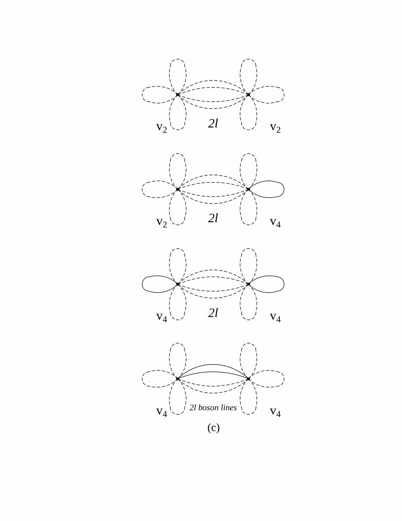
Third, we consider the two-vertex graphs constructed from v2 and v4, which are shownin Fig. 4(c). The sum of the amplitudes for these graphs is identical to A2 in Eq. (4.9) withthe replacement α→ β:
A3 = A2
∣
∣
∣
α→β. (4.10)
Fourth, we examine the two-vertex graphs constructed from one of v1 and v3 and oneof v2 and v4. These graphs are shown in Fig. 4(d). For each value of l the sum of theamplitudes for these graphs is
A4(l) = − v1v2Λα+β+2−2l
∫
dx∆2l(x)
(α + 1 − l)!(β + 1 − l)!2α+β+2−2l(2l)!+
v1v4gΛα+β+2−2l
∫
dx∆2l(x)
(α+ 1 − l)!(β − l)!2α+β+1−2l(2l)!
+v2v3gΛ
α+β+2−2l∫
dx∆2l(x)
(α− l)!(β + 1 − l)!2α+β+1−2l(2l)!− v3v4g
2Λα+β+2−2l∫
dx∆2l(x)
(α− l)!(β − l)!2α+β−2l(2l)!
+v3v4Λ
α+β−2l∫
dx∆2l(x)Tr S(x)S(x)
(α− l)!(β − l)!2α+β+1−2l(2l)!. (4.11)
Again, we must sum over all possible values of l; in all of the above terms except the last,l ranges from 1 to ∞, but in the v3v4 term representing boson- and fermion-exchange, lranges from 0 to ∞. Also, we again use the integral identity in Eq. (4.7). As before, whenwe simplify the expression A4(l) there is a remarkable cancellation of the ∆2l(x) integralsfor all values of α and β. We obtain the following simple sum:
A4 =∑
l
A4(l) = g2δ2Λα+β+1(2α+ 1)!(2β + 1)!∞∑
l=1
22l−α−β−4
(2l − 1)!(α + 1 − l)!(β + 1 − l)!. (4.12)
Next, we consider the two-vertex graphs constructed from v5 and v7, which are shown inFig. 4(e). For each value of l the sum of the amplitudes for these graphs is
A5(l) = − v25Λ
2α+2γ−2l∫
dx∆2l+1(x)
[(α + γ − l)!]222α+2γ+1−2l(2l + 1)!
+v5v7gΛ
2α+2γ−2l∫
dx∆2l+1(x)
(α + γ − l)!(α + γ − 1 − l)!22α+2γ−1−2l(2l + 1)!
− v27g
2Λ2α+2γ−2l∫
dx∆2l+1(x)
[(α + γ − 1 − l)!]222α+2γ−1−2l(2l + 1)!
+v27Λ
2α+2γ−2−2l∫
dx∆2l+1(x)Tr S(x)S(x)
[(α + γ − 1 − l)!]222α+2γ−2l(2l + 1)!. (4.13)
13

Again, we must sum over all possible values of l; in all of the above terms l ranges from 0to ∞. Also, in the boson- and fermion-exchange graph in the last term, we again use theintegral identity in Eq. (4.7). When we simplify the expression A5(l) there is no longer anycancellation for arbitrary values of α. Thus, the final result still contains an integral over∆2l+1(x). We obtain the following sum:
A5 =∑
l
A5(l) = π2g2δ2α2Λ2α+2γ [(2α+ 2γ − 1)!]22−2α−2γ−3
{
∞∑
l=0
22l
(2l)![(α + γ − l)!]2
+∞∑
l=0
g222l[(2α + 2γ)2 − 1][(2α+ 2γ)2 + 4l + 1]∫
dx∆2l+1(x)
(2l + 1)![(α + γ − l)!]2Λ2l
}
. (4.14)
Sixth, we consider the two-vertex graphs constructed from v6 and v8, which are shown inFig. 4(f). The sum of the amplitudes for these graphs is identical to A5 in Eq. (4.14) withthe replacement α→ β:
A6 = A5
∣
∣
∣
α→β. (4.15)
The seventh and last class of graphs is constructed from one of v5 and v7 and one of v6
and v8. These graphs are shown in Fig. 4(g). It is easy to see that the amplitudes for allsuch graphs are proportional to αβ. Thus, anticipating that at the end of the calculation wewill set both α = 0 and β = 0, we need not calculate the amplitude A7 because it will notcontribute to the ground-state energy density. (Note that before we set α and β to 0, wemust apply the differential operator D in Eq. (2.12). This operator does not have a mixedderivative term and thus it cannot eliminate both factors of α and β.)
The final part of this calculation consists of applying the operator D in Eq. (2.12) toA1 + A2 + A3 + A4 + A5 + A6 + A7 and setting α = 0, β = 0, and γ = 1
2. After a rather
lengthy calculation, we obtain the result
Eground state = D7∑
j=1
Aj
∣
∣
∣
∣
∣
α=β=0, γ=1/2
=1
16δ2g2Λ
2ψ′
(
3
2
)
− 2π2 +∞∑
l=0
√π Γ
(
l − 12
)
(
l − 12
)
Γ(l + 1)−
∞∑
l=1
√π Γ(l)
l Γ(
l + 32
)
+ O(δ3). (4.16)
The sums in this expression may be evaluated easily and we obtain the result
Eground state = 0 + O(δ3). (4.17)
B. Calculation of 〈φ〉 to second order in δ
The graphs that contribute to the vacuum expectation value of the scalar field ariseeither from one-vertex graphs constructed from the odd vertices, v5 through v8, or from twovertex graphs with one odd vertex and one even vertex. Some of these graphs are shown inFig. 5. Again, they fall into natural classes. We first consider the five two-vertex graphs in
14

which an even number of bosons are exchanged between the pairs of α vertices (v1, v3) and(v5, v7). For a given l the sum of the five amplitudes is
v1v5Λ2α+2γ+1−2l
∫
dx∆2l
(α + 1 − l)!(α + γ − l)!(2l)!22α+γ+1−2l− v1v7gΛ
2α+2γ+1−2l∫
dx∆2l
(α + 1 − l)!(α + γ − 1 − l)!(2l)!22α+γ−2l
− v3v5gΛ2α+2γ+1−2l
∫
dx∆2l
(α − l)!(α + γ − l)!(2l)!22α+γ−2l+
v3v7g2Λ2α+2γ+1−2l
∫
dx∆2l
(α− l)!(α + γ − 1 − l)!(2l)!22α+γ−1−2l
−v3v7Λ2α+2γ−1−2l
∫
dx∆2lTr S(x)S(x)
(α− l)!(α + γ − 1 − l)!(2l)!22α+γ−2l. (4.18)
There are five more graphs in which an odd number of bosons are exchanged. The sumof the amplitudes of these graphs is similar to the result in Eq. (4.18) and we do not giveit here. Furthermore, there are ten corresponding graphs in which α is replaced by β andthese are constructed from the vertices v2, v4, v6, and v8. When these twenty amplitudesare combined and summed over l no dramatic cancellation like that in the calculation of theground-state energy density occurs. Thus, we are left with an infinite sum over integrals ofthe coordinate space propagator ∆(x).
Next, we consider the contributions of the twenty graphs, analogous to those above, thatare constructed from one α vertex and one β vertex. That is, we construct all possiblemulti-boson exchange graphs from the vertices (v1, v3) connected to (v6, v8), and (v2, v4)connected to (v5, v7). This calculation simplifies dramatically because only one- and two-particle exchange graphs survive when we apply the derivative operator in Eq. (2.12) andset α = β = 0 and γ = 1/2.
Last, we include the four single-vertex graphs constructed from the vertices v5, v6, v7,and v8.
When we combine all of these calculations we obtain the following result:
〈φ〉 = i√
πΛ/2
{
−δ + δ2
[
1 − ln 2
+g2∫
dx∆(x)
(
∆(x)
2Λ
[
ln(
Λ
2
)
+ ψ(1)]
+
[
1 +∆(x)
Λ
]
ln
[
1 +∆(x)
Λ
]) ]
+O(δ3)
}
. (4.19)
Note that any positive integer power of the propagator ∆(x) in Eq. (4.8) is integrable. How-ever, the value of the propagator at the origin Λ = ∆(0) is a divergent quantity. Therefore,the function ∆(x)/Λ vanishes everywhere except at x = 0, where it is unity. Hence, theintegral involving this ratio in Eq. (4.19) exists and vanishes. Thus, our final result for theone-point function, which measures the parity symmetry breaking in this theory, is
〈φ〉 = i√
πΛ/2[−δ + δ2(1 − ln 2) + O(δ3)]. (4.20)
The fact that the theory is supersymmetric reduces the degree of divergence of this result.At intermediate stages of the calculation, the coefficient of δ2 is proportional to Λ1/2 ln Λ.However, when the boson and fermion contributions are combined, all terms containing ln Λcancel exactly. Thus, the higher-order result is no more divergent than the leading-orderresult.
15

C. Calculation of the fermion-boson mass ratio to second order in δ
We do not discuss this calculation in detail here because a similar one is explained inRef. [10]. The calculation done here is more elaborate because there are twice as manyvertices but the necessary calculations are routine. Our result is
R =Mfermion
Mboson= 1 + O(δ3), (4.21)
which is consistent with the theory being supersymmetric.
V. CONCLUSIONS
In the Schwinger model of two-dimensional electrodynamics with massless fermions thereis an anomaly. If the one-fermion-loop contribution to the photon propagator is calculatednaively one obtains a product of two factors; the first factor vanishes in two-dimensionalspace, and the second factor is a divergent integral. If one is not careful, one gets a quantitythat is formally 0. However, because the integral is divergent, one must evaluate this prod-uct by introducing a regulator; dimensional regulation is an acceptable procedure. As theregulator is removed one obtains a finite, nonvanishing result for the anomaly, namely, thefamous number e2/π. In general, one looks for an anomaly when there is a naive cancellationinvolving divergent quantities that must be regulated. The question that is raised in this pa-per is, do we have an anomaly in the δ expansion that breaks supersymmetry? Specifically,is there an anomaly associated with the cancellation that gives a vanishing ground-stateenergy density in Eq. (3.7)?
A. Dimensional regularization of the ground-state energy density
In the derivation of Eq. (3.7) we combine two numbers that are divergent to obtain0. There are several ways to regulate the integral representing Λ. For example, if we usedimensional regulation and evaluate Λ in 2 − ǫ dimensions, then for small positive ǫ
Λ ∼ 1
2π
∫ ∞
0dp
p1−ǫ
p2 + g2(ǫ→ 0+)
=1
4πg−ǫ
∫ 1
0du u−1+ǫ/2(1 − u)−ǫ/2
=1
4πg−ǫΓ
(
ǫ
2
)
Γ(
1 − ǫ
2
)
=1
4g−ǫ 1
sin(πǫ/2)∼ 1
2πǫg−ǫ (ǫ→ 0+). (5.1)
Furthermore, in d-dimensional space, the representation of the Dirac matrices has rank 2d/2.Thus, the trace of a unit matrix in 2 − ǫ dimensions is
Tr11 = 2(2−ǫ)/2 ∼ 2 − ǫ ln 2 (ǫ→ 0+). (5.2)
16
Thus, the coefficient of the second graph amplitude in Eq. (3.6) should be multiplied by1 − 1
2ǫ ln 2.
We now see that the two graphs do not exactly cancel; rather, the difference in thenumerical coefficients is of order ǫ. Combining the two graphs in (3.6) now gives
ǫ(ln 2)δg2 (2α + 1)!Λα+1
2α+2α!=ǫ ln 2
2√πδg22αΓ
(
α +3
2
)
Λα+1
∼ ln 2
4π3/2δg2Γ
(
α +3
2
)
(2Λ)α (ǫ→ 0+). (5.3)
If we now differentiate with respect to α and set α = 0, we obtain for the ground-stateenergy density
Eground state =ln 2
8πδg2
[
ψ(
3
2
)
+ ln(2Λ)]
+ O(δ2)
∼ ln 2
8πδg2
[
ψ(
3
2
)
− ln(πǫ)]
+ O(δ2) (ǫ→ 0+). (5.4)
Because this is a positive number, it suggests that supersymmetry may be broken.Of course, dimensional regulation violates supersymmetry. Thus, it is not clear whether
the nonzero result in Eq. (5.4) is correct or is merely an artifact of the regularization schemebeing used.
B. Proper-time regularization
If a supersymmetric regulation exists then, of course, there will be no anomaly. Con-versely, if we could establish rigorously that there does not exist any supersymmetric reg-ulation of the delta expansion, then there really would be a breaking of supersymmetry.We do not know for certain whether a supersymmetric regulation of the δ expansion exists.However, we believe that we have found a relatively simple way to regulate the δ expansionthat is consistent with supersymmetry and thus we believe that there is no anomalous struc-ture and that the ground-state energy is truly identically zero. This suggests that while itis relatively easy to break parity symmetry, supersymmetry is extremely rigid and is verydifficult to break.
Our regulation scheme, which we believe respects supersymmetry invariance, is a variantof the proper-time method due to J. Schwinger [15]. (It is well known that the proper-time method correctly yields the anomaly in the Schwinger model.) Here, we will use thismethod to define, in an invariant way, the divergent integral Λ. To make contact with thedimensionally regulated result above, let us work in d dimensions:
Λ =∫ ddp
(2π)d
1
p2 + g2=∫ ddp
(2π)2
∫ ∞
s0
ds e−s(p2+g2). (5.5)
Here, s0 is a proper-time regulator to be taken to 0 at the end of the calculation. We nowinterchange the order of integration in (5.5), and express the momentum integral as theproduct of d one-dimensional integrals:
17

∫ ∞
−∞
dp
2πe−sp2
=1
2√πs. (5.6)
Then, the integral representing Λ is immediately expressed in terms of a single regulatedintegral:
Λ =∫ ∞
s0
ds e−sg2
(
1
2√πs
)d
=gd−2
2dπd/2
∫ ∞
g2s0
dx x−d/2e−x. (5.7)
If we set d = 2 − ǫ as in the previous subsection, the integral converges when s0 = 0, andwe obtain the same result as in (5.1),
Λ ∼ 1
4πΓ(
ǫ
2
)
. (5.8)
However, if we want to preserve supersymmetry, we must remain in two dimensions, in whichcase the integral depends logarithmically upon s0:
d = 2 : Λ =1
4π
∫ ∞
gs0
dx
xe−x ∼ − 1
4π[γ + ln(gs0)], (5.9)
where γ is Euler’s constant.The obvious advantage of this regulation scheme is that it treats bosons and fermions on
an equal footing; the renormalization of the boson and fermion masses is identical. With thisregulation scheme, the ground-state energy density is zero, as expected. Thus, we believethat there is no anomaly in the δ expansion.
ACKNOWLEDGEMENT
We thank A. Das, L. Gamberg, and M. Grisaru for illuminating discussions, and we aregrateful to the U.S. Department of Energy for financial support.
18

REFERENCES
[1] C. M. Bender, K. A. Milton, M. Moshe, S. S. Pinsky, and L. M. Simmons, Jr.,Phys. Rev. Lett. 58, 2615 (1987); C. M. Bender, K. A. Milton, M. Moshe, S. S. Pinsky,and L. M. Simmons, Jr., Phys. Rev. D 37, 1472 (1988).
[2] C. M. Bender, K. A. Milton, S. S. Pinsky, and L. M. Simmons, Jr., J. Math. Phys. 30,1447 (1989).
[3] C. M. Bender, S. Boettcher, and K. A. Milton, J. Math. Phys. 32, 3031 (1991);B. Abraham-Shrauner, C. M. Bender, and R. N. Zitter, J. Math. Phys. 33, 1335 (1992).
[4] C. M. Bender and H. F. Jones, Phys. Rev. D 38, 2526 (1988); H. T. Cho, K. A. Milton,J. Cline, S. S. Pinsky, and L. M. Simmons, Jr., Nucl. Phys. B 329, 574 (1990).
[5] C. M. Bender, F. Cooper, and K. A. Milton, Phys. Rev. D 40, 1354 (1989); C. M. Ben-der, S. Boettcher, and K. A. Milton, Phys. Rev. D 45, 639 (1992); C. M. Bender,F. Cooper, K. Milton, M. Moshe, S. S. Pinsky, and L. M. Simmons, Jr., Phys. Rev. D45, 1248 (1992); C. M. Bender, K. A. Milton, and M. Moshe, Phys. Rev. D 45, 1261(1992).
[6] C. M. Bender, F. Cooper, and K. A. Milton, Phys. Rev. D 39, 3684 (1989); C. M. Ben-der, F. Cooper, G. Kilkup, P. Roy, and L. M. Simmons, Jr., J. Stat. Phys. 64, 395(1991).
[7] C. M. Bender and T. Rebhan, Phys. Rev. D 41, 3269 (1990).[8] C. M. Bender, K. A. Milton, S. S. Pinsky, and L. M. Simmons, Jr., J. Math. Phys. 31,
2722 (1990).[9] C. M. Bender, K. A. Milton, S. S. Pinsky, and L. M. Simmons, Jr., Phys. Lett. B 205,
493 (1988).[10] C. M. Bender and K. A. Milton, Phys. Rev. D 38, 1310 (1988).[11] C. M. Bender and K. A. Milton, Phys. Rev. D 55, R3255 (1997).[12] D. Bessis, private communication.[13] L. Alvarez-Gaume, D. Z. Freedman, and M. T. Grisaru, Harvard University re-
port No. HUTHP 81/B111 (1981), unpublished; T. Murphy and L. O’Raifeartaigh,Nucl. Phys. B218, 484 (1983); E. Witten, Nucl. Phys. 188, 513 (1981).
[14] C. M. Bender and A. Turbiner, Phys. Lett. A 173, 442 (1993).[15] J. Schwinger, Phys. Rev. 82, 664 (1951).
19

FIGURES
FIG. 1. The two graphs contributing to the ground-state energy to first order in δ. These graphs
are constructed from vertices having an even number of boson lines. The symmetry numbers are
shown beside each graph.
FIG. 2. The two graphs contributing to the one-point Green’s function to first order in δ. These
graphs are constructed from vertices having an odd number of boson lines. The symmetry numbers
are shown beside each graph.
FIG. 3. One-particle-irreducible graphs contributing to the mass renormalization of the fermion
and the boson to order δ. There is one graph for the fermion mass shift and two graphs for the
boson mass shift. All graphs are constructed from vertices having an even number of boson lines.
The symmetry numbers for the graphs are shown beside each graph.
FIG. 4. The thirty graphs contributing to the ground-state energy to second order in δ. These
graphs are constructed from the eight vertices in Eq. (4.3). We have organized the graphs into sets
for which the amplitudes combine in a natural way. These sets are labeled (a)–(g).
FIG. 5. Five of the graphs contributing to 〈φ〉 to second order in δ. These graphs are con-
structed from the eight vertices in Eq. (4.3).
20

(a) α+1 boson loops
(b) α boson loops
2-α-1/(α+1)!
2-α-1/α!

(a) α+γ boson loops
(b) α+γ-1 boson loops
2-α-γ/(α+γ)!
2-α-γ/(α+γ-1)!

(a)
α boson loops
(b)
α boson loops
(c)
α-1 boson loops
2-α/α!
2-α/α!
2-α/(α-1)!

v1
v3
v2
v4
(a)

v1 v12l
v1 v32l
v3 v32l
v3 v32l boson lines
(b)
v2 v22l
v2 v42l
v4 v42l
v4 v42l boson lines
(c)

v1 v22l
v1 v42l
v2 v32l
v3 v42l
v3 v42l boson lines
(d)

v5 v52l+1
v5 v72l+1
v7 v72l+1
v7 v72l+1 boson lines
(e)

v6 v62l+1
v6 v82l+1
v8 v82l+1
v8 v82l+1 boson lines
(f)

v5 v62l+1
v5 v82l+1
v6 v72l+1
v7 v82l+1
v7 v82l+1 boson lines
(g)

v1 v52l
v1 v72l
v1 v52l+1
v3 v72l+1
v3 v72l+1 boson lines