Embed Size (px)
Citation preview
Modeling and Optimization of Turning Duplex
Stainless Steels
Von der Fakultät Konstruktions-, Produktions- und Fahrzeugtechnik
der Universität Stuttgart zur Erlangung der
Würde eines Doktors der Ingenieurwissenschaften (Dr.-Ing.)
genehmigte Abhandlung
Vorgelegt von
M. Sc. Rastee Dalshad Ali (Koyee)
aus Erbil, Kurdistan-Irak
Hauptberichter: Univ.-Prof. Dr.-Ing. Prof. h. c. mult. Dr. h. c. mult. Uwe Heisel i. R.
Mitberichter: Prof. Dr. rer. nat. Siegfried Schmauder
Tag der mündlichen Prüfung: 14.04.2015
Institut für Werkzeugmaschinen der Universität Stuttgart
2015


Vorwort
Hiermit möchte ich all denen meinen Dank aussprechen, die mich bei der Entstehung dieser
Arbeit unterstützt und zu ihrem Gelingen beigetragen haben. In diesem Zusammenhang sei
dem Deutsche Akedemische Austauschdienst für die finanzielle Unterstützung und Förderung
gedankt.
Dem Leiter des Institutes, Univ.-Prof. Dr.-Ing. Prof. h. c. mult. Dr. h. c. mult. Uwe Heisel i.
R. gilt mein besonderer Dank für die Möglichkeit zur Durchführung der Arbeit und den dafür
notwendigen Freiraum ebenso wie für die Übernahme des Hauptberichtes und die dabei ent-
standenen Anregungen.
Herrn Prof. Dr. rer. nat. Siegfried Schmauder danke ich sehr herzlich für die teilweise Betreu-
ung meiner Arbeit. Seine freundliche Unterstützung meiner wissenschaftlichen Tätigkeit, sei-
ne ständige Bereitschaft zu fachlichen Diskussionen mit vielen wertvollen Ratschlägen und
konstruktiven Anregungen haben maßgeblich zur Realisierung dieser Arbeit beigetragen.
Herrn Dipl.-Ing Dipl.-Gwl. Rocco Eisseler, meinem langjährigem Kollege und Gruppenleiter,
danke ich für zahlreiche konstruktive fachliche Diskussionen, die ebenso wie seine Tipps zu
formalen Aspekten der schriftlichen Ausarbeitung eine wertvolle Hilfe geleistet haben.
Ein herzlicher Dank gebührt weiterhin meinen Kollegen und Freunden, durch die ich meine
Promotionszeit in schöner Erinnerung behalten werde. Frau Inge Özdemir, Herrn Dr.-Ing.
Michael Schaal, Herrn Dipl.-Ing. Atanas Mishev, Herrn Dipl.-Ing. (FH) Jens Großmann,
Herrn Rolf Bauer und Herrn Dr.-Ing. Johannes Rothmund vielen Dank für Ihre Freundschaft
und Hilfsbereitschaft.
Mein ganz besonderer Dank gilt letztlich meinem Vater Dalshad sowie meinen Geschwistern,
Dipl. Rasper, Dipl.-Ing. Rawand, Dr. Rawa, Dipl.-Ing. Rawen und B.Sc. Suham, und meinen
Cousinen Dr. Narmin Koye, Dr. Bahzad Koye und Dr. Kurdo Koye für ihre fortwährende
liebevolle Unterstützung. Ihr Verständnis, ihre oft endlose Geduld sowie ihre unermüdliche
moralische Aufbauarbeit haben mir den notwendigen familiären Rückhalt zur Durchführung
dieser Arbeit gegeben.
Stuttgart, im April 2015 Rastee D. Ali (Koyee)

Für die Seele meiner Mutter
Bahar Hammadamin Muhammad

Ehrenwörtliche Erklärung
Hiermit erkläre ich, dass ich die vorliegende Arbeit selbstständig verfasst und keine anderen
als die angegebenen Hilfsmittel genutzt habe. Alle wörtlich oder inhaltlich übernommenen
Stellen habe ich als solche gekennzeichnet. Ich versichere außerdem, dass ich die vorliegende
Arbeit keiner anderen Prüfungsbehörde vorgelegt habe und, dass die Arbeit bisher auch auf
keine andere Weise veröffentlicht wurde. Ich bin mir der moralischen und gesetzlichen Kon-
sequenzen einer falschen Aussage bewusst.
Legal statement
I solemnly declare that I have produced this work all by myself. Ideas taken directly or indi-
rectly from other sources are marked as such. This work has not been shown to any other
board of examiners so far and has not been published yet. I am fully aware of moral and legal
consequences of making a false declaration.
Datum: 29.01.2015 Rastee D. Ali (Koyee)
Contents VI
Contents
Nomenclature X
Extended Abstract XIX
1 Einleitung XIX
2 Forschungsmethodik XX
2.1 Hypothesen XXI
2.2 Gliederung der Dissertation XXI
2.3 Die Vorgehensweisen XXII
3 Zusammenfassung XXIX
Summary XXXI
1 Introduction 1
1.1 Frame of reference 4
1.1.1 Metal cutting 5
1.2 Background and aim 24
1.3 Research approach 25
1.4 Research hypothesis 26
1.5 Research questions 27
1.6 Research delimitations 28
1.7 Outline of the dissertation 28
2 State of the art in machining modeling and optimization: A review 32
2.1 Input-output parameter relationship of modeling tools 33
2.1.1 Statistical regression 34
2.1.2 Neural network 39
2.1.3 Fuzzy set theory 43
2.2 Finite element modeling of chip formation processes 47
2.2.1 Basics of FEM formulations and remeshing techniques 49
2.2.2 Historical perspective 52
Contents VII
2.2.3 Scales of the machining modeling 52
2.2.4 Simulation software & phases of metal cutting FEA 53
2.2.5 Advantages and problems associated with numerical cutting modeling 54
2.2.6 Input models and identification of input parameters 56
2.3 Determination of optimal or near-optimal cutting conditions 62
2.3.1 Taguchi Method 63
2.3.2 Response surface methodology (RSM) 68
2.3.3 Nature-inspired meta-heuristic algorithms 73
2.3.4 Multiple Attribute Decision Making (MADM) methods 86
2.4 A systematic methodology for modeling and optimization of cutting processes 102
3 Experimental details 106
3.1 Workpiece materials 106
3.1.1 Mechanical properties and chemical compositions 106
3.1.2 Temperature-dependent physical and mechanical properties of the workpiece
materials 107
3.2 Machine tool and cutting tool 110
3.3 Design of experiments (DOE) 112
3.3.1 Full factorial design 112
3.3.2 Taguchi designs 113
3.3.3 D-Optimal design 115
3.4 Measurement of the machining performance characteristics 116
3.4.1 Measurement of cutting forces and effective cutting power 116
3.4.3 Measurement of surface quality characteristics 117
3.4.4 Measurement of the flank wear 118
3.4.5 Infrared temperature measurement system 120
3.4.6 Chip thickness and chip serration ratio 121
4 Experimental investigation and multi-objective optimization of turning DSSs: A case
study 122
4.1 Pareto optimality 122
Contents VIII
4.2 Performance characteristics 123
4.2.1 Specific cutting pressures 123
4.2.2 The width of maximum flank wear land ( maxVB ) 125
4.3 Bat Algorithm for multi-objective optimization of turning DSSs. 130
4.4 Interim conclusions 132
5 Universal Characteristics Index 134
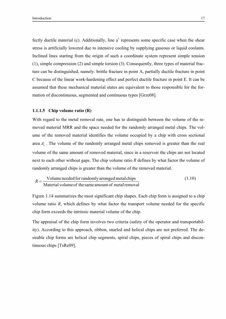
5.1 Estimation of the chip volume ratio 135
5.2 Universal characteristics index 137
5.2.1 TOPSIS 138
5.2.2 VIKOR method 139
5.2.3 GRA 139
5.2.4 UC 139
5.2.5 Fuzzy-MADM 140
5.3 Optimization 142
5.4 Interim conclusions 145
6 Taguchi-MADM-Meta-heuristic concept 146
6.1 Taguchi method 146
6.2 VIKOR method 150
6.3 Meta-heuristic optimization 152
6.4 Interim conclusions 155
7 Application of Fuzzy–MADM approach in optimizing surface quality of stainless
steels 157
7.1 Proposed methodology 157
7.2 Results and discussions 160
7.2.1 Computation of the MSQCIs 160
7.2.2 Fuzzy-MADM method 162
7.3 Confirmation tests 166
7.4 Interim conclusions 167
Contents IX
8 Sustainability-based multi-pass optimization of cutting DSSs 169
8.1 Performance characteristics 170
8.2 Phase I: Parametric cutting investigations 172
8.2.1 Effect of control factors on performance characteristics 173
8.2.2 Parametric optimization of performance characteristics 178
8.3 Phase II: Economics of cutting DSSs 180
8.4 Phase III: Operational sustainability index 182
8.4.1 Optimization of OSI using CSNNS 185
8.5 Interim conclusions 189
9 Numerical modeling and optimization of turning DSSs 193
9.1 3D FEM prediction of the chip serration 194
9.2 3D FEM prediction of the chip serration 198
9.3 Inverse identification of 3D FEM input parameters 202
9.3.1 Proposed methodology 207
9.3.2 Extension of FANNS: a case study 215
9.4 Inverse identification of Usui’s wear model constants 215
9.5 Numerical optimization of turning DSSs 217
9.5.1 Selective control factors 218
9.5.2 Results and discussions 220
9.5.3 Numerical machining performance measure 227
9.6 Interim conclusions 230
10 Conclusions 233
11 References 238
12 Appendix A: Supplementary tabulations A1

Nomenclature X
Nomenclature
List of Latin symbols:
Symbol Unit Definition
A MPa Initial yield strength A Negative ideal solution
*A Positive ideal solution
aA €/(m2.Month) Monthly rent
cA mm2 Cutting area
lA Loudness
pa mm Depth of cut
b Bias
B Strain hardening coefficient
C Strain rate coefficient *C Closeness to the ideal solution
CB Chip-breaker type
fC A constant function of cutting length
CI Consistency Index
CM Cooling medium
nc Coefficient of regression equations
pC J/kg. K Heat capacity
CR Consistency Ratio
2%C Percentage of ON state of the machine
d mm Outside diameter
D MPa Cockcroft-Latham material constant
.critD MPa Critical damage value
DV Degree of diversification
e Error terms in regression and neural network analyses
E J Energy
ce J/mm3 Cutting energy
Nomenclature XI
Symbol Unit Definition
cE €/kWh Electricity cost
jE Entropy of attribute j
E% Percentage error
cF N Main cutting force
fF N Feed cutting force
qf Frequency
rf mm/rev Feed rate
tF N Thrust cutting force
tF% Percentage increase in thrust cutting force
*g Global best
.Geo Insert shape
GRG Grey relational grade
H Chip serration ratio
h mm Chip thickness
tch N/(mm.sec.K) Thermal contact conductance
I Intensity of light of a firefly
cI A Line current
JAS hrs Annual operating hours
k Order of neural network layers
1K € Main time-related costs
1.1k MPa Specific cutting pressure for 1mm2 cutting area
2K € Fixed or the workpiece-related costs
3K € Tool-related costs
bk m2 kg/(sec2 K) Boltzmann constant
bBk € Procurement cost
bEk € Operational cost
bRk € Space cost
bWk € Cost of maintenance and repair

Nomenclature XII
Symbol Unit Definition
ck MPa Specific cutting pressure
ETk € Cost of the spare parts
fk MPa Specific feed pressure
FK € Total production cost
kk €/hrs Coolant cost
LK € Labor cost
MK € Machine hour-rate cost
MLK € Machine and wage rate cost
nK Number of control factors
rK degree Cutting edge anle
KT µm Depth of the crater wear
tk MPa Specific thrust pressure
thk W/(m2.K) Thermal conductivity
WHk € Cost of the tool holder
WPk € Cost of the cutting insert
L Number of levels
cL mm Length of cut
mL €/hrs Hourly wage of labor
rl mm Approach length
sL mm Sample length
tL mm Travel length
m units Number of the production units
m Thermal softening exponent in JC model
MRR mm3/min Material removal rate
N rpm Rotational speed
pn Number of cutting passes
tN Number of experimental trials
Ob Response variable
Nomenclature XIII
Symbol Unit Definition
aP Probability
cP W Cutting power
eP W Effective pwer
MP W Motor power
PN Preference number
rP Pulse emission
spP W Net spindle power
pp% Percentage of the procurement cost
rp% Percentage decrease in flow stress
mQ m2 Machine-tool basement area
NNQ VIKOR index predicted by neural networks
VQ VIKOR index
iq% Percentage of the interest rate
R Chip volume ratio
r € Amount of non-wage costs of the machine operator 2R Coefficient of determination
Ra µm Arithmetic average roughness
adj.R Adjusted coefficient of determination
cR N Resultant cutting force
RI Random Index
iR Regret measure
Rt µm Highest roughness point from the mean
Rz µm Average absolute value of five peaks and valleys
r mm Nose radius
R~
Centroid
S Negative ideal alternative
*S Positive ideal alternative
iS Utility measure
T min Tool life

Nomenclature XIV
Symbol Unit Definition
at hrs Working time
bBt hrs Machine utilization time
ct min Cutting time
et min Production time or time per unit
gt min Basic time
ht min Main process time
it min Idle time
lt years Economic machine life
mT °C Melting temperature
rT °C Reference temperature
nt min Auxiliary process time
qt Target of the neural network
rBt min set-up time
rVt min Nonproductive set-up activities time
rWt min Tool change time
vMt min Machine set-up time
WZt min Time that passes till a single tool is changed
cU Utility constant
lU V Line voltage
V Mean square of neural network error
VB µm Average width of the flank wear land
maxVB µm Maximum width of the flank wear land
nVB µm Average width of the notch wear land
cv m/min Cutting speed
sv m/sec Sliding velocity
w Weight of the attributes
W µm Wear
x Number of machines
Nomenclature XV
Symbol Unit Definition
*x Individual best
sZ Number of cutting edges per insert
List of Greek symbols:
Symbol Unit Definition
n degree Normal rake angle
rand Randomization parameter
z Step size scaling factor in Cuckoo Search algorithm
a Firefly attractiveness
r Random vector drawn from a uniform distribution
w degree Wedge angle
r Euclidean distance between fireflies
Deviation squence
c degree Chip flow angle
Equivalent plastic strain
Equivalent plastic strain rate
0 sec-1 Reference plastic strain rate
f Effective strain
p Von Mises equivalent plastic strain
N/(mm.sec) Heat flux
J Conducted heat
n degree Normal shear angle
s degree Shear angle
p W/m3 Volumetric heat generation
a Randomization parameter in Firefly Algorithm
c degree Relief or clearance angle
dB Signal to Noise ratio
t Taylor-Quinney coefficient
Expectation of occurrence
Inertia function
Nomenclature XVI
Symbol Unit Definition
i degree Inclination angle
w Wavelength in Bat Algorithm
Friction coefficient
A Membership function of set A
c Coulomb friction coefficient
s Shear friction coefficient
T °C Mean tool face temperature
m kg/m3 Density
Degree of uncertainty
1 MPa Principal stress
n MPa Normal stress
MPa Von Mises equivalent stress Learning parameter
f MPa Frictional stress
Random number drawn from a uniform distribution
Acceleration constant
Weight of the strategy Activation function of neurons
g Random number drawn from Gaussian distribution
Learning rate
g Grey relational coefficient
List of abbreviations:
Abbreviation Description
AAD Absolute Average Deviation
AHP Analytical Hierarchy Process
ALE Arbitrary Lagrangian-Eulerian
ANN Artificial Neural Networks
ANOM Analysis of Means
ANOVA Analysis of Variance
APSO Accelerated Particle Swarm Optimization

Nomenclature XVII
Abbreviation Description
BUE Built-up edge
CS Cuckoo Search
CSNNS Cuckoo Search Neural Network Systems
CV Crisp Value
DC Discontinuous Chips
DOE Design of Experiment
DOF Degree of Freedom
DSS Duplex Stainless Steel
FA Firefly Algorithm
FANNS Firefly Algorithm Neural Network System
FEM Finite Element Method
FIS Fuzzy Inference System
GRA Grey Relational Analysis
GTMA Graph Theory and Matrix Approach
JMatPro Java-based Material Properties
LB Lower Bound
LCFC Long Cylindrical and Flat helical Chips
LHCS Long Helical Chip Segments
LM Lower Medium
LRSC Long Ribbon and Snarled Chips
LSC Long Spiral Chips
MADM Multiple Attribute Decision Making
MH Moderately High
ML Moderately Low
MLP Multi-Layer Perceptron
MOBA Multi-Objective Bat Algorithm
MOO Multi-Objective Optimization
MPCI Multi-Performance Characteristics Index
MSE Mean Square Error
MSQCI Multi-Surface Quality Characteristics Index
OA Orthogonal Array
OSI Operational Sustainability Index
PF Pareto Front
Nomenclature XVIII
Abbreviation Description
RMSE Root Mean Square Errors
RSM Response Surface Methodology
SA Simulated Annealing
SCFC Short Cylindrical and Flat helical Chips
SHCS Short Helical Chip Segments
SRSC Short Ribbon and Snarled Chips
SS Sum of Squares
SSC Short Spiral Chips
STDV Standard Deviation
TOPSIS Technique for Order Preference by Similarity to Ideal Solution
UB Upper Bound
UC Utility Concept
UCI Universal Characteristics Index
UM Upper Medium
VH Very High
VL Very Low
Extended Abstract XIX
Extended Abstract
1 Einleitung
Der Mensch nutzt seit rund 5000 Jahren das Metall Eisen. Aber erst im 18. Jahrhundert stoßen
Wissenschaftler in kurzer Folge auf eine ganze Reihe zuvor unbekannter Metalle. Im Jahr
1751 entdeckte z.B. der schwedische Wissenschaftler Axel Cronstedt das Element Nickel.
1778 folgte sein Landsmann Karl Wilhelm Scheele mit dem Element Molybdän. 1797 fand
der Franzose Nicola-Louis Vauquelin ein neues Metall, das er Chrom nannte. Im 19. Jahrhun-
dert experimentierten mehrere Metallurgen erfolgreich mit Eisen-Chrom Legierungen. Zwar
zeigt sich, dass sie besonderes rostbeständig sind, allerdings waren die Gründe hierfür noch
nicht bekannt.
1912 wurde den beiden Deutschen Edward Maurer und Beno Strauß ein Patent auf austeneti-
sche Chrom-Nickel-Stähle erteilt. Noch heute machen die austenitischen Sorten rund 65% der
Weltproduktion an rostfreiem Stahl aus. 1913 wurde in England erstmals martensitischer rost-
freier Stahl hergestellt. Der Entdecker dieser Neuerung war Harry Brearley. Ungefähr zur
selben Zeit, nämlich 1915, entwickelten die US-Amerikaner Becket und Dantsaizen ferriti-
sche rostfreie Stähle. Auf sie entfallen 30% der weltweiten Erzeugung. Bis 1920, also in we-
niger als einem Jahrzehnt, bildete sich auf diese Weise der hauptsächliche Anwendungsgebie-
te.
1930 entwickelten schwedische Metallurgen Stahlsorten, die sowohl ein ferritisches als auch
ein austenitisches Gefüge in einer Legierung vereinen, und bezeichneten diese als rostfreie
Duplexstähle. Duplexstähle revolutionierten zunächst die Zellstoff- und Papierindustrie durch
die Verfügbarkeit beständiger Bauteile. Heute bewähren sie sich in einer ganzen Reihe von
Anwendungen, z.B. in der petrochemischen Industrie oder bei der Meerwasser-Entsalzung,
also dort wo sowohl eine besondere Korrosionsbeständigkeit als auch eine hohe Festigkeit
erforderlich sind.
Seit 1990 findet eine zweite Generation von rostfreien Duplexstähle immer mehr breiteren
Einsatz als Alternative zu den konventionellen rostfreien Stählen. Die Gründe hierfür sind:
1. Geringere Preise durch einen geringeren Anteil an Nickel,
2. Höhere Zugfestigkeit und
Extended Abstract XX
3. Deutlich höhere Korrosionsbeständigkeit gegen durch Chlorid induzierte Spannungs-
korrosion als dies bei austenitischen rostfreien Stählen der Fall ist.
Andererseits sind die rostfreien Duplexstähle normalerweise schwerer zerspanbar als austeni-
tische Sorten mit einer vergleichbaren Korrosionsbeständigkeit. Die Gründe sind: große Zä-
higkeit, niedrige Wärmeleitfähigkeit, hohe Streckgrenzwerte (ca. zweimal höher als austeniti-
sche rostfreie Stähle), spezielle Mikrostruktur (weiches Ferrit neben hartem Austenit), gerin-
ger Schwefel- und Phosphorgehalt, starke Tendenz zu Bildung von Aufbauschneiden und eine
hohe Kaltverfestigungsrate.
Aufgrund der hohen Zähigkeit bilden sich oftmals beim Zerspanen lange Band- oder Wirr-
späne aus, die sich um das Werkstück oder den Werkzeughalter wickeln können. Die Proble-
matik verschärfte sich besonders bei Schlichtoperationen mit geringen Vorschüben und
Schnitttiefen. In der automatisierten Fertigung verringert dies die Produktivität aufgrund von
Maschinenstillstandszeiten sowie geringer Prozesssicherheit in erheblichem Maße.
2 Forschungsmethodik
Vor dem Hintergrund der Komplexität von Zerspanungsuntersuchungen, der Grenzen der
Theorie spanender Prozesse und analytischer Modelle, der Schwierigkeiten bei der Modellie-
rung und Optimierung von Parametern des Zerspanungsprozesses und der Notwendigkeit von
zusätzlichen Kenntnissen über die Zerspanung von duktilen und kaltverfestigten Materialien,
wird in der vorliegenden Dissertation die Zerspanung von rostfreien Duplexstählen am Bei-
spiel des Drehens systematisch untersucht. Neuentwickelte Modellierungs- und Optimie-
rungsverfahren werden systematisch verwendet, um die Zerspanbarkeit rostfreier Duplexstäh-
le präziser abbilden zu können. Das abschließende Ziel der vorliegenden Arbeit ist es, dem
Prozessplaner ein Hilfsmittel an die Hand zu geben, mit dem er, unter Berücksichtigung meh-
rerer und sich häufig widersprechender Leistungsmerkmale, die optimalen Prozessparameter
für die Drehbearbeitung von Duplexstählen finden kann. Auf Ein- und Ausgangkenngrößen
basierende Modellierungs- sowie Optimierungsverfahren, multikriterielle Entscheidungsstra-
tegien (MKES) und Finite-Elemente-Simulationen wurden hier intensiv angewandt. Solche
MKES, die mit der Fuzzy-Set-Theorie in Verbindung stehen, werden ebenfalls vorgeschlagen,
um damit eine Mehrzieloptimierung durchzuführen und für unterschiedliche Schnittbedin-
gungen angepasste Maßnahmen zu erhalten. Ein weiteres Hilfsmittel stellt die Hybridisierung
Extended Abstract XXI
rechnerischer Modellierungs- sowie Optimierungsverfahren dar. Diese werden im Rahmen
der Ansätze zur Zerspanungsoptimierung effektiv angewendet.
2.1 Hypothesen
Ausgehend von der Frage, wie die Verwendung von neu entwickelten Modellierungs- und
Optimierungsverfahren für eine effektive Ableitung von optimierten Zerspanungslösungen
ermöglicht werden kann, werden systematische Untersuchungen unter Einsatz von neuentwi-
ckelten Modellierungs- und Optimierungsverfahren durchgeführt. Zunächst sollen jedoch die
folgenden Hypothesen vorgestellt werden:
1. Statistische Regression und metaheuristische Optimierungsverfahren können zu einer
Reihe von nicht dominanten Zerspanungslösungen führen.
2. Fuzzylogik ist vorteilhaft zur Beseitigung der Diskrepanz in der Rangordnung von Alter-
nativen unter dem Einsatz von MKES.
3. Das Taguchi-MKES-metaheuristisches Konzept kann praktischerweise für Mono- und
Mehrzieloptimierungen verwendet werden.
4. Merkmale der Oberflächenqualität können effizient optimiert werden, wenn MKES mit
der Fuzzy-Set-Theorie gekoppelt werden.
5. Die Multipass-Zerspanung kann nachhaltig optimiert werden, wenn eine systematische
Hybridisierung des Modells der Ein- und Ausgangkenngrößen sowie der Optimierung und
der MKES durchgeführt wird.
6. Es ist ausreichend, die JMatPro Software, MKES und Modelle sowie Optimierungsansät-
ze für Ein- und Ausgangkenngrößen zur Rückwärtsidentifikation von FEM-
Eingangskenngrößen zu benutzen.
2.2 Gliederung der Dissertation
Angesichts der breit angelegten Aufgabenstellung ist die Dissertation in 10 Kapitel gegliedert.
In Kapitel 1 wird eine kurze Einführung in das Hauptthema gegeben und die bei den For-
schungsarbeiten verfolgte wissenschaftliche Methodik behandelt. In Kapitel 2 wird der Stand
der Technik zu den Themenbereichen Modellierung und Optimierung von Zerspanprozessen
dargestellt. Zudem wird ein Überblick über die Vor- und Nachteile der Verfahren und der
abgeleiteten Modellierungs- und Optimierungsansätze gegeben. Im Kapitel 3 werden der ver-
wendete Versuchsaufbau sowie die Details der experimentellen Untersuchungen beschrieben.
Extended Abstract XXII
Kapitel 4 befasst sich mit experimentellen Untersuchungen zum Längsdrehen von rostfreien
Duplexstählen mit beschichteten Wendeschneidplatten. In Kapitel 5 wird die Beseitigung von
Diskrepanzen bei der MKES-Rangordnung durch die Ableitung eines allgemeinen Eigen-
schafts-Zeiger-Index behandelt. In Kapitel 6 wird die Anwendung eines neuen Taguchi-
VIKOR- metaheuristischen Konzepts als angemessener Ansatz für die Mono- und Mehrzielo-
ptimierung der Bearbeitung von rostfreien Duplexstählen aufgeführt. In Kapitel 7 wird die
Taguchi-Methode in Verbindung mit der Fuzzy-MKES für die Optimierung von Merkmalen
der Oberflächengüte angewandt. In Kapitel 8 wird ein systematischer Ansatz vorgelegt, der
unterschiedliche Modellierungs- und Optimierungsverfahren integriert, um die Multipass-
Zerspanung von rostfreien Duplexstählen nachhaltig zu optimieren. Kapitel 9 befasst sich mit
der Rückwärtsidentifikation der FEM-Eingangskenngrößen und der Anwendung der Finite-
Elemente-Simulationen, um damit eine hypothetische Optimierungsstudie durchzuführen. In
Kapitel 10 werden die Forschungsfragen, welche der vorliegenden Arbeit zugrunde lagen,
beantwortet und abschließenden besprochen.
2.3 Die Vorgehensweisen
2.3.1 Die Fledermaus-Mehrzieloptimierung
Im Zusammenhang mit der Haupthypothese stellt sich die erste Forschungsfrage wie folgt:
Kann durch die Anwendung der statistischen Regression und des Metaheuristischen Optimie-
rungsverfahren in Mehrzieloptimierungen eine Reihe von nichtdominierten Zerspanungslö-
sungen effektiv gewonnen werden? Um diese Frage angemessen zu beantworten, wird eine
experimentelle Untersuchung des Längsdrehens von rostfreien Duplexstählen EN 1.4462 und
EN 1.4410 mit beschichteten Wendelschneidplatten durchgeführt. Mit Hilfe des Fledermaus-
Mehrziel-Algorithmus (MOBA) werden Bewertungskriterien wie beispielsweise die Zerspan-
kraftkomponenten und die maximale Verschleißmarkenbreite optimiert und die Pareto Gren-
zen der nicht dominierten Optimierungslösungen ermittelt. Die parametrischen Einflüsse von
Größen wie Schnittgeschwindigkeit, Vorschub und Kühlmedium auf die Bewertungskriterien
werden mit Hilfe von dreidimensionalen Diagrammen dargestellt.
Erste Ergebnisse zeigen, dass die Werte von nicht nutzbringenden Bewertungskriterien bei
der Zerspanung des Werkstoffs EN 1.4410 im Allgemeinen höher liegen, als beim Werkstoff
EN 1.4462. Zudem zeigt die Nasszerspanung im Vergleich zur Trockenzerspanung eine Ver-
besserung der Gesamtbearbeitungsleistung durch geringere Zerspankraftkomponenten und die
Extended Abstract XXIII
Steigerung der Werkzeugstandzeit. Drittens wird nach der Regressionsanalyse ein MOBA zur
Modellierung eingesetzt. Ergebnisse zeigen, dass der MOBA sehr effizient und sehr zuverläs-
sig ist. Er führt effizient zu vielen optimalen Lösungen. Abhängig vom Entscheidungsträger-
vorzug wird die optimale Schnittbedingung identifiziert.
2.3.2 Der allgemeine Eigenschaftenzeiger
Die zweite Forschungsfrage lautet: Ist die Anwendung von Fuzzylogik vorteilhaft zur Besei-
tigung von Widersprüchlichkeiten in der Rangordnung beim Einsatz von MKES? Als bei-
spielhafter Zerspanungsprozess wird hierzu das Plandrehen bei konstanter Schnittgeschwin-
digkeit herangezogen. Das Plandrehen zeichnet sich im Vergleich zum Außenlängsdrehen
durch eine bessere Wirtschaftlichkeit, höhere Oberflächengüte und kürzere Hauptzeit aus.
Leistungsmerkmale wie Spanraumzahl, resultierende Schnittkraft, spezifische Schnittkraft
und Netto-Spindelleistung sollen gleichzeitig optimiert werden.
Unter den vielen maßgeblichen Leistungsmerkmalen ist die Spanraumzahl eine der wichtigs-
ten. Die Spanraumzahl gibt Auskunft über die Sperrigkeit der Späne. Sie wird aus dem Ver-
hältnis von Spänevolumen zu Spanungsvolumen gebildet. Allerdings ist die messtechnische
Erfassung des Spänevolumens in der Praxis nicht einfach. Um dieses zumindest hinreichend
abschätzen zu können, wird deshalb eine neue Methode vorgeschlagen. Zunächst werden qua-
litative Informationen über die Späne in einer Spanbruchtabelle dargestellt. Anschließend
werden die Späne gemäß den bekannten Standardspanformen klassifiziert. Dann kommt die
Fuzzylogik zum Einsatz, wobei Regeln formuliert werden, um die qualitativen Informationen
zu fuzzifizieren. Abschließend werden die fuzzifizierten Daten im Fuzzy-Inferenz-System zu
quantitativen Daten defuzzifiziert und zur Vorhersage der Spanrauzahl genutzt.
Die unterschiedlichen Leistungsmerkmale werden zudem mit Hilfe von MKES wie TOPSIS,
VIKOR, GRA und UA in einem einzelnen MKES-Index zusammengeführt. Basierend auf
einer unterschiedlichen MKES-Präferenz und der Tatsache, dass keine MKES als optimales
Verfahren anzusehen ist, wird schließlich die Mamdani-Fuzzy-Begründung genutzt, um den
Widerspruch zwischen den MKES aufzulösen und einen allgemeinen Index abzuleiten. Dieser
Index wird als allgemeiner Eigenschaftenzeiger (UCI) bezeichnet. Der optimierte UCI wird
anhand der Ergebnisse von zwei weiteren Optimierungsverfahren validiert.
Bei diesen Verfahren handelt es sich um:
1. Die Methode der gewichteten Summen ergänzt durch eine simulierte Abkühlung und
Extended Abstract XXIV
2. Statistische Regression ergänzt durch eine simulierte Abkühlung.
Die Ergebnisse zeigen, dass mit diesem Ansatz die aus anderen anderen Optimierungsverfah-
ren resultierende, durchschnittliche Verbesserung der Leistungsmerkmale übertroffen werden
kann. Im Allgemeinen sind durchschnittliche Verbesserungen zwischen 10% und 40% mög-
lich.
Aus diesen Ergebnissen kann geschlossen werden, dass der neue Ansatz wirkungsvoller ist,
als die anderen klassischen Ansätze.
2.3.3 Das Taguchi-VIKOR-metaheuristische Konzept
Kann das Taguchi-VIKOR-metaheuristische Konzept praktischerweise für Monoziel- und
Mehrzieloptimierungen der Zerspanung von rostfreien Stählen verwendet werden? Dies ist
die dritte Frage in der Folge des Erkenntnisgewinns. Zunächst werden hierzu die Schnittbe-
dingungen als Einflussgrößen und das Plandrehen mit konstanter Schnittgeschwindigkeit als
Zerspanprozess festgelegt.
Anschließend wurden Zerspanversuche gemäß der Taguchi-Methode durchgeführt. Bei der
Taguchi-Methode werden im Wesentlichen orthogonale Felder eingesetzt. Orthogonale Felder
sind Teilfaktorpläne, d.h. es werden nicht alle möglichen Kombinationen von Faktorstufen
durchgespielt, sondern nur eine genau ausgewählte Teilmenge. Durch diesen Ansatz kann
man die Zahl der erforderlichen Experimente erheblich reduzieren. Im konkreten Fall müssen
so anstelle von 125 Experimenten nur 25 Experimente durchgeführt werden. Die Leistungs-
merkmale, die gleichzeitig optimiert werden sollen, sind die Schnittleistung, die resultieren-
den Schnittkräfte, die spezifische Schnittenergie und der arithmetische Mittenrauwert. Die
Vorgehensweise ist wie folgt:
Im ersten Schritt werden die Monozieloptimierungen nach der Taguchi Methode durchge-
führt. Die Taguchi-Methode, das sogenannte Robust Design, ist eine Technik, deren Ziel es
ist, Produkte und Prozesse zu entwickeln, die robust gegen äußere Störeinflüsse sind. Die
Taguchi-Methode nutzt das Signal-Rausch-Verhältnis. Es ist definiert als das Verhältnis der
vorhandenen mittleren Signalleistung zur vorhandenen mittleren Rauschleistung. Es wird oft
im logarithmischen Maßstab dargestellt. Danach werden Mittelwertanalyse und Varianzanaly-
se der Signal-Rausch-Verhältniswerte durchgeführt. Eine Maximierung des Mitten-Signal-
Rausch Verhältnisses minimiert die Verlustkosten und optimiert die Steuerungsgröße.
Extended Abstract XXV
Im zweiten Schritt wird die Mehrzieloptimierung durchgeführt und hierzu die VIKOR-
Methode eingesetzt. VIKOR gehört zu einer Kompromissklassifizierung der MKES. Sie be-
ginnt mit einer Datennormalisierung auf Werte zwischen 0 und 1. Anschließend werden die
Gewichte der einzelnen Leistungsmerkmale mit Hilfe der Entropiegewichtsmethode berech-
net. Anschließend erfolgt die statistische Kalkulation der Utility, Regret und des VIKOR-
Index und der entsprechenden Rangordnung der Alternativen. Man kann diesen Index auch
als Schwerzerspanbarkeitsindex bezeichnen. Je kleiner der Wert des VIKOR-Index desto bes-
ser. Es handelt sich um einen Index, der genau darauf hinweist, wo sich der optimale Schnitt-
parameterbereich befindet.
Der dritte Schritt, um die wirkungsvollsten metaheuristischen Optimierungsverfahren zu er-
mitteln und die exakten Schnittbedingungen zu bestimmen, besteht darin, drei neuentwickelte,
metaheuristische Algorithmen anzuwenden und ihre Leistung zu verglichen. Die betrachteten
drei neuentwickelten, metaheuristischen Optimierungsverfahren sind der Glühwürmchen-
Algorithmus, die beschleunigte Partikel-Schwarm-Optimierung und der Kuckuck-
Suchalgorithmus. Diese Algorithmen wurden entsprechend der gegebenen Entscheidungsva-
riablen, Zielfunktionen und Zwänge eingesetzt. Die Ergebnisse zeigten, dass der Kuckuck-
Suchalgorithmus die anderen Optimierungsalgorithmen übertrifft.
Zusammenfassen wird bewiesen, dass das Taguchi-VIKOR-metaheuristische Konzept prakti-
scherweise für Monoziel- und Mehrzieloptimierung der Zerspanung rostfreier Stähle verwen-
det werden kann.
2.3.4 Die Optimierung von Merkmalen der Oberflächengüte
Die vierte Frage befasst sich mit der Optimierung von Merkmalen der Oberflächengüte. Unter
Zuhilfenahme von MKES und Fuzzy-Set-Theorie werden die Größen zur Bewertung der
Oberflächengüte namentlich der arithmetische Mittenrauwert, die gemittelte Rautiefe und die
maximale Rautiefe parallel optimiert. Zu diesem Zweck wird ein neuer Ansatz dargestellt.
Der Zerspanungsprozess wird wiederum das Plandrehen mit konstanter Schnittgeschwindig-
keit und als Eingangsgrößen die Schnittbedingungen festgelegt. Taguchi-Versuchspläne wer-
den verwendet, um den gesamten Hauptparameterraum mit einer geringen Anzahl von Versu-
chen abarbeiten zu können.
Die Vorgehensweise, die sogenannte Methodik, gliedert sich in fünf Stufen: die erste Stufe
erledigt die Vorverarbeitung der Daten. Diese beinhaltet die Versuchsplanung und die Festle-
Extended Abstract XXVI
gung der Leistungsmerkmale. Im zweiten Schritt werden MKES, wie GTMA und AHP-
TOPSIS benutzt, um einen allgemeinen Index für die Merkmale der Oberflächengüte zu be-
stimmen. Es stellt sich die Frage, warum hier zwei MKES genutzt werden: Es gibt kein
MKES als globales Verfahren, das für alle Arten von Mehrzieloptimierungsproblemen geeig-
net ist. Aus diesem Grund ist der Entscheidungsablauf immer mit Unsicherheiten behaftet.
Um dieses Problem zu lösen, wird im zweiten Schritt die Fuzzy-Set-Theorie herangezogen.
Alle Merkmale der Oberflächengüte müssen in Fuzzy-Trapenznummern überführt werden
und unter Einhaltung von 10%-Unsicherheit im Entscheidungsablauf konvertieren. Dann wird
die Methode der Gewichteten Summen zur Ableitung von Kompromisslösungen verwendet
und die geometrischen Eigenschaften der Trapenznummern werden zur Defuzzifizierung der
Indizes genutzt. Schließlich werden die defuzzifizierten Zahlen nachbearbeitet. Die Nachbe-
arbeitung befasst sich mit der Anwendung der Mittelwert- und Varianzanalyse sowie der Ve-
rifikation der optimierten Ergebnisse.
Nach der Anwendung und Verifikation des Ansatzes, wird die erreichte Verbesserung der
Merkmale der Oberflächengüte ermittelt. Hier zeigt sich, dass Verbesserungen von bis zu
30% bei der Oberflächengüte möglich sind. Deshalb kann zusammenfasst werden, dass die
beschriebene Vorgehensweise zielführend ist.
2.3.5 Die nachhaltige Optimierung der Multipass-Zerspanung
Im Zusammenhang mit den Hypothesen stellt sich die fünfte Frage: ist es möglich, durch eine
systematische Hybridisierung des Modells und der Optimierung der Ein- und Ausgangkenn-
größen und durch die MKES die Multipass-Zerspanung nachhaltig zu optimieren?
Wie bei den zuletzt beschriebenen Vorgehensweisen, wird zunächst die experimentelle Me-
thodik festgelegt. Die Experimente werden am Beispiel des Plandrehens bei konstanter
Schnittgeschwindigkeit im Mehrschnittverfahren durchgeführt. Bekanntermaßen sind die Zu-
sammenhänge zwischen den Eingang- und Ausganggrößen bei der Zerspanung stark nichtli-
near. Außerdem müssen noch kategorische Faktoren zu den Versuchsplänen und Zer-
spanungsmodellen hinzufügt werden. Dazu werden D-Optimale Versuchspläne als sehr ge-
eignet angesehen. Die D-Optimalen Versuchspläne werden nicht mit einem festen Schema
generiert, sondern iterativ aufgebaut. Allerdings sind die Vorteile, wie freie Wahl für die Zahl
der Stufen pro Einflussfaktor, freie Wahl des mathematischen Modells, freie Wahl der Stu-
Extended Abstract XXVII
fenabstände wesentlich größer, als die Nachteile, wie beispielsweise zu wenig Versuchspunk-
te in der Mitte des Versuchsraumes und die Abhängigkeit von Rechenalgorithmen.
Die Steuerungsfaktoren sind hier numerisch und kategorisch. Erstmalig werden Leistungs-
merkmale, wie die prozentuale Erhöhung der radialen Schnittkraft, die Spanraumzahl, die
Wirkleistung und die maximale Verschleißmarkenbreite, in der Zerspanungsoptimierung der
rostfreien Duplexstähle genutzt.
Die Vorgehensweise des Studiums vollzieht sich systematisch in drei Phasen. In Phase 1 wer-
den mathematische Modelle für die Leistungsmerkmale mit der Response-Surface-Methode
(RSM) entwickelt, die Wechselwirkungseffekte zwischen Schnittbedingungen und Leis-
tungsmerkmalen mit Hilfe von dreidimensionalen Diagrammen analysiert und eine parametri-
sche Optimierung der Leistungsmerkmale unter Verwendung des Kuckuck-Suchalgorithmus
durchführt. In der Phase 2 werden umfassende Modelle zur Kalkulation von Produktionskos-
ten und Produktionsraten entwickelt. Um den Konflikt zwischen dem Wunsch nach minimier-
ten Produktionskosten und maximierter Produktionsrate überwinden zu können, wird TOPSIS
als Optimierungsansatz vorgeschlagen. Die Betriebsmittel-belegungszeit, die Hauptzeitkosten,
die Werkzeug- und Werkzeugwechselkosten werden für die Herstellung einer Zahl von
12.000 Stück optimiert und hieraus die beste Alternativ identifiziert. Ein Ansatz zur Modellie-
rung und Optimierung eines Betriebsnachhaltigkeitsindexes (BNI) wird in der dritten Phase
der Vorgehensweise präsentiert. Zuerst wird durch die Anwendung der Mamdani-Implikation
ein neuer Index für die nachhaltige Mehrschnitt-Zerspanung von rostfreien Stählen abgeleitet.
Durch das BNI kann genau bestimmt werden, wo der Bereich nachhaltiger Zerspanungspara-
meter liegt. Der nächste Schritt beinhaltet die Modellierung und Optimierung. Ein neues Ver-
fahren nutzt ein künstliches neuronales Netz mit integriertem Kuckuck-Suchalgorithmus
(CSNNS). Das BNI kann gleichzeitig und effizient durch den entwickelten CSNNS modelliert
und optimiert werden.
Schließlich kann festgehalten werden, dass die systematische Hybridisierung des Modells und
der Optimierung der Ein- und Ausgangkenngrößen sowie die MKES Methoden die Zer-
spanung der rostfreien Duplexstähle nachhaltig optimieren können.
2.3.6 Die Rückwärtsidentifikation der FEM-Eingangskenngrößen
Die nächste Anwendung der Modellierung und Optimierung behandelt die Rückwärtsidentifi-
kation von FEM-Eingangskenngrößen. Für die Zerspanungssimulation ist es ein wesentlicher
Extended Abstract XXVIII
Vorteil, Eingangskenngrößen wie die Thermokontakt-Leifähigkeit, den Coulombschen Reib-
koeffizienten, den Schub-Reibkoeffizienten, den Taylor-Quinney-Koeffizienten, die Festig-
keitsabnahme und das Cockcroft-Latham-Schadenskriterium und deren Wechselwirkung mit
den gegebenen Schnittbedingungen zu kennen.
Bevor die FEM-Simulation erstellt wird, werden die mechanischen und physikalischen Eigen-
schaften der Werkstoffe als Funktion der Temperatur ermittelt. Zu diesem Zweck wurde
JMatPro eine Java-basierte Software zur Herleitung von Materialeigenschaften genutzt. Phy-
sikalische Eigenschaften, wie die Wärmleitfähigkeit, der thermische Ausdehnungs-koeffizient
und die spezifische Wärmekapazität, werden als Funktionen der Temperatur dargestellt. Auch
wurden die mechanischen Eigenschaften, wie Fließkurven, Elastizitätsmodul und Poissonzahl
als Funktion der Temperatur ausgedrückt. Aus diesen wichtigen Informationen wird zunächst
ein Textfile erzeugt, um dieses dann in die Keyword-Datei der aktuellen Simulation kopieren
zu können.
Um die Eignung von JMatPro für Bereitstellung von Daten für Zerspanungssimulationen zu
bewerten, wurde die FE-Simulation unter ähnlichen Eingangsgrößen mit dem Johnson-Cook-
Model verglichen. Die Ergebnisse zeigen, dass die JMatPro-basierte Simulation die Johnson-
Cook Simulation übertrifft, besonders wenn die Späne-Morphologie als Bewertungskriterium
herangezogen wird.
Zur Rückwärtsidentifikation von FEM-Eingangskenngrößen wird ein L18-Taguchi-
Versuchsplan verwendet. Nach den experimentellen Untersuchungen und Simulationsrech-
nungen werden für beide Fälle die prozentualen Fehler zwischen Schnittkraft, Temperatur an
der Werkzeugspitze und Spandicke gerechnet und als Leistungsmerkmale definiert. Dann
wird die VIKOR-Methode verwendet, um alle prozentualen Fehleranteile zu einem Index zu
konvertieren. Dieser Index ist eine Funktion der Eingangsgrößen und wird mit dem neuent-
wickelten FANNS (Firefly Algorithm Neural Network System) optimiert. Am Ende dieser
Phase werden die Ergebnisse validiert.
Nach Abschluss der beschriebenen Vorgehensweise, werden die FEM-Eingangskenngrößen
rückwäsrts identifiziert und die prozentualen Fehleranteile drastisch reduziert. Die Rückwärts-
identifikation wirkt sich mit einer Fehlerminimierung von -60% bis -200% bis auf minimal
±10% aus.
Extended Abstract XXIX
Es kann deshalb gesagt werden, dass die vorgeschlagene Vorgehensweise die Eingangskenn-
größen sehr effektiv identifiziert und die Fehleranteile der FEM-Rechnung zehn bis zwanzig-
fach reduziert.
2.3.7 Hypothetische FEM-Optimierung
In der zweiten Phase der FEM-Studie wird eine neue Vorgehensweise zur FEM-basierten
Optimierung beschrieben. Einflussgrößen wie Spänebrecher, die Form der Wendeschneidplat-
te, das Kühlschmiermedium, die Schnittgrößen und Neigungswinkel werden durch den inten-
siven Einsatz von Taguchi-Optimierungsmethoden und Fuzzylogik optimiert. Die Bewer-
tungskriterien sind in diesem Fall resultierende Schnittkraft, Spannung, Schnitttemperatur und
Verschleißrate. Eine neue Maßnahme wird von diesen Merkmalen abgeleitet. Es werden 81
Regeln je Werkstoff formuliert und in das Mamdani-Fuzzy-Inferenz-System integriert. Die
Ausgabe der Defuzzifizierung wird als numerischer Zerspanungsleistungsindex (NZLI) be-
zeichnet.
Nach der Durchführung der FEM-Simulationen und Ableitung des NZLI, wird eine Mittel-
wertanalyse des NZLI durchgeführt. Je größer der Wert des NZLI ist, desto besser. Abschlie-
ßend zeigen die Ergebnisse, dass die Vorgehensweise für die weitere Entwicklung und Ver-
besserung des Zerspanungsprozesses verwenden werden kann.
3 Zusammenfassung
In der vorliegenden Dissertation wurden Untersuchungen zur Bearbeitung von Duplex-
Edelstählen unter Anwendung unterschiedlicher und systematisch gut strukturierter Modelle
und Optimierungsmethoden durchgeführt. Das Hauptziel, nämlich die Bereitstellung von
optimalen Bearbeitungsparametern für Duplex-Edelstähle, wurde unter Verwendung unter-
schiedlicher Methoden verfolgt. Hierzu zählten eine umfassende statistische Versuchsplanung
zur Durchführung der erforderlichen experimentellen Untersuchungen sowie, als besondere
Herausforderung, die Integration von insgesamt sechs unterschiedlichen Ansätzen zur Erstel-
lung von Modellen und Optimierungsalgorithmen in einem System. Dies waren zum einen die
Verwendung der statistischen Regression und des Multi-Objektive Fledermaus-Algorithmus,
um Sätze von nicht dominierten, optimalen Lösungen beim Zerspanen von zwei unterschied-
lichen Duplex-Stählen (normal EN 1.4462 und super EN 1.4410) zu erhalten. Zweitens war
dies die Ableitung von Fuzzy-Implikationsregeln zur universellen Indizierung, um zum einen

Extended Abstract XXX
Diskrepanz aus dem Ranking von vier unterschiedlichen attributiven Entscheidungsverfahren
zu beseitigen und zum anderen die optimalen Schnittbedingungen zum Plandrehen des auste-
nitischen EN 1.4404 und der beiden Werkstoffe Duplex EN 1.4462 und 1.4410 bei konstanter
Schnittgeschwindigkeit definieren zu können. Drittens wurde ein Taguchi-VIKOR-
metaheuristisches Konzept vorgeschlagen und auf die Mono- und Multi-Objektive-
Optimierung der drei oben genannten Werkstoffe eingesetzt. Viertens wurde ein neuartiges,
auf der Fuzzy-Set-Theorie beruhendes Konzept angewandt, um die Oberflächengüte von Bau-
teilen aus den genannten Werkstoffen zu optimieren. Fünftens wurde das Plandrehen von
Duplexstählen bei konstanter Schnittgeschwindigkeit in Wiederholversuchen unter Verwen-
dung von hybridisierten Methoden zur statistischen Berechnung, Modellierung und Optimie-
rung nachhaltig verbessert. Hierzu wurde ein neuer Nachhaltigkeitsindex definiert und einge-
führt sowie ein neuronales Netzwerk basierend auf einer neuartigen Cuckoo-Search-Methode
für die Modellierung und Optimierung eingesetzt. Abschließend wurden Finite-Elemente-
Simulationen zum Drehen von Duplexstählen durchgeführt und ein neues Verfahren zur in-
versen Identifizierung der Eingangsparameter vorgeschlagen. Optimierungstechniken der Sta-
tistik und Informatik wurden eingesetzt, um die Differenz zwischen experimentell und nume-
risch gewonnenen Ergebnissen zu minimieren. Die Studie hat sich auch mit der hypotheti-
schen Anwendung von Finite-Elemente-Simulationen bei der Identifikation optimaler Bedin-
gungen für das Zerspanen von rostfreien Duplex-Edelstählen befasst.
Summary XXXI
Summary
The global production of stainless steel nearly doubles every ten years and a high growth rate,
which has exceeded that of other metals and alloys, indicate the importance of such alloy
classes. While there is no controversy over the significant contribution of stainless steels to
the well-being of humanity, there is still a lot of room for research works intended to optimize
the application of alloys to the manufacturing processes. Owing to the importance of machin-
ing as one of the most important classes of manufacturing processes, the cutting of stainless
steels attracted a lot of attention long ago. However, there still remain some families of alloys
of which their machining has not been thoroughly investigated yet. Belonging to the family of
alloys and combining properties such as high strength, high corrosion resistance and a rela-
tively low price of modern duplex stainless steels have made the material an attractive alterna-
tive to the more widely used family of austenitic stainless steels. In spite of the importance
and popularity potential, investigations on the machining of modern duplex stainless steels
have attracted little attention until very recently.
On the other hand, with the onset of more and more powerful computers and superior soft-
ware, enthusiasm for computer modeling and the optimization of machining processes has
continued to grow. The interest in computer modeling and optimization is justified by the fact
that perceptive achievement of the optimal process performance is rarely possible, even for a
highly skilled operator. Moreover, the large number of variables as well as the complex and
stochastic nature of the machining process make the decision-making process more difficult.
Therefore, an alternative approach is frequently used to identify the relationship between the
performance characteristics of the process and the control factors via mathematical models
and/or to represent the dynamics of the system via simulation, after the performance of the
process has been optimized using a suitable optimization algorithm.
In the present dissertation, machining investigations into duplex stainless steels are performed
under different and systematically well-structured modeling and optimization frameworks.
Focusing on the main objective of finding optimum machining process parameters and com-
prehensively applying the statistical design of experiments to design the experiments, the
study tackles the challenge of integrating modeling and optimization algorithms using six
different approaches. Firstly, sets of non-dominated optimal solutions are obtained during
cutting standard EN 1.4462 and super EN 1.4410 duplex grades employing statistical regres-
Summary XXXII
sion and Multi-Objective Bat Algorithm. Secondly, fuzzy implication rules are used to derive
a universal characteristics index to simultaneously eliminate the discrepancy among the rank-
ing system of four multiple attribute decision-making methods and define the optimum cut-
ting condition during the facing of austenitic EN 1.4404, duplex EN 1.4462 and 1.4410 stain-
less steels at constant cutting speeds. Thirdly, the Taguchi-VIKOR-Meta-heuristic concept is
proposed and applied to the mono- and multi-objective optimization of austenitic and duplex
stainless steels. Fourthly, a novel approach based on the fuzzy set theory is applied to opti-
mize the multiple surface quality characteristics of austenitic and duplex stainless steels.
Fifthly, the multi-pass facing of duplex stainless steels at constant cutting speeds is sustaina-
bly optimized using the hybridization of statistical and computation modeling as well as op-
timization techniques. A new sustainability index is defined and a novel Cuckoo Search for
neural network system algorithms is employed for the modeling and optimization. Lastly, the
finite element simulation of turning duplex stainless steels is performed, and a novel proce-
dure of the inverse identification of the input parameters is proposed. Statistical and computa-
tional optimization techniques are employed to minimize the percentage difference between
experimental and numerical results. The study also covers the hypothetical application of fi-
nite element simulations in defining the optimum criteria during cutting duplex stainless
steels.
Introduction 1
1 Introduction
There is no doubt that stainless steels are an important class of alloys. Their importance is
manifested in the plenitude of applications that rely on their use. From low-end applications,
like cooking utensils and furniture, to very sophisticated ones, such as space vehicles, the use
of stainless steels is indispensable. In fact, the omnipresence of stainless steels in our daily
life makes it impossible to enumerate their applications [Lula86]. The importance of stainless
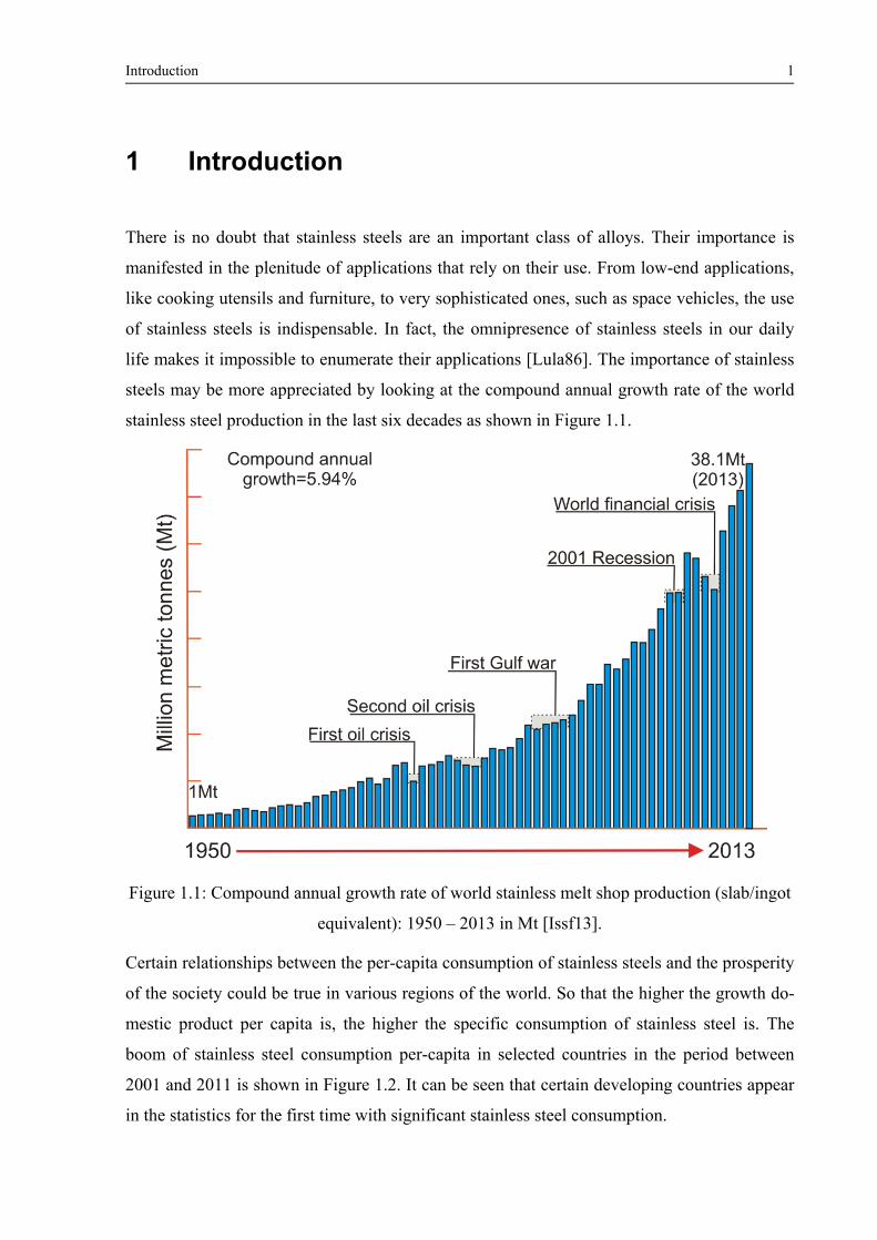
steels may be more appreciated by looking at the compound annual growth rate of the world
stainless steel production in the last six decades as shown in Figure 1.1.
Figure 1.1: Compound annual growth rate of world stainless melt shop production (slab/ingot
equivalent): 1950 – 2013 in Mt [Issf13].
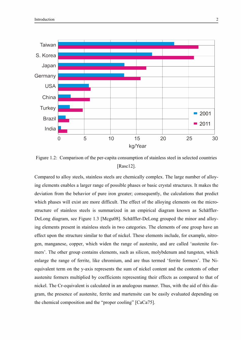
Certain relationships between the per-capita consumption of stainless steels and the prosperity
of the society could be true in various regions of the world. So that the higher the growth do-
mestic product per capita is, the higher the specific consumption of stainless steel is. The
boom of stainless steel consumption per-capita in selected countries in the period between
2001 and 2011 is shown in Figure 1.2. It can be seen that certain developing countries appear
in the statistics for the first time with significant stainless steel consumption.
Introduction 2
Figure 1.2: Comparison of the per-capita consumption of stainless steel in selected countries
[Rasc12].
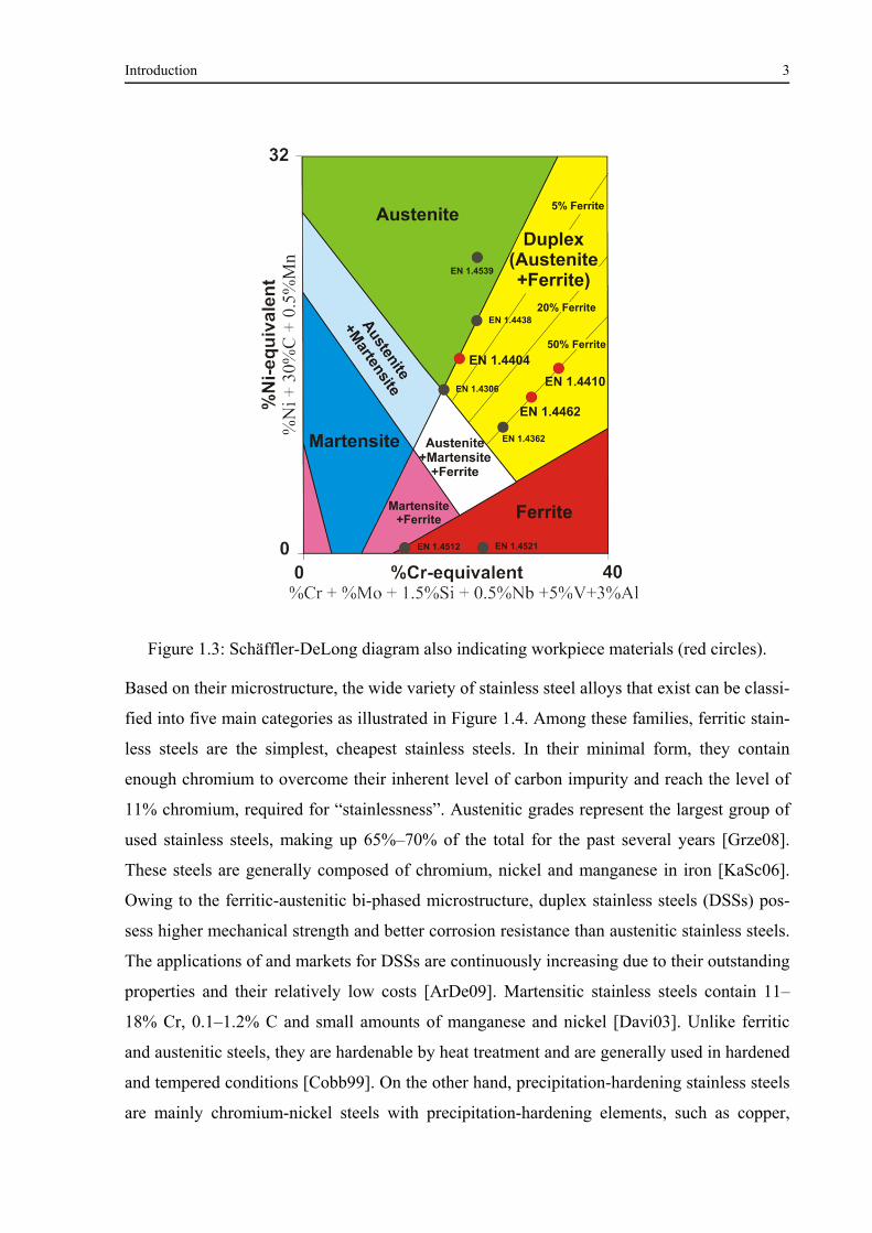
Compared to alloy steels, stainless steels are chemically complex. The large number of alloy-
ing elements enables a larger range of possible phases or basic crystal structures. It makes the
deviation from the behavior of pure iron greater; consequently, the calculations that predict
which phases will exist are more difficult. The effect of the alloying elements on the micro-
structure of stainless steels is summarized in an empirical diagram known as Schäffler-
DeLong diagram, see Figure 1.3 [Mcgu08]. Schäffler-DeLong grouped the minor and alloy-
ing elements present in stainless steels in two categories. The elements of one group have an
effect upon the structure similar to that of nickel. These elements include, for example, nitro-
gen, manganese, copper, which widen the range of austenite, and are called ‘austenite for-
mers’. The other group contains elements, such as silicon, molybdenum and tungsten, which
enlarge the range of ferrite, like chromium, and are thus termed ‘ferrite formers’. The Ni-
equivalent term on the y-axis represents the sum of nickel content and the contents of other
austenite formers multiplied by coefficients representing their effects as compared to that of
nickel. The Cr-equivalent is calculated in an analogous manner. Thus, with the aid of this dia-
gram, the presence of austenite, ferrite and martensite can be easily evaluated depending on
the chemical composition and the “proper cooling” [CaCa75].
Introduction 3
Figure 1.3: Schäffler-DeLong diagram also indicating workpiece materials (red circles).
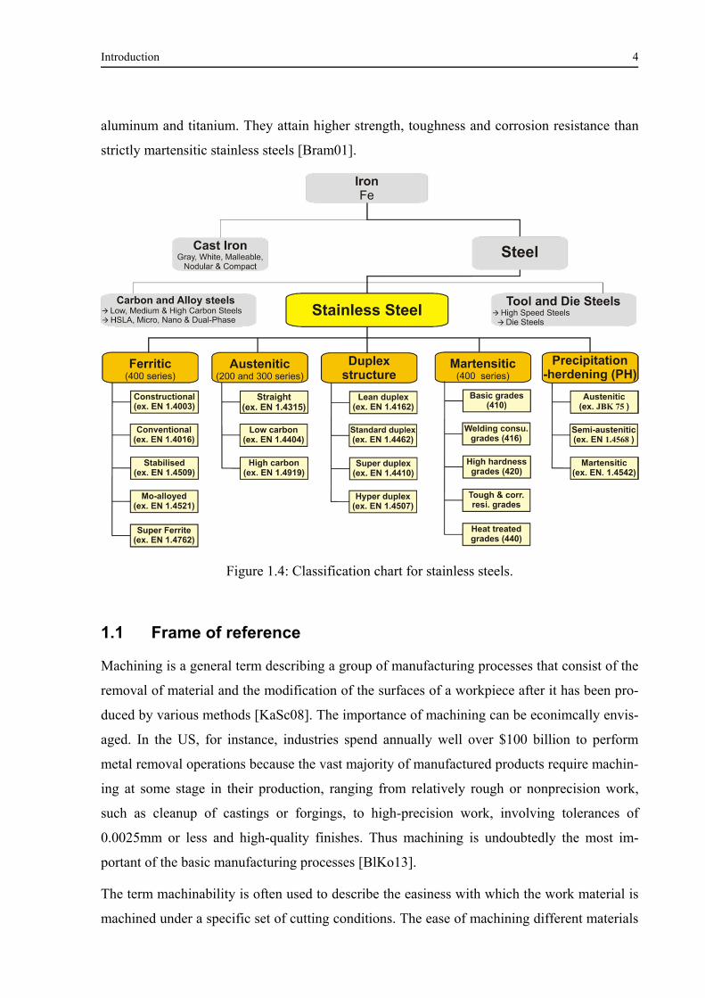
Based on their microstructure, the wide variety of stainless steel alloys that exist can be classi-
fied into five main categories as illustrated in Figure 1.4. Among these families, ferritic stain-
less steels are the simplest, cheapest stainless steels. In their minimal form, they contain
enough chromium to overcome their inherent level of carbon impurity and reach the level of
11% chromium, required for “stainlessness”. Austenitic grades represent the largest group of
used stainless steels, making up 65%–70% of the total for the past several years [Grze08].
These steels are generally composed of chromium, nickel and manganese in iron [KaSc06].
Owing to the ferritic-austenitic bi-phased microstructure, duplex stainless steels (DSSs) pos-
sess higher mechanical strength and better corrosion resistance than austenitic stainless steels.
The applications of and markets for DSSs are continuously increasing due to their outstanding
properties and their relatively low costs [ArDe09]. Martensitic stainless steels contain 11–
18% Cr, 0.1–1.2% C and small amounts of manganese and nickel [Davi03]. Unlike ferritic
and austenitic steels, they are hardenable by heat treatment and are generally used in hardened
and tempered conditions [Cobb99]. On the other hand, precipitation-hardening stainless steels
are mainly chromium-nickel steels with precipitation-hardening elements, such as copper,
Introduction 4
aluminum and titanium. They attain higher strength, toughness and corrosion resistance than
strictly martensitic stainless steels [Bram01].
Figure 1.4: Classification chart for stainless steels.
1.1 Frame of reference
Machining is a general term describing a group of manufacturing processes that consist of the
removal of material and the modification of the surfaces of a workpiece after it has been pro-
duced by various methods [KaSc08]. The importance of machining can be econimcally envis-
aged. In the US, for instance, industries spend annually well over $100 billion to perform
metal removal operations because the vast majority of manufactured products require machin-
ing at some stage in their production, ranging from relatively rough or nonprecision work,
such as cleanup of castings or forgings, to high-precision work, involving tolerances of
0.0025mm or less and high-quality finishes. Thus machining is undoubtedly the most im-
portant of the basic manufacturing processes [BlKo13].
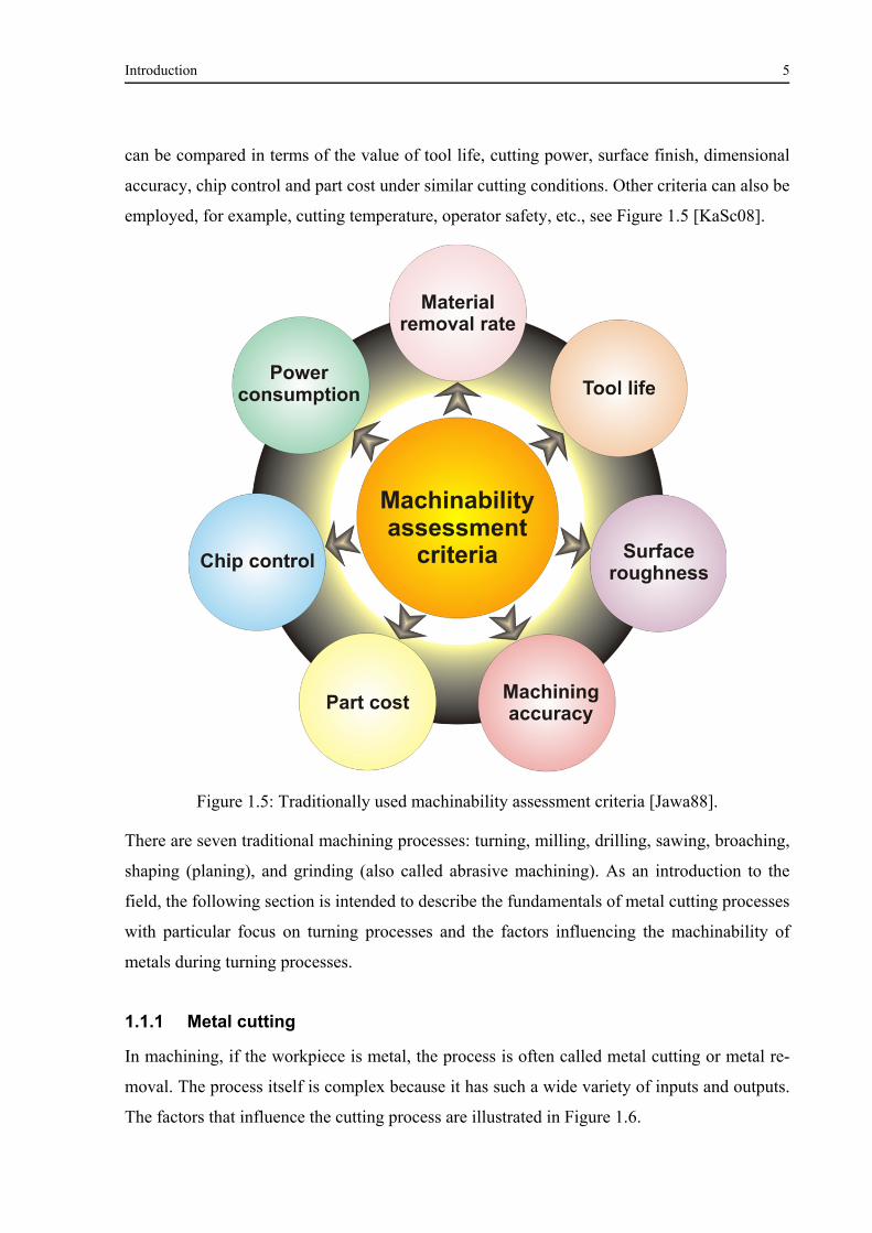
The term machinability is often used to describe the easiness with which the work material is
machined under a specific set of cutting conditions. The ease of machining different materials
Introduction 5
can be compared in terms of the value of tool life, cutting power, surface finish, dimensional
accuracy, chip control and part cost under similar cutting conditions. Other criteria can also be
employed, for example, cutting temperature, operator safety, etc., see Figure 1.5 [KaSc08].
Figure 1.5: Traditionally used machinability assessment criteria [Jawa88].
There are seven traditional machining processes: turning, milling, drilling, sawing, broaching,
shaping (planing), and grinding (also called abrasive machining). As an introduction to the
field, the following section is intended to describe the fundamentals of metal cutting processes
with particular focus on turning processes and the factors influencing the machinability of
metals during turning processes.
1.1.1 Metal cutting
In machining, if the workpiece is metal, the process is often called metal cutting or metal re-
moval. The process itself is complex because it has such a wide variety of inputs and outputs.
The factors that influence the cutting process are illustrated in Figure 1.6.
Introduction 6
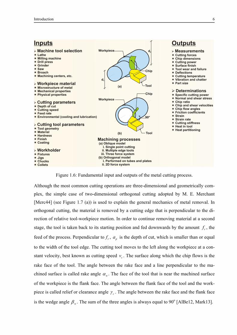
Figure 1.6: Fundamental input and outputs of the metal cutting process.
Although the most common cutting operations are three-dimensional and geometrically com-
plex, the simple case of two-dimensional orthogonal cutting adopted by M. E. Merchant
[Merc44] (see Figure 1.7 (a)) is used to explain the general mechanics of metal removal. In
orthogonal cutting, the material is removed by a cutting edge that is perpendicular to the di-
rection of relative tool-workpiece motion. In order to continue removing material at a second
stage, the tool is taken back to its starting position and fed downwards by the amount rf , the
feed of the process. Perpendicular to rf , pa is the depth of cut, which is smaller than or equal
to the width of the tool edge. The cutting tool moves to the left along the workpiece at a con-
stant velocity, best known as cutting speed cv . The surface along which the chip flows is the
rake face of the tool. The angle between the rake face and a line perpendicular to the ma-
chined surface is called rake angle n . The face of the tool that is near the machined surface
of the workpiece is the flank face. The angle between the flank face of the tool and the work-
piece is called relief or clearance angle c . The angle between the rake face and the flank face
is the wedge angle w . The sum of the three angles is always equal to 90o [AlBe12, Mark13].
Introduction 7
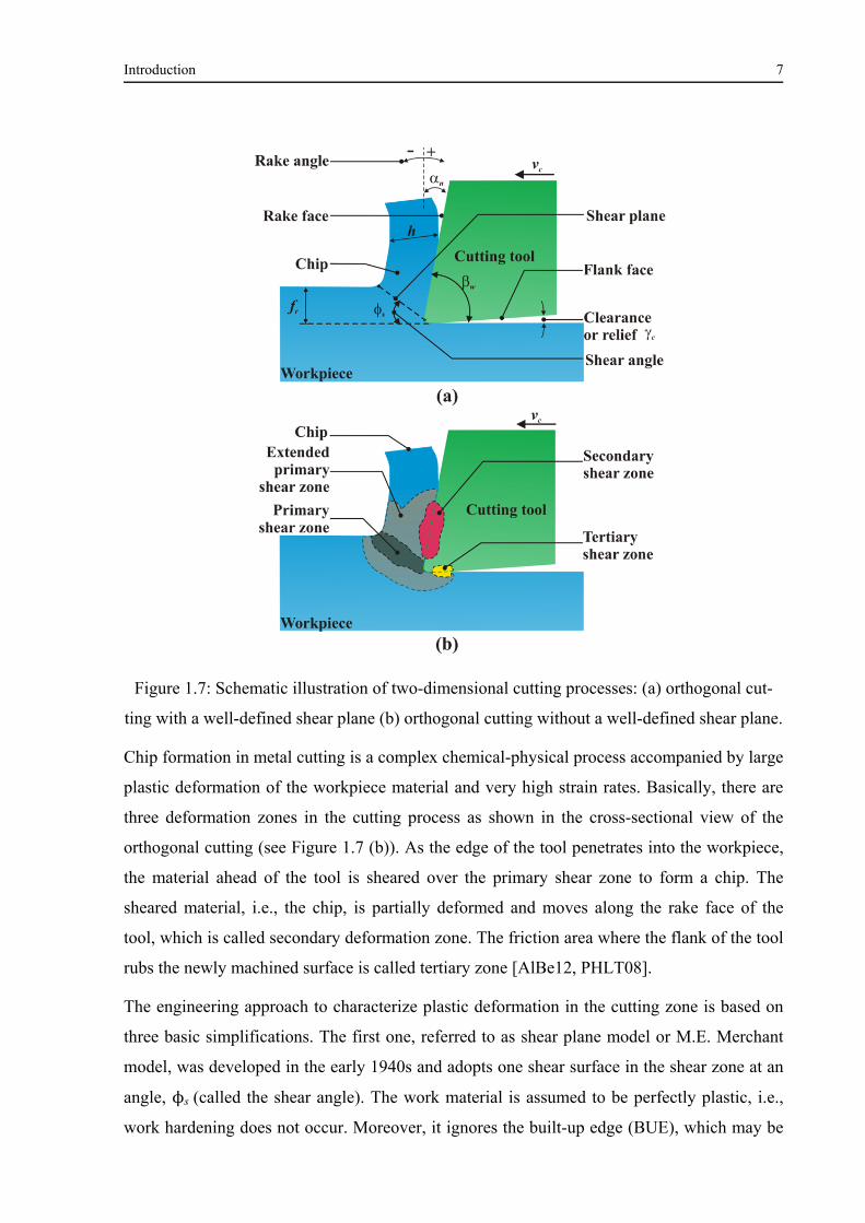
Figure 1.7: Schematic illustration of two-dimensional cutting processes: (a) orthogonal cut-
ting with a well-defined shear plane (b) orthogonal cutting without a well-defined shear plane.
Chip formation in metal cutting is a complex chemical-physical process accompanied by large
plastic deformation of the workpiece material and very high strain rates. Basically, there are
three deformation zones in the cutting process as shown in the cross-sectional view of the
orthogonal cutting (see Figure 1.7 (b)). As the edge of the tool penetrates into the workpiece,
the material ahead of the tool is sheared over the primary shear zone to form a chip. The
sheared material, i.e., the chip, is partially deformed and moves along the rake face of the
tool, which is called secondary deformation zone. The friction area where the flank of the tool
rubs the newly machined surface is called tertiary zone [AlBe12, PHLT08].
The engineering approach to characterize plastic deformation in the cutting zone is based on
three basic simplifications. The first one, referred to as shear plane model or M.E. Merchant
model, was developed in the early 1940s and adopts one shear surface in the shear zone at an
angle, ϕs (called the shear angle). The work material is assumed to be perfectly plastic, i.e.,
work hardening does not occur. Moreover, it ignores the built-up edge (BUE), which may be
Introduction 8
present, as well as chip curl and depicts tool face friction as being elastic rather than plastic.
In 1966, Zorev [Zore63] proposed a ‘fan’-type or pie-shaped shear zone model through re-
placing curvilinear boundaries by straight lines. Later, Oxley [Oxle89] developed a model
with parallel-sided shear bands inclined at a certain angle to the tool motion boundaries
[Grze09].
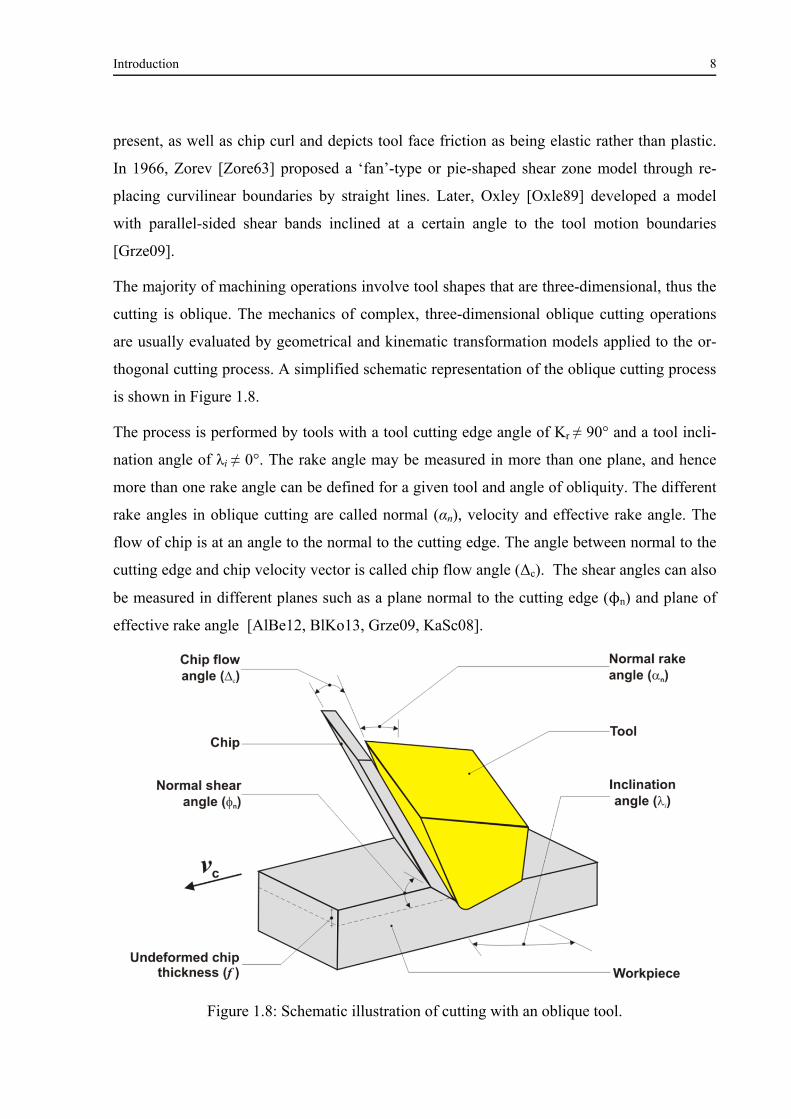
The majority of machining operations involve tool shapes that are three-dimensional, thus the
cutting is oblique. The mechanics of complex, three-dimensional oblique cutting operations
are usually evaluated by geometrical and kinematic transformation models applied to the or-
thogonal cutting process. A simplified schematic representation of the oblique cutting process
is shown in Figure 1.8.
The process is performed by tools with a tool cutting edge angle of Kr ≠ 90° and a tool incli-
nation angle of λi ≠ 0°. The rake angle may be measured in more than one plane, and hence
more than one rake angle can be defined for a given tool and angle of obliquity. The different
rake angles in oblique cutting are called normal (αn), velocity and effective rake angle. The
flow of chip is at an angle to the normal to the cutting edge. The angle between normal to the
cutting edge and chip velocity vector is called chip flow angle (Δc). The shear angles can also
be measured in different planes such as a plane normal to the cutting edge (ϕn) and plane of
effective rake angle [AlBe12, BlKo13, Grze09, KaSc08].
Figure 1.8: Schematic illustration of cutting with an oblique tool.
Introduction 9
1.1.1.1 Surface roughness
Roughness refers to the small, finely spaced deviations from the nominal surface that are de-
termined by the material characteristics and the process that formed the surface [Groo10]. It is
one of the most important measurable quality characteristics and one of the most frequent
customer requirements. Surface roughness greatly affects the functional performance of me-
chanical parts, such as wear resistance, fatigue strength, ability of distributing and holding
lubricant, heat generation and transmission, corrosion resistance, etc.
JIS 1994 has defined six parameters in roughness profiles. The reader should refer to the
standard for complete definitions of each parameter [SeCh06]. However, since the ranges of
definition seem to be dictated by the physical possibilities of existing measuring instruments,
it can be assumed that the definitions can also be extended to values below those, but this
must be investigated.
Ra is the most widely used quantification parameter in surface texture measurement. In
the past, it was also known as center line average (CLA) or in the USA as arithmetic aver-
age (AA). Ra is the arithmetic average value of the profile departure from the mean line
within a sampling length, which can be defined as:
n
ii
L
s
zn
dxxzL
Ras
10
1)(
1
(1.1)
where sL is the sample length, and z is the height from the mean line defined in Figure 1.9.
Rz is the sum of the average absolute value of the height of the five highest peaks as
measured from the average line and the average absolute value of the height of the five
lowest valleys within a portion stretching over a sample length (Ls) in the direction in
which the average line extends.
5
1
5
1 5
1
5
1
iv
ip ii
zzRz (1.2)
where ipz and
ivz are the highest peaks and deepest valleys respectively.
Rt is the sum of the height 5pz of the highest point from the mean line and the height 5vz
of the lowest point from the mean line [Groo10, Grou11, WaCh13].
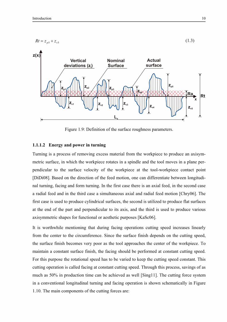
Introduction 10
55 vp zzRt (1.3)
Figure 1.9: Definition of the surface roughness parameters.
1.1.1.2 Energy and power in turning
Turning is a process of removing excess material from the workpiece to produce an axisym-
metric surface, in which the workpiece rotates in a spindle and the tool moves in a plane per-
pendicular to the surface velocity of the workpiece at the tool-workpiece contact point
[DiDi08]. Based on the direction of the feed motion, one can differentiate between longitudi-
nal turning, facing and form turning. In the first case there is an axial feed, in the second case
a radial feed and in the third case a simultaneous axial and radial feed motion [Chry06]. The
first case is used to produce cylindrical surfaces, the second is utilized to produce flat surfaces
at the end of the part and perpendicular to its axis, and the third is used to produce various
axisymmetric shapes for functional or aesthetic purposes [KaSc06].
It is worthwhile mentioning that during facing operations cutting speed increases linearly
from the center to the circumference. Since the surface finish depends on the cutting speed,
the surface finish becomes very poor as the tool approaches the center of the workpiece. To
maintain a constant surface finish, the facing should be performed at constant cutting speed.
For this purpose the rotational speed has to be varied to keep the cutting speed constant. This
cutting operation is called facing at constant cutting speed. Through this process, savings of as
much as 50% in production time can be achieved as well [Sing11]. The cutting force system
in a conventional longitudinal turning and facing operation is shown schematically in Figure
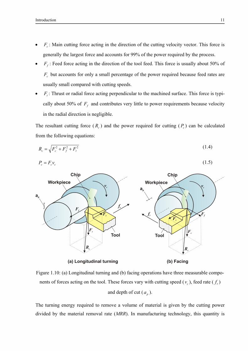
1.10. The main components of the cutting forces are:
Introduction 11
cF : Main cutting force acting in the direction of the cutting velocity vector. This force is
generally the largest force and accounts for 99% of the power required by the process.
fF : Feed force acting in the direction of the tool feed. This force is usually about 50% of
cF but accounts for only a small percentage of the power required because feed rates are
usually small compared with cutting speeds.
tF : Thrust or radial force acting perpendicular to the machined surface. This force is typi-
cally about 50% of fF and contributes very little to power requirements because velocity
in the radial direction is negligible.
The resultant cutting force ( cR ) and the power required for cutting ( cP ) can be calculated
from the following equations:
222tfcc FFFR (1.4)
ccc vFP (1.5)
Figure 1.10: (a) Longitudinal turning and (b) facing operations have three measurable compo-
nents of forces acting on the tool. These forces vary with cutting speed ( cv ), feed rate ( rf )
and depth of cut ( pa ).
The turning energy required to remove a volume of material is given by the cutting power
divided by the material removal rate (MRR). In manufacturing technology, this quantity is
Introduction 12
generally known as the specific (volumetric) cutting energy (ec) and both quantities are equiv-
alent to the specific cutting pressure ( ck ).
cc
c
cpr
cccc k
F
vaf
vF
MRR
Pe
(1.6)
where c is cross-sectional area of the uncut chip. Similarly, the values of the specific cutting
pressures related to the feed forces fk and thrust forces tk can be evaluated using the expres-
sions:
c
ff
Fk
(1.7)
c
tt
Fk
(1.8)
The value of the cutting force can also be predicted using the modified Kienzle equation:
br
a
c fv
kF
1
1.1 100
(1.9)
where F represents the described cutting and resultant forces, 1.1k is the specific cutting pres-
sure for a 1mm2 cross-sectional area of the cut, and the exponents a and b are model con-
stants [BlKo13, Grze09, Kloc11].
1.1.1.3 Tool wear
During metal cutting, cutting tools are subjected to:
high localized stresses at the tip of the tool,
high temperatures, especially along the rake face,
sliding of the chip along the rake face, and
sliding of the tool along the newly cut workpiece surface.
These conditions induce tool wear, which is of major consideration in all machining opera-
tions, as are mold and die wear in casting and metalworking. Tool wear adversely affects tool
life, the quality of the machined surface and its dimensional accuracy, and consequently the
economics of cutting operations.

Introduction 13
Wear is a gradual process, much like the wear of the tip of an ordinary pencil. The rate of tool
wear depends on tool and workpiece materials, tool geometry, process parameters, and the
characteristics of the machine tool. Tool wear and the changes in tool geometry during cutting
manifest themselves in different ways, generally classified as flank wear, crater wear, nose
wear, notching, plastic deformation of the tool tip, chipping, and gross fracture [KaSc06].
Figure 1.11 shows wear forms that occur primarily on turning tools [Kloc11].
Figure 1.11: Characteristic wear forms at the cutting part during the turning process.
Figure 1.12 is a schematic representation of the dimensions of wear. In particular, we distin-
guish the width of flank wear land VB, the displacement of cutting edge toward flank face
SVα and rake face SVγ , the crater depth KT and the crater center distance KM, from which
the crater ratio K = KT/KM is formed.
The mechanisms that cause wear at the tool–chip and tool–work interfaces in machining can
be summarized as follows:
Abrasion. This is a mechanical wearing action caused by hard particles in the work ma-
terial gouging and removing small portions of the tool. This abrasive action occurs in both
flank wear and crater wear; it is a significant cause of flank wear.

Introduction 14
Adhesion. When two metals are forced into contact under high pressure and temperature,
adhesion or welding occur between them. These conditions are present between the chip
and the rake face of the tool. As the chip flows across the tool, small particles of the tool
are broken away from the surface, resulting in attrition of the surface.
Figure 1.12: Wear forms and measured quantities at the cutting part, according to the DIN
ISO 3685 [Kloc11].
Diffusion. This is a process in which an exchange of atoms takes place across a close con-
tact boundary between two materials. In the case of tool wear, diffusion occurs at the tool–
chip boundary, causing the tool surface to become depleted of the atoms responsible for
its hardness. As this process continues, the tool surface becomes more susceptible to abra-
sion and adhesion. Diffusion is believed to be a principal mechanism of crater wear.
Chemical reactions. The high temperatures and clean surfaces at the tool–chip interface in
machining at high speeds can result in chemical reactions, in particular, oxidation, on the
rake face of the tool. The oxidized layer, being softer than the parent tool material, is
sheared away, exposing new material to sustain the reaction process.
Plastic deformation. Another mechanism that contributes to tool wear is plastic defor-
mation of the cutting edge. The cutting forces acting on the cutting edge at high tempera-
Introduction 15
ture cause the edge to deform plastically, making it more vulnerable to abrasion of the tool
surface. Plastic deformation contributes mainly to flank wear.
Most of these tool-wear mechanisms are accelerated at higher cutting speeds and tempera-
tures. From those, diffusion and chemical reaction are especially sensitive to elevated tem-
peratures [Groo10].
1.1.1.4 Chip morphologies in turning
A chip is enormously variable in shape and size in industrial machining operations. The for-
mation of all types of chips involves a shearing of the work material in the region of a plane
extending from the tool edge to the position where the upper surface of the chip leaves the
work surface. Gray cast iron chips, for example, are always fragmented, and the chips of more
ductile materials may be produced as segments, particularly at very low cutting speeds. This
discontinuous chip is one of the principal classes of chip forms and has the practical ad-
vantage that it is easily cleared from the cutting area. Under the majority of cutting conditions,
however, ductile metals and alloys do not fracture on the shear plane, and a continuous chip is
produced. Continuous chips may adopt many shapes - straight, tangled or with different types
of helix. Often they have considerable strength, and the control of the chip shape is one of the
problems confronting machinists and tool designers. Continuous and discontinuous chips are
not two sharply defined categories; every shade of gradation between the two types can be
observed. Another category of chips is observed when layers of workpiece material are grad-
ually deposited on the tool tip, forming the built-up edge (BUE). As it grows larger, the BUE
becomes unstable and eventually breaks apart. Part of the BUE material is carried away by the
tool side of the chips; the rest is randomly deposited on the workpiece surface. The cycle of
BUE formation and destruction is repeated continuously during the cutting operation until
corrective measures are taken [KaSc06, TrWr00].
The formation of chips can be explained in terms of material behavior during the deformation
process using appropriate stress-strain curves and relevant fracture mechanisms. As depicted
in Figure 1.13 (a), continuous chips are related to curve #1 with large plastic flow of the ma-
terial and the characteristic neck of a tensile specimen developed in region II. This phenome-
non is termed by Shaw [Shaw89] as negative strain-hardening in the engineering stress-strain
curve. If the plastic flow is not so intensive and the shear strain slightly exceeds the critical
value of shear strain, the onset of chip segmentation is observed (partially segmented chips vs.
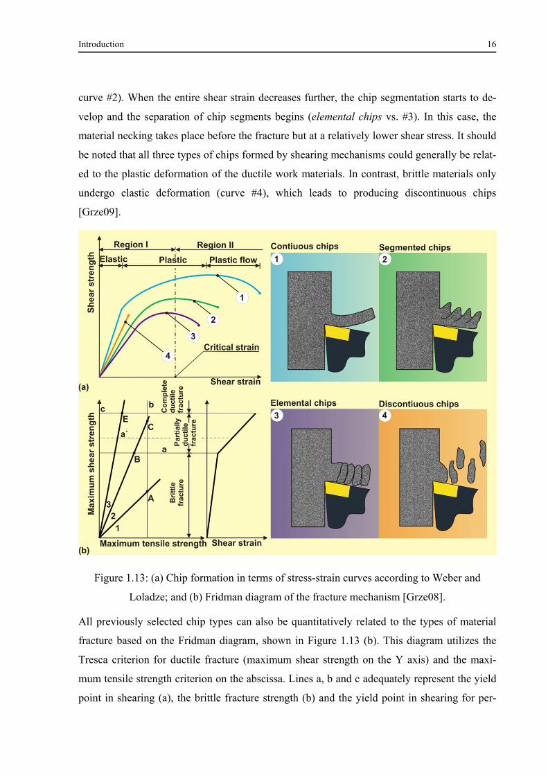
Introduction 16
curve #2). When the entire shear strain decreases further, the chip segmentation starts to de-
velop and the separation of chip segments begins (elemental chips vs. #3). In this case, the
material necking takes place before the fracture but at a relatively lower shear stress. It should
be noted that all three types of chips formed by shearing mechanisms could generally be relat-
ed to the plastic deformation of the ductile work materials. In contrast, brittle materials only
undergo elastic deformation (curve #4), which leads to producing discontinuous chips
[Grze09].
Figure 1.13: (a) Chip formation in terms of stress-strain curves according to Weber and
Loladze; and (b) Fridman diagram of the fracture mechanism [Grze08].
All previously selected chip types can also be quantitatively related to the types of material
fracture based on the Fridman diagram, shown in Figure 1.13 (b). This diagram utilizes the
Tresca criterion for ductile fracture (maximum shear strength on the Y axis) and the maxi-
mum tensile strength criterion on the abscissa. Lines a, b and c adequately represent the yield
point in shearing (a), the brittle fracture strength (b) and the yield point in shearing for per-
Introduction 17
fectly ductile material (c). Additionally, line a’ represents some specific case when the shear
stress is artificially lowered due to intensive cooling by supplying gaseous or liquid coolants.
Inclined lines starting from the origin of such a coordinate system represent simple tension
(1), simple compression (2) and simple torsion (3). Consequently, three types of material frac-
ture can be distinguished, namely: brittle fracture in point A, partially ductile fracture in point
C because of the linear work-hardening effect and perfect ductile fracture in point E. It can be
assumed that these mechanical material states are equivalent to those responsible for the for-
mation of discontinuous, segmented and continuous types [Grze08].
1.1.1.5 Chip volume ratio (R)
With regard to the metal removal rate, one has to distinguish between the volume of the re-
moved material MRR and the space needed for the randomly arranged metal chips. The vol-
ume of the removed material identifies the volume occupied by a chip with cross sectional
area cΑ . The volume of the randomly arranged metal chips removed is greater than the real
volume of the same amount of removed material, since in a reservoir the chips are not located
next to each other without gaps. The chip volume ratio R defines by what factor the volume of
randomly arranged chips is greater than the volume of the removed material.
removalmetalofamountsametheofvolumeMaterial
chipsmetalarrangedrandomlyforneededVolumeR
(1.10)
Figure 1.14 summarizes the most significant chip shapes. Each chip form is assigned to a chip
volume ratio R, which defines by what factor the transport volume needed for the specific
chip form exceeds the intrinsic material volume of the chip.
The appraisal of the chip form involves two criteria (safety of the operator and transportabil-
ity). According to this approach, ribbon, snarled and helical chips are not preferred. The de-
sirable chip forms are helical chip segments, spiral chips, pieces of spiral chips and discon-
tinuous chips [TsRe09].
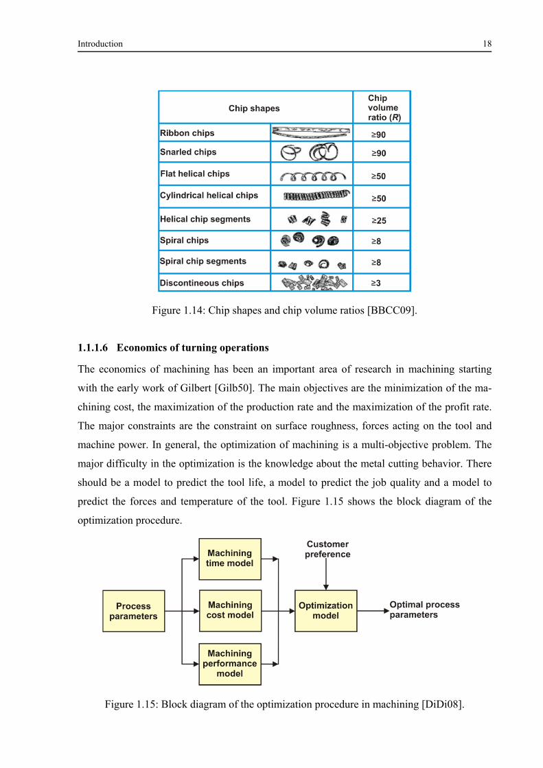
Introduction 18
Figure 1.14: Chip shapes and chip volume ratios [BBCC09].
1.1.1.6 Economics of turning operations
The economics of machining has been an important area of research in machining starting
with the early work of Gilbert [Gilb50]. The main objectives are the minimization of the ma-
chining cost, the maximization of the production rate and the maximization of the profit rate.
The major constraints are the constraint on surface roughness, forces acting on the tool and
machine power. In general, the optimization of machining is a multi-objective problem. The
major difficulty in the optimization is the knowledge about the metal cutting behavior. There
should be a model to predict the tool life, a model to predict the job quality and a model to
predict the forces and temperature of the tool. Figure 1.15 shows the block diagram of the
optimization procedure.
Figure 1.15: Block diagram of the optimization procedure in machining [DiDi08].

Introduction 19
Machining time model
In cutting operations, the machine utilization time bBt is defined as the sum of all nominal
times that a machine requires to accomplish a specified job. It is composed of the time re-
quired to produce m units and the total set-up time rBt :
rBebB ttmt . (1.11)
Production time or time per unit et can be expressed in terms of the basic time gt and the idle
time it as follow:
ige ttt (1.12)
The basic time gt is the sum of the main process time ht and the auxiliary process time nt .
nhg ttt (1.13)
The main cutting time for turning can be calculated using the following expression:
fch Ctt (1.14)
Here, the cutting time ct is the time in which the tool is actually cutting. For longitudinal turn-
ing operations, the cutting time is defined as:
pr
tc n
Nf
Lt
1000
(1.15)
where tL is the total length of tool travel including approach and overrun lengths in mm, pn is
the number of cutting passes, and N is the rotational speed in revolutions per minutes (rpm).
Meanwhile, the cutting time for facing a solid cylinder at a constant rotational speed is calcu-
lated using the following expression:
pr
rc n
Nf
dlt
1000
)2/(
(1.16)
where rl is the approach length and d is the outside diameter in mm. In facing a solid cylinder
at a constant cutting speed, the cutting time (in minutes) is given by the expression:
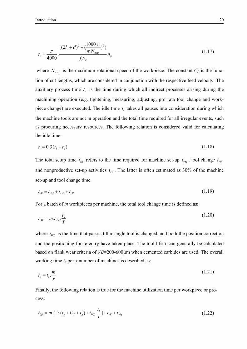
Introduction 20
pcr
cr
c nvf
Nv
dl
t
))1000
()2((
.4000
2
max
2
(1.17)
where maxN is the maximum rotational speed of the workpiece. The constant Cf is the func-
tion of cut lengths, which are considered in conjunction with the respective feed velocity. The
auxiliary process time nt is the time during which all indirect processes arising during the
machining operation (e.g. tightening, measuring, adjusting, pro rata tool change and work-
piece change) are executed. The idle time it takes all pauses into consideration during which
the machine tools are not in operation and the total time required for all irregular events, such
as procuring necessary resources. The following relation is considered valid for calculating
the idle time:
)(3.0 nhi ttt (1.18)
The total setup time rBt refers to the time required for machine set-up vMt , tool change rWt
and nonproductive set-up activities rVt . The latter is often estimated as 30% of the machine
set-up and tool change time.
rVrWvMrB tttt (1.19)
For a batch of m workpieces per machine, the total tool change time is defined as:
T
ttmt hWZrW ..
(1.20)
where WZt is the time that passes till a single tool is changed, and both the position correction
and the positioning for re-entry have taken place. The tool life T can generally be calculated
based on flank wear criteria of VB=200-600µm when cemented carbides are used. The overall
working time ta per x number of machines is described as:
x
mtt ea .
(1.21)
Finally, the following relation is true for the machine utilization time per workpiece or pro-
cess:
vMrVh
WZnfcbB ttT
tttCtmt ].)(3.1[ (1.22)
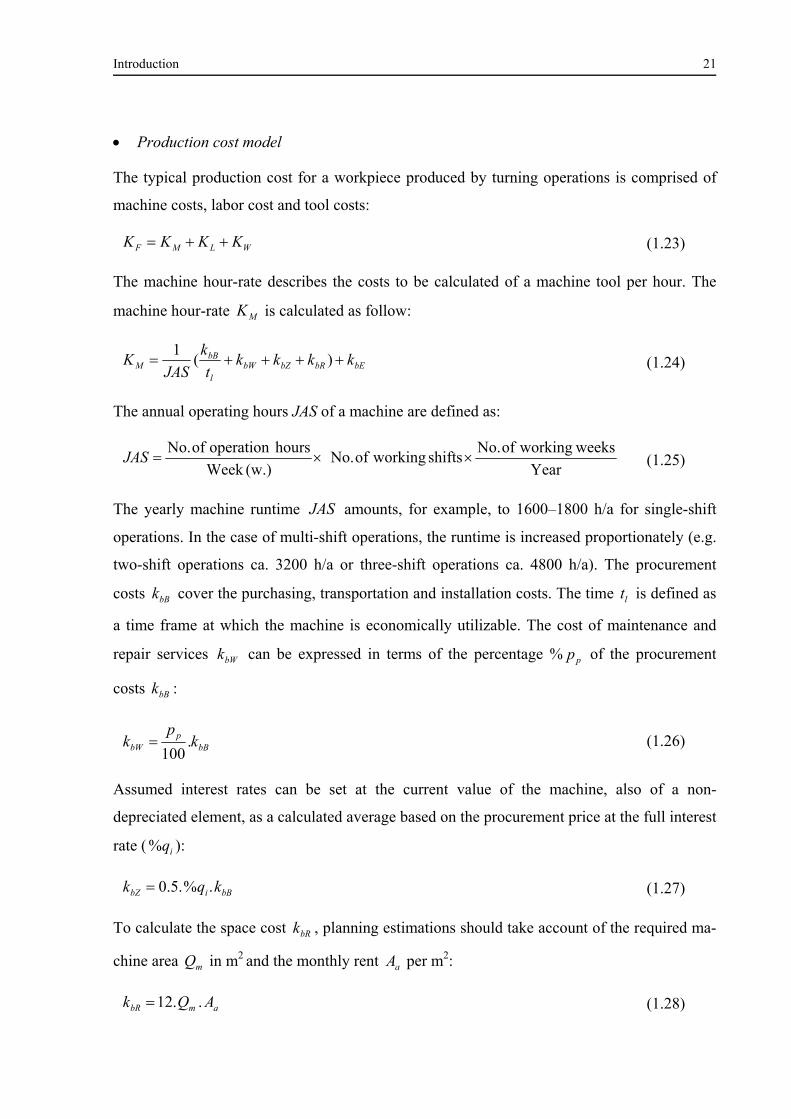
Introduction 21
Production cost model
The typical production cost for a workpiece produced by turning operations is comprised of
machine costs, labor cost and tool costs:
WLMF KKKK (1.23)
The machine hour-rate describes the costs to be calculated of a machine tool per hour. The
machine hour-rate MK is calculated as follow:
bEbRbZbWl
bBM kkkk
t
k
JASK )(
1 (1.24)
The annual operating hours JAS of a machine are defined as:
Year
weeksworkingofNo.shiftsworkingofNo.
(w.)Week
hoursoperationofNo.JAS (1.25)
The yearly machine runtime JAS amounts, for example, to 1600–1800 h/a for single-shift
operations. In the case of multi-shift operations, the runtime is increased proportionately (e.g.
two-shift operations ca. 3200 h/a or three-shift operations ca. 4800 h/a). The procurement
costs bBk cover the purchasing, transportation and installation costs. The time lt is defined as
a time frame at which the machine is economically utilizable. The cost of maintenance and
repair services bWk can be expressed in terms of the percentage % pp of the procurement
costs bBk :
bBp
bW kp
k .100
(1.26)
Assumed interest rates can be set at the current value of the machine, also of a non-
depreciated element, as a calculated average based on the procurement price at the full interest
rate ( iq% ):
bBibZ kqk .%.5.0 (1.27)
To calculate the space cost bRk , planning estimations should take account of the required ma-
chine area mQ in m2 and the monthly rent aA per m2:
ambR AQk ..12 (1.28)

Introduction 22
The operating cost bEk includes the costs of operation energy, lighting and coolant kk . The
electricity costs can be estimated based on the effective cutting power MP , the standard cost
of electricity cE in euro/kWh and the percentage 2%C of being in ON state:
kcMbE kCEPk 2.%. (1.29)
Labor cost LK is calculated as follows:
)1( rLK mL (1.30)
where mL is the gross hourly wage, and r as the amount of the nonwage cost of the operator.
This applies if a new factor that summarizes the machine cost and the wage rate per hour in
terms of previously defined time scales is formulated as:
LbB
arBMML K
t
ttKK .
(1.31)
The costs of typical indexable carbide cutting tools are comprised of the cost of tool holders
WHk , inserts WPk and spare parts ETk :
ETWPWHW kkkK (1.32)
The total insert costs are defined as:
s
WSPhWP ZT
Ktmk
..8.0
.. (1.33)
where WSPK is the cost of an insert, sZ is the number of usable cutting edges per insert, and
0.8 is a safety factor accounts for uncertainty in tool life. The spare parts costs are often ex-
pressed in terms of the percentage of tool holder and insert costs. The final production cost
per unit is obtained by adding the terms in Eqs. 20-35:
]..8.0
..).(.[
1ET
s
WSPhWHLarBMbBF k
ZT
KtmkKttKt
mK (1.34)
Using the previous relationships, one can define the main time-related costs as:
hLM tKx
KK ).1
(1 (1.35)
the fixed or the workpiece-related costs as:
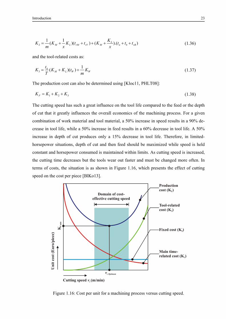
Introduction 23
)).(())(1
(1
2 vBbnL
MrVrMLM tttx
KKttK
xK
mK (1.36)
and the tool-related costs as:
WWLMh K
mtKK
T
tK
1))((3 (1.37)
The production cost can also be determined using [Kloc11, PHLT08]:
321 KKKKF (1.38)
The cutting speed has such a great influence on the tool life compared to the feed or the depth
of cut that it greatly influences the overall economics of the machining process. For a given
combination of work material and tool material, a 50% increase in speed results in a 90% de-
crease in tool life, while a 50% increase in feed results in a 60% decrease in tool life. A 50%
increase in depth of cut produces only a 15% decrease in tool life. Therefore, in limited-
horsepower situations, depth of cut and then feed should be maximized while speed is held
constant and horsepower consumed is maintained within limits. As cutting speed is increased,
the cutting time decreases but the tools wear out faster and must be changed more often. In
terms of costs, the situation is as shown in Figure 1.16, which presents the effect of cutting
speed on the cost per piece [BlKo13].
Figure 1.16: Cost per unit for a machining process versus cutting speed.
Introduction 24
1.2 Background and aim
It is estimated that 15% of the value of all mechanical components manufactured worldwide
is derived from machining operations. Despite this obvious economic and technical im-
portance, it remains one of the least understood manufacturing operations due to the low pre-
dictive ability of the machining models [UsSh82a, Usui88].
In most of the textbooks on machining, a single shear plane model is described. This is based
on the assumption that material removal takes place through shear over a very narrow zone.
As argued by Astakhov [Asta05], this model suffers from a number of drawbacks, viz., infi-
nite strain rate, unrealistically high shear strain, unrealistic behavior of the work material,
improper accounting for the resistance of the work material to cut, unrealistic representation
of the tool–workpiece contact, inapplicability for cutting brittle work materials, incorrect ve-
locity diagram, incorrect force diagram and inability to explain chip curling. Actually the ma-
chining process is so complex that no existing physics-based model seems to describe the
process properly. Other analytical modeling approaches such as the extended three dimen-
sional shear plane model or oblique cutting slip-line field models are either poorly correlated
with experimental results or quite complex, and for their application stress and strain data at
the strain rates encountered in metal machining is needed. This is why other modeling ap-
proaches such as empirical, mechanistic, numerical and artificial intelligence are developed as
alternatives to the metal cutting theory, because the latter did not prove its ability to solve
even simple practical problems [Asta06].
Traditionally, mathematical programming techniques such as linear programming, method of
feasible direction, dynamic programming and geometric programming had been used to solve
optimization problems in machining. However, these traditional methods of optimization do
not fare well over a broad spectrum of problem domains. Moreover, traditional techniques
may not be robust. Numerous performances, constraints and multi-passes make machining
optimization problems complicated, and hence these techniques are not ideal for solving such
problems as they tend to obtain a local optimal solution [VePa10].
On the other hand, a search with the keywords ‘duplex stainless steel’ in popular databases,
such us Science Citation Index-Expand or Scorpus, would reveal tens of recent publications.
This is a vivid testimony of the potential interest in DSSs as a key research topic by various
researchers in the world. However, one can hardly find a scientific article which addresses the
Introduction 25
computational and numerical modeling as well as the optimization of machining regarding
such an important family of stainless steels.
Considering the respective drawbacks of metal cutting theory and traditional optimization
techniques in the modeling and optimizing of machining processes as well as the scarcity of
the work material’s comprehensive machining investigations, the objective of the present dis-
sertation is to address the machinability of DSSs through the systematic application of ad-
vanced modeling and optimization techniques in turning processes. The approaches proposed
here could then be used to optimize the residual machining criteria, for example, towards a
lower manufacturing cost or a more sustainable machining process or a more precise numeri-
cal simulation.
1.3 Research approach
Research in common parlance refers to a search for knowledge. One can also define research
as a scientific and systematic search for pertinent information on a specific topic. In fact, re-
search is an art of scientific investigation. The Advanced Learner’s Dictionary of Current
English lays down the meaning of research as “a careful investigation or inquiry especially
through search for new facts in any branch of knowledge’’ [Hedb89]. The word itself is de-
rived from the French word “rechercher”, which means “to search closely”, and “chercher”
means “to search”. Its literal meaning is “to investigate thoroughly” [Oful13].
Research is an academic activity and the term as such should be used in a technical sense.
According to Clifford Woody, research comprises defining and redefining problems, formu-
lating hypotheses or suggesting solutions, collecting, organizing and evaluating data, making
deductions and reaching conclusions, and at last carefully testing the conclusions to determine
whether they fit the formulated hypotheses [Koth04].
There are two basic approaches to research, viz., a quantitative approach and a qualitative
approach. The former involves the generation of data in quantitative form, which can be sub-
jected to rigorous quantitative analysis in a formal and rigid fashion. A qualitative approach to
research is concerned with the subjective assessment of attitudes, opinions and behavior. Re-
search in such a situation is a function of a researcher’s insights and impressions. Such an
approach to research generates results either in a non-quantitative form or in a form which is
Introduction 26
not subjected to rigorous quantitative analysis. Generally, group interviews, projective tech-
niques and depth interviews are used as the techniques of focus [Koth04].
The quantitative approach can be further sub-classified into inferential, experimental and sim-
ulation approaches to research. The inferential approach usually means survey research, in
which a sample of the population is studied. Experimental approach is characterized by a
much greater control over the research environment, and in this case some variables are ma-
nipulated to observe their effect on other variables. The simulation approach involves the con-
struction of an artificial environment, within which relevant information and data can be gen-
erated. This permits an observation of the dynamic behavior of a system (or its sub-system)
under controlled conditions [DaSa11].
The research approach adopted in the present dissertation is predominantly quantitative. Ex-
perimental and simulation approaches are applied to obtain quantitative results, through which
the conclusions are based on the observations and experience (empiricism). However, since
not all parts of the cutting process may be analyzed through a quantitative approach, addition-
al qualitative observations have been collected, analyzed and converted into quantitative re-
sults. The estimation of chip volume ratio, based on the chip breaking chart, is an example of
data interpretations from qualitative chip morphology format to quantitative chip volume ra-
tio, based on the fuzzy set theory. On multiple occasions, a qualitative approach is also used
as a complement to the quantitative approach.
1.4 Research hypothesis
The application of statistical regression and computational optimization techniques in the
multi-objective optimization of cutting can effectively obtain sets of non-dominated solu-
tions.
Fuzzy set theory principles can be proficiently applied to eliminate the discrepancy of the
ranking system among the multiple attribute decision-making (MADM) methods, thus
promoting the decision-making process.
Coupling the Taguchi method with MADM and meta-heuristic optimization methods can
suitably provide the decision maker and/or process planner with the skills essential for the
mono- and multi-objective optimization of cutting processes.
Introduction 27
Multiple quality characteristics of the machining surface can be efficiently optimized
when MADM methods are coupled with fuzzy set theory.
The sustainability-based optimization of multi-pass cutting operations is possible if the
hybridization of input-output modeling and optimization tools and MADM methods is
systematically performed.
The inverse identification of input parameters in numerical modeling of cutting can be
effectively performed if coupled Java-based material properties (JMatPro) software, de-
sign of experiment (DOE), MADM, computational modeling and meta-heuristic algo-
rithms are applied. The approach can also perform well for hypothetical, numerical opti-
mization studies.
1.5 Research questions
In conjunction with the hypotheses, the following research questions are identified:
Can the application of statistical regression and computational optimization techniques
effectively obtain sets of non-dominated solutions in the multi-objective optimization of
machining DSSs?
Is the application of fuzzy set theory advantageous in eliminating the discrepancy of the
ranking system among the MADM methods and can it achieve better results than other
optimization approaches?
Can the Taguchi-MADM-meta-heuristics concept be conveniently used for the mono- and
multi-objective optimization of cutting stainless steels?
Can multiple quality characteristics of the machining surface be efficiently optimized
when MADM methods are coupled with fuzzy set theory?
Would it be possible for multi-pass cutting operations to be sustainably optimized when
the hybridization of input-output modeling and optimization tools and MADM methods is
systematically performed?
Is it possible to apply Java-based material properties (JMatPro) software, design of experi-
ment (DOE), MADM, computational modeling and meta-heuristic approach to the inverse
identification of the input parameters during the finite element simulation of cutting pro-
cesses? If it is possible, can a hypothetical, numerical optimization study be performed as
a case study?
Introduction 28
1.6 Research delimitations
The important boundaries that have been set for the present dissertation are:
The research is primarily focused on the machining of EN 1.4462 and EN 1.4410 DSSs.
However, in some cases EN 1.4404 austenitic stainless steel grade has been used as a
benchmark for comparison analyses of machinability.
The research has primarily been limited to constant cutting speed facing and longitudinal
turning operations. The latter was seen suitable for conducting multi-objective optimiza-
tion and for numerical modeling.
Coated and uncoated cemented carbide cutting inserts are employed in all experimental
and numerical investigations as they are generally recommended for machining stainless
steels by different manufacturers.
The literature survey in this dissertation will not review non-traditional machining pro-
cesses, unless they are the only processes through which the adaptability of modeling and
optimization approaches is first examined.
The optimization of the tool geometry and the orientation angles is restricted to the nu-
merical modeling.
1.7 Outline of the dissertation
The present work is structured into ten Chapters. Chapter 2 proposes a review of the main
techniques and tools enabling the modeling and the optimization of the cutting process. The
basic concepts and the application potential of several modeling and optimization techniques
in metal cutting processes, classified under several criteria, have been reviewed and critically
appraised. A universal framework for parameter modeling and optimization in metal cutting
processes is also proposed.
A detailed explanation of the experimental setup and the instruments is given in Chapter 3.
Elements of the cutting measurement systems are characterized using illustrative, schematic
diagrams. A brief description of the adopted experimental designs and the involved perfor-
mance characteristics is presented. The chapter also contains an introduction into the tempera-
ture-dependent physical and mechanical properties of the work materials, which were gener-
ated using JMatPro software.
Introduction 29
Chapter 4 presents the experimental investigations into longitudinal turning of duplex stain-
less steel grades with multi-layer coated inserts. The parametric influences of cutting and pro-
cess conditions on the cutting performances are analyzed, and proper interim conclusion
points are drawn. The chapter also presents the multi-objective optimization of machining
duplex stainless steels, based on the nature-inspired Multi-Objective Bat Algorithm (MOBA).
Chapter 5 addresses a new methodology based on Mamdani fuzzy interference of classified
chip shapes in chip breaking charts to predict the chip volume ratio. Several performance
characteristics are considered and converted into four indices using four MADM methods. An
expert system, based on the fuzzy rule modeling approach, is then adopted to combine the
computed four indices into a single Universal Characteristics Index (UCI). First-ranking UCI
values are analyzed and compared with the output of the Weighted Sum Method (WSM), us-
ing a constrained, Simulated Annealing algorithm.
Chapter 6 presents the multi-performance optimization of turning super duplex EN 1.4410,
standard duplex EN 1.4462 and austenitic EN 1.4404 stainless steels, utilizing coupled
Taguchi-based designs, MADM and meta-heuristic algorithms. Nature-inspired meta-heuristic
algorithms such as the Firefly Algorithm (FA), Accelerated Particle Swarm Optimization
(APSO) and Cuckoo Search (CS) are employed and their corresponding performances com-
pered.
In Chapter 7, the Taguchi approach is coupled with fuzzy-multiple attribute decision-making
methods for achieving better surface qualities in constant cutting speed face turning of austen-
itic and duplex stainless steels. Two typical multiple attribute decision-making techniques
were simultaneously adopted to determine multi-surface quality characteristics indices. The
differences in rankings among derived indices are solved through converting each crisp value
into a trapezoidal fuzzy number and unifying them by using the fuzzy simple additive weight
method.
In Chapter 8, a systematic approach, which employs different modeling and optimization
tools under a three phase investigation scheme, is adopted. In phase I, the effect of design
variables such as cutting parameters, cutting fluids and axial length of cuts are investigated
using the D-Optimal method. In the phase II, comprehensive experiment-based production
cost and production rate models are developed. In phase III, expert systems based on the
fuzzy rule modeling approach are adopted to derive measures for machining operational sus-
tainability, called Operational Sustainability Index (OSI). Finally, a new Cuckoo Search Neu-

Introduction 30
ral Network System (CSNNS) is utilized to constrainedly optimize the cutting process per
each cutting scenario.
Chapter 9 provides a novel methodology to inversely calculate the input parameters when
simulating the machining of duplex stainless steels, based on Taguchi-VIKOR coupled with a
Firefly Algorithm Neural Network System (FANNS). Thereafter, design of experiments, nu-
merical simulations and fuzzy rule modeling approaches are employed to optimize types of
cutting tool geometry, process conditions, cutting parameters and tool orientation angles
based on many important performances.
While summaries of the research results obtained in chapters 4-9 can be found separately in
the interim conclusion sections, Chapter 10 serves to provide a concise and overall summary
of the main achievements of the study. Finally, a schematic illustration of the research meth-
odology and the approximate location of the chapters included in this dissertation can be
found in Figure 1.17.
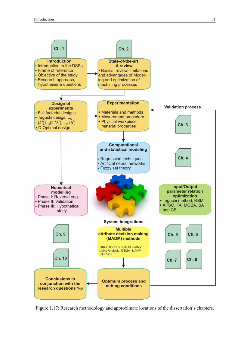
Introduction 31
Figure 1.17: Research methodology and approximate locations of the dissertation’s chapters.
State of the art in machining modeling and optimization: A review 32
2 State of the art in machining modeling and op-
timization: A review
The history of research practice in metal cutting is well documented by Finnie [Finn56], who
identified the work of Cocquilhat [Cocq51] in 1851 as the first research in the area of measur-
ing the work required to remove a given material volume by drilling. However, the first who
argued that the chip is created by shearing ahead of the tool was Time [3] in 1870, when he
presented the results obtained from observing cutting. Astakhov confirmed in his book “Metal
cutting mechanics” that this work is one of the first publications that suggestes a shear plane
theory [Asta98]. It has also been shown that there is no contradiction between Time’s work
and Tresca’s work [Tres73]. In 1873 Tresca argued that the chip in metal cutting is produced
by compression ahead of the tool. Also in 1873, Hartig published tabulations of the power and
work required in cutting metal in his book ‘Versuche über Leistung und Arbeitsverbrauch der
Werkzeugmaschine’, which seems to have been the authoritative work on the subject for sev-
eral years [Hart73]. In 1896 Zvorykin [Zvor96] was the first to provide a physical explanation
for this model; his work resulted in an equation predicting the shear angle. In 1881, Mallock
established the basis of a shear plane model. In his turning experiments, Mallock made hand
drawings of the chip formation process in the course of their formation by means of a micro-
scope, mounted on the tool holder. He also emphasized the importance of friction in the tool-
chip interface [Mall81]. Finnie also reports that a step backward in the understanding of metal
cutting process was taken in 1900, when Reuleaux [Reul00] suggested that a crack occurred
ahead of the tool and that this process could be linked to the splitting of wood. However, it
was the work of Ernst and Merchant in 1941 that made the shear plane model popular. Most
of the fundamental works on metal cutting mechanics refer to this paper, and many analytical
models of orthogonal cutting still use the relations derived from this work [KnBo05, Mark13].
Many efforts have been made to refine Merchant’s model with the aim of improving the pre-
dictive capability [LeSc51, Oxle98, Zore63]. A modern analytical approach, known as the
‘‘unified or generalized mechanics approach’’, has been pursued by Armarego and co-
workers [ArHe00, Arma00] for years and then spread as the mechanistic approach in metal
cutting [EnDK95]. However, due to the nature of the cutting process, which involves plastic
deformation, heat transfer, diffusion, chemical reactions and other complex phenomena in
machining, empirical models have been more successful than analytical ones. Hence, one has
State of the art in machining modeling and optimization: A review 33
not to be surprised when seeing that Taylor’s empirical tool life model [Tayl07], which was
developed in 1907, is still in action today and employed as the basis for many up-to-date stud-
ies of machining economics [QuDa09].
With the advent of powerful computers in the late 1970s and early 1980s, a number of im-
portant changes in machining modeling have been made. The most significant change to the
cutting modeling was the introduction of artificial intelligence techniques. Techniques such as
neural network, fuzzy logic, neuro-fuzzy system, support vector machines [BMUK12,
ÇaEk12, RaRA09, ShGi06, WKFL13] and hidden Markov models [AtOB00, ErLO01,
ScEH05, WaMK02, ZhWH09] have been widely applied in metal cutting performance predic-
tions. On the other hand, in numerical modeling, the emergence of the finite element method
(FEM) must be noted as a powerful numerical method to solve differential equations. In fact,
efforts to apply the FEM of chip formation processes date back to the early 1970s [OkKa71,
TaSD74, TSVO76]. However, due to the extensive computational demands, it was not until
the late 1990s that numerical methods became a useful and practical tool [AÖUD13,
ArÖz09].
In addition, although it is quite important for planning efficient machining processes, the op-
timization of cutting parameters is a complicated target, challenged not only by the complex
nature of the involved phenomena but also by the need for carefully defining realistic optimi-
zation objectives as well as developing and implementing powerful and versatile optimization
techniques. In this sense, stochastic optimization techniques, mainly evolutionary algorithms,
have been widely reported in recent literature [QuDa11]. The discussion here is mainly in-
tended to provide a brief theoretical background to some important machining modeling and
optimization techniques and review the recently used tools.
2.1 Input-output parameter relationship of modeling tools
The first necessary step for process parameter optimization is to understand the principles
governing the manufacturing process by means of developing an explicit mathematical model,
which may be of two types: mechanistic or empirical [BoDr87]. The model in which the func-
tional relationship between input–output and in-process parameters is analytically determined
is called mechanistic model. However, as there is lack of adequate and acceptable mechanistic
models for manufacturing processes, empirical models are generally used in manufacturing
processes. The modeling techniques of input–output and in-process parameter relationships
State of the art in machining modeling and optimization: A review 34
are mainly based on statistical regression, fuzzy set theory and artificial neural networks
[LuSp95]. In terms of the computation methods, modeling based on physics is accomplished
by the computational tools that may be called hard computing methods. On the other hand,
modeling based on data is accomplished by soft computing tools, such as neural networks and
fuzzy sets. Soft computing tools try to generate approximate solutions of the problem in the
presence of uncertain or imprecise physics and/or the process variables. It differs from con-
ventional (hard) computing in that, it is tolerant of imprecision, uncertainty, partial truth and
approximation. A hybrid of hard and soft techniques may also be used [DeDi08].
The modeling techniques of input–output and in-process parameter relationships are mainly
based on statistical regression, fuzzy set theory and artificial neural networks. Figure 2.1 pro-
vides a general classification of different modeling tools for input-output parameter relation-
ships in metal cutting processes. In the following sections, some of these tools will be briefly
explained.
2.1.1 Statistical regression
2.1.1.1 Theoretical background
The data collected through experiments usually exhibits a significant degree of errors or a
‘‘noise.’’ In such a case, there is no need to intersect every point as the individual data points
may be incorrect. Rather, the curve is designed to follow the pattern of points taken in groups.
This approach is known as statistical regression [MoPV12]. It utilizes experimental data on
the related variables to develop a numerical relationship, showing the influence of the inde-
pendent variables on a dependent variable of the system. If nothing is known from theory
about the relationship between independent and dependent variables, a function may be as-
sumed and fitted to the experimental data on the system. Usually a linear function is assumed.
In other cases where a linear function does not properly fit the experimental data, the engineer
might try a polynomial or exponential function [Lazi06]. Regression has been proved to be a
conceptually simple technique for investigating functional relationships between output and
input decision variables of a cutting process and may be useful for cutting process data de-
scription, parameter estimation and control [MuRa06].
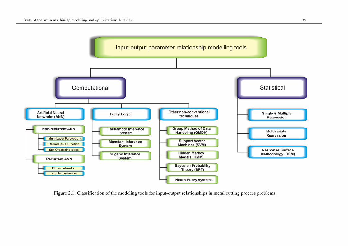
State of the art in machining modeling and optimization: A review 35
Figure 2.1: Classification of the modeling tools for input-output relationships in metal cutting process problems.
State of the art in machining modeling and optimization: A review 36
Regression models can be classified based on the number of involved independent and de-
pendent variables. The models with a single independent variable and a single dependent vari-
able are called single regression models. Moreover, models with a single dependent variable
and two or more independent variables are called multiple regression models. In multivariate
regression by contrast, there are multiple dependent variables and any number of independent
variables. Fitting functions to data in each of these categories can be linear or nonlinear,
hence, the terms of linear and nonlinear regressions. The word ‘linear’ in linear regression
refers to the function’s being a linear combination of basis functions. With the basis functions
1, x, linear combinations have the form xccy o 1 , which is coincidentally a line. On the
other hand, non-linear functions fall into one of three cases: intrinsically linear, intrinsically
nonlinear and intrinsically nonlinear but linearizable. Intrinsically linear functions can be
written in the form nno xcxcxccy ..........2211 , where the ci’s are constants and the xi’s
are the basis functions. Examples of intrinsically nonlinear functions, which can be converted
to intrinsically linear functions, are power and exponential functions. However, functions
such as logistic curves are nonlinear and cannot be transformed into a linear function
[MoSw99].
If a dependent variable y is the function of n independent variables, viz., nxxx ......,,, 21 , then
the multiple linear regression model may be written as:
excxcxccy nno ..........2211 (2.1)
where e is the error term. In the case if there are m observations, one can write the following
m equations:
112121111 .......... excxcxccy nno ,
(2.2)
222222112 .......... excxcxccy nno ,
………………………………………......
mmnnmmom excxcxccy ..........2211 ,
In the matrix form, we can write the above set of equations as:

State of the art in machining modeling and optimization: A review 37
mnmnmm
n
n
m e
e
e
c
c
c
xxx
xxx
xxx
y
y
y
.
.
.
.
..1
......
......
..1
..1
.
.2
1
1
0
21
22221
11211
2
1
(2.3)
or
EXCY (2.4)
Our attempt should be to minimize the error vector E. If all the terms in the vector E are zero,
the model is perfect. Usually we minimize E in least square sense. The sum-squared error is
given by
XCXCYXCXCYYYXCYXCYEE )()( (2.5)
By making use of the property that the transpose of a scalar is equal to the scalar itself, we can
write
YXCXCY (2.6)
Hence,
XCXCYXCYYEE 2 (2.7)
Minimizing this with respect to C, we get
022)(
XCXYXC
EE (2.8)
Thus, the error will be minimized if
YXXCX (2.9)
or
YXXXC 1
)( (2.10)
The coefficient vector can be found by solving for C either from Eq. (2.9) by using any equa-
tion solver routine or from Eq. (2.10). The matrix XXX 1)( is called the pseudo-inverse of
.X The procedure described above for multiple linear regression can also be applied for non-
State of the art in machining modeling and optimization: A review 38
linear regression when y can be expressed as a polynomial function of the dependent variables
[DiDi08].
2.1.1.2 Reviews of applications
Several applications of regression equation-based modeling in metal cutting processes are
reported in literature [ChCh13, ErOz10, GoMG09, KaSR10, MaBh04, MaPa06, MaSa08,
ÖKFD07, SiDM11, WaSK06]. For instance, Senthilkumar et al. have employed multiple re-
gression analysis to determine the constants of Taylor’s tool life equation in machining mar-
tensitic stainless steels. The tool life of alumina-based ceramic cutting tools is evaluated from
these tool wear models, and the effect of various types of wear on tool life were analyzed
[SeRS06]. Aslan et al. have investigated the machining of hardened steel using Al2O3-based
ceramic cutting tools and obtained relationships between the cutting parameters, namely cut-
ting speed, feed and depth of cut, and performance measures such as flank wear and surface
roughness using multiple linear regression [AsCB07]. Kaylan and Choudhury have developed
regression equations for cutting force and flank wear both in dry and cryogenic turning of
EN1.4373 austenitic stainless steel. It was concluded from this work that cryogenic cooling is
a possible answer for high-speed, eco-friendly machining [KaCh08]. Ahmadi and Homami
have developed multiple regression models for analyzing the effect of cutting parameters in
tool wear when machining PH-hardened duplex stainless steels. The effective parameters of
tool wear using ceramic cutting tools have been investigated, and the influence of different
types of wear phenomena has been observed [AhHo12]. Krolczyk et al. examined the influ-
ence of cutting parameters on surface roughness in duplex stainless steel turning processes.
The study included developing a second-order regression model to determine surface rough-
ness. The established equations clearly showed that the feed rate was the main influencing
factor of surface roughness. Surface roughness increased with growing feed rate [KrLG13].
2.1.1.1 Merits and drawbacks of the statistical regression method
Statistical regression may make a decent modeling technique [LiBK03]. However, this tech-
nique may not precisely describe the underlying non-linear complex relationship between the
decision variables and responses. A prior assumption regarding functional relationships (such
as linear, quadratic, higher order polynomial and exponential) between output and input deci-
sion variables is a prerequisite for regression equation-based modeling. Prediction of outputs
for an unknown set of inputs, based on the regression technique, is valid only for the region of
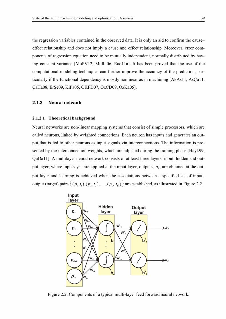
State of the art in machining modeling and optimization: A review 39
the regression variables contained in the observed data. It is only an aid to confirm the cause–
effect relationship and does not imply a cause and effect relationship. Moreover, error com-
ponents of regression equation need to be mutually independent, normally distributed by hav-
ing constant variance [MoPV12, MuRa06, Rao11a]. It has been proved that the use of the
computational modeling techniques can further improve the accuracy of the prediction, par-
ticularly if the functional dependency is mostly nonlinear as in machining [AkAs11, AsÇu11,
ÇaHa08, ErŞe09, KiPa05, ÖKFD07, ÖzCD09, ÖzKa05].
2.1.2 Neural network
2.1.2.1 Theoretical background
Neural networks are non-linear mapping systems that consist of simple processors, which are
called neurons, linked by weighted connections. Each neuron has inputs and generates an out-
put that is fed to other neurons as input signals via interconnections. The information is pre-
sented by the interconnection weights, which are adjusted during the training phase [Hayk99,
QuDa11]. A multilayer neural network consists of at least three layers: input, hidden and out-
put layer, where inputs ip , are applied at the input layer, outputs, ia , are obtained at the out-
put layer and learning is achieved when the associations between a specified set of input–
output (target) pairs ),(.....,),,(),,( 2211 QQ tptptp are established, as illustrated in Figure 2.2.
Figure 2.2: Components of a typical multi-layer feed forward neural network.
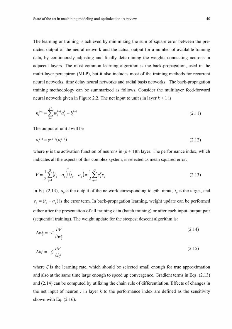
State of the art in machining modeling and optimization: A review 40
The learning or training is achieved by minimizing the sum of square error between the pre-
dicted output of the neural network and the actual output for a number of available training
data, by continuously adjusting and finally determining the weights connecting neurons in
adjacent layers. The most common learning algorithm is the back-propagation, used in the
multi-layer perceptron (MLP), but it also includes most of the training methods for recurrent
neural networks, time delay neural networks and radial basis networks. The back-propagation
training methodology can be summarized as follows. Consider the multilayer feed-forward
neural network given in Figure 2.2. The net input to unit i in layer k + 1 is
1
1
11
ki
kj
S
j
kij
ki bawn
k
(2.11)
The output of unit i will be
)( 111 ki
kki na (2.12)
where ψ is the activation function of neurons in (k + 1)th layer. The performance index, which
indicates all the aspects of this complex system, is selected as mean squared error.
q
Q
q
Tqqq
TQ
qqq eeatatV
11 2
1
2
1 (2.13)
In Eq. (2.13), qa is the output of the network corresponding to thq input, qt is the target, and
)( qqq ate is the error term. In back-propagation learning, weight update can be performed
either after the presentation of all training data (batch training) or after each input–output pair
(sequential training). The weight update for the steepest descent algorithm is:
kij
kij w
Vw
(2.14)
ki
ki b
Vb
(2.15)
where ζ is the learning rate, which should be selected small enough for true approximation
and also at the same time large enough to speed up convergence. Gradient terms in Eqs. (2.13)
and (2.14) can be computed by utilizing the chain rule of differentiation. Effects of changes in
the net input of neuron i in layer k to the performance index are defined as the sensitivity
shown with Eq. (2.16).
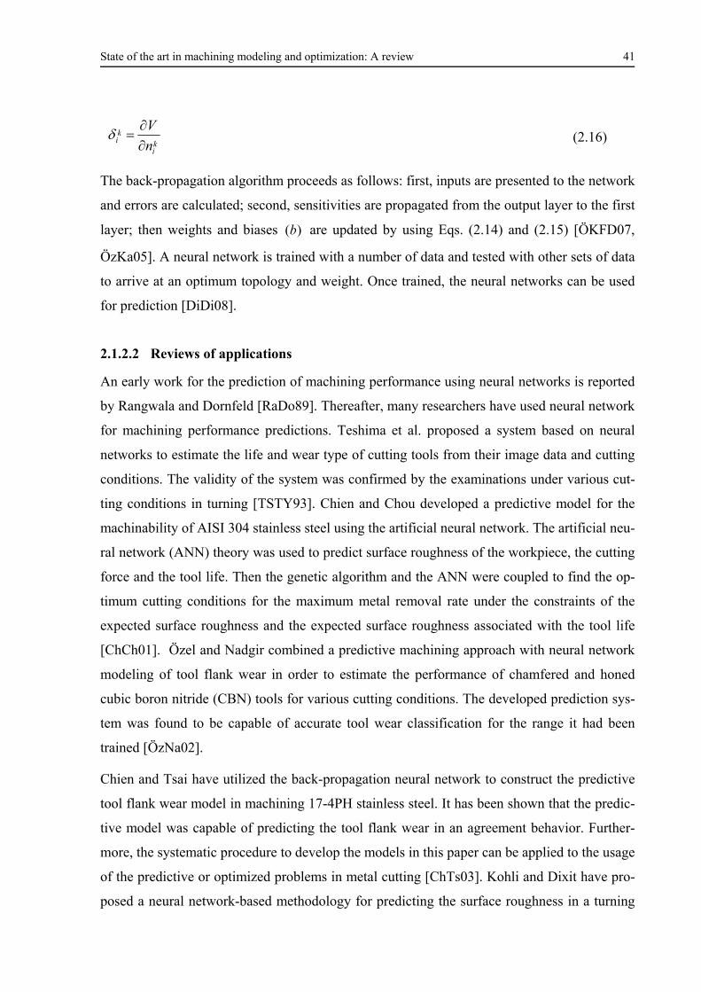
State of the art in machining modeling and optimization: A review 41
ki
ki n
V
(2.16)
The back-propagation algorithm proceeds as follows: first, inputs are presented to the network
and errors are calculated; second, sensitivities are propagated from the output layer to the first
layer; then weights and biases )(b are updated by using Eqs. (2.14) and (2.15) [ÖKFD07,
ÖzKa05]. A neural network is trained with a number of data and tested with other sets of data
to arrive at an optimum topology and weight. Once trained, the neural networks can be used
for prediction [DiDi08].
2.1.2.2 Reviews of applications
An early work for the prediction of machining performance using neural networks is reported
by Rangwala and Dornfeld [RaDo89]. Thereafter, many researchers have used neural network
for machining performance predictions. Teshima et al. proposed a system based on neural
networks to estimate the life and wear type of cutting tools from their image data and cutting
conditions. The validity of the system was confirmed by the examinations under various cut-
ting conditions in turning [TSTY93]. Chien and Chou developed a predictive model for the
machinability of AISI 304 stainless steel using the artificial neural network. The artificial neu-
ral network (ANN) theory was used to predict surface roughness of the workpiece, the cutting
force and the tool life. Then the genetic algorithm and the ANN were coupled to find the op-
timum cutting conditions for the maximum metal removal rate under the constraints of the
expected surface roughness and the expected surface roughness associated with the tool life
[ChCh01]. Özel and Nadgir combined a predictive machining approach with neural network
modeling of tool flank wear in order to estimate the performance of chamfered and honed
cubic boron nitride (CBN) tools for various cutting conditions. The developed prediction sys-
tem was found to be capable of accurate tool wear classification for the range it had been
trained [ÖzNa02].
Chien and Tsai have utilized the back-propagation neural network to construct the predictive
tool flank wear model in machining 17-4PH stainless steel. It has been shown that the predic-
tive model was capable of predicting the tool flank wear in an agreement behavior. Further-
more, the systematic procedure to develop the models in this paper can be applied to the usage
of the predictive or optimized problems in metal cutting [ChTs03]. Kohli and Dixit have pro-
posed a neural network-based methodology for predicting the surface roughness in a turning
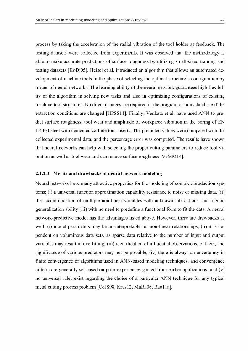
State of the art in machining modeling and optimization: A review 42
process by taking the acceleration of the radial vibration of the tool holder as feedback. The
testing datasets were collected from experiments. It was observed that the methodology is
able to make accurate predictions of surface roughness by utilizing small-sized training and
testing datasets [KoDi05]. Heisel et al. introduced an algorithm that allows an automated de-
velopment of machine tools in the phase of selecting the optimal structure’s configuration by
means of neural networks. The learning ability of the neural network guarantees high flexibil-
ity of the algorithm in solving new tasks and also in optimizing configurations of existing
machine tool structures. No direct changes are required in the program or in its database if the
extraction conditions are changed [HPSS11]. Finally, Venkata et al. have used ANN to pre-
dict surface roughness, tool wear and amplitude of workpiece vibration in the boring of EN
1.4404 steel with cemented carbide tool inserts. The predicted values were compared with the
collected experimental data, and the percentage error was computed. The results have shown
that neural networks can help with selecting the proper cutting parameters to reduce tool vi-
bration as well as tool wear and can reduce surface roughness [VeMM14].
2.1.2.3 Merits and drawbacks of neural network modeling
Neural networks have many attractive properties for the modeling of complex production sys-
tems: (i) a universal function approximation capability resistance to noisy or missing data, (ii)
the accommodation of multiple non-linear variables with unknown interactions, and a good
generalization ability (iii) with no need to predefine a functional form to fit the data. A neural
network-predictive model has the advantages listed above. However, there are drawbacks as
well: (i) model parameters may be un-interpretable for non-linear relationships; (ii) it is de-
pendent on voluminous data sets, as sparse data relative to the number of input and output
variables may result in overfitting; (iii) identification of influential observations, outliers, and
significance of various predictors may not be possible; (iv) there is always an uncertainty in
finite convergence of algorithms used in ANN-based modeling techniques, and convergence
criteria are generally set based on prior experiences gained from earlier applications; and (v)
no universal rules exist regarding the choice of a particular ANN technique for any typical
metal cutting process problem [CoJS98, Krus12, MuRa06, Rao11a].
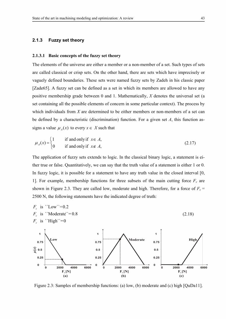
State of the art in machining modeling and optimization: A review 43
2.1.3 Fuzzy set theory
2.1.3.1 Basic concepts of the fuzzy set theory
The elements of the universe are either a member or a non-member of a set. Such types of sets
are called classical or crisp sets. On the other hand, there are sets which have imprecisely or
vaguely defined boundaries. These sets were named fuzzy sets by Zadeh in his classic paper
[Zade65]. A fuzzy set can be defined as a set in which its members are allowed to have any
positive membership grade between 0 and 1. Mathematically, X denotes the universal set (a
set containing all the possible elements of concern in some particular context). The process by
which individuals from X are determined to be either members or non-members of a set can
be defined by a characteristic (discrimination) function. For a given set A, this function as-
signs a value )(xA to every x X such that
, ifonly and if0
, ifonly and if1)(
Ax
AxxA (2.17)
The application of fuzzy sets extends to logic. In the classical binary logic, a statement is ei-
ther true or false. Quantitatively, we can say that the truth value of a statement is either 1 or 0.
In fuzzy logic, it is possible for a statement to have any truth value in the closed interval [0,
1]. For example, membership functions for three subsets of the main cutting force Fc are
shown in Figure 2.3. They are called low, moderate and high. Therefore, for a force of Fc =
2500 N, the following statements have the indicated degree of truth:
0 ``High``= is
0.8 ``=``Moderate is
0.2 ``Low``= is
c
c
c
F
F
F
(2.18)
Figure 2.3: Samples of membership functions: (a) low, (b) moderate and (c) high [QuDa11].
State of the art in machining modeling and optimization: A review 44
Fuzzy set theory may be called a generalization of conventional crisp set theory. Various set-
theoretic operations commonly used in crisp set theory have been defined for fuzzy set theory
as well. These operations reduce their conventional forms for crisp sets. For example, the
intersection of two fuzzy sets A and B, i.e., A⋂B, is defined as a set in which each element has
a membership grade equal to the minimum of its membership grades in A and B. Similarly,
the union of two fuzzy sets A and B, i.e., A⋃B, is defined as the set in which each element has
a membership grade equal to the maximum of its membership grades in A and B. Another
offshoot of fuzzy set theory is fuzzy arithmetic. Fuzzy arithmetic deals with operations on
fuzzy numbers. A fuzzy number is defined as a convex and normalized fuzzy set defined on R
(set of real numbers), of which the membership function is piecewise continuous. If two fuzzy
numbers are represented by ( 1a ,
2a ) and ( 1b ,
2b ) at an α-cut, then the four basic arithmetic
operations are defined as follows:
22112121 ,,,: bababbaaAddition (2.19a)
12212121 ,,,: bababbaanSubtractio (2.19b)
22112121 ,,,: bababbaationMultiplica (2.19c)
12212121 ,,,: bababbaaDivision (2.19d)
The fuzzy set theory can also be used to make predictions from the data by using fuzzy infer-
ence. A fuzzy inference can be defined as a process of mapping from a given input to an out-
put using the theory of fuzzy sets [DiDi08]. The mapping from crisp inputs to crisp outputs is
performed in fuzzy inference systems (FIS). A typical FIS architecture is shown in Figure 2.4.
Three types of FISs have been widely used in engineering applications: Mamdani, Sugeno
and Tsukamoto. Mamdani's fuzzy inference method is the most commonly seen fuzzy meth-
odology. The Mamdani-style fuzzy inference process is performed in four steps: fuzzification
of the input variables, rule evaluation, aggregation of the rule outputs and finally defuzzifica-
tion.
To see how things fit together, suppose that the flank wear of the cutting tool is to be predict-
ed for a particular cutting speed and feed in turning processes. The estimation of flank wear in
this case consists of four steps. In the first step, the crisp values of cutting speed and feed rates
are fuzzified, i.e., they are assigned to linguistic fuzzy sets. Once the independent variables
are fuzzified, the rule evaluation is carried out. In this step, the strength of the various rules is
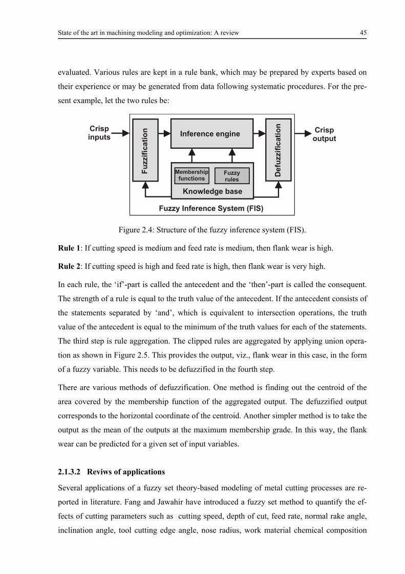
State of the art in machining modeling and optimization: A review 45
evaluated. Various rules are kept in a rule bank, which may be prepared by experts based on
their experience or may be generated from data following systematic procedures. For the pre-
sent example, let the two rules be:
Figure 2.4: Structure of the fuzzy inference system (FIS).
Rule 1: If cutting speed is medium and feed rate is medium, then flank wear is high.
Rule 2: If cutting speed is high and feed rate is high, then flank wear is very high.
In each rule, the ‘if’-part is called the antecedent and the ‘then’-part is called the consequent.
The strength of a rule is equal to the truth value of the antecedent. If the antecedent consists of
the statements separated by ‘and’, which is equivalent to intersection operations, the truth
value of the antecedent is equal to the minimum of the truth values for each of the statements.
The third step is rule aggregation. The clipped rules are aggregated by applying union opera-
tion as shown in Figure 2.5. This provides the output, viz., flank wear in this case, in the form
of a fuzzy variable. This needs to be defuzzified in the fourth step.
There are various methods of defuzzification. One method is finding out the centroid of the
area covered by the membership function of the aggregated output. The defuzzified output
corresponds to the horizontal coordinate of the centroid. Another simpler method is to take the
output as the mean of the outputs at the maximum membership grade. In this way, the flank
wear can be predicted for a given set of input variables.
2.1.3.2 Reviws of applications
Several applications of a fuzzy set theory-based modeling of metal cutting processes are re-
ported in literature. Fang and Jawahir have introduced a fuzzy set method to quantify the ef-
fects of cutting parameters such as cutting speed, depth of cut, feed rate, normal rake angle,
inclination angle, tool cutting edge angle, nose radius, work material chemical composition
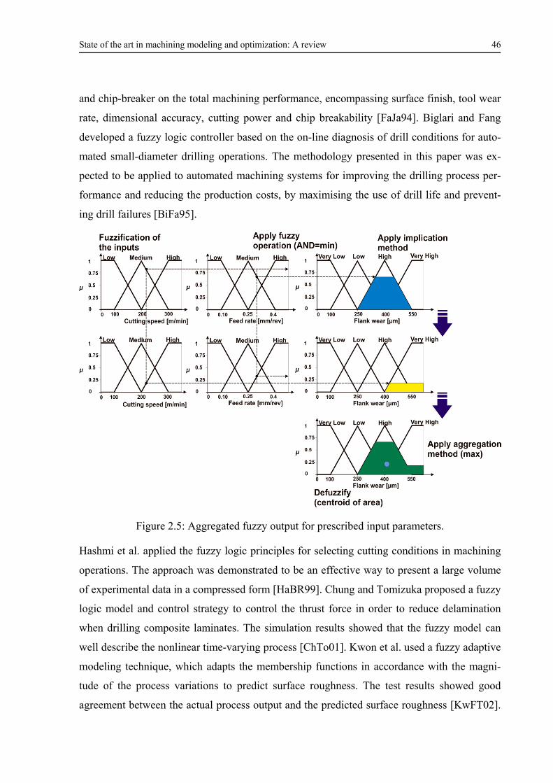
State of the art in machining modeling and optimization: A review 46
and chip-breaker on the total machining performance, encompassing surface finish, tool wear
rate, dimensional accuracy, cutting power and chip breakability [FaJa94]. Biglari and Fang
developed a fuzzy logic controller based on the on-line diagnosis of drill conditions for auto-
mated small-diameter drilling operations. The methodology presented in this paper was ex-
pected to be applied to automated machining systems for improving the drilling process per-
formance and reducing the production costs, by maximising the use of drill life and prevent-
ing drill failures [BiFa95].
Figure 2.5: Aggregated fuzzy output for prescribed input parameters.
Hashmi et al. applied the fuzzy logic principles for selecting cutting conditions in machining
operations. The approach was demonstrated to be an effective way to present a large volume
of experimental data in a compressed form [HaBR99]. Chung and Tomizuka proposed a fuzzy
logic model and control strategy to control the thrust force in order to reduce delamination
when drilling composite laminates. The simulation results showed that the fuzzy model can
well describe the nonlinear time-varying process [ChTo01]. Kwon et al. used a fuzzy adaptive
modeling technique, which adapts the membership functions in accordance with the magni-
tude of the process variations to predict surface roughness. The test results showed good
agreement between the actual process output and the predicted surface roughness [KwFT02].
State of the art in machining modeling and optimization: A review 47
Kirby and Chen developed a surface roughness prediction system for a turning operation, us-
ing a fuzzy-nets modeling technique. A series of validation runs indicate that this system has a
mean accuracy of 95% [KiCh07]. Nandi and Davim studied the drilling performances with
minimum quantity lubricant. Fuzzy logic rules, which were derived based on fuzzy set theory,
were used to develop fuzzy rule-based models. A comparison of the model predictions with
experimental results and those published in literature showed that fuzzy rule-based models
with Tsukamoto-type fuzzy rules excellently describe the trade-off with experimental meas-
urements [NaDa09].
Iqbal et al. presented an expert system, incorporating fuzzy reasoning mechanisms, for opti-
mizing parameters and predicting performance measures in high-speed milling of hardened
AISI D2. This expert system proved to be very effective and efficient for optimizing the hard-
milling process and also for providing important predictions before the start of the actual pro-
cess [IHLD07]. Latha and Senthilkumar predicted the surface roughness of drilled composite
materials using fuzzy logic. The predicted fuzzy output values and measured values were fair-
ly close to each other, which indicated that the fuzzy logic model can be effectively used to
predict the surface roughness in the drilling of composite materials [LaSe10].
2.1.3.3 Merits and drawbacks of fuzzy-based modeling
Fuzzy set theory has been used to model systems that are hard to define precisely. It allows
many variables to be considered, places no demands of linearity, is tolerant to noise and a
suitable technique for manufacturing problems, if multiple quality characteristics exist and the
hierarchy of importance of each objective is not clearly defined. However, fuzzy set theory
suffers from some shortcomings: (i) the rules accrued from the experts or a priori experiments
are not easily amenable to the dynamic change of the underlying process; (ii) an extensive
amount of rules must be stored into a rule base, of which the management is not an easy task;
and (iii) they do not provide the means of utilizing any existing analytical model [Sher94,
ShVi96].
2.2 Finite element modeling of chip formation processes
The basic idea in the finite element method (FEM) is to find the solution of a complicated
problem by replacing it with a simpler one. Since the actual problem is replaced with a sim-
pler one in finding the solution, we will be able to find only an approximate solution rather
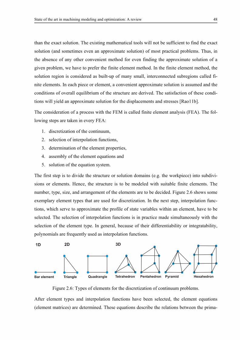
State of the art in machining modeling and optimization: A review 48
than the exact solution. The existing mathematical tools will not be sufficient to find the exact
solution (and sometimes even an approximate solution) of most practical problems. Thus, in
the absence of any other convenient method for even finding the approximate solution of a
given problem, we have to prefer the finite element method. In the finite element method, the
solution region is considered as built-up of many small, interconnected subregions called fi-
nite elements. In each piece or element, a convenient approximate solution is assumed and the
conditions of overall equilibrium of the structure are derived. The satisfaction of these condi-
tions will yield an approximate solution for the displacements and stresses [Rao11b].
The consideration of a process with the FEM is called finite element analysis (FEA). The fol-
lowing steps are taken in every FEA:
1. discretization of the continuum,
2. selection of interpolation functions,
3. determination of the element properties,
4. assembly of the element equations and
5. solution of the equation system.
The first step is to divide the structure or solution domains (e.g. the workpiece) into subdivi-
sions or elements. Hence, the structure is to be modeled with suitable finite elements. The
number, type, size, and arrangement of the elements are to be decided. Figure 2.6 shows some
exemplary element types that are used for discretization. In the next step, interpolation func-
tions, which serve to approximate the profile of state variables within an element, have to be
selected. The selection of interpolation functions is in practice made simultaneously with the
selection of the element type. In general, because of their differentiability or integratability,
polynomials are frequently used as interpolation functions.
Figure 2.6: Types of elements for the discretization of continuum problems.
After element types and interpolation functions have been selected, the element equations
(element matrices) are determined. These equations describe the relations between the prima-
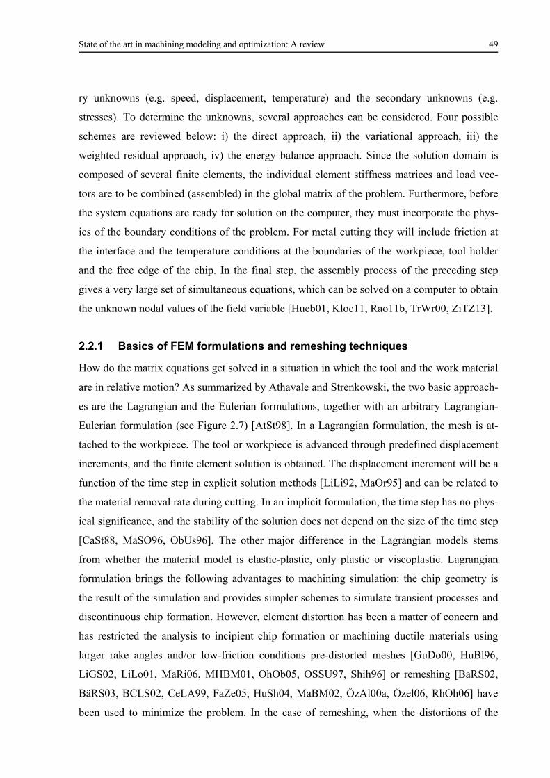
State of the art in machining modeling and optimization: A review 49
ry unknowns (e.g. speed, displacement, temperature) and the secondary unknowns (e.g.
stresses). To determine the unknowns, several approaches can be considered. Four possible
schemes are reviewed below: i) the direct approach, ii) the variational approach, iii) the
weighted residual approach, iv) the energy balance approach. Since the solution domain is
composed of several finite elements, the individual element stiffness matrices and load vec-
tors are to be combined (assembled) in the global matrix of the problem. Furthermore, before
the system equations are ready for solution on the computer, they must incorporate the phys-
ics of the boundary conditions of the problem. For metal cutting they will include friction at
the interface and the temperature conditions at the boundaries of the workpiece, tool holder
and the free edge of the chip. In the final step, the assembly process of the preceding step
gives a very large set of simultaneous equations, which can be solved on a computer to obtain
the unknown nodal values of the field variable [Hueb01, Kloc11, Rao11b, TrWr00, ZiTZ13].
2.2.1 Basics of FEM formulations and remeshing techniques
How do the matrix equations get solved in a situation in which the tool and the work material
are in relative motion? As summarized by Athavale and Strenkowski, the two basic approach-
es are the Lagrangian and the Eulerian formulations, together with an arbitrary Lagrangian-
Eulerian formulation (see Figure 2.7) [AtSt98]. In a Lagrangian formulation, the mesh is at-
tached to the workpiece. The tool or workpiece is advanced through predefined displacement
increments, and the finite element solution is obtained. The displacement increment will be a
function of the time step in explicit solution methods [LiLi92, MaOr95] and can be related to
the material removal rate during cutting. In an implicit formulation, the time step has no phys-
ical significance, and the stability of the solution does not depend on the size of the time step
[CaSt88, MaSO96, ObUs96]. The other major difference in the Lagrangian models stems
from whether the material model is elastic-plastic, only plastic or viscoplastic. Lagrangian
formulation brings the following advantages to machining simulation: the chip geometry is
the result of the simulation and provides simpler schemes to simulate transient processes and
discontinuous chip formation. However, element distortion has been a matter of concern and
has restricted the analysis to incipient chip formation or machining ductile materials using
larger rake angles and/or low-friction conditions pre-distorted meshes [GuDo00, HuBl96,
LiGS02, LiLo01, MaRi06, MHBM01, OhOb05, OSSU97, Shih96] or remeshing [BaRS02,
BäRS03, BCLS02, CeLA99, FaZe05, HuSh04, MaBM02, ÖzAl00a, Özel06, RhOh06] have
been used to minimize the problem. In the case of remeshing, when the distortions of the
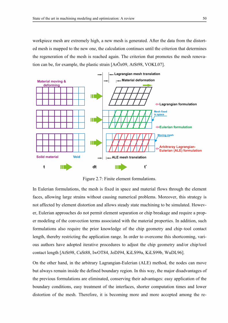
State of the art in machining modeling and optimization: A review 50
workpiece mesh are extremely high, a new mesh is generated. After the data from the distort-
ed mesh is mapped to the new one, the calculation continues until the criterion that determines
the regeneration of the mesh is reached again. The criterion that promotes the mesh renova-
tion can be, for example, the plastic strain [ArÖz09, AtSt98, VOKL07].
Figure 2.7: Finite element formulations.
In Eulerian formulations, the mesh is fixed in space and material flows through the element
faces, allowing large strains without causing numerical problems. Moreover, this strategy is
not affected by element distortion and allows steady state machining to be simulated. Howev-
er, Eulerian approaches do not permit element separation or chip breakage and require a prop-
er modeling of the convection terms associated with the material properties. In addition, such
formulations also require the prior knowledge of the chip geometry and chip–tool contact
length, thereby restricting the application range. In order to overcome this shortcoming, vari-
ous authors have adopted iterative procedures to adjust the chip geometry and/or chip/tool
contact length [AtSt98, CaSt88, IwOT84, JoDJ94, KiLS99a, KiLS99b, WuDL96].
On the other hand, in the arbitrary Lagrangian-Eulerian (ALE) method, the nodes can move
but always remain inside the defined boundary region. In this way, the major disadvantages of
the previous formulations are eliminated, conserving their advantages: easy application of the
boundary conditions, easy treatment of the interfaces, shorter computation times and lower
distortion of the mesh. Therefore, it is becoming more and more accepted among the re-
State of the art in machining modeling and optimization: A review 51
searchers [CMRM13, HaKR08, HoNg13, ÖzZe07, WuJF03]. Despite the above advantages, a
careful numerical treatment of the advection terms is recommended [VOKL07]. More elabo-
rate discussions about the use of ALE formulations in modeling metal machining are present-
ed by Rakotomalala et al. [RaJT93], Olovsson et al.[OlNS99], Movahhedy et al. [MoGA00],
Benson and Okazawa [BeOk04], Pantalé [Pant04] and Madhavan and Adibi-Sedeh
[MaAd05].
In metal cutting modeling, the common problem is related to the element distortion during the
simulations due to severe plastic deformation. The distortion can cause a deterioration of the
FE simulation in terms of convergence rate and numerical errors, or cause the Jacobian de-
terminant to become negative, which makes further analysis impossible. It is often necessary
to redefine the mesh after some stages of deformation. Several techniques are used to reduce
the element distortion: re-meshing, smoothing and refinement. These techniques include the
generation of a completely new finite element mesh out of the existing mesh, increasing the
local element density by reducing the local element size (Figure 2.8(a)) and/or reallocating the
individual nodes to improve the local quality of the elements (Figure 2.8(b)). The discussed
techniques are used in the so-called adaptive mesh procedure. Adaptive mesh refers to a
scheme for finite difference and finite element codes, dynamically changing the size and dis-
tribution of the mesh during the simulations. In the regions of strong gradients of variables
involved, a higher mesh density is needed in order to diminish the solution errors. As these
gradients are not known a priori, the adaptive mesh generation procedure starts with a rela-
tively coarse primary mesh, and after the solution of this primary mesh has been obtained, the
mesh density is increased for the strong gradients [AsOu08].
Figure 2.8: (a) Increase in local mesh density (refinement), (b) reallocation of the nodes
(smoothing).
Finally, it should be noted here that many FE programs utilized to calculate large plastic de-
formations make use of “implicit” methods. For highly dynamic applications on the other
hand, such as crash simulation, explicit time integration is prevalent in FE programs.
State of the art in machining modeling and optimization: A review 52
2.2.2 Historical perspective
For a historical perspective of how FEA is used in metal cutting research, the reader is first
referred to the comprehensive reviews in the references [ChBl94, Mack03, Mack98]. These
contain most of the significant citations up to the early 2000s. Second, the work undertaken
by Vaz Jr. et al., in which a brief outline of the wide range of complex physical phenomena
involved in chip formation, has been presented in a descriptive manner. Several numerical
strategies used for simulation were also reviewed, and a short discussion of their relative mer-
its and drawbacks was presented [VOKL07]. Third, an interesting reviewing contribution re-
garding the simulation of cutting and machining processes was reported by Lorong et al. The
contributions provided by researchers from all over the world and published in the Proceed-
ings of the European Scientific Association for material FORMing (ESAFORM) Conferences
were highlighted [LoMT07]. Finally, the collection of papers edited by Arrazola et al. sum-
marizes the state-of-the-art developments in the modeling of machining processes during the
last 15 years, since the last CIRP keynote paper on the modeling of machining was produced
in 1998. This includes a critical assessment of the relevant modeling techniques and their ap-
plicability and/or limitations for the prediction of the complex machining operations per-
formed in industry. The paper includes contributions from academia and industry and serves
as a comprehensive report of recent progress as well as a roadmap for future directions
[AÖUD13].
2.2.3 Scales of the machining modeling
In order to effectively simulate a typical material removal process, all the input parameters
that can have a remarkable influence on the attained results, such as machine tool, coolant,
cutting tool, tool holder, tool clamping, workpiece, assembly, etc., should be considered.
However, considering the whole machining system, it seems quite complex to solve one given
problem. Therefore, in many cases the area or elements that are going to be analyzed in depth
are isolated from the rest of the system. Depending on the problem to be studied, the FEM of
machining processes can be focused on three scales, namely: (i) macroscale, (ii) mesoscale
and (iii) microscale (see Figure 2.9). The first scale accounts for the interaction of the ma-
chine tool with the entire workpiece and tool engagement system [RaLB05, RLHB06]. In the
second scale, only the area where the chip is formed is considered so that performances, such
as cutting forces, residual stresses, tool temperature and stresses, etc., can be reasonably pre-
dicted [ACRU08, AuBi06, SoAD04, UhSZ07, DiCM01, GrBN05, GuLi02, HeSK13, KlKr05,
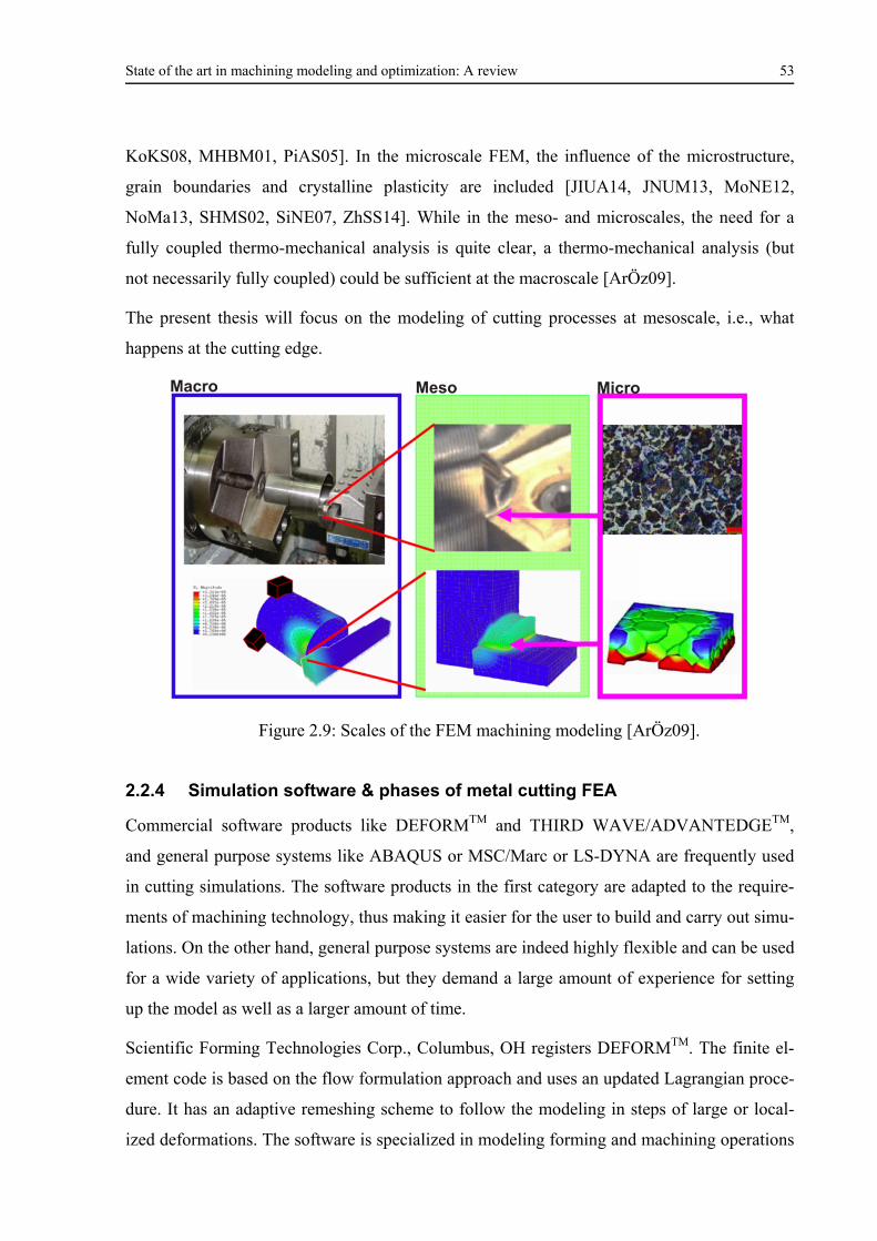
State of the art in machining modeling and optimization: A review 53
KoKS08, MHBM01, PiAS05]. In the microscale FEM, the influence of the microstructure,
grain boundaries and crystalline plasticity are included [JIUA14, JNUM13, MoNE12,
NoMa13, SHMS02, SiNE07, ZhSS14]. While in the meso- and microscales, the need for a
fully coupled thermo-mechanical analysis is quite clear, a thermo-mechanical analysis (but
not necessarily fully coupled) could be sufficient at the macroscale [ArÖz09].
The present thesis will focus on the modeling of cutting processes at mesoscale, i.e., what
happens at the cutting edge.
Figure 2.9: Scales of the FEM machining modeling [ArÖz09].
2.2.4 Simulation software & phases of metal cutting FEA
Commercial software products like DEFORMTM and THIRD WAVE/ADVANTEDGETM,
and general purpose systems like ABAQUS or MSC/Marc or LS-DYNA are frequently used
in cutting simulations. The software products in the first category are adapted to the require-
ments of machining technology, thus making it easier for the user to build and carry out simu-
lations. On the other hand, general purpose systems are indeed highly flexible and can be used
for a wide variety of applications, but they demand a large amount of experience for setting
up the model as well as a larger amount of time.
Scientific Forming Technologies Corp., Columbus, OH registers DEFORMTM. The finite el-
ement code is based on the flow formulation approach and uses an updated Lagrangian proce-
dure. It has an adaptive remeshing scheme to follow the modeling in steps of large or local-
ized deformations. The software is specialized in modeling forming and machining operations
State of the art in machining modeling and optimization: A review 54
in 2D and 3D, based on an implicit integration method with fully coupled thermo-mechanical
analysis [AsOu08, Kloc11].
From the standpoint of the users of the above software products, a typical finite element anal-
ysis takes place in three phases: (i) data preparation with the preprocessor (input), (ii) pro-
cessing (calculation) and (ii) evaluation of the results with the postprocessor (output). Figure
2.10 summarizes the parameters that are involved in the FEA of metal cutting processes.
2.2.5 Advantages and problems associated with numerical cutting modeling
The finite element method can provide a comprehensive and in some cases complementary
approach to experimental, mechanistic or analytical approaches to study machining process
[ACRU08, KlBW05, ÖzKS08]. It provides some advantages, basically due to the following
aspects: access to fields of values of thermo-mechanical variables, consideration of the non-
linear effects of the friction at the tool–chip interface, ability to perform virtual machining
tests that are difficult to justify experimentally (new tool geometries and materials or coat-
ings) or to study cases that are difficult to carry out (zero friction coefficient, materials with
ideal behavior, etc.) [AsOu08]. However, at this stage, it can be said that basically three kinds
of problems can be found that relate to numerical cutting modeling, prior to becoming a relia-
ble tool for industry (see Figure 2.10):
1. Identification of finite element model input parameters: material constitutive behavior,
friction, thermal parameters, damage and wear. A sensitivity study showed the influence
of input parameters on results. From this study, information about the uncertainty origi-
nated by input parameter identification can be estimated, and the remarkable difficulties in
obtaining quantitative results can be pointed out. For instance, moving the yield stress
(one of the best-known material coefficients) from 200 MPa to 900 MPa can lead to a
temperature increase of 30% from an average value of 1240 K (i.e. of around 372 K).
Thus it can be estimated that an uncertainty of 30 MPa can give an uncertainty in tempera-
ture of approximately 15 K [AsOu08].
2. Finite element model definition: boundary conditions, integration frame (explicit, implic-
it), formulations can lead to different quantitative results, calculation times, etc.
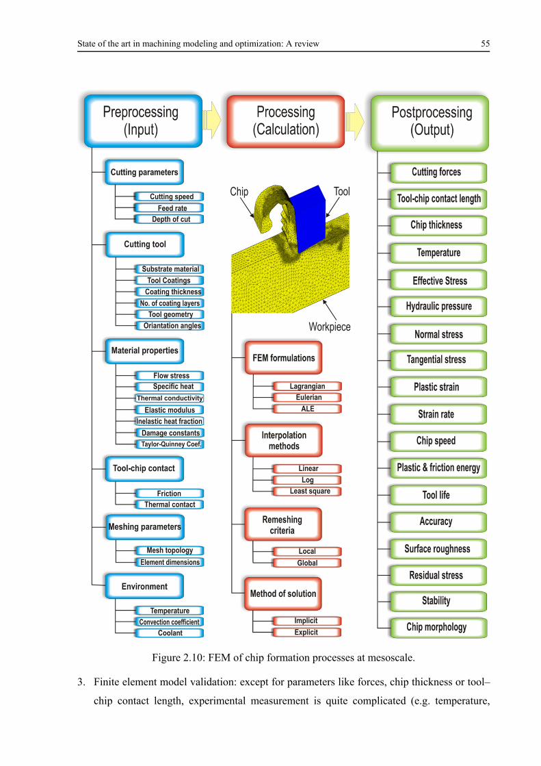
State of the art in machining modeling and optimization: A review 55
Figure 2.10: FEM of chip formation processes at mesoscale.
3. Finite element model validation: except for parameters like forces, chip thickness or tool–
chip contact length, experimental measurement is quite complicated (e.g. temperature,
State of the art in machining modeling and optimization: A review 56
strain, strain rate) and in some cases quite difficult at this stage (strain rate, stresses, etc.).
Thus model validation is quite difficult because experimental means are not available or
they are not suitable enough [ArÖz09].
2.2.6 Input models and identification of input parameters
The success and reliability of modeling depends upon accurate mechanical data (elastic con-
stants, flow stress, friction, fracture stress/ strain, etc.) and thermo-physical data (density,
thermal conductivity, heat capacity, etc.) [ArÖz10, CaCG08, ÖzAl00b, Özel06, ÖzSS10,
SaAG05, SiÖz10]. Thus, a characterization in the extreme conditions of machining is needed,
i.e., for strains of 100–700%, strain-rates up to 106 s-1, temperatures between 500 and 1400
°C, high heating rates close to 106 °C s-1 and high pressures near 2–3 GPa. A realistic material
model should also include strain-hardening and thermal softening due to dynamic recovery or
recrystallization. Therefore, other modeling approaches have been proposed, and flow stress
data has been generated for machining a range of commonly known work materials
[BWLM14, CaCG08, WaOh02, Chil06, GuWW06, Karp11, OHAS12, OzZe06, RhOh06,
ShKA01, SLCM01].
2.2.6.1 Constitutive behavior of the work materials
The mechanical behavior of materials is an essential component of technology which has re-
ceived considerable attention over many years. Of particular interest is the response of mate-
rials to mechanical and thermal loadings, the influence of environmental factors, and the con-
ditions and mechanisms of failure. The terms “constitutive equations” and “material model-
ing” are usually applied to the analytical representation of the material response characteris-
tics prior to total failure [Bodn02]. As the latter is the major and important module of any
numerical code used for the simulation of the machining process, the accuracy of the simula-
tion largely depends on the accuracy of the predictability of the material model. The need for
the greater accuracy of the flow prediction has encouraged many researchers [LiCh11,
LiKh99, Zeri04] to develop suitable constitutive models for different materials. In this con-
text, many empirical, semi-empirical and physically-based constitutive equations have been
proposed over the course of time. The list of these equations can be found in various review
[LiCh11, LiKh99] and overview articles [SMBS10, VoAb05] on constitutive models
[SPBA14].
State of the art in machining modeling and optimization: A review 57
Unfortunately, a universal material model suitable for all cutting simulations remains one of
the important unaccomplished tasks. Due to the typical high strain, strain rate temperature and
temperature gradient in machining, it is not always easy to determine the flow stress curves by
experiment. Furthermore, experimental methods such as the Split-Hopkinson-Bar-Test are
quite expensive and require a large number of experiments to be conducted. On the other
hand, empirical material laws which describe the flow stress as a function of strain, strain rate
and temperature contain specific material constants, which have to be determined by regres-
sion analyses or by the least squares method and verified experimentally. During the last three
decades, a multitude of such models have been suggested [KaTU83, MaOk83, Oxle64]. The
most notably are the engineering-based and physically-based models. In both fields, the earli-
est contributions were made by Johnson and Cook [JoCo83, JoCo85] and Zerilli and Arm-
strong in 1980s [ZeAr87, Zeri04] respectively. Additionally, JMatPro, an acronym for Java-
based Materials Properties, can also be employed to calculate a wide range of material proper-
ties. These properties include thermo-physical, physical properties, time-temperature-
transformation diagrams, stress/strain diagrams, proof and tensile stress, hardness, coarsening
and creep. A feature of this program is that the calculations are based on sound physical prin-
ciples rather than purely statistical methods. Thus, many of the shortcomings of methods such
as the regression analysis can be overcome. With this program, a sensitivity to microstructures
can be included for many of the properties and the true inter-relationship between properties
can be developed, for example, in the modeling of creep and precipitation hardening
[SGLM03]. Figure 2.11 shows an example of the predicted relationship between true stress
and true strain for duplex stainless steel materials using JMatPro software.
It is worthwhile mentioning that in recent years, the inverse identification of the constitutive
model parameters has been proposed as an alternative method for defining the constitutive
equation coefficients, so that the models remain valid for large ranges of conditions during
machining [KlLB13, PAMC07, ShBä11, ShBä12].
2.2.6.2 Friction
Since the rate of tool wear heavily depends on the frictional conditions at the tool–chip inter-
face, an accurate modeling is of critical practical importance [Özel06]. Friction under very
extreme conditions is prevalent at the tool–chip interface (1-2 GPa, 500–100 °C) [ZMYP11].
In the earlier analyses of machining, frictional stresses )( f on the tool rake face have been
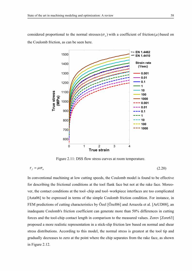
State of the art in machining modeling and optimization: A review 58
considered proportional to the normal stresses )( n with a coefficient of friction )( based on
the Coulomb friction, as can be seen here.
Figure 2.11: DSS flow stress curves at room temperature.
nf (2.20)
In conventional machining at low cutting speeds, the Coulomb model is found to be effective
for describing the frictional conditions at the tool flank face but not at the rake face. Moreo-
ver, the contact conditions at the tool–chip and tool–workpiece interfaces are too complicated
[Asta06] to be expressed in terms of the simple Coulomb friction condition. For instance, in
FEM predictions of cutting characteristics by Özel [Özel06] and Arrazola et al. [ArUD08], an
inadequate Coulomb's friction coefficient can generate more than 50% differences in cutting
forces and the tool-chip contact length in comparison to the measured values. Zorev [Zore63]
proposed a more realistic representation in a stick-slip friction law based on normal and shear
stress distributions. According to this model, the normal stress is greatest at the tool tip and
gradually decreases to zero at the point where the chip separates from the rake face, as shown
in Figure 2.12.
0 1 2 3 4
600
700
800
900
1000
1100
1200
1300
1400
1500
True strain
Tru
e s
tress
(MP
a)
0.0010.010.111010010000.0010.010.11101001000
EN 1.4462EN 1.4410
Strain rate (1/sec)
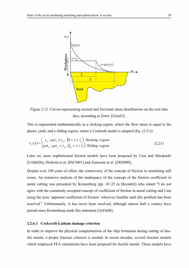
State of the art in machining modeling and optimization: A review 59
Figure 2.12: Curves representing normal and frictional stress distributions on the tool rake
face, according to Zorev [Zore63].
This is represented mathematically as a sticking region, where the flow stress is equal to the
plastic yield, and a sliding region, where a Coulomb model is adopted (Eq. (2.21)).
regionSlidinglxl
regionStickinglxx
cppnn
ppnpf ,:
0,:)(
(2.21)
Later on, more sophisticated friction models have been proposed by Usui and Shirakashi
[UsSh82b], Dirikolu et al. [DiCM01] and Zemzemi et al. [ZRSD09].
Despite over 100 years of effort, the controversy of the concept of friction in machining still
exists. An extensive analysis of the inadequacy of the concept of the friction coefficient in
metal cutting was presented by Kronenberg (pp. 18−25 in [Kron66]) who stated “I do not
agree with the commonly accepted concept of coefficient of friction in metal cutting and I am
using the term ‘apparent coefficient of friction’ wherever feasible until this problem has been
resolved.” Unfortunately, it has never been resolved, although almost half a century have
passed since Kronenberg made this statement [AsOu08].
2.2.6.3 Cockcroft-Latham damage criterion
In order to improve the physical comprehension of the chip formation during cutting of duc-
tile metals, a proper fracture criterion is needed. In recent decades, several fracture models
which employed FEA simulations have been proposed for ductile metals. These models have
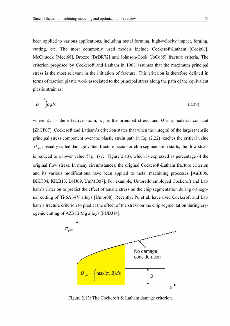
State of the art in machining modeling and optimization: A review 60
been applied to various applications, including metal forming, high-velocity impact, forging,
cutting, etc. The most commonly used models include Cockcroft-Latham [Cock68],
McCintock [Mccl68], Brozzo [BrDR72] and Johnson-Cook [JoCo85] fracture criteria. The
criterion proposed by Cockcroft and Latham in 1968 assumes that the maximum principal
stress is the most relevant in the initiation of fracture. This criterion is therefore defined in
terms of traction plastic work associated to the principal stress along the path of the equivalent
plastic strain as:
dDf
0
1 (2.22)
where f is the effective strain, 1 is the principal stress, and D is a material constant
[ZhCP07]. Cockcroft and Latham’s criterion states that when the integral of the largest tensile
principal stress component over the plastic strain path in Eq. (2.22) reaches the critical value
.critD , usually called damage value, fracture occurs or chip segmentation starts, the flow stress
is reduced to a lower value rp% (see Figure 2.13), which is expressed as percentage of the
original flow stress. In many circumstances, the original Cockcroft-Latham fracture criterion
and its various modifications have been applied to metal machining processes [AuBi06,
BiKT04, KlLB13, LoJJ09, UmMO07]. For example, Umbrello employed Cockcroft and Lat-
ham’s criterion to predict the effect of tensile stress on the chip segmentation during orthogo-
nal cutting of Ti-6Al-4V alloys [Umbr08]. Recently, Pu et al. have used Cockcroft and Lat-
ham’s fracture criterion to predict the effect of the stress on the chip segmentation during cry-
ogenic cutting of AZ31B Mg alloys [PUDJ14].
Figure 2.13: The Cockcroft & Latham damage criterion.

State of the art in machining modeling and optimization: A review 61
2.2.6.4 Thermal contact conductance
The thermal contact conductance tch , also known as the heat transfer coefficient, describes
the heat flux of two solids in contact and is defined as follows:
Thtc
(2.23)
where ΔT is the temperature difference at the contacting surfaces, and the heat flux is de-
fined as:
dt
d
dA
d (2.24)
where A is the area of contact surface, and is the conducted heat in (J). It is recognized that
thermal contact conductance is a function of several parameters, the dominant ones being the
type of contacting materials, the macro- and micro-geometry of the contacting surfaces, the
temperature, the interfacial pressure, the type of lubricant or contaminant and its thickness
[RoBC03].
2.2.6.5 Taylor-Quinney coefficient
As the mechanical behavior is affected by temperature (softening effect), plastic deformation
is accompanied by heat generation, which results in a temperature rise. The heat generation
due to this phenomenon is described by the following relationship:
ptp (2.25)
where p is the volumetric heat generation due to plastic work in (W/m3), is the von Mises
equivalent stress in (MPa), p is the von Mises equivalent plastic strain, and t is the Taylor-
Quinney coefficient, which represents the proportion of plastic works converted into heat.
Haddag and Nouari have shown a strong dependency of t on both strain and strain rate for
various engineering materials. Within the confines of their constitutive framework, the as-
sumption that t is constant was inconsistent with the rate independence of the stored energy
of cold work, which was a fundamental consequence of thermodynamics. It would seem that
the only justification for a priori assumptions on t is a lack of information on the stored en-
State of the art in machining modeling and optimization: A review 62
ergy of cold work. Therefore, this coefficient is considered as an unknown input value, which
has been specified in cutting simulations [HaNo13].
2.3 Determination of optimal or near-optimal cutting conditions
Machining optimization is the systematic and scientific approach for solving problems associ-
ated with engineering decision-making in selecting the best production method, process pa-
rameters or operational conditions. The ultimate goal of such problems is to either minimize
the efforts required or maximize the desired benefits. Efforts required and benefits desired in a
machining situation can be expressed according to the decision variables. Machining optimi-
zation can be defined as the process of finding such decision variables that give the maximum
or minimum value of one or more objective functions subject to some resource, capacity or
process constraint [Özel09].
With time, complexity in metal cutting process dynamics has increased, and as a conse-
quence, problems related to the determination of optimal or near-optimal decision variables
are faced with discrete and continuous parameter spaces with multi-modal, differentiable as
well as non-differentiable objective functions or responses. The search for optimal or accepta-
ble near-optimal solutions by a suitable optimization technique based on input–output and in-
process parameter relationship or objective function formulated from models with or without
constraints, is a critical and difficult task for researchers and practitioners [BAPS05, BASP06,
CaGu00, ChTs96, HuLL01, VPAS03, Yild13a]. A large number of techniques has been de-
veloped by researchers to solve these types of parameter optimization problems and may be
classified as conventional and nonconventional optimization techniques.
Whereas conventional techniques attempt to provide a local optimal solution, non-
conventional techniques based on developed extrinsic models or objective functions are only
an approximation and attempt to provide near-optimal cutting conditions. Conventional tech-
niques may be broadly classified into two categories. In the first category, experimental tech-
niques that include statistical design of experiment, such as the Taguchi method, and response
surface design methodology (RSM) are referred to. In the second category, iterative mathe-
matical search techniques, such as linear programming (LP), non-linear programming (NLP),
and dynamic programming (DP) algorithms are included. Non-conventional, meta-heuristic
search-based techniques, which are sufficiently general and extensively used by researchers in
recent times, are based on biological, molecular or neurological phenomena that mimic the
State of the art in machining modeling and optimization: A review 63
metaphor of natural biological evolution and/or the social behavior of species. To mimic the
efficient behavior of these species, various researchers have developed computational systems
that seek fast and robust solutions to complex optimization problems [MuRa06, Rao11a]. Ex-
amples of these algorithms include Simulated Annealing (SA), Genetic Algorithm (GA), Par-
ticle Swarm Optimization (PSO), Firefly Algorithm (FA), Cuckoo Search (CS), Bat Algo-
rithm (BA), etc.
2.3.1 Taguchi Method
2.3.1.1 Basic concepts in Taguchi’s design and optimization procedure
The Taguchi method, named for Genechi Taguchi, the Japanese statistician who developed
and advocated the method, is a powerful problem-solving tool which can improve the perfor-
mance of the product quality, process, design and system with a great decrease in experiment
time cost. This method, which contains the design of experiment theory and the quality loss
function concept, can carry out the robust design of processes and products and solve several
optimal problems in manufacture industries. Professor Genichi Taguchi used the term robust
for the product or processes which perform consistently on target and are relatively insensitive
to factors that are difficult to control. He referred to these uncontrollable factors as noise fac-
tors. He also developed a methodology for finding the optimum settings of control factors and
making a product or process insensitive to noise factors [Mont09, Ross95]. Various steps of
the Taguchi method are shown in Figure 2.14.
To design an experiment means to choose the optimal experiment design to be simultaneously
used for varying all the analyzed factors. There are many different experimental designs that
provide options for the investigator, who must perform experiments to address a variety of
questions under a range of conditions and limitations. Several important considerations de-
termine which experimental design is appropriate for a given investigation. As there are many
parameters in machining, conducting a large number of experiments employing classical ex-
perimental design methods could be very costly, complex and not easy to use. This problem is
overcome in the Taguchi method, which uses a special design of orthogonal arrays (OA) to
study the entire major parameter space with only a small number of experiments. Commonly
used orthogonal arrays include the L4, L9, L12, L16, L18, L25 and L27. A complete listing of
OAs is presented by Phadke [Blan04, Phad89].
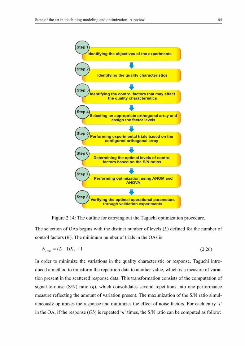
State of the art in machining modeling and optimization: A review 64
Figure 2.14: The outline for carrying out the Taguchi optimization procedure.
The selection of OAs begins with the distinct number of levels (L) defined for the number of
control factors (K). The minimum number of trials in the OAs is
1)1(min nt KLN (2.26)
In order to minimize the variations in the quality characteristic or response, Taguchi intro-
duced a method to transform the repetition data to another value, which is a measure of varia-
tion present in the scattered response data. This transformation consists of the computation of
signal-to-noise (S/N) ratio (η), which consolidates several repetitions into one performance
measure reflecting the amount of variation present. The maximization of the S/N ratio simul-
taneously optimizes the response and minimizes the effect of noise factors. For each entry ‘i’
in the OA, if the response (Ob) is repeated ‘n’ times, the S/N ratio can be computed as follow:
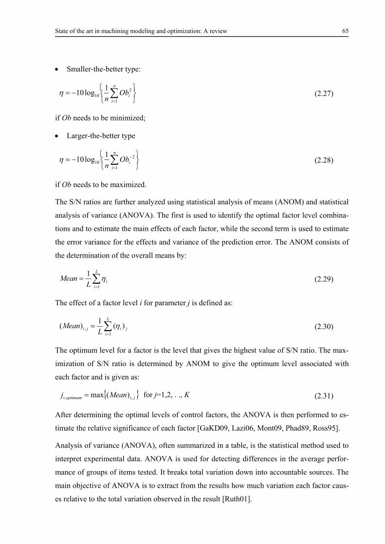
State of the art in machining modeling and optimization: A review 65
Smaller-the-better type:
n
iiOb
n 1
210
1log10 (2.27)
if Ob needs to be minimized;
Larger-the-better type
n
iiOb
n 1
210
1log10 (2.28)
if Ob needs to be maximized.
The S/N ratios are further analyzed using statistical analysis of means (ANOM) and statistical
analysis of variance (ANOVA). The first is used to identify the optimal factor level combina-
tions and to estimate the main effects of each factor, while the second term is used to estimate
the error variance for the effects and variance of the prediction error. The ANOM consists of
the determination of the overall means by:
L
iiL
Mean1
1 (2.29)
The effect of a factor level i for parameter j is defined as:
L
ijiji L
Mean1
, )(1
)( (2.30)
The optimum level for a factor is the level that gives the highest value of S/N ratio. The max-
imization of S/N ratio is determined by ANOM to give the optimum level associated with
each factor and is given as:
jioptimumi Meanj ,, )(max for j=1,2, . ., K (2.31)
After determining the optimal levels of control factors, the ANOVA is then performed to es-
timate the relative significance of each factor [GaKD09, Lazi06, Mont09, Phad89, Ross95].
Analysis of variance (ANOVA), often summarized in a table, is the statistical method used to
interpret experimental data. ANOVA is used for detecting differences in the average perfor-
mance of groups of items tested. It breaks total variation down into accountable sources. The
main objective of ANOVA is to extract from the results how much variation each factor caus-
es relative to the total variation observed in the result [Ruth01].
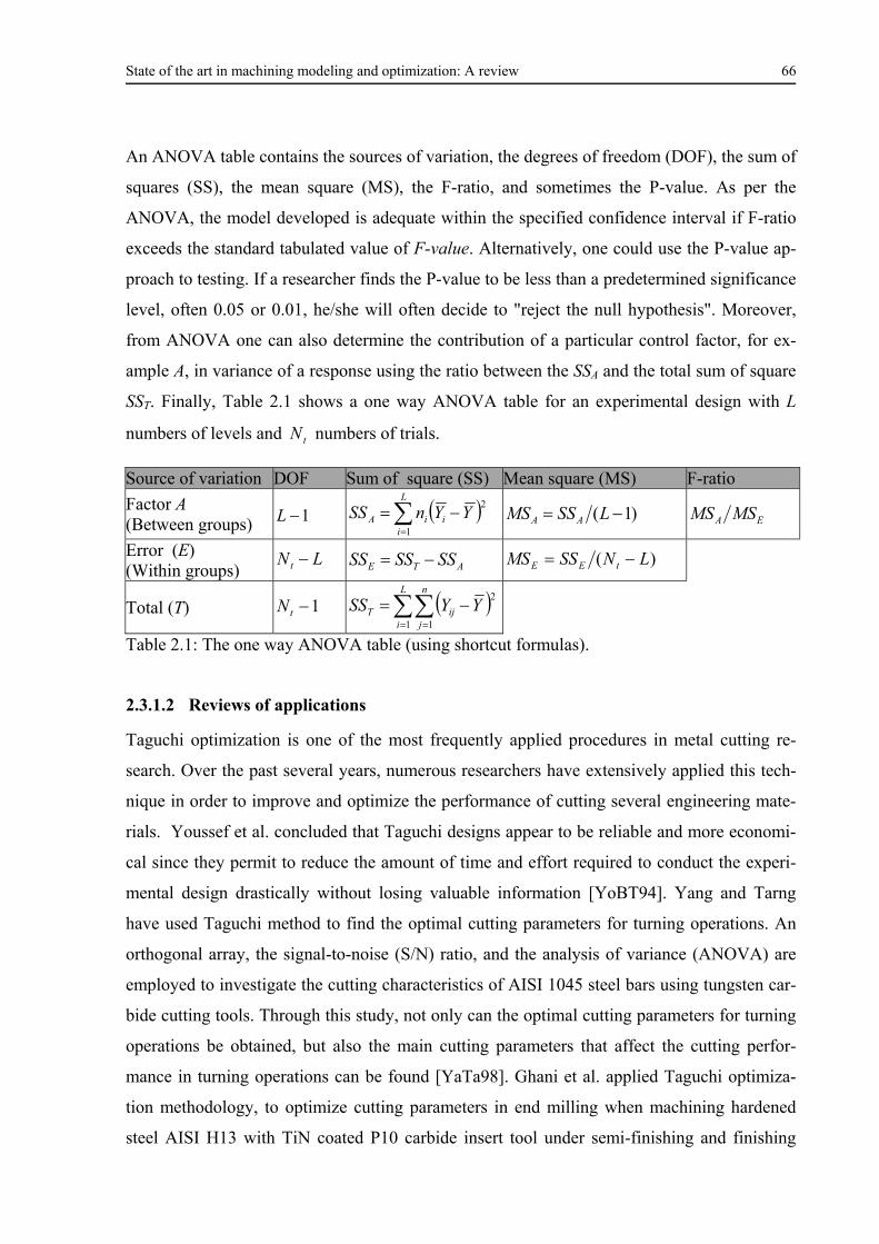
State of the art in machining modeling and optimization: A review 66
An ANOVA table contains the sources of variation, the degrees of freedom (DOF), the sum of
squares (SS), the mean square (MS), the F-ratio, and sometimes the P-value. As per the
ANOVA, the model developed is adequate within the specified confidence interval if F-ratio
exceeds the standard tabulated value of F-value. Alternatively, one could use the P-value ap-
proach to testing. If a researcher finds the P-value to be less than a predetermined significance
level, often 0.05 or 0.01, he/she will often decide to "reject the null hypothesis". Moreover,
from ANOVA one can also determine the contribution of a particular control factor, for ex-
ample A, in variance of a response using the ratio between the SSA and the total sum of square
SST. Finally, Table 2.1 shows a one way ANOVA table for an experimental design with L
numbers of levels and tN numbers of trials.
Source of variation DOF Sum of square (SS) Mean square (MS) F-ratio
Factor A (Between groups) 1L
L
iiiA YYnSS
1
2 )1( LSSMS AA EA MSMS
Error (E) (Within groups)
LNt ATE SSSSSS )( LNSSMS tEE
Total (T) 1tN
L
i
n
jijT YYSS
1 1
2
Table 2.1: The one way ANOVA table (using shortcut formulas).
2.3.1.2 Reviews of applications
Taguchi optimization is one of the most frequently applied procedures in metal cutting re-
search. Over the past several years, numerous researchers have extensively applied this tech-
nique in order to improve and optimize the performance of cutting several engineering mate-
rials. Youssef et al. concluded that Taguchi designs appear to be reliable and more economi-
cal since they permit to reduce the amount of time and effort required to conduct the experi-
mental design drastically without losing valuable information [YoBT94]. Yang and Tarng
have used Taguchi method to find the optimal cutting parameters for turning operations. An
orthogonal array, the signal-to-noise (S/N) ratio, and the analysis of variance (ANOVA) are
employed to investigate the cutting characteristics of AISI 1045 steel bars using tungsten car-
bide cutting tools. Through this study, not only can the optimal cutting parameters for turning
operations be obtained, but also the main cutting parameters that affect the cutting perfor-
mance in turning operations can be found [YaTa98]. Ghani et al. applied Taguchi optimiza-
tion methodology, to optimize cutting parameters in end milling when machining hardened
steel AISI H13 with TiN coated P10 carbide insert tool under semi-finishing and finishing
State of the art in machining modeling and optimization: A review 67
conditions of high speed cutting. The study shows that the Taguchi method is suitable to solve
the stated problem with minimum number of trials as compared with a full factorial design
[GhCH04]. Gaitonde et al. presented the application of Taguchi optimization method for sim-
ultaneous minimization of burr height and burr thickness influenced by cutting conditions and
drill geometry when drilling EN 1.4404 stainless steel. An approach of Taguchi design for
multi-objective optimization problem is proposed. The effectiveness of proposed method is
demonstrated through simulation results and experimental verifications [GKAS06]. Cetin et
al. evaluated the performances of six cutting fluids for reducing of surface roughness, and
cutting and feed forces during turning of AISI 304L austenitic stainless steel with carbide
insert tool under Taguchi's L18 mixed level parameter design. Confirmation tests applied for
Taguchi results and developed regression equations indicated reliable results [COKD11].
Philip et al. have successfully optimized the dry turning parameters of two different grades of
nitrogen alloyed duplex stainless steel by using Taguchi method. The cutting parameters are
optimized using signal to noise ratio and the analysis of variance. The effects of cutting speed
and feed rate on surface roughness, cutting force and tool wear were analyzed. Through
Taguchi’s optimization procedure, feed rate has been identified as the more significant pa-
rameter influencing the surface roughness and cutting force and cutting speed as the more
significant parameter influencing the tool wear [PhCM14].
2.3.1.3 Strength and limitations of Taguchi optimization procedure
Taguchi methods of experimental design were introduced into the western industries in the
early 1980s. For instance, Taguchi’s introduction of the method to several major American
companies, including AT & T, Xerox and Ford, resulted in significant improvement of prod-
uct and process quality [AnKa96]. It has proved to be successful in many manufacturing areas
including plastics, automotive, metal fabrication, process and semi-conductors and today even
the service industry is using this powerful technique for tackling service delivery time-related
problems [RoAK00]. Maghsoodloo et al. have described the Taguchi's major contributions as:
quantifying quality as deviation from the ideal target through quadratic loss function,
introduction of OAs to simplify the use of DOE and
definition and use of the S/N ratio, which combines the mean and standard deviation into
one measure [MOJH04].
State of the art in machining modeling and optimization: A review 68
It is important to note that Taguchi’s philosophy is inherently sound and his attempt to inte-
grate statistical methods into the powerful engineering process is absolutely praiseworthy.
However, his approach to experimental design and of course data analysis methods could be
enhanced by integrating other alternative but powerful methods developed by researchers in
the area. The following are the various technical issues which undermine Taguchi’s approach
to experimental design and optimization.
Use of linear graphs which often lead to misleading conclusions.
Disregarded modern graphical and analytical methods for rapid understanding [AnPr02].
Taguchi rarely considers interactions among the control variables. In fact, many of the
designs advocated by Taguchi do not allow estimation of these interactions [MyMA09].
Taguchi proposes a short term, one-time improvement technique to reduce the number and
cost of experimentations, which may eventually lead to sub-optimal solutions.
Taguchi’s method refers to optimization without intrinsic empirical or mechanistic model-
ing during experimentation. This type of technique closes the possibility for greater in-
depth knowledge of the process [Box88, MyMA09].
Alternative methods, claimed to be efficient for simultaneous optimization of multiple
responses such as data transformation and using dual-response surface technique [MiPe63,
UmSm59] and Lambda plot [Box88], are available in the literature where basic goals of
Taguchi method are achieved by simultaneous optimization of mean and standard devia-
tion without the use of controversial S/N ratio.
Taguchi method for multiple objective optimization problems, as shown by Phadke
[Phad89], is purely based on judgmental and subjective process knowledge [MuRa06].
2.3.2 Response surface methodology (RSM)
2.3.2.1 Basic concepts
The collective term "Response surface methodology" refers to a collection of statistical and
mathematical techniques useful for developing, improving, and optimizing processes. It also
has important applications in the design, development, and formulation of new products, as
well as in the improvement of existing product designs. The separate term "response" refers to
any characteristic, or variable, where variation has been observed, and this variation is the
subject of a scientific or engineering research effort. As the word implies, a response is the
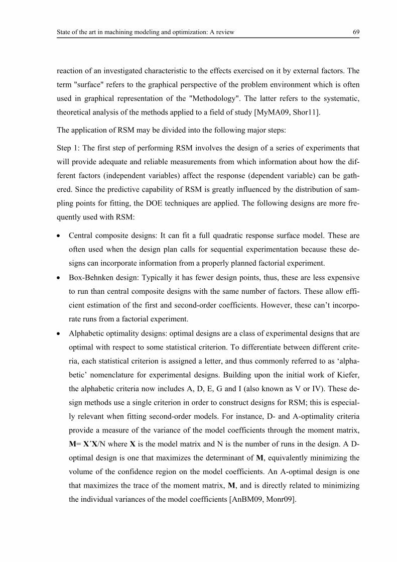
State of the art in machining modeling and optimization: A review 69
reaction of an investigated characteristic to the effects exercised on it by external factors. The
term "surface" refers to the graphical perspective of the problem environment which is often
used in graphical representation of the "Methodology". The latter refers to the systematic,
theoretical analysis of the methods applied to a field of study [MyMA09, Shor11].
The application of RSM may be divided into the following major steps:
Step 1: The first step of performing RSM involves the design of a series of experiments that
will provide adequate and reliable measurements from which information about how the dif-
ferent factors (independent variables) affect the response (dependent variable) can be gath-
ered. Since the predictive capability of RSM is greatly influenced by the distribution of sam-
pling points for fitting, the DOE techniques are applied. The following designs are more fre-
quently used with RSM:
Central composite designs: It can fit a full quadratic response surface model. These are
often used when the design plan calls for sequential experimentation because these de-
signs can incorporate information from a properly planned factorial experiment.
Box-Behnken design: Typically it has fewer design points, thus, these are less expensive
to run than central composite designs with the same number of factors. These allow effi-
cient estimation of the first and second-order coefficients. However, these can’t incorpo-
rate runs from a factorial experiment.
Alphabetic optimality designs: optimal designs are a class of experimental designs that are
optimal with respect to some statistical criterion. To differentiate between different crite-
ria, each statistical criterion is assigned a letter, and thus commonly referred to as ‘alpha-
betic’ nomenclature for experimental designs. Building upon the initial work of Kiefer,
the alphabetic criteria now includes A, D, E, G and I (also known as V or IV). These de-
sign methods use a single criterion in order to construct designs for RSM; this is especial-
ly relevant when fitting second-order models. For instance, D- and A-optimality criteria
provide a measure of the variance of the model coefficients through the moment matrix,
M= X´X/N where X is the model matrix and N is the number of runs in the design. A D-
optimal design is one that maximizes the determinant of M, equivalently minimizing the
volume of the confidence region on the model coefficients. An A-optimal design is one
that maximizes the trace of the moment matrix, M, and is directly related to minimizing
the individual variances of the model coefficients [AnBM09, Monr09].
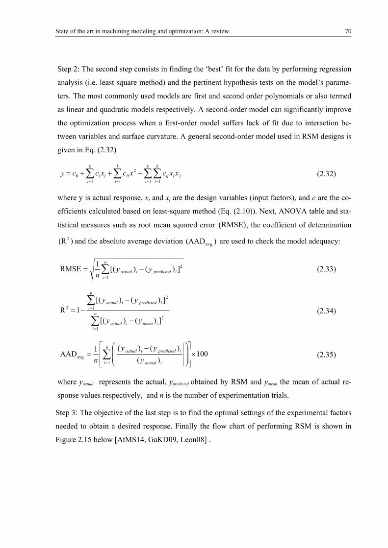
State of the art in machining modeling and optimization: A review 70
Step 2: The second step consists in finding the ‘best’ fit for the data by performing regression
analysis (i.e. least square method) and the pertinent hypothesis tests on the model’s parame-
ters. The most commonly used models are first and second order polynomials or also termed
as linear and quadratic models respectively. A second-order model can significantly improve
the optimization process when a first-order model suffers lack of fit due to interaction be-
tween variables and surface curvature. A general second-order model used in RSM designs is
given in Eq. (2.32)
ji
k
i
k
iij
k
iiii
k
ii xxcxcxccy
1 1
2
110 (2.32)
where y is actual response, xi and xj are the design variables (input factors), and c are the co-
efficients calculated based on least-square method (Eq. (2.10)). Next, ANOVA table and sta-
tistical measures such as root mean squared error (RMSE), the coefficient of determination
)(R 2 and the absolute average deviation )(AADavg. are used to check the model adequacy:
n
iipredictediactual yy
n 1
2])()[(1
RMSE (2.33)
n
iimeaniactual
n
iipredictediactual
yy
yy
1
2
1
2
2
])()[(
])()[(1R (2.34)
100)(
)()(1AAD
1avg.
n
i iactual
ipredictediactual
y
yy
n (2.35)
where yactual represents the actual, ypredicted obtained by RSM and ymean the mean of actual re-
sponse values respectively, and n is the number of experimentation trials.
Step 3: The objective of the last step is to find the optimal settings of the experimental factors
needed to obtain a desired response. Finally the flow chart of performing RSM is shown in
Figure 2.15 below [AtMS14, GaKD09, Leon08] .
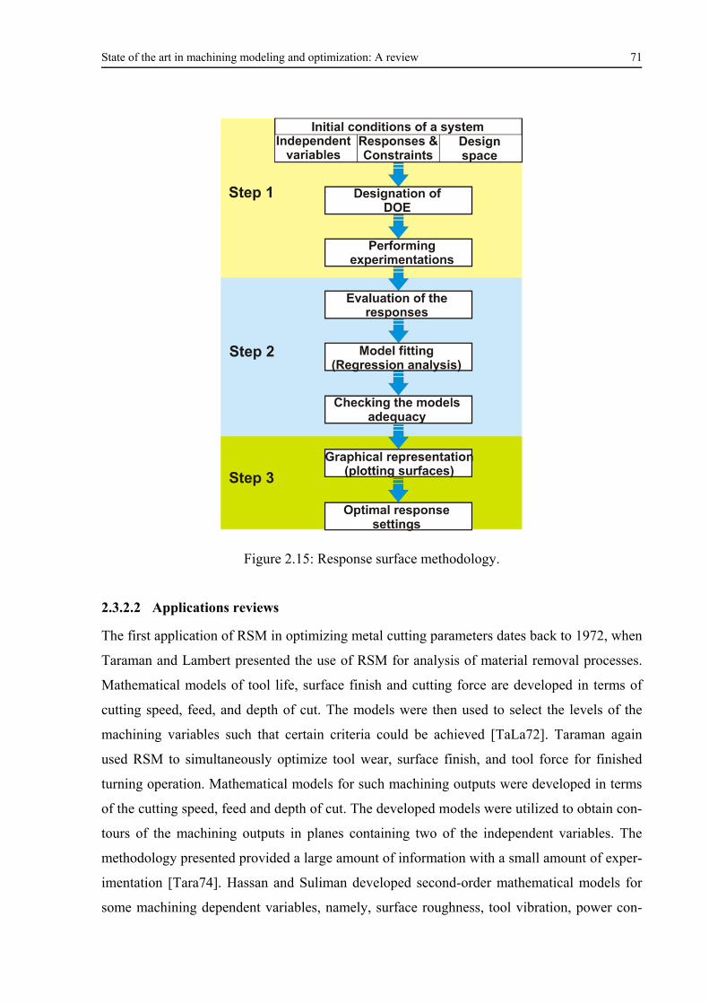
State of the art in machining modeling and optimization: A review 71
Figure 2.15: Response surface methodology.
2.3.2.2 Applications reviews
The first application of RSM in optimizing metal cutting parameters dates back to 1972, when
Taraman and Lambert presented the use of RSM for analysis of material removal processes.
Mathematical models of tool life, surface finish and cutting force are developed in terms of
cutting speed, feed, and depth of cut. The models were then used to select the levels of the
machining variables such that certain criteria could be achieved [TaLa72]. Taraman again
used RSM to simultaneously optimize tool wear, surface finish, and tool force for finished
turning operation. Mathematical models for such machining outputs were developed in terms
of the cutting speed, feed and depth of cut. The developed models were utilized to obtain con-
tours of the machining outputs in planes containing two of the independent variables. The
methodology presented provided a large amount of information with a small amount of exper-
imentation [Tara74]. Hassan and Suliman developed second-order mathematical models for
some machining dependent variables, namely, surface roughness, tool vibration, power con-
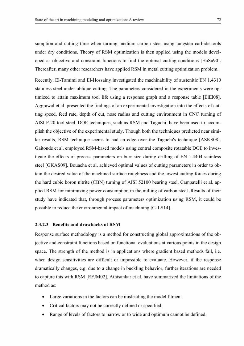
State of the art in machining modeling and optimization: A review 72
sumption and cutting time when turning medium carbon steel using tungsten carbide tools
under dry conditions. Theory of RSM optimization is then applied using the models devel-
oped as objective and constraint functions to find the optimal cutting conditions [HaSu90].
Thereafter, many other researchers have applied RSM in metal cutting optimization problem.
Recently, El-Tamimi and El-Hossainy investigated the machinability of austenitic EN 1.4310
stainless steel under oblique cutting. The parameters considered in the experiments were op-
timized to attain maximum tool life using a response graph and a response table [ElEl08].
Aggrawal et al. presented the findings of an experimental investigation into the effects of cut-
ting speed, feed rate, depth of cut, nose radius and cutting environment in CNC turning of
AISI P-20 tool steel. DOE techniques, such as RSM and Taguchi, have been used to accom-
plish the objective of the experimental study. Though both the techniques predicted near simi-
lar results, RSM technique seems to had an edge over the Taguchi's technique [ASKS08].
Gaitonde et al. employed RSM-based models using central composite rotatable DOE to inves-
tigate the effects of process parameters on burr size during drilling of EN 1.4404 stainless
steel [GKAS09]. Bouacha et al. achieved optimal values of cutting parameters in order to ob-
tain the desired value of the machined surface roughness and the lowest cutting forces during
the hard cubic boron nitrite (CBN) turning of AISI 52100 bearing steel. Campatelli et al. ap-
plied RSM for minimizing power consumption in the milling of carbon steel. Results of their
study have indicated that, through process parameters optimization using RSM, it could be
possible to reduce the environmental impact of machining [CaLS14].
2.3.2.3 Benefits and drawbacks of RSM
Response surface methodology is a method for constructing global approximations of the ob-
jective and constraint functions based on functional evaluations at various points in the design
space. The strength of the method is in applications where gradient based methods fail, i.e.
when design sensitivities are difficult or impossible to evaluate. However, if the response
dramatically changes, e.g. due to a change in buckling behavior, further iterations are needed
to capture this with RSM [RFJM02]. Athisankar et al. have summarized the limitations of the
method as:
Large variations in the factors can be misleading the model fitment.
Critical factors may not be correctly defined or specified.
Range of levels of factors to narrow or to wide and optimum cannot be defined.
State of the art in machining modeling and optimization: A review 73
Lack of use of good statistical principles, and
Over-reliance on computer that make sure the results for good sense [AtMS14].
2.3.3 Nature-inspired meta-heuristic algorithms
Optimization techniques can be grouped into two broad categories: numeric and stochastic
approaches. The first group comprises exact algorithmic methods, with a solid mathematical
foundation, for obtaining the global optimum. Numeric approaches commonly use iterative
algorithms. They include the gradient-based approaches, the descendent method and the sim-
plex algorithm. On the contrary, stochastic optimization tries to imitate some natural process-
es, which, although they do not guarantee the consecution of the global optimum, they allow
good enough solutions to be obtained. These heuristics have a strong random component.
Techniques such as evolutionary algorithms and simulated annealing are included in this
group [QuDa11].
Heuristics is a solution strategy by trial-and-error to produce acceptable solutions to a com-
plex problem in a reasonably practical time. The complexity of the problem of interest makes
it impossible to search every possible solution or combination, the aim is to find good, feasi-
ble solutions in an acceptable timescale. There is no guarantee that the best solutions can be
found, and we even do not know whether an algorithm will work and why if it does work. The
idea is that an efficient but practical algorithm that will work most of the time and be able to
produce good quality solutions. Among the found quality solutions, it is expected that some of
them are nearly optimal, though there is no guarantee for such optimality [Yang10a].
Further development over the heuristic algorithms is the so-called meta-heuristic algorithms.
Here meta- means ‘beyond’ or ‘higher level’ and they generally perform better than simple
heuristics [Yang14a]. Meta-heuristics, in their original definition, are solution methods that
orchestrate an interaction between local improvement procedures and higher level strategies
to create a process capable of escaping from local optima and performing a robust search of a
solution space. Over time, these methods have also come to include any procedures that em-
ploy strategies for overcoming the trap of local optimality in complex solution spaces, espe-
cially those procedures that utilize one or more neighborhood structures as a means of defin-
ing admissible moves to transition from one solution to another, or to build or destroy solu-
tions in constructive and destructive processes [GePo10].
State of the art in machining modeling and optimization: A review 74
In the most generic term, the main source of inspiration for meta-heuristic algorithms is Na-
ture. Therefore, almost all new algorithms can be referred to as nature-inspired. By far the
majority of nature-inspired algorithms are based on some successful characteristics of biolog-
ical system. Therefore, the largest fraction of nature-inspired algorithms is biology-inspired,
or bio-inspired for short. Among bio-inspired algorithms, a special class of algorithms has
been developed by drawing inspiration from swarm intelligence. Therefore, some of the bio-
inspired algorithms can be called swarm-intelligence based. In fact, algorithms based on
swarm intelligence are among the most popular. Good examples are Ant Colony Optimization
[DoCa99], Particle Swarm Optimization [KeEb95], Cuckoo Search [YaDe09], Bat Algorithm
[Yang10b], and Firefly Algorithm [FiYB13, FYBF13, Yang09].
Obviously, not all algorithms were based on biological systems. Many algorithms have been
developed by using inspiration from physical and chemical systems. Some may even be based
on music [Loga01]. Though not all of them are efficient, a few algorithms have proved to be
very efficient and thus have become popular tools for solving real-world problems. Among
these algorithms, many algorithms such as Particle Swarm Optimization, Cuckoo Search and
Firefly Algorithm, have gained popularity due to their high efficiency. In the current litera-
ture, there are about 40 different algorithms. Fister et al. divided all existing algorithms into
four major categories: swarm intelligence-based, bio-inspired (but not SI-based), phys-
ics/chemistry-based, and others [FYBF13]. For the sake of more convenience, five examples
per each of the above categories are shown in Figure 2.16.
Mathematically speaking, it is possible to write an optimization problem in the generic form:
).....,,2,1(),(minimum Mifin
x
x (2.36)
).....,,2,1(,0)(tosubjected Jjj x (2.37)
).....,,2,1(,0)( Kkk x (2.38)
where )(xif , )(xj and )(xk are functions of the design vector
x Tnxxx ).........,,,( 21 (2.39)
where the components ix of x ; are called design or decision variables, and they can be real
continuous, discrete or a mixture of these two. The functions )(xif where ).....,,2,1( Mi are
called the objective functions, and in the case of M = 1, there is only a single objective. The
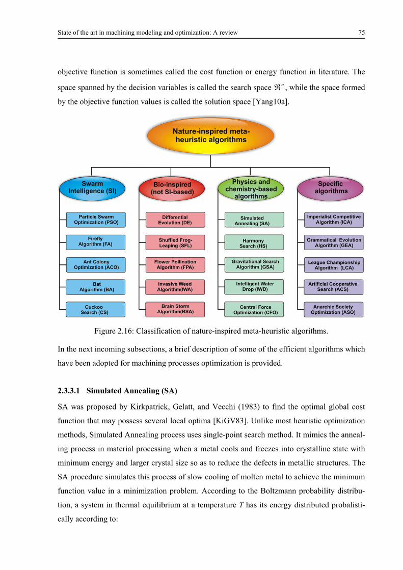
State of the art in machining modeling and optimization: A review 75
objective function is sometimes called the cost function or energy function in literature. The
space spanned by the decision variables is called the search space n , while the space formed
by the objective function values is called the solution space [Yang10a].
Figure 2.16: Classification of nature-inspired meta-heuristic algorithms.
In the next incoming subsections, a brief description of some of the efficient algorithms which
have been adopted for machining processes optimization is provided.
2.3.3.1 Simulated Annealing (SA)
SA was proposed by Kirkpatrick, Gelatt, and Vecchi (1983) to find the optimal global cost
function that may possess several local optima [KiGV83]. Unlike most heuristic optimization
methods, Simulated Annealing process uses single-point search method. It mimics the anneal-
ing process in material processing when a metal cools and freezes into crystalline state with
minimum energy and larger crystal size so as to reduce the defects in metallic structures. The
SA procedure simulates this process of slow cooling of molten metal to achieve the minimum
function value in a minimization problem. According to the Boltzmann probability distribu-
tion, a system in thermal equilibrium at a temperature T has its energy distributed probalisti-
cally according to:
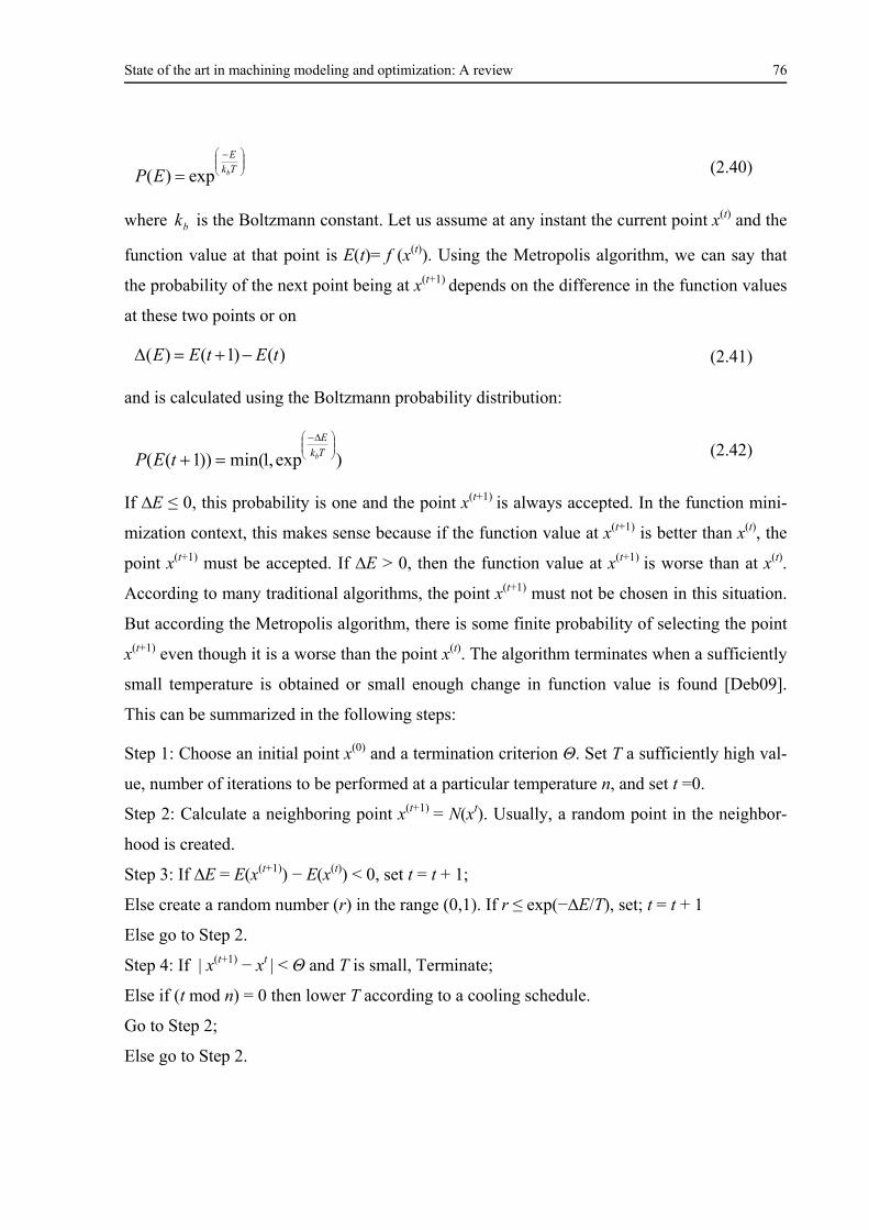
State of the art in machining modeling and optimization: A review 76
Tk
E
bEP exp)( (2.40)
where bk is the Boltzmann constant. Let us assume at any instant the current point x(t) and the
function value at that point is E(t)= f (x(t)). Using the Metropolis algorithm, we can say that
the probability of the next point being at x(t+1) depends on the difference in the function values
at these two points or on
)()1()( tEtEE (2.41)
and is calculated using the Boltzmann probability distribution:
)exp,1min())1((
Tk
E
btEP (2.42)
If ∆E ≤ 0, this probability is one and the point x(t+1) is always accepted. In the function mini-
mization context, this makes sense because if the function value at x(t+1) is better than x(t), the
point x(t+1) must be accepted. If ∆E > 0, then the function value at x(t+1) is worse than at x(t).
According to many traditional algorithms, the point x(t+1) must not be chosen in this situation.
But according the Metropolis algorithm, there is some finite probability of selecting the point
x(t+1) even though it is a worse than the point x(t). The algorithm terminates when a sufficiently
small temperature is obtained or small enough change in function value is found [Deb09].
This can be summarized in the following steps:
Step 1: Choose an initial point x(0) and a termination criterion Θ. Set T a sufficiently high val-
ue, number of iterations to be performed at a particular temperature n, and set t =0.
Step 2: Calculate a neighboring point x(t+1) = N(xt). Usually, a random point in the neighbor-
hood is created.
Step 3: If ∆E = E(x(t+1)) − E(x(t)) < 0, set t = t + 1;
Else create a random number (r) in the range (0,1). If r ≤ exp(−∆E/T), set; t = t + 1
Else go to Step 2.
Step 4: If | x(t+1) − xt | < Θ and T is small, Terminate;
Else if (t mod n) = 0 then lower T according to a cooling schedule.
Go to Step 2;
Else go to Step 2.
State of the art in machining modeling and optimization: A review 77
Despite the numerous capabilities of SA, its application in optimization of cutting conditions
for various machining performances was given less attention by researchers. Earlier, Chen
and Tsai developed an optimization algorithm based on the SA algorithm and the Hooke-
Jeeves pattern search (PS) for optimization of multi-pass turning operations. Experimental
results indicate that the proposed nonlinear constrained optimization algorithm, named
SA/PS, is effective for solving complex machining optimization problems [ChTs96]. Khan et
al. have concluded that Genetic Algorithm (GA), SA and the continuous SA which are non-
gradient based optimization techniques are reliable and accurate for solving machining opti-
mization problems and offer certain advantages over gradient based methods [KhPS97]. Juan
et al. applied SA to the polynomial network to determine the optimal cutting parameters for
minimum production cost in high speed machining SKD61 tool steels [JuYL03]. Wnag et al.
used Genetic Simulated Annealing (GSA), which is a hybrid of GA and SA, to determine op-
timal machining parameters for milling operations. For comparison, basic GA is also chosen
as another optimization method. An application example that has previously been solved us-
ing geometric programming method is presented. The results indicate that GSA is more effi-
cient than GA and geometric programming in the application of cutting optimization
[WaWR04]. Zain et al. presented the estimation of the optimal effect of the radial rake angle
of the tool, combined with cutting speed and feed in influencing the surface roughness result
during end milling Ti-6Al-4V alloy. They concluded that SA is an effective tool for estimat-
ing the minimum surface roughness values as compared to the experimental and regression
modeling results [ZaHS10].
2.3.3.2 Accelerated Particle Swarm Optimization (APSO)
Particle Swarm Optimization (PSO) was developed by Kennedy and Eberhard (1995) based
on the swarm behavior such as fish and bird schooling in nature [KeEb95]. Since then, PSO
has generated much wider interests and forms an exciting, ever expanding research subject
called swarm intelligence. This algorithm searches the space of an objective function by ad-
justing the trajectories of individual agents, called particles, as the piecewise paths formed by
positional vectors in a quasi-stochastic manner.
The PSO selects a number of particles to represent a swarm. Each particle in the swarm is a
potential solution to the optimization problem under consideration. A particle explores the
search domain by moving around. This move is decided by making use of its own experience
and the collective experience of the swarm. Each particle has three main parameters: position,
State of the art in machining modeling and optimization: A review 78
velocity, and fitness. Position represents the decision variables of the optimization problem,
velocity determines the rate of change of the position, and fitness is the value of the objective
function at the particle’s current position. The fitness value is a measure of how good is the
solution it represents for the optimization problem [YaKa13].
The movement of a swarming particle consists of two major components: a stochastic com-
ponent and a deterministic component. Each particle is attracted toward the position of the
current global best g*and its own best location *ix in history, while at the same time it has a
tendency to move randomly. Let xi and vi be the position vector and velocity of particle i, re-
spectively. The new velocity vector is determined by the following formula:
)()( *2
*1
1 ti
tii
ti
ti xgxxvv (2.43)
Where 1 and 2 are two random vectors drawn from a uniform distribution and ς is the ran-
domization factor. The parameters ς and Ω are the learning parameters and acceleration con-
stants, which can typically be taken as, say, ς = Ω =2. The initial locations of all particles
should be distributed relatively uniformly so that they can sample over most regions, which is
especially important for multimodal problems. The initial velocity of a particle can be taken
as zero, i.e., 00 tiv [YaKa13]. The new positions can then be updated by:
11 ti
ti
ti vxx (2.44)
In Figure 2.17, a flowchart of the standard PSO algorithm is shown.
PSO is now widely used in solving tough optimization problems due to its low computational
complexity, easy implementation and relatively few parameters. However, PSO also has sev-
eral major shortcomings; it may suffer from premature convergence for highly multimodal
problems. To overcome this, there are many PSO variants, which have been formed mainly by
slight variations of certain terms and parameters in the PSO, especially by introducing inertia
parameter and by hybridizing with other algorithms. Among many variants of PSO, the most
noticeable improvement is possibly the use of inertia function Λ(t) so that tiv is replaced by
tivt)( :
)()()( *2
*1
1 ti
tii
ti
ti xgxxvtv (2.45)
where Λ takes the value between 0 and 1. In the simplest case, the inertia function can be tak-
en as a constant, typically Λ≈ 0.5 − 0.9.
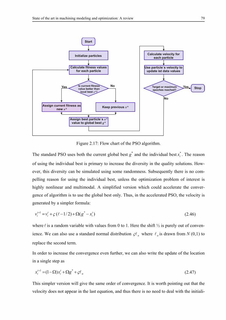
State of the art in machining modeling and optimization: A review 79
Figure 2.17: Flow chart of the PSO algorithm.
The standard PSO uses both the current global best g* and the individual best *ix . The reason
of using the individual best is primary to increase the diversity in the quality solutions. How-
ever, this diversity can be simulated using some randomness. Subsequently there is no com-
pelling reason for using the individual best, unless the optimization problem of interest is
highly nonlinear and multimodal. A simplified version which could accelerate the conver-
gence of algorithm is to use the global best only. Thus, in the accelerated PSO, the velocity is
generated by a simpler formula:
)()2/1( *1 ti
ti
ti xgvv (2.46)
where is a random variable with values from 0 to 1. Here the shift ½ is purely out of conven-
ience. We can also use a standard normal distribution n where n is drawn from N (0,1) to
replace the second term.
In order to increase the convergence even further, we can also write the update of the location
in a single step as
nti
ti gxx *1 )1( (2.47)
This simpler version will give the same order of convergence. It is worth pointing out that the
velocity does not appear in the last equation, and thus there is no need to deal with the initiali-
State of the art in machining modeling and optimization: A review 80
zation of velocity vectors. Therefore, the accelerated PSO is much simpler to implement. Here
the randomization term n provides the ability for the system to escape any local optima if
is chosen to be consistent with the scales of the problem of interest [Yang14a].
Many researchers and practitioners used PSO in metal cutting process parameter optimization
problems. Chandrasekaran et al. reviewed the application of major soft computing tools such
as neural networks, fuzzy sets, GA, SA, ACO, and PSO to four traditional machining pro-
cesses, namely turning, milling, drilling, and grinding. The paper highlights the progress
made in this area and discusses the issues that need to be addressed [CMKD10]. Costa et al.
addressed the machining economies problem concerning the multi-pass turning by a Hybrid
Particle Swarm Optimization technique (HPSO). The significant outcomes of the research
highlighted that HPSO can be taken into account as a useful and powerful technique for opti-
mizing machining problems [CoCF11]. Yusup et al. gave an overview of PSO techniques to
optimize machining process parameter of both traditional and modern machining from 2007
to 2011. From their review, the most machining process considered in PSO was multi-pass
turning while the most considered machining performance was production costs [YuZH12].
Escamilla-Salazar et al. used PSO to optimize machining parameters in high speed milling
processes where multiple conflicting objectives are presented. The relationships between ma-
chining parameters and the performance measures of interest are obtained by using experi-
mental data and a hybrid system using a PSO and a neural network. Results showed that PSO
is an effective method for solving multi-objective optimization problems and also that an in-
tegrated system of neural networks and swarm intelligence can be used to solve complex ma-
chining optimization problems [ETGZ13]. Recently, Marco et al. presented a proposal, how
to successfully gain optimal cutting parameters for certain performances using PSO
[MSTM14].
2.3.3.3 Firefly Algorithm (FA)
FA is one of the recent swarm intelligence methods developed by Yang in 2008 and is a kind
of stochastic, nature-inspired, meta-heuristic algorithm that can be applied for solving the
hardest optimization problems. The algorithm is inspired by the flashing lights of fireflies in
nature. Such flashing light may serve as the primary courtship signals for mating. Besides
attracting mating partners, the flashing light may also serve to warn off potential predators.
The algorithm has been formulated by assuming:

State of the art in machining modeling and optimization: A review 81
All fireflies are unisex so that one firefly will be attracted to other fireflies regardless of
their sex.
Attractiveness is proportional to their light intensities. The less bright will be moving to-
wards the brighter one. It will move randomly if there is no brighter one.
The brightness of a firefly is affected or determined by the landscape of the objective
function.
The light intensity and attractiveness are in some way synonymous. While the intensity is
referred to as an absolute measure of emitted light by the firefly, the attractiveness is a relative
measure of the light that should be seen in the eyes of the beholders and judged by other fire-
flies. The attractiveness )( ra and light intensities I )( r of each firefly are considered to
decrease monotonically depending on the distance r as:
2
0)( raes aa
(2.48)
2
0)( raeIsI tt
(2.49)
where 0a and
0tI denote the maximum attractiveness and light intensities respectively (i.e.
at δr = 0), and γa is the light absorption coefficient, which controls the decrease of the light
intensity. The light intensity It of a firefly representing the solution xi and is proportional to
the value of fitness function )()( iit xfxI . The distance between any two fireflies xi and xj is
expressed as the Euclidean distance by the base Firefly Algorithm, as follows:
m
ij
dk
kjkikjir xxxx
1
2)( (2.50)
where dm denotes the dimensionality of the problem. The movement of the i-th firefly is at-
tracted to another more attractive firefly j. In this manner, the following equation is applied:
grandijaii xxess ijra
)(2
01 (2.51)
where g is a random number drawn from Gaussian distribution and rand is the randomiza-
tion parameter.
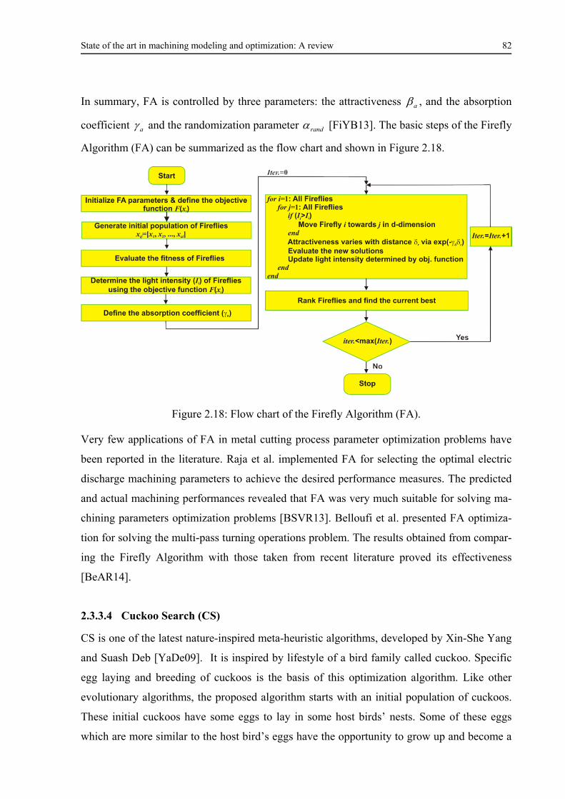
State of the art in machining modeling and optimization: A review 82
In summary, FA is controlled by three parameters: the attractiveness a , and the absorption
coefficient a and the randomization parameter rand [FiYB13]. The basic steps of the Firefly
Algorithm (FA) can be summarized as the flow chart and shown in Figure 2.18.
Figure 2.18: Flow chart of the Firefly Algorithm (FA).
Very few applications of FA in metal cutting process parameter optimization problems have
been reported in the literature. Raja et al. implemented FA for selecting the optimal electric
discharge machining parameters to achieve the desired performance measures. The predicted
and actual machining performances revealed that FA was very much suitable for solving ma-
chining parameters optimization problems [BSVR13]. Belloufi et al. presented FA optimiza-
tion for solving the multi-pass turning operations problem. The results obtained from compar-
ing the Firefly Algorithm with those taken from recent literature proved its effectiveness
[BeAR14].
2.3.3.4 Cuckoo Search (CS)
CS is one of the latest nature-inspired meta-heuristic algorithms, developed by Xin-She Yang
and Suash Deb [YaDe09]. It is inspired by lifestyle of a bird family called cuckoo. Specific
egg laying and breeding of cuckoos is the basis of this optimization algorithm. Like other
evolutionary algorithms, the proposed algorithm starts with an initial population of cuckoos.
These initial cuckoos have some eggs to lay in some host birds’ nests. Some of these eggs
which are more similar to the host bird’s eggs have the opportunity to grow up and become a

State of the art in machining modeling and optimization: A review 83
mature cuckoo. Other eggs are detected by host birds and are killed. The grown eggs reveal
the suitability of the nests in that area. The more eggs survive in an
Each cuckoo lays one egg at a time, and dumps its egg in a randomly chosen nest;
The best nest with high-quality eggs will be carried over to the next generation;
The number of available host nests is fixed, and the egg laid by a cuckoo is discovered by
the host bird with a probability ap between 0 and 1. In this case, the host bird can either
get rid of the egg, or simply abandon the nest and build a completely new nest.
The CS algorithm uses a balanced combination of a local random walk and the global ex-
plorative random walk, controlled by a switching parameter ap . The local random walk can
be written as
)()(1 tk
tjaz
ti
ti xxpHxx (2.52)
where tjx and t
kx are two different solutions selected randomly by random permutation, H( )
is a Heaviside function and is a random number drawn from a uniform distribution. On the
other hand, the global random walk is carried out by using Lévy flights
),,(1 sLxx zti
ti (2.53)
where is the expectation of occurrence and s is the step length, and
)0(1)2/sin()(
),( 01
ss
ssL
(2.54)
Here 0z is the step size scaling factor, which should be related to the scales of the prob-
lem of interest. The above equation is essentially the stochastic equation for a random walk.
In general, a random walk is a Markov chain whose next state/location only depends on the
current location (the first term in the above equation) and the transition probability (the sec-
ond term). However, a substantial fraction of the new solutions should be generated by far
field randomization and their locations should be far enough from the current best solution;
this will make sure that the system will not be trapped in a local optimum [Yang14b]. Based
on the previous descriptions, the basic steps of the CS algorithm can be summarized as flow
chart and is shown in Figure 2.19.
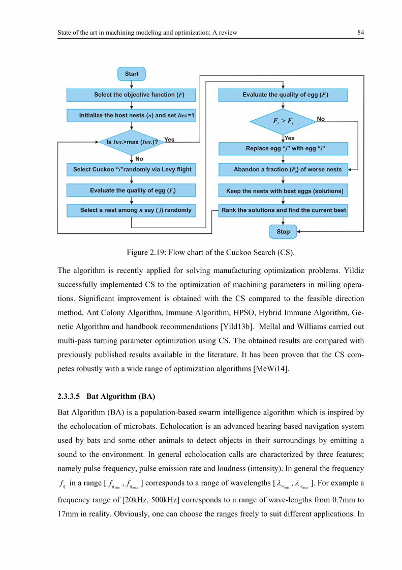
State of the art in machining modeling and optimization: A review 84
Figure 2.19: Flow chart of the Cuckoo Search (CS).
The algorithm is recently applied for solving manufacturing optimization problems. Yildiz
successfully implemented CS to the optimization of machining parameters in milling opera-
tions. Significant improvement is obtained with the CS compared to the feasible direction
method, Ant Colony Algorithm, Immune Algorithm, HPSO, Hybrid Immune Algorithm, Ge-
netic Algorithm and handbook recommendations [Yild13b]. Mellal and Williams carried out
multi-pass turning parameter optimization using CS. The obtained results are compared with
previously published results available in the literature. It has been proven that the CS com-
petes robustly with a wide range of optimization algorithms [MeWi14].
2.3.3.5 Bat Algorithm (BA)
Bat Algorithm (BA) is a population-based swarm intelligence algorithm which is inspired by
the echolocation of microbats. Echolocation is an advanced hearing based navigation system
used by bats and some other animals to detect objects in their surroundings by emitting a
sound to the environment. In general echolocation calls are characterized by three features;
namely pulse frequency, pulse emission rate and loudness (intensity). In general the frequency
qf in a range [minqf ,
maxqf ] corresponds to a range of wavelengths [minw ,
maxw ]. For example a
frequency range of [20kHz, 500kHz] corresponds to a range of wave-lengths from 0.7mm to
17mm in reality. Obviously, one can choose the ranges freely to suit different applications. In

State of the art in machining modeling and optimization: A review 85
order to develop a standard Bat Algorithm, the following approximate or idealized rules are
applied:
All bats use echolocation to sense distance, and they also ‘know’ the difference between
food/prey and background barriers in some magical way;
Bats fly randomly with velocity vi at position xi with a frequencyminqf , varying wavelength
and loudness 0l
A to search for prey. They can automatically adjust the wavelength (or fre-
quency) of their emitted pulses and adjust the rate of pulse emission r ∊ [0, 1], depend-
ing on the proximity of their target;
Although the loudness can vary in many ways, we assume that the loudness varies from a
large (positive) 0l
A to a minimum constant value minlA .
For the bats in simulations, we have to define the rules how their positions xi and velocities vi
in a d-dimensional search space are updated. The new solutions tix and velocities t
iv at time
step t are given by:
rqqqq ffffi
)(minmaxmin
(2.55)
iqti
ti
ti fxxvv )( *1 (2.56)
ti
ti
ti vxx 1 (2.57)
where r ∈ [0, 1] is a random vector drawn from a uniform distribution. Here x* is the current
global best location (solution) which is located after comparing all the solutions among all the
n bats at each iteration t. The loudness and pulse rate can vary with iteration t in the following
way:
tl
tl ii
ACA 11 (2.58)
)exp(1 201 tCir
tri
(2.59)
Here C1 and C2 are constants. In fact, C1 is similar to the cooling factor of a cooling schedule
in the SA, which is discussed earlier. In the simplest case, we can use C1= C2, and in fact C1 =
C2 =0.9 can be used in most simulations.
Bat Algorithm has been extended to Multi-Objective Bat Algorithm (MOBA) by Yang, and
preliminary results suggested that it is very efficient [YaHo12, YaKa13, Yang10b, Yang11,
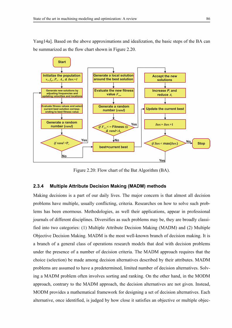
State of the art in machining modeling and optimization: A review 86
Yang14a]. Based on the above approximations and idealization, the basic steps of the BA can
be summarized as the flow chart shown in Figure 2.20.
Figure 2.20: Flow chart of the Bat Algorithm (BA).
2.3.4 Multiple Attribute Decision Making (MADM) methods
Making decisions is a part of our daily lives. The major concern is that almost all decision
problems have multiple, usually conflicting, criteria. Researches on how to solve such prob-
lems has been enormous. Methodologies, as well their applications, appear in professional
journals of different disciplines. Diversifies as such problems may be, they are broadly classi-
fied into two categories: (1) Multiple Attribute Decision Making (MADM) and (2) Multiple
Objective Decision Making. MADM is the most well-known branch of decision making. It is
a branch of a general class of operations research models that deal with decision problems
under the presence of a number of decision criteria. The MADM approach requires that the
choice (selection) be made among decision alternatives described by their attributes. MADM
problems are assumed to have a predetermined, limited number of decision alternatives. Solv-
ing a MADM problem often involves sorting and ranking. On the other hand, in the MODM
approach, contrary to the MADM approach, the decision alternatives are not given. Instead,
MODM provides a mathematical framework for designing a set of decision alternatives. Each
alternative, once identified, is judged by how close it satisfies an objective or multiple objec-
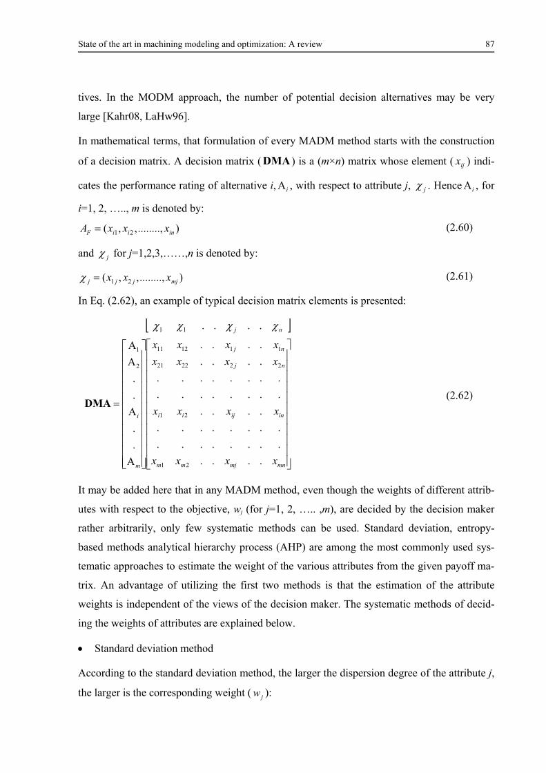
State of the art in machining modeling and optimization: A review 87
tives. In the MODM approach, the number of potential decision alternatives may be very
large [Kahr08, LaHw96].
In mathematical terms, that formulation of every MADM method starts with the construction
of a decision matrix. A decision matrix ( DMA ) is a (m×n) matrix whose element ( ijx ) indi-
cates the performance rating of alternative i, i , with respect to attribute j, j . Hence i , for
i=1, 2, ….., m is denoted by:
(2.60)
and j for j=1,2,3,……,n is denoted by:
(2.61)
In Eq. (2.62), an example of typical decision matrix elements is presented:
mnmjmm
inijii
nj
nj
m
i
nj
xxxx
xxxx
xxxx
xxxx
....
........
........
....
........
........
....
....
.
.
.
.
....
21
21
222221
111211
2
1
11
DMA
(2.62)
It may be added here that in any MADM method, even though the weights of different attrib-
utes with respect to the objective, wj (for j=1, 2, ….. ,m), are decided by the decision maker
rather arbitrarily, only few systematic methods can be used. Standard deviation, entropy-
based methods analytical hierarchy process (AHP) are among the most commonly used sys-
tematic approaches to estimate the weight of the various attributes from the given payoff ma-
trix. An advantage of utilizing the first two methods is that the estimation of the attribute
weights is independent of the views of the decision maker. The systematic methods of decid-
ing the weights of attributes are explained below.
Standard deviation method
According to the standard deviation method, the larger the dispersion degree of the attribute j,
the larger is the corresponding weight ( jw ):
)........,,,( 21 iniiF xxxA
)........,,,( 21 mjjjj xxx
State of the art in machining modeling and optimization: A review 88
n
jj
jj
STDV
STDVw
1
(2.63)
where jSTDV represent the standard deviation of the j attribute.
Entropy method
Shannon and Weaver [ShWe49] proposed the entropy concept and this concept has been high-
lighted by Zeleny [Zele98] for deciding the objective weights of attributes. Entropy is a meas-
ure of uncertainty in the information formulated using probability theory. It indicates that a
broad distribution represents more uncertainty than does a sharply peaked one. The process of
calculation of Entropy weights can be divided into the following steps:
Step1: For a given normalized DMA, ijr , estimate entropy Ej of the set of alternatives for at-
tribute j:
)ln()ln(
1
1ij
m
iijj rr
mE
(2.64)
for i =1, 2,…., m and j=1, 2, ...., n.
Step 2: Compute degree of diversification jDV of the information provided by the outcomes
of attribute j:
jj EDV 1 (2.65)
Step 3: Normalized weights of the criterion are
n
jj
jj
DV
DVw
1
(2.66)
If the entropy value is high, the uncertainty contained in the criterion vector is high (Step 1),
diversification of the information is low (Step 2) and correspondingly the criterion is less im-
portant (Step 3).
AHP
As mentioned before, both of the standard deviation method and entropy method calculate the
objective weights of the attributes without giving any consideration to the preferences of the
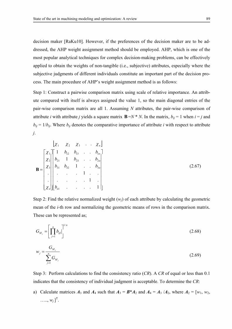
State of the art in machining modeling and optimization: A review 89
decision maker [RaKu10]. However, if the preferences of the decision maker are to be ad-
dressed, the AHP weight assignment method should be employed. AHP, which is one of the
most popular analytical techniques for complex decision-making problems, can be effectively
applied to obtain the weights of non-tangible (i.e., subjective) attributes, especially where the
subjective judgments of different individuals constitute an important part of the decision pro-
cess. The main procedure of AHP’s weight assignment method is as follows:
Step 1: Construct a pairwise comparison matrix using scale of relative importance. An attrib-
ute compared with itself is always assigned the value 1, so the main diagonal entries of the
pair-wise comparison matrix are all 1. Assuming N attributes, the pair-wise comparison of
attribute i with attribute j yields a square matrix B =N * N. In the matrix, bij = 1 when i = j and
bij = 1/bij. Where bij denotes the comparative importance of attribute i with respect to attribute
j.
1....
.1....
..1...
..1
..1
..1
.
.
..
1
33231
22321
11312
3
2
1
321
n
n
n
n
n
n
b
bbb
bbb
bbb
B (2.67)
Step 2: Find the relative normalized weight (wj) of each attribute by calculating the geometric
mean of the i-th row and normalizing the geometric means of rows in the comparison matrix.
These can be represented as;
nn
jijlM bG
j
/1
1
(2.68)
n
jM
M
j
j
j
G
Gw
1
(2.69)
Step 3: Perform calculations to find the consistency ratio (CR). A CR of equal or less than 0.1
indicates that the consistency of individual judgment is acceptable. To determine the CR:
a) Calculate matrices A3 and A4 such that A3 = B*A2 and A4 = A3 /A2, where A2 = [w1, w2,
….., wj ]T.
State of the art in machining modeling and optimization: A review 90
b) Determine the maximum Eigen value λmax that is the average of matrix A4.
c) Calculate the consistency index (CI) using:
1max
n
nCI
(2.70)
d) Calculate the CR:
RI
CICR (2.71)
where RI is the random index .
The next incoming subsections will focus on the MADM methods whose number of alterna-
tives has been predetermined. Through which, the decision maker is guided to se-
lect/prioritize/rank a finite number of courses of action.
2.3.4.1 Technique for Order Preference by Similarity to Ideal Solution (TOPSIS)
Multiple attribute decision making methods such as Technique for Order Preference by Simi-
larity to Ideal Solution (TOPSIS) is utilized to convert the multi-objective optimization of
many objectives into a single objective optimization problem. The technique is based on the
concept that the chosen alternative should have the shortest Euclidean distance from the ideal
solution. The ideal solution is a hypothetical solution for which all attribute values correspond
to the maximum attribute values in the database comprising the satisfying solutions; the nega-
tive-ideal solution is the hypothetical solution for which all attribute values correspond to the
minimum attribute values in the above-mentioned database. TOPSIS, thus, gives a solution
that is not only closest to the hypothetically best, but which is also farthest from the hypothet-
ically worst. The steps involved for calculating the TOPSIS values are as follows:
Step 1: Formulate the multi-performance problem in DM format as per Eq. (2.62).
Step 2: Construct the normalized decision matrix, Rij whose elements can be represented as:
m
iij
ijij
x
xr
1
2
(2.72)
Step 3: Construct the weighted normalised decision matrix. This is obtained by the multiplica-
tion of each element of the column of the matrix Rij with its associated weight wj. Hence, the
elements of the weighted normalized matrix are expressed as:
State of the art in machining modeling and optimization: A review 91
ijjij rw (2.73)
Step 4: Determine the “ideal” (best) and “negative ideal” (worst) solutions. The ideal (best)
and negative ideal (worst) solution can be expressed as:
***
2*1
'*
,...,,...,,solution ideal Positive
,......,2,1,)(min;)(max
nj
ijiiji miforJjifJjif
(2.74)
nj
ijiiji miforJjifJjif
,...,,...,,solution ideal Negative
,......,2,1,)(max;)(min
21
'
(2.75)
Where, J is the set of cost type criteria and J′ is the set of benefit type criteria.
Step 5: Obtain the separation measures. The separation of each alternative from the ideal one
is given by Euclidean distance. Therefore, the separation from positive ideal alternative is:
n
jiijiS
1
2** )( (2.76)
Similarly, the separation from the negative ideal alternative is:
n
jiijiS
1
2)( (2.77)
Step 6: The relative closeness of a particular alternative to the ideal solution Ci* can be evalu-
ated as:
**
ii
ii SS
SC
(2.78)
10;......,,2,1 * iCmi
Step 7: Rank the preference order, so that the alternative that has the shortest distance to the
ideal solution is ranked first [ChSr13, LaHw96, SiDM11].
TOPSIS has been used to solve MADM problem in various scenarios. Rao and Davim sug-
gested a logical procedure based TOPSIS and AHP together to help in selection of a suitable
material from among a large number of available alternative materials for a given engineering
application [RaDa08]. Singh et al. adopted TOPSIS in combination with Taguchi’s robust
design philosophy to optimize multiple surface roughness parameters of machined glass fiber
reinforced polymer [SiDM11]. Sivapirakasam et al. developed a combination of Taguchi and
State of the art in machining modeling and optimization: A review 92
fuzzy TOPSIS methods to solve multi-response parameter optimization problems in green
manufacturing. The model can be used as a systematic framework for parameter optimization
in environmentally conscious manufacturing processes [SiMS11]. Thirumalai and Senthilku-
maar proposed TOPSIS for selecting a single solution from non-dominated solutions obtained
by non-sorted genetic algorithm for multi-objective functions of high-speed machining of
Inconel 718 [ThSe13].
TOPSIS is useful when dealing with a large number of alternatives and attributes, good for
both qualitative and quantitative data, relatively easy and fast. The output can be a preferential
ranking of the candidate materials [JaEd13a]. However, the method based on Euclidean dis-
tance does not consider correlation between indices, thus causing information overlap which,
in turn, affects the decision results. Thus, the reduction of indicator correlation within the ap-
plication often relies on qualitative analysis, the aim being to try to increase index independ-
ence during the process of index screening. These conditions make this approach strongly
subjective [WaWa14].
2.3.4.2 VIKOR method
The VIKOR method was originally introduced in 1998 for multi-criteria optimization of com-
plex systems. It determines the compromise ranking-list, the compromise solution, and the
weight stability intervals for preference stability of the compromise solution obtained with the
initial (given) weights. This method focuses on ranking and selecting from a set of alterna-
tives in the presence of conflicting criteria. It introduces the multi-criteria ranking index based
on the particular measure of ‘‘closeness’’ to the ‘‘ideal’’ solution. It is developed from the
Lp-metric used as an aggregating function in a compromise programming method [Yu73,
Zele98]. The method involves the following steps:
Step 1: Arrange the elements of the MADM problem in DMA format as per Eq. (2.62).
Step 2: Determine the best *ix and the worst
ix values of all attribute functions. If the ith
function represents a benefit then:
ijj
i xx max* (2.79)
ijj
i xx min (2.80)
Step 3: Compute the values of utility measure iS and regret iR measure by the relations:
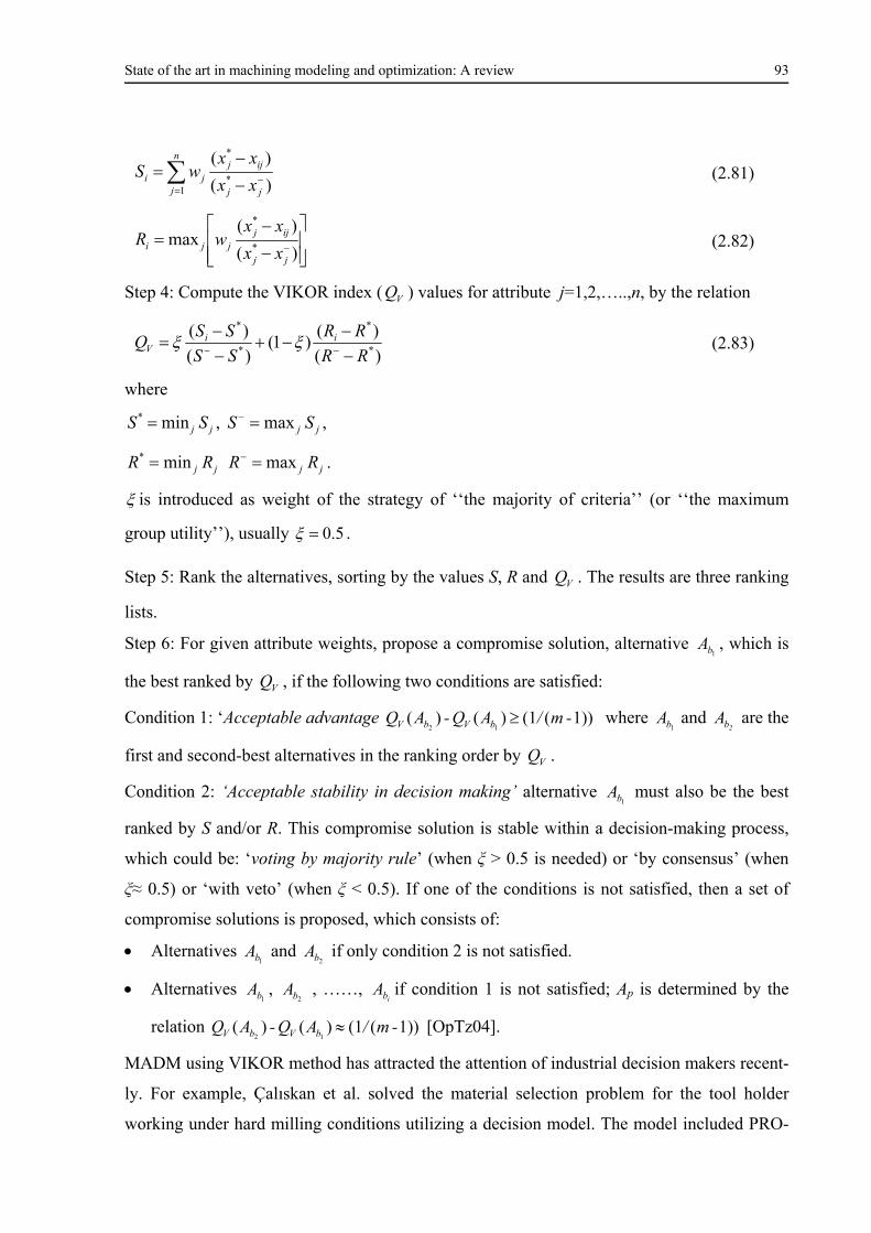
State of the art in machining modeling and optimization: A review 93
)(
)(*
*
1
jj
ijjn
jji xx
xxwS (2.81)
)(
)(max
*
*
jj
ijjjji xx
xxwR (2.82)
Step 4: Compute the VIKOR index ( VQ ) values for attribute j=1,2,…..,n, by the relation
)(
)()1(
)(
)(*
*
*
*
RR
RR
SS
SSQ ii
V
(2.83)
where
jj SS min* , jj SS max ,
jj RR min* jj RR max .
is introduced as weight of the strategy of ‘‘the majority of criteria’’ (or ‘‘the maximum
group utility’’), usually 5.0 .
Step 5: Rank the alternatives, sorting by the values S, R and VQ . The results are three ranking
lists.
Step 6: For given attribute weights, propose a compromise solution, alternative 1bA , which is
the best ranked by VQ , if the following two conditions are satisfied:
Condition 1: ‘Acceptable advantage -m/ AQ-AQ bVbV 1))((1)()(12 where
1bA and 2bA are the
first and second-best alternatives in the ranking order by VQ .
Condition 2: ‘Acceptable stability in decision making’ alternative 1bA must also be the best
ranked by S and/or R. This compromise solution is stable within a decision-making process,
which could be: ‘voting by majority rule’ (when ξ > 0.5 is needed) or ‘by consensus’ (when
ξ≈ 0.5) or ‘with veto’ (when ξ < 0.5). If one of the conditions is not satisfied, then a set of
compromise solutions is proposed, which consists of:
Alternatives 1bA and
2bA if only condition 2 is not satisfied.
Alternatives 1bA ,
2bA , ……, ibA if condition 1 is not satisfied; Ap is determined by the
relation -m/ AQ-AQ bVbV 1))((1)()(12 [OpTz04].
MADM using VIKOR method has attracted the attention of industrial decision makers recent-
ly. For example, Çalıskan et al. solved the material selection problem for the tool holder
working under hard milling conditions utilizing a decision model. The model included PRO-
State of the art in machining modeling and optimization: A review 94
METHEE (Preference Ranking Organization METHod for Enrichment Evaluation), TOPSIS
and VIKOR methods for the ranking of the alternative materials according to determined cri-
teria [ÇKKG13]. Jahan and Edwards presented new VIKOR method for ranking materials
with simultaneous availability of interval data and all types of criteria. It has been shown that
the proposed method is able to address effectively mixed data, with precise and imprecise
values, and with interval data [JaEd13b].
The VIKOR is an effective tool in the MADM, particularly in a situation where the decision
maker is not able, or does not know how to describe his/her preference at the beginning of
system design. The obtained compromise solution can be accepted by the decision maker’s
because it provides a maximum group utility of the majority represented by min S and a min-
imum of the individual regret of the opponent represented by min R. The compromise solu-
tions can be the basis for negotiations containing the decision maker’s preference by criteria
weights [OpTz04]. Although the VIKOR method is an effective tool for MADM problems,
some errors would occur when some attributes have no difference among the alternatives, the
utility measure has no difference among the alternatives and the regret measure has no differ-
ence among the alternatives [Chan10].
2.3.4.3 Grey relational analysis
A system that has none of information is defined as a black system, while a system that is full
of information is called white. Systems between these extremes are described as being grey,
hazy, or fuzzy. Therefore, a grey system means that a system in which a part of information is
known and a part of information is unknown. Grey systems theory was initiated by Deng in
1982. The system has three approaches such as grey relational analysis (GRA), grey cluster-
ing, grey decision making [Julo82, Julo89].
GRA is an impact evaluation model that measures the degree of similarity or difference be-
tween the comparability sequence and the reference sequence based on the grade of relation
known as grey relational grade (GRG) [ChTo07]. So that, if an alternative gets the highest
gray relational grade with the reference sequence, it means that comparability sequence is
most similar to the reference sequence and that alternative would be the best choice [Fung03].
In recent years, the grey relational analysis has become the powerful tool to analyse the pro-
cesses with multiple performance characteristics. It has been widely applied in the last fifteen
years in several research fields [Yin13]. It provides an efficient solution to multi-input and
discrete data problems. In grey relational analysis, the complex multiple response optimiza-
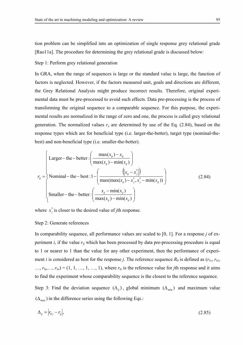
State of the art in machining modeling and optimization: A review 95
tion problem can be simplified into an optimization of single response grey relational grade
[Rao11a]. The procedure for determining the grey relational grade is discussed below:
Step 1: Perform grey relational generation
In GRA, when the range of sequences is large or the standard value is large, the function of
factors is neglected. However, if the factors measured unit, goals and directions are different,
the Grey Relational Analysis might produce incorrect results. Therefore, original experi-
mental data must be pre-processed to avoid such effects. Data pre-processing is the process of
transforming the original sequence to a comparable sequence. For this purpose, the experi-
mental results are normalized in the range of zero and one, the process is called grey relational
generation. The normalized values rij are determined by use of the Eq. (2.84), based on the
response types which are for beneficial type (i.e. larger-the-better), target type (nominal-the-
best) and non-beneficial type (i.e. smaller-the-better).
)min()max(
)min(:bettertheSmaller
))min(,)max(max(1:besttheNominal
)min()max(
)max(:bettertheLarger
**
*
ijij
ijij
ijjjij
jij
ijij
ijij
ij
xx
xx
xxxx
xx
xx
xx
r (2.84)
where *jx is closer to the desired value of jth response.
Step 2: Generate references
In comparability sequence, all performance values are scaled to [0, 1]. For a response j of ex-
periment i, if the value rij which has been processed by data pre-processing procedure is equal
to 1 or nearer to 1 than the value for any other experiment, then the performance of experi-
ment i is considered as best for the response j. The reference sequence R0 is defined as (r01, r02,
…, r0j,…, r0n) = (1, 1, …, 1, …, 1), where r0j is the reference value for jth response and it aims
to find the experiment whose comparability sequence is the closest to the reference sequence.
Step 3: Find the deviation sequence )( ij , global minimum )( min and maximum value
)( max in the difference series using the following Eqs.:
,0 ijjij rr (2.85)
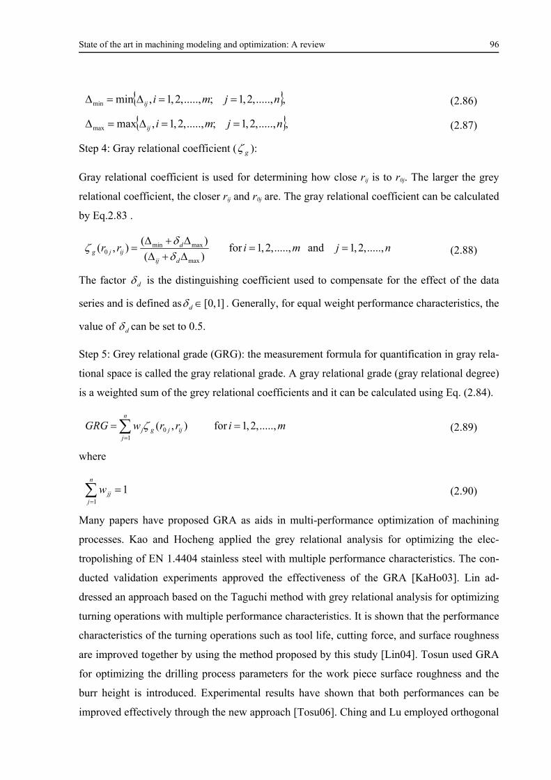
State of the art in machining modeling and optimization: A review 96
,.....,,2,1;.....,,2,1,minmin njmiij (2.86)
,.....,,2,1;.....,,2,1,maxmax njmiij (2.87)
Step 4: Gray relational coefficient ( g ):
Gray relational coefficient is used for determining how close rij is to r0j. The larger the grey
relational coefficient, the closer rij and r0j are. The gray relational coefficient can be calculated
by Eq.2.83 .
njmirrdij
dijjg .....,,2,1and.....,,2,1for
)(
)(),(
max
maxmin0
(2.88)
The factor d is the distinguishing coefficient used to compensate for the effect of the data
series and is defined as ]1,0[d . Generally, for equal weight performance characteristics, the
value of d can be set to 0.5.
Step 5: Grey relational grade (GRG): the measurement formula for quantification in gray rela-
tional space is called the gray relational grade. A gray relational grade (gray relational degree)
is a weighted sum of the grey relational coefficients and it can be calculated using Eq. (2.84).
mirrwGRG ijjg
n
jj .....,,2,1for),( 0
1
(2.89)
where
11
n
jjjw (2.90)
Many papers have proposed GRA as aids in multi-performance optimization of machining
processes. Kao and Hocheng applied the grey relational analysis for optimizing the elec-
tropolishing of EN 1.4404 stainless steel with multiple performance characteristics. The con-
ducted validation experiments approved the effectiveness of the GRA [KaHo03]. Lin ad-
dressed an approach based on the Taguchi method with grey relational analysis for optimizing
turning operations with multiple performance characteristics. It is shown that the performance
characteristics of the turning operations such as tool life, cutting force, and surface roughness
are improved together by using the method proposed by this study [Lin04]. Tosun used GRA
for optimizing the drilling process parameters for the work piece surface roughness and the
burr height is introduced. Experimental results have shown that both performances can be
improved effectively through the new approach [Tosu06]. Ching and Lu employed orthogonal
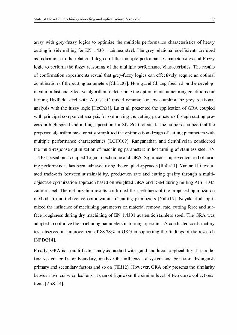
State of the art in machining modeling and optimization: A review 97
array with grey-fuzzy logics to optimize the multiple performance characteristics of heavy
cutting in side milling for EN 1.4301 stainless steel. The grey relational coefficients are used
as indications to the relational degree of the multiple performance characteristics and Fuzzy
logic to perform the fuzzy reasoning of the multiple performance characteristics. The results
of confirmation experiments reveal that grey-fuzzy logics can effectively acquire an optimal
combination of the cutting parameters [ChLu07]. Horng and Chiang focused on the develop-
ment of a fast and effective algorithm to determine the optimum manufacturing conditions for
turning Hadfield steel with Al2O3/TiC mixed ceramic tool by coupling the grey relational
analysis with the fuzzy logic [HoCh08]. Lu et al. presented the application of GRA coupled
with principal component analysis for optimizing the cutting parameters of rough cutting pro-
cess in high-speed end milling operation for SKD61 tool steel. The authors claimed that the
proposed algorithm have greatly simplified the optimization design of cutting parameters with
multiple performance characteristics [LCHC09]. Ranganathan and Senthilvelan considered
the multi-response optimization of machining parameters in hot turning of stainless steel EN
1.4404 based on a coupled Taguchi technique and GRA. Significant improvement in hot turn-
ing performances has been achieved using the coupled approach [RaSe11]. Yan and Li evalu-
ated trade-offs between sustainability, production rate and cutting quality through a multi-
objective optimization approach based on weighted GRA and RSM during milling AISI 1045
carbon steel. The optimization results confirmed the usefulness of the proposed optimization
method in multi-objective optimization of cutting parameters [YaLi13]. Nayak et al. opti-
mized the influence of machining parameters on material removal rate, cutting force and sur-
face roughness during dry machining of EN 1.4301 austenitic stainless steel. The GRA was
adopted to optimize the machining parameters in turning operation. A conducted confirmatory
test observed an improvement of 88.78% in GRG in supporting the findings of the research
[NPDG14].
Finally, GRA is a multi-factor analysis method with good and broad applicability. It can de-
fine system or factor boundary, analyze the influence of system and behavior, distinguish
primary and secondary factors and so on [JiLi12]. However, GRA only presents the similarity
between two curve collections. It cannot figure out the similar level of two curve collections’
trend [ZhXi14].
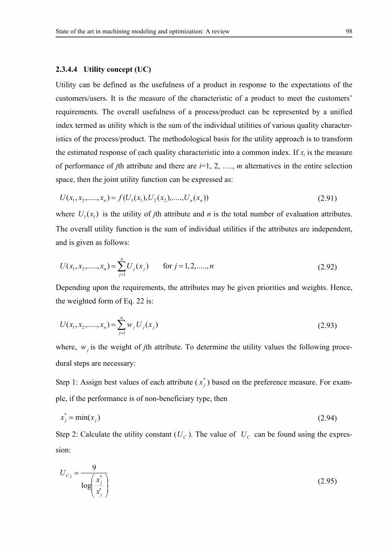
State of the art in machining modeling and optimization: A review 98
2.3.4.4 Utility concept (UC)
Utility can be defined as the usefulness of a product in response to the expectations of the
customers/users. It is the measure of the characteristic of a product to meet the customers’
requirements. The overall usefulness of a process/product can be represented by a unified
index termed as utility which is the sum of the individual utilities of various quality character-
istics of the process/product. The methodological basis for the utility approach is to transform
the estimated response of each quality characteristic into a common index. If xj is the measure
of performance of jth attribute and there are i=1, 2, …., m alternatives in the entire selection
space, then the joint utility function can be expressed as:
))(),.....,(),((),.....,,( 221121 nnn xUxUxUfxxxU (2.91)
where )( 11 xU is the utility of jth attribute and n is the total number of evaluation attributes.
The overall utility function is the sum of individual utilities if the attributes are independent,
and is given as follows:
njxUxxxU j
n
jjn .....,,2,1for)(),.....,,(
121
(2.92)
Depending upon the requirements, the attributes may be given priorities and weights. Hence,
the weighted form of Eq. 22 is:
)(),.....,,(1
21 j
n
jjjn xUwxxxU
(2.93)
where, jw is the weight of jth attribute. To determine the utility values the following proce-
dural steps are necessary:
Step 1: Assign best values of each attribute ( *jx ) based on the preference measure. For exam-
ple, if the performance is of non-beneficiary type, then
)min(*jj xx (2.94)
Step 2: Calculate the utility constant ( CU ). The value of CU can be found using the expres-
sion:
j
j
jC
x
xU
*
log
9
(2.95)
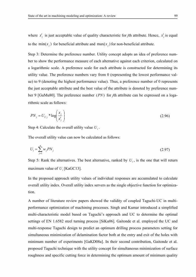
State of the art in machining modeling and optimization: A review 99
where jx is just acceptable value of quality characteristic for jth attribute. Hence, jx is equal
to the )(min jx for beneficial attribute and )(max jx for non-beneficial attribute.
Step 3: Determine the preference number. Utility concept adopts an idea of preference num-
ber to show the performance measure of each alternative against each criterion, calculated on
a logarithmic scale. A preference scale for each attribute is constructed for determining its
utility value. The preference numbers vary from 0 (representing the lowest performance val-
ue) to 9 (denoting the highest performance value). Thus, a preference number of 0 represents
the just acceptable attribute and the best value of the attribute is denoted by preference num-
ber 9 [GuMu80]. The preference number )(PN for jth attribute can be expressed on a loga-
rithmic scale as follows:
j
j
jCj x
xUPN log* (2.96)
Step 4: Calculate the overall utility value iU .
The overall utility value can now be calculated as follows:
j
n
jji PNwU
1
(2.97)
Step 5: Rank the alternatives. The best alternative, ranked by iU , is the one that will return
maximum value of iU [KaGC13].
In the proposed approach utility values of individual responses are accumulated to calculate
overall utility index. Overall utility index servers as the single objective function for optimiza-
tion.
A number of literature review papers showed the validity of coupled Taguchi-UC in multi-
performance optimization of machining processes. Singh and Kumar introduced a simplified
multi-characteristic model based on Taguchi’s approach and UC to determine the optimal
settings of EN 1.6582 steel turning process [SiKu06]. Gaitonde et al. employed the UC and
multi-response Taguchi design to predict an optimum drilling process parameters setting for
simultaneous minimization of delamination factor both at the entry and exit of the holes with
minimum number of experiments [GaKD08a]. In their second contribution, Gaitonde et al.
proposed Taguchi technique with the utility concept for simultaneous minimization of surface
roughness and specific cutting force in determining the optimum amount of minimum quality
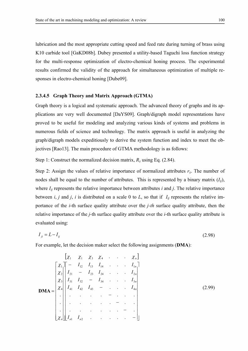
State of the art in machining modeling and optimization: A review 100
lubrication and the most appropriate cutting speed and feed rate during turning of brass using
K10 carbide tool [GaKD08b]. Dubey presented a utility-based Taguchi loss function strategy
for the multi-response optimization of electro-chemical honing process. The experimental
results confirmed the validity of the approach for simultaneous optimization of multiple re-
sponses in electro-chemical honing [Dube09].
2.3.4.5 Graph Theory and Matrix Approach (GTMA)
Graph theory is a logical and systematic approach. The advanced theory of graphs and its ap-
plications are very well documented [DaYS09]. Graph/digraph model representations have
proved to be useful for modeling and analyzing various kinds of systems and problems in
numerous fields of science and technology. The matrix approach is useful in analyzing the
graph/digraph models expeditiously to derive the system function and index to meet the ob-
jectives [Rao13]. The main procedure of GTMA methodology is as follows:
Step 1: Construct the normalized decision matrix, Rij using Eq. (2.84).
Step 2: Assign the values of relative importance of normalized attributes rij. The number of
nodes shall be equal to the number of attributes. This is represented by a binary matrix (Iij),
where Iij represents the relative importance between attributes i and j. The relative importance
between i, j and j, i is distributed on a scale 0 to L, so that if Iij represents the relative im-
portance of the i-th surface quality attribute over the j-th surface quality attribute, then the
relative importance of the j-th surface quality attribute over the i-th surface quality attribute is
evaluated using:
ijji ILI (2.98)
For example, let the decision maker select the following assignments (DMA):
.....
.......
.......
.......
...
...
...
...
.
.
.
...
21
4434241
3343231
2242321
1141312
4
3
2
1
4311
nn
n
n
n
n
n
n
II
IIII
IIII
IIII
IIII
DMA (2.99)
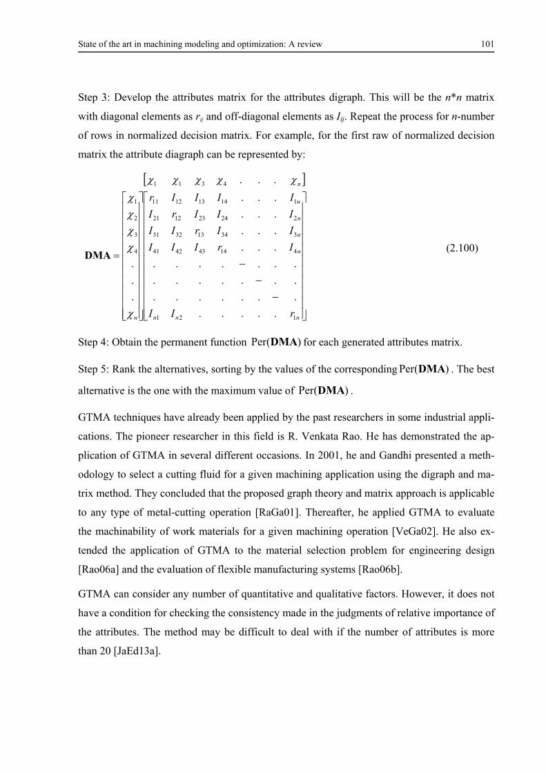
State of the art in machining modeling and optimization: A review 101
Step 3: Develop the attributes matrix for the attributes digraph. This will be the n*n matrix
with diagonal elements as rij and off-diagonal elements as Iij. Repeat the process for n-number
of rows in normalized decision matrix. For example, for the first raw of normalized decision
matrix the attribute diagraph can be represented by:
nnn
n
n
n
n
n
n
rII
IrIII
IIrII
IIIrI
IIIIr
121
414434241
334133231
224231221
114131211
4
3
2
1
4311
.....
.......
.......
.......
...
...
...
...
.
.
.
...
DMA (2.100)
Step 4: Obtain the permanent function )(Per DMA for each generated attributes matrix.
Step 5: Rank the alternatives, sorting by the values of the corresponding )(Per DMA . The best
alternative is the one with the maximum value of )(Per DMA .
GTMA techniques have already been applied by the past researchers in some industrial appli-
cations. The pioneer researcher in this field is R. Venkata Rao. He has demonstrated the ap-
plication of GTMA in several different occasions. In 2001, he and Gandhi presented a meth-
odology to select a cutting fluid for a given machining application using the digraph and ma-
trix method. They concluded that the proposed graph theory and matrix approach is applicable
to any type of metal-cutting operation [RaGa01]. Thereafter, he applied GTMA to evaluate
the machinability of work materials for a given machining operation [VeGa02]. He also ex-
tended the application of GTMA to the material selection problem for engineering design
[Rao06a] and the evaluation of flexible manufacturing systems [Rao06b].
GTMA can consider any number of quantitative and qualitative factors. However, it does not
have a condition for checking the consistency made in the judgments of relative importance of
the attributes. The method may be difficult to deal with if the number of attributes is more
than 20 [JaEd13a].
State of the art in machining modeling and optimization: A review 102
2.4 A systematic methodology for modeling and optimization of
cutting processes
Comprehensive schemes for modeling and optimizing turning process parameters are present-
ed in Figure 2.21 and Figure 2.22, respectively. The schemes also suggest various approaches
suitable for single and multi-objective problems. The detailed steps of the schemes are de-
scribed below.
Step 1: Formulate the cutting process optimization problem spotlighting its significance in
terms of the adopted criteria, such as production cost, quality characteristics and/or process
performance measures.
Step 2: Designate the relevant process decision and response variables. Independent cutting
variables such as cutting and process conditions, tool materials and coatings, tool shape, sur-
face finish and sharpness, workpiece material and condition, characteristics of the machine
tool and workpiece holding and fixturing can be potential decisions variables. Meanwhile,
dependent cutting variables such as type of chip produced, energy dissipated during cutting,
temperature rise in the workpiece, the tool and the chip, tool wear and failure, surface finish
and surface integrity are potential response variables.
Step 3: Plan and design of the cutting experiments using factorial designs, Taguchi designs,
response surface designs, …., etc. Selecting appropriate experimental layout will reduce the
number of experiments, which in turn reduces the cost and time involved in the experimenta-
tion.
Step 4: Represent the collected technical data graphically employing histograms, contour
maps, surface plots, …., etc. This will provide a primary insight into the mean, the variability,
and the control state of critical quality characteristics and identify the need for further im-
provement.
Step 5: In the case of Taguchi’s robust design methodology, compute the S/N ratio to mini-
mize the variations in the response. Otherwise, model the process through:
Developing empirical models to express the complex relationship between decision and
response variables based on prevailing constraints and assumptions need to be applied.
The type of optimization modeling techniques used to express the objective function de-
termines its accuracy and the possibility of reaching a global optimum solution. Therefore,
a great attention has to be made to find a model expressing the case with simplest form
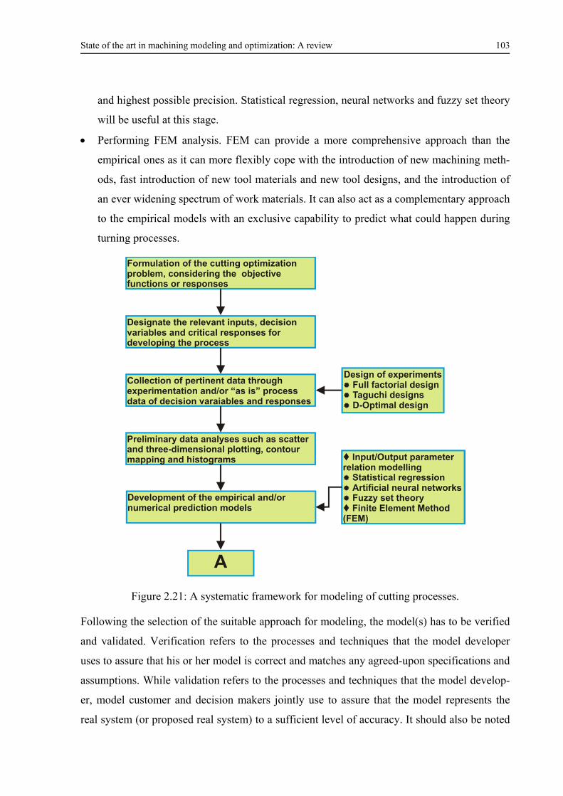
State of the art in machining modeling and optimization: A review 103
and highest possible precision. Statistical regression, neural networks and fuzzy set theory
will be useful at this stage.
Performing FEM analysis. FEM can provide a more comprehensive approach than the
empirical ones as it can more flexibly cope with the introduction of new machining meth-
ods, fast introduction of new tool materials and new tool designs, and the introduction of
an ever widening spectrum of work materials. It can also act as a complementary approach
to the empirical models with an exclusive capability to predict what could happen during
turning processes.
Figure 2.21: A systematic framework for modeling of cutting processes.
Following the selection of the suitable approach for modeling, the model(s) has to be verified
and validated. Verification refers to the processes and techniques that the model developer
uses to assure that his or her model is correct and matches any agreed-upon specifications and
assumptions. While validation refers to the processes and techniques that the model develop-
er, model customer and decision makers jointly use to assure that the model represents the
real system (or proposed real system) to a sufficient level of accuracy. It should also be noted
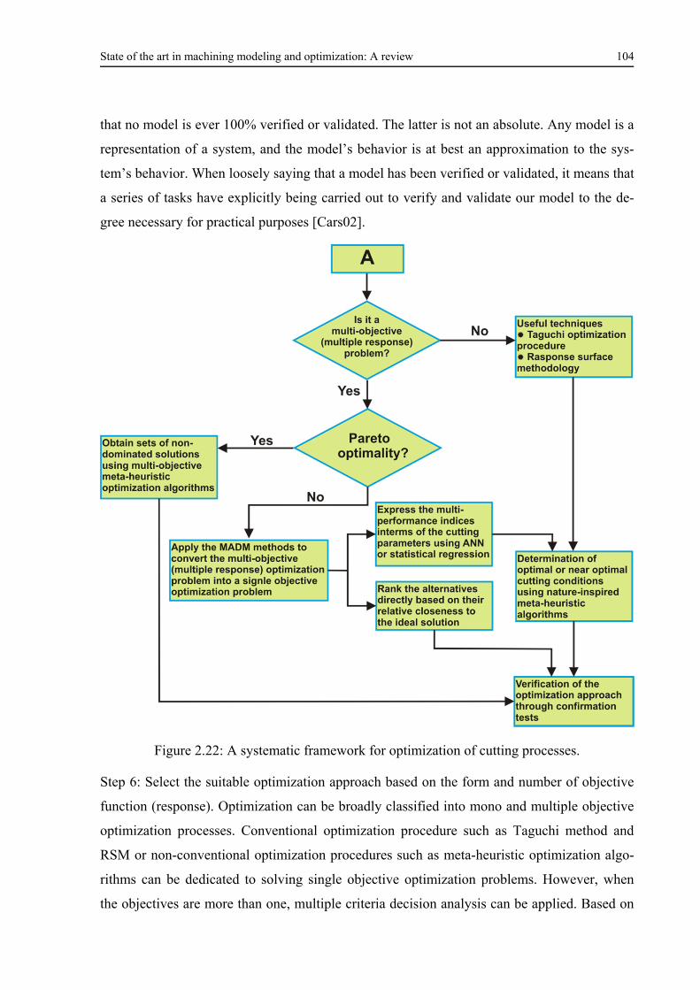
State of the art in machining modeling and optimization: A review 104
that no model is ever 100% verified or validated. The latter is not an absolute. Any model is a
representation of a system, and the model’s behavior is at best an approximation to the sys-
tem’s behavior. When loosely saying that a model has been verified or validated, it means that
a series of tasks have explicitly being carried out to verify and validate our model to the de-
gree necessary for practical purposes [Cars02].
Figure 2.22: A systematic framework for optimization of cutting processes.
Step 6: Select the suitable optimization approach based on the form and number of objective
function (response). Optimization can be broadly classified into mono and multiple objective
optimization processes. Conventional optimization procedure such as Taguchi method and
RSM or non-conventional optimization procedures such as meta-heuristic optimization algo-
rithms can be dedicated to solving single objective optimization problems. However, when
the objectives are more than one, multiple criteria decision analysis can be applied. Based on

State of the art in machining modeling and optimization: A review 105
the predetermination and limitations on the number of decision alternatives, the optimization
problem can be solved employing a typical multi-objective optimization algorithm or a
MADM method. When multiple near optimal solutions are necessary, nature inspired multi-
objective optimization algorithms such as MOBA can be utilized. However, when the number
of decision alternatives is pre-determined, MADM methods should be employed. The out-
come of the MADM methods can be related to the decision variables using input/output pro-
cess parameter relationship modeling techniques and further optimized as a mono-objective
optimization problem using meta-heuristic or any other optimization algorithms.
Step 7: Conduct confirmation tests to verify the optimized process parameter(s).
Experimental details 106
3 Experimental details
The four major sections of this chapter describe the technical and experimental fundamentals
of the present dissertation. In the first section, mechanical properties and chemical composi-
tions of the adopted workpiece materials is briefly described. Additionally, results of
JMatPro’s software to predict temperature-dependent mechanical and physical behavior of the
workpiece materials are presented. In the second section, a brief description of the involved
cutting tools and machine tool is given. The utilized DOE techniques to plan the experiments
are reported in the third section of the present chapter. The last section is dedicated to the ex-
perimental techniques employed to measure the machining performance characteristics.
3.1 Workpiece materials
3.1.1 Mechanical properties and chemical compositions
Altogether, three grades of stainless steels are used, namely austenitic EN 1.4404 (or AISI
316L), standard duplex EN 1.4462 (or SAF 2205) and super duplex EN 1.4410 (or SAF
2507). The first grade which is chosen as benchmark for machinability comparison analyses is
an extra low carbon modification of type 1.4401. EN 1.4404 is a molybdenum-containing
austenitic stainless steel intended to provide improved corrosion resistance relative to type
1.4307 in moderately corrosive process environments, particularly those containing chlorides
or other halides. It has been used in handling many chemicals used by the process industries,
including pulp and paper, textile, food, pharmaceutical, medical, and other chemical pro-
cessing equipment. EN 1.4462 with equal amounts of ferrite and austenite is a duplex stain-
less steel that exhibits approximately two times higher mechanical strength, lower thermal
expansion, better corrosion resistance and higher thermal conductivity than EN 1.4404. The
material is suitable for use in production tubing and flow lines for the extraction of oil and gas
from sour wells, in refineries and in process solutions contaminated with chlorides. The good
mechanical and corrosion properties make EN 1.4462 an economical choice in many applica-
tions by reducing the life cycle cost of the equipment. Additionally, EN 1.4410 is also ferritic-
austenitic stainless steel. It combines the most desirable properties of both ferritic and austen-
itic steels. The higher chromium and molybdenum contents provide higher mechanical
strength, resistance to pitting, crevice, and corrosion resistance than type 1.4462. The duplex
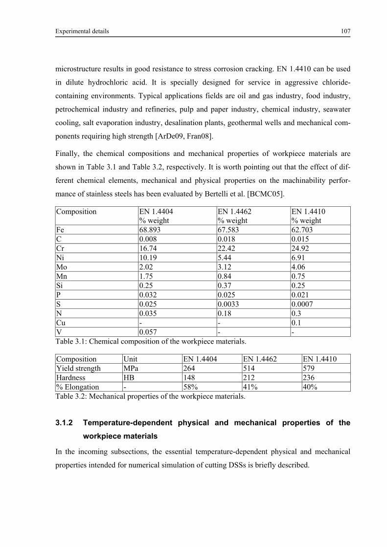
Experimental details 107
microstructure results in good resistance to stress corrosion cracking. EN 1.4410 can be used
in dilute hydrochloric acid. It is specially designed for service in aggressive chloride-
containing environments. Typical applications fields are oil and gas industry, food industry,
petrochemical industry and refineries, pulp and paper industry, chemical industry, seawater
cooling, salt evaporation industry, desalination plants, geothermal wells and mechanical com-
ponents requiring high strength [ArDe09, Fran08].
Finally, the chemical compositions and mechanical properties of workpiece materials are
shown in Table 3.1 and Table 3.2, respectively. It is worth pointing out that the effect of dif-
ferent chemical elements, mechanical and physical properties on the machinability perfor-
mance of stainless steels has been evaluated by Bertelli et al. [BCMC05].
Composition
EN 1.4404 % weight
EN 1.4462 % weight
EN 1.4410 % weight
Fe 68.893 67.583 62.703 C 0.008 0.018 0.015 Cr 16.74 22.42 24.92 Ni 10.19 5.44 6.91 Mo 2.02 3.12 4.06 Mn 1.75 0.84 0.75 Si 0.25 0.37 0.25 P 0.032 0.025 0.021 S 0.025 0.0033 0.0007 N 0.035 0.18 0.3 Cu - - 0.1 V 0.057 - - Table 3.1: Chemical composition of the workpiece materials.
Composition Unit EN 1.4404 EN 1.4462 EN 1.4410 Yield strength MPa 264 514 579 Hardness HB 148 212 236 % Elongation - 58% 41% 40% Table 3.2: Mechanical properties of the workpiece materials.
3.1.2 Temperature-dependent physical and mechanical properties of the
workpiece materials
In the incoming subsections, the essential temperature-dependent physical and mechanical
properties intended for numerical simulation of cutting DSSs is briefly described.
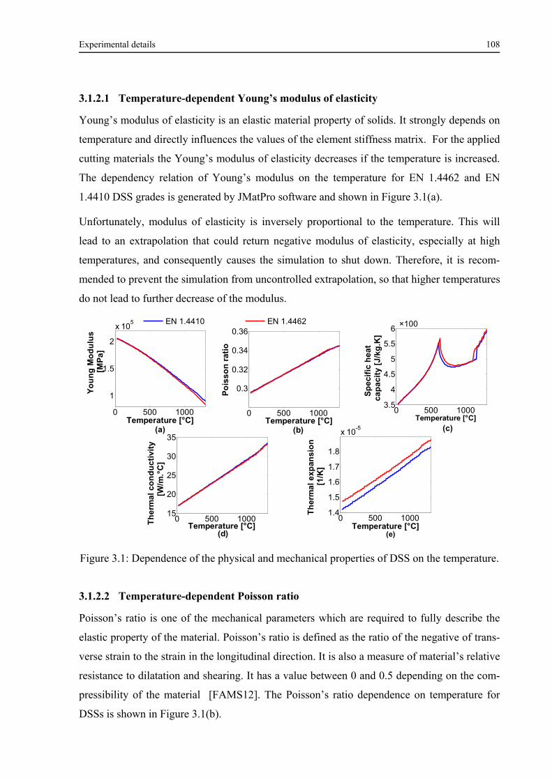
Experimental details 108
3.1.2.1 Temperature-dependent Young’s modulus of elasticity
Young’s modulus of elasticity is an elastic material property of solids. It strongly depends on
temperature and directly influences the values of the element stiffness matrix. For the applied
cutting materials the Young’s modulus of elasticity decreases if the temperature is increased.
The dependency relation of Young’s modulus on the temperature for EN 1.4462 and EN
1.4410 DSS grades is generated by JMatPro software and shown in Figure 3.1(a).
Unfortunately, modulus of elasticity is inversely proportional to the temperature. This will
lead to an extrapolation that could return negative modulus of elasticity, especially at high
temperatures, and consequently causes the simulation to shut down. Therefore, it is recom-
mended to prevent the simulation from uncontrolled extrapolation, so that higher temperatures
do not lead to further decrease of the modulus.
Figure 3.1: Dependence of the physical and mechanical properties of DSS on the temperature.
3.1.2.2 Temperature-dependent Poisson ratio
Poisson’s ratio is one of the mechanical parameters which are required to fully describe the
elastic property of the material. Poisson’s ratio is defined as the ratio of the negative of trans-
verse strain to the strain in the longitudinal direction. It is also a measure of material’s relative
resistance to dilatation and shearing. It has a value between 0 and 0.5 depending on the com-
pressibility of the material [FAMS12]. The Poisson’s ratio dependence on temperature for
DSSs is shown in Figure 3.1(b).
0 500 1000
1
1.5
2
x 105
Temperature [°C]
Yo
un
g M
od
ulu
s
[M
Pa
]
0 500 1000
0.3
0.32
0.34
0.36
Temperature [°C]
Po
iss
on
rat
io
0 500 10001.4
1.5
1.6
1.7
1.8
x 10-5
Temperature [°C]
Th
erm
al
ex
pan
sio
n
[1
/K]
0 500 100015
20
25
30
35
Temperature [°C]Th
erm
al
con
du
cti
vit
y
[
W/m
.°C
]
0 500 10003.5
4
4.5
5
5.5
6
Temperature [°C]
Sp
eci
fic
he
at
ca
pa
cit
y [J
/kg
.K]
EN 1.4410 EN 1.4462 ×100
(d)
(c)(b)(a)
(e)
Experimental details 109
3.1.2.3 Temperature-dependent specific heat capacity
In machining and forming, the lower the specific heat of a certain material, the higher the
temperature will rise [YoEA11]. When different materials are machined with the same tool,
cutting fluid and feed rate, the proportionality relation of temperature generated will be as per
the following expression:
pmth
rcT Ck
fvk
c~
(3.1)
where T is the mean tool face temperature; ck is the specific cutting pressure; thk is the ther-
mal conductivity; m is the density and pC is the specific heat capacity of the workmaterial
[Shaw89]. In Figure 3.1(c), the specific heat capacities for the described DSSs as functions of
temperature are visible.
3.1.2.4 Temperature-dependent thermal conductivity
When a material is deformed elastically, the energy required for the operation is stored in the
material as strain energy, and no heat is generated. However, when a material is deformed
plastically, most of the energy used is converted into heat. In metal cutting, the material is
subjected to extremely high strains, and elastic deformation forms a very small proportion of
the total deformation; therefore, it may be assumed that all the energy is converted into heat.
Heat generation in metal cutting leads to temperature rise at the tool-chip interface. Among
the factors that affect the cutting temperature, heat dispersion into the work and thickness of
the tensile layer in the cutting process is thermal conductivity. Materials with higher thermal
conductivity are responsible for production of lower temperature at cutting edge. Thermal
conductivity ( thk ) has a significant effect on the thickness of the tensile layer, where higher
thk results in thicker tensile layers [Jkau08]. As expected, the thermal conductivity is predict-
ed to be mainly affected by the temperature. Figure 3.1(d) shows the effects of temperature on
the thermal conductivity of DSSs.
3.1.2.5 Temperature-dependent coefficient of thermal expansion
DSSs have lower thermal expansion coefficients than austenitic stainless steels, similar to
those of carbon steel and can therefore offer certain design advantages. Thermal expansion
Experimental details 110
coefficients have also shown dependence on the temperature as can be observed in Figure 3.1
(e).
In addition to the flow stress curves (shown in Figure 2.11), aforementioned physical and me-
chanical properties of the workpiece materials are expected to affect the outcome of the FEM
simulations substantially. Therefore, a great deal of attention is needed to be paid when enter-
ing the data to the material module of the utilized FEM software.
3.2 Machine tool and cutting tool
A CNC lathe CTX 420 Linear V5 with maximum drive power 25kW and a speed range of 35-
7000rpm is used to perform the experiments. In Figure 3.2, a brief description of the machine
and its technical data are presented.
Recommended by SANDVIK Coromant, for medium-duty turning operations of stainless
steels, negative 80° rhombic-shape coated carbide inserts with ISO codes of CNMG 120408-
MM 2025 and CNMG 120408-QM 2025 are used throughout most of the empirical investiga-
tions. The basic difference between the two inserts lies in the employed chip breaker geome-
tries. The MM designation has a sharp positive edge and open chip breaker which promotes
low cutting force and more stable cutting operation. The QM designation has also a positive
edge but 5-7° less in sharpness. It can be considered as an alternative solution to the chip-
breaker geometry MM when more machining stability is needed. Both inserts have a 5.5 μm
thick multilayer chemical vapor deposition (CVD) coating (TiN/TiCN/Al2O3) on a cemented
carbide substrate. The CVD coating consists of a thick, moderate temperature chemical vapor
deposition of TiN for wear resistance and with low coefficient of friction, TiCN for wear re-
sistance and thermal stability and Al2O3 for heat and crater wear resistance. The overall per-
formance of the inserts is expected to show excellent resistance to both mechanical and ther-
mal shock. On the other hand, in order to facilitate the optimization of insert shape and chip
breaker geometry through numerical investigations, rhombic cemented carbide of ISO desig-
nation; CNMA 120412-IC20 is employed. IC20 is an uncoated carbide grade suitable for
semi-finishing, finishing and semi-roughing of aluminum, cast iron and stainless steel. All the
inserts were mounted on a right hand style PCLNL-2525M-12 ISO type tool holder with tool
geometry as follows: including angle 80°, back rake angle n ,6 clearance angle c 5°
and approach angle 95°.
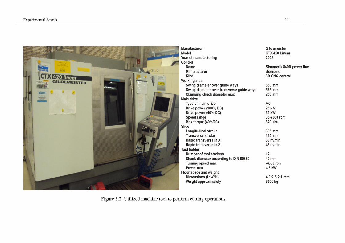
Experimental details 111
Figure 3.2: Utilized machine tool to perform cutting operations.
Experimental details 112
3.3 Design of experiments (DOE)
An experiment takes a central place in science, particularly nowadays, due to the complexity
of problems science deals with. The question of efficiency of using an experiment is therefore
imposed. J. Bernal has made estimation that scientific research is organized and done fairly
chaotically so that the coefficient of its usability is about 2%. To increase research efficiency,
it is necessary to introduce something completely new into classical experimental research.
One kind of innovation could be, to apply statistical mathematical methods or to develop de-
sign of experiments. DOE is a planned approach for determining cause and effect relation-
ships [Lazi06].
In machining processes, when the objective is to find the correlation between the response(s)
and the control factors included, it is possible to plan the experiments using DOE approach so
as to reduce the number of experiments, which in turn reduces the time and cost involved in
the experimentation. All the factors included in the DOE are varied simultaneously. The in-
fluence of unknown or non-included factors is minimized by properly randomizing the exper-
iment. Mathematical methods are used not only at the final stage of the study, when the eval-
uation and analysis of the experimental data are conducted, but also throughout all the stages
of DOE, i.e. from the formalization of a priori information till the decision-making stage. This
allows answering of important questions: “What is the minimum number of tests that should
be conducted? Which parameters should be taken into consideration? Which method(s) is
(are) better to use in the evaluation and analysis of experimental data [Asta06, Mont09]?
Based on the general purpose of experimentation, which essentially included the development
of modeling and/or optimization of machining, the following DOE approaches have been ap-
plied in the present dissertation:
3.3.1 Full factorial design
A full factorial design (FFD) includes all possible combinations of the levels for all control
factors. It allows the study of the effect of each control factor on the response variable, as well
as the effects of interactions between control factors on the response variable. In the early
stages of experimental work, FFD has been applied to
determine the specific cutting pressure c1.1k ,
define sets of non-dominated optimal straight turning solutions using MOBA,
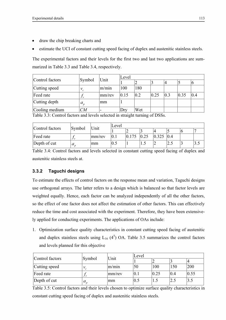
Experimental details 113
draw the chip breaking charts and
estimate the UCI of constant cutting speed facing of duplex and austenitic stainless steels.
The experimental factors and their levels for the first two and last two applications are sum-
marized in Table 3.3 and Table 3.4, respectively.
Control factors Symbol Unit Level 1 2 3 4 5 6
Cutting speed cv m/min 100 180
Feed rate rf mm/rev 0.15 0.2 0.25 0.3 0.35 0.4
Cutting depth pa mm 1
Cooling medium CM - Dry Wet Table 3.3: Control factors and levels selected in straight turning of DSSs.
Control factors Symbol Unit Level 1 2 3 4 5 6 7
Feed rate rf mm/rev 0.1 0.175 0.25 0.325 0.4
Depth of cut pa mm 0.5 1 1.5 2 2.5 3 3.5
Table 3.4: Control factors and levels selected in constant cutting speed facing of duplex and
austenitic stainless steels at.
3.3.2 Taguchi designs
To estimate the effects of control factors on the response mean and variation, Taguchi designs
use orthogonal arrays. The latter refers to a design which is balanced so that factor levels are
weighted equally. Hence, each factor can be analyzed independently of all the other factors,
so the effect of one factor does not affect the estimation of other factors. This can effectively
reduce the time and cost associated with the experiment. Therefore, they have been extensive-
ly applied for conducting experiments. The applications of OAs include:
1. Optimization surface quality characteristics in constant cutting speed facing of austenitic
and duplex stainless steels using L16 (45) OA. Table 3.5 summarizes the control factors
and levels planned for this objective
Control factors Symbol Unit Level 1 2 3 4
Cutting speed cv m/min 50 100 150 200
Feed rate rf mm/rev 0.1 0.25 0.4 0.55
Depth of cut pa mm 0.5 1.5 2.5 3.5
Table 3.5: Control factors and their levels chosen to optimize surface quality characteristics in
constant cutting speed facing of duplex and austenitic stainless steels.
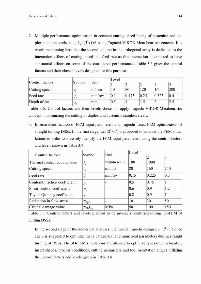
Experimental details 114
2. Multiple performance optimization in constant cutting speed facing of austenitic and du-
plex stainless steels using L25 (55) OA using Taguchi-VIKOR-Meta-heuristic concept. It is
worth mentioning here that the second column in the orthogonal array is dedicated to the
interaction effects of cutting speed and feed rate as this interaction is expected to have
substantial effects on some of the considered performances. Table 3.6 gives the control
factors and their chosen levels designed for this purpose.
Control factors Symbol Unit Level 1 2 3 4 5
Cutting speed cv m/min 40 80 120 160 200
Feed rate rf mm/rev 0.1 0.175 0.25 0.325 0.4
Depth of cut pa mm 0.5 1 1.5 2 2.5
Table 3.6: Control factors and their levels chosen to apply Taguchi-VIKOR-Metaheuristic
concept in optimizing the cutting of duplex and austenitic stainless steels.
3. Inverse identification of FEM input parameters and Taguchi-based FEM optimization of
straight turning DSSs. In the first stage, L18 (21×37) is proposed to conduct the FEM simu-
lations in order to inversely identify the FEM input parameters using the control factors
and levels shown in Table 3.7.
Control factors Symbol Unit Level 1 2 3
Thermal contact conductance tch N/(mm.sec.K) 100 1000
Cutting speed cv m/min 80 160 240
Feed rate rf mm/rev 0.15 0.225 0.3
Coulomb friction coefficient cμ - 0.5 0.75 1
Shear friction coefficient sμ - 0.6 0.9 1.2
Taylor-Quinney coefficient tκ - 0.8 0.9 1
Reduction in flow stress rp% - 10 30 50
Critical damage value crit.D% MPa 50 100 150
Table 3.7: Control factors and levels planned to be inversely identified during 3D-FEM of
cutting DSSs.
In the second stage of the numerical analyses, the mixed Taguchi design L18 (21×37) once
again is suggested to optimize many categorical and numerical parameters during straight
turning of DSSs. The 3D-FEM simulations are planned to optimize types of chip breaker,
insert shapes, process conditions, cutting parameters and tool orientation angles utilizing
the control factors and levels given in Table 3.8.
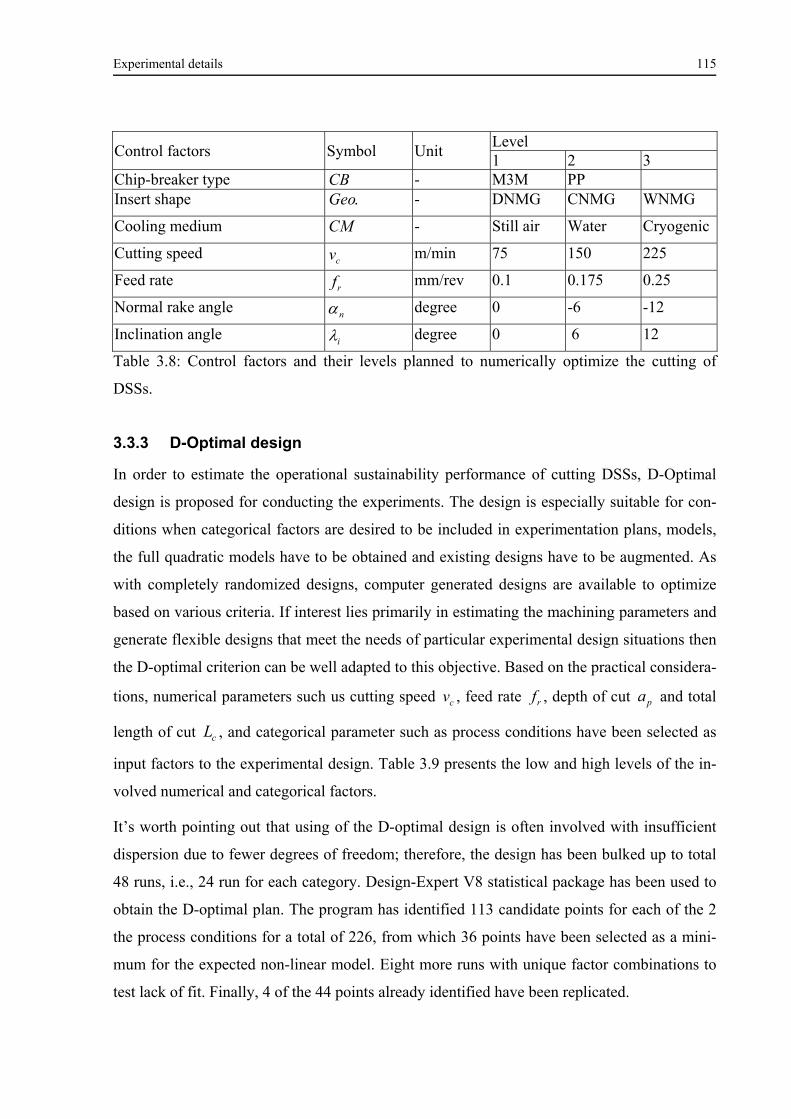
Experimental details 115
Control factors Symbol Unit Level 1 2 3
Chip-breaker type CB - M3M PP Insert shape .Geo - DNMG CNMG WNMG
Cooling medium CM - Still air Water Cryogenic
Cutting speed cv m/min 75 150 225
Feed rate rf mm/rev 0.1 0.175 0.25
Normal rake angle n degree 0 -6 -12
Inclination angle i degree 0 6 12
Table 3.8: Control factors and their levels planned to numerically optimize the cutting of
DSSs.
3.3.3 D-Optimal design
In order to estimate the operational sustainability performance of cutting DSSs, D-Optimal
design is proposed for conducting the experiments. The design is especially suitable for con-
ditions when categorical factors are desired to be included in experimentation plans, models,
the full quadratic models have to be obtained and existing designs have to be augmented. As
with completely randomized designs, computer generated designs are available to optimize
based on various criteria. If interest lies primarily in estimating the machining parameters and
generate flexible designs that meet the needs of particular experimental design situations then
the D-optimal criterion can be well adapted to this objective. Based on the practical considera-
tions, numerical parameters such us cutting speed cv , feed rate rf , depth of cut pa and total
length of cut cL , and categorical parameter such as process conditions have been selected as
input factors to the experimental design. Table 3.9 presents the low and high levels of the in-
volved numerical and categorical factors.
It’s worth pointing out that using of the D-optimal design is often involved with insufficient
dispersion due to fewer degrees of freedom; therefore, the design has been bulked up to total
48 runs, i.e., 24 run for each category. Design-Expert V8 statistical package has been used to
obtain the D-optimal plan. The program has identified 113 candidate points for each of the 2
the process conditions for a total of 226, from which 36 points have been selected as a mini-
mum for the expected non-linear model. Eight more runs with unique factor combinations to
test lack of fit. Finally, 4 of the 44 points already identified have been replicated.
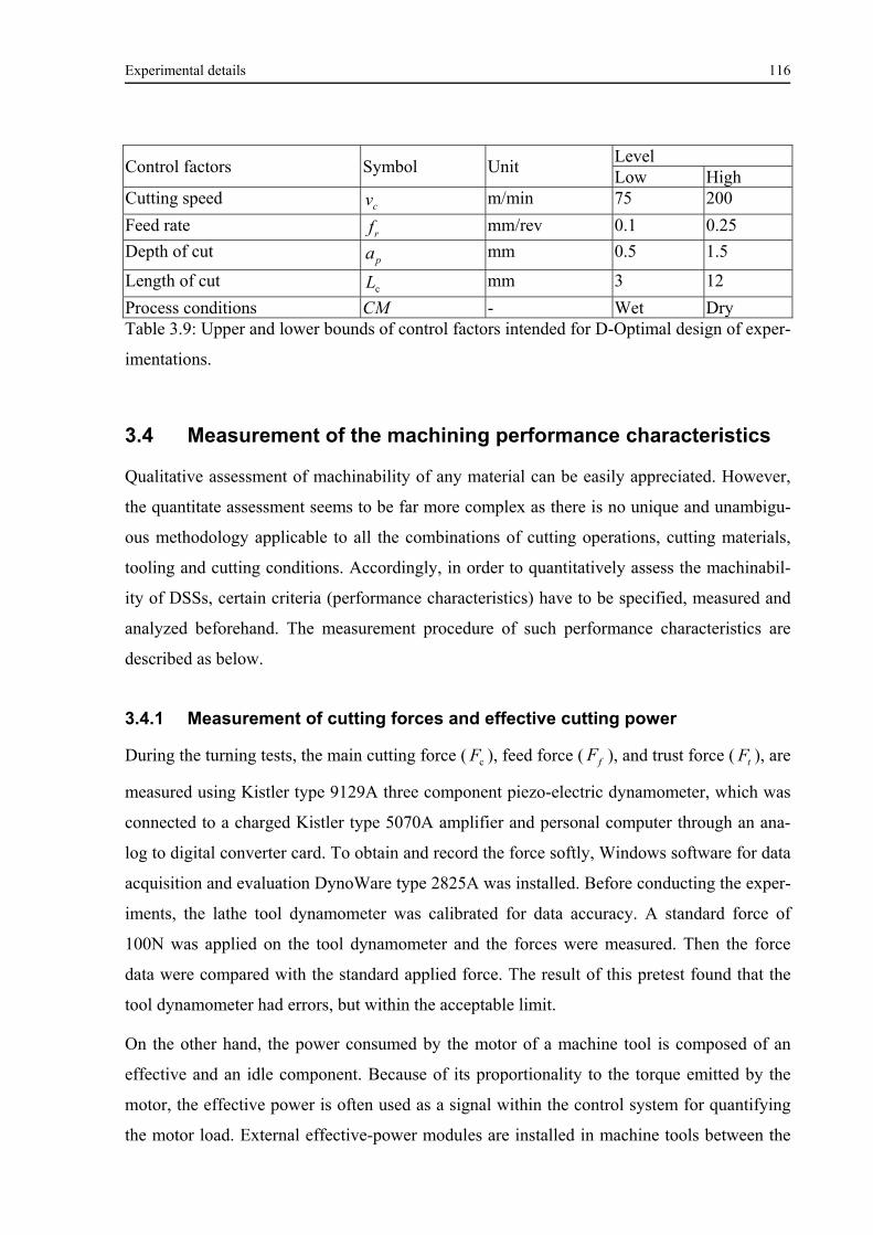
Experimental details 116
Control factors Symbol Unit Level Low High
Cutting speed cv m/min 75 200
Feed rate rf mm/rev 0.1 0.25
Depth of cut pa mm 0.5 1.5
Length of cut cL mm 3 12
Process conditions CM - Wet Dry Table 3.9: Upper and lower bounds of control factors intended for D-Optimal design of exper-
imentations.
3.4 Measurement of the machining performance characteristics
Qualitative assessment of machinability of any material can be easily appreciated. However,
the quantitate assessment seems to be far more complex as there is no unique and unambigu-
ous methodology applicable to all the combinations of cutting operations, cutting materials,
tooling and cutting conditions. Accordingly, in order to quantitatively assess the machinabil-
ity of DSSs, certain criteria (performance characteristics) have to be specified, measured and
analyzed beforehand. The measurement procedure of such performance characteristics are
described as below.
3.4.1 Measurement of cutting forces and effective cutting power
During the turning tests, the main cutting force ( cF ), feed force ( fF ), and trust force ( tF ), are
measured using Kistler type 9129A three component piezo-electric dynamometer, which was
connected to a charged Kistler type 5070A amplifier and personal computer through an ana-
log to digital converter card. To obtain and record the force softly, Windows software for data
acquisition and evaluation DynoWare type 2825A was installed. Before conducting the exper-
iments, the lathe tool dynamometer was calibrated for data accuracy. A standard force of
100N was applied on the tool dynamometer and the forces were measured. Then the force
data were compared with the standard applied force. The result of this pretest found that the
tool dynamometer had errors, but within the acceptable limit.
On the other hand, the power consumed by the motor of a machine tool is composed of an
effective and an idle component. Because of its proportionality to the torque emitted by the
motor, the effective power is often used as a signal within the control system for quantifying
the motor load. External effective-power modules are installed in machine tools between the
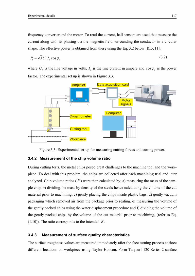
Experimental details 117
frequency converter and the motor. To read the current, hall sensors are used that measure the
current along with its phasing via the magnetic field surrounding the conductor in a circular
shape. The effective power is obtained from these using the Eq. 3.2 below [Kloc11].
acl IUP cos3e (3.2)
where lU is the line voltage in volts, cI is the line current in ampere and acos is the power
factor. The experimental set up is shown in Figure 3.3.
Figure 3.3: Experimental set-up for measuring cutting forces and cutting power.
3.4.2 Measurement of the chip volume ratio
During cutting tests, the metal chips posed great challenges to the machine tool and the work-
piece. To deal with this problem, the chips are collected after each machining trial and later
analyzed. Chip volume ratios ( R ) were then calculated by; a) measuring the mass of the sam-
ple chip, b) dividing the mass by density of the steels hence calculating the volume of the cut
material prior to machining, c) gently placing the chips inside plastic bags, d) gently vacuum
packaging which removed air from the package prior to sealing, e) measuring the volume of
the gently packed chips using the water displacement procedure and f) dividing the volume of
the gently packed chips by the volume of the cut material prior to machining, (refer to Eq.
(1.10)). The ratio corresponds to the intended R .
3.4.3 Measurement of surface quality characteristics
The surface roughness values are measured immediately after the face turning process at three
different locations on workpiece using Taylor-Hobson, Form Talysurf 120 Series 2 surface
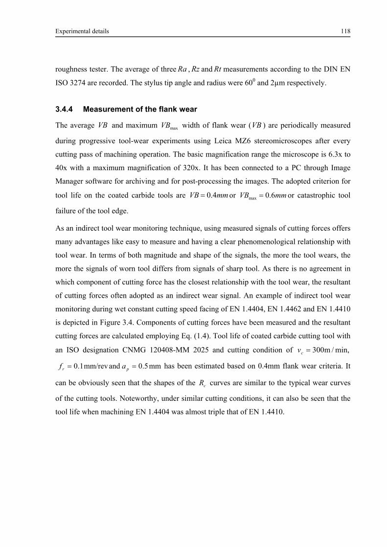
Experimental details 118
roughness tester. The average of three Ra , Rz and Rt measurements according to the DIN EN
ISO 3274 are recorded. The stylus tip angle and radius were 600 and 2µm respectively.
3.4.4 Measurement of the flank wear
The average VB and maximum maxVB width of flank wear (VB ) are periodically measured
during progressive tool-wear experiments using Leica MZ6 stereomicroscopes after every
cutting pass of machining operation. The basic magnification range the microscope is 6.3x to
40x with a maximum magnification of 320x. It has been connected to a PC through Image
Manager software for archiving and for post-processing the images. The adopted criterion for
tool life on the coated carbide tools are mmVB 4.0 or mmVB 6.0max or catastrophic tool
failure of the tool edge.
As an indirect tool wear monitoring technique, using measured signals of cutting forces offers
many advantages like easy to measure and having a clear phenomenological relationship with
tool wear. In terms of both magnitude and shape of the signals, the more the tool wears, the
more the signals of worn tool differs from signals of sharp tool. As there is no agreement in
which component of cutting force has the closest relationship with the tool wear, the resultant
of cutting forces often adopted as an indirect wear signal. An example of indirect tool wear
monitoring during wet constant cutting speed facing of EN 1.4404, EN 1.4462 and EN 1.4410
is depicted in Figure 3.4. Components of cutting forces have been measured and the resultant
cutting forces are calculated employing Eq. (1.4). Tool life of coated carbide cutting tool with
an ISO designation CNMG 120408-MM 2025 and cutting condition of min,/m300cv
mm5.0 andmm/rev1.0 pr af has been estimated based on 0.4mm flank wear criteria. It
can be obviously seen that the shapes of the cR curves are similar to the typical wear curves
of the cutting tools. Noteworthy, under similar cutting conditions, it can also be seen that the
tool life when machining EN 1.4404 was almost triple that of EN 1.4410.
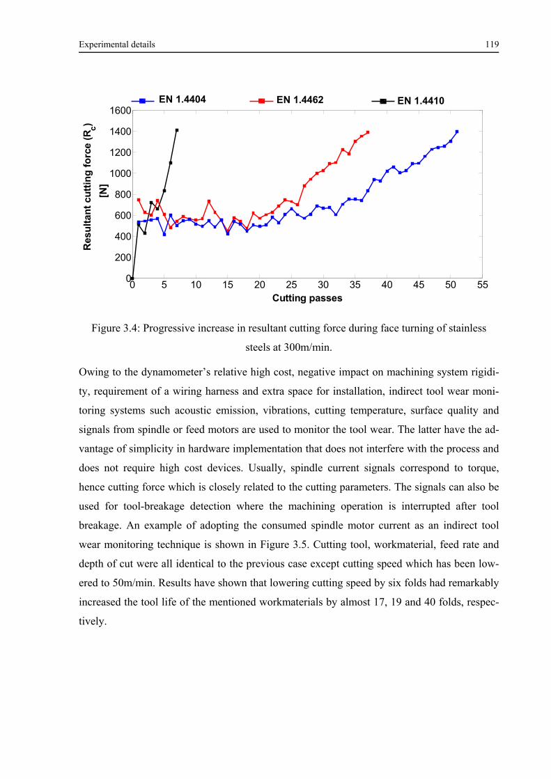
Experimental details 119
Figure 3.4: Progressive increase in resultant cutting force during face turning of stainless
steels at 300m/min.
Owing to the dynamometer’s relative high cost, negative impact on machining system rigidi-
ty, requirement of a wiring harness and extra space for installation, indirect tool wear moni-
toring systems such acoustic emission, vibrations, cutting temperature, surface quality and
signals from spindle or feed motors are used to monitor the tool wear. The latter have the ad-
vantage of simplicity in hardware implementation that does not interfere with the process and
does not require high cost devices. Usually, spindle current signals correspond to torque,
hence cutting force which is closely related to the cutting parameters. The signals can also be
used for tool-breakage detection where the machining operation is interrupted after tool
breakage. An example of adopting the consumed spindle motor current as an indirect tool
wear monitoring technique is shown in Figure 3.5. Cutting tool, workmaterial, feed rate and
depth of cut were all identical to the previous case except cutting speed which has been low-
ered to 50m/min. Results have shown that lowering cutting speed by six folds had remarkably
increased the tool life of the mentioned workmaterials by almost 17, 19 and 40 folds, respec-
tively.
0 5 10 15 20 25 30 35 40 45 50 550
200
400
600
800
1000
1200
1400
1600
Cutting passes
Res
ult
ant
cutt
ing
fo
rce
(Rc)
[
N]
EN 1.4404 EN 1.4462 EN 1.4410
Experimental details 120
Figure 3.5: Progressive increase in electrical current consumption during face turning of stain-
less steels at 50m/min.
3.4.5 Infrared temperature measurement system
Although, infrared (IR) cameras are quite expensive, they remain one of the most promising
solutions for temperature measurement since they allow for a non-contact, extensive meas-
urement of temperature. Thus, the problem of perturbation of the heat flow in the tool and
changes the results is avoided. The fast response of the IR camera lets high, cutting speeds to
be used in machining experiments, since it can capture the transient changes and the stages of
chip formation and entanglement around the workpiece, the tool holder and the tool post. In
the present dissertation, high-resolution thermo-graphic camera of brand VarioCam head
Hires 640 by InfraTec is used to film the chip formation and measure the chip temperature at
a resolution of 640×480 pixels, spectral range of 7.5-14 µm, temperature measuring range -40
-1200°C, measurement accuracy of ±2% and an external data storage at 60 Hz on external
computer via FireWire. The IR camera is placed straight above the rake face of the tool. The
lens of the camera is protected against possible impacts of the chips flying about. The images
in the films are examined and the mean of maximum temperature in the middle of the chips
are recorded. A schematic diagram of the cutting temperature measurement system using IR
camera is shown in Figure 3.6.
0 100 200 300 400 500 600 700 8002
3
4
5
6
7
Cutting passes
Co
sum
ed e
lect
rica
l cu
rren
t
[A]
EN 1.4404 EN 1.4462 EN 1.4410
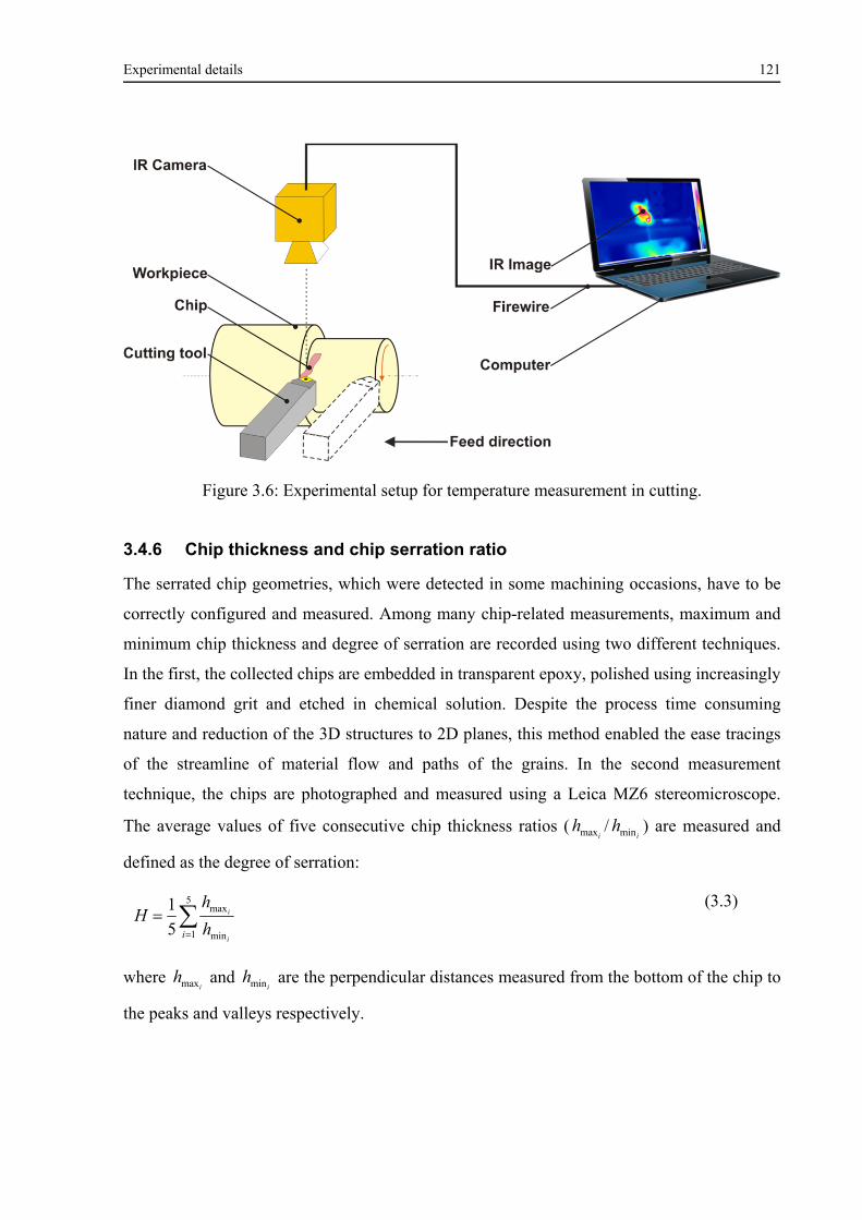
Experimental details 121
Figure 3.6: Experimental setup for temperature measurement in cutting.
3.4.6 Chip thickness and chip serration ratio
The serrated chip geometries, which were detected in some machining occasions, have to be
correctly configured and measured. Among many chip-related measurements, maximum and
minimum chip thickness and degree of serration are recorded using two different techniques.
In the first, the collected chips are embedded in transparent epoxy, polished using increasingly
finer diamond grit and etched in chemical solution. Despite the process time consuming
nature and reduction of the 3D structures to 2D planes, this method enabled the ease tracings
of the streamline of material flow and paths of the grains. In the second measurement
technique, the chips are photographed and measured using a Leica MZ6 stereomicroscope.
The average values of five consecutive chip thickness ratios (i
hmax /i
hmin ) are measured and
defined as the degree of serration:
5
1 min
max
5
1
i i
i
h
hH
(3.3)
where i
hmax and i
hmin are the perpendicular distances measured from the bottom of the chip to
the peaks and valleys respectively.
Experimental investigation and multi-objective optimization of turning DSSs: A case study 122
4 Experimental investigation and multi-objective
optimization of turning DSSs: A case study
In this chapter, experimental investigations on turning EN 1.4462 and EN 1.4410 DSS grades
with multi-layer coated carbide inserts are presented. Single-point wet and dry longitudinal
turning tests of 55 mm diameter cylindrical bars are conducted as per Table 3.3. Performance
characteristics such as cutting forces and tool wears are measured employing the measure-
ment techniques described in the previous chapter. The parametric influences of cutting
speed, feed rate and process conditions on the cutting performances such as resultant cutting
forces and tool wear are analyzed and proper interim conclusions are drawn. Nature-inspired
meta-heuristic Bat Algorithm is then employed to handle the multi-objective optimization of
the conflicting performances. Finally, the optimum cutting condition for each process condi-
tion can be selected from calculated Pareto-optimal fronts by the user according to the plan-
ning requirements.
4.1 Pareto optimality
Multi-objective optimization problems are more complicated than single objective optimiza-
tion as in many cases the decision maker has to find and/or approximate the Pareto optimality
fronts. In addition, algorithms have to be modified to accommodate multi-objectives properly.
The concept of Pareto optimum was formulated by Vilfredo Pareto in the 19th century, and
constitutes by itself the origin of research in multi-objective optimization. A solution vector
Tnuuuu ),.....,,( 21 is said to dominate another vector T
nvvvv ),.....,,( 21 if and only if
ii vu ≤ for ii vunini :.....,,2,1and.....,,2,1 . In other words, no component of u
is larger than the corresponding component of v , and at least one component is smaller. Simi-
larly, we can define another dominance relationship ≼ by:
u ≼v ⟺ u ≺v ˅u = v (4.1)
It is worth pointing out that for maximization problems, the dominance can be defined by
replacing ≺ with ≻. Therefore, a point *x is called a non-dominated solution if no solu-
tion can be found that dominates it [Coel99]. The Pareto front PF of a multi-objective can be
defined as the set of non-dominated solutions so that
Experimental investigation and multi-objective optimization of turning DSSs: A case study 123
ssSsSsPF : (4.2)
or in term of the Pareto optimal set in the search space
)()(:* xxxxPF GG (4.3)
where TKGGG ),.....,,( 21G . To obtain a good approximation to Pareto front, a diverse range
of solutions should be generated using efficient techniques [GuBa09, KoCS06].
In the present chapter, Bat Algorithm (BA) is extended to find and/or approximate Pareto
fronts, hence solving multi-objective machining optimization problem.
4.2 Performance characteristics
4.2.1 Specific cutting pressures
The specific cutting pressure is often considered as an indication to the machinability of a
given workmaterial. The higher the specific cutting pressure the lower is the machinability of
the workmaterial. The specific cutting pressures for turning EN 1.4462 and EN 1.4410 were
calculated from the cutting data employing Eqs. (1.6-8) and the results are shown in Figure
4.1. Based on a quick review of the results;
No drastic difference between the cutting pressures of dry and wet conditions was ob-
served. However, overall wet machining shows an improvement in the machining perfor-
mance through lower cutting pressures.
Generally, lower average values of the specific cutting pressures are noticed when cutting
EN 1.4462 than EN 1.4410.
The cutting pressures are generally showed a decreasing trend with increasing cutting
speed and feed rate. The maximum values are located in low ranges of cutting speed and
feed rate.
Modified Kienzle’s formula (Eq. (1.9)) can be applied to evaluate the parametric effects of
cutting conditions on the cutting forces empirically. The model fitting has employed the
least square method. Summary of models coefficients are listed in Table 4.1. It should be
noted that the average at wet cutting is generally 5% lower than at dry cutting for both
workmaterials and of turning EN 1.4410 is generally 25.281% higher than of turning EN
1.4462.
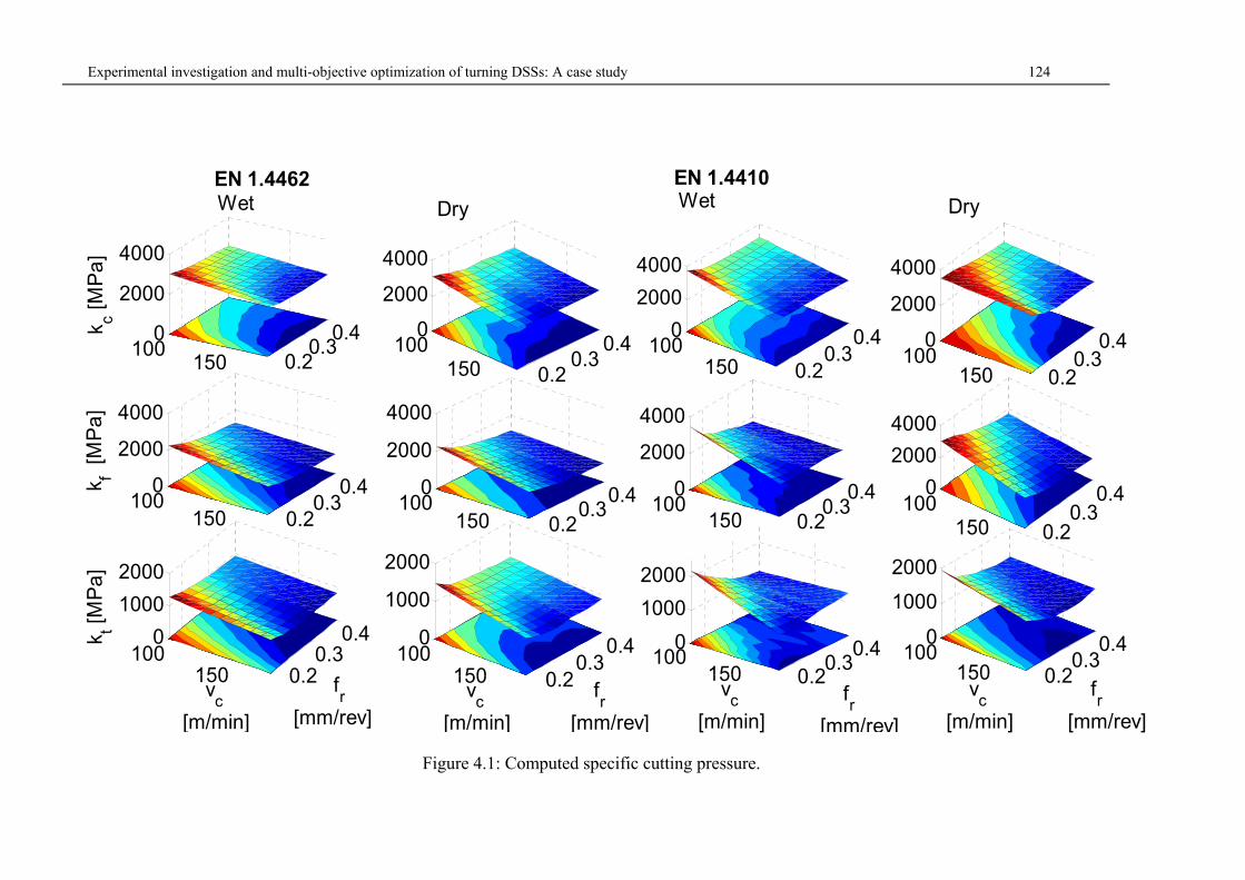
Experimental investigation and multi-objective optimization of turning DSSs: A case study 124
Figure 4.1: Computed specific cutting pressure.
100150 0.2
0.30.40
2000
4000
100150 0.2
0.30.40
2000
4000
100150 0.2
0.30.40
2000
4000
k c [M
Pa
]
100150 0.2
0.30.4
0
2000
4000
100150 0.2
0.30.40
2000
4000
100150 0.2
0.30.40
2000
4000
100150 0.2
0.30.40
2000
4000
k f [M
Pa
]
100150 0.2
0.30.40
2000
4000
100150 0.2
0.30.40
1000
2000
100150 0.2
0.30.40
1000
2000
100150 0.2
0.30.40
1000
2000
k t [M
Pa
]
100150 0.2
0.30.40
1000
2000
DryWetEN 1.4410EN 1.4462
Wet Dry
vc
[m/min]
vc
[m/min]
vc
[m/min]
vc
[m/min] f
r[mm/rev]
fr
[mm/rev]
fr
[mm/rev] f
r[mm/rev]
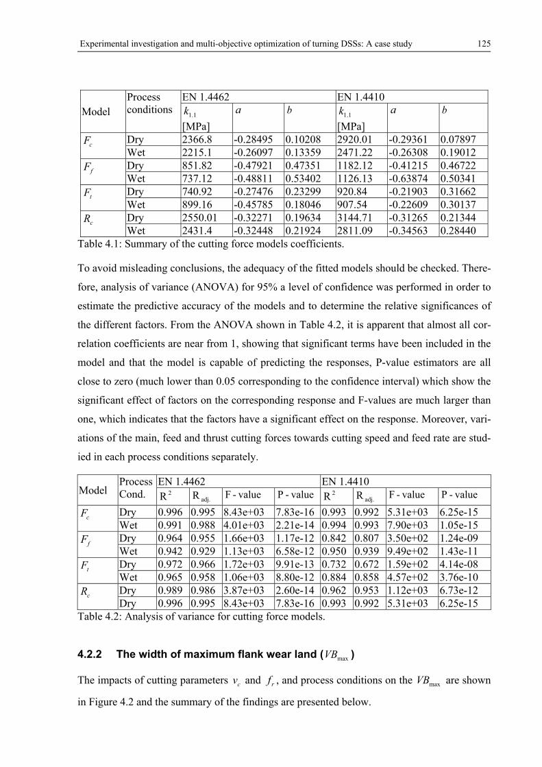
Experimental investigation and multi-objective optimization of turning DSSs: A case study 125
Model Process conditions
EN 1.4462 EN 1.4410
1.1k
[MPa]
a b1.1k
[MPa]
a b
cF Dry 2366.8 -0.28495 0.10208 2920.01 -0.29361 0.07897 Wet 2215.1 -0.26097 0.13359 2471.22 -0.26308 0.19012
fF Dry 851.82 -0.47921 0.47351 1182.12 -0.41215 0.46722 Wet 737.12 -0.48811 0.53402 1126.13 -0.63874 0.50341
tF Dry 740.92 -0.27476 0.23299 920.84 -0.21903 0.31662 Wet 899.16 -0.45785 0.18046 907.54 -0.22609 0.30137
cR Dry 2550.01 -0.32271 0.19634 3144.71 -0.31265 0.21344 Wet 2431.4 -0.32448 0.21924 2811.09 -0.34563 0.28440
Table 4.1: Summary of the cutting force models coefficients.
To avoid misleading conclusions, the adequacy of the fitted models should be checked. There-
fore, analysis of variance (ANOVA) for 95% a level of confidence was performed in order to
estimate the predictive accuracy of the models and to determine the relative significances of
the different factors. From the ANOVA shown in Table 4.2, it is apparent that almost all cor-
relation coefficients are near from 1, showing that significant terms have been included in the
model and that the model is capable of predicting the responses, P-value estimators are all
close to zero (much lower than 0.05 corresponding to the confidence interval) which show the
significant effect of factors on the corresponding response and F-values are much larger than
one, which indicates that the factors have a significant effect on the response. Moreover, vari-
ations of the main, feed and thrust cutting forces towards cutting speed and feed rate are stud-
ied in each process conditions separately.
Model Process Cond.
EN 1.4462 EN 1.4410 2R adj.R value-F value-P 2R adj.R value-F value-P
cF Dry 0.996 0.995 8.43e+03 7.83e-16 0.993 0.992 5.31e+03 6.25e-15 Wet 0.991 0.988 4.01e+03 2.21e-14 0.994 0.993 7.90e+03 1.05e-15
fF Dry 0.964 0.955 1.66e+03 1.17e-12 0.842 0.807 3.50e+02 1.24e-09 Wet 0.942 0.929 1.13e+03 6.58e-12 0.950 0.939 9.49e+02 1.43e-11
tF Dry 0.972 0.966 1.72e+03 9.91e-13 0.732 0.672 1.59e+02 4.14e-08 Wet 0.965 0.958 1.06e+03 8.80e-12 0.884 0.858 4.57e+02 3.76e-10
cR Dry 0.989 0.986 3.87e+03 2.60e-14 0.962 0.953 1.12e+03 6.73e-12 Dry 0.996 0.995 8.43e+03 7.83e-16 0.993 0.992 5.31e+03 6.25e-15
Table 4.2: Analysis of variance for cutting force models.
4.2.2 The width of maximum flank wear land ( maxVB )
The impacts of cutting parameters cv and rf , and process conditions on the maxVB are shown
in Figure 4.2 and the summary of the findings are presented below.
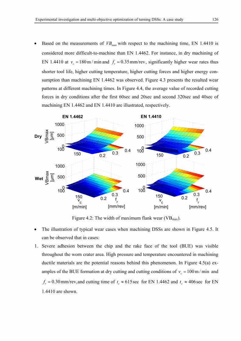
Experimental investigation and multi-objective optimization of turning DSSs: A case study 126
Based on the measurements of maxVB with respect to the machining time, EN 1.4410 is
considered more difficult-to-machine than EN 1.4462. For instance, in dry machining of
EN 1.4410 at min/m180cv and mm/rev35.0rf , significantly higher wear rates thus
shorter tool life, higher cutting temperature, higher cutting forces and higher energy con-
sumption than machining EN 1.4462 was observed. Figure 4.3 presents the resulted wear
patterns at different machining times. In Figure 4.4, the average value of recorded cutting
forces in dry conditions after the first 60sec and 20sec and second 320sec and 40sec of
machining EN 1.4462 and EN 1.4410 are illustrated, respectively.
Figure 4.2: The width of maximum flank wear (VBmax).
The illustration of typical wear cases when machining DSSs are shown in Figure 4.5. It
can be observed that in cases:
1. Severe adhesion between the chip and the rake face of the tool (BUE) was visible
throughout the worn crater area. High pressure and temperature encountered in machining
ductile materials are the potential reasons behind this phenomenon. In Figure 4.5(a) ex-
amples of the BUE formation at dry cutting and cutting conditions of min/m100cv and
mm/rev,30.0rf and cutting time of sec615ct for EN 1.4462 and sec406ct for EN
1.4410 are shown.
100150 0.2
0.30.4
0
500
1000
VB
max
[µ
m]
100150 0.2
0.30.4
0
500
1000
VB
max
[µ
m]
100150 0.2
0.30.40
500
1000
100150 0.2
0.30.4
0
500
1000
EN 1.4462 EN 1.4410
vc
[m/min]
fr
[mm/rev]
vc
[m/min]
fr
[mm/rev]
Wet
Dry
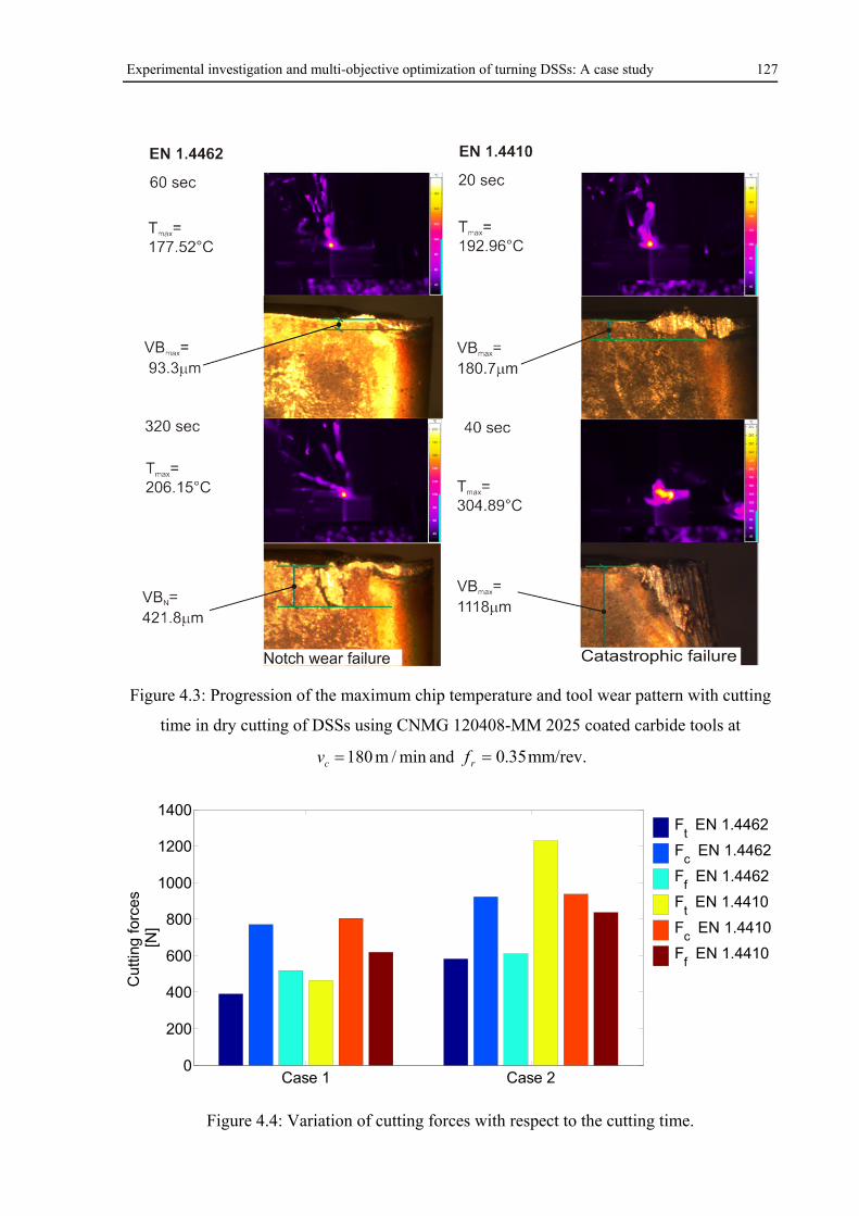
Experimental investigation and multi-objective optimization of turning DSSs: A case study 127
Figure 4.3: Progression of the maximum chip temperature and tool wear pattern with cutting
time in dry cutting of DSSs using CNMG 120408-MM 2025 coated carbide tools at
min/m180cv and mm/rev.35.0rf
Figure 4.4: Variation of cutting forces with respect to the cutting time.
1 20
200
400
600
800
1000
1200
1400
Cut
ting
forc
es
[N]
F
t EN 1.4462
Fc EN 1.4462
Ff EN 1.4462
Ft EN 1.4410
Fc EN 1.4410
Ff EN 1.4410
Case 2Case 1
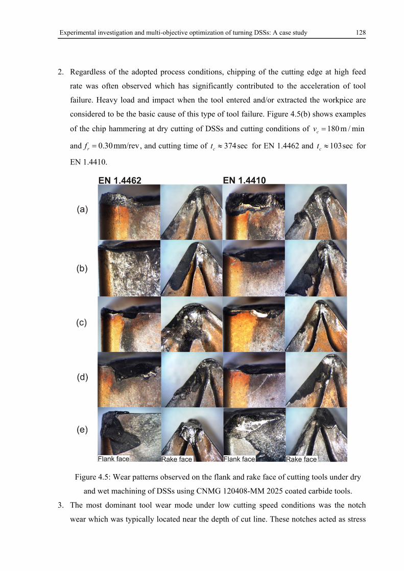
Experimental investigation and multi-objective optimization of turning DSSs: A case study 128
2. Regardless of the adopted process conditions, chipping of the cutting edge at high feed
rate was often observed which has significantly contributed to the acceleration of tool
failure. Heavy load and impact when the tool entered and/or extracted the workpice are
considered to be the basic cause of this type of tool failure. Figure 4.5(b) shows examples
of the chip hammering at dry cutting of DSSs and cutting conditions of min/m180cv
and mm/rev30.0rf , and cutting time of sec374ct for EN 1.4462 and sec103ct for
EN 1.4410.
Figure 4.5: Wear patterns observed on the flank and rake face of cutting tools under dry
and wet machining of DSSs using CNMG 120408-MM 2025 coated carbide tools.
3. The most dominant tool wear mode under low cutting speed conditions was the notch
wear which was typically located near the depth of cut line. These notches acted as stress
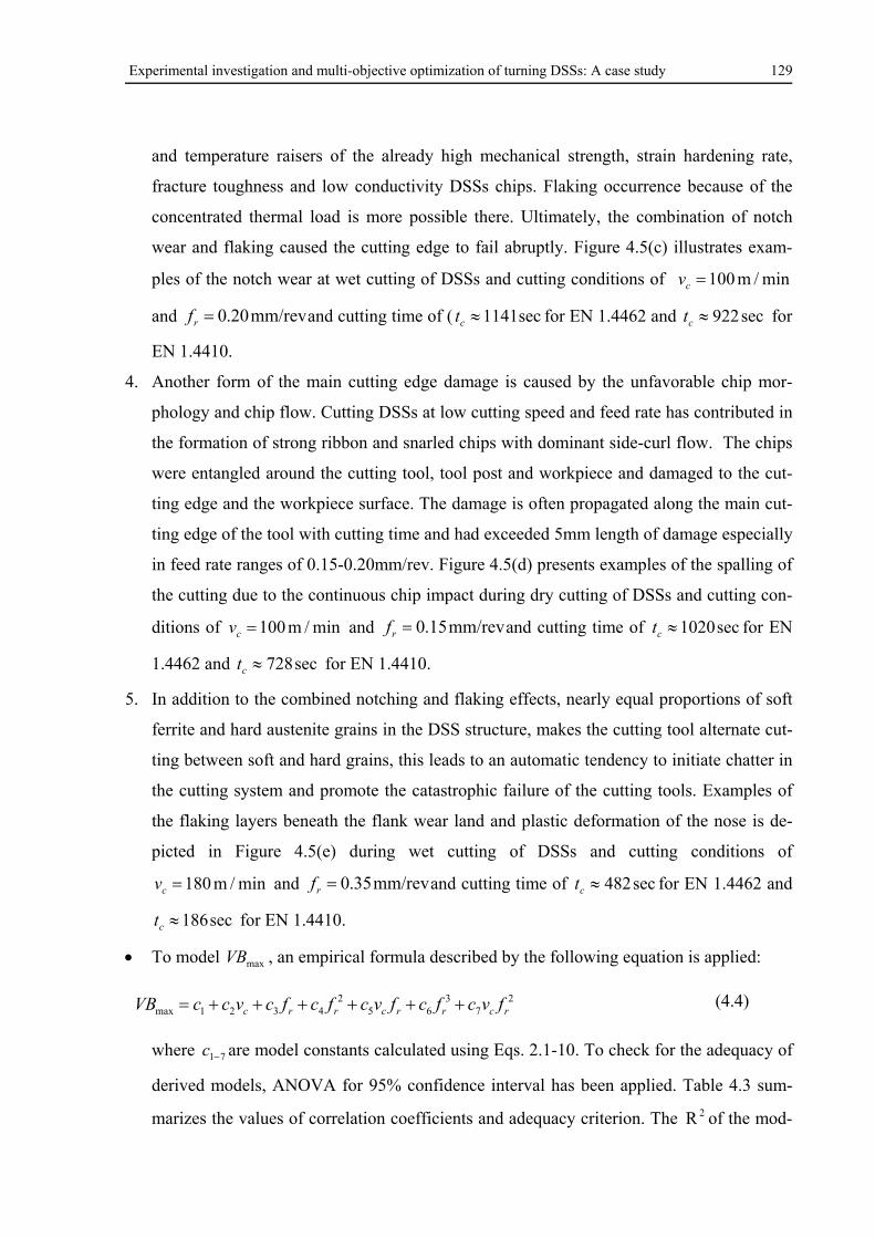
Experimental investigation and multi-objective optimization of turning DSSs: A case study 129
and temperature raisers of the already high mechanical strength, strain hardening rate,
fracture toughness and low conductivity DSSs chips. Flaking occurrence because of the
concentrated thermal load is more possible there. Ultimately, the combination of notch
wear and flaking caused the cutting edge to fail abruptly. Figure 4.5(c) illustrates exam-
ples of the notch wear at wet cutting of DSSs and cutting conditions of min/m100cv
and mm/rev20.0rf and cutting time of ( sec1141ct for EN 1.4462 and sec922ct for
EN 1.4410.
4. Another form of the main cutting edge damage is caused by the unfavorable chip mor-
phology and chip flow. Cutting DSSs at low cutting speed and feed rate has contributed in
the formation of strong ribbon and snarled chips with dominant side-curl flow. The chips
were entangled around the cutting tool, tool post and workpiece and damaged to the cut-
ting edge and the workpiece surface. The damage is often propagated along the main cut-
ting edge of the tool with cutting time and had exceeded 5mm length of damage especially
in feed rate ranges of 0.15-0.20mm/rev. Figure 4.5(d) presents examples of the spalling of
the cutting due to the continuous chip impact during dry cutting of DSSs and cutting con-
ditions of min/m100cv and mm/rev15.0rf and cutting time of sec1020ct for EN
1.4462 and sec728ct for EN 1.4410.
5. In addition to the combined notching and flaking effects, nearly equal proportions of soft
ferrite and hard austenite grains in the DSS structure, makes the cutting tool alternate cut-
ting between soft and hard grains, this leads to an automatic tendency to initiate chatter in
the cutting system and promote the catastrophic failure of the cutting tools. Examples of
the flaking layers beneath the flank wear land and plastic deformation of the nose is de-
picted in Figure 4.5(e) during wet cutting of DSSs and cutting conditions of
min/m180cv and mm/rev35.0rf and cutting time of sec482ct for EN 1.4462 and
sec186ct for EN 1.4410.
To model maxVB , an empirical formula described by the following equation is applied:
27
365
24321max rcrrcrrc fvcfcfvcfcfcvccVB (4.4)
where 71c are model constants calculated using Eqs. 2.1-10. To check for the adequacy of
derived models, ANOVA for 95% confidence interval has been applied. Table 4.3 sum-
marizes the values of correlation coefficients and adequacy criterion. The 2R of the mod-
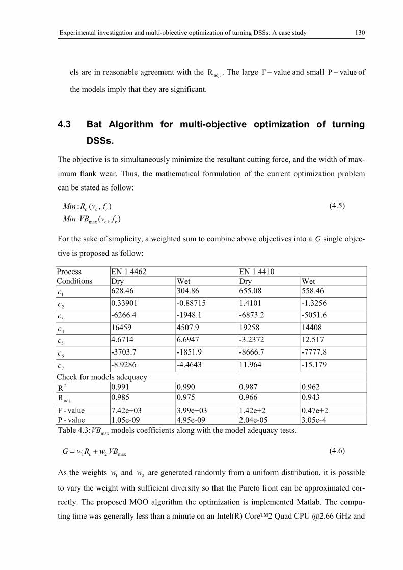
Experimental investigation and multi-objective optimization of turning DSSs: A case study 130
els are in reasonable agreement with the adj.R . The large valueF and small valueP of
the models imply that they are significant.
4.3 Bat Algorithm for multi-objective optimization of turning
DSSs.
The objective is to simultaneously minimize the resultant cutting force, and the width of max-
imum flank wear. Thus, the mathematical formulation of the current optimization problem
can be stated as follow:
),(:
),(:
max rc
rcc
fvVBMin
fvRMin
(4.5)
For the sake of simplicity, a weighted sum to combine above objectives into a G single objec-
tive is proposed as follow:
Process Conditions
EN 1.4462 EN 1.4410 Dry Wet Dry Wet
1c 628.46 304.86 655.08 558.46
2c 0.33901 -0.88715 1.4101 -1.3256
3c -6266.4 -1948.1 -6873.2 -5051.6
4c 16459 4507.9 19258 14408
5c 4.6714 6.6947 -3.2372 12.517
6c -3703.7 -1851.9 -8666.7 -7777.8
7c -8.9286 -4.4643 11.964 -15.179
Check for models adequacy 2R 0.991 0.990 0.987 0.962
adj.R 0.985 0.975 0.966 0.943
value-F 7.42e+03 3.99e+03 1.42e+2 0.47e+2 value-P 1.05e-09 4.95e-09 2.04e-05 3.05e-4
Table 4.3: maxVB models coefficients along with the model adequacy tests.
max21 VBwRwG c (4.6)
As the weights 1w and 2w are generated randomly from a uniform distribution, it is possible
to vary the weight with sufficient diversity so that the Pareto front can be approximated cor-
rectly. The proposed MOO algorithm the optimization is implemented Matlab. The compu-
ting time was generally less than a minute on an Intel(R) Core™2 Quad CPU @2.66 GHz and
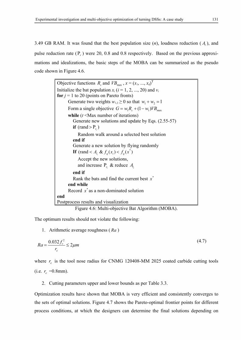
Experimental investigation and multi-objective optimization of turning DSSs: A case study 131
3.49 GB RAM. It was found that the best population size (n), loudness reduction ( lA ), and
pulse reduction rate ( r ) were 20, 0.8 and 0.8 respectively. Based on the previous approxi-
mations and idealizations, the basic steps of the MOBA can be summarized as the pseudo
code shown in Figure 4.6.
Objective functions cR and maxVB , x = (x1, ..., xd)T
Initialize the bat population xi (i = 1, 2, ..., 20) and vi for j = 1 to 20 (points on Pareto fronts) Generate two weights w1,2 ≥ 0 so that 121 ww
Form a single objective max11 )1( VBwRwG c
while (t <Max number of iterations) Generate new solutions and update by Eqs. (2.55-57) if )(rand
ir
Random walk around a selected best solution end if Generate a new solution by flying randomly If )()(&(rand *xfxfA qiqli
Accept the new solutions, and increase
ir & reduce
ilA
end if Rank the bats and find the current best *x end while Record *x as a non-dominated solution end Postprocess results and visualization
Figure 4.6: Multi-objective Bat Algorithm (MOBA).
The optimum results should not violate the following:
1. Arithmetic average roughness ( Ra )
mr
fRa r
2032.0 2
(4.7)
where r is the tool nose radius for CNMG 120408-MM 2025 coated carbide cutting tools
(i.e. r =0.8mm).
2. Cutting parameters upper and lower bounds as per Table 3.3.
Optimization results have shown that MOBA is very efficient and consistently converges to
the sets of optimal solutions. Figure 4.7 shows the Pareto-optimal frontier points for different
process conditions, at which the designers can determine the final solutions depending on
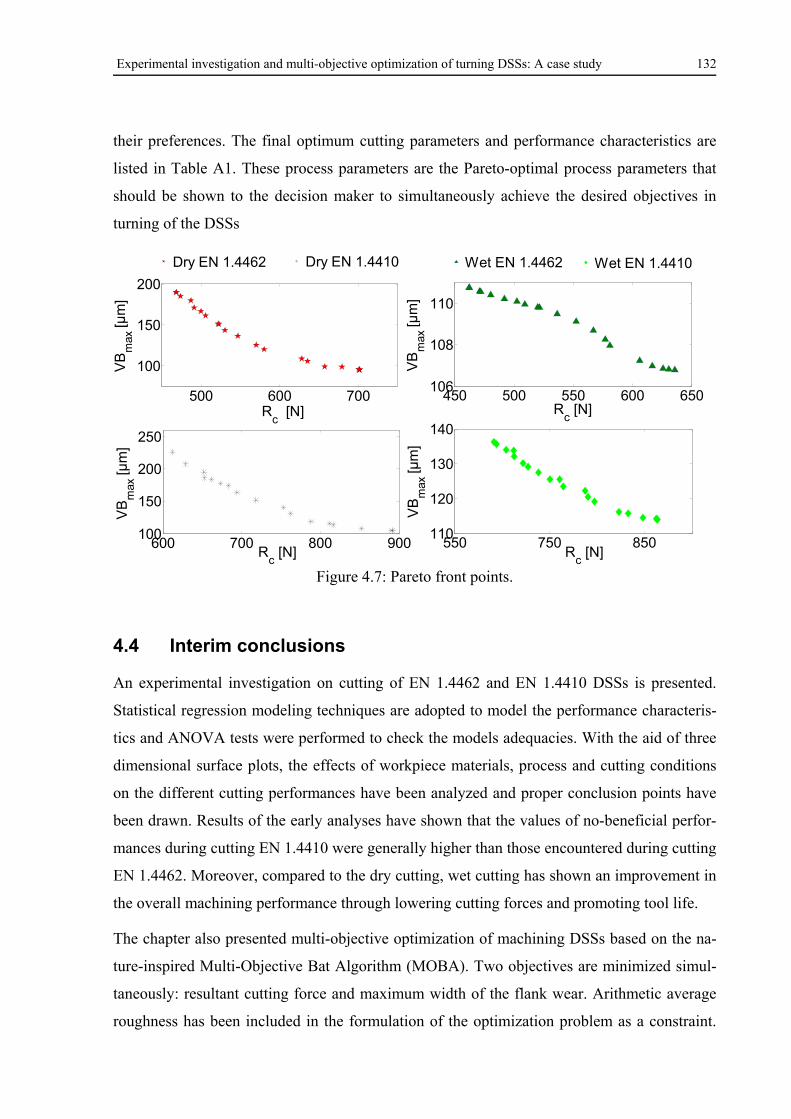
Experimental investigation and multi-objective optimization of turning DSSs: A case study 132
their preferences. The final optimum cutting parameters and performance characteristics are
listed in Table A1. These process parameters are the Pareto-optimal process parameters that
should be shown to the decision maker to simultaneously achieve the desired objectives in
turning of the DSSs
Figure 4.7: Pareto front points.
4.4 Interim conclusions
An experimental investigation on cutting of EN 1.4462 and EN 1.4410 DSSs is presented.
Statistical regression modeling techniques are adopted to model the performance characteris-
tics and ANOVA tests were performed to check the models adequacies. With the aid of three
dimensional surface plots, the effects of workpiece materials, process and cutting conditions
on the different cutting performances have been analyzed and proper conclusion points have
been drawn. Results of the early analyses have shown that the values of no-beneficial perfor-
mances during cutting EN 1.4410 were generally higher than those encountered during cutting
EN 1.4462. Moreover, compared to the dry cutting, wet cutting has shown an improvement in
the overall machining performance through lowering cutting forces and promoting tool life.
The chapter also presented multi-objective optimization of machining DSSs based on the na-
ture-inspired Multi-Objective Bat Algorithm (MOBA). Two objectives are minimized simul-
taneously: resultant cutting force and maximum width of the flank wear. Arithmetic average
roughness has been included in the formulation of the optimization problem as a constraint.
500 600 700
100
150
200
Rc [N]
VB
max
[µm
]
450 500 550 600 650106
108
110
Rc [N]
VB
max
[µm
]
600 700 800 900100
150
200
250
Rc [N]
VB
max
[µm
]
550 750 850110
120
130
140
Rc [N]
VB
max
[µm
]
Wet EN 1.4410Wet EN 1.4462Dry EN 1.4462 Dry EN 1.4410

Experimental investigation and multi-objective optimization of turning DSSs: A case study 133
Results of optimization have shown that MOBA is very efficient and highly reliable. It has
provided Pareto frontiers of non-dominated solution sets for optimum cutting conditions, ena-
bling decision maker and/or process planner with a resourceful and efficient means of achiev-
ing the optimum cutting conditions.
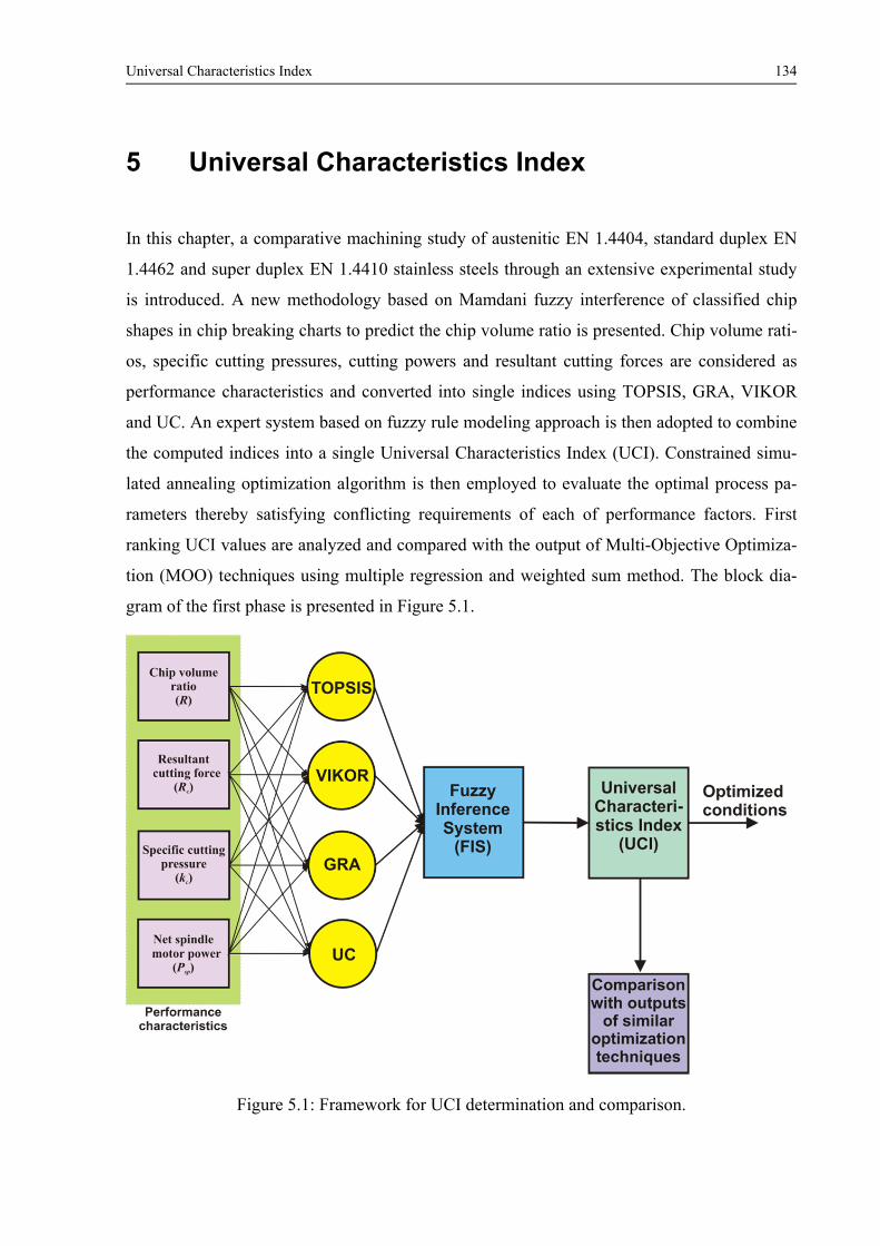
Universal Characteristics Index 134
5 Universal Characteristics Index
In this chapter, a comparative machining study of austenitic EN 1.4404, standard duplex EN
1.4462 and super duplex EN 1.4410 stainless steels through an extensive experimental study
is introduced. A new methodology based on Mamdani fuzzy interference of classified chip
shapes in chip breaking charts to predict the chip volume ratio is presented. Chip volume rati-
os, specific cutting pressures, cutting powers and resultant cutting forces are considered as
performance characteristics and converted into single indices using TOPSIS, GRA, VIKOR
and UC. An expert system based on fuzzy rule modeling approach is then adopted to combine
the computed indices into a single Universal Characteristics Index (UCI). Constrained simu-
lated annealing optimization algorithm is then employed to evaluate the optimal process pa-
rameters thereby satisfying conflicting requirements of each of performance factors. First
ranking UCI values are analyzed and compared with the output of Multi-Objective Optimiza-
tion (MOO) techniques using multiple regression and weighted sum method. The block dia-
gram of the first phase is presented in Figure 5.1.
Figure 5.1: Framework for UCI determination and comparison.
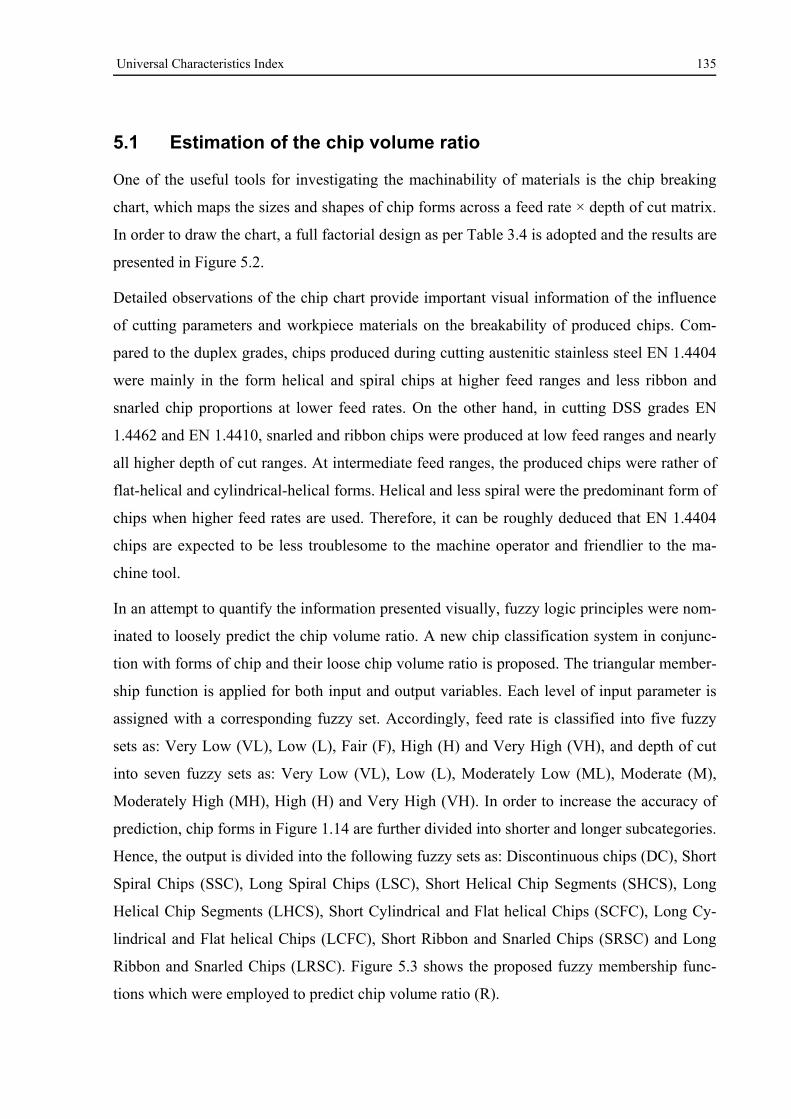
Universal Characteristics Index 135
5.1 Estimation of the chip volume ratio
One of the useful tools for investigating the machinability of materials is the chip breaking
chart, which maps the sizes and shapes of chip forms across a feed rate × depth of cut matrix.
In order to draw the chart, a full factorial design as per Table 3.4 is adopted and the results are
presented in Figure 5.2.
Detailed observations of the chip chart provide important visual information of the influence
of cutting parameters and workpiece materials on the breakability of produced chips. Com-
pared to the duplex grades, chips produced during cutting austenitic stainless steel EN 1.4404
were mainly in the form helical and spiral chips at higher feed ranges and less ribbon and
snarled chip proportions at lower feed rates. On the other hand, in cutting DSS grades EN
1.4462 and EN 1.4410, snarled and ribbon chips were produced at low feed ranges and nearly
all higher depth of cut ranges. At intermediate feed ranges, the produced chips were rather of
flat-helical and cylindrical-helical forms. Helical and less spiral were the predominant form of
chips when higher feed rates are used. Therefore, it can be roughly deduced that EN 1.4404
chips are expected to be less troublesome to the machine operator and friendlier to the ma-
chine tool.
In an attempt to quantify the information presented visually, fuzzy logic principles were nom-
inated to loosely predict the chip volume ratio. A new chip classification system in conjunc-
tion with forms of chip and their loose chip volume ratio is proposed. The triangular member-
ship function is applied for both input and output variables. Each level of input parameter is
assigned with a corresponding fuzzy set. Accordingly, feed rate is classified into five fuzzy
sets as: Very Low (VL), Low (L), Fair (F), High (H) and Very High (VH), and depth of cut
into seven fuzzy sets as: Very Low (VL), Low (L), Moderately Low (ML), Moderate (M),
Moderately High (MH), High (H) and Very High (VH). In order to increase the accuracy of
prediction, chip forms in Figure 1.14 are further divided into shorter and longer subcategories.
Hence, the output is divided into the following fuzzy sets as: Discontinuous chips (DC), Short
Spiral Chips (SSC), Long Spiral Chips (LSC), Short Helical Chip Segments (SHCS), Long
Helical Chip Segments (LHCS), Short Cylindrical and Flat helical Chips (SCFC), Long Cy-
lindrical and Flat helical Chips (LCFC), Short Ribbon and Snarled Chips (SRSC) and Long
Ribbon and Snarled Chips (LRSC). Figure 5.3 shows the proposed fuzzy membership func-
tions which were employed to predict chip volume ratio (R).
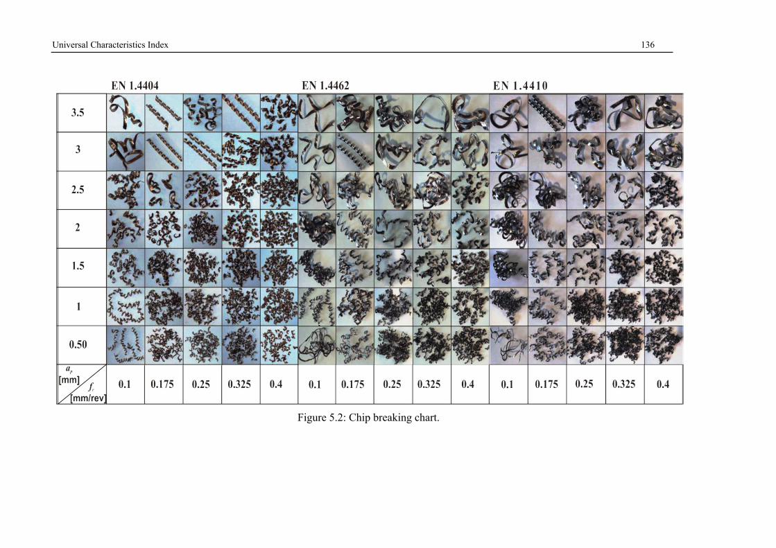
Universal Characteristics Index 136
Figure 5.2: Chip breaking chart.
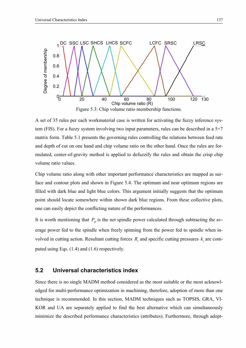
Universal Characteristics Index 137
Figure 5.3: Chip volume ratio membership functions.
A set of 35 rules per each workmaterial case is written for activating the fuzzy inference sys-
tem (FIS). For a fuzzy system involving two input parameters, rules can be described in a 5×7
matrix form. Table 5.1 presents the governing rules controlling the relations between feed rate
and depth of cut on one hand and chip volume ratio on the other hand. Once the rules are for-
mulated, center-of-gravity method is applied to defuzzify the rules and obtain the crisp chip
volume ratio values.
Chip volume ratio along with other important performance characteristics are mapped as sur-
face and contour plots and shown in Figure 5.4. The optimum and near optimum regions are
filled with dark blue and light blue colors. This argument initially suggests that the optimum
point should locate somewhere within shown dark blue regions. From these collective plots,
one can easily depict the conflicting nature of the performances.
It is worth mentioning that spP is the net spindle power calculated through subtracting the av-
erage power fed to the spindle when freely spinning from the power fed to spindle when in-
volved in cutting action. Resultant cutting forces cR and specific cutting pressures ck are com-
puted using Eqs. (1.4) and (1.6) respectively.
5.2 Universal characteristics index
Since there is no single MADM method considered as the most suitable or the most acknowl-
edged for multi-performance optimization in machining, therefore, adoption of more than one
technique is recommended. In this section, MADM techniques such as TOPSIS, GRA, VI-
KOR and UA are separately applied to find the best alternative which can simultaneously
minimize the described performance characteristics (attributes). Furthermore, through adopt-
0 20 40 60 80 100 120 1300
0.2
0.4
0.6
0.8
1
Chip volume ratio (R)
Deg
ree
of m
embe
rshi
pLSCSSCDC SHCS LHCS SCFC LCFC SRSC LRSC
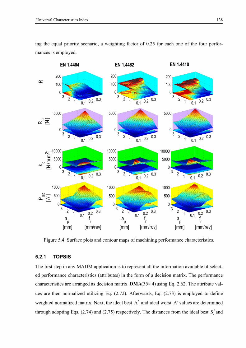
Universal Characteristics Index 138
ing the equal priority scenario, a weighting factor of 0.25 for each one of the four perfor-
mances is employed.
Figure 5.4: Surface plots and contour maps of machining performance characteristics.
5.2.1 TOPSIS
The first step in any MADM application is to represent all the information available of select-
ed performance characteristics (attributes) in the form of a decision matrix. The performance
characteristics are arranged as decision matrix )435( DMA using Eq. 2.62. The attribute val-
ues are then normalized utilizing Eq. (2.72). Afterwards, Eq. (2.73) is employed to define
weighted normalized matrix. Next, the ideal best * and ideal worst - values are determined
through adopting Eqs. (2.74) and (2.75) respectively. The distances from the ideal best *iS and
0.1 0.2 0.3123
0
100
200
R
0.1 0.2 0.312
30
5000
Rc
[N]
0.1 0.2 0.3123
0
5000
10000
k c
[N/m
m2 ]
0.1 0.2 0.312
30
500
1000
fr
[mm/rev]
ap
[mm]
Psp
[W]
0.1 0.2 0.3123
0
100
200
0.1 0.2 0.312
30
5000
0.1 0.2 0.3123
0
5000
10000
0.1 0.2 0.312
30
500
1000
fr
[mm/rev]
ap
[mm]
0.1 0.2 0.3123
0
100
200
0.1 0.2 0.312
30
5000
0.1 0.2 0.3123
0
5000
10000
0.1 0.2 0.31
23
0
500
1000
fr
[mm/rev]
ap
[mm]
EN 1.4404 EN 1.4462 EN 1.4410
Universal Characteristics Index 139
ideal worst iS solutions and the relative closeness to the ideal solution ( *
iC ) are measured
utilizing Eqs. (2.76-78). Finally, The results are ranked by the relative degree of approxima-
tion. The best alternative is the one which has the shortest Euclidean distance to the ideal so-
lution.
5.2.2 VIKOR method
The best ix and the worst *
ix values of all criterion functions are computed using Eqs. (2.79)
and (2.80) respectively. Thereafter, Eqs. (2.81-83) are utilized to compute the utility iS and
regret iR measures, and VIKOR index VQ . The alternatives are then ranked by the values iS ,
iR and VQ . The results are three ranking lists with no difference in ranking order. The values
of first rank alternative were in acceptable advantage range and both iS and iR by consensus
proved the stability in decision making.
5.2.3 GRA
The adopted attributes are of non-beneficial kind where low values are always desired. There-
fore, when using GRA as a MADM method, the ‘smaller-the-better’ option should be em-
ployed as a normalizing method using the last term in Eq. (2.84). The values of deviation se-
quence ij , which is the absolute difference between reference sequence jr0 , and the compa-
rability sequence ijr values, are computed using Eq. (2.85). The global minimum ( min ) and
maximum values ( max ) are directly computed employing Eqs. (2.86) and (2.87) respectively.
In all cases, min and max were equal to 0 and 1 respectively. Since, all the attributes have
equal weighting, d is assigned to be 0.5. Afterwards, Grey relational coefficients g and
Grey relational grade GRG are evaluated using Eqs. (2.88) and (2.89) respectively. Finally,
the alternatives are ranked based on theGRG values so that the largest has specified the best.
5.2.4 UC
Owing to the non-beneficial nature of performances, Eq. (2.94) is directly used to specify the
best value of each attribute. Afterwards, Eqs. (2.95-97) are employed to determine the values
the utility constant jCU , preference number jPN and the overall utility value iU , respective-
ly. The best alternative is then ranked according to the iU values.
Universal Characteristics Index 140
5.2.5 Fuzzy-MADM
The output of the previous MADM methods showed different ranking outcomes, which will
cause uncertainty and confusions to the decision maker and/or process planne. In order to
eliminate the discrepancy of these methods and obtain a more general solution, fuzzy logic
principles is proposed to solve the problem. The individual MADM-indices are combined into
a single and comprehensive index called the Universal Characteristics Index (UCI).
Matlab software was used to construct the inference model of the UCI. The MADM-indices
were first adjusted to a notionally common scale between null and one, using simple normali-
zation methods. So that the digit ‘one’ represents the most desirable and ‘null’ is the least de-
sirable alternative. The outputs of the previous MADM-methods are designated as input vari-
ables to the FIS and are assigned with the following fuzzy sets: Small (S), Medium (M) and
Large (Lg). The output variable has the following nine levels: Extremely Low (EL), Very
Low (VL), Low (L), Lower Medium (LM), Medium (M), Upper Medium (UM), High (H),
Very High (VH) and Extremely High (EH). Mamdani implication method is employed for the
fuzzy inference reasoning. The relationship between system input and output is expressed by
an “If-Then” type. Totally 81 fuzzy rules per material were formulated. A sample of the for-
mulated fuzzy rules is listed below.
(EL) is then UCI(S) is UA and (S) isGRA and (S) is VIKOR and (S) is TOPSIS:1Rule(VL) is then UCI(M) is UA and (S) isGRA and (S) is VIKOR and (S) is TOPSIS:2Rule(L) is then UCI(Lg) is UA and (S) isGRA and (S) is VIKOR and (S) is TOPSIS:3Rule
.
(VH) is then UCI(M) is UA and (Lg) isGRA and is(Lg) VIKOR and (Lg) is TOPSIS:80Rule(EH) is then UCI(Lg) is UA and (Lg) isGRA and is(Lg) VIKOR and (Lg) is TOPSIS:81Rule
The values of cutting performances and the developed UCIs are shown in Table A2. In order
to evaluate the strength of the statistical relationship between the computed MADM-indices
and the developed UCIs, Spearman’s rank-order correlation is applied, see Table 5.2. The
near to one values of UCI coefficients are good indications of strong statistical relationship
with other MADM-indices. The ranks of the estimated UCI values along with the ranks of the
four MADM methods are shown in Figure 5.5. Noteworthy is the problem of MADM-
methods rank differences which justifies the application of fuzzy logic to solve it.
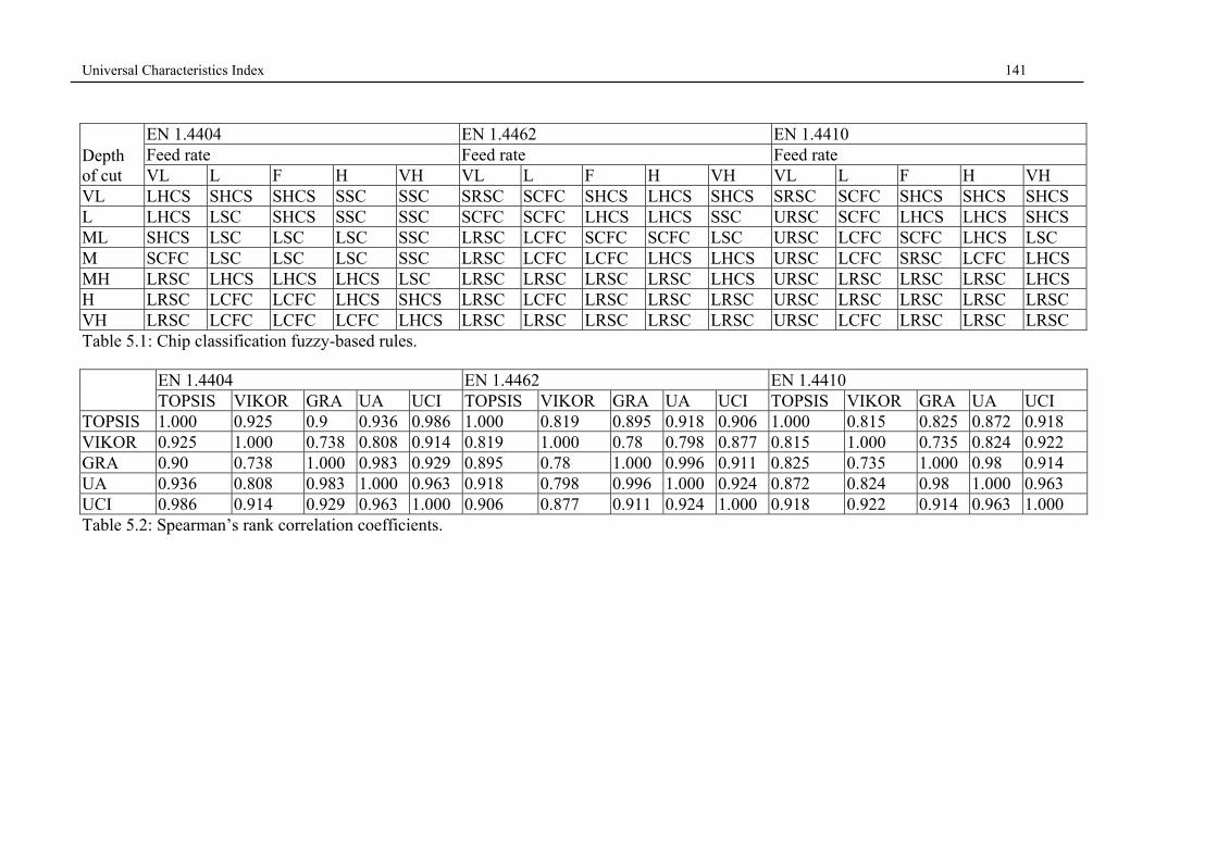
Universal Characteristics Index 141
Depth of cut
EN 1.4404 EN 1.4462 EN 1.4410 Feed rate Feed rate Feed rate VL L F H VH VL L F H VH VL L F H VH
VL LHCS SHCS SHCS SSC SSC SRSC SCFC SHCS LHCS SHCS SRSC SCFC SHCS SHCS SHCS L LHCS LSC SHCS SSC SSC SCFC SCFC LHCS LHCS SSC URSC SCFC LHCS LHCS SHCS ML SHCS LSC LSC LSC SSC LRSC LCFC SCFC SCFC LSC URSC LCFC SCFC LHCS LSC M SCFC LSC LSC LSC SSC LRSC LCFC LCFC LHCS LHCS URSC LCFC SRSC LCFC LHCS MH LRSC LHCS LHCS LHCS LSC LRSC LRSC LRSC LRSC LHCS URSC LRSC LRSC LRSC LHCS H LRSC LCFC LCFC LHCS SHCS LRSC LCFC LRSC LRSC LRSC URSC LRSC LRSC LRSC LRSC VH LRSC LCFC LCFC LCFC LHCS LRSC LRSC LRSC LRSC LRSC URSC LCFC LRSC LRSC LRSC Table 5.1: Chip classification fuzzy-based rules.
EN 1.4404 EN 1.4462 EN 1.4410 TOPSIS VIKOR GRA UA UCI TOPSIS VIKOR GRA UA UCI TOPSIS VIKOR GRA UA UCI
TOPSIS 1.000 0.925 0.9 0.936 0.986 1.000 0.819 0.895 0.918 0.906 1.000 0.815 0.825 0.872 0.918 VIKOR 0.925 1.000 0.738 0.808 0.914 0.819 1.000 0.78 0.798 0.877 0.815 1.000 0.735 0.824 0.922 GRA 0.90 0.738 1.000 0.983 0.929 0.895 0.78 1.000 0.996 0.911 0.825 0.735 1.000 0.98 0.914 UA 0.936 0.808 0.983 1.000 0.963 0.918 0.798 0.996 1.000 0.924 0.872 0.824 0.98 1.000 0.963 UCI 0.986 0.914 0.929 0.963 1.000 0.906 0.877 0.911 0.924 1.000 0.918 0.922 0.914 0.963 1.000 Table 5.2: Spearman’s rank correlation coefficients.
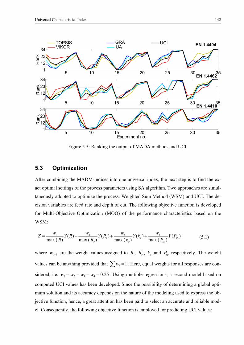
Universal Characteristics Index 142
Figure 5.5: Ranking the output of MADA methods and UCI.
5.3 Optimization
After combining the MADM-indices into one universal index, the next step is to find the ex-
act optimal settings of the process parameters using SA algorithm. Two approaches are simul-
taneously adopted to optimize the process: Weighted Sum Method (WSM) and UCI. The de-
cision variables are feed rate and depth of cut. The following objective function is developed
for Multi-Objective Optimization (MOO) of the performance characteristics based on the
WSM:
)()(max
)()(max
)()(max
)()(max
4321sp
spc
cc
c
PYP
wkY
k
wRY
R
wRY
R
wZ (5.1)
where 41w are the weight values assigned to R , cR , ck and spP respectively. The weight
values can be anything provided that 1 iw . Here, equal weights for all responses are con-
sidered, i.e. 25.04321 wwww . Using multiple regressions, a second model based on
computed UCI values has been developed. Since the possibility of determining a global opti-
mum solution and its accuracy depends on the nature of the modeling used to express the ob-
jective function, hence, a great attention has been paid to select an accurate and reliable mod-
el. Consequently, the following objective function is employed for predicting UCI values:
5 10 15 20 25 30 351
12
23
34
Ran
k
5 10 15 20 25 30 351
12
23
34
Ran
k
5 10 15 20 25 30 351
12
23
34
Experiment no.
Ran
k
EN 1.4404
EN 1.4410
TOPSISVIKOR
GRAUA
UCI
EN 1.4462
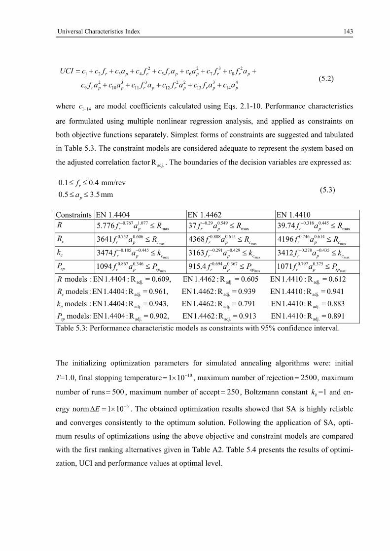
Universal Characteristics Index 143
414
313
2212
311
310
29
28
37
265
24321
pprprprppr
prrpprrpr
acafcafcafcacafc
afcfcacafcfcacfccUCI
(5.2)
where 141c are model coefficients calculated using Eqs. 2.1-10. Performance characteristics
are formulated using multiple nonlinear regression analysis, and applied as constraints on
both objective functions separately. Simplest forms of constraints are suggested and tabulated
in Table 5.3. The constraint models are considered adequate to represent the system based on
the adjusted correlation factor adj.R . The boundaries of the decision variables are expressed as:
mm5.35.0
mm/rev4.01.0
p
r
a
f (5.3)
Constraints EN 1.4404 EN 1.4462 EN 1.4410 R
max077.1767.0776.5 Raf pr max
549.029.037 Raf pr max445.0318.074.39 Raf pr
cR max
606.0752.03641 cpr Raf max
615.0808.04368 cpr Raf max
614.0746.04196 cpr Raf
ck max
445.0185.03474 cpr kaf max
429.0291.03163 cpr kaf max
435.0278.03412 cpr kaf
spP max
346.0867.01094 sppr Paf max
367.0694.04.915 sppr Paf max
375.0797.01071 sppr Paf
0.612 = R:1.4410 EN 0.605= R : 1.4462 EN 0.609,= R:1.4404 EN : models adj.adj.adj.R
0.941 = R:1.4410 EN 0.939= R : 1.4462 EN 0.961,= R:1.4404 EN :models adj.adj.adj.cR
0.883 = R:1.4410 EN 0.791= R : 1.4462 EN 0.943,= R:1.4404 EN :models adj.adj.adj.ck
0.891 = R:1.4410 EN 0.913= R : 1.4462 EN 0.902,= R:1.4404 EN :models adj.adj.adj.spP
Table 5.3: Performance characteristic models as constraints with 95% confidence interval.
The initializing optimization parameters for simulated annealing algorithms were: initial
T=1.0, final stopping temperature 10101 , maximum number of rejection 2500 , maximum
number of runs 500 , maximum number of accept 250 , Boltzmann constant bk =1 and en-
ergy norm 5101 E . The obtained optimization results showed that SA is highly reliable
and converges consistently to the optimum solution. Following the application of SA, opti-
mum results of optimizations using the above objective and constraint models are compared
with the first ranking alternatives given in Table A2. Table 5.4 presents the results of optimi-
zation, UCI and performance values at optimal level.
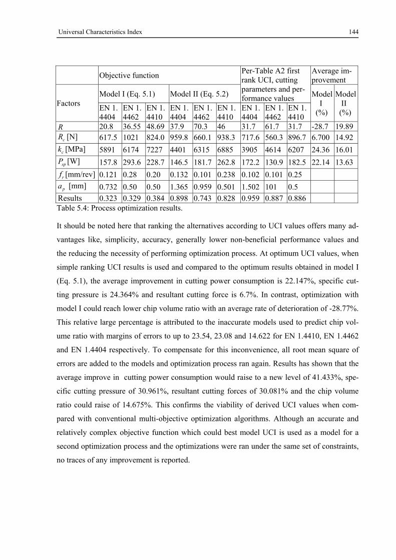
Universal Characteristics Index 144
Objective function Per-Table A2 first rank UCI, cutting parameters and per-formance values
Average im-provement
Factors Model I (Eq. 5.1) Model II (Eq. 5.2) Model
I (%)
Model II (%)
EN 1. 4404
EN 1. 4462
EN 1. 4410
EN 1. 4404
EN 1. 4462
EN 1. 4410
EN 1. 4404
EN 1. 4462
EN 1. 4410
R 20.8 36.55 48.69 37.9 70.3 46 31.7 61.7 31.7 -28.7 19.89
cR [N] 617.5 1021 824.0 959.8 660.1 938.3 717.6 560.3 896.7 6.700 14.92
ck [MPa] 5891 6174 7227 4401 6315 6885 3905 4614 6207 24.36 16.01
spP [W] 157.8 293.6 228.7 146.5 181.7 262.8 172.2 130.9 182.5 22.14 13.63
rf [mm/rev] 0.121 0.28 0.20 0.132 0.101 0.238 0.102 0.101 0.25
pa [mm] 0.732 0.50 0.50 1.365 0.959 0.501 1.502 101 0.5
Results 0.323 0.329 0.384 0.898 0.743 0.828 0.959 0.887 0.886 Table 5.4: Process optimization results.
It should be noted here that ranking the alternatives according to UCI values offers many ad-
vantages like, simplicity, accuracy, generally lower non-beneficial performance values and
the reducing the necessity of performing optimization process. At optimum UCI values, when
simple ranking UCI results is used and compared to the optimum results obtained in model I
(Eq. 5.1), the average improvement in cutting power consumption is 22.147%, specific cut-
ting pressure is 24.364% and resultant cutting force is 6.7%. In contrast, optimization with
model I could reach lower chip volume ratio with an average rate of deterioration of -28.77%.
This relative large percentage is attributed to the inaccurate models used to predict chip vol-
ume ratio with margins of errors to up to 23.54, 23.08 and 14.622 for EN 1.4410, EN 1.4462
and EN 1.4404 respectively. To compensate for this inconvenience, all root mean square of
errors are added to the models and optimization process ran again. Results has shown that the
average improve in cutting power consumption would raise to a new level of 41.433%, spe-
cific cutting pressure of 30.961%, resultant cutting forces of 30.081% and the chip volume
ratio could raise of 14.675%. This confirms the viability of derived UCI values when com-
pared with conventional multi-objective optimization algorithms. Although an accurate and
relatively complex objective function which could best model UCI is used as a model for a
second optimization process and the optimizations were ran under the same set of constraints,
no traces of any improvement is reported.
Universal Characteristics Index 145
5.4 Interim conclusions
For the studied range of process parameters, the resulting chip form was strongly influ-
enced by the workpiece material and cutting conditions. When machining super duplex
EN 1.4410 and standard duplex EN 1.4462 stainless steels, snarled and ribbon chips were
the dominant at lower feed ranges and nearly all higher depth of cut ranges. Meanwhile,
flat helical and cylindrical helical chips at medium feed ranges and helical and less spiral
chips at higher feed ranges were the dominant. Chips obtained when machining austenitic
EN 1.4404 stainless steel are friendlier to the machine and generally produce lower rib-
bon, snarled and flat helical chips. Fuzzy logic principles were applied to quantify the in-
formation presented in chip breaking chart and could successfully predicts the chip vol-
ume ratio.
In the present chapter, the objective was to simultaneously minimize performance charac-
teristics such as chip volume ratio, resultant cutting forces, specific cutting pressures and
net spindle powers. Because the values of above non-beneficial performance characteris-
tics when machining austenitic EN 1.4404 were generally lower than standard duplex EN
1.4462 and super duplex EN 1.4410 grades, therefore, one can roughly conclude that the
machinability of EN 1.4404 is better than EN 1.4462 and EN 1.4410.
The multiple performance characteristics were successfully converted into single MADM-
indices using TOPSIS, VIKOR, GRA and UA. Due to the differences among MADM
preferences and rankings, and the absence of a reference defining a ‘super method’, fuzzy
rule modeling approach was proposed to eliminate the discrepancy among the MADM
methods and derive a single characterization index called UCI. Spearman’s rank correla-
tion coefficients have confirmed that the proposed index had a very good correlation with
the output of other MPCI methods. Predicted UCI values have been analyzed and com-
pared with output of other optimization techniques. A remarkable improvement in reduc-
tion of cutting power consumption, specific cutting pressure and resultant cutting forces
has been reported when direct ranking system of predicted UCI indices are set as opti-
mum.
Taguchi-MADM-Meta-heuristic concept 146
6 Taguchi-MADM-Meta-heuristic concept
The main objective of this chapter is to examine the machinability of different grades of stain-
less steels in seeking simultaneous improvement in performance characteristics (or response
factors) using different statistical and mathematical tools. Accordingly, multi-performance
optimization of turning austenitic EN 1.4404, standard duplex EN 1.4462 and super duplex
EN 1.4410 stainless steels utilizing coupled Taguchi-based designs, multiple attribute deci-
sion making (MADM) and meta-heuristic algorithms is experimentally addressed. The flow
chart of the methodology presented in this chapter is shown in Figure 6.1. Surface roughness,
specific cutting energy, cutting power and resultant cutting forces are optimized per each ma-
terial under Taguchi optimization procedure and combined as a single, cutting parameter de-
pendent Multi-Performance Characteristics Index (MPCI) using VIKOR method. Analysis of
means (ANOM) and Analysis of variance (ANOVA) are employed to designate the optimum
level of cutting parameters and to investigate the influence of cutting parameters and their
interactions on the computed index, respectively. Nature-inspired meta-heuristic algorithms
such as; Firefly Algorithm (FA), Accelerated Particle Swarm Optimization (APSO) and
Cuckoo Search (CS) are used to constrainedly optimize the developed MPCIs and find the
exact setting of optimum cutting parameter. Finally, a comparison analysis is conducted in
order to designate the algorithm which has shown the best performance in quickly and con-
sistently converge to the global optimum point.
6.1 Taguchi method
In order to systematically approach the variance in controllable input factors and to observe
the effect of these factors and their interactions on the output performance parameters, an L25
(56) orthogonal array proposed by Taguchi is used in the experimental procedure per each
workpiece material (see Table 3.6) using coated carbide cutting tool of ISO designation
CNMG 120408-MM 2025. The control factors are the three known cutting parameters which
are cutting speed ( cv ), feed rate ( rf ) and depth of cut ( pa ). Under a full factorial run and in
the case of three factors with five levels, 53=125 experiments should be conducted. In accord-
ance with Taguchi’s method the standard orthogonal array L25 with only one fifth of that
number of experiments could be used. However, the selection of L25 orthogonal array, that
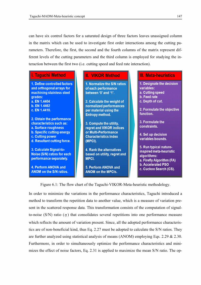
Taguchi-MADM-Meta-heuristic concept 147
can have six control factors for a saturated design of three factors leaves unassigned column
in the matrix which can be used to investigate first order interactions among the cutting pa-
rameters. Therefore, the first, the second and the fourth columns of the matrix represent dif-
ferent levels of the cutting parameters and the third column is employed for studying the in-
teraction between the first two (i.e. cutting speed and feed rate interaction).
Figure 6.1: The flow chart of the Taguchi-VIKOR-Meta-heuristic methodology.
In order to minimize the variations in the performance characteristics, Taguchi introduced a
method to transform the repetition data to another value, which is a measure of variation pre-
sent in the scattered response data. This transformation consists of the computation of signal-
to-noise (S/N) ratio ( ) that consolidates several repetitions into one performance measure
which reflects the amount of variation present. Since, all the adopted performance characteris-
tics are of non-beneficial kind, thus Eq. 2.27 must be adopted to calculate the S/N ratios. They
are further analyzed using statistical analysis of means (ANOM) employing Eqs. 2.29 & 2.30.
Furthermore, in order to simultaneously optimize the performance characteristics and mini-
mizes the effect of noise factors, Eq. 2.31 is applied to maximize the mean S/N ratio. The op-
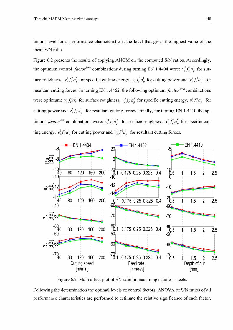
Taguchi-MADM-Meta-heuristic concept 148
timum level for a performance characteristic is the level that gives the highest value of the
mean S/N ratio.
Figure 6.2 presents the results of applying ANOM on the computed S/N ratios. Accordingly,
the optimum control levelfactor combinations during turning EN 1.4404 were: 215prc afv for sur-
face roughness, 554prc afv for specific cutting energy, 111
prc afv for cutting power and 114prc afv for
resultant cutting forces. In turning EN 1.4462, the following optimum levelfactor combinations
were optimum: 215prc afv for surface roughness, 533
prc afv for specific cutting energy, 111prc afv for
cutting power and 113prc afv for resultant cutting forces. Finally, for turning EN 1.4410 the op-
timum levelfactor combinations were: 214prc afv for surface roughness, 534
prc afv for specific cut-
ting energy, 111prc afv for cutting power and 114
prc afv for resultant cutting forces.
Figure 6.2: Main effect plot of SN ratio in machining stainless steels.
Following the determination the optimal levels of control factors, ANOVA of S/N ratios of all
performance characteristics are performed to estimate the relative significance of each factor.
40 80 120 160 200-10
-8
-6
Ra
[d
B]
40 80 120 160 200-14
-12
-10
e c [d
B]
40 80 120 160 200-80
-60
-40
Pc
[dB
]
40 80 120 160 200-70
-65
-60
Cutting speed [m/min]
Rc
[dB
]
0.1 0.175 0.25 0.325 0.4-20
0
20
0.1 0.175 0.25 0.325 0.4
-14
-12
-10
0.1 0.175 0.25 0.325 0.4-80
-70
-60
0.1 0.175 0.25 0.325 0.4-70
-60
-50
Feed rate [mm/rev]
0.5 1 1.5 2 2.5-10
-5
0.5 1 1.5 2 2.5-20
-10
0
0.5 1 1.5 2 2.5-80
-70
-60
0.5 1 1.5 2 2.5-70
-60
-50
Depth of cut [mm]
EN 1.4404 EN 1.4462 EN 1.4410
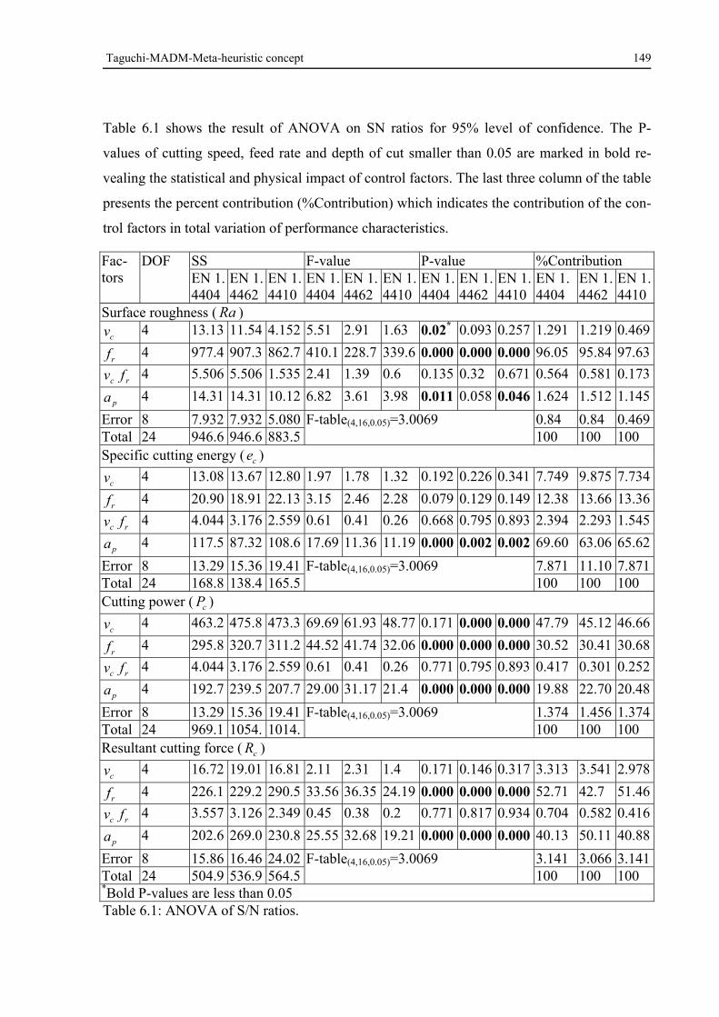
Taguchi-MADM-Meta-heuristic concept 149
Table 6.1 shows the result of ANOVA on SN ratios for 95% level of confidence. The P-
values of cutting speed, feed rate and depth of cut smaller than 0.05 are marked in bold re-
vealing the statistical and physical impact of control factors. The last three column of the table
presents the percent contribution (%Contribution) which indicates the contribution of the con-
trol factors in total variation of performance characteristics.
Fac-tors
DOF SS F-value P-value %Contribution EN 1. 4404
EN 1. 4462
EN 1.4410
EN 1.4404
EN 1.4462
EN 1.4410
EN 1.4404
EN 1.4462
EN 1. 4410
EN 1. 4404
EN 1.4462
EN 1.4410
Surface roughness ( Ra )
cv 4 13.13 11.54 4.152 5.51 2.91 1.63 0.02* 0.093 0.257 1.291 1.219 0.469
rf 4 977.4 907.3 862.7 410.1 228.7 339.6 0.000 0.000 0.000 96.05 95.84 97.63
rc fv 4 5.506 5.506 1.535 2.41 1.39 0.6 0.135 0.32 0.671 0.564 0.581 0.173
pa 4 14.31 14.31 10.12 6.82 3.61 3.98 0.011 0.058 0.046 1.624 1.512 1.145
Error 8 7.932 7.932 5.080 F-table(4,16,0.05)=3.0069 0.84 0.84 0.469Total 24 946.6 946.6 883.5 100 100 100 Specific cutting energy ( ce )
cv 4 13.08 13.67 12.80 1.97 1.78 1.32 0.192 0.226 0.341 7.749 9.875 7.734
rf 4 20.90 18.91 22.13 3.15 2.46 2.28 0.079 0.129 0.149 12.38 13.66 13.36
rc fv 4 4.044 3.176 2.559 0.61 0.41 0.26 0.668 0.795 0.893 2.394 2.293 1.545
pa 4 117.5 87.32 108.6 17.69 11.36 11.19 0.000 0.002 0.002 69.60 63.06 65.62
Error 8 13.29 15.36 19.41 F-table(4,16,0.05)=3.0069 7.871 11.10 7.871Total 24 168.8 138.4 165.5 100 100 100 Cutting power ( cP )
cv 4 463.2 475.8 473.3 69.69 61.93 48.77 0.171 0.000 0.000 47.79 45.12 46.66
rf 4 295.8 320.7 311.2 44.52 41.74 32.06 0.000 0.000 0.000 30.52 30.41 30.68
rc fv 4 4.044 3.176 2.559 0.61 0.41 0.26 0.771 0.795 0.893 0.417 0.301 0.252
pa 4 192.7 239.5 207.7 29.00 31.17 21.4 0.000 0.000 0.000 19.88 22.70 20.48
Error 8 13.29 15.36 19.41 F-table(4,16,0.05)=3.0069 1.374 1.456 1.374Total 24 969.1 1054. 1014. 100 100 100 Resultant cutting force ( cR )
cv 4 16.72 19.01 16.81 2.11 2.31 1.4 0.171 0.146 0.317 3.313 3.541 2.978
rf 4 226.1 229.2 290.5 33.56 36.35 24.19 0.000 0.000 0.000 52.71 42.7 51.46
rc fv 4 3.557 3.126 2.349 0.45 0.38 0.2 0.771 0.817 0.934 0.704 0.582 0.416
pa 4 202.6 269.0 230.8 25.55 32.68 19.21 0.000 0.000 0.000 40.13 50.11 40.88
Error 8 15.86 16.46 24.02 F-table(4,16,0.05)=3.0069 3.141 3.066 3.141Total 24 504.9 536.9 564.5 100 100 100 *Bold P-values are less than 0.05 Table 6.1: ANOVA of S/N ratios.
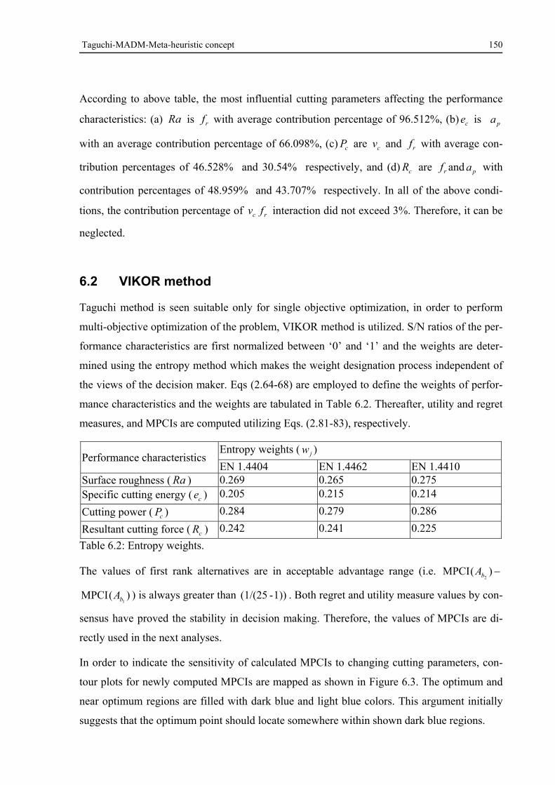
Taguchi-MADM-Meta-heuristic concept 150
According to above table, the most influential cutting parameters affecting the performance
characteristics: (a) Ra is rf with average contribution percentage of 96.512%, (b) ce is pa
with an average contribution percentage of 66.098%, (c) cP are cv and rf with average con-
tribution percentages of 46.528% and 30.54% respectively, and (d) cR are rf and pa with
contribution percentages of 48.959% and 43.707% respectively. In all of the above condi-
tions, the contribution percentage of rc fv interaction did not exceed 3%. Therefore, it can be
neglected.
6.2 VIKOR method
Taguchi method is seen suitable only for single objective optimization, in order to perform
multi-objective optimization of the problem, VIKOR method is utilized. S/N ratios of the per-
formance characteristics are first normalized between ‘0’ and ‘1’ and the weights are deter-
mined using the entropy method which makes the weight designation process independent of
the views of the decision maker. Eqs (2.64-68) are employed to define the weights of perfor-
mance characteristics and the weights are tabulated in Table 6.2. Thereafter, utility and regret
measures, and MPCIs are computed utilizing Eqs. (2.81-83), respectively.
Performance characteristics Entropy weights ( )jw
EN 1.4404 EN 1.4462 EN 1.4410 Surface roughness ( Ra ) 0.269 0.265 0.275 Specific cutting energy ( ce ) 0.205 0.215 0.214
Cutting power ( cP ) 0.284 0.279 0.286
Resultant cutting force ( cR ) 0.242 0.241 0.225
Table 6.2: Entropy weights.
The values of first rank alternatives are in acceptable advantage range (i.e. )(MPCI2bA
)(MPCI1bA ) is always greater than 1))-(1/(25 . Both regret and utility measure values by con-
sensus have proved the stability in decision making. Therefore, the values of MPCIs are di-
rectly used in the next analyses.
In order to indicate the sensitivity of calculated MPCIs to changing cutting parameters, con-
tour plots for newly computed MPCIs are mapped as shown in Figure 6.3. The optimum and
near optimum regions are filled with dark blue and light blue colors. This argument initially
suggests that the optimum point should locate somewhere within shown dark blue regions.
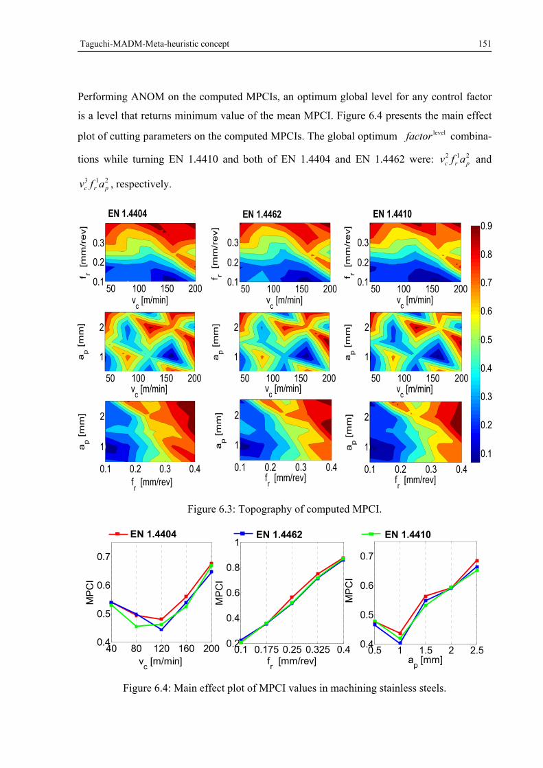
Taguchi-MADM-Meta-heuristic concept 151
Performing ANOM on the computed MPCIs, an optimum global level for any control factor
is a level that returns minimum value of the mean MPCI. Figure 6.4 presents the main effect
plot of cutting parameters on the computed MPCIs. The global optimum levelfactor combina-
tions while turning EN 1.4410 and both of EN 1.4404 and EN 1.4462 were: 212prc afv and
213prc afv , respectively.
Figure 6.3: Topography of computed MPCI.
Figure 6.4: Main effect plot of MPCI values in machining stainless steels.
40 80 120 160 2000.4
0.5
0.6
0.7
vc [m/min]
MP
CI
0.1 0.175 0.25 0.325 0.40.2
0.4
0.6
0.8
1
fr [mm/rev]
MP
CI
0.5 1 1.5 2 2.50.4
0.5
0.6
0.7
ap [mm]
MP
CI
EN 1.4462EN 1.4404 EN 1.4410
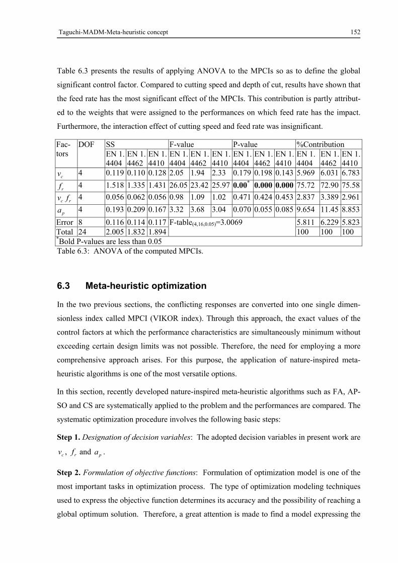
Taguchi-MADM-Meta-heuristic concept 152
Table 6.3 presents the results of applying ANOVA to the MPCIs so as to define the global
significant control factor. Compared to cutting speed and depth of cut, results have shown that
the feed rate has the most significant effect of the MPCIs. This contribution is partly attribut-
ed to the weights that were assigned to the performances on which feed rate has the impact.
Furthermore, the interaction effect of cutting speed and feed rate was insignificant.
Fac-tors
DOF SS F-value P-value %Contribution EN 1. 4404
EN 1. 4462
EN 1.4410
EN 1.4404
EN 1.4462
EN 1.4410
EN 1.4404
EN 1.4462
EN 1. 4410
EN 1. 4404
EN 1.4462
EN 1.4410
cv 4 0.119 0.110 0.128 2.05 1.94 2.33 0.179 0.198 0.143 5.969 6.031 6.783
rf 4 1.518 1.335 1.431 26.05 23.42 25.97 0.00* 0.000 0.000 75.72 72.90 75.58
rc fv 4 0.056 0.062 0.056 0.98 1.09 1.02 0.471 0.424 0.453 2.837 3.389 2.961
pa 4 0.193 0.209 0.167 3.32 3.68 3.04 0.070 0.055 0.085 9.654 11.45 8.853
Error 8 0.116 0.114 0.117 F-table(4,16,0.05)=3.0069 5.811 6.229 5.823Total 24 2.005 1.832 1.894 100 100 100 *Bold P-values are less than 0.05 Table 6.3: ANOVA of the computed MPCIs.
6.3 Meta-heuristic optimization
In the two previous sections, the conflicting responses are converted into one single dimen-
sionless index called MPCI (VIKOR index). Through this approach, the exact values of the
control factors at which the performance characteristics are simultaneously minimum without
exceeding certain design limits was not possible. Therefore, the need for employing a more
comprehensive approach arises. For this purpose, the application of nature-inspired meta-
heuristic algorithms is one of the most versatile options.
In this section, recently developed nature-inspired meta-heuristic algorithms such as FA, AP-
SO and CS are systematically applied to the problem and the performances are compared. The
systematic optimization procedure involves the following basic steps:
Step 1. Designation of decision variables: The adopted decision variables in present work are
cv , rf and pa .
Step 2. Formulation of objective functions: Formulation of optimization model is one of the
most important tasks in optimization process. The type of optimization modeling techniques
used to express the objective function determines its accuracy and the possibility of reaching a
global optimum solution. Therefore, a great attention is made to find a model expressing the
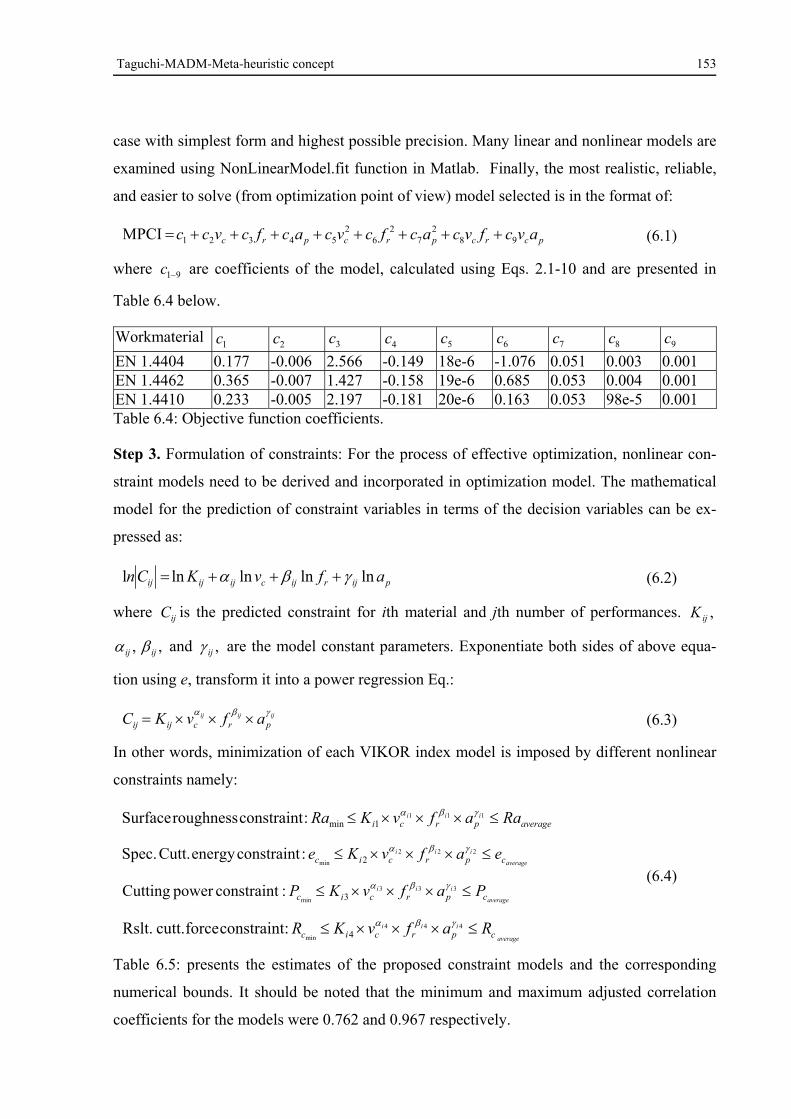
Taguchi-MADM-Meta-heuristic concept 153
case with simplest form and highest possible precision. Many linear and nonlinear models are
examined using NonLinearModel.fit function in Matlab. Finally, the most realistic, reliable,
and easier to solve (from optimization point of view) model selected is in the format of:
pcrcprcprc avcfvcacfcvcacfcvcc 982
72
62
54321MPCI (6.1)
where 91c are coefficients of the model, calculated using Eqs. 2.1-10 and are presented in
Table 6.4 below.
Workmaterial 1c 2c 3c 4c 5c 6c 7c 8c 9c
EN 1.4404 0.177 -0.006 2.566 -0.149 18e-6 -1.076 0.051 0.003 0.001 EN 1.4462 0.365 -0.007 1.427 -0.158 19e-6 0.685 0.053 0.004 0.001 EN 1.4410 0.233 -0.005 2.197 -0.181 20e-6 0.163 0.053 98e-5 0.001 Table 6.4: Objective function coefficients.
Step 3. Formulation of constraints: For the process of effective optimization, nonlinear con-
straint models need to be derived and incorporated in optimization model. The mathematical
model for the prediction of constraint variables in terms of the decision variables can be ex-
pressed as:
pijrijcijijij afvKCn lnlnlnlnl (6.2)
where ijC is the predicted constraint for ith material and jth number of performances. ,ijK
,ij ,ij and ,ij are the model constant parameters. Exponentiate both sides of above equa-
tion using e, transform it into a power regression Eq.:
ijijij
prcijij afvKC (6.3)
In other words, minimization of each VIKOR index model is imposed by different nonlinear
constraints namely:
averageprci RaafvKRa iii 1111min:constraintroughnessSurface
average
iiicprcic eafvKe 222
min 2:constraintenergyCutt. Spec.
average
iiicprcic PafvKP 333
min 3:constraintpowerCutting
average
iiicprcic RafvKR 444
min 4:constraintforcecutt.Rslt.
(6.4)
Table 6.5: presents the estimates of the proposed constraint models and the corresponding
numerical bounds. It should be noted that the minimum and maximum adjusted correlation
coefficients for the models were 0.762 and 0.967 respectively.
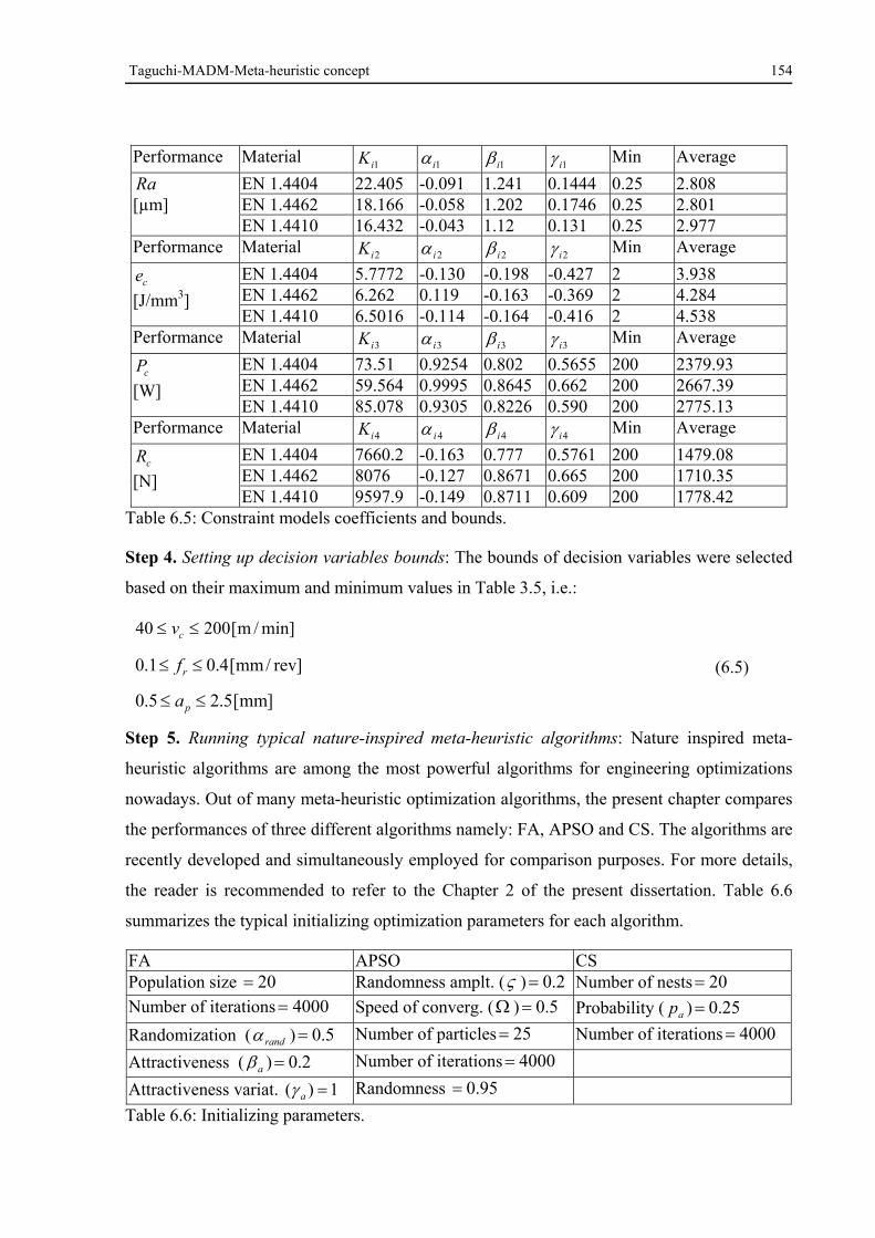
Taguchi-MADM-Meta-heuristic concept 154
Performance Material 1iK 1i 1i 1i Min Average
Ra [µm]
EN 1.4404 22.405 -0.091 1.241 0.1444 0.25 2.808 EN 1.4462 18.166 -0.058 1.202 0.1746 0.25 2.801 EN 1.4410 16.432 -0.043 1.12 0.131 0.25 2.977
Performance Material 2iK 2i 2i 2i Min Average
ce
[J/mm3]
EN 1.4404 5.7772 -0.130 -0.198 -0.427 2 3.938 EN 1.4462 6.262 0.119 -0.163 -0.369 2 4.284 EN 1.4410 6.5016 -0.114 -0.164 -0.416 2 4.538
Performance Material 3iK 3i 3i 3i Min Average
cP
[W]
EN 1.4404 73.51 0.9254 0.802 0.5655 200 2379.93 EN 1.4462 59.564 0.9995 0.8645 0.662 200 2667.39 EN 1.4410 85.078 0.9305 0.8226 0.590 200 2775.13
Performance Material 4iK 4i 4i 4i Min Average
cR
[N]
EN 1.4404 7660.2 -0.163 0.777 0.5761 200 1479.08 EN 1.4462 8076 -0.127 0.8671 0.665 200 1710.35 EN 1.4410 9597.9 -0.149 0.8711 0.609 200 1778.42
Table 6.5: Constraint models coefficients and bounds.
Step 4. Setting up decision variables bounds: The bounds of decision variables were selected
based on their maximum and minimum values in Table 3.5, i.e.:
min]/m[20040 cv
]rev/mm[4.01.0 rf
]mm[5.25.0 pa
(6.5)
Step 5. Running typical nature-inspired meta-heuristic algorithms: Nature inspired meta-
heuristic algorithms are among the most powerful algorithms for engineering optimizations
nowadays. Out of many meta-heuristic optimization algorithms, the present chapter compares
the performances of three different algorithms namely: FA, APSO and CS. The algorithms are
recently developed and simultaneously employed for comparison purposes. For more details,
the reader is recommended to refer to the Chapter 2 of the present dissertation. Table 6.6
summarizes the typical initializing optimization parameters for each algorithm.
FA APSO CS Population size 20 Randomness amplt. ( ) 2.0 Number of nests 20
Number of iterations 4000 Speed of converg. ( ) 5.0 Probability ( ap ) 25.0
Randomization ( rand ) 5.0 Number of particles 25 Number of iterations 4000
Attractiveness ( a ) 2.0 Number of iterations 4000
Attractiveness variat. 1)( a Randomness 95.0
Table 6.6: Initializing parameters.
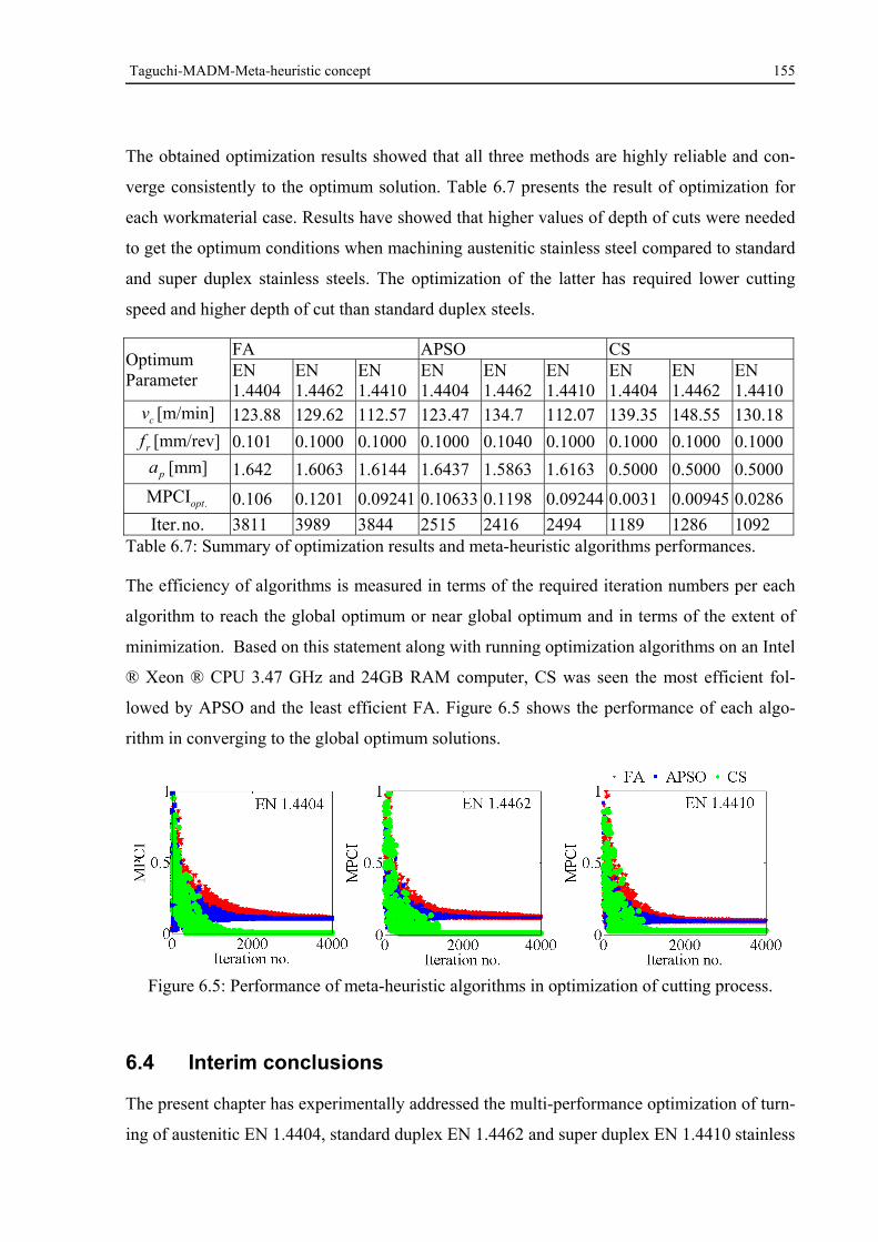
Taguchi-MADM-Meta-heuristic concept 155
The obtained optimization results showed that all three methods are highly reliable and con-
verge consistently to the optimum solution. Table 6.7 presents the result of optimization for
each workmaterial case. Results have showed that higher values of depth of cuts were needed
to get the optimum conditions when machining austenitic stainless steel compared to standard
and super duplex stainless steels. The optimization of the latter has required lower cutting
speed and higher depth of cut than standard duplex steels.
Optimum Parameter
FA APSO CS EN
1.4404 EN
1.4462 EN1.4410
EN 1.4404
EN1.4462
EN1.4410
EN 1.4404
EN
1.4462 EN1.4410
cv [m/min] 123.88 129.62 112.57 123.47 134.7 112.07 139.35 148.55 130.18
rf [mm/rev] 0.101 0.1000 0.1000 0.1000 0.1040 0.1000 0.1000 0.1000 0.1000
pa [mm] 1.642 1.6063 1.6144 1.6437 1.5863 1.6163 0.5000 0.5000 0.5000
.MPCIopt 0.106 0.1201 0.09241 0.10633 0.1198 0.09244 0.0031 0.00945 0.0286
no. Iter. 3811 3989 3844 2515 2416 2494 1189 1286 1092 Table 6.7: Summary of optimization results and meta-heuristic algorithms performances.
The efficiency of algorithms is measured in terms of the required iteration numbers per each
algorithm to reach the global optimum or near global optimum and in terms of the extent of
minimization. Based on this statement along with running optimization algorithms on an Intel
® Xeon ® CPU 3.47 GHz and 24GB RAM computer, CS was seen the most efficient fol-
lowed by APSO and the least efficient FA. Figure 6.5 shows the performance of each algo-
rithm in converging to the global optimum solutions.
Figure 6.5: Performance of meta-heuristic algorithms in optimization of cutting process.
6.4 Interim conclusions
The present chapter has experimentally addressed the multi-performance optimization of turn-
ing of austenitic EN 1.4404, standard duplex EN 1.4462 and super duplex EN 1.4410 stainless
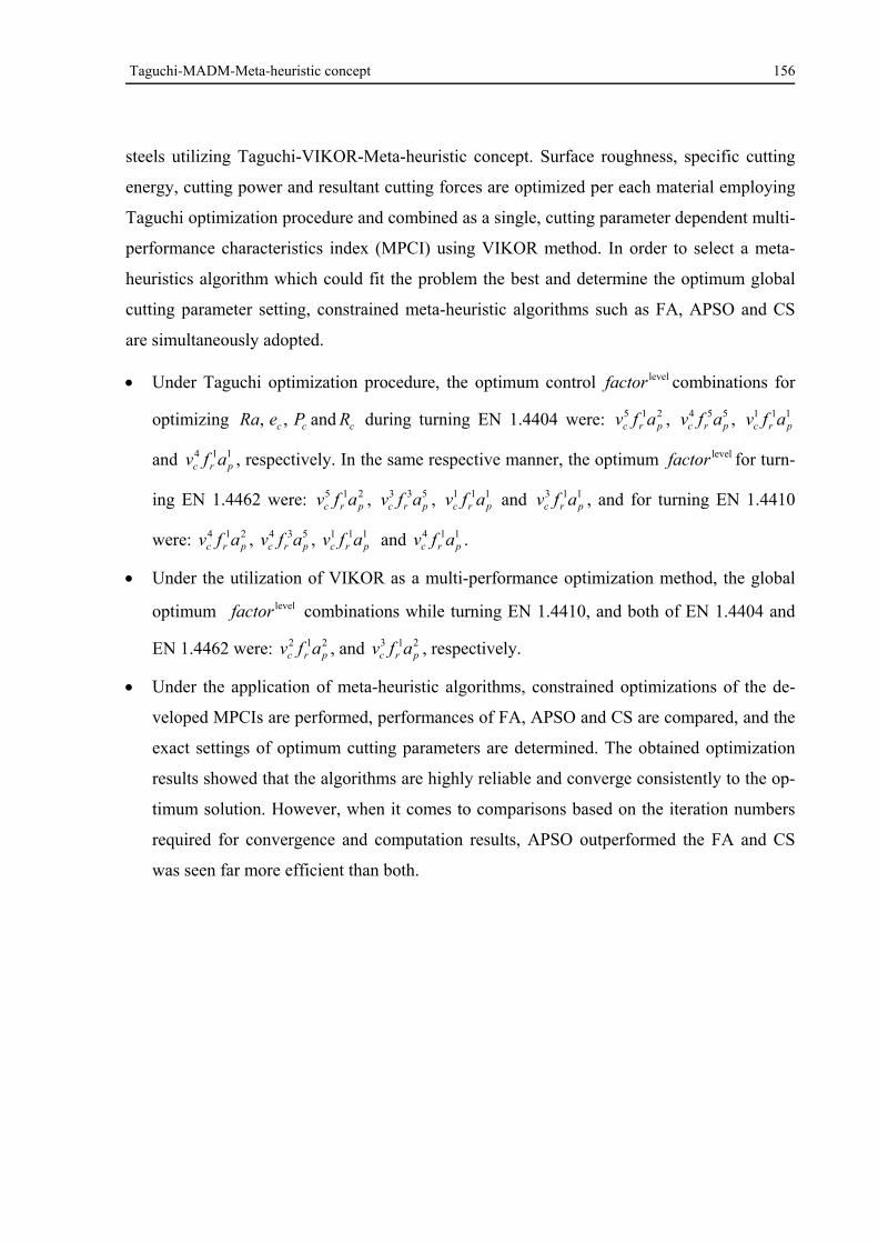
Taguchi-MADM-Meta-heuristic concept 156
steels utilizing Taguchi-VIKOR-Meta-heuristic concept. Surface roughness, specific cutting
energy, cutting power and resultant cutting forces are optimized per each material employing
Taguchi optimization procedure and combined as a single, cutting parameter dependent multi-
performance characteristics index (MPCI) using VIKOR method. In order to select a meta-
heuristics algorithm which could fit the problem the best and determine the optimum global
cutting parameter setting, constrained meta-heuristic algorithms such as FA, APSO and CS
are simultaneously adopted.
Under Taguchi optimization procedure, the optimum control levelfactor combinations for
optimizing ccc RPeRa and,, during turning EN 1.4404 were: 215prc afv , 554
prc afv , 111prc afv
and 114prc afv , respectively. In the same respective manner, the optimum levelfactor for turn-
ing EN 1.4462 were: 215prc afv , 533
prc afv , 111prc afv and 113
prc afv , and for turning EN 1.4410
were: 214prc afv , 534
prc afv , 111prc afv and 114
prc afv .
Under the utilization of VIKOR as a multi-performance optimization method, the global
optimum levelfactor combinations while turning EN 1.4410, and both of EN 1.4404 and
EN 1.4462 were: 212prc afv , and 213
prc afv , respectively.
Under the application of meta-heuristic algorithms, constrained optimizations of the de-
veloped MPCIs are performed, performances of FA, APSO and CS are compared, and the
exact settings of optimum cutting parameters are determined. The obtained optimization
results showed that the algorithms are highly reliable and converge consistently to the op-
timum solution. However, when it comes to comparisons based on the iteration numbers
required for convergence and computation results, APSO outperformed the FA and CS
was seen far more efficient than both.
Application of Fuzzy–MADM approach in optimizing surface quality of stainless steels 157
7 Application of Fuzzy–MADM approach in opti-
mizing surface quality of stainless steels
In this chapter, Taguchi approach is coupled with fuzzy-MADM methods for achieving better
surface quality in constant cutting speed face turning of EN 1.4404 austenitic, EN 1.4462
standard duplex and EN 1.4410 super duplex stainless steels. MADM methods such as
GTMA and AHP-TOPSIS are simultaneously adopted to combine well-known surface quality
characteristics like arithmetic average ( Ra ), average distance between the highest peak and
lowest valley ( Rz ) and maximum height of the profile ( Rt ) into a single index called multi-
surface quality characteristics index ( MSQCI ). The differences in rankings between derived
indices are solved through converting each crisp values into trapezoidal fuzzy number and
unifying them using fuzzy simple additive weight method. The fuzzy numbers are then def-
fuzified into crisp values employing techniques like; the spread, mode and area between cen-
troid of centroids. The results are further analyzed using analysis of means (ANOM) and
analysis of variance (ANOVA). Finally, confirmation tests are conducted to verify the ob-
tained optimal results.
7.1 Proposed methodology
The novel approach proposed in this chapter can be summarized into five stages as shown in
Figure 7.1. Following the determination of MSQCI crisp values for each alternative using
described MADM approaches, they are converted into fuzzy numbers. The reason behind the
conversion into fuzzy refers to the fact that none of MADM methods can be considered as the
‘super method’ appropriate to all decision making situations. This implies that it is critical to
select the most appropriate method to solve the problem under consideration, since the use of
unsuitable method always leads to misleading decisions. Therefore, to avoid risking, a level of
uncertainty in each computed MSQCI is accounted for, so that the decision maker is uncer-
tain or partially certain based on the values of adopted membership functions.
The fuzzification process of crisp MSQCI values (CV ) into fuzzy number MSQCI
),,,( 4321 aaaa is governed by the following expressions:
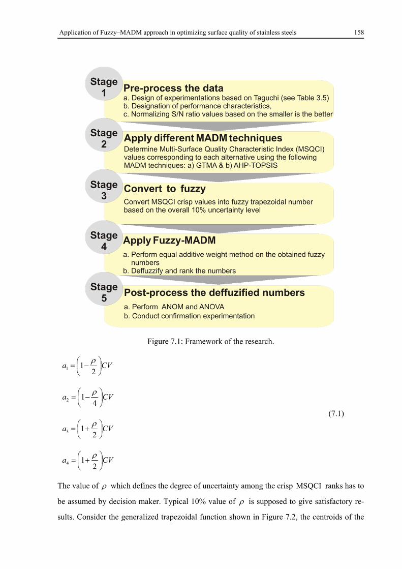
Application of Fuzzy–MADM approach in optimizing surface quality of stainless steels 158
Figure 7.1: Framework of the research.
CVa
211
CVa
412
CVa
213
CVa
214
(7.1)
The value of which defines the degree of uncertainty among the crisp MSQCI ranks has to
be assumed by decision maker. Typical 10% value of is supposed to give satisfactory re-
sults. Consider the generalized trapezoidal function shown in Figure 7.2, the centroids of the
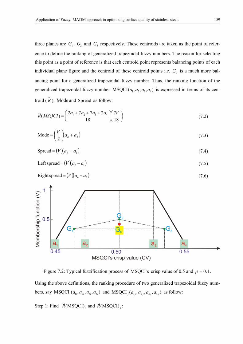
Application of Fuzzy–MADM approach in optimizing surface quality of stainless steels 159
three planes are 1G , 2G and 3G respectively. These centroids are taken as the point of refer-
ence to define the ranking of generalized trapezoidal fuzzy numbers. The reason for selecting
this point as a point of reference is that each centroid point represents balancing points of each
individual plane figure and the centroid of these centroid points i.e. 0G is a much more bal-
ancing point for a generalized trapezoidal fuzzy number. Thus, the ranking function of the
generalized trapezoidal fuzzy number ),,,(MSQCI 4321 aaaa is expressed in terms of its cen-
troid ( R~
), Mode and Spread as follow:
18
7
18
2772)(
~ 4321 VaaaaMSQCIR (7.2)
322Mode aa
V
(7.3)
14Spread aaV (7.4)
12spreadLeft aaV (7.5)
34spreadRight aaV (7.6)
Figure 7.2: Typical fuzzification process of sMSQCI' crisp value of 0.5 and 1.0 .
Using the above definitions, the ranking procedure of two generalized trapezoidal fuzzy num-
bers, say ),,,(MSQCI 4321 iiiii aaaa and ),,,(MSQCI 4321 jjjjj aaaa as follow:
Step 1: Find iR )MSQCI(~
and jR )MSQCI(~
:
Application of Fuzzy–MADM approach in optimizing surface quality of stainless steels 160
If ji RR )MSQCI(~
)MSQCI(~ then i)MSQCI( outperforms j)MSQCI( .
If ji RR )MSQCI(~
)MSQCI(~ then j)MSQCI( outperforms i)MSQCI( .
Otherwise, comparisons are not possible and proceed to the next step.
Step 2: Find i)MSQCI(Mode and j)MSQCI(Mode :
If ji )MSQCI(Mode)MSQCI(Mode then i)MSQCI( outperforms .)MSQCI( j
If ji )MSQCI(Mode)MSQCI(Mode then j)MSQCI( outperforms .)MSQCI( i
Otherwise, comparisons are not possible and proceed to the next step.
Step 3: Find i)MSQCI(Spread and j)MSQCI(Spread :
If ji )MSQCI(Spread)MSQCI(Spread then j)MSQCI( outperforms i)MSQCI( .
If ji )MSQCI(Spread)MSQCI(Spread then i)MSQCI( outperforms j)MSQCI( .
Otherwise, comparisons are not possible and proceed to the next step.
Step 4: Find i)MSQCI(spreadLeft and j)MSQCI(spreadLeft :
If ji )MSQCI(spreadLeft )MSQCI(spreadLeft then i)MSQCI( outperforms j)MSQCI( .
If ji )MSQCI(spreadLeft )MSQCI(spreadLeft then j)MSQCI( outperforms i)MSQCI( .
Otherwise, comparisons are not possible and proceed to the next step.
Step 5: Find i)MSQCI(spreadRight and j)MSQCI(spreadRight :
If ji )MSQCI(spreadRight )MSQCI(spreadRight then j)MSQCI( outperforms i)MSQCI(
If ji )MSQCI(spreadRight )MSQCI(spreadRight then i)MSQCI( outperforms j)MSQCI(
Otherwise, comparisons are not possible and proceed to the next step.
7.2 Results and discussions
7.2.1 Computation of the MSQCIs
The experimental layout plan and result as per Taguchi orthogonal array for the current inves-
tigation is illustrated in Table A3. From this layout, one can easily conclude that the mean
Application of Fuzzy–MADM approach in optimizing surface quality of stainless steels 161
values of non-beneficial surface quality characteristics during turning super DSS EN 1.4410
are higher than of standard DSS EN 1.4462 and austenitic stainless steel EN 1.4404. The lat-
ter has the least mean values of non-beneficial surface quality characteristics.
MADM methods are coupled with Taguchi design to overcome the problem of finding the
best alternative for situations where there is more than one performance. Because the selected
quality characteristics are of non-beneficial nature, the smaller-the-better criterion is adopted
in this study. Therefore, Eq. (2.27) is utilized to transform the real roughness values into S/N
ratio values. The following sections briefly describe the procedure of MSQCI calculations.
7.2.1.1 Computation of MSQCIs using GTMA
The decision problem is formulated in matrix format using Eq. (2.60-62). Then, larger-the-
better term of Eq. (2.84) is used to normalize the S/N ratio to minimize the scale effect. In
order to assign the weight to each normalized performance, the superiority of one perfor-
mance over another has to be considered. In industry, the arithmetic average roughness ( Ra )
is more pronounced when it comes to the evaluation of surface quality. Therefore, the follow-
ing relative importance scheme is adopted (refer to Eq. (2.99)):
5.0225.0
5.0225.0
475.0475.0
Ra
Rz
Rt
DMA
RaRzRt
GTMA
(7.7)
Then attributes matrix can be written based on Eq. (2.100). It is similar to matrix equation
above but also with presence of diagonal elements. To estimate the permanent of matrices, a
Matlab code has been programmed. The determined permanent values represent MSQCI
using GTMA. From the values of MSQCI it is understood that alternatives A5, A13 and A1
are the best choices among the considered sixteen alternatives when surface qualities of EN
1.4404, EN 1.4462 and EN 1.4410 are needed to be optimized respectively.
7.2.1.2 Computation of MSQCI using AHP-TOPSIS
To determine the MSQCI values using AHP-TOPSIS method, Eq. (2.72) is employed first to
normalize the computed S/N ratios. The comparison process requires that the relative normal-
ized weights used in AHP-TOPSIS to be equal to those used in the GTMA method. Following
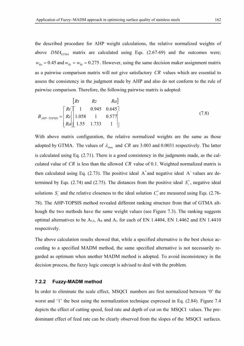
Application of Fuzzy–MADM approach in optimizing surface quality of stainless steels 162
the described procedure for AHP weight calculations, the relative normalized weights of
above GTMADMA matrix are calculated using Eqs. (2.67-69) and the outcomes were;
45.0Raw and 275.0 RtRz ww . However, using the same decision maker assignment matrix
as a pairwise comparison matrix will not give satisfactory CR values which are essential to
assess the consistency in the judgment made by AHP and also do not conform to the rule of
pairwise comparison. Therefore, the following pairwise matrix is adopted:
1733.155.1
577.01058.1
645.0945.01
Ra
Rz
Rt
B
RaRzRt
TOPSISAHP
(7.8)
With above matrix configuration, the relative normalized weights are the same as those
adopted by GTMA. The values of max and CR are 3.003 and 0.0031 respectively. The latter
is calculated using Eq. (2.71). There is a good consistency in the judgments made, as the cal-
culated value of CR is less than the allowed CR value of 0.1. Weighted normalized matrix is
then calculated using Eq. (2.73). The positive ideal * and negative ideal values are de-
termined by Eqs. (2.74) and (2.75). The distances from the positive ideal *iS , negative ideal
solutions iS and the relative closeness to the ideal solution *
iC are measured using Eqs. (2.76-
78). The AHP-TOPSIS method revealed different ranking structure from that of GTMA alt-
hough the two methods have the same weight values (see Figure 7.3). The ranking suggests
optimal alternatives to be A13, A9 and A1 for each of EN 1.4404, EN 1.4462 and EN 1.4410
respectively.
The above calculation results showed that, while a specified alternative is the best choice ac-
cording to a specified MADM method, the same specified alternative is not necessarily re-
garded as optimum when another MADM method is adopted. To avoid inconsistency in the
decision process, the fuzzy logic concept is advised to deal with the problem.
7.2.2 Fuzzy-MADM method
In order to eliminate the scale effect, MSQCI numbers are first normalized between ‘0’ the
worst and ‘1’ the best using the normalization technique expressed in Eq. (2.84). Figure 7.4
depicts the effect of cutting speed, feed rate and depth of cut on the MSQCI values. The pre-
dominant effect of feed rate can be clearly observed from the slopes of the MSQCI surfaces.
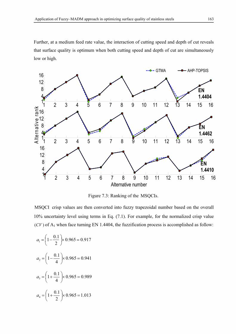
Application of Fuzzy–MADM approach in optimizing surface quality of stainless steels 163
Further, at a medium feed rate value, the interaction of cutting speed and depth of cut reveals
that surface quality is optimum when both cutting speed and depth of cut are simultaneously
low or high.
Figure 7.3: Ranking of the MSQCIs.
MSQCI crisp values are then converted into fuzzy trapezoidal number based on the overall
10% uncertainty level using terms in Eq. (7.1). For example, for the normalized crisp value
)(CV of A1 when face turning EN 1.4404, the fuzzification process is accomplished as follow:
917.0965.02
1.011
a
941.0965.04
1.012
a
989.0965.04
1.013
a
013.1965.02
1.014
a
1 2 3 4 5 6 7 8 9 10 11 12 13 14 15 16148
1216
1 2 3 4 5 6 7 8 9 10 11 12 13 14 15 16148
1216
Alte
rnat
ive
rank
1 2 3 4 5 6 7 8 9 10 11 12 13 14 15 16148
1216
Alternative number
GTMA AHP-TOPSIS
EN 1.4410
EN 1.4462
EN 1.4404
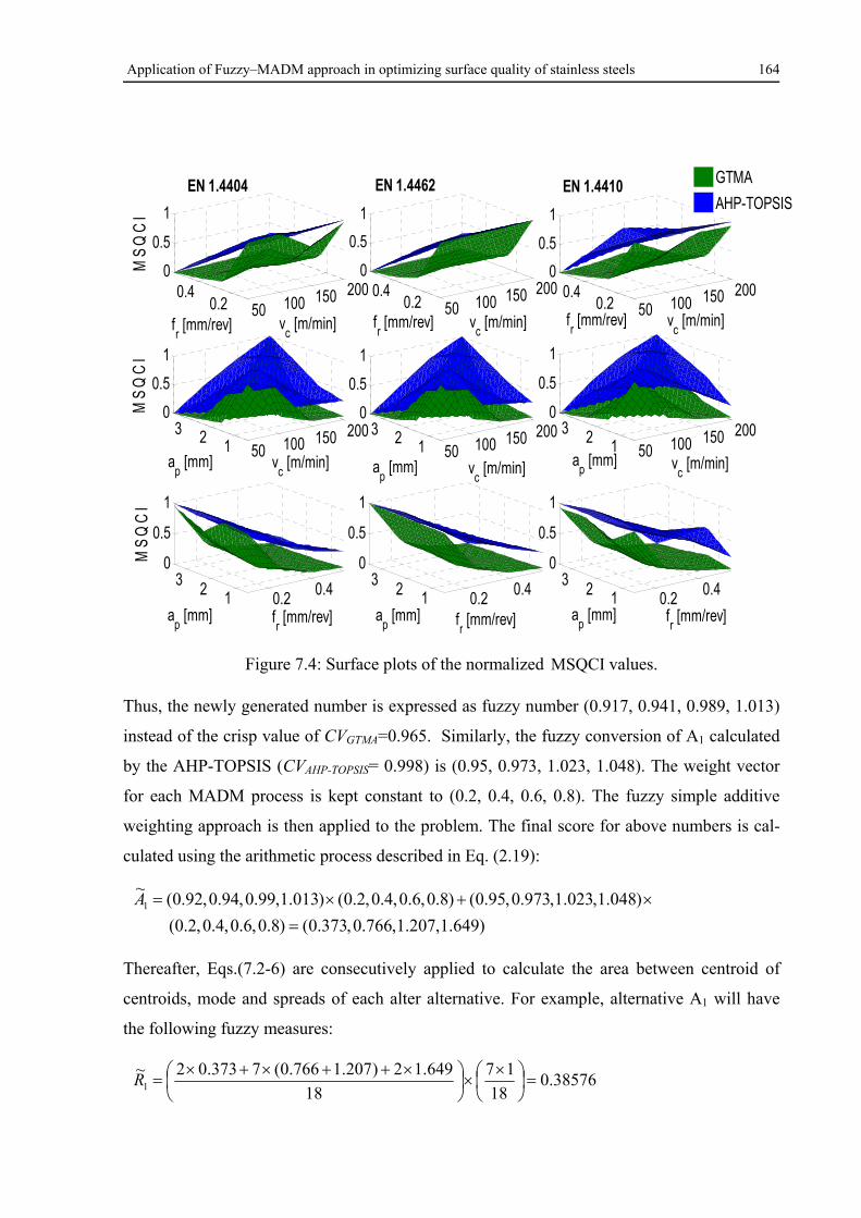
Application of Fuzzy–MADM approach in optimizing surface quality of stainless steels 164
Figure 7.4: Surface plots of the normalized MSQCI values.
Thus, the newly generated number is expressed as fuzzy number (0.917, 0.941, 0.989, 1.013)
instead of the crisp value of CVGTMA=0.965. Similarly, the fuzzy conversion of A1 calculated
by the AHP-TOPSIS (CVAHP-TOPSIS= 0.998) is (0.95, 0.973, 1.023, 1.048). The weight vector
for each MADM process is kept constant to (0.2, 0.4, 0.6, 0.8). The fuzzy simple additive
weighting approach is then applied to the problem. The final score for above numbers is cal-
culated using the arithmetic process described in Eq. (2.19):
)649.1,207.1,766.0,373.0()8.0,6.0,4.0,2.0(
)048.1,023.1,973.0,95.0()8.0,6.0,4.0,2.0()013.1,99.0,94.0,92.0(~
1
A
Thereafter, Eqs.(7.2-6) are consecutively applied to calculate the area between centroid of
centroids, mode and spreads of each alter alternative. For example, alternative A1 will have
the following fuzzy measures:
38576.018
17
18
649.12)207.1766.0(7373.02~1
R
50 100 150 2000.2
0.40
0.5
1
vc [m/min]f
r [mm/rev]
MS
QC
I
50 100 150 200123
0
0.5
1
vc [m/min]a
p [mm]
MS
QC
I
0.20.412
30
0.5
1
fr [mm/rev]a
p [mm]
MS
QC
I
50 100 150 2000.2
0.40
0.5
1
vc [m/min]f
r [mm/rev]
50 100 150 200123
0
0.5
1
vc [m/min]a
p [mm]
0.20.412
30
0.5
1
fr [mm/rev]a
p [mm]
50 100 150 2000.2
0.40
0.5
1
vc [m/min]f
r [mm/rev]
50 100 150 200123
0
0.5
1
vc [m/min]a
p [mm]
0.20.412
30
0.5
1
fr [mm/rev]a
p [mm]
GTMA
AHP-TOPSISEN 1.4404 EN 1.4410EN 1.4462
Application of Fuzzy–MADM approach in optimizing surface quality of stainless steels 165
987.0207.1766.02
1Mode1
276.1373.0649.11Spread1
393.0373.0766.01spreadLeft 1
442.0207.1649.11spreadRight 1
The same procedure is repeated for the reminder of alternatives. These parameters have
shown much less sensitivity toward change in weights than their MSQCI counterparts. For
example changing the weight vector to (0.25, 0.5, 0.75, 1) will not cause any change in rank-
ing order. The optimum alternative is defined as an alternative which gives maximum ( R~
),
Mode and Spread values. Since the values of these criterions do not present any conflict
numbers and no difference in ranking order is noticed among R~
, mode and spread values,
therefore, the alternatives could be ranked directly depending on R~
. Table A4 lists the com-
puted R~
, mode, spread values. It also shows the ranking of the alternatives according to the R~
values.
Performing analysis of means on computed R~
values, the levels of optimum cutting condition
which corresponds to the levels of maximum R~
value could be determined as shown in Fig-
ure 7.5. The reason behind the preference of higher optimum depth of cut in cutting EN1.4410
workmaterial refers to the more breakable, less entangled and better morphology of the chips
which often tended to accumulate around the cutting area.
Analysis of variance is then conducted on the computed R~
values suggesting linear models as
per Table 7.1. Statistically significant relationship between cutting variables and performance
characteristics at the 95% confidence level were proved based on relatively big differences
between 49.3F ,0.05)table(3,12 and individual model ratioF values. The adjusted correlation factor
)(R adj. is in very good agreement with predicted correlation factor )(R pred. which supports the
prediction power of the model. value-P of terms which are less than 0.05 are designated as
significant terms and marked bold. The last three column of the table shows the percent con-
tribution (%Contribution) of each factor. Notably, the contribution of feed rate in determining
the surface quality is in average over 90%. However, one has to expect less pronouncing ef-
fect when the feed domain is covering smaller ranges.
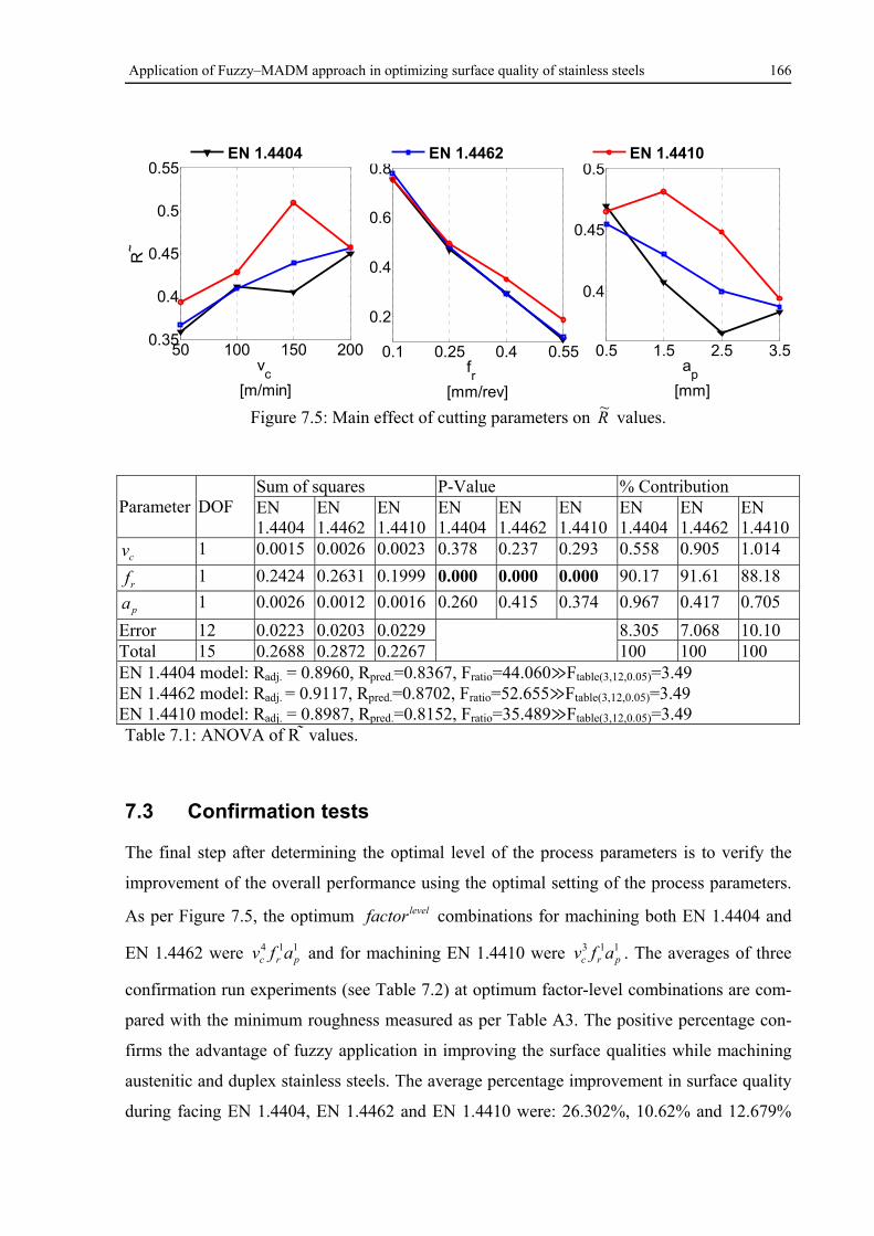
Application of Fuzzy–MADM approach in optimizing surface quality of stainless steels 166
Figure 7.5: Main effect of cutting parameters on R~
values.
Parameter
DOF
Sum of squares P-Value % Contribution EN 1.4404
EN 1.4462
EN 1.4410
EN 1.4404
EN 1.4462
EN 1.4410
EN 1.4404
EN 1.4462
EN 1.4410
cv 1 0.0015 0.0026 0.0023 0.378 0.237 0.293 0.558 0.905 1.014
rf 1 0.2424 0.2631 0.1999 0.000 0.000 0.000 90.17 91.61 88.18
pa 1 0.0026 0.0012 0.0016 0.260 0.415 0.374 0.967 0.417 0.705
Error 12 0.0223 0.0203 0.0229 8.305 7.068 10.10 Total 15 0.2688 0.2872 0.2267 100 100 100 EN 1.4404 model: Radj. = 0.8960, Rpred.=0.8367, Fratio=44.060≫Ftable(3,12,0.05)=3.49 EN 1.4462 model: Radj. = 0.9117, Rpred.=0.8702, Fratio=52.655≫Ftable(3,12,0.05)=3.49 EN 1.4410 model: Radj. = 0.8987, Rpred.=0.8152, Fratio=35.489≫Ftable(3,12,0.05)=3.49 Table 7.1: ANOVA of R values.
7.3 Confirmation tests
The final step after determining the optimal level of the process parameters is to verify the
improvement of the overall performance using the optimal setting of the process parameters.
As per Figure 7.5, the optimum levelfactor combinations for machining both EN 1.4404 and
EN 1.4462 were 114prc afv and for machining EN 1.4410 were 113
prc afv . The averages of three
confirmation run experiments (see Table 7.2) at optimum factor-level combinations are com-
pared with the minimum roughness measured as per Table A3. The positive percentage con-
firms the advantage of fuzzy application in improving the surface qualities while machining
austenitic and duplex stainless steels. The average percentage improvement in surface quality
during facing EN 1.4404, EN 1.4462 and EN 1.4410 were: 26.302%, 10.62% and 12.679%
50 100 150 2000.35
0.4
0.45
0.5
0.55
vc
[m/min]
R~
0.1 0.25 0.4 0.55
0.2
0.4
0.6
0.8
fr
[mm/rev]
0.5 1.5 2.5 3.5
0.4
0.45
0.5
ap
[mm]
EN 1.4404 EN 1.4462 EN 1.4410
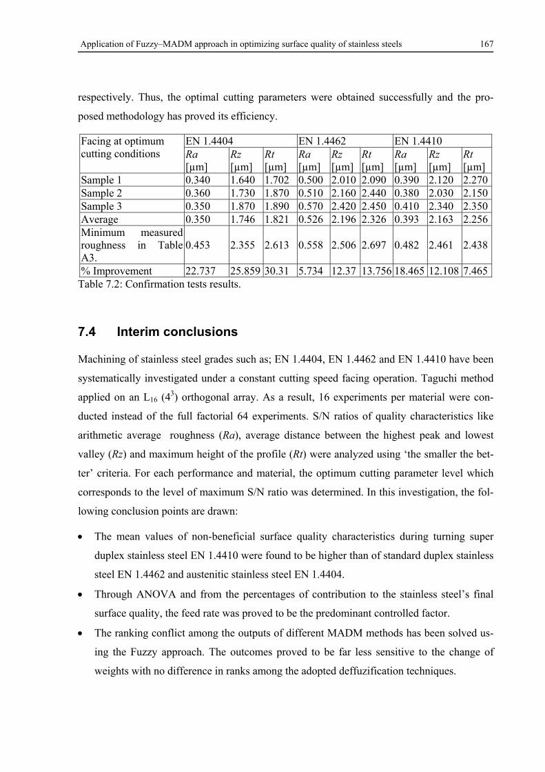
Application of Fuzzy–MADM approach in optimizing surface quality of stainless steels 167
respectively. Thus, the optimal cutting parameters were obtained successfully and the pro-
posed methodology has proved its efficiency.
Facing at optimum cutting conditions
EN 1.4404 EN 1.4462 EN 1.4410 Ra [µm]
Rz [µm]
Rt [µm]
Ra [µm]
Rz [µm]
Rt [µm]
Ra [µm]
Rz [µm]
Rt [µm]
Sample 1 0.340 1.640 1.702 0.500 2.010 2.090 0.390 2.120 2.270Sample 2 0.360 1.730 1.870 0.510 2.160 2.440 0.380 2.030 2.150Sample 3 0.350 1.870 1.890 0.570 2.420 2.450 0.410 2.340 2.350Average 0.350 1.746 1.821 0.526 2.196 2.326 0.393 2.163 2.256Minimum measured roughness in Table A3.
0.453 2.355 2.613 0.558 2.506 2.697 0.482 2.461 2.438
% Improvement 22.737 25.859 30.31 5.734 12.37 13.756 18.465 12.108 7.465Table 7.2: Confirmation tests results.
7.4 Interim conclusions
Machining of stainless steel grades such as; EN 1.4404, EN 1.4462 and EN 1.4410 have been
systematically investigated under a constant cutting speed facing operation. Taguchi method
applied on an L16 (43) orthogonal array. As a result, 16 experiments per material were con-
ducted instead of the full factorial 64 experiments. S/N ratios of quality characteristics like
arithmetic average roughness (Ra), average distance between the highest peak and lowest
valley (Rz) and maximum height of the profile (Rt) were analyzed using ‘the smaller the bet-
ter’ criteria. For each performance and material, the optimum cutting parameter level which
corresponds to the level of maximum S/N ratio was determined. In this investigation, the fol-
lowing conclusion points are drawn:
The mean values of non-beneficial surface quality characteristics during turning super
duplex stainless steel EN 1.4410 were found to be higher than of standard duplex stainless
steel EN 1.4462 and austenitic stainless steel EN 1.4404.
Through ANOVA and from the percentages of contribution to the stainless steel’s final
surface quality, the feed rate was proved to be the predominant controlled factor.
The ranking conflict among the outputs of different MADM methods has been solved us-
ing the Fuzzy approach. The outcomes proved to be far less sensitive to the change of
weights with no difference in ranks among the adopted deffuzification techniques.

Application of Fuzzy–MADM approach in optimizing surface quality of stainless steels 168
The optimum levelfactor combinations while turning EN 1.4404, EN 1.4462 and EN
1.4410 were: 114prc afv , 114
prc afv and 113prc afv respectively.
Utilizing the optimum levelfactor combinations for confirmation test, the average percent-
age improvement in surface quality during facing EN 1.4404, EN 1.4462 and EN 1.4410
were: 26.302 %, 10.62% and 12.679% respectively.
Sustainability-based multi-pass optimization of cutting DSSs 169
8 Sustainability-based multi-pass optimization of
cutting DSSs
More recently there has been an increased interest in achieving sustainable manufacturing
through implementation of sustainability principles in machining practices. Sustainability
principles are considering: machining costs, energy consumption, waste management, envi-
ronmental impact, operational safety and personal health. In order to address this concern, the
present chapter adopts a systematic approach which employs different modeling and optimi-
zation tools under a three phase investigation scheme. In phase I, the effect of control factors
such as cutting parameters, cutting fluids and axial length of cuts are investigated using the D-
Optimal method. The mathematical models for performance characteristics such as; percent-
age increase in thrust cutting force ( tF% ), effective cutting power ( eP ), maximum tool flank
wear ( maxVB ) and chip volume ratio ( R ) are developed using response surface methodology
(RSM). The adequacy of derived models for each cutting scenario is checked using analysis
of variance (ANOVA). Parametric meta-heuristic optimization using Cuckoo Search (CS)
algorithm is then performed to determine the optimum design variable set for each perfor-
mance.
In the phase II, comprehensive experiment-based production cost and production rate models
are analyzed. To overcome the conflict between the desire of minimizing the production cost
and maximizing the production rate, compromise solutions are suggested using Technique for
Order Preference by Similarity to Ideal Solution (TOPSIS). The alternatives are ranked ac-
cording to their relative closeness to the ideal solution. In the phase III, expert systems based
on fuzzy rule modeling approach are adopted to derive measures of machining operational
sustainability called operational sustainability index (OSI). ANN-based models are developed
to study the effect of control factors on computed OSIs. Cuckoo Search neural network sys-
tems (CSNNS) are finally utilized to constrainedly optimize the cutting process per each cut-
ting scenario. The most appropriate cutting setup to ensure successful turning of standard EN
1.4462 and super EN 1.4410 for each scenario is selected in accordance with conditions
which give the maximum OSI. The flowchart of the study is shown in Figure 8.1.
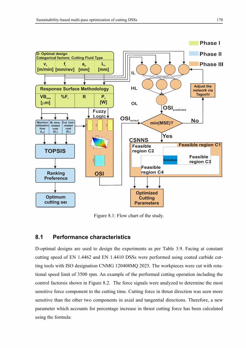
Sustainability-based multi-pass optimization of cutting DSSs 170
Figure 8.1: Flow chart of the study.
8.1 Performance characteristics
D-optimal designs are used to design the experiments as per Table 3.9. Facing at constant
cutting speed of EN 1.4462 and EN 1.4410 DSSs were performed using coated carbide cut-
ting tools with ISO designation CNMG 120408MQ 2025. The workpieces were cut with rota-
tional speed limit of 3500 rpm. An example of the performed cutting operation including the
control factorsis shown in Figure 8.2. The force signals were analyzed to determine the most
sensitive force component to the cutting time. Cutting force in thrust direction was seen more
sensitive than the other two components in axial and tangential directions. Therefore, a new
parameter which accounts for percentage increase in thrust cutting force has been calculated
using the formula:
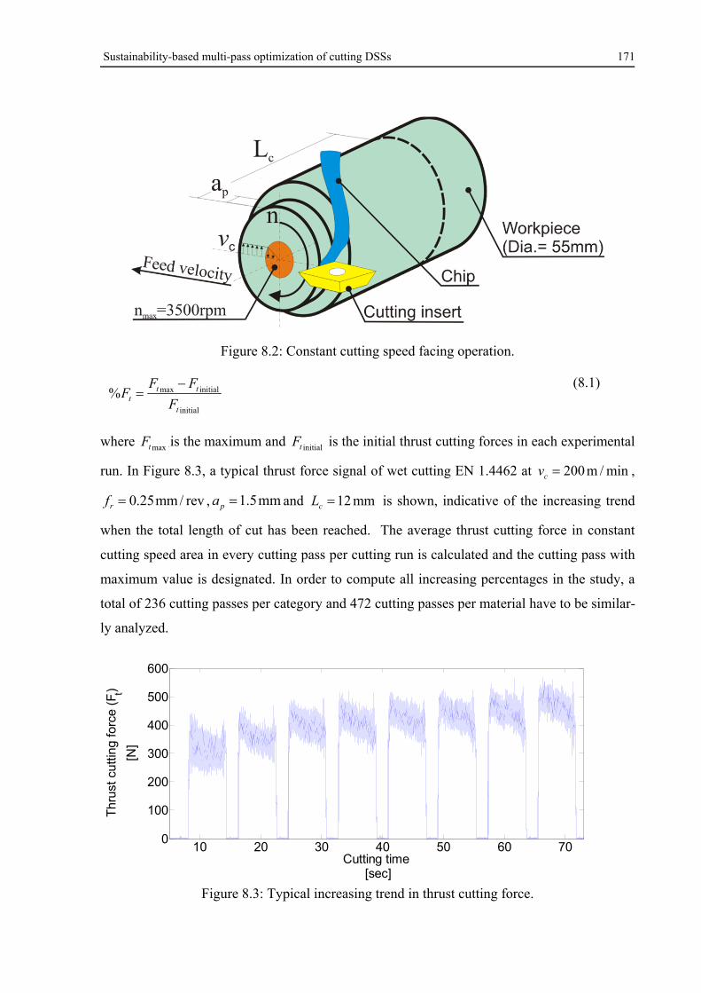
Sustainability-based multi-pass optimization of cutting DSSs 171
Figure 8.2: Constant cutting speed facing operation.
initial
initialmax%t
ttt F
FFF
(8.1)
where maxtF .is the maximum and initialtF is the initial thrust cutting forces in each experimental
run. In Figure 8.3, a typical thrust force signal of wet cutting EN 1.4462 at min/m200cv ,
rev/mm25.0rf , mm5.1pa and mm12cL is shown, indicative of the increasing trend
when the total length of cut has been reached. The average thrust cutting force in constant
cutting speed area in every cutting pass per cutting run is calculated and the cutting pass with
maximum value is designated. In order to compute all increasing percentages in the study, a
total of 236 cutting passes per category and 472 cutting passes per material have to be similar-
ly analyzed.
Figure 8.3: Typical increasing trend in thrust cutting force.
10 20 30 40 50 60 700
100
200
300
400
500
600
Cutting time [sec]
Thr
ust c
uttin
g fo
rce
(Ft)
[N]
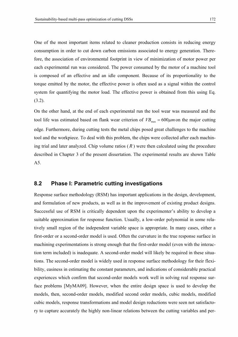
Sustainability-based multi-pass optimization of cutting DSSs 172
One of the most important items related to cleaner production consists in reducing energy
consumption in order to cut down carbon emissions associated to energy generation. There-
fore, the association of environmental footprint in view of minimization of motor power per
each experimental run was considered. The power consumed by the motor of a machine tool
is composed of an effective and an idle component. Because of its proportionality to the
torque emitted by the motor, the effective power is often used as a signal within the control
system for quantifying the motor load. The effective power is obtained from this using Eq.
(3.2).
On the other hand, at the end of each experimental run the tool wear was measured and the
tool life was estimated based on flank wear criterion of mVB 600max on the major cutting
edge. Furthermore, during cutting tests the metal chips posed great challenges to the machine
tool and the workpiece. To deal with this problem, the chips were collected after each machin-
ing trial and later analyzed. Chip volume ratios ( R ) were then calculated using the procedure
described in Chapter 3 of the present dissertation. The experimental results are shown Table
A5.
8.2 Phase I: Parametric cutting investigations
Response surface methodology (RSM) has important applications in the design, development,
and formulation of new products, as well as in the improvement of existing product designs.
Successful use of RSM is critically dependent upon the experimenter’s ability to develop a
suitable approximation for response function. Usually, a low-order polynomial in some rela-
tively small region of the independent variable space is appropriate. In many cases, either a
first-order or a second-order model is used. Often the curvature in the true response surface in
machining experimentations is strong enough that the first-order model (even with the interac-
tion term included) is inadequate. A second-order model will likely be required in these situa-
tions. The second-order model is widely used in response surface methodology for their flexi-
bility, easiness in estimating the constant parameters, and indications of considerable practical
experiences which confirm that second-order models work well in solving real response sur-
face problems [MyMA09]. However, when the entire design space is used to develop the
models, then, second-order models, modified second order models, cubic models, modified
cubic models, response transformations and model design reductions were seen not satisfacto-
ry to capture accurately the highly non-linear relations between the cutting variables and per-
Sustainability-based multi-pass optimization of cutting DSSs 173
formance characteristics. Therefore, an intermediate and reasonable solution was found for all
the cases when second-order non-linear mathematical models in terms of natural variables are
selected to predict the performance characteristics (Y ) for each condition category in sepa-
rate, which were of the following form:
cpcrprccpc
rccprccprc
LacLfcafcLvcavc
fvcLcacfcvcLcacfcvccY
3424231413
122
442
332
222
1143210
(8.2)
The values of the regression coefficients as defined above are determined using the Eqs. (2.1-
10). The reader is advised to review the basic concepts of the RSM presented in Chapter 2 of
the present study.
8.2.1 Effect of control factors on performance characteristics
The values of regression coefficients in natural form and various statistics about the statistical
validity of the developed models at a 95% confidence interval are given in Table A5. The
statistical correlation factors such as 2R and adj.R indicates that the models fit the data well. As
per analysis of variance (ANOVA) technique, since the calculated value of value-F of all
developed second-order models are greater than the standard tabulated value of )(14,9,0.05 tableF
03.3 , then the models are considered adequate within the confidence limit. The adequate
precision (Aprec.), for all models are greater than 4, which indicate an adequate signal to noise
ratio, thus the models can be used to navigate the design space.
8.2.1.1 Effect of control factors on the percentage increase in thrust cutting force (%Ft)
In phase I, the developed RSM models were utilized to study the interaction effects of select-
ed independent variables on tF% . To analyze the interaction effects, three dimensional plots
were generated considering two parameter at a time while the other parameters are held con-
stant at their respective center levels. These interaction plots are presented in Figure 8.4a.
From which, the following observations can be made:
For a given depth and length of cut, tF% approaches its minimum value as cutting speed
and feed rate increase to certain specified limit. Beyond that limit it starts to increase
again. When the materials are cut dry, lower cutting speed and feed rates are preferred to
minimize tF% . The values of obtained tF% when EN 1.4410 are cut were higher than EN
Sustainability-based multi-pass optimization of cutting DSSs 174
1.4462 due to the generally higher mechanical strength of EN 1.4410 and fewer weight
percentage of assisting machinability elements such as sulfur and phosphorus, see Table
3.1.
For a specified cutting speed and feed rate, depth of cut values of (1.25-1.5mm) were seen
to give the minimum tF% , as they reduce the ploughing effect, produce friendlier-to-
machine chips and exert a more stable cutting process. Generally, lower values of depths
of cuts are recommended when process conditions are dry and/or super DSS EN 1.4410 is
machined. Values lower than tool nose radius of 0.8mm have to be avoided.
When cutting speed, feed rate and depth of cut are set at a specified value, tF% is ex-
pected to increase with the increase of total length of cut. However, the slopes of tF% ver-
sus total length of cut were seen steeper at higher levels of cutting speeds.
8.2.1.2 Effect of control factors on the effective cutting power (Pe)
Effective power measurement systems are characterized by the fact that they do not affect the
mechanical properties of the machine tool. The machining torque can be measured during the
operation without the integration of external sensors into the electric flux of the machine. The
primary area of application is the recognition of tool fractures and collisions in the workspace.
Sufficiently large force changes are necessary for efficient wear monitoring. When monitor-
ing cutting processes, usually external effective-power measurement tools are used, often with
associated evaluation software and visualization unit [Kloc11].
Figure 8.4b. illustrates the interaction effects of the independent variables on the effective
cutting power. It is seen from this collective figure that:
Effective cutting power is most sensitive to cutting speed variations when other parame-
ters are kept constant. Maximum and minimum consumptions in effective cutting power
are seen at wet cutting of EN 1.4462 and dry cutting of EN 1.4410 respectively.
Effective cutting power is less sensitive to the length of cut variations as far as the cutting
tool does not suffer the catastrophic chipping in the cutting edges.
Minimum consumption in effective cutting power results when the feed rate is in the
range 0.125-0.175 mm/rev of dry cutting and 0.1-0.15mm/rev of wet cutting.
Two-factor interaction models were seen accurate enough to explain the interaction effects
of cutting parameters on the effective cutting power.
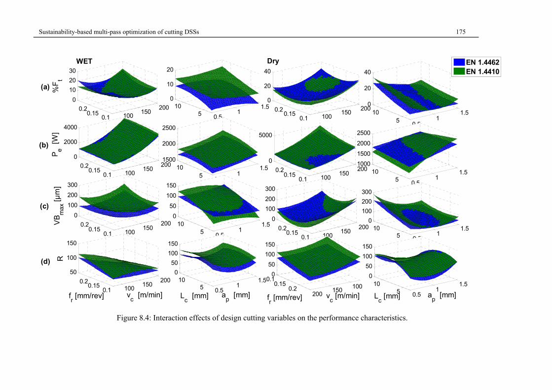
Sustainability-based multi-pass optimization of cutting DSSs 175
Figure 8.4: Interaction effects of design cutting variables on the performance characteristics.
100150
200
0.10.15
0.2
0
10
20
30
%F
t
0.51
1.55
100
10
20
100
150200
0.10.15
0.2
0
20
40
0.51
1.55
100
20
40
100150
200
0.10.15
0.2
0
2000
4000
Pe
[W]
0.51
1.55
101500
2000
2500
100150
200
0.10.15
0.2
0
5000
0.5
11.5
510
1000
1500
2000
2500
100150
200
0.10.15
0.2
0
100
200
300
VB
max
[µ
m]
0.51
1.55
100
50
100
150
100
150200
0.10.15
0.2
0
100
200
300
0.5
11.5
510
0
100
200
300
100150
200
0.10.15
0.2
50
100
150
R
0.51
1.55
100
50
100
150
ap [mm] L
c [mm]
100150
200
0.10.15
0.2
0
50
100
150
vc [m/min]
0.5
11.5
510
0
50
100
150
ap [mm] L
c [mm]
EN 1.4462EN 1.4410
fr [mm/rev]f
r [mm/rev] v
c [m/min]
(a)
(b)
(c)
(d)
WET Dry
Sustainability-based multi-pass optimization of cutting DSSs 176
8.2.1.3 Effect of control factors on the maximum width of tool flank wear (VBmax)
Tool wear has a remarkable influence in tool life, cutting forces, vibration, quality of the ma-
chined surface and its dimensional accuracy, and consequently, the economics of cutting op-
erations. In this study off-line modeling of the maximum flank wear lands (VBmax ) are de-
scribed as functions of independent cutting variables. Figure 8.4c depicts the interaction con-
tour plots of VBmax as per RSM models tabulated in Table A6. It can be found that:
During the course of the dry cutting of DSSs, an increased built up edge formation on the
tool, obvious inferior chip morphologies, more aggressive notch wear on the major and
minor cutting edges and inferior surface qualities were noticed. Therefore, when cutting
DSSs, generous amount of cutting fluid is always recommended.
Wet cutting at cutting parameter ranges of m/min,160100cv 25.015.0 rf mm/rev,
mm0.175.0 pa for machining EN 1.4462 and m/min,160120cv 15.0rf
mm/rev,20.0 mm5.125.1 pa for machining EN 1.4410 were seen optimum in mini-
mizing the tool flank wear.
Dry machining is possible when cutting parameters are set appropriately. The settings in-
clude; machining of EN 1.4462 at m/min,11075cv rev,/mm2.015.0 rf
mm5.11pa and maximum 6/ pc aL , and machining of EN 1.4410 at 75cv
m/min,90 rev,/mm175.0125.0 rf mm35.18.0 pa and maximum 4/ pc aL .
Direct linear correlations between tF% and max%VB with reasonable coefficients of de-
terminations ( 2R ) were noticed:
Cutting of DSS EN 1.4462
Wet: 7.0R 2
149.35)(%4198.5max tFVB (8.3)
Dry: 92.0R 2
549.18)(%7696.7max tFVB (8.4)
Sustainability-based multi-pass optimization of cutting DSSs 177
Cutting of DSS EN 1.4410
Wet: 71.0R 2
793.16)(%5767.6max rFVB (8.5)
Dry: 93.0R 2
494.63)(%918.9max rFVB (8.6)
8.2.1.4 Effect of control factors on the on the chip volume ratio (R)
The chip shapes are assessed according to two criteria: transportability and danger for the
machine operator. It is no problem to move short, broken chips, such as fragmented spiral
chips, in containers. By contrast, this is impossible for ribbon chips, since they always de-
mand special treatment (breaking in the chip breaker or briquetting) in order to make them
ready for transport. In a plant with automated manufacturing equipment, where many chips
occur, these treatment procedures are very expensive. Consequently, as an alternative, always
the aim is to produce chip forms that can be handled easily. Since long ribbon chips and en-
tangled chips, whose edges are very sharp, could possibly endanger the machine operator and
cause safety risks [TsRe09]. At this stage, utilizing the chip volume ratio R , the spatial re-
quirement for the chips is considered. Each chip form is assigned to a chip volume ratio R ,
which defines by what factor the transport volume needed for the specific chip form exceeds
the intrinsic material volume of the chip. According to the assignments presented in Figure
1.14, 90R for snarled and ribbon chips, 9050 R for coiled, flat helical and cylindrical
helical chips, 5025 R for short coiled chips, 258 R for spiral chips and 83 R for
short chip particles. It is clear from Figure 8.4d that;
Higher values of cutting speeds and feed rates are necessary to minimize the chip volume
ratio.
In wet cutting of DSSs, friendlier-to-machine chip forms were produced because of the
less encountered friction in the contact area between the chip and rake face.
Ribbon and snarled chip forms were common when the metals are machined at feed rate
and depth of cuts lower than 0.15 mm/rev and 1mm respectively. At intermediate feed
ranges, the produced chips were rather of flat-helical and cylindrical-helical forms. The
chip forms were rather short coiled chips at higher feed ranges.
Sustainability-based multi-pass optimization of cutting DSSs 178
Under the same machining conditions which might produce continuous chips, different
chip forms were possible due to continuous entanglement of chips especially when
6/ pc aL .
Due to the higher proof and tensile strength, and, lower sulfur and phosphor constituents
to assist chip breaking, R values of cutting EN 1.4410 were generally higher than of cut-
ting EN 1.4462.
The tendency to enhance chip segmentation is expected to rise when the chip curl radius is
reduced, the coolant pressure is increased and the coolant restricted to smaller area of the
chip.
8.2.2 Parametric optimization of performance characteristics
The first optimization process in this investigation is formulated as follow:
Objective function
Formulation of optimization model is one of the most important tasks in optimization process.
The type of optimization modeling techniques used to express the objective function deter-
mines its accuracy and the possibility of reaching a global optimum solution. The developed
response surface models, expressed by Eq. (8.2) and presented previously in Table A6 are
used as both objective and constraint functions.
Decision variables
Process parameters considered in the optimization problem were cutting speed, feed rate,
depth of cut and length of cut. The length of cut and depth of cuts were set constant at their
maximum values to account for the maximum production rates and ensure an integer pc aL /
ratio due to the imposed practical considerations. Therefore, the parameter bounds for the
decision parameters were set as described below:
mm12
mm5.1
rev/mm25.01.0
min/m20075
c
p
r
c
L
a
f
v
(8.7)
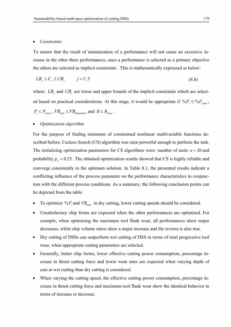
Sustainability-based multi-pass optimization of cutting DSSs 179
Constraints
To ensure that the result of minimization of a performance will not cause an excessive in-
crease in the other three performances, once a performance is selected as a primary objective
the others are selected as implicit constraints . This is mathematically expressed as below:
3:1 jUBCLB jjj (8.8)
where: jLB and jUB are lower and upper bounds of the implicit constraints which are select-
ed based on practical considerations. At this stage, it would be appropriate if max%% tt FF ,
maxee PP , max(max)max VBVB and maxRR .
Optimization algorithm
For the purpose of finding minimum of constrained nonlinear multivariable functions de-
scribed before, Cuckoo Search (CS) algorithm was seen powerful enough to perform the task.
The initializing optimization parameters for CS algorithms were: number of nests 20n and
probability 25.0ap . The obtained optimization results showed that CS is highly reliable and
converge consistently to the optimum solution. In Table 8.1, the presented results indicate a
conflicting influence of the process parameter on the performance characteristics in conjunc-
tion with the different process conditions. As a summary, the following conclusion points can
be depicted from the table:
To optimize tF% and maxVB in dry cutting, lower cutting speeds should be considered.
Unsatisfactory chip forms are expected when the other performances are optimized. For
example, when optimizing the maximum tool flank wear, all performances show major
decreases, while chip volume ratios show a major increase and the reverse is also true.
Dry cutting of DSSs can outperform wet cutting of DSS in terms of total progressive tool
wear, when appropriate cutting parameters are selected.
Generally, better chip forms, lower effective cutting power consumption, percentage in-
crease in thrust cutting force and lower wear rates are expected when varying depth of
cuts at wet cutting than dry cutting is considered.
When varying the cutting speed, the effective cutting power consumption, percentage in-
crease in thrust cutting force and maximum tool flank wear show the identical behavior in
terms of increase or decrease.
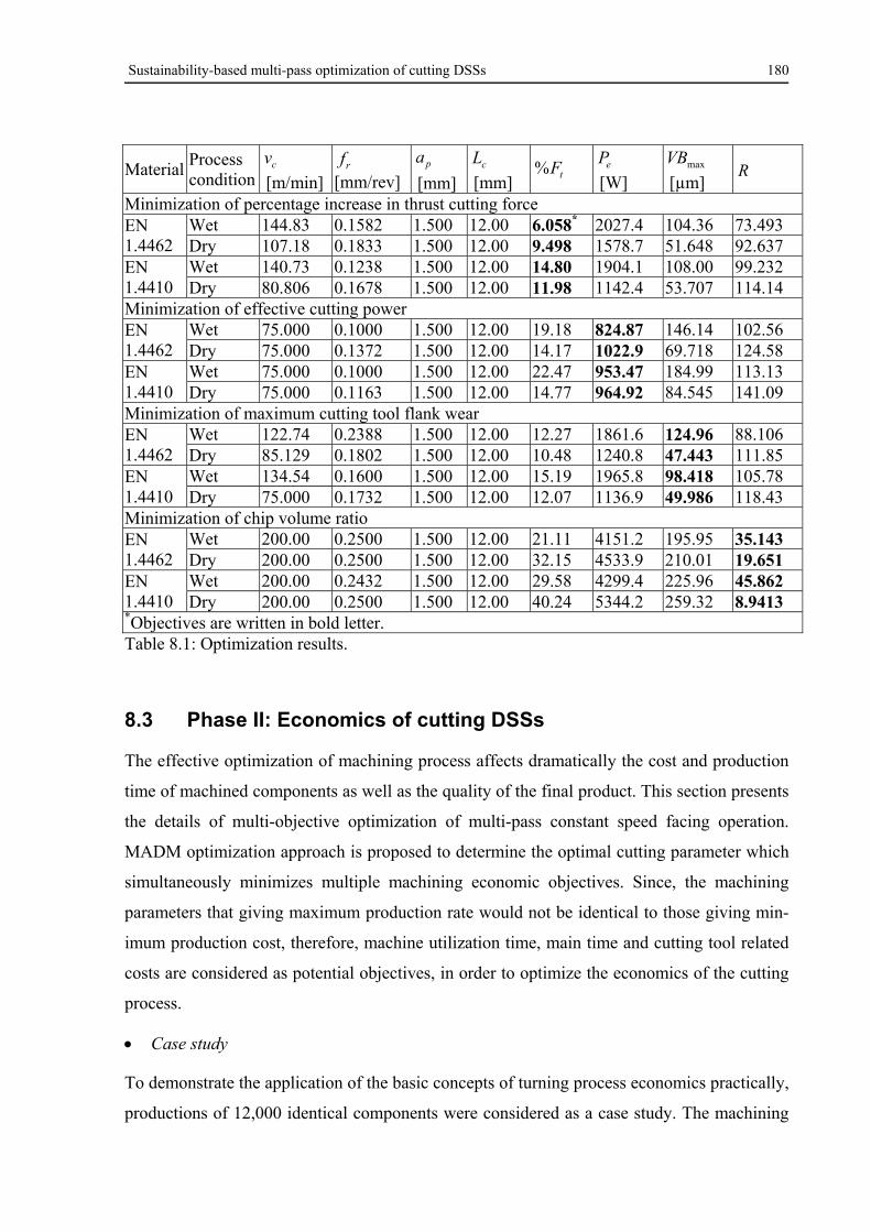
Sustainability-based multi-pass optimization of cutting DSSs 180
Material Process condition
cv
[m/min] rf
[mm/rev] pa
[mm] cL
[mm] tF% eP
[W] maxVB
[µm] R
Minimization of percentage increase in thrust cutting force EN 1.4462
Wet 144.83 0.1582 1.500 12.00 6.058* 2027.4 104.36 73.493 Dry 107.18 0.1833 1.500 12.00 9.498 1578.7 51.648 92.637
EN 1.4410
Wet 140.73 0.1238 1.500 12.00 14.80 1904.1 108.00 99.232 Dry 80.806 0.1678 1.500 12.00 11.98 1142.4 53.707 114.14
Minimization of effective cutting power EN 1.4462
Wet 75.000 0.1000 1.500 12.00 19.18 824.87 146.14 102.56 Dry 75.000 0.1372 1.500 12.00 14.17 1022.9 69.718 124.58
EN 1.4410
Wet 75.000 0.1000 1.500 12.00 22.47 953.47 184.99 113.13 Dry 75.000 0.1163 1.500 12.00 14.77 964.92 84.545 141.09
Minimization of maximum cutting tool flank wear EN 1.4462
Wet 122.74 0.2388 1.500 12.00 12.27 1861.6 124.96 88.106 Dry 85.129 0.1802 1.500 12.00 10.48 1240.8 47.443 111.85
EN 1.4410
Wet 134.54 0.1600 1.500 12.00 15.19 1965.8 98.418 105.78 Dry 75.000 0.1732 1.500 12.00 12.07 1136.9 49.986 118.43
Minimization of chip volume ratio EN 1.4462
Wet 200.00 0.2500 1.500 12.00 21.11 4151.2 195.95 35.143 Dry 200.00 0.2500 1.500 12.00 32.15 4533.9 210.01 19.651
EN 1.4410
Wet 200.00 0.2432 1.500 12.00 29.58 4299.4 225.96 45.862 Dry 200.00 0.2500 1.500 12.00 40.24 5344.2 259.32 8.9413
*Objectives are written in bold letter. Table 8.1: Optimization results.
8.3 Phase II: Economics of cutting DSSs
The effective optimization of machining process affects dramatically the cost and production
time of machined components as well as the quality of the final product. This section presents
the details of multi-objective optimization of multi-pass constant speed facing operation.
MADM optimization approach is proposed to determine the optimal cutting parameter which
simultaneously minimizes multiple machining economic objectives. Since, the machining
parameters that giving maximum production rate would not be identical to those giving min-
imum production cost, therefore, machine utilization time, main time and cutting tool related
costs are considered as potential objectives, in order to optimize the economics of the cutting
process.
Case study
To demonstrate the application of the basic concepts of turning process economics practically,
productions of 12,000 identical components were considered as a case study. The machining
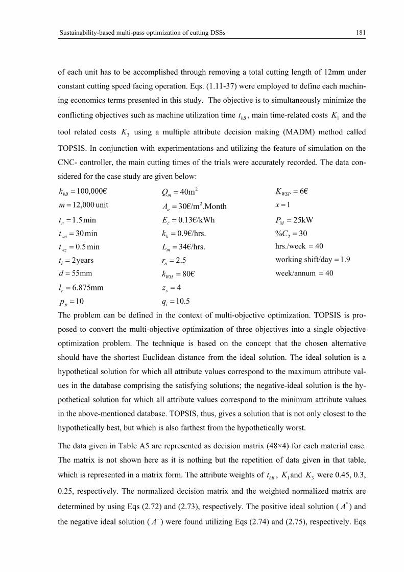
Sustainability-based multi-pass optimization of cutting DSSs 181
of each unit has to be accomplished through removing a total cutting length of 12mm under
constant cutting speed facing operation. Eqs. (1.11-37) were employed to define each machin-
ing economics terms presented in this study. The objective is to simultaneously minimize the
conflicting objectives such as machine utilization time bBt , main time-related costs 1K and the
tool related costs 3K using a multiple attribute decision making (MADM) method called
TOPSIS. In conjunction with experimentations and utilizing the feature of simulation on the
CNC- controller, the main cutting times of the trials were accurately recorded. The data con-
sidered for the case study are given below:
€000,100bBk 2m40mQ €6WSPK
unit000,12m Month.€/m30 2aA 1x
min5.1nt Whk€/13.0cE Wk25MP
min30vmt €/hrs.9.0kk 30% 2 C
min5.0wzt hrs.€/34mL 40hrs./week
years2lt 5.2nr 9.1shift/day working
mm55d €80WHk 40week/annum
mm875.6rl 4sz
10pp 5.10iq
The problem can be defined in the context of multi-objective optimization. TOPSIS is pro-
posed to convert the multi-objective optimization of three objectives into a single objective
optimization problem. The technique is based on the concept that the chosen alternative
should have the shortest Euclidean distance from the ideal solution. The ideal solution is a
hypothetical solution for which all attribute values correspond to the maximum attribute val-
ues in the database comprising the satisfying solutions; the negative-ideal solution is the hy-
pothetical solution for which all attribute values correspond to the minimum attribute values
in the above-mentioned database. TOPSIS, thus, gives a solution that is not only closest to the
hypothetically best, but which is also farthest from the hypothetically worst.
The data given in Table A5 are represented as decision matrix (48×4) for each material case.
The matrix is not shown here as it is nothing but the repetition of data given in that table,
which is represented in a matrix form. The attribute weights of bBt , 1K and 3K were 0.45, 0.3,
0.25, respectively. The normalized decision matrix and the weighted normalized matrix are
determined by using Eqs (2.72) and (2.73), respectively. The positive ideal solution ( *A ) and
the negative ideal solution ( A ) were found utilizing Eqs (2.74) and (2.75), respectively. Eqs
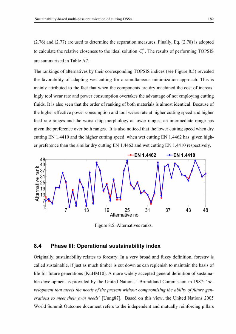
Sustainability-based multi-pass optimization of cutting DSSs 182
(2.76) and (2.77) are used to determine the separation measures. Finally, Eq. (2.78) is adopted
to calculate the relative closeness to the ideal solution *iC . The results of performing TOPSIS
are summarized in Table A7.
The rankings of alternatives by their corresponding TOPSIS indices (see Figure 8.5) revealed
the favorability of adapting wet cutting for a simultaneous minimization approach. This is
mainly attributed to the fact that when the components are dry machined the cost of increas-
ingly tool wear rate and power consumption overtakes the advantage of not employing cutting
fluids. It is also seen that the order of ranking of both materials is almost identical. Because of
the higher effective power consumption and tool wears rate at higher cutting speed and higher
feed rate ranges and the worst chip morphology at lower ranges, an intermediate range has
given the preference over both ranges. It is also noticed that the lower cutting speed when dry
cutting EN 1.4410 and the higher cutting speed when wet cutting EN 1.4462 has given high-
er preference than the similar dry cutting EN 1.4462 and wet cutting EN 1.4410 respectively.
Figure 8.5: Alternatives ranks.
8.4 Phase III: Operational sustainability index
Originally, sustainability relates to forestry. In a very broad and fuzzy definition, forestry is
called sustainable, if just as much timber is cut down as can replenish to maintain the basis of
life for future generations [KuHM10]. A more widely accepted general definition of sustaina-
ble development is provided by the United Nations ’ Brundtland Commission in 1987: ‘de-
velopment that meets the needs of the present without compromising the ability of future gen-
erations to meet their own needs’ [Unng87]. Based on this view, the United Nations 2005
World Summit Outcome document refers to the independent and mutually reinforcing pillars
1 7 13 19 25 31 37 43 4817
13192531374348
Alternative no.
Alte
rna
tive
ra
nk
EN 1.4462 EN 1.4410
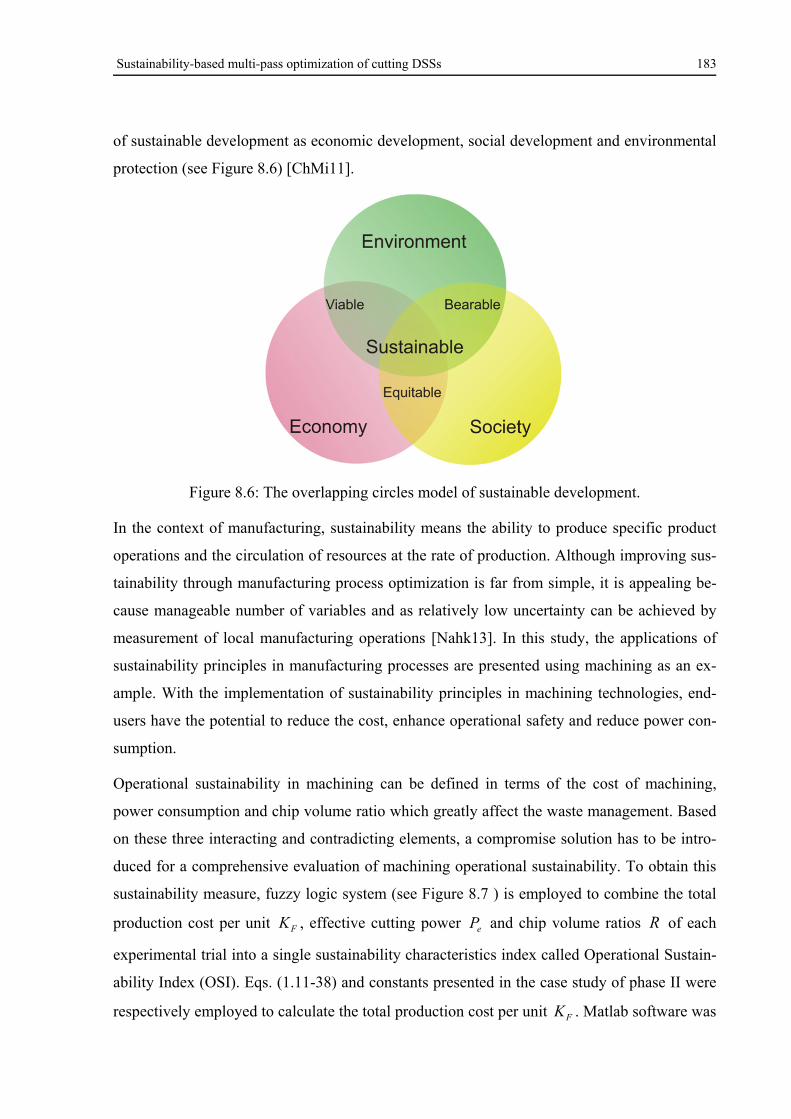
Sustainability-based multi-pass optimization of cutting DSSs 183
of sustainable development as economic development, social development and environmental
protection (see Figure 8.6) [ChMi11].
Figure 8.6: The overlapping circles model of sustainable development.
In the context of manufacturing, sustainability means the ability to produce specific product
operations and the circulation of resources at the rate of production. Although improving sus-
tainability through manufacturing process optimization is far from simple, it is appealing be-
cause manageable number of variables and as relatively low uncertainty can be achieved by
measurement of local manufacturing operations [Nahk13]. In this study, the applications of
sustainability principles in manufacturing processes are presented using machining as an ex-
ample. With the implementation of sustainability principles in machining technologies, end-
users have the potential to reduce the cost, enhance operational safety and reduce power con-
sumption.
Operational sustainability in machining can be defined in terms of the cost of machining,
power consumption and chip volume ratio which greatly affect the waste management. Based
on these three interacting and contradicting elements, a compromise solution has to be intro-
duced for a comprehensive evaluation of machining operational sustainability. To obtain this
sustainability measure, fuzzy logic system (see Figure 8.7 ) is employed to combine the total
production cost per unit FK , effective cutting power eP and chip volume ratios R of each
experimental trial into a single sustainability characteristics index called Operational Sustain-
ability Index (OSI). Eqs. (1.11-38) and constants presented in the case study of phase II were
respectively employed to calculate the total production cost per unit FK . Matlab software was
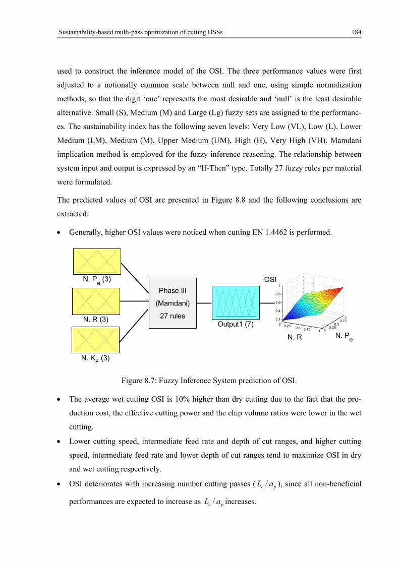
Sustainability-based multi-pass optimization of cutting DSSs 184
used to construct the inference model of the OSI. The three performance values were first
adjusted to a notionally common scale between null and one, using simple normalization
methods, so that the digit ‘one’ represents the most desirable and ‘null’ is the least desirable
alternative. Small (S), Medium (M) and Large (Lg) fuzzy sets are assigned to the performanc-
es. The sustainability index has the following seven levels: Very Low (VL), Low (L), Lower
Medium (LM), Medium (M), Upper Medium (UM), High (H), Very High (VH). Mamdani
implication method is employed for the fuzzy inference reasoning. The relationship between
system input and output is expressed by an “If-Then” type. Totally 27 fuzzy rules per material
were formulated.
The predicted values of OSI are presented in Figure 8.8 and the following conclusions are
extracted:
Generally, higher OSI values were noticed when cutting EN 1.4462 is performed.
Figure 8.7: Fuzzy Inference System prediction of OSI.
The average wet cutting OSI is 10% higher than dry cutting due to the fact that the pro-
duction cost, the effective cutting power and the chip volume ratios were lower in the wet
cutting.
Lower cutting speed, intermediate feed rate and depth of cut ranges, and higher cutting
speed, intermediate feed rate and lower depth of cut ranges tend to maximize OSI in dry
and wet cutting respectively.
OSI deteriorates with increasing number cutting passes ( pc aL / ), since all non-beneficial
performances are expected to increase as pc aL / increases.
N. Pe (3)
N. R (3)
N. KF (3)
Output1 (7)
Phase III
(Mamdani)
27 rules0 0.25 0.5 0.75 1 0
0.250.5
0.7510.1
0,4
0,6
0,8
1
N. PeN. R
OSI
Sustainability-based multi-pass optimization of cutting DSSs 185
For the equal cutting length scenario of facing EN 1.4462 and EN 1.4410, the maximum
OSIs are obtained when alternatives number 8 are selected.
8.4.1 Optimization of OSI using CSNNS
Due to the highly complex relation between cutting parameters and OSI, the RSM was seen
no longer efficient to accurately predict the values of OSI. Serious divergences were noticed
between experimental data and predicted values for several points. Therefore, a multilayer
perceptron (MLP) ANN which can describe the relationships with more precision was inte-
grated with Cuckoo Search meta-heuristic algorithm to perform the task of modeling and op-
timization of OSIs. The neural networks have two layers: one hidden layer and one output
layer. The hidden layer uses a sigmoid-type transference function:
)](exp[1
1)(
ii xwbxf (8.9)
while the output layer uses a linear function:
iipredicted xwbOutput (8.10)
where iw an b are the weights and biases of the network respectively. To facilitate the neural
network training process, all the inputs were normalized using the following equation:
1)(
)(2
minmax
min
xx
xxxi (8.11)
This normalization maps all the inputs and OSI between -1 and +1. The ANN architecture
consists of 4 neurons in the input layer, 1 neuron in the output layer. The weights and biases
of the network are initialized to small random values to avoid immediate saturation in the re-
spective functions. The network was trained by using gradient descendent with momentum
back propagation algorithm. In this algorithm four parameters must be tuned: learning rate RL ,
momentum constant cM , training epochs pE and number of hidden neurons nH . For this
tuning the Taguchi design L9(34) was used to find the most convenient values for achieving
no only lower root mean square, but also good generalization capability, giving the following
values: 0705.0RL , 5895.0cM , 5000pE and 7nH . Basic concepts of ANN and
Taguchi optimization procedure have been previously described in Chapter 2 of the present
Sustainability-based multi-pass optimization of cutting DSSs 186
dissertation. Therefore, the reader is advised to review it, in order to facilitate a better under-
standing of the adopted modeling and optimization techniques.
The performance of the ANNs was statistically measured by the root mean squared error
(RMSE), the coefficient of determination ( 2R ) and the absolute average deviation ( avg.AAD )
obtained using Eqs. (2.33-35). It must be remarked that number of hidden neurons guarantee
that there are more training samples than the total amount of free parameters, thus the training
process is mathematically determined.The R-squared statistics of the models were generally
greater than 0.99, which indicate that the models as fitted explain over 99% of the variability
in OSI. The trained networks achieved RSME and avg.AAD values below target (0.0001) and
(1%) respectively. It must be mentioned that the relationships between variables are complex,
which prove the application of artificial neural networks very advantageous.
Neural network models are then integrated with the Cuckoo Search optimization algorithm, so
that solutions which will provide useful information to the user during the selection of ma-
chining parameters are obtained. The architecture of the Cuckoo Search Neural Network Sys-
tem (CSNNS) is shown in Figure 8.9. CS outperforms many existing algorithms such as ge-
netic algorithm and Particle Swarm Optimization. This superiority can be attributed to the fact
that CS uses a combination of vectorized mutation, crossover by permutation and Le'vy
flights and selective elitism among the best solutions. In addition, the not-so-good solutions
can be replaced systematically by new solutions, and new solutions are often generated by
preferring quality solutions in the solution sets. Thus, the mechanism of the overall search
moves is more subtle and balanced, compared with the simple mechanism used in PSO
[Yang14b]. The number of host nests (or the population size n) and the probabilities ( ap )
were tuned using trial and error method. The population size of (25) and probability of (0.25)
were found sufficient in this case.
The selected decision variables were cutting parameters for each process condition. They
were defined for the ranges between the minimum and maximum experimental levels present-
ed in Table 2. OSIs were selected as the objective functions to maximize:
),,,( cprcii LafvOSI (8.12)
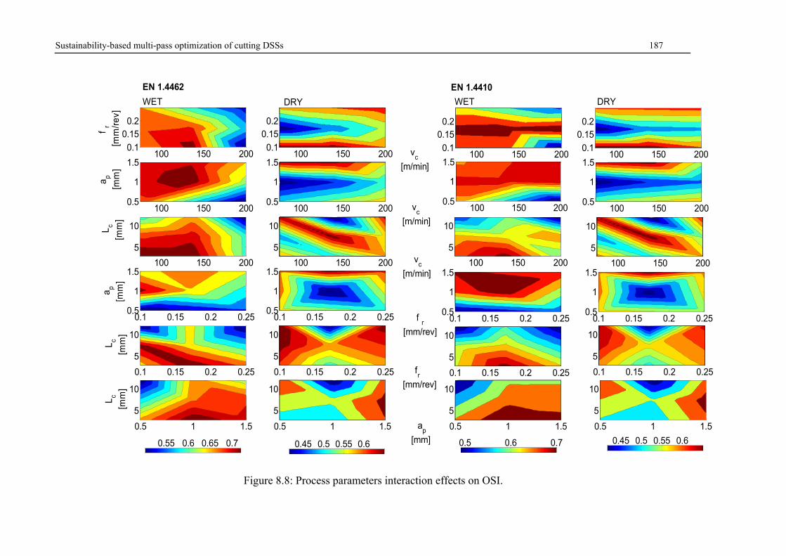
Sustainability-based multi-pass optimization of cutting DSSs 187
Figure 8.8: Process parameters interaction effects on OSI.
f r
[m
m/r
ev]
100 150 2000.1
0.150.2
a p
[m
m]
100 150 2000.5
1
1.5
L c
[m
m]
100 150 200
5
10
f r
[mm/rev]
ap
[m
m]
0.1 0.15 0.2 0.250.5
1
1.5
L c
[
mm
]
0.1 0.15 0.2 0.25
5
10
Lc
[m
m]
0.5 1 1.5
5
10
100 150 2000.1
0.150.2
100 150 2000.5
1
1.5
100 150 200
5
10
0.1 0.15 0.2 0.250.5
1
1.5
0.1 0.15 0.2 0.25
5
10
ap
[mm]
0.5 1 1.5
5
10
100 150 2000.1
0.150.2
100 150 2000.5
1
1.5
vc
[m/min] 100 150 200
5
10
0.1 0.15 0.2 0.250.5
1
1.5
0.1 0.15 0.2 0.25
5
10
0.5 1 1.5
5
10
100 150 2000.1
0.150.2
100 150 2000.5
1
1.5
100 150 200
5
10
0.1 0.15 0.2 0.250.5
1
1.5
0.1 0.15 0.2 0.25
5
10
0.5 1 1.5
5
10
0.55 0.6 0.65 0.7 0.45 0.5 0.55 0.6 0.5 0.6 0.7 0.45 0.5 0.55 0.6
EN 1.4410
fr
[mm/rev]
vc
[m/min]
vc
[m/min]
WET DRY WET DRY
EN 1.4462
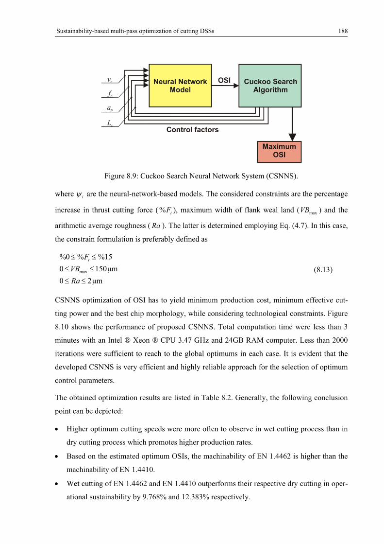
Sustainability-based multi-pass optimization of cutting DSSs 188
Figure 8.9: Cuckoo Search Neural Network System (CSNNS).
where i are the neural-network-based models. The considered constraints are the percentage
increase in thrust cutting force ( tF% ), maximum width of flank weal land ( maxVB ) and the
arithmetic average roughness ( Ra ). The latter is determined employing Eq. (4.7). In this case,
the constrain formulation is preferably defined as
μm20
μm1500
15%%0%
max
Ra
VB
Ft
(8.13)
CSNNS optimization of OSI has to yield minimum production cost, minimum effective cut-
ting power and the best chip morphology, while considering technological constraints. Figure
8.10 shows the performance of proposed CSNNS. Total computation time were less than 3
minutes with an Intel ® Xeon ® CPU 3.47 GHz and 24GB RAM computer. Less than 2000
iterations were sufficient to reach to the global optimums in each case. It is evident that the
developed CSNNS is very efficient and highly reliable approach for the selection of optimum
control parameters.
The obtained optimization results are listed in Table 8.2. Generally, the following conclusion
point can be depicted:
Higher optimum cutting speeds were more often to observe in wet cutting process than in
dry cutting process which promotes higher production rates.
Based on the estimated optimum OSIs, the machinability of EN 1.4462 is higher than the
machinability of EN 1.4410.
Wet cutting of EN 1.4462 and EN 1.4410 outperforms their respective dry cutting in oper-
ational sustainability by 9.768% and 12.383% respectively.
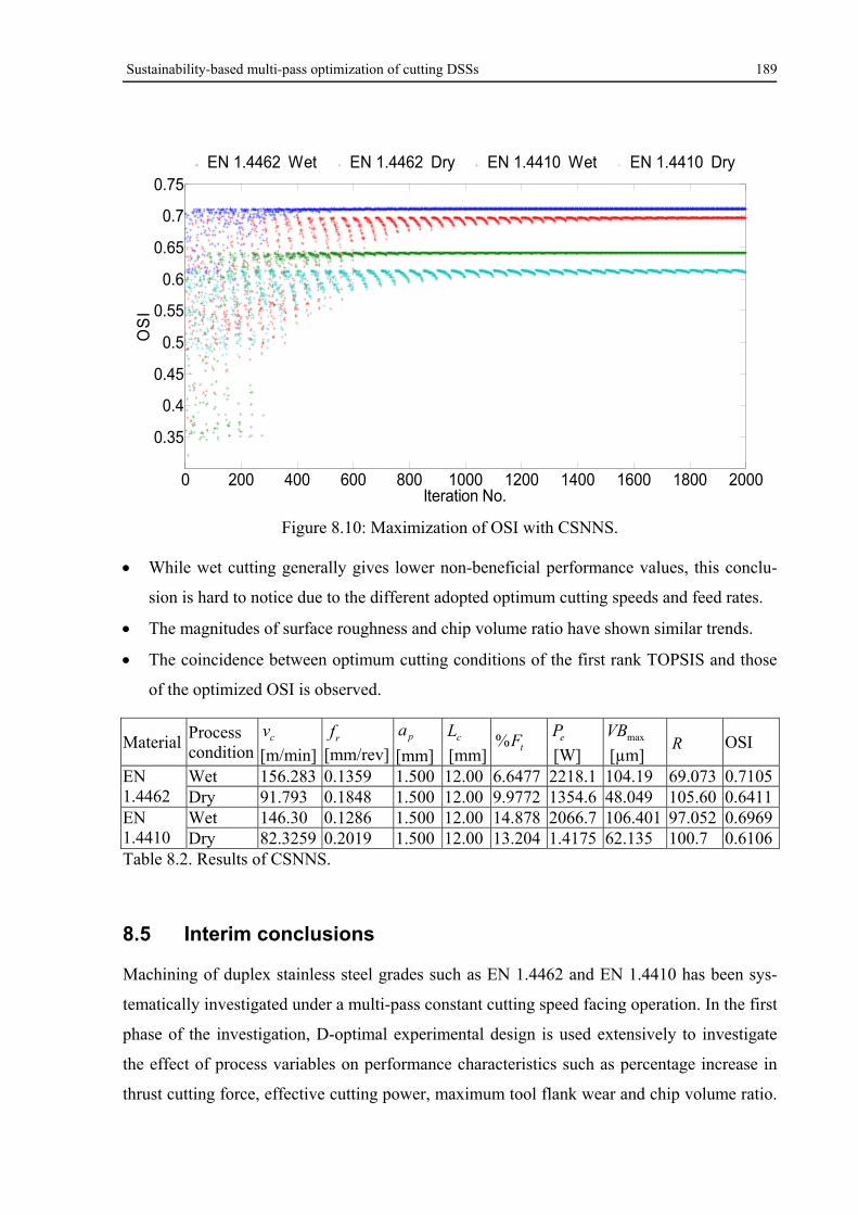
Sustainability-based multi-pass optimization of cutting DSSs 189
Figure 8.10: Maximization of OSI with CSNNS.
While wet cutting generally gives lower non-beneficial performance values, this conclu-
sion is hard to notice due to the different adopted optimum cutting speeds and feed rates.
The magnitudes of surface roughness and chip volume ratio have shown similar trends.
The coincidence between optimum cutting conditions of the first rank TOPSIS and those
of the optimized OSI is observed.
Material Process condition
cv
[m/min] rf
[mm/rev]pa
[mm]cL
[mm]tF% eP
[W] maxVB
[µm] R OSI
EN 1.4462
Wet 156.283 0.1359 1.500 12.00 6.6477 2218.1 104.19 69.073 0.7105Dry 91.793 0.1848 1.500 12.00 9.9772 1354.6 48.049 105.60 0.6411
EN 1.4410
Wet 146.30 0.1286 1.500 12.00 14.878 2066.7 106.401 97.052 0.6969Dry 82.3259 0.2019 1.500 12.00 13.204 1.4175 62.135 100.7 0.6106
Table 8.2. Results of CSNNS.
8.5 Interim conclusions
Machining of duplex stainless steel grades such as EN 1.4462 and EN 1.4410 has been sys-
tematically investigated under a multi-pass constant cutting speed facing operation. In the first
phase of the investigation, D-optimal experimental design is used extensively to investigate
the effect of process variables on performance characteristics such as percentage increase in
thrust cutting force, effective cutting power, maximum tool flank wear and chip volume ratio.
0 200 400 600 800 1000 1200 1400 1600 1800 2000
0.35
0.4
0.45
0.5
0.55
0.6
0.65
0.7
0.75
Iteration No.
OS
I
EN 1.4462
Wet EN 1.4462
Dry EN 1.4410
Wet EN 1.4410
Dry
Sustainability-based multi-pass optimization of cutting DSSs 190
Based on RSM, effective empirical relationships to predict performance characteristics at
95% confidence level were developed. ANOVA used to check the adequacy of the models.
The models were then analyzed using 3D surface graphs and used to study the interaction
effects of process parameters. At the end of the first phase, constrained Cuckoo Search algo-
rithm is selected to perform optimization of the performance characteristics thereby defining
the optimum process conditions. The following general conclusions can be drawn from the
first phase of the investigation:
The values of obtained tF% when EN 1.4410 steels are cut were higher than EN 1.4462
steels. They have shown direct linear correlations with maximum tool flank wear and
proportional dependency on pc aL / ratio, and approached their minimum values as cutting
speed and feed rate increased to certain specified limit. However, when the materials are
cut dry, lower cutting speed and feed rates than wet cutting are preferred to minimize tF% .
Generally, the two-factor interaction models were seen accurate enough to explain the
dependency relation between effective cutting power and independent variables. Their
minimum consumption were seen when the feed rate is in the range 0.125-0.175 mm/rev
of dry cutting and 0.1-0.15mm/rev of wet cutting and the rest of the remained independent
variables are kept at their lowest levels.
Wet cutting at cutting parameter ranges of m/min,160100cv 15.0rf mm/rev,25.0
mm0.175.0 pa for machining EN 1.4462 and m/min,160120 cv 15.0rf
mm/rev,20.0 mm5.125.1 pa for machining EN 1.4410 were seen optimum in mini-
mizing the tool flank wear. Dry machining is possible when cutting parameters are set ap-
propriately. The settings include; machining of EN 1.4462 at m/min,11075cv
mm/rev,20.015.0 rf mm5.11pa and maximum ,6/ pc aL and machining of EN
1.4410 at m/min,9075cv mm/rev,175.0125.0 rf mm35.18.0 pa and maxi-
mum 4/ pc aL .
Ribbon and snarled chip forms were common when the DSSs are machined at feed rate
and depth of cuts lower than 0.15 mm/rev and 1mm respectively. In wet cutting, friendli-
er-to-machine chip forms were produced and the R values of cutting EN 1.4410 were gen-
erally seen higher than of cutting EN 1.4462. Under the same machining conditions
Sustainability-based multi-pass optimization of cutting DSSs 191
which might produce continuous chips, different chip forms were also possible, especially
when 6/ pc aL .
In the second phase of the study, the measurements were used to develop a comprehensive
machining economics model. A case study of producing 12000 units of per each experimental
run is considered and the corresponding machining costs and production rates were deter-
mined. Summarizing the conclusion points depicted at this stage:
The optimization conflict between machining economics attributes, such as simultaneous
minimization of machine utilization time bBt , main time-related costs 1K and the tool re-
lated costs 3K could be effectively solved employing TOPSIS.
The alternatives were ranked based on their computed relative closeness to the ideal solu-
tion C*. The ranking of the alternatives has revealed that the intermediate range of cutting
speed, feed rates at wet cutting produce the optimum choice to minimize the considered
attributes simultaneously.
The order of ranking of both materials is almost identical. However, under the same cut-
ting condition, lower cutting speed when dry cutting EN 1.4410 and higher cutting speed
when wet cutting EN 1.4462 has shown higher preference than similar dry cutting EN
1.4462 and wet cutting EN 1.4410 respectively.
In the third phase of the study, the computed performances in the first and second phases were
utilized to derive a new index of measuring machining sustainability called operational sus-
tainability index (OSI). Based on the Mamdani implication method for the fuzzy inference
reasoning, normalized production cost per unit to consider the economics of the machining
process, normalized effective cutting power to assess the energy demand of the machining
process and normalized chip volume ratio to consider the chip morphology were successfully
employed to define the OSI. The optimal machining parameters were tabulated and many
conclusion points were extracted:
To accurately model and constrainedly optimize the highly nonlinear OSIs, neural net-
work models could be integrated with Cuckoo Search algorithm and form Cuckoo Search
Neural Network System which is abbreviated as CSNNS. Results have indicated the effi-
ciency of the proposed approach for solving the optimization problem effectively.

Sustainability-based multi-pass optimization of cutting DSSs 192
Generally, higher OSI values were noticed when wet cutting of DSSs are performed. For
instance, in this study, wet cutting of EN 1.4462 and EN 1.4410 outperforms their respec-
tive dry cutting in operational sustainability by 9.768% and 12.383% respectively.
Based on the predicted OSIs values, the machinability of EN 1.4462 is higher than the
machinability of EN 1.4410.
Lower cutting speed, intermediate feed rate depth of cut ranges, and higher cutting speed,
intermediate feed rate and lower depth of cut ranges tend to maximize OSI in dry and wet
cutting respectively.
Results also showed coincidence between optimum cutting conditions in second and third
phases.
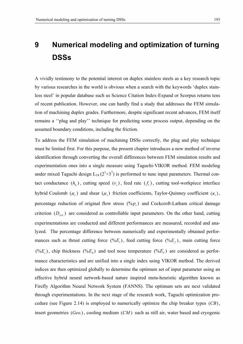
Numerical modeling and optimization of turning DSSs 193
9 Numerical modeling and optimization of turning
DSSs
A vividly testimony to the potential interest on duplex stainless steels as a key research topic
by various researches in the world is obvious when a search with the keywords ‘duplex stain-
less steel’ in popular database such us Science Citation Index-Expand or Scorpus returns tens
of recent publication. However, one can hardly find a study that addresses the FEM simula-
tion of machining duplex grades. Furthermore, despite significant recent advances, FEM itself
remains a ‘‘plug and play’’ technique for predicting some process output, depending on the
assumed boundary conditions, including the friction.
To address the FEM simulation of machining DSSs correctly, the plug and play technique
must be limited first. For this purpose, the present chapter introduces a new method of inverse
identification through converting the overall differences between FEM simulation results and
experimentation ones into a single measure using Taguchi-VIKOR method. FEM modeling
under mixed Taguchi design L18 (21×37) is performed to tune input parameters. Thermal con-
tact conductance )( tch , cutting speed )( cv , feed rate )( rf , cutting tool-workpiece interface
hybrid Coulomb )( c and shear )( s friction coefficients, Taylor-Quinney coefficient )( t ,
percentage reduction of original flow stress )(% rp and Cockcroft-Latham critical damage
criterion )( .critD are considered as controllable input parameters. On the other hand, cutting
experimentations are conducted and different performances are measured, recorded and ana-
lyzed. The percentage difference between numerically and experimentally obtained perfor-
mances such as thrust cutting force )(% tE , feed cutting force )(% fE , main cutting force
)(% cE , chip thickness )(% hE and tool nose temperature )(% TE are considered as perfor-
mance characteristics and are unified into a single index using VIKOR method. The derived
indices are then optimized globally to determine the optimum set of input parameter using an
effective hybrid neural network-based nature inspired meta-heuristic algorithm known as
Firefly Algorithm Neural Network System (FANNS). The optimum sets are next validated
through experimentations. In the next stage of the research work, Taguchi optimization pro-
cedure (see Figure 2.14) is employed to numerically optimize the chip breaker types )(CB ,
insert geometries .)(Geo , cooling medium )(CM such as still air, water based and cryogenic
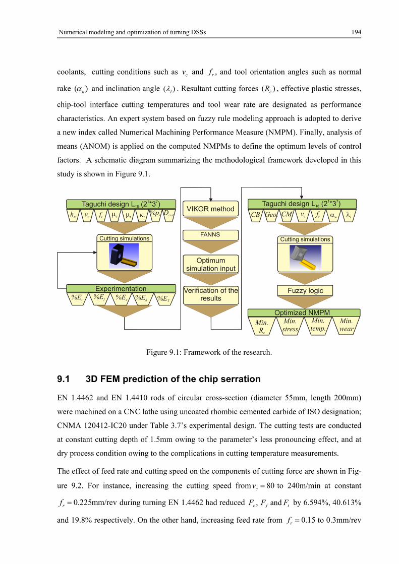
Numerical modeling and optimization of turning DSSs 194
coolants, cutting conditions such as cv and rf , and tool orientation angles such as normal
rake )( n and inclination angle )( i . Resultant cutting forces )( cR , effective plastic stresses,
chip-tool interface cutting temperatures and tool wear rate are designated as performance
characteristics. An expert system based on fuzzy rule modeling approach is adopted to derive
a new index called Numerical Machining Performance Measure (NMPM). Finally, analysis of
means (ANOM) is applied on the computed NMPMs to define the optimum levels of control
factors. A schematic diagram summarizing the methodological framework developed in this
study is shown in Figure 9.1.
Figure 9.1: Framework of the research.
9.1 3D FEM prediction of the chip serration
EN 1.4462 and EN 1.4410 rods of circular cross-section (diameter 55mm, length 200mm)
were machined on a CNC lathe using uncoated rhombic cemented carbide of ISO designation;
CNMA 120412-IC20 under Table 3.7’s experimental design. The cutting tests are conducted
at constant cutting depth of 1.5mm owing to the parameter’s less pronouncing effect, and at
dry process condition owing to the complications in cutting temperature measurements.
The effect of feed rate and cutting speed on the components of cutting force are shown in Fig-
ure 9.2. For instance, increasing the cutting speed from 80cv to 240m/min at constant
mm/rev225.0rf during turning EN 1.4462 had reduced tfc FFF and, by 6.594%, 40.613%
and 19.8% respectively. On the other hand, increasing feed rate from 15.0rf to 0.3mm/rev
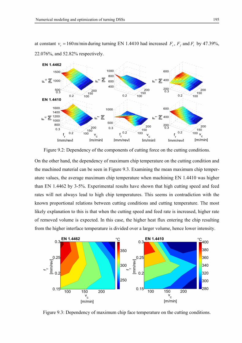
Numerical modeling and optimization of turning DSSs 195
at constant m/min160cv during turning EN 1.4410 had increased tfc FFF and, by 47.39%,
22.076%, and 52.82% respectively.
Figure 9.2: Dependency of the components of cutting force on the cutting conditions.
On the other hand, the dependency of maximum chip temperature on the cutting condition and
the machined material can be seen in Figure 9.3. Examining the mean maximum chip temper-
ature values, the average maximum chip temperature when machining EN 1.4410 was higher
than EN 1.4462 by 3-5%. Experimental results have shown that high cutting speed and feed
rates will not always lead to high chip temperatures. This seems in contradiction with the
known proportional relations between cutting conditions and cutting temperature. The most
likely explanation to this is that when the cutting speed and feed rate is increased, higher rate
of removed volume is expected. In this case, the higher heat flux entering the chip resulting
from the higher interface temperature is divided over a larger volume, hence lower intensity.
Figure 9.3: Dependency of maximum chip face temperature on the cutting conditions.
100150
200
0.2
0.3
500
1000
Ff
[N]
100150
200
0.2
400
600
800
1000
Ff
[N]
100150
200
0.20.3
800
1000
1200
1400
1600
Fc
[N]
100150
200
0.20.3
500
1000
1500
Fc
[N]
100150
200
0.2
0.3200
400
600
Ft
[N]
100150
200
0.2
0.3200
400
600
Ft
[N]
EN 1.4462
vc
[m/min]
vc
[m/min]
vc
[m/min]
fr
[mm/rev]
fr
[mm/rev]
fr
[mm/rev]
EN 1.4410
vc
[m/min]
f r
[mm
/rev
]
100 150 2000.15
0.2
0.25
0.3
vc
[m/min]
f r
[mm
/rev
]
100 150 2000.15
0.2
0.25
0.3
250
300
350
280
300
320
340
360
380
400°C°C EN 1.4410EN 1.4462
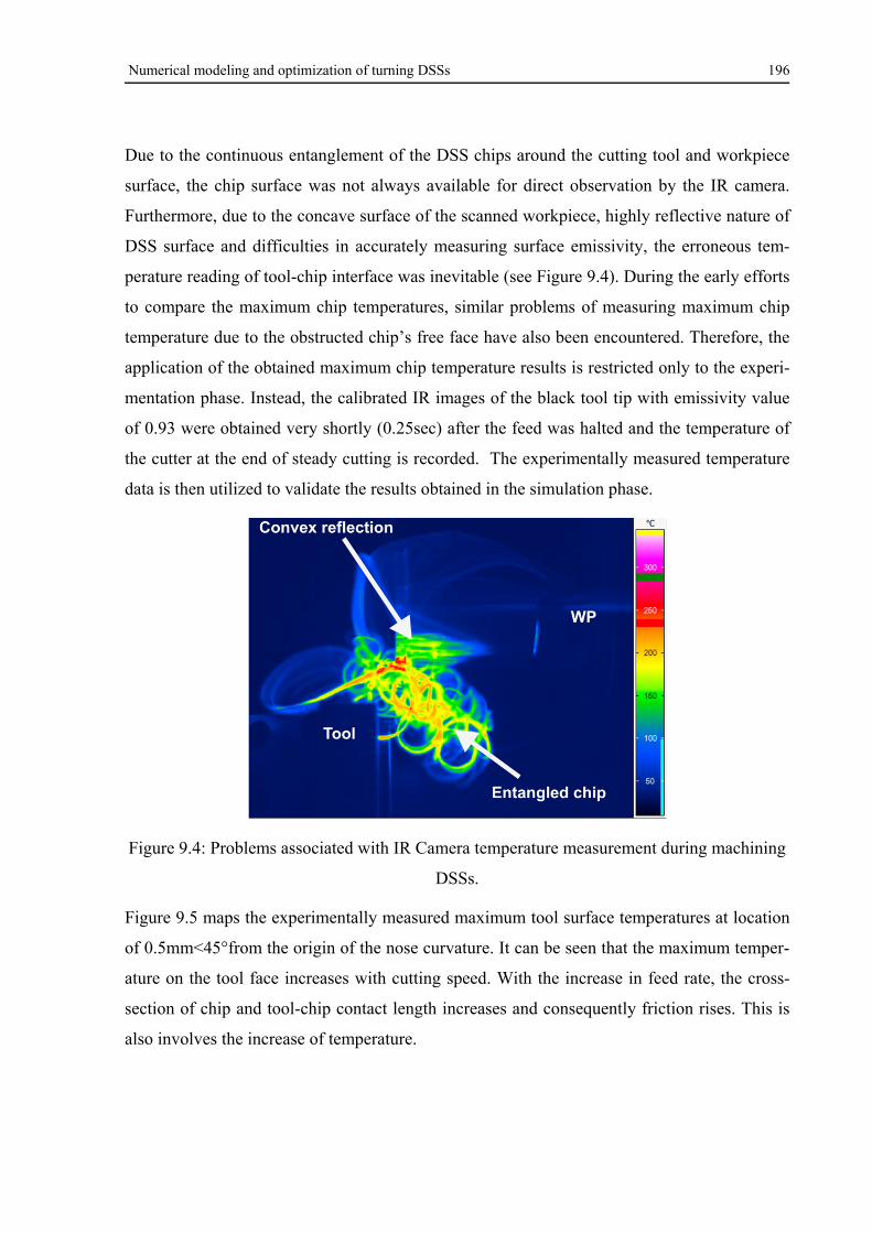
Numerical modeling and optimization of turning DSSs 196
Due to the continuous entanglement of the DSS chips around the cutting tool and workpiece
surface, the chip surface was not always available for direct observation by the IR camera.
Furthermore, due to the concave surface of the scanned workpiece, highly reflective nature of
DSS surface and difficulties in accurately measuring surface emissivity, the erroneous tem-
perature reading of tool-chip interface was inevitable (see Figure 9.4). During the early efforts
to compare the maximum chip temperatures, similar problems of measuring maximum chip
temperature due to the obstructed chip’s free face have also been encountered. Therefore, the
application of the obtained maximum chip temperature results is restricted only to the experi-
mentation phase. Instead, the calibrated IR images of the black tool tip with emissivity value
of 0.93 were obtained very shortly (0.25sec) after the feed was halted and the temperature of
the cutter at the end of steady cutting is recorded. The experimentally measured temperature
data is then utilized to validate the results obtained in the simulation phase.
Figure 9.4: Problems associated with IR Camera temperature measurement during machining
DSSs.
Figure 9.5 maps the experimentally measured maximum tool surface temperatures at location
of 0.5mm<45°from the origin of the nose curvature. It can be seen that the maximum temper-
ature on the tool face increases with cutting speed. With the increase in feed rate, the cross-
section of chip and tool-chip contact length increases and consequently friction rises. This is
also involves the increase of temperature.
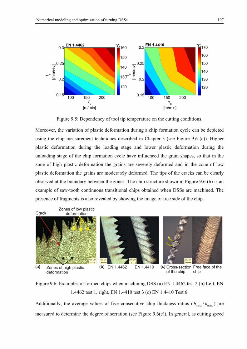
Numerical modeling and optimization of turning DSSs 197
Figure 9.5: Dependency of tool tip temperature on the cutting conditions.
Moreover, the variation of plastic deformation during a chip formation cycle can be depicted
using the chip measurement techniques described in Chapter 3 (see Figure 9.6 (a)). Higher
plastic deformation during the loading stage and lower plastic deformation during the
unloading stage of the chip formation cycle have influenced the grain shapes, so that in the
zone of high plastic deformation the grains are severely deformed and in the zone of low
plastic deformation the grains are moderately deformed. The tips of the cracks can be clearly
observed at the boundary between the zones. The chip structure shown in Figure 9.6 (b) is an
example of saw-tooth continuous transitional chips obtained when DSSs are machined. The
presence of fragments is also revealed by showing the image of free side of the chip.
Figure 9.6: Examples of formed chips when machining DSS (a) EN 1.4462 test 2 (b) Left, EN
1.4462 test 1, right, EN 1.4410 test 3 (c) EN 1.4410 Test 6.
Additionally, the average values of five consecutive chip thickness ratios (i
hmax /i
hmin ) are
measured to determine the degree of serration (see Figure 9.6(c)). In general, as cutting speed
vc
[m/min]
f r
[mm
/rev
]
100 150 2000.15
0.2
0.25
0.3
120
130
140
150
160
f r
[mm
/rev
]
vc
[m/min]
100 150 2000.15
0.2
0.25
0.3
120
130
140
150
160
170°C°CEN 1.4462 EN 1.4410
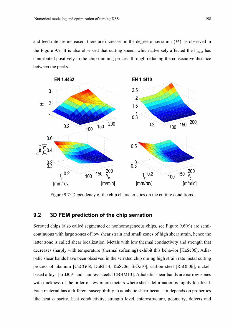
Numerical modeling and optimization of turning DSSs 198
and feed rate are increased, there are increases in the degree of serration )(H as observed in
the Figure 9.7. It is also observed that cutting speed, which adversely affected the hmax, has
contributed positively in the chip thinning process through reducing the consecutive distance
between the peeks.
Figure 9.7: Dependency of the chip characteristics on the cutting conditions.
9.2 3D FEM prediction of the chip serration
Serrated chips (also called segmented or nonhomogeneous chips, see Figure 9.6(c)) are semi-
continuous with large zones of low shear strain and small zones of high shear strain, hence the
latter zone is called shear localization. Metals with low thermal conductivity and strength that
decreases sharply with temperature (thermal softening) exhibit this behavior [KaSc06]. Adia-
batic shear bands have been observed in the serrated chip during high strain rate metal cutting
process of titanium [CaCG08, DuRF14, KaSc06, SiÖz10], carbon steel [RhOh06], nickel-
based alloys [LoJJ09] and stainless steels [CBBM13]. Adiabatic shear bands are narrow zones
with thickness of the order of few micro-meters where shear deformation is highly localized.
Each material has a different susceptibility to adiabatic shear because it depends on properties
like heat capacity, heat conductivity, strength level, microstructure, geometry, defects and
100 150 2000.2
0.31
1.5
2
2.5
100 150 2000.2
1
2
3
H
100 150 2000.2
0.30
0.5
100 150 2000.2
0.30.2
0.4
0.6
h m
ax
[
mm
]
fr
[mm/rev]
EN 1.4462 EN 1.4410
vc
[m/min]
vc
[m/min]
fr
[mm/rev]
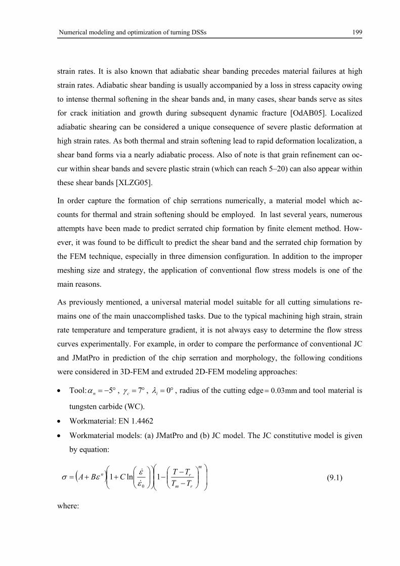
Numerical modeling and optimization of turning DSSs 199
strain rates. It is also known that adiabatic shear banding precedes material failures at high
strain rates. Adiabatic shear banding is usually accompanied by a loss in stress capacity owing
to intense thermal softening in the shear bands and, in many cases, shear bands serve as sites
for crack initiation and growth during subsequent dynamic fracture [OdAB05]. Localized
adiabatic shearing can be considered a unique consequence of severe plastic deformation at
high strain rates. As both thermal and strain softening lead to rapid deformation localization, a
shear band forms via a nearly adiabatic process. Also of note is that grain refinement can oc-
cur within shear bands and severe plastic strain (which can reach 5–20) can also appear within
these shear bands [XLZG05].
In order capture the formation of chip serrations numerically, a material model which ac-
counts for thermal and strain softening should be employed. In last several years, numerous
attempts have been made to predict serrated chip formation by finite element method. How-
ever, it was found to be difficult to predict the shear band and the serrated chip formation by
the FEM technique, especially in three dimension configuration. In addition to the improper
meshing size and strategy, the application of conventional flow stress models is one of the
main reasons.
As previously mentioned, a universal material model suitable for all cutting simulations re-
mains one of the main unaccomplished tasks. Due to the typical machining high strain, strain
rate temperature and temperature gradient, it is not always easy to determine the flow stress
curves experimentally. For example, in order to compare the performance of conventional JC
and JMatPro in prediction of the chip serration and morphology, the following conditions
were considered in 3D-FEM and extruded 2D-FEM modeling approaches:
Tool: 5n , 7c , 0i , radius of the cutting edge mm03.0 and tool material is
tungsten carbide (WC).
Workmaterial: EN 1.4462
Workmaterial models: (a) JMatPro and (b) JC model. The JC constitutive model is given
by equation:
m
rm
rn
TT
TTCBA 1ln1
0
(9.1)
where:
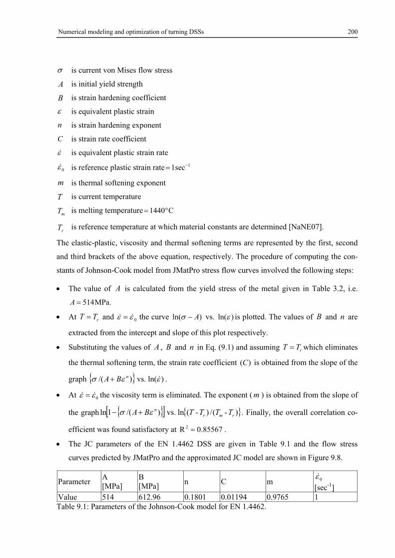
Numerical modeling and optimization of turning DSSs 200
is current von Mises flow stress
A is initial yield strength
B is strain hardening coefficient
is equivalent plastic strain
n is strain hardening exponent
C is strain rate coefficient
is equivalent plastic strain rate
0 is reference plastic strain rate 1sec1
m is thermal softening exponent
T is current temperature
mT is melting temperature C1440
rT is reference temperature at which material constants are determined [NaNE07].
The elastic-plastic, viscosity and thermal softening terms are represented by the first, second
and third brackets of the above equation, respectively. The procedure of computing the con-
stants of Johnson-Cook model from JMatPro stress flow curves involved the following steps:
The value of A is calculated from the yield stress of the metal given in Table 3.2, i.e.
MPa.514A
At rTT and 0 the curve )ln( A vs. )ln( is plotted. The values of B and n are
extracted from the intercept and slope of this plot respectively.
Substituting the values of A , B and n in Eq. (9.1) and assuming rTT which eliminates
the thermal softening term, the strain rate coefficient )(C is obtained from the slope of the
graph )ln(vs.)/( nBA .
At 0 the viscosity term is eliminated. The exponent ( m ) is obtained from the slope of
the graph )(/)(lnvs.)/(1ln rmrn T-TT-TBA . Finally, the overall correlation co-
efficient was found satisfactory at 85567.0R 2 .
The JC parameters of the EN 1.4462 DSS are given in Table 9.1 and the flow stress
curves predicted by JMatPro and the approximated JC model are shown in Figure 9.8.
Parameter A [MPa]
B [MPa]
n C m 0
[sec-1] Value 514 612.96 0.1801 0.01194 0.9765 1 Table 9.1: Parameters of the Johnson-Cook model for EN 1.4462.
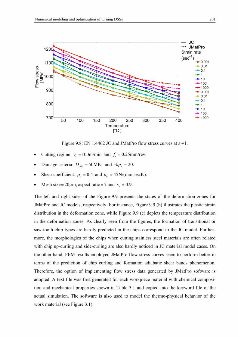
Numerical modeling and optimization of turning DSSs 201
Figure 9.8: EN 1.4462 JC and JMatPro flow stress curves at ε =1.
Cutting regime: m/min100cv and mm/rev.25.0rf
Damage criteria: MPa50. critD and .20% rp
Shear coefficient: 4.0s and K).N/(mm.sec.45tch
Mesh size20µm, aspect ratio7 and .9.0t
The left and right sides of the Figure 9.9 presents the states of the deformation zones for
JMatPro and JC models, respectively. For instance, Figure 9.9 (b) illustrates the plastic strain
distribution in the deformation zone, while Figure 9.9 (c) depicts the temperature distribution
in the deformation zones. As clearly seen from the figures, the formation of transitional or
saw-tooth chip types are hardly predicted in the chips correspond to the JC model. Further-
more, the morphologies of the chips when cutting stainless steel materials are often related
with chip up-curling and side-curling are also hardly noticed in JC material model cases. On
the other hand, FEM results employed JMatPro flow stress curves seem to perform better in
terms of the prediction of chip curling and formation adiabatic shear bands phenomenon.
Therefore, the option of implementing flow stress data generated by JMatPro software is
adopted. A text file was first generated for each workpiece material with chemical composi-
tion and mechanical properties shown in Table 3.1 and copied into the keyword file of the
actual simulation. The software is also used to model the thermo-physical behavior of the
work material (see Figure 3.1).
50 100 150 200 250 300 350 400700
800
900
1000
1100
1200
Flo
w s
tres
s[M
Pa]
Temperature[°C ]
0.0010.010.111010010000.0010.010.11101001000
JCJMatPro
Strain rate
(sec-1)
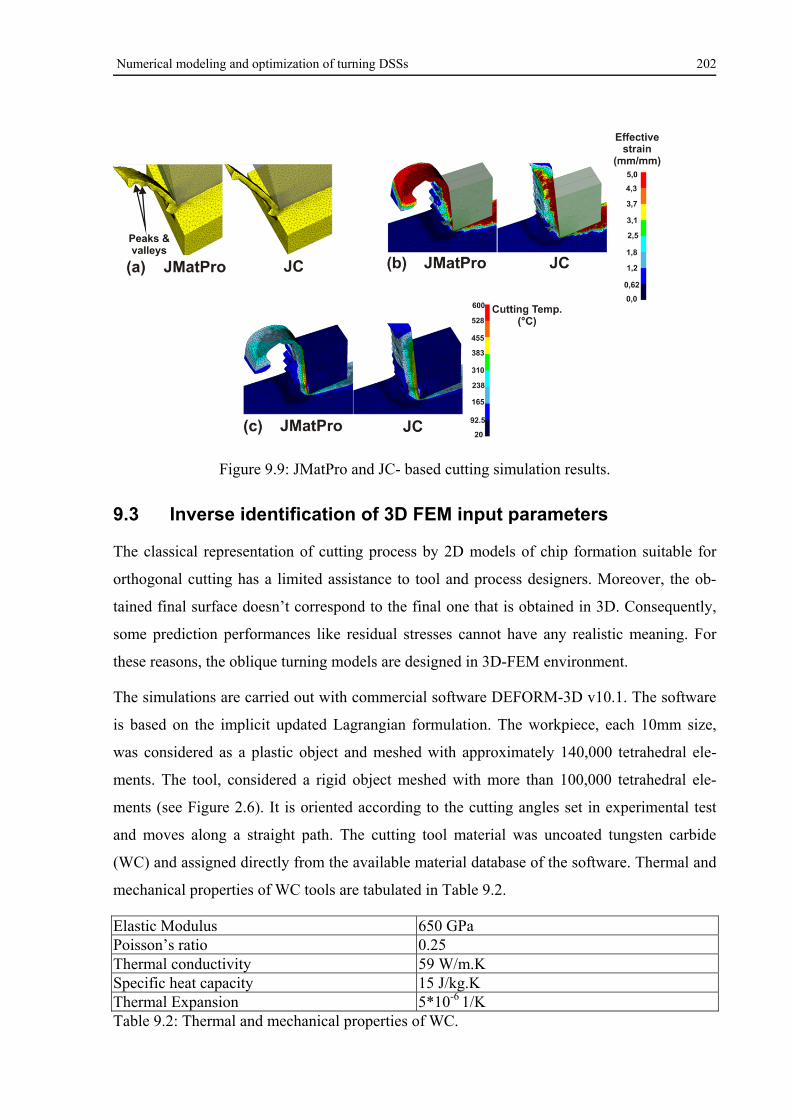
Numerical modeling and optimization of turning DSSs 202
Figure 9.9: JMatPro and JC- based cutting simulation results.
9.3 Inverse identification of 3D FEM input parameters
The classical representation of cutting process by 2D models of chip formation suitable for
orthogonal cutting has a limited assistance to tool and process designers. Moreover, the ob-
tained final surface doesn’t correspond to the final one that is obtained in 3D. Consequently,
some prediction performances like residual stresses cannot have any realistic meaning. For
these reasons, the oblique turning models are designed in 3D-FEM environment.
The simulations are carried out with commercial software DEFORM-3D v10.1. The software
is based on the implicit updated Lagrangian formulation. The workpiece, each 10mm size,
was considered as a plastic object and meshed with approximately 140,000 tetrahedral ele-
ments. The tool, considered a rigid object meshed with more than 100,000 tetrahedral ele-
ments (see Figure 2.6). It is oriented according to the cutting angles set in experimental test
and moves along a straight path. The cutting tool material was uncoated tungsten carbide
(WC) and assigned directly from the available material database of the software. Thermal and
mechanical properties of WC tools are tabulated in Table 9.2.
Elastic Modulus 650 GPa Poisson’s ratio 0.25 Thermal conductivity 59 W/m.K Specific heat capacity 15 J/kg.K Thermal Expansion 5*10-6 1/K Table 9.2: Thermal and mechanical properties of WC.
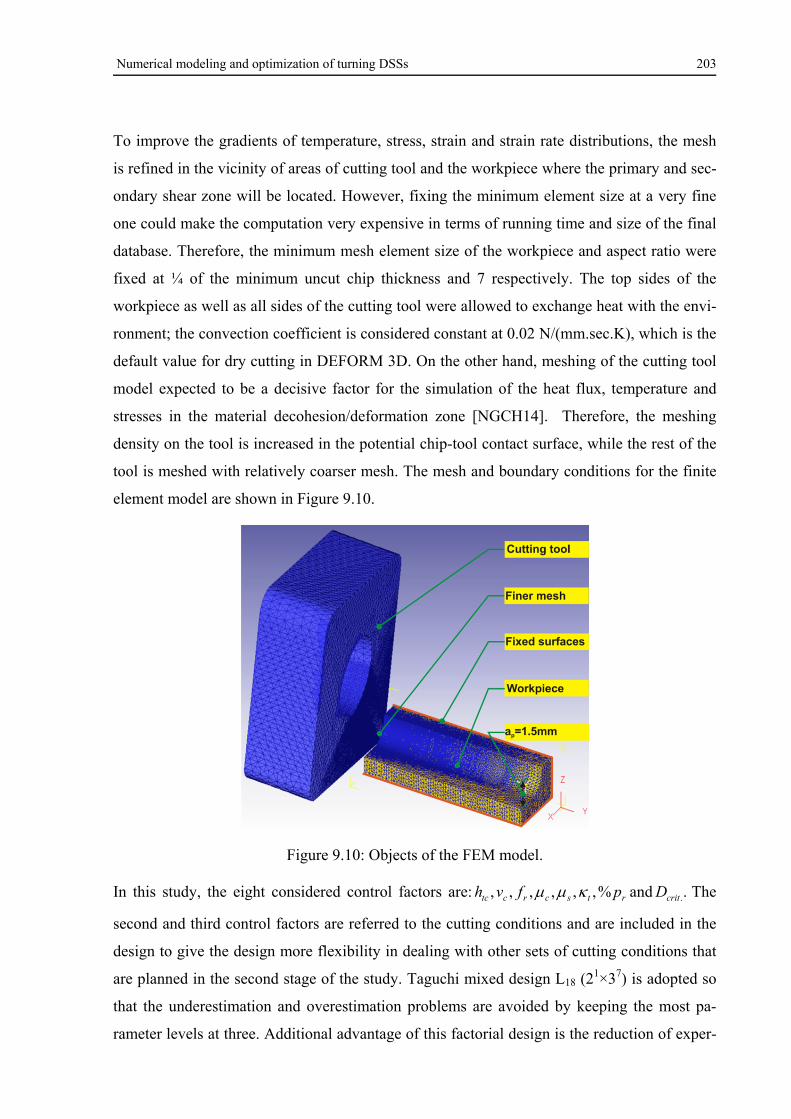
Numerical modeling and optimization of turning DSSs 203
To improve the gradients of temperature, stress, strain and strain rate distributions, the mesh
is refined in the vicinity of areas of cutting tool and the workpiece where the primary and sec-
ondary shear zone will be located. However, fixing the minimum element size at a very fine
one could make the computation very expensive in terms of running time and size of the final
database. Therefore, the minimum mesh element size of the workpiece and aspect ratio were
fixed at ¼ of the minimum uncut chip thickness and 7 respectively. The top sides of the
workpiece as well as all sides of the cutting tool were allowed to exchange heat with the envi-
ronment; the convection coefficient is considered constant at 0.02 N/(mm.sec.K), which is the
default value for dry cutting in DEFORM 3D. On the other hand, meshing of the cutting tool
model expected to be a decisive factor for the simulation of the heat flux, temperature and
stresses in the material decohesion/deformation zone [NGCH14]. Therefore, the meshing
density on the tool is increased in the potential chip-tool contact surface, while the rest of the
tool is meshed with relatively coarser mesh. The mesh and boundary conditions for the finite
element model are shown in Figure 9.10.
Figure 9.10: Objects of the FEM model.
In this study, the eight considered control factors are: .and%,,,,,, .critrtscrctc Dpfvh The
second and third control factors are referred to the cutting conditions and are included in the
design to give the design more flexibility in dealing with other sets of cutting conditions that
are planned in the second stage of the study. Taguchi mixed design L18 (21×37) is adopted so
that the underestimation and overestimation problems are avoided by keeping the most pa-
rameter levels at three. Additional advantage of this factorial design is the reduction of exper-
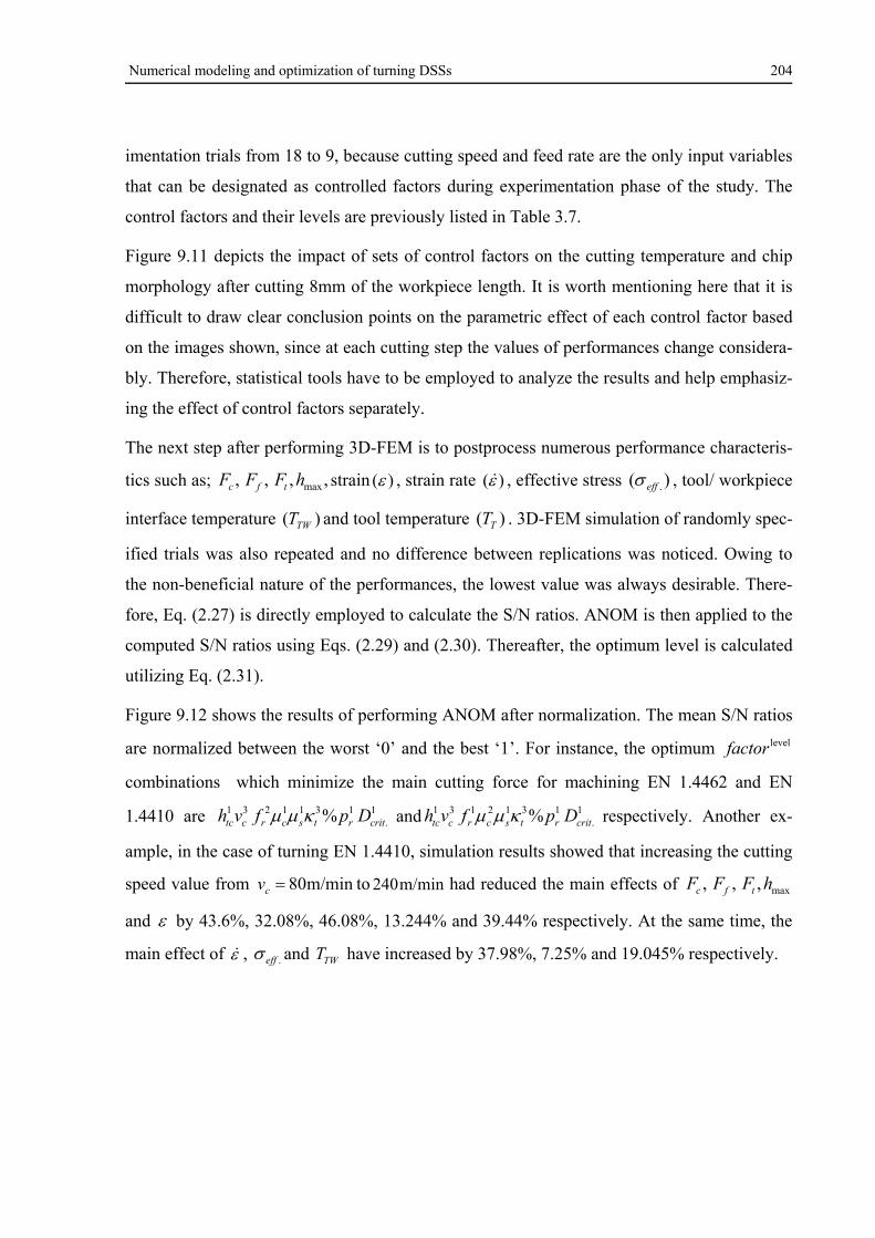
Numerical modeling and optimization of turning DSSs 204
imentation trials from 18 to 9, because cutting speed and feed rate are the only input variables
that can be designated as controlled factors during experimentation phase of the study. The
control factors and their levels are previously listed in Table 3.7.
Figure 9.11 depicts the impact of sets of control factors on the cutting temperature and chip
morphology after cutting 8mm of the workpiece length. It is worth mentioning here that it is
difficult to draw clear conclusion points on the parametric effect of each control factor based
on the images shown, since at each cutting step the values of performances change considera-
bly. Therefore, statistical tools have to be employed to analyze the results and help emphasiz-
ing the effect of control factors separately.
The next step after performing 3D-FEM is to postprocess numerous performance characteris-
tics such as; ,,,, maxhFFF tfc strain )( , strain rate )( , effective stress )( .eff , tool/ workpiece
interface temperature )( TWT and tool temperature )( TT . 3D-FEM simulation of randomly spec-
ified trials was also repeated and no difference between replications was noticed. Owing to
the non-beneficial nature of the performances, the lowest value was always desirable. There-
fore, Eq. (2.27) is directly employed to calculate the S/N ratios. ANOM is then applied to the
computed S/N ratios using Eqs. (2.29) and (2.30). Thereafter, the optimum level is calculated
utilizing Eq. (2.31).
Figure 9.12 shows the results of performing ANOM after normalization. The mean S/N ratios
are normalized between the worst ‘0’ and the best ‘1’. For instance, the optimum levelfactor
combinations which minimize the main cutting force for machining EN 1.4462 and EN
1.4410 are 1.
1311231 % critrtscrctc Dpfvh and 1.
1312131 % critrtscrctc Dpfvh respectively. Another ex-
ample, in the case of turning EN 1.4410, simulation results showed that increasing the cutting
speed value from m/min80cv to m/min240 had reduced the main effects of max,,, hFFF tfc
and by 43.6%, 32.08%, 46.08%, 13.244% and 39.44% respectively. At the same time, the
main effect of , .eff and TWT have increased by 37.98%, 7.25% and 19.045% respectively.
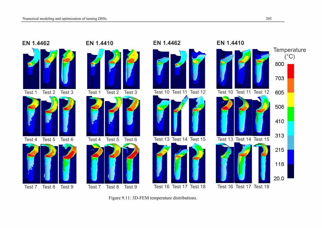
Numerical modeling and optimization of turning DSSs 205
Figure 9.11: 3D-FEM temperature distributions.
Numerical modeling and optimization of turning DSSs 206
Figure 9.12: Main effect plots of the effect of control factors on the cutting performances during turning EN 1.4410 and EN 1.4462 DSS.
500 10000
0.5
1
htc
[N/(mm.sec.K)]100 150 200
0
0.5
1
vc [m/min]
0.2 0.30
0.5
1
fr [mm/rev]
0.6 0.8 10
0.5
1
µc
0.6 0.8 1 1.20
0.5
1
µsN
orm
aliz
ed
S/N
ra
tio
0.8 0.9 10
0.5
1
Kt
20 400
0.5
1
%pr
50 100 1500
0.5
1
Dcrit
[MPa]
500 1000
0.20.40.6
htc
[N/(mm.sec.K)]100 150 200
0.20.40.60.8
vc [m/min]
Ff
Fc
Fr
EffectiveStrain
StrainRate
EffectiveStress
InterfaceTemp.
Temp.Tool
hmax
0.20 0.300.2
0.4
0.6
fr [mm/rev]
0.6 0.8 10.2
0.4
0.6
µc
0.6 0.8 1 1.20.2
0.4
0.6
µs
0.8 0.9 10.2
0.4
0.6
Kt
20 400.2
0.4
0.6
%pr
50 100 1500.2
0.4
0.6
Dcrit
[MPa]
EN 1.4410EN 1.4462
Numerical modeling and optimization of turning DSSs 207
9.3.1 Proposed methodology
9.3.1.1 Analyses of the error percentages
The percentage of differences between the experimentally measured cutting forces, tool tem-
peratures and thicknesses, and the FEM-predicted ones are computed using the percentage of
difference expression ( E% ):
100%
FEM
FEMEXP
Y
YYE (9.2)
where EXPY represents the experimental performance values and FEMY the simulated perfor-
mance values. To estimate the effect of the control factors and important interactions on the
E% , percentage of contribution of each control factor on variance of the corresponding error
percentage should be computed. The control factor that returns highest contribution percent-
age is designated as the prime factor. For the sake of more convenience, percentages are
drawn in pie charts and shown in Figure 9.13. For instance, in the case of turning EN 1.4462,
the control factors which are expected to play important roles in minimizing the percentage
differences of feed force fE% , cutting force cE% , thrust force tE% , tool temperature TE%
and chip thickness hE% were s , t , s and ctc vh , s and tch , and s respectively.
Results of E% computations versus the experimental order are illustrated in Figure 9.14. It
can be seen that the predicted feed and thrust force components are generally underestimated
except for some few cases at MPa150. critD . Severe fluctuations of fE% and tE% were gen-
erally in the range of -40% to 195%. On the other hand, cE% has shown better agreements
with the range of approximately -40% to 45%. Furthermore, comparing the TT and maxh , the
E% between experimental and FEM values also fluctuate between over and under estimation,
with very few cases in which absolute E% were less than 5%. These results show the strong
impact of control factors on the outputs of the FEM. The next sections describe the study ap-
proach intended to simultaneously minimize all the differences between measured and pre-
dicted performances.
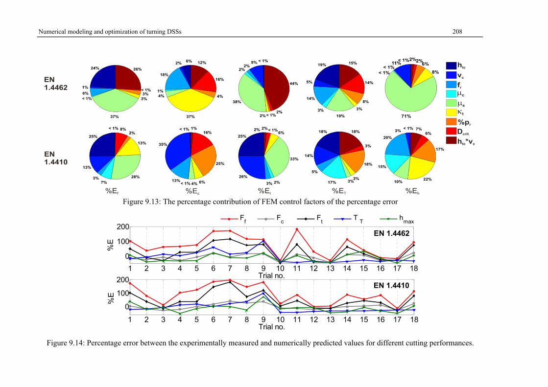
Numerical modeling and optimization of turning DSSs 208
Figure 9.13: The percentage contribution of FEM control factors of the percentage error
Figure 9.14: Percentage error between the experimentally measured and numerically predicted values for different cutting performances.
1 2 3 4 5 6 7 8 9 10 11 12 13 14 15 16 17 18
0
100
200
%E
Trial no.
1 2 3 4 5 6 7 8 9 10 11 12 13 14 15 16 17 18
0
100
200
Trial no.
%E
Ff
Fc
Ft
T T
hmax
EN 1.4462
EN 1.4410
Numerical modeling and optimization of turning DSSs 209
9.3.1.2 Application of VIKOR method
In order to simultaneously minimize the multiple error percentages and determine the best
alternative (trial no.), VIKOR method is proposed. The procedure of calculating VIKOR indi-
ces for each workmaterial case is started with the representation of decision matrix through
assigning fE% , cE% , tE% , TE% and hE% as attributes (columns) of the matrix. The criteria
weights have are set using the standard deviation method as per equation (2.63). The best and
the worst values of all the criteria in weighted normalized decision matrices are identified
using Eqs. (2.79) and (2.80). The values of utility )(S and regret )(R measures are calculated
using Eqs. (2.81) and (2.82), respectively. The VIKOR index values )( VQ are then calculated
using Eq. (2.83). For both work material cases, the values of the first and second ranked al-
ternatives are in acceptable advantage range, i.e. AQ-AQ bVbV )()(12
is always greater than
0.058821))(18(1 -/ . For example, the )(2bV AQ and AQ bV )(
1of EN 1.4462 are 0.106 and
0.012 respectively, which satisfies condition 1, i.e. 0.106-0.012=0.094 is greater than
0.05882. Both regret and utility measure values by consensus prove the stability in decision
making. Therefore, the values of VQ are directly used in the next analyses. Based on the out-
comes of the VIKOR method, the best alternatives during cutting EN 1.4410 and EN 1.4462
were alternatives no. 15 and no. 6 respectively. Performing the ANOM, it can be proved that
the optimum levelfactor sets for machining EN 1.4462 and EN 1.4410 are:
3.
2322112 % critrtscrctc Dpfvh and 3.
2332322 % critrtscrctc Dpfvh respectively.
The combination of these control factors should minimize the difference between experi-
mental and numerical results. Figure 9.15 maps the effect of cutting speed interactions with
the rest of control factors on the VQ values. The dark blue areas represent the favored regions
where the difference between experimental and numerical performances should be minimum.
9.3.1.3 Firefly Algorithm Neural Network System (FANNS)
To establish a useful relationship between independent variables ( rtscrctc pfvh %,,,,,,
.and critD ) and dependent variable ( VQ ), supervised feed-forward MLP-neural networks with
back-propagation (BP) as learning algorithm were adopted. The MLP-neural networks used in
this study have two layers: one hidden layer and one output layer. The hidden layer uses a
sigmoid-type transference function and the output layer uses a linear function.
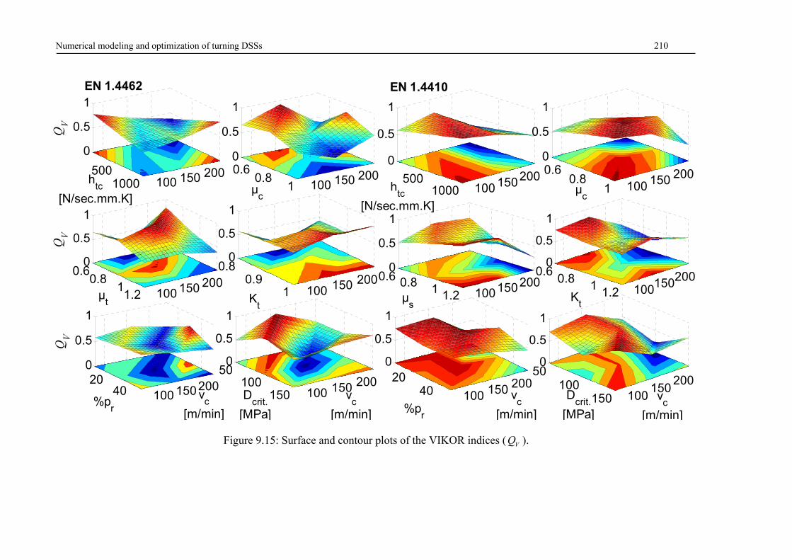
Numerical modeling and optimization of turning DSSs 210
Figure 9.15: Surface and contour plots of the VIKOR indices ( VQ ).
5001000 100 150 200
0
0.5
1
QV
0.60.8
1 100 150 200
0
0.5
1
0.60.8
11.2 100 150 200
0
0.5
1
QV
0.80.9
1 100 150 200
0
0.5
1
2040 100 150200
0
0.5
1
QV
5001000 100 150200
0
0.5
1
0.60.8
1 100 150 200
0
0.5
1
0.6 0.8 1 1.2 1001502000
0.5
1
0.60.8
11.2 100150200
0
0.5
1
2040 100 150 200
0
0.5
1
50100
150 100150
200
0
0.5
1
50100
150 100 150 200
0
0.5
1
µsK
t
%pr
htc
[N/sec.mm.K]
EN 1.4462
htc
[N/sec.mm.K]
Kt
Dcrit.
[MPa]
µt
vc
[m/min]
vc
[m/min]
Dcrit.
[MPa]
vc
[m/min]
vc
[m/min]%p
r
EN 1.4410
µc
µc
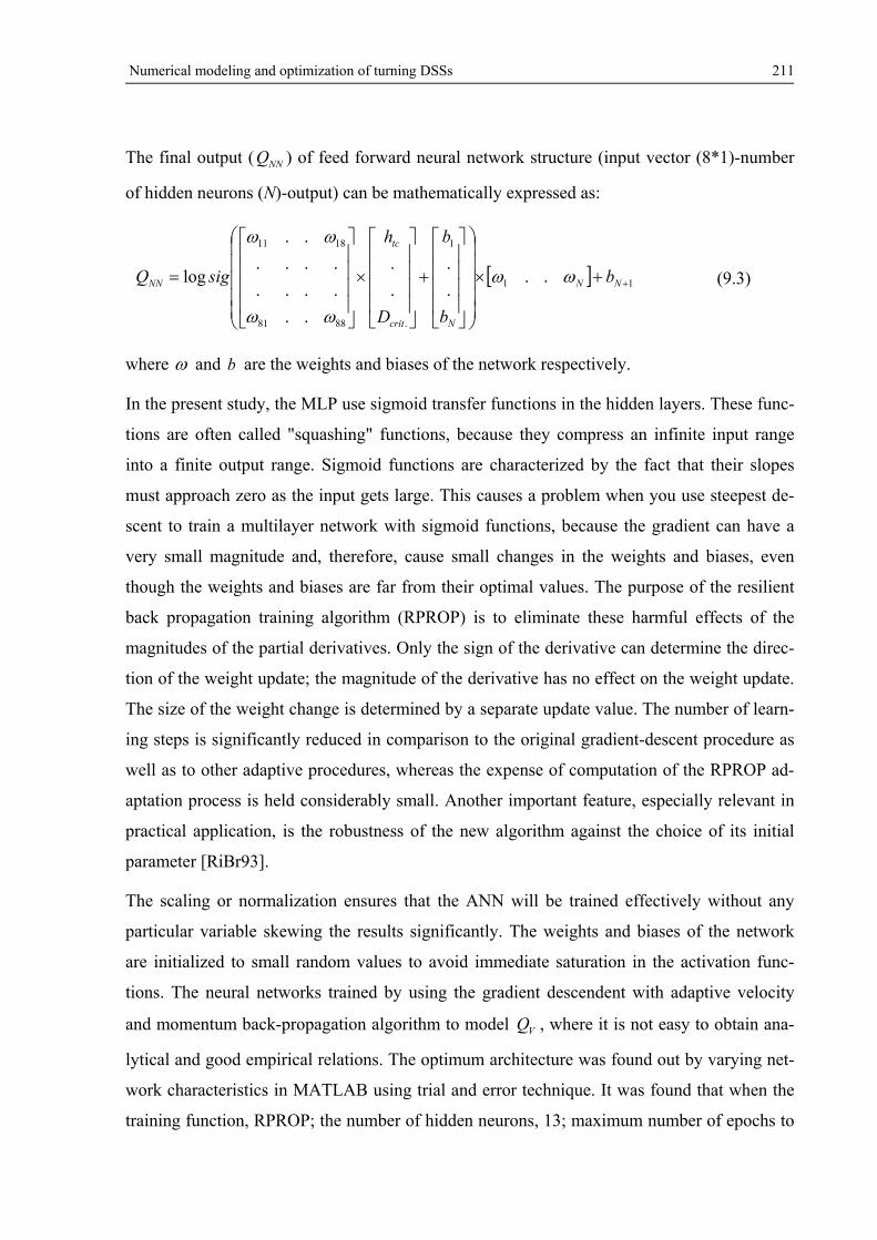
Numerical modeling and optimization of turning DSSs 211
The final output ( NNQ ) of feed forward neural network structure (input vector (8*1)-number
of hidden neurons (N)-output) can be mathematically expressed as:
11
1
.8881
1811
...
.
.
.
..
....
....
..
log
NN
Ncrit
tc
NN b
b
b
D
h
sigQ
(9.3)
where and b are the weights and biases of the network respectively.
In the present study, the MLP use sigmoid transfer functions in the hidden layers. These func-
tions are often called "squashing" functions, because they compress an infinite input range
into a finite output range. Sigmoid functions are characterized by the fact that their slopes
must approach zero as the input gets large. This causes a problem when you use steepest de-
scent to train a multilayer network with sigmoid functions, because the gradient can have a
very small magnitude and, therefore, cause small changes in the weights and biases, even
though the weights and biases are far from their optimal values. The purpose of the resilient
back propagation training algorithm (RPROP) is to eliminate these harmful effects of the
magnitudes of the partial derivatives. Only the sign of the derivative can determine the direc-
tion of the weight update; the magnitude of the derivative has no effect on the weight update.
The size of the weight change is determined by a separate update value. The number of learn-
ing steps is significantly reduced in comparison to the original gradient-descent procedure as
well as to other adaptive procedures, whereas the expense of computation of the RPROP ad-
aptation process is held considerably small. Another important feature, especially relevant in
practical application, is the robustness of the new algorithm against the choice of its initial
parameter [RiBr93].
The scaling or normalization ensures that the ANN will be trained effectively without any
particular variable skewing the results significantly. The weights and biases of the network
are initialized to small random values to avoid immediate saturation in the activation func-
tions. The neural networks trained by using the gradient descendent with adaptive velocity
and momentum back-propagation algorithm to model VQ , where it is not easy to obtain ana-
lytical and good empirical relations. The optimum architecture was found out by varying net-
work characteristics in MATLAB using trial and error technique. It was found that when the
training function, RPROP; the number of hidden neurons, 13; maximum number of epochs to
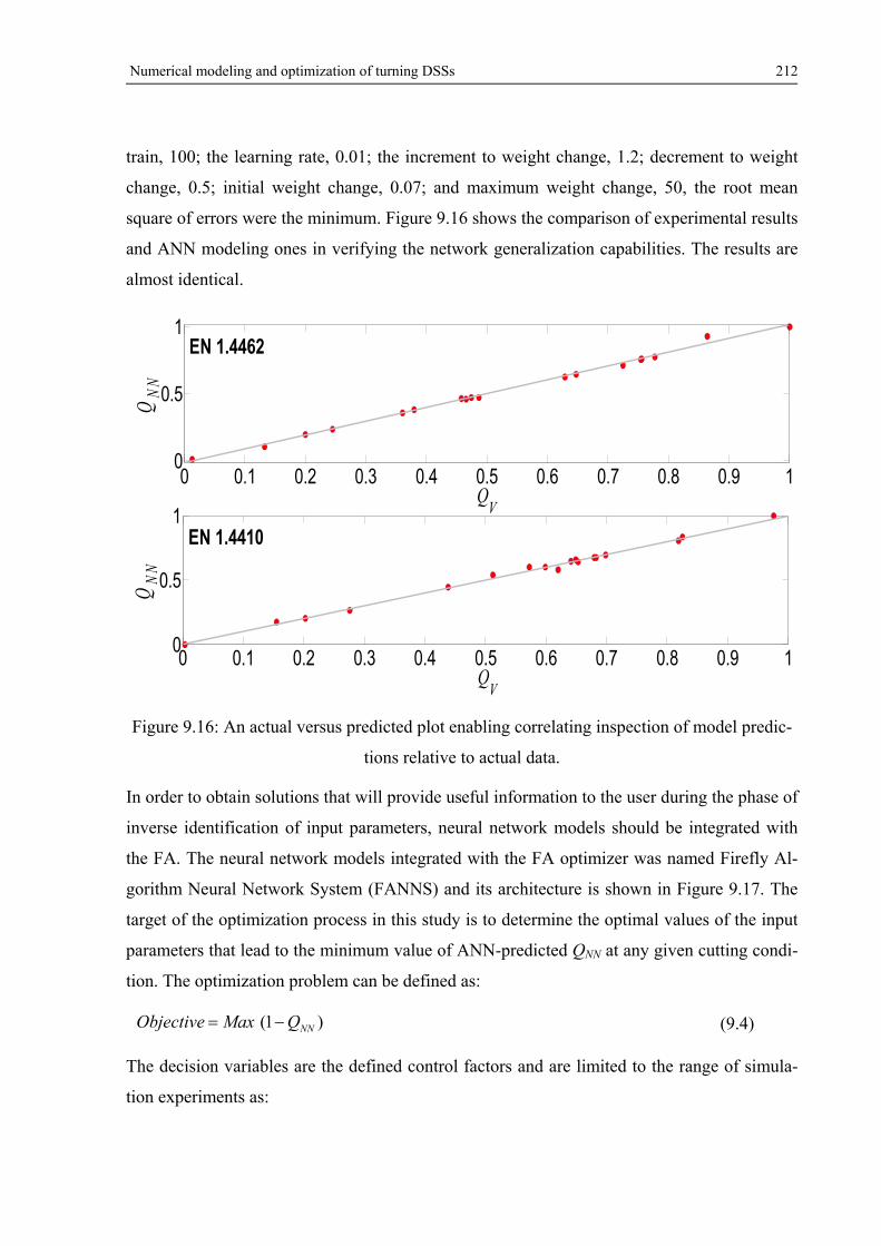
Numerical modeling and optimization of turning DSSs 212
train, 100; the learning rate, 0.01; the increment to weight change, 1.2; decrement to weight
change, 0.5; initial weight change, 0.07; and maximum weight change, 50, the root mean
square of errors were the minimum. Figure 9.16 shows the comparison of experimental results
and ANN modeling ones in verifying the network generalization capabilities. The results are
almost identical.
Figure 9.16: An actual versus predicted plot enabling correlating inspection of model predic-
tions relative to actual data.
In order to obtain solutions that will provide useful information to the user during the phase of
inverse identification of input parameters, neural network models should be integrated with
the FA. The neural network models integrated with the FA optimizer was named Firefly Al-
gorithm Neural Network System (FANNS) and its architecture is shown in Figure 9.17. The
target of the optimization process in this study is to determine the optimal values of the input
parameters that lead to the minimum value of ANN-predicted QNN at any given cutting condi-
tion. The optimization problem can be defined as:
)1( NNQMaxObjective (9.4)
The decision variables are the defined control factors and are limited to the range of simula-
tion experiments as:
0 0.1 0.2 0.3 0.4 0.5 0.6 0.7 0.8 0.9 10
0.5
1
QV
QN
N
0 0.1 0.2 0.3 0.4 0.5 0.6 0.7 0.8 0.9 10
0.5
1
QV
QN
N
EN 1.4462
EN 1.4410
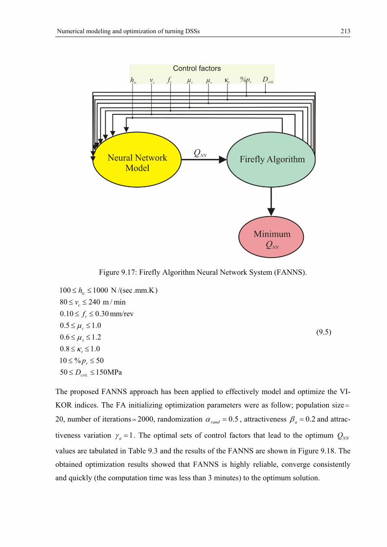
Numerical modeling and optimization of turning DSSs 213
Figure 9.17: Firefly Algorithm Neural Network System (FANNS).
MPa15050
50%10
0.18.0
2.16.0
0.15.0
mm/rev30.010.0
min/m24080
).mm.K/(secN1000100
.
crit
r
t
s
c
r
c
tc
D
p
f
v
h
(9.5)
The proposed FANNS approach has been applied to effectively model and optimize the VI-
KOR indices. The FA initializing optimization parameters were as follow; population size
20, number of iterations 2000, randomization 5.0rand , attractiveness 2.0a and attrac-
tiveness variation 1a . The optimal sets of control factors that lead to the optimum NNQ
values are tabulated in Table 9.3 and the results of the FANNS are shown in Figure 9.18. The
obtained optimization results showed that FANNS is highly reliable, converge consistently
and quickly (the computation time was less than 3 minutes) to the optimum solution.
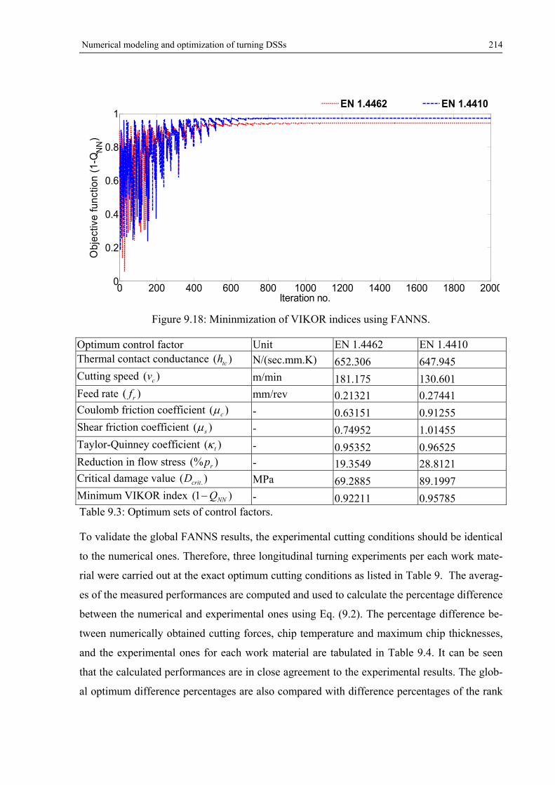
Numerical modeling and optimization of turning DSSs 214
Figure 9.18: Mininmization of VIKOR indices using FANNS.
Optimum control factor Unit EN 1.4462 EN 1.4410 Thermal contact conductance )( tch N/(sec.mm.K) 652.306 647.945 Cutting speed )( cv m/min 181.175 130.601 Feed rate )( rf mm/rev 0.21321 0.27441 Coulomb friction coefficient )( c - 0.63151 0.91255 Shear friction coefficient )( s - 0.74952 1.01455 Taylor-Quinney coefficient )( t - 0.95352 0.96525 Reduction in flow stress )(% rp - 19.3549 28.8121 Critical damage value )( .critD MPa 69.2885 89.1997 Minimum VIKOR index )1( NNQ - 0.92211 0.95785 Table 9.3: Optimum sets of control factors.
To validate the global FANNS results, the experimental cutting conditions should be identical
to the numerical ones. Therefore, three longitudinal turning experiments per each work mate-
rial were carried out at the exact optimum cutting conditions as listed in Table 9. The averag-
es of the measured performances are computed and used to calculate the percentage difference
between the numerical and experimental ones using Eq. (9.2). The percentage difference be-
tween numerically obtained cutting forces, chip temperature and maximum chip thicknesses,
and the experimental ones for each work material are tabulated in Table 9.4. It can be seen
that the calculated performances are in close agreement to the experimental results. The glob-
al optimum difference percentages are also compared with difference percentages of the rank
0 200 400 600 800 1000 1200 1400 1600 1800 20000
0.2
0.4
0.6
0.8
1
Iteration no.
Obj
ectiv
e fu
nctio
n (1
-QN
N)
EN 1.4462 EN 1.4410
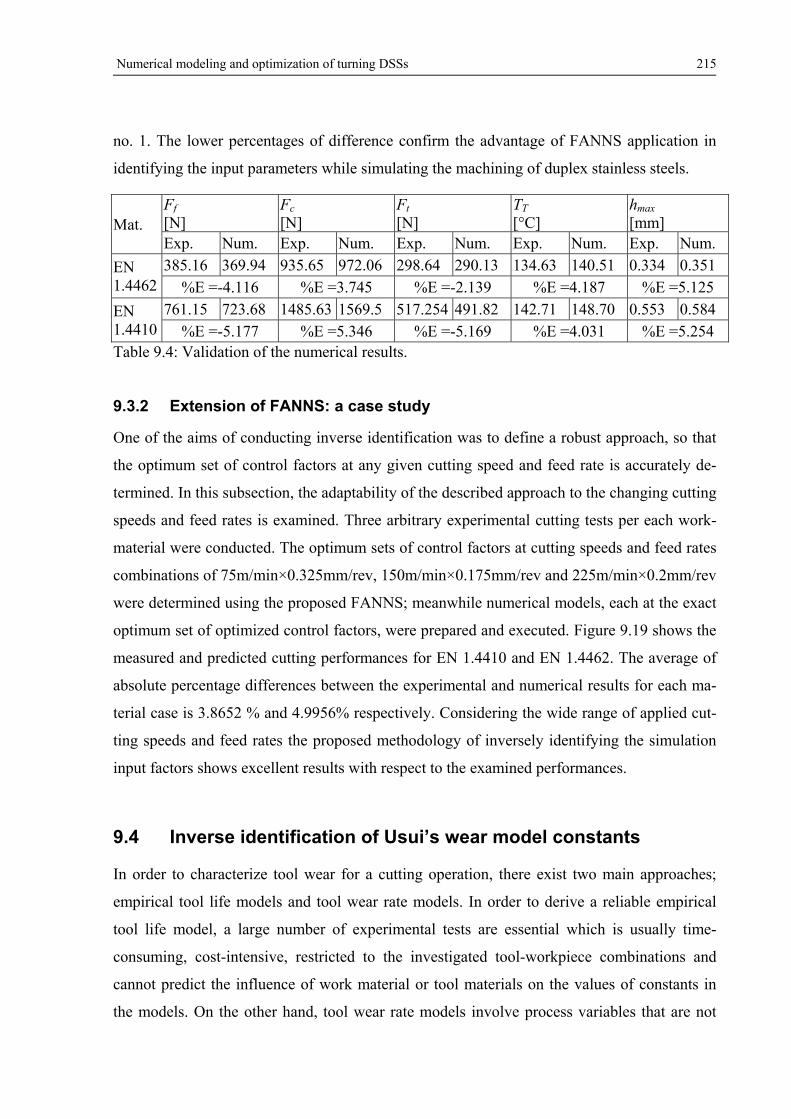
Numerical modeling and optimization of turning DSSs 215
no. 1. The lower percentages of difference confirm the advantage of FANNS application in
identifying the input parameters while simulating the machining of duplex stainless steels.
Mat.
Ff
[N] Fc
[N] Ft
[N] TT
[°C] hmax
[mm] Exp. Num. Exp. Num. Exp. Num. Exp. Num. Exp. Num.
EN 1.4462
385.16 369.94 935.65 972.06 298.64 290.13 134.63 140.51 0.334 0.351 %E =-4.116 %E =3.745 %E =-2.139 %E =4.187 %E =5.125
EN 1.4410
761.15 723.68 1485.63 1569.5 517.254 491.82 142.71 148.70 0.553 0.584 %E =-5.177 %E =5.346 %E =-5.169 %E =4.031 %E =5.254
Table 9.4: Validation of the numerical results.
9.3.2 Extension of FANNS: a case study
One of the aims of conducting inverse identification was to define a robust approach, so that
the optimum set of control factors at any given cutting speed and feed rate is accurately de-
termined. In this subsection, the adaptability of the described approach to the changing cutting
speeds and feed rates is examined. Three arbitrary experimental cutting tests per each work-
material were conducted. The optimum sets of control factors at cutting speeds and feed rates
combinations of 75m/min×0.325mm/rev, 150m/min×0.175mm/rev and 225m/min×0.2mm/rev
were determined using the proposed FANNS; meanwhile numerical models, each at the exact
optimum set of optimized control factors, were prepared and executed. Figure 9.19 shows the
measured and predicted cutting performances for EN 1.4410 and EN 1.4462. The average of
absolute percentage differences between the experimental and numerical results for each ma-
terial case is 3.8652 % and 4.9956% respectively. Considering the wide range of applied cut-
ting speeds and feed rates the proposed methodology of inversely identifying the simulation
input factors shows excellent results with respect to the examined performances.
9.4 Inverse identification of Usui’s wear model constants
In order to characterize tool wear for a cutting operation, there exist two main approaches;
empirical tool life models and tool wear rate models. In order to derive a reliable empirical
tool life model, a large number of experimental tests are essential which is usually time-
consuming, cost-intensive, restricted to the investigated tool-workpiece combinations and
cannot predict the influence of work material or tool materials on the values of constants in
the models. On the other hand, tool wear rate models involve process variables that are not
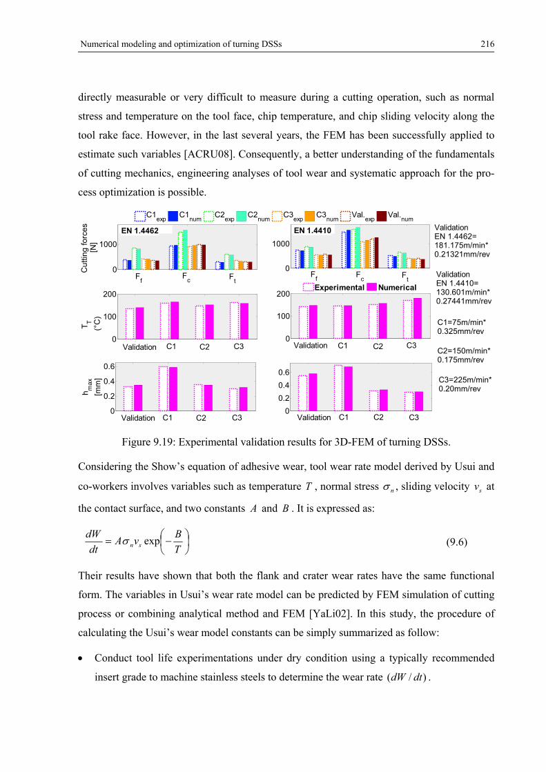
Numerical modeling and optimization of turning DSSs 216
directly measurable or very difficult to measure during a cutting operation, such as normal
stress and temperature on the tool face, chip temperature, and chip sliding velocity along the
tool rake face. However, in the last several years, the FEM has been successfully applied to
estimate such variables [ACRU08]. Consequently, a better understanding of the fundamentals
of cutting mechanics, engineering analyses of tool wear and systematic approach for the pro-
cess optimization is possible.
Figure 9.19: Experimental validation results for 3D-FEM of turning DSSs.
Considering the Show’s equation of adhesive wear, tool wear rate model derived by Usui and
co-workers involves variables such as temperature T , normal stress n , sliding velocity sv at
the contact surface, and two constants A and B . It is expressed as:
T
BvA
dt
dWsn exp (9.6)
Their results have shown that both the flank and crater wear rates have the same functional
form. The variables in Usui’s wear rate model can be predicted by FEM simulation of cutting
process or combining analytical method and FEM [YaLi02]. In this study, the procedure of
calculating the Usui’s wear model constants can be simply summarized as follow:
Conduct tool life experimentations under dry condition using a typically recommended
insert grade to machine stainless steels to determine the wear rate )/( dtdW .
1 2 30
1000
Cu
ttin
g f
orc
es
[N]
1 2 3 40
100
200
TT
(°C
)
1 2 3 40
0.2
0.4
0.6
hm
ax
[mm
]
1 2 30
1000
1 2 3 40
100
200
1 2 3 40
0.2
0.4
0.6
Experimental Numerical
C1exp
C1num
C2exp
C2num
C3exp
C3num
Val.exp
Val.num
ValidationEN 1.4462=181.175m/min*0.21321mm/rev
Validation C1 C2 C3 Validation C2C1 C3
EN 1.4462 EN 1.4410
Ff
Fc F
tF
fF
c Ft
Validation C1 C2 C3 Validation C1 C2 C3C2=150m/min*0.175mm/rev
ValidationEN 1.4410=130.601m/min*0.27441mm/rev
C1=75m/min*0.325mm/rev
C3=225m/min*0.20mm/rev
Numerical modeling and optimization of turning DSSs 217
To estimate the variables in Eq. (9.6), prepare identical to the experimentations, fully cou-
pled thermo-mechanical and FANNS-optimized 3D-FE models, and run the simulations.
Collect the numerically estimated ,T n and sv .
Fit the nonlinear Usui’s model to determine the constants A and B .
Seven arbitrary multi-pass dry turning tests of EN 1.4410 and EN 1.4462 DSS bars were per-
formed on a variable spindle speed CNC lathe using rhombic CNMA 120412-IC20 uncoated
cemented carbide inserts. Thereafter, logarithmic plots of tool wear versus cutting time were
drawn and the slopes )/( dtdW were determined. Meanwhile, the 3D-FE cutting simulations
were carried out based on the proposed procedure. The tool is considered rigid with no wear-
ing possibility. Values of ,T n and sv were directly extracted from simulation results. Matlab
function NonLinearModel.fit was then utilized to fit the model and test its adequacy through
various statistical diagnostic tools. The adjusted correlation factor ( adj.R ) was in very good
agreement with predicted correlation factor ( pred.R ) which supports the prediction power of
the model and were generally above 0.94. The RMSE for EN 1.4462 and EN 1.4410 Usui
wear models were 0.000314 and 0.000469 respectively. The final form of the constants Usui’s
wear models can be constructed as;
Tv
dt
dW
Tv
dt
dW
sn
sn
5203.992exp101704.7
8.1172exp100478.6
9
EN1.4410
9
EN1.4462
(9.7)
9.5 Numerical optimization of turning DSSs
In the second stage of the present study, a hypothetical benchmark-analysis based on the
Taguchi optimization procedure is suggested. The objective is to select the best combination
of criterions such as; chip breakers type )(CB , tool geometry .)(Geo , cooling medium applica-
tion )(CM , cutting conditions such as cv and rf , and tool orientation angles such as normal
rake )( n and inclination angle )( i for an effective machining of EN 1.4462 and EN 1.4410
DSSs. For this purpose, Taguchi’s mixed design L18 (21×37) is once again seen the most ap-
propriate because of its attractive characteristics which combines the highest possible number
of levels along with largest number of criterion and smallest number of experiments. Another
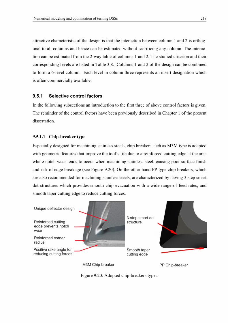
Numerical modeling and optimization of turning DSSs 218
attractive characteristic of the design is that the interaction between column 1 and 2 is orthog-
onal to all columns and hence can be estimated without sacrificing any column. The interac-
tion can be estimated from the 2-way table of columns 1 and 2. The studied criterion and their
corresponding levels are listed in Table 3.8. Columns 1 and 2 of the design can be combined
to form a 6-level column. Each level in column three represents an insert designation which
is often commercially available.
9.5.1 Selective control factors
In the following subsections an introduction to the first three of above control factors is given.
The reminder of the control factors have been previously described in Chapter 1 of the present
dissertation.
9.5.1.1 Chip-breaker type
Especially designed for machining stainless steels, chip breakers such as M3M type is adapted
with geometric features that improve the tool’s life due to a reinforced cutting edge at the area
where notch wear tends to occur when machining stainless steel, causing poor surface finish
and risk of edge breakage (see Figure 9.20). On the other hand PP type chip breakers, which
are also recommended for machining stainless steels, are characterized by having 3 step smart
dot structures which provides smooth chip evacuation with a wide range of feed rates, and
smooth taper cutting edge to reduce cutting forces.
Figure 9.20: Adopted chip-breakers types.
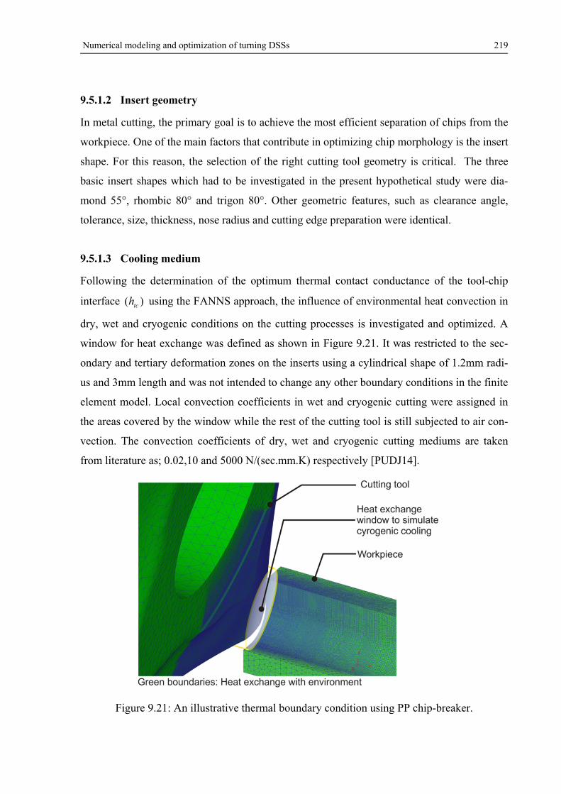
Numerical modeling and optimization of turning DSSs 219
9.5.1.2 Insert geometry
In metal cutting, the primary goal is to achieve the most efficient separation of chips from the
workpiece. One of the main factors that contribute in optimizing chip morphology is the insert
shape. For this reason, the selection of the right cutting tool geometry is critical. The three
basic insert shapes which had to be investigated in the present hypothetical study were dia-
mond 55°, rhombic 80° and trigon 80°. Other geometric features, such as clearance angle,
tolerance, size, thickness, nose radius and cutting edge preparation were identical.
9.5.1.3 Cooling medium
Following the determination of the optimum thermal contact conductance of the tool-chip
interface )( tch using the FANNS approach, the influence of environmental heat convection in
dry, wet and cryogenic conditions on the cutting processes is investigated and optimized. A
window for heat exchange was defined as shown in Figure 9.21. It was restricted to the sec-
ondary and tertiary deformation zones on the inserts using a cylindrical shape of 1.2mm radi-
us and 3mm length and was not intended to change any other boundary conditions in the finite
element model. Local convection coefficients in wet and cryogenic cutting were assigned in
the areas covered by the window while the rest of the cutting tool is still subjected to air con-
vection. The convection coefficients of dry, wet and cryogenic cutting mediums are taken
from literature as; 0.02,10 and 5000 N/(sec.mm.K) respectively [PUDJ14].
Figure 9.21: An illustrative thermal boundary condition using PP chip-breaker.
Numerical modeling and optimization of turning DSSs 220
9.5.2 Results and discussions
Once the turning simulations has been finished, numerous cutting performances such as re-
sultant cutting forces, temperatures,…,etc. have been extracted. The S/N ratio of each perfor-
mance is computed and the main effect plots of the normalized S/N ratios are plotted as
shown in Figure 9.22. The level which returns maximum normalized S/N ratio is assigned as
the optimum level. Further statistical analyses are performed to specify statistically significant
control factors. Figure 9.23 exhibits the percentage of contribution of each control factor on
the variance of the corresponding cutting performance. The following sub-sections, the effects
of control factors on each single cutting performance are briefly described.
9.5.2.1 Influence of control factors on the resultant cutting forces (Rc)
Based on a quick review of the 3D-FEM results, the following conclusion points can be
drawn:
The optimum insert designations which minimize cR during turning EN 1.4462 and EN
1.4410 can be described in ISO norms as: WNMG 060408-PP and CNMG 120408-PP re-
spectively.
In spite of the advantageous aspects of increasing cutting speed, applying coolant and cry-
ogenic conditions in increasing the productivity and reducing the overall cR values, re-
sults has shown a limited influence of these control factors on the mean cR values. This
statement is supported by the slopes of the cR curves in Figure 9.22
Among the considered control factors, feed rate had shown the strongest impact on the
resultant cutting forces (see Figure 9.23).
The optimum values of cutting tool orientation angles expressed by ranges of investigated
rake and inclination angles are -6° and 0° respectively.
9.5.2.2 Influence of control factors on the effective strain
Without relating the hardening parameters in the loading function to the experimental uniaxial
stress-strain curve, the work-hardening theory of plasticity cannot be applied in practical
terms. In order to correlate the test results obtained by different load programs, the introduc-
tion of any strain and stress variables, that are functions of plastic strain and plastic stress, and
Numerical modeling and optimization of turning DSSs 221
can be plotted against each other is considered useful. These variables are often called effec-
tive strain and effective stress.
DSSs are a group of stainless steel alloys that are characterized by high work-hardening rate.
They are machined at very high strain rates which increase the work hardening rate and caus-
ing higher resistance to plastic deformation. Generally, the following observation points can
be made:
The average effective plastic strain when machining EN 1.4462 was 13.2% lower than the
corresponding EN 1.4410.
Employing chip breaker type PP has generally caused lower effective strain values.
Detrimental control factors vary considerably per work material family.
Higher values of effective strains are observed when the cooling medium on the tool is
cryogenic.
Main effects of effective strain decreases with increasing cutting speed.
Mean effective strains are found to be minimum at the feed rate range of 0.1-0.175
mm/rev and inclination angle range of 6°-12°.
Minimum effective strain value when cutting EN 1.4462 and EN 1.4410 at 0n and
12n respectively.
9.5.2.3 Influence of control factors on the effective stress
Effective plastic stress is considered a relevant characteristic of the cutting process which
characterizes the level of resistance to cutting. The correlation between the state of this per-
formance imposed by the cutting tool in the layer being removed and the fracture strain of the
work material could be used to estimate the physical efficiency of the cutting process. In
summary to the results, the following conclusions can be drawn:
The effective stress encountered in cutting EN 1.4410 was 12% higher than EN 1.4462.
The optimum control levelfactor combinations of cutting EN 1.4462 and EN 1.4410 were
2311211 . inrc fvCMGeoCB and 2312221 . inrc fvCMGeoCB respectively.
Increasing the rake angle in negative direction and inclination angle in positive direction
generally increases the effective stress.
The minimum effective plastic stress of 1261.48MPa and 1492.01MPa when cutting EN
1.4462 and EN 1.4410 were respectively recorded at experiment no. 9.
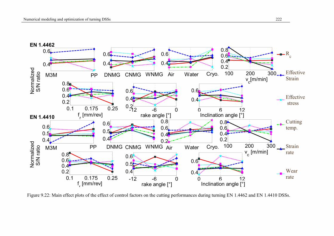
Numerical modeling and optimization of turning DSSs 222
Figure 9.22: Main effect plots of the effect of control factors on the cutting performances during turning EN 1.4462 and EN 1.4410 DSSs.
1 2
0.4
0.6
No
rma
lize
d
S/N
ra
tio
1 2 3
0.4
0.6
1 2 3
0.4
0.6
-12 -6 00.2
0.4
0.6
0 6 12
0.4
0.6
1 20.40.50.6
No
rma
lize
d
S/N
ra
tio
Rc
EffectiveStrain
Effective stress
Cuttingtemp.
Strainrate
Wearrate
1 2 3
0.4
0.5
0.6
1 2 30.20.40.60.8
-12 -6 0
0.4
0.5
0.6
0 6 120.4
0.6
100 200 3000.20.40.60.8
0.1 0.175 0.250.20.40.60.8
100 200 3000.20.40.60.8
0.1 0.175 0.250.20.40.60.8
PP
Inclination angle [°]
Cryo.WaterAir
Cryo.WaterAirWNMGCNMG
WNMGCNMGDNMG
DNMG
fr [mm/rev]
PPM3M
M3M
fr [mm/rev] rake angle [°] Inclination angle [°]
vc[m/min]
EN 1.4462
rake angle [°]
vc [m/min]
EN 1.4410
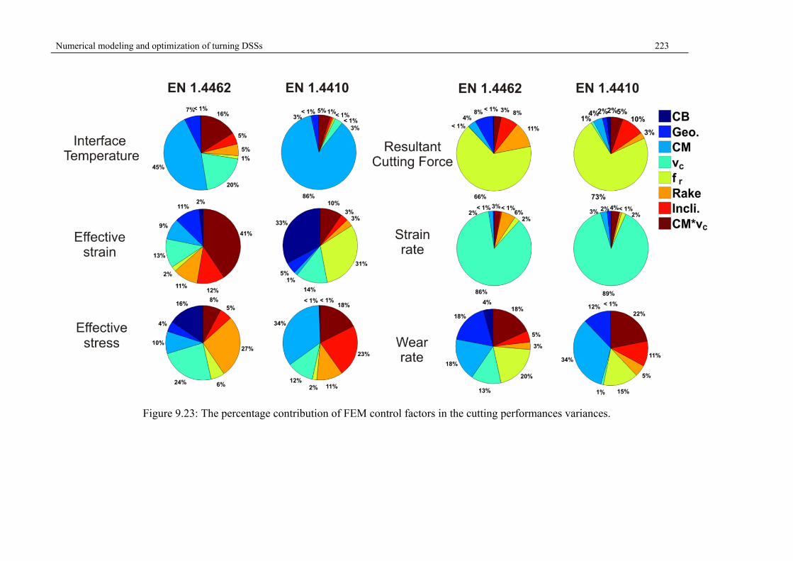
Numerical modeling and optimization of turning DSSs 223
Figure 9.23: The percentage contribution of FEM control factors in the cutting performances variances.
Numerical modeling and optimization of turning DSSs 224
When cutting EN 1.4462, process conditions such as CMfv rc ,, and CMvc interaction
has contributed to the effective stress values by 48%. On the other hand, when cutting EN
1.4410, they had contributed by as much as 66%.
9.5.2.4 Influence of control factors on the cutting temperature
Mean contact temperature at the tool–chip interface (also is referred to as the cutting tempera-
ture) is the basic tribological characteristics of the tool–chip interface. It plays a major role in
the formation of crater on the tool face and leads to failure of tool by softening and thermal
stresses. This temperature is the most suitable parameter to correlate the tribological condi-
tions with tool wear. Control factors that affect the tool-chip interface temperature are; work-
piece and tool material, tool geometry, cutting conditions and cutting medium. Fortunately,
most of these factors are included in the original design of simulation experimentations. Fig-
ure 9.24 depicts the state of cutting temperature distribution in the primary and secondary
deformation zones of the workpiece. The results of the numerical studies on temperatures in
cutting DSSs can be summarized as follows:
Mean cutting temperatures at dry cutting when machining EN 1.4462 and EN 1.4410 were
36.3% and 53.5% higher than at corresponding cryogenic process conditions.
The contribution of water-based coolant in lowering the average cutting temperature has
not exceeded 7.8% in both material cases.
Minimum mean cutting temperature when cutting EN 1.4462 and EN 1.4410 has been
recorded at experimental run 16 and 15 respectively.
Cooling medium, cutting condition and their interaction accounts for most of contribu-
tions in cutting temperature variations.
The optimum control factorlevel combinations of cutting EN 1.4462 and EN 1.4410 were
1231332 . inrc fvCMGeoCB and 2321321 . inrc fvCMGeoCB respectively.
The average cutting temperature when machining EN 1.4462 was 9.85% lower than the
corresponding EN 1.4410.
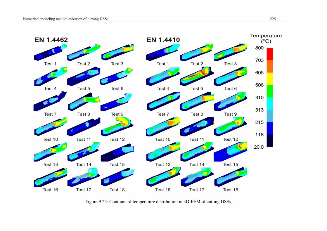
Numerical modeling and optimization of turning DSSs 225
Figure 9.24: Contours of temperature distribution in 3D-FEM of cutting DSSs.
Numerical modeling and optimization of turning DSSs 226
9.5.2.5 Influence of control factors on the strain rate
The flow stress curves shown in Figure 2.11 exhibit sensitivity to temperature and strain rate.
This sensitivity is directly related with time and temperature dependency of the mechanisms
that govern the deformation and the evolution of the deformation in the material. The main
mechanism by which plastic strain takes place is thermally activated motion of dislocations
past obstacles that exist within the lattice over a wide range of strain rates and cutting temper-
atures. The material response is significantly affected by the nature and density of the obsta-
cles (which may change as the deformation takes place). When dealing with metals, experi-
mental results show that the stress required for plastic strain often reduces with the increase of
temperature and with the decrease of plastic strain rate [GiWu97]. It can then be said that
temperature and plastic strain rate greatly influence the material response. In general, the
stress decreases with the increasing of temperature and decreasing the plastic strain rate. Ac-
tually, temperature and strain rate effects are coupled, since one influences the other. Temper-
ature affects the rate of deformation, which is controlled mainly by a thermally activated
mechanism. On the other hand, plastic strain at high rate generates significant heating and
cause an increase in temperature which leads to mechanical instability and the localization of
deformation into narrow sheets of material (the adiabatic shear bands), which act as precursor
for eventual material failure [DaMa09]. As generalization to the given results in Figure 9.22
and Figure 9.23, the following concluding points can be depicted:
Average strain rate values under cutting EN 1.4462 and EN 1.4410 are of 2.067×10⁵ sec-1
and 3.23×10⁵ 1/sec respectively.
Increasing cutting speeds from 100m/min to 300m/min at lower feed rates of 0.1mm/rev
had drastically increased the strain rate values.
Mean strain rate values in cryogenic cutting conditions during cutting EN 1.4462 and EN
1.4410 were respectively 9.158% and 11.863% lower than the corresponding still air con-
ditions.
3321332 . inrc fvCMGeoCB and 3321322 . inrc fvCMGeoCB were the optimum control
levelfactor combinations which have minimized the strain rate when cutting EN 1.4462 and
EN 1.4410, respectively.
Numerical modeling and optimization of turning DSSs 227
9.5.2.6 Influence of control factors on the tool wear
Eq. (9.7) has been used in conjunction with finite element simulation to model wear of WC
cutting tools. The simulation results related to the tool wear were obtained in terms of tool
wear rate, total wear depth and tool temperature. Average values of tool wear rates are statis-
tically analyzed and plotted as shown in Figure 9.22 and Figure 9.23. Figure 9.25 maps the
contours of wear depth in the nose area of the employed cutting tools after 7mm longitudinal
cutting. As it can be observed that the locations and intensity of tool wear depths are functions
of work materials and control factors. Considering the effect of these factors, the summary of
the findings are presented below.
The optimum control levelfactor combinations which have minimized the tool wear rate
during cutting EN 1.4462 and EN 1.4410 were 2311312 . inrc fvCMGeoCB and
2121312 . inrc fvCMGeoCB respectively.
For both workmaterials, major percentage of contributions of 69% and 72% in variance of
tool wear rate were attributed to the process and cutting conditions and their subsequent
interactions.
The average tool wear rate when machining EN 1.4462 was 5.365% lower than the corre-
sponding EN 1.4410.
Contour profiles of tool wear depth shown in Figure 9.25 coincide with temperature dis-
tribution at rake and flank faces of the cutting tools in Figure 9.26. Maximum wear depths
are occurred in positions at rake and flank surfaces where the tool temperature is the high-
est.
9.5.3 Numerical machining performance measure
The previous analyses of machining performances have showed different control levelfactor
preferences. This will cause confusions to the process designer or the machinist who interest-
ed in finding the best compromise combination of control factors which simultaneously opti-
mize the machining of DSSs. Therefore, a new machining performance measure has to be
defined. In this section of the work, fuzzy logic system is employed to combine the normal-
ized performances, such as the resultant cutting force, effective stress, cutting temperature and
tool wear rate into a single characteristics index called numerical machining performance
measure (NMPM).
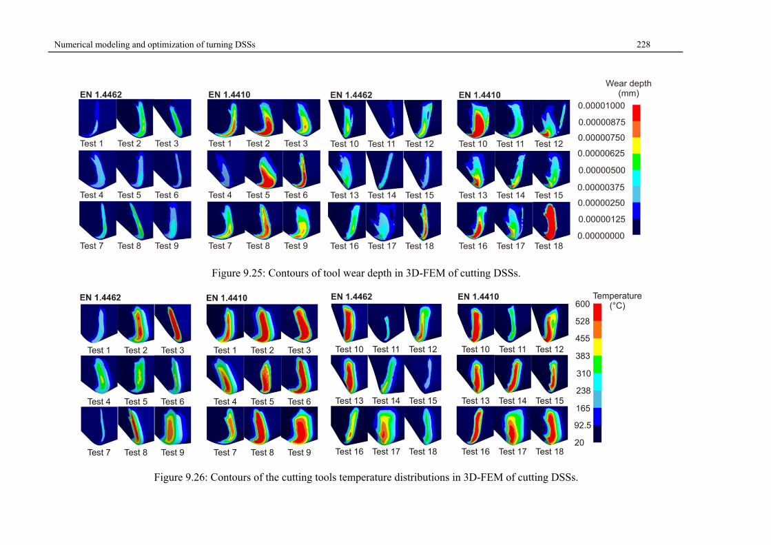
Numerical modeling and optimization of turning DSSs 228
Figure 9.25: Contours of tool wear depth in 3D-FEM of cutting DSSs.
Figure 9.26: Contours of the cutting tools temperature distributions in 3D-FEM of cutting DSSs.
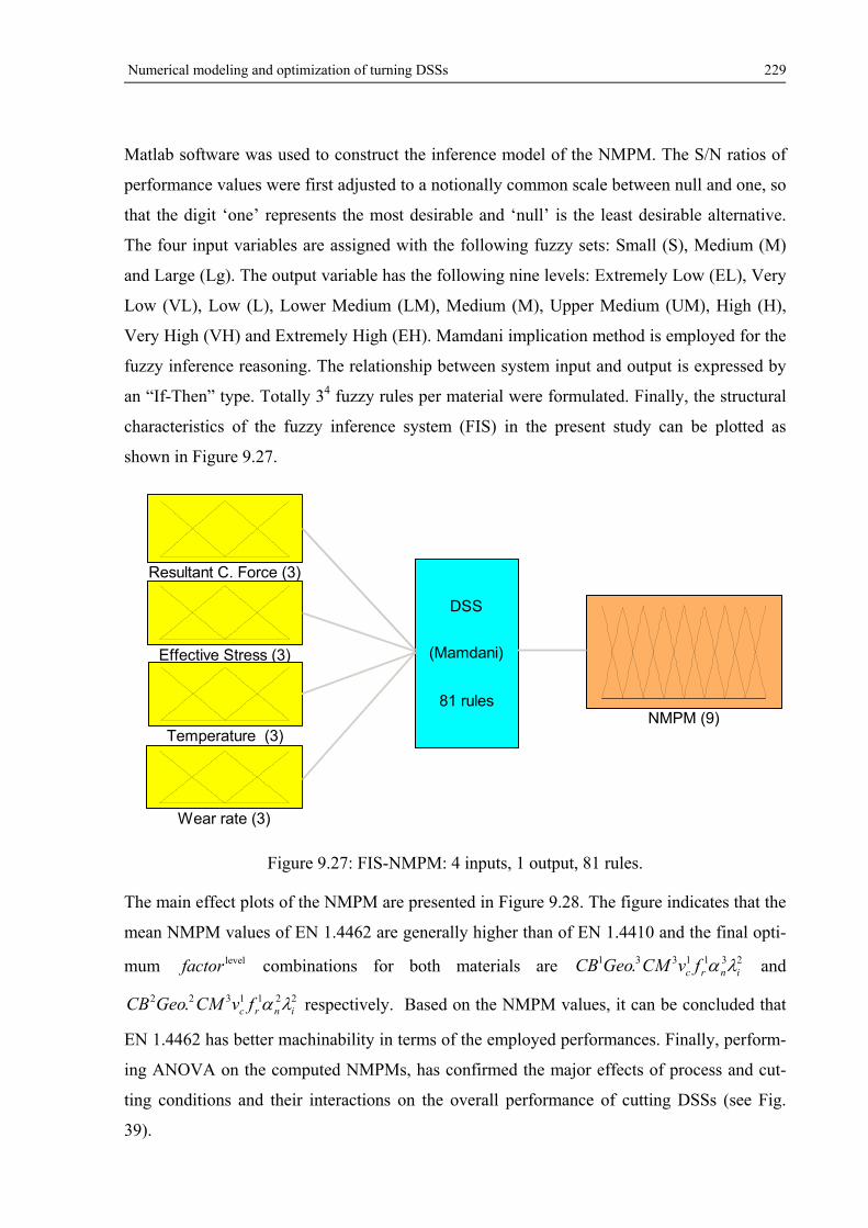
Numerical modeling and optimization of turning DSSs 229
Matlab software was used to construct the inference model of the NMPM. The S/N ratios of
performance values were first adjusted to a notionally common scale between null and one, so
that the digit ‘one’ represents the most desirable and ‘null’ is the least desirable alternative.
The four input variables are assigned with the following fuzzy sets: Small (S), Medium (M)
and Large (Lg). The output variable has the following nine levels: Extremely Low (EL), Very
Low (VL), Low (L), Lower Medium (LM), Medium (M), Upper Medium (UM), High (H),
Very High (VH) and Extremely High (EH). Mamdani implication method is employed for the
fuzzy inference reasoning. The relationship between system input and output is expressed by
an “If-Then” type. Totally 34 fuzzy rules per material were formulated. Finally, the structural
characteristics of the fuzzy inference system (FIS) in the present study can be plotted as
shown in Figure 9.27.
Figure 9.27: FIS-NMPM: 4 inputs, 1 output, 81 rules.
The main effect plots of the NMPM are presented in Figure 9.28. The figure indicates that the
mean NMPM values of EN 1.4462 are generally higher than of EN 1.4410 and the final opti-
mum levelfactor combinations for both materials are 2311331 . inrc fvCMGeoCB and
2211322 . inrc fvCMGeoCB respectively. Based on the NMPM values, it can be concluded that
EN 1.4462 has better machinability in terms of the employed performances. Finally, perform-
ing ANOVA on the computed NMPMs, has confirmed the major effects of process and cut-
ting conditions and their interactions on the overall performance of cutting DSSs (see Fig.
39).
Resultant C. Force (3)
Effective Stress (3)
Temperature (3)
Wear rate (3)
NMPM (9)
DSS
(Mamdani)
81 rules
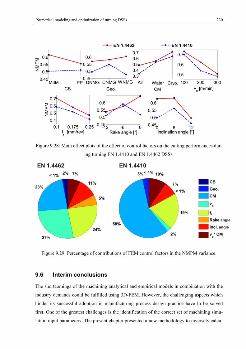
Numerical modeling and optimization of turning DSSs 230
Figure 9.28: Main effect plots of the effect of control factors on the cutting performances dur-
ing turning EN 1.4410 and EN 1.4462 DSSs.
Figure 9.29: Percentage of contributions of FEM control factors in the NMPM variance.
9.6 Interim conclusions
The shortcomings of the machining analytical and empirical models in combination with the
industry demands could be fulfilled using 3D-FEM. However, the challenging aspects which
hinder its successful adoption in manufacturing process design practice have to be solved
first. One of the greatest challenges is the identification of the correct set of machining simu-
lation input parameters. The present chapter presented a new methodology to inversely calcu-
1 20.45
0.5
0.55
0.6
NM
PM
1 2 30.45
0.5
0.55
0.6
1 2 30.30.40.50.60.7
100 200 300
0.5
0.6
0.7
0.1 0.175 0.25
0.4
0.5
0.6
0.7
NM
PM
-12 -6 00.45
0.5
0.55
0.6
0 6 120.45
0.5
0.55
0.6
EN 1.4462 EN 1.4410
Cryo.WaterAir
Geo.
CNMG WNMGM3M DNMGPP
fr [mm/rev] Rake angle [°] Inclination angle [°]
CB CM vc [m/min]
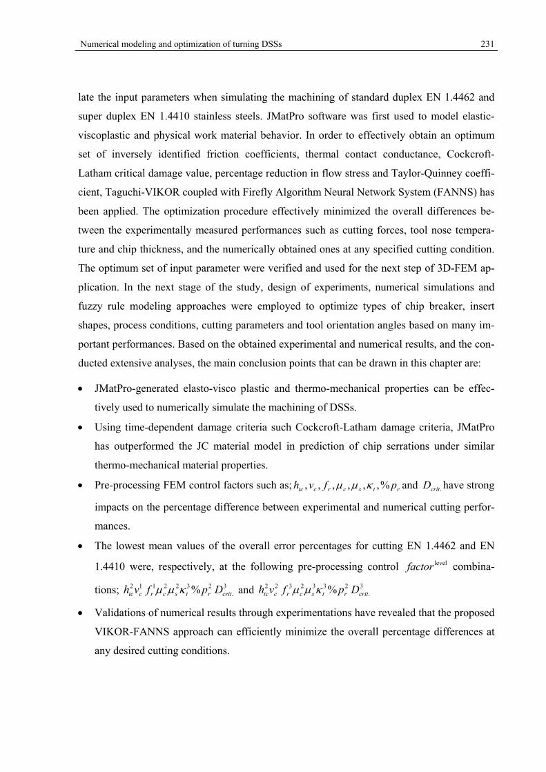
Numerical modeling and optimization of turning DSSs 231
late the input parameters when simulating the machining of standard duplex EN 1.4462 and
super duplex EN 1.4410 stainless steels. JMatPro software was first used to model elastic-
viscoplastic and physical work material behavior. In order to effectively obtain an optimum
set of inversely identified friction coefficients, thermal contact conductance, Cockcroft-
Latham critical damage value, percentage reduction in flow stress and Taylor-Quinney coeffi-
cient, Taguchi-VIKOR coupled with Firefly Algorithm Neural Network System (FANNS) has
been applied. The optimization procedure effectively minimized the overall differences be-
tween the experimentally measured performances such as cutting forces, tool nose tempera-
ture and chip thickness, and the numerically obtained ones at any specified cutting condition.
The optimum set of input parameter were verified and used for the next step of 3D-FEM ap-
plication. In the next stage of the study, design of experiments, numerical simulations and
fuzzy rule modeling approaches were employed to optimize types of chip breaker, insert
shapes, process conditions, cutting parameters and tool orientation angles based on many im-
portant performances. Based on the obtained experimental and numerical results, and the con-
ducted extensive analyses, the main conclusion points that can be drawn in this chapter are:
JMatPro-generated elasto-visco plastic and thermo-mechanical properties can be effec-
tively used to numerically simulate the machining of DSSs.
Using time-dependent damage criteria such Cockcroft-Latham damage criteria, JMatPro
has outperformed the JC material model in prediction of chip serrations under similar
thermo-mechanical material properties.
Pre-processing FEM control factors such as; rtscrctc pfvh %,,,,,, and .critD have strong
impacts on the percentage difference between experimental and numerical cutting perfor-
mances.
The lowest mean values of the overall error percentages for cutting EN 1.4462 and EN
1.4410 were, respectively, at the following pre-processing control levelfactor combina-
tions; 3.
2322112 % critrtscrctc Dpfvh and 3.
2332322 % critrtscrctc Dpfvh
Validations of numerical results through experimentations have revealed that the proposed
VIKOR-FANNS approach can efficiently minimize the overall percentage differences at
any desired cutting conditions.

Numerical modeling and optimization of turning DSSs 232
Hypothetical benchmark-analysis based on the Taguchi optimization procedure can be
numerically employed to select the best combination of criterions such as;CB , .Geo , ,CM
cv , rf , n and i per cutting performance.
Performing ANOM of the derived NMPM values has indicated that the final optimum
levelfactor combinations during cutting EN 1.4462 and EN 1.4410 are 331 . CMGeoCB
2311inrc fv and 2211322 . inrc fvCMGeoCB respectively.
Conclusions 233
10 Conclusions
Recognizing the complexity of machinability investigations, the limitations of metal cutting
theory and analytical modeling, the difficulties of modeling and optimization of machining
process parameters and the necessity of extra knowledge to be gained from machining of duc-
tile and strain hardening materials, the present dissertation has systematically investigated
machining of DSSs through systematic application of advanced modeling and optimization
techniques in turning processes. The ultimate goal of this dissertation was to provide the pro-
cess planner and/ or the decision maker the selection capability of obtaining the optimum pro-
cess parameters under the consideration of multiple and often conflicting performances. The
application of input-output parameter relationship modeling and optimization tools and finite
element simulations has been broadly demonstrated. MADM methods, often coupled with
fuzzy set theory, are also proposed to perform multi-objective optimization and obtain differ-
ent cutting performance measures. Hybridization of computational modeling and optimization
techniques was another tool that has been effectively applied to the machining optimization
problem. In conjunction with the research questions that motivated the present dissertation,
the following concluding remarks can be drawn:
Research question 1:
Can the application of statistical regression and computational optimization techniques effec-
tively obtain sets of non-dominated solutions in multi-objective optimization of machining
DSSs?
In answer to the first research question, an experimental investigation on cutting of EN 1.4462
and EN 1.4410 DSSs is conducted. Statistical regression modeling techniques are adopted to
model the performance characteristics and ANOVA tests were performed to check the models
adequacies. Multi-objective optimization of machining DSSs based on the nature-inspired
MOBA is performed to simultaneously minimize resultant cutting force and the maximum
width of flank wear. Results of optimization have shown that MOBA is very efficient and
highly reliable. It has provided Pareto frontiers of non-dominated solution sets for optimum
cutting conditions, enabling decision makers and/or process planner with a resourceful and
efficient means of achieving the optimum cutting conditions. Therefore, statistical regression
Conclusions 234
and meta-heuristics can be effectively applied to the multi-objective optimization of cutting
processes.
Research question 2:
Is the application of fuzzy set theory advantageous in eliminating the discrepancy of ranking
system among the MADM methods and obtain better results than other optimization ap-
proaches?
In response to the second research question, a comparative machining study of austenitic EN
1.4404, and EN 1.4462 and EN 1.4410 is primarily performed. Considering, chip volume ra-
tio, resultant cutting forces, specific cutting pressures and net spindle powers potential per-
formance characteristics, TOPSIS, VIKOR, GRA and UA were simultaneously applied to
optimize the cutting of the stainless steels. Owing to the existing discrepancy among the
above MADM methods, fuzzy rule modeling approach was proposed to derive a single char-
acterization index called UCI. In comparison to the outcomes of other optimization approach-
es, a remarkable improvement in reduction of cutting power consumption, specific cutting
pressure and resultant cutting forces has been reported when direct ranking system of predict-
ed UCI indices are set as optimum. Hence, fuzzy set theory has not only proved to be advan-
tageous in eliminating the discrepancy of ranking system among the MADM methods but also
obtained better results than other optimization approaches.
Research question 3:
Can Taguchi-MADM-meta-heuristics concept be conveniently used for mono and multi-
objective optimization of cutting stainless steels?
To answer the third research question, multi-performance optimization of turning of EN
1.4404, EN 1.4462 and EN 1.4410 has been first experimentally addressed. Utilizing
Taguchi-VIKOR-Meta-heuristic as multi-performance optimization concept, performance
characteristics such as; surface roughness, specific cutting energy, cutting power and resultant
cutting forces are simultaneously and constrainedly optimized. Optimization performance of
FA, APSO and CS algorithms are compared, and the exact settings of optimum cutting pa-
rameters are determined. The obtained optimization results showed that the algorithms are
highly reliable and converge consistently to the optimum solution. However, when it comes to
comparisons based on the iteration numbers required for convergence and computation re-
sults, APSO outperformed the FA and CS was seen far more efficient than both. Thus, the
Conclusions 235
proposed Taguchi-VIKOR-Meta-heuristic concept has enabled the decision maker and/or pro-
cess planner with tools suitable for mono objective optimization using Taguchi optimization
procedure, multi-objective optimization using VIKOR method and constrained optimization
using the most efficient meta-heuristic algorithm.
Research question 4:
Can multiple machining surface quality characteristics be efficiently optimized when MADM
methods are coupled with fuzzy set theory?
In order to answer the fourth research question, multiple surface quality characteristics of
stainless steel grades such as; EN 1.4404, EN 1.4462 and EN 1.4410 have been systematically
investigated under a constant cutting speed facing operation. MADM methods such as GTMA
and AHP-TOPSIS are simultaneously adopted to combine well-known surface quality charac-
teristics such as Ra , Rz and Rt into a single index called MSQCI. The differences in rank-
ings between derived indices are solved through converting each crisp values into trapezoidal
fuzzy number and unifying them using fuzzy simple additive weight method. The optimum
levelfactor combinations have been defined and onContributi% of the control factors are de-
termined. Confirmation test results have shown that the average percentage improvement in
surface quality during facing EN 1.4404, EN 1.4462 and EN 1.4410 were: 26.302%, 10.62%
and 12.679%, respectively. Thus, multiple machining surface quality performances could be
efficiently optimized when MADM methods are coupled with fuzzy set theory.
Research question 5:
Would it be possible for multi-pass cutting operations to be sustainably optimized when the
hybridization of input-output modeling and optimization tools and MADM methods is system-
atically performed?
In answer to the fifth research question, a systematic approach which employed different
modeling and optimization tools under a three phase investigation scheme has been conducted
to sustainably optimize the multi-pass constant cutting speed facing of DSSs. In the first
phase of the investigation, D-optimal experimental design is used extensively to investigate
the effect of process variables on performance characteristics such as percentage increase in
thrust cutting force, effective cutting power, maximum tool flank wear and chip volume ratio.
The models were then analyzed using 3D surface graphs and used to study the interaction
effects of process parameters. At the end of the first phase, constrained Cuckoo Search algo-
Conclusions 236
rithm is selected to perform optimization of the performance characteristics thereby defining
the optimum process conditions. In the second phase, the optimization conflict between ma-
chining economics attributes, such as simultaneous minimization of machine utilization time,
main time-related costs and the tool related costs effectively solved employing TOPSIS. In
the third phase of the study, the computed performances in the first and second phases were
utilized to derive a new index of measuring machining sustainability called operational sus-
tainability index (OSI). To accurately model and constrainedly optimize the highly nonlinear
OSIs, CSNNS has been developed. The numerous conclusive results obtained in this exten-
sive investigation has proved the potential of hybridization of input-output modeling and op-
timization tools and MADM methods when they systematically applied to the multi-pass cut-
ting operations.
Research question 6:
Is it possible to apply JMatPro, DOE, MADM, computational modeling and meta-heuristic
approach in inverse identification of the input parameters during finite element simulation of
cutting processes? If it is possible, can a hypothetical numerical optimization study be per-
formed as a case study?
In response to the last research question, a novel approach of inverse identification of input
parameters in 3D-FEM of turning DSSs has been proposed. Adopting JMatPro software for
generating of temperature dependent physical and elastic-viscoplastic properties of DSSs, the
optimum 3D-FEM control levelfactor combination of rtscrctc pfvh ,%,,,,, and .critD has been
effectively defined under Taguchi-VIKOR-FANNS approach. Validations of the numerical
results experimentally have proved the versatility of the approach accurately. The approach is
then employed to define the optimum set of control factors for the rest of the planned investi-
gations. In the next stage, a hypothetical 3D-FEM machining optimization study is then con-
ducted and the optimum set of criterions such as; ,CB .,Geo ,CM ,cv ,rf n and i per each
cutting performance is defined using Taguchi optimization procedure. Finally, an expert sys-
tem based on fuzzy rule modeling approach is adopted to simultaneously optimize resultant
cutting forces, effective plastic stresses, chip-tool interface cutting temperatures and tool wear
rate through deriving NMPMs and performing ANOM. Hence, the adopted hypothetical study
can also act as a framework for investigating; ever widening spectrum of cutting tool and
workpiece materials, new tool designs, including indexable inserts with complex chip forming

Conclusions 237
geometry, coatings cause new phenomena, new machining methods such as circular milling,
and high speed machining.
References 238
11 References
[ACRU08] ATTANASIO, A. ; CERETTI, E. ; RIZZUTI, S. ; UMBRELLO, D. ; MICARI, F.: 3D Finite Element Analysis of Tool Wear in Machining. In: CIRP Annals - Manufacturing Technology Bd. 57 (2008), S. 61–64 — ISBN 0007-8506
[AhHo12] AHMADI, E. ; HOMAMI, R. M.: Experimental Investigation and Mathematical Modeling of Composite Ceramic Cutting Tools with Alumina Base in the Machining Process of PH- Hardened Austenitic-Ferritic ( Duplex ) Stainless Steel. In: Int J Advanced Design and Manufacturing Technology Bd. 5 (2012), Nr. 2
[AkAs11] AKKUŞ, H. ; ASILTURK, I.: Predicting Surface Roughness of AISI 4140 Steel in Hard Turning Process through Artificial Neural Network, Fuzzy Logic and Regression Models. In: Scientific Research and Essays Bd. 6 (2011), S. 2729–2736
[AlBe12] ALTINTAS, Y. ; BER, A. A.: Manufacturing Automation: Metal Cutting Mechanics, Machine Tool Vibrations, and CNC Design. Bd. 54. New York, USA, 2012 — ISBN 9780521172479
[AnBM09] ANDERSON-COOK, C. M. ; BORROR, C. M. ; MONTGOMERY, D. C.: Response Surface Design Evaluation and Comparison. In: Journal of Statistical Planning and Inference Bd. 139 (2009), S. 629–641 — ISBN 0378-3758
[AnKa96] ANTONY, J. ; KAYE, M.: Optimisation of Core Tube Life using Taguchi Experimental Design Methodology. In: Quality World Bd. 3 (1996), S. 42–50 — ISBN 1352-8769
[AnPr02] ANTONY, J. ; PREECE, D.: Understanding, Managing, and Implementing Quality: Frameworks, Techniques, and Cases. London, UK : Routledge, 2002 — ISBN 0-415-22271-0
[AÖUD13] ARRAZOLA, P. J. ; ÖZEL, T. ; UMBRELLO, D. ; DAVIES, M. ; JAWAHIR, I. S.: Recent Advances in Modelling of Metal Machining Processes. In: CIRP Annals - Manufacturing Technology Bd. 62 (2013), S. 695–718 — ISBN 0007-8506
[ArDe09] ARMAS, I. A. ; DEGALAIX, S. M.: Duplex Stainless Steels. London, UK : ISTE Ltd., 2009 — ISBN 9781848211377
[ArHe00] ARMAREGO, E. J. A. ; HERATH, A. B.: Predictive Models for Machining with Multi-Edge Form Tools Based on a Generalised Cutting Approach. In: CIRP Annals - Manufacturing Technology Bd. 49 (2000), S. 25–30
[Arma00] ARMAREGO, E. J. A.: The Unified-Generalized Mechanics of Cutting Approach-A Step Towards a House of Predictive Performance Models for Machining Operations. In: Machining Science and Technology Bd. 4 (2000), S. 319–362
References 239
[ArÖz09] ARRAZOLA, P. J. ; ÖZEL, T.: Finite Element Modeling of Machining Processes. In: ÖZEL, T. ; DAVIM, J. P. (Hrsg.): Intelligent Machining Modeling and Optimization of the Machining Processes and Systems. London, UK : ISTE Ltd. & John Wiley & Sons, Inc., 2009 — ISBN 9781848211292, S. 125–163
[ArÖz10] ARRAZOLA, P. J. ; ÖZEL, T.: Investigations on the Effects of Friction Modeling in Finite Element Simulation of Machining. In: International Journal of Mechanical Sciences Bd. 52 (2010), S. 31–42 — ISBN 0020-7403
[ArUD08] ARRAZOLA, P. J. ; UGARTE, D. ; DOMÍNGUEZ, X.: A New Approach for the Friction Identification during Machining through the Use of Finite Element Modeling. In: International Journal of Machine Tools and Manufacture Bd. 48 (2008), S. 173–183
[AsCB07] ASLAN, E. ; CAMUŞCU, N. ; BIRGÖREN, B.: Design Optimization of Cutting Parameters when Turning Hardened AISI 4140 Steel (63 HRC) with Al2O3 + TiCN Mixed Ceramic tool. In: Materials and Design Bd. 28 (2007), S. 1618–1622
[AsÇu11] ASILTÜRK, İ. ; ÇUNKAŞ, M.: Modeling and Prediction of Surface Roughness in Turning Operations using Artificial Neural Network and Multiple Regression Method. In: Expert Systems with Applications Bd. 38 (2011), S. 5826–5832 — ISBN 0957-4174
[ASKS08] AGGARWAL, A. ; SINGH, H. ; KUMAR, P. ; SINGH, M.: Optimizing Power Consumption for CNC Turned Parts using Response Surface Methodology and Taguchi’s Technique-A Comparative Analysis. In: Journal of Materials Processing Technology Bd. 200 (2008), S. 373–384
[AsOu08] ASTAKHOV, V. P. ; OUTEIRO, J. C.: Metal Cutting Mechanics, Finite Element Modelling. In: DAVIM, J. P. (Hrsg.): Machining: Fundamentals and recent advances. London, UK, 2008 — ISBN 9781848002128, S. 1–25
[Asta05] ASTAKHOV, V. P.: On the Inadequacy of the Single-Shear Plane Model of Chip Formation. In: International Journal of Mechanical Sciences Bd. 47 (2005), S. 1649–1672 — ISBN 0020-7403
[Asta06] ASTAKHOV, V. P.: Tribology of Metal Cutting. Bd. 52. Oxford, UK : Elsevier, 2006 — ISBN 9780080451497
[Asta98] ASTAKHOV, V. P.: Metal Cutting Mechanics. Boca Raton, USA : CRC Press LLC, 1998 — ISBN 9780849318955
[AtMS14] ATHISANKAR, P. ; MACHAVARAM, R. ; SHANKAR, K.: System Identification of a Composite Plate using Hybrid Response Surface Methodology and Particle Swarm Optimization in Time Domain. In: Measurement Bd. 55 (2014), Nr. 0, S. 499–511
[AtOB00] ATLAS, L. ; OSTENDORF, M. ; BERNARD, G. D.: Hidden Markov Models for Monitoring Machining Tool-Wear. In: 2000 IEEE International Conference on Acoustics, Speech, and Signal Processing. Proceedings (Cat. No.00CH37100) Bd. 6 (2000) — ISBN 0-7803-6293-4
References 240
[AtSt98] ATHAVALE, S. M. ; STRENKOWSKI, J. S.: Finite Element Modeling of Machining: from Proof-of-Concept to Engineering Applications. In: Machining Science and Technology Bd. 2, Taylor & Francis (1998), Nr. 2, S. 317–342
[AuBi06] AURICH, J. C. C. ; BIL, H.: 3D Finite Element Modelling of Segmented Chip Formation. In: CIRP Annals - Manufacturing Technology Bd. 55 (2006), S. 47–50
[BAPS05] BASKAR, N. ; ASOKAN, P. ; PRABHAHARAN, G. ; SARAVANAN, R.: Optimization of Machining Parameters for Milling Operations using Non-Conventional Methods. In: International Journal of Advanced Manufacturing Technology Bd. 25 (2005), S. 1078–1088 — ISBN 0017000319
[BaRS02] BAKER, M. ; ROSLER, J. ; SIEMERS, C.: A Finite Element Model of High Speed Metal Cutting with Adiabatic Shearing. In: Computers & Structures Bd. 80 (2002), S. 495–513
[BäRS03] BÄKER, M. ; RÖSLER, J. ; SIEMERS, C.: The Influence of Thermal Conductivity on Segmented Chip formation. In: Computational Materials Science. Bd. 26, 2003, S. 175–182
[BASP06] BASKAR, N. ; ASOKAN, P. ; SARAVANAN, R. ; PRABHAHARAN, G.: Selection of Optimal Machining Parameters for Multi-Tool Milling Operations using a Memetic Algorithm. In: Journal of Materials Processing Technology Bd. 174 (2006), S. 239–249 — ISBN 0924-0136
[BBCC09] BÖLLINGHAUS, T. ; BYRNE, G. ; CHERPAKOV, B. ; CHLEBUS, E. ; CROSS, C. ; DENKENA, B. ; DILTHEY, U. ; HATSUZAWA, T. ; U. A.: Manufacturing Engineering. In: GROTE, K.-H. ; ANTONSSON, E. K. (Hrsg.): Springer Handbook of Mechanical Engineering. Berlin, Germany : Springer, 2009 — ISBN 9783540491316, S. 523–785
[BCLS02] BOROUCHAKI, H. ; CHEROUAT, A. ; LAUG, P. ; SAANOUNI, K.: Adaptive Remeshing for Ductile Fracture Prediction in Metal Forming. In: Comptes Rendus - Mecanique Bd. 330 (2002), S. 709–716
[BCMC05] BERTELLI, R ; CRISTEL, R ; MELOTTI, G ; CECCON, T: Stainless Steels Machinability Assessment Model. In: KULJANIC, E. (Hrsg.): AMST’05 Advanced Manufacturing Systems and Technology SE - 56, CISM International Centre for Mechanical Sciences. Bd. 486 : Springer Vienna, 2005 — ISBN 9783211265376, S. 577–588
[BeAR14] BELLOUFI, A. ; ASSAS, M. ; REZGUI, I.: Intelligent Selection of Machining Parameters in Multipass Turnings using Firefly Algorithm. In: Modelling and Simulation in Engineering (2014), S. 1–6
[BeOk04] BENSON, D. J. ; OKAZAWA, S.: Contact in a Multi-Material Eulerian Finite Element Formulation. In: Computer Methods in Applied Mechanics and Engineering Bd. 193 (2004), S. 4277–4298 — ISBN 1619534592
References 241
[BiFa95] BIGLARI, F. R. ; FANG, X. D.: Real-Time Fuzzy Logic Control for Maximising the Tool Life of Small-Diameter Drills. In: Fuzzy Sets and Systems Bd. 72 (1995), Nr. 1, S. 91–101
[BiKT04] BIL, H. ; KILIÇ, S. E. ; TEKKAYA, A. E.: A Comparison of Orthogonal Cutting Data from Experiments with Three Different Finite Element Models. In: International Journal of Machine Tools and Manufacture Bd. 44 (2004), S. 933–944 — ISBN 08906955 (ISSN)
[Blan04] LE BLANC, D. C.: Statistics: Concepts and Applications for Science, Statistics: Concepts and Applications for Science. London, UK : Jones and Bartlett, 2004 — ISBN 0-7637-4699-1
[BlKo13] BLACK, J. T. ; KOHSER, R. A.: DeGarmo’s Materials and Processes in Manufacturing. Hoboken, USA : John Wiley & Sons, Inc., 2013 — ISBN 9780470055120
[BMUK12] BREZAK, D. ; MAJETIC, D. ; UDILJAK, T. ; KASAC, J.: Tool wear estimation using an analytic fuzzy classifier and support vector machines. In: Journal of intelligent … Bd. 23, Springer US (2012), Nr. 3, S. 797–809
[Bodn02] BODNER, S.: Formulation of a Unified Constitutive Theory of Elastic-Viscoplastic Behavior. In: Unified Plasticity for Engineering Applications SE - 1, Mathematical Concepts and Methods in Science and Engineering. Bd. 47 : Springer, 2002 — ISBN 9781461351283, S. 1–70
[BoDr87] BOX, G. E. P. ; DRAPER, N. R.: Empirical model-building and response surfaces, Wiley series in probability and mathematical statistics: Applied probability and statistics. New York, USA : Wiley, 1987 — ISBN 9780471810339
[Box88] BOX, G.: Signal-to-Noise Ratios, Performance Criteria, and Transformations. In: Technometrics Bd. 30 (1988), S. 1–17
[Bram01] BRAMFITT, B. L.: Metallographer’s Guide: Practice and Procedures for Irons and Steels, EngineeringPro collection. Metals Park .USA, USA : ASM International, 2001 — ISBN 0-87170-748-9
[BrDR72] BROZZO, P. ; DELUCA, B. ; REDINA, R. A.: A New Method for the Prediction of the Formability Limits of Metals Sheets. In: Proceeding 7th Biennial Conference Int. Deep Drawing Research Group (1972), S. 3.1–3.5
[BSVR13] BHARATHI, R., S. ; SRINIVAS, P., C. V. ; VAMSHEE, K., K. ; RAGUNATHAN, A. ; VINESH, S.: Optimization of Electrical Discharge Machining Parameters on Hardened Die Steel using Firefly Algorithm. In: Engineering with Computers, Springer-Verlag (2013), S. 1–9
[BWLM14] BUCHKREMER, S. ; WU, B. ; LUNG, D. ; MÜNSTERMANN, S. ; KLOCKE, F. ; BLECK, W.: FE-Simulation of Machining Processes with a New Material Model. In: Journal of Materials Processing Technology Bd. 214 (2014), S. 599–611
References 242
[CaCa75] CASTRO, R ; CADENET, J. J.: Welding Metallurgy of Stainless and Heat-resisting Steels : Cambridge University Press, 1975 — ISBN 0-521-20431-3
[CaCG08] CALAMAZ, M. ; COUPARD, D. ; GIROT, F.: A New Material Model for 2D Numerical Simulation of Serrated Chip formation when Machining Titanium Alloy Ti-6Al-4V. In: International Journal of Machine Tools and Manufacture Bd. 48 (2008), S. 275–288 — ISBN 0022-3115
[ÇaEk12] ÇAYDAŞ, U. ; EKICI, S.: Support Vector Machines Models for Surface Roughness Prediction in CNC Turning of AISI 304 Austenitic Stainless Steel. In: Journal of Intelligent Manufacturing Bd. 23 (2012), S. 639–650
[CaGu00] CAKIR, M. C. ; GURARDA, A.: Optimization of Machining Conditions for Multi-Tool Milling Operations. In: International Journal of Production Research Bd. 38, Taylor & Francis (2000), Nr. 15, S. 3537–3552
[ÇaHa08] ÇAYDAŞ, U. ; HASÇALIK, A.: A Study on Surface Roughness in Abrasive Waterjet Machining Process using Artificial Neural Networks and Regression Analysis Method. In: Journal of Materials Processing Technology Bd. 202 (2008), S. 574–582 — ISBN 0878499180
[CaLS14] CAMPATELLI, G. ; LORENZINI, L. ; SCIPPA, A.: Optimization of Process Parameters using a Response Surface Method for Minimizing Power Consumption in the Milling of Carbon Steel. In: Journal of Cleaner Production Bd. 66 (2014), S. 309–316
[Cars02] CARSON, J. S.: Model Verification and Validation. In: Proceedings of the 2002 Winter Simulation Conference (2002), S. 52–58
[CaSt88] CARROLL, J. T. ; STRENKOWSKI, J. S.: Finite Element Models of Orthogonal Cutting with Application to Single Point Diamond Turning. In: International Journal of Mechanical Sciences Bd. 30 (1988), S. 899–920
[CBBM13] CHAGAS, G. M. P. ; BARBOSA, P. A. ; BARBOSA, C. A. ; MACHADO, I. F.: Thermal Analysis of the Chip formation in Austenitic Stainless Steel. In: Procedia CIRP Bd. 8 (2013), S. 293–298
[CeLA99] CERETTI, E. ; LUCCHI, M. ; ALTAN, T.: FEM Simulation of Orthogonal Cutting: Serrated Chip formation. In: Journal of Materials Processing Technology Bd. 95 (1999), S. 17–26
[Chan10] CHANG, C. L.: A Modified VIKOR Method for Multiple Criteria Analysis. In: Environmental Monitoring and Assessment Bd. 168, Springer Netherlands (2010), Nr. 1-4, S. 339–344
[ChBl94] CHEN, A. G. ; BLACK, J. T.: FEM Modeling in Metal Cutting. In: Manufacturing Review Bd. 7 (1994), Nr. 2, S. 120–133
References 243
[ChCh01] CHIEN, W. -T. ; CHOU, C. Y.: The Predictive Model for Machinability of 304 Stainless Steel. In: Journal of Materials Processing Technology Bd. 118 (2001), Nr. 1–3, S. 442–447
[ChCh13] CHINCHANIKAR, S. ; CHOUDHURY, S. K. K.: Effect of Work Material Hardness and Cutting Parameters on Performance of Coated Carbide Tool when Turning Hardened Steel: An Optimization Approach. In: Measurement: Journal of the International Measurement Confederation Bd. 46 (2013), S. 1572–1584
[Chil06] CHILDS, T. H. C.: Numerical Experiments on the Influence of Material and other Variables on Plane Strain Continuous Chip formation in Metal Machining. In: International Journal of Mechanical Sciences Bd. 48 (2006), S. 307–322
[ChLu07] CHING-KAO, C. ; LU, H. S.: The Optimal Cutting-Parameter Selection of Heavy Cutting Process in Side Milling for SUS304 Stainless Steel. In: The International Journal of Advanced Manufacturing Technology Bd. 34, Springer-Verlag (2007), Nr. 5-6, S. 440–447
[ChMi11] CHICK, A. ; MICKLETHWAITE, P.: Design for Sustainable Change: How Design and Designers Can Drive the Sustainability Agenda, Required reading range: Course reader. Laussane, Switzerland : Bloomsbury Academic, 2011 — ISBN 9782940411306
[Chry06] CHRYSSOLOURIS, G.: Manufacturing Systems: Theory and Practice, Mechanical Engineering Series. New York, USA : Springer, 2006 — ISBN 9780387284316
[ChSr13] CHITTARANJAN, D. ; SRINIVAS, C.: Evaluation of Metal Strip-Layout Selection using AHP and TOPSIS Method. In: Advanced Materials Manufacturing & Characterization Bd. 3 (2013), Nr. 1, S. 425–429
[ChTo01] CHUNG, B. M. ; TOMIZUKA, M.: Fuzzy Logic Modeling and Control for Drilling of Composite Laminates. In: 10th IEEE International Conference on Fuzzy Systems Bd. 1 (2001) — ISBN 0-7803-7293-X
[ChTo07] CHAN, J. W. K. ; TONG, T. K. L.: Multi-Criteria Material Selections and End-of-Life Product Strategy: Grey Relational Analysis Approach. In: Materials and Design Bd. 28 (2007), S. 1539–1546 — ISBN 0261-3069
[ChTs03] CHIEN, W. T. ; TSAI, C. S.: The Investigation on the Prediction of Tool Wear and the Determination of Optimum Cutting Conditions in Machining 17-4PH Stainless Steel. In: Journal of Materials Processing Technology. Bd. 140, 2003, S. 340–345
[ChTs96] CHEN, M. -C. ; TSAI, D. -M.: A Simulated Annealing Approach for Optimization of Multi-Pass Turning Operations. In: International Journal of Production Research Bd. 34 (1996), Nr. 10, S. 2803–2825
[ÇKKG13] ÇALIŞKAN, H. ; KURŞUNCU, B. ; KURBANOĜLU, C. ; GÜVEN, Y.: Material Selection for the Tool Holder Working under Hard Milling Conditions using Different
References 244
Multi Criteria Decision Making Methods. In: Materials and Design Bd. 45 (2013), S. 473–479 — ISBN 3782235258
[CMKD10] CHANDRASEKARAN, M. ; MURALIDHAR, M. ; KRISHNA, C. M. ; DIXIT, U. S.: Application of Soft Computing Techniques in Machining Performance Prediction and Optimization: A Literature Review. In: The International Journal of Advanced Manufacturing Technology Bd. 46, Springer-Verlag (2010), Nr. 5-8, S. 445–464 — ISBN 0268-3768
[CMRM13] COURBON, C. ; MABROUKI, T. ; RECH, J. ; MAZUYER, D. ; D’ERAMO, E.: On the Existence of A Thermal Contact Resistance at the Tool-Chip Interface in Dry Cutting of AISI 1045: formation Mechanisms and Influence on the Cutting Process. In: Applied Thermal Engineering. Bd. 50, 2013, S. 1311–1325
[Cobb99] COBB, H. M. (Hrsg.): Steel Products Manual: Stainless Steels. Warrendale, USA : Iron and Steel Society, 1999 — ISBN 1-886362-34-3
[CoCF11] COSTA, A. ; CELANO, G. ; FICHERA, S.: Optimization of Multi-Pass Turning Economies through a Hybrid Particle Swarm Optimization Technique. In: The International Journal of Advanced Manufacturing Technology Bd. 53, Springer-Verlag (2011), Nr. 5-8, S. 421–433
[Cock68] COCKCROFT, M. G., LATHAM, D. J.: Ductility and the Workability of Metals. In: Journal of the Institute of Metals Bd. 96 (1968), S. 33–39
[Cocq51] COCQUILHAT, M.: Expériences sur la Resistance Utile Produite dans le Forage. In: Annales Travaux Publics en Belgique Bd. 10 (1851), S. 199–215
[Coel99] COELLO, C. A. C.: An Updated Survey of Evolutionary Multiobjective Optimization Techniques: State of the Art and Future Trends. In: Proceedings of the Congress on Evolutionary Computation. Washington, DC : IEEE, 1999, S. 3–13
[CoJS98] COIT, D. W. ; JACKSON, B. T. ; SMITH, A. E.: Static Neural Network Process Models: Considerations and Case Studies. In: International Journal of Production Research Bd. 36 (1998), Nr. 11, S. 2953–2967 — ISBN 0020754981
[COKD11] CETIN, M. H. ; OZCELIK, B. ; KURAM, E. ; DEMIRBAS, E.: Evaluation of Vegetable based Cutting Fluids with Extreme Pressure and Cutting Parameters in Turning of AISI 304L by Taguchi Method. In: Journal of Cleaner Production Bd. 19 (2011), S. 2049–2056
[DaMa09] DAVIM, J. P. ; MARANHÃO, C.: A Study of Plastic Strain and Plastic Strain Rate in Machining of Steel AISI 1045 using FEM Analysis. In: Materials and Design Bd. 30 (2009), S. 160–165 — ISBN 0261-3069
[DaSa11] DANIEL, P. S. ; SAM, A. G.: Research Methodology. New Delhi, India : Chowla Offset Press, 2011 — ISBN 9788178359007
References 245
[Davi03] DAVIS, J. R.: Handbook of Materials for Medical Devices. Materials Park, USA, USA : ASM International, 2003 — ISBN 0-87170-790
[DaYS09] DARVISH, M. ; YASAEI, M. ; SAEEDI, A.: Application of the Graph Theory and Matrix Methods to Contractor Ranking. In: International Journal of Project Management Bd. 27 (2009), S. 610–619 — ISBN 02637863
[Deb09] DEB, K.: Optimization for Engineering Design: Algorithms and Examples. New Delhi, India : Prentice-Hall of India, 2009 — ISBN 9788120309432
[DeDi08] DEB, S. ; DIXIT, U. S.: Intelligent Machining: Computational Methods and Optimization. In: Machining SE - 12 : Springer London, 2008 — ISBN 9781848002128, S. 329–358
[DiCM01] DIRIKOLU, M. H. ; CHILDS, T. H. C. ; MAEKAWA, K.: Finite-Element Analysis of Machining with the Tool Edge Considered. In: International Journal of Mechanical Sciences Bd. 43 (2001), S. 2699–2713
[DiDi08] DIXIT, P. M. ; DIXIT, U. S.: Modeling of Metal Forming and Machining Processes by Finite Element and Soft Computing Methods, Engineering Materials and Processes. London, UK : Springer, 2008 — ISBN 9781848001886
[DoCa99] DORIGO, M. ; CARO, G. D.: Ant Colony Optimization: A New Meta-Heuristic. In: Proceedings of the 1999 Congress on Evolutionary Computation-CEC99 (Cat. No. 99TH8406) Bd. 2 (1999), S. 1470–1477 — ISBN 0-7803-5536-9
[Dube09] DUBEY, A. K.: Optimization of Electro-Chemical Honing using Utility-based Taguchi Approach. In: The International Journal of Advanced Manufacturing Technology Bd. 41, Springer-Verlag (2009), Nr. 7-8, S. 749–759
[DuRF14] DUCOBU, F. ; RIVIÈRE-LORPHÈVRE, E. ; FILIPPI, E.: Numerical Contribution to the Comprehension of Saw-toothed Ti6Al4V Chip formation in Orthogonal Cutting. In: International Journal of Mechanical Sciences Bd. 81 (2014), S. 77–87
[ElEl08] EL-TAMIMI, A. M. ; EL-HOSSAINY, T. M.: Investigating the Tool Life, Cutting Force Components, and Surface Roughness of AISI 302 Stainless Steel Material under Oblique Machining. In: Materials and Manufacturing Processes Bd. 23 (2008), Nr. 4, S. 427–438
[EnDK95] ENDRES, W. J. ; DEVOR, R. E. ; KAPOOR, S. G.: A Dual-Mechanism Approach to the Prediction of Machining Forces, Part 1: Model Development. In: Journal of Engineering for Industry Bd. 117 (1995), S. 534–541
[ErLO01] ERTUNC, H. M. ; LOPARO, K. A. ; OCAK, H.: Tool Wear Condition Monitoring in Drilling Operations Using Hidden Markov Models (HMMs). In: International Journal of Machine Tools and Manufacture Bd. 41 (2001), S. 1363–1384
References 246
[ErOz10] EREN, T. ; OZBAYOGLU, M. E. E.: Real Time Optimization of Drilling Parameters During Drilling Operations. In: SPE Oil and Gas India Conference and Exhibition, 2010, S. 1–14
[ErŞe09] ERDIK, T. ; ŞEN, Z.: Prediction of Tool Wear using Regression and ANN Models in End-Milling Operation A Critical Review. In: International Journal of Advanced Manufacturing Technology Bd. 43 (2009), S. 765–766
[ETGZ13] ESCAMILLA-SALAZAR, I. G. ; TORRES-TREVIÑO, L. M. ; GONZÁLEZ-ORTÍZ, B. ; ZAMBRANO, P. C.: Machining Optimization using Swarm intelligence in Titanium (6Al 4V) Alloy. In: The International Journal of Advanced Manufacturing Technology Bd. 67, Springer-Verlag (2013), Nr. 1-4, S. 535–544
[FaJa94] FAND, X. D. ; JAWAHIR, I. S.: Predicting Total Machining Performance in Finish Turning using Integrated Fuzzy-Set Models of the Machinability Parameters. In: International Journal of Production Research Bd. 32 (1994), Nr. 4, S. 833–849
[FAMS12] FATHI, J. ; ASHRAFI, S. ; MOVLA, H. ; SOBHAIAN, S.: A Novel Method to Determine Poisson’s Ratio by Beta-Ray Absorption Experiment. In: Applied Radiation and Isotopes Bd. 70 (2012), S. 823–826
[FaZe05] FANG, G. ; ZENG, P.: Three-Dimensional Thermo-Elastic-Plastic Coupled FEM Simulations for Metal Oblique Cutting Processes. In: Journal of Materials Processing Technology Bd. 168 (2005), S. 42–48
[Finn56] FINNIE, I.: Review of the Metal Cutting Analyses of the Past Hundred Years. In: Mech Eng Bd. 78 (1956), Nr. 8, S. 715–721
[FiYB13] FISTER, I. ; YANG, X. -S. ; BREST, J.: A Comprehensive Review of Firefly Algorithms. In: Swarm and Evolutionary Computation Bd. 13 (2013), S. 34–46
[Fran08] FRANCOIS C.: Ferrous Metals and Their Alloys. London, UK : Springer, 2008 — ISBN 9781846286681
[Fung03] FUNG, C. P.: Manufacturing Process Optimization for Wear Property of Fiber-ReinForced Polybutylene Terephthalate Composites with Grey Relational Analysis. In: Wear Bd. 254 (2003), S. 298–306
[FYBF13] FISTER, I. ; YANG, X. -S. ; BREST, J. ; FISTER, D.: A Brief Review of Nature-inspired Algorithms for Optimization. In: Elektrotehniski Vestnik/Electrotechnical Review Bd. 80 (2013), S. 116–122
[GaKD08a] GAITONDE, V. N. ; KARNIK, S. R. ; DAVIM, J. P.: Taguchi Multiple-Performance Characteristics Optimization in Drilling of Medium Density Fibreboard (MDF) to Minimize Delamination using Utility Concept. In: Journal of Materials Processing Technology Bd. 196 (2008), S. 73–78
References 247
[GaKD08b] GAITONDE, V. N. ; KARNIK, S. R. ; DAVIM, J. P.: Selection of Optimal MQL and Cutting Conditions for Enhancing Machinability in Turning of Brass. In: Journal of Materials Processing Technology Bd. 204 (2008), S. 459–464
[GaKD09] GAITONDE, V. N. ; KARNIK, S. R. ; DAVIM, J. P.: Design of Experiments. In: ÖZEL, T. ; DAVIM, J. P. (Hrsg.): Intelligent Machining Modeling and Optimization of the Machining Processes and Systems. London, UK : ISTE Ltd. & John Wiley & Sons, Inc., 2009 — ISBN 9781848211292, S. 216–243
[GePo10] GENDREAU, M. ; POTVIN, J. -Y.: Tabu Search. In: GLOVER, F. ; KOCHENBERGER, G. A. (Hrsg.): Handbook of Metaheuristics. Bd. 146. Dordrecht, Holland, 2010 — ISBN 9781441916631, S. 648
[GhCH04] GHANI, J. A. ; CHOUDHURY, I. A. ; HASSAN, H. H.: Application of Taguchi Method in the Optimization of End Milling Parameters. In: Journal of Materials Processing Technology Bd. 145 (2004), S. 84–92
[Gilb50] GILBERT, W. W.: Economics of Machining. In: In Machining Theory and Practice. Materials Park, USA : American Society of Metals, 1950, S. 465–485
[GiWu97] GILAT, A. ; WU, X.: Plastic Deformation of 1020 Steel over a Wide Range of Strain Rates and Temperatures. In: International Journal of Plasticity Bd. 13 (1997), S. 611–632
[GKAS06] GAITONDE, V. N. ; KARNIK, S. R. ; ACHYUTHA, B. T. ; SIDDESWARAPPA, B.: Taguchi Approach with Multiple Performance Characteristics for Burr Size Minimization in Drilling. In: Journal of Scientific and Industrial Research Bd. 65 (2006), S. 977–981 — ISBN 0836237498
[GKAS09] GAITONDE, V. N. ; KARNIK, S. R. R ; ACHYUTHA, B. T. T. ; SIDDESWARAPPA, B. ; DAVIM, J. P.: Predicting Burr Size in Drilling of AISI 316L Stainless Steel using Response Surface Analysis. In: International Journal of Materials and Product Technology Bd. 35 (2009), S. 228–245
[GoMG09] GOPALSAMY, B. M. ; MONDAL, B. ; GHOSH, S.: Taguchi Method and ANOVA: An Approach for Process Parameters Pptimization of Hard Machining while Machining Hardened Steel. In: Journal of Scientific and Industrial Research Bd. 68 (2009), S. 686–695 — ISBN 9474112444
[GrBN05] GRZESIK, W. ; BARTOSZUK, M. ; NIESLONY, P.: Finite Element Modelling of Temperature Distribution in the Cutting Zone in Turning Processes with Differently Coated Tools. In: Journal of Materials Processing Technology Bd. 164–165 (2005), S. 1204–1211
[Groo10] GROOVER, M. P.: Fundamentals of Modern Manufacturing: Materials, Processes, and Systems. Hoboken, USA : John Wiley & Sons, Inc., 2010 — ISBN 9780470467002
References 248
[Grou11] GROUS, A.: Applied Metrology for Manufacturing Engineering, ISTE. London, UK : ISTE Ltd. & John Wiley & Sons, Inc., 2011 — ISBN 9781848211889
[Grze08] GRZESIK, W.: Advanced Machining Processes of Metallic Materials: Theory, Modelling and Applications. Amsterdam, Holland : Elsevier Science, 2008 — ISBN 9780080445342
[Grze09] GRZESIK, W.: Analytical and Mechanistic Modeling of Machining Processes. In: OZEL, T. ; DAVIM, J. P. (Hrsg.): Intelligent Machining Modeling and Optimization of the Machining Processes and Systems. London, UK : ISTE Ltd. & John Wiley & Sons, Inc., 2009 — ISBN 978-1-84821-129-2, S. 72–121
[GuBa09] GUJARATHI, A. M ; BABU, B. V.: Improved Strategies of Multi-objective Differential Evolution (MODE) for Multi-objective Optimization. In: Indian International Conference on Artificial Intelligence 2009 (2009), S. 933–948 — ISBN 9780972741279
[GuDo00] GUO, Y. B. ; DORNFELD, D. A.: Finite Element Modeling of Burr formation Process in Drilling 304 Stainless Steel. In: Journal of Manufacturing Science and Engineering, Transactions of the ASME Bd. 122 (2000), S. 612–619
[GuLi02] GUO, Y. B. ; LIU, C. R.: 3D FEA Modeling of Hard Turning. In: Journal of Manufacturing Science and Engineering Bd. 124 (2002), S. 189–199 — ISBN 10871357
[GuMu80] GUPTA, V. ; MURTHY, P. N.: An introduction to Engineering Design Method. New Delhi, India, India : Tata McGraw-Hill, 1980 — ISBN 9780070964419
[GuWW06] GUO, Y. B. ; WEN, Q. ; WOODBURY, K. A.: Dynamic Material Behavior Modeling Using Internal State Variable Plasticity and Its Application in Hard Machining Simulations. In: Journal of Manufacturing Science and Engineering Bd. 128 (2006), S. 749–759
[HaBR99] HASHMI, K. ; EL BARADIE, M. A. ; RYAN, M.: Fuzzy-Logic Intelligent Selection of Machining Parameters. In: Journal of Materials Processing Technology Bd. 94 (1999), S. 94–111
[HaKR08] HAGLUND, A. J. ; KISHAWY, H. A. ; ROGERS, R. J.: An Exploration of Friction Models for the Chip-Tool Interface using an Arbitrary Lagrangian-Eulerian Finite Element Model. In: Wear Bd. 265 (2008), S. 452–460 — ISBN 0043-1648
[HaNo13] HADDAG, B. ; NOUARI, M.: Tool Wear and Heat Transfer Analyses in Dry Machining based on Multi-Steps Numerical Modelling and Experimental Validation. In: Wear Bd. 302 (2013), S. 1158–1170
[Hart73] HARTIG, E.: Versuche über Leistung und Arbeitsverbrauch der Werkzeugmaschine. 3. Aufl. Leipzig, Germany, Germany : Druck und Verlag von B. G. Teubner, 1873
References 249
[HaSu90] HASSAN, G. A. ; SULIMAN, S. M. A.: Experimental Modelling and Optimization of Turning Medium Carbon Steel. In: International Journal of Production Research Bd. 28 (1990), Nr. 6, S. 1057–1065
[Hayk99] HAYKIN, S. S.: Neural Networks: A Comprehensive Foundation, International edition. Upper Saddle River, USA, USA : Prentice Hall, 1999 — ISBN 81-7808-300-0
[Hedb89] HEDBERG, J.: Oxford Advanced Learner’s Dictionary of Current English. Bd. 83. 4. Aufl. Oxford, UK : Oxford University Press, 1989 — ISBN 0194001024
[HeSK13] HEISEL, U. ; STORCHAK, M. ; KRIVORUCHKO, D.: Thermal Effects in Orthogonal Cutting. In: Production Engineering Bd. 7, Springer-Verlag (2013), Nr. 2-3, S. 203–211
[HoCh08] HORNG, J. T. ; CHIANG, K. T.: A Grey and Fuzzy Algorithms integrated Approach to the Optimization of Turning Hadfield Steel with Al2O3/Tic Mixed Ceramic Tool. In: Journal of Materials Processing Technology Bd. 207 (2008), S. 89–97
[HoNg13] HOSSEINKHANI, K. ; NG, E.: Analysis of the Cutting Mechanics under the Influence of Worn Tool Geometry. In: Procedia CIRP. Bd. 8, 2013, S. 117–122
[HPSS11] HEISEL, U. ; PASTERNAK, S. ; STORCHAK, M. ; SOLOPOVA, O.: Optimal Configurations of the Machine Tool Structure by Means of Neural Networks. In: Production Engineering Bd. 5, Springer-Verlag (2011), Nr. 2, S. 219–226
[HuBl96] HUANG, J. M. ; BLACK, J. T.: An Evaluation of Chip Separation Criteria for the FEM Simulation of Machining. In: Journal of Manufacturing Science and Engineering Bd. 118 (1996), S. 545–554
[Hueb01] HUEBNER, K. H.: The Finite Element Method for Engineers, A Wiley-Interscience publication. 4. Aufl. Rosewood Drive, USA : John Wiley & Sons, Inc., 2001 — ISBN 0-471-37078-9
[HuLL01] HUI, Y. V. ; LEUNG, L. C. ; LINN, R: Optimal Machining Conditions with Costs of Quality and Tool Maintenance for Turning. In: International Journal of Production Research Bd. 39 (2001), Nr. 4, S. 647–665
[HuSh04] HUA, J. ; SHIVPURI, R.: Prediction of Chip Morphology and Segmentation during the Machining of Titanium Alloys. In: Journal of Materials Processing Technology. Bd. 150, 2004 — ISBN 1614292787, S. 124–133
[IHLD07] IQBAL, A. ; HE, N. ; LI, L. ; DAR, N. U.: A Fuzzy Expert System for Optimizing Parameters and Predicting Performance Measures in Hard-Milling Process. In: Expert Systems with Applications Bd. 32 (2007), S. 1020–1027 — ISBN 0957-4174
[Issf13] ISSF: Stainless Steel in Figures. Brussels, Belgium, Belgium, 2013
References 250
[IwOT84] IWATA, K. ; OSAKADA, K. ; TERASAKA, Y.: Process Modeling of Orthogonal Cutting by the Rigid-Plastic Finite Element Method. In: Journal of Engineering Materials and Technology, Transactions of the ASME Bd. 106 (1984), S. 132–138 — ISBN 00944289 (ISSN)
[JaEd13a] JAHAN, A. ; EDWARDS, K. L.: Multi-criteria Decision Analysis for Supporting the Selection of Engineering Materials in Product Design, 2013 — ISBN 9780080993867
[JaEd13b] JAHAN, A. ; EDWARDS, K. L.: VIKOR Method for Material Selection Problems with Interval Numbers and Target-based Criteria. In: Materials and Design Bd. 47 (2013), S. 759–765
[Jawa88] JAWAHIR, I. S.: The Chip Control Factor in Machinability Assessments: Recent Trends. In: Journal of Mechanical Working Technology Bd. 17 (1988), S. 213–224
[JiLi12] JIN, D. ; LIN, S.: Advances in Computer Science and Information Engineering: Volume 2, Advances in Intelligent and Soft Computing. Heidelberg, Germany : Springer, 2012 — ISBN 9783642302237
[JIUA14] JAFARIAN, F. ; IMAZ CIARAN, M. ; UMBRELLO, D. ; ARRAZOLA, P. J. ; FILICE, L. ; AMIRABADI, H.: Finite Element Simulation of Machining Inconel 718 Alloy including Microstructure Changes. In: International Journal of Mechanical Sciences Bd. 88 (2014), Nr. 0, S. 110–121
[Jkau08] J. KAUSHISH: Manufacturing Processes. 2. Aufl. New Delhi, India, India : Prentice-Hall of India Pvt. Limited, 2008 — ISBN 9788120333529
[JNUM13] JOHANSSON, M. P. ; NORRBY, N. ; ULLBRAND, J. ; M’SAOUBI, R. ; ODÉN, M.: Effects on Microstructure and Properties in Decomposed Arc Evaporated Ti1-xAlxN Coatings during Metal Cutting. In: Surface and Coatings Technology Bd. 235 (2013), S. 181–185
[JoCo83] JOHNSON, G. R. ; COOK, W. H.: A Constitutive Model and Data for Metals Subjected to Large Strains, High Strain Rates and High Temperatures. In: 7th International Symposium on Ballistics (1983), S. 541–547
[JoCo85] JOHNSON, G. R. ; COOK, W. H.: Fracture Characteristics of Three Metals Subjected to Various Strains, Strain Rates, Temperatures and Pressures. In: Engineering Fracture Mechanics Bd. 21 (1985), S. 31–48 — ISBN 0013-7944
[JoDJ94] JOSHI, V. S. ; DIXIT, P. M. ; JAIN, V. K.: Viscoplastic Analysis of Metal Cutting by Finite Element Method. In: International Journal of Machine Tools and Manufacture Bd. 34 (1994), S. 553–571
[Julo82] JU-LONG, D.: Control Problems of Grey Systems. In: Systems & Control Letters Bd. 1 (1982), S. 288–294 — ISBN 0167-6911
References 251
[Julo89] JULONG, D.: Introduction to Grey System Theory. In: The Journal of Grey System1 Bd. 1 (1989), S. 1–24
[JuYL03] JUAN, H. ; YU, S. F. ; LEE, B. Y.: The Optimal Cutting-Parameter Selection of Production Cost in HSM for SKD61 Tool Steels. In: International Journal of Machine Tools and Manufacture Bd. 43 (2003), S. 679–686
[KaCh08] KALYAN, K. ; CHOUDHURY, S. K. K.: Investigation of Tool Wear and Cutting Force in Cryogenic Machining using Design of Experiments. In: Journal of Materials Processing Technology Bd. 203 (2008), S. 95–101 — ISBN 0924-0136
[KaGC13] KARANDE, P. ; GAURI, S. K. ; CHAKRABORTY, S.: Applications of Utility Concept and Desirability Function for Materials Selection. In: Materials and Design Bd. 45 (2013), S. 349–358
[KaHo03] KAO, P. S. ; HOCHENG, H.: Optimization of Electrochemical Polishing of Stainless Steel by Grey Relational Analysis. In: Journal of Materials Processing Technology. Bd. 140, 2003 — ISBN 0924-0136, S. 255–259
[Kahr08] KAHRAMAN, C.: Multi-Criteria Decision Making Methods and Fuzzy Sets. In: Fuzzy Multi-Criteria Decision Making. Bd. 16, 2008 — ISBN 9780387768137, S. 1–18
[Karp11] KARPAT, Y.: . Temperature Dependent Flow Softening of Titanium Alloy Ti6Al4V: An Investigation using Finite Element Simulation of Machining. In: Journal of Materials Processing Technology Bd. 211 (2011), S. 737–749
[KaSc06] KALPAKJIAN, S. ; SCHMIT, S. R.: Manufacturing Engineering and Technology. 5. Aufl. Upper Saddle River, USA : Pearson Education, Inc., 2006 — ISBN 0-13-148965-8
[KaSc08] KALPAKJIAN, S. ; SCHMIT, S. R.: Manufacturing Processes for Engineering Materials. 5. Aufl. Upper Saddle River, USA : Pearson Education Inc, 2008 — ISBN 9789810679538
[KaSR10] KALADHAR, M. ; SUBBAIAH, K. V. ; RAO, K. N.: Optimization of Process Parameters Inturning of AISI202 Austenitic Stainless Steel. In: ARPN Journal of Engineering and Applied Sciences Bd. 5 (2010), Nr. 9, S. 79–87
[KaTU83] KATSUHIRO, M. ; TAKAHIRO, S. ; USUI, E.: . Flow Stress of Low Carbon Steel at High Temperature and Strain Rate (Part 2) - Flow Stress under Variable Temperature and Variable Strain Rate. In: Bulletin of the Japan Society of Precision Engineering Bd. 17 (1983), Nr. 3, S. 167–172
[KeEb95] KENNEDY, J. ; EBERHART, R.: Particle Swarm Optimization. In: Neural Networks, 1995. Proceedings., IEEE International Conference on. Bd. 4, 1995 — ISBN VO - 4, S. 1942–1948 vol.4
References 252
[KhPS97] KHAN, Z. ; PRASAD, B. ; SINGH, T.: Machining Condition Optimization by Genetic Algorithms and Simulated Annealing. In: Computers & Operations Research Bd. 24 (1997), Nr. 7, S. 647–657
[KiCh07] KIRBY, E. D. ; CHEN, J. C.: Development of a Fuzzy-Nets-based Surface Roughness Prediction System in Turning Operations. In: Computers and Industrial Engineering Bd. 53 (2007), S. 30–42 — ISBN 0360-8352
[KiGV83] KIRKPATRICK, S. ; GELATT, C. D. ; VECCHI, M. P.: Optimization by Simulated Annealing. In: Science Bd. 220 (1983), S. 671–680 — ISBN 1095-9203 (Electronic)r0036-8075 (Linking)
[KiLS99a] KIM, K.W. ; LEE, W. Y. ; SIN, H. C.: Finite Element Analysis of Machining with the Tool Edge Considered. In: Journal of Materials Processing Technology Bd. 86 (1999), S. 45–55
[KiLS99b] KIM, K. W. ; LEE, W. Y. ; SIN, H.: A Finite Element Analysis for the Characteristics of Temperature and Stress in Micro-Machining Considering the Size Effect. In: International Journal of Machine Tools and Manufacture Bd. 39 (1999), S. 1507–1524 — ISBN 0890-6955
[KiPa05] KIM, B. ; PARK, K.: Modeling Plasma Etching Process using a Radial Basis Function Network. In: Microelectronic Engineering Bd. 77 (2005), S. 150–157
[KlBW05] KLOCKE, F. ; BRINKSMEIER, E. ; WEINERT, K.: Capability Profile of Hard Cutting and Grinding Processes. In: CIRP Annals - Manufacturing Technology Bd. 54 (2005), S. 22–45 — ISBN 0007-8506
[KlKr05] KLOCKE, F. ; KRATZ, H.: Advanced Tool Edge Geometry for High Precision Hard Turning. In: CIRP Annals - Manufacturing Technology Bd. 54 (2005), S. 47–50
[KlLB13] KLOCKE, F. ; LUNG, D. ; BUCHKREMER, S.: Inverse Identification of the Constitutive Equation of Inconel 718 and AISI 1045 from FE Machining Simulations. In: Procedia CIRP. Bd. 8. Turin, Italy, 2013, S. 212–217
[Kloc11] KLOCKE, F.: Manufacturing Processes 1: Cutting, RWTHedition. Heidelberg, Germany, Germany : Springer, 2011 — ISBN 9783642119798
[KnBo05] KNIGHT, W. A. ; BOOTHROYD, G.: Fundamentals of Metal Machining and Machine Tools, Third Edition, Manufacturing engineering and materials processing. Boca Raton, USA, USA : Taylor & Francis, 2005 — ISBN 9781574446593
[KoCS06] KONAK, A. ; COIT, D. W. ; SMITH, A. E.: Multi-Objective Optimization using Genetic Algorithms: A Tutorial. In: Reliability Engineering & System Safety Bd. 91 (2006), S. 992–1007 — ISBN 0951-8320
[KoDi05] KOHLI, A. ; DIXIT, U. S.: A Neural-Network-based Methodology for the Prediction of Surface Roughness in a Turning Process. In: International Journal of Advanced Manufacturing Technology Bd. 25 (2005), S. 118–129
References 253
[KoKS08] KOSE, E. ; KURT, A. ; SEKER, U.: The Effects of the Feed Rate on the Cutting Tool Stresses in Machining of Inconel 718. In: Journal of Materials Processing Technology Bd. 196 (2008), S. 165–173
[Koth04] KOTHARI, C. R.: Research Methodology: Methods and Techniques. New Delhi, India : New Age International Publishers, 2004 — ISBN 9788122424881
[KrLG13] KROLCZYK, G. ; LEGUTKO, S. ; GAJEK, M.: . Predicting the Surface Roughness in the Dry Machining of Duplex Stainless Steel ( DSS ). In: METALURGIJA Bd. 52 (2013), Nr. 2, S. 259–262
[Kron66] KRONENBERG, M.: Machining Science and Application: Theory and Practice for Operation and Development of Machining Processes. London, UK, UK : Pergamon Press, 1966 — ISBN 9780080116273
[Krus12] KRUSE, F. C.: Predictions, Nonlinearities and Portfolio Choice, Reihe: Katallaktik. Kologne, Germany : Josef Eul Verlag GmbH, 2012 — ISBN 9783844101850
[KuHM10] KUNDISCH, D. ; HERRMANN, P. ; MEIER, C.: Sustainable Process Management - Status Quo and Perspectives. In: DANGELMAIER, W. ; BLECKEN, A. ; DELIUS, R. ; KLÖPFER, S. (Hrsg.): Advanced Manufacturing and Sustainable Logistics SE - 9, Lecture Notes in Business Information Processing. Bd. 46 : Springer Berlin Heidelberg, 2010 — ISBN 9783642124617, S. 94–106
[KwFT02] KWON, Y. ; FISCHER, G. W. ; TSENG, T. L.: Fuzzy Neuron Adaptive Modeling to Predict Surface Roughness under Process Variations in CNC Turning. In: Journal of Manufacturing Systems Bd. 21 (2002), S. 440–450
[LaHw96] LAI, Y. J. ; HWANG, C. L.: Fuzzy Multiple Objective Decision Making: Methods and Applications. Berlin, Germany : Springer Verlag, 1996 — ISBN 9783540575955
[LaSe10] LATHA, B. ; SENTHILKUMAR, V. S.: Modeling and Analysis of Surface Roughness Parameters in Drilling GFRP Composites Using Fuzzy Logic. In: Materials and Manufacturing Processes Bd. 25 (2010), S. 817–827 — ISBN 10426914
[Lazi06] LAZIC, Z. R.: Design of Experiments in Chemical Engineering: A Practical Guide. Weinheim,, Germany : Wiley-VCH Verlag, 2006 — ISBN 3-527-31142-4
[LCHC09] LU, H. S. ; CHANG, C. K. ; HWANG, N. C. ; CHUNG, C. T.: Grey Relational Analysis Coupled with Principal Component Analysis for Optimization Design of the Cutting Parameters in High-Speed End Milling. In: Journal of Materials Processing Technology Bd. 209 (2009), S. 3808–3817 — ISBN 0924-0136
[Leon08] LEON, M. P.: Full Wafer Map Response Surface Models for Combinatorial Chemical Vapor Deposition Reactor Operations, University of Maryland, College Park, 2008
References 254
[LeSc51] LEE, E. H. ; SCHAFFER, B. W.: The Theory of Plasticity Applied to a Problem of Machining. In: Transactions of ASME, Journal of Applied Mechanics Bd. 18 (1951), S. 405–413
[LiBK03] LIN, J. T. ; BHATTACHARYYA, D. ; KECMAN, V.: Multiple Regression and Neural Networks Analyses in Composites Machining. In: Composites Science and Technology Bd. 63 (2003), S. 539–548
[LiCh11] LIN, Y.C. ; CHEN, X. -M.: A Critical Review of Experimental Results and Constitutive Descriptions for Metals and Alloys in Hot Working. In: Materials & Design Bd. 32 (2011), S. 1733–1759 — ISBN 02613069
[LiGS02] LI, K. ; GAO, X. L. ; SUTHERLAND, J. W.: Finite Element Simulation of the Orthogonal Metal Cutting Process for Qualitative understanding of the Effects of Crater Wear on the Chip formation Process. In: Journal of Materials Processing Technology Bd. 127 (2002), S. 309–324 — ISBN 1906487189
[LiKh99] LIANG, R. ; KHAN, A. S.: A Critical Review of Experimental Results and Constitutive Models for BCC and FCC Metals over a Wide Range of Strain Rates and Temperatures. In: International Journal of Plasticity Bd. 15 (1999), S. 963–980 — ISBN 0749-6419
[LiLi92] LIN, Z. C. ; LIN, S. Y.: A Coupled Finite Element Model of Thermo-Elastic-Plastic Large Deformation for Orthogonal Cutting. In: Journal of Engineering Materials and Technology Bd. 114 (1992), Nr. 2, S. 218–226
[LiLo01] LIN, Z. C. ; LO, S. P.: 2-D Discontinuous Chip Cutting Model by using Strain Energy Density Theory and Elastic-Plastic Finite Element Method. In: International Journal of Mechanical Sciences Bd. 43 (2001), S. 381–398 — ISBN 8862737645
[Lin04] LIN, C. L.: Use of the Taguchi Method and Grey Relational Analysis to Optimize Turning Operations with Multiple Performance Characteristics. In: Materials and Manufacturing Processes Bd. 19 (2004), S. 209–220
[Loga01] LOGANATHAN, G. V.: A New Heuristic Optimization Algorithm: Harmony Search. In: Simulation Bd. 76 (2001), S. 60–68
[LoJJ09] LORENTZON, J. ; JÄRVSTRÅT, N. ; JOSEFSON, B. L.: Modelling Chip Formation of Alloy 718. In: Journal of Materials Processing Technology Bd. 209 (2009), S. 4645–4653 — ISBN 0924-0136
[LoMT07] LORONG, P. ; MICARI, F. ; TOURATIER, M.: Modelling of Cutting and Machining: 10 Years of ESAFORM Activity. In: Advances in Material Forming SE - 13 : Springer Paris, 2007 — ISBN 9782287721427, S. 225–236
[Lula86] LULA, R. A.: Stainless Steels. Metals Park .USA : American Society for Metals, 1986 — ISBN 9780871702081
References 255
[LuSp95] LUONG, L. H. S. ; SPEDDING, T. A.: A Neural-Network System for Predicting Machining Behaviour. In: Journal of Materials Processing Technology Bd. 52. Hoboken, USA (1995), S. 585–591
[MaAd05] MADHAVAN, V. ; ADIBI-SEDEH, A. H.: Understanding of Finite Element Analysis Results under the Framework of Oxley’s Machining Model. In: Machining Science and Technology Bd. 9 (2005), S. 345–368
[MaBh04] MANNA, A. ; BHATTACHARYYA, B.: Investigation for Optimal Parametric Combination for Achieving better Surface Finish during Turning of Al/SiC-MMC. In: The International Journal of Advanced Manufacturing Technology Bd. 23 (2004), S. 658–665 — ISBN 02683768
[MaBM02] MAMALIS, A. G. ; BRANIS, A. S. ; MANOLAKOS, D. E.: Modelling of Precision Hard Cutting using Implicit Finite Element Methods. In: Journal of Materials Processing Technology Bd. 123 (2002), S. 464–475
[Mack03] MACKERLE, J.: Finite Element Analysis and Simulation of Machining: An Addendum. In: International Journal of Machine Tools and Manufacture Bd. 43 (2003), S. 103–114 — ISBN 0890-6955
[Mack98] MACKERLE, J.: Finite-Element Analysis and Simulation of Machining: A Bibliography (1976–1996). In: Journal of Materials Processing Technology Bd. 86 (1998), S. 17–44 — ISBN 0924-0136
[Mall81] MALLOCK, A.: The Action of Cutting Tools. In: Proc Roy Soc Lond Bd. 33 (1881), S. 127–139
[MaOk83] MAEKAWA, K. ; OKAMURA, H.: Deformational Behavior and Constitutive Equation of Concrete using the Elasto-Plastic and Fracture Model. In: Journal of the Faculty of Engineering, University of Tokyo, Series B Bd. 37 (1983), Nr. 2, S. 253–328
[MaOr95] MARUSICH, T. D. ; ORTIZ, M.: Modelling and Simulation of High Speed Machining. In: international journal for numerical methods in engineering Bd. 38 (1995), S. 3675–3694
[MaPa06] MAHAPATRA, S. S. ; PATNAIK, A.: Optimization of Wire Electrical Discharge Machining (WEDM) Process Parameters using Taguchi Method. In: The International Journal of Advanced Manufacturing Technology Bd. 34 (2006), S. 911–925 — ISBN 0268-3768
[MaRi06] MABROUKI, T. ; RIGAL, J. F.: A Contribution to a Qualitative understanding of Thermo-Mechanical Effects during Chip formation in Hard Turning. In: Journal of Materials Processing Technology Bd. 176 (2006), S. 214–221
[Mark13] MARKOPOULOS, A. P.: Finite Element Method in Machining Processes, SpringerBriefs in Applied Sciences and Technology. London, UK : Springer, 2013 — ISBN 9781447143291
References 256
[MaSa08] MANNA, A. ; SALODKAR, S.: Optimization of Machining Conditions for Effective Turning of E0300 Alloy Steel. In: Journal of Materials Processing Technology Bd. 203 (2008), S. 147–153
[MaSO96] MAEKAWA, K. ; SHIRAKASHI, T. ; OBIKAWA, T.: Recent Progress of Computer Aided Simulation of Chip Flow and Tool Damage in Metal Machining. In: Proceedings of the Institution of Mechanical Engineers, Part B: Journal of Engineering Manufacture Bd. 210 (1996), S. 233–242
[Mccl68] MC-CLINTOCK, F. A.: A Criterion for Ductile Fracture by the Growth of Holes. In: Journal of Applied Mechanics Bd. 35 (1968), S. 363–371
[Mcgu08] MCGUIRE, M. F.: Stainless Steels for Design Engineers. Materials Park, USA, USA : ASM International, 2008 — ISBN 9780871707178
[Merc44] MERCHANT, M. E.: Basic Mechanics of the Metal-Cutting Process. In: Journal of Applied Mech Bd. 11 (1944), S. 168–175
[MeWi14] MELLAL, M. ; WILLIAMS, E.: Cuckoo Optimization Algorithm for Unit Production Cost in Multi-Pass Turning Operations. In: The International Journal of Advanced Manufacturing Technology, Springer London (2014), S. 1–10
[MHBM01] MAMALIS, A. G. ; HORVÁTH, M. ; BRANIS, A. S. ; MANOLAKOS, D. E.: Finite Element Simulation of Chip formation in Orthogonal Metal Cutting. In: Journal of Materials Processing Technology Bd. 110 (2001), S. 19–27
[MiPe63] MICHAELS, S. F. ; PENGILLY, P. J.: Maximum yield for specific cost. In: Applied Statistics Bd. 12 (1963), S. 189–193
[MoGA00] MOVAHHEDY, M. ; GADALA, M. S. ; ALTINTAS, Y.: Simulation of the Orthogonal Metal Cutting Process using An Arbitrary Lagrangian-Eulerian Finite-Element Method. In: Journal of Materials Processing Technology Bd. 103 (2000), S. 267–275 — ISBN 0924-0136
[MOJH04] MAGHSOODLOO, S. ; OZDEMIR, G. ; JORDAN, V. ; HUANG, C.: Strengths and Limitations of Taguchi’s Contributions to Quality, Manufacturing, and Process Engineering. In: Journal of Manufacturing Systems Bd. 23 (2004), Nr. 2, S. 73–126
[MoNE12] MOHAMMED, W. M. ; NG, E. ; ELBESTAWI, M. A.: Modeling the Effect of Compacted Graphite Iron Microstructure on Cutting Forces and Tool Wear. In: CIRP Journal of Manufacturing Science and Technology Bd. 5 (2012), S. 87–101
[Monr09] MONROE, E. M.: Optimal Experimental Designs for Accelerated Life Tests with Censoring and Constraints, Arizona State University, 2009
[Mont09] MONTGOMERY, D. C: Design and Analysis of Experiments. Cary, USA : John Wiley & Sons, Inc., 2009 — ISBN 9780470398821
References 257
[MoPV12] MONTGOMERY, D. C. ; PECK, E. A. ; VINING, G . G.: Introduction to Linear Regression Analysis, Wiley Series in Probability and Statistics. Hoboken, USA : John Wiley & Sons, Inc., 2012 — ISBN 9780470542811
[MoSw99] MOONEY, D. D. ; SWIFT, R. J.: A Course in Mathematical Modeling, Classroom resource materials. Washington D.C., USA : Mathematical Association of America, 1999 — ISBN 0-88385-712-X
[MSTM14] MARKO, H. ; SIMON, K. ; TOMAZ, I. ; MATEJ, P. ; JOZE, B. ; MIRAN, B.: Turning Parameters Optimization using Particle Swarm Optimization. In: Procedia Engineering. Bd. 69, 2014, S. 670–677
[MuRa06] MUKHERJEE, I. ; RAY, P. K.: A Review of Optimization Techniques in Metal Cutting Processes. In: Computers and Industrial Engineering Bd. 50 (2006), S. 15–34 — ISBN 9780470686652
[MyMA09] MYERS, R. H. ; MONTGOMERY, D. C. ; ANDERSON-COOK, C. M.: Response Surface Methodology: Process and Product Optimization Using Designed Experiments, Wiley Series in Probability and Statistics. 3. Aufl. Rosewood Drive, USA, USA : John Wiley & Sons, Inc., 2009 — ISBN 9780470174463
[NaDa09] NANDI, A. K. ; DAVIM, J. P.: A Study of Drilling Performances with Minimum Quantity of Lubricant using Fuzzy Logic Rules. In: Mechatronics Bd. 19 (2009), S. 218–232
[Nahk13] NAHKALA, S.: Aligning Product Design Methods and Tools for Sustainability. In: NEE, A. Y. C. ; SONG, B. ; ONG, S.-K. (Hrsg.): Re-engineering Manufacturing for Sustainability SE - 9 : Springer Singapore, 2013 — ISBN 9789814451475, S. 53–58
[NaNE07] NASR, M. ; NG, E.-G. ; ELBESTAWI, M.: Effects of Workpiece Thermal Properties on Machining-induced Residual Stresses - Thermal Softening and Conductivity. In: Proceedings of the Institution of Mechanical Engineers, Part B: Journal of Engineering Manufacture Bd. 221 (2007), Nr. 9, S. 1387–1400
[NGCH14] NIESŁONY, P. ; GRZESIK, W. ; CHUDY, R. ; HABRAT, W.: Meshing Strategies in FEM Simulation of the Machining Process. In: Archives of Civil and Mechanical Engineering (2014)
[NoMa13] NOUARI, M. ; MAKICH, H.: Experimental Investigation on the Effect of the Material Microstructure on Tool Wear when Machining Hard Titanium Alloys. In: International Journal of Refractory Metals and Hard Materials Bd. 41 (2013), S. 259–269
[NPDG14] NAYAK, S. K. ; PATRO, J. K. ; DEWANGAN, S. ; GANGOPADHYAY, S.: Multi-objective Optimization of Machining Parameters During Dry Turning of AISI 304 Austenitic Stainless Steel Using Grey Relational Analysis. In: Procedia Materials Science Bd. 6 (2014), Nr. 0, S. 701–708
References 258
[ObUs96] OBIKAWA, T. ; USUI, E.: Computational Machining of Titanium Alloy - Finite Element Modeling and a few Results. In: Journal of Manufacturing Science and Engineering, Transactions of the ASME Bd. 118 (1996), S. 208 — ISBN 10871357
[OdAB05] ODESHI, A. G. ; AL-AMEERI, S. ; BASSIM, M. N.: Effect of High Strain Rate on Plastic Deformation of a Low Alloy Steel Subjected to Ballistic Impact. In: Journal of Materials Processing Technology Bd. 162–163 (2005), Nr. 0, S. 385–391
[Oful13] OFULLA, A. V. O.: The Secrets of Hidden Knowledge: How Understanding Things in the Physical Realm Nurtures Life. Bloomington, USA : Abbott Press, 2013 — ISBN 9781458209306
[OHAS12] OLOVSJÖ, S. ; HAMMERSBERG, P. ; AVDOVIC, P. ; STÅHL, J. E. ; NYBORG, L.: Methodology for Evaluating Effects of Material Characteristics on Machinability -Theory and Statistics-based Modelling Applied on Alloy 718. In: The International Journal of Advanced Manufacturing Technology Bd. 59, Springer-Verlag (2012), Nr. 1-4, S. 55–66
[OhOb05] OHBUCHI, Y. ; OBIKAWA, T.: Adiabatic Shear in Chip formation with Negative Rake Angle. In: International Journal of Mechanical Sciences Bd. 47 (2005), S. 1377–1392
[ÖKFD07] ÖZEL, T. ; KARPAT, Y. ; FIGUEIRA, L. ; DAVIM, J. P.: Modelling of Surface Finish and Tool Flank Wear in Turning of AISI D2 Steel with Ceramic Wiper Inserts. In: Journal of Materials Processing Technology Bd. 189 (2007), S. 192–198
[OkKa71] OKUSHIMA, K. ; KAKINO, Y.: The Residual Stress Produced by Metal Cutting. In: Annals of the CIRP Bd. 20 (1971), Nr. 1, S. 13–14
[OlNS99] OLOVSSON, LA. ; NILSSON, L. ; SIMONSSON, K.: ALE Formulation for the Solution of Two-Dimensional Metal Cutting Problems. In: Computers and Structures Bd. 72 (1999), S. 497–507 — ISBN 0045-7949
[OpTz04] OPRICOVIC, SE. ; TZENG, G. H.: Compromise Solution by MCDM Methods: A Comparative Analysis of VIKOR and TOPSIS. In: European Journal of Operational Research Bd. 156 (2004), S. 445–455 — ISBN 0377-2217
[OSSU97] OBIKAWA, T. ; SASAHARA, H. ; SHIRAKASHI, T. ; USUI, E.: Application of Computational Machining Method to Discontinuous Chip Formation. In: Journal of Manufacturing Science and Engineering Bd. 119 (1997), S. 667
[Oxle64] OXLEY, P. L. B.: Introducing Strain-Rate Dependent Work Material Properties into the Analysis of Orthogonal Cutting. In: CIRP Annals - Manufacturing Technology Bd. 13 (1964), S. 127–138
[Oxle89] OXLEY, P. L. B.: The Mechanics of Machining: An Analytical Approach to Assessing Machinability, Ellis Horwood series in mechanical engineering. New York, USA : Halsted Press, 1989 — ISBN 9780745800073
References 259
[Oxle98] OXLEY, P. L. B.: Development and Application of a Predictive Machining Theory. In: Machining Science and Technology Bd. 2 (1998), S. 165–189
[ÖzAl00a] ÖZEL, T. ; ALTAN, T.: Process Simulation using Finite Element Method - Prediction of Cutting Forces, Tool Stresses and Temperatures in High-Speed Flat End Milling. In: International Journal of Machine Tools and Manufacture Bd. 40 (2000), S. 713–738
[ÖzAl00b] ÖZEL, T. ; ALTAN, T.: Determination of Workpiece Flow Stress and Friction at the Chip-Tool Contact for High-Speed Cutting. In: International Journal of Machine Tools and Manufacture Bd. 40 (2000), S. 133–152
[ÖzCD09] ÖZEL, T. ; CORREIA, A. E. ; DAVIM, J. P.: Neural Network Process Modelling for Turning of Steel Parts using Conventional and Wiper Inserts. In: International Journal of Materials and Product Technology Bd. 35 (2009), S. 246
[Özel06] ÖZEL, T.: The Influence of Friction Models on Finite Element Simulations of Machining. In: International Journal of Machine Tools and Manufacture Bd. 46 (2006), S. 518–530 — ISBN 0890-6955
[Özel09] ÖZEL, T.: Single and Multi-Objective Optimization Methods. In: ÖZEL, T. ; DAVIM, J. P. (Hrsg.): Intelligent Machining Modeling and Optimization of the Machining Processes and Systems. London, UK : ISTE Ltd. & John Wiley & Sons, Inc., 2009 — ISBN 9781848211292, S. 245–267
[ÖzKa05] ÖZEL, T. ; KARPAT, Y.: Predictive Modeling of Surface Roughness and Tool Wear in Hard Turning using Regression and Neural Networks. In: International Journal of Machine Tools and Manufacture Bd. 45 (2005), S. 467–479 — ISBN 0890-6955
[ÖzKS08] ÖZEL, T. ; KARPAT, Y. ; SRIVASTAVA, A.: Hard Turning with Variable Micro-Geometry PcBN Tools. In: CIRP Annals - Manufacturing Technology Bd. 57 (2008), S. 73–76 — ISBN 0007-8506
[ÖzNa02] ÖZEL, T. ; NADGIR, A.: Prediction of Flank Wear by using Back Propagation Neural Network Modeling when Cutting Hardened H-13 Steel with Chamfered and Honed CBN Tools. In: International Journal of Machine Tools and Manufacture Bd. 42 (2002), S. 287–297
[ÖzSS10] ÖZEL, T. ; SIMA, M. ; SRIVASTAVA, A. K.: Finite Element Simulation of High Speed Machining Ti–6Al–4V Alloy using Modified Material Models. In: Transactions of the NAMRI/SME Bd. 38 (2010), S. 49–56
[OzZe06] OZEL, T. ; ZEREN, E.: A Methodology to Determine Work Material Flow Stress and Tool-Chip Interfacial Friction Properties by Using Analysis of Machining. In: Journal of Manufacturing Science and Engineering Bd. 128 (2006), S. 119
References 260
[ÖzZe07] ÖZEL, T. ; ZEREN, E.: Finite Element Modeling the Influence of Edge Roundness on the Stress and Temperature Fields induced by High-Speed Machining. In: Int J Adv Manuf Tech Bd. 35 (2007), S. 255–267 — ISBN 02683768
[PAMC07] PUJANA, J. ; ARRAZOLA, P. J. ; M’SAOUBI, R. ; CHANDRASEKARAN, H.: Analysis of the Inverse Identification of Constitutive Equations Applied in Orthogonal Cutting Process. In: International Journal of Machine Tools and Manufacture Bd. 47 (2007), S. 2153–2161
[Pant04] PANTALE, O.: 2D and 3D Numerical Models of Metal Cutting with Damage Effects. In: Computer Methods in Applied Mechanics and Engineering Bd. 193 (2004), S. 4383–4399
[Phad89] PHADKE, M. S.: Quality Engineering Using Robust Design. Englewood Cliffs, USA : Prentice-Hall, 1989 — ISBN 0-13-745167-9
[PhCM14] PHILIP, S. D. ; CHANDRAMOHAN, P. ; MOHANRAJ, M.: Optimization of Surface Roughness, Cutting Force and Tool Wear of Nitrogen Alloyed Duplex Stainless Steel in A Dry Turning Process using Taguchi Method. In: Measurement Bd. 49 (2014), S. 205–215
[PHLT08] PAUCKSCH, E. ; HOLSTEN, S. ; LINß, M. ; TIKAL, F.: Zerspantechnik: Prozesse, Werkzeuge, Technologien. Wiesbaden, Germany : Vieweg Teubner Verlag, 2008 — ISBN 9783834802798
[PiAS05] PIENDL, S. ; AURICH, J. C. ; STEINICKE, M.: 3D Finite-Element Simulation of Chip Formation in Turning. In: Proceedings of the 8th CIRP international workshop on modelling of machining operations, Chemnitz, Germany, 2005, S. 225–234
[PUDJ14] PU, Z. ; UMBRELLO, D. ; DILLON, O. W. ; JAWAHIR, I. S.: Finite Element Simulation of Residual Stresses in Cryogenic Machining of AZ31B Mg Alloy. In: Procedia CIRP. Bd. 13, 2014, S. 282–287
[QuDa09] QUIZA, R. ; DAVIM, J. P.: Computational Modelling of Machining Systems. In: OZEL, T. ; DAVIM, J. P. (Hrsg.): Intelligent Machining Modeling and Optimization of the Machining Processes and Systems. London, UK : ISTE Ltd. & John Wiley & Sons, Inc., 2009 — ISBN 978-1-84821-129-2, S. 174–209
[QuDa11] QUIZA, R. ; DAVIM, J. P.: Computational Methods and Optimization. In: DAVIM, J. P. (Hrsg.): Machining of hard materials. London, UK : Springer-Verlag London Limited, 2011 — ISBN 9781849964494, S. 191–208
[RaDa08] RAO, R. V. ; DAVIM, J. P.: A Decision-Making Framework Model for Material Selection using A Combined Multiple attribute Decision-Making Method. In: The International Journal of Advanced Manufacturing Technology Bd. 35, Springer-Verlag (2008), Nr. 7-8, S. 751–760
References 261
[RaDo89] RANGWALA, S. S. ; DORNFELD, D. A.: Learning and Optimization of Machining Operations using Computing Abilities of Neural Networks. In: IEEE Transactions on Systems, Man and Cybernetics Bd. 19 (1989), S. 299–314
[RaGa01] RAO, R.V. ; GANDHI, O P: Digraph and Matrix Method for the Selection, Identification and Comparison of Metal-Cutting Fluids. In: Proceedings of the Institution of Mechanical Engineers Bd. 215 (2001), Nr. 1, S. 25–33
[RaJT93] RAKOTOMALALA, R. ; JOYOT, P. ; TOURATIER, M.: Arbitrary Lagrangian-Eulerian Thermomechanical Finite-Element Model of Material Cutting. In: Communications in numerical methods in engineering Bd. 9 (1993), Nr. January, S. 975–987
[RaKu10] RAJU, K. S. ; KUMAR, D. N.: Multicriterion Analysis in Engineering and Management. New Delhi, India : Prentice-Hall Of India Pvt. Limited, 2010 — ISBN 9788120339767
[RaLB05] RATCHEV, S. ; LIU, S. ; BECKER, A. A.: Error Compensation Strategy in Milling Flexible Thin-Wall Parts. In: Journal of Materials Processing Technology. Bd. 162–163, 2005 — ISBN 0924-0136, S. 673–681
[Rao06a] RAO, R. V.: A Material Selection Model using Graph Theory and Matrix Approach. In: Materials Science and Engineering A Bd. 431 (2006), S. 248–255
[Rao06b] RAO, R.V.: A Decision-Making Framework Model for Evaluating Flexible Manufacturing Systems using Digraph and Matrix Methods. In: The International Journal of Advanced Manufacturing Technology Bd. 30, Springer-Verlag (2006), Nr. 11-12, S. 1101–1110
[Rao11a] RAO, R.V. V.: Advanced Modeling and Optimization of Manufacturing Processes. In: , Springer Series in Advanced Manufacturing. London, UK, UK : Springer, 2011 — ISBN 9780857290144, S. 1–54
[Rao11b] RAO, S. S. ; RAO, S. S. (Hrsg.): The Finite Element Method in Engineering. Fifth Edit. Aufl. Boston, USA : Butterworth-Heinemann, 2011 — ISBN 9781856176613
[Rao13] RAO, R. V.: Decision Making in Manufacturing Environment using Graph Theory and Fuzzy Multiple attribute Decision Making Methods. London, UK : Springer London, 2013 — ISBN 9781447143758
[RaRA09] RAMESH, R. ; RAVI KUMAR, K. S. ; ANIL, G.: Automated Intelligent Manufacturing System for Surface Finish Control in CNC Milling using Support Vector Machines. In: The International Journal of Advanced Manufacturing Technology Bd. 42, Springer-Verlag (2009), Nr. 11-12, S. 1103–1117
[Rasc12] RASCH, M.: 100 Jahre nichtrostender Stahl: Historisches und Aktuelles. 1. Aufl. Aufl. Essen, Germany : Klartext Verlag, 2012 — ISBN 9783837500950
References 262
[RaSe11] RANGANATHAN, S. ; SENTHILVELAN, T.: Multi-Response Optimization of Machining Parameters in Hot Turning using Grey Analysis. In: International Journal of Advanced Manufacturing Technology Bd. 56 (2011), S. 455–462 — ISBN 0017001131985
[Reul00] REULEAUX, F.: Über den Taylor whiteschen Werkzeugsstahl. In: Verein zur Beforderung des Gewerbefleißes in Preussen Bd. 79 (1900), S. 179
[RFJM02] REDHE, M. ; FORSBERG, J. ; JANSSON, T. ; MARKLUND, P. O. ; NILSSON, L.: Using the Response Surface Methodology and the D-Optimality Criterion in Crashworthiness Related Problems. In: Structural and Multidisciplinary Optimization Bd. 24, Springer-Verlag (2002), Nr. 3, S. 185–194
[RhOh06] RHIM, S. H. ; OH, S. I. I.: Prediction of Serrated Chip formation in Metal Cutting Process with New Flow Stress Model for AISI 1045 Steel. In: Journal of Materials Processing Technology Bd. 171 (2006), S. 417–422 — ISBN 0924-0136
[RiBr93] RIEDMILLER, M. ; BRAUN, H.: A Direct Adaptive Method for Faster Backpropagation Learning: The RPROP Algorithm. In: Proceedings of the IEEE International Conference on Neural Networks (ICNN). San Francisco, 1993, S. 586–591
[RLHB06] RATCHEV, S. ; LIU, S. ; HUANG, W. ; BECKER, A. A.: . An Advanced FEA based Force induced Error Compensation Strategy in Milling. In: International Journal of Machine Tools and Manufacture Bd. 46 (2006), Nr. 5, S. 542–551
[RoAK00] ROWLANDS, H. ; ANTONY, J. ; KNOWLES, G.: An Application of Experimental Design for Process Optimisation. In: The TQM Magazine Bd. 12, Emerald (2000), Nr. 2, S. 78–84
[RoBC03] ROSOCHOWSKA, M. ; BALENDRA, R. ; CHODNIKIEWICZ, K.: Measurements of Thermal Contact Conductance. In: Journal of Materials Processing Technology Bd. 135 (2003), S. 204–210
[Ross95] ROSS, P. J.: Taguchi Techniques for Quality Engineering: Loss Function, Orthogonal Experiments, Parameter and Tolerance Design. 2. Aufl. New York, USA : McGraw Hill Professional, 1995 — ISBN 0-07-100884-5
[Ruth01] RUTHERFORD, A.: ANOVA and ANCOVA: A GLM Approach. Gateshead, UK : SAGE Publications Ltd, 2001 — ISBN 0-7619-5160-1
[SaAG05] SARTKULVANICH, P. ; ALTAN, T. ; GÖCMEN, A.: Effects of Flow Stress and Friction Models in Finite Element Simulation of Orthogonal Cutting—A Sensitivity Analysis. In: Machining Science and Technology Bd. 9 (2005), S. 1–26
[ScEH05] SCHEFFER, C. ; ENGELBRECHT, H. ; HEYNS, P. S.: A Comparative Evaluation of Neural Networks and Hidden Markov Models for Monitoring Turning Tool Wear. In: Neural Computing & Applications Bd. 14, Springer-Verlag (2005), Nr. 4, S. 325–336
References 263
[SeCh06] SEAH, M. ; CHIFFRE, L.: Surface and Interface Characterization. In: CZICHOS, H. ; SAITO, T. ; SMITH, L. (Hrsg.): Springer Handbook of Materials Measurement Methods SE - 6. Berlin, Germany : Springer, 2006 — ISBN 9783540207856, S. 229–280
[SeRS06] SENTHILKUMAR, A. ; RAJA, D. A. ; SORNAKUMAR, T.: The Effect of Tool Wear on Tool Life of Alumina-Based Ceramic Cutting Tools while Machining Hardened Martensitic Stainless Steel. In: Journal of Materials Processing Technology Bd. 173 (2006), S. 151–156
[SGLM03] SAUNDERS, N. ; GUO, U. K. Z. ; LI, X. ; MIODOWNIK, A. P. ; SCHILLÉ, J. -PH.: Using JmatPro to Model Materials Properties and Behavior. In: Jom Bd. 55 (2003), Nr. 12, S. 60–65
[Shaw89] SHAW, M. C.: Metal Cutting Principles. 3. Aufl. Oxford, UK, UK : Oxford Clarendon Press, 1989 — ISBN 9780195142068
[ShBä11] SHROT, AV. ; BÄKER, M.: How to Identify Johnson-Cook Parameters from Machining Simulations. In: AIP Conference Proceedings. Bd. 1353, 2011 — ISBN 9780735409118, S. 29–34
[ShBä12] SHROT, A. ; BÄKER, M.: Determination of Johnson–Cook Parameters from Machining Simulations. In: Computational Materials Science Bd. 52 (2012), Nr. 1, S. 298–304
[Sher94] SHERIDAN, T. B.: Human Supervisory Control. In: SALVENDY, G. ; KARWOWSKI, W. (Hrsg.): Design of Work and Development of Personnel in Advanced Manufacturing, Wiley-Interscience publication. New York, USA : Wiley, 1994 — ISBN 0-471-59447-4, S. 79–103
[ShGi06] SHI, D. ; GINDY, N. N.: Tool Wear Predictive Model Based on Least Squares Support Vector Machines. In: Mechanical Systems and Signal Processing Bd. 21 (2006), S. 1799–1814
[Shih96] SHIH, A. J.: Finite Element Analysis of the Rake Angle Effects in Orthogonal Metal Cutting. In: International Journal of Mechanical Sciences Bd. 38 (1996), S. 1–17 — ISBN 0791810291
[ShKA01] SHATLA, M. ; KERK, C. ; ALTAN, T.: Process Modeling in Machining. Part II: Validation and Applications of the Determined Flow Stress Data. In: International Journal of Machine Tools and Manufacture Bd. 41 (2001), S. 1659–1680 — ISBN 0890-6955
[SHMS02] SHIVPURI, R. ; HUA, J. ; MITTAL, P. ; SRIVASTAVA, A. K. ; LAHOTI, G. D.: Microstructure-Mechanics Interactions in Modeling Chip Segmentation during Titanium Machining. In: CIRP Annals - Manufacturing Technology Bd. 51 (2002), S. 71–74 — ISBN 00078506
References 264
[Shor11] SHORE, H.: Response Modeling Methodology: Empirical Modeling for Engineering and Science. In: Wiley Interdisciplinary Reviews: Computational Statistics Bd. 3. Rosewood Drive, USA, World Scientific Publishing Co. (2011), S. 357–372
[ShVi96] SHIN, Y. C. ; VISHNUPAD, P.: Neuro-Fuzzy Control of Complex Manufacturing Processes. In: International Journal of Production Research Bd. 34, Taylor & Francis (1996), Nr. 12, S. 3291–3309
[ShWe49] SHANNON, C. E. ; WEAVER, W.: The Mathematical Theory of Communication. Bd. 27, 1949 — ISBN 0252725484
[SiDM11] SINGH, AN. ; DATTA, S. ; MAHAPATRA, S. S.: Application of TOPSIS in the Taguchi Method for Optimal Machining Parameter Selection. In: Journal for Manufacturing Science & Production Bd. 11 (2011), Nr. 1-3, S. 49–60
[SiKu06] SINGH, H. ; KUMAR, P.: Optimizing Multi-Machining Characteristics Through Taguchi’s Approach and Utility Concept. In: Journal of Manufacturing Technology Management Bd. 17 (2006), Nr. 2, S. 255–274
[SiMS11] SIVAPIRAKASAM, S. P. ; MATHEW, J. ; SURIANARAYANAN, M.: Multi-attribute Decision Making for Green Electrical Discharge Machining. In: Expert Systems with Applications Bd. 38 (2011), S. 8370–8374
[SiNE07] SIMONEAU, A. ; NG, E. ; ELBESTAWI, M. A.: Modeling the Effects of Microstructure in Metal Cutting. In: International Journal of Machine Tools and Manufacture Bd. 47 (2007), S. 368–375 — ISBN 0890-6955
[Sing11] SINGH, S.: Handbook of Mechanical Engineering. New Delhi, India : S. Chand & Company Ltd., 2011 — ISBN 9788121935876
[SiÖz10] SIMA, M. ; ÖZEL, T.: Modified Material Constitutive Models for Serrated Chip formation Simulations and Experimental Validation in Machining of Titanium Alloy Ti-6Al-4V. In: International Journal of Machine Tools and Manufacture Bd. 50 (2010), S. 943–960 — ISBN 0890-6955
[SLCM01] SZYMURA-OLEKSIAK, J. ; LÓSARCZYK, A. ; CIOS, A. ; MYCEK, B. ; PASZKIEWICZ, Z. ; SZKLARCZYK, S. ; STANKIEWICZ, D.: Process Modeling in Machining. Part I: Determination of Flow Stress Data. In: International Journal of Machine Tools and Manufacture Bd. 41 (2001), S. 1511–1534 — ISBN 0890-6955
[SMBS10] SAMANTARAY, D. ; MANDAL, S. ; BHADURI, A. K. ; SIVAPRASAD, P. V.: An Overview on Constitutive Modelling to Predict Elevated Temperature Flow Behaviour of Fast Reactor Structural Materials. In: Transactions of the Indian Institute of Metals Bd. 63, Springer-Verlag (2010), Nr. 6, S. 823–831
[SoAD04] SOO, S. L. ; ASPINWALL, D. K. ; DEWES, R. C.: 3D FE Modelling of the Cutting of Inconel 718. In: Journal of Materials Processing Technology. Bd. 150, 2004, S. 116–123
References 265
[SPBA14] SAMANTARAY, D. ; PATEL, A. ; BORAH, U. ; ALBERT, S. K. ; BHADURI, A. K.: Constitutive Flow Behavior of IFAC-1 Austenitic Stainless Steel Depicting Strain Saturation over a Wide Range of Strain Rates and Temperatures. In: Materials and Design Bd. 56 (2014), S. 565–571
[TaLa72] TARAMAN, K. S. ; LAMBERT, B. K.: Application of Response Surface Methodology to the Selection of Machining Variables. In: A I I E Transactions Bd. 4 (1972), Nr. 2, S. 111–115
[Tara74] TARAMAN, K. S.: Multi Machining Output—Multi independent Variable Turning Research by Response Surface Methodology. In: International Journal of Production Research Bd. 12 (1974), Nr. 2, S. 233–245
[TaSD74] TAY, A. O. ; STEVENSON, M. G. ; DAVIS, G. V.: Using the Finite Element Method to Determine Temperature Distributions in Orthogonal Machining. In: Proceedings of the Institution of Mechanical Engineers Bd. 188 (1974), S. 627–268
[Tayl07] TAYLOR, F. W.: On the Art of Cutting Metals. New York, USA : American society of mechanical engineers, 1907
[ThSe13] THIRUMALAI, R. ; SENTHILKUMAAR, J. S.: Multi-Criteria Decision Making in the Selection of Machining Parameters for Inconel 718. In: Journal of Mechanical Science and Technology Bd. 27, Korean Society of Mechanical Engineers (2013), Nr. 4, S. 1109–1116
[Tosu06] TOSUN, N.: Determination of Optimum Parameters for Multi-Performance Characteristics in Drilling by using Grey Relational Analysis. In: International Journal of Advanced Manufacturing Technology Bd. 28 (2006), S. 450–455
[Tres73] TRESCA, H.: Mémoires sur le Rabotage des Métaux. In: Bulletin de la Société d’ Encouragement pour l’ Industrie Nationale (1873), S. 585–607
[TrWr00] TRENT, E. M. ; WRIGHT, P. K. ; BUTTERWORTH-HEINEMANN (Hrsg.): Metal Cutting. 4. Aufl. Boston, USA, 2000 — ISBN 9780750670692
[TsRe09] TSCHÄTSCH, H. ; REICHELT, A.: Applied Machining Technology. 8. Aufl. Heidelberg, Germany, Germany : Springer, 2009 — ISBN 9783642010071
[TSTY93] TESHIMA, T. ; SHIBASAKA, T. ; TAKUMA, M. ; YAMAMOTO, A. ; IWATA, K.: Estimation of Cutting Tool Life by Processing Tool Image Data with Neural Network. In: CIRP Annals - Manufacturing Technology Bd. 42 (1993), S. 59–62 — ISBN 0007-8506
[TSVO76] TAY, A. O. ; STEVENSON, M. G. ; DE VAHL DAVIS, G. ; OXLEY, P. L. B.: A Numerical Method for Calculating Temperature Distributions in Machining, from Force and Shear Angle Measurements. In: International Journal of Machine Tool Design and Research Bd. 16 (1976), S. 335–349 — ISBN 00207357
References 266
[UhSZ07] UHLMANN, E. ; VON DER SCHULENBURG, M. G. ; ZETTIER, R.: Finite Element Modeling and Cutting Simulation of Inconel 718. In: CIRP Annals - Manufacturing Technology Bd. 56 (2007), S. 61–64
[Umbr08] UMBRELLO, D.: Finite Element Simulation of Conventional and High Speed Machining of Ti6Al4V Alloy. In: Journal of Materials Processing Technology Bd. 196 (2008), S. 79–87 — ISBN 0924-0136
[UmMO07] UMBRELLO, D. ; M’SAOUBI, R. ; OUTEIRO, J. C.: The Influence of Johnson-Cook Material Constants on Finite Element Simulation of Machining of AISI 316L Steel. In: International Journal of Machine Tools and Manufacture Bd. 47 (2007), S. 462–470 — ISBN 0890-6955
[UmSm59] UMLAND, A. W. ; SMITH, W. N.: The Use of LaGrange Multipliers with Response Surfaces. In: Technometrics Bd. 1 (1959), Nr. 3, S. 289–292
[Unng87] UN-NGO: Our Common Future: World Commission on Environment and Development. Oxford, UK, 1987
[UsSh82a] USUI, E. ; SHIRAKASHI, T.: Mechanics of Metal Cutting—from ‘‘Description’’ to ‘‘Predictive’’ Theory. In: On the art of cutting metals—75 years later. Phoenix, USA : Production Engineering Division (PED), ASME, 1982
[UsSh82b] USUI, E. ; SHIRAKASHI, T.: Mechanics of machining - from „Descriptive“ to „Predictive“ Theory. In: American Society of Mechanical Engineers, Production Engineering Division (Publication) PED Bd. 7 (1982), S. 13–35
[Usui88] USUI, E.: Progress of „Predictive“ Theories in Metal Cutting. In: JSME international journal. Ser. 3, Bd. 31 (1988), Nr. 2, S. 363
[VeGa02] VENKATA, R. R. ; GANDHI, O. P.: Digraph and Matrix Methods for the Machinability Evaluation of Work Materials. In: International Journal of Machine Tools and Manufacture Bd. 42 (2002), S. 321–330
[VeMM14] VENKATA, R. K. ; MURTHY, B. S. N. ; MOHAN, R. N.: Prediction of Cutting Tool Wear, Surface Roughness and Vibration of Work Piece in Boring of AISI 316 Steel with Artificial Neural Network. In: Measurement: Journal of the International Measurement Confederation Bd. 51 (2014), S. 63–70
[VePa10] VENKATA, R. R. ; PAWAR, P. J.: Parameter Optimization of a Multi-pass Milling Process Using Non-traditional Optimization Algorithms. In: Applied Soft Computing Journal Bd. 10 (2010), S. 445–456 — ISBN 1568-4946
[VoAb05] VOYIADJIS, G. Z. ; ABED, F. H.: Microstructural based Models for BCC and FCC Metals with Temperature and Strain Rate Dependency. In: Mechanics of Materials. Bd. 37, 2005 — ISBN 0167-6636, S. 355–378
[VOKL07] VAZ JR., M. ; OWEN, D. R. J. ; KALHORI, V. ; LUNDBLAD, M. ; LINDGREN, L.-E. E. ; VAZ, M.: Modelling and Simulation of Machining Processes. In: Archives of
References 267
Computational Methods in Engineering Bd. 14, Kluwer Academic Publishers (2007), Nr. 2, S. 173–204
[VPAS03] VIJAYAKUMAR, K. ; PRABHAHARAN, G. ; ASOKAN, P. ; SARAVANAN, R.: Optimization of Multi-Pass Turning Operations using Ant Colony System. In: International Journal of Machine Tools and Manufacture Bd. 43 (2003), S. 1633–1639
[WaCh13] WANG, Q. J. ; CHUNG, Y.-W.: Encyclopedia of Tribology. In: . Bd. 193. New York, USA : Springer Science & Business Media, 2013 — ISBN 9780387928968
[WaMK02] WANG, L. ; MEHRABI, M. G. ; KANNATEY, A. E.: Hidden Markov Model-based Tool Wear Monitoring in Turning. In: Journal of Manufacturing Science and Engineering Bd. 124 (2002), S. 651
[WaOh02] WARNECKE, G. ; OH, J. -D.: A new Thermo-viscoplastic Material Model for Finite-Element-Analysis of the Chip Formation Process. In: CIRP Annals - Manufacturing Technology Bd. 51 (2002), S. 79–82
[WaSK06] WALIA, R. S. ; SHAN, H. S. ; KUMAR, P.: Multi-Response Optimization of CFAAFM Process Through Taguchi Method and Utility Concept. In: Materials and Manufacturing Processes Bd. 21 (2006), Nr. 8, S. 907–914
[WaWa14] WANG, Z. X. ; WANG, Y. Y.: Evaluation of the Provincial Competitiveness of the Chinese High-Tech industry using An Improved TOPSIS Method. In: Expert Systems with Applications Bd. 41 (2014), S. 2824–2831
[WaWR04] WANG, Z. G. ; WONG, Y. S. ; RAHMAN, M.: Optimisation of Multi-Pass Milling using Genetic Algorithm and Genetic Simulated Annealing. In: International Journal of Advanced Manufacturing Technology Bd. 24 (2004), S. 727–732
[WKFL13] WANG, X. ; KANG, M. ; FU, X. ; LI, C.: Predictive Modeling of Surface Roughness in Lenses Precision Turning Using Regression and Support Vector Machines. In: The International Journal of Advanced Manufacturing Technology, Springer London (2013), S. 1–9
[WuDL96] WU, J. -S. ; DILLON JR., O. W. ; LU, W. -Y.: Thermo-Viscoplastic Modeling of Machining Process using a Mixed Finite Element Method. In: Journal of Manufacturing Science and Engineering, Transactions of the ASME Bd. 118 (1996), S. 470
[WuJF03] WU, W. T. ; JINN, J. T. ; FISCHER, C. E.: Handbook of Workability and Process Design. In: DIETER, G. E. ; KUHN, H. A. ; SEMIATIN, S. L. (Hrsg.): . Materials Park, USA, USA : ASM International, 2003 — ISBN 9780871707789, S. 220–231
[XLZG05] XUE, Q. ; LIAO, X. Z. ; ZHU, Y. T. ; GRAY, G. T.: Formation Mechanisms of Nanostructures in Stainless Steel during High-Strain-Rate Severe Plastic Deformation. In: Materials Science and Engineering Bd. 410–411 (2005), S. 252–256 — ISBN 0921-5093
References 268
[YaDe09] YANG, X. -S. ; DEB, S.: Cuckoo Search via Lévy Flights. In: 2009 World Congress on Nature and Biologically Inspired Computing, NABIC 2009 - Proceedings. Coimbatore, India, 2009 — ISBN 9781424456123, S. 210–214
[YaHo12] YANG, X. -S. ; HOSSEIN, G. A.: Bat Algorithm: A Novel Approach for Global Engineering Optimization. In: Engineering Computations Bd. 29 (2012), Nr. 5, S. 464–483
[YaKa13] YANG, X. -S. ; KARAMANOGLU, M.: Swarm Intelligence and Bio-Inspired Computation: An Overview. In: Swarm Intelligence and Bio-Inspired Computation, 2013 — ISBN 978-0-12405-163-8, S. 3–23
[YaLi02] YANG, X. ; LIU, C. R.: A New Stress-based Model of Friction Behavior in Machining and its Significant Impact on Residual Stresses Computed by Finite Element Method. In: International Journal of Mechanical Sciences Bd. 44 (2002), S. 703–723
[YaLi13] YAN, J. ; LI, L.: Multi-Objective Optimization of Milling Parameters – the Trade-offs Between Energy, Production Rate and Cutting Quality. In: Journal of Cleaner Production Bd. 52 (2013), S. 462–471
[Yang09] YANG, X. -S.: Firefly Algorithms for Multimodal Optimization. In: Lecture Notes in Computer Science (including subseries Lecture Notes in Artificial Intelligence and Lecture Notes in Bioinformatics). Bd. 5792 LNCS. Heidelberg, Germany, 2009 — ISBN 3642049435, S. 169–178
[Yang10a] YANG, X. -S.: Engineering Optimization: An Introduction with Metaheuristic Applications. Hoboken, USA : John Wiley & Sons, Inc., 2010 — ISBN 9780470582466
[Yang10b] YANG, X. -S.: A New Metaheuristic Bat-inspired Algorithm. In: Studies in Computational Intelligence. Bd. 284, 2010 — ISBN 9783642125379, S. 65–74
[Yang11] YANG, X. -S.: Bat Algorithm for Multi-Objective Optimisation. In: International Journal of Bio-Inspired Computation Bd. 3 (2011), S. 267–274
[Yang14a] YANG, X. -S.: Nature-Inspired Optimization Algorithms. London, UK : Elsevier Science, 2014 — ISBN 9780124167438
[Yang14b] YANG, X. -S.: Cuckoo Search and Firefly Algorithm: Overview and Analysis. In: Studies in Computational Intelligence Bd. 516 (2014), S. 1–26 — ISBN 9783319021409
[YaTa98] YANG, W. H. ; TARNG, Y. S.: Design Optimization of Cutting Parameters for Turning Operations based on the Taguchi Method. In: Journal of Materials Processing Technology Bd. 84 (1998), S. 122–129
References 269
[Yild13a] YILDIZ, A. R.: Optimization of Cutting Parameters in Multi-Pass Turning using Artificial Bee Colony-based Approach. In: Information Sciences. Bd. 220, 2013, S. 399–407
[Yild13b] YILDIZ, A. R.: Cuckoo Search Algorithm for the Selection of Optimal Machining Parameters in Milling Operations. In: The International Journal of Advanced Manufacturing Technology Bd. 64, Springer-Verlag (2013), Nr. 1-4, S. 55–61
[Yin13] YIN, M. -S.: Fifteen Years of Grey System Theory Research: A Historical Review and Bibliometric Analysis. In: Expert Systems with Applications Bd. 40 (2013), S. 2767–2775 — ISBN 0957-4174
[YoBT94] YOUSSEF, Y. A. ; BEAUCHAMP, Y. ; THOMAS, M.: Comparison of a Full Factorial Experiment to Fractional and Taguchi Designs in A Lathe Dry Turning Operation. In: Computers & Industrial Engineering Bd. 27 (1994), Nr. 1–4, S. 59–62
[YoEA11] YOUSSEF, H. A. ; EL-HOFY, H. A. ; AHMED, M. H.: Manufacturing Technology: Materials, Processes, and Equipment. Boca Raton, USA, USA : Taylor & Francis, 2011 — ISBN 9781439810859
[Yu73] YU, P. L.: A Class of Solutions for Group Decision Problems. In: Management Science Bd. 19 (1973), S. 936–946
[YuZH12] YUSUP, N. ; ZAIN, A. M. ; HASHIM, S. Z. M.: Overview of PSO for Optimizing Process Parameters of Machining. In: Procedia Engineering. Bd. 29, 2012, S. 914–923
[Zade65] ZADEH, L. A.: Fuzzy Sets. In: Information and Control Bd. 8 (1965), S. 338–353 — ISBN 0019-9958
[ZaHS10] ZAIN, A. M. ; HARON, H. ; SHARIF, S.: Simulated Annealing to Estimate the Optimal Cutting Conditions for Minimizing Surface Roughness in End Milling Ti-6Al-4V. In: Machining Science and Technology Bd. 14 (2010), Nr. 1, S. 43–62
[ZeAr87] ZERILLI, F. J. ; ARMSTRONG, R. W.: Dislocation-Mechanics-based Constitutive Relations for Material Dynamics Calculations. In: Journal of Applied Physics Bd. 61 (1987), S. 1816–1825 — ISBN 0021-8979
[Zele98] ZELENY, M.: Multiple Criteria Decision Making: Eight Concepts of Optimality. In: Human Systems Management Bd. 17 (1998), S. 97–107 — ISBN 9780070727953
[Zeri04] ZERILLI, F. J.: Dislocation mechanics-based constitutive equations. In: Metallurgical and Materials Transactions A Bd. 35 (2004), S. 2547–2555 — ISBN 1073-5623
[ZhCP07] ZHENG, C. ; CESAR DE SA, J. M. A. ; PIRES, F.: A Comparison of Models for Ductile Fracture Prediction in forging Processes. In: Computer Methods in Materials Science Bd. 7 (2007), Nr. 4, S. 389–396
References 270
[ZhSS14] ZHANG, X. P. ; SHIVPURI, R. ; SRIVASTAVA, A. K.: Role of Phase Transformation in Chip Segmentation during High Speed Machining of Dual Phase Titanium Alloys. In: Journal of Materials Processing Technology Bd. 214 (2014), S. 3048–3066
[ZhWH09] ZHU, K. ; WONG, Y. S. ; HONG, G. S.: Multi-Category Micro-Milling Tool Wear Monitoring with Continuous Hidden Markov Models. In: Mechanical Systems and Signal Processing Bd. 23 (2009), S. 547–560
[ZhXi14] ZHANG, L. ; XIE, L.: Modeling and Computation in Engineering III. London, UK : Taylor & Francis, 2014 — ISBN 9781138026803
[ZiTZ13] ZIENKIEWICZ, O. C. C. ; TAYLOR, R. L. L. ; ZHU, J. Z. Z.: The Finite Element Method: Its Basis and Fundamentals. 6. Aufl. Oxford, UK : Elsevier Science, 2013 — ISBN 0-7506-6320-0
[ZMYP11] ZHANG, Q. ; MAHFOUF, M. ; YATES, J. R. ; PINNA, C. ; PANOUTSOS, G. ; BOUMAIZA, S. ; GREENE, R. J. ; DE LEON, L.: Modeling and Optimal Design of Machining-Induced Residual Stresses in Aluminium Alloys Using a Fast Hierarchical Multiobjective Optimization Algorithm. In: Materials and Manufacturing Processes Bd. 26 (2011), S. 508–520 — ISBN 1042-6914
[Zore63] ZOREV, N.: Inter-Relationship Between Shear Processes Occurring along Tool Face and on Shear Plane in Metal Cutting. In: ASME International Research in Production Engineering (1963), S. 42–49
[ZRSD09] ZEMZEMI, F. ; RECH, J. ; BEN SALEM, W. ; DOGUI, A. ; KAPSA, P.: Identification of a Friction Model at Tool/Chip/Workpiece Interfaces in Dry Machining of AISI4142 Treated Steels. In: Journal of Materials Processing Technology Bd. 209 (2009), S. 3978–3990
[Zvor96] ZVORYKIN, K. A.: On the Force and Energy Necessary to Separate the Chip from the Workpiece (in Russian). In: Vetnik Promyslennostie (1896), S. 123
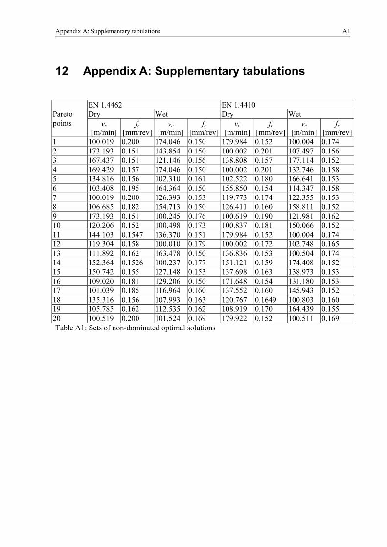
Appendix A: Supplementary tabulations A1
12 Appendix A: Supplementary tabulations
Pareto points
EN 1.4462 EN 1.4410 Dry Wet Dry Wet
vc [m/min]
fr [mm/rev]
vc [m/min]
fr [mm/rev]
vc [m/min]
fr [mm/rev]
vc [m/min]
fr [mm/rev]
1 100.019 0.200 174.046 0.150 179.984 0.152 100.004 0.174 2 173.193 0.151 143.854 0.150 100.002 0.201 107.497 0.156 3 167.437 0.151 121.146 0.156 138.808 0.157 177.114 0.152 4 169.429 0.157 174.046 0.150 100.002 0.201 132.746 0.158 5 134.816 0.156 102.310 0.161 102.522 0.180 166.641 0.153 6 103.408 0.195 164.364 0.150 155.850 0.154 114.347 0.158 7 100.019 0.200 126.393 0.153 119.773 0.174 122.355 0.153 8 106.685 0.182 154.713 0.150 126.411 0.160 158.811 0.152 9 173.193 0.151 100.245 0.176 100.619 0.190 121.981 0.162 10 120.206 0.152 100.498 0.173 100.837 0.181 150.066 0.152 11 144.103 0.1547 136.370 0.151 179.984 0.152 100.004 0.174 12 119.304 0.158 100.010 0.179 100.002 0.172 102.748 0.165 13 111.892 0.162 163.478 0.150 136.836 0.153 100.504 0.174 14 152.364 0.1526 100.237 0.177 151.121 0.159 174.408 0.152 15 150.742 0.155 127.148 0.153 137.698 0.163 138.973 0.153 16 109.020 0.181 129.206 0.150 171.648 0.154 131.180 0.153 17 101.039 0.185 116.964 0.160 137.552 0.160 145.943 0.152 18 135.316 0.156 107.993 0.163 120.767 0.1649 100.803 0.160 19 105.785 0.162 112.535 0.162 108.919 0.170 164.439 0.155 20 100.519 0.200 101.524 0.169 179.922 0.152 100.511 0.169 Table A1: Sets of non-dominated optimal solutions
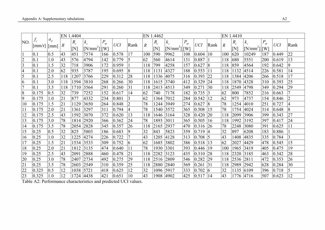
Appendix A: Supplementary tabulations A2
NO. rf [mm/r]
pa
[mm]
EN 1.4404 EN 1.4462 EN 1.4410
R cR
[N] ck
[N/mm2]spP
[W] UCI Rank R cR
[N] ck
[N/mm2] spP
[W] UCI Rank R cR
[N] ck
[N/mm2]spP
[W] UCI Rank
1 0.1 0.5 43 451 7574 166 0.578 17 100 590 9962 108 0.604 10 100 620 10249 187 0.449 22 2 0.1 1.0 43 576 4794 142 0.779 5 62 560 4614 131 0.887 1 118 680 5551 200 0.619 13 3 0.1 1.5 32 718 3906 172 0.959 1 118 799 4258 157 0.627 8 118 859 4564 192 0.642 9 4 0.1 2.0 62 935 3787 195 0.695 8 118 1131 4327 188 0.553 11 118 1132 4514 226 0.581 14 5 0.1 2.5 118 1207 3766 229 0.312 28 118 1336 4075 316 0.393 22 118 1384 4206 266 0.518 17 6 0.1 3.0 118 1594 3810 268 0.266 30 118 1615 3740 412 0.329 24 118 1870 4328 310 0.393 25 7 0.1 3.5 118 1710 3564 291 0.260 31 118 2413 4513 349 0.271 30 118 2549 4798 349 0.294 29 8 0.175 0.5 32 739 7252 152 0.617 14 62 740 7178 182 0.735 3 62 800 7852 216 0.663 7 9 0.175 1.0 21 877 4332 234 0.801 3 62 1364 7012 284 0.542 12 62 973 4737 154 0.846 2 10 0.175 1.5 21 1129 3650 264 0.848 2 78 1244 3949 274 0.627 8 78 1254 4010 251 0.727 4 11 0.175 2.0 21 1361 3297 311 0.794 4 78 1540 3572 365 0.508 15 78 1754 4024 314 0.648 8 12 0.175 2.5 43 1592 3070 372 0.620 13 118 1646 3164 328 0.420 20 118 2099 3906 399 0.343 27 13 0.175 3.0 78 1814 2920 366 0.362 24 78 1893 3011 365 0.505 16 118 1992 3192 397 0.417 24 14 0.175 3.5 78 2054 2828 345 0.357 26 118 2165 2937 470 0.316 26 78 2248 3080 391 0.625 11 15 0.25 0.5 32 825 5803 186 0.683 9 32 843 5823 359 0.719 4 32 897 6208 183 0.886 1 16 0.25 1.0 32 1225 4274 226 0.722 7 43 1205 4128 313 0.708 5 43 1408 4835 335 0.784 3 17 0.25 1.5 21 1534 3533 309 0.752 6 62 1685 3802 386 0.518 13 62 2027 4429 478 0.545 15 18 0.25 2.0 21 1812 3135 474 0.640 11 78 1930 3301 393 0.446 19 100 1965 3419 405 0.475 19 19 0.25 2.5 43 2091 2888 460 0.478 21 118 2282 3123 435 0.310 28 118 2320 3185 463 0.342 28 20 0.25 3.0 78 2407 2734 492 0.275 29 118 2516 2809 546 0.282 29 118 2536 2811 472 0.353 26 21 0.25 3.5 78 2603 2549 310 0.359 25 118 2880 2840 569 0.261 31 118 2989 2942 628 0.284 30 22 0.325 0.5 12 1038 5721 418 0.625 12 32 1096 5917 333 0.702 6 32 1135 6109 396 0.718 5 23 0.325 1.0 12 1724 4438 421 0.651 10 43 1908 4902 425 0.517 14 43 1776 4716 507 0.623 12 Table A2: Performance characteristics and predicted UCI values.
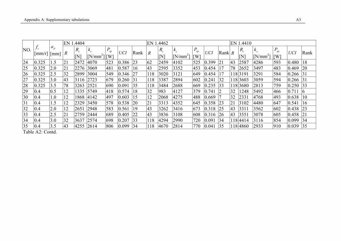
Appendix A: Supplementary tabulations A3
NO. rf [mm/r]
pa
[mm]
EN 1.4404 EN 1.4462 EN 1.4410
R cR
[N] ck
[N/mm2]spP
[W] UCI Rank R cR
[N] ck
[N/mm2] spP
[W] UCI Rank R cR
[N] ck
[N/mm2]spP
[W] UCI Rank
24 0.325 1.5 21 2472 4070 523 0.386 23 62 2459 4102 525 0.399 21 43 2587 4286 593 0.480 18 25 0.325 2.0 21 2276 3069 481 0.587 16 43 2595 3352 453 0.454 17 78 2652 3497 483 0.469 20 26 0.325 2.5 32 2899 3004 549 0.346 27 118 3020 3121 649 0.454 17 118 3191 3291 584 0.266 31 27 0.325 3.0 43 3116 2723 679 0.260 31 118 3387 2894 602 0.241 32 118 3603 3059 594 0.266 31 28 0.325 3.5 78 3263 2521 690 0.091 35 118 3484 2688 669 0.235 33 118 3680 2813 759 0.250 33 29 0.4 0.5 12 1335 5749 418 0.574 18 32 983 4127 379 0.741 2 32 1248 5492 466 0.711 6 30 0.4 1.0 12 1868 4142 497 0.603 15 12 2068 4275 488 0.669 7 32 2331 4768 493 0.638 10 31 0.4 1.5 12 2329 3450 578 0.538 20 21 3313 4352 645 0.358 23 21 3102 4480 647 0.541 16 32 0.4 2.0 12 2651 2948 583 0.561 19 43 3262 3416 673 0.318 25 43 3311 3562 602 0.438 23 33 0.4 2.5 21 2759 2444 689 0.405 22 43 3836 3108 608 0.316 26 43 3551 3078 605 0.458 21 34 0.4 3.0 32 3637 2574 698 0.207 33 118 4294 2990 720 0.091 34 118 4414 3116 854 0.099 34 35 0.4 3.5 43 4255 2614 806 0.099 34 118 4670 2814 770 0.041 35 118 4860 2933 910 0.039 35 Table A2: Contd.
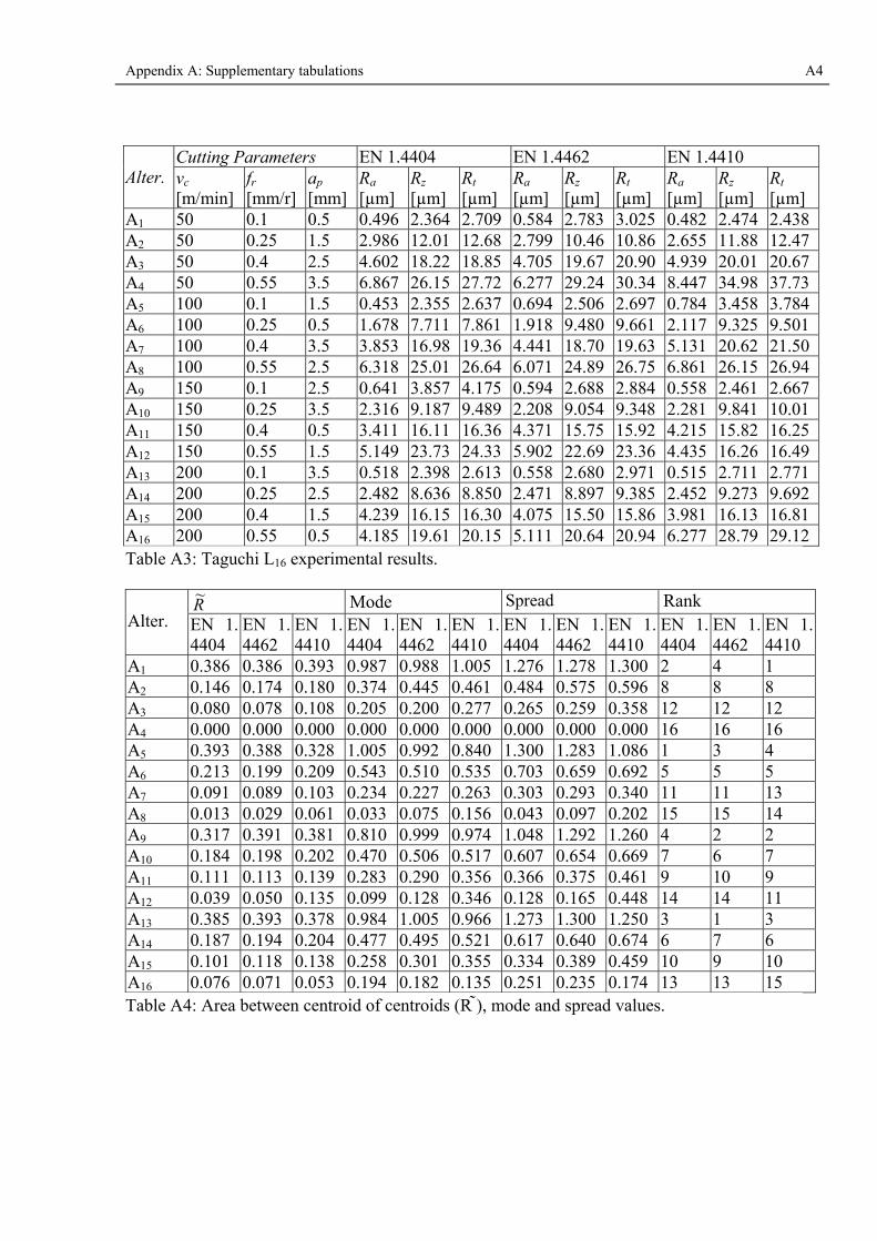
Appendix A: Supplementary tabulations A4
Alter.
Cutting Parameters EN 1.4404 EN 1.4462 EN 1.4410 vc
[m/min] fr [mm/r]
ap
[mm] Ra
[µm] Rz
[µm] Rt
[µm] Ra
[µm] Rz
[µm] Rt
[µm] Ra
[µm] Rz
[µm] Rt
[µm] A1 50 0.1 0.5 0.496 2.364 2.709 0.584 2.783 3.025 0.482 2.474 2.438 A2 50 0.25 1.5 2.986 12.01 12.68 2.799 10.46 10.86 2.655 11.88 12.47 A3 50 0.4 2.5 4.602 18.22 18.85 4.705 19.67 20.90 4.939 20.01 20.67 A4 50 0.55 3.5 6.867 26.15 27.72 6.277 29.24 30.34 8.447 34.98 37.73 A5 100 0.1 1.5 0.453 2.355 2.637 0.694 2.506 2.697 0.784 3.458 3.784 A6 100 0.25 0.5 1.678 7.711 7.861 1.918 9.480 9.661 2.117 9.325 9.501 A7 100 0.4 3.5 3.853 16.98 19.36 4.441 18.70 19.63 5.131 20.62 21.50 A8 100 0.55 2.5 6.318 25.01 26.64 6.071 24.89 26.75 6.861 26.15 26.94 A9 150 0.1 2.5 0.641 3.857 4.175 0.594 2.688 2.884 0.558 2.461 2.667 A10 150 0.25 3.5 2.316 9.187 9.489 2.208 9.054 9.348 2.281 9.841 10.01 A11 150 0.4 0.5 3.411 16.11 16.36 4.371 15.75 15.92 4.215 15.82 16.25 A12 150 0.55 1.5 5.149 23.73 24.33 5.902 22.69 23.36 4.435 16.26 16.49 A13 200 0.1 3.5 0.518 2.398 2.613 0.558 2.680 2.971 0.515 2.711 2.771 A14 200 0.25 2.5 2.482 8.636 8.850 2.471 8.897 9.385 2.452 9.273 9.692 A15 200 0.4 1.5 4.239 16.15 16.30 4.075 15.50 15.86 3.981 16.13 16.81 A16 200 0.55 0.5 4.185 19.61 20.15 5.111 20.64 20.94 6.277 28.79 29.12 Table A3: Taguchi L16 experimental results.
Alter.
R~
Mode Spread Rank EN 1. 4404
EN 1. 4462
EN 1. 4410
EN 1.4404
EN 1.4462
EN 1. 4410
EN 1.4404
EN 1.4462
EN 1. 4410
EN 1. 4404
EN 1.4462
EN 1. 4410
A1 0.386 0.386 0.393 0.987 0.988 1.005 1.276 1.278 1.300 2 4 1 A2 0.146 0.174 0.180 0.374 0.445 0.461 0.484 0.575 0.596 8 8 8 A3 0.080 0.078 0.108 0.205 0.200 0.277 0.265 0.259 0.358 12 12 12 A4 0.000 0.000 0.000 0.000 0.000 0.000 0.000 0.000 0.000 16 16 16 A5 0.393 0.388 0.328 1.005 0.992 0.840 1.300 1.283 1.086 1 3 4 A6 0.213 0.199 0.209 0.543 0.510 0.535 0.703 0.659 0.692 5 5 5 A7 0.091 0.089 0.103 0.234 0.227 0.263 0.303 0.293 0.340 11 11 13 A8 0.013 0.029 0.061 0.033 0.075 0.156 0.043 0.097 0.202 15 15 14 A9 0.317 0.391 0.381 0.810 0.999 0.974 1.048 1.292 1.260 4 2 2 A10 0.184 0.198 0.202 0.470 0.506 0.517 0.607 0.654 0.669 7 6 7 A11 0.111 0.113 0.139 0.283 0.290 0.356 0.366 0.375 0.461 9 10 9 A12 0.039 0.050 0.135 0.099 0.128 0.346 0.128 0.165 0.448 14 14 11 A13 0.385 0.393 0.378 0.984 1.005 0.966 1.273 1.300 1.250 3 1 3 A14 0.187 0.194 0.204 0.477 0.495 0.521 0.617 0.640 0.674 6 7 6 A15 0.101 0.118 0.138 0.258 0.301 0.355 0.334 0.389 0.459 10 9 10 A16 0.076 0.071 0.053 0.194 0.182 0.135 0.251 0.235 0.174 13 13 15 Table A4: Area between centroid of centroids (R ), mode and spread values.
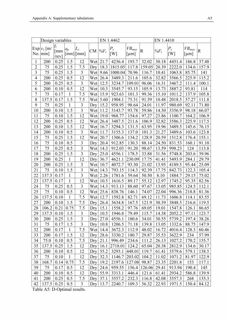
Appendix A: Supplementary tabulations A5
Design variables EN 1.4462 EN 1.4410
ExpNo.
vc [m/ min]
fr [mm/rev]
ap [mm]
Lc [mm]
CM %Ft Pe [W]
VBmax [µm]
R %Ft Pe [W]
VBmax
[µm] R
1 200 0.25 1.5 12 Wet 21.7 4236.4 193.7 32.02 30.18 4451.4 186.8 37.482 75 0.25 1.5 7.5 Dry 18.3 1815.05 117.8 159.05 20.39 2222.0 134.6 157.93 75 0.25 1.5 3 Wet 9.66 1000.04 70.96 116.7 10.41 1063.8 85.75 141 4 200 0.25 0.5 12 Wet 26.4 3489.3 211.6 105.6 32.82 3566.5 225.9 115.25 200 0.25 0.5 3 Wet 12.5 3234.7 109.01 96.06 16.31 3467.2 111.4 100.16 200 0.10 0.5 12 Wet 10.3 3545.7 93.15 105.9 13.73 3887.2 93.81 114 7 75 0.17 1 7.5 Wet 15.9 923.63 101.3 99.36 15.10 1011.2 137.9 105.88 137.5 0.17 1.5 7.5 Wet 5.60 1904.1 75.31 91.59 10.48 2018.5 57.27 111.89 75 0.25 1 3 Dry 15.2 958.95 98.64 24.01 11.97 980.69 92.11 71.8010 200 0.10 1.5 3 Wet 11.2 3143.7 93.78 59.86 14.30 3356.9 98.18 66.0711 75 0.10 1.5 12 Wet 19.0 968.77 154.6 97.27 23.86 1100.7 164.2 106.912 200 0.25 0.5 12 Wet 26.4 3487.5 211.6 106.9 32.82 3586.3 225.9 117.513 200 0.10 1.5 12 Wet 16.7 3294.3 131.5 63.95 19.96 3489.5 145.6 76.1514 200 0.10 0.5 3 Wet 11.7 3155.3 137.0 101.3 21.27 3489.6 103.6 123.815 75 0.25 1.5 12 Wet 20.7 1306.6 134.2 128.9 20.59 1512.8 176.4 155.116 75 0.10 0.5 3 Dry 20.4 912.85 130.3 88.14 24.50 831.53 160.1 91.1017 75 0.25 0.5 3 Wet 14.3 912.03 91.20 98.67 13.59 998.23 124 113.818 200 0.25 1.5 3 Dry 25.0 4556.1 178.5 33.88 31.56 5748.8 203.6 39.9619 200 0.25 1 12 Dry 36.7 4621.1 230.09 17.75 41.41 5493.9 284.1 29.7920 200 0.25 1.5 3 Wet 10.7 4072.7 93.30 21.02 13.95 4189.5 95.44 25.0921 75 0.10 1.5 3 Wet 14.3 793.15 114.3 92.39 17.75 842.73 122.3 105.422 137.5 0.17 1 3 Wet 2.26 1781.6 59.64 50.50 8.10 1884.7 29.15 75.0223 137.5 0.17 1 12 Wet 10.5 1616.5 89.17 55.12 12.97 1745.2 95.35 82.5624 75 0.25 0.5 3 Wet 14.3 913.13 88.60 97.67 13.05 985.85 124.5 112.125 75 0.10 0.5 12 Wet 25.6 838.76 146.1 74.07 22.04 996.36 218.8 81.3626 137.5 0.10 1 7.5 Wet 12.7 1592.8 82.71 69.12 11.73 1606.8 114.1 83.5527 200 0.10 1.5 7.5 Dry 26.4 3634.8 167.5 121.9 30.39 3848.5 216.6 119.528 106.2 0.21 0.75 7.5 Dry 15.1 1558.2 97.76 69.05 19.01 1547.8 126.1 86.6529 137.5 0.10 1.5 3 Dry 10.5 1946.8 79.49 115.7 14.38 2052.2 97.11 123.730 200 0.25 1.5 3 Dry 27.0 4556.1 180.6 34.01 30.55 5739.2 197.4 38.2631 75 0.17 1.5 3 Dry 10.8 1206.5 71.18 139.8 13.05 1332.6 88.75 147.932 200 0.17 1 7.5 Wet 14.4 3672.3 112.9 48.02 16.72 4016.4 128.3 60.4633 200 0.17 1.5 12 Dry 28.6 3330.2 180.7 29.87 35.53 3622.9 234 57.9934 75.0 0.10 0.5 7.5 Dry 21.1 996.49 234.6 111.2 26.13 1027.2 170.2 155.735 137.5 0.25 1.5 12 Dry 16.1 2718.01 124.2 65.04 20.38 2812.9 134.6 30.1736 200 0.10 0.5 12 Dry 55.2 3293.1 448.01 119.7 61.41 3579.6 579.1 138.537 75 0.10 1 12 Dry 32.3 1146.7 203.02 104.2 11.02 1071.2 81.97 122.938 168.7 0.14 0.75 7.5 Dry 19.2 2197.6 127.08 98.87 23.35 2201.8 153 117.139 75 0.17 0.5 12 Dry 24.6 959.55 156.4 126.06 29.41 913.94 190.4 145 40 200 0.10 0.5 12 Dry 55.9 3313.1 446.4 121.6 61.41 2934.2 586.8 139.941 200 0.25 0.5 7.5 Dry 37.1 3557.2 232.3 116.8 42.08 3557.3 268 135.342 137.5 0.25 0.5 3 Dry 13.7 2240.7 109.3 56.32 22.93 1971.5 150.4 84.12
Table A5: D-Optimal results.

Appendix A: Supplementary tabulations A6
Design variables EN 1.4462 EN 1.4410
ExpNo.
vc [m/ min]
fr [mm/rev]
ap [mm]
Lc [mm]
CM %Ft Pe [W]
VBmax [µm]
R %Ft Pe [W]
VBmax
[µm] R
43 200 0.10 1 3 Dry 24.2 3207.7 152.5 64.14 26.89 3514.1 185 91.9844 75 0.25 0.5 12 Wet 25.4 998.86 122.3 107.10 18.37 1208.4 215.8 118 45 75 0.10 0.5 3 Wet 17.4 759.17 132.5 70.77 20.11 845.42 151.7 80.7546 75 0.25 0.5 12 Dry 29.5 1052.5 216.3 119.9 34.71 955.32 205.8 128.647 75 0.10 1.5 12 Dry 17.5 1051.1 113.0 112.5 23.05 1075.7 153.2 140.948 200 0.17 0.5 3 Dry 18.2 3232.6 119.0 69.33 22.81 3447.9 153.7 65.26
Table A5: Contd.
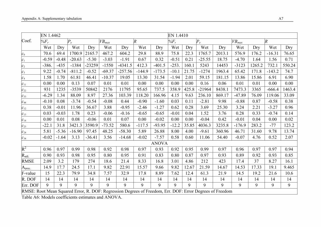
Appendix A: Supplementary tabulation A7
Coef.
EN 1.4462 EN 1.4410 %Fr Pe VBmax R %Fr Pe VBmax R
Wet Dry Wet Dry Wet Dry Wet Dry Wet Dry Wet Dry Wet Dry Wet Dry c0 70.6 69.4 1700.9 2165.7 467.2 604.2 29.8 88.9 75.8 22.3 1765.7 2013.1 576.9 176.2 -16.31 76.65 c1 -0.59 -0.48 -20.63 -5.30 -3.03 -1.91 0.67 0.32 -0.51 0.21 -25.55 18.75 -4.70 1.64 1.56 0.71 c2 -386. -435 -1384 -23259 -1550 -4341.5 412.3 -401.5 -253. 160.1 5243 14453 -3123 1265.2 732.1 550.24 c3 9.22 -0.74 -811.2 -0.52 -69.37 -257.56 -144.9 -173.5 -10.1 21.75 -1274 1963.4 65.42 171.8 -143.2 74.7 c4 1.58 1.70 61.81 46.41 -10.37 19.05 13.30 31.54 -1.94 2.01 59.15 181.15 13.86 15.86 6.91 6.90 c11 0.00 0.00 0.13 0.07 0.01 0.01 0.00 0.00 0.00 0.00 0.16 0.06 0.01 0.01 0.00 0.00 c22 931 1235 -3539 50842 2176 11795 95.65 737.5 358.9 425.8 -21964 8438.1 7473.3 3365 -666.4 1463.4 c33 -6.29 1.34 88.09 8.97 27.36 103.39 118.20 166.96 4.15 9.63 236.10 869.17 -47.89 76.09 119.06 33.09 c44 -0.10 0.08 -3.74 -0.54 -0.08 0.44 -0.90 -1.60 0.03 0.11 -2.81 9.98 -0.88 0.87 -0.58 0.38 c12 0.38 -0.01 11.96 36.67 3.88 -0.95 -2.46 -1.27 0.62 0.28 3.69 25.30 3.24 2.21 -3.27 0.96 c13 0.03 -0.03 1.78 0.23 -0.06 -0.16 -0.65 -0.65 -0.01 0.04 1.52 3.76 0.28 0.33 -0.74 0.14 c14 0.00 0.01 0.08 -0.06 0.01 0.07 0.00 -0.02 0.00 0.00 -0.04 0.42 -0.01 0.04 0.00 0.02 c23 -22.1 31.8 3421.3 3590.9 -73.52 580.6 -117.5 -93.95 -12.2 35.85 4036.3 3235.8 -176.9 283.2 -77 123.2 c24 5.81 -5.36 -16.90 97.45 48.25 -58.30 5.89 26.88 8.00 4.00 -9.61 360.96 46.71 31.60 9.78 13.74 c34 -0.02 -1.64 3.13 -36.41 3.56 -14.68 -0.02 -7.57 0.58 0.60 11.06 54.40 -0.07 4.76 0.52 2.07
ANOVA R2 0.96 0.97 0.99 0.98 0.92 0.98 0.97 0.93 0.92 0.95 0.99 0.97 0.96 0.97 0.97 0.94 Radj. 0.90 0.93 0.98 0.95 0.80 0.95 0.91 0.83 0.80 0.87 0.97 0.93 0.89 0.92 0.93 0.85 RMSE 2.09 3.2 179 274 18.6 21.4 8.33 16.8 3.01 4.86 212 423 17.4 37 8.27 16.1 Aprec. 14.9 17.7 24.5 17.1 9.82 22.91 15.57 9.66 9.82 12.67 21.59 14.67 14.53 17.33 19.1 9.465 F-value 15 22.3 79.9 34.8 7.57 32.9 17.8 8.89 7.62 12.4 61.3 21.9 14.5 19.2 21.6 10.6 R. DOF 14 14 14 14 14 14 14 14 14 14 14 14 14 14 14 14 Err. DOF 9 9 9 9 9 9 9 9 9 9 9 9 9 9 9 9 RMSE: Root Mean Squared Error, R. DOF: Regression Degrees of Freedom, Err. DOF: Error Degrees of Freedom Table A6: Models coefficients estimates and ANOVA.
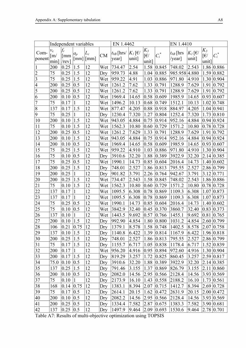
Appendix A: Supplementary tabulation A8
Independent variables EN 1.4462 EN 1.4410
Com-ponent
vc [m/ min]
fr [mm/rev]
ap [mm]
Lc [mm]
CM tbB [hrs/year]
K1 [€/ unit]
K3
[€/ unit]
Ci*
tbB [hrs /year]
K1 [€/ unit]
K3
[€/ unit]
Ci*
1 200 0.25 1.5 12 Wet 734.47 2.54 1.58 0.845 748.02 2.543 1.86 0.886 2 75 0.25 1.5 12 Dry 959.73 4.88 1.04 0.885 985.958 4.880 1.59 0.882 3 75 0.25 1.5 12 Wet 959.22 4.91 1.03 0.886 971.80 4.910 1.30 0.904 4 200 0.25 0.5 12 Wet 1261.2 7.62 1.33 0.791 1288.9 7.629 1.91 0.792 5 200 0.25 0.5 12 Wet 1261.2 7.62 1.33 0.791 1288.9 7.629 1.91 0.792 6 200 0.10 0.5 12 Wet 1969.4 14.65 0.58 0.609 1985.9 14.65 0.93 0.607 7 75 0.17 1 12 Wet 1496.2 10.13 0.68 0.749 1512.1 10.13 1.02 0.748 8 137 0.17 1.5 12 Wet 877.47 4.205 0.88 0.918 884.97 4.205 1.04 0.941 9 75 0.25 1 12 Dry 1230.4 7.320 1.27 0.804 1252.4 7.320 1.73 0.810 10 200 0.10 1.5 12 Wet 943.05 4.884 0.75 0.914 952.16 4.884 0.94 0.924 11 75 0.10 1.5 12 Wet 1562.3 10.80 0.60 0.729 1571.2 10.80 0.78 0.728 12 200 0.25 0.5 12 Wet 1261.2 7.629 1.33 0.791 1288.9 7.629 1.91 0.792 13 200 0.10 1.5 12 Wet 943.05 4.884 0.75 0.914 952.16 4.884 0.94 0.924 14 200 0.10 0.5 12 Wet 1969.4 14.65 0.58 0.609 1985.9 14.65 0.93 0.607 15 75 0.25 1.5 12 Wet 959.22 4.910 1.03 0.886 971.80 4.910 1.30 0.904 16 75 0.10 0.5 12 Dry 3910.6 32.20 1.88 0.389 3922.9 32.20 2.14 0.385 17 75 0.25 0.5 12 Wet 1990.1 14.73 0.85 0.604 2016.4 14.73 1.40 0.602 18 200 0.25 1.5 12 Dry 748.01 2.527 1.86 0.813 795.55 2.527 2.86 0.799 19 200 0.25 1 12 Dry 901.82 3.791 2.26 0.764 942.67 3.791 3.12 0.771 20 200 0.25 1.5 12 Wet 734.47 2.543 1.58 0.845 748.02 2.543 1.86 0.886 21 75 0.10 1.5 12 Wet 1562.3 10.80 0.60 0.729 1571.2 10.80 0.78 0.728 22 137 0.17 1 12 Wet 1095.5 6.308 0.78 0.869 1109.3 6.308 1.07 0.873 23 137 0.17 1 12 Wet 1095.5 6.308 0.78 0.869 1109.3 6.308 1.07 0.873 24 75 0.25 0.5 12 Wet 1990.1 14.73 0.85 0.604 2016.4 14.73 1.40 0.602 25 75 0.10 0.5 12 Wet 3842.9 32.40 0.45 0.370 3860.7 32.40 0.83 0.373 26 137 0.10 1 12 Wet 1443.5 9.692 0.57 0.766 1455.1 9.692 0.81 0.765 27 200 0.10 1.5 12 Dry 992.90 4.854 1.80 0.800 1031.2 4.854 2.60 0.799 28 106 0.21 0.75 12 Dry 1379.1 8.578 1.58 0.748 1402.5 8.578 2.07 0.758 29 137 0.10 1.5 12 Dry 1140.8 6.422 1.39 0.814 1167.9 6.422 1.96 0.818 30 200 0.25 1.5 12 Dry 748.01 2.527 1.86 0.813 795.55 2.527 2.86 0.799 31 75 0.17 1.5 12 Dry 1155.7 6.717 1.05 0.838 1178.4 6.717 1.52 0.839 32 200 0.17 1 12 Wet 956.20 4.916 0.95 0.894 972.60 4.916 1.30 0.904 33 200 0.17 1.5 12 Dry 819.29 3.257 1.72 0.825 860.45 3.257 2.59 0.817 34 75.0 0.10 0.5 12 Dry 3910.6 32.20 1.88 0.389 3922.9 32.20 2.14 0.385 35 137 0.25 1.5 12 Dry 791.46 3.155 1.37 0.869 826.79 3.155 2.11 0.860 36 200 0.10 0.5 12 Dry 2082.0 14.56 2.95 0.566 2128.4 14.56 3.93 0.569 37 75 0.10 1 12 Dry 2173.9 16.10 1.43 0.558 2188.2 16.10 1.73 0.561 38 168 0.14 0.75 12 Dry 1383.1 8.394 2.07 0.715 1412.7 8.394 2.69 0.728 39 75 0.17 0.5 12 Dry 2614.1 20.15 1.62 0.472 2631.9 20.15 2.00 0.472 40 200 0.10 0.5 12 Dry 2082.2 14.56 2.95 0.566 2128.4 14.56 3.93 0.569 41 200 0.25 0.5 12 Dry 1334.4 7.582 2.87 0.675 1383.3 7.582 3.90 0.681 42 137 0.25 0.5 12 Dry 1497.9 9.464 2.09 0.693 1530.6 9.464 2.78 0.701 Table A7: Results of multi-objective optimization using TOPSIS
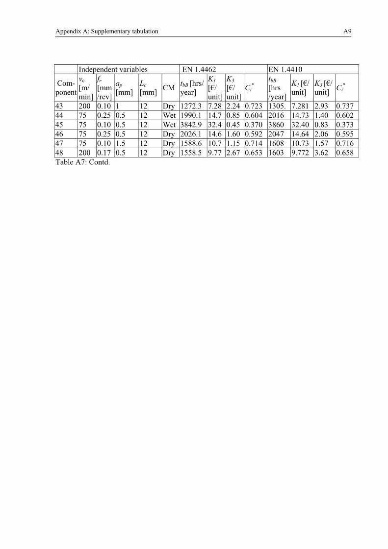
Appendix A: Supplementary tabulation A9
Independent variables EN 1.4462 EN 1.4410
Com-ponent
vc [m/ min]
fr [mm/rev]
ap [mm]
Lc [mm]
CM tbB [hrs/year]
K1
[€/ unit]
K3
[€/ unit]
Ci*
tbB
[hrs /year]
K1 [€/ unit]
K3 [€/unit]
Ci*
43 200 0.10 1 12 Dry 1272.3 7.28 2.24 0.723 1305. 7.281 2.93 0.737 44 75 0.25 0.5 12 Wet 1990.1 14.7 0.85 0.604 2016 14.73 1.40 0.602 45 75 0.10 0.5 12 Wet 3842.9 32.4 0.45 0.370 3860 32.40 0.83 0.373 46 75 0.25 0.5 12 Dry 2026.1 14.6 1.60 0.592 2047 14.64 2.06 0.595 47 75 0.10 1.5 12 Dry 1588.6 10.7 1.15 0.714 1608 10.73 1.57 0.716 48 200 0.17 0.5 12 Dry 1558.5 9.77 2.67 0.653 1603 9.772 3.62 0.658 Table A7: Contd.