Embed Size (px)
Citation preview
Feature Article
Modeling of Molecular Transfer inHeterophase Polymerization
Hugo F. Hernandez, Klaus Tauer*
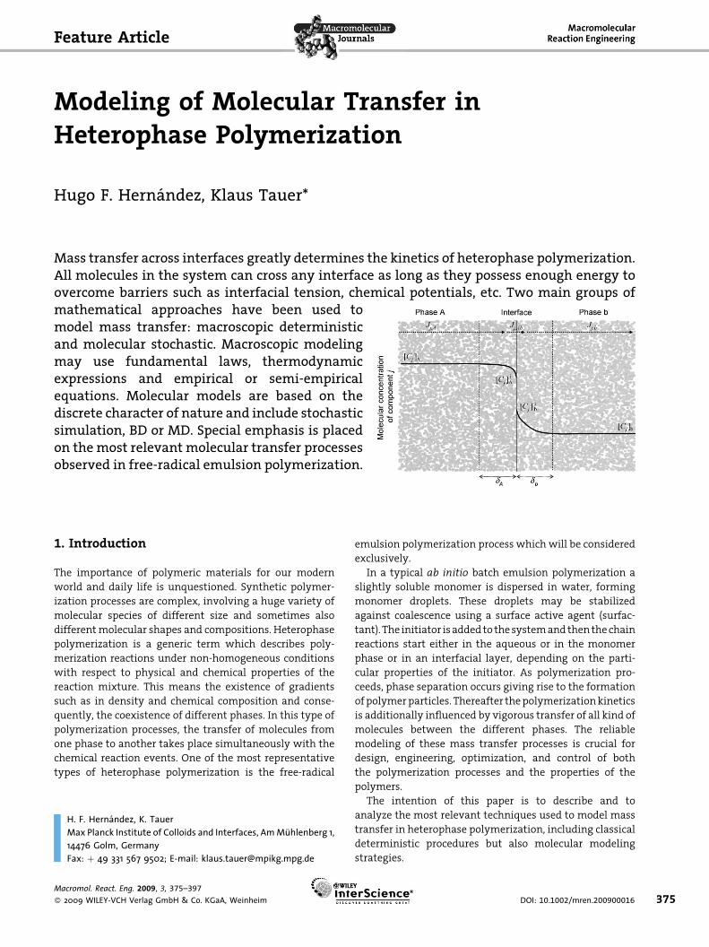
Mass transfer across interfaces greatly determines the kinetics of heterophase polymerization.All molecules in the system can cross any interface as long as they possess enough energy toovercome barriers such as interfacial tension, chemical potentials, etc. Two main groups ofmathematical approaches have been used tomodel mass transfer: macroscopic deterministicand molecular stochastic. Macroscopic modelingmay use fundamental laws, thermodynamicexpressions and empirical or semi-empiricalequations. Molecular models are based on thediscrete character of nature and include stochasticsimulation, BD or MD. Special emphasis is placedon themost relevant molecular transfer processesobserved in free-radical emulsion polymerization.
1. Introduction
The importance of polymeric materials for our modern
world and daily life is unquestioned. Synthetic polymer-
ization processes are complex, involving a huge variety of
molecular species of different size and sometimes also
differentmolecular shapes and compositions. Heterophase
polymerization is a generic term which describes poly-
merization reactions under non-homogeneous conditions
with respect to physical and chemical properties of the
reaction mixture. This means the existence of gradients
such as in density and chemical composition and conse-
quently, the coexistence of different phases. In this type of
polymerization processes, the transfer of molecules from
one phase to another takes place simultaneously with the
chemical reaction events. One of the most representative
types of heterophase polymerization is the free-radical
H. F. Hernandez, K. TauerMax Planck Institute of Colloids and Interfaces, Am Muhlenberg 1,14476 Golm, GermanyFax: þ 49 331 567 9502; E-mail: [email protected]
Macromol. React. Eng. 2009, 3, 375–397
� 2009 WILEY-VCH Verlag GmbH & Co. KGaA, Weinheim
emulsion polymerization process which will be considered
exclusively.
In a typical ab initio batch emulsion polymerization a
slightly soluble monomer is dispersed in water, forming
monomer droplets. These droplets may be stabilized
against coalescence using a surface active agent (surfac-
tant). The initiator isadded to thesystemandthenthechain
reactions start either in the aqueous or in the monomer
phase or in an interfacial layer, depending on the parti-
cular properties of the initiator. As polymerization pro-
ceeds, phase separation occurs giving rise to the formation
ofpolymerparticles. Thereafter thepolymerizationkinetics
is additionally influenced by vigorous transfer of all kind of
molecules between the different phases. The reliable
modeling of these mass transfer processes is crucial for
design, engineering, optimization, and control of both
the polymerization processes and the properties of the
polymers.
The intention of this paper is to describe and to
analyze the most relevant techniques used to model mass
transfer in heterophase polymerization, including classical
deterministic procedures but also molecular modeling
strategies.
DOI: 10.1002/mren.200900016 375
H. F. Hernandez, K. Tauer
376
The paper is organized as follows. In Section 2, a more
detailed description of radical heterophase polymerization
processes ispresented. Section3describes themost relevant
methods used to model mass transfer between phases. In
Section 4 some of the most relevant transfer events
occurring in free-radical emulsion polymerization are
analyzed and discussed considering the differentmodeling
strategies. Finally, in Section 5 besides some concluding
thoughts possible future trends in modeling of mass
transfer processes in heterogeneous systems are briefly
discussed.
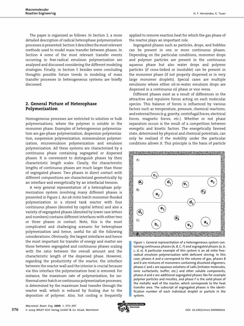
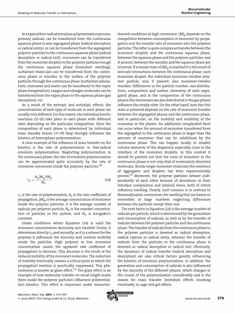
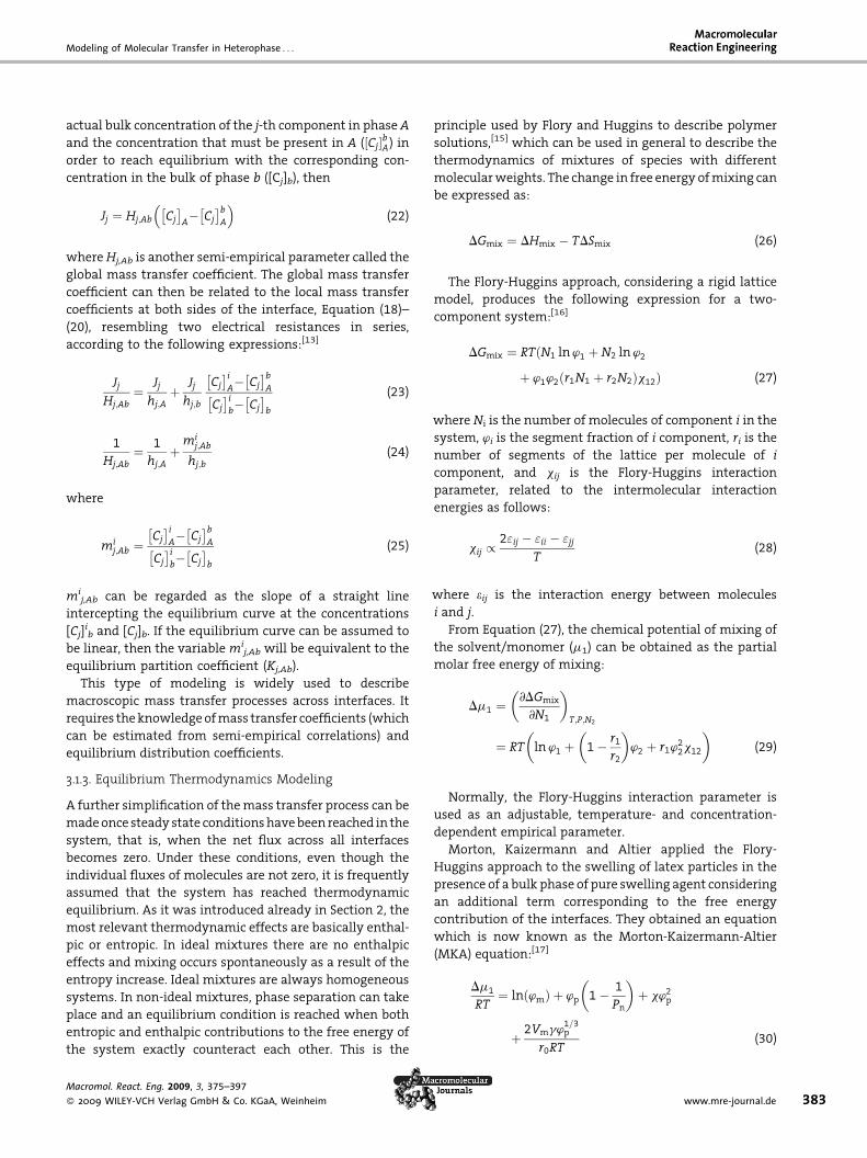
Figure 1. General representation of a heterogeneous system con-taining continuous phases (A, B, C, F) and segregated phases (a, b,c, d, e). A particular example of this system is an ab initio free-radical emulsion polymerization with deficient stirring. In thiscase, phases A and a correspond to the volume of gas, phases Band b are mixtures of monomers containing dissolved oligomers,phases C and c are aqueous solutions of salts (initiator molecules,ionic surfactants, buffer, etc.) and other soluble components,phases d and e are additional segregated phases like for examplepolymer particles and micelles, and phase F is the solid phase ofthe metallic wall of the reactor, which corresponds to the heattransfer area. The subscript of segregated phases is the identi-fication number of each individual droplet or particle in thesystem.
2. General Picture of HeterophasePolymerization
Homogeneous processes are restricted to solution or bulk
polymerizations, where the polymer is soluble in the
monomer phase. Examples of heterogeneous polymeriza-
tion are gas-phase polymerization, dispersion polymeriza-
tion, suspension polymerization, miniemulsion polymer-
ization, microemulsion polymerization and emulsion
polymerization. All these systems are characterized by a
continuous phase containing segregated or dispersed
phases. It is convenient to distinguish phases by their
characteristic length scales. Clearly, the characteristic
lengths of continuous phases are much larger than those
of segregated phases. Two phases in direct contact with
different compositions are characterized geometrically by
an interface and energetically by an interfacial tension.
A very general representation of a heterophase poly-
merization system involving many different phases is
presented in Figure 1. An ab initio batch monomer-flooded
polymerization in a stirred tank reactor with four
continuous phases (denoted by capital letters) and also a
variety of segregated phases (denoted by lower case letters
and numbers) contains different interfaceswith either two
or three phases in contact. Note, this is the most
complicated and challenging scenario for heterophase
polymerization and hence, useful for all the following
considerations. Obviously, the largest interfaces and hence
the most important for transfer of energy and matter are
those between segregated and continuous phases scaling
with the ratio between the overall amount and the
characteristic length of the dispersed phase. However,
regarding the productivity of the reactor, the interface
between the reactor wall and the interior is crucial because
via this interface the polymerization heat is removed. For
instance, the maximum rate of polymerization, for iso-
thermalsemi-batchorcontinuouspolymerizationprocesses,
is determined by the maximum heat transfer through the
reactor wall, which is reduced by fouling due to the
deposition of polymer. Also, hot cooling is frequently
Macromol. React. Eng. 2009, 3, 375–397
� 2009 WILEY-VCH Verlag GmbH & Co. KGaA, Weinheim
applied to remove reaction heat for which the gas phase of
the reactor plays an important role.
Segregated phases such as particles, drops, and bubbles
can be present in one or more continuous phases.
Depending on the particular conditions, monomer drops
and polymer particles are present in the continuous
aqueous phase but also water drops and polymer
particles (if cross-linked or insoluble) can be present in
the monomer phase (if not properly dispersed or in very
large monomer droplets). Special cases are multiple
emulsions where either oil-in-water emulsion drops are
dispersed in a continuous oil phase or vice versa.
Different phases exist as a result of differences in the
attractive and repulsive forces acting on each molecular
species. This balance of forces is influenced by various
factors such as temperature, pressure, chemical reactions,
andexternal forces (e.g. gravity, centrifugal forces, electrical
forces, magnetic forces, etc.). Whether or not phase
separation occurs is the result of a competition between
energetic and kinetic factors. The energetically favored
state, determined by physical and chemical potentials, can
only be realized if the mobility under the particular
conditions allows it. This principle is the basis of particle
DOI: 10.1002/mren.200900016
Modeling of Molecular Transfer in Heterophase . . .
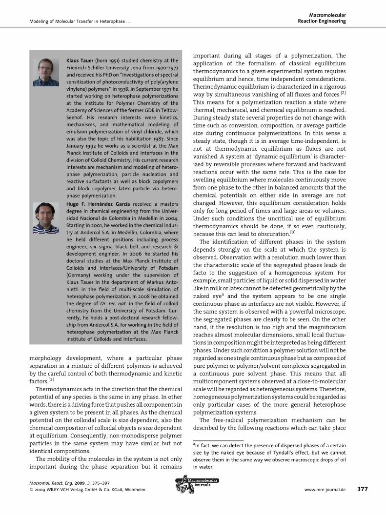
Klaus Tauer (born 1951) studied chemistry at theFriedrich Schiller University Jena from 1970–1977and received his PhD on ‘‘Investigations of spectralsensitization of photoconductivity of poly(arylenevinylene) polymers’’ in 1978. In September 1977 hestarted working on heterophase polymerizationsat the Institute for Polymer Chemistry of theAcademy of Sciences of the former GDR in Teltow-Seehof. His research interests were kinetics,mechanisms, and mathematical modeling ofemulsion polymerization of vinyl chloride, whichwas also the topic of his habilitation 1987. SinceJanuary 1992 he works as a scientist at the MaxPlanck Institute of Colloids and Interfaces in thedivision of Colloid Chemistry. His current researchinterests are mechanism and modeling of hetero-phase polymerization, particle nucleation andreactive surfactants as well as block copolymersand block copolymer latex particle via hetero-phase polymerization.Hugo F. Hernandez Garcıa received a mastersdegree in chemical engineering from the Univer-sidad Nacional de Colombia in Medellin in 2004.Starting in 2001, he worked in the chemical indus-try at Andercol S.A. in Medellin, Colombia, wherehe held different positions including processengineer, six sigma black belt and research &development engineer. In 2006 he started hisdoctoral studies at the Max Planck Institute ofColloids and Interfaces/University of Potsdam(Germany) working under the supervision ofKlaus Tauer in the department of Markus Anto-nietti in the field of multi-scale simulation ofheterophase polymerization. In 2008 he obtainedthe degree of Dr. rer. nat. in the field of colloidchemistry from the University of Potsdam. Cur-rently, he holds a post-doctoral research fellow-ship from Andercol S.A. for working in the field ofheterophase polymerization at the Max PlanckInstitute of Colloids and Interfaces.
aIn fact, we can detect the presence of dispersed phases of a certainsize by the naked eye because of Tyndall’s effect, but we cannotobserve them in the same way we observe macroscopic drops of oilin water.
morphology development, where a particular phase
separation in a mixture of different polymers is achieved
by the careful control of both thermodynamic and kinetic
factors.[1]
Thermodynamics acts in the direction that the chemical
potential of any species is the same in any phase. In other
words, there isadriving force thatpushesall components in
a given system to be present in all phases. As the chemical
potential on the colloidal scale is size dependent, also the
chemical composition of colloidal objects is size dependent
at equilibrium. Consequently, non-monodisperse polymer
particles in the same system may have similar but not
identical compositions.
The mobility of the molecules in the system is not only
important during the phase separation but it remains
Macromol. React. Eng. 2009, 3, 375–397
� 2009 WILEY-VCH Verlag GmbH & Co. KGaA, Weinheim
important during all stages of a polymerization. The
application of the formalism of classical equilibrium
thermodynamics to a given experimental system requires
equilibrium and hence, time independent considerations.
Thermodynamic equilibrium is characterized in a rigorous
way by simultaneous vanishing of all fluxes and forces.[2]
This means for a polymerization reaction a state where
thermal, mechanical, and chemical equilibrium is reached.
During steady state several properties do not change with
time such as conversion, composition, or average particle
size during continuous polymerizations. In this sense a
steady state, though it is in average time-independent, is
not at thermodynamic equilibrium as fluxes are not
vanished. A system at ’dynamic equilibrium’ is character-
ized by reversible processes where forward and backward
reactions occur with the same rate. This is the case for
swelling equilibrium where molecules continuously move
from one phase to the other in balanced amounts that the
chemical potentials on either side in average are not
changed. However, this equilibrium consideration holds
only for long period of times and large areas or volumes.
Under such conditions the uncritical use of equilibrium
thermodynamics should be done, if so ever, cautiously,
because this can lead to obscuration.[3]
The identification of different phases in the system
depends strongly on the scale at which the system is
observed. Observation with a resolution much lower than
the characteristic scale of the segregated phases leads de
facto to the suggestion of a homogeneous system. For
example, small particles of liquid or soliddispersed inwater
like inmilk or latex cannot bedetected geometrically by the
naked eyea and the system appears to be one single
continuous phase as interfaces are not visible. However, if
the same system is observed with a powerful microscope,
the segregated phases are clearly to be seen. On the other
hand, if the resolution is too high and the magnification
reaches almost molecular dimensions, small local fluctua-
tions incompositionmightbe interpretedasbeingdifferent
phases.Under suchconditionapolymer solutionwill notbe
regardedasonesingle continuousphasebutas composedof
pure polymer or polymer/solvent complexes segregated in
a continuous pure solvent phase. This means that all
multicomponent systems observed at a close-to-molecular
scalewill be regarded as heterogeneous systems. Therefore,
homogeneouspolymerizationsystemscouldbe regardedas
only particular cases of the more general heterophase
polymerization systems.
The free-radical polymerization mechanism can be
described by the following reactions which can take place
www.mre-journal.de 377
H. F. Hernandez, K. Tauer
378
in all phases:
Macrom
� 2009
Initiator decomposition : I!kd 2R� (1)
Initiation : R� þM!ki P�1 (2)
Propagation : P�i þM!kp
P�iþ1 (3)
Termination by combination : P�i þ P�j !ktc
Diþj (4)
Termination bydisproportionation :(5)
P�i þ P�j !ktd
Di þMj
Chain transfer : P�i þ T!kfTDi þ T� (6)
The nomenclature used in reactions (1) to (6) is the
following:
kx: C
hemical reaction rate coefficient of reaction xI: In
itiator moleculeR�: P
rimary radicalM: M
onomer moleculeMj: P
olymer molecule with chain length j and oneavailable double bond
Pi�: P
olymer radical with chain length iDi: D
ead polymer with chain length iT: C
hain transfer agent. T can represent the monomer(chain transfer tomonomer), the samepolymer chain
(backbiting), a different polymer chain (branching),
or any other molecule present in the system with a
labile hydrogen atom (e.g. surfactant, solvent, etc.)
T�: R
adical derived from the chain transfer agent.Simultaneously with the chemical changes physical
events take place. It is convenient to describe these phase
transfers by first order kinetic coefficients.
Transfer from a continuous phase to a segregated phase
dispersed in that continuous phase (absorption or entry):
CX !ka;Xyi
Cy;i (7)
Transfer from a segregated phase dispersed in a
continuous phase to that continuous phase (desorption
or exit):
Cy;i !k0;yiX
CX (8)
Transfer from a continuous phase to another continuous
phase:
CX !kc;XZ
CZ (9)
ol. React. Eng. 2009, 3, 375–397
WILEY-VCH Verlag GmbH & Co. KGaA, Weinheim
In Equation (7)–(9), the following nomenclature is used:
ka, k0, kc: mass transfer rate coefficients for absorption,
desorption and transfer between continuous phases,
respectively.
CX: Molecule C in continuous phase X
Cy,i: Molecule C in the i-th segregated phase of y
It is important to notice that the molecular transfer
between two different segregated phases is not possible
because intermediate steps througha continuousphase are
always required. In general, phase transfer events can only
take place between phases in direct contact. The condition
for steady state can be expressed as follows:
ka;Xyi C½ ��X¼ k0;yiX C½ ��yi (10)
kc;XZ C½ ��X¼ kc;ZX C½ ��Z (11)
where the brackets and superscript ‘‘�’’ indicate concentra-
tions and steady state, respectively. Equation (10) corre-
sponds to the steady state between a continuous phase (X)
and a phase segregated in that continuous phase (yi).
Equation (11) expresses the steady state condition between
two continuous phases in direct contact (X and Z). Notice
also that at steady state:
C½ ��XC½ ��yi
¼ k0;yiX
ka;Xyi¼ KXyi (12)
C½ ��X� ¼ k0;ZX ¼ KXZ (13)
C½ �Z ka;XZ
where KXyi and KXZ are the partition coefficients between
the phases X and yi, and X and Z, respectively. The partition
coefficients are constant for a particular set of conditions,
and as can be seen,will be affected by the same factors that
influence the kinetics of phase transfer in the system (e.g.
temperature, composition, pressure, etc.). More details
about partition coefficients will be given in Section 3.
There are two thermodynamic effects determining
the transfer of molecules between phases. The first is
the entropic effect caused by the random motion of the
molecules in all directions. This random motion is
responsible for the uniform local concentration observed
in perfectly mixed systems. The second is the enthalpic
effect caused by different attractive and repulsive forces
acting on the diffusing molecule. These forces can either
facilitate or impede phase transfer of a given molecule.
In principle, every single molecular species present in
the system can be transferred from one phase to
another. However, local attractive and repulsive forces
between the molecules, mainly at the interfaces (e.g.
interfacial tension), determine the easinesswithwhich this
transfer takes place.
DOI: 10.1002/mren.200900016
Modeling of Molecular Transfer in Heterophase . . .
Ina typical free-radical emulsionpolymerizationprocess,
primary radicals can be transferred from the continuous
aqueous phase to any segregated phase (radical absorption
or radical entry), or can be transferred from the segregated
polymer particles to the continuous aqueous phase (radical
desorption or radical exit); monomers can be transferred
from themonomer droplets to the polymer particles trough
the continuous aqueous phase (monomer swelling);
surfactant molecules can be transferred from the contin-
uous phase or micelles to the surface of the polymer
particles through the continuous phase (surfactant adsorp-
tion); monomer and water can be transferred to the vapor
phase (evaporation); oxygen andnitrogenmolecules canbe
transferred from the vapor phase to the aqueous phase (gas
absorption), etc.
As a result of the entropic and enthalpic effects, the
concentrations of each type of molecule in each phase are
usuallyverydifferent. For this reason, the individual kinetic
reactions (1)–(6) take place in each phase with different
rates depending on the particular composition. Since the
composition of each phase is determined by individual
mass transfer events (7)–(9) they strongly influence the
kinetics of heterophase polymerization.
A clear example of the influence of mass transfer on the
kinetics is the rate of polymerization in free-radical
emulsion polymerization. Neglecting polymerization in
the continuous phase, the rate of emulsion polymerization
can be approximated quite accurately by the rate of
monomer conversion inside the polymer particles:[4]
Macrom
� 2009
rp ¼kp M½ �pnNp
NA(14)
rp is the rate of polymerization, kp is the rate coefficient of
propagation, [M]p is theaverage concentration ofmonomer
inside the polymer particles, n is the average number of
radicals per polymer particle, Np is the number concentra-
tion of particles in the system, and NA is Avogadro’s
constant.
Under conditions where Equation (14) is valid the
monomer concentration decisively acts twofold. Firstly, it
determines directly rp and secondly, as it is a solvent for the
polymer it influences the viscosity and controls mobility
inside the particles. High polymer or low monomer
concentration causes the apparent rate coefficient of
propagation to decrease. This decrease is the result of the
reducedmobility of themonomermolecules. The reduction
of mobility eventually reaches a critical point at which the
propagation reaction is practically suppressed. This phe-
nomenon is known as glass effect.[5] The glass effect is an
example of how molecular transfer on small length scales
(here inside the polymer particles) influences polymeriza-
tion kinetics. This effect is important under monomer-
ol. React. Eng. 2009, 3, 375–397
WILEY-VCH Verlag GmbH & Co. KGaA, Weinheim
starved conditions at high conversion. [M]p depends on the
competition between consumption of monomer by propa-
gation and the transfer rate of monomer into the polymer
particles. The latter isquitecomplexas transferbetweenthe
monomer droplets and the continuous aqueous phase,
between the aqueous phase and the polymer particles, and
if present, between themicelles and the aqueous phase are
involved. If a steady state of [M]p is reached it is the result of
intricate interactions between the continuous phase, each
monomer droplet, the individual monomer-swollen poly-
mer particle, and, if present, also monomer-swollen
micelles. Differences in the particle number, size distribu-
tions, composition and surface chemistry of each segre-
gated phase, and in the composition of the continuous
phases (themonomers are also distributed in the gasphase)
influence the steady state. On the other hand, how fast this
state is achieved depends on the rate of monomer transfer
between the segregated phases and the continuous phase,
and in particular, on the mobility and solubility of the
monomer in the phases. An additional complicated facet
can occur when the amount of monomer transferred from
the segregated to the continuous phase is larger than the
amount of monomer that can be solubilized by the
continuous phase. This can happen locally in smaller
volume elements of the dispersion especially close to the
interface of the monomer droplets. In this context it
should be pointed out that the state of monomer in the
continuous phase is not only that of molecularly dissolved
molecules. Beside singlemonomermolecules the existence
of aggregates and droplets has been experimentally
proved.[6] Moreover, the polymer particles behave inde-
pendently of each other because of deviations in their
interface composition and internal stress, both of which
influence swelling. Clearly, such scenario is in contrast to
thermodynamic conclusions for swelling that are based on
ensembles of large numbers neglecting differences
between the particles except their size.
The next factor in Equation (14) is the average number of
radicals per particle,which is determinedby the generation
and consumption of radicals, as well as by the transfer of
radicals between the polymer particles and the continuous
phase. The transfer of radicals fromthe continuousphase to
the polymer particles is denoted as radical absorption,
radical capture or radical entry, whereas the transfer of
radicals from the particles to the continuous phase is
denoted as radical desorption or radical exit. Obviously,
the dynamics of radical transfer (radical absorption and
desorption) are also critical factors greatly influencing
the kinetics of emulsion polymerization. In addition, the
generation and consumption of radicals is also influenced
by the viscosity of the different phases, which changes in
the course of the polymerization considerably and is the
reason for mass transfer limitation effects resulting
eventually in cage and gel effects.
www.mre-journal.de 379
H. F. Hernandez, K. Tauer
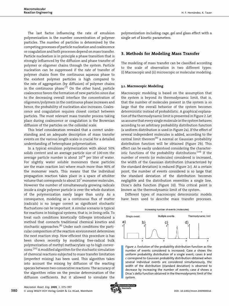
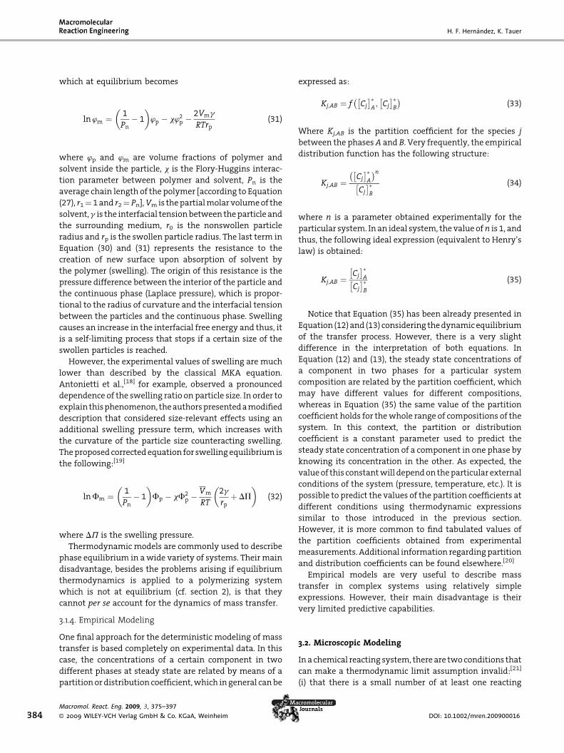
Figure 2. Evolution of the probability distribution function as thenumber of events considered is increased: Case a shows theuniform probability distribution of a single event; cases b andc correspond to Gaussian probability distribution obtained whenseveral individual events are considered simultaneously, thewidth of the distribution (standard deviation) is observed todecrease by increasing the number of events; case d shows aDirac’s delta function obtained in the thermodynamic limit of thesystem.
380
The last factor influencing the rate of emulsion
polymerization is the number concentration of polymer
particles. The number of particles is determined by the
competing processes of particle nucleation and coalescence
or coagulation andbothprocesses dependonmass transfer.
Particle nucleation is in principle a phase transition that is
strongly influenced by the diffusion and phase transfer of
polymer or oligomer chains through the system. Particle
nucleation can be suppressed if the rate of transfer of
polymer chains from the continuous aqueous phase to
the existent polymer particles is high compared to
the rate of aggregation (by diffusion) of polymer chains
in the continuous phase.[7] On the other hand, particle
coalescence favors the formation of newparticles since due
to the decreasing overall interface the concentration of
oligomers/polymers in the continuous phase increases and
hence, the probability of nucleation also increases. Coales-
cence and coagulation requires closest contact between
particles. The most relevant mass transfer process taking
place during coalescence or coagulation is the Brownian
diffusion of the particles on the colloidal scale.
This brief consideration revealed that a correct under-
standing and an adequate description of mass transfer
events on the various length scales is crucial for a detailed
understanding of heterophase polymerization.
In a typical emulsion polymerization with about 50%
solids content and an average particle size of 100nm the
average particle number is about 1018 per liter of water.
For slightly water soluble monomers these particles
are the main reaction loci where much more than 90% of
the monomer reacts. This means that the individual
propagation reaction takes place in a space of attoliter
volume that corresponds to about 107monomermolecules.
However the number of simultaneously growing radicals
inside a single polymer particle is over the whole duration
of the polymerization rarely larger than unity. As a
consequence, modeling as a continuous flux of matter
(radicals) is no longer correct as significant stochastic
fluctuations can be important. A similar scenario is typical
for reactions in biological systems, that is, in living cells. To
treat such conditions kinetically Gillespie introduced a
method that connects traditional chemical kinetics and
stochastic approaches.[8] Under such conditions the parti-
cular composition of the reaction environment determines
the next reaction step. How efficient this procedure is has
been shown recently by modeling free-radical bulk
polymerization of methyl methacrylate up to high conver-
sions.[25]Amodifiedalgorithmfor thestochastic simulation
of chemical reactions subjected tomass transfer limitation
(imperfect mixing) has been used. This algorithm takes
into account the mixing by diffusion of the reacting
species between two consecutive reactions. The accuracy of
the algorithm relies on the precise determination of the
diffusion coefficients. But it allowed to simulate the
Macromol. React. Eng. 2009, 3, 375–397
� 2009 WILEY-VCH Verlag GmbH & Co. KGaA, Weinheim
polymerization including cage, gel and glass effect with a
single set of kinetic parameters.
3. Methods for Modeling Mass Transfer
The modeling of mass transfer can be classified according
to the scale of observation in two different types:
(i) Macroscopic and (ii) microscopic or molecular modeling.
3.1. Macroscopic Modeling
Macroscopic modeling is based on the assumption that
the system is beyond its thermodynamic limit, that is,
that the number of molecules present in the system is so
large that the overall behavior of the system becomes
deterministic instead of probabilistic. A graphical explana-
tionof the thermodynamic limit is presented inFigure2. Let
usassumethat everysinglemolecule in thesystembehaves
according to an arbitrary probability distribution function
(a uniform distribution is used in Figure 2a). If the effect of
several independent molecules is added, according to the
central limit theorem[9] a normal or Gaussian probability
distribution function will be obtained (Figure 2b). This
effect can be easily understood considering the character-
istic functions of the probability distributions.[10] If the
number of events (or molecules) considered is increased,
the width of the Gaussian distribution (characterized by
the standard deviation) is reduced (Figure 2c). At a certain
point, the number of events considered is so large that
the standard deviation of the distribution becomes
negligible and the distribution resembles a single line,
Dirac’s delta function (Figure 2d). This critical point is
known as the thermodynamic limit of the system.
Different types of macroscopic deterministic models
have been used to describe mass transfer processes.
DOI: 10.1002/mren.200900016
Modeling of Molecular Transfer in Heterophase . . .
These models can be subdivided in (i) first principles,
(ii) semi-empirical, (iii) equilibrium thermodynamics, and
(iv) empirical models.
3.1.1. First-Principles Modeling
First-Principles or Fundamentalmodels ofmass transfer are
basedonthedifferential equationsobtainedbyFick[11] after
following the same method employed by Fourier to
describe heat transfer. Fick’s results for isotropic materials
can be summarized in two laws as follows:
Macrom
� 2009
Ji ¼ �Dir Ci½ � (15)
@ Ci½ � 2
@t¼ Dir Ci½ � (16)
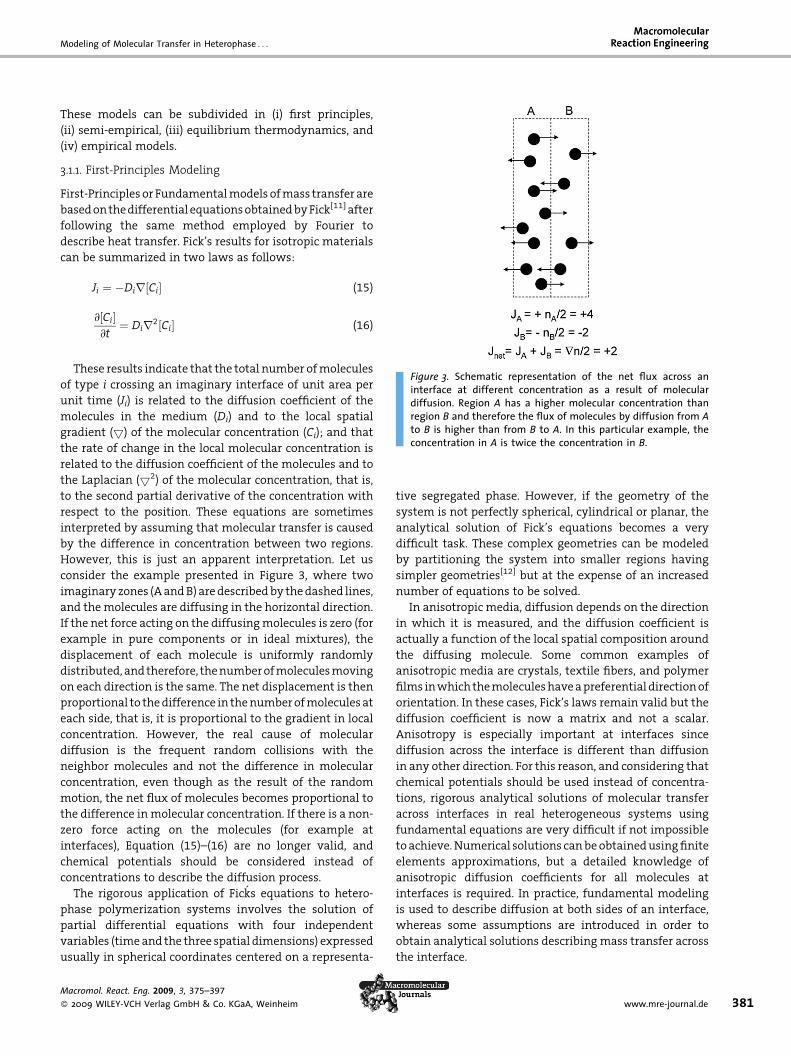
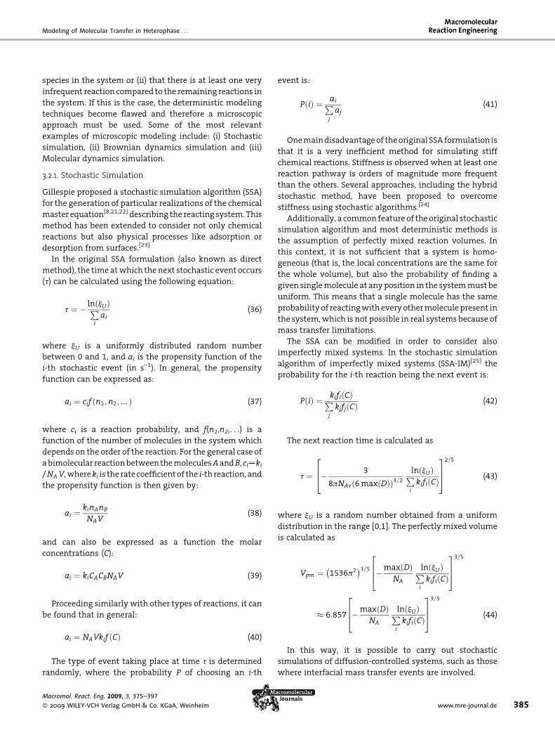
Figure 3. Schematic representation of the net flux across aninterface at different concentration as a result of moleculardiffusion. Region A has a higher molecular concentration thanregion B and therefore the flux of molecules by diffusion from Ato B is higher than from B to A. In this particular example, theconcentration in A is twice the concentration in B.
These results indicate that the total number ofmolecules
of type i crossing an imaginary interface of unit area per
unit time (Ji) is related to the diffusion coefficient of the
molecules in the medium (Di) and to the local spatial
gradient (5) of the molecular concentration (Ci); and that
the rate of change in the local molecular concentration is
related to the diffusion coefficient of the molecules and to
the Laplacian (52) of the molecular concentration, that is,
to the second partial derivative of the concentration with
respect to the position. These equations are sometimes
interpreted by assuming that molecular transfer is caused
by the difference in concentration between two regions.
However, this is just an apparent interpretation. Let us
consider the example presented in Figure 3, where two
imaginary zones (AandB) aredescribedby thedashed lines,
and themolecules are diffusing in the horizontal direction.
If the net force acting on the diffusingmolecules is zero (for
example in pure components or in ideal mixtures), the
displacement of each molecule is uniformly randomly
distributed, andtherefore, thenumberofmoleculesmoving
on each direction is the same. The net displacement is then
proportional to thedifference in thenumberofmolecules at
each side, that is, it is proportional to the gradient in local
concentration. However, the real cause of molecular
diffusion is the frequent random collisions with the
neighbor molecules and not the difference in molecular
concentration, even though as the result of the random
motion, the net flux of molecules becomes proportional to
the difference inmolecular concentration. If there is a non-
zero force acting on the molecules (for example at
interfaces), Equation (15)–(16) are no longer valid, and
chemical potentials should be considered instead of
concentrations to describe the diffusion process.
The rigorous application of Ficks equations to hetero-
phase polymerization systems involves the solution of
partial differential equations with four independent
variables (timeand the three spatial dimensions) expressed
usually in spherical coordinates centered on a representa-
ol. React. Eng. 2009, 3, 375–397
WILEY-VCH Verlag GmbH & Co. KGaA, Weinheim
tive segregated phase. However, if the geometry of the
system is not perfectly spherical, cylindrical or planar, the
analytical solution of Fick’s equations becomes a very
difficult task. These complex geometries can be modeled
by partitioning the system into smaller regions having
simpler geometries[12] but at the expense of an increased
number of equations to be solved.
In anisotropic media, diffusion depends on the direction
in which it is measured, and the diffusion coefficient is
actually a function of the local spatial composition around
the diffusing molecule. Some common examples of
anisotropic media are crystals, textile fibers, and polymer
films inwhich themoleculeshaveapreferential directionof
orientation. In these cases, Fick’s laws remain valid but the
diffusion coefficient is now a matrix and not a scalar.
Anisotropy is especially important at interfaces since
diffusion across the interface is different than diffusion
in any other direction. For this reason, and considering that
chemical potentials should be used instead of concentra-
tions, rigorous analytical solutions of molecular transfer
across interfaces in real heterogeneous systems using
fundamental equations are very difficult if not impossible
to achieve.Numerical solutions canbeobtainedusingfinite
elements approximations, but a detailed knowledge of
anisotropic diffusion coefficients for all molecules at
interfaces is required. In practice, fundamental modeling
is used to describe diffusion at both sides of an interface,
whereas some assumptions are introduced in order to
obtain analytical solutions describing mass transfer across
the interface.
www.mre-journal.de 381
H. F. Hernandez, K. Tauer
382
3.1.2. Semi-Empirical Modeling
A significant simplification of
Fick’s equations can be obtained
by assuming that the bulk of
eachphase (bothcontinuousand
segregated) isperfectlymixed. In
this case, mass transfer of a
certain molecular species is
expressed as a function of the
difference in concentration of
this species at both sides of the
interface, using semi-empirical
parameters denoted as local
mass transfer coefficients
(h)b.[13] A typical representation
of an interface is presented in
Figure 4. For this example, the
net flux of molecules across the
interface (Jj,Ab) can be calculated
as:
bLocalthe litfusionwhichcients.
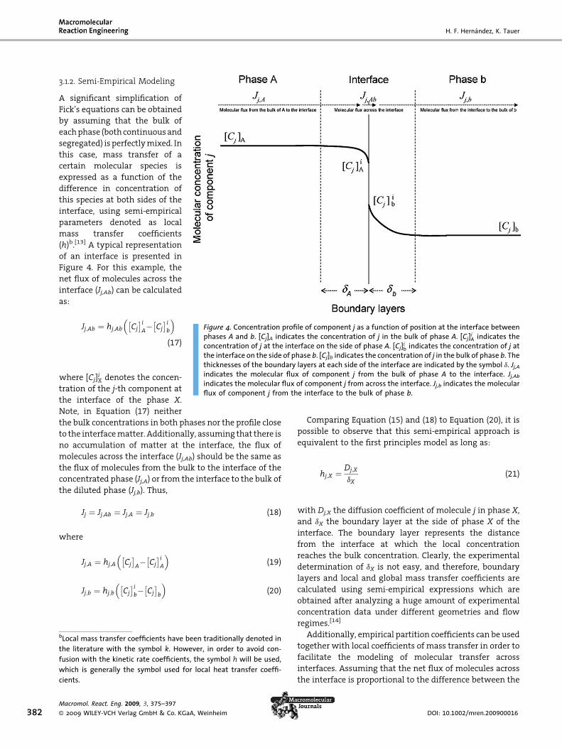
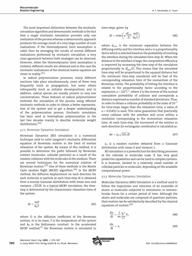
Figure 4. Concentration profile of component j as a function of position at the interface betweenphases A and b. [Cj]A indicates the concentration of j in the bulk of phase A. [Cj]i
A indicates theconcentration of j at the interface on the side of phase A. [Cj]i
b indicates the concentration of j atthe interface on the side of phase b. [C ] indicates the concentration of j in the bulk of phase b. The
Macrom
� 2009
Jj;Ab ¼ hj;Ab Cj
� �i
A� Cj
� �i
b
� �(17)
j b
thicknesses of the boundary layers at each side of the interface are indicated by the symbol d. Jj,Aindicates the molecular flux of component j from the bulk of phase A to the interface. Jj,Abindicates the molecular flux of component j from across the interface. Jj,b indicates the molecularflux of component j from the interface to the bulk of phase b.
where [Cj]iX denotes the concen-
tration of the j-th component at
the interface of the phase X.
Note, in Equation (17) neither
the bulk concentrations in both phases nor the profile close
to the interfacematter. Additionally, assuming that there is
no accumulation of matter at the interface, the flux of
molecules across the interface (Jj,Ab) should be the same as
the flux of molecules from the bulk to the interface of the
concentrated phase (Jj,A) or from the interface to the bulk of
the diluted phase (Jj,b). Thus,
Jj ¼ Jj;Ab ¼ Jj;A ¼ Jj;b (18)
where
Jj;A ¼ hj;A Cj
� �A� Cj
� �i
A
� �(19)
J ¼ h C� �i � C
� �� �(20)
j;b j;b j b j bmass transfer coefficients have been traditionally denoted inerature with the symbol k. However, in order to avoid con-with the kinetic rate coefficients, the symbol h will be used,is generally the symbol used for local heat transfer coeffi-
ol. React. Eng. 2009, 3, 375–397
WILEY-VCH Verlag GmbH & Co. KGaA, Weinheim
Comparing Equation (15) and (18) to Equation (20), it is
possible to observe that this semi-empirical approach is
equivalent to the first principles model as long as:
hj;X ¼ Dj;X
dX(21)
with Dj,X the diffusion coefficient of molecule j in phase X,
and dX the boundary layer at the side of phase X of the
interface. The boundary layer represents the distance
from the interface at which the local concentration
reaches the bulk concentration. Clearly, the experimental
determination of dX is not easy, and therefore, boundary
layers and local and global mass transfer coefficients are
calculated using semi-empirical expressions which are
obtained after analyzing a huge amount of experimental
concentration data under different geometries and flow
regimes.[14]
Additionally, empirical partition coefficients can be used
together with local coefficients of mass transfer in order to
facilitate the modeling of molecular transfer across
interfaces. Assuming that the net flux of molecules across
the interface is proportional to the difference between the
DOI: 10.1002/mren.200900016
Modeling of Molecular Transfer in Heterophase . . .
actual bulk concentration of the j-th component in phase A
and the concentration that must be present in A (½Cj�bA) inorder to reach equilibrium with the corresponding con-
centration in the bulk of phase b ([Cj]b), then
Macrom
� 2009
Jj ¼ Hj;Ab Cj
� �A� Cj
� �b
A
� �(22)
where Hj,Ab is another semi-empirical parameter called the
global mass transfer coefficient. The global mass transfer
coefficient can then be related to the local mass transfer
coefficients at both sides of the interface, Equation (18)–
(20), resembling two electrical resistances in series,
according to the following expressions:[13]
Jj
Hj;Ab¼ Jj
hj;Aþ Jj
hj;b
Cj
� �i
A� Cj
� �b
A
Cj
� �i
b� Cj
� �b
(23)
1 1 mij;Ab
Hj;Ab¼
hj;Aþ
hj;b(24)
where
mij;Ab ¼
Cj
� �i
A� Cj
� �b
A
Cj
� �i
b� Cj
� �b
(25)
mij,Ab can be regarded as the slope of a straight line
intercepting the equilibrium curve at the concentrations
[Cj]ib and [Cj]b. If the equilibrium curve can be assumed to
be linear, then the variable mij,Ab will be equivalent to the
equilibrium partition coefficient (Kj,Ab).
This type of modeling is widely used to describe
macroscopic mass transfer processes across interfaces. It
requires theknowledgeofmass transfer coefficients (which
can be estimated from semi-empirical correlations) and
equilibrium distribution coefficients.
3.1.3. Equilibrium Thermodynamics Modeling
A further simplification of themass transfer process can be
madeonce steady state conditionshavebeen reached in the
system, that is, when the net flux across all interfaces
becomes zero. Under these conditions, even though the
individual fluxes of molecules are not zero, it is frequently
assumed that the system has reached thermodynamic
equilibrium. As it was introduced already in Section 2, the
most relevant thermodynamic effects are basically enthal-
pic or entropic. In ideal mixtures there are no enthalpic
effects and mixing occurs spontaneously as a result of the
entropy increase. Ideal mixtures are always homogeneous
systems. In non-ideal mixtures, phase separation can take
place and an equilibrium condition is reached when both
entropic and enthalpic contributions to the free energy of
the system exactly counteract each other. This is the
ol. React. Eng. 2009, 3, 375–397
WILEY-VCH Verlag GmbH & Co. KGaA, Weinheim
principle used by Flory and Huggins to describe polymer
solutions,[15] which can be used in general to describe the
thermodynamics of mixtures of species with different
molecularweights. The change in free energy ofmixing can
be expressed as:
DGmix ¼ DHmix � TDSmix (26)
The Flory-Huggins approach, considering a rigid lattice
model, produces the following expression for a two-
component system:[16]
DGmix ¼ RTðN1 ln’1 þ N2 ln ’2
þ ’1’2ðr1N1 þ r2N2Þx12Þ (27)
where Ni is the number of molecules of component i in the
system, wi is the segment fraction of i component, ri is the
number of segments of the lattice per molecule of i
component, and xij is the Flory-Huggins interaction
parameter, related to the intermolecular interaction
energies as follows:
xij /2"ij � "ii � "jj
T(28)
where eij is the interaction energy between molecules
i and j.
From Equation (27), the chemical potential of mixing of
the solvent/monomer (m1) can be obtained as the partial
molar free energy of mixing:
Dm1 ¼ @DGmix
@N1
� �T;P;N2
¼ RT ln ’1 þ 1� r1r2
� �’2 þ r1’
22x12
� �(29)
Normally, the Flory-Huggins interaction parameter is
used as an adjustable, temperature- and concentration-
dependent empirical parameter.
Morton, Kaizermann and Altier applied the Flory-
Huggins approach to the swelling of latex particles in the
presence of a bulk phase of pure swelling agent considering
an additional term corresponding to the free energy
contribution of the interfaces. They obtained an equation
which is now known as the Morton-Kaizermann-Altier
(MKA) equation:[17]
Dm1
RT¼ lnð’mÞ þ ’p 1� 1
Pn
� �þ x’2p
þ2Vmg’
1=3p
r0RT(30)
www.mre-journal.de 383
H. F. Hernandez, K. Tauer
384
which at equilibrium becomes
Macrom
� 2009
ln ’m ¼ 1
Pn� 1
� �’p � x’2p �
2Vmg
RTrp(31)
where wp and wm are volume fractions of polymer and
solvent inside the particle, x is the Flory-Huggins interac-
tion parameter between polymer and solvent, Pn is the
average chain length of the polymer [according to Equation
(27), r1¼ 1and r2¼ Pn],Vm is thepartialmolar volumeof the
solvent, g is the interfacial tensionbetween theparticle and
the surrounding medium, r0 is the nonswollen particle
radius and rp is the swollen particle radius. The last term in
Equation (30) and (31) represents the resistance to the
creation of new surface upon absorption of solvent by
the polymer (swelling). The origin of this resistance is the
pressure difference between the interior of the particle and
the continuous phase (Laplace pressure), which is propor-
tional to the radius of curvature and the interfacial tension
between the particles and the continuous phase. Swelling
causes an increase in the interfacial free energy and thus, it
is a self-limiting process that stops if a certain size of the
swollen particles is reached.
However, the experimental values of swelling are much
lower than described by the classical MKA equation.
Antonietti et al.,[18] for example, observed a pronounced
dependence of the swelling ratio on particle size. In order to
explain thisphenomenon, theauthorspresentedamodified
description that considered size-relevant effects using an
additional swelling pressure term, which increases with
the curvature of the particle size counteracting swelling.
Theproposed corrected equation for swellingequilibriumis
the following:[19]
lnFm ¼ 1
Pn� 1
� �Fp � xF2
p �Vm
RT
2g
rpþ DP
� �(32)
where DP is the swelling pressure.
Thermodynamic models are commonly used to describe
phase equilibrium in awide variety of systems. Theirmain
disadvantage, besides the problems arising if equilibrium
thermodynamics is applied to a polymerizing system
which is not at equilibrium (cf. section 2), is that they
cannot per se account for the dynamics of mass transfer.
3.1.4. Empirical Modeling
One final approach for the deterministic modeling of mass
transfer is based completely on experimental data. In this
case, the concentrations of a certain component in two
different phases at steady state are related by means of a
partitionor distribution coefficient,which in general canbe
ol. React. Eng. 2009, 3, 375–397
WILEY-VCH Verlag GmbH & Co. KGaA, Weinheim
expressed as:
Kj;AB ¼ f Cj
� ��A; Cj
� ��B
� �(33)
Where Kj,AB is the partition coefficient for the species j
between the phases A and B. Very frequently, the empirical
distribution function has the following structure:
Kj;AB ¼Cj
� ��A
� �n
Cj
� ��B
(34)
where n is a parameter obtained experimentally for the
particular system. In an ideal system, the value ofn is 1, and
thus, the following ideal expression (equivalent to Henry’s
law) is obtained:
Kj;AB ¼Cj
� ��A
Cj
� ��B
(35)
Notice that Equation (35) has been already presented in
Equation (12)and (13) considering thedynamicequilibrium
of the transfer process. However, there is a very slight
difference in the interpretation of both equations. In
Equation (12) and (13), the steady state concentrations of
a component in two phases for a particular system
composition are related by the partition coefficient, which
may have different values for different compositions,
whereas in Equation (35) the same value of the partition
coefficient holds for thewhole range of compositions of the
system. In this context, the partition or distribution
coefficient is a constant parameter used to predict the
steady state concentration of a component in one phase by
knowing its concentration in the other. As expected, the
valueof this constantwill dependon theparticular external
conditions of the system (pressure, temperature, etc.). It is
possible to predict the values of the partition coefficients at
different conditions using thermodynamic expressions
similar to those introduced in the previous section.
However, it is more common to find tabulated values of
the partition coefficients obtained from experimental
measurements. Additional information regardingpartition
and distribution coefficients can be found elsewhere.[20]
Empirical models are very useful to describe mass
transfer in complex systems using relatively simple
expressions. However, their main disadvantage is their
very limited predictive capabilities.
3.2. Microscopic Modeling
In a chemical reacting system, there are twoconditions that
can make a thermodynamic limit assumption invalid:[21]
(i) that there is a small number of at least one reacting
DOI: 10.1002/mren.200900016
Modeling of Molecular Transfer in Heterophase . . .
species in the system or (ii) that there is at least one very
infrequent reaction compared to the remaining reactions in
the system. If this is the case, the deterministic modeling
techniques become flawed and therefore a microscopic
approach must be used. Some of the most relevant
examples of microscopic modeling include: (i) Stochastic
simulation, (ii) Brownian dynamics simulation and (iii)
Molecular dynamics simulation.
3.2.1. Stochastic Simulation
Gillespie proposed a stochastic simulation algorithm (SSA)
for the generation of particular realizations of the chemical
master equation[8,21,22] describing the reacting system. This
method has been extended to consider not only chemical
reactions but also physical processes like adsorption or
desorption from surfaces.[23]
In the original SSA formulation (also known as direct
method), the timeatwhich thenext stochastic event occurs
(t) can be calculated using the following equation:
Macrom
� 2009
t ¼ � lnðjUÞPi
ai(36)
where jU is a uniformly distributed random number
between 0 and 1, and ai is the propensity function of the
i-th stochastic event (in s–1). In general, the propensity
function can be expressed as:
ai ¼ cif ðn1;n2; ::; Þ (37)
where ci is a reaction probability, and f(n1,n2,. . .) is a
function of the number of molecules in the system which
depends on the order of the reaction. For the general case of
abimolecular reactionbetweenthemoleculesAandB, ci ki
/NA V,whereki is the rate coefficientof the i-th reaction, and
the propensity function is then given by:
ai ¼kinAnB
NAV(38)
and can also be expressed as a function the molar
concentrations (C):
ai ¼ kiCACBNAV (39)
Proceeding similarly with other types of reactions, it can
be found that in general:
ai ¼ NAVkif ðCÞ (40)
The type of event taking place at time t is determined
randomly, where the probability P of choosing an i-th
ol. React. Eng. 2009, 3, 375–397
WILEY-VCH Verlag GmbH & Co. KGaA, Weinheim
event is:
PðiÞ ¼ aiPj
aj(41)
Onemaindisadvantageof theoriginal SSAformulation is
that it is a very inefficient method for simulating stiff
chemical reactions. Stiffness is observed when at least one
reaction pathway is orders of magnitude more frequent
than the others. Several approaches, including the hybrid
stochastic method, have been proposed to overcome
stiffness using stochastic algorithms.[24]
Additionally, a common feature of the original stochastic
simulation algorithm and most deterministic methods is
the assumption of perfectly mixed reaction volumes. In
this context, it is not sufficient that a system is homo-
geneous (that is, the local concentrations are the same for
the whole volume), but also the probability of finding a
given singlemolecule at anyposition in the systemmustbe
uniform. This means that a single molecule has the same
probabilityof reactingwitheveryothermoleculepresent in
the system,which is not possible in real systems because of
mass transfer limitations.
The SSA can be modified in order to consider also
imperfectly mixed systems. In the stochastic simulation
algorithm of imperfectly mixed systems (SSA-IM)[25] the
probability for the i-th reaction being the next event is:
PðiÞ ¼ kifiðCÞPj
kjfjðCÞ(42)
The next reaction time is calculated as
t ¼ � 3
8pNAv 6maxðDÞð Þ3=2lnðjUÞP
i
kifiðCÞ
264
3752=5
(43)
where jU is a random number obtained from a uniform
distribution in the range [0,1]. The perfectly mixed volume
is calculated as
Vpm ¼ 1536p2� �1=5 �maxðDÞ
NA
lnðjUÞPi
kifiðCÞ
264
3753=5
� 6:857 �maxðDÞNA
lnðjUÞPi
kifiðCÞ
264
3753=5
(44)
In this way, it is possible to carry out stochastic
simulations of diffusion-controlled systems, such as those
where interfacial mass transfer events are involved.
www.mre-journal.de 385
H. F. Hernandez, K. Tauer
386
The most important distinction between the stochastic
simulation algorithmanddeterministicmethods is the fact
that a single stochastic simulation provides only one
realization of theprocesswhereas adeterministic approach
produces the average result of a very large number of such
realizations. If the thermodynamic limit assumption is
valid, then by averaging the results of several different
realizations performed by stochastic simulation, a very
close agreement between both strategies can be observed.
However, when the thermodynamic limit assumption is
violated, different results are obtained and in this case the
stochastic realizations of the chemical master equation are
closer to reality.[21]
In radical polymerization processes, many different
reactions take place simultaneously, some of them very
frequently (such as propagation), but some others
infrequently (such as initiator decomposition), and in
addition, radical species are usually present in very low
concentrations. These features of radical polymerization
motivate the simulation of the process using efficient
stochastic methods in order to obtain a better representa-
tion of the system and to get a deeper understanding
of the polymerization process. Stochastic simulation
has been used in heterophase polymerization in the
last two decades mainly to describe molecular weight
distributions.[26]
3.2.2. Brownian Dynamics Simulation
Brownian Dynamics (BD) simulation is a numerical
technique used to solve Langevin’s stochastic differential
equation of Brownian motion in the limit of motion
relaxation of the system. By means of this method, it is
possible to determine the paths followed by Brownian
entities (molecules, colloidal particles) as a result of the
randomcollisionswith themolecules in themedium. There
are several techniques for the numerical solution of
Brownian motion.[27] One of these methods is the Monte
Carlo random flight (MCRF) algorithm.[28] In the MCRF
method, the diffusive displacement on each direction for
each molecule or particle at each time-step dt is obtained
from a normal Gaussian distribution with mean zero and
varianceffiffiffiffiffiffiffiffiffiffiffiffi2Ddt
p. In a typical MCRF simulation, the time-
step is determined by the characteristic relaxation time of
the system:
Macrom
� 2009
dt ¼ mD
kBT(45)
where D is the diffusion coefficient of the Brownian
entities, m is its mass, T is the temperature of the system
and kB is the Boltzmann constant. In the accelerated
MCRF method,[7] the Brownian motion is simulated in
ol. React. Eng. 2009, 3, 375–397
WILEY-VCH Verlag GmbH & Co. KGaA, Weinheim
time-steps given by
dt ¼ max ad2min
D;
mD
kBT
� �(46)
where dmin is the minimum separation between the
diffusing entity and the interface and a is a proportionality
factorwhich is selectedbasedon theprobabilityof reaching
the interface during the simulated time-step dt. When the
distance to the interface is large, the computationefficiency
is improved by increasing the time step of the simulation
proportionally to d2min/D. This means that the simulated
time-step will be proportional to the squared distance but
the minimum time-step considered will be that of the
corresponding relaxation time of the momentum of the
Brownian entity. The probability of hitting the interface is
related to the proportionality factor according to the
expression a¼ (2Z2)–1, where Z is the inverse of the normal
cumulative probability of collision and corresponds a
distance expressed asnumber of standarddeviations. Thus,
in order to obtain a collision probability in the order of 10–7
for time-steps larger than the relaxation time, a value of
a¼ 0.01852 is used. This value guarantees that practically
every collision with the interface will occur within a
resolution corresponding to the momentum relaxation
time. At each time-step, the movement of the entities in
each direction (in rectangular coordinates) is calculated as:
dx ¼ jG
ffiffiffiffiffiffiffiffiffiffiffiffiffi2Dr dt
p(47)
jG is a random number obtained from a Gaussian
distribution with mean 0 and variance 1.
BD simulation is a powerful tool for describing processes
at the colloidal or molecular scale. It has very good
predictive capabilities and can be used in complex systems.
It is however, limited to a relatively small number of
colloidal particles ormolecules, depending on the available
computational power.
3.2.3. Molecular Dynamics Simulation
Molecular Dynamics (MD) Simulation is a method used to
follow the trajectories and velocities of an ensemble of
atoms or molecules subjected to interatomic or intermo-
lecular forces for a certain period of time. Although the
atoms and molecules are composed of quantum particles,
their motion can be satisfactorily described by the classical
equations of motion:[29]
dvi
dt¼ 1
mi
Xj6¼i
Fij (48)
dxi ¼ vi (49)
dtDOI: 10.1002/mren.200900016
Modeling of Molecular Transfer in Heterophase . . .
where vi is the velocity, mi is the mass and xi is the
position of the i-th molecule, Fij is the interaction
force between the i-th and j-th molecules, and t is the
time. Additional external or internal (mean field) forces
can also be considered.
MD simulation can also be used to model mass transfer
in a system at the molecular scale. MD offers the most
accuratepictureofthemoleculartransferprocesses;however,
it is extremely computational demanding and today, it can
only be used to simulate relatively small systems.
3.3. Multiscale Simulation
Finally, it isworthmentioning a new trend in themodeling
of complex systems, which consists in the integration of
different simulationmethods for describing thebehavior of
the system at widely different time and length scales. This
integration is usually known as multiscale simulation.
Multiscale simulation can be defined as the enabling
technology of science and engineering that links phenom-
ena, models and information between various scales of
complex systems.[30] Growth in a number of critical
technological areas, such as nanotechnology, biotechnol-
ogy and microscale systems, may be accelerated and
catalyzed by such multiscale modeling and computational
paradigm.[31] The challenge in multiscale simulation is the
seamless coupling between the various models while
meeting conservation-laws, numerical convergence, stabi-
lity and computational speed. For example, MD simulation
is a very good alternative for the determination of
molecular diffusion coefficients, which can then be used
in first-principles or in BD simulations to describe mass
transfer at larger scales.[32] In general for complex systems,
not a single method should be used to describe all the
processes taking place simultaneously at very different
time and length scales. In particular for heterophase
polymerization, multiscale simulation has already been
shown to be a valuable technique to obtain more precise
descriptions of the process.[7,33]
4. Relevant Molecular Transfer Processes inHeterophase Polymerization
In this Section, some examples of the use of different
modeling strategies for describing mass transfer in hetero-
phase polymerization, and in particular in free-radical
emulsion polymerization, are presented.
4.1. Molecular Absorption: Radical Entry
In an emulsion polymerization process the simultaneous
highmolecularweight andhighpolymerization rate is only
Macromol. React. Eng. 2009, 3, 375–397
� 2009 WILEY-VCH Verlag GmbH & Co. KGaA, Weinheim
possible to achieve if the polymer particles contain an odd
number of low-molecular-weight radicals. In this case, at
least one single radical will always survive termination
and continue to propagate until the monomer in the
particle is depleted. The presence of an odd number of
radicals inside theparticles ispossible thanks to thetransfer
of the activity of single radicals from the continuous
phase to the polymer particle (radical capture), or from the
polymer particle to the continuous phase (radical deso-
rption). The free radicals transferred from one phase to the
other can be primary radicals (generated after the separa-
tion of paired electrons) or growing chains (formed after
the propagation of primary radicals) of any length.[34] The
phase-transfer process of a radical takes place when a
radical reaches the interface between the polymer particle
and the continuous phase and its kinetic energy is high
enough to overcome the resistance to transfer at the
interface.
Different mechanisms have been proposed as rate-
determining steps in order to describe the kinetics of
radical capture by polymer particles:
� C
ollisional mechanism. The limiting step for theabsorption of radicals is assumed to be the ballistic
collision between the radicals and the polymer particles.
In this case, the rate of radical capture is proportional to
the surface area of the polymer particles.[35] This
approach is based on fundamental principles assuming
a ballistic motion of the radicals. The rate of radical
capture in this case is given by
r ¼ pkBT
2m
� �1=2
d2pNA R½ �wNp (50)
where kB is Boltzmann constant, T is temperature and m is
the mass of the entering radical.
� D
iffusion-controlled mechanism. Given that both radi-cals and particles are suspended in a continuous
condensed phase (water), it is likely improbable that
they can follow perfect ballistic trajectories without
colliding with water molecules, resulting in a change in
their directions and velocities. As a result of themultiple
collisions with the continuous-phase molecules, the
overall displacement of the radicals and particles is not
ballistic but diffusional. For diluted dispersions of
polymer particles, the rate of collision by diffusion is
given by Smoluchowski equation:[36]
r ¼ 2pDwdpNA R½ �wNp (51)
where Dw is the diffusion coefficient of the radicals in the
continuous phase, dp is the diameter of the particles, [R]w is
themolarconcentrationof radicals inthecontinuousphase.
www.mre-journal.de 387
H. F. Hernandez, K. Tauer
388
In this case, the rate of radical capture depends linearly on
the particle diameter. Equation (51) is the analytical
solution of the fundamental Fick’s equations applied to a
singleparticledispersed inan infinitemedium.Considering
thatnoteverycollisionbetweenradicalandparticle leads to
a radical absorption event, and that not every absorbed
radical reacts inside the particle affecting the kinetics of
polymerization, a rate-reduction factor or an absorption
efficiency factor (F) is included in the model:[37]
Macrom
� 2009
r ¼ 2pDwdpNA R½ �wNpF (52)
F represents the absorption efficiency factor that
describes the degree to which absorption is lowered
compared to irreversible capture, which can be given by
F ¼ 1
Dw
KReqDp X cothX � 1ð Þ
� �þ W 0
(53)
where X ¼ dp
2
ffiffiffiffiffiffiffiffiffiffiffiffiffiffiffiffiffiffiffiffiffiffiffiffiffiffiffiffiffiffiffiffiffiffiffiffiffiffikp M½ �pþktpðn=vpÞ
Dp
sand KReq is the equili-
briumpartition coefficient of radicals between theparticles
and water, W’ is the potential energy barrier, Dp is the
diffusion coefficient for the radicals inside the particle, kp is
the propagation rate constant, [M]p is the monomer
concentration in particles, n is the number of radicals per
particle, NA is Avogadro’s number and vp is the particle
volume. A different expression for the efficiency factorwas
proposed by Nomura:[38]
F ¼kp M½ �pþktpðn=vpÞ
ko þ kp M½ �pþktpðn=vpÞ(54)
where ko is the overall radical desorption rate constant for a
particle.
� C
olloidal mechanism. Penboss et al.[39] considered thatthe polymer particles are electrostatically-stabilized
polymer colloids and used the DLVO theory to determine
the rate of radical absorption by colloidal aggregation.
The resulting dependence of the rate of radical capture to
the size of the particles was found to be approximately
linear:
r ¼ pDwdr dp þ dr
� �NA R½ �wNpk exp � Em
kBT
� �(55)
where dr is the diameter of the radical, k is the reciprocal of
the Debye length and Em is the energy barrier (electrostatic
repulsion) of the capture process. This expression has been
ol. React. Eng. 2009, 3, 375–397
WILEY-VCH Verlag GmbH & Co. KGaA, Weinheim
obtained also from Fick’s equations in infinitely diluted
dispersions, but considering stabilization only by electro-
static repulsion. It is therefore very similar to the diffusion-
controlled mechanism, Equation (52).
� P
ropagation-controlled mechanism. Maxwell et al.[40]proposed that the rate-determining step is the growth of
the radicals in the continuous phase up to a certain
critical chain-length after which the capture process is
imminent. According to this model, only oligomeric
radicals of a critical chain length can enter the particles,
and these radicals do not participate in any other
reaction. Entry is independent of particles’ size and
charge. The rate of radical capture assuming a propaga-
tion-controlled mechanism is:
r ¼ NAkpw
NIMz�1½ � M½ �w (56)
where kpw is the propagation rate constant in the aqueous
phase, [M]w is the monomer concentration in the aqueous
phase and N is the concentration of particles in the
dispersion. By substituting the steady-state concentration
of (z–1)-mer radicals [IMz–1], the approximate expressions
for r and the initiator efficiency, fentry are:
r ¼ 2NAkd I½ �N
ffiffiffiffiffiffiffiffiffiffiffiffiffiffiffiffikd I½ �ktw
pkpw M½ �w
þ 1
( )1�z
¼ 2NAkd I½ �N
fentry (57)
ffiffiffiffiffiffiffiffiffiffiffiffiffiffiffiffip( )1�z
fentry ¼ kd I½ �ktw
kpw M½ �wþ 1 (58)
where z� 1þ int(–23 kJ �mol–1/(RT ln[Msat]w)) is the critical
chain length for irreversible capture.
� M
olecular stochastic simulation. BD simulation has alsobeen used to determine capture rate coefficients.[41,42]
The ratio between the collision rate coefficient obtained
by BD simulation (kc) and the ideal rate coefficient given
by Smoluchowski’s equation, Equation (51), is defined as
Smoluchowski number (Sm):
Sm ¼ kc
2pDrdpNA(59)
At very low volume fractions of polymer particles
BD simulation predicts the collision rate coefficient
obtained with the Smoluchowski equation (Sm¼ 1),
while for concentrated polymer dispersions (volume
fractions> 0.1%) the Smoluchowski number, and there-
DOI: 10.1002/mren.200900016
Modeling of Molecular Transfer in Heterophase . . .
fore the capture rate coefficient, presents a linear
dependencewith respect to the volume fraction of polymer
particles in the dispersion.
Macrom
� 2009
Sm ¼ yfp þ 1 (60)
where y is a dimensionless constant obtained for the
system under the particular conditions considered in the
simulation and fp is the volume fraction of particles in
the dispersion.
Similar conclusions were obtained by Rzepiela et al.,[43]
who found that the rate of aggregation of colloidal particles
obtained by simulation always exceeds the value predicted
by Smoluchowski theory for fast aggregation, and only for
volumefractionsbelowabout0.1%thediscrepancy is small.
The values of the rate of radical absorption obtained by BD
simulation under a wide range of conditions were used to
obtain the following semi-empirical expression:
kc ¼ 2pDrNA
ypNd4p
6þ dp
!(61)
Thismeans that the effect of polymer volume fraction on
collision kinetics under diffusion-controlled conditions
explains the different results obtained during the experi-
mental determination of radical capture kinetics in
emulsion polymerization.[41]
Interaction forces, interfacial tensions, the presence of
stabilizer molecules at the surface of the polymer particles
and many other physical and chemical effects may lead to
an increase in free energy during radical capture, and thus,
to the existence of an energy barrier for radical capture. In
these cases, only a fraction of the radicals collidingwith the
particles will be effectively captured (capture efficiency)
and the other will bounce back. When a radical is not
captured by a particle because of the energy barrier, the
radical will remain close to the particle surface and
therefore it will have a very high probability of hitting
the same particle again, leading to a series of multiple
collisions in a very short time before the radical goes away
from the particle surface. BD simulations show that the
effect of the magnitude of the energy barrier at different
temperatures on the capture efficiency canbedescribed ina
general way as:[42]
kc ¼kc0 ; E < E�
kc0e�ðE � E�Þ3RT ; E � E�
8<: (62)
where kc0 is the capture rate coefficient in the absence of
energybarriers, Equation (61), and E� is themagnitude of an
apparent threshold energy caused by multiple collisions
between a radical and a polymer particle.
ol. React. Eng. 2009, 3, 375–397
WILEY-VCH Verlag GmbH & Co. KGaA, Weinheim
4.2. Molecular Desorption: Radical Exit
The process of radical desorption can be regarded as the
opposite to radical capture. In this case, a free radical is
transferred from the interior of the particles to the
continuous phase. The mechanism by which this transfer
takes place is also similar: the radical must reach the
particle surface and then it must overcome the barrier for
desorption exerted by the interface. Desorption results in a
decrease in the concentrationof radicals in theparticles and
hence causes the rate of polymerization to decrease. For
many importantemulsionpolymerizationsystems, exit is a
major (if not the only) cause of the loss of free-radical
activity inside a particle.
Ugelstad et al.[44]were the first to propose that the rate of
radical desorptionwas inverselyproportional to thesurface
of the particle, although quantitative results were not
available. Nomura andHarada,[45] aware of the necessity of
estimating quantitatively the rate coefficient for radical
desorption from the particles for the prediction of rates of
emulsion polymerization, developed the first quantitative
modelof radicaldesorptionusingasemi-empiricalmodelof
interfacial mass transfer. They continued improving this
model during more than one decade. Asua et al.[46] com-
plemented themodel of desorption by considering the fate
of the radicals in the aqueous phase. Further improvements
of the semi-empirical model have been proposed by
considering the layer of stabilizer around electrosterically
stabilized polymer particles as an additional resistance to
the desorption process.[47] The semi-empirical macroscopic
model of equilibrium radical desorption developed by
Nomura and coworkers has been widely used to describe
radical desorption in heterophase polymerization. How-
ever, the thermodynamic limit assumption involved in the
derivation of this model may not be fulfilled by a radical
desorption process in a real emulsion polymerization
system, because in this case the radicals are present in a
very low concentration inside or around the particles.
The diffusion-controlled mechanism for radical deso-
rption is widely accepted right now, but there are minor
differences regarding the mathematical treatment of the
problem leading to different expressions for the rate of
radical desorption; however, all of them predict the same
inverse dependence on the surface area of theparticles. One
of the reasons for the use of different expressions is caused
by different interpretations of the desorption process. In
order to avoid confusion, the following types of desorption
are considered:[48]
� S
imple radical desorption. It is the result of the diffusivemotion of the radicals when no reactions are considered
inside the polymer particles. The rate coefficient of
simple radical desorption (k0) is determined by the
velocity at which the radical diffuses out of the particle
and it is a function of the particle size (dp) and
www.mre-journal.de 389
H. F. Hernandez, K. Tauer
390
the diffusion coefficient of the radical inside the polymer
particle (Dp):
Macrom
� 2009
k0 ¼ lDp
d2p
(63)
where l is a constant with a value of 60.
� E
quilibrium radical desorption. The equilibriumdesorption of a radical takes into account the different
solubility of the radicals between the polymer particles
and the aqueous phase. The rate coefficient of equili-
brium radical desorption (k0�) can be related to the
simple radical desorption rate coefficient by:
k�0 ¼ k0
1þ KeqDp
Dw
dw
dp
� � (64)
where Dw is the diffusion coefficient of the radical in the
aqueous phase, Keq is the partition coefficient of the radical
between the polymer particle and the aqueous phase, dw is
the thickness of the stagnant layer in the aqueous phase
and dp is the thickness of the diffusion layer in the polymer
phase.
� N
et radical desorption. The net desorption of a radicaloccurs when the radical escapes the polymer particle
after surviving the competitive reactions taking place
inside. The rate coefficient of net radical desorption (K0)
is determined by:
K0 ¼ krgen þ r� �
� k�0
k�0 þ
Pi
ki;p(65)
where ki,p is the rate of the i-th reaction involving radicals
and krgen is the rate of generation of desorbing radicals
inside the particle.
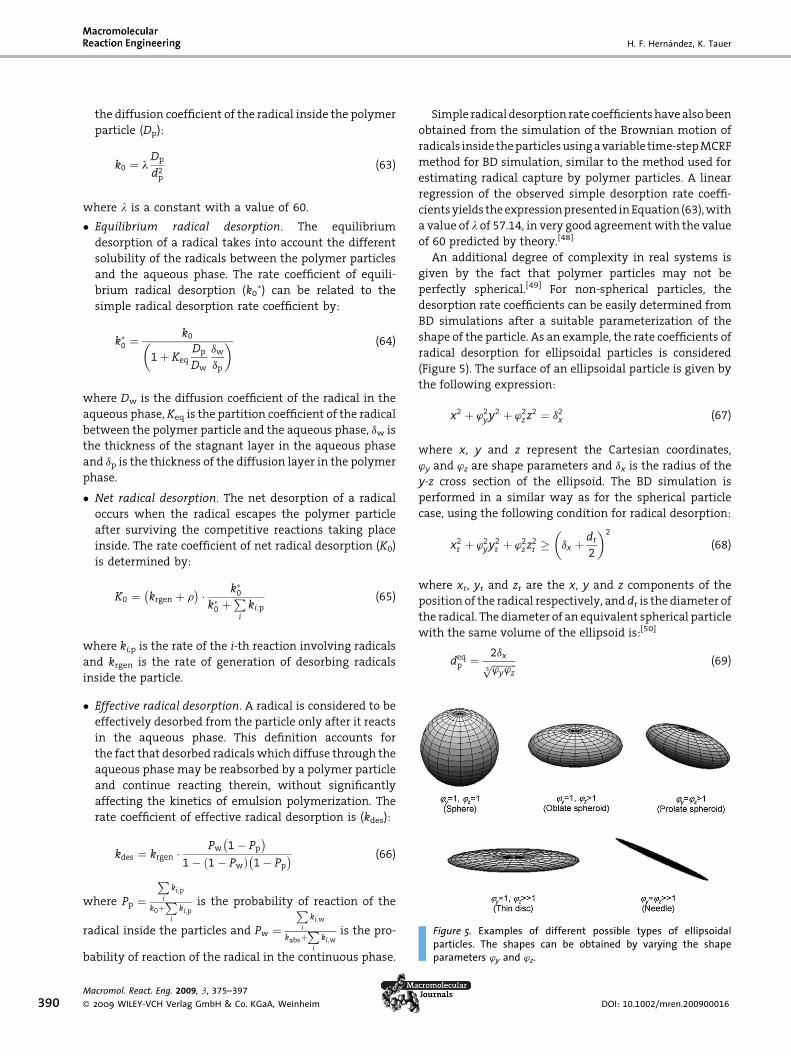
� E
ffective radical desorption. A radical is considered to beeffectively desorbed from the particle only after it reacts
in the aqueous phase. This definition accounts for
the fact that desorbed radicalswhich diffuse through the
aqueous phase may be reabsorbed by a polymer particle
and continue reacting therein, without significantly
affecting the kinetics of emulsion polymerization. The
rate coefficient of effective radical desorption is (kdes):
kdes ¼ krgen �Pw 1� Pp
� �1� 1� Pwð Þ 1� Pp
� � (66)
P
Figure 5. Examples of different possible types of ellipsoidalparticles. The shapes can be obtained by varying the shapeparameters wy and wz.
where Pp ¼ i
ki;p
k0þP
i
ki;pis the probability of reaction of the
radical inside the particles and Pw ¼
Pi
ki;w
kabsþP
i
ki;wis the pro-
bability of reaction of the radical in the continuous phase.
ol. React. Eng. 2009, 3, 375–397
WILEY-VCH Verlag GmbH & Co. KGaA, Weinheim
Simple radical desorption rate coefficientshavealsobeen
obtained from the simulation of the Brownian motion of
radicals inside theparticlesusingavariable time-stepMCRF
method for BD simulation, similar to the method used for
estimating radical capture by polymer particles. A linear
regression of the observed simple desorption rate coeffi-
cientsyields theexpressionpresented inEquation (63),with
a value of l of 57.14, in very good agreementwith the value
of 60 predicted by theory.[48]
An additional degree of complexity in real systems is
given by the fact that polymer particles may not be
perfectly spherical.[49] For non-spherical particles, the
desorption rate coefficients can be easily determined from
BD simulations after a suitable parameterization of the
shape of the particle. As an example, the rate coefficients of
radical desorption for ellipsoidal particles is considered
(Figure 5). The surface of an ellipsoidal particle is given by
the following expression:
x2 þ ’2yy2 þ ’2
z z2 ¼ d2x (67)
where x, y and z represent the Cartesian coordinates,
wy and wz are shape parameters and dx is the radius of the
y-z cross section of the ellipsoid. The BD simulation is
performed in a similar way as for the spherical particle
case, using the following condition for radical desorption:
x2r þ ’2
yy2r þ ’2
z z2r � dx þdr
2
� �2
(68)
where xr, yr and zr are the x, y and z components of the
position of the radical respectively, and dr is the diameter of
the radical. The diameter of an equivalent spherical particle
with the same volume of the ellipsoid is:[50]
deqp ¼ 2dxffiffiffiffiffiffiffiffiffiffi
’y’z3p (69)
DOI: 10.1002/mren.200900016
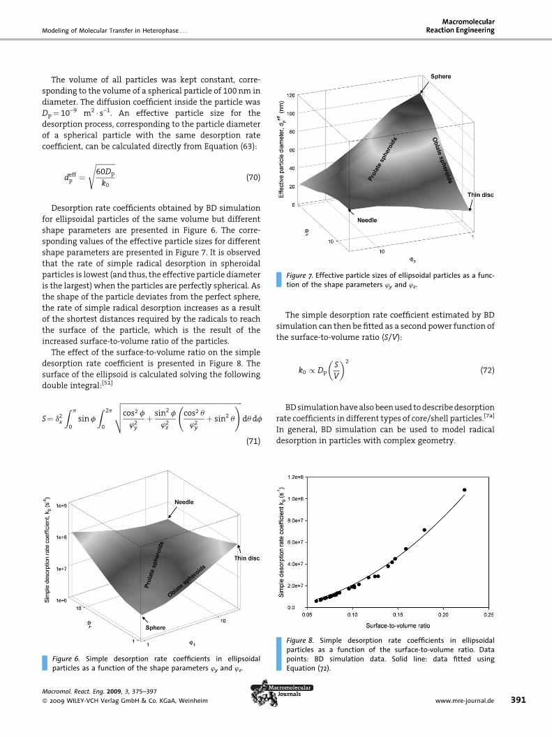
Modeling of Molecular Transfer in Heterophase . . .
The volume of all particles was kept constant, corre-
sponding to the volume of a spherical particle of 100nm in
diameter. The diffusion coefficient inside the particle was
Dp¼ 10–9 m2 � s–1. An effective particle size for the
desorption process, corresponding to the particle diameter
of a spherical particle with the same desorption rate
coefficient, can be calculated directly from Equation (63):
S¼ d2x
Figpar
Macrom
� 2009
deffp ¼
ffiffiffiffiffiffiffiffiffiffiffi60Dp
k0
s(70)
Figure 7. Effective particle sizes of ellipsoidal particles as a func-tion of the shape parameters wy and wz.
Desorption rate coefficients obtained by BD simulation
for ellipsoidal particles of the same volume but different
shape parameters are presented in Figure 6. The corre-
sponding values of the effective particle sizes for different
shape parameters are presented in Figure 7. It is observed
that the rate of simple radical desorption in spheroidal
particles is lowest (and thus, the effective particle diameter
is the largest) when the particles are perfectly spherical. As
the shape of the particle deviates from the perfect sphere,
the rate of simple radical desorption increases as a result
of the shortest distances required by the radicals to reach
the surface of the particle, which is the result of the
increased surface-to-volume ratio of the particles.
The effect of the surface-to-volume ratio on the simple
desorption rate coefficient is presented in Figure 8. The
surface of the ellipsoid is calculated solving the following
double integral:[51]
Z p
0sinf
Z 2p
0
ffiffiffiffiffiffiffiffiffiffiffiffiffiffiffiffiffiffiffiffiffiffiffiffiffiffiffiffiffiffiffiffiffiffiffiffiffiffiffiffiffiffiffiffiffiffiffiffiffiffiffiffiffiffiffiffiffiffiffiffiffiffiffiffiffiffiffiffifficos2 f
’2y
þ sin2 f
’2z
cos2 u
’2y
þ sin2 u
!vuut du df
(71)
ure 6. Simple desorption rate coefficients in ellipsoidalticles as a function of the shape parameters wy and wz.
ol. React. Eng. 2009, 3, 375–397
WILEY-VCH Verlag GmbH & Co. KGaA, Weinheim
The simple desorption rate coefficient estimated by BD
simulation can then be fitted as a second power function of
the surface-to-volume ratio (S/V):
FiguparpoiEqu
k0 / DpS
V
� �2
(72)
BDsimulationhavealsobeenused todescribedesorption
rate coefficients in different types of core/shell particles.[7a]
In general, BD simulation can be used to model radical
desorption in particles with complex geometry.
re 8. Simple desorption rate coefficients in ellipsoidalticles as a function of the surface-to-volume ratio. Datants: BD simulation data. Solid line: data fitted usingation (72).
www.mre-journal.de 391
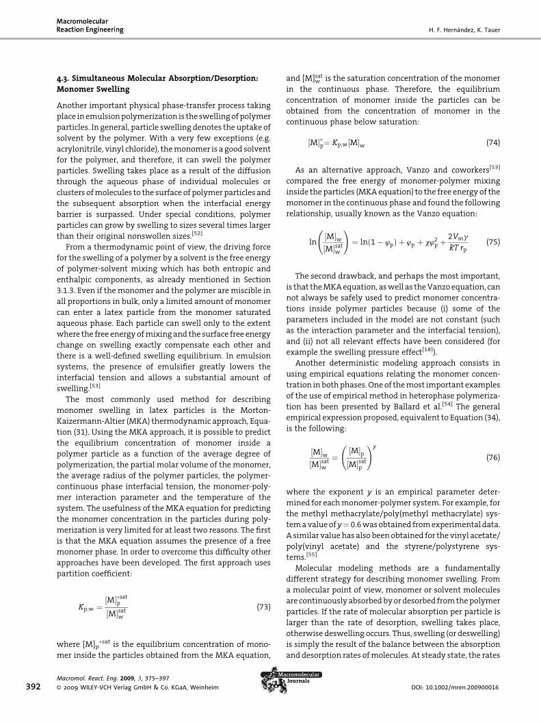
H. F. Hernandez, K. Tauer
392
4.3. Simultaneous Molecular Absorption/Desorption:Monomer Swelling
Another important physical phase-transfer process taking
place inemulsionpolymerization is theswellingofpolymer
particles. In general, particle swelling denotes the uptake of
solvent by the polymer. With a very few exceptions (e.g.
acrylonitrile, vinyl chloride), themonomer is a good solvent
for the polymer, and therefore, it can swell the polymer
particles. Swelling takes place as a result of the diffusion
through the aqueous phase of individual molecules or
clusters ofmolecules to the surface of polymerparticles and
the subsequent absorption when the interfacial energy
barrier is surpassed. Under special conditions, polymer
particles can grow by swelling to sizes several times larger
than their original nonswollen sizes.[52]
From a thermodynamic point of view, the driving force
for the swelling of a polymer by a solvent is the free energy
of polymer-solvent mixing which has both entropic and
enthalpic components, as already mentioned in Section
3.1.3. Even if themonomer and the polymer aremiscible in
all proportions in bulk, only a limited amount of monomer
can enter a latex particle from the monomer saturated
aqueous phase. Each particle can swell only to the extent
where the free energy ofmixing and the surface free energy
change on swelling exactly compensate each other and
there is a well-defined swelling equilibrium. In emulsion
systems, the presence of emulsifier greatly lowers the
interfacial tension and allows a substantial amount of
swelling.[53]
The most commonly used method for describing
monomer swelling in latex particles is the Morton-
Kaizermann-Altier (MKA) thermodynamic approach, Equa-
tion (31). Using the MKA approach, it is possible to predict
the equilibrium concentration of monomer inside a
polymer particle as a function of the average degree of
polymerization, the partial molar volume of the monomer,
the average radius of the polymer particles, the polymer-
continuous phase interfacial tension, the monomer-poly-
mer interaction parameter and the temperature of the
system. The usefulness of the MKA equation for predicting
the monomer concentration in the particles during poly-
merization is very limited for at least two reasons. The first
is that the MKA equation assumes the presence of a free
monomer phase. In order to overcome this difficulty other
approaches have been developed. The first approach uses
partition coefficient:
Macrom
� 2009
Kp;w ¼M½ ��satp
M½ �satw
(73)
where [M]p�sat is the equilibrium concentration of mono-
mer inside the particles obtained from the MKA equation,
ol. React. Eng. 2009, 3, 375–397
WILEY-VCH Verlag GmbH & Co. KGaA, Weinheim
and [M]satw is the saturation concentration of the monomer
in the continuous phase. Therefore, the equilibrium
concentration of monomer inside the particles can be
obtained from the concentration of monomer in the
continuous phase below saturation:
M½ ��p¼ Kp;w M½ �w (74)
As an alternative approach, Vanzo and coworkers[53]
compared the free energy of monomer-polymer mixing
inside the particles (MKAequation) to the free energy of the
monomer in the continuous phase and found the following
relationship, usually known as the Vanzo equation:
lnM½ �wM½ �satw
!¼ lnð1� ’pÞ þ ’p þ x’2p þ
2Vmg
RT rp(75)
The second drawback, and perhaps the most important,
is that theMKAequation, aswell as theVanzoequation, can
not always be safely used to predict monomer concentra-
tions inside polymer particles because (i) some of the
parameters included in the model are not constant (such
as the interaction parameter and the interfacial tension),
and (ii) not all relevant effects have been considered (for
example the swelling pressure effect[18]).
Another deterministic modeling approach consists in
using empirical equations relating the monomer concen-
tration inbothphases.Oneof themost important examples
of the use of empirical method in heterophase polymeriza-
tion has been presented by Ballard et al.[54] The general
empirical expression proposed, equivalent to Equation (34),
is the following:
M½ �wM½ �satw
¼M½ �pM½ �satp
!y
(76)
where the exponent y is an empirical parameter deter-
mined for eachmonomer-polymer system. For example, for
the methyl methacrylate/poly(methyl methacrylate) sys-
temavalueofy¼ 0.6wasobtained fromexperimental data.
A similar valuehas also beenobtained for the vinyl acetate/
poly(vinyl acetate) and the styrene/polystyrene sys-
tems.[55]
Molecular modeling methods are a fundamentally
different strategy for describing monomer swelling. From
a molecular point of view, monomer or solvent molecules
are continuouslyabsorbedbyordesorbed fromthepolymer
particles. If the rate of molecular absorption per particle is
larger than the rate of desorption, swelling takes place,
otherwise deswelling occurs. Thus, swelling (or deswelling)
is simply the result of the balance between the absorption
and desorption rates ofmolecules. At steady state, the rates
DOI: 10.1002/mren.200900016
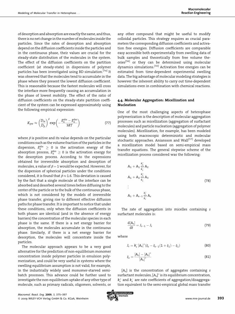
Modeling of Molecular Transfer in Heterophase . . .
ofdesorptionandabsorptionareexactly thesame,andthus,
there isnonet change in thenumberofmolecules inside the
particles. Since the rates of desorption and absorption
dependon thediffusion coefficients inside theparticles and
in the continuous phase, their values are crucial for the
steady-state distribution of the molecules in the system.
The effect of the diffusion coefficients on the partition
coefficient (at steady-state) in dispersions of polymer
particles has been investigated using BD simulation.[7a] It
was observed that themolecules tend to accumulate in the
phase where they present the lowest diffusion coefficient.
This is reasonable because the fastest molecules will cross
the interface more frequently causing an accumulation in
the phase of lowest mobility. The effect of the ratio of
diffusion coefficients on the steady-state partition coeffi-
cient of the system can be expressed approximately using
the following empirical expression:
Macrom
� 2009
Kpw � Dw
Dp
� �b
exp � Eabsa � Edes
a
3RT
� �(77)
where b is positive and its value depends on the particular
conditions suchas thevolumefractionof theparticles in the
dispersion, Eabsa � 0 is the activation energy of the
absorption process, Edesa � 0 is the activation energy for
the desorption process. According to the expressions
obtained for irreversible absorption and desorption of
molecules, a value of b¼ 1would be expected. However, for
the dispersion of spherical particles under the conditions
considered, it is found that b� 1.6. This deviation is caused
by the fact that a single molecule at the interface can be
absorbedanddesorbed several timesbefore diffusing to the
center of the particle or to the bulk of the continuous phase,
which is not considered by the models of irreversible
phase transfer, giving rise to different effective diffusion
paths for phase transfer. It is important to notice that under
these conditions, only when the diffusion coefficients in
both phases are identical (and in the absence of energy
barriers) the concentration of themolecular species in each
phase is the same. If there is a net energy barrier for
absorption, the molecules accumulate in the continuous
phase. Similarly, if there is a net energy barrier for
desorption, the molecules will concentrate inside the
particles.
The molecular approach appears to be a very good
alternative for the prediction of non-equilibriummonomer
concentration inside polymer particles in emulsion poly-
merization, and could be very useful in systems where the
swelling equilibrium assumption is not valid, for example,
in the industrially widely used monomer-starved semi-
batch processes. This advance could be further used to
investigate thenon-equilibriumuptakeof anyother typeof
molecule, such as primary radicals, oligomers, solvents, or
ol. React. Eng. 2009, 3, 375–397
WILEY-VCH Verlag GmbH & Co. KGaA, Weinheim
any other compound that might be useful to modify
colloidal particles. This strategy requires as crucial para-
meters the corresponding diffusion coefficients and activa-
tion free energies. Diffusion coefficients are comparable
easy accessible both experimentally from swelling data of
bulk samples and theoretically from free volume the-
ories[56] or they can be determined using molecular
dynamics simulations.[32] Activation free energies can be
estimated from time-dependent experimental swelling
data. The big advantage ofmolecularmodeling strategies is
however the inherent ability to carry out time-dependent
simulations even in combination with chemical reactions.
4.4. Molecular Aggregation: Micellization andNucleation
One of the most challenging aspects of heterophase
polymerization is the description ofmolecular aggregation
processes such as micellization (aggregation of surfactant
molecules) and particle nucleation (aggregation of polymer
molecules). Micellization, for example, has been modeled
using both macroscopic deterministic and molecular
stochastic approaches. Aniansson and Wall[57] developed
a micellization model based on semi-empirical mass
transfer equations. The general stepwise scheme of the
micellization process considered was the following:
A1 þ A1 ,kþ2
k�2
A2
A1 þ A2 ,kþ3
k�3
A3
..
.
A1 þ As�1 ,kþ
s
k�s
As
(78)
The rate of aggregation into micelles containing s
surfactant molecules is:
d As½ �dt
¼ Js�1 � Js (79)
where
Js ¼ k�s As½ �� js � js�1ð1þ j1Þ � j1ð Þ (80)
As½ � � As½ ��
js ¼ As½ �� (81)[As] is the concentration of aggregates containing s
surfactantmolecules, [As]� is its equilibrium concentration,
kþs and k�
s are rate coefficients of aggregation/disaggrega-
tion equivalent to the semi-empirical global mass transfer
www.mre-journal.de 393

H. F. Hernandez, K. Tauer
394
coefficients, Js is thefluxofaggregatesof size s in thespaceof
cluster sizes (the number of aggregates of size s absorbing
one additionalmolecule per unit time), and js is the relative
concentration of aggregates of size s away from the
equilibrium. In this approach, molecular aggregates con-
taining the same number of surfactant molecules are
considered to be different segregated phases, and the
aggregation (disaggregation) process involves the transfer
of an individual surfactant molecule from (to) the
continuous phase.
The thermodynamic formulation of the micellization
process[58] completelyneglectsdynamicsbut considers that
thesystemreachesequilibriumwhentheGibb’s freeenergy
is at its minimum.
Macrom
� 2009
m0s þ kBT lnXs ¼ s m0
1 þ kBT lnX1
� �(82)
m0s is the standard chemical potential of an aggregate of s
surfactant molecules, and Xs is the mole fraction of these
aggregates in the solution.As it canbe seen inEquation (82),
the transfer of individual surfactant molecules towards
surfactant aggregates is driven by the differences in
chemical potential between the aggregates and the
individual surfactant molecules. This model requires a
very precise determination of the chemical potentials, as
given by Nagarajan and Ruckenstein.[59]
In addition,micellization kinetics has also beenmodeled
using classical or modern nucleation theories.[60] Nuclea-
tion andmicellization are very similar processes consisting
of the spontaneous aggregation of individual entities
(atoms, molecules or ions). However, this was not realized
during the early development of their kinetic models.
Nucleationmodels, like for example theclassicalnucleation
theory (CNT),[61] are usually obtained by integrating the
semi-empirical approach with equilibrium thermody-
namics. Nucleation is an aggregation process where only
aggregates above a certain size are stable. At this critical
size, the Gibb’s free energy of the aggregate is at its
maximum. Aggregates with sizes smaller than the critical
size have a limited probability of growing because the free
energy increases with each aggregation step. However,
the growth of subcritical aggregates is favored by the
presence of thermal fluctuations. When an aggregate
reaches the critical size, its growth becomes spontaneous
because fromnowoneach further aggregation step leads to
a decrease in the free energy. The flux of aggregates is
assumed to be determined by the free energy of formation
of an aggregate according to the Boltzmann’s distribution:
Js ¼ jþs As½ � 1� expDWs þ ln Asþ1½ �
As½ �
� �kBT
0@
1A
0@
1A (83)
ol. React. Eng. 2009, 3, 375–397
WILEY-VCH Verlag GmbH & Co. KGaA, Weinheim
where jþs is the number of molecules absorbed from the
continuous phase by the aggregate of size sper unit of time,
andDWs is the difference in aggregationwork between the
aggregate of size sþ 1 and the aggregate of size s, which are
defined by:
Ws ¼ms � sm1
kBT(84)
ms is the chemical potential of the molecular aggregates of
size s; jþs is usually determined using Smoluchowski’s
equation, which is basically the solution of Fick’s equation
for the absorption ofmolecules by amolecular aggregate in
infinite dilution.
Smit et al.[62] proposed the use of MD simulation for
investigating the surfactant aggregation process. This
model requires the definition of potential functions for
each type of interaction: hydrophobic-hydrophobic, hydro-
phobic-hydrophilic and hydrophilic-hydrophilic, either as
covalent bonds, e.g. harmonic potentials, Equation (85), or
asvanderWaals interactions, e.g. Lennard-Jonespotentials,
Equation (86) and (87). Although computationally demand-
ing, thismethod allowed the description of the dynamics of
micellization as well as of its equilibrium properties.
Uij ¼kF rij � sij
� �22
(85)
fijðrijÞ � fijðRcijÞ rij � Rc
ij
Fij ¼ 0 rij > Rcij(86)
sij� �12 sij
� �6" #
fijðrijÞ ¼ 4"ijrij
�rij
(87)
where Uij is the covalent interaction between two atoms i
and j, kF is a force constant, rij is the distance between the
two atoms, sij is an interaction length parameter,Fij is the
van der Waals interaction potential between atoms i and j,
fij is a Lennard-Jones-type interactionpotential, and eij is an
interaction energy parameter.
Alternatively, a more general aggregation scheme has
been solved by Mavelli[63] using Gillespie’s stochastic
simulation algorithm. The general aggregation scheme is
the following:
Ai þ Aj ,kþ
i;j
k�i;j
Aiþj (88)
The kinetic constants were determined as follows:
kþi;j ¼ Ki;jk
�i;j (89)
DOI: 10.1002/mren.200900016
Modeling of Molecular Transfer in Heterophase . . .
� i!j! �
Macrom
� 2009
ki;j ¼ ði þ jÞ ði þ j � 1Þ! k0 (90)
where
Ki;j ¼ij
ði þ jÞ S½ �Pði þ jÞPðiÞPðjÞ (91)
exp � "i
� �
PðiÞ ¼ kBTPj exp � "j
kBT
� � (92)
i � nmax� �2
"i ¼ inmax
"0 (93)
[S] is the total surfactant concentration, nmax is the
maximum aggregation number considered, and k�0 and e0
are parameters of the model.
Also for ab initio heterophase polymerization, particle
nucleation can be considered as being the product of
molecular aggregation.[64,65] However, the situation is
complicated as both the concentration and the physico-
chemical properties of the aggregating species changewith
time. Moreover, the presence of segregated phases (mainly
monomer drops and latex particles) strongly influences the
nucleation process due to interactionswith the aggregates.
This interaction lowers the free energy of nucleation and
thus increases theprobabilityofparticle formation. There is
experimental evidence that this so-called ‘‘heterogeneous
nucleation’’ is not only crucial for the formation of clouds
and rain drops in the atmosphere,[66] but also for particle
nucleation in heterogeneous polymerization.[65]
5. Conclusion
Mass transfer across interfaces is one of the most common
and important events taking place in heterogeneous
systems. In particular for heterophase polymerization, it
has been observed that transfer of molecules (radicals,
monomer, surfactant, etc.) between different phases
strongly determines the polymerization kinetics. Several
different approaches have been used for modeling inter-
facial mass transport, which can be classified in two main
groups: macroscopic deterministic and molecular stochas-
tic approaches. All modeling techniques available are not
contradictory but complementary between each other,
because they are suitable for describing different aspects of
the process, possibly under different conditions. Thus, for
example, equilibrium thermodynamic models do not
describe dynamic effects but are very fast alternatives to
model final equilibrium conditions (if they are kinetically
accessible). Molecular dynamics simulations are able to
describewithmicroscopic detail the dynamics ofmolecular
ol. React. Eng. 2009, 3, 375–397
WILEY-VCH Verlag GmbH & Co. KGaA, Weinheim
transfer processes, but they are limited only to very small
systems, usually far from equilibrium. The best modeling
approach that can be used to describe a mass transfer
process will be determined not only by the particular
conditions of the process (e.g. if the system is at the
thermodynamic limit or not), but also on the purpose of
modeling, that is, on the information expected to be
obtained from the model (e.g. predicting results under
different conditions, describing the process in a fast and
simple way, etc.).
Given that each modeling method offers certain parti-
cular advantages, future developments in mass transfer
modeling should be focused on the seamless integration of
different methods, usually at different time and length
scales (multiscale simulation). The biggest challenge in
multiscale simulationmaybe the development of accurate,
fast and efficient ab initio multiscale simulation methods;
that is, to simulate mass transfer processes from the
knowledge only of the composition of the system using
neither empirical parameters nor previous experimental
results, providing accurate information at all relevant
scales (from the molecular to the macroscopic) and using
reasonable computation power. The state of the art in
multiscale simulation, in particular of mass transfer
processes, is still far away from this goal, and therefore,
there are still plentyofpossibilities ofnewdevelopments in
this direction.
Molecular-scalemodeling approaches offer new insights
into the mechanism of heterophase polymerization and
interestingly, allow certain generalizationswhichwere not
possible with macroscopic deterministic modeling.
Acknowledgements: The Max Planck Society is gratefullyacknowledged for the financial support of this research. H. H.would also like to acknowledge Andercol SA (Colombia) for thegranting of a research fellowship.
Received: March 10, 2009; Revised: June 12, 2009; Accepted: June17, 2009; Published online: August 4, 2009; DOI: 10.1002/mren.200900016
Keywords: emulsion polymerization; molecular dynamics; mo-lecular modeling; radical polymerization; simulations; swelling
[1] [1a] D. C. Sundberg, A. P. Casassa, J. Pantazopoulos, M. R.Muscato, B. Kronberg, J. Berg, J. Appl. Polym. Sci. 1990, 41,1425; [1b] Y.-C. Chen, V. Dimonie, M. S. El-Aasser, Macromol-ecules 1991, 24, 3779; [1c] O. J. Karlsson, J. M. Stubbs, R. H.Carrier, D. C. Sundberg, Polym. React. Eng. 2003, 11, 589.
[2] S. R. DeGroot, P. Mazur, ‘‘Non-Equilibrium Thermodynamics’’,Dover Publications, New York 1984, p. 267.
[3] H. J. Morowitz, ‘‘Beginnings of Cellular Life’’, Yale UniversityPress, New Haven 1992, p. 72.
[4] C. S. Chern, ‘‘Principles and Applications of Emulsion Polymeri-zation’’, J. Wiley & Sons, Hoboken 2008.
www.mre-journal.de 395
H. F. Hernandez, K. Tauer
396
[5] G. Odian, ‘‘Principles of Polymerization’’, 4th edition, Wiley-Interscience, Hoboken 2004, p. 198.
[6] [6a] S. Kozempel, K. Tauer, G. Rother, Polymer 2005, 46, 1169.[6b] K. Tauer, S. Kozempel, G. Rother, J. Colloid Interface Sci.2007, 312, 432.
[7] [7a] H. F. Hernandez, Ph. D. Thesis, Universitat Potsdam 2008.[7b] H. F. Hernandez, K. Tauer, Comp. -Aided Chem. Eng. 2008,25, 769.
[8] D. T. Gillespie, J. Comp. Phys. 1976, 22, 403.[9] N. G. van Kampen, ‘‘Stochastic processes in chemistry and
physics’’, Elsevier, Amsterdam 1992.[10] C. W. Gardiner, ‘‘Handbook of stochastic methods’’, Springer,
Berlin 1994.[11] A. Fick, Ann. Phys. 1855 170, 59.[12] H. Gomez, I. Colominas, F. Navarrina, M. Casteleiro, Comput.
Methods Appl. Mech. Eng. 2007, 196, 1757.[13] R. E. Treybal, ‘‘Mass-Transfer Operations’’, 3rd edition,
McGraw-Hill, Singapore 1981, p. 104.[14] J. G. Knudsen, H. C. Hottel, A. F. Saforim, P. C. Wankat, K. S.
Knaebel, ‘‘Heat and Mass Transfer’’, in: Perry’s ChemicalEngineers’ Handbook, 7th edition, R. H. Perry, D. W. Green,J. O. Maloney, Eds., McGraw-Hill, New York 1997, p. 5-1.
[15] P. J. Flory, ‘‘Principles of Polymer Chemistry’’, CornellUniversity Press, Ithaca 1953, p. 495.
[16] T. W. de Loos, ‘‘Polymer Thermodynamics’’, in: Handbook ofPolymer Reaction Engineering Meyer, Volume 1, T. Meyer, J.Keurentjes, Eds., WILEY-VCH, Weinheim 2005, p. 17.
[17] M. Morton, S. Kaizerman, M. W. Altier, J. Colloid Sci. 1954, 9,300.
[18] [18a] M. Antonietti, H. Kaspar, K. Tauer, Langmuir 1996, 12,6211. [18b] K. Tauer, H. Kaspar, M. Antonietti, Colloid Polym.Sci. 2000, 278, 814.
[19] H. Kaspar, Ph. D. Thesis, Universitat Potsdam 1996.[20] A. Leo, C. Hansch, D. Elkins, Chem. Rev. 1971, 71, 525.[21] D. T. Gillespie, Annu. Rev. Phys. Chem. 2007, 58, 35.[22] D. T. Gillespie, J. Phys. Chem. 1977, 81, 2340.[23] [23a] J. W. Evans, ‘‘Kinetic Monte Carlo simulation of non-
equilibrium lattice-gas models: Basic and refined algorithmsapplied to surface adsorption processes’’, in: Handbook ofMaterials Modeling, S. Yip, (Ed., Springer, Dordrecht, 2005,p. 1753. [23b] A. Chatterjee, D. G. Vlachos, J. Comp. -AidedMater. Des. 2007, 14, 253. [23c] R. Erban, S. J. Chapman, Phys.Rev. E 2007, 75, 041116.
[24] [24a] Y. Cao, D. Gillespie, L. Petzold, J. Comp. Phys. 2005, 206,395. [24b] H. Salis, Y. Kaznessis, J. Chem. Phys. 2005, 122,054103.
[25] H. F. Hernandez,, K. Tauer, Macromol. Symp. 2008, 271, 64.[26] [26a] H. Tobita, Y. Takada, M. Nomura, Macromolecules 1994,
27, 3804. [26b] H. Tobita, Acta Polym. 1995, 46, 185.[27] J. C. Chen, A. S. Kim, Adv. Colloid Interface Sci. 2004, 112,
159.[28] [28a] V. M. Bluett, J. B. Green, J. Phys. Chem. A 2006, 110, 6112.
[28b] C. E. Bolton, N. J. B. Green, R. Harris, S. M. Pimblott,J. Phys. Chem. A 1998, 102, 730.
[29] [29a] H. J. C. Berendsen, ‘‘Simulating the physical world’’,Cambridge University Press, New York 2007. [29b] D. Frenkel,B. Smit, ‘‘ Understanding molecular simulation’’, AcademicPress, San Diego 2002.
[30] M. Fermeglia, S. Pricl, Prog. Org. Coat. 2007, 58, 187.[31] A. Chatterjee, M. A. Snyder, D. G. Vlachos, Chem. Eng. Sci. 2004,
59, 5559.[32] [32a] V. A. Harmandaris, N. P. Adhikari, N. F. A. van der Vegt,
K. Kremer, B. A. Mann, R. Voelkel, H. Weiss, C. C. Liew,Macromolecules 2007, 40, 7026. [32b] V. A. Harmandaris,
Macromol. React. Eng. 2009, 3, 375–397
� 2009 WILEY-VCH Verlag GmbH & Co. KGaA, Weinheim
N. P. Adhikari, N. F. A. van der Vegt, K. Kremer, Macromol-ecules 2006, 39, 6708.
[33] H. F. Hernandez, K. Tauer, AIChE Annual Meeting, ConferenceProceedings, Philadelphia 2008.
[34] [34a] K. Tauer, S. Nozari, A. M. I. Ali, Macromolecules 2005, 38,8611. [34b] M. Goicoechea, M. J. Barandiaran, J. M. Asua,Macromolecules 2006, 39, 5165.
[35] [35a] R. M. Fitch, C. H. Tsai, ‘‘Particle formation in polymercolloids III: Prediction of the number of particles by a homo-geneous nucleation theory’’, in: Polymer Colloids, R. M. Fitch,(Ed., Plenum, New York 1971, p. 73 [35b] J. L. Gardon, J. Polym.Sci. A: Polym. Chem. 1968, 6, 623.
[36] W. V. Smith,, R. H. Ewart, J. Chem. Phys. 1948, 16, 592.[37] J. Ugelstad, F. K. Hansen, Rubber Chem. Technol. 1976, 49,
536.[38] M. Nomura, H. Tobita, K. Suzuki, Adv. Polym. Sci. 2005, 175, 1.[39] I. A. Penboss, R. G. Gilbert, D. H. Napper, J. Chem. Soc., Faraday
Trans. I 1983, 79, 2247.[40] I. A. Maxwell, B. R. Morrison, D. H. Napper, R. G. Gilbert,
Macromolecules 1991, 24, 1629.[41] H. F. Hernandez, K. Tauer, Ind. Eng. Chem. Res. 2007, 46,
4480.[42] H. F. Hernandez, K. Tauer, Macromol. Symp. 2007, 259, 274.[43] A. A. Rzepiela, J. H. J. van Opheusden, T. van Vliet, J. Colloid
Interface Sci. 2001, 244, 43.[44] J. Ugelstad, P. C. Mork, J. O. Aasen, J. Polym. Sci. A-1 1967, 5,
2281.[45] M. Nomura, M. Harada, J. Appl. Polym. Sci. 1981, 26, 17.[46] J. M. Asua, E. D. Sudol, M. S. El-Aasser, J. Polym. Sci., Part A:
Polym. Chem. 1989, 27, 3903.[47] [47a] J. M. Asua, Macromolecules 2003, 36, 6245. [47b] S. C.
Thickett, R. G. Gilbert, Macromolecules 2006, 39, 2081.[48] H. F. Hernandez, K. Tauer, Ind. Eng. Chem. Res. 2008, 47, 9795.[49] [49a] M. Okubo, T. Miya, H. Minami, R. Takekoh, J. Appl.
Polym. Sci. 2002, 83, 2013. [49b] A. Pich, Y. Lu, H.-J. P. Adler,T. Schmidt, K.-F. Arndt, Polymer 2002, 43, 5723. [49c]E. Eisenriegler, A. Bringer, J. Chem. Phys. 2007, 127, 034904.
[50] D. Zwillinger, ‘‘CRC Standard Mathematical Table andFormulae’’, 31st edition, Chapman & Hall/CRC, Boca Raton2003, p. 372.
[51] E. W. Weisstein, ‘‘CRC Concise Encyclopedia of Mathematics’’,2nd edition, Chapman & Hall/CRC, Boca Raton 2002, p. 873.
[52] J. Ugelstad, H. R. Mfutakamba, P. C. Mørk, T. Ellingsen, A.Berge, R. Schmid, L. Holm, A. Jørgedal, F. K. Hansen, K. Nustad,J. Polym. Sci. : Polym. Symp. 1985, 72, 225.
[53] E. Vanzo, R. H.Marchessault, V. Stannet, J. Colloid Sci. 1965, 20,62.
[54] M. J. Ballard, D. H. Napper, R. G. Gilbert, J. Polym. Sci., Part. A:Polym. Chem. 1984, 22, 3225.
[55] R. G. Gilbert, ‘‘Emulsion polymerization. A MechanisticApproach’’, Academic Press, London 1995.
[56] [56a] H. Fujita, Adv. Polym. Sci. 1961, 3, 1; [56b] J. S. Vrentas,J. L. Duda, Macromolecules 1976, 9, 785.
[57] E. A. G. Aniansson, S. N. Wall, J. Phys. Chem. 1974, 78, 1024.[58] C. Tanford, ‘‘The hydrophobic effect: Formation of micelles and
biological membranes’’, 2nd edition, Krieger Publishing, Mala-bar 1991, p. 60.
[59] R. Nagarajan, E. Ruckenstein, Langmuir 1991, 7, 2934.[60] A. K. Shchekin, F. M. Kuni, A. P. Grinin, A. I. Rusanov, ‘‘Nuclea-
tion in micellization processes’’, in: Nucleation Theory andApplications, J. W. P. Schmelzer, (Ed., Wiley-VCH, Weinheim2005, p. 312.
[61] D. Kashchiev, ‘‘Nucleation: Basic theory with applications’’,Butterworth-Heinemann, Oxford 2000.
DOI: 10.1002/mren.200900016

Modeling of Molecular Transfer in Heterophase . . .
[62] B. Smit, P. A. J. Hilbers, K. Esselink, L. A. M. Rupert, N. M. vanOs, A. G. Schlijper, J. Phys. Chem. 1991, 95, 6361.
[63] F. Mavelli, Progr. Colloid Polym. Sci. 1997, 103, 155.[64] [63a] I. Kuhn, K. Tauer, Macromolecules 1995, 28, 8122. [63b] I.
Kuhn, Ph. D. Thesis, Universitat Potsdam 1996.
Macromol. React. Eng. 2009, 3, 375–397
� 2009 WILEY-VCH Verlag GmbH & Co. KGaA, Weinheim
[65] K. Tauer, H. F. Hernandez, S. Kozempel, O. Lazareva,P. Nazaran, Colloid Polym. Sci. 2007, 286, 499.
[66] A. Laaksonen, V. Talanquer, D. W. Oxtoby, Annu. Rev. Phys.Chem. 1995, 46, 489.
www.mre-journal.de 397


