Embed Size (px)
Citation preview
Modelling and characterization of a modified 3-DoF pneumaticGough-Stewart platform
by
Hendrik Jacobus Theron
Submitted in partial fulfilment of the requirements for the degree
Master of Engineering (Mechanical Engineering)
in the
Department of Mechanical and Aeronautical Engineering
Faculty of Engineering, Built Environment and Information Technology
UNIVERSITY OF PRETORIA
July 2016
© University of Pretoria
SUMMARY
Modelling and characterization of a modified 3-DoF pneumatic Gough-Stewart platform
by
Hendrik Jacobus Theron
Supervisor(s): Prof N J Theron
Department: Mechanical and Aeronautical Engineering
University: University of Pretoria
Degree: Master of Engineering (Mechanical Engineering)
Keywords: Pneumatic, Stribeck, Gough-Stewart, Matlab®, Simulink®, MSC
ADAMS®, ISO-6358, Co-simulation, Inverse Kinematics, Mass Flow,
Deck Motion Simulator, Nonlinear
Stabilised line of sight optical payloads for maritime vessels require variable platform conditions
during the development, test and evaluation phases. A ship deck motion simulator is one means of
generating such conditions in a controlled laboratory environment. This dissertation describes the
aspects of the modelling, identification and validation of a ship motion simulator, in the form of a
pneumatically actuated 3-DOF modified Gough-Stewart manipulator, to generate a realistic simula-
tion environment for controller design. The simulation environment is a Matlab® supervised MSC
ADAMS®/Matlab® Simulink® co-simulation in which Simulink® houses the pneumatic model, the
friction model, and the controller, and ADAMS® runs the dynamic model of the physical hardware.
A similar simulator cannot be found in published literature forcing a development of the model from
the ground up, using published information as a foundation. The simulator model is broken up at the
subsystem level which comprises the valve mass flow model, the piston chamber and force model,
the complete actuator model and finally the complete ship simulator model. Each of these is derived,
identified, and validated. The requirements of the simulator as well as the simulation environment
is derived from real-life measurements done on seafaring vessels. An inverse kinematic solution is
presented as a set of lookup tables which are generated from the outputs of MSC ADAMS® by ma-
nipulating the simulator platform over the whole range of movements through Matlab®. The reverse
of the process is then used to ensure that actuator extensions generate the correct platform attitude -
© University of Pretoria
the attitude errors as shown to be infinitely small. Two valve mass flow models are proposed, a clas-
sical model and an ISO model, the first derived from thermodynamic principles and the second based
on the ISO-6358 standard. The parameters of the two models are identified through experimental
charging and discharging of a constant volume pressure chamber and sampling the temporal pressure
and temperature outputs. The mass flow is calculated from the measured data through parameter es-
timation. Validation is done by comparing the temporal pressure outputs of the models with the actual
measured pressure signals. The mean absolute error for the best fit ISO model is less than half of the
Classic model at 0.4 MPa (MAE < 2 kPa) and the temporal pressure relationships in the closed-loop
and open-loop tests shows a 93% correlation against measured pressure signals. The combination
of the derived actuator chamber model and the valve mass flow model produces a realistic actuator
model. The force equation of each of the actuators makes provision for a nonlinear friction compon-
ent. The actuator friction model is based on a simple stick-slip relation with an acceleration dependent
Stribeck function and an exponential viscous friction component. This model is also identified with
data from the actual hardware. The complete ship motion simulator model is validated through open-
loop as well as closed-loop tests. The open-loop tests are performed with chirp or sinusoidal signal
excitation from a stable elevated offset starting condition. The ratio of the measured and simulated
extension amplitudes in the open-loop is larger than 0.95 while the ratio of the rise times (tm/ts) is ap-
proximately 0.85. The closed-loop validation tests are conducted with both heave and roll inputs and
compared well with the real system. A 14% difference in the actuator position amplitude (between
the simulated and measured systems), and a 20% slower extension rate at 0.05 Hz that increases at
1 Hz to match the measured rate are observed. The maximum large signal bandwidth is 0.617 Hz,
and is only limited by the mass flow. A simplified plant model is derived and compared with the high
performance model and is subsequently used for a state feedback controller design and evaluation.
The final controller gains deliver a stable system with the same 0.617Hz bandwidth limitation and a
controller that is insensitive to loop gain changes from 0.5 to 15.
© University of Pretoria
OPSOMMING
Die modellering en karakterisering van ’n gemodifiseerde 3-GvV pneumatiese
Gough-Stewart platform
deur
Hendrik Jacobus Theron
Studieleier(s): Prof N J Theron
Departement: Meganiese en Lugvaartkundige Ingieurswese
Universiteit: Universiteit van Pretoria
Graad: Magister in Ingenieurswese (Meganiese Ingenieurswese)
Sleutelwoorde: Pneumaties, Stribeck, Gough-Stewart, Matlab®, Simulink®, MSC
ADAMS®, ISO-6358, Inverse kinematika, Massavloei, Skeepsdeksim-
ulator, Nie-linieêr
Optiese loonvragte vir maritieme vaartuie, waarvan die siglyn gestabiliseer word, benodig verander-
like platform toestande tydens ontwikkeling, toets en evaluasie. Een manier om veranderlike dektoes-
tande in ’n laboratorium te emuleer, is deur ’n skeepsdeksimulator te gebruik. Hierdie verhandeling
beskryf aspekte van die modelering, stelsel identifikasie en validasie van ’n drie grade van vryheid
skeepsdeksimulator wat gebruik word om ’n realistiese simulasieomgewing te skep. Die simulator
is in die vorm van ’n gemodifiseerde pneumatiese Gough-Stewart manipulator. ’n Gesamentlike
MSC ADAMS®/Matlab® Simulink® simulasie, wat deur Matlab® bedryf word, vorm ’n simulasie-
omgewing waarin ADAMS® die dinamiese model van die fisiese hardeware huisves, en Simulink®
die pneumatiese model, die wrywingsmodel en die beheerder hanteer. Daar kan geen soortgelyke
simulator gevind word in gepubliseerde literatuur nie, wat tot gevolg het dat ’n model van eerste
beginsels opgestel is deur die gepubliseerde inligting as fondasie te gebruik. Die simulasiemodel is
opgebreek op substelselvlak wat die massavloei model van die klep, die silinderkamermodel, sowel as
die kragmodel van die suier, die volledige aktuatormodel en ook, laastens, die volledige skeepsdek-
simulatormodel insluit. Al hierdie modelle is afgelei, die parameters geïdentifiseer and gevalideer.
Die behoeftestellings van die simulator, sowel as die simulasieomgewing, is afgelei uit werklike me-
tings van soortgelyke seevarende vaartuie. Opsoektabelle, wat bereken is deur met Matlab® die simu-
© University of Pretoria
latorplatform binne MSC ADAMS® deur sy volledige bewegingsberyk te manipuleer, stel die inverse
kinematika voor. Infinietdesimale klein foute is verkry deur die proses in tru aan te wend en die
platform oriëntasie tydens verskeie aktuatortposisies te toets. Daar is twee klep massavloeimodelle
beskryf, ’n klassieke model wat van basiese termodinamiese geginsels afgelei is, en ’n ISO model
wat gebaseer is op die ISO-6358 standaard. Beide hierdie modelle se parameters is deur eksperi-
mentele stelselidentifikasieprosedures bepaal tydens opblaas- en afblaastoetse. Hiervoor is ’n kon-
stante volume druktenk gebruik en beide die tydafhanklike interne druk en lugtemperature is gemeet.
Die massavloei is bepaal deur parameterestimasietegnieke toe te pas op die voorgestelde modelle, en
validering deur die tydafhanklike druk te vergelyk met die uitsette van die modelle. By ’n werksdruk
van 0.4 MPa is die gemiddelde absolute fout van die ISO model minder as die helfte van die fout van
die klassieke model (MAE < 2 kPa), en die tydafhanklike drukverwantskap in beide die geslotelus-,
sowel as die ooplustoetse toon ’n 93% korrelasie teen die gemete drukwaardes. Die kombinasie van
die afgeleide silindermodel en die klep massavloeimodel lewer ’n geloofwaardige wrywingslose aktu-
atormodel, en deur die dinamiese kragvergelyking te gebruik, word dit aangevul deur ’n nie-linieêre
wrywingskomponent. ’n Steek-glip wrywingsmodel met ’n versnellingsafhanklike Stribeckfunksie
en ’n eksponetiële viskeuse wrywingskomponent stel die aktuatorwrywing voor. Die wrywingsmodel
is ook geïdentifiseer deur werklike gemete data. Die valideringsoefening van die volledige skeepsdek-
simulator is voltooi deur beide ooplustoetse, sowel as gelotelustoetse uit te voer. Die ooplustoetse is
vanaf halfuitgestrekte aktuatorposisies gedoen deur sinusoïdale en tjirp opwekkingsseine te gebruik.
Die amplitudeverhouding tussen die gemete posisies en die gesimuleerde posisies is groter as 95%,
terwyl die stygtydverhouding (tm/ts) ongeveer 0.85 is. Vir geslotelusvaliderinstoetse is beide deining
and rol stelpunte as insette gebruik en die simulasie resultate is met die werklike gemete waardes
vergeleik. Die gemete amplitude van die aktuatorposisie is ongeveer 14% kleiner as die gesimuleerde
amplitude, die gemete aktuatorspoed is ongeveer 20% stadiger by 0.06 Hz en terwyl dit ongeveer
dieselfde is by 1 Hz. Die maksimum grootseinbandwydte is 0.617 Hz en word beperk deur die mass-
vloeivermoë van die klep. ’n Vereenvoudigde stelselmodel is afgelei, ’n toestandsterugvoerbeheerder
is ontwerp en die beheerder ge-evalueer met beide die hoë akkuraatheid model, sowel as die vereen-
voudigde model. Die finale beheerder lewer ’n stabiele stelsel met dieselfde 0.617Hz bandwydte wat
onsensitief is vir luswinsveranderinge vanaf 0.5 tot 15.
© University of Pretoria
TABLE OF CONTENTS
Acronyms
List of symbols
CHAPTER 1 Introduction 19
1.1 Problem Statement . . . . . . . . . . . . . . . . . . . . . . . . . . . . . . . . . . . 19
1.1.1 Background . . . . . . . . . . . . . . . . . . . . . . . . . . . . . . . . . . . 19
1.1.2 Research gap . . . . . . . . . . . . . . . . . . . . . . . . . . . . . . . . . . 20
1.2 Research Goals . . . . . . . . . . . . . . . . . . . . . . . . . . . . . . . . . . . . . 21
1.3 Research Objectives . . . . . . . . . . . . . . . . . . . . . . . . . . . . . . . . . . . 21
1.4 Contribution . . . . . . . . . . . . . . . . . . . . . . . . . . . . . . . . . . . . . . . 23
1.5 Overview of study . . . . . . . . . . . . . . . . . . . . . . . . . . . . . . . . . . . . 23
CHAPTER 2 System Description and Literature Survey 25
2.1 Ship Dynamics . . . . . . . . . . . . . . . . . . . . . . . . . . . . . . . . . . . . . 25
2.2 Modular Stand Alone Tracker (MODSAT) . . . . . . . . . . . . . . . . . . . . . . . 27
2.3 Ship Motion Simulator (SMS) . . . . . . . . . . . . . . . . . . . . . . . . . . . . . 29
2.4 Combined MODSAT and SMS . . . . . . . . . . . . . . . . . . . . . . . . . . . . . 32
2.5 Literature Survey . . . . . . . . . . . . . . . . . . . . . . . . . . . . . . . . . . . . 32
2.5.1 Geometry, Kinematics and Dynamics . . . . . . . . . . . . . . . . . . . . . 33
2.5.2 Pneumatic Actuators . . . . . . . . . . . . . . . . . . . . . . . . . . . . . . 34
2.5.3 Control . . . . . . . . . . . . . . . . . . . . . . . . . . . . . . . . . . . . . 39
CHAPTER 3 SMS Kinematics 41
3.1 SMS Computer Aided Design (CAD) Model . . . . . . . . . . . . . . . . . . . . . . 41
3.2 SMS Kinematic Vector Diagram Model . . . . . . . . . . . . . . . . . . . . . . . . 44
3.2.1 Gough-Stewart Vector Kinematics . . . . . . . . . . . . . . . . . . . . . . . 44
© University of Pretoria
3.2.2 SMS Vector Kinematics . . . . . . . . . . . . . . . . . . . . . . . . . . . . 47
3.3 MSC ADAMS® Multi-body Dynamics . . . . . . . . . . . . . . . . . . . . . . . . . 49
3.4 Integration between MSC ADAMS® and Matlab® . . . . . . . . . . . . . . . . . . . 51
3.5 ADAMS® Kinematic Simulation . . . . . . . . . . . . . . . . . . . . . . . . . . . . 57
CHAPTER 4 Theoretical Pneumatic Models 60
4.1 Pneumatic System . . . . . . . . . . . . . . . . . . . . . . . . . . . . . . . . . . . . 60
4.1.1 Pneumatic Actuator Subsystem Matlab® Model . . . . . . . . . . . . . . . . 62
4.1.2 Valve . . . . . . . . . . . . . . . . . . . . . . . . . . . . . . . . . . . . . . 63
4.1.3 Actuator . . . . . . . . . . . . . . . . . . . . . . . . . . . . . . . . . . . . . 73
4.1.4 Pneumatic Connections . . . . . . . . . . . . . . . . . . . . . . . . . . . . . 79
4.1.5 Pneumatic Reservoir . . . . . . . . . . . . . . . . . . . . . . . . . . . . . . 81
CHAPTER 5 Mass Flow Characterisation 82
5.1 Theoretical Models . . . . . . . . . . . . . . . . . . . . . . . . . . . . . . . . . . . 82
5.1.1 Classic Mass Flow Model . . . . . . . . . . . . . . . . . . . . . . . . . . . 82
5.1.2 ISO Mass Flow Model . . . . . . . . . . . . . . . . . . . . . . . . . . . . . 84
5.2 Valve Flow Measurements . . . . . . . . . . . . . . . . . . . . . . . . . . . . . . . 86
5.2.1 Pneumatic Measurement setup . . . . . . . . . . . . . . . . . . . . . . . . . 86
5.2.2 Temperature Measurement . . . . . . . . . . . . . . . . . . . . . . . . . . . 87
5.2.3 Test Matrix . . . . . . . . . . . . . . . . . . . . . . . . . . . . . . . . . . . 89
5.3 Valve Characteristics - Processing . . . . . . . . . . . . . . . . . . . . . . . . . . . 90
5.3.1 Signal Processing . . . . . . . . . . . . . . . . . . . . . . . . . . . . . . . . 90
5.3.2 Discharge Coefficient . . . . . . . . . . . . . . . . . . . . . . . . . . . . . . 95
5.3.3 Sonic Conductance . . . . . . . . . . . . . . . . . . . . . . . . . . . . . . . 101
5.4 Coefficient and Model Validity . . . . . . . . . . . . . . . . . . . . . . . . . . . . . 107
5.4.1 Classic Model and ISO Model Temporal Pressure Comparison . . . . . . . . 109
5.4.2 Classic Model and ISO Model Mass Flow Comparison . . . . . . . . . . . . 115
5.4.3 ISO Model Coefficients . . . . . . . . . . . . . . . . . . . . . . . . . . . . . 121
CHAPTER 6 Friction In Pneumatic Systems 124
6.1 Friction Identification Test Setup . . . . . . . . . . . . . . . . . . . . . . . . . . . . 125
6.2 Friction Identification Procedure . . . . . . . . . . . . . . . . . . . . . . . . . . . . 128
6.3 Friction Identification Data Sets . . . . . . . . . . . . . . . . . . . . . . . . . . . . 129
© University of Pretoria
6.4 Friction Model . . . . . . . . . . . . . . . . . . . . . . . . . . . . . . . . . . . . . 135
6.5 Festo Actuator Friction Model . . . . . . . . . . . . . . . . . . . . . . . . . . . . . 138
CHAPTER 7 Simulation Model Validation 142
7.1 Festo Actuator Model Validation . . . . . . . . . . . . . . . . . . . . . . . . . . . . 142
7.1.1 Matlab® Simulink® Model Description . . . . . . . . . . . . . . . . . . . . 142
7.1.2 Matlab®/ADAMS® Actuator Model Description . . . . . . . . . . . . . . . 146
7.2 Actuator Model Validation . . . . . . . . . . . . . . . . . . . . . . . . . . . . . . . 147
7.3 SMS Model Validation . . . . . . . . . . . . . . . . . . . . . . . . . . . . . . . . . 151
7.3.1 SMS Matlab® Simulink® Model . . . . . . . . . . . . . . . . . . . . . . . . 152
7.3.2 Real Time Work Shop (RTW) Controller . . . . . . . . . . . . . . . . . . . 154
7.3.3 SMS Controller Hardware . . . . . . . . . . . . . . . . . . . . . . . . . . . 157
7.3.4 Open-Loop Tests . . . . . . . . . . . . . . . . . . . . . . . . . . . . . . . . 160
7.3.5 Closed-loop Tests . . . . . . . . . . . . . . . . . . . . . . . . . . . . . . . . 167
7.3.6 Closed-loop Results . . . . . . . . . . . . . . . . . . . . . . . . . . . . . . 170
CHAPTER 8 SMS Controller 175
8.1 Simplified Plant Model . . . . . . . . . . . . . . . . . . . . . . . . . . . . . . . . . 175
8.2 State Feedback Compensation . . . . . . . . . . . . . . . . . . . . . . . . . . . . . 178
CHAPTER 9 Conclusion 184
9.1 Summary . . . . . . . . . . . . . . . . . . . . . . . . . . . . . . . . . . . . . . . . 184
9.1.1 Kinematics . . . . . . . . . . . . . . . . . . . . . . . . . . . . . . . . . . . 185
9.1.2 Pneumatic Models and Mass Flow Characterisation . . . . . . . . . . . . . . 185
9.1.3 Friction Model and Friction Identification . . . . . . . . . . . . . . . . . . . 186
9.1.4 SMS Model Validation . . . . . . . . . . . . . . . . . . . . . . . . . . . . . 187
9.1.5 Simplified Plant Model and Control . . . . . . . . . . . . . . . . . . . . . . 189
9.2 Evaluation of Objectives . . . . . . . . . . . . . . . . . . . . . . . . . . . . . . . . 190
9.3 Future Work . . . . . . . . . . . . . . . . . . . . . . . . . . . . . . . . . . . . . . . 193
REFERENCES 195
APPENDIX A Definitions 201
APPENDIX B Matlab® RTW Embedded Coder Integration With Code Composer
Studio V5.5 204
© University of Pretoria

B.1 Overview . . . . . . . . . . . . . . . . . . . . . . . . . . . . . . . . . . . . . . . . 204
B.1.1 Guide . . . . . . . . . . . . . . . . . . . . . . . . . . . . . . . . . . . . . . 205
B.1.2 Code Composer Studio (CCS) . . . . . . . . . . . . . . . . . . . . . . . . . 207
APPENDIX C NIST Thermocouple Coefficients 210
APPENDIX D Simplified Model Parameters 211
APPENDIX E Simplified Model Controller Design Parameters 212
© University of Pretoria

ACRONYMS
ADAMS Automated Dynamic Analysis of Mechanical Systems
ADC Analog to Digital Converter
APRBS Amplitude Modulated Pseudo-Random Binary Signal
CAD Computer Aided Design
CAN Controller Area Network
CCS Code Composer Studio
CoG Centre of Gravity
CSIR Council For Scientific And Industrial Research
DAC Digital to Analog Converter
DIN Deutsches Institut für Normung
DPSS Defence, Peace, Safety and Security
DSP Digital Signal Processor
EMF Electromotive Force
FOV Field Of View
GUI Graphical User Interface
© University of Pretoria

IMU Inertial Measurement Unit
INS Inertial Navigation System
ISO International Organisation for Standardisation
JTAG Joint Test Action Group
LOS Line Of Sight
MAE Mean Absolute Error
MBD Multibody Dynamic
MISO Multi Input Single Output
MODSAT Modular Stand Alone Tracker
MSC MacNeal-Schwendler Corporation
NIST National Institute of Standards and Technology
OSS Optronics Sensor Systems
PC Personal Computer
PD Proportional Differential
PI Proportional Integral
PID Proportional Differential Integral
PSD Power Spectral Density
PWM Pulse Width Modulation
RTW Real Time Work Shop
RX Receive
© University of Pretoria

SAT Stand Alone Tracker
SBD Specification Based Design
SCI Serial Communication Interface
SF State Feedback
SID System Identification
SMC Sliding Mode Controller
SMS Ship Motion Simulator
SNR Signal to Noise Ratio
STP Standard Temperature and Pressure
TI Texas Instruments
UAV Unmanned Aerial Vehicle
USB Universal Serial Bus
© University of Pretoria
LIST OF SYMBOLS
A Area [m2], Surface Environment
a Acceleration [m.s−2]
Aa Surface area of the piston in chambers a
Ab Surface area of the piston in chambers b
aDB Dead band large signal gain coefficient
Ai The ith piston area
Ak The kth piston area
AL Lower piston area [m2]
α Specific heat capacity ratio for air in a chamber
αc Ratio of the system natural frequency and the closed-loop natural frequency
α f Friction transient function
αi Specific heat capacity ratios for air entering a chamber
αo Specific heat capacity ratios for air leaving a chamber
Ar Sectional area of the piston rod
aRMS RMS Acceleration value [m.s−2]
AU Upper piston area [m2]
Av Valve orifice area
Ava Valve Orifice a Area
Avb Valve Orifice b Area
Ave Effective valve orifice area
b Critical pressure ratio
bDB Dead band y-intercept
β Viscous friction coefficient
b f Viscous friction component [N.s.m−1]
C Sonic Conductance [m3.(s.Pa)−1]
© University of Pretoria
c Spring constant [N.m−1]
C0 Open-loop forward gain [m.s−1.V−1]
C1 Choked flow function coefficient
c1 Spring constant [N.m−1]
C2 Subsonic flow function coefficient
c2 Spring constant [N.m−1]
Cd Nozzle discharge coefficient
cDB Dead band change over coefficient
ci Thermocouple temperature coefficients
cp Specific heat capacity at a constant pressure
cV Specific heat capacity at a constant volume
dB Spool barrel diameter
δ Stribeck exponent
∆F f Exponential friction force offset [N]
E Thermocouple Electromotive Force (EMF) [mV ]
e Specific energy, energy per unit mass of a gas [J.kg−1]
ε f Stiction velocity limit [m.s−1]
ek Specific kinetic energy [J.kg−1]
ep Specific potential energy [J.kg−1]
f1 Chirp generator initial frequency [Hz]
f2 Chirp generator final frequency [Hz]
Fa Force on surface a
Fb Force on surface b
FC Coulomb friction force [N]
FC1 Coulomb friction force for accelerating movement [N]
FC2 Coulomb friction force for decelerating movement [N]
fcycle Actuator test frequency [Hz]
Ff Friction force
Ff ric Friction force
FL External load force
fmax Maximum frequency required by SMS [Hz]
FP Pneumatic force [N]
Fr Force on the piston due to the rod area
© University of Pretoria

FRes Resultant force, Difference between the pneumatic force and the friction force [N]
FS Stiction force [N]
FUE Unmodelled friction force effects [N]
FV Viscous friction force [N]
g Gravitational constant
γ2 Kurtosis of the data set
γ f Exponential friction force constant [s.m−1]
GD Differential gain
GI Integral gain
GP Proportional gain
G(s) System transfer function
H Enthalpy
h Specific enthalpy
H1 Enthalpy in state 1
H2 Enthalpy in state 2
hi Specific enthalpy of the input gas
ho Specific enthalpy of the outlet gas
Ka Acceleration gain
κ Ratio of specific heat capacities
Kc Loop stability gain
km Model adjustment gain
Kp Proportional gain
Kv Velocity gain
L Actuator stroke length
` Liter
lS Valve orifice segment length
m Mass in general
m Subsonic Index
m1 Mass in state one
m2 Mass in state two
m Air Mass flow rate
ma Air Mass flow rate into chamber a
mb Air Mass flow rate into chamber b
© University of Pretoria
mi Inflowing Air Mass flow rate
mo Outflowing Air Mass flow rate
mv Valve Air Mass flow rate
min Minute
ML Mass of the load
Mp Mass of the piston
MT Total mass
µ Mean of a data set
µFS Mean of a actuator stiction force samples [N]
µp1 Mean of a actuator chamber 1 pressure estimation residuals [Pa]
µp2 Mean of a actuator chamber 2 pressure estimation residuals [Pa]
µv Mean of a actuator velocity estimation residuals [m.s−1]
µx Mean of a actuator linear displacement estimation residuals [m]
ν1 Air velocity in state 1 [m.s−1]
N Number of orifice slots
ν Air velocity [m.s−1]
ν2 Air velocity in state 2 [m.s−1]
νi Air velocity of the input
νo Air velocity of the output
ωc Closed-loop natural frequency [rad.s−1]
ωs Characteristic natural frequency [rad.s−1]
p Pressure [Pa]
p1 Pole 1
p1 Pressure in state 1 [Pa]
p2 Pole 2
p2 Pressure in state 2 [Pa]
p3 Pole 3
pA Ambient Pressure [Pa]
pa Pressure in chamber a [Pa]
pb Pressure in chamber b [Pa]
p Average absolute pressure [Pa]
pc Pressure in charging chamber [Pa]
pc0 Initial pressure in charging chamber [Pa]
© University of Pretoria
pcr Critical Pressure ratio
pc Rate of pressure change in the charging chamber [Pa.s−1]
pk Rate of pressure change in the kth chamber [Pa.s−1]
pl Rate of pressure change in the lower chamber [Pa.s−1]
pu Rate of pressure change in the upper chamber [Pa.s−1]
pe End pressure [Pa]
pest Estimated pressure [Pa]
pL Pressure in the lower chamber [Pa]
pl Pressure in the lower chamber [Pa]
pL(Measured) Measured pressure in the lower chamber [Pa]
pm Measured pressure [Pa]
pR Reservoir pressure [Pa]
ps Supply Pressure [Pa]
Ψ Flow function
ps Start pressure [Pa]
pt Theortical pressure [Pa]
pU Pressure in the upper chamber [Pa]
pu Pressure in the upper chamber [Pa]
pU(Measured) Measured pressure in the upper chamber [Pa]
Q Thermal Energy [J]
q Volumetric flow rate [`.min−1]
Q Thermal Energy Rate [J.s−1]
R Specific gas constant = R/M [R0 = 288 J.kg−1.K−1]
rB Radius of the valve barrel
ρ Density
x Piston acceleration
σ Standard deviation
σ1 Viscous friction coefficient for accelerating movement [N.s.m−1]
σ2 Viscous friction coefficient for decelerating movement [N.s.m−1]
σFS Standard deviation of the stiction force samples [N]
σp1 Standard deviation of the actuator chamber 1 pressure estimation residuals [Pa]
σp2 Standard deviation of the actuator chamber 2 pressure estimation residuals [Pa]
σv Standard deviation of the actuator velocity estimation residuals [m.s−1]
© University of Pretoria
σx Standard deviation of the actuator linear displacement estimation residuals [m]
T Temperature [K]
t Time [s]
T1 Temperature in state 1 [K]
Ta Temperature in chamber a [K]
Tb Temperature in chamber b [K]
TCJ Thermocouple cold junction temperature [◦C]
te End time
θS Circle segment included angle
Ti Inflow gas temperature [K]
TK Thermocouple temperature [◦C]
To Outflow gas temperature [K]
T (s) Closed-loop transfer function
Ts Sample time
ts Start time
tTarget Time at which the end frequency of a chirp signal will be generated
u Internal system specific energy
U(s) Laplace transform of the u state in the model [V ]
Uw Winding voltage [V ]
V Volumetric environment, Volume [m3]
v Per unit volume, Velocity [m.s−1]
v1 Per unit volume in state 1
v2 Per unit volume in state 2
Va Volume in chamber a [m3]
Vb Volume in chamber b [m3]
Vc Volume in a chamber [m3]
Vdi Dead volume in an actuator chamber [m3]
Vdk Dead volume in actuator chamber k [m3]
V Temporal change in volume
Vi Function input voltage [V ]
Vimax Maximum input voltage [V ]
VL Lower chamber volume [m3]
vmax Maximum velocity [m.s−1]
© University of Pretoria
Vo Function output voltage [V ]
Vomax Maximum output voltage [V ]
VR Reservoir volume [m3]
VS Valve spool voltage [V ]
vS Stribeck velocity [m.s−1]
VSol(Measured) Measured solenoid signal [V ]
VU Upper chamber volume [m3]
Vvs Valve input voltage [V ]
Vx Linear displacement senor voltage [V ]
W Rate of mechanical energy
Wf low Rate of air flow energy
wO Width of the valve orifice
WS Mechanical shaft energy [J]
wS Width of the valve spool sealing surface
WS Rate of mechanical shaft energy
x x coordinate, Piston displacement
x Mean value of x
x Piston rate
xO Open distance of the valve orifice
X(s) Laplace transform of the x state in the model [m]
xS Displacement of the valve spool
xSmax MAximum displacement of the valve spool
z z coordinate
z1 z1 coordinate, height
z2 z2 coordinate, height
ζ Stribeck velocity modification constant [s2.m−1]
ζc Closed-loop damping ratio
ζ f Damping ratio
z height
zi Height of the inlet state
zo Height of the oulet state
© University of Pretoria
CHAPTER 1
INTRODUCTION
1.1 PROBLEM STATEMENT
1.1.1 Background
A maritime vessel can be equipped with a suite of sensors to enable the crew to monitor the vessel’s
surrounding environment. In many cases this includes short and long range electro-optical sensor
packs. Maritime vessels are not stationary platforms and platform motion has to be countered by
means of active Line Of Sight (LOS) stabilisation, especially in the case of the long range equip-
ment. This is typically integrated into the pointing or tracking system carrying the electro-optical
payloads. The development of a stabilisation system usually has a preliminary phase during which
the algorithms are tested and refined in a controlled laboratory environment that can be far removed
from the coast and suitable ships. The effectiveness of the stabilisation also has to be assessed through
actual mounting platform motion before the integration onto the maritime vessels.
It is, therefore, necessary to simulate the hull and deck motion of, in this case, large maritime vessels
under various conditions and to excite the tracking system realistically. A pneumatic Ship Motion
Simulator (SMS) was designed and built by the Optronics Sensor Systems (OSS) group in the De-
fence, Peace, Safety and Security (DPSS) unit of the Council For Scientific And Industrial Research
(CSIR) to emulate the movement of the ship deck, resulting in a cheap, effective, but highly nonlinear
system which is challenging to control.
The CSIR sponsored SMS system by DPSS was initially designed as an open-loop excitation system
as part of a larger stabilisation project. The envisaged method of usage of the SMS was only a
© University of Pretoria
Chapter 1 Introduction
post design analysis of sensor stabilisation with arbitrary motion generated by random band limited
signals measured with a frame mounted Inertial Measurement Unit (IMU). As the stabilisation project
progressed, the necessity for closed-loop, real world representative motion became more important,
requiring closed-loop control and measured attitude tracking from the SMS.
With the initial choices made on the usage of the system, the changes to that envisaged usage and the
design choices made on the physical structure of the pneumatic system, a series of challenges arose in
the downstream processes. The most dominant challenge is the understanding of the behaviour of a
pneumatically actuated emulation platform, to generate a model of this platform that is an acceptable
representation of reality, and to devise a control system for the platform.
1.1.2 Research gap
As part of any large scale study, the status quo in terms of the topic and the background science need
to be assessed. An analysis of the system requirements, a reflection of the applied constraints, and a
literature survey was done (described in detail in § 2). From this one could conclude that, although
there are numerous motion simulation systems in operation and under development - many having a
similar structure to the SMS - none could be found that had the exact same modified Gough-Stewart
layout and make use of a pneumatic actuation system. These two facts were given as constraints to
the development of the control system, as the actual system has already been constructed. It became
clear that a reliable dynamic model of the physical system as well as a reliable model of the pneumatic
subsystem were needed to derive a system transfer function through a system identification process.
This is necessary for a systematic controller design procedure and to prevent unfounded controller
architectures and gain values to be tried without prior knowledge of the expected performance.
In many of the published cases, various solutions to the modelling and control architecture problems
were presented, ranging from very complex, single domain models to very simplistic ”text book”
models. The gaps identified, relating to this specific engineering problem, are the absence of a dy-
namic model for this type of modified Gough-Stewart platform, a simulation environment that can use
this model to develop controllers, and a proven controller architecture with controller configuration
parameters.
Department of Mechanical and Aeronautical EngineeringUniversity of Pretoria
20
© University of Pretoria
Chapter 1 Introduction
1.2 RESEARCH GOALS
The primary focus of the research done by the project sponsor, the CSIR, is the improvement of the
imaging suites on moving platforms. In this domain the CSIR is actively working on techniques to im-
prove the LOS stability of electro-optical systems as well as the enhancement of the captured imagery
through computational post processing. This research revolves around the mechanical stabilisation
and the test and evaluation of stabilisation systems.
The goal of this engineering research project is to find an optimal combination of models, processes,
and controlling techniques to enable the control systems engineer to excite a stabilised sensor pack in a
real world realistic fashion, and to ultimately achieve a controllable simulator. In order to achieve this,
a firm understanding of the dynamics of the simulator system, a working knowledge of pneumatic ac-
tuated systems, and a reliable simulation infrastructure is needed. This knowledge of pneumatic sys-
tems and physical modelling, together with the use of engineering tools such as MacNeal-Schwendler
Corporation (MSC) Automated Dynamic Analysis of Mechanical Systems (ADAMS)® will enhance
the long term strategic capability to design other simulators.
1.3 RESEARCH OBJECTIVES
The engineering problem statement of designing a stable, representative SMS to excite stabilised
optronic sensor packs was derived from the characteristics of the maritime vessels to be fitted with
the optronic sensor packs and the design constrained by the availability of development time, and the
estimated budget for the development. A controller to augment the simulator and to realise realistic
sea faring deck motion forms, therefore, an important part of the development.
Various ways to meet the controller requirements can be followed. A brute force, gut feel controller
could be designed and the gains ”tweaked” until the system complies to requirements, a process that
will most probably end in damage to the equipment or ultimate failure in the design task. A more
theoretically based approach to follow would include the development of models by first principle
derivation or black box system excitation and identification, and then model based controller design -
a more favoured approach.
The modelling and characterisation of systems as complex and nonlinear as the SMS system is clearly
not a simple task. The generation of explicit mathematical relationships will take up a lot of time, and
Department of Mechanical and Aeronautical EngineeringUniversity of Pretoria
21
© University of Pretoria
Chapter 1 Introduction
the validation thereof, even longer. Any previously published literature, validated models, and high
level simulation tools will ease this task and expedite the project. Merging the validated model with
a high level simulation environment then forms part of an evaluation suite that can be used to test a
range of controllers, from simple linear controllers to complex nonlinear controllers.
The following objectives based on the envisaged activities listed above are:
• To effectively search the scholarly domains for published literature and to get an understand-
ing of the scope of the modelling and control challenge that accompanies pneumatic systems.
To find, during this survey, suitable system descriptions, models, controller techniques, and
guidance to assumptions and pitfalls to expedite the development of a controllable SMS.
• To generate a detailed simulation model of the SMS that can be used to develop controller
architectures and test the controlled system in simulation before transferring the controller to
the actual hardware. This comprises a set of secondary objectives, i.e.:
– to derive a detailed mechanical model of the system, including rotational points, moving
masses, moments of inertia, and movement restrictions,
– to generate a Multibody Dynamic (MBD) model to be used in MSC ADAMS® to simulate
the dynamics of the SMS and non-pneumatic parts of the actuators,
– to derive and validate a pneumatic model for the actuators,
– to derive and validate a friction model for the actuators, and
– to integrate the models into Matlab® Simulink®, and generate a co-simulation between
MSC ADAMS® and Simulink®.
• To validate the dynamic simulation of the complete system and
• To linearise the system model and design a first order controller to meet the requirements of the
simulator.
Department of Mechanical and Aeronautical EngineeringUniversity of Pretoria
22
© University of Pretoria
Chapter 1 Introduction
1.4 CONTRIBUTION
The most important contribution made through the study is a validated SMS simulation environment,
using derived models of the mechanical structure, the pneumatic system, and the friction behaviour
of the actuators in an MSC ADAMS® /Matlab® Simulink® co-simulation. This environment enables
the CSIR to develop and test new controllers for the SMS, and other systems, before applying them
to actual sensitive hardware.
A new process for finding the inverse kinematic solution for a modified Gough-Stewart manipulator,
in the form of lookup tables, was defined and verified.
Two valve models were defined, one derived from basic thermodynamic principles and one based on
model described in the ISO-6358 standard. A comparison was done between the two models and the
ISO model found to be the more accurate of the two.
A non-linear phenomenon was observed on the viscous friction behaviour of the actuator, and a new
stick-slip friction model proposed. This new model was validated through experimentation.
1.5 OVERVIEW OF STUDY
The study presented in this document was done in six separate parts or phases along six basic en-
gineering disciplines. It started with a system and requirements analysis and literature survey, then
a geometric and kinematic modelling and dynamic simulation phase, a pneumatic system modelling
phase, a friction modelling phase, a model integration and validation phase, and a controller design
phase.
In the first phase described in Chapter 2 the supplied SMS system was documented in terms of con-
struction, size, weight, actuation, and payload. The requirements of the client, DPSS, for the final
simulator system was analysed and the system parameters extracted from deck motion measurements
of actual maritime vessels. With these requirements in mind, a literature survey was conducted to
assess the state of available information on the subject and to determine the scope of the problem.
The separate tasks to be completed to realise an operational simulator were planned.
During the second part of the study, the geometric model was defined and a solution for solving the
inverse kinematics sought. A process to find a kinematic solution was defined using MSC ADAMS®
Department of Mechanical and Aeronautical EngineeringUniversity of Pretoria
23
© University of Pretoria
Chapter 1 Introduction
as a solving tool and a full kinematic (and dynamic) Matlab®/ADAMS® co-simulation was built to
be used as a full dynamic simulator in the subsequent phases. This is described in Chapter 3.
The next two parts of the study were closely linked through the equipment and test procedures used.
The third part revolved around deriving a physics based theoretical model, called the classic model,
for the pneumatic system using thermodynamic principles (Chapter 4) and finding the coefficients
that will describe the SMS system accurately (Chapter 5). A series of experiments were done to
identify the coefficients used in the model. From a mismatch between actual measured mass flow and
theoretical mass flow, an updated valve model, the ISO model (based on ISO-6358), was defined and
a comparison done between this model and the classic model. This updated model was subsequently
used in the full dynamic co-simulation.
The objective of the fourth part of the study as described in Chapter 6 was to model the friction in the
pneumatic actuators. A friction model was derived and once again a series of experiments was done
to identify the coefficients used in this model. A simple stick-slip model with a unique exponential
viscous friction component was derived.
All the parts of the SMS model were then integrated and the actual hardware fitted with a controller
and software support system. A model validation, both in open-loop and in closed-loop was conduc-
ted. This is described in Chapter 7 with the supporting results.
Finally, the sixth and last part of the study (Chapter 8), which will pave the way for future controller
studies, was a simplification of the actuator system based on published literature and the evaluation
of a state feedback controller.
The document is then concluded in Chapter 9 with an overview of the work done in each section of
the study, an evaluation of the objectives and a proposal to continuation of the research.
Department of Mechanical and Aeronautical EngineeringUniversity of Pretoria
24
© University of Pretoria
CHAPTER 2
SYSTEM DESCRIPTION AND LITERATURE SURVEY
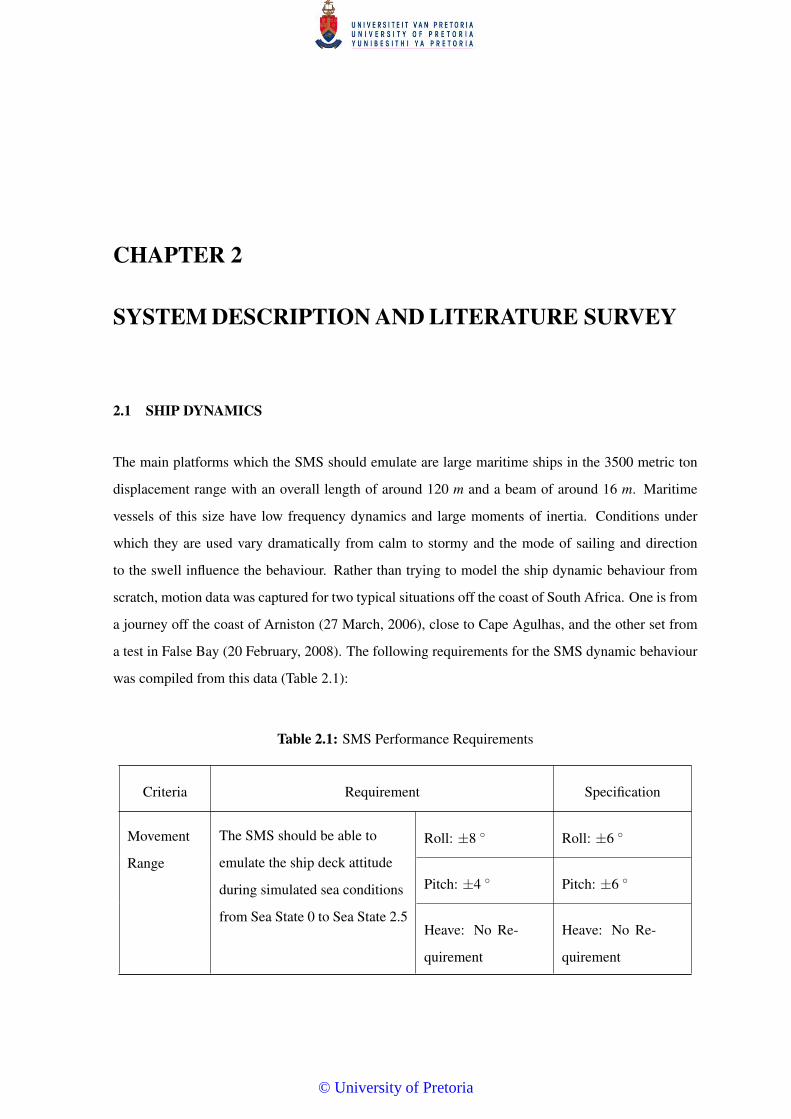
2.1 SHIP DYNAMICS
The main platforms which the SMS should emulate are large maritime ships in the 3500 metric ton
displacement range with an overall length of around 120 m and a beam of around 16 m. Maritime
vessels of this size have low frequency dynamics and large moments of inertia. Conditions under
which they are used vary dramatically from calm to stormy and the mode of sailing and direction
to the swell influence the behaviour. Rather than trying to model the ship dynamic behaviour from
scratch, motion data was captured for two typical situations off the coast of South Africa. One is from
a journey off the coast of Arniston (27 March, 2006), close to Cape Agulhas, and the other set from
a test in False Bay (20 February, 2008). The following requirements for the SMS dynamic behaviour
was compiled from this data (Table 2.1):
Table 2.1: SMS Performance Requirements
Criteria Requirement Specification
Movement
Range
The SMS should be able to
emulate the ship deck attitude
during simulated sea conditions
from Sea State 0 to Sea State 2.5
Roll: ±8 ◦ Roll: ±6 ◦
Pitch: ±4 ◦ Pitch: ±6 ◦
Heave: No Re-
quirement
Heave: No Re-
quirement
© University of Pretoria
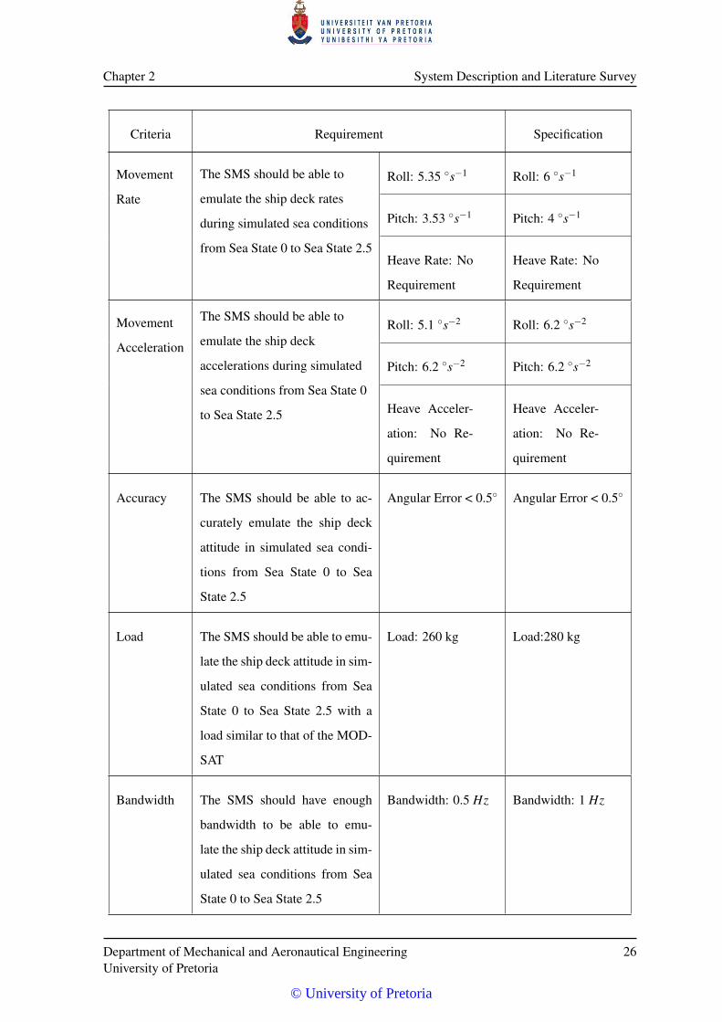
Chapter 2 System Description and Literature Survey
Criteria Requirement Specification
Movement
Rate
The SMS should be able to
emulate the ship deck rates
during simulated sea conditions
from Sea State 0 to Sea State 2.5
Roll: 5.35 ◦s−1 Roll: 6 ◦s−1
Pitch: 3.53 ◦s−1 Pitch: 4 ◦s−1
Heave Rate: No
Requirement
Heave Rate: No
Requirement
Movement
Acceleration
The SMS should be able to
emulate the ship deck
accelerations during simulated
sea conditions from Sea State 0
to Sea State 2.5
Roll: 5.1 ◦s−2 Roll: 6.2 ◦s−2
Pitch: 6.2 ◦s−2 Pitch: 6.2 ◦s−2
Heave Acceler-
ation: No Re-
quirement
Heave Acceler-
ation: No Re-
quirement
Accuracy The SMS should be able to ac-
curately emulate the ship deck
attitude in simulated sea condi-
tions from Sea State 0 to Sea
State 2.5
Angular Error < 0.5◦ Angular Error < 0.5◦
Load The SMS should be able to emu-
late the ship deck attitude in sim-
ulated sea conditions from Sea
State 0 to Sea State 2.5 with a
load similar to that of the MOD-
SAT
Load: 260 kg Load:280 kg
Bandwidth The SMS should have enough
bandwidth to be able to emu-
late the ship deck attitude in sim-
ulated sea conditions from Sea
State 0 to Sea State 2.5
Bandwidth: 0.5 Hz Bandwidth: 1 Hz
Department of Mechanical and Aeronautical EngineeringUniversity of Pretoria
26
© University of Pretoria
Chapter 2 System Description and Literature Survey
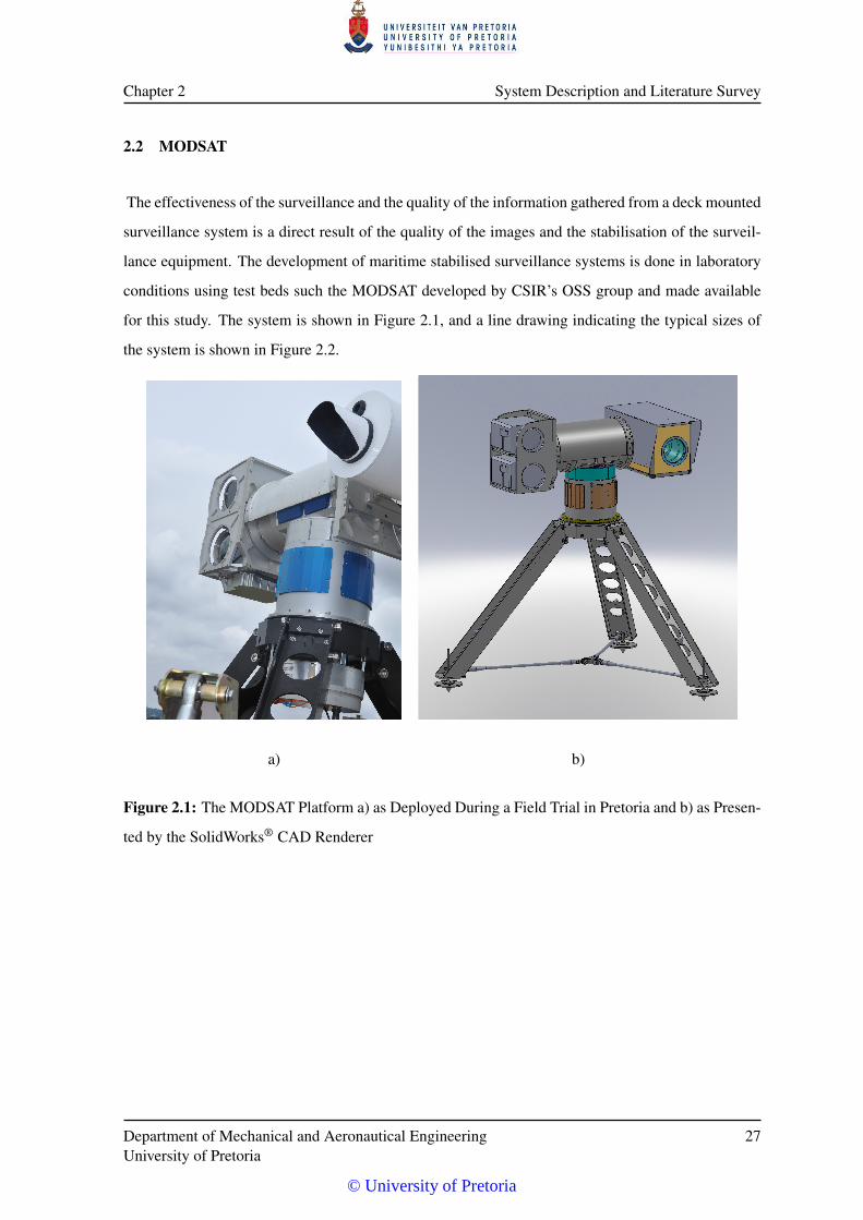
2.2 MODSAT
The effectiveness of the surveillance and the quality of the information gathered from a deck mounted
surveillance system is a direct result of the quality of the images and the stabilisation of the surveil-
lance equipment. The development of maritime stabilised surveillance systems is done in laboratory
conditions using test beds such the MODSAT developed by CSIR’s OSS group and made available
for this study. The system is shown in Figure 2.1, and a line drawing indicating the typical sizes of
the system is shown in Figure 2.2.
a) b)
Figure 2.1: The MODSAT Platform a) as Deployed During a Field Trial in Pretoria and b) as Presen-
ted by the SolidWorks® CAD Renderer
Department of Mechanical and Aeronautical EngineeringUniversity of Pretoria
27
© University of Pretoria
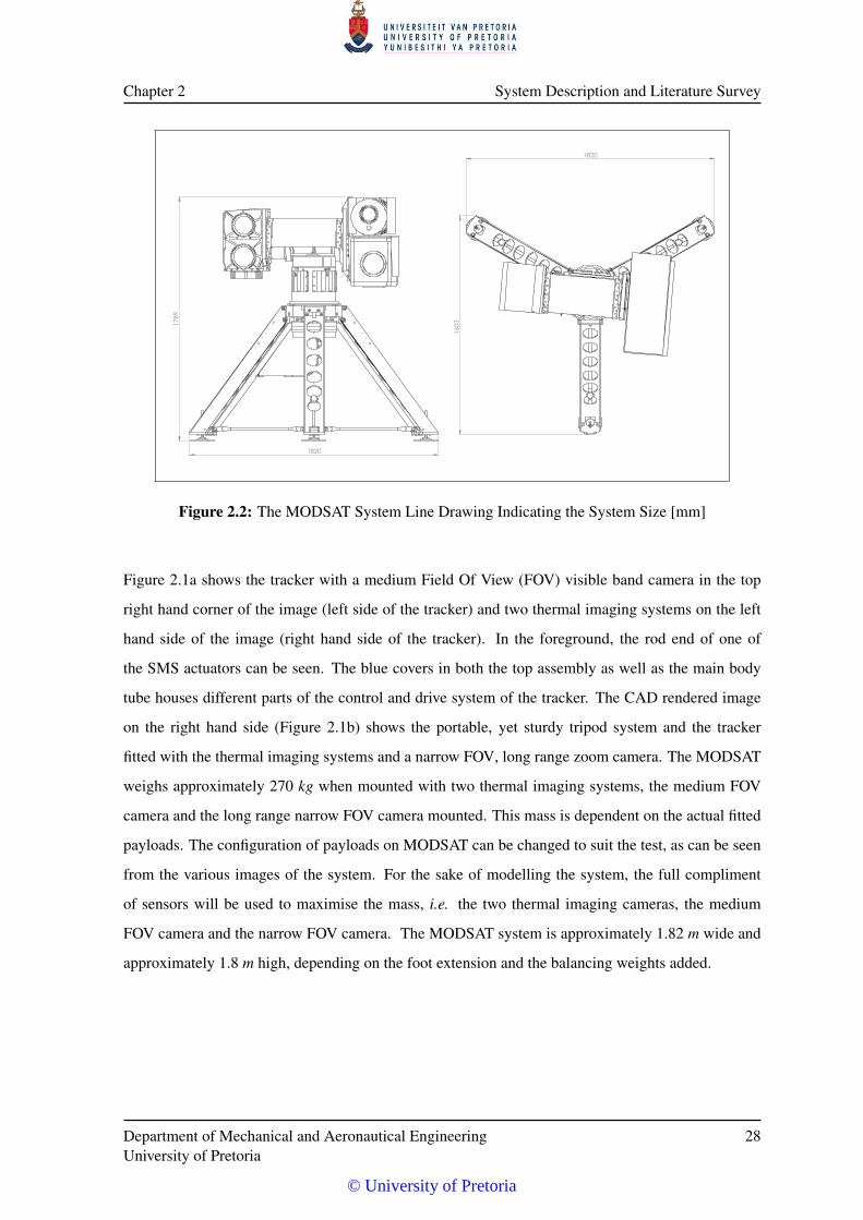
Chapter 2 System Description and Literature Survey
1820
178
9
160
3
1820
Figure 2.2: The MODSAT System Line Drawing Indicating the System Size [mm]
Figure 2.1a shows the tracker with a medium Field Of View (FOV) visible band camera in the top
right hand corner of the image (left side of the tracker) and two thermal imaging systems on the left
hand side of the image (right hand side of the tracker). In the foreground, the rod end of one of
the SMS actuators can be seen. The blue covers in both the top assembly as well as the main body
tube houses different parts of the control and drive system of the tracker. The CAD rendered image
on the right hand side (Figure 2.1b) shows the portable, yet sturdy tripod system and the tracker
fitted with the thermal imaging systems and a narrow FOV, long range zoom camera. The MODSAT
weighs approximately 270 kg when mounted with two thermal imaging systems, the medium FOV
camera and the long range narrow FOV camera mounted. This mass is dependent on the actual fitted
payloads. The configuration of payloads on MODSAT can be changed to suit the test, as can be seen
from the various images of the system. For the sake of modelling the system, the full compliment
of sensors will be used to maximise the mass, i.e. the two thermal imaging cameras, the medium
FOV camera and the narrow FOV camera. The MODSAT system is approximately 1.82 m wide and
approximately 1.8 m high, depending on the foot extension and the balancing weights added.
Department of Mechanical and Aeronautical EngineeringUniversity of Pretoria
28
© University of Pretoria
Chapter 2 System Description and Literature Survey
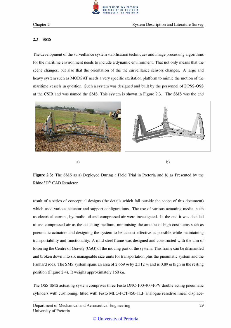
2.3 SMS
The development of the surveillance system stabilisation techniques and image processing algorithms
for the maritime environment needs to include a dynamic environment. That not only means that the
scene changes, but also that the orientation of the the surveillance sensors changes. A large and
heavy system such as MODSAT needs a very specific excitation platform to mimic the motion of the
maritime vessels in question. Such a system was designed and built by the personnel of DPSS-OSS
at the CSIR and was named the SMS. This system is shown in Figure 2.3. The SMS was the end
a) b)
Figure 2.3: The SMS as a) Deployed During a Field Trial in Pretoria and b) as Presented by the
Rhino3D® CAD Renderer
result of a series of conceptual designs (the details which fall outside the scope of this document)
which used various actuator and support configurations. The use of various actuating media, such
as electrical current, hydraulic oil and compressed air were investigated. In the end it was decided
to use compressed air as the actuating medium, minimising the amount of high cost items such as
pneumatic actuators and designing the system to be as cost effective as possible while maintaining
transportability and functionality. A mild steel frame was designed and constructed with the aim of
lowering the Centre of Gravity (CoG) of the moving part of the system. This frame can be dismantled
and broken down into six manageable size units for transportation plus the pneumatic system and the
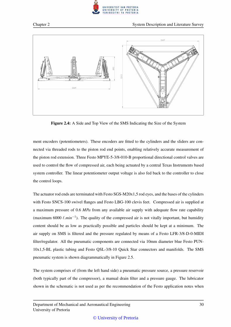
Panhard rods. The SMS system spans an area of 2.669 m by 2.312 m and is 0.89 m high in the resting
position (Figure 2.4). It weighs approximately 160 kg.
The OSS SMS actuating system comprises three Festo DNC-100-400-PPV double acting pneumatic
cylinders with cushioning, fitted with Festo MLO-POT-450-TLF analogue resistive linear displace-
Department of Mechanical and Aeronautical EngineeringUniversity of Pretoria
29
© University of Pretoria
Chapter 2 System Description and Literature Survey
2669
890
2669
231
2 Figure 2.4: A Side and Top View of the SMS Indicating the Size of the System
ment encoders (potentiometers). These encoders are fitted to the cylinders and the sliders are con-
nected via threaded rods to the piston rod end points, enabling relatively accurate measurement of
the piston rod extension. Three Festo MPYE-5-3/8-010-B proportional directional control valves are
used to control the flow of compressed air, each being actuated by a central Texas Instruments based
system controller. The linear potentiometer output voltage is also fed back to the controller to close
the control loops.
The actuator rod ends are terminated with Festo SGS-M20x1,5 rod eyes, and the bases of the cylinders
with Festo SNCS-100 swivel flanges and Festo LBG-100 clevis feet. Compressed air is supplied at
a maximum pressure of 0.6 MPa from any available air supply with adequate flow rate capability
(maximum 6000 `.min−1). The quality of the compressed air is not vitally important, but humidity
content should be as low as practically possible and particles should be kept at a minimum. The
air supply on SMS is filtered and the pressure regulated by means of a Festo LFR-3/8-D-0-MIDI
filter/regulator. All the pneumatic components are connected via 10mm diameter blue Festo PUN-
10x1,5-BL plastic tubing and Festo QSL-3/8-10 Quick Star connectors and manifolds. The SMS
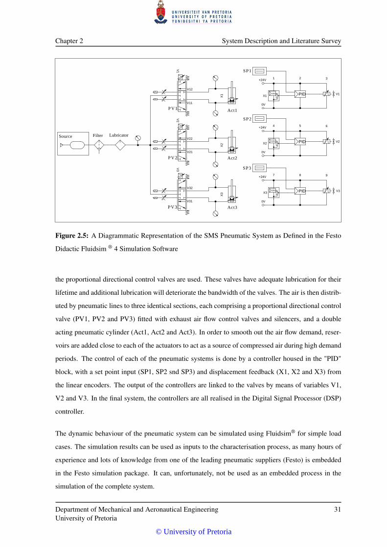
pneumatic system is shown diagrammatically in Figure 2.5.
The system comprises of (from the left hand side) a pneumatic pressure source, a pressure reservoir
(both typically part of the compressor), a manual drain filter and a pressure gauge. The lubricator
shown in the schematic is not used as per the recommendation of the Festo application notes when
Department of Mechanical and Aeronautical EngineeringUniversity of Pretoria
30
© University of Pretoria
Chapter 2 System Description and Literature Survey
X1
V11
V12
V1
V21
V22
V2
V31
V32
V3
V1PIDX110V
X2X3
0V
+24V
V2PIDX210V
V3PIDX310V
0V
+24V
0V
+24V
PV1
PV2
PV3
Act1
Act2
Act3
Source Filter Lubricator
SP1
SP2
SP3
1 2 3
4 5 6
7 8 9
Figure 2.5: A Diagrammatic Representation of the SMS Pneumatic System as Defined in the Festo
Didactic Fluidsim ® 4 Simulation Software
the proportional directional control valves are used. These valves have adequate lubrication for their
lifetime and additional lubrication will deteriorate the bandwidth of the valves. The air is then distrib-
uted by pneumatic lines to three identical sections, each comprising a proportional directional control
valve (PV1, PV2 and PV3) fitted with exhaust air flow control valves and silencers, and a double
acting pneumatic cylinder (Act1, Act2 and Act3). In order to smooth out the air flow demand, reser-
voirs are added close to each of the actuators to act as a source of compressed air during high demand
periods. The control of each of the pneumatic systems is done by a controller housed in the "PID"
block, with a set point input (SP1, SP2 snd SP3) and displacement feedback (X1, X2 and X3) from
the linear encoders. The output of the controllers are linked to the valves by means of variables V1,
V2 and V3. In the final system, the controllers are all realised in the Digital Signal Processor (DSP)
controller.
The dynamic behaviour of the pneumatic system can be simulated using Fluidsim® for simple load
cases. The simulation results can be used as inputs to the characterisation process, as many hours of
experience and lots of knowledge from one of the leading pneumatic suppliers (Festo) is embedded
in the Festo simulation package. It can, unfortunately, not be used as an embedded process in the
simulation of the complete system.
Department of Mechanical and Aeronautical EngineeringUniversity of Pretoria
31
© University of Pretoria
Chapter 2 System Description and Literature Survey
2.4 COMBINED MODSAT AND SMS
The combination of the MODSAT and the SMS described in the previous two sections results in
a surveillance system with an emulated maritime vessel movement. The MODSAT and SMS are
integrated by placing the tripod feet onto the end loading plates of the SMS. These feet are then
bolted down to prevent them from slipping off the loading plates. The SMS base plate is secured to
the ground by either bolting it to the floor or to large anchor plates fixed onto the ground by means of
four 900mm long anchor pegs.
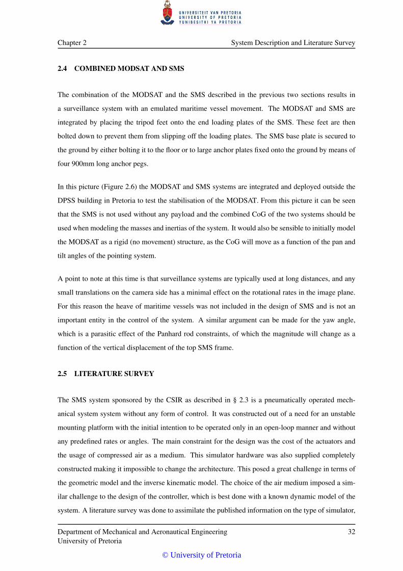
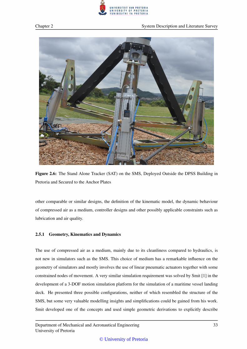
In this picture (Figure 2.6) the MODSAT and SMS systems are integrated and deployed outside the
DPSS building in Pretoria to test the stabilisation of the MODSAT. From this picture it can be seen
that the SMS is not used without any payload and the combined CoG of the two systems should be
used when modeling the masses and inertias of the system. It would also be sensible to initially model
the MODSAT as a rigid (no movement) structure, as the CoG will move as a function of the pan and
tilt angles of the pointing system.
A point to note at this time is that surveillance systems are typically used at long distances, and any
small translations on the camera side has a minimal effect on the rotational rates in the image plane.
For this reason the heave of maritime vessels was not included in the design of SMS and is not an
important entity in the control of the system. A similar argument can be made for the yaw angle,
which is a parasitic effect of the Panhard rod constraints, of which the magnitude will change as a
function of the vertical displacement of the top SMS frame.
2.5 LITERATURE SURVEY
The SMS system sponsored by the CSIR as described in § 2.3 is a pneumatically operated mech-
anical system system without any form of control. It was constructed out of a need for an unstable
mounting platform with the initial intention to be operated only in an open-loop manner and without
any predefined rates or angles. The main constraint for the design was the cost of the actuators and
the usage of compressed air as a medium. This simulator hardware was also supplied completely
constructed making it impossible to change the architecture. This posed a great challenge in terms of
the geometric model and the inverse kinematic model. The choice of the air medium imposed a sim-
ilar challenge to the design of the controller, which is best done with a known dynamic model of the
system. A literature survey was done to assimilate the published information on the type of simulator,
Department of Mechanical and Aeronautical EngineeringUniversity of Pretoria
32
© University of Pretoria
Chapter 2 System Description and Literature Survey
Figure 2.6: The Stand Alone Tracker (SAT) on the SMS, Deployed Outside the DPSS Building in
Pretoria and Secured to the Anchor Plates
other comparable or similar designs, the definition of the kinematic model, the dynamic behaviour
of compressed air as a medium, controller designs and other possibly applicable constraints such as
lubrication and air quality.
2.5.1 Geometry, Kinematics and Dynamics
The use of compressed air as a medium, mainly due to its cleanliness compared to hydraulics, is
not new in simulators such as the SMS. This choice of medium has a remarkable influence on the
geometry of simulators and mostly involves the use of linear pneumatic actuators together with some
constrained nodes of movement. A very similar simulation requirement was solved by Smit [1] in the
development of a 3-DOF motion simulation platform for the simulation of a maritime vessel landing
deck. He presented three possible configurations, neither of which resembled the structure of the
SMS, but some very valuable modelling insights and simplifications could be gained from his work.
Smit developed one of the concepts and used simple geometric derivations to explicitly describe
Department of Mechanical and Aeronautical EngineeringUniversity of Pretoria
33
© University of Pretoria
Chapter 2 System Description and Literature Survey
the inverse kinematics of the simulator. The latter being made possible by the simplest choice of
actuation.
Other contributions to the simulator design came from Chiew et al. [2] with a Gough-Stewart platform
based driving simulator and Qu et al. [3] with the derivation of the inverse kinematics of variant of the
Gough-Stewart platform replacing three of the actuators with fixed length rods, similar to the design
philosophy of the SMS. In both these cases the Gough-Stewart platform was used as the basis of the
design and in both cases the inverse kinematics was derived in explicit form. The Gough-Stewart
platform is a well researched design based on the initial work done by Gough et al. [4] on a universal
tyre test machine in 1962 and Stewart [5] on a variant of the 6-DOF parallel manipulator, mainly
for flight simulation. The, now commonly phrased, hexapod has more similarity with the Gough
design than that of Stewart, having six linear actuators connecting a movable platform to a static base
through rotary joints. In the case of the normal hexapod, the inverse kinematics has a very simple
explicit set of equations, whereas the forward kinematics has to be calculated using numerical solvers.
The same explicit inverse kinematic solution is claimed by Qu et al. adding the fixed length arms into
the equation solver. This method seems to have great potential for derivation of the SMS geometry
and kinematics.
An approach to ease the design of complex systems in the Mechatronics domain is to migrate the
model from a pure first principles derivation to a more abstract higher level model using simulation
tools. This comes at the cost of getting familiar with the modelling and simulation software (in time)
and the cost of the commercial software acquisition (in monetary value). Typical software packages
that can be used for this purpose is Matlab®, Simulink®, Festo’s Fluidsim and MSC ADAMS®.
Based on publications by, amongst others, Brezina et al. [6] and Baran et al. [7], ADAMS® can
be used as a development platform for dynamic modelling of a mechanical system such as SMS as
well as for embedding controller designs and analyzing the implementations thereof with Matlab®
Simulink® co-simulations. This method of development presents great promise in the definition of
the inverse kinematics, the definition of the dynamic model, the system identification process as well
as the testing of controller designs once the model is validated.
2.5.2 Pneumatic Actuators
Pneumatically operated systems, compared to their hydraulic counterparts, are preferred in environ-
ments where the actuation rates are slower, the positions or extensions of the actuators are controlled
Department of Mechanical and Aeronautical EngineeringUniversity of Pretoria
34
© University of Pretoria
Chapter 2 System Description and Literature Survey
by hard stops or buffers and where the impact of a compressible fluid is low on the controllability
of the system. The cost of the actuators are typically much lower than that of electro-mechanical or
hydraulic actuators. In the same light, the support and maintenance on pneumatic systems tends to be
lower and the service air is available in most buildings.
With these reasons in mind, pneumatic actuators have been used fairly extensively in more precisely
controlled systems and a fair amount of modelling, simulation and controller design has been done in
this domain. The main topics addressed in the modeling of pneumatic circuits are the valve mass flow
characteristics, the temporal air transport characteristics and the effects of changes in pressure and
temperature in charging and discharging cycles of varying size volumes such as linear actuators
Pneumatic circuit theory is based in the thermodynamic behaviour of air under different pressures
and flow rates. A physics based thermodynamic foundation as taught in most graduate engineering
courses is a good starting point in understanding the issues at hand. Reference text books such as
that by Crowe [8] is written in a more applied fashion and expands on many of the assumptions made
to ease the modelling scope and effort. Other published works that can be used include texts on the
design and analysis of pneumatic systems and circuits such as those by Anderson [9] and Beater [10].
The latter two of the text books have a very pragmatic way of approaching the modelling and control
of pneumatic systems with a simplified entry from theoretical thermodynamic principles, making
them ideal for engineering problem solving.
The problem statement of a pneumatic model and a control system for SMS can be broken down to
generating the necessary models for the air flow or mass flow through the valve orifices, the rate of
pressure change in the actuator volumes, the resultant actuator force that can be transferred to the
load, the change of volume of actuator as a result of the movement of the load and and the effects
of that pressure and volume change on the mass flow. In essence a set of differential equations that
needs to be solved.
One of the most complete sources of pneumatic modelling found in the survey was that of Richer et al.
[11]. In this publication Richer models the piston load dynamics, the cylinder chambers, the valves,
the connecting lines and the friction. On closer inspection a series of assumptions and simplifications
were made that would make the detailed models possibly incompatible with our system. These were
primarily the use of the classic derivation for the mass flow through the valve and the valve orifices
modelled as circular holes overlapping with straight edges.
Department of Mechanical and Aeronautical EngineeringUniversity of Pretoria
35
© University of Pretoria
Chapter 2 System Description and Literature Survey
Firstly, the initial investigation of the SMS pneumatic system revealed that the assumptions of single
orifice valve flow models might not hold in a system with multiple orifices in the flow, most of
which are not optimised for laminar flow. It is also very probable that contraction will occur between
orifices and tubing. A further search for more realistic models resulted in the flow models described
in the ISO-6358-1:2013(EN) [12] and ISO-6358-2:2013(EN) [13] standards, initially proposed by
Purdue et al. [14] and generalised by Sanville [15]. These models effectively exchanges the discharge
coefficient and effective area for a lumped sonic conductance entity, a variable critical pressure ratio
and a modified flow function.
Secondly, the valve orifice geometry described in Richer’s work differed from that of the Festo valves
used in the SMS system. A simplified effective valve area model was proposed by Smit [1] and Šitum
et al. [16] but still included an quadratic relationship between valve area and valve spool deflection
that did not agree with the valve geometry.
Other very valuable sources of information include the valve flow models derived by Ben-Dov et al.
[17] and that of Nouri et al. [18] that proposed a method of determining the effective valve area
through a series of fixed volume measurement with the assumption of an ideal isentropic mass flow.
The critical pressure ratio is also assumed to be constant; an assumption that needs to be verified. Also
the model described in the paper by Van der Merwe et al. [19] that showed the relationship between
the basic flow model through a restriction and the more general ISO-6358-1:2013(EN) description of
the valve.
The theoretical models found in literature were numerous having varying amounts of assumption,
simplification and accuracy. In most cases, the models were deemed too complex to determine the
parameters accurately and too costly in terms of computation to consider for use in a large simulation.
A well described model of the actual actuator used in SMS with identified and validated coefficients
could not be found in literature. This forced the literature survey into the domain of experimental
system identification.
The experimental configurations needed to accurately identify the parameters of the pneumatic sys-
tem in many cases involved specialised equipment and sensors. Simple experiments with the inferring
of entities such as flow rate from the measurement of pressure are used in many of the studies sur-
veyed. The most representative flow measurements using the inference principle are done using iso-
thermal discharge method described in ISO-6358-2:2013(E) [13]. This method relies on the change
Department of Mechanical and Aeronautical EngineeringUniversity of Pretoria
36
© University of Pretoria
Chapter 2 System Description and Literature Survey
of pressure in an isothermal chamber during a discharging cycle, using the choked flow region for the
determination of the sonic conductance and the subsonic region for the critical pressure ratio and the
flow function modifier. This method is described in great detail by Wang et al. [20] including the
construction of the isothermal chamber, the assumptions and the calculation methods. This method
involves both specialised equipment and is limited to on the discharging phase. A similar experiment
is described by Kawashima et al. [21] for both the charging and discharging phases. Accuracy of
the coefficients is, in both these cases, the major driving force behind the methods, delivering flow
rates to within a 1 % error [22] and sonic conductance values to within 3 % uncertainty. As this level
of accuracy is not of prime importance for a controller design process, the isothermal chamber can
be exchanged for a normal pressure vessel with the accompanying assumptions regarding the heat
transfer coefficient being close to 1 for a discharging process and 1.4 for a charging process. This
method has successfully been used by Nouri et al. [23] and Van der Merwe et al. [19].
From this survey it can be seen that pneumatics models are in abundance, although the background
and derivation of those models are in many cases unknown. It makes sense to understand the under-
lying thermodynamic principles and to redo some of the derivations to ensure that the assumptions
are valid and that the models are not used outside of their designed conditions. A good example is
the assumptions made to derive the valve flow model, being that of an adiabatic process (i.e. no heat
exchange occurs), no contraction of flow and zero upstream velocity. The derivation is also done
for a single orifice with well rounded edges, which has to be expanded to sharp edges and multiple
orifices. A comparison and error analysis between these very theoretical (classical) models and the
more realistic models such as the ISO-6358 model, and validating these models with experimental
results would be time well spent.
2.5.2.1 Friction
From all the pneumatic systems modelling resources found in published literature the friction contri-
bution to the nonlinear behaviour is noticeable. As described by Fleck et al. [24] pneumatic systems,
especially miniature ones, are plagued by a discontinuous and highly nonlinear relationship between
friction force and traversing velocity. This in combination with the compressibility of the operating
medium, being compressed air, results in a lot of higher order modes in a control system. The draw-
back of pneumatic systems lie in the poor pneumatic force vs. friction force ratio. Similar statements
are made by authors such as Nouri et al. [23], Ning et al. [25] and Richer et al. [26]. The friction
Department of Mechanical and Aeronautical EngineeringUniversity of Pretoria
37
© University of Pretoria
Chapter 2 System Description and Literature Survey
contribution is very often neglected due to the complexity of accurate friction models, and in many
cases a static or semi-static model is derived and used in applications. These simplifications typically
have adverse effects on the tracking performance of control systems.
Friction models in pneumatic systems presented in literature vary greatly in complexity and accuracy.
These range from completely ignoring the fact of friction by assuming frictionless actuators [17],
simple stick-slip friction models including static friction, Coulomb friction and velocity dependent
viscous friction [1], [25], [27] to very complex friction models with static, pre-sliding, transient and
sliding regimes and hysteresis [23], [28], [29]. These models have their origins in the friction model
development of Dahl [30] describing the interference of surfaces as spring like interactions. This
gave rise to a Coulomb friction model with lag being introduced in the friction force at velocity
reversals. The inclusion of effects like the Stribeck effect and hysteresis has been most effectively
added with the development of the LuGre model by Canudas de Wit et al. [31], a co-operation
between the Lund Institute of Technology and the Polytechnic of Grenoble. The LuGre model was
later improved by Swevers et al. to incorporate hysteresis [32], also known as the Leuven model.
Improvements on the LuGre and Leuven models are ongoing. A model such as Dupont et al.’s elasto-
plastic model [33] includes a function to minimize drift in the pre-sliding regime of the LuGre model,
which includes an irreversible (plastic) component. Similarly, a computationally effective physically
motivated general friction model such as the General Maxwell-Slip model is proposed by Lampaert
et al. [34] to minimise stack overflow in the Leuven model.
The identification of the parameters in the friction models once again poses a challenge. Methods to
exercise the systems to reveal their characteristics are well published, albeit complex in nature and
resource intensive. Friction, as a parasitic force, can be derived from the common system dynamic
equations if the forces can be measured with accuracy in the presence of uncertainty and noise. Using
facilities to activate the friction modes in actuators and to effectively decouple the forces from each
other is the preferred way to determine the friction model coefficients. In the absence of such facilities
the actual instrumented actuators need to be used. A very applicable study was conducted by Belforte
et al. [35] comparing the friction behaviour of cylinders of different diameters. The velocity steady
state condition was the prime focus of the study, and less so the transients at zero velocity. A similar
test series was conducted by Andrighetto et al. [36] comparing the friction behaviour in pneumatic
actuators from several manufacturers. Static friction vs. velocity maps were generated through the
inference of friction force from the load dynamic equation. Once again, the dynamically varying
effects were ignored. A study that applied the Leeuven model and represented the hysteresis of the
Department of Mechanical and Aeronautical EngineeringUniversity of Pretoria
38
© University of Pretoria
Chapter 2 System Description and Literature Survey
pneumatic seals as well as the differences in the viscous friction coefficients for accelerating and
decelerating movement was done by Nouri et al. [23]. Another noticeable contribution to the domain
was made by the same author with experimental results pointing out the effects of supply pressure on
the friction behaviour of the seals [37].
2.5.3 Control
Once the dynamic model of the system, consisting of the mechanical and geometric models, the in-
fluences of the payload, the dynamic characteristics of the pneumatic system and the influence of
nonlinear effects such as friction and large scale mass flow is generated and validated, the model can
be used for the development and testing of a control system. Controller design methodology is an ex-
tremely wide field of study, as is the choice of controller architecture and the type of controller.
Numerous text books have been published on the control of systems in the presence of friction as well
as other nonlinear effects such as gear backlash, nonlinear gain and dead band behaviour. The most
notable text referenced in the domain of controlling pneumatic systems with emphasis on control
of machines is ”Control of Machines with Friction” by Brian Armstrong-Hélouvry [38]. The basic
principles are covered in great detail and enables the reader to develop strategies for controller design.
More generic text books such as [39] form the basis of the skill set of control engineering and is
always a starting point for controller design. Other texts on nonlinear controller design methodology
and structure are available and are too many to list.
In the light of the overwhelming amount of literature available, more focus was given to tried and
tested control schemes of systems resembling the SMS system. That means others pneumatically
actuated systems or subsystems with medium to low absolute accuracy and low bandwidth require-
ments. Once again the work done by Richer et al. [11] jumps to the foreground. In this study it was
shown that a full order Sliding Mode Controller (SMC) provided excellent control and tracking of a
pneumatic actuator. This came at the expense of a very complex control law and the use of numerical
observers for the spool displacement and delayed variables. A reduced order controller gave slightly
lower performance results but still required a vast amount of computational resources. This nonlinear
controller was also adopted by Smit [1] in the control of an Unmanned Aerial Vehicle (UAV) landing
platform simulator, and Laghrouche et al. [40] and Bigras [41] in general pneumatic control studies.
A comparison between a SMC design based on the nonlinear model of the pneumatic plant vs. a
design based on a linearized plant was conducted as presented by Bone et al. [42]. The tracking
Department of Mechanical and Aeronautical EngineeringUniversity of Pretoria
39
© University of Pretoria
Chapter 2 System Description and Literature Survey
performance of the nonlinear based controller was marginally better than that of the linearized model,
and both were better than previously published controllers under the same conditions. Linearizing the
plant does seem to add a bit of sensitivity on the working point and the load.
The use of fuzzy logic and neural networks have also been exploited, albeit to a lesser degree than
other linear and nonlinear techniques. An example of an adaptive neural network control strategy is
described in a paper delivered by Yu [43] outlining a Proportional Differential Integral (PID) control-
ler that will ”self-tune” as the conditions change. A similar approach has been followed by Šitum et
al. [44] to compensate for changing friction behaviour and air supply variations using a fuzzy logic
modifier and a PID controller. In both cases the self-compensating behaviour of the controllers makes
them more robust and involve less tuning during the life cycle of the systems.
The older and most often used methods of controlling pneumatic systems are still tuned PID control-
lers based on simplified and linearized plants. Proportional Integral (PI), Proportional Differential
(PD) and PID controllers can be tuned to deliver good results on various system architectures, as long
as a stable system can be realised to perform the identification process, as reported by Hamiti et al.
[45]. Controllers can be synthesised by using auto-tuning methods such a the Chien-Hrones-Reswick
method as described in this publication, or manually as described by Šitum et al. [16] and Beater
[10]. Techniques to improve the response of the systems and to minimise limit cycles and the effect
of stiction has been employed in many of the more traditional control schemes. Feedback from pres-
sure sensors and acceleration feedback to stabilize the system has been employed by Wang et al. [46]
with acceptable results. Traditional control techniques still have a role to play in pneumatic systems
as it is well studied, well known and simple to implement. It does rely largely on knowledge of the
behaviour of the plant model.
Department of Mechanical and Aeronautical EngineeringUniversity of Pretoria
40
© University of Pretoria
CHAPTER 3
SMS KINEMATICS
The SMS is a special form of a Gough-Stewart platform which can be defined as a subclass of parallel
manipulators. Parallel manipulators, in contrast to serial manipulators that have a series of links joined
by articulated joints in series (like a human arm), has multiple simple links all working in a parallel
fashion, similar to two human arms lifting a load.
The first (known) example of such a manipulator was the tyre test machine constructed by Gough and
Whitehall in 1954-1955 ([47], [4]). The publication that really sparked interest in research into paral-
lel manipulators was the paper published by Stewart in 1965 [5], describing a flight simulator.
The definition of a Gough-Stewart platform can be formulated as a parallel manipulator consisting of
two platforms connected by six prismatic joints acting in parallel. The one platform is fixed to the
ground (base) and the other moving, with all the base platform joints in the base plane and moving
the platform joints in the same moving platform plane.
Although the SMS is not strictly a Gough-Stewart platform, as some of the joints are not in the same
plane, and three of the prismatic joints are replaced by Panhard rods, the same principles will hold for
the kinematics and dynamics of the system.
3.1 SMS CAD MODEL
The SMS was designed by Mr. Mark Holloway (CSIR, DPSS-OSS) to be easily manufacturable,
using the Solidworks® CAD package. Solid models of the pneumatic components were downloaded
from the Festo web site, checked for dimensional conformance and used in the design process. The
complete simulator, including fasteners, but excluding welding, was modelled to accurately determine
© University of Pretoria
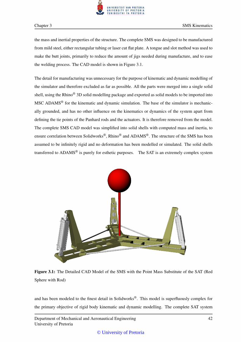
Chapter 3 SMS Kinematics
the mass and inertial properties of the structure. The complete SMS was designed to be manufactured
from mild steel, either rectangular tubing or laser cut flat plate. A tongue and slot method was used to
make the butt joints, primarily to reduce the amount of jigs needed during manufacture, and to ease
the welding process. The CAD model is shown in Figure 3.1.
The detail for manufacturing was unnecessary for the purpose of kinematic and dynamic modelling of
the simulator and therefore excluded as far as possible. All the parts were merged into a single solid
shell, using the Rhino® 3D solid modelling package and exported as solid models to be imported into
MSC ADAMS® for the kinematic and dynamic simulation. The base of the simulator is mechanic-
ally grounded, and has no other influence on the kinematics or dynamics of the system apart from
defining the tie points of the Panhard rods and the actuators. It is therefore removed from the model.
The complete SMS CAD model was simplified into solid shells with computed mass and inertia, to
ensure correlation between Solidworks®, Rhino® and ADAMS®. The structure of the SMS has been
assumed to be infinitely rigid and no deformation has been modelled or simulated. The solid shells
transferred to ADAMS® is purely for esthetic purposes. The SAT is an extremely complex system
Figure 3.1: The Detailed CAD Model of the SMS with the Point Mass Substitute of the SAT (Red
Sphere with Rod)
and has been modeled to the finest detail in Solidworks®. This model is superfluously complex for
the primary objective of rigid body kinematic and dynamic modelling. The complete SAT system
Department of Mechanical and Aeronautical EngineeringUniversity of Pretoria
42
© University of Pretoria
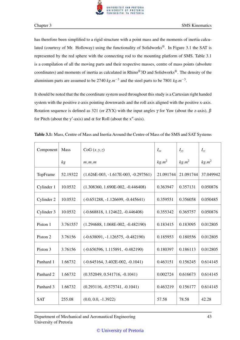
Chapter 3 SMS Kinematics
has therefore been simplified to a rigid structure with a point mass and the moments of inertia calcu-
lated (courtesy of Mr. Holloway) using the functionality of Solidworks®. In Figure 3.1 the SAT is
represented by the red sphere with the connecting rod to the mounting platform of SMS. Table 3.1
is a compilation of all the moving parts and their respective masses, centre of mass points (absolute
coordinates) and moments of inertia as calculated in Rhino®3D and Solidworks®. The density of the
aluminium parts are assumed to be 2740 kg.m−3 and the steel parts to be 7801 kg.m−3.
It should be noted that the the coordinate system used throughout this study is a Cartesian right handed
system with the positive z-axis pointing downwards and the roll axis aligned with the positive x-axis.
Rotation sequence is defined as 321 (or ZYX) with the input angles γ for Yaw (about the z-axis), β
for Pitch (about the y′-axis) and α for Roll (about the x′′-axis).
Table 3.1: Mass, Centre of Mass and Inertia Around the Centre of Mass of the SMS and SAT Systems
Component Mass CoG (x,y,z) Ixx Iyy Izz
kg m,m,m kg.m2 kg.m2 kg.m2
TopFrame 52.19322 (1.626E-003, -1.617E-003, -0.297561) 21.091744 21.091744 37.049942
Cylinder 1 10.0532 (1.308360, 1.690E-002, -0.446408) 0.363947 0.357131 0.050876
Cylinder 2 10.0532 (-0.651288, -1.126699, -0.445641) 0.359551 0.356058 0.050485
Cylinder 3 10.0532 (-0.668818, 1.124622, -0.446408) 0.355342 0.365757 0.050876
Piston 1 3.761557 (1.294688, 1.068E-002, -0.482190) 0.183415 0.183095 0.012805
Piston 2 3.76156 (-0.638091, -1.126575, -0.482190) 0.185953 0.180556 0.012805
Piston 3 3.76156 (-0.656596, 1.115891, -0.482190) 0.180397 0.186113 0.012805
Panhard 1 1.66732 (-0.645164, 3.402E-002, -0.1041) 0.463151 0.156245 0.614145
Panhard 2 1.66732 (0.352049, 0.541716, -0.1041) 0.002724 0.616673 0.614145
Panhard 3 1.66732 (0.293116, -0.575741, -0.1041) 0.463219 0.156177 0.614145
SAT 255.08 (0.0, 0.0, -1.3922) 57.58 78.58 42.28
Department of Mechanical and Aeronautical EngineeringUniversity of Pretoria
43
© University of Pretoria
Chapter 3 SMS Kinematics
3.2 SMS KINEMATIC VECTOR DIAGRAM MODEL
A complex model that contains physical dimensions, volume and stiffness constants does not add any
value to the derivation of the kinematics of the SMS. As mentioned previously, the SMS is not strictly
speaking a Gough-Stewart platform as all the joints of the moving platform are not in the same plane
and neither are the joints on the stationary platform. A free body diagram of the simulator geometry
has been generated to clarify the connections and to give insight into the possible mathematical defin-
itions of the kinematics. This derivation is not seen as part of the problem statement, as the kinematics
will be calculated by MSC ADAMS®, but is an ongoing effort to improve the mathematical model.
The process of deriving a set of equations for the SMS geometry and kinematics has been based on
existing derivations of firstly, the Gough-Stewart platform and secondly, the SMS.
3.2.1 Gough-Stewart Vector Kinematics
It can generally be stated that the inverse kinematics can be derived for a Gough-Stewart platform by
using the principle of a rotated and translated platform [2], the orientation uniquely defined by the six
leg lengths. The layout of a general Gough-Stewart platform is shown in Figure 3.2a. The system is
referenced by a grounded right handed frame {B} with axes xB, yB and zB, and a moving right handed
frame {P} with axes xP, yP and zP aligned with the platform. Points B1 to B6 are located on the base
and are all stationary points. Points P1 to P6 are located on the moving platform and are connected
to the base through legs l1 to l6. If we define a leg vector for the ith leg li (Figure 3.2b), referenced
in the B frame as Bli = [lix, liy, liz]T and a translation of Bd and a rotation (defined by the input angles
α ,β and γ) is applied to the moving platform, the leg vectors can be expressed as
B~li = BPR P~pi +
B~d− B~bi, (3.1)
with B~d = [x,y,z]T the translated position of frame {P}, P~pi = [pix, piy, piz]T the vector describing
the upper attachment points relative to frame {P}, B~bi = [bix,biy,biz]T the vector describing the base
attachments points relative to frame {B} and BPR the 3x3 matrix defining the rotation of the {P} frame
referenced to the {B} frame. From the basic theory of axis rotation ([48], [49]) the rotation matrices
Department of Mechanical and Aeronautical EngineeringUniversity of Pretoria
44
© University of Pretoria
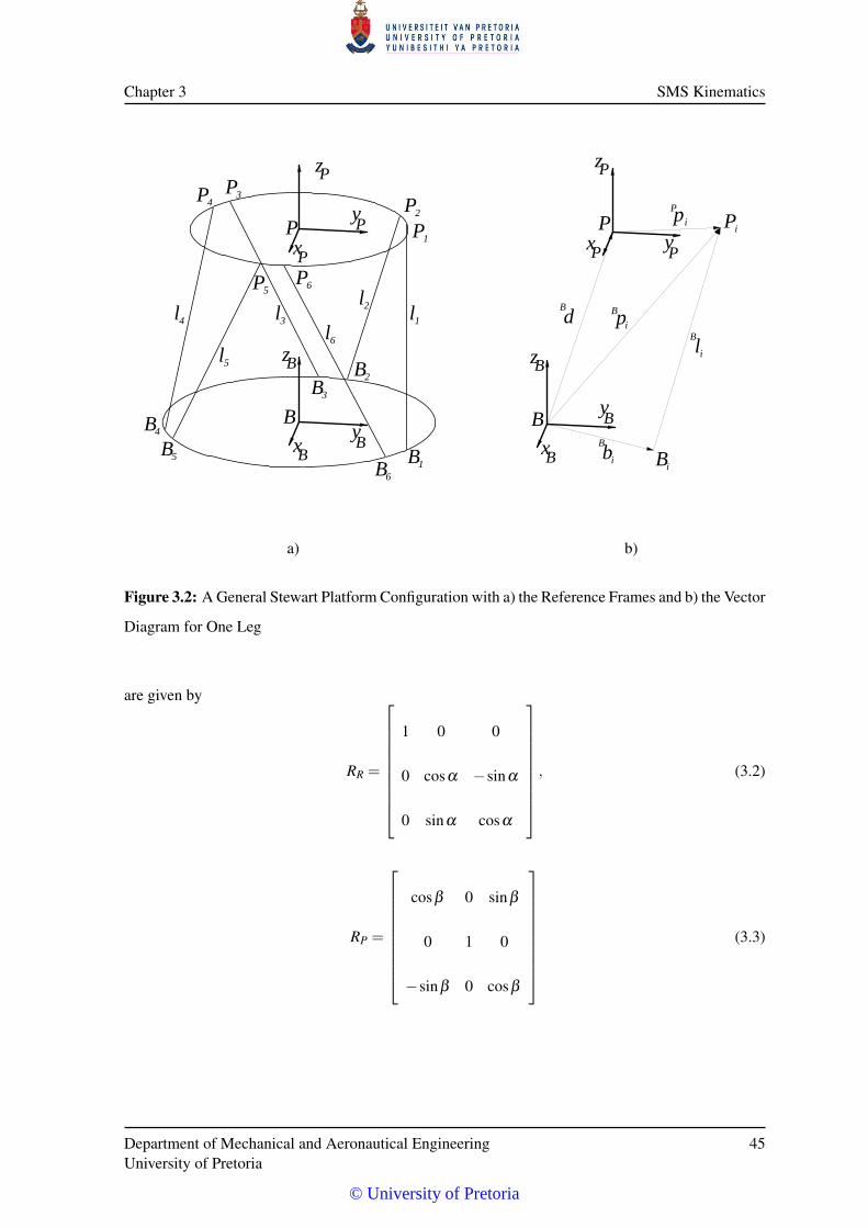
Chapter 3 SMS Kinematics
l
l6
l5
l4 3l 1l
P
Py
z
P
Bz
By
Bx
B
5B4B
3B2B
6B 1B
Px
6PP5
4P 3P2P
1P
2
P
p
p
zP
idB
B
ib
ilB
i
Py
i
iP
B
yB
Bz
Bx
B
PxP
B
a) b)
Figure 3.2: A General Stewart Platform Configuration with a) the Reference Frames and b) the Vector
Diagram for One Leg
are given by
RR =
1 0 0
0 cosα −sinα
0 sinα cosα
, (3.2)
RP =
cosβ 0 sinβ
0 1 0
−sinβ 0 cosβ
(3.3)
Department of Mechanical and Aeronautical EngineeringUniversity of Pretoria
45
© University of Pretoria
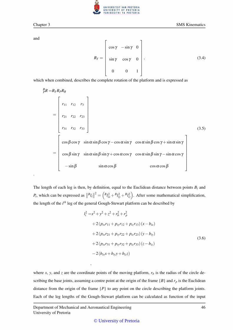
Chapter 3 SMS Kinematics
and
RY =
cosγ −sinγ 0
sinγ cosγ 0
0 0 1
, (3.4)
which when combined, describes the complete rotation of the platform and is expressed as
BPR =RY RPRR
=
r11 r12 r3
r21 r22 r23
r31 r32 r33
=
cosβ cosγ sinα sinβ cosγ− cosα sinγ cosα sinβ cosγ + sinα sinγ
cosβ sinγ sinα sinβ sinγ + cosα cosγ cosα sinβ sinγ− sinα cosγ
−sinβ sinα cosβ cosα cosβ
(3.5)
.
The length of each leg is then, by definition, equal to the Euclidean distance between points Bi and
Pi, which can be expressed as∥∥Bli∥∥2
=(
Bl2ix +
Bl2iy +
Bl2iz
). After some mathematical simplification,
the length of the ith leg of the general Gough-Stewart platform can be described by
l2i =x2 + y2 + z2 + r2
b + r2p
+2(pixr11 + piyr12 + pizr13)(x−bix)
+2(pixr21 + piyr22 + pizr23)(y−biy)
+2(pixr31 + piyr32 + pizr33)(z−biz)
−2(bixx+biyy+bizz)
,
(3.6)
where x, y, and z are the coordinate points of the moving platform, rb is the radius of the circle de-
scribing the base joints, assuming a centre point at the origin of the frame {B} and rp is the Euclidean
distance from the origin of the frame {P} to any point on the circle describing the platform joints.
Each of the leg lengths of the Gough-Stewart platform can be calculated as function of the input
Department of Mechanical and Aeronautical EngineeringUniversity of Pretoria
46
© University of Pretoria
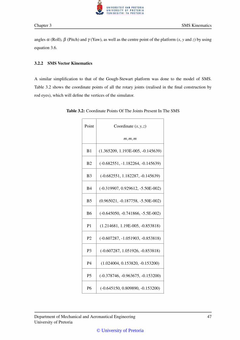
Chapter 3 SMS Kinematics
angles α (Roll), β (Pitch) and γ (Yaw), as well as the centre point of the platform (x, y and z) by using
equation 3.6.
3.2.2 SMS Vector Kinematics
A similar simplification to that of the Gough-Stewart platform was done to the model of SMS.
Table 3.2 shows the coordinate points of all the rotary joints (realised in the final construction by
rod eyes), which will define the vertices of the simulator.
Table 3.2: Coordinate Points Of The Joints Present In The SMS
Point Coordinate (x,y,z)
m,m,m
B1 (1.365209, 1.193E-005, -0.145639)
B2 (-0.682551, -1.182264, -0.145639)
B3 (-0.682551, 1.182287, -0.145639)
B4 (-0.319907, 0.929612, -5.50E-002)
B5 (0.965021, -0.187758, -5.50E-002)
B6 (-0.645050, -0.741866, -5.5E-002)
P1 (1.214681, 1.19E-005, -0.853818)
P2 (-0.607287, -1.051903, -0.853818)
P3 (-0.607287, 1.051926, -0.853818)
P4 (1.024004, 0.153820, -0.153200)
P5 (-0.378746, -0.963675, -0.153200)
P6 (-0.645150, 0.809890, -0.153200)
Department of Mechanical and Aeronautical EngineeringUniversity of Pretoria
47
© University of Pretoria
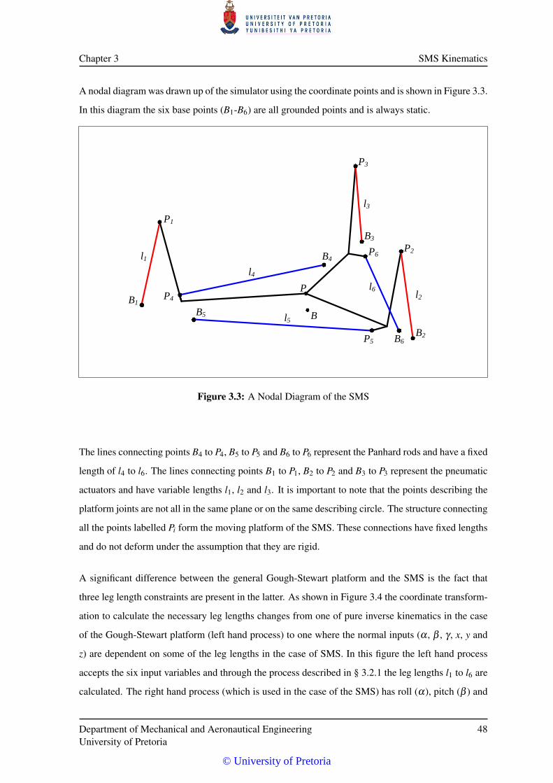
Chapter 3 SMS Kinematics
A nodal diagram was drawn up of the simulator using the coordinate points and is shown in Figure 3.3.
In this diagram the six base points (B1-B6) are all grounded points and is always static.
P3
B3
P6
B2B6P5
B5
B1
P2
P1
B4
P4
l3
l2l6
l5
l4
l1
P
B
Figure 3.3: A Nodal Diagram of the SMS
The lines connecting points B4 to P4, B5 to P5 and B6 to P6 represent the Panhard rods and have a fixed
length of l4 to l6. The lines connecting points B1 to P1, B2 to P2 and B3 to P3 represent the pneumatic
actuators and have variable lengths l1, l2 and l3. It is important to note that the points describing the
platform joints are not all in the same plane or on the same describing circle. The structure connecting
all the points labelled Pi form the moving platform of the SMS. These connections have fixed lengths
and do not deform under the assumption that they are rigid.
A significant difference between the general Gough-Stewart platform and the SMS is the fact that
three leg length constraints are present in the latter. As shown in Figure 3.4 the coordinate transform-
ation to calculate the necessary leg lengths changes from one of pure inverse kinematics in the case
of the Gough-Stewart platform (left hand process) to one where the normal inputs (α , β , γ , x, y and
z) are dependent on some of the leg lengths in the case of SMS. In this figure the left hand process
accepts the six input variables and through the process described in § 3.2.1 the leg lengths l1 to l6 are
calculated. The right hand process (which is used in the case of the SMS) has roll (α), pitch (β ) and
Department of Mechanical and Aeronautical EngineeringUniversity of Pretoria
48
© University of Pretoria
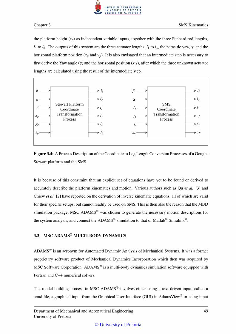
Chapter 3 SMS Kinematics
the platform height (zp) as independent variable inputs, together with the three Panhard rod lengths,
l4 to l6. The outputs of this system are the three actuator lengths, l1 to l3, the parasitic yaw, γ , and the
horizontal platform position (xp and yp). It is also envisaged that an intermediate step is necessary to
first derive the Yaw angle (γ) and the horizontal position (x,y), after which the three unknown actuator
lengths are calculated using the result of the intermediate step.
Stewart PlatformCoordinate
TransformationProcess
α
β
xp
yp
zp
l1
l2
l3
l4
l5
l6
SMSCoordinate
TransformationProcess
α
β
xp
ypzp
l1
l2
l3l4
l5
l6
Figure 3.4: A Process Description of the Coordinate to Leg Length Conversion Processes of a Gough-
Stewart platform and the SMS
It is because of this constraint that an explicit set of equations have yet to be found or derived to
accurately describe the platform kinematics and motion. Various authors such as Qu et al. [3] and
Chiew et al. [2] have reported on the derivation of inverse kinematic equations, all of which are valid
for their specific setups, but cannot readily be used on SMS. This is then also the reason that the MBD
simulation package, MSC ADAMS® was chosen to generate the necessary motion descriptions for
the system analysis, and connect the ADAMS® simulation to that of Matlab® Simulink®.
3.3 MSC ADAMS® MULTI-BODY DYNAMICS
ADAMS® is an acronym for Automated Dynamic Analysis of Mechanical Systems. It was a former
proprietary software product of Mechanical Dynamics Incorporation which then was acquired by
MSC Software Corporation. ADAMS® is a multi-body dynamics simulation software equipped with
Fortran and C++ numerical solvers.
The model building process in MSC ADAMS® involves either using a text driven input, called a
.cmd file, a graphical input from the Graphical User Interface (GUI) in AdamsView® or using input
Department of Mechanical and Aeronautical EngineeringUniversity of Pretoria
49
© University of Pretoria
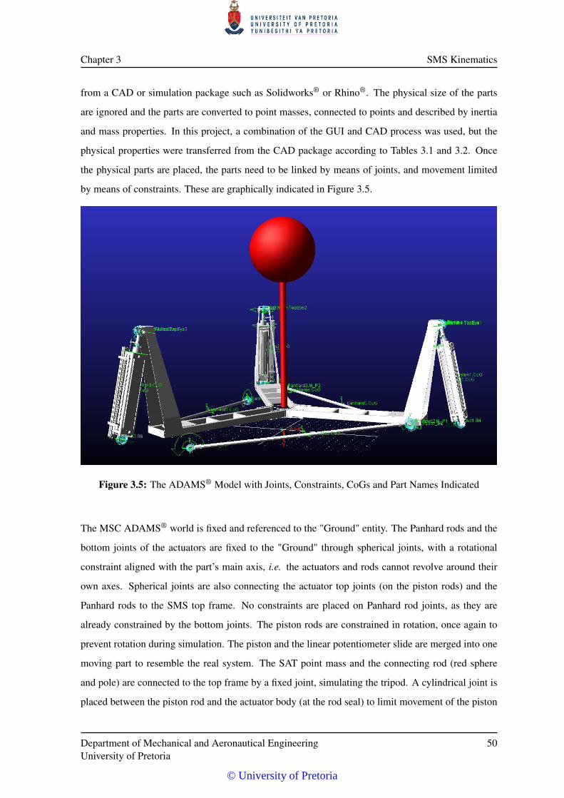
Chapter 3 SMS Kinematics
from a CAD or simulation package such as Solidworks® or Rhino®. The physical size of the parts
are ignored and the parts are converted to point masses, connected to points and described by inertia
and mass properties. In this project, a combination of the GUI and CAD process was used, but the
physical properties were transferred from the CAD package according to Tables 3.1 and 3.2. Once
the physical parts are placed, the parts need to be linked by means of joints, and movement limited
by means of constraints. These are graphically indicated in Figure 3.5.
Figure 3.5: The ADAMS® Model with Joints, Constraints, CoGs and Part Names Indicated
The MSC ADAMS® world is fixed and referenced to the "Ground" entity. The Panhard rods and the
bottom joints of the actuators are fixed to the "Ground" through spherical joints, with a rotational
constraint aligned with the part’s main axis, i.e. the actuators and rods cannot revolve around their
own axes. Spherical joints are also connecting the actuator top joints (on the piston rods) and the
Panhard rods to the SMS top frame. No constraints are placed on Panhard rod joints, as they are
already constrained by the bottom joints. The piston rods are constrained in rotation, once again to
prevent rotation during simulation. The piston and the linear potentiometer slide are merged into one
moving part to resemble the real system. The SAT point mass and the connecting rod (red sphere
and pole) are connected to the top frame by a fixed joint, simulating the tripod. A cylindrical joint is
placed between the piston rod and the actuator body (at the rod seal) to limit movement of the piston
Department of Mechanical and Aeronautical EngineeringUniversity of Pretoria
50
© University of Pretoria
Chapter 3 SMS Kinematics
and piston rod in only one direction, once again aligned with the actuator main axis. This joint has
the facility to include seal friction, which is not used in the current simulation. A further constraint
is placed on every actuator to limit movement past the end stops of the pneumatic actuators. This
contact force is placed between the piston and the actuator end stops and acts as an exponentially
growing force as a function of depression depth. In the absence of this end stop force, the piston will
be able to move past the ends of the actuators.
The actuating forces in the ADAMS® model is placed between the pistons and the relevant actu-
ator bodies and aligned with the axis of movement. These are all single component forces, called
"SFORCE_1" to "SFORCE_3". The extension of each actuator is measured as the magnitude of
the vector distance between a point on the piston (Piston.CoG) and actuator body (M_Ref), which
co-insides with the piston CoG point at zero extension (DM(Act1.M_Ref, Piston1.CoG)). Both the
forces and the measurements are placed in the model as state variables.
3.4 INTEGRATION BETWEEN MSC ADAMS® AND MATLAB®
A facility was created in MSC ADAMS® to link other simulation packages to it. This is done by
means of ADAMS®’ "System Elements" and variables. In order to generate the link between Matlab®
and ADAMS®, a force (in the case of actuator 1) will be generated by Simulink® and then passed
to the ADAMS® model through a State Variable called "PF1", which is explicitly linked to the one-
dimensional force "SFORCE_1". The force is placed in the ADAMS® model between the piston
assembly and the actuator body, aligned with the instantaneous coordinates of the top and bottom
spherical joints on the actuator (Direction: Between Two Bodies In Line-Of-Sight) and uses a function
to update its value (VARVAL(.SMS.PF1)) at every time step.
The evaluation of the runtime expression "DM(Act1.M_Ref, Piston1.CoG)", which determines the
extension of the actuator, generates a feedback length, which is passed to State Variable "X1" and can
be read by Simulink®.
The Plant Export function (in ADAMS®) is used to generate the nonlinear Simulink® model of the
ADAMS® system. In this case a plant was exported with forces ".SMS.PF1", ".SMS.PF2" and
".SMS.PF3" as inputs, and world angles ".SMS.Pitch", ".SMS.Roll" and ".SMS.Yaw" and actuator
extensions ".SMS.X1", ".SMS.X2" and ".SMS.X3" as outputs. The other state variables such as x
and x can also be added to the feedback. The "target" was set as "Matlab" with a "nonlinear" ana-
Department of Mechanical and Aeronautical EngineeringUniversity of Pretoria
51
© University of Pretoria
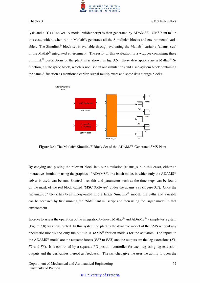
Chapter 3 SMS Kinematics
lysis and a "C++" solver. A model builder script is then generated by ADAMS®, "SMSPlant.m" in
this case, which, when run in Matlab®, generates all the Simulink® blocks and environmental vari-
ables. The Simulink® block set is available through evaluating the Matlab® variable "adams_sys"
in the Matlab® integrated environment. The result of this evaluation is a wrapper containing three
Simulink® descriptions of the plant as is shown in fig. 3.6. These descriptions are a Matlab® S-
function, a state space block, which is not used in our simulations and a sub-system block containing
the same S-function as mentioned earlier, signal multiplexers and some data storage blocks.
Figure 3.6: The Matlab® Simulink® Block Set of the ADAMS® Generated SMS Plant
By copying and pasting the relevant block into our simulation (adams_sub in this case), either an
interactive simulation using the graphics of ADAMS®, or a batch mode, in which only the ADAMS®
solver is used, can be run. Control over this and parameters such as the time steps can be found
on the mask of the red block called "MSC Software" under the adams_sys (Figure 3.7). Once the
"adams_sub" block has been incorporated into a larger Simulink® model, the paths and variable
can be accessed by first running the "SMSPlant.m" script and then using the larger model in that
environment.
In order to assess the operation of the integration between Matlab® and ADAMS® a simple test system
(Figure 3.8) was constructed. In this system the plant is the dynamic model of the SMS without any
pneumatic models and only the built-in ADAMS® friction models for the actuators. The inputs to
the ADAMS® model are the actuator forces (PF1 to PF3) and the outputs are the leg extensions (X1,
X2 and X3). It is controlled by a separate PD position controller for each leg using leg extension
outputs and the derivatives thereof as feedback. The switches give the user the ability to open the
Department of Mechanical and Aeronautical EngineeringUniversity of Pretoria
52
© University of Pretoria
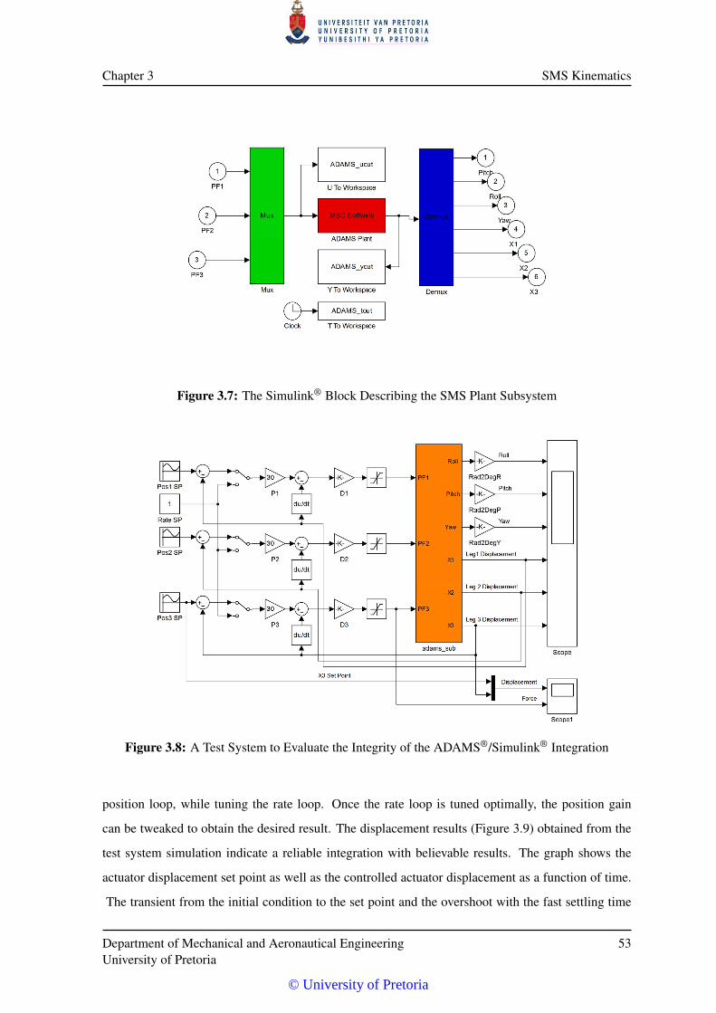
Chapter 3 SMS Kinematics
Figure 3.7: The Simulink® Block Describing the SMS Plant Subsystem
Figure 3.8: A Test System to Evaluate the Integrity of the ADAMS®/Simulink® Integration
position loop, while tuning the rate loop. Once the rate loop is tuned optimally, the position gain
can be tweaked to obtain the desired result. The displacement results (Figure 3.9) obtained from the
test system simulation indicate a reliable integration with believable results. The graph shows the
actuator displacement set point as well as the controlled actuator displacement as a function of time.
The transient from the initial condition to the set point and the overshoot with the fast settling time
Department of Mechanical and Aeronautical EngineeringUniversity of Pretoria
53
© University of Pretoria
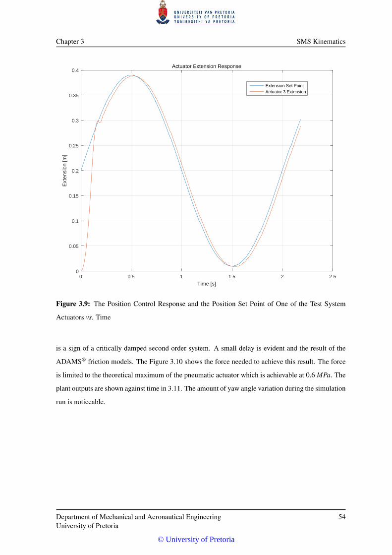
Chapter 3 SMS Kinematics
0 0.5 1 1.5 2 2.5
Time [s]
0
0.05
0.1
0.15
0.2
0.25
0.3
0.35
0.4E
xten
sion
[m]
Actuator Extension Response
Extension Set PointActuator 3 Extension
Figure 3.9: The Position Control Response and the Position Set Point of One of the Test System
Actuators vs. Time
is a sign of a critically damped second order system. A small delay is evident and the result of the
ADAMS® friction models. The Figure 3.10 shows the force needed to achieve this result. The force
is limited to the theoretical maximum of the pneumatic actuator which is achievable at 0.6 MPa. The
plant outputs are shown against time in 3.11. The amount of yaw angle variation during the simulation
run is noticeable.
Department of Mechanical and Aeronautical EngineeringUniversity of Pretoria
54
© University of Pretoria
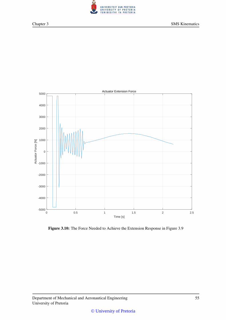
Chapter 3 SMS Kinematics
0 0.5 1 1.5 2 2.5
Time [s]
-5000
-4000
-3000
-2000
-1000
0
1000
2000
3000
4000
5000
Act
uato
r F
orce
[N]
Actuator Extension Force
Figure 3.10: The Force Needed to Achieve the Extension Response in Figure 3.9
Department of Mechanical and Aeronautical EngineeringUniversity of Pretoria
55
© University of Pretoria
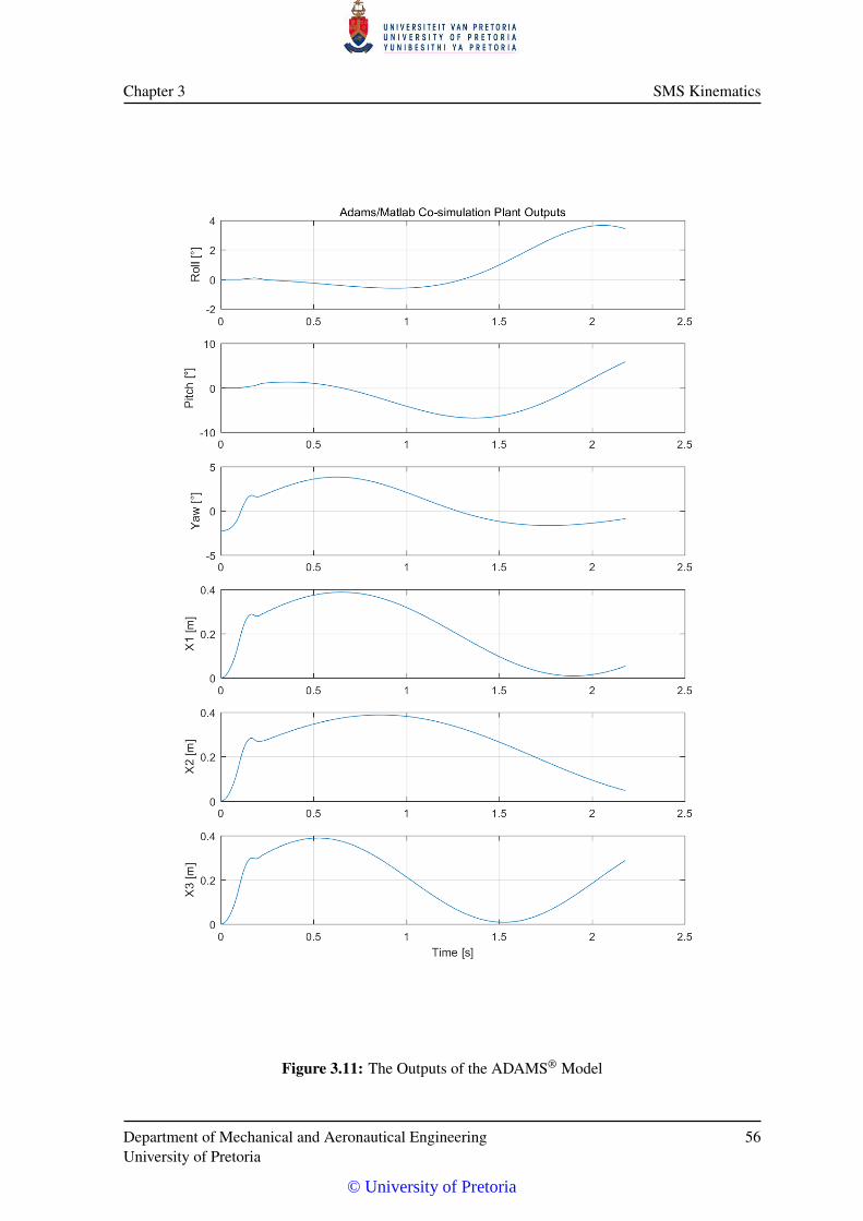
Chapter 3 SMS Kinematics
Figure 3.11: The Outputs of the ADAMS® Model
Department of Mechanical and Aeronautical EngineeringUniversity of Pretoria
56
© University of Pretoria
Chapter 3 SMS Kinematics
3.5 ADAMS® KINEMATIC SIMULATION
An inverse kinematic solution for the SMS can be found by using a dedicated solver during the
operation of the system, which will transform the Pitch and Roll angles of the measured data into
actuator lengths. The controller, which is typically not linked with ADAMS®, will then use these
actuator lengths as set points to control each leg length. Included in the ADAMS® package is a well
developed set of solver algorithms, which can be used in either a non real-time co-simulation or as a
pre-process to convert a measured data set, or as a tool to derive a numerical function or lookup table
that can be included into the real time simulation. The advantage of the latter is that the time to find
a solution for every time step would be the same, as the time taken for the lookup and interpolation
functions are deterministic. A second argument to be made for the lookup and interpolation process
is that once the function has been defined, ADAMS® is no longer necessary for the operation of the
system.
The existing ADAMS® model (as described in §3.3) was modified from one using three forces to
effect the orientation of the platform and the SAT to one using a general motion to manipulate the
orientation of the platform at a pre-defined working height, solving and exporting the calculated
actuator extension lengths.
The changes involved removing the three single component forces ( "SFORCE_1" to "SFORCE_3"),
freeing up the actuators to translate along their z-axes and adding a general motion onto the platform,
aligned with (and moving with) the coordinate system of the platform. Three constraints are placed on
the movement, and hence on the CoG of the platform, the first being the height which is maintained
at 0.5m above the ground, and the other two linked to the input variables "PitchIn" and "RollIn"
that govern the platform attitude. Together with the three Panhard Rods, the system is well defined.
Output variables "EX1", "EX2" and "EX3" are linked to the translational magnitude between the
actuator body reference ("Act1.M_Ref") and the piston CoG ("Pistonx.CoG"), the same variable used
for the position control feedback.
Department of Mechanical and Aeronautical EngineeringUniversity of Pretoria
57
© University of Pretoria
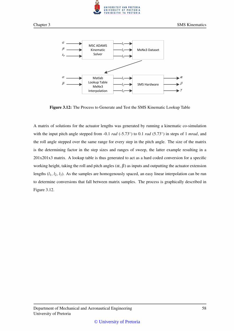
Chapter 3 SMS Kinematics
MSC ADAMSKinematic
Solverzp
MxNx3 Dataset
l1l2l3
MatlabLookup Table
MxNx3Interpolation
l1l2l3
SMS Hardware
Figure 3.12: The Process to Generate and Test the SMS Kinematic Lookup Table
A matrix of solutions for the actuator lengths was generated by running a kinematic co-simulation
with the input pitch angle stepped from -0.1 rad (-5.73◦) to 0.1 rad (5.73◦) in steps of 1 mrad, and
the roll angle stepped over the same range for every step in the pitch angle. The size of the matrix
is the determining factor in the step sizes and ranges of sweep, the latter example resulting in a
201x201x3 matrix. A lookup table is thus generated to act as a hard coded conversion for a specific
working height, taking the roll and pitch angles (α , β ) as inputs and outputting the actuator extension
lengths (l1, l2, l3). As the samples are homogenously spaced, an easy linear interpolation can be run
to determine conversions that fall between matrix samples. The process is graphically described in
Figure 3.12.
Department of Mechanical and Aeronautical EngineeringUniversity of Pretoria
58
© University of Pretoria
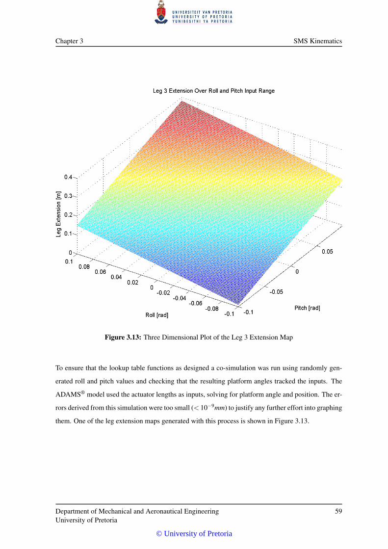
Chapter 3 SMS Kinematics
Figure 3.13: Three Dimensional Plot of the Leg 3 Extension Map
To ensure that the lookup table functions as designed a co-simulation was run using randomly gen-
erated roll and pitch values and checking that the resulting platform angles tracked the inputs. The
ADAMS® model used the actuator lengths as inputs, solving for platform angle and position. The er-
rors derived from this simulation were too small (< 10−9mm) to justify any further effort into graphing
them. One of the leg extension maps generated with this process is shown in Figure 3.13.
Department of Mechanical and Aeronautical EngineeringUniversity of Pretoria
59
© University of Pretoria
CHAPTER 4
THEORETICAL PNEUMATIC MODELS
The chapter starts off with a description of a pneumatic actuator subsystem. It is then expanded into
the different parts, each of which is described in a mathematical form. Each section in this chapter is
laid out in three parts, a description of the pneumatic part, a theoretical model of the pneumatic part
and the Matlab® Simulink® model of the part.
4.1 PNEUMATIC SYSTEM
The pneumatic system, as previously described in the introduction (§ 2.3) and diagrammatically rep-
resented in Figure 2.5 consist of three identical parts, each linked to one of the three legs of the
simulator. A schematic representation of one of these pneumatic actuator subsystems is shown in
Figure 4.1. The main parts of this subsystem are, starting from the left, the reservoir, the valve, the
actuator with the displacement sensor and the load. The latter consists of internal actuator forces,
external mass induced forces and external perturbations. Some of the more relevant variables are also
shown and will be referred to in more detail in subsequent sections.
As one works towards expressions for the force on the piston rod, which is a function of the pressure
in each chamber, it is necessary to derive an expression for the change of pressure in each chamber. By
following a process as depicted in Figure 4.2, each section of the pneumatic system can be described
from fundamental thermodynamic and physical principles. The input to the system is the valve
control voltage Vvs (or Uw from the Festo datasheet) in Volt which is converted to a valve piston spool
displacement xS in m, which in turn is transformed into a valve port area Ava and Avb, both in m2. The
valve port area is used, together with the supply pressure ps and chamber pressures, pa and pb, all in
Pa to calculate the air mass flow rates, ma and mb in kg.s−1 through the valve ports into and out of
© University of Pretoria
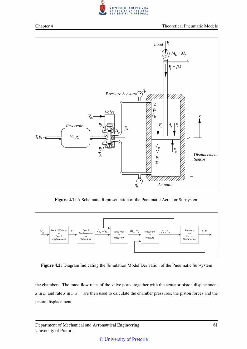
Chapter 4 Theoretical Pneumatic Models
DisplacementSensor
Actuator
Pressure Sensorspb
Valve
Reservoir rFrAbFx
x
x.+Ff
aF
AvTs sp
AT
VR pR
vs
pa
V
Ap
pA
pM+
FL
LM
Vapa
pb
Vb
Ab
Aa
aT
s
Load
Figure 4.1: A Schematic Representation of the Pneumatic Actuator Subsystem
Control Voltage=>
Spool displacement
Spool Displacement
=>Valve Area
Valve Area =>
Mass Flow
Mass Flow=>
Pressure
,a bm m ,va vbA AsxvsV ,a bp p Pressure
=>Force,
Displacement
,x x
Figure 4.2: Diagram Indicating the Simulation Model Derivation of the Pneumatic Subsystem
the chambers. The mass flow rates of the valve ports, together with the actuator piston displacement
x in m and rate x in m.s−1 are then used to calculate the chamber pressures, the piston forces and the
piston displacement.
Department of Mechanical and Aeronautical EngineeringUniversity of Pretoria
61
© University of Pretoria
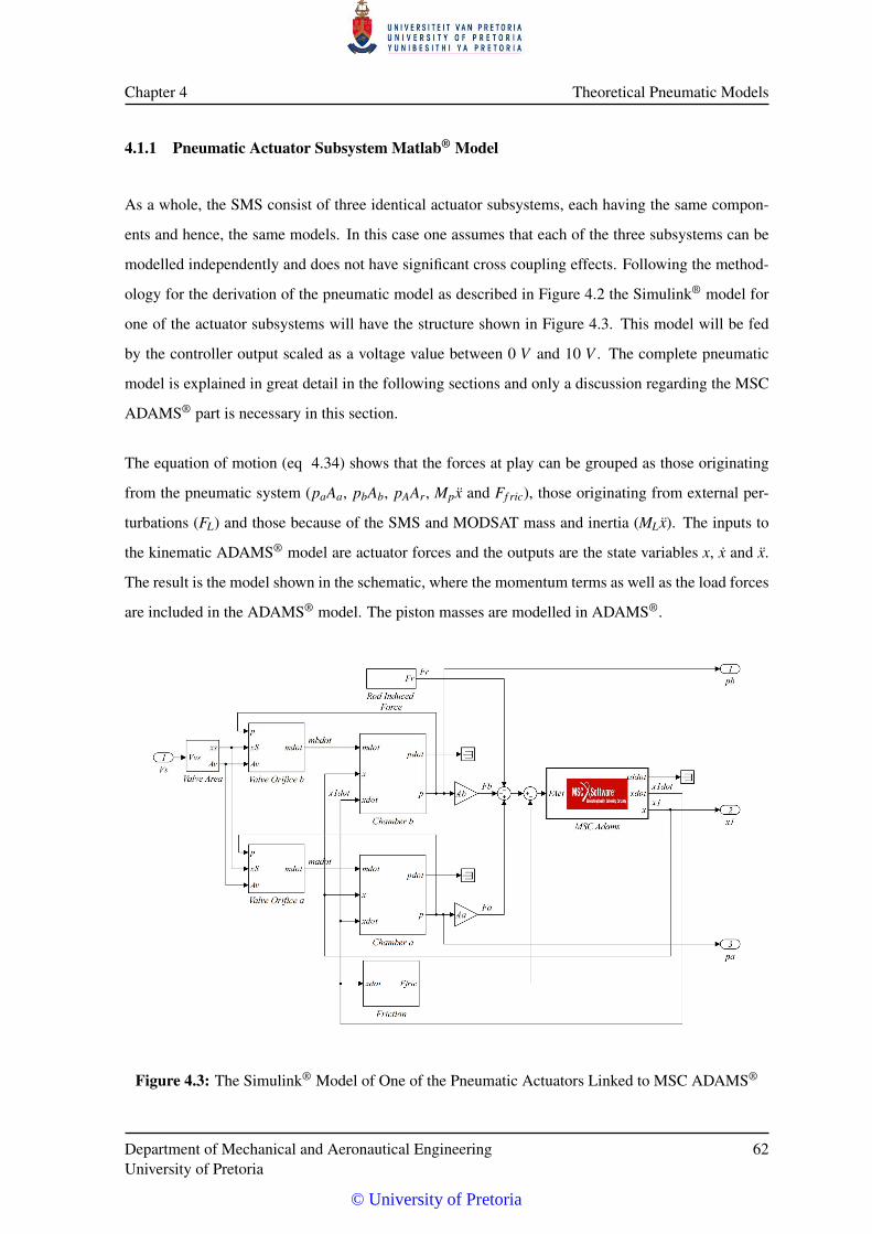
Chapter 4 Theoretical Pneumatic Models
4.1.1 Pneumatic Actuator Subsystem Matlab® Model
As a whole, the SMS consist of three identical actuator subsystems, each having the same compon-
ents and hence, the same models. In this case one assumes that each of the three subsystems can be
modelled independently and does not have significant cross coupling effects. Following the method-
ology for the derivation of the pneumatic model as described in Figure 4.2 the Simulink® model for
one of the actuator subsystems will have the structure shown in Figure 4.3. This model will be fed
by the controller output scaled as a voltage value between 0 V and 10 V . The complete pneumatic
model is explained in great detail in the following sections and only a discussion regarding the MSC
ADAMS® part is necessary in this section.
The equation of motion (eq 4.34) shows that the forces at play can be grouped as those originating
from the pneumatic system (paAa, pbAb, pAAr, Mpx and Ff ric), those originating from external per-
turbations (FL) and those because of the SMS and MODSAT mass and inertia (MLx). The inputs to
the kinematic ADAMS® model are actuator forces and the outputs are the state variables x, x and x.
The result is the model shown in the schematic, where the momentum terms as well as the load forces
are included in the ADAMS® model. The piston masses are modelled in ADAMS®.
Figure 4.3: The Simulink® Model of One of the Pneumatic Actuators Linked to MSC ADAMS®
Department of Mechanical and Aeronautical EngineeringUniversity of Pretoria
62
© University of Pretoria
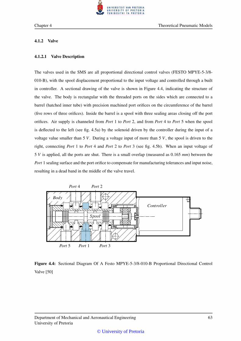
Chapter 4 Theoretical Pneumatic Models
4.1.2 Valve
4.1.2.1 Valve Description
The valves used in the SMS are all proportional directional control valves (FESTO MPYE-5-3/8-
010-B), with the spool displacement proportional to the input voltage and controlled through a built
in controller. A sectional drawing of the valve is shown in Figure 4.4, indicating the structure of
the valve. The body is rectangular with the threaded ports on the sides which are connected to a
barrel (hatched inner tube) with precision machined port orifices on the circumference of the barrel
(five rows of three orifices). Inside the barrel is a spool with three sealing areas closing off the port
orifices. Air supply is channeled from Port 1 to Port 2, and from Port 4 to Port 5 when the spool
is deflected to the left (see fig. 4.5a) by the solenoid driven by the controller during the input of a
voltage value smaller than 5 V . During a voltage input of more than 5 V , the spool is driven to the
right, connecting Port 1 to Port 4 and Port 2 to Port 3 (see fig. 4.5b). When an input voltage of
5 V is applied, all the ports are shut. There is a small overlap (measured as 0.165 mm) between the
Port 1 sealing surface and the port orifice to compensate for manufacturing tolerances and input noise,
resulting in a dead band in the middle of the valve travel.
Body
Controller
Spool
Port 4 Port 2
Port 5 Port 1 Port 3
Figure 4.4: Sectional Diagram Of A Festo MPYE-5-3/8-010-B Proportional Directional Control
Valve [50]
Department of Mechanical and Aeronautical EngineeringUniversity of Pretoria
63
© University of Pretoria
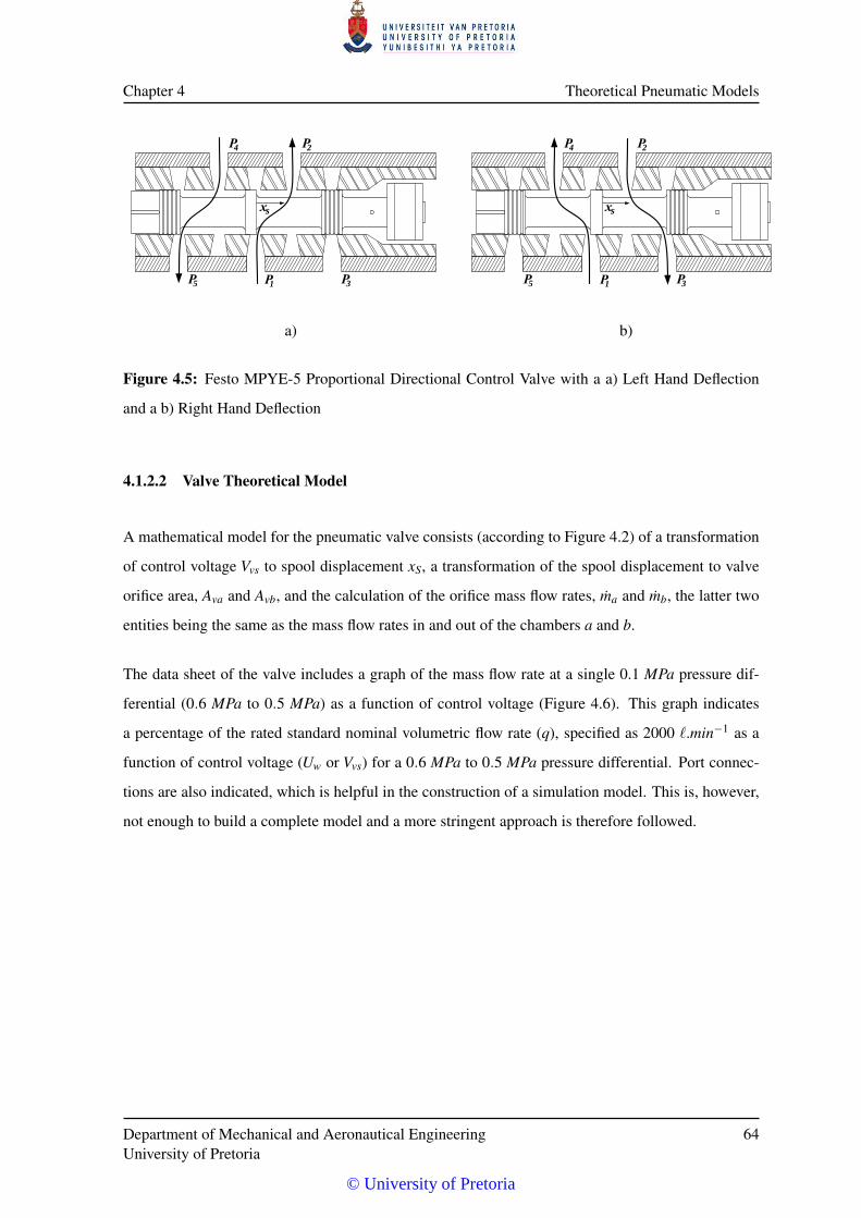
Chapter 4 Theoretical Pneumatic Models
2
1
4
5 3
s
2
1
4
5 3
s
a) b)
Figure 4.5: Festo MPYE-5 Proportional Directional Control Valve with a a) Left Hand Deflection
and a b) Right Hand Deflection
4.1.2.2 Valve Theoretical Model
A mathematical model for the pneumatic valve consists (according to Figure 4.2) of a transformation
of control voltage Vvs to spool displacement xS, a transformation of the spool displacement to valve
orifice area, Ava and Avb, and the calculation of the orifice mass flow rates, ma and mb, the latter two
entities being the same as the mass flow rates in and out of the chambers a and b.
The data sheet of the valve includes a graph of the mass flow rate at a single 0.1 MPa pressure dif-
ferential (0.6 MPa to 0.5 MPa) as a function of control voltage (Figure 4.6). This graph indicates
a percentage of the rated standard nominal volumetric flow rate (q), specified as 2000 `.min−1 as a
function of control voltage (Uw or Vvs) for a 0.6 MPa to 0.5 MPa pressure differential. Port connec-
tions are also indicated, which is helpful in the construction of a simulation model. This is, however,
not enough to build a complete model and a more stringent approach is therefore followed.
Department of Mechanical and Aeronautical EngineeringUniversity of Pretoria
64
© University of Pretoria
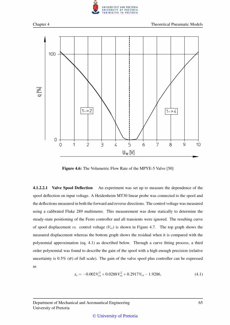
Chapter 4 Theoretical Pneumatic Models
Figure 4.6: The Volumetric Flow Rate of the MPYE-5 Valve [50]
4.1.2.2.1 Valve Spool Deflection An experiment was set up to measure the dependence of the
spool deflection on input voltage. A Heidenheim MT30 linear probe was connected to the spool and
the deflections measured in both the forward and reverse directions. The control voltage was measured
using a calibrated Fluke 289 multimeter. This measurement was done statically to determine the
steady-state positioning of the Festo controller and all transients were ignored. The resulting curve
of spool displacement vs. control voltage (Vvs) is shown in Figure 4.7. The top graph shows the
measured displacement whereas the bottom graph shows the residual when it is compared with the
polynomial approximation (eq. 4.1) as described below. Through a curve fitting process, a third
order polynomial was found to describe the gain of the spool with a high enough precision (relative
uncertainty is 0.5% (σ ) of full scale). The gain of the valve spool plus controller can be expressed
as
xs =−0.002V 3vs +0.0288V 2
vs +0.2917Vvs−1.9286, (4.1)
Department of Mechanical and Aeronautical EngineeringUniversity of Pretoria
65
© University of Pretoria
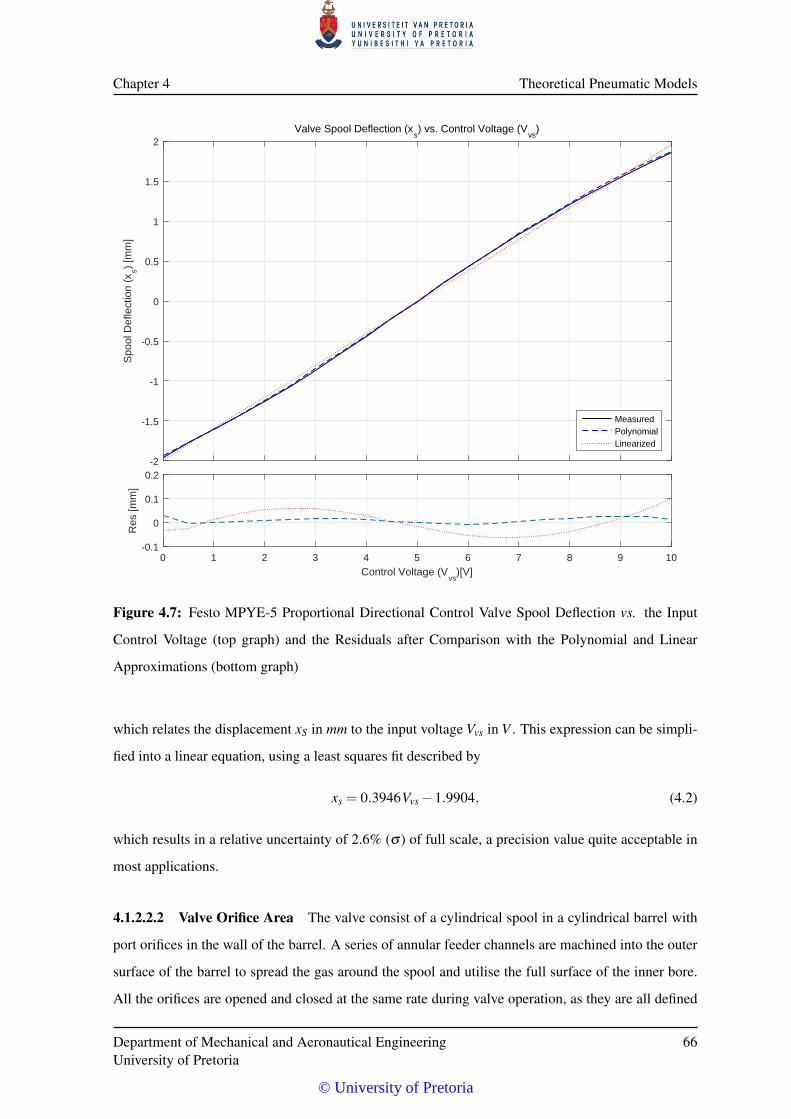
Chapter 4 Theoretical Pneumatic Models
-2
-1.5
-1
-0.5
0
0.5
1
1.5
2
Spo
ol D
efle
ctio
n (x
s) [m
m]
Valve Spool Deflection (xs) vs. Control Voltage (V
vs)
MeasuredPolynomialLinearized
0 1 2 3 4 5 6 7 8 9 10Control Voltage (V
vs)[V]
-0.1
0
0.1
0.2
Res
[mm
]
Figure 4.7: Festo MPYE-5 Proportional Directional Control Valve Spool Deflection vs. the Input
Control Voltage (top graph) and the Residuals after Comparison with the Polynomial and Linear
Approximations (bottom graph)
which relates the displacement xS in mm to the input voltage Vvs in V . This expression can be simpli-
fied into a linear equation, using a least squares fit described by
xs = 0.3946Vvs−1.9904, (4.2)
which results in a relative uncertainty of 2.6% (σ ) of full scale, a precision value quite acceptable in
most applications.
4.1.2.2.2 Valve Orifice Area The valve consist of a cylindrical spool in a cylindrical barrel with
port orifices in the wall of the barrel. A series of annular feeder channels are machined into the outer
surface of the barrel to spread the gas around the spool and utilise the full surface of the inner bore.
All the orifices are opened and closed at the same rate during valve operation, as they are all defined
Department of Mechanical and Aeronautical EngineeringUniversity of Pretoria
66
© University of Pretoria
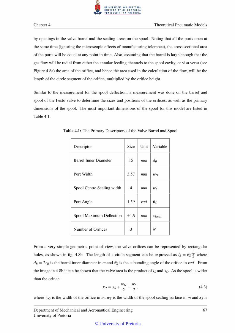
Chapter 4 Theoretical Pneumatic Models
by openings in the valve barrel and the sealing areas on the spool. Noting that all the ports open at
the same time (ignoring the microscopic effects of manufacturing tolerance), the cross sectional area
of the ports will be equal at any point in time. Also, assuming that the barrel is large enough that the
gas flow will be radial from either the annular feeding channels to the spool cavity, or visa versa (see
Figure 4.8a) the area of the orifice, and hence the area used in the calculation of the flow, will be the
length of the circle segment of the orifice, multiplied by the orifice height.
Similar to the measurement for the spool deflection, a measurement was done on the barrel and
spool of the Festo valve to determine the sizes and positions of the orifices, as well as the primary
dimensions of the spool. The most important dimensions of the spool for this model are listed in
Table 4.1.
Table 4.1: The Primary Descriptors of the Valve Barrel and Spool
Descriptor Size Unit Variable
Barrel Inner Diameter 15 mm dB
Port Width 3.57 mm wO
Spool Centre Sealing width 4 mm wS
Port Angle 1.59 rad θS
Spool Maximum Deflection ±1.9 mm xSmax
Number of Orifices 3 N
From a very simple geometric point of view, the valve orifices can be represented by rectangular
holes, as shown in fig. 4.8b. The length of a circle segment can be expressed as lS = θSdB2 where
dB = 2rB is the barrel inner diameter in m and θS is the subtending angle of the orifice in rad. From
the image in 4.8b it can be shown that the valve area is the product of lS and xO. As the spool is wider
than the orifice:
xO = xS +wO
2− wS
2, (4.3)
where wO is the width of the orifice in m, wS is the width of the spool sealing surface in m and xS is
Department of Mechanical and Aeronautical EngineeringUniversity of Pretoria
67
© University of Pretoria
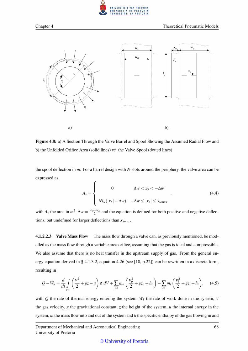
Chapter 4 Theoretical Pneumatic Models
s
Br
sl
Ow
Sw Ox
Sx
Sw
sl
vA
a) b)
Figure 4.8: a) A Section Through the Valve Barrel and Spool Showing the Assumed Radial Flow and
b) the Unfolded Orifice Area (solid lines) vs. the Valve Spool (dotted lines)
the spool deflection in m. For a barrel design with N slots around the periphery, the valve area can be
expressed as
Av =
0 ∆w < xS <−∆w
NlS (|xS|+∆w) −∆w≤ |xS| ≤ xSmax
, (4.4)
with Av the area in m2, ∆w = wO−wS2 and the equation is defined for both positive and negative deflec-
tions, but undefined for larger deflections than xSmax.
4.1.2.2.3 Valve Mass Flow The mass flow through a valve can, as previously mentioned, be mod-
elled as the mass flow through a variable area orifice, assuming that the gas is ideal and compressible.
We also assume that there is no heat transfer in the upstream supply of gas. From the general en-
ergy equation derived in § 4.1.3.2, equation 4.26 (see [10, p.22]) can be rewritten in a discrete form,
resulting in
Q−WS =ddt
∫cv
(ν2
2+gz+u
)ρ dV +∑
csmo
(ν2
o
2+gzo +ho
)−∑
csmi
(ν2
i
2+gzi +hi
), (4.5)
with Q the rate of thermal energy entering the system, WS the rate of work done in the system, ν
the gas velocity, g the gravitational constant, z the height of the system, u the internal energy in the
system, m the mass flow into and out of the system and h the specific enthalpy of the gas flowing in and
Department of Mechanical and Aeronautical EngineeringUniversity of Pretoria
68
© University of Pretoria
Chapter 4 Theoretical Pneumatic Models
out of the system. If it is assumed that the gas is stationary in the closed volume, the volume does not
move, there is no time dependent changes of the internal volumetric energy and the system describes
an orifice in which the gas is transformed from state 1 to state 2, the equation can be generalised
to
Q+m1ν2
12
+m1gz1 +H1 =WS +m2ν2
22
+m2gz2 +H2, (4.6)
by integrating with respect to time, rearranging the terms and accepting that the H = mh. In such a
system without heat transfer (Q = 0), the enthalpy difference can be written as
H1−H2 =−∫ 2
1V d p (4.7)
and by noting that the potential energy of a gas plays an insignificant role, eq. 4.6 will simplify
to
−∫ 2
1V d p =Ws +
mν22
2− mν2
12
. (4.8)
To derive a relationship (similar to St. Venant and Wantzel, 1839, [10, p.30]) for the mass flow through
an orifice, one can start off with a source (reservoir) of gas with infinite volume, with a temperature
T1, a pressure p1 and a mass of m1. Venting the gas from the reservoir through a well rounded nozzle,
so that no flow contraction occurs, the stationary gas (inside the container) will be accelerated to a gas
velocity of ν2. If it is assumed that there is no mechanical work done, and no heat transfer through
the vessel’s surface (Q = 0, and WS = 0), eq. 4.8 will describe the relationship between the energies
in the vessel and those in the downstream flow. As previously stated, there is assumed to be no heat
exchange, resulting in an adiabatic system for which the relationship
p1vκ1 = p2vκ
2 = pvκ , (4.9)
holds. Changing the equation to one of "per unit" by using the specific volume (v = Vm ) and substitut-
ing v = v1
(p1p
) 1κ
from eq 4.9 into the left hand side of the energy equation (eq 4.8), it can be rewritten
as
−∫ 2
1vd p =−v1 p
1κ
1
∫ 2
1p−1κ d p =
ν22
2, (4.10)
which, through integration and some rearranging results in
κ
κ−1p1
ρ1=
ν22
2+
κ
κ−1p2
ρ2. (4.11)
By rearranging eq 4.9 and adding the isothermal relationship, Beater [10] has shown that the velocity
of the gas at any cross section of the nozzle at pressure p2 can be expressed by
ν2 =
√√√√√2RT1
(κ
κ−1
)1−(
p2
p1
) (κ−1)κ
. (4.12)
Department of Mechanical and Aeronautical EngineeringUniversity of Pretoria
69
© University of Pretoria
Chapter 4 Theoretical Pneumatic Models
From the continuity equation (m = A1ν1ρ1 = A2ν2ρ2 = Aνρ) and the relationship for the gas density
in an isentropic process
ρ2 =p1
RT1
(p2
p1
) 1κ
, (4.13)
the mass flow from the reservoir through the well rounded nozzle can be described as
m = Ap1
√2
RT1
√√√√( κ
κ−1
)[(p2
p1
) 2κ
−(
p2
p1
)(κ+1)/κ]. (4.14)
A flow function (Ψ) can be defined so that the mass flow can be simplified to
m = Ap1Ψ
√2
RT1(4.15)
and
Ψ =
√√√√( κ
κ−1
)[(p2
p1
) 2κ
−(
p2
p1
)(κ+1)/κ]. (4.16)
At this time it is prudent to investigate the flow capacity of a nozzle or orifice. As the pressure differ-
ential over the nozzle or orifice increases, the flow of air will increase to a point where the velocity
will become supersonic. Any further increase in the upstream pressure, or decrease in downstream
pressure will not result in an increase in flow. The maximum flow rate (according to eq 4.14) can be
found by evaluating the derivative of the flow function and finding the zero point. One can define a
critical pressure ratio pcr =p2p1
and substitute it into eq. 4.16, take the derivative of (the square of) the
flow function to the critical pressure and the latter is
d(Ψ2)
d pcr=
κ
κ−1
2p
2−κ
κcr
κ− (κ +1) p
1κcr
κ
. (4.17)
The maximum can be shown to be at
pcr =
(2
κ +1
) κ
κ−1
∣∣∣∣∣ d(Ψ2)d pcr
=0
, (4.18)
with a maximum of
Ψmax =
(2
κ +1
) 1κ−1√
κ
(κ +1)
∣∣∣∣∣ pdpu=pcr
. (4.19)
This derivation is a very ideal situation and can be applied with very small errors on well rounded
nozzles with predominantly laminar flow and negligible approach velocity. This is, however, not the
case for valves in general. Valves tend to have sharp edges, which will result in turbulent flow and a
reduction in mass flow rate due to losses and contraction. It is common, for a compressible fluid such
as gas, to define a discharge coefficient Cd which is a function of the pressure ratio [10, p.34], and
Department of Mechanical and Aeronautical EngineeringUniversity of Pretoria
70
© University of Pretoria
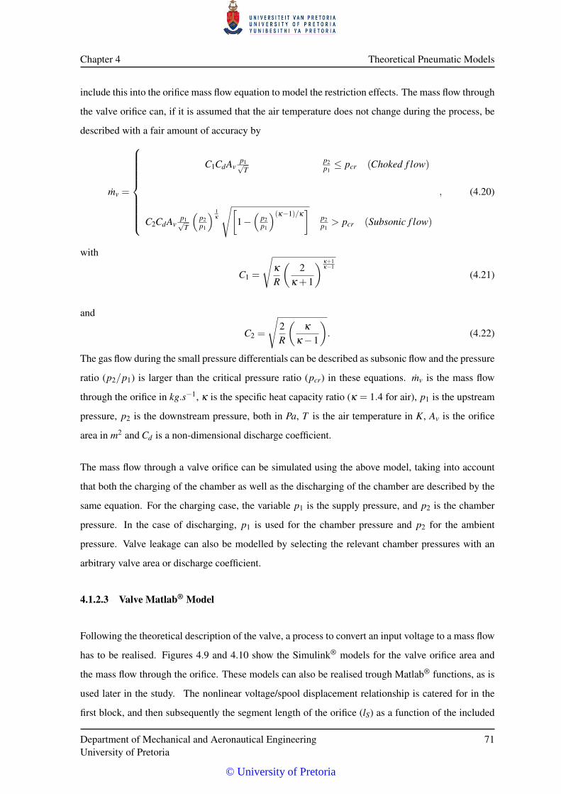
Chapter 4 Theoretical Pneumatic Models
include this into the orifice mass flow equation to model the restriction effects. The mass flow through
the valve orifice can, if it is assumed that the air temperature does not change during the process, be
described with a fair amount of accuracy by
mv =
C1CdAvp1√
Tp2p1≤ pcr (Choked f low)
C2CdAvp1√
T
(p2p1
) 1κ
√[1−(
p2p1
)(κ−1)/κ]
p2p1
> pcr (Subsonic f low)
, (4.20)
with
C1 =
√κ
R
(2
κ +1
) κ+1κ−1
(4.21)
and
C2 =
√2R
(κ
κ−1
). (4.22)
The gas flow during the small pressure differentials can be described as subsonic flow and the pressure
ratio (p2/p1) is larger than the critical pressure ratio (pcr) in these equations. mv is the mass flow
through the orifice in kg.s−1, κ is the specific heat capacity ratio (κ = 1.4 for air), p1 is the upstream
pressure, p2 is the downstream pressure, both in Pa, T is the air temperature in K, Av is the orifice
area in m2 and Cd is a non-dimensional discharge coefficient.
The mass flow through a valve orifice can be simulated using the above model, taking into account
that both the charging of the chamber as well as the discharging of the chamber are described by the
same equation. For the charging case, the variable p1 is the supply pressure, and p2 is the chamber
pressure. In the case of discharging, p1 is used for the chamber pressure and p2 for the ambient
pressure. Valve leakage can also be modelled by selecting the relevant chamber pressures with an
arbitrary valve area or discharge coefficient.
4.1.2.3 Valve Matlab® Model
Following the theoretical description of the valve, a process to convert an input voltage to a mass flow
has to be realised. Figures 4.9 and 4.10 show the Simulink® models for the valve orifice area and
the mass flow through the orifice. These models can also be realised trough Matlab® functions, as is
used later in the study. The nonlinear voltage/spool displacement relationship is catered for in the
first block, and then subsequently the segment length of the orifice (lS) as a function of the included
Department of Mechanical and Aeronautical EngineeringUniversity of Pretoria
71
© University of Pretoria
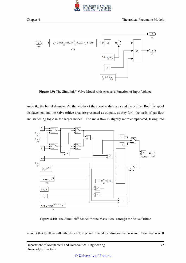
Chapter 4 Theoretical Pneumatic Models
Figure 4.9: The Simulink® Valve Model with Area as a Function of Input Voltage
angle θS, the barrel diameter dB, the widths of the spool sealing area and the orifice. Both the spool
displacement and the valve orifice area are presented as outputs, as they form the basis of gas flow
and switching logic in the larger model. The mass flow is slightly more complicated, taking into
Figure 4.10: The Simulink® Model for the Mass Flow Through the Valve Orifice
account that the flow will either be choked or subsonic, depending on the pressure differential as well
Department of Mechanical and Aeronautical EngineeringUniversity of Pretoria
72
© University of Pretoria
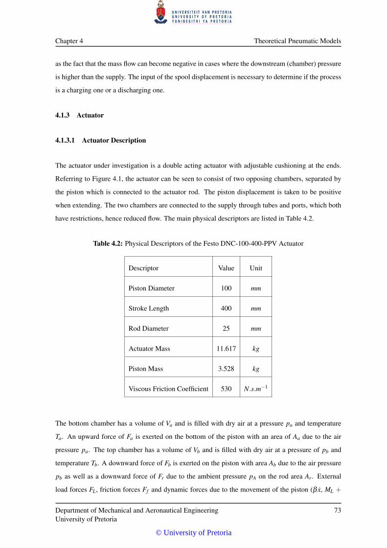
Chapter 4 Theoretical Pneumatic Models
as the fact that the mass flow can become negative in cases where the downstream (chamber) pressure
is higher than the supply. The input of the spool displacement is necessary to determine if the process
is a charging one or a discharging one.
4.1.3 Actuator
4.1.3.1 Actuator Description
The actuator under investigation is a double acting actuator with adjustable cushioning at the ends.
Referring to Figure 4.1, the actuator can be seen to consist of two opposing chambers, separated by
the piston which is connected to the actuator rod. The piston displacement is taken to be positive
when extending. The two chambers are connected to the supply through tubes and ports, which both
have restrictions, hence reduced flow. The main physical descriptors are listed in Table 4.2.
Table 4.2: Physical Descriptors of the Festo DNC-100-400-PPV Actuator
Descriptor Value Unit
Piston Diameter 100 mm
Stroke Length 400 mm
Rod Diameter 25 mm
Actuator Mass 11.617 kg
Piston Mass 3.528 kg
Viscous Friction Coefficient 530 N.s.m−1
The bottom chamber has a volume of Va and is filled with dry air at a pressure pa and temperature
Ta. An upward force of Fa is exerted on the bottom of the piston with an area of Aa due to the air
pressure pa. The top chamber has a volume of Vb and is filled with dry air at a pressure of pb and
temperature Tb. A downward force of Fb is exerted on the piston with area Ab due to the air pressure
pb as well as a downward force of Fr due to the ambient pressure pA on the rod area Ar. External
load forces FL, friction forces Ff and dynamic forces due to the movement of the piston (β x, ML +
Department of Mechanical and Aeronautical EngineeringUniversity of Pretoria
73
© University of Pretoria
Chapter 4 Theoretical Pneumatic Models
Mpx) are also indicated. In order to balance the forces and control the piston to a predefined position
x, detailed models of the chamber pressures and friction forces will be derived. It is assumed that all
the mechanical parts are rigid and will not deform under load or pressure.
4.1.3.2 Theoretical Actuator Model
4.1.3.2.1 Chamber Model The Actuator chambers can be likened with pressure vessels or cyl-
inders with a variable volume and restricted in and outlets. The pneumatic processes involved in the
charging and discharging of such cylinders can be described as either adiabatic or isentropic or iso-
thermal. Previous work published on the subject includes that of Ben-Dov [17], McDonnel et al. [51]
and Ning et al. [25], all of which used an adiabatic assumption. Richer [26] used the assumption that
the charging process of the cylinder is adiabatic and that the discharging process is isothermal as pro-
posed by Al-Ibrahim [52] in 1992. The latter argued that the charging process is irreversibly adiabatic
and the discharging process a better approximation of isothermal than of adiabatic (or isentropic). A
derivation by Šitum et al. [53] using the energy conservation theorem for a controlled volume of gas
was also done with the assumption of an adiabatic process. In most cases the process lies somewhere
between adiabatic and isothermal and the polytropic index is assumed to be between 1 and 1.4 (as
proposed by Richer [26]) and should be verified during the model validation process.
Using a similar approach to Šitum [53] and Richer [26], basing it on the principle of a control volume
(See [8]) with the application of the Reynolds transport theorem, the general energy equation
Q−W =dUdt
, (4.23)
can be rewritten as
Q−W =ddt
∫cv
eρ dV +∫cs
eρν dA, (4.24)
where Q is the net rate of thermal energy entering the system, W is the net rate at which the system
does work, e is the energy per unit mass (specific energy) of the gas, ρ is the gas density, ν is the
homogenous gas velocity through the control surface and V and A are the volumetric and surface
environments respectively. The environment can be likened to the chamber of the actuator. If we
assume that the rate of work W is the sum of the flow work Wf low and the mechanical work WS,
eq. 4.24 can be expanded to
Q−WS−∫cs
pρ
ρν dA =ddt
∫cv
(ep + ek +u)ρ dV +∫cs
(ep + ek +u)ρν dA, (4.25)
Department of Mechanical and Aeronautical EngineeringUniversity of Pretoria
74
© University of Pretoria
Chapter 4 Theoretical Pneumatic Models
with p the gas pressure, ep and ek the potential energy and kinetic energy of the gas respectively
and u the specific internal energy of the control volume. By applying the property of enthalpy and
assuming that the specific enthalpy is the sum of the internal energy of the system and the product of
the pressure and the volume (h = pρ+u), eq. 4.25 can be expressed as
Q−WS =ddt
∫cv
(ep + ek +u)ρ dV+∫cs
(ep + ek +h)ρν dA. (4.26)
Finally, by accepting that the gas in the control volume has no significant movement, hence insignific-
ant kinetic energy and insignificant potential energy, the first two terms in the volumetric integral can
be dropped. Similarly the gas passing through the control surface has limited speed, and once again
insignificant kinetic energy (less than 2% of the thermal energy at ν = 100 m.s−1 and T = 293 K
according to [10, p.114]) and zero potential energy according to the ideal gas law, so that the first two
terms in the surface integral can also be left out. If then, the flow across the control surface is through
discrete ports and the velocity is uniformly distributed across each port and u = cV T is substituted,
then the energy equation becomes
Q−WS + mihi− moho =ddt
(cV T ρV ) . (4.27)
By substituting h = cV T (the enthalpy for an ideal gas), the mechanical work (WS = pV ) and ρT = pR
into eq 4.27, and noting that the thermal exchange through the chamber surface is zero (Q = 0) the
energy equation for an adiabatic process can be expressed as
cp (miTi− moTo) =ddt
(cV pR
V)+ pV , (4.28)
in which mi and Ti are the mass flow rate and temperature of the gas entering the chamber and mo
and To are the mass flow rate and temperature of the gas exiting the chamber. cp is the specific heat
capacity of the gas at a constant pressure, cV is the specific heat capacity of the gas at a constant
volume, R is the universal gas constant, p is the chamber pressure and V is the chamber volume.
When using the relationships cV = Rκ−1 , cp = cV +R (Mayer’s equation) and κ =
cpcV
and rearranging
the terms to express the chamber pressure change, eq 4.28 can be rewritten as
p =κRV
(miTi− moTo)−κpV
V . (4.29)
This result is the same as that of Richer [26, eq10] and Šitum [53] for an adiabatic process with
To = Ti. It should be noted that the assumption of an irreversible adiabatic process with a κ of 1.4
might need to be amended by rather defining the process as a polytropic one and using different heat
capacity ratios depending on the charging/discharging state of the chamber. Therefore, as the heat
Department of Mechanical and Aeronautical EngineeringUniversity of Pretoria
75
© University of Pretoria
Chapter 4 Theoretical Pneumatic Models
capacity ratio can only vary between 1 and 1.4, the correct value can be estimated during a validation
process. To enable this feature, eq. 4.29 can be amended to
p =RV(αimiTi−αomoTo)−α
pV
V , (4.30)
where αi, αi and α are the heat ratios related to the input mass flow, the output mass flow and the
chamber gas. As per the suggestion of Richer, αi should be close to 1.4 and αo should be close to 1,
with α around 1.2 ([52]).
As the pressure change in the chamber is a function of the change in volume and the volume itself, and
the volume in each chamber is linked to the piston position, the volume in the chambers (i = {a,b})
can be expressed as
Vi =Vdi +Ai
(L2± x)∀ − L
2≤ x≤ L
2(4.31)
where Vdi is the dead (or inactive) volume of each chamber, Ai is the piston area, L is the maximum
stroke length and x is the piston displacement relative to the centre of the stroke. This equation is
only defined for −L2 ≤ x ≤ L
2 . The areas of the piston in the two chambers and hence the volume of
the two chambers, are not the same as the top chamber has a reduced volume due to the piston rod.
By substituting eq. 4.31 into eq. 4.30 and noting that V = Aix, the time derivative of the chamber
pressures can be rewritten as
pi =R
Vdi +Ai(L
2 ± x) (αimiTi−αomoTo)−
α piAi
Vdi +Ai(L
2 ± x) x. (4.32)
This equation, as stated by Richer [26], accounts for the change of pressure due to mass flow (air flow)
in and out of the ports connected to the chamber (first term) as well as the change of pressure due to
the movement of the piston and hence the change in chamber volume (second term). It does not, in
its current state, account for leakage of air through the piston seal, which in this study is neglected, as
the piston seals are of nitrile rubber and leakage rates are deemed insignificant against the flow rates
during operation. If the temperatures of the incoming air, the outgoing air and the chamber is taken
to be equal (an isothermal process), the temperature subscripts can be dropped.
4.1.3.2.2 Simple Friction Model In a pneumatic system, the main sources of nonlinearity are
the compressible nature of the air (gas), the airflow-pressure relationship and the stick-slip nature
of the pneumatic seals. The latter (friction contribution) is under investigation in this section and
further expanded in § 6. Various models have been proposed, ranging from "ignoring the problem",
the application of the Stribeck stiction model ([53],[23]), some more specific seal models such as
Department of Mechanical and Aeronautical EngineeringUniversity of Pretoria
76
© University of Pretoria
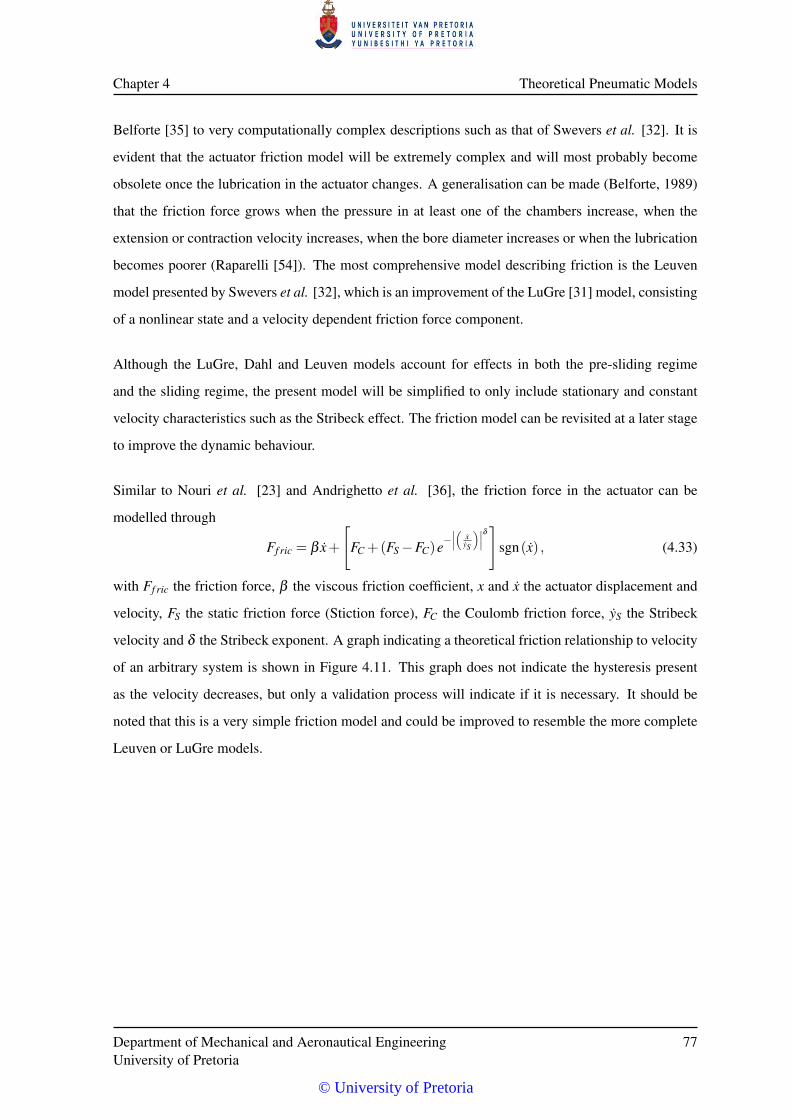
Chapter 4 Theoretical Pneumatic Models
Belforte [35] to very computationally complex descriptions such as that of Swevers et al. [32]. It is
evident that the actuator friction model will be extremely complex and will most probably become
obsolete once the lubrication in the actuator changes. A generalisation can be made (Belforte, 1989)
that the friction force grows when the pressure in at least one of the chambers increase, when the
extension or contraction velocity increases, when the bore diameter increases or when the lubrication
becomes poorer (Raparelli [54]). The most comprehensive model describing friction is the Leuven
model presented by Swevers et al. [32], which is an improvement of the LuGre [31] model, consisting
of a nonlinear state and a velocity dependent friction force component.
Although the LuGre, Dahl and Leuven models account for effects in both the pre-sliding regime
and the sliding regime, the present model will be simplified to only include stationary and constant
velocity characteristics such as the Stribeck effect. The friction model can be revisited at a later stage
to improve the dynamic behaviour.
Similar to Nouri et al. [23] and Andrighetto et al. [36], the friction force in the actuator can be
modelled through
Ff ric = β x+
[FC +(FS−FC)e−
∣∣∣( xyS
)∣∣∣δ]sgn(x) , (4.33)
with Ff ric the friction force, β the viscous friction coefficient, x and x the actuator displacement and
velocity, FS the static friction force (Stiction force), FC the Coulomb friction force, yS the Stribeck
velocity and δ the Stribeck exponent. A graph indicating a theoretical friction relationship to velocity
of an arbitrary system is shown in Figure 4.11. This graph does not indicate the hysteresis present
as the velocity decreases, but only a validation process will indicate if it is necessary. It should be
noted that this is a very simple friction model and could be improved to resemble the more complete
Leuven or LuGre models.
Department of Mechanical and Aeronautical EngineeringUniversity of Pretoria
77
© University of Pretoria
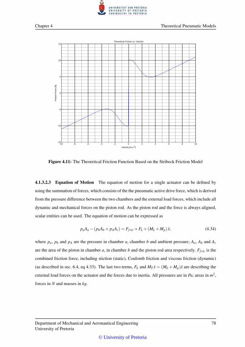
Chapter 4 Theoretical Pneumatic Models
-10 -8 -6 -4 -2 0 2 4 6 8 10-15
-10
-5
0
5
10
15
Velocity [m.s-1]
Fric
tion
Forc
e [N
]
Theoretical Friction vs. Velocity
Figure 4.11: The Theoretical Friction Function Based on the Stribeck Friction Model
4.1.3.2.3 Equation of Motion The equation of motion for a single actuator can be defined by
using the summation of forces, which consists of the the pneumatic active drive force, which is derived
from the pressure difference between the two chambers and the external load forces, which include all
dynamic and mechanical forces on the piston rod. As the piston rod and the force is always aligned,
scalar entities can be used. The equation of motion can be expressed as
paAa− (pbAb + pAAr) = Ff ric +FL +(ML +Mp) x, (4.34)
where pa, pb and pA are the pressure in chamber a, chamber b and ambient pressure; Aa, Ab and Ar
are the area of the piston in chamber a, in chamber b and the piston rod area respectively. Ff ric is the
combined friction force, including stiction (static), Coulomb friction and viscous friction (dynamic)
(as described in sec. 6.4, eq 4.33). The last two terms, FL and MT x = (ML +Mp)x are describing the
external load forces on the actuator and the forces due to inertia. All pressures are in Pa, areas in m2,
forces in N and masses in kg.
Department of Mechanical and Aeronautical EngineeringUniversity of Pretoria
78
© University of Pretoria
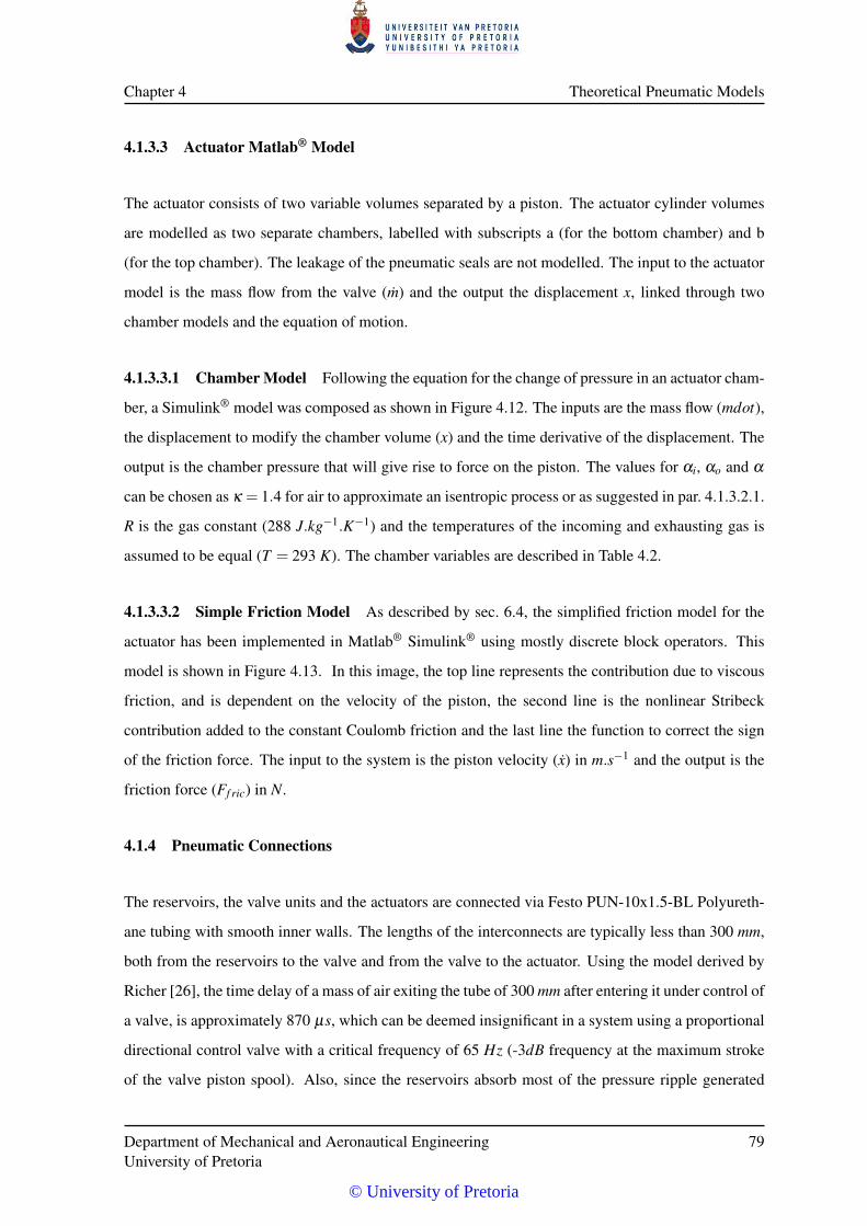
Chapter 4 Theoretical Pneumatic Models
4.1.3.3 Actuator Matlab® Model
The actuator consists of two variable volumes separated by a piston. The actuator cylinder volumes
are modelled as two separate chambers, labelled with subscripts a (for the bottom chamber) and b
(for the top chamber). The leakage of the pneumatic seals are not modelled. The input to the actuator
model is the mass flow from the valve (m) and the output the displacement x, linked through two
chamber models and the equation of motion.
4.1.3.3.1 Chamber Model Following the equation for the change of pressure in an actuator cham-
ber, a Simulink® model was composed as shown in Figure 4.12. The inputs are the mass flow (mdot),
the displacement to modify the chamber volume (x) and the time derivative of the displacement. The
output is the chamber pressure that will give rise to force on the piston. The values for αi, αo and α
can be chosen as κ = 1.4 for air to approximate an isentropic process or as suggested in par. 4.1.3.2.1.
R is the gas constant (288 J.kg−1.K−1) and the temperatures of the incoming and exhausting gas is
assumed to be equal (T = 293 K). The chamber variables are described in Table 4.2.
4.1.3.3.2 Simple Friction Model As described by sec. 6.4, the simplified friction model for the
actuator has been implemented in Matlab® Simulink® using mostly discrete block operators. This
model is shown in Figure 4.13. In this image, the top line represents the contribution due to viscous
friction, and is dependent on the velocity of the piston, the second line is the nonlinear Stribeck
contribution added to the constant Coulomb friction and the last line the function to correct the sign
of the friction force. The input to the system is the piston velocity (x) in m.s−1 and the output is the
friction force (Ff ric) in N.
4.1.4 Pneumatic Connections
The reservoirs, the valve units and the actuators are connected via Festo PUN-10x1.5-BL Polyureth-
ane tubing with smooth inner walls. The lengths of the interconnects are typically less than 300 mm,
both from the reservoirs to the valve and from the valve to the actuator. Using the model derived by
Richer [26], the time delay of a mass of air exiting the tube of 300 mm after entering it under control of
a valve, is approximately 870 µs, which can be deemed insignificant in a system using a proportional
directional control valve with a critical frequency of 65 Hz (-3dB frequency at the maximum stroke
of the valve piston spool). Also, since the reservoirs absorb most of the pressure ripple generated
Department of Mechanical and Aeronautical EngineeringUniversity of Pretoria
79
© University of Pretoria
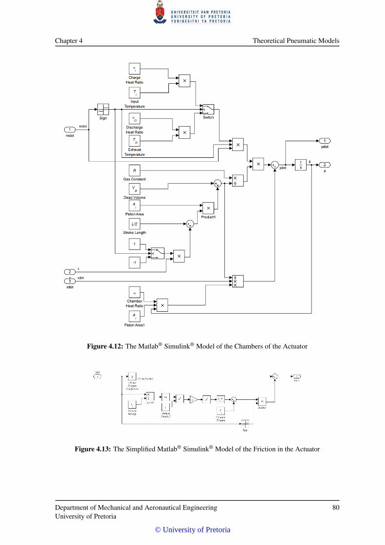
Chapter 4 Theoretical Pneumatic Models
Figure 4.12: The Matlab® Simulink® Model of the Chambers of the Actuator
Figure 4.13: The Simplified Matlab® Simulink® Model of the Friction in the Actuator
Department of Mechanical and Aeronautical EngineeringUniversity of Pretoria
80
© University of Pretoria
Chapter 4 Theoretical Pneumatic Models
through the supply tubing and the mass flow rate reduction is only 0.0002%, the tube effects will be
ignored.
4.1.5 Pneumatic Reservoir
During an extension or contraction of the actuator, air is being channeled to either of the two actuator
chambers. The volume of air used in one full extension-contraction cycle of the actuator equals the
maximum combined volume of the two chambers. This air has to be supplied from the pneumatic
source, in our case a portable or a permanently installed compressor. Due to the connection from the
compressor to the SMS being a tube with a finite inner diameter and due to the friction between the air
and the inner pipe surface, a pressure loss and a mass flow rate reduction during dynamic operation is
present. This results in fluctuations in the supply pressure to the system.
Analogous to the smoothing effect of a capacitor on the supply voltage of a power supply with a finite
resistance, a pneumatic reservoir can smooth out the pressure fluctuations on the supply lines close
to the valves and actuators. It is for this reason that a 5` Festo reservoir was added to each of the
simulator legs. For the purpose of this document, the reservoirs are not modelled in detail, but the
supply pressure is assumed to be smoothed and constant.
Department of Mechanical and Aeronautical EngineeringUniversity of Pretoria
81
© University of Pretoria
CHAPTER 5
MASS FLOW CHARACTERISATION
The control of a pneumatic system is largely dependent on the friction characteristics and the mass
flow characteristics of the system. The latter is the subject of this section. A theoretical model was
derived from first principles in §4.1 resulting in a model that uses the assumptions of an ideal gas and
adiabatic process. The supply pressure is also assumed to be constant.
The mass flow through the valve into and out of the actuator chambers gives rise to the change in
pressure and hence the exerted force on the load. It is, therefore, necessary to characterise the mass
flow through the controlling unit (i.e. the valve and tubes) and to populate the unknown variables in
the theoretical model.
The test setup with two reservoirs was used, assuming that a reservoir of a constant volume will
have the same temporal pressure response as a chamber of the actuator with the output rod held
captive.
5.1 THEORETICAL MODELS
5.1.1 Classic Mass Flow Model
The normal pneumatic system layout using proportional control valves is described graphically in
Figure 4.1. The valve and the actuator chambers are connected through lossless tubing. The derivation
of the mass flow has been done from first principles in § 4.1.2.2.3 and §4.1.3.2.1. In this derivation
we assume that the air supply is at ambient temperature, no change in the supply temperature occurs,
and that the process is isentropic.
© University of Pretoria
Chapter 5 Mass Flow Characterisation
From this derivation and from various sources in literature (Beater [10], Van der Merwe et al. [19]
and Šitum [44]) the general form of mass flow through an orifice with a known effective area (Av), a
discharge coefficient of Cd and ideal air flow can be expressed as
mv =
C1CdAvp1√
Tp2p1≤ pcr (Choked f low)
C2CdAvp1√
T
(p2p1
) 1κ
√[1−(
p2p1
)(κ−1)/κ]
p2p1
> pcr (Subsonic f low),
(5.1)
with
C1 =
√κ
R
(2
κ +1
) κ+1κ−1
, (5.2)
and
C2 =
√2R
(κ
κ−1
). (5.3)
where p1 is the supply pressure, T is the supply air temperature and κ is the ratio of specific heat
capacities of the gas moving through the orifice. pcr is the critical pressure ratio where flow changes
from choked to subsonic. This theoretical model assumes no contraction, friction or heat transfer,
which will be later shown to influence the shape of the flow function. From equation 4.32, the pressure
change in the actuator chambers pk can be expressed as
pk =R
Vdk +Ak(L
2 ± x) (αimiTi−αomoTo)−
α pAk
Vdk +Ak(L
2 ± x) x. (5.4)
Vdk is the dead (or inactive) volume of each chamber, Ak is the piston area, L is the maximum stroke
length and x is the piston displacement relative to the centre of the stroke, x the rate of displacement,
αi, αo and α are the heat capacity ratios related to the input mass flow, the output mass flow and the
chamber gas, mi and Ti are the mass flow rate and temperature of the gas entering the chamber and
mo and To are the mass flow rate and temperature of the gas exiting the chamber respectively.
By arguing that the the captive actuator has a constant chamber volume, the actuator can be replaced
by a pressure vessel with a constant volume such as an air reservoir. The equation for pressure change
in the actuator (eq. 5.4) can be simplified by noting that that the actuator extension rate (x) is zero
and the second term can be ignored. It can also be assumed that the outlet mass flow is insignificant
in the case of charging as the upstream pressure is much higher than the chamber pressure. In the
discharging case the inlet mass flow approaches zero and the first term can be ignored. The pressure
Department of Mechanical and Aeronautical EngineeringUniversity of Pretoria
83
© University of Pretoria
Chapter 5 Mass Flow Characterisation
change in the pressure vessel can then be expressed as
pc =
αiRTimi
Vcf or charging
−αoRTomoVc
f or discharging.
(5.5)
with αi and αo the inlet and outlet heat capacity ratios, R the gas constant, Ti and To the inlet and
outlet air temperatures, mi and mo the inlet and outlet mass flow rates and Vc the volume of the test
chamber.
By combining eq. 5.5 and eq. 5.1 and assuming that the air temperature equals the ambient air tem-
perature, the change in chamber pressure for the charging cycle can be expressed as
pc =
CdAvC1
αiR√
TVc
p1p2p1≤ pcr
CdAvC2αiR√
T p1Vc
(p2p1
)1/κ
√1−(
p2p1
)(κ−1)/κ p2p1
> pcr.
(5.6)
As proposed by, amongst others, Richer [11] and van der Merwe et al. [19] the value for αi for the
charging cycle in an isentropic system is assumed close to the isentropic expansion index κ = 1.4 for
air. For the discharging cycle, αo is assumed close to one indicating an isothermal process.
The mass flow rate at large pressure differentials is essentially independent of the actual differen-
tial, and can therefore be used to calculate the discharge coefficient with reasonable accuracy. By
focussing only on the choked flow region, the first term of eq. 5.6 can be rewritten as
Cd =pcVc
p1αiAvC1R√
T ,(5.7)
which expresses the discharge coefficient for the specific valve opening. This coefficient is for now
assumed to be constant for all pressure differentials.
5.1.2 ISO Mass Flow Model
The simplification of the pneumatic system for valve mass flow model identification (sec 5.1.1) as-
sumes that the orifices are ideal, no contraction is present and that only a single orifice is used.
Although a discharge coefficient (Cd) is used, this only adds a linear gain to the system, and does not
change the shape of the flow function. In reality, this assumption does not hold as the valve has losses
due to friction, turbulent flow, heat transfer and contraction.
Department of Mechanical and Aeronautical EngineeringUniversity of Pretoria
84
© University of Pretoria
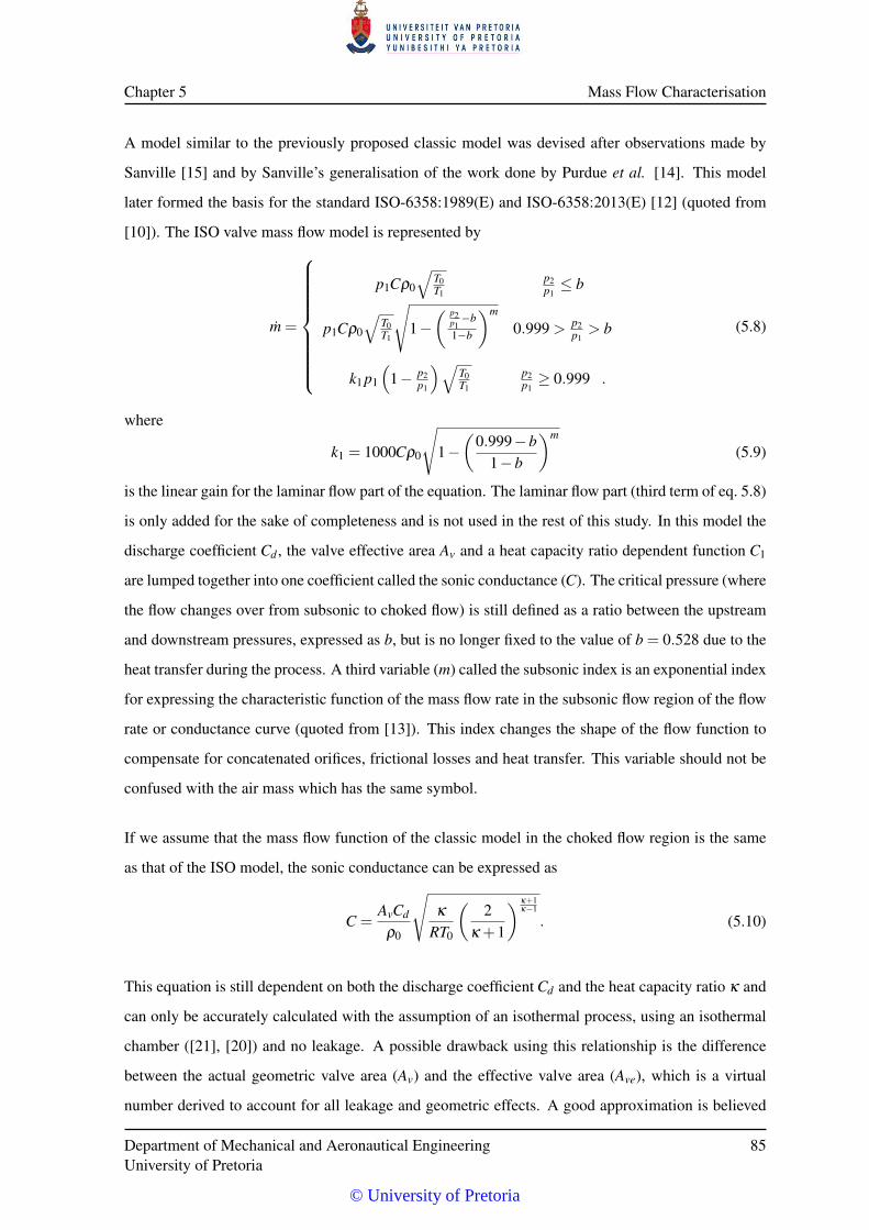
Chapter 5 Mass Flow Characterisation
A model similar to the previously proposed classic model was devised after observations made by
Sanville [15] and by Sanville’s generalisation of the work done by Purdue et al. [14]. This model
later formed the basis for the standard ISO-6358:1989(E) and ISO-6358:2013(E) [12] (quoted from
[10]). The ISO valve mass flow model is represented by
m =
p1Cρ0
√T0T1
p2p1≤ b
p1Cρ0
√T0T1
√1−( p2
p1−b
1−b
)m
0.999 > p2p1
> b
k1 p1
(1− p2
p1
)√T0T1
p2p1≥ 0.999 .
(5.8)
where
k1 = 1000Cρ0
√1−(
0.999−b1−b
)m
(5.9)
is the linear gain for the laminar flow part of the equation. The laminar flow part (third term of eq. 5.8)
is only added for the sake of completeness and is not used in the rest of this study. In this model the
discharge coefficient Cd , the valve effective area Av and a heat capacity ratio dependent function C1
are lumped together into one coefficient called the sonic conductance (C). The critical pressure (where
the flow changes over from subsonic to choked flow) is still defined as a ratio between the upstream
and downstream pressures, expressed as b, but is no longer fixed to the value of b = 0.528 due to the
heat transfer during the process. A third variable (m) called the subsonic index is an exponential index
for expressing the characteristic function of the mass flow rate in the subsonic flow region of the flow
rate or conductance curve (quoted from [13]). This index changes the shape of the flow function to
compensate for concatenated orifices, frictional losses and heat transfer. This variable should not be
confused with the air mass which has the same symbol.
If we assume that the mass flow function of the classic model in the choked flow region is the same
as that of the ISO model, the sonic conductance can be expressed as
C =AvCd
ρ0
√κ
RT0
(2
κ +1
) κ+1κ−1
. (5.10)
This equation is still dependent on both the discharge coefficient Cd and the heat capacity ratio κ and
can only be accurately calculated with the assumption of an isothermal process, using an isothermal
chamber ([21], [20]) and no leakage. A possible drawback using this relationship is the difference
between the actual geometric valve area (Av) and the effective valve area (Ave), which is a virtual
number derived to account for all leakage and geometric effects. A good approximation is believed
Department of Mechanical and Aeronautical EngineeringUniversity of Pretoria
85
© University of Pretoria
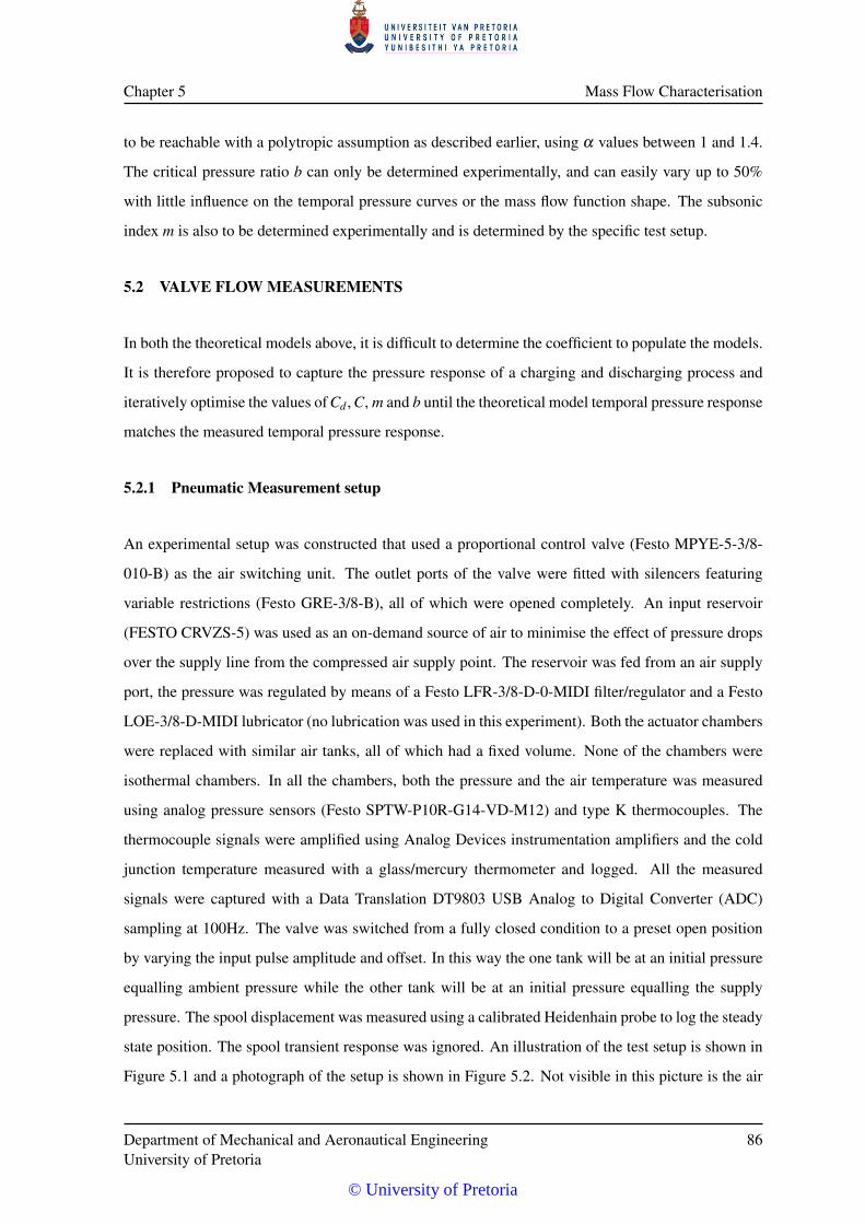
Chapter 5 Mass Flow Characterisation
to be reachable with a polytropic assumption as described earlier, using α values between 1 and 1.4.
The critical pressure ratio b can only be determined experimentally, and can easily vary up to 50%
with little influence on the temporal pressure curves or the mass flow function shape. The subsonic
index m is also to be determined experimentally and is determined by the specific test setup.
5.2 VALVE FLOW MEASUREMENTS
In both the theoretical models above, it is difficult to determine the coefficient to populate the models.
It is therefore proposed to capture the pressure response of a charging and discharging process and
iteratively optimise the values of Cd , C, m and b until the theoretical model temporal pressure response
matches the measured temporal pressure response.
5.2.1 Pneumatic Measurement setup
An experimental setup was constructed that used a proportional control valve (Festo MPYE-5-3/8-
010-B) as the air switching unit. The outlet ports of the valve were fitted with silencers featuring
variable restrictions (Festo GRE-3/8-B), all of which were opened completely. An input reservoir
(FESTO CRVZS-5) was used as an on-demand source of air to minimise the effect of pressure drops
over the supply line from the compressed air supply point. The reservoir was fed from an air supply
port, the pressure was regulated by means of a Festo LFR-3/8-D-0-MIDI filter/regulator and a Festo
LOE-3/8-D-MIDI lubricator (no lubrication was used in this experiment). Both the actuator chambers
were replaced with similar air tanks, all of which had a fixed volume. None of the chambers were
isothermal chambers. In all the chambers, both the pressure and the air temperature was measured
using analog pressure sensors (Festo SPTW-P10R-G14-VD-M12) and type K thermocouples. The
thermocouple signals were amplified using Analog Devices instrumentation amplifiers and the cold
junction temperature measured with a glass/mercury thermometer and logged. All the measured
signals were captured with a Data Translation DT9803 USB Analog to Digital Converter (ADC)
sampling at 100Hz. The valve was switched from a fully closed condition to a preset open position
by varying the input pulse amplitude and offset. In this way the one tank will be at an initial pressure
equalling ambient pressure while the other tank will be at an initial pressure equalling the supply
pressure. The spool displacement was measured using a calibrated Heidenhain probe to log the steady
state position. The spool transient response was ignored. An illustration of the test setup is shown in
Figure 5.1 and a photograph of the setup is shown in Figure 5.2. Not visible in this picture is the air
Department of Mechanical and Aeronautical EngineeringUniversity of Pretoria
86
© University of Pretoria
Chapter 5 Mass Flow Characterisation
service unit and the signal capture unit (ADC and the Personal Computer (PC)).
pas
Ti, pS
Tl, pl
Tu, pu
DT9803 ADC
PC
Figure 5.1: Graphical Diagram Of The Valve Flow Characterisation Test Setup
Figure 5.2: Photograph Of The Valve Flow Characterisation Test Setup
5.2.2 Temperature Measurement
Important variables in all pneumatic processes are the air temperature and the change in air temperat-
ure. The assumptions of an isothermal process made earlier depend largely on the temperature profile
Department of Mechanical and Aeronautical EngineeringUniversity of Pretoria
87
© University of Pretoria
Chapter 5 Mass Flow Characterisation
during the charging and discharging cycles. Should the air temperature stay constant, the processes
can be classified as isothermal and the derivations done are all valid. Reality, however, dictates dif-
ferent, and the air temperature does vary to different extents. The air temperature is therefore added
to the set of measurement variables and was measured by adding thermocouples to the air reservoirs.
The drainage plugs underneath the reservoirs were modified to accept the 1.5mm diameter sheathed
type K thermocouples, which were epoxied into the plugs to facilitate an air tight seal. The tips of the
thermocouples were placed as close as possible to the centres of the reservoirs. The time constants of
the thermocouples were unknown but assumed to be in the order of seconds. A literature search re-
vealed time constant values between 0.4s and 6s for insulated sheathes of 1.5mm diameter depending
on the flow and gas conditions. No measurements were taken to determine the time constants due to
time constraints. The data gathered by the temperature sensors were therefore used as a global indica-
tion of the temperature trends rather than an absolute data set to be used in the calculations. Once the
thermocouples are characterised, the measured values can be trusted and used in the analysis.
The thermocouples were connected to Analog Devices instrumentation amplifier circuits (INA110)
and set up with a linear gain of 500. The amplifiers were routed differentially to the ADC to minimise
the common mode electronic noise. Offsets were assumed to be negligible and the linearity of the
amplifiers to be perfect. The cold junction temperature was measured during each experiment and
added to the calculated result of the sensors.
According to the National Institute of Standards and Technology (NIST)[55] the temperature of a
type K thermocouple relative to the cold junction temperature can be expressed as
TK =9
∑i=0
ciE i, (5.11)
where TK is the thermocouple temperature in ◦C, ci are the coefficients for the temperature subrange
0-1372 ◦C and E is the thermocouple EMF in mV . It should be noted that the measured voltage is the
generated thermocouple EMF multiplied by 500 due to the amplifiers. The coefficients are tabulated
in Appendix C, Table C.1.
Taking into account that the thermocouple cold junction is at room temperature, the air temperature
as measured by the thermocouple is given by
T = TK +TCJ, (5.12)
with TCJ the cold junction temperature in ◦C.
Department of Mechanical and Aeronautical EngineeringUniversity of Pretoria
88
© University of Pretoria
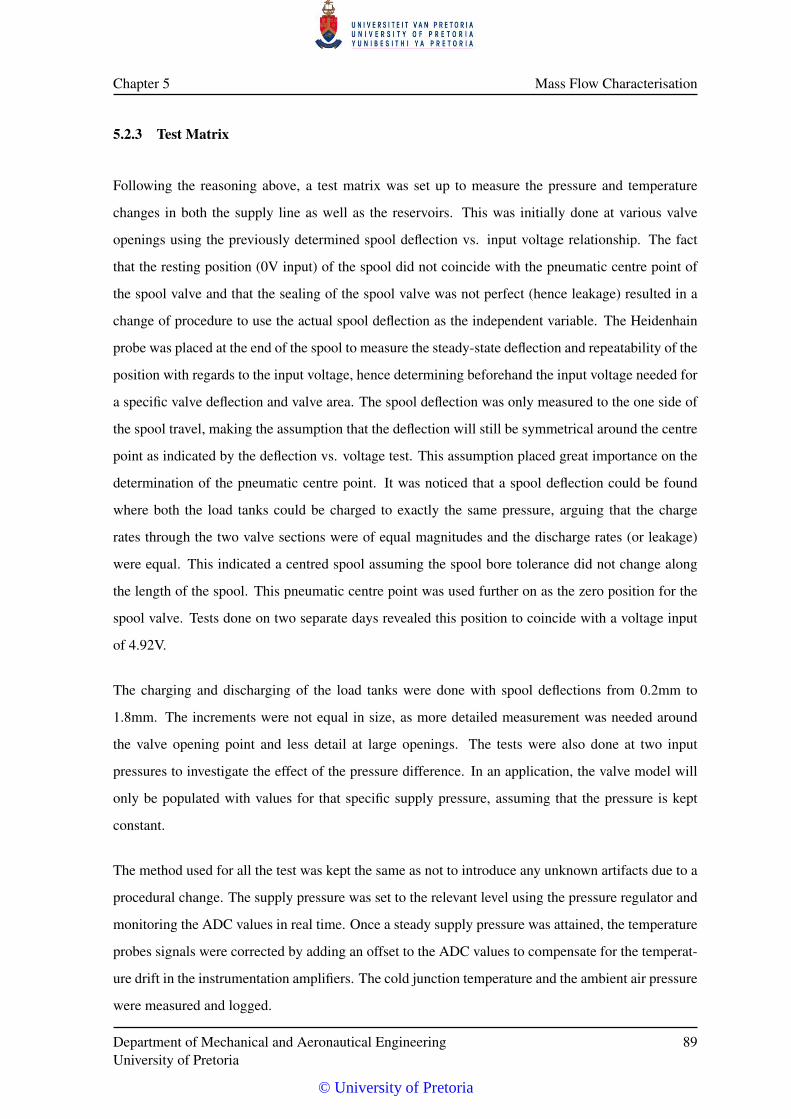
Chapter 5 Mass Flow Characterisation
5.2.3 Test Matrix
Following the reasoning above, a test matrix was set up to measure the pressure and temperature
changes in both the supply line as well as the reservoirs. This was initially done at various valve
openings using the previously determined spool deflection vs. input voltage relationship. The fact
that the resting position (0V input) of the spool did not coincide with the pneumatic centre point of
the spool valve and that the sealing of the spool valve was not perfect (hence leakage) resulted in a
change of procedure to use the actual spool deflection as the independent variable. The Heidenhain
probe was placed at the end of the spool to measure the steady-state deflection and repeatability of the
position with regards to the input voltage, hence determining beforehand the input voltage needed for
a specific valve deflection and valve area. The spool deflection was only measured to the one side of
the spool travel, making the assumption that the deflection will still be symmetrical around the centre
point as indicated by the deflection vs. voltage test. This assumption placed great importance on the
determination of the pneumatic centre point. It was noticed that a spool deflection could be found
where both the load tanks could be charged to exactly the same pressure, arguing that the charge
rates through the two valve sections were of equal magnitudes and the discharge rates (or leakage)
were equal. This indicated a centred spool assuming the spool bore tolerance did not change along
the length of the spool. This pneumatic centre point was used further on as the zero position for the
spool valve. Tests done on two separate days revealed this position to coincide with a voltage input
of 4.92V.
The charging and discharging of the load tanks were done with spool deflections from 0.2mm to
1.8mm. The increments were not equal in size, as more detailed measurement was needed around
the valve opening point and less detail at large openings. The tests were also done at two input
pressures to investigate the effect of the pressure difference. In an application, the valve model will
only be populated with values for that specific supply pressure, assuming that the pressure is kept
constant.
The method used for all the test was kept the same as not to introduce any unknown artifacts due to a
procedural change. The supply pressure was set to the relevant level using the pressure regulator and
monitoring the ADC values in real time. Once a steady supply pressure was attained, the temperature
probes signals were corrected by adding an offset to the ADC values to compensate for the temperat-
ure drift in the instrumentation amplifiers. The cold junction temperature and the ambient air pressure
were measured and logged.
Department of Mechanical and Aeronautical EngineeringUniversity of Pretoria
89
© University of Pretoria
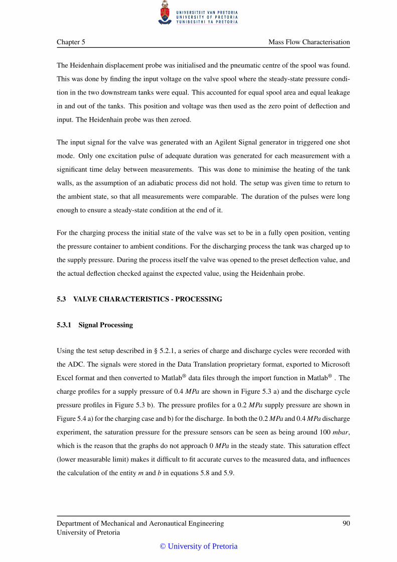
Chapter 5 Mass Flow Characterisation
The Heidenhain displacement probe was initialised and the pneumatic centre of the spool was found.
This was done by finding the input voltage on the valve spool where the steady-state pressure condi-
tion in the two downstream tanks were equal. This accounted for equal spool area and equal leakage
in and out of the tanks. This position and voltage was then used as the zero point of deflection and
input. The Heidenhain probe was then zeroed.
The input signal for the valve was generated with an Agilent Signal generator in triggered one shot
mode. Only one excitation pulse of adequate duration was generated for each measurement with a
significant time delay between measurements. This was done to minimise the heating of the tank
walls, as the assumption of an adiabatic process did not hold. The setup was given time to return to
the ambient state, so that all measurements were comparable. The duration of the pulses were long
enough to ensure a steady-state condition at the end of it.
For the charging process the initial state of the valve was set to be in a fully open position, venting
the pressure container to ambient conditions. For the discharging process the tank was charged up to
the supply pressure. During the process itself the valve was opened to the preset deflection value, and
the actual deflection checked against the expected value, using the Heidenhain probe.
5.3 VALVE CHARACTERISTICS - PROCESSING
5.3.1 Signal Processing
Using the test setup described in § 5.2.1, a series of charge and discharge cycles were recorded with
the ADC. The signals were stored in the Data Translation proprietary format, exported to Microsoft
Excel format and then converted to Matlab® data files through the import function in Matlab® . The
charge profiles for a supply pressure of 0.4 MPa are shown in Figure 5.3 a) and the discharge cycle
pressure profiles in Figure 5.3 b). The pressure profiles for a 0.2 MPa supply pressure are shown in
Figure 5.4 a) for the charging case and b) for the discharge. In both the 0.2 MPa and 0.4 MPa discharge
experiment, the saturation pressure for the pressure sensors can be seen as being around 100 mbar,
which is the reason that the graphs do not approach 0 MPa in the steady state. This saturation effect
(lower measurable limit) makes it difficult to fit accurate curves to the measured data, and influences
the calculation of the entity m and b in equations 5.8 and 5.9.
Department of Mechanical and Aeronautical EngineeringUniversity of Pretoria
90
© University of Pretoria
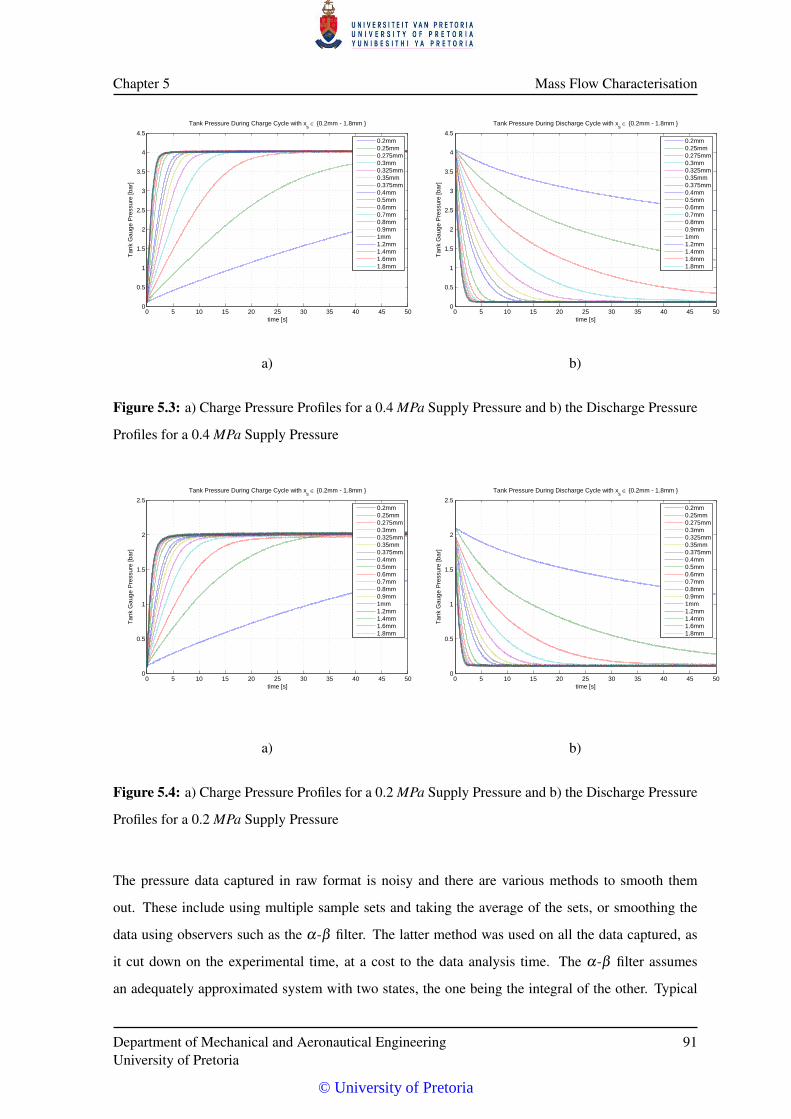
Chapter 5 Mass Flow Characterisation
0 5 10 15 20 25 30 35 40 45 500
0.5
1
1.5
2
2.5
3
3.5
4
4.5
Tank Pressure During Charge Cycle with xs {0.2mm - 1.8mm }
time [s]
Tan
k G
auge
Pre
ssur
e [b
ar]
0.2mm0.25mm0.275mm0.3mm0.325mm0.35mm0.375mm0.4mm0.5mm0.6mm0.7mm0.8mm0.9mm1mm1.2mm1.4mm1.6mm1.8mm
0 5 10 15 20 25 30 35 40 45 500
0.5
1
1.5
2
2.5
3
3.5
4
4.5
Tank Pressure During Discharge Cycle with xs {0.2mm - 1.8mm }
time [s]
Tan
k G
auge
Pre
ssur
e [b
ar]
0.2mm0.25mm0.275mm0.3mm0.325mm0.35mm0.375mm0.4mm0.5mm0.6mm0.7mm0.8mm0.9mm1mm1.2mm1.4mm1.6mm1.8mm
a) b)
Figure 5.3: a) Charge Pressure Profiles for a 0.4 MPa Supply Pressure and b) the Discharge Pressure
Profiles for a 0.4 MPa Supply Pressure
0 5 10 15 20 25 30 35 40 45 500
0.5
1
1.5
2
2.5
Tank Pressure During Charge Cycle with xs {0.2mm - 1.8mm }
time [s]
Tan
k G
auge
Pre
ssur
e [b
ar]
0.2mm0.25mm0.275mm0.3mm0.325mm0.35mm0.375mm0.4mm0.5mm0.6mm0.7mm0.8mm0.9mm1mm1.2mm1.4mm1.6mm1.8mm
0 5 10 15 20 25 30 35 40 45 500
0.5
1
1.5
2
2.5
Tank Pressure During Discharge Cycle with xs {0.2mm - 1.8mm }
time [s]
Tan
k G
auge
Pre
ssur
e [b
ar]
0.2mm0.25mm0.275mm0.3mm0.325mm0.35mm0.375mm0.4mm0.5mm0.6mm0.7mm0.8mm0.9mm1mm1.2mm1.4mm1.6mm1.8mm
a) b)
Figure 5.4: a) Charge Pressure Profiles for a 0.2 MPa Supply Pressure and b) the Discharge Pressure
Profiles for a 0.2 MPa Supply Pressure
The pressure data captured in raw format is noisy and there are various methods to smooth them
out. These include using multiple sample sets and taking the average of the sets, or smoothing the
data using observers such as the α-β filter. The latter method was used on all the data captured, as
it cut down on the experimental time, at a cost to the data analysis time. The α-β filter assumes
an adequately approximated system with two states, the one being the integral of the other. Typical
Department of Mechanical and Aeronautical EngineeringUniversity of Pretoria
91
© University of Pretoria
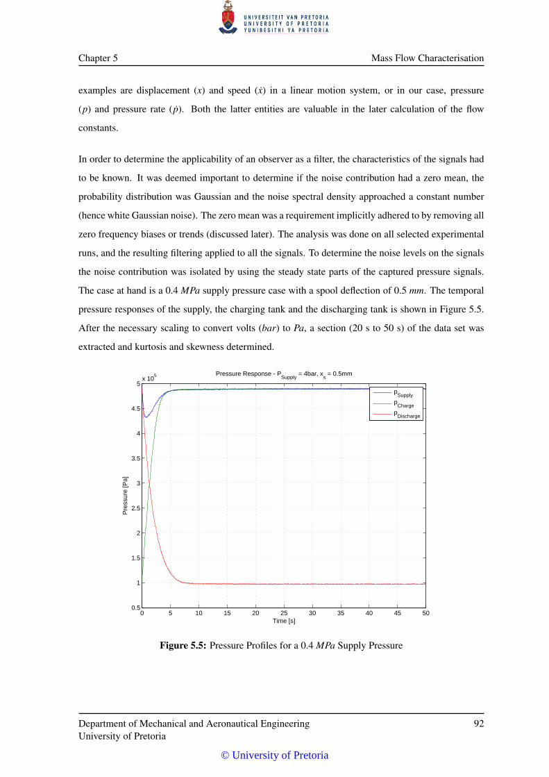
Chapter 5 Mass Flow Characterisation
examples are displacement (x) and speed (x) in a linear motion system, or in our case, pressure
(p) and pressure rate ( p). Both the latter entities are valuable in the later calculation of the flow
constants.
In order to determine the applicability of an observer as a filter, the characteristics of the signals had
to be known. It was deemed important to determine if the noise contribution had a zero mean, the
probability distribution was Gaussian and the noise spectral density approached a constant number
(hence white Gaussian noise). The zero mean was a requirement implicitly adhered to by removing all
zero frequency biases or trends (discussed later). The analysis was done on all selected experimental
runs, and the resulting filtering applied to all the signals. To determine the noise levels on the signals
the noise contribution was isolated by using the steady state parts of the captured pressure signals.
The case at hand is a 0.4 MPa supply pressure case with a spool deflection of 0.5 mm. The temporal
pressure responses of the supply, the charging tank and the discharging tank is shown in Figure 5.5.
After the necessary scaling to convert volts (bar) to Pa, a section (20 s to 50 s) of the data set was
extracted and kurtosis and skewness determined.
0 5 10 15 20 25 30 35 40 45 500.5
1
1.5
2
2.5
3
3.5
4
4.5
5x 10
5 Pressure Response - PSupply
= 4bar, xs = 0.5mm
Time [s]
Pre
ssur
e [P
a]
p
Supply
pCharge
pDischarge
Figure 5.5: Pressure Profiles for a 0.4 MPa Supply Pressure
Department of Mechanical and Aeronautical EngineeringUniversity of Pretoria
92
© University of Pretoria
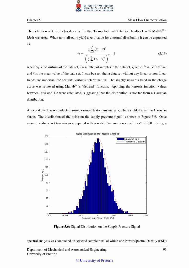
Chapter 5 Mass Flow Characterisation
The definition of kurtosis (as described in the "Computational Statistics Handbook with Matlab® "
[56]) was used. When normalised to yield a zero value for a normal distribution it can be expressed
as
γ2 =
1n
n∑
i=1(xi− x)4(
1n
n∑
i=1(xi− x)2
)2 −3, (5.13)
where γ2 is the kurtosis of the data set, n is number of samples in the data set, xi is the ith value in the set
and x is the mean value of the data set. It can be seen that a data set without any linear or non-linear
trends are important for accurate kurtosis determination. The slightly upwards trend in the charge
curve was removed using Matlab® ’s "detrend" function. Applying the kurtosis function, values
between 0.24 and 1.2 were calculated, suggesting that the distribution is not far from a Gaussian
distribution.
A second check was conducted, using a simple histogram analysis, which yielded a similar Gaussian
shape. The distribution of the noise on the supply pressure signal is shown in Figure 5.6. Once
again, the shape is Gaussian as compared with a scaled Gaussian curve with a σ of 300. Lastly, a
-1500 -1000 -500 0 500 1000 15000
20
40
60
80
100
120
140
160
180
200Noise Distribution on the Pressure Channels
Deviation from Steady State [Pa]
Fre
quen
cy []
Measured DataTheoretical Gaussian
Figure 5.6: Signal Distribution on the Supply Pressure Signal
spectral analysis was conducted on selected sample runs, of which one Power Spectral Density (PSD)
Department of Mechanical and Aeronautical EngineeringUniversity of Pretoria
93
© University of Pretoria
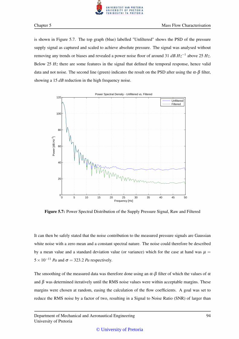
Chapter 5 Mass Flow Characterisation
is shown in Figure 5.7. The top graph (blue) labelled "Unfiltered" shows the PSD of the pressure
supply signal as captured and scaled to achieve absolute pressure. The signal was analysed without
removing any trends or biases and revealed a power noise floor of around 31 dB.Hz−1 above 25 Hz.
Below 25 Hz there are some features in the signal that defined the temporal response, hence valid
data and not noise. The second line (green) indicates the result on the PSD after using the α-β filter,
showing a 15 dB reduction in the high frequency noise.
0 5 10 15 20 25 30 35 40 45 500
20
40
60
80
100
120Power Spectral Density - Unfiltered vs. Filtered
Frequency [Hz]
Pow
er [d
B.H
z-1]
UnfilteredFiltered
Figure 5.7: Power Spectral Distribution of the Supply Pressure Signal, Raw and Filtered
It can then be safely stated that the noise contribution to the measured pressure signals are Gaussian
white noise with a zero mean and a constant spectral nature. The noise could therefore be described
by a mean value and a standard deviation value (or variance) which for the case at hand was µ =
5×10⁻¹¹ Pa and σ = 323.2 Pa respectively.
The smoothing of the measured data was therefore done using an α-β filter of which the values of α
and β was determined iteratively until the RMS noise values were within acceptable margins. These
margins were chosen at random, easing the calculation of the flow coefficients. A goal was set to
reduce the RMS noise by a factor of two, resulting in a Signal to Noise Ratio (SNR) of larger than
Department of Mechanical and Aeronautical EngineeringUniversity of Pretoria
94
© University of Pretoria
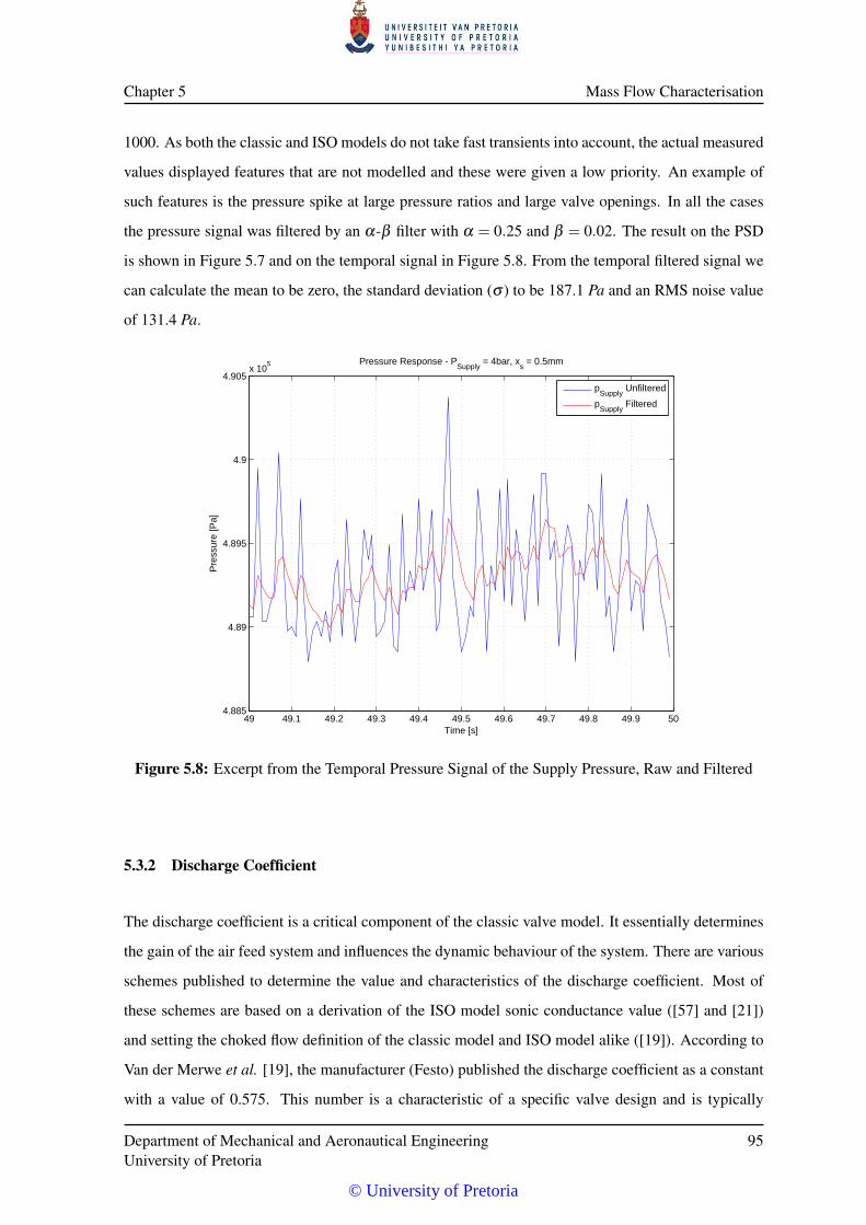
Chapter 5 Mass Flow Characterisation
1000. As both the classic and ISO models do not take fast transients into account, the actual measured
values displayed features that are not modelled and these were given a low priority. An example of
such features is the pressure spike at large pressure ratios and large valve openings. In all the cases
the pressure signal was filtered by an α-β filter with α = 0.25 and β = 0.02. The result on the PSD
is shown in Figure 5.7 and on the temporal signal in Figure 5.8. From the temporal filtered signal we
can calculate the mean to be zero, the standard deviation (σ ) to be 187.1 Pa and an RMS noise value
of 131.4 Pa.
49 49.1 49.2 49.3 49.4 49.5 49.6 49.7 49.8 49.9 504.885
4.89
4.895
4.9
4.905x 10
5 Pressure Response - PSupply
= 4bar, xs = 0.5mm
Time [s]
Pre
ssur
e [P
a]
p
Supply Unfiltered
pSupply
Filtered
Figure 5.8: Excerpt from the Temporal Pressure Signal of the Supply Pressure, Raw and Filtered
5.3.2 Discharge Coefficient
The discharge coefficient is a critical component of the classic valve model. It essentially determines
the gain of the air feed system and influences the dynamic behaviour of the system. There are various
schemes published to determine the value and characteristics of the discharge coefficient. Most of
these schemes are based on a derivation of the ISO model sonic conductance value ([57] and [21])
and setting the choked flow definition of the classic model and ISO model alike ([19]). According to
Van der Merwe et al. [19], the manufacturer (Festo) published the discharge coefficient as a constant
with a value of 0.575. This number is a characteristic of a specific valve design and is typically
Department of Mechanical and Aeronautical EngineeringUniversity of Pretoria
95
© University of Pretoria
Chapter 5 Mass Flow Characterisation
determined by the manufacturer and published as part of a maximum flow rate specification. Also in
this publication, the value of Cd was taken to be a constant and the gain varied by changing the valve
area to suit the flow rate. This could counter the effects of leakage and effective valve area.
The approach was to use the classic model and the test setup described earlier to determine the value(s)
for Cd by doing a series of charge and discharge cycles and then applying the first term of eq. 5.4 by
rewriting the expression to isolate the discharge coefficient Cd . The valve area (Av) was calculated
using the geometric layout of the valve as described by Eq. 4.4.
The signals were all smoothed using the α-β filter described earlier, and the pressure and temperature
corrected and scaled to absolute pressure and temperature in Pa and K. A by-product of the smoothing
process of the chamber pressure data (pu and pl) is the rate of pressure change (pu and pl). Using the
relationship shown in eq. 5.7 the discharge coefficient was calculated with αi either the inlet or outlet
heat ratios, 1.4 and 1 respectively. It should be noted that for the charging case the supply pressure
was used for p1 and the chamber pressure change for pc. For the discharging case, the chamber
pressure was used for p1 and the direction of air flow necessitated a negative sign.
An example of the calculated discharge coefficient and the chamber pressure for the charging cycle
with a supply pressure of 0.4 MPa and a spool deflection of 0.55 mm is shown in Figure 5.9 and for
the discharging cycle in Figure 5.10.
Department of Mechanical and Aeronautical EngineeringUniversity of Pretoria
96
© University of Pretoria
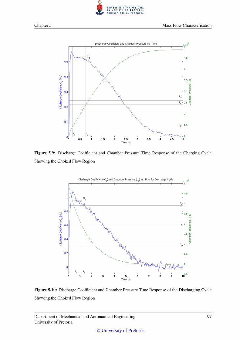
Chapter 5 Mass Flow Characterisation
0 0.5 1 1.5 2 2.5 3 3.5 4 4.5 50
0.1
0.2
0.3
0.4
0.5
Discharge Coefficient and Chamber Pressure vs. Time
Time [s]
Dis
char
ge C
oeffi
cien
t Cd [N
U]
pcr
pe
ps
ts
te
Cd
0 0.5 1 1.5 2 2.5 3 3.5 4 4.5 51
1.5
2
2.5
3
3.5
4
4.5
5x 10
5
Cha
mbe
r P
ress
ure
[Pa]
Figure 5.9: Discharge Coefficient and Chamber Pressure Time Response of the Charging Cycle
Showing the Choked Flow Region
0 1 2 3 4 5 6 7 8 9 10
0
0.2
0.4
0.6
0.8
1
pcr
pe
ps
ts
te
Cd
Discharge Coefficient (Cd) and Chamber Pressure (p
c) vs. Time for Discharge Cycle
Time [s]
Dis
char
ge C
oeffi
cien
t Cd [N
U]
0 1 2 3 4 5 6 7 8 9 100.5
1
1.5
2
2.5
3
3.5
4
4.5
5x 10
5
Cha
mbe
r P
ress
ure
p c [Pa]
Figure 5.10: Discharge Coefficient and Chamber Pressure Time Response of the Discharging Cycle
Showing the Choked Flow Region
Department of Mechanical and Aeronautical EngineeringUniversity of Pretoria
97
© University of Pretoria
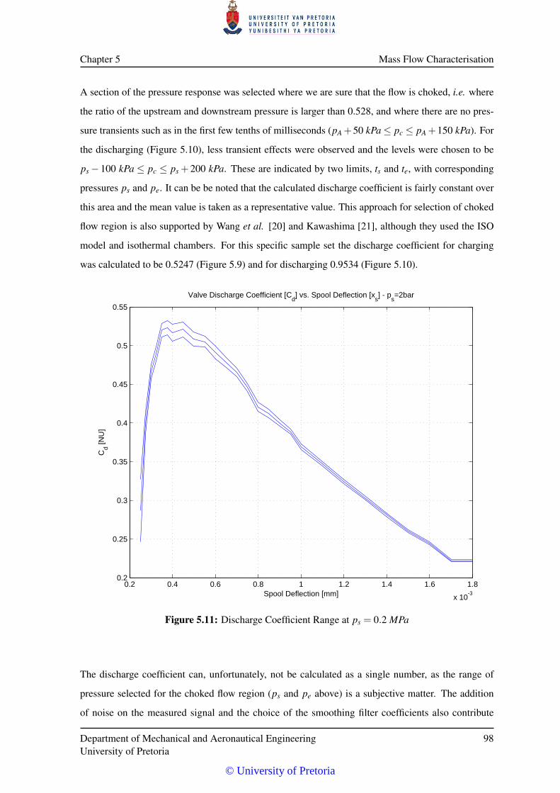
Chapter 5 Mass Flow Characterisation
A section of the pressure response was selected where we are sure that the flow is choked, i.e. where
the ratio of the upstream and downstream pressure is larger than 0.528, and where there are no pres-
sure transients such as in the first few tenths of milliseconds (pA +50 kPa≤ pc ≤ pA +150 kPa). For
the discharging (Figure 5.10), less transient effects were observed and the levels were chosen to be
ps− 100 kPa ≤ pc ≤ ps + 200 kPa. These are indicated by two limits, ts and te, with corresponding
pressures ps and pe. It can be be noted that the calculated discharge coefficient is fairly constant over
this area and the mean value is taken as a representative value. This approach for selection of choked
flow region is also supported by Wang et al. [20] and Kawashima [21], although they used the ISO
model and isothermal chambers. For this specific sample set the discharge coefficient for charging
was calculated to be 0.5247 (Figure 5.9) and for discharging 0.9534 (Figure 5.10).
0.2 0.4 0.6 0.8 1 1.2 1.4 1.6 1.8
x 10-3
0.2
0.25
0.3
0.35
0.4
0.45
0.5
0.55
Valve Discharge Coefficient [Cd] vs. Spool Deflection [x
s] - p
s=2bar
Spool Deflection [mm]
Cd [N
U]
Figure 5.11: Discharge Coefficient Range at ps = 0.2 MPa
The discharge coefficient can, unfortunately, not be calculated as a single number, as the range of
pressure selected for the choked flow region (ps and pe above) is a subjective matter. The addition
of noise on the measured signal and the choice of the smoothing filter coefficients also contribute
Department of Mechanical and Aeronautical EngineeringUniversity of Pretoria
98
© University of Pretoria
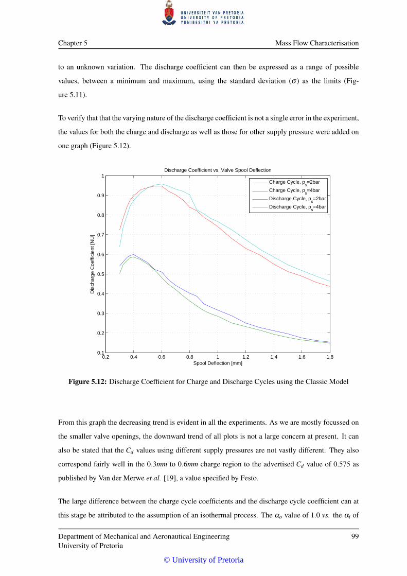
Chapter 5 Mass Flow Characterisation
to an unknown variation. The discharge coefficient can then be expressed as a range of possible
values, between a minimum and maximum, using the standard deviation (σ ) as the limits (Fig-
ure 5.11).
To verify that that the varying nature of the discharge coefficient is not a single error in the experiment,
the values for both the charge and discharge as well as those for other supply pressure were added on
one graph (Figure 5.12).
0.2 0.4 0.6 0.8 1 1.2 1.4 1.6 1.80.1
0.2
0.3
0.4
0.5
0.6
0.7
0.8
0.9
1Discharge Coefficient vs. Valve Spool Deflection
Spool Deflection [mm]
Dis
char
ge C
oeffi
cien
t [N
U]
Charge Cycle, p
s=2bar
Charge Cycle, ps=4bar
Discharge Cycle, ps=2bar
Discharge Cycle, ps=4bar
Figure 5.12: Discharge Coefficient for Charge and Discharge Cycles using the Classic Model
From this graph the decreasing trend is evident in all the experiments. As we are mostly focussed on
the smaller valve openings, the downward trend of all plots is not a large concern at present. It can
also be stated that the Cd values using different supply pressures are not vastly different. They also
correspond fairly well in the 0.3mm to 0.6mm charge region to the advertised Cd value of 0.575 as
published by Van der Merwe et al. [19], a value specified by Festo.
The large difference between the charge cycle coefficients and the discharge cycle coefficient can at
this stage be attributed to the assumption of an isothermal process. The αo value of 1.0 vs. the αi of
Department of Mechanical and Aeronautical EngineeringUniversity of Pretoria
99
© University of Pretoria
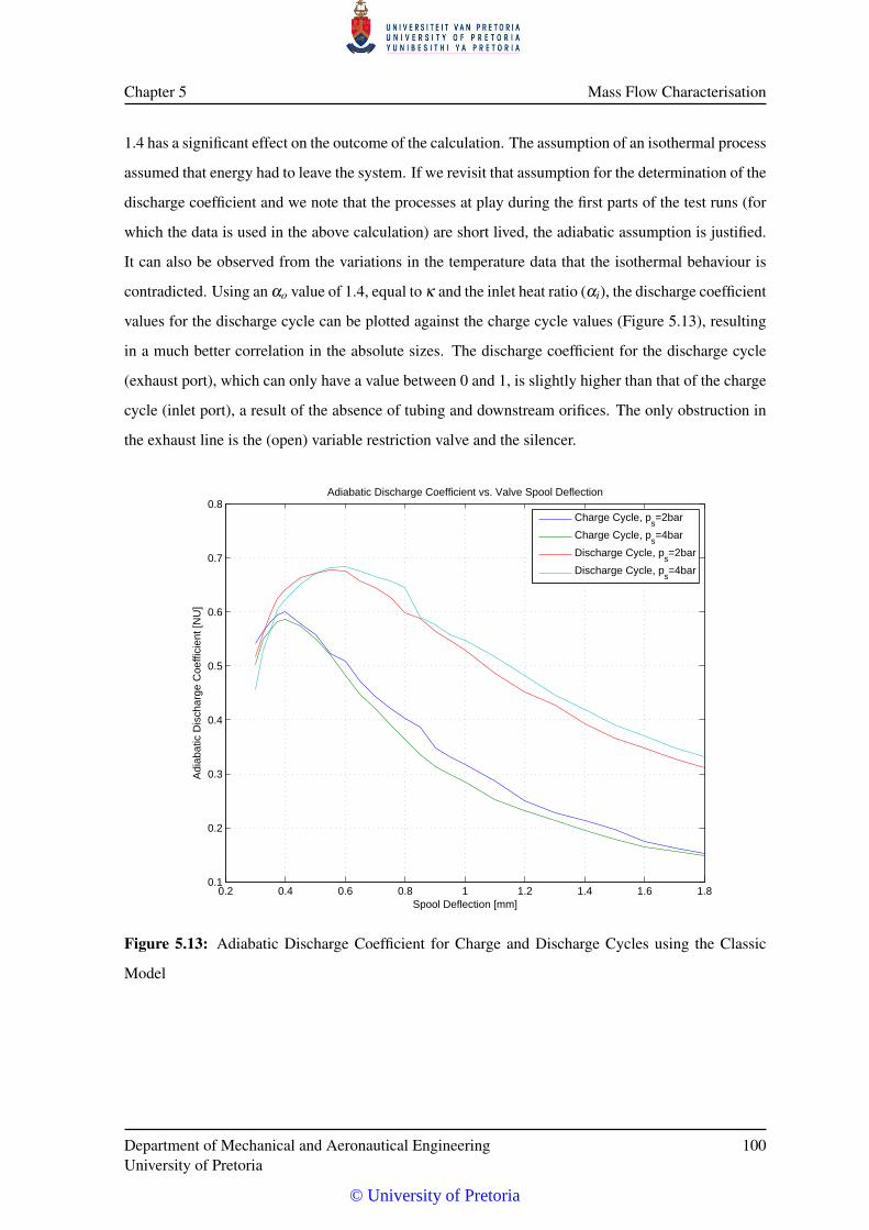
Chapter 5 Mass Flow Characterisation
1.4 has a significant effect on the outcome of the calculation. The assumption of an isothermal process
assumed that energy had to leave the system. If we revisit that assumption for the determination of the
discharge coefficient and we note that the processes at play during the first parts of the test runs (for
which the data is used in the above calculation) are short lived, the adiabatic assumption is justified.
It can also be observed from the variations in the temperature data that the isothermal behaviour is
contradicted. Using an αo value of 1.4, equal to κ and the inlet heat ratio (αi), the discharge coefficient
values for the discharge cycle can be plotted against the charge cycle values (Figure 5.13), resulting
in a much better correlation in the absolute sizes. The discharge coefficient for the discharge cycle
(exhaust port), which can only have a value between 0 and 1, is slightly higher than that of the charge
cycle (inlet port), a result of the absence of tubing and downstream orifices. The only obstruction in
the exhaust line is the (open) variable restriction valve and the silencer.
0.2 0.4 0.6 0.8 1 1.2 1.4 1.6 1.80.1
0.2
0.3
0.4
0.5
0.6
0.7
0.8Adiabatic Discharge Coefficient vs. Valve Spool Deflection
Spool Deflection [mm]
Adi
abat
ic D
isch
arge
Coe
ffici
ent [
NU
]
Charge Cycle, p
s=2bar
Charge Cycle, ps=4bar
Discharge Cycle, ps=2bar
Discharge Cycle, ps=4bar
Figure 5.13: Adiabatic Discharge Coefficient for Charge and Discharge Cycles using the Classic
Model
Department of Mechanical and Aeronautical EngineeringUniversity of Pretoria
100
© University of Pretoria
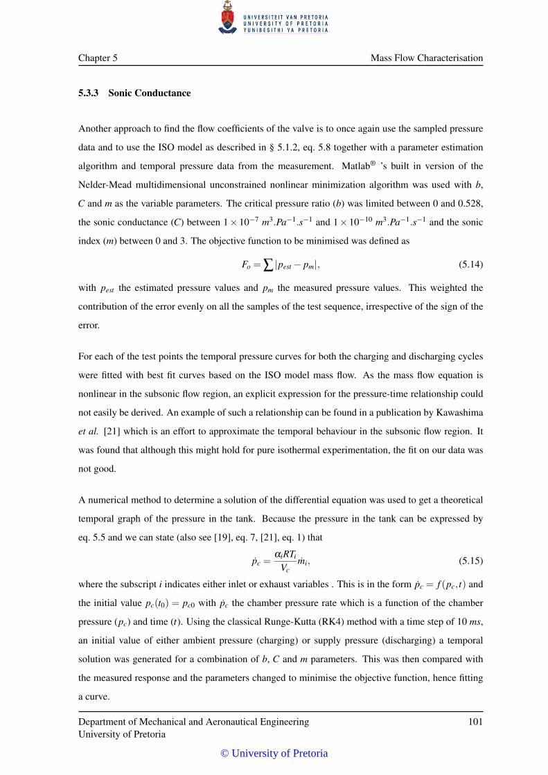
Chapter 5 Mass Flow Characterisation
5.3.3 Sonic Conductance
Another approach to find the flow coefficients of the valve is to once again use the sampled pressure
data and to use the ISO model as described in § 5.1.2, eq. 5.8 together with a parameter estimation
algorithm and temporal pressure data from the measurement. Matlab® ’s built in version of the
Nelder-Mead multidimensional unconstrained nonlinear minimization algorithm was used with b,
C and m as the variable parameters. The critical pressure ratio (b) was limited between 0 and 0.528,
the sonic conductance (C) between 1× 10⁻⁷ m3.Pa−1.s−1 and 1× 10⁻¹⁰ m3.Pa−1.s−1 and the sonic
index (m) between 0 and 3. The objective function to be minimised was defined as
Fo = ∑ |pest − pm|, (5.14)
with pest the estimated pressure values and pm the measured pressure values. This weighted the
contribution of the error evenly on all the samples of the test sequence, irrespective of the sign of the
error.
For each of the test points the temporal pressure curves for both the charging and discharging cycles
were fitted with best fit curves based on the ISO model mass flow. As the mass flow equation is
nonlinear in the subsonic flow region, an explicit expression for the pressure-time relationship could
not easily be derived. An example of such a relationship can be found in a publication by Kawashima
et al. [21] which is an effort to approximate the temporal behaviour in the subsonic flow region. It
was found that although this might hold for pure isothermal experimentation, the fit on our data was
not good.
A numerical method to determine a solution of the differential equation was used to get a theoretical
temporal graph of the pressure in the tank. Because the pressure in the tank can be expressed by
eq. 5.5 and we can state (also see [19], eq. 7, [21], eq. 1) that
pc =αiRTi
Vcmi, (5.15)
where the subscript i indicates either inlet or exhaust variables . This is in the form pc = f (pc, t) and
the initial value pc(t0) = pc0 with pc the chamber pressure rate which is a function of the chamber
pressure (pc) and time (t). Using the classical Runge-Kutta (RK4) method with a time step of 10 ms,
an initial value of either ambient pressure (charging) or supply pressure (discharging) a temporal
solution was generated for a combination of b, C and m parameters. This was then compared with
the measured response and the parameters changed to minimise the objective function, hence fitting
a curve.
Department of Mechanical and Aeronautical EngineeringUniversity of Pretoria
101
© University of Pretoria
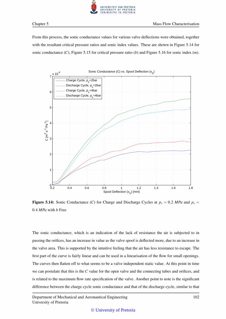
Chapter 5 Mass Flow Characterisation
From this process, the sonic conductance values for various valve deflections were obtained, together
with the resultant critical pressure ratios and sonic index values. These are shown in Figure 5.14 for
sonic conductance (C), Figure 5.15 for critical pressure ratio (b) and Figure 5.16 for sonic index (m).
0.2 0.4 0.6 0.8 1 1.2 1.4 1.6 1.80
1
2
3
4
5
6
7x 10
-8 Sonic Conductance (C) vs. Spool Deflection (xS)
Spool Deflection (xS) [mm]
C [m
3 .s-1
.Pa-1
]
Charge Cycle, p
s=2bar
Discharge Cycle, ps=2bar
Charge Cycle, ps=4bar
Discharge Cycle, ps=4bar
Figure 5.14: Sonic Conductance (C) for Charge and Discharge Cycles at ps = 0.2 MPa and ps =
0.4 MPa with b Free
The sonic conductance, which is an indication of the lack of resistance the air is subjected to in
passing the orifices, has an increase in value as the valve spool is deflected more, due to an increase in
the valve area. This is supported by the intuitive feeling that the air has less resistance to escape. The
first part of the curve is fairly linear and can be used in a linearisation of the flow for small openings.
The curves then flatten off to what seems to be a valve independent static value. At this point in time
we can postulate that this is the C value for the open valve and the connecting tubes and orifices, and
is related to the maximum flow rate specification of the valve. Another point to note is the significant
difference between the charge cycle sonic conductance and that of the discharge cycle, similar to that
Department of Mechanical and Aeronautical EngineeringUniversity of Pretoria
102
© University of Pretoria
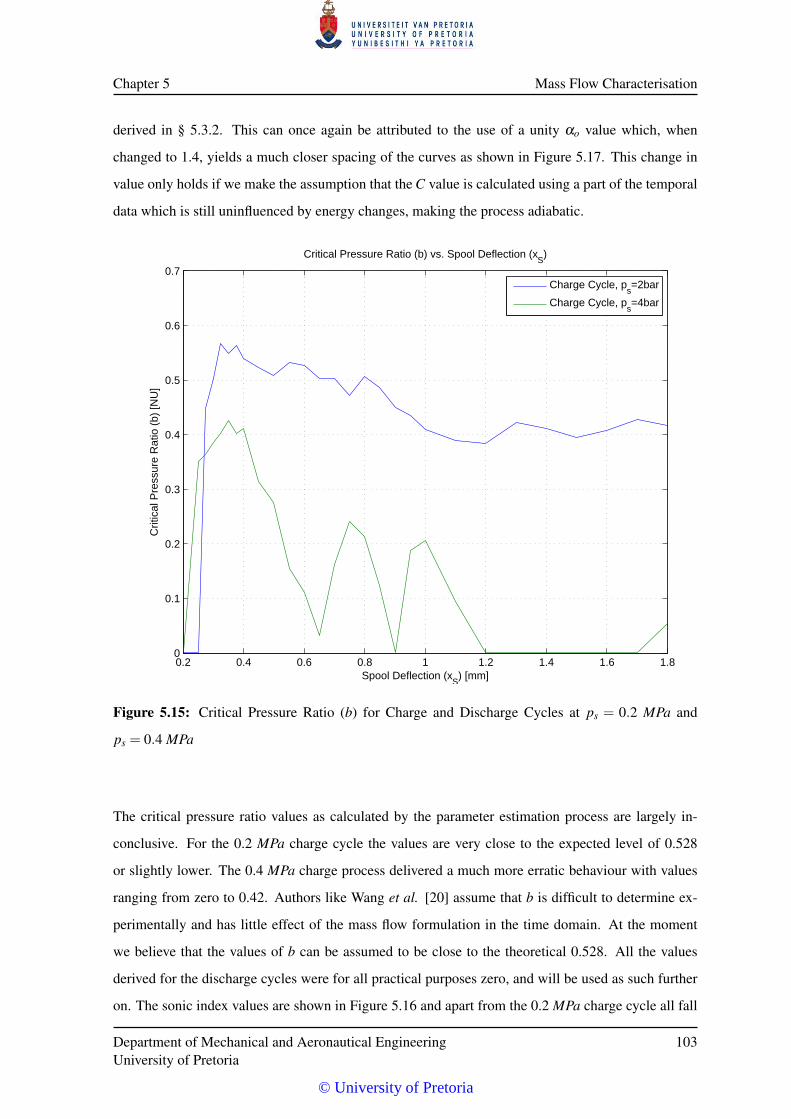
Chapter 5 Mass Flow Characterisation
derived in § 5.3.2. This can once again be attributed to the use of a unity αo value which, when
changed to 1.4, yields a much closer spacing of the curves as shown in Figure 5.17. This change in
value only holds if we make the assumption that the C value is calculated using a part of the temporal
data which is still uninfluenced by energy changes, making the process adiabatic.
0.2 0.4 0.6 0.8 1 1.2 1.4 1.6 1.80
0.1
0.2
0.3
0.4
0.5
0.6
0.7
Critical Pressure Ratio (b) vs. Spool Deflection (xS)
Spool Deflection (xS) [mm]
Crit
ical
Pre
ssur
e R
atio
(b)
[NU
]
Charge Cycle, p
s=2bar
Charge Cycle, ps=4bar
Figure 5.15: Critical Pressure Ratio (b) for Charge and Discharge Cycles at ps = 0.2 MPa and
ps = 0.4 MPa
The critical pressure ratio values as calculated by the parameter estimation process are largely in-
conclusive. For the 0.2 MPa charge cycle the values are very close to the expected level of 0.528
or slightly lower. The 0.4 MPa charge process delivered a much more erratic behaviour with values
ranging from zero to 0.42. Authors like Wang et al. [20] assume that b is difficult to determine ex-
perimentally and has little effect of the mass flow formulation in the time domain. At the moment
we believe that the values of b can be assumed to be close to the theoretical 0.528. All the values
derived for the discharge cycles were for all practical purposes zero, and will be used as such further
on. The sonic index values are shown in Figure 5.16 and apart from the 0.2 MPa charge cycle all fall
Department of Mechanical and Aeronautical EngineeringUniversity of Pretoria
103
© University of Pretoria
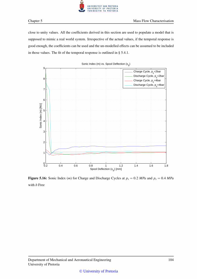
Chapter 5 Mass Flow Characterisation
close to unity values. All the coefficients derived in this section are used to populate a model that is
supposed to mimic a real world system. Irrespective of the actual values, if the temporal response is
good enough, the coefficients can be used and the un-modelled effects can be assumed to be included
in those values. The fit of the temporal response is outlined in § 5.4.1.
0.2 0.4 0.6 0.8 1 1.2 1.4 1.6 1.80
1
2
3
4
5
6
7
8
9
Sonic Index (m) vs. Spool Deflection (xS)
Spool Deflection (xS) [mm]
Son
ic In
dex
(m)
[NU
]
Charge Cycle, p
s=2bar
Discharge Cycle, ps=2bar
Charge Cycle, ps=4bar
Discharge Cycle, ps=4bar
Figure 5.16: Sonic Index (m) for Charge and Discharge Cycles at ps = 0.2 MPa and ps = 0.4 MPa
with b Free
Department of Mechanical and Aeronautical EngineeringUniversity of Pretoria
104
© University of Pretoria
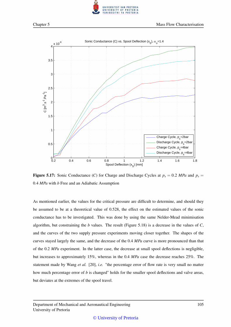
Chapter 5 Mass Flow Characterisation
0.2 0.4 0.6 0.8 1 1.2 1.4 1.6 1.80
0.5
1
1.5
2
2.5
3
3.5
4x 10
-8 Sonic Conductance (C) vs. Spool Deflection (xS),
o=1.4
Spool Deflection (xS) [mm]
C [m
3 .s-1
.Pa-1
]
Charge Cycle, ps=2bar
Discharge Cycle, ps=2bar
Charge Cycle, ps=4bar
Discharge Cycle, ps=4bar
Figure 5.17: Sonic Conductance (C) for Charge and Discharge Cycles at ps = 0.2 MPa and ps =
0.4 MPa with b Free and an Adiabatic Assumption
As mentioned earlier, the values for the critical pressure are difficult to determine, and should they
be assumed to be at a theoretical value of 0.528, the effect on the estimated values of the sonic
conductance has to be investigated. This was done by using the same Nelder-Mead minimisation
algorithm, but constraining the b values. The result (Figure 5.18) is a decrease in the values of C,
and the curves of the two supply pressure experiments moving closer together. The shapes of the
curves stayed largely the same, and the decrease of the 0.4 MPa curve is more pronounced than that
of the 0.2 MPa experiment. In the latter case, the decrease at small spool deflections is negligible,
but increases to approximately 15%, whereas in the 0.4 MPa case the decrease reaches 25%. The
statement made by Wang et al. [20], i.e. "the percentage error of flow rate is very small no matter
how much percentage error of b is changed" holds for the smaller spool deflections and valve areas,
but deviates at the extremes of the spool travel.
Department of Mechanical and Aeronautical EngineeringUniversity of Pretoria
105
© University of Pretoria
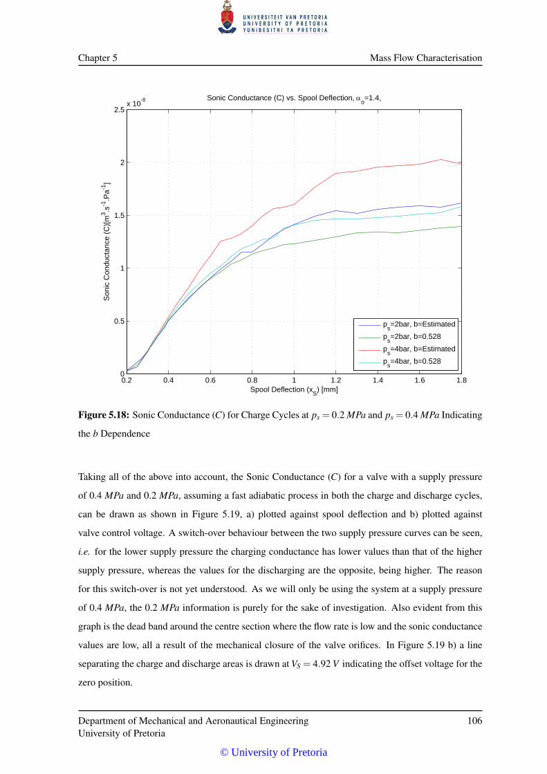
Chapter 5 Mass Flow Characterisation
0.2 0.4 0.6 0.8 1 1.2 1.4 1.6 1.80
0.5
1
1.5
2
2.5x 10
-8 Sonic Conductance (C) vs. Spool Deflection, o=1.4,
Spool Deflection (xS) [mm]
Son
ic C
ondu
ctan
ce (
C)[
m3 .s
-1.P
a-1]
ps=2bar, b=Estimated
ps=2bar, b=0.528
ps=4bar, b=Estimated
ps=4bar, b=0.528
Figure 5.18: Sonic Conductance (C) for Charge Cycles at ps = 0.2 MPa and ps = 0.4 MPa Indicating
the b Dependence
Taking all of the above into account, the Sonic Conductance (C) for a valve with a supply pressure
of 0.4 MPa and 0.2 MPa, assuming a fast adiabatic process in both the charge and discharge cycles,
can be drawn as shown in Figure 5.19, a) plotted against spool deflection and b) plotted against
valve control voltage. A switch-over behaviour between the two supply pressure curves can be seen,
i.e. for the lower supply pressure the charging conductance has lower values than that of the higher
supply pressure, whereas the values for the discharging are the opposite, being higher. The reason
for this switch-over is not yet understood. As we will only be using the system at a supply pressure
of 0.4 MPa, the 0.2 MPa information is purely for the sake of investigation. Also evident from this
graph is the dead band around the centre section where the flow rate is low and the sonic conductance
values are low, all a result of the mechanical closure of the valve orifices. In Figure 5.19 b) a line
separating the charge and discharge areas is drawn at VS = 4.92 V indicating the offset voltage for the
zero position.
Department of Mechanical and Aeronautical EngineeringUniversity of Pretoria
106
© University of Pretoria
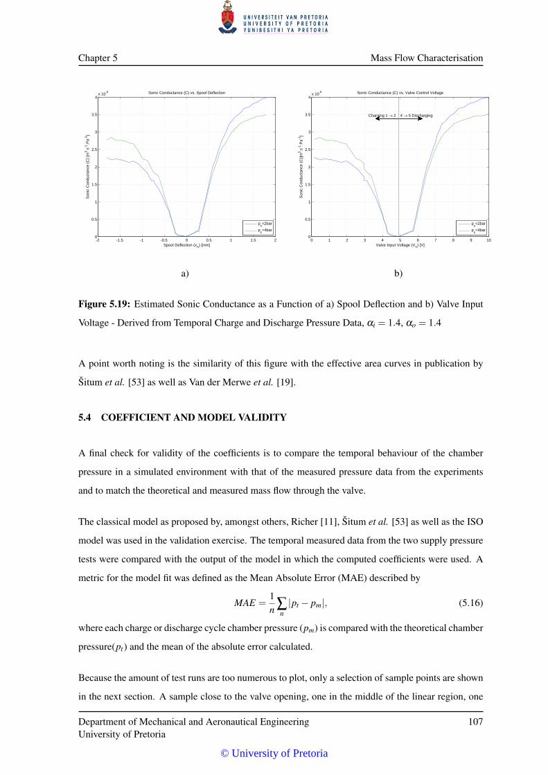
Chapter 5 Mass Flow Characterisation
-2 -1.5 -1 -0.5 0 0.5 1 1.5 20
0.5
1
1.5
2
2.5
3
3.5
4x 10
-8 Sonic Conductance (C) vs. Spool Deflection
Spool Deflection (xS) [mm]
Son
ic C
ondu
ctan
ce (
C)
[m3 .s
-1.P
a-1]
ps=2bar
ps=4bar
0 1 2 3 4 5 6 7 8 9 100
0.5
1
1.5
2
2.5
3
3.5
4x 10
-8 Sonic Conductance (C) vs. Valve Control Voltage
Valve Input Voltage (VS) [V]
Son
ic C
ondu
ctan
ce (
C)[
m3 .s
-1.P
a-1]
4 5 DischargingCharging 1 2
ps=2bar
ps=4bar
a) b)
Figure 5.19: Estimated Sonic Conductance as a Function of a) Spool Deflection and b) Valve Input
Voltage - Derived from Temporal Charge and Discharge Pressure Data, αi = 1.4, αo = 1.4
A point worth noting is the similarity of this figure with the effective area curves in publication by
Šitum et al. [53] as well as Van der Merwe et al. [19].
5.4 COEFFICIENT AND MODEL VALIDITY
A final check for validity of the coefficients is to compare the temporal behaviour of the chamber
pressure in a simulated environment with that of the measured pressure data from the experiments
and to match the theoretical and measured mass flow through the valve.
The classical model as proposed by, amongst others, Richer [11], Šitum et al. [53] as well as the ISO
model was used in the validation exercise. The temporal measured data from the two supply pressure
tests were compared with the output of the model in which the computed coefficients were used. A
metric for the model fit was defined as the Mean Absolute Error (MAE) described by
MAE =1n ∑
n|pt − pm|, (5.16)
where each charge or discharge cycle chamber pressure (pm) is compared with the theoretical chamber
pressure(pt) and the mean of the absolute error calculated.
Because the amount of test runs are too numerous to plot, only a selection of sample points are shown
in the next section. A sample close to the valve opening, one in the middle of the linear region, one
Department of Mechanical and Aeronautical EngineeringUniversity of Pretoria
107
© University of Pretoria
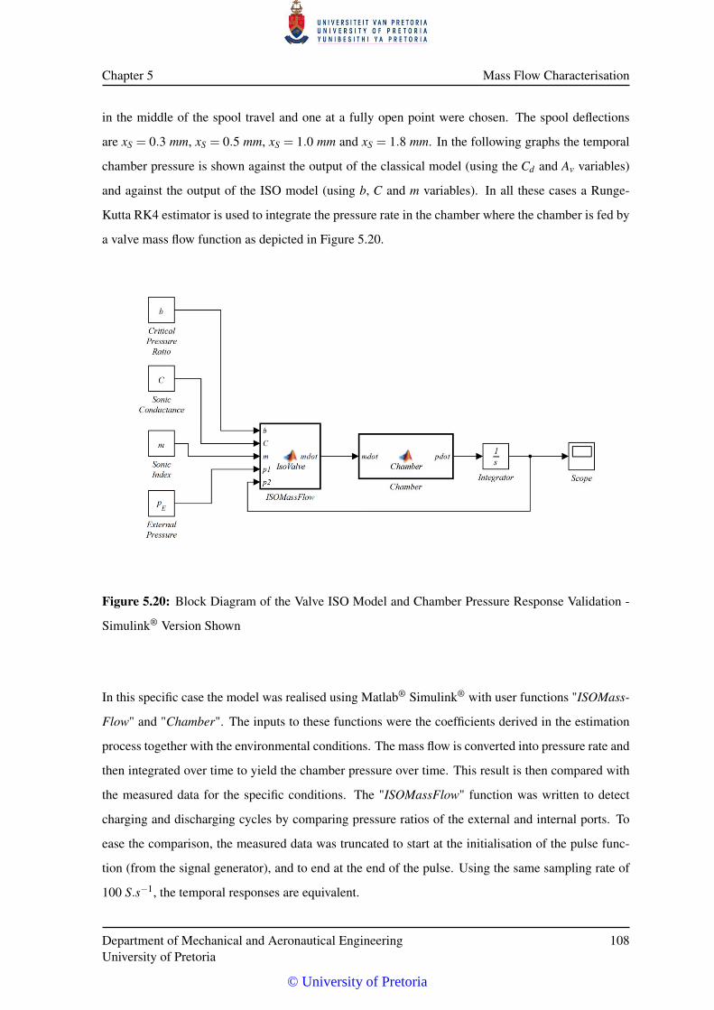
Chapter 5 Mass Flow Characterisation
in the middle of the spool travel and one at a fully open point were chosen. The spool deflections
are xS = 0.3 mm, xS = 0.5 mm, xS = 1.0 mm and xS = 1.8 mm. In the following graphs the temporal
chamber pressure is shown against the output of the classical model (using the Cd and Av variables)
and against the output of the ISO model (using b, C and m variables). In all these cases a Runge-
Kutta RK4 estimator is used to integrate the pressure rate in the chamber where the chamber is fed by
a valve mass flow function as depicted in Figure 5.20.
Figure 5.20: Block Diagram of the Valve ISO Model and Chamber Pressure Response Validation -
Simulink® Version Shown
In this specific case the model was realised using Matlab® Simulink® with user functions "ISOMass-
Flow" and "Chamber". The inputs to these functions were the coefficients derived in the estimation
process together with the environmental conditions. The mass flow is converted into pressure rate and
then integrated over time to yield the chamber pressure over time. This result is then compared with
the measured data for the specific conditions. The "ISOMassFlow" function was written to detect
charging and discharging cycles by comparing pressure ratios of the external and internal ports. To
ease the comparison, the measured data was truncated to start at the initialisation of the pulse func-
tion (from the signal generator), and to end at the end of the pulse. Using the same sampling rate of
100 S.s−1, the temporal responses are equivalent.
Department of Mechanical and Aeronautical EngineeringUniversity of Pretoria
108
© University of Pretoria
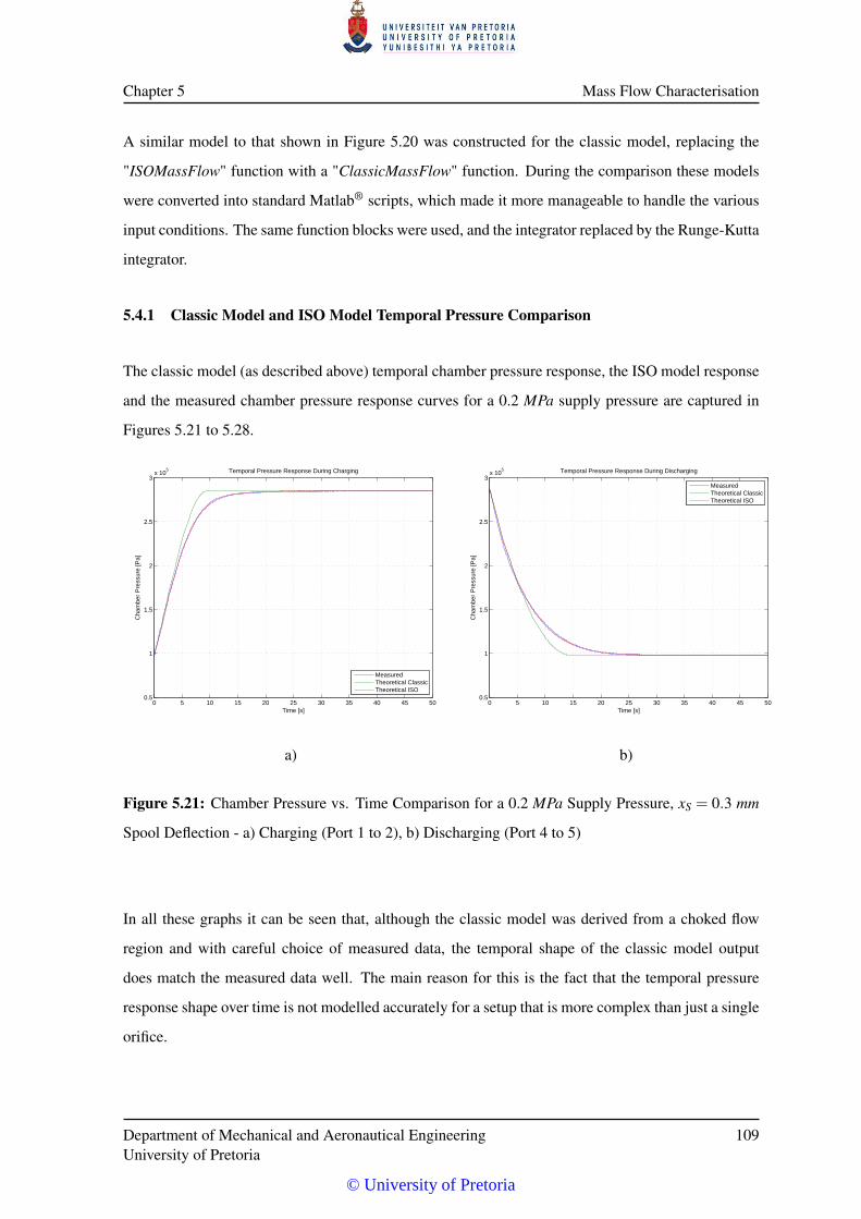
Chapter 5 Mass Flow Characterisation
A similar model to that shown in Figure 5.20 was constructed for the classic model, replacing the
"ISOMassFlow" function with a "ClassicMassFlow" function. During the comparison these models
were converted into standard Matlab® scripts, which made it more manageable to handle the various
input conditions. The same function blocks were used, and the integrator replaced by the Runge-Kutta
integrator.
5.4.1 Classic Model and ISO Model Temporal Pressure Comparison
The classic model (as described above) temporal chamber pressure response, the ISO model response
and the measured chamber pressure response curves for a 0.2 MPa supply pressure are captured in
Figures 5.21 to 5.28.
0 5 10 15 20 25 30 35 40 45 500.5
1
1.5
2
2.5
3x 10
5 Temporal Pressure Response During Charging
Time [s]
Cha
mbe
r P
ress
ure
[Pa]
MeasuredTheoretical ClassicTheoretical ISO
0 5 10 15 20 25 30 35 40 45 500.5
1
1.5
2
2.5
3x 10
5 Temporal Pressure Response During Discharging
Time [s]
Cha
mbe
r P
ress
ure
[Pa]
MeasuredTheoretical ClassicTheoretical ISO
a) b)
Figure 5.21: Chamber Pressure vs. Time Comparison for a 0.2 MPa Supply Pressure, xS = 0.3 mm
Spool Deflection - a) Charging (Port 1 to 2), b) Discharging (Port 4 to 5)
In all these graphs it can be seen that, although the classic model was derived from a choked flow
region and with careful choice of measured data, the temporal shape of the classic model output
does match the measured data well. The main reason for this is the fact that the temporal pressure
response shape over time is not modelled accurately for a setup that is more complex than just a single
orifice.
Department of Mechanical and Aeronautical EngineeringUniversity of Pretoria
109
© University of Pretoria
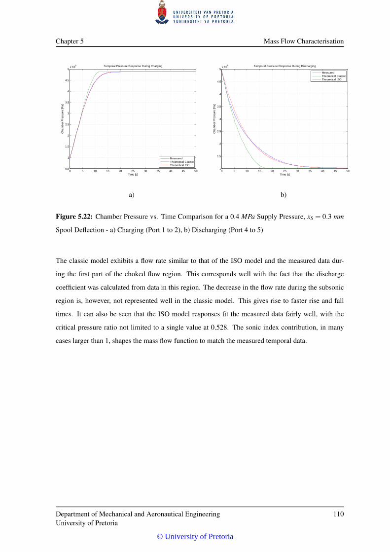
Chapter 5 Mass Flow Characterisation
0 5 10 15 20 25 30 35 40 45 500.5
1
1.5
2
2.5
3
3.5
4
4.5
5x 10
5 Temporal Pressure Response During Charging
Time [s]
Cha
mbe
r P
ress
ure
[Pa]
MeasuredTheoretical ClassicTheoretical ISO
0 5 10 15 20 25 30 35 40 45 501
1.5
2
2.5
3
3.5
4
4.5
5x 10
5 Temporal Pressure Response During Discharging
Time [s]
Cha
mbe
r P
ress
ure
[Pa]
MeasuredTheoretical ClassicTheoretical ISO
a) b)
Figure 5.22: Chamber Pressure vs. Time Comparison for a 0.4 MPa Supply Pressure, xS = 0.3 mm
Spool Deflection - a) Charging (Port 1 to 2), b) Discharging (Port 4 to 5)
The classic model exhibits a flow rate similar to that of the ISO model and the measured data dur-
ing the first part of the choked flow region. This corresponds well with the fact that the discharge
coefficient was calculated from data in this region. The decrease in the flow rate during the subsonic
region is, however, not represented well in the classic model. This gives rise to faster rise and fall
times. It can also be seen that the ISO model responses fit the measured data fairly well, with the
critical pressure ratio not limited to a single value at 0.528. The sonic index contribution, in many
cases larger than 1, shapes the mass flow function to match the measured temporal data.
Department of Mechanical and Aeronautical EngineeringUniversity of Pretoria
110
© University of Pretoria
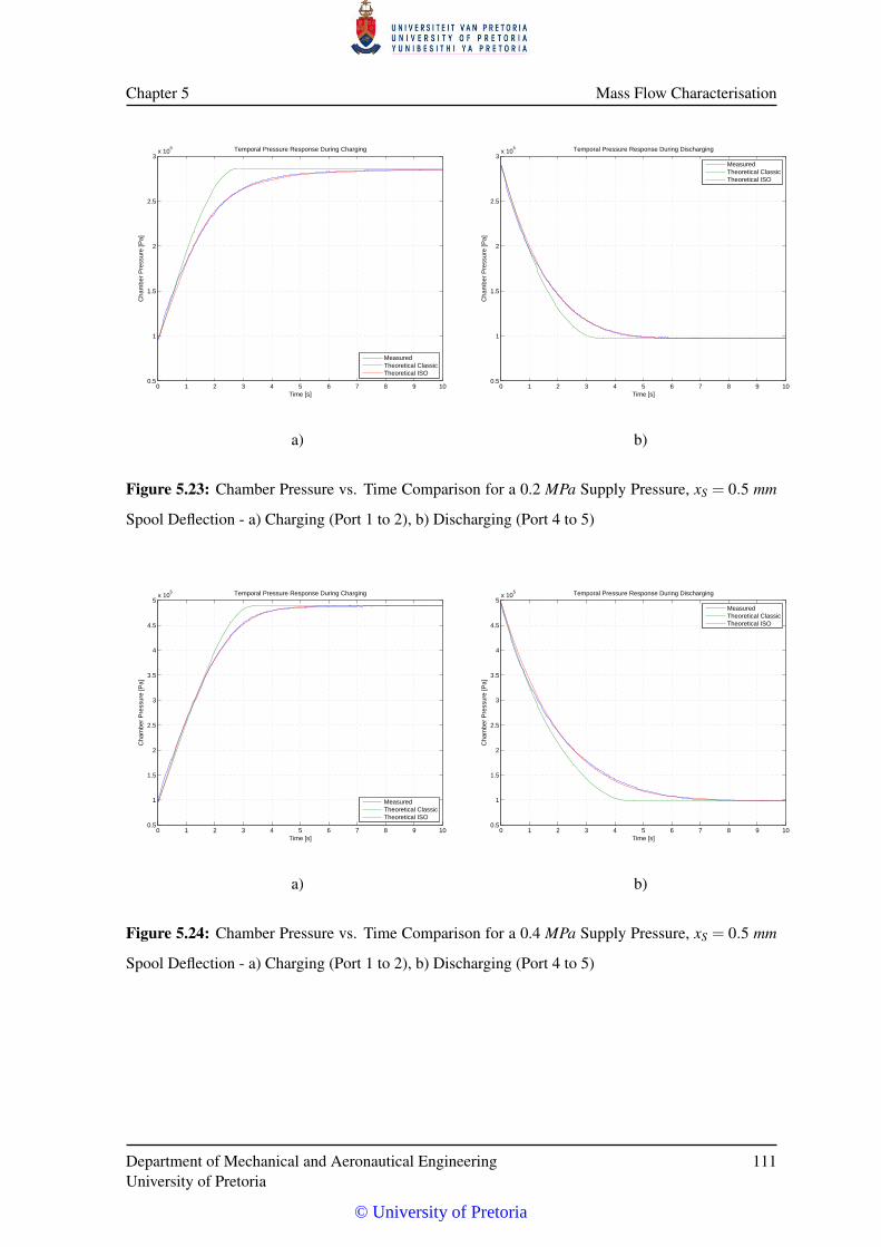
Chapter 5 Mass Flow Characterisation
0 1 2 3 4 5 6 7 8 9 100.5
1
1.5
2
2.5
3x 10
5 Temporal Pressure Response During Charging
Time [s]
Cha
mbe
r P
ress
ure
[Pa]
MeasuredTheoretical ClassicTheoretical ISO
0 1 2 3 4 5 6 7 8 9 100.5
1
1.5
2
2.5
3x 10
5 Temporal Pressure Response During Discharging
Time [s]
Cha
mbe
r P
ress
ure
[Pa]
MeasuredTheoretical ClassicTheoretical ISO
a) b)
Figure 5.23: Chamber Pressure vs. Time Comparison for a 0.2 MPa Supply Pressure, xS = 0.5 mm
Spool Deflection - a) Charging (Port 1 to 2), b) Discharging (Port 4 to 5)
0 1 2 3 4 5 6 7 8 9 100.5
1
1.5
2
2.5
3
3.5
4
4.5
5x 10
5 Temporal Pressure Response During Charging
Time [s]
Cha
mbe
r P
ress
ure
[Pa]
MeasuredTheoretical ClassicTheoretical ISO
0 1 2 3 4 5 6 7 8 9 100.5
1
1.5
2
2.5
3
3.5
4
4.5
5x 10
5 Temporal Pressure Response During Discharging
Time [s]
Cha
mbe
r P
ress
ure
[Pa]
MeasuredTheoretical ClassicTheoretical ISO
a) b)
Figure 5.24: Chamber Pressure vs. Time Comparison for a 0.4 MPa Supply Pressure, xS = 0.5 mm
Spool Deflection - a) Charging (Port 1 to 2), b) Discharging (Port 4 to 5)
Department of Mechanical and Aeronautical EngineeringUniversity of Pretoria
111
© University of Pretoria
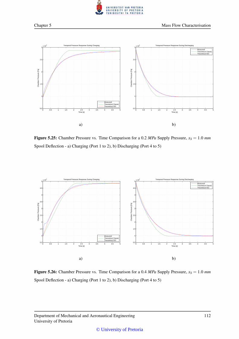
Chapter 5 Mass Flow Characterisation
0 0.5 1 1.5 2 2.5 3 3.5 4 4.5 50.5
1
1.5
2
2.5
3x 10
5 Temporal Pressure Response During Charging
Time [s]
Cha
mbe
r P
ress
ure
[Pa]
MeasuredTheoretical ClassicTheoretical ISO
0 0.5 1 1.5 2 2.5 3 3.5 4 4.5 50.5
1
1.5
2
2.5
3x 10
5 Temporal Pressure Response During Discharging
Time [s]
Cha
mbe
r P
ress
ure
[Pa]
MeasuredTheoretical ClassicTheoretical ISO
a) b)
Figure 5.25: Chamber Pressure vs. Time Comparison for a 0.2 MPa Supply Pressure, xS = 1.0 mm
Spool Deflection - a) Charging (Port 1 to 2), b) Discharging (Port 4 to 5)
0 0.5 1 1.5 2 2.5 3 3.5 4 4.5 50.5
1
1.5
2
2.5
3
3.5
4
4.5
5x 10
5 Temporal Pressure Response During Charging
Time [s]
Cha
mbe
r P
ress
ure
[Pa]
MeasuredTheoretical ClassicTheoretical ISO
0 0.5 1 1.5 2 2.5 3 3.5 4 4.5 50.5
1
1.5
2
2.5
3
3.5
4
4.5
5x 10
5 Temporal Pressure Response During Discharging
Time [s]
Cha
mbe
r P
ress
ure
[Pa]
MeasuredTheoretical ClassicTheoretical ISO
a) b)
Figure 5.26: Chamber Pressure vs. Time Comparison for a 0.4 MPa Supply Pressure, xS = 1.0 mm
Spool Deflection - a) Charging (Port 1 to 2), b) Discharging (Port 4 to 5)
Department of Mechanical and Aeronautical EngineeringUniversity of Pretoria
112
© University of Pretoria
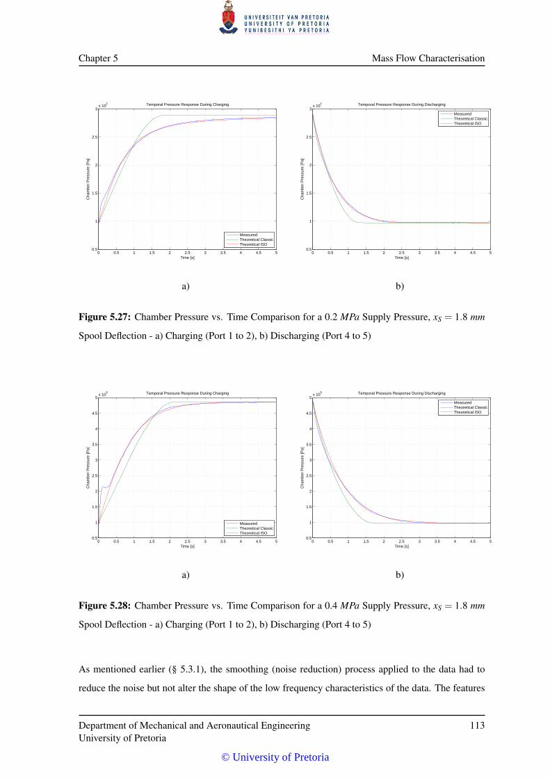
Chapter 5 Mass Flow Characterisation
0 0.5 1 1.5 2 2.5 3 3.5 4 4.5 50.5
1
1.5
2
2.5
3x 10
5 Temporal Pressure Response During Charging
Time [s]
Cha
mbe
r P
ress
ure
[Pa]
MeasuredTheoretical ClassicTheoretical ISO
0 0.5 1 1.5 2 2.5 3 3.5 4 4.5 50.5
1
1.5
2
2.5
3x 10
5 Temporal Pressure Response During Discharging
Time [s]
Cha
mbe
r P
ress
ure
[Pa]
MeasuredTheoretical ClassicTheoretical ISO
a) b)
Figure 5.27: Chamber Pressure vs. Time Comparison for a 0.2 MPa Supply Pressure, xS = 1.8 mm
Spool Deflection - a) Charging (Port 1 to 2), b) Discharging (Port 4 to 5)
0 0.5 1 1.5 2 2.5 3 3.5 4 4.5 50.5
1
1.5
2
2.5
3
3.5
4
4.5
5x 10
5 Temporal Pressure Response During Charging
Time [s]
Cha
mbe
r P
ress
ure
[Pa]
MeasuredTheoretical ClassicTheoretical ISO
0 0.5 1 1.5 2 2.5 3 3.5 4 4.5 50.5
1
1.5
2
2.5
3
3.5
4
4.5
5x 10
5 Temporal Pressure Response During Discharging
Time [s]
Cha
mbe
r P
ress
ure
[Pa]
MeasuredTheoretical ClassicTheoretical ISO
a) b)
Figure 5.28: Chamber Pressure vs. Time Comparison for a 0.4 MPa Supply Pressure, xS = 1.8 mm
Spool Deflection - a) Charging (Port 1 to 2), b) Discharging (Port 4 to 5)
As mentioned earlier (§ 5.3.1), the smoothing (noise reduction) process applied to the data had to
reduce the noise but not alter the shape of the low frequency characteristics of the data. The features
Department of Mechanical and Aeronautical EngineeringUniversity of Pretoria
113
© University of Pretoria
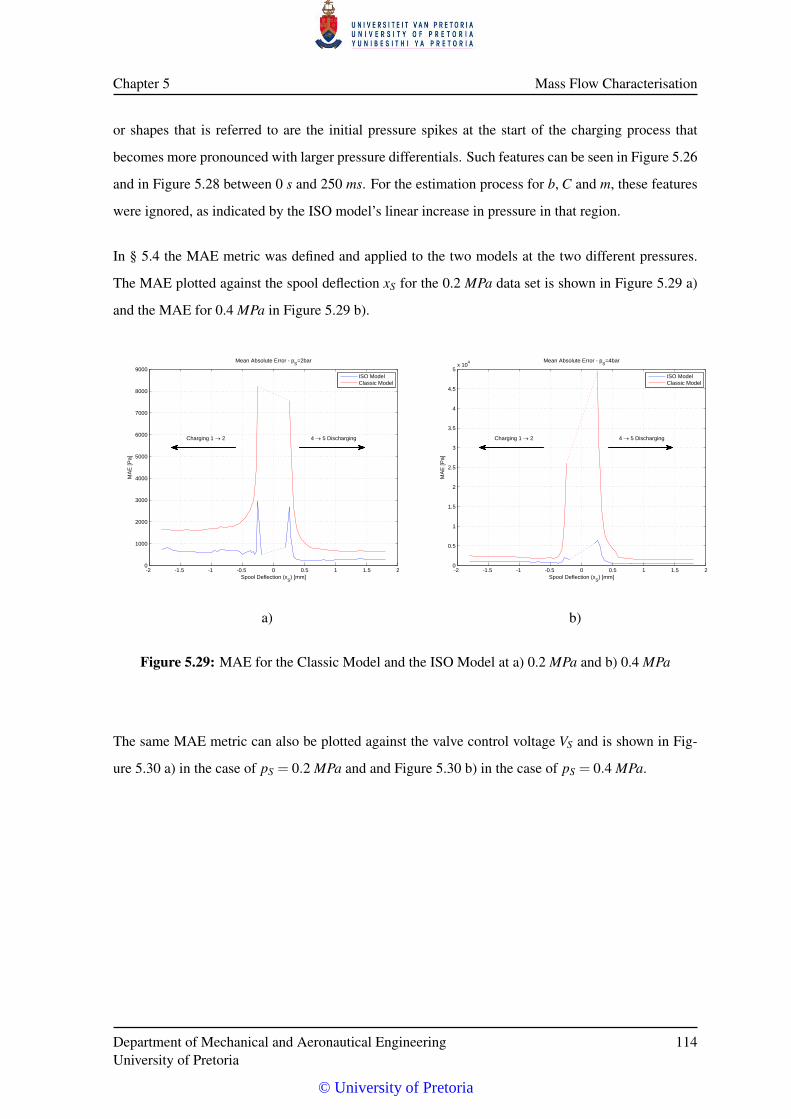
Chapter 5 Mass Flow Characterisation
or shapes that is referred to are the initial pressure spikes at the start of the charging process that
becomes more pronounced with larger pressure differentials. Such features can be seen in Figure 5.26
and in Figure 5.28 between 0 s and 250 ms. For the estimation process for b, C and m, these features
were ignored, as indicated by the ISO model’s linear increase in pressure in that region.
In § 5.4 the MAE metric was defined and applied to the two models at the two different pressures.
The MAE plotted against the spool deflection xS for the 0.2 MPa data set is shown in Figure 5.29 a)
and the MAE for 0.4 MPa in Figure 5.29 b).
-2 -1.5 -1 -0.5 0 0.5 1 1.5 20
1000
2000
3000
4000
5000
6000
7000
8000
9000
4 5 DischargingCharging 1 2
Spool Deflection (xS) [mm]
MA
E [P
a]
Mean Absolute Error - pS=2bar
ISO ModelClassic Model
-2 -1.5 -1 -0.5 0 0.5 1 1.5 20
0.5
1
1.5
2
2.5
3
3.5
4
4.5
5x 10
4
Spool Deflection (xS) [mm]
MA
E [P
a]
Mean Absolute Error - pS=4bar
4 5 DischargingCharging 1 2
ISO ModelClassic Model
a) b)
Figure 5.29: MAE for the Classic Model and the ISO Model at a) 0.2 MPa and b) 0.4 MPa
The same MAE metric can also be plotted against the valve control voltage VS and is shown in Fig-
ure 5.30 a) in the case of pS = 0.2 MPa and and Figure 5.30 b) in the case of pS = 0.4 MPa.
Department of Mechanical and Aeronautical EngineeringUniversity of Pretoria
114
© University of Pretoria
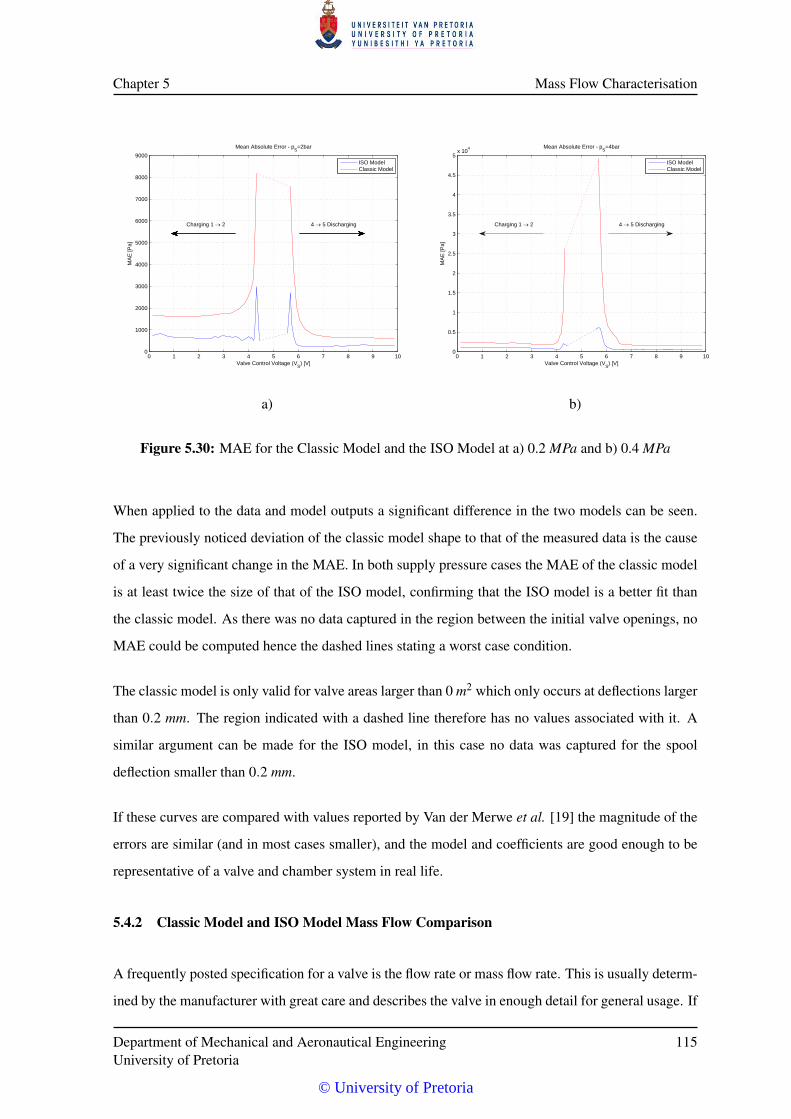
Chapter 5 Mass Flow Characterisation
0 1 2 3 4 5 6 7 8 9 100
1000
2000
3000
4000
5000
6000
7000
8000
9000
4 5 DischargingCharging 1 2
Valve Control Voltage (VS) [V]
MA
E [P
a]
Mean Absolute Error - pS=2bar
ISO ModelClassic Model
0 1 2 3 4 5 6 7 8 9 100
0.5
1
1.5
2
2.5
3
3.5
4
4.5
5x 10
4
4 5 DischargingCharging 1 2
Valve Control Voltage (VS) [V]
MA
E [P
a]
Mean Absolute Error - pS=4bar
ISO ModelClassic Model
a) b)
Figure 5.30: MAE for the Classic Model and the ISO Model at a) 0.2 MPa and b) 0.4 MPa
When applied to the data and model outputs a significant difference in the two models can be seen.
The previously noticed deviation of the classic model shape to that of the measured data is the cause
of a very significant change in the MAE. In both supply pressure cases the MAE of the classic model
is at least twice the size of that of the ISO model, confirming that the ISO model is a better fit than
the classic model. As there was no data captured in the region between the initial valve openings, no
MAE could be computed hence the dashed lines stating a worst case condition.
The classic model is only valid for valve areas larger than 0 m2 which only occurs at deflections larger
than 0.2 mm. The region indicated with a dashed line therefore has no values associated with it. A
similar argument can be made for the ISO model, in this case no data was captured for the spool
deflection smaller than 0.2 mm.
If these curves are compared with values reported by Van der Merwe et al. [19] the magnitude of the
errors are similar (and in most cases smaller), and the model and coefficients are good enough to be
representative of a valve and chamber system in real life.
5.4.2 Classic Model and ISO Model Mass Flow Comparison
A frequently posted specification for a valve is the flow rate or mass flow rate. This is usually determ-
ined by the manufacturer with great care and describes the valve in enough detail for general usage. If
Department of Mechanical and Aeronautical EngineeringUniversity of Pretoria
115
© University of Pretoria
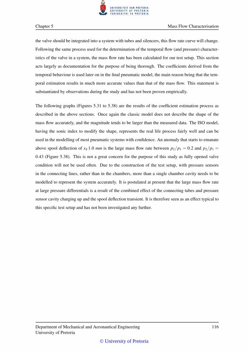
Chapter 5 Mass Flow Characterisation
the valve should be integrated into a system with tubes and silencers, this flow rate curve will change.
Following the same process used for the determination of the temporal flow (and pressure) character-
istics of the valve in a system, the mass flow rate has been calculated for our test setup. This section
acts largely as documentation for the purpose of being thorough. The coefficients derived from the
temporal behaviour is used later on in the final pneumatic model, the main reason being that the tem-
poral estimation results in much more accurate values than that of the mass flow. This statement is
substantiated by observations during the study and has not been proven empirically.
The following graphs (Figures 5.31 to 5.38) are the results of the coefficient estimation process as
described in the above sections. Once again the classic model does not describe the shape of the
mass flow accurately, and the magnitude tends to be larger than the measured data. The ISO model,
having the sonic index to modify the shape, represents the real life process fairly well and can be
used in the modelling of most pneumatic systems with confidence. An anomaly that starts to emanate
above spool deflection of xS 1.0 mm is the large mass flow rate between p2/p1 = 0.2 and p2/p1 =
0.43 (Figure 5.38). This is not a great concern for the purpose of this study as fully opened valve
condition will not be used often. Due to the construction of the test setup, with pressure sensors
in the connecting lines, rather than in the chambers, more than a single chamber cavity needs to be
modelled to represent the system accurately. It is postulated at present that the large mass flow rate
at large pressure differentials is a result of the combined effect of the connecting tubes and pressure
sensor cavity charging up and the spool deflection transient. It is therefore seen as an effect typical to
this specific test setup and has not been investigated any further.
Department of Mechanical and Aeronautical EngineeringUniversity of Pretoria
116
© University of Pretoria
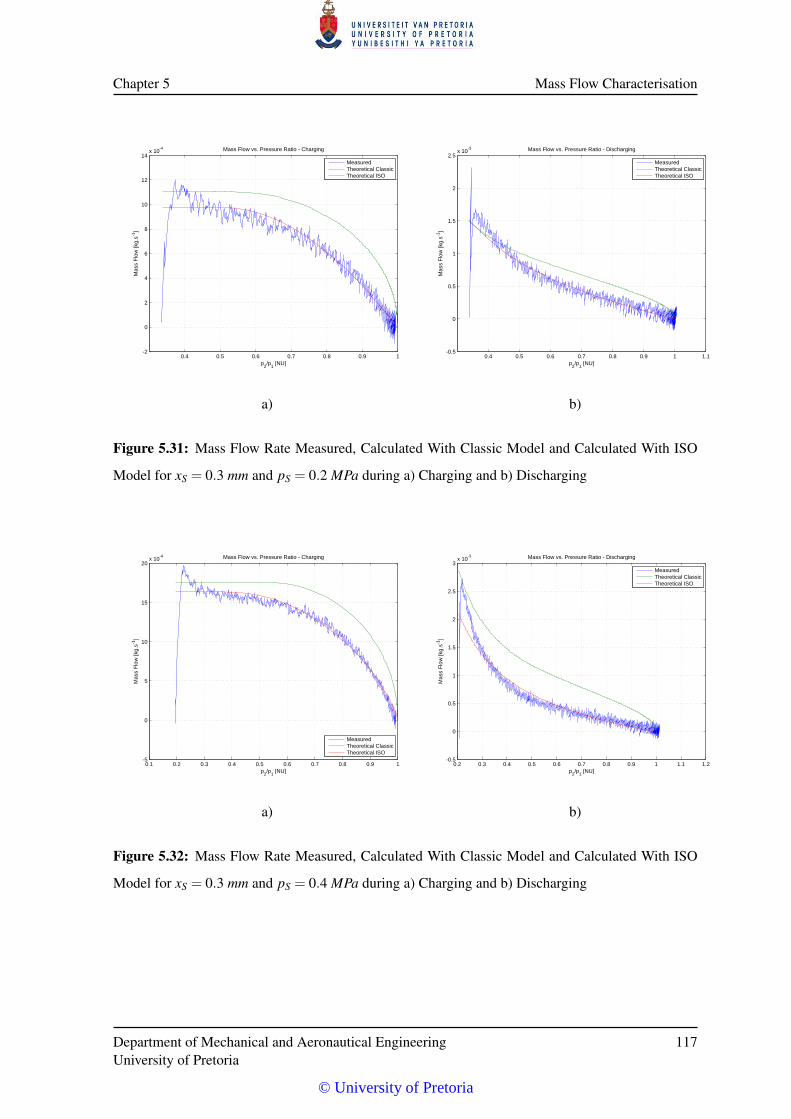
Chapter 5 Mass Flow Characterisation
0.4 0.5 0.6 0.7 0.8 0.9 1-2
0
2
4
6
8
10
12
14x 10
-4 Mass Flow vs. Pressure Ratio - Charging
p2/p
1 [NU]
Mas
s F
low
[kg.
s-1]
MeasuredTheoretical ClassicTheoretical ISO
0.4 0.5 0.6 0.7 0.8 0.9 1 1.1-0.5
0
0.5
1
1.5
2
2.5x 10
-3 Mass Flow vs. Pressure Ratio - Discharging
p2/p
1 [NU]
Mas
s F
low
[kg.
s-1]
MeasuredTheoretical ClassicTheoretical ISO
a) b)
Figure 5.31: Mass Flow Rate Measured, Calculated With Classic Model and Calculated With ISO
Model for xS = 0.3 mm and pS = 0.2 MPa during a) Charging and b) Discharging
0.1 0.2 0.3 0.4 0.5 0.6 0.7 0.8 0.9 1-5
0
5
10
15
20x 10
-4 Mass Flow vs. Pressure Ratio - Charging
p2/p
1 [NU]
Mas
s F
low
[kg.
s-1]
MeasuredTheoretical ClassicTheoretical ISO
0.2 0.3 0.4 0.5 0.6 0.7 0.8 0.9 1 1.1 1.2-0.5
0
0.5
1
1.5
2
2.5
3x 10
-3 Mass Flow vs. Pressure Ratio - Discharging
p2/p
1 [NU]
Mas
s F
low
[kg.
s-1]
MeasuredTheoretical ClassicTheoretical ISO
a) b)
Figure 5.32: Mass Flow Rate Measured, Calculated With Classic Model and Calculated With ISO
Model for xS = 0.3 mm and pS = 0.4 MPa during a) Charging and b) Discharging
Department of Mechanical and Aeronautical EngineeringUniversity of Pretoria
117
© University of Pretoria
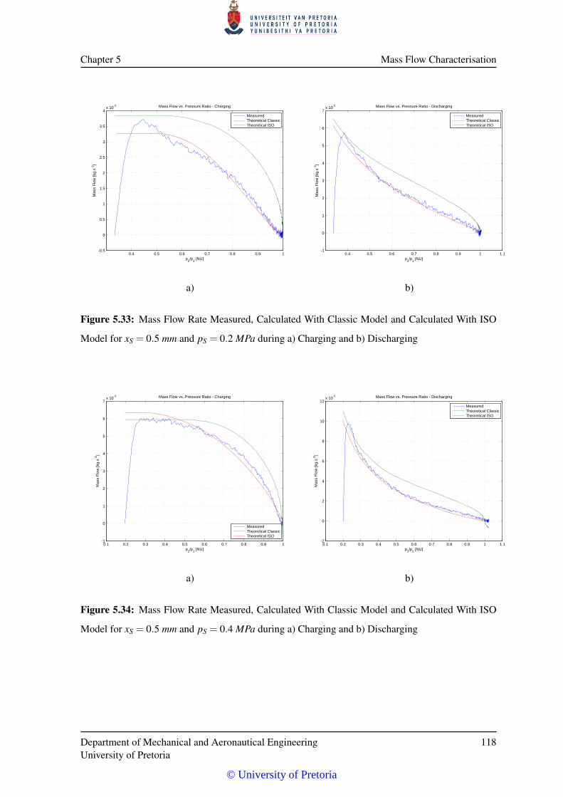
Chapter 5 Mass Flow Characterisation
0.4 0.5 0.6 0.7 0.8 0.9 1-0.5
0
0.5
1
1.5
2
2.5
3
3.5
4x 10
-3 Mass Flow vs. Pressure Ratio - Charging
p2/p
1 [NU]
Mas
s F
low
[kg.
s-1]
MeasuredTheoretical ClassicTheoretical ISO
0.4 0.5 0.6 0.7 0.8 0.9 1 1.1-1
0
1
2
3
4
5
6
7x 10
-3 Mass Flow vs. Pressure Ratio - Discharging
p2/p
1 [NU]
Mas
s F
low
[kg.
s-1]
MeasuredTheoretical ClassicTheoretical ISO
a) b)
Figure 5.33: Mass Flow Rate Measured, Calculated With Classic Model and Calculated With ISO
Model for xS = 0.5 mm and pS = 0.2 MPa during a) Charging and b) Discharging
0.1 0.2 0.3 0.4 0.5 0.6 0.7 0.8 0.9 1-1
0
1
2
3
4
5
6
7x 10
-3 Mass Flow vs. Pressure Ratio - Charging
p2/p
1 [NU]
Mas
s F
low
[kg.
s-1]
MeasuredTheoretical ClassicTheoretical ISO
0.1 0.2 0.3 0.4 0.5 0.6 0.7 0.8 0.9 1 1.1-2
0
2
4
6
8
10
12x 10
-3 Mass Flow vs. Pressure Ratio - Discharging
p2/p
1 [NU]
Mas
s F
low
[kg.
s-1]
MeasuredTheoretical ClassicTheoretical ISO
a) b)
Figure 5.34: Mass Flow Rate Measured, Calculated With Classic Model and Calculated With ISO
Model for xS = 0.5 mm and pS = 0.4 MPa during a) Charging and b) Discharging
Department of Mechanical and Aeronautical EngineeringUniversity of Pretoria
118
© University of Pretoria
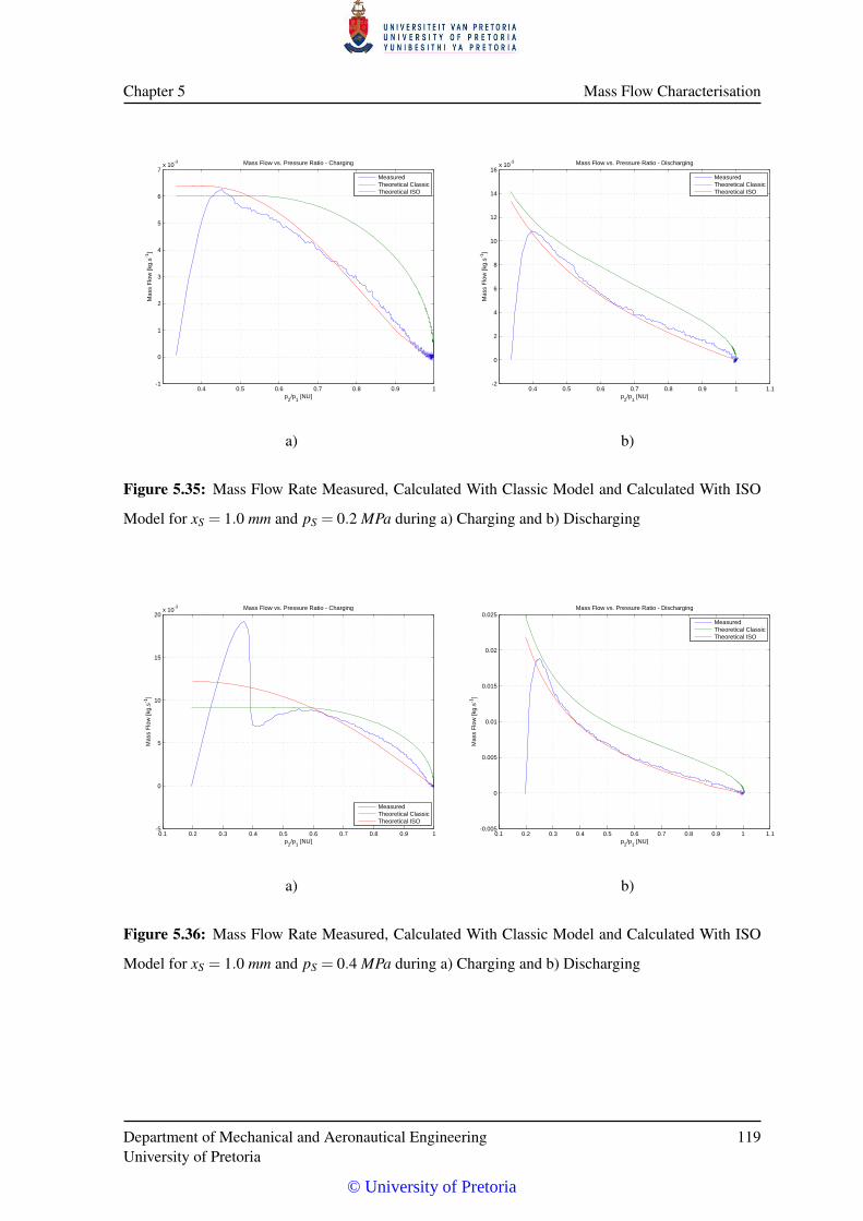
Chapter 5 Mass Flow Characterisation
0.4 0.5 0.6 0.7 0.8 0.9 1-1
0
1
2
3
4
5
6
7x 10
-3 Mass Flow vs. Pressure Ratio - Charging
p2/p
1 [NU]
Mas
s F
low
[kg.
s-1]
MeasuredTheoretical ClassicTheoretical ISO
0.4 0.5 0.6 0.7 0.8 0.9 1 1.1-2
0
2
4
6
8
10
12
14
16x 10
-3 Mass Flow vs. Pressure Ratio - Discharging
p2/p
1 [NU]
Mas
s F
low
[kg.
s-1]
MeasuredTheoretical ClassicTheoretical ISO
a) b)
Figure 5.35: Mass Flow Rate Measured, Calculated With Classic Model and Calculated With ISO
Model for xS = 1.0 mm and pS = 0.2 MPa during a) Charging and b) Discharging
0.1 0.2 0.3 0.4 0.5 0.6 0.7 0.8 0.9 1-5
0
5
10
15
20x 10
-3 Mass Flow vs. Pressure Ratio - Charging
p2/p
1 [NU]
Mas
s F
low
[kg.
s-1]
MeasuredTheoretical ClassicTheoretical ISO
0.1 0.2 0.3 0.4 0.5 0.6 0.7 0.8 0.9 1 1.1-0.005
0
0.005
0.01
0.015
0.02
0.025Mass Flow vs. Pressure Ratio - Discharging
p2/p
1 [NU]
Mas
s F
low
[kg.
s-1]
MeasuredTheoretical ClassicTheoretical ISO
a) b)
Figure 5.36: Mass Flow Rate Measured, Calculated With Classic Model and Calculated With ISO
Model for xS = 1.0 mm and pS = 0.4 MPa during a) Charging and b) Discharging
Department of Mechanical and Aeronautical EngineeringUniversity of Pretoria
119
© University of Pretoria
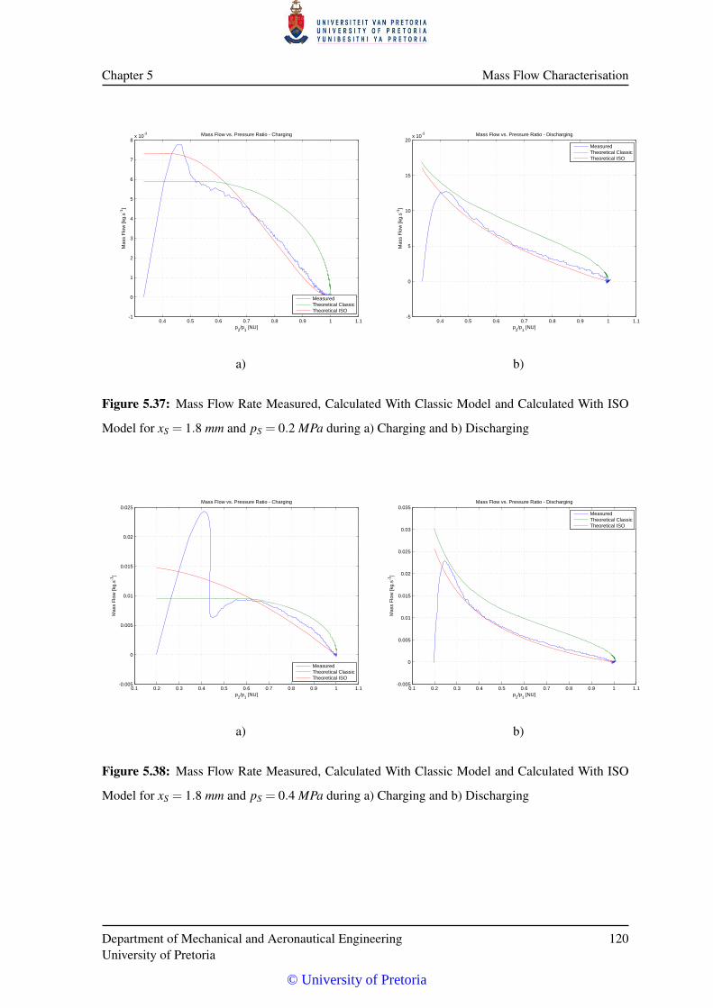
Chapter 5 Mass Flow Characterisation
0.4 0.5 0.6 0.7 0.8 0.9 1 1.1-1
0
1
2
3
4
5
6
7
8x 10
-3 Mass Flow vs. Pressure Ratio - Charging
p2/p
1 [NU]
Mas
s F
low
[kg.
s-1]
MeasuredTheoretical ClassicTheoretical ISO
0.4 0.5 0.6 0.7 0.8 0.9 1 1.1-5
0
5
10
15
20x 10
-3 Mass Flow vs. Pressure Ratio - Discharging
p2/p
1 [NU]
Mas
s F
low
[kg.
s-1]
MeasuredTheoretical ClassicTheoretical ISO
a) b)
Figure 5.37: Mass Flow Rate Measured, Calculated With Classic Model and Calculated With ISO
Model for xS = 1.8 mm and pS = 0.2 MPa during a) Charging and b) Discharging
0.1 0.2 0.3 0.4 0.5 0.6 0.7 0.8 0.9 1 1.1-0.005
0
0.005
0.01
0.015
0.02
0.025Mass Flow vs. Pressure Ratio - Charging
p2/p
1 [NU]
Mas
s F
low
[kg.
s-1]
MeasuredTheoretical ClassicTheoretical ISO
0.1 0.2 0.3 0.4 0.5 0.6 0.7 0.8 0.9 1 1.1-0.005
0
0.005
0.01
0.015
0.02
0.025
0.03
0.035Mass Flow vs. Pressure Ratio - Discharging
p2/p
1 [NU]
Mas
s F
low
[kg.
s-1]
MeasuredTheoretical ClassicTheoretical ISO
a) b)
Figure 5.38: Mass Flow Rate Measured, Calculated With Classic Model and Calculated With ISO
Model for xS = 1.8 mm and pS = 0.4 MPa during a) Charging and b) Discharging
Department of Mechanical and Aeronautical EngineeringUniversity of Pretoria
120
© University of Pretoria
Chapter 5 Mass Flow Characterisation
5.4.3 ISO Model Coefficients
The estimated ISO model coefficients for the FESTO MPYE-5-3/8-010-B proportional directional
control valve connected to a 5` pneumatic reservoir through a 10mm diameter Festo polyurethane
tube are tabulated in Tables 5.1 and 5.2. These coefficients are later used in the analysis of the SMS
pneumatic system.
Department of Mechanical and Aeronautical EngineeringUniversity of Pretoria
121
© University of Pretoria
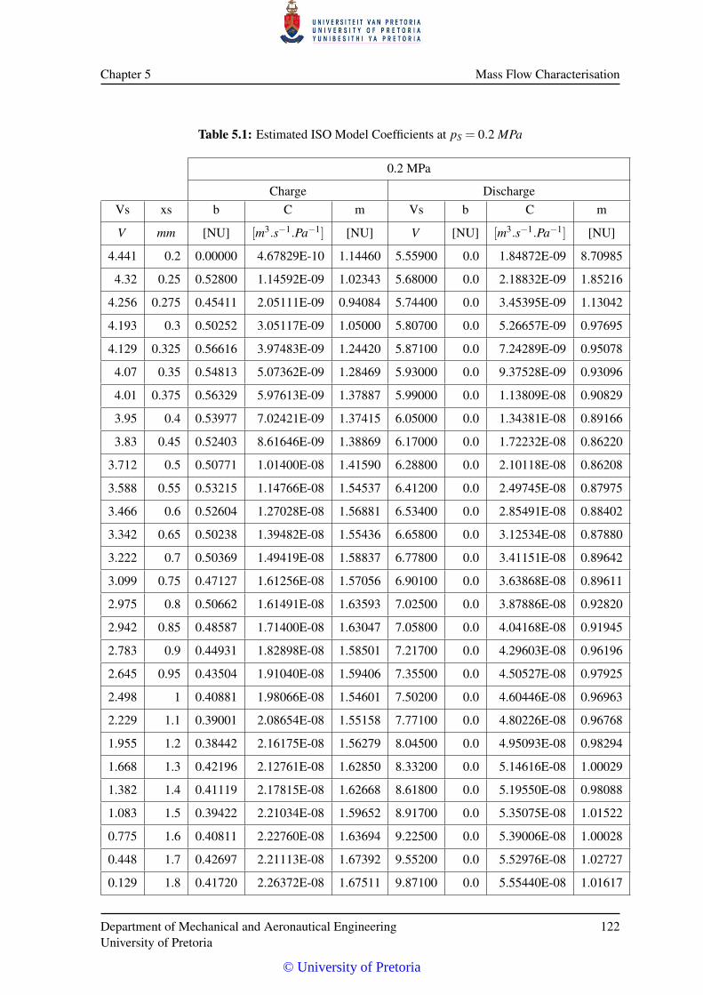
Chapter 5 Mass Flow Characterisation
Table 5.1: Estimated ISO Model Coefficients at pS = 0.2 MPa
0.2 MPa
Charge DischargeVs xs b C m Vs b C m
V mm [NU] [m3.s−1.Pa−1] [NU] V [NU] [m3.s−1.Pa−1] [NU]
4.441 0.2 0.00000 4.67829E-10 1.14460 5.55900 0.0 1.84872E-09 8.70985
4.32 0.25 0.52800 1.14592E-09 1.02343 5.68000 0.0 2.18832E-09 1.85216
4.256 0.275 0.45411 2.05111E-09 0.94084 5.74400 0.0 3.45395E-09 1.13042
4.193 0.3 0.50252 3.05117E-09 1.05000 5.80700 0.0 5.26657E-09 0.97695
4.129 0.325 0.56616 3.97483E-09 1.24420 5.87100 0.0 7.24289E-09 0.95078
4.07 0.35 0.54813 5.07362E-09 1.28469 5.93000 0.0 9.37528E-09 0.93096
4.01 0.375 0.56329 5.97613E-09 1.37887 5.99000 0.0 1.13809E-08 0.90829
3.95 0.4 0.53977 7.02421E-09 1.37415 6.05000 0.0 1.34381E-08 0.89166
3.83 0.45 0.52403 8.61646E-09 1.38869 6.17000 0.0 1.72232E-08 0.86220
3.712 0.5 0.50771 1.01400E-08 1.41590 6.28800 0.0 2.10118E-08 0.86208
3.588 0.55 0.53215 1.14766E-08 1.54537 6.41200 0.0 2.49745E-08 0.87975
3.466 0.6 0.52604 1.27028E-08 1.56881 6.53400 0.0 2.85491E-08 0.88402
3.342 0.65 0.50238 1.39482E-08 1.55436 6.65800 0.0 3.12534E-08 0.87880
3.222 0.7 0.50369 1.49419E-08 1.58837 6.77800 0.0 3.41151E-08 0.89642
3.099 0.75 0.47127 1.61256E-08 1.57056 6.90100 0.0 3.63868E-08 0.89611
2.975 0.8 0.50662 1.61491E-08 1.63593 7.02500 0.0 3.87886E-08 0.92820
2.942 0.85 0.48587 1.71400E-08 1.63047 7.05800 0.0 4.04168E-08 0.91945
2.783 0.9 0.44931 1.82898E-08 1.58501 7.21700 0.0 4.29603E-08 0.96196
2.645 0.95 0.43504 1.91040E-08 1.59406 7.35500 0.0 4.50527E-08 0.97925
2.498 1 0.40881 1.98066E-08 1.54601 7.50200 0.0 4.60446E-08 0.96963
2.229 1.1 0.39001 2.08654E-08 1.55158 7.77100 0.0 4.80226E-08 0.96768
1.955 1.2 0.38442 2.16175E-08 1.56279 8.04500 0.0 4.95093E-08 0.98294
1.668 1.3 0.42196 2.12761E-08 1.62850 8.33200 0.0 5.14616E-08 1.00029
1.382 1.4 0.41119 2.17815E-08 1.62668 8.61800 0.0 5.19550E-08 0.98088
1.083 1.5 0.39422 2.21034E-08 1.59652 8.91700 0.0 5.35075E-08 1.01522
0.775 1.6 0.40811 2.22760E-08 1.63694 9.22500 0.0 5.39006E-08 1.00028
0.448 1.7 0.42697 2.21113E-08 1.67392 9.55200 0.0 5.52976E-08 1.02727
0.129 1.8 0.41720 2.26372E-08 1.67511 9.87100 0.0 5.55440E-08 1.01617
Department of Mechanical and Aeronautical EngineeringUniversity of Pretoria
122
© University of Pretoria
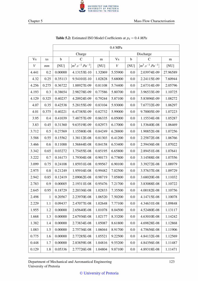
Chapter 5 Mass Flow Characterisation
Table 5.2: Estimated ISO Model Coefficients at pS = 0.4 MPa
0.4 MPa
Charge DischargeVs xs b C m Vs b C m
V mm [NU] [m3.s−1.Pa−1] [NU] V [NU] [m3.s−1.Pa−1] [NU]
4.441 0.2 0.00000 4.13153E-10 1.32069 5.55900 0.0 2.03974E-09 27.96589
4.32 0.25 0.35113 9.54101E-10 1.02828 5.68000 0.0 2.24115E-09 7.60944
4.256 0.275 0.36722 1.88927E-09 0.81108 5.74400 0.0 2.67314E-09 2.05796
4.193 0.3 0.38654 2.98278E-09 0.77586 5.80700 0.0 3.96533E-09 1.10725
4.129 0.325 0.40237 4.20924E-09 0.79244 5.87100 0.0 5.83896E-09 1.08272
4.07 0.35 0.42538 5.28155E-09 0.83104 5.93000 0.0 7.67732E-09 1.06297
4.01 0.375 0.40221 6.47385E-09 0.82732 5.99000 0.0 9.70005E-09 1.07223
3.95 0.4 0.41039 7.48757E-09 0.86335 6.05000 0.0 1.15534E-08 1.05287
3.83 0.45 0.31360 9.63519E-09 0.82973 6.17000 0.0 1.53640E-08 1.06469
3.712 0.5 0.27569 1.15580E-08 0.84249 6.28800 0.0 1.90852E-08 1.07256
3.588 0.55 0.15562 1.38112E-08 0.81303 6.41200 0.0 2.25872E-08 1.06766
3.466 0.6 0.11088 1.56844E-08 0.84158 6.53400 0.0 2.59436E-08 1.07022
3.342 0.65 0.03272 1.75455E-08 0.85195 6.65800 0.0 2.89451E-08 1.07641
3.222 0.7 0.16173 1.79304E-08 0.90173 6.77800 0.0 3.14588E-08 1.07556
3.099 0.75 0.24108 1.85931E-08 0.99567 6.90100 0.0 3.39272E-08 1.08979
2.975 0.8 0.21249 1.95916E-08 0.99482 7.02500 0.0 3.57637E-08 1.09729
2.942 0.85 0.12419 2.09062E-08 0.98719 7.05800 0.0 3.68020E-08 1.11032
2.783 0.9 0.00005 2.19311E-08 0.95476 7.21700 0.0 3.83088E-08 1.10722
2.645 0.95 0.18729 2.20336E-08 1.02833 7.35500 0.0 4.00182E-08 1.10756
2.498 1 0.20567 2.23970E-08 1.06520 7.50200 0.0 4.14715E-08 1.10078
2.229 1.1 0.09437 2.47077E-08 1.02648 7.77100 0.0 4.34631E-08 1.09848
1.955 1.2 0.00000 2.65640E-08 1.01078 8.04500 0.0 4.52480E-08 1.13117
1.668 1.3 0.00000 2.67936E-08 1.02177 8.33200 0.0 4.63010E-08 1.14242
1.382 1.4 0.00000 2.73834E-08 1.05087 8.61800 0.0 4.69828E-08 1.12868
1.083 1.5 0.00000 2.75736E-08 1.06044 8.91700 0.0 4.75656E-08 1.11906
0.775 1.6 0.00000 2.77285E-08 1.05521 9.22500 0.0 4.84132E-08 1.12569
0.448 1.7 0.00000 2.83859E-08 1.04816 9.55200 0.0 4.84356E-08 1.11487
0.129 1.8 0.05336 2.77726E-08 1.04804 9.87100 0.0 4.89318E-08 1.11471
Department of Mechanical and Aeronautical EngineeringUniversity of Pretoria
123
© University of Pretoria
CHAPTER 6
FRICTION IN PNEUMATIC SYSTEMS
The friction model using only the Stribeck effect or only combinations of Coulomb and viscous fric-
tion in general has limitations when used in dynamic systems. These classical models do not describe
hysteresis or varying stiction force, nor do they describe the small movements prior to slipping. In the
pneumatic system under investigation, the deformation of the pneumatic seals could be lumped with
the latter and seen as a pre-sliding elasto-plastic deformation.
Many of the modern friction models are based on the LuGre model [31], which saw the light as a result
of a co-operative effort between the Lund Institute of Technology and the Polytechnic of Grenoble.
The model combines the Dahl model [30] with the Stribeck steady-state behaviour and describes
surfaces as non-uniform on a microscopic level that make contact at a number of asperities. These
contacts act similar to elastic bristles or springs that deform linearly under a tangential force and give
rise to a friction force. No physical movement on the bristle contacts occur at this stage, although the
one surface will move relative to the other. This is also called the pre-sliding regime.
As the force is increased in magnitude a transition regime is entered as some of the bristles will start
to slip and in the case of the LuGre model the behaviour of the friction force is based on the average
behaviour of the bristles. The system then moves into the sliding regime. The LuGre model has been
improved by Swevers et al. to incorporate hysteresis [32]. This is known as the Leeuven model. Other
models such as Dupont et al.’s elasto-plastic models [33] includes a function to minimize drift, and a
computationally effective physically motivated general friction model such as the General Maxwell-
Slip model [34].
These models have been developed over the last 30 years and can accurately represent various friction
systems. As the scope of this study is limited, a detailed model will not be used, but rather one that
© University of Pretoria
Chapter 6 Friction In Pneumatic Systems
will represent more dominant behaviour of the SMS.
We have therefore decided on a point symmetric model with a classic static friction region (FS) with
a very small amount of pre-sliding movement. A constant Coulomb friction component together with
a Stribeck function describes the gross-sliding region of the movement. Experimentation will reveal
if the decreasing velocity curve will follow the increasing velocity curve, in which case the friction
force will be described by
Ff = sgn(v)
[FC +(FS−FC1)e−
∣∣∣ vvS
∣∣∣δ]+σ1v (6.1)
with FC the Coulomb friction component, FS the maximum stiction force, v the linear velocity and δ
the Stribeck exponent. vS is the Stribeck velocity and determines the minima of the Stribeck curve.
The gradient of the friction curve is defined by σ1. The Stribeck curve decreases with an increase in
velocity and is bounded by the static force (FS) and the Coulomb force (FC) as proposed by Armstrong-
Hélouvry [38].
A more general model in which the Coulomb friction and the friction slope for the accelerating and
decelerating parts of the movement can differ was proposed by Nouri [37] and is given by
Ff = α f
sgn(v)
[FC1 +(FS−FC1)e−
∣∣∣ vvS
∣∣∣δ]+σ1v sgn(a) = sgn(ν)
sgn(v)FC2 +σ2v sgn(a) 6= sgn(ν)
(6.2)
where FC1 and σ1 are the Coulomb friction coefficient and viscous friction coefficient for the accel-
erating travel and FC2 and σ2 are the Coulomb friction coefficient and viscous friction coefficient for
the decelerating travel respectively. α f is a function to model the stick-slip behaviour close to the
origin (very low velocities).
6.1 FRICTION IDENTIFICATION TEST SETUP
In order to determine the extent of the contribution of the friction forces in the pneumatic actuators,
an investigation into the magnitude and complexity of the friction was done.
Friction attributes such as the Stribeck coefficients, the viscous and Coulomb friction coefficients and
hysteresis function of pneumatic actuators can be determined in a few ways. One way is to excite
the actuator externally with an instrumented linear exciter (push-pull excitation), thereby accurately
determining the static friction force (Stiction), the Coulomb friction, and the rate dependent viscous
Department of Mechanical and Aeronautical EngineeringUniversity of Pretoria
125
© University of Pretoria
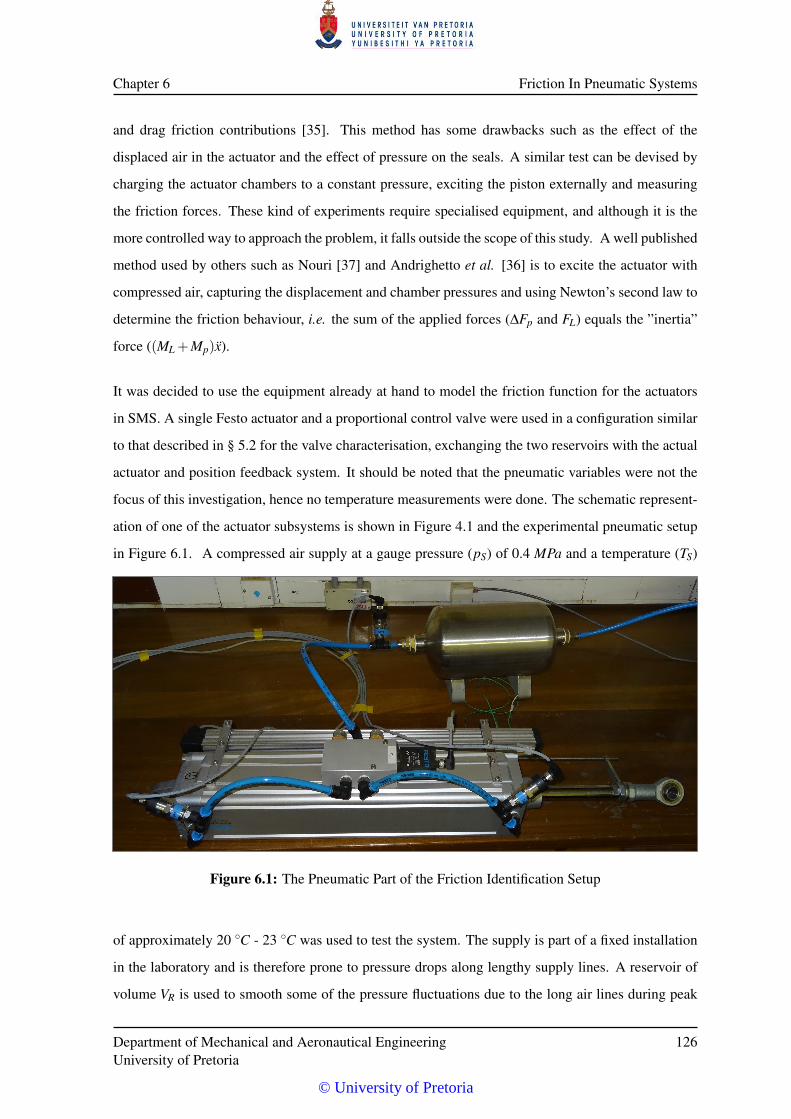
Chapter 6 Friction In Pneumatic Systems
and drag friction contributions [35]. This method has some drawbacks such as the effect of the
displaced air in the actuator and the effect of pressure on the seals. A similar test can be devised by
charging the actuator chambers to a constant pressure, exciting the piston externally and measuring
the friction forces. These kind of experiments require specialised equipment, and although it is the
more controlled way to approach the problem, it falls outside the scope of this study. A well published
method used by others such as Nouri [37] and Andrighetto et al. [36] is to excite the actuator with
compressed air, capturing the displacement and chamber pressures and using Newton’s second law to
determine the friction behaviour, i.e. the sum of the applied forces (∆Fp and FL) equals the ”inertia”
force ((ML +Mp)x).
It was decided to use the equipment already at hand to model the friction function for the actuators
in SMS. A single Festo actuator and a proportional control valve were used in a configuration similar
to that described in § 5.2 for the valve characterisation, exchanging the two reservoirs with the actual
actuator and position feedback system. It should be noted that the pneumatic variables were not the
focus of this investigation, hence no temperature measurements were done. The schematic represent-
ation of one of the actuator subsystems is shown in Figure 4.1 and the experimental pneumatic setup
in Figure 6.1. A compressed air supply at a gauge pressure (pS) of 0.4 MPa and a temperature (TS)
Figure 6.1: The Pneumatic Part of the Friction Identification Setup
of approximately 20 ◦C - 23 ◦C was used to test the system. The supply is part of a fixed installation
in the laboratory and is therefore prone to pressure drops along lengthy supply lines. A reservoir of
volume VR is used to smooth some of the pressure fluctuations due to the long air lines during peak
Department of Mechanical and Aeronautical EngineeringUniversity of Pretoria
126
© University of Pretoria
Chapter 6 Friction In Pneumatic Systems
air demand and delivers compressed air to the valve and actuator at a pressure of pR. The Festo 5/3
proportional control valve is energised by a signal generator Vvs that can vary the frequency, amp-
litude, dead-band compensation and centre offset. The waveform can be adjusted to control the rate
of actuator movement and the actuator acceleration to suit the experiment at hand. Two Festo pressure
sensors convert the instantaneous chamber input pressures (pa and pb) to analogue signals that are
proportional to the guage pressure at the input ports. Due to physical limitations on the actuator, the
pressure sensors had to be mounted on the feed line of the two chambers, and could not be set up to
measure the chamber pressures directly. Pressure errors can be expected at high mass flow rates due
to the transport delay through the pneumatic junctions and ports. Because of this, the mass flow rate
was kept as low as possible and the excitation frequency below 1 Hz.
As the actuator under test had end cushioning, the experimental travel of the actuator was limited
to the centre section of the total actuator travel, staying well clear of the last 50 mm at the ends.
According to the Festo data sheet, the cushioning length is 32 mm, in which region area and flow
characteristics are unknown, and the calculation of the friction can become erroneous.
The actuator is used in a horizontal orientation, driving only the linear displacement sensor wiper
through the connecting rod. It is operated without any load in the direction of the movement, i.e.
FL = 0. The moving mass (Mp) in the actuator consists of the piston, the piston rod, the rod eye with
its locking nuts, the displacement sensor connecting rod and its fastening plate, and the displacement
sensor wiper block. The friction and the mass of the wiper block has been assumed to be negligible.
The masses of these components are tabulated in Table 6.1 and when added up equals approximately
3.64 kg. The piston diameter is 100 mm and the piston rod diameter 25 mm.
The subsystem is connected to a Data Translation DT9803 ADC by which the time domain signals can
be captured. A sampling rate of 1 kS.s−1 is used to ensure resolution of fast transients of the pressure
signals. Signals measured in these experiments are the supply pressure (pS), the valve excitation
voltage (Vvs), the chamber pressures (pa and pb) and the linear resistive displacement sensor voltage
(Vx) translated to displacement (x).
Department of Mechanical and Aeronautical EngineeringUniversity of Pretoria
127
© University of Pretoria
Chapter 6 Friction In Pneumatic Systems
Table 6.1: Theoretical Mass Of The Moving Components
Component Mass [kg]
Piston and Rod 3.064
Rod Eye and Nut 0.432
Connecting Hardware 0.143
3.639
6.2 FRICTION IDENTIFICATION PROCEDURE
Referring to the setup described in § 6.1, Newton’s second law can be written in terms of the applied
and net forces on the piston as
(ML +Mp)x = Fa−Fb−Fr−FL−Ff (6.3)
where Fa is the pneumatic force on the lower face of the piston, Fb is the pneumatic force on the
top surface of the piston, and Fr is the force due to the ambient air pressure on the rod; all in N. FL
represents the load and is assumed to be equal to zero. The friction force counteracting the piston
movement is denoted by Ff and will be expressed as a complex non-linear function which is depend-
ent on the piston position (x), the piston rate (x), the piston acceleration (x), the chamber pressures
(pa and pb [37]), and the state of lubrication, amongst others. The dynamic force due to the mass of
the piston balances the equation when the load is removed (ML = 0). The force terms can further be
expressed as
Mpx = paAa− (pbAb + pAAr)−Ff (6.4)
where pa and pb are the instantaneous chamber pressures in Pa, Aa and Ab are the two piston areas
respectively in m2, pA is the ambient pressure in Pa, and Ar is the rod area in m2.
As described in § 6.1, the signals derived from the setup are captured with a Data Translation DT9803
ADC, transformed into comma delimited text data with the Data Translation ”QuickDAQ 2013” soft-
ware and imported into Matlab®. As the data acquisition process and the sensors are the same as that
used in the valve characterisation process (§ 5.3.1) the kurtosis and skewness can be assumed to be
the same as in that experiment. The noise component of the signals can therefore be assumed to be
white Gaussian noise with a zero mean, a Gaussian probability distribution and a noise spectral dens-
Department of Mechanical and Aeronautical EngineeringUniversity of Pretoria
128
© University of Pretoria
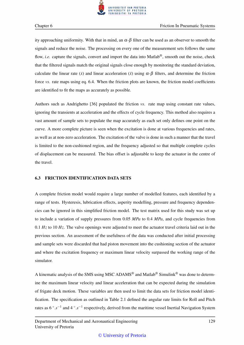
Chapter 6 Friction In Pneumatic Systems
ity approaching uniformity. With that in mind, an α-β filter can be used as an observer to smooth the
signals and reduce the noise. The processing on every one of the measurement sets follows the same
flow, i.e. capture the signals, convert and import the data into Matlab®, smooth out the noise, check
that the filtered signals match the original signals close enough by monitoring the standard deviation,
calculate the linear rate (x) and linear acceleration (x) using α-β filters, and determine the friction
force vs. rate maps using eq. 6.4. When the friction plots are known, the friction model coefficients
are identified to fit the maps as accurately as possible.
Authors such as Andrighetto [36] populated the friction vs. rate map using constant rate values,
ignoring the transients at acceleration and the effects of cycle frequency. This method also requires a
vast amount of sample sets to populate the map accurately as each set only defines one point on the
curve. A more complete picture is seen when the excitation is done at various frequencies and rates,
as well as at non-zero acceleration. The excitation of the valve is done in such a manner that the travel
is limited to the non-cushioned region, and the frequency adjusted so that multiple complete cycles
of displacement can be measured. The bias offset is adjustable to keep the actuator in the centre of
the travel.
6.3 FRICTION IDENTIFICATION DATA SETS
A complete friction model would require a large number of modelled features, each identified by a
range of tests. Hysteresis, lubrication effects, asperity modelling, pressure and frequency dependen-
cies can be ignored in this simplified friction model. The test matrix used for this study was set up
to include a variation of supply pressures from 0.05 MPa to 0.4 MPa, and cycle frequencies from
0.1 Hz to 10 Hz. The valve openings were adjusted to meet the actuator travel criteria laid out in the
previous section. An assessment of the usefulness of the data was conducted after initial processing
and sample sets were discarded that had piston movement into the cushioning section of the actuator
and where the excitation frequency or maximum linear velocity surpassed the working range of the
simulator.
A kinematic analysis of the SMS using MSC ADAMS® and Matlab® Simulink® was done to determ-
ine the maximum linear velocity and linear acceleration that can be expected during the simulation
of frigate deck motion. These variables are then used to limit the data sets for friction model identi-
fication. The specification as outlined in Table 2.1 defined the angular rate limits for Roll and Pitch
rates as 6 ◦.s−1 and 4 ◦.s−1 respectively, derived from the maritime vessel Inertial Navigation System
Department of Mechanical and Aeronautical EngineeringUniversity of Pretoria
129
© University of Pretoria
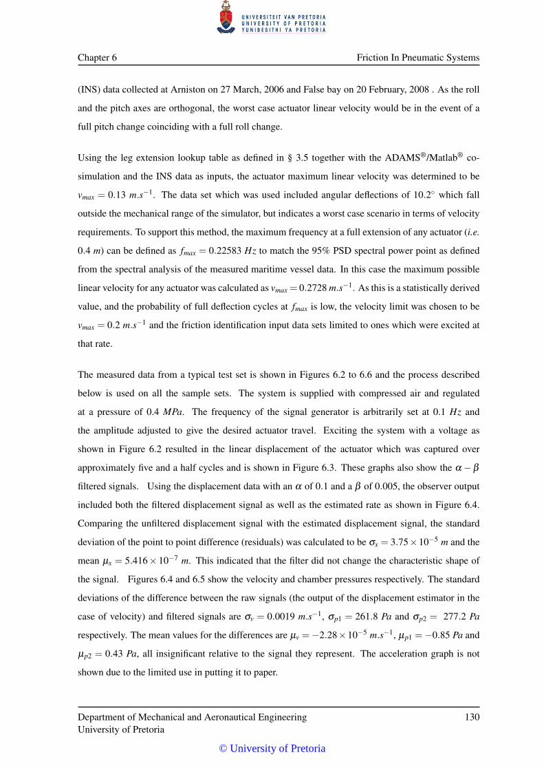
Chapter 6 Friction In Pneumatic Systems
(INS) data collected at Arniston on 27 March, 2006 and False bay on 20 February, 2008 . As the roll
and the pitch axes are orthogonal, the worst case actuator linear velocity would be in the event of a
full pitch change coinciding with a full roll change.
Using the leg extension lookup table as defined in § 3.5 together with the ADAMS®/Matlab® co-
simulation and the INS data as inputs, the actuator maximum linear velocity was determined to be
vmax = 0.13 m.s−1. The data set which was used included angular deflections of 10.2◦ which fall
outside the mechanical range of the simulator, but indicates a worst case scenario in terms of velocity
requirements. To support this method, the maximum frequency at a full extension of any actuator (i.e.
0.4 m) can be defined as fmax = 0.22583 Hz to match the 95% PSD spectral power point as defined
from the spectral analysis of the measured maritime vessel data. In this case the maximum possible
linear velocity for any actuator was calculated as vmax = 0.2728 m.s−1. As this is a statistically derived
value, and the probability of full deflection cycles at fmax is low, the velocity limit was chosen to be
vmax = 0.2 m.s−1 and the friction identification input data sets limited to ones which were excited at
that rate.
The measured data from a typical test set is shown in Figures 6.2 to 6.6 and the process described
below is used on all the sample sets. The system is supplied with compressed air and regulated
at a pressure of 0.4 MPa. The frequency of the signal generator is arbitrarily set at 0.1 Hz and
the amplitude adjusted to give the desired actuator travel. Exciting the system with a voltage as
shown in Figure 6.2 resulted in the linear displacement of the actuator which was captured over
approximately five and a half cycles and is shown in Figure 6.3. These graphs also show the α −β
filtered signals. Using the displacement data with an α of 0.1 and a β of 0.005, the observer output
included both the filtered displacement signal as well as the estimated rate as shown in Figure 6.4.
Comparing the unfiltered displacement signal with the estimated displacement signal, the standard
deviation of the point to point difference (residuals) was calculated to be σx = 3.75×10⁻⁵ m and the
mean µx = 5.416× 10⁻⁷ m. This indicated that the filter did not change the characteristic shape of
the signal. Figures 6.4 and 6.5 show the velocity and chamber pressures respectively. The standard
deviations of the difference between the raw signals (the output of the displacement estimator in the
case of velocity) and filtered signals are σv = 0.0019 m.s−1, σp1 = 261.8 Pa and σp2 = 277.2 Pa
respectively. The mean values for the differences are µv =−2.28×10⁻⁵ m.s−1, µp1 =−0.85 Pa and
µp2 = 0.43 Pa, all insignificant relative to the signal they represent. The acceleration graph is not
shown due to the limited use in putting it to paper.
Department of Mechanical and Aeronautical EngineeringUniversity of Pretoria
130
© University of Pretoria
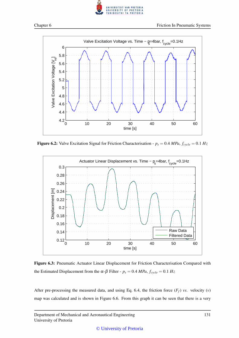
Chapter 6 Friction In Pneumatic Systems
0 10 20 30 40 50 604.2
4.4
4.6
4.8
5
5.2
5.4
5.6
5.8
6
Valve Excitation Voltage vs. Time − ps=4bar, f
cycle=0.1Hz
time [s]
Val
ve E
xcita
tion
Vol
tage
[Vvs
]
Figure 6.2: Valve Excitation Signal for Friction Characterisation - ps = 0.4 MPa, fcycle = 0.1 Hz
0 10 20 30 40 50 600.12
0.14
0.16
0.18
0.2
0.22
0.24
0.26
0.28
0.3
Actuator Linear Displacement vs. Time − ps=4bar, f
cycle=0.1Hz
time [s]
Dis
plac
emen
t [m
]
Raw DataFiltered Data
Figure 6.3: Pneumatic Actuator Linear Displacement for Friction Characterisation Compared with
the Estimated Displacement from the α-β Filter - ps = 0.4 MPa, fcycle = 0.1 Hz
After pre-processing the measured data, and using Eq. 6.4, the friction force (Ff ) vs. velocity (v)
map was calculated and is shown in Figure 6.6. From this graph it can be seen that there is a very
Department of Mechanical and Aeronautical EngineeringUniversity of Pretoria
131
© University of Pretoria
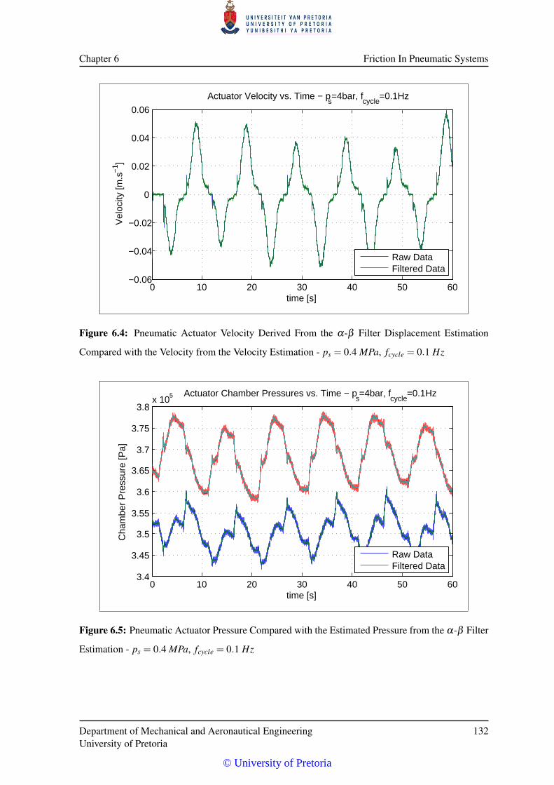
Chapter 6 Friction In Pneumatic Systems
0 10 20 30 40 50 60−0.06
−0.04
−0.02
0
0.02
0.04
0.06
Actuator Velocity vs. Time − ps=4bar, f
cycle=0.1Hz
time [s]
Vel
ocity
[m.s
−1 ]
Raw DataFiltered Data
Figure 6.4: Pneumatic Actuator Velocity Derived From the α-β Filter Displacement Estimation
Compared with the Velocity from the Velocity Estimation - ps = 0.4 MPa, fcycle = 0.1 Hz
0 10 20 30 40 50 603.4
3.45
3.5
3.55
3.6
3.65
3.7
3.75
3.8x 10⁵ Actuator Chamber Pressures vs. Time − p
s=4bar, f
cycle=0.1Hz
time [s]
Cha
mbe
r P
ress
ure
[Pa]
Raw DataFiltered Data
Figure 6.5: Pneumatic Actuator Pressure Compared with the Estimated Pressure from the α-β Filter
Estimation - ps = 0.4 MPa, fcycle = 0.1 Hz
Department of Mechanical and Aeronautical EngineeringUniversity of Pretoria
132
© University of Pretoria
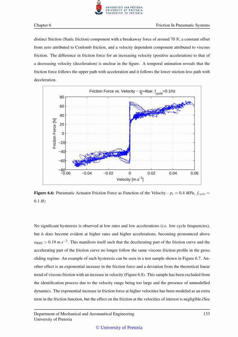
Chapter 6 Friction In Pneumatic Systems
distinct Stiction (Static friction) component with a breakaway force of around 70 N, a constant offset
from zero attributed to Coulomb friction, and a velocity dependent component attributed to viscous
friction. The difference in friction force for an increasing velocity (positive acceleration) to that of
a decreasing velocity (deceleration) is unclear in the figure. A temporal animation reveals that the
friction force follows the upper path with acceleration and it follows the lower stiction-less path with
deceleration.
−0.06 −0.04 −0.02 0 0.02 0.04 0.06−80
−60
−40
−20
0
20
40
60
80
Friction Force vs. Velocity − ps=4bar, f
cycle=0.1Hz
Velocity [m.s−1]
Fric
tion
For
ce [N
]
Figure 6.6: Pneumatic Actuator Friction Force as Function of the Velocity - ps = 0.4 MPa, fcycle =
0.1 Hz
No significant hysteresis is observed at low rates and low accelerations (i.e. low cycle frequencies),
but it does become evident at higher rates and higher accelerations, becoming pronounced above
aRMS > 0.19 m.s−2. This manifests itself such that the decelerating part of the friction curve and the
accelerating part of the friction curve no longer follow the same viscous friction profile in the gross
sliding regime. An example of such hysteresis can be seen in a test sample shown in Figure 6.7. An-
other effect is an exponential increase in the friction force and a deviation from the theoretical linear
trend of viscous friction with an increase in velocity (Figure 6.8). This sample has been excluded from
the identification process due to the velocity range being too large and the presence of unmodelled
dynamics. The exponential increase in friction force at higher velocities has been modeled as an extra
term in the friction function, but the effect on the friction at the velocities of interest is negligible.(See
Department of Mechanical and Aeronautical EngineeringUniversity of Pretoria
133
© University of Pretoria
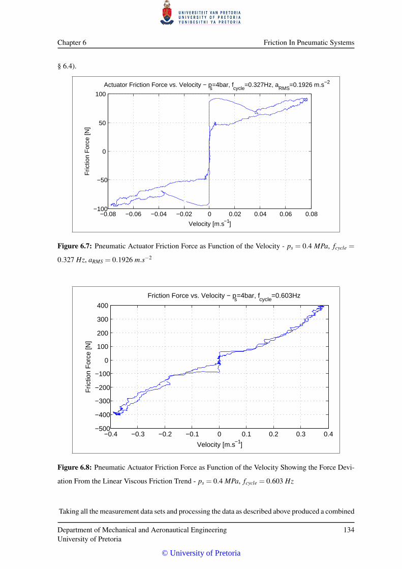
Chapter 6 Friction In Pneumatic Systems
§ 6.4).
−0.08 −0.06 −0.04 −0.02 0 0.02 0.04 0.06 0.08−100
−50
0
50
100
Actuator Friction Force vs. Velocity − ps=4bar, f
cycle=0.327Hz, a
RMS=0.1926 m.s−2
Velocity [m.s−1]
Fric
tion
For
ce [N
]
Figure 6.7: Pneumatic Actuator Friction Force as Function of the Velocity - ps = 0.4 MPa, fcycle =
0.327 Hz, aRMS = 0.1926 m.s−2
−0.4 −0.3 −0.2 −0.1 0 0.1 0.2 0.3 0.4−500
−400
−300
−200
−100
0
100
200
300
400
Friction Force vs. Velocity − ps=4bar, f
cycle=0.603Hz
Velocity [m.s−1]
Fric
tion
For
ce [N
]
Figure 6.8: Pneumatic Actuator Friction Force as Function of the Velocity Showing the Force Devi-
ation From the Linear Viscous Friction Trend - ps = 0.4 MPa, fcycle = 0.603 Hz
Taking all the measurement data sets and processing the data as described above produced a combined
Department of Mechanical and Aeronautical EngineeringUniversity of Pretoria
134
© University of Pretoria
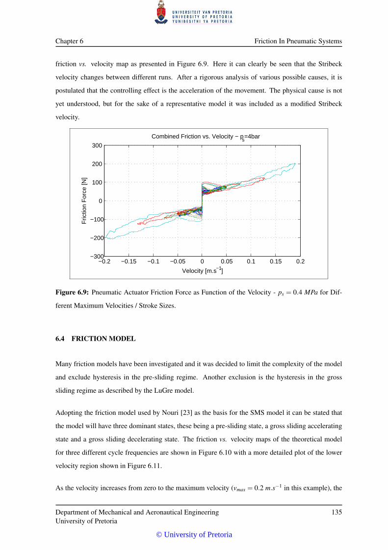
Chapter 6 Friction In Pneumatic Systems
friction vs. velocity map as presented in Figure 6.9. Here it can clearly be seen that the Stribeck
velocity changes between different runs. After a rigorous analysis of various possible causes, it is
postulated that the controlling effect is the acceleration of the movement. The physical cause is not
yet understood, but for the sake of a representative model it was included as a modified Stribeck
velocity.
−0.2 −0.15 −0.1 −0.05 0 0.05 0.1 0.15 0.2−300
−200
−100
0
100
200
300
Combined Friction vs. Velocity − ps=4bar
Velocity [m.s−1]
Fric
tion
For
ce [N
]
Figure 6.9: Pneumatic Actuator Friction Force as Function of the Velocity - ps = 0.4 MPa for Dif-
ferent Maximum Velocities / Stroke Sizes.
6.4 FRICTION MODEL
Many friction models have been investigated and it was decided to limit the complexity of the model
and exclude hysteresis in the pre-sliding regime. Another exclusion is the hysteresis in the gross
sliding regime as described by the LuGre model.
Adopting the friction model used by Nouri [23] as the basis for the SMS model it can be stated that
the model will have three dominant states, these being a pre-sliding state, a gross sliding accelerating
state and a gross sliding decelerating state. The friction vs. velocity maps of the theoretical model
for three different cycle frequencies are shown in Figure 6.10 with a more detailed plot of the lower
velocity region shown in Figure 6.11.
As the velocity increases from zero to the maximum velocity (vmax = 0.2 m.s−1 in this example), the
Department of Mechanical and Aeronautical EngineeringUniversity of Pretoria
135
© University of Pretoria
Chapter 6 Friction In Pneumatic Systems
friction force initially increases to a large value according to the stiction force. The modern friction
models use the concept of an average asperity contact deflection that is initially elastic in nature,
gradually starts slipping (a smooth transient - a combination of elastic and plastic slippage) and enter
the gross sliding regime which is in theory purely plastic in nature.
In the SMS model the initial pre-sliding regime is simplified to a smooth transient between two
stiction limits (ε f , see Figures 6.10 to 6.12) that reach a peak of FS. The friction function follows
the top of the curve for increasing velocity and the bottom curve for decreasing velocity. Below
the stiction limit (ε f ) the curve will transition back to a friction force of zero at zero velocity. The
function is point symmetrical (or an ”odd function”) and the reverse will occur during the negative
velocity cycle. At the end of the transient region the friction decreases with an increase in velocity
which is described by the Stribeck function. Acceleration dependent friction together with the linear
viscous friction component (FV ) and the constant Coulomb friction component (FC1) give the curve
its characteristic form. In its pure form, the friction function will be asymptotic to a line crossing
the y-axis at FC1 and a gradient of σ1. A similar line can be constructed for the decreasing velocity
crossing the y-axis at FC2 and having a gradient of σ2.
From some of the experiments, a deviation from the pure linear form was observed, forcing the model
to include an exponential term to account for the deviation. The offset (∆F f ) from the linear curve
is attributed to unmodelled effects, the cause of which cannot be explained at present, but makes
the model more representative. At low velocities the exponential term has very little effect, but
becomes prominent at higher velocities. The SMS operating velocities fall outside the exponential
region.
Detailed plots close to the origin are shown in Figures 6.11 and 6.12 (Note that the three curves in
this plot are identical in the pre-sliding region and are congruent).
The friction model is then described by a direction determined point symmetric function Ff described
by
Ff = α f
sgn(v)
[FC1 +(FS−FC1)e
−(∣∣∣ v
aζ vS
∣∣∣δ)+FUE
(e(γ f |v|)−1
)]+σ1v sgn(a) = sgn(v)
sgn(v)[FC2 +FUE
(e(γ f |v|)−1
)]+σ2v sgn(a) 6= sgn(v)
(6.5)
with FC1 and FC2 the Coulomb friction (in N) y-intercepts respectively, FS the maximum Stiction force
(in N), v the linear velocity in m.s−1, a the linear acceleration in m.s−2 and δ the Stribeck exponent.
Department of Mechanical and Aeronautical EngineeringUniversity of Pretoria
136
© University of Pretoria
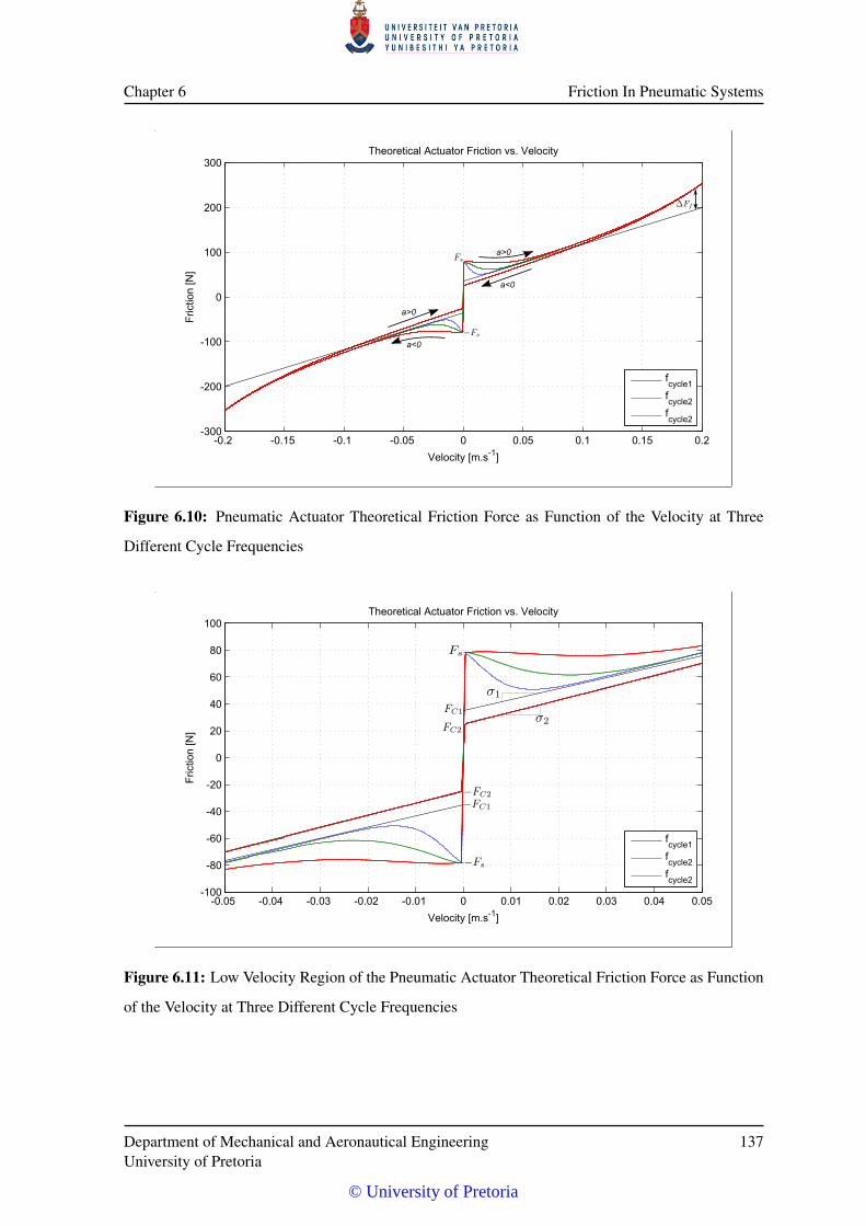
Chapter 6 Friction In Pneumatic Systems
-0.2 -0.15 -0.1 -0.05 0 0.05 0.1 0.15 0.2-300
-200
-100
0
100
200
300Theoretical Actuator Friction vs. Velocity
Velocity [m.s-1]
Fric
tion
[N]
fcycle1
fcycle2
fcycle2
a>0
a<0
a>0
a<0
Figure 6.10: Pneumatic Actuator Theoretical Friction Force as Function of the Velocity at Three
Different Cycle Frequencies
-0.05 -0.04 -0.03 -0.02 -0.01 0 0.01 0.02 0.03 0.04 0.05-100
-80
-60
-40
-20
0
20
40
60
80
100Theoretical]Actuator]Friction]vs.]Velocity
Velocity][m.s-1]
Fric
tion]
[N]
fcycle1
fcycle2
fcycle2
Figure 6.11: Low Velocity Region of the Pneumatic Actuator Theoretical Friction Force as Function
of the Velocity at Three Different Cycle Frequencies
Department of Mechanical and Aeronautical EngineeringUniversity of Pretoria
137
© University of Pretoria
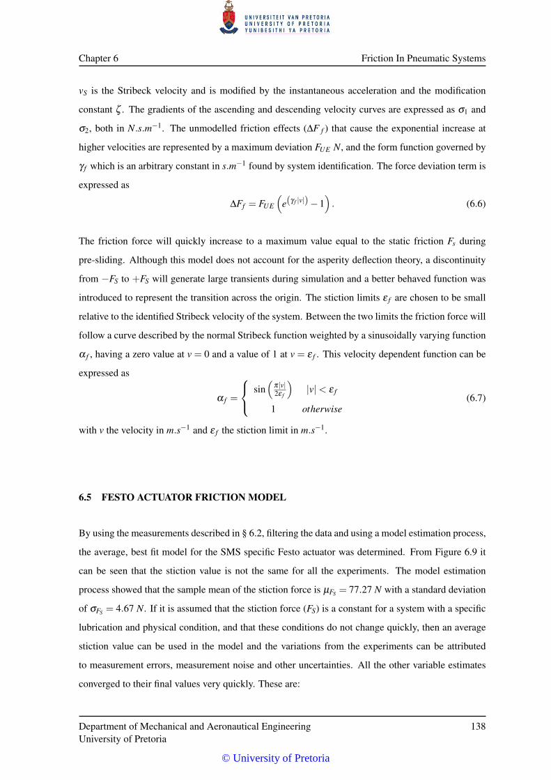
Chapter 6 Friction In Pneumatic Systems
vS is the Stribeck velocity and is modified by the instantaneous acceleration and the modification
constant ζ . The gradients of the ascending and descending velocity curves are expressed as σ1 and
σ2, both in N.s.m−1. The unmodelled friction effects (∆F f ) that cause the exponential increase at
higher velocities are represented by a maximum deviation FUE N, and the form function governed by
γ f which is an arbitrary constant in s.m−1 found by system identification. The force deviation term is
expressed as
∆Ff = FUE
(e(γ f |v|)−1
). (6.6)
The friction force will quickly increase to a maximum value equal to the static friction Fs during
pre-sliding. Although this model does not account for the asperity deflection theory, a discontinuity
from −FS to +FS will generate large transients during simulation and a better behaved function was
introduced to represent the transition across the origin. The stiction limits ε f are chosen to be small
relative to the identified Stribeck velocity of the system. Between the two limits the friction force will
follow a curve described by the normal Stribeck function weighted by a sinusoidally varying function
α f , having a zero value at v = 0 and a value of 1 at v = ε f . This velocity dependent function can be
expressed as
α f =
sin(
π|v|2ε f
)|v|< ε f
1 otherwise(6.7)
with v the velocity in m.s−1 and ε f the stiction limit in m.s−1.
6.5 FESTO ACTUATOR FRICTION MODEL
By using the measurements described in § 6.2, filtering the data and using a model estimation process,
the average, best fit model for the SMS specific Festo actuator was determined. From Figure 6.9 it
can be seen that the stiction value is not the same for all the experiments. The model estimation
process showed that the sample mean of the stiction force is µFS = 77.27 N with a standard deviation
of σFS = 4.67 N. If it is assumed that the stiction force (FS) is a constant for a system with a specific
lubrication and physical condition, and that these conditions do not change quickly, then an average
stiction value can be used in the model and the variations from the experiments can be attributed
to measurement errors, measurement noise and other uncertainties. All the other variable estimates
converged to their final values very quickly. These are:
Department of Mechanical and Aeronautical EngineeringUniversity of Pretoria
138
© University of Pretoria
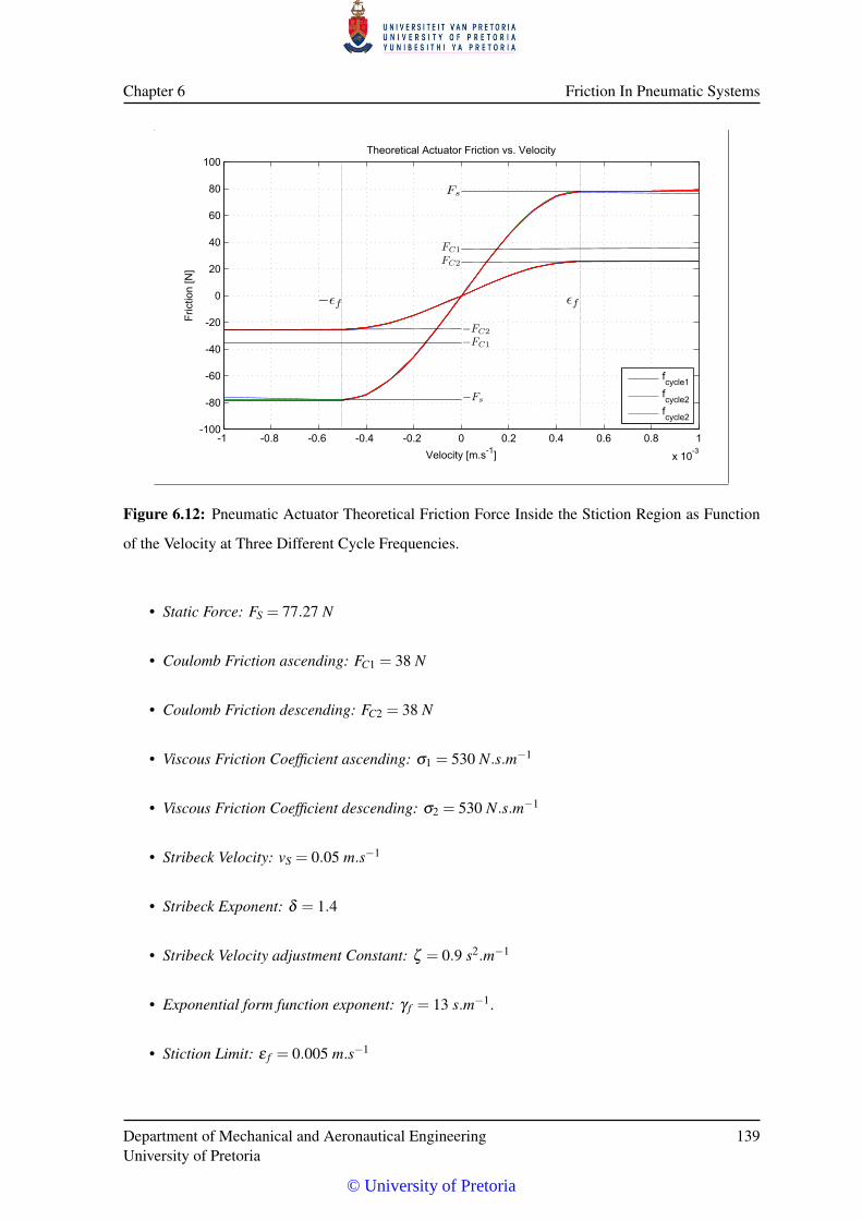
Chapter 6 Friction In Pneumatic Systems
-1 -0.8 -0.6 -0.4 -0.2 0 0.2 0.4 0.6 0.8 1
x]10-3
-100
-80
-60
-40
-20
0
20
40
60
80
100Theoretical]Actuator]Friction]vs.]Velocity
Velocity][m.s-1]
Fric
tion]
[N]
fcycle1
fcycle2
fcycle2
Figure 6.12: Pneumatic Actuator Theoretical Friction Force Inside the Stiction Region as Function
of the Velocity at Three Different Cycle Frequencies.
• Static Force: FS = 77.27 N
• Coulomb Friction ascending: FC1 = 38 N
• Coulomb Friction descending: FC2 = 38 N
• Viscous Friction Coefficient ascending: σ1 = 530 N.s.m−1
• Viscous Friction Coefficient descending: σ2 = 530 N.s.m−1
• Stribeck Velocity: vS = 0.05 m.s−1
• Stribeck Exponent: δ = 1.4
• Stribeck Velocity adjustment Constant: ζ = 0.9 s2.m−1
• Exponential form function exponent: γ f = 13 s.m−1.
• Stiction Limit: ε f = 0.005 m.s−1
Department of Mechanical and Aeronautical EngineeringUniversity of Pretoria
139
© University of Pretoria
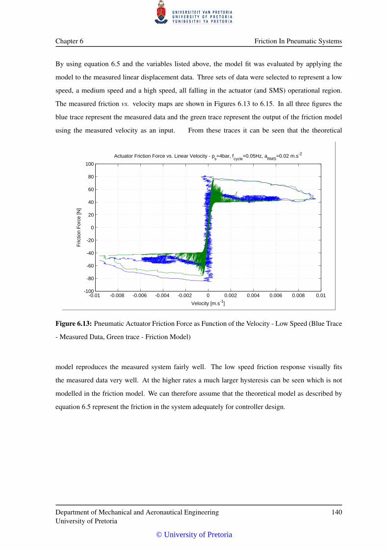
Chapter 6 Friction In Pneumatic Systems
By using equation 6.5 and the variables listed above, the model fit was evaluated by applying the
model to the measured linear displacement data. Three sets of data were selected to represent a low
speed, a medium speed and a high speed, all falling in the actuator (and SMS) operational region.
The measured friction vs. velocity maps are shown in Figures 6.13 to 6.15. In all three figures the
blue trace represent the measured data and the green trace represent the output of the friction model
using the measured velocity as an input. From these traces it can be seen that the theoretical
-0.01 -0.008 -0.006 -0.004 -0.002 0 0.002 0.004 0.006 0.008 0.01-100
-80
-60
-40
-20
0
20
40
60
80
100
Actuator Friction Force vs. Linear Velocity - ps=4bar, f
cycle=0.05Hz, a
RMS=0.02 m.s-2
Velocity [m.s-1]
Fric
tion
For
ce [N
]
Figure 6.13: Pneumatic Actuator Friction Force as Function of the Velocity - Low Speed (Blue Trace
- Measured Data, Green trace - Friction Model)
model reproduces the measured system fairly well. The low speed friction response visually fits
the measured data very well. At the higher rates a much larger hysteresis can be seen which is not
modelled in the friction model. We can therefore assume that the theoretical model as described by
equation 6.5 represent the friction in the system adequately for controller design.
Department of Mechanical and Aeronautical EngineeringUniversity of Pretoria
140
© University of Pretoria

Chapter 6 Friction In Pneumatic Systems
-0.05 -0.04 -0.03 -0.02 -0.01 0 0.01 0.02 0.03 0.04-100
-80
-60
-40
-20
0
20
40
60
80
Actuator Friction Force vs. Linear Velocity - ps=4bar, f
cycle=0.04Hz, a
RMS=0.0263 m.s-2
Velocity [m.s-1]
Fric
tion
For
ce [N
]
Figure 6.14: Pneumatic Actuator Friction Force as Function of the Velocity - Medium Speed (Blue
Trace - Measured Data, Green trace - Friction Model)
-0.2 -0.15 -0.1 -0.05 0 0.05 0.1 0.15 0.2-250
-200
-150
-100
-50
0
50
100
150
200
250
Actuator Friction Force vs. Linear Velocity - ps=4bar, f
cycle=0.05Hz, a
RMS=0.3461 m.s-2
Velocity [m.s-1]
Fric
tion
For
ce [N
]
Figure 6.15: Pneumatic Actuator Friction Force as Function of the Velocity - High Speed (Blue Trace
- Measured Data, Green trace - Friction Model)
Department of Mechanical and Aeronautical EngineeringUniversity of Pretoria
141
© University of Pretoria
CHAPTER 7
SIMULATION MODEL VALIDATION
The pneumatic system model, the kinematic and dynamic model in ADAMS®, and the friction model
developed in the previous stages of the study have to be validated to ensure a reliable rendition of
reality. As the system model complexity increases, and lower level models are combined into a larger
higher level model and the effects of unmodelled phenomena accumulate. The specific contribution
of those effects on the results become unclear making the validation process difficult and fault finding
impossible.
A Matlab® Simulink® simulation of one of the actuators was compiled and various scenarios ex-
ecuted to assess the reliability of the models. These scenarios were similar to the actuator friction
identification process, chosen to fall within the operational domain of the SMS. The same exper-
imental configuration used for the friction identification (§ 6.1) was used in the validation of the
actuator model. Once the pure theoretical model was validated the simulation was expanded to an
ADAMS®/Matlab® Simulink® co-simulation. The pneumatic and friction models were tested against
the experimental data by initially using a single actuator model and subsequently the full SMS model.
A series of open-loop and closed-loop experiments were designed and executed and a comparison
done between the measured data and the simulated data.
7.1 FESTO ACTUATOR MODEL VALIDATION
7.1.1 Matlab® Simulink® Model Description
The test setup as described in § 6.1 was used and a series of additional tests were conducted with
varying frequencies over a range of 0.1 Hz to 1 Hz and an amplitude range of 0 V to 2 V . The
© University of Pretoria
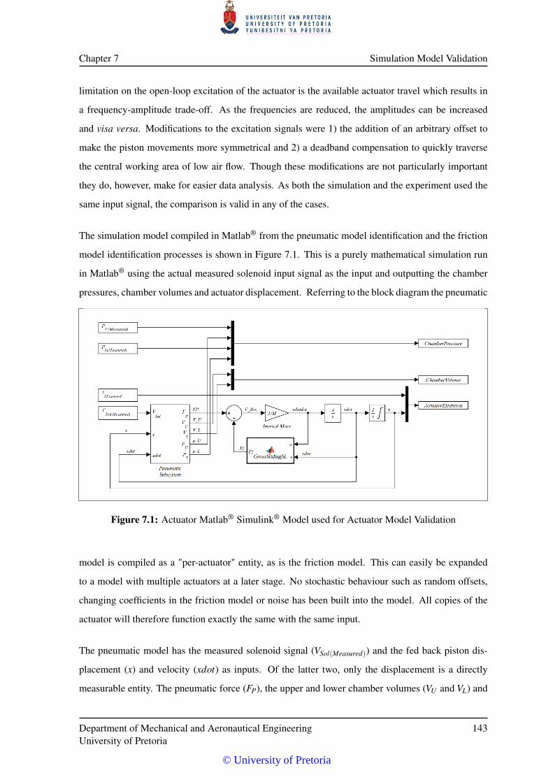
Chapter 7 Simulation Model Validation
limitation on the open-loop excitation of the actuator is the available actuator travel which results in
a frequency-amplitude trade-off. As the frequencies are reduced, the amplitudes can be increased
and visa versa. Modifications to the excitation signals were 1) the addition of an arbitrary offset to
make the piston movements more symmetrical and 2) a deadband compensation to quickly traverse
the central working area of low air flow. Though these modifications are not particularly important
they do, however, make for easier data analysis. As both the simulation and the experiment used the
same input signal, the comparison is valid in any of the cases.
The simulation model compiled in Matlab® from the pneumatic model identification and the friction
model identification processes is shown in Figure 7.1. This is a purely mathematical simulation run
in Matlab® using the actual measured solenoid input signal as the input and outputting the chamber
pressures, chamber volumes and actuator displacement. Referring to the block diagram the pneumatic
Figure 7.1: Actuator Matlab® Simulink® Model used for Actuator Model Validation
model is compiled as a "per-actuator" entity, as is the friction model. This can easily be expanded
to a model with multiple actuators at a later stage. No stochastic behaviour such as random offsets,
changing coefficients in the friction model or noise has been built into the model. All copies of the
actuator will therefore function exactly the same with the same input.
The pneumatic model has the measured solenoid signal (VSol(Measured)) and the fed back piston dis-
placement (x) and velocity (xdot) as inputs. Of the latter two, only the displacement is a directly
measurable entity. The pneumatic force (FP), the upper and lower chamber volumes (VU and VL) and
Department of Mechanical and Aeronautical EngineeringUniversity of Pretoria
143
© University of Pretoria
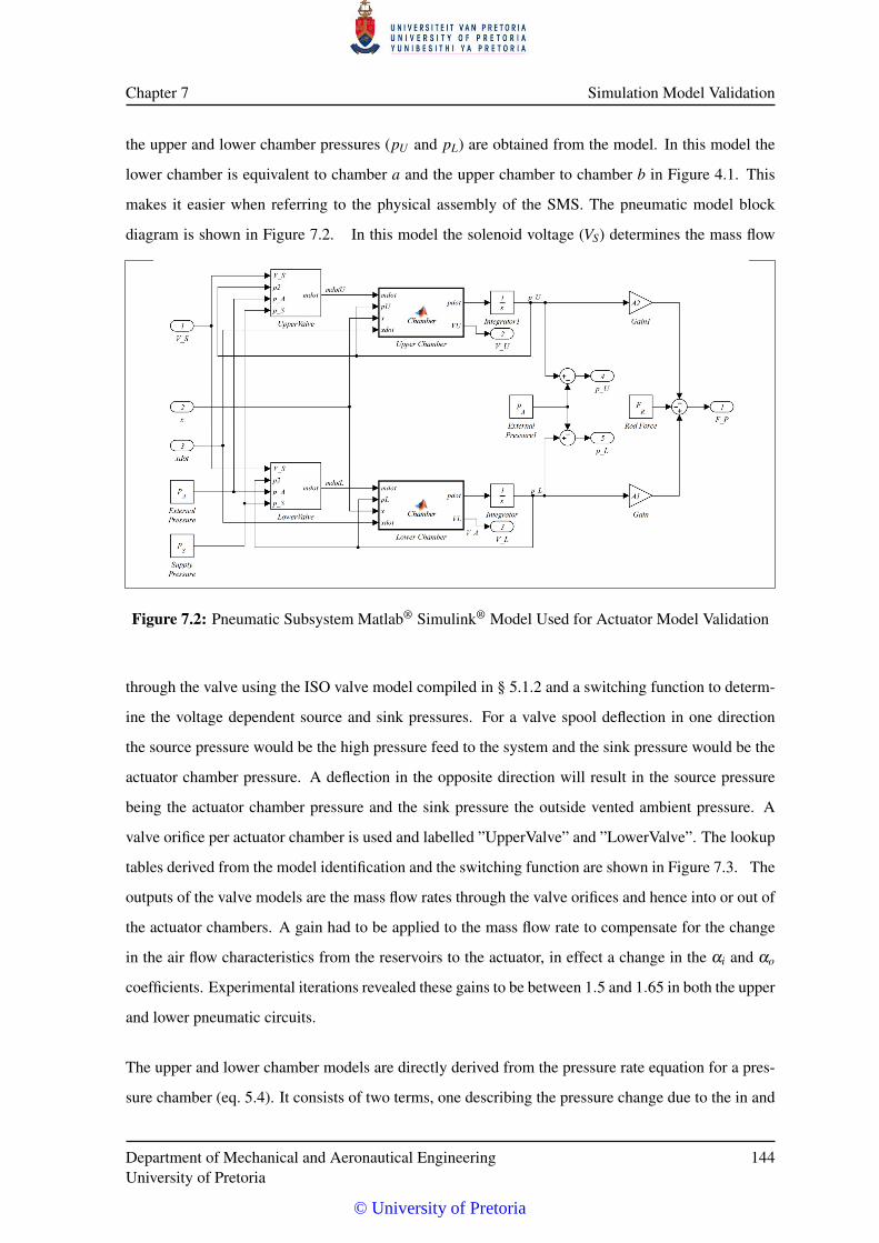
Chapter 7 Simulation Model Validation
the upper and lower chamber pressures (pU and pL) are obtained from the model. In this model the
lower chamber is equivalent to chamber a and the upper chamber to chamber b in Figure 4.1. This
makes it easier when referring to the physical assembly of the SMS. The pneumatic model block
diagram is shown in Figure 7.2. In this model the solenoid voltage (VS) determines the mass flow
Figure 7.2: Pneumatic Subsystem Matlab® Simulink® Model Used for Actuator Model Validation
through the valve using the ISO valve model compiled in § 5.1.2 and a switching function to determ-
ine the voltage dependent source and sink pressures. For a valve spool deflection in one direction
the source pressure would be the high pressure feed to the system and the sink pressure would be the
actuator chamber pressure. A deflection in the opposite direction will result in the source pressure
being the actuator chamber pressure and the sink pressure the outside vented ambient pressure. A
valve orifice per actuator chamber is used and labelled ”UpperValve” and ”LowerValve”. The lookup
tables derived from the model identification and the switching function are shown in Figure 7.3. The
outputs of the valve models are the mass flow rates through the valve orifices and hence into or out of
the actuator chambers. A gain had to be applied to the mass flow rate to compensate for the change
in the air flow characteristics from the reservoirs to the actuator, in effect a change in the αi and αo
coefficients. Experimental iterations revealed these gains to be between 1.5 and 1.65 in both the upper
and lower pneumatic circuits.
The upper and lower chamber models are directly derived from the pressure rate equation for a pres-
sure chamber (eq. 5.4). It consists of two terms, one describing the pressure change due to the in and
Department of Mechanical and Aeronautical EngineeringUniversity of Pretoria
144
© University of Pretoria
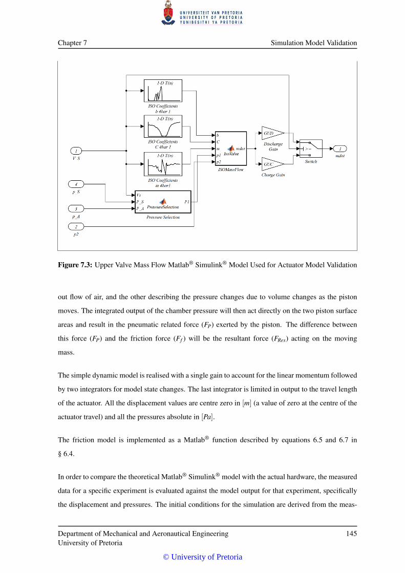
Chapter 7 Simulation Model Validation
Figure 7.3: Upper Valve Mass Flow Matlab® Simulink® Model Used for Actuator Model Validation
out flow of air, and the other describing the pressure changes due to volume changes as the piston
moves. The integrated output of the chamber pressure will then act directly on the two piston surface
areas and result in the pneumatic related force (FP) exerted by the piston. The difference between
this force (FP) and the friction force (Ff ) will be the resultant force (FRes) acting on the moving
mass.
The simple dynamic model is realised with a single gain to account for the linear momentum followed
by two integrators for model state changes. The last integrator is limited in output to the travel length
of the actuator. All the displacement values are centre zero in [m] (a value of zero at the centre of the
actuator travel) and all the pressures absolute in [Pa].
The friction model is implemented as a Matlab® function described by equations 6.5 and 6.7 in
§ 6.4.
In order to compare the theoretical Matlab® Simulink® model with the actual hardware, the measured
data for a specific experiment is evaluated against the model output for that experiment, specifically
the displacement and pressures. The initial conditions for the simulation are derived from the meas-
Department of Mechanical and Aeronautical EngineeringUniversity of Pretoria
145
© University of Pretoria
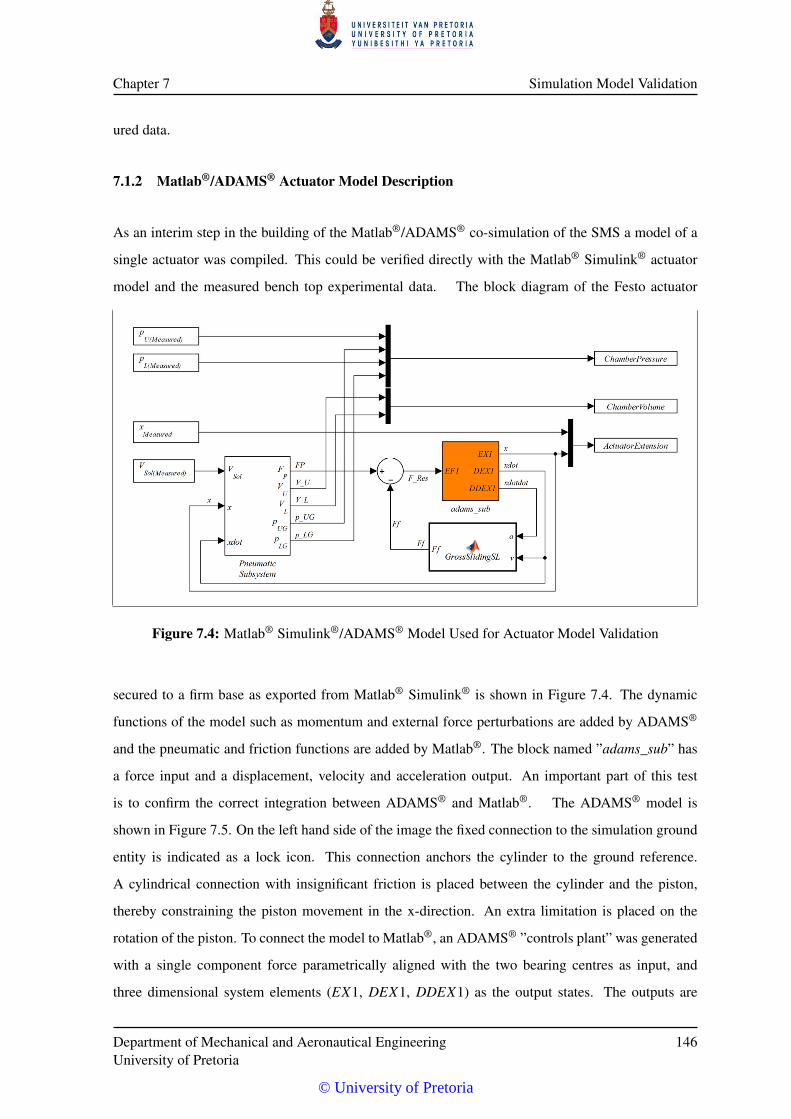
Chapter 7 Simulation Model Validation
ured data.
7.1.2 Matlab®/ADAMS® Actuator Model Description
As an interim step in the building of the Matlab®/ADAMS® co-simulation of the SMS a model of a
single actuator was compiled. This could be verified directly with the Matlab® Simulink® actuator
model and the measured bench top experimental data. The block diagram of the Festo actuator
Figure 7.4: Matlab® Simulink®/ADAMS® Model Used for Actuator Model Validation
secured to a firm base as exported from Matlab® Simulink® is shown in Figure 7.4. The dynamic
functions of the model such as momentum and external force perturbations are added by ADAMS®
and the pneumatic and friction functions are added by Matlab®. The block named ”adams_sub” has
a force input and a displacement, velocity and acceleration output. An important part of this test
is to confirm the correct integration between ADAMS® and Matlab®. The ADAMS® model is
shown in Figure 7.5. On the left hand side of the image the fixed connection to the simulation ground
entity is indicated as a lock icon. This connection anchors the cylinder to the ground reference.
A cylindrical connection with insignificant friction is placed between the cylinder and the piston,
thereby constraining the piston movement in the x-direction. An extra limitation is placed on the
rotation of the piston. To connect the model to Matlab®, an ADAMS® ”controls plant” was generated
with a single component force parametrically aligned with the two bearing centres as input, and
three dimensional system elements (EX1, DEX1, DDEX1) as the output states. The outputs are
Department of Mechanical and Aeronautical EngineeringUniversity of Pretoria
146
© University of Pretoria
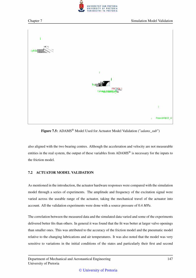
Chapter 7 Simulation Model Validation
xxx
y
z
y
zz
y
ytivarg nigirO83_REKRAM.1rednilyC 14_REKRAM.1rednilyC
xx
y
z
y
z GoC.1rednilyC1_ECROFS
GoC.notsiP
zz
x
y
x
y 04_REKRAM.1rednilyC1_NOITCIRF
93_REKRAM.notsiP
x
y
z 24_REKRAM.notsiP
F rotautcAotse
xzy
Figure 7.5: ADAMS® Model Used for Actuator Model Validation (”adams_sub”)
also aligned with the two bearing centres. Although the acceleration and velocity are not measurable
entities in the real system, the output of these variables from ADAMS® is necessary for the inputs to
the friction model.
7.2 ACTUATOR MODEL VALIDATION
As mentioned in the introduction, the actuator hardware responses were compared with the simulation
model through a series of experiments. The amplitude and frequency of the excitation signal were
varied across the useable range of the actuator, taking the mechanical travel of the actuator into
account. All the validation experiments were done with a source pressure of 0.4 MPa.
The correlation between the measured data and the simulated data varied and some of the experiments
delivered better fits than others. In general it was found that the fit was better at larger valve openings
than smaller ones. This was attributed to the accuracy of the friction model and the pneumatic model
relative to the changing lubrications and air temperatures. It was also noted that the model was very
sensitive to variations in the initial conditions of the states and particularly their first and second
Department of Mechanical and Aeronautical EngineeringUniversity of Pretoria
147
© University of Pretoria
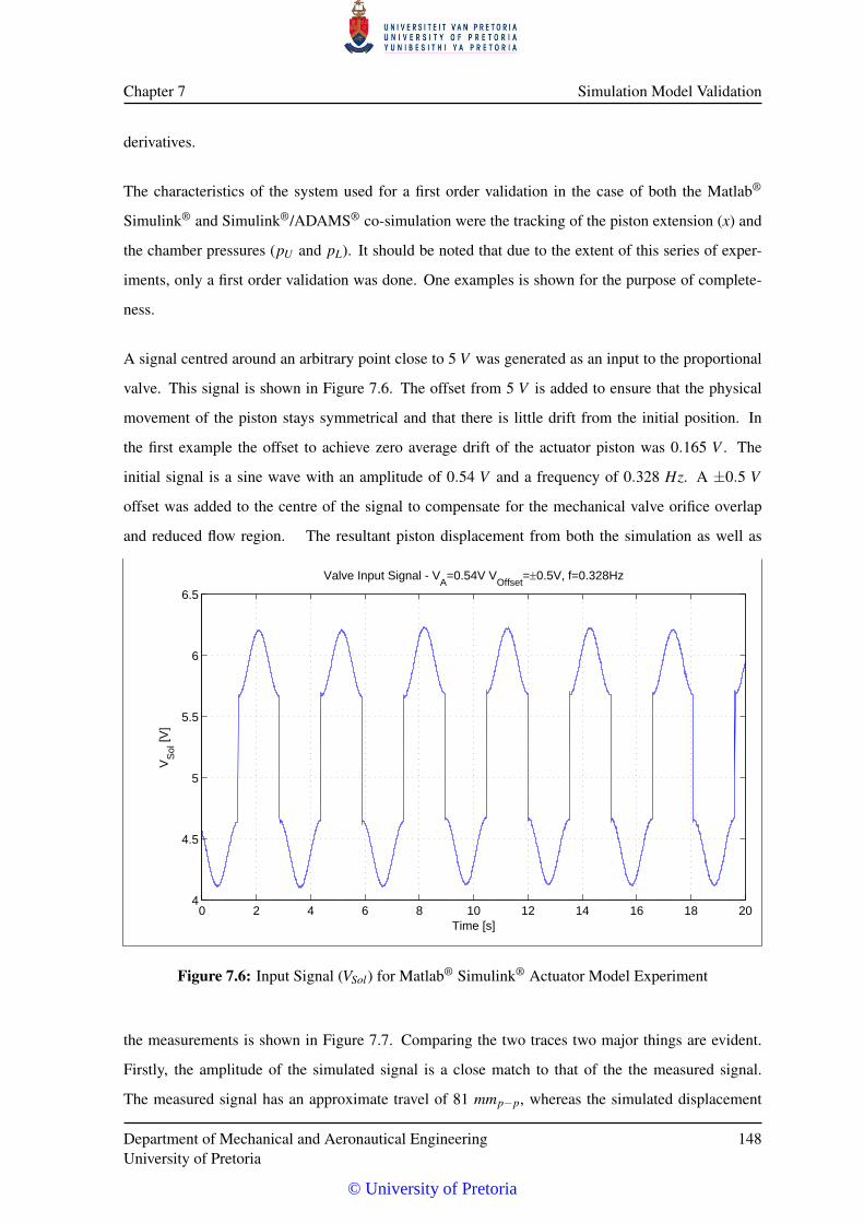
Chapter 7 Simulation Model Validation
derivatives.
The characteristics of the system used for a first order validation in the case of both the Matlab®
Simulink® and Simulink®/ADAMS® co-simulation were the tracking of the piston extension (x) and
the chamber pressures (pU and pL). It should be noted that due to the extent of this series of exper-
iments, only a first order validation was done. One examples is shown for the purpose of complete-
ness.
A signal centred around an arbitrary point close to 5 V was generated as an input to the proportional
valve. This signal is shown in Figure 7.6. The offset from 5 V is added to ensure that the physical
movement of the piston stays symmetrical and that there is little drift from the initial position. In
the first example the offset to achieve zero average drift of the actuator piston was 0.165 V . The
initial signal is a sine wave with an amplitude of 0.54 V and a frequency of 0.328 Hz. A ±0.5 V
offset was added to the centre of the signal to compensate for the mechanical valve orifice overlap
and reduced flow region. The resultant piston displacement from both the simulation as well as
0 2 4 6 8 10 12 14 16 18 204
4.5
5
5.5
6
6.5
Valve Input Signal - VA=0.54V V
Offset=0.5V, f=0.328Hz
Time [s]
VS
ol [V
]
Figure 7.6: Input Signal (VSol) for Matlab® Simulink® Actuator Model Experiment
the measurements is shown in Figure 7.7. Comparing the two traces two major things are evident.
Firstly, the amplitude of the simulated signal is a close match to that of the the measured signal.
The measured signal has an approximate travel of 81 mmp−p, whereas the simulated displacement
Department of Mechanical and Aeronautical EngineeringUniversity of Pretoria
148
© University of Pretoria
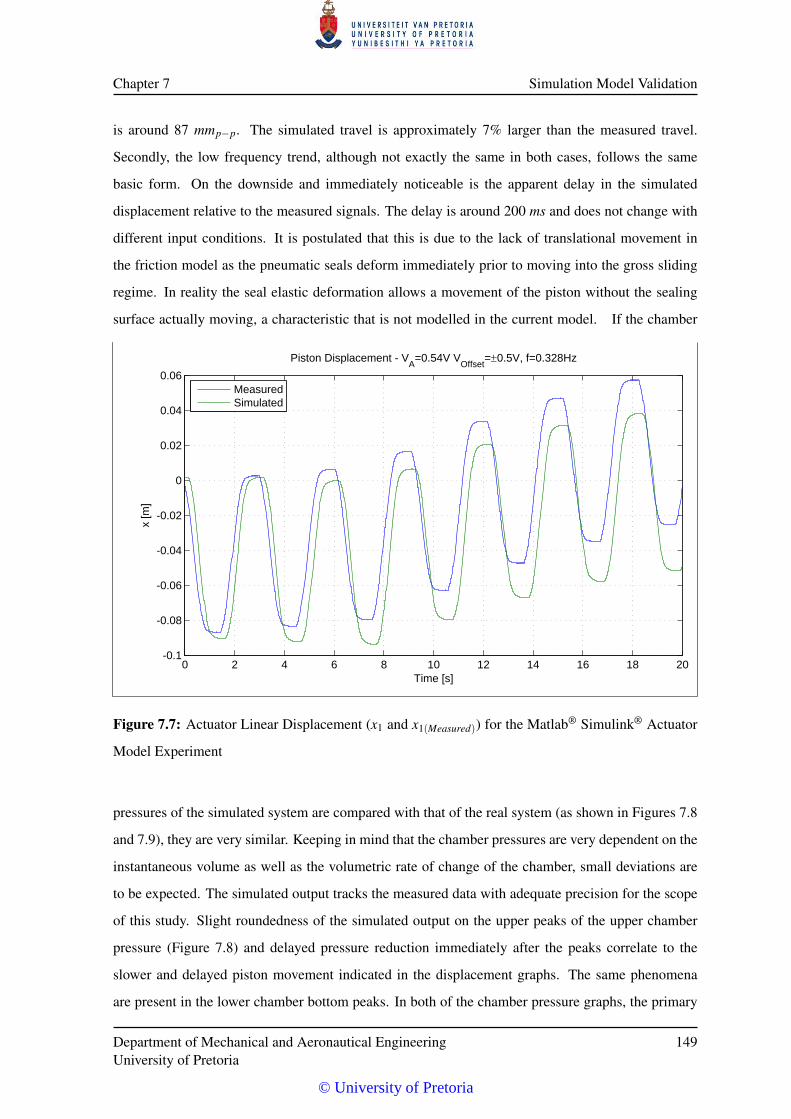
Chapter 7 Simulation Model Validation
is around 87 mmp−p. The simulated travel is approximately 7% larger than the measured travel.
Secondly, the low frequency trend, although not exactly the same in both cases, follows the same
basic form. On the downside and immediately noticeable is the apparent delay in the simulated
displacement relative to the measured signals. The delay is around 200 ms and does not change with
different input conditions. It is postulated that this is due to the lack of translational movement in
the friction model as the pneumatic seals deform immediately prior to moving into the gross sliding
regime. In reality the seal elastic deformation allows a movement of the piston without the sealing
surface actually moving, a characteristic that is not modelled in the current model. If the chamber
0 2 4 6 8 10 12 14 16 18 20-0.1
-0.08
-0.06
-0.04
-0.02
0
0.02
0.04
0.06
Piston Displacement - VA=0.54V V
Offset=0.5V, f=0.328Hz
Time [s]
x [m
]
MeasuredSimulated
Figure 7.7: Actuator Linear Displacement (x1 and x1(Measured)) for the Matlab® Simulink® Actuator
Model Experiment
pressures of the simulated system are compared with that of the real system (as shown in Figures 7.8
and 7.9), they are very similar. Keeping in mind that the chamber pressures are very dependent on the
instantaneous volume as well as the volumetric rate of change of the chamber, small deviations are
to be expected. The simulated output tracks the measured data with adequate precision for the scope
of this study. Slight roundedness of the simulated output on the upper peaks of the upper chamber
pressure (Figure 7.8) and delayed pressure reduction immediately after the peaks correlate to the
slower and delayed piston movement indicated in the displacement graphs. The same phenomena
are present in the lower chamber bottom peaks. In both of the chamber pressure graphs, the primary
Department of Mechanical and Aeronautical EngineeringUniversity of Pretoria
149
© University of Pretoria
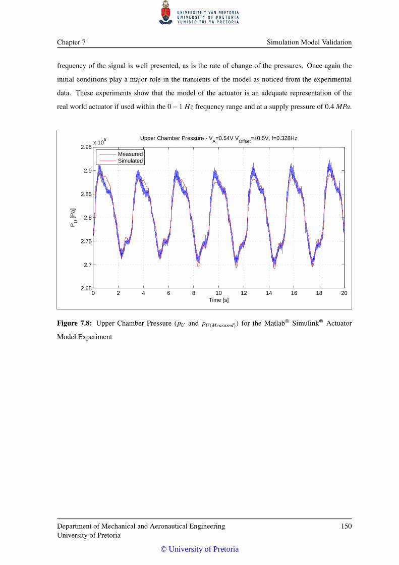
Chapter 7 Simulation Model Validation
frequency of the signal is well presented, as is the rate of change of the pressures. Once again the
initial conditions play a major role in the transients of the model as noticed from the experimental
data. These experiments show that the model of the actuator is an adequate representation of the
real world actuator if used within the 0−1 Hz frequency range and at a supply pressure of 0.4 MPa.
0 2 4 6 8 10 12 14 16 18 202.65
2.7
2.75
2.8
2.85
2.9
2.95x 10
5 Upper Chamber Pressure - VA=0.54V V
Offset=0.5V, f=0.328Hz
Time [s]
PU
[Pa]
MeasuredSimulated
Figure 7.8: Upper Chamber Pressure (pU and pU(Measured)) for the Matlab® Simulink® Actuator
Model Experiment
Department of Mechanical and Aeronautical EngineeringUniversity of Pretoria
150
© University of Pretoria
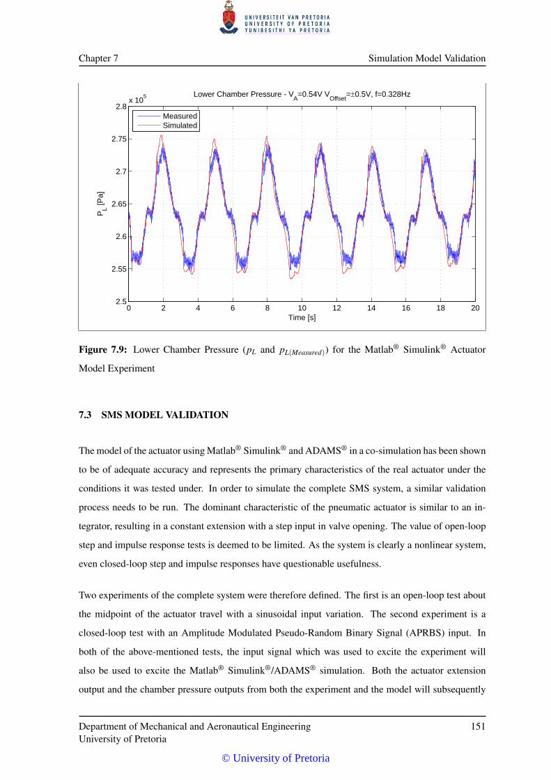
Chapter 7 Simulation Model Validation
0 2 4 6 8 10 12 14 16 18 202.5
2.55
2.6
2.65
2.7
2.75
2.8x 10
5 Lower Chamber Pressure - VA=0.54V V
Offset=0.5V, f=0.328Hz
Time [s]
PL [P
a]
MeasuredSimulated
Figure 7.9: Lower Chamber Pressure (pL and pL(Measured)) for the Matlab® Simulink® Actuator
Model Experiment
7.3 SMS MODEL VALIDATION
The model of the actuator using Matlab® Simulink® and ADAMS® in a co-simulation has been shown
to be of adequate accuracy and represents the primary characteristics of the real actuator under the
conditions it was tested under. In order to simulate the complete SMS system, a similar validation
process needs to be run. The dominant characteristic of the pneumatic actuator is similar to an in-
tegrator, resulting in a constant extension with a step input in valve opening. The value of open-loop
step and impulse response tests is deemed to be limited. As the system is clearly a nonlinear system,
even closed-loop step and impulse responses have questionable usefulness.
Two experiments of the complete system were therefore defined. The first is an open-loop test about
the midpoint of the actuator travel with a sinusoidal input variation. The second experiment is a
closed-loop test with an Amplitude Modulated Pseudo-Random Binary Signal (APRBS) input. In
both of the above-mentioned tests, the input signal which was used to excite the experiment will
also be used to excite the Matlab® Simulink®/ADAMS® simulation. Both the actuator extension
output and the chamber pressure outputs from both the experiment and the model will subsequently
Department of Mechanical and Aeronautical EngineeringUniversity of Pretoria
151
© University of Pretoria
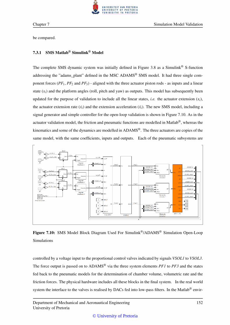
Chapter 7 Simulation Model Validation
be compared.
7.3.1 SMS Matlab® Simulink® Model
The complete SMS dynamic system was initially defined in Figure 3.8 as a Simulink® S-function
addressing the ”adams_plant” defined in the MSC ADAMS® SMS model. It had three single com-
ponent forces (PF1, PF2 and PF3) - aligned with the three actuator piston rods - as inputs and a linear
state (xi) and the platform angles (roll, pitch and yaw) as outputs. This model has subsequently been
updated for the purpose of validation to include all the linear states, i.e. the actuator extension (xi),
the actuator extension rate (xi) and the extension acceleration (xi). The new SMS model, including a
signal generator and simple controller for the open-loop validation is shown in Figure 7.10. As in the
actuator validation model, the friction and pneumatic functions are modelled in Matlab®, whereas the
kinematics and some of the dynamics are modelled in ADAMS®. The three actuators are copies of the
same model, with the same coefficients, inputs and outputs. Each of the pneumatic subsystems are
Figure 7.10: SMS Model Block Diagram Used For Simulink®/ADAMS® Simulation Open-Loop
Simulations
controlled by a voltage input to the proportional control valves indicated by signals VSOL1 to VSOL3.
The force output is passed on to ADAMS® via the three system elements PF1 to PF3 and the states
fed back to the pneumatic models for the determination of chamber volume, volumetric rate and the
friction forces. The physical hardware includes all these blocks in the final system. In the real world
system the interface to the valves is realised by DACs fed into low-pass filters. In the Matlab® envir-
Department of Mechanical and Aeronautical EngineeringUniversity of Pretoria
152
© University of Pretoria
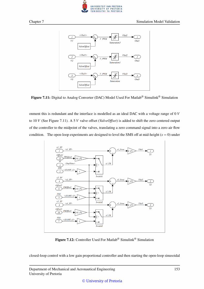
Chapter 7 Simulation Model Validation
Figure 7.11: Digital to Analog Converter (DAC) Model Used For Matlab® Simulink® Simulation
onment this is redundant and the interface is modelled as an ideal DAC with a voltage range of 0 V
to 10 V (See Figure 7.11). A 5 V valve offset (ValveOffset) is added to shift the zero centered output
of the controller to the midpoint of the valves, translating a zero command signal into a zero air flow
condition. The open-loop experiments are designed to level the SMS off at mid-height (x = 0) under
Figure 7.12: Controller Used For Matlab® Simulink® Simulation
closed-loop control with a low gain proportional controller and then starting the open-loop sinusoidal
Department of Mechanical and Aeronautical EngineeringUniversity of Pretoria
153
© University of Pretoria
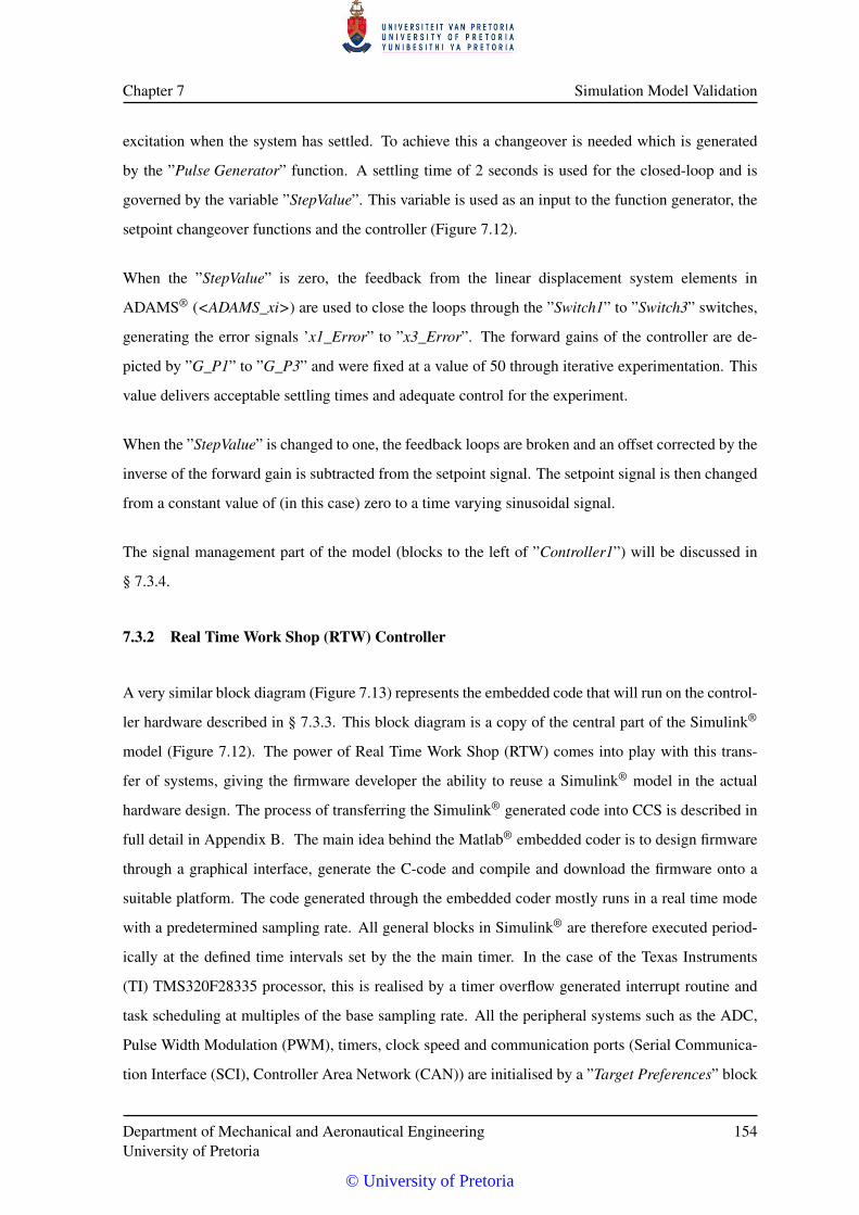
Chapter 7 Simulation Model Validation
excitation when the system has settled. To achieve this a changeover is needed which is generated
by the ”Pulse Generator” function. A settling time of 2 seconds is used for the closed-loop and is
governed by the variable ”StepValue”. This variable is used as an input to the function generator, the
setpoint changeover functions and the controller (Figure 7.12).
When the ”StepValue” is zero, the feedback from the linear displacement system elements in
ADAMS® (<ADAMS_xi>) are used to close the loops through the ”Switch1” to ”Switch3” switches,
generating the error signals ’x1_Error” to ”x3_Error”. The forward gains of the controller are de-
picted by ”G_P1” to ”G_P3” and were fixed at a value of 50 through iterative experimentation. This
value delivers acceptable settling times and adequate control for the experiment.
When the ”StepValue” is changed to one, the feedback loops are broken and an offset corrected by the
inverse of the forward gain is subtracted from the setpoint signal. The setpoint signal is then changed
from a constant value of (in this case) zero to a time varying sinusoidal signal.
The signal management part of the model (blocks to the left of ”Controller1”) will be discussed in
§ 7.3.4.
7.3.2 Real Time Work Shop (RTW) Controller
A very similar block diagram (Figure 7.13) represents the embedded code that will run on the control-
ler hardware described in § 7.3.3. This block diagram is a copy of the central part of the Simulink®
model (Figure 7.12). The power of Real Time Work Shop (RTW) comes into play with this trans-
fer of systems, giving the firmware developer the ability to reuse a Simulink® model in the actual
hardware design. The process of transferring the Simulink® generated code into CCS is described in
full detail in Appendix B. The main idea behind the Matlab® embedded coder is to design firmware
through a graphical interface, generate the C-code and compile and download the firmware onto a
suitable platform. The code generated through the embedded coder mostly runs in a real time mode
with a predetermined sampling rate. All general blocks in Simulink® are therefore executed period-
ically at the defined time intervals set by the the main timer. In the case of the Texas Instruments
(TI) TMS320F28335 processor, this is realised by a timer overflow generated interrupt routine and
task scheduling at multiples of the base sampling rate. All the peripheral systems such as the ADC,
Pulse Width Modulation (PWM), timers, clock speed and communication ports (Serial Communica-
tion Interface (SCI), Controller Area Network (CAN)) are initialised by a ”Target Preferences” block
Department of Mechanical and Aeronautical EngineeringUniversity of Pretoria
154
© University of Pretoria
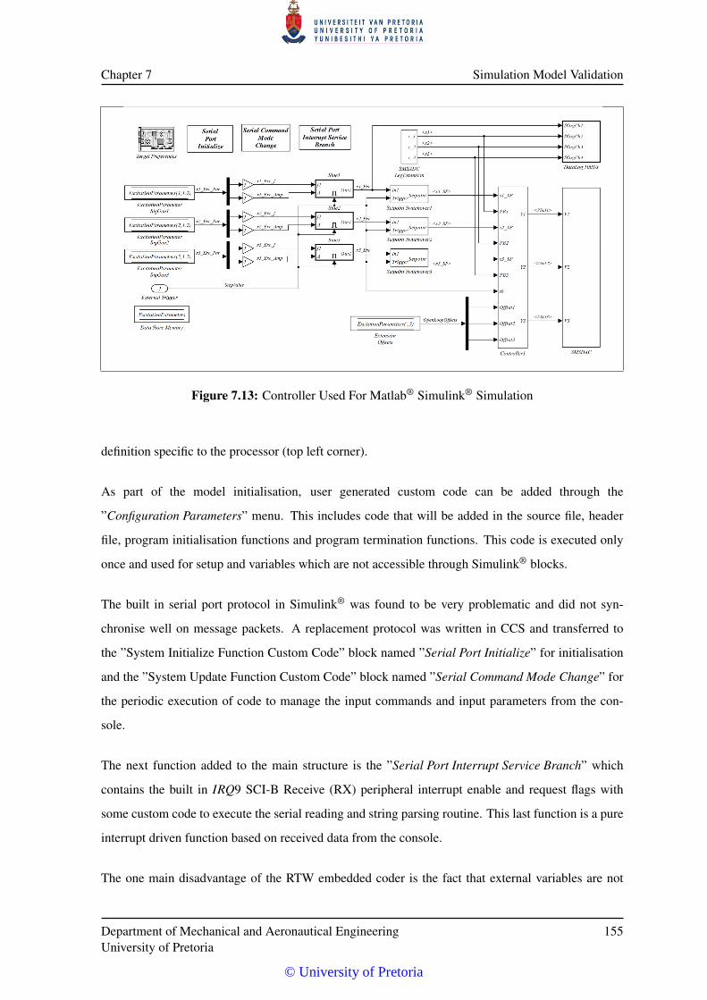
Chapter 7 Simulation Model Validation
Figure 7.13: Controller Used For Matlab® Simulink® Simulation
definition specific to the processor (top left corner).
As part of the model initialisation, user generated custom code can be added through the
”Configuration Parameters” menu. This includes code that will be added in the source file, header
file, program initialisation functions and program termination functions. This code is executed only
once and used for setup and variables which are not accessible through Simulink® blocks.
The built in serial port protocol in Simulink® was found to be very problematic and did not syn-
chronise well on message packets. A replacement protocol was written in CCS and transferred to
the ”System Initialize Function Custom Code” block named ”Serial Port Initialize” for initialisation
and the ”System Update Function Custom Code” block named ”Serial Command Mode Change” for
the periodic execution of code to manage the input commands and input parameters from the con-
sole.
The next function added to the main structure is the ”Serial Port Interrupt Service Branch” which
contains the built in IRQ9 SCI-B Receive (RX) peripheral interrupt enable and request flags with
some custom code to execute the serial reading and string parsing routine. This last function is a pure
interrupt driven function based on received data from the console.
The one main disadvantage of the RTW embedded coder is the fact that external variables are not
Department of Mechanical and Aeronautical EngineeringUniversity of Pretoria
155
© University of Pretoria
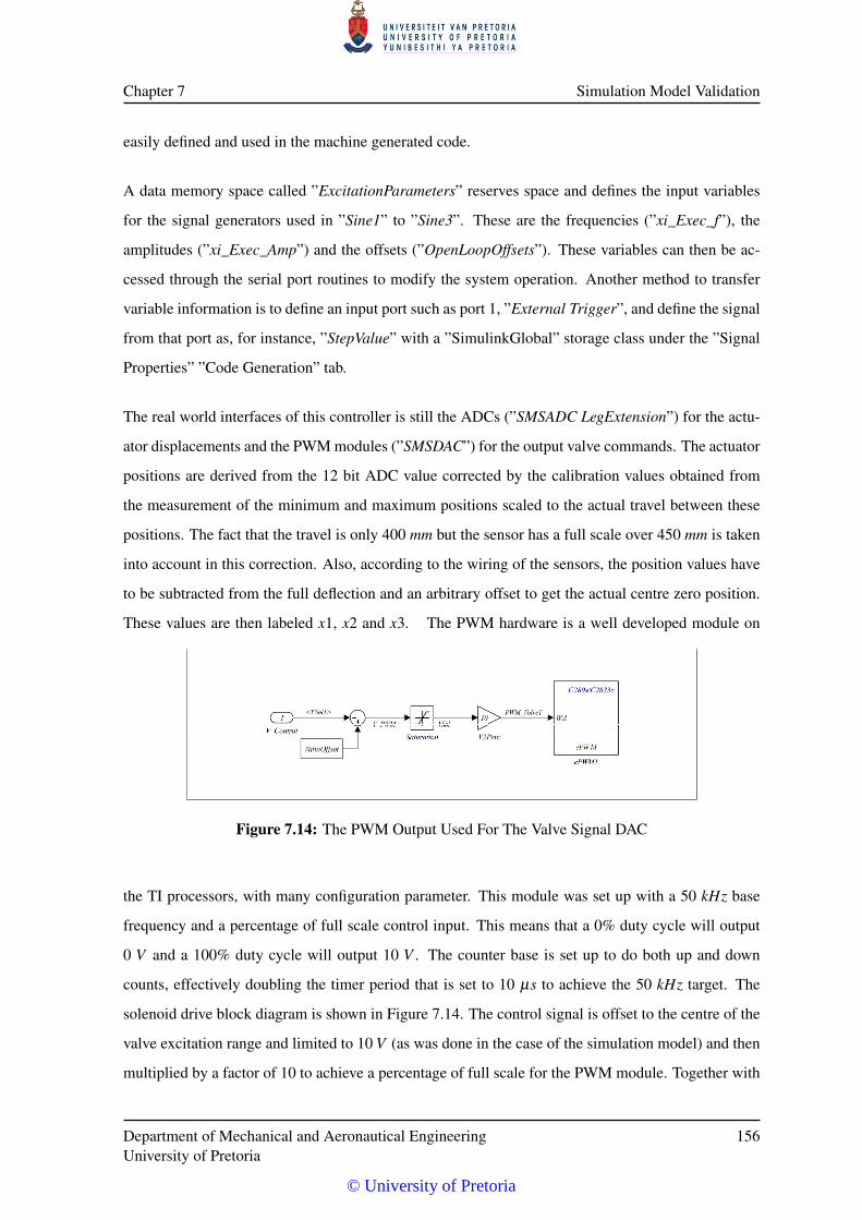
Chapter 7 Simulation Model Validation
easily defined and used in the machine generated code.
A data memory space called ”ExcitationParameters” reserves space and defines the input variables
for the signal generators used in ”Sine1” to ”Sine3”. These are the frequencies (”xi_Exec_f”), the
amplitudes (”xi_Exec_Amp”) and the offsets (”OpenLoopOffsets”). These variables can then be ac-
cessed through the serial port routines to modify the system operation. Another method to transfer
variable information is to define an input port such as port 1, ”External Trigger”, and define the signal
from that port as, for instance, ”StepValue” with a ”SimulinkGlobal” storage class under the ”Signal
Properties” ”Code Generation” tab.
The real world interfaces of this controller is still the ADCs (”SMSADC LegExtension”) for the actu-
ator displacements and the PWM modules (”SMSDAC”) for the output valve commands. The actuator
positions are derived from the 12 bit ADC value corrected by the calibration values obtained from
the measurement of the minimum and maximum positions scaled to the actual travel between these
positions. The fact that the travel is only 400 mm but the sensor has a full scale over 450 mm is taken
into account in this correction. Also, according to the wiring of the sensors, the position values have
to be subtracted from the full deflection and an arbitrary offset to get the actual centre zero position.
These values are then labeled x1, x2 and x3. The PWM hardware is a well developed module on
Figure 7.14: The PWM Output Used For The Valve Signal DAC
the TI processors, with many configuration parameter. This module was set up with a 50 kHz base
frequency and a percentage of full scale control input. This means that a 0% duty cycle will output
0 V and a 100% duty cycle will output 10 V . The counter base is set up to do both up and down
counts, effectively doubling the timer period that is set to 10 µs to achieve the 50 kHz target. The
solenoid drive block diagram is shown in Figure 7.14. The control signal is offset to the centre of the
valve excitation range and limited to 10 V (as was done in the case of the simulation model) and then
multiplied by a factor of 10 to achieve a percentage of full scale for the PWM module. Together with
Department of Mechanical and Aeronautical EngineeringUniversity of Pretoria
156
© University of Pretoria
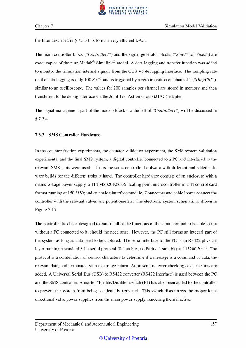
Chapter 7 Simulation Model Validation
the filter described in § 7.3.3 this forms a very efficient DAC.
The main controller block (”Controller1”) and the signal generator blocks (”Sine1” to ”Sine3”) are
exact copies of the pure Matlab® Simulink® model. A data logging and transfer function was added
to monitor the simulation internal signals from the CCS V5 debugging interface. The sampling rate
on the data logging is only 100 S.s−1 and is triggered by a zero transition on channel 1 (”DlogCh1”),
similar to an oscilloscope. The values for 200 samples per channel are stored in memory and then
transferred to the debug interface via the Joint Test Action Group (JTAG) adapter.
The signal management part of the model (Blocks to the left of ”Controller1”) will be discussed in
§ 7.3.4.
7.3.3 SMS Controller Hardware
In the actuator friction experiments, the actuator validation experiment, the SMS system validation
experiments, and the final SMS system, a digital controller connected to a PC and interfaced to the
relevant SMS parts were used. This is the same controller hardware with different embedded soft-
ware builds for the different tasks at hand. The controller hardware consists of an enclosure with a
mains voltage power supply, a TI TMS320F28335 floating point microcontroller in a TI control card
format running at 150 MHz and an analog interface module. Connectors and cable looms connect the
controller with the relevant valves and potentiometers. The electronic system schematic is shown in
Figure 7.15.
The controller has been designed to control all of the functions of the simulator and to be able to run
without a PC connected to it, should the need arise. However, the PC still forms an integral part of
the system as long as data need to be captured. The serial interface to the PC is an RS422 physical
layer running a standard 8-bit serial protocol (8 data bits, no Parity, 1 stop bit) at 115200 b.s−1. The
protocol is a combination of control characters to determine if a message is a command or data, the
relevant data, and terminated with a carriage return. At present, no error checking or checksums are
added. A Universal Serial Bus (USB) to RS422 converter (RS422 Interface) is used between the PC
and the SMS controller. A master "Enable/Disable" switch (P1) has also been added to the controller
to prevent the system from being accidentally activated. This switch disconnects the proportional
directional valve power supplies from the main power supply, rendering them inactive.
Department of Mechanical and Aeronautical EngineeringUniversity of Pretoria
157
© University of Pretoria
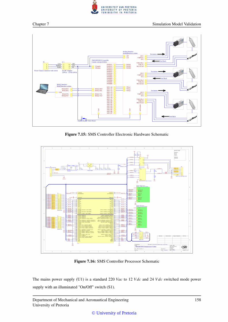
Chapter 7 Simulation Model Validation
1
1
2
2
3
3
4
4
D D
C C
B B
A A
CSIR - DPSSMeiring Naude RdBrummeriaPretoriaSouth Africa1.00
11/02/2015 13:44:12
D:\Altium\Projects\SMS\SMS Controller.SchDocTitle:
Size: Doc No:Date:
File name:
Revision:
Sheet ofTime:
A4
SMS Controller
Classification:
Item No:
Revision: Revision Date: Approval Signature: ECP No:
VSupplyVReturn
ADC-A0ADC-A1ADC-A2ADC-A3ADC-A4ADC-A5ADC-A6ADC-A7ADC-B0ADC-B1ADC-B2ADC-B3ADC-B4ADC-B5ADC-B6ADC-B7
PWMA1PWMA2PWMA3PWMA4PWMA5PWMA6PWMB1PWMB2PWMB3PWMB4PWMB5PWMB6
RS422 RX+RS422 RX-
RS422 TX-RS422 TX+
Gnd
TMS320F28335 ControllerComms concept.SchDoc
220Vac - 12Vdc/24Vdc
1Live
2Neutral
3Earth 4 12V
5 0V
6 24VU 1
AC/DC Adapter
123
P1
Power Chassis connector with switch
12V
PWM1PWM2PWM3
VPos1VPos2VPos3
VMLO1
VMLO2
VMLO3
VMPYE1
VMPYE2
VMPYE3
Gnd
24V
24V
Enab
le
VMLOEx1
VMLOEx2
VMLOEx3
MLO1Gnd
MLO2Gnd
MLO3Gnd
24V1
24V2
24V3
0V1
0V2
0V3
Analog InterfaceAnalogInterface.schdoc
RS422TX+RS422TX-
RS422RX+RS422RX-
USB
RS422 InterfaceRS422Interface.schdoc
Excitation
Feed Back
Excitation
Feed Back
Excitation
Feed BackS1
Enable/Disable Valve Power
Figure 7.15: SMS Controller Electronic Hardware Schematic
1
1
2
2
3
3
4
4
5
5
6
6
7
7
8
8
D D
C C
B B
A A
0
CSIR - DPSSMeiring Naude RdBrummeriaPretoriaSouth Africa
0
1 111/02/2015 13:49:33
D:\Altium\Projects\SMS\Comms concept.SchDocTitle:
Size: Doc No:Date:
File name:
Revision:
Sheet ofTime:
A3
TMS320F28335 Interprocessor Comms
Classification:
Item No:
Revision: Revision Date: Approval Signature: ECP No:
2
MCLKR-A MFSR-A
MDR-AMFSX-A
MDX-AMCLKX-A
MCLKR-A
MCLKX-A
MDR-A
MDX-A
MFSR-A
MFSX-A
MCLKX-AE
MCLKR-AE
MFSX-AE
MFSR-AE
MCLKR-AE MFSR-AE
MFSX-AE
MCLKX-AE
MDX-AE
MDR-AEMDR-AEMDX-AE
Resource Usage:
McBSP-A SCI- ASCI-BCAN A
ADCA/BPWMA/B
CANRX-A CANTX-A
Gnd
VCCU3
SN65HVD233D Canbus Tranceiver
CANTX-A
CANRX-A
CANRS-A
CANLBK-A
GND
CANLBK-ACANRS-A
10k
R4120RR5
1kR6
GND
RS232 TXRS232 RX
RS232 RXRS232 TX
V33D-ISO1
ISO-RX-RS2322
GND_ISO6
ADC-B07
ADC-B19
ADC-B211
ADC-B313
ADC-B415
ADC-B517
ADC-B619
ADC-B721
ADC-A0 57
ADC-A1 59
ADC-A2 61
ADC-A3 63
ADC-A4 65
ADC-A5 67
ADC-A6 69
ADC-A7 71
Gnd8
Gnd10
Gnd12
Gnd14
Gnd 58
Gnd 60
Gnd 62
Gnd 64
GPIO-58 / MCLKR-A / XD21 (EMIF)18
GPIO-60 / MCLKR-B / XD19 (EMIF)20
GPIO-62 / SCIRX-C / XD17 (EMIF)22
GPIO-59 / MFSR-A / XD20 (EMIF) 68
GPIO-61 / MFSR-B / XD18 (EMIF) 70
GPIO-63 / SCITX-C / XD16 (EMIF) 72
GPIO-00 / EPWM-1A23
GPIO-02 / EPWM-2A24
GPIO-04 / EPWM-3A25
GPIO-06 / EPWM-4A / SYNCI / SYNCO26
Gnd27
GPIO-08 / EPWM-5A / CANTX-B / ADCSOC-A28
GPIO-10 / EPWM-6A / CANRX-B / ADCSOC-B29
GPIO-48 / ECAP5 / XD31 (EMIF)30
GPIO-8431
GPIO-8632
GPIO-12 / TZ-1 / CANTX-B / MDX-B33
GPIO-15 / TZ-4 / SCIRX-B / MFSX-B34
GPIO-24 / ECAP-1 / EQEPA-2 / MDX-B35
GPIO-26 / ECAP-3 / EQEPI-2 / MCLKX-B36
Gnd37
GPIO-16 / SPISIMO-A / CANTX-B / TZ-538
GPIO-18 / SPICLK-A / SCITX-B39
GPIO-20 / EQEPA-1 / MDX-A / CANTX-B40
GPIO-22 / EQEPS-1 / MCLKX-A / SCITX-B41
GPIO-8742
GPIO-28 / SCIRX-A / Resv / TZ543
GPIO-30 / CANRX-A44
GPIO-32 / I2CSDA / SYNCI / ADCSOCA45
GPIO-34 / ECAP1 / XREADY (EMIF)46
Gnd47
TCK48
TMS49
EMU150
GPIO-01 / EPWM-1B / MFSR-B 73
GPIO-03 / EPWM-2B / MCLKR-B 74
GPIO-05 / EPWM-3B / MFSR-A / ECAP-1 75
GPIO-07 / EPWM-4B / MCLKR-A / ECAP-2 76
+5V in 77
GPIO-09 / EPWM-5B / SCITX-B / ECAP-3 78
GPIO-11 / EPWM-6B / SCIRX-B / ECAP-4 79
GPIO-49 / ECAP6 / XD30 (EMIF) 80
GPIO-85 81
+5V in 82
GPIO-13 / TZ-2 / CANRX-B / MDR-B 83
GPIO-14 / TZ-3 / SCITX-B / MCLKX-B 84
GPIO-25 / ECAP-2 / EQEPB-2 / MDR-B 85
GPIO-27 / ECAP-4 / EQEPS-2 / MFSX-B 86
+5V in 87
GPIO-17 / SPISOMI-A / CANRX-B / TZ-6 88
GPIO-19 / SPISTE-A / SCIRX-B 89
GPIO-21 / EQEPB-1 / MDR-A / CANRX-B 90
GPIO-23 / EQEPI-1 / MFSX-A / SCIRX-B 91
+5V in 92
GPIO-29 / SCITX-A / Resv / TZ6 93
GPIO-31 / CANTX-A 94
GPIO-33 / I2CSCL / SYNCO / ADCSOCB 95
+5V in 96
TDI 97
TDO 98
TRSTn 99
EMU0 100
V33D-ISO 51
ISO-TX-RS232 52
GND_ISO 56
CC1
In1
Gnd
2
En3 Nr 4
Out 5U1
TPS73233DBV
GND
3.3V
+5V
GND GND
+5V
+5V
+5V
+5V
+5V
Gnd-ISO Gnd-ISO
V33-ISO V33-ISO
GND
12345678
P1ERNI 8 Way Maxibridge Blue 1
2345678
P2
ERNI 8 Way Maxibridge Green
GND
3.3V10kR1
10kR2
GND
3.3V
V33-ISO
Gnd-ISO
SCITX-B
SCIRX-B
SCIRX-B
SCITX-B
SCITXE-B
SCIRXE-B
SCIRXE-B
SCITXE-B
MCLKX-AMCLKX-AE
MCLKR-AEMCLKR-A
MDX-AMDX-AE
MDR-A
MFSX-AMFSX-AE
MFSR-AEMFSR-A
MDR-AE
+3.3V
Gnd
McBSP LVDS DriversMcBSP_LVDS_Drivers.schdoc
3.3V
GND
3.3V
MCLKR-AMCLKX-A
MDR-AMDX-A
MFSR-AMFSX-A
MCLKX-AE
MFSX-AE
MDX-AE
MCLKX-AEMCLKX-AMCLKR-A
MDX-AEMDX-AMDR-A
MFSX-AEMFSX-AMFSR-A
+3.3V
Gnd
McBSP CANBus DriversMcBSP_CANBus_Drivers.schdoc
GND
3.3V
10µF25V
+ C1
100nFC2
100nFC4
10nFC3
100nFC5
100nFC6
1 23 45 67 89 1011 1213 14
P5
Header 7X2TMS
TDITDOTCK
EMU0EMU1TRSTn
TMSTDI
TDOTCK
EMU0 EMU1
TRSTn
3.3V
GND
JTAG
1 23 45 67 89 1011 1213 1415 1617 1819 2021 2223 2425 2627 2829 3031 32
P3
Header 16X2
ADC-A0ADC-A1ADC-A2ADC-A3ADC-A4ADC-A5ADC-A6ADC-A7ADC-B0ADC-B1ADC-B2ADC-B3ADC-B4ADC-B5ADC-B6ADC-B7
ADC-A0
ADC-A1
ADC-A2
ADC-A3
ADC-B0
ADC-B1
ADC-B2
ADC-B3
ADC-B4
ADC-B5
ADC-B6
ADC-B7
ADC-A4
ADC-A5
ADC-A6
ADC-A7GND
PWMA1PWMA2PWMA3PWMA4
PWMB1PWMB2PWMB3PWMB41 2
3 45 67 89 1011 1213 1415 1617 1819 2021 2223 24
P4
Header 12X2
PWMA1PWMA2PWMA3PWMA4
PWMB1PWMB2PWMB3PWMB4
GND
PWMB5PWMB6
PWMA5PWMA6PWMA5
PWMA6
PWMB5PWMB6
D1OSRAM LG N971
1kR3
GND
1
3
2
4
E1
EMI filter
DI
RO
RE
DE
GndGnd
VCCVCC
U2MAX3491ESD
CANBUS_P
CANBUS_N
VSupplyVReturn
ADC-A0ADC-A1ADC-A2ADC-A3ADC-A4ADC-A5ADC-A6ADC-A7ADC-B0ADC-B1ADC-B2ADC-B3ADC-B4ADC-B5ADC-B6ADC-B7
PWMA1PWMA2PWMA3PWMA4PWMA5PWMA6PWMB1PWMB2PWMB3PWMB4PWMB5PWMB6
RS422 RX+RS422 RX-
RS422 TX-RS422 TX+
Gnd
Figure 7.16: SMS Controller Processor Schematic
The mains power supply (U1) is a standard 220 Vac to 12 V dc and 24 V dc switched mode power
supply with an illuminated "On/Off" switch (S1).
Department of Mechanical and Aeronautical EngineeringUniversity of Pretoria
158
© University of Pretoria
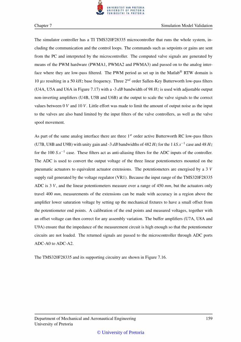
Chapter 7 Simulation Model Validation
The simulator controller has a TI TMS320F28335 microcontroller that runs the whole system, in-
cluding the communication and the control loops. The commands such as setpoints or gains are sent
from the PC and interpreted by the microcontroller. The computed valve signals are generated by
means of the PWM hardware (PWMA1, PWMA2 and PWMA3) and passed on to the analog inter-
face where they are low-pass filtered. The PWM period as set up in the Matlab® RTW domain is
10 µs resulting in a 50 kHz base frequency. Three 2nd order Sallen-Key Butterworth low-pass filters
(U4A, U5A and U6A in Figure 7.17) with a -3 dB bandwidth of 98 Hz is used with adjustable output
non-inverting amplifiers (U4B, U5B and U6B) at the output to scale the valve signals to the correct
values between 0 V and 10 V . Little effort was made to limit the amount of output noise as the input
to the valves are also band limited by the input filters of the valve controllers, as well as the valve
spool movement.
As part of the same analog interface there are three 1st order active Butterworth RC low-pass filters
(U7B, U8B and U9B) with unity gain and -3 dB bandwidths of 482 Hz for the 1 kS.s−1 case and 48 Hz
for the 100 S.s−1 case. These filters act as anti-aliasing filters for the ADC inputs of the controller.
The ADC is used to convert the output voltage of the three linear potentiometers mounted on the
pneumatic actuators to equivalent actuator extensions. The potentiometers are energised by a 3 V
supply rail generated by the voltage regulator (VR1). Because the input range of the TMS320F28335
ADC is 3 V , and the linear potentiometers measure over a range of 450 mm, but the actuators only
travel 400 mm, measurements of the extensions can be made with accuracy in a region above the
amplifier lower saturation voltage by setting up the mechanical fixtures to have a small offset from
the potentiometer end points. A calibration of the end points and measured voltages, together with
an offset voltage can then correct for any assembly variation. The buffer amplifiers (U7A, U8A and
U9A) ensure that the impedance of the measurement circuit is high enough so that the potentiometer
circuits are not loaded. The returned signals are passed to the microcontroller through ADC ports
ADC-A0 to ADC-A2.
The TMS320F28335 and its supporting circuitry are shown in Figure 7.16.
Department of Mechanical and Aeronautical EngineeringUniversity of Pretoria
159
© University of Pretoria
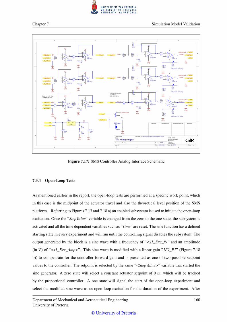
Chapter 7 Simulation Model Validation
1
1
2
2
3
3
4
4
D D
C C
B B
A A
CSIR - DPSSMeiring Naude RdBrummeriaPretoriaSouth Africa1.00
11/02/2015 12:39:56
D:\Altium\Projects\SMS\AnalogInterface.SchDocTitle:
Size: Doc No:Date:
File name:
Revision:
Sheet ofTime:
A4
SMS Analog Interface
Classification:
Item No:
Revision: Revision Date: Approval Signature: ECP No:12V
VPos1
VMLO3
Gnd
VMLO2
VMLO1
VPos2
VPos3
GND
12V
Vin VoutGND
VR1LM317
157RR13
220RR14
GND
3V
100uF16V
C7100uF16V
C14
GNDGND
5
67B
84
U7BAD822AN
100nC15
3k3
R27
12V
GNDGND
5
67B
84
U8BAD822AN
100nC16
3k3
R28
GND
5
67B
84
U9BAD822AN
100nC17
3k3
R29
GND
Butterworth LP Filter-3dB BW: 482 Hz
24V
K1
Relay-SPDT
24VSwitched
GND
D2
1N4148
24VEnable
VMLOEx1
VMLOEx2
VMLOEx3
GND
MLO1Gnd
MLO2Gnd
MLO3Gnd
GND
GND
3V
3V
3V 2
31A
84
U7AAD822AN
1k
R24
2
31A
84
U8AAD822AN
12V
GND
1k
R25
2
31A
84
U9AAD822AN
12V
GND
1k
R26
2
31A
84
U4AAD822AN
GND
12V
8k2
R7
15k
R10
220n
C11
100nC8
GND
PWM15
67B
84
U4BAD822AN
50KR21
10kR18
GND
1k
R15
PWM1
PWM2
VMPYE1
VMPYE2
PWM3 VMPYE3
Adjust to 0-10V swing
VValve1
2
31A
84
U5AAD822AN
GND
12V
8k2
R8
15k
R11
220n
C12
100nC9
GND
PWM25
67B
84
U5BAD822AN
50KR22
10kR19
GND
1k
R16
Adjust to 0-10V swing
VValve2
2
31A
84
U6AAD822AN
GND
12V
8k2
R9
15k
R12
220n
C13
100nC10
GND
PWM35
67B
84
U6BAD822AN
50KR23
10kR20
GND
1k
R17
Adjust to 0-10V swing
VValve3
Butterworth LP FilterSallen Key-3dB BW: 98 Hz
24V1
24V2
24V3
0V1
0V2
0V3
24VSwitched
24VSwitched
24VSwitched
GND
GND
GND
Figure 7.17: SMS Controller Analog Interface Schematic
7.3.4 Open-Loop Tests
As mentioned earlier in the report, the open-loop tests are performed at a specific work point, which
in this case is the midpoint of the actuator travel and also the theoretical level position of the SMS
platform. Referring to Figures 7.13 and 7.18 a) an enabled subsystem is used to initiate the open-loop
excitation. Once the ”StepValue” variable is changed from the zero to the one state, the subsystem is
activated and all the time dependent variables such as ”Time” are reset. The sine function has a defined
starting state in every experiment and will run until the controlling signal disables the subsystem. The
output generated by the block is a sine wave with a frequency of ”<x1_Exc_f>” and an amplitude
(in V ) of ”<x1_Ecx_Amp>”. This sine wave is modified with a linear gain ”1/G_P1” (Figure 7.18
b)) to compensate for the controller forward gain and is presented as one of two possible setpoint
values to the controller. The setpoint is selected by the same ”<StepValue>” variable that started the
sine generator. A zero state will select a constant actuator setpoint of 0 m, which will be tracked
by the proportional controller. A one state will signal the start of the open-loop experiment and
select the modified sine wave as an open-loop excitation for the duration of the experiment. After
Department of Mechanical and Aeronautical EngineeringUniversity of Pretoria
160
© University of Pretoria
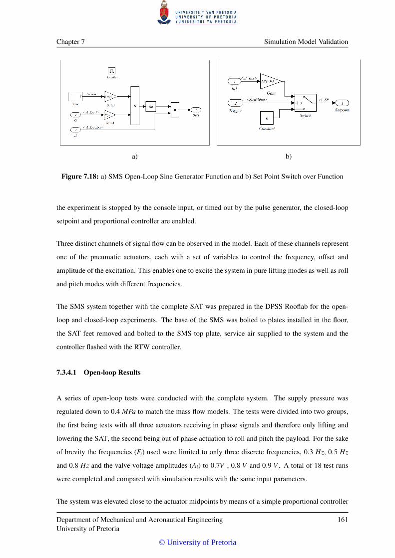
Chapter 7 Simulation Model Validation
a) b)
Figure 7.18: a) SMS Open-Loop Sine Generator Function and b) Set Point Switch over Function
the experiment is stopped by the console input, or timed out by the pulse generator, the closed-loop
setpoint and proportional controller are enabled.
Three distinct channels of signal flow can be observed in the model. Each of these channels represent
one of the pneumatic actuators, each with a set of variables to control the frequency, offset and
amplitude of the excitation. This enables one to excite the system in pure lifting modes as well as roll
and pitch modes with different frequencies.
The SMS system together with the complete SAT was prepared in the DPSS Rooflab for the open-
loop and closed-loop experiments. The base of the SMS was bolted to plates installed in the floor,
the SAT feet removed and bolted to the SMS top plate, service air supplied to the system and the
controller flashed with the RTW controller.
7.3.4.1 Open-loop Results
A series of open-loop tests were conducted with the complete system. The supply pressure was
regulated down to 0.4 MPa to match the mass flow models. The tests were divided into two groups,
the first being tests with all three actuators receiving in phase signals and therefore only lifting and
lowering the SAT, the second being out of phase actuation to roll and pitch the payload. For the sake
of brevity the frequencies (Fi) used were limited to only three discrete frequencies, 0.3 Hz, 0.5 Hz
and 0.8 Hz and the valve voltage amplitudes (Ai) to 0.7V , 0.8 V and 0.9 V . A total of 18 test runs
were completed and compared with simulation results with the same input parameters.
The system was elevated close to the actuator midpoints by means of a simple proportional controller
Department of Mechanical and Aeronautical EngineeringUniversity of Pretoria
161
© University of Pretoria
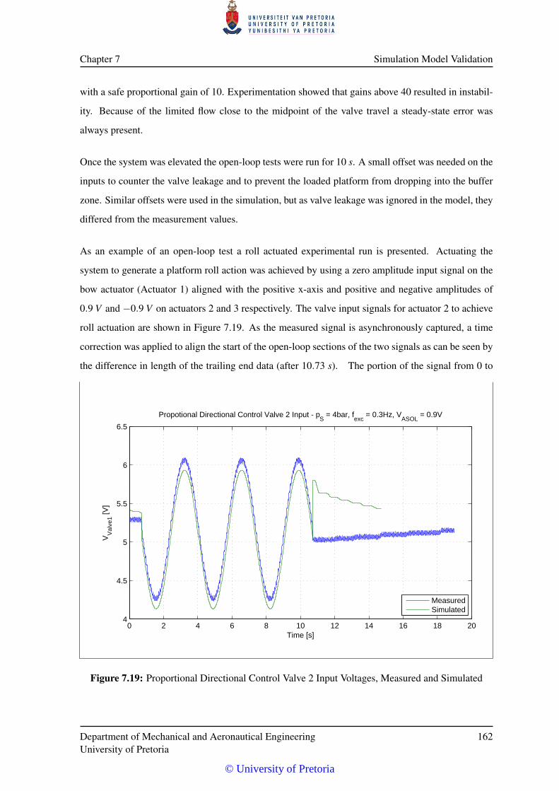
Chapter 7 Simulation Model Validation
with a safe proportional gain of 10. Experimentation showed that gains above 40 resulted in instabil-
ity. Because of the limited flow close to the midpoint of the valve travel a steady-state error was
always present.
Once the system was elevated the open-loop tests were run for 10 s. A small offset was needed on the
inputs to counter the valve leakage and to prevent the loaded platform from dropping into the buffer
zone. Similar offsets were used in the simulation, but as valve leakage was ignored in the model, they
differed from the measurement values.
As an example of an open-loop test a roll actuated experimental run is presented. Actuating the
system to generate a platform roll action was achieved by using a zero amplitude input signal on the
bow actuator (Actuator 1) aligned with the positive x-axis and positive and negative amplitudes of
0.9 V and −0.9 V on actuators 2 and 3 respectively. The valve input signals for actuator 2 to achieve
roll actuation are shown in Figure 7.19. As the measured signal is asynchronously captured, a time
correction was applied to align the start of the open-loop sections of the two signals as can be seen by
the difference in length of the trailing end data (after 10.73 s). The portion of the signal from 0 to
0 2 4 6 8 10 12 14 16 18 204
4.5
5
5.5
6
6.5
Propotional Directional Control Valve 2 Input - pS = 4bar, f
exc = 0.3Hz, V
ASOL = 0.9V
Time [s]
VV
alve
1 [V
]
MeasuredSimulated
Figure 7.19: Proportional Directional Control Valve 2 Input Voltages, Measured and Simulated
Department of Mechanical and Aeronautical EngineeringUniversity of Pretoria
162
© University of Pretoria
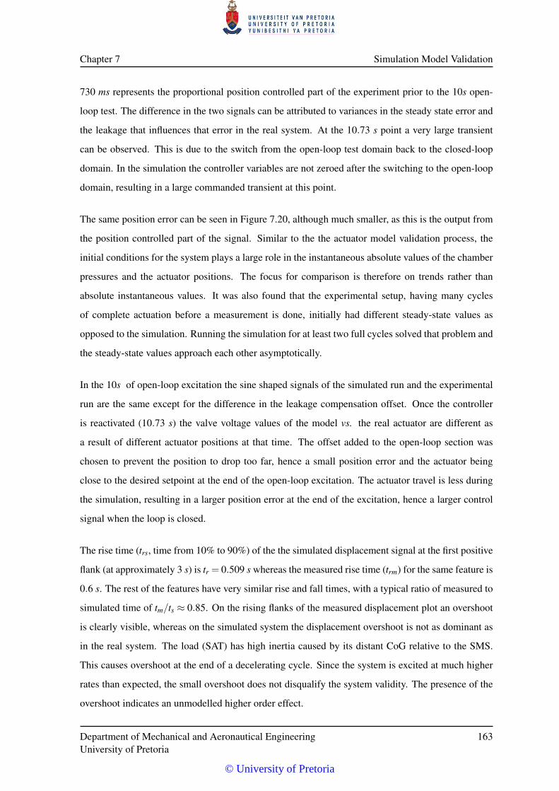
Chapter 7 Simulation Model Validation
730 ms represents the proportional position controlled part of the experiment prior to the 10s open-
loop test. The difference in the two signals can be attributed to variances in the steady state error and
the leakage that influences that error in the real system. At the 10.73 s point a very large transient
can be observed. This is due to the switch from the open-loop test domain back to the closed-loop
domain. In the simulation the controller variables are not zeroed after the switching to the open-loop
domain, resulting in a large commanded transient at this point.
The same position error can be seen in Figure 7.20, although much smaller, as this is the output from
the position controlled part of the signal. Similar to the the actuator model validation process, the
initial conditions for the system plays a large role in the instantaneous absolute values of the chamber
pressures and the actuator positions. The focus for comparison is therefore on trends rather than
absolute instantaneous values. It was also found that the experimental setup, having many cycles
of complete actuation before a measurement is done, initially had different steady-state values as
opposed to the simulation. Running the simulation for at least two full cycles solved that problem and
the steady-state values approach each other asymptotically.
In the 10s of open-loop excitation the sine shaped signals of the simulated run and the experimental
run are the same except for the difference in the leakage compensation offset. Once the controller
is reactivated (10.73 s) the valve voltage values of the model vs. the real actuator are different as
a result of different actuator positions at that time. The offset added to the open-loop section was
chosen to prevent the position to drop too far, hence a small position error and the actuator being
close to the desired setpoint at the end of the open-loop excitation. The actuator travel is less during
the simulation, resulting in a larger position error at the end of the excitation, hence a larger control
signal when the loop is closed.
The rise time (trs, time from 10% to 90%) of the the simulated displacement signal at the first positive
flank (at approximately 3 s) is tr = 0.509 s whereas the measured rise time (trm) for the same feature is
0.6 s. The rest of the features have very similar rise and fall times, with a typical ratio of measured to
simulated time of tm/ts ≈ 0.85. On the rising flanks of the measured displacement plot an overshoot
is clearly visible, whereas on the simulated system the displacement overshoot is not as dominant as
in the real system. The load (SAT) has high inertia caused by its distant CoG relative to the SMS.
This causes overshoot at the end of a decelerating cycle. Since the system is excited at much higher
rates than expected, the small overshoot does not disqualify the system validity. The presence of the
overshoot indicates an unmodelled higher order effect.
Department of Mechanical and Aeronautical EngineeringUniversity of Pretoria
163
© University of Pretoria
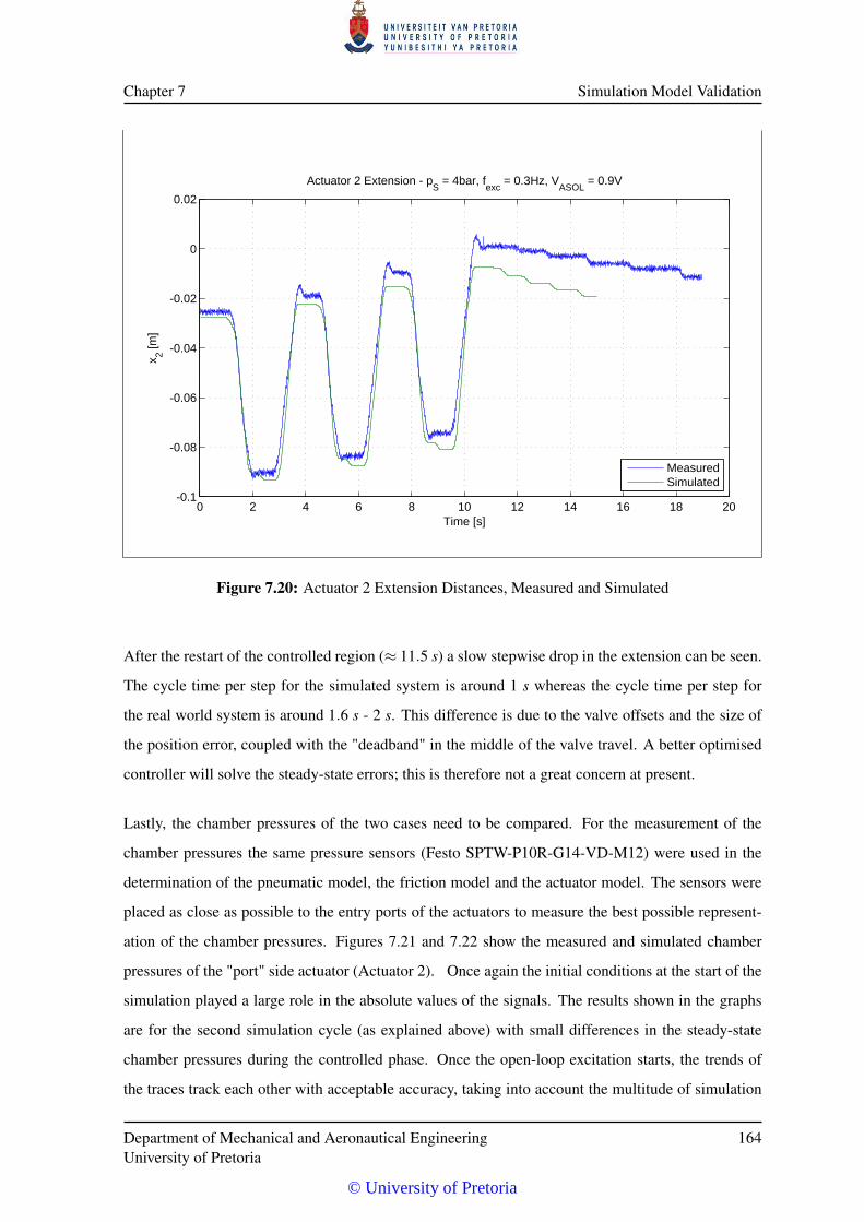
Chapter 7 Simulation Model Validation
0 2 4 6 8 10 12 14 16 18 20-0.1
-0.08
-0.06
-0.04
-0.02
0
0.02
Actuator 2 Extension - pS = 4bar, f
exc = 0.3Hz, V
ASOL = 0.9V
Time [s]
x 2 [m]
MeasuredSimulated
Figure 7.20: Actuator 2 Extension Distances, Measured and Simulated
After the restart of the controlled region (≈ 11.5 s) a slow stepwise drop in the extension can be seen.
The cycle time per step for the simulated system is around 1 s whereas the cycle time per step for
the real world system is around 1.6 s - 2 s. This difference is due to the valve offsets and the size of
the position error, coupled with the "deadband" in the middle of the valve travel. A better optimised
controller will solve the steady-state errors; this is therefore not a great concern at present.
Lastly, the chamber pressures of the two cases need to be compared. For the measurement of the
chamber pressures the same pressure sensors (Festo SPTW-P10R-G14-VD-M12) were used in the
determination of the pneumatic model, the friction model and the actuator model. The sensors were
placed as close as possible to the entry ports of the actuators to measure the best possible represent-
ation of the chamber pressures. Figures 7.21 and 7.22 show the measured and simulated chamber
pressures of the "port" side actuator (Actuator 2). Once again the initial conditions at the start of the
simulation played a large role in the absolute values of the signals. The results shown in the graphs
are for the second simulation cycle (as explained above) with small differences in the steady-state
chamber pressures during the controlled phase. Once the open-loop excitation starts, the trends of
the traces track each other with acceptable accuracy, taking into account the multitude of simulation
Department of Mechanical and Aeronautical EngineeringUniversity of Pretoria
164
© University of Pretoria
Chapter 7 Simulation Model Validation
0 2 4 6 8 10 12 14 16 18 202.9
3
3.1
3.2
3.3
3.4
3.5
3.6
3.7x 10
5 Lower Chamber Pressure for Actuator 2 - pS = 4bar, f
exc = 0.3Hz, V
ASOL = 0.9V
Time [s]
p L1 [P
a]
MeasuredSimulated
Figure 7.21: Actuator 2 Lower Chamber Pressure, Measured and Simulated
errors that accumulate. Although all the high frequency components are not modelled, the behaviour
is the same, and there is not significant delays or instabilities. The simulated system also seems to
have a more damped response than the real system, as the ringing at the end of the cycles are less
pronounced. This behaviour will need to be taken into account once the controller stability comes
into play. A controller that synthesises a marginally stable simulated system could cause instability
in the real hardware.
Taking the experimental results of the open-loop tests and comparing them visually with that of the
model, a high level of similarity can be seen. A reinforcing of the test of ”likeness” is the use of the
normalised cross-correlation operation and the determining of the cross-correlation coefficient. Per
definition this is a value between −1 and 1 where 1 means a perfect fit, zero means no correlation at
all and −1 means an anti-correlation. We will therefore strive for a value as close as possible to one.
Using Matlab’s definition of normalised cross-correlation as shown in eq. 7.2 and using the zero lag
Department of Mechanical and Aeronautical EngineeringUniversity of Pretoria
165
© University of Pretoria
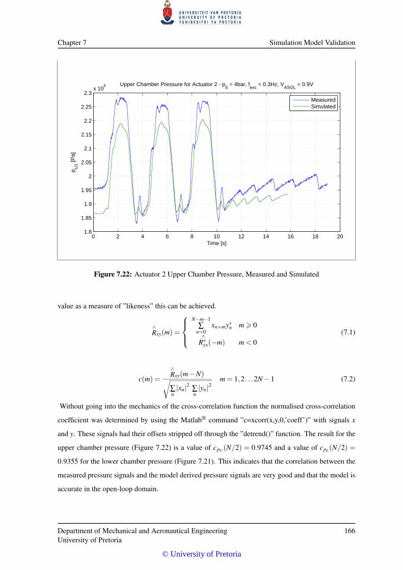
Chapter 7 Simulation Model Validation
0 2 4 6 8 10 12 14 16 18 201.8
1.85
1.9
1.95
2
2.05
2.1
2.15
2.2
2.25
2.3x 10
5 Upper Chamber Pressure for Actuator 2 - pS = 4bar, f
exc = 0.3Hz, V
ASOL = 0.9V
Time [s]
p U1 [P
a]
MeasuredSimulated
Figure 7.22: Actuator 2 Upper Chamber Pressure, Measured and Simulated
value as a measure of ”likeness” this can be achieved.
∧Rxy(m) =
N−m−1
∑n=0
xn+my∗n m > 0∧
R∗yx(−m) m < 0(7.1)
c(m) =
∧Rxy(m−N)√∑n|xn|2 ∑
n|yn|2
m = 1,2 . . .2N−1 (7.2)
Without going into the mechanics of the cross-correlation function the normalised cross-correlation
coefficient was determined by using the Matlab® command ”c=xcorr(x,y,0,’coeff’)” with signals x
and y. These signals had their offsets stripped off through the ”detrend()” function. The result for the
upper chamber pressure (Figure 7.22) is a value of cpU (N/2) = 0.9745 and a value of cpL(N/2) =
0.9355 for the lower chamber pressure (Figure 7.21). This indicates that the correlation between the
measured pressure signals and the model derived pressure signals are very good and that the model is
accurate in the open-loop domain.
Department of Mechanical and Aeronautical EngineeringUniversity of Pretoria
166
© University of Pretoria
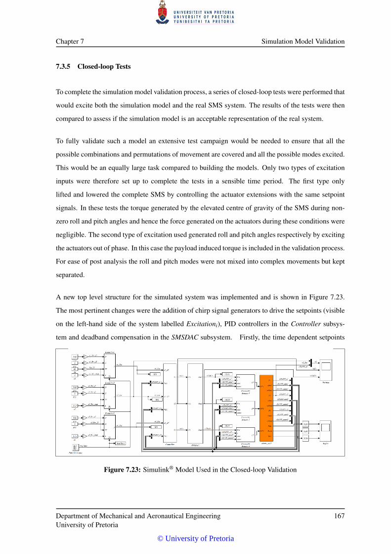
Chapter 7 Simulation Model Validation
7.3.5 Closed-loop Tests
To complete the simulation model validation process, a series of closed-loop tests were performed that
would excite both the simulation model and the real SMS system. The results of the tests were then
compared to assess if the simulation model is an acceptable representation of the real system.
To fully validate such a model an extensive test campaign would be needed to ensure that all the
possible combinations and permutations of movement are covered and all the possible modes excited.
This would be an equally large task compared to building the models. Only two types of excitation
inputs were therefore set up to complete the tests in a sensible time period. The first type only
lifted and lowered the complete SMS by controlling the actuator extensions with the same setpoint
signals. In these tests the torque generated by the elevated centre of gravity of the SMS during non-
zero roll and pitch angles and hence the force generated on the actuators during these conditions were
negligible. The second type of excitation used generated roll and pitch angles respectively by exciting
the actuators out of phase. In this case the payload induced torque is included in the validation process.
For ease of post analysis the roll and pitch modes were not mixed into complex movements but kept
separated.
A new top level structure for the simulated system was implemented and is shown in Figure 7.23.
The most pertinent changes were the addition of chirp signal generators to drive the setpoints (visible
on the left-hand side of the system labelled Excitationi), PID controllers in the Controller subsys-
tem and deadband compensation in the SMSDAC subsystem. Firstly, the time dependent setpoints
Figure 7.23: Simulink® Model Used in the Closed-loop Validation
Department of Mechanical and Aeronautical EngineeringUniversity of Pretoria
167
© University of Pretoria
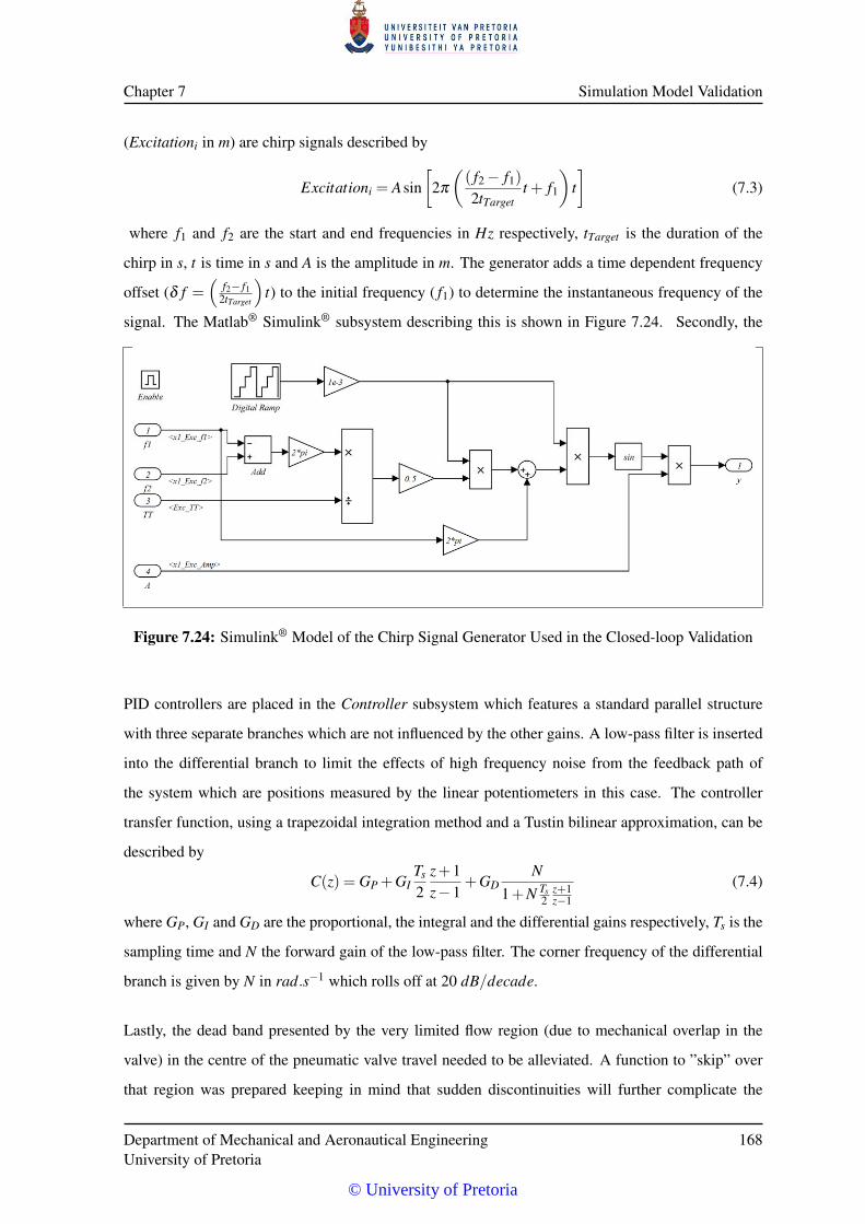
Chapter 7 Simulation Model Validation
(Excitationi in m) are chirp signals described by
Excitationi = Asin[
2π
(( f2− f1)
2tTargett + f1
)t]
(7.3)
where f1 and f2 are the start and end frequencies in Hz respectively, tTarget is the duration of the
chirp in s, t is time in s and A is the amplitude in m. The generator adds a time dependent frequency
offset (δ f =(
f2− f12tTarget
)t) to the initial frequency ( f1) to determine the instantaneous frequency of the
signal. The Matlab® Simulink® subsystem describing this is shown in Figure 7.24. Secondly, the
Figure 7.24: Simulink® Model of the Chirp Signal Generator Used in the Closed-loop Validation
PID controllers are placed in the Controller subsystem which features a standard parallel structure
with three separate branches which are not influenced by the other gains. A low-pass filter is inserted
into the differential branch to limit the effects of high frequency noise from the feedback path of
the system which are positions measured by the linear potentiometers in this case. The controller
transfer function, using a trapezoidal integration method and a Tustin bilinear approximation, can be
described by
C(z) = GP +GITs
2z+1z−1
+GDN
1+N Ts2
z+1z−1
(7.4)
where GP, GI and GD are the proportional, the integral and the differential gains respectively, Ts is the
sampling time and N the forward gain of the low-pass filter. The corner frequency of the differential
branch is given by N in rad.s−1 which rolls off at 20 dB/decade.
Lastly, the dead band presented by the very limited flow region (due to mechanical overlap in the
valve) in the centre of the pneumatic valve travel needed to be alleviated. A function to ”skip” over
that region was prepared keeping in mind that sudden discontinuities will further complicate the
Department of Mechanical and Aeronautical EngineeringUniversity of Pretoria
168
© University of Pretoria
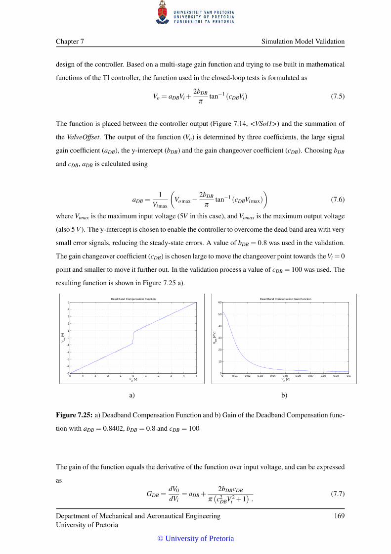
Chapter 7 Simulation Model Validation
design of the controller. Based on a multi-stage gain function and trying to use built in mathematical
functions of the TI controller, the function used in the closed-loop tests is formulated as
Vo = aDBVi +2bDB
πtan−1 (cDBVi) (7.5)
The function is placed between the controller output (Figure 7.14, <VSol1>) and the summation of
the ValveOffset. The output of the function (Vo) is determined by three coefficients, the large signal
gain coefficient (aDB), the y-intercept (bDB) and the gain changeover coefficient (cDB). Choosing bDB
and cDB, aDB is calculated using
aDB =1
Vimax
(Vomax−
2bDB
πtan−1 (cDBVimax)
)(7.6)
where Vimax is the maximum input voltage (5V in this case), and Vomax is the maximum output voltage
(also 5 V ). The y-intercept is chosen to enable the controller to overcome the dead band area with very
small error signals, reducing the steady-state errors. A value of bDB = 0.8 was used in the validation.
The gain changeover coefficient (cDB) is chosen large to move the changeover point towards the Vi = 0
point and smaller to move it further out. In the validation process a value of cDB = 100 was used. The
resulting function is shown in Figure 7.25 a).
-5 -4 -3 -2 -1 0 1 2 3 4 5-5
-4
-3
-2
-1
0
1
2
3
4
5Dead Band Compensation Function
Vin
[V]
Vou
t [V]
0 0.01 0.02 0.03 0.04 0.05 0.06 0.07 0.08 0.09 0.10
10
20
30
40
50
60Dead Band Compensation Gain Function
Vin
[V]
GD
B [V
/V]
a) b)
Figure 7.25: a) Deadband Compensation Function and b) Gain of the Deadband Compensation func-
tion with aDB = 0.8402, bDB = 0.8 and cDB = 100
The gain of the function equals the derivative of the function over input voltage, and can be expressed
as
GDB =dV0
dVi= aDB +
2bDBcDB
π(c2
DBV 2i +1
).
(7.7)
Department of Mechanical and Aeronautical EngineeringUniversity of Pretoria
169
© University of Pretoria
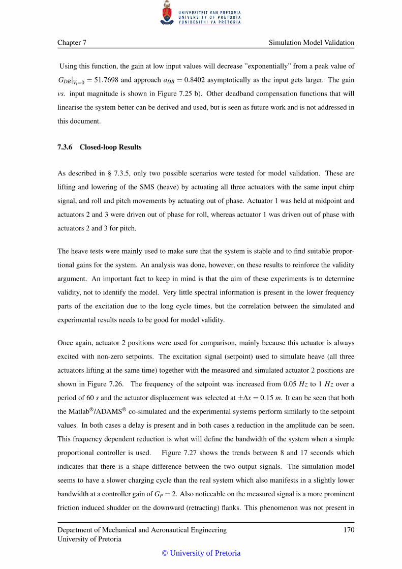
Chapter 7 Simulation Model Validation
Using this function, the gain at low input values will decrease ”exponentially” from a peak value of
GDB|Vi=0 = 51.7698 and approach aDB = 0.8402 asymptotically as the input gets larger. The gain
vs. input magnitude is shown in Figure 7.25 b). Other deadband compensation functions that will
linearise the system better can be derived and used, but is seen as future work and is not addressed in
this document.
7.3.6 Closed-loop Results
As described in § 7.3.5, only two possible scenarios were tested for model validation. These are
lifting and lowering of the SMS (heave) by actuating all three actuators with the same input chirp
signal, and roll and pitch movements by actuating out of phase. Actuator 1 was held at midpoint and
actuators 2 and 3 were driven out of phase for roll, whereas actuator 1 was driven out of phase with
actuators 2 and 3 for pitch.
The heave tests were mainly used to make sure that the system is stable and to find suitable propor-
tional gains for the system. An analysis was done, however, on these results to reinforce the validity
argument. An important fact to keep in mind is that the aim of these experiments is to determine
validity, not to identify the model. Very little spectral information is present in the lower frequency
parts of the excitation due to the long cycle times, but the correlation between the simulated and
experimental results needs to be good for model validity.
Once again, actuator 2 positions were used for comparison, mainly because this actuator is always
excited with non-zero setpoints. The excitation signal (setpoint) used to simulate heave (all three
actuators lifting at the same time) together with the measured and simulated actuator 2 positions are
shown in Figure 7.26. The frequency of the setpoint was increased from 0.05 Hz to 1 Hz over a
period of 60 s and the actuator displacement was selected at ±∆x = 0.15 m. It can be seen that both
the Matlab®/ADAMS® co-simulated and the experimental systems perform similarly to the setpoint
values. In both cases a delay is present and in both cases a reduction in the amplitude can be seen.
This frequency dependent reduction is what will define the bandwidth of the system when a simple
proportional controller is used. Figure 7.27 shows the trends between 8 and 17 seconds which
indicates that there is a shape difference between the two output signals. The simulation model
seems to have a slower charging cycle than the real system which also manifests in a slightly lower
bandwidth at a controller gain of GP = 2. Also noticeable on the measured signal is a more prominent
friction induced shudder on the downward (retracting) flanks. This phenomenon was not present in
Department of Mechanical and Aeronautical EngineeringUniversity of Pretoria
170
© University of Pretoria
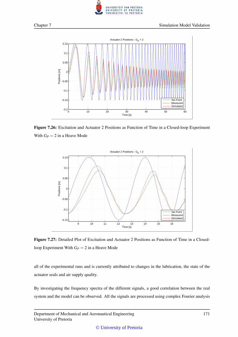
Chapter 7 Simulation Model Validation
0 10 20 30 40 50 60-0.2
-0.15
-0.1
-0.05
0
0.05
0.1
0.15
Actuator 2 Positions - GP = 2
Time [s]
Pos
ition
s [m
]
Set PointMeasuredSimulated
Figure 7.26: Excitation and Actuator 2 Positions as Function of Time in a Closed-loop Experiment
With GP = 2 in a Heave Mode
9 10 11 12 13 14 15 16
-0.15
-0.1
-0.05
0
0.05
0.1
0.15
Actuator 2 Positions - GP = 2
Time [s]
Pos
ition
s [m
]
Set PointMeasuredSimulated
Figure 7.27: Detailed Plot of Excitation and Actuator 2 Positions as Function of Time in a Closed-
loop Experiment With GP = 2 in a Heave Mode
all of the experimental runs and is currently attributed to changes in the lubrication, the state of the
actuator seals and air supply quality.
By investigating the frequency spectra of the different signals, a good correlation between the real
system and the model can be observed. All the signals are processed using complex Fourier analysis
Department of Mechanical and Aeronautical EngineeringUniversity of Pretoria
171
© University of Pretoria
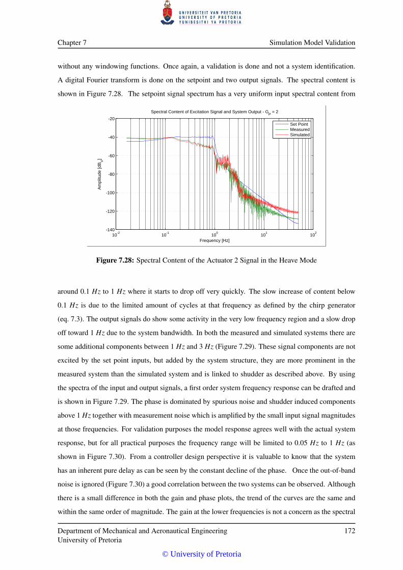
Chapter 7 Simulation Model Validation
without any windowing functions. Once again, a validation is done and not a system identification.
A digital Fourier transform is done on the setpoint and two output signals. The spectral content is
shown in Figure 7.28. The setpoint signal spectrum has a very uniform input spectral content from
10-2
10-1
100
101
102
-140
-120
-100
-80
-60
-40
-20
Spectral Content of Excitation Signal and System Output - GP = 2
Frequency [Hz]
Am
plitu
de [d
BV]
Set PointMeasuredSimulated
Figure 7.28: Spectral Content of the Actuator 2 Signal in the Heave Mode
around 0.1 Hz to 1 Hz where it starts to drop off very quickly. The slow increase of content below
0.1 Hz is due to the limited amount of cycles at that frequency as defined by the chirp generator
(eq. 7.3). The output signals do show some activity in the very low frequency region and a slow drop
off toward 1 Hz due to the system bandwidth. In both the measured and simulated systems there are
some additional components between 1 Hz and 3 Hz (Figure 7.29). These signal components are not
excited by the set point inputs, but added by the system structure, they are more prominent in the
measured system than the simulated system and is linked to shudder as described above. By using
the spectra of the input and output signals, a first order system frequency response can be drafted and
is shown in Figure 7.29. The phase is dominated by spurious noise and shudder induced components
above 1 Hz together with measurement noise which is amplified by the small input signal magnitudes
at those frequencies. For validation purposes the model response agrees well with the actual system
response, but for all practical purposes the frequency range will be limited to 0.05 Hz to 1 Hz (as
shown in Figure 7.30). From a controller design perspective it is valuable to know that the system
has an inherent pure delay as can be seen by the constant decline of the phase. Once the out-of-band
noise is ignored (Figure 7.30) a good correlation between the two systems can be observed. Although
there is a small difference in both the gain and phase plots, the trend of the curves are the same and
within the same order of magnitude. The gain at the lower frequencies is not a concern as the spectral
Department of Mechanical and Aeronautical EngineeringUniversity of Pretoria
172
© University of Pretoria
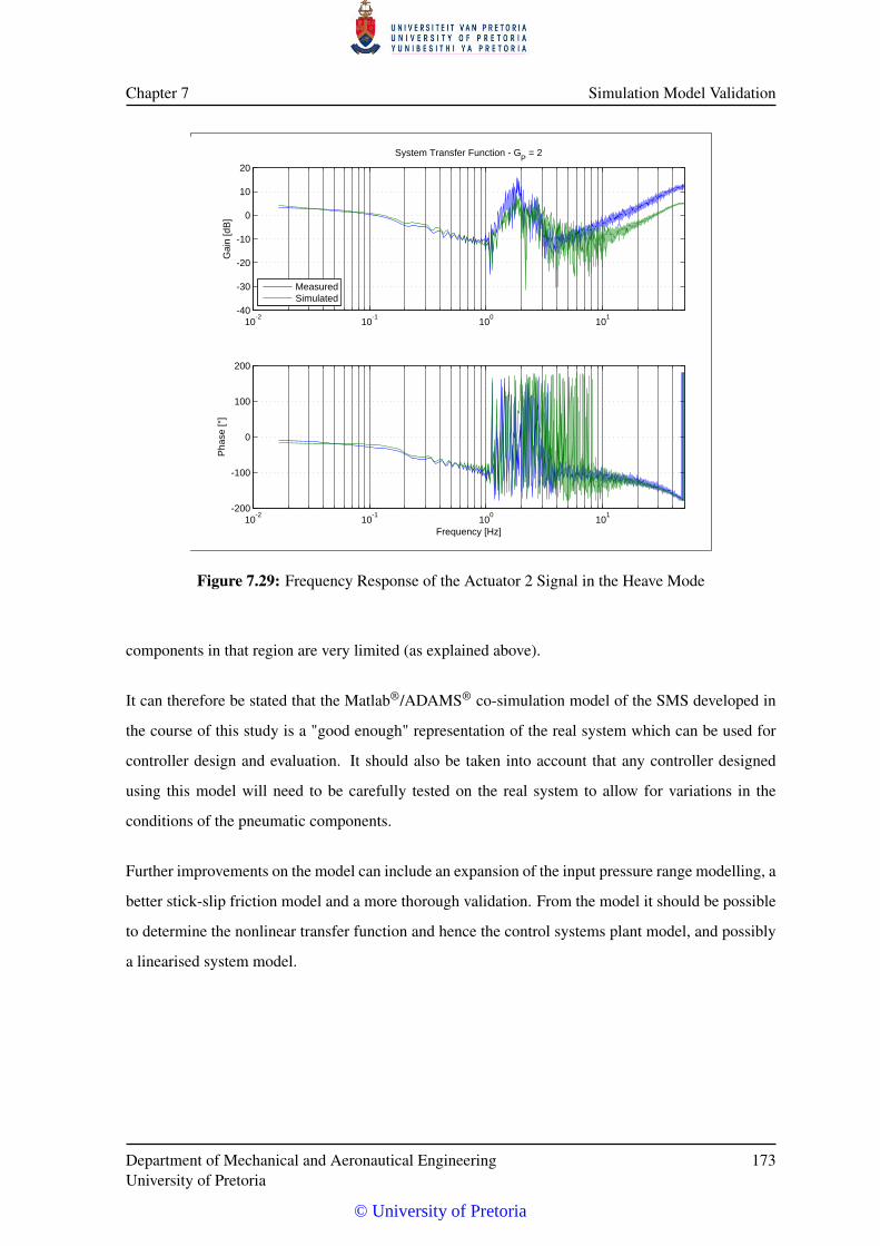
Chapter 7 Simulation Model Validation
10-2
10-1
100
101
-40
-30
-20
-10
0
10
20
Gai
n [d
B]
System Transfer Function - GP = 2
10-2
10-1
100
101
-200
-100
0
100
200
Frequency [Hz]
Pha
se [°
]
MeasuredSimulated
Figure 7.29: Frequency Response of the Actuator 2 Signal in the Heave Mode
components in that region are very limited (as explained above).
It can therefore be stated that the Matlab®/ADAMS® co-simulation model of the SMS developed in
the course of this study is a "good enough" representation of the real system which can be used for
controller design and evaluation. It should also be taken into account that any controller designed
using this model will need to be carefully tested on the real system to allow for variations in the
conditions of the pneumatic components.
Further improvements on the model can include an expansion of the input pressure range modelling, a
better stick-slip friction model and a more thorough validation. From the model it should be possible
to determine the nonlinear transfer function and hence the control systems plant model, and possibly
a linearised system model.
Department of Mechanical and Aeronautical EngineeringUniversity of Pretoria
173
© University of Pretoria
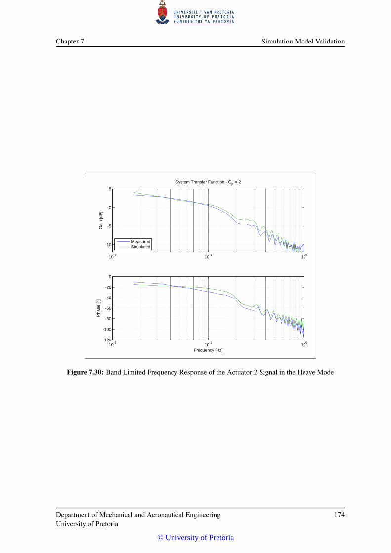
Chapter 7 Simulation Model Validation
10-2
10-1
100
-10
-5
0
5
Gai
n [d
B]
System Transfer Function - GP = 2
10-2
10-1
100
-120
-100
-80
-60
-40
-20
0
Frequency [Hz]
Pha
se [°
]
MeasuredSimulated
Figure 7.30: Band Limited Frequency Response of the Actuator 2 Signal in the Heave Mode
Department of Mechanical and Aeronautical EngineeringUniversity of Pretoria
174
© University of Pretoria
CHAPTER 8
SMS CONTROLLER
The mathematical model for the SMS system carrying a payload similar to the SAT was derived from
first principles in chapters 3 to 6. This model was validated in chapter 7.3 and can be described as an
acceptable representation of the real system. The high fidelity model is too complex for the purpose
of classical controller design and has to be simplified to a characteristic level. A controller can be
designed with this simple model to reach the specification set out at the start of the study. It can
then be tested with the high fidelity Matlab®/ADAMS® model and then transferred to the real system
once stability has been achieved. This method has been adopted to protect the equipment on the SAT
during controller development.
This chapter details the simplified SMS model with some assumptions, the design of controllers
using the root locus design method as well as state feedback compensation and some simulation
results.
8.1 SIMPLIFIED PLANT MODEL
Refer back to the closed-loop frequency response curve of the SMS (Figure 7.29) obtained from a
chirp input signal and a proportional controlled system with a controller gain of two. The shape
of the response is characteristic of a system with a flat low frequency response that drops off at
approximately 10 dB per decade from 0.1 Hz to 1 Hz. The phase decreases monotonically from
around −20◦ at 0.05 Hz down to −100◦ at 1 Hz. A lack of excitation frequency components above
1 Hz makes it impossible to determine the high frequency gain or phase roll-off.
A simple characteristic model is proposed by Šitum et al. [16] that describes the pneumatic actuator
and load as a mass and double spring system with viscous friction and it is shown in Figure 8.1.
© University of Pretoria
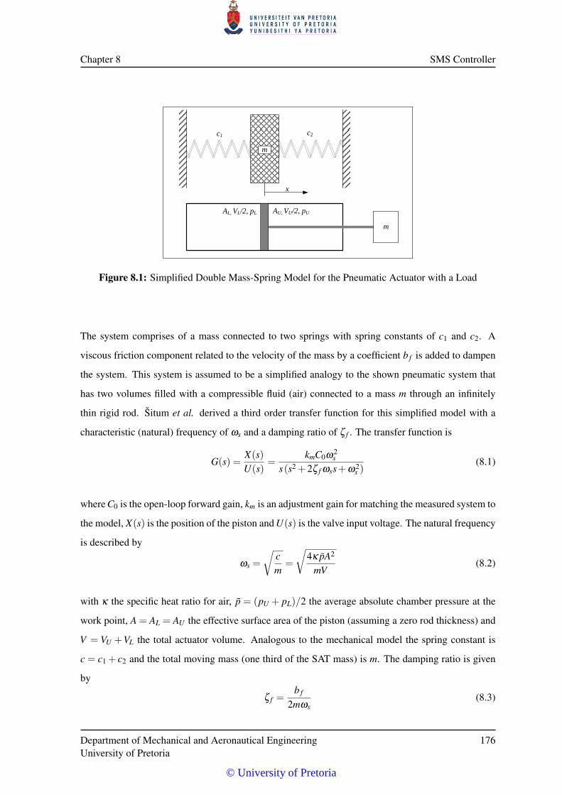
Chapter 8 SMS Controller
x
m
c1 c2
AL, VL/2, pL AU, VU/2, pU
m
Figure 8.1: Simplified Double Mass-Spring Model for the Pneumatic Actuator with a Load
The system comprises of a mass connected to two springs with spring constants of c1 and c2. A
viscous friction component related to the velocity of the mass by a coefficient b f is added to dampen
the system. This system is assumed to be a simplified analogy to the shown pneumatic system that
has two volumes filled with a compressible fluid (air) connected to a mass m through an infinitely
thin rigid rod. Šitum et al. derived a third order transfer function for this simplified model with a
characteristic (natural) frequency of ωs and a damping ratio of ζ f . The transfer function is
G(s) =X(s)U(s)
=kmC0ω2
s
s(s2 +2ζ f ωss+ω2s )
(8.1)
where C0 is the open-loop forward gain, km is an adjustment gain for matching the measured system to
the model, X(s) is the position of the piston and U(s) is the valve input voltage. The natural frequency
is described by
ωs =
√cm
=
√4κ pA2
mV(8.2)
with κ the specific heat ratio for air, p = (pU + pL)/2 the average absolute chamber pressure at the
work point, A = AL = AU the effective surface area of the piston (assuming a zero rod thickness) and
V = VU +VL the total actuator volume. Analogous to the mechanical model the spring constant is
c = c1 + c2 and the total moving mass (one third of the SAT mass) is m. The damping ratio is given
by
ζ f =b f
2mωs(8.3)
Department of Mechanical and Aeronautical EngineeringUniversity of Pretoria
176
© University of Pretoria
Chapter 8 SMS Controller
where b f = 530 N.s.m−1 is the viscous friction coefficient as derived in § 6.4 and § 6.5.
A series of open-loop tests were performed with the Matlab®/ADAMS® simulation and the for-
ward gain (C0) determined from the resulting data. The nonlinear nature of the system came to
the forefront as the gain value varied from C0 = 0.1 m.s−1.V−1 for an input voltage of u = 5 V to
C0 = 0.85 m.s−1.V−1 for a voltage of u = 0.5 V . As the system will mostly be controlled in close
proximity of the setpoint (assuming decent setpoint tracking) the valve control voltages will be closer
to the lower limit of u = 0.5 V and therefore a C0 value of 0.85 m.s−1.V−1 was used. Smaller values
will put the system in the nonlinear region of the deadband compensation function and complicate
the simplified model.
Using the values determined in the pneumatic and friction modelling portions of the study the un-
known values for the model were determined (values shown in Appendix D, Table D.1) and the
transfer function populated. In order to compare the simplified model with the validated model the
loop was closed with a forward controller gain of Kp = 2 and the closed-loop transfer function derived
as
T (s) =X(s)R(s)
=KpG
1+KpG=
KpC0ω2s
s(s2 +2ζ f ωss+ω2s )+KpC0ω2
s .(8.4)
The gain and the phase of the simplified model frequency response was compared with the gain and
phase of the measured data frequency response, as well as the high-fidelity simulation model fre-
quency responses; all at 1 Hz. The adjustment gain (km) was iteratively changed until a representative
closed-loop model could be derived. It turned out that the adjustment gain was redundant and settled
on values close to km = 1. Comparing the frequency response of the complete nonlinear actuator
model and the that of the simplified model as shown in Figure 8.2, the gain in the nonlinear systems
(the real system and the Matlab®/ADAMS® model) is higher than 0 dB (as discussed in section 7.3.6)
and higher than that of the linear simplified model, but in both the systems it rolls off from approxim-
ately −1 dB at 0.1 Hz to approximately −11 dB at 1 Hz. The resonant peak in the simplified model
is situated at ≈ 4 Hz and cannot be compared to the nonlinear system due to the excitation bandwidth
limitation. The phase in both models is around −20◦ at the low frequencies and settles at around
−80◦ at 1 Hz.
From this comparison one can deduce that the simplified model has value in the design of a controller
for the SMS, and this will be discussed in the next section.
Department of Mechanical and Aeronautical EngineeringUniversity of Pretoria
177
© University of Pretoria
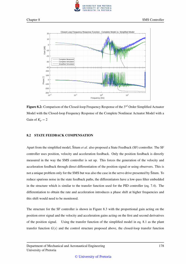
Chapter 8 SMS Controller
-40
-30
-20
-10
0
10
20
Gai
n [d
B]
Closed Loop Frequency Response Function - Complete Model vs. Simplified Model
Complete MeasuredComplete SimulatedSimplified Simulated
10-2 10-1 100 101
Frequency [Hz]
-300
-200
-100
0
100
200
Pha
se [°
]
Figure 8.2: Comparison of the Closed-loop Frequency Response of the 3rd Order Simplified Actuator
Model with the Closed-loop Frequency Response of the Complete Nonlinear Actuator Model with a
Gain of Kp = 2
8.2 STATE FEEDBACK COMPENSATION
Apart from the simplified model, Šitum et al. also proposed a State Feedback (SF) controller. The SF
controller uses position, velocity and acceleration feedback. Only the position feedback is directly
measured in the way the SMS controller is set up. This forces the generation of the velocity and
acceleration feedback through direct differentiation of the position signal or using observers. This is
not a unique problem only for the SMS but was also the case in the servo drive presented by Šitum. To
reduce spurious noise in the state feedback paths, the differentiators have a low-pass filter embedded
in the structure which is similar to the transfer function used for the PID controller (eq. 7.4). The
differentiation to obtain the rate and acceleration introduces a phase shift at higher frequencies and
this shift would need to be monitored.
The structure for the SF controller is shown in Figure 8.3 with the proportional gain acting on the
position error signal and the velocity and acceleration gains acting on the first and second derivatives
of the position signal. Using the transfer function of the simplified model in eq. 8.1 as the plant
transfer function G(s) and the control structure proposed above, the closed-loop transfer function
Department of Mechanical and Aeronautical EngineeringUniversity of Pretoria
178
© University of Pretoria
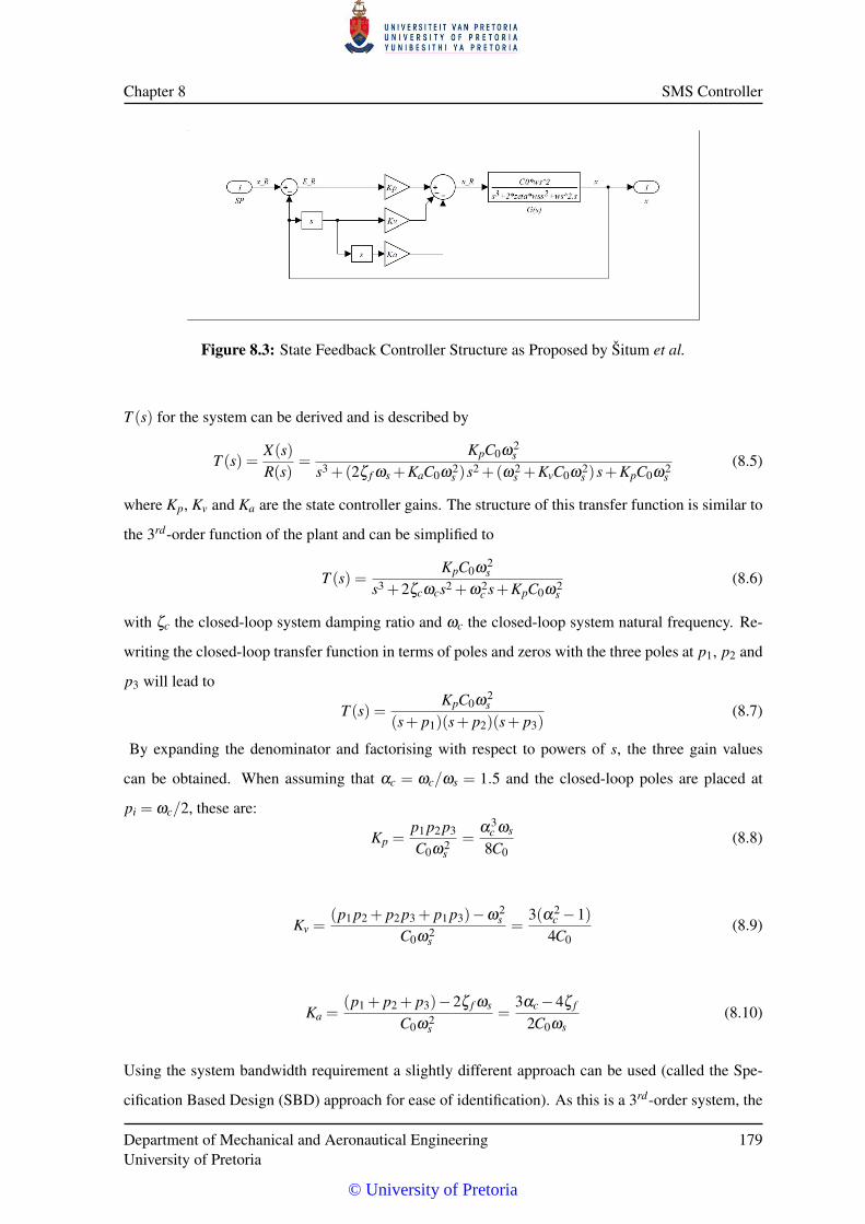
Chapter 8 SMS Controller
Figure 8.3: State Feedback Controller Structure as Proposed by Šitum et al.
T (s) for the system can be derived and is described by
T (s) =X(s)R(s)
=KpC0ω2
s
s3 +(2ζ f ωs +KaC0ω2s )s2 +(ω2
s +KvC0ω2s )s+KpC0ω2
s(8.5)
where Kp, Kv and Ka are the state controller gains. The structure of this transfer function is similar to
the 3rd-order function of the plant and can be simplified to
T (s) =KpC0ω2
s
s3 +2ζcωcs2 +ω2c s+KpC0ω2
s(8.6)
with ζc the closed-loop system damping ratio and ωc the closed-loop system natural frequency. Re-
writing the closed-loop transfer function in terms of poles and zeros with the three poles at p1, p2 and
p3 will lead to
T (s) =KpC0ω2
s
(s+ p1)(s+ p2)(s+ p3)(8.7)
By expanding the denominator and factorising with respect to powers of s, the three gain values
can be obtained. When assuming that αc = ωc/ωs = 1.5 and the closed-loop poles are placed at
pi = ωc/2, these are:
Kp =p1 p2 p3
C0ω2s
=α3
c ωs
8C0(8.8)
Kv =(p1 p2 + p2 p3 + p1 p3)−ω2
s
C0ω2s
=3(α2
c −1)4C0
(8.9)
Ka =(p1 + p2 + p3)−2ζ f ωs
C0ω2s
=3αc−4ζ f
2C0ωs(8.10)
Using the system bandwidth requirement a slightly different approach can be used (called the Spe-
cification Based Design (SBD) approach for ease of identification). As this is a 3rd-order system, the
Department of Mechanical and Aeronautical EngineeringUniversity of Pretoria
179
© University of Pretoria
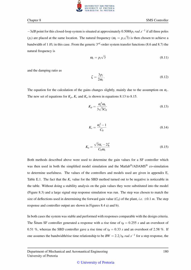
Chapter 8 SMS Controller
−3dB point for this closed-loop system is situated at approximately 0.5088pi rad.s−1 if all three poles
(pi) are placed at the same location. The natural frequency (ωc = pi√
3) is then chosen to achieve a
bandwidth of 1 Hz in this case. From the generic 3rd-order system transfer functions (8.6 and 8.7) the
natural frequency is
ωc = pi√
3 (8.11)
and the damping ratio as
ζ =3pi
2ωc. (8.12)
The equation for the calculation of the gains changes slightly, mainly due to the assumption on αc.
The new set of equations for Kp, Kv and Ka is shown in equations 8.13 to 8.15.
Kp =α3
c ωs
3√
3C0(8.13)
Kv =α2
c −1C0
(8.14)
Ka =
√3αc−2ζ
C0ωs(8.15)
Both methods described above were used to determine the gain values for a SF controller which
was then used in both the simplified model simulation and the Matlab®/ADAMS® co-simulation
to determine usefulness. The values of the controllers and models used are given in appendix E,
Table E.1. The fact that the Kv value for the SBD method turned out to be negative is noticeable in
the table. Without doing a stability analysis on the gain values they were substituted into the model
(Figure 8.3) and a large signal step response simulation was run. The step was chosen to match the
size of deflections used in determining the forward gain value (C0) of the plant, i.e. ±0.1 m. The step
response and controller output are shown in Figures 8.4 a) and b).
In both cases the system was stable and performed with responses comparable with the design criteria.
The Šitum SF controller generated a response with a rise time of tR = 0.255 s and an overshoot of
0.51 %, whereas the SBD controller gave a rise time of tR = 0.33 s and an overshoot of 2.58 %. If
one assumes the bandwidth/rise time relationship to be BW = 2.2/tR rad.s−1 for a step response, the
Department of Mechanical and Aeronautical EngineeringUniversity of Pretoria
180
© University of Pretoria
Chapter 8 SMS Controller
0.8 1 1.2 1.4 1.6 1.8 2 2.2 2.4
0
0.02
0.04
0.06
0.08
0.1
0.12
0.14
0.16
0.18
0.2
Time [s]
Pos
ition
[m]
Step Response Of the SF Controller with Simplified Plant Model
Set PointSitum ModelSBD Model
0.8 1 1.2 1.4 1.6 1.8 2 2.2 2.4
0
0.5
1
1.5
2
2.5
3
3.5
Time [s]
V [V
]
Controller Output Of the SF Controller with Simplified Plant Model
Set PointSitum ModelSBD Model
a) b)
Figure 8.4: a) Step Response and b) Controller Output Response of the State Feedback (SF) Con-
troller Closed-loop System
bandwidth of the Šitum controller system is 1.37 Hz and that of the SBD controller system is 1.06 Hz,
which corresponds well with the design criteria and the frequency analysis of the systems.
A high fidelity simulation of the controller in the Simulink®/ADAMS® SMS model was implemented
by replacing the controller as described in section 7.3.5 with the new SF controller and making sure
the system performs as expected. An additional loop gain value (Kc) was inserted to study the effects
of the loop gain on system stability. In both cases of the SF controller the simulation resulted in
unstable closed-loop systems with the actuators extending uncontrollably to their maximum extension
limits. It was obvious that the simplified model did not account for enough characteristics present in
the nonlinear system to be used for linearised controller design. Although it can be argued that
the simplified model was derived for small signal use only, the controllers designed were excited in
both the small signal linear regime as well as the large signal nonlinear regime and fared equally
poor.
It was found that by reducing the Ka value dramatically, the stability improved, although the response
became slow and sluggish. The values quoted by Šitum et al. revealed a very sluggish but stable
system and also revealed that the controller structure does have merit. The ratios between the Kp and
Kv values of the Šitum et al. were similar to the values found in this study, but the Ka value of Šitum
et al. was much smaller. The system could be made stable by reducing the acceleration contribution,
although it resulted in a very acceleration sensitive system. By removing the acceleration feedback
(making Ka = 0), a marginally stable system with a steady-state limit cycle could be achieved. The
limit cycle could be minimised by reducing the overall loop gain.
Department of Mechanical and Aeronautical EngineeringUniversity of Pretoria
181
© University of Pretoria
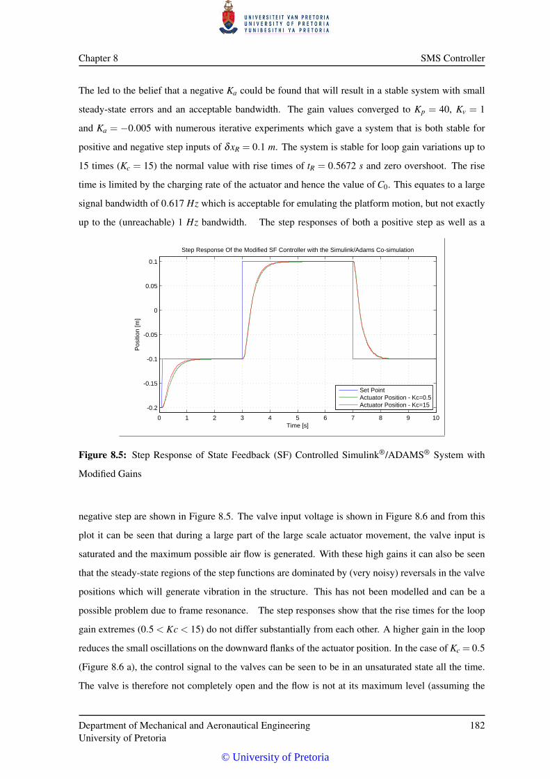
Chapter 8 SMS Controller
The led to the belief that a negative Ka could be found that will result in a stable system with small
steady-state errors and an acceptable bandwidth. The gain values converged to Kp = 40, Kv = 1
and Ka = −0.005 with numerous iterative experiments which gave a system that is both stable for
positive and negative step inputs of δxR = 0.1 m. The system is stable for loop gain variations up to
15 times (Kc = 15) the normal value with rise times of tR = 0.5672 s and zero overshoot. The rise
time is limited by the charging rate of the actuator and hence the value of C0. This equates to a large
signal bandwidth of 0.617 Hz which is acceptable for emulating the platform motion, but not exactly
up to the (unreachable) 1 Hz bandwidth. The step responses of both a positive step as well as a
0 1 2 3 4 5 6 7 8 9 10
-0.2
-0.15
-0.1
-0.05
0
0.05
0.1
Step Response Of the Modified SF Controller with the Simulink/Adams Co-simulation
Time [s]
Pos
ition
[m]
Set PointActuator Position - Kc=0.5Actuator Position - Kc=15
Figure 8.5: Step Response of State Feedback (SF) Controlled Simulink®/ADAMS® System with
Modified Gains
negative step are shown in Figure 8.5. The valve input voltage is shown in Figure 8.6 and from this
plot it can be seen that during a large part of the large scale actuator movement, the valve input is
saturated and the maximum possible air flow is generated. With these high gains it can also be seen
that the steady-state regions of the step functions are dominated by (very noisy) reversals in the valve
positions which will generate vibration in the structure. This has not been modelled and can be a
possible problem due to frame resonance. The step responses show that the rise times for the loop
gain extremes (0.5 < Kc < 15) do not differ substantially from each other. A higher gain in the loop
reduces the small oscillations on the downward flanks of the actuator position. In the case of Kc = 0.5
(Figure 8.6 a), the control signal to the valves can be seen to be in an unsaturated state all the time.
The valve is therefore not completely open and the flow is not at its maximum level (assuming the
Department of Mechanical and Aeronautical EngineeringUniversity of Pretoria
182
© University of Pretoria
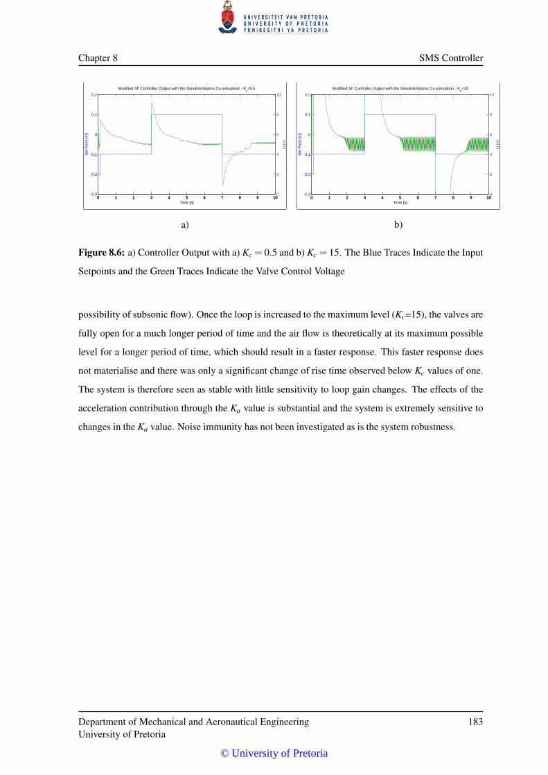
Chapter 8 SMS Controller
0 1 2 3 4 5 6 7 8 9 10-0.3
-0.2
-0.1
0
0.1
0.2
Time [s]
Set
Poi
nt [m
]Modified SF Controller Output with the Simulink/Adams Co-simulation - K
c=0.5
0 1 2 3 4 5 6 7 8 9 100
2
4
6
8
10
U [V
]
0 1 2 3 4 5 6 7 8 9 10-0.3
-0.2
-0.1
0
0.1
0.2
Time [s]
Set
Poi
nt [m
]
Modified SF Controller Output with the Simulink/Adams Co-simulation - Kc=15
0 1 2 3 4 5 6 7 8 9 100
2
4
6
8
10
U [V
]
a) b)
Figure 8.6: a) Controller Output with a) Kc = 0.5 and b) Kc = 15. The Blue Traces Indicate the Input
Setpoints and the Green Traces Indicate the Valve Control Voltage
possibility of subsonic flow). Once the loop is increased to the maximum level (Kc=15), the valves are
fully open for a much longer period of time and the air flow is theoretically at its maximum possible
level for a longer period of time, which should result in a faster response. This faster response does
not materialise and there was only a significant change of rise time observed below Kc values of one.
The system is therefore seen as stable with little sensitivity to loop gain changes. The effects of the
acceleration contribution through the Ka value is substantial and the system is extremely sensitive to
changes in the Ka value. Noise immunity has not been investigated as is the system robustness.
Department of Mechanical and Aeronautical EngineeringUniversity of Pretoria
183
© University of Pretoria
CHAPTER 9
CONCLUSION
9.1 SUMMARY
The precursor to this Master’s degree study was the design and building of a Ship Motion Simulator
(SMS) by the personnel of CSIR - DPSS to excite the inertial sensors of an optical tracker (SAT).
The simulator was designed to be portable, clean in operation by using compressed air, and capable
of manipulating the mass of the tracker in a similar fashion as the deck of a maritime vessel. The
simulator was designed in the form of a modified Gough-Stewart platform, but exchanging three of
the normal actuators with Panhard rods. It was to be used with random, open-loop excitation, but that
changed to a requirement for traceable closed-loop excitation.
The SMS was consequently made available for this study into the behaviour and performance of
pneumatic actuators as well as the geometry of this specific version of modified Gough-Stewart plat-
form. It started with an analysis of the requirements of the system, using actual measured maritime
vessel deck motion to compile specifications. The supplied SMS was tested against this require-
ment throughout the study to assess if the basic design complies. A geometric description derived
from CAD models together with mass, moments of inertia, and operational limitations was compiled.
The supplied pneumatic subsystem was described and a first iteration simulation done using Festo
Fluidsim®. The subsequent phases of the study covered the kinematics of the system, the integration
of ADAMS® and Matlab®, the theoretical and validated pneumatic models, an analysis of the noise
on the measurement process, the friction models, both theoretical and validated, the SMS system
model validation, and a first order controller design.
The following sections contain a concise description of the results of the various stages of the
© University of Pretoria
Chapter 9 Conclusion
study.
9.1.1 Kinematics
A geometric model was derived for the simulator by using the theory of axis transformation through
rotation matrixes. The inverse kinematics (the equations that define the actuator extensions for a
required platform orientation) was derived, but in the absence of an explicit set of equations for the
inverse kinematics of the system a process was devised to calculate a lookup table with the orientation
angles as indices with the output being the actuator extensions. This process used the solvers in MSC
ADAMS® in a co-simulation between MSC ADAMS® and Matlab® Simulink®. A test for correctness
of the lookup table was done by reversing the process and measuring the platform orientation given a
series of input angles. This process returned infinitely small errors on the orientation.
9.1.2 Pneumatic Models and Mass Flow Characterisation
The modelling of the pneumatic subsystems was approached by assessing what has been published
in the scientific domain in the form of text books, papers, and theses and then building on that.
Theoretical mass flow models, based on the work of Beater [10], Richer [26] and Šitum [53] was
derived from first principles, resulting in (what is referred to as) the classic pneumatic model. The
linearity of the valve spool deflection vs. the input control voltage was measured and described by a
third order polynomial (eq. 4.1). It was also found that the relationship between the geometric valve
orifice area and the spool deflection differed from the published circular orifice model used by Richer
et al. [26] and Smit [1] and was deemed not to be applicable in the valves used in this system. A
linear area derivation was done to replace the circular area description. The combination of the above
two equations gave rise to an accurate valve input vs. geometric area model.
A second valve mass flow model proposed by Beater [10] was implemented and called the ISO model.
The classic model and the ISO model parameters were identified through a series of experiments as
described in § 5.2 and a comparison made to determine the fit to real data. In order to apply an ob-
server (α - β filter) to reduce the measurement noise, the measurement noise characteristics (mean
value, probability distribution, spectral density) were analysed to confirm if the noise is white Gaus-
sian noise. The kurtosis and the skewness as well as a histogram analysis confirm the latter.
In the case of the classic model, the discharge coefficient as a function of the spool deflection was
Department of Mechanical and Aeronautical EngineeringUniversity of Pretoria
185
© University of Pretoria
Chapter 9 Conclusion
the identified entity. The discharge coefficient together with the geometric orifice area have the same
meaning as the effective area stated by Van der Merwe et al. [19] who used a constant value for the
discharge coefficient. A comparison was made between the two models and it was found that the ISO
model represented the actual system better in both the charging and discharging cycles. The mass flow
through the valve is shown in Figures 5.31 to 5.38. The ISO model includes modifiers to account for
fluid contraction and compounded restrictions of flow which were excluded from the classic model
by assumption. The most dominant variable in the ISO model is the sonic conductance which has
an input voltage relationship graphically illustrated in Figure 5.19b and tabulated in Table 5.2. It has
also been shown that the MAE of the ISO model (Figure 5.30b) is significantly lower than that of the
classic model.
9.1.3 Friction Model and Friction Identification
The friction modelling of a pneumatic system is a study domain on its own and can be done to different
levels of precision. The friction in these systems are always nonlinear and in most cases exhibit some
form of hysteresis. As explain in detail in Chapter 6, the friction models developed in the last 20 years
have increased in dimension, making them accurate but computationally costly. The goal was to find
a reasonable friction model to reproduce the shuddering observed on the real SMS. The decision was
made to use a simple stick-slip model identified over the operational range of the SMS, rather than a
complex LuGre model or the Leeuven model, both modelling pre-sliding and hysteresis.
A friction model based on a small pre-sliding regime bounded by a peak static friction force at the
moment when sliding starts, a constant Coulomb friction component, and an increasing viscous fric-
tion sliding regime modified by the Stribeck curve was adopted. The model is based on the work of
Nouri [23] and offers the freedom to have different viscous friction coefficients for increasing and de-
creasing velocities. The typical friction vs. velocity relationship is shown in Figure 6.10. A series of
experiments were conducted to explore the friction problem, gather data to identify the friction para-
meters, and to validate the friction model. During this process two very important factors emerged,
the first being the fact that the viscous friction increases exponentially at higher velocities and the
second being that the Stribeck curve and Stribeck velocity are modified by the acceleration of the
actuator. These two phenomena were introduced into the friction model as an acceleration dependent
Stribeck velocity scaled by a modification constant ζ and an exponential viscous friction.
The friction function derived from the system identification process as described in § 6.5 is expressed
Department of Mechanical and Aeronautical EngineeringUniversity of Pretoria
186
© University of Pretoria
Chapter 9 Conclusion
by Eqs. 6.5 and 6.7. The result is a model that produced a friction behaviour that closely resembled
that of the actual measured data, as shown in Figure 6.14.
A friction validation process was run to ensure that the model produced the same results as the real
system. During the model validation process it became evident that the quality of the air supply and
the level of lubrication of the actuator changed the friction behaviour dramatically. With that said, the
validation still produced very good correlation between the model and the real system, reinforcing
the trust level in the friction model. As will be covered later on, the friction model and the com-
pressibility of the fluid generated very true to life instabilities and limit cycles in the complete system
simulation.
9.1.4 SMS Model Validation
A validation process was necessary to assess the quality of the simulation model. The validation
was approached from a subsystem level all the way to the complete SMS and SAT. Throughout the
study, when a model for a single component was proposed, a validation was done to ensure that the
model could be trusted. This was done for the valve mass flow model and the friction model after
the identification processes as was shown in previous two sections. When combining these models
into a larger scale model, the errors and unmodelled effects accumulate and the actual causes of error
becomes unknown.
To minimise this accumulation of errors, the final validation was broken up in phases starting from
subsystem to system level. Initially a pure Matlab® Simulink® simulation using a model of a single
actuator without any external load was run, ensuring that the Matlab®/ADAMS® co-simulation is
functional and correct. Then a series of open-loop tests are done with the full SMS system, replicating
the conditions and scenarios in simulation, and comparing the results. Finally, a series of closed-loop
tests are done in the same fashion, comparing the simulation results with that of the real system.
Once the experiments are migrated towards the complete SMS system, laboratory instrumentation
had some shortcomings and the necessity arose for a dedicated system controller which is described
in § 7.3.3. Additional signals were also captured for model validation purposes using the same Data
Translation ADC as in the initial tests.
The results of the validation tests were extremely favourable and gave a high level of confidence
Department of Mechanical and Aeronautical EngineeringUniversity of Pretoria
187
© University of Pretoria
Chapter 9 Conclusion
in the models. The Matlab®/ADAMS® actuator simulation produced extension rates and chamber
pressures that tracked the measured data very well. Initial conditions for the test runs have a large
influence on the absolute signals, as expected for nonlinear systems, but using the measured initial
pressures and extensions in the simulation resulted in a very good correlation. There were high
frequency differences that were attributed to unmodelled effects, but even with these differences the
visual correlation was good enough not to justify any further processing. An example of the actuator
extension and the chamber pressure comparisons for the no-load condition are shown in Figures 7.7
to 7.9.
Once the full system validation was started, the tests were executed in such a manner as to ensure the
safety of the mounted optical equipment. Instability that manifests itself in the shaking of the SMS
can result in the failure of the leveling mechanisms of the SAT, a condition that needs to be avoided at
all cost. The initial simulation runs to test the controller identified the margins of stability, gave a feel
for the controller gains, and minimised unstable situations on the real system. The open-loop tests
were conducted from a central working point after leveling the SMS off with a simple proportional
controller. Once again the correlation between the simulation model and the real measured signals
were very good. The tracking of the signals, as the example shown in Figure 7.20 and Figure 7.21,
from the two scenarios (simulation vs. actual) was not as good as in the case of the single actuator,
mainly due to accumulated unmodelled effects, and justified an analysis of the fit. The coefficients of
cross-correlation between the chamber pressures of the simulation and the real system (see § 7.3.4.1)
was above cp(N/2) = 0.935 for all the test runs, resulting in a high probability that the model is accur-
ate enough for control. An arbitrary threshold for similarity used so far in this study is a correlation
figure larger than 0.8.
The excitation used was either a chirp signal with a frequency range of 0.05 Hz to 1 Hz or a single
frequency sine wave. Out of the open-loop tests it became apparent that dead-band compensation
would be necessary and was added for the closed-loop tests. The dead-band compensation ensured
significant excitation in the small signal region when linear controllers were used. Heave and roll
tests for closed-loop response were conducted, and revealed a system with a large signal bandwidth
of no more than 0.617 Hz, which is limited by the mass flow rate at 0.4 MPa.
Similar to the open-loop tests, the closed-loop tests produced outputs with great similarity between
the simulated and the actual signals. A temporal comparison (Figure 7.27) revealed that the simulated
system signals once again tracked those of the real measured system, albeit with a 14% reduction in
Department of Mechanical and Aeronautical EngineeringUniversity of Pretoria
188
© University of Pretoria
Chapter 9 Conclusion
peak to peak amplitude and rise time. The actual system has a more pronounced friction induced
shudder on the retraction phase, a slower charge rate and, hence, a lower overall bandwidth. The
closed-loop spectral response of the system (Figure 7.30) confirmed the reduction in bandwidth for
an arbitrary proportional gain. Similar uncontrolled effects in both the real system and the simulated
system around the 2 Hz point could also be observed (Figure 7.29) and showed that the model is an
acceptable representation of the the real system in the closed-loop.
9.1.5 Simplified Plant Model and Control
Because the main purpose of this engineering study is to find a realistic model for the SMS for the
purpose of controller design, a controller design exercise was added. The controller used for the
model validation was a generic PID controller that was implemented as a proportional controller due
to the integration and derivative gains being zero. An expansion of this study, as will be mentioned
in § 9.3, is the design of nonlinear controllers such as sliding mode controllers as used by Smit [1] or
reduced order controllers as used by Richer et al. [11].
In this study a simplified model of a pneumatic actuator was devised similar to that which is described
by Šitum et al. [16]. This model is described (§ 8.1) by a third order transfer function with a natural
frequency (ωs) and a damping coefficient (ζ f ). A closed-loop transfer function was derived and
described by eq. 8.4
It was shown that the simplified model exhibited the same low pass characteristics as the complex
SMS system model and thus the real system. A state feedback controller was designed from the
chosen ratio (αc = 1.5) between the open-loop natural frequency and the closed-loop natural fre-
quency, placing the closed-loop poles at half the desired closed-loop natural frequency and calculat-
ing the gain values for the controller. This method focused mainly on stability and the suppression of
the resonance. A second approach was investigated in which the system bandwidth requirement was
used to place the poles, i.e. at the -3 dB point of the resulting 3rd-order system.
In both cases the step responses were favourable when tested with both large and small step sizes. The
magnitudes of the solenoid valve inputs in both cases were within physical bounds and the systems
were stable in both cases. The Šitum controller resulted in a system rise time of tR = 0.255 s and
a bandwidth of 1.37 Hz, whereas the SBD based controller gave a rise time of tR = 0.33 s and a
bandwidth of 1.06 Hz.
Department of Mechanical and Aeronautical EngineeringUniversity of Pretoria
189
© University of Pretoria
Chapter 9 Conclusion
This turned out to be only half of the truth as only the extending actuator movement was assessed
and the stiction coupled with the compressibility of the air resulted in feedback of the high accel-
eration values not catered for in the simplified model. The latter became apparent when the high
fidelity simulation model was used to ensure the stability of the controller. It became evident that the
positive feedback of the acceleration (due to a positive value for Ka) was at the core of the problem,
and once corrected by using negative values for Ka, resulted in a controlled system with adequate
bandwidth (BW > 0.5 Hz) and stability. The bandwidth is ultimately limited by the mass flow of the
charging circuit, and the system stability is insensitive to changes to the loop gain because of this
limitation.
9.2 EVALUATION OF OBJECTIVES
A very ambitious engineering study to understand the domain of pneumatic system modelling and
control was undertaken. An in depth study of the academic domain as well the published literature
domain was done and more information was found than what could be assimilated in the duration of
this study. Various formal texts in terms of books were found on the subject, a few which were chosen
to feed the initial introduction on pneumatic systems and compressible fluids. A vast number of
papers from reputable sources were scoured for information pertaining to similar systems, structures
processes, and designs. There is also an unfathomable amount of information available from online
sources, many of which add to the confusion in the domain. From all these sources, a selection
of relevant publications and information sources were made and the theoretical knowledge on the
pneumatic domain built up from a rudimentary level to a level of acceptable understanding.
The first objective was just that, finding relevant information to expedite the development of a con-
trolled SMS system.
The second objective was the generation of a detailed model of the SMS system so that it can be
used for controller development and controller testing. It is fair to say that the task of the model
development has been executed in a methodical and systematic fashion. As this is an engineering
problem, the use of advanced tools made for faster progress, such as the determination of the inverse
kinematics and the co-simulation between Matlab® and MSC ADAMS®. Commercially accepted
standards such as the ISO-6358 model of the valve flow represented the actual flow phenomena better
than the classical physics based models, although the latter was the starting point of most of the
pneumatic studies found in literature.
Department of Mechanical and Aeronautical EngineeringUniversity of Pretoria
190
© University of Pretoria
Chapter 9 Conclusion
In modeling the mechanical structure, some limitations in the typical design philosophy of cost ef-
fective systems came to the forefront, i.e. that component cost saving can result in large development
time spending. That said, if the system was designed as a Gough-Stewart platform and the inverse
kinematics were explicitly defined, the use and integration of ADAMS® would have been of a lower
priority and the development of the dynamic simulation could have taken much longer with poor
results.
The knowledge of transforming physical mechanical structures into simulation models in ADAMS®
resulted in a steep learning curve. Once mastered, the power of high level simulation has great value.
A Matlab® Simulink®/ADAMS® co-simulation was realised and used for finding the solution to the
inverse kinematic problem and to link Matlab® Simulink® pneumatic models, friction models and
controllers to ADAMS®.
The flow of air through a pneumatic system with the accompanying thermal changes in the air prop-
erties due to the rate at which pressure changes occur, all formed part of the domain of pneumatic
system modelling. As mentioned in the summary section (§ 9.1) of the project, a pneumatic model of
the actuators used in the SMS was modelled through a combination of first principle derivations and
models presented as part of the ISO-6358 standard. The latter became important during the mass flow
validation process in which it was found that the classic model did not represent the valve adequately.
The coefficients pertaining to this specific case of actuator were obtained through experimentation
and published inference techniques.
A deviation from the normally accepted classical flow models was made in the sense that the orifice
(or valve) area was kept constant and the changing variable was the discharge coefficient. Normally,
the area would be lumped into an effective area and the discharge coefficient would be kept constant.
Computationally, the two methods are equivalent, producing the same results. Another deviation was
the choice of the isentropic constant for the identification process. It was chosen to be the same
for both the charging and discharging processes, assuming that the model uses the same structure in
validation and simulation. The effect of the choice of constants is therefore cancelled through other
lumped and some unmodelled effects during coefficient identification.
The friction behaviour of the actuator was modelled using a much simpler model than is available.
The time constraints on the project as well as the possible gain in complicating the model was taken
into account and a model with limited hysteresis and a simple smoothed stick-slip transient was
Department of Mechanical and Aeronautical EngineeringUniversity of Pretoria
191
© University of Pretoria
Chapter 9 Conclusion
defined, identified, and validated. An exponential viscous friction component was identified and
added to the model. The contribution in the final model of this exponential term is unknown, as is the
reason for this extra term. A general shortcoming in the process of both the pneumatic identification
and the friction identification is the limited cycles or test points used in the process, as well as the
limited variation in the different types of excitation. In the case of the friction model as well the
pneumatic model, the same instrumentation was used for the System Identification (SID) and the
validation process. This could potentially introduce instrumentation induced errors that is common to
both the processes and cancel each other. An independent instrumentation calibration and validation
process could prevent this from happening. It can, however, be stated that the final model validation
revealed no significant un-modelled effects, which would ease the mind on the errors induced by the
instrumentation.
As mentioned earlier, the integration of Matlab® Simulink® and ADAMS® was successfully com-
pleted and the co-simulation delivered similar characteristics as the actual system. This gives great
confidence in the validity of the simulation system as a controller development environment. As a
main objective, the validation of the system was done in the open-loop as well as in a closed-loop
mode. In both cases the simulated response correlated well with reality which means that the object-
ive has been reached.
Controller design for a nonlinear system such as the SMS is a non-trivial task that will consume a lot
of effort and time. At the start of the larger project, the scope of the nonlinear effects was grossly un-
derestimated. An effort was made to use the newly developed simulation environment for controller
design with reasonable results. A simplified linear model was derived for the actuators using pub-
lished techniques and a state feedback controller designed for it. The response of the controller was
acceptable, falling within the bandwidth requirement set at the start of the study. The platform angular
tracking of the setpoints also fell within the requirements. The controller turned out to be robust under
the test conditions, which excluded external disturbances or SAT payload movements. A limitation
was found in the maximum angular rate (large signal response) limited by the maximum flow rate of
the pneumatic system, hence limiting the bandwidth and any higher bandwidth developments. Due
to the lack of a suitable sensor and time limitations, the accuracy of the platform movement was not
verified through measurement.
Department of Mechanical and Aeronautical EngineeringUniversity of Pretoria
192
© University of Pretoria
Chapter 9 Conclusion
9.3 FUTURE WORK
As time and budget is played off against accuracy and fidelity, a project or a study needs to be confined
to only the necessary work and effort. Such was the case with the characterisation, modelling, and
control of the SMS. The output of the study adhered well to the initial requirements and the objectives
were reached, some with some assumptions. In all the disciplines covered in this study more work
and expansion is possible and in some cases necessary. Herewith an assessment of further work that
should be undertaken.
From a requirements perspective, more real world measurements should be done on a variety of
maritime vessels of various size classes to fully populate the data set for deck motion requirements. At
the moment the SMS is a single vessel simulator that can manage up to sea state 4. Higher number sea
states will necessitate higher bandwidth and larger absolute angular range on the platform, which in
turn will result in a redesign of the mechanical structure. This will be best realised through a parallel
manipulator such as a full complement Gough-Stewart platform or a hexapod. Another expansion
would be that of simulating smaller vessels with higher natural frequencies, hence the same angular
range but with larger bandwidth. Linked to the mechanical structure and the electronic controller
is the inverse kinematic model that has further investigation possibilities. A real-time solver for the
geometry or an explicit description of the geometry, if it exists, would ease the preparation time
for lookup tables and can be implemented in the embedded controller or the maritime deck data
source.
The pneumatic model of the actuator is well developed in structure, but can be expanded to simulate
deck motion with other source pressures. This would entail model identification over lower as well
as higher than the current 0.2 MPa and 0.4 MPa source pressures. It would be time consuming to
identify the flow coefficients over a large range of pressures, in which case better system identific-
ation techniques could be employed. An ambitious continuation of the pneumatic problem would
be a component parameter based model definition. Similar functionality can be found in software
packages such as Festo’s Fluidsim, with the drawback that only a few parameters are adjustable and
the simulator cannot be integrated with other packages such as MBD simulators (MSC ADAMS®) or
Matlab®.
A vast amount of work is still possible on the friction behaviour of pneumatic seals and actuators. The
most prominent is the inclusion of hysteresis and lubrication effects on the dynamic friction models.
Department of Mechanical and Aeronautical EngineeringUniversity of Pretoria
193
© University of Pretoria
Chapter 9 Conclusion
Also, the effect of pressure on the sealing force between the piston and the cylinder is only touched
on in a few publications. A factor found specifically in this study is the effect of the instrumentation
quality in terms of accuracy and noise figures and suitability of the sensors in terms of bandwidth,
reliability, and accuracy. An analysis of these effects would be worthwhile to do.
In the controller domain, the environment for developing the controller has been put in place with a
first iteration of linearized controller design completed. The use of nonlinear controller techniques
as well as additional sensor feedback for Multi Input Single Output (MISO) control is a natural
progression from this study.
Department of Mechanical and Aeronautical EngineeringUniversity of Pretoria
194
© University of Pretoria
REFERENCES
[1] P. E. Smit, “Development of a 3-DoF motion simulation platform,” Thesis, Stellenbosch :
University of Stellenbosch, 2010. [Online]. Available: http://hdl.handle.net/10019.1/4155
[2] Y. Chiew, M. Abdul Jalil, and M. Hussein, “Kinematic modeling of driving simulator motion
platform,” in Proc. 2008 Innovative Technologies in Intelligent Systems and Industrial Applica-
tions IEEE Conf., July 2008, pp. 30–34.
[3] Z. Qu and Z. Ye, “Kinematics analysis of certain novel 3-DoF parallel manipulator,” in Proc.
2011 3rd Pacific-Asia Conference on Circuits, Communications and System, July 2011, pp. 1–3.
[4] V. E. Gough and S. Whitehall, “Universal tyre test machine,” Proc. 9th International Technical
Congress F.I.S.I.T.A., vol. 117, pp. 117–137, 1962.
[5] D. Stewart, “A platform with six degrees of freedom,” Proc. Institute of Mechanical Engineers,
vol. 180, no. 1, pp. 371–386, 1965.
[6] T. Brezina, Z. Hadas, and J. Vetiska, “Using of co-simulation ADAMS-Simulink for develop-
ment of mechatronic systems,” in Mechatronika 14th Int Symp., June 2011, pp. 59–64.
[7] D. Baran and W. Lisowski, “Numerical simulation and co-simulation in analysis of manipulat-
ors’ dynamics,” AGH Journal on Mechanics and Control, vol. 32, no. 4, pp. 129–135, 2013.
[8] C.T. Crowe et al., Engineering Fluid Mechanics, 9th ed. John Wiley & Sons, 2009.
[9] B. Andersen, The Analysis and Design of Pneumatic Systems. Krieger Publishing Company,
2001.
[10] P. Beater, Pneumatic Drives: System Design, Modelling and Control. Springer-Verlag, Berlin,
© University of Pretoria
References
Heidelberg, 2007.
[11] E. Richer and Y. Hurmuzlu, “A high performance pneumatic force actuator system: Part 2 –
nonlinear controller design,” Journal of Dynamic Systems, Measurement, and Control, vol. 122,
no. 3, pp. 426–434, Jun. 1999.
[12] ISO 6358-1:2013(EN), Pneumatic fluid power – Determination of flow-rate characteristics of
components using compressible fluids – Part 1: General rules and test methods for steady-state
flow, Std. ISO 6358-1:2013(EN), 2013.
[13] ISO 6358-2:2013(EN), Pneumatic fluid power – Determination of flow-rate characteristics
of components using compressible fluids – Part 2: Alternative test methods, Std. ISO 6358-
2:2013(EN), 2013.
[14] D. Purdue, D. Wood, and M. M.J. Townsley, “The design of pneumatic circuits,” Fluid Power
International, pp. 27–36, 1969.
[15] Sanville, F. E., “A new method of specifying the flow capacity of pneumatic fluid power valves,”
in Proc. 2nd Int. Fluid Power Symposium, BHRA, Ed. Guildford, England: BHRA, 1971, pp.
37–47.
[16] Ž. Šitum and J. Petric, “Modeling and control of servopneumatic drive,” Strojarstvo, vol. 43, no.
1-3, pp. 29–39, 2001.
[17] D. Ben-Dov and S. Salcudean, “A force-controlled pneumatic actuator,” IEEE Trans. Robot.
Autom., vol. 11, no. 6, pp. 906 –911, Dec 1995.
[18] B. M. Y. Nouri and M. B. Y. Saudi, “Experimental modelling and identification of compressible
flow through proportional directional control valves,” Universal Journal of Control and Auto-
mation, vol. 2, pp. 4–13, 2014.
[19] J. Van der Merwe, J. H. Muller, and C. Scheffer, “Parameter identification and evaluation of a
proportional directional flow control valve model,” R & D J SAIMECHE, vol. 29, pp. 18–25,
2013.
[20] T. Wang, L. Zhao, T. Zhao, T. Kagawa, and W. Fan, “Determination of flow rate characteristics
Department of Mechanical and Aeronautical EngineeringUniversity of Pretoria
196
© University of Pretoria
References
for pneumatic components during isothermal discharge by integral algorithm,” J Dyn Syst-T
ASME, vol. 134, no. 6, pp. 061 005–1–061 005–8, Sept 2012.
[21] K. Kawashima, Y. Ishii, T. Funaki, and T. Kagawa, “Determination of flow rate characteristics
of pneumatic solenoid valves using an isothermal chamber,” J Fluid Eng, vol. 126, no. 2, pp.
273–279, May 2004.
[22] K. Kawashima, T. Kagawa, and T. Fujita, “Instantaneous flow rate measurement of ideal gases,”
Journal of dynamic systems, measurement, and control, vol. 122, no. 1, pp. 174–178, 2000.
[23] B. Nouri, F. Al-Bender, J. Swevers, P. Vanherek, and H. V. Brussel, “Modelling a pneumatic
servo positioning system with friction,” in Proc. 2000 American Control Conference, vol. 2,
2000, pp. 1067–1071.
[24] C. Fleck and M. Meuser, “New servo-control concept for pneumatic drives which are subject to
strong friction forces,” O+P Journal lhydraulik und Pneumatik 47, no. 8, pp. 548–554, 2003.
[25] S. Ning and G. Bone, “Development of a nonlinear dynamic model for a servo pneumatic po-
sitioning system,” in Proc. IEEE Int Conf. Mechatronics & Automation, vol. 1, July 2005, pp.
43–48.
[26] E. Richer and Y. Hurmuzlu, “A high performance pneumatic force actuator system: Part 1 –
nonlinear mathematical model,” J Dyn Syst-T ASME, vol. 122, no. 3, pp. 416–425, Jun. 1999.
[27] F. Najafi, M. Fathi, and M. Saadat, “Dynamic modelling of servo pneumatic actuators with
cushioning,” The International Journal of Advanced Manufacturing Technology, vol. 42, pp.
757–765, June 2009.
[28] X. B. Tran and H. Yanada, “Dynamic friction behaviors of pneumatic cylinders,” Intelligent
Control and Automation, vol. 4, pp. 180–190, May 2013.
[29] K. Khayati, P. Bigras, and L.-A. Dessaint, “Lugre model-based friction compensation and posi-
tioning control for a pneumatic actuator using multi-objective output-feedback control via LMI
optimization,” Elsevier Mechatronics, vol. 19, no. 4, pp. 535–547, 2009.
[30] P. Dahl, “A solid friction model,” DTIC Document, Tech. Rep. TOR-0158(3107-18)-1, May
Department of Mechanical and Aeronautical EngineeringUniversity of Pretoria
197
© University of Pretoria
References
1968.
[31] C. Canudas de Wit, H. Olsson, K. J. Åström, and P. Lischinsky, “A new model for control of
systems with friction,” IEEE Transactions on Automatic Control, vol. 40, no. 3, pp. 419–425,
March 1995.
[32] J. Swevers, F. Al-Bender, C. Ganseman, and T. Projogo, “An integrated friction model structure
with improved presliding behavior for accurate friction compensation,” IEEE Transactions on
Automatic Control, vol. 45, no. 4, pp. 675–686, April 2000.
[33] P. Dupont, V. Hayward, B. Armstrong, and F. Altpeter, “Single state elastoplastic friction mod-
els,” IEEE Transactions on Automatic Control, vol. 47, no. 5, pp. 787–792, 2002.
[34] V. Lampaert, J. Swevers, and F. Al-Bender, “Modification of the Leuven integrated friction
model structure,” IEEE Transactions on Automatic Control, vol. 47, no. 4, pp. 683–687, April
2002.
[35] G. Belforte, G. Mattiazzo, S. Mauro, and L. R. Tokashiki, “Measurement of friction force in
pneumatic cylinders,” Tribotest Journal, vol. 10, no. 1, pp. 33–48, Sept. 2003.
[36] P. L. Andrighetto, A. C. Valdiero, and L. Carlotto, “Study of the friction behavior in industrial
pneumatic actuators,” in ABCM Symposium Series in Mechatronics, vol. 2, 2006, pp. 369–376.
[37] B. M. Nouri, “Friction identification in mechatronic systems,” ISA transactions, vol. 43, no. 2,
pp. 205–216, 2004.
[38] B. Armstrong-Hélouvry, Control of Machines with Friction, ser. The Kluwer International Series
in Engineering and Computer Science: Robotics : vision, manipulation and sensors. Springer
US, 1991.
[39] J. Slotine and W. Li, Applied Nonlinear Control. Prentice Hall, 1991.
[40] S. Laghrouche, M. Smaoui, X. Brun, and F. Plestan, “Robust second order sliding mode con-
troller for electropneumatic actuator,” in Proc. 2004 American Control Conference, vol. 6, 2004,
pp. 5090–5095.
[41] P. Bigras, “Sliding-mode observer as a time-variant estimator for control of pneumatic systems,”
Department of Mechanical and Aeronautical EngineeringUniversity of Pretoria
198
© University of Pretoria
References
Journal of Dynamic Systems, Measurement, and Control, vol. 127, no. 3, pp. 499–502, Aug.
2004.
[42] G. Bone and S. Ning, “Experimental comparison of position tracking control algorithms for
pneumatic cylinder actuators,” IEEE/ASME Transactions on Mechatronics, vol. 12, no. 5, pp.
557–561, Oct 2007.
[43] X. Yu, “Study on servo control strategy for pneumatic manipulator,” in 2010 International Con-
ference on Measuring Technology and Mechatronics Automation (ICMTMA), vol. 3, March
2010, pp. 641–644.
[44] Z. Šitum, D. Pavkovic, and B. Novakovic, “Servo pneumatic position control using fuzzy PID
gain scheduling,” Journal of dynamic systems, measurement, and control, vol. 126, no. 2, pp.
376–387, 2004.
[45] K. Hamiti, A. Voda-Besançon, and H. Roux-Buisson, “Position control of a pneumatic actuator
under the influence of stiction,” Control Engineering Practice, vol. 4, no. 8, pp. 1079–1088,
1996.
[46] J. Wang, J. Pu, and P. Moore, “A practical control strategy for servo-pneumatic actuator sys-
tems,” Control Engineering Practice, vol. 7, no. 12, pp. 1483–1488, 1999.
[47] L. J. du Plessis, “Design and optimum operation of a re-configurable planar Gough-Stewart
machining platform,” Doctoral Thesis, University of Pretoria, 2001.
[48] E. W. Weisstein, “Euler angles,” accessed 2013.02.07. [Online]. Available: http:
//mathworld.wolfram.com/EulerAngles.html
[49] Online, “Euler angles,” http://en.wikipedia.org/wiki/Euler_angles, accessed 2013.02.07.
[Online]. Available: http://en.wikipedia.org/wiki/Euler_angles
[50] Festo, “Proportional directional control valves mpye,” Festo data sheet, May 2012.
[51] B. McDonell and J. Bobrow, “Modeling, identification, and control of a pneumatically actuated
robot,” in Proceedings of the 1997 IEEE International Conference on Robotics and Automation,
vol. 1, April 1997, pp. 124–129.
Department of Mechanical and Aeronautical EngineeringUniversity of Pretoria
199
© University of Pretoria
References
[52] A. M. Al-Ibrahim and P. D. R. Otis, “Transient air temperature and pressure measurements dur-
ing the charging and discharging processes of an actuating pneumatic cylinder,” in Proceedings
of the 45th National Conference on Fluid Power. National Fluid Power Association, March
1992.
[53] Ž. Šitum, D. Kosic, and M. Essert, “Nonlinear mathematical model of a servo pneumatic sys-
tem,” in 9th International Research/Expert Conference" Trends in the Development of Ma-
chinery and Associated Technology". Antalya, Turkey: TMT 2005, Antalya, Turkey, Sept.
2005.
[54] T. Raparelli, A. M. Bertetto, and L. Mazza, “Experimental and numerical study of friction
in an elastomeric seal for pneumatic cylinders,” Tribology International, vol. 30, no. 7,
pp. 547–552, 1997. [Online]. Available: http://www.sciencedirect.com/science/article/pii/
S0301679X97000157
[55] NIST, “NIST Thermocouple EMF tables,” accessed 03/02/2014. [Online]. Available:
http://srdata.nist.gov/its90/download/type_k.tab
[56] W. Martinez and A. Martinez, Computational Statistics Handbook with MATLAB, ser. Chapman
& Hall/CRC Computer Science & Data Analysis. Taylor & Francis, 2001, p.55.
[57] J. Wang, J. Wang, N. Daw, and Q. Wu, “Identification of pneumatic cylinder friction parameters
using genetic algorithms,” IEEE/ASME Transactions on Mechatronics, vol. 9, no. 1, pp. 100–
107, March 2004.
[58] Wikipedia, “Adiabatic process,” [Online; accessed 31.01.2013]. [Online]. Available:
http://en.wikipedia.org/wiki/Adiabatic_process
[59] ——, “Isentropic process,” accessed 31.01.2013. [Online]. Available: http://en.wikipedia.org/
wiki/Isentropic_process
[60] ——, “First law of thermodynamics,” accessed 31.01.2013. [Online]. Available: http:
//en.wikipedia.org/wiki/First_law_of_thermodynamics
[61] ——, “Second law of thermodynamics,” accessed 31.01.2013. [Online]. Available:
http://en.wikipedia.org/wiki/Second_law_of_thermodynamics
Department of Mechanical and Aeronautical EngineeringUniversity of Pretoria
200
© University of Pretoria
APPENDIX A
DEFINITIONS
Adiabatic process An adiabatic process is any process occurring without gain or loss of heat within
a system (i.e. during the process the system is thermodynamically isolated; there is no heat
transfer to/from the surroundings). This is usually associated with a fast increase in pressure,
during which time no thermal exchange can happen [58].
Continuity Equation - Ideal Duct If a duct is assumed to be of a rigid nature and does not deform
during the process and a steady flow of particles is present, the mass flow rate at any cross
section of the duct, irrespective of the cross sectional area at any particular section, will be the
same. For a compressible fluid, the continuity equation will reduce to ρ2A2V2 = ρ1A1V1 [8].
Kinematics The branch of mechanics that studies the motion of a body or a system of bodies without
consideration given to its mass or the forces acting on it. It is also referred to as the geometry
of motion.
Forward Kinematics Definition applied to parallel manipulators. The forward kinematics of a
Gough-Stewart parallel manipulator is finding the position and orientation of the mobile plat-
form when the strut lengths are known.
Inverse Kinematics Definition applied to parallel manipulators. The problem of inverse kinematics
for Gough-Stewart parallel manipulators can be defined as finding the strut lengths needed to
position the mobile platform in a certain position with the desired orientation.
Isentropic process An Isentropic process is one that takes place from initiation to completion
without an increase or decrease in the entropy of the system, i.e., the entropy of the system
© University of Pretoria
References
remains constant. An isentropic flow is a flow that is both adiabatic and reversible [59].
First Law of Thermodynamics The first law of thermodynamics states that the change in the in-
ternal energy of a closed system is equal to the amount of heat supplied to the system, minus
the amount of work done by the system on its surroundings. The law of conservation of energy
states that the energy of an isolated system is constant [60].
Multibody Dynamic System A MBD system is one that consists of solid bodies or links that are
connected to each other by joints that restrict their relative motion. The study of MBD is
the analysis of how mechanical systems move under the influence of forces, also known as
forward dynamics. A study of the inverse problem, i.e. what forces are necessary to make the
mechanical system move in a specific manner is known as inverse dynamics.
Physical Standard Condition The Physical Standard Conditions for air (defined by Deutsches In-
stitut für Normung (DIN) 1343) is a standard temperature of TN = 273.15 K (0◦C), a standard
pressure of pN = 101.325 kPa, a gas constant of RN = 286.9 N m kg−1 K−1 and a relative
humidity of 0%.
Standard Temperature and Pressure (STP) The standard conditions for temperature and pressure
are standard sets of conditions for experimental measurements established to allow compar-
isons to be made between different sets of data. According to International Organisation for
Standardisation (ISO) 5011 it is defined as TST P = 293.15 K (20◦C), pST P = 101.325 kPa (1
atm) and 50% relative humidity.
Second Law of Thermodynamics The second law of thermodynamics states that the entropy of an
isolated system never decreases, because isolated systems spontaneously evolve towards ther-
modynamic equilibrium, the state of maximum entropy. The final entropy of an irreversible
process is always greater than the initial entropy. For a reversible process, the entropy does not
change, and the final entropy equals the initial entropy of the system. Such a process is called
an isentropic process (See Isentropic Process) [61].
Technical Standard Condition The technical Standard Condition is defined by ISO 6358 as an
alternative standard to DIN 1343, as it is more practical to measure and easier to achieve.
According to ISO 6358 the standard temperature is T0 = 293.15 K, the standard pressure is
p0 = 100 kPa, the gas constant is R0 = 288 N.m.kg−1.K−1 and the relative humidity is 65%.
Department of Mechanical and Aeronautical EngineeringUniversity of Pretoria
202
© University of Pretoria

References
This standard is mostly used in the conversion between volumetric flow rate (V ) and mass flow
rate (m) in gasses.
Department of Mechanical and Aeronautical EngineeringUniversity of Pretoria
203
© University of Pretoria
APPENDIX B
MATLAB® RTW EMBEDDED CODER INTEGRATION
WITH CODE COMPOSER STUDIO V5.5
B.1 OVERVIEW
Goal: To integrate the C code generated by Matlab®’s embedded coder into CCS V5.5 and to make it
available in a CCS project for later modification, compilation and debugging.
Setup/Equipment:
• TMS320F28335 Control Card with 20MHz crystal (http://www.ti.com/tool/
tmdscncd28335)
• Texas Instruments Docking station (http://www.ti.com/tool/
tmdsdock28346-168)
• Spectrum Digital XDS510USB programmer/debugger
• Matlab R2012b V8.0.0.783
• Matlab Embedded Coder V6.3
• MATLAB Coder V2.3
• Simulink Coder V8.3
• Simulink V8.0
© University of Pretoria
References
• CCS V5.5.0.00077
B.1.1 Guide
This is a step-by-step guide to get a Simulink® model coded and programmed into the pro-
cessor:
B.1.1.1 Environment
1) Install Matlab®, Simulink® and the Embedded Coder Support packages. Ensure that a
Simulink® model can be generated and saved. 2) Install CCS (http://www.ti.com/tool/
ccstudio), the header files (http://www.ti.com/tool/sprc530) for the processor, the
Flash APIs (http://www.ti.com/tool/sprc539) and RTOS/Bios tools (http://www.
ti.com/tool/sysbios). Header files and processor support can also be found in the con-
trol suite installation (http://www.ti.com/tool/controlsuite). 3) Open Matlab® and
type ver in the command window to check for the embedded and RTW tools. 4) Type check-
EnvSetup(’ccsv5’,’f28335’,’check’). This will display the current environmental variables set to in-
tegrate CCS with Matlab®. It should look something like this:
» checkEnvSetup(’ccsv5’,’f28335’,’check’)
1. CCSv5 (Code Composer Studio) Your version : 5.5.0 Required version: 5.0 or later Required for :
Code Generation TI_DIR=“D:\TI\ccsv5”
2. CGT (Texas Instruments C2000 Code Generation Tools) Your version : 6.2.3 Required ver-
sion: 5.2.1 to 6.0.2 Required for : Code generation C2000_CGT_INSTALLDIR=“D:\TI\ccsv5\
tools\compiler\c2000_6.2.3”
3. DSP/BIOS (Real Time Operating System) Your version : 5.42.01.09 Required version: 5.33.05 to
5.41.11.38 Required for : Code generation CCSV5_DSPBIOS_INSTALLDIR=“D:\TI\bios_5_
42_01_09”
4. XDC Tools (eXpress DSP Components) Your version : Required version: 3.16.02.32 or later
Required for : Code generation
Department of Mechanical and Aeronautical EngineeringUniversity of Pretoria
205
© University of Pretoria
References
5. Flash Tools (TMS320C28335 Flash APIs) Your version : 2.10 Required version: 2.10 Re-
quired for : Flash Programming FLASH_28335_API_INSTALLDIR=“D:\TI\Flash28_API\
Flash28335_API_V210”
If they are incorrect or missing, do step 5. The XDC Tools are not important for C2000 pro-
cessors.
5) Type checkEnvSetup(’ccsv5’,’f28335’,’setup’) to set up the environmental variables inside Matlab®.
Follow the prompts to identify the directories. After setting the variables, check them for correctness
using step 4. To get the variable loaded every time you start Matlab®, generate Windows System
Variables by opening
Control Panel\System and Security\System
(Win Button-Pause) and selecting Advanced system settings. Select Environmental Variables and add
the following System variables:
• TI_DIR="D:\TI\ccsv5"
• C2000_CGT_INSTALLDIR="D:\TI\ccsv5\tools\compiler\c2000_6.2.3"
• CCSV5_DSPBIOS_INSTALLDIR="D:\TI\bios_5_42_01_09"
• FLASH_28335_API_INSTALLDIR="D:\TI\Flash28_API\Flash28335_API_
V210"
to match the Matlab® variables. Restart the PC.
6) Type xmakefilesetup in the Matlab® command window. Untick Display operational configurations
only and select ticcs_c2000_ccsv5 from the Configuration dropdown. Appl and check the paths under
Tool Directories are the same as defined in the Environment setup. Clone the setup by selecting New...
at Configuration. Give the Config a new name, e.g. ticcs_c2000_ccsv5_OSS. Select this config.
7) Open a new Simulik Model and save it as e.g. “Sample.slx”. Select the Library Browser and drag
the Target Preferences (ISA Card Icon) from Embedded Coder/Embedded Targets. It will open a
window titled “sample/Target Preferences: Initialize Model Configuration Parameters”. Select Texas
Instruments Code Composer Studio v5 (makefile generation only), the F28335 of choice and select
Department of Mechanical and Aeronautical EngineeringUniversity of Pretoria
206
© University of Pretoria
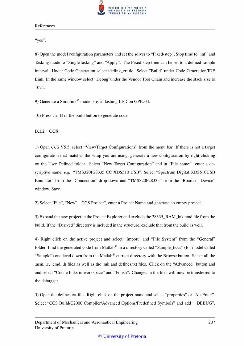
References
“yes”.
8) Open the model configuration parameters and set the solver to “Fixed-step”, Stop time to “inf” and
Tasking mode to “SingleTasking” and “Apply”. The Fixed-step time can be set to a defined sample
interval. Under Code Generation select idelink_ert.tlc. Select "Build" under Code Generation/IDE
Link. In the same window select “Debug”under the Vendor Tool Chain and increase the stack size to
1024.
9) Generate a Simulink® model e.g. a flashing LED on GPIO34.
10) Press ctrl-B or the build button to generate code.
B.1.2 CCS
1) Open CCS V5.5, select “View/Target Configurations” from the menu bar. If there is not a target
configuration that matches the setup you are using, generate a new configuration by right-clicking
on the User Defined folder. Select “New Target Configuration” and in “File name:” enter a de-
scriptive name, e.g. “TMS320F28335 CC XDS510 USB”. Select “Spectrum Digital XDS510USB
Emulator” from the “Connection” drop-down and “TMS320F28335” from the “Board or Device”
window. Save.
2) Select “File”, “New”, “CCS Project”, enter a Project Name and generate an empty project.
3) Expand the new project in the Project Explorer and exclude the 28335_RAM_lnk.cmd file from the
build. If the “Derived” directory is included in the structure, exclude that from the build as well.
4) Right click on the active project and select “Import” and “File System" from the “General”
folder. Find the generated code from Matlab® in a directory called “Sample_ticcs” (for model called
“Sample”) one level down from the Matlab® current directory with the Browse button. Select all the
.asm, .c, .cmd, .h files as well as the .mk and defines.txt files. Click on the “Advanced” button and
and select “Create links in workspace” and “Finish”. Changes in the files will now be transferred to
the debugger.
5) Open the defines.txt file. Right click on the project name and select “properties” or “Alt-Enter”.
Select “CCS Build/C2000 Compiler/Advanced Options/Predefined Symbols” and add “_DEBUG”,
Department of Mechanical and Aeronautical EngineeringUniversity of Pretoria
207
© University of Pretoria
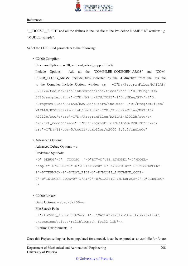
References
“__TICCSC__”, “RT” and all the defines in the .txt file to the Pre-define NAME “-D” window e.g.
“MODEL=sample”.
6) Set the CCS Build parameters to the following:
• C2000 Compiler:
Processor Options: -v 28, -ml, -mt, –float_support fpu32
Include Options: Add all the "COMPILER_CODEGEN_ARGS" and "COM-
PILER_TCCFG_ARGS" include files indicated by the -I directive from the .mk file
to the Compiler Include Options window e.g. -I"D:/ProgramFiles/MATLAB/
R2012b/toolbox/idelink/extensions/ticcs/inc"-I"D:/MEng/RTW/
CCS5/sample_ticcs"-I"D:/MEng/RTW/CCS5"-I"D:/MEng/RTW"-I"D:
/ProgramFiles/MATLAB/R2012b/extern/include"-I"D:/ProgramFiles/
MATLAB/R2012b/simulink/include"-I"D:/ProgramFiles/MATLAB/
R2012b/rtw/c/src"-I"D:/ProgramFiles/MATLAB/R2012b/rtw/c/
src/ext_mode/common"-I"D:/ProgramFiles/MATLAB/R2012b/rtw/c/
ert"-I"D:/TI/ccsv5/tools/compiler/c2000_6.2.3/include"
• Advanced Options:
Advanced Debug Options: -g
Predefined Symbols:
-D"_DEBUG"-D"__TICCSC__"-D"RT"-D"USE_RTMODEL"-D"MODEL=
sample"-D"NUMST=1"-D"NCSTATES=0"-D"HAVESTDIO="-D"ONESTEPFCN=
1"-D"TERMFCN=1"-D"MAT_FILE=0"-D"MULTI_INSTANCE_CODE=
0"-D"INTEGER_CODE=0"-D"MT=0"-D"CLASSIC_INTERFACE=0"-D"TID01EQ=
0"
• C2000 Linker:
Basic Options: -stack0x400-w
File Search Path:
-l"rts2800_fpu32.lib"and-l"..\MATLAB\R2012b\toolbox\idelink\
extensions\ticcs\rtlib\IQmath_fpu32.lib"-x
Runtime Environment: -c
Once this Project setting has been populated for a model, it can be exported as an .xml file for future
Department of Mechanical and Aeronautical EngineeringUniversity of Pretoria
208
© University of Pretoria

References
use. Right click on the project and select “Export", C/C++ Project Settings, “Next", Export file name
and “Finish". Using the import function, these settings can be imported into new projects.
7) Build and debug as usual. Changes in the Simulink® model will also be transferred to the files in
the build.
Department of Mechanical and Aeronautical EngineeringUniversity of Pretoria
209
© University of Pretoria
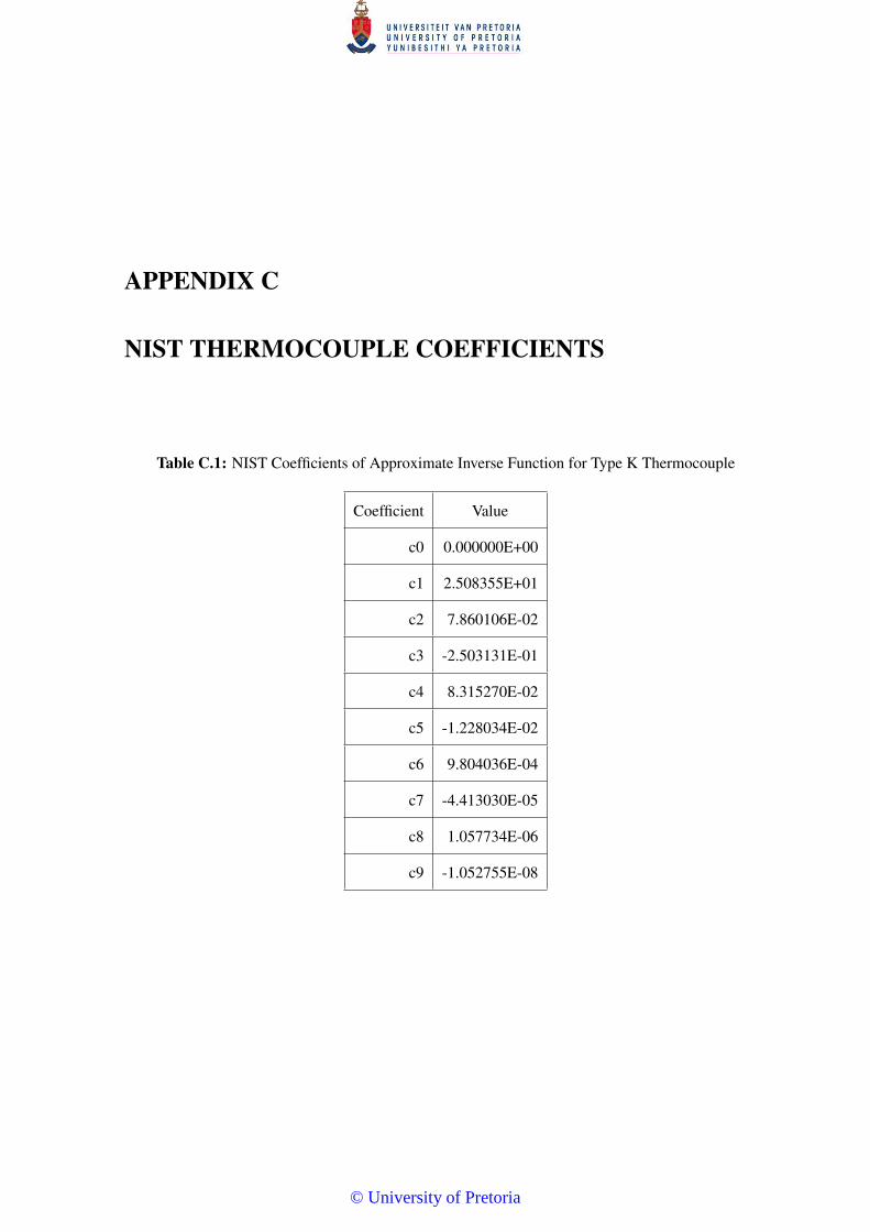
APPENDIX C
NIST THERMOCOUPLE COEFFICIENTS
Table C.1: NIST Coefficients of Approximate Inverse Function for Type K Thermocouple
Coefficient Value
c0 0.000000E+00
c1 2.508355E+01
c2 7.860106E-02
c3 -2.503131E-01
c4 8.315270E-02
c5 -1.228034E-02
c6 9.804036E-04
c7 -4.413030E-05
c8 1.057734E-06
c9 -1.052755E-08
© University of Pretoria
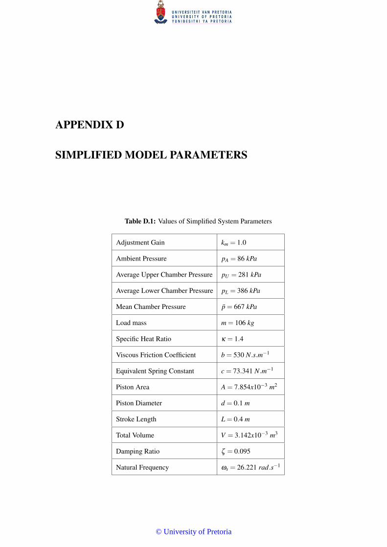
APPENDIX D
SIMPLIFIED MODEL PARAMETERS
Table D.1: Values of Simplified System Parameters
Adjustment Gain km = 1.0
Ambient Pressure pA = 86 kPa
Average Upper Chamber Pressure pU = 281 kPa
Average Lower Chamber Pressure pL = 386 kPa
Mean Chamber Pressure p = 667 kPa
Load mass m = 106 kg
Specific Heat Ratio κ = 1.4
Viscous Friction Coefficient b = 530 N.s.m−1
Equivalent Spring Constant c = 73.341 N.m−1
Piston Area A = 7.854x10⁻³ m2
Piston Diameter d = 0.1 m
Stroke Length L = 0.4 m
Total Volume V = 3.142x10⁻³ m3
Damping Ratio ζ = 0.095
Natural Frequency ωs = 26.221 rad.s−1
© University of Pretoria
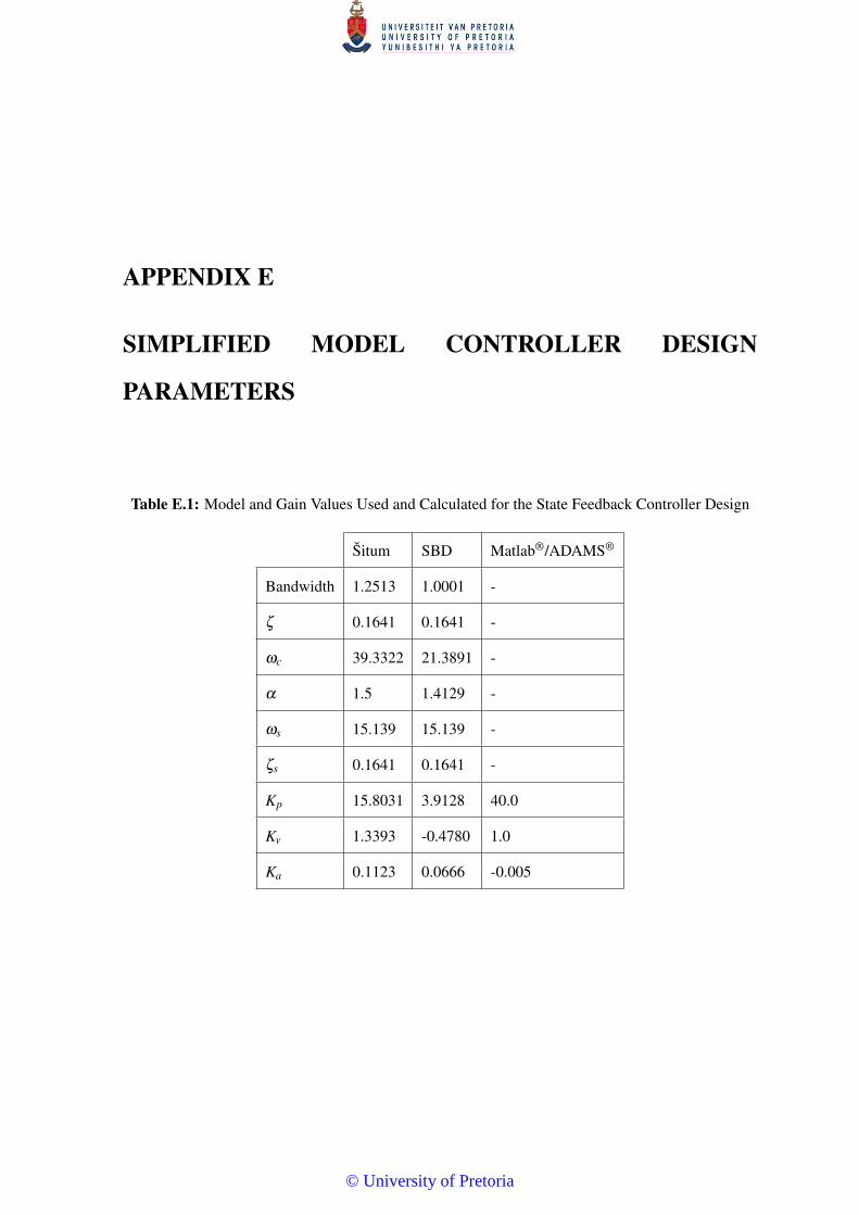
APPENDIX E
SIMPLIFIED MODEL CONTROLLER DESIGN
PARAMETERS
Table E.1: Model and Gain Values Used and Calculated for the State Feedback Controller Design
Šitum SBD Matlab®/ADAMS®
Bandwidth 1.2513 1.0001 -
ζ 0.1641 0.1641 -
ωc 39.3322 21.3891 -
α 1.5 1.4129 -
ωs 15.139 15.139 -
ζs 0.1641 0.1641 -
Kp 15.8031 3.9128 40.0
Kv 1.3393 -0.4780 1.0
Ka 0.1123 0.0666 -0.005
© University of Pretoria


