Modelling of Convolutional Encoders with Viterbi Decoders for

Asian Journal of Engineering and Technology (ISSN: 2321 – 2462)

Volume 02 – Issue 05, October 2014

Asian Online Journals (www.ajouronline.com) 356

Modelling of Convolutional Encoders with Viterbi Decoders for

Next Generation Broadband Wireless Access Systems

Benson Ojedayo1, Ayodeji Ireti Fasiku

2 and O. Elohor Oyinloye

3

1,2 Computer Engineering Department, Faculty of Engineering,

Ekiti State University, Ado – Ekiti, Nigeria. 2Email: iretiayous76 {at} yahoo.com

3Computer Science Department, Faculty of Science Ekiti State University,Ado – Ekiti, Nigeria

___________________________________________________________________________________________________

ABSTRACT--- Channel coding is known to be a form of modifying or scrambling a message between the source and

the receiver so that the message is not corrupted before it is received; or in some cases known, the message may

contain error. There are different forms of scrambling a message and detecting the error in the case there is one. The

first is to request the message again called Automatic Repeat request (ARQ) and the other is to correct the message

before getting to the destination Forward error correction (FEC). This research paper presents a system on the

Convolutional encoding and the Viterbi decoding which is a Forward error correction method and the system was

modelled using Matlab with special consideration for next generation broadband wireless access system.

Keywords--- Channel coding, Automatic Repeat request, Forward error correction, Matlab, Broadband Wireless Access

System, Convolutional encoding and the Viterbi decoding

_________________________________________________________________________________________________

1. INTRODUCTION

Communication is an act of conveying message form one point to the other. Communication is not perfect even if the

message is accurately stated because it may be corrupted during transmission for example if the message “I am now able

to graduate” is transmitted and it is received in error, it can mean a completely different thing even with just a bit that was received in error like “I am noT able to graduate”. As a result when a message travels from an information source to

a destination both the sender and the receiver would like assurance that the received message is free from errors and if it

contains error it will be detected and corrected. Richard W Hamming in 1974 was motivated by mistake which occurred

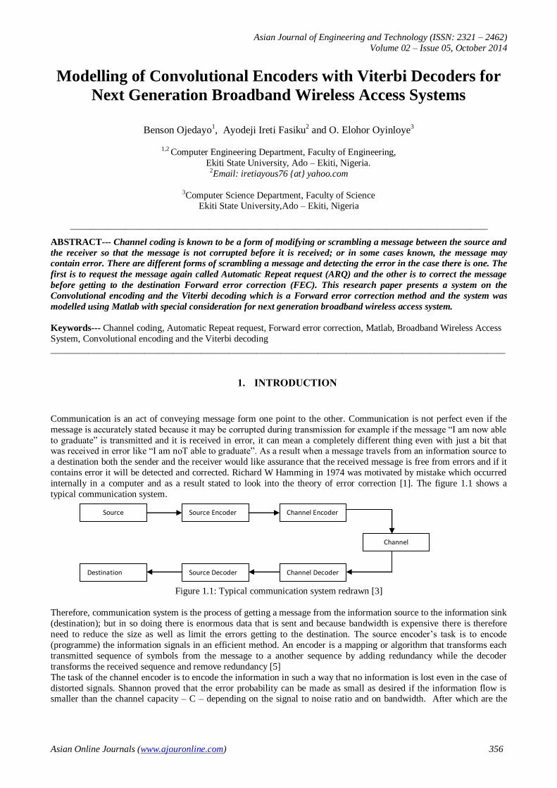
internally in a computer and as a result stated to look into the theory of error correction [1]. The figure 1.1 shows a

typical communication system.

Figure 1.1: Typical communication system redrawn [3]

Therefore, communication system is the process of getting a message from the information source to the information sink

(destination); but in so doing there is enormous data that is sent and because bandwidth is expensive there is therefore

need to reduce the size as well as limit the errors getting to the destination. The source encoder’s task is to encode

(programme) the information signals in an efficient method. An encoder is a mapping or algorithm that transforms each

transmitted sequence of symbols from the message to a another sequence by adding redundancy while the decoder

transforms the received sequence and remove redundancy [5]

The task of the channel encoder is to encode the information in such a way that no information is lost even in the case of

distorted signals. Shannon proved that the error probability can be made as small as desired if the information flow is smaller than the channel capacity – C – depending on the signal to noise ratio and on bandwidth. After which are the

Channel

Channel Decoder Source Decoder

Destination

Source Encoder Channel Encoder Source




corresponding decoders that reinstate the signal back to its initial state before it was encoded. And finally the information

at the destination is hopefully error free.

In 1948 the fundamental concepts and mathematical theory of information transmission were laid by C. E Shannon [4]

He perceived that it is achievable to transmit digital information over noisy channel with arbitrary negligible error

probability if there is proper channel coding and decoding in place. Shannon’s says the goal of error free transmission

can be achieved if the information transmission rate is less than the channel capacity. He did not however indicate how to achieve the task, his theory which is called the Shannon capacity theory was the theory that opens many researchers to

the finding of efficient method for error-control coding by introducing redundancies to allow for error correction.

Earlier in information theory before the works of Shannon; is the works of Nyquist and Hartley [3]. Nyquist initiate the

minimum frequency band to transmit independent discrete signals at a given rate whilst Hartley suggested the use of

logarithmic measure for information;

He suggested that the information transmitted is proportional to the logarithm of the number of different signals we use.

A different approach is what Shannon used; he suggested that the signal is not to be considered but the information. The

information symbolizes encoded signals, which are information carriers. This implies that it is possible to transmit

signals that do not carry any information at all.

Shannon theory equation [equation 1.1] stated below is mainly to prove that any communication channel could be

characterized by a capacity at which information could be reliably transmitted. It should be noted that, for higher signal-

to-noise ratios, the doubling of the signal (transmitted) power (3 dB) increases capacity for only one bit per second per-Hertz of the bandwidth.

C = B log2 (1 + ) ---------------------------------- (1.1)

C = channel capacity in bits/sec

B = bandwidth in Hertz

S/N = signal to noise ratio.

Most of Shannon’s coding theorems applied to sources and channels without memory. In the last decade and a half,

considerable progress has been made in establishing coding theorems for more general situations [17]; but recently, the

work now incorporate the proving of the channel coding theorem for stationary continuous-time channels with

asymptotically vanishing memory.

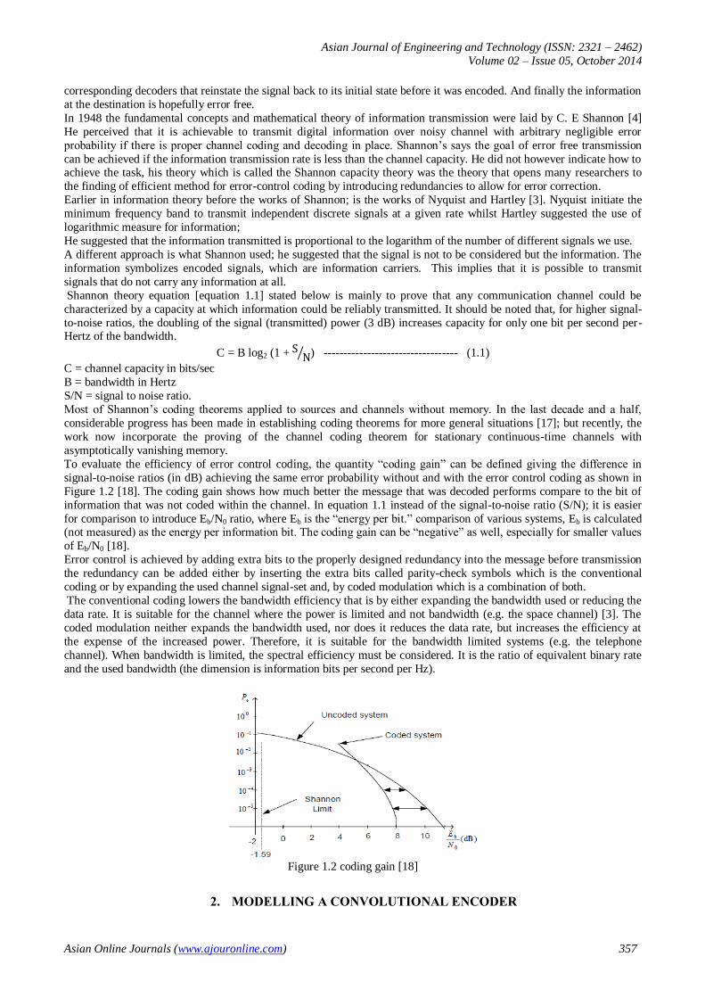
To evaluate the efficiency of error control coding, the quantity “coding gain” can be defined giving the difference in

signal-to-noise ratios (in dB) achieving the same error probability without and with the error control coding as shown in

Figure 1.2 [18]. The coding gain shows how much better the message that was decoded performs compare to the bit of

information that was not coded within the channel. In equation 1.1 instead of the signal-to-noise ratio (S/N); it is easier

for comparison to introduce Eb/N0 ratio, where Eb is the “energy per bit.” comparison of various systems, Eb is calculated (not measured) as the energy per information bit. The coding gain can be “negative” as well, especially for smaller values

of Eb/N0 [18].

Error control is achieved by adding extra bits to the properly designed redundancy into the message before transmission

the redundancy can be added either by inserting the extra bits called parity-check symbols which is the conventional

coding or by expanding the used channel signal-set and, by coded modulation which is a combination of both.

The conventional coding lowers the bandwidth efficiency that is by either expanding the bandwidth used or reducing the

data rate. It is suitable for the channel where the power is limited and not bandwidth (e.g. the space channel) [3]. The

coded modulation neither expands the bandwidth used, nor does it reduces the data rate, but increases the efficiency at

the expense of the increased power. Therefore, it is suitable for the bandwidth limited systems (e.g. the telephone

channel). When bandwidth is limited, the spectral efficiency must be considered. It is the ratio of equivalent binary rate

and the used bandwidth (the dimension is information bits per second per Hz).

Figure 1.2 coding gain [18]

2. MODELLING A CONVOLUTIONAL ENCODER




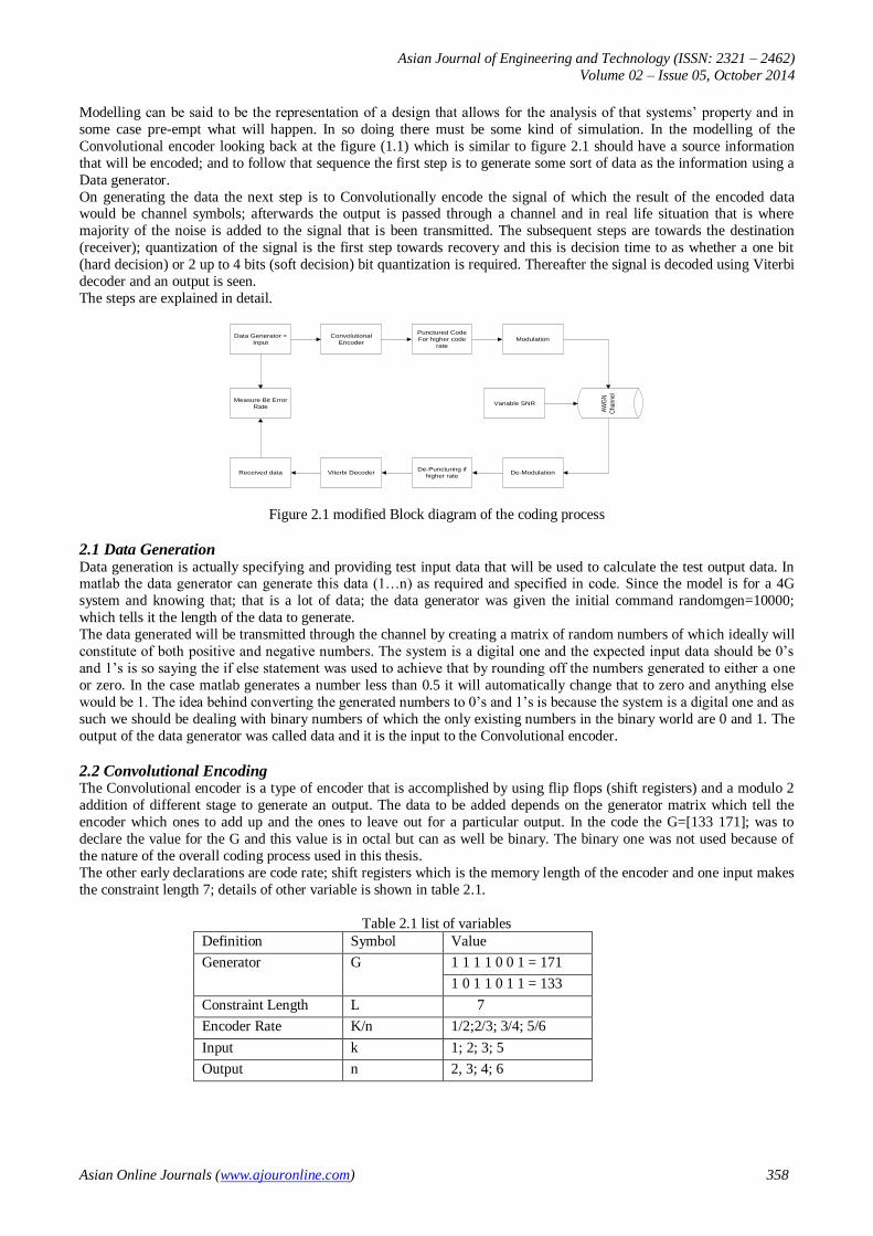
Modelling can be said to be the representation of a design that allows for the analysis of that systems’ property and in

some case pre-empt what will happen. In so doing there must be some kind of simulation. In the modelling of the

Convolutional encoder looking back at the figure (1.1) which is similar to figure 2.1 should have a source information

that will be encoded; and to follow that sequence the first step is to generate some sort of data as the information using a

Data generator.

On generating the data the next step is to Convolutionally encode the signal of which the result of the encoded data would be channel symbols; afterwards the output is passed through a channel and in real life situation that is where

majority of the noise is added to the signal that is been transmitted. The subsequent steps are towards the destination

(receiver); quantization of the signal is the first step towards recovery and this is decision time to as whether a one bit

(hard decision) or 2 up to 4 bits (soft decision) bit quantization is required. Thereafter the signal is decoded using Viterbi

decoder and an output is seen.

The steps are explained in detail.

Data Generator =

Input

Convolutional

Encoder

Punctured Code

For higher code

rate

Modulation

AW

GN

Cha

nnel

Received data Viterbi DecoderDe-Puncturing if

higher rate De-Modulation

Variable SNRMeasure Bit Error

Rate

Figure 2.1 modified Block diagram of the coding process

2.1 Data Generation Data generation is actually specifying and providing test input data that will be used to calculate the test output data. In matlab the data generator can generate this data (1…n) as required and specified in code. Since the model is for a 4G

system and knowing that; that is a lot of data; the data generator was given the initial command randomgen=10000;

which tells it the length of the data to generate.

The data generated will be transmitted through the channel by creating a matrix of random numbers of which ideally will

constitute of both positive and negative numbers. The system is a digital one and the expected input data should be 0’s

and 1’s is so saying the if else statement was used to achieve that by rounding off the numbers generated to either a one

or zero. In the case matlab generates a number less than 0.5 it will automatically change that to zero and anything else

would be 1. The idea behind converting the generated numbers to 0’s and 1’s is because the system is a digital one and as

such we should be dealing with binary numbers of which the only existing numbers in the binary world are 0 and 1. The

output of the data generator was called data and it is the input to the Convolutional encoder.

2.2 Convolutional Encoding The Convolutional encoder is a type of encoder that is accomplished by using flip flops (shift registers) and a modulo 2

addition of different stage to generate an output. The data to be added depends on the generator matrix which tell the

encoder which ones to add up and the ones to leave out for a particular output. In the code the G=[133 171]; was to

declare the value for the G and this value is in octal but can as well be binary. The binary one was not used because of

the nature of the overall coding process used in this thesis.

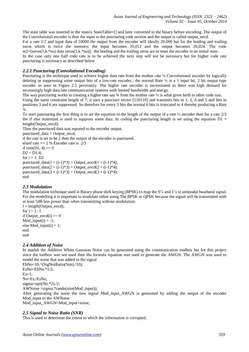
The other early declarations are code rate; shift registers which is the memory length of the encoder and one input makes

the constraint length 7; details of other variable is shown in table 2.1.

Table 2.1 list of variables

Definition Symbol Value

Generator G 1 1 1 1 0 0 1 = 171

1 0 1 1 0 1 1 = 133

Constraint Length L 7

Encoder Rate K/n 1/2;2/3; 3/4; 5/6

Input k 1; 2; 3; 5

Output n 2, 3; 4; 6




The state table was inserted in the matrix StateTable=[] and later converted to the binary before encoding. The output of

the Convolutional encoder is then the input to the puncturing code section and the output is called output_encd.

For a rate 1/2 and input data of 10000 the output from the encoder will ideally 20,000 but for the leading and trailing

zeros which is twice the memory; the input becomes 10,012 and the output becomes 20,024. The code

m2=[zeros(1,k.*nu) data zeros(1,k.*nu)]; the leading and the trailing zeros are to reset the encoder to an initial state.

In the case only one half code rate is to be achieved the next step will not be necessary but for higher code rate puncturing is necessary as described below

2.2.1 Puncturing (Convolutional Encoding) Puncturing is the technique used to achieve higher data rate from the mother rate ½ Convolutional encoder by logically

deleting or suppressing some output bits of a low-rate encoder.; the normal Rate ½ is a 1 input bit, 2 bit output type

encoder as seen in Figure 2.5 previously. The higher rate encoder is necessitated as there was high demand for

increasingly high data rate communication systems with limited bandwidth and energy.

The way puncturing works in creating a higher rate say ¾ from the mother rate ½ is what gives birth to other code rate.

Using the same constraint length of 7; it uses a puncture vector [110110] and transmits bits in 1, 2, 4 and 5 and bits in positions 3 and 6 are suppressed. So therefore for every 3 bits the normal 6 bits is truncated to 4 thereby producing a Rate

¾.

To start puncturing the first thing is to set the equation to the length of the output of a rate ½ encoder then for a rate 2/3

the if else statement is used to suppress some data. In coding the puncturing length is set using the equation D1 =

length(Output_encd);

Then the punctured data was equated to the encoder output.

punctured_data = Output_encd;

if the rate is set to be 2 then the output of the encoder is punctured.

elseif rate == 2 % Encoder rate is 2/3

if rem(D1, 4) == 0

D2 = D1/4;

for i = 1: D2 punctured_data(1 + (i-1)*3) = Output_encd(1 + (i-1)*4);

punctured_data(2 + (i-1)*3) = Output_encd(2 + (i-1)*4);

punctured_data(3 + (i-1)*3) = Output_encd(3 + (i-1)*4);

end

2.3 Modulation The modulation technique used is Binary phase shift keying (BPSK) to map the 0’s and 1’s to antipodal baseband signal.

For the modelling it is important to modulate either using The BPSK or QPSK because the signal will be transmitted with

at least 5dB less power than when transmitting without modulation. l = length(Output_encd);

for i = 1 : l

if Output_encd(i) == 0

Mod_input(i) = -1;

else Mod_input(i) = 1;

end

end

2.4 Addition of Noise In matlab the Additive White Gaussian Noise can be generated using the communication toolbox but for this project

since the toolbox was not used then the formula equation was used to generate the AWGN. The AWGN was used to

model the noise that was added to the signal

EbNo=10.^(SigNoiRatio(Sim)./10);

EsNo=EbNo.*1/2;

Es=1;

No=Es./EsNo;

sigma=sqrt(No.*2)./2;

AWNoise =sigma.*randn(size(Mod_input));

After generating the noise the new signal Mod_input_AWGN is generated by adding the output of the encoder

Mod_input to the AWNoise. Mod_input_AWGN=Mod_input+noise;

2.5 Signal to Noise Ratio (SNR) This is used to determine the extent to which the information is corrupted.




It is expressed as a fraction of signal power to noise power; and it is normally written as Eb/N0 (the energy per bit to

noise power spectral density ratio (bit/s)/Hz)

The higher the Signal to Noise Ratio the lesser the Bit Error Rate.

The SigNoiRatio=[-1:1:12]; is used to vary the signal to noise at a step interval of 1 between -1 and 12dB.

for Sim=1:length(SigNoiRatio)

NoOfBitErrors=0; TotalNoOfBits=0;

2.6 De-Modulation This is the stage to recover the original message that was mapped to -1 and +1 back to the 0 and 1.

2.7 De-Puncturing This is the stage where some zeros are added to the code to make up for the removed ones at the puncturing stage. It is necessary to add the zeros because when decoding without those missing bit the decoder will produce a different result.

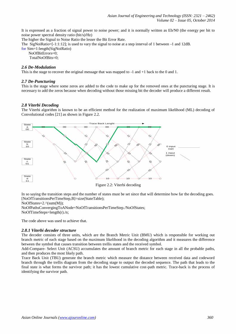
2.8 Viterbi Decoding The Viterbi algorithm is known to be an efficient method for the realization of maximum likelihood (ML) decoding of

Convolutional codes [21] as shown in Figure 2.2.

State

a

00

State

d

11

State

c

01

State

b

10

00

11

00 00 00 00 00

11111111 11

10

01

10 10 101001

01 0101

11 00 0000 00111111

10 10 10

01 01 01

0 input

(up)

1 input

(down)

Trace Back Lenght

Figure 2.2: Viterbi decoding

In so saying the transition steps and the number of states must be set since that will determine how far the decoding goes. [NoOfTransitionsPerTimeStep,B]=size(StateTable);

NoOfStates=2.^(sum(M));

NoOfPathsConvergingToANode=NoOfTransitionsPerTimeStep./NoOfStates;

NoOfTimeSteps=length(r)./n;

The code above was used to achieve that.

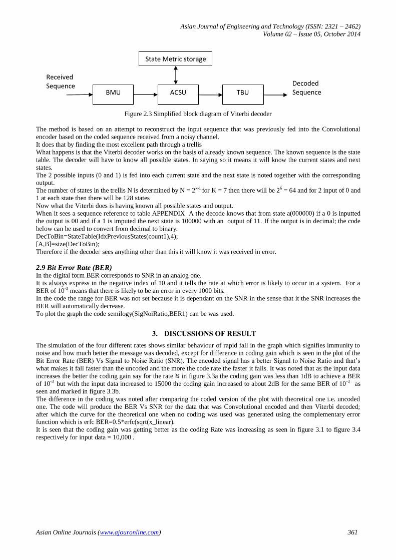
2.8.1 Viterbi decoder structure The decoder consists of three units, which are the Branch Metric Unit (BMU) which is responsible for working out

branch metric of each stage based on the maximum likelihood in the decoding algorithm and it measures the difference

between the symbol that causes transition between trellis states and the received symbol.

Add-Compare- Select Unit (ACSU) accumulates the amount of branch metric for each stage in all the probable paths,

and then produces the most likely path.

Trace Back Unit (TBU) generate the branch metric which measure the distance between received data and codeword

branch through the trellis diagram from the decoding stage to output the decoded sequence. The path that leads to the

final state is what forms the survivor path; it has the lowest cumulative cost-path metric. Trace-back is the process of

identifying the survivor path.




Figure 2.3 Simplified block diagram of Viterbi decoder

The method is based on an attempt to reconstruct the input sequence that was previously fed into the Convolutional

encoder based on the coded sequence received from a noisy channel.

It does that by finding the most excellent path through a trellis

What happens is that the Viterbi decoder works on the basis of already known sequence. The known sequence is the state

table. The decoder will have to know all possible states. In saying so it means it will know the current states and next

states.

The 2 possible inputs (0 and 1) is fed into each current state and the next state is noted together with the corresponding output.

The number of states in the trellis N is determined by N = 2k-1 for K = 7 then there will be 26 = 64 and for 2 input of 0 and

1 at each state then there will be 128 states

Now what the Viterbi does is having known all possible states and output.

When it sees a sequence reference to table APPENDIX A the decode knows that from state a(000000) if a 0 is inputted

the output is 00 and if a 1 is imputed the next state is 100000 with an output of 11. If the output is in decimal; the code

below can be used to convert from decimal to binary.

DecToBin=StateTable(IdxPreviousStates(count1),4);

[A,B]=size(DecToBin);

Therefore if the decoder sees anything other than this it will know it was received in error.

2.9 Bit Error Rate (BER) In the digital form BER corresponds to SNR in an analog one.

It is always express in the negative index of 10 and it tells the rate at which error is likely to occur in a system. For a

BER of 10-3 means that there is likely to be an error in every 1000 bits.

In the code the range for BER was not set because it is dependant on the SNR in the sense that it the SNR increases the

BER will automatically decrease.

To plot the graph the code semilogy(SigNoiRatio,BER1) can be was used.

3. DISCUSSIONS OF RESULT

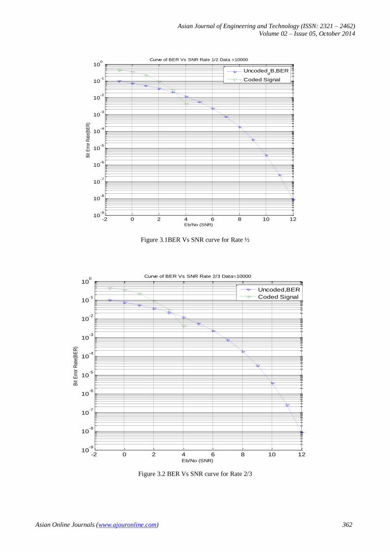
The simulation of the four different rates shows similar behaviour of rapid fall in the graph which signifies immunity to

noise and how much better the message was decoded, except for difference in coding gain which is seen in the plot of the

Bit Error Rate (BER) Vs Signal to Noise Ratio (SNR). The encoded signal has a better Signal to Noise Ratio and that’s

what makes it fall faster than the uncoded and the more the code rate the faster it falls. It was noted that as the input data

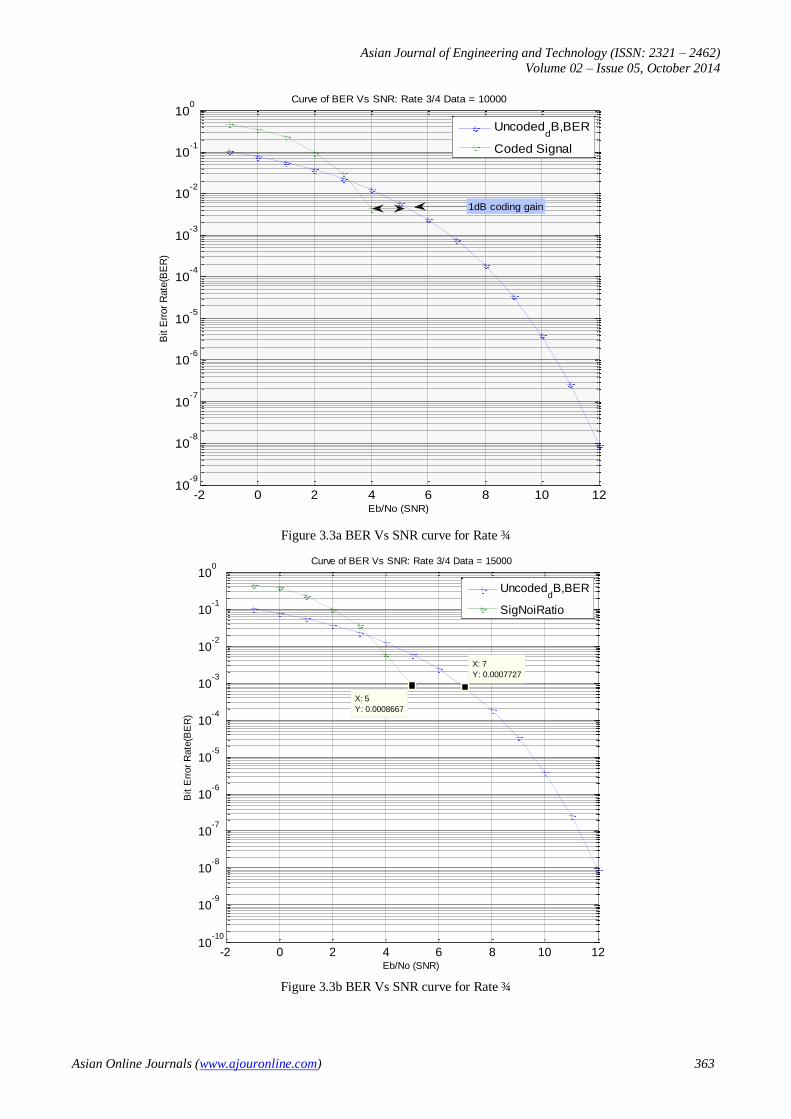
increases the better the coding gain say for the rate ¾ in figure 3.3a the coding gain was less than 1dB to achieve a BER

of 10-3 but with the input data increased to 15000 the coding gain increased to about 2dB for the same BER of 10-3 as

seen and marked in figure 3.3b.

The difference in the coding was noted after comparing the coded version of the plot with theoretical one i.e. uncoded

one. The code will produce the BER Vs SNR for the data that was Convolutional encoded and then Viterbi decoded;

after which the curve for the theoretical one when no coding was used was generated using the complementary error function which is erfc BER=0.5*erfc(sqrt(x_linear).

It is seen that the coding gain was getting better as the coding Rate was increasing as seen in figure 3.1 to figure 3.4

respectively for input data = 10,000 .

BMU TBU ACSU

Received Sequence Decoded

Sequence

State Metric storage




Figure 3.1BER Vs SNR curve for Rate ½

Figure 3.2 BER Vs SNR curve for Rate 2/3

-2 0 2 4 6 8 10 1210

-9

10-8

10-7

10-6

10-5

10-4

10-3

10-2

10-1

100

Curve of BER Vs SNR Rate 1/2 Data =10000

Eb/No (SNR)

Bit

Err

or R

ate(

BE

R)

UncodeddB,BER

Coded Signal

-2 0 2 4 6 8 10 1210

-9

10-8

10-7

10-6

10-5

10-4

10-3

10-2

10-1

100

Curve of BER Vs SNR Rate 2/3 Data=10000

Eb/No (SNR)

Bit

Err

or R

ate(

BE

R)

Uncoded,BER

Coded Signal




Figure 3.3a BER Vs SNR curve for Rate ¾

Figure 3.3b BER Vs SNR curve for Rate ¾

-2 0 2 4 6 8 10 1210

-10

10-9

10-8

10-7

10-6

10-5

10-4

10-3

10-2

10-1

100

Curve of BER Vs SNR: Rate 3/4 Data = 15000

Eb/No (SNR)

Bit E

rror

Rate

(BE

R)

X: 5

Y: 0.0008667

X: 7

Y: 0.0007727

UncodeddB,BER

SigNoiRatio

-2 0 2 4 6 8 10 1210

-9

10-8

10-7

10-6

10-5

10-4

10-3

10-2

10-1

100

Curve of BER Vs SNR: Rate 3/4 Data = 10000

Eb/No (SNR)

Bit E

rror

Rate

(BE

R)

UncodeddB,BER

Coded Signal

1dB coding gain




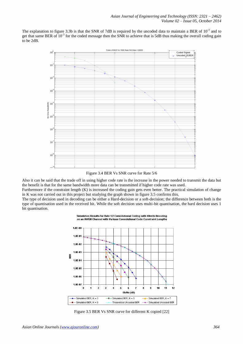
The explanation to figure 3.3b is that the SNR of 7dB is required by the uncoded data to maintain a BER of 10-3 and to

get that same BER of 10-3 for the coded message then the SNR to achieve that is 5dB thus making the overall coding gain

to be 2dB.

Figure 3.4 BER Vs SNR curve for Rate 5/6

Also it can be said that the trade off in using higher code rate is the increase in the power needed to transmit the data but

the benefit is that for the same bandwidth more data can be transmitted if higher code rate was used.

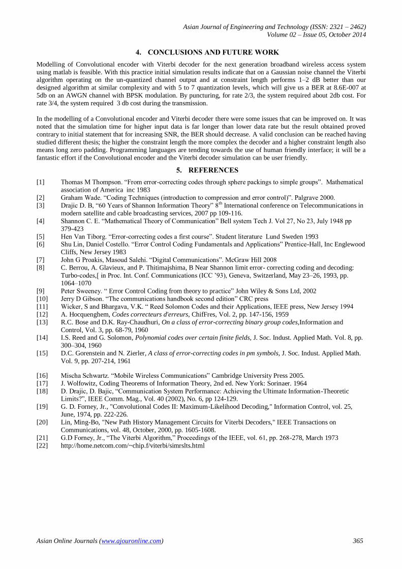
Furthermore if the constraint length (K) is increased the coding gain gets even better. The practical simulation of change

in K was not carried out in this project but studying the graph shown in figure 3.5 confirms this.

The type of decision used in decoding can be either a Hard-decision or a soft-decision; the difference between both is the

type of quantisation used in the received bit. While the soft decision uses multi-bit quantisation, the hard decision uses 1 bit quantisation.

Figure 3.5 BER Vs SNR curve for different K copied [22]

-2 0 2 4 6 8 10 1210

-9

10-8

10-7

10-6

10-5

10-4

10-3

10-2

10-1

100

Curve of BER Vs SNR Rate 5/6 Data =10000

Eb/No (SNR)

Bit E

rror

Rate

(BE

R)

Coded Signal

UncodeddB,BER




4. CONCLUSIONS AND FUTURE WORK

Modelling of Convolutional encoder with Viterbi decoder for the next generation broadband wireless access system

using matlab is feasible. With this practice initial simulation results indicate that on a Gaussian noise channel the Viterbi algorithm operating on the un-quantized channel output and at constraint length performs 1–2 dB better than our

designed algorithm at similar complexity and with 5 to 7 quantization levels, which will give us a BER at 8.6E-007 at

5db on an AWGN channel with BPSK modulation. By puncturing, for rate 2/3, the system required about 2db cost. For

rate 3/4, the system required 3 db cost during the transmission.

In the modelling of a Convolutional encoder and Viterbi decoder there were some issues that can be improved on. It was

noted that the simulation time for higher input data is far longer than lower data rate but the result obtained proved

contrary to initial statement that for increasing SNR, the BER should decrease. A valid conclusion can be reached having

studied different thesis; the higher the constraint length the more complex the decoder and a higher constraint length also

means long zero padding. Programming languages are tending towards the use of human friendly interface; it will be a

fantastic effort if the Convolutional encoder and the Viterbi decoder simulation can be user friendly.

5. REFERENCES

[1] Thomas M Thompson. “From error-correcting codes through sphere packings to simple groups”. Mathematical

association of America inc 1983

[2] Graham Wade. “Coding Techniques (introduction to compression and error control)”. Palgrave 2000.

[3] Drajic D. B, “60 Years of Shannon Information Theory” 8th International conference on Telecommunications in

modern satellite and cable broadcasting services, 2007 pp 109-116.

[4] Shannon C. E. “Mathematical Theory of Communication” Bell system Tech J. Vol 27, No 23, July 1948 pp

379-423

[5] Hen Van Tiborg. “Error-correcting codes a first course”. Student literature Lund Sweden 1993 [6] Shu Lin, Daniel Costello. “Error Control Coding Fundamentals and Applications” Prentice-Hall, Inc Englewood

Cliffs, New Jersey 1983

[7] John G Proakis, Masoud Salehi. “Digital Communications”. McGraw Hill 2008

[8] C. Berrou, A. Glavieux, and P. Thitimajshima, B Near Shannon limit error- correcting coding and decoding:

Turbo-codes,[ in Proc. Int. Conf. Communications (ICC ’93), Geneva, Switzerland, May 23–26, 1993, pp.

1064–1070

[9] Peter Sweeney. “ Error Control Coding from theory to practice” John Wiley & Sons Ltd, 2002

[10] Jerry D Gibson. “The communications handbook second edition” CRC press

[11] Wicker, S and Bhargava, V.K. “ Reed Solomon Codes and their Applications, IEEE press, New Jersey 1994

[12] A. Hocquenghem, Codes correcteurs d'erreurs, ChifFres, Vol. 2, pp. 147-156, 1959

[13] R.C. Bose and D.K. Ray-Chaudhuri, On a class of error-correcting binary group codes,Information and

Control, Vol. 3, pp. 68-79, 1960 [14] I.S. Reed and G. Solomon, Polynomial codes over certain finite fields, J. Soc. Indust. Applied Math. Vol. 8, pp.

300–304, 1960

[15] D.C. Gorenstein and N. Zierler, A class of error-correcting codes in pm symbols, J. Soc. Indust. Applied Math.

Vol. 9, pp. 207-214, 1961

[16] Mischa Schwartz. “Mobile Wireless Communications” Cambridge University Press 2005.

[17] J. Wolfowitz, Coding Theorems of Information Theory, 2nd ed. New York: Sorinaer. 1964

[18] D. Drajic, D. Bajic, “Communication System Performance: Achieving the Ultimate Information-Theoretic Limits?”, IEEE Comm. Mag., Vol. 40 (2002), No. 6, pp 124-129.

[19] G. D. Forney, Jr., "Convolutional Codes II: Maximum-Likelihood Decoding," Information Control, vol. 25,

June, 1974, pp. 222-226.

[20] Lin, Ming-Bo, "New Path History Management Circuits for Viterbi Decoders," IEEE Transactions on

Communications, vol. 48, October, 2000, pp. 1605-1608.

[21] G.D Forney, Jr., “The Viterbi Algorithm,” Proceedings of the IEEE, vol. 61, pp. 268-278, March 1973

[22] http://home.netcom.com/~chip.f/viterbi/simrslts.html

Documents

Modelling of Convolutional Encoders with Viterbi Decoders for