0COGRAPHY 22: 251-260, Copenhagen 1999

Modelling wildlife distributions: Logistic Multiple Regression vs"Overlap Analysis

, C. Brito, E. G. Crespo and O. S. Paulo

Brito. .1. C , Crespo, L. G. and Paulo, O. S. 1999. Modelling wildlife distributions:Logistic Multiple Regression vs Overlap Analysis, Ecography 22: 251 260.

We compare the results, benefits and disadvantages of two techniques for modellingwildlife speeies distribution: Logistic Regression and Overlap Analysis. While Logis-tic Regression uses mathematic equations to correlate variables with presence/abseneeof the speeies. Overlap Analysis simply combine variables with the presence points,eliminating the non-explanatory variables and recombining the others. Both tech-niques were performed in a Geographic Information System and we attempted tominimise the spatial autocorrelation of data. The speeies used was the Schreiber"sgreen lizard Laccriti sclirciberi and the study area was Portugal, using 10 x If) kmUTM squares. Both techniques identified the same group of variables as the mostimportant for explaining the distribution of the species. Both techniques gave highaverage eorreet classification rates for the squares with presence of the species (79"/!for Logistic Regression and 92"Ai for Overlap Analysis). Correct absence classificationwas higher with Logistic Regression {73'Mi) than with Overlap Analysis (32%),Overlap Analysis tends to maximise the potential area of occurrence of the species,which induces a reduced correct classification of absences, since many absences willfall in the potential area. This is because a single presence in a given class of avariable makes all the area of ihat class to be considered as potential. The techniquedoes not consider that the speeies may occasionally occupy an unfavourable region.Although, in Logistic Regression, modelling procedures are more complex andtime-consuming, the results are more statistically robust. Moreover. Logistic Regres-sion has the capability of associating probability of occurrence to the potential area.Overlap Analysis is very simple in building procedures and swift in obtaining reliablepotential areas. It is a valid technique especially in exploratory analysis of speciesdistributions or in ihc initial stages of research when data may be scarce.

J. C. Brito (j(i.se.hrito((bjc.iil.p!). E. G. Crespo und O. S. Paulo, Centra dt BiolagiaAiiihicnial. Fac. dc Ciencias da Univ. de Lisbon.. P-1700 Lisboa. Portugal.

Lfse of multivariate Statistics for model species distribu- habitat preferences (Pereira and Itami 1991, Greentions and habitat has increased in the last two decades 1996, North and Reynolds 1996), Use of regression

and a wide variety of techniques is used, such as models for newer applications, such as modelling spe-fjrincipal Components Analysis, Canonical Correlation cies demography (Forsman 1997), extinction probabil-i4.nalysis, Discriminant Function Analysis, Artificial ity (Bustamantc 1997) and metapopulation dynamicsNeural Networks, Classification and Regression Trees, (Sjogren and Ray 1996), is now common. ParticularlyCieneralizcd Linear Models or Regression Analysis. Re- Logistic Regression has been shown to be a powerfulgression models have been widely employed either to tool, capable of analysing the effects of one or severalpredict species distributions (Walker 1990. Osborne and independent variables, discrete or continuous, over a

[ijigar 1992, Mladenoff et al, 1995, Augustin et al. 1996. dichotomic (presence/absence) or polychotomic dcpen-rito et al. 1996), abundance/densities (Gates ct al. dent variable. Logistic Regression model has the form:994, Kintron et al. 1996. Schonrogge et al. 1996) or n:(x) = e ' '/Xl +e^'^'), where n(x) is the probability of

j^ccepted 30 September 1998

opyright © ECOGRAPHY 1999SN 0906-7590

Tinted in Ireland all rights reserved

22:3 i\Wi) 251

occurrence of a given species, ranging from 0 to 1.The g(x) value is obtained by a regression equation ofthe form: g{x) ^ po + Pi 'i + P- 2 + ••- + Pp j where pois a constant and P^.-Pp are the coefficients of therespective independent variables X|...Xp (Hosmer andLemeshow 1989).

Nevertheless, an easier and faster method of ob-taining potential distribution areas of species distribu-tion is Overlap Analysis. This method simplycombines variables with the presence of species, elimi-nating those with no explanatory power, and re-combining the remaining. Maps of potentialoccurrence of species are obtained as well as informa-tion on the importance of each variable class lor thespecies.

Both modelling techniques have been improvedwith their integration with Geographic InformationSystems (GIS). The use of GIS has increased becauseit provides means to store, display and analyse spatialdata. Moreover it allows one to derive predietivemodels from relations between the data and extrapo-late species potential distribution, abundance or habi-tat preferences from those models (Haslett 1990,Stoms et al. 1993).

The aims of this work are to model the distributionof Schreiber's green lizard Lacerla schreiberi, Bedriaga1878 using Logistic Regression and Overlap Analysisand then comparing results, benefits and disadvan-tages of each method. Both models were developed ina Geographie Information System.

Lacerta schreiheri is an endemie speeies from theIberian Peninsula, limited to the north-western andcentral system with some isolated populations in thesouth (Brito et al. 1998). It is a medium-sized lizard(adult snout-vent length: 117-120 mm) with markedsexual dimorphism, adult males being smaller andstronger than females, and having an intense blue eol-oration on the head during the mating season. It oeeursfrom sea level up to 2100 m, but it is more usual inmountainous regions. It inhabits places that have highhumidity, such as margins of streams (Brito et al. 1998),but is a good stone wall and bush climber. The speeiesfeeds mainly on Coleoptera, Formicidae and Diptera(Marco and Perez-Mellado 1988). It is a speeies of highinterest for conservation, being included in the Habitatsdirective (92/43/EEC). The distribution area modelledrelates only to Portugal.

Methods

The data

Between 1994 and 1996. 466 UTM (Universal Trans-verse of Mereator) 10 x 10 km squares were sampledin order to detect the presenee of L. schreiberi. Thesesampled squares represent 45'X> of the area of Portu-

gal. The sampling strategy was based on the previ-ously known distribution area of the species (Crespoand Oliveira 1989, Marco and Polio 1993. Malkmus1995) and the aim was to delimit it with aeeuracy.The preliminary results of distribution were publishedin Brito et al. (1996). In Fig. I is presented the actualknown distribution area of this speeies in Portugalaccording to Brito et al. (1998).

A matrix was built in which the absence or pres-enee (O/l) of the speeies (dependent variable) wasrecorded for the 466 sampled UTM squares (257 withpresence and 209 with absence of the speeies). Thesesquares were characterised with nine independentvariables (Table 1), defined from the Portuguese envi-ronmental atlas (Anon. 1983). To each class of avariable, we attributed a different value that makesthe variations occur in unitary steps.

Dealing with spatial autocorrelation

In regression analysis spatial autocorrelation of theinformation is sometimes ignored (e.g. Romero andReal 1996, Brito et al. 1996). Spatial autocorrelationhas the effect of reducing the number of independentobservations, which can lead to a loss of power ofthe model since observations are influeneed by neigh-bouring areas that tend to have similar conditions(Anselin 1993. Augustin et al. 1996). In this study, weattempted to minimise the spatial autoeorrelation ofdata by using non-adjacent information.

••••*4U!

rVa • • • •; • • • • • '

A - Serra de Sirtra

B - Serra de S.Mamede

C - Serra de Monchique e Cereal

D - Sierra de las Villuercas

E - Montes de Totedo

F - Sierra Oe San Andres

Fig. 1. Dislribulion area of Lacerta schreiheri in tlie IberianPeninsi]la (shadow area) and in Portugal (each circle repre-sents an observalion in a 10 x 10 km UTM grid). Adaptedfrom Brito et al. (1998).

252 ECOGRAPF^Y 22:? (1999)

Table I. Independent variables considered for the analysis.

Variable Description Units Code

Air humidityjllvapotranspirationI (isolation"E'emperatureIfrecipitationSoil drainingSoilI cology

Altitude a.s.l.Relative humidity at 09.00 GMTAmount of water returned to the atmosphereNumber of hours of sunlight per yearDaily average air temperatureTotal amount per yearAmount of water in the streamsType of soilPhyto-edapho-climatic information

mmh

mmmm

ALTHUMEVPINSTEMPREDRASOIECO

To measure spatial autocorrelation of the dcpen-ibnt variable we calculated Moran's I (Cliff and OrdIP73), using the Autocorr procedure of the Idrisi forWindows (Eastman 1995) GTS package. We used theQueen's case type of spatial autocorrelation, whichtests if squares with determined values have a com-lion edge and/or vertex (Cliff and Ord 1973). Valuesof Moran's I range between —1 and + 1 . Valuesi; ose to + 1 indicate a smooth surface, with eachsquare containing values very similar to the neigh-bouring ones, and values close to — 1 indicate veryrough or fractured surfaces, with adjacent squares ofdifferent values (Eastman 1995). The Autocorr proce-djure measures spatial autocorrelation for adjacentneighbours of a square, which is called first lag, andfij>r subsequent lags increasing distance neighbours(Eastman 1995), allowing the building of corrclo-grams. These correlograms can relate the level of spa-ti|al autocorrelation with increasing distances, anddetermine the distance beyond which spatial autocor-relation has no further influence on the data (Kintronet al. 1996). In Fig. 2 we present the correlogram ofVIoran's I related with the distance. We decided toase the 10 km limit because it reduces almost 50%:he autocorrelation and because the 20 km limitwould imply a great loss of information since only466 squares with information were available.

Therefore, the initial set with 466 squares was di-vided into 10 sets with 100 squares each. To choosethe squares in each set we used a regular grid, whichdid not allow any neighbouring 10 km squares to beiiicluded in any model. Squares were picked ran-fdpmly. with no neighbouring squares, and withoutrijjplacement within a set. That means that in one setthere are no repeated squares, but there are repeatedsquares across the 10 sets. These 10 sets were used tobuild 10 regression models, with Logistic Regression,md 10 potential areas of occurrence, with the Over-iip Analysis.I Usually it is advantageous to have more absences

;ftian presences in the sets, because it is expected thatabsences will present greater variability (Pereira andIjami 1991). Nevertheless, in the Logistic Regression,i jhen the sets were biased for one of them we noted>|verfitting of coefficients, in the Odds ratio estimation

i toCiRAPHV 22;3 (1999)

(see next section). Moreover predictive success is sen-sitive to proportion of presences/absences (Hosmerand Lemeshow 1989) and the larger will be favoured,despite the fit of the model. Therefore, we opted forusing ca 50% of presences and absences in each set.

Logistic Regression Analysis

The models were built with Egret software (Anon.1991). The building strategy followed the proceduresrecommended by Hosmer and Lemeshow (1989) andBrito et al. (1996): on a first step a univariate analysisis performed, where statistics of each variable are ax-amined. In a second step a multivariate analysis isperformed and the variables are ranked according tothe resulting statistics of these two steps. Then abackward stepwise elimination process takes place, re-moving the variables with p > 0.25 in the Waid-test,or those whose Odds ratio estimation includes thevalue one (95% confidence) or those thai do not sig-nificantly contribute to the model, estimated by theG-test.

The variables considered relevant during the multi-variate analysis were tested for their linearity. Thisprocedure is done with a univariate analysis of thetransformed variable in x-, log(x) and x • log(x). Ifany of these transformations increased the predictivepower of the model it was retained and the non-transformed variable was removed. Since there is ahigh degree of correlation between the independent

Fig. 2. Spatial autocorrelation of Lactrta schreiberi observa-tions, measured by Moran's I in relation to distance. Barsrepresent the variance of Moran's I.

253

Table 2. Correlation marix between the independent variables. Correlations marked with * are significant at

Variable HUM EVP INS TEM PRE DRA SOI ECO

ALTHUMEVPINSTEMPREDRASOI

- 0 . 4 0 * 0.13*0,08-

-0.34*0,04

-0.68*-

-0.64*0.14*

-0.44*0,55*-

0.37*0,010.87*

-0 .71*-0.58*

_

0-42*-0.02

0.83*-0.70*- 0 . 6 1 *

0.95*-

0.55*-0.20*

0.19*-0 .21*-0 .41*

0.32*0.34*

-0.73*0.20*

-0.35*0.50*0.70*

-0 ,51*-0.54*-0.39*

variables (Table 2), we checked for possible interactionsbetween variables, by adding the term x • y, where xand y are two different variables, in the model. If thepower of the model increased substaniially with theadding of ihc interaction, then the interaction wasretained.

The 10 models of probability occuircnce were thencompared with each other in three ways: 1) frequencyof occurrence of the independent variables in the mod-els, and relation of these with the dependent variable.,linear/non-linear and positive/negative. 2) Measures ofthe lit ol the model, through correet classification ratesand statistical tests. The model classifies squares with acontinuous value of probability of occurrence between0 and I. Defining a cut-off point, above which weconsider thai the species is present, we can detect if themodel correctly classifies a square with presence orabsence. During this analysis we ran the model with allthe cut-off points between 0,0 and 1.0, with intervals ofO.I, and obtained correct classification rates for pres-ences, absences and both. As a statistical test, we usedthe Pearson X" vvhich measures the aeeuracy of themodel in terms of probability for a given square con-fronted with the real data for that square. If the modelgives a high probability of oecurrenee (e.g. 0.8) for asquare and the species is absent or the inverse situationof giving a small probability of oecurrenee (e.g. 0.2) fora square where the species is present, that means thatthe mode! does not fit the data very well- The value ofx" is obtained by:

0.5.r(Vi, TC;)-, w h e r e

The term KJ is the probability of occurrence of thespeeies in a given square (ranging from 0.0 to LO).whi!e y, is the real data, that is 0 if the species is absentor 1 if the species is present. The Pearson /- follows thenormal distribution of a /'-test, with the null hypothe-sis that the model fits the original data, and thereforethe greater the difference between the .\- and the x^ willmean that the model wil! better fit the data. Thedifferences between X" and X' were recorded to meastirethe power of the model. 3( Validation of the model:each model was applied on the other nine sets (100

squares). Correct classification rates were again ob-tained for the presences, absences and both, usingalways 0.5 as cut-off point. The use of an optimisedcut-off point would have increased correct classificationrates, but at this stage we considered that a commoncut-off point was more objective and would allow abetter comparison of models.

Then we built a final model with ihe most frequentvariables and interactions that appeared in the 10 mod-els, and using the total information (466 squares). Inthis model, we checked the correct classification rates,for all possible cut-off points, as well as the Pearson X'.

For model output we used the GIS package Tntmips(Anon, 1997). Using the "Spatial Manipulation Lan-guage'" module of that software, we created line eom-mands that allowed automatic combination of differentlayers, according to the regression equations obtained.The final outputs were maps with probability of oeeur-rence of L. schrcihcri in Portuaal.

Overlap Analysis

To develop the 10 potential areas we used GIS paekageIdrisi for Windows. Each independent variable wasadded to the layer with the presence points of L.schix'iheri. When classes of variables did not overlapwith the distribution of the species, whieh indicates thatthe speeies avoids these areas, those classes weredeleted- We excluded also entire variables wheneveroccurrence points overlapped all the classes of thevaiiabic, which means that the variable does not ex-plain ihe presence of the species. Therefore, new vari-ables only with classes with points of occurrence of thespecies were obtained.

In the next step, we assign the value of I to everyclass with occurrence points and 0 to the remainingarea, t\ir each variable. Next we multiplied all variables,automatieally eliminating the areas that are not eom-mon to every potential area for each variable.

The result is maps with potential areas of occurrenceof the species.

The 10 potential areas wer*e then compared with eaehother, in a similar way as with Logistic Regression: I)frequeney of occurrence of the independent variables inthe 10 areas, and determination of what are the most

254 ECOCRAPHY 22:3 (1999)

Table 3. Variables included in the ten sets for the logislic regression and for the overlap analysis, p,, is the constant of thet:quaiion and P|...p^ the cocliccicnts of the \f...x^ variables.

Set

12314i5678

]90

Set

1234567189

110

Po

-4.54111.71

-0.1751-10.02

-0-3211-5.142-1.514

-11.92-0.4499

11.56

Variable

PREPREPREPREPREPREPREPREPREPRE

Pi^i

-0.0171 INS=-2,769 TEM-0,8731 INS

0.7843 TEM-0.6511 INS

0.678 TEM0.7107 PRE1.024 DRA

-0,6430 INS-0.6713 INS

1 Variable

INSINSINSINSINSINSINSINSINSINS

Logistic Regression

1.053 HUM1.086 PRE2,004 ECO1.784 SOI0.1406 PRE-0.0514 DRA-

-0.0309 INS^1.215 HUM1,119 HUM0.910 EVP

0.1073 PRExALT0.7671 TEM X ECO

-0.2758 DRA X ECO-0.1492 INS X SOI-0,3843 HUM X EVP

0.1338 P R E x H U M

-0.3304 ECO X SOI0.1034 DRA X SOI0.3432 DRA X ALT

Overlap Analysis2 Variable

DRADRADRADRADRADRADRADRADRADRA

3 Variable 4

EVPEVPEVPEVPEVPEVPEVPEVPEVPEVP

P4''4

-4.463 ECO0,1605 PREx

P5^5

DRA0.2752 P R E x H U M1.902 HUM

-0.6062 ECO

-0.07703 ALT-

-2.682 ALT

Variable 5

HUMTEMECOTEMTEMTEMTEMECOTEMTEM

2.223 SOI

Variable 6

HUMHUMECO

HUM

.ijnportant classes for the variables. 2) Measures of theof the areas. During this analysis, we overlapped the

pirea with the presences of the set and obtained correcti:^erlapping rates for presences. 3) Validation of thebireas: eaeh area was overlapped with the presenees ofItjie other nine sets and the total presences (257S(juares), The non-potential area was overlapped withi\\e total absences (209 squares). Correct overlapping^jites were again obtained for the presenees and ab-st'nees. With the most frequent variables of the 10potential areas, we built a final potential area of occur-rence of the speeies. We tested it for its predictivepower in the all the sets, lolal presences and absences,through eorrect overlapping rates.

'esults

jiOgistic Regression Analysis

!he 10 regression equations obtained for the 10 sets areresented in Table 3 and the frequeney of occurr-cnce

and relation of the independent variables with thedependent variable in the 10 models in Table 4. The!v|ariabtes that arc more frequent, although not signifi-cantly more frequent (/--test; p < 0.70; DF = 8), andappear to have a more determinant role in L. schreiberidjistribution are insolation (INS) and preeipitation(PRE). being the species more frequent in areas withl^gher levels of PRE (positive relation) and less INSrhegative relation). The most frequent interaction be-

;COt}RAPHY :2;3 (1995)

tween variables in the total of the 10 models (Table 4)is PRE X HUM, but again not significantly more fre-quent (^--test; p < 1.0; DF = 9) that the other recordedInteractions,

The Pearson X' 'o'' e n h equation is presented inTable 5. after being applied to the total set (466squares). In all models the null hypothesis was notrejeeted, which means that they all fit the data cor-rectly. Nevertheless models 4 and 5 have greater predic-tive power, since they have greater differences. Resultsof the G-test for eaeh model are presented in Table 5and no significant differenees between G-test valueswere detected (/'-test; p < 0.30; DF = 9).

Before determining eorrect classification rates, wehad to decide which was the best cut-off point. As an

Table 4. Frequency ol" occurrence and relation of the indepen-dent variables with the dependent variable (presence/absence),and the most frequent interaction between variables, in thetotal of the 10 regression equations.

Variable

INSPREHUMDRAECOTEMALTSOIEVPPRExHUM

Frequency of oc-currence

7765 '433322

Relation with the de-pendent variable

Linear negativeLinear positiveLinear positiveLinear positiveLinear negativeLinear positiveLinear positiveLinear positiveLinear positive

Linear positive

255

Table 5. Pearson y} results (p = 0.95), when applied to the total set and G-test results for the 10 regression equations.

Model Difterence between x-' and DF G-Iest

1234567S910

86.08985.03088,44961-16266.76876.49582.22280.54375.17475.601

119.871118.752118.752118.752118.752118.752120.990117.632119.871118.752

33.81933.72230.30357.59051.98442.25738.76837.08944.69743.15!

96959595959597949695

45.36471.60474.26675.30575.92861.67965.94765.17259.75468.384

example, in Fig. 3 we present correct classificationrates for model 3. being evident that the best cut-offpoint should be 0.4 because it optimises the correctclassification of presences, absences and both to-gether. In Table 6 we present correct classificationrates for each equation, when applied to the totalset, after choosing the best cut-off point. No signifi-cant differences between models were detected {j^-test; p<0.3(); DF = 9), but best models seem to be 3and 4 beeause they have high correct classificationrates in presences, absences and both. Average cor-rect classification rate for presences is higher, com-pared to absences classification rates.

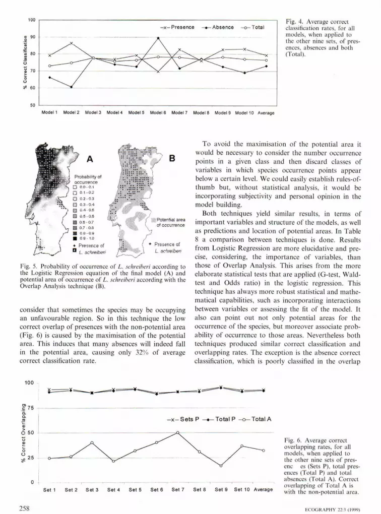
The average correct classification for the 10 mod-els is presented in Fig. 4, when applied on the othernine sets. There arc no significant differences betweenthe models in the average correct classification ofpresences (/^-test; p < 0.98: DF — 9), absences {y^-test; p<0.50; DF - 9) and both (x^-test; p<0.99;DF = 9). Again average correct classification rate forpresences is higher, compared to absences classifica-tion rates, except for model 6.

Using the most frequent variables in the 10 regres-sion equations and the most frequent interaction, webuild a final regression. The equation obtained is asfollows: g(x) - - 0.9830 - 0.353(TNS) + 0.4147(DRA)+ 0.07317(PRFx HUM). The value of G-test is214.308 and with Pearson ^- the model obtained sig-nificant differences, being x- = 349.773 (p = 0.001).The best cut-off point is again 0.5, atid the modelwas applied to the initial set (466 squares) and the10 sets of 100 squares for measurement of correctclassification rates model. On average, the correctclassification of presences is 79%, absences is 80%and both is 79%>.

The probability of occurrence of L. schreiberi ac-cording to this model is represented in Fig. 5.

Overlap Analysis

The variables that were kept for eaeh of the 10 setsare presented in Table 3 and the frequency of occur-

rence of the independent variables in the 10 potentialareas is presented in Table 7. We present also theclasses of variables that were removed because no L.schreiheri points occurred on them. The most fre-quent variables arc precipitation (PRE), insolation(INS), soil draining (DRA) and evapotranspiration(EVP).

Then we overlapped the 10 potential areas withthe presences of the H) sets (100 squares each) andtotal of presences (257 squares). The total of ab-sences (209 squares) was overlapped with the non-potential area. We present in Fig. 6 the averagecorrect overlapping of these potential areas with thepresences or absences, and there are no significantdifferences between the 10 areas (/--test; p < 0.99;DF = 9). Nevertheless, the area produced by set 7seems to be the most aeeurate, since it has thehighest correct overlapping of absences with the non-potential area. With this technique correct overlap-ping is always higher with presences that withabsences.

With the most frequent variables of the potentialareas, we built a model for a final potential area(Fig. 5) and tested again its predictive power. Cor-rect overlapping with the presences of the 10 setswas on average 92%j, with total presences 92%i andwith total absences

-100 ,<

OO 0.1 0.2 0.3 0.4 0.5 0.6 0.7 0.8 0.9 1.0Cut-off point

Fig. 3. Correct classification rates, for model 3, considering allpossible cut-otT points, at 0.1 inlervals.

256 Rror.RAPHY 22:_1

Mliable 6. Classification rates for each model when applied lo the total set. The cut-off poitit used was determined by analysis ofsimilar plots of Fig. 4 for each model, x is the average and SD the standard deviation.

lodel % of presences elassifiedeorrcctly

81.787.388.6K2.590.286,387.979.688.387.986.0

3.5

% of absences classifiedcorrectly

65.075.683.989.271.869.473.882.670.076.275.87.5

"/u of total correctclassification

75.083.086.085.083.078.082.081.0Hi.O83.081.73.2

cut-olT pointchosen

0.50,50.40.40.40.40.50.50.50.5_

IMscussion

< Comparison of techniques

Using presence/absence data to model habitat suit-ability may present accuracy problems and has beenqyestioned (North and Reynolds 1996). Admitting 0for absence means that a particular habitat is unsuit-able for the species. Nevertheless, the habitat may bestiitable but the species simply was not detected dueid inadequate field sampling strategy, low populationdensities or inter-specific competition. In that case, itwpuld be preferable to use abundance/density dataliajther than presence/absence. This stands true forW)rks done in relatively small areas (where preciseabundance/density data are easier to obtain), or whenmodelling microhabitat preferences. However whentrving to model species distributions or working withlk:ge sampling units (10 x 10 km squares or more),li-ing presence/absence data is a valid technique be-cause it can overcome field problems and give anirtial perspective of the species distribution.

According to the frequency of occurrence of theiii dependent variables all of the 10 regression equa-tions, biophysical variables (TNS and PRE) are moreinfluential on L. schreiheri distribution than others ex-clusively physical (ALT or SOT). The results clearlyp(Mnt out a preference for rainy areas with reducedijisolation. Comparing Figs I and 5 one can noticethat higher probability areas, indicated by the model,follow closely the species actual distribution, with

of actual presences being correctly classified.The most important variables in the Overlap Anal-

ysis are the same as in the Logistic Regression (com-pare Tables 4 and 7), with one exception. Removingthe lower or higher classes of a variable indicatesindirectly that the species has positive or negative re-lation with thai variable, respectively. Comparing Ta-Hh 4 and 7, one can notice that the positive relationo|fi PRE variable, detected by Logistic Regression, is

IDGRAPHY 22:3

also detected indirectly by Overlap Analysis, when re-moving the lower classes. These similar results in theimportance and relation of variables, for both tech-niques, were common for all variables. Exceptionswere HUM and EVP. which have alternate levels ofimportance, but common relations with the dependentvariable, for both techniques. Technique predictivepower is very high and comparing Figs 2 and 5, pres-ences of the species overlap perfectly the potentialarea, with 92% of correct overlapping.

In wildlife distribution models the best variablesmay come by chance as well as correct classificationrates. Use of different data sets with examination ofthe frequency of occurrence of variables and testingthe models in all different sets overcomes this prob-lem. These procedures can give an actual idea of theimportant variables and of the real power of themodel.

Misclassification can happen due to reduced sensi-tivity or specificity. Sensitivity measures the ability ofthe model to correctly classify actual presences aspresences and specificity measure the abihty to cor-rectly classify actual absences as absences. Tt is alwayspreferable to have a model with great sensitivity for itis unacceptable that a model classifies wrongly actualpresences of species. Low specificity can come fromsampling error and so it is not so dramatic for amodel to classify an absence as a presence. In model3 we might have chosen 0.4 or 0.5 as cut-off point(Fig. 3). but we opted for 0.4 because it optimises thepresence correct classification. This criterion was usedin all models of the Logistic Regression and that iswhy average correct classification rates of presencesare higher than that of absences (Table 6),

Comparing Figs 1 and 5. it is evident that thistechnique maximises the potential area of occurrenceof the species. This is because a single occurrencepoint in a given class makes all the area of that classto be considered as potential. The technique does not

257

50

-X-Presence -Absence -o—Total

Model 1 Model 2 Model 3 Model A Model 5 Model 6 Model 7 Model S Model 9 Model 10 Average

Fig. 4. Average correctclassification rates, for allmodels, wlien applied 1othe other nine sets, of pres-ences, absences and both{Total).

Presence of_ _ _ i L schreiberi

Fig. 5. Probability of occurrence of L. .•nhreihcri according tothe Logistic Regression equation of the final model (A) andpotential area of occurrence of L. schreilwri according with theOverlap Analysis technique (B).

consider that sometimes the species may be occupyingan unfavourable region. So in this technique the lowcorrect overlap of presences with the non-potential area{Fig. 6) is caused by the maximisation of the potentialarea. This induces thai many absences will indeed fallin the potential area, causing only 32% of averagecorrect classification rate.

To avoid the maximisation of the potential area itwould be necessary to consider ihc number occurrencepoints in a given class and then discard classes ofvariables in which species occurrence points appearbelow a certain level. We could easily establish rules-of-thumb but, without statistical analysis, it would beincorporating subjectivity and personal opinion in themodel building.

Both techniques yield similar results, in terms ofimportant variables and structure of the models, as wellas predictions and location of potential areas. In Table8 a comparison between techniques is done. Resultsfrom Logistic Regression are more elucidative and pre-cise, considering, the importance of variables, thanthose of Overlap Analysis. This arises from the moreelaborate statistical tests that are applied (G-test. Wald-test and Odds ratio) in the logistic regression. Thistechnique has always more robust statistical and mathe-matical capabilities, such as incorporating interactionsbetween variables or assessing the fit of the model. Italso can point out not only potential areas for theoccurrence of the species, but moreover associate prob-ability of occurrence to those areas. Nevertheless bothtechniques produced similar correct classification andoverlapping rates. The exception is the absence correctclassification, which is poorly classified in the overlap

100

75

O 50

25

- x - S e t s P •Total P • Total A

Sel 1 Set 2 Set 3 Set 4 Set 5 Set 6 Set 7 Set 8 Set 9 Set 10 Average

Fig. 6, Average correctoverlapping rates, for allmodels, when applied tothe other nine sets of pres-enc es (Sets P), Iota! pres-ences (Total P) and totalabsences (Total A). Correctoverlapping of Total A iswith tiic non-potential area.

258 tCOGRAPHY 22;

able 7. Frequency of occurrence of the independent vari-ables in the 10 poientiai areas and classes of variables re-

oved, in the Overlap Analysis building procedure.

tlariable

CRA

E|VPI

msPRE

EMUM

EjCOA!LTSOI

Frequency of occur-rence

10

10

1010

74300

Excluded classes

All lower than 150mmAll lower than 450mmAll above 3000 h yrAll lower (han 500mmAll above i7.5XLower 65%--_

.lialysis due to the maxitnisation of the potential area,fact, this is the greater problem of this analysis,

b(|cause in the presence correct classification it has ahigher rate, 92% against 79'>(i of Logistic Regression.Overlap Analysis is particularly interesting due to thesimplicity in building procedures and to the swiftness inc|lptaining reliable potential areas. It is a valid techniqueespecially in exploratory analysis of species distribu-tions or in the initial stages of research when data mayb« scarce. The potential area defined by this techniquemight be useful for further prospection of the species,bijit investigators should be aware of the maximisationpiloblcm. Investigators should also be aware of theOliher techniques, such Artiticial Neural Networks,v jiich do not require a linear relationship between theindependent variables and the presence absence vari-able (Guegan et al. 1998). and can be also very usefull

ecological modelling.

In both techniques the power of the models couldve been greatly improved if using variables not so'hly correlated (Table 2) or by using biotic variables.Hi

such as variables reflecting habitat traits, food availabil-ity, competing species or predators abundance. Never-theless when using these kinds of variables carefulattention should be paid to their accuracy and viability.

Ecological requirements of L. schreiberi

This species seems to be greatly dependent of humidand rainy areas, and Marco and Polio (1993) and Britoet al. (1996) had already stated this fact. This depen-dence is in strict accordance with its distribution area,because this species is present only in areas with levelsof precipitation above 800 mm y r " ' .

The habitats in which L. schreiheri may be found arethe margins of watercourses where the vegetation iscomposed of species with Atlantic characteristics andtypical of high rainfall environments, and very humidforests of English and Pyrenean oak (Brito et al. 1998).Hence there is again a similarity between necessity ofpermanent water and an occupied habitat that canprovide it with this requirement.

The constant presence of water seems to be a crucialfactor for this species, for it is regularly absent fromareas where there is no running water throughout theyear, which corresponds roughly to levels of precipita-tion < 800 mm yr ~' . It is not known at what level thewater is important, if it affects the adults physiologi-cally and or if the development of eggs requires greatsoil humidity. Physiological studies on the adults andeggs could be made to obtain a better knowledge of thisspecies.

Acknowledgements This work was supported by the Eu-ropean Community program LIFE ""Programa para o Con-hecimento e Gestao do Patrimonio Natural" and thePortuguese Nature Conservation Institute (lCN). We thankElisa Oliveira and all the colleagues who helped us in the(ieldwork. We thank aiso J. Arntzen. R. Marquez and A.Filipe for their helpful comments on earlier versions of themanuscript.

ible 8. Comparison between Logistic Regression and Overlap Anal>sis techniques of modelling species distributions-

Logistic Regression Overlap Analysis

Possibility of dealing with Spatialautocorrelationxessing Importance o( variables

Jtermine effects of Interaction betweenvariablesJtermine Relation of the independentvariables with the dependent oneAccessing the Fit of the model

Pi])ssibility of using Validation samplesFijaal results in terms of Potential areas of' occurrence of species

Final results in terms of Probability ofI occurrence in a given area

Piecision of the predicted Potential area

Yes

Ye.s, by statistical analysis

Yes

Yes, directly

Yes. by percentages of correct classificationand statistical analysisYesYes

Yes

Good

Yes

Yes, by percentages ofoverlappingNo

Yes. indirectly

Yes. by percentages ofcorreci overlappingYesYes

No

Good, but with tendency tonnaximisation

)GRAPHY 22:3 (1999) 259

ReferencesMin. do Amb. RecursosAnon. 1983. Atlas do Ambiente.

Naturiiis. Lisboa.Anon. 1991. nGRET - Stalistica! atialysis package. - Stal,

and Epidctniol. Res. Corp., Seattle. WA 98105, USA.Anon, 1997, The Map and Image Processing System ver, 5,7,

- Lincoln, USA,Anselin. L, 1993, Discrete space auto regressive models. - In:

Goodcliild, M. F,. Parks, B. O, and Steyaert. L, T, {eds).Environmental modelling with GIS, Oxford Univ. Press,pp. 454 469.

Aiigiistin, N, 11,. Mugglestone. M, A, and Buckland, S, T,1996. An autologistic model for the spatial distribution ofwildlife, - J, AppI, Ecol. 33; 339 347,

Brito, J, C, et al, 1996, Di.slribution of Schreiber's green lizard(Laceria .schreiheri) in Porlugal: a predictive model. -Herpetol, J, 6: 43-47,

Brito, J, C , Paulo. O. S, and Crespo, E, G, 1998. Distributionand habifats of Schreiber's green lizard [Lacena .schreiberi)in Portugal. - Herpetol. J, 8: 187-194,

Bustamantc, J. 1997, Predictive models for lesser kestrel !-\iIci>luiuiiuinni distribution, abundance and extiction in south-ern Spain, - Biol. Conserv. 80: 153- 160,

Cliff. A, D, and Ord. J, K, 1973. Spatial autocorrelation, -Pion. London.

Crespo, E. G, and Olivcira. M. E. 1989, Atlas da Distribuigaodos Anllbios e Repteis de Portugal Continental. SN-PRCN. Lisboa.

Eastman, J, R, 1995, IDRISI for Windows - User's guide ver.1,0, - Clark Labs for Cartogr, Tech. and Geogr, Anal,Clark Univ., USA,

Forstrtan. A, 1997. Growth and survival of Vipera hems in avariable environtnent. In: Thorpe. R, S,, Wuster. W, atidMalhotra, A, (eds). Venomous snakes. Ecology, evolutionand snakebite. The Zool, Soc, of London, Oxford, pp,143-154,

Gates. S. et al, 1994, Declining farmland bird species: mod-elling geographical patterns of abundance in Britain, - In:Edwards, P, J., May, R, M, and Webb, N. R. (eds).Large-scale ecology and conservation biology. Blackwell,pp. 111-128,

Green. R. E. 1996, Factors affecting the population density ofthe corncrake O-t-.v crc.x in Britain and Iieland, - J, Appl,Eeol, 33: 237-248,

Guegan, J,-F,. Lek, S. and Oberdorff. T. 1998. Energyavailability and habitat heterogeneity predict global river-ine fish diversity. - Nature 391: 382-384.

Haslett, J, R, 1990. Geographic information syslems: a newapproach to habitat definition and the study of distribu-tions. - Trends Ecol, Evol. 5: 214 218,

Hosmer. Jr D, W, and Lenieshow. S, 1989, Applied LogisticRegression, - John Wiley,

Kintron. U. et al, 1996, Spatial analysis of the distribution oftsetse flies in the Lambwe Valley. Kenya, using LandsatTM satellite imagery and GIS. - J, Anim. Ecol, 65:371-380,

Malktnus. R, 1995. Die Amphibien und Rcptilien Portiigals.Madeiras und der Azoren. - Weslarp Wissenschaften.Magdeburg.

Marco, A, and Perez-Mellado, V. 1988. Alimentacion de l.uc-cria schreiheri Bedriaga, 1878 (Sauria: Lacertidae) en elSisEema Central, - Rev, Espafi. Herpetol, 3: 133- 141,

Marco, A, and Polio, C, P. 1993, Analisis .biogeografico de ladistribucion del lagarto verdinegro (Laceria .sehreiberiBedriaga 1878), Ecologia 7: 457-466,

Mladenoff, D. J, et al, 1995. A regional landseape analysi.s andprediction of favorable gray wolf habitat in the northernGreat Lakes region. Conserv, Biol, 9: 279-294,

Nortli, M, P. and Reynolds, J, H, 1996. Microhabitat analysisiisinc radiotelemetry locations and polytomous logistic re-gression. - J, Wildl, Manage. 60: 639 65.1

Osb"orne. P, E, and Tigar. B, J. 1992. Interpreting bird atlasdata using logistic models: an exatnple from Lesotho,Southern Africa, - J. Appl. Ecol, 29: 55 62,

Pereira. J, M, C, and Itami, R, M, 1991, GlS-based habitatmodeling using logistic multiple regression: a study of theMt, Graham red squirrel. - Photogr. Eng, and RemoteSensing 57: 1475-1486,

Romero, J, and Real, R, 1996. Macroenvironmental factors asulnmate determinants of distribution of eommon toad andnatterjack in the south of Spain. Ecography 19: 305-312.

Sjogren, P. and Ray. C, 1996. Using logistic regression tomodel metapopulation dynamics: large-scale forestry extir-pates Ihe pool frog, - In: McCullough. D, R, (ed.|, Meta-populations and wildlife conservation. Island Press,Washington, pp, 111-137.

Schonrogge, K., Stone, G, N. and Crawley. M. J. 1996.Abundance patterns and species richness of the parasitoidsand inquilines of the alien gall-former Aiuiricus quercusculi-cis (Hymenoptera: Cynipidae), Oikos 77: 507 518,

Stonis. D, M, et al, 1993, Geographic analysis of Californiacondor sighting data, Conser\. Biol, 7: 148 159.

Walker. P, A, 1990, Modelltng wildlife distributions using aHeoiiraphic information system: kangaroos in relation loclimate, J. Biogeogr. 17: 279-289.

260 ECOGRAPHY 22:3 (t999)