Embed Size (px)
Citation preview
i
TToowwaarrddss rreelliiaabbllee ccoonnttaaccttss ooff mmoolleeccuullaarr eelleeccttrroonniicc
ddeevviicceess ttoo ggoolldd eelleeccttrrooddeess
Peter F. Cafe
A Thesis submitted as required for the fulfilment of a
Doctorate of Philosophy at the University of Sydney
MMaarrcchh 22000088
ii
DDeeccllaarraattiioonn
I declare that the work presented in this thesis is all my own (other than where figures, quotations, results and tables have been extracted from other publications or persons and have been expressly referenced as such in the narrative), with the following exceptions:
The theoretical calculations of Chapter 2 were performed by Professor Jeffery R Reimers and Dr Ante Bilic of Sydney University, School of Chemistry.
DFT calculations of conductance for pyrazine, 4,4′-bipyridine and TATPP were performed by Mr Sören Wolthat of Sydney University, School of Chemistry.
Peter Cafe
iii
AAcckknnoowwlleeddggeemmeennttss “A friend walks in when everyone else walks out”
- Unknown Source
Jeff Reimers has been an excellent supervisor, and an almost inexhaustible font of knowledge and effort, but most of all he’s a real, dedicated and selfless human being. He has provided the most helpful and gentle guidance throughout.
Thanks to Jan Herrmann for those long days (and nights) looking at molecules with me.
To Jens Ulstrup and everyone at DTU, many thanks for 2 very productive months on STM and helping me feel quite welcome in Denmark.
Thanks to Stuart Lindsay and his team in ASU for likewise helping me to come to grips with the instrument, and showing great hospitality (with some distractions provided by Mr Steve Woodward and his mates).
It has been an honour to work closely with dignitaries like Prof Noel Hush and Prof Max Crossley.
Dr Iain M Blake has not only provided many of the chemicals used throughout my PhD years, but has also provided valuable discussions about various solvent molecules which provided a breakthrough in the understanding of pyrazine conduction. These discussions were made all the more piquant by the occasional contributions of Peter Brotherhood.
Dr Ante Bilic kindly and humbly provided many of the theoretical calculations used in this thesis. I thank him for this but more so for his inspiring and valuable friendship over the past 5 years.
Thanks to all in the Reimers Group at Sydney Uni, past and present, you’ve each been helpful and kind to me, and a pleasure to know.
I would like to pay tribute to the Florence and Bertie Gritton Trust for the provision of a PhD Scholarship.
I also thank the Australian Research Council, the Electron Microscope Unit of the University of Sydney, and the Danish Research Council for Technology and Production Sciences for funding this research, and the Australian Partnership of Advanced Computation (APAC) and the Australian Centre for Advanced Computing and Communications (AC3) for the provision of computer resources.
iv
PPuubblliiccaattiioonnss aarriissiinngg ffrroomm tthhiiss wwoorrkk
“Chemisorbed and Physisorbed Structures for 1,10-Phenanthroline and
Dipyrido[3,2-a:2′,3′-c]phenazine on Au(111)” Peter F. Cafea, Allan G.
Larsena, Wenrong Yanga, Ante Bilica, Iain M. Blakea, Maxwell J. Crossleya,
Jingdong Zhangb, Hainer Wackerbarthb, Jens Ulstrupb, and Jeffrey R. Reimersa*
Journal of Physical Chemistry C, Volume 111, Issue 46, pages 17285-
17296 (2007)1
The Journal of Physical Chemistry C, published by the American Chemical Society, publishes
scientific articles reporting research on the following sub-disciplines of physical chemistry:
Nanoparticles and nanostructures
Surfaces, interfaces, and catalysis
Electron transport, optical and electronic devices
Energy conversion and storage
a School of Chemistry, The University of Sydney, NSW, 2006, Australia b Department of Chemistry and NanoDTU, Technical University of Denmark, DK-2800 Lyngby, Denmark
v
SSYYNNOOPPSSIISS OOFF TTHHIISS TTHHEESSIISS
The aim of this thesis is to more fully understand and explain the binding
mechanism of organic molecules to the Au(111) surface and to explore the conduction
of such molecules. It consists of five discreet chapters connected to each other by the
central theme of “The Single Molecule Device: Conductance and Binding”. There is a
deliberate concentration on azine linkers, in particular those with a 1,10-phenanthroline-
type bidentate configuration at each end. This linker unit is called a “molecular alligator
clip” and is investigated as an alternative to the thiol linker unit more commonly used.
Chapter 1 places the work in the broad context of Molecular Electronics and
establishes the need for this research.
In Chapter 2 the multiple break-junction technique (using a Scanning Tunnelling
Microscope or similar device) was used to investigate the conductance of various
molecules with azine linkers. A major finding of those experiments is that solvent
interactions are a key factor in the conductance signal of particular molecules. Some
solvents interfere with the molecule’s interaction with and attachment to the gold
electrodes. One indicator of the degree of this interference is the extent of the
enhancement or otherwise of the gold quantized conduction peak at 1.0 G0. Below 1.0
G0 a broad range for which the molecule enhances conduction indicates that solvent
interactions contribute to a variety of structures which could bridge the electrodes, each
with their own specific conductance value. The use of histograms with a Log10 scale for
conductance proved useful for observing broad range features.
vi
Another factor which affects the conductance signal is the geometric alignment
of the molecule (or the molecule-solvent structure) to the gold electrode, and the
molecular alignment is explored in Chapters 3 for 1,10-phenanthroline (PHEN) and
Chapter 4 for thiols.
In Chapter 3 STM images, electrochemistry, and Density Functional Theory
(DFT) are used to determine 1,10-phenanthroline (PHEN) structures on the Au(111)
surface. It is established that PHEN binds in two modes, a physisorbed state and a
chemisorbed state. The chemisorbed state is more stable and involves the extraction of
gold from the bulk to form adatom-PHEN entities which are highly mobile on the gold
surface. Surface pitting is viewed as evidential of the formation of the adatom-molecule
entities. DFT calculations in this chapter were performed by Ante Bilic and Jeffery
Reimers.
The conclusions to Chapter 3 implicate the adatom as a binding mode of thiols
to gold and this is explored in Chapter 4 by a timely review of nascent research in the
field. The adatom motif is identified as the major binding structure for thiol terminated
molecules to gold, using the explanation of surface pitting in Chapter 3 as major
evidence and substantiated by emergent literature, both experimental and theoretical.
Furthermore, the effect of this binding mode on conductance is explored and structures
relevant to the break-junction experiment of Chapter 2 are identified and their
conductance values compared. Finally, as a result of researching extensive reports of
molecular conductance values, and having attempted the same, a simple method for
predicting the conductance of single molecules is presented based upon the tunneling
conductance formula.
vii
TTaabbllee ooff CCoonntteennttss Declaration iii
Acknowledgements ii
Publications iv
Synopsis v
Chapter 1 General Introduction..............................1-1 Chapter 1 General Introduction..............................1-1
1-0 Synopsis of Chapter 1: General Introduction 1-1
1-1 Background 1-3
1.1.1 The background and context of molecular electronics............................... 1-3 1.1.2 What is molecular electronics? .................................................................. 1-4 1.1.3 Sydney University Molecular Electronics Group and the program of work which has led to this thesis...................................................................................... 1-5
1-2 Current factors in molecular electronics research 1-7
1.2.1 Constraints of research in molecular electronics....................................... 1-7 1.2.1.1 Making functioning molecular devices 1-7 1.2.1.2 Molecular self-assembly of devices 1-9
1.2.2 Integration of molecular devices: the molecular “Alligator Clip”.......... 1-10 1.2.3 Experimental techniques for molecular conduction experiments............. 1-13
1.2.3.1 Crossed wires junctions 1-13 1.2.3.2 Break-junctions 1-14 1.2.3.3 Scanning tunnelling microscopy (STM) 1-15 1.2.3.4 Multiple break junctions with statistical analysis 1-16 1.2.3.5 Conducting atomic force microscopy (cAFM) 1-17
1-3 Research activities 1-19
1.3.1 Overseas visits .......................................................................................... 1-19 1.3.2 Design and fit of new laboratory at Sydney University............................ 1-20
1-4 Conclusions to Chapter 1 1-22
viii
Chapter 2 Break-Junction Experiments. ................2-1 Chapter 2 Break-Junction Experiments. ................2-1
2-0 Synopsis for Chapter 2 2-1
2-1 Introduction to Chapter 2 2-5
2.1.1 Description of the break-junction experiment ............................................ 2-5 2.1.2 Instrument provided at Sydney University – Molecular Imaging PicoPlus2-6 2.1.3 Basic break-junction procedure on the Molecular Imaging system........... 2-8 2.1.4 Basic break-junction procedure on CSIRO’s “home made” system........ 2-10 2.1.5 Use of Gold substrates and wires. ............................................................ 2-10 2.1.6 Quantum of Conductance (Go) observed in Gold Wires .......................... 2-11 2.1.7 Conductance observed in molecules......................................................... 2-13 2.1.8 Summary of conductance values of selected molecules............................ 2-14 2.1.9 Tunnelling Decay Constant ...................................................................... 2-18
2-2 Particulars of the break-junction experimental work 2-19
2.2.1 Summary of molecules investigated.......................................................... 2-19 2.2.2 Experimental procedure ........................................................................... 2-22
2.2.2.1 Instrument used at Sydney University, advantages and disadvantages. 2-26 2.2.2.2 Instrument used at CSIRO, advantages and disadvantages. 2-29
2.2.3 Use of logarithmic amplifier..................................................................... 2-31
2-3 General comment on experiments and results 2-34
2.3.1 Terminology and treatment of raw data. .................................................. 2-34 2.3.1.1 Special analysis techniques used. 2-36 2.3.1.2 Various gain settings used at CSIRO 2-37 2.3.1.3 Gold quantized conduction peaks 2-38
2.3.2 Other data selection and analysis techniques used in literature.............. 2-40
2-4 Investigations of 1,8-octanedithiol 2-43
2.4.1 Rationalization: ........................................................................................ 2-43 2.4.2 Background research................................................................................ 2-43 2.4.3 Experimental set-up:................................................................................. 2-43 2.4.4 The sets of sweeps for 1,8-octanedithiol................................................... 2-44 2.4.5 Results from all sets of data for 1,8-octanedithiol.................................... 2-44 2.4.6 Discussion of 1,8-octanedithiol results .................................................... 2-48 2.4.7 Conclusion of 1,8-octanedithiol Results ................................................... 2-49
2-5 Investigations of 4,4′-bipyridine 2-50
2.5.1 Rationalization: ........................................................................................ 2-50 2.5.2 Background research................................................................................ 2-50 2.5.3 Experimental set-up:................................................................................. 2-50 2.5.4 The sets of sweeps for 4,4′-bipyridine ...................................................... 2-51 2.5.5 Results from 4,4′-bipyridine (all sets)....................................................... 2-51 2.5.6 Log10 histograms of 4,4′-bipyridine.......................................................... 2-54 2.5.7 Discussion and further analysis of 4,4′-bipyridine results ....................... 2-56 2.5.8 Conclusion of 4,4′-bipyridine results........................................................ 2-59
ix
2-6 Investigations of TATPP 2-60
2.6.1 Rationalization: ........................................................................................ 2-60 2.6.2 Background research................................................................................ 2-60
2.6.2.1 Similar molecules 2-60 2.6.2.2 Theoretical value of conductance for TATPP 2-63
2.6.3 Experimental set-up:................................................................................. 2-63 2.6.4 The sets of sweeps for TATPP .................................................................. 2-63 2.6.5 Results from TATPP (all sets) .................................................................. 2-64 2.6.6 Discussion of TATPP results .................................................................... 2-68
2.6.6.1 Difficulty in observing conductance for TATPP 2-69 2.6.7 Conclusion of TATPP results ................................................................... 2-71
2-7 Investigation of pyrazine 2-72
2.7.1 Rationalization: ........................................................................................ 2-72 2.7.2 Background research................................................................................ 2-72 2.7.3 Experimental set-up:................................................................................. 2-73 2.7.4 The sets of sweeps for pyrazine ................................................................ 2-74 2.7.5 Results from all sets of data for pyrazine. ................................................ 2-75 2.7.6 Discussion of pyrazine results:................................................................. 2-80
2.7.6.1 General observations 2-80 2.7.6.2 In phenyloctane 2-81 2.7.6.3 In toluene 2-83 2.7.6.4 In aqueous solvent 2-84 2.7.6.5 In carbontetrachloride 2-85
2.7.7 Conclusion of pyrazine results ................................................................. 2-86
2-8 Investigation of bis-appended porphyrin 2-88
2.8.1 Rationalization: ........................................................................................ 2-88 2.8.2 Background research................................................................................ 2-89
2.8.2.1 Similar molecules 2-89 2.8.2.2 Theoretical value of conductance for bis-appended porphyrin 2-93
2.8.3 Experimental set-up:................................................................................. 2-94 2.8.4 The sets of sweeps for bis-porphyrin ........................................................ 2-94 2.8.5 Results from bis-por (all sets)................................................................... 2-95 2.8.6 Discussion of bisporph results................................................................ 2-105 2.8.7 Conclusion of bispor results ................................................................... 2-107
2-9 General conclusion to Chapter 2: break-junction experiments 2-108
Chapter 3 Chemisorbed and Physisorbed Structures for 1,10-Phenanthroline and Dipyrido[3,2-a:2′,3′-
c]phenazine on Au(111) .......................................... .....3-1
Chapter 3 Chemisorbed and Physisorbed Structuresfor 1,10-Phenanthroline and Dipyrido[3,2-a:2′,3′-
c]phenazine on Au(111) .................................................3-1
3-0 Synopsis for Chapter 3 3-1
3-1 Introduction to Chapter 3 3-3
x
3.1.1 Established research – 1,10-phenanthroline monolayers .......................... 3-3 3.1.1.1 1,10-phenanthroline on Au(111) 3-4 3.1.1.2 1,10-phenanthroline on Cu(111) 3-5 3.1.1.3 Surface pitting in monolayers on Au 3-6
3.1.2 Experimental presentments of this chapter –STM images.......................... 3-6 3.1.3 Theoretical presentments of this chapter – DFT etc .................................. 3-7
3-2 Methods of Chapter 3 3-8
3.2.1 Chemicals. .................................................................................................. 3-8 3.2.2 Ex situ STM of pre-assembled PHEN monolayers. .................................... 3-8 3.2.3 In situ STM of PHEN and DPPZ monolayers on single-crystal gold electrodes. ............................................................................................................... 3-9 3.2.4 Electrochemistry. ...................................................................................... 3-10 3.2.5 Calculations of adsorbates on gold surfaces............................................ 3-10 3.2.6 Calculations on models used to investigate dispersive interactions. ....... 3-12
3-3 Results of Chapter 3 3-13
3.3.1 In situ STM studies of PHEN monolayer formation. ................................ 3-13 3.3.2 Electrochemistry of PHEN monolayers.................................................... 3-17 3.3.3 STM of PHEN monolayers after electrochemical preparation. ............... 3-20 3.3.4 In situ STM of DPPZ monolayers............................................................. 3-23 3.3.5 DFT-Calculated structures of PHEN monolayers.................................... 3-27 3.3.6 MP2 and CASPT2 calculations on the role of dispersive interactions in monolayer production........................................................................................... 3-33
3-4 Discussion: how PHEN and DPPZ molecules and monolayers bind to the Au(111) surface 3-37
3-5 Conclusions to Chapter 3: PHEN binding to gold and relevance to thiol binding 3-41
Chapter 4 The Nature and Conduction of Thiols Chemisorbed to Gold. ............................................. .....4-1
Chapter 4 The Nature and Conduction of ThiolsChemisorbed to Gold. ....................................................4-1
4-0 Synopsis for Chapter 4 4-1
4-1 Introduction to Chapter 4 4-2
4.1.1 Importance of determining the binding mode............................................. 4-2 4.1.2 Work of this chapter - adatom configuration in the thiol binding to gold.. 4-3 4.1.3 NOTE concerning thiol and thiyl terminology: .......................................... 4-3
4-2 The adatom configuration of thiols bound to gold and its implications regarding molecular conduction. 4-5
4.2.1 Bond geometry: analysis of the dithiol results of Chapter 2 ...................... 4-5
xi
4.2.1.1 Analysis of the binding geometry of thiol linker to the Au(111) surface 4-7 4.2.1.1.1 BINDING ANGLE 4-8 4.2.1.1.2 UNDERLYING GEOMETRY OF THE GOLD ATOMS INVOLVED IN THE
THIOL BOND. 4-10 4.2.1.2 Thiol binding during a break-junction experiment. 4-14
4.2.2 Conductivity of thiols bound on an adatom.............................................. 4-17
4-3 Conclusion to Chapter 4: dithiol binding and conductance. 4-21
Chapter 5 Simple Methods for Estimating Molecular Conductivity. ................................................ ................5-1
Chapter 5 Simple Methods for Estimating MolecularConductivity. ..................................................................5-1
5-0 Synopsis for Chapter 5 5-1
5-1 Introduction to Chapter 5 5-3
5.1.1 Need for a simpler method for determining molecular conductance. ........ 5-3 5.1.2 The work of this chapter: exploiting the tunnelling conductance formula 5-4
5-2 Tunneling conductance formula and its use to determine the conduction of single molecules. 5-5
5.2.1 The unit of the conductance quantum, G0................................................... 5-5 5.2.2 The tunnelling conduction formula............................................................. 5-5 5.2.3 Values determined from prior research...................................................... 5-6
5.2.3.1 Thiols 5-6 5.2.3.2 Amines 5-7 5.2.3.3 Thiols, amines and acids 5-8
5.2.4 Method (a): Simple use of the conduction formula – determining the conductance of 1,12-dodecanedithiol ..................................................................... 5-8 5.2.5 Method (b): Further use of the conduction formula – determining the conduction of 1,4-bezenedimethanediamine........................................................... 5-9
5-3 Conclusion to Chapter 5: the use of the tunneling conductance formula to determine the conduction of single molecules. 5-11
Chapter 6 Bibliography ....................................... ....6-1 Chapter 6 Bibliography .............................................6-1
Chapter 7 APPENDICES.........................................7-1 Chapter 7 APPENDICES.........................................7-1
7-0 Appendices 7-1
7-1 APPENDIX 1: Plan and design of laboratory. 7-1

xii
7-2 APPENDIX 2: Supporting Information for Chapter 2 7-4
7.2.1 Additional histograms for pyrazine ............................................................ 7-4 7.2.2 Additional histograms for bis-appended porphyrin ................................. 7-12
7-3 APPENDIX 3: Supporting Information for Chapter 3 7-17
7.3.1 STM images of Au(111). ........................................................................... 7-17 7.3.2 STM images of phenanthroline on Au(111) in-situ. ................................. 7-18 7.3.3 Images depicting long-range order. ......................................................... 7-20 7.3.4 Reductive desorption of the PHEN monolayer......................................... 7-22 7.3.5 Oxidation of gold surfaces containing PHEN monolayers. ..................... 7-24 7.3.6 Full version of references. ........................................................................ 7-25

xiii
TToowwaarrddss rreelliiaabbllee ccoonnttaaccttss ooff mmoolleeccuullaarr eelleeccttrroonniicc
ddeevviicceess ttoo ggoolldd eelleeccttrrooddeess
UUnniivveerrssiittyy ooff SSyyddnneeyy
“After climbing a great hill, one only finds that
there are many more hills to climb.” (Nelson Mandella)

xiv
Molecular Electronics Thesis – Peter Cafe Chapter 1
General Introduction Page 1-1
ChaptteerChap r 1 Geeneerrall IInttrroduccttiion 1 G n a n odu on
1-0 Synopsis of Chapter 1: General Introduction The general introduction explores the background of the field of Molecular
Electronics, with reference to the last 50 years of technological advance in the
semiconductor industry, and views Molecular Electronics as an inheritor of the mantle of
Moore’s Law. Molecular Electronics is defined as the control of individual molecules or
particular groups of molecules such that we can make them do useful tasks and replace
larger scale devices.
The Molecular Electronics Group within the School of Chemistry, Sydney
University, is introduced.
Some constraints of Molecular Electronics are outlined and a number of basic
tasks of research are identified, with the following two singled out for focus in this
thesis:
To measure single molecule conductance.
To define the contact of molecules to other components.
The binding module of a molecule is introduced as a molecular “Alligator Clip”,
and self-assembly is identified as a critical process in device manufacture, however
binding modes and self-assembly mechanisms are in need of further understanding.
Molecular Electronics Thesis – Peter Cafe Chapter 1
A brief mention is made of five common types of molecular conduction
experimental techniques, whilst this research has chosen the multiple break-junction
technique with statistical analysis as the most suitable.
Three additional major research activities are described.
The Chapter concludes by connecting each of the subsequent research chapters
(Chapters 2 to 5) to develop a general theme that can be briefly described as:
The Single Molecule Device: Conductance and Binding.
General Introduction Page 1-2
Molecular Electronics Thesis – Peter Cafe Chapter 1
General Introduction Page 1-3
1-1 Background
1.1.1 The background and context of molecular electronics
“Molecular electronics is thus very much about contacts”2.
The massive worldwide semiconductor industry drives the even more massive
software and hardware development sector with its succession of breakthroughs in speed
and miniaturisation. Expectations are generally high that the industry can deliver
continuous advances in the basic building blocks which function in such things as mobile
phones, computers, portable MP3 players, and even toasters and fluffy toys, and that the
rate of advancement is predictable. This “axiom” is commonly referred to as “Moore’s
Law”, being formally presented in 1965 by Gordon Moore, Director of Fairchild
Semiconductor's Research and Development Laboratories, in the 35th anniversary issue
of Electronics magazine3. He intonated that transistor density on a computer microchip
will double, and costs will halve, each twelve months, and this has been (roughly) borne
out by empirical observation to the present time. In the 1990s, it was generally accepted
that Moore's Law implied that computing power at fixed cost would continue to double
every 18 months. This periodic doubling means exponential growth, which has now
placed current silicon-chip development “bang-up” against the fundamental physical
limits of conventional microelectronics. Moore recently admitted that Moore’s Law, in
its current form, with CMOS silicon, will “run out of gas” in 2017.4 Speculations on the
continued application of Moore's Law therefore lean towards radical departures from
silicon technology to such things as molecular electronics, quantum computing, spin
devices, bio-computing, DNA computers, and other theoretically possible information
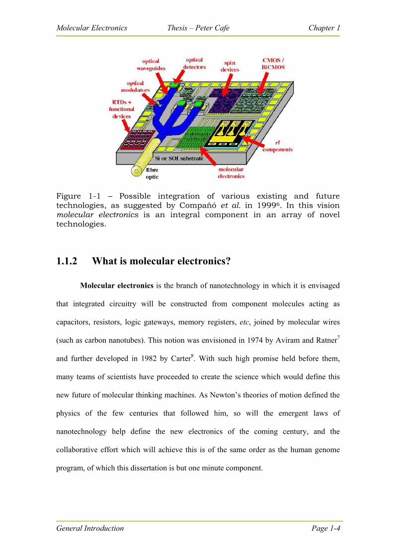
processing mechanisms5 (and their integration, as suggested in Figure 1-1).
Molecular Electronics Thesis – Peter Cafe Chapter 1
Figure 1-1 – Possible integration of various existing and future technologies, as suggested by Compañó et al. in 19996. In this vision molecular electronics is an integral component in an array of novel technologies.
1.1.2 What is molecular electronics?
Molecular electronics is the branch of nanotechnology in which it is envisaged
that integrated circuitry will be constructed from component molecules acting as
capacitors, resistors, logic gateways, memory registers, etc, joined by molecular wires
(such as carbon nanotubes). This notion was envisioned in 1974 by Aviram and Ratner7
and further developed in 1982 by Carter8. With such high promise held before them,
many teams of scientists have proceeded to create the science which would define this
new future of molecular thinking machines. As Newton’s theories of motion defined the
physics of the few centuries that followed him, so will the emergent laws of
nanotechnology help define the new electronics of the coming century, and the
collaborative effort which will achieve this is of the same order as the human genome
program, of which this dissertation is but one minute component.
General Introduction Page 1-4
Molecular Electronics Thesis – Peter Cafe Chapter 1
General Introduction Page 1-5
We may view molecular electronics as the design, fabrication and assembly of
molecules into functioning electronic circuits.
“Molecular electronics … allows chemical engineering of
organic molecules with their physical and electronic properties
tailored by synthetic methods”. [Reed 2003, p32]9
In 2001 Carroll and Gorman asked the question “Can we control the position of
individual molecules or particular groups of molecules such that we can make them do
useful tasks?”; and furthermore “Can we use the intrinsic properties of these molecules
to replace larger scale devices?”10. They define molecular electronics as the search for
the answers to these questions.
1.1.3 Sydney University Molecular Electronics Group and
the program of work which has led to this thesis.
The Molecular Electronics Group at Sydney University (officially since
January 2002) has been one of the contributing research groups in this field. Their major
contributions have been in the theoretical modelling of the forces which govern the
behaviour of the basic components of matter – chemical binding and electron transport.
However to expand on and verify their theoretical results, they have recently developed
an experimental research program, commenced in 2003, which was pioneered by the
present author as a research student (as expounded in subsequent chapters and
supporting information).
The initial aim of this program was to measure experimentally the conductive
properties of select molecules, and hence a large portion of this thesis is devoted to
single molecule conduction and the experiments conducted are described in detail with
Molecular Electronics Thesis – Peter Cafe Chapter 1
their results and implications (Chapter 2). However co-incident research at Sydney
University and elsewhere highlighted the need for more clearly defined contact
geometries2, 11, 12. Thus another important and basic result of this research examines the
linker unit which joins component molecules to gold electrodes, and defines the possible
geometries for the bonding of 1,10 phenanthroline to the gold(111) surface (Chapter 3),
with implications for the very important thiol linkages also (which are further developed
in Chapter 4). The determination of the binding geometries of 1,10 phenanthroline on
gold (111) is supported by STM imaging and theoretical calculations using density
functional theory.
The development of techniques to do this is in itself remarkable as we seek
measurements of nanometers and nanoamps. At this realm of measurement we are close
to the limits of observability as we attempt to distinguish between the effects of our
observation tools and the quantities we seek to measure. However scanning probe
microscopy (first reported by Binnig in 198213) has given unprecedented access to the
miniature world of molecules, particularly in imaging ordered monolayers to atomic
resolution.
Here the use of the multiple STM Break-Junction technique has been used to
perform measurements of single molecule conduction14. (Initially some molecular
conduction experiments were tried using the conducting Atomic Force Microscope
[cAFM], after Cui, et al. (2001)15, however this method proved extremely difficult to
reproduce and since it was first published in 2001 very little further research has
occurred using this method: the original research group has since revised the method
[and results] in 2007.16)
General Introduction Page 1-6
Molecular Electronics Thesis – Peter Cafe Chapter 1
General Introduction Page 1-7
1-2 Current factors in molecular electronics
research
1.2.1 Constraints of research in molecular electronics
Scientific research aims to more fully explain the natural world and reconfigure it
in novel (and beneficial) ways, and in so doing helps to define the future, and in a wide
range of applications from biology to computing, this is certainly the case for molecular
electronics and its umbrella discipline of nanotechnology. This exciting potential is one
point even opposing visionaries K Eric Drexler and Rick Smalley agree upon:
“Like Drexler, Smalley believes that the potential of
nanotechnology to benefit humanity is almost limitless”17.
Numerous candidate molecules have been proposed, probed and even proven
(theoretically or experimentally) to be possible electronic components, however actual
device fabrication (on a commercial level) has proven elusive, with formidable
engineering and production barriers to be overcome – among them connectivity and the
stochastic behaviour of individual molecules18.
1.2.1.1 Making functioning molecular devices
It is generally accepted in molecular electronics that if the field is to reach its
proposed potential (i.e., to replace silicon technology in chip manufacture) then science
not only needs to discover and define the molecules, and not only to develop ingenious
methods to probe these molecules, but also to come upon a way to mass-produce the
Molecular Electronics Thesis – Peter Cafe Chapter 1
General Introduction Page 1-8
devices which use them, and arms of nanotechnological research are reaching into areas
of device fabrication, reproducibility, etc: i.e. cost-effective, consumer appropriate and
marketable techniques. Thus the concept of “Self-Assembly” has become important, to
which this thesis contributes a more complete understanding (Chapter 3).
In 1999 The European Commission IST Programme Future and Emerging
Technologies identified four problems in the (then) state of research into molecular
electronics:6[Section 2.2.4.5]
“Intramolecular electronics are far behind other alternative concepts as
none of the following issues have yet been demonstrated:
Self-assembly of single devices at reasonable (or small) integration
densities, let alone integration with conducting molecular wires.
appropriate yield of devices from chemical or biological reactions
for fabricating or manufacturing of circuits;
high data bandwidths for interconnects;
the potential for low cost per bit has not been demonstrated.”
These issues certainly present challenges to researchers such as myself and the
Molecular Electronics Group at Sydney University, however all indications are that the
research will result in some remarkable breakthroughs. For example problems associated
with high current flow and “band-width” through single molecules have already been
addressed by the possibility of Quantum-dot Cellular Automata (QCA) [reported by
Hush 200319]:
“Craig Lent and colleagues have discussed the possibility of
molecular-scale computing devices that operate without the flow
of continuous current. This type of computation can, in principle,
be achieved by quantum-dot cellular automata (QCA)” 20
Molecular Electronics Thesis – Peter Cafe Chapter 1
General Introduction Page 1-9
1.2.1.2 Molecular self-assembly of devices
In 1999 it was noted that, despite the predictions, not a single transistor had been
created on the basis of molecular electronics:
“… A number of proposals have appeared in the literature for
molecular devices but few have been demonstrated. No real
molecular three-terminal transistor device defined in this
roadmap has yet been demonstrated”6
Nevertheless just four years later Stan and Franzon (2003), et al, listed a number
of molecular electronic devices which had been made, including resonant tunnelling
diode devices, programmable molecular switches, carbon nanotube transistors, and
diodes21, and at the present time a Google® Patent search on “Molecular Electronic
Device” returns over 800 registered USA patents, and include such “inventions” as
nanowires, shift registers, wire transistors, amplifiers, memory, dielectrics, rectifiers,
switches, as well as systems of manipulation, integration, orientation, testing, assembly
and programming.
Yet a commercially proven device is yet to be engineered and a production-
model molecular computer component is still some decades away. Presently researched
methods or components are stepping stones to the future:
“Granted, they are not yet at the stage where these molecular
devices are ready for production and can be incorporated into
circuits. In fact, some may never directly see the actual light of
commercialisation. They are enabling technologies —
technologies on which commercialised versions will be developed.
But the need is defined, the trend is clear, and the maturing
process of refining and advancing these designs is moving
forward.”22
Molecular Electronics Thesis – Peter Cafe Chapter 1
General Introduction Page 1-10
At the very least, one result of this research is an increase in the understanding
and specialized utilization of molecular bonds, which may be of particular use in drug
discovery, synthesis and delivery, catalysts, and chemical storage23, 24, as well as
biological repair systems25, 26. However, even if complete molecular scale computer
chips do not eventuate as a reality in our life-times, it is most likely that we will soon see
the fabrication of molecular devices which will integrate with and complement other
branches of technology21, 27.
Molecular electronics is defining the science which will take us into that future.
1.2.2 Integration of molecular devices: the molecular
“Alligator Clip”
When talking about circuitry, the current reference point is silicon wafer, with
feature sizes of the order of 200 nm. For molecular electronics to deliver significant
benefits (commensurate with the magnitude of the research), we should expect feature
sizes at least 2 orders of magnitude smaller than this, with similar decreases in power
consumption and heat loss, and increases in computational speed.
In both research and ultimate device manufacture, we need to interface with these
systems.
“At the heart of the problem is the need to interface reliably with
an individual molecule.” 28
Molecular Electronics as it is envisaged involves the exact placement of
individual molecules in relation to other molecules. It involves the precise joining of
“function” molecules to “wire” molecules, function molecules being certain designer
Molecular Electronics Thesis – Peter Cafe Chapter 1
General Introduction Page 1-11
molecules which will act as memory devices29, diodes30, logic gates31, transistors32, etc,
i.e. the basic components of an electronic circuit, and some possibilities in such
architectures and “bottom-up” fabrication (i.e. self-assembly) have been explored by
Stan and Franzon, et al.21.
This construction process works in the biological world by proteins, the machines
which connect sites on molecules to sites on other molecules, and it happens in aqueous
environments. However proteins are yet to be discovered which will operate in non-
aqueous media or function with the types of molecules that traditionally define the chip
industry, silicons, oxides, metals and semi-conductors. We are yet to discover all the
ways of designing these specific placements, and ways of mass-manufacturing the
process. The requirement of exact synthesis of molecular circuits is a challenge for the
near future, however, organic-metal complexes and self-assembly techniques are being
developed to meet these function and fabrication constraints21
A similar level of precision is required in the current state of play in the
experimental research. Individual molecules need to be addressed experimentally and
interrogated. Despite Smalley’s “fat finger” and “sticky finger” descriptions of the
problems of such precision17, practical methods are currently being utilised to at least
probe individual molecules. Common instruments used to investigate molecules are
microscopes such as the STM and AFM.
However the stochastic nature of molecular co-ordination is to be addressed. It
has become apparent through the research of this thesis and others that if molecular scale
devices are to be testable at least and most probably useable at all, stable and predictable
bonds to metal or semiconductor electrodes are a prerequisite2, 12, 33.
Molecular Electronics Thesis – Peter Cafe Chapter 1
General Introduction Page 1-12
In this thesis the functional group which tethers a molecule to a metallic surface
(terminal) is dubbed an “Alligator Clip”, after Tour34, 35, Hush36 and Crossley37, and in
the thesis of Anton Grigoriev38. Hermann et al. refer to a linking and self-organising
motif as the “universal adapter”39; it’s an “anchor” according to Tao40, and is called
“solder” by Devens Gust41.
Seminario, Zacarias and Tour (1999)35 first described these linking functional
groups as “molecular alligator clips” and found by density functional theory calculations
that the terminal groups of sulfur, selenium and tellurium bound well to gold, and of
these sulfur has been used extensively in both theoretical and practical research.
However he found that the isonitrile had limited use as an alligator clip, as it “was only
possible when the connection was made to one Au atom, and in this case the trend in the
electron affinity, provided by the negative of the LUMO, dropped abruptly.” (p. 758).
However since then nitrile linkers to gold have been observed experimentally to form
monolayers by both monodentate42-47, bidentate48-53, and even terdentate54 nitrile ligands
and to bridge break-junctions, as both amines40, 43, 55 and azines56, and several nitrile-type
“alligator clips” have otherwise been proposed37, 57.
This thesis establishes that the single Au atom binding for the bi-dentate ligand
1,10-phenanthroline is in fact both stable and predictable when that Au atom is an
adatom on the Au(111) surface, and it’s position on the surface is stabilised (i.e. locked-
in) by the intermolecular interactions of the organic molecules.
Molecular Electronics Thesis – Peter Cafe Chapter 1
General Introduction Page 1-13
1.2.3 Experimental techniques for molecular conduction
experiments
With the conduction characteristics of single molecules being the most important
aspect of current research into molecular electronics, five important methods have been
developed to measure the current passing through a molecule. They are the use of
Crossed-Wire Junctions, Break Junctions, Scanning Tunnelling Microscopy (STM),
conducting Atomic Force Microscopy (cAFM), and in addition to the single break-
junction experiment a recent technique involves the use of a modified STM to perform
multiple break-junction experiments and perform statistical analysis on the hundreds of
current traces produced14. All methods involve gold electrodes, high levels of purity, and
tethering of an organic species to the gold electrode (“alligator clip”). The analysis of
most methods require some speculation about the bond geometry between the molecule
and the gold electrode and/or evidence of the formation of some sort of consistent
monolayer.
1.2.3.1 Crossed wires junctions
A junction is formed between two thin wires. One wire passes over the other and
oriented at right angles to it. The distance between the wires is controlled quite
accurately down to sub-Angstrom units by a magnetic device. The wires typically are
gold and are 10m in diameter. One of the wires is covered in a monolayer of the
molecule of interest. The wires are brought together until a current is detected. This
method was pioneered by Kushmerick et al. in 200258 and has been used to study several
different types of molecules.59
In this method, if the current remains stable during small movements of the
crossed-wires it is assumed that the molecules have bonded stably to both wires. The
Molecular Electronics Thesis – Peter Cafe Chapter 1
General Introduction Page 1-14
number of molecules forming the bridge between the two wires is unknown (but is
typically less than ten), but the results are integer multiples of a “lowest curve” which is
the current in a single molecular bridge.
1.2.3.2 Break-junctions
In this method, typically a gold wire is stretched until it breaks, and held near that
break point. The gap spans two atomically fine tips of gold. The stretching and breaking
of the wire are obtained by etching a thin gold line onto a substrate and then 3-point
bending the substrate until the gold line breaks. The bending is controlled by a piezo-
electric device and can control the movement to within an Angstrom. The point of
breakage is determined by the moment the current through the wire ceases. The tips are
then exposed to a solution containing the molecule of interest and a monolayer forms on
the exposed tips of the gold. The gap is slowly brought back together again until a
current forms (but not back to the point of breakage). (See Figure 2-2, page 2-5) The
measurement of current follows the same methods as in Crossed-Wire Junctions60-62
However with break junctions the material characteristics of the metal at the
point of breakage are difficult to determine. The metal is definitely stressed and
deformed and so the geometric alignment of the molecules on the surface of the gold
cannot be determined. It has been shown that bond geometry has a great effect on current
flow63, and so with this method it cannot be guaranteed that results are integer multiples
of a single molecule.
Molecular Electronics Thesis – Peter Cafe Chapter 1
General Introduction Page 1-15
1.2.3.3 Scanning tunnelling microscopy (STM)
In STM an “atomically fine” conducting tip is brought near a surface until a
current is detected. That current is a tunnelling current theoretically flowing between one
atom on the tip and one atom on the surface. The tip is rastered across the surface and
most commonly a feedback-loop (with high gain) adjusts the height of the tip to maintain
constant current (constant current mode). The height of the tip is presented as a topology
image of the surface. Alternatively, with low gain, the height does not change
dramatically and a current image is generated (“constant height mode”).
The STM has enabled surface scanning to be conducted precisely to vertical
resolutions of 0.01 Angstroms and horizontal resolutions of a few Angstroms. As well as
being able to precisely map surfaces to extremely fine resolutions, it can perform
tunnelling spectroscopy on the surface.64, 65
The tip must be close to the surface to allow tunnelling to occur but not touch the
surface (shorting of the tip on the surface or “crashing”). The instrument is sensitive to
both electrostatic and acoustic interference and needs to be isolated from these
influences. The surface must allow tunnelling (i.e. be non-insulating).
The constant current mode “topology” image obtained from STM is not
necessarily a true topology of the surface but rather a map of electronic density of states
on the surface. Both topology and conduction affect the appearance of the image.
Constant height mode can only be used to scan small flat regions, because with low gain
the tip is more likely to crash into surface irregularities, however it is extremely sensitive
to molecular features and slight changes in conductance across the surface.
STM has been used by many researchers to study the conduction of single
molecules.66, 67
Molecular Electronics Thesis – Peter Cafe Chapter 1
General Introduction Page 1-16
1.2.3.4 Multiple break junctions with statistical analysis
In 2003 Nongjian J. Tao14 et al. first used a modified STM to hold stationary a
gold tip at a point on the gold surface (in the presence of a dilute solution of a molecule
of interest), then repeatedly crash the tip into the surface and withdraw. This would form
a micro-thin gold wire then break it, with one or more molecules bridging the break for a
brief moment as the tip withdraws. The technique can quickly perform thousands of
break junction experiments on a specific molecule. The conductance traces are then
screened and collated to produce a histogram showing peaks of conduction relating to
multiples of the single molecule. This method has been reproduced by others using both
STM42 and custom made devices43.
If one already has an STM, this is perhaps the easiest method to obtain reliable
results because little additional equipment is required and it uses large numbers of
individual break-junction experiments so that data can be analysed with some statistical
certainty. However since the first reported results of this experiment by Tao, it has
become apparent that the methods of data selection and collating of the conductance
traces are critical in producing results which lead to meaningful conductance peaks in the
histograms. Certain novel techniques of analysis have been published since, including
tunnelling background subtraction and log scale graphing of conductance68; and “last
step analysis”69, which are each explored in Section 2.3.2. Although this method does
not resolve this issue of bond geometry mentioned above, peak(s) in the histograms will
appear at conductances indicating the most likely bond configuration(s) given the specific
experimental conditions.
Molecular Electronics Thesis – Peter Cafe Chapter 1
General Introduction Page 1-17
1.2.3.5 Conducting atomic force microscopy (cAFM)
In Atomic Force Microscopy (AFM) a tip of extremely fine sharpness is attached
to a flexible cantilever and is brought into contact with a surface, and rastered across a
surface. The vertical movements of the tip (in response to dispersion forces between the
tip and the surface) are magnified some thousands of times by reflection of a laser off the
back of the cantilever and detected by a four-quadrant photo-diode. This method can also
detect twisting movements of the cantilever.
This device measures topology to horizontal and vertical resolutions using a feed-
back loop to control the height of the tip, similar to the STM. However with AFM the
surface need not be conductive. It also gives a greater idea of pure topology because it is
not affected by conduction variations throughout the surface. However the resolution is
generally not as high as STM and it is extremely difficult to obtain molecular recognition
by AFM.
In conducting Atomic Force Microscopy (cAFM) the tip is coated with a
conductive layer and a current can be passed through the tip to the surface and current
image can be produced which is virtually independent of the topology. The measurement
of conduction can be separated from the mechanism of the tip, which is not the case in
STM.70
Once a feature is identified by the AFM, such as a molecule of interest, the tip
can be positioned on that point and an I-V curve taken. In 2001 Cui, et al.15 first used
this method to identify gold nanoparticles attached to one end an 1,8-octanedithiol
molecule whose other end was tethered to a gold(111) surface (the octanedithiol was
sparsely inserted into an existing monolayer of “insulating” 1-octanemonothiols), and

Molecular Electronics Thesis – Peter Cafe Chapter 1
then run an I-V sweep through the nanoparticle to obtain the I-V characteristics of the
dithiol molecule.
Despite initial anticipation about the method, it proved more difficult than
expected to reproduce and one of the original authors later conceded this and revised the
method (and results)16. (For this current thesis the method was attempted for many
months but was difficult to master and quite expensive.)
General Introduction Page 1-18
Molecular Electronics Thesis – Peter Cafe Chapter 1
General Introduction Page 1-19
1-3 Research activities The results which are reported in the following chapters have been supported by
the major activities and collaborations which are listed below:
1.3.1 Overseas visits
Collaborative research secondments of the author were as follows:
To: Arizona State University (ASU), Tempe, Arizona USA: Department of
Physics and Astronomy (3 months):
From September to November 2003 work was done for three months with
Professor Stuart M Lindsay and his team, who have pioneered major breakthroughs in
the field of molecular electronics. The purpose of the visit was to learn the techniques of
the conducting AFM method of single molecule conduction15. Although the method
could not be successfully reproduced, the experimental experience allowed the nanoPrep
Lab at Sydney University to be properly designed (see below). Also during this time
valuable training was experienced at Molecular Imaging Inc, Ash Ave, Tempe, Arizona
in use of the AFM, gold substrate preparation and H2 flame annealing.
To: Technical University of Denmark, DK-2800 Lyngby, Denmark:
Department of Chemistry and NanoDTU, (2 months)
In September and October 2006 work was done with Professor Jens Ulstrup and
his team. Their work has mainly been in high resolution STM images of molecular
monolayers on gold surfaces. The purpose of the visit was to investigate 1,10-
phenanthroline and DPPZ monolayers on Au(111) and to learn better STM techniques.
Molecular Electronics Thesis – Peter Cafe Chapter 1
General Introduction Page 1-20
1.3.2 Design and fit of new laboratory at Sydney University
The experimental arm of the Sydney University molecular electronics group was
completely new in 2003. Before any research could be carried out the proper facilities
had to be established. Thus, initial research activities were centred around the design and
furbishment of an appropriate laboratory, in conjunction with the Electron Microscope
Unit at Sydney University (EMU). This presented an opportunity to get involved in the
specification of the instrument and the design of the lab, which contained numerous
challenges given the space and budget restrictions and the lack of prior experience in the
field within the University.
Based upon the research papers, many discussions with Dr Jens Ulstrup, and the
secondment at ASU in the labs of Dr Stuart Lindsay, the nanoPrep Lab, situated in the
basement of the EMU has been designed and completed. It includes the following major
equipment procurements and positioning:
Molecular Imaging Picoscan Plus combination AFM and STM.
Large chemical fume hood with ducting to the roof and a scrubbing filter.
Laminar flow cabinet with hepafilter.
Millipore Water filtering system.
Drying Oven
Hydrogen Flame annealing apparatus.
Dr Jens Ulstrup was a visiting fellow at Sydney University during March to June 2003. He is from Technical University of Denmark and has pioneered much work on the formation of monolayers and the use of the STM in single molecule experiments.
Molecular Electronics Thesis – Peter Cafe Chapter 1
Provision of inert gas (argon and nitrogen)
Acid storage cabinet.
Flammables storage cabinet.
Schröedinger Sharpener (for making fine STM tips)
In addition to the major equipment purchases and fittings, there were all the
necessary tools, glassware, chemicals, protective devices and equipment. The area of the
laboratory had to accommodate all these in a functional way, as well as include suitable
storage areas, shelving, bench tops and work spaces. Services of water, power, lighting,
positive flow of fresh air, supply of general consumables (paper towels, gloves, etc)
waste disposal, contaminated waste disposal, and seating were all specified whilst
considerations were given to all aspects of occupational health and safety.
Drawings of the nanoPrep Lab design in plan (Figure Appendix-1-67) and in
sketches (Figure Appendix-1-68) are included in Supporting Information, Section 7-1.
General Introduction Page 1-21
Molecular Electronics Thesis – Peter Cafe Chapter 1
General Introduction Page 1-22
1-4 Conclusions to Chapter 1 Molecular electronics is a natural inheritor of Moore’s Law, whether the research
results in “molecules which can perform useful tasks” or merely “enabling
technologies”. Self-assembly is a fundamental concept for mass production of devices.
Whilst the field of Molecular Electronics holds tremendous promise, clear
definitions of molecular behaviour within electronic circuitry are needed.
The most obvious and critical of these definitions is the conductance of a
molecule. Definitions of the mechanism of self-assembly and interface with electrodes
are also required.
However the single molecule in this context does not exist: it is part of a circuit,
bound to gold electrodes in one form or another, via a tethering device, and thus
becomes part of an extended molecule which includes the electrodes. Solvent binding
during break-junction experiments also contributes to a variety of possible structures.
The long-range electron interactions between the electrodes, the tethering device, and the
molecule, and the solvent interactions, play an important role. In this sense, there is no
point where the molecule ends and the electrode begins: i.e. the molecule cannot be
simply taken out of this context and its resistance calibrated like a light bulb.
The contextual nature of the molecule in its miniaturised circuit has to be
classified. The “alligator clip” is itself a vital component of the circuit and the nature of
the binding, its strength, orientation and geometry, are critical factors in the electronic
behaviour of the circuit and need to be determined.
Molecular Electronics Thesis – Peter Cafe Chapter 1
In Chapter 2 this thesis meets these challenges by providing experimental
research into conductance values for single molecules using a modified STM to
perform multiple break-junctions with statistical analysis.
In Chapter 3 it contributes by exploring one such tethering device in detail, the
1,10-phenanthroline “alligator clip”, determining its binding modes, binding strength,
and contact geometry. This is done by a combination of STM imaging, electrochemistry,
and theoretical techniques using DFT and a priori calculations.
In Chapter 4 it extends findings on the binding modes of 1,10-phenanthroline to
the binding modes of thiols in general, using surface pitting as the connecting evidence,
and drawing upon extensive nascent research in support.
The research methods of theory and experiment move forward often hand-in-
hand, each calibrating against the other. Both are tedious and time consuming, but
theoretical calculations can often provide answers for experimental situations and give
clues as to what may or may not be expected from a given experimental configuration,
sometimes allowing the experimentalist to focus on more likely outcomes.
In Chapter 5 it presents simple methods of calculating the conductance of single
molecules, which may assist both current experimental and theoretical methods.
General Introduction Page 1-23

Molecular Electronics Thesis – Peter Cafe Chapter 1
General Introduction Page 1-24
(Blank Page)
Molecular Electronics Thesis – Peter Cafe Chapter 2
Break-Junction Experiments Page 2-1
ChaptteerChap r 2 Brreeak--Junccttiion Expeerriimeenttss.. 2 B ak Jun on Exp m n
2-0 Synopsis for Chapter 2
This chapter focuses on the break-junction technique of determining single
molecule conductance, and performs the experiment on five different molecules.
Conductance can be expressed in units of the Conductance Quantum, G0, which has a
value of 7.7480917 × 10⁻⁵ Siemens.
The introduction in this chapter gives important background and includes a useful
table outlining the reported conduction of various relevant molecules (from prior
research), and introduces the tunnelling decay formula. (The values in this table and the
tunnelling decay formula inspired the proposition outlined in Chapter 5.)
The general introductory comments on the experimental section include a
discussion concerning various selection criteria and data analysis techniques for
analysing the large amounts of data arising from hundreds of break-junction experiments
(Section 2.3.2 below, page 2-40).
From the experimental work, generally, it was found that enhancement of the
gold quantized conduction peak at 1.0 G0 was a reliable indicator that the molecule was
able to bind to the gold in the expected way (i.e. attached at one end by its “alligator
clip”). The use of log10 scale histograms enabled long-range effects to be observed.
The standard in this chapter expresses all molecular conductance values in units of 10-4 G0 for easy comparison The exception is for bis-appended porphyrin where the conductance was expressed in units of G0.
Molecular Electronics Thesis – Peter Cafe Chapter 2
Break-Junction Experiments Page 2-2
Solvent effects played an important role in the range of conductance values observed:
this was established in pyrazine and extrapolated to the other molecules.
Brief results for the five molecules on which the STM Break-Junction
experiments were conducted are as follows (the molecular structures are outlined in
Table 2-1 below):
1. 1,8-octanedithiol (Section 2-4): which, with a linear amplifier, has produced
a single molecule conductance value of 2.5x10⁻⁴ G0, agreeing with prior
literature (which used a logarithmic amplifier). However the results are not
as distinct. Nevertheless, it establishes that the methods and technical
equipment are capable of measuring single molecule conduction.
2. 4,4′-bipyridine (Section 2-5): Conduction of a single molecule was not
established conclusively. Broad enhancement of conduction (over the
solvent) was observed in the range from 10 to 150 x10-4 G0. Gold peaks were
enhanced by the presence of 4,4′-bipyridine, indicating that the molecule
interacts with the gold.
3. TATPP. (Section 2-6) In the solvents chosen (toluene and phenyloctane)
TATPP showed no conductance peaks and did not indicate enhancement of
the gold quantized conduction peak, most possibly due to its 4 middle
nitrogen atoms and conjugated ring backbone being attracted to the gold
surface. Considerations are given to redesigning the molecule to prevent
adherence of its middle section to gold, and to make it more soluble.
4. pyrazine (Section 2-7): The “single value” of the conductance of pyrazine
proved to be quite elusive, however through the application of log10
conductance scale histograms various long range features of pyrazine
Molecular Electronics Thesis – Peter Cafe Chapter 2
Break-Junction Experiments Page 2-3
conductance were uncovered. These proved to be solvent dependent. In most
organic solvents the pyrazine could still interact with the gold and extend the
gold quantized conduction peak, however this did not occur in the aqueous
solvent. Of the organic solvents, carbontetrachloride provided the least
solvent interactions and a peak was observed at 10 x10-4 G0: however, from
these experiments alone, it cannot be ascribed to the conduction of a single
pyrazine molecule. Aromatic solvents with delocalised electron systems
form strong interactions with pyrazine71 and possibly prevent it from
interacting with the gold electrodes. This is more pronounced in toluene,
which is so similar to pyrazine in size and structure that it prevents all
interactions with gold, showing no enhancement of the gold quantized
conduction peak and no enhancement of conduction over the whole range of
G0 values investigated. However in phenyloctane the solvent interactions are
not as strong and the gold quantized conduction peaks are enhanced, and
there is a broad range in which conduction is enhanced also. The broad
ranges of conductance are ascribed to alternative structures involving
pyrazine and the solvent.
5. bis-appended porphyrin (Section 2-8): Results from various sets were
inconsistent, highlighting the difficulties associated with this molecule. Even
gold interactions (evidenced by enhancement of the gold peak) were
inconsistent and underscore the subtle nature of solvent effects. Some sets of
data indicated a peak at 0.1 G0, with another at 0.2 G0, but the structure(s)
which caused the peaks cannot be determined.
Molecular Electronics Thesis – Peter Cafe Chapter 2
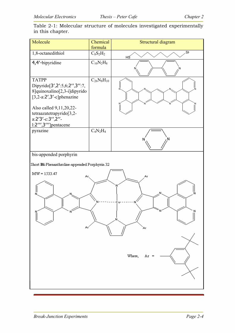
Table 2-1: Molecular structure of molecules investigated experimentally in this chapter.
Molecule Chemicalformula
Structural diagram
1,8-octanedithiol C8S2H2 HS
SH
4,4′-bipyridine C10N2H8
N N
TATPP Dipyrido[3′,2′:5,6;2′′,3′′:7,8]quinoxalino[2,3-i]dipyrido [3,2-a:2′,3′-c]phenazine Also called 9,11,20,22-tetraazatetrapyrido[3,2-a:2′3′-c:3′′,2′′-l:2′′′,3′′′]pentacene
C26N8H10
N
N N
N
N
N N
N
pyrazine C4N2H4
bis-appended porphyrin
Break-Junction Experiments Page 2-4

Molecular Electronics Thesis – Peter Cafe Chapter 2
2-1 Introduction to Chapter 2
“A basic task in molecular electronics is to
understand electron transport through a single molecule
bridged across two electrodes.”72
2.1.1 Description of the break-junction experiment
A break-junction is a nanoscale “gap” between two conducting electrodes into which is
inserted a molecule whose conduction properties need to be investigated. Initially the
two electrodes are touching or fused or even the one continuous piece of wire, which is
stretched until the separation occurs, forming the minute gap between the broken ends of
the electrodes. The molecule bridges the gap to complete an electric circuit. Initial break-
junction experiments, like the one represented in Figure 2-2 below, allowed just one or a
few measurement to be taken. The mechanical control of the break junction gap is by
bending or pulling the electrodes and can be controlled to a level of angstroms by careful
design of the equipment and/or the use of a piezoelectric device to control the necessary
force.
Break-Junction Experiments Page 2-5
Figure 2-2: Schematic of one type of mechanically controllable Break Junction (courtesy of Chongwu Zhou73). (See also Section 1.2.3.2 above)
Molecular Electronics Thesis – Peter Cafe Chapter 2
Break-Junction Experiments Page 2-6
A piezoelectric tube is used in the mechanical control of the tips in STM and
AFM scanning microscopy, where X,Y and Z displacement is controlled within a
nanometer or less by application of potential to the sides of the tube. The STM scanner is
easily adapted to perform break junction experiments provided the STM controller and
the software have the necessary functionality.
A Scanning Tunnelling Microscope (STM) instrument was first reported by Xu
and Tao in 200314 to perform multiple break-junction trials in a medium containing the
molecule of interest, and the conduction of a single molecule was found by statistical
analysis of the data from hundreds of conduction traces.
For the work expressed in this thesis, two different systems were available. The
system used at Sydney University was a commercial STM (from Molecular Imaging).
The system used at CSIRO (Lindfield) was a “home made” device. Relative advantages
and disadvantages of the two different systems are discussed in Section 2.2.2 below.
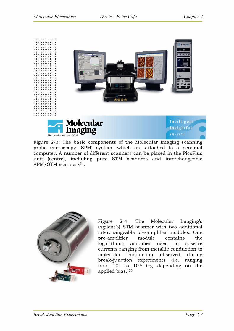
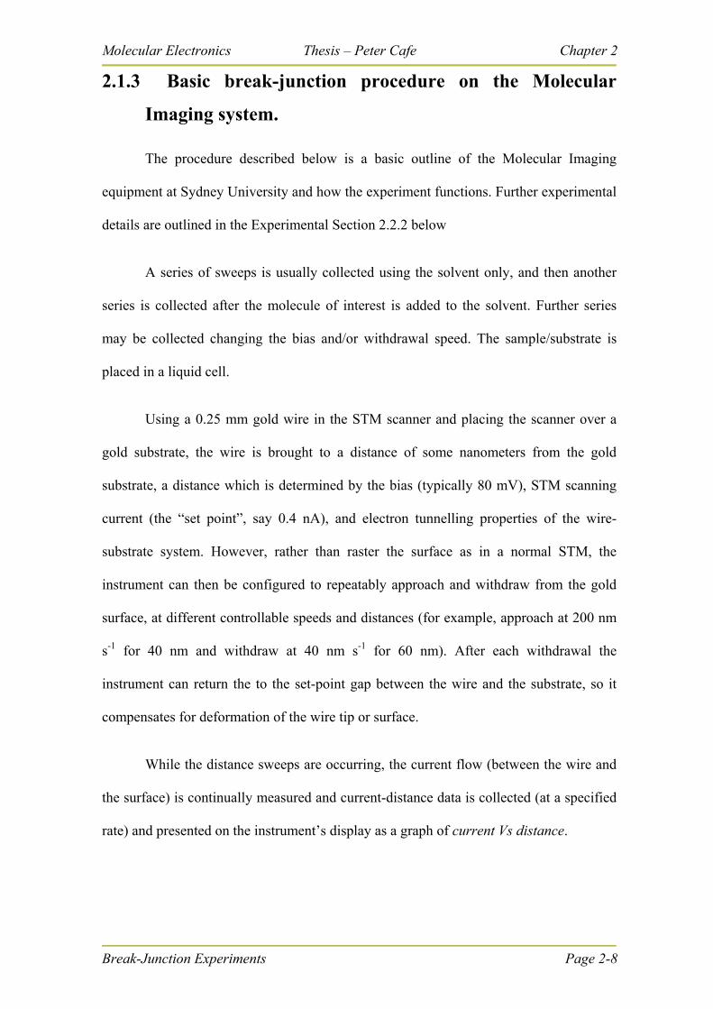
2.1.2 Instrument provided at Sydney University – Molecular
Imaging PicoPlus
The instrument used at Sydney University was a Molecular Imaging PicoPlus
system with a Picoscan 2500 controller unit (see Figure 2-3 below), and using the
Molecular Imaging’s STM scanner (see Figure 2-4 below). (Note that since November
2005 Molecular Imaging products have been branded as Agilent products.)
The software loaded on the personal computer which drives the
controller/instrument is called PicoScan 5.3.
Molecular Electronics Thesis – Peter Cafe Chapter 2
Figure 2-3: The basic components of the Molecular Imaging scanning probe microscopy (SPM) system, which are attached to a personal computer. A number of different scanners can be placed in the PicoPlus unit (centre), including pure STM scanners and interchangeable AFM/STM scanners74.
Figure 2-4: The Molecular Imaging’s (Agilent’s) STM scanner with two additional interchangeable pre-amplifier modules. One pre-amplifier module contains the logarithmic amplifier used to observe currents ranging from metallic conduction to molecular conduction observed during break-junction experiments (i.e. ranging from 103 to 10-5 G0, depending on the applied bias.)75
Break-Junction Experiments Page 2-7
Molecular Electronics Thesis – Peter Cafe Chapter 2
Break-Junction Experiments Page 2-8
2.1.3 Basic break-junction procedure on the Molecular
Imaging system.
The procedure described below is a basic outline of the Molecular Imaging
equipment at Sydney University and how the experiment functions. Further experimental
details are outlined in the Experimental Section 2.2.2 below
A series of sweeps is usually collected using the solvent only, and then another
series is collected after the molecule of interest is added to the solvent. Further series
may be collected changing the bias and/or withdrawal speed. The sample/substrate is
placed in a liquid cell.
Using a 0.25 mm gold wire in the STM scanner and placing the scanner over a
gold substrate, the wire is brought to a distance of some nanometers from the gold
substrate, a distance which is determined by the bias (typically 80 mV), STM scanning
current (the “set point”, say 0.4 nA), and electron tunnelling properties of the wire-
substrate system. However, rather than raster the surface as in a normal STM, the
instrument can then be configured to repeatably approach and withdraw from the gold
surface, at different controllable speeds and distances (for example, approach at 200 nm
s-1 for 40 nm and withdraw at 40 nm s-1 for 60 nm). After each withdrawal the
instrument can return the to the set-point gap between the wire and the substrate, so it
compensates for deformation of the wire tip or surface.
While the distance sweeps are occurring, the current flow (between the wire and
the surface) is continually measured and current-distance data is collected (at a specified
rate) and presented on the instrument’s display as a graph of current Vs distance.
Molecular Electronics Thesis – Peter Cafe Chapter 2
The approach speed is usually not important but the approach distance should be
just sufficient to allow the tip to crash into the surface. This is observed by saturation
current.
The withdrawal speed is typically from 1 nm s-1 to 40 nm s-1 and should be
adjusted facilitate observations: that is, to observe gold conduction steps or molecular
conduction steps in the current Vs distance graphs.
The number of data points is usually around 2000. At a known withdrawal speed
the withdrawal distance from one data point to the next may be calculated (for example,
0.2 Angstroms per data point).
With the linear amplifier the current range is extremely limited and it is not
possible to observe gold conduction steps with the linear amplifier available at Sydney
University. The current values are converted directly to conductance values (in units of
the conductance quantum), using the bias and the formula:
G V
906,12 I G0 , where I is in amps and V in volts. (see Section 2.1.6
below).
With the logarithmic amplifier the current values are actually a pseudo-log of the
true current and have to be converted to true current values using a conversion table,
which is constructed using a series of known resistors (see Section 2.2.3 below). Then
the true current values are converted to conductance values using the same formula.
Break-Junction Experiments Page 2-9
Molecular Electronics Thesis – Peter Cafe Chapter 2
Break-Junction Experiments Page 2-10
2.1.4 Basic break-junction procedure on CSIRO’s “home
made” system.
The system used at CSIRO (Lindfield) was a “home made” device. It consisted
of a tip-holder mounted to a 1 dimensional piezo-electric device, a liquid-cell sample
holder, a signal generator and oscilloscope, other electronics, and in-house developed
software. It was quite functional for the break-junction experiment, being purpose-built
by an expert in electronics and computer programming (Jan Herrmann).
The procedure for using it was basically similar to that for the Sydney University
set-up, except that it could take thicker gold wires (up to 0.5 mm in diameter) and there
was no “set-point” to control the initial distance between the wire and the substrate.
Although the software had a complicated human interface, it had additional triggers to
control the vertical motion of the wire and to assist in data collection and presentation.
Further details of the system are expressed in Section 2.2.2.2 below and elsewhere43.
2.1.5 Use of Gold substrates and wires.
The most common form of electrode used in molecular electronics is gold. Gold
offers the advantages of remaining reasonably pure for the time of the experiment in the
presence of both air, most solvents and even most electrolytes. However there is a limit
to the type of molecules which will bind to gold and form the electrode-molecule-
electrode linkage. The most common is the thiol linkage (which is considered to be a
covalent bond), but alternatives are sought. This body of work is mainly concerned with
the amine or azine linkage, which bind more weakly as a ligand to a metal atom (or ion)
because of the electron affinity of the nitrogen atom. If the metal atom is part of the gold
electrode surface then we have the connection through which conduction can take place.
Molecular Electronics Thesis – Peter Cafe Chapter 2
Break-Junction Experiments Page 2-11
A bidentate ligand such as 1,10-phenanthroline is a comparable alternative to the thiol
linker (Chapter 3).
Gold also has the property that its surface is somewhat fluid. That is, atoms
which are released from bulk may migrate over the surface quite freely, with a very
small energy barrier to movement to neighbouring sites with local energy minima. This
occurs even though the atom is still strongly bound to the surface (this is established in
Chapter 3 and Chapter 4). It explains why, for example, it is impossible to maintain a
thin gold wire during break-junction experiments. The atoms tend to migrate from the
bulk back towards the thinnest part of the wire in order to reduce its surface-area to
volume ratio (which reduces its overall energy). The speed of the break-junction
experiment must be greater than the speed at which atoms can migrate back down the
wire. But the speed must also be slow enough that the molecule has time to bridge the
gap and that a number of data points (recording the current) may be recorded while it is
there.
2.1.6 Quantum of Conductance (Go) observed in Gold Wires
Current measurements during the separation of fused gold electrodes show that
the current drops in a series of plateaus (see Figure 2-5 below). As the electrodes are
separated (from a fused initial contact allowing a high level of metallic conduction) the
gold thread which connects the two electrodes becomes increasingly thin. Its
conductance is then roughly proportional to its cross-sectional area. With continued
stretching, the diameter of the thinnest part of the wire decreases by discreet amounts of
atoms related to the circumference at that point in time. This continues until the wire is a
chain of single atoms, just before it breaks. Untiedt, et al, (2002) have established that
the gold wire (consisting of a chain of single gold atoms) is most likely to be formed of a
chain of one or 2 atoms, while forming chains of more than 3 gold atoms seems most
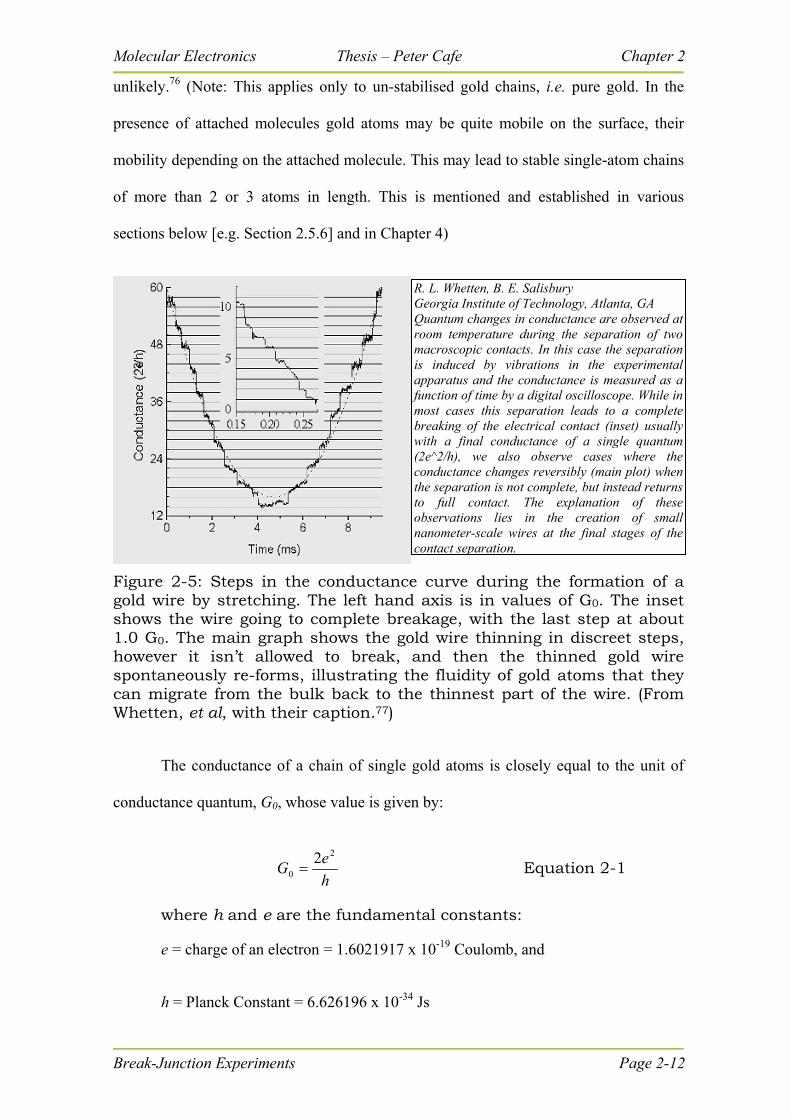
Molecular Electronics Thesis – Peter Cafe Chapter 2
unlikely.76 (Note: This applies only to un-stabilised gold chains, i.e. pure gold. In the
presence of attached molecules gold atoms may be quite mobile on the surface, their
mobility depending on the attached molecule. This may lead to stable single-atom chains
of more than 2 or 3 atoms in length. This is mentioned and established in various
sections below [e.g. Section 2.5.6] and in Chapter 4)
R. L. Whetten, B. E. Salisbury Georgia Institute of Technology, Atlanta, GA Quantum changes in conductance are observed at room temperature during the separation of two macroscopic contacts. In this case the separation is induced by vibrations in the experimental apparatus and the conductance is measured as a function of time by a digital oscilloscope. While in most cases this separation leads to a complete breaking of the electrical contact (inset) usually with a final conductance of a single quantum (2e^2/h), we also observe cases where the conductance changes reversibly (main plot) when the separation is not complete, but instead returns to full contact. The explanation of these observations lies in the creation of small nanometer-scale wires at the final stages of the contact separation.
Figure 2-5: Steps in the conductance curve during the formation of a gold wire by stretching. The left hand axis is in values of G0. The inset shows the wire going to complete breakage, with the last step at about 1.0 G0. The main graph shows the gold wire thinning in discreet steps, however it isn’t allowed to break, and then the thinned gold wire spontaneously re-forms, illustrating the fluidity of gold atoms that they can migrate from the bulk back to the thinnest part of the wire. (From Whetten, et al, with their caption.77)
The conductance of a chain of single gold atoms is closely equal to the unit of
conductance quantum, G0, whose value is given by:
h
eG0
2
2
Equation 2-1
where h and e are the fundamental constants:
e = charge of an electron = 1.6021917 x 10⁻¹⁹ Coulomb, and
h = Planck Constant = 6.626196 x 10⁻³⁴ Js
Break-Junction Experiments Page 2-12
Molecular Electronics Thesis – Peter Cafe Chapter 2
This gives a value of G0 as 7.7480917 × 10⁻⁵ Siemens.
This is analogous to a resistor with a value of 12,906.4 Ω (i.e. conductance is the
reciprocal of resistance). Thus, from measurements of the observed current (I) under a
fixed bias (V), the conductance (expressed in units of the conductance quantum) can be
found simply using Ohms law (V=IR) and a constant, as follows:
Conductance (in units of the conductance quantum),
G V
906,12 I
G0 Equation 2-2
2.1.7 Conductance observed in molecules.
When the break-junction experiment is conducted within a medium containing
conducting molecules, further conductance steps are sometimes observed somewhat
below the value of 1.0 G0. This is understood to be instances when one or more of the
conducting molecules bridge the gap between the electrodes after the last gold wire has
snapped. The use of a Scanning Tunnelling Microscope to do this was first reported by
Xu, et al, in 200314 (See Figure 2-6 below), using the Molecular Imaging Picoscan and
additional software and hardware, with a logarithmic amplifier. They also analysed
thousands of repeated break junction experiments by simply binning the data from
conductance traces, which produced histograms with peaks representing conductance of
one molecule or multiples thereof. Their results are included in the summary in Table 2-
2 (page 2-15, below).
Break-Junction Experiments Page 2-13
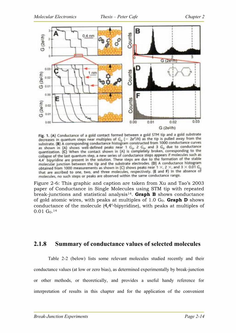
Molecular Electronics Thesis – Peter Cafe Chapter 2
Figure 2-6: This graphic and caption are taken from Xu and Tao’s 2003 paper of Conductance in Single Molecules using STM tip with repeated break-junctions and statistical analysis14. Graph B shows conductance of gold atomic wires, with peaks at multiples of 1.0 G0. Graph D shows conductance of the molecule (4,4′-bipyridine), with peaks at multiples of 0.01 G0.14
2.1.8 Summary of conductance values of selected molecules
Table 2-2 (below) lists some relevant molecules studied recently and their
conductance values (at low or zero bias), as determined experimentally by break-junction
or other methods, or theoretically, and provides a useful handy reference for
interpretation of results in this chapter and for the application of the convenient
Break-Junction Experiments Page 2-14
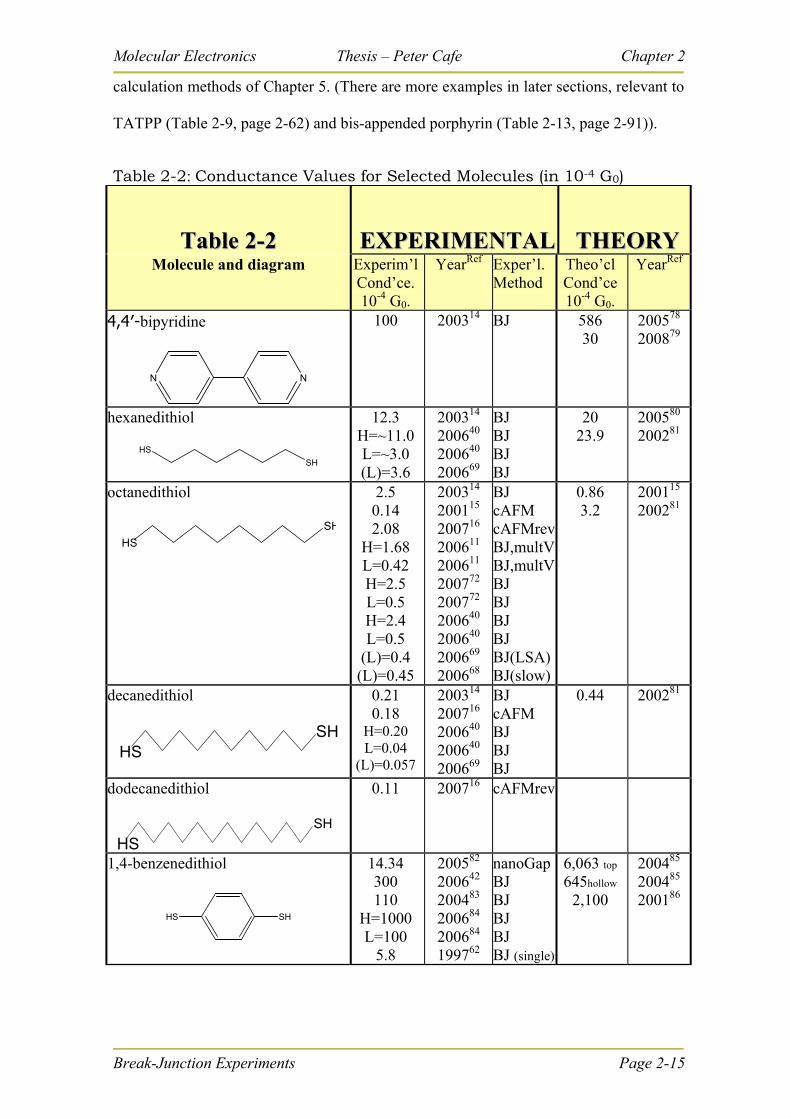
Molecular Electronics Thesis – Peter Cafe Chapter 2
calculation methods of Chapter 5. (There are more examples in later sections, relevant to
TATPP (Table 2-9, page 2-62) and bis-appended porphyrin (Table 2-13, page 2-91)).
Table 2-2: Conductance Values for Selected Molecules (in 10-4 G0)
Break-Junction Experiments Page 2-15
Table 2-2 2 ETable 2- EXXPPEERRIIMMEENNTTAALL
TTHHEEOORRYY Molecule and diagram Experim’l
Cond’ce. 10-4 G0.
YearRef Exper’l. Method
Theo’cl Cond’ce 10-4 G0.
YearRef
4,4′-bipyridine
N N
100
200314 BJ 586 30
200578 200879
hexanedithiol
HS
SH
12.3 H=~11.0 L=~3.0 (L)=3.6
200314 200640 200640 200669
BJ BJ BJ BJ
20 23.9
200580 200281
octanedithiol
HS
SH
2.5 0.14 2.08
H=1.68 L=0.42 H=2.5 L=0.5 H=2.4 L=0.5
(L)=0.4 (L)=0.45
200314 200115 200716 200611 200611 200772 200772 200640 200640 200669 200668
BJ cAFM cAFMrevBJ,multVBJ,multVBJ BJ BJ BJ BJ(LSA)BJ(slow)
0.86 3.2
200115 200281
decanedithiol
HSSH
0.21 0.18
H=0.20 L=0.04
(L)=0.057
200314 200716 200640 200640 200669
BJ cAFM BJ BJ BJ
0.44 200281
dodecanedithiol
HSSH
0.11 200716 cAFMrev
1,4-benzenedithiol
HS SH
14.34 300 110
H=1000 L=100
5.8
200582 200642 200483 200684 200684 199762
nanoGapBJ BJ BJ BJ BJ (single)
6,063 top 645hollow
2,100
200485 200485 200186
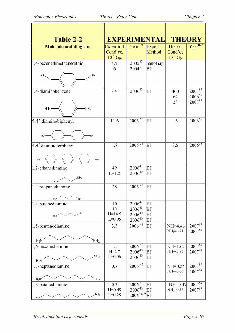
Molecular Electronics Thesis – Peter Cafe Chapter 2
TTaabbllee 22--22 EEXXPPEERRIIMMEENNTTAALL TTHHEEOORRYY
Break-Junction Experiments Page 2-16
Molecule and diagram Experim’l Cond’ce. 10-4 G0.
YearRef Exper’l. Method
Theo’cl YearRef
Cond’ce 10-4 G0.
1,4-bezenedimethanedithiol
SHHS
4.9 6
200582 200483
nanoGapBJ
1,4-diaminobenzene
NH2H2N
64
200642 BJ 460 64 28
200787 200655 200788
4,4′-diaminobiphenyl
H2N N 2H
11.6
2006 55 BJ 16
200655
4,4’-diaminoterphenyl
H2N N 2H
1.8
2006 55 BJ 3.5
200655
1,2-ethanediamine
H2N
NH2
49 L=1.2
200642 200640
BJ BJ
1,3-propanediamine
H2N N 2H
28
2006 42 BJ
1,4-butanediamine
H2N
NH2
10 10
H=14.5 L=0.95
200642 200643 200640 200640
BJ BJ BJ BJ
1,5-pentanediamine
H2N N 2H
3.5
2006 42 BJ NH=4.46 NH2=6.71
200789 200789
1,6-hexanediamine
H2N
NH2
1.5 H=2.7 L=0.06
2006 42 200640 200640
BJ BJ BJ
NH=1.67 NH2=3.95
200789 200789
1,7-heptanediamine
H2N N 2H
0.7
2006 42 BJ NH=0.55 NH2=0.63
200789 200789
1,8-octanediamine
H2N
NH2
0.3 H=0.49 L=0.28
2006 42 200640 200640, 89
BJ BJ BJ
NH=0.47NH2=0.56
200789 200789
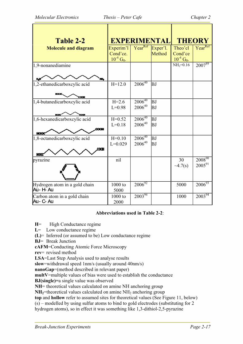
Molecular Electronics Thesis – Peter Cafe Chapter 2
TTaabbllee 22--22 EEXXPPEERRIIMMEENNTTAALL TTHHEEOORRYY
Break-Junction Experiments Page 2-17
Molecule and diagram Experim’l Cond’ce. 10-4 G0.
YearRef Exper’l. Method
Theo’cl YearRef
Cond’ce 10-4 G0.
1,9-nonanediamine
NH2=0.16 200789
1,2-ethanedicarboxcylic acid
H=12.0 200640 BJ
1,4-butanedicarboxcylic acid
H=2.6 L=0.98
200640 200640
BJ BJ
1,6-hexanedicarboxcylic acid
H=0.52 L=0.18
200640 200640
BJ BJ
1,8-octanedicarboxcylic acid
H=0.10 L=0.029
200640 200640
BJ BJ
pyrazine
nil 30 ~4.7(s)
200890 200591
Hydrogen atom in a gold chain Au-H-Au
1000 to 5000
200692 5000 200693
Carbon atom in a gold chain Au-C-Au
1000 to 2000
200394 1000 200394
Abbreviations used in Table 2-2:
H= High Conductance regime L= Low conductance regime (L)= Inferred (or assumed to be) Low conductance regime BJ= Break Junction cAFM=Conducting Atomic Force Microscopy rev= revised method LSA=Last Step Analysis used to analyse results slow=withdrawal speed 1nm/s (usually around 40nm/s) nanoGap=(method described in relevant paper) multV=multiple values of bias were used to establish the conductance BJ(single)=a single value was observed NH= theoretical values calculated on amine NH anchoring group NH2=theoretical values calculated on amine NH2 anchoring group top and hollow refer to assumed sites for theoretical values (See Figure 11, below) (s) – modelled by using sulfur atoms to bind to gold electrodes (substituting for 2 hydrogen atoms), so in effect it was something like 1,3-dithiol-2,5-pyrazine
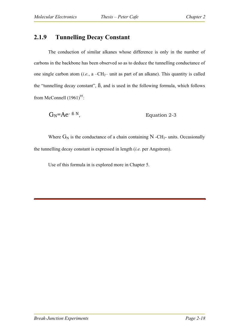
Molecular Electronics Thesis – Peter Cafe Chapter 2
2.1.9 Tunnelling Decay Constant
The conduction of similar alkanes whose difference is only in the number of
carbons in the backbone has been observed so as to deduce the tunnelling conductance of
one single carbon atom (i.e., a –CH2– unit as part of an alkane). This quantity is called
the “tunnelling decay constant”, ß, and is used in the following formula, which follows
from McConnell (1961)95:
GN=Ae- ß N, Equation 2-3
Where GN is the conductance of a chain containing N -CH2- units. Occasionally
the tunnelling decay constant is expressed in length (i.e. per Angstrom).
Use of this formula in is explored more in Chapter 5.
Break-Junction Experiments Page 2-18
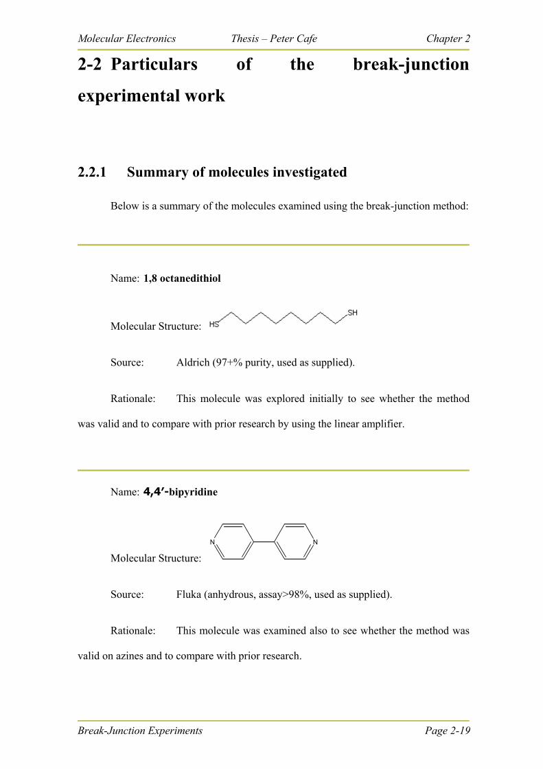
Molecular Electronics Thesis – Peter Cafe Chapter 2
2-2 Particulars of the break-junction
experimental work
2.2.1 Summary of molecules investigated
Below is a summary of the molecules examined using the break-junction method:
Name: 1,8 octanedithiol
Molecular Structure:
Source: Aldrich (97+% purity, used as supplied).
Rationale: This molecule was explored initially to see whether the method
was valid and to compare with prior research by using the linear amplifier.
Name: 4,4′-bipyridine
Molecular Structure:
N N
Source: Fluka (anhydrous, assay>98%, used as supplied).
Rationale: This molecule was examined also to see whether the method was
valid on azines and to compare with prior research.
Break-Junction Experiments Page 2-19
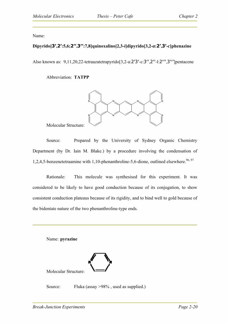
Molecular Electronics Thesis – Peter Cafe Chapter 2
Name:
Dipyrido[3′,2′:5,6;2′′,3′′:7,8]quinoxalino[2,3-i]dipyrido[3,2-a:2′,3′-c]phenazine
Also known as: 9,11,20,22-tetraazatetrapyrido[3,2-a:2′3′-c:3′′,2′′-l:2′′′,3′′′]pentacene
Abbreviation: TATPP
Molecular Structure:
N
N N
N
N
N N
N
Source: Prepared by the University of Sydney Organic Chemistry
Department (by Dr. Iain M. Blake.) by a procedure involving the condensation of
1,2,4,5-benzenetetraamine with 1,10-phenanthroline-5,6-dione, outlined elsewhere.96, 97
Rationale: This molecule was synthesised for this experiment. It was
considered to be likely to have good conduction because of its conjugation, to show
consistent conduction plateaus because of its rigidity, and to bind well to gold because of
the bidentate nature of the two phenanthroline-type ends.
Name: pyrazine
Molecular Structure:
Source: Fluka (assay >98% , used as supplied.)
Break-Junction Experiments Page 2-20
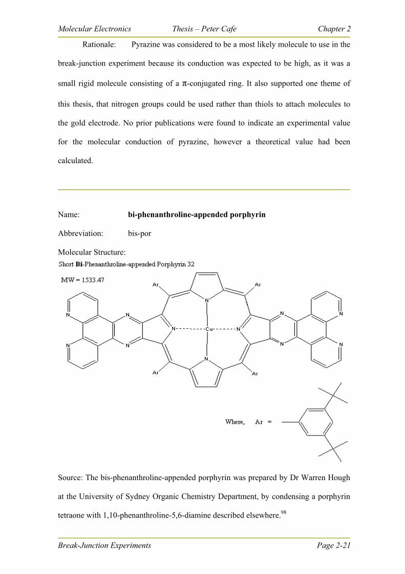
Molecular Electronics Thesis – Peter Cafe Chapter 2
Rationale: Pyrazine was considered to be a most likely molecule to use in the
break-junction experiment because its conduction was expected to be high, as it was a
small rigid molecule consisting of a π-conjugated ring. It also supported one theme of
this thesis, that nitrogen groups could be used rather than thiols to attach molecules to
the gold electrode. No prior publications were found to indicate an experimental value
for the molecular conduction of pyrazine, however a theoretical value had been
calculated.
Name: bi-phenanthroline-appended porphyrin
Abbreviation: bis-por
Molecular Structure:
Source: The bis-phenanthroline-appended porphyrin was prepared by Dr Warren Hough
at the University of Sydney Organic Chemistry Department, by condensing a porphyrin
tetraone with 1,10-phenanthroline-5,6-diamine described elsewhere.98
Break-Junction Experiments Page 2-21
Molecular Electronics Thesis – Peter Cafe Chapter 2
Rationale: Porphyrins are of particular interest to organic chemists at Sydney
University as possible candidates for molecular wires and devices98, 99. A likely method
of securing such molecules to gold electrodes is via the phenanthroline “alligator clip”36,
hence this molecule has been synthesised. However very little experimental work has
been done on it and on the conductance of porphyrins in general. This is the first attempt
to obtain its molecular conduction.
2.2.2 Experimental procedure
The break junction experiments carried out in this thesis were either conducted at:
Sydney University’s Electron Microscope Unit (USYD)
or
The Commonwealth Serum and Investigation Research Organisation
laboratories located at Lindfield NSW (CSIRO),
with slight differences in the experimental procedure at the two sites, and with two very
different instruments, for which there is more information in the next section.
Water: Throughout the experiment all water referred to, for both cleaning and
experimentation, was rated 18.2 MΩ Millipore® water fed from the town water supply.
Glassware: Cleaning of all glassware and the liquid cell was done by simmering
in ~15% nitric acid for more than 1 hour, after which they were rinsed copiously, left to
soak for 30 minutes, and rinsed copiously again in water.
Gold: Gold tips were prepared by cutting 0.25 mm gold wire at USYD or 0.5
mm wire at CSIRO with snips. They were then H2 flame purified, and at CSIRO they
Break-Junction Experiments Page 2-22
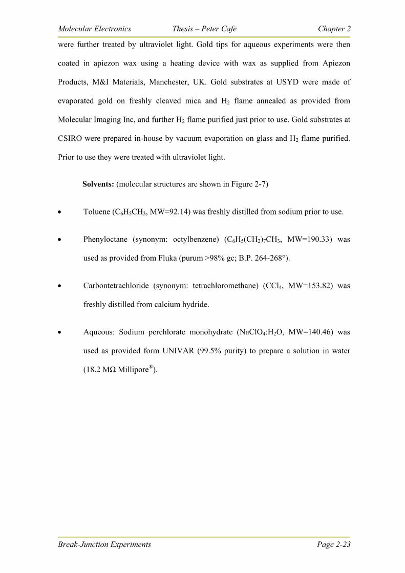
Molecular Electronics Thesis – Peter Cafe Chapter 2
Break-Junction Experiments Page 2-23
were further treated by ultraviolet light. Gold tips for aqueous experiments were then
coated in apiezon wax using a heating device with wax as supplied from Apiezon
Products, M&I Materials, Manchester, UK. Gold substrates at USYD were made of
evaporated gold on freshly cleaved mica and H2 flame annealed as provided from
Molecular Imaging Inc, and further H2 flame purified just prior to use. Gold substrates at
CSIRO were prepared in-house by vacuum evaporation on glass and H2 flame purified.
Prior to use they were treated with ultraviolet light.
Solvents: (molecular structures are shown in Figure 2-7)
Toluene (C6H5CH3, MW=92.14) was freshly distilled from sodium prior to use.
Phenyloctane (synonym: octylbenzene) (C6H5(CH2)7CH3, MW=190.33) was
used as provided from Fluka (purum >98% gc; B.P. 264-268°).
Carbontetrachloride (synonym: tetrachloromethane) (CCl4, MW=153.82) was
freshly distilled from calcium hydride.
Aqueous: Sodium perchlorate monohydrate (NaClO4:H2O, MW=140.46) was
used as provided form UNIVAR (99.5% purity) to prepare a solution in water
(18.2 MΩ Millipore®).
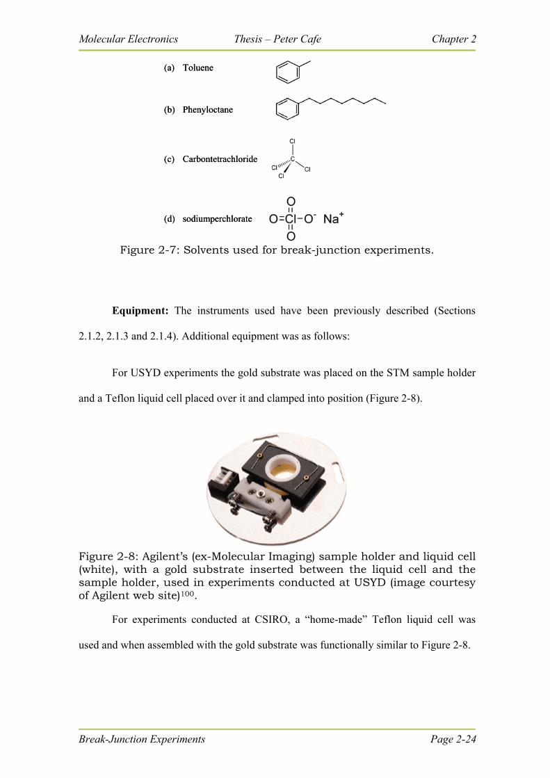
Molecular Electronics Thesis – Peter Cafe Chapter 2
(a) Toluene
(b) Phenyloctane
(c) Carbontetrachloride
(d) sodiumperchlorate
(a) Toluene
(b) Phenyloctane
(c) Carbontetrachloride
(d) sodiumperchlorate
Figure 2-7: Solvents used for break-junction experiments.
Equipment: The instruments used have been previously described (Sections
2.1.2, 2.1.3 and 2.1.4). Additional equipment was as follows:
For USYD experiments the gold substrate was placed on the STM sample holder
and a Teflon liquid cell placed over it and clamped into position (Figure 2-8).
Figure 2-8: Agilent’s (ex-Molecular Imaging) sample holder and liquid cell (white), with a gold substrate inserted between the liquid cell and the sample holder, used in experiments conducted at USYD (image courtesy of Agilent web site)100.
For experiments conducted at CSIRO, a “home-made” Teflon liquid cell was
used and when assembled with the gold substrate was functionally similar to Figure 2-8.
Break-Junction Experiments Page 2-24
Molecular Electronics Thesis – Peter Cafe Chapter 2
Break-Junction Experiments Page 2-25
Procedure: For USYD, first the gold tip was placed in the head of the STM unit
(Figure 2-4) and the unit placed in position in the PicoPlus II (Figure 2-3), and the height
of the sample plate adjusted using a dummy sample plate. Then the solvent was placed in
the liquid cell to about half-full and the sample plate inserted beneath the STM scanner
unit. The STM was set to approach the sample. When it engaged (i.e. when it detected
the “set point” current) the custom spectroscopy script (“current Vs distance”) was
opened and parameters entered which enabled the gold tip to approach the surface and
crash into the gold substrate, and then withdraw at a specific speed, and it was also set to
perform multiple sweeps. (If sets of sweeps were required in air, this was first done
without the solvent, and then done again with the solvent.)
For the volatile solvents toluene and carbontetrachloride the experiment was
conducted in a glass environmental chamber with a petri dish containing the solvent
placed in the bottom of the chamber (to saturate the air in the chamber). The
environmental chamber is shown in the PicoPlus II unit in Figure 2-3.
Various sets of sweeps were conducted in the solvent (or air) adjusting the
parameters as necessary for each set (e.g. bias or withdrawal speed).
After all the sets for the solvent were done, a solution of the solvent and the
molecule was prepared at double the required molarity. The sample plate was removed
(or when the environmental chamber was used, the STM scanner was removed) and the
liquid cell “topped-up” with the solution containing the molecule. The components were
then reassembled and various sets of sweeps were conducted on the molecule.
For experiments conducted at CSIRO, the procedure was extremely similar, with
the only difference being in the way the unit was assembled and in the operation of the
Molecular Electronics Thesis – Peter Cafe Chapter 2
Break-Junction Experiments Page 2-26
approach of the gold tip and how the software then controlled the instrument (described
elsewhere43).
2.2.2.1 Instrument used at Sydney University, advantages
and disadvantages.
The experiments conducted at Sydney University used a Molecular Imaging
STM (Scanning Tunnelling Microscope: see Section 2.1.3 above) with parameters
entered into its operating software to control the motion of the gold probe. The main
advantages of using this system were:
1. The functionality already existed in the instrument and the only extra item
required was the gold wire to make the tips.
2. The instrument could be configured to carry out multiple successive sweeps
without user intervention.
3. By fine adjustment of the set-point current and switching on the option to
“restore servo” after each sweep, the instrument was able to reset the initial
distance for the start of the next sweep. This gave rise to greater consistency
in the sweeps and allowed for smaller movement of the tip. (During each
sweep there is an amount of distortion to the surface and the tip, changing the
geometric alignment. This means that at the end of one sweep, the gap
between the tip and surface may not be the same as it was at the beginning,
even though the movement up was equal to the movement down. By using
the set-point current, the gap between tip and surface can be restored prior to
the next sweep.)

Molecular Electronics Thesis – Peter Cafe Chapter 2
Break-Junction Experiments Page 2-27
4. It was contained within a vibrational isolation unit.
The main disadvantages of the using STM scanner were:
1. The functionality of the software did not allow the option to trigger
movement based upon current events. This means that there was no direct
control over how much the tip crashed into the gold surface (it was controlled
indirectly by resetting the height to the set-point current.) and at what points
in withdrawal to start and stop data collection. This also meant that the user
had to observe the current traces of each sweep continually to monitor for
anomalies and to stop and reset the experiment as necessary.
2. There was no functionality in the software to reject sweeps. Given that only
10 to 30% of sweeps show evidence of molecular conduction, the extraction
of relevant data was quite difficult, given the amount of data that had to be
analysed.
3. The gold wire could be no more than 0.25 mm in diameter and, being gold,
was often too soft and flexible to stay in position or remain straight. Short
wires had to be used but sometimes they wouldn’t reach the sample without
the STM nose hitting the sides of the liquid cell.
4. The instrument and the environment had a number of performance and
operational shortcomings which added to the difficulties of the experiment,
sometimes causing confusion trying to interpret what was being observed,
and at other times causing significant delays.
Molecular Electronics Thesis – Peter Cafe Chapter 2
Break-Junction Experiments Page 2-28
5. Experiments were initially done using the standard STM head (i.e. with a
linear amplifier), which had a limited range. It could observe conduction in
the molecular range (i.e. around 10-4 G0), but not the metallic range (i.e. gold
conduction, around 1.0 G0.), so that it wasn’t clear whether the break-
junctions were being correctly formed each time.
6. Later a logarithmic amplifier was obtained, which could observe
conduction over a range from less than 10-5 up to 103 G0, so that it was
possible to observe both molecular and gold conduction in the one sweep.
The logarithmic amplifier needed to be calibrated (by creating a calibration
file using a number of known resistors: see Section 2.2.3 below for further
details) and the data files created by the instrument’s software had to be
converted using the calibration file. Programs were written in FORTRAN to
do the data manipulation.
7. The PicoScan 5.3 software, which operated the controller and was the human
interface, presented immediate graphs (traces) of each sweep on screen as
Current Vs Distance curves. From these graphs it was possible to identify
steps in the conduction curves which may indicate metallic or molecular
conduction. However the graphs did not display results in conductance
values. For the linear amplifier it was a simple piece of mathematics to
determine the conductance value represented by a current step, and the step
could then be identified. However for the logarithmic amplifier it was more
difficult to evaluate apparent conduction steps. Furthermore, there was no
functionality to present ongoing histograms of the accumulated data: final
results of sets of sweeps could only be determined well after the experiment
had finished.
Molecular Electronics Thesis – Peter Cafe Chapter 2
Break-Junction Experiments Page 2-29
2.2.2.2 Instrument used at CSIRO, advantages and
disadvantages.
The experiments conducted at CSIRO used a “Home Made” instrument built by
Jan Herrmann43, which consisted of a mounting tube attached to a piezo device which in
turn was attached to a stepper-motor. The whole device was placed over the sample,
which was covered in a PTFE (Teflon) liquid cell. There were a number of different
amplifiers available to explore different conduction ranges, as well as a logarithmic
amplifier. The software which controlled the device was also written by Dr Jan
Herrmann of CSIRO. The main advantages of this instrument were:
1. The mounting tube allowed thicker gold wire to be used (up to 0.5 mm
diameter), providing greater rigidity to the system.
2. The software included functionality to control the break-junction
depending on current triggers. This allowed placement of the tip to be
reset automatically if gold conduction was not evidenced.
3. Data from each sweep was immediately presented on screen (in values of
G0) and the cumulative data from the set was displayed as a histogram,
updated after each sweep. This enabled the experimenter to know
immediately what kind of results were developing.
4. The software also enabled the device to reset its vertical position if there
was too much or not enough conduction (and ignore the data), allowing
sweeps to run without the need of user observation, and obtaining a
higher percentage of data files with valid data.
Molecular Electronics Thesis – Peter Cafe Chapter 2
Break-Junction Experiments Page 2-30
5. It was possible to define many more data points in a given range with the
CSIRO equipment, enabling even very small molecular conduction steps
to be captured.
6. The computer was loaded with “PC Anywhere” and so effectively once
the sample was set up, the experiment could be conducted from a remote
site (e.g. from home), allowing large numbers of sweeps to be run with
convenient observation, and also allowing some parameters to be changed
remotely.
The main disadvantages of the CSIRO system were:
1. The instrument had no horizontal displacement. If, for some reason, the
spot on the sample had become unsuitable for further sweeps, it had to be
disengaged and moved manually.
2. It used a linear amplifier. It had a high range of about 3 or 4 orders of
magnitude, and the range was extended by changing the gain setting,
which enabled the operator to examine all possible conduction ranges
from 13.0 G0 to 10-7 G0, however it was usually not possible to observe
gold conduction and molecular conduction in the one sweep (see Section
2.3.1.2 below).
3. After each sweep it returned the tip to the original height (in absolute
reckoning), which meant that if the surface or tip had deformed during the
previous sweep, the next sweep started either too close or too far from the
Molecular Electronics Thesis – Peter Cafe Chapter 2
Break-Junction Experiments Page 2-31
surface (i.e. it did not rely upon tunnelling current to reset the actual gap
between the tip and the sample).
4. The software had a complicated user interface.
However, since the software was written in-house, most of the disadvantages
could possibly be addressed in some future re-write of the software.
2.2.3 Use of logarithmic amplifier
The logarithmic amplifier used at Sydney University enables current
measurements to be taken over a range encompassing many orders of magnitude, and so
it enables both gold steps and molecule steps to be observed in the one conduction
sweep. However the amplifier is nominally logarithmic and the only way to convert to
actual current is to construct a “calibration curve” using a series of known resistors and
sweeping over a bias range for each resistor.
Various resistors were purchased from KA Electronics and Dick Smith
Electronics and each was measured using a high quality multimeter (see Table 2-3
below). Each resistor in turn was bridged between the STM Scanner (with the
logarithmic amplifier inserted) and the mounting plate, and was swept in the bias range –
10 to +10 volts and the output from the log amplifier (log current) tabled against the
actual current (which is the input (bias) divided by the resistor value). The results are
graphed in Figure 2-9 (low range) and Figure 2-10 (high range) below. From these sets
of data a single conversion table was created which was used for the analysis in
experimental sections to convert log-amp current to actual current.
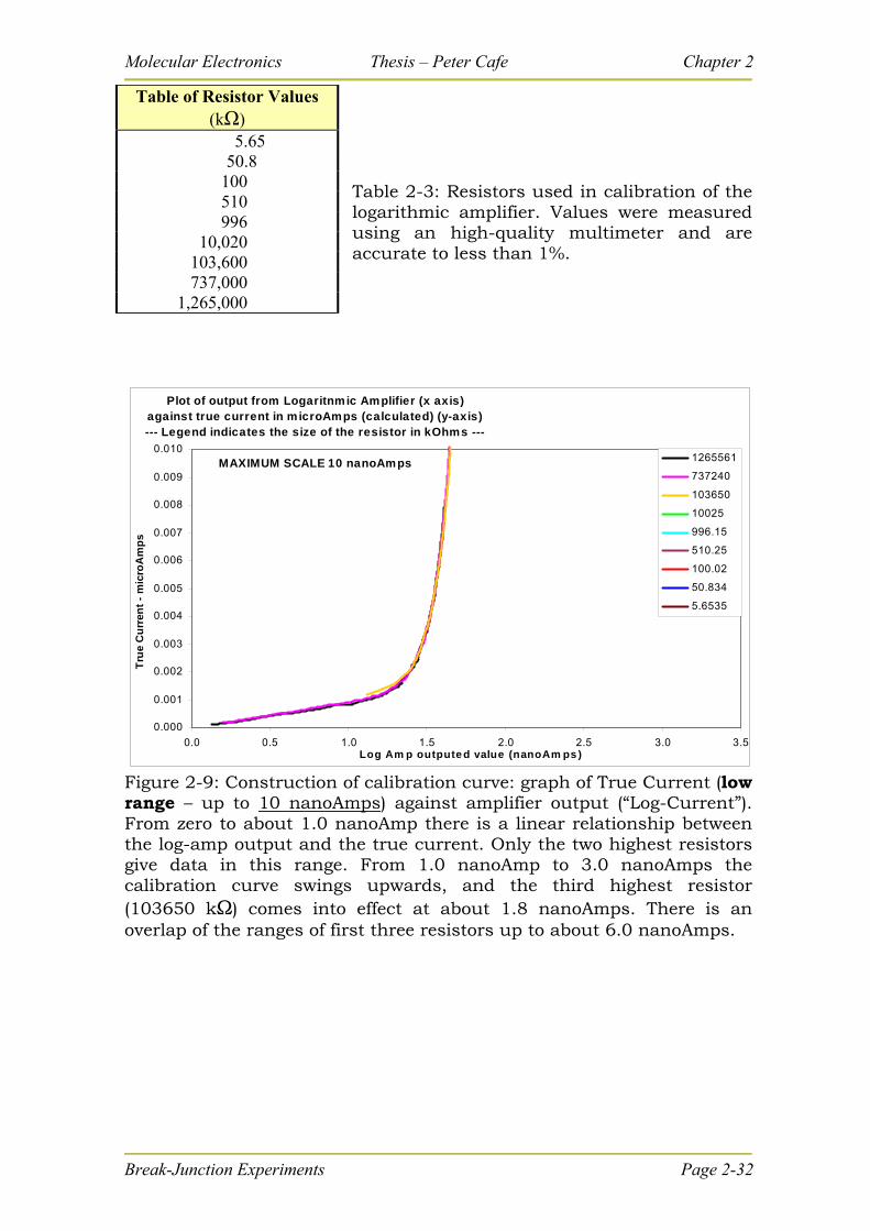
Molecular Electronics Thesis – Peter Cafe Chapter 2
Table of Resistor Values (kΩ)
5.65 50.8 100 510 996 10,020 103,600 737,000 1,265,000
Table 2-3: Resistors used in calibration of the logarithmic amplifier. Values were measured using an high-quality multimeter and are accurate to less than 1%.
Plot of output from Logaritnmic Amplifier (x axis) against true current in microAmps (calculated) (y-axis)--- Legend indicates the size of the resistor in kOhms ---
MAXIMUM SCALE 10 nanoAmps
0.000
0.001
0.002
0.003
0.004
0.005
0.006
0.007
0.008
0.009
0.010
0.0 0.5 1.0 1.5 2.0 2.5 3.0 3.5Log Am p outpute d value (nanoAm ps )
Tru
e C
urr
ent
- m
icro
Am
ps
1265561
737240
103650
10025
996.15
510.25
100.02
50.834
5.6535
Figure 2-9: Construction of calibration curve: graph of True Current (low range – up to 10 nanoAmps) against amplifier output (“Log-Current”). From zero to about 1.0 nanoAmp there is a linear relationship between the log-amp output and the true current. Only the two highest resistors give data in this range. From 1.0 nanoAmp to 3.0 nanoAmps the calibration curve swings upwards, and the third highest resistor (103650 kΩ) comes into effect at about 1.8 nanoAmps. There is an overlap of the ranges of first three resistors up to about 6.0 nanoAmps.
Break-Junction Experiments Page 2-32
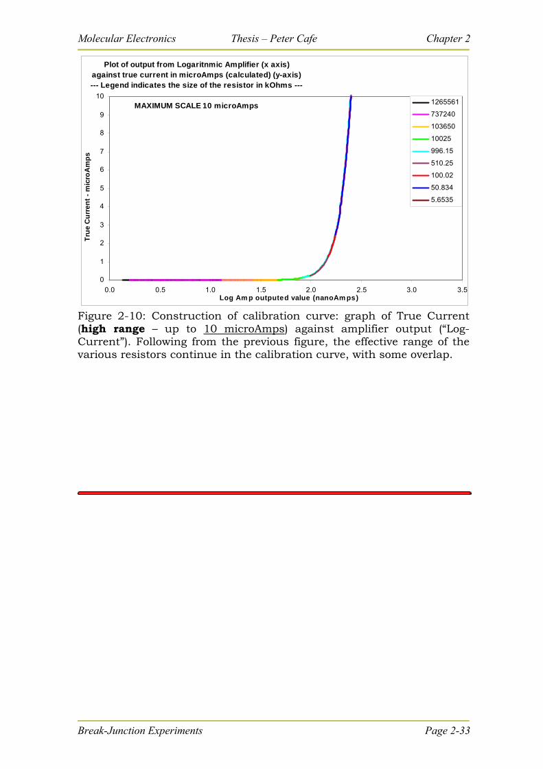
Molecular Electronics Thesis – Peter Cafe Chapter 2
Plot of output from Logaritnmic Amplifier (x axis) against true current in microAmps (calculated) (y-axis)--- Legend indicates the size of the resistor in kOhms ---
MAXIMUM SCALE 10 microAmps
0
1
2
3
4
5
6
7
8
9
10
0.0 0.5 1.0 1.5 2.0 2.5 3.0 3.5Log Am p outputed value (nanoAm ps)
Tru
e C
urr
ent
- m
icro
Am
ps
1265561
737240
103650
10025
996.15
510.25
100.02
50.834
5.6535
Figure 2-10: Construction of calibration curve: graph of True Current (high range – up to 10 microAmps) against amplifier output (“Log-Current”). Following from the previous figure, the effective range of the various resistors continue in the calibration curve, with some overlap.
Break-Junction Experiments Page 2-33
Molecular Electronics Thesis – Peter Cafe Chapter 2
2-3 General comment on experiments and results
General details of the experimental preparation are given in Section 2.2.2 and
include sources and purity of chemicals and solvents, and general sample preparation
and experimental techniques which are not particular to individual molecules. Anything
particular to a set of experiments or a molecule is described under the molecule’s
individual heading from Section 2-4 to 2-8 below.
2.3.1 Terminology and treatment of raw data.
Each withdrawal of the gold wire from the surface is called a “sweep”. A group
of sweeps with the same conditions done consecutively is called a “set”, and a set may
comprise hundreds of sweeps. For each of the five molecules investigated, a number of
sets were collected, including solvent-only sets. If sets were collected consecutively as
part of the one experiment they are called a group. A “trace” is the graph of data from a
single sweep, and it may show a “step”, which is a consecutive series of data points with
roughly the same conduction value, which is generally considered to be a “conduction
event”: either the conduction of a single molecule, multiple molecules, or metallic gold
wires of thickness one or more gold atoms. Some traces have multiple steps. Other traces
may have no steps or ill-defined steps.
The raw data values for each set of sweeps were converted to values of
conductance quantum, G0, as follows:
With the linear amplifier the raw data values were actual current (I in amps).
The current values are converted directly to conductance values (G) using the
bias (V in volts) and the formula G V
906,12 I G0 (see Section 2.1.6
above).
Break-Junction Experiments Page 2-34
Molecular Electronics Thesis – Peter Cafe Chapter 2
Break-Junction Experiments Page 2-35
With the logarithmic amplifier the raw data values were a nominal log of the
true current and had to be converted to true current values using the
conversion table, which is constructed using a series of known resistors (see
Section 2.2.3 above). Then the true current values are converted to
conductance values using the same formula as above.
With the data produced at CSIRO, the raw data values were true conductance
values in G0, so no further conversion was necessary.
The sets of data (in G0 values) were analysed by two different methods. Both
methods defined a certain range of G0 values to which the analysis was limited. The
difference in the two methods was in the way in which sweeps were rejected, leaving a
number of valid sweeps.
Rejection Method 1: The only criterion by which a sweep was rejected was if the
first data point did not reach a “saturation value” (this would indicate that metallic
conduction was not achieved and the gold wire did not form). Thus all other sweeps
were included. The reasoning behind this method was that sweeps may include
instances of conduction events which may not be indicated by clear steps but which may
be evidenced in the overall summation of data (following Quek, et al., 200787, who
found that most conduction steps were less than 1 Angstrom wide and used all 59,000
sweeps on benzenediamine without filtering).
Rejection Method 2: In addition to the rejection criterion of Method 1, individual
sweeps were also rejected if there were not 200 or more data points in the defined
analysis range. The reasoning behind this method was that most of the sweeps indicated
Where a linear amplifier was used saturation or gold conduction could not be established and so all sweeps were included in the analysis.
Molecular Electronics Thesis – Peter Cafe Chapter 2
Break-Junction Experiments Page 2-36
noise (erratic conduction signals) in the analysis range and that any true conduction
event would be indicated by a significant step in the individual trace. This method
resulted in very few individual sweeps being accepted. The range was determined by an
arbitrarily chosen upper bound, and then both the lower bound and the bin size were 1%
of the upper bound.
Both methods relied on “binning” of the data, in which the data from all valid
sweeps in a given set was collated into bins using a defined range of G0 values and a
certain bin size, usually resulting in anywhere between 40 and 200 bins per range. Each
bin would cover a small extent of the data range and would have a “count”, which was
the total number of data points from all valid sweeps of the given set which fell into that
bin. Each bin also had a mid-point value.
In order to compare different data sets the count was divided by the number of
valid sweeps, and histograms were drawn graphing “Counts per Valid Sweep” against
conductance, G0 (where G0 was the mid-point value of the bin). A peak in the histogram
would indicate if a set showed a consistent conduction event (according to the reasoning
of each method).
2.3.1.1 Special analysis techniques used.
Apart from the standard practise of binning the data to form histograms, the
following techniques were applied:
(a) Normalising data by dividing by the number of valid sweeps: (This
technique was applied in all analyses). It was found that the most valid method for
comparing different sets of data was to normalise each set by dividing by the number of
Molecular Electronics Thesis – Peter Cafe Chapter 2
Break-Junction Experiments Page 2-37
valid sweeps (previous paragraph). This gave a powerful tool for comparing molecule
sets against solvent sets within the same group, and to some extent across groups
provided the bin size was the same. This method has not been reported before.
(b) Rejection of sweeps without 200 data-points in the defined range: As
described above in Rejection Method 2, this was method applied to all molecules when
binning was done on a linear scale within a defined range. This method has also not been
reported before.
(c) Log G0 scale graphs: Where possible additional histograms were also
constructed using a log10 scale for the horizontal axis (conductance). This was proven to
be a useful technique to view the overall effect of the molecule to conductance over a
wide range (i.e. over 6 orders of magnitude, from 10-5 G0 to 10 G0), which in some cases
showed no peaks in linear scale histograms. This method was reported by Gonzalez, et
al, (2006).68
(d) Gaussian smoothing: In one group of data obtained from CSIRO it was
useful to apply Gaussian smoothing to join different data sets. This is a common
statistical analysis technique, and has been used in break-junction experiments before43.
2.3.1.2 Various gain settings used at CSIRO
At CSIRO a linear amplifier was used. However it had a variable gain setting, so
that even though the range of the amplifier was limited, it was possible to look at various
conductance ranges by changing the gain setting. By this method each set of sweeps was
done at a fixed gain setting and limited to a particular range (for example the “gold
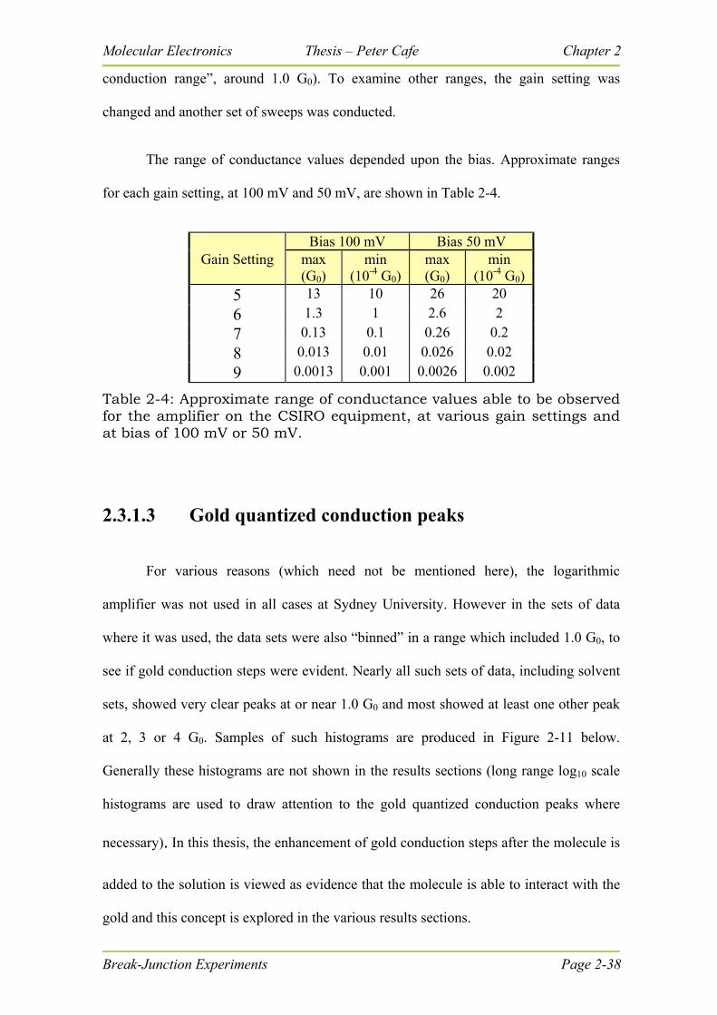
Molecular Electronics Thesis – Peter Cafe Chapter 2
Break-Junction Experiments Page 2-38
conduction range”, around 1.0 G0). To examine other ranges, the gain setting was
changed and another set of sweeps was conducted.
The range of conductance values depended upon the bias. Approximate ranges
for each gain setting, at 100 mV and 50 mV, are shown in Table 2-4.
Bias 100 mV Bias 50 mV Gain Setting max
(G0) min
(10-4 G0) max (G0)
min (10-4 G0)
5 13 10 26 20
6 1.3 1 2.6 2
7 0.13 0.1 0.26 0.2
8 0.013 0.01 0.026 0.02
9 0.0013 0.001 0.0026 0.002
Table 2-4: Approximate range of conductance values able to be observed for the amplifier on the CSIRO equipment, at various gain settings and at bias of 100 mV or 50 mV.
2.3.1.3 Gold quantized conduction peaks
For various reasons (which need not be mentioned here), the logarithmic
amplifier was not used in all cases at Sydney University. However in the sets of data
where it was used, the data sets were also “binned” in a range which included 1.0 G0, to
see if gold conduction steps were evident. Nearly all such sets of data, including solvent
sets, showed very clear peaks at or near 1.0 G0 and most showed at least one other peak
at 2, 3 or 4 G0. Samples of such histograms are produced in Figure 2-11 below.
Generally these histograms are not shown in the results sections (long range log10 scale
histograms are used to draw attention to the gold quantized conduction peaks where
necessary). In this thesis, the enhancement of gold conduction steps after the molecule is
added to the solution is viewed as evidence that the molecule is able to interact with the
gold and this concept is explored in the various results sections.
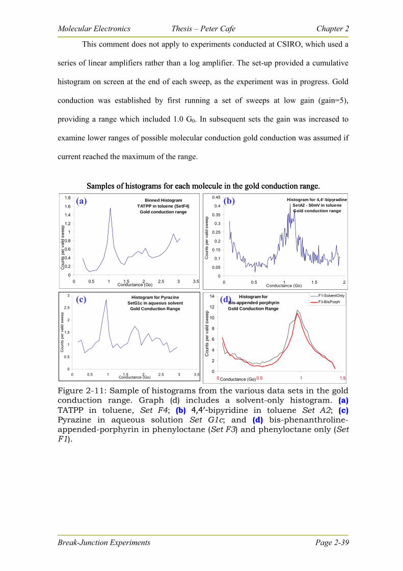
Molecular Electronics Thesis – Peter Cafe Chapter 2
This comment does not apply to experiments conducted at CSIRO, which used a
series of linear amplifiers rather than a log amplifier. The set-up provided a cumulative
histogram on screen at the end of each sweep, as the experiment was in progress. Gold
conduction was established by first running a set of sweeps at low gain (gain=5),
providing a range which included 1.0 G0. In subsequent sets the gain was increased to
examine lower ranges of possible molecular conduction gold conduction was assumed if
current reached the maximum of the range.
Break-Junction Experiments Page 2-39
Binned Histogram TATPP in toluene (SetF4)
Gold conduction range
0
0.2
0.4
0.6
0.8
1
1.2
1.4
1.6
1.8
0 0.5 1 1.5 2 2.5 3 3.5Conductance (Go)
Cou
nts
per
valid
sw
eep
Histogram for 4,4'-bipyradineSetA2 - 50mV in tolueneGold conduction range
0
0.05
0.1
0.15
0.2
0.25
0.3
0.35
0.4
0.45
0 0.5 1 1.5Conductance (Go)
Cou
nts
per
valid
sw
eep
2
Histogram for PyrazineSetG1c in aqueous solvent
Gold Conduction Range
0
0.5
1
1.5
2
2.5
3
0 0.5 1 1.5 2 2.5 3 3.5Conductance (Go)
Co
un
ts p
er
valid
sw
ee
p
Histogram for Bis-appended porphyrinGold Conduction Range
0
2
4
6
8
10
12
14
0 0.5 1 1.5C )onductance (Go
Cou
nts
per
valid
sw
eep
F1-SolventOnly
F3-BisPorph
Samples of histograms for each molecule in the gold conduction range.
(a) (b)
(c) (d)
Samples of histograms for each molecule in the gold conduction range.
Binned Histogram TATPP in toluene (SetF4)
Gold conduction range
0
0.2
0.4
0.6
0.8
1
1.2
1.4
1.6
1.8
0 0.5 1 1.5 2 2.5 3 3.5Conductance (Go)
Cou
nts
per
valid
sw
eep
Histogram for 4,4'-bipyradineSetA2 - 50mV in tolueneGold conduction range
0
0.05
0.1
0.15
0.2
0.25
0.3
0.35
0.4
0.45
0 0.5 1 1.5 2Conductance (Go)
Cou
nts
per
valid
sw
eep
Histogram for PyrazineSetG1c in aqueous solvent
Gold Conduction Range
0
0.5
1
1.5
2
2.5
3
0 0.5 1 1.5 2 2.5 3 3.5Conductance (Go)
Co
un
ts p
er
valid
sw
ee
p
Histogram for Bis-appended porphyrinGold Conduction Range
0
2
4
6
8
10
12
14
onductance (Go
Cou
nts
per
valid
sw
eep
0 0.5 1 1.5C )
F1-SolventOnly
F3-BisPorphHistogram for Pyrazine
SetG1c in aqueous solventGold Conduction Range
0
0.5
1
1.5
2
2.5
3
0 0.5 1 1.5 2 2.5 3 3.5Conductance (Go)
Co
un
ts p
er
valid
sw
ee
p
F1-SolventOnlyHistogram for Bis-appended porphyrinGold Conduction Range
0
2
4
6
8
10
12
14
onductance (Go
Cou
nts
per
valid
sw
eep
F3-BisPorph
0 0.5 1 1.5C )
Samples of histograms for each molecule in the gold conduction range.
(a) (b)
(c) (d)
Figure 2-11: Sample of histograms from the various data sets in the gold conduction range. Graph (d) includes a solvent-only histogram. (a) TATPP in toluene, Set F4; (b) 4,4′-bipyridine in toluene Set A2; (c) Pyrazine in aqueous solution Set G1c; and (d) bis-phenanthroline-appended-porphyrin in phenyloctane (Set F3) and phenyloctane only (Set F1).
Molecular Electronics Thesis – Peter Cafe Chapter 2
Break-Junction Experiments Page 2-40
2.3.2 Other data selection and analysis techniques used in
literature.
Usually with break-junction experiments there are four types of conduction traces
which may be produced by a single sweep:
A. Traces which show clear steps in the molecular conduction region (40-
50%*),
B. Traces which show noise in the same region (20%*),
C. Traces which drop smoothly and steeply to very low conduction (tunnelling),
which produce little data in the molecular conduction region (30%*), and
D. Traces which do not commence from a saturation value, which indicate that
an effective break-junction has not formed.
* The percentages of traces A, B and C are from Li, et al, (2006)101 on 1,8-
octanedithiol: See Chapter 4 Figure 4-57 on page 4-6 for examples of the three types of
traces. Li avoids traces of type D by using interface software. For sets of solvent-only
sweeps, the percentage of traces of type C is much greater, but solvent sets still
occasionally show steps or noise in the molecular conduction area87.
Type D are traces which are produced because the mechanical control of the tip
does not create an effective break-junction. With overriding software to interface with
the STM controls during the experiment one can gain more sophisticated control over the
movement of the gold tip and greatly reduce the “bad data” and eliminate all type-D
traces. Such software was not available in this work.
Molecular Electronics Thesis – Peter Cafe Chapter 2
Break-Junction Experiments Page 2-41
A narrower selection of data would selectively enhance the histograms produced
in this thesis, but the underlying histogram peaks should appear to some extent, even
with all the types of curves included, as noted by Gonzalez, et al, (2006)68:
“Data selections do not help improve the result.”
and
“The situation is unsatisfactory, because there is at present no generally accepted objective selection criterion.”
It is not always clear how prior researchers have selected their data (i.e. what
criteria did they use for rejecting invalid sweeps): in some cases they have expressly
stated that no data selection techniques were employed43 (other than rejecting traces of
type D based upon saturation, which seems to be a universal practise), and in others they
probably used filters to reject a number of individual sweeps to improve the peaks in
their histograms, however some leading researchers have been quite vague in the specific
method of filtering (i.e. whether they manually trawled through the data to select
desirable traces [subjective], or they used an algorithm built into their software
[objective])56, 101. But data selection has been a common practise for enhancing results.
The percentage of curves which produce “good” data varies considerably: from as much
as 80%11 to as little as 15%72, and this is often dependent on the type of molecule being
investigated. For 1,8-octanedithiol the percentage was typically 40%101, 15% for
perylene tetracarboxcylic72, and 20 % for oligoaniline11. It is common to have 20 to 30%
of sweeps producing noise in the molecular conduction region (i.e. no clear steps40).
Even the solvent-only sets have a small percentages of traces with features which appear
like molecular conduction steps101.
Molecular Electronics Thesis – Peter Cafe Chapter 2
Many research groups (including ours) have struggled with the concept and
method of data selection. Perhaps because, as we found, it is often the case that
individual traces have good steps but the binned histograms show no distinct peaks42, 43.
Gonzalez, et al, (2006)68 applied an algorithm to their data which extracted data
from distinct plateaus (steps) only and then constructed the histogram from this selected
data. With this method there was no need pre-select the “good” curves. They also used a
method of plotting against log G rather than G, and also they subtracted the base-line,
which was determined from solvent-only sweeps. With these methods their histograms
became more distinct.
Jang, et al, (2006) used “last step analysis”, where only the last plateau was used
to construct a histogram. Their algorithm found the last step by first finding the last
sudden drop and then looking at the data which appeared immediately before it. With
this method there is no need for prior data selection.
In the work to prepare this thesis a number of different analysis techniques were
investigated, including last step analysis, slope analysis, data smoothing, Fourier
analysis, noise reduction, base-line subtraction and various sweep rejection criteria.
However none of these techniques gave both significant and consistent improvements in
results. Only the two different rejection methods described above have been included in
the presentation.
Break-Junction Experiments Page 2-42
Molecular Electronics Thesis – Peter Cafe Chapter 2
Break-Junction Experiments Page 2-43
2-4 Investigations of 1,8-octanedithiol
1,8-octanedithiol.
(For a comment about thiol and thiyl terminology see Section 4.1.3 below)
2.4.1 Rationalization:
As a preliminary series, the 1,8-octanedithiol was examined to establish “proof of
concept”. It is one of the most studied molecules in molecular electronics and its
conduction has been measured in a variety of ways, both experimentally and
theoretically. It was also one of the first to be used in the same type of break-junction
experiment and clear results have been obtained by Tao14.
The linear amplifier was used in these experiments.
2.4.2 Background research
Various experimental and theoretical values for the conductance of 1,8-octane
dithiol are reported in Table 2-2 above, on page 2-15. A high-conductance regime and a
low-conductance regime have been identified, corresponding to two different binding
configurations of the molecule to the gold electrodes (these concepts are taken up more
fully in Chapter 4). The generally accepted values for conductance of a single 1,8-
octanedithiol molecule are 2.5 x 10⁻⁴ G0 (high conductance) and 0.5 x 10⁻⁴ G0 (low
conductance).
2.4.3 Experimental set-up:
The break-junction experiments were carried out in approximately 1 mM of 1,8-
octanedithiol in toluene.
Molecular Electronics Thesis – Peter Cafe Chapter 2
Break-Junction Experiments Page 2-44
2.4.4 The sets of sweeps for 1,8-octanedithiol
Three sets of sweeps were recorded, one solvent-only set labelled Set A0 and two
dithiol sets labelled Set A1 and Set B2. The parameters for these sets are listed in Table
2-5 below.
Set item bias Solvent Amp number of sweeps
withdrawal speed (nm s-1)
A0 solvent only -50 mV toluene lin 296 12 A1 1,8-octanedithiol -50 mV toluene lin 887 12 B2 1,8-octanedithiol +50 mV toluene lin 824 12
Table 2-5: Parameters for the sets of sweeps relating to 1,8-octanedithiol
A selection of individual traces for Set A1 is shown in Figure 2-13 below.
2.4.5 Results from all sets of data for 1,8-octanedithiol.
The data from the three sets of sweeps was analysed according to both Method 1
and Method 2 (Section 2.3.1 above) and the resultant histograms are shown in Figure 2-
12 below. In units of 10-4 G0, Method 1 shows two possible peaks for Set A1 at 2.4 and
5.9 (with 656 valid sweeps), and no definite peaks for Set B2 (209 valid sweeps),
whereas Method 2 shows two strong peaks for Set A1 at 2.2 and 5.8 (but with only 21
valid sweeps) and no peaks for Set B2 (81 valid sweeps). Both methods show no peaks in
the solvent-only set. (The steep rising parts of the graphs below 1.5 x 10⁻⁴ G0 are due to
the limitations of the instrument.)
These results are set out in Table 2-6, page 2-47 below and compared with
standard results from Li, et al,101.

Molecular Electronics Thesis – Peter Cafe Chapter 2
Break-Junction Experiments Page 2-45
Because the linear amplifier was used for 1,8-octanedithiol and thus the data
covered a small range, there was no advantage to be gained by plotting against Log10 of
conductance.
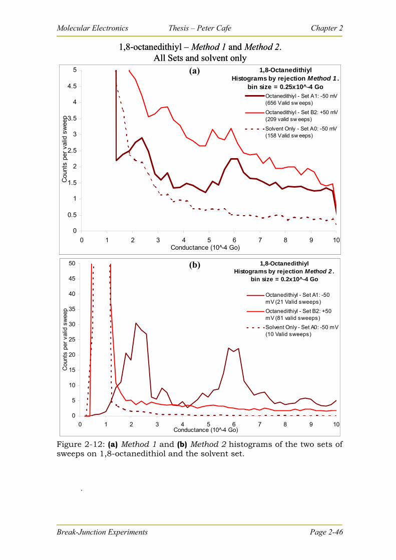
Molecular Electronics Thesis – Peter Cafe Chapter 2
1,8-OctanedithiylHistograms by rejection Method 1 .
bin size = 0.25x10^-4 Go
0
0.5
1
1.5
2
2.5
3
3.5
4
4.5
5
0 1 2 3 4 5 6 7 8 9 1Conductance (10 -4 Go)
Cou
nts
per
valid
sw
eep
0
Octanedithiyl - Set A1: -50 mV(656 Valid sw eeps)
Octanedithiyl - Set B2: +50 mV(209 valid sw eeps)
Solvent Only - Set A0: -50 mV(158 Valid sw eeps)
1,8-OctanedithiylHistograms by rejection Method 2 .
bin size = 0.2x10^-4 Go
0
5
10
15
20
25
30
35
40
45
50
0 1 2 3 4 5 6 7 8 9 1Conductance (10 -4 Go)
Cou
nts
per
valid
sw
eep
0
Octanedithiyl - Set A1: -50mV (21 Valid sweeps)
Octanedithiyl - Set B2: +50mV (81 valid sweeps)
Solvent Only - Set A0: -50 mV(10 Valid sweeps)
1,8-octanedithiyl – Method 1 and Method 2.All Sets and solvent only
(a)
(b)
Figure 2-12: (a) Method 1 and (b) Method 2 histograms of the two sets of sweeps on 1,8-octanedithiol and the solvent set.
.
Break-Junction Experiments Page 2-46
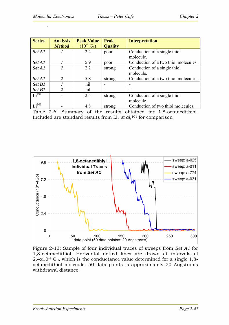
Molecular Electronics Thesis – Peter Cafe Chapter 2
.
Series Analysis Method
Peak Value (10-4 G0)
Peak Quality
Interpretation
Set A1 1 2.4 poor Conduction of a single thiol molecule.
Set A1 1 5.9 poor Conduction of a two thiol molecules.Set A1 2 2.2 strong Conduction of a single thiol
molecule. Set A1 2 5.8 strong Conduction of a two thiol molecules.Set B1 1 nil - - Set B1 2 nil - - Li101 - 2.5 strong Conduction of a single thiol
molecule. Li101 - 4.8 strong Conduction of two thiol molecules. Table 2-6: Summary of the results obtained for 1,8-octanedithiol. Included are standard results from Li, et al,101 for comparison
1,8-octanedithiylIndividual Traces
from Set A1
0
2.4
4.8
7.2
9.6
0 50 100 150 200 250 300data point (50 data points=~20 Angstroms)
Co
nd
uct
an
ce (
10
^-4
Go
)
sweep: a-025
sweep: a-011
sweep: a-774
sweep: a-031
Figure 2-13: Sample of four individual traces of sweeps from Set A1 for 1,8-octanedithiol. Horizontal dotted lines are drawn at intervals of 2.4x10⁻⁴ G0, which is the conductance value determined for a single 1,8-octanedithiol molecule. 50 data points is approximately 20 Angstroms withdrawal distance.
Break-Junction Experiments Page 2-47
Molecular Electronics Thesis – Peter Cafe Chapter 2
Break-Junction Experiments Page 2-48
2.4.6 Discussion of 1,8-octanedithiol results
Set A1 show similarity with prior research (e.g. Li, et al,101 and Chen, et al,40 –
see Table 2-2, page 2-15 above) and establish that the procedure and the instrument are
capable of performing single molecule conductance measurements, with the conductance
of a single 1,8-octanedithiol molecule being 2.5x10⁻⁴ G0. However Set B2 does not show
clear peaks (it has very weak broad peaks which differ slightly from Set A1 and prior
research, but are within the same order of magnitude). The explanation for the lack of
clear peaks in Set B2 may lie in the fact that the tip bias was positive rather than
negative, though it is unclear exactly how this would affect the results in a non-
electrochemical cell and an insulating solvent.
The use of the linear amplifier restricts the observable range such that it cannot
be established that a gold bridge has been formed prior to creation of the break-junction,
however the results from Set A1 indicate that it is still possible to obtain reliable
evidence of molecular conduction without this. Furthermore, with the linear amp, the
window of current range is limited to a factor of 10, and to extend the results to explore a
different G0 range the bias must be modified (for example an increase in the bias from 5
mV to 50 mV (then to 500 mV) will decrease the mid-range from approximately 10-2 G0
to 10-3 G0 (then to 10-4 G0), however such large bias changes cannot be considered an
independent variable and Li, et al, report that histogram peaks broaden and decrease in
height with higher voltages (over 80 mV, say), as well as shift slightly101.
The results have established that the general methods of instrument usage and
sample preparation techniques are adequate for detecting conductance in single
molecules. Much greater sampling is required in order to obtain qualitative results
however.
Molecular Electronics Thesis – Peter Cafe Chapter 2
2.4.7 Conclusion of 1,8-octanedithiol Results
The conductance of a single 1,8-octanedithiol molecule has been determined
with a linear amplifier to be 2.5x10⁻⁴ G0, agreeing with prior literature for the same
break-junction but which used a logarithmic amplifier. However the results are not as
distinct. Nevertheless, the aim was achieved, that is that the techniques and method were
adequate for observation of single molecule conductance.
Chapter 4 gives a more thorough treatment of the general body of literature based
upon the binding mode of thiol monolayers to gold, and the resulting implications for
conductance measurements in break-junction experiments.
Break-Junction Experiments Page 2-49
Molecular Electronics Thesis – Peter Cafe Chapter 2
Break-Junction Experiments Page 2-50
2-5 Investigations of 4,4′-bipyridine
4,4′-bipyridine.
2.5.1 Rationalization:
4,4′-bipyridine has previously been researched experimentally and theoretically.
Experimentally, it has the highest reliable conductance value of the list of relevant
molecules in Table 2-2 (page 2-15, above), and was the first molecule reported by Xu
and Tao (2003) in their ground breaking paper which introduced the repeated break-
junction method for determining molecular conductance14. It was considered important
for this current thesis to reproduce these results and to draw conclusions, if possible,
concerning the method. The logarithmic amplifier was used for this molecule.
2.5.2 Background research
Conductance of a single 4,4′-bipyridine molecule has been found to be:
100 x 10-4 G0 by experimental methods, in an aqueous solvent14.
30 x 10-4 G0 by an unpublished theoretical calculation (provided by Mr Sören
Wolthat in a personal communication).
586 x 10-4 G0 by a published theoretical calculation.78
2.5.3 Experimental set-up:
The break-junction experiments involving 4,4′-bipyridine were carried out in a
solution of approximately 10 mM of 4,4′-bipyridine in toluene.

Molecular Electronics Thesis – Peter Cafe Chapter 2
Break-Junction Experiments Page 2-51
2.5.4 The sets of sweeps for 4,4′-bipyridine
Five sets of sweeps were recorded, one solvent-only set labelled Set B3 and four
bipyridine sets labelled Set A1, Set A2, Set B1 and Set B2. The parameters for these sets
are listed in Table 2-7.
Set item bias Solvent Amp number of sweeps
withdrawal speed (nm s-1)
B3 solvent only 50 mV toluene Log 297 12 A1 4,4′-bipyridine 20 mV toluene Log 157 12 A2 4,4′-bipyridine 50 mV toluene Log 730 12 B1 4,4′-bipyridine 30 mV toluene Log 212 12 B2 4,4′-bipyridine 60 mV toluene Log 1000 12
Table 2-7: Parameters for the sets of sweeps relating to 4,4′-bipyridine.
2.5.5 Results from 4,4′-bipyridine (all sets)
The data from the five sets of sweeps was analysed according to both Method 1
and Method 2 (Section 2.3.1 above).
Using Method 1, the conductance histograms from the four 4,4′-bipyridine sets
are individually graphed with the solvent curve (Figure 2-14 below), and then graphed
together on the one graph after baseline subtraction of the solvent curve (Figure 2-15
below). Using Method 2, all sweeps were rejected in all sets except for 2 sweeps in Set
A1, and the resultant histogram for that set is shown (Figure 2-16 below).
Both Method 1 and Method 2 show possible peaks (which hardly rose above the
noise level) for Set A1 at around 110 x 10-4 G0, with no clear peaks in any of the other
sets, including the solvent only set.
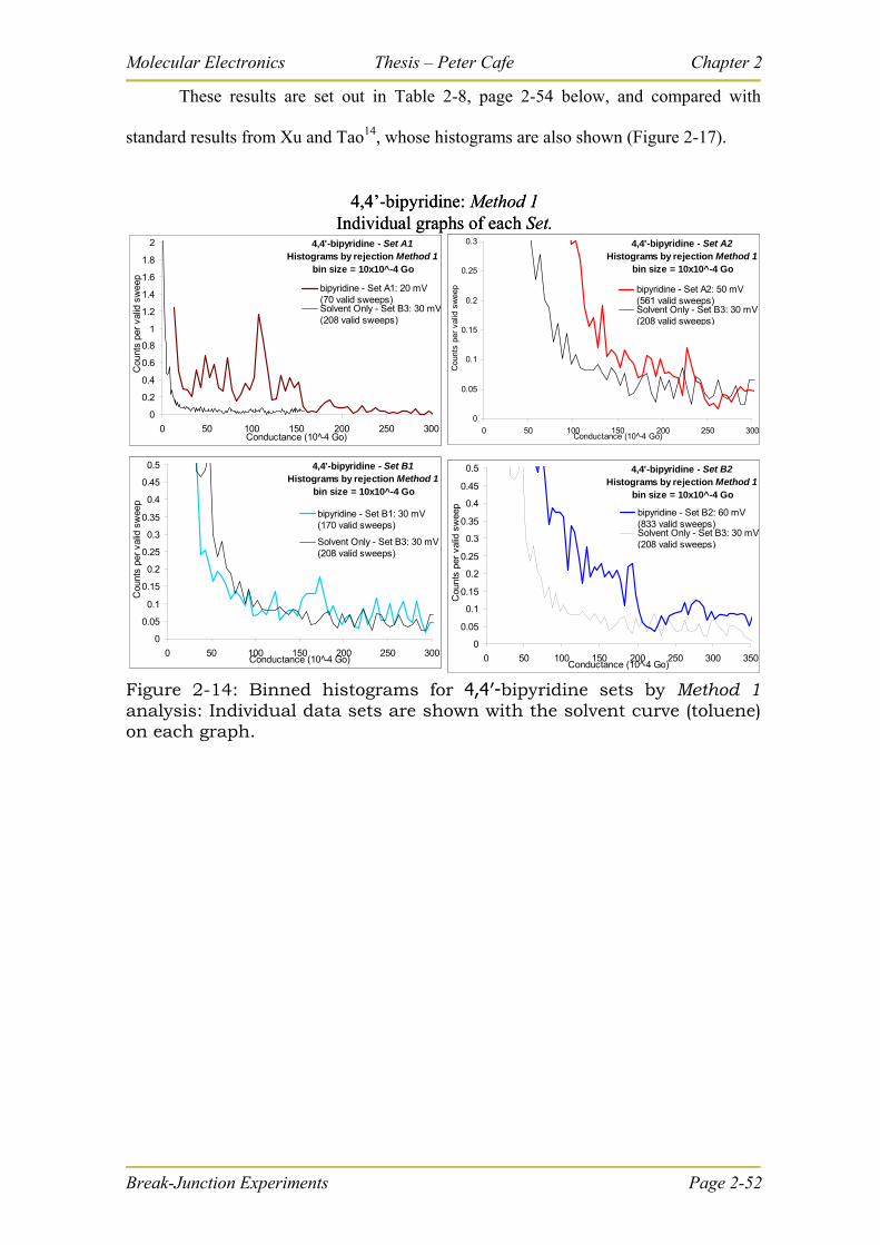
Molecular Electronics Thesis – Peter Cafe Chapter 2
These results are set out in Table 2-8, page 2-54 below, and compared with
standard results from Xu and Tao14, whose histograms are also shown (Figure 2-17).
4,4'-bipyridine - Set A2 Histograms by rejection Method 1
bin size = 10x10^-4 Go
0
0.05
0.1
0.15
0.2
0.25
0.3
0 50 100 150 200 250 300Conductance (10 -4 Go)
Cou
nts
per
valid
sw
eep bipyridine - Set A2: 50 mV
(561 valid sweeps)Solvent Only - Set B3: 30 mV(208 valid sweeps)
4,4'-bipyridine - Set A1 Histograms by rejection Method 1
bin size = 10x10^-4 Go
0
0.2
0.4
0.6
0.8
1
1.2
1.4
1.6
1.8
2
0 50 100 150 200 250 300Conductance (10 -4 Go)
Cou
nts
per
valid
sw
eep
bipyridine - Set A1: 20 mV(70 valid sweeps)Solvent Only - Set B3: 30 mV(208 valid sweeps)
4,4'-bipyridine - Set B1 Histograms by rejection Method 1
bin size = 10x10^-4 Go
0
0.05
0.1
0.15
0.2
0.25
0.3
0.35
0.4
0.45
0.5
0 50 100 150 200 250 300Conductance (10 -4 Go)
Cou
nts
per
valid
sw
eep
bipyridine - Set B1: 30 mV(170 valid sweeps)
Solvent Only - Set B3: 30 mV(208 valid sweeps)
4,4'-bipyridine - Set B2 Histograms by rejection Method 1
bin size = 10x10^-4 Go
0
0.05
0.1
0.15
0.2
0.25
0.3
0.35
0.4
0.45
0.5
0 50 100 150 200 250 300 350Conductance (10 -4 Go)
Cou
nts
per
valid
sw
eep
bipyridine - Set B2: 60 mV(833 valid sweeps)Solvent Only - Set B3: 30 mV(208 valid sweeps)
4,4’-bipyridine: Method 1 Individual graphs of each Set.
Figure 2-14: Binned histograms for 4,4′-bipyridine sets by Method 1 analysis: Individual data sets are shown with the solvent curve (toluene) on each graph.
Break-Junction Experiments Page 2-52
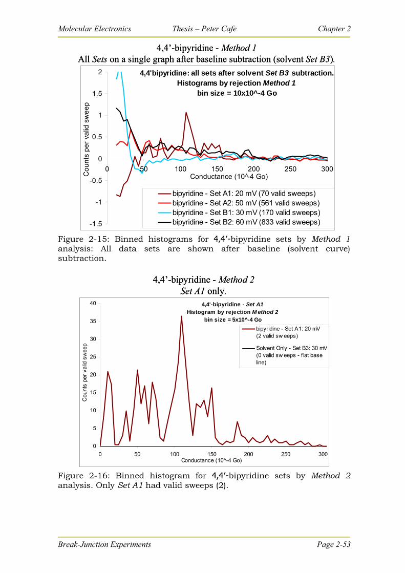
Molecular Electronics Thesis – Peter Cafe Chapter 2
4,4’-bipyridine - Method 1 All Sets on a single graph after baseline subtraction (solvent Set B3).
4,4'bipyridine: all sets after solvent Set B3 subtraction. Histograms by rejection Method 1
bin size = 10x10^-4 Go
-1.5
-1
-0.5
0
0.5
1
1.5
2
0 50 100 150 200 250 300Conductance (10 -4 Go)C
ou
nts
pe
r va
lid s
we
ep
bipyridine - Set A1: 20 mV (70 valid sweeps)bipyridine - Set A2: 50 mV (561 valid sweeps)bipyridine - Set B1: 30 mV (170 valid sweeps)bipyridine - Set B2: 60 mV (833 valid sweeps)
Figure 2-15: Binned histograms for 4,4′-bipyridine sets by Method 1 analysis: All data sets are shown after baseline (solvent curve) subtraction.
4,4'-bipyridine - Set A1 Histogram by rejection M ethod 2
bin size = 5x10^-4 Go
0
5
10
15
20
25
30
35
40
0 50 100 150 200 250 300Conductance (10^-4 Go)
Cou
nts
per
valid
sw
eep
bipyridine - Set A1: 20 mV (2 valid sw eeps)
Solvent Only - Set B3: 30 mV(0 valid sw eeps - f lat baseline)
4,4’-bipyridine - Method 2 Set A1 only.
Figure 2-16: Binned histogram for 4,4′-bipyridine sets by Method 2 analysis. Only Set A1 had valid sweeps (2).
Break-Junction Experiments Page 2-53
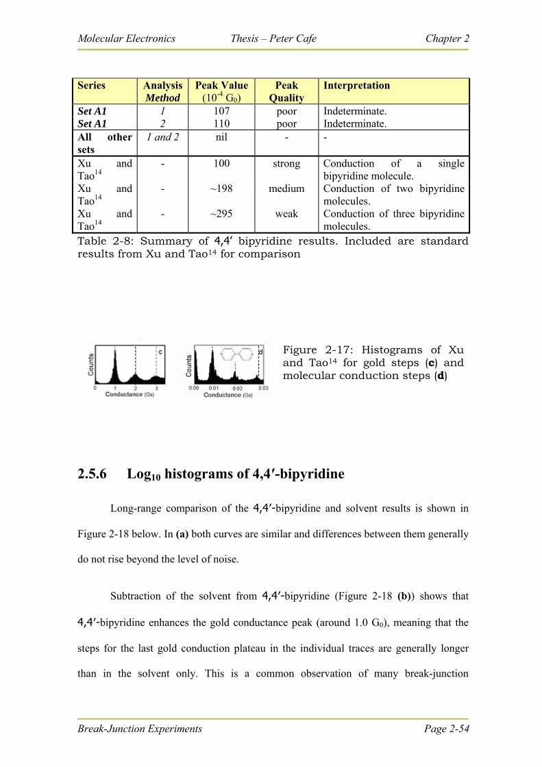
Molecular Electronics Thesis – Peter Cafe Chapter 2
Series Analysis Method
Peak Value (10-4 G0)
Peak Quality
Interpretation
Set A1 1 107 poor Indeterminate. Set A1 2 110 poor Indeterminate. All other sets
1 and 2 nil - -
Xu and Tao14
- 100 strong Conduction of a single bipyridine molecule.
Xu and Tao14
- ~198 medium Conduction of two bipyridine molecules.
Xu and Tao14
- ~295 weak Conduction of three bipyridine molecules.
Table 2-8: Summary of 4,4’ bipyridine results. Included are standard results from Xu and Tao14 for comparison
Figure 2-17: Histograms of Xu and Tao14 for gold steps (c) and molecular conduction steps (d)
2.5.6 Log10 histograms of 4,4′-bipyridine
Long-range comparison of the 4,4′-bipyridine and solvent results is shown in
Figure 2-18 below. In (a) both curves are similar and differences between them generally
do not rise beyond the level of noise.
Subtraction of the solvent from 4,4′-bipyridine (Figure 2-18 (b)) shows that
4,4′-bipyridine enhances the gold conductance peak (around 1.0 G0), meaning that the
steps for the last gold conduction plateau in the individual traces are generally longer
than in the solvent only. This is a common observation of many break-junction
Break-Junction Experiments Page 2-54
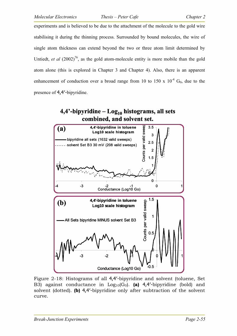
Molecular Electronics Thesis – Peter Cafe Chapter 2
experiments and is believed to be due to the attachment of the molecule to the gold wire
stabilising it during the thinning process. Surrounded by bound molecules, the wire of
single atom thickness can extend beyond the two or three atom limit determined by
Untiedt, et al (2002)76, as the gold atom-molecule entity is more mobile than the gold
atom alone (this is explored in Chapter 3 and Chapter 4). Also, there is an apparent
enhancement of conduction over a broad range from 10 to 150 x 10-4 G0, due to the
presence of 4,4′-bipyridine.
4,4'-bipyridine in tolueneLog10 scale histogram
0
0.5
1
1.5
2
2.5
3
3.5
-4 -3 -2 -1 0 1Conductance (Log10 Go)
Cou
nts
per
valid
sw
eep
bipyridine all sets (1632 valid sweeps)
solvent Set B3 30 mV (208 valid sweeps)
4,4'-bipyridine in tolueneLog10 scale histogram
-0.5
0
0.5
1
1.5
-4 -3 -2 -1 0 1
Conductance (Log10 Go)
Cou
nts
per
valid
sw
eep
All Sets bipyridine MINUS solvent Set B3
4,4’-bipyridine – Log10 histograms, all sets combined, and solvent set.
(a)
(b)
4,4'-bipyridine in tolueneLog10 scale histogram
0
0.5
1
1.5
2
2.5
3
3.5
-4 -3 -2 -1 0 1Conductance (Log10 Go)
Cou
nts
per
valid
sw
eep
bipyridine all sets (1632 valid sweeps)
solvent Set B3 30 mV (208 valid sweeps)
4,4'-bipyridine in tolueneLog10 scale histogram
-0.5
0
0.5
1
1.5
-4 -3 -2 -1 0 1
Conductance (Log10 Go)
Cou
nts
per
valid
sw
eep
All Sets bipyridine MINUS solvent Set B3
4,4’-bipyridine – Log10 histograms, all sets combined, and solvent set.
(a)
(b)
Figure 2-18: Histograms of all 4,4′-bipyridine and solvent (toluene, Set B3) against conductance in Log10(G0). (a) 4,4′-bipyridine (bold) and solvent (dotted). (b) 4,4′-bipyridine only after subtraction of the solvent curve.
Break-Junction Experiments Page 2-55
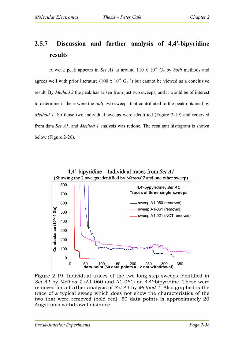
Molecular Electronics Thesis – Peter Cafe Chapter 2
Break-Junction Experiments Page 2-56
2.5.7 Discussion and further analysis of 4,4′-bipyridine
results
A weak peak appears in Set A1 at around 110 x 10-4 G0 by both methods and
agrees well with prior literature (100 x 10-4 G014) but cannot be viewed as a conclusive
result. By Method 2 the peak has arisen from just two sweeps, and it would be of interest
to determine if these were the only two sweeps that contributed to the peak obtained by
Method 1. So those two individual sweeps were identified (Figure 2-19) and removed
from data Set A1, and Method 1 analysis was redone. The resultant histogram is shown
below (Figure 2-20).
4,4’-bipyridine – Individual traces from Set A1 (Showing the 2 sweeps identified by Method 2 and one other sweep)
4,4'-bypyridine, Set A1Traces of three single sweeps
0
100
200
300
400
500
600
700
800
0 50 100 150 200 250 300 350data point (50 data points = ~2 nm withdrawal)
Co
nd
uct
ance
(10
^-4
Go
)
sweep A1-060 (removed)
sweep A1-061 (removed)
sweep-A1-021 (NOT removed)
Figure 2-19: Individual traces of the two long-step sweeps identified in Set A1 by Method 2 (A1-060 and A1-061) on 4,4′-bipyridine. These were removed for a further analysis of Set A1 by Method 1. Also graphed is the trace of a typical sweep which does not show the characteristics of the two that were removed (bold red). 50 data points is approximately 20 Angstroms withdrawal distance.
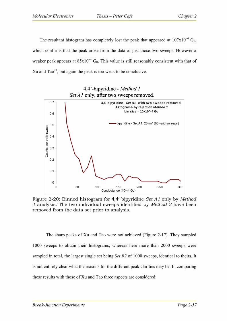
Molecular Electronics Thesis – Peter Cafe Chapter 2
The resultant histogram has completely lost the peak that appeared at 107x10–4 G0,
which confirms that the peak arose from the data of just those two sweeps. However a
weaker peak appears at 85x10–4 G0. This value is still reasonably consistent with that of
Xu and Tao14, but again the peak is too weak to be conclusive.
4,4'-bipyridine - Set A1 w ith two sweeps removed.Histograms by rejection M ethod 1
bin size = 10x10^-4 Go
0
0.1
0.2
0.3
0.4
0.5
0.6
0.7
0 50 100 150 200 250 300Conductance (10^-4 Go)
Cou
nts
per
valid
sw
eep
bipyridine - Set A1: 20 mV (68 valid sw eeps)
4,4’-bipyridine - Method 1 Set A1 only, after two sweeps removed.
Figure 2-20: Binned histogram for 4,4′-bipyridine Set A1 only by Method 1 analysis. The two individual sweeps identified by Method 2 have been removed from the data set prior to analysis.
The sharp peaks of Xu and Tao were not achieved (Figure 2-17). They sampled
1000 sweeps to obtain their histograms, whereas here more than 2000 sweeps were
sampled in total, the largest single set being Set B2 of 1000 sweeps, identical to theirs. It
is not entirely clear what the reasons for the different peak clarities may be. In comparing
these results with those of Xu and Tao three aspects are considered:
Break-Junction Experiments Page 2-57
Molecular Electronics Thesis – Peter Cafe Chapter 2
Break-Junction Experiments Page 2-58
a) Selection Criteria: Xu and Tao give no indication what criteria they used to
select (or reject) individual sweeps. Subsequent papers by the same research group
indicate that as many as 85% of sweeps may be rejected because they did not show clear
molecular conduction steps (see Section 2.3.2, Page 2-40, above, for a more complete
discussion of data selection techniques), and it may be reasonable to assume that they
were selective in the representation of their data for this paper also. Knowledge of and
application of the same technique may have enhanced the results of this thesis. Their
equipment was more sophisticated in that they had more direct control over the motion
of the tip in relation to current triggers, and this would have produced more consistent
data and enabled a better “fine-tuning” of the experiment in process to produce more
traces with molecular conduction steps.
b) Molecule concentration and solvent: Xu and Tao used a concentration of 1
mM bipyridine in 0.1 M NaClO4 aqueous solution, whereas in this research it was ~10
mM in toluene. It may be possible that the lower concentration is more amenable to a
single molecule binding to the gold terminals of the break-junction. According to one
report, the choice of solvent probably makes little difference,101 however this is
contradicted in the findings for pyrazine (Section 2-7 below). In the electrolyte it is
possible to introduce electrochemical control (next point).
c) Electrochemical Control: Xu and Tao used a wax-coated gold tip in an
electrolyte and charged the solution at a positive potential in relation to both gold tip and
the gold substrate (at a positive bias the conduction steps would appear but at a negative
bias the conduction steps would not appear). Such experiments require wax-insulated
tips and an electrochemical cell and specialist techniques not available to this current
research. Their average step width was 0.9 nm for the single molecule conduction step,
whereas here (in toluene with no electrochemical control) one of the longest steps is only
Molecular Electronics Thesis – Peter Cafe Chapter 2
0.6 nm (represented in Figure 2-19 above). As the binding strength of 4,4′-bipyridine to
a gold electrode depends on the electrode potential46, it is expected that should such
technology become available it would greatly increase the quality of results with 4,4′-
bipyridine and all amine or azine linker molecules.
2.5.8 Conclusion of 4,4′-bipyridine results
The conductance of a single 4,4′-bipyridine molecule (in toluene) has not been
established. The weak peak between 85 and 110 x 10-4 G0 agrees with prior research
done in aqueous solution, but cannot be distinguished from noise conclusively. It is also
reasonably close to theoretical values of 30 x 10-4 G079 and 586 x 10-4 G0
78.
An unambiguous result is that 4,4′-bipyridine produces higher gold quantized
conduction peaks and thus longer gold conduction plateaus, suggesting that it stabilises
the single-atom gold chain during the breaking of the junction and allows it to extend
beyond the 2 or 3 atom limit determined by Untiedt76, or at least allows it to stay at that
length longer by providing highly mobile 4,4′-bipyridine-gold atom units which can
rush to the narrowest parts of the wire to thicken it.
There is a broad enhancement of conduction (compared to toluene alone) over the
range from 10 to 150 x 10-4 G0.
Better results would possibly be obtained under electrochemical control with the
solution charged at a positive bias in relation to both gold electrodes. Better software
control during the experiment (i.e. appropriate triggers) would eliminate a number of
unhelpful sweeps prior to data collection and allow greater consistency in results. Further
technical resources are required to improve upon these results.
Break-Junction Experiments Page 2-59
Molecular Electronics Thesis – Peter Cafe Chapter 2
Break-Junction Experiments Page 2-60
2-6 Investigations of TATPP
Dipyrido[3′,2′:5,6;2′′,3′′:7,8]quinoxalino[2,3-i]dipyrido[3,2-a:2′,3′-c]phenazine
Abbreviation: TATPP
Note: This molecule is called TATPP because it appears often in literature under
the following name:
9,11,20,22-tetraazatetrapyrido[3,2-a:2′3′-c:3′′,2′′-l:2′′′,3′′′]pentacene.
2.6.1 Rationalization:
This molecule was synthesised for this experiment. It was considered to be likely
to have good conduction because of its conjugation, to show consistent conduction
plateaus because of its rigidity, and to bind well to gold because of the bidentate nature
of the two phenanthroline-type ends. Determination of its conductance value was
considered an important step in the process of creating molecular wires from fused
porphyrins with phenanthroline-type “alligator clips” (See the rationalisation for bis-
phenanthroline-appended-porphyrin in Section 2.8.1 below).
2.6.2 Background research
2.6.2.1 Similar molecules
Long, multiply-conjugated molecules have recently be subjected to break-
junction experiments by Li, et al, (2007)72 to determine their conductance values. These
molecules and their different conduction results are reproduced in Table 2-9, below,
along with TATPP. Although there are substantial differences to TATPP, an electron
traversing each molecule would travel similar pathways (in terms of bonds and
Molecular Electronics Thesis – Peter Cafe Chapter 2
Break-Junction Experiments Page 2-61
conjugations traversed, as well as length), however there would be less conduction
pathways available to an electron in TATPP.
Li attributes the differences in conduction of these molecules to different
electronic couplings between the molecule and the electrodes, mainly caused by the
different anchoring groups (i.e. the length of the anchoring group and whether it is
conjugated or not; greater length = lesser conductance; more conjugations = more
conductance).
Graphite is a conductor because of its multiple conjugations and multiple
pathways.
In terms of Li’s explanation, TATPP would have a better coupling to the gold
electrode than the best conductor in his series. The number of conjugations and pathways
is similar. However the four incorporated central nitrogen atoms may have a slightly
decreasing effect on conductance.
The example of these molecules suggests that TATPP might have a similar
conductance, say between 0.1 and 1.0 x10⁻⁴G0. (The side double bonded oxygen groups
in Li’s molecules may have a significant effect on conductance however it is
unquantifiable and has to be ignored.)
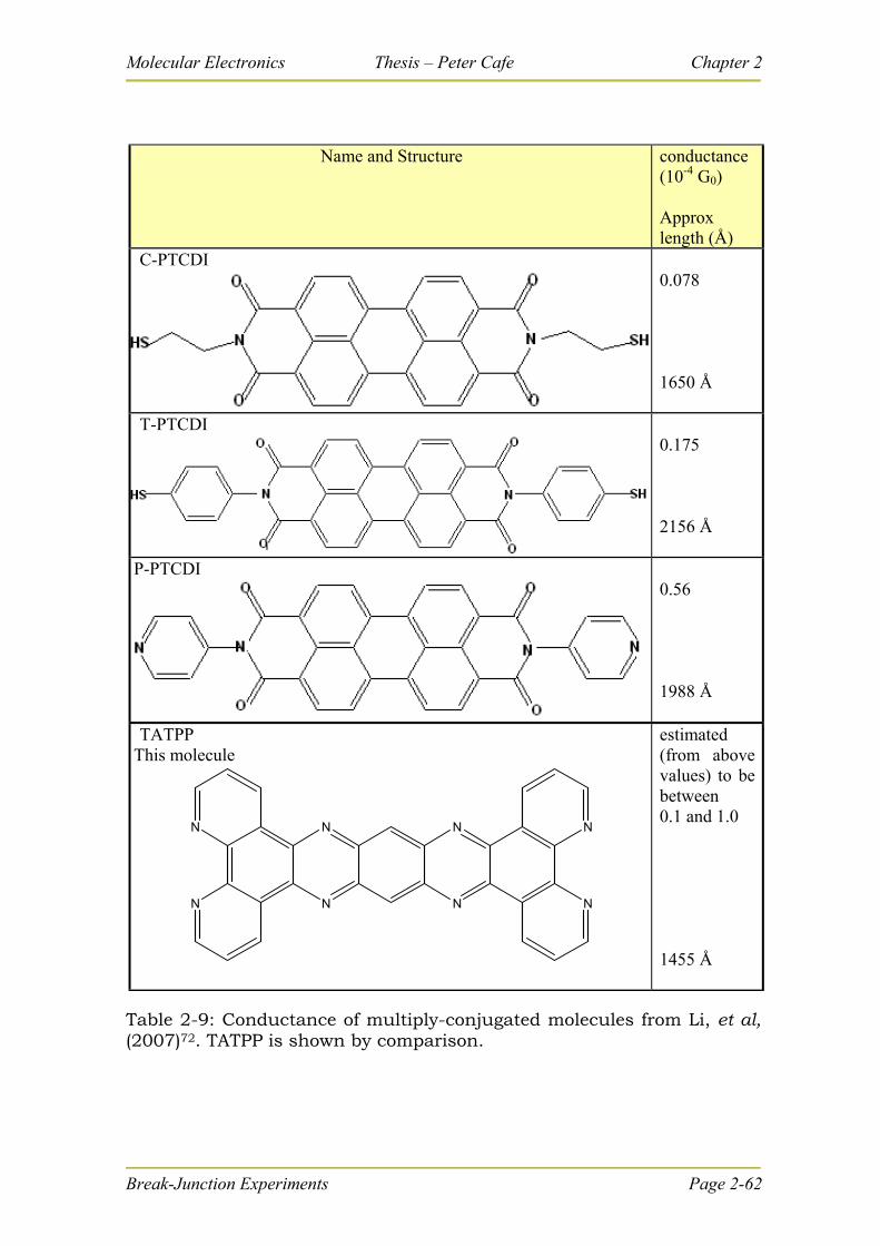
Molecular Electronics Thesis – Peter Cafe Chapter 2
Name and Structure conductance (10-4 G0) Approx length (Å)
C-PTCDI 0.078 1650 Å
T-PTCDI
0.175 2156 Å
P-PTCDI
0.56 1988 Å
TATPP This molecule
N
N N
N
N
N
N
N
estimated (from above values) to be between 0.1 and 1.0
1455 Å
Table 2-9: Conductance of multiply-conjugated molecules from Li, et al, (2007)72. TATPP is shown by comparison.
Break-Junction Experiments Page 2-62
Molecular Electronics Thesis – Peter Cafe Chapter 2
Break-Junction Experiments Page 2-63
2.6.2.2 Theoretical value of conductance for TATPP
An unpublished theoretical value of conductance for TATPP is 0.01 x 10⁻⁴ Go,
provided by Mr Sören Wolthat in a personal communication (based upon the model
shown in Figure 2-27).
2.6.3 Experimental set-up:
TATPP was dissolved in the solvent using a sonicator, then allowed to stand for
more than one hour, and experimental samples were drawn from the middle of the
solution so as to avoid both sedimentary and floating particles which may have been
present.
For Group A the final experimental concentration was less than 1 mM in toluene;
for Group F it was ~5 mM in toluene, and for Group G it was ~5 mM in phenyloctane.
2.6.4 The sets of sweeps for TATPP
Group A: Linear Amplifier: Three sets of sweeps were recorded with the linear
amplifier, one solvent-only set labelled Set A0 (toluene) and two TATPP sets labelled Set
A2 and Set B1. All used a bias of 50 mV.
Group F: Logarithmic Amplifier and toluene: Four sets of sweeps were
recorded using the log amplifier and toluene as the solvent, two on the solvent only,
labelled Set F1 and Set F2, and two on TATPP labelled Set F3 and Set F4 (each at 40
mV and 80 mV).
Group G: Logarithmic Amplifier and phenyloctane: Four other sets also used
the log amplifier but were done in a different solvent, phenyloctane. One set was the
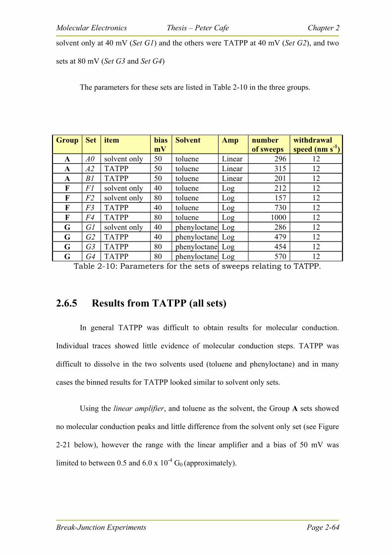
Molecular Electronics Thesis – Peter Cafe Chapter 2
Break-Junction Experiments Page 2-64
solvent only at 40 mV (Set G1) and the others were TATPP at 40 mV (Set G2), and two
sets at 80 mV (Set G3 and Set G4)
The parameters for these sets are listed in Table 2-10 in the three groups.
Group Set item biasmV
Solvent Amp number of sweeps
withdrawal speed (nm s-1)
A A0 solvent only 50 toluene Linear 296 12 A A2 TATPP 50 toluene Linear 315 12 A B1 TATPP 50 toluene Linear 201 12 F F1 solvent only 40 toluene Log 212 12 F F2 solvent only 80 toluene Log 157 12 F F3 TATPP 40 toluene Log 730 12 F F4 TATPP 80 toluene Log 1000 12 G G1 solvent only 40 phenyloctane Log 286 12 G G2 TATPP 40 phenyloctane Log 479 12 G G3 TATPP 80 phenyloctane Log 454 12 G G4 TATPP 80 phenyloctane Log 570 12
Table 2-10: Parameters for the sets of sweeps relating to TATPP.
2.6.5 Results from TATPP (all sets)
In general TATPP was difficult to obtain results for molecular conduction.
Individual traces showed little evidence of molecular conduction steps. TATPP was
difficult to dissolve in the two solvents used (toluene and phenyloctane) and in many
cases the binned results for TATPP looked similar to solvent only sets.
Using the linear amplifier, and toluene as the solvent, the Group A sets showed
no molecular conduction peaks and little difference from the solvent only set (see Figure
2-21 below), however the range with the linear amplifier and a bias of 50 mV was
limited to between 0.5 and 6.0 x 10⁻⁴ G0 (approximately).
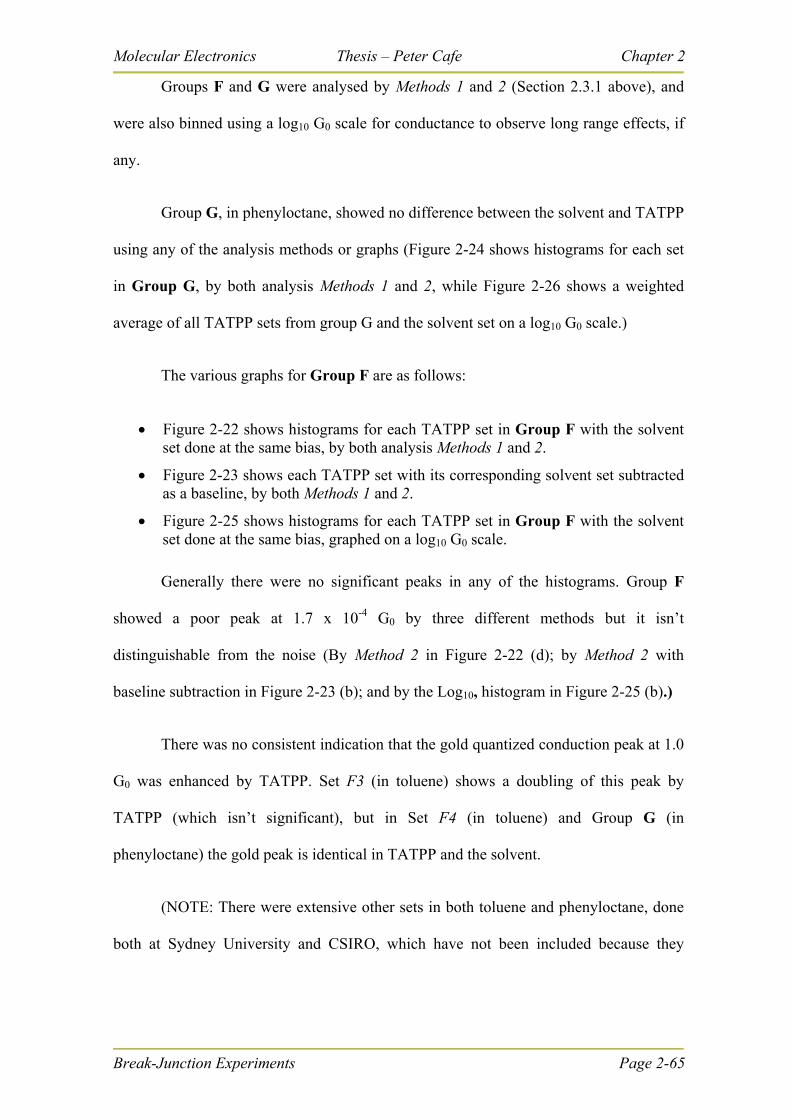
Molecular Electronics Thesis – Peter Cafe Chapter 2
Break-Junction Experiments Page 2-65
Groups F and G were analysed by Methods 1 and 2 (Section 2.3.1 above), and
were also binned using a log10 G0 scale for conductance to observe long range effects, if
any.
Group G, in phenyloctane, showed no difference between the solvent and TATPP
using any of the analysis methods or graphs (Figure 2-24 shows histograms for each set
in Group G, by both analysis Methods 1 and 2, while Figure 2-26 shows a weighted
average of all TATPP sets from group G and the solvent set on a log10 G0 scale.)
The various graphs for Group F are as follows:
Figure 2-22 shows histograms for each TATPP set in Group F with the solvent set done at the same bias, by both analysis Methods 1 and 2.
Figure 2-23 shows each TATPP set with its corresponding solvent set subtracted as a baseline, by both Methods 1 and 2.
Figure 2-25 shows histograms for each TATPP set in Group F with the solvent set done at the same bias, graphed on a log10 G0 scale.
Generally there were no significant peaks in any of the histograms. Group F
showed a poor peak at 1.7 x 10⁻⁴ G0 by three different methods but it isn’t
distinguishable from the noise (By Method 2 in Figure 2-22 (d); by Method 2 with
baseline subtraction in Figure 2-23 (b); and by the Log10, histogram in Figure 2-25 (b).)
There was no consistent indication that the gold quantized conduction peak at 1.0
G0 was enhanced by TATPP. Set F3 (in toluene) shows a doubling of this peak by
TATPP (which isn’t significant), but in Set F4 (in toluene) and Group G (in
phenyloctane) the gold peak is identical in TATPP and the solvent.
(NOTE: There were extensive other sets in both toluene and phenyloctane, done
both at Sydney University and CSIRO, which have not been included because they
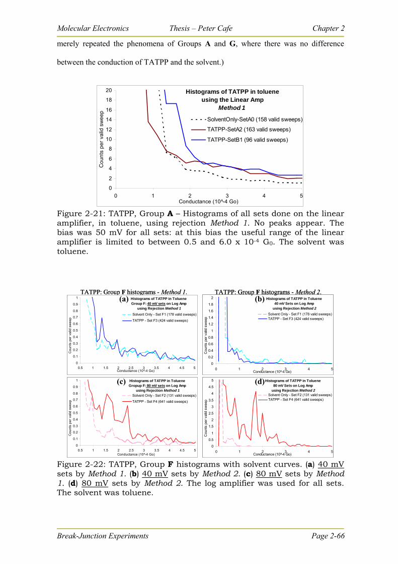
Molecular Electronics Thesis – Peter Cafe Chapter 2
merely repeated the phenomena of Groups A and G, where there was no difference
between the conduction of TATPP and the solvent.)
Histograms of TATPP in toluene using the Linear Amp
Method 1
0
2
4
6
8
10
12
14
16
18
20
0 1 2 3 4 5Conductance (10 -4 Go)
Co
un
ts p
er
valid
sw
ee
p
SolventOnly-SetA0 (158 valid sweeps)
TATPP-SetA2 (163 valid sweeps)
TATPP-SetB1 (96 valid sweeps)
Figure 2-21: TATPP, Group A – Histograms of all sets done on the linear amplifier, in toluene, using rejection Method 1. No peaks appear. The bias was 50 mV for all sets: at this bias the useful range of the linear amplifier is limited to between 0.5 and 6.0 x 10⁻⁴ G0. The solvent was toluene.
Histograms of TATPP in Toluene40 mV Sets on Log Amp
using Rejection Method 2
0
0.2
0.4
0.6
0.8
1
1.2
1.4
1.6
1.8
2
0 1 2 3 4Conductance (10 -4 Go)
Cou
nts
per
valid
sw
eep
5
Solvent Only - Set F1 (178 valid sweeps)TATPP - Set F3 (424 valid sweeps)
Histograms of TATPP in Toluene80 mV Sets on Log Amp
using Rejection Method 2
0
0.5
1
1.5
2
2.5
3
3.5
4
4.5
5
0 1 2 3 4 5Conductance (10 -4 Go)
Cou
nts
per
valid
sw
eep
Solvent Only - Set F2 (131 valid sweeps)TATPP - Set F4 (641 valid sweeps)
TATPP: Group F histograms - Method 2.
Histograms of TATPP in TolueneGropup F: 80 mV sets on Log Amp
using Rejection Method 1
0
0.1
0.2
0.3
0.4
0.5
0.6
0.7
0.8
0.9
1
0.5 1 1.5 2 2.5 3 3.5 4 4.5 5Conductance (10 -4 Go)
Co
un
ts p
er
valid
sw
ee
p
Solvent Only - Set F2 (131 valid sweeps)
TATPP - Set F4 (641 valid sweeps)
TATPP: Group F histograms - Method 1.Histograms of TATPP in TolueneGroup F: 40 mV sets on Log Amp
using Rejection Method 1
0
0.1
0.2
0.3
0.4
0.5
0.6
0.7
0.8
0.9
1
0.5 1 1.5 2 2.5 3 3.5 4 4.5 5Conductance (10 -4 Go)
Co
un
ts p
er
valid
sw
ee
p
Solvent Only - Set F1 (178 valid sweeps)
TATPP - Set F3 (424 valid sweeps)
(a)
(c) (d)
(b) Histograms of TATPP in Toluene40 mV Sets on Log Amp
using Rejection Method 2
0
0.2
0.4
0.6
0.8
1
1.2
1.4
1.6
1.8
2
0 1 2 3 4Conductance (10 -4 Go)
Cou
nts
per
valid
sw
eep
5
Solvent Only - Set F1 (178 valid sweeps)TATPP - Set F3 (424 valid sweeps)
Histograms of TATPP in Toluene80 mV Sets on Log Amp
using Rejection Method 2
0
0.5
1
1.5
2
2.5
3
3.5
4
4.5
5
0 1 2 3 4 5Conductance (10 -4 Go)
Cou
nts
per
valid
sw
eep
Solvent Only - Set F2 (131 valid sweeps)TATPP - Set F4 (641 valid sweeps)
TATPP: Group F histograms - Method 2.
Histograms of TATPP in TolueneGropup F: 80 mV sets on Log Amp
using Rejection Method 1
0
0.1
0.2
0.3
0.4
0.5
0.6
0.7
0.8
0.9
1
0.5 1 1.5 2 2.5 3 3.5 4 4.5 5Conductance (10 -4 Go)
Co
un
ts p
er
valid
sw
ee
p
Solvent Only - Set F2 (131 valid sweeps)
TATPP - Set F4 (641 valid sweeps)
TATPP: Group F histograms - Method 1.Histograms of TATPP in TolueneGroup F: 40 mV sets on Log Amp
using Rejection Method 1
0
0.1
0.2
0.3
0.4
0.5
0.6
0.7
0.8
0.9
1
0.5 1 1.5 2 2.5 3 3.5 4 4.5 5Conductance (10 -4 Go)
Co
un
ts p
er
valid
sw
ee
p
Solvent Only - Set F1 (178 valid sweeps)
TATPP - Set F3 (424 valid sweeps)
(a)
(c) (d)
(b)
Figure 2-22: TATPP, Group F histograms with solvent curves. (a) 40 mV sets by Method 1. (b) 40 mV sets by Method 2. (c) 80 mV sets by Method 1. (d) 80 mV sets by Method 2. The log amplifier was used for all sets. The solvent was toluene.
Break-Junction Experiments Page 2-66
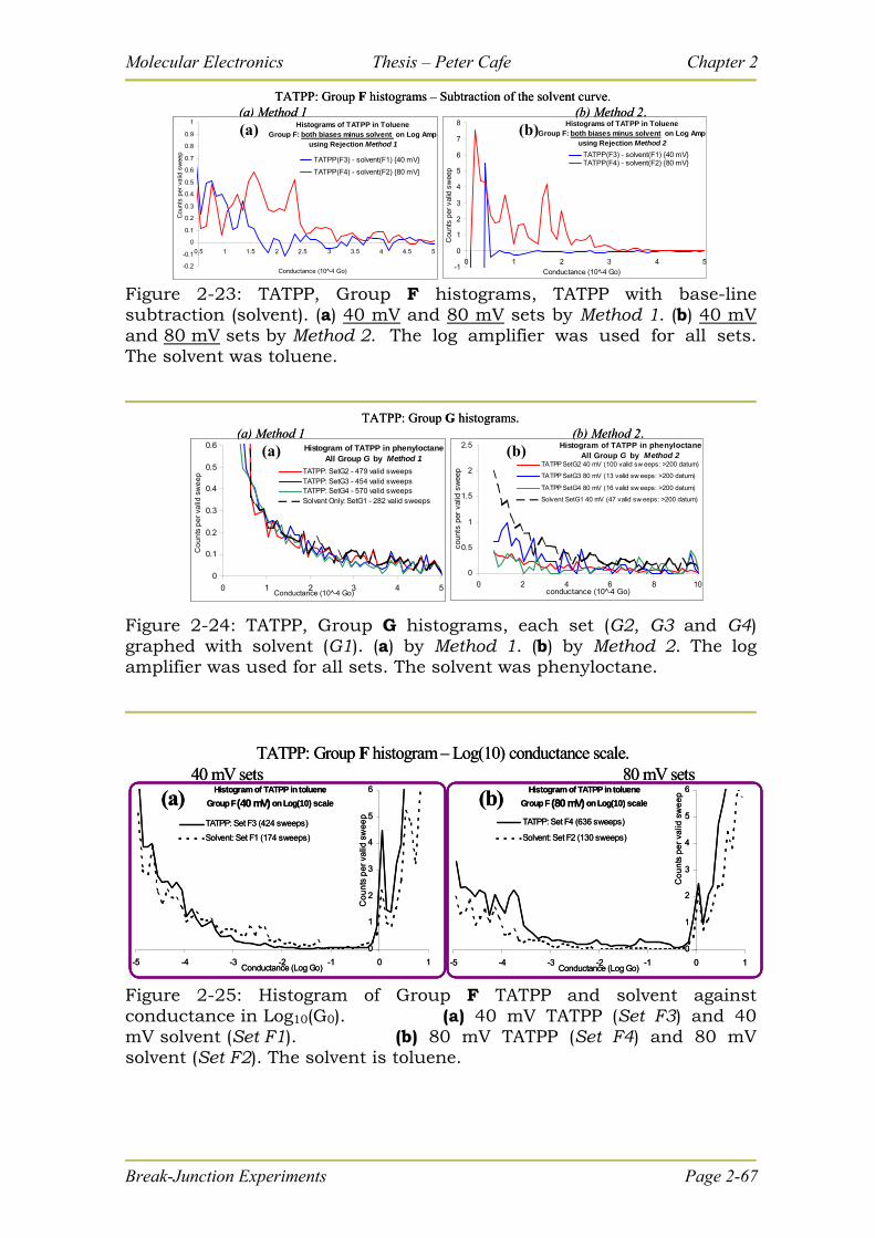
Molecular Electronics Thesis – Peter Cafe Chapter 2
Break-Junction Experiments Page 2-67
Histograms of TATPP in TolueneGroup F: both biases minus solvent on Log Amp
using Rejection Method 2
-1
0
1
2
3
4
5
6
7
8
0 1 2 3 4 5
Conductance (10 -4 Go)
Cou
nts
per
valid
sw
eep
TATPP(F3) - solvent(F1) 40 mVTATPP(F4) - solvent(F2) 80 mV
TATPP: Group F histograms – Subtraction of the solvent curve. (a) Method 1 (b) Method 2.
Histograms of TATPP in TolueneGroup F: both biases minus solvent on Log Amp
using Rejection Method 1
-0.2
-0.1
0
0.1
0.2
0.3
0.4
0.5
0.6
0.7
0.8
0.9
1
0.5 1 1.5 2 2.5 3 3.5 4 4.5 5
Conductance (10 -4 Go)
Cou
nts
per
valid
sw
eep
TATPP(F3) - solvent(F1) 40 mV
TATPP(F4) - solvent(F2) 80 mV
(a) (b) Histograms of TATPP in TolueneGroup F: both biases minus solvent on Log Amp
using Rejection Method 2
-1
0
1
2
3
4
5
6
7
8
0 1 2 3 4 5
Conductance (10 -4 Go)
Cou
nts
per
valid
sw
eep
TATPP(F3) - solvent(F1) 40 mVTATPP(F4) - solvent(F2) 80 mV
TATPP: Group F histograms – Subtraction of the solvent curve. (a) Method 1 (b) Method 2.
Histograms of TATPP in TolueneGroup F: both biases minus solvent on Log Amp
using Rejection Method 1
-0.2
-0.1
0
0.1
0.2
0.3
0.4
0.5
0.6
0.7
0.8
0.9
1
0.5 1 1.5 2 2.5 3 3.5 4 4.5 5
Conductance (10 -4 Go)
Cou
nts
per
valid
sw
eep
TATPP(F3) - solvent(F1) 40 mV
TATPP(F4) - solvent(F2) 80 mV
(a) (b)
Figure 2-23: TATPP, Group F histograms, TATPP with base-line subtraction (solvent). (a) 40 mV and 80 mV sets by Method 1. (b) 40 mV and 80 mV sets by Method 2. The log amplifier was used for all sets. The solvent was toluene.
Histogram of TATPP in phenyloctaneAll Group G by Method 2
0
0.5
1
1.5
2
2.5
0 2 4 6 8conductance (10 -4 Go)
coun
ts p
er v
alid
sw
eep
10
TATPP SetG2 40 mV (100 valid sw eeps: >200 datum)
TATPP SetG3 80 mV (13 valid sw eeps: >200 datum)
TATPP SetG4 80 mV (16 valid sw eeps: >200 datum)
Solvent SetG1 40 mV (47 valid sw eeps: >200 datum)
Histogram of TATPP in phenyloctaneAll Group G by Method 1
0
0.1
0.2
0.3
0.4
0.5
0.6
0 1 2 3 4 5Conductance (10 -4 Go)
Co
un
ts p
er
valid
sw
ee
p TATPP: SetG2 - 479 valid sweepsTATPP: SetG3 - 454 valid sweepsTATPP: SetG4 - 570 valid sweepsSolvent Only: SetG1 - 282 valid sweeps
TATPP: Group G histograms. (a) Method 1 (b) Method 2.
(a) (b) Histogram of TATPP in phenyloctaneAll Group G by Method 2
0
0.5
1
1.5
2
2.5
0 2 4 6 8conductance (10 -4 Go)
coun
ts p
er v
alid
sw
eep
10
TATPP SetG2 40 mV (100 valid sw eeps: >200 datum)
TATPP SetG3 80 mV (13 valid sw eeps: >200 datum)
TATPP SetG4 80 mV (16 valid sw eeps: >200 datum)
Solvent SetG1 40 mV (47 valid sw eeps: >200 datum)
Histogram of TATPP in phenyloctaneAll Group G by Method 1
0
0.1
0.2
0.3
0.4
0.5
0.6
0 1 2 3 4 5Conductance (10 -4 Go)
Co
un
ts p
er
valid
sw
ee
p TATPP: SetG2 - 479 valid sweepsTATPP: SetG3 - 454 valid sweepsTATPP: SetG4 - 570 valid sweepsSolvent Only: SetG1 - 282 valid sweeps
TATPP: Group G histograms. (a) Method 1 (b) Method 2.
(a) (b)
Figure 2-24: TATPP, Group G histograms, each set (G2, G3 and G4) graphed with solvent (G1). (a) by Method 1. (b) by Method 2. The log amplifier was used for all sets. The solvent was phenyloctane.
Histogram of TATPP in toluene
Group F (40 mV) on Log(10) scale
0
1
2
3
4
5
6
-5 -4 -3 -2 -1 0 1Conductance (Log Go)
Co
un
ts p
er
valid
sw
ee
p
TATPP: Set F3 (424 sweeps)
Solvent: Set F1 (174 sweeps)
Histogram of TATPP in toluene
Group F (80 mV) on Log(10) scale
0
1
2
3
4
5
6
-5 -4 -3 -2 -1 0 1Conductance (Log Go)
Co
un
ts p
er
valid
sw
ee
p
TATPP: Set F4 (636 sweeps)
Solvent: Set F2 (130 sweeps)
TATPP: Group F histogram – Log(10) conductance scale. 40 mV sets 80 mV sets
(a) (b)Histogram of TATPP in toluene
Group F (40 mV) on Log(10) scale
0
1
2
3
4
5
6
-5 -4 -3 -2 -1 0 1Conductance (Log Go)
Co
un
ts p
er
valid
sw
ee
p
TATPP: Set F3 (424 sweeps)
Solvent: Set F1 (174 sweeps)
Histogram of TATPP in toluene
Group F (80 mV) on Log(10) scale
0
1
2
3
4
5
6
-5 -4 -3 -2 -1 0 1Conductance (Log Go)
Co
un
ts p
er
valid
sw
ee
p
TATPP: Set F4 (636 sweeps)
Solvent: Set F2 (130 sweeps)
TATPP: Group F histogram – Log(10) conductance scale. 40 mV sets 80 mV sets
(a) (b)
Figure 2-25: Histogram of Group F TATPP and solvent against conductance in Log10(G0). (a) 40 mV TATPP (Set F3) and 40 mV solvent (Set F1). (b) 80 mV TATPP (Set F4) and 80 mV solvent (Set F2). The solvent is toluene.
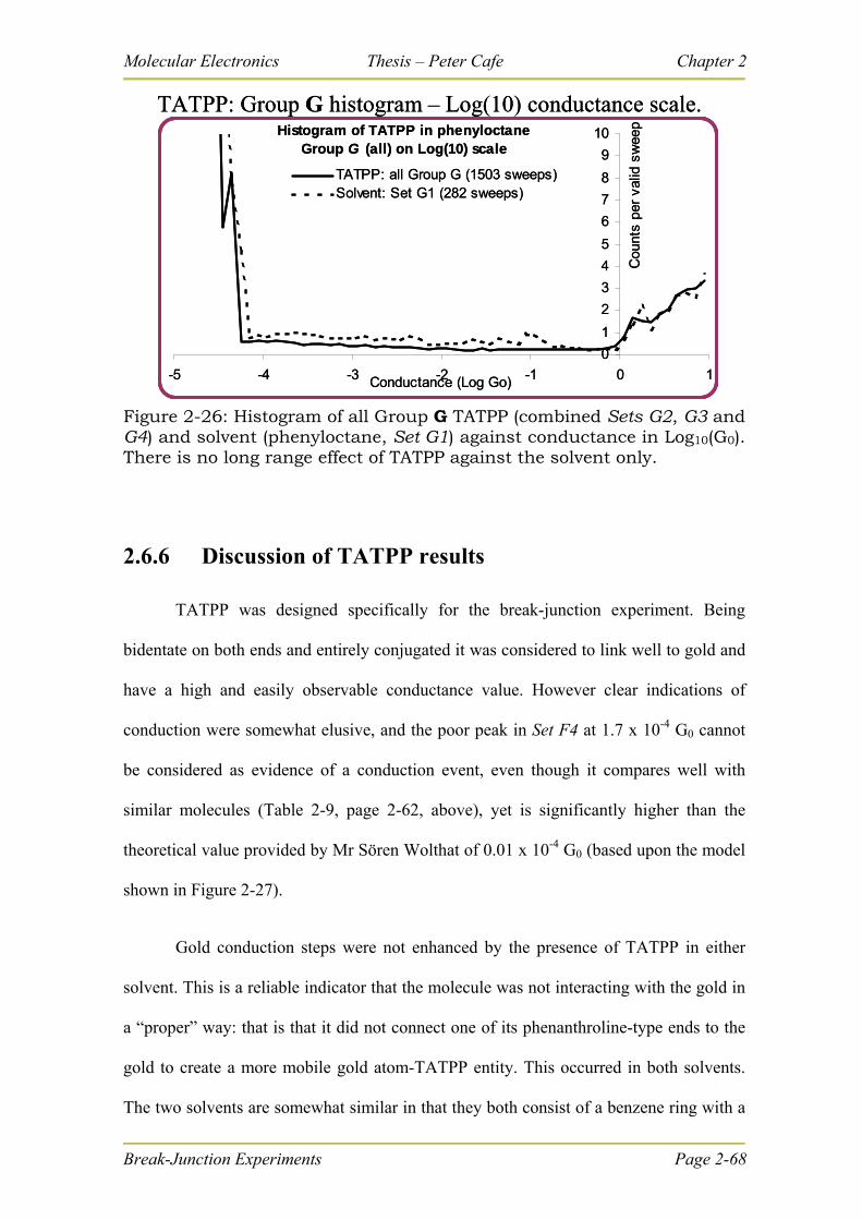
Molecular Electronics Thesis – Peter Cafe Chapter 2
Histogram of TATPP in phenyloctaneGroup G (all) on Log(10) scale
0
1
2
3
4
5
6
7
8
9
10
-5 -4 -3 -2 -1 0 1Conductance (Log Go)
Cou
nts
per
valid
sw
eep
TATPP: all Group G (1503 sweeps)Solvent: Set G1 (282 sweeps)
TATPP: Group G histogram – Log(10) conductance scale. Histogram of TATPP in phenyloctane
Group G (all) on Log(10) scale
0
1
2
3
4
5
6
7
8
9
10
-5 -4 -3 -2 -1 0 1Conductance (Log Go)
Cou
nts
per
valid
sw
eep
TATPP: all Group G (1503 sweeps)Solvent: Set G1 (282 sweeps)
TATPP: Group G histogram – Log(10) conductance scale.
Figure 2-26: Histogram of all Group G TATPP (combined Sets G2, G3 and G4) and solvent (phenyloctane, Set G1) against conductance in Log10(G0). There is no long range effect of TATPP against the solvent only.
2.6.6 Discussion of TATPP results
TATPP was designed specifically for the break-junction experiment. Being
bidentate on both ends and entirely conjugated it was considered to link well to gold and
have a high and easily observable conductance value. However clear indications of
conduction were somewhat elusive, and the poor peak in Set F4 at 1.7 x 10⁻⁴ G0 cannot
be considered as evidence of a conduction event, even though it compares well with
similar molecules (Table 2-9, page 2-62, above), yet is significantly higher than the
theoretical value provided by Mr Sören Wolthat of 0.01 x 10⁻⁴ G0 (based upon the model
shown in Figure 2-27).
Gold conduction steps were not enhanced by the presence of TATPP in either
solvent. This is a reliable indicator that the molecule was not interacting with the gold in
a “proper” way: that is that it did not connect one of its phenanthroline-type ends to the
gold to create a more mobile gold atom-TATPP entity. This occurred in both solvents.
The two solvents are somewhat similar in that they both consist of a benzene ring with a
Break-Junction Experiments Page 2-68
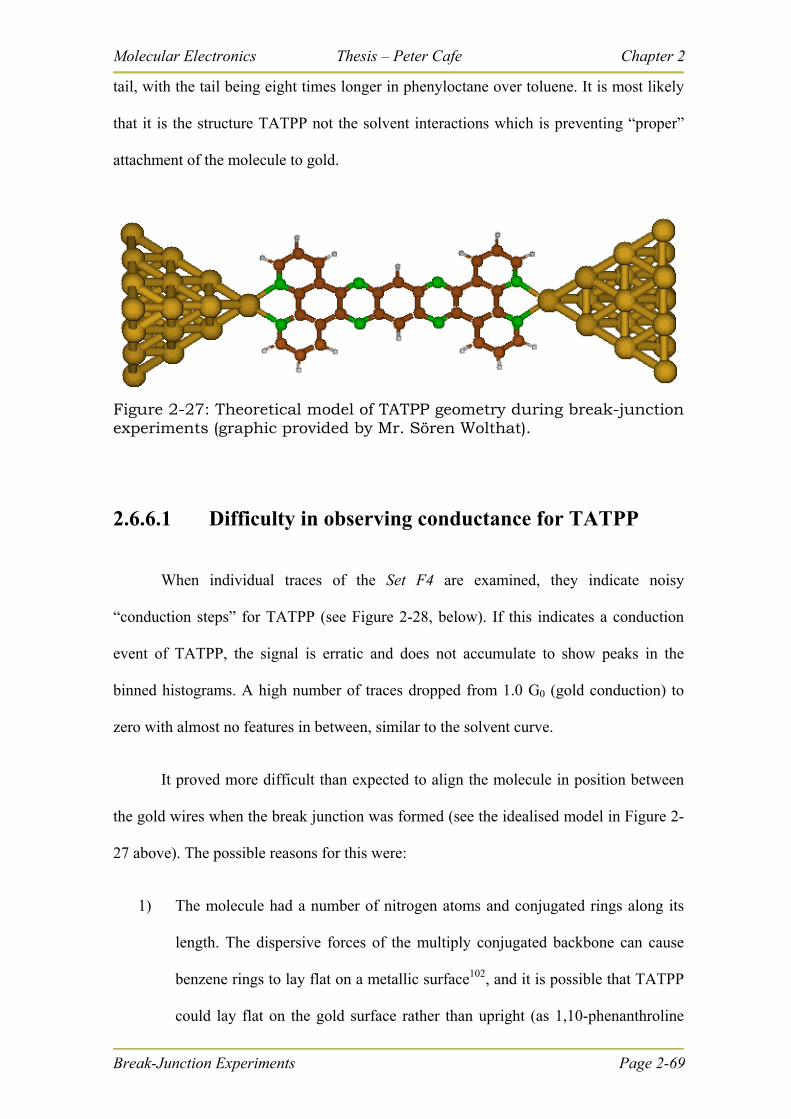
Molecular Electronics Thesis – Peter Cafe Chapter 2
tail, with the tail being eight times longer in phenyloctane over toluene. It is most likely
that it is the structure TATPP not the solvent interactions which is preventing “proper”
attachment of the molecule to gold.
Figure 2-27: Theoretical model of TATPP geometry during break-junction experiments (graphic provided by Mr. Sören Wolthat).
2.6.6.1 Difficulty in observing conductance for TATPP
When individual traces of the Set F4 are examined, they indicate noisy
“conduction steps” for TATPP (see Figure 2-28, below). If this indicates a conduction
event of TATPP, the signal is erratic and does not accumulate to show peaks in the
binned histograms. A high number of traces dropped from 1.0 G0 (gold conduction) to
zero with almost no features in between, similar to the solvent curve.
It proved more difficult than expected to align the molecule in position between
the gold wires when the break junction was formed (see the idealised model in Figure 2-
27 above). The possible reasons for this were:
1) The molecule had a number of nitrogen atoms and conjugated rings along its
length. The dispersive forces of the multiply conjugated backbone can cause
benzene rings to lay flat on a metallic surface102, and it is possible that TATPP
could lay flat on the gold surface rather than upright (as 1,10-phenanthroline
Break-Junction Experiments Page 2-69
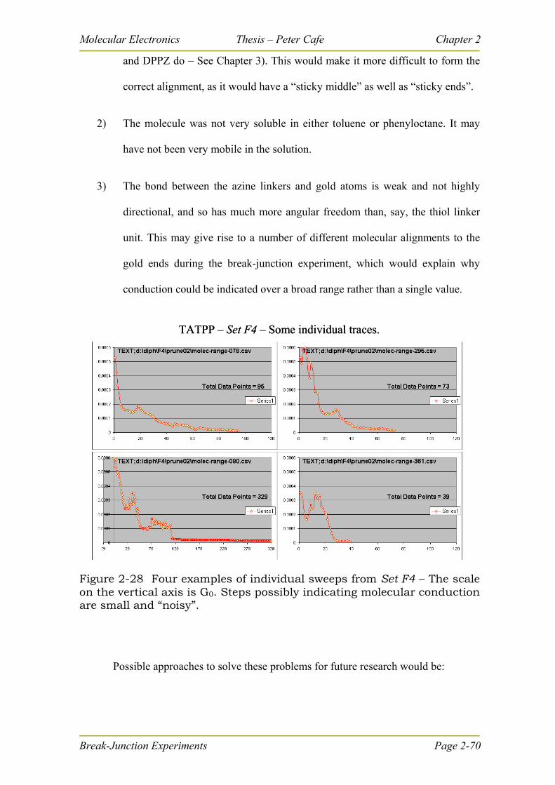
Molecular Electronics Thesis – Peter Cafe Chapter 2
and DPPZ do – See Chapter 3). This would make it more difficult to form the
correct alignment, as it would have a “sticky middle” as well as “sticky ends”.
2) The molecule was not very soluble in either toluene or phenyloctane. It may
have not been very mobile in the solution.
3) The bond between the azine linkers and gold atoms is weak and not highly
directional, and so has much more angular freedom than, say, the thiol linker
unit. This may give rise to a number of different molecular alignments to the
gold ends during the break-junction experiment, which would explain why
conduction could be indicated over a broad range rather than a single value.
TATPP – Set F4 – Some individual traces.TATPP – Set F4 – Some individual traces.
Figure 2-28 Four examples of individual sweeps from Set F4 – The scale on the vertical axis is G0. Steps possibly indicating molecular conduction are small and “noisy”.
Possible approaches to solve these problems for future research would be:
Break-Junction Experiments Page 2-70
Molecular Electronics Thesis – Peter Cafe Chapter 2
a) Create another similar molecule with side groups in the middle (e.g. tetrabutyl)
which would both offer steric hindrance to the molecule laying flat on gold, and
provide greater solubility.
b) Perform the experiment in an electrochemical cell with a positive bias applied to
the solution14.
2.6.7 Conclusion of TATPP results
It is difficult to observe the conductance of TATPP in the break-junction
experiment because of its low solubility and possible stickiness to gold in its middle, due
to the centre nitrogen atoms in the conjugated π-bonded backbone. No conclusive
conduction event was observed.
Most probably, TATPP did not adhere to the gold surface in a way that would
facilitate observance of single molecule conduction – that is, it was not bound to the gold
by its phenanthroline-type alligator clips: either because of solvent interactions or
because it laid flat on the gold (being attracted by its central nitrogen atoms as well as its
end ones). Further investigations which could determine this were hampered because it
was difficult to find other solvents which could dissolve TATPP.
Better results may be obtained by performing the experiment under
electrochemical control, or by redesigning the molecule to have better solubility and to
be less prone to lay flat on the gold surface.
Break-Junction Experiments Page 2-71
Molecular Electronics Thesis – Peter Cafe Chapter 2
2-7 Investigation of pyrazine
pyrazine: C4H4N2
2.7.1 Rationalization:
Pyrazine, bipyridine, TATPP and DPPZ are typical ligands used to developing
more complex devices containing ruthenium, osmium, or other metal atoms and/or ions
and/or metallated porphyrins which are being considered as possible molecular
electronic devices.103-105 As far back as 1966 pyrazine was considered useful in
vanadium superconductors106.
Pyrazine was considered to be a most likely molecule to use in the break-junction
experiment because its conduction was expected to be high, as it was a small rigid cyclic
molecule consisting solely of π-bonds. It also supported the theme of this thesis, that
nitrogen groups could be used rather than thiols to attach molecules to the gold electrode.
No prior publications give an experimental value for the molecular conduction of
pyrazine, however a theoretical value had been calculated. Pyrazine is also soluble in a
number of solvents, both polar and non-polar.
2.7.2 Background research
Interestingly, there is no published background research (experimental). Given
that pyrazine is a most likely candidate for molecular conduction experiments (previous
Break-Junction Experiments Page 2-72
Molecular Electronics Thesis – Peter Cafe Chapter 2
Break-Junction Experiments Page 2-73
paragraph) it may not be through a lack of attempts. (As the results here show, the
“single value” of the conductance of pyrazine is quite elusive. Insubstantial peaks
appeared in most conductance histograms plotted on a short-range linear scale, and it
was only through the log10 graphs of the conductance histograms that evidence of
pyrazine’s conduction becomes apparent.)
An unpublished theoretical value of conductance for pyrazine is 30 x 10-4 Go
(provided by Mr Sören Wolthat in a personal communication).
The other theoretical value of 4.7 x 10⁻⁴ Go listed in Table 2-2 may not be very
helpful as it was modelled by using sulfur atoms to bind to gold electrodes (substituting
for 2 hydrogen atoms), so in effect it was something like 1,3-dithiol-2,5-pyrazine
2.7.3 Experimental set-up:
Pyrazine readily dissolved in all solvents. The final concentration (and solvent)
used for each group was:
Group C: ~10mM in phenyloctane
Group D: ~5mM in toluene
Group E: ~30mM in toluene
Group G: ~20mM in 0.1 M sodium perchlorate (aqueous).
Group H: ~10mM in carbontetrachloride
Group K: ~10 mM in phenyloctane
Group L: ~10mM in carbontetrachloride
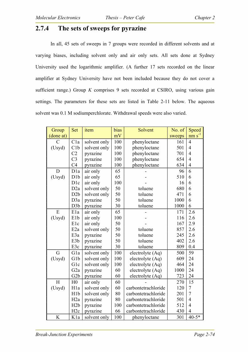
Molecular Electronics Thesis – Peter Cafe Chapter 2
Break-Junction Experiments Page 2-74
2.7.4 The sets of sweeps for pyrazine
In all, 45 sets of sweeps in 7 groups were recorded in different solvents and at
varying biases, including solvent only and air only sets. All sets done at Sydney
University used the logarithmic amplifier. (A further 17 sets recorded on the linear
amplifier at Sydney University have not been included because they do not cover a
sufficient range.) Group K comprises 9 sets recorded at CSIRO, using various gain
settings. The parameters for these sets are listed in Table 2-11 below. The aqueous
solvent was 0.1 M sodiumperchlorate. Withdrawal speeds were also varied.
Group (done at)
Set item biasmV
Solvent No. of sweeps
Speed nm s-1
C C1a solvent only 100 phenyloctane 161 4 (Usyd) C1b solvent only 100 phenyloctane 501 4
C2 pyrazine 100 phenyloctane 701 4 C3 pyrazine 100 phenyloctane 654 4 C4 pyrazine 100 phenyloctane 634 4
D D1a air only 65 - 96 6 (Usyd) D1b air only 65 - 510 6
D1c air only 100 - 16 6 D2a solvent only 50 toluene 680 6 D2b solvent only 50 toluene 471 6 D3a pyrazine 50 toluene 1000 6 D3b pyrazine 30 toluene 1000 6
E E1a air only 65 - 171 2.6 (Usyd) E1b air only 100 - 116 2.6
E1c air only 50 - 167 2.9 E2a solvent only 50 toluene 857 2.6 E3a pyrazine 50 toluene 245 2.6 E3b pyrazine 50 toluene 402 2.6 E3c pyrazine 30 toluene 809 0.4
G G1a solvent only 100 electrolyte (Aq) 500 59 (Usyd) G1b solvent only 100 electrolyte (Aq) 609 24
G1c solvent only 100 electrolyte (Aq) 464 24 G2a pyrazine 60 electrolyte (Aq) 1000 24 G2b pyrazine 60 electrolyte (Aq) 723 24
H H0 air only 60 - 270 15 (Usyd) H1a solvent only 60 carbontetrachloride 120 7
H1b solvent only 80 carbontetrachloride 201 7 H2a pyrazine 80 carbontetrachloride 501 4 H2b pyrazine 100 carbontetrachloride 512 4 H2c pyrazine 66 carbontetrachloride 430 4
K K1a solvent only 100 phenyloctane 301 40-5*
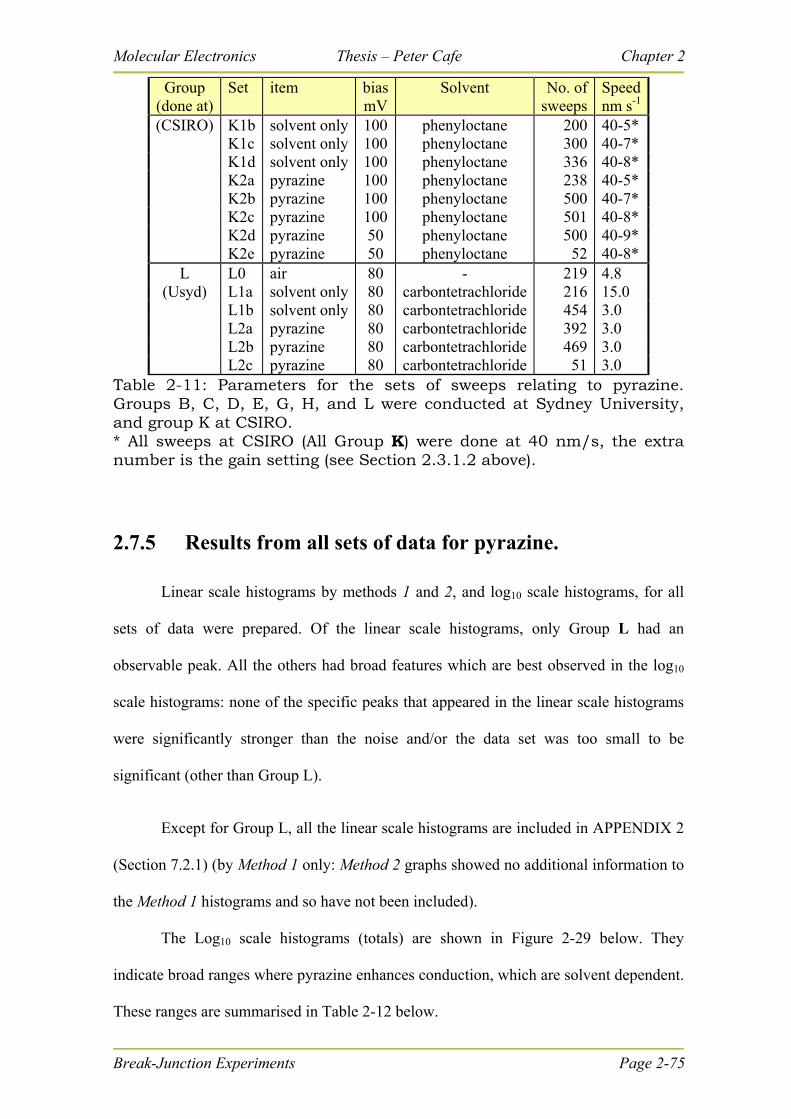
Molecular Electronics Thesis – Peter Cafe Chapter 2
Break-Junction Experiments Page 2-75
Group (done at)
Set item biasmV
Solvent No. of sweeps
Speed nm s-1
(CSIRO) K1b solvent only 100 phenyloctane 200 40-5* K1c solvent only 100 phenyloctane 300 40-7* K1d solvent only 100 phenyloctane 336 40-8* K2a pyrazine 100 phenyloctane 238 40-5* K2b pyrazine 100 phenyloctane 500 40-7* K2c pyrazine 100 phenyloctane 501 40-8* K2d pyrazine 50 phenyloctane 500 40-9* K2e pyrazine 50 phenyloctane 52 40-8*
L L0 air 80 - 219 4.8 (Usyd) L1a solvent only 80 carbontetrachloride 216 15.0
L1b solvent only 80 carbontetrachloride 454 3.0 L2a pyrazine 80 carbontetrachloride 392 3.0 L2b pyrazine 80 carbontetrachloride 469 3.0 L2c pyrazine 80 carbontetrachloride 51 3.0
Table 2-11: Parameters for the sets of sweeps relating to pyrazine. Groups B, C, D, E, G, H, and L were conducted at Sydney University, and group K at CSIRO. * All sweeps at CSIRO (All Group K) were done at 40 nm/s, the extra number is the gain setting (see Section 2.3.1.2 above).
2.7.5 Results from all sets of data for pyrazine.
Linear scale histograms by methods 1 and 2, and log10 scale histograms, for all
sets of data were prepared. Of the linear scale histograms, only Group L had an
observable peak. All the others had broad features which are best observed in the log10
scale histograms: none of the specific peaks that appeared in the linear scale histograms
were significantly stronger than the noise and/or the data set was too small to be
significant (other than Group L).
Except for Group L, all the linear scale histograms are included in APPENDIX 2
(Section 7.2.1) (by Method 1 only: Method 2 graphs showed no additional information to
the Method 1 histograms and so have not been included).
The Log10 scale histograms (totals) are shown in Figure 2-29 below. They
indicate broad ranges where pyrazine enhances conduction, which are solvent dependent.
These ranges are summarised in Table 2-12 below.

Molecular Electronics Thesis – Peter Cafe Chapter 2
Break-Junction Experiments Page 2-76
Experiments in phenyloctane were conducted at both Sydney University (Group
C) and CSIRO (Group K). The log10 scale histograms (totals) for each are shown in
Figure 2-30 below with trend lines for both pyrazine and solvent.
The log10 scale (total) histogram for Group G (aqueous solvent - Figure 2-29 (d))
is reproduced with trend lines in Figure 2-32.
Solvent Group Figure
Conductance range which is enhanced by the
presence of pyrazine (10-4 G0)
Enhance gold
conductance peak?
phenyloctane C
K
Figure 2-30 (a)
Figure 2-30 (b)
very broad, from 1 to 1000 trend line peak at 4.0
broad, from 1.0 to 100, trend line peak at about 11.0
No.
yes, x3
toluene D
E
Figure 2-29 (b)
Figure 2-29 (c)
Nil.
Nil
very much, x 8
Yes aqueous
20 mM NaClO4 G Figure 2-29 (d)
Figure 2-32 from about 300 to 3200 trend line peak at 1300
reversed
carbon-tetrachloride
H
L
Figure 2-29 (e)
Figure 2-29 (f)
generally lower than 25, with a peak at 10.
from 7.0 to 18.0, with a sharp peak at 12.0
extremely, x12
extremely, x60
Table 2-12: Summary of all results from pyrazine log10 histograms, all solvents.
In Figure 2-29 (c) (Set E in toluene) there is a strong peak for pyrazine around 1 x 10⁻⁴ G0. However the same peak is also present in the solvent-only curve. The pyrazine curve is consistently a factor of 4 times the solvent curve for the entire data range, so there is no specific range for which pyrazine enhances conduction. This peak has to be ignored and there are no specific conductance features for pyrazine from this histogram.
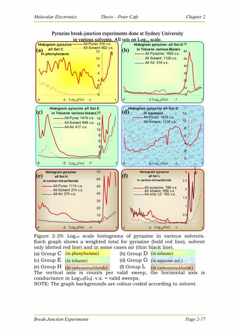
Molecular Electronics Thesis – Peter Cafe Chapter 2
Histogram pyrazineall Set L
in carbon-tetrachloride
0
0.5
1
1.5
2
2.5
3
-5 -3 -1 1
All pyrazine: 789 v.sAll solvent: 656 v.s.Air-only L0: 183 v.s.
Histogram pyrazine: all Set Din Toluene various Biases
0
10
20
30
40
50
60
70
-5 -3 -1 1
All Pyrazine: 1920 v.s.All Solvent: 1129 v.s.All Air: 519 v.s.
Histogram pyrazine all Set H
in carbon tetrachloride
0
10
20
30
40
50
60
70
-5 -3 -1 1
All-Pyraz 1114 v.s.All-Solvent 274 v.s.All-Air 270 v.s.
Histogram pyrazine all Set C
in phenyloctane
0
2
4
6
8
10
12
-5 -3 -1 1
All-Pyraz 316 v.s.All-Solvent 662 v.s.
Histogram pyrazine all Set G in aqueous
0
2
4
6
8
10
12
-5 -3 -1 1
All-Pyraz: 1618 v.s.All-Solvent: 1316 v.s.
Histogram pyrazine all Set E in Toluene various biases.
0
2
4
6
8
10
12
14
16
-5 -3 -1 1
All-Pyraz 1419 v.s.All-Solvent 848 v.s.All-Air 417 v.s.
Pyrazine break-junction experiments done at Sydney Universityin various solvents. All sets on Log10 scale.
Log10(Go)
Log10(Go) Log10(Go)
Log10(Go)
Log10(Go) Log10(Go)
(a) (b)
(c) (d)
(f)(e)Histogram pyrazine
all Set Lin carbon-tetrachloride
0
0.5
1
1.5
2
2.5
3
-5 -3 -1 1
All pyrazine: 789 v.sAll solvent: 656 v.s.Air-only L0: 183 v.s.
Histogram pyrazine: all Set Din Toluene various Biases
0
10
20
30
40
50
60
70
-5 -3 -1 1
All Pyrazine: 1920 v.s.All Solvent: 1129 v.s.All Air: 519 v.s.
Histogram pyrazine all Set H
in carbon tetrachloride
0
10
20
30
40
50
60
70
-5 -3 -1 1
All-Pyraz 1114 v.s.All-Solvent 274 v.s.All-Air 270 v.s.
Histogram pyrazine all Set C
in phenyloctane
0
2
4
6
8
10
12
-5 -3 -1 1
All-Pyraz 316 v.s.All-Solvent 662 v.s.
Histogram pyrazine all Set G in aqueous
0
2
4
6
8
10
12
-5 -3 -1 1
All-Pyraz: 1618 v.s.All-Solvent: 1316 v.s.
Histogram pyrazine all Set E in Toluene various biases.
0
2
4
6
8
10
12
14
16
-5 -3 -1 1
All-Pyraz 1419 v.s.All-Solvent 848 v.s.All-Air 417 v.s.
Pyrazine break-junction experiments done at Sydney Universityin various solvents. All sets on Log10 scale.
Log10(Go)
Log10(Go) Log10(Go)
Log10(Go)
Log10(Go) Log10(Go)
(a) (b)
(c) (d)
(f)(e)
Figure 2-29: Log10 scale histograms of pyrazine in various solvents. Each graph shows a weighted total for pyrazine (bold red line), solvent only (dotted red line) and in some cases air (thin black line). (a) Group C (b) Group D (c) Group E (d) Group G (e) Group H (f) Group L The vertical axis is counts per valid sweep, the horizontal axis is conductance in Log10(G0). v.s. = valid sweeps. NOTE: The graph backgrounds are colour-coded according to solvent.
(in carbontetrachloride)
(in toluene)
(in phenyloctane)
(in carbontetrachloride)
(in aqueous sol.)
(in toluene)
Break-Junction Experiments Page 2-77
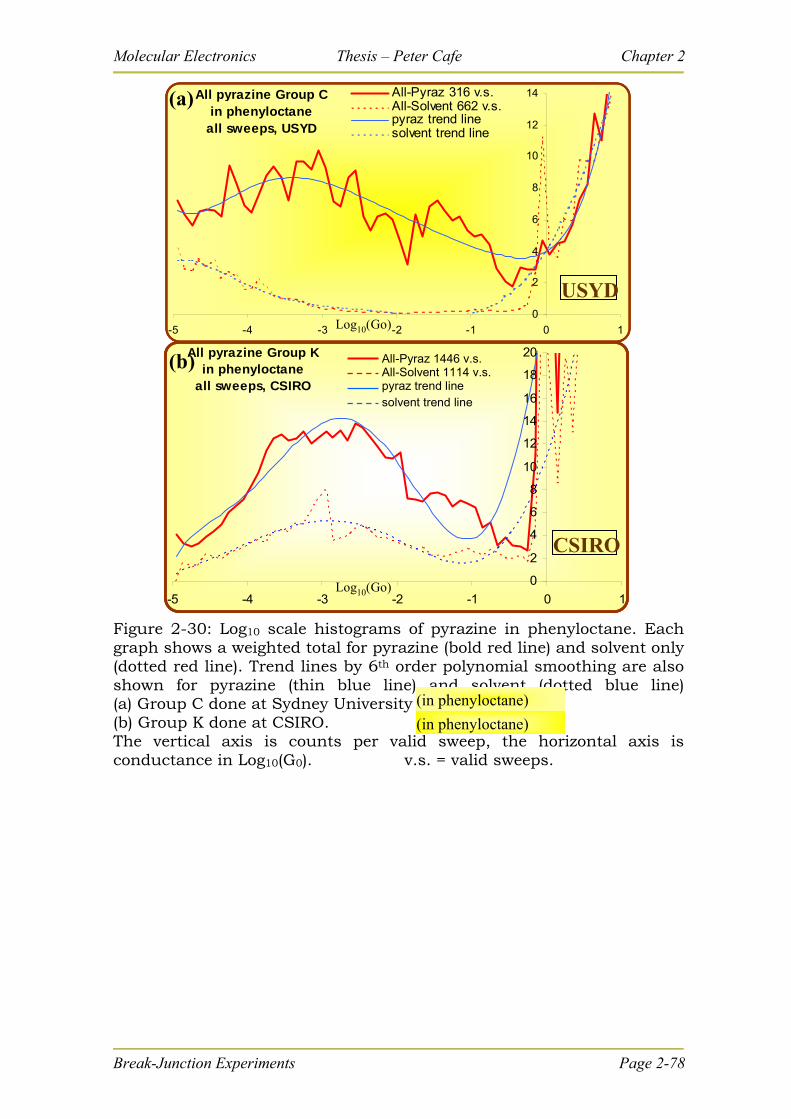
Molecular Electronics Thesis – Peter Cafe Chapter 2
All pyrazine Group K in phenyloctane
all sweeps, CSIRO
0
2
4
6
8
10
12
14
16
18
20
-5 -4 -3 -2 -1 0 1
All pyrazine Group C in phenyloctane
all sweeps, USYD
0
2
4
6
8
10
12
14
-5 -4 -3 -2 -1 0 1
All-Pyraz 316 v.s.All-Solvent 662 v.s.pyraz trend linesolvent trend line
Log10(Go)
Log10(Go)
(a)
(b) All-Pyraz 1446 v.s.All-Solvent 1114 v.s.pyraz trend linesolvent trend line
Break-Junction Experiments Page 2-78
USYD
CSIRO
All pyrazine Group K in phenyloctane
all sweeps, CSIRO
0
2
4
6
8
10
12
14
16
18
20
-5 -4 -3 -2 -1 0 1
All pyrazine Group C in phenyloctane
all sweeps, USYD
0
2
4
6
8
10
12
14
-5 -4 -3 -2 -1 0 1
All-Pyraz 316 v.s.All-Solvent 662 v.s.pyraz trend linesolvent trend line
Log10(Go)
Log10(Go)
(a)
(b) All-Pyraz 1446 v.s.All-Solvent 1114 v.s.pyraz trend linesolvent trend line
USYD
CSIRO
Figure 2-30: Log10 scale histograms of pyrazine in phenyloctane. Each graph shows a weighted total for pyrazine (bold red line) and solvent only (dotted red line). Trend lines by 6th order polynomial smoothing are also shown for pyrazine (thin blue line) and solvent (dotted blue line) (a) Group C done at Sydney University (b) Group K done at CSIRO. The vertical axis is counts per valid sweep, the horizontal axis is conductance in Log10(G0). v.s. = valid sweeps.
(in phenyloctane)
(in phenyloctane)
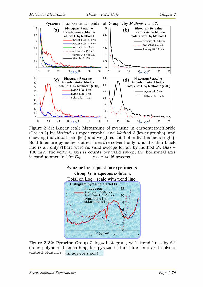
Molecular Electronics Thesis – Peter Cafe Chapter 2
Histogram Pyrazine in carbon-tetrachloride
Each Set L by Method 2 (>200)
0
10
20
30
40
50
60
70
80
90
0 10 20 30 40 50 60
pyraz L2a: 4 v.spyraz L2b: 2 v.s.solv. L1a: 1 v.s.
Histogram Pyrazine in carbon-tetrachloride
Totals Set L by Method 2 (>200)
0
10
20
30
40
50
60
0 10 20 30 40 50 60
pyraz all: 6 v.s
solv. L1a: 1 v.s.
Histogram Pyrazine in carbon-tetrachloride
Totals Set L by Method 1
0
0.5
1
1.5
2
2.5
3
0 10 20 30 40 50 60
pyrazine all: 828 v.s.
solvent all: 656 v.s.
Air-only L0: 183 v.s.
Histogram Pyrazine in carbon-tetrachlorideall Set L by Method 1
0
0.5
1
1.5
2
2.5
3
0 10 20 30 40 50 60
pyrazine L2a: 374 v.s.
pyrazine L2b: 415 v.s.
pyrazine L2c: 39 v.s.
solvent L1a: 208 v.s.
solvent L1b: 448 v.s.
Air-only L0: 183 v.s.
Pyrazine in carbon-tetrachloride – all Group L by Methods 1 and 2.
(a) (b)
(c) (d)
10-4 Go 10-4 Go
10-4 Go 10-4 Go
Histogram Pyrazine in carbon-tetrachloride
Each Set L by Method 2 (>200)
0
10
20
30
40
50
60
70
80
90
0 10 20 30 40 50 60
pyraz L2a: 4 v.spyraz L2b: 2 v.s.solv. L1a: 1 v.s.
Histogram Pyrazine in carbon-tetrachloride
Totals Set L by Method 2 (>200)
0
10
20
30
40
50
60
0 10 20 30 40 50 60
pyraz all: 6 v.s
solv. L1a: 1 v.s.
Histogram Pyrazine in carbon-tetrachloride
Totals Set L by Method 1
0
0.5
1
1.5
2
2.5
3
0 10 20 30 40 50 60
pyrazine all: 828 v.s.
solvent all: 656 v.s.
Air-only L0: 183 v.s.
Histogram Pyrazine in carbon-tetrachlorideall Set L by Method 1
0
0.5
1
1.5
2
2.5
3
0 10 20 30 40 50 60
pyrazine L2a: 374 v.s.
pyrazine L2b: 415 v.s.
pyrazine L2c: 39 v.s.
solvent L1a: 208 v.s.
solvent L1b: 448 v.s.
Air-only L0: 183 v.s.
Pyrazine in carbon-tetrachloride – all Group L by Methods 1 and 2.
(a) (b)
(c) (d)
10-4 Go 10-4 Go
10-4 Go 10-4 Go
Figure 2-31: Linear scale histograms of pyrazine in carbontetrachloride (Group L) by Method 1 (upper graphs) and Method 2 (lower graphs), and showing individual sets (left) and weighted total of individual sets (right). Bold lines are pyrazine, dotted lines are solvent only, and the thin black line is air only (There were no valid sweeps for air by method 2). Bias = 100 mV. The vertical axis is counts per valid sweep, the horizontal axis is conductance in 10-4 G0. v.s. = valid sweeps.
Histogram pyrazine all Set G in aqueous
0
2
4
6
8
10
12
-5 -3 -1 1
All-Pyraz: 1618 v.s.All-Solvent: 1316 v.s.pyraz trend linesolvent trend line
Log10(Go)
Pyrazine break-junction experiments.Group G in aqueous solution.
Total on Log10 scale with trend line.Histogram pyrazine all Set G
in aqueous
0
2
4
6
8
10
12
-5 -3 -1 1
All-Pyraz: 1618 v.s.All-Solvent: 1316 v.s.pyraz trend linesolvent trend line
Log10(Go)
Pyrazine break-junction experiments.Group G in aqueous solution.
Total on Log10 scale with trend line.
Figure 2-32: Pyrazine Group G log10 histogram, with trend lines by 6th order polynomial smoothing for pyrazine (thin blue line) and solvent (dotted blue line) (in aqueous sol.)
Break-Junction Experiments Page 2-79

Molecular Electronics Thesis – Peter Cafe Chapter 2
Break-Junction Experiments Page 2-80
2.7.6 Discussion of pyrazine results:
2.7.6.1 General observations
Each solvent has broad ranges of conductance where pyrazine shows a
conduction signal greater than solvent. Sharp peaks are elusive for pyrazine (except in
the Group L in carbontetrachloride). The general explanations for the broad ranges are as
follows:
1. The pyrazine molecule inserts itself into the break-junction in a variety of
geometric configurations, each with its own characteristic conductance. This
would account for a number of different conductance values, which may vary by
as much as an order of magnitude or more.
2. Sometimes 2 or more pyrazine molecules are bridging the gap at the same time,
however if there are different geometric configurations available to each
molecule, then the conductance of two molecules will not necessarily be double
the conductance of one molecule.
3. The pyrazine may somehow join as a multiple of more than one molecule in a
line, stacked to each other by interactions between the conjugated rings.
4. The solvent may interact with the pyrazine forming complexes.
5. Variation of withdrawal speeds had no observable effect on conduction.
6. Finally, the configuration of the terminal gold atom(s) to which the pyrazine
connects can contribute to a variation in conduction (this is shown for thiol
conduction in Chapter 4).
All of these factors combined give rise to a very wide range of results which are
indicated by the broad ranges in the histograms.
Molecular Electronics Thesis – Peter Cafe Chapter 2
Break-Junction Experiments Page 2-81
Interaction of pyrazine with the solvent molecule, particularly solvents with a
conjugated ring (see Figure 2-34), is the most significant contributor to this broad
range71. Pyrazine conduction in each solvent is considered separately below:
2.7.6.2 In phenyloctane
The results obtained at Sydney University (Group C) and CSIRO (Group K)
show high similarity over the broad range (Figure 2-30), with 316 and 1446 valid sweeps
respectively. With over a thousand individual traces, the CSIRO data should be taken as
most reliable. However the Sydney University data, done on completely different
equipment, is viewed as an independent verification of the CSIRO data. The peak of the
fitted trend line is 11.0 x 10⁻⁴ G0 (CSIRO) and this is confirmed with the USYD peak
being quite close (4.0 x 10⁻⁴ G0).
In the CSIRO data, the extensive broadness of the peak is over 2 orders of
magnitude, from 1 to 100 x 10-4 G0. (This is more or less confirmed by the USYD data,
which is however much broader but with a smaller data set.) Such a range could
encompass many different pyrazine configurations between the gold electrodes,
including configurations involving solvent interactions. The peak at 11.0 x 10⁻⁴ G0
represents the mid range and not necessarily the conduction of a single molecule. It
could perhaps suggest the conductance of the most likely configuration of pyrazine
molecule(s), but even this conclusion cannot be drawn with any certainty from this data
alone.
A sharp spike in the Group C data at about 10-4.2 G0 has affected the trend line. This spike is most likely a noisy aberration, and if removed then one would expect the peak of the trend line to be closer to the Group K result (11x10-4 G0).
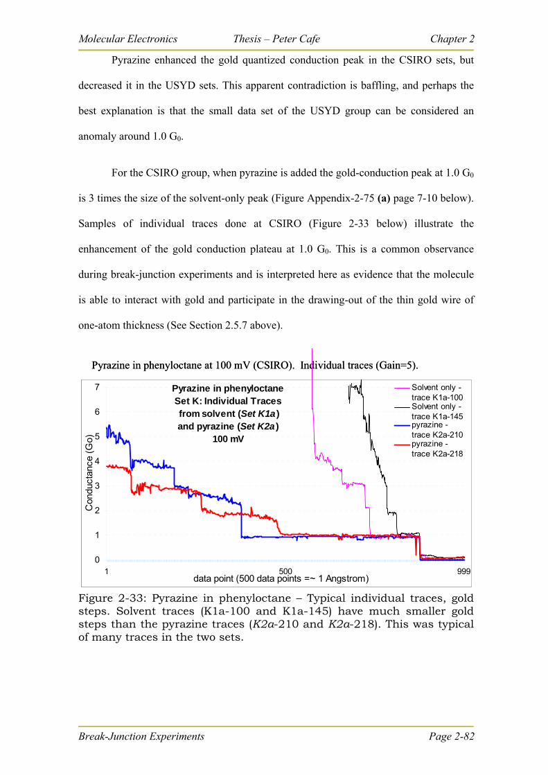
Molecular Electronics Thesis – Peter Cafe Chapter 2
Pyrazine enhanced the gold quantized conduction peak in the CSIRO sets, but
decreased it in the USYD sets. This apparent contradiction is baffling, and perhaps the
best explanation is that the small data set of the USYD group can be considered an
anomaly around 1.0 G0.
For the CSIRO group, when pyrazine is added the gold-conduction peak at 1.0 G0
is 3 times the size of the solvent-only peak (Figure Appendix-2-75 (a) page 7-10 below).
Samples of individual traces done at CSIRO (Figure 2-33 below) illustrate the
enhancement of the gold conduction plateau at 1.0 G0. This is a common observance
during break-junction experiments and is interpreted here as evidence that the molecule
is able to interact with gold and participate in the drawing-out of the thin gold wire of
one-atom thickness (See Section 2.5.7 above).
Pyrazine in phenyloctane at 100 mV (CSIRO). Individual traces (Gain=5).
Pyrazine in phenyloctane Set K: Individual Traces from solvent (Set K1a ) and pyrazine (Set K2a )
100 mV
0
1
2
3
4
5
6
7
1 500 999data point (500 data points =~ 1 Angstrom)
Con
duct
ance
(G
o)
Solvent only -trace K1a-100Solvent only -trace K1a-145pyrazine - trace K2a-210pyrazine - trace K2a-218
Figure 2-33: Pyrazine in phenyloctane – Typical individual traces, gold steps. Solvent traces (K1a-100 and K1a-145) have much smaller gold steps than the pyrazine traces (K2a-210 and K2a-218). This was typical of many traces in the two sets.
Break-Junction Experiments Page 2-82
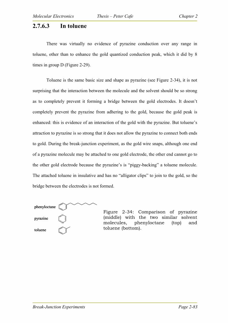
Molecular Electronics Thesis – Peter Cafe Chapter 2
2.7.6.3 In toluene
There was virtually no evidence of pyrazine conduction over any range in
toluene, other than to enhance the gold quantized conduction peak, which it did by 8
times in group D (Figure 2-29).
Toluene is the same basic size and shape as pyrazine (see Figure 2-34), it is not
surprising that the interaction between the molecule and the solvent should be so strong
as to completely prevent it forming a bridge between the gold electrodes. It doesn’t
completely prevent the pyrazine from adhering to the gold, because the gold peak is
enhanced: this is evidence of an interaction of the gold with the pyrazine. But toluene’s
attraction to pyrazine is so strong that it does not allow the pyrazine to connect both ends
to gold. During the break-junction experiment, as the gold wire snaps, although one end
of a pyrazine molecule may be attached to one gold electrode, the other end cannot go to
the other gold electrode because the pyrazine’s is “piggy-backing” a toluene molecule.
The attached toluene in insulative and has no “alligator clips” to join to the gold, so the
bridge between the electrodes is not formed.
phenyloctane
pyrazine
toluene
phenyloctane
pyrazine
toluene
Figure 2-34: Comparison of pyrazine (middle) with the two similar solvent molecules, phenyloctane (top) and toluene (bottom).
Break-Junction Experiments Page 2-83
Molecular Electronics Thesis – Peter Cafe Chapter 2
Break-Junction Experiments Page 2-84
2.7.6.4 In aqueous solvent
(The aqueous solvent was 0.1 M sodiumperchlorate.)
A large range of enhanced conduction was evident in the aqueous solvent but at
much higher values than the organic solvents. Strong solvent-molecule interactions are a
significant factor in the conduction histogram of pyrazine in the aqueous solvent. Unlike
the solvents toluene and phenyloctane that bond with the pyrazine via π–stacking of the
similar conjugated rings, the pyrazine-water complex is flat. The water molecule lies in
the plane of the aromatic ring, and the lone pair of electrons on the nitrogen atom
functions as the acceptor in the NH-O hydrogen bond.107 The species bridging the gold
electrodes is most probably a complex with a variety of structures and geometries.
However it does conduct better than the aqueous solvent alone over a high and broad
range, from 300 to 3200 x 10-4 G0.
At the lower conductance range, lower than 300 x 10-4 G0, the addition of
pyrazine lowers the conductance histogram peaks. I.E. there are less conduction events
in the range where pyrazine indicated conduction in the organic solvents. This indicates
that the components that conduct in the organic solvent (which are one or more pyrazine
molecules in various configurations) are prevented from conducting when in the
presence of water. In water conductance is dominated by water-pyrazine complexes that
have a higher conductance than pyrazine alone.
The peak of the enhanced conduction range is 1300 x 10-4 G0. This probably
indicates the conductance of a preferred configuration of the pyrazine-water complex
which dominates conduction, however it gives no indication of that structure.
Molecular Electronics Thesis – Peter Cafe Chapter 2
Break-Junction Experiments Page 2-85
It is interesting to note that in water alone the gold steps are quite high (~10
counts per valid sweep), much higher than in air or other solvents (~4 cpvs) (compare (d)
with (b), (c), (d) and (f) in Figure 2-29). However when pyrazine is added the
enhancement completely reverses.
2.7.6.5 In carbontetrachloride
When pyrazine is added to carbontetrachloride the conduction is enhanced over a
small range (compared to the other solvents), and the enhancement is much lower.
There is a peak in the conduction curves for Group H at ~ 10 x 10-4 G0: it is not a
sharp peak but with over 1000 valid sweeps the curve has little noise and the peak is
definite; nevertheless the peak in Group L (789 v.s.) is much sharper at 12 x 10-4 G0
(Figure 2-29 (e) and (f)). The same peak is evidenced in the linear plots of Group L at
~11 x 10-4 G0 (Figure 2-31).
The peak identified by group G is confirmed to be a single conduction event by
the sharpness of the same peak in Group L. That is, this value is the conductance of a
specific configuration of pyrazine between two gold electrodes, and that this is the
preferred configuration of pyrazine between the electrodes when in the solvent
carbontetrachloride.
Still, it does not prove conclusively that it is the conduction of a single molecule
of pyrazine.
Carbontetrachloride is a smaller solvent molecule than toluene or phenyloctane,
and most importantly it has no aromatic or -system. Therefore its attraction to pyrazine
is not through π–stacking of similar conjugated rings. There is less steric hindrance to
Molecular Electronics Thesis – Peter Cafe Chapter 2
Break-Junction Experiments Page 2-86
the motion of the pyrazine molecule(s) and it can couple between the gold electrodes
more easily.
In carbontetrachloride the gold steps are dramatically enhanced by the addition of
pyrazine. (The solvent alone does not enhance the gold steps.) Because of lower solvent-
pyrazine interactions, the pyrazine is able to bind independently to the gold and
participate in the drawing-out process during the creation of the gold wire of single-atom
thickness (See Section 2.5.6 above where this is first mentioned).
2.7.7 Conclusion of pyrazine results
Pyrazine-solvent interactions play an important role in the conductance of
pyrazine during break-junction experiments. A small, non-conjugated solvent such as
carbontetrachloride allows the pyrazine to interact with the gold without solvent
interference. This is evidenced by the extreme enhancement of the gold quantized
conduction peaks.
Brolo (1998) noted that pyrazine is able to form a monolayer on Au(111)45. Thus
there is an attraction and a co-ordination of geometry between pyrazine and the Au(111)
surface. During the break-junction experiment this attraction is brought into play by
stabilising the gold wire when it is one gold atom in diameter, and allowing it to stretch
to lengths beyond the 2 or 3 atom limit determined by Untiedt, et al, (2002)76.
Larger solvent molecules with conjugated rings interfere with the interaction
between pyrazine and gold, but do not completely prevent it. One end of the pyrazine
molecule may be free to attach to the gold surface (and enhance the gold quantized
conduction peak, as in toluene and phenyloctane). But the other end may be hindered,
and in the case of toluene with its close binding, completely prevented from attaching to
Molecular Electronics Thesis – Peter Cafe Chapter 2
the other gold electrode. The effect is not so drastic in phenyloctane, where the solvent is
not so similar to pyrazine, but it still gives rise to a number of alternative structures,
making it difficult to observe a single value for the conduction of pyrazine.
In water the conduction is dominated by the polar solvent (giving a high but
broad conductance range), with the hydrogen-bonded water molecules preventing the
pyrazine’s sticky ends (N atoms) from attaching to gold (evidenced by a decrease in the
gold quantized conduction peak.). With electrochemical control (See Section 2.5.7 above
and 14) it may be possible to control the pyrazine-water interactions by providing a
driving force to attract the pyrazine away from the water to the gold terminals.
In a sealed jar, unsolvated pyrazine is highly crystalline and sublimes at room
temperature within the closed container, reforming pyrazine crystals at the neck of the
jar. This implies that there is one mode of solidification with high order but weak
intermolecular bonding. Individual molecules loosen easily from the end of pyrazine
stacks and there is no other binding mode to facilitate a liquid phase. Toluene can
substitute for pyrazine in π-stacking, creating short insulating “crystals” in solution (i.e.,
dimeric, trimeric and longer stacks of pyrazine and toluene). Phenyloctane also does to
some extent, but it gives up its pyrazine attachment more easily.
A specific conductance peak for pyrazine is found at 10 x 10-4 G0. It cannot be
determined from these results that this is definitely a single pyrazine molecule standing
upright between two gold electrodes with its nitrogen atoms attached to the gold
terminals. Before that could be determined there would need to be more than one peak at
multiples of this value. However it is quite close to the two theoretical values provided
(which are 30 x 10-4 Go and 4.7 x 10⁻⁴ Go, see Section 2.7.2 above).
Break-Junction Experiments Page 2-87
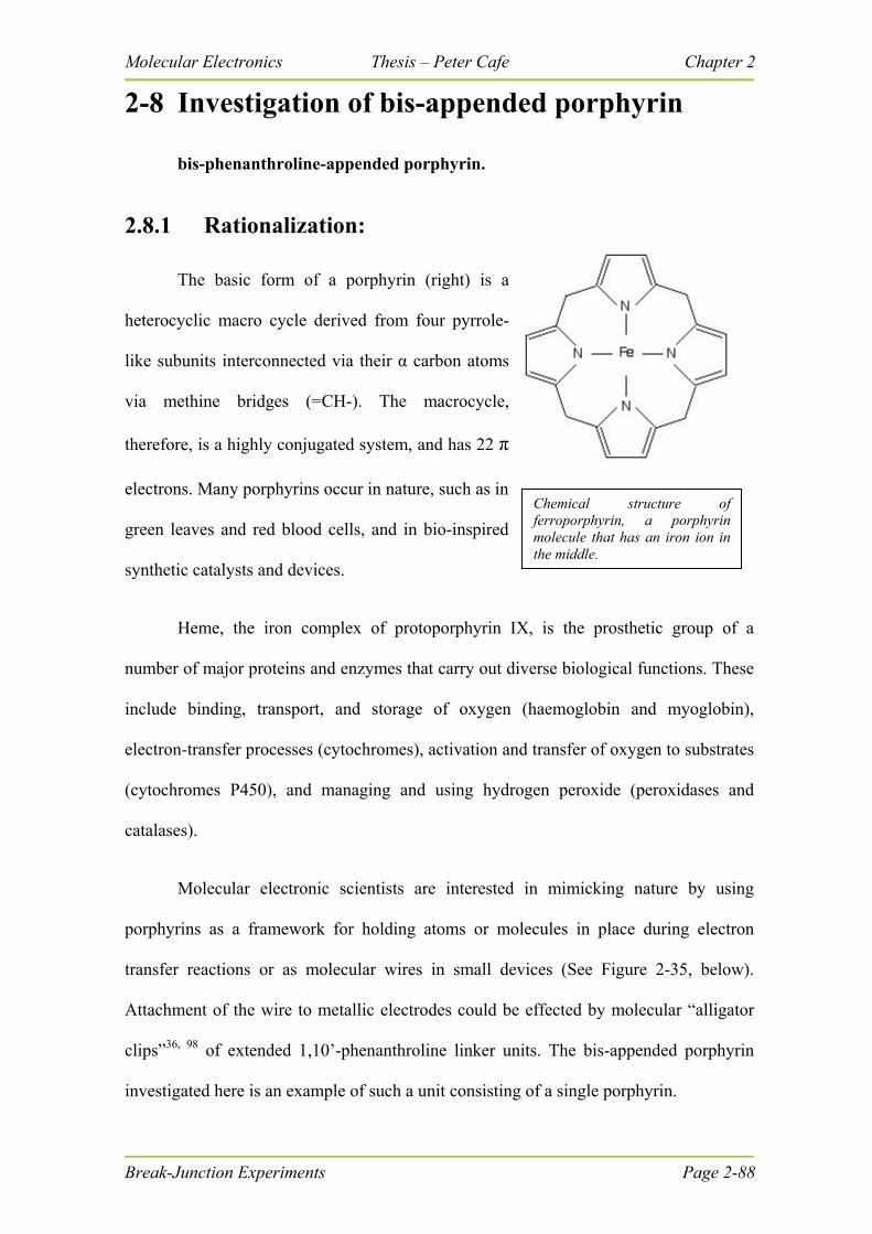
Molecular Electronics Thesis – Peter Cafe Chapter 2
2-8 Investigation of bis-appended porphyrin
bis-phenanthroline-appended porphyrin.
2.8.1 Rationalization:
The basic form of a porphyrin (right) is a
heterocyclic macro cycle derived from four pyrrole-
like subunits interconnected via their α carbon atoms
via methine bridges (=CH-). The macrocycle,
therefore, is a highly conjugated system, and has 22 π
electrons. Many porphyrins occur in nature, such as in
green leaves and red blood cells, and in bio-inspired
synthetic catalysts and devices.
Heme, the iron complex of protoporphyrin IX, is the prosthetic group of a
number of major proteins and enzymes that carry out diverse biological functions. These
include binding, transport, and storage of oxygen (haemoglobin and myoglobin),
electron-transfer processes (cytochromes), activation and transfer of oxygen to substrates
(cytochromes P450), and managing and using hydrogen peroxide (peroxidases and
catalases).
Molecular electronic scientists are interested in mimicking nature by using
porphyrins as a framework for holding atoms or molecules in place during electron
transfer reactions or as molecular wires in small devices (See Figure 2-35, below).
Attachment of the wire to metallic electrodes could be effected by molecular “alligator
clips”36, 98 of extended 1,10’-phenanthroline linker units. The bis-appended porphyrin
investigated here is an example of such a unit consisting of a single porphyrin.
Chemical structure of ferroporphyrin, a porphyrin molecule that has an iron ion in the middle.
Break-Junction Experiments Page 2-88
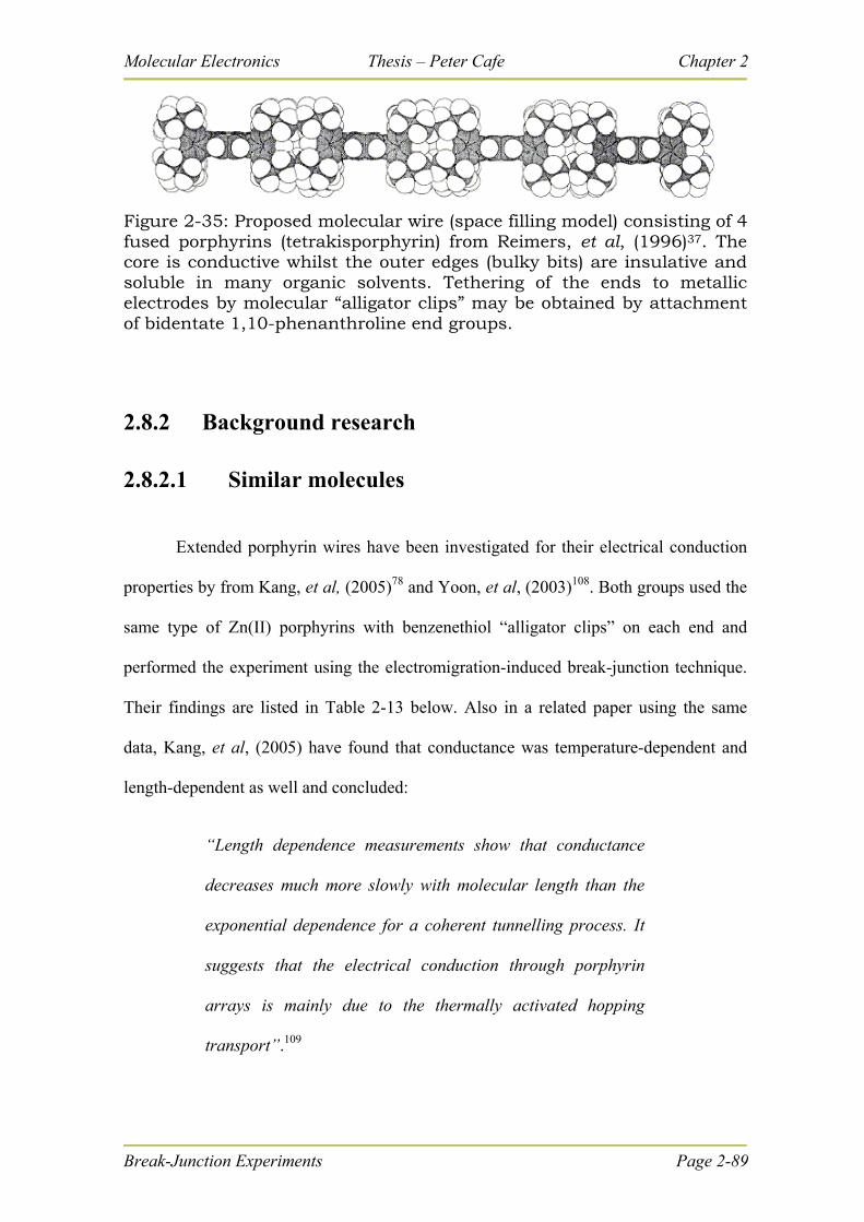
Molecular Electronics Thesis – Peter Cafe Chapter 2
Figure 2-35: Proposed molecular wire (space filling model) consisting of 4 fused porphyrins (tetrakisporphyrin) from Reimers, et al, (1996)37. The core is conductive whilst the outer edges (bulky bits) are insulative and soluble in many organic solvents. Tethering of the ends to metallic electrodes by molecular “alligator clips” may be obtained by attachment of bidentate 1,10-phenanthroline end groups.
2.8.2 Background research
2.8.2.1 Similar molecules
Extended porphyrin wires have been investigated for their electrical conduction
properties by from Kang, et al, (2005)78 and Yoon, et al, (2003)108. Both groups used the
same type of Zn(II) porphyrins with benzenethiol “alligator clips” on each end and
performed the experiment using the electromigration-induced break-junction technique.
Their findings are listed in Table 2-13 below. Also in a related paper using the same
data, Kang, et al, (2005) have found that conductance was temperature-dependent and
length-dependent as well and concluded:
“Length dependence measurements show that conductance
decreases much more slowly with molecular length than the
exponential dependence for a coherent tunnelling process. It
suggests that the electrical conduction through porphyrin
arrays is mainly due to the thermally activated hopping
transport”.109
Break-Junction Experiments Page 2-89
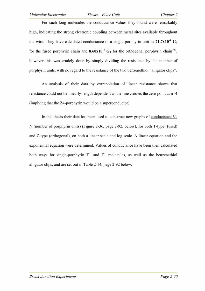
Molecular Electronics Thesis – Peter Cafe Chapter 2
Break-Junction Experiments Page 2-90
For such long molecules the conductance values they found were remarkably
high, indicating the strong electronic coupling between metal sites available throughout
the wire. They have calculated conductance of a single porphyrin unit as 71.7x10⁻⁴ G0
for the fused porphyrin chain and 8.60x10⁻⁴ G0 for the orthogonal porphyrin chain109,
however this was crudely done by simply dividing the resistance by the number of
porphyrin units, with no regard to the resistance of the two benzenethiol “alligator clips”.
An analysis of their data by extrapolation of linear resistance shows that
resistance could not be linearly-length dependent as the line crosses the zero point at n=4
(implying that the Z4-porphyrin would be a superconductor).
In this thesis their data has been used to construct new graphs of conductance Vs
N (number of porphyrin units) (Figure 2-36, page 2-92, below), for both T-type (fused)
and Z-type (orthogonal), on both a linear scale and log scale. A linear equation and the
exponential equation were determined. Values of conductance have been then calculated
both ways for single-porphyrin T1 and Z1 molecules, as well as the benzenethiol
alligator clips, and are set out in Table 2-14, page 2-92 below.
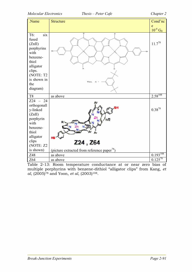
Molecular Electronics Thesis – Peter Cafe Chapter 2
.Name Structure Cond’nce 10-4 G0
T6: six fused (ZnII) porphyrins with benzene-thiol alligator clips. (NOTE: T2 is shown in the diagram)
N
N N
N
Ar
Ar
Zn++
Where, Ar =
N
N N
N
Ar
Ar
Zn++HS SH
11.778
T8 as above 2.58108 Z24 – 24 orthogonally-linked (ZnII) porphyrin with benzene-thiol alligator clips (NOTE: Z2 is shown)
(picture extracted from reference paper78)
0.3878
Z48 as above 0.193108 Z64 as above 0.12578
Table 2-13: Room temperature conductance at or near zero bias of multiple porphyrins with benzene-dithiol “alligator clips” from Kang, et al, (2005)78 and Yoon, et al, (2003)108.
Break-Junction Experiments Page 2-91
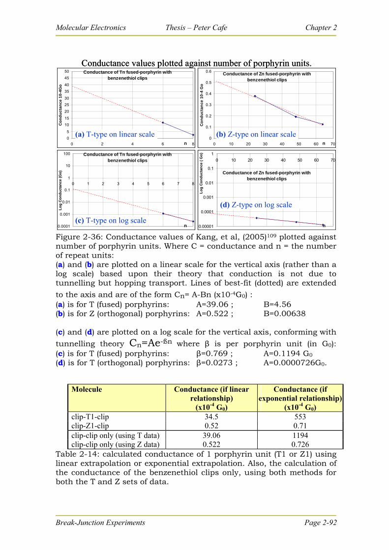
Molecular Electronics Thesis – Peter Cafe Chapter 2
Conductance of Tn fused-porphyrin with benzenethiol clips
0
5
10
15
20
25
30
35
40
45
50
0 2 4 6 8n
Co
nd
uc
tan
ce
10
-4G
o
Conductance of Zn fused-porphyrin with benzenethiol clips
0
0.1
0.2
0.3
0.4
0.5
0.6
0 10 20 30 40 50 60 70n
Co
nd
uc
tan
ce
10
-4 G
o
Conductance of Tn fused-porphyrin with benzenethiol clips
0.0001
0.001
0.01
0.1
1
10
100
0 1 2 3 4 5 6 7 8
n
Lo
g C
on
du
ctan
ce (
Go
) Conductance of Zn fused-porphyrin with benzenethiol clips
0.00001
0.0001
0.001
0.01
0.1
1
0 10 20 30 40 50 60 70
n
Lo
g C
on
du
ctan
ce (
Go
)
Conductance values plotted against number of porphyrin units.
(a) T-type on linear scale (b) Z-type on linear scale
(c) T-type on log scale
(d) Z-type on log scale
Conductance of Tn fused-porphyrin with benzenethiol clips
0
5
10
15
20
25
30
35
40
45
50
0 2 4 6 8n
Co
nd
uc
tan
ce
10
-4G
o
Conductance of Zn fused-porphyrin with benzenethiol clips
0
0.1
0.2
0.3
0.4
0.5
0.6
0 10 20 30 40 50 60 70n
Co
nd
uc
tan
ce
10
-4 G
o
Conductance of Tn fused-porphyrin with benzenethiol clips
0.0001
0.001
0.01
0.1
1
10
100
0 1 2 3 4 5 6 7 8
n
Lo
g C
on
du
ctan
ce (
Go
) Conductance of Zn fused-porphyrin with benzenethiol clips
0.00001
0.0001
0.001
0.01
0.1
1
0 10 20 30 40 50 60 70
n
Lo
g C
on
du
ctan
ce (
Go
)
Conductance values plotted against number of porphyrin units.
(a) T-type on linear scale (b) Z-type on linear scale
(c) T-type on log scale
(d) Z-type on log scale
Figure 2-36: Conductance values of Kang, et al, (2005)109 plotted against number of porphyrin units. Where C = conductance and n = the number of repeat units: (a) and (b) are plotted on a linear scale for the vertical axis (rather than a log scale) based upon their theory that conduction is not due to tunnelling but hopping transport. Lines of best-fit (dotted) are extended
to the axis and are of the form Cn= A-Bn (x10-4G0) : (a) is for T (fused) porphyrins: A=39.06 ; B=4.56 (b) is for Z (orthogonal) porphyrins: A=0.522 ; B=0.00638 (c) and (d) are plotted on a log scale for the vertical axis, conforming with
tunnelling theory Cn=Ae-ßn where β is per porphyrin unit (in G0): (c) is for T (fused) porphyrins: β=0.769 ; A=0.1194 G0
(d) is for T (orthogonal) porphyrins: β=0.0273 ; A=0.0000726G0.
Molecule Conductance (if linear
relationship) (x10-4 G0)
Conductance (if exponential relationship)
(x10-4 G0) clip-T1-clip 34.5 553 clip-Z1-clip 0.52 0.71 clip-clip only (using T data) 39.06 1194 clip-clip only (using Z data) 0.522 0.726
Table 2-14: calculated conductance of 1 porphyrin unit (T1 or Z1) using linear extrapolation or exponential extrapolation. Also, the calculation of the conductance of the benzenethiol clips only, using both methods for both the T and Z sets of data.
Break-Junction Experiments Page 2-92
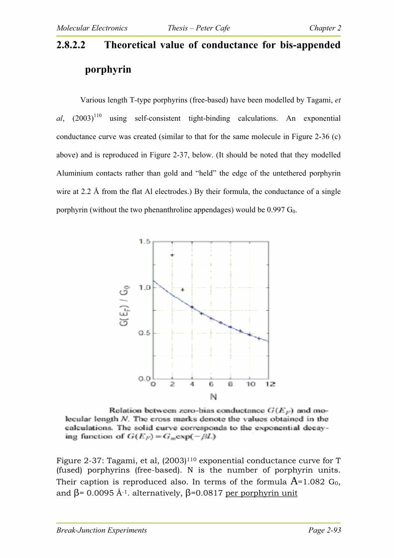
Molecular Electronics Thesis – Peter Cafe Chapter 2
2.8.2.2 Theoretical value of conductance for bis-appended
porphyrin
Various length T-type porphyrins (free-based) have been modelled by Tagami, et
al, (2003)110 using self-consistent tight-binding calculations. An exponential
conductance curve was created (similar to that for the same molecule in Figure 2-36 (c)
above) and is reproduced in Figure 2-37, below. (It should be noted that they modelled
Aluminium contacts rather than gold and “held” the edge of the untethered porphyrin
wire at 2.2 Å from the flat Al electrodes.) By their formula, the conductance of a single
porphyrin (without the two phenanthroline appendages) would be 0.997 G0.
Figure 2-37: Tagami, et al, (2003)110 exponential conductance curve for T (fused) porphyrins (free-based). N is the number of porphyrin units.
Their caption is reproduced also. In terms of the formula A=1.082 G0, and β= 0.0095 Å-1. alternatively, β=0.0817 per porphyrin unit
Break-Junction Experiments Page 2-93
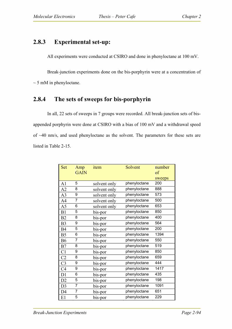
Molecular Electronics Thesis – Peter Cafe Chapter 2
Break-Junction Experiments Page 2-94
2.8.3 Experimental set-up:
All experiments were conducted at CSIRO and done in phenyloctane at 100 mV.
Break-junction experiments done on the bis-porphyrin were at a concentration of
~ 5 mM in phenyloctane.
2.8.4 The sets of sweeps for bis-porphyrin
In all, 22 sets of sweeps in 7 groups were recorded. All break-junction sets of bis-
appended porphyrin were done at CSIRO with a bias of 100 mV and a withdrawal speed
of ~40 nm/s, and used phenyloctane as the solvent. The parameters for these sets are
listed in Table 2-15.
Set Amp
GAIN item Solvent number
of sweeps
A1 5 solvent only phenyloctane 200
A2 8 solvent only phenyloctane 888
A3 9 solvent only phenyloctane 573
A4 7 solvent only phenyloctane 500
A5 6 solvent only phenyloctane 653
B1 5 bis-por phenyloctane 850
B2 8 bis-por phenyloctane 400
B3 9 bis-por phenyloctane 564
B4 5 bis-por phenyloctane 200
B5 6 bis-por phenyloctane 1394
B6 7 bis-por phenyloctane 550
B7 8 bis-por phenyloctane 519
C1 9 bis-por phenyloctane 850
C2 8 bis-por phenyloctane 659
C3 9 bis-por phenyloctane 444
C4 9 bis-por phenyloctane 1417
D1 6 bis-por phenyloctane 435
D2 5 bis-por phenyloctane 198
D3 7 bis-por phenyloctane 1091
D4 7 bis-por phenyloctane 651
E1 5 bis-por phenyloctane 229

Molecular Electronics Thesis – Peter Cafe Chapter 2
Break-Junction Experiments Page 2-95
Set Amp GAIN
item Solvent number of sweeps
E2 6 bis-por phenyloctane 444
E3 6 bis-por phenyloctane 700
F0 bis-por phenyloctane
F1 5 solvent only phenyloctane 371
F2 9 solvent only phenyloctane 642
F3 5 bis-por phenyloctane 1000
G1 9 bis-por phenyloctane 1033
G2 6 bis-por phenyloctane 1285
G3 6 bis-por phenyloctane 1332
Table 2-15: Summary of sets of sweeps on bis-appended
2.8.5 Results from bis-por (all sets)
Equipment at CSIRO has a linear amplifier with a set-able gain to probe different
conduction ranges (see Section 2.3.1.2). Prior to each set of sweeps a certain gain setting
is selected, which gives results lying in a certain conductance range. Results have been
grouped according to the gain setting.
Some conductance features of bis-por were evident in the histograms using a
log10 conductance scale. These histograms are reproduced on the following six pages,
one for each of the gain settings (5, 6, 7, 8 and 9), and a composite histogram of all data
sets over all ranges (Figure 2-38 to Figure 2-43).
Using Methods 1 and 2 there are some peaks in the gain = 6 sets, and these
histograms are shown in Figure 2-44. Method 1 and 2 histograms for all the other gain
settings show no peaks and are included in APPENDIX 2, page 7-12.
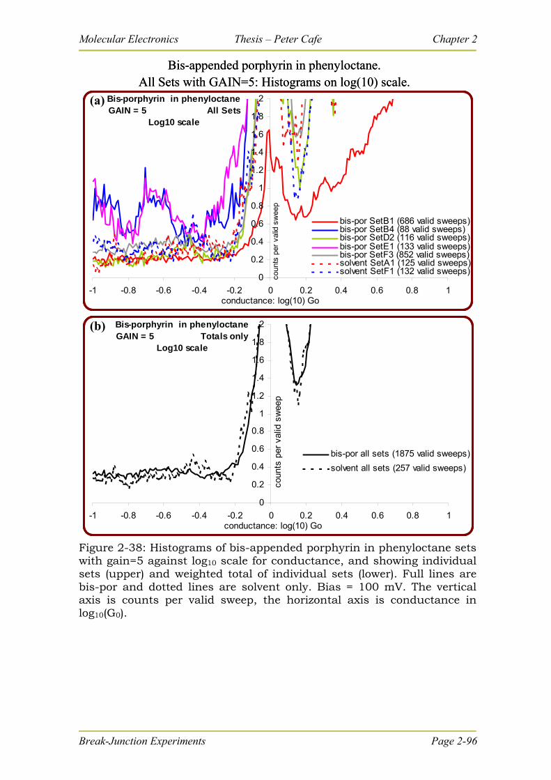
Molecular Electronics Thesis – Peter Cafe Chapter 2
Bis-porphyrin in phenyloctaneGAIN = 5 Totals only
Log10 scale
0
0.2
0.4
0.6
0.8
1
1.2
1.4
1.6
1.8
2
-1 -0.8 -0.6 -0.4 -0.2 0 0.2 0.4 0.6 0.8 1conductance: log(10) Go
coun
ts p
er v
alid
sw
eep
bis-por all sets (1875 valid sweeps)
solvent all sets (257 valid sweeps)
Bis-porphyrin in phenyloctaneGAIN = 5 All Sets
Log10 scale
0
0.2
0.4
0.6
0.8
1
1.2
1.4
1.6
1.8
2
-1 -0.8 -0.6 -0.4 -0.2 0 0.2 0.4 0.6 0.8 1conductance: log(10) Go
coun
ts p
er v
alid
sw
eep
bis-por SetB1 (686 valid sweeps)bis-por SetB4 (88 valid sweeps)bis-por SetD2 (116 valid sweeps)bis-por SetE1 (133 valid sweeps)bis-por SetF3 (852 valid sweeps)solvent SetA1 (125 valid sweeps)solvent SetF1 (132 valid sweeps)
Bis-appended porphyrin in phenyloctane.All Sets with GAIN=5: Histograms on log(10) scale.
(b)
(a)
Figure 2-38: Histograms of bis-appended porphyrin in phenyloctane sets with gain=5 against log10 scale for conductance, and showing individual sets (upper) and weighted total of individual sets (lower). Full lines are bis-por and dotted lines are solvent only. Bias = 100 mV. The vertical axis is counts per valid sweep, the horizontal axis is conductance in log10(G0).
Break-Junction Experiments Page 2-96
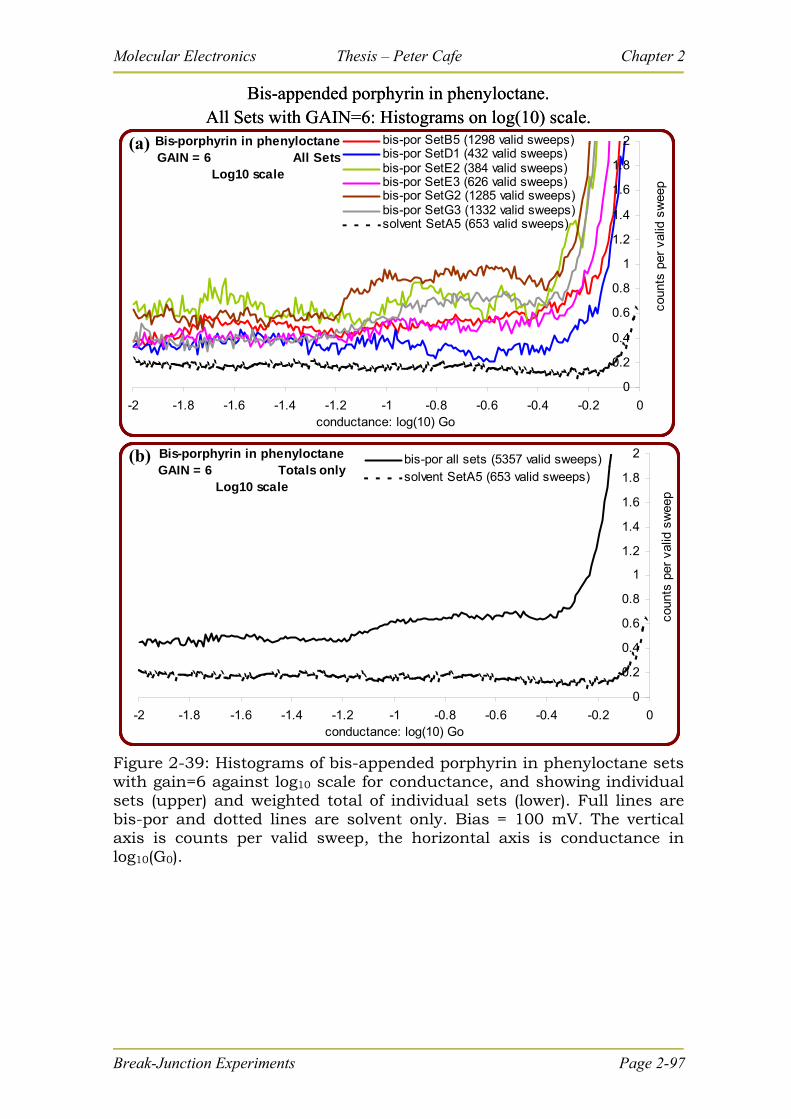
Molecular Electronics Thesis – Peter Cafe Chapter 2
Bis-porphyrin in phenyloctaneGAIN = 6 Totals only
Log10 scale
0
0.2
0.4
0.6
0.8
1
1.2
1.4
1.6
1.8
2
-2 -1.8 -1.6 -1.4 -1.2 -1 -0.8 -0.6 -0.4 -0.2 0conductance: log(10) Go
coun
ts p
er v
alid
sw
eep
bis-por all sets (5357 valid sweeps)solvent SetA5 (653 valid sweeps)
Bis-porphyrin in phenyloctaneGAIN = 6 All Sets
Log10 scale
0
0.2
0.4
0.6
0.8
1
1.2
1.4
1.6
1.8
2
-2 -1.8 -1.6 -1.4 -1.2 -1 -0.8 -0.6 -0.4 -0.2 0conductance: log(10) Go
coun
ts p
er v
alid
sw
eep
bis-por SetB5 (1298 valid sweeps)bis-por SetD1 (432 valid sweeps)bis-por SetE2 (384 valid sweeps)bis-por SetE3 (626 valid sweeps)bis-por SetG2 (1285 valid sweeps)bis-por SetG3 (1332 valid sweeps)solvent SetA5 (653 valid sweeps)
Bis-appended porphyrin in phenyloctane.All Sets with GAIN=6: Histograms on log(10) scale.
(b)
(a)
Figure 2-39: Histograms of bis-appended porphyrin in phenyloctane sets with gain=6 against log10 scale for conductance, and showing individual sets (upper) and weighted total of individual sets (lower). Full lines are bis-por and dotted lines are solvent only. Bias = 100 mV. The vertical axis is counts per valid sweep, the horizontal axis is conductance in log10(G0).
Break-Junction Experiments Page 2-97
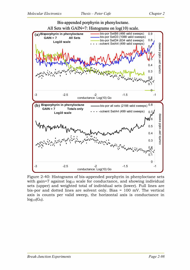
Molecular Electronics Thesis – Peter Cafe Chapter 2
Bisporphyrin in phenyloctaneGAIN = 7 Totals only
Log10 scale
0
0.1
0.2
0.3
0.4
0.5
0.6
0.7
0.8
-3 -2.5 -2 -1.5 -1conductance: Log(10) Go
coun
ts p
er v
alid
sw
eep
bis-por all sets (2188 valid sweeps)
solvent SetA4 (499 valid sweeps)
Bisporphyrin in phenyloctaneGAIN = 7 All Sets
Log10 scale
0
0.1
0.2
0.3
0.4
0.5
0.6
0.7
0.8
0.9
-3 -2.5 -2 -1.5 -1conductance: Log(10) Go
coun
ts p
er v
alid
sw
eep
bis-por SetB6 (466 valid sweeps)bis-por SetD3 (1088 valid sweeps)bis-por SetD4 (634 valid sweeps)solvent SetA4 (499 valid sweeps)
(b)
(a)
Bis-appended porphyrin in phenyloctane.All Sets with GAIN=7: Histograms on log(10) scale.
Figure 2-40: Histograms of bis-appended porphyrin in phenyloctane sets with gain=7 against log10 scale for conductance, and showing individual sets (upper) and weighted total of individual sets (lower). Full lines are bis-por and dotted lines are solvent only. Bias = 100 mV. The vertical axis is counts per valid sweep, the horizontal axis is conductance in log10(G0).
Break-Junction Experiments Page 2-98
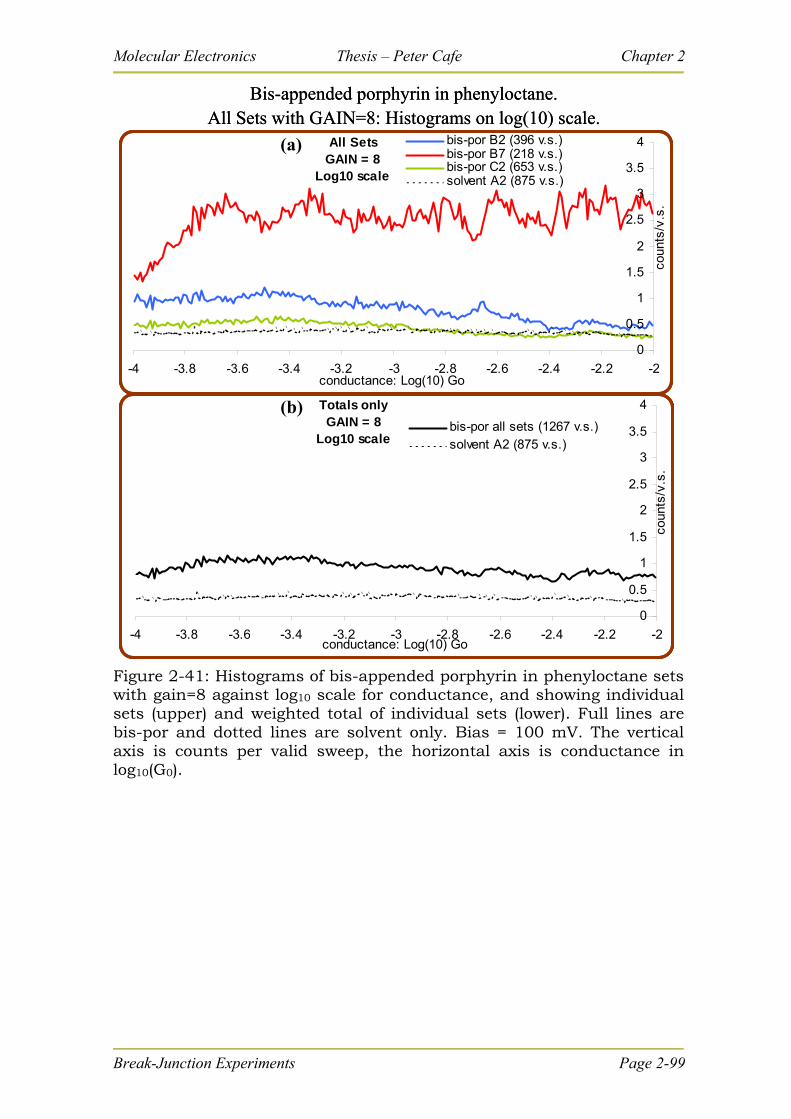
Molecular Electronics Thesis – Peter Cafe Chapter 2
Bis-appended porphyrin in phenyloctane.All Sets with GAIN=8: Histograms on log(10) scale.
All SetsGAIN = 8
Log10 scale
0
0.5
1
1.5
2
2.5
3
3.5
4
-4 -3.8 -3.6 -3.4 -3.2 -3 -2.8 -2.6 -2.4 -2.2 -2conductance: Log(10) Go
coun
ts/v
.s.
bis-por B2 (396 v.s.)bis-por B7 (218 v.s.)bis-por C2 (653 v.s.)solvent A2 (875 v.s.)
Totals onlyGAIN = 8
Log10 scale
0
0.5
1
1.5
2
2.5
3
3.5
4
-4 -3.8 -3.6 -3.4 -3.2 -3 -2.8 -2.6 -2.4 -2.2 -2conductance: Log(10) Go
coun
ts/v
.s.
bis-por all sets (1267 v.s.)solvent A2 (875 v.s.)
(a)
(b)
Figure 2-41: Histograms of bis-appended porphyrin in phenyloctane sets with gain=8 against log10 scale for conductance, and showing individual sets (upper) and weighted total of individual sets (lower). Full lines are bis-por and dotted lines are solvent only. Bias = 100 mV. The vertical axis is counts per valid sweep, the horizontal axis is conductance in log10(G0).
Break-Junction Experiments Page 2-99
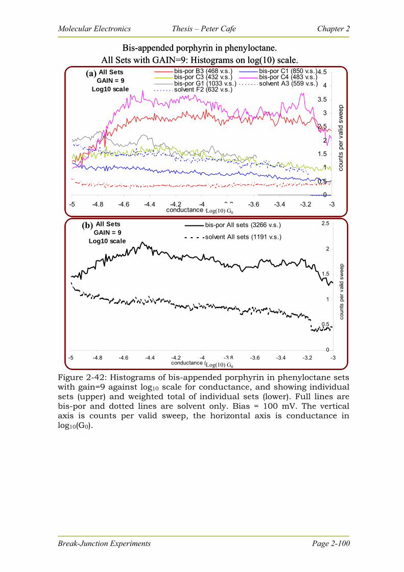
Molecular Electronics Thesis – Peter Cafe Chapter 2
Bis-appended porphyrin in phenyloctane.All Sets with GAIN=9: Histograms on log(10) scale.
All SetsGAIN = 9
Log10 scale
0
0.5
1
1.5
2
2.5
3
3.5
4
4.5
-5 -4.8 -4.6 -4.4 -4.2 -4 -3.8 -3.6 -3.4 -3.2 -3conductance (x10 -4 Go)
coun
ts p
er v
alid
sw
eep
bis-por B3 (468 v.s.) bis-por C1 (850 v.s.)bis-por C3 (432 v.s.) bis-por C4 (483 v.s.)bis-por G1 (1033 v.s.) solvent A3 (559 v.s.)solvent F2 (632 v.s.)
All SetsGAIN = 9
Log10 scale
0
0.5
1
1.5
2
2.5
-5 -4.8 -4.6 -4.4 -4.2 -4 -3.8 -3.6 -3.4 -3.2 -3conductance (x10^-4 Go)
coun
ts p
er v
alid
sw
eep
bis-por All sets (3266 v.s.)
solvent All sets (1191 v.s.)
(a)
(b)
Log(10) G0
Log(10) G0
Bis-appended porphyrin in phenyloctane.All Sets with GAIN=9: Histograms on log(10) scale.
All SetsGAIN = 9
Log10 scale
0
0.5
1
1.5
2
2.5
3
3.5
4
4.5
-5 -4.8 -4.6 -4.4 -4.2 -4 -3.8 -3.6 -3.4 -3.2 -3conductance (x10 -4 Go)
coun
ts p
er v
alid
sw
eep
bis-por B3 (468 v.s.) bis-por C1 (850 v.s.)bis-por C3 (432 v.s.) bis-por C4 (483 v.s.)bis-por G1 (1033 v.s.) solvent A3 (559 v.s.)solvent F2 (632 v.s.)
All SetsGAIN = 9
Log10 scale
0
0.5
1
1.5
2
2.5
-5 -4.8 -4.6 -4.4 -4.2 -4 -3.8 -3.6 -3.4 -3.2 -3conductance (x10^-4 Go)
coun
ts p
er v
alid
sw
eep
bis-por All sets (3266 v.s.)
solvent All sets (1191 v.s.)
(a)
(b)
Log(10) G0
Log(10) G0 Figure 2-42: Histograms of bis-appended porphyrin in phenyloctane sets with gain=9 against log10 scale for conductance, and showing individual sets (upper) and weighted total of individual sets (lower). Full lines are bis-por and dotted lines are solvent only. Bias = 100 mV. The vertical axis is counts per valid sweep, the horizontal axis is conductance in log10(G0).
Break-Junction Experiments Page 2-100
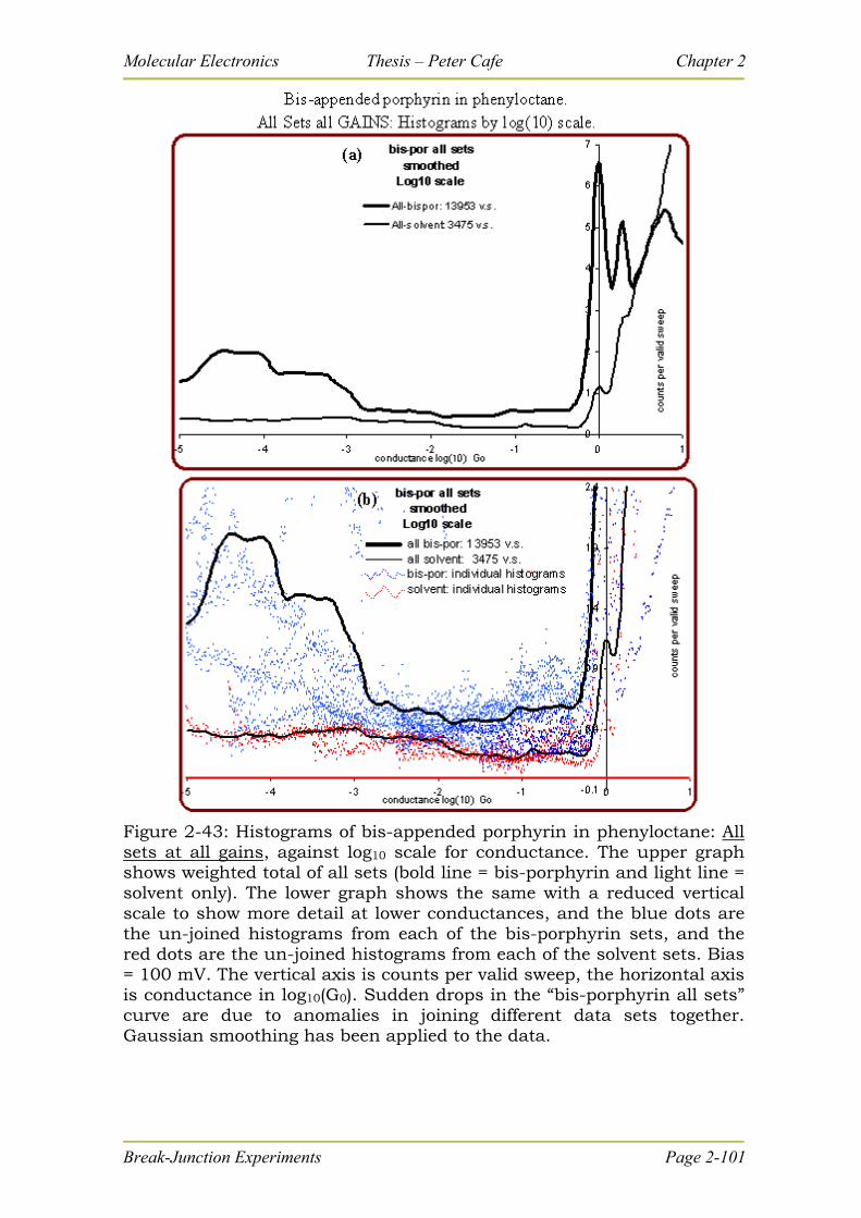
Molecular Electronics Thesis – Peter Cafe Chapter 2
Figure 2-43: Histograms of bis-appended porphyrin in phenyloctane: All sets at all gains, against log10 scale for conductance. The upper graph shows weighted total of all sets (bold line = bis-porphyrin and light line = solvent only). The lower graph shows the same with a reduced vertical scale to show more detail at lower conductances, and the blue dots are the un-joined histograms from each of the bis-porphyrin sets, and the red dots are the un-joined histograms from each of the solvent sets. Bias = 100 mV. The vertical axis is counts per valid sweep, the horizontal axis is conductance in log10(G0). Sudden drops in the “bis-porphyrin all sets” curve are due to anomalies in joining different data sets together. Gaussian smoothing has been applied to the data.
Break-Junction Experiments Page 2-101
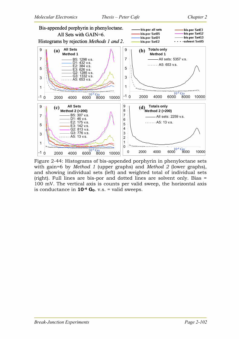
Molecular Electronics Thesis – Peter Cafe Chapter 2
All SetsMethod 2 (>200)
-1
1
3
5
7
9
0 2000 4000 6000 8000 10000
B5: 307 v.s.D1: 46 v.s.E2: 175 v.s.E3: 142 v.s.G2: 813 v.s.G3: 776 v.s.A5: 13 v.s.
Totals onlyMethod 1
-1
1
3
5
7
9
0 2000 4000 6000 8000 10000
All sets: 5357 v.s.
A5: 653 v.s.
All SetsMethod 1
-1
1
3
5
7
9
0 2000 4000 6000 8000 10000
B5: 1298 v.s.D1: 432 v.s.E2: 384 v.s.E3: 626 v.s.G2: 1285 v.s.G3: 1332 v.s.A5: 653 v.s.
Bis-appended porphyrin in phenyloctane.All Sets with GAIN=6.
Histograms by rejection Methods 1 and 2.
(a) (b)
Totals onlyMethod 2 (>200)
0123456789
0 2000 4000 6000 8000 10000
All sets: 2259 v.s.
A5: 13 v.s.
10-4 Go 10-4 Go
10-4 Go10-4 Go
(c) (d)All SetsMethod 2 (>200)
-1
1
3
5
7
9
0 2000 4000 6000 8000 10000
B5: 307 v.s.D1: 46 v.s.E2: 175 v.s.E3: 142 v.s.G2: 813 v.s.G3: 776 v.s.A5: 13 v.s.
Totals onlyMethod 1
-1
1
3
5
7
9
0 2000 4000 6000 8000 10000
All sets: 5357 v.s.
A5: 653 v.s.
All SetsMethod 1
-1
1
3
5
7
9
0 2000 4000 6000 8000 10000
B5: 1298 v.s.D1: 432 v.s.E2: 384 v.s.E3: 626 v.s.G2: 1285 v.s.G3: 1332 v.s.A5: 653 v.s.
Bis-appended porphyrin in phenyloctane.All Sets with GAIN=6.
Histograms by rejection Methods 1 and 2.
(a) (b)
Totals onlyMethod 2 (>200)
0123456789
0 2000 4000 6000 8000 10000
All sets: 2259 v.s.
A5: 13 v.s.
10-4 Go 10-4 Go
10-4 Go10-4 Go
(c) (d)
Figure 2-44: Histograms of bis-appended porphyrin in phenyloctane sets with gain=6 by Method 1 (upper graphs) and Method 2 (lower graphs), and showing individual sets (left) and weighted total of individual sets (right). Full lines are bis-por and dotted lines are solvent only. Bias = 100 mV. The vertical axis is counts per valid sweep, the horizontal axis is conductance in 10-4 G0. v.s. = valid sweeps.
Break-Junction Experiments Page 2-102
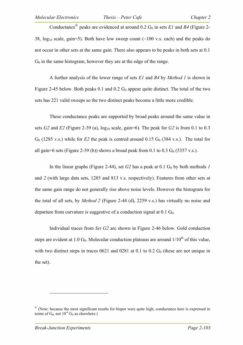
Molecular Electronics Thesis – Peter Cafe Chapter 2
Break-Junction Experiments Page 2-103
Conductance peaks are evidenced at around 0.2 G0 in sets E1 and B4 (Figure 2-
38, log10 scale, gain=5). Both have low sweep count (~100 v.s. each) and the peaks do
not occur in other sets at the same gain. There also appears to be peaks in both sets at 0.1
G0 in the same histogram, however they are at the edge of the range.
A further analysis of the lower range of sets E1 and B4 by Method 1 is shown in
Figure 2-45 below. Both peaks 0.1 and 0.2 G0 appear quite distinct. The total of the two
sets has 221 valid sweeps so the two distinct peaks become a little more credible.
These conductance peaks are supported by broad peaks around the same value in
sets G2 and E2 (Figure 2-39 (a), log10 scale, gain=6). The peak for G2 is from 0.1 to 0.3
G0 (1285 v.s.) while for E2 the peak is centred around 0.15 G0 (384 v.s.). The total for
all gain=6 sets (Figure 2-39 (b)) shows a broad peak from 0.1 to 0.3 G0 (5357 v.s.).
In the linear graphs (Figure 2-44), set G2 has a peak at 0.1 G0 by both methods 1
and 2 (with large data sets, 1285 and 813 v.s. respectively). Features from other sets at
the same gain range do not generally rise above noise levels. However the histogram for
the total of all sets, by Method 2 (Figure 2-44 (d), 2259 v.s.) has virtually no noise and
departure from curvature is suggestive of a conduction signal at 0.1 G0.
Individual traces from Set G2 are shown in Figure 2-46 below. Gold conduction
steps are evident at 1.0 G0. Molecular conduction plateaus are around 1/10th of this value,
with two distinct steps in traces 0621 and 0281 at 0.1 to 0.2 G0 (these are not unique in
the set).
(Note: because the most significant results for bispor were quite high, conductance here is expressed in terms of G0, not 10-4 G0 as elsewhere.)
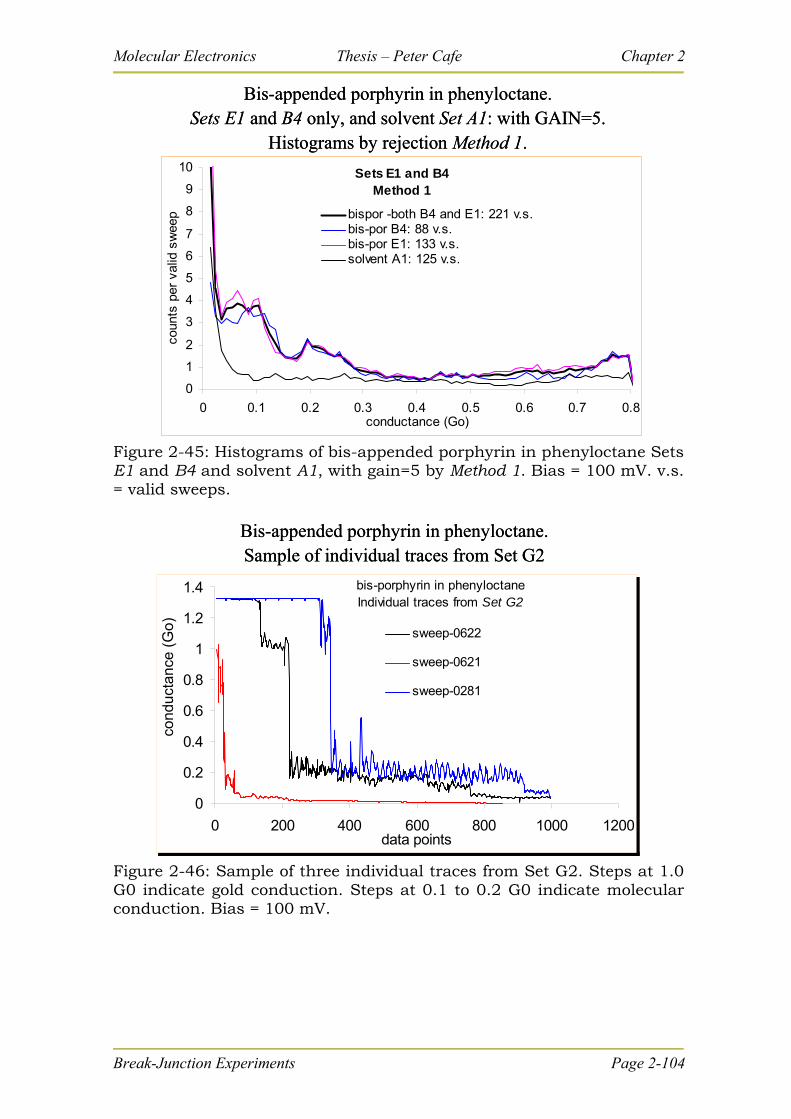
Molecular Electronics Thesis – Peter Cafe Chapter 2
Sets E1 and B4Method 1
0
1
2
3
4
5
6
7
8
9
10
0 0.1 0.2 0.3 0.4 0.5 0.6 0.7 0.8conductance (Go)
coun
ts p
er v
alid
sw
eep bispor -both B4 and E1: 221 v.s.
bis-por B4: 88 v.s.bis-por E1: 133 v.s.solvent A1: 125 v.s.
Bis-appended porphyrin in phenyloctane.Sets E1 and B4 only, and solvent Set A1: with GAIN=5.
Histograms by rejection Method 1.
Figure 2-45: Histograms of bis-appended porphyrin in phenyloctane Sets E1 and B4 and solvent A1, with gain=5 by Method 1. Bias = 100 mV. v.s. = valid sweeps.
bis-porphyrin in phenyloctaneIndividual traces from Set G2
0
0.2
0.4
0.6
0.8
1
1.2
1.4
0 200 400 600 800 1000 1200data points
cond
ucta
nce
(Go) sweep-0622
sweep-0621
sweep-0281
Bis-appended porphyrin in phenyloctane.Sample of individual traces from Set G2
bis-porphyrin in phenyloctaneIndividual traces from Set G2
0
0.2
0.4
0.6
0.8
1
1.2
1.4
0 200 400 600 800 1000 1200data points
cond
ucta
nce
(Go) sweep-0622
sweep-0621
sweep-0281
Bis-appended porphyrin in phenyloctane.Sample of individual traces from Set G2
Figure 2-46: Sample of three individual traces from Set G2. Steps at 1.0 G0 indicate gold conduction. Steps at 0.1 to 0.2 G0 indicate molecular conduction. Bias = 100 mV.
Break-Junction Experiments Page 2-104
Molecular Electronics Thesis – Peter Cafe Chapter 2
Break-Junction Experiments Page 2-105
Other log10 graphs (Figure 2-40 to Figure 2-43) do not show distinct peaks but a
general enhancement in conduction over the whole range, particularly in the range from
0.1 to 0.6 G0, and lower than 0.001 G0.
The gold quantized conduction peak (in total) is significantly enhanced (Figure 2-
43 (a)), however this is mainly due to Sets G2 and G3 (Figure 2-44 (a)). Other sets show
much smaller or no enhancement of the gold peak.
2.8.6 Discussion of bisporph results
A conduction event (or series of events) of bis-appended porphyrin is evidenced
at between 0.1 and 0.3 G0. There are two distinct peaks at 0.1 G0 and 0.2 G0. From the
available data it cannot be determined what configurations of the molecule are involved.
This is a much higher value than expected. Although theoretically the
conductance of a single porphyrin (freebased, without the two phenanthroline
appendages) has been calculated to be 0.997 G0 (Section 2.8.2.2), an experimental value
for a Zn based porphyrin is between 0.0001 and 0.05 G0 (Section 2.8.2.1). There are few
results to compare with and the variation in past research is quite high. The result here
does not necessarily contradict prior research.
One possible geometry is that the porphyrin is laying flat between the two tips of
the break-junction terminals, and that the conduction is primarily via the central copper
atom, which, because of the metallic throughway, would be expected to have high
conduction, near or just below 1.0 G0. The broad value of the present result is not
inconsistent with this scenario. However it is difficult under this scenario to explain the
presence of two conductance peaks at 0.1 and 0.2 G0.
Molecular Electronics Thesis – Peter Cafe Chapter 2
Break-Junction Experiments Page 2-106
Another possible geometry is that the porphyrin is standing lengthwise between
the two break-junction terminals with its phenanthroline ends joining the two gold
terminals. The individual traces, 0622 and 0281 (Figure 2-46) indicate two steps, one at
0.2 G0 and another at 0.1 G0. These may indicate the conductance of two and one bis-por
molecules respectively. If they do, then the porphyrin could not be lying flat between the
two electrodes. Two molecules can bridge the gap simultaneously only if they are
positioned lengthwise.
Bispor enhances conduction over a broad range (Figure 2-43), but not
consistently, suggesting that the mechanism is not a general mechanism but specific to
the conduction of bispor given the experimental parameters (gold terminals, solvent
interactions, etc). In general it was quite difficult to obtain consistent data for the bis-
porphyrin with many sets appearing little different to the solvent-only sets or having no
distinct features other than a broad enhancement of conduction.
Prior research has ascribed a peak at 0.2 G0 to a carbon atom in the gold chain
(“After several hours of experiment 500 curves gave a peak at about 0.2 G0, whose
occurrence increases with time”.94), however in that work there is no mention of a peak
at 0.1 G0 or of two peaks. Here such peaks do not appear in the solvent only histograms.
So this explanation is dismissed.
In only two sets was the gold conduction step significantly enhanced by the
addition of bispor. This indicates that the molecule has difficulty attaching “properly” to
the gold and this was only significantly achieved in those two sets. By “properly” it is
meant that the molecule attaches by one of its phenanthroline-type alligator clips.
Molecular Electronics Thesis – Peter Cafe Chapter 2
2.8.7 Conclusion of bispor results
Some results show a conduction event for bisappended porphyrin in
phenyloctane at 0.1 G0, with a second conduction event at 0.2 G0. The presence of two
peaks, one a multiple of the other, may lead to speculation that it is the conduction of one
and two bispor molecules standing vertically between the gold terminals with the
phenanthroline “alligator clips” joining the electrodes. However it is an extremely high
value which has no support from other sources, and so it is sagacious to avoid such a
rash conclusion. It may simply be due to the bispor molecule laying flat between the
gold electrodes, or it may be a solvent effect. However the peak should be noted even
though it cannot be conclusively explained.
Bispor can interact with the gold at one end, which is evidenced by the increase
in the gold conduction steps, however this wasn’t always achieved, most likely due to
solvent interactions. The gold-bispor attachment may be susceptible to subtle changes in
the concentration (which would vary over time due to solvent evaporation) or other
experimental factors.
Break-Junction Experiments Page 2-107
Molecular Electronics Thesis – Peter Cafe Chapter 2
Break-Junction Experiments Page 2-108
2-9 General conclusion to Chapter 2: break-
junction experiments
Conclusions relating to the specific molecules are outlined in the relevant
sections above and need not be repeated here. General conclusions from the whole series
of experiments are expressed below.
Experiments on 1,8-octanedithiol have established that the method and
equipment are adequate.
The observation of the enhancement of the gold conduction step at 1.0 G0 has
emerged as an indicator that the molecule can interact with gold. That is, it attaches to
the gold by its azine or thiol “alligator clip”. Drawing upon results of Chapters 3 and 4,
the molecule is bound to a gold adatom and the adatom-molecule unit is highly mobile
and can extend the time for which a single-atom gold chain exists during the break-
junction experiment.
Should this enhancement of the gold peak not occur, it is unlikely that the
experiment will go on to produce signals for the conduction of a single molecule. That is,
if one end cannot attach, it is unlikely that two ends will attach in a specific geometric
alignment.
For this reason the general increase in conduction of pyrazine in aqueous solution
at a high range can be dismissed as a solvent dominated phenomenon, as there was no
prior indication that the pyrazine attached independently to the gold (i.e. the gold peak
was not enhanced by the addition of pyrazine).
Despite prior research to the contrary,101 the solvent was observed to play an
important role in the conduction behaviour of many molecules. The difference here is
Molecular Electronics Thesis – Peter Cafe Chapter 2
that the molecules in which this observation was made all relied on azine linkers to the
gold electrode (the prior research looked at 1,8-octanedithiol in toluene, dodecane, water,
and 0.1M NaClO4). Future break-junction experiments on molecules with conjugated
rings and/or azine linkers will require a careful selection of solvent(s) and experimental
conditions (such as electrochemical control) to isolate these effects.
The use of log10 scale histograms has surfaced as a powerful tool for observing
long range enhancement of conduction of the molecule over the solvent alone, which has
received little attention until now. It identifies the fact that multiple configurations of the
molecule are possible between the break-junction electrodes to produce this broad range,
and these configurations include solvent effects. With many configurations possible it is
quite difficult to isolate the configuration that indicates the conduction of a single
molecule (if such a single configuration exists within the experimental parameters).
All the experiments on molecules with azine alligator clips would be enhanced
by a tool that enabled electrochemical control of the liquid cell to break to solvent
dominated effects and drive the molecule to attach to the gold terminals.
Break-Junction Experiments Page 2-109

Molecular Electronics Thesis – Peter Cafe Chapter 2
Break-Junction Experiments Page 2-110
(blank page)
Molecular Electronics Thesis – Peter Cafe Chapter 3
Phenanthroline Monolayers Page 3-1
ChaptteerChap r 3 Cheemiissorrbeed and Physsiissorrbeed
Sttrrucctturreess fforr 1,,10--Pheenantthrrolliinee and
Diipyrriido[[3,,2--a::2′′,,3′′--cc]]pheenazziinee on
Au((111))
3 Ch m o b d and Phy o b d
S u u o 1 10 Ph nan h o n and
D py do 3 2 a 2 3 ph na n on
Au 111
3-0 Synopsis for Chapter 3 Scanning tunnelling microscopy (STM) images of 1,10-phenanthroline (PHEN)
and dipyrido[3,2-a:2′,3′-c]phenazine (DPPZ) on Au(111) are recorded using both in situ
and ex situ techniques. The images of PHEN depict regimes of physisorption (relatively
weak bonding) and chemisorption (relatively strong bonding with rearrangement of
covalent bonds or structure) whilst DPPZ is only physisorbed. All physisorbed
structures are not pitted and fluctuate dynamically, involving aligned (4 4) surface
domains with short-range (ca. 20 molecules) order for PHEN but unaligned chains with
medium-range (ca. 100 molecules) order for DPPZ. In contrast, the chemisorbed PHEN
monolayers remain stable for days, are associated with surface pitting, and form a (4
13)R46 lattice with long-range order. The density of pitted atoms on large gold
terraces is shown to match the density of chemisorbed molecules, suggesting that gold
adatoms link PHEN to the surface. For PHEN, chemisorbed and physisorbed adsorbate
structures are optimised using plane-wave density-functional theory (DFT) calculations
Molecular Electronics Thesis – Peter Cafe Chapter 3
for the surface structure. Realistic binding energies are then obtained adding dispersive
corrections determined using complete-active-space self-consistent field calculations
using 2nd-order perturbation theory (CASPT2) applied to cluster-interaction models. A
fine balance between the large adsorbate-adsorbate dispersive forces, adsorbate-surface
dispersive forces, gold ligation energy, and surface mining energy is shown to dictate the
observed phenomena, leading to high surface mobility and substrate/surface lattice
incommensurability. Increasing the magnitude of the dispersive forces through use of
DPPZ rather than PHEN to disturb this balance produced physisorbed monolayers
without pits and/or surface registration but with much longer-range order. Analogies are
drawn with similar but poorly understood processes involved in the binding of thiols to
Au(111).
Theoretical calculations in this chapter were performed by Ante Bilic and Jeffery
Reimers.
Phenanthroline Monolayers Page 3-2
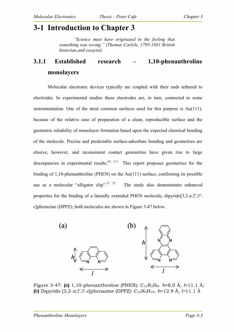
Molecular Electronics Thesis – Peter Cafe Chapter 3
3-1 Introduction to Chapter 3 “Science must have originated in the feeling that
something was wrong.” (Thomas Carlyle, 1795-1881 British historian and essayist)
3.1.1 Established research – 1,10-phenanthroline
monolayers
Molecular electronic devices typically are coupled with their ends tethered to
electrodes. In experimental studies these electrodes are, in turn, connected to some
instrumentation. One of the most common surfaces used for this purpose is Au(111),
because of the relative ease of preparation of a clean, reproducible surface and the
geometric reliability of monolayer formation based upon the expected chemical bonding
of the molecule. Precise and predictable surface-adsorbate bonding and geometries are
elusive, however, and inconsistent contact geometries have given rise to large
discrepancies in experimental results.43, 111 This report proposes geometries for the
binding of 1,10-phenanthroline (PHEN) on the Au(111) surface, confirming its possible
use as a molecular “alligator clip”.37, 57 The study also demonstrates enhanced
properties for the binding of a laterally extended PHEN molecule, dipyrido[3,2-a:2′,3′-
c]phenazine (DPPZ); both molecules are shown in Figure 3-47 below.
N N
NNh
l
N N
l
h
(a) (b)
N N
NNh
l
N N
l
h
(a) (b)
Figure 3-47: (a) 1,10-phenanthroline (PHEN): C12N2H8. h=8.0 Å, l=11.1 Å; (b) Dipyrido [3,2-a:2′,3′-c]phenazine (DPPZ): C18N4H10. h=12.9 Å, l=11.1 Å
Phenanthroline Monolayers Page 3-3
Molecular Electronics Thesis – Peter Cafe Chapter 3
Phenanthroline Monolayers Page 3-4
3.1.1.1 1,10-phenanthroline on Au(111)
1,10-Phenanthroline monolayers from aqueous solution on Au(111) were first
observed by Cunha, Jin and Tao by means of electrochemical Scanning Tunnelling
Microscopy (in-situ STM) and shown to form locally ordered, complex and variable
structures (1997).48 Important features of the monolayer noted in that study include:
1. The monolayer forms spontaneously.
2. The molecules stand with their axes vertical to the substrate surface and the
nitrogen atoms facing the surface.
3. They form long chains of stacked molecules (like rolls of coins).
4. The PHEN molecules in each chain are aligned at 60° to the chain, with each
molecule stacked slightly off-centre to its neighbours.
5. Stacking faults may occur along the chain, commonly forming groups of only 3,
6 or 9 fully aligned PHEN molecules.
6. Reversible phase transitions in the monolayer (order to disorder to order, etc.)
occur with variations in the electrochemical potential of the substrate working
electrode, attributed112 to the large molecular dipole moment.
7. The monolayers can produce pits in the surface with a depth of typically one
gold layer.
8. The pit sizes increase with increasing gold-substrate potential and decrease
(and/or “islands” are formed) when this potential is then decreased.
9. Each PHEN molecule is observed in “high-resolution” (topology differential)
images as two small bright features 3 Å apart indicating the alignment of the
aromatic plane with respect to the chain propagation direction. The most intense
signal in regular topology images has recently been attributed to the hydrogen
atoms opposite the nitrogen head group.112
Molecular Electronics Thesis – Peter Cafe Chapter 3
Phenanthroline Monolayers Page 3-5
In order to analyse the PHEN structure for its possible use as an “alligator clip”
linking covalently attached functional molecular units to the gold surface, enhanced
regularity in its monolayers must be obtained, and possible effects due to interactions
between attached groups on neighbouring molecules must be anticipated. For example,
if strong surface – head group interactions control the monolayer structure, then the
structure should be insensitive to the properties of attached entities other than, say,
strong steric repulsions that they may induce. If the inter-PHEN interactions are
significant, however, then the nature of the interactions between the attached units would
always be critical. The net effect for PHEN-based systems is that means must be
obtained for either eliminating or controlling the inherent PHEN stacking faults, phase
transitions, pit formation, and long to medium range monolayer irregularity;
understanding the basic nature of the surface – head group and intra-monolayer
interactions are critical to this process.
3.1.1.2 1,10-phenanthroline on Cu(111)
The structure of PHEN on Cu(111) has also been observed113 and has many
features in common with that on Au(111) including the presence of ordered regions with
very similar structure. As the lattice vectors for Cu(111) are 12% shorter than those for
Au(111), this implies that the surface and substrate lattices are unrelated and hence the
metal to head group interaction is of secondary importance. However there are also
important differences such as increased long range order on Cu(111), no pitting on
Cu(111), and a most significant change in the alignment of adlayer domains: these are
only found at 120° orientations on Au(111) but occur at all angles on Cu(111). The
nature of the interaction between PHEN and Au(111) thus remains an open question.
Molecular Electronics Thesis – Peter Cafe Chapter 3
Phenanthroline Monolayers Page 3-6
3.1.1.3 Surface pitting in monolayers on Au
Of the issues raised for PHEN monolayers on Au(111), the one that is most
general is that of surface pitting. Cunha et al.48 attributed the surface pitting to surface
stress induced by the strong adsorption of the PHEN molecules on the surface, following
the explanation expounded earlier by McDermott et al.114 for pitting during thiol-based
Au(111) monolayer formation. Thiols are known to form strong covalent chemisorptive
bonds with gold,115 in contrast to the weaker interactions expected for the binding of
nitrogen-based electron donors including bidentate ligands such as PHEN48 and 2,3′-
bipyridine49, 116 as well as monodentate ligands such as pyridine,117-119 ammonia,118, 120
and amines.42 Nevertheless, pitting is observed in monolayers of all of these classes of
bindings, making this phenomenon of general interest. The observed structure of PHEN
on Cu(111) which is clearly due to physisorption and involves no pitting provides a
useful reference system.113
3.1.2 Experimental presentments of this chapter –STM
images
This chapter presents STM images of PHEN on Au(111). These images are
obtained by varying the type of substrate used, the conditions of monolayer formation,
including the degree and nature of electrochemical control, the solvents used in
monolayer formation and in monolayer imaging (aqueous and non-aqueous), the size of
the terraces on the Au(111) surface, and the monolayer maturation time. The motivation
for this work is to find motifs from amongst the demonstrated48 wide range available that
enhance regularity, enable monolayer control, and reveal the nature of the forces that
control the monolayer structure. Some images, recorded as a function of time during
Molecular Electronics Thesis – Peter Cafe Chapter 3
monolayer formation using in situ STM techniques,115, 121 show evidence for an initial
scenario in which there is no pitting and the monolayer changes dynamically between
structures with fixed surface registration. Other images recorded after pre-preparation of
the monolayer, show a stable pitted phase. The density of the pits, and the nature of the
structure observed in high-resolution images are determined. Also presented are the first
STM images of dipyrido [3,2-a:2′,3′-c]phenazine (DPPZ) on Au(111), a laterally
extended PHEN derivative that shows the type of extended conjugation that may be
useful in a molecular device attached to a PHEN–type alligator clip.37, 57 This part of the
study allows the monolayer formation conditions to be varied through changes to the
intermolecular interactions between adsorbate molecules.
3.1.3 Theoretical presentments of this chapter – DFT etc
The observed PHEN and DPPZ surface patterns are then interpreted using plane-
wave Density-Functional Theory (DFT) to simulate the structure of physisorbed and
chemisorbed monolayers, with chemisorption predicted to involve the formation of gold
adatoms above the (111) surface that chelate the adsorbed molecules. These calculations
are supported by 2nd-order Møller-Plesset perturbation theory (MP2) and Complete-
Active-Space Self-Consistent-Field (CASSCF) combined with MP2 calculations122
(CASPT2), of the dispersive intermolecular and physisorptive forces. These forces are
not included in modern DFT functionals and do not account for the strong attraction that
occurs between PHEN (and DPPZ) molecules112 and between gold and aromatic
molecules.102 The combination of CASPT2 with DFT provides a comprehensive
description of phenanthroline-based binding to gold, exposing many issues of direct
relevance to the chemisorption of thiols and amines to gold.
Phenanthroline Monolayers Page 3-7
Molecular Electronics Thesis – Peter Cafe Chapter 3
Phenanthroline Monolayers Page 3-8
3-2 Methods of Chapter 3
3.2.1 Chemicals.
1,10-Phenanthroline was purchased from Aldrich and used as received. Dipyrido[3,2-
a:2′,3′-c]phenazine was synthesized from 1,10-phenanthroline-5,6-dione using the
method of Amoouyal et al.123 with 98% yield. It was purified using silica
chromatography followed by recrystallisation from chloroform/pentane. Phenyloctane
was used as supplied from Fluka (Purum Grade; > 98% purity with boiling point 264-
268 C). Millipore water from a Milli-Q 18.2 m cm filter was used throughout.
3.2.2 Ex situ STM of pre-assembled PHEN monolayers.
Glassware was cleaned in Piranha solution and rinsed copiously in water. Gold
on mica substrates were purchased from Molecular Imaging and annealed by a hydrogen
flame for a few minutes prior to use. PHEN was dissolved in water by ultrasonication
for 30 min at ~ 50 ºC and a 30 mM PHEN solution in 0.1 M NaClO4 was prepared. The
monolayer was formed from the aqueous solution with an applied potential of +0.7 V vs.
SCE to the gold working electrode for an hour using a potentiostat with a calibrated 0.25
mm platinum wire as the reference and counter electrodes. The sample was then gently
rinsed several times with water and three times with ethanol (99.9% decanted from bulk
as received from Redox Pty Ltd) and left standing (in air) for at least a day. The pre-
assembled monolayers remained stable for at least several days under ambient conditions
as well as throughout STM imaging.
The STM images were obtained by a Molecular Imaging Picoscan II instrument;
the STM tips were made from Pt0.8/Ir0.2 wire cut using precision wire snips. A PTFE
(poly-tetra-fluoro-ethylene) liquid cell was used with phenyloctane as the imaging
medium.
Molecular Electronics Thesis – Peter Cafe Chapter 3
Phenanthroline Monolayers Page 3-9
3.2.3 In situ STM of PHEN and DPPZ monolayers on
single-crystal gold electrodes.
Glassware was cleaned by boiling in 15% nitric acid solution and rinsed
copiously in Millipore water. Gold substrates were electropolished in 0.1 M H2SO4 at
~20 V DC bias, then rinsed successively in 1.0 M HCl and water, and annealed at 850 ºC
for 6 hours. Before use, the Au(111) was further freshly annealed by a hydrogen flame
and quenched in Millipore water which was saturated with H2. The STM images were
recorded using a Molecular Imaging Picoscan (USA) instrument using tips cut from 0.25
mm tungsten wire, sharpened by electrochemical etching (approx 15 V AC in approx 1.0
M KOH), and insulated by coating with Apiezon wax. Potential measurements were
made using a platinum reference electrode that was calibrated against a SCE electrode
after each measurement.
For the experiments on PHEN monolayers, a home-made Au(111)-electrode was
used.124-126 Single crystal beads were prepared by melting gold wire (99.999%, Ø 1.0
mm), with the (111) surface selected using a laser and fixed in position using a polymer
adhesive before polishing. A solution of 0.36 mM PHEN and 50 mM KClO4 (Sigma-
Aldrich 99.99%) in water pH 6.5 (HClO4, Fluka, Ultrapure) was freshly prepared and
added to the STM cell to form the monolayers.
For the experiments on DPPZ, the adsorbate was dissolved in Analytical Grade
ethanol using a sonicator. The Au(111)-substrate was a disk 12 mm in diameter and ~1
mm thick (Surface Preparation Laboratories, The Netherlands). The substrate was
exposed to the solution for 24 hours with no potential control, rinsed with Millipore
Molecular Electronics Thesis – Peter Cafe Chapter 3
Phenanthroline Monolayers Page 3-10
water, and mounted in the microscope. Imaging was conducted under potential control
in a 0.1 M phosphate buffer at pH 6.9.
3.2.4 Electrochemistry.
Reductive desorption experiments were conducted in a standard electrochemical
cell using the CH Instrument 900B potentiostat. The reductive desorption experiments
were carried out in either 0.1M KOH/water or 0.1M KClO4/water solution. In both cases
the solution had been de-aerated with nitrogen for 30 min. Recorded voltammograms
showed clear indication of a reductive desorption current present in the first scan, which
disappeared in subsequent scans. The current caused by the reductive desorption was
determined as the difference between the first and second scan. Integration of this curve
gave a precise measure of the average density of the monolayer. More details are
provided in Appendix 7-3.
3.2.5 Calculations of adsorbates on gold surfaces.
All computations involving surfaces were carried out using the Vienna Ab initio
Simulation Package (VASP),127, 128 A plane-wave basis set was employed to expand the
electronic wave functions using ultrasoft pseudopotentials,129, 130 which allows the use of
a low energy cut-off for the plane-wave basis set. The functional of Perdew and Wang
(PW91),131 a form of the generalized gradient approximation (GGA), was used
throughout to model the electron-electron exchange and correlation interactions. The
relaxation of atom positions was performed using a conjugate-gradient optimisation
procedure.
The gold surface was modelled using supercells consisting of gold slabs three
atomic layers thick separated by a vacuum region of 10-layer equivalent thickness;
periodic boundary conditions were applied in all three Cartesian directions. While
Molecular Electronics Thesis – Peter Cafe Chapter 3
Phenanthroline Monolayers Page 3-11
improved convergence of the results could have been obtained by expanding the lattice
to four layers thick, the improvements produced would be much less than other
shortcomings of the calculations and so are not warranted. The interlayer spacing was
taken from the analogously computed132 value of the gold bulk lattice parameter, 4.2 Å,
giving bulk Au-Au bond lengths of 2.970 Å, 3% longer than the observed value of 2.885
Å. All calculations included 16 gold atoms per layer. In low-coverage calculations, a
single molecule was placed in the vacuum region on the upper side of the slab. This
represents 1/16 ML coverage relative to surface atoms, sufficiently low that the
molecules in adjacent cells are well separated. In high-coverage calculations, three
PHEN molecules were included per unit cell, giving a density in accord with the high-
density phase observed experimentally. Mostly, a (4 4) supersurface cell was used,
resulting in the PHEN molecules being ordered into linear chains. To examine the
observed stacking faults in linear chains, some calculations were also performed using a
(4 13)R46º supersurface lattice. Wood’s notation133 is used to name the surface
lattices. For both lattices, Brillouin-zone integrations were conducted on a 3 × 3 × 1 k-
point Monkhorst-Pack grid with a Methfessel-Paxton smearing134 of 0.2 eV. VASP
calculations pertinent to gas-phase molecules employed cells of the same size as the
supercells, an integration using the k-point only and a Gaussian smearing of only 0.01
eV. An energy of 348 eV, dictated by the pseudopotential of nitrogen, was set for the
plane-wave basis-set cut-off in all computations. All calculations were performed spin
unpolarised without correction for the dipole moment135 of the sample as test
calculations indicated that these effects were insignificant in the present context.
Molecular Electronics Thesis – Peter Cafe Chapter 3
3.2.6 Calculations on models used to investigate dispersive
interactions.
Calculations were performed for both PHEN dimers at their surface-optimised
geometries and for PHEN above either a sheet of 16 gold atoms representing the surface
or this sheet with an additional adatom above it. The calculations on the PHEN dimers
were performed using GAUSSIAN-03136 for the PW91 density functionals and using
TURBOMOLE137 for the MP2 methodology; these employed the extensive 6-31++G**
basis set,138 required by the close spacing found between the molecules in the monolayer.
The PW91 calculations on the PHEN-sheet systems were performed by GAUSSIAN-03
whilst the CASPT2 calculations were performed using MOLCAS-5.2,139 all with the 6-
31G basis set138 for C, N, and H and LANL2DZ140 for Au. The CASPT2 calculations
included either 10 (for the flat Au sheet) or 11 (for the sheet with the adatom) electrons
in 13 active orbitals. All energies were corrected for basis-set superposition error.141
Phenanthroline Monolayers Page 3-12
Molecular Electronics Thesis – Peter Cafe Chapter 3
Phenanthroline Monolayers Page 3-13
3-3 Results of Chapter 3
3.3.1 In situ STM studies of PHEN monolayer formation.
To calibrate the STM instrument, the single-crystal gold substrates were scanned
and results showing the gold (22 3) reconstruction lines are provided in Supporting
Information Figure Appendix-3-82. Also provided therein are images of poorly ordered
monolayers taken during the early stages of monolayer formation (Figure Appendix-3-
83), images of an atypical highly ordered domain (Figure Appendix-3-82), images of
overlapping regions (Figure Appendix-3-85 and Figure Appendix-3-86), and
experimental details describing how sub-molecular resolution is obtained. From these
figures it is clear that uncontrolled drift of the STM tip across the surface is negligible
throughout the experiment.
A revealing high-resolution in situ STM image of the surface is shown in Figure
3-48 below. It was obtained in the constant-current mode with the height of the tip
constantly adjusted by a feedback loop to maintain the tunnelling current at a set-point
value. While it is usual to show the height of the tip as a function of the scan (a
topography image), Figure 3-48 shows instead the deviation of the current from the set-
point value, presenting for this system higher-resolution information than that found in
the topology image. In the limit of large STM feedback, the current-deviation is small
and the image formally depicts the first derivative of the topology with respect to the
(left to right) scan direction. Further discussion of the nature of the imaging process is
referred to Section 7.3.2 wherein topology (STM tip height) and derivative (set-point
current deviation) images are compared.
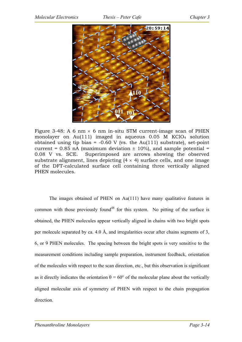
Molecular Electronics Thesis – Peter Cafe Chapter 3
101_
101_
011_
011_
110_
110_
101_
101_
011_
011_
110_
110_
Figure 3-48: A 6 nm 6 nm in-situ STM current-image scan of PHEN monolayer on Au(111) imaged in aqueous 0.05 M KClO4 solution obtained using tip bias = -0.60 V (vs. the Au(111) substrate), set-point current = 0.85 nA (maximum deviation 10%), and sample potential = 0.08 V vs. SCE. Superimposed are arrows showing the observed substrate alignment, lines depicting (4 4) surface cells, and one image of the DFT-calculated surface cell containing three vertically aligned PHEN molecules.
The images obtained of PHEN on Au(111) have many qualitative features in
common with those previously found48 for this system. No pitting of the surface is
obtained, the PHEN molecules appear vertically aligned in chains with two bright spots
per molecule separated by ca. 4.0 Å, and irregularities occur after chains segments of 3,
6, or 9 PHEN molecules. The spacing between the bright spots is very sensitive to the
measurement conditions including sample preparation, instrument feedback, orientation
of the molecules with respect to the scan direction, etc., but this observation is significant
as it directly indicates the orientation = 60 of the molecular plane about the vertically
aligned molecular axis of symmetry of PHEN with respect to the chain propagation
direction.
Phenanthroline Monolayers Page 3-14
Molecular Electronics Thesis – Peter Cafe Chapter 3
The STM image shown in Figure 3-48 is regular throughout domains but three
domain boundaries are evident within the image. The smallest reproducible unit of the
surface structure has cell vectors of length 11.1 Å at an internal angle of 122, consistent
with a (4 4) supersurface layer. On this single-crystal gold substrate, the adlayer
surface-cell vectors all align to within 2 to the substrate [
101 ], [ ], and [
110 110
]
crystallographic directions. In Table 3-16 below the observed surface cell properties are
compared to those of the Au(111) surface and those from DFT simulations (see Section
3.3.5); the observed substrate dimensions are in excellent agreement (5%) with those
expected for an ordered (4 4) layer. Alternation between two of the three possible
orientations of the cell vectors on the surface gives rise to the domain boundaries seen in
the figure, as indicated by the superimposed lines. Each cell contains three pairs of
bright spots indicating that three PHEN molecules comprise this repeat unit. Indeed, the
observed surface coverage of density of = 0.18 PHEN molecules per surface Au atom
is consistent with this implied 3:16 ratio. Note that while the observed substrate surface-
cell dimensions for PHEN on Au(111) are very similar to those observed113 on Cu(111),
the observation of strict alignment of the adsorbate lattice with the substrate indicates
that these systems are qualitatively different in nature.
Phenanthroline Monolayers Page 3-15
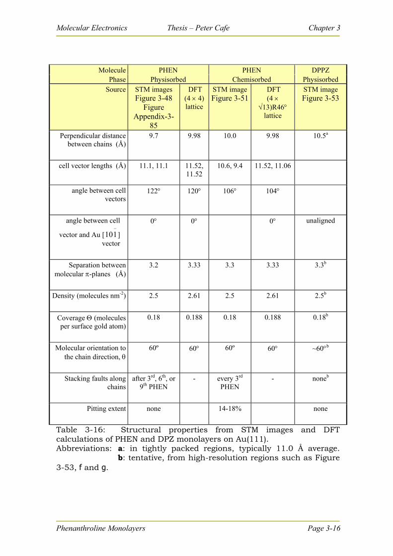
Molecular Electronics Thesis – Peter Cafe Chapter 3
Molecule PHEN PHEN DPPZ Phase Physisorbed Chemisorbed Physisorbed
Source STM images Figure 3-48
Figure Appendix-3-
85
DFT (4 4) lattice
STM image Figure 3-51
DFT (4
13)R46 lattice
STM image Figure 3-53
Perpendicular distance between chains (Å)
9.7 9.98 10.0 9.98 10.5a
cell vector lengths (Å) 11.1, 11.1 11.52, 11.52
10.6, 9.4 11.52, 11.06
angle between cell vectors
122 120 106 104
angle between cell
vector and Au [ ] vector
110
0 0 0 unaligned
Separation between molecular -planes (Å)
3.2 3.33 3.3 3.33 3.3b
Density (molecules nm-2) 2.5 2.61 2.5 2.61 2.5b
Coverage (molecules per surface gold atom)
0.18 0.188 0.18 0.188 0.18b
Molecular orientation to the chain direction,
60º 60 60º 60 ~60b
Stacking faults along chains
after 3rd, 6th, or 9th PHEN
- every 3rd PHEN
- noneb
Pitting extent none 14-18% none
Table 3-16: Structural properties from STM images and DFT calculations of PHEN and DPZ monolayers on Au(111). Abbreviations: a: in tightly packed regions, typically 11.0 Å average. b: tentative, from high-resolution regions such as Figure 3-53, f and g.
Phenanthroline Monolayers Page 3-16
Molecular Electronics Thesis – Peter Cafe Chapter 3
The observed domain boundaries for PHEN on Au(111) are associated with
stacking-fault dislocations of the chains by one Au-Au bond vector (one quarter of a unit
cell vector) in the [ ] direction. An image of three stacked molecules in a (4 4)
surface cell taken from DFT calculations (see Section
110
3.3.5) is superimposed on Figure
3-48 above. Its properties are consistent with all of the STM observations. Further, this
structural motif can account for the myriad of patterns48 observed for PHEN monolayers
simply by changing the pattern of the stacking faults. A longer-range perception of the
structure imaged in Figure 3-48 is provided in Figure Appendix-3-85 where the STM
scans of overlapping regions are provided. Figure Appendix-3-86 also provides images
of an extended surface region containing just one domain.
The images shown in Figure Appendix-3-83 indicate that after initial exposure of
the Au(111) to PHEN, long chains of PHEN molecules form but these chains are not
ordered with respect to either each other or the substrate. With time ordered structures
such as those in Figure 3-48 appear but these continue to fluctuate, as indicated in Figure
Appendix-3-85. The monolayer is thus one reflecting dynamic equilibrium between a
large number of structures each typically with good short-range order, i.e. order within
the (4 4) cells, but poor medium-range order, i.e., only 6 to 20 of these cells form
together into ordered domains.
3.3.2 Electrochemistry of PHEN monolayers.
The difference between the first and second sweeps obtained using cyclic
voltammetry for PHEN monolayers on Au(111), highlighting the electrochemical signal
Phenanthroline Monolayers Page 3-17
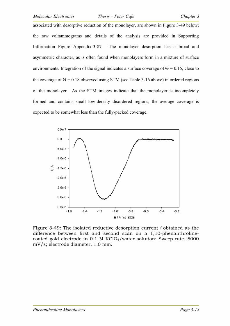
Molecular Electronics Thesis – Peter Cafe Chapter 3
associated with desorptive reduction of the monolayer, are shown in Figure 3-49 below;
the raw voltammograms and details of the analysis are provided in Supporting
Information Figure Appendix-3-87. The monolayer desorption has a broad and
asymmetric character, as is often found when monolayers form in a mixture of surface
environments. Integration of the signal indicates a surface coverage of = 0.15, close to
the coverage of = 0.18 observed using STM (see Table 3-16 above) in ordered regions
of the monolayer. As the STM images indicate that the monolayer is incompletely
formed and contains small low-density disordered regions, the average coverage is
expected to be somewhat less than the fully-packed coverage.
Figure 3-49: The isolated reductive desorption current i obtained as the difference between first and second scan on a 1,10-phenanthroline-coated gold electrode in 0.1 M KClO4/water solution: Sweep rate, 5000 mV/s; electrode diameter, 1.0 mm.
Phenanthroline Monolayers Page 3-18
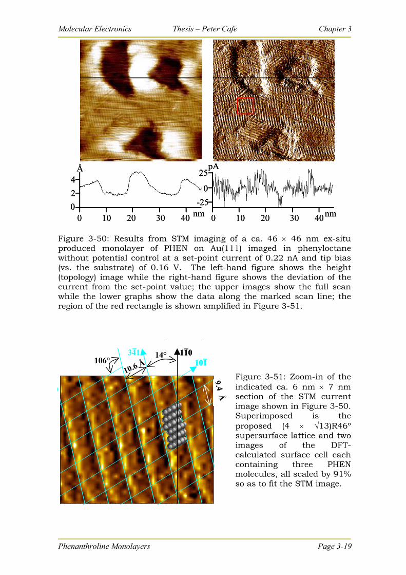
Molecular Electronics Thesis – Peter Cafe Chapter 3
0
2
4Å
0 10 20 30 40 nm0
2
4Å
0 10 20 30 40 nm-25
0
25pA
0 10 20 30 40nm-25
0
25pA
0 10 20 30 40nm
Figure 3-50: Results from STM imaging of a ca. 46 46 nm ex-situ produced monolayer of PHEN on Au(111) imaged in phenyloctane without potential control at a set-point current of 0.22 nA and tip bias (vs. the substrate) of 0.16 V. The left-hand figure shows the height (topology) image while the right-hand figure shows the deviation of the current from the set-point value; the upper images show the full scan while the lower graphs show the data along the marked scan line; the region of the red rectangle is shown amplified in Figure 3-51.
Phenanthroline Monolayers Page 3-19
106°14° 110
_110
_
9.4 Å
10.6 Å 101_
101_341
_
Figure 3-51: Zoom-in of the indicated ca. 6 nm 7 nm section of the STM current image shown in Figure 3-50. Superimposed is the proposed (4 13)R46º supersurface lattice and two images of the DFT-calculated surface cell each containing three PHEN molecules, all scaled by 91% so as to fit the STM image.
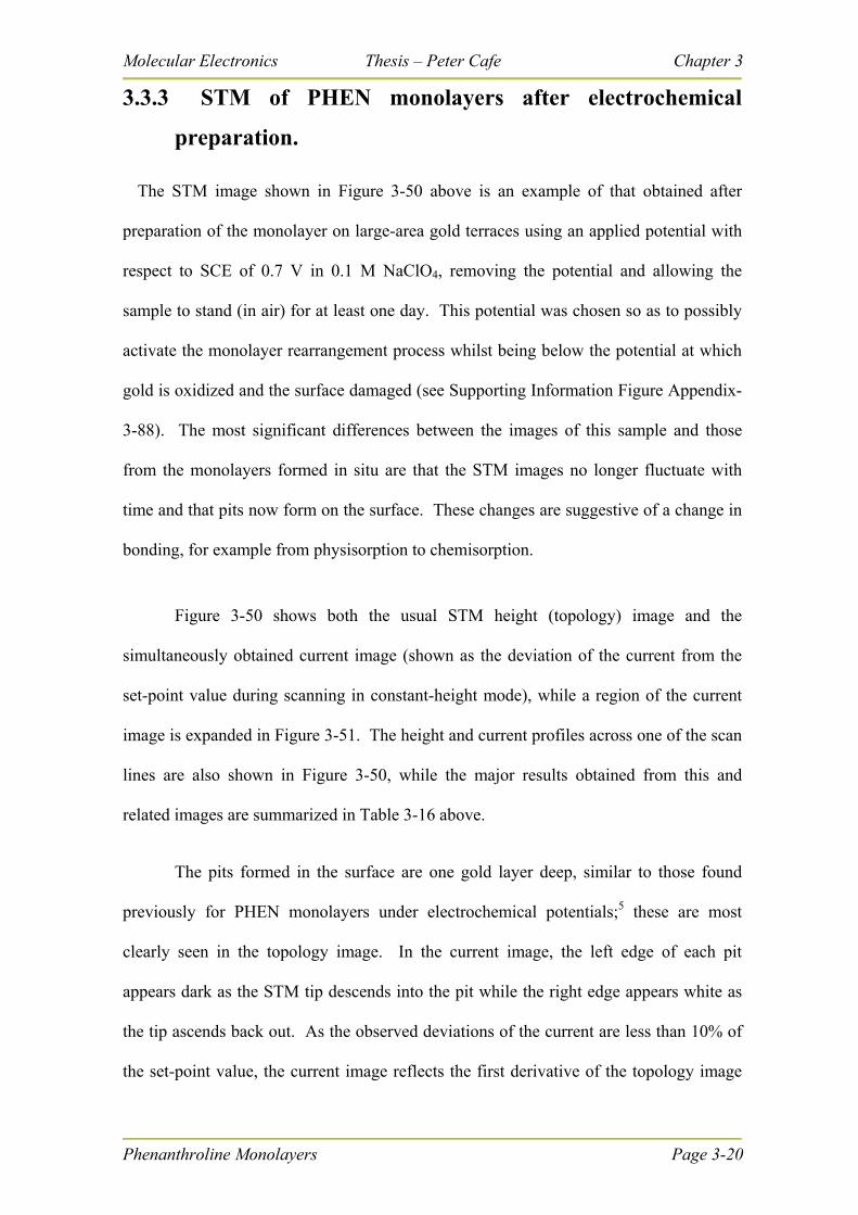
Molecular Electronics Thesis – Peter Cafe Chapter 3
Phenanthroline Monolayers Page 3-20
3.3.3 STM of PHEN monolayers after electrochemical
preparation.
The STM image shown in Figure 3-50 above is an example of that obtained after
preparation of the monolayer on large-area gold terraces using an applied potential with
respect to SCE of 0.7 V in 0.1 M NaClO4, removing the potential and allowing the
sample to stand (in air) for at least one day. This potential was chosen so as to possibly
activate the monolayer rearrangement process whilst being below the potential at which
gold is oxidized and the surface damaged (see Supporting Information Figure Appendix-
3-88). The most significant differences between the images of this sample and those
from the monolayers formed in situ are that the STM images no longer fluctuate with
time and that pits now form on the surface. These changes are suggestive of a change in
bonding, for example from physisorption to chemisorption.
Figure 3-50 shows both the usual STM height (topology) image and the
simultaneously obtained current image (shown as the deviation of the current from the
set-point value during scanning in constant-height mode), while a region of the current
image is expanded in Figure 3-51. The height and current profiles across one of the scan
lines are also shown in Figure 3-50, while the major results obtained from this and
related images are summarized in Table 3-16 above.
The pits formed in the surface are one gold layer deep, similar to those found
previously for PHEN monolayers under electrochemical potentials;5 these are most
clearly seen in the topology image. In the current image, the left edge of each pit
appears dark as the STM tip descends into the pit while the right edge appears white as
the tip ascends back out. As the observed deviations of the current are less than 10% of
the set-point value, the current image reflects the first derivative of the topology image
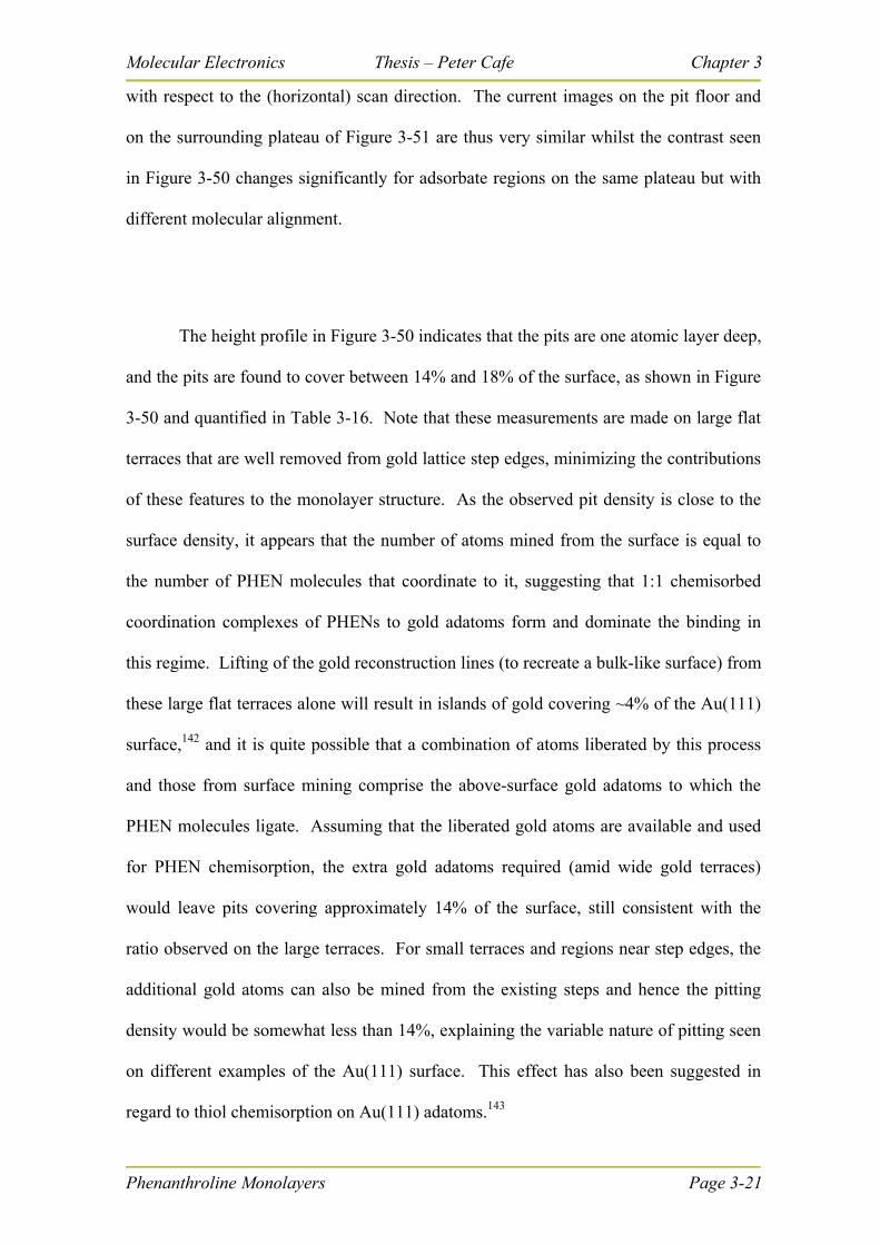
Molecular Electronics Thesis – Peter Cafe Chapter 3
Phenanthroline Monolayers Page 3-21
with respect to the (horizontal) scan direction. The current images on the pit floor and
on the surrounding plateau of Figure 3-51 are thus very similar whilst the contrast seen
in Figure 3-50 changes significantly for adsorbate regions on the same plateau but with
different molecular alignment.
The height profile in Figure 3-50 indicates that the pits are one atomic layer deep,
and the pits are found to cover between 14% and 18% of the surface, as shown in Figure
3-50 and quantified in Table 3-16. Note that these measurements are made on large flat
terraces that are well removed from gold lattice step edges, minimizing the contributions
of these features to the monolayer structure. As the observed pit density is close to the
surface density, it appears that the number of atoms mined from the surface is equal to
the number of PHEN molecules that coordinate to it, suggesting that 1:1 chemisorbed
coordination complexes of PHENs to gold adatoms form and dominate the binding in
this regime. Lifting of the gold reconstruction lines (to recreate a bulk-like surface) from
these large flat terraces alone will result in islands of gold covering ~4% of the Au(111)
surface,142 and it is quite possible that a combination of atoms liberated by this process
and those from surface mining comprise the above-surface gold adatoms to which the
PHEN molecules ligate. Assuming that the liberated gold atoms are available and used
for PHEN chemisorption, the extra gold adatoms required (amid wide gold terraces)
would leave pits covering approximately 14% of the surface, still consistent with the
ratio observed on the large terraces. For small terraces and regions near step edges, the
additional gold atoms can also be mined from the existing steps and hence the pitting
density would be somewhat less than 14%, explaining the variable nature of pitting seen
on different examples of the Au(111) surface. This effect has also been suggested in
regard to thiol chemisorption on Au(111) adatoms.143
Molecular Electronics Thesis – Peter Cafe Chapter 3
The enlarged image shown in Figure 3-51 is quite regular and appears to conform to the
(4 13)R46º supercell lattice superimposed on the figure. Within each unit cell there
appears four streaks oriented in the [
101 ] direction comprising adjacent intense black
and white streaks separated by a less intense pair. At first appearance, this image looks
quite different to the high-resolution images shown in Figure 3-48, but a mapping
between the observed features may easily be constructed. This mapping is based on the
DFT-optimised monolayer structure (see Section 3.3.5 below and Figure 3-55) that is
also superimposed on Figure 3-51 depicting three PHEN molecules per unit cell in a
lattice dominated by a single regular stacking fault. It is the only feasible molecular
orientation that is consistent with the observed lattice parameters and image properties.
Based on this model, the streaks apparent in Figure 3-51 depict not single PHEN
molecules on the surface but rather result from blurring in the direction of stacking of
similar features on adjacent molecules. The relative intensities of the two bright spots
per PHEN molecule shown previously in Figure 3-48 vary with the feedback settings,
scanning direction, and the sample orientation, each spot indicating that the STM tip is
rising as the result of the motion of the tip over some region of the molecule. It is hence
feasible that the image of the monolayer could appear as seen in Figure 3-51. Indeed, a
small increase in the intermolecular space between two PHEN molecules stacked side by
side in Figure 3-48 would naively be expected to make one of the white dots brighter and
its neighbouring region darker as the tip can presumably descend further into the
intermolecular space. The alignment of the 3 PHEN molecules in the surface cell is in
Figure 3-51 shown to reflect this interpretation of the image.
Phenanthroline Monolayers Page 3-22
Molecular Electronics Thesis – Peter Cafe Chapter 3
Phenanthroline Monolayers Page 3-23
Quantitative measurements of the observed lattice properties are compared to
properties calculated using DFT for the (4 13)R46º supercell lattice in Table 3-16.
The observed angle between the cell vectors of 106 is very close to the anticipated value
of 104, but the observed unit cell vectors are on average too small by 9%. As the
method of sample preparation used prevents the calibration of the STM scanner to the
gold reconstruction lines, errors of this magnitude are feasible. Also, the preparation
method prevents the experimental confirmation of the registry between the surface and
substrate lattice vectors. Not only is the (4 13)R46º supercell lattice envisioned in
Figure 3-51 consistent with the quantitative results from the simulations but also it arises
simply by regular application of an observed dislocation process to an observed
substrate registry, see Figure 3-48.
3.3.4 In situ STM of DPPZ monolayers.
DPPZ readily formed monolayers of long chains of molecules standing vertically
on the surface when prepared in ethanol and imaged by in situ STM in aqueous solution,
as shown in Figure 3-52 and Figure 3-53. In Figure 3-52, six consecutive height
(topology) images of the same region are shown (a to f). The first image (Figure 3-52 a)
shows a highly ordered region near the top left-hand corner, a central region containing
defect areas, and a more ordered bottom right-hand corner. Over the course of the scans,
the disordered region gains order and Figure 3-52 d shows most molecules forming in
oriented chains but the spacing between the chains is not regular and hence some
disorder remains. However, in the frame Figure 3-52 e, the defect region again becomes
more pronounced, evolving slightly in Figure 3-52 f; the differences between Figure 3-
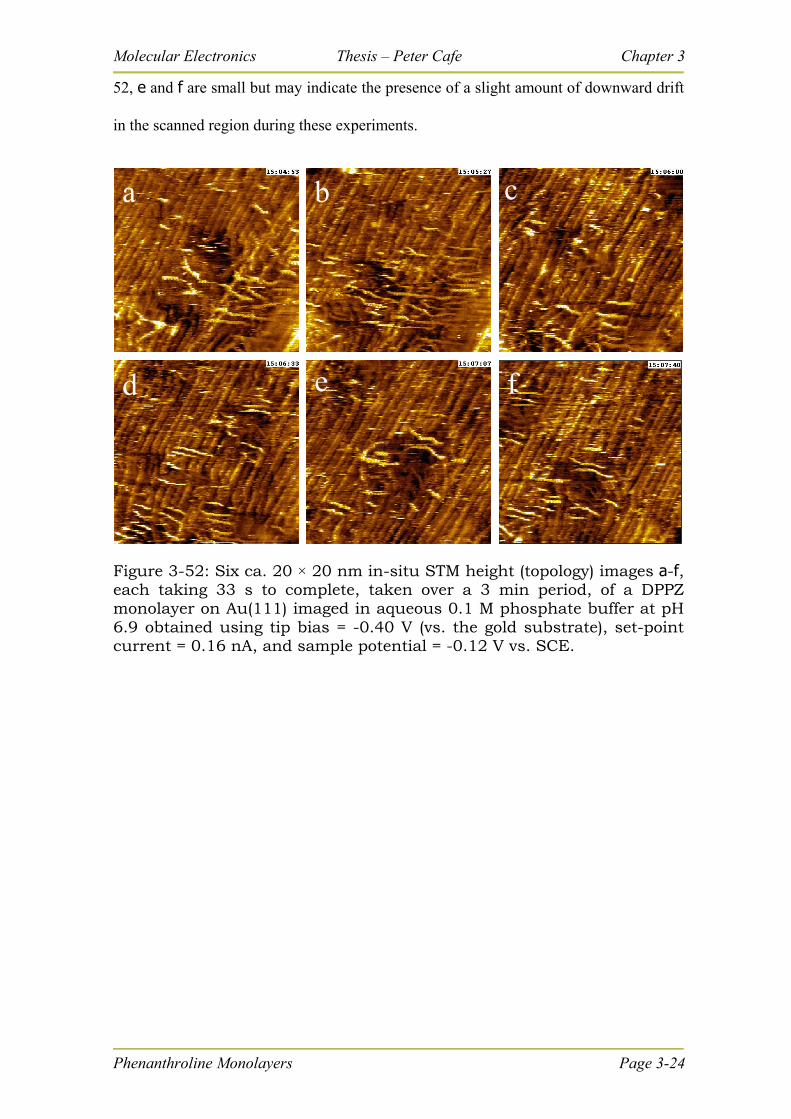
Molecular Electronics Thesis – Peter Cafe Chapter 3
52, e and f are small but may indicate the presence of a slight amount of downward drift
in the scanned region during these experiments.
a
d
b c
e f
Figure 3-52: Six ca. 20 × 20 nm in-situ STM height (topology) images a-f, each taking 33 s to complete, taken over a 3 min period, of a DPPZ monolayer on Au(111) imaged in aqueous 0.1 M phosphate buffer at pH 6.9 obtained using tip bias = -0.40 V (vs. the gold substrate), set-point current = 0.16 nA, and sample potential = -0.12 V vs. SCE.
Phenanthroline Monolayers Page 3-24
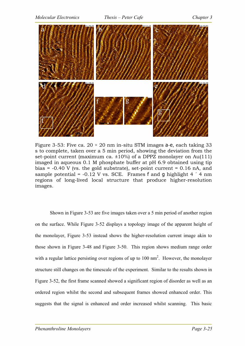
Molecular Electronics Thesis – Peter Cafe Chapter 3
b c
d e
f g
fg
a
Figure 3-53: Five ca. 20 × 20 nm in-situ STM images a-e, each taking 33 s to complete, taken over a 5 min period, showing the deviation from the set-point current (maximum ca. ±10%) of a DPPZ monolayer on Au(111) imaged in aqueous 0.1 M phosphate buffer at pH 6.9 obtained using tip bias = -0.40 V (vs. the gold substrate), set-point current = 0.16 nA, and sample potential = -0.12 V vs. SCE. Frames f and g highlight 4 ´ 4 nm regions of long-lived local structure that produce higher-resolution images.
Shown in Figure 3-53 are five images taken over a 5 min period of another region
on the surface. While Figure 3-52 displays a topology image of the apparent height of
the monolayer, Figure 3-53 instead shows the higher-resolution current image akin to
those shown in Figure 3-48 and Figure 3-50. This region shows medium range order
with a regular lattice persisting over regions of up to 100 nm2. However, the monolayer
structure still changes on the timescale of the experiment. Similar to the results shown in
Figure 3-52, the first frame scanned showed a significant region of disorder as well as an
ordered region whilst the second and subsequent frames showed enhanced order. This
suggests that the signal is enhanced and order increased whilst scanning. This basic
Phenanthroline Monolayers Page 3-25
Molecular Electronics Thesis – Peter Cafe Chapter 3
Phenanthroline Monolayers Page 3-26
quality of the surface did not change after two hours, and the domains with and without
long-range order are persistent at room temperature.
While the observed long-range order of the monolayer is poor, the short to
medium range order for these DPPZ monolayers is significantly enhanced compared to
the ca. maximum 20 nm2 fully-ordered regions evident in Figure 3-48 and Figure 3-50
for PHEN monolayers. Long range order does not form as the spacing between the long
DPPZ chains varies. In Figure 3-53 a, the chains are separated by 12-13 Å, but as order
increases in the subsequent frames the average perpendicular distance between the
chains decreased to 11 Å. High-resolution images of the large sample were difficult to
obtain. The apparent pixelation along the chains evident in Figure 3-53 is in general not
believed to be indicative of resolved structural features and this would imply unrealistic
intermolecular spacings of 1.5 – 2.5 Å. However, in certain regions of the images such
as those highlighted in Figure 3-53, f and g, the slightly more closely packed monolayer
structure appeared robust over many scans and closely resembles that of PHEN in its
physisorbed phase shown in Figure 3-48. The structural properties tentatively assigned
to these DPPZ monolayers in Table 3-16 are based on these more highly resolved
sections of the images.
An important feature of the observed STM images of DPPZ is the absence of
surface pitting, suggesting that the monolayer is physisorbed. No evidence for stacking
faults in the chain structure is found in the higher resolution regions of the images.
However, all images show the chains meandering over the surface, indicating that
precise surface registration is not required for monolayer production. This also suggests
a physisorbed structure. The DPPZ monolayer on Au(111) appears to have more in
Molecular Electronics Thesis – Peter Cafe Chapter 3
Phenanthroline Monolayers Page 3-27
common with the monolayer of PHEN on Cu(111)113 than it does with PHEN on
Au(111).
3.3.5 DFT-Calculated structures of PHEN monolayers.
DFT calculations for the binding of benzene and nitrogen-bound molecules to
Au(111) and related surfaces typically produce realistic structures but do not include the
important dispersive contribution to the binding energy and hence considerably
underestimate the strength of the interaction. The effect is more profound for aromatic-
surface type interactions that favour horizontal alignment of molecules such as
benzene102 and PHEN than it is for the nitrogen-binding interactions that favour vertical
alignment. Hence it is anticipated that the DFT calculations cannot reproduce the
observed energetics of PHEN binding in these configurations; however, the structures
produced in each case should be realistic, making these results a useful starting point for
enhanced descriptions of the energetics. (The dispersive forces are weakly directional
and so do not change the structure as much as the energetics. i.e. the results are
qualatively reliable.) First the structures were determined, and then by using ab initio
methods in the following subsection the relative strengths of the omitted dispersive
interactions were estimated. Initial studies are performed using the (4 4) supercell
found for physisorbed PHEN and the (4 13)R46 lattice found for the chemisorbed
phase.
Firstly, calculations are performed placing just one PHEN molecule in the (4 4)
supercell, a low coverage of just one PHEN per 16 gold surface atoms. The PW91
density-functional predicts vertical PHEN attachment above the surface at the structure
shown in Figure 3-54 below with an energy of ΔE = –3.4 kcal mol-1. The potential
energy surface shows only minor variation as the molecule is tilted parallel with the
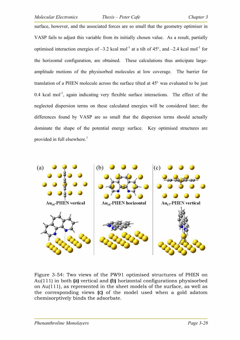
Molecular Electronics Thesis – Peter Cafe Chapter 3
surface, however, and the associated forces are so small that the geometry optimiser in
VASP fails to adjust this variable from its initially chosen value. As a result, partially
optimised interaction energies of –3.2 kcal mol-1 at a tilt of 45, and –2.4 kcal mol-1 for
the horizontal configuration, are obtained. These calculations thus anticipate large-
amplitude motions of the physisorbed molecules at low coverage. The barrier for
translation of a PHEN molecule across the surface tilted at 45 was evaluated to be just
0.4 kcal mol-1, again indicating very flexible surface interactions. The effect of the
neglected dispersion terms on these calculated energies will be considered later; the
differences found by VASP are so small that the dispersion terms should actually
dominate the shape of the potential energy surface. Key optimised structures are
provided in full elsewhere.1
(a) (b) (c)(a) (b) (c)
Figure 3-54: Two views of the PW91 optimised structures of PHEN on Au(111) in both (a) vertical and (b) horizontal configurations physisorbed on Au(111), as represented in the sheet models of the surface, as well as the corresponding views (c) of the model used when a gold adatom chemisorptively binds the adsorbate.
Phenanthroline Monolayers Page 3-28
Molecular Electronics Thesis – Peter Cafe Chapter 3
Phenanthroline Monolayers Page 3-29
Next, calculations relevant to the observed physisorbed phase were performed
placing three PHEN molecules into the (4 4) supersurface cell, a density of three
molecules per 16 surface gold atoms. Only vertically stacked molecules are feasible at
this density and PW91 predicts an interaction energy of ΔE = –1.1 kcal mol-1, expressed
per mol of PHEN adsorbate. The observed spacing between equivalent atoms in the
PHEN molecules apparent in Figure 3-48 and Figure 3-50 is 3.8 Å, a value
incommensurate with the substrate lattice (the intermolecular spacing between the PHEN
-planes is thus 3.8 sin = 3.2 Å, as indicated in Table 3-16). The
incommensurability arises as three PHEN molecules span four Au-Au surface bonds
providing a theoretical spacing of 2.88*4/3 = 3.84 Å. Clearly the three PHEN molecules
per unit cell must reside in different registrations with respect to the surface layer, and
this effect contributes to the calculated reduced binding of the PHEN molecules as the
density increases. However, PW91 calculations for the periodic array of PHEN
molecules in the absence of the gold substrate indicate a repulsive energy of 1.6 kcal
mol-1, accounting for most of the decreased stability. It is hence again clear that minimal
energy costs are predicted by PW91 to be associated with translation of PHEN molecules
across the surface. The dispersive contribution not withstanding, this accounts for the
observed high mobility in physisorbed PHEN monolayers.
Finally, as the experimental results depicted in Figure 3-50 suggest that the stable
monolayer found for PHEN on Au(111) contains gold adatoms above the surface
chemisorbing each PHEN, two possible chemisorbed structures were optimised using
PW91, one in the (4 4) supersurface cell supporting linear chains and the other one in
the (4 13)R46º cell supporting regular stacking faults at every third PHEN. The
resulting structures are shown in Figure 3-55 below and given in detail in the Appendix
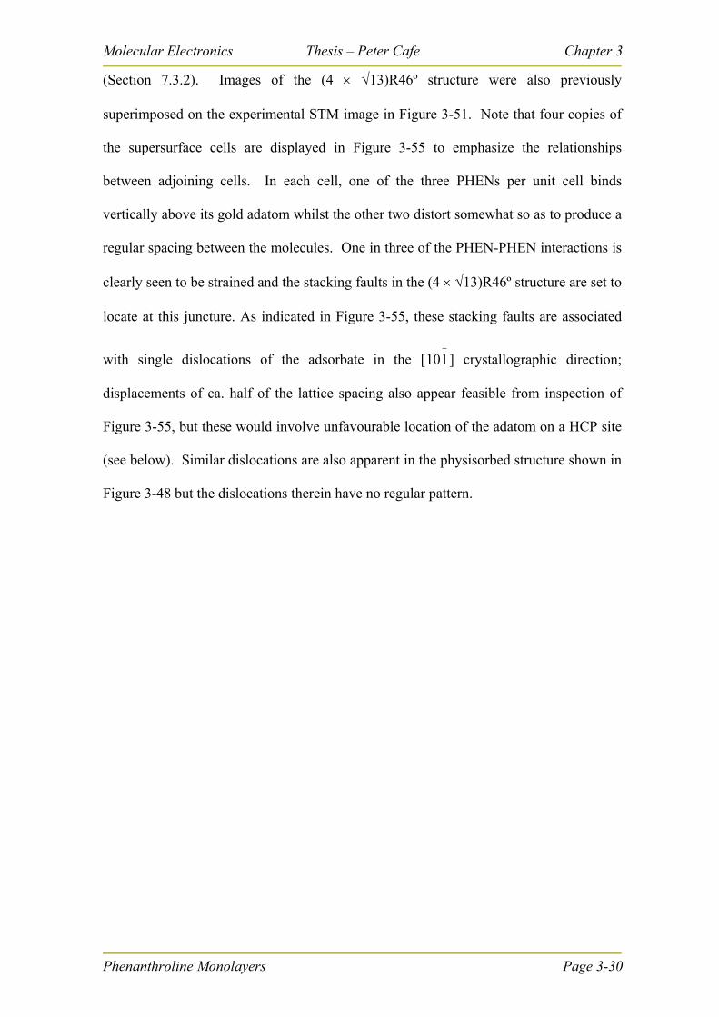
Molecular Electronics Thesis – Peter Cafe Chapter 3
(Section 7.3.2). Images of the (4 13)R46º structure were also previously
superimposed on the experimental STM image in Figure 3-51. Note that four copies of
the supersurface cells are displayed in Figure 3-55 to emphasize the relationships
between adjoining cells. In each cell, one of the three PHENs per unit cell binds
vertically above its gold adatom whilst the other two distort somewhat so as to produce a
regular spacing between the molecules. One in three of the PHEN-PHEN interactions is
clearly seen to be strained and the stacking faults in the (4 13)R46º structure are set to
locate at this juncture. As indicated in Figure 3-55, these stacking faults are associated
with single dislocations of the adsorbate in the [ ] crystallographic direction;
displacements of ca. half of the lattice spacing also appear feasible from inspection of
110
Figure 3-55, but these would involve unfavourable location of the adatom on a HCP site
(see below). Similar dislocations are also apparent in the physisorbed structure shown in
Figure 3-48 but the dislocations therein have no regular pattern.
Phenanthroline Monolayers Page 3-30
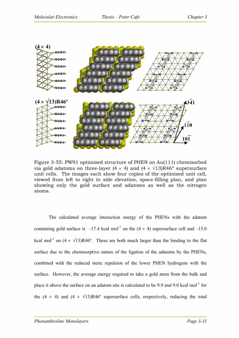
Molecular Electronics Thesis – Peter Cafe Chapter 3
(4 13)R46º
(4 4)
(4 13)R46º
(4 4)
Figure 3-55: PW91 optimised structure of PHEN on Au(111) chemisorbed via gold adatoms on three-layer (4 4) and (4 13)R46º supersurface unit cells. The images each show four copies of the optimised unit cell, viewed from left to right in side elevation, space-filling plan, and plan showing only the gold surface and adatoms as well as the nitrogen atoms.
The calculated average interaction energy of the PHENs with the adatom
containing gold surface is –17.4 kcal mol-1 on the (4 4) supersurface cell and –15.0
kcal mol-1 on (4 13)R46º. These are both much larger than the binding to the flat
surface due to the chemisorptive nature of the ligation of the adatoms by the PHENs,
combined with the reduced steric repulsion of the lower PHEN hydrogens with the
surface. However, the average energy required to take a gold atom from the bulk and
place it above the surface on an adatom site is calculated to be 9.9 and 9.0 kcal mol-1 for
the (4 4) and (4 13)R46º supersurface cells, respectively, reducing the total
Phenanthroline Monolayers Page 3-31
Molecular Electronics Thesis – Peter Cafe Chapter 3
Phenanthroline Monolayers Page 3-32
chemisorption energy to –7.5 kcal mol-1 and –6.0 kcal.mol-1, respectively. While these
values are much larger than the weak physisorptive interaction of –1.1 kcal mol-1
calculated previously, proper treatment of the omitted dispersive interactions is required
before conclusions can be reached concerning the relative stabilities of the different
types of physisorptive and chemisorptive binding considered. However, as another
check on the reliability of the approach, the energies of mining atoms from the surface
has also been calculated, obtaining energies within 2 kcal mol-1 from the bulk-atom
results used in the above calculation. These values differ depending on the nature of the
step edges before and after the mining process. As there appears to be only a very small
energy difference between surface and bulk gold atoms, and as the precise nature of the
pits produced is highly variable, use of the bulk values appears to be most appropriate.
The optimised structures shown in Figure 3-55 have the gold adatoms located on
FCC sites of the surface. Structures for the (4 4) supersurface lattice with these atoms
located above HCP and top sites were calculated to be higher in energy by 3.0 and 13.4
kcal mol-1, respectively, while similar structures above bridge sites were found to be of
high energy and unstable. Calculations at low coverage (1 PHEN per 16 surface gold
atoms) indicated that the chemisorption energy of a single adatom to PHEN is –15.4 kcal
mol-1 at the FCC site and –14.8 kcal mol-1 at the HCP site. These energies are both much
lower than the average binding energy of –7.5 kcal mol-1 at high coverage. A variety of
different approaches was considered to interpret this effect, all leading to the conclusion
that it costs 2.5 to 3 kcal mol-1 to assemble two gold adatoms on adjacent FCC sites. The
barrier to translation of a single adatom/PHEN complex across the surface at low
coverage was evaluated to be less than 4 kcal mol-1, similar to the barrier for translating a
PHEN molecule between two adjacent adatoms. Hence even the chemisorbed structure
Molecular Electronics Thesis – Peter Cafe Chapter 3
Phenanthroline Monolayers Page 3-33
is predicted to be quite mobile on the surface, explaining how it is that the geometrical
distortions shown in Figure 3-55 that arise due to the incommensurate adsorbate and
substrate lattices do not lead to significant energy penalties. Similar mobility has also
been calculated for thiol chemisorption to adatoms on Au(111).144
3.3.6 MP2 and CASPT2 calculations on the role of
dispersive interactions in monolayer production.
The coordinates of the three pairs of nearest-neighbour PHEN molecules were
extracted from the (4 4) optimised structure shown in Figure 3-55 and used in gas-
phase calculations of the adsorbate-adsorbate interaction energy by PW91 and MP2. The
MP2 calculations include the dispersive contributions that are not included in current
DFT functionals such as PW91. The MP2 interaction energies, after basis-set
superposition-error correction, are –10.3 kcal mol-1 between the strained PHENs (see
Figure 3-55) and –10.6 kcal mol-1 between the others, averaging –10.5 kcal mol-1.
However, the corresponding PW91 average interaction energy is 2.2 kcal mol-1, slightly
more repulsive than the average energy of 1.5 kcal mol-1 from VASP PW91 calculations
of the entire PHEN monolayer. These results indicate that the calculated VASP PW91
energies for high-density monolayers should be corrected by –13 kcal mol-1 in order to
account for the dispersive interaction between the adsorbate molecules. Key results are
summarized in Table 3-17 below.
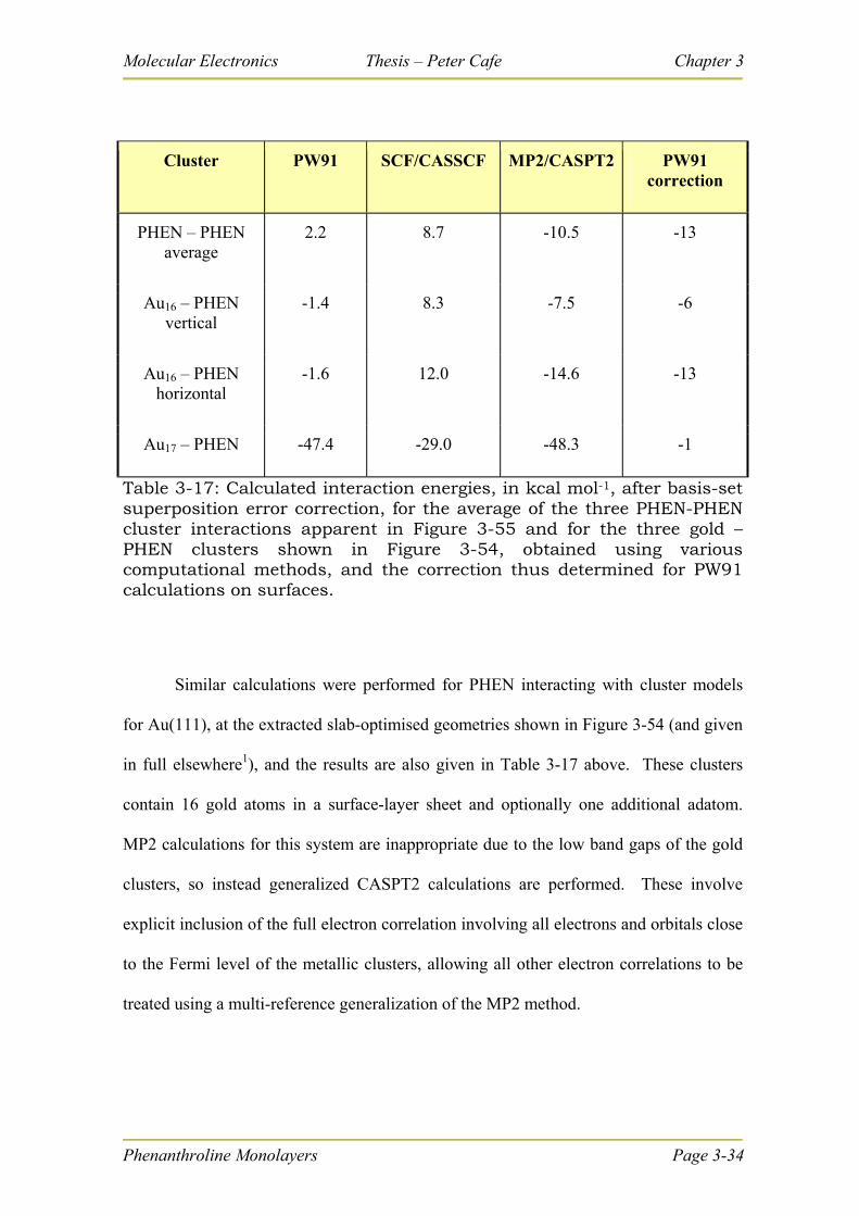
Molecular Electronics Thesis – Peter Cafe Chapter 3
Phenanthroline Monolayers Page 3-34
Cluster PW91 SCF/CASSCF MP2/CASPT2 PW91 correction
PHEN – PHEN average
2.2 8.7 -10.5 -13
Au16 – PHEN vertical
-1.4 8.3 -7.5 -6
Au16 – PHEN horizontal
-1.6 12.0 -14.6 -13
Au17 – PHEN -47.4 -29.0 -48.3 -1
Table 3-17: Calculated interaction energies, in kcal mol-1, after basis-set superposition error correction, for the average of the three PHEN-PHEN cluster interactions apparent in Figure 3-55 and for the three gold – PHEN clusters shown in Figure 3-54, obtained using various computational methods, and the correction thus determined for PW91 calculations on surfaces.
Similar calculations were performed for PHEN interacting with cluster models
for Au(111), at the extracted slab-optimised geometries shown in Figure 3-54 (and given
in full elsewhere1), and the results are also given in Table 3-17 above. These clusters
contain 16 gold atoms in a surface-layer sheet and optionally one additional adatom.
MP2 calculations for this system are inappropriate due to the low band gaps of the gold
clusters, so instead generalized CASPT2 calculations are performed. These involve
explicit inclusion of the full electron correlation involving all electrons and orbitals close
to the Fermi level of the metallic clusters, allowing all other electron correlations to be
treated using a multi-reference generalization of the MP2 method.
Molecular Electronics Thesis – Peter Cafe Chapter 3
Three established scenarios provide paradigms for the interactions considered:
the interaction of ammonia with a single gold atom,145 the interaction of ammonia with a
gold surface,118 and the interaction of benzene with copper102 surfaces. For ammonia
interacting with a single gold atom,145 GGA-type density functions predict binding
energies varying by over a factor of two, but PW91 is one of the most reliable of these
methods, overestimating the binding by just 10%. As a result, we would expect that
PW91 adequately describes the chemisorption process of PHEN binding to a gold
adatom. PW91 also provides a realistic description of the energetics of ammonia
sticking to Au(111),118 despite it being clear that the dispersive interaction between the
ammonia lone-pair and the filled gold orbital is important to the interaction. This
scenario is similar to PHEN binding vertically to a flat gold surface, though the
interactions of nitrogen lone pairs with gold decrease in hybridisation order sp3 > sp2 >
sp, and in addition the lower PHEN hydrogen atoms prevent proper access of the
adsorbate to the surface. Hence the relative importance of the dispersive interactions is
expected to be larger for PHEN binding and thus reduced accuracy is expected for PW91
in the description of this binding. Finally, PW91 predicts negligible binding for benzene
to Au(111), Cu(111), and Cu(110), similar to the results described earlier for PHEN
adsorbing horizontally on Au(111), while the observed interactions are quite substantial
and 12-17 kcal mol-1 more attractive.102, 146-148 CASPT2 is the only available
computational method that includes the key dispersive terms in a realistic way. CASPT2
predicts a correction of 24 kcal mol-1 for benzene on Cu(110) for which the deficiency in
the PW91 adsorption energy is 17 kcal mol-1, in reasonable agreement with the
experimental data. As CASPT2 also provides an excellent description of chemisorptive
interactions, it is expected to provide a realistic description of the shortcomings of the
2zd
Phenanthroline Monolayers Page 3-35
Molecular Electronics Thesis – Peter Cafe Chapter 3
full-surface VASP DFT PW91 calculations for all the physisorption and chemisorption
scenarios considered herein.
The energies calculated using PW91, CASSCF (the intermediate stage in the
CASPT2 calculations that does not include dispersion), and CASPT2 are shown in Table
3-17 for the three clusters from Figure 3-54. PW91 again predicts negligible binding for
the physisorbed clusters (ca. –1 kcal mol-1), while CASSCF predicts significant repulsion
(8 to 12 kcal mol-1), and CASPT2 predicts strong binding: –7.5 kcal mol-1 for the vertical
structure and –14.6 kcal mol-1 for the horizontal one. All methods predict strong binding
for the chemisorbed structure involving a gold adatom. The results lead to energy
corrections for the VASP surface PW91 calculations of –6, –13, and –1 kcal mol-1 for the
physisorbed vertical, physisorbed horizontal, and (4 4)-lattice chemisorbed scenarios,
respectively, in qualitative agreement with expectations based on known scenarios for
binding in similar environments.102, 118, 145
Phenanthroline Monolayers Page 3-36
Molecular Electronics Thesis – Peter Cafe Chapter 3
Phenanthroline Monolayers Page 3-37
3-4 Discussion: how PHEN and DPPZ molecules
and monolayers bind to the Au(111) surface
The final estimated interactions for PHEN with Au(111) in some critical
configurations are given in Table 3-18 below, obtained by combination of the PW91
calculated energies for the periodic adsorbate (also shown in the table) with the
dispersion correction energies taken from Table 3-18. DFT calculations for the
physisorption of PHEN on Au(111) predict weak binding that marginally prefers vertical
alignment of the adsorbate, but the magnitude of the binding is far too small to account
for the experimental observation that stable monolayers do form at room temperature.
However, the corrected energies of –9 kcal mol-1 vertical and –15 kcal mol-1 horizontal
provide estimates of plausible magnitude that clearly favour horizontal binding at low
coverage. The orientation will be sensitive to applied bias, however, owing to the large
dipole moment of the PHEN which drives vertical alignment under positive applied
voltages,112 as has been directly observed in related systems.49, 116
At intermediate coverage, PHEN dimers may start to form on the surface. The
corrected interaction energy for a vertically oriented dimer from Table 3-18 is –15 kcal
mol-1, the same value as obtained for the horizontal single molecule. While the
calculations are not capable of discerning the fine differences in relative energy that
control actual monolayer production and dynamics, they clearly indicate a scenario in
which molecules agglomerate to form a structured layer at higher adsorbate exposures.
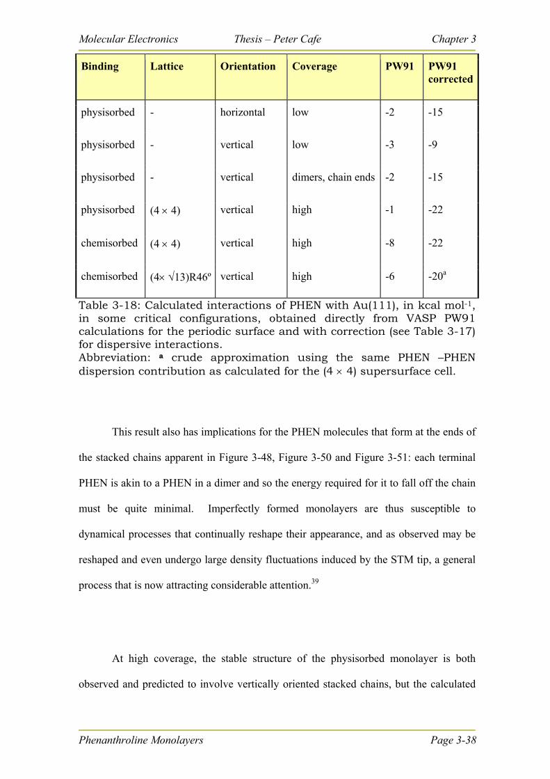
Molecular Electronics Thesis – Peter Cafe Chapter 3
Phenanthroline Monolayers Page 3-38
Binding Lattice Orientation Coverage PW91 PW91 corrected
physisorbed - horizontal low -2 -15
physisorbed - vertical low -3 -9
physisorbed - vertical dimers, chain ends -2 -15
physisorbed (4 4) vertical high -1 -22
chemisorbed (4 4) vertical high -8 -22
chemisorbed (4 13)R46º vertical high -6 -20a
Table 3-18: Calculated interactions of PHEN with Au(111), in kcal mol-1, in some critical configurations, obtained directly from VASP PW91 calculations for the periodic surface and with correction (see Table 3-17) for dispersive interactions. Abbreviation: a crude approximation using the same PHEN –PHEN dispersion contribution as calculated for the (4 4) supersurface cell.
This result also has implications for the PHEN molecules that form at the ends of
the stacked chains apparent in Figure 3-48, Figure 3-50 and Figure 3-51: each terminal
PHEN is akin to a PHEN in a dimer and so the energy required for it to fall off the chain
must be quite minimal. Imperfectly formed monolayers are thus susceptible to
dynamical processes that continually reshape their appearance, and as observed may be
reshaped and even undergo large density fluctuations induced by the STM tip, a general
process that is now attracting considerable attention.39
At high coverage, the stable structure of the physisorbed monolayer is both
observed and predicted to involve vertically oriented stacked chains, but the calculated
Molecular Electronics Thesis – Peter Cafe Chapter 3
Phenanthroline Monolayers Page 3-39
interaction energies after correction are –22 kcal mol-1 for both the physisorbed and
chemisorbed (4 4) structures; crudely assuming that the same PHEN-PHEN dispersive
contribution applied to the (4 13)R46º chemisorbed one, its corrected interaction
energy would be 1.5 kcal mol-1 less bound than this. Again, while these calculations
cannot predict the small differences in these energies with accuracy, they indicate that
the various types of binding should be comparable in energy. The experimental results
indicate that once the chemisorbed structure forms, attaining high regularity with a
minimum number of chain ends, the monolayer structure becomes stable over long
periods of time. Also, as the ligation process directs vertical rather than horizontal
alignment, the conformational flexibility of the chemisorbed structures are greatly
reduced so that the PHEN molecules at the ends of chains become stable to
rearrangement, locking in the overall structure. In addition to these stabilizing effects,
the calculations also suggest that the barriers to rearrangement of the chemisorbed
structures are at least 3 kcal mol-1 more than those for rearranging the physisorbed
structures, slowing rates by an order of magnitude.
The purpose for measuring the structure of DPPZ on Au(111) was to induce a
small but significant perturbation to the energy balance depicted above for PHEN. Due
to the additional rings (see Figure 3-47), the dispersive interactions favouring vertical
stacking are increased whilst the vertically oriented head-group to surface interactions
and the steric packing interactions are less affected. The result is that the driving force
for the molecules that terminate a surface chain to fall off the chain are reduced,
manifested experimentally through the production of long stable chains and much more
regular monolayers. Also, the apparent absence of stacking faults in the DPPZ chains
indicates that the dispersive interaction favours linear chains while, as revealed from the
Molecular Electronics Thesis – Peter Cafe Chapter 3
PW91 calculations, the substrate lattice effects drive the dislocation. The observed
meandering of the chains in Figure 3-53 also indicates that the increased inter-adsorbate
interaction, which is sufficiently soft to permit meandering, now dominates the adsorbate
to head group interactions, which acts to register the adsorbate into discrete sites above
the surface.
Nucleation of ordered PHEN monolayers on Au(111) is known to occur along
the gold reconstruction lines.48 This may occur because of an increased physisorptive
interaction arising from the altered gold surface structure, or may arise as it is
energetically easier to mine the additional gold surface atom from the reconstruction than
it is to mine either the unreconstructed (111) surface or bulk gold atoms.149 If the
reconstruction is indeed lifted by this process, then the adatom could either be
transported and deposited at a step edge or other irregularity, facilitating growth of a
physisorbed layer, or additional atoms could be extracted from step edges or the top
surface layer (thus forming pits), facilitating growth of a chemisorbed layer. The degree
of pitting produced by PHEN on Au(111) can be reversibly controlled through the
application of a surface potential,48 an observation that is understood in terms of a
scenario in which physisorbed and chemisorbed structures have very similar energies.
As the dispersive interaction between two PHENs on adjacent sites in which one is
chemisorbed and the other is physisorbed will be small, the lack of observation of mixed
chemisorbed and physisorbed layers can readily be understood: interconversion requires
a phase change from one form to the other.
Phenanthroline Monolayers Page 3-40
Molecular Electronics Thesis – Peter Cafe Chapter 3
Phenanthroline Monolayers Page 3-41
3-5 Conclusions to Chapter 3: PHEN binding to
gold and relevance to thiol binding
Two distinct states of adhesion of PHEN to Au(111) are found, a physisorbed
state in which the PHEN molecules interact with the normal gold surface, and a
chemisorbed state involving gold adatoms chelating the molecules to the surface.
Energetic calculations indicate that these adsorbates are both strongly bound to the
surface and of similar energy. While the chemisorbed state (at full monolayer coverage)
is stable for extended periods of time, the physisorbed state is dynamically fluctuating at
room temperature. Such fluctuations are possible owing to unstable chain ends and small
barriers for diffusion of the physisorbed molecules across the surface and their
reorientation. Changing between aqueous and non-aqueous solvents (without applied
electrochemical potentials) had little effect on the qualitative nature of the monolayer,
suggesting that solvent interactions are not critical. However, dispersive forces acting
both between the adsorbate molecules and between the molecules and the surface are
shown to be very important, controlling the energetics and dynamics of the system; for
chemisorption, the relative strengths of the ligand bond and the energy required to
produce the gold adatoms also contribute to this fine balance. Modulation of the
intermolecular dispersive forces through extension of the aromatic ring system from
PHEN to DPPZ is shown to change the balance of the forces realizing a reduced chain-
end effect, fewer stacking faults, and much longer chains. For PHEN on Au(111), after
initial adsorption, the molecular chains are disordered with respect to both themselves
and the substrate lattice, but full registration with the substrate occurs as the monolayer
matures. No such maturation is observed for DPPZ on Au(111), however. Indeed, the
structure of DPPZ on Au(111) is very similar to that of PHEN on Cu(111), a structure
Molecular Electronics Thesis – Peter Cafe Chapter 3
Phenanthroline Monolayers Page 3-42
for which the substrate lattice spacings are too small to allow for proper registration of a
high-density monolayer.113 The substitution of DPPZ for PHEN and the substitution of
Cu for Au thus both have similar effects on the structure of PHEN on Au(111).
In the chemisorbed state, prior to full surface monolayer coverage, the PHEN-
adatom entity has little barrier to translation across the surface and so even though still
strongly bound to the surface remaining upright, it has high mobility (see Figure 3-56
below). Thus whilst the monolayer is forming the PHEN-adatom units simply stack in
long chains in a structure that is determined not so much by the gold substrate as by the
dispersive forces between the molecules as they stack against each other standing upright
upon the gold surface, with the gold adatoms registering above hollow sites in the (111)
surface. However the stacking of the PHEN molecules and the registration of the gold
adatoms with the surface are incommensurable. Whilst the PHEN-adatom bond is both
strong and flexible enough to accommodate this incommensurability, the dispersive
forces holding the PHEN molecules together in long chains are neither strong nor
flexible enough to accommodate it. At full monolayer coverage pressure from tightly
packed neighbouring chains, together with the incommensurability of the chain with the
surface, results in a slip in the chains, and the dimensions of the incommensurability
dictate that this slip will most likely occur at each third molecule in the chain.
Experimentally, a connection between pitting of the gold surface and
chemisorption was established through examination of the pits formed on very large flat
gold terraces, structures in which the number of atoms taken from the pitted volume
matched the PHEN surface coverage. Pitting observed around step edges and other
defects is much more difficult to quantify due to the complex interplay in these
dynamically changing structures.
Molecular Electronics Thesis – Peter Cafe Chapter 3
Phenanthroline Monolayers Page 3-43
Significant surface pitting also appears consistently when molecular monolayers
are formed on gold using thiol or other ligand tethers. McDermott et al. have examined
the phenomenon of surface pitting114 in alkanethiol monolayers based on supposed150
correlations of the pitting with alkane chain length. Their suggestion is that the driving
force of the pitting is the shrinkage of the uppermost layer of gold atoms due to electron
sharing between the sulfur and gold atoms, adding electron density to the attractive
mantle for the electrons between the gold atoms at a three-fold hollow binding site and
thus increasing the attractive force between the three-fold hollow atoms. This
interpretation has also been adopted by Cunha et al.48 in relation to pits formed in
phenanthroline monolayers. However, while substantial charge transfer is associated
with thiol monolayer formation,151 very little is involved in PHEN binding, questioning
the general applicability of the mechanism.
Here the cause of the pitting is attributed to the PHEN molecules mining gold
atoms from the surface to bind with as they move from the physisorbed state to the
chemisorbed state. These adatoms can be taken from terrace edges, however on large flat
(111) terraces these atoms are initially mined from lifting of the gold reconstruction lines
or spot defects in the (111) surface, initiating a pit with step edges from which
subsequent adatoms are mined, continuing until enough atoms are taken from the surface
to accommodate each PHEN in a 1:1 ratio. Cunha et al.48 found that the pitting both
increased and decreased via electrochemical control, complementing this theory, as the
two states are energetically close to each other and the movement from one to the other
can be driven by electrochemical control. As the PHEN molecule moves back to the
physisorbed state it donates its adatom back to the gold surface, reducing the pit size or
forming islands.
Molecular Electronics Thesis – Peter Cafe Chapter 3
Phenanthroline Monolayers Page 3-44
The pitting effects depicted in the McDermott et al. model are realistic but do not
account for the complex balance of forces associated with the mining of surface atoms in
order to maximize the surface to head group and inter-adsorbate interactions. As the
McDermott model is generally inadequate for PHEN and perhaps thiol monolayers and
this research has established that pitting is caused by adatom formation, so that pitting,
when it appears, is the most direct evidence available that the monolayer has formed via
adatoms. It is thus likely that there exists a close analogy between the processes depicted
herein for PHEN and those operative for thiols, and indeed quantitative calculations have
explored this possibility in detail.43, 152
Thiol monolayer formation on gold can be associated with a large number of
motifs depicting the formation of surface pits and vacancy islands.150, 153, 154 It is this
complexity that makes difficult isolation of the key effects controlling the process.
However, for PHEN monolayers on gold, the results show that stable chemisorbed
phases are intrinsically associated with gold adatom binding, while a range of alternate
structures at comparable energies are also isolated. Adatoms have also been implicated
in the binding of amines to gold,42 and it is thus not unreasonable to suggest that such
structures are also important for thiol binding. Indeed, the only available experimental
information on the gold-sulfur geometry in thiol monolayers indicates that the sulfur sits
vertically above a gold atom,155, 156 as is expected only when adatoms are involved,157
and DFT149, 158 simulations indicate that thiol monolayers can extract gold from the
reconstruction lines to produce adatom-bound adsorbates.158 The results thus strengthen
the case for significant adatom involvement in thiol monolayers.
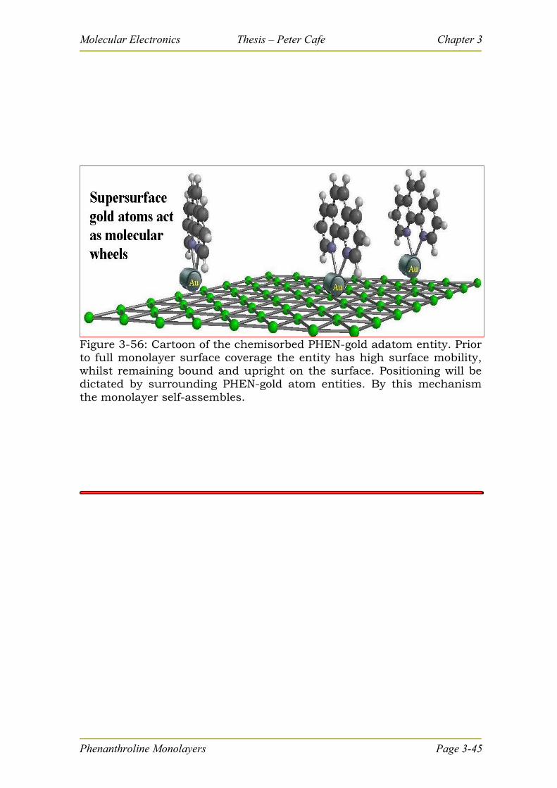
Molecular Electronics Thesis – Peter Cafe Chapter 3
Figure 3-56: Cartoon of the chemisorbed PHEN-gold adatom entity. Prior to full monolayer surface coverage the entity has high surface mobility, whilst remaining bound and upright on the surface. Positioning will be dictated by surrounding PHEN-gold atom entities. By this mechanism the monolayer self-assembles.
Phenanthroline Monolayers Page 3-45

Molecular Electronics Thesis – Peter Cafe Chapter 3
Phenanthroline Monolayers Page 3-46
(blank Page)
Molecular Electronics Thesis – Peter Cafe Chapter 4
ChaptteerChap r 4 Thee Natturree and Conduccttiion off
Thiiollss Cheemiissorrbeed tto Golld..
4 Th Na u and Condu on o
Th o Ch m o b d o Go d
4-0 Synopsis for Chapter 4
This chapter examines various research publications in the area of thiol binding to
gold and makes natural extensions to the body of literature using conclusions drawn from
Chapters 2 and 3. Through a thorough examination of the binding mode of the thiol (i.e. the
deprotonated thiol) linker to gold with the help of extensive literature reports, it concludes
that the gold adatom is implicated as a primary binding mechanism of thiols to the Au(111)
surface (similar to the 1,10-phenanthroline linker studied in Chapter 3).
The adatom configuration is extended to dithiol binding to two gold terminals during
the break-junction experiment, and it is determined that thiols are connected to the gold
terminals via adatoms at one or both ends, with a fourfold decrease in conductivity
respectively, giving rise to distinct peaks (or sets of peaks) in break-junction histograms.
Broadness of peaks observed in the histograms of break-junction experiments is
mainly due to angular distortion of the molecule in relation to the gold electrode.
Thiols chemisorbed to gold Page 4-1
Molecular Electronics Thesis – Peter Cafe Chapter 4
Thiols chemisorbed to gold Page 4-2
4-1 Introduction to Chapter 4
“Great things are not done by impulse, but by a series of
small things brought together.” (Vincent Van Gough)
4.1.1 Importance of determining the binding mode
“At the heart of the problem is the need to interface
reliably with an individual molecule.”28
At the Faraday Discussions #133, “Molecular Wires And Nanoscale Conductors”
Manchester, September 2003, a world leader in experimental research into single molecule
conduction, Professor Stuart Lindsay (Arizona State University), expressed a view that
further research into molecular conductance, particularly theoretically, was being hampered
by a limited understanding of the contact geometry (of the molecule with the metal
electrode)33.
At that same conference this author presented a poster titled “Electrical conduction
through single molecules: the nature of self-assembled monolayers: the bonding of nitrogen
to the surface in 1,10-phenanthroline”. The theme of the poster was on the binding
geometry of a molecule to gold, determining that 1,10-phenanthroline could bind to the
Au(111) surface via a gold adatom (this poster was a preliminary delivery of the work
which forms the basis of Chapter 3 of this thesis).
In most experimental work involving monolayer formation on gold, great care is
taken to produce flat terraces of Au(111) surface upon which the monolayer can form and
be characterised. The immediate assumption was that the molecules of the monolayer bound
Molecular Electronics Thesis – Peter Cafe Chapter 4
Thiols chemisorbed to gold Page 4-3
directly to the Au(111) surface, and for a number of years the assumption was followed
axiomatically in subsequent theoretical modelling.
However a common feature of many, but not all, monolayers was surface pitting, at
a depth equal to one gold lattice parameter (i.e. the pitting was in the Au(111) surface, not
the monolayer). Until the explanation of the adatom mode of binding of molecules to gold1,
the cause of the surface pitting was never adequately explained.
Since 2003 a number of publications have addressed the issue of contact geometry,
yet by 2007 “detailed understanding of the role of contact geometry is still required”111, and
the weight of those publications is yet to be brought to bear upon a conclusion, particularly
for thiol-based monolayers. The implications for molecular conduction, and in particular
conduction observed in break-junction experiments, have received little attention.
4.1.2 Work of this chapter - adatom configuration in the thiol
binding to gold
The results section (Section 4-2) presents a dissertation on the method of binding of
the thiol radical to gold using a body of nascent research, both experimental and theoretical.
It then explores how this impinges on break-junction experiments and the measured
conductance values. It resumes a theme from Chapter 3 which implicates the adatom in the
binding of 1,10-phenanthroline to gold, and develops this with the theme of Chapter 2,
molecular conductance.
4.1.3 NOTE concerning thiol and thiyl terminology:
When a thiol binds to gold it does so covalently with the loss of a hydrogen atom.
The resultant linking unit is termed a thiyl (or thiyl radical). However it is very common to

Molecular Electronics Thesis – Peter Cafe Chapter 4
see in literature the resultant bound species described as a “thiol”, perhaps because the name
is more familiar, or perhaps because it refers to the source molecule, even though it is
technically incorrect. Because this thesis draws upon many sources which use the term
“thiol” instead of “thiyl”, it has become necessary to follow that convention, particularly
when citing or referring to another author’s work. The reader must understand that where the
term “thiol” is used to describe a molecule covalently bound to gold, it means “thiyl”.
UUPAC advises that thiyl is synonymous with sulfenyl radicals, and due to inconsistencies
in use the term is not recommended.159
Occasionally the term “thiolate” is also seen in literature to (mistakenly) describe
the chemisorbed deprotonated thiol. It is incorrect because a thiolate species is an ionic
entity which would bond ionically to gold, which is not the case.
Thiols chemisorbed to gold Page 4-4
Molecular Electronics Thesis – Peter Cafe Chapter 4
Thiols chemisorbed to gold Page 4-5
4-2 The adatom configuration of thiols bound to
gold and its implications regarding molecular
conduction.
This section outlines the result of literature research which arose due to the nature of
experimental results presented in Chapter 2, that is that molecular conduction was not always
a single value quantity, and also from the work presented in Chapter 3, which drew analogies
with “similar but poorly understood processes involved in the binding of thiols to Au(111).”
It falls into two sub-sections, the first examines the binding mode(s) of thiols to gold
and the second examines how the binding geometry affects molecular conductance.
4.2.1 Bond geometry: analysis of the dithiol results of Chapter
2
One would perhaps expect that if a molecule had a single value of conductance when
trapped within a gold break-junction then its conductance value would be highly consistent
and the resultant binned histogram would show extremely clear peaks at the conductance
values: indeed there would be no need to construct histograms. However the position of
specific steps from trace to trace vary, and the histogram peaks are broad, both here (Chapter
2) and in Li, et al,101 (reproduced in Figure 4-57 below), and generally all similar
experiments on all molecules. Furthermore, Li’s work particularises two sets of conduction
regimes, which they have labelled High and Low (Table 4-19 below).
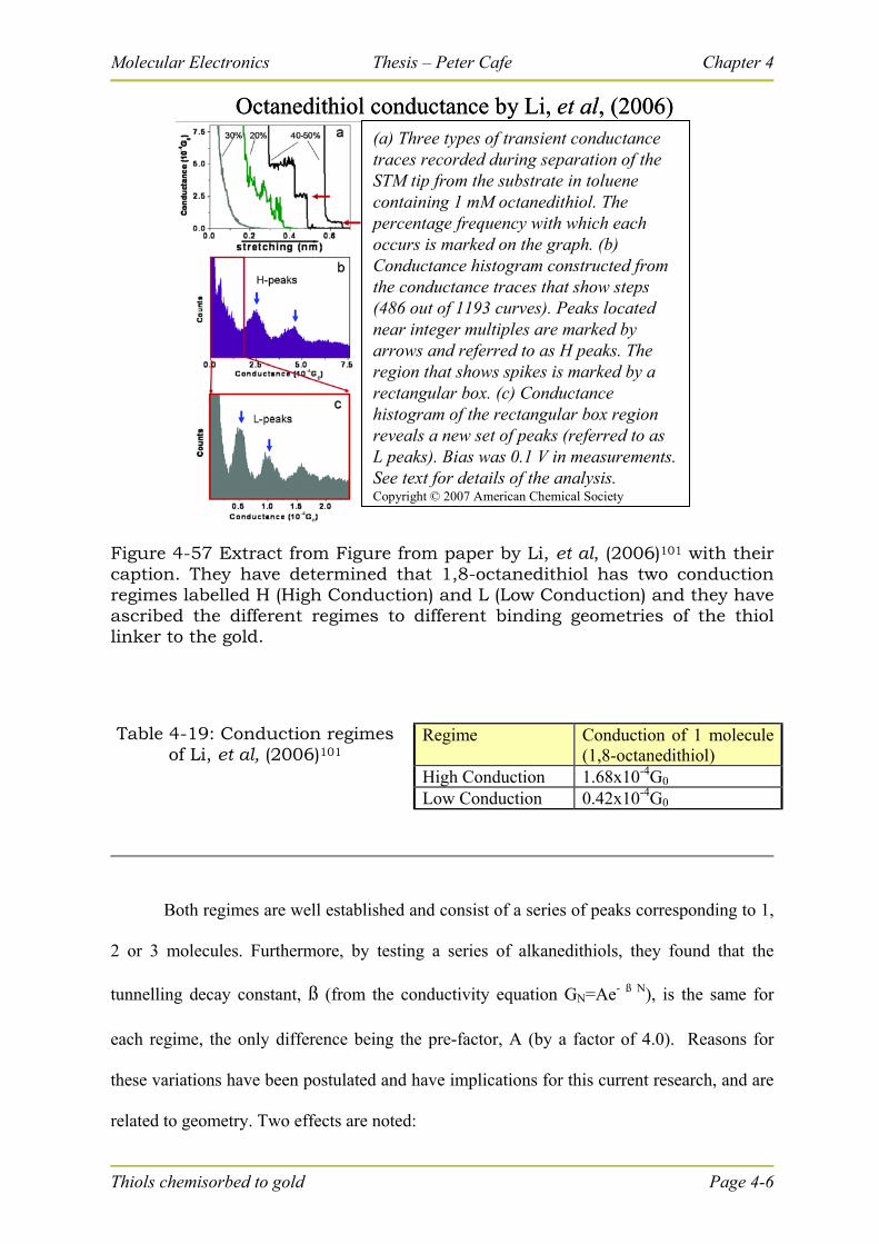
Molecular Electronics Thesis – Peter Cafe Chapter 4
(a) Three types of transient conductance traces recorded during separation of the STM tip from the substrate in toluene containing 1 mM octanedithiol. The percentage frequency with which each occurs is marked on the graph. (b) Conductance histogram constructed from the conductance traces that show steps (486 out of 1193 curves). Peaks located near integer multiples are marked by arrows and referred to as H peaks. The region that shows spikes is marked by a rectangular box. (c) Conductance histogram of the rectangular box region reveals a new set of peaks (referred to as L peaks). Bias was 0.1 V in measurements. See text for details of the analysis.Copyright © 2007 American Chemical Society
Octanedithiol conductance by Li, et al, (2006)(a) Three types of transient conductance traces recorded during separation of the STM tip from the substrate in toluene containing 1 mM octanedithiol. The percentage frequency with which each occurs is marked on the graph. (b) Conductance histogram constructed from the conductance traces that show steps (486 out of 1193 curves). Peaks located near integer multiples are marked by arrows and referred to as H peaks. The region that shows spikes is marked by a rectangular box. (c) Conductance histogram of the rectangular box region reveals a new set of peaks (referred to as L peaks). Bias was 0.1 V in measurements. See text for details of the analysis.Copyright © 2007 American Chemical Society
Octanedithiol conductance by Li, et al, (2006)
Figure 4-57 Extract from Figure from paper by Li, et al, (2006)101 with their caption. They have determined that 1,8-octanedithiol has two conduction regimes labelled H (High Conduction) and L (Low Conduction) and they have ascribed the different regimes to different binding geometries of the thiol linker to the gold.
Table 4-19: Conduction regimes of Li, et al, (2006)101
Regime Conduction of 1 molecule (1,8-octanedithiol)
High Conduction 1.68x10⁻⁴G0 Low Conduction 0.42x10⁻⁴G0
Both regimes are well established and consist of a series of peaks corresponding to 1,
2 or 3 molecules. Furthermore, by testing a series of alkanedithiols, they found that the
tunnelling decay constant, ß (from the conductivity equation GN=Ae- ß N), is the same for
each regime, the only difference being the pre-factor, A (by a factor of 4.0). Reasons for
these variations have been postulated and have implications for this current research, and are
related to geometry. Two effects are noted:
Thiols chemisorbed to gold Page 4-6
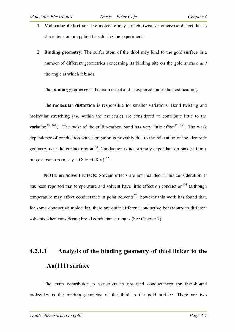
Molecular Electronics Thesis – Peter Cafe Chapter 4
Thiols chemisorbed to gold Page 4-7
1. Molecular distortion: The molecule may stretch, twist, or otherwise distort due to
shear, tension or applied bias during the experiment.
2. Binding geometry: The sulfur atom of the thiol may bind to the gold surface in a
number of different geometries concerning its binding site on the gold surface and
the angle at which it binds.
The binding geometry is the main effect and is explored under the next heading.
The molecular distortion is responsible for smaller variations. Bond twisting and
molecular stretching (i.e. within the molecule) are considered to contribute little to the
variation56, 160,). The twist of the sulfur-carbon bond has very little effect12, 161. The weak
dependence of conduction with elongation is probably due to the relaxation of the electrode
geometry near the contact region160. Conduction is not strongly dependant on bias (within a
range close to zero, say –0.8 to +0.8 V)162.
NOTE on Solvent Effects: Solvent effects are not included in this consideration. It
has been reported that temperature and solvent have little effect on conduction101 (although
temperature may affect conductance in polar solvents72) however this work has found that,
for some conductive molecules, there are quite different conductive behaviours in different
solvents when considering broad conductance ranges (See Chapter 2).
4.2.1.1 Analysis of the binding geometry of thiol linker to the
Au(111) surface
The main contributor to variations in observed conductances for thiol-bound
molecules is the binding geometry of the thiol to the gold surface. There are two
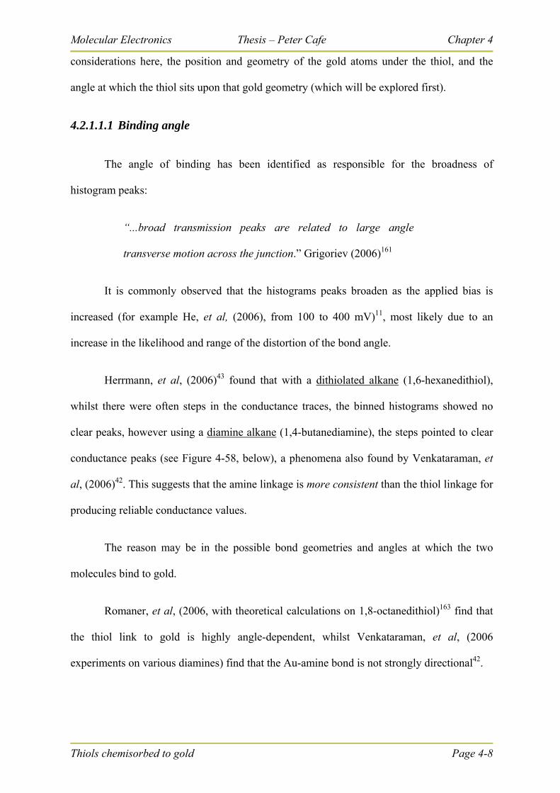
Molecular Electronics Thesis – Peter Cafe Chapter 4
Thiols chemisorbed to gold Page 4-8
considerations here, the position and geometry of the gold atoms under the thiol, and the
angle at which the thiol sits upon that gold geometry (which will be explored first).
4.2.1.1.1 Binding angle
The angle of binding has been identified as responsible for the broadness of
histogram peaks:
“...broad transmission peaks are related to large angle
transverse motion across the junction.” Grigoriev (2006)161
It is commonly observed that the histograms peaks broaden as the applied bias is
increased (for example He, et al, (2006), from 100 to 400 mV)11, most likely due to an
increase in the likelihood and range of the distortion of the bond angle.
Herrmann, et al, (2006)43 found that with a dithiolated alkane (1,6-hexanedithiol),
whilst there were often steps in the conductance traces, the binned histograms showed no
clear peaks, however using a diamine alkane (1,4-butanediamine), the steps pointed to clear
conductance peaks (see Figure 4-58, below), a phenomena also found by Venkataraman, et
al, (2006)42. This suggests that the amine linkage is more consistent than the thiol linkage for
producing reliable conductance values.
The reason may be in the possible bond geometries and angles at which the two
molecules bind to gold.
Romaner, et al, (2006, with theoretical calculations on 1,8-octanedithiol)163 find that
the thiol link to gold is highly angle-dependent, whilst Venkataraman, et al, (2006
experiments on various diamines) find that the Au-amine bond is not strongly directional42.
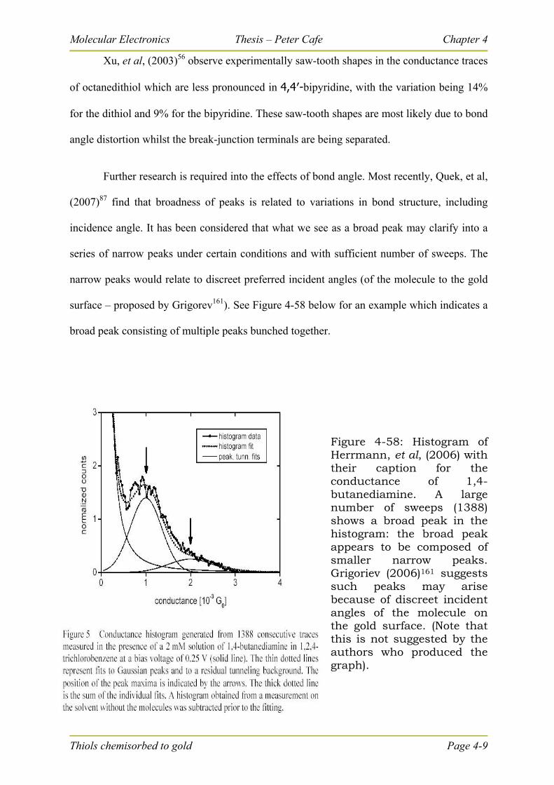
Molecular Electronics Thesis – Peter Cafe Chapter 4
Xu, et al, (2003)56 observe experimentally saw-tooth shapes in the conductance traces
of octanedithiol which are less pronounced in 4,4′-bipyridine, with the variation being 14%
for the dithiol and 9% for the bipyridine. These saw-tooth shapes are most likely due to bond
angle distortion whilst the break-junction terminals are being separated.
Further research is required into the effects of bond angle. Most recently, Quek, et al,
(2007)87 find that broadness of peaks is related to variations in bond structure, including
incidence angle. It has been considered that what we see as a broad peak may clarify into a
series of narrow peaks under certain conditions and with sufficient number of sweeps. The
narrow peaks would relate to discreet preferred incident angles (of the molecule to the gold
surface – proposed by Grigorev161). See Figure 4-58 below for an example which indicates a
broad peak consisting of multiple peaks bunched together.
Figure 4-58: Histogram of Herrmann, et al, (2006) with their caption for the conductance of 1,4-butanediamine. A large number of sweeps (1388) shows a broad peak in the histogram: the broad peak appears to be composed of smaller narrow peaks. Grigoriev (2006)161 suggests such peaks may arise because of discreet incident angles of the molecule on the gold surface. (Note that this is not suggested by the authors who produced the graph).
Thiols chemisorbed to gold Page 4-9
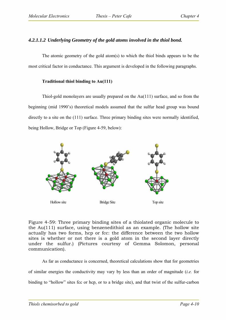
Molecular Electronics Thesis – Peter Cafe Chapter 4
4.2.1.1.2 Underlying Geometry of the gold atoms involved in the thiol bond.
The atomic geometry of the gold atom(s) to which the thiol binds appears to be the
most critical factor in conductance. This argument is developed in the following paragraphs.
Traditional thiol binding to Au(111)
Thiol-gold monolayers are usually prepared on the Au(111) surface, and so from the
beginning (mid 1990’s) theoretical models assumed that the sulfur head group was bound
directly to a site on the (111) surface. Three primary binding sites were normally identified,
being Hollow, Bridge or Top (Figure 4-59, below):
Hollow site Bridge Site Top site
Figure 4-59: Three primary binding sites of a thiolated organic molecule to the Au(111) surface, using benzenedithiol as an example. (The hollow site actually has two forms, hcp or fcc: the difference between the two hollow sites is whether or not there is a gold atom in the second layer directly under the sulfur.) (Pictures courtesy of Gemma Solomon, personal communication).
As far as conductance is concerned, theoretical calculations show that for geometries
of similar energies the conductivity may vary by less than an order of magnitude (i.e. for
binding to “hollow” sites fcc or hcp, or to a bridge site), and that twist of the sulfur-carbon
Thiols chemisorbed to gold Page 4-10
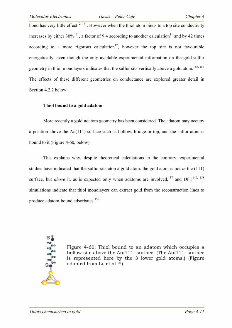
Molecular Electronics Thesis – Peter Cafe Chapter 4
bond has very little effect12, 161. However when the thiol atom binds to a top site conductivity
increases by either 30%161, a factor of 9.4 according to another calculation11 and by 42 times
according to a more rigorous calculation12, however the top site is not favourable
energetically, even though the only available experimental information on the gold-sulfur
geometry in thiol monolayers indicates that the sulfur sits vertically above a gold atom.155, 156
The effects of these different geometries on conductance are explored greater detail in
Section 4.2.2 below.
Thiol bound to a gold adatom
More recently a gold-adatom geometry has been considered. The adatom may occupy
a position above the Au(111) surface such as hollow, bridge or top, and the sulfur atom is
bound to it (Figure 4-60, below).
This explains why, despite theoretical calculations to the contrary, experimental
studies have indicated that the sulfur sits atop a gold atom: the gold atom is not in the (111)
surface, but above it, as is expected only when adatoms are involved,157 and DFT149, 158
simulations indicate that thiol monolayers can extract gold from the reconstruction lines to
produce adatom-bound adsorbates.158
Figure 4-60: Thiol bound to an adatom which occupies a hollow site above the Au(111) surface. (The Au(111) surface is represented here by the 3 lower gold atoms.) (Figure adapted from Li, et al101)
Thiols chemisorbed to gold Page 4-11
Molecular Electronics Thesis – Peter Cafe Chapter 4
Thiols chemisorbed to gold Page 4-12
This binding site has received little attention until very recently. (Even an extremely
thorough analysis of thiol-gold binding as recently as September 2006 by Vericat, et al,164
did not consider it, even though they highlighted surface pitting of Au(111), which is
evidence of the formation of gold adatoms – see Chapter 3.)
This thesis has shown that the adatom is the binding mode of chemisorbed 1,10-
phenanthroline to Au(111) (Chapter 3), and it was recently found to be the preferred binding
mode for isocyanides onto the Au(111) surface (Gilman, 2006)165. Venkataraman, et al,
(2006) recently proposed that binding of amine to gold was via an adatom...
“... with sufficient angular flexibility for easy junction formation but
well-defined electronic coupling of the N lone pair to the Au.”42.....
... and even more recently they identified it as the most likely binding mode87 (using
theoretical calculations).
For thiol binding to Au(111) there are a large number of recent helpful publications:
An insightful theoretical analysis of the formation of methanethiol monolayers has
recently been prepared by Wang, et al, (2007)166, modelling the system that appears in
experimental research in STM images. They have determined that a methanethiol monolayer
may form (from the dissociation of dimethyldisulfide), and that at a low surface coverage the
monolayer is formed onto gold adatoms which are produced on the (111) surface via the
lifting of the reconstruction, and that above a surface coverage of 7.8% (thiol head groups to
gold surface atoms) the adatoms are drawn from the (111) surface leaving behind vacancy
islands (pits) in the (111) surface. The adatom is implicated in thiol binding to the gold
surface, and the formation of the thiol-gold adatom entity is endothermic.
Molecular Electronics Thesis – Peter Cafe Chapter 4
Thiols chemisorbed to gold Page 4-13
Batista, et al., (2006)160 find theoretically that the thiol link may draw gold atoms
towards it from the bulk, implying that the terminal of the thiol with the gold may include an
adatom. Yu, et al., (2006)167 have established through X-ray standing wave experiments that
the thiol absorption to gold is via thiol-adatom units which are mobile on the gold surface.
Cometto, et al., (2005)144 highlight the mobility of thiols on gold with the adatom implicated
also. Maksymovych, et al, (2006)168 establish the adatom-thiol unit as responsible for the
binding of the methanethiol to the gold and the formation of pits. Romaner, et al, (2006)163
finds that the sulfur combines more strongly to an adatom than a perfectly planar surface
(referring to theoretical calculations done on 1,4-benzenedithiol sandwiched between 2 gold
electrodes). In a thorough approach including STM scans during in situ electrochemistry and
extensive theoretical modelling, Esplandiu, et al, (2005)143 conclude that thiols bind to a
“defect layer” of gold atoms above the gold surface (i.e. adatoms), and determine that the
thiol-adatom entity forms on step edges then and has little barrier to translation across the
surface.
What has become evident from various research papers in the last two or three years
and from the work of Chapter 3 is that pit formation alone is strong evidence of the
formation of gold adatom-thiol entities that are the anchors of the molecule to the gold
surface. Furthermore, these molecule-adatom units are mobile and intermolecular forces (of
the absorbed molecule) then dictate the most energetically favourable structuring of these
units on the surface (See the cartoon in Figure 4-61 below.)
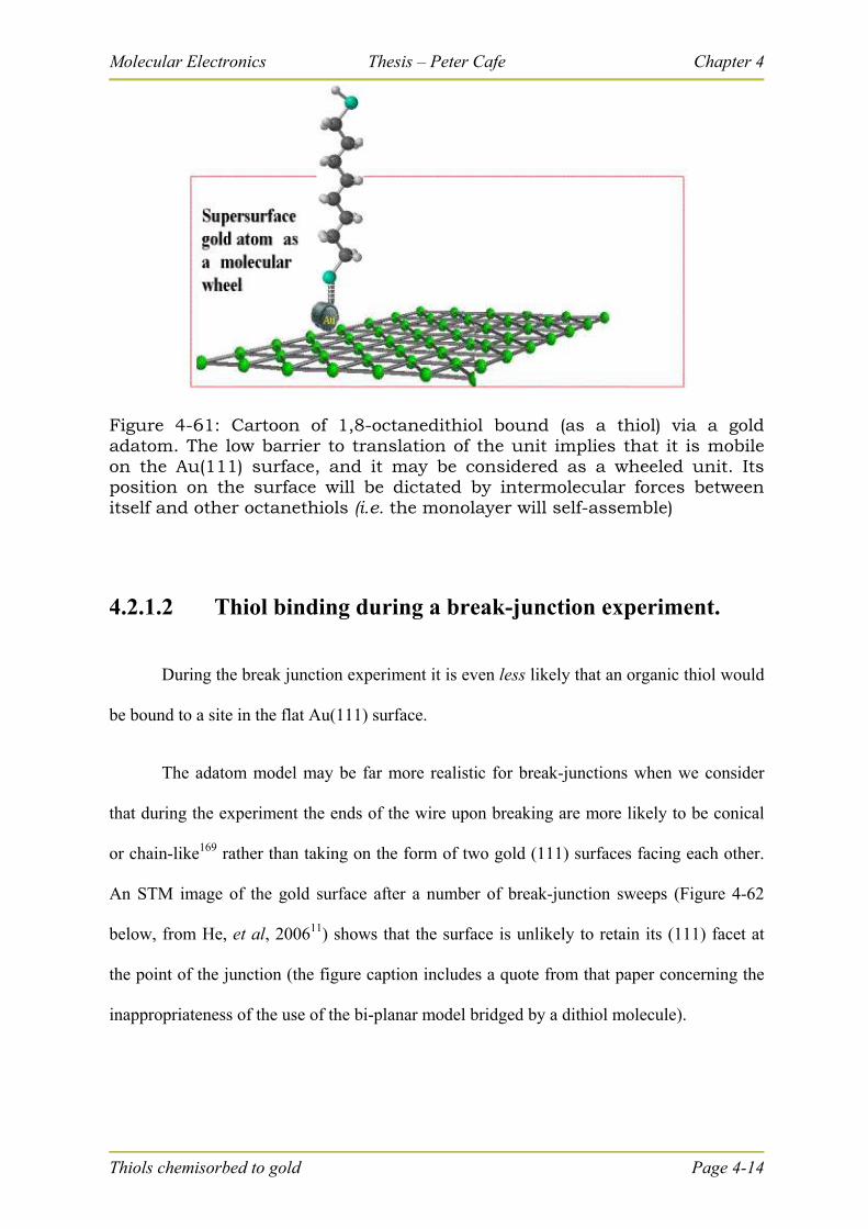
Molecular Electronics Thesis – Peter Cafe Chapter 4
Figure 4-61: Cartoon of 1,8-octanedithiol bound (as a thiol) via a gold adatom. The low barrier to translation of the unit implies that it is mobile on the Au(111) surface, and it may be considered as a wheeled unit. Its position on the surface will be dictated by intermolecular forces between itself and other octanethiols (i.e. the monolayer will self-assemble)
4.2.1.2 Thiol binding during a break-junction experiment.
During the break junction experiment it is even less likely that an organic thiol would
be bound to a site in the flat Au(111) surface.
The adatom model may be far more realistic for break-junctions when we consider
that during the experiment the ends of the wire upon breaking are more likely to be conical
or chain-like169 rather than taking on the form of two gold (111) surfaces facing each other.
An STM image of the gold surface after a number of break-junction sweeps (Figure 4-62
below, from He, et al, 200611) shows that the surface is unlikely to retain its (111) facet at
the point of the junction (the figure caption includes a quote from that paper concerning the
inappropriateness of the use of the bi-planar model bridged by a dithiol molecule).
Thiols chemisorbed to gold Page 4-14

Molecular Electronics Thesis – Peter Cafe Chapter 4
Figure 4-62: STM Image of the gold surface after a number of break-junction sweeps, from He, et al, 200611. they quote: “One important factor may be the use of a planar Au(111) model for the contact; a glance at Fig 1b (left) shows how inappropriate this is. More realistic models of the contact geometry will require simulations of much greater complexity.”11
In a similar thiol break-junction paper, Li, et al, (2006)101 identify that it is unlikely
that during a break junction experiment the dithiol molecule will be bound to two opposing
flat Au(111) surfaces. They isolate two binding modes for consideration at each end of the
molecule:
The thiol binds to a hollow site in the Au(111) surface,
and
The thiol binds to a gold adatom which sits upon the Au(111) surface.
When the dithiol molecule is sandwiched between 2 gold electrodes, the most likely
configurations of the two bonds are:
Hollow-Molecule-Adatom
and
Adatom-Molecule-Adatom
Thiols chemisorbed to gold Page 4-15
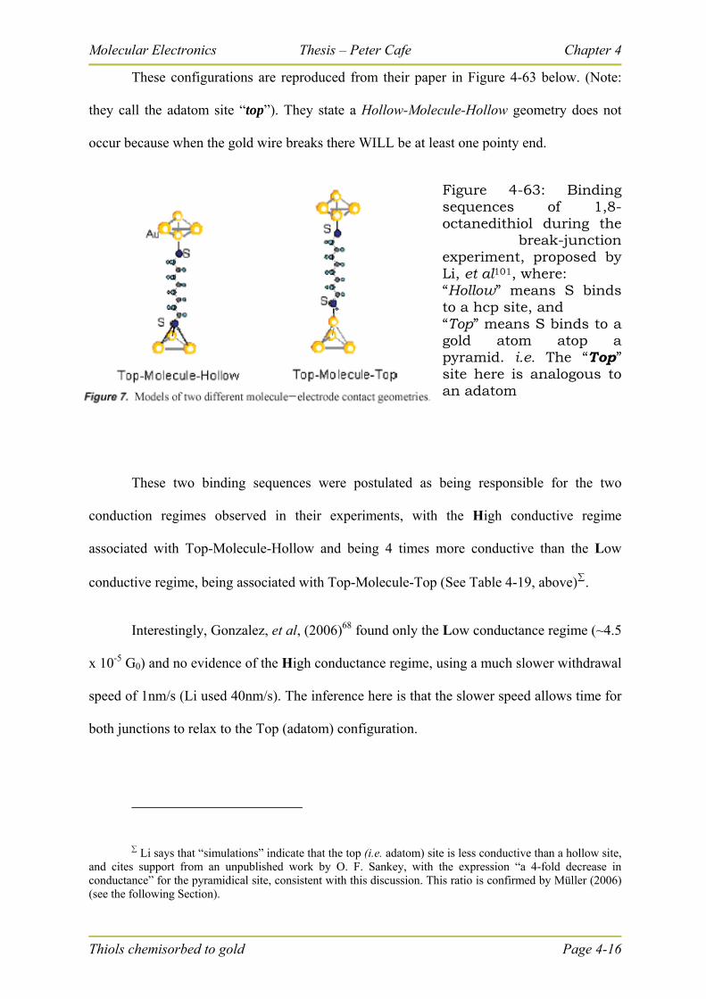
Molecular Electronics Thesis – Peter Cafe Chapter 4
These configurations are reproduced from their paper in Figure 4-63 below. (Note:
they call the adatom site “top”). They state a Hollow-Molecule-Hollow geometry does not
occur because when the gold wire breaks there WILL be at least one pointy end.
Figure 4-63: Binding sequences of 1,8-octanedithiol during the
break-junction experiment, proposed by Li, et al101, where: “Hollow” means S binds to a hcp site, and “Top” means S binds to a gold atom atop a pyramid. i.e. The “Top” site here is analogous to an adatom
These two binding sequences were postulated as being responsible for the two
conduction regimes observed in their experiments, with the High conductive regime
associated with Top-Molecule-Hollow and being 4 times more conductive than the Low
conductive regime, being associated with Top-Molecule-Top (See Table 4-19, above).
Interestingly, Gonzalez, et al, (2006)68 found only the Low conductance regime (~4.5
x 10-5 G0) and no evidence of the High conductance regime, using a much slower withdrawal
speed of 1nm/s (Li used 40nm/s). The inference here is that the slower speed allows time for
both junctions to relax to the Top (adatom) configuration.
Thiols chemisorbed to gold Page 4-16
Li says that “simulations” indicate that the top (i.e. adatom) site is less conductive than a hollow site, and cites support from an unpublished work by O. F. Sankey, with the expression “a 4-fold decrease in conductance” for the pyramidical site, consistent with this discussion. This ratio is confirmed by Müller (2006) (see the following Section).
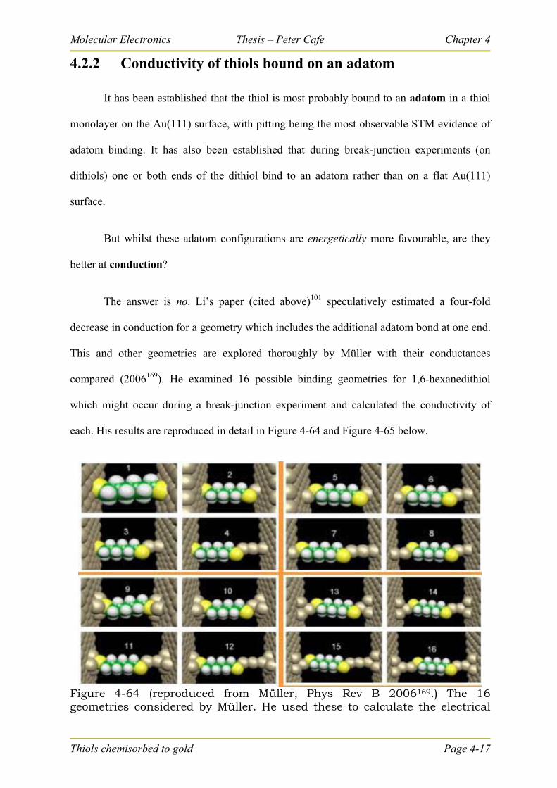
Molecular Electronics Thesis – Peter Cafe Chapter 4
4.2.2 Conductivity of thiols bound on an adatom
It has been established that the thiol is most probably bound to an adatom in a thiol
monolayer on the Au(111) surface, with pitting being the most observable STM evidence of
adatom binding. It has also been established that during break-junction experiments (on
dithiols) one or both ends of the dithiol bind to an adatom rather than on a flat Au(111)
surface.
But whilst these adatom configurations are energetically more favourable, are they
better at conduction?
The answer is no. Li’s paper (cited above)101 speculatively estimated a four-fold
decrease in conduction for a geometry which includes the additional adatom bond at one end.
This and other geometries are explored thoroughly by Müller with their conductances
compared (2006169). He examined 16 possible binding geometries for 1,6-hexanedithiol
which might occur during a break-junction experiment and calculated the conductivity of
each. His results are reproduced in detail in Figure 4-64 and Figure 4-65 below.
Figure 4-64 (reproduced from Müller, Phys Rev B 2006169.) The 16 geometries considered by Müller. He used these to calculate the electrical
Thiols chemisorbed to gold Page 4-17
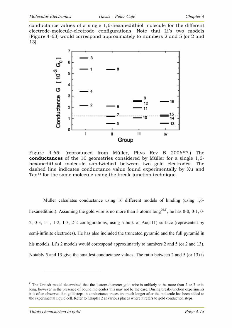
Molecular Electronics Thesis – Peter Cafe Chapter 4
conductance values of a single 1,6-hexanedithiol molecule for the different electrode-molecule-electrode configurations. Note that Li’s two models (Figure 4-63) would correspond approximately to numbers 2 and 5 (or 2 and 13).
Figure 4-65: (reproduced from Müller, Phys Rev B 2006169.) The conductances of the 16 geometries considered by Müller for a single 1,6-hexanedithyol molecule sandwiched between two gold electrodes. The dashed line indicates conductance value found experimentally by Xu and Tao14 for the same molecule using the break-junction technique.
Müller calculates conductance using 16 different models of binding (using 1,6-
hexanedithiol). Assuming the gold wire is no more than 3 atoms long76,, he has 0-0, 0-1, 0-
2, 0-3, 1-1, 1-2, 1-3, 2-2 configurations, using a bulk of Au(111) surface (represented by
semi-infinite electrodes). He has also included the truncated pyramid and the full pyramid in
his models. Li’s 2 models would correspond approximately to numbers 2 and 5 (or 2 and 13).
Notably 5 and 13 give the smallest conductance values. The ratio between 2 and 5 (or 13) is
The Untiedt model determined that the 1-atom-diameter gold wire is unlikely to be more than 2 or 3 units long, however in the presence of bound molecules this may not be the case. During break-junction experiments it is often observed that gold steps in conductance traces are much longer after the molecule has been added to the experimental liquid cell. Refer to Chapter 2 at various places where it refers to gold conduction steps.
Thiols chemisorbed to gold Page 4-18
Molecular Electronics Thesis – Peter Cafe Chapter 4
Thiols chemisorbed to gold Page 4-19
4.4 to 1, agreeing remarkably with the experimentally-determined ratio between the H and L
for Li, 1.68:0.42 (i.e. 4.0 to 1).
There is also good convergence with the work of Batista, et al, (2006)160, who found
that the inclusion of a single gold atom between the thiol and the gold electrode (at one end
only) decreases the conduction by a factor of three (performing theoretical calculations on
octanedithiol).
In Gonzales68, slower tip withdrawal (one 40th of the speed of Li) only the Low
conduction regime is observed, which could be interpreted in this way: in the slower
withdrawal there is sufficient time for the gold to arrange in pyramidical shapes at both ends,
so the configuration top-molecule-top (using Li’s terminology) would prevail, which gives
the Low conduction. Li himself observed that top-molecule-top often followed top-
molecule-hollow, but never the other way around. This implies that at slow enough speeds
pyramidical shapes would eventually form on both ends.
Jang, et al, (2006)69 find only the Low conductance regime (0.44 x 10⁻⁴ G0) for 1,8-
octanedithiol using “last step analysis”, and also finds Low conductance values for 1,6-
hexanedithiol (3.6 x 10⁻⁴ G0) and decanedithiol (0.057 x 10⁻⁴ G0) which are the same fraction
(¼) of the corresponding High conductance values found by Xu, et al (2003)14 (being 12.3 x
10-4 G0 and 0.021.0 x 10-4 G0 respectively). The implication is that the same dependence of
conduction on binding geometry is similar for all alkanedithiols (and possibly by extension
to all organic thiols).
Similar reports on H and L for the anchoring groups of diamines and dicarboxylic
acids show the factor is not ¼ but 1/15th and 1/10th respectively40 (See Table 4-19, page 4-6,
above,).
Molecular Electronics Thesis – Peter Cafe Chapter 4
A corollary of Müller’s work is that he found that certain theoretical configurations
agreed better than others with the experimental results of Xu and Tao14. It has long been
observed that theoretical approaches to conductance of molecules usually give conductances
of at least an order of magnitude greater than experimentally observed values161, 165.
However Müller does have theoretical conductances which agree with the work of Xu and
Tao. Müller’s finding suggests that more careful selection of binding geometries may lead to
greater convergence of theoretically and experimentally observed conductances.
Other papers add somewhat to the discussion:
Grigoriev, et al, (2006) found theoretically if the sulfur atom binds to a 3-atom gold
island there is an order of magnitude decrease in conductivity161.
Batista, et al, (2006) determined theoretically that the main contribution to variation
in conduction is the number of gold atoms between the molecule and the gold
“slab”160.
Basch, et al, (2005) observed that small changes which break the symmetry can have
a tremendous effect152.
Thiols chemisorbed to gold Page 4-20
Molecular Electronics Thesis – Peter Cafe Chapter 4
4-3 Conclusion to Chapter 4: dithiol binding and
conductance.
Having performed break-junction experiments on 1,8-octanedithiol (Chapter 2), and
established surface pitting as direct evidence adatom binding of 1,10-phenanthroline to the
Au(111) surface (Chapter 3), and considering the all publications cited above, and in
particular contrasting the papers of Müller and Li, et al, it is a conclusion of this thesis that
during the break-junction experiment only certain electrode tip configurations prevail, the
two most likely having adatoms involved in binding at one or both ends.
Different conduction regimes are related to the different binding modes. An adatom-
molecule-hollow configuration will show as a High conduction regime. An adatom-
molecule-adatom configuration will show as a Low conduction regime. In dithiols the ratio
between High and Low regimes is 4:1, and this ratio is different for other linker units.
In slower withdrawals only the Low conductance regime is observed.
Broadness of histogram peaks (in break-junction experiments) is mainly due to
variations in the angle at which the molecule binds to the gold, and to a lesser degree to other
distortions. In most thiol monolayers on gold, the thiol preferentially binds to an adatom
upon the Au(111) surface and the entity is mobile; the adatoms are extracted from the bulk
leaving pits. In break-junction experiments these adatoms are expressed as the points of
small pyramids. It is determined that during the break-junction experiment the main binding
modes of thiol to the gold electrodes involve a gold adatom at one or both ends.
Thiols chemisorbed to gold Page 4-21

Molecular Electronics Thesis – Peter Cafe Chapter 4
Thiols chemisorbed to gold Page 4-22
(blank page)

Molecular Electronics Thesis – Peter Cafe Chapter 5
Simple Computational Methods Page 5-1
ChaptteerChap r 5 Siimpllee Meetthodss fforr Essttiimattiing
Molleeccullarr Conduccttiiviitty..
5 S mp M hod o E ma ng
Mo u a Condu v y
5-0 Synopsis for Chapter 5
This chapter examines publications in the use of the tunnelling conduction formula
GN =Ae- ßN, (Section 5-2) where:
GN is the conductance of N “simple” repeat units.
ß is the tunnelling decay constant per unit, and
A is the constant pre-factor, which is largely related to the type of linker units at the ends of the molecule (e.g. thiols, amines, etc).
By natural extension to the body of literature two methods are developed which
exploit the tunnelling conduction formula, as follows:
Method (a): To extend a known series of molecules (such as alkanedithiols) –
this involves manipulation of the tunnelling decay constant, ß.
Method (b): To impute from one series of molecules (such as alkanedithiols) to
another series of molecules (such as alkanediamines) whose difference is solely
in the linker units at each end. This involves manipulation of the pre-factor, A.
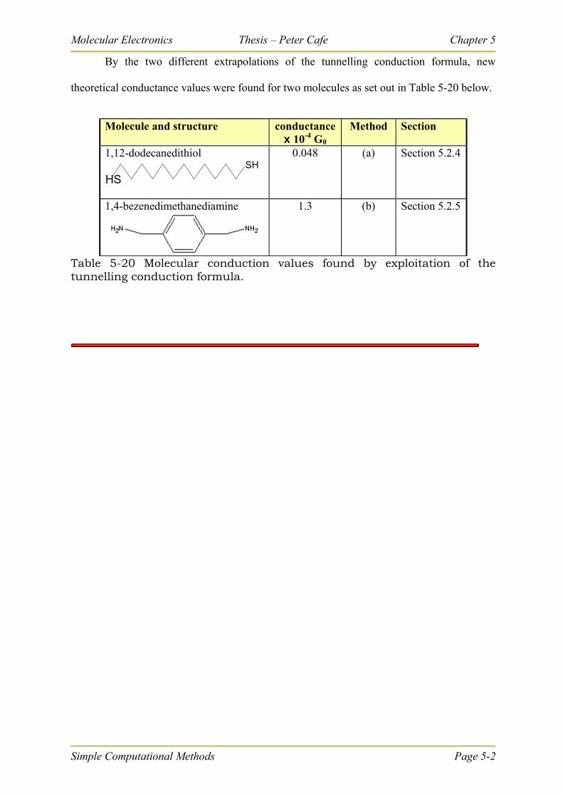
Molecular Electronics Thesis – Peter Cafe Chapter 5
By the two different extrapolations of the tunnelling conduction formula, new
theoretical conductance values were found for two molecules as set out in Table 5-20 below.
Molecule and structure conductancex 10-4 G0
Method Section
1,12-dodecanedithiol
HSSH
0.048 (a) Section 5.2.4
1,4-bezenedimethanediamine
1.3 (b) Section 5.2.5
Table 5-20 Molecular conduction values found by exploitation of the tunnelling conduction formula.
Simple Computational Methods Page 5-2
Molecular Electronics Thesis – Peter Cafe Chapter 5
Simple Computational Methods Page 5-3
5-1 Introduction to Chapter 5
“Everything should be made as simple as possible,
but not simpler.” (Albert Einstein)
5.1.1 Need for a simpler method for determining molecular
conductance.
Both experimental and theoretical methods for determining single molecule
conductance are quite difficult and expensive.
Experimental work requires a functioning preparation laboratory with clean areas
and pure water supply, as well as an instrument capable of probing a single molecule (such
as an STM), and each experiment requires components of pure gold. Equipment and sample
preparation may take a full day or more and requires a high level of expertise, as does the
operation of the instrument. Furthermore, the number of failures, for various reasons, is
very high. Post experimental analysis of results is also quite time-consuming.
Theoretical calculations of molecular conductance are also laborious, and are still
expensive in computer resources and require a high level of expertise. Traditional density
functional theory (DFT) calculations are insufficient and lead to large discrepancies with
experimental values19. Sophisticated methods required to obtain more accurate conduction
values are only just emerging170, and yet still results often vary from established
experimental results by an order of magnitude or more78, 87, 161.
A number of reliable conductance values of simple molecules are coming to light
through various research groups around the world (See Chapter 2, Table 2-2, page 2-15
Molecular Electronics Thesis – Peter Cafe Chapter 5
above). By comparing similar molecules patterns may appear which can be defined and
extrapolated to other molecules.
If these patterns do appear, they offer a much simpler method of calculating the
conductance of single molecules, and may improve on the accuracy of complicated DFT
calculations. At the very least, they will provide a “ball-park” figure, which may give some
assurance or guidance to a researcher, or may help the experimentalist in his search for
evidence of conduction contained within thousands of data files.
5.1.2 The work of this chapter: exploiting the tunnelling
conductance formula
This chapter presents determinations resulting from applying and extending the
reports of prior literature in the area of molecular electronics. The results section (Section 5-
2) presents the tunnelling conductance formula and uses it with prior experimental results to
calculate conductance values for other molecules. Although this may seem an obvious thing
to do, no published research has yet appeared which has done so. This is most probably
because the reliability of the formula is only just coming to the fore, as it depends on a
reliable body of prior results for individual molecules, which is only just emerging, and
which, for a number of relevant molecules, has been conveniently collated in Chapter 2
(Table 2-2).
Simple Computational Methods Page 5-4
Molecular Electronics Thesis – Peter Cafe Chapter 5
5-2 Tunneling conductance formula and its use to
determine the conduction of single molecules.
5.2.1 The unit of the conductance quantum, G0.
The conductance quantum is the quantised unit of conductance. It appears when
measuring the conductance of a quantum point contact. It is a fundamental physical constant.
The value of the quantum of conductance, G0, is given by:
h
eG0
2
2
Equation 5-1
where h and e are the fundamental constants:
e = charge of an electron = 1.6021917 x 10⁻¹⁹ Coulomb, and
h = Planck Constant = 6.626196 x 10⁻³⁴ Js
This gives a value of G0 as 7.7480917 × 10⁻⁵ Siemens.
The conductance of chain of single gold atoms is close to 1.0 G0, whilst the
conductance of many of the single organic molecule studied in literature is generally around
10-4 G0 (±2 orders of magnitude).
5.2.2 The tunnelling conduction formula
The conduction of similar alkanes whose difference is only in the number of carbons
in the backbone has been observed so as to deduce the tunnelling conductance of one single
carbon atom (i.e., a –CH2– unit as part of an alkane). This quantity is called the “tunnelling
decay constant”, ß, and is used in the following formula, which follows from McConnell
(1961)95:
Simple Computational Methods Page 5-5
Molecular Electronics Thesis – Peter Cafe Chapter 5
Simple Computational Methods Page 5-6
GN=Ae- ßN, Equation 5-2
Where GN is the conductance of a chain containing N -CH2- units. Occasionally the
tunnelling decay constant is expressed in length (i.e. per Angstrom).
A is the pre-factor and is found to relate to the linker units at each end of the
molecule.
If this formula holds consistently then it obviously can be used to predict the
conduction of other molecules.
5.2.3 Values determined from prior research
Various research groups have tried to quantify the parameters in the tunnelling
conductance formula, and their findings show a high consistency, as set out below.
5.2.3.1 Thiols
For alkanes with chemisorbed thiol end groups, the value of ß has been calculated as
1.07±0.05 per -CH2- unit and A=1.3 G0, using experimental data by Xu, et al, (2003)14.
Jang, et al, (2006)69 confirm a value of ß=1.0 per -CH2- unit for alkanedithiols, and
A=0.22 G0, using a break-junction with various withdrawal speeds (4 to 40 nm/s).
Similar work by Li, et al, (2006)101 found experimentally (on various chemisorbed
alkanedithiols) that the dithiols regularly produced two series histograms for each molecule,
which they labelled high (H) and low (L). They determined that the tunnelling decay
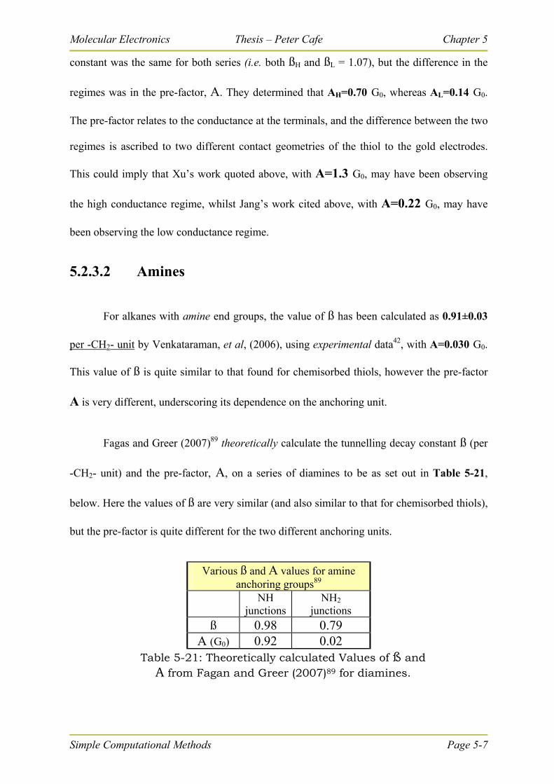
Molecular Electronics Thesis – Peter Cafe Chapter 5
Simple Computational Methods Page 5-7
constant was the same for both series (i.e. both ßH and ßL = 1.07), but the difference in the
regimes was in the pre-factor, A. They determined that AH=0.70 G0, whereas AL=0.14 G0.
The pre-factor relates to the conductance at the terminals, and the difference between the two
regimes is ascribed to two different contact geometries of the thiol to the gold electrodes.
This could imply that Xu’s work quoted above, with A=1.3 G0, may have been observing
the high conductance regime, whilst Jang’s work cited above, with A=0.22 G0, may have
been observing the low conductance regime.
5.2.3.2 Amines
For alkanes with amine end groups, the value of ß has been calculated as 0.91±0.03
per -CH2- unit by Venkataraman, et al, (2006), using experimental data42, with A=0.030 G0.
This value of ß is quite similar to that found for chemisorbed thiols, however the pre-factor
A is very different, underscoring its dependence on the anchoring unit.
Fagas and Greer (2007)89 theoretically calculate the tunnelling decay constant ß (per
-CH2- unit) and the pre-factor, A, on a series of diamines to be as set out in Table 5-21,
below. Here the values of ß are very similar (and also similar to that for chemisorbed thiols),
but the pre-factor is quite different for the two different anchoring units.
Various ß and A values for amine anchoring groups89
NH junctions
NH2 junctions
ß 0.98 0.79 A (G0) 0.92 0.02
Table 5-21: Theoretically calculated Values of ß and A from Fagan and Greer (2007)89 for diamines.
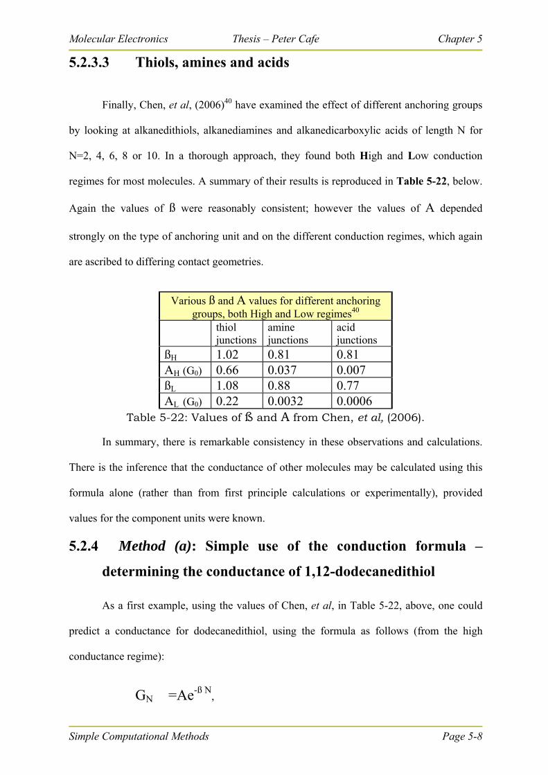
Molecular Electronics Thesis – Peter Cafe Chapter 5
Simple Computational Methods Page 5-8
5.2.3.3 Thiols, amines and acids
Finally, Chen, et al, (2006)40 have examined the effect of different anchoring groups
by looking at alkanedithiols, alkanediamines and alkanedicarboxylic acids of length N for
N=2, 4, 6, 8 or 10. In a thorough approach, they found both High and Low conduction
regimes for most molecules. A summary of their results is reproduced in Table 5-22, below.
Again the values of ß were reasonably consistent; however the values of A depended
strongly on the type of anchoring unit and on the different conduction regimes, which again
are ascribed to differing contact geometries.
Various ß and A values for different anchoring groups, both High and Low regimes40
thiol junctions
amine junctions
acid junctions
ßH 1.02 0.81 0.81 AH (G0) 0.66 0.037 0.007 ßL 1.08 0.88 0.77 AL (G0) 0.22 0.0032 0.0006
Table 5-22: Values of ß and A from Chen, et al, (2006).
In summary, there is remarkable consistency in these observations and calculations.
There is the inference that the conductance of other molecules may be calculated using this
formula alone (rather than from first principle calculations or experimentally), provided
values for the component units were known.
5.2.4 Method (a): Simple use of the conduction formula –
determining the conductance of 1,12-dodecanedithiol
As a first example, using the values of Chen, et al, in Table 5-22, above, one could
predict a conductance for dodecanedithiol, using the formula as follows (from the high
conductance regime):
GN =Ae-ß N,
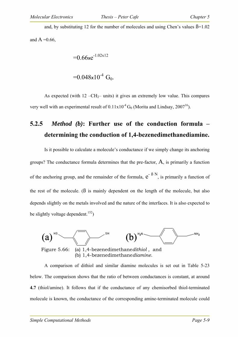
Molecular Electronics Thesis – Peter Cafe Chapter 5
and, by substituting 12 for the number of molecules and using Chen’s values ß=1.02
and A =0.66,
=0.66xe-1.02x12
=0.048x10⁻⁴ G0.
As expected (with 12 –CH2– units) it gives an extremely low value. This compares
very well with an experimental result of 0.11x10⁻⁴ G0 (Morita and Lindsay, 200716).
5.2.5 Method (b): Further use of the conduction formula –
determining the conduction of 1,4-bezenedimethanediamine.
Is it possible to calculate a molecule’s conductance if we simply change its anchoring
groups? The conductance formula determines that the pre-factor, A, is primarily a function
of the anchoring group, and the remainder of the formula, e- ß N, is primarily a function of
the rest of the molecule. (ß is mainly dependent on the length of the molecule, but also
depends slightly on the metals involved and the nature of the interfaces. It is also expected to
be slightly voltage dependent.152)
(a) (b)(a) (b)
Figure 5.66: (a) 1,4-bezenedimethanedithiol , and (b) 1,4-bezenedimethanediamine.
A comparison of dithiol and similar diamine molecules is set out in Table 5-23
below. The comparison shows that the ratio of between conductances is constant, at around
4.7 (thiol/amine). It follows that if the conductance of any chemisorbed thiol-terminated
molecule is known, the conductance of the corresponding amine-terminated molecule could
Simple Computational Methods Page 5-9

Molecular Electronics Thesis – Peter Cafe Chapter 5
be calculated by dividing by 4.7. By this method, the conduction of 1,4-
bezenedimethanediamine would be found by dividing that of 1,4-bezenedimethanedithiol by
4.7 (See the molecular structures in Figure 5.66 above). With the conductance of the dithiol
as 6.0x10⁻⁴ G083 the diamine is:
1,4-bezenedimethanediamine (calculated) = 6.0 ÷4.7 = 1.3 x10⁻⁴ G0,
This value is yet to be verified by any means, theoretical or experimental, but which
we must consider to be reasonably accurate.
dithiol Molecule
Conductance (10-4G0)
ref diamine Molecule
Conductance (10-4G0)
ref Ratio
thiol/amine
hexanedithiol 11 40 hexanediamine 2.7 40 4.1
octanedithiol 2.4 40 octanediamine 0.49 40 4.9
benzenedithiol 300 42 benzenediamine 64 42 4.7 Table 5-23: Comparison of dithiol and diamine conductances (where they exist in the same paper)
Simple Computational Methods Page 5-10
Molecular Electronics Thesis – Peter Cafe Chapter 5
Simple Computational Methods Page 5-11
5-3 Conclusion to Chapter 5: the use of the
tunneling conductance formula to determine the
conduction of single molecules.
In the first example, with the most basic application of the tunnelling conductance
formula, 1,12-dodecanedithiol was predicted to have a conductance of 0.048 x 10⁻⁴ G0,
comparing well with an experimental result. This type of application of the formula is
obvious, and is secure and has a strong theoretical basis, established in Section 5.2.3. But it
has limited application in that it can only be applied to longer or shorter versions of
molecules which have already been investigated, three or four of which are needed to
establish the parameters ß and A. As symmetry has an effect also, there might be slight
variations for odd and even members of the series.
In the second example 1,4-bezenedimethanediamine was predicted to have a
conductance of 0.048 x 10⁻⁴ G0. There were no comparisons available in the literature. The
method relied on the assumption that the pre-factor, A, was a function solely of the
anchoring unit. The examples used showed a very consistent ratio between the thiol and the
corresponding amine. Given that the ratio can be systematically established, the method is
sound and reliable. It offers a very convenient and powerful method for estimating the
conductance of whole families of molecules based upon known conductance of another
family of molecules, the difference in the two families being in the anchoring units.
Current theoretical methods for determining single molecule conductance involve
first principle calculations and the best methods consider large amounts of atomic data and
include a number of user-defined parametric adjustments – that is, they are computationally
laborious and somewhat subjective. Even so, calculated results can differ from well-

Molecular Electronics Thesis – Peter Cafe Chapter 5
established experimental results by an order of magnitude or more78, 161 (see also Table 2-2),
and whilst there may be some understanding of the reasons for this, it remains elusively
unquantifiable. In theoretical calculations a variety of realistic computational approaches are
available, resulting in predictions that can vary by an order of magnitude or more. Larger
uncertainties can arise in worst-case scenarios involving physisorbed molecules such as the
azines studied in this thesis. In general, Density-Functional Theory is inaccurate for
calculations of conductance because of its inability to treat long range electron correlation
effects, the asymptotic potential error and the band-gap error.19
DFT calculations also require an initial “guess” of geometry, which may in itself be
inappropriate, as developed in Chapter 4. These methods do not require such a guess.
The methods (a) and (b) presented here are extraordinarily simple and are reliable if
based upon established experimental values and used with molecules whose conduction is
primarily via a tunnelling mechanism. They will prove more useful as further reliable
experimental data reaches the pool of public knowledge.
Highly conjugated molecules and in particular polymeric porphyrin chains or carbon
nanotubes may conduct metallically (thermally activated hopping process)109 or even
ballistically171, and in addition to the exponential term of the conduction formula there would
be other terms, such as a linear component which would be simply related to Ohm’s Law.
Simple Computational Methods Page 5-12
Molecular Electronics Thesis – Peter Cafe Bibliography
Bibliography Page 6-1
ChaptteerChap r 6 Biiblliiogrraphy 6 B b og aphy
1. Cafe, P.F., Larsen, A.G., Yang, W., Bilic, A., Blake, I.M., Crossley, M.J., Zhang, J., Wackerbarth, H., Ulstrup, J., and Reimers, J.R., Chemisorbed and Physisorbed Structures for 1,10-Phenanthroline and Dipyrido[3,2-a:2',3'-c]phenazine on Au(111). J. Phys. Chem. C, 2007. 111(46): p. 17285-17296.
2. Hipps, K.W., It's all about contacts. (Perspective: Molecular Electronics). Science, 2001. 294(5542): p. 536.
3. Moore, G.E., Cramming more Components onto Integrated Circuits. Electronics, 1965: p. 114-117.
4. Jurvetson, S.T., Transcending Moore's Law with Molecular Electronics and Nanotechnology. Nanotechnology Law and Business, 2004. 1(1): p. 70 - 90.
5. Tuomi, I., The Lives and Death of Moore's Law. First Monday (http://www.firstmonday.org/issues/issue7_11/tuomi/#author), 2002. 7(11).
6. Compañó, R., Molenkamp, L., and Paul, D., Technology Roadmap for Nanoelectronics, R. Compañó, L. Molenkamp, and P. DJ, Editors. 1999, European Commission IST Programme Future and Emerging Technologies.
7. Aviram, A. and Ratner, M.A., Molecular Rectifiers. Chemical Physics Letters, 1974. 29: p. 277.
8. Carter, F.L., Progress in concepts of conformational switching and molecular electronic devices. 1982: Nav. Res. Lab., Washington DC. 24.
9. Reed, M.A. and Lee, T., Molecular Nanoelectronics 2003: Stevenson Ranch, CA : American Scientific Publishers.
10. Carroll, R.L. and Gorman, C.B., The Genesis of Molecular Electronics. Angewandte Chemie International Edition, 2002. 41(73): p. 4378.
11. He, J., Sankey, O.F., Lee, M., Tao, N.J., Li, X., and Lindsay, S.M. Measuring single molecule conductance with break junctions. in Faraday Discussions 131 - Molecular Wires and Conductors. 2006.
12. Solomon, G.C., Riemers, J.R., and Hush, N.S., Overcoming computational uncertainties to reveal chemical sensitivity in single molecule conduction calculations. J Chemical Physics, 2005. 122(224502): p. 1 - 7.
13. Binnig, G. and Rohrer, H., Scanning tunneling microscopy. Applied Physics Letters, 1982. 40: p. 178-180.
14. Xu, B. and Tao, N.J., Measurement of Single-Molecule Resistance by Repeated Formation of Molecular Junctions. Science, 2003. 301(5637): p. 1221 - 1224.
15. Cui, X.D., Primak, A., Zarate, X., Tomfohr, J., Sankey, O.F., Moore, A.L., Moore, T.A., Gust, D., Harris, G., and Lindsay, Reproducible Measurement of Single-Molecule Conductivity. Science, 2001. 294(5542): p. 571 - 574.
16. Morita, T. and Lindsay, S.M., Determination of Single Molecule Conductances of Alkanedithiols by Conducting-Atomic Force Microscopy with Large Gold Nanoparticles. J American Chemical Society, 2007. 129(23): p. 7262 -7263.
Molecular Electronics Thesis – Peter Cafe Bibliography
Bibliography Page 6-2
17. Smalley, R. and Drexler, K., Open Debate: "NANOTECHNOLOGY": Drexler and Smalley make the case for and against 'molecular assemblers'. Chemical and Engineering News, 2003. 81(48): p. 37-42.
18. McGimpsey, W.G. Molecular Electronics - Past, Present, Future? in Molecular Engineering - The next five years. 2002. Worcester, Mass, USA: Second International Corporate/Academic Roundtable on Emerging Technologies.
19. Reimers, J.R., Cai, Z.-L., Bilic, A., and Hush, N.S., Molecular Electronics III - Chapter "The appropriateness of Density Functional Theory for the Calculation of Molecular Electronics Properties". Vol. 1006. 2003, New York: New York Academy of Sciences.
20. Lent, C.S. and Timler, J., Power gain and dissipation in quantum-dot cellular automata. J Applied Physics, 2002. 91(2): p. 823-831.
21. Stan, M.R., Franzon, P.D., Goldstein, S.C., Lach, J.C., and Ziegler, M.M., Molecular Electronics: From Devices and Interconnects to Circuits and Architecture. Proceedings of the IEEE, 2003. 91(11): p. 1940 - 1957.
22. Smith, E.M. Nano panelist sees molecular devices as next step toward smaller, cheaper, faster devices (James J. Marek, Jr.). ASME NEWS. 27 Apr 2007; http://www.asmenews.org/archives/backissues/aug01/features/nanopan.html.
23. Shi, N., Yim, G., Han, M., Xu, Z., Fan, X., Li, H., and Hong, J., Coordination driving self-assembly of gold nanoparticles and tetrapyridylporphine into hollow spheres. Chemistry Letters, 2005. 34(11): p. 1468 - 1469.
24. Caruso, F., Caruso, R.A., and Mohwald, H., Nanoengineering of Inorganic and Hybrid Hollow Spheres by Colloidal Templating. Science, 1998. 282: p. 1111-4
25. Greco, R.S., Nanoscale Technology in Biological Systems. 2005: CRC Press. 26. Wowk, B., Cell Repair Technology. Cryonics, 1988. 9(7)(96): p. 21 - 32. 27. Stan, M.R., Rose, G.S., Ziegler, M.M., and Brown, C.L. Hybrid CMOS/Molecular
Electronics Circuits. in 19th International Conference on VLSI Design - IEEE. 2006: IEEE.
28. Allen, T.E.G., The Conduction of Selected Platinum and Nickel Acetylides 2003, University of Sydney, Honours thesis in School of Chemistry
29. Li, C., Fan, W., Lei, B., Zhang, D., Han, S., Tang, T., Liu, X., Liu, Z., Asano, S., Meyyappan, M., Han, J., and Zhou, C., Multilevel memory based on molecular devices. Applied Physics Letters, 2004. 84(11): p. 1949-1951.
30. Ashwell, G.J., Urasinska, B., and Tyrrell, W.D., Molecules that mimic Schottky diodes. Phys. Chem. Chem. Phys, 2006. 8(28): p. 3314 - 3319.
31. Huang, Y., Duan, X., Cui, Y., Lauhon, L.J., Kim, K.-H., and Lieber, C.M., Logic Circuits with Carbon Nanotube Transistors. Science, 2001. 294(5545): p. 1313 - 1317.
32. Bachtold, A., Hadley, P., Nakanishi, T., and Dekker, C., Logic Circuits with Carbon Nanotube Transistors. Science, 2001. 294(5545): p. 1317-1320.
33. Lindsay, S.M. Closing Remarks. in Faraday Discussions 131 - Molecular Wires and Conductors. 2006. Manchester.
34. Tour, J.M., Molecular Electronics: Commercial Insights, Chemistry, Devices. Architecture and Programming. 2003: World Scientific. 600.
35. Seminario, J.M., Zacarias, A.G., and M, T.J., Molecular Alligator Clips for Single Molecule Electronics. Studies of Group 16 and Isonitriles Interfaced with Au Contacts. J American Chemical Society, 1999. 121(2): p. 411 - 416.
36. Bilic, A., Reimers, J.R., and Hush, N.S., Adsorption of pyridine on the gold(111) surface: implications for molecular "alligator clips". J. Phys. Chem. B, 2002. 106: p. 6740-7.
Molecular Electronics Thesis – Peter Cafe Bibliography
Bibliography Page 6-3
37. Reimers, J.R., Hall, L.E., Crossley, M.J., and Hush, N.S., Rigid fused oligoporphyrins as potential versatile molecular wires. J. Phys. Chem. A, 1999. 103: p. 4385 - 4397.
38. Grigoriev, A., Molecular Alligator Clips - A study of metal-molecule contacts for molecular electronics, 2004, Chalmers University of Technology, Goteborg, Sweeden, PhD thesis in Dept of Microtechnology and Nanoscience
39. Hermann, B.A., Scherer, L.J., Housecroft, C.E., and Constable, E.C., Self-Organized Monolayers: A Route to Conformational Switching and Read-Out of Functional Supramolecular Assemblies by Scanning Probe Methods. Advanced Funcional Materials, 2006. 16: p. 221-235.
40. Chen, F., Li, X., Hihath, J., Huang, Z., and Tao, N.J., Effect of anchoring groups on single-molecule conductance: comparative study of thiol-, amine-, and carboxylic-acid-terminated molecules. J American Chemical Society, 2006. 128: p. 15874 - 15881.
41. Hathaway, J. Nature's Smallest Shock ASU Research, Tempe, AZ. 12 Jan 2008; http://researchmag.asu.edu/stories/shock.html.
42. Venkataraman, L., Klare, J.E., Tam, I.W., Nickolls, C., Hybertsen, M.S., and Steigerwald, M.L., Single Molecule Circuits with Well-Defined Molecular Conductance. Nano Letters, 2006. 6(3): p. 458-462.
43. Herrmann, J., Müller, K.-H., Wei, G., Bray, D., Roberts, M., Raguse, B., and Wieczorek, L. Contact effects in single-molecule conduction. in ICONN2006. 2006. Brisbane.
44. Yu, H.Z., Zhao, J.W., Wang, Y., Q, Cai, S.M., and Liu, Z.F., Fabricating an azobenzene self-assembled monolayer via step-by-step surface modification of a cysteamine monolayer on gold. Journal of Electroanalytical Chemistry, 1997. 438(1-2): p. 221-224.
45. Brolo, A.G., Irish, D.E., Szymanski, G., and Lipkowski, J., Relationship between SERS Intensity and Both Surface Coverage and Morphology for Pyrazine Adsorbed on a Polycrystalline Gold Electrode. Langmuir, 1998. 14(2): p. 517 -527.
46. Cunha, F., Tao, N.J., Wang, X.W., Jin, Q., Duong, B., and D'Agnese, J., Potential-induced phase transitions in 2,2'-bipyridine and 4,4'-bipyridine monolayers on Au(111) studied by in Situ scanning tunneling microscopy and atomic force microscopy. Langmuir, 1996. 12: p. 6410 - 6418.
47. Kim, B.S., Beebe, J.M., Jun, Y., Zhu, X.-Y., and Frisbie, C.D., Correlation between HOMO Alignment and Contact Resistance in Molecular Junctions: Aromatic Thiols versus Aromatic Isocyanides. J American Chemical Society; (Communication), 2006. 128(15): p. 4970-4971.
48. Cunha, F., Jin, Q., Tao, N.J., and Li, C.Z., Structural Phase Transition in Self-Assembled 1,10 phenanthroline monolayer on Au(111). Surface Science, 1997. 389: p. 19-28.
49. Pinheiro, L.S. and Temperini, M.L.A., Coadsorption of 2-mercaptopyrimidine and 1,10'-phenanthroline on Au(111) as seen by STM. Surface Science, 1999. 441: p. 53.
50. Dominguez, O., Echegoyen, L., Cunha, F., and Tao, N., Self-Assembled Fullerene-Derivative Monolayers on a Gold Substrate Using Phenanthroline-Au Interactions. Langmuir, 1998. 14(4): p. 821-824.
51. Yang, D., Bizzotto, D., Lipkowski, J., Pettinger, B., and Mirwald, S., Electrochemical and second harmonic generation studies of 2,2'-bipyridine adsorption at the Au(111) electrode surface. J Physical Chemistry, 1994. 98(28): p. 7083 - 7089.
Molecular Electronics Thesis – Peter Cafe Bibliography
Bibliography Page 6-4
52. Noda, H., Minoha, T., Wan, L.-J., and Osawa, M., Adsorption and ordered phase formation of 2,2'-bipyridine on Au(111): a combined surface-enhanced infrared and STM study. Journal of Electroanalytical Chemistry, 2000. 481(1): p. 62 - 68.
53. Cunha, F. and Tao, N.J., Surface charge-induced order-disorder transition in am organic monolayer. Phys. Rev. Lett., 1995. 75(12): p. 2376 - 2379.
54. Pinheiro, L.S. and Temperini, M.L.A., STM study of 2,2':6'2''-terpyridine self-assembly on Au(111). Surface Science, 2000. 464(2-3): p. 176 - 182.
55. Venkataraman, L., Klare, J.E., Nuckolls, C., Hybertsen, M.S., and Steigerwald, M.L., Dependence of single-molecule junction conductance on molecular conformation. Nature, 2006. 442(7105): p. 904-907.
56. Xu, B.Q., Xiao, X., and Tao, N.J., Measurements of Single Molecule Electromechanical Properties. J American Chemical Society, 2003. 125(52): p. 16164-16165.
57. Crossley, M.J., Burn, P.L., Langford, S.J., and Prashar, J.K., Enantioselective recognition of histidine and lysine esters by porphyrin chiral clefts and detection of amino acid conformations in the bound state. J. Chem. Soc. Chem. Commun., 1995: p. 1925 - 1927.
58. Kushmerick, J.G., Holt, D.B., Yang, J.C., Naciri, J., Moore, M.H., and Shashidar, R., Metal-Molecule Contacts and Charge Transports across Monomolecular Monolayers. Phys. Rev. Lett., 2002. 89(8): p. 243.
59. Schull, T.L., Kushmerick, J.G., Petterson, C.H., George, C., Moore, M.H., and Shashidar, R., Ligand Effects on Charge Transport in Platinum Complexes. J American Chemical Society, 2003. 125(11): p. 3202-3.
60. Reichert, J., Ochs, R., Beckman, D., Weber, H.B., Mayor, M., and Lohneysen, H.V., Driving Current through Single Organic Molecules. Phys. Rev. Lett., 2002. 88(17): p. 176804.
61. Weber, H.B., Reichert, J., Weigend, F., Ochs, R., Beckman, D., Mayor, M., Alrichs, R., and Lohneysen, H.V., Electron Transport through Single Conjugated Molecules. Chemical Physics, 2002. 281: p. 113-125.
62. Reed, M.A., Zhou, C., Muller, C.J., Burgin, T.P., and Tour, J.M., Conductance of a Molecular Junction. Science, 2001. 294(5542): p. 252 - 254.
63. Yaliraki, N., Kemp, S.N., and Ratner, M.A., The injecting energy at molecule/metal interfaces: Implications for conductance of Molecular Junctions from an ab initio Molecular Description. J American Chemical Society, 1999. 111(15): p. 6997-7002.
64. Binnig, G. and Rohrer, H., Scanning tunneling microscopy. Helvetica Physica Acta, 1982. 55: p. 726-35.
65. Binnig, G. and Rohrer, H., Scanning Tunneling Microscopy. IBM J. Research and Development, 1986. 30(4): p. 355-369.
66. Blum, A.S., Yang, J.C., Shashidhar, R., and Ratna B, Comparing the Conductivity of Molecular wires with The Scanning Tunneling Microscope. Applied Physics Letters, 2003. 82(19): p. 3322-3324.
67. Fan, F.F., Yang, J., Cai, L., Price, D.W., Dirk, S.M., Kosynkin, D.V., Yao, Y., Rawlett, A.M., Tour, J.M., and Bard, A.J., Charge Transport Through Self-Assembled Monolayers of Compounds of Interest in Molecular Electronics. J American Chemical Society, 1999. 103: p. 4006-4010.
68. Gonzalez, M.T., Wu, S., Huber, R., van der Molen, S.J., Schonenberger, C., and Calame, M., Electrical Conductance of Molecular Junctions by a Robust Statistical Analysis. Nano Letters, 2006. 6(10): p. 2238-2242.
69. Jang, S.-Y., Reddy, P., Majumdar, A., and Segalman, R.A., Interpretation of Stochastic Events in Single Molecule Conductance Measurements. Nano Letters, 2006. 6(10): p. 2362 -2367.
Molecular Electronics Thesis – Peter Cafe Bibliography
Bibliography Page 6-5
70. Leatherman, G., Durantini, E.N., Gust, D., Moore, A.L., Moore, T.A., Stone, S., Zhou, Z., Rez , P., Liu, Y.Z., and Lindsay, S.M., Carotene as a Molecular Wire: Conducting Atomic Force Microscopy. J American Chemical Society, 1999. 103: p. 4006-4010.
71. Hurst, D.T., Thakrar, U.B., Wells, C.H.J., and Wyer, J., An N.M.R. Study of Electron Donor-Electron Acceptor Interaction Between Aromatic Hydrocarbons and Diazines. Australian Journal of Chemistry, 1989. 42: p. 1313-9.
72. Li, X., Hihath, J., Chen, F., Masuda, T., Zang, L., and Tao, N.J., Thermally activated electron transport in single redox molecules. J American Chemical Society, 2007. 40(30).
73. Zhou, C. About Self. Center for Microelectronic Materials and Structures Yale Univ. 29 July 2007; http://www.yale.edu/ee100/chongwu/CHONGWU.HTML.
74. Molec.com. Molecular Imaging’s PicoPlus Microscope. Agilent. 18 Jan 2007; http://www.orgchem.ugent.be/fdp/pdf/AFM%20PicoPlus.pdf.
75. Molec.com. Molecular Imaging's STM unit. Agilent. 22 Feb 2007; http://cp.literature.agilent.com/litweb/pdf/5989-5997EN.pdf.
76. Untiedt, C., Yanson, A.I., Grande, R., Rubio-Bollinger, G., Agrait, N., Viera, S., and van Ruitenbeek, J.M., Calibration of the length of a chain of single gold atoms. Phys. Rev. B, 2002. 66: p. 085418.
77. Whetten, R.L. and Salisbury, B.E. Quantum Conductance. Georgia Institute of Technology, Atlanta, Georgia. 29 July 2007; http://www.physics.gatech.edu/research/whetten/rec_results/quantum_cond.html.
78. Kang, B.K., Aratani, N., Lim, J.K., Kim, D., Osuka, A., and Yoo, K.-H., Electrical transport properties and their reproducibility for linear porphyrin arrays. Materials Science and Engineering C, 2005. 26: p. 1023-1027.
79. Wohlthat, S., Conductance of various organic molecules - Personal Communication, 2008, (Sydney University).
80. Hu, Y., Zhu, Y., Gao, H., and Guo, H., Conductance of an Ensemble of Molecular Wires: A Statistical Analysis. Phys. Rev. Lett., 2005. 95: p. 156803.
81. Tomfohr, J. and Sankey, O.F., Simple Estimates of the Electron Transport Properties of Molecules. Phys. Status Solidi B, 2002. 233: p. 59-69.
82. Halimun, H., Mahapatro, A.K., Choi, J., Lodha, S., Janes, D., and Gosh, S., Device structure for electronic transport through individual molecules using nanoelectrodes. Applied Physics Letters, 2005. 87(233509): p. 3.
83. Xiao, X., Xu, B.Q., and Tao, N.J., Measurement of Single Molecule Conductance: Benzenedithiol and Benzenedimethanethiol. Nano Letters, 2004. 4(2): p. 267-271.
84. Tsutsui, M., Teramae, Y., Kurokawa, S., and Sakai, A., High-conductance states of single benzenedithiol molecules. Applied Physics Letters, 2006. 89(16): p. 163111.
85. Tomfohr, J. and Sankey, O.F., Theoretical analysis of electron transport through organic molecules. J Chemical Physics, 2004. 120: p. 1542.
86. Lang, N.D. and Avouris, P., Electrical conductance of individual molecules. Phys. Rev. B, 2001. 64(12): p. 125323.
87. Quek, S.Y., Venkataraman, L., Choi, H.J., Louie, S.G., Hybertsen, M.S., and Neaton, J.B., Amine-gold linked single-molecule junctions: Experiment and theory. Condensed Matter arXiv:, 2007. 0707: p. 2091v1.
88. Ning, J., Li, R., Shen, X., Qian, Z., Hou, S., Rocha, A.R., and Sanvito, S., First-principles calculation on the zero-bias conductance of a gold/1,4-diaminobenzene/gold molecular junction. Nanotechnology, 2007. 18: p. 345206 (6pp).
89. Fagas, G. and Greer, J.C., Tunnelling in alkanes anchored to gold electrodes via amine end groups. arXiv:, 2007. 0706.: p. 0835v1.
Molecular Electronics Thesis – Peter Cafe Bibliography
Bibliography Page 6-6
90. Wohlthat, S., Conductance of various organic molecules - Personal Communication, 2007, (Sydney University).
91. Cheng, W.W., Chen, H., Note, R., Mizuseki, H., and Kawazoe, Y., Electron transport through molecular wire: effect of isomery. Physica E, 2005. 25: p. 643-646.
92. Csonka, S., Halbritter, A., and Mihály, G., Pulling gold nanowires with a hydrogen clamp: Strong interactions of hydrogen molecules with gold nanojunctions. Phys. Rev. B, 2006. 73(07): p. 075405 (6).
93. Jelenic, P., Perez, R., Ortega, J., and Flores, F., Hydrogen dissociation over Au nanowires and the fractional conductance quantum. Phys. Rev. Lett., 2006. 96(046): p. 046803.
94. Rego, L.G.C., Rocha, A.R., Rodrigues, V., and Ugarte, D., Role of structural evolution in the quantum conductance behaviour of gold nanowires during stretching. Phys. Rev. B, 2003. 67(04): p. 045412 (10).
95. McConnell, H.M., Intramolecular Charge Transfer in Aromatic Free Radicals J Chemical Physics, 1961. 35(2): p. 508-515
96. Kim, M.-J., Konduri, R., Ye, H., MacDonnell, F.K., Puntoriero, F., Serroni, S., Campagna, S., Holder, T., Kinsel, G., and Rajeshwar, K., Dinuclear Ruthenium(II) Polypyridyl Complexes Containing Large, Redox-Active, Aromatic Bridging Ligands: Synthesis, Characterization, and Intramolecular Quenching of MLCT Excited States Inorganic Chemistry, 2002. 41: p. 2471.
97. Chiorboli, C., Fracasso, S., Ravaglia, M., Scandola, F., Campagna, S., Wouters, K.L., Konduri, R., and MacDonnell, F.M., Primary Photoinduced Processes in Bimetallic Dyads with Extended Aromatic Bridges. Tetraazatetrapyridopentacene Complexes of Ruthenium(II) and Osmium(II) Inorganic Chemistry, 2005. 44(23): p. 8368.
98. Hough, W.A., Synthesis and properties of oligoporphyrins: Studies for use as molecular wires., 2003, Sydney University, PhD thesis in School of Chemistry
99. Crossley, M.J. and Burn, P.L., An approach to porphyrin-based molecular wires: Synthesis of a Bis(porphyrin)tetraone and its conversion to a Linearly Conjugated Tetrakisporphyrin system. J. Chem. Soc. Chem. Commun., 1991: p. 1569.
100. Molec.com. Liquid Cell. Agilent. 14 Aug 2007; http://www.molec.com/products_accessories.html#cells.
101. Li, X., He, J., Hihath, J., Xu, B., Lindsay, S.M., and Tao, N., Conductance of Single Alkanedithiols: Conduction Mechanism and Effect of Molecule-Electrode Contacts. J American Chemical Society, 2006. 128(6): p. 2135 -2141.
102. Bilic, A., Reimers, J.R., Hush, N.S., Hoft, R.C., and Ford, M.J., Adsorption of benzene on copper, silver, and gold surfaces. J. Chem. Theory and Comput., 2006. 2: p. 1093.
103. Fantacci, S., de Angelis, F., Wang, J., Bernhard, S., and Selloni, A., A combined computational and experimental study of polynuclear Ru-TPPZ complexes: insights into the electronic and optical properties of co-ordination polymers. . J American Chemical Society, 2004. 126: p. 9715.
104. Araki, K., de Souza Lima, S., and Winnischofer, H. Thin Molecular Films of Supramolecular Porphyrins. in Anais da Academia Brasileira de Ciências 2000. Rio de Janeiro.
105. Ito, T., Hamaguchi, T., Nagino, H., Yamaguchi, T., Kido, H., Zavarine, I.S., Richmond, T., Washington, J., and Kubiak, C.P., Electron Transfer on the Infrared Vibrational Time Scale in the Mixed Valence State of 1,4-Pyrazine- and 4,4'-Bipyridine-Bridged Ruthenium Cluster Complexes. J American Chemical Society, 1999. 121: p. 4625-32.
106. McConnell, H.M., Gamble, F.R., and Hoffman, G.M. Interactions between superconductors and organic molecules. in National Academy of Sciences. 1967.
Molecular Electronics Thesis – Peter Cafe Bibliography
Bibliography Page 6-7
107. Caminati, W., Favero, L.B., Favero, P.G., Maris, A., and Melandri, S., Intermolecular Hydrogen Bonding between Water and Pyrazine. Angewandte Chemie International Edition, 1998. 37(6): p. 792 - 795.
108. Yoon, D.H., Lee, S.B., Yoo, K.-H., J, K., Lim, J.K., Aratani, N., Tsuda, A., Osuka, A., and Kim, D., Electrical conduction through linear porphyrin arrays. J American Chemical Society, 2003. 125: p. 11062-11064.
109. Kang, B.K., Aratani, N., Lim, J.K., Kim, D., Osuka, A., and Yoo, K.-H., Length and temperature dependance of electrical conduction through dithiolated porphyrin arrays. Chemical Physics Letters, 2005. 412: p. 303-306.
110. Tagami, K., Tsukada, M., Matsumoto, T., and Kawai, T., Electronic transport properties of free-based tape-porphyrin molecular wires studied by self-consistent tight-binding calculations. Phys. Rev. B, 2003. 67: p. 245324.
111. Lindsay, S.M. and Ratner, M.A., Molecular Transport Junctions: Clearing Mists. Advanced Materials, 2007. 19(1): p. 23.
112. Lee, K.H., Suh, Y., Lee, C., Hwang, Y.G., Koo, H.-J., Whangbo, M.-H., and J. Phys. Chem. B 2005, 15322., Investigation of the scanning tunneling microscopy image, the stacking pattern, and the bias-voltage-dependent structural instability of 1,10'-phenanthroline molecules adsorbed on au(111) in terms of electronic structure calculations. J. Phys. Chem. B, 2005. 109(32): p. 15322.
113. Sugimasa, M., Inukai, J., and Itaya, K., Adlayer of 1,10-Phenanthroline on Cu(111) in acidic Solution: An in situ STM Study. J. Electrochemical Soc, 2003. 150: p. E266.
114. McDermott, C.A., McDermott, M.T., Green, J.B., and Porter, M.D., Structural Origins of the Surface Depressions at Alkanethiolate Monolayers on Au(111): a Scanning Tunneling and Atomic Force Microscopic Investigation. J Physical Chemistry, 1995. 99: p. 13257-13267.
115. Zhang, J., Christensen, H.E.M., Ooi, B.L., and Ulstrup, J., In situ STM Imaging and Direct Electrochemistry of Pyrococcus furiosus Ferredoxin Assembled on Thiolate-Modified Au(111) Surfaces. Langmuir, 2004. 20(23): p. 10200-10207.
116. Pinheiro, L.S. and Temperini, M.L.A., Coadsorption of 2-mercaptopyrimidine and 2,2'-bipyridine on Au(111) studied by scanning tunneling microscopy. Surface Science, 1999. 441: p. 45-52.
117. Lipkowski, J. and Stolberg, L., Molecular adsorption at gold and silver electrodes. , in Adsorption of molecules at metal electrodes, P.N. Ross, Editor. 1992, Vch, New York: New York. p. pp171.
118. Bilic, A., Reimers, J.R., Hush, N.S., and Hafner, J., Adsorption of ammonia on the gold (111) surface. J Chemical Physics, 2002. 116: p. 8981-7.
119. Hébert, P., Le Rille, A., Zheng, W.Q., and Tadjeddine, A., Vibrational Spectroscopic Study of the Adsorption of Pyridine at the Au(111)-Electrolyte Interface by In Situ Difference Frequency Generation. J. Electroanal. Chem, 1998. 447: p. 5-9.
120. Kay, B.D., Lykke, K.R., Creighton, J.R., and Ward, S.J., The influence of adsorbate–absorbate hydrogen bonding in molecular chemisorption: NH3, HF, and H2O on Au(111). J Chemical Physics, 1989. 91: p. 5120.
121. Albrecht, T., Guckian, A., Ulstrup, J., and Vos, J.G., Transistor-like Behavior of Transition Metal Complexes. Nano Letters, 2005. 5(7): p. 1451-1455.
122. Andersson, K., Malmqvist, P.-Å., and Roos, B.O., Second-order perturbation theory with a complete active space self-consistent field reference function. J Chemical Physics, 1992. 96,: p. 1218.
123. Amouyal, E., Homsi, A., Chambron, J.C., and Sauvage, J.P., Synthesis and study of a mixed-ligand ruthenium(II) complex in its ground and excited states: Bis(2,2'-bipyridine)(dipyrido[3,2-a:2',3'-c]phenazine-N4N5)ruthenium(II). J. Chem. Soc. Dalton Trans., 1990: p. 1841-1845.
Molecular Electronics Thesis – Peter Cafe Bibliography
Bibliography Page 6-8
124. Chi, Q., Zhang, J., Friis, E.P., Andersen, J.E.T., and Ulstrup, J., Electrochemistry of self-assembled monolayers of the blue copper protein Pseudomonas aeruginosa azurin on Au(111). Electrochemistry Communications, 1999. 1(3,4): p. 91-96.
125. Zhang, J., Chi, Q., Nielsen, J.U., Friis, E.P., Andersen, J.E.T., and Ulstrup, J., Two-Dimensional Cysteine and Cystine Cluster Networks on Au(111) Disclosed by Voltammetry and in Situ Scanning Tunneling Microscopy. Langmuir, 2000. 16(18): p. 7229-7237.
126. Chi, Q., Zhang, J., Nielsen, J.U., Friis, E.P., Chorkendorff, I., Canters, G.W., Andersen, J.E.T., and Ulstrup, J., Molecular Monolayers and Interfacial Electron Transfer of Pseudomonas aeruginosa Azurin on Au(111). J American Chemical Society, 2000. 122(17): p. 4047-4055.
127. Kresse, G. and Hafner, J., Ab initio molecular dynamics for liquid metals'. Phys. Rev. B, 1993. 47: p. RC558.
128. Kresse, G. and Furthmüller, J., Efficiency of ab-initio total energy calculations for metals and semiconductors using a plane-wave basis set. Computational Materials Science, 1996. 6: p. 15.
129. Vanderbilt, D., Soft self-consistent pseudopotentials in a generalized eigenvalues formalism. Phys. Rev. B, 1990. 41: p. 7892-7895.
130. Kresse, G. and Hafner, J., Norm-conserving and ultrasoft pseudopotentials for first-row and transition elements. J. Phys. Condens. Matter, 1994. 6: p. 8245.
131. Perdew, J.P. and Wang, Y., Accurate and simple analytic representation of the electron-gas correlation energy. Phys. Rev. B, 1992. 45: p. 13244.
132. Bilic, A., Reimers, J.R., Hofer, W.A., and Hush, N.S., Adsorption sites of maleic anhydride on Si(100) revisited: inter row versus intra row attachment. Chemical Physics Letters, 2004. 385: p. 341-4.
133. Hubbard, A.T., Ed, The Handbook of Surface Imaging and Visualization 1995, Boca Raton: CRC Press: Boca Raton.
134. Methfessel, A. and Paxton, A.T., Special points for Brillouin-zone integrations. Phys. Rev. B, 1989. 40: p. 3616.
135. Neugebauer, J. and Scheffler, M., Adsorbate-substrate and adsorbate-adsorbate interactions of Na and K adlayers on Al(111). Phys. Rev. B, 1992. 46(24): p. 16067 - 16080.
136. Frisch, M.J., Trucks, G.W., Schegal, H.B., Scuseria, G.E., Robb, M.A., Cheeseman, J.R., Montgomery, J.A., Vreven, T., Kudin, K.N., Burant, J.C., Millam, J.M., Tomasi, J., Barone, V., Mennuci, B., Cossi, M., Petersson, G.A., Nakatsuji, H., Hada, M., Ehara, M., Toyota, K., Fukuda, R., Hasegawa, J., Ishida, M., Nakajima, T., Honda, Y., Kitao, O., Nakai, H., Klene, M., Li, X., Knox, J.E., Hratchian, H.P., Cross, J.B., Adamo, C., Jaramillo, J., Gomperts, R., Stratmann, R.E., Yazyev, O., Austin, A.J., Cammi, R., Pomelli, C., Ochterski, J.W., Ayala, P.A., Morokuma, K., Voth, G.A., Salvador, P., Dannenberg, J.J., Zakrzewski, V.G., Dapprich, S., Daniels, A.D., Strain, M.C., Farkas, O., Malick, D.K., Rabuck, A.D., Raghavachari, K., Foresman, J.B., Ortiz, J.V., Cui, Q., Baboul, A.G., Clifford, S., Cioslowski, J., Stefanov, B.B., Liu, G., Liashenko, A., Piskorz, P., Komaromi, I., Martin, R.L., Fox, D.J., Keith, T., Al-Laham, M.A., Peng, C.Y., Nanayakkara, A., Challacombe, M., Gill, P.M.W., Johnson, B.G., Chen, W., Wong, M.W., Gonzalez, C., and Pople, J.A., Gaussian 03, Revision b.02. 2003, Pittsburgh PA: Gaussian, Inc.
137. Ahlrichs, R., Bär, M., Baron, H.P., and et al, TURBOLMOLE-4.0. 1997, University of Karlsruhe: Quantum Chemistry Group.
138. Hehre, W.J., Ditchfield, R., and Pople, J.A., Self-consistent molecular orbital methods. XII. Further extensions of Gaussian-type basis sets for use in molecular
Molecular Electronics Thesis – Peter Cafe Bibliography
Bibliography Page 6-9
orbital studies of organic molecules. J American Chemical Society, 1972. 56: p. 2257-2261.
139. Andersson, K., Barysz, M., Bernhardsson, A., Blomberg, M.R.A., Cooper, D.L., Fleig, T., Fülscher, M.P., Gagliardi, C.d., Hess, B.A., Karlström, G., Lindh, R., Malmqvist, P.-Å., Neogrády, P., Olsen, J., Roos, B.O., Sadlej, A.J., Schütz, M., Schimmelpfennig, B., Seijo, L., Serrano-Andrés, L., Siegbahn, P.E.M., Stålring, J., Thorsteinsson, T., Veryazov, V., and Widmark, P.-O., Molcas Version 5. 2000, Lund: University of Lund.
140. Hay, P.J. and Wadt, W.R., Abinitio Effective Core Potentials for Molecular Calculations - Potentials for K to Au Including the Outermost Core Orbitals. J Chemical Physics, 1985. 82: p. 270-283.
141. Boys, S.F. and Bernardi, F., The calculation of small molecular interactions by the differences of separate total energies. Some procedures with reduced errors. Mol. Phys, 1970. 19(4): p. 553 - 566.
142. Tao, N.J. and Lindsay, S.M., Surface Science Letters, 1992. 274: p. L546. 143. Esplandiu, M.J., Carot, M.L., Cometto, F.P., Macagno, V.A., and Patrito, E.M.,
Electrochemical STM investigation of 1,8-octanedithiol monolayers on Au(111). Surface Science, 2005. 600(1): p. 155-172.
144. Cometto, F.P., Paredes-Olivera, P., Macagno, V.A., and Patrito, E.M., Density Functional Theory Study of the Adsorption of Alkanethiols on Cu(111), Ag(111), and Au(111) in the Low and High Coverage Regimes. J. Phys. Chem. B, 2005. 109(46): p. 21737-21748.
145. Lambropoulos, N.A., Reimers, J.R., and Hush, N.S., Accurate computational methods for gold ligand complexes: application to AuNH3. J Chemical Physics, 2002. 116: p. 10277-86.
146. Xi, M., Yang, M.X., Jo, S.K., Bent, B.E., and Stevens, P., Benzene adsorption on Cu(111): Formation of a stable bilayer. J Chemical Physics, 1994. 101(10): p. 9122.
147. Lukes, S., Vollmer, S., Witte, G., and Wöll, C., Adsorption of acenes on flat and vicinal Cu(111) surfaces: Step induced formation of lateral order J Chemical Physics, 2001. 114(22): p. 10123-10130.
148. Rogers, B.L., Shapter, J.G., and Ford, M.J., Ab Initio Study of Benzene Absorption on the Cu(110) Surface and Simulation of STM Images. Surface Science, 2004. 548: p. 29.
149. Wang, Y., Hush, N.S., and Reimers, J.R., Simulation of the Au(111) (22 x sqrt3) surface reconstruction. Phys. Rev. B, 2007. 75: p. 233416-1-4.
150. Kim, Y.-T. and Bard, A.J., Imaging and Etching of Self-Assembled n-Octadecanethiol Layers on Gold with the Scanning Tunnelling Microscope. Langmuir, 1992. 8: p. 1096-1102.
151. Bilic, A., Reimers, J.R., and Hush, N.S., The structure, energetics, and nature of the chemical bonding of phenylthiol adsorbed on the Au(111) surface: implications for density-functional calculations of molecular-electronic conduction. J Chemical Physics, 2005. 122: p. 094708-1-15.
152. Basch, H., Cohen, R., and Ratner M, A., Interface Geometry and Molecular Junction Conductance: Geometric Fluctuation and Stochastic Switching. Nano Letters, 2005. 5(9): p. 1668-1675.
153. Wackerbarth, H., Marie, R., Grubb, M., Zhang, J., Hansen, A.G., Chorkendorff, I., Christensen, C.B.V., Boisen, A., and Ulstrup, J., Thiol- and disulfide-modified oligonucleotide monolayer structures on polycrystalline and single-crystal Au(111) surfaces. J. Solid State Electrochemistry, 2004. 8(7): p. 474-481.
Molecular Electronics Thesis – Peter Cafe Bibliography
Bibliography Page 6-10
154. Darling, S.B., Rosenbaum, A.W., Wang, Y., and Sibener, S.J., "Coexistence of the (23×v3) Au(111) Reconstruction and a Striped Phase Self-Assembled Monolayer". Langmuir, 2002. 18(20): p. 7462-7468.
155. Kondoh, H., Iwasaki, M., Shimada, T., Amemiya, K., Yokoyama, T., and Ohta, T., Adsorption of Tholates to Singly Coordinated Sites on Au(111) Evidenced by Photoelectron Diffraction. Phys. Rev. Lett., 2003. 90(6): p. 066102-1-4.
156. Roper, M.G., Skegg, M.P., Fisher, C.J., Lee, J.J., Dhanak, V.R., Woodruff, D.P., and Jones, R.G., Atop adsorption site of sulphur head groups in gold-thiolate self-assembled monolayers. Chemical Physics Letters, 2004. 389(1-3): p. 87-91.
157. Molina, L.M. and Hammer, B., Thoretical study of thiol-induced reconstructions on the Au(111) surface. Chemical Physics Letters, 2002. 360: p. 264-271.
158. Wang, Y., Reimers, J.R., and Hush, N.S., alleviate reconstruction. J American Chemical Society, 2007. submitted JA0743442.
159. McNaught, A.D., Wilkinson, A., Nic, M., Jirat, J., Kosata, B., and Jenkins, A., IUPAC. Compendium of Chemical Terminology, 2nd ed. (the "Gold Book"). 1997, Blackwell Scientific Publications: Oxford.
160. Batista, R.J.C., Ordejon, P., Chacham, H., and Artacho, E., Resistive and rectifying effects of pulling gold atoms at thiol-gold nano-contacts. Condensed Matter arXiv:, 2006: p. 0609558 v1.
161. Grigoriev, A., Skoldberg, J., and Wendin, G., Critical Roles of metal-molecule contact in electron transport through molecular-wire junctions. Phys. Rev. B, 2006. 74: p. 045401.
162. Haiss, W., Nickolls, C., van Zalingre, H., Higgins, S., Bethell, D., and Schiffrin, D.J., Measurement of single molecule conductivity using the spontaneous formation of molecular wires. Phys. Chem. Chem. Phys, 2004. 2004(6): p. 4330-4337.
163. Romaner, L., Heimel, G., Gruber, M., Bredas, J.-L., and Zojer, E., Stretching and breaking of a molecular junction. small, 2006. 2(12): p. 1468-1475.
164. Vericat, C., Vela, M.E., Benitez, G.A., Gago, J.A.M., Torrelles, X., and Salvarezza, R.C., Surface Characterisation of sulfur and Alkanethiol self-assembled monolayers on Au(111). J. Phys. Chem.: Condensed Matter, 2006. 18: p. R867-R900.
165. Gilman, Y., Allen, P.B., and Hybertsen, M.S., Density-functional study of adsorption of isocyanides on the gold (111) surface. Condensed Matter arXiv:, 2006. 0411320(v2): p. 0411320.
166. Wang, Y., Hush, N.S., and Reimers, J.R., Formation of gold-methanethiyl self-assembled monolayers. Phys. Rev. B, 2007. 75(23): p. 233416.
167. Yu, M., Bovet, N., Satterley, C., Bengio, S., Lovelock, K.R.J., Milligan, P.K., Jones, R.G., Woodruff, D.P., and Dhanak, V.R., True nature of an archetypical self-assembly system: mobile Au-thiolate species on Au(111). Phys. Rev. Lett., 2006. 97: p. 166102.
168. Maksymovych, P., Sorescu, D.C., and Yates, J.T.J., Gold-adatom-mediated bonding in self-assembled short chain alkanethiolate species on the Au(111) surface. Phys. Rev. Lett., 2006. 97: p. 146103.
169. Müller, K.-H., Effect of the atomic configuration of gold electrodes on the electrical conduction of alkanedithiol molecules. Phys. Rev. B, 2006. 73: p. 045403.
170. Wohlthat, S., Pauly, F., and Reimers, J.R., The conduction properties of α,ω-diaminoalkanes and hydrazine bridging gold electrodes. Chemical Physics Letters (article in press, accepted), 2008.
171. Poncharal, P., Berger, C., Yi, Y., Wang, Z.L., and de Heer, W.A., Room Temperature Ballistic Conduction in Carbon Nanotubes. J. Phys. Chem. B, 2002. 106(47): p. 12104 - 12118.

Molecular Electronics Thesis – Peter Cafe Bibliography
172. Andersson, K., Blomberg, M.R.A., Fülscher, M.P., Karlstöm, G., Lundh, R., Malmqvist, P.-A., Neogrády, P., Olsen, J., Roos, B.O., Sadlej, A.J., and et al, MOLCAS Version 5. 2002, Lund, Sweden: Lund University.
END
Bibliography Page 6-11

Molecular Electronics Thesis – Peter Cafe Bibliography
Bibliography Page 6-12
(blank page)

Molecular Electronics Thesis – Peter Cafe APPENDICES
APPENDICES Page 7-1
ChaptteerChap r 7 APPENDIICES 7 APPEND CES
7-0 Appendices The following sections include data, images, tables and figures which would detract
from the narrative of the thesis if included in their relevant sections, nevertheless add
somewhat to the body of work, or are necessary for some reason, or give fuller explanation.
7-1 APPENDIX 1: Plan and design of laboratory.
The following plans are referred to in Section 1.3.2 on page 1-20 above.
The author’s plan and sketches used in designing the nanoPrep Lab at Sydney University are presented below in Figure Appendix-1-67 and Figure Appendix-1-68:
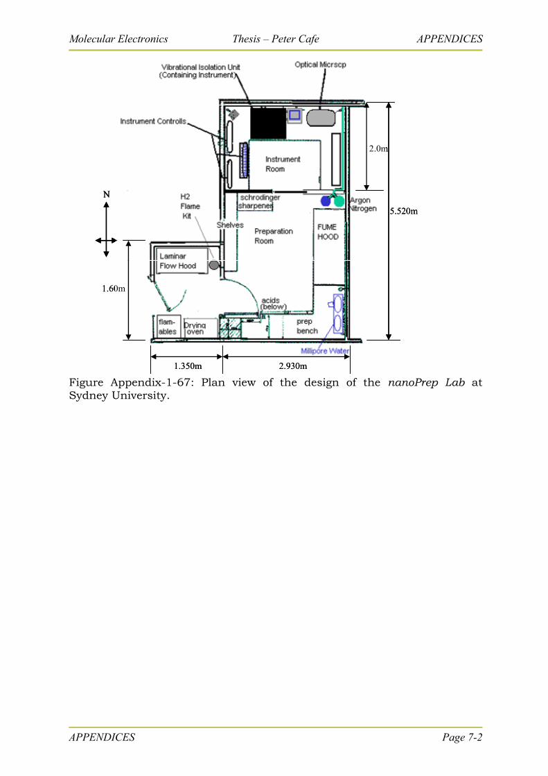
Molecular Electronics Thesis – Peter Cafe APPENDICES
5.520m
2.0m
N
2.930m1.350m
1.60m
2.0m
5.520m
2.0m
NN
2.930m1.350m
1.60m
2.0m
Figure Appendix-1-67: Plan view of the design of the nanoPrep Lab at Sydney University.
APPENDICES Page 7-2
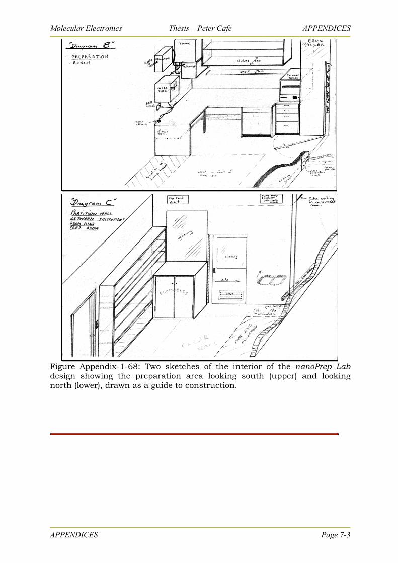
Molecular Electronics Thesis – Peter Cafe APPENDICES
Figure Appendix-1-68: Two sketches of the interior of the nanoPrep Lab design showing the preparation area looking south (upper) and looking north (lower), drawn as a guide to construction.
APPENDICES Page 7-3
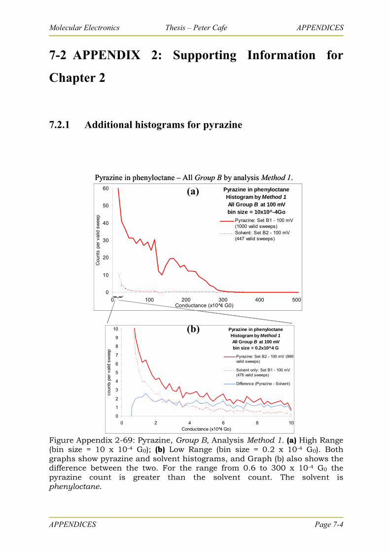
Molecular Electronics Thesis – Peter Cafe APPENDICES
7-2 APPENDIX 2: Supporting Information for
Chapter 2
7.2.1 Additional histograms for pyrazine
Pyrazine in phenyloctane Histogram by Method 1All Group B at 100 mVbin size = 10x10^-4Go
0
10
20
30
40
50
60
0 100 200 300 400 500Conductance (x10 4 G0)
Cou
nts
per
valid
sw
eep
Pyrazine: Set B1 - 100 mV(1000 valid sweeps) Solvent: Set B2 - 100 mV (447 valid sweeps)
Pyrazine in phenyloctane – All Group B by analysis Method 1.
0.6
(a)
Pyrazine in phenyloctaneHistogram by Method 1All Group B at 100 mVbin size = 0.2x10^4 G
0
1
2
3
4
5
6
7
8
9
10
0 2 4 6 8 1Conductance (x10 4 Go)
coun
ts p
er v
alid
sw
eep
0
Pyrazine: Set B2 - 100 mV (999valid sweeps)
Solvent only: Set B1 - 100 mV(476 valid sweeps)
Difference (Pyrazine - Solvent)
(b)
Figure Appendix 2-69: Pyrazine, Group B, Analysis Method 1. (a) High Range (bin size = 10 x 10-4 G0); (b) Low Range (bin size = 0.2 x 10⁻⁴ G0). Both graphs show pyrazine and solvent histograms, and Graph (b) also shows the difference between the two. For the range from 0.6 to 300 x 10-4 G0 the pyrazine count is greater than the solvent count. The solvent is phenyloctane.
APPENDICES Page 7-4
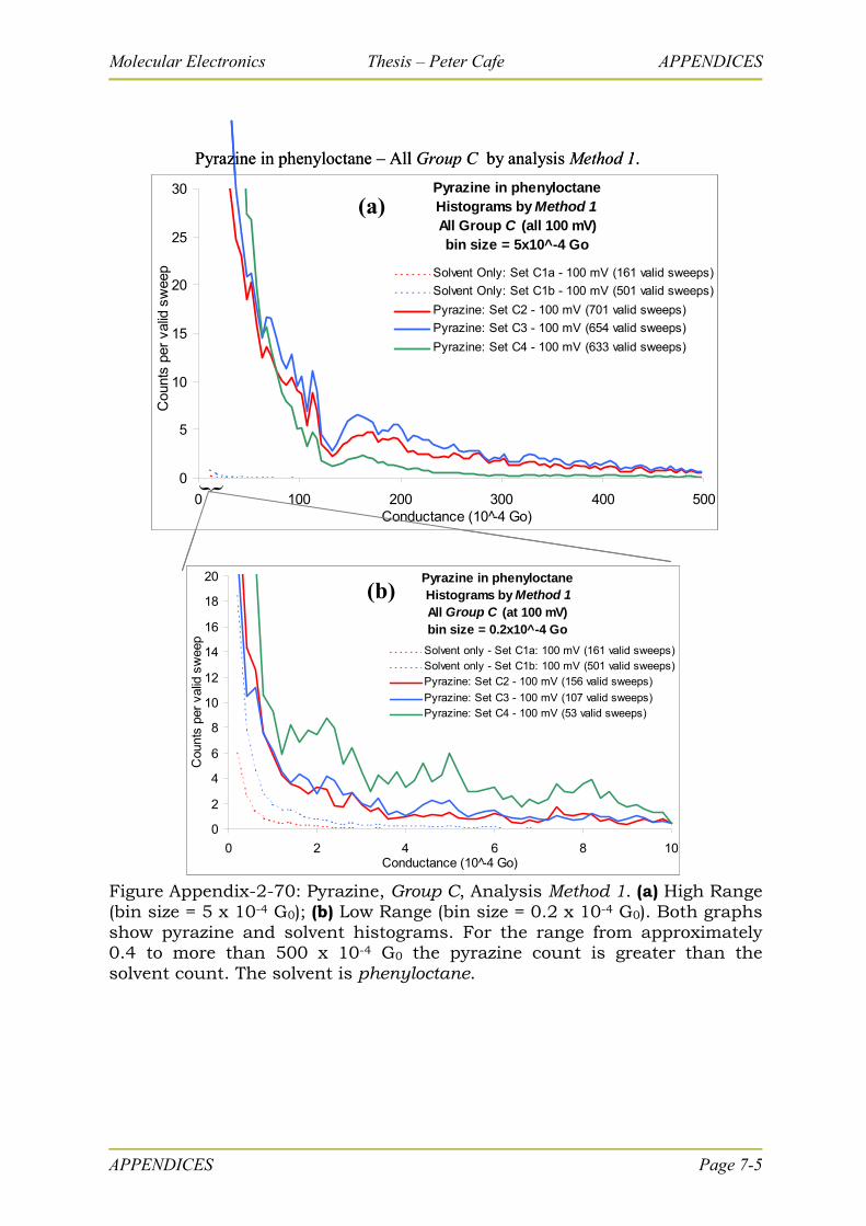
Molecular Electronics Thesis – Peter Cafe APPENDICES
Pyrazine in phenyloctane Histograms by Method 1All Group C (at 100 mV)bin size = 0.2x10^-4 Go
0
2
4
6
8
10
12
14
16
18
20
0 2 4 6 8 10Conductance (10 -4 Go)
Cou
nts
per
valid
sw
eep
Solvent only - Set C1a: 100 mV (161 valid sweeps)Solvent only - Set C1b: 100 mV (501 valid sweeps)Pyrazine: Set C2 - 100 mV (156 valid sweeps)
Pyrazine: Set C3 - 100 mV (107 valid sweeps)Pyrazine: Set C4 - 100 mV (53 valid sweeps)
Pyrazine in phenyloctaneHistograms by Method 1All Group C (all 100 mV)bin size = 5x10^-4 Go
0
5
10
15
20
25
30
0 100 200 300 400 500Conductance (10 -4 Go)
Cou
nts
per
valid
sw
eep Solvent Only: Set C1a - 100 mV (161 valid sweeps)
Solvent Only: Set C1b - 100 mV (501 valid sweeps)
Pyrazine: Set C2 - 100 mV (701 valid sweeps)
Pyrazine: Set C3 - 100 mV (654 valid sweeps)
Pyrazine: Set C4 - 100 mV (633 valid sweeps)
Pyrazine in phenyloctane – All Group C by analysis Method 1.
(b)
(a)
Figure Appendix-2-70: Pyrazine, Group C, Analysis Method 1. (a) High Range (bin size = 5 x 10⁻⁴ G0); (b) Low Range (bin size = 0.2 x 10⁻⁴ G0). Both graphs show pyrazine and solvent histograms. For the range from approximately 0.4 to more than 500 x 10-4 G0 the pyrazine count is greater than the solvent count. The solvent is phenyloctane.
APPENDICES Page 7-5
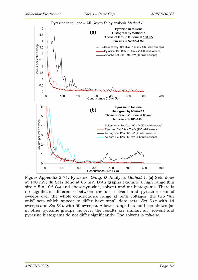
Molecular Electronics Thesis – Peter Cafe APPENDICES
Pyrazine in tolueneHistogram by Method 1
Those of Group D done at 65 mVbin size = 5x10^-4 Go
0
1
2
3
4
5
6
0 100 200 300 400 500 600 700Conductance (10 -4 Go)
Cou
nts
per
valid
sw
eep
Solvent only: Set D2b - 65 mV (471 valid sweeps)
Pyrazine: Set D3a - 65 mV (995 valid sweeps)
Air only: Set D1a - 65 mV (50 valid sweeps)
Air only: Set D1b - 65 mV (455 valid sweeps)
Pyrazine in tolueneHistogram by Method 1
Those of Group D done at 100 mVbin size = 5x10^-4 Go
0
0.5
1
1.5
2
2.5
3
3.5
4
4.5
5
0 100 200 300 400 500 600 700Conductance (10 -4 Go)
Cou
nts
per
valid
sw
eep
Solvent only: Set D2a - 100 mV (660 valid sweeps)
Pyrazine: Set D3b - 100 mV (1000 valid sweeps)
Air only: Set D1c - 100 mV (14 valid sweeps)
Pyrazine in toluene – All Group D by analysis Method 1.
(a)
(b)Pyrazine in toluene
Histogram by Method 1Those of Group D done at 65 mV
bin size = 5x10^-4 Go
0
1
2
3
4
5
6
0 100 200 300 400 500 600 700Conductance (10 -4 Go)
Cou
nts
per
valid
sw
eep
Solvent only: Set D2b - 65 mV (471 valid sweeps)
Pyrazine: Set D3a - 65 mV (995 valid sweeps)
Air only: Set D1a - 65 mV (50 valid sweeps)
Air only: Set D1b - 65 mV (455 valid sweeps)
Pyrazine in tolueneHistogram by Method 1
Those of Group D done at 100 mVbin size = 5x10^-4 Go
0
0.5
1
1.5
2
2.5
3
3.5
4
4.5
5
0 100 200 300 400 500 600 700Conductance (10 -4 Go)
Cou
nts
per
valid
sw
eep
Solvent only: Set D2a - 100 mV (660 valid sweeps)
Pyrazine: Set D3b - 100 mV (1000 valid sweeps)
Air only: Set D1c - 100 mV (14 valid sweeps)
Pyrazine in toluene – All Group D by analysis Method 1.
(a)
(b)
Figure Appendix-2-71: Pyrazine, Group D, Analysis Method 1. (a) Sets done at 100 mV; (b) Sets done at 65 mV. Both graphs examine a high range (bin size = 5 x 10⁻⁴ G0) and show pyrazine, solvent and air histograms. There is no significant difference between the air, solvent and pyrazine sets of sweeps over the whole conductance range at both voltages (the two “Air only” sets which appear to differ have small data sets: Set D1c with 14 sweeps and Set D1a with 50 sweeps). A lower range has not been shown (as in other pyrazine groups) however the results are similar: air, solvent and pyrazine histograms do not differ significantly. The solvent is toluene.
APPENDICES Page 7-6
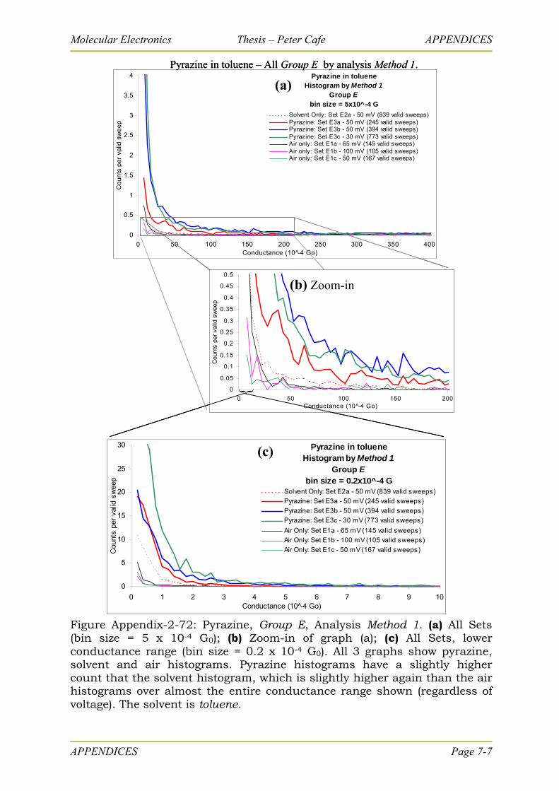
Molecular Electronics Thesis – Peter Cafe APPENDICES
Pyrazine in tolueneHistogram by Method 1
Group E bin size = 5x10^-4 G
0
0.5
1
1.5
2
2.5
3
3.5
4
0 50 100 150 200 250 300 350 400Conductance (10 -4 Go)
Co
un
ts p
er
valid
sw
ee
pSolvent Only: Set E2a - 50 mV (839 valid sweeps)Pyrazine: Set E3a - 50 mV (245 valid sweeps)Pyrazine: Set E3b - 50 mV (394 valid sweeps)Pyrazine: Set E3c - 30 mV (773 valid sweeps)Air only: Set E1a - 65 mV (145 valid sweeps)Air only: Set E1b - 100 mV (105 valid sweeps)Air only: Set E1c - 50 mV (167 valid sweeps)
Pyrazine in toluene – All Group E by analysis Method 1.
(a)
0
0.05
0.1
0.15
0.2
0.25
0.3
0.35
0.4
0.45
0.5
0 50 100 150 200Conductance (10^-4 Go)
Cou
nts
per
valid
sw
eep
Pyrazine in tolueneHistogram by Method 1
Group E bin size = 0.2x10^-4 G
0
5
10
15
20
25
30
0 1 2 3 4 5 6 7 8 9 10Conductance (10 -4 Go)
Cou
nts
per
valid
sw
eep
Solvent Only: Set E2a - 50 mV (839 valid sweeps)
Pyrazine: Set E3a - 50 mV (245 valid sweeps)
Pyrazine: Set E3b - 50 mV (394 valid sweeps)
Pyrazine: Set E3c - 30 mV (773 valid sweeps)
Air Only: Set E1a - 65 mV (145 valid sweeps)
Air Only: Set E1b - 100 mV (105 valid sweeps)
Air Only: Set E1c - 50 mV (167 valid sweeps)
(c)
(b) Zoom-in
Pyrazine in tolueneHistogram by Method 1
Group E bin size = 5x10^-4 G
0
0.5
1
1.5
2
2.5
3
3.5
4
0 50 100 150 200 250 300 350 400Conductance (10 -4 Go)
Co
un
ts p
er
valid
sw
ee
pSolvent Only: Set E2a - 50 mV (839 valid sweeps)Pyrazine: Set E3a - 50 mV (245 valid sweeps)Pyrazine: Set E3b - 50 mV (394 valid sweeps)Pyrazine: Set E3c - 30 mV (773 valid sweeps)Air only: Set E1a - 65 mV (145 valid sweeps)Air only: Set E1b - 100 mV (105 valid sweeps)Air only: Set E1c - 50 mV (167 valid sweeps)
Pyrazine in toluene – All Group E by analysis Method 1.
(a)
0
0.05
0.1
0.15
0.2
0.25
0.3
0.35
0.4
0.45
0.5
0 50 100 150 200Conductance (10^-4 Go)
Cou
nts
per
valid
sw
eep
Pyrazine in tolueneHistogram by Method 1
Group E bin size = 0.2x10^-4 G
0
5
10
15
20
25
30
0 1 2 3 4 5 6 7 8 9 10Conductance (10 -4 Go)
Cou
nts
per
valid
sw
eep
Solvent Only: Set E2a - 50 mV (839 valid sweeps)
Pyrazine: Set E3a - 50 mV (245 valid sweeps)
Pyrazine: Set E3b - 50 mV (394 valid sweeps)
Pyrazine: Set E3c - 30 mV (773 valid sweeps)
Air Only: Set E1a - 65 mV (145 valid sweeps)
Air Only: Set E1b - 100 mV (105 valid sweeps)
Air Only: Set E1c - 50 mV (167 valid sweeps)
(c)
(b) Zoom-in
Figure Appendix-2-72: Pyrazine, Group E, Analysis Method 1. (a) All Sets (bin size = 5 x 10⁻⁴ G0); (b) Zoom-in of graph (a); (c) All Sets, lower conductance range (bin size = 0.2 x 10⁻⁴ G0). All 3 graphs show pyrazine, solvent and air histograms. Pyrazine histograms have a slightly higher count that the solvent histogram, which is slightly higher again than the air histograms over almost the entire conductance range shown (regardless of voltage). The solvent is toluene.
APPENDICES Page 7-7
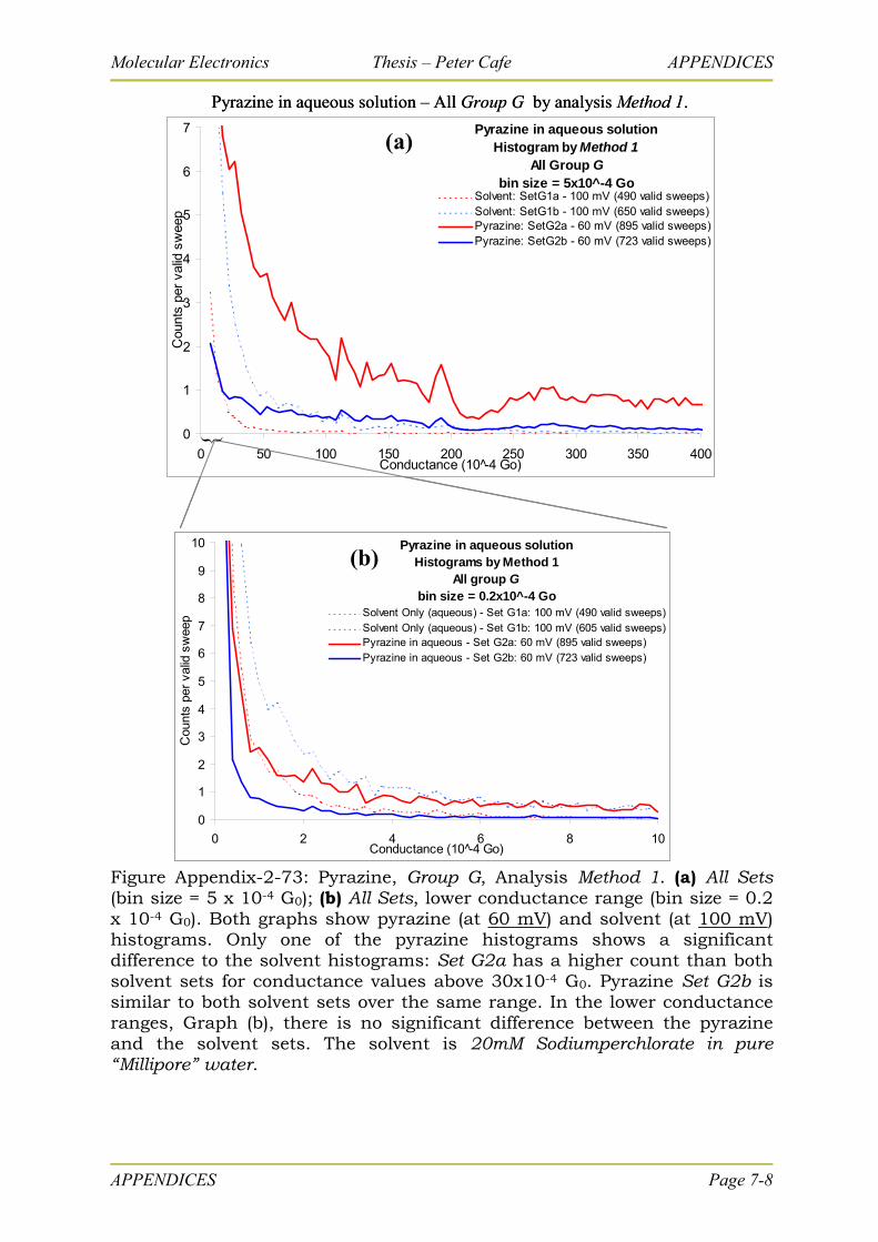
Molecular Electronics Thesis – Peter Cafe APPENDICES
Pyrazine in aqueous solution Histogram by Method 1
All Group G bin size = 5x10^-4 Go
0
1
2
3
4
5
6
7
0 50 100 150 200 250 300 350 400Conductance (10 -4 Go)
Cou
nts
per
valid
sw
eep
Solvent: SetG1a - 100 mV (490 valid sweeps)Solvent: SetG1b - 100 mV (650 valid sweeps)Pyrazine: SetG2a - 60 mV (895 valid sweeps)Pyrazine: SetG2b - 60 mV (723 valid sweeps)
Pyrazine in aqueous solution – All Group G by analysis Method 1.
(a)
Pyrazine in aqueous solutionHistograms by Method 1
All group Gbin size = 0.2x10^-4 Go
0
1
2
3
4
5
6
7
8
9
10
0 2 4 6 8 10Conductance (10 -4 Go)
Cou
nts
per
valid
sw
eep Solvent Only (aqueous) - Set G1a: 100 mV (490 valid sweeps)
Solvent Only (aqueous) - Set G1b: 100 mV (605 valid sweeps)Pyrazine in aqueous - Set G2a: 60 mV (895 valid sweeps)Pyrazine in aqueous - Set G2b: 60 mV (723 valid sweeps)
(b)
Figure Appendix-2-73: Pyrazine, Group G, Analysis Method 1. (a) All Sets (bin size = 5 x 10⁻⁴ G0); (b) All Sets, lower conductance range (bin size = 0.2 x 10⁻⁴ G0). Both graphs show pyrazine (at 60 mV) and solvent (at 100 mV) histograms. Only one of the pyrazine histograms shows a significant difference to the solvent histograms: Set G2a has a higher count than both solvent sets for conductance values above 30x10-4 G0. Pyrazine Set G2b is similar to both solvent sets over the same range. In the lower conductance ranges, Graph (b), there is no significant difference between the pyrazine and the solvent sets. The solvent is 20mM Sodiumperchlorate in pure “Millipore” water.
APPENDICES Page 7-8
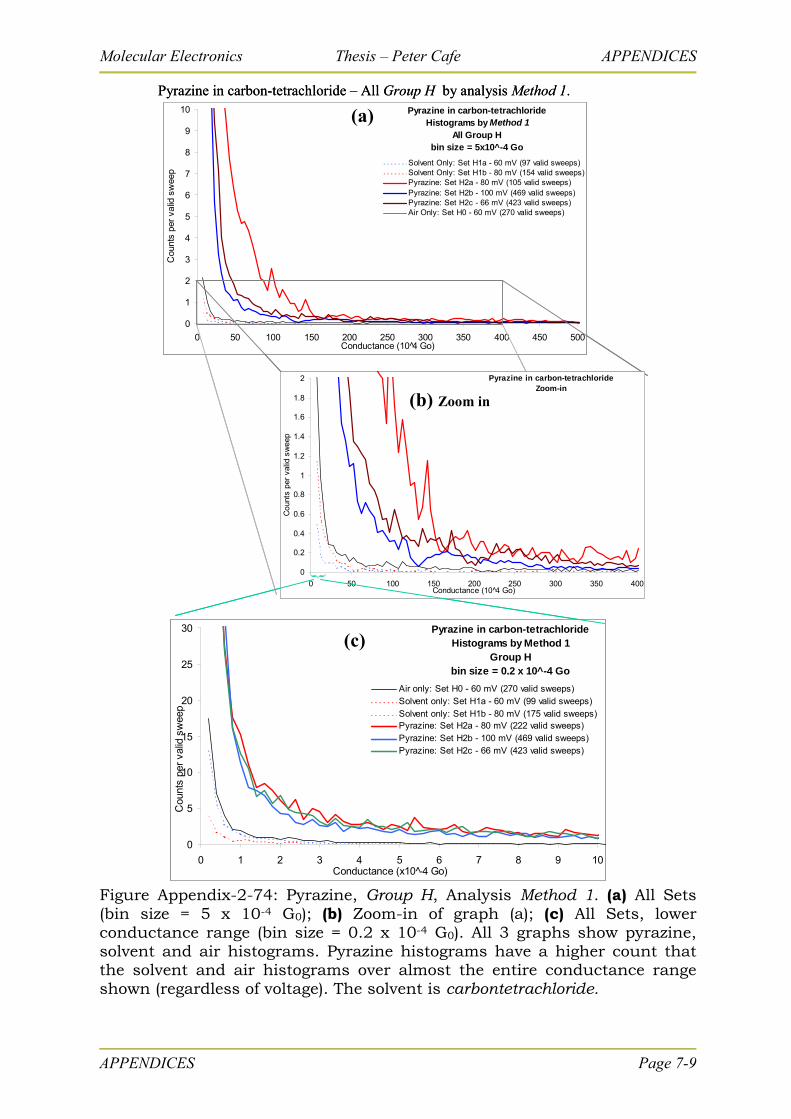
Molecular Electronics Thesis – Peter Cafe APPENDICES
Pyrazine in carbon-tetrachloride Histograms by Method 1
All Group Hbin size = 5x10^-4 Go
0
1
2
3
4
5
6
7
8
9
10
0 50 100 150 200 250 300 350 400 450 500Conductance (10 4 Go)
Cou
nts
per
valid
sw
eep
Solvent Only: Set H1a - 60 mV (97 valid sweeps)Solvent Only: Set H1b - 80 mV (154 valid sweeps)Pyrazine: Set H2a - 80 mV (105 valid sweeps)Pyrazine: Set H2b - 100 mV (469 valid sweeps)Pyrazine: Set H2c - 66 mV (423 valid sweeps)Air Only: Set H0 - 60 mV (270 valid sweeps)
Pyrazine in carbon-tetrachloride – All Group H by analysis Method 1.
(a)
Pyrazine in carbon-tetrachlorideZoom-in
0
0.2
0.4
0.6
0.8
1
1.2
1.4
1.6
1.8
2
0 50 100 150 200 250 300 350 400Conductance (10 4 Go)
Cou
nts
per
valid
sw
eep
(b) Zoom in
Pyrazine in carbon-tetrachlorideHistograms by Method 1
Group Hbin size = 0.2 x 10^-4 Go
0
5
10
15
20
25
30
0 1 2 3 4 5 6 7 8 9 10Conductance (x10 -4 Go)
Cou
nts
per
valid
sw
eep
Air only: Set H0 - 60 mV (270 valid sweeps)Solvent only: Set H1a - 60 mV (99 valid sweeps)Solvent only: Set H1b - 80 mV (175 valid sweeps)Pyrazine: Set H2a - 80 mV (222 valid sweeps)Pyrazine: Set H2b - 100 mV (469 valid sweeps)Pyrazine: Set H2c - 66 mV (423 valid sweeps)
(c)
Figure Appendix-2-74: Pyrazine, Group H, Analysis Method 1. (a) All Sets (bin size = 5 x 10⁻⁴ G0); (b) Zoom-in of graph (a); (c) All Sets, lower conductance range (bin size = 0.2 x 10⁻⁴ G0). All 3 graphs show pyrazine, solvent and air histograms. Pyrazine histograms have a higher count that the solvent and air histograms over almost the entire conductance range shown (regardless of voltage). The solvent is carbontetrachloride.
APPENDICES Page 7-9
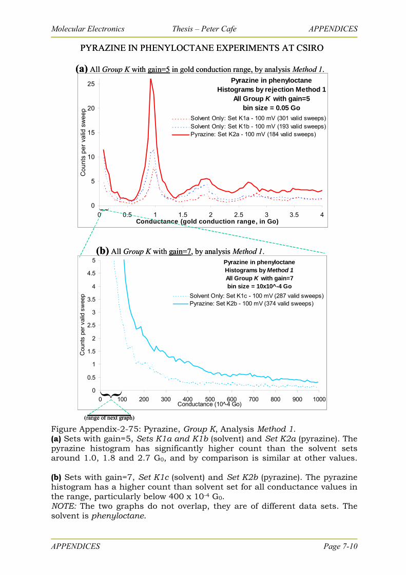
Molecular Electronics Thesis – Peter Cafe APPENDICES
Pyrazine in phenyloctaneHistograms by Method 1All Group K with gain=7bin size = 10x10^-4 Go
0
0.5
1
1.5
2
2.5
3
3.5
4
4.5
5
0 100 200 300 400 500 600 700 800 900 1000Conductance (10 -4 Go)
Cou
nts
per
valid
sw
eep Solvent Only: Set K1c - 100 mV (287 valid sweeps)
Pyrazine: Set K2b - 100 mV (374 valid sweeps)
(a) All Group K with gain=5 in gold conduction range, by analysis Method 1.
(b) All Group K with gain=7, by analysis Method 1.
Pyrazine in phenyloctaneHistograms by rejection Method 1
All Group K with gain=5bin size = 0.05 Go
0
5
10
15
20
25
0 0.5 1 1.5 2 2.5 3 3.5 4Conductance (gold conduction range, in Go)
Co
un
ts p
er
valid
sw
ee
p
Solvent Only: Set K1a - 100 mV (301 valid sweeps)Solvent Only: Set K1b - 100 mV (193 valid sweeps)Pyrazine: Set K2a - 100 mV (184 valid sweeps)
PYRAZINE IN PHENYLOCTANE EXPERIMENTS AT CSIRO
(range of next graph)
Pyrazine in phenyloctaneHistograms by Method 1All Group K with gain=7bin size = 10x10^-4 Go
0
0.5
1
1.5
2
2.5
3
3.5
4
4.5
5
0 100 200 300 400 500 600 700 800 900 1000Conductance (10 -4 Go)
Cou
nts
per
valid
sw
eep Solvent Only: Set K1c - 100 mV (287 valid sweeps)
Pyrazine: Set K2b - 100 mV (374 valid sweeps)
(a) All Group K with gain=5 in gold conduction range, by analysis Method 1.
(b) All Group K with gain=7, by analysis Method 1.
Pyrazine in phenyloctaneHistograms by rejection Method 1
All Group K with gain=5bin size = 0.05 Go
0
5
10
15
20
25
0 0.5 1 1.5 2 2.5 3 3.5 4Conductance (gold conduction range, in Go)
Co
un
ts p
er
valid
sw
ee
p
Solvent Only: Set K1a - 100 mV (301 valid sweeps)Solvent Only: Set K1b - 100 mV (193 valid sweeps)Pyrazine: Set K2a - 100 mV (184 valid sweeps)
PYRAZINE IN PHENYLOCTANE EXPERIMENTS AT CSIRO
(range of next graph) Figure Appendix-2-75: Pyrazine, Group K, Analysis Method 1. (a) Sets with gain=5, Sets K1a and K1b (solvent) and Set K2a (pyrazine). The pyrazine histogram has significantly higher count than the solvent sets around 1.0, 1.8 and 2.7 G0, and by comparison is similar at other values. (b) Sets with gain=7, Set K1c (solvent) and Set K2b (pyrazine). The pyrazine histogram has a higher count than solvent set for all conductance values in the range, particularly below 400 x 10-4 G0. NOTE: The two graphs do not overlap, they are of different data sets. The solvent is phenyloctane.
APPENDICES Page 7-10
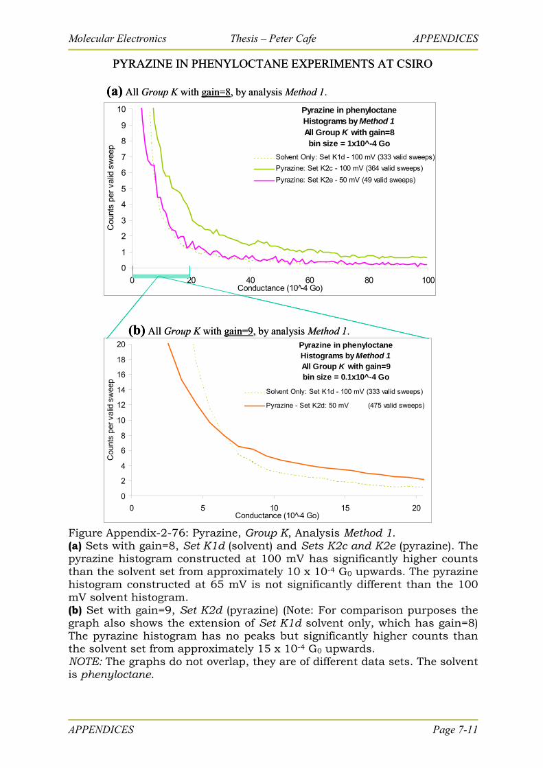
Molecular Electronics Thesis – Peter Cafe APPENDICES
Pyrazine in phenyloctaneHistograms by Method 1All Group K with gain=8bin size = 1x10^-4 Go
0
1
2
3
4
5
6
7
8
9
10
0 20 40 60 80Conductance (10 -4 Go)
Cou
nts
per
valid
sw
eep
100
Solvent Only: Set K1d - 100 mV (333 valid sweeps)
Pyrazine: Set K2c - 100 mV (364 valid sweeps)
Pyrazine: Set K2e - 50 mV (49 valid sweeps)
PYRAZINE IN PHENYLOCTANE EXPERIMENTS AT CSIRO
(a) All Group K with gain=8, by analysis Method 1.
(b) All Group K with gain=9, by analysis Method 1.Pyrazine in phenyloctaneHistograms by Method 1All Group K with gain=9bin size = 0.1x10^-4 Go
0
2
4
6
8
10
12
14
16
18
20
0 5 10 15 20Conductance (10 -4 Go)
Cou
nts
per
valid
sw
eep
Solvent Only: Set K1d - 100 mV (333 valid sweeps)
Pyrazine - Set K2d: 50 mV (475 valid sweeps)
Figure Appendix-2-76: Pyrazine, Group K, Analysis Method 1. (a) Sets with gain=8, Set K1d (solvent) and Sets K2c and K2e (pyrazine). The pyrazine histogram constructed at 100 mV has significantly higher counts than the solvent set from approximately 10 x 10-4 G0 upwards. The pyrazine histogram constructed at 65 mV is not significantly different than the 100 mV solvent histogram. (b) Set with gain=9, Set K2d (pyrazine) (Note: For comparison purposes the graph also shows the extension of Set K1d solvent only, which has gain=8) The pyrazine histogram has no peaks but significantly higher counts than the solvent set from approximately 15 x 10-4 G0 upwards. NOTE: The graphs do not overlap, they are of different data sets. The solvent is phenyloctane.
APPENDICES Page 7-11
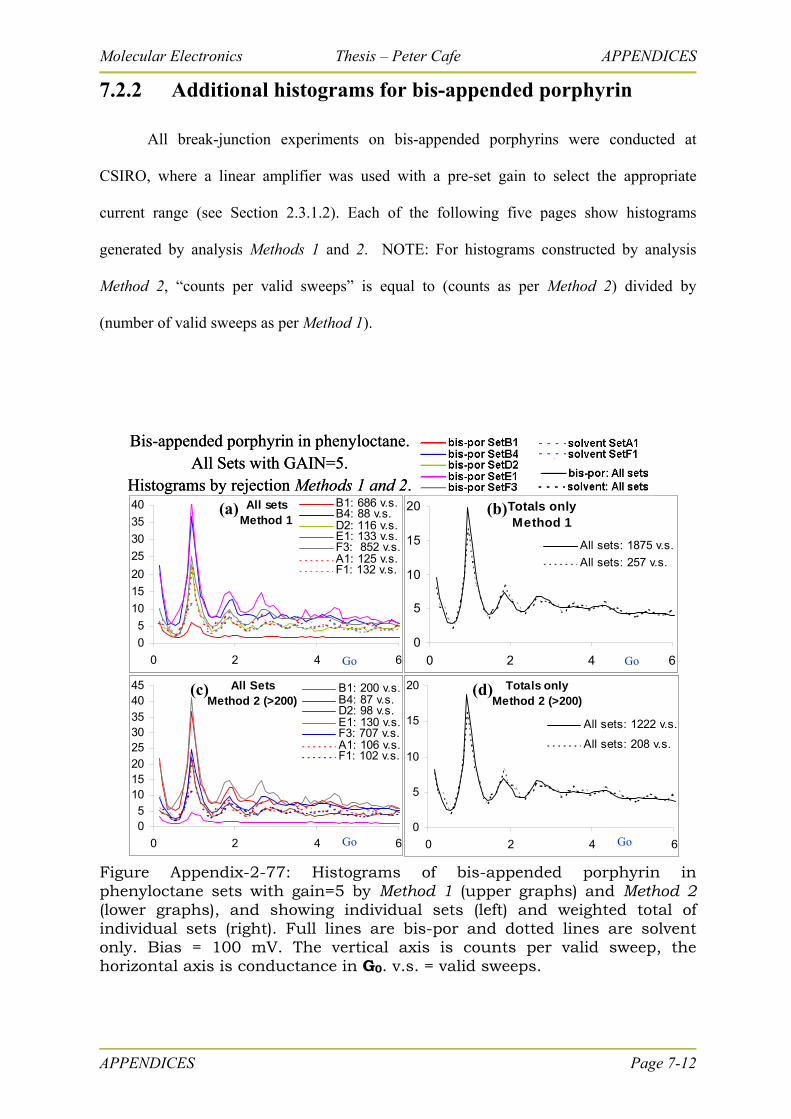
Molecular Electronics Thesis – Peter Cafe APPENDICES
7.2.2 Additional histograms for bis-appended porphyrin
All break-junction experiments on bis-appended porphyrins were conducted at
CSIRO, where a linear amplifier was used with a pre-set gain to select the appropriate
current range (see Section 2.3.1.2). Each of the following five pages show histograms
generated by analysis Methods 1 and 2. NOTE: For histograms constructed by analysis
Method 2, “counts per valid sweeps” is equal to (counts as per Method 2) divided by
(number of valid sweeps as per Method 1).
Bis-appended porphyrin in phenyloctane.All Sets with GAIN=5.
Histograms by rejection Methods 1 and 2.
All SetsMethod 2 (>200)
05
1015202530354045
0 2 4 6
B1: 200 v.s.B4: 87 v.s.D2: 98 v.s.E1: 130 v.s.F3: 707 v.s.A1: 106 v.s.F1: 102 v.s.
Totals onlyMethod 2 (>200)
0
5
10
15
20
0 2 4 6
All sets: 1222 v.s.
All sets: 208 v.s.
All setsMethod 1
0
5
10
15
20
25
30
35
40
0 2 4 6
B1: 686 v.s.B4: 88 v.s.D2: 116 v.s.E1: 133 v.s.F3: 852 v.s.A1: 125 v.s.F1: 132 v.s.
Totals onlyMethod 1
0
5
10
15
20
0 2 4 6
All sets: 1875 v.s.
All sets: 257 v.s.
Go
Go Go
Go
(b)(a)
(c) (d)
Figure Appendix-2-77: Histograms of bis-appended porphyrin in phenyloctane sets with gain=5 by Method 1 (upper graphs) and Method 2 (lower graphs), and showing individual sets (left) and weighted total of individual sets (right). Full lines are bis-por and dotted lines are solvent only. Bias = 100 mV. The vertical axis is counts per valid sweep, the horizontal axis is conductance in G0. v.s. = valid sweeps.
APPENDICES Page 7-12
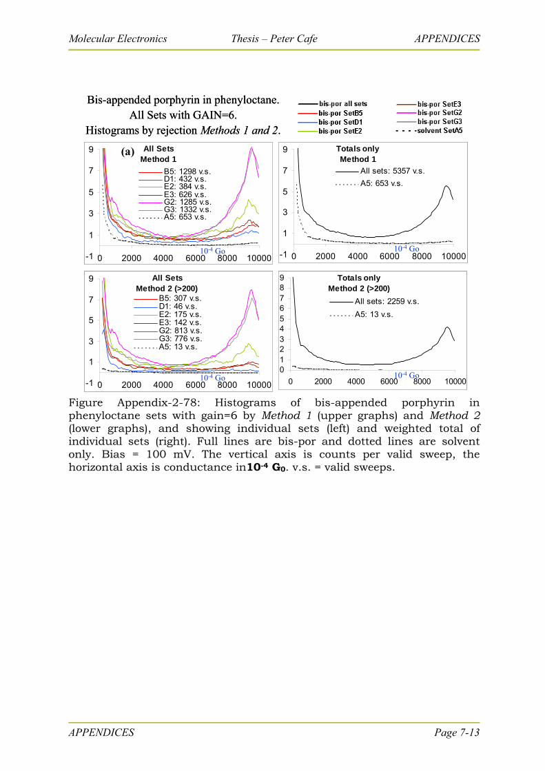
Molecular Electronics Thesis – Peter Cafe APPENDICES
All SetsMethod 1
-1
1
3
5
7
9
0 2000 4000 6000 8000 10000
B5: 1298 v.s.D1: 432 v.s.E2: 384 v.s.E3: 626 v.s.G2: 1285 v.s.G3: 1332 v.s.A5: 653 v.s.
Bis-appended porphyrin in phenyloctane.All Sets with GAIN=6.
Histograms by rejection Methods 1 and 2.
(a)
(b)All Sets
Method 2 (>200)
-1
1
3
5
7
9
0 2000 4000 6000 8000 10000
B5: 307 v.s.D1: 46 v.s.E2: 175 v.s.E3: 142 v.s.G2: 813 v.s.G3: 776 v.s.A5: 13 v.s.
Totals onlyMethod 2 (>200)
0123456789
0 2000 4000 6000 8000 10000
All sets: 2259 v.s.
A5: 13 v.s.
Totals onlyMethod 1
-1
1
3
5
7
9
0 2000 4000 6000 8000 10000
All sets: 5357 v.s.
A5: 653 v.s.
10-4 Go 10-4 Go
10-4 Go10-4 Go
Figure Appendix-2-78: Histograms of bis-appended porphyrin in phenyloctane sets with gain=6 by Method 1 (upper graphs) and Method 2 (lower graphs), and showing individual sets (left) and weighted total of individual sets (right). Full lines are bis-por and dotted lines are solvent only. Bias = 100 mV. The vertical axis is counts per valid sweep, the horizontal axis is conductance in10-4 G0. v.s. = valid sweeps.
APPENDICES Page 7-13
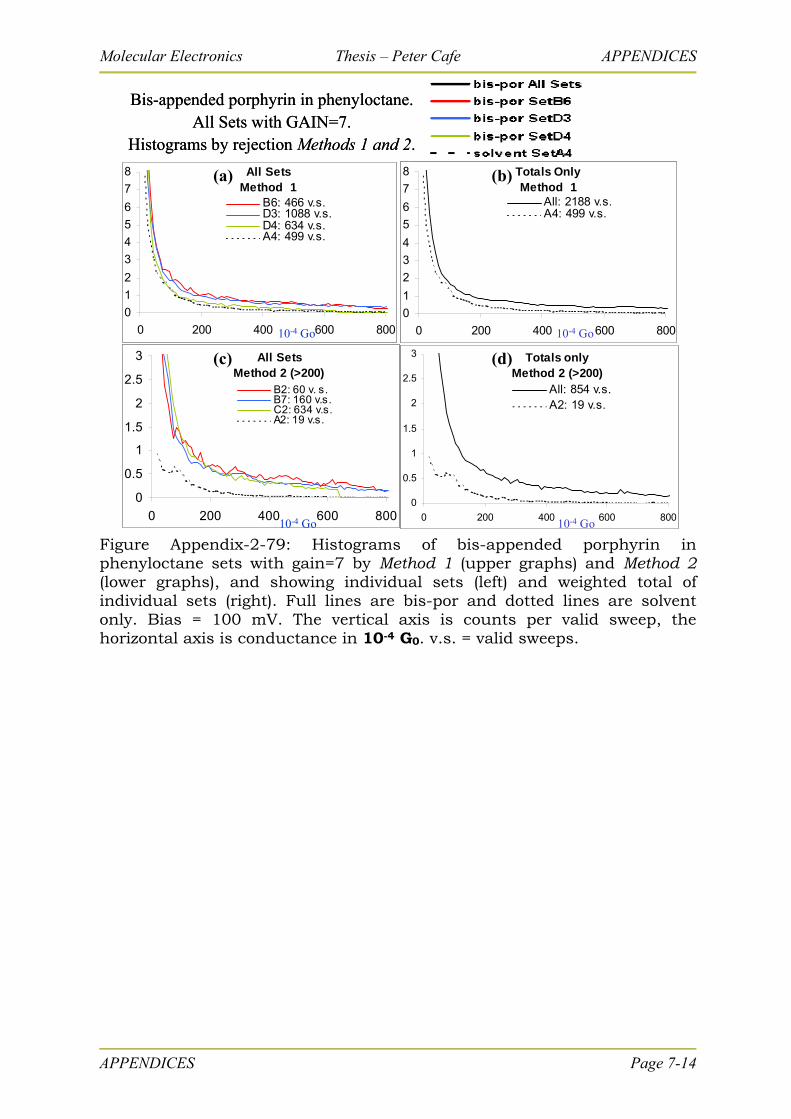
Molecular Electronics Thesis – Peter Cafe APPENDICES
All Sets Method 2 (>200)
0
0.5
1
1.5
2
2.5
3
0 200 400 600 800
B2: 60 v. s.B7: 160 v.s.C2: 634 v.s.A2: 19 v.s.
Totals only Method 2 (>200)
0
0.5
1
1.5
2
2.5
3
0 200 400 600 800
All: 854 v.s.A2: 19 v.s.
Totals OnlyMethod 1
0
1
2
3
4
5
6
7
8
0 200 400 600 800
All: 2188 v.s.A4: 499 v.s.
All SetsMethod 1
0
1
2
3
4
5
6
7
8
0 200 400 600 800
B6: 466 v.s.D3: 1088 v.s.D4: 634 v.s.A4: 499 v.s.
Bis-appended porphyrin in phenyloctane.All Sets with GAIN=7.
Histograms by rejection Methods 1 and 2.
(a) (b)
(c) (d)
10-4 Go
10-4 Go 10-4 Go
10-4 Go
Figure Appendix-2-79: Histograms of bis-appended porphyrin in phenyloctane sets with gain=7 by Method 1 (upper graphs) and Method 2 (lower graphs), and showing individual sets (left) and weighted total of individual sets (right). Full lines are bis-por and dotted lines are solvent only. Bias = 100 mV. The vertical axis is counts per valid sweep, the horizontal axis is conductance in 10-4 G0. v.s. = valid sweeps.
APPENDICES Page 7-14
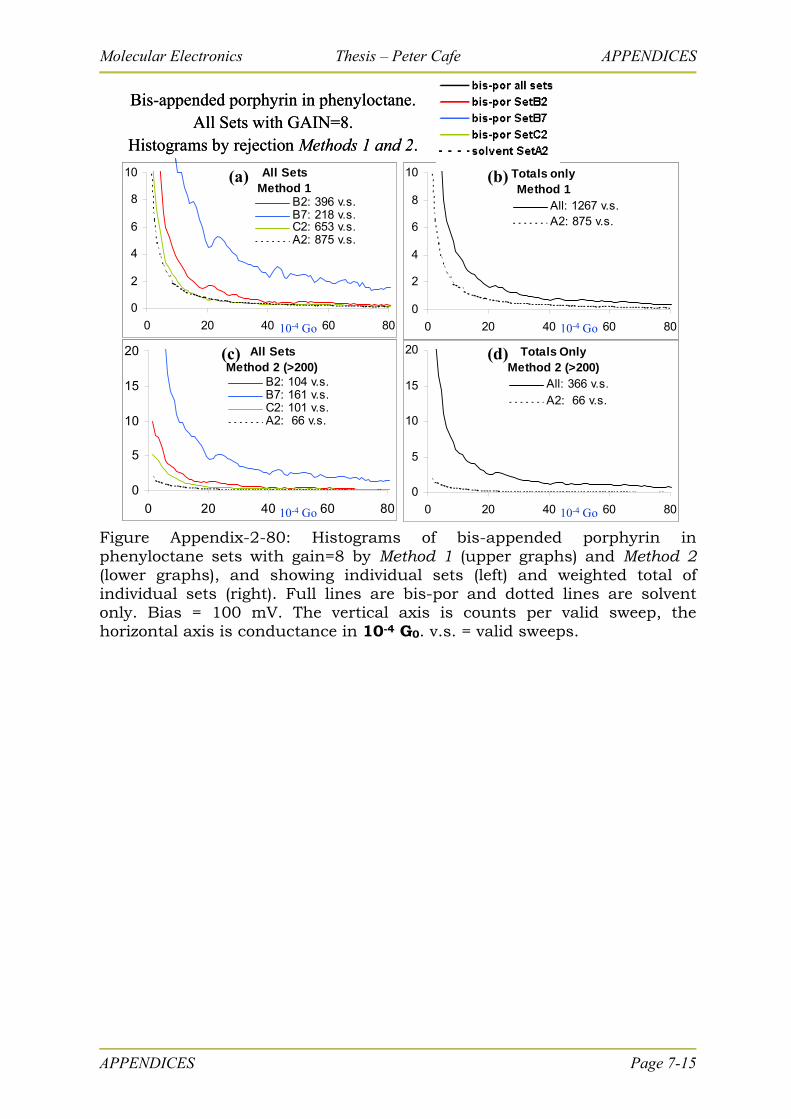
Molecular Electronics Thesis – Peter Cafe APPENDICES
Totals onlyMethod 1
0
2
4
6
8
10
0 20 40 60 80
All: 1267 v.s.A2: 875 v.s.
Totals OnlyMethod 2 (>200)
0
5
10
15
20
0 20 40 60 80
All: 366 v.s.A2: 66 v.s.
All SetsMethod 2 (>200)
0
5
10
15
20
0 20 40 60 80
B2: 104 v.s.B7: 161 v.s.C2: 101 v.s.A2: 66 v.s.
Bis-appended porphyrin in phenyloctane.All Sets with GAIN=8.
Histograms by rejection Methods 1 and 2.
All SetsMethod 1
0
2
4
6
8
10
0 20 40 60 80
B2: 396 v.s.B7: 218 v.s.C2: 653 v.s.A2: 875 v.s.
10-4 Go
10-4 Go 10-4 Go
10-4 Go
(a) (b)
(c) (d)
Figure Appendix-2-80: Histograms of bis-appended porphyrin in phenyloctane sets with gain=8 by Method 1 (upper graphs) and Method 2 (lower graphs), and showing individual sets (left) and weighted total of individual sets (right). Full lines are bis-por and dotted lines are solvent only. Bias = 100 mV. The vertical axis is counts per valid sweep, the horizontal axis is conductance in 10-4 G0. v.s. = valid sweeps.
APPENDICES Page 7-15
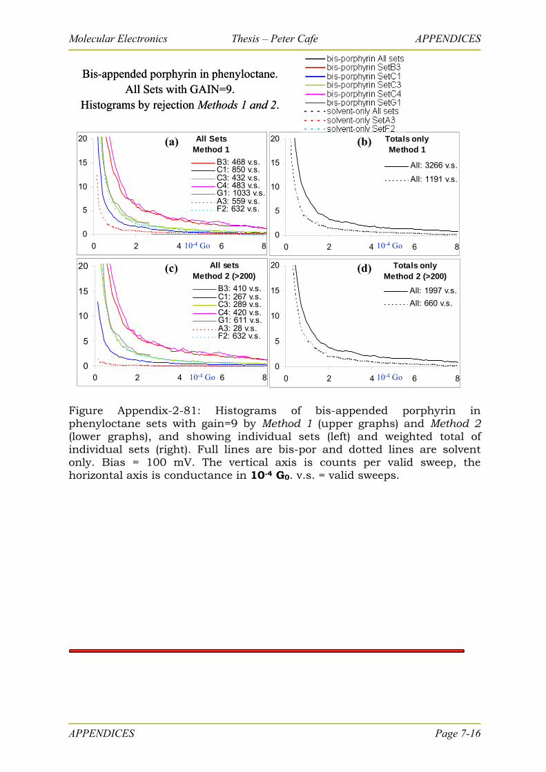
Molecular Electronics Thesis – Peter Cafe APPENDICES
Bis-appended porphyrin in phenyloctane.All Sets with GAIN=9.
Histograms by rejection Methods 1 and 2.
Totals onlyMethod 1
0
5
10
15
20
0 2 4 6 8
APPENDICES Page 7-16
Figure Appendix-2-81: Histograms of bis-appended porphyrin in phenyloctane sets with gain=9 by Method 1 (upper graphs) and Method 2 (lower graphs), and showing individual sets (left) and weighted total of individual sets (right). Full lines are bis-por and dotted lines are solvent only. Bias = 100 mV. The vertical axis is counts per valid sweep, the horizontal axis is conductance in 10-4 G0. v.s. = valid sweeps.
All: 3266 v.s.
All: 1191 v.s.
All SetsMethod 1
0
5
10
15
20
0 2 4 6 8
B3: 468 v.s.C1: 850 v.s.C3: 432 v.s.C4: 483 v.s.G1: 1033 v.s.A3: 559 v.s.F2: 632 v.s.
Totals onlyMethod 2 (>200)
0
5
10
15
20
0 2 4 6 8
All: 1997 v.s.
All: 660 v.s.
All setsMethod 2 (>200)
0
5
10
15
20
0 2 4 6 8
B3: 410 v.s.C1: 267 v.s.C3: 289 v.s.C4: 420 v.s.G1: 611 v.s.A3: 28 v.s.F2: 632 v.s.
10-4 Go
10-4 Go
10-4 Go
10-4 Go
(a) (b)
(c) (d)
Bis-appended porphyrin in phenyloctane.All Sets with GAIN=9.
Histograms by rejection Methods 1 and 2.
Totals onlyMethod 1
0
5
10
15
20
0 2 4 6 8
All: 3266 v.s.
All: 1191 v.s.
All SetsMethod 1
0
5
10
15
20
0 2 4 6 8
B3: 468 v.s.C1: 850 v.s.C3: 432 v.s.C4: 483 v.s.G1: 1033 v.s.A3: 559 v.s.F2: 632 v.s.
Totals onlyMethod 2 (>200)
0
5
10
15
20
0 2 4 6 8
All: 1997 v.s.
All: 660 v.s.
All setsMethod 2 (>200)
0
5
10
15
20
0 2 4 6 8
B3: 410 v.s.C1: 267 v.s.C3: 289 v.s.C4: 420 v.s.G1: 611 v.s.A3: 28 v.s.F2: 632 v.s.
10-4 Go
10-4 Go
10-4 Go
10-4 Go
(a) (b)
(c) (d)
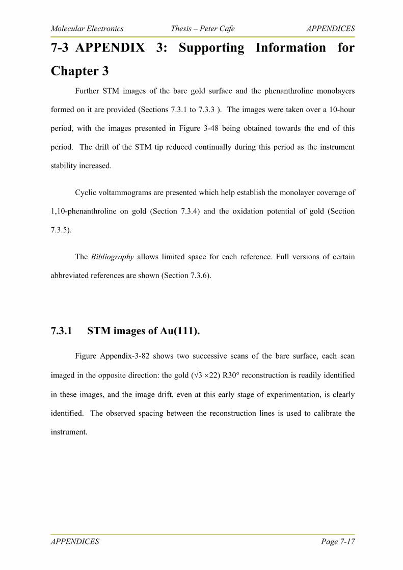
Molecular Electronics Thesis – Peter Cafe APPENDICES
APPENDICES Page 7-17
7-3 APPENDIX 3: Supporting Information for
Chapter 3 Further STM images of the bare gold surface and the phenanthroline monolayers
formed on it are provided (Sections 7.3.1 to 7.3.3 ). The images were taken over a 10-hour
period, with the images presented in Figure 3-48 being obtained towards the end of this
period. The drift of the STM tip reduced continually during this period as the instrument
stability increased.
Cyclic voltammograms are presented which help establish the monolayer coverage of
1,10-phenanthroline on gold (Section 7.3.4) and the oxidation potential of gold (Section
7.3.5).
The Bibliography allows limited space for each reference. Full versions of certain
abbreviated references are shown (Section 7.3.6).
7.3.1 STM images of Au(111).
Figure Appendix-3-82 shows two successive scans of the bare surface, each scan
imaged in the opposite direction: the gold (3 22) R30° reconstruction is readily identified
in these images, and the image drift, even at this early stage of experimentation, is clearly
identified. The observed spacing between the reconstruction lines is used to calibrate the
instrument.
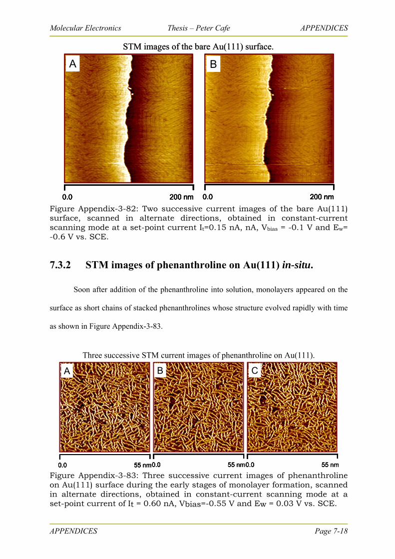
Molecular Electronics Thesis – Peter Cafe APPENDICES
0.0 200 nm
B
0.0 200 nm0.0 200 nm0.0 200 nm
BA
0.0 200 nm
A
0.0 200 nm0.0 200 nm0.0 200 nm
STM images of the bare Au(111) surface.
0.0 200 nm
B
0.0 200 nm0.0 200 nm0.0 200 nm
BA
0.0 200 nm
A
0.0 200 nm0.0 200 nm0.0 200 nm
STM images of the bare Au(111) surface.
Figure Appendix-3-82: Two successive current images of the bare Au(111) surface, scanned in alternate directions, obtained in constant-current scanning mode at a set-point current It=0.15 nA, nA, Vbias = -0.1 V and Ew= -0.6 V vs. SCE.
7.3.2 STM images of phenanthroline on Au(111) in-situ.
Soon after addition of the phenanthroline into solution, monolayers appeared on the
surface as short chains of stacked phenanthrolines whose structure evolved rapidly with time
as shown in Figure Appendix-3-83.
0.0 55 nm0.0 55 nm0.0 55 nm0.0 55 nm0.0 55 nm0.0 55 nm0.0 55 nm0.0 55 nm0.0 55 nm0.0 55 nm0.0 55 nm0.0 55 nm
A B C
Three successive STM current images of phenanthroline on Au(111).
Figure Appendix-3-83: Three successive current images of phenanthroline on Au(111) surface during the early stages of monolayer formation, scanned in alternate directions, obtained in constant-current scanning mode at a set-point current of It = 0.60 nA, Vbias=-0.55 V and Ew = 0.03 V vs. SCE.
APPENDICES Page 7-18
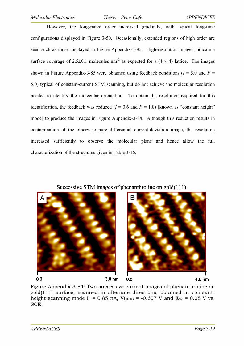
Molecular Electronics Thesis – Peter Cafe APPENDICES
However, the long-range order increased gradually, with typical long-time
configurations displayed in Figure 3-50. Occasionally, extended regions of high order are
seen such as those displayed in Figure Appendix-3-85. High-resolution images indicate a
surface coverage of 2.50.1 molecules nm-2 as expected for a (4 4) lattice. The images
shown in Figure Appendix-3-85 were obtained using feedback conditions (I = 5.0 and P =
5.0) typical of constant-current STM scanning, but do not achieve the molecular resolution
needed to identify the molecular orientation. To obtain the resolution required for this
identification, the feedback was reduced (I = 0.6 and P = 1.0) [known as “constant height”
mode] to produce the images in Figure Appendix-3-84. Although this reduction results in
contamination of the otherwise pure differential current-deviation image, the resolution
increased sufficiently to observe the molecular plane and hence allow the full
characterization of the structures given in Table 3-16.
0.0 3.8 nm
A
0.0 3.8 nm0.0 3.8 nm
A
0.0 4.6 nm
B
0.0 4.6 nm0.0 4.6 nm
B
Successive STM images of phenanthroline on gold(111)
0.0 3.8 nm
A
0.0 3.8 nm0.0 3.8 nm
A
0.0 4.6 nm
B
0.0 4.6 nm0.0 4.6 nm
B
Successive STM images of phenanthroline on gold(111)
Figure Appendix-3-84: Two successive current images of phenanthroline on gold(111) surface, scanned in alternate directions, obtained in constant-height scanning mode It = 0.85 nA, Vbias = -0.607 V and Ew = 0.08 V vs. SCE.
APPENDICES Page 7-19
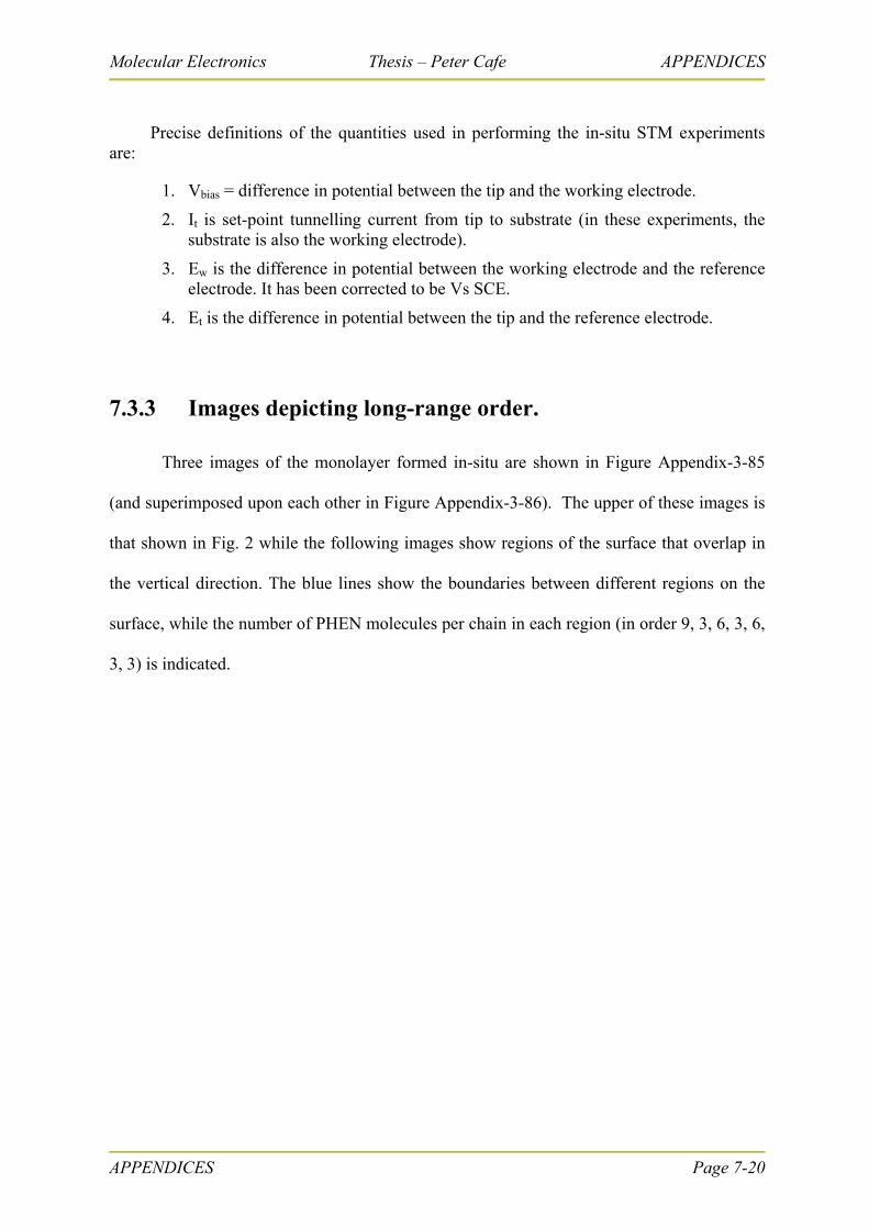
Molecular Electronics Thesis – Peter Cafe APPENDICES
APPENDICES Page 7-20
Precise definitions of the quantities used in performing the in-situ STM experiments are:
1. Vbias = difference in potential between the tip and the working electrode.
2. It is set-point tunnelling current from tip to substrate (in these experiments, the substrate is also the working electrode).
3. Ew is the difference in potential between the working electrode and the reference electrode. It has been corrected to be Vs SCE.
4. Et is the difference in potential between the tip and the reference electrode.
7.3.3 Images depicting long-range order.
Three images of the monolayer formed in-situ are shown in Figure Appendix-3-85
(and superimposed upon each other in Figure Appendix-3-86). The upper of these images is
that shown in Fig. 2 while the following images show regions of the surface that overlap in
the vertical direction. The blue lines show the boundaries between different regions on the
surface, while the number of PHEN molecules per chain in each region (in order 9, 3, 6, 3, 6,
3, 3) is indicated.
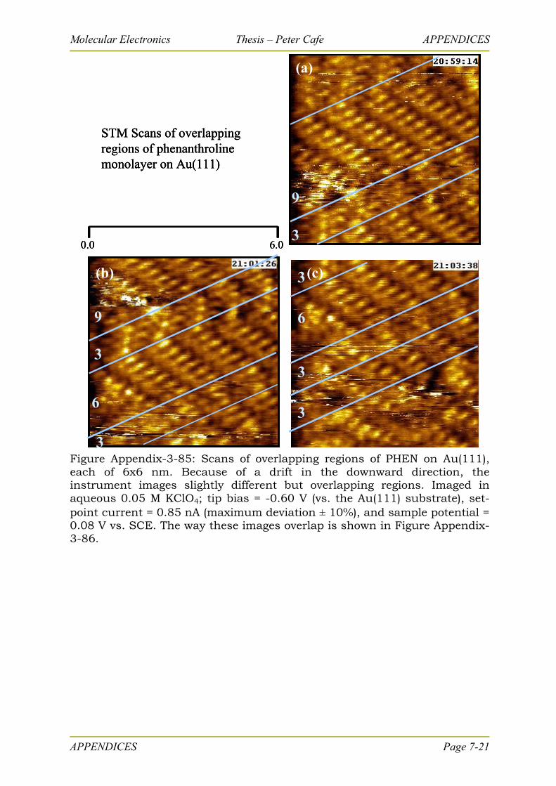
Molecular Electronics Thesis – Peter Cafe APPENDICES
9
3
9
3
6
3
3
3
6
3
STM Scans of overlapping regions of phenanthroline monolayer on Au(111)
(a)
(b) (c)
0.0 6.0
9
3
9
3
6
3
3
3
6
3
STM Scans of overlapping regions of phenanthroline monolayer on Au(111)
(a)
(b) (c)
9
3
9
3
9
3
6
3
9
3
6
3
3
3
6
3
3
3
6
3
STM Scans of overlapping regions of phenanthroline monolayer on Au(111)
(a)
(b) (c)
0.0 6.00.0 6.0
Figure Appendix-3-85: Scans of overlapping regions of PHEN on Au(111), each of 6x6 nm. Because of a drift in the downward direction, the instrument images slightly different but overlapping regions. Imaged in aqueous 0.05 M KClO4; tip bias = -0.60 V (vs. the Au(111) substrate), set-point current = 0.85 nA (maximum deviation ± 10%), and sample potential = 0.08 V vs. SCE. The way these images overlap is shown in Figure Appendix-3-86.
APPENDICES Page 7-21
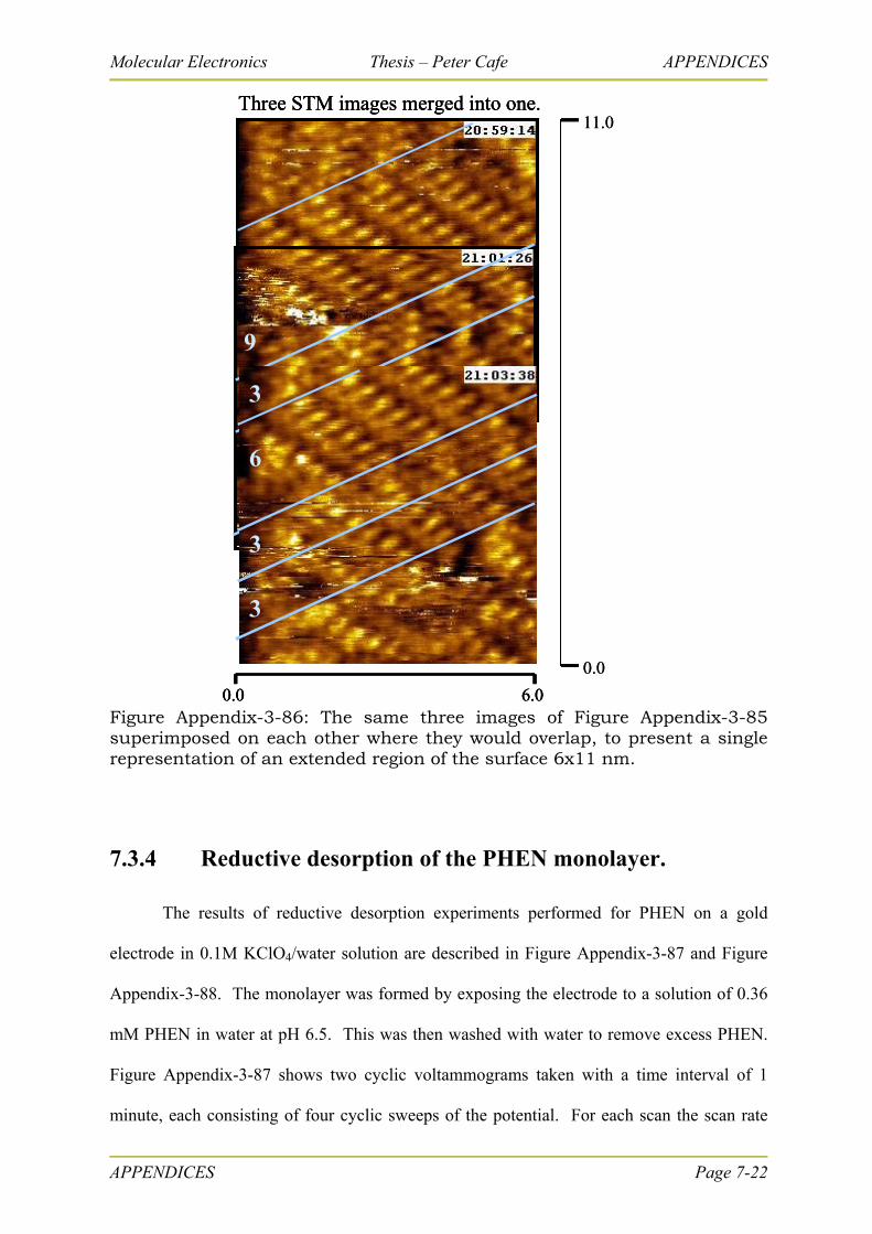
Molecular Electronics Thesis – Peter Cafe APPENDICES
9
3
9
3
6
3
3
3
6
3
Three STM images merged into one.
0.0 6.0
0.0
11.0
9
3
9
3
6
3
3
3
6
3
Three STM images merged into one.
9
3
9
3
6
3
3
3
6
3
9
3
9
3
9
3
6
3
9
3
6
3
3
3
6
3
3
3
6
3
Three STM images merged into one.
0.0 6.00.0 6.0
0.0
11.0
Figure Appendix-3-86: The same three images of Figure Appendix-3-85 superimposed on each other where they would overlap, to present a single representation of an extended region of the surface 6x11 nm.
7.3.4 Reductive desorption of the PHEN monolayer.
The results of reductive desorption experiments performed for PHEN on a gold
electrode in 0.1M KClO4/water solution are described in Figure Appendix-3-87 and Figure
Appendix-3-88. The monolayer was formed by exposing the electrode to a solution of 0.36
mM PHEN in water at pH 6.5. This was then washed with water to remove excess PHEN.
Figure Appendix-3-87 shows two cyclic voltammograms taken with a time interval of 1
minute, each consisting of four cyclic sweeps of the potential. For each scan the scan rate
APPENDICES Page 7-22
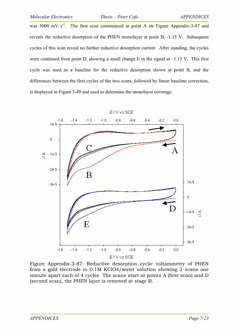
Molecular Electronics Thesis – Peter Cafe APPENDICES
was 5000 mV s-1. The first scan commenced at point A on Figure Appendix-3-87 and
reveals the reductive desorption of the PHEN monolayer at point B, -1.15 V. Subsequent
cycles of this scan reveal no further reductive desorption current. After standing, the cycles
were continued from point D, showing a small change E in the signal at –1.15 V. This first
cycle was used as a baseline for the reductive desorption shown at point B, and the
differences between the first cycles of the two scans, followed by linear baseline correction,
is displayed in Figure 3-49 and used to determine the monolayer coverage.
Figure Appendix-3-87: Reductive desorption cyclic voltammetry of PHEN from a gold electrode in 0.1M KClO4/water solution showing 2 scans one minute apart each of 4 cycles The scans start at points A (first scan) and D (second scan), the PHEN layer is removed at stage B.
APPENDICES Page 7-23
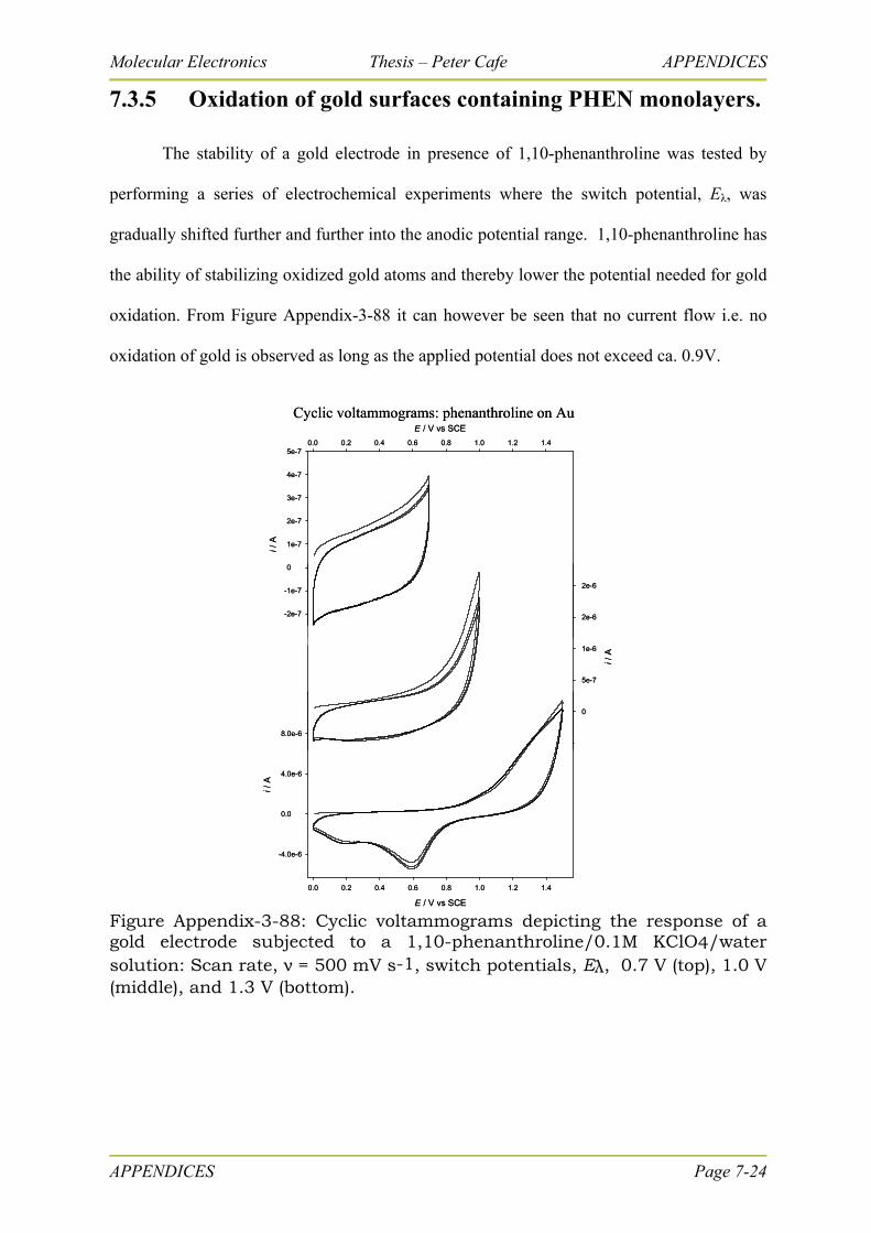
Molecular Electronics Thesis – Peter Cafe APPENDICES
7.3.5 Oxidation of gold surfaces containing PHEN monolayers.
The stability of a gold electrode in presence of 1,10-phenanthroline was tested by
performing a series of electrochemical experiments where the switch potential, Eλ, was
gradually shifted further and further into the anodic potential range. 1,10-phenanthroline has
the ability of stabilizing oxidized gold atoms and thereby lower the potential needed for gold
oxidation. From Figure Appendix-3-88 it can however be seen that no current flow i.e. no
oxidation of gold is observed as long as the applied potential does not exceed ca. 0.9V.
E / V vs SCE
0.0 0.2 0.4 0.6 0.8 1.0 1.2 1.4
i / A
-3e-7
-2e-7
-1e-7
0
1e-7
2e-7
3e-7
4e-7
5e-7
i / A
-5e-7
0
5e-7
1e-6
2e-6
2e-6
E / V vs SCE
0.0 0.2 0.4 0.6 0.8 1.0 1.2 1.4
i / A
-4.0e-6
0.0
4.0e-6
8.0e-6
1.2e-5
Cyclic voltammograms: phenanthroline on AuE / V vs SCE
0.0 0.2 0.4 0.6 0.8 1.0 1.2 1.4
i / A
-3e-7
-2e-7
-1e-7
0
1e-7
2e-7
3e-7
4e-7
5e-7
i / A
-5e-7
0
5e-7
1e-6
2e-6
2e-6
E / V vs SCE
0.0 0.2 0.4 0.6 0.8 1.0 1.2 1.4
i / A
-4.0e-6
0.0
4.0e-6
8.0e-6
1.2e-5
Cyclic voltammograms: phenanthroline on Au
Figure Appendix-3-88: Cyclic voltammograms depicting the response of a gold electrode subjected to a 1,10-phenanthroline/0.1M KClO4/water solution: Scan rate, ν = 500 mV s-1, switch potentials, Eλ, 0.7 V (top), 1.0 V (middle), and 1.3 V (bottom).
APPENDICES Page 7-24
Molecular Electronics Thesis – Peter Cafe APPENDICES
7.3.6 Full version of references.
136 "Gaussian 03, Revision B.02" Frisch, M. J.; Trucks, G. W.; Schlegel, H. B.; Scuseria, G. E.; Robb, M. A.; Cheeseman, J. R.; Montgomery, J. A.; Vreven, T.; Kudin, K. N.; Burant, J. C.; Millam, J. M.; S., I. S.; Tomasi, J.; Barone, V.; Mennuci, B.; Cossi, M.; G., S.; N., R.; Petersson, G. A.; Nakatsuji, H.; Hada, M.; Ehara, M.; Toyota, K.; Fukuda, R.; Hasegawa, J.; Ishida, M.; Nakajima, T.; Honda, Y.; Kitao, O.; Nakai, H.; Klene, M.; Li, X.; Knox, J. E.; Hratchian, H. P.; Cross, J. B.; Adamo, C.; Jaramillo, J.; Gomperts, R.; Stratmann, R. E.; Yazyev, O.; Austin, A. J.; Cammi, R.; Pomelli, C.; Ochterski, J. W.; Ayala, P. A.; Morokuma, K.; Voth, G. A.; Salvador, P.; Dannenberg, J. J.; Zakrzewski, V. G.; Dapprich, S.; Daniels, A. D.; Strain, M. C.; Farkas, O.; Malick, D. K.; Rabuck, A. D.; Raghavachari, K.; Foresman, J. B.; Ortiz, J. V.; Cui, Q.; Baboul, A. G.; Clifford, S.; Cioslowski, J.; Stefanov, B. B.; Liu, G.; Liashenko, A.; Piskorz, P.; Komaromi, I.; Martin, R. L.; Fox, D. J.; Keith, T.; Al-Laham, M. A.; Peng, C. Y.; Nanayakkara, A.; Challacombe, M.; Gill, P. M. W.; Johnson, B. G.; Chen, W.; Wong, M. W.; Gonzalez, C.; Pople, J. A. Gaussian 03, Revision B.02; Gaussian, Inc., Pittsburgh PA, 2003.
137 "TURBOLMOLE-4.0" Ahlrichs, R.; Bär, M.; Baron, H. P.; Bauernschmitt, R.; Böcker, S.; Ehrig, M.; Eichkorn, K.; Elliot, S.; Haase, F.; Häser, M.; Horn, H.; Huber, C.; Huniar, U.; Kattannek, M.; Kölmel, C.; Kollwitz, M.; Ochsenfeld, C.; Öhm, H.; Schäfer, A.; Schneider, U.; Treutler, O.; von Arnim, M.; Weigend, F.; Weis, P.; Weiss, H. TURBOLMOLE-4.0; Quantum Chemistry Group: University of Karlsruhe, 1997.
172 "Molcas Version 5" Andersson, K.; Barysz, M.; Bernhardsson, A.; Blomberg, M. R. A.; Cooper, D. L.; Fleig, T.; Fülscher, M. P.; Gagliardi, C. d.; Hess, B. A.; Karlström, G.; Lindh, R.; Malmqvist, P.-Å.; Neogrády, P.; Olsen, J.; Roos, B. O.; Sadlej, A. J.; Schütz, M.; Schimmelpfennig, B.; Seijo, L.; Serrano-Andrés, L.; Siegbahn, P. E. M.; Stålring, J.; Thorsteinsson, T.; Veryazov, V.; Widmark, P.-O. Molcas Version 5; University of Lund: Lund, 2000.
266 pages 52868 words 284635 Characters
APPENDICES Page 7-25

Molecular Electronics Thesis – Peter Cafe APPENDICES
APPENDICES Page 7-26
(blank page)