U N I V E R S I T Y O F N E W S O U T H W A L E S

S C H O O L O F E C O N O M I C S

H O N O U R S T H E S I S

STUCK IN TRAFFIC (DATA)

ANALYSING THE SPATIAL STRUCTURE OF SYDNEY WITH TRAVEL TIME DATA

Author:

Aaron W O N G

Student ID: 5075103

Supervisor:

A/Prof. Glenn O T T O

Bachelor of Economics (Honours) (Econometrics & Economics)

A N D

Bachelor of Commerce (Finance)

November 2019

ii

Declaration

I hereby declare that this submission is my own work and that, to the best of my

knowledge, it contains no material which has been written by another person or

persons, except where due acknowledgement has been made. This thesis has not been

submitted for the award of any degree or diploma at the University of New South Wales,

or at any other institute of higher education.

..................................................

Aaron Wong,

22nd November 2019

Acknowledgements

I would first like to thank my supervisor Glenn Otto, for all the time and effort you have

invested in my research this year. I am grateful for your guidance and support. Thank

you for patiently answering all my questions, contemplating my ideas and reading all

of my drafts. Your advice has been invaluable in making this thesis possible. Thank you

also for your encouragement throughout the year when I was having doubts. Hopefully

your students next year will write shorter theses!

Thank you to everyone who took the time to read my drafts and provide valuable

advice on my writing. My thanks go to Jono, Tash, Elif and Max for your suggestions and

feedback. Thank you to Federico Masera for your insightful comments and suggestions

on Part II. Thanks also go to Jim for assisting with data acquisition.

This year has been an amazing year of learning and intellectual challenge not only

in the thesis but in the coursework. Thank you to all the course lecturers who have

taken our understanding and appreciation of economics to new heights and pushed

us past all our intellectual limits. To Anuj Bhowmik and Gabriele Gratton, thank you

for completely rebuilding our understanding of microeconomics. To Stanley Cho and

Pratiti Chatterjee, thanks for the sheep and the beers, and for teaching us macro from

the very microfoundations. To Denzil Fiebig, for taking us on a fascinating journey

through discrete choice models every Monday night. To Pauline Grosjean and Federico

Masera, for giving us the tools to identify what is really happening.

Thank you to Tess Stafford for your work in co-ordinating this year. This year has gone by

about as smoothly as it could have. Without your efforts, Honours would not have been

possible. Thanks for looking out for us and keeping us in the loop with the sudden

move upstairs this year. Thank you also to Pauline Grosjean and Sarah Walker for

facilitating the Honours seminars this year. The practical guidance and feedback on our

presentations have been invaluable in making this thesis as polished as can be.

iii

iv

I would like to thank the Reserve Bank of Australia and Herbert Smith Freehills for

their generous financial support this year. Thank you also to the Microeconomics 1

and Introductory Econometrics teams for employing me this year. I am grateful for the

opportunity to share my love of economics with a new crop of undergraduates and

hopefully at least one of them will be motivated to take Honours in the future.

HONOURS! We made it to the finish line! Through the struggles, achievements and

struggles again this has been an incredible year spent with incredible people. Thank

you. I am astounded every day by the quality and volume of work that everyone has

managed to accomplish this year, and the incredible endurance and motivation in the

hours that some of you have pulled. I am surprised we did not get cabin fever with the

amount of time we spent together this year. I want to make a special mention to those

with whom I endured three courses in Term 1. An absolutely moronic decision, but I

couldn’t ask for a better group to persevere with. A special thanks to Jono, Jack and Nick

for your friendship this year. Jono, it has been an honour to share a desk with you for

the better part of the year. I will always remember our conversations and the random

thoughts we have shared thanks to our spatial proximity. I look forward to seeing the

great things every one of you will go on to accomplish and coming together again in

the future to reminisce about the challenging but rewarding year that was Honours

2019.

It has been an absolute privilege to get to know such a highly motivated and fun group

of people. Our “hour in the yard” and desk-side conversations were a highlight, with

our awful humour echoing through the corridors. Thanks to everyone who organised

drinks and other social events where we could forget the stress of the year for a night.

Thank you especially for your delicious BBQs this year Jono! This year has also been

surprisingly active, which has been invaluable for keeping me motivated and sane.

I enjoyed kicking the footy around with everyone and improving my hand-eye co-

ordination. Thanks to Gabriele for starting the climbing crew with me, Jack and others,

and I am keen to ascend to new heights with you all next year. I thoroughly enjoyed our

hike, Nick and Jack, and am looking forward our next trip.

Finally, I want to thank those who have seen far too little of me this year. Thank you to

my family for supporting me these last two and a bit decades. Mum and Dad, thank you

for fostering my love of learning and encouraging me to pursue my interests. Without

your unconditional love and support, I would never have made it here in the first place.

To Kristie, thank you for your support this year and encouraging me through rough

patches. Thank you for putting up with my grumpiness. I always looked forward to our

time together this year as a welcome change from my thesis.

Table of Contents

Table of Contents v

List of Figures viii

List of Tables x

Attributions xiv

A Guide to this Thesis xv

Abstract 1

I Estimating Rent Gradients in Greater Sydney: A Travel Time DataApproach 2

1 Introduction 3

2 Literature review 7

3 Methodology 12

3.1 Alonso-Muth-Mills model of urban spatial structure . . . . . . . . . . . . . 12

3.2 Econometric modelling approaches . . . . . . . . . . . . . . . . . . . . . . . 15

3.2.1 Hedonic pricing models . . . . . . . . . . . . . . . . . . . . . . . . . . 15

3.2.2 Spatial models . . . . . . . . . . . . . . . . . . . . . . . . . . . . . . . . 17

4 Data 21

4.1 Travel time data . . . . . . . . . . . . . . . . . . . . . . . . . . . . . . . . . . . 21

4.2 Property sales data . . . . . . . . . . . . . . . . . . . . . . . . . . . . . . . . . 23

4.3 Land valuations data . . . . . . . . . . . . . . . . . . . . . . . . . . . . . . . . 26

4.4 Neighbourhood controls . . . . . . . . . . . . . . . . . . . . . . . . . . . . . . 28

4.5 Property sales data summary statistics . . . . . . . . . . . . . . . . . . . . . 28

4.6 Land values data summary statistics . . . . . . . . . . . . . . . . . . . . . . . 32

4.7 Mapping the data . . . . . . . . . . . . . . . . . . . . . . . . . . . . . . . . . . 35

v

vi TABLE OF CONTENTS

4.7.1 Property sales data travel time maps . . . . . . . . . . . . . . . . . . . 35

4.7.2 Land valuations data travel time maps . . . . . . . . . . . . . . . . . 37

4.8 Testing for spatial dependence in the data . . . . . . . . . . . . . . . . . . . 38

5 Results and discussion 40

5.1 Model specification . . . . . . . . . . . . . . . . . . . . . . . . . . . . . . . . . 42

5.1.1 Lagrange Multiplier test of spatial correlation . . . . . . . . . . . . . 44

5.2 Estimates from property sales data . . . . . . . . . . . . . . . . . . . . . . . . 45

5.2.1 Distance specifications . . . . . . . . . . . . . . . . . . . . . . . . . . 47

5.2.2 Travel time specifications . . . . . . . . . . . . . . . . . . . . . . . . . 49

5.3 Estimates from land valuations data . . . . . . . . . . . . . . . . . . . . . . . 52

5.3.1 Distance specifications . . . . . . . . . . . . . . . . . . . . . . . . . . 54

5.3.2 Travel time specifications . . . . . . . . . . . . . . . . . . . . . . . . . 55

5.4 Estimating the value of congestion . . . . . . . . . . . . . . . . . . . . . . . . 58

5.5 Out-of-sample predictive power . . . . . . . . . . . . . . . . . . . . . . . . . 60

5.6 Willingness to pay calculations . . . . . . . . . . . . . . . . . . . . . . . . . . 62

5.7 Robustness tests . . . . . . . . . . . . . . . . . . . . . . . . . . . . . . . . . . . 63

5.8 Limitations . . . . . . . . . . . . . . . . . . . . . . . . . . . . . . . . . . . . . . 65

6 Conclusion 68

6.1 Policy implications . . . . . . . . . . . . . . . . . . . . . . . . . . . . . . . . . 68

6.2 Concluding remarks . . . . . . . . . . . . . . . . . . . . . . . . . . . . . . . . 69

II Measuring Land Value Uplift: Difference in Differences Estim-ates from Sydney Metro Northwest 72

1 Introduction 73

2 Literature review 77

3 Background 81

4 Methodology 83

4.1 Challenges to identifying treatment effects . . . . . . . . . . . . . . . . . . . 86

5 Data 89

5.1 Travel time data . . . . . . . . . . . . . . . . . . . . . . . . . . . . . . . . . . . 89

5.2 Land valuations data . . . . . . . . . . . . . . . . . . . . . . . . . . . . . . . . 94

5.3 Neighbourhood variables . . . . . . . . . . . . . . . . . . . . . . . . . . . . . 95

5.4 Summary statistics . . . . . . . . . . . . . . . . . . . . . . . . . . . . . . . . . 96

6 Results and discussion 100

TABLE OF CONTENTS vii

6.1 Land value uplift estimates . . . . . . . . . . . . . . . . . . . . . . . . . . . . 100

6.1.1 Willingness to pay calculations . . . . . . . . . . . . . . . . . . . . . . 102

6.2 Robustness tests . . . . . . . . . . . . . . . . . . . . . . . . . . . . . . . . . . . 103

6.2.1 Alternative distance models . . . . . . . . . . . . . . . . . . . . . . . . 103

6.2.2 Statistical noise DiD . . . . . . . . . . . . . . . . . . . . . . . . . . . . 105

6.3 Limitations . . . . . . . . . . . . . . . . . . . . . . . . . . . . . . . . . . . . . . 106

7 Conclusion 109

References 111

Appendices 123

A Part 1: Additional travel time maps 125

A.1 Property sales data travel time maps . . . . . . . . . . . . . . . . . . . . . . . 125

A.2 Land valuations data travel time maps . . . . . . . . . . . . . . . . . . . . . 127

B Part 1: Variable names and descriptions 130

C Part 1: Regression residual plots 131

C.1 Sales data residual plots . . . . . . . . . . . . . . . . . . . . . . . . . . . . . . 131

C.2 Land value data residual plots . . . . . . . . . . . . . . . . . . . . . . . . . . 132

D Part 1: Sales data robustness tests 133

D.1 Log-level linear regression model results . . . . . . . . . . . . . . . . . . . . 133

D.2 Level-level spatial error model . . . . . . . . . . . . . . . . . . . . . . . . . . 134

D.2.1 Distance specifications . . . . . . . . . . . . . . . . . . . . . . . . . . 135

D.2.2 Travel time specifications . . . . . . . . . . . . . . . . . . . . . . . . . 135

D.3 Log-level spatial autoregressive models . . . . . . . . . . . . . . . . . . . . . 137

D.4 Level-level spatial autoregressive models . . . . . . . . . . . . . . . . . . . . 138

D.5 Sales price dependent variable regressions . . . . . . . . . . . . . . . . . . . 141

D.6 Log-log comparison models estimated by OLS . . . . . . . . . . . . . . . . . 142

E Part 1: Valuations data robustness tests 144

E.1 Log-level linear regression model results . . . . . . . . . . . . . . . . . . . . 144

E.2 Level-level spatial error model . . . . . . . . . . . . . . . . . . . . . . . . . . 145

E.2.1 Distance specifications . . . . . . . . . . . . . . . . . . . . . . . . . . 146

E.2.2 Travel time specifications . . . . . . . . . . . . . . . . . . . . . . . . . 147

E.3 Log-level spatial autoregressive models . . . . . . . . . . . . . . . . . . . . . 149

E.4 Level-level spatial autoregressive models . . . . . . . . . . . . . . . . . . . . 150

E.5 Land value dependent variable regressions . . . . . . . . . . . . . . . . . . . 153

viii TABLE OF CONTENTS

E.6 Log-log comparison models estimated by OLS . . . . . . . . . . . . . . . . . 154

F Part 1: Full tables for sales regressions 156

F.1 Log-level models . . . . . . . . . . . . . . . . . . . . . . . . . . . . . . . . . . 156

F.2 Level-level models . . . . . . . . . . . . . . . . . . . . . . . . . . . . . . . . . 160

G Part 1: Full tables for land values regressions 165

G.1 Log-level models . . . . . . . . . . . . . . . . . . . . . . . . . . . . . . . . . . 165

G.2 Level-level models . . . . . . . . . . . . . . . . . . . . . . . . . . . . . . . . . 169

G.3 Congestion model . . . . . . . . . . . . . . . . . . . . . . . . . . . . . . . . . 173

H Part 2: DiD identification tests 176

H.1 Treatment and baseline outcomes regression . . . . . . . . . . . . . . . . . 176

H.2 Parallel trends assumption graphs . . . . . . . . . . . . . . . . . . . . . . . . 176

I Part 2: Full regression tables 179

I.1 Main DiD regression . . . . . . . . . . . . . . . . . . . . . . . . . . . . . . . . 179

I.2 Alternate DiD regressions . . . . . . . . . . . . . . . . . . . . . . . . . . . . . 179

J Part 2: Additional robustness checks 181

K Willingness to pay calculations 183

K.1 Part 1 WTP estimates . . . . . . . . . . . . . . . . . . . . . . . . . . . . . . . . 184

K.2 Part 2 WTP estimates . . . . . . . . . . . . . . . . . . . . . . . . . . . . . . . . 186

List of Figures

3.1 AMM model calibrated to representative Australian city . . . . . . . . . . . 13

3.2 Idealised rent gradient . . . . . . . . . . . . . . . . . . . . . . . . . . . . . . . 13

4.1 Location of the Sydney CBD, Parramatta and Macquarie Park . . . . . . . . 22

4.2 Median property sales price at SA2 level . . . . . . . . . . . . . . . . . . . . . 25

4.3 Median property sales price per square metre at SA2 level . . . . . . . . . . 25

4.4 Median land values at SA2 level . . . . . . . . . . . . . . . . . . . . . . . . . . 27

4.5 Median land values per square metre at SA2 level . . . . . . . . . . . . . . . 28

4.6 Scatter plot of sale prices and drive times to Sydney CBD . . . . . . . . . . 31

4.7 Scatter plot of sale prices and public transport travel times to Sydney CBD 31

4.8 Scatter plot of land values and drive times to Sydney CBD . . . . . . . . . . 34

4.9 Scatter plot of land values and public transport travel times to Sydney CBD 34

4.10 Drive times to Sydney CBD . . . . . . . . . . . . . . . . . . . . . . . . . . . . 36

4.11 Public transport times to Sydney CBD . . . . . . . . . . . . . . . . . . . . . . 36

4.12 Drive times to Sydney CBD . . . . . . . . . . . . . . . . . . . . . . . . . . . . 37

4.13 Public transport times to Sydney CBD . . . . . . . . . . . . . . . . . . . . . . 38

5.1 Marginal effect of Sydney distance on property prices per m2 . . . . . . . . 48

5.2 Marginal effect of Sydney drive time on property prices per m2 . . . . . . . 50

5.3 Marginal effect of Sydney transit time on property prices per m2 . . . . . . 51

5.4 Marginal effect of Sydney distance on land values per m2 . . . . . . . . . . 55

5.5 Marginal effect of Sydney drive time on land values per m2 . . . . . . . . . 56

5.6 Marginal effect of Sydney transit time on land values per m2 . . . . . . . . 57

5.7 Spatial cross-validation folds (repetitions 1-4) . . . . . . . . . . . . . . . . . 60

3.1 Sydney Metro route map . . . . . . . . . . . . . . . . . . . . . . . . . . . . . . 81

4.1 Idealised land value uplift curve . . . . . . . . . . . . . . . . . . . . . . . . . 83

4.2 Treatment effects in a DiD model . . . . . . . . . . . . . . . . . . . . . . . . . 86

5.1 Treated and control properties . . . . . . . . . . . . . . . . . . . . . . . . . . 91

ix

x LIST OF FIGURES

5.2 Travel times prior to Sydney Metro . . . . . . . . . . . . . . . . . . . . . . . . 92

5.3 Travel times after opening of Sydney Metro . . . . . . . . . . . . . . . . . . . 93

5.4 Demeaned land value change (2012-18) . . . . . . . . . . . . . . . . . . . . . 95

6.1 Predicted land values/m2 with 95% CI . . . . . . . . . . . . . . . . . . . . . . 102

6.2 Change in land values by distance to nearest Metro station . . . . . . . . . 105

A.1 Drive times to Parramatta . . . . . . . . . . . . . . . . . . . . . . . . . . . . . 125

A.2 Public transport times to Parramatta . . . . . . . . . . . . . . . . . . . . . . 126

A.3 Drive times to Macquarie Park . . . . . . . . . . . . . . . . . . . . . . . . . . 126

A.4 Public transport times to Macquarie Park . . . . . . . . . . . . . . . . . . . . 127

A.5 Drive times to Parramatta . . . . . . . . . . . . . . . . . . . . . . . . . . . . . 127

A.6 Public transport times to Parramatta . . . . . . . . . . . . . . . . . . . . . . 128

A.7 Drive times to Macquarie Park . . . . . . . . . . . . . . . . . . . . . . . . . . 128

A.8 Public transport times to Macquarie Park . . . . . . . . . . . . . . . . . . . . 129

C.1 Plot of Studentized residuals and fitted values of sqmval ue . . . . . . . . . 131

C.2 Plot of Studentized residuals and fitted values of ln(sqmval ue) . . . . . . 131

C.3 Plot of Studentized residuals and fitted values of sqmval ue . . . . . . . . . 132

C.4 Plot of Studentized residuals and fitted values of ln(sqmval ue) . . . . . . 132

D.1 Marginal effect of Sydney distance on land values per m2 . . . . . . . . . . 135

D.2 Marginal effect of Sydney drive time on land values per m2 . . . . . . . . . 136

D.3 Marginal effect of Sydney transit time on land values per m2 . . . . . . . . 136

E.1 Marginal effect of Sydney distance on land values per m2 . . . . . . . . . . 147

E.2 Marginal effect of Sydney drive time on land values per m2 . . . . . . . . . 148

E.3 Marginal effect of Sydney transit time on land values per m2 . . . . . . . . 148

H.1 Parallel trends assumption checks (travel time treatment) . . . . . . . . . . 177

H.2 Parallel trends assumption checks (distance-based treatment) . . . . . . . 178

List of Tables

4.1 Summary statistics for the property sales data . . . . . . . . . . . . . . . . . 29

4.2 Residential property type counts . . . . . . . . . . . . . . . . . . . . . . . . . 30

4.3 Summary statistics for the land value data . . . . . . . . . . . . . . . . . . . 32

4.4 Residential zone code counts . . . . . . . . . . . . . . . . . . . . . . . . . . . 33

4.5 Moran’s I test results . . . . . . . . . . . . . . . . . . . . . . . . . . . . . . . . 39

5.1 Comparison of AIC scores for sales data models . . . . . . . . . . . . . . . . 41

5.2 Summary of property value changes for average property . . . . . . . . . . 42

5.3 Lagrange Multiplier tests of spatial autocorrelation . . . . . . . . . . . . . . 44

5.4 Spatial error model regression results using ln(Sales price per m2

). . . . . 46

5.5 Spatial error model regression results using ln(Sales price per m2

). . . . . 53

5.6 Marginal value of congestion estimates . . . . . . . . . . . . . . . . . . . . . 59

5.7 Spatial cross-validation out-of-sample prediction performance results . . 61

5.1 Summary statistics . . . . . . . . . . . . . . . . . . . . . . . . . . . . . . . . . 96

5.2 Zoning classifications of sample data . . . . . . . . . . . . . . . . . . . . . . 96

5.3 Summary statistics by treatment status . . . . . . . . . . . . . . . . . . . . . 98

5.4 Difference in means tests . . . . . . . . . . . . . . . . . . . . . . . . . . . . . 99

6.1 Difference in differences regression estimates . . . . . . . . . . . . . . . . . 101

6.2 Willingness to pay for 1 hour of travel time savings . . . . . . . . . . . . . . 103

6.3 Difference in differences regression alternative specification estimates . . 104

6.4 Difference in differences robustness regression estimates . . . . . . . . . . 106

B.1 Variable names and descriptions . . . . . . . . . . . . . . . . . . . . . . . . . 130

D.1 Linear regression results (l sqmval ue) . . . . . . . . . . . . . . . . . . . . . 133

D.2 SEM regression results (Sales price per m2) . . . . . . . . . . . . . . . . . . . 134

D.3 SARM regression results (l sqmval ue) . . . . . . . . . . . . . . . . . . . . . . 137

D.4 SARM total impact distance estimates (% points) (l sqmval ue) . . . . . . . 138

D.5 SARM total impact travel time estimates (% points) (l sqmval ue) . . . . . 138

xi

xii LIST OF TABLES

D.6 SARM regression results (sqmval ue) . . . . . . . . . . . . . . . . . . . . . . 138

D.7 SARM total impact distance estimates (sqmval ue) . . . . . . . . . . . . . . 140

D.8 SARM total impact travel time estimates (sqmval ue) . . . . . . . . . . . . 140

D.9 Linear regression results (Sales price) . . . . . . . . . . . . . . . . . . . . . . 141

D.10 Log-level and Log-log model comparisons (l sqmval ue) . . . . . . . . . . . 142

E.1 Linear regression results (l sqmval ue) . . . . . . . . . . . . . . . . . . . . . 144

E.2 SEM regression results (sqmval ue) . . . . . . . . . . . . . . . . . . . . . . . 145

E.3 SARM regression results (l sqmval ue) . . . . . . . . . . . . . . . . . . . . . . 149

E.4 SARM total impact distance estimates (% points) (l sqmval ue) . . . . . . . 150

E.5 SARM total impact travel time estimates (% points) (l sqmval ue) . . . . . 150

E.6 SARM regression results (sqmval ue) . . . . . . . . . . . . . . . . . . . . . . 150

E.7 SARM total impact distance estimates (sqmval ue) . . . . . . . . . . . . . . 152

E.8 SARM total impact travel time estimates (sqmval ue) . . . . . . . . . . . . 153

E.9 Linear regression results (Land value) . . . . . . . . . . . . . . . . . . . . . . 153

E.10 Log-level and Log-log model comparisons (l sqmval ue) . . . . . . . . . . . 154

F.1 Linear regression results (l sqmval ue) . . . . . . . . . . . . . . . . . . . . . 156

F.2 SEM regression results (l sqmval ue) . . . . . . . . . . . . . . . . . . . . . . 157

F.3 SARM regression results (l sqmval ue) . . . . . . . . . . . . . . . . . . . . . . 159

F.4 Linear regression results (sqmval ue) . . . . . . . . . . . . . . . . . . . . . . 160

F.5 SEM regression results (sqmval ue) . . . . . . . . . . . . . . . . . . . . . . . 162

F.6 SARM regression results (sqmval ue) . . . . . . . . . . . . . . . . . . . . . . 163

G.1 Linear regression results (l sqmval ue) . . . . . . . . . . . . . . . . . . . . . 165

G.2 SEM regression results (l sqmval ue) . . . . . . . . . . . . . . . . . . . . . . 166

G.3 SARM regression results (l sqmval ue) . . . . . . . . . . . . . . . . . . . . . . 168

G.4 Linear regression results (sqmval ue) . . . . . . . . . . . . . . . . . . . . . . 169

G.5 SEM regression results (sqmval ue) . . . . . . . . . . . . . . . . . . . . . . . 170

G.6 SARM regression results (sqmval ue) . . . . . . . . . . . . . . . . . . . . . . 172

G.7 Marginal value of congestion estimates . . . . . . . . . . . . . . . . . . . . . 173

H.1 Treatment and baseline outcomes regression . . . . . . . . . . . . . . . . . 176

I.1 Difference in differences regression estimates . . . . . . . . . . . . . . . . . 179

I.2 Difference in differences regression alternative specification estimates . . 180

J.1 DiD regression: No neighbourhood controls . . . . . . . . . . . . . . . . . . 181

J.2 DiD regression: No fixed effects . . . . . . . . . . . . . . . . . . . . . . . . . . 181

J.3 DiD regression: No clustered standard errors . . . . . . . . . . . . . . . . . . 182

K.1 List of assumptions . . . . . . . . . . . . . . . . . . . . . . . . . . . . . . . . . 183

LIST OF TABLES xiii

K.2 Sensitivity tests for sales price drive time WTP estimates . . . . . . . . . . . 184

K.3 Sensitivity tests for sales price transit time WTP estimates . . . . . . . . . . 184

K.4 Sensitivity tests for land valuations drive time WTP estimates . . . . . . . . 185

K.5 Sensitivity tests for land valuations transit time WTP estimates . . . . . . . 185

K.6 Sensitivity tests for DiD travel time WTP estimates . . . . . . . . . . . . . . 186

Attributions

This research includes computations using the computational cluster Katana supported

by Research Technology Services at UNSW Sydney.

Incorporates or developed using G-NAF © PSMA Australia Limited licensed by the

Commonwealth of Australia under the Open Geo-coded National Address File (G-NAF)

End User Licence Agreement.

NSW Land Values data: © State of New South Wales through the Office of the Valuer

General 2019.

Sydney property sales data: © Australian Property Monitors 2019.

Travel time data: © Google 2019.

xiv

A Guide to this Thesis

This thesis estimates the willingness to pay of commuters to reduce their cost of travel

to employment in Sydney using a unique dataset of Google Maps travel time data.

I divide my thesis into two Parts in order to answer this question from two related

perspectives.

The first Part considers a cross-sectional equilibrium approach to estimating the value

of commuting time from a Sydney-wide perspective. The second Part uses a difference

in differences estimator to measure the value of commuting time by exploiting variation

in travel times from the opening of Sydney Metro Northwest.

Although the two Parts are related, each Part has its own story to tell, with the literature,

dataset and methodology being sufficiently different such that combining the parts

would muddle the motivation for my research.

While each Part is structured as a separate thesis, I make several references throughout

Part II to content contained within Part I to avoid repeating myself excessively. Thus,

I recommend that the reader read this two-part thesis sequentially to avoid loss of

information. This is especially the case for the chapters relating to the conceptual

framework, theory and methodology.

xv

Abstract

Most studies of urban rent gradients and estimates of land value uplift from infra-

structure projects use distances from employment and transport facilities as a proxy

for accessibility. However, commuters value reducing travel times to their destinations,

not distances. In this thesis, I construct a novel dataset of travel time data scraped

from Google Maps to analyse the spatial structure of Sydney. I use travel times to the

Sydney CBD, Parramatta and Macquarie Park to estimate rent gradients using a spatially

correlated hedonic pricing model for a cross-section of residential properties using data

on sales prices and land valuations (Part I). I exploit variation in travel times caused

by the opening of the Sydney Metro Northwest railway line on a panel dataset of land

valuations to estimate willingness to pay (WTP) for reduced travel time to employment

in Sydney using a difference in differences estimator (Part II). I find that travel time

models materially improve goodness of fit and out-of-sample predictive power relative

to distance-based models. I calculate the WTP of commuters to reduce travel times in

Sydney, finding that commuters positively value accessibility to Sydney and Parramatta

by road and public transport, and negatively value additional travel time caused by

congestion. My results have applications in increasing the predictive power of land

valuers’ automated valuation models, improving assumptions on the value of travel time

savings used in cost-benefit analysis and land value capture mechanisms for funding new

infrastructure, and optimising the setting of motorway tolls and congestion charges for

entering congested city centres.

1

Part I

Estimating Rent Gradients in Greater

Sydney: A Travel Time Data Approach

2

C H A P T E R 1

Introduction

In addition to speculating on property prices, complaining about urban sprawl and long

commutes is a popular pastime of Sydneysiders (Livingston, 2019; Riga, 2019). Most

individuals aim to minimise commuting because it is a mental and physical burden

(Stutzer & Frey, 2008). From an economic perspective, commuting creates disutility

due to the opportunity cost of time and monetary costs of travelling (McArthur, Kleppe,

Thorsen & Ubøe, 2011). Thus, commuters are willing to pay to avoid these costs by

living in a location that minimises their travel costs, subject to financial constraints.

This willingness to pay for accessibility to employment and amenities is capitalised into

the value of land and hence variation in land values can be used to quantify variation

in accessibility across cities (Grislain-Letrémy & Katossky, 2014).

It is likely that travel time to a location matters more than commuting distance, despite

the preference in most of the literature to use distances as a proxy for accessibility (see

Bowes and Ihlanfeldt (2001), Hill (2012), S. Ryan (1999) for a review). This hypothesis

is supported by research that shows land value uplift surrounding new transport

infrastructure projects (Bowes & Ihlanfeldt, 2001; Du & Mulley, 2006, 2012; McIntosh,

Trubka & Newman, 2014; Mulley & Tsai, 2016; Yen, Mulley, Shearer & Burke, 2018). An

infrastructure project that physically reduces the distance between work and home

would be quite expensive. Instead most transport projects aim to increase the speed

at which people can move from A to B, so changes in travel time should be what is

valued by commuters — a proposition I investigate in this thesis. I examine whether

travel time models improve the explanatory and predictive power of hedonic pricing

models compared to models that use distances as a proxy for accessibility. I also

examine whether the inclusion of employment sub-centres improves model estimation

compared to monocentric models. By measuring variation in travel times and property

values in Sydney, I estimate the value that the average commuter associates with

reduced commuting times to employment.

I construct a unique dataset of driving and public transport travel times scraped from

Google Maps. Using this dataset, I estimate the impact of changes in travel time to major

3

4 CHAPTER 1. INTRODUCTION

Sydney employment centres on residential property sales prices and land values using

spatial regression methods to estimate hedonic price models. The travel time data takes

into account traffic congestion for drive times, and delays and interchange times for

public transport, providing a dataset that is as close as possible to being representative

of real commutes. The results provide an estimate of commuters’ willingness to pay

to live closer to these centres, controlling for property characteristics, zoning effects

and neighbourhood demographics. I source these datasets from Australian Property

Monitors (APM), the NSW Valuer General and from the 2016 Census conducted by the

Australian Bureau of Statistics (ABS).

I examine whether travel times are a better measure of accessibility to employment

and amenities compared to straight-line distances. Existing theoretical models of cities

such as the Alonso-Muth-Mills model — and most research that is based upon it

— include the assumption that commuting costs can be measured as a function of

Euclidean distance from a single Central Business District (CBD). I replace this with a

more accurate measure of commuting costs — travel times by car and public transport.

Given that commuters experience disutility from increased commuting time rather

than distance (McArthur et al., 2011), I hypothesise that replacing distance measures

with time measures should increase the explanatory power of spatial models. I also

generalise from the assumption of a monocentric and homogeneous city by including

commuting times to Parramatta and Macquarie Park in Sydney, non-employment

amenities (beaches) and neighbourhood heterogeneity in the form of socio-economic

variables.

My results present the first direct estimates of the present value of travel time sav-

ings and the value of congestion for commuters in Sydney using unit record data,

improving on previous rent gradients estimated using distance-based models at the

more aggregate suburb level (Abelson, Joyeux & Mahuteau, 2013). I find that including

travel times as a measure of accessibility improves the explanatory power of hedonic

models of property prices relative to models using distances to centres. For out-of-

sample prediction, the travel time models also outperform the distance models, with

my measure of prediction accuracy — root mean squared error (RMSE) — improving

by over 30% for some specifications. However, the land value models exhibit different

performance characteristics, with travel time models not outperforming distance

models — a finding I attribute to the methodology used by the valuers in constructing

the dataset.

I find that households are willing to pay for properties that are more accessible to the

Sydney CBD and Parramatta by road or public transport. The magnitudes of estimates

5

vary between models, but the signs are robust to model specification. For the model

containing travel time data to Sydney, Parramatta and Macquarie Park, I find that the

average commuter is willing to pay about $3,400 (all currency values are in Australian

dollars) more (0.30% of the property price) to be 1 minute closer to the Sydney CBD by

road and $4,100 (0.36% of the property price) to be closer by public transport. For the

land value models, I estimate the value of 1 minute in road accessibility improvements

to be worth about $3,500 (0.42% of land value) and about $2,200 (0.26% of land value)

for improved public transport accessibility. This calculation assumes a property with a

sales price of $1.15 million and a land value of $826,800, with a commute to Sydney of

49 minutes’ drive and 69 minutes by public transport.

Commuters also value improved accessibility to employment in Parramatta by road and

public transport. I find that these effects diminish as travel times increase, suggesting

commuters closest to the centre are most sensitive to changes in travel times. I also

find that accessibility to Macquarie Park is not valued positively by commuters, with

marginal effects that suggest accessibility to Macquarie Park diminishes property

values. This result may be the result of interactions between the variables measuring

accessibility to the other major centres, rather than a significant result in itself. In a

cross-sectional framework, travel times and property values are likely to be endogenous

and Sydney residents are also likely to have sorted themselves into preferred locations,

hence these results should be interpreted from a long-run equilibrium perspective, as

opposed to a causal effect.

I find that commuters negatively value road congestion that increases drive times above

free flowing uncongested drive times. A 1 minute increase in congestion is associated

with a $2,200 decrease in land values for the average property in Sydney, holding free-

flowing drive times to the Sydney CBD constant. Similarly, this effect is present for

commutes to Parramatta and Macquarie Park, with commuters valuing a 1 minute

reduction in congestion at $1,500 and $1,900 for the average property.

These results are useful for industry with applications such as automated valuation

modelling. By using regression techniques to complement traditional land valuation,

the scale and consistency of valuations can be improved. My results also support

previous research (McIntosh et al., 2014) finding evidence of land value uplift in

Australia around infrastructure projects that improve commute times. Estimates of the

willingness to pay for reducing commute times are a key input into cost-benefit analysis

of infrastructure projects. Thus, my more direct estimates of willingness to pay for travel

time savings may improve the appraisal of transport projects and hence contribute to

the better allocation of public funds for infrastructure. These estimates can be used for

6 CHAPTER 1. INTRODUCTION

pricing land value capture mechanisms that tax part of the land value uplift associated

with new infrastructure to fund transport projects (Medda, 2012). For example, enabling

a levy to be designed that is proportional to travel time savings rather than just distance.

My estimates of the value of the disutility of congestion can also inform the pricing of

congestion charges for travel into city centres during peak times.

C H A P T E R 2

Literature review

The spatial economics literature began as the study of land rent by Ricardo (1821), which

was developed by von Thünen (1826) into a model of agricultural land use. This model

predicts the use of a piece of land at a given distance from a market town as a function

of the cost of transport and the maximum rent that the farmer is willing to pay. For

developed urban areas, the theoretical basis for much of the urban economics literature

is based on the model of urban spatial structure developed by Alonso (1964), Muth

(1969) and Mills (1967) (AMM model). This model formalises the observation that there

is a compensatory trade-off between commuting costs within an urban area and the

price of land and living space. The AMM model assumes a stylised city with all residents

commuting to work in a central business district at the centre of the urban area. The

costs of commuting are simply expressed as a function of the cost of commuting per

unit of distance and the distance travelled by each resident. The model predicts that

the price per square metre of housing is a decreasing function of distance to the CBD

(Brueckner, 1987). I discuss the model in greater detail in section 3.1.

Using hedonic methods first developed by Rosen (1974), I estimate the empirical

relationship between commuting times and property values in Sydney. Hedonic

regressions are a widely used revealed preference method that reveal consumers’

marginal willingness to pay (WTP) for individual attributes of a differentiated product.

Hedonic models have been used to determine the impact on house prices of partic-

ular characteristics. A survey of the literature by Hill (2012) explored previous work

examining the effect of environmental bads such as pollution (Anselin & Lozano-Gracia,

2008; McMillen, 2004; Zabel & Kiel, 2000); goods such as public parks, public services

provision; and crime (Gibbons & Machin, 2003; Rouwendal & van der Straaten, 2008;

Song & Knaap, 2004). However, hedonic regression models can produce misleading

results in the event of functional form misspecification, omitted variables and failure

to control for spatial effects (Kuminoff, Parmeter & Pope, 2010). Hill (2012) argues that

researchers should make greater use of spatial econometric methods and geospatial

data to improve hedonic estimations of the value of housing attributes. I contribute to

improving these estimates by using spatial econometric methods in this Part.

7

8 CHAPTER 2. LITERATURE REVIEW

There are opportunities for my analysis to extend the use of spatial hedonic regression

modelling. According to a survey of the literature by Higgins and Kanaroglou (2016),

about 40% of the 104 North American studies they surveyed did not use any spatial

methods in the econometric analysis. Hill (2012) notes that house prices are likely

to be spatially dependent as many of the determinants of price are neighbourhood

characteristics that are difficult to quantify explicitly (consider the “character” of a

wealthy neighbourhood versus a more disadvantaged one). In a study of the WTP to live

away from hazardous industrial plants in France, Grislain-Letrémy and Katossky (2014)

show that a parametric ordinary least squares model performs less well compared

to semi-parametric models that estimate a series of local regressions that weight

observations inversely by distance, such that more distant properties are weighted

less. They found that this model is less sensitive to small changes in the sample or

specification of the functional form. More importantly, the parametric model leads

to a significant bias in the estimation of the marginal WTP, with statistical tests

showing that the distributions estimated by the parametric and semi-parametric

models are substantially different. Similarly, Du and Mulley (2012) analyse the effects

of accessibility on property values and note that spatial dependence (where there is

interdependence between observations as a result of their relative locations in space)

will result in biased estimated coefficients. The presence of spatial error dependence

(where the error terms follow a spatial autoregressive process) leads to unbiased,

but inefficiently estimated coefficients. Prior research examining the performance of

non-parametric spatial models find that they almost always outperform parametric

approaches in terms of the mean-square error for out-of-sample prediction (Bao & Wan,

2004; Martins-Filho & Bin, 2005; Pace, 1993). Thus, implementing spatial econometric

techniques in this Part is essential for credible estimation.

I use data on both property transaction prices and assessed land values in this Part.

Property sales data is the best representation of the market value of property, but as

this Part is interested in the accessibility of land, the value of the structure on top of the

land must be partialled out using hedonic price modelling techniques. On the other

hand, land valuations data appears to be better suited for this task as it aims to provide

the unimproved value of the land on a property (NSW Valuer General, 2017a, 2017b).

However, this dataset relies on professional valuers accurately isolating the value of

the land from the rest of the property. In addition, anecdotal comments from some

researchers have suggested that this dataset may be prone to downward biases, such

as Kendall and Tulip (2018), who wrote that valuations may be biased downwards if

property owners only challenge high estimates of their land value, but not low estimates.

While property sales data is more popular in the literature (Higgins & Kanaroglou,

2016), statutory land values have also featured in the literature. One example is work by

9

McIntosh et al. (2014), who used land valuations for residential properties in Perth to

estimate the WTP for transport access.

Commuting cost is the key parameter that my research examines. Past empirical studies

of the effect of transport costs focused on using distance to transport facilities or the city

centre as the measure of accessibility. However, transportation facilities are not a final

destination for commuters, merely an intermediary providing connectivity between

origins and destinations. Thus, studies that focus on access to transport facilities may

not accurately reflect changes in travel costs (Bowes & Ihlanfeldt, 2001; S. Ryan, 1999).

My research builds on the AMM model by treating commuting costs as a function of

travel times using Google Maps travel time data (Google, 2019), which is superior to

straight-line distance proxy for accessibility.

Outside of the economics literature, recent research has started making use of travel

time data. In the civil engineering literature, Wu and Levinson (2019) examine the num-

ber of jobs and workers accessible within a 30 minute commute from the population-

weighted average household. Terrill, Batrouney, Etherington and Parsonage (2017)

use Google Maps data to examine road congestion in Sydney and Melbourne at

different times of the day and week. They find that congestion varies greatly across

Sydney, worsening closer to the Sydney CBD, but relatively minor around other sub-

centres. Congestion is also much less severe than commonly believed, with the average

commute into the Sydney CBD incurring an average delay of only 11 minutes compared

to free-flow drive time. For commuters to locations other than the Sydney CBD, average

delays are rarely more than 5 minutes longer than free flowing traffic. However, trip

times are unreliable, which forces commuters to leave earlier to take into account

potential extra delays, which are an additional commuting cost.

Palm and Niemeier (2019) measure the effect of accessibility to employment using data

from a limited subset of the urban transportation network. They examine the effects of

accessibility improvements from private bus shuttle services provided by technology

firms in San Francisco to their employees on rents in the city. They compare a simple

distance-based model to a more complex model that groups locations into bands

determined by travel time-weighted accessibility to employment. They conclude that

the more complex model does not produce any significant improvement in explanatory

power relative to the distance-based model. While this research is related, the focus on

private shuttle buses limits the external validity of the results to broader commuter

choices compared to the wider scope of my research.

Ibeas, Cordera, dell’Olio, Coppola and Dominguez (2012) examine the effects of in-

creased density of transit lines present in areas of housing in Santander, Spain. They

10 CHAPTER 2. LITERATURE REVIEW

find that property values increase by 1.8% for each additional transit line within each

district. They also find a positive relationship between accessibility by car and property

values, with a 1 minute reduction in travel times to the Santander city centre increasing

property values by 0.5% to 1.1% depending on the model specification. Their research

found that the spatial error model, which incorporates spatial autocorrelation in the

error term, to be the most suitable model for modelling spatial relationships in their

dataset as measured by model fit and theoretically consistent parameter estimates.

More broadly, there is a wide body of literature examining the spatial structure of cities

globally. However, given that the structure of cities vary considerably around the world,

overseas results may not be applicable to an Australian context. As a result, I now turn

to two key papers investigating the spatial structure of cities in Australia by Kulish,

Richards and Gillitzer (2012) and Abelson et al. (2013).

From a more theoretical perspective, Kulish et al. (2012) calibrate the AMM model to a

representative Australian city, finding that the model reasonably represents Australian

urban centres. Their representative city matches the characteristics of a large Australian

city with a population of around 2 million people and simulates a coastal location

by restricting housing construction to half the circular area around the CBD. From

their results, the AMM model suggests that a doubling in transport costs will result in a

significantly stronger incentive to live closer to the CBD, shrinking the representative

city from a radius of 35 km to 21 km. Dwelling prices closer to the CBD rise, while those

further away fall. Households face higher housing costs but have smaller dwellings un-

der this scenario. Conversely, lower transport costs through well-directed infrastructure

investment will enable households to live further from the CBD and reduce the cost

of housing. These findings show that the AMM model is an appropriate framework for

estimating Sydney’s rent gradient using travel time data.

Previous research focusing on Sydney has only been conducted at a more aggregate

level, which limits the detail of conclusions that can be drawn. Abelson et al. (2013)

examine median house prices across 626 suburbs across Sydney, comparing the

explanatory power of three spatial hedonic models. They use three models that take

into account spatial correlations in the dependent variable, independent variables and

error term. These are referred to as spatial lag, spatial Durbin and spatial error models.

Their work explained median house prices by Euclidean distance from the CBD and

amenities, housing characteristics, regional location in Sydney, crime rates and suburb

density. They find that access to the CBD and coastline, larger house and lot sizes, and

lower crime rates increase house values. The effects of access to transport infrastructure

were more ambiguous, but this is likely to be an effect of the use of suburb-level data

instead of individual property data. They also find that access to sub-centres have no

11

impact on house prices. However, Euclidean distance approaches can be problematic

as distance is only a proxy for accessibility and in the case of geographically challenging

cities, the proxy can be especially weak. As a measure of proximity, travel times to

employment are a more direct approach, as people value transit times more than

distance travelled. Higgins and Kanaroglou’s (2016) extensive review of literature on

land value uplift modelling using hedonic techniques discusses the issues associated

with the use of distance as a proxy for accessibility and its drawbacks relative to more

direct measures. I improve on this paper by extending the analysis to unit record

data on individual properties and incorporating travel time data as my accessibility

measure.

C H A P T E R 3

Methodology

This chapter describes the theoretical and empirical models used in this Part. The

theoretical basis of this Part is the Alonso-Muth-Mills (AMM) model, which I discuss in

section 3.1. While I extend this model using new approaches to commuting costs, the

core model remains through its key insight into the trade-off between commuting costs

and housing costs (Alonso, 1964; Mills, 1967; Muth, 1969). In section 3.2, I introduce the

hedonic pricing framework that is used to capture the predictions of the AMM model

and describe the various spatial regression models that are used in my thesis.

3.1 Alonso-Muth-Mills model of urban spatial structure

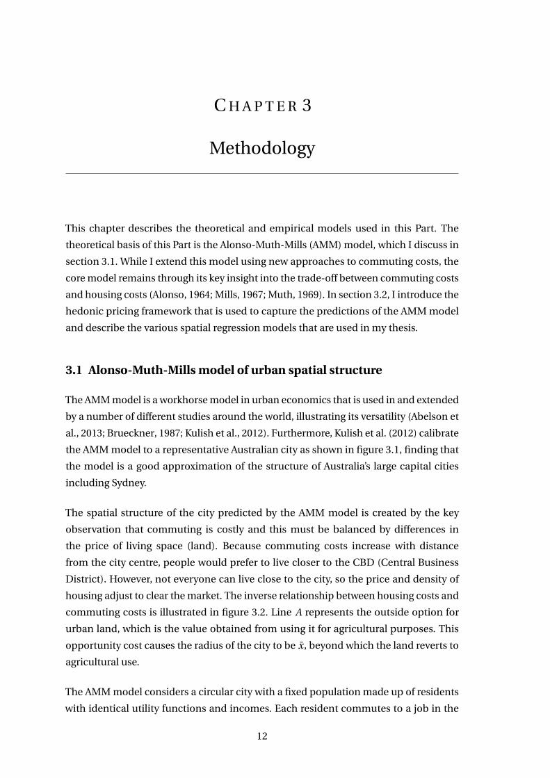
The AMM model is a workhorse model in urban economics that is used in and extended

by a number of different studies around the world, illustrating its versatility (Abelson et

al., 2013; Brueckner, 1987; Kulish et al., 2012). Furthermore, Kulish et al. (2012) calibrate

the AMM model to a representative Australian city as shown in figure 3.1, finding that

the model is a good approximation of the structure of Australia’s large capital cities

including Sydney.

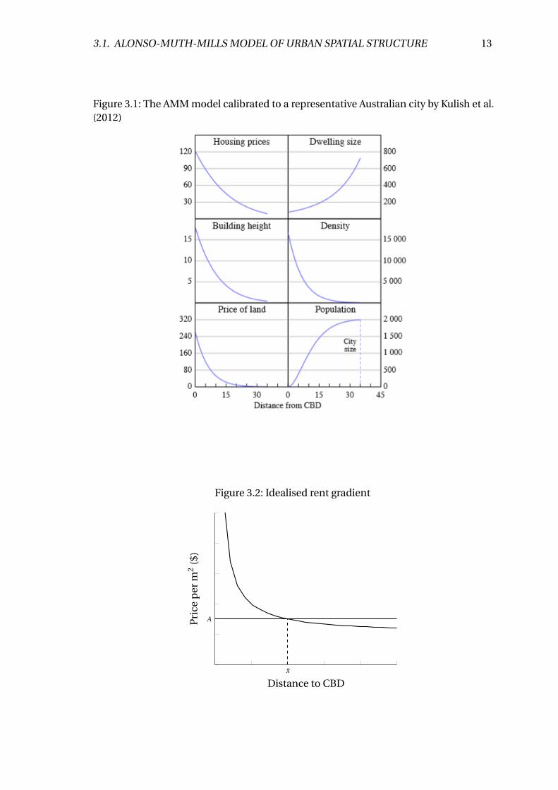
The spatial structure of the city predicted by the AMM model is created by the key

observation that commuting is costly and this must be balanced by differences in

the price of living space (land). Because commuting costs increase with distance

from the city centre, people would prefer to live closer to the CBD (Central Business

District). However, not everyone can live close to the city, so the price and density of

housing adjust to clear the market. The inverse relationship between housing costs and

commuting costs is illustrated in figure 3.2. Line A represents the outside option for

urban land, which is the value obtained from using it for agricultural purposes. This

opportunity cost causes the radius of the city to be x̄, beyond which the land reverts to

agricultural use.

The AMM model considers a circular city with a fixed population made up of residents

with identical utility functions and incomes. Each resident commutes to a job in the

12

3.1. ALONSO-MUTH-MILLS MODEL OF URBAN SPATIAL STRUCTURE 13

Figure 3.1: The AMM model calibrated to a representative Australian city by Kulish et al.(2012)

Figure 3.2: Idealised rent gradient

x̄

A

Distance to CBD

Pri

cep

erm

2($

)

14 CHAPTER 3. METHODOLOGY

CBD located in the centre of the city along a dense radial road network. Each resident

earns identical incomes which are used to purchase a housing good (of which land is an

input) and a composite non-housing good that represents all other consumption. The

original AMM model assumes that the only parameter of interest in relation to housing

is land area, even though real-world dwellings are characterised by a vector of different

attributes. Because land prices increase closer to the CBD, residents will economise

on the use of land by building more dwellings per unit of land, e.g. building smaller

dwellings in apartment towers instead of detached houses. Hence, the city structure is

characterised by dense and small dwellings close to the CBD, and less dense and larger

dwellings further away.

In the model, households maximise their utility function ν(c, q), a function of a

composite non-housing good c and quantity of housing q (in m2). If we replace c using

the budget constraint pq + c = y − t x, where p is the price per unit of housing, y is

income, t is commuting cost per unit of distance, x is distance from the CBD and u is

the constant utility level attained by all households, then the maximisation problem

becomes:

max{q}

ν(y − t x −pq, q) = u (3.1)

The optimality conditions of the model are given by:

νq (y − t x −pq, q)

νc (y − t x −pq, q)= p (3.2)

ν(y − t x −pq, q) = u (3.3)

By solving the maximisation problem, it can be shown that equations 3.2 and 3.3 give

solutions for q and p as functions of y , t , u and x.

Because transport costs vary between locations, the price per unit of land must vary to

allow this condition to hold. Brueckner (1987) shows that:

∂q

∂x= η∂p

∂x> 0 (3.4)

∂p

∂t< 0,

∂q

∂t> 0 (3.5)

3.2. ECONOMETRIC MODELLING APPROACHES 15

where η< 0 is the slope of the demand curve.

Equation 3.4 implies that with increasing distance from the CBD, the quantity of land

consumed is increasing and the unit price of land is decreasing. This result makes

sense, as consumers living far from the CBD need to be compensated for their longer

commutes, otherwise no one would voluntarily live far away from the centre. Similarly,

equation 3.5 implies that increasing commuting costs (t ) decrease the unit price of land

(p) and increase the quantity of land (q) consumed.

Naturally, the AMM model’s simple yet powerful structure results in some limitations.

First, the model assumes that individuals have identical incomes and preferences,

which is unrealistic. However, the basic structure and insights from the model do not

change even in models that allow for heterogeneity. Many analyses using the AMM

model also assume a monocentric city, with no sub-centres or other amenities outside

of the city centre affecting household location choices. However, the model can be

easily extended to take these factors into account (Henderson & Mitra, 1996), which I

do by including three employment centres throughout my analysis. The AMM model

also exists in partial equilibrium, as other markets such as labour or capital markets are

exogenous to the model. Finally, the model is static, providing insights into long-run

equilibrium structure of the city, rather than the dynamics of urban change (Kulish et

al., 2012).

3.2 Econometric modelling approaches

Econometric modelling links the theoretical predictions of the AMM model to real life

data. In this Part, the focus is on estimating the magnitude of the first order conditions of

prices with respect to travel times as shown in equation 3.5. The AMM model predicts

that this parameter should take on a negative value, so I expect that the regression

coefficients on travel time should also be negative. Spatial data require the use of

modelling approaches that take the additional spatial information into account. While

I start with a brief exposition of hedonic pricing models, the focus of this section is on

specifying a variety of spatial regression models that are able to handle the challenges

and opportunities posed by spatial data.

3.2.1 Hedonic pricing models

Hedonic pricing models were conceptualised by Rosen (1974) and consider the ob-

served price of a product to be the sum of the implicit values of a vector of observable

characteristics. The implicit prices of each attribute are estimated through multiple

linear regression analysis (Abelson et al., 2013). The equation that is estimated is of

reduced form, as we only observe the equilibrium of supply and demand, as opposed

16 CHAPTER 3. METHODOLOGY

to estimating the individual supply and demand structural equations (Kuminoff et al.,

2010).

Hedonic pricing is useful for products that are highly differentiated, with an extensive

literature estimating prices for products subject to rapid technological change, such as

computers. Property is a special case where each individual observation has a unique

vector of characteristics, which makes the hedonic method more powerful compared to

other approaches to pricing housing such as repeat-sales methods or regional median

pricing approaches (Hill, 2012).

The ability for hedonic models to incorporate a wide variety of observable character-

istics in a relatively flexible, yet simple, parametric approach makes hedonic models

the model of choice for a large body of literature in urban economics (Hill, 2012). For

housing, observable characteristics can be roughly divided into physical or locational

characteristics. For the models using land valuations data as the dependent variable,

I am able to avoid estimating most physical characteristics of the property as these

factors are supposed to be excluded from the value of land by the valuation process

(NSW Valuer General, 2017a). Locational attributes include the geographic location

of the property relative to amenities such as parks, schools and beaches; proximity to

employment centres; and the characteristics of the surrounding neighbourhood.

Hedonic models are not without their drawbacks. Standard hedonic models assume

that the observations in the regression are independent of one another, which is very

likely to be violated in the case of spatial data such as housing (Du & Mulley, 2012).

The second assumption of hedonic modelling is that the price is obtained through

a perfectly competitive market equilibrium. This is a problematic assumption with

regards to housing, given that each unit of housing has unique characteristics due to its

location.

Finally, misspecifying the hedonic price function will seriously undermine estimation of

economic values through omitted variable bias. Frequently, the source of this problem

for housing models are neighbourhood characteristics that are valued by households,

but not observed by the researcher (Kuminoff et al., 2010). In recent years, more

literature is correcting for this by using spatial hedonic models that reduce the issue

of omitted variable bias by adding spatial fixed effects that absorb the price effect of

spatially clustered omitted variables. Monte Carlo analysis by Kuminoff et al. (2010)

found that including spatial fixed effects substantially reduces the bias from omitted

variables in cross-sectional data.

3.2. ECONOMETRIC MODELLING APPROACHES 17

3.2.2 Spatial models

There exist several classes of models that incorporate the spatial nature of the data

I am using. To motivate the use of these models, I introduce the concept of spatial

dependence and discuss what this means for traditional regression methods. The

following explanation borrows from LeSage and Pace (2008).

To contrast the nature of non-spatial and spatial data, I begin by considering the

properties of the data generating process for conventional cross-sectional non-spatial

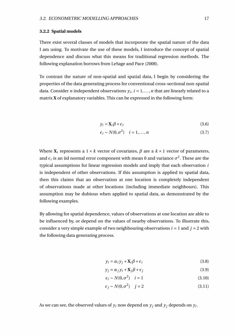
data. Consider n independent observations yi , i = 1, . . . ,n that are linearly related to a

matrix X of explanatory variables. This can be expressed in the following form:

yi = Xiβ+εi (3.6)

εi ∼ N (0,σ2) i = 1, . . . ,n (3.7)

Where Xi represents a 1× k vector of covariates, β are a k × 1 vector of parameters,

and εi is an iid normal error component with mean 0 and variance σ2. These are the

typical assumptions for linear regression models and imply that each observation i

is independent of other observations. If this assumption is applied to spatial data,

then this claims that an observation at one location is completely independent

of observations made at other locations (including immediate neighbours). This

assumption may be dubious when applied to spatial data, as demonstrated by the

following examples.

By allowing for spatial dependence, values of observations at one location are able to

be influenced by, or depend on the values of nearby observations. To illustrate this,

consider a very simple example of two neighbouring observations i = 1 and j = 2 with

the following data generating process.

yi =αi y j +Xiβ+εi (3.8)

y j =α j yi +X jβ+ε j (3.9)

εi ∼ N (0,σ2) i = 1 (3.10)

ε j ∼ N (0,σ2) j = 2 (3.11)

As we can see, the observed values of yi now depend on y j and y j depends on yi .

18 CHAPTER 3. METHODOLOGY

As a concrete example, consider a hedonic pricing model of sales prices of houses as the

dependent variable and a vector of observed physical and location characteristics as

the explanatory variables. Suppose a house sells for a much higher price than predicted

by its characteristics and this coincides with the opening of a new train station nearby.

We would expect that this higher price will signal to nearby homeowners that the value

of their houses may have also increased. Consequentially, they will also increase the

asking price of their own properties. In the absence of a spatially dependent model,

this flow-on effect from nearby properties is not captured. As a result, a model that

incorporates the selling prices of neighbouring properties has improved explanatory

power relative to a model that does not.

Spatial spillover effects create problems with model estimation. These spatial spillover

effects can be considered from two perspectives: as spatial dependence in the explanat-

ory variables or a spatially correlated error term (Abelson et al., 2013). At minimum if the

error term is spatially correlated, ordinary least squares (OLS) estimates are unbiased

but inefficient (similar to serial correlation problems with time-series regression).

However, in the presence of omitted spatially correlated variables, the OLS estimate will

be biased and inefficient (Du & Mulley, 2012). Models of spatial dependence consider

the spatial spillover effects to be an integral part of the model, and hence directly

model for it as one of the explanatory variables. In contrast, a model with a spatially

correlated error term considers the spatial spillovers to be a nuisance term that needs

to be addressed through the disturbance term of the model (LeSage & Pace, 2008). This

motivates the different classes of spatial model which I discuss.

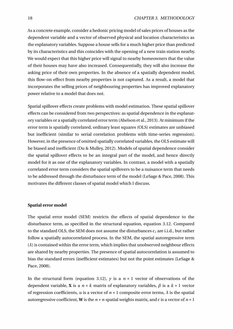
Spatial error model

The spatial error model (SEM) restricts the effects of spatial dependence to the

disturbance term, as specified in the structural equation, equation 3.12. Compared

to the standard OLS, the SEM does not assume the disturbances εi are i.i.d., but rather

follow a spatially autocorrelated process. In the SEM, the spatial autoregressive term

(λ) is contained within the error term, which implies that unobserved neighbour effects

are shared by nearby properties. The presence of spatial autocorrelation is assumed to

bias the standard errors (inefficient estimates) but not the point estimates (LeSage &

Pace, 2008).

In the structural form (equation 3.12), y is a n × 1 vector of observations of the

dependent variable, X is a n × k matrix of explanatory variables, β is a k × 1 vector

of regression coefficients, u is a vector of n ×1 composite error terms, λ is the spatial

autoregressive coefficient, W is the n×n spatial weights matrix, and ε is a vector of n×1

3.2. ECONOMETRIC MODELLING APPROACHES 19

i.i.d. error terms. The reduced form of the structural equation is expressed in equation

3.14.

y = Xβ+u (3.12)

u =λWu +ε (3.13)

y = Xβ+ (In −λW)−1u (3.14)

ε∼ N (0,σ2In) (3.15)

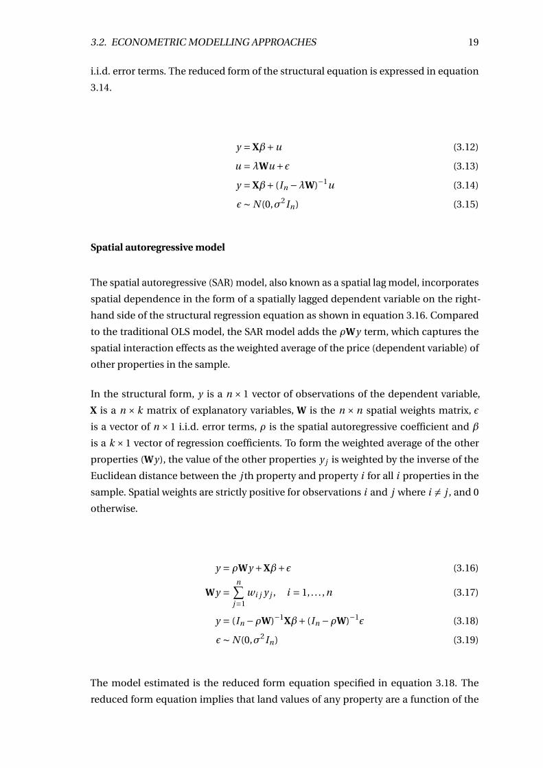
Spatial autoregressive model

The spatial autoregressive (SAR) model, also known as a spatial lag model, incorporates

spatial dependence in the form of a spatially lagged dependent variable on the right-

hand side of the structural regression equation as shown in equation 3.16. Compared

to the traditional OLS model, the SAR model adds the ρWy term, which captures the

spatial interaction effects as the weighted average of the price (dependent variable) of

other properties in the sample.

In the structural form, y is a n × 1 vector of observations of the dependent variable,

X is a n × k matrix of explanatory variables, W is the n ×n spatial weights matrix, ε

is a vector of n × 1 i.i.d. error terms, ρ is the spatial autoregressive coefficient and β

is a k ×1 vector of regression coefficients. To form the weighted average of the other

properties (Wy), the value of the other properties y j is weighted by the inverse of the

Euclidean distance between the j th property and property i for all i properties in the

sample. Spatial weights are strictly positive for observations i and j where i 6= j , and 0

otherwise.

y = ρWy +Xβ+ε (3.16)

Wy =n∑

j=1wi j y j , i = 1, . . . ,n (3.17)

y = (In −ρW)−1Xβ+ (In −ρW)−1ε (3.18)

ε∼ N (0,σ2In) (3.19)

The model estimated is the reduced form equation specified in equation 3.18. The

reduced form equation implies that land values of any property are a function of the

20 CHAPTER 3. METHODOLOGY

property’s own characteristics and the characteristics of neighbouring properties, with

the effect of neighbours diminishing with the spatial weight operator. This model can

be estimated by maximum likelihood (Abelson et al., 2013).

Interpreting spatial autoregressive models is different to interpreting standard linear

regression models. The coefficients on a spatial model are partial derivatives only in the

case of the spatial error model, but this is not true in the case where spatial dependence

is present in the dependent variable or explanatory variables. Simple partial derivative

interpretations fail due to the need to take into account the effect of spatial spillovers

in the model, which require the consideration of direct and indirect effects. The direct

effect of a variable xr on y is the average over all observations of the marginal effects of

xi r on yi : (1/n)∑n

i=1(∂yi /∂xi r ). The indirect effect is defined as∑n

i=1

∑nj=1,i 6= j (∂yi /∂x j r ).

The total effect is simply the sum of the direct and indirect effects (LeSage & Pace,

2008). Golgher and Voss (2015) derive the direct and indirect effects of changes in the

explanatory variables on the observed outcomes.

C H A P T E R 4

Data

This chapter provides a descriptive and preliminary analysis of the data used in the

empirical analysis. The aim of this Part is to estimate the value that households place

on access to employment and amenity. This is done using an estimate of the rent (price)

gradient for Sydney and requires data on property values, a measure of commuting

costs and property attributes unrelated to the cost of commuting.

I measure property values using transaction prices and land valuations. Property sales

prices best reflect the value that the market is willing to pay for property. However,

property price data can complicate estimation as hedonic price modelling needs to be

used to partial out the value of the structure, which is not influenced by the accessibility

of the property. Land valuation data is used as it has the advantage of eliminating the

need to control for the characteristics of residential structures (houses or apartments),

but these valuations reflect the judgement of professional valuers rather than the

market price. I use sales of residential housing in Sydney in 2018 as my property price

dataset and a random sample of July 2018 land values for 40,000 locations obtained from

the NSW Valuer General as my land valuations dataset. These properties are then linked

with travel time data from Google Maps and neighbourhood characteristics information

from the 2016 Census using the Australian National Geocoded Address Dataset (PSMA

Australia, 2018).

I describe the collection of the travel time data in section 4.1. I discuss and provide

visualisations of the sales data and land valuations data in sections 4.2 and 4.3. I

analyse the descriptive statistics for the data in sections 4.5 and 4.6, along with some

maps which illustrate the spatial distribution of travel times in section 4.7. I conduct a

statistical test for spatial dependence in the data in section 4.8.

4.1 Travel time data

Variation in commuting costs are the key driver of differential property prices under

the AMM model. As discussed previously, most of the existing literature has focused

21

22 CHAPTER 4. DATA

on explaining commuting costs using straight-line distances from the CBD. In this

study, I use Google Maps travel time data as a novel measure of variation in commuting

costs. The commuting cost data used in this Part consists of the travel times for a

random sample of 40,000 residential properties with associated land values and 8,073

residential properties that transacted in 2018 within the Greater Sydney GCCSA (Greater

Capital City Statistical Area) during the morning peak (7AM–9AM) to the three largest

employment areas in Sydney (Sydney/North Sydney, Parramatta and Macquarie Park).

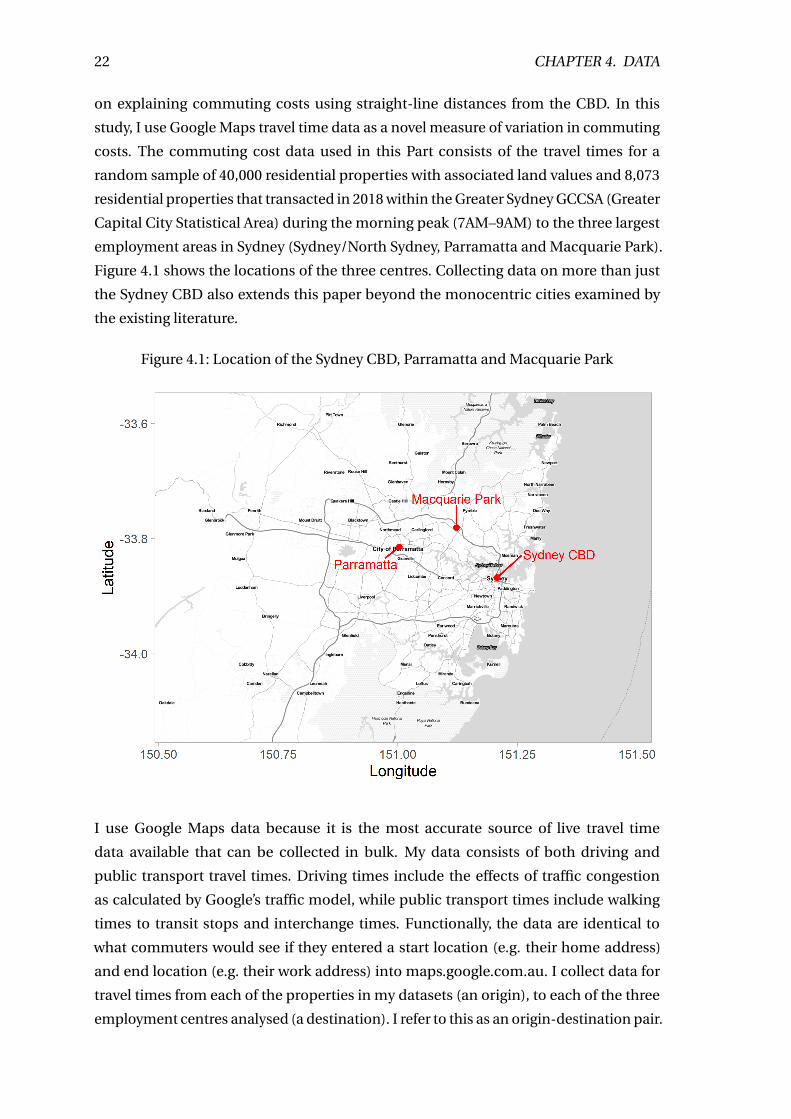
Figure 4.1 shows the locations of the three centres. Collecting data on more than just

the Sydney CBD also extends this paper beyond the monocentric cities examined by

the existing literature.

Figure 4.1: Location of the Sydney CBD, Parramatta and Macquarie Park

I use Google Maps data because it is the most accurate source of live travel time

data available that can be collected in bulk. My data consists of both driving and

public transport travel times. Driving times include the effects of traffic congestion

as calculated by Google’s traffic model, while public transport times include walking

times to transit stops and interchange times. Functionally, the data are identical to

what commuters would see if they entered a start location (e.g. their home address)

and end location (e.g. their work address) into maps.google.com.au. I collect data for

travel times from each of the properties in my datasets (an origin), to each of the three

employment centres analysed (a destination). I refer to this as an origin-destination pair.

4.2. PROPERTY SALES DATA 23

I construct this dataset by coding an R script that calls the Google Maps Distance Matrix

API (Application Programming Interface). This API takes an origin-destination pair and

transit mode and returns the duration and distance travelled. For the land valuations

dataset, I collected travel times between July 2018 and May 2019, and for the sales

dataset, I collected travel times between September 2019 and October 2019. Collecting

data during the morning peak allows me to capture the effects of congestion.

As part of the data collection and cleaning process, some observations were removed

due to errors in the collection of travel time data. Outlier travel time values were

discarded if the drive times exceeded 240 minutes or if the public transport times

exceeded 300 minutes. These outliers were caused by the Google Maps script erro-

neously computing travel times to the incorrect locations. For example, one address

was incorrectly parsed as being from outside NSW and hence produced a completely

incorrect travel time. Occasional server connectivity errors also resulted in missing data

points. This process only affected a small share of the sample; in the land values data

the number of observations was reduced from 40,000 to 38,514.

Some limitations of the data include the lack of information on traffic flows/volumes for

specific routes as the API is only able to provide travel times between origin-destination

pairs. Public transport travel time data is also not disaggregated into walking, waiting

and actual travelling time in the data provided by the API. Google also limits the number

of API calls that can be made for free to 40,000 each month, which forced the collection

of data over a long period of time, meaning there is potentially some variation in the

comparability of data collected in different months. However, I was careful not to collect

data during periods of known reduced commuter flow, such as public holidays and the

Christmas/New Years and Easter holiday periods.

4.2 Property sales data

As a measure of property values, I source property sales data from Australian Property

Monitors, a commercial provider of property transactions data. The data cover all

recorded residential property sales within Greater Sydney for 2018. The property

sales data includes information on the sale price, sale date, address, geographical

coordinates, land area, count of bedrooms, count of bathrooms, and count of parking

spaces among other property characteristics. I compare estimates using this dataset to

my estimations using land valuations data, improving the robustness of my analysis.

Property sales data are also preferred by the literature as they reflect the actual

valuations placed by the market on the value of property, rather than the value that

professional valuers believe an unimproved land lot is worth. However, unlike land

24 CHAPTER 4. DATA

values data, the sales data may not reflect the overall housing stock as it only contains

properties that were sold in 2018.

The data cleaning process involved filtering out duplicates, sales outside the Sydney

GCCSA and properties that were missing key characteristics data (transaction price,

transaction date, bedrooms, bathrooms and area). The original dataset contained

around 163,000 entries, but most of these were duplicates as data was recorded at

each stage of the sales process until settlement. After this initial cleaning, I took a

random sample of 9,000 properties from the whole dataset in order to fit within financial

constraints of scraping Google Maps travel time data. After geocoding properties

to their corresponding ASGS (Australian Statistical Geography Standard) Statistical

Area 1 (SA1), I merged neighbourhood demographics data from the 2016 ABS Census

with each property sale. I calculated the Euclidean distance from each property to

the Sydney CBD, Parramatta, Macquarie Park and the nearest coastline using the

geosphere GIS package in R (Hijmans, 2019). I removed remaining duplicates and

outliers based on sales prices that were higher than $10 million or below $100,000

as they are unrepresentative of the property market in Sydney, which removed less

than 200 properties from the data. Properties with extremely large or small prices per

square metre were also omitted as these indicate that the property area was incorrectly

recorded. As previously described, properties with erroneous travel time measurements

were also omitted. Together, this process reduced the dataset from the original 163,000

entries to 8,073 sales.

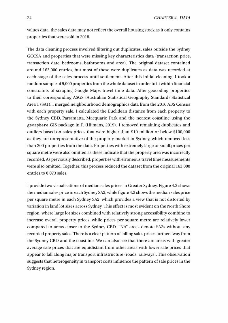
I provide two visualisations of median sales prices in Greater Sydney. Figure 4.2 shows

the median sales price in each Sydney SA2, while figure 4.3 shows the median sales price

per square metre in each Sydney SA2, which provides a view that is not distorted by

variation in land lot sizes across Sydney. This effect is most evident on the North Shore

region, where large lot sizes combined with relatively strong accessibility combine to

increase overall property prices, while prices per square metre are relatively lower

compared to areas closer to the Sydney CBD. “NA” areas denote SA2s without any

recorded property sales. There is a clear pattern of falling sales prices further away from

the Sydney CBD and the coastline. We can also see that there are areas with greater

average sale prices that are equidistant from other areas with lower sale prices that

appear to fall along major transport infrastructure (roads, railways). This observation

suggests that heterogeneity in transport costs influence the pattern of sale prices in the

Sydney region.

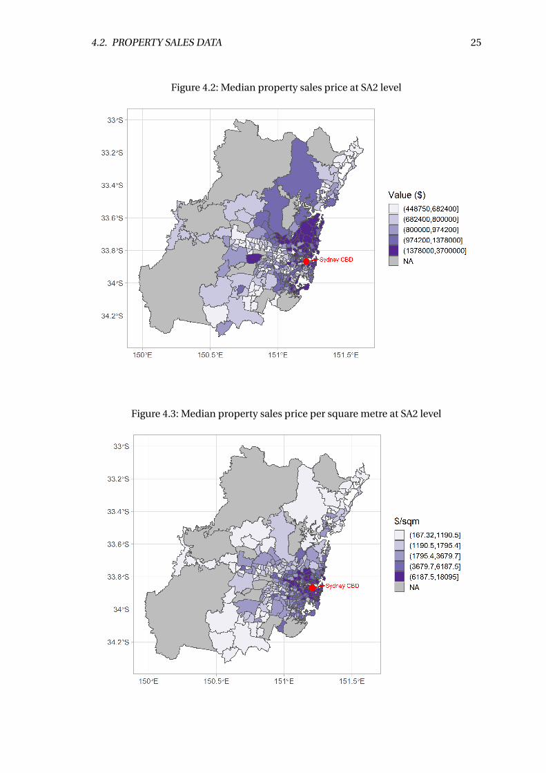
4.2. PROPERTY SALES DATA 25

Figure 4.2: Median property sales price at SA2 level

Figure 4.3: Median property sales price per square metre at SA2 level

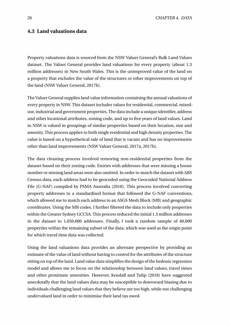
26 CHAPTER 4. DATA

4.3 Land valuations data

Property valuations data is sourced from the NSW Valuer General’s Bulk Land Values

dataset. The Valuer General provides land valuations for every property (about 1.3

million addresses) in New South Wales. This is the unimproved value of the land on

a property that excludes the value of the structures or other improvements on top of

the land (NSW Valuer General, 2017b).

The Valuer General supplies land value information containing the annual valuations of

every property in NSW. This dataset includes values for residential, commercial, mixed-

use, industrial and government properties. The data include a unique identifier, address

and other locational attributes, zoning code, and up to five years of land values. Land

in NSW is valued in groupings of similar properties based on their location, size and

amenity. This process applies to both single residential and high density properties. The

value is based on a hypothetical sale of land that is vacant and has no improvements

other than land improvements (NSW Valuer General, 2017a, 2017b).

The data cleaning process involved removing non-residential properties from the

dataset based on their zoning code. Entries with addresses that were missing a house

number or missing land areas were also omitted. In order to match the dataset with ABS

Census data, each address had to be geocoded using the Geocoded National Address

File (G-NAF) compiled by PSMA Australia (2018). This process involved converting

property addresses to a standardised format that followed the G-NAF conventions,

which allowed me to match each address to an ASGS Mesh Block (MB) and geographic

coordinates. Using the MB codes, I further filtered the data to include only properties

within the Greater Sydney GCCSA. This process reduced the initial 1.3 million addresses

in the dataset to 1,050,000 addresses. Finally, I took a random sample of 40,000

properties within the remaining subset of the data, which was used as the origin point

for which travel time data was collected.

Using the land valuations data provides an alternate perspective by providing an

estimate of the value of land without having to control for the attributes of the structure

sitting on top of the land. Land value data simplifies the design of the hedonic regression

model and allows me to focus on the relationship between land values, travel times

and other proximate amenities. However, Kendall and Tulip (2018) have suggested

anecdotally that the land values data may be susceptible to downward biasing due to

individuals challenging land values that they believe are too high, while not challenging

undervalued land in order to minimise their land tax owed.

4.3. LAND VALUATIONS DATA 27

I provide two visualisations of the median land values in Greater Sydney. Figure 4.4

shows the median land value in each Sydney SA2, while figure 4.5 shows the median

value of land per square metre in each Sydney SA2, which provides a view that is not

distorted by variation in land lot sizes across Sydney.

Like with the sales price data, land values exceed land values per square metre mostly

in the North Shore region. Similarly, there is also a clear pattern of falling land values

further away from the Sydney CBD and the coastline. Like the sales data maps, we can

see that there are areas with greater average land values that are equidistant from other

areas with lower land values that appear to fall along major transport infrastructure

routes. This observation indicates that, like the sales data, heterogeneity in transport

costs influence the pattern of land values in the Sydney region.

Figure 4.4: Median land values at SA2 level

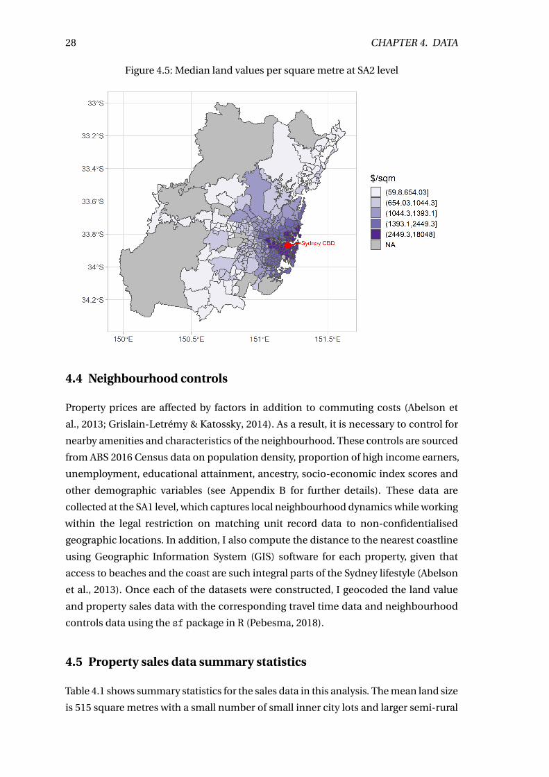
28 CHAPTER 4. DATA

Figure 4.5: Median land values per square metre at SA2 level

4.4 Neighbourhood controls

Property prices are affected by factors in addition to commuting costs (Abelson et

al., 2013; Grislain-Letrémy & Katossky, 2014). As a result, it is necessary to control for

nearby amenities and characteristics of the neighbourhood. These controls are sourced

from ABS 2016 Census data on population density, proportion of high income earners,

unemployment, educational attainment, ancestry, socio-economic index scores and

other demographic variables (see Appendix B for further details). These data are

collected at the SA1 level, which captures local neighbourhood dynamics while working

within the legal restriction on matching unit record data to non-confidentialised

geographic locations. In addition, I also compute the distance to the nearest coastline

using Geographic Information System (GIS) software for each property, given that

access to beaches and the coast are such integral parts of the Sydney lifestyle (Abelson

et al., 2013). Once each of the datasets were constructed, I geocoded the land value

and property sales data with the corresponding travel time data and neighbourhood

controls data using the sf package in R (Pebesma, 2018).

4.5 Property sales data summary statistics

Table 4.1 shows summary statistics for the sales data in this analysis. The mean land size

is 515 square metres with a small number of small inner city lots and larger semi-rural

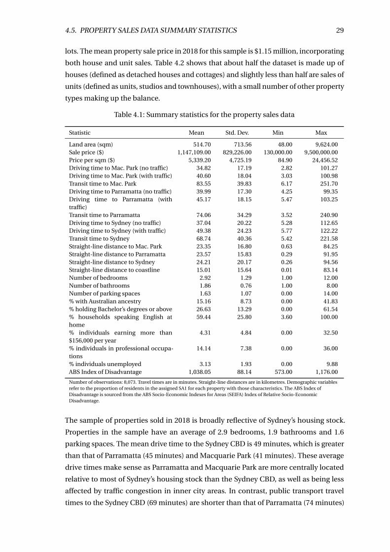
4.5. PROPERTY SALES DATA SUMMARY STATISTICS 29

lots. The mean property sale price in 2018 for this sample is $1.15 million, incorporating

both house and unit sales. Table 4.2 shows that about half the dataset is made up of

houses (defined as detached houses and cottages) and slightly less than half are sales of

units (defined as units, studios and townhouses), with a small number of other property

types making up the balance.

Table 4.1: Summary statistics for the property sales data

Statistic Mean Std. Dev. Min Max

Land area (sqm) 514.70 713.56 48.00 9,624.00Sale price ($) 1,147,109.00 829,226.00 130,000.00 9,500,000.00Price per sqm ($) 5,339.20 4,725.19 84.90 24,456.52Driving time to Mac. Park (no traffic) 34.82 17.19 2.82 101.27Driving time to Mac. Park (with traffic) 40.60 18.04 3.03 100.98Transit time to Mac. Park 83.55 39.83 6.17 251.70Driving time to Parramatta (no traffic) 39.99 17.30 4.25 99.35Driving time to Parramatta (withtraffic)

45.17 18.15 5.47 103.25

Transit time to Parramatta 74.06 34.29 3.52 240.90Driving time to Sydney (no traffic) 37.04 20.22 5.28 112.65Driving time to Sydney (with traffic) 49.38 24.23 5.77 122.22Transit time to Sydney 68.74 40.36 5.42 221.58Straight-line distance to Mac. Park 23.35 16.80 0.63 84.25Straight-line distance to Parramatta 23.57 15.83 0.29 91.95Straight-line distance to Sydney 24.21 20.17 0.26 94.56Straight-line distance to coastline 15.01 15.64 0.01 83.14Number of bedrooms 2.92 1.29 1.00 12.00Number of bathrooms 1.86 0.76 1.00 8.00Number of parking spaces 1.63 1.07 0.00 14.00% with Australian ancestry 15.16 8.73 0.00 41.83% holding Bachelor’s degrees or above 26.63 13.29 0.00 61.54% households speaking English athome

59.44 25.80 3.60 100.00

% individuals earning more than$156,000 per year

4.31 4.84 0.00 32.50

% individuals in professional occupa-tions

14.14 7.38 0.00 36.00

% individuals unemployed 3.13 1.93 0.00 9.88ABS Index of Disadvantage 1,038.05 88.14 573.00 1,176.00

Number of observations: 8,073. Travel times are in minutes. Straight-line distances are in kilometres. Demographic variablesrefer to the proportion of residents in the assigned SA1 for each property with those characteristics. The ABS Index ofDisadvantage is sourced from the ABS Socio-Economic Indexes for Areas (SEIFA) Index of Relative Socio-EconomicDisadvantage.

The sample of properties sold in 2018 is broadly reflective of Sydney’s housing stock.

Properties in the sample have an average of 2.9 bedrooms, 1.9 bathrooms and 1.6

parking spaces. The mean drive time to the Sydney CBD is 49 minutes, which is greater

than that of Parramatta (45 minutes) and Macquarie Park (41 minutes). These average

drive times make sense as Parramatta and Macquarie Park are more centrally located

relative to most of Sydney’s housing stock than the Sydney CBD, as well as being less

affected by traffic congestion in inner city areas. In contrast, public transport travel

times to the Sydney CBD (69 minutes) are shorter than that of Parramatta (74 minutes)

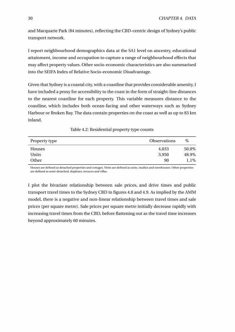
30 CHAPTER 4. DATA

and Macquarie Park (84 minutes), reflecting the CBD-centric design of Sydney’s public

transport network.

I report neighbourhood demographics data at the SA1 level on ancestry, educational

attainment, income and occupation to capture a range of neighbourhood effects that

may affect property values. Other socio-economic characteristics are also summarised

into the SEIFA Index of Relative Socio-economic Disadvantage.

Given that Sydney is a coastal city, with a coastline that provides considerable amenity, I

have included a proxy for accessibility to the coast in the form of straight-line distances

to the nearest coastline for each property. This variable measures distance to the

coastline, which includes both ocean-facing and other waterways such as Sydney

Harbour or Broken Bay. The data contain properties on the coast as well as up to 83 km

inland.

Table 4.2: Residential property type counts

Property type Observations %

Houses 4,033 50.0%Units 3,950 48.9%Other 90 1.1%

Houses are defined as detached properties and cottages. Units are defined as units, studios and townhouses. Other propertiesare defined as semi-detached, duplexes, terraces and villas.

I plot the bivariate relationship between sale prices, and drive times and public

transport travel times to the Sydney CBD in figures 4.8 and 4.9. As implied by the AMM

model, there is a negative and non-linear relationship between travel times and sale

prices (per square metre). Sale prices per square metre initially decrease rapidly with

increasing travel times from the CBD, before flattening out as the travel time increases

beyond approximately 60 minutes.

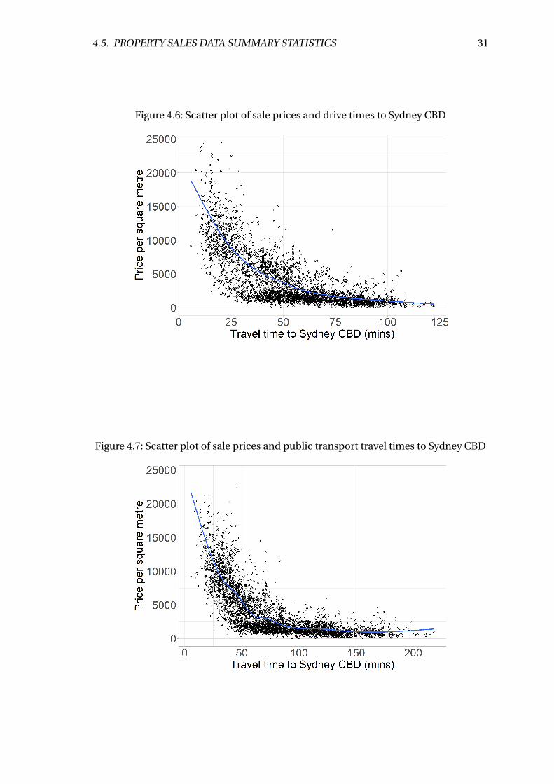
4.5. PROPERTY SALES DATA SUMMARY STATISTICS 31

Figure 4.6: Scatter plot of sale prices and drive times to Sydney CBD

Figure 4.7: Scatter plot of sale prices and public transport travel times to Sydney CBD

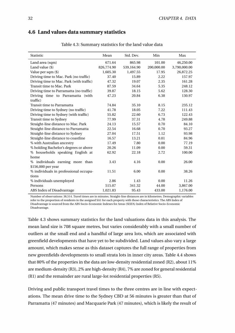
32 CHAPTER 4. DATA

4.6 Land values data summary statistics

Table 4.3: Summary statistics for the land value data

Statistic Mean Std. Dev. Min Max

Land area (sqm) 671.64 865.98 101.00 46,250.00Land value ($) 826,774.90 539,164.90 200,000.00 3,790,000.00Value per sqm ($) 1,605.30 1,497.55 17.95 26,872.25Driving time to Mac. Park (no traffic) 37.40 15.89 2.22 157.97Driving time to Mac. Park (with traffic) 47.32 19.07 2.35 161.28Transit time to Mac. Park 87.59 34.64 5.35 248.12Driving time to Parramatta (no traffic) 39.87 18.15 5.62 128.30Driving time to Parramatta (withtraffic)

47.23 20.84 6.38 130.97

Transit time to Parramatta 74.84 35.10 8.15 235.12Driving time to Sydney (no traffic) 41.78 18.05 7.22 111.43Driving time to Sydney (with traffic) 55.82 22.60 6.73 122.43Transit time to Sydney 77.99 37.31 4.78 249.88Straight-line distance to Mac. Park 24.13 15.57 0.70 84.10Straight-line distance to Parramatta 22.54 16.68 0.70 93.27Straight-line distance to Sydney 27.04 17.51 1.12 93.98Straight-line distance to coastline 16.57 13.21 0.01 84.96% with Australian ancestry 17.49 7.80 0.00 77.19% holding Bachelor’s degrees or above 20.26 11.09 0.00 59.31% households speaking English athome

62.92 22.18 2.72 100.00

% individuals earning more than$156,000 per year

3.43 4.16 0.00 26.00

% individuals in professional occupa-tions

11.51 6.00 0.00 38.26

% individuals unemployed 2.86 1.43 0.00 11.26Persons 515.07 341.32 44.00 3,867.00ABS Index of Disadvantage 1,021.83 95.43 433.00 1,176.00

Number of observations: 38,514. Travel times are in minutes. Straight-line distances are in kilometres. Demographic variablesrefer to the proportion of residents in the assigned SA1 for each property with those characteristics. The ABS Index ofDisadvantage is sourced from the ABS Socio-Economic Indexes for Areas (SEIFA) Index of Relative Socio-EconomicDisadvantage.

Table 4.3 shows summary statistics for the land valuations data in this analysis. The

mean land size is 708 square metres, but varies considerably with a small number of

outliers at the small end and a handful of large area lots, which are associated with

greenfield developments that have yet to be subdivided. Land values also vary a large

amount, which makes sense as this dataset captures the full range of properties from

new greenfields developments to small strata lots in inner city areas. Table 4.4 shows

that 80% of the properties in the data are low-density residential zoned (R2), about 11%

are medium-density (R3), 2% are high-density (R4), 7% are zoned for general residential

(R1) and the remainder are rural large-lot residential properties (R5).

Driving and public transport travel times to the three centres are in line with expect-

ations. The mean drive time to the Sydney CBD at 56 minutes is greater than that of

Parramatta (47 minutes) and Macquarie Park (47 minutes), which is likely the result of

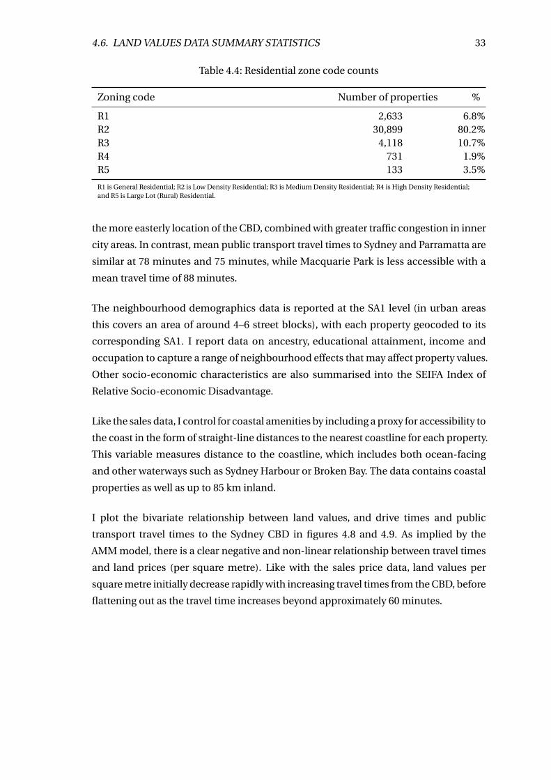
4.6. LAND VALUES DATA SUMMARY STATISTICS 33

Table 4.4: Residential zone code counts

Zoning code Number of properties %

R1 2,633 6.8%R2 30,899 80.2%R3 4,118 10.7%R4 731 1.9%R5 133 3.5%

R1 is General Residential; R2 is Low Density Residential; R3 is Medium Density Residential; R4 is High Density Residential;and R5 is Large Lot (Rural) Residential.

the more easterly location of the CBD, combined with greater traffic congestion in inner

city areas. In contrast, mean public transport travel times to Sydney and Parramatta are

similar at 78 minutes and 75 minutes, while Macquarie Park is less accessible with a

mean travel time of 88 minutes.

The neighbourhood demographics data is reported at the SA1 level (in urban areas

this covers an area of around 4–6 street blocks), with each property geocoded to its

corresponding SA1. I report data on ancestry, educational attainment, income and

occupation to capture a range of neighbourhood effects that may affect property values.

Other socio-economic characteristics are also summarised into the SEIFA Index of

Relative Socio-economic Disadvantage.

Like the sales data, I control for coastal amenities by including a proxy for accessibility to

the coast in the form of straight-line distances to the nearest coastline for each property.

This variable measures distance to the coastline, which includes both ocean-facing

and other waterways such as Sydney Harbour or Broken Bay. The data contains coastal

properties as well as up to 85 km inland.

I plot the bivariate relationship between land values, and drive times and public

transport travel times to the Sydney CBD in figures 4.8 and 4.9. As implied by the

AMM model, there is a clear negative and non-linear relationship between travel times

and land prices (per square metre). Like with the sales price data, land values per

square metre initially decrease rapidly with increasing travel times from the CBD, before

flattening out as the travel time increases beyond approximately 60 minutes.

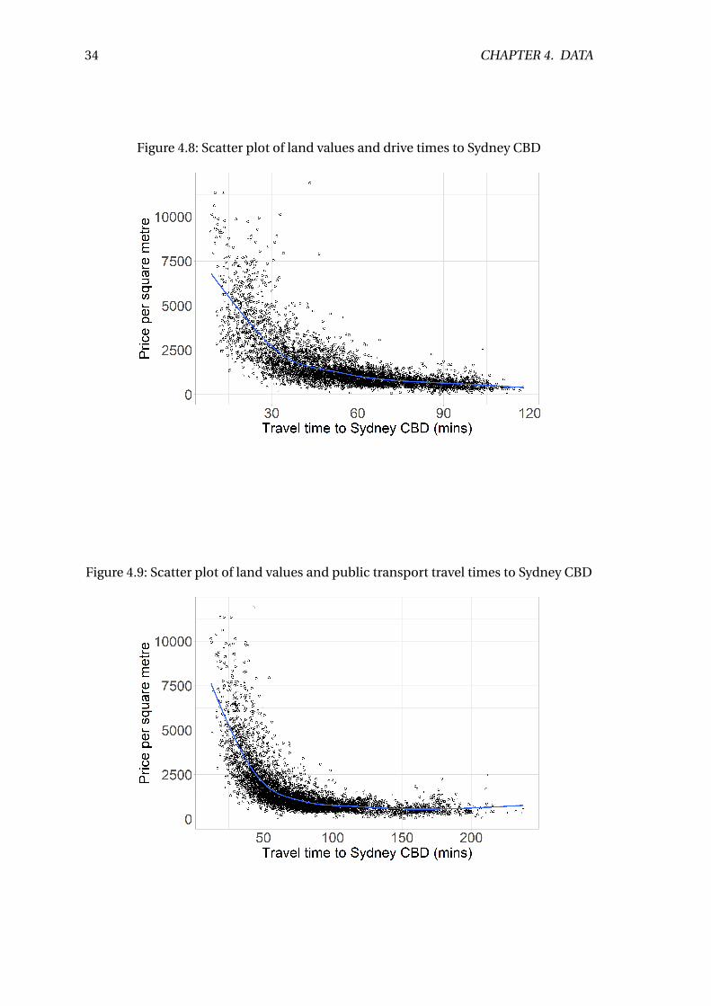
34 CHAPTER 4. DATA

Figure 4.8: Scatter plot of land values and drive times to Sydney CBD

Figure 4.9: Scatter plot of land values and public transport travel times to Sydney CBD

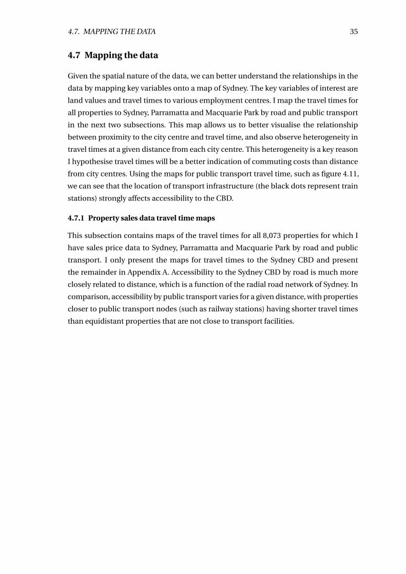
4.7. MAPPING THE DATA 35

4.7 Mapping the data

Given the spatial nature of the data, we can better understand the relationships in the

data by mapping key variables onto a map of Sydney. The key variables of interest are

land values and travel times to various employment centres. I map the travel times for

all properties to Sydney, Parramatta and Macquarie Park by road and public transport

in the next two subsections. This map allows us to better visualise the relationship

between proximity to the city centre and travel time, and also observe heterogeneity in

travel times at a given distance from each city centre. This heterogeneity is a key reason

I hypothesise travel times will be a better indication of commuting costs than distance

from city centres. Using the maps for public transport travel time, such as figure 4.11,

we can see that the location of transport infrastructure (the black dots represent train

stations) strongly affects accessibility to the CBD.

4.7.1 Property sales data travel time maps

This subsection contains maps of the travel times for all 8,073 properties for which I

have sales price data to Sydney, Parramatta and Macquarie Park by road and public

transport. I only present the maps for travel times to the Sydney CBD and present

the remainder in Appendix A. Accessibility to the Sydney CBD by road is much more

closely related to distance, which is a function of the radial road network of Sydney. In

comparison, accessibility by public transport varies for a given distance, with properties

closer to public transport nodes (such as railway stations) having shorter travel times

than equidistant properties that are not close to transport facilities.

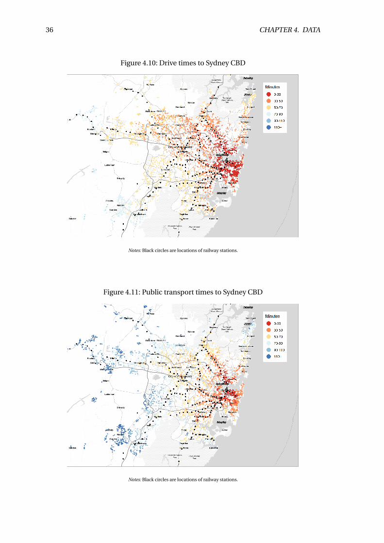
36 CHAPTER 4. DATA

Figure 4.10: Drive times to Sydney CBD

Notes: Black circles are locations of railway stations.

Figure 4.11: Public transport times to Sydney CBD

Notes: Black circles are locations of railway stations.

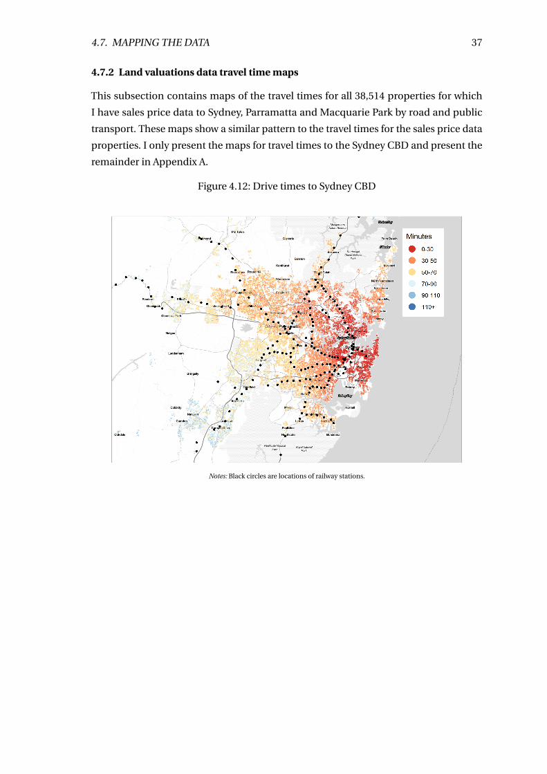
4.7. MAPPING THE DATA 37

4.7.2 Land valuations data travel time maps

This subsection contains maps of the travel times for all 38,514 properties for which

I have sales price data to Sydney, Parramatta and Macquarie Park by road and public

transport. These maps show a similar pattern to the travel times for the sales price data

properties. I only present the maps for travel times to the Sydney CBD and present the

remainder in Appendix A.

Figure 4.12: Drive times to Sydney CBD

Notes: Black circles are locations of railway stations.

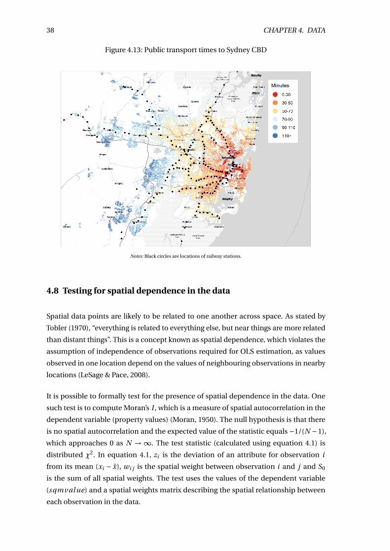
38 CHAPTER 4. DATA

Figure 4.13: Public transport times to Sydney CBD

Notes: Black circles are locations of railway stations.

4.8 Testing for spatial dependence in the data

Spatial data points are likely to be related to one another across space. As stated by

Tobler (1970), “everything is related to everything else, but near things are more related

than distant things”. This is a concept known as spatial dependence, which violates the

assumption of independence of observations required for OLS estimation, as values

observed in one location depend on the values of neighbouring observations in nearby

locations (LeSage & Pace, 2008).

It is possible to formally test for the presence of spatial dependence in the data. One

such test is to compute Moran’s I , which is a measure of spatial autocorrelation in the

dependent variable (property values) (Moran, 1950). The null hypothesis is that there

is no spatial autocorrelation and the expected value of the statistic equals −1/(N −1),

which approaches 0 as N → ∞. The test statistic (calculated using equation 4.1) is

distributed χ2. In equation 4.1, zi is the deviation of an attribute for observation i

from its mean (xi − x̄), wi j is the spatial weight between observation i and j and S0

is the sum of all spatial weights. The test uses the values of the dependent variable

(sqmval ue) and a spatial weights matrix describing the spatial relationship between

each observation in the data.

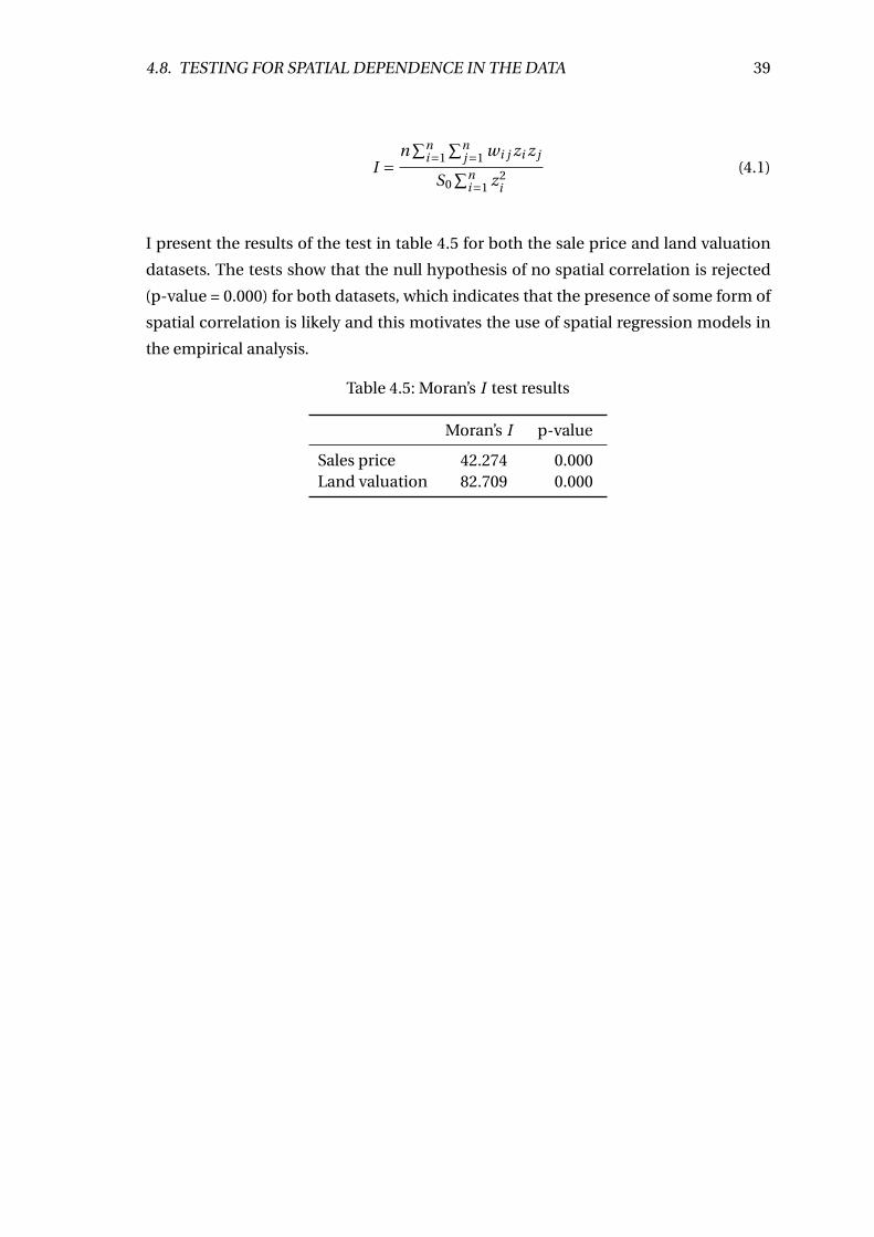
4.8. TESTING FOR SPATIAL DEPENDENCE IN THE DATA 39

I =n

∑ni=1

∑nj=1 wi j zi z j

S0∑n

i=1 z2i

(4.1)

I present the results of the test in table 4.5 for both the sale price and land valuation

datasets. The tests show that the null hypothesis of no spatial correlation is rejected

(p-value = 0.000) for both datasets, which indicates that the presence of some form of

spatial correlation is likely and this motivates the use of spatial regression models in

the empirical analysis.

Table 4.5: Moran’s I test results

Moran’s I p-value

Sales price 42.274 0.000Land valuation 82.709 0.000

C H A P T E R 5

Results and discussion

In this chapter, I present estimates of the value of accessibility to employment in Sydney

using a variety of model specifications. Starting with simple monocentric models of

Sydney, I examine the explanatory and predictive power of traditional distance models,

comparing them with travel time models and analyse the estimates of willingness to

pay for increased accessibility to employment centres. I then examine how willingness

to pay changes when the models are extended to include sub-centres. To account

for the effects of spatial correlation across observations, I estimate these results using

spatial regression methods in addition to linear regressions using OLS. The preferred

functional form for the dependent variable is the natural logarithm as it addresses

outliers in the right tail of the data, improves the normality of the residuals and is

the preferred functional form in the literature. I then estimate alternative models that

explicitly model for the effects of congestion on travel times to examine the premium

that commuters place on avoiding congested roads. To investigate the predictive power

of travel time models, I examine out-of-sample prediction performance of the model

using spatial cross-validation techniques. These models are estimated using both the

land valuations and property sales datasets, with the dependent variable in the model

being land values and transaction prices. Finally, I discuss the limitations and areas that

can be improved in future research. For brevity, I have excluded the coefficient estimates

for the controls from the regression tables, the full regression tables are available in

Appendix F and G.

Overall, the results support my new travel time data methodology. The results show

that additional accessibility measures to sub-centres in Sydney are both statistically

significant and improve the explanatory power of the hedonic models. The coefficients

on accessibility to Sydney are negative and show a diminishing non-linear effect with

decreased proximity, which concords with the predictions of the theoretical AMM

model. Access measures to Parramatta also generally behave in line with expectations.

I find that the travel time models materially improve the power of the model to explain

variation in property sales prices compared to distance-based models when measured

in terms of the Akaike information criterion (AIC) (Akaike, 1974; Lee & Ghosh, 2009) as

40

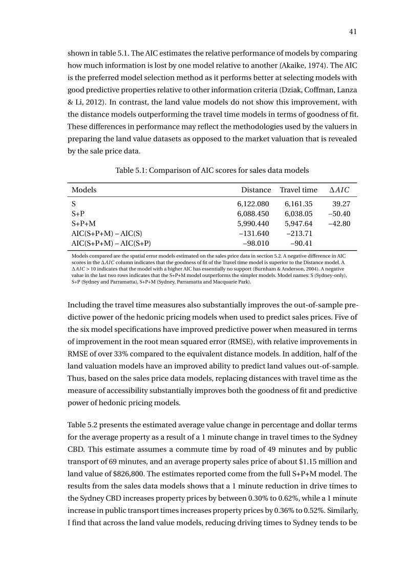
41

shown in table 5.1. The AIC estimates the relative performance of models by comparing

how much information is lost by one model relative to another (Akaike, 1974). The AIC

is the preferred model selection method as it performs better at selecting models with

good predictive properties relative to other information criteria (Dziak, Coffman, Lanza

& Li, 2012). In contrast, the land value models do not show this improvement, with

the distance models outperforming the travel time models in terms of goodness of fit.

These differences in performance may reflect the methodologies used by the valuers in

preparing the land value datasets as opposed to the market valuation that is revealed

by the sale price data.

Table 5.1: Comparison of AIC scores for sales data models

Models Distance Travel time ∆AIC

S 6,122.080 6,161.35 39.27S+P 6,088.450 6,038.05 −50.40S+P+M 5,990.440 5,947.64 −42.80AIC(S+P+M) – AIC(S) −131.640 −213.71AIC(S+P+M) – AIC(S+P) −98.010 −90.41

Models compared are the spatial error models estimated on the sales price data in section 5.2. A negative difference in AICscores in the ∆AIC column indicates that the goodness of fit of the Travel time model is superior to the Distance model. A∆AIC > 10 indicates that the model with a higher AIC has essentially no support (Burnham & Anderson, 2004). A negativevalue in the last two rows indicates that the S+P+M model outperforms the simpler models. Model names: S (Sydney-only),S+P (Sydney and Parramatta), S+P+M (Sydney, Parramatta and Macquarie Park).

Including the travel time measures also substantially improves the out-of-sample pre-

dictive power of the hedonic pricing models when used to predict sales prices. Five of

the six model specifications have improved predictive power when measured in terms

of improvement in the root mean squared error (RMSE), with relative improvements in

RMSE of over 33% compared to the equivalent distance models. In addition, half of the

land valuation models have an improved ability to predict land values out-of-sample.

Thus, based on the sales price data models, replacing distances with travel time as the

measure of accessibility substantially improves both the goodness of fit and predictive

power of hedonic pricing models.

Table 5.2 presents the estimated average value change in percentage and dollar terms

for the average property as a result of a 1 minute change in travel times to the Sydney

CBD. This estimate assumes a commute time by road of 49 minutes and by public

transport of 69 minutes, and an average property sales price of about $1.15 million and

land value of $826,800. The estimates reported come from the full S+P+M model. The

results from the sales data models shows that a 1 minute reduction in drive times to

the Sydney CBD increases property prices by between 0.30% to 0.62%, while a 1 minute

increase in public transport times increases property prices by 0.36% to 0.52%. Similarly,

I find that across the land value models, reducing driving times to Sydney tends to be

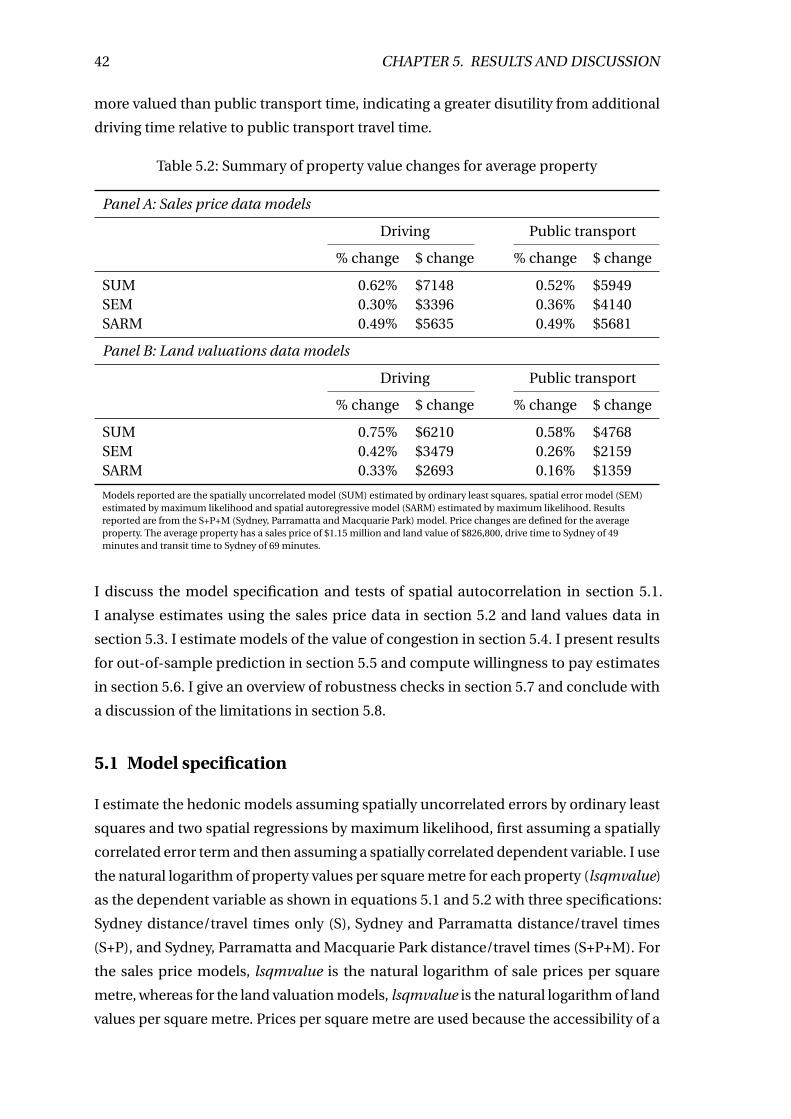
42 CHAPTER 5. RESULTS AND DISCUSSION

more valued than public transport time, indicating a greater disutility from additional

driving time relative to public transport travel time.

Table 5.2: Summary of property value changes for average property

Panel A: Sales price data models

Driving Public transport

% change $ change % change $ change

SUM 0.62% $7148 0.52% $5949SEM 0.30% $3396 0.36% $4140SARM 0.49% $5635 0.49% $5681

Panel B: Land valuations data models

Driving Public transport

% change $ change % change $ change

SUM 0.75% $6210 0.58% $4768SEM 0.42% $3479 0.26% $2159SARM 0.33% $2693 0.16% $1359

Models reported are the spatially uncorrelated model (SUM) estimated by ordinary least squares, spatial error model (SEM)estimated by maximum likelihood and spatial autoregressive model (SARM) estimated by maximum likelihood. Resultsreported are from the S+P+M (Sydney, Parramatta and Macquarie Park) model. Price changes are defined for the averageproperty. The average property has a sales price of $1.15 million and land value of $826,800, drive time to Sydney of 49minutes and transit time to Sydney of 69 minutes.

I discuss the model specification and tests of spatial autocorrelation in section 5.1.

I analyse estimates using the sales price data in section 5.2 and land values data in

section 5.3. I estimate models of the value of congestion in section 5.4. I present results

for out-of-sample prediction in section 5.5 and compute willingness to pay estimates

in section 5.6. I give an overview of robustness checks in section 5.7 and conclude with

a discussion of the limitations in section 5.8.

5.1 Model specification

I estimate the hedonic models assuming spatially uncorrelated errors by ordinary least

squares and two spatial regressions by maximum likelihood, first assuming a spatially

correlated error term and then assuming a spatially correlated dependent variable. I use

the natural logarithm of property values per square metre for each property (lsqmvalue)

as the dependent variable as shown in equations 5.1 and 5.2 with three specifications:

Sydney distance/travel times only (S), Sydney and Parramatta distance/travel times

(S+P), and Sydney, Parramatta and Macquarie Park distance/travel times (S+P+M). For

the sales price models, lsqmvalue is the natural logarithm of sale prices per square

metre, whereas for the land valuation models, lsqmvalue is the natural logarithm of land

values per square metre. Prices per square metre are used because the accessibility of a

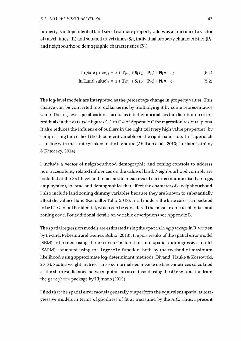
5.1. MODEL SPECIFICATION 43

property is independent of land size. I estimate property values as a function of a vector

of travel times (Ti) and squared travel times (Si), individual property characteristics (Pi)

and neighbourhood demographic characteristics (Ni).

ln(Sale price)i =α+Tiτ1 +Siτ2 +Piφ+Niη+εi (5.1)

ln(Land value)i =α+Tiτ1 +Siτ2 +Piφ+Niη+εi (5.2)

The log-level models are interpreted as the percentage change in property values. This

change can be converted into dollar terms by multiplying it by some representative

value. The log-level specification is useful as it better normalises the distribution of the

residuals in the data (see figures C.1 to C.4 of Appendix C for regression residual plots).

It also reduces the influence of outliers in the right tail (very high value properties) by

compressing the scale of the dependent variable on the right-hand side. This approach

is in line with the strategy taken in the literature (Abelson et al., 2013; Grislain-Letrémy

& Katossky, 2014).

I include a vector of neighbourhood demographic and zoning controls to address

non-accessibility related influences on the value of land. Neighbourhood controls are

included at the SA1 level and incorporate measures of socio-economic disadvantage,

employment, income and demographics that affect the character of a neighbourhood.

I also include land zoning dummy variables because they are known to substantially

affect the value of land (Kendall & Tulip, 2018). In all models, the base case is considered

to be R1 General Residential, which can be considered the most flexible residential land

zoning code. For additional details on variable descriptions see Appendix B.

The spatial regression models are estimated using the spatialreg package in R, written

by Bivand, Pebesma and Gomez-Rubio (2013). I report results of the spatial error model

(SEM) estimated using the errorsarlm function and spatial autoregressive model

(SARM) estimated using the lagsarlm function, both by the method of maximum

likelihood using approximate log-determinant methods (Bivand, Hauke & Kossowski,

2013). Spatial weight matrices are row-normalised inverse distance matrices calculated

as the shortest distance between points on an ellipsoid using the distm function from

the geosphere package by Hijmans (2019).

I find that the spatial error models generally outperform the equivalent spatial autore-

gressive models in terms of goodness of fit as measured by the AIC. Thus, I present

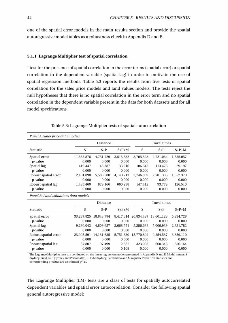
44 CHAPTER 5. RESULTS AND DISCUSSION

one of the spatial error models in the main results section and provide the spatial

autoregressive model tables as a robustness check in Appendix D and E.

5.1.1 Lagrange Multiplier test of spatial correlation

I test for the presence of spatial correlation in the error terms (spatial error) or spatial

correlation in the dependent variable (spatial lag) in order to motivate the use of

spatial regression methods. Table 5.3 reports the results from five tests of spatial

correlation for the sales price models and land values models. The tests reject the

null hypotheses that there is no spatial correlation in the error term and no spatial

correlation in the dependent variable present in the data for both datasets and for all

model specifications.

Table 5.3: Lagrange Multiplier tests of spatial autocorrelation

Panel A: Sales price data models

Distance Travel times

Statistic S S+P S+P+M S S+P S+P+M

Spatial error 11,335.876 4,751.729 3,513.632 3,705.323 2,721.034 1,555.057p-value 0.000 0.000 0.000 0.000 0.000 0.000

Spatial lag 419.447 45.387 33.216 106.645 113.476 29.197p-value 0.000 0.000 0.000 0.000 0.000 0.000

Robust spatial error 12,401.890 5,585.508 4,140.713 3,746.089 2,701.336 1,652.370p-value 0.000 0.000 0.000 0.000 0.000 0.000

Robust spatial lag 1,485.460 879.166 660.298 147.412 93.779 126.510p-value 0.000 0.000 0.000 0.000 0.000 0.000

Panel B: Land valuations data models

Distance Travel times

Statistic S S+P S+P+M S S+P S+P+M

Spatial error 33,237.825 18,843.794 8,417.614 20,834.487 13,601.128 5,834.728p-value 0.000 0.000 0.000 0.000 0.000 0.000

Spatial lag 9,280.042 4,809.657 2,668.571 5,386.688 5,006.939 2,831.782p-value 0.000 0.000 0.000 0.000 0.000 0.000

Robust spatial error 23,995.591 14,131.635 5,751.630 15,770.892 9,254.537 3,659.110p-value 0.000 0.000 0.000 0.000 0.000 0.000

Robust spatial lag 37.807 97.499 2.587 323.093 660.348 656.164p-value 0.000 0.000 0.108 0.000 0.000 0.000

The Lagrange Multiplier tests are conducted on the linear regression models presented in Appendix D and E. Model names: S(Sydney-only), S+P (Sydney and Parramatta), S+P+M (Sydney, Parramatta and Macquarie Park). Test statistics andcorresponding p-values are distributed χ2(1).

The Lagrange Multiplier (LM) tests are a class of tests for spatially autocorrelated

dependent variables and spatial error autocorrelation. Consider the following spatial

general autoregressive model:

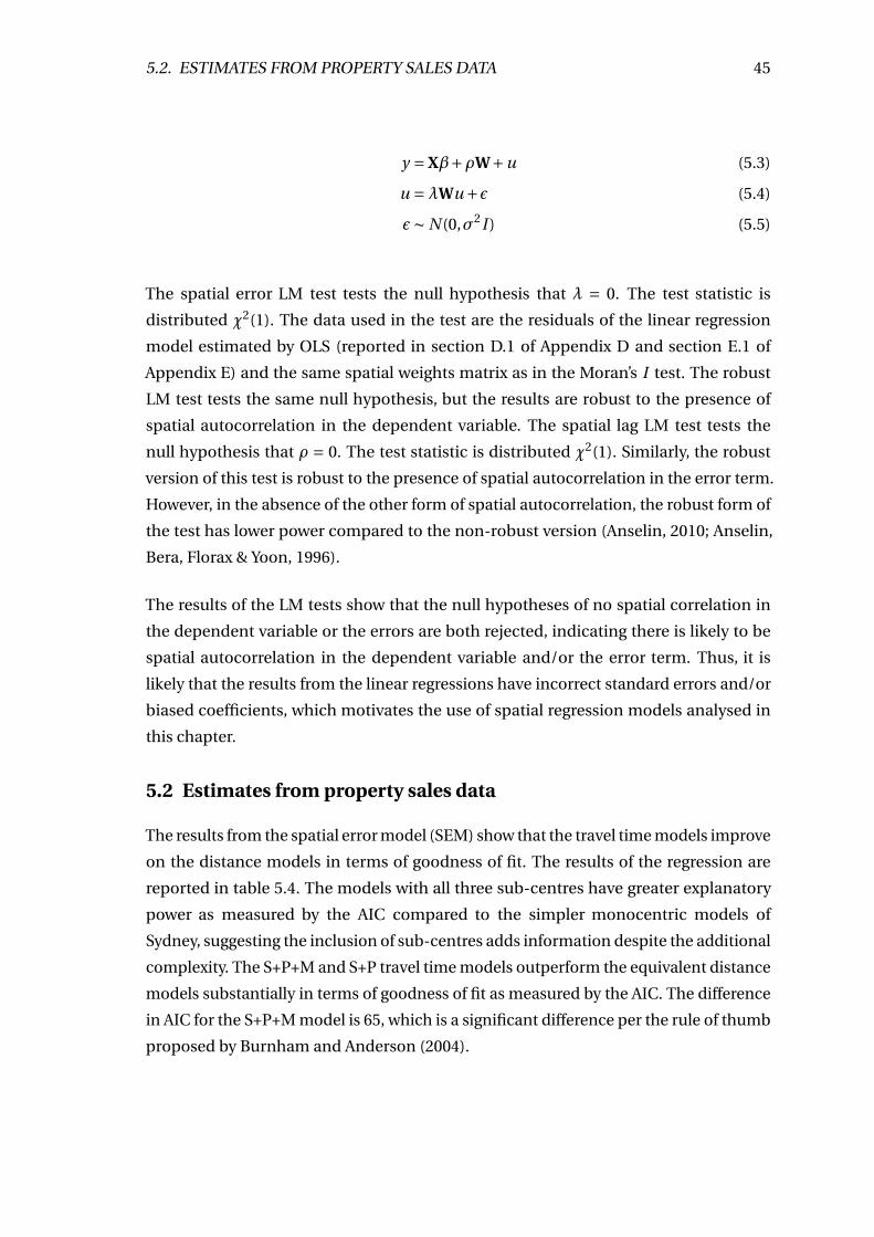
5.2. ESTIMATES FROM PROPERTY SALES DATA 45

y = Xβ+ρW+u (5.3)

u =λWu +ε (5.4)

ε∼ N (0,σ2I ) (5.5)

The spatial error LM test tests the null hypothesis that λ = 0. The test statistic is

distributed χ2(1). The data used in the test are the residuals of the linear regression

model estimated by OLS (reported in section D.1 of Appendix D and section E.1 of

Appendix E) and the same spatial weights matrix as in the Moran’s I test. The robust

LM test tests the same null hypothesis, but the results are robust to the presence of

spatial autocorrelation in the dependent variable. The spatial lag LM test tests the

null hypothesis that ρ = 0. The test statistic is distributed χ2(1). Similarly, the robust

version of this test is robust to the presence of spatial autocorrelation in the error term.

However, in the absence of the other form of spatial autocorrelation, the robust form of

the test has lower power compared to the non-robust version (Anselin, 2010; Anselin,

Bera, Florax & Yoon, 1996).

The results of the LM tests show that the null hypotheses of no spatial correlation in

the dependent variable or the errors are both rejected, indicating there is likely to be

spatial autocorrelation in the dependent variable and/or the error term. Thus, it is

likely that the results from the linear regressions have incorrect standard errors and/or

biased coefficients, which motivates the use of spatial regression models analysed in

this chapter.

5.2 Estimates from property sales data

The results from the spatial error model (SEM) show that the travel time models improve

on the distance models in terms of goodness of fit. The results of the regression are

reported in table 5.4. The models with all three sub-centres have greater explanatory

power as measured by the AIC compared to the simpler monocentric models of

Sydney, suggesting the inclusion of sub-centres adds information despite the additional

complexity. The S+P+M and S+P travel time models outperform the equivalent distance

models substantially in terms of goodness of fit as measured by the AIC. The difference

in AIC for the S+P+M model is 65, which is a significant difference per the rule of thumb

proposed by Burnham and Anderson (2004).

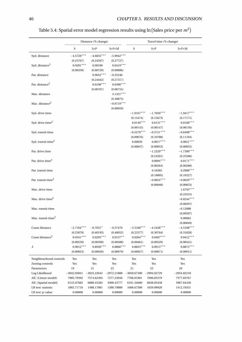
46 CHAPTER 5. RESULTS AND DISCUSSION

Table 5.4: Spatial error model regression results using ln(Sales price per m2

)Distance (% change) Travel time (% change)

S S+P S+P+M S S+P S+P+M

Syd. distance −4.5728∗∗∗ −4.6835∗∗∗ −5.9942∗∗∗

(0.23767) (0.24597) (0.27727)

Syd. distance2 0.0281∗∗∗ 0.00100 0.0419∗∗∗

(0.00359) (0.00729) (0.00886)

Par. distance 0.9652∗∗∗ −0.25246

(0.24442) (0.27317)

Par. distance2 0.0198∗∗∗ 0.0396∗∗∗

(0.00707) (0.00755)

Mac. distance 3.1321∗∗∗

(0.30875)

Mac. distance2 −0.0719∗∗∗

(0.00959)

Syd. drive time −1.9167∗∗∗ −1.7050∗∗∗ −1.9417∗∗∗

(0.15474) (0.15673) (0.17171)

Syd. drive time2 0.0140∗∗∗ 0.0131∗∗∗ 0.0168∗∗∗

(0.00143) (0.00147) (0.00156)

Syd. transit time −0.5579∗∗∗ −0.5721∗∗∗ −0.6498∗∗∗

(0.09676) (0.10788) (0.11104)

Syd. transit time2 0.00059 0.0017∗∗∗ 0.0021∗∗∗

(0.00047) (0.00053) (0.00055)

Par. drive time −1.2329∗∗∗ −1.7390∗∗∗

(0.24201) (0.25286)

Par. drive time2 0.0094∗∗∗ 0.0171∗∗∗

(0.00264) (0.00280)

Par. transit time 0.16365 0.2908∗∗∗

(0.10005) (0.10327)

Par. transit time2 −0.0024∗∗∗ −0.0029∗∗∗

(0.00048) (0.00053)

Mac. drive time 1.6793∗∗∗

(0.25553)

Mac. drive time2 −0.0244∗∗∗

(0.00297)

Mac. transit time −0.12088

(0.09507)

Mac. transit time2 0.00063

(0.00049)

Coast distance −2.7164∗∗∗ −0.7031∗ −0.57470 −3.3160∗∗∗ −4.5458∗∗∗ −4.5108∗∗∗

(0.25078) (0.40193) (0.40052) (0.23377) (0.30764) (0.31828)

Coast distance2 0.0341∗∗∗ 0.0205∗∗∗ 0.0137∗∗ 0.0264∗∗∗ 0.0407∗∗∗ 0.0412∗∗∗

(0.00539) (0.00590) (0.00588) (0.00461) (0.00529) (0.00541)

λ 0.9012∗∗∗ 0.8930∗∗∗ 0.8860∗∗∗ 0.8833∗∗∗ 0.8913∗∗∗ 0.8875∗∗∗

(0.00823) (0.00926) (0.00979) (0.00927) (0.00871) (0.00911)

Neighbourhood controls Yes Yes Yes Yes Yes Yes

Zoning controls Yes Yes Yes Yes Yes Yes

Parameters 19 21 23 21 25 29

Log Likelihood −3042.03841 −3023.22642 −2972.21888 −3059.67300 −2994.02729 −2954.82218

AIC (Linear model) 7985.79392 7574.62365 7377.23656 7766.01901 7696.05379 7377.83767

AIC (Spatial model) 6122.07682 6088.45284 5990.43777 6161.34600 6038.05458 5967.64436

LR test: statistic 1865.71710 1488.17081 1388.79880 1606.67300 1659.99920 1412.19331

LR test: p-value 0.00000 0.00000 0.00000 0.00000 0.00000 0.00000

5.2. ESTIMATES FROM PROPERTY SALES DATA 47

Distance (% change) Travel time (% change)

S S+P S+P+M S S+P S+P+M

Standard errors in parenthesis. ∗∗∗p < 0.01; ∗∗p < 0.05; ∗p < 0.1. Coefficients transformed to percentages. All travel times are

in minutes. All distances are in kilometres. Results reported are spatial error models estimated by maximum likelihood.

Number of observations in all models is 8,073. Model names: S (Sydney-only), S+P (Sydney and Parramatta), S+P+M (Sydney,

Parramatta and Macquarie Park). Full model tables can be found in Appendix F and G.

Controls: Neighbourhood controls are demographic variables for the SA1 that each property belongs to and controls for ABS

SEIFA Disadvantage Index, population % with Australian ancestry, population % with Bachelor’s degree or above, population

% unemployed, population % with income above $130,000 per year, population % speaking English at home, and population

% working in a professional occupation. Zoning controls are dummy variables for Low Density Residential, Medium Density

Residential, High Density Residential, Large Lot (Rural) Residential. The base case is General Residential.

The SEM is the preferred model as it controls for spatial dependency in the error term

revealed in the Lagrange Multiplier test and outperforms the spatial autoregressive

model in terms of goodness of fit as measured by the AIC. The log-level models also

outperform the level-level models in terms of explanatory power, which are included in

section D.2 of Appendix D as a robustness check. I also report the results and discussion

of the spatial autoregressive model for the log-level and level-level specification in

sections D.3 and D.4 of Appendix D.

The SEM incorporates a spatially autoregressive error term, which explicitly addresses

spatial non-stationarity in the unobservables, which contrasts with the OLS estimation

method which assumes spatial non-stationarity is not present. Assuming that the

dependent variable is spatially uncorrelated, using the SEM means that the estimates

are unbiased and the standard errors are efficient. The structure of the spatial error

model is shown in equations 5.6 and 5.7.

y = Xβ+u (5.6)

u =λWu +ε (5.7)

ε∼ N (0,σ2In) (5.8)

5.2.1 Distance specifications

The distance results from the spatial error models are in line with theoretical expect-

ations, showing an inverse and non-linear relationship between distance from the

Sydney CBD and property prices. My estimates show that a 1 km increase in distance to

the Sydney CBD decreases property prices by around 6% in the vicinity of the CBD. This

effect is non-linear and diminishes with distance, with the marginal effect decreasing

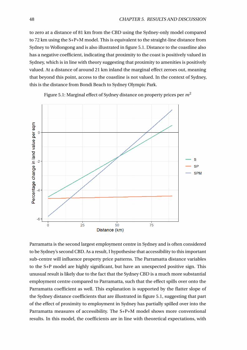
48 CHAPTER 5. RESULTS AND DISCUSSION

to zero at a distance of 81 km from the CBD using the Sydney-only model compared

to 72 km using the S+P+M model. This is equivalent to the straight-line distance from

Sydney to Wollongong and is also illustrated in figure 5.1. Distance to the coastline also

has a negative coefficient, indicating that proximity to the coast is positively valued in

Sydney, which is in line with theory suggesting that proximity to amenities is positively

valued. At a distance of around 21 km inland the marginal effect zeroes out, meaning

that beyond this point, access to the coastline is not valued. In the context of Sydney,

this is the distance from Bondi Beach to Sydney Olympic Park.

Figure 5.1: Marginal effect of Sydney distance on property prices per m2

Parramatta is the second largest employment centre in Sydney and is often considered

to be Sydney’s second CBD. As a result, I hypothesise that accessibility to this important

sub-centre will influence property price patterns. The Parramatta distance variables

to the S+P model are highly significant, but have an unexpected positive sign. This

unusual result is likely due to the fact that the Sydney CBD is a much more substantial

employment centre compared to Parramatta, such that the effect spills over onto the

Parramatta coefficient as well. This explanation is supported by the flatter slope of

the Sydney distance coefficients that are illustrated in figure 5.1, suggesting that part

of the effect of proximity to employment in Sydney has partially spilled over into the

Parramatta measures of accessibility. The S+P+M model shows more conventional

results. In this model, the coefficients are in line with theoretical expectations, with

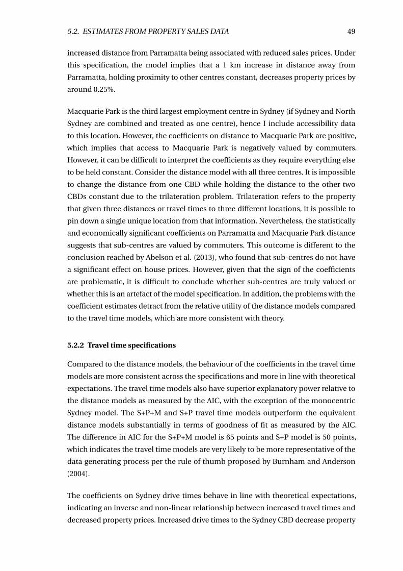
5.2. ESTIMATES FROM PROPERTY SALES DATA 49

increased distance from Parramatta being associated with reduced sales prices. Under

this specification, the model implies that a 1 km increase in distance away from

Parramatta, holding proximity to other centres constant, decreases property prices by

around 0.25%.

Macquarie Park is the third largest employment centre in Sydney (if Sydney and North

Sydney are combined and treated as one centre), hence I include accessibility data

to this location. However, the coefficients on distance to Macquarie Park are positive,

which implies that access to Macquarie Park is negatively valued by commuters.

However, it can be difficult to interpret the coefficients as they require everything else

to be held constant. Consider the distance model with all three centres. It is impossible

to change the distance from one CBD while holding the distance to the other two

CBDs constant due to the trilateration problem. Trilateration refers to the property

that given three distances or travel times to three different locations, it is possible to

pin down a single unique location from that information. Nevertheless, the statistically

and economically significant coefficients on Parramatta and Macquarie Park distance

suggests that sub-centres are valued by commuters. This outcome is different to the

conclusion reached by Abelson et al. (2013), who found that sub-centres do not have

a significant effect on house prices. However, given that the sign of the coefficients

are problematic, it is difficult to conclude whether sub-centres are truly valued or

whether this is an artefact of the model specification. In addition, the problems with the

coefficient estimates detract from the relative utility of the distance models compared

to the travel time models, which are more consistent with theory.

5.2.2 Travel time specifications

Compared to the distance models, the behaviour of the coefficients in the travel time

models are more consistent across the specifications and more in line with theoretical

expectations. The travel time models also have superior explanatory power relative to

the distance models as measured by the AIC, with the exception of the monocentric

Sydney model. The S+P+M and S+P travel time models outperform the equivalent

distance models substantially in terms of goodness of fit as measured by the AIC.

The difference in AIC for the S+P+M model is 65 points and S+P model is 50 points,

which indicates the travel time models are very likely to be more representative of the

data generating process per the rule of thumb proposed by Burnham and Anderson

(2004).

The coefficients on Sydney drive times behave in line with theoretical expectations,

indicating an inverse and non-linear relationship between increased travel times and

decreased property prices. Increased drive times to the Sydney CBD decrease property

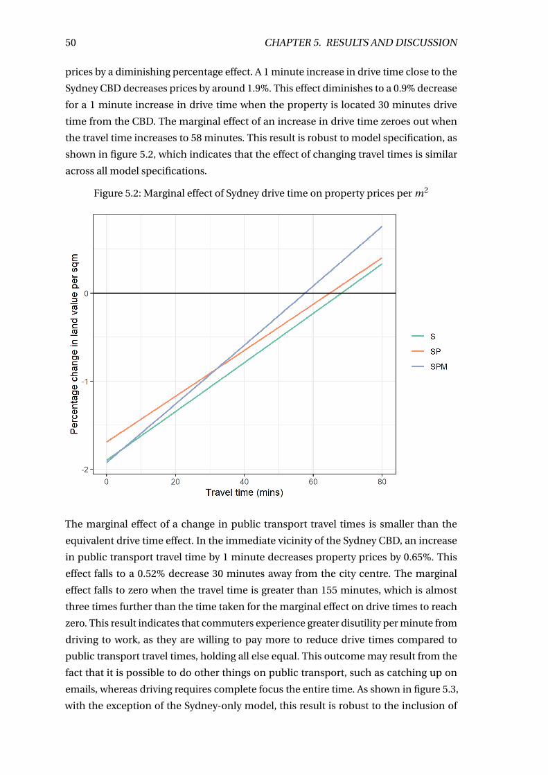
50 CHAPTER 5. RESULTS AND DISCUSSION

prices by a diminishing percentage effect. A 1 minute increase in drive time close to the

Sydney CBD decreases prices by around 1.9%. This effect diminishes to a 0.9% decrease

for a 1 minute increase in drive time when the property is located 30 minutes drive

time from the CBD. The marginal effect of an increase in drive time zeroes out when

the travel time increases to 58 minutes. This result is robust to model specification, as

shown in figure 5.2, which indicates that the effect of changing travel times is similar

across all model specifications.

Figure 5.2: Marginal effect of Sydney drive time on property prices per m2

The marginal effect of a change in public transport travel times is smaller than the

equivalent drive time effect. In the immediate vicinity of the Sydney CBD, an increase

in public transport travel time by 1 minute decreases property prices by 0.65%. This

effect falls to a 0.52% decrease 30 minutes away from the city centre. The marginal

effect falls to zero when the travel time is greater than 155 minutes, which is almost

three times further than the time taken for the marginal effect on drive times to reach

zero. This result indicates that commuters experience greater disutility per minute from

driving to work, as they are willing to pay more to reduce drive times compared to

public transport travel times, holding all else equal. This outcome may result from the

fact that it is possible to do other things on public transport, such as catching up on

emails, whereas driving requires complete focus the entire time. As shown in figure 5.3,

with the exception of the Sydney-only model, this result is robust to the inclusion of

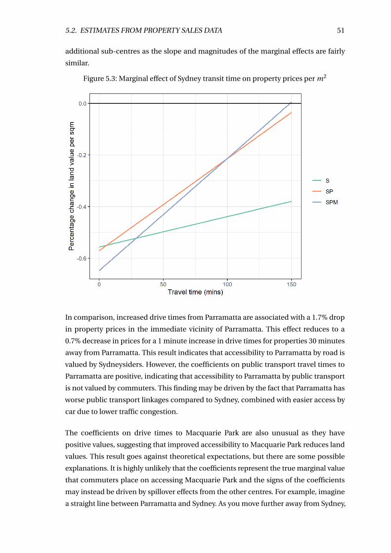
5.2. ESTIMATES FROM PROPERTY SALES DATA 51

additional sub-centres as the slope and magnitudes of the marginal effects are fairly

similar.

Figure 5.3: Marginal effect of Sydney transit time on property prices per m2

In comparison, increased drive times from Parramatta are associated with a 1.7% drop

in property prices in the immediate vicinity of Parramatta. This effect reduces to a

0.7% decrease in prices for a 1 minute increase in drive times for properties 30 minutes

away from Parramatta. This result indicates that accessibility to Parramatta by road is

valued by Sydneysiders. However, the coefficients on public transport travel times to

Parramatta are positive, indicating that accessibility to Parramatta by public transport

is not valued by commuters. This finding may be driven by the fact that Parramatta has

worse public transport linkages compared to Sydney, combined with easier access by

car due to lower traffic congestion.

The coefficients on drive times to Macquarie Park are also unusual as they have

positive values, suggesting that improved accessibility to Macquarie Park reduces land

values. This result goes against theoretical expectations, but there are some possible

explanations. It is highly unlikely that the coefficients represent the true marginal value

that commuters place on accessing Macquarie Park and the signs of the coefficients

may instead be driven by spillover effects from the other centres. For example, imagine

a straight line between Parramatta and Sydney. As you move further away from Sydney,

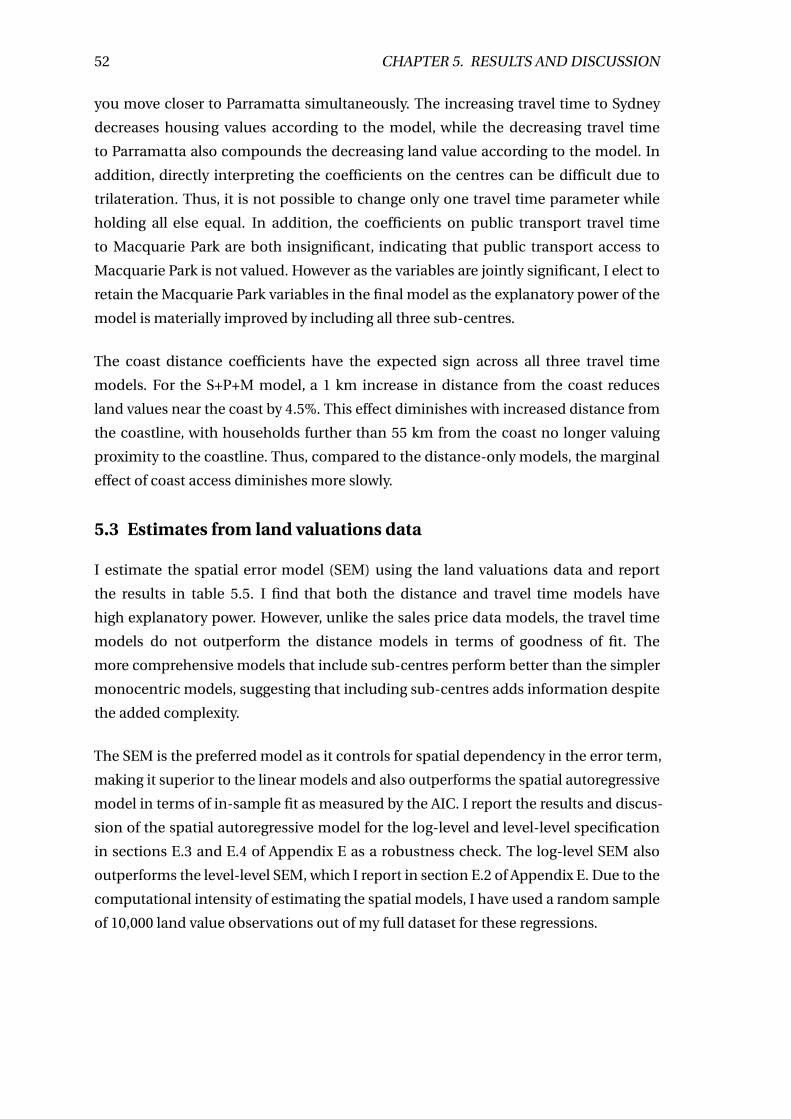
52 CHAPTER 5. RESULTS AND DISCUSSION

you move closer to Parramatta simultaneously. The increasing travel time to Sydney

decreases housing values according to the model, while the decreasing travel time

to Parramatta also compounds the decreasing land value according to the model. In

addition, directly interpreting the coefficients on the centres can be difficult due to

trilateration. Thus, it is not possible to change only one travel time parameter while

holding all else equal. In addition, the coefficients on public transport travel time

to Macquarie Park are both insignificant, indicating that public transport access to

Macquarie Park is not valued. However as the variables are jointly significant, I elect to

retain the Macquarie Park variables in the final model as the explanatory power of the

model is materially improved by including all three sub-centres.

The coast distance coefficients have the expected sign across all three travel time

models. For the S+P+M model, a 1 km increase in distance from the coast reduces

land values near the coast by 4.5%. This effect diminishes with increased distance from

the coastline, with households further than 55 km from the coast no longer valuing

proximity to the coastline. Thus, compared to the distance-only models, the marginal

effect of coast access diminishes more slowly.

5.3 Estimates from land valuations data

I estimate the spatial error model (SEM) using the land valuations data and report

the results in table 5.5. I find that both the distance and travel time models have

high explanatory power. However, unlike the sales price data models, the travel time

models do not outperform the distance models in terms of goodness of fit. The

more comprehensive models that include sub-centres perform better than the simpler

monocentric models, suggesting that including sub-centres adds information despite

the added complexity.

The SEM is the preferred model as it controls for spatial dependency in the error term,

making it superior to the linear models and also outperforms the spatial autoregressive

model in terms of in-sample fit as measured by the AIC. I report the results and discus-

sion of the spatial autoregressive model for the log-level and level-level specification

in sections E.3 and E.4 of Appendix E as a robustness check. The log-level SEM also

outperforms the level-level SEM, which I report in section E.2 of Appendix E. Due to the

computational intensity of estimating the spatial models, I have used a random sample

of 10,000 land value observations out of my full dataset for these regressions.

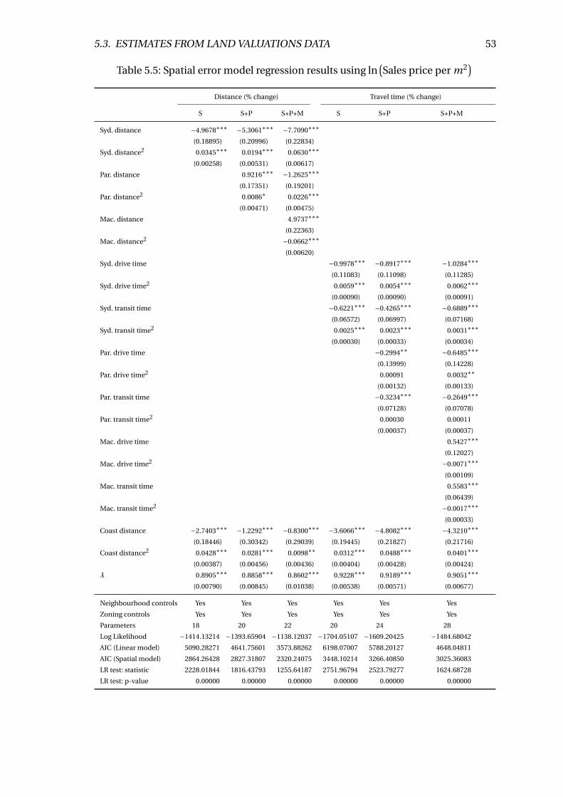
5.3. ESTIMATES FROM LAND VALUATIONS DATA 53

Table 5.5: Spatial error model regression results using ln(Sales price per m2

)Distance (% change) Travel time (% change)

S S+P S+P+M S S+P S+P+M

Syd. distance −4.9678∗∗∗ −5.3061∗∗∗ −7.7090∗∗∗

(0.18895) (0.20996) (0.22834)

Syd. distance2 0.0345∗∗∗ 0.0194∗∗∗ 0.0630∗∗∗

(0.00258) (0.00531) (0.00617)

Par. distance 0.9216∗∗∗ −1.2625∗∗∗

(0.17351) (0.19201)

Par. distance2 0.0086∗ 0.0226∗∗∗

(0.00471) (0.00475)

Mac. distance 4.9737∗∗∗

(0.22363)

Mac. distance2 −0.0662∗∗∗

(0.00620)

Syd. drive time −0.9978∗∗∗ −0.8917∗∗∗ −1.0284∗∗∗

(0.11083) (0.11098) (0.11285)

Syd. drive time2 0.0059∗∗∗ 0.0054∗∗∗ 0.0062∗∗∗

(0.00090) (0.00090) (0.00091)

Syd. transit time −0.6221∗∗∗ −0.4265∗∗∗ −0.6889∗∗∗

(0.06572) (0.06997) (0.07168)

Syd. transit time2 0.0025∗∗∗ 0.0023∗∗∗ 0.0031∗∗∗

(0.00030) (0.00033) (0.00034)

Par. drive time −0.2994∗∗ −0.6485∗∗∗

(0.13999) (0.14228)

Par. drive time2 0.00091 0.0032∗∗

(0.00132) (0.00133)

Par. transit time −0.3234∗∗∗ −0.2649∗∗∗

(0.07128) (0.07078)

Par. transit time2 0.00030 0.00011

(0.00037) (0.00037)

Mac. drive time 0.5427∗∗∗

(0.12027)

Mac. drive time2 −0.0071∗∗∗

(0.00109)

Mac. transit time 0.5583∗∗∗

(0.06439)

Mac. transit time2 −0.0017∗∗∗

(0.00033)

Coast distance −2.7403∗∗∗ −1.2292∗∗∗ −0.8300∗∗∗ −3.6066∗∗∗ −4.8082∗∗∗ −4.3210∗∗∗

(0.18446) (0.30342) (0.29039) (0.19445) (0.21827) (0.21716)

Coast distance2 0.0428∗∗∗ 0.0281∗∗∗ 0.0098∗∗ 0.0312∗∗∗ 0.0488∗∗∗ 0.0401∗∗∗

(0.00387) (0.00456) (0.00436) (0.00404) (0.00428) (0.00424)

λ 0.8905∗∗∗ 0.8858∗∗∗ 0.8602∗∗∗ 0.9228∗∗∗ 0.9189∗∗∗ 0.9051∗∗∗

(0.00790) (0.00845) (0.01038) (0.00538) (0.00571) (0.00677)

Neighbourhood controls Yes Yes Yes Yes Yes Yes

Zoning controls Yes Yes Yes Yes Yes Yes

Parameters 18 20 22 20 24 28

Log Likelihood −1414.13214 −1393.65904 −1138.12037 −1704.05107 −1609.20425 −1484.68042

AIC (Linear model) 5090.28271 4641.75601 3573.88262 6198.07007 5788.20127 4648.04811

AIC (Spatial model) 2864.26428 2827.31807 2320.24075 3448.10214 3266.40850 3025.36083

LR test: statistic 2228.01844 1816.43793 1255.64187 2751.96794 2523.79277 1624.68728

LR test: p-value 0.00000 0.00000 0.00000 0.00000 0.00000 0.00000

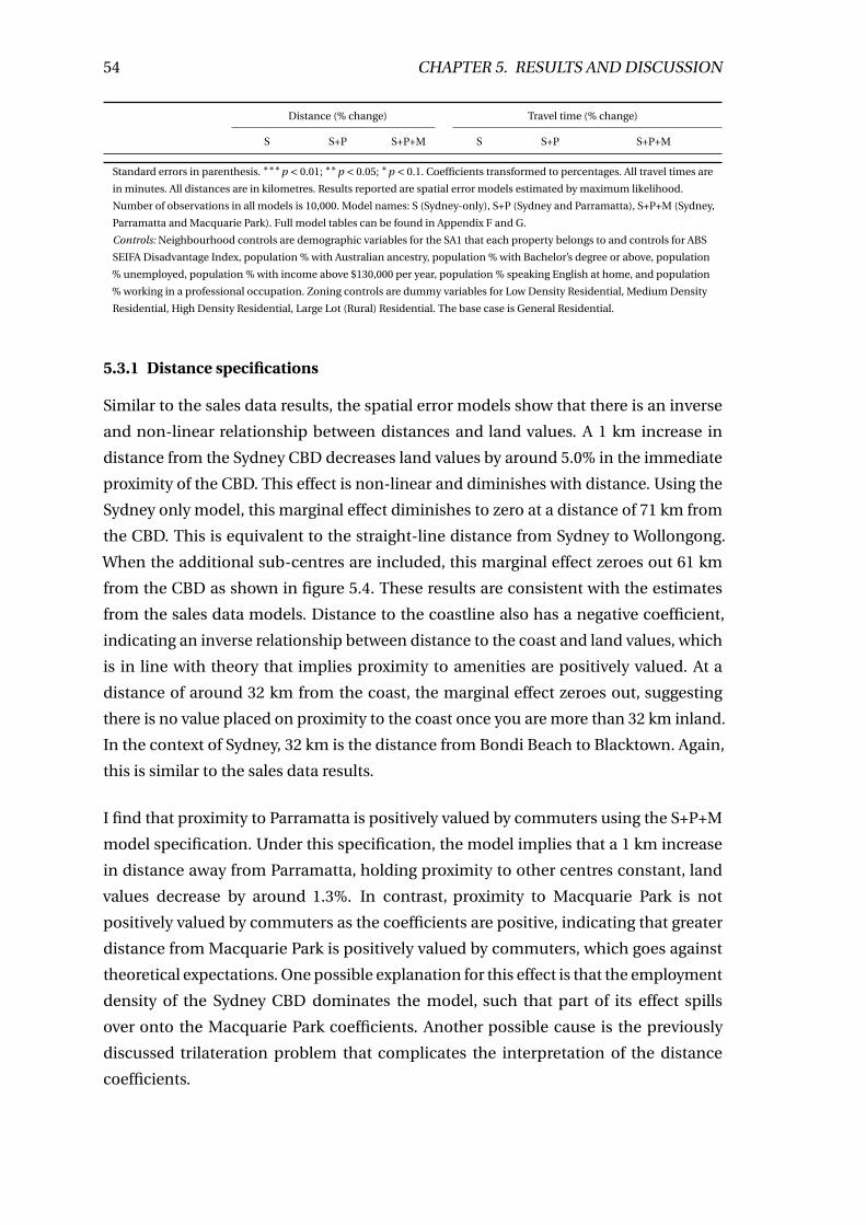
54 CHAPTER 5. RESULTS AND DISCUSSION

Distance (% change) Travel time (% change)

S S+P S+P+M S S+P S+P+M

Standard errors in parenthesis. ∗∗∗p < 0.01; ∗∗p < 0.05; ∗p < 0.1. Coefficients transformed to percentages. All travel times are

in minutes. All distances are in kilometres. Results reported are spatial error models estimated by maximum likelihood.

Number of observations in all models is 10,000. Model names: S (Sydney-only), S+P (Sydney and Parramatta), S+P+M (Sydney,

Parramatta and Macquarie Park). Full model tables can be found in Appendix F and G.

Controls: Neighbourhood controls are demographic variables for the SA1 that each property belongs to and controls for ABS

SEIFA Disadvantage Index, population % with Australian ancestry, population % with Bachelor’s degree or above, population

% unemployed, population % with income above $130,000 per year, population % speaking English at home, and population

% working in a professional occupation. Zoning controls are dummy variables for Low Density Residential, Medium Density

Residential, High Density Residential, Large Lot (Rural) Residential. The base case is General Residential.

5.3.1 Distance specifications

Similar to the sales data results, the spatial error models show that there is an inverse

and non-linear relationship between distances and land values. A 1 km increase in

distance from the Sydney CBD decreases land values by around 5.0% in the immediate

proximity of the CBD. This effect is non-linear and diminishes with distance. Using the

Sydney only model, this marginal effect diminishes to zero at a distance of 71 km from

the CBD. This is equivalent to the straight-line distance from Sydney to Wollongong.

When the additional sub-centres are included, this marginal effect zeroes out 61 km

from the CBD as shown in figure 5.4. These results are consistent with the estimates

from the sales data models. Distance to the coastline also has a negative coefficient,

indicating an inverse relationship between distance to the coast and land values, which

is in line with theory that implies proximity to amenities are positively valued. At a

distance of around 32 km from the coast, the marginal effect zeroes out, suggesting

there is no value placed on proximity to the coast once you are more than 32 km inland.

In the context of Sydney, 32 km is the distance from Bondi Beach to Blacktown. Again,

this is similar to the sales data results.

I find that proximity to Parramatta is positively valued by commuters using the S+P+M

model specification. Under this specification, the model implies that a 1 km increase

in distance away from Parramatta, holding proximity to other centres constant, land

values decrease by around 1.3%. In contrast, proximity to Macquarie Park is not

positively valued by commuters as the coefficients are positive, indicating that greater

distance from Macquarie Park is positively valued by commuters, which goes against

theoretical expectations. One possible explanation for this effect is that the employment

density of the Sydney CBD dominates the model, such that part of its effect spills

over onto the Macquarie Park coefficients. Another possible cause is the previously

discussed trilateration problem that complicates the interpretation of the distance

coefficients.

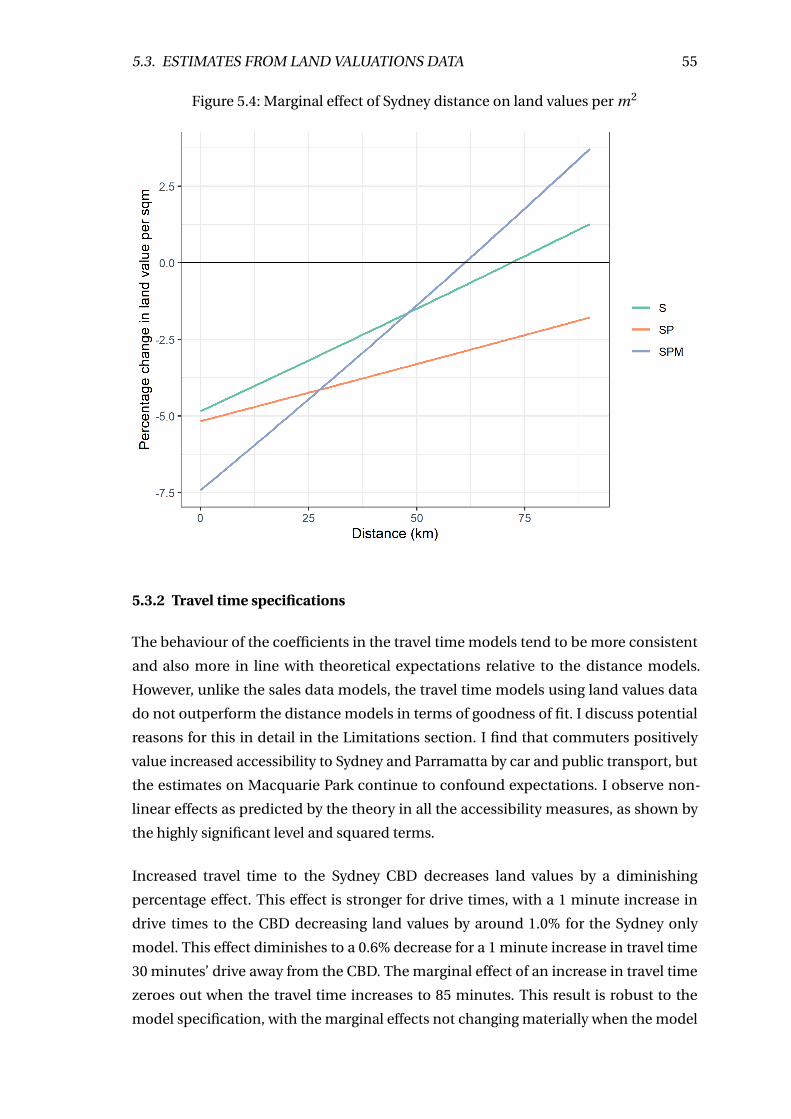
5.3. ESTIMATES FROM LAND VALUATIONS DATA 55

Figure 5.4: Marginal effect of Sydney distance on land values per m2

5.3.2 Travel time specifications

The behaviour of the coefficients in the travel time models tend to be more consistent

and also more in line with theoretical expectations relative to the distance models.

However, unlike the sales data models, the travel time models using land values data

do not outperform the distance models in terms of goodness of fit. I discuss potential

reasons for this in detail in the Limitations section. I find that commuters positively

value increased accessibility to Sydney and Parramatta by car and public transport, but

the estimates on Macquarie Park continue to confound expectations. I observe non-

linear effects as predicted by the theory in all the accessibility measures, as shown by

the highly significant level and squared terms.

Increased travel time to the Sydney CBD decreases land values by a diminishing

percentage effect. This effect is stronger for drive times, with a 1 minute increase in

drive times to the CBD decreasing land values by around 1.0% for the Sydney only

model. This effect diminishes to a 0.6% decrease for a 1 minute increase in travel time

30 minutes’ drive away from the CBD. The marginal effect of an increase in travel time

zeroes out when the travel time increases to 85 minutes. This result is robust to the

model specification, with the marginal effects not changing materially when the model

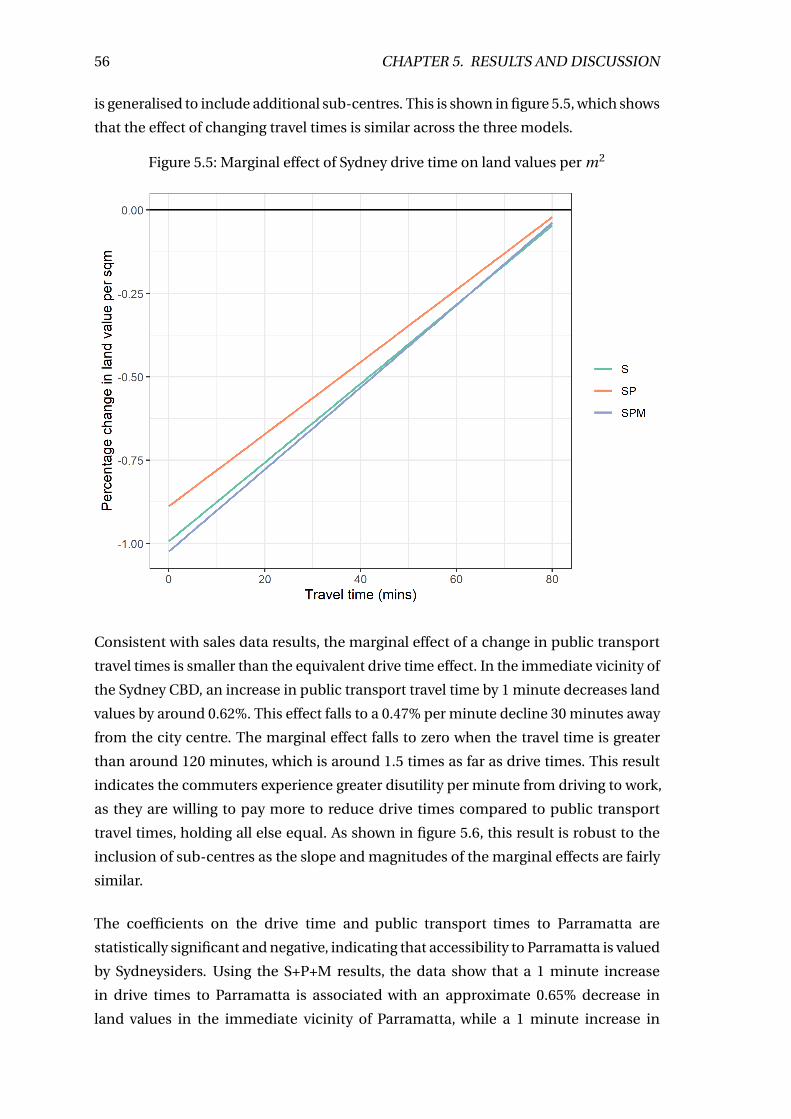
56 CHAPTER 5. RESULTS AND DISCUSSION

is generalised to include additional sub-centres. This is shown in figure 5.5, which shows

that the effect of changing travel times is similar across the three models.

Figure 5.5: Marginal effect of Sydney drive time on land values per m2

Consistent with sales data results, the marginal effect of a change in public transport

travel times is smaller than the equivalent drive time effect. In the immediate vicinity of

the Sydney CBD, an increase in public transport travel time by 1 minute decreases land

values by around 0.62%. This effect falls to a 0.47% per minute decline 30 minutes away

from the city centre. The marginal effect falls to zero when the travel time is greater

than around 120 minutes, which is around 1.5 times as far as drive times. This result

indicates the commuters experience greater disutility per minute from driving to work,

as they are willing to pay more to reduce drive times compared to public transport

travel times, holding all else equal. As shown in figure 5.6, this result is robust to the

inclusion of sub-centres as the slope and magnitudes of the marginal effects are fairly

similar.

The coefficients on the drive time and public transport times to Parramatta are

statistically significant and negative, indicating that accessibility to Parramatta is valued

by Sydneysiders. Using the S+P+M results, the data show that a 1 minute increase

in drive times to Parramatta is associated with an approximate 0.65% decrease in

land values in the immediate vicinity of Parramatta, while a 1 minute increase in

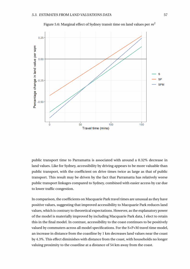
5.3. ESTIMATES FROM LAND VALUATIONS DATA 57

Figure 5.6: Marginal effect of Sydney transit time on land values per m2

public transport time to Parramatta is associated with around a 0.32% decrease in

land values. Like for Sydney, accessibility by driving appears to be more valuable than

public transport, with the coefficient on drive times twice as large as that of public

transport. This result may be driven by the fact that Parramatta has relatively worse

public transport linkages compared to Sydney, combined with easier access by car due

to lower traffic congestion.

In comparison, the coefficients on Macquarie Park travel times are unusual as they have

positive values, suggesting that improved accessibility to Macquarie Park reduces land

values, which is contrary to theoretical expectations. However, as the explanatory power

of the model is materially improved by including Macquarie Park data, I elect to retain

this in the final model. In contrast, accessibility to the coast continues to be positively

valued by commuters across all model specifications. For the S+P+M travel time model,

an increase in distance from the coastline by 1 km decreases land values near the coast

by 4.3%. This effect diminishes with distance from the coast, with households no longer

valuing proximity to the coastline at a distance of 54 km away from the coast.

58 CHAPTER 5. RESULTS AND DISCUSSION

5.4 Estimating the value of congestion

Commuters experience additional disutility from traffic congestion and the value

of congestion is capitalised into land values as shown in table 5.6. Congestion is

measured as the difference between the drive time in traffic less the drive time without

traffic, which are unique datapoints that are available in my dataset. Commuters

experience disutility from increased free-flow (without congestion) drive times, as

shown by the negative coefficient on the Free-flow drive time variables for Sydney and

Parramatta. Commuters also experience disutility from worsening congestion during

peak hours, which is measured by the Congestion delay variables, which is constructed

by subtracting the free-flow drive time (no traffic) from the congested (with traffic) drive

time.

Using the log-level specification of the SEM, a 1 minute increase in congested drive

time to the Sydney CBD is associated with a 0.26% decrease in land values. Similarly,

commuters dislike increased road congestion to Parramatta, with a 1 minute increase

in drive times corresponding to a 0.17% decrease in land values. Finally, while the sign

on free-flow travel time to Macquarie Park exhibits the same unusual positive sign like

in previous models, the negative coefficient on the congested drive time differential

shows that commuters also value a reduction in congestion to Macquarie Park, with a

1 minute increase in congested drive time being associated with a 0.22% decrease in

land values. These results are all statistically significant, although their significance is

affected by model specification choices. Note that for interpretability reasons, I have

specified a simplified model with only linear terms on the drive times instead of the fully

featured models in previous sections that included squared terms on all accessibility

variables.

These estimates have useful policy implications for congestion charging. I find that

the average commuter values the present discounted value of 1 minute of congestion

when driving into the Sydney CBD at about $2,200 for the average property, which

can be converted to an hourly willingness to pay equal to $17.64 (per the method in

Appendix K). This amount represents the value that the average commuter places on

reducing congestion in their daily commute by one hour. Thus, this estimate can be

used to set an upper bound on a congestion charge for travelling into the Sydney CBD.

That is, if a hypothetical congestion charge was expected to reduce congestion by 1

hour for the average journey into the Sydney CBD, then commuters would be willing to

pay up to $17.64 for the right to drive into the city. Naturally, if the scale of congestion

improvements was expected to be smaller, then the congestion charge could be scaled

down accordingly.

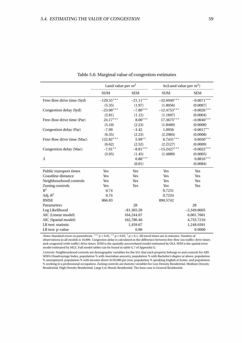
5.4. ESTIMATING THE VALUE OF CONGESTION 59

Table 5.6: Marginal value of congestion estimates

Land value per m2 ln(Land value per m2)

SUM SEM SUM SEM

Free-flow drive time (Syd) −129.55∗∗∗ −21.11∗∗∗ −32.6940∗∗∗ −0.0071∗∗∗(5.35) (1.97) (1.8056) (0.0007)

Congestion delay (Syd) −23.00∗∗∗ −7.80∗∗∗ −12.4753∗∗∗ −0.0026∗∗∗(2.81) (1.12) (1.1697) (0.0004)

Free-flow drive time (Par) 24.17∗∗∗ 8.00∗∗∗ 17.3675∗∗∗ −0.0040∗∗∗(5.10) (2.23) (1.8489) (0.0008)

Congestion delay (Par) −7.99 −3.42 1.0956 −0.0017∗∗(6.35) (2.23) (2.2984) (0.0008)

Free-flow drive time (Mac) 122.82∗∗∗ 5.99∗∗ 6.7431∗∗∗ 0.0030∗∗∗(6.62) (2.52) (2.2127) (0.0009)

Congestion delay (Mac) −7.91∗∗ −8.81∗∗∗ −15.2427∗∗∗ −0.0022∗∗∗(3.95) (1.45) (1.4889) (0.0005)

λ 0.88∗∗∗ 0.8816∗∗∗(0.01) (0.0084)

Public transport times Yes Yes Yes YesCoastline distance Yes Yes Yes YesNeighbourhood controls Yes Yes Yes YesZoning controls Yes Yes Yes YesR2 0.74 0.7231Adj. R2 0.74 0.7224RMSE 866.83 890.5742Parameters 28 28Log Likelihood −81,365.20 −2,349.8605AIC (Linear model) 164,244.07 6,001.7601AIC (Spatial model) 162,786.40 4,755.7210LR test: statistic 1,459.67 1,248.0391LR test: p-value 0.00 0.0000

Notes: Standard errors in parenthesis. ∗∗∗p < 0.01, ∗∗p < 0.05, ∗p < 0.1. All travel times are in minutes. Number ofobservations in all models is 10,000. Congestion delay is calculated as the difference between free-flow (no traffic) drive timesand congested (with traffic) drive times. SUM is the spatially uncorrelated model estimated by OLS. SEM is the spatial errormodel estimated by MLE. Full model tables can be found in table G.7 of Appendix G.

Controls: Neighbourhood controls are demographic variables for the SA1 that each property belongs to and controls for ABSSEIFA Disadvantage Index, population % with Australian ancestry, population % with Bachelor’s degree or above, population% unemployed, population % with income above $130,000 per year, population % speaking English at home, and population% working in a professional occupation. Zoning controls are dummy variables for Low Density Residential, Medium DensityResidential, High Density Residential, Large Lot (Rural) Residential. The base case is General Residential.

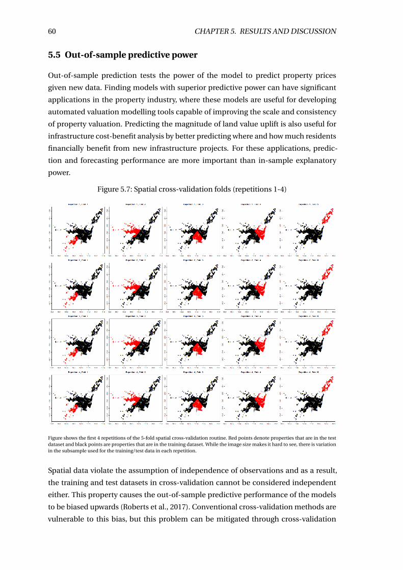
60 CHAPTER 5. RESULTS AND DISCUSSION

5.5 Out-of-sample predictive power

Out-of-sample prediction tests the power of the model to predict property prices

given new data. Finding models with superior predictive power can have significant

applications in the property industry, where these models are useful for developing

automated valuation modelling tools capable of improving the scale and consistency

of property valuation. Predicting the magnitude of land value uplift is also useful for

infrastructure cost-benefit analysis by better predicting where and how much residents

financially benefit from new infrastructure projects. For these applications, predic-

tion and forecasting performance are more important than in-sample explanatory

power.

Figure 5.7: Spatial cross-validation folds (repetitions 1-4)

Figure shows the first 4 repetitions of the 5-fold spatial cross-validation routine. Red points denote properties that are in the testdataset and black points are properties that are in the training dataset. While the image size makes it hard to see, there is variationin the subsample used for the training/test data in each repetition.

Spatial data violate the assumption of independence of observations and as a result,

the training and test datasets in cross-validation cannot be considered independent

either. This property causes the out-of-sample predictive performance of the models

to be biased upwards (Roberts et al., 2017). Conventional cross-validation methods are

vulnerable to this bias, but this problem can be mitigated through cross-validation

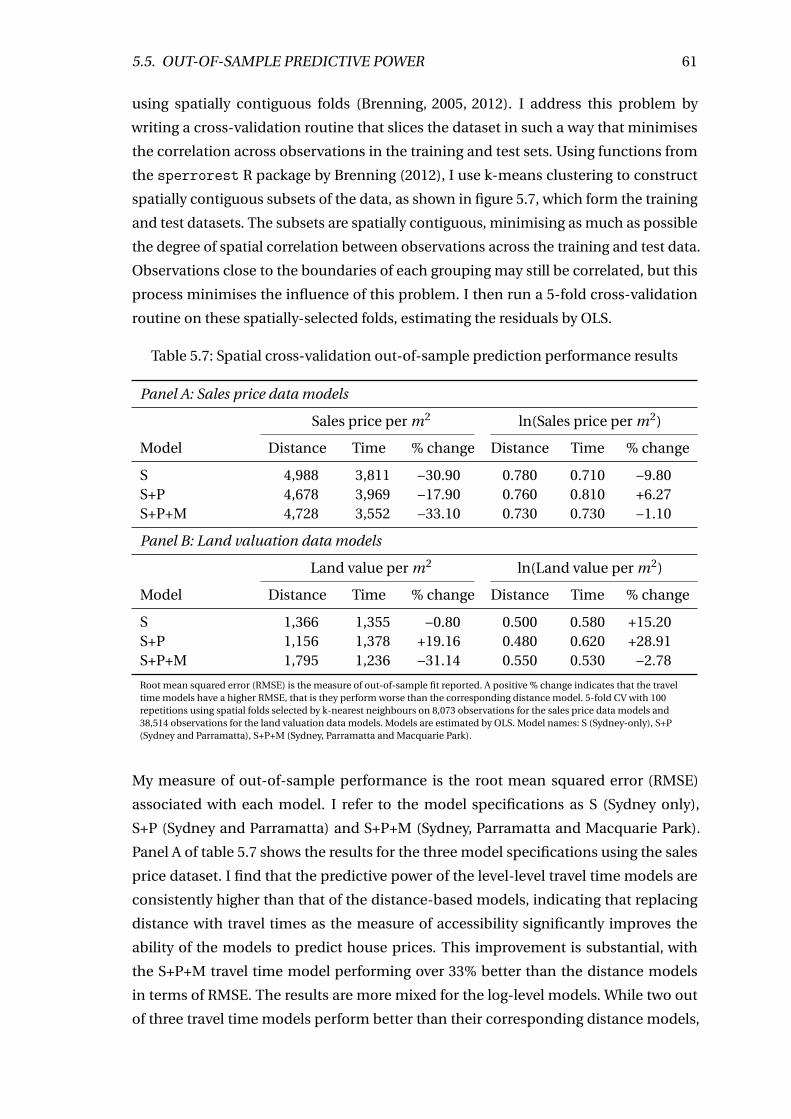
5.5. OUT-OF-SAMPLE PREDICTIVE POWER 61

using spatially contiguous folds (Brenning, 2005, 2012). I address this problem by

writing a cross-validation routine that slices the dataset in such a way that minimises

the correlation across observations in the training and test sets. Using functions from

the sperrorest R package by Brenning (2012), I use k-means clustering to construct

spatially contiguous subsets of the data, as shown in figure 5.7, which form the training

and test datasets. The subsets are spatially contiguous, minimising as much as possible

the degree of spatial correlation between observations across the training and test data.

Observations close to the boundaries of each grouping may still be correlated, but this

process minimises the influence of this problem. I then run a 5-fold cross-validation

routine on these spatially-selected folds, estimating the residuals by OLS.

Table 5.7: Spatial cross-validation out-of-sample prediction performance results

Panel A: Sales price data models

Sales price per m2 ln(Sales price per m2)

Model Distance Time % change Distance Time % change

S 4,988 3,811 −30.90 0.780 0.710 −9.80S+P 4,678 3,969 −17.90 0.760 0.810 +6.27S+P+M 4,728 3,552 −33.10 0.730 0.730 −1.10

Panel B: Land valuation data models

Land value per m2 ln(Land value per m2)

Model Distance Time % change Distance Time % change

S 1,366 1,355 −0.80 0.500 0.580 +15.20S+P 1,156 1,378 +19.16 0.480 0.620 +28.91S+P+M 1,795 1,236 −31.14 0.550 0.530 −2.78

Root mean squared error (RMSE) is the measure of out-of-sample fit reported. A positive % change indicates that the traveltime models have a higher RMSE, that is they perform worse than the corresponding distance model. 5-fold CV with 100repetitions using spatial folds selected by k-nearest neighbours on 8,073 observations for the sales price data models and38,514 observations for the land valuation data models. Models are estimated by OLS. Model names: S (Sydney-only), S+P(Sydney and Parramatta), S+P+M (Sydney, Parramatta and Macquarie Park).

My measure of out-of-sample performance is the root mean squared error (RMSE)

associated with each model. I refer to the model specifications as S (Sydney only),

S+P (Sydney and Parramatta) and S+P+M (Sydney, Parramatta and Macquarie Park).

Panel A of table 5.7 shows the results for the three model specifications using the sales

price dataset. I find that the predictive power of the level-level travel time models are

consistently higher than that of the distance-based models, indicating that replacing

distance with travel times as the measure of accessibility significantly improves the

ability of the models to predict house prices. This improvement is substantial, with

the S+P+M travel time model performing over 33% better than the distance models

in terms of RMSE. The results are more mixed for the log-level models. While two out

of three travel time models perform better than their corresponding distance models,

62 CHAPTER 5. RESULTS AND DISCUSSION

the scale of the improvement in predictive power is less substantial. In addition, the

S+P travel time model does not outperform the equivalent distance model. Overall,

these results strongly suggest that travel times are a better measure of accessibility to

employment, especially for industry applications where predictive power is the most

important measure.

I also compute out-of-sample prediction scores for the land value data models, where

the results are more mixed. I find that half of the land value travel time models

outperform their distance-based equivalents. For the Sydney-only model, the log-

level distance model outperforms the log-level travel time model, while the level-level

models have very similar predictive power. When using the S+P model, both the level-

level and log-level travel time models perform worse than the distance models. Thus,

when only accessibility to the Sydney CBD is considered, existing distance-based

models are sufficient to explain the variation in land values across Greater Sydney.

However, the level-level S+P+M travel time model improves out-of-sample fit by 31%

compared to the distances-based model. Similarly, the log-level specification produces

a smaller improvement of around 2.8%. Thus, incorporating additional travel time data

leads to a substantial improvement in the predictive power of hedonic price models

when a polycentric city structure is considered.

5.6 Willingness to pay calculations

I compute the present discounted value of reducing future travel times in this section

and convert these estimates to hourly willingness to pay (WTP). Assuming an average

land value of $826,700 and property sales price of $1.15 million, and commute times

of 49 minutes by road and 69 minutes by public transport, I estimate that the average

property price increase resulting from a 1 minute decrease in all future commuting trips

by road is about $3,396. This value can be considered to be the present value of future

travel time savings that are capitalised into the value of the house. For public transport,

the present discounted value of a 1 minute reduction in trip times is about $4,140. For

the land value data models, the average land value uplift from a 1 minute decrease in

future road commutes is about $3,479. For public transport, the present discounted

value of a 1 minute reduction in trip times is about $2,159. For the land value models,

this value represents the present value of future travel time savings that are capitalised

into the value of the land.

While the present value of total future travel time savings are interesting, converting

these figures into willingness to pay for per trip savings are easier to understand

and interpret. Using assumptions detailed in Appendix K on the relevant discount

rate, number of hours worked per year and the number of working years remaining, I

5.7. ROBUSTNESS TESTS 63

calculate that commuters value a 1 hour reduction in driving times to Sydney at $27.22

per hour and a 1 hour reduction in public transport travel times at $33.19 per hour. In

comparison, I calculate from the land value models that commuters value a 1 hour

reduction in driving times to Sydney at $27.89 per hour and a 1 hour reduction in public

transport travel times at $17.31 per hour. This lower value for public transport for the

land value estimates is in line with previous results that find that the disutility of public

transport commute time to be lower than driving commute times. While the results

for the value of driving are consistent across the datasets, the value of public transport

times are divergent. I am unsure what is driving this difference and future research may

wish to further investigate this discrepancy.

These figures represent the central scenarios, but within the full range of reasonable

assumed values, this number varies from $18.76 to $52.05 per hour of driving and $22.33

to $61.94 per hour of public transport travel using the sales price models. In comparison,

the range of reasonable assumed values from the land value models are $18.76 to $52.05

per hour of driving and $11.64 to $32.30 per hour of public transport travel.

As a comparison, transport agencies often use 40% of the average wage rate as a

proxy for the amount that commuters are willing to pay to reduce their commute time.

However, the reliability of this figure is strongly disputed, for example, see Hensher

(2019) and Douglas and Jones (2018). Calculations using this assumption produce

an estimate of $17.20 per hour (40%× $42.99) (data sourced from Australian Bureau

of Statistics (ABS, 2019a, 2019b)). Thus, there are some substantial differences in the

estimated WTP from my study compared with the assumed values used in industry,

suggesting that if my results are more accurate, then transport improvements are likely

to be undervalued under the existing methodology. For full calculations see Appendix

K.

5.7 Robustness tests

I perform a range of robustness tests to check the sensitivity of results to different model

specifications and estimation methods for both the sales data and land valuations

data. I report the results of these tests in Appendix D and E. Overall, I find that my

results are robust to model specification and while the magnitudes of some estimates

change across estimation methods, for the most part the direction of the coefficients

are unchanged.

I re-estimate my models by OLS to investigate whether ignoring the effects of spatial

dependence have an effect on the results. I find that while the magnitudes of the

coefficients vary compared to the SEM results, the direction of the estimates mostly

64 CHAPTER 5. RESULTS AND DISCUSSION

remain the same. The magnitudes on the distance and travel time variables do not

vary in any systemic manner, indicating the OLS estimates are not consistently over or

underestimating the effects relative to the spatial models. These estimates are reported

in table D.1 of Appendix D for the sales price estimates and table E.1 of Appendix E for

the land valuation estimates.

Similarly, the results from estimating spatial autoregressive models (SARM) are also

similar to the main results in this chapter. Including indirect spillover effects in the

SARM increases the size of the effect observed as expected, but does not change the

sign of the results. The initial effects of accessibility changes are consistently larger

when indirect impacts are taken into account, but the marginal effect also diminishes

more rapidly, such that when compared to the other models, the marginal effect of

changes in accessibility zero out at similar distances and travel times. For the SARMs,

estimates are reported in tables D.3 and D.6 of Appendix D for the sales price models

and tables E.3 and E.6 of Appendix E for the land valuation models.

I test whether my results are robust to respecifying the dependent variable as land

values and sales prices per square metre instead of the natural logarithms. I find that

the level-level models perform worse in terms of explanatory power compared to the

log-level models, likely due to the presence of outliers and a non-linear relationship in

the dependent variable that the level-level models capture less well compared with the

log-level models. However, the signs of the results mostly do not change, indicating that

the results are robust to this change of specification as well. These results are reported

in table D.2 of Appendix D for the sales price models and table E.2 of Appendix E for the

land valuation models. I also compare the performance of log-log models with log-level

models, finding that the preferred log-level specification outperforms in all cases. See

table D.10 of Appendix D for sales data results and table E.10 of Appendix E for land

value data results.

As an additional check, I run the sales price and land value models using sales price and

land values as the dependent variable, without dividing the values by land area. The

explanatory power of this model specification is consistently lower than both the level

sales price/land value per square metre and the natural logarithm of sales price/land

values. This result makes sense as the preferred models take into account the fact that

accessibility does not change as a function of land area. While the magnitudes of the

estimates vary, the results are qualitatively similar to the main models. I report the

results for the sales price models in table D.9 of Appendix D and the land value models

in table E.9 of Appendix E.

5.8. LIMITATIONS 65

5.8 Limitations

This Part investigates whether travel time data is a useful addition to hedonic modelling

of property prices. I find evidence supporting the use of travel time models over

distance-based models in both explanatory and predictive applications, with these res-

ults mostly robust to different model specifications and estimation methods. However,

it is important to discuss the limitations of my findings and suggest pathways for future

researchers to address these issues.

While the sales data models outperform the distance models in terms of explaining in-

sample variation of property sales prices, this is not true of the models estimated on the

land valuations data. The AIC of the distance-based land valuations models indicates

that they have a superior fit relative to the equivalent travel time models. A possible

explanation for this is the way that the land value data is constructed. While the land

values data is of high quality, it fundamentally does not reflect market outcomes in the

way that housing sales data does. Land valuation data is constructed by professional

valuers overseen by the NSW Valuer General and it is possible that their valuation of

the land’s accessibility uses distance as a proxy instead of travel times. Similarly, while

the travel time specifications of the sales data models significantly outperform in terms

of out-of-sample predictive ability compared to the distance specifications, the results

are mixed for the land value data models. Some models provided large improvements

in out-of-sample prediction using travel time data relative to distance data, while other

specifications suggested that the travel time models actually performed worse. Future

research should examine the discrepancy between the conclusions reached using sales

data and land value data.

The behaviour of the coefficients on the Macquarie Park data cause some concern. In

most of the models specified, the travel times and distance to Macquarie Park suggest

that households would pay to live further away from that centre, which goes against

theoretical expectations that people prefer to live closer to amenity and employment.

There are some possible explanations for this result. The first is that Macquarie Park is

not a sufficiently important centre to model, such that when it is included in the model,

some of the effects of the larger centres, i.e. Sydney CBD, spill over into the coefficient.

This explanation potentially makes sense, as moving further away from Sydney CBD

necessitates moving closer to Macquarie Park if, for example you head in a northerly

direction. As previously discussed, there is also a potential trilateration problem. As a

result, the coefficients may have unexpected values as the model attempts to impose a

ceteris paribus interpretation when one is not possible.

66 CHAPTER 5. RESULTS AND DISCUSSION

Future research should aim to incorporate monetary costs of travel as monetary travel

costs and travel time costs are positively correlated, meaning that it is likely that

the coefficients on the time travel cost parameters are biased upward. Note that the

monetary cost differential between travel modes is quite small, especially compared

to the increase in travel times that would be faced by commuters who choose to

change modes to save money, meaning this bias should be relatively minor. It would

also be interesting to decompose public transport travel times into walking, waiting,

interchange and actual travelling times, as prior research has found that commuters

tend to value these components differently. However, it is currently not possible to

extract individual travel time components from the Google Maps travel time API data,

but perhaps this will be added as a feature in the future.

While financial constraints prevented me from doing so in this thesis, including travel

time measures to non-employment amenities is an important extension to modelling

the value of variations in accessibility of different locations. Access to amenities such

as schools, shopping centres and parkland are likely to be valued by commuters as

well as employment. Another future extension to this project is to collect travel time

data for the same sample of properties in the future, say in three to five years time.

This allows the researcher to construct a panel dataset of travel times and land values,

allowing for property-specific fixed effects to be controlled and better isolating the

causal effect of changes in travel times. This would resolve a number of omitted

variable problems that are associated with property-specific or neighbourhood-specific

unobserved attributes.

The dispersed nature of employment in Sydney is a shortcoming of the theoretical

basis and empirical methods used in this Part. My estimation method assumes that

employment in three designated major centres are what are valued by households. This

is a limiting assumption given that only 14% of workers (312,310 of 2,262,010) actually

work in the Sydney CBD, 2% work in Parramatta and another 2% work in Macquarie

Park. The second largest employment “location” in Sydney with 4% of workers is

actually those with no fixed workplace address (ABS, 2016). In addition, access to

other amenities such as parks, schools and shopping centres may also be valued by

households and could be included in the travel time dataset with additional resources.

However, compared to previous work that has generally assumed a monocentric city,

my inclusion of three centres produces a more realistic model of Sydney.

One alternative specification that may ameliorate this issue are gravity models, which

have been widely used in regional science and civil engineering (Ahlfeldt, 2010; Kau &

Sirmans, 1979). With the collection of a large amount of additional data, it would be

5.8. LIMITATIONS 67

possible to estimate a gravity-based specification of the hedonic model estimated in this

Part. The gravity model is based on two assumptions (Handy & Niemeier, 1997). The first

is that areas with greater employment mass or greater amenity are more desirable. The

second is that areas that are more accessible are also more desirable. By applying these

principles, a gravity model approach would involve constructing a single employment-

weighted travel time from each property.

One implementation would use granular employment data from the Census at the SA1

level and scrape travel times from Google Maps for each pair of SA1s i and j as the

measure of travel cost ci j . This measure is then used to weight employment E j at each

location j , creating a measure of accessibility Ai for each location i to employment

as shown in equation 5.9. Properties can then be assigned their corresponding SA1,

creating a more accurate summary measure of employment accessibility for each

property that should be superior to the three centres approach I have used.

Ai =n∑

j=1E j f (ci j ) (5.9)

However, combining this specification with my travel time data approach is much more

resource intensive. Using the idealised SA1 method involves computing travel times for

n(n −1) pairs of locations. Given there are 11,171 SA1s in Sydney, this results in over

124 million API calls. A less granular compromise is to use Travel Zones as defined

by Transport for NSW, which are each designed to have standardised trip generation

levels. There are 2,722 Travel Zones within Greater Sydney, which would require a

comparatively smaller 7.4 million API calls.

C H A P T E R 6

Conclusion

6.1 Policy implications

My research has numerous implications for industry and government. My new hedonic

pricing models for property prices are a significant improvement on the existing

distance-based modelling approaches. My results show that using travel times as a

measure of accessibility instead of proxying using distances can substantially improve

the out-of-sample predictive accuracy of these models, which is the key performance

indicator for valuing new properties or land lots. This finding has implications for

automated valuation modelling, which aims to automate the work performed by

professional valuers to improve the scale and consistency of property valuations.

These results also have applications in infrastructure cost-benefit analysis (CBA). One

of the main benefits measured by a CBA is the value of travel time savings for users

of the new transport infrastructure. As previously discussed, existing CBA guidelines

call for the use of a crude approximation that takes 40% of average hourly wages as the

value of travel time savings to commuters (Douglas & Jones, 2018; Hensher, 2019). These

assessments could be improved by replacing this measure with the more empirically-

derived willingness to pay (WTP) estimates for travel time savings that I calculate in

this Part using cross-sectional models, but also from my estimates in the next Part of

my thesis using a difference in differences approach. Better measures of WTP mean

that CBA more accurately quantifies the true costs and benefits of infrastructure, which

would improve the allocation of scarce public investment funds to the projects that

provide the greatest benefit to the community.

Infrastructure often suffers from funding difficulties leading to cancellations or delays.

Value capture has been suggested as a mechanism for governments to fund projects

by taxing those who benefit the most from new infrastructure (Medda, 2012). However,

many proposed value capture mechanisms have been criticised for arbitrarily classify-

ing some properties as beneficiaries of a project while other properties across the road

are exempted from paying the tax due to a lack of accurate measures of who actually

68

6.2. CONCLUDING REMARKS 69

benefits from the project (Terrill & Emslie, 2017). Increasing the granularity of project

benefit measurement by using travel time savings instead of distance cutoffs may

improve the equity of value capture funding mechanisms by more accurately applying

them to properties that are receiving benefits from new transport infrastructure.

My estimates of the value of congestion to road commuters provide insight into

proposals to implement congestion charging for driving into the city centre during

the morning peak. Congestion charging has been proposed as a method to ration

scarce road space to the users who have the highest WTP to drive into congested

city centres (Terrill, Moran & Ha, 2019). My estimates of the WTP to reduce additional

travel time due to congestion are an upper bound on a potential congestion charge for

travelling into the Sydney CBD. This estimate can be combined with traffic modelling

that computes the reduction in congestion from imposing a congestion charge to

predict the correct toll to levy on drivers. Similarly, motorway operators may also use the

congestion estimates as a guide to setting motorway tolls by comparing the decrease in

drive times from using the toll road versus untolled, but congested surface roads. For

example, since the estimate of the value of 1 hour of congestion is $17.64, then if the

tolled motorway saved an hour in relative travel times, this implies drivers would be

willing to pay up to $17.64 to drive on it.

6.2 Concluding remarks

Variation in property values reveal commuters’ willingness to pay to reduce their

travel times. I extend existing hedonic modelling of property values in Sydney by

constructing a unique dataset of travel times using Google Maps and estimating the

relationship between property values and travel times in Sydney. I find that using

travel times as the measure of accessibility significantly improves the goodness of fit

of hedonic property pricing models compared to existing models using straight-line

distances as measured by the AIC for the spatial regression models and R2 for the linear

models. Adding major employment sub-centres such as Parramatta and Macquarie

Park improve explanatory and predictive power of models and provide evidence in

favour of a polycentric city structure in Sydney. The travel time models also outperform

distance models in predicting property prices out-of-sample as measured by which

model minimises the RMSE. I also find evidence and estimate values for the disutility

that commuters place on congestion on their drive to work. However, the models

estimated using the land values dataset differ and do not find that travel time models

outperform distance models, but this result is likely to be driven by the methodology

used by valuers in constructing these estimates of land values.

70 CHAPTER 6. CONCLUSION

I estimate two spatial hedonic models: spatial error models and spatial autoregress-

ive models, in order to avoid spatial biases from autocorrelation in the errors and

dependent variable. These models have improved fits compared to equivalent models

estimated by OLS, which do not explicitly model the effects of spatial dependence. I

find that in most cases, the spatial error model provides a superior fit as measured by

the AIC.

These estimates of property value changes in relation to travel time changes are of

policy significance in the context of funding urban transport infrastructure through

capturing land value uplift. I find that drive times and public transit times significantly

explain a large amount of variation in property values across Sydney after controlling

for neighbourhood, demographic and zoning characteristics. I find that households

value accessibility to the Sydney CBD and Parramatta through both driving and public

transport modes and that these effects diminish as travel times increase, suggesting

commuters closest to the centre are more sensitive to changes in travel times.

Commuters tend to value reducing driving times to employment centres more than

reducing public transport travel times. This implies that commuters experience greater

disutility from driving than taking public transport, which makes sense as commuters

can do other things while on the train or bus, whereas distracted driving is dangerous.

Commuters also experience disutility from increased road congestion in addition to

that of free-flow drive times to all three employment centres.

However, access to Macquarie Park is not valued positively, with households signific-

antly preferring to have less access to Macquarie Park, which is an unusual result that

warrants further research. This may be the result of interactions between the variables

measuring accessibility to the other major centres, rather than a significant result

in itself. As travel times and property values are likely to be endogenous, especially

in a cross-sectional framework, these results should be interpreted from a long-run

equilibrium perspective, as opposed to a causal effect.

There is a discrepancy in the results from the sales price models and land valuation

models. While the results from the sales price models show that travel times produce

a material improvement in model fit and predictive power, the results are less clear

for the land value models. It is possible that this result is driven by the methodologies

used in constructing the land values dataset by the NSW Valuer General, as the valuers

may be using distance as an accessibility proxy, hence driving the results in this Part.

I propose a number of pathways for future research that may help to ameliorate

these problems, including using a gravity model approach to modelling accessibility to

6.2. CONCLUDING REMARKS 71

address dispersed employment in Sydney and adding additional accessibility measures

to better model household travelling preferences.

These findings have substantial implications for industry and research. They are the

first direct estimates of the present value of travel time savings and the value of

congestion for commuters in Sydney, improving on previous rent gradients estimated

using distance-based models at more aggregate levels. These estimates are useful for

industry with applications in automated valuation modelling, which would increase

the scalability and consistency of property valuation. My results also provide improved

valuations of commuter travel time savings, which are a key input into cost-benefit

analysis of infrastructure projects and hence could contribute to the better allocation

of scarce public funds for infrastructure.

Part II

Measuring Land Value Uplift: Difference

in Differences Estimates from Sydney

Metro Northwest

72

C H A P T E R 1

Introduction

Five announcements, four cancellations and 21 years later, Sydney Metro Northwest

opened to passenger service on 26 May 2019 and finally gave residents of north-

west Sydney an alternative to often delayed and unreliable bus services (Kontominas,

2019). Unreliable buses are annoying, but commuting in general creates disutility.

Commuters travelling from home to work incur monetary costs and the opportunity

cost of time from travelling. Commuting is also a mental and physical burden for most

individuals (Stutzer & Frey, 2008) and individuals have been shown to be willing to pay

to avoid these costs (McArthur et al., 2011). Hence, properties located in more accessible

locations contain the capitalised values of the willingness to pay for accessibility to

employment and amenities (Grislain-Letrémy & Katossky, 2014). This observation

motivates both Parts of this thesis, but in Part II, I address endogeneity challenges in

my earlier analysis caused by a cross-sectional approach by using a quasi-experimental

methodology. I conduct a difference in differences (DiD) analysis using a panel dataset

that exploits land value uplift generated by the opening of the Sydney Metro Northwest

rapid transit line. By exploiting variation in travel times and land values of properties

in the vicinity of the Metro, I am able to estimate the value that the average commuter

is willing to pay to reduce commute times.

I use a DiD approach with panel data to estimate the effect of changes in travel time

on land values. This approach is uncommon in the literature, which is mostly made up

of cross-sectional studies of housing prices on distances to transport facilities. These

studies are affected by potential omitted variables and endogeneity issues, meaning

they are limited in their causal interpretation. A smaller number of studies take a DiD

approach to repeated cross-sectional data, an improvement on single-period cross-

sections, but remain vulnerable to biased estimates if key determinants of house prices

are omitted. Simulation studies by Kuminoff et al. (2010) suggest that DiD estimators

are least prone to bias in the presence of omitted variables compared to cross-sectional

regression designs.

73

74 CHAPTER 1. INTRODUCTION

My DiD exploits the opening of Sydney Metro Northwest, a rapid transit railway line

in north-west Sydney running from Chatswood to Tallawong. The opening of this

line created a change in travel times for commuters living in properties within the

catchment area of stations while leaving other residents unaffected. Treated properties

are defined as those for which travel times to the Sydney CBD by metro and rail are now

faster than if they continued to take buses into the city. Control properties have a travel

time to the Sydney CBD that is faster if they continue to catch buses to the city rather

than switch modes to the new metro. Thus, the pre-existing location of properties acts

as a treatment assignment mechanism by determining whether or not that property

will benefit from the availability of the Metro. The magnitude of the treatment is the

change in travel times as a result of switching modes to the Metro, which measures

changes in accessibility to employment in Sydney. I use travel time data collected in

May 2019 to measure pre-Metro travel times, while data collected in July 2019 measures

post-Metro opening travel times. The value of accessibility is measured by changes in

land values across properties and time. I use land values from July 2012 as the measure

of pre-construction valuations and July 2018 as the measure of post-opening valuations

(as July 2019 data are not yet available).

Transport infrastructure projects focus on reducing travel times, not physically moving

locations closer to one another because it would be very expensive to attempt this. It

is likely what is valued by commuters is the travel time to a location, not the physical

distance travelled. Thus, I break with the traditional distance-based approach taken

by most of the literature (Mohammad, Graham & Melo, 2015; Mulley, Ma, Clifton,

Yen & Burke, 2016; Mulley & Tsai, 2016; Murray, 2016; Yen et al., 2018). Instead, I

scrape Google Maps travel time data for morning peak travel times from locations in

north-west Sydney to the Sydney CBD from before and after the Metro opened. Using

travel time data brings us closer to a true measure of accessibility, as stations are an

intermediary, not a final destination for commuters (S. Ryan, 1999). Thus, a travel time-

based approach is likely to be a better measure of accessibility to employment and

amenities.

Regressing changes in land values on changes in travel time across treated and control

properties, I find that households in north-west Sydney are willing to pay 0.36% more

for property that is located 1 minute closer to the Sydney CBD by public transport,

which is equivalent to an increase in land value of $3,190 per minute saved for the

average property relative to properties experiencing no accessibility improvement. By

treating this land value change as the capitalised present value of all future commuting

travel time savings, using assumptions on the relevant discount rate, number of hours

worked per year and the number of working years remaining in the average commuters’

75

career, I calculate that commuters value reducing their commute time at about $25 per

hour.

My analysis is the first econometric analysis of the Sydney Metro Northwest project,

which is the first rapid transit system in Australia. Thus, the results from this analysis

are different from any other transport mode previously analysed in this country. Existing

work has analysed most forms of transport around the world, including heavy rail, light

rail, rapid transit and bus rapid transit (see Higgins and Kanaroglou (2016), S. Ryan

(1999) for a review). There is a lack of consensus in the literature regarding the scale

of value uplift due to transport improvements, with most studies finding a significant

positive effect for decreasing distance and travel times. On the contrary, a number of

papers find unexpected opposite impacts or no significant change, indicating that the

returns of each transport project are highly influenced by idiosyncratic factors.

The DiD approach reduces the influence of omitted variable bias relative to other

approaches by controlling for time-invariant individual property characteristics (Ku-

minoff et al., 2010). I also control for local demographic and socio-economic trends

using data from the 2011 and 2016 Censuses to account for unbalanced pre-trends. The

sign and significance of land value change estimates are robust to the functional form

of the model and the results show the same direction when more traditional distance-

based models are estimated as well. Despite this quasi-experimental approach taken

to the data, endogeneity issues are not fully resolved. It is possible that some of the

assumptions required for DiD estimators to identify a causal effect may not hold in

both my data and the research designs employed in previous DiD studies of transport

projects. Thus, while my results are an improvement on cross-sectional findings, I do

not claim that the value uplift measured is a causal effect.

My estimates of hourly willingness to pay (WTP) for accessibility improvements have

direct application in infrastructure cost-benefit analysis (CBA). The key economic

benefit included in CBA is the value of travel time savings for infrastructure users and

hence accurate measures of the value of time are essential for correctly appraising

infrastructure projects. The more precise measures of WTP in this Part improve on

existing approximations, which use a proportion of average wages. Better estimates of

WTP enable policymakers to more accurately calculate the true costs and benefits of

infrastructure, improving the likelihood that scarce public funds are allocated to the

projects that provide the greatest benefit to the community.

My results also have implications for the development of value capture mechanisms

for funding infrastructure investments that are increasingly part of the policy debate

(Medda, 2012; Murray, 2016; Yen et al., 2018). Value capture is a proposed method for

76 CHAPTER 1. INTRODUCTION

funding the cost of infrastructure by taxing part of the benefit that accrues to nearby

residents in the form of increased property values as a result of the capitalisation of

accessibility improvements in the land value. Existing value capture methods that are

based on distance cutoffs are criticised for arbitrarily assigning properties within a

certain distance to a taxed group, while neighbouring properties just outside are not

taxed (Terrill & Emslie, 2017). In addition, the use of distances means that a proxy

for accessibility is being used instead of a direct measure. By using travel times, a

continuous variable that directly measures changes in accessibility, I provide a solution

to this problem that may enable a mechanism that more equitably levies households

proportionately to the accessibility gain they receive from new transport infrastructure

investments.

C H A P T E R 2

Literature review

There is a substantial literature measuring value uplift as a result of new transport pro-

jects (see S. Ryan (1999) and Higgins and Kanaroglou (2016) for a comprehensive review

of the literature). These studies have examined most forms of transport, including rapid

transit, heavy rail, light rail, bus rapid transit and motorways. This literature review

focuses on railway studies as this is most similar to the Sydney Metro project I examine.

I discuss the choices that previous researchers have made when measuring accessibility

and land value, as well as model specification and functional form, and the implications

this has for my research.

Improved accessibility is the main benefit imparted by transport infrastructure im-

provements. However, accessibility can be a difficult concept to quantify as shown

by a substantial literature devoted to measurements of this concept that struggle to

reach a consensus. Urban theory treats accessibility as having two dimensions: an

attraction element and an impedance element. Commuters are attracted to certain

locations that bring benefits such as amenities or employment. However, travel costs

create an impedance to reaching these destinations and thus commuters engage in

a personal cost-benefit decision process that aggregates into city-wide travel patterns

(Handy & Niemeier, 1997). The most common way of measuring changes in accessibility

effectively sidesteps the issue, using the distance of properties to the transport facility

as a proxy (Cervero & Kang, 2011; Higgins & Kanaroglou, 2016; Mohammad et al., 2015;

Mulley & Tsai, 2016; Murray, 2016; Yen et al., 2018). This approach may not accurately

reflect changes in travel costs as “a transportation facility is not a final destination; it

is an intermediary source of connection between an origin and destination.” (S. Ryan,

1999). While many of these studies have found results that are in line with theoretical

expectations (an inverse relationship between distance from the station and property

values), this approach is problematic from a theoretical perspective.

The choice of distance cutoff is essentially arbitrary, with different papers specifying a

variety of distances. The most popular approach is to group properties into discrete bins

that are based on varying distances from the nearest station. For example, Mohammad

77

78 CHAPTER 2. LITERATURE REVIEW

et al. (2015) uses three bins, for properties located between 0–500 m, 500–1000 m and

1000–1500 m of Dubai Metro stations. Similarly, Murray (2016) classifies properties

located within 2 km from Gold Coast Light Rail Transit (GCLRT) stops into a series of

bins at 100 m intervals. This binning method allows for variation in the effect of the

transport project across space to be captured. An alternative approach is to classify

properties in a binary control/treatment way. Yen et al. (2018) uses this approach

by classifying properties within 800 m of each GCLRT stop as treated properties, and

properties between 800–1600 m away from stops as control properties. This method

is more restrictive, as it averages out the effect on all treated properties into one value

and does not allow varying accessibility to the transport facility to have a differing

effect.

A more direct measure of commuting costs is to examine changes in travel times as a

result of a project. While this measure does not capture the monetary component of

transport costs, it better captures the time dimension of commuting costs as theorised

in the AMM model compared to using distances to facilities. This approach is less

common in the literature, with a review by Higgins and Kanaroglou (2016) finding that

out of 106 North American studies surveyed, only four used changes in travel times as

a measure of accessibility. However, usage of travel time data has started to appear in

more recent work, such as in analysis of changes in accessibility from the Tyne and

Wear Metro in north-east England by Du and Mulley (2012). Thus, I contribute to this

literature by applying travel time data in a difference in differences (DiD) framework to

analyse the effect of accessibility changes on land value.

The dependent variable in studies of value uplift needs to effectively measure the

impact of the transport projects on property values. The majority of studies in the

literature tend to favour the use of market sales data from property transactions

(Higgins & Kanaroglou, 2016). They argue that this choice better represents the market

price of transport accessibility compared to alternate measures (Mohammad et al.,

2015; Mulley & Tsai, 2016; Yen et al., 2018). However, a number of papers elect to

make use of land valuations data (Higgins & Kanaroglou, 2016; Murray, 2016). I have

elected to follow this approach as it enables me to construct a balanced panel dataset,

which controls for unobserved time-invariant heterogeneity in the individual properties

(Murray, 2016), reducing the risk of omitted variable bias. In addition, using property

sales data means that the DiD is performed using repeated cross-sections, which is

vulnerable to omitted variable bias if all the properties of the land and structure are

not controlled for (Kuminoff et al., 2010). Controlling for the characteristics of the

structure sitting on top of the land is not a problem when land valuations data are

used. Overall, out of all the studies surveyed by Higgins and Kanaroglou (2016), 80% use

79

sales price data, 10% use land valuations data and the remaining 10% use market rents.

An alternative approach is the pseudo-panel data method constructed by Mohammad

et al. (2015), which groups similar properties together that were sold at different times

into aggregate units for analysis. These time-aggregated units are then treated as if they

were individual panel data observations.

Measures of willingness to pay for improved accessibility are sensitive to the choice

of model structure and time scale, which in my case is affected by data availability.

The choice of model structure has a substantial effect on the signs and magnitudes of

estimated value uplift. Kuminoff et al. (2010) conduct a simulation study that compares

cross-sectional models with and without spatial fixed effects, first differenced models

and DiD models. The study finds that overall, the DiD estimator is best suited to hedonic

estimation with panel data, when measured in terms of the bias of the estimates in

the presence of omitted variables. The magnitudes of estimates from cross-sectional

hedonic models also tend to be larger than the estimates produced by DiD class models

(Mohammad et al., 2015). This difference further motivates my use of a DiD estimator

using a panel dataset.

There is also variation in the extent of uplift measured in the literature as a result of

choices of time scale. There is considerable variation in the timing of value uplift due

to idiosyncrasies of individual projects (Yen et al., 2018). Most of the literature aims

to capture the total amount of land value uplift as a result of a transport project by

collecting property data from before the announcement of a project to well after a

project has been opened to passenger service (Du & Mulley, 2007; Mohammad et al.,

2015; Murray, 2016). For example, Mohammad et al. (2015) collect sales data between

2007 and 2011 to measure the effect of the opening of the Dubai Metro in 2009. In

contrast, Murray (2016) uses up to 69 years of land valuation panel data for properties

in the Gold Coast region to measure the total value uplift of the Gold Coast Light Rail.

He finds that aggregate land values have increased by $300 million as a result of the

project, which represents around 25% of the project cost. Yen et al. (2018) instead

examine timing effects on land value uplift — a less well-researched area — using data

from prior to project announcement (1996), before financial commitment (2002), post-

commitment (2006), construction (2011) and opening (2016). They find that prices

start to increase after announcement, but the largest increases do not occur until

firm financial commitments have been made by government. Increases slow during

construction and operation periods. While this is interesting, external validity may be

of concern due to the unique circumstances of each infrastructure project. For example,

the long history of announcements and cancellations of the project I am studying may

80 CHAPTER 2. LITERATURE REVIEW

affect the responsiveness of land values in north-west Sydney to the announcement of

the line in 2011.

These differing specifications have resulted in variation in the size of estimated effects

of changes in accessibility. It can also be difficult to compare projects due to their

choice of transit mode (for example, value uplift from a motorway project is likely very

different to light rail), distance measures, dependent variable and functional forms. A

survey of the literature by Higgins and Kanaroglou (2016) finds very large variation in

estimated effects of North American heavy rail projects, with value changes estimated

for properties within 400 m of railway stations ranging from –49% to +49%. Analysis

on the effects of the Mandurah railway line in Perth by McIntosh et al. (2014) find

increases in land value of 28%, 13% and 8% for properties within 400 m, 800 m and

1600 m of stations. Although there has been previous research on value uplift effects

from rapid transit lines internationally (for example, Du and Mulley (2007), Mohammad

et al. (2015)), Sydney Metro is the first rapid transit system in Australia meaning there

is little domestic research on this mode of transport. Mohammad et al. (2015) find

significant and positive uplift for residential properties within 1 km of Dubai Metro

stations (7.8% increase) and significant effects for commercial properties within 1.5 km

of stations (41% increase). While international comparisons provide some guidance

as to expected effects, there is a significant opportunity for me to contribute to the

literature with my preliminary estimates of land value uplift and willingness to pay for

improved accessibility from analysing Sydney Metro Northwest.

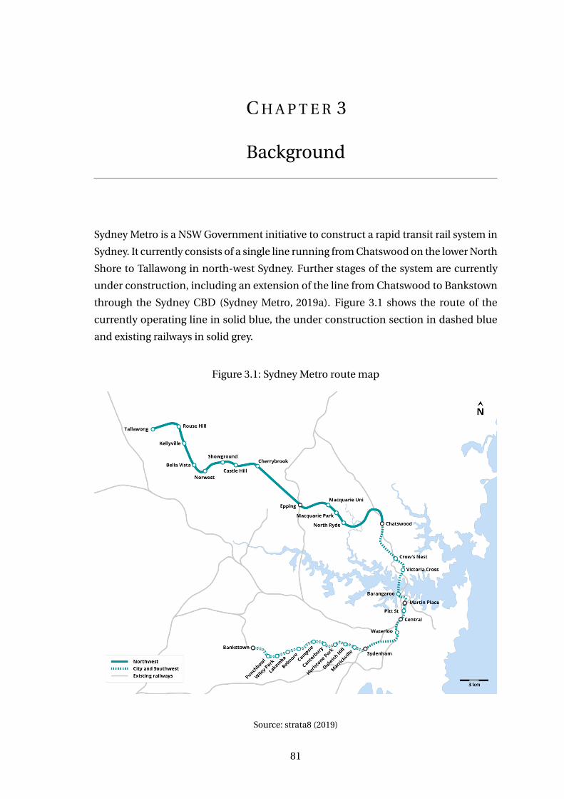
C H A P T E R 3

Background

Sydney Metro is a NSW Government initiative to construct a rapid transit rail system in

Sydney. It currently consists of a single line running from Chatswood on the lower North

Shore to Tallawong in north-west Sydney. Further stages of the system are currently

under construction, including an extension of the line from Chatswood to Bankstown

through the Sydney CBD (Sydney Metro, 2019a). Figure 3.1 shows the route of the

currently operating line in solid blue, the under construction section in dashed blue

and existing railways in solid grey.

Figure 3.1: Sydney Metro route map

Source: strata8 (2019)

81

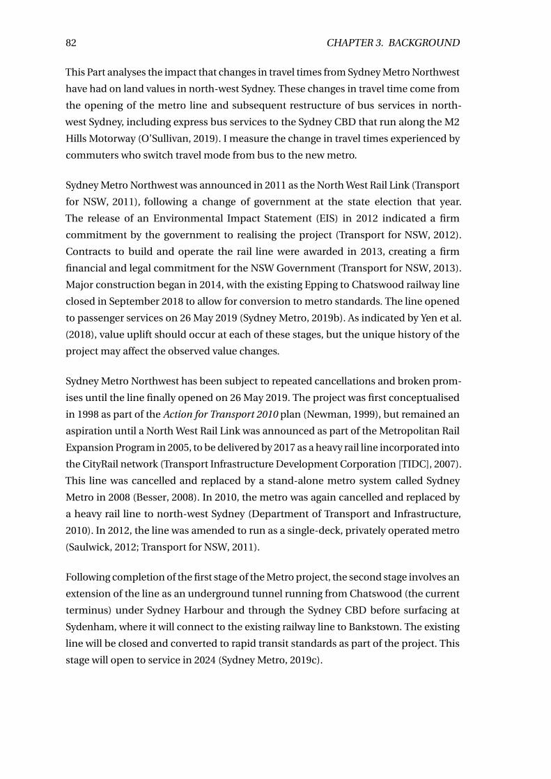
82 CHAPTER 3. BACKGROUND

This Part analyses the impact that changes in travel times from Sydney Metro Northwest

have had on land values in north-west Sydney. These changes in travel time come from

the opening of the metro line and subsequent restructure of bus services in north-

west Sydney, including express bus services to the Sydney CBD that run along the M2

Hills Motorway (O’Sullivan, 2019). I measure the change in travel times experienced by

commuters who switch travel mode from bus to the new metro.

Sydney Metro Northwest was announced in 2011 as the North West Rail Link (Transport

for NSW, 2011), following a change of government at the state election that year.

The release of an Environmental Impact Statement (EIS) in 2012 indicated a firm

commitment by the government to realising the project (Transport for NSW, 2012).

Contracts to build and operate the rail line were awarded in 2013, creating a firm

financial and legal commitment for the NSW Government (Transport for NSW, 2013).

Major construction began in 2014, with the existing Epping to Chatswood railway line

closed in September 2018 to allow for conversion to metro standards. The line opened

to passenger services on 26 May 2019 (Sydney Metro, 2019b). As indicated by Yen et al.

(2018), value uplift should occur at each of these stages, but the unique history of the

project may affect the observed value changes.

Sydney Metro Northwest has been subject to repeated cancellations and broken prom-

ises until the line finally opened on 26 May 2019. The project was first conceptualised

in 1998 as part of the Action for Transport 2010 plan (Newman, 1999), but remained an

aspiration until a North West Rail Link was announced as part of the Metropolitan Rail

Expansion Program in 2005, to be delivered by 2017 as a heavy rail line incorporated into

the CityRail network (Transport Infrastructure Development Corporation [TIDC], 2007).

This line was cancelled and replaced by a stand-alone metro system called Sydney

Metro in 2008 (Besser, 2008). In 2010, the metro was again cancelled and replaced by

a heavy rail line to north-west Sydney (Department of Transport and Infrastructure,

2010). In 2012, the line was amended to run as a single-deck, privately operated metro

(Saulwick, 2012; Transport for NSW, 2011).

Following completion of the first stage of the Metro project, the second stage involves an

extension of the line as an underground tunnel running from Chatswood (the current

terminus) under Sydney Harbour and through the Sydney CBD before surfacing at

Sydenham, where it will connect to the existing railway line to Bankstown. The existing

line will be closed and converted to rapid transit standards as part of the project. This

stage will open to service in 2024 (Sydney Metro, 2019c).

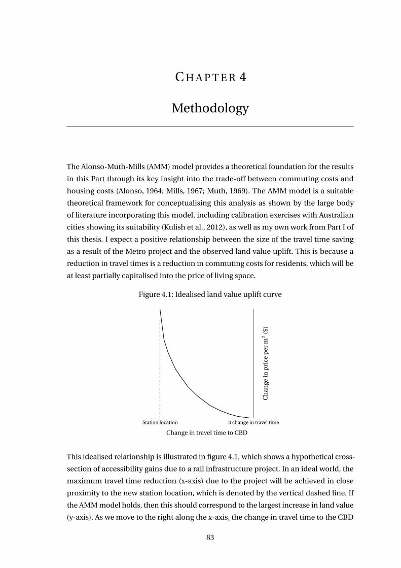
C H A P T E R 4

Methodology

The Alonso-Muth-Mills (AMM) model provides a theoretical foundation for the results

in this Part through its key insight into the trade-off between commuting costs and

housing costs (Alonso, 1964; Mills, 1967; Muth, 1969). The AMM model is a suitable

theoretical framework for conceptualising this analysis as shown by the large body

of literature incorporating this model, including calibration exercises with Australian

cities showing its suitability (Kulish et al., 2012), as well as my own work from Part I of

this thesis. I expect a positive relationship between the size of the travel time saving

as a result of the Metro project and the observed land value uplift. This is because a

reduction in travel times is a reduction in commuting costs for residents, which will be

at least partially capitalised into the price of living space.

Figure 4.1: Idealised land value uplift curve

Station location 0 change in travel time

Change in travel time to CBD

Ch

ange

inp

rice

per

m2

($)

This idealised relationship is illustrated in figure 4.1, which shows a hypothetical cross-

section of accessibility gains due to a rail infrastructure project. In an ideal world, the

maximum travel time reduction (x-axis) due to the project will be achieved in close

proximity to the new station location, which is denoted by the vertical dashed line. If

the AMM model holds, then this should correspond to the largest increase in land value

(y-axis). As we move to the right along the x-axis, the change in travel time to the CBD

83

84 CHAPTER 4. METHODOLOGY

falls towards zero and the model predicts that the corresponding positive change in

land values should also fall to zero, until there is no change in travel time and no land

value uplift.

Like in Part I of this thesis, I treat land values as a composite value made up of a bundle

of individual observable attributes of the block of land, one of which is accessibility to

employment. This framework draws on an extensive literature based on the hedonic

pricing model conceptualised by Rosen (1974). Using a multiple linear regression

model, I can estimate the implicit prices for each attribute, including the willingness to

pay for accessibility to employment. The application of hedonic methods in this Part is

otherwise the same as in Part I.

In order to measure the effect of changes in travel time on property values in Sydney,

I use a difference in differences (DiD) approach to exploit variation in travel times

as a result of the Sydney Metro Northwest project. The DiD approach is a quasi-

experimental method that can be used to exploit natural experiments where only a

fraction of a given population is exposed to a treatment and this population is observed

both prior to and after the treatment takes effect (Abadie, 2005). I estimate the DiD

model in Stata (StataCorp, 2015) using the reghdfe package written by Correia (2016),

which estimates linear regression models with multi-level fixed effects.

The policy change is the opening of Sydney Metro Northwest and the treatment that

results is improved accessibility to employment and amenities due to better rail access

in the area. Treatment assignment is determined by whether post-Metro travel times by

switching to a combination of metro and rail to the Sydney CBD are faster than the post-

Metro travel time by bus to the Sydney CBD for each property. The treatment variable

is a continuous variable measuring travel times, meaning that the magnitude of the

effect is allowed to vary depending on the extent of the travel time savings. Variation in

travel times are measured by collecting travel time in May 2019 (prior to the opening

of Sydney Metro) and July 2019 (after the opening of the line). To measure the value

placed on these improvements in accessibility, I use data from July 2012 measuring land

values prior to the start of construction of the metro as the pre-treatment dependent

variable and data from July 2018 as the post-treatment dependent variable to measure

land values after opening. While the Metro did not open until late May 2019, July 2018

data is the most recent currently available and hence I have been forced to rely on older

data.

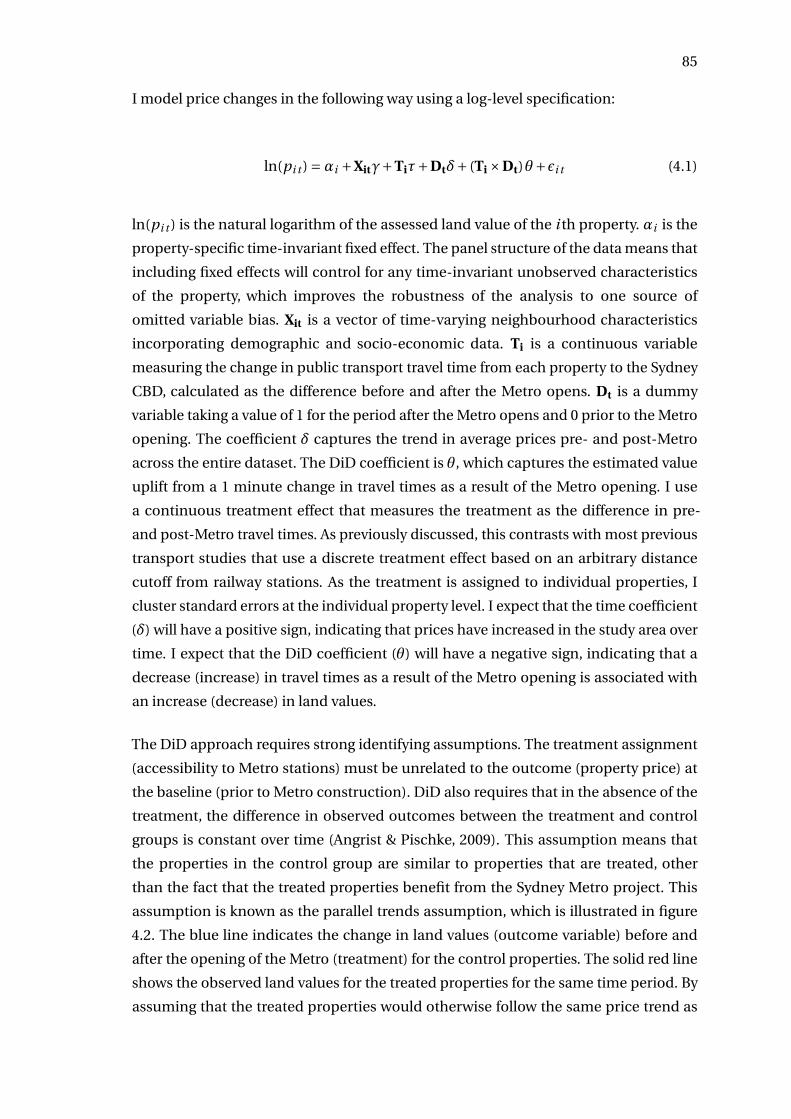
85

I model price changes in the following way using a log-level specification:

ln(pi t ) =αi +Xitγ+Tiτ+Dtδ+ (Ti ×Dt)θ+εi t (4.1)

ln(pi t ) is the natural logarithm of the assessed land value of the i th property. αi is the

property-specific time-invariant fixed effect. The panel structure of the data means that

including fixed effects will control for any time-invariant unobserved characteristics

of the property, which improves the robustness of the analysis to one source of

omitted variable bias. Xit is a vector of time-varying neighbourhood characteristics

incorporating demographic and socio-economic data. Ti is a continuous variable

measuring the change in public transport travel time from each property to the Sydney

CBD, calculated as the difference before and after the Metro opens. Dt is a dummy

variable taking a value of 1 for the period after the Metro opens and 0 prior to the Metro

opening. The coefficient δ captures the trend in average prices pre- and post-Metro

across the entire dataset. The DiD coefficient is θ, which captures the estimated value

uplift from a 1 minute change in travel times as a result of the Metro opening. I use

a continuous treatment effect that measures the treatment as the difference in pre-

and post-Metro travel times. As previously discussed, this contrasts with most previous

transport studies that use a discrete treatment effect based on an arbitrary distance

cutoff from railway stations. As the treatment is assigned to individual properties, I

cluster standard errors at the individual property level. I expect that the time coefficient

(δ) will have a positive sign, indicating that prices have increased in the study area over

time. I expect that the DiD coefficient (θ) will have a negative sign, indicating that a

decrease (increase) in travel times as a result of the Metro opening is associated with

an increase (decrease) in land values.

The DiD approach requires strong identifying assumptions. The treatment assignment

(accessibility to Metro stations) must be unrelated to the outcome (property price) at

the baseline (prior to Metro construction). DiD also requires that in the absence of the

treatment, the difference in observed outcomes between the treatment and control

groups is constant over time (Angrist & Pischke, 2009). This assumption means that

the properties in the control group are similar to properties that are treated, other

than the fact that the treated properties benefit from the Sydney Metro project. This

assumption is known as the parallel trends assumption, which is illustrated in figure

4.2. The blue line indicates the change in land values (outcome variable) before and

after the opening of the Metro (treatment) for the control properties. The solid red line

shows the observed land values for the treated properties for the same time period. By

assuming that the treated properties would otherwise follow the same price trend as

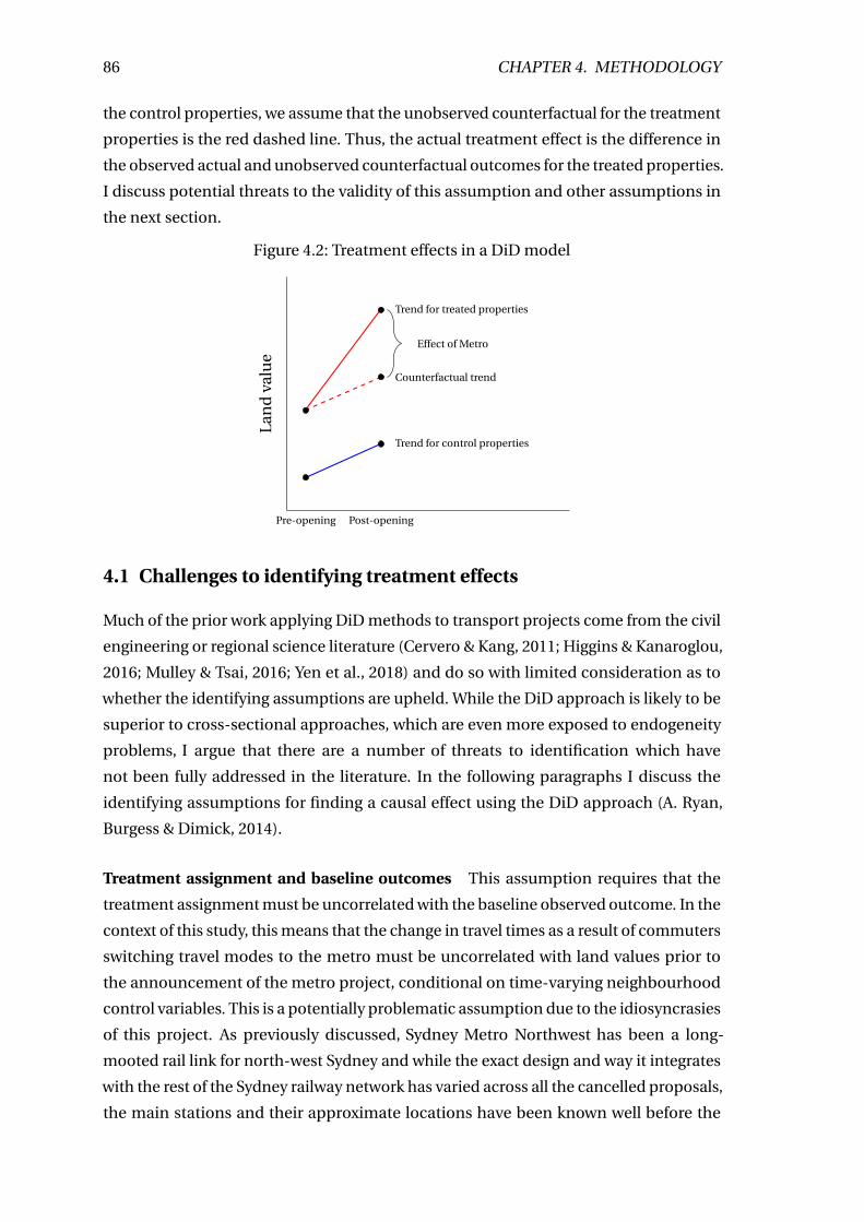
86 CHAPTER 4. METHODOLOGY

the control properties, we assume that the unobserved counterfactual for the treatment

properties is the red dashed line. Thus, the actual treatment effect is the difference in

the observed actual and unobserved counterfactual outcomes for the treated properties.

I discuss potential threats to the validity of this assumption and other assumptions in

the next section.

Figure 4.2: Treatment effects in a DiD model

Pre-opening Post-opening

Trend for treated properties

Counterfactual trend

Trend for control properties

Effect of Metro

Lan

dva

lue

4.1 Challenges to identifying treatment effects

Much of the prior work applying DiD methods to transport projects come from the civil

engineering or regional science literature (Cervero & Kang, 2011; Higgins & Kanaroglou,

2016; Mulley & Tsai, 2016; Yen et al., 2018) and do so with limited consideration as to

whether the identifying assumptions are upheld. While the DiD approach is likely to be

superior to cross-sectional approaches, which are even more exposed to endogeneity

problems, I argue that there are a number of threats to identification which have

not been fully addressed in the literature. In the following paragraphs I discuss the

identifying assumptions for finding a causal effect using the DiD approach (A. Ryan,

Burgess & Dimick, 2014).

Treatment assignment and baseline outcomes This assumption requires that the

treatment assignment must be uncorrelated with the baseline observed outcome. In the

context of this study, this means that the change in travel times as a result of commuters

switching travel modes to the metro must be uncorrelated with land values prior to

the announcement of the metro project, conditional on time-varying neighbourhood

control variables. This is a potentially problematic assumption due to the idiosyncrasies

of this project. As previously discussed, Sydney Metro Northwest has been a long-

mooted rail link for north-west Sydney and while the exact design and way it integrates

with the rest of the Sydney railway network has varied across all the cancelled proposals,

the main stations and their approximate locations have been known well before the

4.1. CHALLENGES TO IDENTIFYING TREATMENT EFFECTS 87

2011 announcement date of the actually realised project. As a result, it is possible that

developers and commuters have already started to bid up prices in the vicinity of the

Metro stations and hence the baseline land valuations are predictors of the size of

the treatment effect. This hypothesis can be empirically tested by regressing baseline

land values on the change in travel times and a vector of time-varying neighbourhood

controls (see table H.1 of Appendix H for regression tables). I find that there is no

significant relationship between the two, indicating that treatment assignment and

baseline land valuations are not predictors of each other.

Parallel trends assumption The parallel trends assumption (PTA) requires that in the

absence of the treatment, the difference in observed outcomes between the treatment

and control groups is constant over time. The usual method for investigating the validity

of this assumption is to visually check for pre-trends in the data (Wing, Simon & Bello-

Gomez, 2018). Unfortunately, the oldest land values data published by the NSW Valuer

General dates back to July 2012, which is the year I use as the baseline year. While land

values are likely available prior to this, enquiries with the Valuer General’s office have

gone unanswered as of the submission date of this thesis.

While it is not possible to perform pre-trends analysis on the outcome variable, I

substitute this with data on the demographic control variables collected from the 2006,

2011 and 2016 Census. Ideally, the data should show a parallel trend between 2006 and

2011, which are time periods prior to the beginning of the treatment. For most of the

control variables, the trend between these two years are roughly parallel, which provides

some support for the PTA. I plot the data in figures H.1 and H.2 of Appendix H.

Despite this, there is a possibility that this assumption may not be upheld due to the

long history of this project. The PTA would be violated if residents and developers

started bidding up prices along the Metro route prior to the project being officially

announced, as this pre-emptive purchasing prior to the project announcement would

produce a deviation from a common trend compared to properties in the control areas.

This violation would upwardly bias the size of the treatment effect as there would

already be a pre-existing upward trend in prices in the treatment group above that

of the control group.

Stable Unit Treatment Value Assumption The Stable Unit Treatment Value Assump-

tion (SUTVA) assumes that there is no interference across treatment units, meaning that

when the treatment (in this case a transport project) is applied to one unit, this does

not affect the outcome (land value change) for another unit. SUTVA is not a plausible

assumption in the case of spatial data (Clarke, 2017; Laffers & Mellace, 2016), where it is

well established that spatial spillover effects exist (LeSage, 2008). These spillovers create

88 CHAPTER 4. METHODOLOGY

a situation where it is likely that the value uplift effects of the Metro project on properties

that directly benefit from a reduction in travel time will spill over onto neighbouring

properties that do not directly benefit, especially given my strict definition of treated

properties being only ones that receive a travel time reduction as a result of access to

the Metro line.

Overall, there is the possibility that some of the identifying assumptions of the DiD

estimator are violated. However, these issues are not isolated to my analysis, but also

previously conducted research that uses this particular approach to assessing the effects

of transport projects. As a result, it is difficult to claim that my results — or the results

of previous research employing a DiD estimator — identify the causal effect of changes

in travel time on property prices or land values. Despite this, as work by Kuminoff et

al. (2010) show, DiD estimates are a step closer to finding the true effect relative to

cross-sectional and other non-panel data methods.

C H A P T E R 5

Data

Part II of this thesis aims to exploit the opening of a new metro train line in north-west

Sydney to create variation in travel time to measure the value that commuters place

on commuting costs. To measure changes in travel times, I scrape public transport

travel time data from 7,007 locations in north-west Sydney to the Sydney CBD using

the Google Maps API. The choice of properties was based on the number of data points

that could be obtained for free from Google Maps in the time available to write this

Part. To measure the value that commuters place on reducing travel times, I construct

a panel dataset using land valuations data from the NSW Valuer General that aims to

measure land values prior to the announcement of the project and after the opening of

the project to the public. I also control for time-varying neighbourhood characteristics

of the properties, such as demographic and socio-economic trends using ABS Census

data from 2011 and 2016. To link these datasets together, I use the Australian Geocoded

National Address File dataset compiled by PSMA Australia (2018).

5.1 Travel time data

My measure of the size of the treatment effect is the change in travel time to the Sydney

CBD for each residential property that results from a modal shift from bus to metro

rail that occurs after the opening of the Metro line, assuming that commuters take

the transit mode that is fastest for them. This data was collected by scraping Google

Maps using the Google Maps API as a novel measure of variation in commuting costs.

This dataset is an improvement on the preferred methods in the literature of using a

distance-based catchment area around new train stations, as discussed in the literature

review. The travel time data used in this Part are travel times to the Sydney CBD, which

is defined as 1 Martin Place, Sydney. I collected this data during the morning peak

between 7 AM and 9 AM.

Google Maps data is used as it is the most accurate source of live travel time data

available that can be collected in bulk. My data consists of public transport travel

times that include walking times to transit stops and interchange times. The data are

89

90 CHAPTER 5. DATA

functionally identical to what commuters would see if they entered a start location (e.g.

their home address) and end location (e.g. their work address) into maps.google.com.au.

I collect data for travel times from each of the properties in my dataset (an origin) to the

Sydney CBD (a destination). I refer to this as an origin-destination pair. I construct this

dataset by coding an R script that calls the Google Maps Distance Matrix API. This API

takes an origin-destination pair and transit mode and returns the duration and distance

travelled. I collected this data in May 2019 and July 2019 during the morning peak in

order to capture the effects of congestion.

While it would have been ideal to collect the travel time data corresponding with the

date of the pre-opening land values data (July 2012), Google Maps can only scrape travel

times contemporaneously. As I had not yet had the idea for this thesis in 2012, I use

May 2019 data as an approximation to public transport travel times for 2012. Given

that bus infrastructure has not substantially changed in the intervening years, this is a

reasonable approximation.

As part of the data collection and cleaning process, some observations were removed

due to errors in the collection of travel time data. These omissions were the result of

incorrect travel times that resulted from Google incorrectly locating the property and

connectivity errors in receiving the data point that resulted in missing data. In addition,

outlier travel time values were discarded if the public transport times exceeded 300

minutes. These outliers were caused by the Google Maps script erroneously computing

travel times to the incorrect locations (for example, one address was incorrectly

parsed as being from outside NSW and hence produced a completely incorrect travel

time).

Some limitations of the data include the lack of information on traffic flows/volumes for

specific routes as the API is only able to provide travel times between origin-destination

pairs. Public transport travel times are also not broken up into walking, waiting and

actual travelling times in the API-provided data. Google also limits the number of API

calls that can be made for free, which restricted the size of the sample for which I was

able to collect data in the time available.

Figure 5.1 shows the properties in the sample divided into treatment and control

properties. Treated properties are classified by whether they have a public transport

travel time to the Sydney CBD by metro and rail modes faster than the travel time by

bus, after the Metro line opened. The figure shows that most of the treated properties lie

in close proximity to the location of each of the new Metro stations, these are marked

on the map as black triangles. One thing to note is that there are many properties

that are close to the stations that do not experience any substantial improvement in

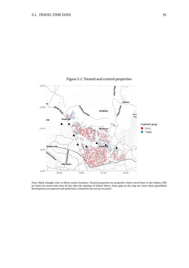
5.1. TRAVEL TIME DATA 91

Figure 5.1: Treated and control properties

Notes: Black triangles refer to Metro station locations. Treated properties are properties where travel times to the Sydney CBDare faster by metro/train than by bus after the opening of Sydney Metro. Some gaps in the map are areas where greenfieldsdevelopments are planned and subdivision of land lots has not yet occurred.

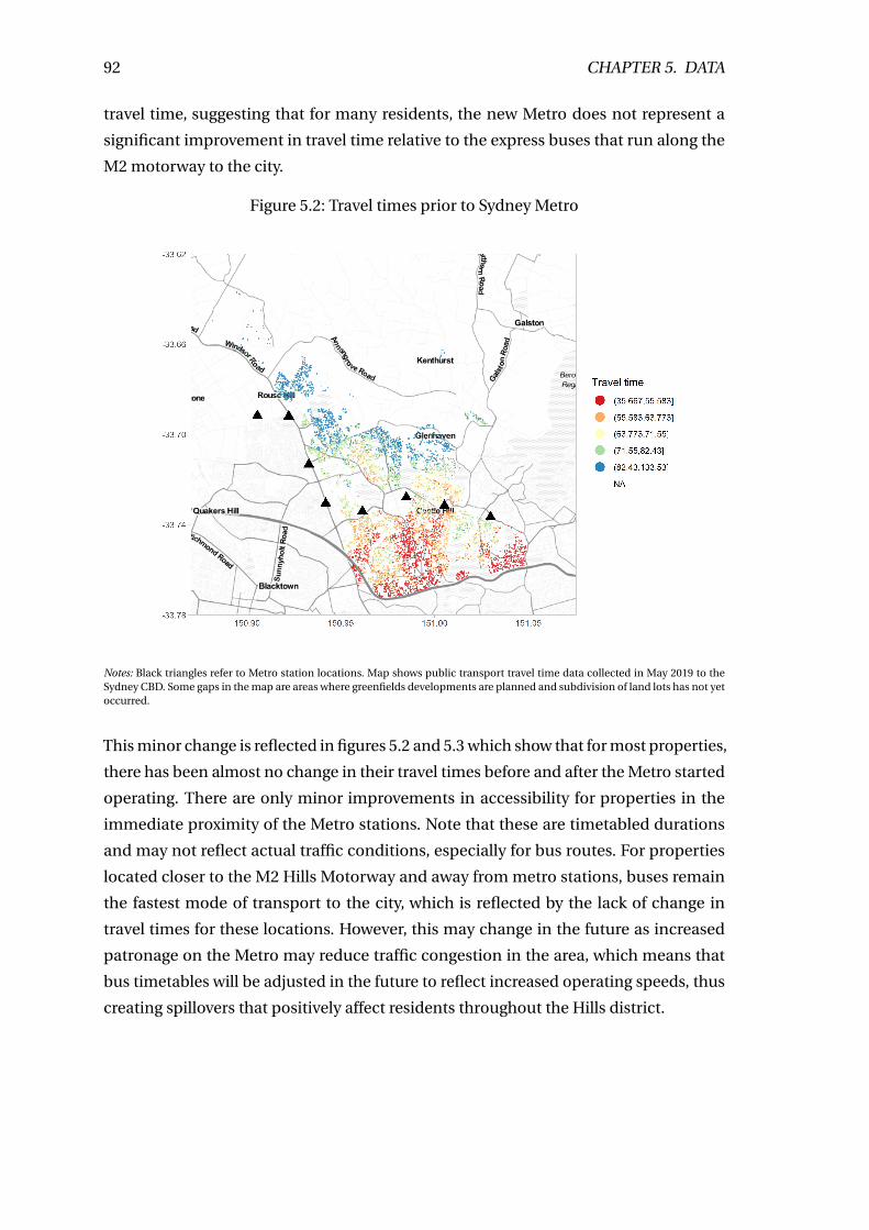
92 CHAPTER 5. DATA

travel time, suggesting that for many residents, the new Metro does not represent a

significant improvement in travel time relative to the express buses that run along the

M2 motorway to the city.

Figure 5.2: Travel times prior to Sydney Metro

Notes: Black triangles refer to Metro station locations. Map shows public transport travel time data collected in May 2019 to theSydney CBD. Some gaps in the map are areas where greenfields developments are planned and subdivision of land lots has not yetoccurred.

This minor change is reflected in figures 5.2 and 5.3 which show that for most properties,

there has been almost no change in their travel times before and after the Metro started

operating. There are only minor improvements in accessibility for properties in the

immediate proximity of the Metro stations. Note that these are timetabled durations

and may not reflect actual traffic conditions, especially for bus routes. For properties

located closer to the M2 Hills Motorway and away from metro stations, buses remain

the fastest mode of transport to the city, which is reflected by the lack of change in

travel times for these locations. However, this may change in the future as increased

patronage on the Metro may reduce traffic congestion in the area, which means that

bus timetables will be adjusted in the future to reflect increased operating speeds, thus

creating spillovers that positively affect residents throughout the Hills district.

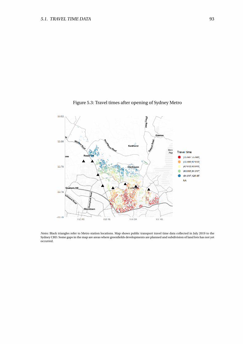
5.1. TRAVEL TIME DATA 93

Figure 5.3: Travel times after opening of Sydney Metro

Notes: Black triangles refer to Metro station locations. Map shows public transport travel time data collected in July 2019 to theSydney CBD. Some gaps in the map are areas where greenfields developments are planned and subdivision of land lots has not yetoccurred.

94 CHAPTER 5. DATA

5.2 Land valuations data

Similar to Part I, I use property valuations data sourced from the NSW Valuer General’s

Bulk Land Values dataset. The Valuer General provides land valuations for every

property (around 1.3 million addresses) in New South Wales. This is a valuation of

the unimproved value of land on a property that excludes the value of the structures or

other improvements on the land (NSW Valuer General, 2017b). Land valuations data is

advantageous as it avoids the problems associated with controlling for the attributes of

the property that is on top of the land, simplifying the design of the hedonic regression

model.

The specific land values that I have used for this study are a sample of valuations from

properties located within the Hills Shire from July 2012 and July 2018. This represents

the oldest and most recent publicly available land values data. Using the bulk land

values file issued in July 2017, which is the oldest publicly available, I was able to encode

property values from July 2012, while the most recent land values data provided the land

values for July 2018. Data from July 2019 are not yet available and based on the dates

that previous years’ data were released by the Valuer General, are unlikely to be available

until January 2020.

The data cleaning process involved removing non-residential properties from the

dataset based on their zoning code. Entries with addresses that were missing a house

number or missing land areas were also omitted. In order to match the dataset with ABS

Census data, each address had to be geocoded using the Geocoded National Address

File (G-NAF) compiled by PSMA Australia (2018). This step involved converting property

addresses to a standardised format that followed the G-NAF conventions, allowing me

to match each address to an ASGS Mesh Block (MB) and geographic coordinates.

As a simple filtering mechanism to capture only properties of interest, I subset the data

to only include properties within the boundaries of The Hills Shire Local Government

Area (LGA). Finally, I took a random sample of the data and collected travel times for

this sample to leave me with my final sample of 7,007 properties. I later realised a more

granular filtering mechanism would have also captured some properties of interest in

the Blacktown City Council LGA to the west of Windsor Road, but unfortunately the

travel time data had already been collected in May and as it was not possible to collect

past travel time data from Google Maps, the study area could not be expanded.

Figure 5.4 shows the demeaned land value change in the Hills Shire. Overall, land values

have risen significantly for all properties between 2012 and 2018. The figure shows the

increase in land values above or below the mean increase of all the properties. That is,

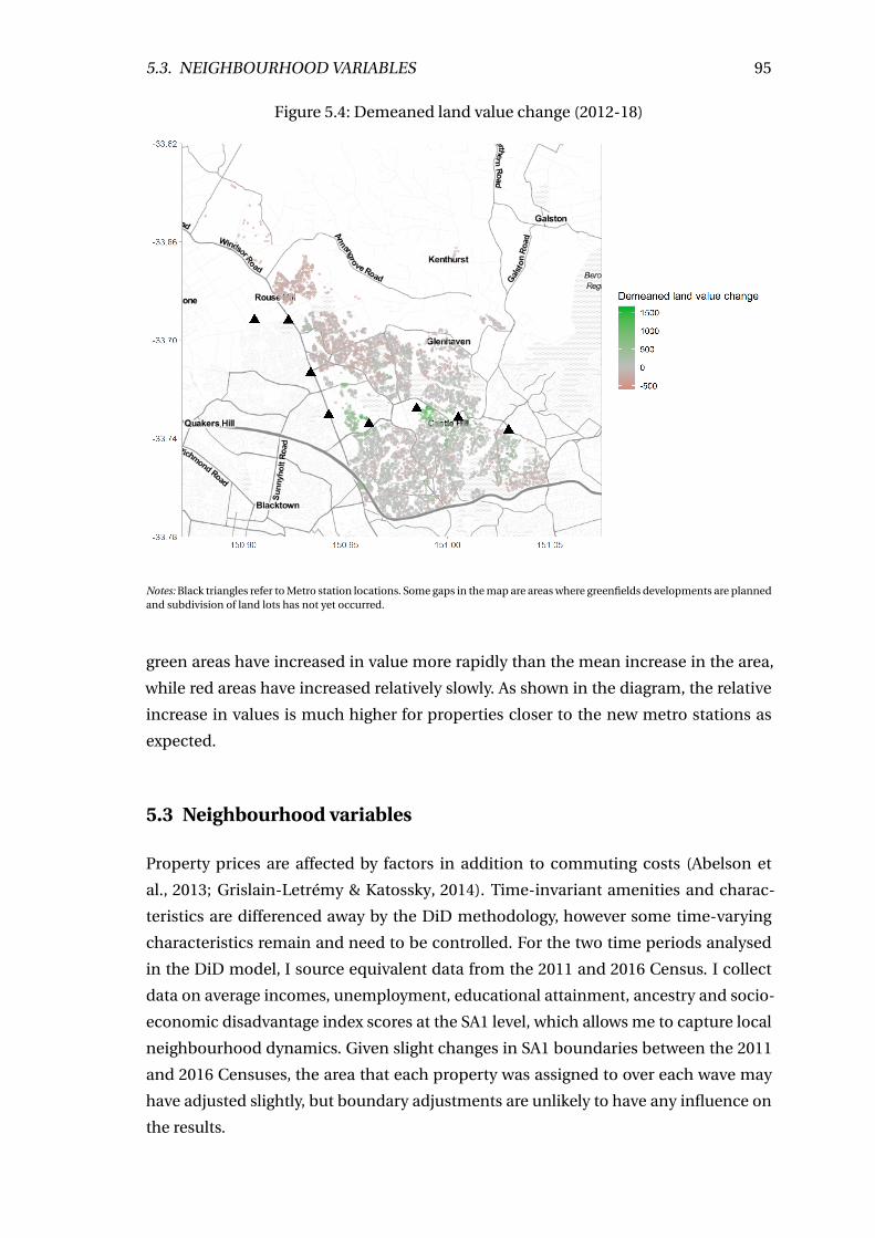
5.3. NEIGHBOURHOOD VARIABLES 95

Figure 5.4: Demeaned land value change (2012-18)

Notes: Black triangles refer to Metro station locations. Some gaps in the map are areas where greenfields developments are plannedand subdivision of land lots has not yet occurred.

green areas have increased in value more rapidly than the mean increase in the area,

while red areas have increased relatively slowly. As shown in the diagram, the relative

increase in values is much higher for properties closer to the new metro stations as

expected.

5.3 Neighbourhood variables

Property prices are affected by factors in addition to commuting costs (Abelson et

al., 2013; Grislain-Letrémy & Katossky, 2014). Time-invariant amenities and charac-

teristics are differenced away by the DiD methodology, however some time-varying

characteristics remain and need to be controlled. For the two time periods analysed

in the DiD model, I source equivalent data from the 2011 and 2016 Census. I collect

data on average incomes, unemployment, educational attainment, ancestry and socio-

economic disadvantage index scores at the SA1 level, which allows me to capture local

neighbourhood dynamics. Given slight changes in SA1 boundaries between the 2011

and 2016 Censuses, the area that each property was assigned to over each wave may

have adjusted slightly, but boundary adjustments are unlikely to have any influence on

the results.

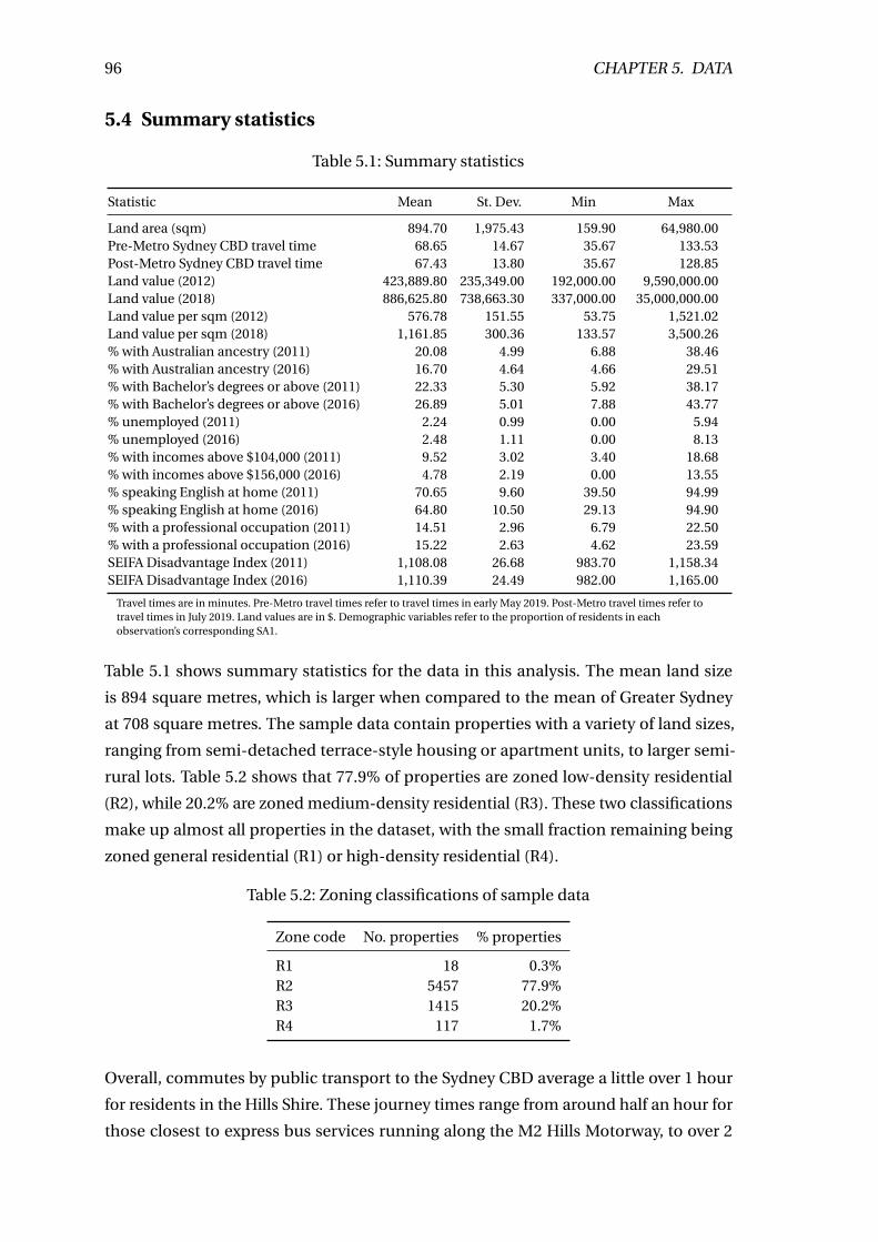
96 CHAPTER 5. DATA

5.4 Summary statistics

Table 5.1: Summary statistics

Statistic Mean St. Dev. Min Max

Land area (sqm) 894.70 1,975.43 159.90 64,980.00Pre-Metro Sydney CBD travel time 68.65 14.67 35.67 133.53Post-Metro Sydney CBD travel time 67.43 13.80 35.67 128.85Land value (2012) 423,889.80 235,349.00 192,000.00 9,590,000.00Land value (2018) 886,625.80 738,663.30 337,000.00 35,000,000.00Land value per sqm (2012) 576.78 151.55 53.75 1,521.02Land value per sqm (2018) 1,161.85 300.36 133.57 3,500.26% with Australian ancestry (2011) 20.08 4.99 6.88 38.46% with Australian ancestry (2016) 16.70 4.64 4.66 29.51% with Bachelor’s degrees or above (2011) 22.33 5.30 5.92 38.17% with Bachelor’s degrees or above (2016) 26.89 5.01 7.88 43.77% unemployed (2011) 2.24 0.99 0.00 5.94% unemployed (2016) 2.48 1.11 0.00 8.13% with incomes above $104,000 (2011) 9.52 3.02 3.40 18.68% with incomes above $156,000 (2016) 4.78 2.19 0.00 13.55% speaking English at home (2011) 70.65 9.60 39.50 94.99% speaking English at home (2016) 64.80 10.50 29.13 94.90% with a professional occupation (2011) 14.51 2.96 6.79 22.50% with a professional occupation (2016) 15.22 2.63 4.62 23.59SEIFA Disadvantage Index (2011) 1,108.08 26.68 983.70 1,158.34SEIFA Disadvantage Index (2016) 1,110.39 24.49 982.00 1,165.00

Travel times are in minutes. Pre-Metro travel times refer to travel times in early May 2019. Post-Metro travel times refer totravel times in July 2019. Land values are in $. Demographic variables refer to the proportion of residents in eachobservation’s corresponding SA1.

Table 5.1 shows summary statistics for the data in this analysis. The mean land size

is 894 square metres, which is larger when compared to the mean of Greater Sydney

at 708 square metres. The sample data contain properties with a variety of land sizes,

ranging from semi-detached terrace-style housing or apartment units, to larger semi-

rural lots. Table 5.2 shows that 77.9% of properties are zoned low-density residential

(R2), while 20.2% are zoned medium-density residential (R3). These two classifications

make up almost all properties in the dataset, with the small fraction remaining being

zoned general residential (R1) or high-density residential (R4).

Table 5.2: Zoning classifications of sample data

Zone code No. properties % properties

R1 18 0.3%R2 5457 77.9%R3 1415 20.2%R4 117 1.7%

Overall, commutes by public transport to the Sydney CBD average a little over 1 hour

for residents in the Hills Shire. These journey times range from around half an hour for

those closest to express bus services running along the M2 Hills Motorway, to over 2

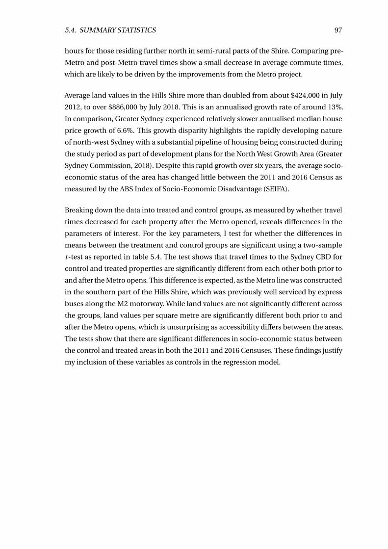
5.4. SUMMARY STATISTICS 97

hours for those residing further north in semi-rural parts of the Shire. Comparing pre-

Metro and post-Metro travel times show a small decrease in average commute times,

which are likely to be driven by the improvements from the Metro project.

Average land values in the Hills Shire more than doubled from about $424,000 in July

2012, to over $886,000 by July 2018. This is an annualised growth rate of around 13%.

In comparison, Greater Sydney experienced relatively slower annualised median house

price growth of 6.6%. This growth disparity highlights the rapidly developing nature

of north-west Sydney with a substantial pipeline of housing being constructed during

the study period as part of development plans for the North West Growth Area (Greater

Sydney Commission, 2018). Despite this rapid growth over six years, the average socio-

economic status of the area has changed little between the 2011 and 2016 Census as

measured by the ABS Index of Socio-Economic Disadvantage (SEIFA).

Breaking down the data into treated and control groups, as measured by whether travel

times decreased for each property after the Metro opened, reveals differences in the

parameters of interest. For the key parameters, I test for whether the differences in

means between the treatment and control groups are significant using a two-sample

t-test as reported in table 5.4. The test shows that travel times to the Sydney CBD for

control and treated properties are significantly different from each other both prior to

and after the Metro opens. This difference is expected, as the Metro line was constructed

in the southern part of the Hills Shire, which was previously well serviced by express

buses along the M2 motorway. While land values are not significantly different across

the groups, land values per square metre are significantly different both prior to and

after the Metro opens, which is unsurprising as accessibility differs between the areas.

The tests show that there are significant differences in socio-economic status between

the control and treated areas in both the 2011 and 2016 Censuses. These findings justify

my inclusion of these variables as controls in the regression model.

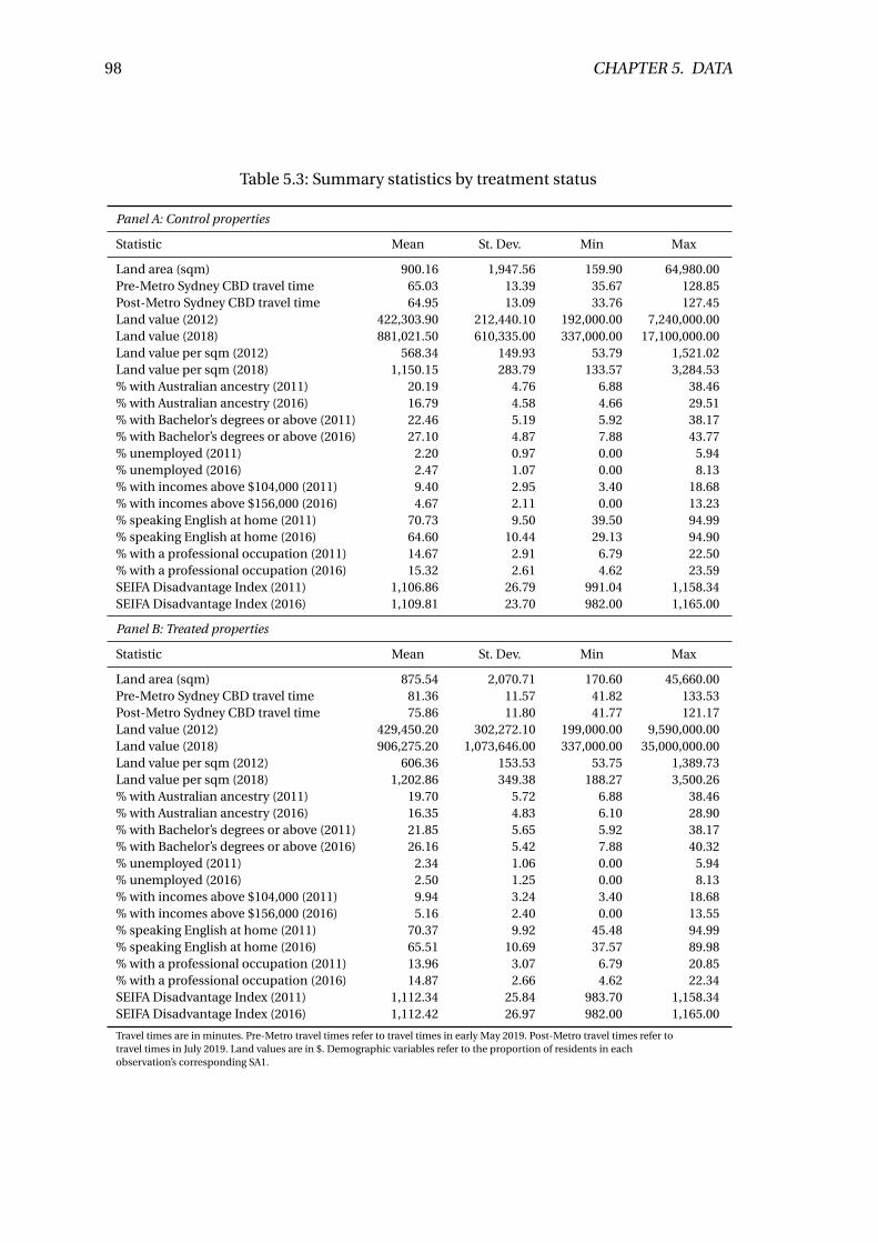
98 CHAPTER 5. DATA

Table 5.3: Summary statistics by treatment status

Panel A: Control properties

Statistic Mean St. Dev. Min Max

Land area (sqm) 900.16 1,947.56 159.90 64,980.00Pre-Metro Sydney CBD travel time 65.03 13.39 35.67 128.85Post-Metro Sydney CBD travel time 64.95 13.09 33.76 127.45Land value (2012) 422,303.90 212,440.10 192,000.00 7,240,000.00Land value (2018) 881,021.50 610,335.00 337,000.00 17,100,000.00Land value per sqm (2012) 568.34 149.93 53.79 1,521.02Land value per sqm (2018) 1,150.15 283.79 133.57 3,284.53% with Australian ancestry (2011) 20.19 4.76 6.88 38.46% with Australian ancestry (2016) 16.79 4.58 4.66 29.51% with Bachelor’s degrees or above (2011) 22.46 5.19 5.92 38.17% with Bachelor’s degrees or above (2016) 27.10 4.87 7.88 43.77% unemployed (2011) 2.20 0.97 0.00 5.94% unemployed (2016) 2.47 1.07 0.00 8.13% with incomes above $104,000 (2011) 9.40 2.95 3.40 18.68% with incomes above $156,000 (2016) 4.67 2.11 0.00 13.23% speaking English at home (2011) 70.73 9.50 39.50 94.99% speaking English at home (2016) 64.60 10.44 29.13 94.90% with a professional occupation (2011) 14.67 2.91 6.79 22.50% with a professional occupation (2016) 15.32 2.61 4.62 23.59SEIFA Disadvantage Index (2011) 1,106.86 26.79 991.04 1,158.34SEIFA Disadvantage Index (2016) 1,109.81 23.70 982.00 1,165.00

Panel B: Treated properties

Statistic Mean St. Dev. Min Max

Land area (sqm) 875.54 2,070.71 170.60 45,660.00Pre-Metro Sydney CBD travel time 81.36 11.57 41.82 133.53Post-Metro Sydney CBD travel time 75.86 11.80 41.77 121.17Land value (2012) 429,450.20 302,272.10 199,000.00 9,590,000.00Land value (2018) 906,275.20 1,073,646.00 337,000.00 35,000,000.00Land value per sqm (2012) 606.36 153.53 53.75 1,389.73Land value per sqm (2018) 1,202.86 349.38 188.27 3,500.26% with Australian ancestry (2011) 19.70 5.72 6.88 38.46% with Australian ancestry (2016) 16.35 4.83 6.10 28.90% with Bachelor’s degrees or above (2011) 21.85 5.65 5.92 38.17% with Bachelor’s degrees or above (2016) 26.16 5.42 7.88 40.32% unemployed (2011) 2.34 1.06 0.00 5.94% unemployed (2016) 2.50 1.25 0.00 8.13% with incomes above $104,000 (2011) 9.94 3.24 3.40 18.68% with incomes above $156,000 (2016) 5.16 2.40 0.00 13.55% speaking English at home (2011) 70.37 9.92 45.48 94.99% speaking English at home (2016) 65.51 10.69 37.57 89.98% with a professional occupation (2011) 13.96 3.07 6.79 20.85% with a professional occupation (2016) 14.87 2.66 4.62 22.34SEIFA Disadvantage Index (2011) 1,112.34 25.84 983.70 1,158.34SEIFA Disadvantage Index (2016) 1,112.42 26.97 982.00 1,165.00

Travel times are in minutes. Pre-Metro travel times refer to travel times in early May 2019. Post-Metro travel times refer totravel times in July 2019. Land values are in $. Demographic variables refer to the proportion of residents in eachobservation’s corresponding SA1.

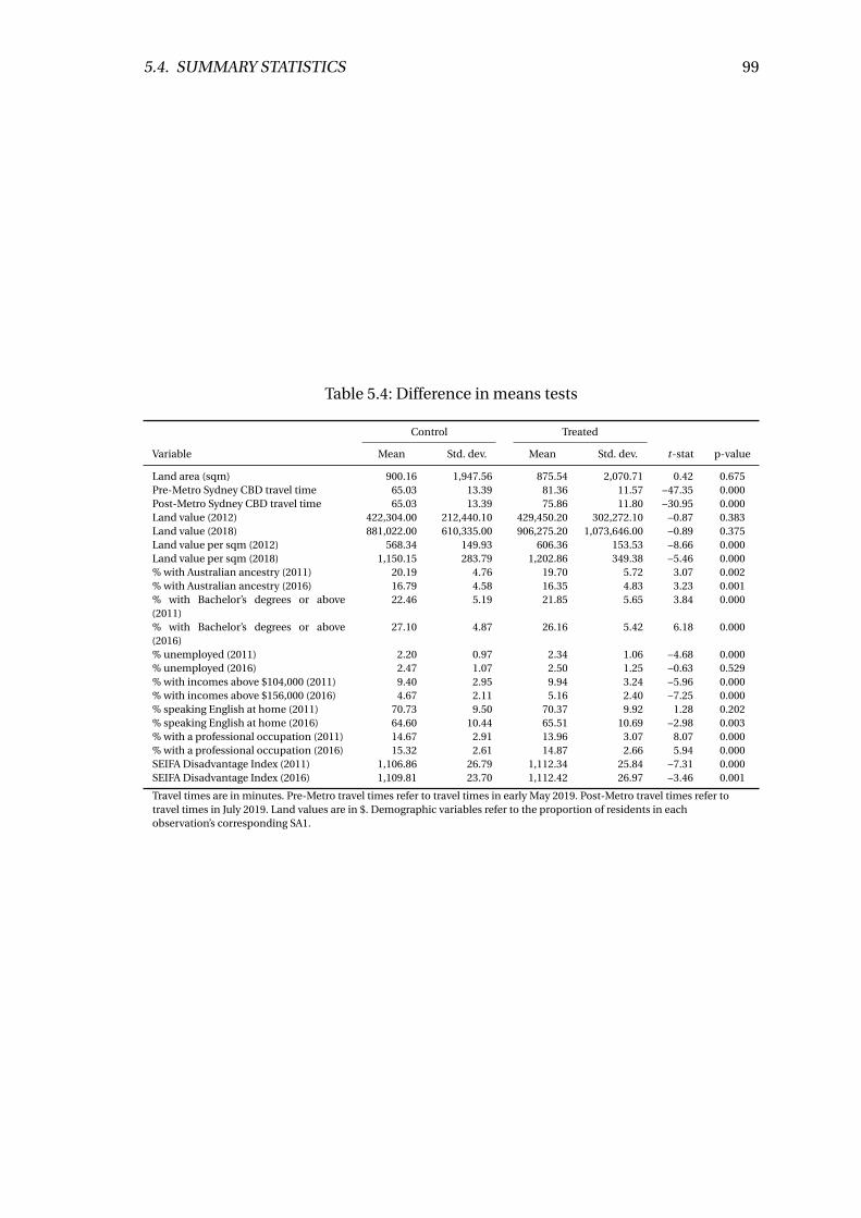
5.4. SUMMARY STATISTICS 99

Table 5.4: Difference in means tests

Control Treated

Variable Mean Std. dev. Mean Std. dev. t-stat p-value

Land area (sqm) 900.16 1,947.56 875.54 2,070.71 0.42 0.675Pre-Metro Sydney CBD travel time 65.03 13.39 81.36 11.57 −47.35 0.000Post-Metro Sydney CBD travel time 65.03 13.39 75.86 11.80 −30.95 0.000Land value (2012) 422,304.00 212,440.10 429,450.20 302,272.10 −0.87 0.383Land value (2018) 881,022.00 610,335.00 906,275.20 1,073,646.00 −0.89 0.375Land value per sqm (2012) 568.34 149.93 606.36 153.53 −8.66 0.000Land value per sqm (2018) 1,150.15 283.79 1,202.86 349.38 −5.46 0.000% with Australian ancestry (2011) 20.19 4.76 19.70 5.72 3.07 0.002% with Australian ancestry (2016) 16.79 4.58 16.35 4.83 3.23 0.001% with Bachelor’s degrees or above(2011)

22.46 5.19 21.85 5.65 3.84 0.000

% with Bachelor’s degrees or above(2016)

27.10 4.87 26.16 5.42 6.18 0.000

% unemployed (2011) 2.20 0.97 2.34 1.06 −4.68 0.000% unemployed (2016) 2.47 1.07 2.50 1.25 −0.63 0.529% with incomes above $104,000 (2011) 9.40 2.95 9.94 3.24 −5.96 0.000% with incomes above $156,000 (2016) 4.67 2.11 5.16 2.40 −7.25 0.000% speaking English at home (2011) 70.73 9.50 70.37 9.92 1.28 0.202% speaking English at home (2016) 64.60 10.44 65.51 10.69 −2.98 0.003% with a professional occupation (2011) 14.67 2.91 13.96 3.07 8.07 0.000% with a professional occupation (2016) 15.32 2.61 14.87 2.66 5.94 0.000SEIFA Disadvantage Index (2011) 1,106.86 26.79 1,112.34 25.84 −7.31 0.000SEIFA Disadvantage Index (2016) 1,109.81 23.70 1,112.42 26.97 −3.46 0.001

Travel times are in minutes. Pre-Metro travel times refer to travel times in early May 2019. Post-Metro travel times refer totravel times in July 2019. Land values are in $. Demographic variables refer to the proportion of residents in eachobservation’s corresponding SA1.

C H A P T E R 6

Results and discussion

In this chapter, I present and discuss estimates of the willingness to pay for improved

accessibility to employment in the Sydney CBD based on changes in travel times

resulting from the Sydney Metro Northwest project. I perform robustness checks by

estimating regressions using specifications measuring land value uplift with distance-

based approaches and by randomising the travel time data to demonstrate that the

significant results are unlikely to be the result of statistical noise. I then discuss potential

limitations of this study.

6.1 Land value uplift estimates

I find that reducing travel times to the Sydney CBD results in an increase in land values

for the affected properties. I present the estimation results from the DiD models in

table 6.1. I estimate the results using three specifications. Column (1) shows a level-

level model with the land value of each property as the outcome variable (model 1).

Column (2) shows a level-level model with land value per square metre as the outcome

variable (model 2). Column (3) shows a log-level model with the natural logarithm of

land value as the outcome variable (model 3). All the models are run with controls for

neighbourhood demographic and socio-economic characteristics, individual property

fixed effects and heteroskedasticity-robust standard errors clustered at the individual

property level. The models have high explanatory power, especially the square metre

value (model 2) and logged land value (model 3) models.

The coefficient of interest is the interaction between the post-Metro time dummy and

public transport travel time to the Sydney CBD in minutes. This coefficient is the DiD

estimate of the land value uplift that accrues to the average property as a result of

a 1 minute decrease in public transport travel times over the six years between July

2012 and July 2018. The results are highly significant and have the expected signs as

predicted by theory. Model (2) shows that a 1 minute decrease in transit times to the

Sydney CBD increases land values by about $3,400 for the average sized property. In

percentage terms using model (3), a 1 minute decrease in travel times increases land

100

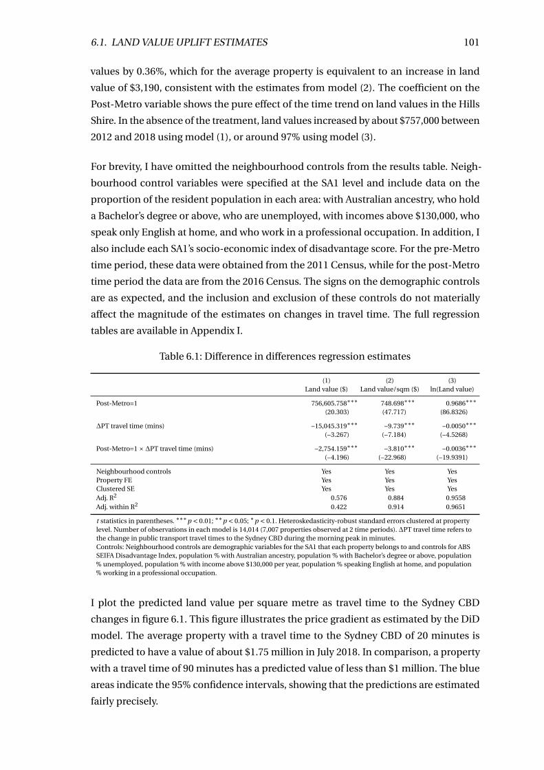
6.1. LAND VALUE UPLIFT ESTIMATES 101

values by 0.36%, which for the average property is equivalent to an increase in land

value of $3,190, consistent with the estimates from model (2). The coefficient on the

Post-Metro variable shows the pure effect of the time trend on land values in the Hills

Shire. In the absence of the treatment, land values increased by about $757,000 between

2012 and 2018 using model (1), or around 97% using model (3).

For brevity, I have omitted the neighbourhood controls from the results table. Neigh-

bourhood control variables were specified at the SA1 level and include data on the

proportion of the resident population in each area: with Australian ancestry, who hold

a Bachelor’s degree or above, who are unemployed, with incomes above $130,000, who

speak only English at home, and who work in a professional occupation. In addition, I

also include each SA1’s socio-economic index of disadvantage score. For the pre-Metro

time period, these data were obtained from the 2011 Census, while for the post-Metro

time period the data are from the 2016 Census. The signs on the demographic controls

are as expected, and the inclusion and exclusion of these controls do not materially

affect the magnitude of the estimates on changes in travel time. The full regression

tables are available in Appendix I.

Table 6.1: Difference in differences regression estimates

(1) (2) (3)Land value ($) Land value/sqm ($) ln(Land value)

Post-Metro=1 756,605.758∗∗∗ 748.698∗∗∗ 0.9686∗∗∗(20.303) (47.717) (86.8326)

∆PT travel time (mins) −15,045.319∗∗∗ −9.739∗∗∗ −0.0050∗∗∗(−3.267) (−7.184) (−4.5268)

Post-Metro=1 × ∆PT travel time (mins) −2,754.159∗∗∗ −3.810∗∗∗ −0.0036∗∗∗(−4.196) (−22.968) (−19.9391)

Neighbourhood controls Yes Yes YesProperty FE Yes Yes YesClustered SE Yes Yes YesAdj. R2 0.576 0.884 0.9558Adj. within R2 0.422 0.914 0.9651

t statistics in parentheses. ∗∗∗p < 0.01; ∗∗p < 0.05; ∗p < 0.1. Heteroskedasticity-robust standard errors clustered at propertylevel. Number of observations in each model is 14,014 (7,007 properties observed at 2 time periods). ∆PT travel time refers tothe change in public transport travel times to the Sydney CBD during the morning peak in minutes.Controls: Neighbourhood controls are demographic variables for the SA1 that each property belongs to and controls for ABSSEIFA Disadvantage Index, population % with Australian ancestry, population % with Bachelor’s degree or above, population% unemployed, population % with income above $130,000 per year, population % speaking English at home, and population% working in a professional occupation.

I plot the predicted land value per square metre as travel time to the Sydney CBD

changes in figure 6.1. This figure illustrates the price gradient as estimated by the DiD

model. The average property with a travel time to the Sydney CBD of 20 minutes is

predicted to have a value of about $1.75 million in July 2018. In comparison, a property

with a travel time of 90 minutes has a predicted value of less than $1 million. The blue

areas indicate the 95% confidence intervals, showing that the predictions are estimated

fairly precisely.

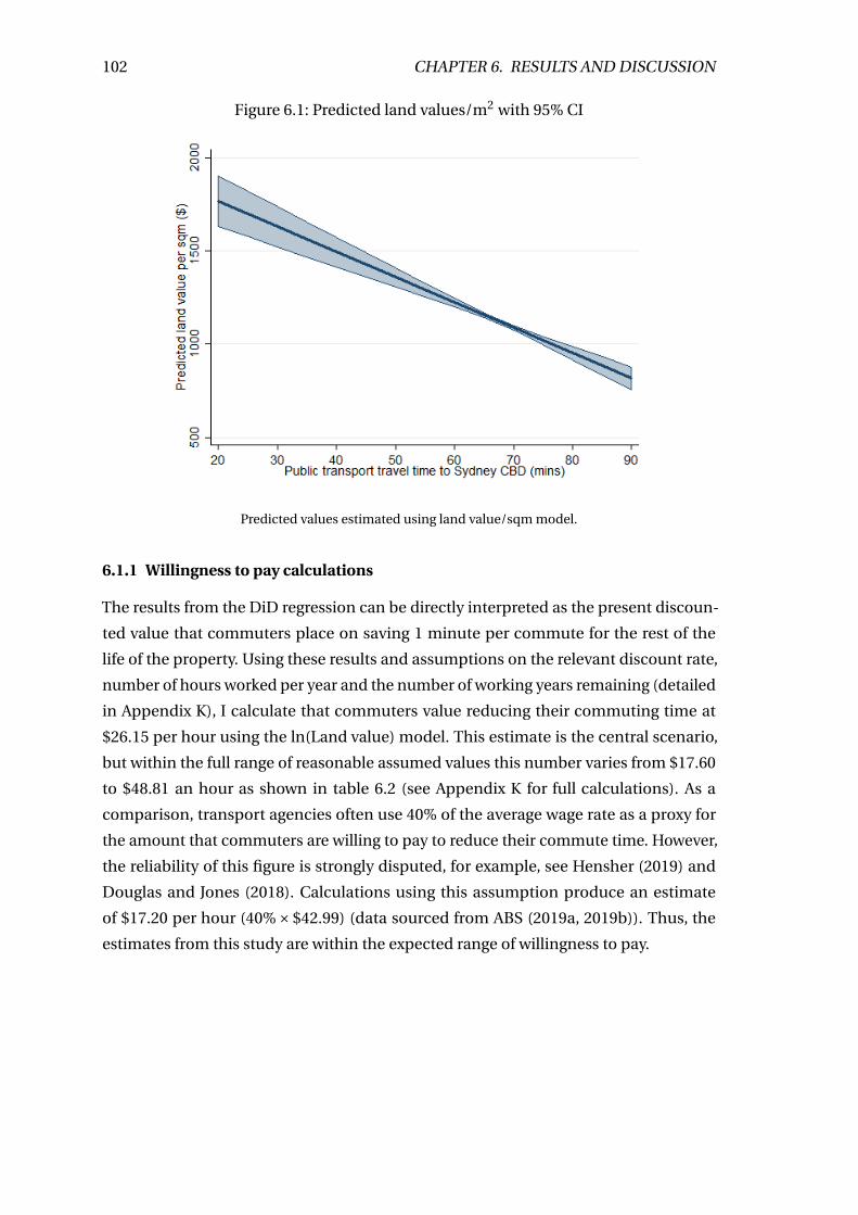
102 CHAPTER 6. RESULTS AND DISCUSSION

Figure 6.1: Predicted land values/m2 with 95% CI

Predicted values estimated using land value/sqm model.

6.1.1 Willingness to pay calculations

The results from the DiD regression can be directly interpreted as the present discoun-

ted value that commuters place on saving 1 minute per commute for the rest of the

life of the property. Using these results and assumptions on the relevant discount rate,

number of hours worked per year and the number of working years remaining (detailed

in Appendix K), I calculate that commuters value reducing their commuting time at

$26.15 per hour using the ln(Land value) model. This estimate is the central scenario,

but within the full range of reasonable assumed values this number varies from $17.60

to $48.81 an hour as shown in table 6.2 (see Appendix K for full calculations). As a

comparison, transport agencies often use 40% of the average wage rate as a proxy for

the amount that commuters are willing to pay to reduce their commute time. However,

the reliability of this figure is strongly disputed, for example, see Hensher (2019) and

Douglas and Jones (2018). Calculations using this assumption produce an estimate

of $17.20 per hour (40%×$42.99) (data sourced from ABS (2019a, 2019b)). Thus, the

estimates from this study are within the expected range of willingness to pay.

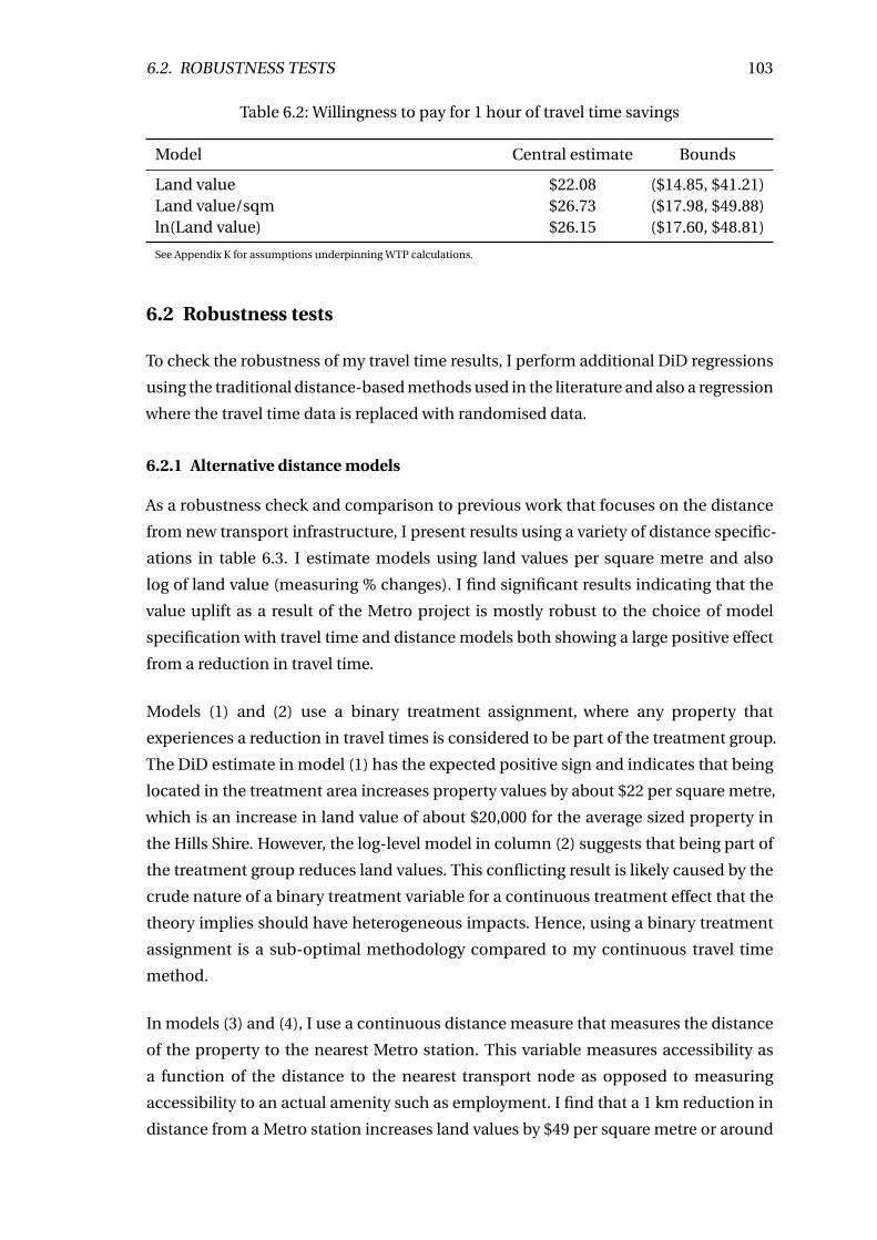
6.2. ROBUSTNESS TESTS 103

Table 6.2: Willingness to pay for 1 hour of travel time savings

Model Central estimate Bounds

Land value $22.08 ($14.85, $41.21)Land value/sqm $26.73 ($17.98, $49.88)ln(Land value) $26.15 ($17.60, $48.81)

See Appendix K for assumptions underpinning WTP calculations.

6.2 Robustness tests

To check the robustness of my travel time results, I perform additional DiD regressions

using the traditional distance-based methods used in the literature and also a regression

where the travel time data is replaced with randomised data.

6.2.1 Alternative distance models

As a robustness check and comparison to previous work that focuses on the distance

from new transport infrastructure, I present results using a variety of distance specific-

ations in table 6.3. I estimate models using land values per square metre and also

log of land value (measuring % changes). I find significant results indicating that the

value uplift as a result of the Metro project is mostly robust to the choice of model

specification with travel time and distance models both showing a large positive effect

from a reduction in travel time.

Models (1) and (2) use a binary treatment assignment, where any property that

experiences a reduction in travel times is considered to be part of the treatment group.

The DiD estimate in model (1) has the expected positive sign and indicates that being

located in the treatment area increases property values by about $22 per square metre,

which is an increase in land value of about $20,000 for the average sized property in

the Hills Shire. However, the log-level model in column (2) suggests that being part of

the treatment group reduces land values. This conflicting result is likely caused by the

crude nature of a binary treatment variable for a continuous treatment effect that the

theory implies should have heterogeneous impacts. Hence, using a binary treatment

assignment is a sub-optimal methodology compared to my continuous travel time

method.

In models (3) and (4), I use a continuous distance measure that measures the distance

of the property to the nearest Metro station. This variable measures accessibility as

a function of the distance to the nearest transport node as opposed to measuring

accessibility to an actual amenity such as employment. I find that a 1 km reduction in

distance from a Metro station increases land values by $49 per square metre or around

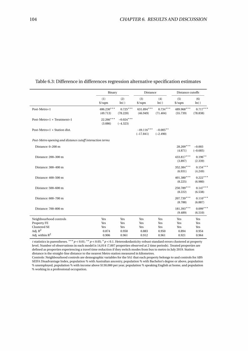
104 CHAPTER 6. RESULTS AND DISCUSSION

Table 6.3: Difference in differences regression alternative specification estimates

Binary Distance Distance cutoffs

(1) (2) (3) (4) (5) (6)$/sqm ln(·) $/sqm ln(·) $/sqm ln(·)

Post-Metro=1 486.230∗∗∗ 0.725∗∗∗ 631.894∗∗∗ 0.734∗∗∗ 489.968∗∗∗ 0.717∗∗∗(49.713) (78.220) (46.949) (71.404) (55.739) (78.838)

Post-Metro=1 × Treatment=1 22.266∗∗∗ −0.024∗∗∗(3.086) (−4.323)

Post-Metro=1 × Station dist. −49.116∗∗∗ −0.005∗∗(−17.841) (−2.490)

Post-Metro opening and distance cutoff interaction terms

Distance: 0–200 m 28.209∗∗∗ −0.003(4.871) (−0.685)

Distance: 200–300 m 433.817∗∗∗ 0.196∗∗(3.897) (2.339)

Distance: 300–400 m 352.384∗∗∗ 0.154∗∗∗(6.931) (4.249)

Distance: 400–500 m 401.380∗∗∗ 0.222∗∗∗(8.225) (6.980)

Distance: 500–600 m 250.789∗∗∗ 0.147∗∗∗(8.222) (6.538)

Distance: 600–700 m 207.739∗∗∗ 0.110∗∗∗(8.788) (6.887)

Distance: 700–800 m 181.393∗∗∗ 0.099∗∗∗(9.489) (6.510)

Neighbourhood controls Yes Yes Yes Yes Yes YesProperty FE Yes Yes Yes Yes Yes YesClustered SE Yes Yes Yes Yes Yes YesAdj. R2 0.874 0.950 0.883 0.950 0.894 0.954Adj. within R2 0.906 0.961 0.912 0.961 0.921 0.964

t statistics in parentheses. ∗∗∗p < 0.01; ∗∗p < 0.05; ∗p < 0.1. Heteroskedasticity-robust standard errors clustered at propertylevel. Number of observations in each model is 14,014 (7,007 properties observed at 2 time periods). Treated properties aredefined as properties experiencing a travel time reduction if they switch modes from bus to metro in July 2019. Stationdistance is the straight-line distance to the nearest Metro station measured in kilometres.Controls: Neighbourhood controls are demographic variables for the SA1 that each property belongs to and controls for ABSSEIFA Disadvantage Index, population % with Australian ancestry, population % with Bachelor’s degree or above, population% unemployed, population % with income above $130,000 per year, population % speaking English at home, and population% working in a professional occupation.

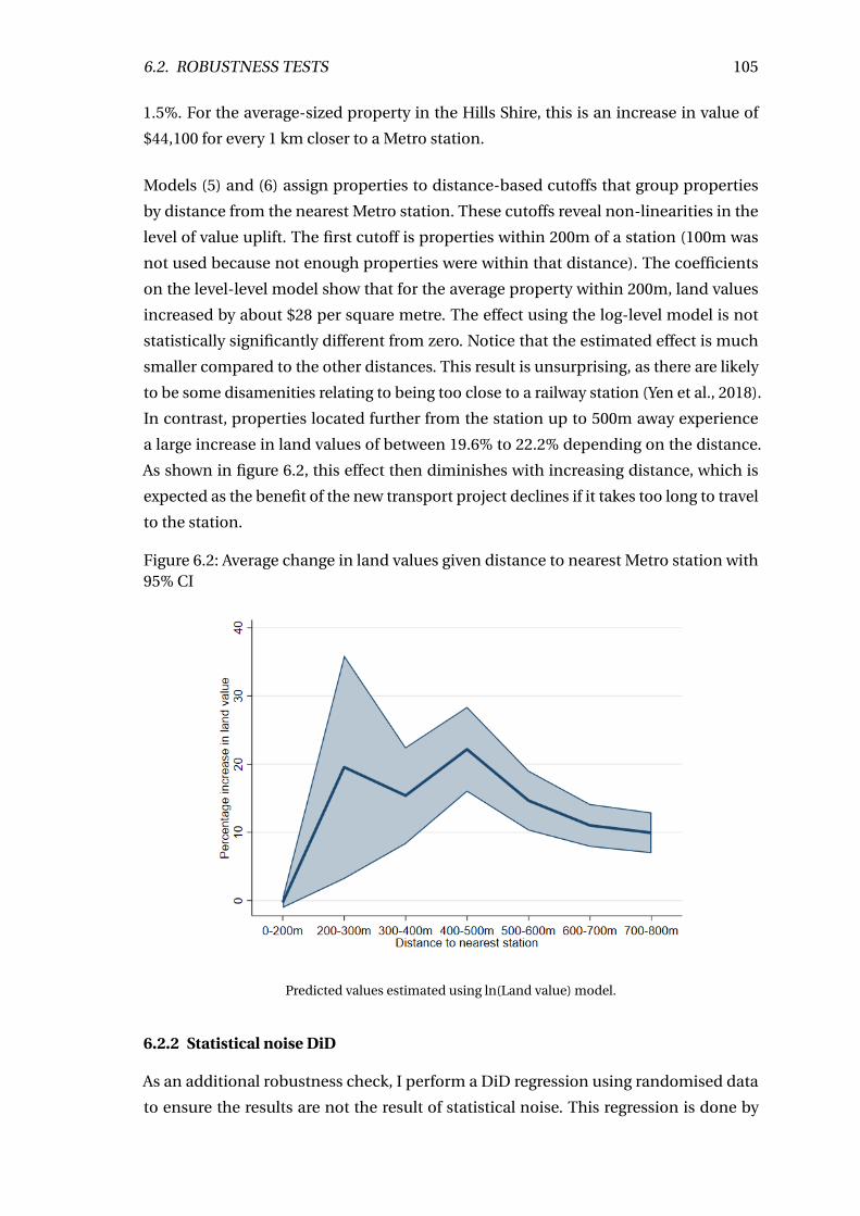
6.2. ROBUSTNESS TESTS 105

1.5%. For the average-sized property in the Hills Shire, this is an increase in value of

$44,100 for every 1 km closer to a Metro station.

Models (5) and (6) assign properties to distance-based cutoffs that group properties

by distance from the nearest Metro station. These cutoffs reveal non-linearities in the

level of value uplift. The first cutoff is properties within 200m of a station (100m was

not used because not enough properties were within that distance). The coefficients

on the level-level model show that for the average property within 200m, land values

increased by about $28 per square metre. The effect using the log-level model is not

statistically significantly different from zero. Notice that the estimated effect is much

smaller compared to the other distances. This result is unsurprising, as there are likely

to be some disamenities relating to being too close to a railway station (Yen et al., 2018).

In contrast, properties located further from the station up to 500m away experience

a large increase in land values of between 19.6% to 22.2% depending on the distance.

As shown in figure 6.2, this effect then diminishes with increasing distance, which is

expected as the benefit of the new transport project declines if it takes too long to travel

to the station.

Figure 6.2: Average change in land values given distance to nearest Metro station with95% CI

Predicted values estimated using ln(Land value) model.

6.2.2 Statistical noise DiD

As an additional robustness check, I perform a DiD regression using randomised data

to ensure the results are not the result of statistical noise. This regression is done by

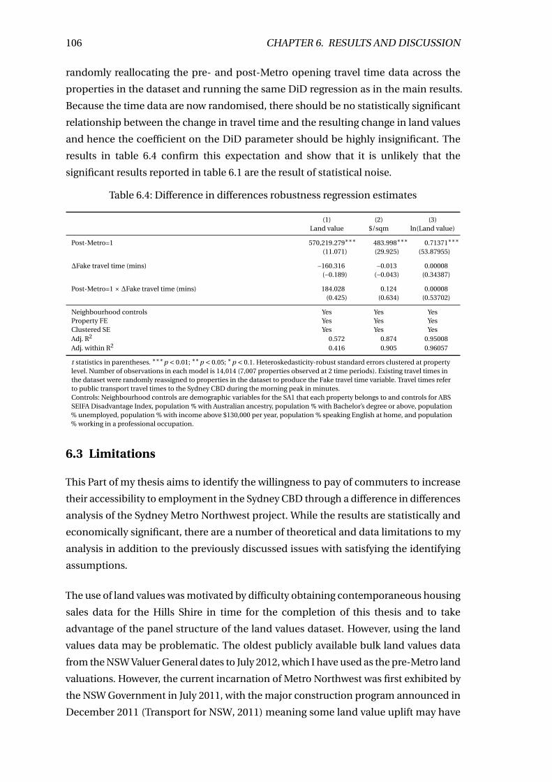
106 CHAPTER 6. RESULTS AND DISCUSSION

randomly reallocating the pre- and post-Metro opening travel time data across the

properties in the dataset and running the same DiD regression as in the main results.

Because the time data are now randomised, there should be no statistically significant

relationship between the change in travel time and the resulting change in land values

and hence the coefficient on the DiD parameter should be highly insignificant. The

results in table 6.4 confirm this expectation and show that it is unlikely that the

significant results reported in table 6.1 are the result of statistical noise.

Table 6.4: Difference in differences robustness regression estimates

(1) (2) (3)Land value $/sqm ln(Land value)

Post-Metro=1 570,219.279∗∗∗ 483.998∗∗∗ 0.71371∗∗∗(11.071) (29.925) (53.87955)

∆Fake travel time (mins) −160.316 −0.013 0.00008(−0.189) (−0.043) (0.34387)

Post-Metro=1 × ∆Fake travel time (mins) 184.028 0.124 0.00008(0.425) (0.634) (0.53702)

Neighbourhood controls Yes Yes YesProperty FE Yes Yes YesClustered SE Yes Yes YesAdj. R2 0.572 0.874 0.95008Adj. within R2 0.416 0.905 0.96057

t statistics in parentheses. ∗∗∗p < 0.01; ∗∗p < 0.05; ∗p < 0.1. Heteroskedasticity-robust standard errors clustered at propertylevel. Number of observations in each model is 14,014 (7,007 properties observed at 2 time periods). Existing travel times inthe dataset were randomly reassigned to properties in the dataset to produce the Fake travel time variable. Travel times referto public transport travel times to the Sydney CBD during the morning peak in minutes.Controls: Neighbourhood controls are demographic variables for the SA1 that each property belongs to and controls for ABSSEIFA Disadvantage Index, population % with Australian ancestry, population % with Bachelor’s degree or above, population% unemployed, population % with income above $130,000 per year, population % speaking English at home, and population% working in a professional occupation.

6.3 Limitations

This Part of my thesis aims to identify the willingness to pay of commuters to increase

their accessibility to employment in the Sydney CBD through a difference in differences

analysis of the Sydney Metro Northwest project. While the results are statistically and

economically significant, there are a number of theoretical and data limitations to my

analysis in addition to the previously discussed issues with satisfying the identifying

assumptions.

The use of land values was motivated by difficulty obtaining contemporaneous housing

sales data for the Hills Shire in time for the completion of this thesis and to take

advantage of the panel structure of the land values dataset. However, using the land

values data may be problematic. The oldest publicly available bulk land values data

from the NSW Valuer General dates to July 2012, which I have used as the pre-Metro land

valuations. However, the current incarnation of Metro Northwest was first exhibited by

the NSW Government in July 2011, with the major construction program announced in

December 2011 (Transport for NSW, 2011) meaning some land value uplift may have

6.3. LIMITATIONS 107

already started occurring. On the other hand, Yen et al. (2018) find that the largest

value uplift occurs when firm financial commitments have been made by government,

such as the signing of major construction contracts. Since the first major contract (for

tunnelling) was signed in June 2013 (Transport for NSW, 2013), it is possible that most

value uplift occurred after that date, reducing the magnitude of the downward bias.

In addition, while the project has been conceptualised since the late 1990s (Newman,

1999), repeated cancellations and re-announcements are likely to have reduced the

public credibility of the NSW Government’s announcement of the project — at least

until firm contractual commitments were made (Gordon, Mulley, Stevens & Daniels,

2013). However, overall it is likely that land values started increasing prior to July

2012. Furthermore, as discussed in the Methodology chapter, the lack of pre-2012 data

also prevents me from conducting pre-trends analysis on the outcome variable to

investigate whether the parallel trends assumption of the DiD estimator can be feasibly

upheld. These limitations can be addressed by using older land value data, which are

known to be held by the Valuer General. Unfortunately, I was unable to obtain it by the

submission date of this thesis despite multiple attempts at contact.

At the other end of the timeline, I use land values data from July 2018 as an approxim-

ation of the post-Metro land valuations. However, Sydney Metro Northwest opened to

revenue service in May 2019 (Sydney Metro, 2019b). Hence, it is likely that some of the

value uplift due to the project has not yet been fully capitalised into the price of land

in the study area. Furthermore, the literature show that value uplift is sometimes not

fully capitalised into land values until a number of years after project opening (Higgins

& Kanaroglou, 2016; McIntosh et al., 2014). The solution is to wait until land value data

dating to July 2019 (or later) is released, likely by January 2020 based on the release

timeline of previous land value data. These data issues likely lead to an underestimate

of the total land value uplift as a result of the Metro project, if value uplift already started

prior to July 2012 and did not fully conclude by July 2018. This is especially the case if

price changes have a lagged response to changes in accessibility. These issues mean

that the estimates of willingness to pay for increased accessibility will be downwardly

biased compared to the true value.

There may also be further difficulties in land valuation due to the large number of

greenfields developments occurring in the north west. As previously noted, there are

some gaps in the maps where no properties are sampled, which correspond to areas

where new developments were still being planned and lots were not yet subdivided in

2012. These missing areas primarily affect stations in the more northerly sections of the

line and while analysis of the effects on land values of these new developments would

108 CHAPTER 6. RESULTS AND DISCUSSION

be interesting, they cannot be captured as they are recorded in the land values dataset

as very large blocks of land instead of individual subdivisions.

This study is affected by the multi-stage scope of the Sydney Metro project. The

Northwest Metro is the first stage of the Sydney Metro project, with the second stage that

connects Chatswood to Bankstown via the Sydney CBD currently under construction

(Sydney Metro, 2019a). This stage will further reduce travel times from north-west

Sydney to the Sydney CBD via a new route that is faster than the existing North Shore

line, which has implications for my analysis. There is a high degree of credibility in

the community that the travel time reductions will be realised upon completion and

opening in 2024, because the project is already under construction. Thus, it is possible

that part of the future value of this travel time saving will be in the process of being

capitalised into land values in the study area, which would result in an overestimate

of the true value of the willingness to pay, as the partial reduction in travel times from

stage one is attributed to the rise in land values that represent residents responding to

the cumulative gains from both stage one and two.

Similar to the limitations in Part I of this thesis, this part is also affected by the dispersed

nature of employment in Sydney. My estimation method assumes that accessibility to

employment in the Sydney CBD is the only location of employment that matters. Access

to employment in other nearby major centres such as Macquarie Park and Parramatta

are also likely to inform the locational decisions of households in north-west Sydney.

Unfortunately, I was unable to collect travel time data to these locations due to time

constraints. However, including additional centres still suffers from what is essentially

an arbitrary choice of what employment centres matter. A more agnostic approach is to

use a gravity model approach (see Ahlfeldt (2010), Kau and Sirmans (1979)) that allows

me to construct a single employment-weighted travel time from each property. I have

discussed this approach in depth in section 5.8 of Part I.

C H A P T E R 7

Conclusion

This Part uses a difference in differences model to estimate commuters’ willingness

to pay for improved accessibility to employment in Sydney by exploiting variation in

travel times and land values resulting from the opening of the Sydney Metro Northwest

rapid transit rail line in north-west Sydney. I produce the first estimates of willingness

to pay for the first rapid transit line in Sydney using a quasi-experiment panel data

approach with a unique dataset constructed from Google Maps travel time data. This

study demonstrates the feasibility of using travel time data as a means of separating

properties into treatment and control groups that is more realistic than the existing

distance-based approaches used in the literature.

After controlling for local demographics and socio-economic variables, I find that

there is a significant relationship between reduced travel times and increased land

values as assessed by the NSW Valuer General. The value uplift produced by the

Metro project is robust to alternative specifications that are preferred in the literature,

including a binary distance-based assignment into treatment and control groups, and

also using multiple discrete distance-based bins to measure a varying effect over

different distances from metro stations. Under both these specifications, I observe a

significant effect of the Metro on land value uplift. Compared to the results from Part

I, the estimated willingness to pay is lower. The cross-sectional approach produces

magnitudes about double that of the baseline estimates using the travel time DiD model.

This is in line with findings from the literature that show cross-sectional models tend

to produce larger estimates than quasi-experimental approaches.

However, this is an early study and it is possible that estimates are underestimating

the value uplift from the project due to the value change not yet fully capitalising

into property values in the area. In addition, the multi-stage nature of the Sydney

Metro project means there is a risk of confounding the benefits of future stages of

the project with the benefits of the currently open stage, as some of the value uplift

of future improvements may already be capitalising themselves into property values,

possibly producing an overestimation of the gains. There can also be improvements to

109

110 CHAPTER 7. CONCLUSION

the measure of accessibility; future researchers could use a gravity-based approach

to weighting employment across the whole of Greater Sydney, rather than solely

measuring accessibility to the Sydney CBD.

My results improve on existing measures of the value of travel time savings for users

of transport infrastructure, enabling more accurate cost-benefit analysis of transport

projects compared to existing methods using assumed proportions of average wages

(Douglas & Jones, 2018; Hensher, 2019). Better measures of willingness to pay improves

the quality of cost-benefit analyses, ensuring that the most productive and beneficial

infrastructure is funded first.

My research has implications for the policy debate surrounding the funding mechan-

isms for transport infrastructure projects. My results confirm that transport projects

lead to significant land value uplift for the surrounding properties that benefit from

this project. Value capture has been proposed as a mechanism for governments to fund

projects by taxing those who benefit the most from new infrastructure (Medda, 2012).

A common criticism of distance cutoff studies is that the cutoff is essentially arbitrary

and applying such a mechanism to a tax would arbitrarily include some properties

in the taxed group, while excluding neighbours from paying the tax (Terrill & Emslie,

2017). By using a continuous travel time approach to measuring value uplift from the

project, I address this criticism of value capture mechanisms and provide a better

mechanism design that ensures property owners equitably contribute to infrastructure

investment.

References

Abadie, A. (2005). Semiparametric difference-in-differences estimators. The Review of

Economic Studies, 72(1), 1–19. doi:10.1111/0034-6527.00321

Abelson, P., Joyeux, R. & Mahuteau, S. (2013). Modelling house prices across Sydney.

Australian Economic Review, 46(3), 269–285. doi:10.1111/j.1467-8462.2013.12013.

x

Ahlfeldt, G. (2010). If Alonso was right: Modeling accessibility and explaining the

residential land gradient. Journal of Regional Science, 51(2), 318–338. doi:10.1111/

j.1467-9787.2010.00694.x

Akaike, H. (1974). A new look at the statistical model identification. IEEE Transactions

on Automatic Control, 19(6), 716–723. doi:10.1109/tac.1974.1100705

Alonso, W. (1964). Location and land use : Toward a general theory of land rent. doi:10.

4159/harvard.9780674730854

Angrist, J. D. & Pischke, J.-S. (2009, February 11). Mostly harmless econometrics: An

empiricist’s companion. PRINCETON UNIV PR. Retrieved from https : / / www.

ebook.de/de/product/7491167/joshua_david_angrist_jorn_steffen_pischke_

mostly_harmless_econometrics_an_empiricist_s_companion.html

111

112 REFERENCES

Anselin, L. (2010). Spatial econometrics: Methods and models (studies in operational

regional science). Springer.

Anselin, L., Bera, A. K., Florax, R. & Yoon, M. J. (1996). Simple diagnostic tests for spatial

dependence. Regional Science and Urban Economics, 26(1), 77–104. doi:10.1016/

0166-0462(95)02111-6

Anselin, L. & Lozano-Gracia, N. (2008). Errors in variables and spatial effects in hedonic

house price models of ambient air quality. Empirical Economics, 34(1), 5–34.

doi:10.1007/978-3-7908-2070-6_2

Australian Bureau of Statistics. (2016). Census of population and housing. ABS.

Australian Bureau of Statistics. (2019a, August 15). Average weekly earnings, australia,

may 2019 (tech. rep. No. 6202.2). ABS.

Australian Bureau of Statistics. (2019b, September 19). Labour force, australia, aug 2019

(tech. rep. No. 6302.0). ABS.

Bao, H. X. & Wan, A. T. (2004). On the use of spline smoothing in estimating hedonic

housing price models: Empirical evidence using Hong Kong data. Real Estate

Economics, 32(3), 487–507. doi:10.1111/j.1080-8620.2004.00100.x

Besser, L. (2008, March 31). Metro will be too fast to get on. Retrieved from https://

www.smh.com.au/national/metro- will- be- too- fast- to- get- on- 20080331-

gds7gn.html

Bivand, R., Hauke, J. & Kossowski, T. (2013). Computing the Jacobian in Gaussian

spatial autoregressive models: An illustrated comparison of available methods.

Geographical Analysis, 45(2), 150–179. doi:10.1111/gean.12008

REFERENCES 113

Bivand, R., Pebesma, E. & Gomez-Rubio, V. (2013). Applied spatial data analysis with R,

second edition. Springer, NY. Retrieved from http://www.asdar-book.org/

Bowes, D. R. & Ihlanfeldt, K. R. (2001). Identifying the impacts of rail transit stations on

residential property values. Journal of Urban Economics, 50(1), 1–25. doi:10.1006/

juec.2001.2214

Brenning, A. (2005). Spatial prediction models for landslide hazards: Review, compar-

ison and evaluation. Natural Hazards and Earth System Science, 5(6), 853–862.

doi:10.5194/nhess-5-853-2005

Brenning, A. (2012). Spatial cross-validation and bootstrap for the assessment of

prediction rules in remote sensing: The R package sperrorest. In 2012 IEEE

international geoscience and remote sensing symposium. doi:10.1109/igarss.2012.

6352393

Brueckner, J. K. (1987). The structure of urban equilibria: A unified treatment of the

Muth-Mills model. Handbook of regional and urban economics, 821–845. doi:10.

1016/s1574-0080(87)80006-8

Burnham, K. P. & Anderson, D. R. (2004). Multimodel inference. Sociological Methods &

Research, 33(2), 261–304. doi:10.1177/0049124104268644

Cervero, R. & Kang, C. D. (2011). Bus rapid transit impacts on land uses and land values

in Seoul, Korea. Transport Policy, 18(1), 102–116. doi:10.1016/j.tranpol.2010.06.

005

Clarke, D. (2017). Estimating difference-in-differences in the presence of spillovers (MPRA

Paper No. 81604). University Library of Munich, Germany. Retrieved from https:

//ideas.repec.org/p/pra/mprapa/81604.html

114 REFERENCES

Correia, S. (2016). Linear models with high-dimensional fixed effects: An efficient and

feasible estimator. Duke University. Working Paper.

Department of Transport and Infrastructure. (2010, February 1). Metropolitan transport

plan: Connecting the city of cities. Department of Transport and Infrastructure

(NSW).

Douglas, N. & Jones, M. (2018, October 30). Estimating the value of private travel time

for NSW. In Australasian transport research forum 2018 proceedings.

Du, H. & Mulley, C. (2006). Relationship between transport accessibility and land value.

Transportation Research Record: Journal of the Transportation Research Board,

1977(1), 197–205. doi:10.1177/0361198106197700123

Du, H. & Mulley, C. (2007). The short-term land value impacts of urban rail transit:

Quantitative evidence from Sunderland, UK. Land Use Policy, 24(1), 223–233.

doi:10.1016/j.landusepol.2005.12.003

Du, H. & Mulley, C. (2012). Understanding spatial variations in the impact of accessibil-

ity on land value using geographically weighted regression. Journal of Transport

and Land Use, 5(2). doi:10.5198/jtlu.v5i2.225

Dziak, J. J., Coffman, D. L., Lanza, S. T. & Li, R. (2012, June 27). Sensitivity and specificity

of information criteria. Pennsylvania State University.

Gibbons, S. & Machin, S. (2003). Valuing English primary schools. Journal of Urban

Economics, 53(2), 197–219. doi:10.1016/s0094-1190(02)00516-8

Golgher, A. B. & Voss, P. R. (2015). How to interpret the coefficients of spatial models:

Spillovers, direct and indirect effects. Spatial Demography, 4(3), 175–205. doi:10.

1007/s40980-015-0016-y

REFERENCES 115

Google. (2019, June 20). Developer guide: Distance matrix API. Google Inc.

Gordon, C., Mulley, C., Stevens, N. & Daniels, R. (2013). Public–private contracting and

incentives for public transport: Can anything be learned from the sydney metro

experience? Transport Policy, 27, 73–84. doi:10.1016/j.tranpol.2013.01.009

Greater Sydney Commission. (2018, March 1). Our Greater Sydney 2056: Central city

district plan - connecting communities. GSC.

Grislain-Letrémy, C. & Katossky, A. (2014). The impact of hazardous industrial facilities

on housing prices: A comparison of parametric and semiparametric hedonic

price models. Regional Science and Urban Economics, 49, 93–107. doi:10.1016/j.

regsciurbeco.2014.09.002

Handy, S. & Niemeier, D. (1997). Measuring accessibility: An exploration of issues and

alternatives. Environment and Planning A, 29, 1175–1194.

Henderson, V. & Mitra, A. (1996). The new urban landscape: Developers and edge

cities. Regional Science and Urban Economics, 26(6), 613–643. doi:10.1016/s0166-

0462(96)02136-9

Hensher, D. (2019). Using the average wage rate to assess the merit of value of travel

time savings: A concern and clarification. Transport Findings. doi:10.32866/5772

Higgins, C. D. & Kanaroglou, P. S. (2016). Forty years of modelling rapid transit’s land

value uplift in North America: Moving beyond the tip of the iceberg. Transport

Reviews, 36(5), 610–634. doi:10.1080/01441647.2016.1174748

Hijmans, R. J. (2019). Geosphere: Spherical trigonometry. R package version 1.5-10.

Retrieved from https://CRAN.R-project.org/package=geosphere

116 REFERENCES

Hill, R. J. (2012). Hedonic price indexes for residential housing: A survey, evaluation and

taxonomy. Journal of Economic Surveys, no–no. doi:10.1111/j.1467-6419.2012.

00731.x

Ibeas, Á., Cordera, R., dell’Olio, L., Coppola, P. & Dominguez, A. (2012). Modelling trans-

port and real-estate values interactions in urban systems. Journal of Transport

Geography, 24, 370–382. doi:10.1016/j.jtrangeo.2012.04.012

Kau, J. B. & Sirmans, C. (1979). The functional form of the gravity model. International

Regional Science Review, 4(2), 127–136. doi:10.1177/016001767900400202

Kendall, R. & Tulip, P. (2018). The effect of zoning on housing prices. Reserve Bank of

Australia Research Discussion Paper. doi:10.2139/ssrn.3149272

Kontominas, B. (2019, May 5). Sydney metro northwest to open to its first commuters

on may 26. Retrieved from https://www.abc.net.au/news/2019-05-05/sydney-

metro-driverless-trains-to-open-on-may-26/11081490

Kulish, M., Richards, A. & Gillitzer, C. (2012). Urban structure and housing prices: Some

evidence from australian cities. Economic Record, 88(282), 303–322. doi:10.1111/j.

1475-4932.2012.00829.x

Kuminoff, N. V., Parmeter, C. F. & Pope, J. C. (2010). Which hedonic models can we trust

to recover the marginal willingness to pay for environmental amenities? Journal

of Environmental Economics and Management, 60(3), 145–160. doi:10 . 1016 / j.

jeem.2010.06.001

Laffers, L. & Mellace, G. (2016, February 15). Identification of the average treatment effect

when SUTVA is violated.

REFERENCES 117

Lee, H. & Ghosh, S. K. (2009). Performance of information criteria for spatial models.

Journal of Statistical Computation and Simulation, 79(1), 93–106. doi:10.1080/

00949650701611143

LeSage, J. (2008). An introduction to spatial econometrics. Revue d’économie industri-

elle, 123(3), 19–44. doi:10.4000/rei.3887

LeSage, J. & Pace, R. K. [Robert Kelley]. (2008, December 26). Introduction to spatial

econometrics. Taylor & Francis Ltd. Retrieved from https://www.ebook.de/de/

product/6873412/james_le_sage_robert_kelley_pace_introduction_to_spatial_

econometrics.html

Livingston, A. (2019, July 30). Capital city commutes are getting longer, with more than

an hour on average each day. Retrieved from https://www.news.com.au/finance/

work/at- work/new- survey- reveals- suburban- dads- are- the- unhappiest- in-

australia/news-story/5b777f661b50354498416bed24922d84

Martins-Filho, C. & Bin, O. (2005). Estimation of hedonic price functions via additive

nonparametric regression. Empirical Economics, 30(1), 93–114. doi:10 . 1007 /

s00181-004-0224-6

McArthur, D. P., Kleppe, G., Thorsen, I. & Ubøe, J. (2011). The impact of monetary costs

on commuting flows. Papers in Regional Science, no–no. doi:10 . 1111 / j. 1435 -

5957.2011.00405.x

McIntosh, J., Trubka, R. & Newman, P. (2014). Can value capture work in a car

dependent city? willingness to pay for transit access in Perth, Western Australia.

Transportation Research Part A: Policy and Practice, 67, 320–339. doi:10.1016/j.tra.

2014.07.008

118 REFERENCES

McMillen, D. P. (2004). Airport expansions and property values: The case of Chicago

O’Hare airport. Journal of Urban Economics, 55(3), 627–640. doi:10.1016/j.jue.

2004.01.001

Medda, F. (2012). Land value capture finance for transport accessibility: A review.

Journal of Transport Geography, 25, 154–161. doi:10.1016/j.jtrangeo.2012.07.013

Mills, E. S. (1967). An aggregative model of resource allocation in a metropolitan area.

The American Economic Review, 57(2), 197–210. Retrieved from http://www.jstor.

org/stable/1821621

Mohammad, S. I., Graham, D. J. & Melo, P. C. (2015). The effect of the dubai metro on

the value of residential and commercial properties. Journal of Transport and Land

Use. doi:10.5198/jtlu.2015.750

Moran, P. A. P. (1950). Notes on continuous stochastic phenomena. Biometrika, 37(1/2),

17. doi:10.2307/2332142

Mulley, C., Ma, L., Clifton, G., Yen, B. & Burke, M. (2016). Residential property value im-

pacts of proximity to transport infrastructure: An investigation of bus rapid transit

and heavy rail networks in brisbane, australia. Journal of Transport Geography, 54,

41–52. doi:10.1016/j.jtrangeo.2016.05.010

Mulley, C. & Tsai, P. C. H. (2016). When and how much does new transport infrastructure

add to property values? evidence from the bus rapid transit system in Sydney,

Australia. Transport Policy, 51, 15–23. doi:10.1016/j.tranpol.2016.01.011

Murray, C. K. (2016). Land value uplift from light rail. SSRN Electronic Journal. doi:10.

2139/ssrn.2834855

REFERENCES 119

Muth, R. M. (1969). Cities and housing: The spatial pattern of urban residential land use

(studies in business & society series). Univ of Chicago Pr.

Newman, J. (1999). Action for transport 2010: An integrated transport plan for sydney

and NSW. Urban Policy and Research, 17(2), 145–149. doi:10.1080/08111149908727800

NSW Valuer General. (2017a, July 1). Valuation of high density residential land. NSW

Valuer General.

NSW Valuer General. (2017b, July 1). Valuation of single residential land. NSW Valuer

General.

O’Sullivan, M. (2019, March 4). New metro line signals change ahead for commuter

habits. Retrieved from https://www.smh.com.au/national/nsw/new-metro-line-

signals-change-ahead-for-commuter-habits-20190304-p511jw.html

Pace, R. K. [R. Kelley]. (1993). Nonparametric methods with applications to hedonic

models. The Journal of Real Estate Finance and Economics, 7(3), 185–204. doi:10.

1007/bf01096965

Palm, M. & Niemeier, D. [Deb]. (2019). Measuring the effect of private transport

job accessibility on rents: The case of San Francisco’s tech shuttles. Transport

Findings. doi:10.32866/5100

Pebesma, E. (2018). Simple Features for R: Standardized Support for Spatial Vector Data.

The R Journal, 10(1), 439–446. doi:10.32614/RJ-2018-009

PSMA Australia. (2018, August 1). Geocoded national address file. Retrieved from https:

//www.psma.com.au/products/g-naf

120 REFERENCES

R Core Team. (2019). R: A language and environment for statistical computing. R

Foundation for Statistical Computing. Vienna, Austria. Retrieved from https://

www.R-project.org/

Ricardo, D. (1821). On the principles of political economy and taxation (3rd ed.).

McMaster University Archive for the History of Economic Thought. Retrieved

from https://EconPapers.repec.org/RePEc:hay:hetboo:ricardo1821

Riga, R. (2019, August 21). Commuting nightmares prompt more families to rethink

the dream of a big suburban home. Retrieved from https://www.abc.net.au/

news / 2019 - 08 - 21 / transport - commute - growing - satellite - suburb - or - city-

apartment/11408324

Roberts, D. R., Bahn, V., Ciuti, S., Boyce, M. S., Elith, J., Guillera-Arroita, G., . . . Dormann,

C. F. (2017). Cross-validation strategies for data with temporal, spatial, hierarch-

ical, or phylogenetic structure. Ecography, 40(8), 913–929. doi:10.1111/ecog.02881

Rosen, S. (1974). Hedonic prices and implicit markets: Product differentiation in pure

competition. Journal of Political Economy, 82(1), 34–55. doi:10.1086/260169

Rouwendal, J. & van der Straaten, J. (2008). The costs and benefits of providing open

space in cities.

Ryan, A., Burgess, J. & Dimick, J. (2014). Why we should not be indifferent to spe-

cification choices for difference-in-differences. Health Services Research, 50(4),

1211–1235. doi:10.1111/1475-6773.12270

Ryan, S. (1999). Property values and transportation facilities: Finding the transportation-

land use connection. Journal of Planning Literature, 13(4). doi:10.1177/08854129922092487

REFERENCES 121

Saulwick, J. (2012, June 20). Sydney transport shake-up: Plan for single deck metro-style

trains and second harbour crossing. Retrieved from https://www.smh.com.au/

national/nsw/sydney-transport-shake-up-plan-for-single-deck-metro-style-

trains-and-second-harbour-crossing-20120620-20ngm.html

Song, Y. & Knaap, G.-J. (2004). Measuring the effects of mixed land uses on housing

values. Regional Science and Urban Economics, 34(6), 663–680. doi:10 . 1016 / j.

regsciurbeco.2004.02.003

StataCorp. (2015). Stata statistical software: Release 14. StataCorp LP.

strata8. (2019, June 1). Map of Sydney Metro: Map of sydney metro as of its opening in

may 2019, including lines under construction. Wikipedia. Retrieved from https:

//en.wikipedia.org/wiki/File:Map_of_Sydney_Metro.svg

Stutzer, A. & Frey, B. S. (2008). Stress that doesn’t pay: The commuting paradox.

Scandinavian Journal of Economics, 110(2), 339–366. doi:10.1111/j.1467-9442.

2008.00542.x

Sydney Metro. (2019a). About Sydney Metro. Retrieved from https://www.sydneymetro.

info/about

Sydney Metro. (2019b, May 5). North west opening data announced. Retrieved from

https://www.sydneymetro.info/article/north-west-opening-date-announced

Sydney Metro. (2019c). Project overview: About sydney metro city & southwest. Re-

trieved from https://www.sydneymetro.info/citysouthwest/project-overview

Terrill, M., Batrouney, H., Etherington, S. & Parsonage, H. (2017, October 2). Stuck in

traffic? road congestion in Sydney and Melbourne (Report No. 2017-10). Grattan

Institute.

122 REFERENCES

Terrill, M. & Emslie, O. (2017). What price value capture? Grattan Institute.

Terrill, M., Moran, G. & Ha, J. (2019, October 1). Right time, right place, right price. A

practical plan for congestion charging in sydney and melbourne (G. Institute, Ed.).

Tobler, W. R. (1970). A computer movie simulating urban growth in the Detroit region.

Economic Geography, 46, 234. doi:10.2307/143141

Transport for NSW. (2011, December 14). North west rail link - stage 1 major civil

construction works: State significant infrastructure application report. Transport

for NSW.

Transport for NSW. (2012, October 1). Environmental impact statement stage 2 - stations,

rail infrastructure and systems. Transport for NSW.

Transport for NSW. (2013, June 25). Getting on with the job: $1.15 billion tunnelling

contract on north west rail link. Retrieved from https : / / www. transport . nsw.

gov.au/newsroom- and- events/media- releases/getting- on- job- 115- billion-

tunnelling-contract-on-north-west

Transport Infrastructure Development Corporation. (2007, May 1). North west rail link:

Preferred project report. Transport Infrastructure Development Corporation.

von Thünen, J. H. (1826). Der isolierte staat in beziehung auf landwirtschaft und

nationalökonomie. eingeleitet von heinrich waentig. doi:10.5962/bhl.title.28726

Wing, C., Simon, K. & Bello-Gomez, R. A. (2018). Designing difference in difference

studies: Best practices for public health policy research. Annual Review of Public

Health, 39(1), 453–469. doi:10.1146/annurev-publhealth-040617-013507

Wu, H. & Levinson, D. (2019, June 7). Access across Australia. TransportLab, School of

Civil Engineering, University of Sydney.

REFERENCES 123

Yen, B. T., Mulley, C., Shearer, H. & Burke, M. (2018). Announcement, construction or

delivery: When does value uplift occur for residential properties? evidence from

the Gold Coast light rail system in Australia. Land Use Policy, 73, 412–422. doi:10.

1016/j.landusepol.2018.02.007

Zabel, J. & Kiel, K. (2000). Estimating the demand for air quality in four U.S. cities. Land

Economics, 76(2), 174–194. doi:10.2307/3147223

Appendices

124

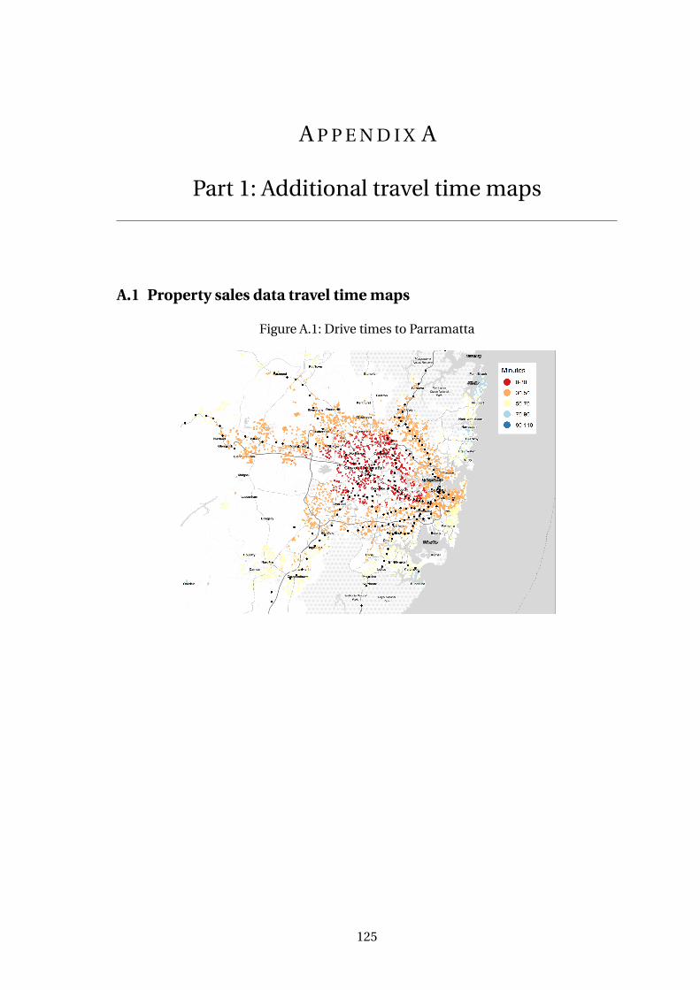
A P P E N D I X A

Part 1: Additional travel time maps

A.1 Property sales data travel time maps

Figure A.1: Drive times to Parramatta

125

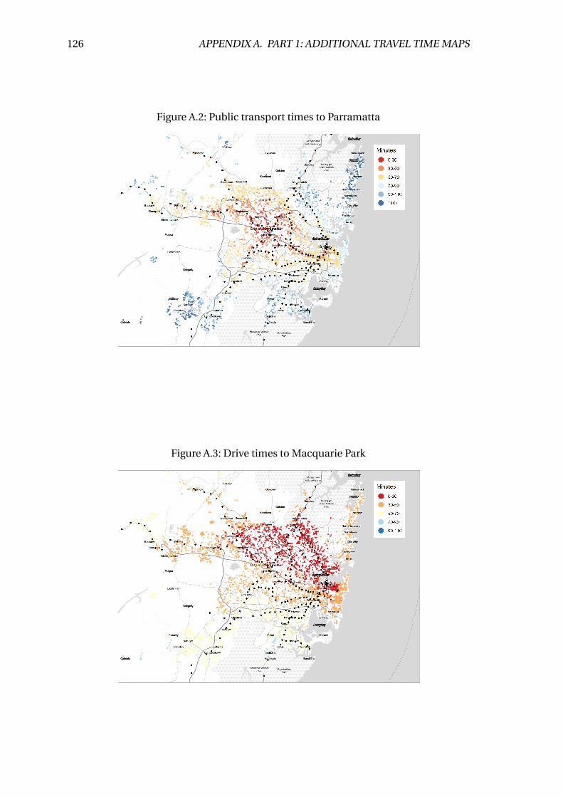
126 APPENDIX A. PART 1: ADDITIONAL TRAVEL TIME MAPS

Figure A.2: Public transport times to Parramatta

Figure A.3: Drive times to Macquarie Park

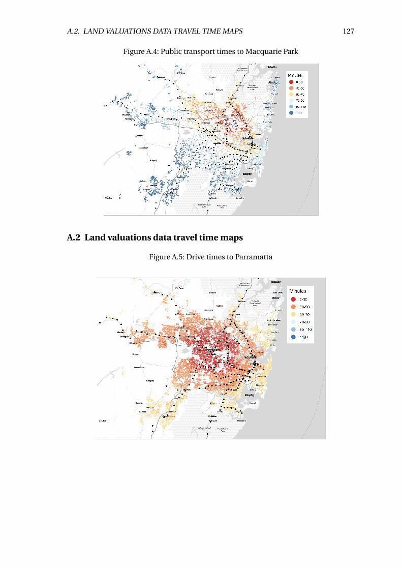
A.2. LAND VALUATIONS DATA TRAVEL TIME MAPS 127

Figure A.4: Public transport times to Macquarie Park

A.2 Land valuations data travel time maps

Figure A.5: Drive times to Parramatta

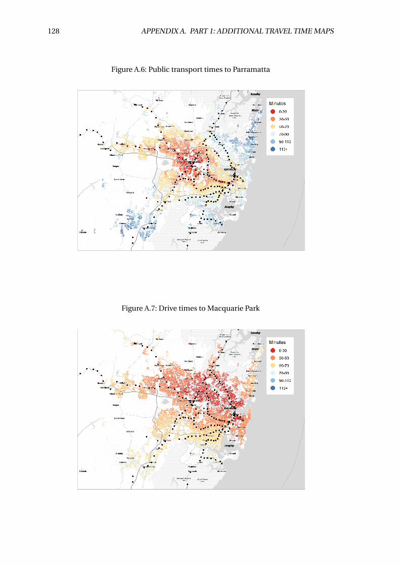
128 APPENDIX A. PART 1: ADDITIONAL TRAVEL TIME MAPS

Figure A.6: Public transport times to Parramatta

Figure A.7: Drive times to Macquarie Park

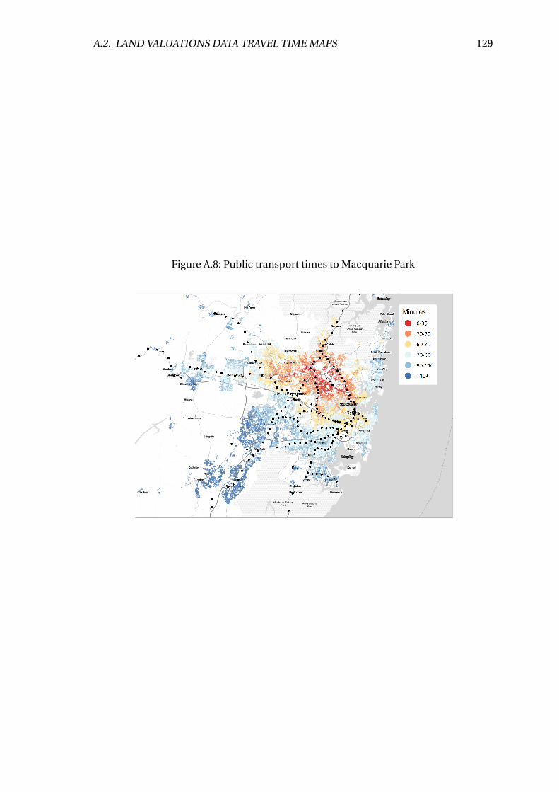
A.2. LAND VALUATIONS DATA TRAVEL TIME MAPS 129

Figure A.8: Public transport times to Macquarie Park

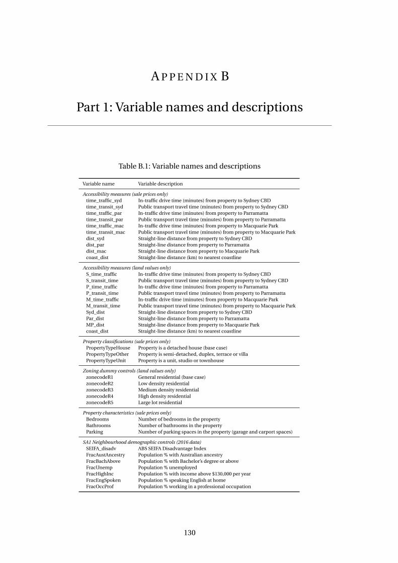
A P P E N D I X B

Part 1: Variable names and descriptions

Table B.1: Variable names and descriptions

Variable name Variable description

Accessibility measures (sale prices only)time_traffic_syd In-traffic drive time (minutes) from property to Sydney CBDtime_transit_syd Public transport travel time (minutes) from property to Sydney CBDtime_traffic_par In-traffic drive time (minutes) from property to Parramattatime_transit_par Public transport travel time (minutes) from property to Parramattatime_traffic_mac In-traffic drive time (minutes) from property to Macquarie Parktime_transit_mac Public transport travel time (minutes) from property to Macquarie Parkdist_syd Straight-line distance from property to Sydney CBDdist_par Straight-line distance from property to Parramattadist_mac Straight-line distance from property to Macquarie Parkcoast_dist Straight-line distance (km) to nearest coastline

Accessibility measures (land values only)S_time_traffic In-traffic drive time (minutes) from property to Sydney CBDS_transit_time Public transport travel time (minutes) from property to Sydney CBDP_time_traffic In-traffic drive time (minutes) from property to ParramattaP_transit_time Public transport travel time (minutes) from property to ParramattaM_time_traffic In-traffic drive time (minutes) from property to Macquarie ParkM_transit_time Public transport travel time (minutes) from property to Macquarie ParkSyd_dist Straight-line distance from property to Sydney CBDPar_dist Straight-line distance from property to ParramattaMP_dist Straight-line distance from property to Macquarie Parkcoast_dist Straight-line distance (km) to nearest coastline

Property classifications (sale prices only)PropertyTypeHouse Property is a detached house (base case)PropertyTypeOther Property is semi-detached, duplex, terrace or villaPropertyTypeUnit Property is a unit, studio or townhouse

Zoning dummy controls (land values only)zonecodeR1 General residential (base case)zonecodeR2 Low density residentialzonecodeR3 Medium density residentialzonecodeR4 High density residentialzonecodeR5 Large lot residential

Property characteristics (sale prices only)Bedrooms Number of bedrooms in the propertyBathrooms Number of bathrooms in the propertyParking Number of parking spaces in the property (garage and carport spaces)

SA1 Neighbourhood demographic controls (2016 data)SEIFA_disadv ABS SEIFA Disadvantage IndexFracAustAncestry Population % with Australian ancestryFracBachAbove Population % with Bachelor’s degree or aboveFracUnemp Population % unemployedFracHighInc Population % with income above $130,000 per yearFracEngSpoken Population % speaking English at homeFracOccProf Population % working in a professional occupation

130

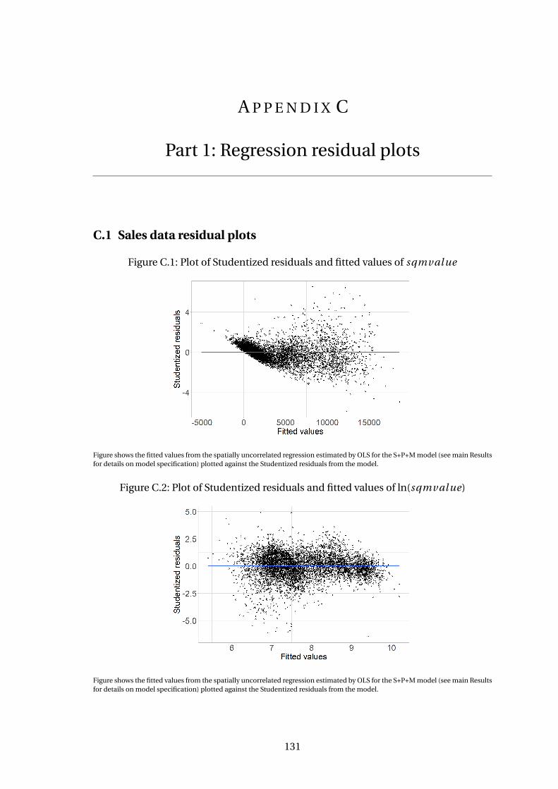
A P P E N D I X C

Part 1: Regression residual plots

C.1 Sales data residual plots

Figure C.1: Plot of Studentized residuals and fitted values of sqmval ue

Figure shows the fitted values from the spatially uncorrelated regression estimated by OLS for the S+P+M model (see main Resultsfor details on model specification) plotted against the Studentized residuals from the model.

Figure C.2: Plot of Studentized residuals and fitted values of ln(sqmval ue)

Figure shows the fitted values from the spatially uncorrelated regression estimated by OLS for the S+P+M model (see main Resultsfor details on model specification) plotted against the Studentized residuals from the model.

131

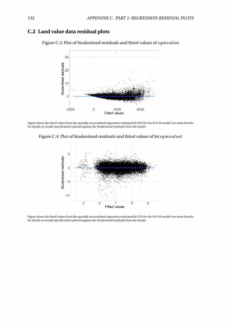
132 APPENDIX C. PART 1: REGRESSION RESIDUAL PLOTS

C.2 Land value data residual plots

Figure C.3: Plot of Studentized residuals and fitted values of sqmval ue

Figure shows the fitted values from the spatially uncorrelated regression estimated by OLS for the S+P+M model (see main Resultsfor details on model specification) plotted against the Studentized residuals from the model.

Figure C.4: Plot of Studentized residuals and fitted values of ln(sqmval ue)

Figure shows the fitted values from the spatially uncorrelated regression estimated by OLS for the S+P+M model (see main Resultsfor details on model specification) plotted against the Studentized residuals from the model.

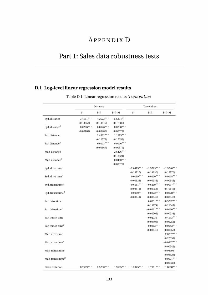
A P P E N D I X D

Part 1: Sales data robustness tests

D.1 Log-level linear regression model results

Table D.1: Linear regression results (l sqmval ue)

Distance Travel time

S S+P S+P+M S S+P S+P+M

Syd. distance −3.4161∗∗∗ −4.2623∗∗∗ −5.6234∗∗∗

(0.13553) (0.13845) (0.17386)

Syd. distance2 0.0206∗∗∗ −0.0126∗∗∗ 0.0298∗∗∗

(0.00161) (0.00407) (0.00577)

Par. distance 2.4562∗∗∗ 1.1915∗∗∗

(0.12572) (0.17056)

Par. distance2 0.0153∗∗∗ 0.0156∗∗∗

(0.00367) (0.00379)

Mac. distance 2.6426∗∗∗

(0.18821)

Mac. distance2 −0.0450∗∗∗

(0.00370)

Syd. drive time −2.0479∗∗∗ −1.9725∗∗∗ −1.9740∗∗∗

(0.13725) (0.14230) (0.15770)

Syd. drive time2 0.0119∗∗∗ 0.0120∗∗∗ 0.0138∗∗∗

(0.00123) (0.00136) (0.00146)

Syd. transit time −0.6581∗∗∗ −0.6499∗∗∗ −0.9037∗∗∗

(0.08811) (0.09953) (0.10142)

Syd. transit time2 0.0009∗∗ 0.0022∗∗∗ 0.0028∗∗∗

(0.00041) (0.00047) (0.00048)

Par. drive time 0.6631∗∗∗ −0.9292∗∗∗

(0.19174) (0.21347)

Par. drive time2 −0.0061∗∗∗ 0.0120∗∗∗

(0.00206) (0.00231)

Par. transit time −0.02736 0.4143∗∗∗

(0.09505) (0.09754)

Par. transit time2 −0.0013∗∗∗ −0.0043∗∗∗

(0.00046) (0.00050)

Mac. drive time 2.0797∗∗∗

(0.22357)

Mac. drive time2 −0.0307∗∗∗

(0.00242)

Mac. transit time −0.08593

(0.08328)

Mac. transit time2 0.0021∗∗∗

(0.00039)

Coast distance −0.7589∗∗∗ 2.5230∗∗∗ 1.9505∗∗∗ −1.2975∗∗∗ −1.7061∗∗∗ −1.8668∗∗∗

133

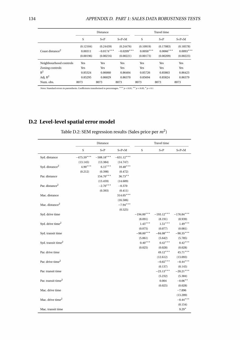
134 APPENDIX D. PART 1: SALES DATA ROBUSTNESS TESTS

Distance Travel time

S S+P S+P+M S S+P S+P+M

(0.12104) (0.24439) (0.24476) (0.10919) (0.17083) (0.18578)

Coast distance2 0.00311 −0.0174∗∗∗ −0.0209∗∗∗ 0.0050∗∗∗ 0.0066∗∗∗ 0.0093∗∗∗

(0.00196) (0.00216) (0.00221) (0.00173) (0.00209) (0.00223)

Neighbourhood controls Yes Yes Yes Yes Yes Yes

Zoning controls Yes Yes Yes Yes Yes Yes

R2 0.85324 0.86060 0.86404 0.85726 0.85863 0.86423

Adj. R2 0.85295 0.86029 0.86370 0.85694 0.85824 0.86379

Num. obs. 8073 8073 8073 8073 8073 8073

Notes: Standard errors in parenthesis. Coefficients transformed to percentages. ∗∗∗p < 0.01; ∗∗p < 0.05; ∗p < 0.1

D.2 Level-level spatial error model

Table D.2: SEM regression results (Sales price per m2)

Distance Travel time

S S+P S+P+M S S+P S+P+M

Syd. distance −475.59∗∗∗ −508.18∗∗∗ −631.12∗∗∗

(13.145) (13.384) (14.747)

Syd. distance2 4.90∗∗∗ 6.15∗∗∗ 10.48∗∗∗

(0.212) (0.398) (0.472)

Par. distance 154.70∗∗∗ 36.73∗∗

(13.459) (14.609)

Par. distance2 −2.70∗∗∗ −0.370

(0.393) (0.411)

Mac. distance 314.05∗∗∗

(16.506)

Mac. distance2 −7.94∗∗∗

(0.525)

Syd. drive time −194.00∗∗∗ −193.12∗∗∗ −176.84∗∗∗

(8.091) (8.191) (8.939)

Syd. drive time2 1.43∗∗∗ 1.51∗∗∗ 1.49∗∗∗

(0.075) (0.077) (0.081)

Syd. transit time −98.00∗∗∗ −84.08∗∗∗ −90.35∗∗∗

(5.061) (5.642) (5.785)

Syd. transit time2 0.40∗∗∗ 0.42∗∗∗ 0.42∗∗∗

(0.025) (0.028) (0.028)

Par. drive time 49.12∗∗∗ 45.71∗∗∗

(12.612) (13.093)

Par. drive time2 −0.65∗∗∗ −0.44∗∗∗

(0.137) (0.145)

Par. transit time −23.13∗∗∗ −20.21∗∗∗

(5.232) (5.384)

Par. transit time2 0.004 −0.06∗∗

(0.025) (0.028)

Mac. drive time −7.896

(13.289)

Mac. drive time2 −0.44∗∗∗

(0.154)

Mac. transit time 9.29∗

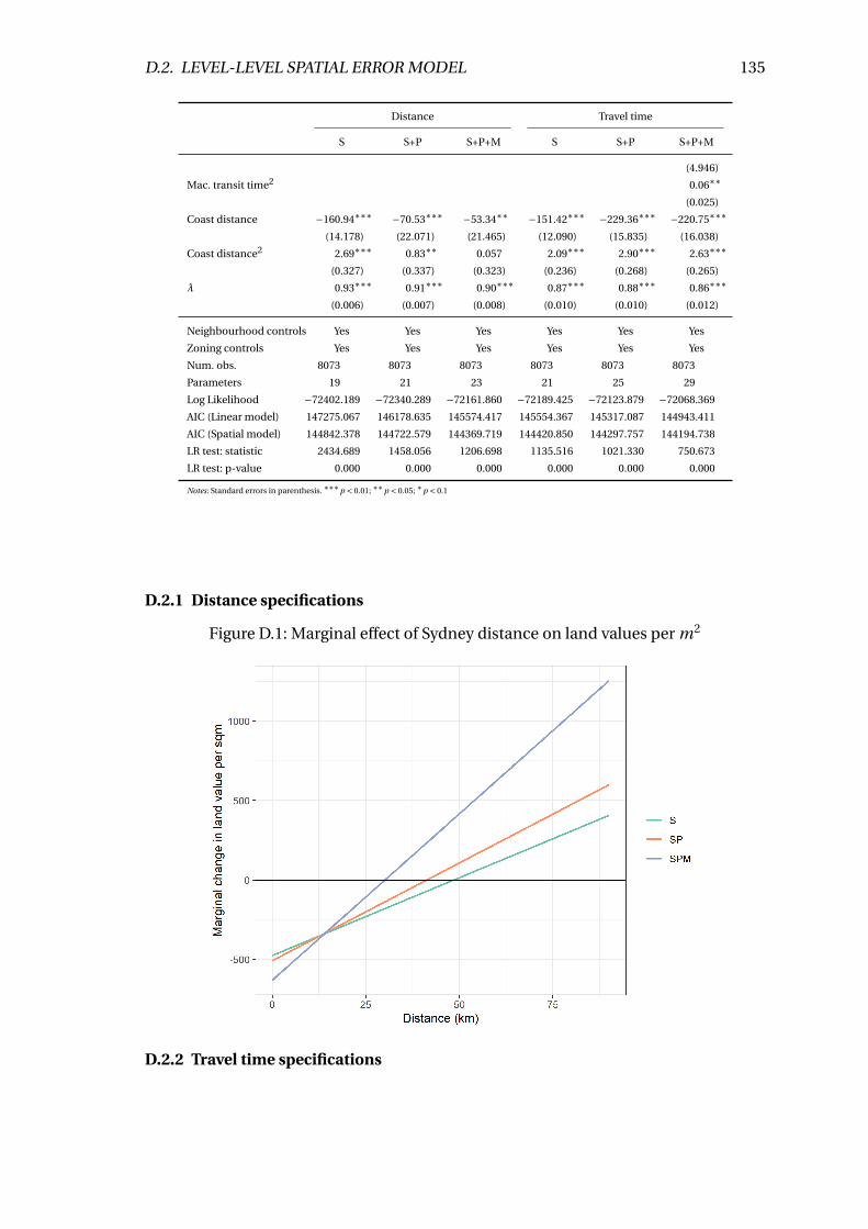
D.2. LEVEL-LEVEL SPATIAL ERROR MODEL 135

Distance Travel time

S S+P S+P+M S S+P S+P+M

(4.946)

Mac. transit time2 0.06∗∗

(0.025)

Coast distance −160.94∗∗∗ −70.53∗∗∗ −53.34∗∗ −151.42∗∗∗ −229.36∗∗∗ −220.75∗∗∗

(14.178) (22.071) (21.465) (12.090) (15.835) (16.038)

Coast distance2 2.69∗∗∗ 0.83∗∗ 0.057 2.09∗∗∗ 2.90∗∗∗ 2.63∗∗∗

(0.327) (0.337) (0.323) (0.236) (0.268) (0.265)

λ 0.93∗∗∗ 0.91∗∗∗ 0.90∗∗∗ 0.87∗∗∗ 0.88∗∗∗ 0.86∗∗∗

(0.006) (0.007) (0.008) (0.010) (0.010) (0.012)

Neighbourhood controls Yes Yes Yes Yes Yes Yes

Zoning controls Yes Yes Yes Yes Yes Yes

Num. obs. 8073 8073 8073 8073 8073 8073

Parameters 19 21 23 21 25 29

Log Likelihood −72402.189 −72340.289 −72161.860 −72189.425 −72123.879 −72068.369

AIC (Linear model) 147275.067 146178.635 145574.417 145554.367 145317.087 144943.411

AIC (Spatial model) 144842.378 144722.579 144369.719 144420.850 144297.757 144194.738

LR test: statistic 2434.689 1458.056 1206.698 1135.516 1021.330 750.673

LR test: p-value 0.000 0.000 0.000 0.000 0.000 0.000

Notes: Standard errors in parenthesis. ∗∗∗p < 0.01; ∗∗p < 0.05; ∗p < 0.1

D.2.1 Distance specifications

Figure D.1: Marginal effect of Sydney distance on land values per m2

D.2.2 Travel time specifications

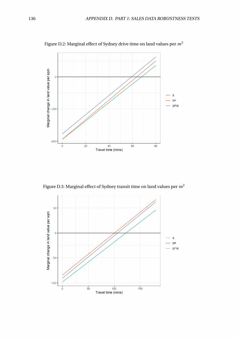
136 APPENDIX D. PART 1: SALES DATA ROBUSTNESS TESTS

Figure D.2: Marginal effect of Sydney drive time on land values per m2

Figure D.3: Marginal effect of Sydney transit time on land values per m2

D.3. LOG-LEVEL SPATIAL AUTOREGRESSIVE MODELS 137

D.3 Log-level spatial autoregressive models

Table D.3: SARM regression results (l sqmval ue)

Distance Travel time

S S+P S+P+M S S+P S+P+M

Syd. distance 0.10296 −0.7164∗∗∗ −2.1967∗∗∗

(0.14553) (0.16694) (0.19012)

Syd. distance2 0.0058∗∗∗ −0.0075∗ 0.0477∗∗∗

(0.00145) (0.00396) (0.00553)

Par. distance 2.3295∗∗∗ 1.5395∗∗∗

(0.12051) (0.16257)

Par. distance2 −0.00317 −0.0088∗∗

(0.00361) (0.00369)

Mac. distance 2.3127∗∗∗

(0.17976)

Mac. distance2 −0.0525∗∗∗

(0.00353)

Syd. drive time −1.8750∗∗∗ −1.5975∗∗∗ −1.7129∗∗∗

(0.13026) (0.13440) (0.14807)

Syd. drive time2 0.0166∗∗∗ 0.0118∗∗∗ 0.0157∗∗∗

(0.00117) (0.00128) (0.00138)

Syd. transit time −0.2687∗∗∗ −0.3540∗∗∗ −0.6391∗∗∗

(0.08359) (0.09373) (0.09600)

Syd. transit time2 0.0010∗∗∗ 0.0022∗∗∗ 0.0030∗∗∗

(0.00038) (0.00045) (0.00045)

Par. drive time 0.4278∗∗ −0.3574∗

(0.17822) (0.21051)

Par. drive time2 0.0055∗∗∗ 0.0144∗∗∗

(0.00194) (0.00224)

Par. transit time −0.11736 0.13662

(0.08737) (0.09724)

Par. transit time2 −0.0013∗∗∗ −0.0025∗∗∗

(0.00042) (0.00049)

Mac. drive time 1.3916∗∗∗

(0.18314)

Mac. drive time2 −0.0226∗∗∗

(0.00197)

Mac. transit time 0.1097∗∗∗

(0.03708)

Mac. transit time2 0.0002∗∗

(0.00011)

Coast distance 0.08060 2.2763∗∗∗ 1.7074∗∗∗ 0.6557∗∗∗ 1.6674∗∗∗ 1.5625∗∗∗

(0.10690) (0.23591) (0.23463) (0.12103) (0.18488) (0.19521)

Coast distance2 −0.0037∗∗ −0.0222∗∗∗ −0.0284∗∗∗ −0.0115∗∗∗ −0.0224∗∗∗ −0.0201∗∗∗

(0.00172) (0.00208) (0.00212) (0.00172) (0.00212) (0.00221)

ρ 0.7360∗∗∗ 0.7245∗∗∗ 0.7368∗∗∗ 0.6319∗∗∗ 0.7013∗∗∗ 0.6822∗∗∗

(0.01935) (0.02075) (0.01997) (0.02031) (0.01905) (0.02033)

Neighbourhood controls Yes Yes Yes Yes Yes Yes

Zoning controls Yes Yes Yes Yes Yes Yes

Num. obs. 8073 8073 8073 8073 8073 8073

Parameters 19 21 23 21 25 29

Log Likelihood −3635.86441 −3451.54166 −3339.16507 −3480.31021 −3383.25030 −3285.29233

AIC (Linear model) 7985.79392 7574.62365 7377.23656 7766.01901 7696.05379 7377.83767

AIC (Spatial model) 7309.72882 6945.08332 6724.33013 7002.62041 6816.50060 6628.58466

LR test: statistic 678.06510 631.54033 654.90643 765.39860 881.55319 751.25301

LR test: p-value 0.00000 0.00000 0.00000 0.00000 0.00000 0.00000

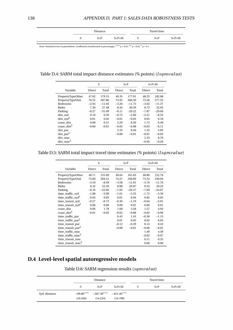
138 APPENDIX D. PART 1: SALES DATA ROBUSTNESS TESTS

Distance Travel time

S S+P S+P+M S S+P S+P+M

Notes: Standard errors in parenthesis. Coefficients transformed to percentages. ∗∗∗p < 0.01; ∗∗p < 0.05; ∗p < 0.1

Table D.4: SARM total impact distance estimates (% points) (l sqmval ue)

S S+P S+P+M

Variable Direct Total Direct Total Direct Total

PropertyTypeOther 47.62 179.15 49.35 177.91 48.25 182.06PropertyTypeUnit 76.52 287.86 73.92 266.50 73.56 277.55Bedrooms −2.94 −11.05 −3.26 −11.75 −3.02 −11.37Baths 7.30 27.48 8.43 30.39 8.73 32.93Parking −8.27 −31.09 −8.11 −29.22 −7.87 −29.69dist_syd 0.10 0.39 −0.72 −2.60 −2.21 −8.35dist_syd2 0.01 0.02 −0.01 −0.03 0.05 0.18coast_dist 0.08 0.31 2.29 8.26 1.72 6.49coast_dist2 −0.00 −0.01 −0.02 −0.08 −0.03 −0.11dist_par 2.35 8.46 1.55 5.85dist_par2 −0.00 −0.01 −0.01 −0.03dist_mac 2.33 8.79dist_mac2 −0.05 −0.20

Table D.5: SARM total impact travel time estimates (% points) (l sqmval ue)

S S+P S+P+M

Variable Direct Total Direct Total Direct Total

PropertyTypeOther 48.71 131.69 48.64 161.83 48.80 152.70PropertyTypeUnit 75.60 204.41 74.57 248.09 73.52 230.04Bedrooms −3.10 −8.39 −3.58 −11.91 −3.76 −11.76Baths 8.32 22.49 8.98 29.87 9.35 29.25Parking −8.16 −22.06 −7.93 −26.37 −7.69 −24.07time_traffic_syd −1.88 −5.09 −1.61 −5.35 −1.72 −5.39time_traffic_syd2 0.02 0.05 0.01 0.04 0.02 0.05time_transit_syd −0.27 −0.73 −0.36 −1.19 −0.64 −2.01time_transit_syd2 0.00 0.00 0.00 0.01 0.00 0.01coast_dist 0.66 1.78 1.68 5.58 1.57 4.92coast_dist2 −0.01 −0.03 −0.02 −0.08 −0.02 −0.06time_traffic_par 0.43 1.43 −0.36 −1.13time_traffic_par2 0.01 0.02 0.02 0.05time_transit_par −0.12 −0.39 0.14 0.43time_transit_par2 −0.00 −0.01 −0.00 −0.01time_traffic_mac 1.40 4.38time_traffic_mac2 −0.02 −0.07time_transit_mac 0.11 0.35time_transit_mac2 0.00 0.00

D.4 Level-level spatial autoregressive models

Table D.6: SARM regression results (sqmval ue)

Distance Travel time

S S+P S+P+M S S+P S+P+M

Syd. distance −99.80∗∗∗ −267.38∗∗∗ −421.46∗∗∗

(10.436) (14.224) (14.700)

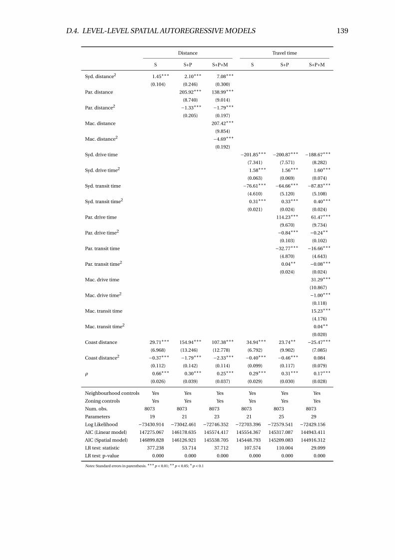
D.4. LEVEL-LEVEL SPATIAL AUTOREGRESSIVE MODELS 139

Distance Travel time

S S+P S+P+M S S+P S+P+M

Syd. distance2 1.45∗∗∗ 2.10∗∗∗ 7.08∗∗∗

(0.104) (0.246) (0.300)

Par. distance 205.92∗∗∗ 138.99∗∗∗

(8.740) (9.014)

Par. distance2 −1.33∗∗∗ −1.79∗∗∗

(0.205) (0.197)

Mac. distance 207.42∗∗∗

(9.854)

Mac. distance2 −4.69∗∗∗

(0.192)

Syd. drive time −201.85∗∗∗ −200.87∗∗∗ −188.67∗∗∗

(7.341) (7.571) (8.282)

Syd. drive time2 1.58∗∗∗ 1.56∗∗∗ 1.60∗∗∗

(0.063) (0.069) (0.074)

Syd. transit time −76.61∗∗∗ −64.66∗∗∗ −87.83∗∗∗

(4.610) (5.120) (5.108)

Syd. transit time2 0.31∗∗∗ 0.33∗∗∗ 0.40∗∗∗

(0.021) (0.024) (0.024)

Par. drive time 114.23∗∗∗ 61.47∗∗∗

(9.670) (9.734)

Par. drive time2 −0.84∗∗∗ −0.24∗∗

(0.103) (0.102)

Par. transit time −32.77∗∗∗ −16.66∗∗∗

(4.870) (4.643)

Par. transit time2 0.04∗∗ −0.08∗∗∗

(0.024) (0.024)

Mac. drive time 31.29∗∗∗

(10.867)

Mac. drive time2 −1.00∗∗∗

(0.118)

Mac. transit time 15.23∗∗∗

(4.176)

Mac. transit time2 0.04∗∗

(0.020)

Coast distance 29.71∗∗∗ 154.94∗∗∗ 107.38∗∗∗ 34.94∗∗∗ 23.74∗∗ −25.47∗∗∗

(6.968) (13.246) (12.778) (6.792) (9.902) (7.085)

Coast distance2 −0.37∗∗∗ −1.79∗∗∗ −2.33∗∗∗ −0.40∗∗∗ −0.46∗∗∗ 0.084

(0.112) (0.142) (0.114) (0.099) (0.117) (0.079)

ρ 0.66∗∗∗ 0.30∗∗∗ 0.25∗∗∗ 0.29∗∗∗ 0.31∗∗∗ 0.17∗∗∗

(0.026) (0.039) (0.037) (0.029) (0.030) (0.028)

Neighbourhood controls Yes Yes Yes Yes Yes Yes

Zoning controls Yes Yes Yes Yes Yes Yes

Num. obs. 8073 8073 8073 8073 8073 8073

Parameters 19 21 23 21 25 29

Log Likelihood −73430.914 −73042.461 −72746.352 −72703.396 −72579.541 −72429.156

AIC (Linear model) 147275.067 146178.635 145574.417 145554.367 145317.087 144943.411

AIC (Spatial model) 146899.828 146126.921 145538.705 145448.793 145209.083 144916.312

LR test: statistic 377.238 53.714 37.712 107.574 110.004 29.099

LR test: p-value 0.000 0.000 0.000 0.000 0.000 0.000

Notes: Standard errors in parenthesis. ∗∗∗p < 0.01; ∗∗p < 0.05; ∗p < 0.1

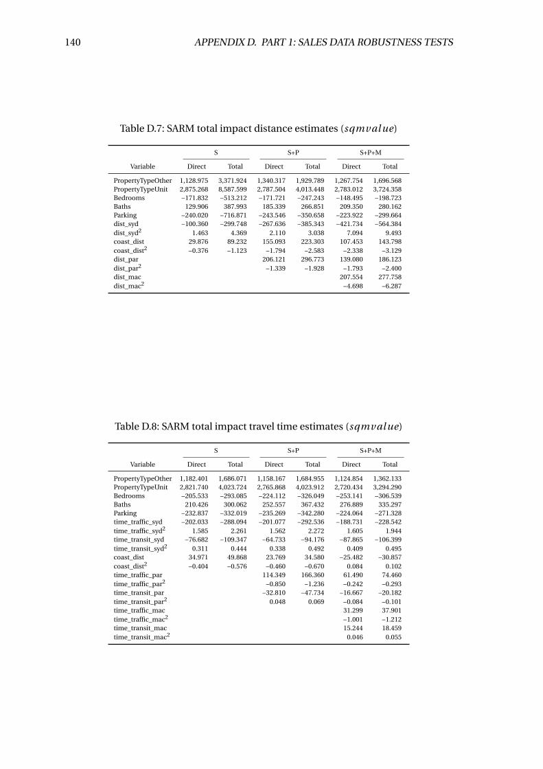
140 APPENDIX D. PART 1: SALES DATA ROBUSTNESS TESTS

Table D.7: SARM total impact distance estimates (sqmval ue)

S S+P S+P+M

Variable Direct Total Direct Total Direct Total

PropertyTypeOther 1,128.975 3,371.924 1,340.317 1,929.789 1,267.754 1,696.568PropertyTypeUnit 2,875.268 8,587.599 2,787.504 4,013.448 2,783.012 3,724.358Bedrooms −171.832 −513.212 −171.721 −247.243 −148.495 −198.723Baths 129.906 387.993 185.339 266.851 209.350 280.162Parking −240.020 −716.871 −243.546 −350.658 −223.922 −299.664dist_syd −100.360 −299.748 −267.636 −385.343 −421.734 −564.384dist_syd2 1.463 4.369 2.110 3.038 7.094 9.493coast_dist 29.876 89.232 155.093 223.303 107.453 143.798coast_dist2 −0.376 −1.123 −1.794 −2.583 −2.338 −3.129dist_par 206.121 296.773 139.080 186.123dist_par2 −1.339 −1.928 −1.793 −2.400dist_mac 207.554 277.758dist_mac2 −4.698 −6.287

Table D.8: SARM total impact travel time estimates (sqmval ue)

S S+P S+P+M

Variable Direct Total Direct Total Direct Total

PropertyTypeOther 1,182.401 1,686.071 1,158.167 1,684.955 1,124.854 1,362.133PropertyTypeUnit 2,821.740 4,023.724 2,765.868 4,023.912 2,720.434 3,294.290Bedrooms −205.533 −293.085 −224.112 −326.049 −253.141 −306.539Baths 210.426 300.062 252.557 367.432 276.889 335.297Parking −232.837 −332.019 −235.269 −342.280 −224.064 −271.328time_traffic_syd −202.033 −288.094 −201.077 −292.536 −188.731 −228.542time_traffic_syd2 1.585 2.261 1.562 2.272 1.605 1.944time_transit_syd −76.682 −109.347 −64.733 −94.176 −87.865 −106.399time_transit_syd2 0.311 0.444 0.338 0.492 0.409 0.495coast_dist 34.971 49.868 23.769 34.580 −25.482 −30.857coast_dist2 −0.404 −0.576 −0.460 −0.670 0.084 0.102time_traffic_par 114.349 166.360 61.490 74.460time_traffic_par2 −0.850 −1.236 −0.242 −0.293time_transit_par −32.810 −47.734 −16.667 −20.182time_transit_par2 0.048 0.069 −0.084 −0.101time_traffic_mac 31.299 37.901time_traffic_mac2 −1.001 −1.212time_transit_mac 15.244 18.459time_transit_mac2 0.046 0.055

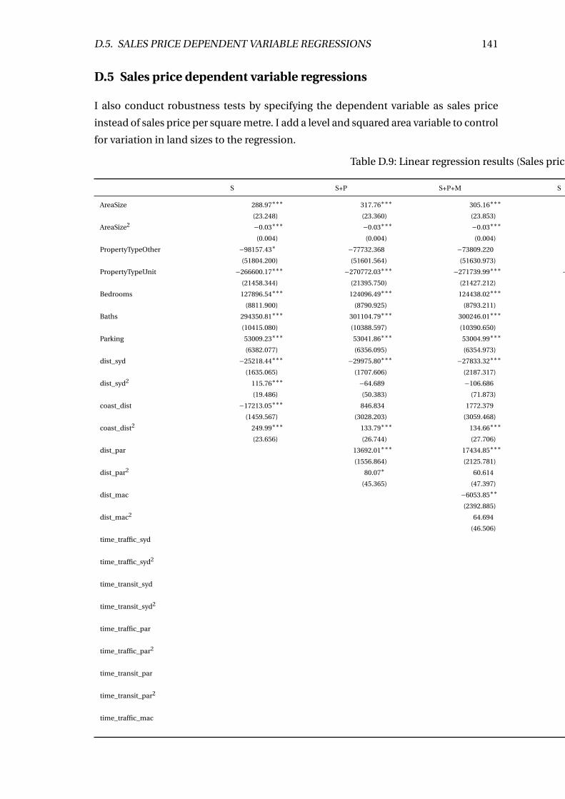
D.5. SALES PRICE DEPENDENT VARIABLE REGRESSIONS 141

D.5 Sales price dependent variable regressions

I also conduct robustness tests by specifying the dependent variable as sales price

instead of sales price per square metre. I add a level and squared area variable to control

for variation in land sizes to the regression.

Table D.9: Linear regression results (Sales price)

S S+P S+P+M S S+P S+P+M

AreaSize 288.97∗∗∗ 317.76∗∗∗ 305.16∗∗∗ 307.00∗∗∗ 296.98∗∗∗ 318.01∗∗∗

(23.248) (23.360) (23.853) (23.290) (23.531) (23.680)

AreaSize2 −0.03∗∗∗ −0.03∗∗∗ −0.03∗∗∗ −0.03∗∗∗ −0.03∗∗∗ −0.03∗∗∗

(0.004) (0.004) (0.004) (0.004) (0.004) (0.004)

PropertyTypeOther −98157.43∗ −77732.368 −73809.220 −93535.01∗ −96198.76∗ −97801.19∗

(51804.200) (51601.564) (51630.973) (51743.158) (51736.518) (51263.324)

PropertyTypeUnit −266600.17∗∗∗ −270772.03∗∗∗ −271739.99∗∗∗ −274981.55∗∗∗ −280692.78∗∗∗ −290547.21∗∗∗

(21458.344) (21395.750) (21427.212) (21532.599) (21590.264) (21456.632)

Bedrooms 127896.54∗∗∗ 124096.49∗∗∗ 124438.02∗∗∗ 119759.32∗∗∗ 120979.78∗∗∗ 115573.41∗∗∗

(8811.900) (8790.925) (8793.211) (8813.875) (8830.818) (8768.405)

Baths 294350.81∗∗∗ 301104.79∗∗∗ 300246.01∗∗∗ 302477.33∗∗∗ 301365.83∗∗∗ 304765.48∗∗∗

(10415.080) (10388.597) (10390.650) (10427.829) (10440.007) (10344.296)

Parking 53009.23∗∗∗ 53041.86∗∗∗ 53004.99∗∗∗ 53253.03∗∗∗ 52994.93∗∗∗ 51775.80∗∗∗

(6382.077) (6356.095) (6354.973) (6379.287) (6381.567) (6321.642)

dist_syd −25218.44∗∗∗ −29975.80∗∗∗ −27833.32∗∗∗

(1635.065) (1707.606) (2187.317)

dist_syd2 115.76∗∗∗ −64.689 −106.686

(19.486) (50.383) (71.873)

coast_dist −17213.05∗∗∗ 846.834 1772.379 −25027.88∗∗∗ −27383.04∗∗∗ −36387.91∗∗∗

(1459.567) (3028.203) (3059.468) (1333.724) (2093.213) (2302.091)

coast_dist2 249.99∗∗∗ 133.79∗∗∗ 134.66∗∗∗ 304.28∗∗∗ 334.62∗∗∗ 428.03∗∗∗

(23.656) (26.744) (27.706) (21.168) (25.688) (27.765)

dist_par 13692.01∗∗∗ 17434.85∗∗∗

(1556.864) (2125.781)

dist_par2 80.07∗ 60.614

(45.365) (47.397)

dist_mac −6053.85∗∗

(2392.885)

dist_mac2 64.694

(46.506)

time_traffic_syd −11467.91∗∗∗ −13003.96∗∗∗ −5126.24∗∗∗

(1677.900) (1743.718) (1952.674)

time_traffic_syd2 46.96∗∗∗ 65.12∗∗∗ 32.76∗

(14.977) (16.632) (18.088)

time_transit_syd −1762.976 −160.705 −2249.00∗

(1076.781) (1219.875) (1257.106)

time_transit_syd2 −10.92∗∗ −20.94∗∗∗ −13.86∗∗

(5.002) (5.820) (5.898)

time_traffic_par 2879.477 −3831.274

(2352.761) (2646.048)

time_traffic_par2 −40.270 60.96∗∗

(25.285) (28.702)

time_transit_par −2822.77∗∗ −1337.008

(1165.446) (1209.317)

time_transit_par2 17.77∗∗∗ −7.446

(5.641) (6.249)

time_traffic_mac −2062.431

(2773.098)

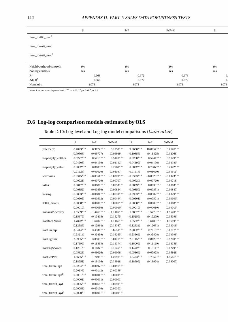
142 APPENDIX D. PART 1: SALES DATA ROBUSTNESS TESTS

S S+P S+P+M S S+P S+P+M

time_traffic_mac2 −110.60∗∗∗

(30.105)

time_transit_mac 1116.956

(1032.038)

time_transit_mac2 19.33∗∗∗

(4.823)

Neighbourhood controls Yes Yes Yes Yes Yes Yes

Zoning controls Yes Yes Yes Yes Yes Yes

R2 0.669 0.672 0.673 0.670 0.671 0.678

Adj. R2 0.668 0.672 0.672 0.669 0.670 0.676

Num. obs. 8073 8073 8073 8073 8073 8073

Notes: Standard errors in parenthesis. ∗∗∗p < 0.01; ∗∗p < 0.05; ∗p < 0.1

D.6 Log-log comparison models estimated by OLS

Table D.10: Log-level and Log-log model comparisons (l sqmval ue)

S S+P S+P+M S S+P S+P+M

(Intercept) 8.4823∗∗∗ 8.3174∗∗∗ 8.1750∗∗∗ 9.9650∗∗∗ 10.0054∗∗∗ 9.7126∗∗∗

(0.09566) (0.09777) (0.09949) (0.10857) (0.11475) (0.12068)

PropertyTypeOther 0.5277∗∗∗ 0.5213∗∗∗ 0.5120∗∗∗ 0.5250∗∗∗ 0.5244∗∗∗ 0.5129∗∗∗

(0.04208) (0.04190) (0.04112) (0.04199) (0.04196) (0.04180)

PropertyTypeUnit 0.8032∗∗∗ 0.8003∗∗∗ 0.7760∗∗∗ 0.8032∗∗∗ 0.7987∗∗∗ 0.7922∗∗∗

(0.01624) (0.01620) (0.01597) (0.01617) (0.01620) (0.01615)

Bedrooms −0.0345∗∗∗ −0.0351∗∗∗ −0.0370∗∗∗ −0.0323∗∗∗ −0.0326∗∗∗ −0.0323∗∗∗

(0.00721) (0.00720) (0.00707) (0.00720) (0.00720) (0.00718)

Baths 0.0847∗∗∗ 0.0888∗∗∗ 0.0953∗∗∗ 0.0839∗∗∗ 0.0839∗∗∗ 0.0863∗∗∗

(0.00852) (0.00850) (0.00834) (0.00850) (0.00851) (0.00847)

Parking −0.0893∗∗∗ −0.0881∗∗∗ −0.0839∗∗∗ −0.0903∗∗∗ −0.0902∗∗∗ −0.0879∗∗∗

(0.00503) (0.00502) (0.00494) (0.00501) (0.00501) (0.00500)

SEIFA_disadv 0.0008∗∗∗ 0.0008∗∗∗ 0.0007∗∗∗ 0.0008∗∗∗ 0.0008∗∗∗ 0.0008∗∗∗

(0.00010) (0.00010) (0.00010) (0.00010) (0.00010) (0.00010)

FracAustAncestry −1.5589∗∗∗ −1.4469∗∗∗ −1.1105∗∗∗ −1.5887∗∗∗ −1.5773∗∗∗ −1.5520∗∗∗

(0.15375) (0.15405) (0.15275) (0.15255) (0.15259) (0.15196)

FracBachAbove −1.7822∗∗∗ −1.6402∗∗∗ −1.1166∗∗∗ −1.6582∗∗∗ −1.6403∗∗∗ −1.3619∗∗∗

(0.12685) (0.12964) (0.13167) (0.12634) (0.12631) (0.13019)

FracUnemp 3.3414∗∗∗ 3.4536∗∗∗ 3.6551∗∗∗ 2.9052∗∗∗ 2.7815∗∗∗ 3.0717∗∗∗

(0.33514) (0.33499) (0.33265) (0.33165) (0.33508) (0.33598)

FracHighInc 2.9985∗∗∗ 3.0503∗∗∗ 3.0147∗∗∗ 2.8115∗∗∗ 2.8429∗∗∗ 2.9240∗∗∗

(0.17896) (0.18383) (0.18374) (0.18005) (0.18129) (0.18339)

FracEngSpoken −0.1261∗∗ −0.1187∗∗ −0.1545∗∗ −0.1472∗∗ −0.1314∗∗ −0.1279∗∗

(0.05923) (0.06026) (0.06006) (0.05866) (0.05973) (0.05948)

FracOccProf 1.8655∗∗∗ 1.7495∗∗∗ 1.2797∗∗∗ 1.8423∗∗∗ 1.7352∗∗∗ 1.5561∗∗∗

(0.18751) (0.19106) (0.18948) (0.18699) (0.18974) (0.19007)

time_traffic_syd −0.0204∗∗∗ −0.0197∗∗∗ −0.0197∗∗∗

(0.00137) (0.00142) (0.00158)

time_traffic_syd2 0.0001∗∗∗ 0.0001∗∗∗ 0.0001∗∗∗

(0.00001) (0.00001) (0.00001)

time_transit_syd −0.0065∗∗∗ −0.0065∗∗∗ −0.0090∗∗∗

(0.00088) (0.00100) (0.00101)

time_transit_syd2 0.0000∗∗ 0.0000∗∗∗ 0.0000∗∗∗

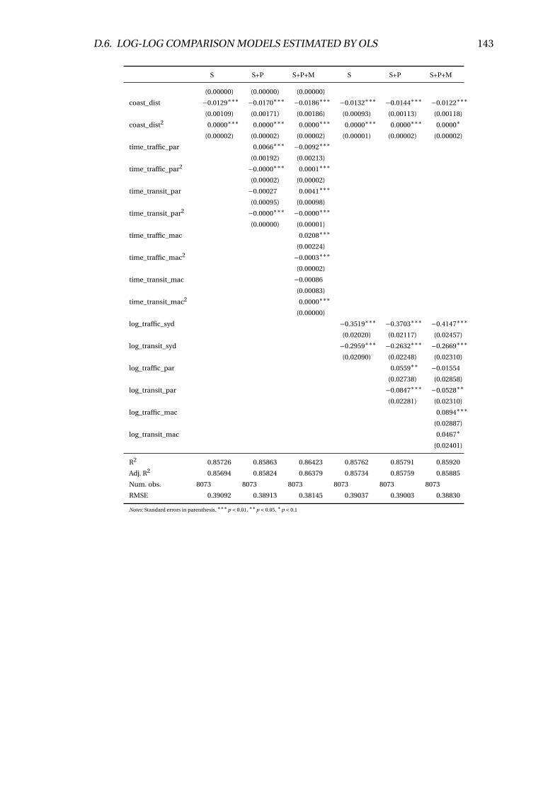
D.6. LOG-LOG COMPARISON MODELS ESTIMATED BY OLS 143

S S+P S+P+M S S+P S+P+M

(0.00000) (0.00000) (0.00000)

coast_dist −0.0129∗∗∗ −0.0170∗∗∗ −0.0186∗∗∗ −0.0132∗∗∗ −0.0144∗∗∗ −0.0122∗∗∗

(0.00109) (0.00171) (0.00186) (0.00093) (0.00113) (0.00118)

coast_dist2 0.0000∗∗∗ 0.0000∗∗∗ 0.0000∗∗∗ 0.0000∗∗∗ 0.0000∗∗∗ 0.0000∗

(0.00002) (0.00002) (0.00002) (0.00001) (0.00002) (0.00002)

time_traffic_par 0.0066∗∗∗ −0.0092∗∗∗

(0.00192) (0.00213)

time_traffic_par2 −0.0000∗∗∗ 0.0001∗∗∗

(0.00002) (0.00002)

time_transit_par −0.00027 0.0041∗∗∗

(0.00095) (0.00098)

time_transit_par2 −0.0000∗∗∗ −0.0000∗∗∗

(0.00000) (0.00001)

time_traffic_mac 0.0208∗∗∗

(0.00224)

time_traffic_mac2 −0.0003∗∗∗

(0.00002)

time_transit_mac −0.00086

(0.00083)

time_transit_mac2 0.0000∗∗∗

(0.00000)

log_traffic_syd −0.3519∗∗∗ −0.3703∗∗∗ −0.4147∗∗∗

(0.02020) (0.02117) (0.02457)

log_transit_syd −0.2959∗∗∗ −0.2632∗∗∗ −0.2669∗∗∗

(0.02090) (0.02248) (0.02310)

log_traffic_par 0.0559∗∗ −0.01554

(0.02738) (0.02858)

log_transit_par −0.0847∗∗∗ −0.0528∗∗

(0.02281) (0.02310)

log_traffic_mac 0.0894∗∗∗

(0.02887)

log_transit_mac 0.0467∗

(0.02401)

R2 0.85726 0.85863 0.86423 0.85762 0.85791 0.85920

Adj. R2 0.85694 0.85824 0.86379 0.85734 0.85759 0.85885

Num. obs. 8073 8073 8073 8073 8073 8073

RMSE 0.39092 0.38913 0.38145 0.39037 0.39003 0.38830

Notes: Standard errors in parenthesis. ∗∗∗p < 0.01, ∗∗p < 0.05, ∗p < 0.1

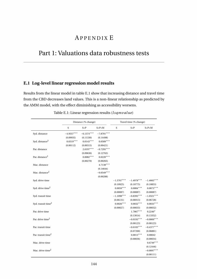
A P P E N D I X E

Part 1: Valuations data robustness tests

E.1 Log-level linear regression model results

Results from the linear model in table E.1 show that increasing distance and travel time

from the CBD decreases land values. This is a non-linear relationship as predicted by

the AMM model, with the effect diminishing as accessibility worsens.

Table E.1: Linear regression results (l sqmval ue)

Distance (% change) Travel time (% change)

S S+P S+P+M S S+P S+P+M

Syd. distance −4.9557∗∗∗ −6.1374∗∗∗ −7.8701∗∗∗

(0.09935) (0.11330) (0.14498)

Syd. distance2 0.0319∗∗∗ 0.0143∗∗∗ 0.0509∗∗∗

(0.00112) (0.00315) (0.00421)

Par. distance 2.0197∗∗∗ −0.7295∗∗∗

(0.09636) (0.12763)

Par. distance2 0.0082∗∗∗ 0.0220∗∗∗

(0.00270) (0.00265)

Mac. distance 4.7138∗∗∗

(0.14644)

Mac. distance2 −0.0549∗∗∗

(0.00288)

Syd. drive time −1.3767∗∗∗ −1.4978∗∗∗ −1.4665∗∗∗

(0.10925) (0.10775) (0.10853)

Syd. drive time2 0.0059∗∗∗ 0.0084∗∗∗ 0.0073∗∗∗

(0.00087) (0.00087) (0.00087)

Syd. transit time −1.1098∗∗∗ −0.8395∗∗∗ −1.0321∗∗∗

(0.06131) (0.06913) (0.06728)

Syd. transit time2 0.0026∗∗∗ 0.0032∗∗∗ 0.0033∗∗∗

(0.00027) (0.00033) (0.00032)

Par. drive time 1.7867∗∗∗ 0.2240∗

(0.13014) (0.13352)

Par. drive time2 −0.0193∗∗∗ −0.0069∗∗∗

(0.00123) (0.00123)

Par. transit time −0.6105∗∗∗ −0.4377∗∗∗

(0.07200) (0.06881)

Par. transit time2 0.0013∗∗∗ 0.00042

(0.00036) (0.00034)

Mac. drive time 0.6749∗∗∗

(0.12446)

Mac. drive time2 −0.0097∗∗∗

(0.00111)

144

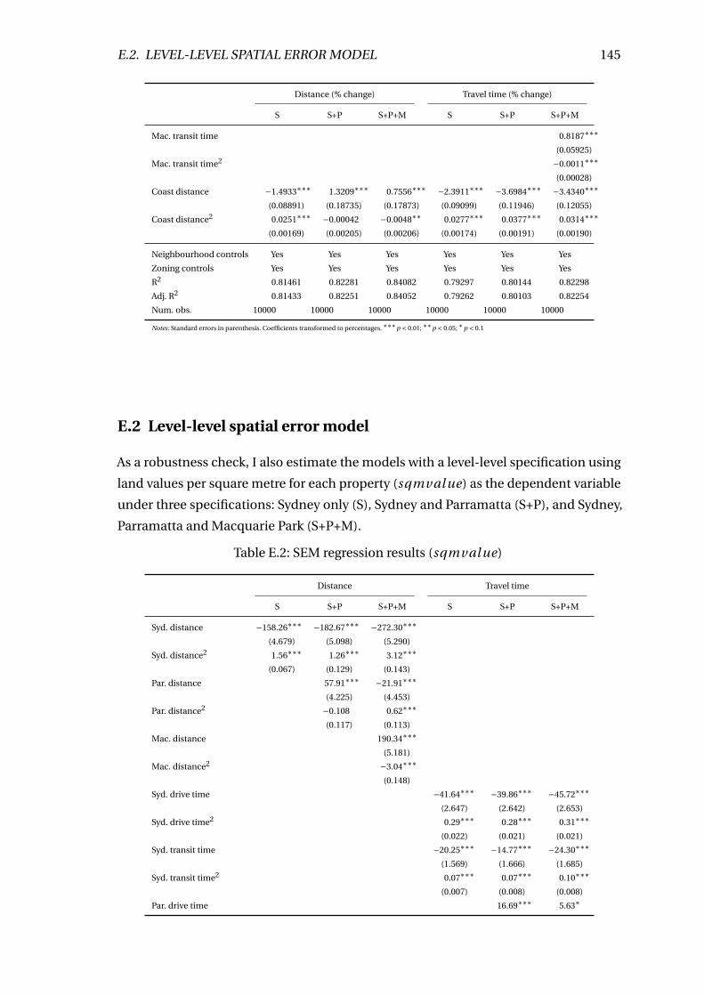
E.2. LEVEL-LEVEL SPATIAL ERROR MODEL 145

Distance (% change) Travel time (% change)

S S+P S+P+M S S+P S+P+M

Mac. transit time 0.8187∗∗∗

(0.05925)

Mac. transit time2 −0.0011∗∗∗

(0.00028)

Coast distance −1.4933∗∗∗ 1.3209∗∗∗ 0.7556∗∗∗ −2.3911∗∗∗ −3.6984∗∗∗ −3.4340∗∗∗

(0.08891) (0.18735) (0.17873) (0.09099) (0.11946) (0.12055)

Coast distance2 0.0251∗∗∗ −0.00042 −0.0048∗∗ 0.0277∗∗∗ 0.0377∗∗∗ 0.0314∗∗∗

(0.00169) (0.00205) (0.00206) (0.00174) (0.00191) (0.00190)

Neighbourhood controls Yes Yes Yes Yes Yes Yes

Zoning controls Yes Yes Yes Yes Yes Yes

R2 0.81461 0.82281 0.84082 0.79297 0.80144 0.82298

Adj. R2 0.81433 0.82251 0.84052 0.79262 0.80103 0.82254

Num. obs. 10000 10000 10000 10000 10000 10000

Notes: Standard errors in parenthesis. Coefficients transformed to percentages. ∗∗∗p < 0.01; ∗∗p < 0.05; ∗p < 0.1

E.2 Level-level spatial error model

As a robustness check, I also estimate the models with a level-level specification using

land values per square metre for each property (sqmval ue) as the dependent variable

under three specifications: Sydney only (S), Sydney and Parramatta (S+P), and Sydney,

Parramatta and Macquarie Park (S+P+M).

Table E.2: SEM regression results (sqmval ue)

Distance Travel time

S S+P S+P+M S S+P S+P+M

Syd. distance −158.26∗∗∗ −182.67∗∗∗ −272.30∗∗∗

(4.679) (5.098) (5.290)

Syd. distance2 1.56∗∗∗ 1.26∗∗∗ 3.12∗∗∗

(0.067) (0.129) (0.143)

Par. distance 57.91∗∗∗ −21.91∗∗∗

(4.225) (4.453)

Par. distance2 −0.108 0.62∗∗∗

(0.117) (0.113)

Mac. distance 190.34∗∗∗

(5.181)

Mac. distance2 −3.04∗∗∗

(0.148)

Syd. drive time −41.64∗∗∗ −39.86∗∗∗ −45.72∗∗∗

(2.647) (2.642) (2.653)

Syd. drive time2 0.29∗∗∗ 0.28∗∗∗ 0.31∗∗∗

(0.022) (0.021) (0.021)

Syd. transit time −20.25∗∗∗ −14.77∗∗∗ −24.30∗∗∗

(1.569) (1.666) (1.685)

Syd. transit time2 0.07∗∗∗ 0.07∗∗∗ 0.10∗∗∗

(0.007) (0.008) (0.008)

Par. drive time 16.69∗∗∗ 5.63∗

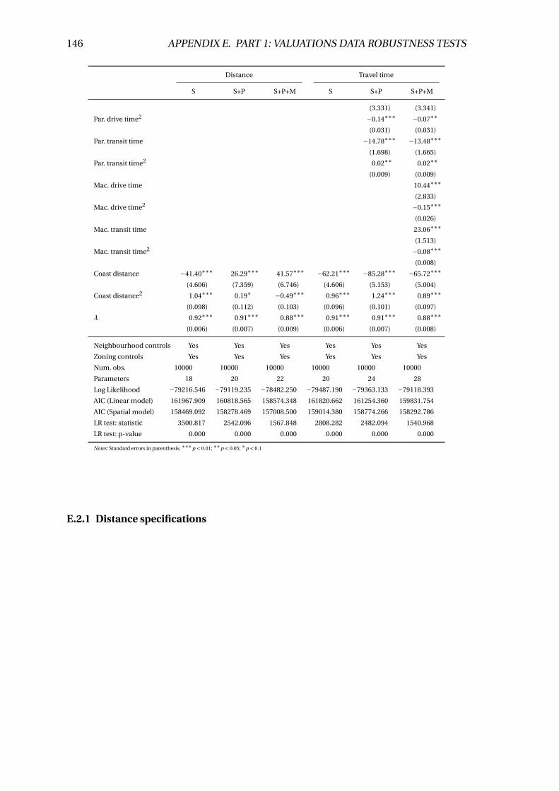
146 APPENDIX E. PART 1: VALUATIONS DATA ROBUSTNESS TESTS

Distance Travel time

S S+P S+P+M S S+P S+P+M

(3.331) (3.341)

Par. drive time2 −0.14∗∗∗ −0.07∗∗

(0.031) (0.031)

Par. transit time −14.78∗∗∗ −13.48∗∗∗

(1.698) (1.665)

Par. transit time2 0.02∗∗ 0.02∗∗

(0.009) (0.009)

Mac. drive time 10.44∗∗∗

(2.833)

Mac. drive time2 −0.15∗∗∗

(0.026)

Mac. transit time 23.06∗∗∗

(1.513)

Mac. transit time2 −0.08∗∗∗

(0.008)

Coast distance −41.40∗∗∗ 26.29∗∗∗ 41.57∗∗∗ −62.21∗∗∗ −85.28∗∗∗ −65.72∗∗∗

(4.606) (7.359) (6.746) (4.606) (5.153) (5.004)

Coast distance2 1.04∗∗∗ 0.19∗ −0.49∗∗∗ 0.96∗∗∗ 1.24∗∗∗ 0.89∗∗∗

(0.098) (0.112) (0.103) (0.096) (0.101) (0.097)

λ 0.92∗∗∗ 0.91∗∗∗ 0.88∗∗∗ 0.91∗∗∗ 0.91∗∗∗ 0.88∗∗∗

(0.006) (0.007) (0.009) (0.006) (0.007) (0.008)

Neighbourhood controls Yes Yes Yes Yes Yes Yes

Zoning controls Yes Yes Yes Yes Yes Yes

Num. obs. 10000 10000 10000 10000 10000 10000

Parameters 18 20 22 20 24 28

Log Likelihood −79216.546 −79119.235 −78482.250 −79487.190 −79363.133 −79118.393

AIC (Linear model) 161967.909 160818.565 158574.348 161820.662 161254.360 159831.754

AIC (Spatial model) 158469.092 158278.469 157008.500 159014.380 158774.266 158292.786

LR test: statistic 3500.817 2542.096 1567.848 2808.282 2482.094 1540.968

LR test: p-value 0.000 0.000 0.000 0.000 0.000 0.000

Notes: Standard errors in parenthesis. ∗∗∗p < 0.01; ∗∗p < 0.05; ∗p < 0.1

E.2.1 Distance specifications

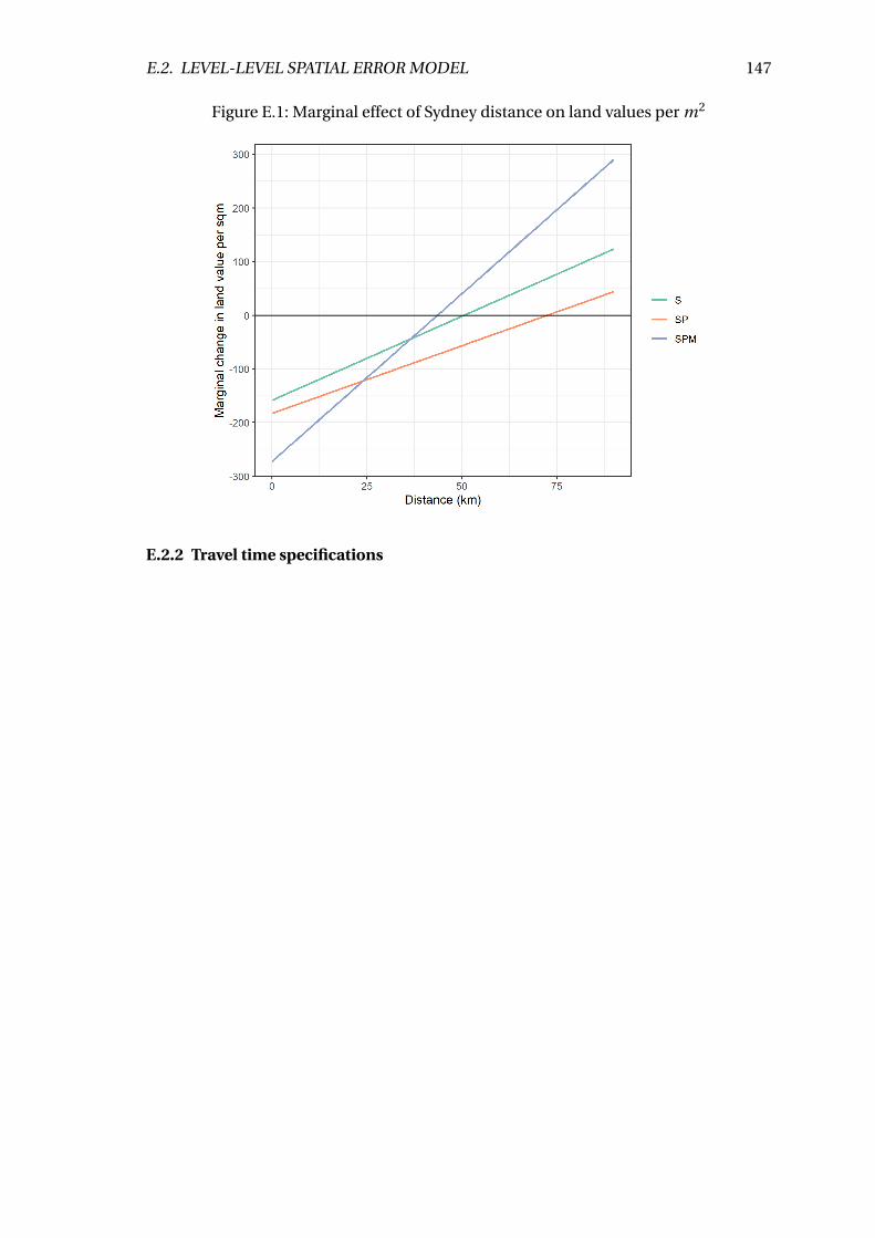
E.2. LEVEL-LEVEL SPATIAL ERROR MODEL 147

Figure E.1: Marginal effect of Sydney distance on land values per m2

E.2.2 Travel time specifications

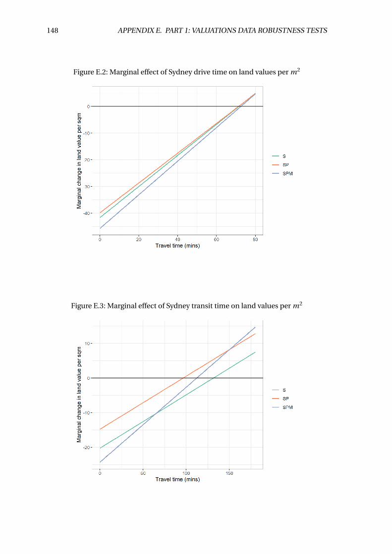
148 APPENDIX E. PART 1: VALUATIONS DATA ROBUSTNESS TESTS

Figure E.2: Marginal effect of Sydney drive time on land values per m2

Figure E.3: Marginal effect of Sydney transit time on land values per m2

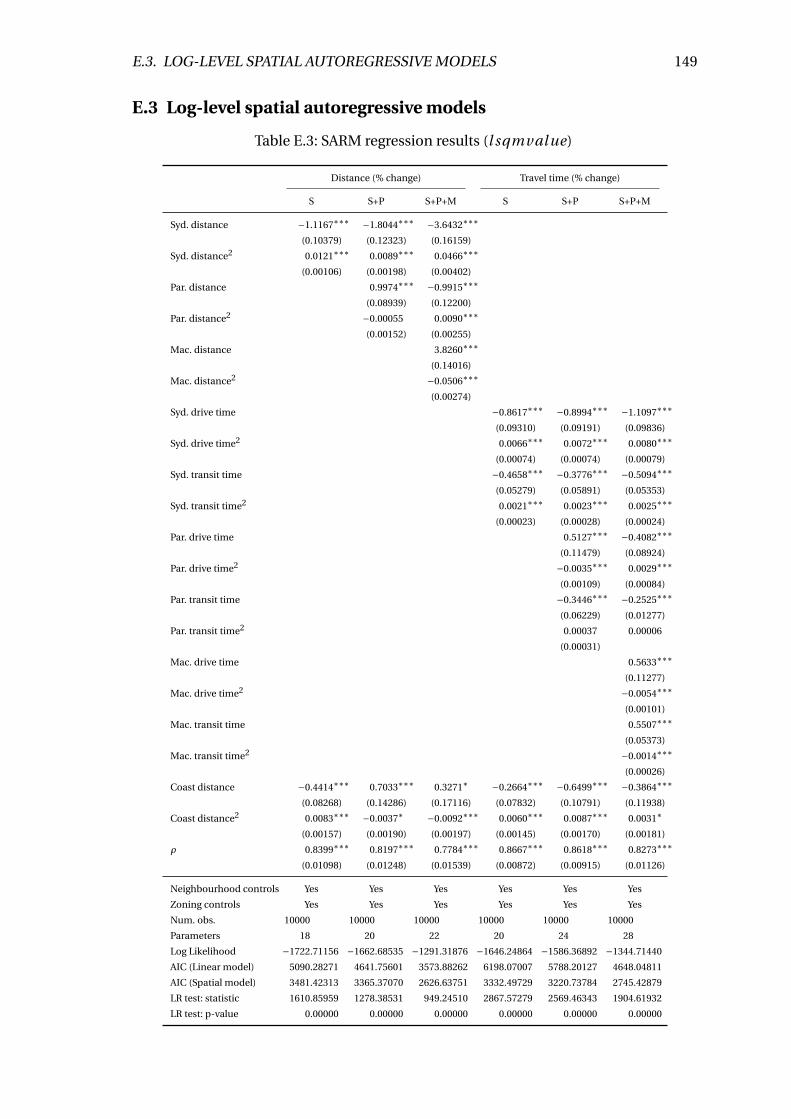
E.3. LOG-LEVEL SPATIAL AUTOREGRESSIVE MODELS 149

E.3 Log-level spatial autoregressive models

Table E.3: SARM regression results (l sqmval ue)

Distance (% change) Travel time (% change)

S S+P S+P+M S S+P S+P+M

Syd. distance −1.1167∗∗∗ −1.8044∗∗∗ −3.6432∗∗∗

(0.10379) (0.12323) (0.16159)

Syd. distance2 0.0121∗∗∗ 0.0089∗∗∗ 0.0466∗∗∗

(0.00106) (0.00198) (0.00402)

Par. distance 0.9974∗∗∗ −0.9915∗∗∗

(0.08939) (0.12200)

Par. distance2 −0.00055 0.0090∗∗∗

(0.00152) (0.00255)

Mac. distance 3.8260∗∗∗

(0.14016)

Mac. distance2 −0.0506∗∗∗

(0.00274)

Syd. drive time −0.8617∗∗∗ −0.8994∗∗∗ −1.1097∗∗∗

(0.09310) (0.09191) (0.09836)

Syd. drive time2 0.0066∗∗∗ 0.0072∗∗∗ 0.0080∗∗∗

(0.00074) (0.00074) (0.00079)

Syd. transit time −0.4658∗∗∗ −0.3776∗∗∗ −0.5094∗∗∗

(0.05279) (0.05891) (0.05353)

Syd. transit time2 0.0021∗∗∗ 0.0023∗∗∗ 0.0025∗∗∗

(0.00023) (0.00028) (0.00024)

Par. drive time 0.5127∗∗∗ −0.4082∗∗∗

(0.11479) (0.08924)

Par. drive time2 −0.0035∗∗∗ 0.0029∗∗∗

(0.00109) (0.00084)

Par. transit time −0.3446∗∗∗ −0.2525∗∗∗

(0.06229) (0.01277)

Par. transit time2 0.00037 0.00006

(0.00031)

Mac. drive time 0.5633∗∗∗

(0.11277)

Mac. drive time2 −0.0054∗∗∗

(0.00101)

Mac. transit time 0.5507∗∗∗

(0.05373)

Mac. transit time2 −0.0014∗∗∗

(0.00026)

Coast distance −0.4414∗∗∗ 0.7033∗∗∗ 0.3271∗ −0.2664∗∗∗ −0.6499∗∗∗ −0.3864∗∗∗

(0.08268) (0.14286) (0.17116) (0.07832) (0.10791) (0.11938)

Coast distance2 0.0083∗∗∗ −0.0037∗ −0.0092∗∗∗ 0.0060∗∗∗ 0.0087∗∗∗ 0.0031∗

(0.00157) (0.00190) (0.00197) (0.00145) (0.00170) (0.00181)

ρ 0.8399∗∗∗ 0.8197∗∗∗ 0.7784∗∗∗ 0.8667∗∗∗ 0.8618∗∗∗ 0.8273∗∗∗

(0.01098) (0.01248) (0.01539) (0.00872) (0.00915) (0.01126)

Neighbourhood controls Yes Yes Yes Yes Yes Yes

Zoning controls Yes Yes Yes Yes Yes Yes

Num. obs. 10000 10000 10000 10000 10000 10000

Parameters 18 20 22 20 24 28

Log Likelihood −1722.71156 −1662.68535 −1291.31876 −1646.24864 −1586.36892 −1344.71440

AIC (Linear model) 5090.28271 4641.75601 3573.88262 6198.07007 5788.20127 4648.04811

AIC (Spatial model) 3481.42313 3365.37070 2626.63751 3332.49729 3220.73784 2745.42879

LR test: statistic 1610.85959 1278.38531 949.24510 2867.57279 2569.46343 1904.61932

LR test: p-value 0.00000 0.00000 0.00000 0.00000 0.00000 0.00000

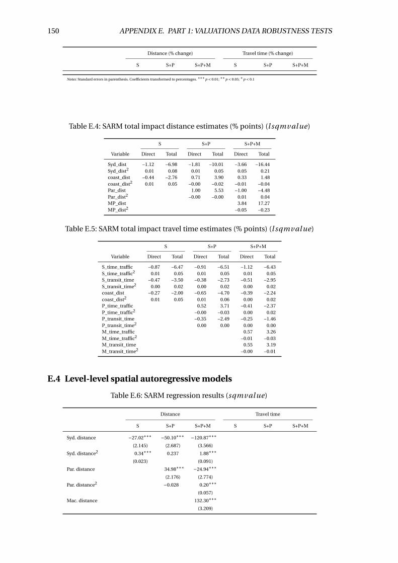
150 APPENDIX E. PART 1: VALUATIONS DATA ROBUSTNESS TESTS

Distance (% change) Travel time (% change)

S S+P S+P+M S S+P S+P+M

Notes: Standard errors in parenthesis. Coefficients transformed to percentages. ∗∗∗p < 0.01; ∗∗p < 0.05; ∗p < 0.1

Table E.4: SARM total impact distance estimates (% points) (l sqmval ue)

S S+P S+P+M

Variable Direct Total Direct Total Direct Total

Syd_dist −1.12 −6.98 −1.81 −10.01 −3.66 −16.44Syd_dist2 0.01 0.08 0.01 0.05 0.05 0.21coast_dist −0.44 −2.76 0.71 3.90 0.33 1.48coast_dist2 0.01 0.05 −0.00 −0.02 −0.01 −0.04Par_dist 1.00 5.53 −1.00 −4.48Par_dist2 −0.00 −0.00 0.01 0.04MP_dist 3.84 17.27MP_dist2 −0.05 −0.23

Table E.5: SARM total impact travel time estimates (% points) (l sqmval ue)

S S+P S+P+M

Variable Direct Total Direct Total Direct Total

S_time_traffic −0.87 −6.47 −0.91 −6.51 −1.12 −6.43S_time_traffic2 0.01 0.05 0.01 0.05 0.01 0.05S_transit_time −0.47 −3.50 −0.38 −2.73 −0.51 −2.95S_transit_time2 0.00 0.02 0.00 0.02 0.00 0.02coast_dist −0.27 −2.00 −0.65 −4.70 −0.39 −2.24coast_dist2 0.01 0.05 0.01 0.06 0.00 0.02P_time_traffic 0.52 3.71 −0.41 −2.37P_time_traffic2 −0.00 −0.03 0.00 0.02P_transit_time −0.35 −2.49 −0.25 −1.46P_transit_time2 0.00 0.00 0.00 0.00M_time_traffic 0.57 3.26M_time_traffic2 −0.01 −0.03M_transit_time 0.55 3.19M_transit_time2 −0.00 −0.01

E.4 Level-level spatial autoregressive models

Table E.6: SARM regression results (sqmval ue)

Distance Travel time

S S+P S+P+M S S+P S+P+M

Syd. distance −27.02∗∗∗ −50.10∗∗∗ −120.87∗∗∗

(2.145) (2.687) (3.566)

Syd. distance2 0.34∗∗∗ 0.237 1.88∗∗∗

(0.023) (0.091)

Par. distance 34.98∗∗∗ −24.94∗∗∗

(2.176) (2.774)

Par. distance2 −0.028 0.20∗∗∗

(0.057)

Mac. distance 132.30∗∗∗

(3.209)

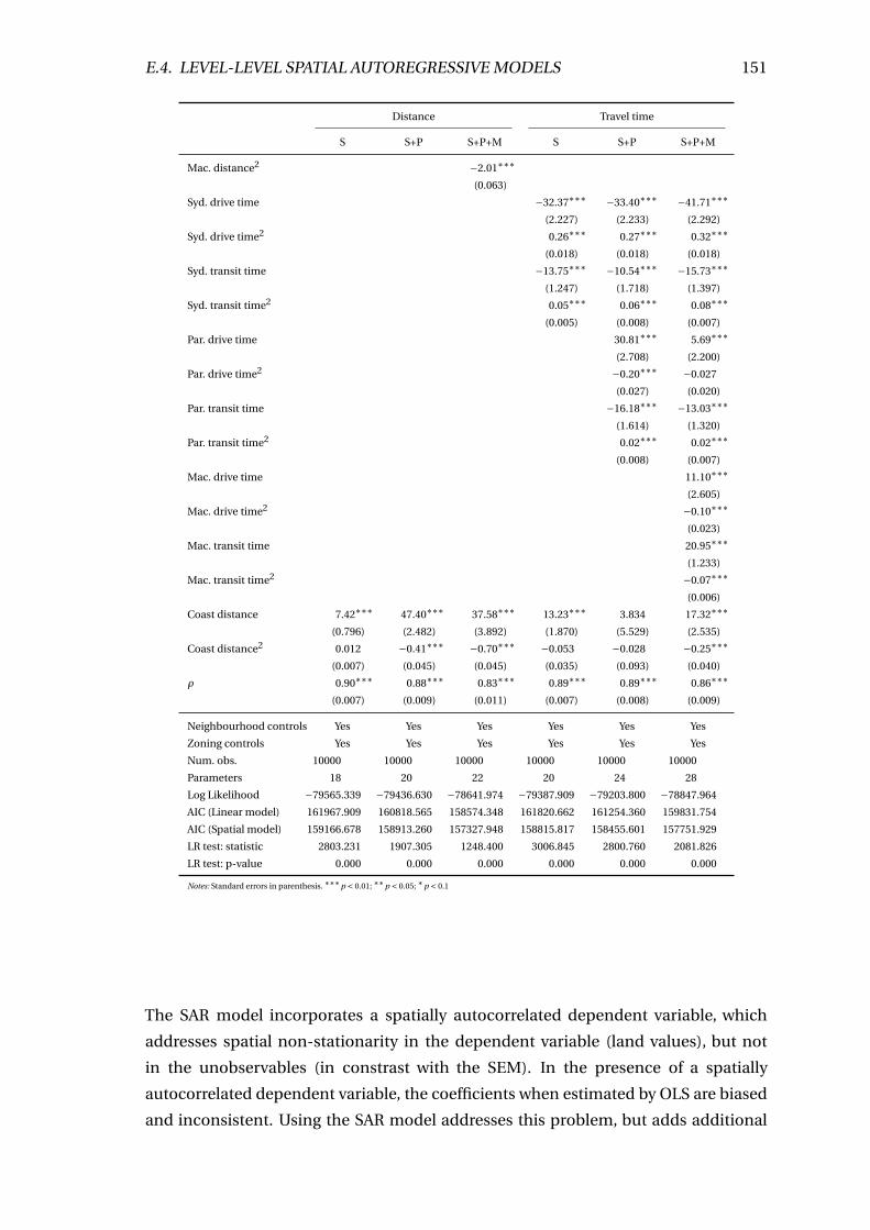
E.4. LEVEL-LEVEL SPATIAL AUTOREGRESSIVE MODELS 151

Distance Travel time

S S+P S+P+M S S+P S+P+M

Mac. distance2 −2.01∗∗∗

(0.063)

Syd. drive time −32.37∗∗∗ −33.40∗∗∗ −41.71∗∗∗

(2.227) (2.233) (2.292)

Syd. drive time2 0.26∗∗∗ 0.27∗∗∗ 0.32∗∗∗

(0.018) (0.018) (0.018)

Syd. transit time −13.75∗∗∗ −10.54∗∗∗ −15.73∗∗∗

(1.247) (1.718) (1.397)

Syd. transit time2 0.05∗∗∗ 0.06∗∗∗ 0.08∗∗∗

(0.005) (0.008) (0.007)

Par. drive time 30.81∗∗∗ 5.69∗∗∗

(2.708) (2.200)

Par. drive time2 −0.20∗∗∗ −0.027

(0.027) (0.020)

Par. transit time −16.18∗∗∗ −13.03∗∗∗

(1.614) (1.320)

Par. transit time2 0.02∗∗∗ 0.02∗∗∗

(0.008) (0.007)

Mac. drive time 11.10∗∗∗

(2.605)

Mac. drive time2 −0.10∗∗∗

(0.023)

Mac. transit time 20.95∗∗∗

(1.233)

Mac. transit time2 −0.07∗∗∗

(0.006)

Coast distance 7.42∗∗∗ 47.40∗∗∗ 37.58∗∗∗ 13.23∗∗∗ 3.834 17.32∗∗∗

(0.796) (2.482) (3.892) (1.870) (5.529) (2.535)

Coast distance2 0.012 −0.41∗∗∗ −0.70∗∗∗ −0.053 −0.028 −0.25∗∗∗

(0.007) (0.045) (0.045) (0.035) (0.093) (0.040)

ρ 0.90∗∗∗ 0.88∗∗∗ 0.83∗∗∗ 0.89∗∗∗ 0.89∗∗∗ 0.86∗∗∗

(0.007) (0.009) (0.011) (0.007) (0.008) (0.009)

Neighbourhood controls Yes Yes Yes Yes Yes Yes

Zoning controls Yes Yes Yes Yes Yes Yes

Num. obs. 10000 10000 10000 10000 10000 10000

Parameters 18 20 22 20 24 28

Log Likelihood −79565.339 −79436.630 −78641.974 −79387.909 −79203.800 −78847.964

AIC (Linear model) 161967.909 160818.565 158574.348 161820.662 161254.360 159831.754

AIC (Spatial model) 159166.678 158913.260 157327.948 158815.817 158455.601 157751.929

LR test: statistic 2803.231 1907.305 1248.400 3006.845 2800.760 2081.826

LR test: p-value 0.000 0.000 0.000 0.000 0.000 0.000

Notes: Standard errors in parenthesis. ∗∗∗p < 0.01; ∗∗p < 0.05; ∗p < 0.1

The SAR model incorporates a spatially autocorrelated dependent variable, which

addresses spatial non-stationarity in the dependent variable (land values), but not

in the unobservables (in constrast with the SEM). In the presence of a spatially

autocorrelated dependent variable, the coefficients when estimated by OLS are biased

and inconsistent. Using the SAR model addresses this problem, but adds additional

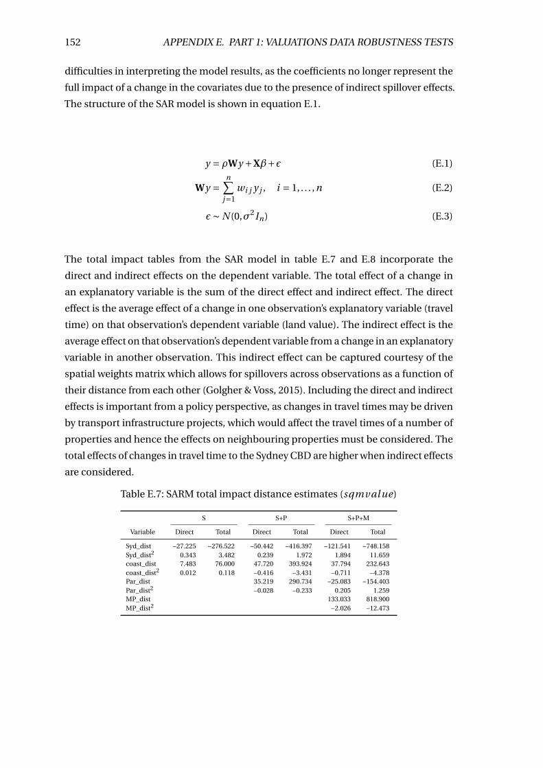
152 APPENDIX E. PART 1: VALUATIONS DATA ROBUSTNESS TESTS

difficulties in interpreting the model results, as the coefficients no longer represent the

full impact of a change in the covariates due to the presence of indirect spillover effects.

The structure of the SAR model is shown in equation E.1.

y = ρWy +Xβ+ε (E.1)

Wy =n∑

j=1wi j y j , i = 1, . . . ,n (E.2)

ε∼ N (0,σ2In) (E.3)

The total impact tables from the SAR model in table E.7 and E.8 incorporate the

direct and indirect effects on the dependent variable. The total effect of a change in

an explanatory variable is the sum of the direct effect and indirect effect. The direct

effect is the average effect of a change in one observation’s explanatory variable (travel

time) on that observation’s dependent variable (land value). The indirect effect is the

average effect on that observation’s dependent variable from a change in an explanatory

variable in another observation. This indirect effect can be captured courtesy of the

spatial weights matrix which allows for spillovers across observations as a function of

their distance from each other (Golgher & Voss, 2015). Including the direct and indirect

effects is important from a policy perspective, as changes in travel times may be driven

by transport infrastructure projects, which would affect the travel times of a number of

properties and hence the effects on neighbouring properties must be considered. The

total effects of changes in travel time to the Sydney CBD are higher when indirect effects

are considered.

Table E.7: SARM total impact distance estimates (sqmval ue)

S S+P S+P+M

Variable Direct Total Direct Total Direct Total

Syd_dist −27.225 −276.522 −50.442 −416.397 −121.541 −748.158Syd_dist2 0.343 3.482 0.239 1.972 1.894 11.659coast_dist 7.483 76.000 47.720 393.924 37.794 232.643coast_dist2 0.012 0.118 −0.416 −3.431 −0.711 −4.378Par_dist 35.219 290.734 −25.083 −154.403Par_dist2 −0.028 −0.233 0.205 1.259MP_dist 133.033 818.900MP_dist2 −2.026 −12.473

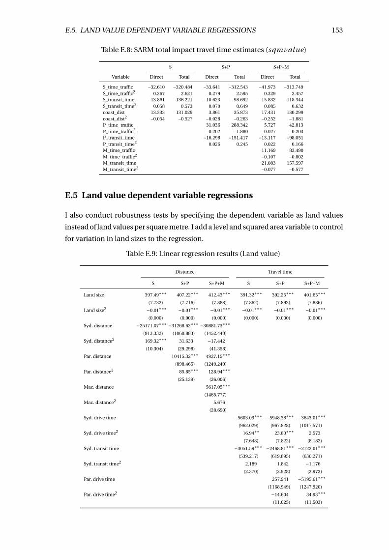
E.5. LAND VALUE DEPENDENT VARIABLE REGRESSIONS 153

Table E.8: SARM total impact travel time estimates (sqmval ue)

S S+P S+P+M

Variable Direct Total Direct Total Direct Total

S_time_traffic −32.610 −320.484 −33.641 −312.543 −41.973 −313.749S_time_traffic2 0.267 2.621 0.279 2.595 0.329 2.457S_transit_time −13.861 −136.221 −10.623 −98.692 −15.832 −118.344S_transit_time2 0.058 0.573 0.070 0.649 0.085 0.632coast_dist 13.333 131.029 3.861 35.873 17.431 130.299coast_dist2 −0.054 −0.527 −0.028 −0.263 −0.252 −1.881P_time_traffic 31.036 288.342 5.727 42.813P_time_traffic2 −0.202 −1.880 −0.027 −0.203P_transit_time −16.298 −151.417 −13.117 −98.051P_transit_time2 0.026 0.245 0.022 0.166M_time_traffic 11.169 83.490M_time_traffic2 −0.107 −0.802M_transit_time 21.083 157.597M_transit_time2 −0.077 −0.577

E.5 Land value dependent variable regressions

I also conduct robustness tests by specifying the dependent variable as land values

instead of land values per square metre. I add a level and squared area variable to control

for variation in land sizes to the regression.

Table E.9: Linear regression results (Land value)

Distance Travel time

S S+P S+P+M S S+P S+P+M

Land size 397.49∗∗∗ 407.22∗∗∗ 412.43∗∗∗ 391.32∗∗∗ 392.25∗∗∗ 401.65∗∗∗

(7.732) (7.716) (7.888) (7.862) (7.892) (7.886)

Land size2 −0.01∗∗∗ −0.01∗∗∗ −0.01∗∗∗ −0.01∗∗∗ −0.01∗∗∗ −0.01∗∗∗

(0.000) (0.000) (0.000) (0.000) (0.000) (0.000)

Syd. distance −25171.07∗∗∗ −31268.62∗∗∗ −30881.73∗∗∗

(913.332) (1060.883) (1452.440)

Syd. distance2 169.32∗∗∗ 31.633 −17.442

(10.304) (29.298) (41.358)

Par. distance 10415.32∗∗∗ 4927.15∗∗∗

(898.465) (1249.240)

Par. distance2 85.85∗∗∗ 128.94∗∗∗

(25.139) (26.006)

Mac. distance 5617.05∗∗∗

(1465.777)

Mac. distance2 5.676

(28.690)

Syd. drive time −5603.03∗∗∗ −5948.38∗∗∗ −3643.01∗∗∗

(962.029) (967.828) (1017.571)

Syd. drive time2 16.94∗∗ 23.80∗∗∗ 2.573

(7.648) (7.822) (8.182)

Syd. transit time −3051.59∗∗∗ −2468.81∗∗∗ −2722.01∗∗∗

(539.217) (619.895) (630.271)

Syd. transit time2 2.189 1.842 −1.176

(2.370) (2.928) (2.972)

Par. drive time 257.941 −5195.61∗∗∗

(1168.949) (1247.920)

Par. drive time2 −14.604 34.93∗∗∗

(11.025) (11.503)

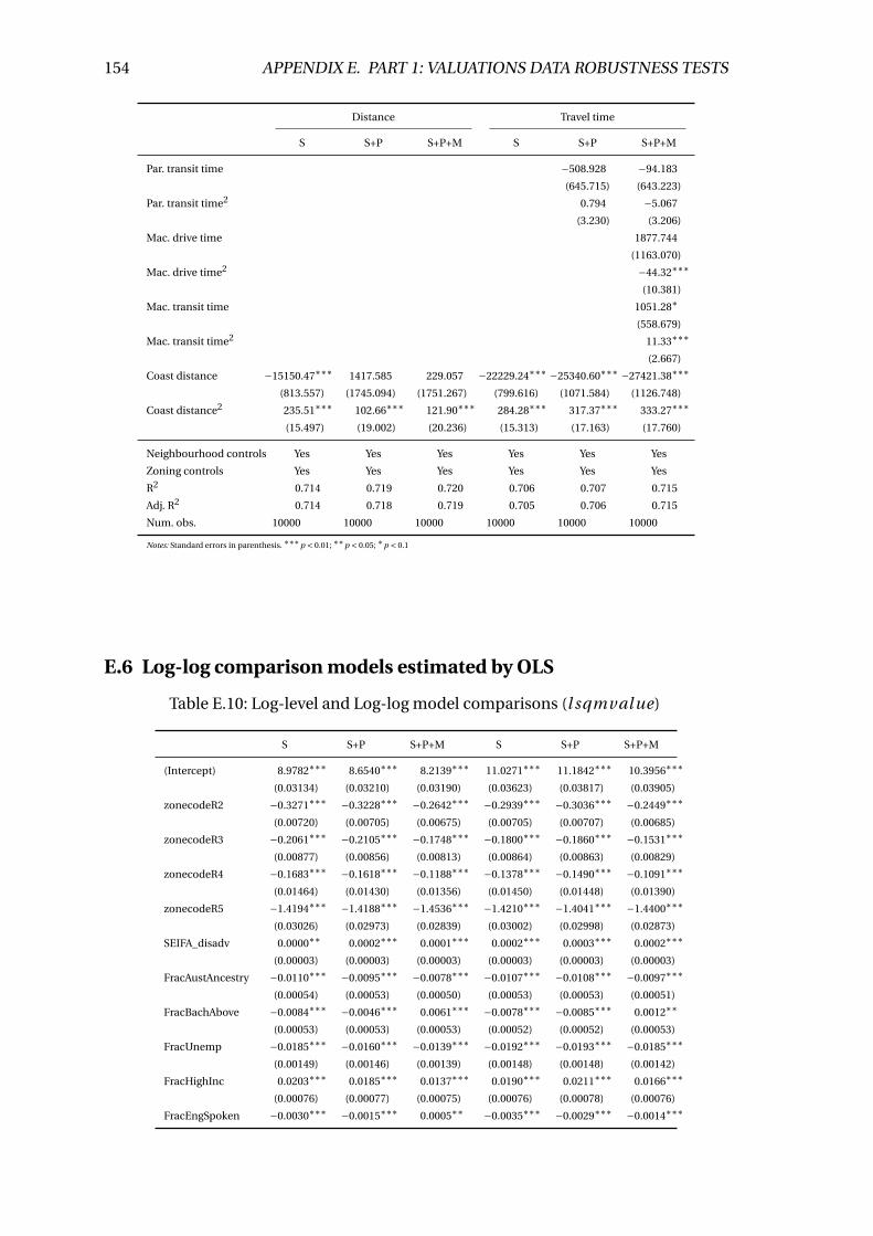
154 APPENDIX E. PART 1: VALUATIONS DATA ROBUSTNESS TESTS

Distance Travel time

S S+P S+P+M S S+P S+P+M

Par. transit time −508.928 −94.183

(645.715) (643.223)

Par. transit time2 0.794 −5.067

(3.230) (3.206)

Mac. drive time 1877.744

(1163.070)

Mac. drive time2 −44.32∗∗∗

(10.381)

Mac. transit time 1051.28∗

(558.679)

Mac. transit time2 11.33∗∗∗

(2.667)

Coast distance −15150.47∗∗∗ 1417.585 229.057 −22229.24∗∗∗ −25340.60∗∗∗ −27421.38∗∗∗

(813.557) (1745.094) (1751.267) (799.616) (1071.584) (1126.748)

Coast distance2 235.51∗∗∗ 102.66∗∗∗ 121.90∗∗∗ 284.28∗∗∗ 317.37∗∗∗ 333.27∗∗∗

(15.497) (19.002) (20.236) (15.313) (17.163) (17.760)

Neighbourhood controls Yes Yes Yes Yes Yes Yes

Zoning controls Yes Yes Yes Yes Yes Yes

R2 0.714 0.719 0.720 0.706 0.707 0.715

Adj. R2 0.714 0.718 0.719 0.705 0.706 0.715

Num. obs. 10000 10000 10000 10000 10000 10000

Notes: Standard errors in parenthesis. ∗∗∗p < 0.01; ∗∗p < 0.05; ∗p < 0.1

E.6 Log-log comparison models estimated by OLS

Table E.10: Log-level and Log-log model comparisons (l sqmval ue)

S S+P S+P+M S S+P S+P+M

(Intercept) 8.9782∗∗∗ 8.6540∗∗∗ 8.2139∗∗∗ 11.0271∗∗∗ 11.1842∗∗∗ 10.3956∗∗∗

(0.03134) (0.03210) (0.03190) (0.03623) (0.03817) (0.03905)

zonecodeR2 −0.3271∗∗∗ −0.3228∗∗∗ −0.2642∗∗∗ −0.2939∗∗∗ −0.3036∗∗∗ −0.2449∗∗∗

(0.00720) (0.00705) (0.00675) (0.00705) (0.00707) (0.00685)

zonecodeR3 −0.2061∗∗∗ −0.2105∗∗∗ −0.1748∗∗∗ −0.1800∗∗∗ −0.1860∗∗∗ −0.1531∗∗∗

(0.00877) (0.00856) (0.00813) (0.00864) (0.00863) (0.00829)

zonecodeR4 −0.1683∗∗∗ −0.1618∗∗∗ −0.1188∗∗∗ −0.1378∗∗∗ −0.1490∗∗∗ −0.1091∗∗∗

(0.01464) (0.01430) (0.01356) (0.01450) (0.01448) (0.01390)

zonecodeR5 −1.4194∗∗∗ −1.4188∗∗∗ −1.4536∗∗∗ −1.4210∗∗∗ −1.4041∗∗∗ −1.4400∗∗∗

(0.03026) (0.02973) (0.02839) (0.03002) (0.02998) (0.02873)

SEIFA_disadv 0.0000∗∗ 0.0002∗∗∗ 0.0001∗∗∗ 0.0002∗∗∗ 0.0003∗∗∗ 0.0002∗∗∗

(0.00003) (0.00003) (0.00003) (0.00003) (0.00003) (0.00003)

FracAustAncestry −0.0110∗∗∗ −0.0095∗∗∗ −0.0078∗∗∗ −0.0107∗∗∗ −0.0108∗∗∗ −0.0097∗∗∗

(0.00054) (0.00053) (0.00050) (0.00053) (0.00053) (0.00051)

FracBachAbove −0.0084∗∗∗ −0.0046∗∗∗ 0.0061∗∗∗ −0.0078∗∗∗ −0.0085∗∗∗ 0.0012∗∗

(0.00053) (0.00053) (0.00053) (0.00052) (0.00052) (0.00053)

FracUnemp −0.0185∗∗∗ −0.0160∗∗∗ −0.0139∗∗∗ −0.0192∗∗∗ −0.0193∗∗∗ −0.0185∗∗∗

(0.00149) (0.00146) (0.00139) (0.00148) (0.00148) (0.00142)

FracHighInc 0.0203∗∗∗ 0.0185∗∗∗ 0.0137∗∗∗ 0.0190∗∗∗ 0.0211∗∗∗ 0.0166∗∗∗

(0.00076) (0.00077) (0.00075) (0.00076) (0.00078) (0.00076)

FracEngSpoken −0.0030∗∗∗ −0.0015∗∗∗ 0.0005∗∗ −0.0035∗∗∗ −0.0029∗∗∗ −0.0014∗∗∗

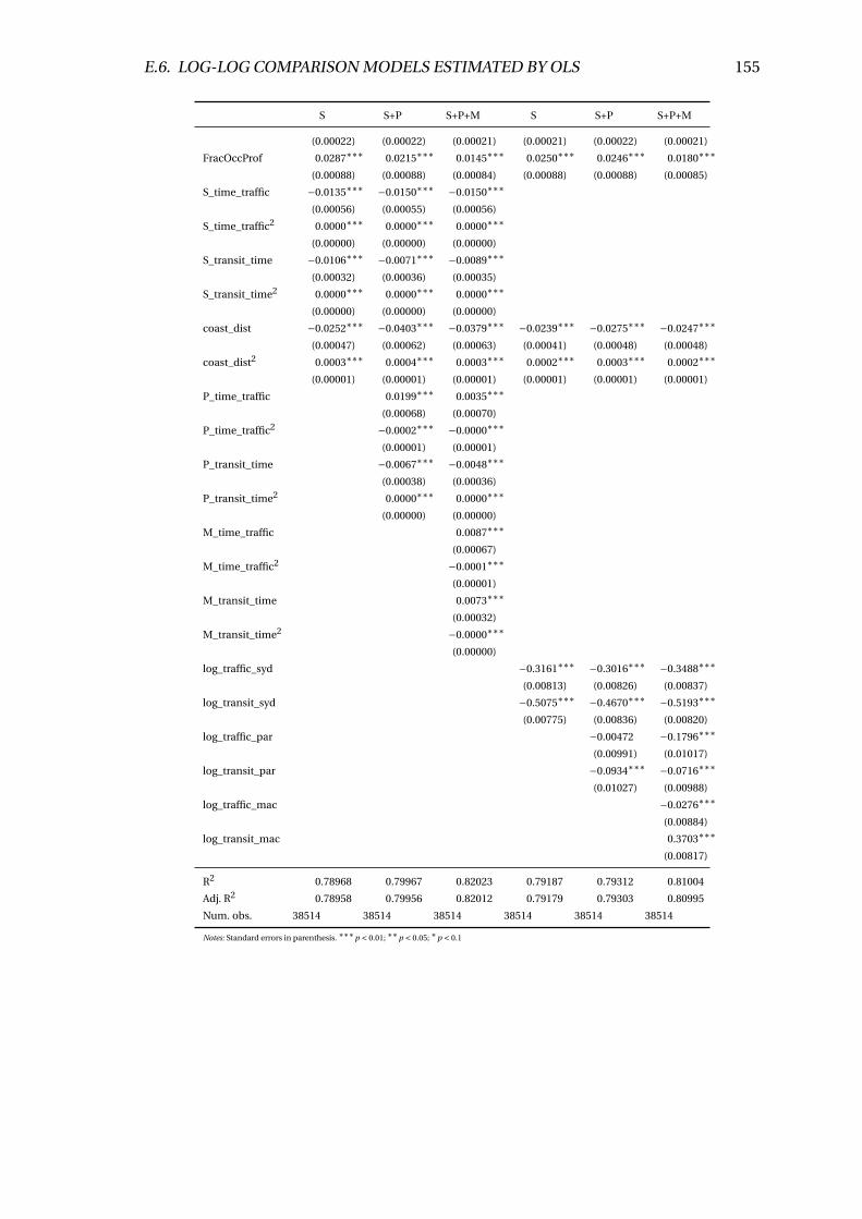
E.6. LOG-LOG COMPARISON MODELS ESTIMATED BY OLS 155

S S+P S+P+M S S+P S+P+M

(0.00022) (0.00022) (0.00021) (0.00021) (0.00022) (0.00021)

FracOccProf 0.0287∗∗∗ 0.0215∗∗∗ 0.0145∗∗∗ 0.0250∗∗∗ 0.0246∗∗∗ 0.0180∗∗∗

(0.00088) (0.00088) (0.00084) (0.00088) (0.00088) (0.00085)

S_time_traffic −0.0135∗∗∗ −0.0150∗∗∗ −0.0150∗∗∗

(0.00056) (0.00055) (0.00056)

S_time_traffic2 0.0000∗∗∗ 0.0000∗∗∗ 0.0000∗∗∗

(0.00000) (0.00000) (0.00000)

S_transit_time −0.0106∗∗∗ −0.0071∗∗∗ −0.0089∗∗∗

(0.00032) (0.00036) (0.00035)

S_transit_time2 0.0000∗∗∗ 0.0000∗∗∗ 0.0000∗∗∗

(0.00000) (0.00000) (0.00000)

coast_dist −0.0252∗∗∗ −0.0403∗∗∗ −0.0379∗∗∗ −0.0239∗∗∗ −0.0275∗∗∗ −0.0247∗∗∗

(0.00047) (0.00062) (0.00063) (0.00041) (0.00048) (0.00048)

coast_dist2 0.0003∗∗∗ 0.0004∗∗∗ 0.0003∗∗∗ 0.0002∗∗∗ 0.0003∗∗∗ 0.0002∗∗∗

(0.00001) (0.00001) (0.00001) (0.00001) (0.00001) (0.00001)

P_time_traffic 0.0199∗∗∗ 0.0035∗∗∗

(0.00068) (0.00070)

P_time_traffic2 −0.0002∗∗∗ −0.0000∗∗∗

(0.00001) (0.00001)

P_transit_time −0.0067∗∗∗ −0.0048∗∗∗

(0.00038) (0.00036)

P_transit_time2 0.0000∗∗∗ 0.0000∗∗∗

(0.00000) (0.00000)

M_time_traffic 0.0087∗∗∗

(0.00067)

M_time_traffic2 −0.0001∗∗∗

(0.00001)

M_transit_time 0.0073∗∗∗

(0.00032)

M_transit_time2 −0.0000∗∗∗

(0.00000)

log_traffic_syd −0.3161∗∗∗ −0.3016∗∗∗ −0.3488∗∗∗

(0.00813) (0.00826) (0.00837)

log_transit_syd −0.5075∗∗∗ −0.4670∗∗∗ −0.5193∗∗∗

(0.00775) (0.00836) (0.00820)

log_traffic_par −0.00472 −0.1796∗∗∗

(0.00991) (0.01017)

log_transit_par −0.0934∗∗∗ −0.0716∗∗∗

(0.01027) (0.00988)

log_traffic_mac −0.0276∗∗∗

(0.00884)

log_transit_mac 0.3703∗∗∗

(0.00817)

R2 0.78968 0.79967 0.82023 0.79187 0.79312 0.81004

Adj. R2 0.78958 0.79956 0.82012 0.79179 0.79303 0.80995

Num. obs. 38514 38514 38514 38514 38514 38514

Notes: Standard errors in parenthesis. ∗∗∗p < 0.01; ∗∗p < 0.05; ∗p < 0.1

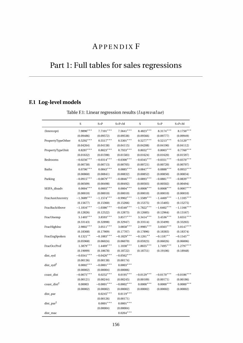
A P P E N D I X F

Part 1: Full tables for sales regressions

F.1 Log-level models

Table F.1: Linear regression results (l sqmval ue)

S S+P S+P+M S S+P S+P+M

(Intercept) 7.9890∗∗∗ 7.7101∗∗∗ 7.5641∗∗∗ 8.4823∗∗∗ 8.3174∗∗∗ 8.1750∗∗∗

(0.09486) (0.09572) (0.09538) (0.09566) (0.09777) (0.09949)

PropertyTypeOther 0.5292∗∗∗ 0.5517∗∗∗ 0.5301∗∗∗ 0.5277∗∗∗ 0.5213∗∗∗ 0.5120∗∗∗

(0.04264) (0.04158) (0.04115) (0.04208) (0.04190) (0.04112)

PropertyTypeUnit 0.8287∗∗∗ 0.8023∗∗∗ 0.7933∗∗∗ 0.8032∗∗∗ 0.8003∗∗∗ 0.7760∗∗∗

(0.01632) (0.01598) (0.01583) (0.01624) (0.01620) (0.01597)

Bedrooms −0.0256∗∗∗ −0.0314∗∗∗ −0.0300∗∗∗ −0.0345∗∗∗ −0.0351∗∗∗ −0.0370∗∗∗

(0.00730) (0.00713) (0.00705) (0.00721) (0.00720) (0.00707)

Baths 0.0706∗∗∗ 0.0843∗∗∗ 0.0885∗∗∗ 0.0847∗∗∗ 0.0888∗∗∗ 0.0953∗∗∗

(0.00860) (0.00841) (0.00832) (0.00852) (0.00850) (0.00834)

Parking −0.0915∗∗∗ −0.0879∗∗∗ −0.0846∗∗∗ −0.0893∗∗∗ −0.0881∗∗∗ −0.0839∗∗∗

(0.00509) (0.00498) (0.00492) (0.00503) (0.00502) (0.00494)

SEIFA_disadv 0.0004∗∗∗ 0.0003∗∗∗ 0.0004∗∗∗ 0.0008∗∗∗ 0.0008∗∗∗ 0.0007∗∗∗

(0.00010) (0.00010) (0.00010) (0.00010) (0.00010) (0.00010)

FracAustAncestry −1.3689∗∗∗ −1.1574∗∗∗ −0.9902∗∗∗ −1.5589∗∗∗ −1.4469∗∗∗ −1.1105∗∗∗

(0.15677) (0.15360) (0.15266) (0.15375) (0.15405) (0.15275)

FracBachAbove −1.1816∗∗∗ −1.0386∗∗∗ −0.6540∗∗∗ −1.7822∗∗∗ −1.6402∗∗∗ −1.1166∗∗∗

(0.12826) (0.12522) (0.12873) (0.12685) (0.12964) (0.13167)

FracUnemp 5.1403∗∗∗ 3.8593∗∗∗ 3.8577∗∗∗ 3.3414∗∗∗ 3.4536∗∗∗ 3.6551∗∗∗

(0.33143) (0.32898) (0.32947) (0.33514) (0.33499) (0.33265)

FracHighInc 2.9802∗∗∗ 3.0511∗∗∗ 3.0858∗∗∗ 2.9985∗∗∗ 3.0503∗∗∗ 3.0147∗∗∗

(0.18368) (0.17909) (0.17707) (0.17896) (0.18383) (0.18374)

FracEngSpoken 0.1321∗∗ −0.1883∗∗∗ −0.1829∗∗∗ −0.1261∗∗ −0.1187∗∗ −0.1545∗∗

(0.05968) (0.06024) (0.06070) (0.05923) (0.06026) (0.06006)

FracOccProf 1.3879∗∗∗ 1.4469∗∗∗ 1.1038∗∗∗ 1.8655∗∗∗ 1.7495∗∗∗ 1.2797∗∗∗

(0.19099) (0.18678) (0.18722) (0.18751) (0.19106) (0.18948)

dist_syd −0.0341∗∗∗ −0.0426∗∗∗ −0.0562∗∗∗

(0.00136) (0.00138) (0.00174)

dist_syd2 0.0002∗∗∗ −0.0001∗∗∗ 0.0003∗∗∗

(0.00002) (0.00004) (0.00006)

coast_dist −0.0075∗∗∗ 0.0252∗∗∗ 0.0195∗∗∗ −0.0129∗∗∗ −0.0170∗∗∗ −0.0186∗∗∗

(0.00121) (0.00244) (0.00245) (0.00109) (0.00171) (0.00186)

coast_dist2 0.00003 −0.0001∗∗∗ −0.0002∗∗∗ 0.0000∗∗∗ 0.0000∗∗∗ 0.0000∗∗∗

(0.00002) (0.00002) (0.00002) (0.00002) (0.00002) (0.00002)

dist_par 0.0245∗∗∗ 0.0119∗∗∗

(0.00126) (0.00171)

dist_par2 0.0001∗∗∗ 0.0001∗∗∗

(0.00004) (0.00004)

dist_mac 0.0264∗∗∗

156

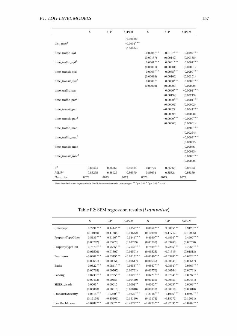
F.1. LOG-LEVEL MODELS 157

S S+P S+P+M S S+P S+P+M

(0.00188)

dist_mac2 −0.0004∗∗∗

(0.00004)

time_traffic_syd −0.0204∗∗∗ −0.0197∗∗∗ −0.0197∗∗∗

(0.00137) (0.00142) (0.00158)

time_traffic_syd2 0.0001∗∗∗ 0.0001∗∗∗ 0.0001∗∗∗

(0.00001) (0.00001) (0.00001)

time_transit_syd −0.0065∗∗∗ −0.0065∗∗∗ −0.0090∗∗∗

(0.00088) (0.00100) (0.00101)

time_transit_syd2 0.0000∗∗ 0.0000∗∗∗ 0.0000∗∗∗

(0.00000) (0.00000) (0.00000)

time_traffic_par 0.0066∗∗∗ −0.0092∗∗∗

(0.00192) (0.00213)

time_traffic_par2 −0.0000∗∗∗ 0.0001∗∗∗

(0.00002) (0.00002)

time_transit_par −0.00027 0.0041∗∗∗

(0.00095) (0.00098)

time_transit_par2 −0.0000∗∗∗ −0.0000∗∗∗

(0.00000) (0.00001)

time_traffic_mac 0.0208∗∗∗

(0.00224)

time_traffic_mac2 −0.0003∗∗∗

(0.00002)

time_transit_mac −0.00086

(0.00083)

time_transit_mac2 0.0000∗∗∗

(0.00000)

R2 0.85324 0.86060 0.86404 0.85726 0.85863 0.86423

Adj. R2 0.85295 0.86029 0.86370 0.85694 0.85824 0.86379

Num. obs. 8073 8073 8073 8073 8073 8073

Notes: Standard errors in parenthesis. Coefficients transformed to percentages. ∗∗∗p < 0.01; ∗∗p < 0.05; ∗p < 0.1

Table F.2: SEM regression results (l sqmval ue)

S S+P S+P+M S S+P S+P+M

(Intercept) 8.7291∗∗∗ 8.4414∗∗∗ 8.2359∗∗∗ 8.8652∗∗∗ 9.0865∗∗∗ 8.9126∗∗∗

(0.11059) (0.11688) (0.11632) (0.10998) (0.11712) (0.12096)

PropertyTypeOther 0.5133∗∗∗ 0.5196∗∗∗ 0.5144∗∗∗ 0.4960∗∗∗ 0.4894∗∗∗ 0.4900∗∗∗

(0.03782) (0.03778) (0.03759) (0.03798) (0.03765) (0.03750)

PropertyTypeUnit 0.7579∗∗∗ 0.7585∗∗∗ 0.7535∗∗∗ 0.7409∗∗∗ 0.7285∗∗∗ 0.7265∗∗∗

(0.01509) (0.01507) (0.01501) (0.01525) (0.01519) (0.01513)

Bedrooms −0.0302∗∗∗ −0.0319∗∗∗ −0.0315∗∗∗ −0.0346∗∗∗ −0.0328∗∗∗ −0.0326∗∗∗

(0.00651) (0.00651) (0.00647) (0.00655) (0.00649) (0.00647)

Baths 0.0822∗∗∗ 0.0841∗∗∗ 0.0853∗∗∗ 0.0867∗∗∗ 0.0864∗∗∗ 0.0869∗∗∗

(0.00765) (0.00765) (0.00761) (0.00770) (0.00764) (0.00761)

Parking −0.0739∗∗∗ −0.0735∗∗∗ −0.0720∗∗∗ −0.0721∗∗∗ −0.0704∗∗∗ −0.0697∗∗∗

(0.00453) (0.00453) (0.00450) (0.00456) (0.00453) (0.00451)

SEIFA_disadv 0.0001∗ 0.00015 0.0002∗∗ 0.0002∗∗ 0.0003∗∗∗ 0.0003∗∗∗

(0.00010) (0.00010) (0.00010) (0.00010) (0.00010) (0.00010)

FracAustAncestry −1.0815∗∗∗ −1.0250∗∗∗ −0.9220∗∗∗ −1.2318∗∗∗ −1.1966∗∗∗ −1.0692∗∗∗

(0.15159) (0.15162) (0.15130) (0.15171) (0.15072) (0.15081)

FracBachAbove −0.6787∗∗∗ −0.6907∗∗∗ −0.4772∗∗∗ −1.0273∗∗∗ −0.9233∗∗∗ −0.8289∗∗∗

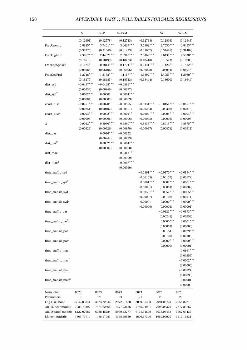
158 APPENDIX F. PART 1: FULL TABLES FOR SALES REGRESSIONS

S S+P S+P+M S S+P S+P+M

(0.12601) (0.12578) (0.12743) (0.12794) (0.12816) (0.12943)

FracUnemp 3.8815∗∗∗ 3.7401∗∗∗ 3.6627∗∗∗ 3.5969∗∗∗ 3.7530∗∗∗ 3.8453∗∗∗

(0.31375) (0.31546) (0.31433) (0.31657) (0.31428) (0.31482)

FracHighInc 2.3767∗∗∗ 2.4482∗∗∗ 2.3918∗∗∗ 2.6162∗∗∗ 2.6131∗∗∗ 2.5538∗∗∗

(0.18519) (0.18499) (0.18423) (0.18418) (0.18573) (0.18706)

FracEngSpoken −0.1124∗ −0.1814∗∗∗ −0.1724∗∗∗ −0.2141∗∗∗ −0.1426∗∗ −0.1512∗∗

(0.05985) (0.06106) (0.06096) (0.06028) (0.06054) (0.06048)

FracOccProf 1.2716∗∗∗ 1.3158∗∗∗ 1.1117∗∗∗ 1.6897∗∗∗ 1.4055∗∗∗ 1.2960∗∗∗

(0.18475) (0.18485) (0.18543) (0.18444) (0.18600) (0.18646)

dist_syd −0.0457∗∗∗ −0.0468∗∗∗ −0.0599∗∗∗

(0.00238) (0.00246) (0.00277)

dist_syd2 0.0002∗∗∗ 0.00001 0.0004∗∗∗

(0.00004) (0.00007) (0.00009)

coast_dist −0.0271∗∗∗ −0.0070∗ −0.00575 −0.0331∗∗∗ −0.0454∗∗∗ −0.0451∗∗∗

(0.00251) (0.00402) (0.00401) (0.00234) (0.00308) (0.00318)

coast_dist2 0.0003∗∗∗ 0.0002∗∗∗ 0.0001∗∗ 0.0002∗∗∗ 0.0004∗∗∗ 0.0004∗∗∗

(0.00005) (0.00006) (0.00006) (0.00005) (0.00005) (0.00005)

λ 0.9012∗∗∗ 0.8930∗∗∗ 0.8860∗∗∗ 0.8833∗∗∗ 0.8913∗∗∗ 0.8875∗∗∗

(0.00823) (0.00926) (0.00979) (0.00927) (0.00871) (0.00911)

dist_par 0.0096∗∗∗ −0.00252

(0.00244) (0.00273)

dist_par2 0.0002∗∗∗ 0.0004∗∗∗

(0.00007) (0.00008)

dist_mac 0.0313∗∗∗

(0.00309)

dist_mac2 −0.0007∗∗∗

(0.00010)

time_traffic_syd −0.0191∗∗∗ −0.0170∗∗∗ −0.0194∗∗∗

(0.00155) (0.00157) (0.00172)

time_traffic_syd2 0.0001∗∗∗ 0.0001∗∗∗ 0.0001∗∗∗

(0.00001) (0.00001) (0.00002)

time_transit_syd −0.0055∗∗∗ −0.0057∗∗∗ −0.0065∗∗∗

(0.00097) (0.00108) (0.00111)

time_transit_syd2 0.00001 0.0000∗∗∗ 0.0000∗∗∗

(0.00000) (0.00001) (0.00001)

time_traffic_par −0.0123∗∗∗ −0.0173∗∗∗

(0.00242) (0.00253)

time_traffic_par2 0.0000∗∗∗ 0.0001∗∗∗

(0.00003) (0.00003)

time_transit_par 0.00164 0.0029∗∗∗

(0.00100) (0.00103)

time_transit_par2 −0.0000∗∗∗ −0.0000∗∗∗

(0.00000) (0.00001)

time_traffic_mac 0.0167∗∗∗

(0.00256)

time_traffic_mac2 −0.0002∗∗∗

(0.00003)

time_transit_mac −0.00121

(0.00095)

time_transit_mac2 0.00001

(0.00000)

Num. obs. 8073 8073 8073 8073 8073 8073

Parameters 19 21 23 21 25 29

Log Likelihood −3042.03841 −3023.22642 −2972.21888 −3059.67300 −2994.02729 −2954.82218

AIC (Linear model) 7985.79392 7574.62365 7377.23656 7766.01901 7696.05379 7377.83767

AIC (Spatial model) 6122.07682 6088.45284 5990.43777 6161.34600 6038.05458 5967.64436

LR test: statistic 1865.71710 1488.17081 1388.79880 1606.67300 1659.99920 1412.19331

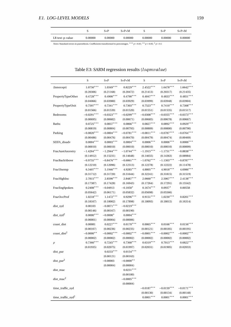
F.1. LOG-LEVEL MODELS 159

S S+P S+P+M S S+P S+P+M

LR test: p-value 0.00000 0.00000 0.00000 0.00000 0.00000 0.00000

Notes: Standard errors in parenthesis. Coefficients transformed to percentages. ∗∗∗p < 0.01; ∗∗p < 0.05; ∗p < 0.1

Table F.3: SARM regression results (l sqmval ue)

S S+P S+P+M S S+P S+P+M

(Intercept) 1.0750∗∗∗ 1.0349∗∗∗ 0.8229∗∗∗ 2.4522∗∗∗ 1.6478∗∗∗ 1.6642∗∗∗

(0.20306) (0.21168) (0.20472) (0.21413) (0.20317) (0.21435)

PropertyTypeOther 0.4728∗∗∗ 0.4900∗∗∗ 0.4790∗∗∗ 0.4847∗∗∗ 0.4833∗∗∗ 0.4851∗∗∗

(0.04066) (0.03980) (0.03929) (0.03999) (0.03948) (0.03904)

PropertyTypeUnit 0.7597∗∗∗ 0.7341∗∗∗ 0.7303∗∗∗ 0.7523∗∗∗ 0.7410∗∗∗ 0.7308∗∗∗

(0.01566) (0.01539) (0.01520) (0.01551) (0.01535) (0.01517)

Bedrooms −0.0291∗∗∗ −0.0323∗∗∗ −0.0299∗∗∗ −0.0308∗∗∗ −0.0355∗∗∗ −0.0373∗∗∗

(0.00695) (0.00682) (0.00671) (0.00685) (0.00678) (0.00667)

Baths 0.0725∗∗∗ 0.0837∗∗∗ 0.0866∗∗∗ 0.0827∗∗∗ 0.0892∗∗∗ 0.0929∗∗∗

(0.00819) (0.00804) (0.00793) (0.00809) (0.00800) (0.00790)

Parking −0.0820∗∗∗ −0.0804∗∗∗ −0.0781∗∗∗ −0.0811∗∗∗ −0.0787∗∗∗ −0.0764∗∗∗

(0.00486) (0.00476) (0.00470) (0.00479) (0.00474) (0.00469)

SEIFA_disadv 0.0004∗∗∗ 0.0003∗∗∗ 0.0004∗∗∗ 0.0006∗∗∗ 0.0006∗∗∗ 0.0006∗∗∗

(0.00010) (0.00010) (0.00010) (0.00010) (0.00010) (0.00009)

FracAustAncestry −1.4264∗∗∗ −1.2944∗∗∗ −1.0744∗∗∗ −1.1915∗∗∗ −1.1751∗∗∗ −0.8838∗∗∗

(0.14912) (0.15231) (0.14648) (0.14655) (0.14363) (0.08984)

FracBachAbove −0.9755∗∗∗ −0.8476∗∗∗ −0.6061∗∗∗ −1.0762∗∗∗ −1.1303∗∗∗ −0.8787∗∗∗

(0.12210) (0.12096) (0.12313) (0.12278) (0.12222) (0.11478)

FracUnemp 6.3407∗∗∗ 5.1946∗∗∗ 4.9285∗∗∗ 4.8805∗∗∗ 4.9018∗∗∗ 4.6986∗∗∗

(0.31712) (0.31720) (0.31644) (0.32241) (0.31815) (0.31519)

FracHighInc 2.7815∗∗∗ 2.8590∗∗∗ 2.8487∗∗∗ 2.0660∗∗∗ 2.5067∗∗∗ 2.4138∗∗∗

(0.17387) (0.17428) (0.16943) (0.17264) (0.17291) (0.15542)

FracEngSpoken 0.2408∗∗∗ −0.04913 −0.1050∗ 0.1674∗∗∗ 0.0937∗ 0.00558

(0.05642) (0.06171) (0.05832) (0.05698) (0.05566)

FracOccProf 1.0218∗∗∗ 1.1472∗∗∗ 0.9296∗∗∗ 0.9151∗∗∗ 1.0230∗∗∗ 0.8201∗∗∗

(0.18167) (0.18002) (0.17898) (0.18093) (0.18015) (0.16314)

dist_syd 0.00103 −0.0071∗∗∗ −0.0219∗∗∗

(0.00146) (0.00167) (0.00190)

dist_syd2 0.0000∗∗∗ −0.0000∗ 0.0004∗∗∗

(0.00001) (0.00004) (0.00006)

coast_dist 0.00081 0.0227∗∗∗ 0.0170∗∗∗ 0.0065∗∗∗ 0.0166∗∗∗ 0.0156∗∗∗

(0.00107) (0.00236) (0.00235) (0.00121) (0.00185) (0.00195)

coast_dist2 −0.0000∗∗ −0.0002∗∗∗ −0.0002∗∗∗ −0.0001∗∗∗ −0.0002∗∗∗ −0.0002∗∗∗

(0.00002) (0.00002) (0.00002) (0.00002) (0.00002) (0.00002)

ρ 0.7360∗∗∗ 0.7245∗∗∗ 0.7368∗∗∗ 0.6319∗∗∗ 0.7013∗∗∗ 0.6822∗∗∗

(0.01935) (0.02075) (0.01997) (0.02031) (0.01905) (0.02033)

dist_par 0.0233∗∗∗ 0.0154∗∗∗

(0.00121) (0.00163)

dist_par2 −0.00003 −0.0000∗∗

(0.00004) (0.00004)

dist_mac 0.0231∗∗∗

(0.00180)

dist_mac2 −0.0005∗∗∗

(0.00004)

time_traffic_syd −0.0187∗∗∗ −0.0159∗∗∗ −0.0171∗∗∗

(0.00130) (0.00134) (0.00148)

time_traffic_syd2 0.0001∗∗∗ 0.0001∗∗∗ 0.0001∗∗∗

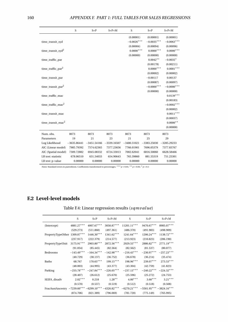
160 APPENDIX F. PART 1: FULL TABLES FOR SALES REGRESSIONS

S S+P S+P+M S S+P S+P+M

(0.00001) (0.00001) (0.00001)

time_transit_syd −0.0026∗∗∗ −0.0035∗∗∗ −0.0063∗∗∗

(0.00084) (0.00094) (0.00096)

time_transit_syd2 0.0000∗∗∗ 0.0000∗∗∗ 0.0000∗∗∗

(0.00000) (0.00000) (0.00000)

time_traffic_par 0.0042∗∗ −0.0035∗

(0.00178) (0.00211)

time_traffic_par2 0.0000∗∗∗ 0.0001∗∗∗

(0.00002) (0.00002)

time_transit_par −0.00117 0.00137

(0.00087) (0.00097)

time_transit_par2 −0.0000∗∗∗ −0.0000∗∗∗

(0.00000) (0.00000)

time_traffic_mac 0.0139∗∗∗

(0.00183)

time_traffic_mac2 −0.0002∗∗∗

(0.00002)

time_transit_mac 0.0011∗∗∗

(0.00037)

time_transit_mac2 0.0000∗∗

(0.00000)

Num. obs. 8073 8073 8073 8073 8073 8073

Parameters 19 21 23 21 25 29

Log Likelihood −3635.86441 −3451.54166 −3339.16507 −3480.31021 −3383.25030 −3285.29233

AIC (Linear model) 7985.79392 7574.62365 7377.23656 7766.01901 7696.05379 7377.83767

AIC (Spatial model) 7309.72882 6945.08332 6724.33013 7002.62041 6816.50060 6628.58466

LR test: statistic 678.06510 631.54033 654.90643 765.39860 881.55319 751.25301

LR test: p-value 0.00000 0.00000 0.00000 0.00000 0.00000 0.00000

Notes: Standard errors in parenthesis. Coefficients transformed to percentages. ∗∗∗p < 0.01; ∗∗p < 0.05; ∗p < 0.1

F.2 Level-level models

Table F.4: Linear regression results (sqmval ue)

S S+P S+P+M S S+P S+P+M

(Intercept) 4881.27∗∗∗ 4007.67∗∗∗ 3050.87∗∗∗ 11201.11∗∗∗ 9470.67∗∗∗ 8985.07∗∗∗

(529.273) (511.860) (497.361) (486.370) (491.983) (498.909)

PropertyTypeOther 1309.87∗∗∗ 1446.30∗∗∗ 1341.62∗∗∗ 1241.64∗∗∗ 1206.24∗∗∗ 1138.72∗∗∗

(237.917) (222.379) (214.577) (213.923) (210.823) (206.190)

PropertyTypeUnit 3175.91∗∗∗ 2903.80∗∗∗ 2872.56∗∗∗ 2929.55∗∗∗ 2886.82∗∗∗ 2771.19∗∗∗

(91.054) (85.445) (82.564) (82.562) (81.537) (80.077)

Bedrooms −143.49∗∗∗ −164.34∗∗∗ −142.98∗∗∗ −216.43∗∗∗ −230.97∗∗∗ −257.23∗∗∗

(40.729) (38.137) (36.752) (36.678) (36.214) (35.474)

Baths 68.767 170.65∗∗∗ 199.15∗∗∗ 198.96∗∗∗ 239.07∗∗∗ 273.53∗∗∗

(48.003) (44.995) (43.377) (43.304) (42.759) (41.823)

Parking −255.78∗∗∗ −247.84∗∗∗ −226.05∗∗∗ −237.13∗∗∗ −240.22∗∗∗ −224.32∗∗∗

(28.407) (26.612) (25.670) (25.596) (25.272) (24.753)

SEIFA_disadv 2.02∗∗∗ 0.218 1.28∗∗ 4.00∗∗∗ 3.60∗∗∗ 3.21∗∗∗

(0.570) (0.537) (0.519) (0.512) (0.518) (0.508)

FracAustAncestry −7239.60∗∗∗ −6299.10∗∗∗ −4326.82∗∗∗ −6270.21∗∗∗ −5501.95∗∗∗ −3824.16∗∗∗

(874.706) (821.389) (796.069) (781.720) (775.149) (765.995)

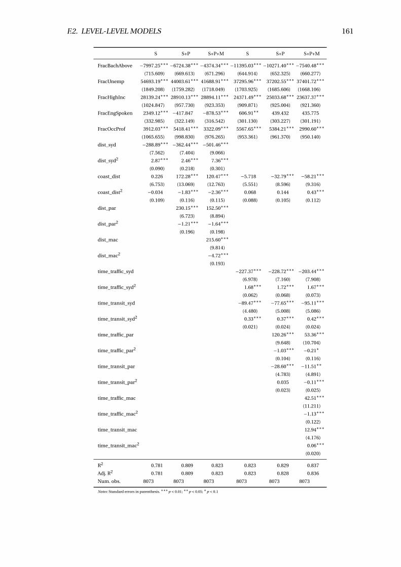
F.2. LEVEL-LEVEL MODELS 161

S S+P S+P+M S S+P S+P+M

FracBachAbove −7997.25∗∗∗ −6724.38∗∗∗ −4374.34∗∗∗ −11395.03∗∗∗ −10271.40∗∗∗ −7540.48∗∗∗

(715.609) (669.613) (671.296) (644.914) (652.325) (660.277)

FracUnemp 54693.19∗∗∗ 44003.61∗∗∗ 41688.91∗∗∗ 37295.96∗∗∗ 37202.55∗∗∗ 37401.72∗∗∗

(1849.208) (1759.282) (1718.049) (1703.925) (1685.606) (1668.106)

FracHighInc 28139.24∗∗∗ 28910.13∗∗∗ 28894.11∗∗∗ 24371.49∗∗∗ 25033.68∗∗∗ 23637.37∗∗∗

(1024.847) (957.730) (923.353) (909.871) (925.004) (921.360)

FracEngSpoken 2349.12∗∗∗ −417.847 −878.53∗∗∗ 606.91∗∗ 439.432 435.775

(332.985) (322.149) (316.542) (301.130) (303.227) (301.191)

FracOccProf 3912.03∗∗∗ 5418.41∗∗∗ 3322.09∗∗∗ 5567.65∗∗∗ 5384.21∗∗∗ 2990.60∗∗∗

(1065.655) (998.830) (976.265) (953.361) (961.370) (950.140)

dist_syd −288.89∗∗∗ −362.44∗∗∗ −501.46∗∗∗

(7.562) (7.404) (9.066)

dist_syd2 2.87∗∗∗ 2.46∗∗∗ 7.36∗∗∗

(0.090) (0.218) (0.301)

coast_dist 0.226 172.28∗∗∗ 120.47∗∗∗ −5.718 −32.79∗∗∗ −58.21∗∗∗

(6.753) (13.069) (12.763) (5.551) (8.596) (9.316)

coast_dist2 −0.034 −1.83∗∗∗ −2.36∗∗∗ 0.068 0.144 0.43∗∗∗

(0.109) (0.116) (0.115) (0.088) (0.105) (0.112)

dist_par 230.15∗∗∗ 152.50∗∗∗

(6.723) (8.894)

dist_par2 −1.21∗∗∗ −1.64∗∗∗

(0.196) (0.198)

dist_mac 215.60∗∗∗

(9.814)

dist_mac2 −4.72∗∗∗

(0.193)

time_traffic_syd −227.37∗∗∗ −228.72∗∗∗ −203.44∗∗∗

(6.978) (7.160) (7.908)

time_traffic_syd2 1.68∗∗∗ 1.72∗∗∗ 1.67∗∗∗

(0.062) (0.068) (0.073)

time_transit_syd −89.47∗∗∗ −77.65∗∗∗ −95.11∗∗∗

(4.480) (5.008) (5.086)

time_transit_syd2 0.33∗∗∗ 0.37∗∗∗ 0.42∗∗∗

(0.021) (0.024) (0.024)

time_traffic_par 120.26∗∗∗ 53.36∗∗∗

(9.648) (10.704)

time_traffic_par2 −1.03∗∗∗ −0.21∗

(0.104) (0.116)

time_transit_par −28.60∗∗∗ −11.51∗∗

(4.783) (4.891)

time_transit_par2 0.035 −0.11∗∗∗

(0.023) (0.025)

time_traffic_mac 42.51∗∗∗

(11.211)

time_traffic_mac2 −1.13∗∗∗

(0.122)

time_transit_mac 12.94∗∗∗

(4.176)

time_transit_mac2 0.06∗∗∗

(0.020)

R2 0.781 0.809 0.823 0.823 0.829 0.837

Adj. R2 0.781 0.809 0.823 0.823 0.828 0.836

Num. obs. 8073 8073 8073 8073 8073 8073

Notes: Standard errors in parenthesis. ∗∗∗p < 0.01; ∗∗p < 0.05; ∗p < 0.1

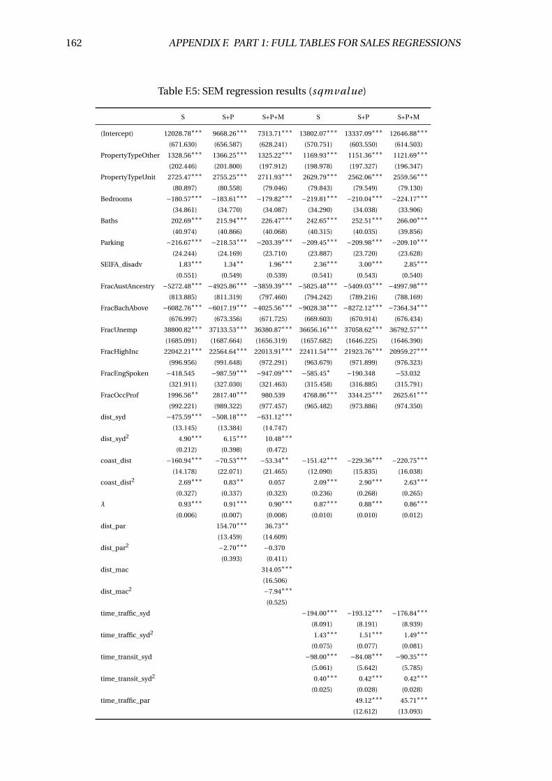
162 APPENDIX F. PART 1: FULL TABLES FOR SALES REGRESSIONS

Table F.5: SEM regression results (sqmval ue)

S S+P S+P+M S S+P S+P+M

(Intercept) 12028.78∗∗∗ 9668.26∗∗∗ 7313.71∗∗∗ 13802.07∗∗∗ 13337.09∗∗∗ 12646.88∗∗∗

(671.630) (656.587) (628.241) (570.751) (603.550) (614.503)

PropertyTypeOther 1328.56∗∗∗ 1366.25∗∗∗ 1325.22∗∗∗ 1169.93∗∗∗ 1151.36∗∗∗ 1121.69∗∗∗

(202.446) (201.800) (197.912) (198.978) (197.327) (196.347)

PropertyTypeUnit 2725.47∗∗∗ 2755.25∗∗∗ 2711.93∗∗∗ 2629.79∗∗∗ 2562.06∗∗∗ 2559.56∗∗∗

(80.897) (80.558) (79.046) (79.843) (79.549) (79.130)

Bedrooms −180.57∗∗∗ −183.61∗∗∗ −179.82∗∗∗ −219.81∗∗∗ −210.04∗∗∗ −224.17∗∗∗

(34.861) (34.770) (34.087) (34.290) (34.038) (33.906)

Baths 202.69∗∗∗ 215.94∗∗∗ 226.47∗∗∗ 242.65∗∗∗ 252.51∗∗∗ 266.00∗∗∗

(40.974) (40.866) (40.068) (40.315) (40.035) (39.856)

Parking −216.67∗∗∗ −218.53∗∗∗ −203.39∗∗∗ −209.45∗∗∗ −209.98∗∗∗ −209.10∗∗∗

(24.244) (24.169) (23.710) (23.887) (23.720) (23.628)

SEIFA_disadv 1.83∗∗∗ 1.34∗∗ 1.96∗∗∗ 2.36∗∗∗ 3.00∗∗∗ 2.85∗∗∗

(0.551) (0.549) (0.539) (0.541) (0.543) (0.540)

FracAustAncestry −5272.48∗∗∗ −4925.86∗∗∗ −3859.39∗∗∗ −5825.48∗∗∗ −5409.03∗∗∗ −4997.98∗∗∗

(813.885) (811.319) (797.460) (794.242) (789.216) (788.169)

FracBachAbove −6082.76∗∗∗ −6017.19∗∗∗ −4025.56∗∗∗ −9028.38∗∗∗ −8272.12∗∗∗ −7364.34∗∗∗

(676.997) (673.356) (671.725) (669.603) (670.914) (676.434)

FracUnemp 38800.82∗∗∗ 37133.53∗∗∗ 36380.87∗∗∗ 36656.16∗∗∗ 37058.62∗∗∗ 36792.57∗∗∗

(1685.091) (1687.664) (1656.319) (1657.682) (1646.225) (1646.390)

FracHighInc 22042.21∗∗∗ 22564.64∗∗∗ 22013.91∗∗∗ 22411.54∗∗∗ 21923.76∗∗∗ 20959.27∗∗∗

(996.956) (991.648) (972.291) (963.679) (971.899) (976.323)

FracEngSpoken −418.545 −987.59∗∗∗ −947.09∗∗∗ −585.45∗ −190.348 −53.032

(321.911) (327.030) (321.463) (315.458) (316.885) (315.791)

FracOccProf 1996.56∗∗ 2817.40∗∗∗ 980.539 4768.86∗∗∗ 3344.25∗∗∗ 2625.61∗∗∗

(992.221) (989.322) (977.457) (965.482) (973.886) (974.350)

dist_syd −475.59∗∗∗ −508.18∗∗∗ −631.12∗∗∗

(13.145) (13.384) (14.747)

dist_syd2 4.90∗∗∗ 6.15∗∗∗ 10.48∗∗∗

(0.212) (0.398) (0.472)

coast_dist −160.94∗∗∗ −70.53∗∗∗ −53.34∗∗ −151.42∗∗∗ −229.36∗∗∗ −220.75∗∗∗

(14.178) (22.071) (21.465) (12.090) (15.835) (16.038)

coast_dist2 2.69∗∗∗ 0.83∗∗ 0.057 2.09∗∗∗ 2.90∗∗∗ 2.63∗∗∗

(0.327) (0.337) (0.323) (0.236) (0.268) (0.265)

λ 0.93∗∗∗ 0.91∗∗∗ 0.90∗∗∗ 0.87∗∗∗ 0.88∗∗∗ 0.86∗∗∗

(0.006) (0.007) (0.008) (0.010) (0.010) (0.012)

dist_par 154.70∗∗∗ 36.73∗∗

(13.459) (14.609)

dist_par2 −2.70∗∗∗ −0.370

(0.393) (0.411)

dist_mac 314.05∗∗∗

(16.506)

dist_mac2 −7.94∗∗∗

(0.525)

time_traffic_syd −194.00∗∗∗ −193.12∗∗∗ −176.84∗∗∗

(8.091) (8.191) (8.939)

time_traffic_syd2 1.43∗∗∗ 1.51∗∗∗ 1.49∗∗∗

(0.075) (0.077) (0.081)

time_transit_syd −98.00∗∗∗ −84.08∗∗∗ −90.35∗∗∗

(5.061) (5.642) (5.785)

time_transit_syd2 0.40∗∗∗ 0.42∗∗∗ 0.42∗∗∗

(0.025) (0.028) (0.028)

time_traffic_par 49.12∗∗∗ 45.71∗∗∗

(12.612) (13.093)

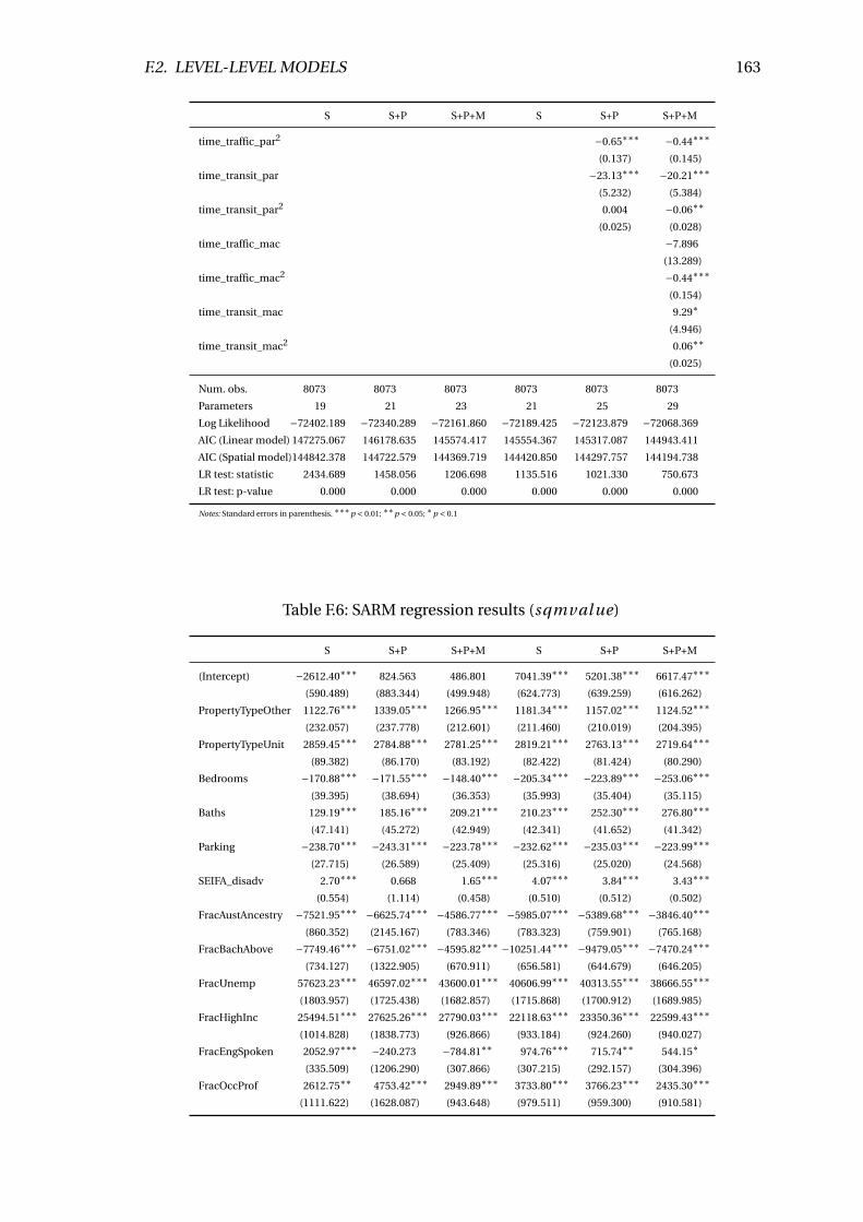
F.2. LEVEL-LEVEL MODELS 163

S S+P S+P+M S S+P S+P+M

time_traffic_par2 −0.65∗∗∗ −0.44∗∗∗

(0.137) (0.145)

time_transit_par −23.13∗∗∗ −20.21∗∗∗

(5.232) (5.384)

time_transit_par2 0.004 −0.06∗∗

(0.025) (0.028)

time_traffic_mac −7.896

(13.289)

time_traffic_mac2 −0.44∗∗∗

(0.154)

time_transit_mac 9.29∗

(4.946)

time_transit_mac2 0.06∗∗

(0.025)

Num. obs. 8073 8073 8073 8073 8073 8073

Parameters 19 21 23 21 25 29

Log Likelihood −72402.189 −72340.289 −72161.860 −72189.425 −72123.879 −72068.369

AIC (Linear model) 147275.067 146178.635 145574.417 145554.367 145317.087 144943.411

AIC (Spatial model)144842.378 144722.579 144369.719 144420.850 144297.757 144194.738

LR test: statistic 2434.689 1458.056 1206.698 1135.516 1021.330 750.673

LR test: p-value 0.000 0.000 0.000 0.000 0.000 0.000

Notes: Standard errors in parenthesis. ∗∗∗p < 0.01; ∗∗p < 0.05; ∗p < 0.1

Table F.6: SARM regression results (sqmval ue)

S S+P S+P+M S S+P S+P+M

(Intercept) −2612.40∗∗∗ 824.563 486.801 7041.39∗∗∗ 5201.38∗∗∗ 6617.47∗∗∗

(590.489) (883.344) (499.948) (624.773) (639.259) (616.262)

PropertyTypeOther 1122.76∗∗∗ 1339.05∗∗∗ 1266.95∗∗∗ 1181.34∗∗∗ 1157.02∗∗∗ 1124.52∗∗∗

(232.057) (237.778) (212.601) (211.460) (210.019) (204.395)

PropertyTypeUnit 2859.45∗∗∗ 2784.88∗∗∗ 2781.25∗∗∗ 2819.21∗∗∗ 2763.13∗∗∗ 2719.64∗∗∗

(89.382) (86.170) (83.192) (82.422) (81.424) (80.290)

Bedrooms −170.88∗∗∗ −171.55∗∗∗ −148.40∗∗∗ −205.34∗∗∗ −223.89∗∗∗ −253.06∗∗∗

(39.395) (38.694) (36.353) (35.993) (35.404) (35.115)

Baths 129.19∗∗∗ 185.16∗∗∗ 209.21∗∗∗ 210.23∗∗∗ 252.30∗∗∗ 276.80∗∗∗

(47.141) (45.272) (42.949) (42.341) (41.652) (41.342)

Parking −238.70∗∗∗ −243.31∗∗∗ −223.78∗∗∗ −232.62∗∗∗ −235.03∗∗∗ −223.99∗∗∗

(27.715) (26.589) (25.409) (25.316) (25.020) (24.568)

SEIFA_disadv 2.70∗∗∗ 0.668 1.65∗∗∗ 4.07∗∗∗ 3.84∗∗∗ 3.43∗∗∗

(0.554) (1.114) (0.458) (0.510) (0.512) (0.502)

FracAustAncestry −7521.95∗∗∗ −6625.74∗∗∗ −4586.77∗∗∗ −5985.07∗∗∗ −5389.68∗∗∗ −3846.40∗∗∗

(860.352) (2145.167) (783.346) (783.323) (759.901) (765.168)

FracBachAbove −7749.46∗∗∗ −6751.02∗∗∗ −4595.82∗∗∗ −10251.44∗∗∗ −9479.05∗∗∗ −7470.24∗∗∗

(734.127) (1322.905) (670.911) (656.581) (644.679) (646.205)

FracUnemp 57623.23∗∗∗ 46597.02∗∗∗ 43600.01∗∗∗ 40606.99∗∗∗ 40313.55∗∗∗ 38666.55∗∗∗

(1803.957) (1725.438) (1682.857) (1715.868) (1700.912) (1689.985)

FracHighInc 25494.51∗∗∗ 27625.26∗∗∗ 27790.03∗∗∗ 22118.63∗∗∗ 23350.36∗∗∗ 22599.43∗∗∗

(1014.828) (1838.773) (926.866) (933.184) (924.260) (940.027)

FracEngSpoken 2052.97∗∗∗ −240.273 −784.81∗∗ 974.76∗∗∗ 715.74∗∗ 544.15∗

(335.509) (1206.290) (307.866) (307.215) (292.157) (304.396)

FracOccProf 2612.75∗∗ 4753.42∗∗∗ 2949.89∗∗∗ 3733.80∗∗∗ 3766.23∗∗∗ 2435.30∗∗∗

(1111.622) (1628.087) (943.648) (979.511) (959.300) (910.581)

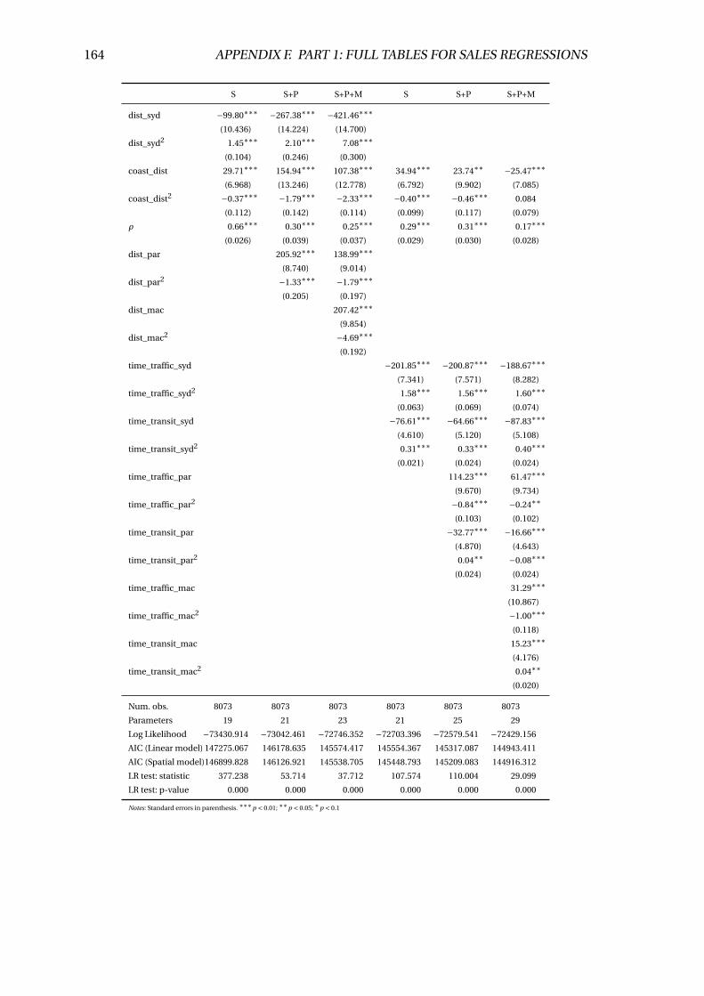
164 APPENDIX F. PART 1: FULL TABLES FOR SALES REGRESSIONS

S S+P S+P+M S S+P S+P+M

dist_syd −99.80∗∗∗ −267.38∗∗∗ −421.46∗∗∗

(10.436) (14.224) (14.700)

dist_syd2 1.45∗∗∗ 2.10∗∗∗ 7.08∗∗∗

(0.104) (0.246) (0.300)

coast_dist 29.71∗∗∗ 154.94∗∗∗ 107.38∗∗∗ 34.94∗∗∗ 23.74∗∗ −25.47∗∗∗

(6.968) (13.246) (12.778) (6.792) (9.902) (7.085)

coast_dist2 −0.37∗∗∗ −1.79∗∗∗ −2.33∗∗∗ −0.40∗∗∗ −0.46∗∗∗ 0.084

(0.112) (0.142) (0.114) (0.099) (0.117) (0.079)

ρ 0.66∗∗∗ 0.30∗∗∗ 0.25∗∗∗ 0.29∗∗∗ 0.31∗∗∗ 0.17∗∗∗

(0.026) (0.039) (0.037) (0.029) (0.030) (0.028)

dist_par 205.92∗∗∗ 138.99∗∗∗

(8.740) (9.014)

dist_par2 −1.33∗∗∗ −1.79∗∗∗

(0.205) (0.197)

dist_mac 207.42∗∗∗

(9.854)

dist_mac2 −4.69∗∗∗

(0.192)

time_traffic_syd −201.85∗∗∗ −200.87∗∗∗ −188.67∗∗∗

(7.341) (7.571) (8.282)

time_traffic_syd2 1.58∗∗∗ 1.56∗∗∗ 1.60∗∗∗

(0.063) (0.069) (0.074)

time_transit_syd −76.61∗∗∗ −64.66∗∗∗ −87.83∗∗∗

(4.610) (5.120) (5.108)

time_transit_syd2 0.31∗∗∗ 0.33∗∗∗ 0.40∗∗∗

(0.021) (0.024) (0.024)

time_traffic_par 114.23∗∗∗ 61.47∗∗∗

(9.670) (9.734)

time_traffic_par2 −0.84∗∗∗ −0.24∗∗

(0.103) (0.102)

time_transit_par −32.77∗∗∗ −16.66∗∗∗

(4.870) (4.643)

time_transit_par2 0.04∗∗ −0.08∗∗∗

(0.024) (0.024)

time_traffic_mac 31.29∗∗∗

(10.867)

time_traffic_mac2 −1.00∗∗∗

(0.118)

time_transit_mac 15.23∗∗∗

(4.176)

time_transit_mac2 0.04∗∗

(0.020)

Num. obs. 8073 8073 8073 8073 8073 8073

Parameters 19 21 23 21 25 29

Log Likelihood −73430.914 −73042.461 −72746.352 −72703.396 −72579.541 −72429.156

AIC (Linear model) 147275.067 146178.635 145574.417 145554.367 145317.087 144943.411

AIC (Spatial model)146899.828 146126.921 145538.705 145448.793 145209.083 144916.312

LR test: statistic 377.238 53.714 37.712 107.574 110.004 29.099

LR test: p-value 0.000 0.000 0.000 0.000 0.000 0.000

Notes: Standard errors in parenthesis. ∗∗∗p < 0.01; ∗∗p < 0.05; ∗p < 0.1

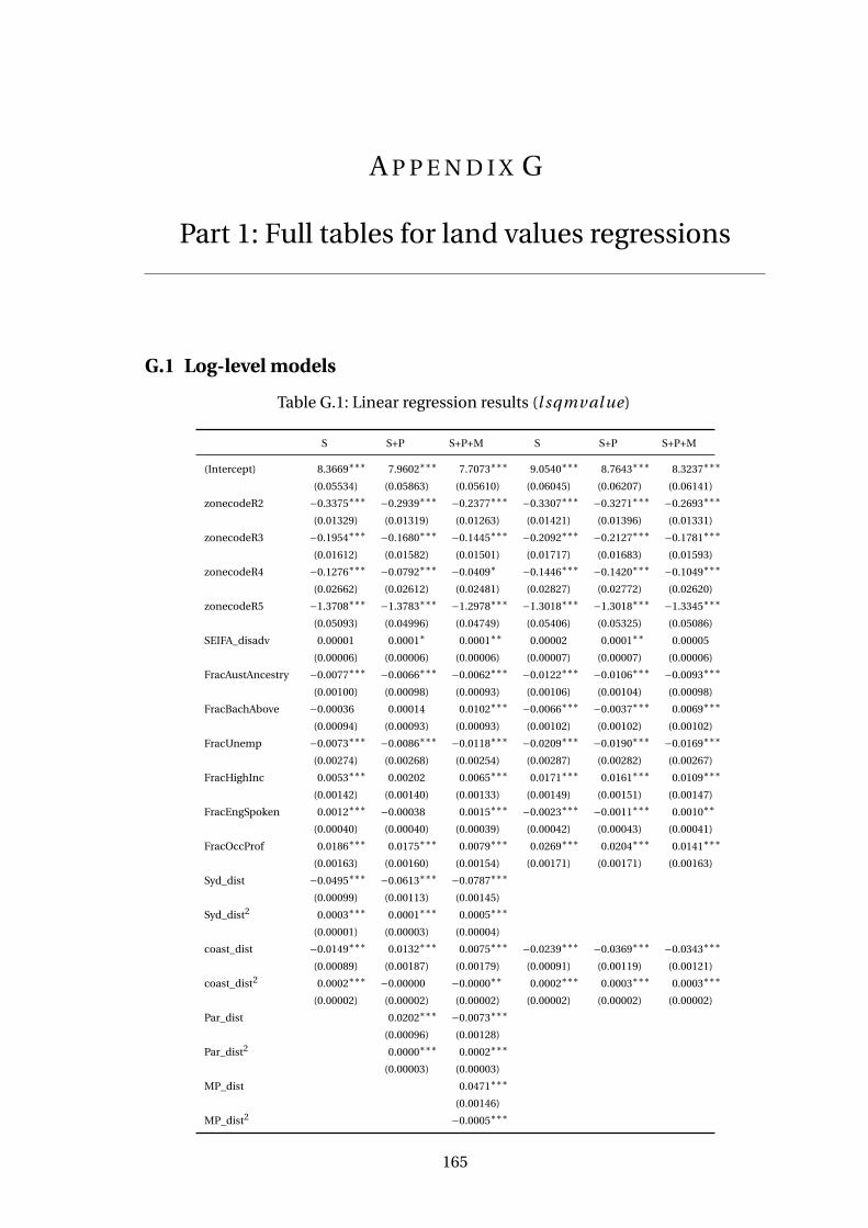
A P P E N D I X G

Part 1: Full tables for land values regressions

G.1 Log-level models

Table G.1: Linear regression results (l sqmval ue)

S S+P S+P+M S S+P S+P+M

(Intercept) 8.3669∗∗∗ 7.9602∗∗∗ 7.7073∗∗∗ 9.0540∗∗∗ 8.7643∗∗∗ 8.3237∗∗∗

(0.05534) (0.05863) (0.05610) (0.06045) (0.06207) (0.06141)

zonecodeR2 −0.3375∗∗∗ −0.2939∗∗∗ −0.2377∗∗∗ −0.3307∗∗∗ −0.3271∗∗∗ −0.2693∗∗∗

(0.01329) (0.01319) (0.01263) (0.01421) (0.01396) (0.01331)

zonecodeR3 −0.1954∗∗∗ −0.1680∗∗∗ −0.1445∗∗∗ −0.2092∗∗∗ −0.2127∗∗∗ −0.1781∗∗∗

(0.01612) (0.01582) (0.01501) (0.01717) (0.01683) (0.01593)

zonecodeR4 −0.1276∗∗∗ −0.0792∗∗∗ −0.0409∗ −0.1446∗∗∗ −0.1420∗∗∗ −0.1049∗∗∗

(0.02662) (0.02612) (0.02481) (0.02827) (0.02772) (0.02620)

zonecodeR5 −1.3708∗∗∗ −1.3783∗∗∗ −1.2978∗∗∗ −1.3018∗∗∗ −1.3018∗∗∗ −1.3345∗∗∗

(0.05093) (0.04996) (0.04749) (0.05406) (0.05325) (0.05086)

SEIFA_disadv 0.00001 0.0001∗ 0.0001∗∗ 0.00002 0.0001∗∗ 0.00005

(0.00006) (0.00006) (0.00006) (0.00007) (0.00007) (0.00006)

FracAustAncestry −0.0077∗∗∗ −0.0066∗∗∗ −0.0062∗∗∗ −0.0122∗∗∗ −0.0106∗∗∗ −0.0093∗∗∗

(0.00100) (0.00098) (0.00093) (0.00106) (0.00104) (0.00098)

FracBachAbove −0.00036 0.00014 0.0102∗∗∗ −0.0066∗∗∗ −0.0037∗∗∗ 0.0069∗∗∗

(0.00094) (0.00093) (0.00093) (0.00102) (0.00102) (0.00102)

FracUnemp −0.0073∗∗∗ −0.0086∗∗∗ −0.0118∗∗∗ −0.0209∗∗∗ −0.0190∗∗∗ −0.0169∗∗∗

(0.00274) (0.00268) (0.00254) (0.00287) (0.00282) (0.00267)

FracHighInc 0.0053∗∗∗ 0.00202 0.0065∗∗∗ 0.0171∗∗∗ 0.0161∗∗∗ 0.0109∗∗∗

(0.00142) (0.00140) (0.00133) (0.00149) (0.00151) (0.00147)

FracEngSpoken 0.0012∗∗∗ −0.00038 0.0015∗∗∗ −0.0023∗∗∗ −0.0011∗∗∗ 0.0010∗∗

(0.00040) (0.00040) (0.00039) (0.00042) (0.00043) (0.00041)

FracOccProf 0.0186∗∗∗ 0.0175∗∗∗ 0.0079∗∗∗ 0.0269∗∗∗ 0.0204∗∗∗ 0.0141∗∗∗

(0.00163) (0.00160) (0.00154) (0.00171) (0.00171) (0.00163)

Syd_dist −0.0495∗∗∗ −0.0613∗∗∗ −0.0787∗∗∗

(0.00099) (0.00113) (0.00145)

Syd_dist2 0.0003∗∗∗ 0.0001∗∗∗ 0.0005∗∗∗

(0.00001) (0.00003) (0.00004)

coast_dist −0.0149∗∗∗ 0.0132∗∗∗ 0.0075∗∗∗ −0.0239∗∗∗ −0.0369∗∗∗ −0.0343∗∗∗

(0.00089) (0.00187) (0.00179) (0.00091) (0.00119) (0.00121)

coast_dist2 0.0002∗∗∗ −0.00000 −0.0000∗∗ 0.0002∗∗∗ 0.0003∗∗∗ 0.0003∗∗∗

(0.00002) (0.00002) (0.00002) (0.00002) (0.00002) (0.00002)

Par_dist 0.0202∗∗∗ −0.0073∗∗∗

(0.00096) (0.00128)

Par_dist2 0.0000∗∗∗ 0.0002∗∗∗

(0.00003) (0.00003)

MP_dist 0.0471∗∗∗

(0.00146)

MP_dist2 −0.0005∗∗∗

165

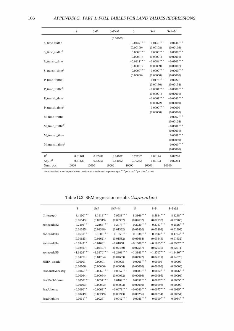
166 APPENDIX G. PART 1: FULL TABLES FOR LAND VALUES REGRESSIONS

S S+P S+P+M S S+P S+P+M

(0.00003)

S_time_traffic −0.0137∗∗∗ −0.0149∗∗∗ −0.0146∗∗∗

(0.00109) (0.00108) (0.00109)

S_time_traffic2 0.0000∗∗∗ 0.0000∗∗∗ 0.0000∗∗∗

(0.00001) (0.00001) (0.00001)

S_transit_time −0.0111∗∗∗ −0.0084∗∗∗ −0.0103∗∗∗

(0.00061) (0.00069) (0.00067)

S_transit_time2 0.0000∗∗∗ 0.0000∗∗∗ 0.0000∗∗∗

(0.00000) (0.00000) (0.00000)

P_time_traffic 0.0178∗∗∗ 0.0022∗

(0.00130) (0.00134)

P_time_traffic2 −0.0001∗∗∗ −0.0000∗∗∗

(0.00001) (0.00001)

P_transit_time −0.0061∗∗∗ −0.0043∗∗∗

(0.00072) (0.00069)

P_transit_time2 0.0000∗∗∗ 0.00000

(0.00000) (0.00000)

M_time_traffic 0.0067∗∗∗

(0.00124)

M_time_traffic2 −0.0001∗∗∗

(0.00001)

M_transit_time 0.0081∗∗∗

(0.00059)

M_transit_time2 −0.0000∗∗∗

(0.00000)

R2 0.81461 0.82281 0.84082 0.79297 0.80144 0.82298

Adj. R2 0.81433 0.82251 0.84052 0.79262 0.80103 0.82254

Num. obs. 10000 10000 10000 10000 10000 10000

Notes: Standard errors in parenthesis. Coefficients transformed to percentages. ∗∗∗p < 0.01; ∗∗p < 0.05; ∗p < 0.1

Table G.2: SEM regression results (l sqmval ue)

S S+P S+P+M S S+P S+P+M

(Intercept) 8.4100∗∗∗ 8.1919∗∗∗ 7.9738∗∗∗ 8.3966∗∗∗ 8.5884∗∗∗ 8.3298∗∗∗

(0.06543) (0.07319) (0.06967) (0.07632) (0.07892) (0.07765)

zonecodeR2 −0.2499∗∗∗ −0.2468∗∗∗ −0.2075∗∗∗ −0.2730∗∗∗ −0.2737∗∗∗ −0.2526∗∗∗

(0.01385) (0.01388) (0.01362) (0.01420) (0.01408) (0.01398)

zonecodeR3 −0.1631∗∗∗ −0.1605∗∗∗ −0.1358∗∗∗ −0.1938∗∗∗ −0.1942∗∗∗ −0.1794∗∗∗

(0.01623) (0.01621) (0.01582) (0.01664) (0.01649) (0.01632)

zonecodeR4 −0.0543∗∗ −0.0469∗ −0.01858 −0.1008∗∗∗ −0.1065∗∗∗ −0.0902∗∗∗

(0.02497) (0.02497) (0.02439) (0.02557) (0.02536) (0.02511)

zonecodeR5 −1.3426∗∗∗ −1.3370∗∗∗ −1.2969∗∗∗ −1.3981∗∗∗ −1.3707∗∗∗ −1.3486∗∗∗

(0.04771) (0.04764) (0.04653) (0.04942) (0.04917) (0.04878)

SEIFA_disadv −0.00001 0.00001 0.00005 −0.0001∗∗∗ −0.00009 −0.00009

(0.00006) (0.00006) (0.00006) (0.00006) (0.00006) (0.00006)

FracAustAncestry −0.0065∗∗∗ −0.0062∗∗∗ −0.0057∗∗∗ −0.0083∗∗∗ −0.0082∗∗∗ −0.0076∗∗∗

(0.00094) (0.00094) (0.00092) (0.00096) (0.00095) (0.00094)

FracBachAbove 0.0058∗∗∗ 0.0054∗∗∗ 0.0102∗∗∗ 0.0057∗∗∗ 0.0057∗∗∗ 0.0085∗∗∗

(0.00093) (0.00093) (0.00093) (0.00099) (0.00098) (0.00099)

FracUnemp −0.0060∗∗ −0.0063∗∗ −0.0079∗∗∗ −0.0080∗∗∗ −0.0077∗∗∗ −0.0085∗∗∗

(0.00249) (0.00249) (0.00243) (0.00256) (0.00254) (0.00251)

FracHighInc 0.0031∗∗ 0.0027∗ 0.0042∗∗∗ 0.0081∗∗∗ 0.0100∗∗∗ 0.0084∗∗∗

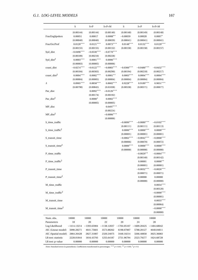
G.1. LOG-LEVEL MODELS 167

S S+P S+P+M S S+P S+P+M

(0.00144) (0.00144) (0.00140) (0.00148) (0.00149) (0.00148)

FracEngSpoken 0.00051 0.00017 0.0008∗∗ −0.00039 0.00028 0.0007∗

(0.00040) (0.00040) (0.00039) (0.00041) (0.00041) (0.00041)

FracOccProf 0.0120∗∗∗ 0.0121∗∗∗ 0.0073∗∗∗ 0.0148∗∗∗ 0.0132∗∗∗ 0.0120∗∗∗

(0.00155) (0.00155) (0.00152) (0.00158) (0.00158) (0.00157)

Syd_dist −0.0496∗∗∗ −0.0530∗∗∗ −0.0770∗∗∗

(0.00189) (0.00210) (0.00228)

Syd_dist2 0.0003∗∗∗ 0.0001∗∗∗ 0.0006∗∗∗

(0.00003) (0.00005) (0.00006)

coast_dist −0.0274∗∗∗ −0.0122∗∗∗ −0.0083∗∗∗ −0.0360∗∗∗ −0.0480∗∗∗ −0.0432∗∗∗

(0.00184) (0.00303) (0.00290) (0.00194) (0.00218) (0.00217)

coast_dist2 0.0004∗∗∗ 0.0002∗∗∗ 0.0001∗∗ 0.0003∗∗∗ 0.0004∗∗∗ 0.0004∗∗∗

(0.00004) (0.00005) (0.00004) (0.00004) (0.00004) (0.00004)

λ 0.8905∗∗∗ 0.8858∗∗∗ 0.8602∗∗∗ 0.9228∗∗∗ 0.9189∗∗∗ 0.9051∗∗∗

(0.00790) (0.00845) (0.01038) (0.00538) (0.00571) (0.00677)

Par_dist 0.0092∗∗∗ −0.0126∗∗∗

(0.00174) (0.00192)

Par_dist2 0.0000∗ 0.0002∗∗∗

(0.00005) (0.00005)

MP_dist 0.0497∗∗∗

(0.00224)

MP_dist2 −0.0006∗∗∗

(0.00006)

S_time_traffic −0.0099∗∗∗ −0.0089∗∗∗ −0.0102∗∗∗

(0.00111) (0.00111) (0.00113)

S_time_traffic2 0.0000∗∗∗ 0.0000∗∗∗ 0.0000∗∗∗

(0.00001) (0.00001) (0.00001)

S_transit_time −0.0062∗∗∗ −0.0042∗∗∗ −0.0068∗∗∗

(0.00066) (0.00070) (0.00072)

S_transit_time2 0.0000∗∗∗ 0.0000∗∗∗ 0.0000∗∗∗

(0.00000) (0.00000) (0.00000)

P_time_traffic −0.0029∗∗ −0.0064∗∗∗

(0.00140) (0.00142)

P_time_traffic2 0.00001 0.0000∗∗

(0.00001) (0.00001)

P_transit_time −0.0032∗∗∗ −0.0026∗∗∗

(0.00071) (0.00071)

P_transit_time2 0.00000 0.00000

(0.00000) (0.00000)

M_time_traffic 0.0054∗∗∗

(0.00120)

M_time_traffic2 −0.0000∗∗∗

(0.00001)

M_transit_time 0.0055∗∗∗

(0.00064)

M_transit_time2 −0.0000∗∗∗

(0.00000)

Num. obs. 10000 10000 10000 10000 10000 10000

Parameters 18 20 22 20 24 28

Log Likelihood −1414.13214 −1393.65904 −1138.12037 −1704.05107 −1609.20425 −1484.68042

AIC (Linear model) 5090.28271 4641.75601 3573.88262 6198.07007 5788.20127 4648.04811

AIC (Spatial model) 2864.26428 2827.31807 2320.24075 3448.10214 3266.40850 3025.36083

LR test: statistic 2228.01844 1816.43793 1255.64187 2751.96794 2523.79277 1624.68728

LR test: p-value 0.00000 0.00000 0.00000 0.00000 0.00000 0.00000

Notes: Standard errors in parenthesis. Coefficients transformed to percentages. ∗∗∗p < 0.01; ∗∗p < 0.05; ∗p < 0.1

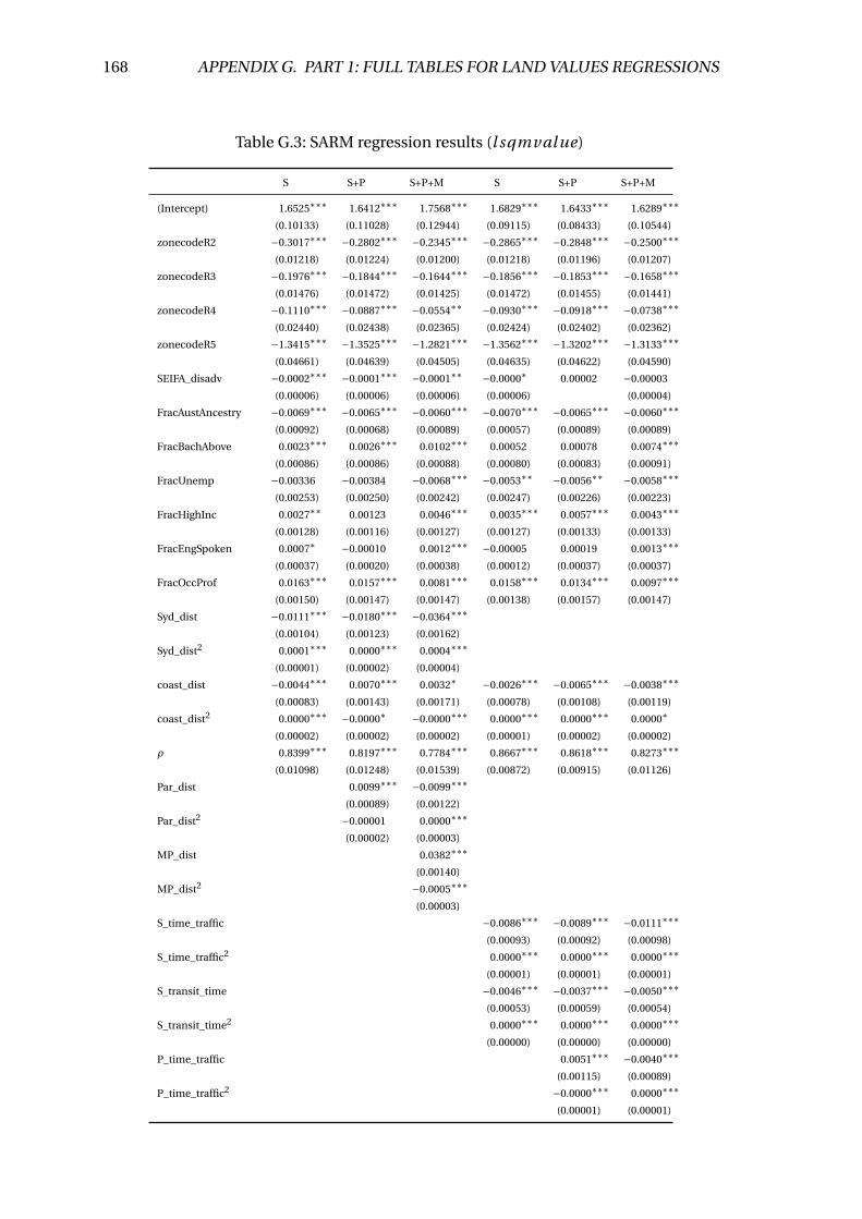
168 APPENDIX G. PART 1: FULL TABLES FOR LAND VALUES REGRESSIONS

Table G.3: SARM regression results (l sqmval ue)

S S+P S+P+M S S+P S+P+M

(Intercept) 1.6525∗∗∗ 1.6412∗∗∗ 1.7568∗∗∗ 1.6829∗∗∗ 1.6433∗∗∗ 1.6289∗∗∗

(0.10133) (0.11028) (0.12944) (0.09115) (0.08433) (0.10544)

zonecodeR2 −0.3017∗∗∗ −0.2802∗∗∗ −0.2345∗∗∗ −0.2865∗∗∗ −0.2848∗∗∗ −0.2500∗∗∗

(0.01218) (0.01224) (0.01200) (0.01218) (0.01196) (0.01207)

zonecodeR3 −0.1976∗∗∗ −0.1844∗∗∗ −0.1644∗∗∗ −0.1856∗∗∗ −0.1853∗∗∗ −0.1658∗∗∗

(0.01476) (0.01472) (0.01425) (0.01472) (0.01455) (0.01441)

zonecodeR4 −0.1110∗∗∗ −0.0887∗∗∗ −0.0554∗∗ −0.0930∗∗∗ −0.0918∗∗∗ −0.0738∗∗∗

(0.02440) (0.02438) (0.02365) (0.02424) (0.02402) (0.02362)

zonecodeR5 −1.3415∗∗∗ −1.3525∗∗∗ −1.2821∗∗∗ −1.3562∗∗∗ −1.3202∗∗∗ −1.3133∗∗∗

(0.04661) (0.04639) (0.04505) (0.04635) (0.04622) (0.04590)

SEIFA_disadv −0.0002∗∗∗ −0.0001∗∗∗ −0.0001∗∗ −0.0000∗ 0.00002 −0.00003

(0.00006) (0.00006) (0.00006) (0.00006) (0.00004)

FracAustAncestry −0.0069∗∗∗ −0.0065∗∗∗ −0.0060∗∗∗ −0.0070∗∗∗ −0.0065∗∗∗ −0.0060∗∗∗

(0.00092) (0.00068) (0.00089) (0.00057) (0.00089) (0.00089)

FracBachAbove 0.0023∗∗∗ 0.0026∗∗∗ 0.0102∗∗∗ 0.00052 0.00078 0.0074∗∗∗

(0.00086) (0.00086) (0.00088) (0.00080) (0.00083) (0.00091)

FracUnemp −0.00336 −0.00384 −0.0068∗∗∗ −0.0053∗∗ −0.0056∗∗ −0.0058∗∗∗

(0.00253) (0.00250) (0.00242) (0.00247) (0.00226) (0.00223)

FracHighInc 0.0027∗∗ 0.00123 0.0046∗∗∗ 0.0035∗∗∗ 0.0057∗∗∗ 0.0043∗∗∗

(0.00128) (0.00116) (0.00127) (0.00127) (0.00133) (0.00133)

FracEngSpoken 0.0007∗ −0.00010 0.0012∗∗∗ −0.00005 0.00019 0.0013∗∗∗

(0.00037) (0.00020) (0.00038) (0.00012) (0.00037) (0.00037)

FracOccProf 0.0163∗∗∗ 0.0157∗∗∗ 0.0081∗∗∗ 0.0158∗∗∗ 0.0134∗∗∗ 0.0097∗∗∗

(0.00150) (0.00147) (0.00147) (0.00138) (0.00157) (0.00147)

Syd_dist −0.0111∗∗∗ −0.0180∗∗∗ −0.0364∗∗∗

(0.00104) (0.00123) (0.00162)

Syd_dist2 0.0001∗∗∗ 0.0000∗∗∗ 0.0004∗∗∗

(0.00001) (0.00002) (0.00004)

coast_dist −0.0044∗∗∗ 0.0070∗∗∗ 0.0032∗ −0.0026∗∗∗ −0.0065∗∗∗ −0.0038∗∗∗

(0.00083) (0.00143) (0.00171) (0.00078) (0.00108) (0.00119)

coast_dist2 0.0000∗∗∗ −0.0000∗ −0.0000∗∗∗ 0.0000∗∗∗ 0.0000∗∗∗ 0.0000∗

(0.00002) (0.00002) (0.00002) (0.00001) (0.00002) (0.00002)

ρ 0.8399∗∗∗ 0.8197∗∗∗ 0.7784∗∗∗ 0.8667∗∗∗ 0.8618∗∗∗ 0.8273∗∗∗

(0.01098) (0.01248) (0.01539) (0.00872) (0.00915) (0.01126)

Par_dist 0.0099∗∗∗ −0.0099∗∗∗

(0.00089) (0.00122)

Par_dist2 −0.00001 0.0000∗∗∗

(0.00002) (0.00003)

MP_dist 0.0382∗∗∗

(0.00140)

MP_dist2 −0.0005∗∗∗

(0.00003)

S_time_traffic −0.0086∗∗∗ −0.0089∗∗∗ −0.0111∗∗∗

(0.00093) (0.00092) (0.00098)

S_time_traffic2 0.0000∗∗∗ 0.0000∗∗∗ 0.0000∗∗∗

(0.00001) (0.00001) (0.00001)

S_transit_time −0.0046∗∗∗ −0.0037∗∗∗ −0.0050∗∗∗

(0.00053) (0.00059) (0.00054)

S_transit_time2 0.0000∗∗∗ 0.0000∗∗∗ 0.0000∗∗∗

(0.00000) (0.00000) (0.00000)

P_time_traffic 0.0051∗∗∗ −0.0040∗∗∗

(0.00115) (0.00089)

P_time_traffic2 −0.0000∗∗∗ 0.0000∗∗∗

(0.00001) (0.00001)

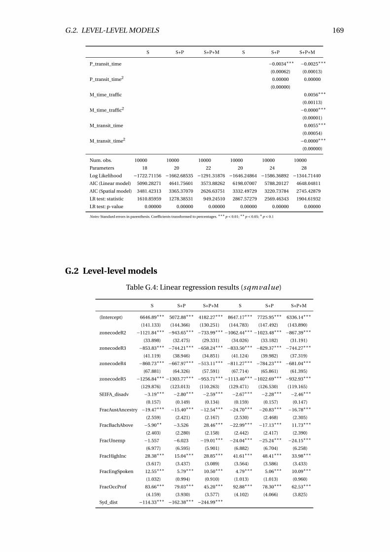
G.2. LEVEL-LEVEL MODELS 169

S S+P S+P+M S S+P S+P+M

P_transit_time −0.0034∗∗∗ −0.0025∗∗∗

(0.00062) (0.00013)

P_transit_time2 0.00000 0.00000

(0.00000)

M_time_traffic 0.0056∗∗∗

(0.00113)

M_time_traffic2 −0.0000∗∗∗

(0.00001)

M_transit_time 0.0055∗∗∗

(0.00054)

M_transit_time2 −0.0000∗∗∗

(0.00000)

Num. obs. 10000 10000 10000 10000 10000 10000

Parameters 18 20 22 20 24 28

Log Likelihood −1722.71156 −1662.68535 −1291.31876 −1646.24864 −1586.36892 −1344.71440

AIC (Linear model) 5090.28271 4641.75601 3573.88262 6198.07007 5788.20127 4648.04811

AIC (Spatial model) 3481.42313 3365.37070 2626.63751 3332.49729 3220.73784 2745.42879

LR test: statistic 1610.85959 1278.38531 949.24510 2867.57279 2569.46343 1904.61932

LR test: p-value 0.00000 0.00000 0.00000 0.00000 0.00000 0.00000

Notes: Standard errors in parenthesis. Coefficients transformed to percentages. ∗∗∗p < 0.01; ∗∗p < 0.05; ∗p < 0.1

G.2 Level-level models

Table G.4: Linear regression results (sqmval ue)

S S+P S+P+M S S+P S+P+M

(Intercept) 6646.89∗∗∗ 5072.88∗∗∗ 4182.27∗∗∗ 8647.17∗∗∗ 7725.95∗∗∗ 6336.14∗∗∗

(141.133) (144.366) (130.251) (144.783) (147.492) (143.890)

zonecodeR2 −1121.84∗∗∗ −943.65∗∗∗ −733.99∗∗∗ −1062.44∗∗∗ −1023.48∗∗∗ −867.39∗∗∗

(33.898) (32.475) (29.331) (34.026) (33.182) (31.191)

zonecodeR3 −853.83∗∗∗ −744.21∗∗∗ −658.24∗∗∗ −833.50∗∗∗ −829.37∗∗∗ −744.27∗∗∗

(41.119) (38.946) (34.851) (41.124) (39.982) (37.319)

zonecodeR4 −860.73∗∗∗ −667.97∗∗∗ −513.11∗∗∗ −811.27∗∗∗ −784.23∗∗∗ −681.04∗∗∗

(67.881) (64.326) (57.591) (67.714) (65.861) (61.395)

zonecodeR5 −1256.84∗∗∗ −1303.77∗∗∗ −953.71∗∗∗ −1113.40∗∗∗ −1022.69∗∗∗ −932.93∗∗∗

(129.876) (123.013) (110.263) (129.471) (126.530) (119.165)

SEIFA_disadv −3.19∗∗∗ −2.80∗∗∗ −2.59∗∗∗ −2.67∗∗∗ −2.28∗∗∗ −2.46∗∗∗

(0.157) (0.149) (0.134) (0.159) (0.157) (0.147)

FracAustAncestry −19.47∗∗∗ −15.40∗∗∗ −12.54∗∗∗ −24.70∗∗∗ −20.83∗∗∗ −16.78∗∗∗

(2.559) (2.421) (2.167) (2.530) (2.468) (2.305)

FracBachAbove −5.90∗∗ −3.526 28.46∗∗∗ −22.99∗∗∗ −17.13∗∗∗ 11.73∗∗∗

(2.403) (2.280) (2.158) (2.442) (2.417) (2.390)

FracUnemp −1.557 −6.023 −19.01∗∗∗ −24.04∗∗∗ −25.24∗∗∗ −24.15∗∗∗

(6.977) (6.595) (5.901) (6.882) (6.704) (6.258)

FracHighInc 28.38∗∗∗ 15.04∗∗∗ 28.85∗∗∗ 41.61∗∗∗ 48.41∗∗∗ 33.98∗∗∗

(3.617) (3.437) (3.089) (3.564) (3.586) (3.433)

FracEngSpoken 12.55∗∗∗ 5.79∗∗∗ 10.50∗∗∗ 4.79∗∗∗ 5.06∗∗∗ 10.09∗∗∗

(1.032) (0.994) (0.910) (1.013) (1.013) (0.960)

FracOccProf 83.66∗∗∗ 79.03∗∗∗ 45.20∗∗∗ 92.88∗∗∗ 78.30∗∗∗ 62.53∗∗∗

(4.159) (3.930) (3.577) (4.102) (4.066) (3.825)

Syd_dist −114.33∗∗∗ −162.38∗∗∗ −244.99∗∗∗

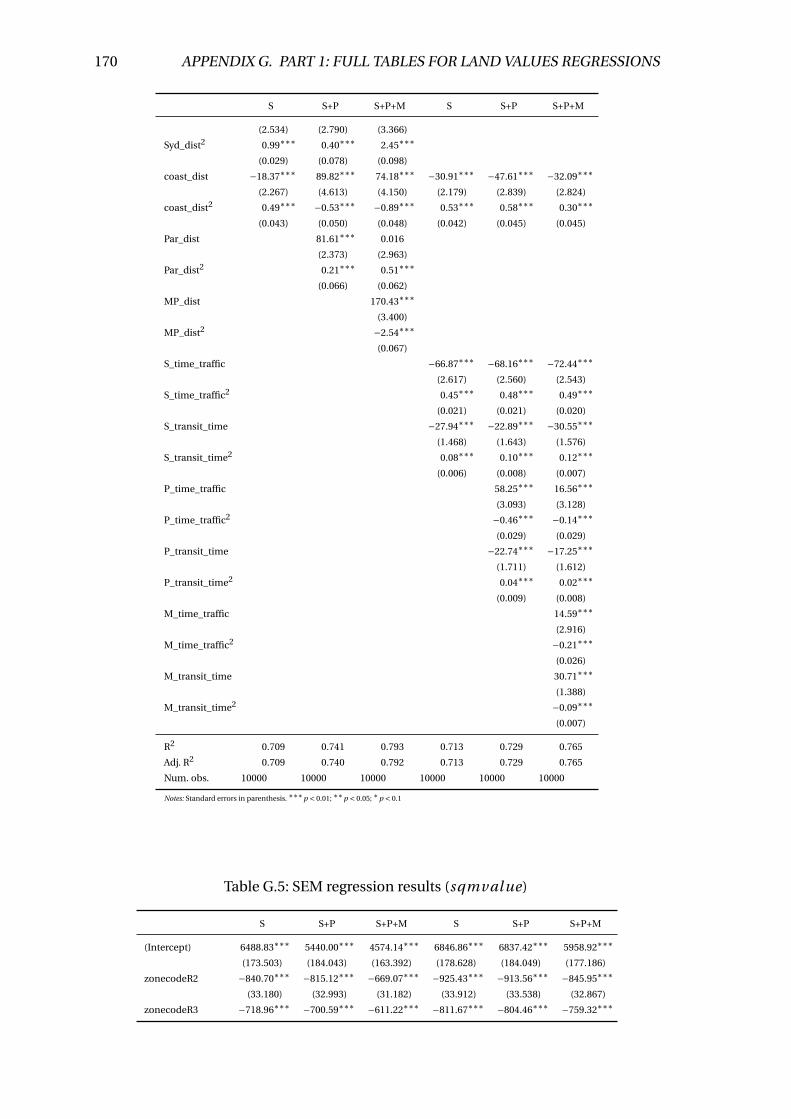
170 APPENDIX G. PART 1: FULL TABLES FOR LAND VALUES REGRESSIONS

S S+P S+P+M S S+P S+P+M

(2.534) (2.790) (3.366)

Syd_dist2 0.99∗∗∗ 0.40∗∗∗ 2.45∗∗∗

(0.029) (0.078) (0.098)

coast_dist −18.37∗∗∗ 89.82∗∗∗ 74.18∗∗∗ −30.91∗∗∗ −47.61∗∗∗ −32.09∗∗∗

(2.267) (4.613) (4.150) (2.179) (2.839) (2.824)

coast_dist2 0.49∗∗∗ −0.53∗∗∗ −0.89∗∗∗ 0.53∗∗∗ 0.58∗∗∗ 0.30∗∗∗

(0.043) (0.050) (0.048) (0.042) (0.045) (0.045)

Par_dist 81.61∗∗∗ 0.016

(2.373) (2.963)

Par_dist2 0.21∗∗∗ 0.51∗∗∗

(0.066) (0.062)

MP_dist 170.43∗∗∗

(3.400)

MP_dist2 −2.54∗∗∗

(0.067)

S_time_traffic −66.87∗∗∗ −68.16∗∗∗ −72.44∗∗∗

(2.617) (2.560) (2.543)

S_time_traffic2 0.45∗∗∗ 0.48∗∗∗ 0.49∗∗∗

(0.021) (0.021) (0.020)

S_transit_time −27.94∗∗∗ −22.89∗∗∗ −30.55∗∗∗

(1.468) (1.643) (1.576)

S_transit_time2 0.08∗∗∗ 0.10∗∗∗ 0.12∗∗∗

(0.006) (0.008) (0.007)

P_time_traffic 58.25∗∗∗ 16.56∗∗∗

(3.093) (3.128)

P_time_traffic2 −0.46∗∗∗ −0.14∗∗∗

(0.029) (0.029)

P_transit_time −22.74∗∗∗ −17.25∗∗∗

(1.711) (1.612)

P_transit_time2 0.04∗∗∗ 0.02∗∗∗

(0.009) (0.008)

M_time_traffic 14.59∗∗∗

(2.916)

M_time_traffic2 −0.21∗∗∗

(0.026)

M_transit_time 30.71∗∗∗

(1.388)

M_transit_time2 −0.09∗∗∗

(0.007)

R2 0.709 0.741 0.793 0.713 0.729 0.765

Adj. R2 0.709 0.740 0.792 0.713 0.729 0.765

Num. obs. 10000 10000 10000 10000 10000 10000

Notes: Standard errors in parenthesis. ∗∗∗p < 0.01; ∗∗p < 0.05; ∗p < 0.1

Table G.5: SEM regression results (sqmval ue)

S S+P S+P+M S S+P S+P+M

(Intercept) 6488.83∗∗∗ 5440.00∗∗∗ 4574.14∗∗∗ 6846.86∗∗∗ 6837.42∗∗∗ 5958.92∗∗∗

(173.503) (184.043) (163.392) (178.628) (184.049) (177.186)

zonecodeR2 −840.70∗∗∗ −815.12∗∗∗ −669.07∗∗∗ −925.43∗∗∗ −913.56∗∗∗ −845.95∗∗∗

(33.180) (32.993) (31.182) (33.912) (33.538) (32.867)

zonecodeR3 −718.96∗∗∗ −700.59∗∗∗ −611.22∗∗∗ −811.67∗∗∗ −804.46∗∗∗ −759.32∗∗∗

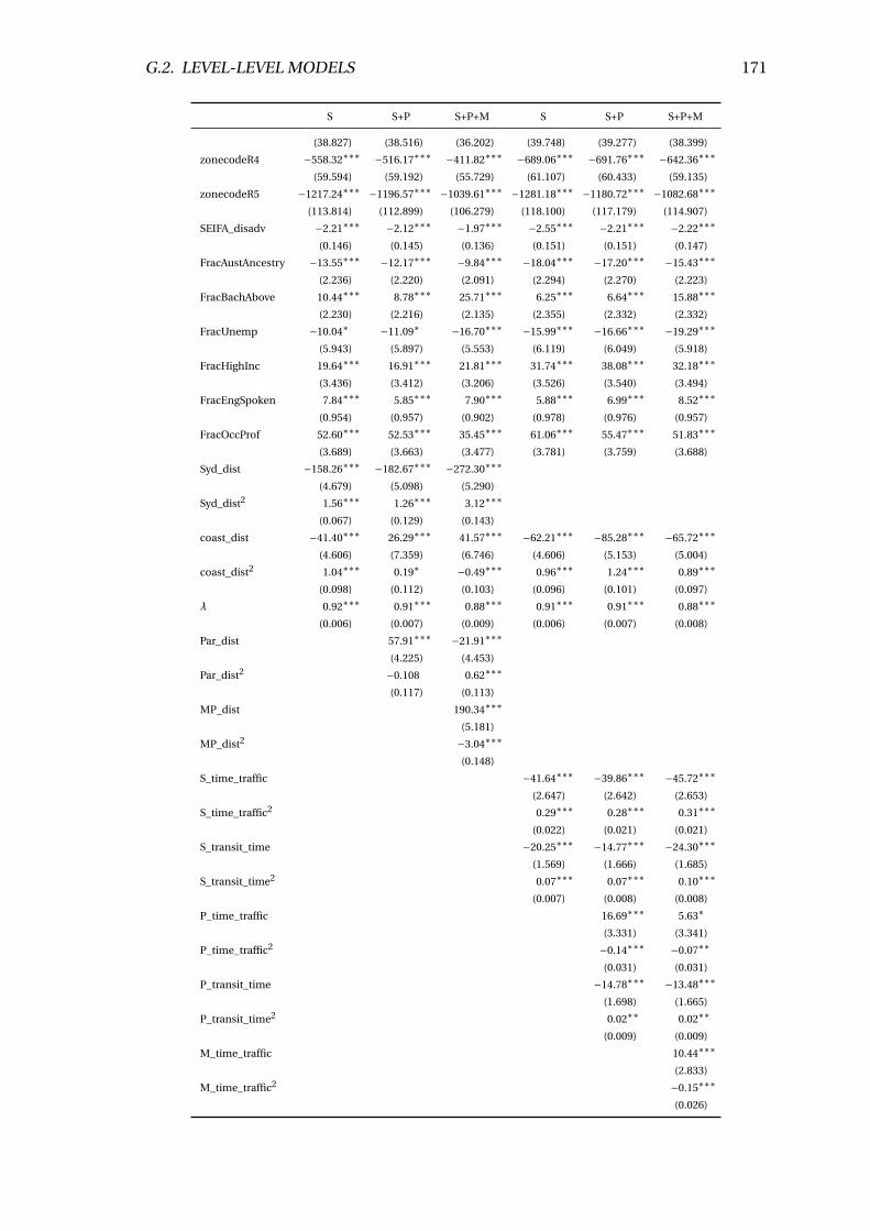
G.2. LEVEL-LEVEL MODELS 171

S S+P S+P+M S S+P S+P+M

(38.827) (38.516) (36.202) (39.748) (39.277) (38.399)

zonecodeR4 −558.32∗∗∗ −516.17∗∗∗ −411.82∗∗∗ −689.06∗∗∗ −691.76∗∗∗ −642.36∗∗∗

(59.594) (59.192) (55.729) (61.107) (60.433) (59.135)

zonecodeR5 −1217.24∗∗∗ −1196.57∗∗∗ −1039.61∗∗∗ −1281.18∗∗∗ −1180.72∗∗∗ −1082.68∗∗∗

(113.814) (112.899) (106.279) (118.100) (117.179) (114.907)

SEIFA_disadv −2.21∗∗∗ −2.12∗∗∗ −1.97∗∗∗ −2.55∗∗∗ −2.21∗∗∗ −2.22∗∗∗

(0.146) (0.145) (0.136) (0.151) (0.151) (0.147)

FracAustAncestry −13.55∗∗∗ −12.17∗∗∗ −9.84∗∗∗ −18.04∗∗∗ −17.20∗∗∗ −15.43∗∗∗

(2.236) (2.220) (2.091) (2.294) (2.270) (2.223)

FracBachAbove 10.44∗∗∗ 8.78∗∗∗ 25.71∗∗∗ 6.25∗∗∗ 6.64∗∗∗ 15.88∗∗∗

(2.230) (2.216) (2.135) (2.355) (2.332) (2.332)

FracUnemp −10.04∗ −11.09∗ −16.70∗∗∗ −15.99∗∗∗ −16.66∗∗∗ −19.29∗∗∗

(5.943) (5.897) (5.553) (6.119) (6.049) (5.918)

FracHighInc 19.64∗∗∗ 16.91∗∗∗ 21.81∗∗∗ 31.74∗∗∗ 38.08∗∗∗ 32.18∗∗∗

(3.436) (3.412) (3.206) (3.526) (3.540) (3.494)

FracEngSpoken 7.84∗∗∗ 5.85∗∗∗ 7.90∗∗∗ 5.88∗∗∗ 6.99∗∗∗ 8.52∗∗∗

(0.954) (0.957) (0.902) (0.978) (0.976) (0.957)

FracOccProf 52.60∗∗∗ 52.53∗∗∗ 35.45∗∗∗ 61.06∗∗∗ 55.47∗∗∗ 51.83∗∗∗

(3.689) (3.663) (3.477) (3.781) (3.759) (3.688)

Syd_dist −158.26∗∗∗ −182.67∗∗∗ −272.30∗∗∗

(4.679) (5.098) (5.290)

Syd_dist2 1.56∗∗∗ 1.26∗∗∗ 3.12∗∗∗

(0.067) (0.129) (0.143)

coast_dist −41.40∗∗∗ 26.29∗∗∗ 41.57∗∗∗ −62.21∗∗∗ −85.28∗∗∗ −65.72∗∗∗

(4.606) (7.359) (6.746) (4.606) (5.153) (5.004)

coast_dist2 1.04∗∗∗ 0.19∗ −0.49∗∗∗ 0.96∗∗∗ 1.24∗∗∗ 0.89∗∗∗

(0.098) (0.112) (0.103) (0.096) (0.101) (0.097)

λ 0.92∗∗∗ 0.91∗∗∗ 0.88∗∗∗ 0.91∗∗∗ 0.91∗∗∗ 0.88∗∗∗

(0.006) (0.007) (0.009) (0.006) (0.007) (0.008)

Par_dist 57.91∗∗∗ −21.91∗∗∗

(4.225) (4.453)

Par_dist2 −0.108 0.62∗∗∗

(0.117) (0.113)

MP_dist 190.34∗∗∗

(5.181)

MP_dist2 −3.04∗∗∗

(0.148)

S_time_traffic −41.64∗∗∗ −39.86∗∗∗ −45.72∗∗∗

(2.647) (2.642) (2.653)

S_time_traffic2 0.29∗∗∗ 0.28∗∗∗ 0.31∗∗∗

(0.022) (0.021) (0.021)

S_transit_time −20.25∗∗∗ −14.77∗∗∗ −24.30∗∗∗

(1.569) (1.666) (1.685)

S_transit_time2 0.07∗∗∗ 0.07∗∗∗ 0.10∗∗∗

(0.007) (0.008) (0.008)

P_time_traffic 16.69∗∗∗ 5.63∗

(3.331) (3.341)

P_time_traffic2 −0.14∗∗∗ −0.07∗∗

(0.031) (0.031)

P_transit_time −14.78∗∗∗ −13.48∗∗∗

(1.698) (1.665)

P_transit_time2 0.02∗∗ 0.02∗∗

(0.009) (0.009)

M_time_traffic 10.44∗∗∗

(2.833)

M_time_traffic2 −0.15∗∗∗

(0.026)

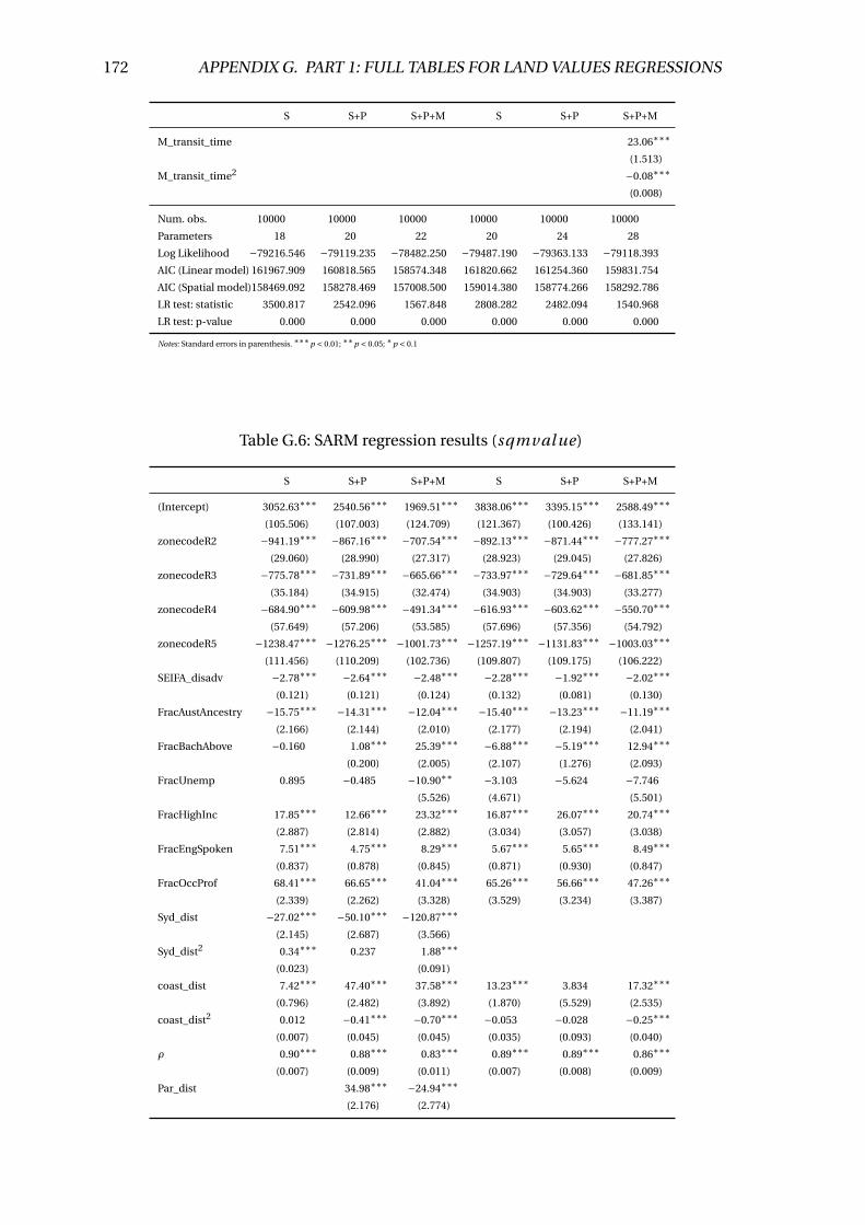
172 APPENDIX G. PART 1: FULL TABLES FOR LAND VALUES REGRESSIONS

S S+P S+P+M S S+P S+P+M

M_transit_time 23.06∗∗∗

(1.513)

M_transit_time2 −0.08∗∗∗

(0.008)

Num. obs. 10000 10000 10000 10000 10000 10000

Parameters 18 20 22 20 24 28

Log Likelihood −79216.546 −79119.235 −78482.250 −79487.190 −79363.133 −79118.393

AIC (Linear model) 161967.909 160818.565 158574.348 161820.662 161254.360 159831.754

AIC (Spatial model)158469.092 158278.469 157008.500 159014.380 158774.266 158292.786

LR test: statistic 3500.817 2542.096 1567.848 2808.282 2482.094 1540.968

LR test: p-value 0.000 0.000 0.000 0.000 0.000 0.000

Notes: Standard errors in parenthesis. ∗∗∗p < 0.01; ∗∗p < 0.05; ∗p < 0.1

Table G.6: SARM regression results (sqmval ue)

S S+P S+P+M S S+P S+P+M

(Intercept) 3052.63∗∗∗ 2540.56∗∗∗ 1969.51∗∗∗ 3838.06∗∗∗ 3395.15∗∗∗ 2588.49∗∗∗

(105.506) (107.003) (124.709) (121.367) (100.426) (133.141)

zonecodeR2 −941.19∗∗∗ −867.16∗∗∗ −707.54∗∗∗ −892.13∗∗∗ −871.44∗∗∗ −777.27∗∗∗

(29.060) (28.990) (27.317) (28.923) (29.045) (27.826)

zonecodeR3 −775.78∗∗∗ −731.89∗∗∗ −665.66∗∗∗ −733.97∗∗∗ −729.64∗∗∗ −681.85∗∗∗

(35.184) (34.915) (32.474) (34.903) (34.903) (33.277)

zonecodeR4 −684.90∗∗∗ −609.98∗∗∗ −491.34∗∗∗ −616.93∗∗∗ −603.62∗∗∗ −550.70∗∗∗

(57.649) (57.206) (53.585) (57.696) (57.356) (54.792)

zonecodeR5 −1238.47∗∗∗ −1276.25∗∗∗ −1001.73∗∗∗ −1257.19∗∗∗ −1131.83∗∗∗ −1003.03∗∗∗

(111.456) (110.209) (102.736) (109.807) (109.175) (106.222)

SEIFA_disadv −2.78∗∗∗ −2.64∗∗∗ −2.48∗∗∗ −2.28∗∗∗ −1.92∗∗∗ −2.02∗∗∗

(0.121) (0.121) (0.124) (0.132) (0.081) (0.130)

FracAustAncestry −15.75∗∗∗ −14.31∗∗∗ −12.04∗∗∗ −15.40∗∗∗ −13.23∗∗∗ −11.19∗∗∗

(2.166) (2.144) (2.010) (2.177) (2.194) (2.041)

FracBachAbove −0.160 1.08∗∗∗ 25.39∗∗∗ −6.88∗∗∗ −5.19∗∗∗ 12.94∗∗∗

(0.200) (2.005) (2.107) (1.276) (2.093)

FracUnemp 0.895 −0.485 −10.90∗∗ −3.103 −5.624 −7.746

(5.526) (4.671) (5.501)

FracHighInc 17.85∗∗∗ 12.66∗∗∗ 23.32∗∗∗ 16.87∗∗∗ 26.07∗∗∗ 20.74∗∗∗

(2.887) (2.814) (2.882) (3.034) (3.057) (3.038)

FracEngSpoken 7.51∗∗∗ 4.75∗∗∗ 8.29∗∗∗ 5.67∗∗∗ 5.65∗∗∗ 8.49∗∗∗

(0.837) (0.878) (0.845) (0.871) (0.930) (0.847)

FracOccProf 68.41∗∗∗ 66.65∗∗∗ 41.04∗∗∗ 65.26∗∗∗ 56.66∗∗∗ 47.26∗∗∗

(2.339) (2.262) (3.328) (3.529) (3.234) (3.387)

Syd_dist −27.02∗∗∗ −50.10∗∗∗ −120.87∗∗∗

(2.145) (2.687) (3.566)

Syd_dist2 0.34∗∗∗ 0.237 1.88∗∗∗

(0.023) (0.091)

coast_dist 7.42∗∗∗ 47.40∗∗∗ 37.58∗∗∗ 13.23∗∗∗ 3.834 17.32∗∗∗

(0.796) (2.482) (3.892) (1.870) (5.529) (2.535)

coast_dist2 0.012 −0.41∗∗∗ −0.70∗∗∗ −0.053 −0.028 −0.25∗∗∗

(0.007) (0.045) (0.045) (0.035) (0.093) (0.040)

ρ 0.90∗∗∗ 0.88∗∗∗ 0.83∗∗∗ 0.89∗∗∗ 0.89∗∗∗ 0.86∗∗∗

(0.007) (0.009) (0.011) (0.007) (0.008) (0.009)

Par_dist 34.98∗∗∗ −24.94∗∗∗

(2.176) (2.774)

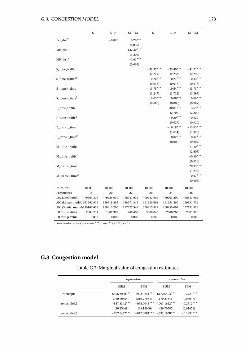
G.3. CONGESTION MODEL 173

S S+P S+P+M S S+P S+P+M

Par_dist2 −0.028 0.20∗∗∗

(0.057)

MP_dist 132.30∗∗∗

(3.209)

MP_dist2 −2.01∗∗∗

(0.063)

S_time_traffic −32.37∗∗∗ −33.40∗∗∗ −41.71∗∗∗

(2.227) (2.233) (2.292)

S_time_traffic2 0.26∗∗∗ 0.27∗∗∗ 0.32∗∗∗

(0.018) (0.018) (0.018)

S_transit_time −13.75∗∗∗ −10.54∗∗∗ −15.73∗∗∗

(1.247) (1.718) (1.397)

S_transit_time2 0.05∗∗∗ 0.06∗∗∗ 0.08∗∗∗

(0.005) (0.008) (0.007)

P_time_traffic 30.81∗∗∗ 5.69∗∗∗

(2.708) (2.200)

P_time_traffic2 −0.20∗∗∗ −0.027

(0.027) (0.020)

P_transit_time −16.18∗∗∗ −13.03∗∗∗

(1.614) (1.320)

P_transit_time2 0.02∗∗∗ 0.02∗∗∗

(0.008) (0.007)

M_time_traffic 11.10∗∗∗

(2.605)

M_time_traffic2 −0.10∗∗∗

(0.023)

M_transit_time 20.95∗∗∗

(1.233)

M_transit_time2 −0.07∗∗∗

(0.006)

Num. obs. 10000 10000 10000 10000 10000 10000

Parameters 18 20 22 20 24 28

Log Likelihood −79565.339 −79436.630 −78641.974 −79387.909 −79203.800 −78847.964

AIC (Linear model) 161967.909 160818.565 158574.348 161820.662 161254.360 159831.754

AIC (Spatial model)159166.678 158913.260 157327.948 158815.817 158455.601 157751.929

LR test: statistic 2803.231 1907.305 1248.400 3006.845 2800.760 2081.826

LR test: p-value 0.000 0.000 0.000 0.000 0.000 0.000

Notes: Standard errors in parenthesis. ∗∗∗p < 0.01; ∗∗p < 0.05; ∗p < 0.1

G.3 Congestion model

Table G.7: Marginal value of congestion estimates

sqmval ue l sqmval ue

SUM SEM SUM SEM

(Intercept) 6106.3920∗∗∗ 5923.3251∗∗∗ 6172.6403∗∗∗ 8.2723∗∗∗

(180.79654) (216.77054) (179.87341) (0.08047)

zonecodeR2 −857.8342∗∗∗ −965.0045∗∗∗ −1001.1622∗∗∗ −0.2612∗∗∗

(36.35448) (39.18906) (36.70585) (0.01451)

zonecodeR3 −767.0457∗∗∗ −877.0884∗∗∗ −891.1958∗∗∗ −0.1933∗∗∗

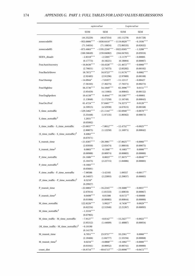
174 APPENDIX G. PART 1: FULL TABLES FOR LAND VALUES REGRESSIONS

sqmval ue l sqmval ue

SUM SEM SUM SEM

(44.35229) (46.67354) (45.11278) (0.01728)

zonecodeR4 −953.0006∗∗∗ −1030.6410∗∗∗ −1119.0020∗∗∗ −0.1936∗∗∗

(71.54034) (71.10834) (72.86535) (0.02632)

zonecodeR5 −873.4663∗∗∗ −1195.2240∗∗∗ −1022.0505∗∗∗ −1.5288∗∗∗

(160.56649) (159.84082) (164.04765) (0.05916)

SEIFA_disadv −2.8318∗∗∗ −2.5305∗∗∗ −3.1179∗∗∗ −0.00005

(0.17773) (0.18221) (0.18004) (0.00007)

FracAustAncestry −16.8436∗∗∗ −18.4528∗∗∗ −21.4672∗∗∗ −0.0060∗∗∗

(2.76651) (2.74375) (2.83282) (0.00102)

FracBachAbove 18.7872∗∗∗ 16.9723∗∗∗ 11.9176∗∗∗ 0.0082∗∗∗

(2.92483) (2.91296) (2.97089) (0.00108)

FracUnemp −14.0944∗ −7.01077 −11.12117 −0.00427

(7.56165) (7.36275) (7.76371) (0.00273)

FracHighInc 56.3736∗∗∗ 54.1849∗∗∗ 65.3996∗∗∗ 0.0151∗∗∗

(3.95459) (4.11003) (4.00845) (0.00152)

FracEngSpoken 10.4158∗∗∗ 8.4044∗∗∗ 10.5387∗∗∗ −0.00001

(1.13848) (1.17250) (1.16749) (0.00043)

FracOccProf 61.4724∗∗∗ 57.8467∗∗∗ 74.3273∗∗∗ 0.0120∗∗∗

(4.59915) (4.52930) (4.67615) (0.00168)

S_time_notraffic −129.5462∗∗∗ −21.1144∗∗∗ −32.6940∗∗∗ −0.0070∗∗∗

(5.35448) (1.97135) (1.80562) (0.00073)

S_time_notraffic2 1.2031∗∗∗

(0.05992)

S_time_traffic - S_time_notraffic −23.0037∗∗∗ −7.8012∗∗∗ −12.4752∗∗∗ −0.0025∗∗∗

(2.80875) (1.12250) (1.16971) (0.00042)

(S_time_traffic - S_time_notraffic)2 0.4062∗∗∗

(0.07071)

S_transit_time −21.6307∗∗∗ −28.3981∗∗∗ −37.8625∗∗∗ −0.0066∗∗∗

(2.03930) (2.03474) (1.88010) (0.00075)

S_transit_time2 0.0803∗∗∗ 0.1368∗∗∗ 0.1683∗∗∗ 0.0000∗∗∗

(0.00988) (0.00974) (0.00883) (0.00000)

P_time_notraffic 24.1686∗∗∗ 8.0023∗∗∗ 17.3675∗∗∗ −0.0040∗∗∗

(5.10475) (2.22715) (1.84886) (0.00083)

P_time_notraffic2 −0.1602∗∗∗

(0.05681)

P_time_traffic - P_time_notraffic −7.98586 −3.42105 1.09557 −0.0017∗∗

(6.34837) (2.22893) (2.29837) (0.00083)

(P_time_traffic - P_time_notraffic)2 0.5210∗

(0.29927)

P_transit_time −22.6804∗∗∗ −16.2245∗∗∗ −19.5680∗∗∗ −0.0037∗∗∗

(2.07814) (1.81533) (1.60810) (0.00067)

P_transit_time2 0.0498∗∗∗ 0.01308 0.0172∗∗ −0.00000

(0.01066) (0.00985) (0.00844) (0.00000)

M_time_notraffic 122.8226∗∗∗ 5.9923∗∗ 6.7430∗∗∗ 0.0029∗∗∗

(6.62234) (2.51946) (2.21267) (0.00093)

M_time_notraffic2 −1.5316∗∗∗

(0.07965)

M_time_traffic - M_time_notraffic −7.9127∗∗ −8.8142∗∗∗ −15.2427∗∗∗ −0.0022∗∗∗

(3.95312) (1.44609) (1.48887) (0.00054)

(M_time_traffic - M_time_notraffic)2 −0.10190

(0.14179)

M_transit_time 6.7051∗∗∗ 23.9757∗∗∗ 33.2361∗∗∗ 0.0060∗∗∗

(2.18466) (1.84777) (1.53194) (0.00068)

M_transit_time2 0.0234∗∗ −0.0868∗∗∗ −0.1002∗∗∗ −0.0000∗∗∗

(0.01041) (0.00952) (0.00741) (0.00000)

coast_dist −16.9754∗∗∗ −69.6713∗∗∗ −23.0098∗∗∗ −0.0472∗∗∗

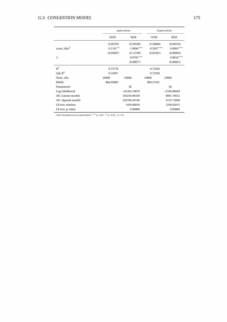
G.3. CONGESTION MODEL 175

sqmval ue l sqmval ue

SUM SEM SUM SEM

(3.66702) (6.28338) (3.40606) (0.00233)

coast_dist2 0.1191∗∗ 1.0696∗∗∗ 0.2957∗∗∗ 0.0005∗∗∗

(0.05807) (0.12190) (0.05501) (0.00005)

λ 0.8795∗∗∗ 0.8816∗∗∗

(0.00877) (0.00841)

R2 0.73778 0.72305

Adj. R2 0.73697 0.72236

Num. obs. 10000 10000 10000 10000

RMSE 866.82883 890.57421

Parameters 28 28

Log Likelihood −81365.19870 −2349.86049

AIC (Linear model) 164244.06558 6001.76012

AIC (Spatial model) 162786.39740 4755.72098

LR test: statistic 1459.66818 1248.03915

LR test: p-value 0.00000 0.00000

Notes: Standard errors in parenthesis. ∗∗∗p < 0.01, ∗∗p < 0.05, ∗p < 0.1

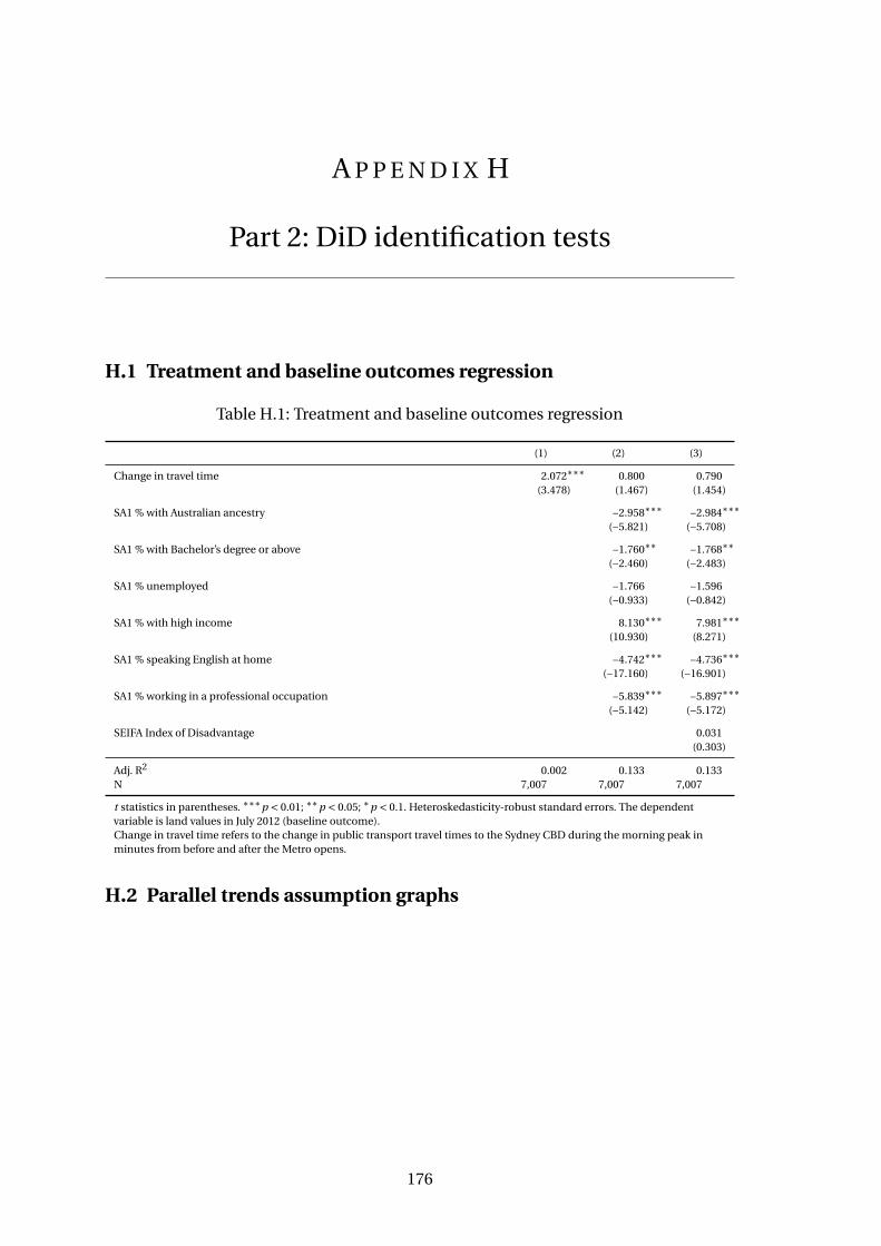
A P P E N D I X H

Part 2: DiD identification tests

H.1 Treatment and baseline outcomes regression

Table H.1: Treatment and baseline outcomes regression

(1) (2) (3)

Change in travel time 2.072∗∗∗ 0.800 0.790(3.478) (1.467) (1.454)

SA1 % with Australian ancestry −2.958∗∗∗ −2.984∗∗∗(−5.821) (−5.708)

SA1 % with Bachelor’s degree or above −1.760∗∗ −1.768∗∗(−2.460) (−2.483)

SA1 % unemployed −1.766 −1.596(−0.933) (−0.842)

SA1 % with high income 8.130∗∗∗ 7.981∗∗∗(10.930) (8.271)

SA1 % speaking English at home −4.742∗∗∗ −4.736∗∗∗(−17.160) (−16.901)

SA1 % working in a professional occupation −5.839∗∗∗ −5.897∗∗∗(−5.142) (−5.172)

SEIFA Index of Disadvantage 0.031(0.303)

Adj. R2 0.002 0.133 0.133N 7,007 7,007 7,007

t statistics in parentheses. ∗∗∗p < 0.01; ∗∗p < 0.05; ∗p < 0.1. Heteroskedasticity-robust standard errors. The dependentvariable is land values in July 2012 (baseline outcome).Change in travel time refers to the change in public transport travel times to the Sydney CBD during the morning peak inminutes from before and after the Metro opens.

H.2 Parallel trends assumption graphs

176

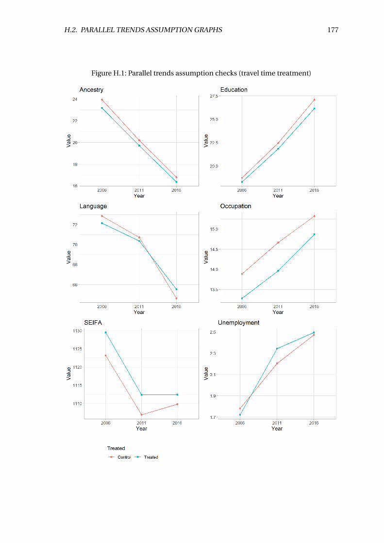
H.2. PARALLEL TRENDS ASSUMPTION GRAPHS 177

Figure H.1: Parallel trends assumption checks (travel time treatment)

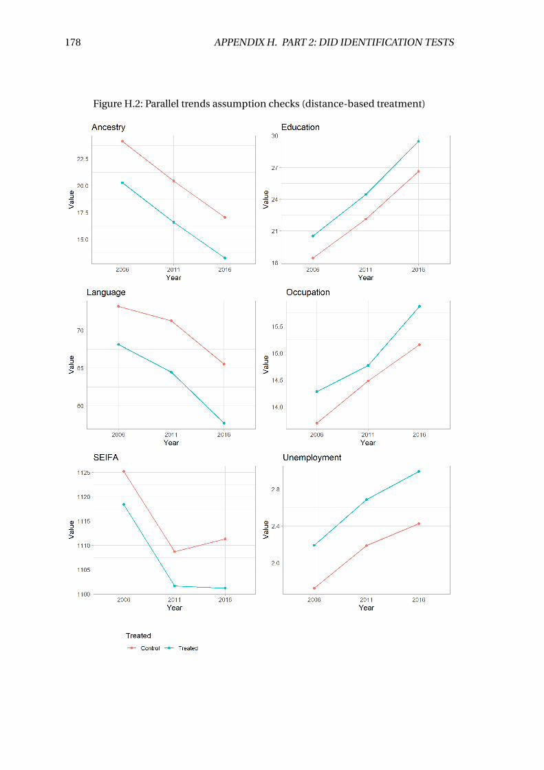
178 APPENDIX H. PART 2: DID IDENTIFICATION TESTS

Figure H.2: Parallel trends assumption checks (distance-based treatment)

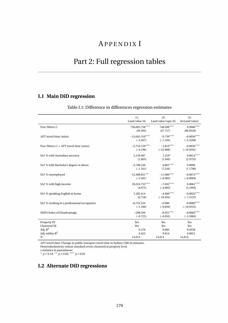
A P P E N D I X I

Part 2: Full regression tables

I.1 Main DiD regression

Table I.1: Difference in differences regression estimates

(1) (2) (3)Land value ($) Land value/sqm ($) ln(Land value)

Post-Metro=1 756,605.758∗∗∗ 748.698∗∗∗ 0.9686∗∗∗(20.303) (47.717) (86.8326)

∆PT travel time (mins) −15,045.319∗∗∗ −9.739∗∗∗ −0.0050∗∗∗(−3.267) (−7.184) (−4.5268)

Post-Metro=1 × ∆PT travel time (mins) −2,754.159∗∗∗ −3.810∗∗∗ −0.0036∗∗∗(−4.196) (−22.968) (−19.9391)

SA1 % with Australian ancestry 2,159.907 1.219∗ 0.0014∗∗∗(1.605) (1.949) (2.9755)

SA1 % with Bachelor’s degree or above −3,798.220 6.801∗∗∗ 0.0009(−1.161) (7.244) (1.1796)

SA1 % unemployed −12,488.851∗∗ −11.006∗∗∗ −0.0073∗∗∗(−2.401) (−6.983) (−6.0084)

SA1 % with high income 18,224.753∗∗∗ −7.032∗∗∗ 0.0061∗∗∗(4.075) (−4.893) (5.1093)

SA1 % speaking English at home 1,182.414 −4.666∗∗∗ −0.0022∗∗∗(0.718) (−10.954) (−7.5125)

SA1 % working in a professional occupation −6,724.554 −0.980 −0.0089∗∗∗(−1.180) (−0.850) (−10.9335)

SEIFA Index of Disadvantage −298.504 −0.951∗∗∗ −0.0003∗∗∗(−0.723) (−6.933) (−3.5904)

Property FE Yes Yes YesClustered SE Yes Yes YesAdj. R2 0.576 0.884 0.9558Adj. within R2 0.422 0.914 0.9651N 14,014 14,014 14,014

∆PT travel time: Change in public transport travel time to Sydney CBD in minutes.Heteroskedasticity-robust standard errors clustered at property level.t statistics in parentheses∗ p < 0.10, ∗∗ p < 0.05, ∗∗∗ p < 0.01

I.2 Alternate DiD regressions

179

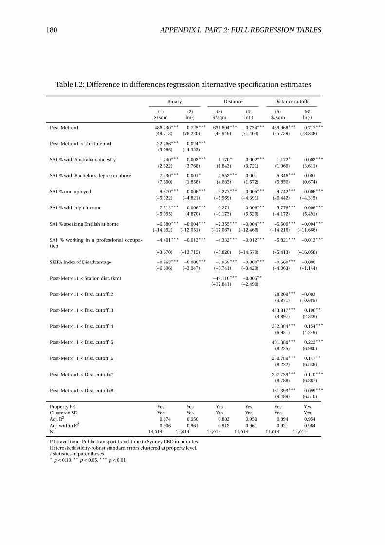
180 APPENDIX I. PART 2: FULL REGRESSION TABLES

Table I.2: Difference in differences regression alternative specification estimates

Binary Distance Distance cutoffs

(1) (2) (3) (4) (5) (6)$/sqm ln(·) $/sqm ln(·) $/sqm ln(·)

Post-Metro=1 486.230∗∗∗ 0.725∗∗∗ 631.894∗∗∗ 0.734∗∗∗ 489.968∗∗∗ 0.717∗∗∗(49.713) (78.220) (46.949) (71.404) (55.739) (78.838)

Post-Metro=1 × Treatment=1 22.266∗∗∗ −0.024∗∗∗(3.086) (−4.323)

SA1 % with Australian ancestry 1.740∗∗∗ 0.002∗∗∗ 1.170∗ 0.002∗∗∗ 1.172∗ 0.002∗∗∗(2.622) (3.768) (1.843) (3.721) (1.960) (3.611)

SA1 % with Bachelor’s degree or above 7.430∗∗∗ 0.001∗ 4.552∗∗∗ 0.001 5.346∗∗∗ 0.001(7.600) (1.858) (4.683) (1.572) (5.856) (0.674)

SA1 % unemployed −9.370∗∗∗ −0.006∗∗∗ −9.277∗∗∗ −0.005∗∗∗ −9.742∗∗∗ −0.006∗∗∗(−5.922) (−4.821) (−5.969) (−4.391) (−6.442) (−4.315)

SA1 % with high income −7.512∗∗∗ 0.006∗∗∗ −0.271 0.006∗∗∗ −5.776∗∗∗ 0.006∗∗∗(−5.035) (4.870) (−0.173) (5.520) (−4.172) (5.491)

SA1 % speaking English at home −6.580∗∗∗ −0.004∗∗∗ −7.355∗∗∗ −0.004∗∗∗ −5.500∗∗∗ −0.004∗∗∗(−14.952) (−12.051) (−17.067) (−12.466) (−14.216) (−11.666)

SA1 % working in a professional occupa-tion

−4.401∗∗∗ −0.012∗∗∗ −4.332∗∗∗ −0.012∗∗∗ −5.821∗∗∗ −0.013∗∗∗

(−3.670) (−13.715) (−3.820) (−14.579) (−5.413) (−16.058)

SEIFA Index of Disadvantage −0.963∗∗∗ −0.000∗∗∗ −0.959∗∗∗ −0.000∗∗∗ −0.560∗∗∗ −0.000(−6.696) (−3.947) (−6.741) (−3.429) (−4.063) (−1.144)

Post-Metro=1 × Station dist. (km) −49.116∗∗∗ −0.005∗∗(−17.841) (−2.490)

Post-Metro=1 × Dist. cutoff=2 28.209∗∗∗ −0.003(4.871) (−0.685)

Post-Metro=1 × Dist. cutoff=3 433.817∗∗∗ 0.196∗∗(3.897) (2.339)

Post-Metro=1 × Dist. cutoff=4 352.384∗∗∗ 0.154∗∗∗(6.931) (4.249)

Post-Metro=1 × Dist. cutoff=5 401.380∗∗∗ 0.222∗∗∗(8.225) (6.980)

Post-Metro=1 × Dist. cutoff=6 250.789∗∗∗ 0.147∗∗∗(8.222) (6.538)

Post-Metro=1 × Dist. cutoff=7 207.739∗∗∗ 0.110∗∗∗(8.788) (6.887)

Post-Metro=1 × Dist. cutoff=8 181.393∗∗∗ 0.099∗∗∗(9.489) (6.510)

Property FE Yes Yes Yes Yes Yes YesClustered SE Yes Yes Yes Yes Yes YesAdj. R2 0.874 0.950 0.883 0.950 0.894 0.954Adj. within R2 0.906 0.961 0.912 0.961 0.921 0.964N 14,014 14,014 14,014 14,014 14,014 14,014

PT travel time: Public transport travel time to Sydney CBD in minutes.Heteroskedasticity-robust standard errors clustered at property level.t statistics in parentheses∗ p < 0.10, ∗∗ p < 0.05, ∗∗∗ p < 0.01

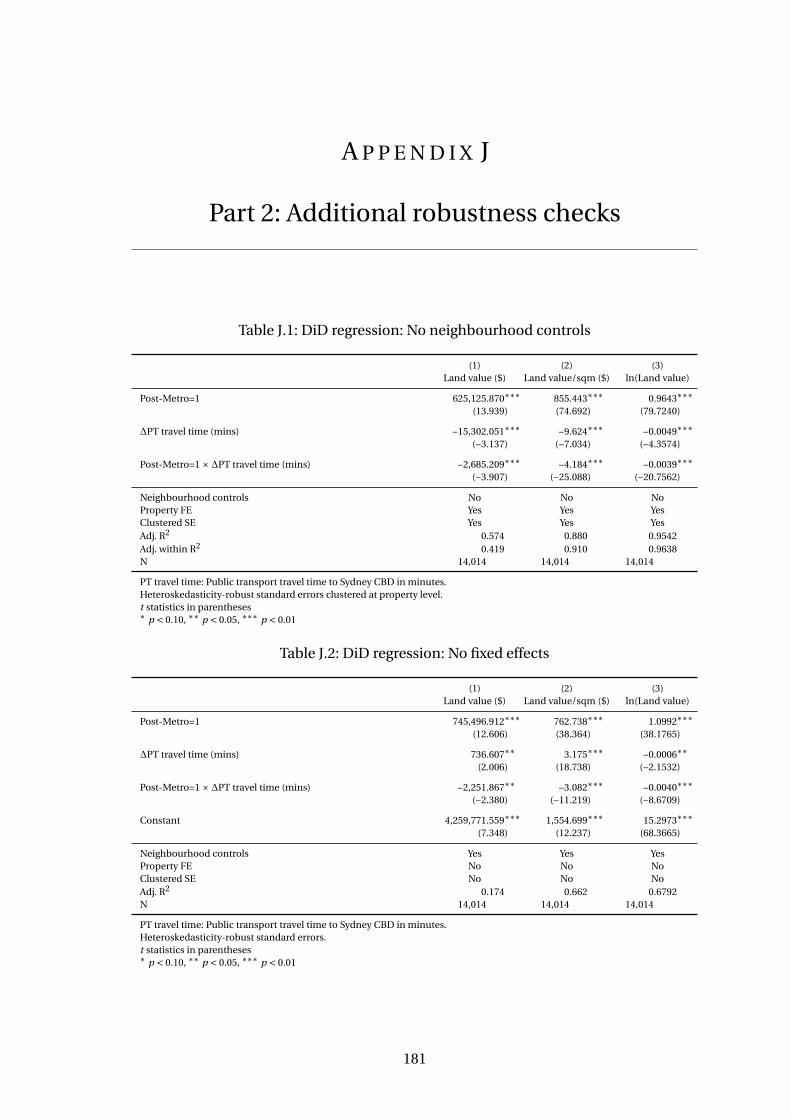
A P P E N D I X J

Part 2: Additional robustness checks

Table J.1: DiD regression: No neighbourhood controls

(1) (2) (3)Land value ($) Land value/sqm ($) ln(Land value)

Post-Metro=1 625,125.870∗∗∗ 855.443∗∗∗ 0.9643∗∗∗(13.939) (74.692) (79.7240)

∆PT travel time (mins) −15,302.051∗∗∗ −9.624∗∗∗ −0.0049∗∗∗(−3.137) (−7.034) (−4.3574)

Post-Metro=1 × ∆PT travel time (mins) −2,685.209∗∗∗ −4.184∗∗∗ −0.0039∗∗∗(−3.907) (−25.088) (−20.7562)

Neighbourhood controls No No NoProperty FE Yes Yes YesClustered SE Yes Yes YesAdj. R2 0.574 0.880 0.9542Adj. within R2 0.419 0.910 0.9638N 14,014 14,014 14,014

PT travel time: Public transport travel time to Sydney CBD in minutes.Heteroskedasticity-robust standard errors clustered at property level.t statistics in parentheses∗ p < 0.10, ∗∗ p < 0.05, ∗∗∗ p < 0.01

Table J.2: DiD regression: No fixed effects

(1) (2) (3)Land value ($) Land value/sqm ($) ln(Land value)

Post-Metro=1 745,496.912∗∗∗ 762.738∗∗∗ 1.0992∗∗∗(12.606) (38.364) (38.1765)

∆PT travel time (mins) 736.607∗∗ 3.175∗∗∗ −0.0006∗∗(2.006) (18.738) (−2.1532)

Post-Metro=1 × ∆PT travel time (mins) −2,251.867∗∗ −3.082∗∗∗ −0.0040∗∗∗(−2.380) (−11.219) (−8.6709)

Constant 4,259,771.559∗∗∗ 1,554.699∗∗∗ 15.2973∗∗∗(7.348) (12.237) (68.3665)

Neighbourhood controls Yes Yes YesProperty FE No No NoClustered SE No No NoAdj. R2 0.174 0.662 0.6792N 14,014 14,014 14,014

PT travel time: Public transport travel time to Sydney CBD in minutes.Heteroskedasticity-robust standard errors.t statistics in parentheses∗ p < 0.10, ∗∗ p < 0.05, ∗∗∗ p < 0.01

181

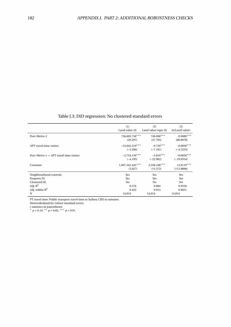
182 APPENDIX J. PART 2: ADDITIONAL ROBUSTNESS CHECKS

Table J.3: DiD regression: No clustered standard errors

(1) (2) (3)Land value ($) Land value/sqm ($) ln(Land value)

Post-Metro=1 756,605.758∗∗∗ 748.698∗∗∗ 0.9686∗∗∗(20.297) (47.704) (86.8078)

∆PT travel time (mins) −15,045.319∗∗∗ −9.739∗∗∗ −0.0050∗∗∗(−3.266) (−7.181) (−4.5255)

Post-Metro=1 × ∆PT travel time (mins) −2,754.159∗∗∗ −3.810∗∗∗ −0.0036∗∗∗(−4.195) (−22.962) (−19.9334)

Constant 1,697,342.445∗∗∗ 2,558.168∗∗∗ 13.8119∗∗∗(3.027) (14.372) (112.8898)

Neighbourhood controls Yes Yes YesProperty FE Yes Yes YesClustered SE No No NoAdj. R2 0.576 0.884 0.9558Adj. within R2 0.422 0.914 0.9651N 14,014 14,014 14,014

PT travel time: Public transport travel time to Sydney CBD in minutes.Heteroskedasticity-robust standard errors.t statistics in parentheses∗ p < 0.10, ∗∗ p < 0.05, ∗∗∗ p < 0.01

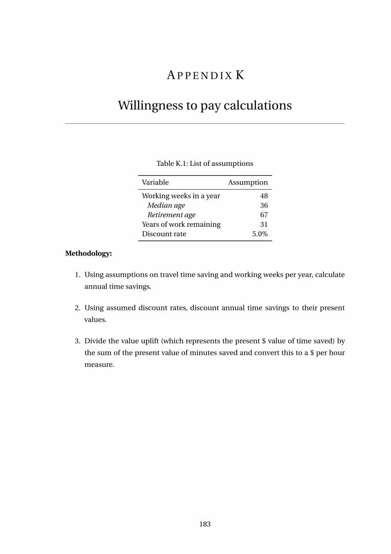
A P P E N D I X K

Willingness to pay calculations

Table K.1: List of assumptions

Variable Assumption

Working weeks in a year 48Median age 36Retirement age 67

Years of work remaining 31Discount rate 5.0%

Methodology:

1. Using assumptions on travel time saving and working weeks per year, calculate

annual time savings.

2. Using assumed discount rates, discount annual time savings to their present

values.

3. Divide the value uplift (which represents the present $ value of time saved) by

the sum of the present value of minutes saved and convert this to a $ per hour

measure.

183

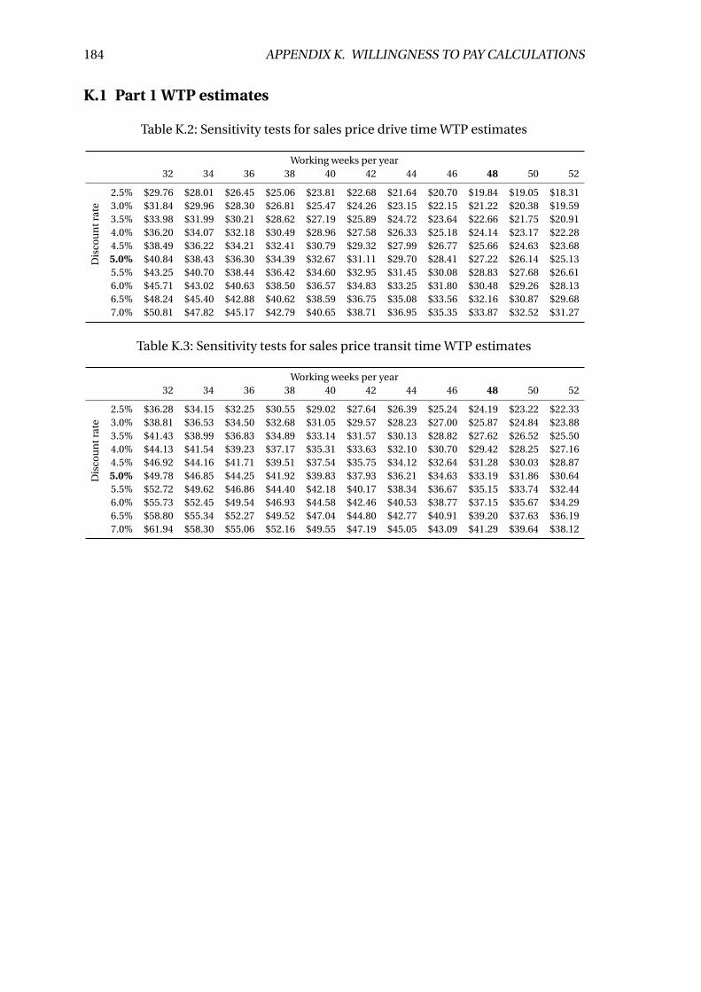
184 APPENDIX K. WILLINGNESS TO PAY CALCULATIONS

K.1 Part 1 WTP estimates

Table K.2: Sensitivity tests for sales price drive time WTP estimates

Working weeks per year

Dis

cou

ntr

ate

32 34 36 38 40 42 44 46 48 50 52

2.5% $29.76 $28.01 $26.45 $25.06 $23.81 $22.68 $21.64 $20.70 $19.84 $19.05 $18.313.0% $31.84 $29.96 $28.30 $26.81 $25.47 $24.26 $23.15 $22.15 $21.22 $20.38 $19.593.5% $33.98 $31.99 $30.21 $28.62 $27.19 $25.89 $24.72 $23.64 $22.66 $21.75 $20.914.0% $36.20 $34.07 $32.18 $30.49 $28.96 $27.58 $26.33 $25.18 $24.14 $23.17 $22.284.5% $38.49 $36.22 $34.21 $32.41 $30.79 $29.32 $27.99 $26.77 $25.66 $24.63 $23.685.0% $40.84 $38.43 $36.30 $34.39 $32.67 $31.11 $29.70 $28.41 $27.22 $26.14 $25.135.5% $43.25 $40.70 $38.44 $36.42 $34.60 $32.95 $31.45 $30.08 $28.83 $27.68 $26.616.0% $45.71 $43.02 $40.63 $38.50 $36.57 $34.83 $33.25 $31.80 $30.48 $29.26 $28.136.5% $48.24 $45.40 $42.88 $40.62 $38.59 $36.75 $35.08 $33.56 $32.16 $30.87 $29.687.0% $50.81 $47.82 $45.17 $42.79 $40.65 $38.71 $36.95 $35.35 $33.87 $32.52 $31.27

Table K.3: Sensitivity tests for sales price transit time WTP estimates

Working weeks per year

Dis

cou

ntr

ate

32 34 36 38 40 42 44 46 48 50 52

2.5% $36.28 $34.15 $32.25 $30.55 $29.02 $27.64 $26.39 $25.24 $24.19 $23.22 $22.333.0% $38.81 $36.53 $34.50 $32.68 $31.05 $29.57 $28.23 $27.00 $25.87 $24.84 $23.883.5% $41.43 $38.99 $36.83 $34.89 $33.14 $31.57 $30.13 $28.82 $27.62 $26.52 $25.504.0% $44.13 $41.54 $39.23 $37.17 $35.31 $33.63 $32.10 $30.70 $29.42 $28.25 $27.164.5% $46.92 $44.16 $41.71 $39.51 $37.54 $35.75 $34.12 $32.64 $31.28 $30.03 $28.875.0% $49.78 $46.85 $44.25 $41.92 $39.83 $37.93 $36.21 $34.63 $33.19 $31.86 $30.645.5% $52.72 $49.62 $46.86 $44.40 $42.18 $40.17 $38.34 $36.67 $35.15 $33.74 $32.446.0% $55.73 $52.45 $49.54 $46.93 $44.58 $42.46 $40.53 $38.77 $37.15 $35.67 $34.296.5% $58.80 $55.34 $52.27 $49.52 $47.04 $44.80 $42.77 $40.91 $39.20 $37.63 $36.197.0% $61.94 $58.30 $55.06 $52.16 $49.55 $47.19 $45.05 $43.09 $41.29 $39.64 $38.12

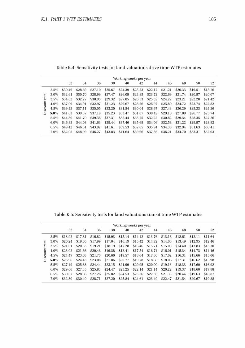
K.1. PART 1 WTP ESTIMATES 185

Table K.4: Sensitivity tests for land valuations drive time WTP estimates

Working weeks per year

Dis

cou

ntr

ate

32 34 36 38 40 42 44 46 48 50 52

2.5% $30.49 $28.69 $27.10 $25.67 $24.39 $23.23 $22.17 $21.21 $20.33 $19.51 $18.763.0% $32.61 $30.70 $28.99 $27.47 $26.09 $24.85 $23.72 $22.69 $21.74 $20.87 $20.073.5% $34.82 $32.77 $30.95 $29.32 $27.85 $26.53 $25.32 $24.22 $23.21 $22.28 $21.424.0% $37.09 $34.91 $32.97 $31.23 $29.67 $28.26 $26.97 $25.80 $24.72 $23.74 $22.824.5% $39.43 $37.11 $35.05 $33.20 $31.54 $30.04 $28.67 $27.43 $26.29 $25.23 $24.265.0% $41.83 $39.37 $37.19 $35.23 $33.47 $31.87 $30.42 $29.10 $27.89 $26.77 $25.745.5% $44.30 $41.70 $39.38 $37.31 $35.44 $33.75 $32.22 $30.82 $29.54 $28.35 $27.266.0% $46.83 $44.08 $41.63 $39.44 $37.46 $35.68 $34.06 $32.58 $31.22 $29.97 $28.826.5% $49.42 $46.51 $43.92 $41.61 $39.53 $37.65 $35.94 $34.38 $32.94 $31.63 $30.417.0% $52.05 $48.99 $46.27 $43.83 $41.64 $39.66 $37.86 $36.21 $34.70 $33.31 $32.03

Table K.5: Sensitivity tests for land valuations transit time WTP estimates

Working weeks per year

Dis

cou

ntr

ate

32 34 36 38 40 42 44 46 48 50 52

2.5% $18.92 $17.81 $16.82 $15.93 $15.14 $14.42 $13.76 $13.16 $12.61 $12.11 $11.643.0% $20.24 $19.05 $17.99 $17.04 $16.19 $15.42 $14.72 $14.08 $13.49 $12.95 $12.463.5% $21.61 $20.33 $19.21 $18.19 $17.28 $16.46 $15.71 $15.03 $14.40 $13.83 $13.304.0% $23.02 $21.66 $20.46 $19.38 $18.41 $17.54 $16.74 $16.01 $15.34 $14.73 $14.164.5% $24.47 $23.03 $21.75 $20.60 $19.57 $18.64 $17.80 $17.02 $16.31 $15.66 $15.065.0% $25.96 $24.43 $23.08 $21.86 $20.77 $19.78 $18.88 $18.06 $17.31 $16.62 $15.985.5% $27.49 $25.88 $24.44 $23.15 $21.99 $20.95 $20.00 $19.13 $18.33 $17.60 $16.926.0% $29.06 $27.35 $25.83 $24.47 $23.25 $22.14 $21.14 $20.22 $19.37 $18.60 $17.886.5% $30.67 $28.86 $27.26 $25.82 $24.53 $23.36 $22.30 $21.33 $20.44 $19.63 $18.877.0% $32.30 $30.40 $28.71 $27.20 $25.84 $24.61 $23.49 $22.47 $21.54 $20.67 $19.88

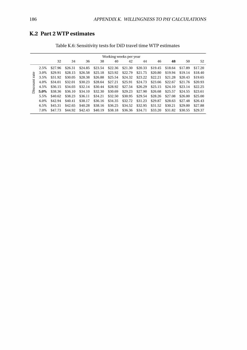
186 APPENDIX K. WILLINGNESS TO PAY CALCULATIONS

K.2 Part 2 WTP estimates

Table K.6: Sensitivity tests for DiD travel time WTP estimates

Working weeks per year

Dis

cou

ntr

ate

32 34 36 38 40 42 44 46 48 50 52

2.5% $27.96 $26.31 $24.85 $23.54 $22.36 $21.30 $20.33 $19.45 $18.64 $17.89 $17.203.0% $29.91 $28.15 $26.58 $25.18 $23.92 $22.79 $21.75 $20.80 $19.94 $19.14 $18.403.5% $31.92 $30.05 $28.38 $26.88 $25.54 $24.32 $23.22 $22.21 $21.28 $20.43 $19.654.0% $34.01 $32.01 $30.23 $28.64 $27.21 $25.91 $24.73 $23.66 $22.67 $21.76 $20.934.5% $36.15 $34.03 $32.14 $30.44 $28.92 $27.54 $26.29 $25.15 $24.10 $23.14 $22.255.0% $38.36 $36.10 $34.10 $32.30 $30.69 $29.23 $27.90 $26.68 $25.57 $24.55 $23.615.5% $40.62 $38.23 $36.11 $34.21 $32.50 $30.95 $29.54 $28.26 $27.08 $26.00 $25.006.0% $42.94 $40.41 $38.17 $36.16 $34.35 $32.72 $31.23 $29.87 $28.63 $27.48 $26.436.5% $45.31 $42.65 $40.28 $38.16 $36.25 $34.52 $32.95 $31.52 $30.21 $29.00 $27.887.0% $47.73 $44.92 $42.43 $40.19 $38.18 $36.36 $34.71 $33.20 $31.82 $30.55 $29.37