MOLECULAR

ROTATION-VIBRATION THEORY

Per Jensen

Physikalisch-Chemisches Institut,

Justus-Liebig-Universitat Giessen,

Heinrich-Buff-Ring 58,

D-35392 Giessen, Germany

and

Flemming Hegelund

Department of Chemistry,

Arhus University, Langelandsgade 140,

DK-8000 Arhus C, Denmark

Second Edition

Justus Liebig University Giessen

December 1993

This document was produced with LATEX on an IBMRISC/6000 340 Workstation. The notes are an extendedversion of a set of lecture notes entitled “Molekyldy-namik” by Per Jensen and Flemming Hegelund, used fora course taught at the Department of Chemistry, Univer-sity of Arhus, Denmark, in the spring of 1979.

Contents

1 Introduction 31.1 The Born-Oppenheimer approximation . . . . . . . . . . . . . . . . . 3

2 The choice of rotation-vibration coordinates 52.1 Translation . . . . . . . . . . . . . . . . . . . . . . . . . . . . . . . . 52.2 Rotation and vibration . . . . . . . . . . . . . . . . . . . . . . . . . . 82.3 The standard coordinates . . . . . . . . . . . . . . . . . . . . . . . . 112.4 The Eckart equations . . . . . . . . . . . . . . . . . . . . . . . . . . . 122.5 Normal coordinates . . . . . . . . . . . . . . . . . . . . . . . . . . . . 15

3 The expansion of the rotation-vibration Hamiltonian 203.1 The Watson Hamiltonian . . . . . . . . . . . . . . . . . . . . . . . . . 203.2 The expansion of the inverse inertial tensor . . . . . . . . . . . . . . . 213.3 The expansion of the potential energy function . . . . . . . . . . . . . 233.4 The expansion of the Hamiltonian . . . . . . . . . . . . . . . . . . . . 24

4 The calculation of the rotation-vibration energies 284.1 The Hamiltonian matrix . . . . . . . . . . . . . . . . . . . . . . . . . 284.2 The diatomic molecule . . . . . . . . . . . . . . . . . . . . . . . . . . 324.3 Perturbation theory . . . . . . . . . . . . . . . . . . . . . . . . . . . . 374.4 Contact transformations . . . . . . . . . . . . . . . . . . . . . . . . . 41

5 Molecular point groups 465.1 Generating operations . . . . . . . . . . . . . . . . . . . . . . . . . . 46

5.1.1 The groups CNv . . . . . . . . . . . . . . . . . . . . . . . . . . 475.1.2 The groups DNh and DNd . . . . . . . . . . . . . . . . . . . . 485.1.3 The groups D(N/2)d (N/2 even) . . . . . . . . . . . . . . . . . 515.1.4 The group C∞v . . . . . . . . . . . . . . . . . . . . . . . . . . 515.1.5 The group D∞h . . . . . . . . . . . . . . . . . . . . . . . . . . 52

1

6 Symmetries of operators 546.1 Symmetric tops and linear molecules . . . . . . . . . . . . . . . . . . 546.2 Products of oriented bases . . . . . . . . . . . . . . . . . . . . . . . . 586.3 Non-degenerate linear combinations of products with two or three

factors of degenerate oriented bases. . . . . . . . . . . . . . . . . . . . 63

7 The basis functions 677.1 Transformation properties . . . . . . . . . . . . . . . . . . . . . . . . 67

7.1.1 Type I (ϕ 6= 0 and ϕ 6= N2) . . . . . . . . . . . . . . . . . . . . 68

7.1.2 Type II (ϕ = 0 or ϕ = N2) . . . . . . . . . . . . . . . . . . . . 70

7.2 Selection rules . . . . . . . . . . . . . . . . . . . . . . . . . . . . . . . 707.2.1 Hamiltonian matrix elements . . . . . . . . . . . . . . . . . . 707.2.2 Transition moments . . . . . . . . . . . . . . . . . . . . . . . . 71

8 Resonances 758.1 Resonance classification . . . . . . . . . . . . . . . . . . . . . . . . . 758.2 Necessary resonances and doublings . . . . . . . . . . . . . . . . . . . 78

8.2.1 Diagonal matrix elements . . . . . . . . . . . . . . . . . . . . 798.2.2 Off-diagonal matrix elements . . . . . . . . . . . . . . . . . . . 818.2.3 Doublings . . . . . . . . . . . . . . . . . . . . . . . . . . . . . 83

9 References 89

A The antisymmetric tensor 91

B Matrix elements of rotational and vibrational operators 92B.1 Rotational operators . . . . . . . . . . . . . . . . . . . . . . . . . . . 92B.2 Non-degenerate vibrational modes . . . . . . . . . . . . . . . . . . . . 94B.3 Degenerate vibrational modes . . . . . . . . . . . . . . . . . . . . . . 94

2

Chapter 1

Introduction

1.1 The Born-Oppenheimer approximation

We consider a molecule consisting of N nuclei with masses mη and charges Cηe,η = 1, 2, . . . , N , and n electrons, each with the mass me and charge −e. Themolecule is not influenced by external fields. We initially describe each nucleus bymeans of its Cartesian coordinates (Xη,Yη,Zη) in an axis system rigidly attachedto the laboratory frame [a laboratory fixed axis system], and each electron by itscoordinates (xi, yi, zi), i = 1, 2, . . . , n, in the same axis system, and we denote theset of all Cartesian coordinates for the nuclei (X1, Y1, Z1, X2, Y2, Z2, . . . , XN , YN ,ZN) as Rn and the set of all Cartesian coordinates for the electrons, (x1, y1, z1, x2,y2, z2, . . .xn, yn, zn) as re. If we consider only Coulomb interaction between theparticles, the non-relativistic Schrodinger equation for the molecule can be writtenas [

Tn + Te + VCoulomb(Rn, re)]ψne(Rn, re) = Eneψne(Rn, re) (1.1.1)

with the molecular wavefunction ψne(Rn, re) and its corresponding eigenvalue Ene.In Eq. (1.1.1), the operator Tn representing the kinetic energy of the nuclei is givenby

Tn = − h2

2

N∑

η=1

1

mη

[∂2

∂X2η

+∂2

∂Y 2η

+∂2

∂Z2η

], (1.1.2)

3

the operator Te representing the kinetic energy of the electrons is given by

Te = − h2

2me

n∑

i=1

[∂2

∂x2i

+∂2

∂y2i

+∂2

∂z2i

](1.1.3)

and the Coulomb potential energy function VCoulomb(Rn, re) is given by

VCoulomb(Rn, re) = −N∑

η=1

n∑

i=1

Cηe2

√(Xη − xi)2 + (Yη − yi)2 + (Zη − zi)2

+∑

i<i′

e2√(xi − xi′)2 + (yi − yi′)2 + (zi − zi′)2

+∑

η<η′

CηCη′e2√(Xη −Xη′)2 + (Yη − Yη′)2 + (Zη − Zη′)2

. (1.1.4)

At the present time, all practical schemes for solving Eq. (1.1.1) are two-stage proce-dures: First an ab initio calculation is carried out, that is, the electronic Schrodinger

equation

[Te + VCoulomb(R

(0)n , re)

]ψe(R

(0)n , re) = V (R(0)

n ) ψe(R(0)n , re) (1.1.5)

is solved for fixed nuclear coordinates R(0)n . By solving Eq. (1.1.5) for many values

of R(0)n , we obtain the effective potential energy function V (Rn), and in the second

step of the calculation we can solve the Schrodinger equation for the nuclear motion

[Tn + V (Rn)]ψn(Rn) = Eneψn(Rn) (1.1.6)

where ψn(Rn) is the nuclear wavefunction. In the approximation defined by Eqs.(1.1.5) and (1.1.6), the total molecular wavefunction is then taken to be

ψne(Rn, re) = ψe(Rn, re)ψn(Rn). (1.1.7)

This approximation is usually credited to Born and Oppenheimer (1927).

We assume here that the ab initio calculation has been carried out and thatconsequently the potential energy function V (Rn) is known. With the known V (Rn)we then develop procedures for solving Eq. (1.1.6) in order to obtain the molecularrovibronic energies Ene and the corresponding wavefunctions ψn(Rn).

4

Chapter 2

The choice of rotation-vibrationcoordinates

2.1 Translation

The first problem that one encounters when developing a method for solving thenuclear Schrodinger equation (1.1.6), is to choose a suitable set of coordinates fordescribing the nuclear motion. This problem does not exist in ab initio theory, whereall existing methods appear to describe the motion of the electrons through theCartesian coordinates (xi, yi, zi) [i = 1, 2, . . . , n]. These coordinates are well suitedto express the atomic-orbital-type basis functions used in ab initio calculations,and consequently they constitute a rather natural choice for the coordinates of theelectronic problem. However, the analogous nuclear Cartesian coordinates (Xη, Yη,Zη) [η = 1, 2, . . . , N ] are entirely inconvenient for setting up Eq. (1.1.6) in a formthat allows it to be solved in an efficient manner. Consequently, we must rewritethe total nuclear Hamiltonian

Htotal = Tn + V (Rn) (2.1.1)

by introducing new, more suitable coordinates. There is no natural, generally appli-cable choice for these coordinates, and the currently available methods for solvingEq. (1.1.6) employ different strategies for choosing them. We shall discuss here thestrategy used in the standard approach.

In general, we obviously need 3N coordinates to describe completely a sys-

5

tem consisting of N nuclei. All methods for solving Eq. (1.1.6) have in commonthat they use three of these coordinates to describe the translational motion of themolecule. During a translation of the molecule, all nuclei move uniformly alongstraight lines without changing their relative positions. Usually the three transla-tional coordinates (X0, Y0, Z0) are chosen as the laboratory-fixed coordinates of thenuclear center of mass

X0

Y0

Z0

=1

∑Nη=1 mη

N∑

η=1

mη

Xη

Yη

Zη

(2.1.2)

where mη is the mass of atom η.1 The remaining 3N − 3 coordinates used todescribe the nuclear motion are socalled internal coordinates; they are invariantunder uniform translation of all nuclei. It is customary to define initially suchcoordinates (t1,X , t1,Y , t1,Z , t2,X , t2,Y , t2,Z , . . . tN−1,X , tN−1,Y , tN−1,Z) through N −1 equations [see Sutcliffe and Tennyson (1991)]

ti,Xti,Yti,Z

=N∑

η=1

Vηi

Xη

Yη

Zη

, i = 1, 2, . . . , N − 1. (2.1.3)

The condition that the coordinates ti,A [A = X, Y , or Z] be invariant under uniformtranslation of the molecule can be expressed through the equation

n∑

η=1

Vηi = 0 for all i = 1, 2, . . . , N − 1. (2.1.4)

Further, it necessary that the Vηi be such that the coordinate transformation definedthrough Eqs. (2.1.2) and (2.1.3),

(X1, Y1, Z1, X1, Y1, Z1, . . . , XN , YN , ZN)

→ (X0, Y0, Z0, t1,X , t1,Y , t1,Z , t2,X , t2,Y , t2,Z , . . . tN−1,X , tN−1,Y , tN−1,Z)(2.1.5)

can be inverted so that it is possible to determine the coordinates (X1, Y1, . . . ,ZN) from the coordinates (X0, Y0, Z0, t1,X , . . . , tN−1,Z). Traditionally, the ti,Acoordinates have been chosen so that they define the positions of the nuclei in anaxis system with axes parallel to the laboratory fixed XY Z system but with originin the nuclear center of mass [see Chapter 6 of Bunker (1979) or Chapter 11 ofWilson et al. (1955)]. This leads to the following values for the Vηi matrix elements

Vηi = δηi −mη∑N

η=1mη

. (2.1.6)

1In rotation-vibration calculations it is accepted practice to use atomic masses rather thannuclear masses. As explained by Bunker and Moss (1980) this compensates to some extent for thebreakdown of the Born-Oppenheimer approximation [see also Gordy and Cook (1970)].

6

In this case, the Vηi matrix elements depend on the nuclear masses and hence theti,A coordinates become mass dependent or isotope dependent. This means thatif we consider two isotopic molecules whose nuclei are arranged such that the twomolecules have the same values of the laboratory-fixed coordinates (X1, Y1, . . . ,ZN), these two molecules will be described by different values of the coordinates(t1,X , t1,Y , . . . , tN−1,Z). It is not necessary that the Vηi matrix elements dependon the nuclear masses, and in many cases it is advantageous to choose them to bemass-independent.

It can be shown that we can write the nuclear kinetic energy operator Tn

as

Tn = − h2

2∑N

η=1 mη

{∂2

∂X20

+∂2

∂Y 20

+∂2

∂Z20

}

+ Trot−vib

(−ih ∂

∂t1,X,−ih ∂

∂t1,Y,−ih ∂

∂t1,Z, . . . ,−ih ∂

∂tN−1,Z

)(2.1.7)

where, as indicated, the kinetic energy operator Trot−vib [which describes the rotation

and vibration of the molecule] only depends on the momenta −ih∂/∂ti,A conjugateto the ti,A coordinates. Since in the absence of external fields, the effective potentialenergy function V (Rn) cannot depend on the coordinates (X0, Y0, Z0) [if we let themolecule undergo a uniform translation of all nuclei corresponding to a change inthe center-of-mass coordinates (X0, Y0, Z0), V (Rn) cannot change], this means thatwe can write Htotal [Eq. (2.1.1)] as the sum of two commuting operators,

Htotal = Ttranslation + Hrot−vib (2.1.8)

where

Ttranslation = − h2

2∑N

η=1 mη

{∂2

∂X20

+∂2

∂Y 20

+∂2

∂Z20

}(2.1.9)

andHrot−vib = Trot−vib + V (Rn). (2.1.10)

Consequently the eigenvalues of Htotal can be written as

Etotal = Etranslation + Erot−vib (2.1.11)

where Etranslation is an eigenvalue of Ttranslation and Erot−vib is an eigenvalue of Hrot−vib.We are not interested in the energy contribution Etranslation from the translationalmotion. The reason is that this contribution is of no importance in the predictionand interpretation of spectroscopic experiments; such experiments do not involve

7

transitions between translational states. We thus simply ignore Ttranslation and con-centrate on the solution of the eigenvalue problem

Hrot−vibψrot−vib = Erot−vibψrot−vib (2.1.12)

which involves the ti,A coordinates only.

2.2 Rotation and vibration

We have been led to introduce the 3N − 3 coordinates ti,A to describe the translation-

free nuclear motion. These coordinates, however, are not ideal for this purpose, andwe must carry out further coordinate transformations before we can attempt to solveEq. (2.1.12). We can think of the nuclei as carrying out a superposition of two kindsof motion:

• uniform rotation of the molecule as a whole. When the molecule rotates with-out the relative positions of the nuclei changing, the effective potential functionV (Rn) obviously does not change when there are no external fields. Conse-quently, the rotation is free, i.e., it is not influenced by V (Rn).

• motion of the nuclei relative to each other, which we will call vibration. Suchmotion obviously is influenced by the effective potential function V (Rn).

When we define the coordinates ti,A as linear combinations of laboratory-fixed coor-dinates [Eq. (2.1.3)], the displacement of any one of the ti,A coordinates will normallyinvolve both rotation of the molecule as a whole and some relative motion of thenuclei. Consequently, V (Rn) will in general depend on all 3N − 3 ti,A’s. We wouldlike to define a new set of 3N − 3 coordinates that reflect correctly the separation ofthe nuclear motion into rotation and vibration. The general strategy for doing this,which is common for all methods of rotation-vibration calculations, is as follows:A Cartesian axis system [the molecule fixed axis system] with origin at the nuclearcenter of mass is attached to the molecule so that it follows the rotational motion[in a sense that we shall discuss below]. The orientation of the molecule fixed axissystem relative to the laboratory fixed XY Z axis system is defined by three Eulerangles (θ, φ, χ) [see Appendix A of Papousek and Aliev (1982)]. We use these anglesas rotational coordinates. Further, we define 3N − 6 new coordinates (q1, q2, q3,. . . , q3N−6) which are invariant not only under uniform translation of the molecule

8

[as were the ti,A’s] but also under uniform rotation of the molecule.2 Obviously wemust select the scheme for attaching the molecule fixed coordinate system to themolecule and define the qi coordinates such that the coordinate transformations

(t1,X , t1,Y , t1,Z , t2,X , t2,Y , t2,Z , . . . tN−1,X , tN−1,Y , tN−1,Z)

↔ (θ, φ, χ, q1, q2, q3, . . . , q3N−6) (2.2.13)

can be carried out in both directions, so that if we know a set of values of thecoordinates ti,A, we can calculate the values of the coordinates (θ, φ, χ, q1, . . . ,q3N−6) and vice versa.

The traditional, spectroscopic approach to solving Eq. (2.1.12) [Eckart,1935; Wilson, 1939; Nielsen, 1951; Wilson et al., 1955; Watson, 1968a; Hoy et

al., 1972; Papousek and Aliev, 1982; Aliev and Watson, 1985] uses vibrational co-ordinates chosen in order to simplify the expression for the kinetic energy operatorTrot−vib. This operator can be written as

Trot−vib = Trot

(θ, φ, χ, Pθ, Pφ, Pχ

)

+ Tvib

(q1, q2, . . . , q3N−6, Pq1

, Pq2, . . . , Pq3N−6

)

+ Trest

(θ, φ, χ, Pθ, Pφ, Pχ, q1, q2, . . . , q3N−6, Pq1

, Pq2, . . . , Pq3N−6

)(2.2.14)

[where Pa denotes the momentum conjugate to a coordinate a], and the rotationaland vibrational coordinates are defined such that the rotation-vibration interaction

term Trest is minimized. The background for this is the following: It follows from thediscussion given above that the effective potential energy function V can only dependon the 3N − 6 coordinates qi. When we write the rotation-vibration HamiltonianHrot−vib as

Hrot−vib = Trot +{Tvib + V

}+ Trest, (2.2.15)

Trot will commute with Tvib + V since these two operators depend on different co-ordinates. In the event that we can neglect Trest we thus have the remaining Hamil-tonian written as a sum of two commuting operators whose eigenvalue problems wecan solve separately and then construct the rotation-vibration wavefunctions as theproduct

ψrot−vib (θ, φ, χ, q1, q2, . . . , q3N−6) = ψrot (θ, φ, χ)ψvib (q1, q2, . . . , q3N−6) . (2.2.16)

2In the “standard theory” for a molecule whose equilibrium geometry is linear, 2 rotationalcoordinates, θ and φ, and 3N − 5 vibrational coordinates are employed [see Papousek and Aliev(1982)]. This is a special case which we will not consider here.

9

In practice, we cannot neglect Trest, but if we can minimize it through our coordinatechoice we might be able to treat it as a perturbation.

The coordinate choice outlined here aims at eliminating rotation-vibrationinteraction terms from the kinetic energy operator. Since these terms depend on thenuclear masses, the coordinates (θ, φ, χ, q1, q2, q3, . . . , q3N−6) which are chosen toeliminate them also become mass-dependent. However, the potential energy functionis not naturally expressed in these mass-dependent coordinates. We normally use aparameterized function of the nuclear coordinates to express the effective potentialfunction V ; we would typically obtain the values of the parameters by fitting thisfunction through a set of ab initio energies with corresponding nuclear geometries.As noted by Hoy et al. (1972), the values of the parameters in V are independentof isotopic substitution provided that we express V as a function of 3N − 6 mass-

independent, geometrically defined coordinates which we might call (R1, R2, R3,. . . , R3N−6). These coordinates are typically instantaneous values of internucleardistances [“bond lengths”] or angles 6 (ABC) defined by three nuclei A, B, and C[“bond angles”]. They are different from the mass-dependent coordinates (q1, q2,. . . , q3N−6) which we have introduced to simplify the kinetic energy operator, sobefore we can solve Eq. (2.1.12) we must express the effective potential function interms of the coordinates chosen for the kinetic energy operator through coordinate

transformations of the type

Ri = Ri(q1, q2, . . . , q3N−6). (2.2.17)

These relations are inserted in the effective potential energy function V and thisfunction can now be seen as depending on the coordinates qi. It is normally possibleto derive exact relations of the type given in Eq. (2.2.17), i.e., the Ri coordinatescan be expressed exactly in terms of the qj coordinates. However, inserting theserelations in the effective potential energy function leads to a mathematically intrac-table form of this function. Consequently, one normally resorts to an approximatecoordinate transformation, in which the Ri coordinates are expressed as power seriesin the qj coordinates [see Eq. (3) of Hoy et al. (1972)]:

Ri ≈ Ri0 +3N−6∑

j=1

B(j)i qj +

3N−6∑

j=1

3N−6∑

k=1

B(jk)i qjqk + . . . . (2.2.18)

In the preceding paragraphs we have outlined the choice of what one mightcall “spectroscopic coordinates”. The form of these coordinates is dictated by thekinetic energy operator, because they are defined so that they minimize the rotation-vibration interaction term Trest in Eq. (2.2.14). Thus it is necessary to transform the

10

potential energy function to make it depend on the spectroscopic coordinates. Inthe beginnings of rotation-vibration theory 50-60 years ago, one only had hopes ofcalculating approximative eigenvalues for a rotation-vibration Hamiltonian in whichrotation and vibration were separated [i.e., in which Trest could be neglected], andconsequently this type of coordinates constituted the only feasible choice. We shallsee in the next section, however, that the “standard” separation of rotation andvibration is possible only if the molecule carries out its vibration in one deep “well”of the potential energy surface. This well defines one equilibrium structure, andthe amplitudes of the vibrational motion must be small compared to the linear di-mensions of this structure. It was realized early [Sayvetz, 1939] that there existedmolecules which carried out vibrations between multiple minima of the potential en-ergy function or whose vibrational amplitudes were not small compared to the lineardimensions of their equilibrium structures, and that in such cases the “standard”treatment must be extended. In modern times, the ideas of Sayvetz were revivedby Hougen, Bunker, and Johns (1970) and inspired the nonrigid bender approach[Hoy and Bunker, 1974; Hoy and Bunker, 1979; Jensen and Bunker, 1983; Jensen,1983; Jensen and Bunker, 1986]. We shall discuss this theoretical model here. Itallows the rotation-vibration energies of a triatomic molecule to be calculated di-rectly from an ab initio potential energy function or the parameters of the potentialenergy function to be refined on the basis of experimental data. The nonrigid benderapproach is an extension of the standard approach in the sense that its assumptionsabout the vibrational motion are less restrictive than those made in the standardtreatment. It does, however, still use “spectroscopic” coordinates chosen to simplifythe kinetic energy operator and facilitate the computation of the rotation-vibrationeigenvalues.

2.3 The standard coordinates

The standard approach to rotation-vibration theory [Eckart, 1935; Wilson andHoward, 1936; Wilson, 1939; Darling and Dennison, 1940; Nielsen, 1951; Wilsonet al., 1955; Watson, 1968a; Hoy et al., 1972; Papousek and Aliev, 1982; Aliev andWatson, 1985] describes molecules whose potential energy surfaces have one mini-mum only, and the molecule fixed coordinate system [see Section 2.2] is defined sothat the configuration of the molecule corresponding to the one minimum [the equi-librium configuration] is rigidly attached to the molecule fixed coordinate system.Hence the equilibrium configuration is described in the molecule fixed axis system

11

through constant position vectors aη for the nuclei η = 1, 2, . . . , N :

aη =

aηx

aηy

aηz

. (2.3.19)

Vibrational motion is then defined as the instantaneous diplacements of the nucleifrom the positions given by the vectors aη, measured along the axes of the moleculefixed coordinate system. As already mentioned, the standard approach assumes thatthese displacements are small compared to the linear dimensions of the equilibriumconfiguration.

2.4 The Eckart equations

We have still not given a precise definition of the molecule fixed coordinate system.If we think of a non-linear molecule [i.e., a molecule whose equilibrium structure isnon-linear], we imagine for a moment that we could photograph an instantaneousconfiguration of the nuclei. On the photograph we would see the nuclei as points,and we could in principle determine their Cartesian, laboratory-fixed coordinates(Xη,Yη,Zη), but we would initially have no way of deciding to which extent themolecule on the picture was displaced from its equilibrium structure, and we wouldhave no way of determining the Euler angles θ, φ, and χ. We obviously need amathematical “recipe” allowing us to position the molecule fixed axis system [andthe equilibrium geometry attached to it] relative to the instantaneous positions of thenuclei. In the standard approach, this recipe is given through the Eckart equations

(Eckart 1935).

In order to formulate the Eckart equations, we define the following columnvectors

rη =

xη

yη

zη

, Rη =

Xη

Yη

Zη

, and R0 =

X0

Y0

Z0

(2.4.20)

where (xη,yη,zη) are the coordinates of nucleus η in the molecule fixed coordinatesystem. Since the molecule fixed coordinate system is rotated by the Euler anglesrelative to the laboratory fixed axis system, we have that

rη = S(θ, φ, χ) {Rη − R0} (2.4.21)

12

where S(θ, φ, χ) is a 3 × 3 matrix effecting the transformation between the moleculefixed and laboratory fixed coordinate system; the elements of this matrix are simpletrigonometric functions of the angles θ, φ, and χ [see Appendix A and Table A.1 ofPapousek and Aliev (1982)].

We now define the instantaneous displacements of the nuclei from the equi-librium configuration, measured along the axes of the molecule fixed coordinatesystem, as column vectors

dη =

dηx

dηy

dηz

= rη − aη, η = 1, 2, . . . , N. (2.4.22)

The vector components dηx, dηy, and dηz, η = 1, 2, . . . , N , are the vibrationalcoordinates. However, we have seen in Section 2.2 that there exist only 3N − 6independent vibrational coordinates and consequently the 3N components of thedη-vectors cannot all be independent. Six of the 3N components are redundant,and consequently there must exist six equations linking all 3N components. Wealready know three of these equations: The molecule fixed coordinate system isdefined to have its origin at the nuclear center of mass [Section 2.2], both when themolecule is in its equilibrium configuration and when it is in an arbitrary, displacedconfiguration. One can easily show that this leads to the equations

N∑

η=1

mηaη =N∑

η=1

mηdη = O (2.4.23)

where O is a zero, three-component column vector. Equation (2.4.23) delivers threeequations connecting the components of the vectors dη. We need to choose threeadditional equations connecting these components, and in order to understand thechoice that is customarily made we consider the classical kinetic energy T of themolecular rotation and vibration. This energy is given by Eq. (3) in Section 11-1 ofWilson et al. (1955):

2T =N∑

η=1

mη (ω × rη) · (ω × rη) +N∑

η=1

mη rη · rη + 2ω ·N∑

η=1

mηrη × rη (2.4.24)

where the vector ω contains the components of the instantaneous angular velocityof the molecule and, for an arbitrary quantity x, x is the time derivative dx/dt.

The last term on the right hand side of Eq. (2.4.24) is the Coriolis couplingterm which represents the dominant part of the interaction between rotation and

13

vibration. We would like to choose the coordinates so that this term disappearscompletely, i.e.,

N∑

i=1

mηrη × rη = O (2.4.25)

where rη is the velocity of nucleus η relative to the molecule fixed axes. This wouldmean that the molecule would have no angular momentum relative to the moleculefixed axes. It turns out that we cannot in general choose coordinates that cause theangular momentum in the molecule fixed axis system [and hence the Coriolis cou-pling term] to disappear. The best we can do is to minimize this angular momentumthrough the Eckart equations [Eckart, 1935] which we can express as

N∑

η=1

mηaη × dη = O. (2.4.26)

Using Eq. (2.4.26) we can easily show that classically

N∑

η=1

mηrη × rη =N∑

η=1

mηdη × dη (2.4.27)

so that the Coriolis coupling term vanishes in the equilibrium configuration when alldη = O. Since we assume that the molecule carries out small oscillations around theequilibrium configuration, the angular momentum in the molecule fixed coordinatesystem is then always small and a high degree of rotation-vibration separation isachieved.

When we insert Eqs. (2.4.21) and (2.4.22) in Eq. (2.4.26) we obtain

N∑

η=1

mηaη × [S(θ, φ, χ) {Rη − R0}] = O. (2.4.28)

In a given instantaneous configuration of the molecule, we can in principle measurethe Cartesian laboratory fixed coordinates contained in the vectors Rη and useEq. (2.1.2) to obtain R0. If we assume that we know the constant vectors aη,Eq. (2.4.28) then delivers three equations in the Euler angles θ, φ, and χ, and wecan solve the equations to obtain these angles as functions of the laboratory-fixedCartesian coordinates.

The first term on the right hand side of Eq. (2.4.24) is the rotational kineticenergy, and we can rewrite it as

N∑

η=1

mη (ω × rη) · (ω × rη) = ωTIω (2.4.29)

14

where a superscript T denotes transposition and the 3 × 3 matrix I contains theinstantaneous moments of inertia and products of inertia [see, for example, Section4.1 of Papousek and Aliev (1982)]. When the molecule is in its equilibrium config-uration, i.e. when all rη = aη, we have that I = Ie, and the elements of Ie dependon the components of the constant vectors aη only. These vectors must be chosensuch that when all rη = aη the relative positions of the nuclei correspond to theminimum of the potential energy function. However in defining the aη we are freeto rotate them relative to the molecule fixed axis system since this does not changethe relative positions of the nuclei. We can use this freedom of choice to make themolecule fixed axis system a principal axis system for the molecule in its equilibriumconfiguration, i.e., to make Ie diagonal. Hence for the molecule in its equilibriumconfiguration we have

ωTIeω = Ie,xx ω2x + Ie,yy ω

2y + Ie,zz ω

2z . (2.4.30)

2.5 Normal coordinates

We have now defined the rotational Euler angle coordinates through the Eckartequations (2.4.26). We now need to define the 3N − 6 vibrational coordinates[which we called (q1, q2, q3, . . . , q3N−6) in Section 2.2]. Through this definition weaim at simplifying the vibrational Hamiltonian. The classical vibrational energy isthe sum of the vibrational kinetic energy, which is given through the second termon the right hand side of Eq. (2.4.24):

Tvib =1

2

N∑

η=1

mη rη · rη =1

2

N∑

η=1

mηdη · dη =1

2

N∑

η=1

mη

{d2

ηx + d2ηy + d2

ηz

}=

1

2dTMd

(2.5.31)and the potential energy V (Rn). In Eq. (2.5.31), d is a column vector with 3N rowscontaining the components of the vectors dη: d1x, d1y, d1z, d2x, . . . , dNz, and M isa 3N × 3N diagonal matrix with M11 = M22 = M33 = m1, M44 = M55 = M66 =m2 and so on.

In the standard approach the potential energy V (Rn) is taken to be a Taylorexpansion in the geometrically defined coordinates defined above:

V (R1,R2, . . . ,R3N−6) =1

2

∑

j,k

fjkRjRk

+1

6

∑

j,k,`

fjk`RjRkR` +1

24

∑

j,k,`,m

fjk`RjRkR`Rm + . . . (2.5.32)

15

where the coordinates Ri are defined as displacements from equilibrium values sothat the configuration in which all Ri = 0 corresponds to the equilibrium geometry[where all first derivatives are zero and where we choose V = 0].

In order to define the vibrational motion of the molecule, we now define 3N− 6 independent, linearized internal coordinates Si through the transformation

Si =N∑

η=1

∑

a=x,y,z

Bi,ηadηa, i = 1, 2, 3, . . . , 3N − 6, (2.5.33)

with the elements of the (3N − 6) × 3N matrix B given as

Bi,ηa =∂Ri

∂dηa; (2.5.34)

the elements of this matrix can be derived using purely geometrical arguments. Inthese coordinates the kinetic energy of the vibrations can be expressed as [see Wilsonet al. (1955)]

Tvib =1

2ST G−1S (2.5.35)

with S being a column vector with 3N − 6 rows containing the Si coordinates and

G = BM−1BT . (2.5.36)

Through the definition of the B matrix we have for small values of the dηa [i.e.,configurations close to equilibrium] that Si ≈ Ri, and we can then write

1

2

∑

j,k

fjkRjRk ≈ 1

2

∑

j,k

fjkSjSk =1

2STFS (2.5.37)

where the matrix F has the elements fjk. Using a standard technique of classicalmechanics, the GF-calculation, we can change to so-called normal coordinates Qk

given through the transformation

dηa =1

√mη

3N−6∑

k=1

`ηa,k Qk. (2.5.38)

The normal coordinates are defined such that

Tvib +1

2

∑

j,k

fjkSjSk =1

2STG−1S +

1

2STFS =

1

2

3N−6∑

k=1

{Q2

k + λkQ2k

}. (2.5.39)

16

In Eqs. (2.5.38) and (2.5.39), the λk are the eigenvalues of the matrix GF; they arerelated to the harmonic vibration wavenumbers ωk of the molecule through

ωk =1

2πc

√λk. (2.5.40)

The coefficients `ηa,k can be obtained from the eigenvectors of the GF matrix, theyare given by Eq. (3.3.10) of Papousek and Aliev (1982):

l = M−1/2BTG−1L. (2.5.41)

In Eq. (2.5.41), l is the 3N × 3N − 6 matrix with elements `ηa,k, and the matrix Lcontains the eigenvectors of the matrix GF, that is, it is determined such that

L−1GFL = Λ (2.5.42)

where Λ is a diagonal matrix with Λkk = λk. When we approximate the vibrationalenergy by the expression in Eq. (2.5.39) [that is, when we neglect expansion termsof third and higher order from Eq. (2.5.32)] we can write this energy as the sum of3N − 6 independent contributions, each one only depending on one Qk coordinateand we have thus simplified considerably the form of the vibrational energy.

We have now defined the coordinates used in the standard approach, andduring this process we have made three choices:

• We have chosen the Eckart equations (2.4.26) to define the Euler angles θ, φ,and χ. The direct reason for making this choice was to minimize the Corioliscoupling term [the third term on the right hand side of Eq. (2.4.24)] whichcontains the major contribution to the rotation-vibration interaction.

• We have rotated the constant aη-vectors relative to the molecule fixed axissystem so that the molecule fixed axes are principal axes when the molecule isin its equilibrium configuration. Thus we obtain that the products of inertiavanish at equilibrium [Eq. (2.4.30)].

• We have chosen the vibrational coordinates to be the normal coordinates Qk,thus eliminating terms coupling different vibrational modes of the moleculefrom the vibrational kinetic energy Tvib and from the harmonic potential en-ergy [Eq. (2.5.37)].

Clearly each choice was made in order to eliminate certain terms in the classicalenergy. Since the eliminated terms in the kinetic energy are mass-dependent, theresulting coordinates are also all mass-dependent in the sense defined in Section 2.1.

17

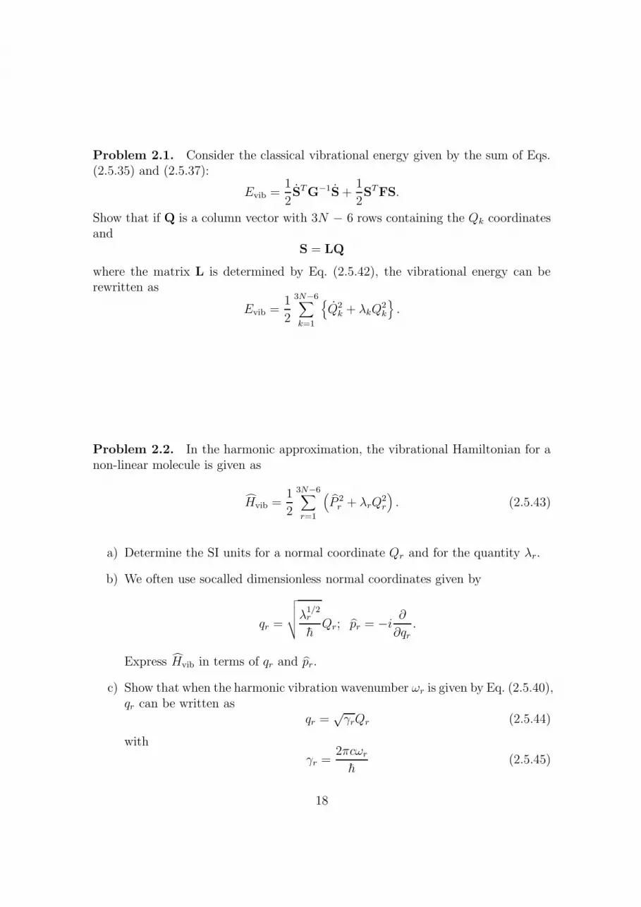
Problem 2.1. Consider the classical vibrational energy given by the sum of Eqs.(2.5.35) and (2.5.37):

Evib =1

2STG−1S +

1

2STFS.

Show that if Q is a column vector with 3N − 6 rows containing the Qk coordinatesand

S = LQ

where the matrix L is determined by Eq. (2.5.42), the vibrational energy can berewritten as

Evib =1

2

3N−6∑

k=1

{Q2

k + λkQ2k

}.

Problem 2.2. In the harmonic approximation, the vibrational Hamiltonian for anon-linear molecule is given as

Hvib =1

2

3N−6∑

r=1

(P 2

r + λrQ2r

). (2.5.43)

a) Determine the SI units for a normal coordinate Qr and for the quantity λr.

b) We often use socalled dimensionless normal coordinates given by

qr =

√√√√λ1/2r

hQr; pr = −i ∂

∂qr.

Express Hvib in terms of qr and pr.

c) Show that when the harmonic vibration wavenumber ωr is given by Eq. (2.5.40),qr can be written as

qr =√γrQr (2.5.44)

with

γr =2πcωr

h(2.5.45)

18

Problem 2.3. The molecule CO2 is linear in its equilibrium configuration. Wenumber the two O nuclei as 1 and 3, respectively, and the C nucleus as 2. Further, weintroduce a molecule fixed coordinate system with the z axis along the molecular axis(with positive direction from nucleus 1 to nucleus 3) and x and y axes perpendicularto the molecular axis.

We introduce four geometrically defined coordinates

R1 =1√2

(r(C − O1) + r(C − O3) − 2r)

R2 =1√2

(r(C − O1) − r(C − O3))

R3 = π − θx

R4 = π − θy

where r(C − O1) and r(C − O3) are the internuclear distances (and r is their equi-librium value) and θx and θy are bond angles measured in the xz and yz planes,respectively.

1. Construct the B matrix.

2. Show that the G matrix has the following non-vanishing matrix elements

G11 =1

mO

(2.5.46)

G22 =2mO +mC

mOmC

(2.5.47)

G33 = G44 =2(2mO +mC)

r2mOmC(2.5.48)

where mO and mC are the atomic masses of oxygen and carbon, respectively.

3. Derive the normal coordinates for CO2.

4. The harmonic vibration wavenumbers for 16O12C16O are experimentally de-termined as ω1

(Σ+

g

)= 1340 cm−1, ω2 (Πu) = 667 cm−1, and ω3 (Σ+

u ) = 2349

cm−1. Calculate the elements of the F matrix.

Use r = 1.162 A.

19

Chapter 3

The expansion of therotation-vibration Hamiltonian

3.1 The Watson Hamiltonian

Watson [1968a] showed that when the classical Hamiltonian function described inChapter 2 is expressed in terms of the coordinates (θ, φ, χ, Q1, Q2, Q3, . . .Q3N−6)and converted to quantum mechanical form using the Podolsky trick [see Chapter7 of Bunker (1979)] the following quantum mechanical Hamiltonian for a non-linearmolecule is obtained:

H =h2

2

∑

α=x,y,z

∑

β=x,y,z

(Jα − πα

)µαβ

(Jβ − πβ

)+

1

2hc

3N−6∑

r=1

ωrp2r

− h2

8

∑

α=x,y,z

µαα + hcV (3.1.1)

Jα component of the total angular momentum along the molecule fixed α axis,measured in units of h.

πα =∑3N−6

r=1

∑3N−6s=1 ζ(α)

rs

√ωs/ωrqrps; vibrational angular momentum.

ζ(α)rs = −ζ (α)

sr =∑

β,γ=x,y,z

∑Nη=1 eαβγ`ηβ,r`ηγ,s, where the antisymmetric tensor ele-

ments eαβγ are defined in Appendix A.

20

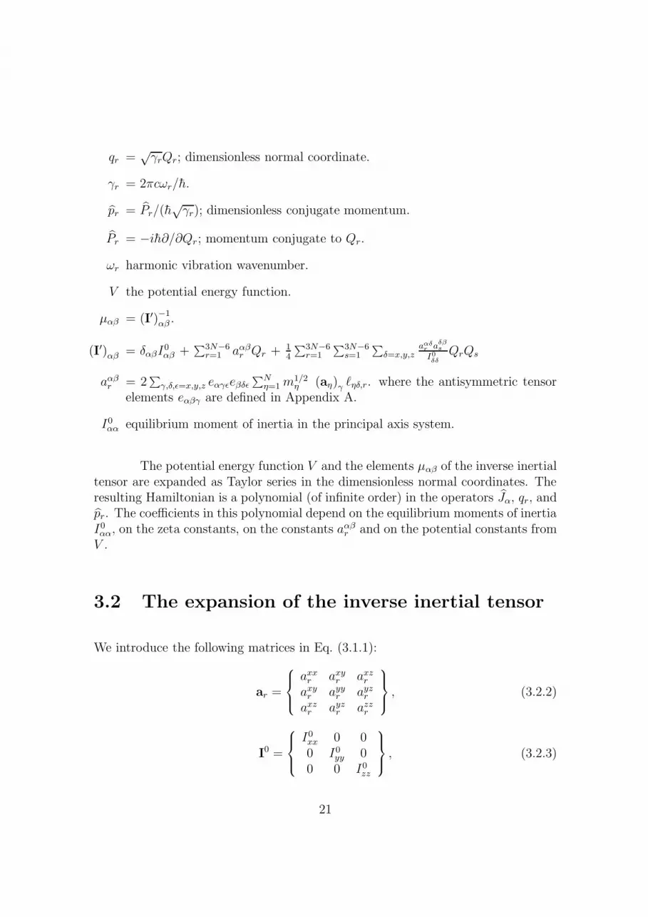
qr =√γrQr; dimensionless normal coordinate.

γr = 2πcωr/h.

pr = Pr/(h√γr); dimensionless conjugate momentum.

Pr = −ih∂/∂Qr; momentum conjugate to Qr.

ωr harmonic vibration wavenumber.

V the potential energy function.

µαβ = (I′)−1αβ .

(I′)αβ = δαβI0αβ +

∑3N−6r=1 aαβ

r Qr + 14

∑3N−6r=1

∑3N−6s=1

∑δ=x,y,z

aαδr aδβ

s

I0δδ

QrQs

aαβr = 2

∑γ,δ,ε=x,y,z eαγεeβδε

∑Nη=1 m

1/2η (aη)γ `ηδ,r. where the antisymmetric tensor

elements eαβγ are defined in Appendix A.

I0αα equilibrium moment of inertia in the principal axis system.

The potential energy function V and the elements µαβ of the inverse inertialtensor are expanded as Taylor series in the dimensionless normal coordinates. Theresulting Hamiltonian is a polynomial (of infinite order) in the operators Jα, qr, andpr. The coefficients in this polynomial depend on the equilibrium moments of inertiaI0αα, on the zeta constants, on the constants aαβ

r and on the potential constants fromV .

3.2 The expansion of the inverse inertial tensor

We introduce the following matrices in Eq. (3.1.1):

ar =

axxr axy

r axzr

axyr ayy

r ayzr

axzr ayz

r azzr

, (3.2.2)

I0 =

I0xx 0 00 I0

yy 00 0 I0

zz

, (3.2.3)

21

and

br =(I0)− 1

2 ar

(I0)− 1

2 . (3.2.4)

With these definitions, we can express the matrix I′ as

I′ = I0 +3N−6∑

r=1

arQr +1

4

3N−6∑

r=1

3N−6∑

s=1

ar

(I0)−1

asQrQs

=(I0) 1

2

{E +

3N−6∑

r=1

brQr +1

4

3N−6∑

r=1

3N−6∑

s=1

brbsQrQs

}(I0) 1

2 (3.2.5)

where E is a 3×3 unit matrix.

Since br and E commute, we obtain

I′ =(I0) 1

2

{E +

1

2

3N−6∑

r=1

brQr

}2 (I0) 1

2 (3.2.6)

and hence

µ =(I0)− 1

2

{E +

1

2

3N−6∑

r=1

brQr

}−2 (I0)− 1

2 . (3.2.7)

We expand the matrix{E + 1

2

∑3N−6r=1 brQr

}−2through the usual binomial expansion

µ =(I0)− 1

2

{E −

3N−6∑

r=1

brQr +3

4

3N−6∑

r=1

3N−6∑

s=1

brbsQrQs

− 1

2

3N−6∑

r=1

3N−6∑

s=1

3N−6∑

t=1

brbsbtQrQsQt + . . .

}(I0)− 1

2 . (3.2.8)

This expansion can be converted to a power series in the dimensionless normalcoordinates

µ =3N−6∑

r=1

µrqr +3N−6∑

r=1

3N−6∑

s=1

µrsqrqs +3N−6∑

r=1

3N−6∑

s=1

3N−6∑

t=1

µrstqrqsqt + . . . (3.2.9)

where the matrices µr, µrs, µrst etc. can be expressed in terms of the matrices ar:

µr = −γ−12

r

(I0)−1

ar

(I0)−1

, (3.2.10)

µrs =3

4γ− 1

2r γ

− 12

s

(I0)−1

ar

(I0)−1

as

(I0)−1

, (3.2.11)

22

µrst = −1

2γ− 1

2r γ

− 12

s γ− 1

2t

(I0)−1

ar

(I0)−1

as

(I0)−1

at

(I0)−1

, (3.2.12)

and so on. Explicit expressions for the matrix elements µαβr , µαβ

rs , µαβrst . . . in the

matrices µαβr , µαβ

rs , µαβrst . . . are obtained through matrix multiplication:

µαβr = − 1√

γr

aαβr

I0ααI

0ββ

, (3.2.13)

µαβrs =

3

4

1√γr

1√γs

∑

δ=x,y,z

aαδr a

δβs

I0ααI

0δδI

0ββ

, (3.2.14)

µαβrst = −1

2

1√γr

1√γs

1√γt

∑

δ=x,y,z

∑

ε=x,y,z

aαδr a

δεs a

εβt

I0ααI

0δδI

0εεI

0ββ

, (3.2.15)

and so on.

3.3 The expansion of the potential energy func-

tion

The potential energy function V is expressed as a Taylor series expansion in thedimensionless normal coordinates. With the convention of Mills [1972] we write Vas

hcV = hc∞∑

n=2

Vn =1

2hc

3N−6∑

r=1

ωrq2r +

1

6hc

3N−6∑

r=1

3N−6∑

s=1

3N−6∑

t=1

φrstqrqsqt

+1

24hc

3N−6∑

r=1

3N−6∑

s=1

3N−6∑

t=1

3N−6∑

u=1

φrstuqrqsqtqu + . . . , (3.3.16)

where φrst is a cubic anharmonic potential constant, φrstu is a quartic anharmonicpotential constant and so on. The potential constants are defined as

φrst =

(∂3V

∂qr∂qs∂qt

)

eq

, (3.3.17)

φrstu =

(∂4V

∂qr∂qs∂qt∂qu

)

eq

, (3.3.18)

and so on, and they all have the dimension cm−1. The numerical factors in the ex-pansion are introduced in order to avoid restrictions on the summation indices. Thederivation of the parameters φrs... on the basis of the expansion coefficients in a Tay-lor expansion of the potential energy function in geometrically defined coordinatesis the subject of Hoy et al. (1972).

23

3.4 The expansion of the Hamiltonian

By inserting the expansions for µ and V in the expression for the Hamiltonian H[Eq. (3.1.1)] we obtain H as the sum of infinitely many operators. Each of theseoperators is a product of vibrational operators qr or pr and rotational operators Jα.We classify the individual terms in the expression for H according to their totalpower n of vibrational operators and the total power m of rotational operators.That is, we express H as the sum

H =2∑

m=0

∞∑

n=0

hn,m (3.4.19)

where we can write the operator hn,m symbolically as

hn,m = (qr, pr)n Jm

α . (3.4.20)

In Eq. (3.4.19) we have taken into account that according to Eq. (3.1.1), m canassume the values 0, 1, or 2 only, whereas n can assume all non-negative values.

The operators hn,0 contain vibrational operators only and originate in

H0 =∞∑

n=0

hn,0 =h2

2

∑

α=x,y,z

∑

β=x,y,z

µαβπαπβ +1

2hc

3N−6∑

r=1

ωrp2r −

h2

8

∑

α=x,y,z

µαα + hcV.

(3.4.21)In obtaining Eq. (3.4.21) we have used that

∑

α=x,y,z

µαβπα =∑

α=x,y,z

παµαβ (3.4.22)

[Watson 1968]. Terms of n’th order in the normal coordinates originating in the pseu-

dopotential U = − h2

8

∑α=x,y,z µαα are customarily assigned to the operator hn+4,0.

All operators hn,1 contain the rotational operators to first order and origi-nate in

H1 =∞∑

n=2

hn,1 = − h2

2

∑

α=x,y,z

∑

β=x,y,z

(Jαµαβπβ + παµαβJβ

)

= − h2

2

∑

α=x,y,z

∑

β=x,y,z

µαβ

(Jαπβ + παJβ

)(3.4.23)

24

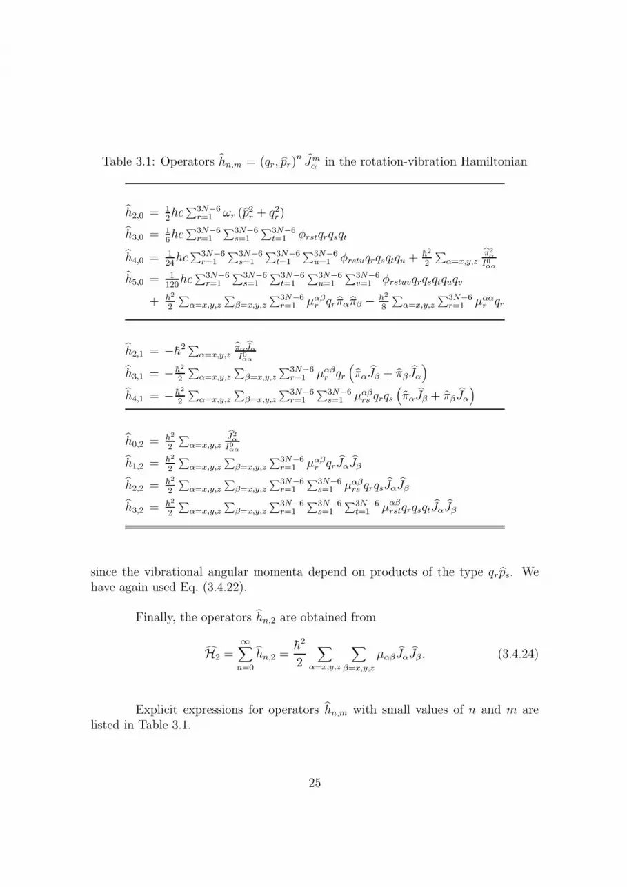
Table 3.1: Operators hn,m = (qr, pr)n Jm

α in the rotation-vibration Hamiltonian

h2,0 = 12hc∑3N−6

r=1 ωr (p2r + q2

r)

h3,0 = 16hc∑3N−6

r=1

∑3N−6s=1

∑3N−6t=1 φrstqrqsqt

h4,0 = 124hc∑3N−6

r=1

∑3N−6s=1

∑3N−6t=1

∑3N−6u=1 φrstuqrqsqtqu + h2

2

∑α=x,y,z

π2α

I0αα

h5,0 = 1120hc∑3N−6

r=1

∑3N−6s=1

∑3N−6t=1

∑3N−6u=1

∑3N−6v=1 φrstuvqrqsqtquqv

+ h2

2

∑α=x,y,z

∑β=x,y,z

∑3N−6r=1 µαβ

r qrπαπβ − h2

8

∑α=x,y,z

∑3N−6r=1 µαα

r qr

h2,1 = −h2∑α=x,y,z

παJα

I0αα

h3,1 = − h2

2

∑α=x,y,z

∑β=x,y,z

∑3N−6r=1 µαβ

r qr(παJβ + πβJα

)

h4,1 = − h2

2

∑α=x,y,z

∑β=x,y,z

∑3N−6r=1

∑3N−6s=1 µαβ

rs qrqs(παJβ + πβJα

)

h0,2 = h2

2

∑α=x,y,z

J2α

I0αα

h1,2 = h2

2

∑α=x,y,z

∑β=x,y,z

∑3N−6r=1 µαβ

r qrJαJβ

h2,2 = h2

2

∑α=x,y,z

∑β=x,y,z

∑3N−6r=1

∑3N−6s=1 µαβ

rs qrqsJαJβ

h3,2 = h2

2

∑α=x,y,z

∑β=x,y,z

∑3N−6r=1

∑3N−6s=1

∑3N−6t=1 µαβ

rstqrqsqtJαJβ

since the vibrational angular momenta depend on products of the type qrps. Wehave again used Eq. (3.4.22).

Finally, the operators hn,2 are obtained from

H2 =∞∑

n=0

hn,2 =h2

2

∑

α=x,y,z

∑

β=x,y,z

µαβJαJβ. (3.4.24)

Explicit expressions for operators hn,m with small values of n and m arelisted in Table 3.1.

25

The order of magnitude of an operator hn,m is given by

hn,m ∼ κLω (3.4.25)

where L is the order of magnitude of hn,m, ω is a typical harmonic vibrationwavenumber of order of magnitude 1000 cm−1), and κ is the Born-Oppenheimerexpansion parameter

κ = 4

√me

MN≈ 0.1. (3.4.26)

In Eq. (3.4.26), me is the electron mass and MN is a typical nuclear mass.

There are two accepted schemes for assigning orders of magnitude to theoperators hn,m. Oka [1967] defines

L = n+ 2m− 2 (3.4.27)

whereas Goldsmith et al. [1956] define

L = n+m− 2. (3.4.28)

The difference between the two schemes obviously lies in the weight attributed tothe rotational operators.

Oka’s estimation of the order of magnitude is based on the expansion of themolecular rotation-vibration Hamiltonian carried out by Born and Oppenheimer.These authors assumed that a rotational constant has the order of magnitude κ2ω,i.e. Erot/Evib ≈ κ2.

With Oka’s definition,

hn,2 ∼ κ2hn,1 ∼ κ4hn,0 (3.4.29)

whereas Goldsmith et al. obtain

hn,2 ∼ κhn,1 ∼ κ2hn,0. (3.4.30)

With the definition of Goldsmith et al., the harmonic oscillator and rigid ro-tor Hamiltonians both have L = 0. This classification scheme is used for carrying outcontact transformations (see below) on the expanded Hamiltonian. Oka’s scheme,which yields L = 2 for the rigid rotor Hamiltonian, is used for direct perturbationcalculations on the Hamiltonian.

26

Table 3.2: The rotation-vibration Hamitonian expanded according to order of mag-nitude

Order L Oka: L = n + 2m− 2 Goldsmith et al.: L = n+m− 2

0 H0 = h2,0 H0 = h2,0 + h0,2

1 H1 = h3,0 H1 = h3,0 + h2,1 + h1,2

2 H2 = h4,0 + h2,1 + h0,2 H2 = h4,0 + h3,1 + h2,2

3 H3 = h5,0 + h3,1 + h1,2 H3 = h5,0 + h4,1 + h3,2

......

L HL = hL+2,0 + hL,1 + hL−2,2 HL = hL+2,0 + hL+1,1 + hL,2

In both schemes, we express the Hamiltonian as

H =∞∑

L=0

HL (3.4.31)

where the operator HL has the order of magnitude κLω. Table 3.2 gives the formalexpressions for the HL operators in both schemes.

Problem 3.1. The rotation-vibration Hamiltonian for a diatomic molecule can bewritten as

H = − h2

2µ

d2

dr2+ V (r) +

1

2µr2J2. (3.4.32)

In Eq. (3.4.32), µ = m1 m2/(m1 +m2) is the reduced mass of the molecule; m1 andm2 are the masses of the two nuclei. Further, r is the instantaneous internucleardistance, V (r) is the potential energy function, and J is the angular momentum.

1. Define a dimensionless normal coordinate q for the diatomic molecule througha GF calculation (Problem 2.3).

2. Expand H in this coordinate, following the procedure described in the preced-ing part of the present chapter.

27

Chapter 4

The calculation of therotation-vibration energies

4.1 The Hamiltonian matrix

In order to calculate the rotation-vibration energies, we construct the matrix of theHamiltonian in a set of basis functions |V LJKM〉. We use the following notation:

V is a symbolic notation for all harmonic oscillator v quantum numbers. Inthe following, the index k denotes an arbitrary vibrational mode, i denotes anon-degenerate vibrational mode and j denotes a degenerate mode.

L is a symbolic notation for all harmonic oscillator `j quantum numbers. |`j| =vj, vj − 2, . . . , 0 or 1.

J is the rotational quantum number describing the length of the total angularmomentum.

K is the rotational quantum number for the projection of the total angular mo-mentum on the molecule-fixed z-axis. Assumes the values −J , −J + 1, . . . ,+J .

M is the rotational quantum number for the projection of the total angular mo-mentum on the space-fixed Z-axis. Assumes the values −J , −J + 1, . . . ,+J .

28

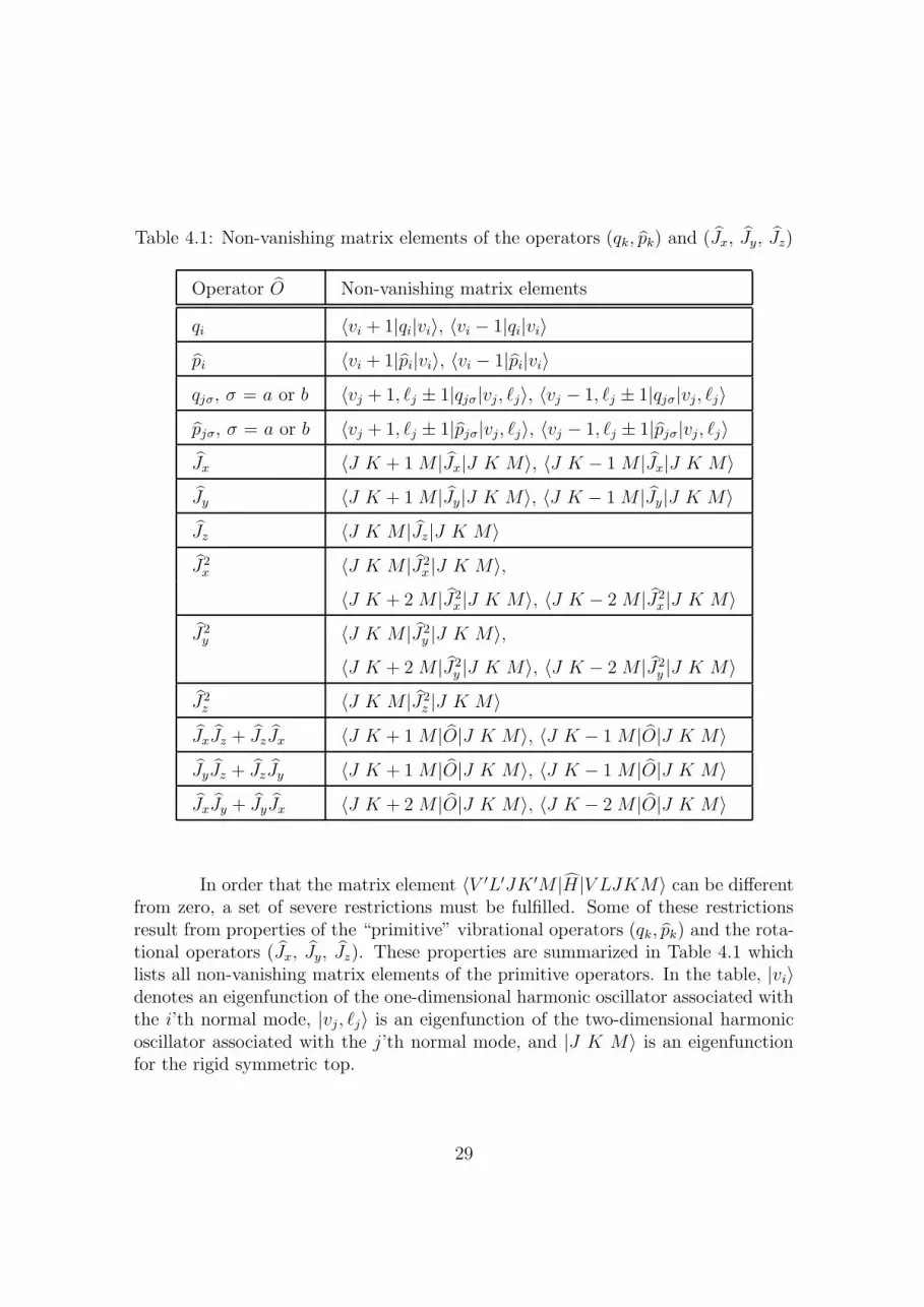
Table 4.1: Non-vanishing matrix elements of the operators (qk, pk) and (Jx, Jy, Jz)

Operator O Non-vanishing matrix elements

qi 〈vi + 1|qi|vi〉, 〈vi − 1|qi|vi〉pi 〈vi + 1|pi|vi〉, 〈vi − 1|pi|vi〉qjσ, σ = a or b 〈vj + 1, `j ± 1|qjσ|vj, `j〉, 〈vj − 1, `j ± 1|qjσ|vj, `j〉pjσ, σ = a or b 〈vj + 1, `j ± 1|pjσ|vj, `j〉, 〈vj − 1, `j ± 1|pjσ|vj, `j〉Jx 〈J K + 1 M |Jx|J K M〉, 〈J K − 1 M |Jx|J K M〉Jy 〈J K + 1 M |Jy|J K M〉, 〈J K − 1 M |Jy|J K M〉Jz 〈J K M |Jz|J K M〉J2

x 〈J K M |J2x |J K M〉,

〈J K + 2 M |J2x |J K M〉, 〈J K − 2 M |J2

x |J K M〉J2

y 〈J K M |J2y |J K M〉,

〈J K + 2 M |J2y |J K M〉, 〈J K − 2 M |J2

y |J K M〉J2

z 〈J K M |J2z |J K M〉

JxJz + JzJx 〈J K + 1 M |O|J K M〉, 〈J K − 1 M |O|J K M〉JyJz + JzJy 〈J K + 1 M |O|J K M〉, 〈J K − 1 M |O|J K M〉JxJy + JyJx 〈J K + 2 M |O|J K M〉, 〈J K − 2 M |O|J K M〉

In order that the matrix element 〈V ′L′JK ′M |H|V LJKM〉 can be differentfrom zero, a set of severe restrictions must be fulfilled. Some of these restrictionsresult from properties of the “primitive” vibrational operators (qk, pk) and the rota-tional operators (Jx, Jy, Jz). These properties are summarized in Table 4.1 whichlists all non-vanishing matrix elements of the primitive operators. In the table, |vi〉denotes an eigenfunction of the one-dimensional harmonic oscillator associated withthe i’th normal mode, |vj, `j〉 is an eigenfunction of the two-dimensional harmonicoscillator associated with the j’th normal mode, and |J K M〉 is an eigenfunctionfor the rigid symmetric top.

29

Table 4.2: Nonvanishing matrix elements 〈V + ∆V L + ∆L J K +∆K M |hn,m|V LJKM〉

Possible values of ∆V , ∆L, and ∆K

∑ |∆vi| n, n− 2, n− 4, . . . , 0 or 1.

∑ |∆`j| n, n− 2, n− 4, . . . , 0 or 1.

|∆K| m, m− 1, m− 2, . . . , 0.

All matrix elements of the operator H are diagonal in J and M . Further,the matrix elements are independent of M so that we can choose to carry throughthe calculation of H’s eigenvalues at a fixed value of M , for example M = 0. Thematrix representation of the Hamiltonian is block diagonal with one block for eachJ value. A general matrix element in such a block is called 〈V +∆V L+∆L J K +∆K M |H|V LJKM〉. We use ∆V as a collective notation for the changes in allv quantum numbers, and ∆L as an analogous notation for the changes in all `jquantum numbers.

The Hamiltonian H is given by Eq. (3.4.19)

H =2∑

m=0

∞∑

n=0

hn,m (4.1.1)

where, as discussed in Section 3.4, the operator hn,m can be written symbolically as(qr, pr)

n Jmα [Eq. (3.4.20)].

In order that a given operator hn,m can contribute to a matrix element

〈V +∆V L+∆L J K+∆K M |H|V LJKM〉, certain restrictions apply to ∆V , ∆L,and ∆K. The total power of vibrational operators in (q, p)n is n, and the maximumchange of a v quantum number that can be caused by this operator product is ±n.This maximum change can only be obtained if an operator product qi

r pn−i (where all

factor operators belong to the same vibrational mode) works on a single factor basisfunction |vr〉 or |vr, `r〉. Similarly, Jm

α , when working on |J K M〉, must necessarilyproduce a change in ∆K for which |∆K ≤ m. The conditions arising from theseconsiderations are summarized in Table 4.2.

30

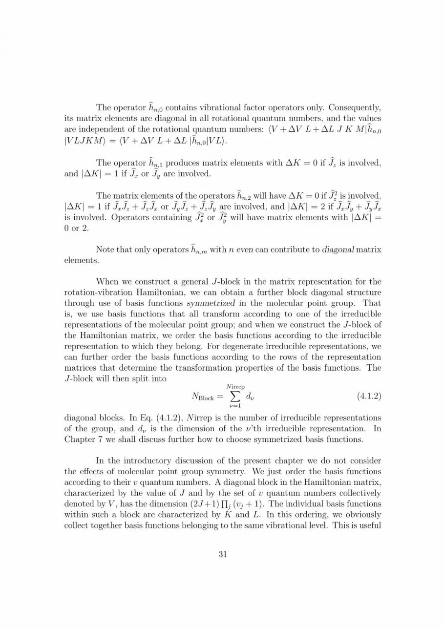
The operator hn,0 contains vibrational factor operators only. Consequently,its matrix elements are diagonal in all rotational quantum numbers, and the valuesare independent of the rotational quantum numbers: 〈V + ∆V L+ ∆L J K M |hn,0

|V LJKM〉 = 〈V + ∆V L + ∆L |hn,0|V L〉.

The operator hn,1 produces matrix elements with ∆K = 0 if Jz is involved,and |∆K| = 1 if Jx or Jy are involved.

The matrix elements of the operators hn,2 will have ∆K = 0 if J2z is involved,

|∆K| = 1 if JxJz + JzJx or JyJz + JzJy are involved, and |∆K| = 2 if JxJy + JyJx

is involved. Operators containing J2x or J2

y will have matrix elements with |∆K| =0 or 2.

Note that only operators hn,m with n even can contribute to diagonal matrixelements.

When we construct a general J-block in the matrix representation for therotation-vibration Hamiltonian, we can obtain a further block diagonal structurethrough use of basis functions symmetrized in the molecular point group. Thatis, we use basis functions that all transform according to one of the irreduciblerepresentations of the molecular point group; and when we construct the J-block ofthe Hamiltonian matrix, we order the basis functions according to the irreduciblerepresentation to which they belong. For degenerate irreducible representations, wecan further order the basis functions according to the rows of the representationmatrices that determine the transformation properties of the basis functions. TheJ-block will then split into

NBlock =N irrep∑

ν=1

dν (4.1.2)

diagonal blocks. In Eq. (4.1.2), N irrep is the number of irreducible representationsof the group, and dν is the dimension of the ν’th irreducible representation. InChapter 7 we shall discuss further how to choose symmetrized basis functions.

In the introductory discussion of the present chapter we do not considerthe effects of molecular point group symmetry. We just order the basis functionsaccording to their v quantum numbers. A diagonal block in the Hamiltonian matrix,characterized by the value of J and by the set of v quantum numbers collectivelydenoted by V , has the dimension (2J+1)

∏j (vj + 1). The individual basis functions

within such a block are characterized by K and L. In this ordering, we obviouslycollect together basis functions belonging to the same vibrational level. This is useful

31

in the discussion of resonances.

4.2 The diatomic molecule

In principle, we calculate the eigenvalues of the rotation-vibration Hamiltonian bycalculating the elements 〈V ′L′JK ′M |H|V LJKM〉 of its matrix representation inthe basis set |V LJKM〉 and then diagonalizing the matrix obtained in this way.With present-day computers it is feasible to carry out this diagonalization by brutenumerical force, at least for small molecules. However, the traditional methodsfor diagonalizing the matrix involve different types of perturbation theory. It isimportant to understand the principle behind these perturbative approaches in orderto appreciate the effects of resonances between molecular states, and consequentlywe review them here. Before we treat the perturbative approaches for a generalmolecule it is instructive to treat the simplest possible case, the diatomic molecule.

It is well known (see, for example, Landau and Lifshitz [1985]) that in theBorn-Oppenheimer approximation, we can write the rotation-vibration Hamiltonianfor a diatomic molecule as

H = − h2

2µ

d2

dr2+ V (r) +

1

2µr2J2. (4.2.3)

In Eq. (4.2.3), µ = m1 m2/(m1+m2) is the reduced mass of the molecule; m1 and m2

are the masses of the two nuclei. The coordinates entering into Eq. (4.2.3) are theinternuclear distance r and two Euler angles θ and φ describing the instantaneousdirection of the molecular axis in space. The dependence on the Euler angles is“hidden” in J2, the square of the total angular momentum. The quantum mechanicalvolume element is chosen as dr sin θ dθ dφ.

It is also well known that spectroscopists customarily write the rotation-vibration energies of a diatomic molecule (i.e., the eigenvalues of the Hamiltoniangiven in Eq. (4.2.3)) as the Dunham expansion:

EvJ/hc =∞∑

j=0

∞∑

k=0

Yjk

(v +

1

2

)j

Jk(J + 1)k (4.2.4)

or as the equivalent expansion

EvJ/hc = Tv +Bv J(J + 1) −DvJ2(J + 1)2 + . . . (4.2.5)

32

where

Tv = ωe

(v +

1

2

)+ ωe xe

(v +

1

2

)2

+ . . . ,

Bv = Be − αe

(v +

1

2

)+ B(2)

(v +

1

2

)2

+ . . . ,

Dv = De +D(1)(v +

1

2

)+D(2)

(v +

1

2

)2

+ . . . , (4.2.6)

and so on. In Eqs. (4.2.4) and (4.2.5) the energy is divided by hc so that theparameters on the right hand sides of the equations are expressed in wavenumberunits.

Now we might initially ask how one should go about deriving Eqs. (4.2.4)and (4.2.5) from Eq. (4.2.3). Towards this end we will apply the principles sketchedin Chapter 3, i.e., we will expand the Hamiltonian. The rotational part of theHamiltonian is the term 1

2µr2 J2 in Eq. (4.2.3). For the diatomic molecule, we can

view the coefficient of J2, 12µr2 , as the only non-vanishing µ-tensor element, and we

write it as1

2µr2=

1

2µ(re + ∆r)2(4.2.7)

where re is the internuclear distance at equilibrium. In Problem 3.1 we expand thisquantity as

1

2µ(re + ∆r)2=

1

2µr2e

{1 − 2

(∆r

re

)+ 3

(∆r

re

)2

− 4(

∆r

re

)3

+ . . .

}. (4.2.8)

Further, we expand the potential energy as described in Section 3.3:

V (r) =1

2k2 ∆r2 +

1

6k3 ∆r3 +

1

24k4 ∆r4 + . . . . (4.2.9)

In the simplest possible approximation to this problem, we retain only theleading term in each of these expansions and obtain the zero’th order Hamiltonian

H0 = − h2

2µ

d2

dr2+

1

2k2 ∆r2 +

1

2µr2e

J2. (4.2.10)

It is easy to verify that in terms of the dimensionless normal coordinate

q =4

√k2µ

h2 ∆r (4.2.11)

33

with conjugate momentum

p = −i ∂∂q

(4.2.12)

H0 is given as

H0 = h

√k2

µ

[−1

2

{p2 + q2

}]+

1

2µr2e

J2. (4.2.13)

We can solve the eigenvalue equation

H0ψ(0)vJ (q, θ, φ) = E

(0)vJ ψ

(0)vJ (q, θ, φ) (4.2.14)

exactly. The solutions are

ψ(0)vJ (r, θ, φ) = Φv(q) YJm(θ, φ) (4.2.15)

where Φv(q) is an eigenfunction of the one-dimensional harmonic oscillator, andYJm(θ, φ) is a spherical harmonic function. The eigenvalues are

E(0)vJ = h

√k2

µ

(v +

1

2

)+

h2

2µr2e

J(J + 1). (4.2.16)

We are clearly on the right track towards deriving Eqs. (4.2.4) and (4.2.5). If wemake the following identifications

ωe =1

2πc

√k2

µ(4.2.17)

and

Be =h

8π2cµr2e

(4.2.18)

Eq. (4.2.16) gives exactly the leading terms in Eq. (4.2.5). How do we get the higherorder terms? We will investigate this by considering an approximation in which wetake the Hamiltonian to be

H1 = H0 −1

µr3e

4

√√√√ h2

k2µqJ2

= h

√k2

µ

[−1

2

{p2 + q2

}]+

1

2µr2e

J2

− 1

µr3e

4

√√√√ h2

k2µqJ2, (4.2.19)

34

that is, we now take into account the two first terms of Eq. (4.2.8) and the first termin Eq. (4.2.9).

We will construct the matrix representation of H1 in the basis set of func-tions

ψ(0)vJ (r, θ, φ) = Φv(q) YJm(θ, φ) = |v; Jm〉, (4.2.20)

and we need to calculate the matrix elements 〈v′; J ′m′|H1|v; Jm〉. If we use that

• |v; Jm〉 is an eigenfunction of H0 [Eq. (4.2.14)].

• all matrix elements of J2 are diagonal in J and m:

J2YJm(θ, φ) = h2J(J + 1)YJm(θ, φ) (4.2.21)

• the operator q has the nonvanishing matrix elements given by Eqs. (B.2.16)and (B.2.17)

we can easily show that the only nonvanishing matrix elements of H1 are

〈v; Jm|H1|v; Jm〉 = E(0)vJ = hcωe

(v +

1

2

)+ hcBeJ(J + 1), (4.2.22)

〈v + 1; Jm|H1|v; Jm〉 = − h2

µr3e

4

√√√√ h2

k2µ

√(v + 1)/2 J(J + 1) (4.2.23)

and

〈v − 1; Jm|H1|v; Jm〉 = − h2

µr3e

4

√√√√ h2

k2µ

√v/2 J(J + 1). (4.2.24)

With these matrix elements, we can construct the matrix representation of H1.The matrix elements are diagonal in J and m, and they do not depend on m.Consequently, we can carry out the calculations for one particular value of m, forinstance m = 0. If we use the notation

Hv′J ′m′;vJm = 〈v′; J ′m′|H1|v; Jm〉 (4.2.25)

we obtain the matrix block for a particular J value and for m = 0 as

HJ =

H0J0;0J0 H0J0;1J0 0 0 . . .H1J0;0J0 H1J0;1J0 H1J0;2J0 0 . . .

0 H2J0;1J0 H2J0;2J0 H2J0;3J0 . . .0 0 H3J0;2J0 H3J0;3J0 . . ....

......

...

. (4.2.26)

35

This matrix has infinitely many elements. If we truncate it at a maximum v-value,vmax say, we can diagonalize the truncated matrix with a computer and obtain thenumerical eigenvalues. This is the variational approach to the problem.

However, as mentioned above the traditional approach to rotation-vibrationtheory involves perturbation theory. That is, we consider H0 to the unperturbed

Hamiltonian and

V = H1 − H0 = − 1

µr3e

4

√√√√ h2

k2µqJ2 (4.2.27)

as a perturbation. Perturbation theory gives us the energy correct to first order as

E(1st−order) = 〈v; Jm|H1|v; Jm〉 = hcωe

(v +

1

2

)+ hcBeJ(J + 1), (4.2.28)

from Eq. (4.2.22). The energy correct to second order is given as

E(2nd−order) = E(1st−order) +∑

v′′J ′′ 6=vJ

|〈v′′; J ′′m|H1|v; Jm〉|2

E(0)vJ − E

(0)v′′J ′′

. (4.2.29)

The only nonvanishing matrix elements entering into the sum are those given byEqs. (4.2.23) and (4.2.24). Using these equations (and Eq. (4.2.22) for E

(0)vJ ) we can

calculate the second order energy as

E(2nd−order) = hcωe

(v +

1

2

)+ hcBeJ(J + 1)

− 1

2hcωe

h2

µr3e

4

√√√√ h2

k2µ

2

J2(J + 1)2. (4.2.30)

We have obviously discovered another term in Eq. (4.2.5). If we identify

De =1

2h2c2ωe

h2

µr3e

4

√√√√ h2

k2µ

2

(4.2.31)

we have expressed in Eq. (4.2.30) the centrifugal distortion term −DeJ2(J + 1)2.

We can tidy up the expression for De given in Eq. (4.2.31). If we use Eq. (4.2.17)to express k2 in terms of ωe and (4.2.18) to express re in terms of Be, we derive

De =4B3

e

ω2e

=(

2Be

ωe

)2

Be (4.2.32)

We have seen here that there are at least two different ways to obtain theeigenvalues of the operator H1:

36

• We can diagonalize numerically the matrix block HJ given in Eq. (4.2.26).This involves the approximation that we truncate the infinitely large matrixafter a maximum v-value, vmax. However we can investigate this approxima-tion numerically by diagonalizing larger and larger matrices until the lowesteigenvalues meet our convergence criteria.

• Through second order perturbation theory we can obtain a closed expression(Eq. (4.2.30)) for the eigenvalues. This calculation involves the approximationinherent in the perturbation theory: the energy distance between interactinglevels (here hcωe) should be large compared with the matrix elements of theperturbation V given by Eq. (4.2.27). This will certainly be the case for low Jvalues, but since the interaction matrix elements are proportional to J(J +1),it might not necessarily be the case for very large J . The terms entering intothe closed form for the energy contain parameters (like De) which dependon the underlying parameters of the Hamiltonian (here re and the potentialexpansion parameters kn).

We have treated here one particular term in Eq. (4.2.5), the centrifugaldistortion term −DeJ

2(J + 1)2. However, we can obtain all the higher order termsin the expansion for the energy given in Eq. (4.2.5) by using perturbation theoryof increasingly higher order on the expansion terms in Eqs. (4.2.8) and (4.2.9).We will give examples of this in a exercise below. For a polyatomic molecule, thetraditional way of obtaining the rotation-vibration energies is in principle identicalto the procedure described here, but it is of course somewhat more complicated dueto the larger number of vibrational coordinates.

4.3 Perturbation theory

The first approach is the direct perturbation calculation, which is sometimes referredto as the van Vleck transformation. It involves direct numerical manipulation of thematrix elements 〈V ′L′JK ′M |H|V LJKM〉 [unlike the contact transformation whichwe shall treat in the next section].

We take the rotation-vibration Hamiltonian to be

H = H0 + λH1 + λ2H2 + λ3H3 + . . . =∞∑

L

λL HL (4.3.33)

37

The perturbation parameter λ has no physical significance. We have introduced itas a book-keeping device allowing us to distinguish the order of magnitude of theoperators making up H. In the final results we will set λ = 1. In Eq. (4.3.33),the operator HL has the order of magnitude κLω, where L can be defined by Eq.(3.4.27) or by Eq. (3.4.28).

We imagine that we have solved the eigenvalue equation for H0:

H0 |n, k〉 = E(0)n |n, k〉. (4.3.34)

In Eq. (4.3.34), the index n numbers the energy levels, and the index k = 1, 2, 3,. . . , k(max)

n numbers degenerate states with the same energy E(0)n .

According to the rules of perturbation theory, we obtain the eigenvalues ofH as expansions in λ. The energies correct to first order are obtained as eigenvaluesof k(max)

n × k(max)n matrix blocks with elements

H(1)kk′(n) = 〈n, k|H0 + H1|n, k′〉, (4.3.35)

whereas the energies correct to second order are obtained as eigenvalues of k(max)n ×

k(max)n matrix blocks with elements

H(2)kk′(n) = 〈n, k|H0 + H1 + H2|n, k′〉

+∑

n′′k′′

(n′′ 6=n)

〈n, k|H1|n′′, k′′〉〈n′′, k′′|H1|n, k′〉E

(0)n − E

(0)n′′

(4.3.36)

and so on. In Eqs. (4.3.35) and (4.3.35) the indices k and k′ assume the values 1, 2,3, . . . , k(max)

n .

In the calculation of molecular rotation-vibration energies we normally iden-tify the index n with the total set of v quantum numbers, V , and the index k withthe set of quantum numbers (K,L). Hence the matrices in Eqs. (4.3.35) and (4.3.35)describe a vibrational state defined by its value of V . However, the perturbationtreatment breaks down if there exist two sets of V quantum numbers having al-

most the same value for the zero order energy E(0)n = E

(0)V , and if the basis states

corresponding to these two sets of V quantum numbers are coupled by off-diagonalmatrix elements. We can express these two conditions as

〈V + ∆V L + ∆L J K + ∆K M |H|V LJKM〉 6= 0 (4.3.37)

38

and

〈V LJKM |H |V LJKM〉≈ 〈V + ∆V L + ∆L J K + ∆K M |H|V + ∆V L + ∆L J K + ∆K M〉.

(4.3.38)

If these conditions are fulfilled, we say that the two states |V + ∆V L+ ∆L J K +∆K M〉 and |V LJKM〉 are quasidegenerate. If we calculate the diagonal matrixelements 〈V LJKM |H |V LJKM〉 where we only take into account the vibrationalenergy in the harmonic approximation, the rotational energy in the rigid rotor ap-proximation, and the Coriolis coupling terms, we can express the difference betweentwo diagonal matrix elements as (for a prolate symmetric top):

∆E = 〈V + ∆V L + ∆L J K + ∆K M |H|V + ∆V L + ∆L J K + ∆K M〉− 〈V LJKM |H|V LJKM〉=

∑

k

∆vkωk + (A−B)((K + ∆K)2 −K2

)

− 2∑

j

Aζj ((K + ∆K) (`j + ∆`j) −K`j)

=∑

k

∆vkωk +

(A−B) ∆K − 2

∑

j

Aζj∆`j − 2∑

j

Aζj`j

∆K

+ 2K

(A− B) ∆K −

∑

j

Aζj∆`j

. (4.3.39)

The rotational constants and the zeta constants have the order of magnitude κ2ω,and ∆K is limited to 0, ±1, and ±2. Consequently the most important contributionto ∆E is the term

∑k ∆vkωk originating in the vibrational energy. On the basis of

this term, we classify quasidegeneracies into to main types: necessary quasidegen-

eracies and accidental quasidegeneracies.

For ∆V = 0 (i.e., all ∆vi = 0), ∆E depends only on differences in the rota-tional and Coriolis energy contributions. We say that all basis functions, character-ized by one particular set of v quantum numbers, are necessarily quasidegenerate.In consequence, the (2J + 1)

∏j (vj + 1) basis functions, that make up a particular

V -block in the Hamitonian matrix, are necessarily quasidegenerate.

An accidental quasidegeneracy has ∆V 6= 0 and

∑

k

∆vkωk ≈ 0. (4.3.40)

39

An accidental quasidegeneracy involves two sets of basis functions, each of whichare necessarily quasidegenerate, and these two sets of basis functions have almostthe same vibrational energy.

We can write the expression for ∆E in Eq. (4.3.39) as

∆E = ∆E0 + CK K (4.3.41)

with

∆E0 =∑

k

∆vkωk +

(A− B) ∆K − 2

∑

j

Aζj`j

∆K (4.3.42)

and

CK = 2

(A− B)∆K −

∑

j

Aζj∆`j

. (4.3.43)

If CK is small relative to ∆E0, we speak about a global quasidegeneracy. In thiscase, the effects of the interaction between basis functions with different v quantumnumbers will be similar for all basis states in the set, independent of K. If CK iscomparable to ∆E0, we have a local degeneracy. It will only be important for someK values given by

K ≈ −∑

k ∆vkωk +{(A−B) ∆K − 2

∑j Aζj∆`j − 2

∑j Aζj`j

}∆K

2[(A− B)∆K −∑

j Aζj∆`j] . (4.3.44)

When we carry perturbation calculations to obtain the eigenvalues of therotation-vibration Hamiltonian, we also consider the effects of accidental quaside-generacy. We then extend the set of basis functions |n, k〉 which we include in theperturbative treatment. The index n no longer corresponds to just one set of Vquantum numbers but describe all sets of V quantum numbers describing the ac-cidentally quasidegenerate basis states. The index k then identifies the individualbasis functions (in particular the (K,L) quantum numbers) in the quasidegenerateset.

If we account for necessary quasidegeneracy only, we find the 1st orderenergies for a given value of J and a given set of V quantum numbers throughdiagonalization of the matrix with elements

H(1)L′K′;LK(V ) = 〈V L′JK ′M |H0 + H1|V LJKM〉. (4.3.45)

40

This matrix has the dimension (2J+1)∏

j(vj +1). Second order perturbation theoryyields the matrix elements

H(2)L′K′;LK(V ) = 〈V L′JK ′M |H0 + H1 + H2|V LJKM〉

+∑

V ′′L′′K′′

(V ′′ 6=V )

〈V L′JK ′M |H1|V L′′JK ′′M〉〈V L′′JK ′′M |H1|V LJKM〉E

(0)V − E

(0)V ′′

(4.3.46)

In the case of necessary quasidegeneracies, we extend this secular problem to com-prise all V quantum numbers in the quasidegenerate set.

4.4 Contact transformations

It is obvious from, for example, Eqs. (4.3.45) and (4.3.46), that when we use directperturbation theory for calculating the rotation-vibration energies, we will obtaincomplicated expressions for the higher order energy corrections. However, the cal-culations of these corrections can be considerably simplified and systematized whenwe use another formulation of the perturbation theory, the socalled contact trans-

formation [Maes and Amat 1957].

We can write a unitary operator as

T = eiλS (4.4.47)

where S is a hermitian, initially arbitrary operator. We use this operator to form anew transformed Hamiltonian

H = T HT−1 = eiλSHe−iλS. (4.4.48)

We obtain the eigenvalues and eigenfunctions for H by solving the Schrodingerequation

Hψ = Eψ (4.4.49)

orT HT−1T ψ = ETψ. (4.4.50)

This shows that the Schrodinger equation for H is

H(T ψ

)= E

(T ψ

). (4.4.51)

41

Hence H and H have identical eigenvalues but the eigenfunctions for H, ψ′ areobtained from the eigenfunctions of H through the transformation

ψ′ = T ψ. (4.4.52)

Both H and H are expanded in λ:

H = H0 + λ H1 + λ2 H2 + . . .

H = H0 + λ H1 + λ2 H2 + . . .

(4.4.53)

and T is expanded as

T = eiλS = 1 + i λ S +1

2!

(i λ S

)2+ . . . . (4.4.54)

Insertion of Eqs. (4.4.53) and (4.4.54) in Eq. (4.4.48) yields

[H0 + λ H1 + λ2 H2 + . . .

]

=[1 + iλS − 1

2λ2S2 + . . .

] [H0 + λH1 + λ2 H2 + . . .

] [1 − iλS − 1

2λ2S2 + . . .

].

(4.4.55)

Both sides of this equation are polynomials in λ. By identifying terms with the samepowers of λ we obtain

H0 = H0

H1 = H1 + i(SH0 − H0S

)

H2 = H2 + i(SH1 − H1S

)− 1

2

(S2H0 + H0S

2)

+ SH0S (4.4.56)

and so on.

The contact transformation does not change H0. The higher order operatorsare changed through addition of operators which may be expressed in terms of thecommutators between the operators contained in H and S. See Amat et al. (1971)for general expressions.

We now choose the arbitrary operator S in such a way that the calculationof the second order energy is simplified. It is clever to choose S so that

〈nk|H1|n′′k′′〉 = 0 for all n′′ 6= n. (4.4.57)

42

When we use Eq. (4.4.57) in Eq. (4.3.36), we see that the energies correct to secondorder are now obtained as eigenvalues of k(max)

n × k(max)n matrix blocks with elements

H(2)kk′(n) = 〈n, k|H0 + H1 + H2|n, k′〉, (4.4.58)

an equation analogous to Eq. (4.3.35) for the first order energies. However, in orderto use Eq. (4.4.58) we must determine the transformed operator H2. That is, wefirst need to obtain an expression for the hermitian operator S.

The operator S fulfills the condition in Eq. (4.4.57), i.e.,

〈nk|H1 + i(SH0 − H0S

)|n′′k′′〉 = 0 for all n′′ 6= n. (4.4.59)

SinceH0 |nk〉 = E(0)

n |nk〉, (4.4.60)

Eq. (4.4.59) yields

〈nk|S|n′′k′′〉 = i〈nk|H1|n′′k′′〉E

(0)n′′ − E

(0)n

; n′′ 6= n. (4.4.61)

It is not possible to determine S further. That is, we can only determine the matrixrepresentation of S. Further we can only determine the matrix elements that areoff-diagonal in n. Matrix elements of H1, that are diagonal in n, are given by

〈nk|H1|nk′〉 = 〈nk|H1 + i(SH0 − H0S

)|nk′〉 = 〈nk|H1|nk′〉. (4.4.62)

Hence we cannot use S to remove matrix elements that couple states with the samevalue of n.

In practice, we determine S by dividing H1 into

H1 = H∗1 + H+

1 . (4.4.63)

The operator H∗1 has only matrix elements 〈nk|H∗

1 |nk′〉 diagonal in n, and H+1

has only matrix elements 〈nk|H+1 |n′′k′′〉, n′′ 6= n. When we consider necessary

quasidegeneracies and use the order-of-magnitude definition by Amat and Nielsen,the operators h3,0 and h1,2 are contained solely in H+

1 (since they involve odd powers

of the vibrational operators). Most of the operator h2,1 also belongs to H+1 , but the

Coriolis coupling term enters into H∗1 ; i.e.,

H∗1 = − h2

I0zz

Jz

∑

j

ζ(z)j (qjapjb − qjbpja) (4.4.64)

43

for a symmetric top. For linear molecules and asymmetric tops, H∗1 = 0. We choose

the operator S so thatH1 = H∗

1 (4.4.65)

which requires [S, H0

]= i H+

1 = i(h3,0 + h1,2 + h2,1 − H∗

1

). (4.4.66)

Detailed expressions are given by Amat et al. (1971). These authors also give ex-pressions for the transformed operators H2 and H3; we quote these expressions inEqs. (4.4.67) and (4.4.68):

H2 =∑

αβγδ

(αβγδ(2) Y

)JαJβJγJδ +

∑

αβγ

∑

a

(αβγ(2) Y

a)paJαJβJγ

+∑

αβ

∑

aba≤b

(αβ(2)Y

abpapbJαJβ +αβ(2) Yabqaqb

)JαJβ

+∑

α

∑

abca≤b≤c

(α(2)Y

abc)papbpcJα

+∑

α

∑

abca≤b

(α(2)Y

cab

) 1

2(qaqbpc + pcqaqb) Jα

+∑

abcda≤b;c≤d

((2)Y

cdab

) 1

2(qaqbpcpd + pcpdqaqb)

+∑

abcda≤b≤c≤d

((2)Yabcd

)qaqbqcqd (4.4.67)

and

H3 =∑

αβγδ

∑

a

(αβγδ(2) Ya

)qaJαJβJγJδ

+∑

αβγ

∑

ab

(αβγ(3) Y

ba

) 1

2(qapb + pbqa) JαJβJγ

+∑

αβ

∑

abcb≤c

(αβ(3)Y

bca

) 1

2(qapbpc + pbpcqa) JαJβ

+∑

αβ

∑

abca≤b≤c

(αβ(3)Yabc

)qaqbqcJαJβ

+∑

α

∑

abcda≤b≤c

(α(3)Y

bcda

) 1

2(qapbpcpd + pbpcpdqa) Jα

44

+∑

α

∑

abcda≤b≤c

(α(3)Y

dabc

) 1

2(qaqbqcpd + pdqaqbqc) Jα

+∑

abcdea≤b≤c≤d≤e

((3)Y

bcdea

) 1

2(qapbpcpdpe + pbpcpdpeqa)

+∑

abcdea≤b≤c;d≤e

((3)Y

deabc

) 1

2(qaqbqcpdpe + pdpeqaqbqc)

+∑

abcdea≤b≤c≤d≤e

((3)Yabcde

)qaqbqcqdqe

+∑

a

((3)Ya

)qa. (4.4.68)

The notation is that of Amat et al. (1971). The Y -quantities are molecular param-eters, the Greek indices α, β, . . . run over the values x, y, and z, and the Latinindices a, b, c, . . . run over the normal vibrations of the molecule.

Problem 4.1. Consider the perturbation

V =

− 1

µr3e

4

√√√√ h2

k2µq +

3

2µr4e

√√√√ h2

k2µq2

J2

+1

6k3

(h2

k2µ

)3/4

q3 +1

24k4

(h2

k2µ

)q4 (4.4.69)

to the Hamiltonian H0 given by Eq. (4.2.13).

1. Determine the energy corrections arising through 1st order perturbation the-ory. Which terms in Eq. (4.2.5) do we obtain in this way?

2. Discuss the energy corrections arising through 2nd order perturbation theory.How do these energy corrections depend on the quantum numbers v and J?

45

Chapter 5

Molecular point groups

5.1 Generating operations

We aim at determining the irreducible representations spanned by the rotational-vibration basis functions |V LJKM〉 and by the rotation-vibration operators Jα, α= x, y, or z, qi, pi, qjσ, and pjσ in the appropriate molecular point group. As thefirst step towards this goal we discuss here the structure of common molecular pointgroups.

Let us consider for a moment the point group C3v. It contains the sixoperations

C3v ={E,C3, C

23 , σ

(xz), σ(2), σ(3)}.

We have chosen a right-handed axis system such that C3 and C23 are rotations of 2π

3

and 4π3

, respectively, around the z axis. The positive direction of the rotations isdefined as the direction in which a right-handed screw will rotate when it advancesin the positive direction of the z axis. The x and y axes are perpendicular to the zaxis and chosen such that the group operation σ(xz) is a reflection in the xz plane.The operations σ(2) and σ(3) are then reflections in planes that contain the z axisand form angles of 2π

3and 4π

3, respectively, with the xz plane.

It is straightforward to verify the following relations

E = C3 C3 C3 =(σ(xz)

)2

C23 = C3 C3

46

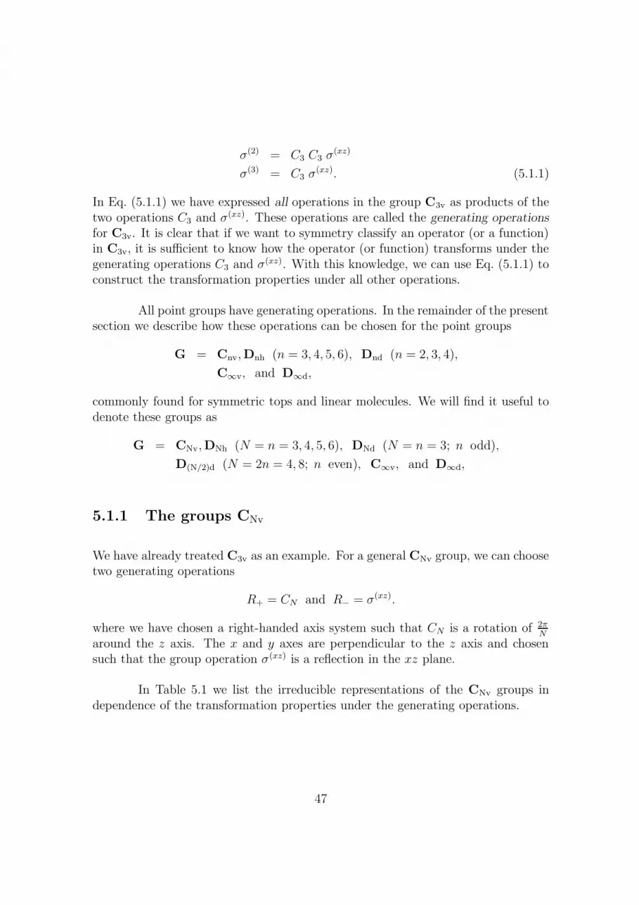
σ(2) = C3 C3 σ(xz)

σ(3) = C3 σ(xz). (5.1.1)

In Eq. (5.1.1) we have expressed all operations in the group C3v as products of thetwo operations C3 and σ(xz). These operations are called the generating operations

for C3v. It is clear that if we want to symmetry classify an operator (or a function)in C3v, it is sufficient to know how the operator (or function) transforms under thegenerating operations C3 and σ(xz). With this knowledge, we can use Eq. (5.1.1) toconstruct the transformation properties under all other operations.

All point groups have generating operations. In the remainder of the presentsection we describe how these operations can be chosen for the point groups

G = Cnv,Dnh (n = 3, 4, 5, 6), Dnd (n = 2, 3, 4),

C∞v, and D∞d,

commonly found for symmetric tops and linear molecules. We will find it useful todenote these groups as

G = CNv,DNh (N = n = 3, 4, 5, 6), DNd (N = n = 3; n odd),

D(N/2)d (N = 2n = 4, 8; n even), C∞v, and D∞d,

5.1.1 The groups CNv

We have already treated C3v as an example. For a general CNv group, we can choosetwo generating operations

R+ = CN and R− = σ(xz).

where we have chosen a right-handed axis system such that CN is a rotation of 2πN

around the z axis. The x and y axes are perpendicular to the z axis and chosensuch that the group operation σ(xz) is a reflection in the xz plane.

In Table 5.1 we list the irreducible representations of the CNv groups independence of the transformation properties under the generating operations.

47

Table 5.1: Irreducible representations for the CNv groups

CNv (N odd) E R+ =CN R− =σ(xz)

A1 1 1 1

A2 1 1 −1

Er, r = 1,2, . . . , N−12

2 2 cos2πrN

0

CNv (N even) E R+ =CN R− =σ(xz)

A1 1 1 1

A2 1 1 −1

B1 1 −1 1

B2 1 −1 −1

Er, r = 1,2, . . . , N2− 1 2 2 cos 2πr

N0

5.1.2 The groups DNh and DNd

Assume that we have two groups, G and H, given as

G = {G1, G2, G3, G4, G5, . . . , Gg}H = {H1, H2, H3, H4, H5, . . . , Hh}

where, as indicated, G has g elements and H has h elements. We assume that allelements in G commute with all elements in H:

GiHk = HkGi. (5.1.2)

We can now construct a new group, P, with gh elements:

P = {G1H1, G1H2, G1H3, . . . G1Hh, G2H1, G2H2, G2H3, . . . G2Hh, . . . , GgHh}

We call P the direct product of G and H and denote it by

P = G ⊗ H. (5.1.3)

48

Table 5.2: Irreducible representations for the Cs and Ci groups

Cs E σh

A′ 1 1

A′′ 1 −1

Ci E i

Ag 1 1

Au 1 −1

We now introduce two simple groups, Cs and Ci:

Cs = {E, σh}Ci = {E, i}

where σh is a reflection in a horizontal plane (perpendicular to the N -fold axis) andi is the inversion. We can then obtain the groups DNh and DNd as direct products:

DNh = CNv ⊗ Cs (N odd) (5.1.4)

DNh = CNv ⊗ Ci (N even) (5.1.5)

DNd = CNv ⊗ Ci (N odd) (5.1.6)

We choose the generating operations for the groups DNh and DNd as:

DNh (N odd) : R+ = CN , R′+ = σh, and R− = C

(x)2

DNh (N even) : R+ = CN , R′+ = i, and R− = C

(x)2

DNd (N odd) : R+ = CN , R′+ = i, and R− = C

(x)2

where C(x)2 is a rotation of π around the x axis which is perpendicular to the N -

fold axis. We can produce such rotations by combining the reflections σ in CNv

with the operations σh and i. Due to the direct product structure of the DNh

and DNd (N odd) groups [Eq. (5.1.6)], it would in fact have been more logical to

choose σ(xz) as a generating operation for DNh and DNd (N odd) instead of C(x)2 .

However, this does not seem to be the customary choice (see, for example, Hegelundet al. [1973]) and we attempt here to follow accepted practice as much as possible.The character tables DNh and DNd (N odd) are easily constructed using the directproduct structure of these groups. In each case, the character table for CNv isextended by a column corresponding to the generating operation σh or i, and thenumber of irreducible representations is doubled. The non-degenerate irreduciblerepresentations are named as the nondegenerate irreducible representations of CNv,they just acquire an additional prime (′) or double prime (′′) depending on whether

49

Table 5.3: Irreducible representations for the DNh groups

DNh (N odd) E R+ = CN R′+ =σh R− =C

(x)2

A′1 1 1 1 1

A′2 1 1 1 −1

E ′r, r = 1,2, . . . , N−1

22 2 cos 2πr

N2 0

A′′1 1 1 −1 1

A′′2 1 1 −1 −1

E ′′r , r = 1,2, . . . , N−1

22 2 cos 2πr

N−2 0

DNh (N even) E R+ =CN R′+ =i R− =C

(x)2

A1g 1 1 1 1

A2g 1 1 1 −1

B1g 1 −1 1 1

B2g 1 −1 1 −1

Erg, r = 1,2, . . . , N2− 1 2 2 cos 2πr

N2 0

A1u 1 1 −1 1

A2u 1 1 −1 −1

B1u 1 −1 −1 1

B2u 1 −1 −1 −1

Eru, r = 1,2, . . . , N2− 1 2 2 cos 2πr

N−2 0

the character under σh is +1 or −1, or a superscript g or u depending on whetherthe character under i is +1 or −1. The character tables are given in the Tables 5.3and 5.4.

50

Table 5.4: Irreducible representations for the DNd groups (N odd)

DNd (N odd) E R+ = CN R′+ =σh R− =C

(x)2

A1g 1 1 1 1

A2g 1 1 1 −1

Erg, r = 1,2, . . . , N−12

2 2 cos 2πrN

2 0

A1u 1 1 −1 1

A2u 1 1 −1 −1

Eru, r = 1,2, . . . , N−12

2 2 cos 2πrN

−2 0

5.1.3 The groups D(N/2)d (N/2 even)

We choose the generating operations of the groups D(N/2)d as

R+ = SN and R− = C(x)2 ,

where we have chosen a right-handed axis system such that SN is an improperrotation of 2π

Naround the z axis. where C

(x)2 is a rotation of π around the x axis

which is perpendicular to the z axis. The group D(N/2)d is isomorphic with CNv,and its character table is identical with the character table for CNv (where N is amultiple of 4) when CN is replaced by SN . The character tables are given in Table5.5.

5.1.4 The group C∞v

We choose the generating operations of the group C∞v as

R+ = C(φ)∞ and R− = σ(xz)

where C(φ)∞ is a rotation of φ (0 ≤ φ ≤ π) around the z axis and σ(xz) is a reflection

in the xz plane. The irreducible representations are given in Table 5.6.

51

Table 5.5: Irreducible representations for the D(N/2)d groups (N/2 even)

D(N/2)d (N/2 even) E R+ =SN R− =C(x)2

A1 1 1 1

A2 1 1 −1

B1 1 −1 1

B2 1 −1 −1

Er, r = 1,2, . . . , N2− 1 2 2 cos 2πr

N0

Table 5.6: Irreducible representations for the C∞v group

C∞v E R+ = C(φ)∞ R− =σ(xz)

A1 = Σ+ 1 1 1

A2 = Σ− 1 1 −1

E1 = Π 2 2 cosφ 0

E2 = ∆ 2 2 cos 2φ 0

E3 = Φ 2 2 cos 3φ 0...

5.1.5 The group D∞h

The group D∞h can be obtained as a direct product

D∞h = C∞v ⊗ Ci

and we choose its generating operations as

R+ = C(φ)∞ R′

+ = i, and R− = C(x)2 .

The irreducible representations are given in Table 5.7.

52

Table 5.7: Irreducible representations for the D∞h group

D∞h E R+ = C(φ)∞ R′

+ =i R− =C(x)2

Σ+g 1 1 1 1

Σ−g 1 1 1 −1

Πg 2 2 cosφ 2 0

∆g 2 2 cos 2φ 2 0

Φg 2 2 cos 3φ 2 0...

Σ+u 1 1 −1 −1

Σ−u 1 1 −1 1

Πu 2 2 cosφ −2 0

∆u 2 2 cos 2φ −2 0

Φu 2 2 cos 3φ −2 0...

53

Chapter 6

Symmetries of operators

6.1 Symmetric tops and linear molecules

We consider here two quantities a′ and b′ which span a degenerate irreducible repre-sentation in a molecular point group. Obviously we only encounter such quantitiesfor symmetric top molecules and linear molecules (and for spherical top moleculeswhich we do not treat here) since for an asymmetric top molecule, all irreduciblerepresentations in the molecular point group are non-degenerate. The degenerateirreducible representation is characterized through the index r given in the tables ofChapter 5. Further, it is necessary to specify whether the representation is of typeg, u, ′ or ′′ (see Chapter 5).

An operation in the molecular point group, R, will generally change thequantities a′ and b′ in the following way

R

{a′

b′

}=

{U

(R)11 a′ + U

(R)12 b′

U(R)21 a′ + U

(R)22 b′

}=

{U

(R)11 U

(R)12

U(R)21 U

(R)22

}{a′

b′

}= U(R)

{a′

b′

}.

(6.1.1)The group of 2 × 2 matrices U(R) is a set of transformation matrices for the irre-ducible representation spanned by (a′, b′). Their traces are the characters belongingto this representation. Now imagine that we consider another set of quantities (a, b)related to (a′, b′) through the equation

{ab

}= V

{a′

b′

}. (6.1.2)

54

where

V =

{V11 V12

V21 V22

}(6.1.3)

is a unitary matrix fulfilling (V−1

)T= V∗ (6.1.4)

where a superscript T denotes transposition and a superscript asterisk denotes com-plex conjugation. It is easy to show that the effect of R on the new quantities (a, b)is given by

R

{ab

}= VU(R)V−1

{ab

}= U(R)

{ab

}. (6.1.5)

The group of 2 × 2 matrices U(R) obtained in this way is a new set of transformationmatrices for the irreducible representation spanned by (a′, b′) (or by (a, b)). Wesay that the two sets of matrices are equivalent. They both represent the sameirreducible representation because they have the same characters since

trace(U(R)

)= trace

(VU(R)V−1

)= trace

(U(R)

)(6.1.6)

It can be shown that if we start with an arbitrary basis (a′, b′) for the irre-ducible representation in question, it is possible to choose the matrix V such thatthe new basis (a, b) obtained through Eq. (6.1.3) has certain simple transformationproperties in the molecular point group, i.e., such that the matrices U(R) are par-ticularly simple. Furthermore, within certain limits we can choose the form of thematrices U(R).

We want to obtain (a, b) as a so-called oriented basis for degenerate irre-ducible representation in question. We define that an oriented basis transforms inthe following way:

CNa = a cos(

2πrN

)+ b sin

(2πrN

)

CNb = −a sin(

2πrN

)+ b cos

(2πrN

) G = CNv,DNh,DNd. (6.1.7)

SNa = a cos(

2πrN

)+ b sin

(2πrN

)

SNb = −a sin(

2πrN

)+ b cos

(2πrN

) G = D(N/2)d. (6.1.8)

C(φ)∞ a = a cos (rφ) + b sin (rφ)

C(φ)∞ b = −a sin (rφ) + b cos (rφ)

}G = C∞v,D∞h. (6.1.9)

σ(xz)a = aσ(xz)b = −b

}G = CNv. (6.1.10)

55

C(x)2 a = a

C(x)2 b = −b

}G = DNh,DNd,D(N/2)d,D∞h.

(6.1.11)

σha = (−1)δaσhb = (−1)δb

}G = DNh (N odd).

(6.1.12)

ia = (−1)δaib = (−1)δb

}G = DNh (N even),DNd.

(6.1.13)

In Eq. (6.1.12), δ = 0 if (a, b) span the irreducible representation E ′r, and δ = 1 if

they span the irreducible representation E ′′r . In Eq. (6.1.13), δ = 0 if (a, b) span the

irreducible representation Erg, and δ = 1 if they span the irreducible representationEru.

The quantities (a, b) are called an oriented basis for the irreducible repre-sentation in question. We say that the basis (a, b) is oriented with respect to thegenerating operations in the group G.

The choice of generating operations is not unique. It is possible to makeother choices than we have made here. For example, a reflection σ(xz) is sometimesused instead of the rotation C

(x)2 for the groups DNh, DNd, D(N/2)d, and D∞h. One

should be aware that the form of the oriented bases can depend on the choice ofgenerating operations, so that when one uses results from the literature, one shouldcarefully investigate which operations have been used for orienting the bases.

We note that the operations σh and i do not influence the orientation ofthe bases. The representation matrices for these operations are always either a 2 ×2 unit matrix, or such a matrix multiplied by −1. This follows from the fact thatthe character for these operations (the trace of the representation matrix) is either+2 or −2, and since the representation matrix is unitary, there are only the twopossibilities mentioned above.

From the oriented basis (a, b) we form a new basis consisting of two quan-tities S(0) and S(1) given by

S(γ) = a+ (−1)γ i b; γ = 0 or 1. (6.1.14)

In Eq. (6.1.14), i is the imaginary number fulfilling i2 = −1, not to be mistaken forthe inversion operation i. From Eqs. (6.1.7–6.1.13) we find the following transfor-

56

mation properties for the quantities S(γ):

CN S(γ) = exp[−(−1)γ i

2πr

N

]S(γ); G = CNv,DNh,DNd. (6.1.15)

SN S(γ) = exp[−(−1)γ i

2πr

N

]S(γ); G = D(N/2)d. (6.1.16)

C(φ)∞ S(γ) = exp [−(−1)γ i φ r] S(γ); G = C∞v,D∞h. (6.1.17)

σ(xz)S(γ) = S(1 − γ); G = CNv. (6.1.18)

C(x)2 S(γ) = S(1 − γ); G = DNh,DNd,D(N/2)d,D∞h. (6.1.19)

σhS(γ) = (−1)δS(γ); G = DNh (N odd). (6.1.20)

iS(γ) = (−1)δS(γ); G = DNh (N even),DNd. (6.1.21)

Clearly the new basis has much simpler transformation properties than the old basis(a, b). In particular, it will be simple to determine the transformation properties ofproducts of the new basis functions.

We will now see how we orient the “degenerate” operators (qja, qjb), (pja, pjb),and (Jx, Jy) which appear in the rotation-vibration Hamiltonian for linear moleculesand symmetric tops.

We choose to define the normal coordinates (Qja, Qjb) in such a way thatthey are oriented. Since the dimensionless normal coordinates (qja, qjb) transformexactly as (Qja, Qjb), (qja, qjb) will also be oriented. The quantities S(γ) are

S(0) = qj(0) = qja + i qjb

S(1) = qj(1) = qja − i qjb. (6.1.22)

The conjugate momentum pjσ transforms exactly as qjσ. Consequently, (pja, pjb) areoriented, and

S(0) = pj(0) = pja + i pjb

S(1) = pj(1) = pja − i pjb. (6.1.23)

The operator Jx transforms as yz − zy, and Jy transforms as zx − xz. Hence

CN Jx = Jx cos(

2πN

)+ Jy sin

(2πN

)

CN Jy = −Jx sin(

2πN

)+ Jy cos

(2πN

) G = CNv,DNh,DNd.

(6.1.24)

SN Jx = Jx cos(

2π{N/2−1}N

)− Jy sin

(2π{N/2−1}

N

)

SN Jy = Jx sin(

2π{N/2−1}N

)+ Jy cos

(2π{N/2−1}

N

) G = D(N/2)d. (6.1.25)

57

C(φ)∞ Jx = Jx cosφ+ Jy sinφ

C(φ)∞ Jy = −Jx sinφ+ Jy cosφ

}G = C∞v,D∞h. (6.1.26)

σ(xz)Jx = −Jx

σ(xz)Jy = Jy

}G = CNv. (6.1.27)

C(x)2 Jx = −Jx

C(x)2 Jy = Jy

}G =

{DNh,DNd,D(N/2)d,D∞h

(6.1.28)

σhJx = −Jx

σhJy = −Jy

}G = DNh (N odd).

(6.1.29)

iJx = Jx

iJy = Jy

}G =

{DNh (N even),DNd.

(6.1.30)

We see that for the groups CNv, DNh, DNd, C∞v, and D∞h, Jx and Jy span adegenerate irreducible representation with r = 1, and for the group DN/2d they spana degenerate irreducible representation with r = N

2− 1. For the groups DNh (N

odd) the irreducible representation is of type ′′, and for DNh (N even), DNd, andD∞h it is of type g.

For the groups CNv, DNh, DNd, C∞v, and D∞h, it is seen that the basis(Jy,−Jx) is oriented so that

S(0) = J(0) = Jy − i Jx

S(1) = J(1) = Jy + i Jx. (6.1.31)

For the groups DN/2d (Jy, Jx) is oriented and

S(0) = J(0) = Jy + i Jx

S(1) = J(1) = Jy − i Jx. (6.1.32)

6.2 Products of oriented bases

We consider here a set of K oriented bases, (a1, b1), (a2, b2), (a3, b3), (a4, b4), . . . ,(aK , bK). Each oriented basis spans a degenerate irreducible representation in thegroup G. The degenerate irreducible representation spanned by (aj, bj) is given

58

by the numerical index rj contained in the symbol for the representation. For thegroups DNh, DNd, and D∞h it is further necessary to specify the symbols g, u, ′ or′′ through the value of δj (see Eqs. (6.1.12) and (6.1.13)).

For j = 1, 2, 3, . . . , K we form the new quantities

Sj(γj) = aj + (−1)γj ibj ; γj = 0 or 1. (6.2.33)

We now construct a product of K factors Sj(γj), one factor for each j = 1, 2, 3, . . . ,Kj. The product is defined by the values of γ1, γ2, γ3, . . . , γK:

A(γ1, γ2, γ3, . . . , γK) = S1(γ1)S2(γ2)S3(γ3) . . . SK(γK)

=K∏

j=1

Sj(γj) =K∏

j=1

(aj + (−1)γj ibj) (6.2.34)

Clearly it is possible to form 2K products of this type, corresponding to the 2K

possible values of γ1, γ2, γ3, . . . , γK. The set of 2K products will span a reduciblerepresentation which we can obtain by forming the direct product of the individualbasis function symmetries.

From Eqs. (6.1.15–6.1.21) we determine the transformation properties ofthe product in Eq. (6.2.34) as

CN A(γ1, γ2, γ3, . . . , γK) = exp

−2π

Ni

K∑

j=1

(−1)γjrj

A(γ1, γ2, γ3, . . . , γK)

(6.2.35)

SN A(γ1, γ2, γ3, . . . , γK) = exp

−2π

Ni

K∑

j=1

(−1)γjrj

A(γ1, γ2, γ3, . . . , γK)

(6.2.36)

C(φ)∞ A(γ1, γ2, γ3, . . . , γK) = exp

−i φ

K∑

j=1

(−1)γjrj

A(γ1, γ2, γ3, . . . , γK)

(6.2.37)

σ(xz)A(γ1, γ2, γ3, . . . , γK) = A(1 − γ1, 1 − γ2, 1 − γ3, . . . , 1 − γK)

(6.2.38)

C(x)2 A(γ1, γ2, γ3, . . . , γK) = A(1 − γ1, 1 − γ2, 1 − γ3, . . . , 1 − γK)

(6.2.39)

σhA(γ1, γ2, γ3, . . . , γK) = (−1)∑K

j=1δj A(γ1, γ2, γ3, . . . , γK)

59

Table 6.1: Characters of the representation spanned by the productsA(γ1, γ2, γ3, . . . , γK) and A(1 − γ1, 1 − γ2, 1 − γ3, . . . , 1 − γK)

Operation Character Groups

E 2 All groups

CN 2 cos[

2πN

∑Kj=1(−1)γjrj

]CNv, DNh, DNd

SN 2 cos[

2πN

∑Kj=1(−1)γjrj

]CN/2d

C(φ)∞ 2 cos

[φ∑K

j=1(−1)γjrj

]C∞v, D∞h.

σ(xz) 0 CNv.

C(x)2 0 DNh, DNd, D(N/2)d, D∞h

σh 2(−1)∑K

j=1δj DNh (N odd).

i 2(−1)∑K

j=1δj DNh (N even), DNd, D∞h.

(6.2.40)

i A(γ1, γ2, γ3, . . . , γK) = (−1)∑K

j=1δj A(γ1, γ2, γ3, . . . , γK) (6.2.41)

(6.2.42)

where

A(1 − γ1, 1 − γ2, 1 − γ3, . . . , 1 − γK) =K∏

j=1

(aj − (−1)γj ibj) (6.2.43)

Since all the groups considered here contain either the generating operationσ(xz) or the generating operation C

(x)2 , it is seen from the above equations that the

products A(γ1, γ2, γ3, . . . , γK) and A(1 − γ1, 1 − γ2, 1 − γ3, . . . , 1 − γK) span a two-dimensional representation in G. The characters of this representation under thegenerating operations are given in Table 6.1.

The 2K products given by Eq. (6.2.34) can be divided into 2K−1 productpairs in the form A(γ1, γ2, γ3, . . . , γK) and A(1 − γ1, 1 − γ2, 1 − γ3, . . . , 1 − γK).The irreducible representation of the group G spanned by this product pair canbe determined from Table 6.1. Obviously, the character under the operations σ(xz)

and C(x)2 is always zero independently of the γj’s. The character under σh or i

60

Table 6.2: Irreducible representations for the product pairs A(γ1, γ2, γ3, . . . , γK) andA(1− γ1, 1− γ2, 1− γ3, . . . , 1− γK) for the groups CNv (N odd), DNh (N odd), andDNd (N odd).

R Irreducible representation

R = Nt A1 + A2

R 6= Nt E|r|, r = R + Nt′.

Table 6.3: Irreducible representations product pairs A(γ1, γ2, γ3, . . . , γK) and A(1−γ1, 1−γ2, 1−γ3, . . . , 1−γK) for the groups CNv (N even), DNh (N even), and DN/2d.

R Irreducible representation

R = Nt A1 + A2

R = N2(2t+ 1) B1 + B2

R 6= N2t E|r|, r = R + Nt′.

depends on the basis function symmetries only (through the δj’s), and not on theγj’s. This means that all product pairs have either a g-type or a u-type symmetry[for G = DNh (N even), DNd, or D∞h], or a ′-type or ′′-type symmetry [for G =DNh (N odd)], depending on whether

∑Kj=1 δj is even or odd. Finally we see that

the characters under CN , SN , and C(φ)∞ depend on the basis function symmetries

(through the indices rj) and on the γj values of the products in question. Table 6.1shows that the quantity

R =K∑

j=1

(−1)γjrj (6.2.44)

determines the symmetry of A(γ1, γ2, γ3, . . . , γK) and A(1−γ1, 1−γ2, 1−γ3, . . . , 1−γK). These symmetries can be determined through comparison of Table 6.1 withthe tables in Section 5.1. The results are given in Tables 6.2–6.4. In these tables, t isan arbitrary integer, and t′ is an integer determined such that |r| attains an allowedvalue. For the groups DNh, DNd (N odd), and D∞h the symmetry type obtainedfrom the value of R must be assigned an index g, u, ′, or ′′ depending on the parityof∑K

j=1 δj.

61

Table 6.4: Irreducible representations product pairs A(γ1, γ2, γ3, . . . , γK) and A(1−γ1, 1 − γ2, 1 − γ3, . . . , 1 − γK) for the groups C∞v and D∞h.

R Irreducible representation

R = 0 Σ+ + Σ−

|R| = 1 Π

|R| = 2 ∆

|R| = 3 Φ...

If we consider the cases for which A(γ1, γ2, γ3, . . . , γK) and A(1 − γ1, 1 −γ2, 1 − γ3, . . . , 1 − γK) span a reducible representation given as the sum of twonon-degenerate irreducible representations. It is easily seen from Eqs. (6.2.38) and(6.2.39) that the new basis function

L+ = A(γ1, γ2, γ3, . . . , γK) + A(1 − γ1, 1 − γ2, 1 − γ3, . . . , 1 − γK)

=K∏

j=1

(aj + (−1)γj ibj) +K∏

j=1

(aj − (−1)γj ibj) (6.2.45)

is unchanged under the operations σ(xz) (for the group CNv) and C(x)2 (for the groups

DNh, DNd, D(N/2)d, D∞h), whereas the basis function

L− = A(γ1, γ2, γ3, . . . , γK) − A(1 − γ1, 1 − γ2, 1 − γ3, . . . , 1 − γK)

=K∏

j=1

(aj + (−1)γj ibj) −K∏

j=1

(aj − (−1)γj ibj) (6.2.46)

changes sign under these operations. Hence the two new basis functions given inEqs. (6.2.45) and (6.2.46) each span a non-degenerate irreducible representation.

We want to use the technique described here to determine operators whichare totally symmetric in the molecular point group, and so our initial, primary inter-est is to find the product pairs (A(γ1, γ2, γ3, . . . , γK), A(1−γ1, 1−γ2, 1−γ3, . . . , 1−γK)) which span non-degenerate irreducible representations when combined as inEqs. (6.2.45) and (6.2.46). We can determine such pairs by systematically workingthrough the 2K−1 sets of γ values γ1, γ2, γ3, . . . , γK defining all possible productpairs. The possible values of γ1, γ2, γ3, . . . , γK are compiled in Table 6.5.

62

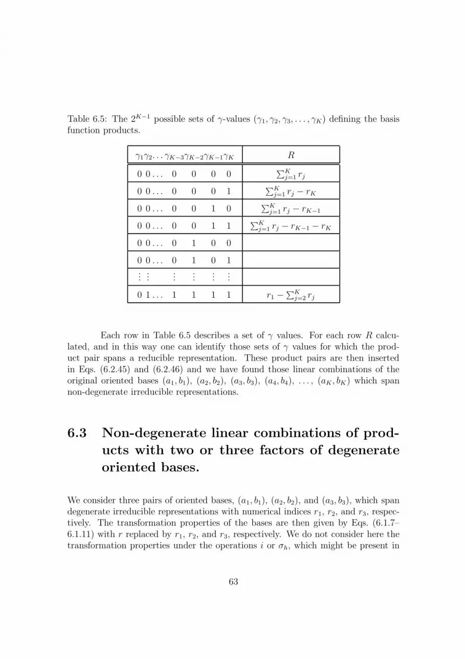
Table 6.5: The 2K−1 possible sets of γ-values (γ1, γ2, γ3, . . . , γK) defining the basisfunction products.

γ1γ2. . . γK−3γK−2γK−1γK R

0 0 . . . 0 0 0 0∑K

j=1 rj

0 0 . . . 0 0 0 1∑K

j=1 rj − rK

0 0 . . . 0 0 1 0∑K

j=1 rj − rK−1

0 0 . . . 0 0 1 1∑K

j=1 rj − rK−1 − rK

0 0 . . . 0 1 0 0

0 0 . . . 0 1 0 1...

......

......

...

0 1 . . . 1 1 1 1 r1 −∑K

j=2 rj

Each row in Table 6.5 describes a set of γ values. For each row R calcu-lated, and in this way one can identify those sets of γ values for which the prod-uct pair spans a reducible representation. These product pairs are then insertedin Eqs. (6.2.45) and (6.2.46) and we have found those linear combinations of theoriginal oriented bases (a1, b1), (a2, b2), (a3, b3), (a4, b4), . . . , (aK, bK) which spannon-degenerate irreducible representations.

6.3 Non-degenerate linear combinations of prod-

ucts with two or three factors of degenerate

oriented bases.

We consider three pairs of oriented bases, (a1, b1), (a2, b2), and (a3, b3), which spandegenerate irreducible representations with numerical indices r1, r2, and r3, respec-tively. The transformation properties of the bases are then given by Eqs. (6.1.7–6.1.11) with r replaced by r1, r2, and r3, respectively. We do not consider here thetransformation properties under the operations i or σh, which might be present in

63

Table 6.6: γ-diagram for product pairs A(γ1, γ2) and A(1− γ1, 1− γ2) involving twodegenerate bases.

γ1 γ2 R

0 0 r1 + r2

0 1 r1 − r2

the molecular point group, since we can easily obtain them from the rules:

g ⊗ g = g

u ⊗ u = g

g ⊗ u = u′ ⊗ ′ = ′

′′ ⊗ ′′ = ′

′ ⊗ ′′ = ′′ (6.3.47)

Hence we concentrate on the symmetry labels A, B, and Er.

We will use here the γ-diagram of Table 6.5 for products involving two orthree factors of degenerate oriented bases. We aim at constructing linear combi-nations of these products with symmetries A1 + A2 or B1 + B2 (where A1 + A2

should be understood as Σ+ + Σ− for the groups C∞v and D∞h).

For products of two degenerate basis functions we obtain the γ-diagram ofTable 6.6.

In order to obtain a product pair with symmetry A1 + A2 we need R = Nt(or R = 0 for linear molecules) and in order that the product pair has symmetryB1 + B2, we must have R = N

2(2t + 1). However, the possible values of r1 and r2

are restricted to rj = 1, 2, 3, . . . , N−12

for N odd and rj = 1, 2, 3, . . . , N2− 1 for

N even. For odd N we thus obtain 2 ≤ r1 + r2 ≤ N − 1 and −N−32

≤ r1 − r2≤ N−3

2. The only possibility of obtaining the irreducible representation A1 + A2 is

consequently R = r1 − r2 = 0, i.e., r1 = r2. There exist no B1 or B2 irreduciblerepresentations for groups with odd N and so we cannot construct a product pairwith these symmetries. For even N , however, we have 2 ≤ r1 + r2 ≤ N − 2 and−N

2+ 2 ≤ r1 − r2 ≤ N

2− 2. In this case we have A1 + A2 symmetry for r1 − r2 =

0, i.e., r1 = r2, and B1 + B2 symmetry for r1 + r2 = N2. The symmetrized linear

64

Table 6.7: Symmetrized product pairs A(γ1, γ2) and A(1− γ1, 1− γ2) involving twodegenerate bases.

Linear combination Symmetry r1, r2 Groups

(a1 + ib1)(a2 − ib2) A1 + A2 r1 = r2 All groups

±(a1 − ib1)(a2 + ib2)

(a1 + ib1)(a2 + ib2) B1 + B2 r1 + r2 CNv (N even), DNh (N even),

±(a1 − ib1)(a2 − ib2) = N2

DN/2d.

Table 6.8: γ-diagram for product pairs A(γ1, γ2, γ3) and A(1 − γ1, 1 − γ2, 1 − γ3)involving three degenerate bases.

γ1 γ2 γ3 R

0 0 0 r1 + r2 + r3

0 0 1 r1 + r2 − r3

0 1 0 r1 − r2 + r3

0 1 1 r1 − r2 − r3

combinations, the conditions on r1 and r2, and the point groups for which theseconditions can be fulfilled, are given in Table 6.7.

For products involving three factors of the degenerate bases (a1, b1), (a2, b2),and (a3, b3), the γ-diagram is given in Table 6.8.

The symmetrized linear combinations are given in Table 6.9.

In Table 6.9 we have not listed the two cases r2 = r1 + r3 and r1 = r2 + r3;they are completely analogous to the case r3 = r1 + r2.

65

Table 6.9: Symmetrized product pairs A(γ1, γ2, γ3) and A(1 − γ1, 1 − γ2, 1 − γ3)involving three degenerate bases.

Linear combination Symmetry r1, r2 Groups

(a1 + ib1)(a2 + ib2)(a3 + ib3) A1 + A2 r1 + r2 CNv,

±(a1 − ib1)(a2 − ib2)(a3 − ib3) +r3 = N DNh (N 6= 4),

DNd,

DN/2d (N 6= 2).

(a1 + ib1)(a2 + ib2)(a3 − ib3) A1 + A2 r3 = r1 + r2 CNv, DNh,

±(a1 − ib1)(a2 − ib2)(a3 + ib3) DNd, (N ≥ 5),

DN/2d (N ≥ 4).

66

Chapter 7

The basis functions

7.1 Transformation properties

We describe here the transformation properties of the basis functions |V LJKM〉[Section 4] under the operations of the molecular point groups. The treatment givenhere exactly follows that of Hegelund et al. (1973).

Table 7.1 summarizes the generating operations defined for the most im-portant point groups for symmetric tops and linear molecules (Chapter 5). It canbe shown that the harmonic oscillator-rigid rotor basis functions have the followingtransformation properties under these generating operations:

R+ |V LJKM〉 = exp[i2π

Nϕ]|V LJKM〉 (7.1.1)

R′+|V LJKM〉 = (−1)η|V LJKM〉; (7.1.2)

R− |V LJKM〉 = (−1)ρ|V − LJ −KM〉 (7.1.3)

The quantities ϕ, η, and ρ defining the transformation properties are givenin Table 7.2. In the table, the quantity t is any integer. In the expressions for ϕ,t is chosen such that −N

2< ϕ ≤ N

2. In the expressions for ρ and η, t is chosen so

that ρ = 0 or 1 and τ = 0 or 1. The sum∑

j rj`j in the definition of ϕ runs overall degenerate normal modes of the molecule in question. Here, rj is the numericalindex on the symmetry symbol Erj

spanned by the j’th normal vibration. For pointgroups with N ≤ 4 no numerical indices occur and all rj = 1. The summations

67

Table 7.1: Generating operations.

Molecular point group R+ R′+ R−

CNv (N ≥ 3) CN σ(xz)

DNh (N ≥ 3; N odd) CN σh C(x)2

DNh (N ≥ 4; N even) CN i C(x)2

DNd (N ≥ 3; N odd) CN i C(x)2

D(N/2)d (N/2 ≥ 2; N/2 even) SN C(x)2

C∞v C(φ)∞ σ(xz)

D∞h C(φ)∞ i C

(x)2

∑vB,

∑vA2

,∑vB2

,∑vΣ+

urepresent sums over the v quantum numbers belonging

to non-degenerate normal modes with symmetries B, A2, B2, and Σ+u , respectively.

The summations∑vu and

∑v(′′), represent sums over the v quantum numbers

belonging to non-degenerate or degenerate normal modes with symmetries of typeu or ′′, respectively.

Equations (7.1.1–7.1.3) show that the two basis functions |V LJKM〉 and|V −LJ −KM〉 form the basis for a two-dimensional representation with the char-acter

exp[i2π

Nϕ]

+ exp[−i 2π

Nϕ]

= 2 cos[2π

Nϕ]

under the R+ operation. From the tables of irreducible representations in Chapter 5we now see that if ϕ = 0, the two-dimensional representation is reducible and of typeA1 + A2. For ϕ = N

2, the two-dimensional representation is also reducible and of

type B1 + B2. In all other cases, the two basis functions span an irreducible, doublydegenerate representation E|ϕ|. Hence we can distinguish the two cases which wecall here Type I and Type II basis functions.

7.1.1 Type I (ϕ 6= 0 and ϕ 6= N2 )

The two basis functions |V LJKM〉 and |V − LJ − KM〉 form the basis for anirreducible, doubly degenerate representation E|ϕ|. No further symmetrization of

68

Table 7.2: Transformation properties of the basis functions

CNv (N ≥ 3; N odd) ϕ = K −∑rj`j +Nt

ρ = J +K +∑vA2

+ 2t

CNv (N ≥ 4; N even) ϕ = K −∑rj`j + (N/2)

∑vB +Nt

ρ = J +K +∑vA2

+∑vB2

+ 2t

DNh (N ≥ 3; N odd) ϕ = K −∑rj`j +Nt

η = K +∑v(′′) + 2t

ρ = J +∑vA2

+ 2t

DNh (N ≥ 4; N even) ϕ = K −∑rj`j + (N/2)

∑vB +Nt

η =∑vu + 2t

ρ = J +∑vA2

+∑vB2

+ 2t

DNd (N ≥ 3; N odd) ϕ = K −∑rj`j +Nt

η =∑vu + 2t

ρ = J +∑vA2

+ 2t

D(N/2)d (N/2 ≥ 2; N/2 even) ϕ = K −∑rj`j + (N/2) [

∑vB +K] +Nt

ρ = J +∑vA2

+∑vB2

+ 2t

C∞v ϕ = 0

ρ = J +∑`j + 2t

D∞h ϕ = 0

η =∑vu + 2t

ρ = J +∑vΣ+

u+ 2t

the basis functions is possible.

69

7.1.2 Type II (ϕ = 0 or ϕ = N2 )

The two basis functions |V LJKM〉 and |V −LJ−KM〉 form the basis for a reducibletwo-dimensional representation A1 + A2 or B1 + B2. In this case, it is easy to verifythat the new basis functions

|V LJKMτ〉 =1√2

[|V LJKM〉 + (−1)ρ+τ |V − LJ −KM〉

], (7.1.4)

where τ = 0 or 1, have the following transformation properties

R+ |V LJKMτ〉 = exp[i2π

Nϕ]|V LJKMτ〉 (7.1.5)

R′+|V LJKMτ〉 = (−1)η|V LJKMτ〉; (7.1.6)

R− |V LJKMτ〉 = (−1)τ |V LJKMτ〉. (7.1.7)

Hence the new basis functions |V LJKMτ〉 span non-degenerate irreducible repre-sentations A1, A2, B1, or B2 in the molecular point group. A special case of a TypeII basis function occurs when K = 0 and all `j = 0 (we refer to this as the K = L= 0 case). We define the corresponding symmetrized basis function as

|V 0J0Mτ〉 = |V 0J0M〉 (7.1.8)

where, by definition, τ = ρ. We say that the basis function is of Type II’. It has thetransformation properties given by Eqs. (7.1.1–7.1.3).

7.2 Selection rules

7.2.1 Hamiltonian matrix elements

On the basis of the results derived in the preceding sections we can immediatelydraw a few conclusions. The first conclusion is concerned with matrix elements of theHamiltonian 〈V ′L′JK ′M |H|V LJKM〉. Unless the two basis functions |V ′L′JK ′M〉and |V LJKM〉 have the same symmetry in the molecular point group, the matrixelement vanishes, i.e., 〈V ′L′JK ′M |H|V LJKM〉 = 0. The symmetry of a basisfunction is determined from the two quantum numbers ϕ and η. Hence for Type Ibasis functions we have

〈V ′L′JK ′M |H|V LJKM〉 6= 0 requires

{∆ϕ = ϕ′ − ϕ = 0∆η = η′ − η = 0

(7.2.9)

70

Type II basis functions are further characterized by the quantum number τ and wehave

〈V ′L′JK ′Mτ ′|H|V LJKMτ〉 6= 0 requires

∆ϕ = ϕ′ − ϕ = 0∆η = η′ − η = 0∆τ = τ ′ − τ = 0

(7.2.10)

It follows from Eqs. (7.2.9) and (7.2.10) that an eigenfunction |ψ〉 of H,obtained through the diagonalization of the matrix representation for H in the basis|V LJKM〉 can be written as linear combination of basis function |V LJKM〉 withcommon values for ϕ, η and, for Type II basis functions, τ , i.e.,

|ψ〉 =∑

V LK

cV LK |V LJKM〉 (7.2.11)

for Type I functions, and

|ψ〉 =∑

V LK

cV LK|V LJKMτ〉 (7.2.12)

for Type II functions. In Eqs. (7.2.11) and (7.2.12), all basis functions |V LJKM〉(or |V LJKMτ〉) have the same values for ϕ and η.

7.2.2 Transition moments

The intensities of electric dipole transitions in molecules are proportional to transi-

tion moments of the type |〈ψi|µA|ψf 〉|2 where |ψi〉 and |ψf〉 are the rotation-vibrationwavefunctions for the initial and final states of the transition, respectively, and µA

is a component of the molecular dipole moment along the space fixed axis A = X,Y , or Z. In order that the transition moment does not vanish, it is necessary thatthe product

A = ψ∗i µA ψf (7.2.13)

contain the totally symmetric irreducible representation of the molecular pointgroup. The symmetry of µA is always such that µA is unchanged under any rotationin the molecular point group, but it changes sign under any improper operation (re-flection, inversion, improper rotation). It is straightforward to derive the followingtransformation properties of A under the various types of generating operations

CN A = exp(−i2π

N∆ϕ

)A (7.2.14)

71

Table 7.3: Selection rules.

Molecular point group Selection rules

CNv (N ≥ 3) ∆ϕ = 0 ∆τ = 1 + 2tDNh (N ≥ 3) ∆ϕ = 0 ∆η = 1 + 2t ∆τ = 0DNd (N ≥ 3; N odd) ∆ϕ = 0 ∆η = 1 + 2t ∆τ = 0D(N/2)d (N/2 ≥ 2; N/2 even) ∆ϕ = N

2+Nt ∆τ = 0

C∞v ∆τ = 1 + 2tD∞h ∆η = 1 + 2t ∆τ = 0

SN A = exp(−i2π

N

[N

2+ ∆ϕ

])A (7.2.15)

i A = (−1)∆η+1A (7.2.16)

σhA = (−1)∆η+1A (7.2.17)

C2A = (−1)∆τA (7.2.18)

σv A = (−1)∆τ+1A (7.2.19)

From these equations, one obtains the selection rules given in Table 7.3.

In order to calculate the transition moment |〈ψi|µA|ψf〉|2 it is necessary toexpress the space fixed dipole moment component µA through the dipole momentcomponents µα, α = x, y, or z, along the molecule-fixed axes. We have

µA =∑

α=x,y,z

µαλAα (7.2.20)

where the quantities λAα are direction cosines effecting the transformation betweenthe space fixed and the molecule fixed coordinate system. The direction cosinesdepend on the three Euler angles θ, φ, and χ whereas the dipole moment componentsµα depend on the vibrational coordinates qj.

In the simplest possible approximation to the rotation-vibration problemwe take the molecular wavefunction to be equal to the basis functions |V LJKM〉,i.e.,

|ψ〉 = |V LJKM〉. (7.2.21)

72

In this case we have

|〈ψi|µA|ψf 〉|2 =

∣∣∣∣∣

⟨ViLiJiKiMi

∣∣∣∣∣∑

α=x,y,z

µαλAα

∣∣∣∣∣VfLfJfKfMf

⟩∣∣∣∣∣

2

(7.2.22)

or

|〈ψi|µA|ψf 〉|2 =

∣∣∣∣∣∑

α=x,y,z

〈ViLi |µα|VfLf 〉 〈JiKiMi |λAα| JfKfMf 〉∣∣∣∣∣

2

. (7.2.23)

In this approximation, allowed transitions must fulfill the vibrational selection rulesdefined by

〈ViLi |µα|VfLf〉 6= 0. (7.2.24)

Problem 7.1.

• Derive the selection rules for dipole absorption transitions in a linear moleculewith point group D∞h.

• Consider the vibrational ground state and a fundamental state with Σ+u sym-

metry. Label the invidual J levels with their symmetry in D∞h. Determinethe allowed transitions between the two vibrational states.

• Consider a degenerate fundamental vibrational state νj with symmetry Πg orΠu. Take into account the rotational `-doubling in νj and assume that thestate given by the rotation-vibration wavefunction

|ψ+〉 =1√2

[|V `j = 1 J K = 1M〉 + |V `j = −1 J K = −1M〉]

has higher energy than that given by

|ψ−〉 =1√2

[|V `j = 1 J K = 1M〉 − |V `j = −1 J K = −1M〉] .

Label the invidual J levels with their symmetry in D∞h.

• Assign e and f labels to the rotation-vibration energy levels in the νj funda-mental levels. These labels are defined such that a state with parity p is an estate if

p (−1)J = +1

and an f state ifp (−1)J = −1

73

• Determine the selection rules on the e and f labels.

Problem 7.2. Consider the molecule H+3 . The equilibrium configuration of this

molecule is an equilateral triangle.

1. Determine the molecular point group of H+3 .

2. Determine the selection rules on the rotation-vibration symmetries for dipoleabsorption.

3. Show that if we approximate the rotation-vibration wavefunctions of H+3 as

simple products |V LJKM〉, rotational transitions within the vibrational groundstate are forbidden.

4. Show that such transitions nevertheless take place (even though they are veryweak) and explain the mechanism through which they attain non-zero inten-sities.

74

Chapter 8

Resonances

8.1 Resonance classification

A non-diagonal matrix element coupling two quasi-degenerate basis functions causesa resonance between the two basis states. The operator in H contributing to thenon-diagonal matrix element is called the resonance operator.

If the diagonal matrix elements for the two basis states are exactly equal, wetalk about a doubling as a special form of resonance. Since the diagonal elements ofH are invariant under a simultaneous sign change ofK and all ` quantum numbers, adoubling will always be found for the two basis states |V LJKM〉 and |V−LJ−KM〉,unless the matrix element coupling them is zero by symmetry. A doubling alwayshas ∆V = 0.

Resonances between two accidentally quasidegenerate states are called acci-

dental resonances. In order for an accidental resonance to be global, we must havethat [Eq. (4.3.40)] ∑

k

∆vkωk ≈ 0 (8.1.1)

and that the energy difference between the resonating basis states depends onlyweakly on K, i.e. [Eq. (4.3.43)]

(A− B)∆K −∑

j

Aζj∆`j ≈ 0. (8.1.2)

75

For a local accidental resonance the condition in Eq. (8.1.1) does not have to bevery well fulfilled. The local resonance is found for basis functions whose K valuesare given by Eq. (4.3.44)

K ≈ −∑

k ∆vkωk +{(A− B)∆K − 2

∑j Aζj∆`j − 2

∑j Aζj`j

}∆K

2[(A− B) ∆K −∑

j Aζj∆`j] . (8.1.3)

Hence a local resonance only influences a few sub-bands in a vibrational band,whereas a global resonance influences all sub-bands.

We speak about rotational and vibrational accidental resonances. A vibra-tional resonance is caused by operators hn,0, that is, by purely vibrational operators.The matrix elements of these operators are diagonal in the rotational quantum num-bers, and their values are independent of these quantum numbers. The expressionfor the energy difference between to interacting basis states in Eq. (4.3.41) is sim-plified to

∆E =∑

k

∆vkωk − 2AK∑

j

ζj∆`j. (8.1.4)

Since |ζj| < 1 and the ∆`j are small integers, the rotational contribution to ∆Ewill be small. Consequently, vibrational resonances are global. They are also calledFermi type resonances.

A rotational resonance is caused by non-diagonal matrix elements of theoperators hn,1 and hn,2. The matrix elements can be diagonal in K, and it will thenbe proportional to K or to K2. Rotational resonances with ∆K = 0 are global.Rotational resonances can also have ∆K = ±1 or ∆K = ±2, and such resonancescan be global or local. Rotational resonances are also called Coriolis type resonances.

Table 8.1 gives a summary of the possible values for |∑k ∆vkωk| correspond-ing to non-diagonal matrix elements of operators hn,m with n ≤ 4 and m = 0, 1, or2. By setting |∑k ∆vkωk| ≈ 0 one then obtains the resonance conditions which canbe formulated as a relation between the normal frequencies. The table also gives theaccepted names for some common resonances together with the operator containingthe resonance operators.

Until now we have discussed accidental resonances only on the basis ofthe possible quasidegeneracy of basis states. However, even if two basis states arequasidegenerate, the resonance between them will only be present if there exists anoperator in the Hamiltonian producing a non-zero matrix element between them.Such an operator must be totally symmetric in the molecular point group. The

76

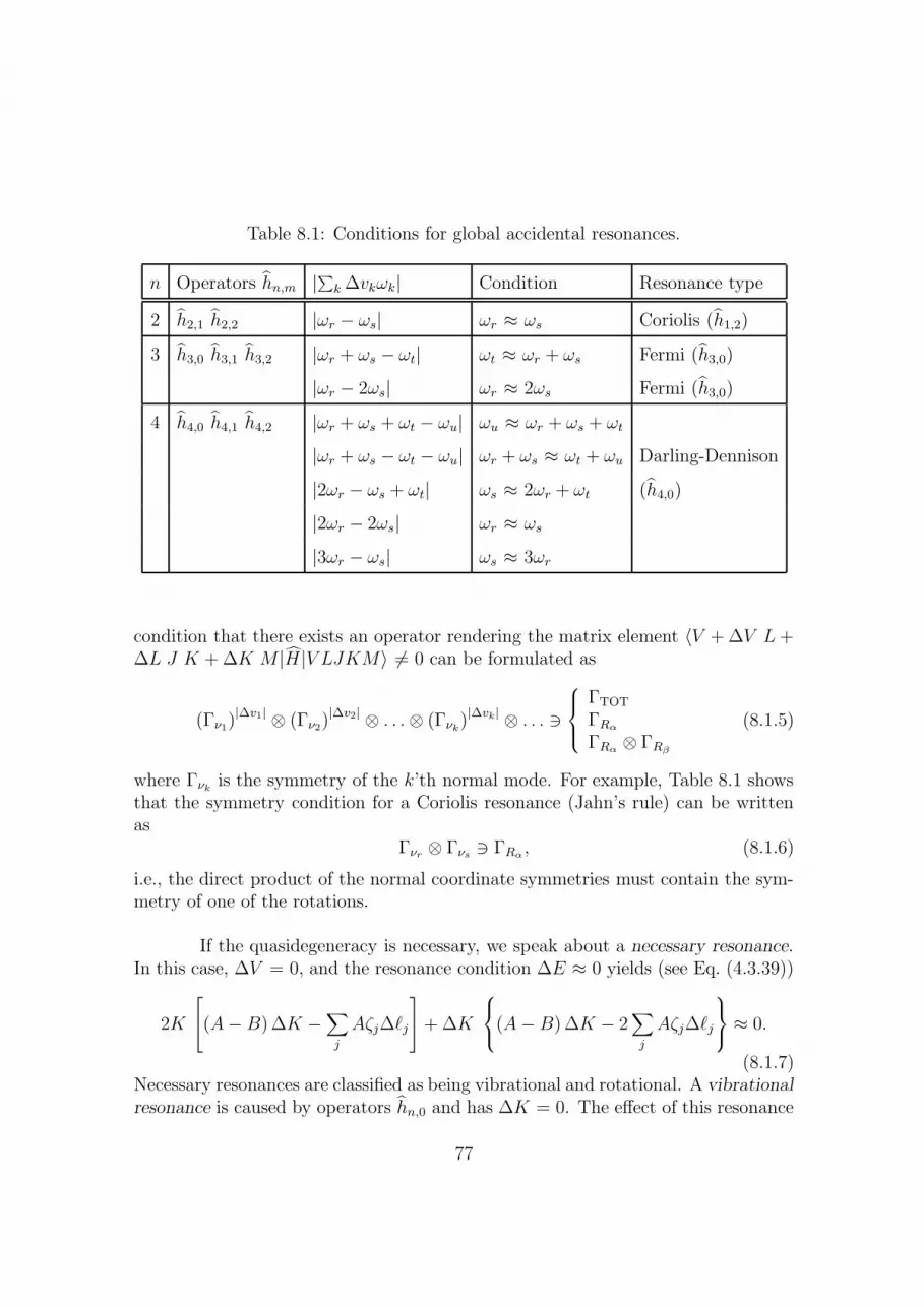
Table 8.1: Conditions for global accidental resonances.

n Operators hn,m |∑k ∆vkωk| Condition Resonance type

2 h2,1 h2,2 |ωr − ωs| ωr ≈ ωs Coriolis (h1,2)

3 h3,0 h3,1 h3,2 |ωr + ωs − ωt| ωt ≈ ωr + ωs Fermi (h3,0)

|ωr − 2ωs| ωr ≈ 2ωs Fermi (h3,0)

4 h4,0 h4,1 h4,2 |ωr + ωs + ωt − ωu| ωu ≈ ωr + ωs + ωt

|ωr + ωs − ωt − ωu| ωr + ωs ≈ ωt + ωu Darling-Dennison

|2ωr − ωs + ωt| ωs ≈ 2ωr + ωt (h4,0)

|2ωr − 2ωs| ωr ≈ ωs

|3ωr − ωs| ωs ≈ 3ωr

condition that there exists an operator rendering the matrix element 〈V + ∆V L+∆L J K + ∆K M |H|V LJKM〉 6= 0 can be formulated as

(Γν1)|∆v1| ⊗ (Γν2

)|∆v2| ⊗ . . .⊗ (Γνk)|∆vk| ⊗ . . . 3

ΓTOT

ΓRα

ΓRα⊗ ΓRβ

(8.1.5)

where Γνkis the symmetry of the k’th normal mode. For example, Table 8.1 shows

that the symmetry condition for a Coriolis resonance (Jahn’s rule) can be writtenas

Γνr⊗ Γνs

3 ΓRα, (8.1.6)

i.e., the direct product of the normal coordinate symmetries must contain the sym-metry of one of the rotations.

If the quasidegeneracy is necessary, we speak about a necessary resonance.In this case, ∆V = 0, and the resonance condition ∆E ≈ 0 yields (see Eq. (4.3.39))

2K

(A− B)∆K −

∑

j

Aζj∆`j

+ ∆K

(A− B) ∆K − 2

∑

j

Aζj∆`j

≈ 0.

(8.1.7)Necessary resonances are classified as being vibrational and rotational. A vibrational

resonance is caused by operators hn,0 and has ∆K = 0. The effect of this resonance

77

Table 8.2: Resonance terminology.

∆V ∆K ∆L Resonance type

0 Necessary

0 6=0 0 Necessary, rotational K-type

0 6=0 6=0 Necessary, rotational `-type

0 0 6=0 Necessary, vibrational `-type

6=0 Accidental

6=0 0, 6=0 0, 6=0 Accidental, rotational, Coriolis-type

6=0 0 0, 6=0 Accidental, vibrational, Fermi-type

is determined by the quantity∑

j Aζj∆`j; for∑

j Aζj∆`j ≈ 0 the resonance will havethe largest effect. Rotational resonances with ∆K 6= 0 will have the largest effectwhen the coefficient of K in Eq. (8.1.7) is small; i.e.

(A− B) ∆K ≈∑

j

Aζj∆`j. (8.1.8)

Rotational resonances that are diagonal in the ` quantum numbers are called K-type

resonances.

Finally we notice that doublings are special cases of necessary resonances.Table 8.2 gives a summary of the terminology used for resonances.

8.2 Necessary resonances and doublings

For symmetric top molecules and linear molecules, necessary resonances are takeninto account in the energy calculation for a given vibrational state through thesolution of the secular problem

det[〈V L′ J K ′ M |H|V LJKM〉 − E δLL′ δKK′

]= 0. (8.2.9)

78

We diagonalize here a matrix with dimension

d = (2J + 1)∏

j

(vj + 1) . (8.2.10)

However, we might be able to split this matrix into a number of sub-blocks by usingsymmetrized basis functions.

We diagonalize the contact transformed operator

H = H0 + H ′1 + H ′

2 + H ′3. (8.2.11)

The explicit form of these operators are given in Chapter II of Amat et al. (1971).With the notation

h′n,m = (q, p)n Jm (8.2.12)

introduced previously, we can express H as

H0 = h2,0 + h0,2

H ′1 = h′2,1

H ′2 = h′0,4 + h′1,3 + h′2,2 + h′3,1 + h′4,0

H ′2 = h′1,4 + h′2,3 + h′3,2 + h′4,1 + h′5,0 (8.2.13)

Only operators hn,m with even n contribute to matrix elements diagonal in the vquantum numbers. These operators are underlined in Eq. (8.2.13). The matrixelements of H are given in Chapter VIII of Amat et al. (1971).

8.2.1 Diagonal matrix elements

We will summarize here some well known results with the aim of identifying theoperators h′n,m producing the various contributions to the matrix elements of H. Adiagonal matrix element is given by

〈V L J K M |H|V LJKM〉 = G(V, L) + F (V, L, J,K) (8.2.14)

where

G(V, L) =∑

r

ωr

(vr +

dr

2

)+ +

∑

r≤r′Xrr′

(vr +

dr

2

)(vr′ +

dr′

2

)+∑

j≤j′gjj′`j`j′

(8.2.15)

79

Table 8.3: Diagonal matrix elements.

Operator Contribution to 〈V L J K M |H|V LJKM〉

H0 h2,0∑

r ωr

(vr + dr

2

)

h0,2 BV J(J + 1) + (AV − BV )K2

H ′1 h′2,1 −2

∑j Aeζ

(z)ja,jb `j K

H ′2 h′0,4 −DJ J

2(J + 1)2 −DJKJ(J + 1)K2 −DKK4

h′2,2 −∑r

[αB

r J (J + 1) +(αA

r − αBr

)K2] (vr + dr

2

)

h′4,0

∑r≤r′ Xrr′

(vr + dr

2

) (vr′ + dr′

2

)+∑

j≤j′ gjj′`j`j′

H ′3 h′2,3

∑j η

Jj `j J(J + 1)K +

∑j η

Kj `j K

3

h′4,1

∑r α

Aζjr

(vr + dr

2

)

and

F (V, L, J,K) = BV J(J + 1) + (AV − BV )K2 − 2∑

j

(Aζ

(z)ja,jb

)V`j K

− DJ J2(J + 1)2 −DJKJ(J + 1)K2 −DKK

4

+∑

j

ηJj `j J(J + 1)K +

∑

j

ηKj `j K

3 (8.2.16)

with

BV = Be −∑

r

αBr

(vr +

dr

2

), (8.2.17)

AV = Ae −∑

r

αAr

(vr +

dr

2

), (8.2.18)

and (Aζ

(z)ja,jb

)V

= Ae ζ(z)ja,jb −

∑

r

αAζjr

(vr +

dr

2

), (8.2.19)

Table 8.3 identifies the operators producing the various contributions to〈V L J K M |H|V LJKM〉.

80

Table 8.4: Matrix elements 〈V + ∆V L + ∆L J K + ∆K M |H|V LJKM〉.

Operator ∆L ∆K

H ′2 h′0,4 0 0, ±1, ±2, ±3, ±4

h′2,2 ∆`j = 0, ±2 0, ±1, ±2

h′4,0 ∆`j = 0, ±2, ±4 0

∆`j = 0, ±2; ∆`j′ = 0, ±2 0

H ′3 h′2,3 ∆`j = 0, ±2 0, ±1, ±2, ±3

h′4,1 ∆`j = 0, ±2, ±4 0, ±1

∆`j = 0, ±2; ∆`j′ = 0, ±2 0, ±1

8.2.2 Off-diagonal matrix elements

The operators H0 and H ′1 do not contribute to the off-diagonal matrix elements.

The different operators present in H ′2 and H ′

3 produce the matrix element typessummarized in Table 8.4.

We can reduce the number of non-vanishing matrix elements considerablythrough symmetry arguments. The general condition is

〈V + ∆V L + ∆L J K + ∆K M |H|V LJKM〉 6= 0 requires

{∆ϕ = 0∆η = 0

(8.2.20)

where ϕ and η are defined in Table 7.2.

For necessary resonances these conditions reduce to

∆K −∑j rj`j = Nt G = CNv, DNh, DNd, (N odd).

∆K −∑j rj`j = N

2∆K +Nt G = D(N/2)d, (N/2 even).

∆K = 2t G = DNh, (N odd).

In Table 8.5 we apply these conditions for second order resonances.

81

Table 8.5: Second order necessary resonances.

Symmetry condition ∆L ∆K Point group

K-type resonance (h′0,4)

∆K = Nt ∆L = 0 ±4 C4v, D4h

∆K = Nt ∆L = 0 ±3 C3v, D3d

Rotational `-type resonance (h′2,2)

∆K − rj∆`j = Nt ∆`j = ±2 ±2 All point groups. rj = 1.

∆K − rj∆`j = Nt ∆`j = ±2 ∓2 CNv, DNh, N even, rj = N2− 1

∆K − rj∆`j = Nt ∆`j = ±2 ∓1 CNv, DNd, N odd, rj = N−12

∆K − rj∆`j = N2

+Nt ∆`j = ±2 ±2 D(N/2)d, rj = 1

∆K − rj∆`j = N2

+Nt ∆`j = ±2 ∓2 D(N/2)d, rj = N2− 1

Vibrational `-type resonance (h′4,0)

rj∆`j = Nt ∆`j = ±4 0 C4v, D4h, D2d

rj∆`j + rj′∆`j′ = Nt ∆`j = 0 All point groups, rj = rj′.

−∆`j′ = ±2

If the off-diagonal matrix element is 〈V − L J −K M |H|V LJKM〉, thatis, if

L = −∆L

2and K = −∆K

2

the resonance causes a doubling. In order that a doubling can occur, ∆L and∆K must contain even numbers only. Consequently, all the necessary second orderresonances except theK-type resonance with (∆L,∆K) = (0,±3) and the rotational`-type resonance with (∆L,∆K) = (±2, 1) can produce doublings. The conditionsfor doublings are given in Table 8.6.

82

Table 8.6: Second order doublings.

Doubling type (∆L,∆K) (L,K) Point group

K-type (0,±4) (0,±2) C4v, D4h, D2d

Rotational `-type (±2,±2) (±1,±1) All point groups, rj = 1.

(±2,∓2) (±1,∓1) CNv, DNh, D(N/2)d, N even,

rj = N2− 1.

Vibrational `-type (±4, 0) (±2, 0) C4v, D4h, D2d

(±2,∓2, 0) (±1,∓1, 0) All point groups, rj = rj′.

8.2.3 Doublings

The secular problem for a doubling has the form

|V LJKM〉|V − LJ −KM〉

∣∣∣∣∣E0 − ε WW ∗ E0 − ε

∣∣∣∣∣ = 0 (8.2.21)

where

E0 = 〈V LJKM |H |V LJKM〉 = 〈V − LJ −KM |H|V − LJ −KM〉 (8.2.22)

and

W = 〈V LJKM |H|V − LJ −KM〉 = 〈V − LJ −KM |H|V LJKM〉∗ (8.2.23)

since the basis functions has the same value for the quantum number ρ (see Table7.2). For the quantum number ϕ we obtain

ϕ′ = −ϕ+Nt1 and ϕ′ = ϕ+Nt2 (8.2.24)

which yields

ϕ =N

2t (8.2.25)

so that the basis functions must be of Type II (Chapter 7) in the case of doubling.

Type II symmetrized basis functions are defined by Eq. (7.1.4):

|V LJKMτ〉 =1√2

[|V LJKM〉 + (−1)ρ+τ |V − LJ −KM〉

](8.2.26)

83

where τ = 0 or 1. The symmetry properties under the generating operation R− aregiven by

R− |V LJKMτ〉 = (−1)τ |V LJKMτ〉. (8.2.27)

If we use the symmetrized functions as basis set, we obtain the matrix elements

〈V LJKMτ ′|H|V LJKMτ〉 = δττ ′

[E0 + (−1)ρ+τ W

](8.2.28)

so that the secular problem is now diagonal. The eigenenergies are given by

〈V LJKMτ |H |V LJKMτ〉 =[E0 + (−1)ρ+τ W

]. (8.2.29)

The separation between the “doubled” levels is

∆E = E(τ = 0) − E(τ = 1) = 2 (−1)ρW. (8.2.30)

Cartwright and Mills (1970) treat the details of the (±2,±2) rotational

`-type doubling also known as the q(+)t -doubling. For this doubling,

K = `t = ±1 (8.2.31)

and

|W | =1

4|q(+)

t | (vt + 1) J(J + 1). (8.2.32)

Hence, the energy separation between the split levels in a fundamental vibrationalstate with vt = 1 is given by

∆E = E(τ = 0) − E(τ = 1) = ±q(+)t J(J + 1). (8.2.33)

The plus or minus sign in Eq. (8.2.33) (and thus the sign of the constant q(+)t )

is chosen through conventions. We will mention here the conventions suggested byHerzberg (1945) and by Cartwright and Mills (1970) and “translate” these defintionsto the τ -formalism of Chapter 7.

For C∞v molecules, Herzberg (1945) suggested the following convention

E(Σ−) − E(Σ+) = (−1)Jq(+)t J(J + 1) (8.2.34)

for a fundamental level.

According to Chapter 5 the generating operation R− for C∞v is chosen asσ(xz) and the character table shows that Σ− corresponds to τ = 1 (that is, char-acter −1 under σ(xz)) and Σ+ corresponds to τ = 0 (character +1 under σ(xz)).Consequently, Herzberg’s convention implies that

E(Σ−) − E(Σ+) = E(τ = 1) − E(τ = 0) = (−1)Jq(+)t J(J + 1). (8.2.35)

84

For IR-active fundamental levels in D∞h molecules, Herzberg (1945) sug-gested the

E(Σ−u ) − E(Σ+

u ) = (−1)Jq(+)t J(J + 1) (8.2.36)

which implies that

E(Σ−u ) − E(Σ+

u ) = E(τ = 0) − E(τ = 1) = (−1)Jq(+)t J(J + 1). (8.2.37)

The difference between C∞v and D∞h molecules is only due to the fact that theR−-operation is chosen differently for these two point groups.

For C3v-molecules, Cartwright and Mills (1970) suggested

E (A1) − E (A2) = (−1)Jq(+)t J(J + 1) (8.2.38)

for a fundamental level. This is equivalent to

E (A1) − E (A2) = E(τ = 0) − E(τ = 1) = (−1)Jq(+)t J(J + 1). (8.2.39)

Based on the considerations in Chapter 7, it would be possible to introducea simple, general definition of the `-doubling constant as

E(τ = 1) − E(τ = 0) =1

2(−1)ρq

(+)t (vt + 1)J(J + 1). (8.2.40)

This definition is valid for all point groups and does not depend on the fundamentallevel being IR or Raman active. Further it would be easy to extend this definitionto other types of doublings.

The definition in Eq. (8.2.40) is equivalent to including the `-doubling as

E(τ) = E0 −1

4(−1)ρ+τq

(+)t (vt + 1)J(J + 1). (8.2.41)

so that the effect of the doubling is to change the rotational constant B for the levelto

BV → B∗V = BV − 1

4(−1)ρ+τq

(+)t (vt + 1) . (8.2.42)

For transitions from K ′′ = `′′ = 0 to K ′ = `′ = ±1, i.e., for the K ′′ = 0subband for a usual perpendicular band, the ground state levels are of type II’ andhave τ ′′ = ρ′′. In this case, the selection rule for τ is

τ ′ = τ ′′ + 2t for G = DNh, DNd, D∞h. (8.2.43)

85

orτ ′ = τ ′′ + 2t+ 1 for G = CNv, C∞v. (8.2.44)

The quantum number ρ is defined as

ρ = J + 2t for G = DNh, DNd, D∞h. (8.2.45)

orρ = J +K + 2t for G = CNv, C∞v. (8.2.46)

This means that transitions of the type II′ → II, where only the upper state isdoubled, will involve one of the doubled components only. The selection rules yieldthat ∆B∗ for the allowed transitions of molecules belonging to the point groups G= DNh, DNd, and D∞h is given by

∆B∗ = ∆B − 1

4(−1)ρ′+τ ′

q(+)t (v′t + 1)

= ∆B − 1

4(−1)J ′+τ ′

q(+)t (v′t + 1)

= ∆B − 1

4(−1)∆Jq

(+)t (v′t + 1) (8.2.47)

whereas for G = CNv and C∞v we obtain

∆B∗ = ∆B − 1

4(−1)J ′+1+J ′′

q(+)t (v′t + 1)

= ∆B − 1

4(−1)∆J+1q

(+)t (v′t + 1) (8.2.48)

This shows that P and R branches have one value for ∆B, whereas Q branches haveanother value. These ∆B-values are related through

∆B∗(P,R) − ∆B∗(Q) =1

2q(+)t (vt + 1) (8.2.49)

Problem 8.1. We consider the Coriolis resonance taking place when two normalfrequencies ωr and ωs are approximately equal (Table 8.1) for a C3v molecule. Theνr normal mode has A1 symmetry and the νs mode has E symmetry.

1. Use the results from Chapter 3 to determine the general form of the operatorcausing this resonance.

2. Use the results from Chapter 6 to determine the exact form of the resonanceoperator.

86

3. Use the results from Chapter 7 to determine ∆L and ∆K so that 〈V +∆V L+∆L J K + ∆K M |H|V LJKM〉 6= 0.

4. Use Appendix B to derive expressions for the non-vanishing matrix elementsof the resonance operator between states with (vr, vs) = (1,0) and (0,1), re-spectively.

Problem 8.2. We consider the Coriolis resonance taking place when two normalfrequencies ωr and ωs are approximately equal (Table 8.1) for a D2d molecule. Theνr normal mode has A1 symmetry and the νs mode has E symmetry. Answer thequestions already posed in Problem 8.1.

Problem 8.3. We consider the Fermi resonance taking place for ωr ≈ 2ωs in aC3v molecule. Both normal modes involved have E symmetry. Answer the questionsalready posed in Problem 8.1. The non-vanishing matrix elements of the resonanceoperator are calculated between states with (vr, vs) = (1,0) and (0,2), respectively.

Problem 8.4. In this rather complicated problem we will derive an expression forthe rotational `-doubling constant q

(+)t for a linear molecule with C∞v symmetry.

We shall show that the rotational `-doubling originates mainly in the operator

h2,1 = h2∑

α=x,y,z

παJα

I0αα

of Table 3.1. Rotational `-doubling in a degenerate fundamental level of a linearmolecule is caused by a matrix element coupling the two states |vt = 1, `t = 1, J,K =1,M〉 and |vt = 1, `t = −1, J,K = −1,M〉. This matrix element is produced throughthe mechanism given in Eq. (4.3.46).

1. Study Table 4.2 to find the possible values of (∆`t,∆K) for non-vanishingmatrix elements of h2,1.

87

2. Consider now Eq. (4.3.46). We intend to use this equation with

|V L′JK ′M〉 = |vt = 1, `t = 1, J,K = 1,M〉,|V LJKM〉 = |vt = 1, `t = −1, J,K = −1,M〉.

and we consider here only the perturbation

H1 = h2,1.

Which values of `t and K must the intermediate state |V L′′JK ′′M〉 in Eq.(4.3.46) have in order that both matrix elements involving this state can benon-vanishing?

3. Use the results from Sections 6.1 and 6.3 (in particular Tables 6.6 and 6.7) tofind the parts of h2,1 which can produce the desired matrix elements.

4. Use the matrix elements from Appendix B to calculate the matrix elementbetween the basis functions |vt = 1, `t = 1, J,K = 1,M〉 and |vt = 1, `t =−1, J,K = −1,M〉. from Eq. (4.3.46). Show that the result is consistent withthe expression

q(+)t =

2B2e

ωt

∑

s

ζ2st

3ω2t + ω2

s

ω2s − ω2

t

88

Chapter 9

References

Aliev, M.R., and Watson, J.K.G., 1985, in: “Molecular Spectroscopy: Modern Re-search”, Vol. III, K. Narahari Rao, ed., Academic Press, Orlando.

Amat, G., Nielsen, H.H., and Tarrago, G., 1971, “Rotation-Vibration of PolyatomicMolecules”, Marcel Dekker, New York.

Born, M., and Oppenheimer, J.R., 1927, Ann. der Physik 84:457.

Bunker, P.R., 1979, “Molecular Symmetry and Spectroscopy”, Academic Press, NewYork.

Bunker, P.R., and Moss, R.E., 1980, J. Mol. Spectrosc. 80:217.

Cartwright, G.J., and Mills, I.M., 1970, J. Mol. Spectrosc. 34:415.

Darling, B.T., and Dennison, D.M., 1940, Phys. Rev. 57:128.

Eckart, C., 1935, Phys. Rev. 47:552.

Goldsmith, M., Amat, G., and Nielsen, H. H., 1956, J. Chem. Phys. 24:1178.

Gordy, W., and Cook, R.L., 1970, “Microwave Molecular Spectra”, John Wiley &Sons, New York.

Hegelund, F., Rasmussen, F., and Brodersen, S., 1973, J. Raman Spectrosc. 1:433.

Herzberg, G., 1945, “Molecular Spectra and Molecular Structure. II. Infrared andRaman Spectra of Polyatomic Molecules”, Van Nostrand, Princeton, NJ.

Hougen, J.T., Bunker, P.R., and Johns, J.W.C., 1970, J. Mol. Spectrosc. 34:136.

Hoy, A.R., and Bunker, P.R., 1974, J. Mol. Spectrosc. 52:439.

Hoy, A.R., and Bunker, P.R., 1979, J. Mol. Spectrosc. 74:1.

Hoy, A.R., Mills, I.M., and Strey, G., 1972, Mol. Phys. 24:1265.

Jensen, P., 1983, Comp. Phys. Rep. 1:1.

Jensen, P., and Bunker, P.R., 1983, J. Mol. Spectrosc. 99:348.

89

Jensen, P., and Bunker, P.R., 1986, J. Mol. Spectrosc. 118:18.

Landau, L.D., and Lifshitz, E.M., 1985, “Lehrbuch der Theoretischen Physik”, Vol.III, “Quantenmechanik”, Akademie-Verlag, Berlin (Ost).

Maes, S., and Amat, G., 1957, Cah. Phys. 11:25.

Nielsen, H.H., 1951, Rev. Mod. Phys. 23:90.

Oka, T., 1967, J. Chem. Phys. 47:5410.

Papousek, D., and Aliev, M.R., 1982, “Molecular Vibrational-Rotational Spectra”,Elsevier, Amsterdam.

Sayvetz, A., 1939, J. Chem. Phys. 7:383.

Sutcliffe, B.T., and Tennyson, J., 1991, Int. J. Quant. Chem. XXXIX:183.

Watson, J.K.G., 1967, J. Chem. Phys. 46:1935.

Watson, J.K.G., 1968a, Mol. Phys. 15:479.

Watson, J.K.G., 1968b, J. Chem. Phys. 48:181.

Watson, J.K.G., 1968c, J. Chem. Phys. 48:4517.

Watson, J.K.G., 1977, in: “Vibrational Spectra and Structure”, J. Durig, ed., Vol.6, Elsevier, Amsterdam.

Wilson, E.B., 1939, J. Chem. Phys. 7:1047.

Wilson, E.B., and Howard, J.B., 1936, J. Chem. Phys. 4:260.

Wilson, E.B., Decius, J.C., and Cross, P., 1955, “Molecular Vibrations”, McGraw-Hill, New York.

90

Appendix A

The antisymmetric tensor

The elements of the unit antisymmetric tensor are defined as

exyz = eyzx = ezxy = +1

exzy = ezyx = eyxz = −1

(A.0.1)

If any pair of indices in αβγ are equal, eαβγ = 0.

91

Appendix B

Matrix elements of rotational andvibrational operators

This appendix lists matrix elements of rotational and vibrational operators. Thephases of the vibrational basis functions |vi〉, |vj`j〉 and of the rotational basis func-tions |JKM〉 are chosen as in the paper by Hegelund et al. (1973).

B.1 Rotational operators

The expressions given in this section are valid for the groups CNv, DNh, DNd, C∞v,and D∞h. For the groups DN/2d the expressions are also valid provided that J(0)

and J(1) are interchanged (see Eqs. (6.1.31) and (6.1.32)).

J(0)|J K M〉 = −i√J(J + 1) −K(K − 1) |J K − 1 M〉 (B.1.1)

J(1)|J K M〉 = i√J(J + 1) −K(K + 1) |J K + 1 M〉 (B.1.2)

Jz|J K M〉 = K |J K M〉 (B.1.3)

J(0)2|J K M〉 = −√J(J + 1) −K(K − 1)

×√J(J + 1) − (K − 1)(K − 2) |J K − 2 M〉 (B.1.4)

92

J(1)2|J K M〉 = −√J(J + 1) −K(K + 1)

×√J(J + 1) − (K + 1)(K + 2) |J K + 2 M〉 (B.1.5)

[J(0)J(1) + J(1)J(0)

]|J K M〉 = 2

[J(J + 1) −K2

]|J K M〉 (B.1.6)

[J(0)Jz + JzJ(0)

]|J K M〉 = [2K − 1] J(0)|J K M〉 (B.1.7)

[J(1)Jz + JzJ(1)

]|J K M〉 = [2K + 1] J(1)|J K M〉 (B.1.8)

J(0)3|J K M〉 = i√J(J + 1) −K(K − 1)

×√J(J + 1) − (K − 1)(K − 2)

×√J(J + 1) − (K − 2)(K − 3) |J K − 3 M〉 (B.1.9)

J(1)3|J K M〉 = −i√J(J + 1) −K(K + 1)

×√J(J + 1) − (K + 1)(K + 2)

×√J(J + 1) − (K + 2)(K + 3) |J K + 3 M〉 (B.1.10)

[J(0)2J(1)2 + J(1)2J(0)2

]|J K M〉

= 2[{J(J + 1) −K2

}2+ 5K2

− 2J(J + 1)]|J K M〉 (B.1.11)

[{J(0)Jz + JzJ(0)

}J(0)2 + J(0)2

{J(0)Jz + JzJ(0)

}]|J K M〉

= 2 (2K − 3) J(0)3 |J K M〉 (B.1.12)

[{J(1)Jz + JzJ(1)

}J(1)2 + J(1)2

{J(1)Jz + JzJ(1)

}]|J K M〉

= 2 (2K + 3) J(1)3 |J K M〉 (B.1.13)

J(0)4|J K M〉 =√J(J + 1) −K(K − 1)

×√J(J + 1) − (K − 1)(K − 2)

×√J(J + 1) − (K − 2)(K − 3)

×√J(J + 1) − (K − 3)(K − 4) |J K − 4 M〉 (B.1.14)

93

J(1)4|J K M〉 =√J(J + 1) −K(K + 1)

×√J(J + 1) − (K + 1)(K + 2)

×√J(J + 1) − (K + 2)(K + 3)

×√J(J + 1) − (K + 3)(K + 4) |J K + 4 M〉 (B.1.15)

B.2 Non-degenerate vibrational modes

〈vi|qi|vi + 1〉 = i〈vi|pi|vi + 1〉 =√

(vi + 1)/2 (B.2.16)

〈vi|qi|vi − 1〉 = −i〈vi|pi|vi − 1〉 =√vi/2 (B.2.17)

〈vi|q2i |vi + 2〉 = i〈vi|p2

i |vi + 2〉 =1

2

√(vi + 1)(vi + 2) (B.2.18)

〈vi|q2i |vi〉 = vi +

1

2(B.2.19)

〈vi|q2i |vi − 2〉 = −i〈vi|p2

i |vi − 2〉 =1

2

√vi(vi − 1) (B.2.20)

〈vi|q3i |vi + 3〉 = −i〈vi|p3

i |vi + 3〉 =√

(vi + 1)(vi + 2)(vi + 3)/8 (B.2.21)

〈vi|q3i |vi + 1〉 = i〈vi|p3

i |vi + 1〉 = 3√

(vi + 1)3/8 (B.2.22)

〈vi|q3i |vi − 1〉 = −i〈vi|p3

i |vi − 1〉 = 3√v3

i /8 (B.2.23)

〈vi|q3i |vi − 3〉 = i〈vi|p3

i |vi − 3〉 =√vi(vi − 1)(vi − 2)/8 (B.2.24)

B.3 Degenerate vibrational modes

qj(0) |vj `j〉 =1√2

√vj + `j + 2 |vj + 1 `j + 1〉

+1√2

√vj − `j |vj − 1 `j + 1〉 (B.3.25)

94

qj(1) |vj `j〉 =1√2

√vj − `j + 2 |vj + 1 `j − 1〉

+1√2

√vj + `j |vj − 1 `j − 1〉 (B.3.26)

pj(0) |vj `j〉 =i√2

√vj + `j + 2 |vj + 1 `j + 1〉

− i√2

√vj − `j |vj − 1 `j + 1〉 (B.3.27)

pj(1) |vj `j〉 =i√2

√vj − `j + 2 |vj + 1 `j − 1〉

− i√2

√vj + `j |vj − 1 `j − 1〉 (B.3.28)

p2j(0) |vj `j〉 = −1

2

√vj + `j + 2

√vj + `j + 4 |vj + 2 `j + 2〉

+√vj + `j + 2

√vj − `j |vj `j + 2〉

− 1

2

√vj − `j − 2

√vj − `j |vj − 2 `j + 2〉 (B.3.29)

p2j(1) |vj `j〉 = −1

2

√vj − `j + 2

√vj − `j + 4 |vj + 2 `j − 2〉

+√vj − `j + 2

√vj + `j |vj `j − 2〉

− 1

2

√vj + `j − 2

√vj + `j |vj − 2 `j − 2〉 (B.3.30)

qj(0)2 |vj `j〉 =1

2

√vj + `j + 2

√vj + `j + 4 |vj + 2 `j + 2〉

+√vj + `j + 2

√vj − `j |vj `j + 2〉

+1

2

√vj − `j − 2

√vj − `j |vj − 2 `j + 2〉 (B.3.31)

qj(1)2 |vj `j〉 =1

2

√vj − `j + 2

√vj − `j + 4 |vj + 2 `j − 2〉

+√vj − `j + 2

√vj + `j |vj `j − 2〉

+1

2

√vj + `j − 2

√vj + `j |vj − 2 `j − 2〉 (B.3.32)

95

qj(0) pj(0) |vj `j〉 = pj(0)qj(0) |vj `j〉

=i

2

√vj + `j + 2

√vj + `j + 4 |vj + 2 `j + 2〉

− i

2

√vj − `j − 2

√vj − `j |vj − 2 `j + 2〉 (B.3.33)

qj(1) pj(1) |vj `j〉 = pj(1)qj(1) |vj `j〉

=i

2

√vj − `j + 2

√vj − `j + 4 |vj + 2 `j − 2〉

− i

2

√vj + `j − 2

√vj + `j |vj − 2 `j − 2〉 (B.3.34)

qj(0) qj(1) |vj `j〉 = (vj + 1) |vj `j〉

+1

2

√vj − `j + 2

√vj + `j + 2 |vj + 2 `j〉

+1

2

√vj − `j

√vj + `j |vj − 2 `j〉 (B.3.35)

pj(0) pj(1) |vj `j〉 = (vj + 1) |vj `j〉

− 1

2

√vj − `j + 2

√vj + `j + 2 |vj + 2 `j〉

− 1

2

√vj − `j

√vj + `j |vj − 2 `j〉 (B.3.36)

qj(0) pj(1) |vj `j〉 = i(1 − `j) |vj `j〉

+i

2

√vj − `j + 2

√vj + `j + 2 |vj + 2 `j〉

− i

2

√vj − `j

√vj + `j |vj − 2 `j〉 (B.3.37)

qj(1) pj(0) |vj `j〉 = i(1 + `j) |vj `j〉

+i

2

√vj − `j + 2

√vj + `j + 2 |vj + 2 `j〉

− i

2

√vj − `j

√vj + `j |vj − 2 `j〉 (B.3.38)

pj(1) qj(0) |vj `j〉 = −i(1 + `j) |vj `j〉

+i

2

√vj − `j + 2

√vj + `j + 2 |vj + 2 `j〉

− i

2

√vj − `j

√vj + `j |vj − 2 `j〉 (B.3.39)

96

pj(0) qj(1) |vj `j〉 = −i(1 − `j) |vj `j〉

+i

2

√vj − `j + 2

√vj + `j + 2 |vj + 2 `j〉

− i

2

√vj − `j

√vj + `j |vj − 2 `j〉 (B.3.40)

For the follwing matrix elements we give only the contributions diagonal in vj:

qj(0)4 |vj `j〉 =3

2

√vj − `j

√vj − `j − 2

×√vj + `j + 2

√vj + `j + 4 |vj `j + 4〉 + . . . (B.3.41)

qj(1)4 |vj `j〉 =3

2

√vj + `j

√vj + `j − 2

×√vj − `j + 2

√vj − `j + 4 |vj `j − 4〉 + . . . (B.3.42)

qj(0)2 pj(0)2 |vj `j〉 = pj(0)2 qj(0)2 |vj `j〉

=1

2

√vj − `j

√vj − `j − 2

×√vj + `j + 2

√vj + `j + 4 |vj `j + 4〉 + . . . (B.3.43)

qj(1)2 pj(1)2 |vj `j〉 = pj(1)2 qj(1)2 |vj `j〉

=1

2

√vj + `j

√vj + `j − 2

×√vj − `j + 2

√vj − `j + 4 |vj `j − 4〉 + . . . (B.3.44)

qj(0) qj(1) pj(0) pj(1) |vj `j〉= pj(0) pj(1) qj(0) qj(1) |vj `j〉

=1

2

[(vj + 1)2 + `2j − 1

]|vj `j〉 + . . . (B.3.45)

qj(0)2qj(1)2 |vj `j〉 =1

2

[3 (vj + 1)2 + `2j − 1

]|vj `j〉 + . . . (B.3.46)

[qj(0)2 pj(1)2 + qj(1)2 pj(0)2

]|vj `j〉

=[pj(1)2 qj(0)2 + pj(0)2 qj(1)2

]|vj `j〉

=[(vj + 1)2 − 3`2j − 5

]|vj `j〉 + . . . (B.3.47)

97