Embed Size (px)
Citation preview
University of New MexicoUNM Digital Repository
Physics & Astronomy ETDs Electronic Theses and Dissertations
Fall 9-14-2017
Molecular Tracers of Star Formation Feedback inNearby GalaxiesMark GorskiUniversity of New Mexico - Main Campus
Follow this and additional works at: https://digitalrepository.unm.edu/phyc_etds
Part of the External Galaxies Commons, and the Physics Commons
This Thesis is brought to you for free and open access by the Electronic Theses and Dissertations at UNM Digital Repository. It has been accepted forinclusion in Physics & Astronomy ETDs by an authorized administrator of UNM Digital Repository. For more information, please [email protected].
Recommended CitationGorski, Mark. "Molecular Tracers of Star Formation Feedback in Nearby Galaxies." (2017). https://digitalrepository.unm.edu/phyc_etds/170
Candidate Department This dissertation is approved, and it is acceptable in quality and form for publication: Approved by the Dissertation Committee: , Chairperson
Molecular Tracers of Star FormationFeedback in Nearby Galaxies
by
Mark Daniel Gorski
B.S., Physics and Astronomy, University of Iowa, 2011
DISSERTATION
Submitted in Partial Fulfillment of the
Requirements for the Degree of
Doctor of Philosophy
Physics
The University of New Mexico
Albuquerque, New Mexico
December, 2017
Dedication
To my mother Cathrine, my father Daniel, my brother Matthew, Grandma and
Grandpa Gorski, and Grandma and Grandpa Benac, for their support over the past
several years. I’m certain they did not always understand what I was doing, but
they gave me their undying support anyways.
iii
Acknowledgments
There are too many people to acknowledge for all their help over the years.
First and foremost I would like to thank Dr. Richard Rand. His guidance,patience, and positivity have been an unwavering source of inspiration in the face ofmany daunting obstacles. I cannot imagine a better advisor.
Next I’d like to thank Dr. Jurgen Ott. His unyielding optimism and excitementabout science helped me become truly invested in my work. I am eternally gratefulfor your supervision, direction, and expertise.
I’d like to thank the rest of the SWAN collaboration Dr. Emmanuel Momjian,Dr. David Meier, Dr. Eva Schinnerer, and Dr. Fabian Walter for their valuableguidance and support.
A big thank you to NRAO for funding me through out the thesis, and the excellentsta↵ in Socorro, NM for helping me through many of the technical issues of radiointerferometry.
Another big thank you to Laura Zschaechner for all the laughs (and sometimesunsettling pranks), and to Charlie Baldwin and Kenneth Obenberger for all the goodtimes and late night study sessions.
Lastly, to Anthony Nelson. Many years ago you inspired me to follow my passionfor astronomy in a world that doesn’t always respect the value of science.
iv
Molecular Tracers of Star FormationFeedback in Nearby Galaxies
by
Mark Daniel Gorski
B.S., Physics and Astronomy, University of Iowa, 2011
PhD., Physics, University of New Mexico, 2017
Abstract
The energy and momentum injected into the ISM from stars has a drastic e↵ect on
the star formation history of a galaxy. This is called feedback. It is responsible for
the ine�cient collapse of the ISM into stars. The “Survey of Water and Ammonia in
Nearby Galaxies” (SWAN) is a survey of molecular line tracers in four nearby galax-
ies. By using molecular tracers of feedback, we provide insights into the star forming
ecosystem of the galaxies NGC 253, IC 342, NGC 6946, and NGC 2146. These galax-
ies were chosen to span an order of magnitude in star formation rate and a variety
of galaxy ecosystems. We have selected the metastable NH3 lines as a temperature
tracer of the dense molecular ISM, the 22 GHz H2O (616 � 523) maser as an indicator
of star formation, and the 36 GHz CH3OH (4�14 � 303) maser which was previously
unexplored in the extragalactic context. Observations of these galaxies with the Very
Large Array (VLA) provides access to 0.1 to 100 pc scales where we can observe how
feedback a↵ects the ISM. We uncover evidence for a uniform two-temperature com-
ponent distribution of the molecular gas across the central kiloparsec of NGC 253 and
IC 342. The temperature distribution does not correlate with any observed feedback
v
e↵ects suggesting that no single e↵ect (supernovae, stellar winds, PDRs, or shocks)
dominates. We identify several new water masers associated with star formation
across all four galaxies. We also show that extragalactic 36 GHz CH3OH masers are
10’s of times more luminous as their Milky Way counterparts, and they are likely
related to large scale weak shocks in the dense molecular ISM. The luminosity of
both the H2O and CH3OH masers appears to correlate with the local star forma-
tion rate. In NGC 253 specifically, we test models of galactic outflows driven by a
nuclear starburst with sub-arcsecond observations of NH3(3,3) masers, H2O masers
and CH3OH masers. From locations and kinematics of the H2O masers, we uncover
evidence for star forming material entrained in the outflow of the galaxy, and provide
the first sub-kpc evidence for the receding side of the outflow.
vi
Contents
List of Figures xi
List of Tables xxv
1 Introduction 1
1.1 Overview . . . . . . . . . . . . . . . . . . . . . . . . . . . . . . . . . . 1
1.2 The Survey of Water and Ammonia in Nearby galaxies (SWAN) . . . 3
1.3 Physics of Molecular Tracers . . . . . . . . . . . . . . . . . . . . . . . 5
1.3.1 Ammonia . . . . . . . . . . . . . . . . . . . . . . . . . . . . . 5
1.3.2 Water . . . . . . . . . . . . . . . . . . . . . . . . . . . . . . . 8
1.3.3 Methanol . . . . . . . . . . . . . . . . . . . . . . . . . . . . . 11
1.4 Radio Interferometry and Synthesis Imaging . . . . . . . . . . . . . . 13
1.4.1 Aperture Synthesis . . . . . . . . . . . . . . . . . . . . . . . . 13
1.4.2 The VLA and the WIDAR Correlator . . . . . . . . . . . . . . 18
2 NGC253: NH3 Thermometry, and H2O and CH3OH Masers 20
vii
Contents
2.1 Overview . . . . . . . . . . . . . . . . . . . . . . . . . . . . . . . . . . 20
2.2 Introduction . . . . . . . . . . . . . . . . . . . . . . . . . . . . . . . . 21
2.3 Observations and Data Reduction . . . . . . . . . . . . . . . . . . . . 24
2.4 Results . . . . . . . . . . . . . . . . . . . . . . . . . . . . . . . . . . . 26
2.4.1 Continuum Emission and Radio Recombination Lines . . . . . 29
2.4.2 Molecular Emission Lines . . . . . . . . . . . . . . . . . . . . 29
2.5 Discussion . . . . . . . . . . . . . . . . . . . . . . . . . . . . . . . . . 51
2.5.1 NH3 Temperatures . . . . . . . . . . . . . . . . . . . . . . . . 51
2.5.2 LVG fitting with RADEX . . . . . . . . . . . . . . . . . . . . 55
2.5.3 Nature of the 36 GHz CH3OH masers . . . . . . . . . . . . . . 57
2.5.4 Impact of Superbubbles on the Dense Molecular ISM . . . . . 58
2.5.5 The Outflow, Masers, and Starburst . . . . . . . . . . . . . . . 60
2.5.6 Millimeter Molecular Lines . . . . . . . . . . . . . . . . . . . . 63
2.6 Summary . . . . . . . . . . . . . . . . . . . . . . . . . . . . . . . . . 75
2.7 Acknowledgments . . . . . . . . . . . . . . . . . . . . . . . . . . . . . 77
3 NH3 Thermometry, H2O and CH3OH in IC 342, NGC6946 and
NGC2146 78
3.1 Overview . . . . . . . . . . . . . . . . . . . . . . . . . . . . . . . . . . 78
3.2 Introduction . . . . . . . . . . . . . . . . . . . . . . . . . . . . . . . . 79
3.3 Observations and Data Reduction . . . . . . . . . . . . . . . . . . . . 81
viii
Contents
3.4 Results . . . . . . . . . . . . . . . . . . . . . . . . . . . . . . . . . . . 82
3.4.1 IC 342 . . . . . . . . . . . . . . . . . . . . . . . . . . . . . . . 83
3.4.2 NGC 6946 . . . . . . . . . . . . . . . . . . . . . . . . . . . . . 93
3.4.3 NGC 2146 . . . . . . . . . . . . . . . . . . . . . . . . . . . . . 96
3.5 Discussion . . . . . . . . . . . . . . . . . . . . . . . . . . . . . . . . . 98
3.5.1 Temperatures . . . . . . . . . . . . . . . . . . . . . . . . . . . 98
3.5.2 H2O Masers . . . . . . . . . . . . . . . . . . . . . . . . . . . . 106
3.5.3 CH3OH Masers . . . . . . . . . . . . . . . . . . . . . . . . . . 107
3.5.4 Maser Luminosities and Star Formation . . . . . . . . . . . . 109
3.6 Summary . . . . . . . . . . . . . . . . . . . . . . . . . . . . . . . . . 113
3.7 Acknowledgments . . . . . . . . . . . . . . . . . . . . . . . . . . . . . 114
4 Sub-arcsecond Maser Diagnostics of NGC 253’s Nuclear Starburst 117
4.1 Overview . . . . . . . . . . . . . . . . . . . . . . . . . . . . . . . . . . 117
4.2 Introduction . . . . . . . . . . . . . . . . . . . . . . . . . . . . . . . . 118
4.3 Observations . . . . . . . . . . . . . . . . . . . . . . . . . . . . . . . . 120
4.4 Results . . . . . . . . . . . . . . . . . . . . . . . . . . . . . . . . . . . 122
4.4.1 H2O . . . . . . . . . . . . . . . . . . . . . . . . . . . . . . . . 122
4.4.2 NH3 . . . . . . . . . . . . . . . . . . . . . . . . . . . . . . . . 130
4.4.3 CH3OH . . . . . . . . . . . . . . . . . . . . . . . . . . . . . . 132
4.5 Discussion . . . . . . . . . . . . . . . . . . . . . . . . . . . . . . . . . 136
ix
Contents
4.5.1 H2O . . . . . . . . . . . . . . . . . . . . . . . . . . . . . . . . 136
4.5.2 NH3(3,3) masers . . . . . . . . . . . . . . . . . . . . . . . . . 137
4.5.3 36 GHz CH3OH masers . . . . . . . . . . . . . . . . . . . . . . 138
4.6 Summary . . . . . . . . . . . . . . . . . . . . . . . . . . . . . . . . . 140
4.7 Acknowledgments . . . . . . . . . . . . . . . . . . . . . . . . . . . . . 140
5 Conclusions and Future Work 142
5.1 Conclusions . . . . . . . . . . . . . . . . . . . . . . . . . . . . . . . . 142
5.2 Future Sub-Arcsecond Studies of NGC 253 . . . . . . . . . . . . . . . 145
5.3 NH3 Thermometry of AGN . . . . . . . . . . . . . . . . . . . . . . . 146
5.3.1 Introduction . . . . . . . . . . . . . . . . . . . . . . . . . . . . 146
5.3.2 The Proposed Experiment . . . . . . . . . . . . . . . . . . . . 148
x
List of Figures
1.1 Energy level diagram of NH3 for levels below 1000 K with values of
J, K in parentheses. This figure was created with energy levels from
the Submillimeter, Millimeter and Microwave Spectral Line Catalog
line list (Pickett et al., 1998). . . . . . . . . . . . . . . . . . . . . . 6
1.2 A simple three level maser energy diagram. The molecule is pumped
to an excited state E3 and de-excited from E2 to E1through stimu-
lated emission. The rate of excitation exceeds that of de-excitation
so as to maintain the population inversion N3 > N1. . . . . . . . . . 9
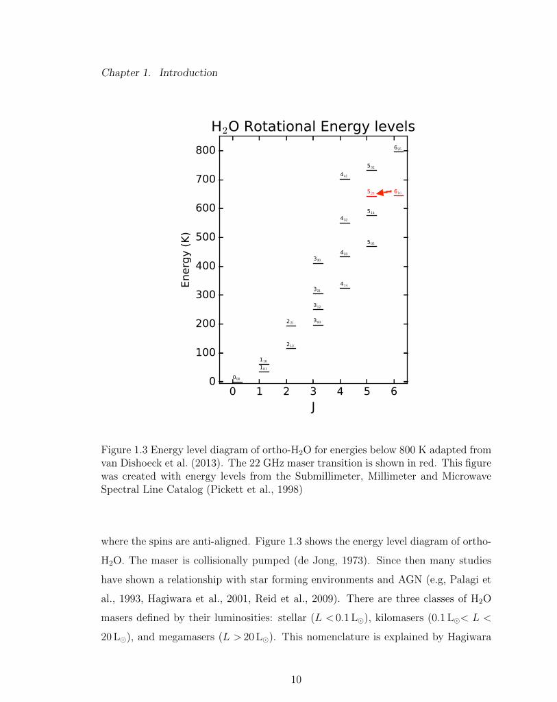
1.3 Energy level diagram of ortho-H2O for energies below 800 K adapted
from van Dishoeck et al. (2013). The 22 GHz maser transition
is shown in red. This figure was created with energy levels from
the Submillimeter, Millimeter and Microwave Spectral Line Catalog
(Pickett et al., 1998) . . . . . . . . . . . . . . . . . . . . . . . . . . 10
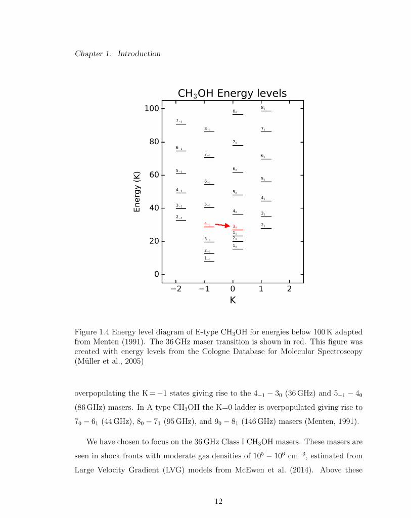
1.4 Energy level diagram of E-type CH3OH for energies below 100 K
adapted from Menten (1991). The 36 GHz maser transition is shown
in red. This figure was created with energy levels from the Cologne
Database for Molecular Spectroscopy (Muller et al., 2005) . . . . . . 12
xi
List of Figures
1.5 The two-element interferometer. The antennae are separated by a
distance b and measure voltages V1 and V2. ⌧g is the delay of the
signal arriving at antenna one relative to antenna two. The output
is then the time-averaged product of the two antennae hV1V2 i. . . . 14
1.6 A one-dimensional slice of the response of the Fourier transform of the
interferometer showing sidelobes. The x-axis shows the displacement
from the source and the y-axis shows the response. . . . . . . . . . . 16
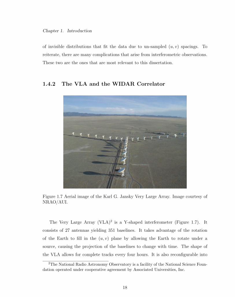
1.7 Aerial image of the Karl G. Jansky Very Large Array. Image courtesy
of NRAO/AUI. . . . . . . . . . . . . . . . . . . . . . . . . . . . . . 18
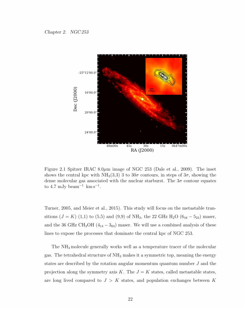
2.1 Spitzer IRAC 8.0µm image of NGC 253 (Dale et al., 2009). The
inset shows the central kpc with NH3(3,3) 3 to 30� contours, in steps
of 3�, showing the dense molecular gas associated with the nuclear
starburst. The 3� contour equates to 4.7 mJy beam�1 km s�1. . . . 22
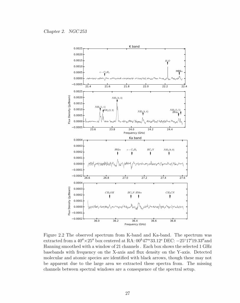
2.2 The observed spectrum from K-band and Ka-band. The spectrum
was extracted from a 4000⇥2500 box centered at RA: 00h47m33.12s
DEC: �25�17019.3300and Hanning smoothed with a window of 21
channels . Each box shows the selected 1 GHz basebands with fre-
quency on the X-axis and flux density on the Y-axis. Detected molec-
ular and atomic species are identified with black arrows, though these
may not be apparent due to the large area we extracted these spectra
from. The missing channels between spectral windows are a conse-
quence of the spectral setup. . . . . . . . . . . . . . . . . . . . . . . 27
xii
List of Figures
2.3 Images of the continuum emission from each of the 1 GHz base-
bands. The images are have not been smoothed to the common 600⇥
400resolution, and have resolutions of 5.100⇥3.100, 5.100⇥3.500, 3.300⇥1.700,
and 2.600⇥1.400, for the 22 GHz, 24 GHz, 27 GHz, and 36 GHz images,
respectively. . . . . . . . . . . . . . . . . . . . . . . . . . . . . . . . 30
2.4 Comparison of star formation and outflow tracers. The plus sign
marks the peak of the 36 GHz continuum. The contours show the
3, 6, and 9� contours of the naturally weighted H56↵ RRL where
1� is 0.08 Jy beam�1 km s�1. (a) H56↵ RRL shows the least dust
obscured star formation. (b) the 36 GHz continuum image shows a
close correlation with the two knots in the RRL. (c) HST WFPC2
H↵ image (Watson et al., 1996). (d) HST P↵ (Alonso-Herrero et al.,
2003) shows the outflow less well than the H↵ but is less obscured
by dust. . . . . . . . . . . . . . . . . . . . . . . . . . . . . . . . . . . 33
2.5 Images of the NH3(3,3) (left column), H2O (center column), and
CH3OH (right column) lines. The top row shows the peak flux images
of the naturally weighted image cubes spanning 300 km s�1 about sys-
temic velocity. The bottom row shows the intensity images smoothed
to the common resolution of 600⇥400. Both the peak flux and inten-
sity images are plotted with the same greyscale. The plus signs mark
locations where spectra were extracted for analysis, and the contin-
uum peak is marked C1. The contour is 60 Jy beam�1 km s�1 of
12CO(J = 1 ! 0) from Bolatto et al. (2013) smoothed to match the
resolution of the VLA data. . . . . . . . . . . . . . . . . . . . . . . . 34
xiii
List of Figures
2.6 Spectra of the NH3(1,1) to (5,5) transitions extracted from locations
A1-A7 and C1. NH3(3,3), plotted in green, shows emission at all
locations, whereas all the other inversion lines are absorbed toward
C1. We have plotted the 12CO(J = 1 ! 0) profile (scaling factor of
0.05 and 2.5 km s�1 resolution) from Bolatto et al. (2013) in black for
comparison. The vertical dashed line denotes the systemic velocity
of NGC 253 of 234 km s�1. . . . . . . . . . . . . . . . . . . . . . . . 35
2.7 Spectrum of the NH3(9,9) line extracted from location A3. The ver-
tical dashed line shows the systemic velocity of 235 km s�1 and the
dotted line shows the best fit, for which the results are listed in Table
2.4. . . . . . . . . . . . . . . . . . . . . . . . . . . . . . . . . . . . . 36
2.8 H2O maser spectra from W1, W2, and W3. W1 shows multiple ve-
locity components. These are labeled a to c. W2 is a spectrally broad
component centered at 233 km s�1. It is highlighted by the grey box
and the best fit spectrum is shown by the dotted line. This compo-
nent appears to consist of many individual masers. The dashed line
shows the CO spectrum, with 2.5 km s�1 resolution, at each location
scaled by 0.025, from Bolatto et al. (2013). . . . . . . . . . . . . . . 37
2.9 Methanol spectra from M1 to M5. CO spectra are plotted with a
dotted line with a flux density scaling factor of 0.25 and o↵set of
0.5 K. The systemic velocity of NGC 253 is denoted with a vertical
dashed line at 234 km s�1. . . . . . . . . . . . . . . . . . . . . . . . 38
xiv
List of Figures
2.10 The NH3 spectra towards C1. The systemic velocity of 234 km s�1
is shown with a vertical dashed line. All the para species of NH3
appear in absorption while the NH3(3,3) line appears in emission.
The solid black line represents the best fit two Gaussian profile. The
individual Gaussian components are plotted with dotted lines. . . . 39
2.11 Super-resolved H2O 0.02, 0.04, 0.08, and 0.16 Jy beam�1 km s�1
contours plotted on the HST WFPC2 H↵ (left; Watson et al., 1996)
map, the HST P↵ (center; Alonso-Herrero et al., 2003), and the RRL
H56↵ (right). The synthesized beam in the bottom left corner of the
left panel shows the 100 circular resolution of the super-resolved cube.
The locations of W1 to W3 are plotted with cyan plus signs from left
to right. . . . . . . . . . . . . . . . . . . . . . . . . . . . . . . . . . . 46
2.12 The solid lines represent the relationship between the kinetic tem-
perature and the rotational temperature. The dashed lines show the
fits to the models represented by equations 2.5 and 2.6, and equation
6 from Ott et al. (2011) . . . . . . . . . . . . . . . . . . . . . . . . . 54
xv
List of Figures
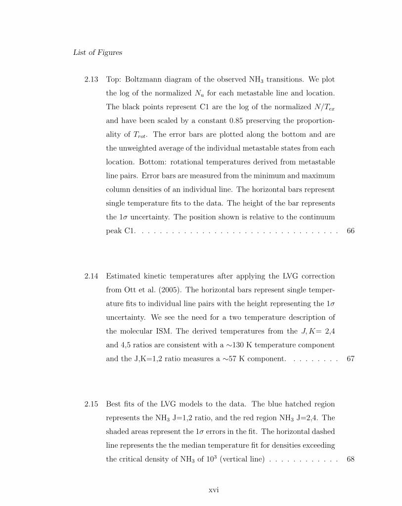
2.13 Top: Boltzmann diagram of the observed NH3 transitions. We plot
the log of the normalized Nu for each metastable line and location.
The black points represent C1 are the log of the normalized N/Tex
and have been scaled by a constant 0.85 preserving the proportion-
ality of Trot. The error bars are plotted along the bottom and are
the unweighted average of the individual metastable states from each
location. Bottom: rotational temperatures derived from metastable
line pairs. Error bars are measured from the minimum and maximum
column densities of an individual line. The horizontal bars represent
single temperature fits to the data. The height of the bar represents
the 1� uncertainty. The position shown is relative to the continuum
peak C1. . . . . . . . . . . . . . . . . . . . . . . . . . . . . . . . . . 66
2.14 Estimated kinetic temperatures after applying the LVG correction
from Ott et al. (2005). The horizontal bars represent single temper-
ature fits to individual line pairs with the height representing the 1�
uncertainty. We see the need for a two temperature description of
the molecular ISM. The derived temperatures from the J, K= 2,4
and 4,5 ratios are consistent with a ⇠130 K temperature component
and the J,K=1,2 ratio measures a ⇠57 K component. . . . . . . . . 67
2.15 Best fits of the LVG models to the data. The blue hatched region
represents the NH3 J=1,2 ratio, and the red region NH3 J=2,4. The
shaded areas represent the 1� errors in the fit. The horizontal dashed
line represents the the median temperature fit for densities exceeding
the critical density of NH3 of 103 (vertical line) . . . . . . . . . . . . 68
xvi
List of Figures
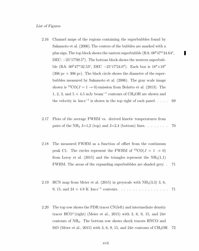
2.16 Channel maps of the regions containing the superbubbles found by
Sakamoto et al. (2006). The centers of the bubbles are marked with a
plus sign. The top block shows the eastern superbubble (RA: 00h47m34.64s,
DEC: �25�17009.500). The bottom block shows the western superbub-
ble (RA: 00h47m32.53s, DEC �25�17024.000). Each box is 1800⇥1800
(306 pc ⇥ 306 pc). The black circle shows the diameter of the super-
bubbles measured by Sakamoto et al. (2006). The gray scale image
shown is 12CO(J = 1 ! 0) emission from Bolatto et al. (2013). The
1, 2, 3, and 5 ⇥ 4.5 mJy beam�1 contours of CH3OH are shown and
the velocity in km s�1 is shown in the top right of each panel. . . . . 69
2.17 Plots of the average FWHM vs. derived kinetic temperatures from
pairs of the NH3 J=1,2 (top) and J=2,4 (bottom) lines. . . . . . . . 70
2.18 The measured FWHM as a function of o↵set from the continuum
peak C1. The circles represent the FWHM of 12CO(J = 1 ! 0)
from Leroy et al. (2015) and the triangles represent the NH3(1,1)
FWHM. The areas of the expanding superbubbles are shaded grey. . 71
2.19 HCN map from Meier et al. (2015) in greyscale with NH3(3,3) 3, 6,
9, 15, and 24 ⇥ 4.8 K km s�1 contours. . . . . . . . . . . . . . . . . 71
2.20 The top row shows the PDR tracer CN(left) and intermediate density
tracer HCO+(right) (Meier et al., 2015) with 3, 6, 9, 15, and 24�
contours of NH3. The bottom row shows shock tracers HNCO and
SiO (Meier et al., 2015) with 3, 6, 9, 15, and 24� contours of CH3OH. 72
xvii
List of Figures
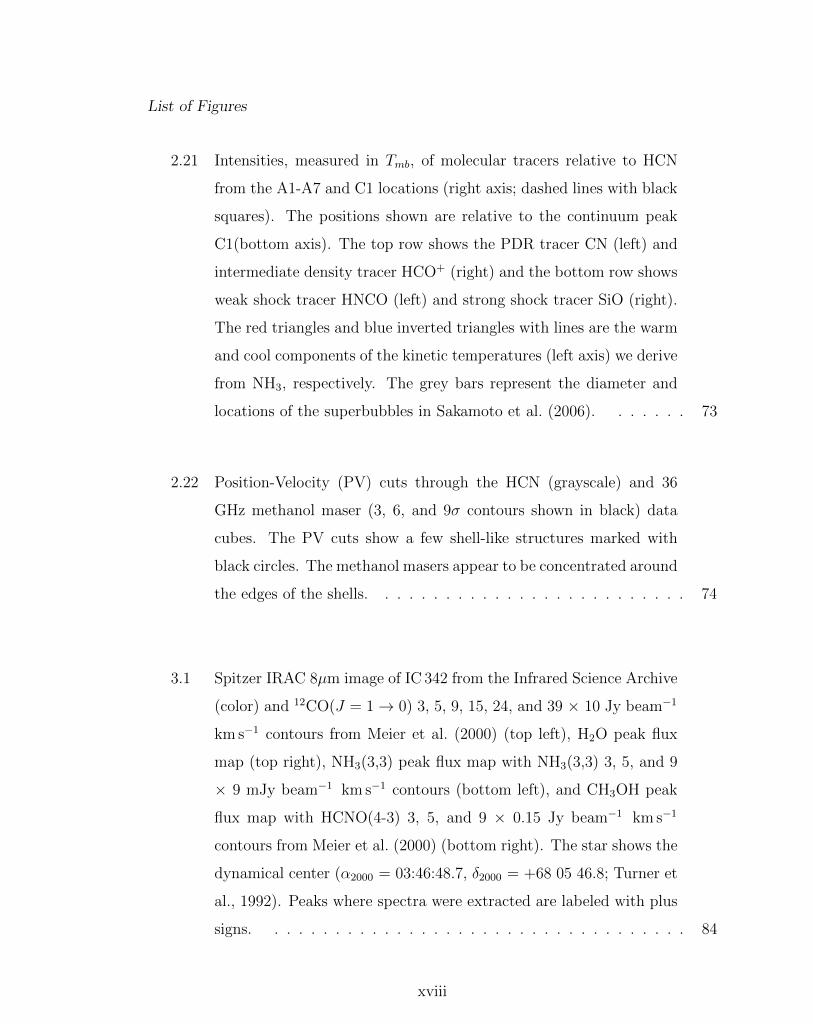
2.21 Intensities, measured in Tmb, of molecular tracers relative to HCN
from the A1-A7 and C1 locations (right axis; dashed lines with black
squares). The positions shown are relative to the continuum peak
C1(bottom axis). The top row shows the PDR tracer CN (left) and
intermediate density tracer HCO+ (right) and the bottom row shows
weak shock tracer HNCO (left) and strong shock tracer SiO (right).
The red triangles and blue inverted triangles with lines are the warm
and cool components of the kinetic temperatures (left axis) we derive
from NH3, respectively. The grey bars represent the diameter and
locations of the superbubbles in Sakamoto et al. (2006). . . . . . . 73
2.22 Position-Velocity (PV) cuts through the HCN (grayscale) and 36
GHz methanol maser (3, 6, and 9� contours shown in black) data
cubes. The PV cuts show a few shell-like structures marked with
black circles. The methanol masers appear to be concentrated around
the edges of the shells. . . . . . . . . . . . . . . . . . . . . . . . . . 74
3.1 Spitzer IRAC 8µm image of IC 342 from the Infrared Science Archive
(color) and 12CO(J = 1 ! 0) 3, 5, 9, 15, 24, and 39 ⇥ 10 Jy beam�1
km s�1 contours from Meier et al. (2000) (top left), H2O peak flux
map (top right), NH3(3,3) peak flux map with NH3(3,3) 3, 5, and 9
⇥ 9 mJy beam�1 km s�1 contours (bottom left), and CH3OH peak
flux map with HCNO(4-3) 3, 5, and 9 ⇥ 0.15 Jy beam�1 km s�1
contours from Meier et al. (2000) (bottom right). The star shows the
dynamical center (↵2000 = 03:46:48.7, �2000 = +68 05 46.8; Turner et
al., 1992). Peaks where spectra were extracted are labeled with plus
signs. . . . . . . . . . . . . . . . . . . . . . . . . . . . . . . . . . . 84
xviii
List of Figures
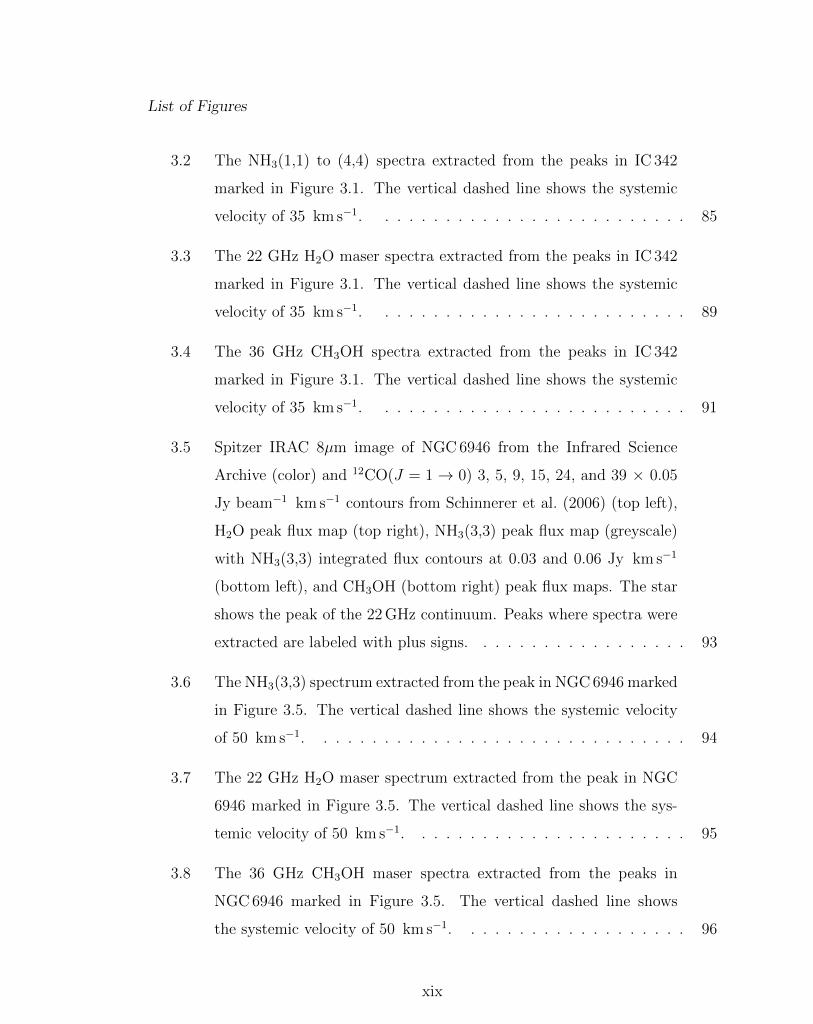
3.2 The NH3(1,1) to (4,4) spectra extracted from the peaks in IC 342
marked in Figure 3.1. The vertical dashed line shows the systemic
velocity of 35 km s�1. . . . . . . . . . . . . . . . . . . . . . . . . . 85
3.3 The 22 GHz H2O maser spectra extracted from the peaks in IC 342
marked in Figure 3.1. The vertical dashed line shows the systemic
velocity of 35 km s�1. . . . . . . . . . . . . . . . . . . . . . . . . . 89
3.4 The 36 GHz CH3OH spectra extracted from the peaks in IC 342
marked in Figure 3.1. The vertical dashed line shows the systemic
velocity of 35 km s�1. . . . . . . . . . . . . . . . . . . . . . . . . . 91
3.5 Spitzer IRAC 8µm image of NGC 6946 from the Infrared Science
Archive (color) and 12CO(J = 1 ! 0) 3, 5, 9, 15, 24, and 39 ⇥ 0.05
Jy beam�1 km s�1 contours from Schinnerer et al. (2006) (top left),
H2O peak flux map (top right), NH3(3,3) peak flux map (greyscale)
with NH3(3,3) integrated flux contours at 0.03 and 0.06 Jy km s�1
(bottom left), and CH3OH (bottom right) peak flux maps. The star
shows the peak of the 22 GHz continuum. Peaks where spectra were
extracted are labeled with plus signs. . . . . . . . . . . . . . . . . . 93
3.6 The NH3(3,3) spectrum extracted from the peak in NGC 6946 marked
in Figure 3.5. The vertical dashed line shows the systemic velocity
of 50 km s�1. . . . . . . . . . . . . . . . . . . . . . . . . . . . . . . 94
3.7 The 22 GHz H2O maser spectrum extracted from the peak in NGC
6946 marked in Figure 3.5. The vertical dashed line shows the sys-
temic velocity of 50 km s�1. . . . . . . . . . . . . . . . . . . . . . . 95
3.8 The 36 GHz CH3OH maser spectra extracted from the peaks in
NGC 6946 marked in Figure 3.5. The vertical dashed line shows
the systemic velocity of 50 km s�1. . . . . . . . . . . . . . . . . . . 96
xix
List of Figures
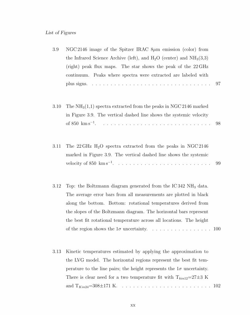
3.9 NGC 2146 image of the Spitzer IRAC 8µm emission (color) from
the Infrared Science Archive (left), and H2O (center) and NH3(3,3)
(right) peak flux maps. The star shows the peak of the 22 GHz
continuum. Peaks where spectra were extracted are labeled with
plus signs. . . . . . . . . . . . . . . . . . . . . . . . . . . . . . . . . 97
3.10 The NH3(1,1) spectra extracted from the peaks in NGC 2146 marked
in Figure 3.9. The vertical dashed line shows the systemic velocity
of 850 km s�1. . . . . . . . . . . . . . . . . . . . . . . . . . . . . . 98
3.11 The 22 GHz H2O spectra extracted from the peaks in NGC 2146
marked in Figure 3.9. The vertical dashed line shows the systemic
velocity of 850 km s�1. . . . . . . . . . . . . . . . . . . . . . . . . . 99
3.12 Top: the Boltzmann diagram generated from the IC 342 NH3 data.
The average error bars from all measurements are plotted in black
along the bottom. Bottom: rotational temperatures derived from
the slopes of the Boltzmann diagram. The horizontal bars represent
the best fit rotational temperature across all locations. The height
of the region shows the 1� uncertainty. . . . . . . . . . . . . . . . . 100
3.13 Kinetic temperatures estimated by applying the approximation to
the LVG model. The horizontal regions represent the best fit tem-
perature to the line pairs; the height represents the 1� uncertainty.
There is clear need for a two temperature fit with Tkin12=27±3 K
and TKin24=308±171 K. . . . . . . . . . . . . . . . . . . . . . . . . 102
xx
List of Figures
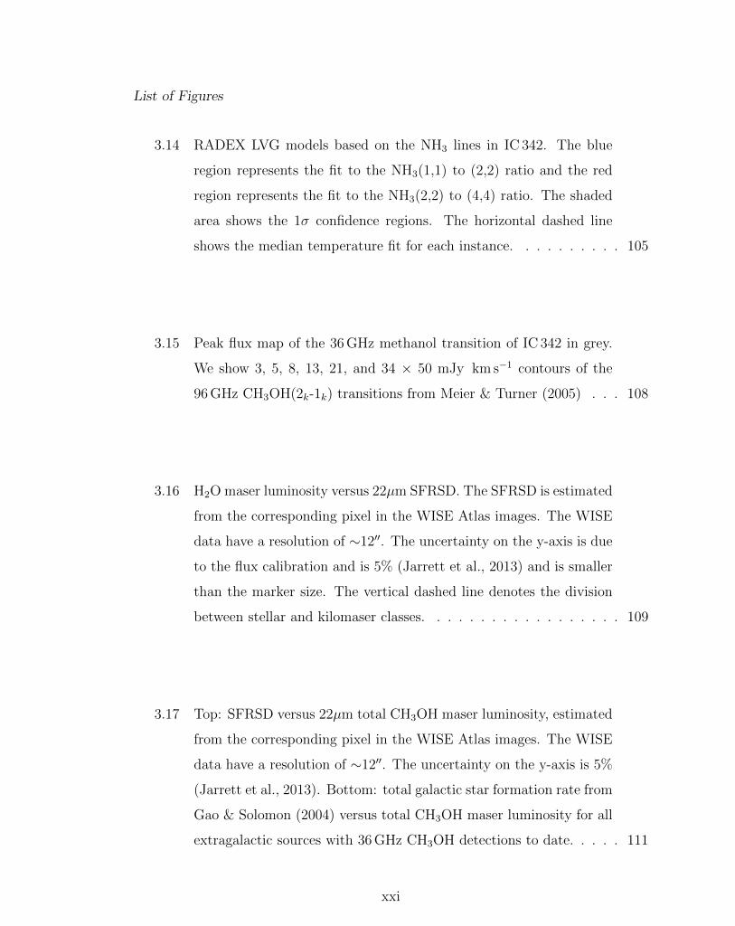
3.14 RADEX LVG models based on the NH3 lines in IC 342. The blue
region represents the fit to the NH3(1,1) to (2,2) ratio and the red
region represents the fit to the NH3(2,2) to (4,4) ratio. The shaded
area shows the 1� confidence regions. The horizontal dashed line
shows the median temperature fit for each instance. . . . . . . . . . 105
3.15 Peak flux map of the 36 GHz methanol transition of IC 342 in grey.
We show 3, 5, 8, 13, 21, and 34 ⇥ 50 mJy km s�1 contours of the
96 GHz CH3OH(2k-1k) transitions from Meier & Turner (2005) . . . 108
3.16 H2O maser luminosity versus 22µm SFRSD. The SFRSD is estimated
from the corresponding pixel in the WISE Atlas images. The WISE
data have a resolution of ⇠1200. The uncertainty on the y-axis is due
to the flux calibration and is 5% (Jarrett et al., 2013) and is smaller
than the marker size. The vertical dashed line denotes the division
between stellar and kilomaser classes. . . . . . . . . . . . . . . . . . 109
3.17 Top: SFRSD versus 22µm total CH3OH maser luminosity, estimated
from the corresponding pixel in the WISE Atlas images. The WISE
data have a resolution of ⇠1200. The uncertainty on the y-axis is 5%
(Jarrett et al., 2013). Bottom: total galactic star formation rate from
Gao & Solomon (2004) versus total CH3OH maser luminosity for all
extragalactic sources with 36 GHz CH3OH detections to date. . . . . 111
xxi
List of Figures
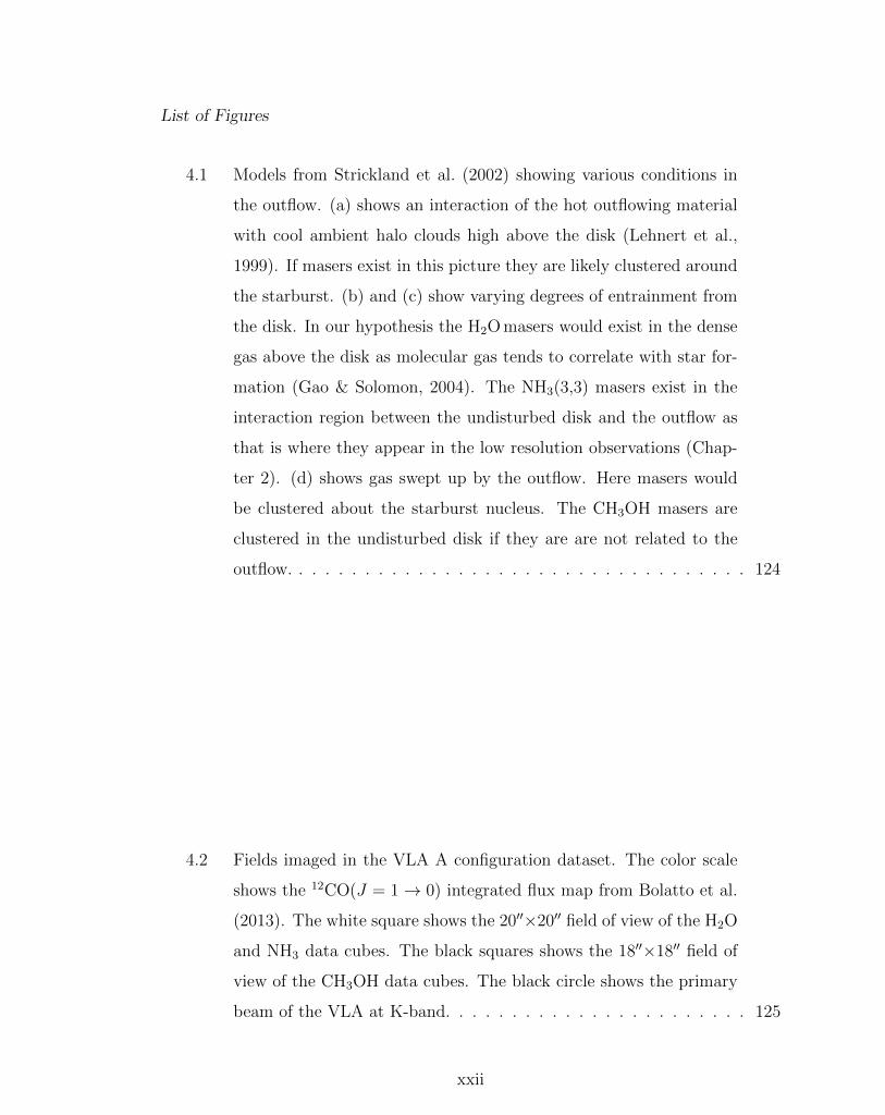
4.1 Models from Strickland et al. (2002) showing various conditions in
the outflow. (a) shows an interaction of the hot outflowing material
with cool ambient halo clouds high above the disk (Lehnert et al.,
1999). If masers exist in this picture they are likely clustered around
the starburst. (b) and (c) show varying degrees of entrainment from
the disk. In our hypothesis the H2O masers would exist in the dense
gas above the disk as molecular gas tends to correlate with star for-
mation (Gao & Solomon, 2004). The NH3(3,3) masers exist in the
interaction region between the undisturbed disk and the outflow as
that is where they appear in the low resolution observations (Chap-
ter 2). (d) shows gas swept up by the outflow. Here masers would
be clustered about the starburst nucleus. The CH3OH masers are
clustered in the undisturbed disk if they are are not related to the
outflow. . . . . . . . . . . . . . . . . . . . . . . . . . . . . . . . . . . 124
4.2 Fields imaged in the VLA A configuration dataset. The color scale
shows the 12CO(J = 1 ! 0) integrated flux map from Bolatto et al.
(2013). The white square shows the 2000⇥2000 field of view of the H2O
and NH3 data cubes. The black squares shows the 1800⇥1800 field of
view of the CH3OH data cubes. The black circle shows the primary
beam of the VLA at K-band. . . . . . . . . . . . . . . . . . . . . . . 125
xxii
List of Figures
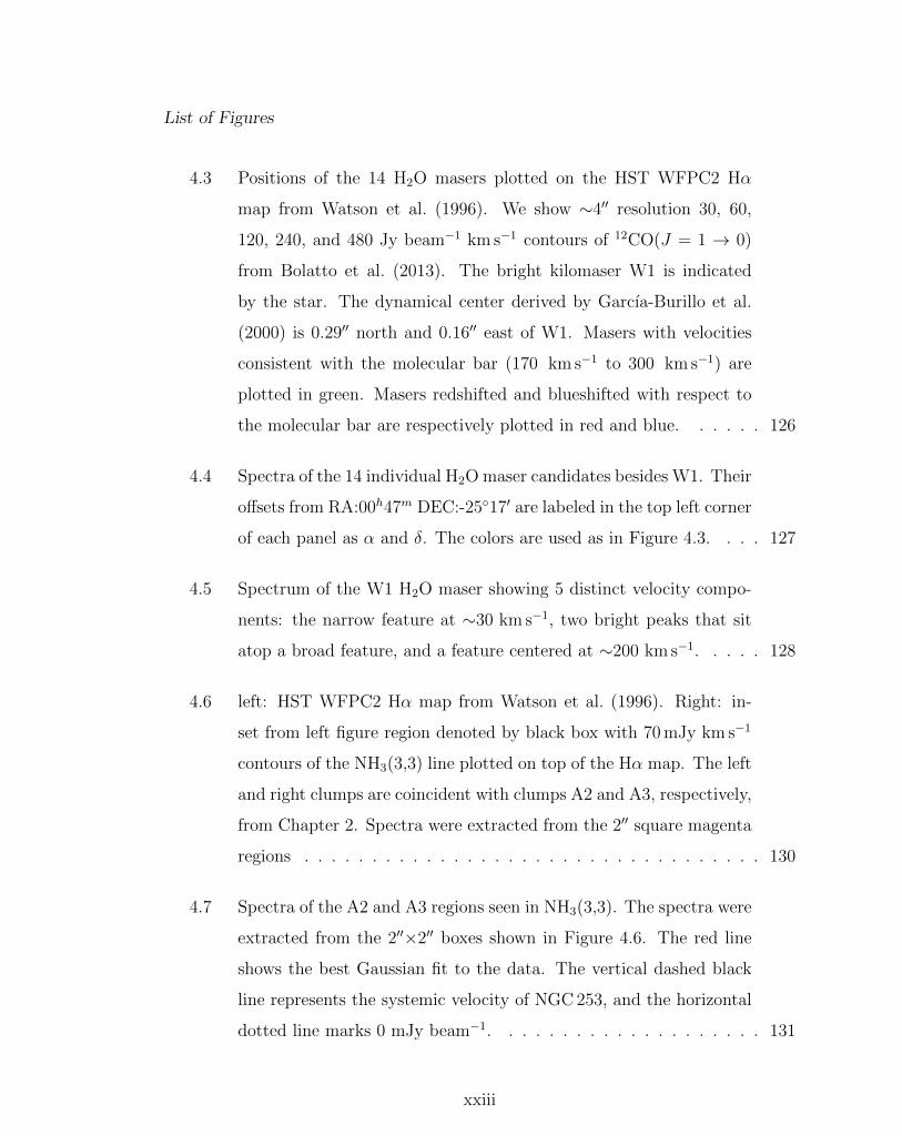
4.3 Positions of the 14 H2O masers plotted on the HST WFPC2 H↵
map from Watson et al. (1996). We show ⇠400 resolution 30, 60,
120, 240, and 480 Jy beam�1 km s�1 contours of 12CO(J = 1 ! 0)
from Bolatto et al. (2013). The bright kilomaser W1 is indicated
by the star. The dynamical center derived by Garcıa-Burillo et al.
(2000) is 0.2900 north and 0.1600 east of W1. Masers with velocities
consistent with the molecular bar (170 km s�1 to 300 km s�1) are
plotted in green. Masers redshifted and blueshifted with respect to
the molecular bar are respectively plotted in red and blue. . . . . . 126
4.4 Spectra of the 14 individual H2O maser candidates besides W1. Their
o↵sets from RA:00h47m DEC:-25�170 are labeled in the top left corner
of each panel as ↵ and �. The colors are used as in Figure 4.3. . . . 127
4.5 Spectrum of the W1 H2O maser showing 5 distinct velocity compo-
nents: the narrow feature at ⇠30 km s�1, two bright peaks that sit
atop a broad feature, and a feature centered at ⇠200 km s�1. . . . . 128
4.6 left: HST WFPC2 H↵ map from Watson et al. (1996). Right: in-
set from left figure region denoted by black box with 70 mJy km s�1
contours of the NH3(3,3) line plotted on top of the H↵ map. The left
and right clumps are coincident with clumps A2 and A3, respectively,
from Chapter 2. Spectra were extracted from the 200 square magenta
regions . . . . . . . . . . . . . . . . . . . . . . . . . . . . . . . . . . 130
4.7 Spectra of the A2 and A3 regions seen in NH3(3,3). The spectra were
extracted from the 200⇥200 boxes shown in Figure 4.6. The red line
shows the best Gaussian fit to the data. The vertical dashed black
line represents the systemic velocity of NGC 253, and the horizontal
dotted line marks 0 mJy beam�1. . . . . . . . . . . . . . . . . . . . 131
xxiii
List of Figures
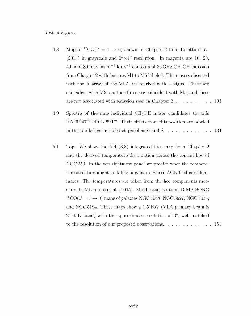
4.8 Map of 12CO(J = 1 ! 0) shown in Chapter 2 from Bolatto et al.
(2013) in grayscale and 600⇥400 resolution. In magenta are 10, 20,
40, and 80 mJy beam�1 km s�1 contours of 36 GHz CH3OH emission
from Chapter 2 with features M1 to M5 labeled. The masers observed
with the A array of the VLA are marked with + signs. Three are
coincident with M3, another three are coincident with M5, and three
are not associated with emission seen in Chapter 2. . . . . . . . . . . 133
4.9 Spectra of the nine individual CH3OH maser candidates towards
RA:00h47m DEC:-25�170. Their o↵sets from this position are labeled
in the top left corner of each panel as ↵ and �. . . . . . . . . . . . . 134
5.1 Top: We show the NH3(3,3) integrated flux map from Chapter 2
and the derived temperature distribution across the central kpc of
NGC 253. In the top rightmost panel we predict what the tempera-
ture structure might look like in galaxies where AGN feedback dom-
inates. The temperatures are taken from the hot components mea-
sured in Miyamoto et al. (2015). Middle and Bottom: BIMA SONG
12CO(J = 1 ! 0) maps of galaxies NGC 1068, NGC 3627, NGC 5033,
and NGC 5194. These maps show a 1.50 FoV (VLA primary beam is
20 at K band) with the approximate resolution of 300, well matched
to the resolution of our proposed observations. . . . . . . . . . . . . 151
xxiv
List of Tables
1.1 Adopted Galaxy Properties . . . . . . . . . . . . . . . . . . . . . . . 4
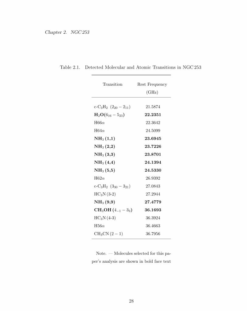
2.1 Detected Molecular and Atomic Transitions in NGC 253 . . . . . . 28
2.2 NGC 253 NH3 Line Parameters From A1-A7 . . . . . . . . . . . . . 40
2.2 NGC 253 NH3 Line Parameters From A1-A7 . . . . . . . . . . . . . 41
2.2 NGC 253 NH3 Line Parameters From A1-A7 . . . . . . . . . . . . . 42
2.2 NGC 253 NH3 Line Parameters From A1-A7 . . . . . . . . . . . . . 43
2.3 Line Parameters Towards C1 . . . . . . . . . . . . . . . . . . . . . . 45
2.4 NH3 (9,9) Line Parameters at A3 . . . . . . . . . . . . . . . . . . . 45
2.5 NGC 253 H2O Maser Candidates . . . . . . . . . . . . . . . . . . . . 47
2.6 NGC 253 CH3OH Maser Candidates . . . . . . . . . . . . . . . . . . 49
2.6 NGC 253 CH3OH Maser Candidates . . . . . . . . . . . . . . . . . . 50
2.7 NGC 253 NH3 LVG Best Fit Values . . . . . . . . . . . . . . . . . . 57
3.1 NH3 Line Parameters . . . . . . . . . . . . . . . . . . . . . . . . . . 86
3.1 NH3 Line Parameters . . . . . . . . . . . . . . . . . . . . . . . . . . 87
xxv
List of Tables
3.1 NH3 Line Parameters . . . . . . . . . . . . . . . . . . . . . . . . . . 88
3.2 H2O Line Parameters . . . . . . . . . . . . . . . . . . . . . . . . . . 90
3.3 CH3OH Line Parameters . . . . . . . . . . . . . . . . . . . . . . . . 92
3.4 NH3 Temperatures . . . . . . . . . . . . . . . . . . . . . . . . . . . 115
3.5 NH3 Abuncance in IC 342 . . . . . . . . . . . . . . . . . . . . . . . . 116
4.1 H2O Maser Candidates . . . . . . . . . . . . . . . . . . . . . . . . . 129
4.2 NH3 Maser Candidates . . . . . . . . . . . . . . . . . . . . . . . . . 131
4.3 CH3OH Maser Candidates . . . . . . . . . . . . . . . . . . . . . . . 135
5.1 Adopted Galaxy Properties . . . . . . . . . . . . . . . . . . . . . . . 149
5.2 VLA K band ionized and molecular lines . . . . . . . . . . . . . . . 152
5.2 VLA K band ionized and molecular lines . . . . . . . . . . . . . . . 153
xxvi
Chapter 1
Introduction
1.1 Overview
It is clear that accurate, physically motivated prescriptions of the underlying con-
nection between the interstellar medium (ISM) and star formation are critical to
understanding galaxy evolution. How molecular clouds are formed, how they turn
molecular gas into stars, and what the impact of mechanical and radiative feedback
processes is, are the main sources of uncertainty limiting future progress (e.g., Kau↵-
mann et al., 1999). This dissertation will focus on observational e↵ects of mechanical
and radiative feedback. Feedback is energy and momentum injected in to the ISM
by stars. Supernovae, stellar winds, photoionization, and shock heating are a few
examples by which energy is fed back into the ISM (e.g., Hopkins et al. (2012)).
Models of galaxy evolution without feedback drastically over-predict star formation
rates and e�ciencies. Therefore feedback is necessary to impede star formation, oth-
erwise a galaxy reaches its peak star formation rate in less than a dynamical time
and quickly converts its baryons to stars shortly after (e.g., Kau↵mann et al., 1999,
Krumholz et al., 2011, Hopkins et al., 2011).
1
Chapter 1. Introduction
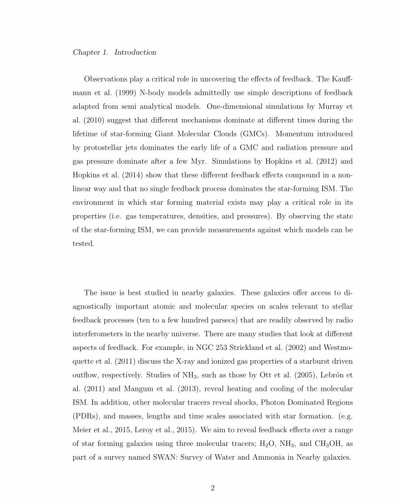
Observations play a critical role in uncovering the e↵ects of feedback. The Kau↵-
mann et al. (1999) N-body models admittedly use simple descriptions of feedback
adapted from semi analytical models. One-dimensional simulations by Murray et
al. (2010) suggest that di↵erent mechanisms dominate at di↵erent times during the
lifetime of star-forming Giant Molecular Clouds (GMCs). Momentum introduced
by protostellar jets dominates the early life of a GMC and radiation pressure and
gas pressure dominate after a few Myr. Simulations by Hopkins et al. (2012) and
Hopkins et al. (2014) show that these di↵erent feedback e↵ects compound in a non-
linear way and that no single feedback process dominates the star-forming ISM. The
environment in which star forming material exists may play a critical role in its
properties (i.e. gas temperatures, densities, and pressures). By observing the state
of the star-forming ISM, we can provide measurements against which models can be
tested.
The issue is best studied in nearby galaxies. These galaxies o↵er access to di-
agnostically important atomic and molecular species on scales relevant to stellar
feedback processes (ten to a few hundred parsecs) that are readily observed by radio
interferometers in the nearby universe. There are many studies that look at di↵erent
aspects of feedback. For example, in NGC 253 Strickland et al. (2002) and Westmo-
quette et al. (2011) discuss the X-ray and ionized gas properties of a starburst driven
outflow, respectively. Studies of NH3, such as those by Ott et al. (2005), Lebron et
al. (2011) and Mangum et al. (2013), reveal heating and cooling of the molecular
ISM. In addition, other molecular tracers reveal shocks, Photon Dominated Regions
(PDRs), and masses, lengths and time scales associated with star formation. (e.g.
Meier et al., 2015, Leroy et al., 2015). We aim to reveal feedback e↵ects over a range
of star forming galaxies using three molecular tracers; H2O, NH3, and CH3OH, as
part of a survey named SWAN: Survey of Water and Ammonia in Nearby galaxies.
2
Chapter 1. Introduction
1.2 The Survey of Water and Ammonia in Nearby
galaxies (SWAN)
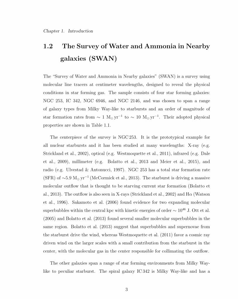
The “Survey of Water and Ammonia in Nearby galaxies” (SWAN) is a survey using
molecular line tracers at centimeter wavelengths, designed to reveal the physical
conditions in star forming gas. The sample consists of four star forming galaxies:
NGC 253, IC 342, NGC 6946, and NGC 2146, and was chosen to span a range
of galaxy types from Milky Way-like to starbursts and an order of magnitude of
star formation rates from ⇠ 1 M� yr�1 to ⇠ 10 M� yr�1. Their adopted physical
properties are shown in Table 1.1.
The centerpiece of the survey is NGC 253. It is the prototypical example for
all nuclear starbursts and it has been studied at many wavelengths: X-ray (e.g.
Strickland et al., 2002), optical (e.g. Westmoquette et al., 2011), infrared (e.g. Dale
et al., 2009), millimeter (e.g. Bolatto et al., 2013 and Meier et al., 2015), and
radio (e.g. Ulvestad & Antonucci, 1997). NGC 253 has a total star formation rate
(SFR) of ⇠5.9 M� yr�1 (McCormick et al., 2013). The starburst is driving a massive
molecular outflow that is thought to be starving current star formation (Bolatto et
al., 2013). The outflow is also seen in X-rays (Strickland et al., 2002) and H↵ (Watson
et al., 1996). Sakamoto et al. (2006) found evidence for two expanding molecular
superbubbles within the central kpc with kinetic energies of order ⇠ 1046 J. Ott et al.
(2005) and Bolatto et al. (2013) found several smaller molecular superbubbles in the
same region. Bolatto et al. (2013) suggest that superbubbles and supernovae from
the starburst drive the wind, whereas Westmoquette et al. (2011) favor a cosmic ray
driven wind on the larger scales with a small contribution from the starburst in the
center, with the molecular gas in the center responsible for collimating the outflow.
The other galaxies span a range of star forming environments from Milky Way-
like to peculiar starburst. The spiral galaxy IC 342 is Milky Way-like and has a
3
Chapter 1. Introduction
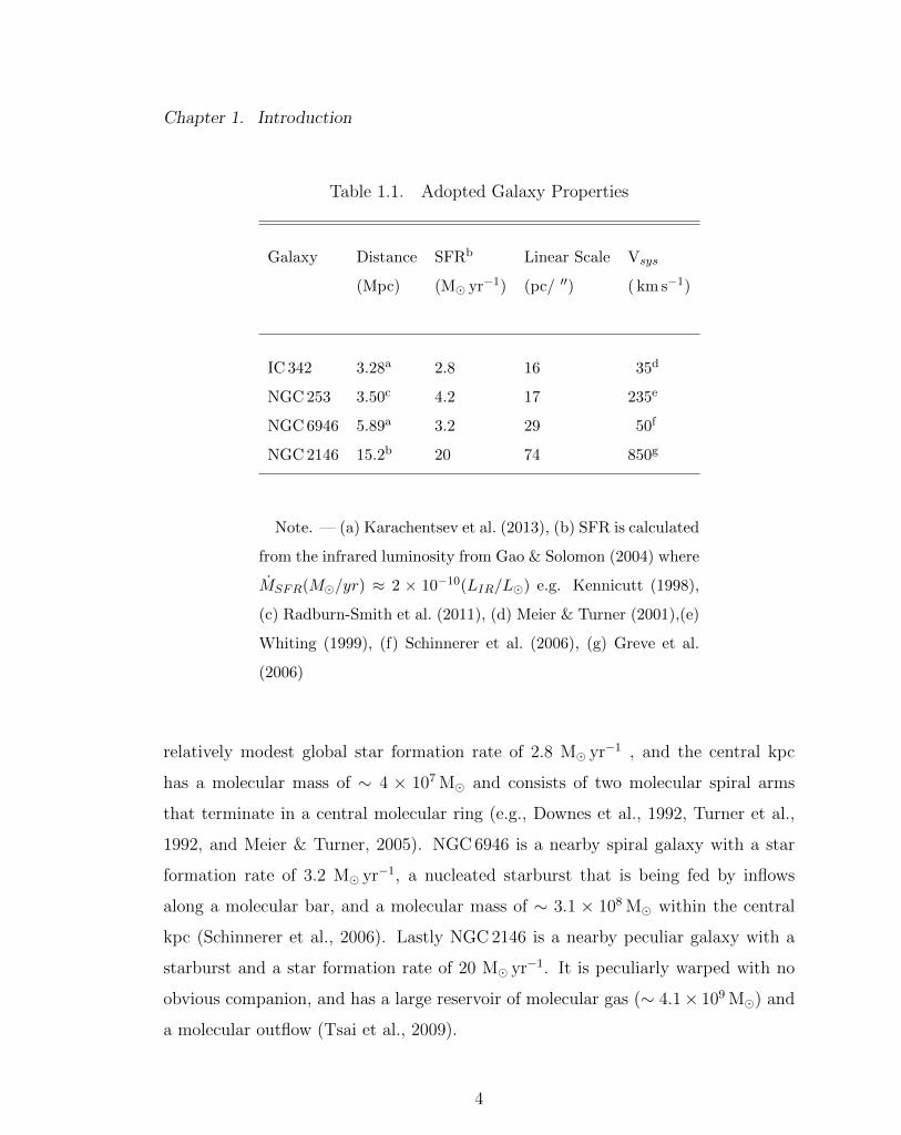
Table 1.1. Adopted Galaxy Properties
Galaxy Distance SFRb Linear Scale Vsys
(Mpc) (M� yr�1) (pc/ 00) ( km s�1)
IC 342 3.28a 2.8 16 35d
NGC253 3.50c 4.2 17 235e
NGC6946 5.89a 3.2 29 50f
NGC2146 15.2b 20 74 850g
Note. — (a) Karachentsev et al. (2013), (b) SFR is calculated
from the infrared luminosity from Gao & Solomon (2004) where
MSFR(M�/yr) ⇡ 2 ⇥ 10�10(LIR/L�) e.g. Kennicutt (1998),
(c) Radburn-Smith et al. (2011), (d) Meier & Turner (2001),(e)
Whiting (1999), (f) Schinnerer et al. (2006), (g) Greve et al.
(2006)
relatively modest global star formation rate of 2.8 M� yr�1 , and the central kpc
has a molecular mass of ⇠ 4 ⇥ 107 M� and consists of two molecular spiral arms
that terminate in a central molecular ring (e.g., Downes et al., 1992, Turner et al.,
1992, and Meier & Turner, 2005). NGC 6946 is a nearby spiral galaxy with a star
formation rate of 3.2 M� yr�1, a nucleated starburst that is being fed by inflows
along a molecular bar, and a molecular mass of ⇠ 3.1 ⇥ 108 M� within the central
kpc (Schinnerer et al., 2006). Lastly NGC 2146 is a nearby peculiar galaxy with a
starburst and a star formation rate of 20 M� yr�1. It is peculiarly warped with no
obvious companion, and has a large reservoir of molecular gas (⇠ 4.1 ⇥ 109 M�) and
a molecular outflow (Tsai et al., 2009).
4
Chapter 1. Introduction
1.3 Physics of Molecular Tracers
We exist in the era of wide-band cm, mm, and sub-mm astronomy. At these wave-
lengths we are able to observe weak but diagnostically important molecular tracers
(e.g., Martın 2011, Martın et al., 2015, Meier et al., 2015). We have selected the
molecules NH3, H2O (masers), and CH3OH (masers) as tracers of the star forming
environment. These molecules are useful as a temperature probe, a star formation
indicator, and a possible new shock tracer, respectively.
1.3.1 Ammonia
Interstellar ammonia was first detected by Cheung et al. (1968). It was the first
polyatomic molecule detected in the ISM. The molecule is a symmetric top and
has a tetrahedral structure. The inversion properties, ortho- and para- species, and
metastable states make NH3 particularly useful in an astronomical context.
We will start with the excitation of the NH3 molecule. We show the energy
level diagram for levels below 1000 K in Figure 1.1. Ho & Townes (1983) present an
excellent description of the NH3 molecule. The rotational states are described by
quantum numbers J and K. J is the total angular momentum, and K is the projected
angular momentum about the molecular symmetry axis. Transitions between K
states are forbidden due to the dipole moment existing only along the molecular axis.
This means that an excited molecule does not readily change K states. Changes
in J with constant K are sometimes referred to as K ladders. States where J>K
are referred to as non-metastable. Non-metastable states have lifetimes of 10-100 s,
meaning that they are rarely seen in an astronomical context where T is too low and
collisional excitations are rare compared to Earth-like atmospheric conditions. These
states quickly decay to metastable states, with lifetimes of ⇠109 s, where J=K. The
states are an inversion doublets. This means the N atom may tunnel through the
5
Chapter 1. Introduction
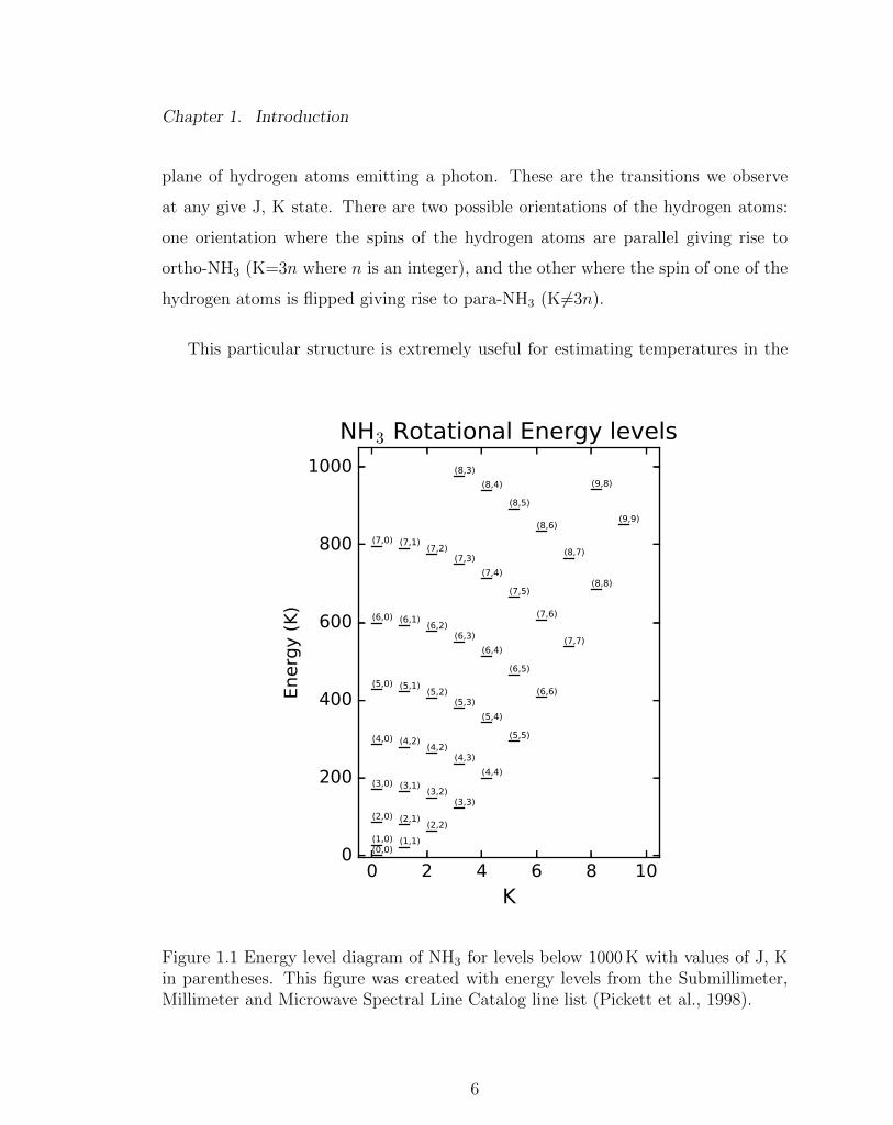
plane of hydrogen atoms emitting a photon. These are the transitions we observe
at any give J, K state. There are two possible orientations of the hydrogen atoms:
one orientation where the spins of the hydrogen atoms are parallel giving rise to
ortho-NH3 (K=3n where n is an integer), and the other where the spin of one of the
hydrogen atoms is flipped giving rise to para-NH3 (K 6=3n).
This particular structure is extremely useful for estimating temperatures in the
Figure 1.1 Energy level diagram of NH3 for levels below 1000 K with values of J, Kin parentheses. This figure was created with energy levels from the Submillimeter,Millimeter and Microwave Spectral Line Catalog line list (Pickett et al., 1998).
6
Chapter 1. Introduction
astronomical context. Because the non-metastable states are short lived, and tran-
sitions between K ladders are forbidden, the NH3 molecule quickly decays to the
metastable states preserving the Boltzmann distribution of the level population.
By measuring multiple metastable states it is then possible to back out the rota-
tional temperature of the gas where the NH3 molecule is excited. Between any two
metastable states (J and J0) the rotational temperature ( TJJ 0)1 is defined by the
ratio of the column densities
NJ 0J 0
NJJ
=gJ 0J 0
J
0(J 0 + 1)
gJJJ(J + 1)exp
⇣�
�E
TJJ 0
⌘(1.1)
where the statistical weights gJJ are 1 for para-NH3 and 2 for ortho-NH3 and �E is
the di↵erence in energy between the two metastable states in Kelvin (Henkel et al.,
2000). The upper inversion states (Nu) may also be substituted for the total column
of an individual state.
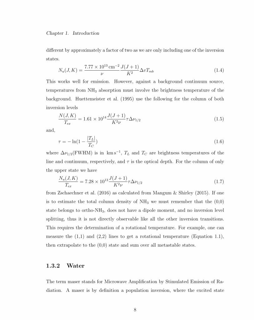
Column densities of NH3 are commonly measured in a few ways. The first is the
total column density of a given J, K state N(J, K)
N(J, K) =1.65 ⇥ 1014 cm�2
⌫
J(J + 1)
K
2�vTex⌧tot (1.2)
where ⌫ is in GHz, �v is in km s�1, Tex is the excitation temperature in K, and ⌧tot is
the sum of the optical depths of the hyperfine transitions (Lebron et al., 2011). Under
the assumption that the gas is optically thin Tex⌧tot is approximately the observed
main beam brightness temperature ⇠ Tmb of the upper state of the inversion doublet.
Thus the equation becomes
N(J, K) =1.65 ⇥ 1014 cm�2
⌫
J(J + 1)
K
2�vTmb (1.3)
making it possible to measure beam averaged column densities. The column density
of the upper inversion state is also commonly used (Henkel et al., 2000). This is
1We write TJJ 0 but we mean TJK where K=J0
7
Chapter 1. Introduction
di↵erent by approximately a factor of two as we are only including one of the inversion
states.
Nu(J, K) =7.77 ⇥ 1013 cm�2
⌫
J(J + 1)
K
2�vTmb (1.4)
This works well for emission. However, against a background continuum source,
temperatures from NH3 absorption must involve the brightness temperature of the
background. Huettemeister et al. (1995) use the following for the column of both
inversion levels
N(J, K)
Tex
= 1.61 ⇥ 1014J(J + 1)
K
2⌫
⌧�⌫1/2 (1.5)
and,
⌧ = � ln(1 �
|TL|
TC
) (1.6)
where �⌫1/2(FWHM) is in km s�1, TL and TC are brightness temperatures of the
line and continuum, respectively, and ⌧ is the optical depth. For the column of only
the upper state we have
Nu(J, K)
Tex
= 7.28 ⇥ 1013J(J + 1)
K
2⌫
⌧�⌫1/2 (1.7)
from Zschaechner et al. (2016) as calculated from Mangum & Shirley (2015). If one
is to estimate the total column density of NH3 we must remember that the (0,0)
state belongs to ortho-NH3, does not have a dipole moment, and no inversion level
splitting, thus it is not directly observable like all the other inversion transitions.
This requires the determination of a rotational temperature. For example, one can
measure the (1,1) and (2,2) lines to get a rotational temperature (Equation 1.1),
then extrapolate to the (0,0) state and sum over all metastable states.
1.3.2 Water
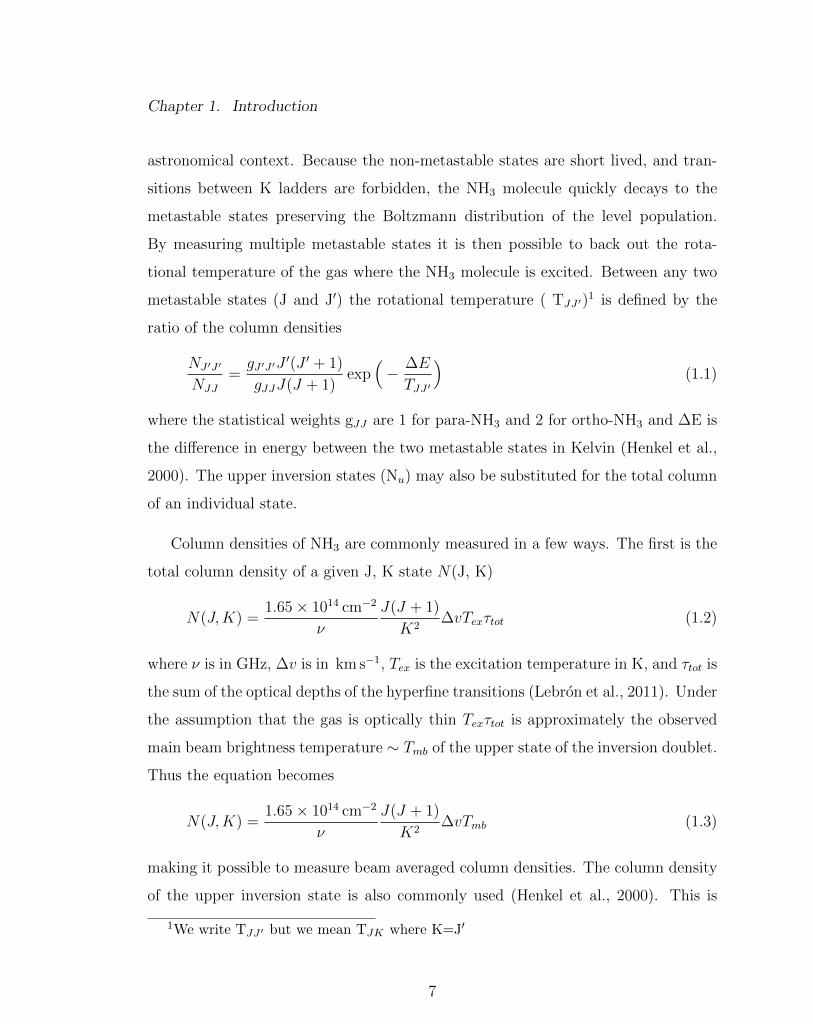
The term maser stands for Microwave Amplification by Stimulated Emission of Ra-
diation. A maser is by definition a population inversion, where the excited state
8
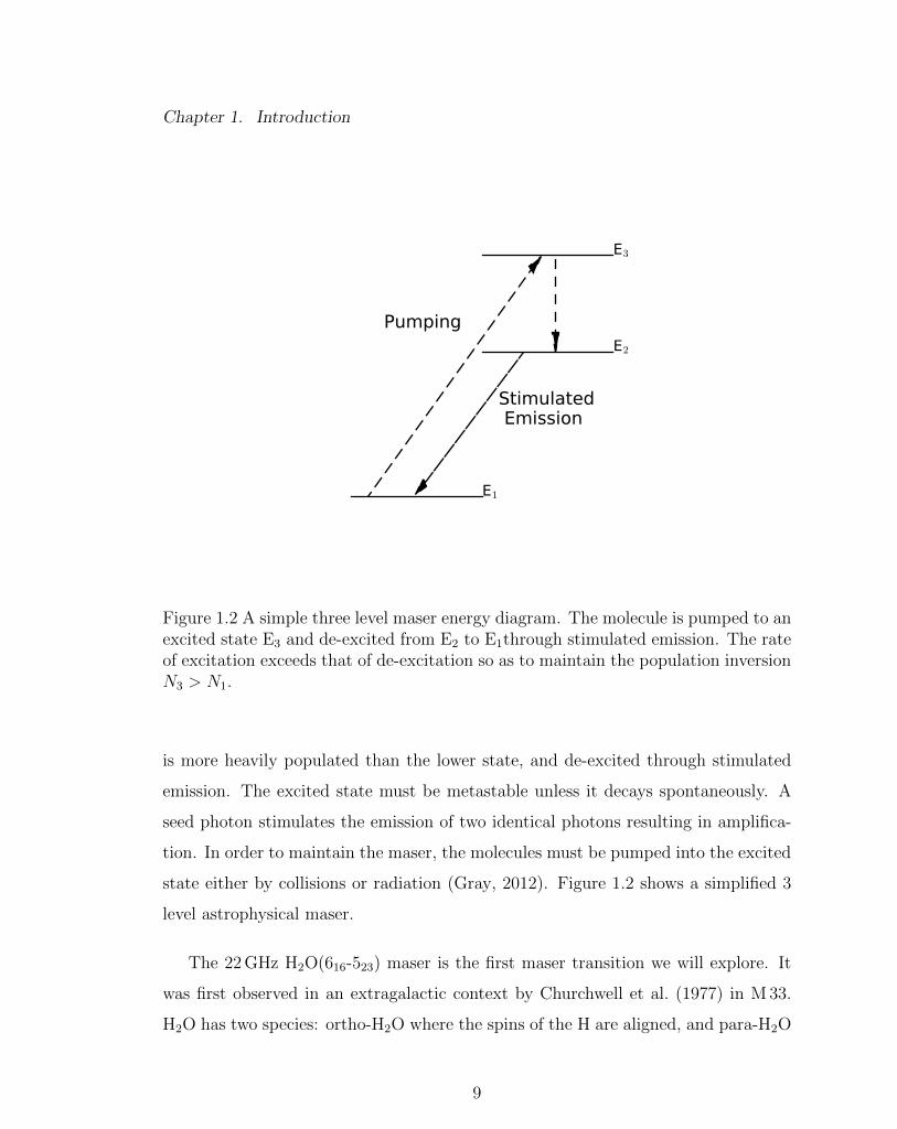
Chapter 1. Introduction
Figure 1.2 A simple three level maser energy diagram. The molecule is pumped to anexcited state E3 and de-excited from E2 to E1through stimulated emission. The rateof excitation exceeds that of de-excitation so as to maintain the population inversionN3 > N1.
is more heavily populated than the lower state, and de-excited through stimulated
emission. The excited state must be metastable unless it decays spontaneously. A
seed photon stimulates the emission of two identical photons resulting in amplifica-
tion. In order to maintain the maser, the molecules must be pumped into the excited
state either by collisions or radiation (Gray, 2012). Figure 1.2 shows a simplified 3
level astrophysical maser.
The 22 GHz H2O(616-523) maser is the first maser transition we will explore. It
was first observed in an extragalactic context by Churchwell et al. (1977) in M 33.
H2O has two species: ortho-H2O where the spins of the H are aligned, and para-H2O
9
Chapter 1. Introduction
Figure 1.3 Energy level diagram of ortho-H2O for energies below 800 K adapted fromvan Dishoeck et al. (2013). The 22 GHz maser transition is shown in red. This figurewas created with energy levels from the Submillimeter, Millimeter and MicrowaveSpectral Line Catalog (Pickett et al., 1998)
where the spins are anti-aligned. Figure 1.3 shows the energy level diagram of ortho-
H2O. The maser is collisionally pumped (de Jong, 1973). Since then many studies
have shown a relationship with star forming environments and AGN (e.g, Palagi et
al., 1993, Hagiwara et al., 2001, Reid et al., 2009). There are three classes of H2O
masers defined by their luminosities: stellar (L < 0.1 L�), kilomasers (0.1 L�< L <
20 L�), and megamasers (L > 20 L�). This nomenclature is explained by Hagiwara
10
Chapter 1. Introduction
et al. (2001).
The conditions under which H2O can mase require gas densities > 106 cm�3 and
kinetic temperatures ⇠ 400 K (Elitzur et al., 1989). These are typically indicators
of strong star formation (the exception being megamasers and evolved stars). The
stellar class is associated with Young Stellar Objects (YSOs) and Asymptotic Giant
Branch (AGB) stars (Palagi et al., 1993). There is a correlation between the mass loss
rate and the luminosity of the maser (e.g., Engels et al., 1986), which can be variable
on time scales of weeks or months (e.g., Claussen et al., 1996). The kilomaser class is
particularly related to strong star formation activity (Hagiwara et al., 2001). These
could be constructed of many stellar masers or they could be the low luminosity
tail of the megamaser class (Tarchi et al., 2011). The most luminous class, the
megamasers, is not necessarily related to star formation but rather dusty molecular
tori around AGN (Claussen & Lo, 1986). Maser spots are typically compact, of the
order of a few pcs, and have sharp velocity profiles, making them excellent tracers
of kinematics (e.g. Reid et al. (2009)). In any case these masers are tracing shocked
hot dense gas, typically related to star formation, making the 22 GHz H2O maser
transition a useful tool in studies of star formation feedback.
1.3.3 Methanol
There are two forms of CH3OH, E and A, depending on the symmetry. CH3OH is
almost a symmetric top molecule. The E-type of methanol has energy levels from
�JK J and the A-type has levels from 0K J (Leurini et al., 2004). The energy
level diagram for E CH3OH is shown in Figure 1.4. There are two forms of methanol
masers. Class I is collisionally pumped and Class II is radiatively pumped (Menten,
1991). E-type CH3OH gives rise to class I 36 GHz and 86 GHz masers. Collisions
excite the molecule into high JK states. These rapidly decay to the K =�1 ladder
11
Chapter 1. Introduction
Figure 1.4 Energy level diagram of E-type CH3OH for energies below 100 K adaptedfrom Menten (1991). The 36 GHz maser transition is shown in red. This figure wascreated with energy levels from the Cologne Database for Molecular Spectroscopy(Muller et al., 2005)
overpopulating the K = �1 states giving rise to the 4�1 � 30 (36 GHz) and 5�1 � 40
(86 GHz) masers. In A-type CH3OH the K=0 ladder is overpopulated giving rise to
70 � 61 (44 GHz), 80 � 71 (95 GHz), and 90 � 81 (146 GHz) masers (Menten, 1991).
We have chosen to focus on the 36 GHz Class I CH3OH masers. These masers are
seen in shock fronts with moderate gas densities of 105 � 106 cm�3, estimated from
Large Velocity Gradient (LVG) models from McEwen et al. (2014). Above these
12
Chapter 1. Introduction
densities the E-type Class I masers are quenched (e.g., Menten, 1991, McEwen et al.,
2014), additionally McEwen et al. (2014) estimate, from LVG models, that kinetic
temperatures > 60 K enhance maser emission. These masers are typically found
in high mass star forming regions (Johnston et al., 1992) and supernova remnants
(McEwen et al., 2014) as an indicator of shocked material.
1.4 Radio Interferometry and Synthesis Imaging
The three molecular species we observe as indicators of the state of the dense ISM
have spectral lines at frequencies spanning 22-36 GHz, or wavelengths in the cm to
mm radio range. In order to resolve GMC scales (10-100 pc) in nearby galaxies we
need to have appreciable resolution. At a distance of 5 Mpc, one arcsecond equates
to ⇠25 pc in spatial resolution. To achieve this resolution one would need to build a
dish with a diameter of ⇠3 km. This is physically unfeasible, therefore a technique
called aperture synthesis is applied.
1.4.1 Aperture Synthesis
Aperture synthesis is a technique combining the outputs of two or more independent
collecting elements to synthesize a single telescope with a collecting area equivalent to
the sum of the collecting areas of the individual elements, and a diameter equivalent
to the longest separation between any two elements. The separation between any
two elements is called a baseline.
Imagine a plane wave of electromagnetic radiation, with frequency ⌫, arriving at
a two-element interferometer (Wilson et al., 2009). These telescopes are separated
by baseline b and both pointed at a source. Each element measures a voltage, V1 and
13
Chapter 1. Introduction
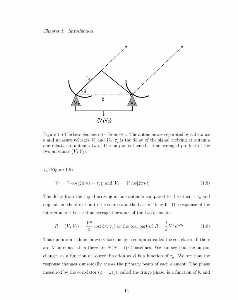
θb
V1 V2
⟨V1V2⟩
τg
Figure 1.5 The two-element interferometer. The antennae are separated by a distanceb and measure voltages V1 and V2. ⌧g is the delay of the signal arriving at antennaone relative to antenna two. The output is then the time-averaged product of thetwo antennae hV1V2 i.
V2 (Figure 1.5).
V1 = V cos[2⇡⌫(t � ⌧g)] and V2 = V cos[2⇡⌫t ] (1.8)
The delay from the signal arriving at one antenna compared to the other is ⌧g and
depends on the direction to the source and the baseline length. The response of the
interferometer is the time averaged product of the two elements:
R = hV1V2 i =V 2
2cos(2⇡⌫⌧g) or the real part of R =
1
2V 2e i!⌧g (1.9)
This operation is done for every baseline by a computer called the correlator. If there
are N antennas, then there are N(N � 1)/2 baselines. We can see that the output
changes as a function of source direction as R is a function of ⌧g. We see that the
response changes sinusoidally across the primary beam of each element. The phase
measured by the correlator (� = !⌧g), called the fringe phase, is a function of b, and
14
Chapter 1. Introduction
angle the source vector makes with the baseline vector, ✓:
� =!
c
b cos(✓) (1.10)
This is a Fourier element of the sky brightness distribution. Each two element
interferometer measures a single Fourier element �/(b cos(✓)). In principle we could
stop here, we can measure a flux and position of the source from the amplitude
and phase of the fringes. If the source is extended we can integrate over the source
after correcting for the primary beam response. However, the position of a source
is only constrained in one direction and we lack sensitivity. To better constrain
source positions with better sensitivity we can add more baselines by adding more
telescopes. It follows that by measuring many Fourier elements we can construct a
well understood response for a point source over the primary beam on the sky.
Moving from the two element interferometer to the many element interferometer
it becomes simpler to work in Fourier space. The east and north directions, along
which the projected baselines on the celestial sphere are measured, are referred to
as u and v. We can then convert back to intensity distribution on the sky, in xy
coordinates, by a Fourier transform. The response of the interferometer is thus the
Fourier transform of the sampling function of the (u, v) plane. We refer to this
response as the “dirty beam”. In essence the interferometer measures the Fourier
response of the sky, via the convolution of the dirty beam and the distribution of
sources on the sky.
Wilson et al. (2009) discuss several methods for calibrating interferometer data.
Here we present the most basic description of the process. Calibration involves
observing three di↵erent calibrators: a flux density calibrator, bandpass calibrator,
and a complex gain and phase calibrator. The flux density calibrator is a source on
the sky that has a known flux density and a well modeled sky brightness distribution.
This allows for the determination of the flux density scale (Perley & Butler, 2017).
The bandpass calibrator is observed to determine frequency dependent changes in
15
Chapter 1. Introduction
the gain. This is typically a strong source with a known spectrum such that a
determination of the bandpass solutions can be made quickly. Lastly, a complex
gain and phase calibrator is observed between integrations on the target source.
The phase calibrator allows for the determination of changes in the atmosphere, or
instrument, that a↵ect the amplitude and phase of the target as a function of time
during an observation. Alternating integrations between the phase calibrator and the
science target are carried out until the desired signal to noise and adequate sampling
of the (u, v) plane are achieved.
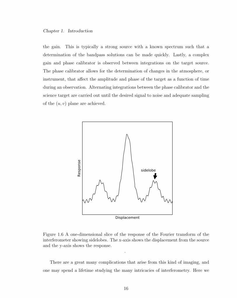
Figure 1.6 A one-dimensional slice of the response of the Fourier transform of theinterferometer showing sidelobes. The x-axis shows the displacement from the sourceand the y-axis shows the response.
.
There are a great many complications that arise from this kind of imaging, and
one may spend a lifetime studying the many intricacies of interferometry. Here we
16
Chapter 1. Introduction
will discuss the issues most related to the rest of this dissertation. The first issue that
every observer will encounter is sidelobes. Because the Fourier space is incompletely
sampled, artifacts erupt around sources (Figure 1.6). The interferometer response
is not completely Gaussian. The image including the sidelobes is called the “dirty
image”. It is the sky brightness distribution convolved with the interferometer re-
sponse. This can be addressed by deconvolving or “cleaning” the image (Hogbom,
1974). The dirty beam is measured from the Fourier transform of the (u, v) coverage
of the array. A clean beam is then determined by a fit to the central peak of the dirty
beam and scaled to conserve the total flux. The CLEAN algorithm then searches
the dirty image for the peak intensity in the dirty image. The algorithm records a
clean component with the position and a fraction of the peak intensity value. The
dirty beam is then convolved with the clean component and subtracted from the
dirty image. This fraction is called the loop gain and low values such as 0.1 to 0.2
help the process to converge. The algorithm proceeds in this fashion until all peaks
above a user defined threshold are found. What remains of the dirty image is called
the residual image. Then a clean image is made by convolving the clean beam with
all the clean components and adding back the residual image. The final image is
then divided by the primary beam response.
The second issue that is most important to this dissertation is that of invisible
distributions. The concept of maximum resolution is familiar to all astronomers.
That is the smallest angular size which can be determined reliably. However, due to
the sampling of Fourier space, an interferometer also has a minimum resolution, or
the largest angular size which can be determined reliably. This is set by the shortest
distance between collecting elements. Some or all of the flux will be invisible because
the interferometer will not be sensitive to the largest angular scales, decreasing the
strength of extended sources in the image. Another way to think about this is
that if a source distribution on the sky has spatial frequencies not sampled by the
interferometer, some flux will not be detected. That is, there is an infinite number
17
Chapter 1. Introduction
of invisible distributions that fit the data due to un-sampled (u, v) spacings. To
reiterate, there are many complications that arise from interferometric observations.
These two are the ones that are most relevant to this dissertation.
1.4.2 The VLA and the WIDAR Correlator
Figure 1.7 Aerial image of the Karl G. Jansky Very Large Array. Image courtesy ofNRAO/AUI.
The Very Large Array (VLA)2 is a Y-shaped interferometer (Figure 1.7). It
consists of 27 antennas yielding 351 baselines. It takes advantage of the rotation
of the Earth to fill in the (u, v) plane by allowing the Earth to rotate under a
source, causing the projection of the baselines to change with time. The shape of
the VLA allows for complete tracks every four hours. It is also reconfigurable into
2The National Radio Astronomy Observatory is a facility of the National Science Foun-dation operated under cooperative agreement by Associated Universities, Inc.
18
Chapter 1. Introduction
four di↵erent configurations with di↵erent maximum baselines and (u, v) coverages.
The A configuration has the largest maximum baseline, 36.4 km, yielding the highest
angular resolution, whereas the D configuration has a maximum baseline of 1.03 km
yielding low angular resolutions but the best sky brightness sensitivity. B and C
configurations have maximum baselines of 11.1 km and 3.4 km, respectively. It is
possible to combine configurations to gain the best (u, v) coverage for a particular
science case.
The Wideband Interferometric Digital ARchitecture (WIDAR) correlator is part
of the Expanded Very Large Array (EVLA) project. The upgrade started in 2001
and was completed in 2011. The telescope was renamed the Karl G. Jansky Very
Large Array (henceforth VLA). The correlator allows for full coverage of radio bands
from 1 to 50 GHz. It can be configured with up to 8 GHz of bandwidth with 16,384
channels, to a maximum of 4,194,304 channels over 0.5 GHz for high spectral reso-
lution (Dougherty & Perley, 2010). This gives the observer a wide range of spectral
capabilities from high spectral resolution to high continuum sensitivity.
As part of commissioning tests, observations the protocluster NGC 6334 targeted
the NH3(1,1) to (6,6) lines, the H64↵ Radio Recombination Line (RRL), and the
25 GHz Methanol line. All lines were detected in 10 minutes on source demonstrat-
ing the power of the WIDAR correlator for spectral line observations (Brogan &
Hunter, 2010). It is this ability that we exploit in this dissertation. Systematics
among observations i.e. di↵erent atmospheric opacities, di↵erent Radio Frequency
Interference (RFI; which would be more time consuming to remove in multiple ob-
servations), and antenna temperatures, are eliminated, because many spectral lines
can be captured in a single observation.
19
Chapter 2
NGC253: NH3 Thermometry, and
H2O and CH3OH Masers
2.1 Overview
We present Karl G Jansky Very Large Array molecular line observations of the nearby
starburst galaxy NGC 253, from SWAN: “Survey of Water and Ammonia in Nearby
galaxies”. SWAN is a molecular line survey at centimeter wavelengths designed to
reveal the physical conditions of star forming gas over a range of star forming galaxies.
NGC 253 has been observed in four 1 GHz bands from 21 to 36 GHz at 600 (⇠ 100 pc)
spatial and 3.5 km s�1 spectral resolution. In total we detect 19 transitions from
seven molecular and atomic species. We have targeted the metastable inversion
transitions of ammonia (NH3) from (1,1) to (5,5) and the (9,9) line, the 22.2 GHz
water (H2O) (616 � 523) maser, and the 36.1 GHz methanol (CH3OH) (4�1 � 30)
maser. Utilizing NH3 as a thermometer, we present evidence for uniform heating over
the central kpc of NGC 253. The molecular gas is best described by a two kinetic
temperature model with a warm 130 K and a cooler 57 K component. A comparison
20
Chapter 2. NGC253
of these observations with previous ALMA results suggests that the molecular gas
is not heated in photon dominated regions or shocks. It is possible that the gas
is heated by turbulence or cosmic rays. In the galaxy center we find evidence for
NH3(3,3) masers. Furthermore, we present velocities and luminosities of three H2O
maser features related to the nuclear starburst. We partially resolve CH3OH masers
seen at the edges of the bright molecular emission, which coincides with expanding
molecular superbubbles. This suggests that the masers are pumped by weak shocks
in the bubble surfaces.
2.2 Introduction
NGC 253 is one of the closest starburst galaxies to the Milky Way. We adopt a
distance of 3.5 Mpc measured from the tip of the red giant branch (Radburn-Smith
et al., 2011) and a systemic velocity of 234 km s�1 in the LSRK frame from Whiting
(1999). All velocities in this chapter will be in the LSRK frame unless otherwise
stated. Figure 2.1 shows a Spitzer 8µm image of NGC 253 (Dale et al., 2009). The
inset shows the central kpc with 3, 6 and 9� contours of NH3(3,3) emission from our
data discussed in Section 2.4.2.1. The disk is inclined at i⇠78� (Pence, 1980). NGC
253 has a total star formation rate (SFR) of ⇠5.9 M� yr�1 of which approximately
half is concentrated into the central kpc (McCormick et al., 2013). The molecular
outflow from the central kpc has a mass-loss rate estimated at 9 M� yr�1 possibly
starving the current star forming event (Bolatto et al., 2013).
Centimeter and millimeter wavelength spectra of galaxies provide access to di-
agnostically important molecular tracers. The molecular gas is often well traced by
CO, however more complex molecules can provide better tracers of gas properties
such as temperature and density, and can be used to trace specific conditions such
as PDRs and shocks (e.g. Fuente et al., 1993, Garcıa-Burillo et al., 2000, Meier &
21
Chapter 2. NGC253
Figure 2.1 Spitzer IRAC 8.0µm image of NGC 253 (Dale et al., 2009). The insetshows the central kpc with NH3(3,3) 3 to 30� contours, in steps of 3�, showing thedense molecular gas associated with the nuclear starburst. The 3� contour equatesto 4.7 mJy beam�1 km s�1.
Turner, 2005, and Meier et al., 2015). This study will focus on the metastable tran-
sitions (J = K) (1,1) to (5,5) and (9,9) of NH3, the 22 GHz H2O (616 � 523) maser,
and the 36 GHz CH3OH (414 � 303) maser. We will use a combined analysis of these
lines to expose the processes that dominate the central kpc of NGC 253.
The NH3 molecule generally works well as a temperature tracer of the molecular
gas. The tetrahedral structure of NH3 makes it a symmetric top, meaning the energy
states are described by the rotation angular momentum quantum number J and the
projection along the symmetry axis K. The J = K states, called metastable states,
are long lived compared to J > K states, and population exchanges between K
22
Chapter 2. NGC253
ladders are forbidden except by collisions. Therefore when NH3 is collisionally excited
( critical density nH2 & 103 cm�3) the K ladders are expected to be populated in
accordance with the kinetic temperature of the gas. As a result, measurements of the
relative intensities of metastable states act as probes of the rotational temperature
of the gas (e.g. Ho & Townes, 1983, Walmsley & Ungerechts, 1983, Lebron et al.,
2011, Ott et al., 2005, Ott et al., 2011, and Mangum et al., 2013).
The NH3(3,3) state can be a maser transition (Walmsley & Ungerechts, 1983),
but it is less well studied than other masers. In the Galaxy there is a weak asso-
ciation of NH3(3,3) masers with dense gas in star forming regions (e.g., Wilson &
Mauersberger, 1990, Mills & Morris, 2013, and Goddi et al., 2015). Here we will use
metastable transitions of NH3 to understand the heating and cooling balance of the
dense molecular ISM in NGC 253.
The H2O and CH3OH masers provide a unique opportunity to probe star forming
environments. The H2O line requires gas densities > 107 cm�3 and kinetic tempera-
tures > 300 K to mase (e.g. Genzel & Downes, 1977). In the Galaxy these masers
are typically found in shocked regions around Young Stellar Objects (YSOs) and
Asymptotic Giant Branch (AGB) stars (e.g. Palagi et al., 1993) and may be used to
identify regions of hot, dense, and/or shocked gas. This is in addition to precisely
tracing kinematics of stellar winds (e.g. Goddi & Moscadelli, 2006), and accretion
disks (e.g., Peck et al., 2003; Lo, 2005; Reid et al., 2009).
Class I (collisionally pumped) and II (radiatively pumped) CH3OH masers are
found in high mass star forming regions (e.g. Ellingsen et al., 2012). Class I masers
are also found in supernova remnants (e.g. McEwen et al., 2014) in the Galaxy. The
Class I masers trace shocks and gas densities > 104 cm�3 (Pratap et al., 2008). The
36.2 GHz CH3OH line studied here is a Class I type maser. We will mostly use these
masers as signposts of shocked material.
23
Chapter 2. NGC253
In §2.3 we describe the observational setup. In §2.4 we report our measurements
of the NH3, H2O, and CH3OH lines in addition to a brief description of the continuum
and the H56↵ Radio Recombination Line (RRL). In §2.5 we discuss the derivation
of temperatures across the molecular bar, the relevance of the H2O masers to the
outflow, the significance of the CH3OH masers, and a comparison with previous
ALMA millimeter molecular lines. Lastly, we summarize our findings in §2.6.
2.3 Observations and Data Reduction
We observed NGC 253 with the 18-26.5 GHz and 26.5-40 GHz (K- and Ka-bands)
receivers of the Karl G. Jansky Very Large Array (VLA)1 (project code: 13A-375).
The K-band observations were carried out on 2013 May 11. The Ka-band observa-
tions were split into two sessions: 2013 May 23 and 2013 May 26. The VLA was
in the DnC hybrid configuration for all these observations. This configuration de-
livers a rounder beam for low declination sources because the north arm is in the
more extended C configuration, while the east and west arms are in D configuration.
The received signal is sampled at each antenna using the 8-bit samplers. These pro-
vide two 1 GHz baseband pairs with both right and left hand circular polarizations.
The correlator was set up to divide each baseband into 8 sub-bands each with 512
channels resulting in a channel width of 250 kHz. This yields a velocity resolution
ranging from 3.0 to 3.3 km s�1 for the K-band, and 2.0 to 2.7 km s�1 for the Ka-
band observations. The baseband pairs were centered at 21.8 GHz and 24.1 GHz
in K-band, 27.1 GHz and 36.4 GHz in Ka-band. They will be referred to as the 22
GHz, 24 GHz, 27 GHz, and 36 GHz basebands, respectively. These were chosen to
include the metastable NH3 transitions from (1,1) with rest frequency 26.6946 GHz,
to (5,5) at 24.5330 GHz, as well as (9,9) at 27.4779 GHz, the H2O(616 � 523) maser
1The National Radio Astronomy Observatory is a facility of the National Science Foun-dation operated under cooperative agreement by Associated Universities, Inc.
24
Chapter 2. NGC253
line at 22.2351 GHz, and the CH3OH(414�303) transition at 36.1693 GHz. All of the
detected lines and their rest frequencies are listed in Table 2.1. The on source time
for the K-band and Ka-band observations was 4.4 hours and 3.6 hours, respectively.
We used 3C48 as the flux density calibrator Perley & Butler (2013), J2253+1608 as
the bandpass calibrator, and J0025-2602 as the complex gain calibrator in all ob-
servations. We alternated between 10 minute intervals on NGC 253 and 1.5 minute
intervals on the complex gain calibrator.
The data were reduced in the Common Astronomy Software Applications (CASA)
package version 4.2.2 (McMullin et al., 2007). At the adopted distance of 3.5 Mpc
the linear scale is ⇠17 pc per arcsecond. The half power primary beam widths of
the VLA for the K- and Ka-bands are 2.10 (⇠2 kpc) and 1.50 (⇠1.5 kpc) respectively.
All data cubes were gridded with 0.2500 pixels, mapped using natural weighting,
CLEANed to ⇠ 3� rms noise, and are regridded to a common velocity resolution of
3.5 km s�1. Continuum subtraction was performed in the (u, v) domain. For the 24
GHz baseband, several baselines were flagged for being noisy yielding a slightly larger
synthesized beam than the 22 GHz baseband. The resulting image cubes are then
smoothed with a Gaussian kernel to a common synthesized beam of 600⇥400 (Position
Angle: 3.00�). The common resolution cubes are used for consistency for all the
observed lines. The resulting rms noise values in the K-band and Ka-band image
cubes are 0.5 mJy beam�1 and 1 mJy beam�1 in a 3.5 km s�1 channel, respectively.
The maser lines of H2O, CH3OH, and NH3(3,3) have also been imaged with 0.2500
pixels and Briggs (robust=0) weighting, yielding a synthesized beam of 400⇥300 for
H2O and NH3(3,3) and 200⇥100 for CH3OH, to better constrain the locations of masing
material. The rms noise in the K-band and Ka-band Briggs weighted image cubes
are 1.5 mJy beam�1 and 3.1 mJy beam�1 in a 3.5 km s�1 channel, respectively. A
super-resolved cube was constructed for the H2O maser data. This was done by
deconvolving a dirty image cube then convolving the CLEAN components with a
100 circular beam. This super-resolved image cube is used to emphasize structures
25
Chapter 2. NGC253
seen in the CLEAN components that are di�cult to discern in the regularly resolved
image cubes. No quantitative measurements are made with the super-resolved cube.
2.4 Results
The full continuum subtracted spectra of our K- and Ka-band observations are pre-
sented in Figure 2.2. We have identified 17 transitions from seven di↵erent molecular
or atomic species shown in Table 2.1. Lines were identified by searching the common
resolution data cubes with a pixel sized beam. We set conditions for a detection
at a peak flux of >1.5 mJy beam�1 channel�1 for K-band and >3.0 mJy beam�1
channel�1 for Ka-band, and a FWHM of &30 km s�1 for thermal lines. For known
maser transitions single channels above 6� are considered detections.
26
Chapter 2. NGC253
Figure 2.2 The observed spectrum from K-band and Ka-band. The spectrum wasextracted from a 4000⇥2500 box centered at RA: 00h47m33.12s DEC: �25�17019.3300andHanning smoothed with a window of 21 channels . Each box shows the selected 1 GHzbasebands with frequency on the X-axis and flux density on the Y-axis. Detectedmolecular and atomic species are identified with black arrows, though these may notbe apparent due to the large area we extracted these spectra from. The missingchannels between spectral windows are a consequence of the spectral setup.
27
Chapter 2. NGC253
Table 2.1. Detected Molecular and Atomic Transitions in NGC 253
Transition Rest Frequency
(GHz)
c-C3H2 (220 � 211) 21.5874
H2O(616 � 523) 22.2351
H66↵ 22.3642
H64↵ 24.5099
NH3 (1,1) 23.6945
NH3 (2,2) 23.7226
NH3 (3,3) 23.8701
NH3 (4,4) 24.1394
NH3 (5,5) 24.5330
H62↵ 26.9392
c-C3H2 (330 � 321) 27.0843
HC3N(3-2) 27.2944
NH3 (9,9) 27.4779
CH3OH(4�1 � 33) 36.1693
HC3N(4-3) 36.3924
H56↵ 36.4663
CH3CN(2 � 1) 36.7956
Note. — Molecules selected for this pa-
per’s analysis are shown in bold face text
28
Chapter 2. NGC253
2.4.1 Continuum Emission and Radio Recombination Lines
The radio continuum emission from NGC 253 is resolved in all four basebands (Figure
2.3). Images were made selecting only line free channels. The flux density measured
in the 24 GHz baseband is 550±30 mJy. This agrees with the value of 520±52 mJy
from Ott et al. (2005). The 36 GHz flux density measures 350±40 mJy in close
agreement with the value of 332.5±0.1 mJy at 31.2 GHz measured by Kepley et
al. (2011). The other continuum flux density measurements are 470±20 mJy and
370±40 mJy for the 22 GHz and 27 GHz basebands, respectively. The spectral index
derived from the K-band basebands is �1.8±0.5 and for Ka-band 0.2 ± 0.4. The
measurements suggest the continuum goes through a minimum between the 24 GHz
and 27 GHz basebands. The H56↵ transition is the strongest radio recombination
line (RRL) we detect. Figure 2.4 shows the relationship between the Hubble (HST)
H↵ (Watson et al., 1996), H56↵, Pa↵ (Alonso-Herrero et al., 2003), and the 36
GHz continuum emission. We treat the H↵ as a tracer of the outflow with heavy
dust obscuration, Pa↵ as a partially obscured star formation tracer and RRL as an
unobscured star formation tracer.
2.4.2 Molecular Emission Lines
Our analysis from here on will focus only on NH3, H2O, and CH3OH. These transi-
tions are shown in bold text in Table 2.1. Intensity and peak flux maps are shown
in Figure 2.5. Spectra have been extracted from the naturally weighted, smoothed
cubes from the pixels at the locations marked by crosses (Figure 2.5) and are shown
in Figures 2.6, 2.8, and 2.9. These locations were selected from the spatial peaks in
the peak flux maps shown, or for spectrally unique characteristics. For example, W2
is not a spatial peak in the peak flux map but was selected for a spectral component
discussed in Section 2.4.2.2. The continuum peak is labeled C1, and identifies the
29
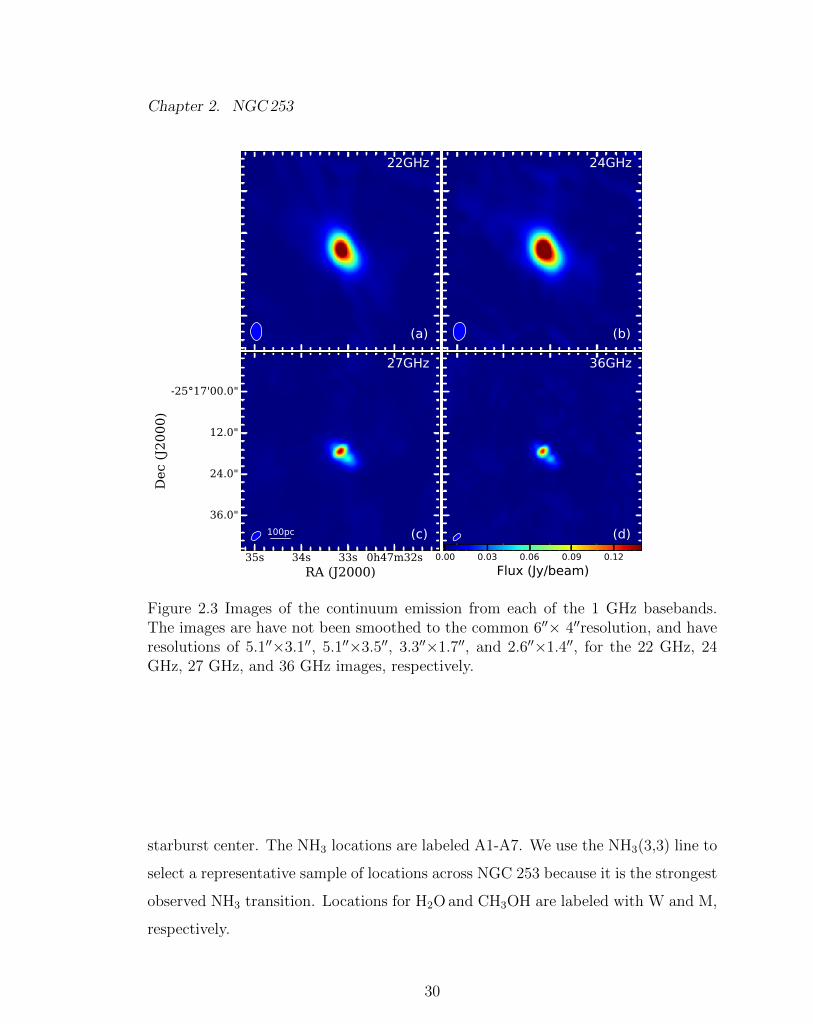
Chapter 2. NGC253
Figure 2.3 Images of the continuum emission from each of the 1 GHz basebands.The images are have not been smoothed to the common 600⇥ 400resolution, and haveresolutions of 5.100⇥3.100, 5.100⇥3.500, 3.300⇥1.700, and 2.600⇥1.400, for the 22 GHz, 24GHz, 27 GHz, and 36 GHz images, respectively.
starburst center. The NH3 locations are labeled A1-A7. We use the NH3(3,3) line to
select a representative sample of locations across NGC 253 because it is the strongest
observed NH3 transition. Locations for H2O and CH3OH are labeled with W and M,
respectively.
30
Chapter 2. NGC253
NH3 Inversion Lines
The observed NH3 emission spans an elongated structure ⇠1 kpc in length about
the continuum peak. The northeast (NE) side of the continuum peak contains three
NH3(3,3) spatial peaks (A1, A2 and A3), which are blueshifted from the systemic
velocity with observed velocities ranging from ⇠ 160 km s�1 to 200 km s�1.The south-
west (SW) side of the continuum peak contains four NH3(3,3) peaks (A4, A5, A6, and
A7), which are redshifted from systemic with velocities ranging from ⇠ 280 km s�1
to 320 km s�1. (Figure 2.5). The peaks A1, A2, and A3 can be cross-identified with
in regions F, E, and D from Ott et al. (2005) and A4, A5, A6 and A7 are analogous
to C, B, and A . It should be noted that this is not a one to one mapping as we
have a smaller beam than the superresolved cube used in Ott et al. (2005). The NH3
spectra from each pixel are shown in Figure 2.6. We detect inversion transitions
NH3(1,1) to (5,5) at all locations. In addition the NH3(9,9) line is weakly detected
at site A3 (Figure 2.7). At the continuum peak all the NH3 transitions are seen
in absorption with the exception of NH3(3,3). Single Gaussians were fitted to the
spectrum extracted from each location, from which we extract the integrated flux,
peak flux, FWHM, and the line center, from the individual pixels marked in Figure
2.5. The properties of the metastable transitions, NH3(1,1) to (5,5), for A1-A7 are
listed in Table 2.2 and C1 in Table 2.3. The weakly detected NH3(9,9) fit results are
listed in Table 2.4. We do not see the NH3 metastable inversion hyperfine transitions
(J=K, �F = 1) as the lines are likely weak and broad enough to be smeared out.
A1, A5 and A6 FWHMs are a few tens of km s�1 wider than the other locations.
These three sites are located on the edges of superbubbles (See section 4.4) discovered
by Sakamoto et al. (2006). At C1, the NH3(3,3) line appears in emission whereas
all other inversion lines appear in absorption (Figure 2.6), interpreted to be due
to the existence of NH3(3,3) masers, confirming the result from Ott et al. (2005).
The NH3(3,3) emission for C1 is not well described by a single Gaussian and thus
31
Chapter 2. NGC253
two Gaussians were fit to the data (Figure 2.10), with FWHMs of 55±3 km s�1
and 130±10 km s�1 and centers of 172±1 km s�1 and 257±5 km s�1, respectively
NH3(3,3)a and NH3(3,3)b.
32
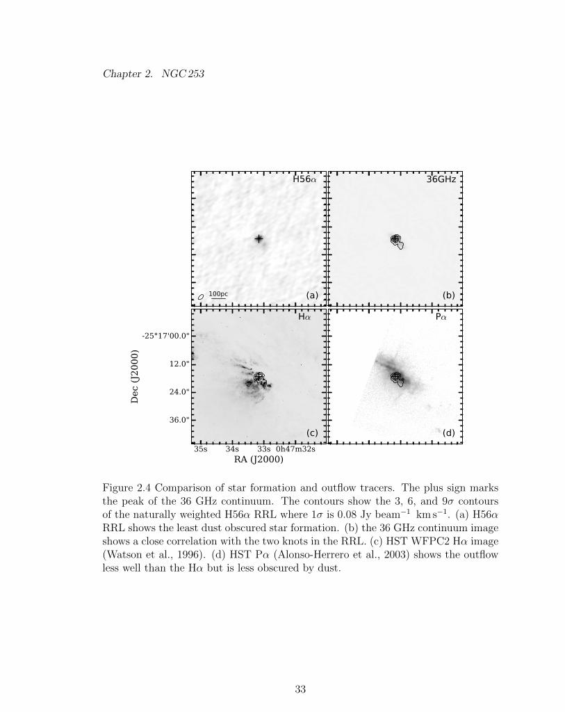
Chapter 2. NGC253
Figure 2.4 Comparison of star formation and outflow tracers. The plus sign marksthe peak of the 36 GHz continuum. The contours show the 3, 6, and 9� contoursof the naturally weighted H56↵ RRL where 1� is 0.08 Jy beam�1 km s�1. (a) H56↵RRL shows the least dust obscured star formation. (b) the 36 GHz continuum imageshows a close correlation with the two knots in the RRL. (c) HST WFPC2 H↵ image(Watson et al., 1996). (d) HST P↵ (Alonso-Herrero et al., 2003) shows the outflowless well than the H↵ but is less obscured by dust.
33
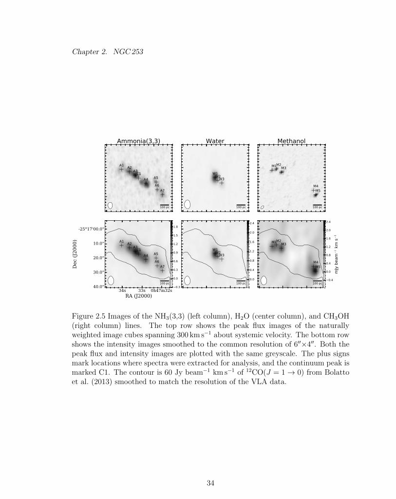
Chapter 2. NGC253
Figure 2.5 Images of the NH3(3,3) (left column), H2O (center column), and CH3OH(right column) lines. The top row shows the peak flux images of the naturallyweighted image cubes spanning 300 km s�1 about systemic velocity. The bottom rowshows the intensity images smoothed to the common resolution of 600⇥400. Both thepeak flux and intensity images are plotted with the same greyscale. The plus signsmark locations where spectra were extracted for analysis, and the continuum peak ismarked C1. The contour is 60 Jy beam�1 km s�1 of 12CO(J = 1 ! 0) from Bolattoet al. (2013) smoothed to match the resolution of the VLA data.
34
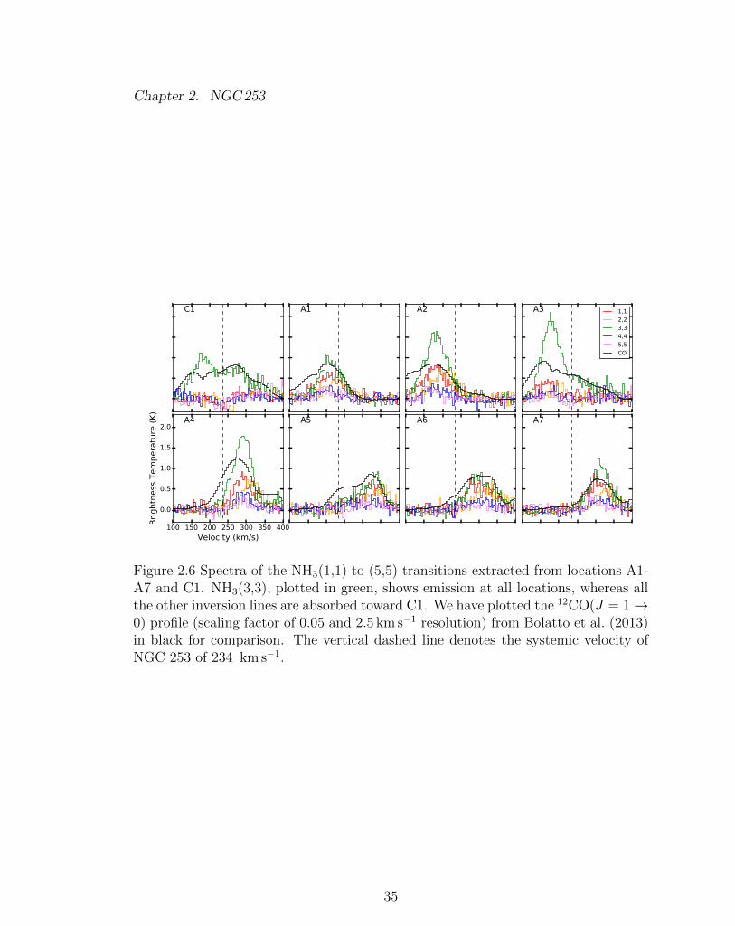
Chapter 2. NGC253
Figure 2.6 Spectra of the NH3(1,1) to (5,5) transitions extracted from locations A1-A7 and C1. NH3(3,3), plotted in green, shows emission at all locations, whereas allthe other inversion lines are absorbed toward C1. We have plotted the 12CO(J = 1 !
0) profile (scaling factor of 0.05 and 2.5 km s�1 resolution) from Bolatto et al. (2013)in black for comparison. The vertical dashed line denotes the systemic velocity ofNGC 253 of 234 km s�1.
35
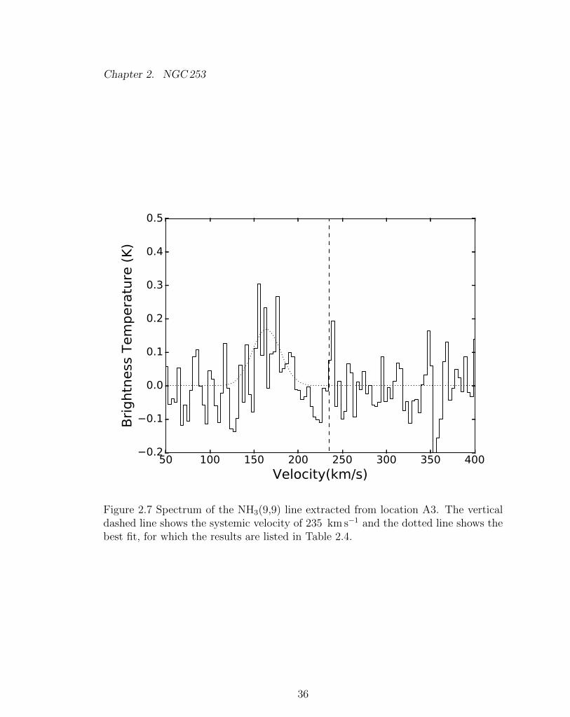
Chapter 2. NGC253
Figure 2.7 Spectrum of the NH3(9,9) line extracted from location A3. The verticaldashed line shows the systemic velocity of 235 km s�1 and the dotted line shows thebest fit, for which the results are listed in Table 2.4.
36
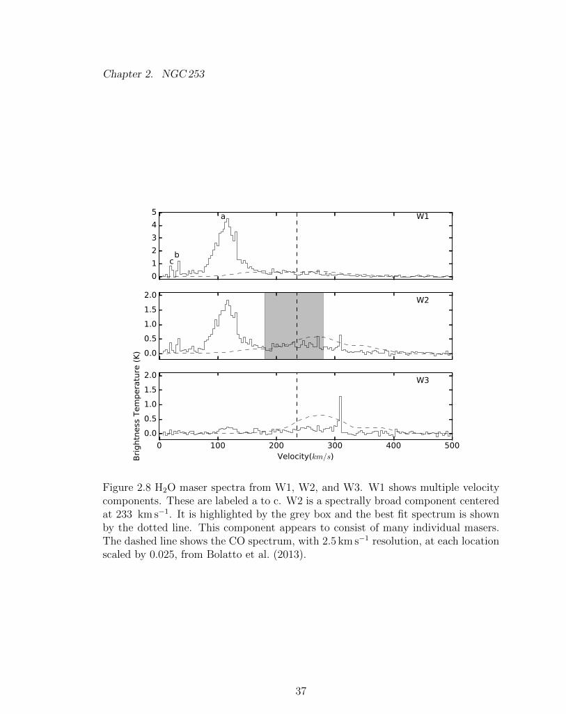
Chapter 2. NGC253
Figure 2.8 H2O maser spectra from W1, W2, and W3. W1 shows multiple velocitycomponents. These are labeled a to c. W2 is a spectrally broad component centeredat 233 km s�1. It is highlighted by the grey box and the best fit spectrum is shownby the dotted line. This component appears to consist of many individual masers.The dashed line shows the CO spectrum, with 2.5 km s�1 resolution, at each locationscaled by 0.025, from Bolatto et al. (2013).
37
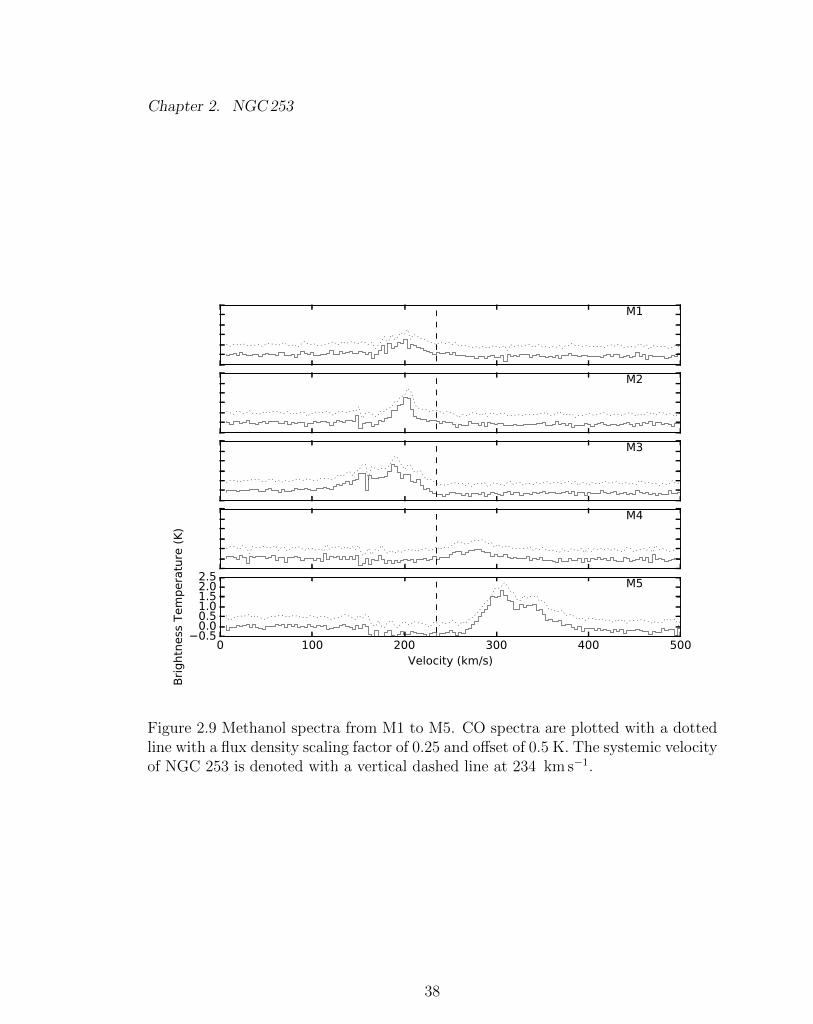
Chapter 2. NGC253
Figure 2.9 Methanol spectra from M1 to M5. CO spectra are plotted with a dottedline with a flux density scaling factor of 0.25 and o↵set of 0.5 K. The systemic velocityof NGC 253 is denoted with a vertical dashed line at 234 km s�1.
38
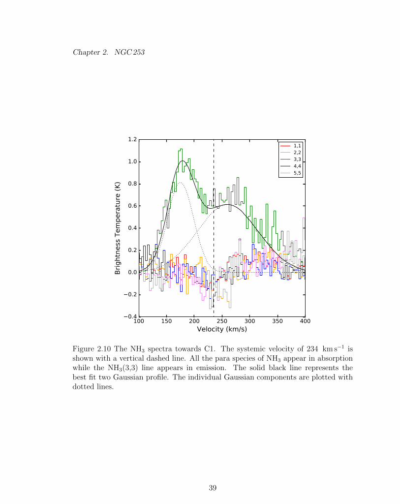
Chapter 2. NGC253
Figure 2.10 The NH3 spectra towards C1. The systemic velocity of 234 km s�1 isshown with a vertical dashed line. All the para species of NH3 appear in absorptionwhile the NH3(3,3) line appears in emission. The solid black line represents thebest fit two Gaussian profile. The individual Gaussian components are plotted withdotted lines.
39
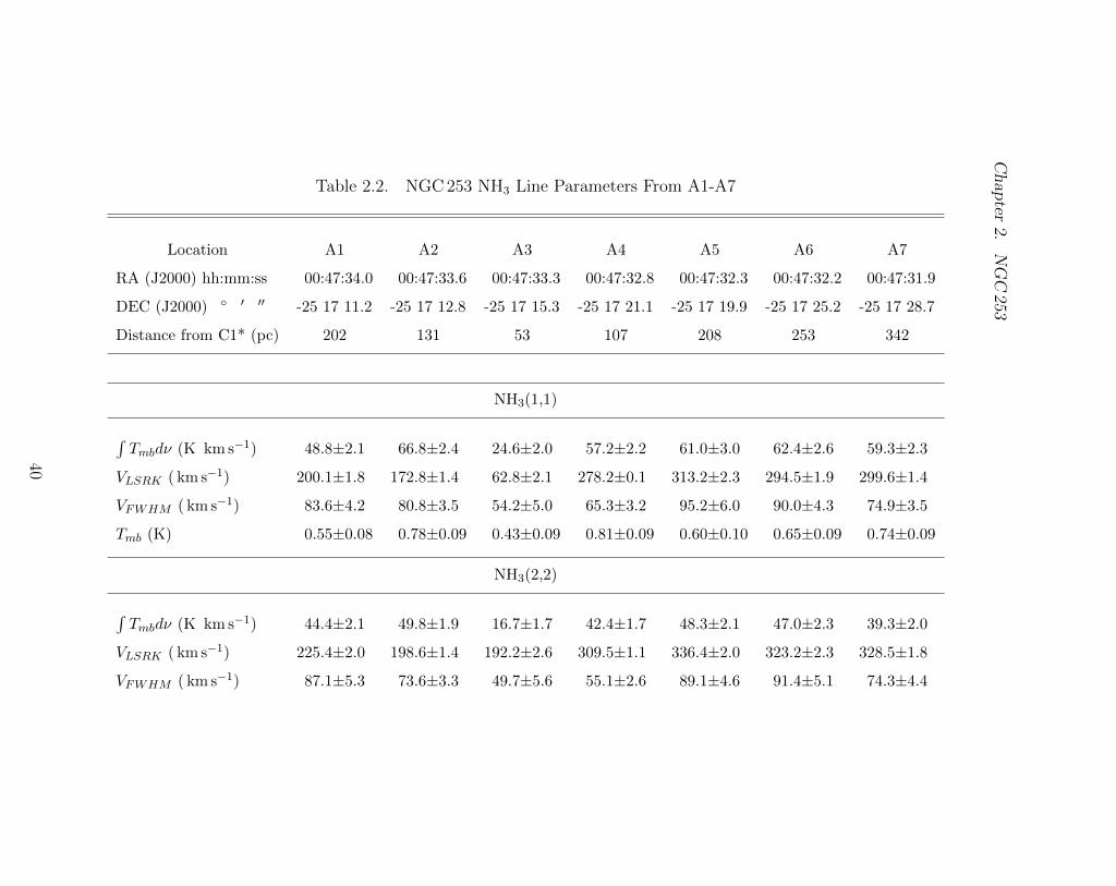
Chapter2.
NGC253
Table 2.2. NGC 253 NH3 Line Parameters From A1-A7
Location A1 A2 A3 A4 A5 A6 A7
RA (J2000) hh:mm:ss 00:47:34.0 00:47:33.6 00:47:33.3 00:47:32.8 00:47:32.3 00:47:32.2 00:47:31.9
DEC (J2000) � 0 00 -25 17 11.2 -25 17 12.8 -25 17 15.3 -25 17 21.1 -25 17 19.9 -25 17 25.2 -25 17 28.7
Distance from C1* (pc) 202 131 53 107 208 253 342
NH3(1,1)
RTmbd⌫ (K km s�1) 48.8±2.1 66.8±2.4 24.6±2.0 57.2±2.2 61.0±3.0 62.4±2.6 59.3±2.3
VLSRK ( km s�1) 200.1±1.8 172.8±1.4 62.8±2.1 278.2±0.1 313.2±2.3 294.5±1.9 299.6±1.4
VFWHM ( km s�1) 83.6±4.2 80.8±3.5 54.2±5.0 65.3±3.2 95.2±6.0 90.0±4.3 74.9±3.5
Tmb (K) 0.55±0.08 0.78±0.09 0.43±0.09 0.81±0.09 0.60±0.10 0.65±0.09 0.74±0.09
NH3(2,2)
RTmbd⌫ (K km s�1) 44.4±2.1 49.8±1.9 16.7±1.7 42.4±1.7 48.3±2.1 47.0±2.3 39.3±2.0
VLSRK ( km s�1) 225.4±2.0 198.6±1.4 192.2±2.6 309.5±1.1 336.4±2.0 323.2±2.3 328.5±1.8
VFWHM ( km s�1) 87.1±5.3 73.6±3.3 49.7±5.6 55.1±2.6 89.1±4.6 91.4±5.1 74.3±4.4
40
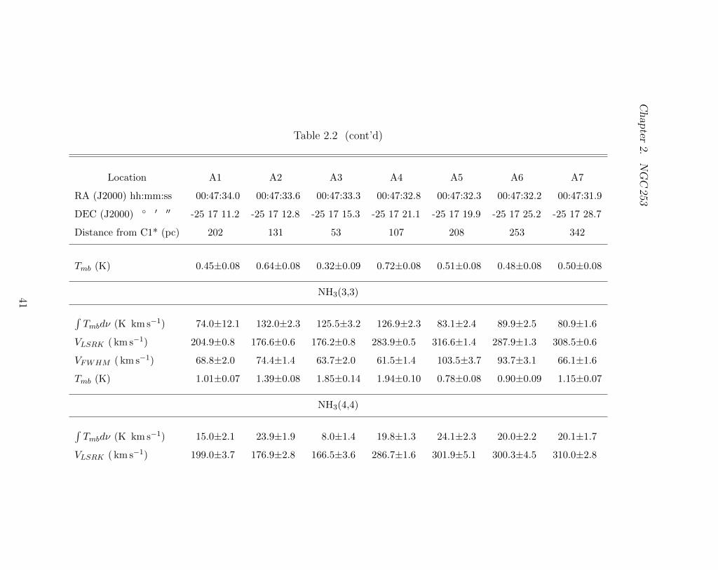
Chapter2.
NGC253
Table 2.2 (cont’d)
Location A1 A2 A3 A4 A5 A6 A7
RA (J2000) hh:mm:ss 00:47:34.0 00:47:33.6 00:47:33.3 00:47:32.8 00:47:32.3 00:47:32.2 00:47:31.9
DEC (J2000) � 0 00 -25 17 11.2 -25 17 12.8 -25 17 15.3 -25 17 21.1 -25 17 19.9 -25 17 25.2 -25 17 28.7
Distance from C1* (pc) 202 131 53 107 208 253 342
Tmb (K) 0.45±0.08 0.64±0.08 0.32±0.09 0.72±0.08 0.51±0.08 0.48±0.08 0.50±0.08
NH3(3,3)
RTmbd⌫ (K km s�1) 74.0±12.1 132.0±2.3 125.5±3.2 126.9±2.3 83.1±2.4 89.9±2.5 80.9±1.6
VLSRK ( km s�1) 204.9±0.8 176.6±0.6 176.2±0.8 283.9±0.5 316.6±1.4 287.9±1.3 308.5±0.6
VFWHM ( km s�1) 68.8±2.0 74.4±1.4 63.7±2.0 61.5±1.4 103.5±3.7 93.7±3.1 66.1±1.6
Tmb (K) 1.01±0.07 1.39±0.08 1.85±0.14 1.94±0.10 0.78±0.08 0.90±0.09 1.15±0.07
NH3(4,4)
RTmbd⌫ (K km s�1) 15.0±2.1 23.9±1.9 8.0±1.4 19.8±1.3 24.1±2.3 20.0±2.2 20.1±1.7
VLSRK ( km s�1) 199.0±3.7 176.9±2.8 166.5±3.6 286.7±1.6 301.9±5.1 300.3±4.5 310.0±2.8
41
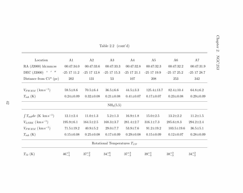
Chapter2.
NGC253
Table 2.2 (cont’d)
Location A1 A2 A3 A4 A5 A6 A7
RA (J2000) hh:mm:ss 00:47:34.0 00:47:33.6 00:47:33.3 00:47:32.8 00:47:32.3 00:47:32.2 00:47:31.9
DEC (J2000) � 0 00 -25 17 11.2 -25 17 12.8 -25 17 15.3 -25 17 21.1 -25 17 19.9 -25 17 25.2 -25 17 28.7
Distance from C1* (pc) 202 131 53 107 208 253 342
VFWHM ( km s�1) 59.5±8.6 70.5±6.4 36.5±6.6 44.5±3.3 125.4±13.7 82.4±10.4 64.8±6.2
Tmb (K) 0.24±0.09 0.32±0.08 0.21±0.08 0.41±0.07 0.17±0.07 0.23±0.08 0.29±0.09
NH3(5,5)
RTmbd⌫ (K km s�1) 12.1±2.4 11.0±1.3 5.2±1.3 16.9±1.8 15.0±2.5 13.2±2.2 11.2±1.5
VLSRK ( km s�1) 195.9±6.1 164.5±2.5 168.3±3.7 281.4±2.7 316.1±7.3 285.6±8.3 294.2±2.4
VFWHM ( km s�1) 71.5±19.2 40.9±5.2 29.0±7.7 53.9±7.6 91.2±19.2 103.5±19.6 36.5±5.1
Tmb (K) 0.15±0.08 0.25±0.08 0.17±0.09 0.29±0.08 0.15±0.09 0.12±0.07 0.28±0.09
Rotational Temperatures TJJ 0
T12 (K) 46+5�4 37+2
�2 34+6�4 37+3
�3 39+4�3 38+3
�3 34+2�2
42
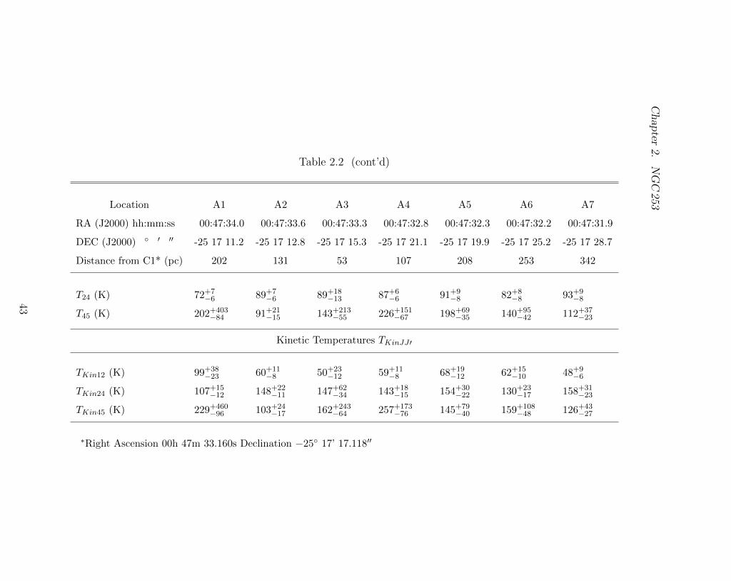
Chapter2.
NGC253
Table 2.2 (cont’d)
Location A1 A2 A3 A4 A5 A6 A7
RA (J2000) hh:mm:ss 00:47:34.0 00:47:33.6 00:47:33.3 00:47:32.8 00:47:32.3 00:47:32.2 00:47:31.9
DEC (J2000) � 0 00 -25 17 11.2 -25 17 12.8 -25 17 15.3 -25 17 21.1 -25 17 19.9 -25 17 25.2 -25 17 28.7
Distance from C1* (pc) 202 131 53 107 208 253 342
T24 (K) 72+7�6 89+7
�6 89+18�13 87+6
�6 91+9�8 82+8
�8 93+9�8
T45 (K) 202+403�84 91+21
�15 143+213�55 226+151
�67 198+69�35 140+95
�42 112+37�23
Kinetic Temperatures TKinJJ 0
TKin12 (K) 99+38�23 60+11
�8 50+23�12 59+11
�8 68+19�12 62+15
�10 48+9�6
TKin24 (K) 107+15�12 148+22
�11 147+62�34 143+18
�15 154+30�22 130+23
�17 158+31�23
TKin45 (K) 229+460�96 103+24
�17 162+243�64 257+173
�76 145+79�40 159+108
�48 126+43�27
⇤Right Ascension 00h 47m 33.160s Declination �25� 17’ 17.11800
43
Chapter 2. NGC253
H2O masers
We identify three regions of H2O maser emission in the data cube, labeled W1 to W3
in Figure 2.5 (center). The W1 H2O maser has been previously observed by Henkel
et al. (2004) and Brunthaler et al. (2009). Spectra at these positions are shown in
Figure 2.8. Regions W1 and W3 are seen as clear, spatially resolved peaks in Figure
2.5. Region W1 shows multiple velocity components with the main peak labeled
W1a, and the minor peaks labeled W1b and W1c. W2 is a faint feature which is not
spatially resolved from W1 and W3, but marks the peak emission of a unique broad
component shown by the shaded region in Figure 2.8. W2 is identified by the peak
emission from the narrow feature at 273 km s�1 channel (Figure 2.8). W1 and W2
show multiple peaks in the spectrum. These were fitted with single Gaussians where
appropriate. The properties are listed in Table 2.5. Single channel features are likely
real, given our spectral resolution, but, were not fitted by Gaussians and thus their
FWHMs are upper limits.
The spectrum of W2 has contributions from W1 and W3 as they are not resolved
from W2. W2 is a broad pedestal spanning ⇠100 km s�1 centered at 233 km s�1 with
several narrow features. Typical line widths in star forming regions are a few 10’s of
km s�1 (e.g., Ho et al., 1987 and Brunthaler et al., 2009). The rest of its properties
are listed in Table 2.5. This component is much better matched to systemic velocity
of NGC 253. W3 is a redshifted single velocity component maser at 303 km s�1.
W1a dominates region W1 and is blueshifted with respect to systemic with an
observed velocity of 109 km s�1. This source is coincident with TH2 and considered
to be the dynamical center (Turner & Ho, 1985). The integrated flux density of the
W1a maser is ⇠ 214 K km s�1 yielding a luminosity of 0.66 L� making it a kilomaser.
The extension is hard to discern in the the peak flux density and integrated flux
maps (Figure 2.5), but it is clearly seen in the contours of the super-resolved image
44
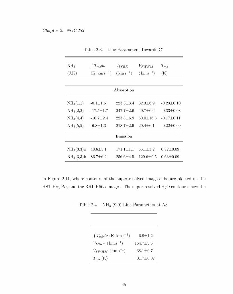
Chapter 2. NGC253
Table 2.3. Line Parameters Towards C1
NH3
RTmbd⌫ VLSRK VFWHM Tmb
(J,K) (K km s�1) ( km s�1) ( km s�1) (K)
Absorption
NH3(1,1) -8.1±1.5 223.3±3.4 32.3±6.9 -0.23±0.10
NH3(2,2) -17.5±1.7 247.7±2.6 49.7±6.6 -0.33±0.08
NH3(4,4) -10.7±2.4 223.8±6.9 60.0±16.3 -0.17±0.11
NH3(5,5) -6.8±1.3 218.7±2.9 29.4±6.1 -0.22±0.09
Emission
NH3(3,3)a 48.6±5.1 171.1±1.1 55.1±3.2 0.82±0.09
NH3(3,3)b 86.7±6.2 256.6±4.5 129.6±9.5 0.63±0.09
in Figure 2.11, where contours of the super-resolved image cube are plotted on the
HST H↵, P↵, and the RRL H56↵ images. The super-resolved H2O contours show the
Table 2.4. NH3 (9,9) Line Parameters at A3
RTmbd⌫ (K km s�1) 6.9±1.2
VLSRK ( km s�1) 164.7±3.5
VFWHM ( km s�1) 38.1±6.7
Tmb (K) 0.17±0.07
45
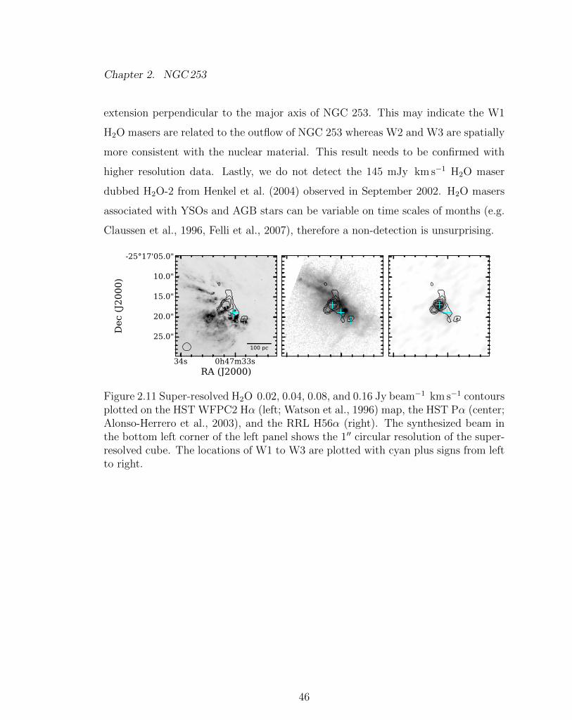
Chapter 2. NGC253
extension perpendicular to the major axis of NGC 253. This may indicate the W1
H2O masers are related to the outflow of NGC 253 whereas W2 and W3 are spatially
more consistent with the nuclear material. This result needs to be confirmed with
higher resolution data. Lastly, we do not detect the 145 mJy km s�1 H2O maser
dubbed H2O-2 from Henkel et al. (2004) observed in September 2002. H2O masers
associated with YSOs and AGB stars can be variable on time scales of months (e.g.
Claussen et al., 1996, Felli et al., 2007), therefore a non-detection is unsurprising.
Figure 2.11 Super-resolved H2O 0.02, 0.04, 0.08, and 0.16 Jy beam�1 km s�1 contoursplotted on the HST WFPC2 H↵ (left; Watson et al., 1996) map, the HST P↵ (center;Alonso-Herrero et al., 2003), and the RRL H56↵ (right). The synthesized beam inthe bottom left corner of the left panel shows the 100 circular resolution of the super-resolved cube. The locations of W1 to W3 are plotted with cyan plus signs from leftto right.
46
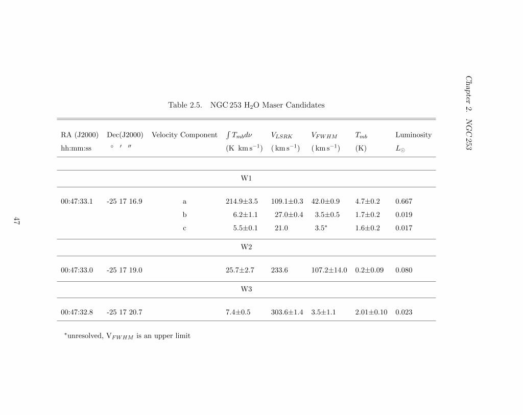
Chapter2.
NGC253
Table 2.5. NGC 253 H2O Maser Candidates
RA (J2000) Dec(J2000) Velocity ComponentR
Tmbd⌫ VLSRK VFWHM Tmb Luminosity
hh:mm:ss � 0 00 (K km s�1) ( km s�1) ( km s�1) (K) L�
W1
00:47:33.1 -25 17 16.9 a 214.9±3.5 109.1±0.3 42.0±0.9 4.7±0.2 0.667
b 6.2±1.1 27.0±0.4 3.5±0.5 1.7±0.2 0.019
c 5.5±0.1 21.0 3.5⇤ 1.6±0.2 0.017
W2
00:47:33.0 -25 17 19.0 25.7±2.7 233.6 107.2±14.0 0.2±0.09 0.080
W3
00:47:32.8 -25 17 20.7 7.4±0.5 303.6±1.4 3.5±1.1 2.01±0.10 0.023
⇤unresolved, VFWHM is an upper limit
47
Chapter 2. NGC253
36 GHz CH3OH masers
Extragalactic 36 GHz CH3OH masers were first detected by Ellingsen et al. (2014)
in NGC 253 with the Australia Telescope Compact Array (ATCA)2 with a 8.000⇥4.200
synthesized beam. Two sources were detected. The emission is likely not thermal in
its nature, despite the large FWHM of the line, due to the total integrated intensity
being ⇠20 times greater than the total integrated intensity from the Galaxy’s central
molecular zone (see Ellingsen et al., 2014). We resolve the two regions previously
seen in Ellingsen et al., 2014 into five di↵erent regions with masers as marked in
the peak flux map. The spectra are extracted from the common resolution (600⇥400)
image cubes and shown in Figure 2.9. The pairs M1 and M2, and M4 and M5 are
not spatially resolved from each other in the common resolution cube. M1 and M2
are spectrally similar, however M4 and M5 show distinct spectral components. The
CH3OH line is very close to the edge of one of our spectral sub-bands. There are small
(3.5 km s�1) gaps between each sub-band where the data collected is untrustworthy,
thus the channel corresponding to 160 km s�1 is lost. We next fit single component
Gaussians where appropriate. The extracted properties of the lines are shown in
Table 2.6. The region M5 was fit with two Gaussians due to the double peak. The
spectral features are narrower than the NH3 (this paper) and 12CO(J = 1 ! 0)
features (Bolatto et al., 2013) from the same locations, with measured FWHMs
spanning a range of 30�80 km s�1. The narrower widths suggest that the 36 GHz
CH3OH emission is not tracing the entirety of the molecular gas.
2The Australia Telescope Compact Array is part of the Australia Telescope, which isfunded by the Commonwealth of Australia for operation as a National Facility managedby CSIRO.
48
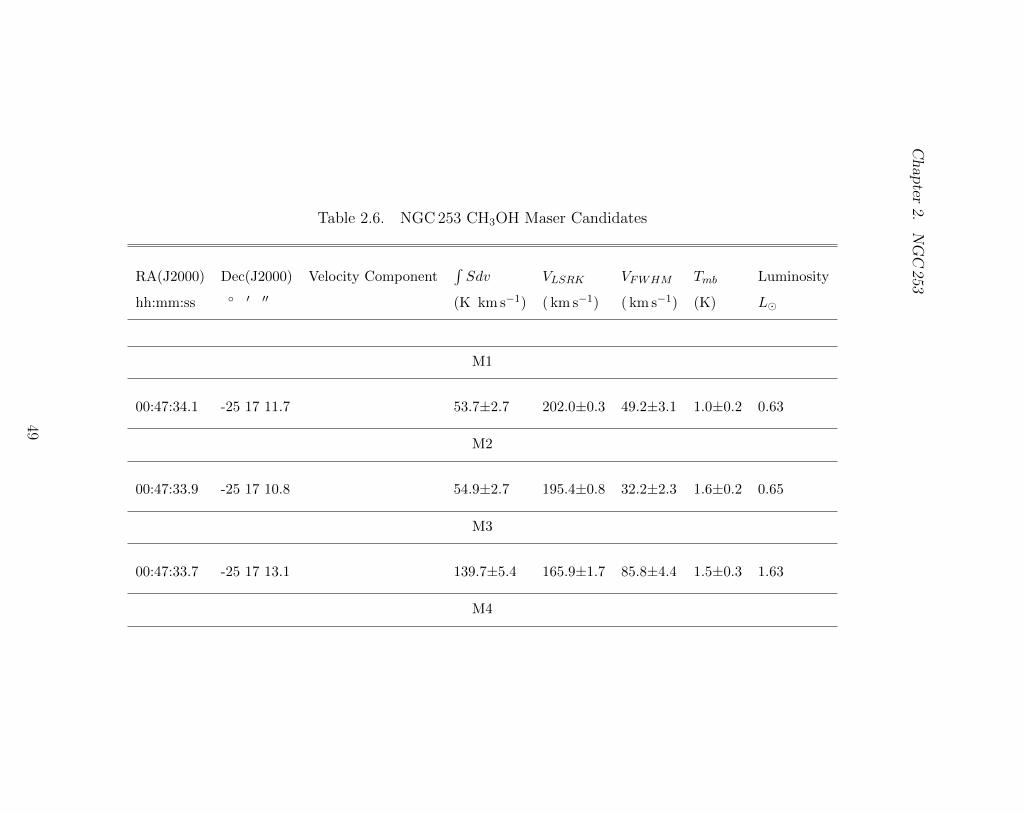
Chapter2.
NGC253
Table 2.6. NGC 253 CH3OH Maser Candidates
RA(J2000) Dec(J2000) Velocity ComponentR
Sdv VLSRK VFWHM Tmb Luminosity
hh:mm:ss � 0 00 (K km s�1) ( km s�1) ( km s�1) (K) L�
M1
00:47:34.1 -25 17 11.7 53.7±2.7 202.0±0.3 49.2±3.1 1.0±0.2 0.63
M2
00:47:33.9 -25 17 10.8 54.9±2.7 195.4±0.8 32.2±2.3 1.6±0.2 0.65
M3
00:47:33.7 -25 17 13.1 139.7±5.4 165.9±1.7 85.8±4.4 1.5±0.3 1.63
M4
49
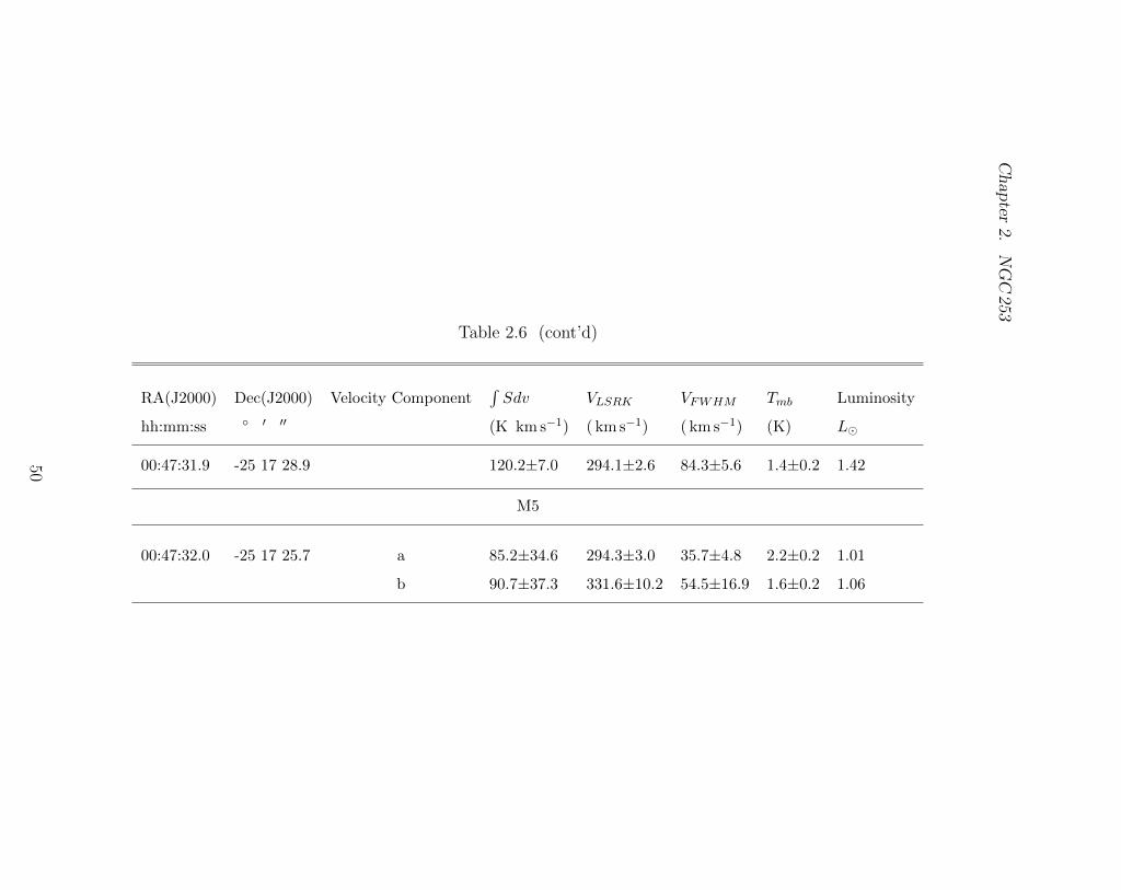
Chapter2.
NGC253
Table 2.6 (cont’d)
RA(J2000) Dec(J2000) Velocity ComponentR
Sdv VLSRK VFWHM Tmb Luminosity
hh:mm:ss � 0 00 (K km s�1) ( km s�1) ( km s�1) (K) L�
00:47:31.9 -25 17 28.9 120.2±7.0 294.1±2.6 84.3±5.6 1.4±0.2 1.42
M5
00:47:32.0 -25 17 25.7 a 85.2±34.6 294.3±3.0 35.7±4.8 2.2±0.2 1.01
b 90.7±37.3 331.6±10.2 54.5±16.9 1.6±0.2 1.06
50
Chapter 2. NGC253
2.5 Discussion
2.5.1 NH3 Temperatures
One advantage of observing NH3 is that many of its transitions are close in frequency
space, and therefore can be observed with single telescope, a single observational
setup, and under the same atmospheric conditions. In addition, the < 5% change
in frequency between the transitions means that their respective (u, v) coverage and
the flux they resolve out are nearly identical. Rotational temperatures can then be
derived from as many pairs of metastable (J = K) states as have been observed.
Assuming optically thin conditions upper level column densities may be determined
from:
Nu(J, K) =7.73 ⇥ 1013
⌫
J(J + 1)
K
2
ZTmb dv (2.1)
where Tmb is the main beam brightness temperature, the column density of the
upper inversion state, Nu, is in cm�2, and the frequency (⌫) is in GHz. A rotational
temperature (TJJ 0) is derived from a pair of the metastable states (J and J0) by:
Nu(J 0, J
0)
Nu(J, J)=
g
0op(2J
0 + 1)
gop(2J + 1)exp
⇣��E
TJJ 0
⌘(2.2)
where the di↵erence in energy between states J and J0, �E, is in K (the corrected
version of the equation in Henkel et al., 2000 as shown in Ott et al., 2005) and
the gop are statistical weights depending on the NH3 species (gop = 1 for para-NH3
and J 6= 3n where n is an integer, and gop = 2 for ortho-NH3 with J=3n). Rotational
temperatures derived from pairs of NH3 transitions, for locations A1 to A7 are shown
in Table 2.2. The rotational temperatures are best illustrated in the Boltzmann
diagram shown in Figure 2.13 (top). We have plotted column densities normalized
by the degeneracy of the inversion doublet on the vertical axis and energy above the
ground state on the horizontal axis. The slopes between any two points are thus
51
Chapter 2. NGC253
proportional to the inverse rotational temperature, i.e. cold gas shows steeper slopes
than warm gas (Equation 3.2). Notice at location C1 we see NH3 in absorption
against the continuum (Figure 2.6) and thus the rotational temperature must be
measured di↵erently (see next paragraph). A3 is located ⇠ 0.5 beams (53 pc) from
C1, thus the emission line is likely partially absorbed, making rotational temperature
measurements here unreliable.
Measuring rotational temperatures from NH3 absorption is not possible without
knowing the excitation temperature Tex and the optical depth ⌧ . Huettemeister et
al. (1995) describes the process of extracting total NH3 column densities N(J,K) (the
sum of both the upper and lower inversion states):
N(J, K)
Tex
= 1.61 ⇥ 1014J(J + 1)
K
2⌫
⌧�⌫1/2 (2.3)
and,
⌧ = � ln(1 �
|TL|
TC
) (2.4)
where the units of �⌫1/2(FWHM) are km s�1, TL and TC are brightness tempera-
tures of the line and continuum, respectively, and ⌧ is the optical depth. We have
no means to measure the transition-dependent excitation temperature, so for sim-
plicity we assume that for each metastable transition Tex is equal. In this case the
rotational temperature can still be derived from Equation 2.2 by substituting N(J,K)
for Nu(J,K). Rotational temperatures for C1 are shown in Table 2.3. Since the col-
umn density at C1 depends on the excitation temperature, the values plotted for
C1 in Figure 2.13 are really N(J,K)/Tex. The spatial dependence of the rotational
temperature is shown in Figure 2.13 (bottom).
The rotational temperature is not necessarily the true thermal temperature of
the gas, i.e. it is not the kinetic temperature, but rather a lower limit. We therefore
employ the functions from Ott et al. (2011) to estimate kinetic temperatures. To
52
Chapter 2. NGC253
convert rotational temperatures for the NH3(2,2) to (4,4) ratio additional fits to the
same LVG models used in Ott et al. (2011) from Ott et al. (2005) were made:
TKin =
8><
>:
1.467 ⇥ T24 � 6.984 for TKin . 100K
27.085 ⇥ exp(0.019 T24) for TKin & 100K(2.5)
and for the NH3(4,4) to (5,5) ratio:
TKin =
8><
>:
1.143 ⇥ T45 � 1.611 for TKin . 50K
21.024 ⇥ exp(0.0198 T45) for TKin & 50K(2.6)
Figure 2.12 shows how the conversion functions fit to the LVG models. We thus derive
kinetic temperatures for adjacent pairs of like species for a total of 3 measurements
at each location (Table 2.2).
If the gas is dominated by a single kinetic temperature, all the rotational temper-
atures should yield that temperature. In the case that the rotational temperatures
do not, either the gas must be represented by multiple kinetic temperatures, or the
LVG approximation does not hold. The LVG corrected kinetic temperatures are
plotted in Figure 2.14. The figures show remarkably little variance in the rotation
and kinetic temperatures measured across all locations. We have fit a single tem-
perature for each line pair across all locations weighted by the errors. We measure
a weighted average for TKin12 of 57 ± 4 K, for TKin24 of 134 ± 8 K , and for TKin45
of 117 ± 16 K. The TKin24 and TKin45 components are consistent within the errors.
The kinetic temperatures of the dense molecular gas in the central kpc of NGC 253
is therefore most consistent with a cool ⇠57 K derived from the (1,1) and (2,2) lines,
and a warm ⇠130 K component derived from the weighted average of the (2,2) to
(4,4) and (4,4) to (5,5) ratios.
The NH3 transitions of NGC 253 have been of interest to many others, but most
recently have been observed with the Australia Telescope Compact Array (ATCA)
(Ott et al., 2005), the VLA (Takano et al., 2005), and the Green Bank Telescope
53
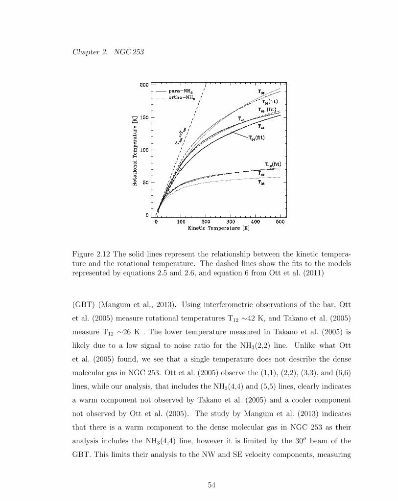
Chapter 2. NGC253
Figure 2.12 The solid lines represent the relationship between the kinetic tempera-ture and the rotational temperature. The dashed lines show the fits to the modelsrepresented by equations 2.5 and 2.6, and equation 6 from Ott et al. (2011)
(GBT) (Mangum et al., 2013). Using interferometric observations of the bar, Ott
et al. (2005) measure rotational temperatures T12 ⇠42 K, and Takano et al. (2005)
measure T12 ⇠26 K . The lower temperature measured in Takano et al. (2005) is
likely due to a low signal to noise ratio for the NH3(2,2) line. Unlike what Ott
et al. (2005) found, we see that a single temperature does not describe the dense
molecular gas in NGC 253. Ott et al. (2005) observe the (1,1), (2,2), (3,3), and (6,6)
lines, while our analysis, that includes the NH3(4,4) and (5,5) lines, clearly indicates
a warm component not observed by Takano et al. (2005) and a cooler component
not observed by Ott et al. (2005). The study by Mangum et al. (2013) indicates
that there is a warm component to the dense molecular gas in NGC 253 as their
analysis includes the NH3(4,4) line, however it is limited by the 3000 beam of the
GBT. This limits their analysis to the NW and SE velocity components, measuring
54
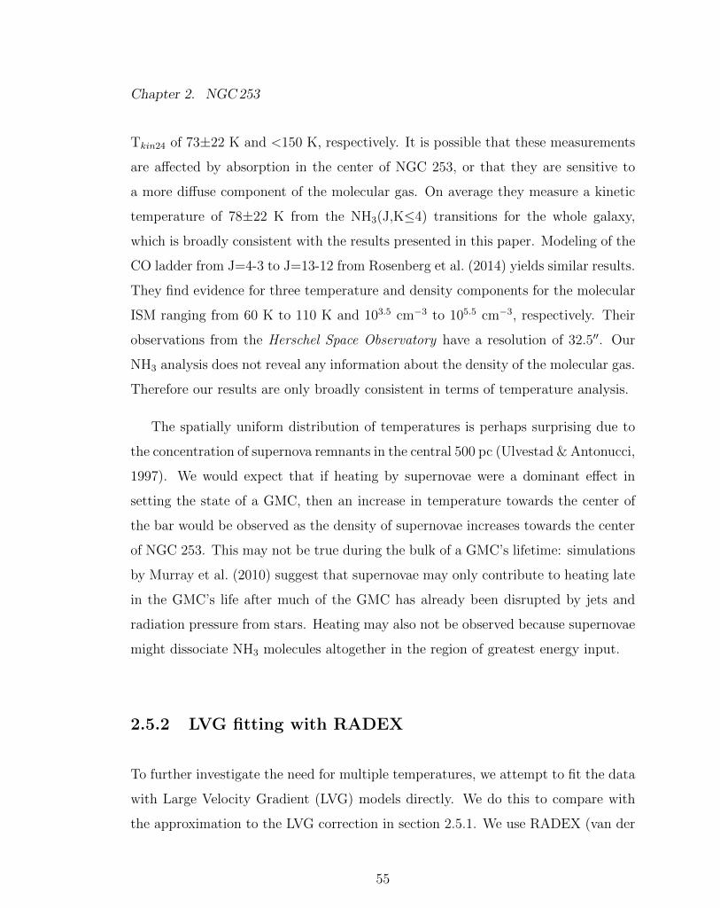
Chapter 2. NGC253
Tkin24 of 73±22 K and <150 K, respectively. It is possible that these measurements
are a↵ected by absorption in the center of NGC 253, or that they are sensitive to
a more di↵use component of the molecular gas. On average they measure a kinetic
temperature of 78±22 K from the NH3(J,K4) transitions for the whole galaxy,
which is broadly consistent with the results presented in this paper. Modeling of the
CO ladder from J=4-3 to J=13-12 from Rosenberg et al. (2014) yields similar results.
They find evidence for three temperature and density components for the molecular
ISM ranging from 60 K to 110 K and 103.5 cm�3 to 105.5 cm�3, respectively. Their
observations from the Herschel Space Observatory have a resolution of 32.500. Our
NH3 analysis does not reveal any information about the density of the molecular gas.
Therefore our results are only broadly consistent in terms of temperature analysis.
The spatially uniform distribution of temperatures is perhaps surprising due to
the concentration of supernova remnants in the central 500 pc (Ulvestad & Antonucci,
1997). We would expect that if heating by supernovae were a dominant e↵ect in
setting the state of a GMC, then an increase in temperature towards the center of
the bar would be observed as the density of supernovae increases towards the center
of NGC 253. This may not be true during the bulk of a GMC’s lifetime: simulations
by Murray et al. (2010) suggest that supernovae may only contribute to heating late
in the GMC’s life after much of the GMC has already been disrupted by jets and
radiation pressure from stars. Heating may also not be observed because supernovae
might dissociate NH3 molecules altogether in the region of greatest energy input.
2.5.2 LVG fitting with RADEX
To further investigate the need for multiple temperatures, we attempt to fit the data
with Large Velocity Gradient (LVG) models directly. We do this to compare with
the approximation to the LVG correction in section 2.5.1. We use RADEX (van der
55
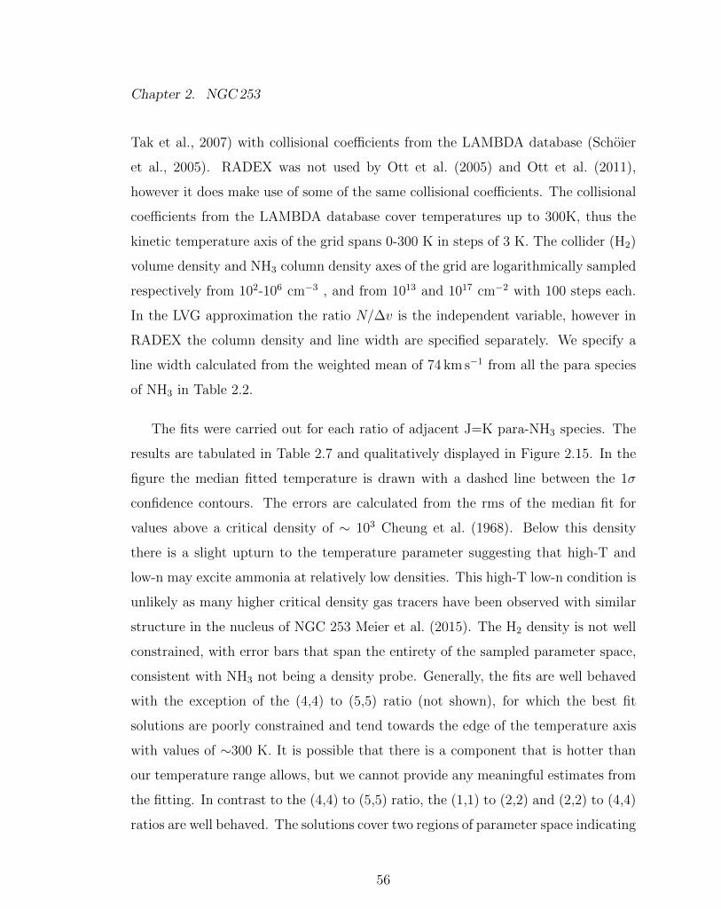
Chapter 2. NGC253
Tak et al., 2007) with collisional coe�cients from the LAMBDA database (Schoier
et al., 2005). RADEX was not used by Ott et al. (2005) and Ott et al. (2011),
however it does make use of some of the same collisional coe�cients. The collisional
coe�cients from the LAMBDA database cover temperatures up to 300K, thus the
kinetic temperature axis of the grid spans 0-300 K in steps of 3 K. The collider (H2)
volume density and NH3 column density axes of the grid are logarithmically sampled
respectively from 102-106 cm�3 , and from 1013 and 1017 cm�2 with 100 steps each.
In the LVG approximation the ratio N/�v is the independent variable, however in
RADEX the column density and line width are specified separately. We specify a
line width calculated from the weighted mean of 74 km s�1 from all the para species
of NH3 in Table 2.2.
The fits were carried out for each ratio of adjacent J=K para-NH3 species. The
results are tabulated in Table 2.7 and qualitatively displayed in Figure 2.15. In the
figure the median fitted temperature is drawn with a dashed line between the 1�
confidence contours. The errors are calculated from the rms of the median fit for
values above a critical density of ⇠ 103 Cheung et al. (1968). Below this density
there is a slight upturn to the temperature parameter suggesting that high-T and
low-n may excite ammonia at relatively low densities. This high-T low-n condition is
unlikely as many higher critical density gas tracers have been observed with similar
structure in the nucleus of NGC 253 Meier et al. (2015). The H2 density is not well
constrained, with error bars that span the entirety of the sampled parameter space,
consistent with NH3 not being a density probe. Generally, the fits are well behaved
with the exception of the (4,4) to (5,5) ratio (not shown), for which the best fit
solutions are poorly constrained and tend towards the edge of the temperature axis
with values of ⇠300 K. It is possible that there is a component that is hotter than
our temperature range allows, but we cannot provide any meaningful estimates from
the fitting. In contrast to the (4,4) to (5,5) ratio, the (1,1) to (2,2) and (2,2) to (4,4)
ratios are well behaved. The solutions cover two regions of parameter space indicating
56
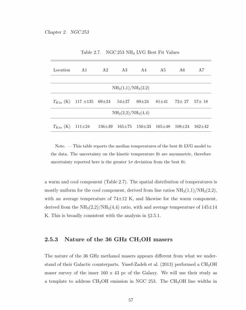
Chapter 2. NGC253
Table 2.7. NGC 253 NH3 LVG Best Fit Values
Location A1 A2 A3 A4 A5 A6 A7
NH3(1,1)/NH3(2,2)
TKin (K) 117 ±135 69±24 54±27 69±24 81±41 72± 27 57± 18
NH3(2,2)/NH3(4,4)
TKin (K) 111±24 156±39 165±75 150±33 165±48 108±24 162±42
Note. — This table reports the median temperatures of the best fit LVG model to
the data. The uncertainty on the kinetic temperature fit are asymmetric, therefore
uncertainty reported here is the greater 1� deviation from the best fit.
a warm and cool component (Table 2.7). The spatial distribution of temperatures is
mostly uniform for the cool component, derived from line ratios NH3(1,1)/NH3(2,2),
with an average temperature of 74±12 K, and likewise for the warm component,
derived from the NH3(2,2)/NH3(4,4) ratio, with and average temperature of 145±14
K. This is broadly consistent with the analysis in §2.5.1.
2.5.3 Nature of the 36 GHz CH3OH masers
The nature of the 36 GHz methanol masers appears di↵erent from what we under-
stand of their Galactic counterparts. Yusef-Zadeh et al. (2013) performed a CH3OH
maser survey of the inner 160 x 43 pc of the Galaxy. We will use their study as
a template to address CH3OH emission in NGC 253. The CH3OH line widths in
57
Chapter 2. NGC253
NGC 253 span tens of km s�1 whereas individual Galactic CH3OHmasers tend to
span a few km s�1. The NGC 253 36 GHz line is spectrally resolved and multiple
components can be fitted (see Table 2.6). The maser with the largest flux found by
Yusef-Zadeh et al. (2013) (number 164) is ⇠ 470 Jy km s�1, which corresponds to an
isotropic luminosity, assuming a distance of 8 kpc, of 1.1 ⇥ 10�3 L�. By comparison
the most luminous CH3OH maser in NGC 253 is 1.63 L�. This would mean that
the beam averaged class I CH3OH masers in NGC 253 are about a thousand times
more luminous than the most luminous CH3OH maser found by Yusef-Zadeh et al.
(2013). Alternatively, there may be thousands of bright masers at similar velocities
in one 600⇥400 beam. Surveys of Class I methanol masers in supernova remnants (e.g
McEwen et al., 2014 and McEwen et al., 2016) have revealed spectrally similar results
to Yusef-Zadeh et al. (2013) with narrow spectral features spanning a few km s�1.
At our spatial resolution of 101⇥67 pc the CH3OH emission is not well resolved, and
the entirety of the Yusef-Zadeh et al. (2013) survey corresponds approximately to
the size of one of our beams. Since there are > 300 sources in a similar region of the
Galaxy, and the NGC 253 spectra show multiple velocity components, it is possible
that there are many components at each location.The broad spectral profile could
be constructed from many masers from protostellar outflows or supernova remnants.
2.5.4 Impact of Superbubbles on the Dense Molecular ISM
Sakamoto et al. (2006) find two superbubbles in NGC 253 in 12CO(J = 2 ! 1) emis-
sion. The shells are ⇠ 100 pc in diameter, have masses of order 106M� and kinetic
energies of order 1046 J, suggesting winds and supernovae from a super star cluster,
or a hypernova, as the creation mechanism. Close to the location where these su-
perbubbles interact with dense molecular gas, as traced by NH3, we observe CH3OH
masers. Figure 2.16 shows 12CO(J = 1 ! 0) channel maps of the superbubbles with
CH3OH contours overlaid. There are two groups of masers. The first is on the north-
58
Chapter 2. NGC253
east side of the galaxy and consists of M1, M2 and M3. The other group consists of
M4 and M5 on the southwest side (Figure 2.5). All the CH3OH masers except M3
can be associated with the Sakamoto superbubbles. The association indicates that
these masers exist where clouds are influenced by the expanding superbubbles. This
relationship is also indicated by larger NH3 linewidths at the locations A1, A5, and
A6, which are nearest the masers and the superbubbles.
The larger observed linewidths are not likely a result of more turbulence within
the clouds. A comparison with the GMCs from Leroy et al. (2015) suggests that the
broader observed line widths in our data are likely a result of beam smearing e↵ects.
With a 200 beam Leroy et al. (2015) are able to resolve individual clouds. Their
clouds are clearly dominated by turbulence, as in all cases the thermal linewidth
is < 1 km s�1 as calculated from our NH3 derived temperatures. Using an average
temperature of 117 K derived from our NH3 analysis, the mean thermal energy stored
in the Leroy et al. (2015) clouds is ⇠ 5⇥1043J, whereas the mechanical energy stored,
as derived from turbulent linewidths, is ⇠ 1 ⇥ 1046J. The turbulent linewidths of
individual GMCs detected in Leroy et al. (2015) appear una↵ected by the impact
of the expanding superbubbles, and in fact appear uniform across the entire central
molecular bar (Figure 2.18). The larger NH3 linewidths observed with a larger beam
suggest instead that the superbubbles are imparting mechanical energy resulting in
bulk translational motion of the GMCs.
The relationship of the clouds to the masers is shown by Figure 2.17, which plots
kinetic temperatures Tkin12 and Tkin24 derived from NH3 against the mean FWHM of
the NH3 transitions. The figure shows little temperature variation toward the shocks
traced by CH3OH. If there is shock heating of the dense molecular gas it must be
highly localized to areas much smaller than the beam such that it does not a↵ect the
overall kinetic temperature measured with ⇠100 pc spatial resolution.
59
Chapter 2. NGC253
2.5.5 The Outflow, Masers, and Starburst
NH3(3,3) masers
The location of the continuum peak (C1) is also the locus of the starburst and the
central base of the molecular and ionized bipolar outflow. Here the para-NH3 lines
are not observed in emission, however the ortho-NH3(3,3) line is. We did not detect
any other ortho species of NH3 at this location to compare with, however Ott et al.
(2005) did observe the ortho (6,6) species to be in absorption at our location C1.
Since NH3(3,3) is the only ortho-NH3 species observed in emission at this location, we
corroborate the interpretation from Ott et al. (2005) that the NH3(3,3) line is masing
here. The spectral line (Figure 2.6) could not be fit with a single Gaussian, but rather
two Gaussians centered at 172 km s�1 and 257 km s�1 with widths of 55 km s�1 and
130 km s�1, respectively NH3(3,3)a and NH3(3,3)b (see Figure 2.10). The existence
of the NH3(3,3) maser suggests that the collision rate in the center of NGC 253
increases or there exists an excess of infrared photons in the center in order to pump
this maser. Currently, there is one other known extragalactic source of NH3(3,3)
masers apart from NGC 253: the Seyfert galaxy NGC 3079 (Miyamoto et al., 2015).
Both galaxies host outflows, but NGC 3079 is host to an active galactic nucleus
(AGN). It hosts a star formation rate of 2.6 M� yr�1 over 4 kpc (Yamagishi et al.,
2010) measured from 1-1000µm emission. Attribution to an AGN driven wind might
be favored because the starburst is weak. Since the mechanism driving the outflows
in these galaxies is di↵erent, we hypothesize that in both cases it is the collision
of the hot ionized outflow cone with the surrounding material that results in the
NH3(3,3) masers.
60
Chapter 2. NGC253
H2O masers
The H2O masers are located within the centermost 200 pc. Being at the center
of the starburst it is likely that all these masers are star formation related due to
bright H↵and IR emission in the central 500pc. Brunthaler et al. (2009) investigated
this location with the VLBA and inferred a pure starburst nature of the masers due
to their similarity to Galactic H2O masers and spatial coincidence with supernova
remnants. Our data, while much lower in resolution, indicate that W1 may be
extended perpendicular to the disk and aligned with the bipolar ionized gas outflow
(Figure 2.11). The spectrum shows evidence of multiple components (Figure 2.8).
W2 contains many individual components within a velocity space ⇠100 km s�1 wide
centered at systemic velocity and includes contributions from W1 and W3. W3 is a
single component maser located to the southwest of the nucleus.
W3 is the simplest H2O maser to explain. It is cospatial with an H II region seen
in Figure 2.4 and has a narrow spectrum. It is likely associated with a massive star
or stars in that region. Its isotropic luminosity of 2 ⇥ 10�2 L� is consistent with
luminosities of the most luminous (⇠ 10�2 L�) YSO H2O masers in the Galaxy (e.g
Palagi et al., 1993).
The H2O maser W1 is the clear oddity in NGC 253. W1 is most clearly seen
in the super-resolved image Figure 2.11. There are three components with observed
velocities in the range 25-109 km s�1, while the systemic velocity of the galaxy is
234 km s�1. The W1 maser emission does not follow the kinematics of the dense
molecular ISM (Figure 2.8). The most luminous and broad component is centered at
109 km s�1. According to Brunthaler et al. (2009) this maser emission is associated
with supernova remnant TH4 (Turner & Ho, 1985 and Ulvestad & Antonucci, 1997).
However, because of the extreme conditions under which H2O is known to mase, in
addition to the locations and velocities, and because no H2O masers are found in
61
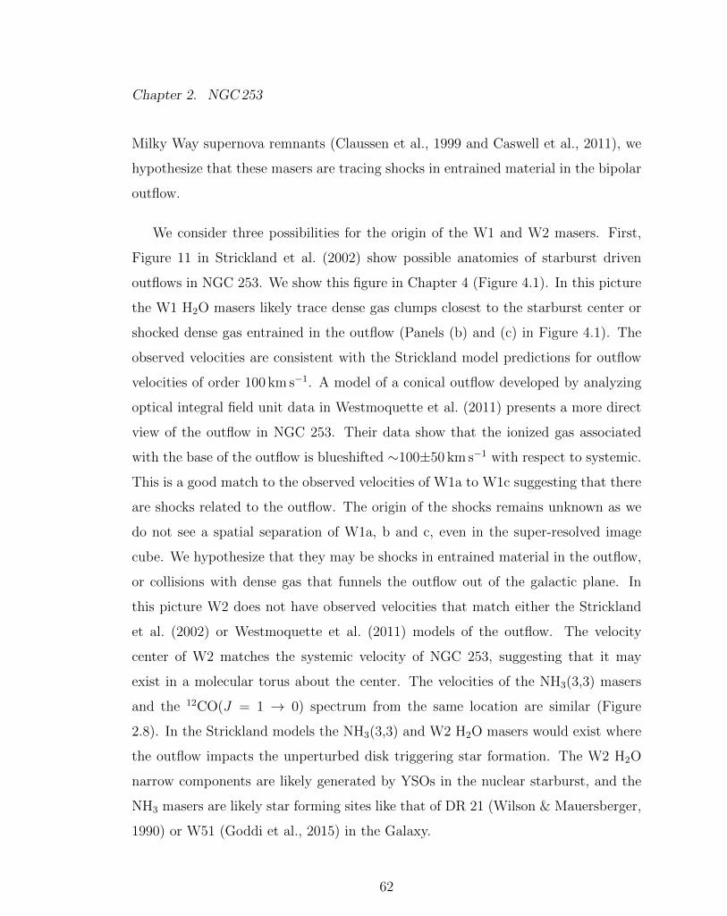
Chapter 2. NGC253
Milky Way supernova remnants (Claussen et al., 1999 and Caswell et al., 2011), we
hypothesize that these masers are tracing shocks in entrained material in the bipolar
outflow.
We consider three possibilities for the origin of the W1 and W2 masers. First,
Figure 11 in Strickland et al. (2002) show possible anatomies of starburst driven
outflows in NGC 253. We show this figure in Chapter 4 (Figure 4.1). In this picture
the W1 H2O masers likely trace dense gas clumps closest to the starburst center or
shocked dense gas entrained in the outflow (Panels (b) and (c) in Figure 4.1). The
observed velocities are consistent with the Strickland model predictions for outflow
velocities of order 100 km s�1. A model of a conical outflow developed by analyzing
optical integral field unit data in Westmoquette et al. (2011) presents a more direct
view of the outflow in NGC 253. Their data show that the ionized gas associated
with the base of the outflow is blueshifted ⇠100±50 km s�1 with respect to systemic.
This is a good match to the observed velocities of W1a to W1c suggesting that there
are shocks related to the outflow. The origin of the shocks remains unknown as we
do not see a spatial separation of W1a, b and c, even in the super-resolved image
cube. We hypothesize that they may be shocks in entrained material in the outflow,
or collisions with dense gas that funnels the outflow out of the galactic plane. In
this picture W2 does not have observed velocities that match either the Strickland
et al. (2002) or Westmoquette et al. (2011) models of the outflow. The velocity
center of W2 matches the systemic velocity of NGC 253, suggesting that it may
exist in a molecular torus about the center. The velocities of the NH3(3,3) masers
and the 12CO(J = 1 ! 0) spectrum from the same location are similar (Figure
2.8). In the Strickland models the NH3(3,3) and W2 H2O masers would exist where
the outflow impacts the unperturbed disk triggering star formation. The W2 H2O
narrow components are likely generated by YSOs in the nuclear starburst, and the
NH3 masers are likely star forming sites like that of DR 21 (Wilson & Mauersberger,
1990) or W51 (Goddi et al., 2015) in the Galaxy.
62
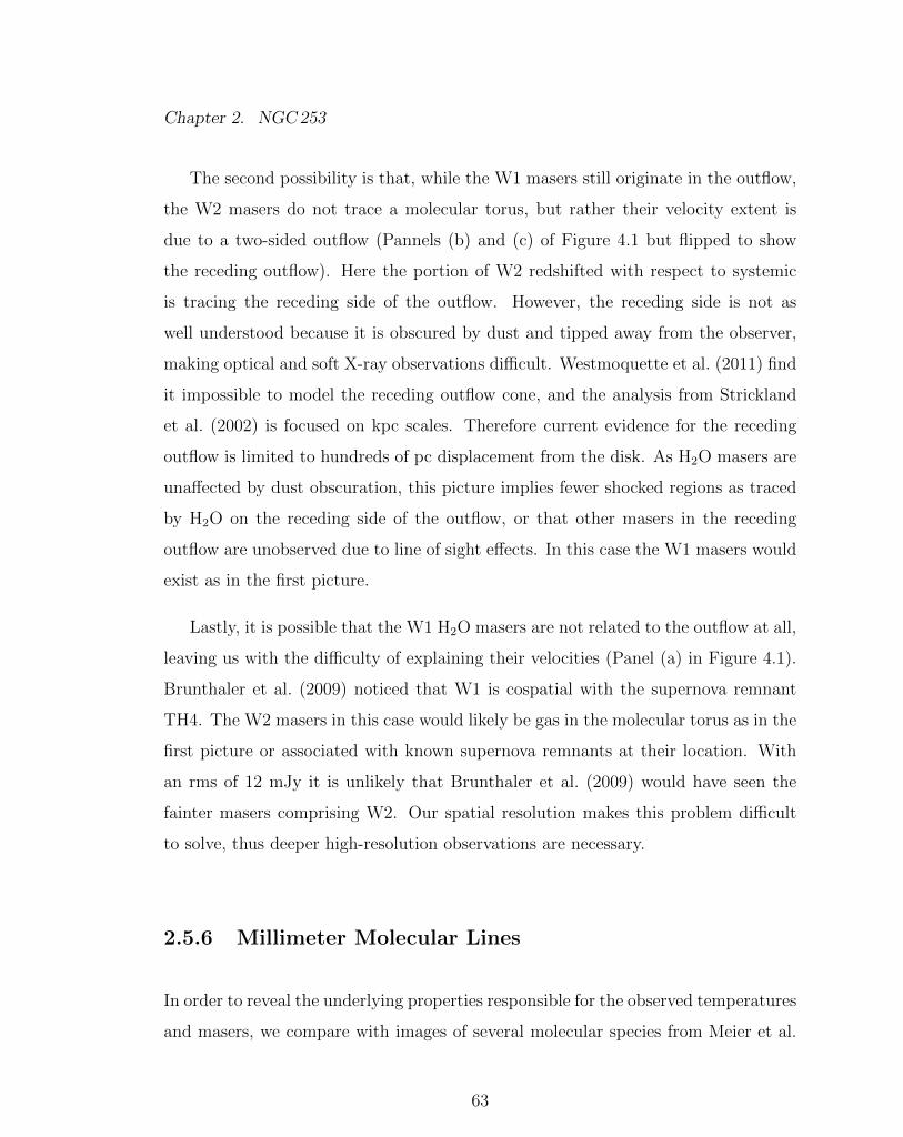
Chapter 2. NGC253
The second possibility is that, while the W1 masers still originate in the outflow,
the W2 masers do not trace a molecular torus, but rather their velocity extent is
due to a two-sided outflow (Pannels (b) and (c) of Figure 4.1 but flipped to show
the receding outflow). Here the portion of W2 redshifted with respect to systemic
is tracing the receding side of the outflow. However, the receding side is not as
well understood because it is obscured by dust and tipped away from the observer,
making optical and soft X-ray observations di�cult. Westmoquette et al. (2011) find
it impossible to model the receding outflow cone, and the analysis from Strickland
et al. (2002) is focused on kpc scales. Therefore current evidence for the receding
outflow is limited to hundreds of pc displacement from the disk. As H2O masers are
una↵ected by dust obscuration, this picture implies fewer shocked regions as traced
by H2O on the receding side of the outflow, or that other masers in the receding
outflow are unobserved due to line of sight e↵ects. In this case the W1 masers would
exist as in the first picture.
Lastly, it is possible that the W1 H2O masers are not related to the outflow at all,
leaving us with the di�culty of explaining their velocities (Panel (a) in Figure 4.1).
Brunthaler et al. (2009) noticed that W1 is cospatial with the supernova remnant
TH4. The W2 masers in this case would likely be gas in the molecular torus as in the
first picture or associated with known supernova remnants at their location. With
an rms of 12 mJy it is unlikely that Brunthaler et al. (2009) would have seen the
fainter masers comprising W2. Our spatial resolution makes this problem di�cult
to solve, thus deeper high-resolution observations are necessary.
2.5.6 Millimeter Molecular Lines
In order to reveal the underlying properties responsible for the observed temperatures
and masers, we compare with images of several molecular species from Meier et al.
63
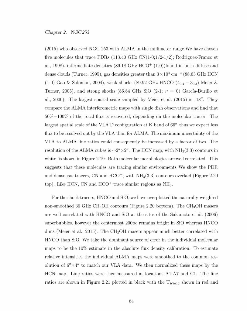
Chapter 2. NGC253
(2015) who observed NGC 253 with ALMA in the millimeter range.We have chosen
five molecules that trace PDRs (113.40 GHz CN(1-0;1/2-1/2); Rodriguez-Franco et
al., 1998), intermediate densities (89.18 GHz HCO+ (1-0))found in both di↵use and
dense clouds (Turner, 1995), gas densities greater than 3⇥104 cm�3 (88.63 GHz HCN
(1-0) Gao & Solomon, 2004), weak shocks (89.92 GHz HNCO (40,4 � 30,3) Meier &
Turner, 2005), and strong shocks (86.84 GHz SiO (2-1; ⌫ = 0) Garcıa-Burillo et
al., 2000). The largest spatial scale sampled by Meier et al. (2015) is 1800. They
compare the ALMA interferometric maps with single dish observations and find that
50%�100% of the total flux is recovered, depending on the molecular tracer. The
largest spatial scale of the VLA D configuration at K band of 6600 thus we expect less
flux to be resolved out by the VLA than for ALMA. The maximum uncertainty of the
VLA to ALMA line ratios could consequently be increased by a factor of two. The
resolution of the ALMA cubes is ⇠200⇥200. The HCN map, with NH3(3,3) contours in
white, is shown in Figure 2.19. Both molecular morphologies are well correlated. This
suggests that these molecules are tracing similar environments We show the PDR
and dense gas tracers, CN and HCO+, with NH3(3,3) contours overlaid (Figure 2.20
top). Like HCN, CN and HCO+ trace similar regions as NH3.
For the shock tracers, HNCO and SiO, we have overplotted the naturally-weighted
non-smoothed 36 GHz CH3OH contours (Figure 2.20 bottom). The CH3OH masers
are well correlated with HNCO and SiO at the sites of the Sakamoto et al. (2006)
superbubbles, however the centermost 200pc remains bright in SiO whereas HNCO
dims (Meier et al., 2015). The CH3OH masers appear much better correlated with
HNCO than SiO. We take the dominant source of error in the individual molecular
maps to be the 10% estimate in the absolute flux density calibration. To estimate
relative intensities the individual ALMA maps were smoothed to the common res-
olution of 600⇥400 to match our VLA data. We then normalized these maps by the
HCN map. Line ratios were then measured at locations A1-A7 and C1. The line
ratios are shown in Figure 2.21 plotted in black with the TKin12 shown in red and
64
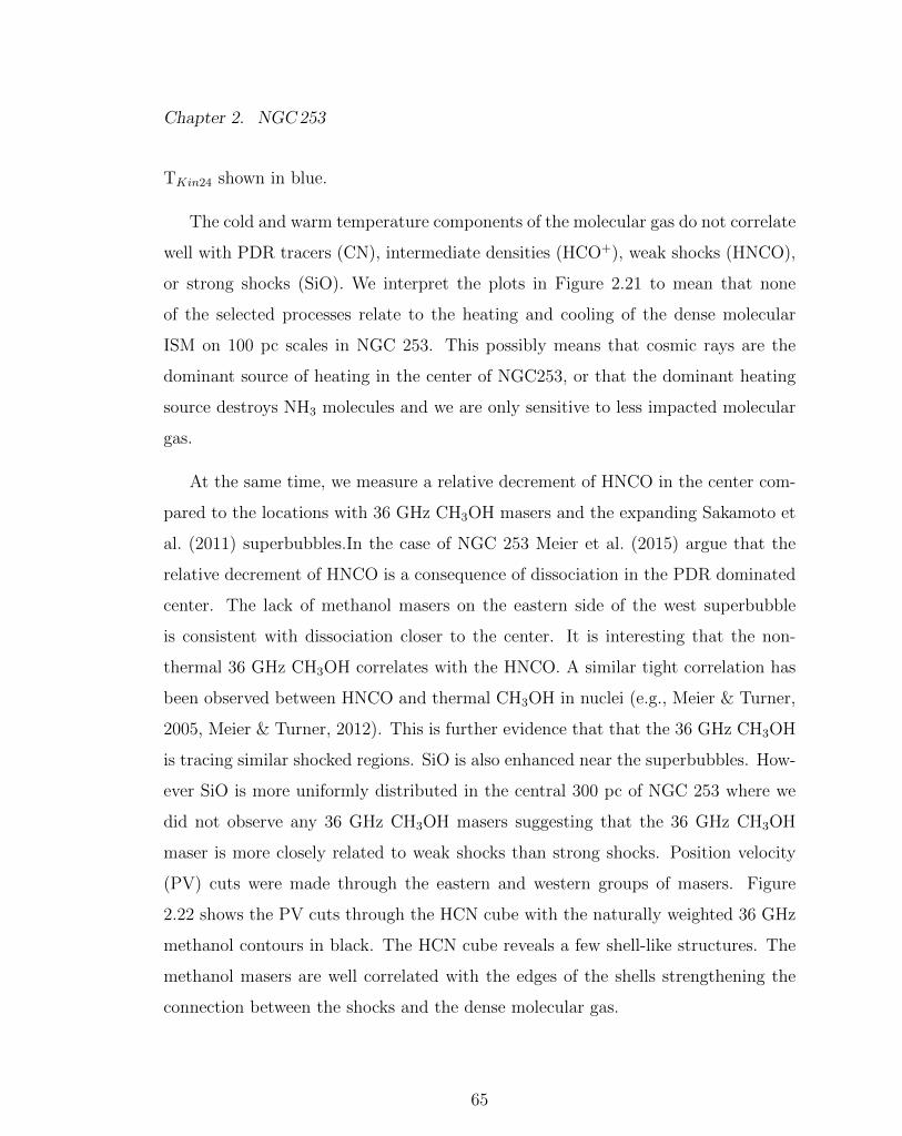
Chapter 2. NGC253
TKin24 shown in blue.
The cold and warm temperature components of the molecular gas do not correlate
well with PDR tracers (CN), intermediate densities (HCO+), weak shocks (HNCO),
or strong shocks (SiO). We interpret the plots in Figure 2.21 to mean that none
of the selected processes relate to the heating and cooling of the dense molecular
ISM on 100 pc scales in NGC 253. This possibly means that cosmic rays are the
dominant source of heating in the center of NGC253, or that the dominant heating
source destroys NH3 molecules and we are only sensitive to less impacted molecular
gas.
At the same time, we measure a relative decrement of HNCO in the center com-
pared to the locations with 36 GHz CH3OH masers and the expanding Sakamoto et
al. (2011) superbubbles.In the case of NGC 253 Meier et al. (2015) argue that the
relative decrement of HNCO is a consequence of dissociation in the PDR dominated
center. The lack of methanol masers on the eastern side of the west superbubble
is consistent with dissociation closer to the center. It is interesting that the non-
thermal 36 GHz CH3OH correlates with the HNCO. A similar tight correlation has
been observed between HNCO and thermal CH3OH in nuclei (e.g., Meier & Turner,
2005, Meier & Turner, 2012). This is further evidence that that the 36 GHz CH3OH
is tracing similar shocked regions. SiO is also enhanced near the superbubbles. How-
ever SiO is more uniformly distributed in the central 300 pc of NGC 253 where we
did not observe any 36 GHz CH3OH masers suggesting that the 36 GHz CH3OH
maser is more closely related to weak shocks than strong shocks. Position velocity
(PV) cuts were made through the eastern and western groups of masers. Figure
2.22 shows the PV cuts through the HCN cube with the naturally weighted 36 GHz
methanol contours in black. The HCN cube reveals a few shell-like structures. The
methanol masers are well correlated with the edges of the shells strengthening the
connection between the shocks and the dense molecular gas.
65
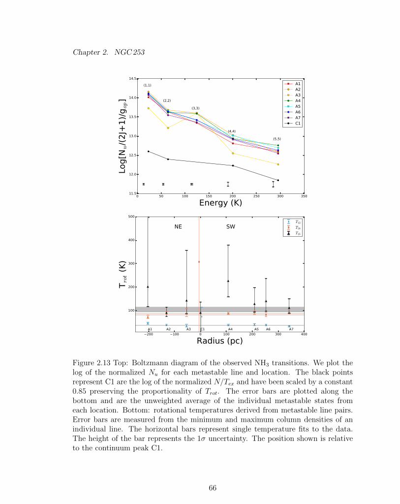
Chapter 2. NGC253
Figure 2.13 Top: Boltzmann diagram of the observed NH3 transitions. We plot thelog of the normalized Nu for each metastable line and location. The black pointsrepresent C1 are the log of the normalized N/Tex and have been scaled by a constant0.85 preserving the proportionality of Trot. The error bars are plotted along thebottom and are the unweighted average of the individual metastable states fromeach location. Bottom: rotational temperatures derived from metastable line pairs.Error bars are measured from the minimum and maximum column densities of anindividual line. The horizontal bars represent single temperature fits to the data.The height of the bar represents the 1� uncertainty. The position shown is relativeto the continuum peak C1.
66
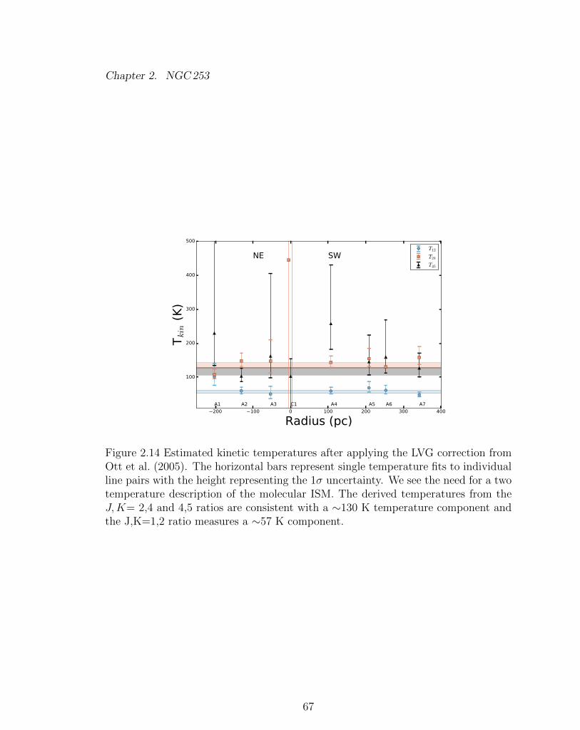
Chapter 2. NGC253
Figure 2.14 Estimated kinetic temperatures after applying the LVG correction fromOtt et al. (2005). The horizontal bars represent single temperature fits to individualline pairs with the height representing the 1� uncertainty. We see the need for a twotemperature description of the molecular ISM. The derived temperatures from theJ, K= 2,4 and 4,5 ratios are consistent with a ⇠130 K temperature component andthe J,K=1,2 ratio measures a ⇠57 K component.
67
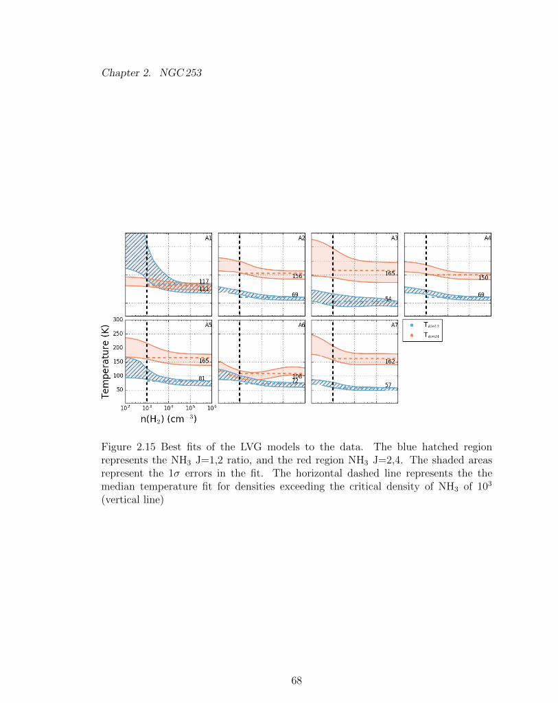
Chapter 2. NGC253
Figure 2.15 Best fits of the LVG models to the data. The blue hatched regionrepresents the NH3 J=1,2 ratio, and the red region NH3 J=2,4. The shaded areasrepresent the 1� errors in the fit. The horizontal dashed line represents the themedian temperature fit for densities exceeding the critical density of NH3 of 103
(vertical line)
68
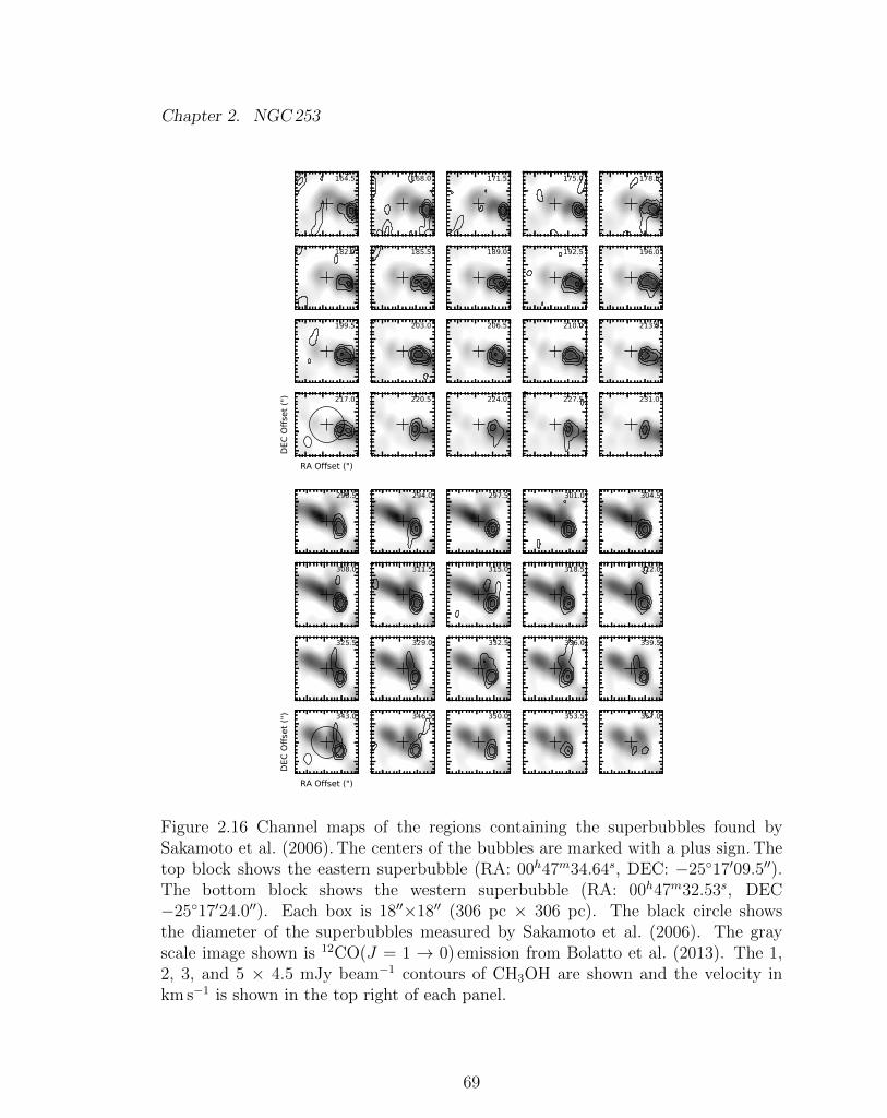
Chapter 2. NGC253
Figure 2.16 Channel maps of the regions containing the superbubbles found bySakamoto et al. (2006). The centers of the bubbles are marked with a plus sign. Thetop block shows the eastern superbubble (RA: 00h47m34.64s, DEC: �25�17009.500).The bottom block shows the western superbubble (RA: 00h47m32.53s, DEC�25�17024.000). Each box is 1800⇥1800 (306 pc ⇥ 306 pc). The black circle showsthe diameter of the superbubbles measured by Sakamoto et al. (2006). The grayscale image shown is 12CO(J = 1 ! 0) emission from Bolatto et al. (2013). The 1,2, 3, and 5 ⇥ 4.5 mJy beam�1 contours of CH3OH are shown and the velocity inkm s�1 is shown in the top right of each panel.
69
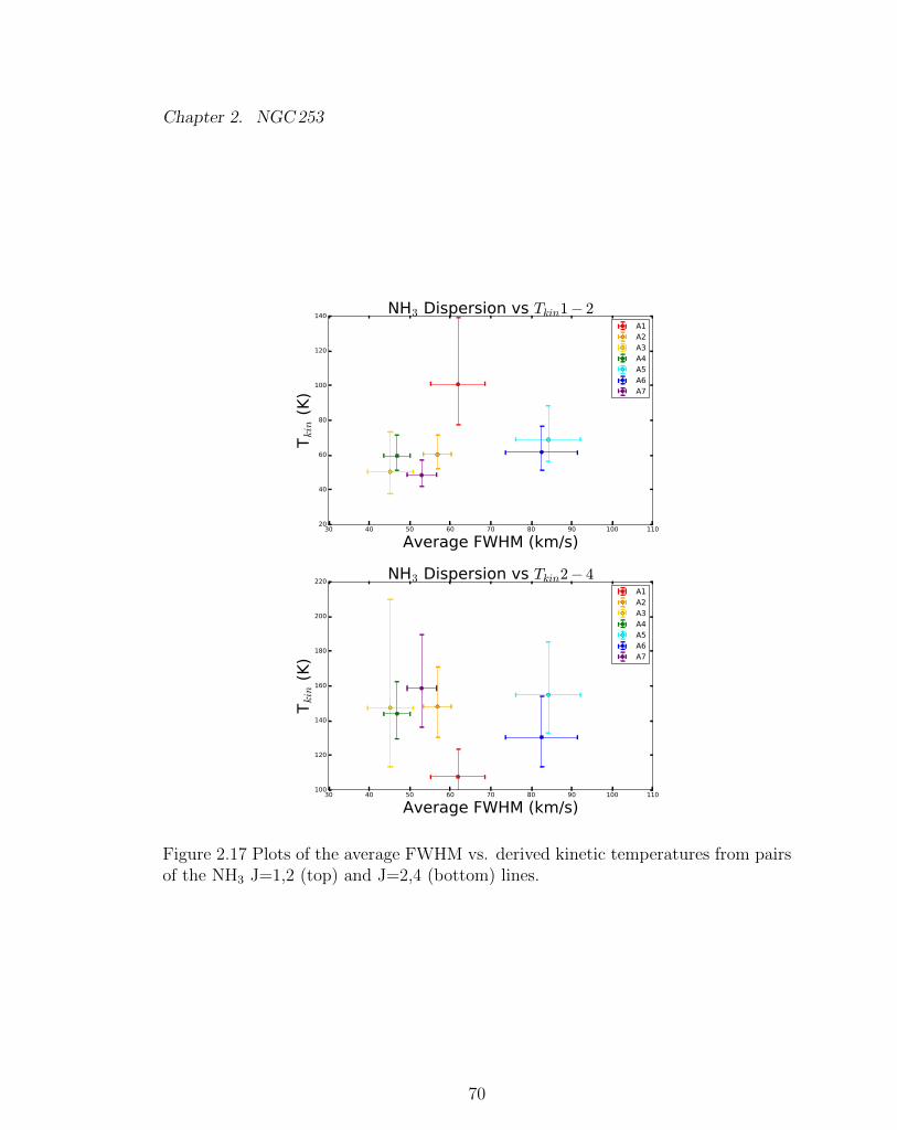
Chapter 2. NGC253
Figure 2.17 Plots of the average FWHM vs. derived kinetic temperatures from pairsof the NH3 J=1,2 (top) and J=2,4 (bottom) lines.
70
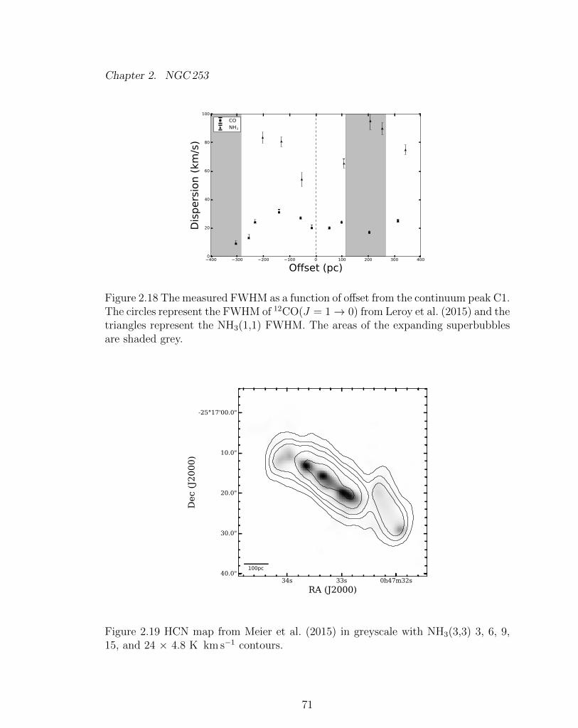
Chapter 2. NGC253
Figure 2.18 The measured FWHM as a function of o↵set from the continuum peak C1.The circles represent the FWHM of 12CO(J = 1 ! 0) from Leroy et al. (2015) and thetriangles represent the NH3(1,1) FWHM. The areas of the expanding superbubblesare shaded grey.
Figure 2.19 HCN map from Meier et al. (2015) in greyscale with NH3(3,3) 3, 6, 9,15, and 24 ⇥ 4.8 K km s�1 contours.
71
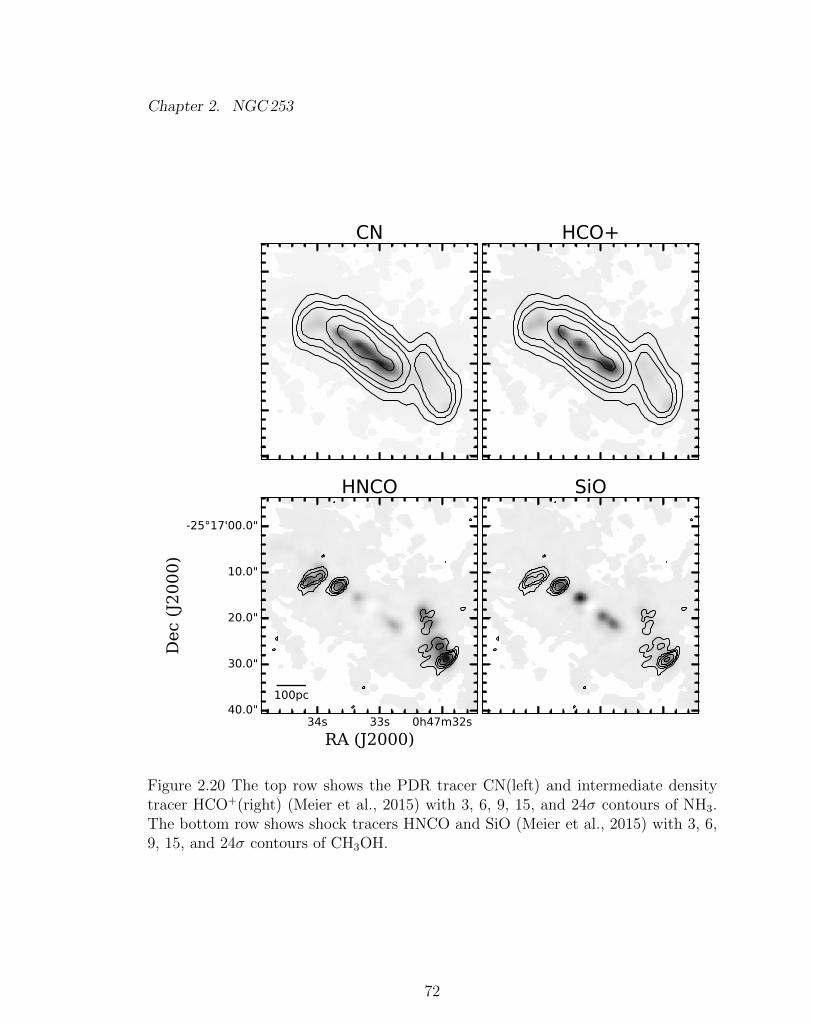
Chapter 2. NGC253
Figure 2.20 The top row shows the PDR tracer CN(left) and intermediate densitytracer HCO+(right) (Meier et al., 2015) with 3, 6, 9, 15, and 24� contours of NH3.The bottom row shows shock tracers HNCO and SiO (Meier et al., 2015) with 3, 6,9, 15, and 24� contours of CH3OH.
72
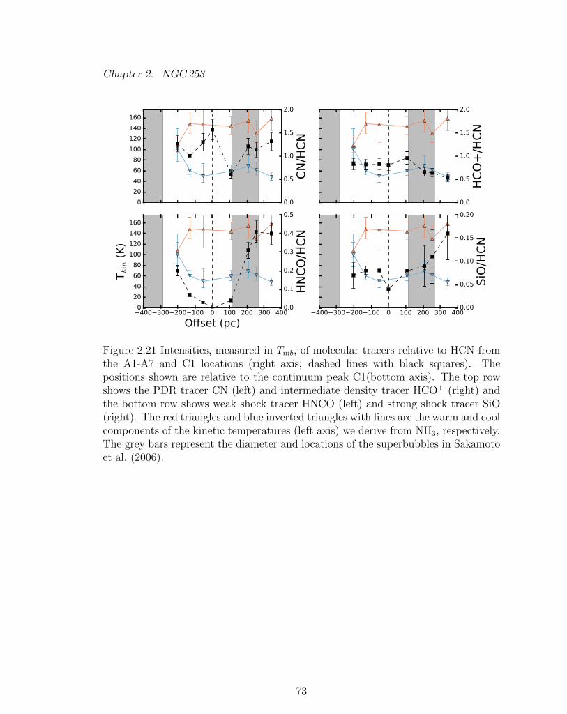
Chapter 2. NGC253
Figure 2.21 Intensities, measured in Tmb, of molecular tracers relative to HCN fromthe A1-A7 and C1 locations (right axis; dashed lines with black squares). Thepositions shown are relative to the continuum peak C1(bottom axis). The top rowshows the PDR tracer CN (left) and intermediate density tracer HCO+ (right) andthe bottom row shows weak shock tracer HNCO (left) and strong shock tracer SiO(right). The red triangles and blue inverted triangles with lines are the warm and coolcomponents of the kinetic temperatures (left axis) we derive from NH3, respectively.The grey bars represent the diameter and locations of the superbubbles in Sakamotoet al. (2006).
73
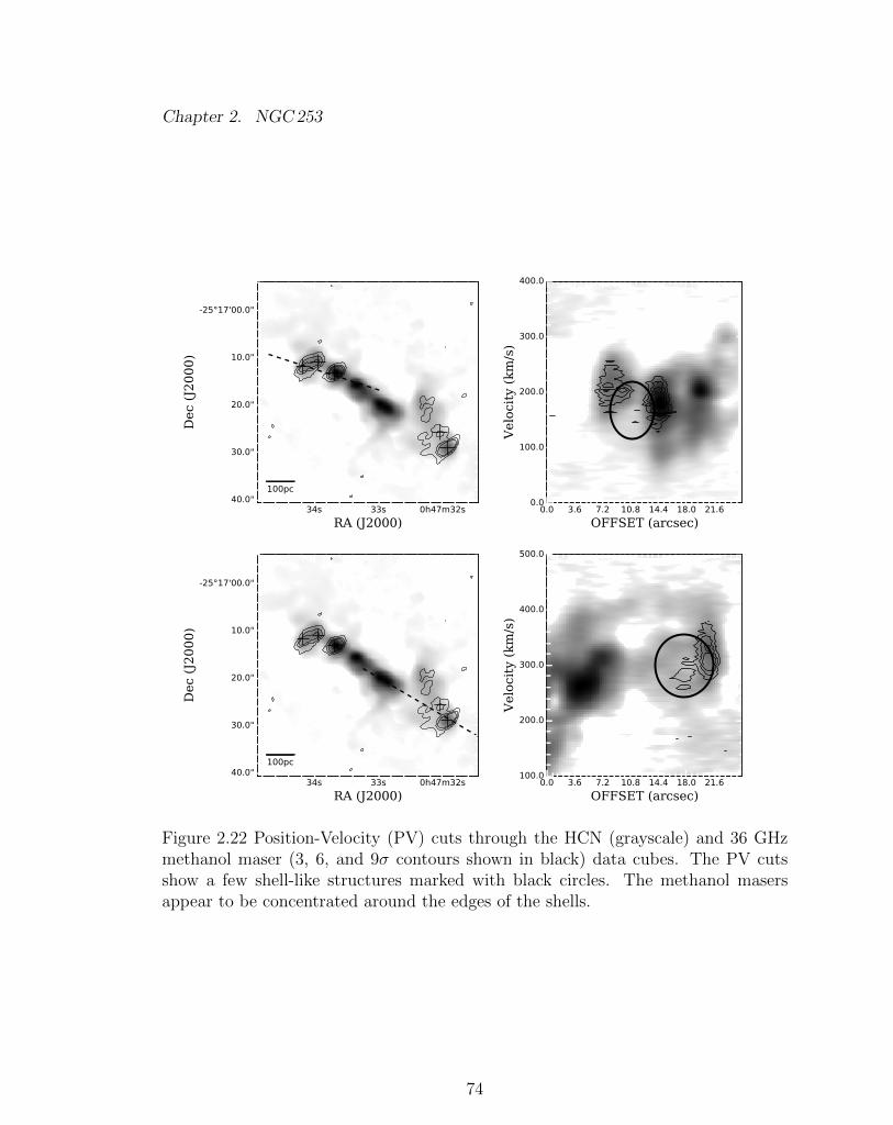
Chapter 2. NGC253
Figure 2.22 Position-Velocity (PV) cuts through the HCN (grayscale) and 36 GHzmethanol maser (3, 6, and 9� contours shown in black) data cubes. The PV cutsshow a few shell-like structures marked with black circles. The methanol masersappear to be concentrated around the edges of the shells.
74
Chapter 2. NGC253
2.6 Summary
We have provided analysis of VLA observations of the dense gas and masers associ-
ated with the nuclear starburst in NGC 253. We conclude the following:
1. We have detected NH3(1,1), (2,2), (3,3), (4,4), and (5,5) in the central kpc of
NGC 253. NH3(9,9) is detected in only one location. No NH3 is observed in
the molecular outflow.
2. We find the molecular gas in NGC 253 to be best described by a spatially
uniform two kinetic temperature model with a warm 130 K component and a
cool 57 K component. The continuum peak (C1) may indeed be hotter as it is
closer to the starburst, but absorption of the metastable para-NH3 lines make
temperature measurements less accurate. Direct LVG analysis corroborates
a two temperature model of NGC 253, though with a cool component of 74
K and a warm component of 145 K. The LVG analysis does hint at a hotter
component greater than 300 K as traced by the NH3(4,4) and NH3(5,5) ratio.
The temperature distribution is not well correlated with PDRs, weak shocks,
or strong shocks, and is constant over the central kpc.
3. We confirm the result from Ott et al. (2005) suggesting that there exist NH3
(3,3) masers in the nucleus of NGC 253. There is currently only one other
known source of extragalactic NH3(3,3) masers, NGC 3079 (Miyamoto et al.,
2015). Both galaxies host outflows, but in NGC 253 the outflow is driven by a
starburst whereas in NGC 3079 it is likely driven by an AGN.
4. Expanding superbubbles do not appear to heat the gas in NGC 253. A com-
parison with the results from Leroy et al. (2015) shows that the linewidths are
dominated by turbulent motions within a GMC. The large NH3 linewidths are
likely due to the bulk motion of the GMCs.
75
Chapter 2. NGC253
5. Three H2O maser features have been observed. The H2O maser W1 is coin-
cident with the continuum peak. We show indications emission is extended
along the minor axis of the galaxy, the spectrum suggests multiple components
and the velocities are more similar to the outflow than the disk. It is likely
that this maser is related to the bipolar outflow of ionized gas, though other
explanations are possible. High resolution followup observations are needed to
confirm a relationship with the bipolar outflow.
W2 is located to the southwest of W1 and shows multiple spectrally unresolved
masers with velocities centered about systemic, suggesting these masers exist
in a circumnuclear torus. It is also possible that W2 may in part trace the
receding side of the outflow. W3 is unresolved and located to the southwest of
W1 and W2. Its progenitor is likely a massive star.
6. We detect five regions with 36 GHz CH3OH masers at the outside edge of the
central kpc as traced by NH3. The spatial proximity and velocities suggest a
relationship with known superbubbles. Position velocity cuts show that all the
36 GHz methanol masers may be related to shell-like features. The 36 GHz
CH3OH morphology and HNCO are similar. This similarity suggests that both
HNCO and 36 GHz methanol masers are tracing similar conditions.
Our analysis reveals the properties of the dense molecular ISM in along the central
kpc of NGC 253 using centimeter and millimeter emission and absorption lines. We
have uncovered relationships with the bipolar outflow, expanding molecular bubbles,
and the nuclear starburst.
76
Chapter 2. NGC253
2.7 Acknowledgments
Mark Gorski acknowledges support from the National Radio Astronomy Observatory
in the form of a graduate student internship, and a Reber Fellowship. We would like
to thank Alberto Bolatto and Adam Leroy for sharing the ALMA image cubes. This
research has made use of the NASA/IPAC Extragalactic Database (NED), which
is maintained by the Jet Propulsion Laboratory, Caltech, under contract with the
National Aeronautics and Space Administration (NASA) and NASA’s Astrophysical
Data System Abstract Service (ADS).
77
Chapter 3
NH3 Thermometry, H2O and
CH3OH in IC 342, NGC6946 and
NGC2146
3.1 Overview
The Survey of Water and Ammonia in Nearby galaxies (SWAN) studies atomic and
molecular species across the nuclei four star forming galaxies: NGC 253, IC 342,
NGC 6946, and NGC 2146. As part of this survey, we present Karl G. Jansky Very
Large Array (VLA) molecular line observations of three galaxies: IC 342, NGC 6946
and NGC 2146. We will compare these observations with NGC 253 from Chapter 2.
These galaxies were chosen to span an order of magnitude in star formation rates and
to select a variety of galaxy types. We target the metastable transitions of ammonia
NH3(1,1) to (5,5), the 22 GHz water (H2O) (616 � 523) maser, and the 36.1 GHz
methanol (CH3OH) (4�1 � 30) maser. We show evidence for uniform heating across
the central kpc of IC 342 with two temperature components for the molecular gas
78
Chapter 3. IC 342, NGC6946 and NGC2146
of 27 K and 308 K, and that the dense molecular gas in NGC 2146 has Tkin <86 K.
We identify two new water masers in IC 342, and one new water maser in each of
NGC 6946 and NGC 2146. The two galaxies NGC 253 and NGC 2146, with the most
vigorous star formation, host H2O kilomasers. Lastly, we detect the first 36 GHz
CH3OH masers in IC 342 and NGC 6946. For the four external galaxies the total
luminosity in each galaxy suggests a correlation with galactic star formation rate,
whereas the morphology is similar to that of HNCO, a weak shock tracer.
3.2 Introduction
In evolutionary models of star forming galaxies, without feedback the ISM tends
to rapidly collapse and form stars in less than a dynamical time, while too much
feedback can completely disrupt giant molecular clouds (GMCs) (e.g., Kau↵mann
et al., 1999; Krumholz et al., 2011; Hopkins et al., 2011). Therefore it is necessary
to check the feedback prescription in cosmological simulations against observations.
Since star formation is largely correlated with dense molecular gas (Gao & Solomon,
2004), the e↵ect of feedback should, in part, influence the state of the dense molecular
ISM. Radio interferometric observations of nearby galaxies provide access to 10-100
pc scales that are related to GMCs.
Measurements of the NH3 metastable transitions provide for calculations of the
rotational temperature, and via Large Velocity Gradient (LVG) models it is possible
to estimate kinetic temperatures with reasonable precision (e.g., Ho & Townes, 1983,
Walmsley & Ungerechts, 1983, Lebron et al., 2011, Ott et al., 2005, Ott et al., 2011,
Mangum et al., 2013, Chapter 2).
The 22 GHz H2O masers are collisionally excited, typically coming from three en-
vironments. The stellar masers are associated with mass loss stages of Young Stellar
Objects (YSOs) and Asymptotic Giant Branch (AGB) stars and are the least lumi-
79
Chapter 3. IC 342, NGC6946 and NGC2146
nous (< 0.1 L� e.g., Palagi et al., 1993). The strongest masers (>20 L�), classified as
megamasers, are typical of nuclear activity (e.g., Braatz et al., 1996). The kilomasers
are of intermediate luminosity between the stellar and megamasers, and are associ-
ated with strong star formation activity (Hagiwara et al., 2001). These could consist
of many stellar class masers, or be the low luminosity tail of the megamaser class,
then they are related to the supermassive black hole (Tarchi et al., 2011). These
masers we use as signposts of shocked material related to star formation.
The Class I, collisionally excited, 36 GHz CH3OH masers are new in the extra-
galactic context. Before this work they had been detected outside the Milky Way
only in NGC 253 (Ellingsen et al., 2014 and Chapter 2 ) and Arp220 (Chen et al.,
2015), where they are three orders of magnitude more luminous than typical Galactic
counterparts.
In Chapter 2 we performed NH3 thermometry, and analyzed H2O and 36 GHz
CH3OH masers, in the central kpc of NGC 253 based on Karl G. Jansky Very Large
Array (VLA)1 observations. We detect the NH3(1,1) to (5,5) lines, and the (9,9)
line. Using the same analysis we will use in this paper we uncovered a cool 57 K
component and a warm 130 K component uniformly distributed across the molecular
disk. There is no apparent correlation of temperature with tracers of dominant forms
of feedback (weak or strong shocks, and PDRs). Within the centermost 100 pc there
is evidence for NH3(3,3) masers, similar to NGC 3079 (Miyamoto et al., 2015). The
strongest water maser in NGC 253 contains many components and shows evidence
for an extension along the minor axis. In addition to the maser’s strong blueshifted
velocity components, this suggests a relationship with the outflow. We resolve the
first detected extragalactic 36 GHz masers (Ellingsen et al., 2014) into five di↵erent
sources. The emission is concentrated around the edges of expanding superbubbles.
The morphology of the emission is similar to HNCO(40,4 � 30,3), a weak shock tracer
1The National Radio Astronomy Observatory is a facility of the National Science Foun-dation operated under cooperative agreement by Associated Universities, Inc.
80
Chapter 3. IC 342, NGC6946 and NGC2146
(Meier et al., 2015), suggesting the two molecules trace similar conditions.
In this chapter we will carry out a similar analysis across the other galaxies in
the SWAN sample (IC 342, NGC 6946, and NGC 2146). In §3.3 we describe the
observational setups, and the data reduction and imaging process. In §3.4 we report
our measurements of the NH3, H2O, and CH3OH lines for each galaxy individually.
In §3.5 we discuss the analysis of the NH3 lines and derived temperatures for each
galaxy where possible; in addition we generate LVG models for IC 342. We also
discuss the H2O and CH3OH masers in each galaxy. In §3.6 we incorporate the
results from Chapter 2 and discuss the relevance of the survey as a whole. Finally,
in §3.7 we summarize our findings.
3.3 Observations and Data Reduction
IC 342 and NGC 6946 were observed with identical frequency setups of the Karl G.
Jansky Very Large Array (VLA) (project code: 10B-161). The correlator was setup
to cover frequency ranges 21.9-22.3 GHz, 23.6-23.7 GHz, and 24.1-24.5 GHz with
500 kHz wide channels (K-band receiver), and 26.8-27.9 GHz and 36.0-37.0 GHz with
1 MHz wide channels (Ka-band receiver). The galaxy NGC 6946 was observed with
two pointings with the same RA(J2000): 20h 35m 52.336s and di↵erent DEC(J2000):
+60� 09’ 32.2100’ and +60� 08’ 56.210”. The galaxy NGC 2146 was observed with
the same correlator setup as NGC 253 in Chapter 2 (project code: 13A-375), with
250 kHz channels, but was not observed in Ka-band. All three galaxies were observed
in the C configuration of the VLA. As in Chapter 2 we target the metastable NH3 lines
from J=K (1,1) to (5,5), the 22.2351 GHz H2O(616�523) maser, and the 36.1693 GHz
CH3OH(414 � 303) maser, though as NGC 2146 did not get observed in Ka-band, so
no analysis of the 36 GHz CH3OH maser is presented for this galaxy.
We calibrated and imaged the data in the Common Astronomy Software Appli-
81
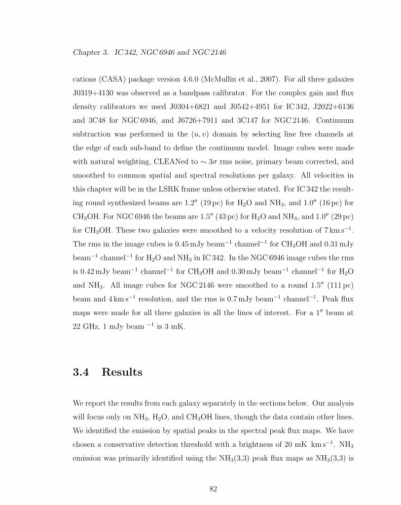
Chapter 3. IC 342, NGC6946 and NGC2146
cations (CASA) package version 4.6.0 (McMullin et al., 2007). For all three galaxies
J0319+4130 was observed as a bandpass calibrator. For the complex gain and flux
density calibrators we used J0304+6821 and J0542+4951 for IC 342, J2022+6136
and 3C48 for NGC 6946, and J6726+7911 and 3C147 for NGC 2146. Continuum
subtraction was performed in the (u, v) domain by selecting line free channels at
the edge of each sub-band to define the continuum model. Image cubes were made
with natural weighting, CLEANed to ⇠ 3� rms noise, primary beam corrected, and
smoothed to common spatial and spectral resolutions per galaxy. All velocities in
this chapter will be in the LSRK frame unless otherwise stated. For IC 342 the result-
ing round synthesized beams are 1.200 (19 pc) for H2O and NH3, and 1.000 (16 pc) for
CH3OH. For NGC 6946 the beams are 1.500 (43 pc) for H2O and NH3, and 1.000 (29 pc)
for CH3OH. These two galaxies were smoothed to a velocity resolution of 7 km s�1.
The rms in the image cubes is 0.45 mJy beam�1 channel�1 for CH3OH and 0.31 mJy
beam�1 channel�1 for H2O and NH3 in IC 342. In the NGC 6946 image cubes the rms
is 0.42 mJy beam�1 channel�1 for CH3OH and 0.30 mJy beam�1 channel�1 for H2O
and NH3. All image cubes for NGC 2146 were smoothed to a round 1.500 (111 pc)
beam and 4 km s�1 resolution, and the rms is 0.7 mJy beam�1 channel�1. Peak flux
maps were made for all three galaxies in all the lines of interest. For a 100 beam at
22 GHz, 1 mJy beam �1 is 3 mK.
3.4 Results
We report the results from each galaxy separately in the sections below. Our analysis
will focus only on NH3, H2O, and CH3OH lines, though the data contain other lines.
We identified the emission by spatial peaks in the spectral peak flux maps. We have
chosen a conservative detection threshold with a brightness of 20 mK km s�1. NH3
emission was primarily identified using the NH3(3,3) peak flux maps as NH3(3,3) is
82
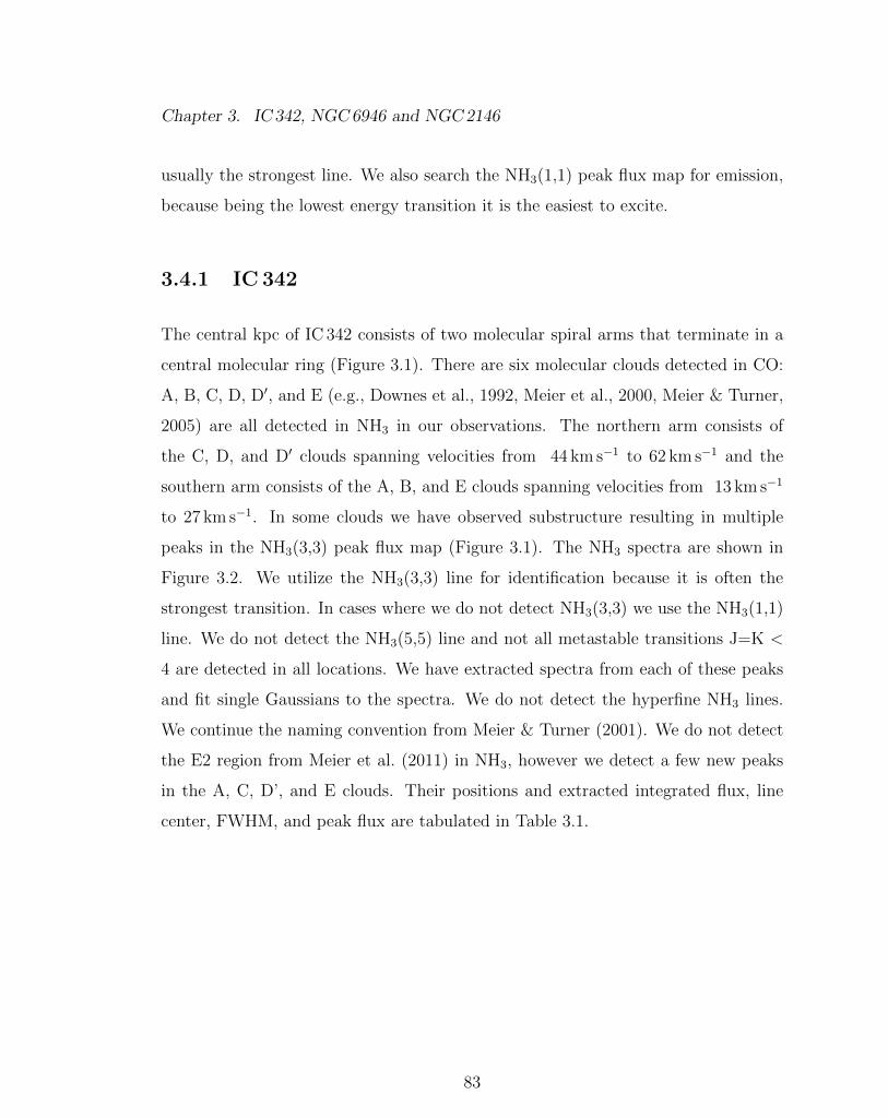
Chapter 3. IC 342, NGC6946 and NGC2146
usually the strongest line. We also search the NH3(1,1) peak flux map for emission,
because being the lowest energy transition it is the easiest to excite.
3.4.1 IC 342
The central kpc of IC 342 consists of two molecular spiral arms that terminate in a
central molecular ring (Figure 3.1). There are six molecular clouds detected in CO:
A, B, C, D, D0, and E (e.g., Downes et al., 1992, Meier et al., 2000, Meier & Turner,
2005) are all detected in NH3 in our observations. The northern arm consists of
the C, D, and D0 clouds spanning velocities from 44 km s�1 to 62 km s�1 and the
southern arm consists of the A, B, and E clouds spanning velocities from 13 km s�1
to 27 km s�1. In some clouds we have observed substructure resulting in multiple
peaks in the NH3(3,3) peak flux map (Figure 3.1). The NH3 spectra are shown in
Figure 3.2. We utilize the NH3(3,3) line for identification because it is often the
strongest transition. In cases where we do not detect NH3(3,3) we use the NH3(1,1)
line. We do not detect the NH3(5,5) line and not all metastable transitions J=K <
4 are detected in all locations. We have extracted spectra from each of these peaks
and fit single Gaussians to the spectra. We do not detect the hyperfine NH3 lines.
We continue the naming convention from Meier & Turner (2001). We do not detect
the E2 region from Meier et al. (2011) in NH3, however we detect a few new peaks
in the A, C, D’, and E clouds. Their positions and extracted integrated flux, line
center, FWHM, and peak flux are tabulated in Table 3.1.
83
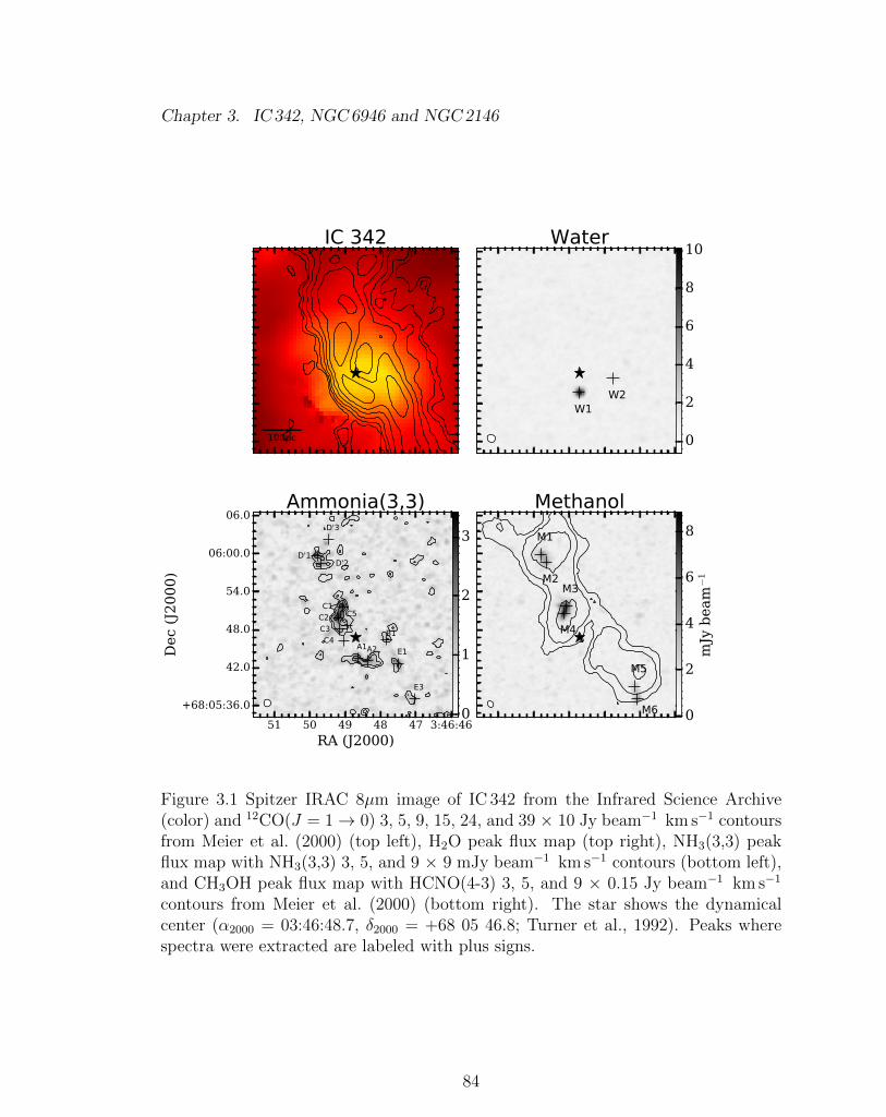
Chapter 3. IC 342, NGC6946 and NGC2146
Figure 3.1 Spitzer IRAC 8µm image of IC 342 from the Infrared Science Archive(color) and 12CO(J = 1 ! 0) 3, 5, 9, 15, 24, and 39 ⇥ 10 Jy beam�1 km s�1 contoursfrom Meier et al. (2000) (top left), H2O peak flux map (top right), NH3(3,3) peakflux map with NH3(3,3) 3, 5, and 9 ⇥ 9 mJy beam�1 km s�1 contours (bottom left),and CH3OH peak flux map with HCNO(4-3) 3, 5, and 9 ⇥ 0.15 Jy beam�1 km s�1
contours from Meier et al. (2000) (bottom right). The star shows the dynamicalcenter (↵2000 = 03:46:48.7, �2000 = +68 05 46.8; Turner et al., 1992). Peaks wherespectra were extracted are labeled with plus signs.
84
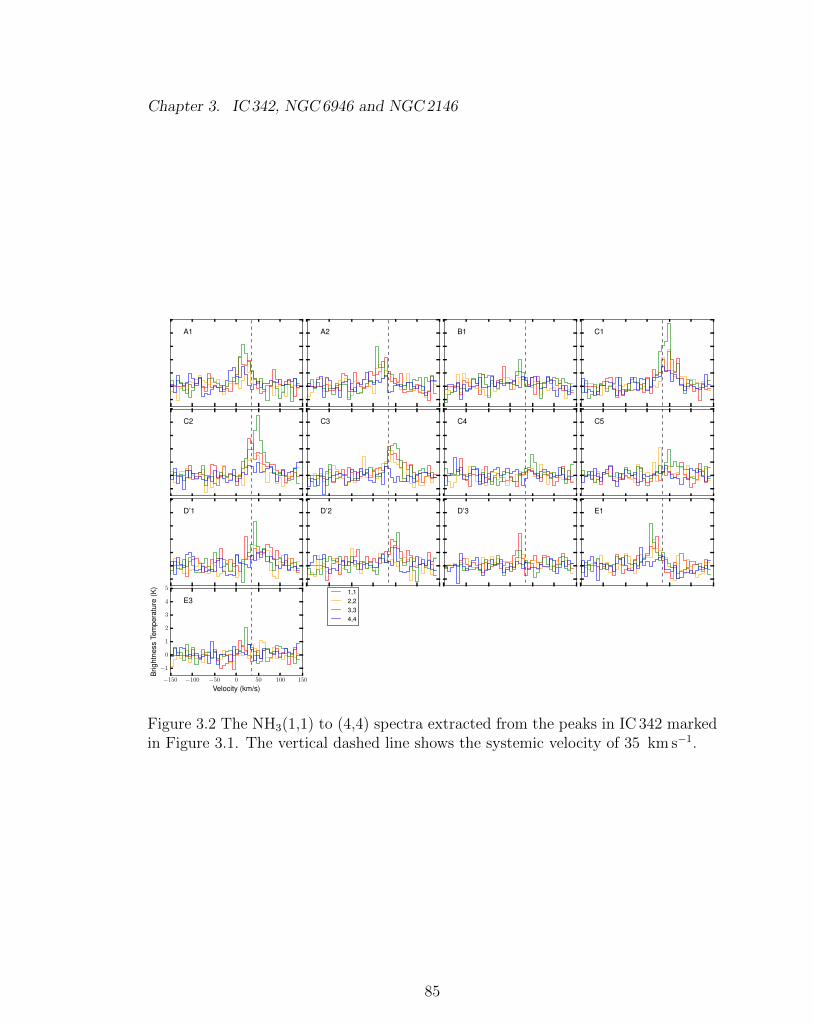
Chapter 3. IC 342, NGC6946 and NGC2146
A1 A2 B1 C1
C2 C3 C4 C5
D’1 D’2 D’3 E1
�150 �100 �50 0 50 100 150
Velocity (km/s)
�1
0
1
2
3
4
5
Brig
htne
ssTe
mpe
ratu
re(K
)
E31,12,23,34,4
Figure 3.2 The NH3(1,1) to (4,4) spectra extracted from the peaks in IC 342 markedin Figure 3.1. The vertical dashed line shows the systemic velocity of 35 km s�1.
85
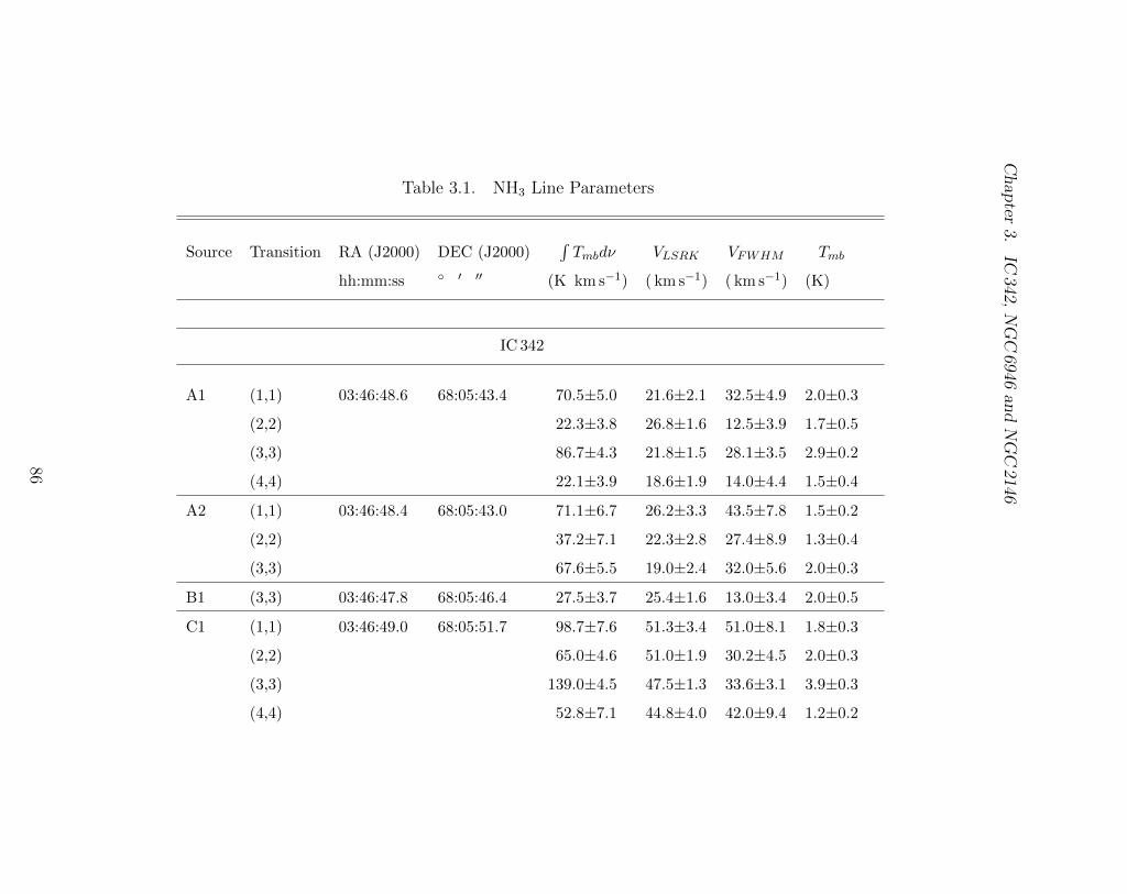
Chapter3.
IC342,NGC6946andNGC2146
Table 3.1. NH3 Line Parameters
Source Transition RA (J2000) DEC (J2000)R
Tmbd⌫ VLSRK VFWHM Tmb
hh:mm:ss � 0 00 (K km s�1) ( km s�1) ( km s�1) (K)
IC 342
A1 (1,1) 03:46:48.6 68:05:43.4 70.5±5.0 21.6±2.1 32.5±4.9 2.0±0.3
(2,2) 22.3±3.8 26.8±1.6 12.5±3.9 1.7±0.5
(3,3) 86.7±4.3 21.8±1.5 28.1±3.5 2.9±0.2
(4,4) 22.1±3.9 18.6±1.9 14.0±4.4 1.5±0.4
A2 (1,1) 03:46:48.4 68:05:43.0 71.1±6.7 26.2±3.3 43.5±7.8 1.5±0.2
(2,2) 37.2±7.1 22.3±2.8 27.4±8.9 1.3±0.4
(3,3) 67.6±5.5 19.0±2.4 32.0±5.6 2.0±0.3
B1 (3,3) 03:46:47.8 68:05:46.4 27.5±3.7 25.4±1.6 13.0±3.4 2.0±0.5
C1 (1,1) 03:46:49.0 68:05:51.7 98.7±7.6 51.3±3.4 51.0±8.1 1.8±0.3
(2,2) 65.0±4.6 51.0±1.9 30.2±4.5 2.0±0.3
(3,3) 139.0±4.5 47.5±1.3 33.6±3.1 3.9±0.3
(4,4) 52.8±7.1 44.8±4.0 42.0±9.4 1.2±0.2
86
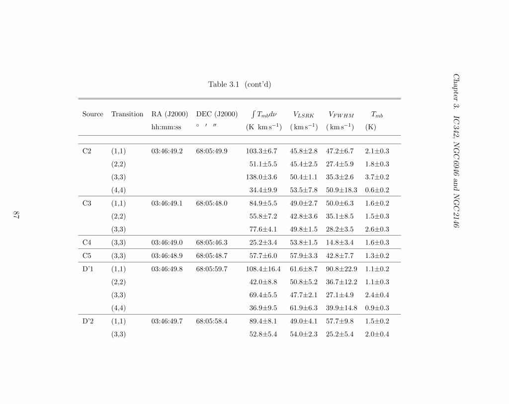
Chapter3.
IC342,NGC6946andNGC2146
Table 3.1 (cont’d)
Source Transition RA (J2000) DEC (J2000)R
Tmbd⌫ VLSRK VFWHM Tmb
hh:mm:ss � 0 00 (K km s�1) ( km s�1) ( km s�1) (K)
C2 (1,1) 03:46:49.2 68:05:49.9 103.3±6.7 45.8±2.8 47.2±6.7 2.1±0.3
(2,2) 51.1±5.5 45.4±2.5 27.4±5.9 1.8±0.3
(3,3) 138.0±3.6 50.4±1.1 35.3±2.6 3.7±0.2
(4,4) 34.4±9.9 53.5±7.8 50.9±18.3 0.6±0.2
C3 (1,1) 03:46:49.1 68:05:48.0 84.9±5.5 49.0±2.7 50.0±6.3 1.6±0.2
(2,2) 55.8±7.2 42.8±3.6 35.1±8.5 1.5±0.3
(3,3) 77.6±4.1 49.8±1.5 28.2±3.5 2.6±0.3
C4 (3,3) 03:46:49.0 68:05:46.3 25.2±3.4 53.8±1.5 14.8±3.4 1.6±0.3
C5 (3,3) 03:46:48.9 68:05:48.7 57.7±6.0 57.9±3.3 42.8±7.7 1.3±0.2
D’1 (1,1) 03:46:49.8 68:05:59.7 108.4±16.4 61.6±8.7 90.8±22.9 1.1±0.2
(2,2) 42.0±8.8 50.8±5.2 36.7±12.2 1.1±0.3
(3,3) 69.4±5.5 47.7±2.1 27.1±4.9 2.4±0.4
(4,4) 36.9±9.5 61.9±6.3 39.9±14.8 0.9±0.3
D’2 (1,1) 03:46:49.7 68:05:58.4 89.4±8.1 49.0±4.1 57.7±9.8 1.5±0.2
(3,3) 52.8±5.4 54.0±2.3 25.2±5.4 2.0±0.4
87
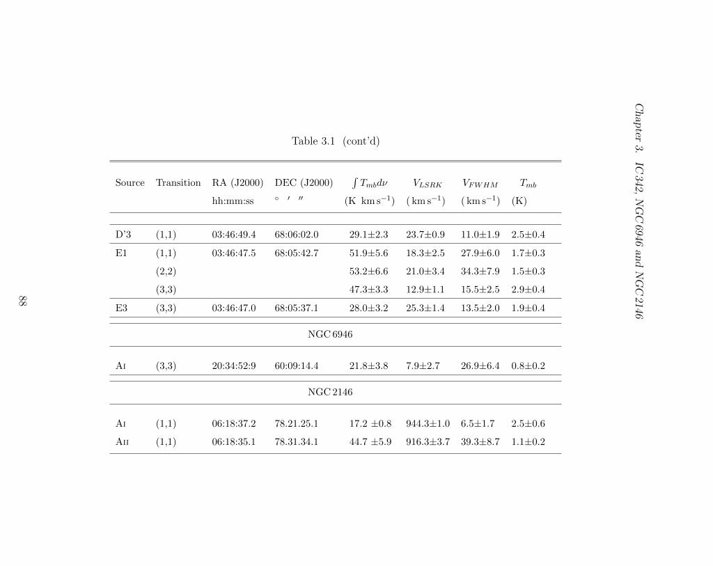
Chapter3.
IC342,NGC6946andNGC2146
Table 3.1 (cont’d)
Source Transition RA (J2000) DEC (J2000)R
Tmbd⌫ VLSRK VFWHM Tmb
hh:mm:ss � 0 00 (K km s�1) ( km s�1) ( km s�1) (K)
D’3 (1,1) 03:46:49.4 68:06:02.0 29.1±2.3 23.7±0.9 11.0±1.9 2.5±0.4
E1 (1,1) 03:46:47.5 68:05:42.7 51.9±5.6 18.3±2.5 27.9±6.0 1.7±0.3
(2,2) 53.2±6.6 21.0±3.4 34.3±7.9 1.5±0.3
(3,3) 47.3±3.3 12.9±1.1 15.5±2.5 2.9±0.4
E3 (3,3) 03:46:47.0 68:05:37.1 28.0±3.2 25.3±1.4 13.5±2.0 1.9±0.4
NGC6946
AI (3,3) 20:34:52:9 60:09:14.4 21.8±3.8 7.9±2.7 26.9±6.4 0.8±0.2
NGC2146
AI (1,1) 06:18:37.2 78.21.25.1 17.2 ±0.8 944.3±1.0 6.5±1.7 2.5±0.6
AII (1,1) 06:18:35.1 78.31.34.1 44.7 ±5.9 916.3±3.7 39.3±8.7 1.1±0.2
88
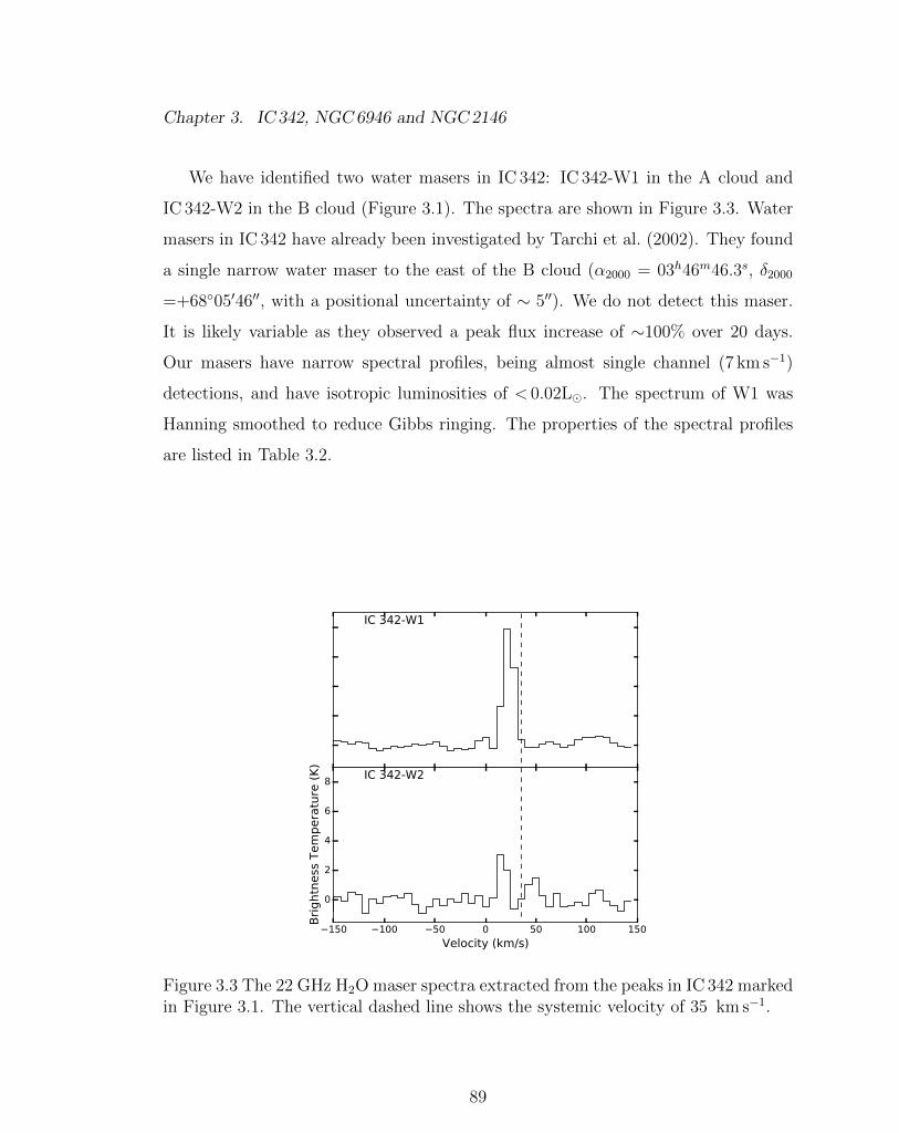
Chapter 3. IC 342, NGC6946 and NGC2146
We have identified two water masers in IC 342: IC 342-W1 in the A cloud and
IC 342-W2 in the B cloud (Figure 3.1). The spectra are shown in Figure 3.3. Water
masers in IC 342 have already been investigated by Tarchi et al. (2002). They found
a single narrow water maser to the east of the B cloud (↵2000 = 03h46m46.3s, �2000
=+68�0504600, with a positional uncertainty of ⇠ 500). We do not detect this maser.
It is likely variable as they observed a peak flux increase of ⇠100% over 20 days.
Our masers have narrow spectral profiles, being almost single channel (7 km s�1)
detections, and have isotropic luminosities of < 0.02L�. The spectrum of W1 was
Hanning smoothed to reduce Gibbs ringing. The properties of the spectral profiles
are listed in Table 3.2.
Figure 3.3 The 22 GHz H2O maser spectra extracted from the peaks in IC 342 markedin Figure 3.1. The vertical dashed line shows the systemic velocity of 35 km s�1.
89
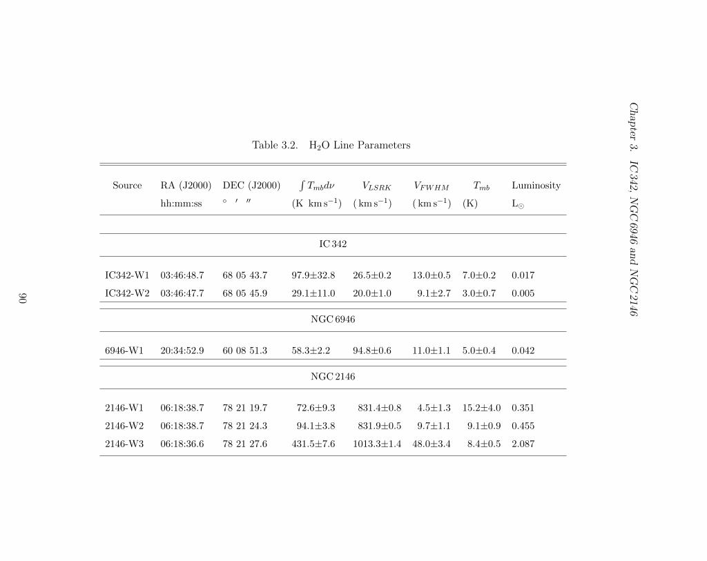
Chapter3.
IC342,NGC6946andNGC2146
Table 3.2. H2O Line Parameters
Source RA (J2000) DEC (J2000)R
Tmbd⌫ VLSRK VFWHM Tmb Luminosity
hh:mm:ss � 0 00 (K km s�1) ( km s�1) ( km s�1) (K) L�
IC 342
IC342-W1 03:46:48.7 68 05 43.7 97.9±32.8 26.5±0.2 13.0±0.5 7.0±0.2 0.017
IC342-W2 03:46:47.7 68 05 45.9 29.1±11.0 20.0±1.0 9.1±2.7 3.0±0.7 0.005
NGC6946
6946-W1 20:34:52.9 60 08 51.3 58.3±2.2 94.8±0.6 11.0±1.1 5.0±0.4 0.042
NGC2146
2146-W1 06:18:38.7 78 21 19.7 72.6±9.3 831.4±0.8 4.5±1.3 15.2±4.0 0.351
2146-W2 06:18:38.7 78 21 24.3 94.1±3.8 831.9±0.5 9.7±1.1 9.1±0.9 0.455
2146-W3 06:18:36.6 78 21 27.6 431.5±7.6 1013.3±1.4 48.0±3.4 8.4±0.5 2.087
90
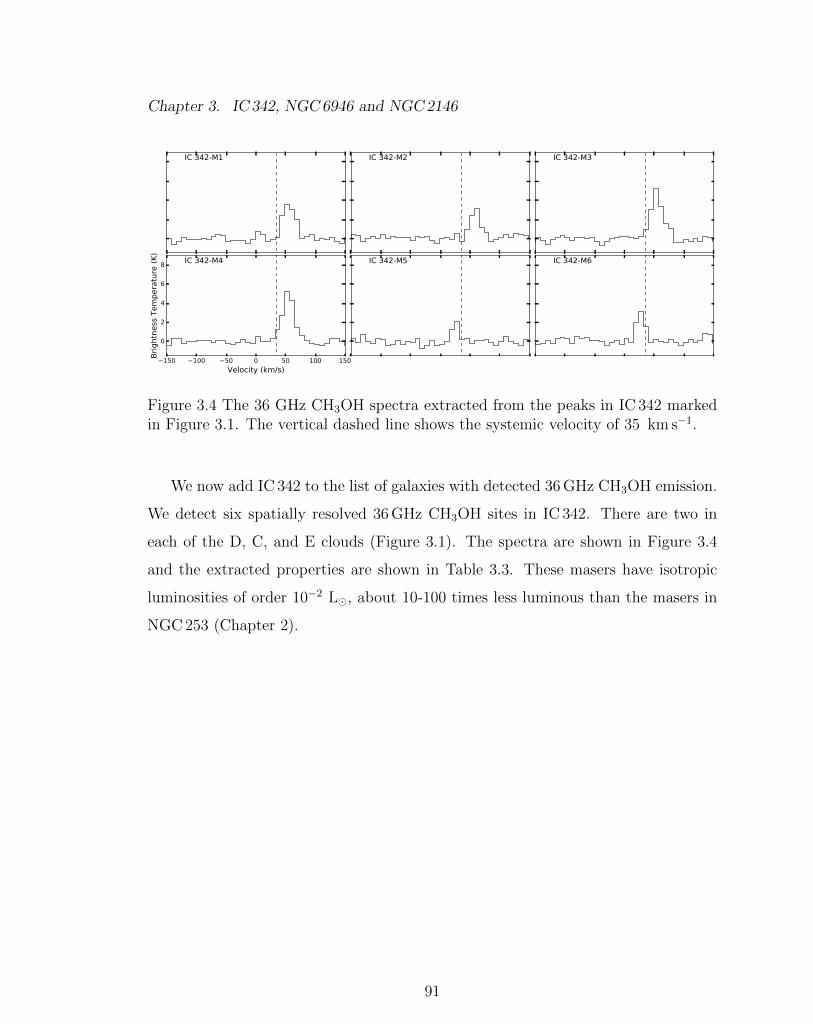
Chapter 3. IC 342, NGC6946 and NGC2146
Figure 3.4 The 36 GHz CH3OH spectra extracted from the peaks in IC 342 markedin Figure 3.1. The vertical dashed line shows the systemic velocity of 35 km s�1.
We now add IC 342 to the list of galaxies with detected 36 GHz CH3OH emission.
We detect six spatially resolved 36 GHz CH3OH sites in IC 342. There are two in
each of the D, C, and E clouds (Figure 3.1). The spectra are shown in Figure 3.4
and the extracted properties are shown in Table 3.3. These masers have isotropic
luminosities of order 10�2 L�, about 10-100 times less luminous than the masers in
NGC 253 (Chapter 2).
91
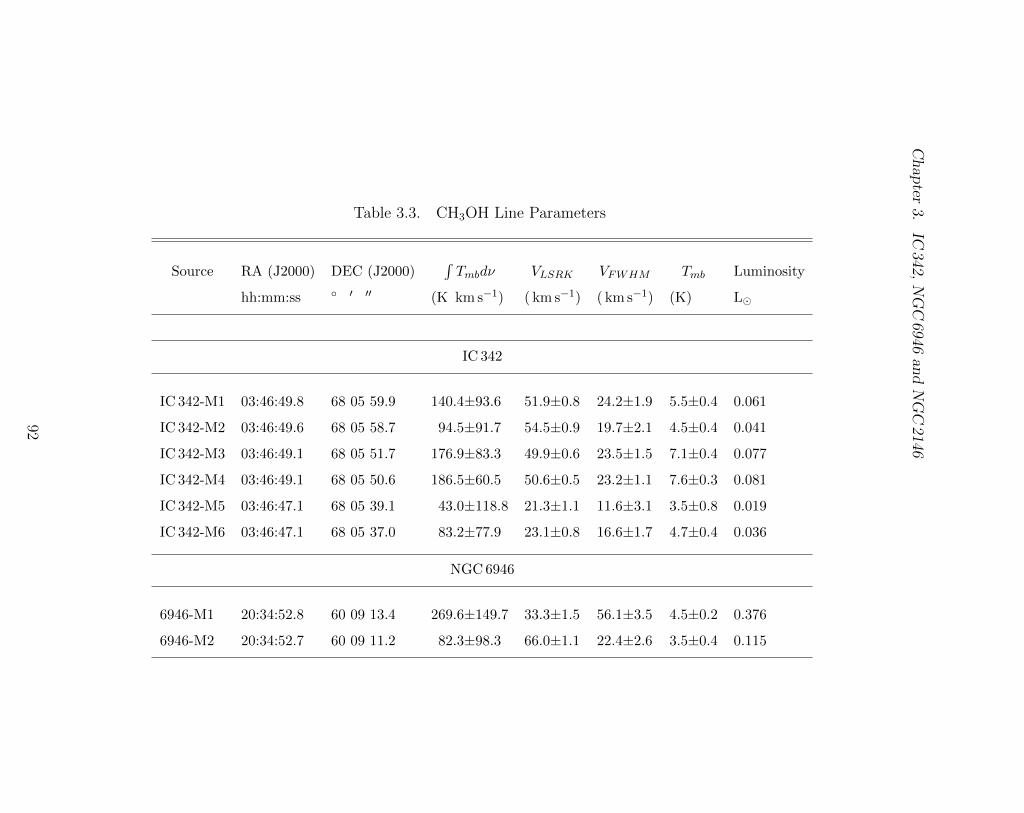
Chapter3.
IC342,NGC6946andNGC2146
Table 3.3. CH3OH Line Parameters
Source RA (J2000) DEC (J2000)R
Tmbd⌫ VLSRK VFWHM Tmb Luminosity
hh:mm:ss � 0 00 (K km s�1) ( km s�1) ( km s�1) (K) L�
IC 342
IC 342-M1 03:46:49.8 68 05 59.9 140.4±93.6 51.9±0.8 24.2±1.9 5.5±0.4 0.061
IC 342-M2 03:46:49.6 68 05 58.7 94.5±91.7 54.5±0.9 19.7±2.1 4.5±0.4 0.041
IC 342-M3 03:46:49.1 68 05 51.7 176.9±83.3 49.9±0.6 23.5±1.5 7.1±0.4 0.077
IC 342-M4 03:46:49.1 68 05 50.6 186.5±60.5 50.6±0.5 23.2±1.1 7.6±0.3 0.081
IC 342-M5 03:46:47.1 68 05 39.1 43.0±118.8 21.3±1.1 11.6±3.1 3.5±0.8 0.019
IC 342-M6 03:46:47.1 68 05 37.0 83.2±77.9 23.1±0.8 16.6±1.7 4.7±0.4 0.036
NGC6946
6946-M1 20:34:52.8 60 09 13.4 269.6±149.7 33.3±1.5 56.1±3.5 4.5±0.2 0.376
6946-M2 20:34:52.7 60 09 11.2 82.3±98.3 66.0±1.1 22.4±2.6 3.5±0.4 0.115
92
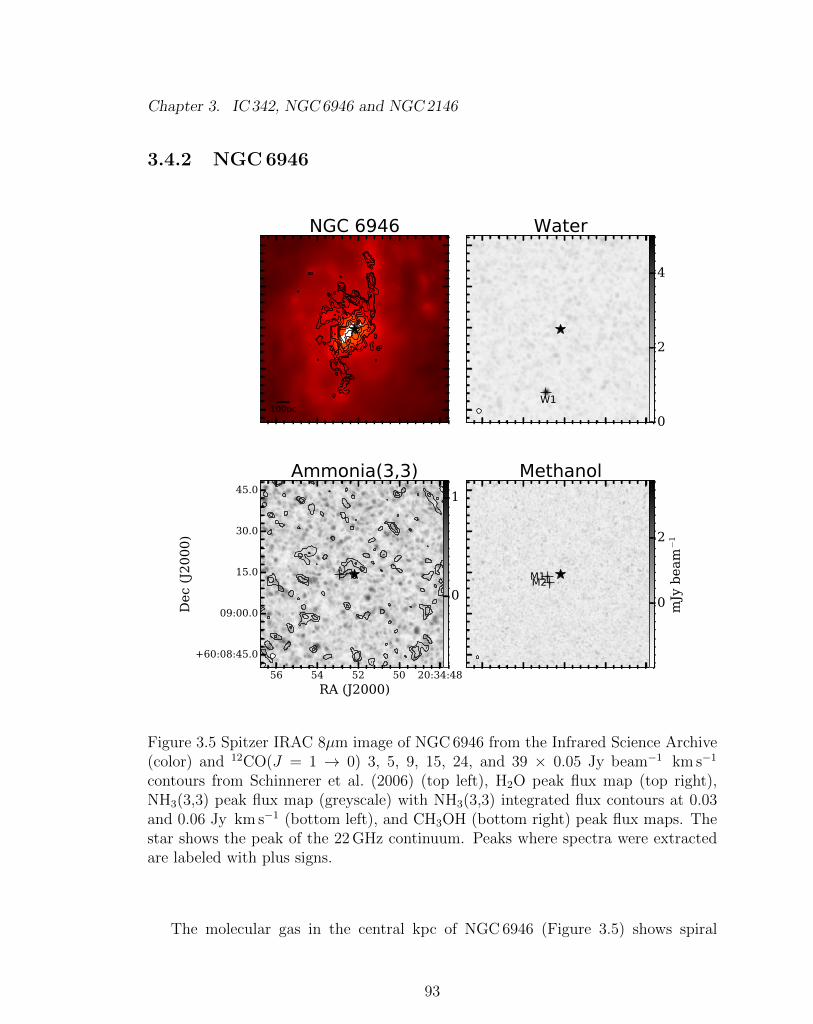
Chapter 3. IC 342, NGC6946 and NGC2146
3.4.2 NGC6946
Figure 3.5 Spitzer IRAC 8µm image of NGC 6946 from the Infrared Science Archive(color) and 12CO(J = 1 ! 0) 3, 5, 9, 15, 24, and 39 ⇥ 0.05 Jy beam�1 km s�1
contours from Schinnerer et al. (2006) (top left), H2O peak flux map (top right),NH3(3,3) peak flux map (greyscale) with NH3(3,3) integrated flux contours at 0.03and 0.06 Jy km s�1 (bottom left), and CH3OH (bottom right) peak flux maps. Thestar shows the peak of the 22 GHz continuum. Peaks where spectra were extractedare labeled with plus signs.
The molecular gas in the central kpc of NGC 6946 (Figure 3.5) shows spiral
93
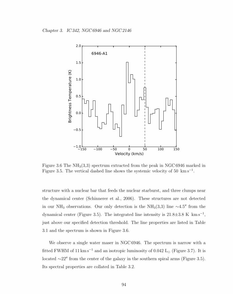
Chapter 3. IC 342, NGC6946 and NGC2146
Figure 3.6 The NH3(3,3) spectrum extracted from the peak in NGC 6946 marked inFigure 3.5. The vertical dashed line shows the systemic velocity of 50 km s�1.
structure with a nuclear bar that feeds the nuclear starburst, and three clumps near
the dynamical center (Schinnerer et al., 2006). These structures are not detected
in our NH3 observations. Our only detection is the NH3(3,3) line ⇠4.500 from the
dynamical center (Figure 3.5). The integrated line intensity is 21.8±3.8 K km s�1,
just above our specified detection threshold. The line properties are listed in Table
3.1 and the spectrum is shown in Figure 3.6.
We observe a single water maser in NGC 6946. The spectrum is narrow with a
fitted FWHM of 11 km s�1 and an isotropic luminosity of 0.042 L� (Figure 3.7). It is
located ⇠2200 from the center of the galaxy in the southern spiral arms (Figure 3.5).
Its spectral properties are collated in Table 3.2.
94
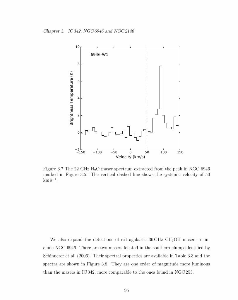
Chapter 3. IC 342, NGC6946 and NGC2146
Figure 3.7 The 22 GHz H2O maser spectrum extracted from the peak in NGC 6946marked in Figure 3.5. The vertical dashed line shows the systemic velocity of 50km s�1.
We also expand the detections of extragalactic 36 GHz CH3OH masers to in-
clude NGC 6946. There are two masers located in the southern clump identified by
Schinnerer et al. (2006). Their spectral properties are available in Table 3.3 and the
spectra are shown in Figure 3.8. They are one order of magnitude more luminous
than the masers in IC 342, more comparable to the ones found in NGC 253.
95
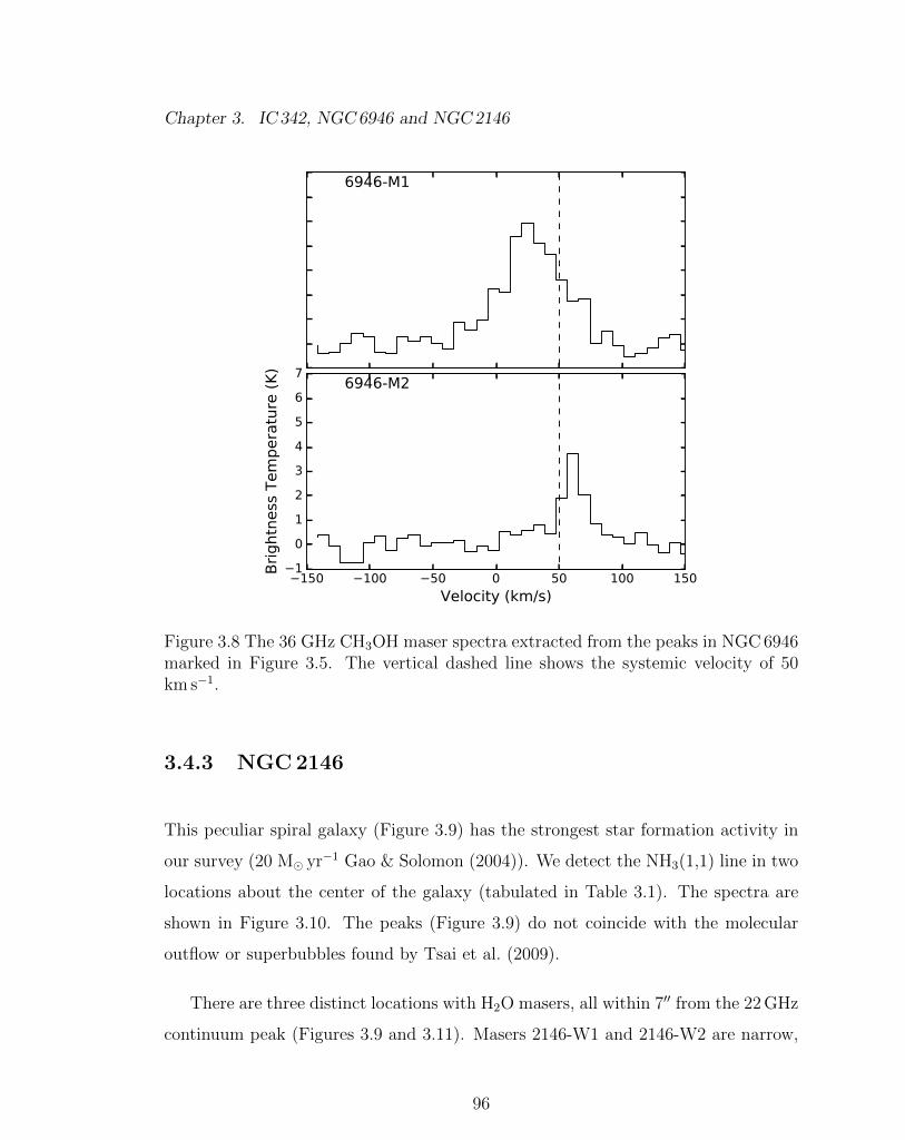
Chapter 3. IC 342, NGC6946 and NGC2146
Figure 3.8 The 36 GHz CH3OH maser spectra extracted from the peaks in NGC 6946marked in Figure 3.5. The vertical dashed line shows the systemic velocity of 50km s�1.
3.4.3 NGC2146
This peculiar spiral galaxy (Figure 3.9) has the strongest star formation activity in
our survey (20 M� yr�1 Gao & Solomon (2004)). We detect the NH3(1,1) line in two
locations about the center of the galaxy (tabulated in Table 3.1). The spectra are
shown in Figure 3.10. The peaks (Figure 3.9) do not coincide with the molecular
outflow or superbubbles found by Tsai et al. (2009).
There are three distinct locations with H2O masers, all within 700 from the 22 GHz
continuum peak (Figures 3.9 and 3.11). Masers 2146-W1 and 2146-W2 are narrow,
96
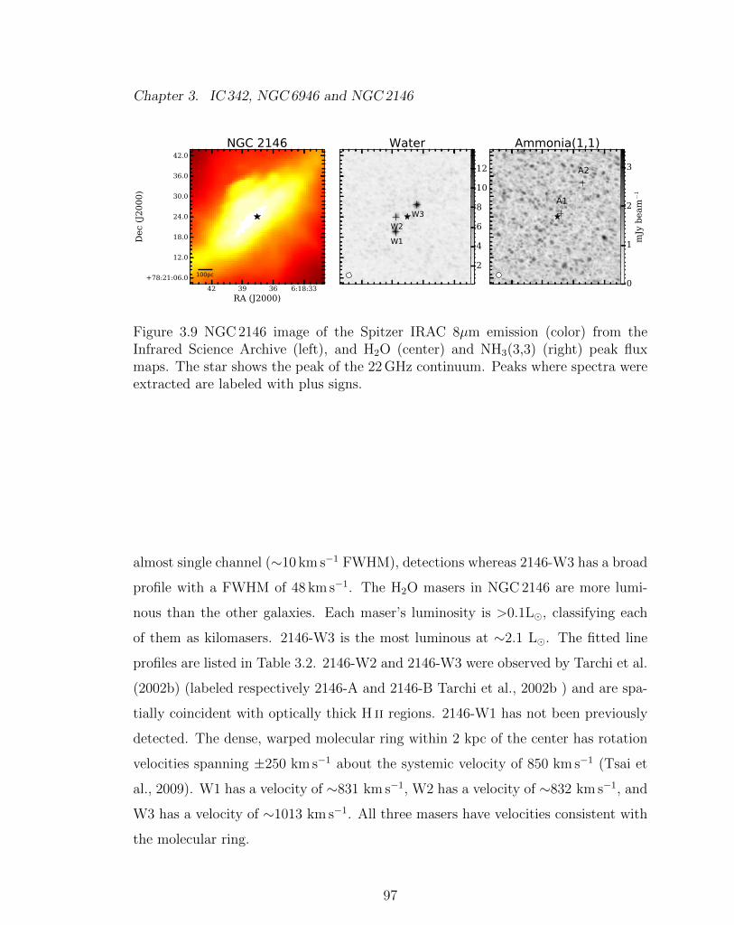
Chapter 3. IC 342, NGC6946 and NGC2146
Figure 3.9 NGC 2146 image of the Spitzer IRAC 8µm emission (color) from theInfrared Science Archive (left), and H2O (center) and NH3(3,3) (right) peak fluxmaps. The star shows the peak of the 22 GHz continuum. Peaks where spectra wereextracted are labeled with plus signs.
almost single channel (⇠10 km s�1 FWHM), detections whereas 2146-W3 has a broad
profile with a FWHM of 48 km s�1. The H2O masers in NGC 2146 are more lumi-
nous than the other galaxies. Each maser’s luminosity is >0.1L�, classifying each
of them as kilomasers. 2146-W3 is the most luminous at ⇠2.1 L�. The fitted line
profiles are listed in Table 3.2. 2146-W2 and 2146-W3 were observed by Tarchi et al.
(2002b) (labeled respectively 2146-A and 2146-B Tarchi et al., 2002b ) and are spa-
tially coincident with optically thick H ii regions. 2146-W1 has not been previously
detected. The dense, warped molecular ring within 2 kpc of the center has rotation
velocities spanning ±250 km s�1 about the systemic velocity of 850 km s�1 (Tsai et
al., 2009). W1 has a velocity of ⇠831 km s�1, W2 has a velocity of ⇠832 km s�1, and
W3 has a velocity of ⇠1013 km s�1. All three masers have velocities consistent with
the molecular ring.
97
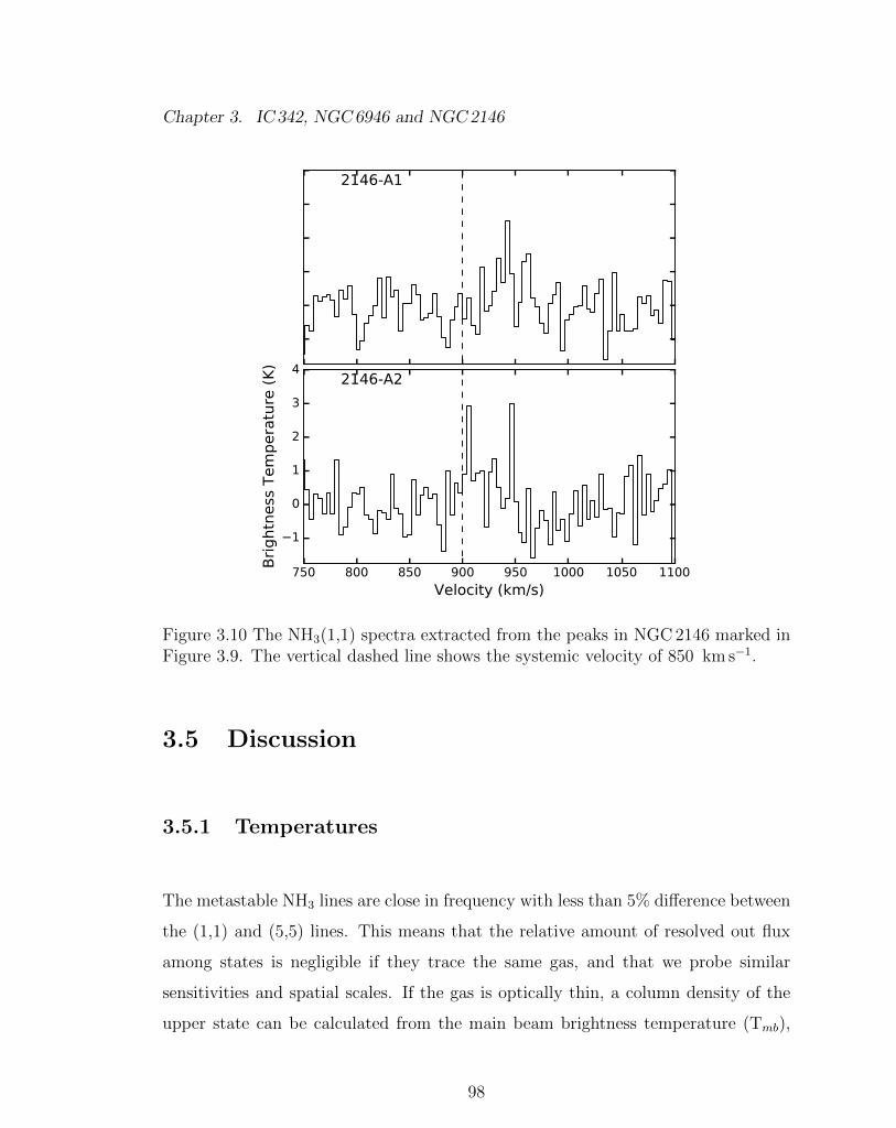
Chapter 3. IC 342, NGC6946 and NGC2146
Figure 3.10 The NH3(1,1) spectra extracted from the peaks in NGC 2146 marked inFigure 3.9. The vertical dashed line shows the systemic velocity of 850 km s�1.
3.5 Discussion
3.5.1 Temperatures
The metastable NH3 lines are close in frequency with less than 5% di↵erence between
the (1,1) and (5,5) lines. This means that the relative amount of resolved out flux
among states is negligible if they trace the same gas, and that we probe similar
sensitivities and spatial scales. If the gas is optically thin, a column density of the
upper state can be calculated from the main beam brightness temperature (Tmb),
98
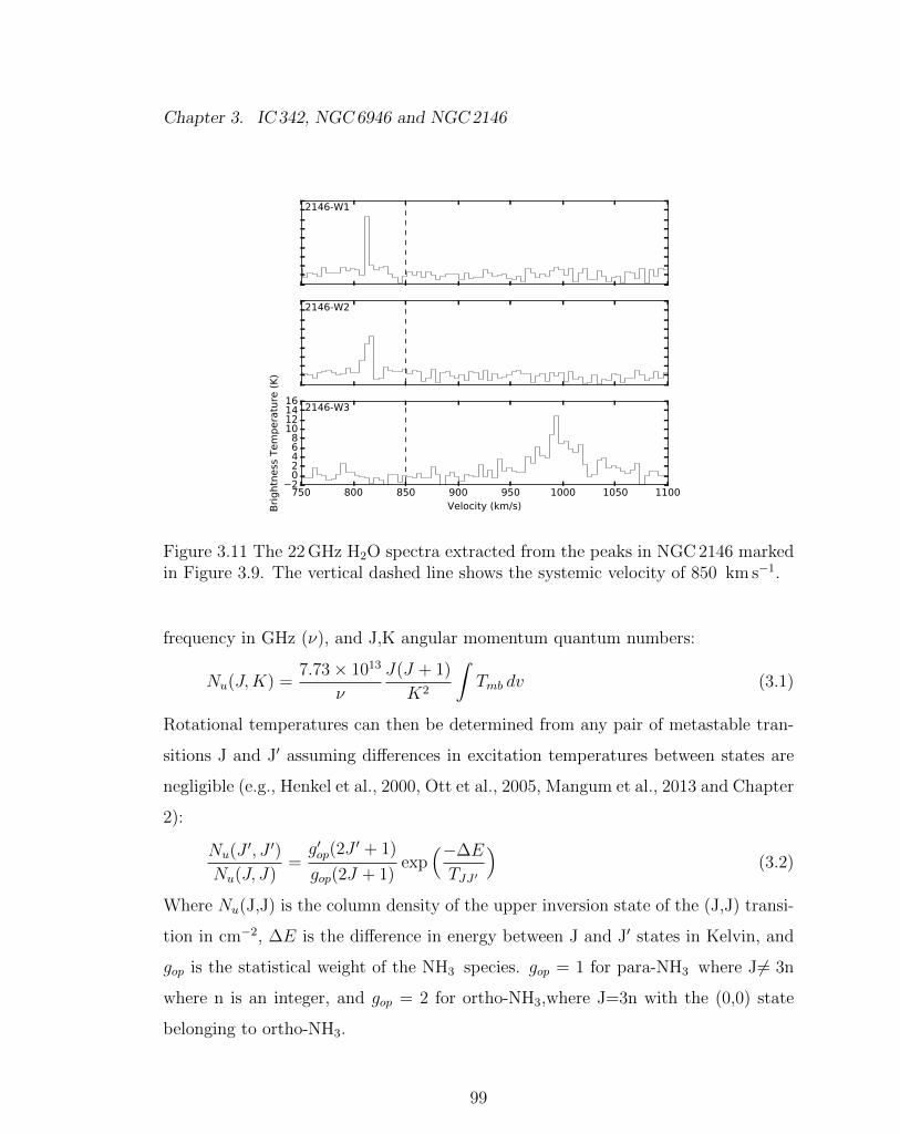
Chapter 3. IC 342, NGC6946 and NGC2146
Figure 3.11 The 22 GHz H2O spectra extracted from the peaks in NGC 2146 markedin Figure 3.9. The vertical dashed line shows the systemic velocity of 850 km s�1.
frequency in GHz (⌫), and J,K angular momentum quantum numbers:
Nu(J, K) =7.73 ⇥ 1013
⌫
J(J + 1)
K
2
ZTmb dv (3.1)
Rotational temperatures can then be determined from any pair of metastable tran-
sitions J and J0 assuming di↵erences in excitation temperatures between states are
negligible (e.g., Henkel et al., 2000, Ott et al., 2005, Mangum et al., 2013 and Chapter
2):
Nu(J 0, J
0)
Nu(J, J)=
g
0op(2J
0 + 1)
gop(2J + 1)exp
⇣��E
TJJ 0
⌘(3.2)
Where Nu(J,J) is the column density of the upper inversion state of the (J,J) transi-
tion in cm�2, �E is the di↵erence in energy between J and J0 states in Kelvin, and
gop is the statistical weight of the NH3 species. gop = 1 for para-NH3 where J6= 3n
where n is an integer, and gop = 2 for ortho-NH3,where J=3n with the (0,0) state
belonging to ortho-NH3.
99
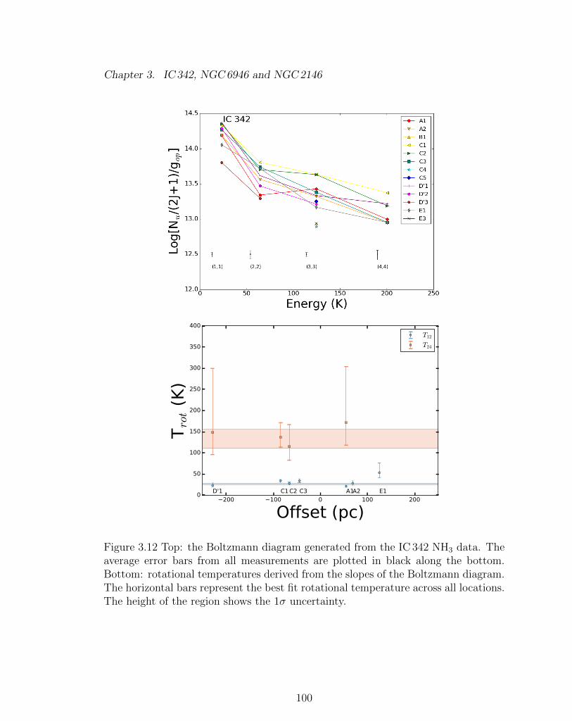
Chapter 3. IC 342, NGC6946 and NGC2146
Figure 3.12 Top: the Boltzmann diagram generated from the IC 342 NH3 data. Theaverage error bars from all measurements are plotted in black along the bottom.Bottom: rotational temperatures derived from the slopes of the Boltzmann diagram.The horizontal bars represent the best fit rotational temperature across all locations.The height of the region shows the 1� uncertainty.
100
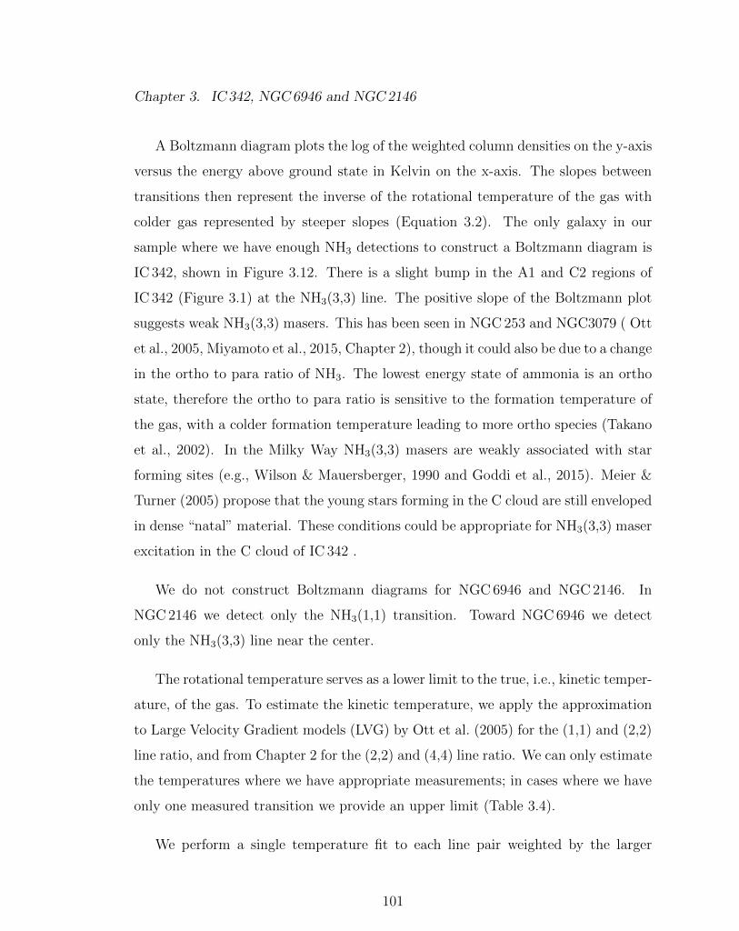
Chapter 3. IC 342, NGC6946 and NGC2146
A Boltzmann diagram plots the log of the weighted column densities on the y-axis
versus the energy above ground state in Kelvin on the x-axis. The slopes between
transitions then represent the inverse of the rotational temperature of the gas with
colder gas represented by steeper slopes (Equation 3.2). The only galaxy in our
sample where we have enough NH3 detections to construct a Boltzmann diagram is
IC 342, shown in Figure 3.12. There is a slight bump in the A1 and C2 regions of
IC 342 (Figure 3.1) at the NH3(3,3) line. The positive slope of the Boltzmann plot
suggests weak NH3(3,3) masers. This has been seen in NGC 253 and NGC3079 ( Ott
et al., 2005, Miyamoto et al., 2015, Chapter 2), though it could also be due to a change
in the ortho to para ratio of NH3. The lowest energy state of ammonia is an ortho
state, therefore the ortho to para ratio is sensitive to the formation temperature of
the gas, with a colder formation temperature leading to more ortho species (Takano
et al., 2002). In the Milky Way NH3(3,3) masers are weakly associated with star
forming sites (e.g., Wilson & Mauersberger, 1990 and Goddi et al., 2015). Meier &
Turner (2005) propose that the young stars forming in the C cloud are still enveloped
in dense “natal” material. These conditions could be appropriate for NH3(3,3) maser
excitation in the C cloud of IC 342 .
We do not construct Boltzmann diagrams for NGC 6946 and NGC 2146. In
NGC 2146 we detect only the NH3(1,1) transition. Toward NGC 6946 we detect
only the NH3(3,3) line near the center.
The rotational temperature serves as a lower limit to the true, i.e., kinetic temper-
ature, of the gas. To estimate the kinetic temperature, we apply the approximation
to Large Velocity Gradient models (LVG) by Ott et al. (2005) for the (1,1) and (2,2)
line ratio, and from Chapter 2 for the (2,2) and (4,4) line ratio. We can only estimate
the temperatures where we have appropriate measurements; in cases where we have
only one measured transition we provide an upper limit (Table 3.4).
We perform a single temperature fit to each line pair weighted by the larger
101
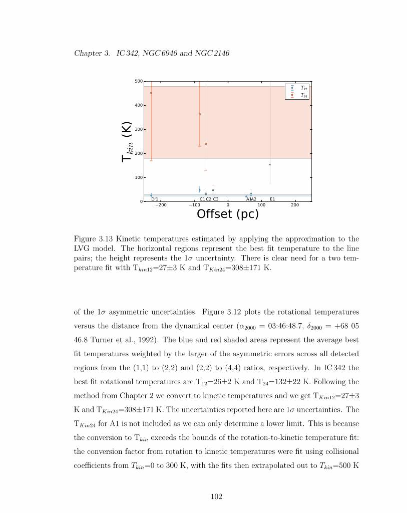
Chapter 3. IC 342, NGC6946 and NGC2146
Figure 3.13 Kinetic temperatures estimated by applying the approximation to theLVG model. The horizontal regions represent the best fit temperature to the linepairs; the height represents the 1� uncertainty. There is clear need for a two tem-perature fit with Tkin12=27±3 K and TKin24=308±171 K.
of the 1� asymmetric uncertainties. Figure 3.12 plots the rotational temperatures
versus the distance from the dynamical center (↵2000 = 03:46:48.7, �2000 = +68 05
46.8 Turner et al., 1992). The blue and red shaded areas represent the average best
fit temperatures weighted by the larger of the asymmetric errors across all detected
regions from the (1,1) to (2,2) and (2,2) to (4,4) ratios, respectively. In IC 342 the
best fit rotational temperatures are T12=26±2 K and T24=132±22 K. Following the
method from Chapter 2 we convert to kinetic temperatures and we get TKin12=27±3
K and TKin24=308±171 K. The uncertainties reported here are 1� uncertainties. The
TKin24 for A1 is not included as we can only determine a lower limit. This is because
the conversion to Tkin exceeds the bounds of the rotation-to-kinetic temperature fit:
the conversion factor from rotation to kinetic temperatures were fit using collisional
coe�cients from Tkin=0 to 300 K, with the fits then extrapolated out to Tkin=500 K
102
Chapter 3. IC 342, NGC6946 and NGC2146
(Ott et al., 2005 and Chapter 2).
Similar to NGC 253 there are two representative temperature components with
1� confidence, and there appears to be no spatial gradient in temperatures across the
central kpc. In Figure 3.13 we plot the kinetic temperatures as a function of o↵set
from the dynamical center. The cool 27 K component is evenly distributed across
the disk. The 308 K component also appears to be uniformly distributed across the
disk, however the large uncertainties may hide a gradient, and in many locations we
do not detect the NH3(4,4) line so the warm component is poorly sampled.
From Meier & Turner (2005) it appears that the A, B, and C clouds are largely
a↵ected by photo dissociation from the nuclear star cluster. A is dominated by PDRs
while B and C are largely a↵ected around the edges. The lack of a temperature
gradient across the C cloud suggests that photon dominated region (PDR) surfaces
do not heat the gas on GMC scales. It is also possible that the NH3 molecule
cannot survive along PDR surfaces as NH3 is photodissociated at ⇠4.1 eV (Suto &
Lee, 1983). This could account for the weaker detections we make towards C4 and
C5 which are ⇠ 30 pc from the dynamical center, while the other brighter emission
regions C1-3 are >10 pc further. To investigate this further we calculate the molecular
abundance of NH3 (NNH3/NH2). We accomplished this by smoothing our ammonia
total flux (moment zero) maps to the resolution of the 12CO(J = 1 ! 0) map
from Levine et al. (1994) (⇠2.700). We only include locations where the NH3(1,1)
line could be reliably detected above 3� (⇠53 K km s�1) in the 2.700 resolution maps.
Then using a Galactic conversion factor from Strong et al. (1988) of Xco=2.3⇥1020
cm�2 (K km s�1)�1 we estimate the column density of H2. The total NH3 column
density is estimated by extrapolating to include the NH3(0,0) state (Ungerechts et
al., 1986). We use the rotational temperature derived earlier of 26 K, and the total
NH3(1,1) column density (not just the upper inversion state) as described in Lebron
et al. (2011). The results are shown in Table 3.5. We do not see evidence for
103
Chapter 3. IC 342, NGC6946 and NGC2146
abundance variations of NH3 as the uncertainty is �35% in all cases, given the rms
of 12.5 km s�1 for the CO map and 17.8 K km s�1 for the NH3(1,1) map.
Meier et al. (2011) analyze the dense gas in IC 342 using HC3N transitions. They
attempt to explain the dense gas conditions with a uniform density and temperature.
These models drastically over-predict the amount of dense gas in IC 342 by 300%-
400% for uniform cold dense gas with Tkin < 30 K. In order to reproduce the observed
masses derived from an optically thin isotopologue of CO, C18O, they invoke a two-
density component model of the gas. For simplicity they assume that Tkin is the
same for both components (30 K). They find that most of the mass is concentrated
in a dense, low filling factor component. They admit that their solution is an over-
simplification. We have measured two temperature components in the center of
IC 342, 27±3 K and 308±171 K with an average, weighted by the average column
densities per location of the NH3(1,1) and NH3(4,4) lines (respectively 1.1⇥1015 cm�2
and 6⇥1014 cm�2), of ⇠129±64 K. This suggests that a dense cold component doesn’t
completely dominate the mass distribution of IC 342.
Compared to NGC 253 (Chapter 2) there appears to be a larger di↵erence between
the cold and warm temperature components in IC 342. The cool gas is cooler (IC 342:
27 K vs. NGC 253: 57 K) and the warm gas is the same temperature within the errors
(IC 342: 308±171 K vs. NGC 253: 134±8 K). This is derived with 1� confidence.
Both galaxies show an even distribution of temperatures across the central kpc.
The kinetic temperatures in NGC 2146 are only upper limits. Using a detection
threshold of 20 K km s�1 for NH3(2,2) line, for the AI cloud we derive an upper
limit of 89 K and for the AII cloud, 23 K. Without detections of the other NH3 lines
we cannot constrain the temperature of the gas any further. There may also be a
warmer component we cannot see. More sensitive observations are necessary in order
to derive temperatures via NH3 thermometry.
104
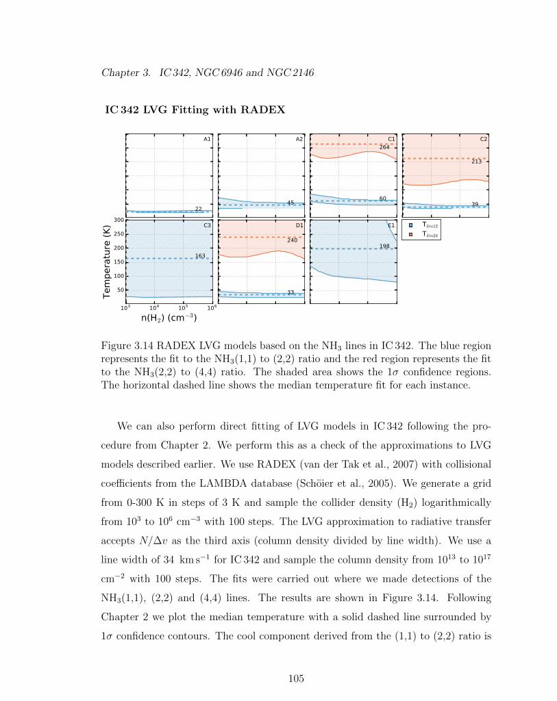
Chapter 3. IC 342, NGC6946 and NGC2146
IC 342 LVG Fitting with RADEX
Figure 3.14 RADEX LVG models based on the NH3 lines in IC 342. The blue regionrepresents the fit to the NH3(1,1) to (2,2) ratio and the red region represents the fitto the NH3(2,2) to (4,4) ratio. The shaded area shows the 1� confidence regions.The horizontal dashed line shows the median temperature fit for each instance.
We can also perform direct fitting of LVG models in IC 342 following the pro-
cedure from Chapter 2. We perform this as a check of the approximations to LVG
models described earlier. We use RADEX (van der Tak et al., 2007) with collisional
coe�cients from the LAMBDA database (Schoier et al., 2005). We generate a grid
from 0-300 K in steps of 3 K and sample the collider density (H2) logarithmically
from 103 to 106 cm�3 with 100 steps. The LVG approximation to radiative transfer
accepts N/�v as the third axis (column density divided by line width). We use a
line width of 34 km s�1 for IC 342 and sample the column density from 1013 to 1017
cm�2 with 100 steps. The fits were carried out where we made detections of the
NH3(1,1), (2,2) and (4,4) lines. The results are shown in Figure 3.14. Following
Chapter 2 we plot the median temperature with a solid dashed line surrounded by
1� confidence contours. The cool component derived from the (1,1) to (2,2) ratio is
105
Chapter 3. IC 342, NGC6946 and NGC2146
shown in blue, and the warm component from the (2,2) to (4,4) line ratio is shown
in red. The fits are unconstrained along the density axis (x-axis) in tune with NH3
not being a good density probe. The fit to the (2,2) to (4,4) ratio is unconstrained
along the temperature axis, therefore we can only provide a lower limit for locations
C2, C3, and D1 of >115 K. The sites C3 and E1 are also unconstrained along the
temperature axis, therefore they are removed from the calculation of the average
temperature from the (1,1) to (2,2) ratio. The average temperature weighted by the
larger of the asymmetric errors is 27±2 K. These results are broadly consistent with
the previous subsection.
3.5.2 H2O Masers
Water masers span a large range of luminosities and can be variable on time scales
of weeks (e.g., Palagi et al., 1993, Claussen et al., 1996 and Braatz et al., 1996).
The water masers in all three galaxies are narrow, single peak spectral features with
FWHM of ⇠10 km s�1. In IC 342 and NGC 6946 the isotropic luminosities of the
masers are of order 0.01 L�. These are likely individual YSO or AGB stars (e.g.,
Palagi et al., 1993). The more luminous of the two masers seen in IC 342 (W1) is
located in the A cloud close to A1 and the other (W2) is located in the B cloud
close to B1. The B cloud is a site of a young star forming region (Meier & Turner,
2005), supporting a possible origin of a YSO. The A cloud is not an active site of
star formation and is dominated by PDRs (Meier & Turner, 2005). Therefore the
W2 maser may be either a stray YSO or an AGB star. Neither of these masers has
been previously observed, though this is likely due to low sensitivity or variability
(⇠10 mJy rms in Tarchi et al., 2002).
In NGC 6946 the maser is located in the southern spiral arm about 350 pc from
the galaxy center. The luminosity is 0.042 L�, which is consistent with stellar maser
106
Chapter 3. IC 342, NGC6946 and NGC2146
rather than kilomaser luminosities. Stellar H2O masers are highly variable (e.g
Claussen et al., 1996) and can be found in nuclear regions and spiral arms of galaxies.
The lack of detections in the center of NGC 6946 is thus unsurprising.
NGC 2146 has the most luminous masers in our sample of galaxies. All three of
these masers have luminosities greater than 0.1 L� classifying them as kilomasers.
Observed in June of 2001, masers W2 and W3 had luminosities of 0.5 L� and 1.5
L� respectively, while W1 was not detected (Tarchi et al., 2002). We observed these
masers in July of 2013. We report isotropic luminosities of 0.455 L� and 2.087 L�
for 2146-W2 and 2146-W3 respectively, an increase of ⇠33% for 2146-W3, whereas
2146-W2 has the same flux as in 2002, but was variable before that (Tarchi et al.,
2002b). We calculate a luminosity of 0.351 L� for 2146-W1. The appearance of
this maser indicates it is variable. Including the masers from NGC 253 (Chapter
2), the galaxies with the most vigorous star formation host the kilomaser class of
H2O masers (253-W1, 2146-W2) while the lower luminosity stellar masers are more
ubiquitous in the SWAN sample (253-W3, IC342-W1 and W2, and 6946-W1).
3.5.3 CH3OH Masers
The 36 GHz CH3OH(414 � 303) maser was first detected in an extragalactic context
by Ellingsen et al. (2014) in NGC 253. These masers were resolved in Chapter 2 and
evidence was given for correlation with weak shocks as the emission is morphologically
similar to HNCO, which is unique compared to other molecular tracers Meier et al.
(2015). We have expanded the set of galaxies with 36 GHz CH3OH masers to include
IC 342 and NGC 6946.
There are six sites with 36 GHz CH3OH emission in IC 342 coincident with the
D’, C and E clouds. The emission is two orders of magnitude less luminous than
the strongest emission found in NGC 253 (Chapter 2). As shown in Figure 3.1,
107
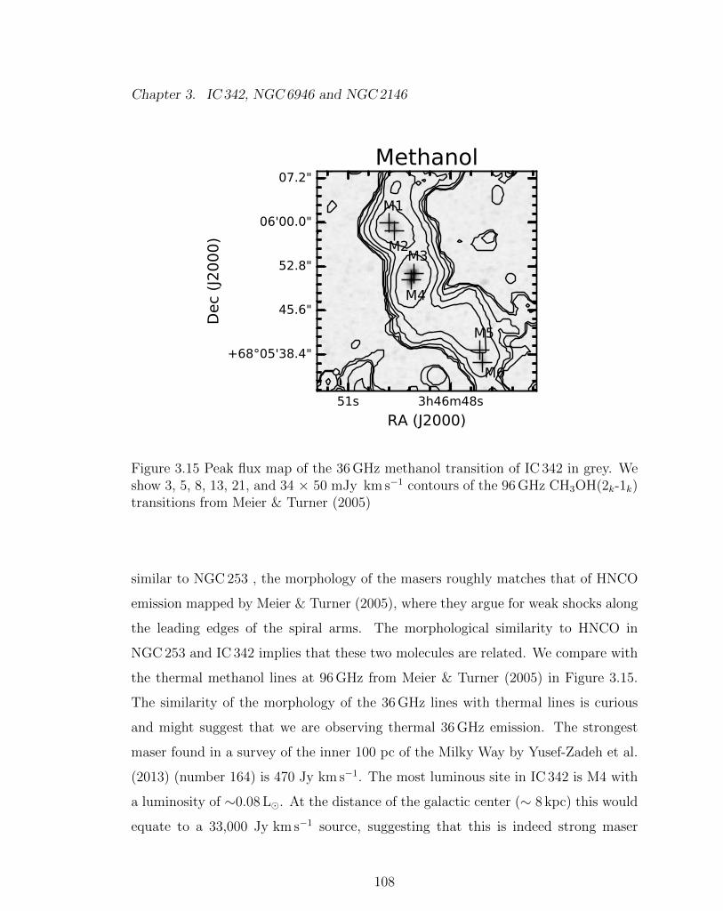
Chapter 3. IC 342, NGC6946 and NGC2146
Figure 3.15 Peak flux map of the 36 GHz methanol transition of IC 342 in grey. Weshow 3, 5, 8, 13, 21, and 34 ⇥ 50 mJy km s�1 contours of the 96 GHz CH3OH(2k-1k)transitions from Meier & Turner (2005)
similar to NGC 253 , the morphology of the masers roughly matches that of HNCO
emission mapped by Meier & Turner (2005), where they argue for weak shocks along
the leading edges of the spiral arms. The morphological similarity to HNCO in
NGC 253 and IC 342 implies that these two molecules are related. We compare with
the thermal methanol lines at 96 GHz from Meier & Turner (2005) in Figure 3.15.
The similarity of the morphology of the 36 GHz lines with thermal lines is curious
and might suggest that we are observing thermal 36 GHz emission. The strongest
maser found in a survey of the inner 100 pc of the Milky Way by Yusef-Zadeh et al.
(2013) (number 164) is 470 Jy km s�1. The most luminous site in IC 342 is M4 with
a luminosity of ⇠0.08 L�. At the distance of the galactic center (⇠ 8 kpc) this would
equate to a 33,000 Jy km s�1 source, suggesting that this is indeed strong maser
108
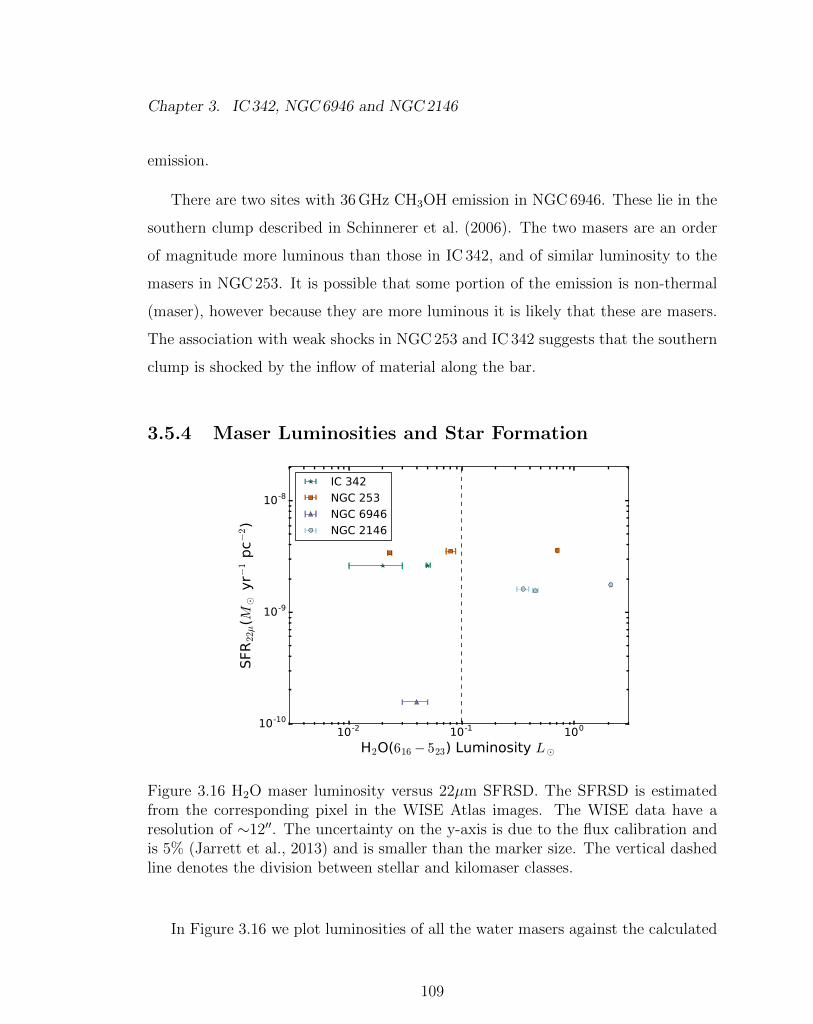
Chapter 3. IC 342, NGC6946 and NGC2146
emission.
There are two sites with 36 GHz CH3OH emission in NGC 6946. These lie in the
southern clump described in Schinnerer et al. (2006). The two masers are an order
of magnitude more luminous than those in IC 342, and of similar luminosity to the
masers in NGC 253. It is possible that some portion of the emission is non-thermal
(maser), however because they are more luminous it is likely that these are masers.
The association with weak shocks in NGC 253 and IC 342 suggests that the southern
clump is shocked by the inflow of material along the bar.
3.5.4 Maser Luminosities and Star Formation
Figure 3.16 H2O maser luminosity versus 22µm SFRSD. The SFRSD is estimatedfrom the corresponding pixel in the WISE Atlas images. The WISE data have aresolution of ⇠1200. The uncertainty on the y-axis is due to the flux calibration andis 5% (Jarrett et al., 2013) and is smaller than the marker size. The vertical dashedline denotes the division between stellar and kilomaser classes.
In Figure 3.16 we plot luminosities of all the water masers against the calculated
109
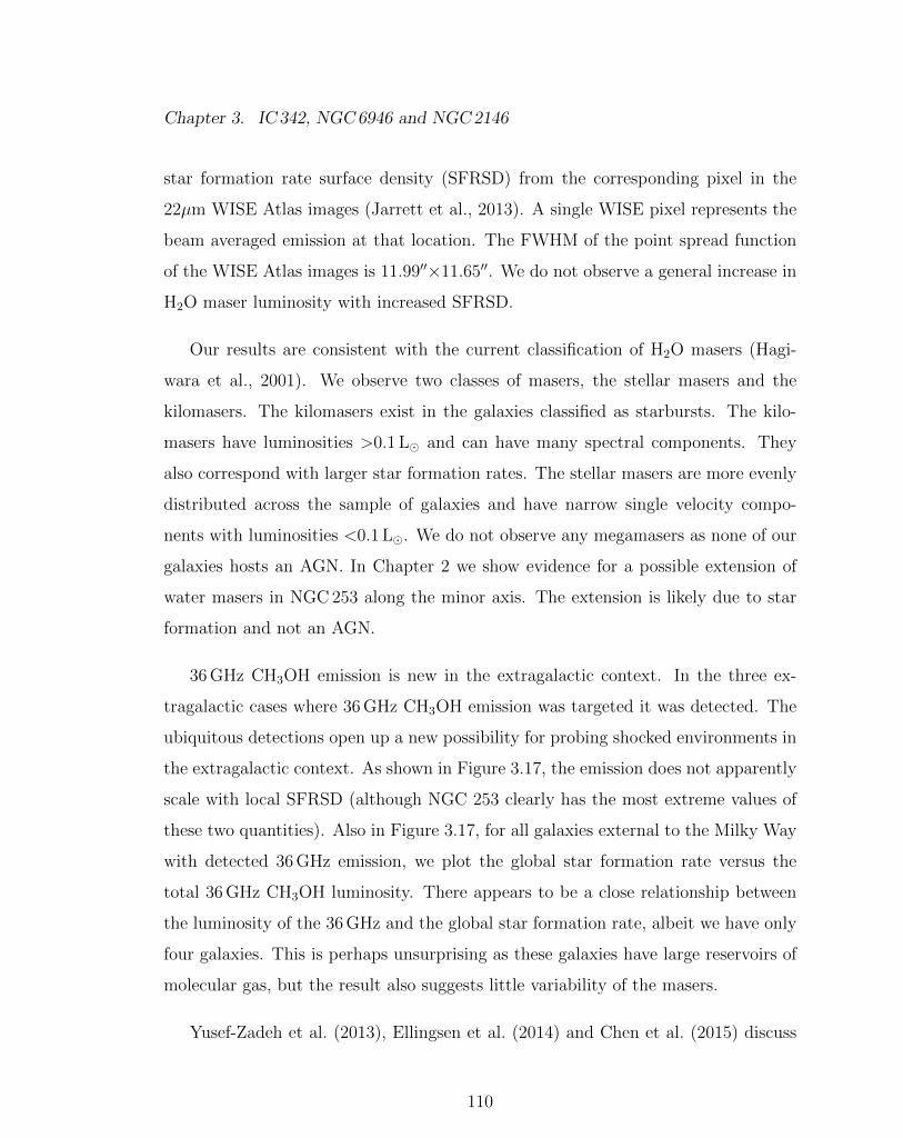
Chapter 3. IC 342, NGC6946 and NGC2146
star formation rate surface density (SFRSD) from the corresponding pixel in the
22µm WISE Atlas images (Jarrett et al., 2013). A single WISE pixel represents the
beam averaged emission at that location. The FWHM of the point spread function
of the WISE Atlas images is 11.9900⇥11.6500. We do not observe a general increase in
H2O maser luminosity with increased SFRSD.
Our results are consistent with the current classification of H2O masers (Hagi-
wara et al., 2001). We observe two classes of masers, the stellar masers and the
kilomasers. The kilomasers exist in the galaxies classified as starbursts. The kilo-
masers have luminosities >0.1 L� and can have many spectral components. They
also correspond with larger star formation rates. The stellar masers are more evenly
distributed across the sample of galaxies and have narrow single velocity compo-
nents with luminosities <0.1 L�. We do not observe any megamasers as none of our
galaxies hosts an AGN. In Chapter 2 we show evidence for a possible extension of
water masers in NGC 253 along the minor axis. The extension is likely due to star
formation and not an AGN.
36 GHz CH3OH emission is new in the extragalactic context. In the three ex-
tragalactic cases where 36 GHz CH3OH emission was targeted it was detected. The
ubiquitous detections open up a new possibility for probing shocked environments in
the extragalactic context. As shown in Figure 3.17, the emission does not apparently
scale with local SFRSD (although NGC 253 clearly has the most extreme values of
these two quantities). Also in Figure 3.17, for all galaxies external to the Milky Way
with detected 36 GHz emission, we plot the global star formation rate versus the
total 36 GHz CH3OH luminosity. There appears to be a close relationship between
the luminosity of the 36 GHz and the global star formation rate, albeit we have only
four galaxies. This is perhaps unsurprising as these galaxies have large reservoirs of
molecular gas, but the result also suggests little variability of the masers.
Yusef-Zadeh et al. (2013), Ellingsen et al. (2014) and Chen et al. (2015) discuss
110
Chapter 3. IC 342, NGC6946 and NGC2146
Figure 3.17 Top: SFRSD versus 22µm total CH3OH maser luminosity, estimatedfrom the corresponding pixel in the WISE Atlas images. The WISE data havea resolution of ⇠1200. The uncertainty on the y-axis is 5% (Jarrett et al., 2013).Bottom: total galactic star formation rate from Gao & Solomon (2004) versus totalCH3OH maser luminosity for all extragalactic sources with 36 GHz CH3OH detectionsto date.
111
Chapter 3. IC 342, NGC6946 and NGC2146
the possibility that cosmic rays release CH3OH into the ISM resulting in higher
abundances towards a galaxy’s center as the cosmic ray density increases; however if
the cosmic ray density is too high CH3OH molecules will be destroyed. Should the
cosmic ray density be highest in the center of galaxies, the concentration of masers
at the edge of the molecular bar in NGC 253 (Ellingsen et al., 2014 and Chapter
2) and IC 342 would be consistent with this idea. However, in Arp 220 Chen et al.
(2015) observe a CH3OH X-ray correlation. They take X-ray emission to reflect the
cosmic ray density. This suggests that methanol is not destroyed in regions where
the cosmic ray density is high. At this point then, this idea is di�cult to test via
extragalactic CH3OH observations.
The similar morphology of the HNCO emission and CH3OH masers in NGC 253
and IC 342 further supports a di↵erent generating mechanism as the HNCO molecule
appears to be anti-correlated with PDRs. Meier & Turner (2005) and Meier et al.
(2015) suggest that weak shocks and/or ice mantel evaporation are related to the
HNCO emission. In IC 342 they suggest the emission is reflective of shocks along the
leading edge of the molecular bar. Because of the morphological similarities between
HNCO and 36 GHz CH3OH, the physical conditions that give rise to emission are
likely related. In Arp220 the CH3OH is correlated with the X-ray plume generated by
a starburst super-wind (Chen et al., 2015). It is possible that the CH3OH is related
to the shocks driven by the wind. In Chapter 2 we suggest the CH3OH masers are
related to shocks in expanding superbubbles. So far, a relationship between 36 GHz
CH3OH emission and with weak shocks would be a more consistent picture across
all galaxies.
It is not yet known what fraction of the emission in these galaxies is thermal
vs. non-thermal (maser). It’s possible there are multiple conditions that give rise
to 36 GHz emission or that separate conditions give rise to thermal versus maser
emission. More in-depth studies are critical to uncover the pumping of the maser
112
Chapter 3. IC 342, NGC6946 and NGC2146
and the nature of the 36 GHz CH3OH line in the extragalactic context.
3.6 Summary
With this chapter we complete the analysis of the H2O, NH3, and CH3OH lines in
the Survey of Water and Ammonia in Nearby galaxies (SWAN). The primary results
are:
1. We have detected metastable NH3 transitions in IC 342, NGC 6946, and NGC
2146. In IC 342 the two molecular spiral arms and the central molecular ring
are traced in NH3(1,1) to (4,4). We make only one detection of the NH3(3,3)
line in NGC 6946 near the center.
2. We detect a uniform 27±3 K dense molecular gas component across the central
kpc of IC 342, and a 308±171 K component, with 1� uncertainties. The direct
LVG models are consistent with our LVG approximation. The temperatures
of the clouds do not appear to be a↵ected by the nuclear PDRs given the
flat temperature distribution across the C cloud. We also provide evidence for
weak NH3(3,3) masers in the A and C clouds. The dense molecular gas in
NGC 2146 must be fairly cold, with T < 89 K, and there is no evidence for a
hot component.
3. Compared to NGC 253, the molecular gas components in IC 342 have a larger
temperature di↵erence, as the cold component is colder. The two temperature
components in both galaxies have flat distributions across their central molec-
ular zones. Individual feedback e↵ects (e.g. supernovae, PDRs, shocks) do not
appear to dominate the distribution of temperatures.
4. We have detected two new stellar H2O masers in IC 342, one in NGC 6946, and
three H2O kilomasers in NGC 2146 of which one was previously undetected.
113
Chapter 3. IC 342, NGC6946 and NGC2146
Across the entire SWAN sample the kilomasers are found in the two starburst
galaxies NGC 253 and NGC 2146, while the lower luminosity stellar masers are
found more uniformly across the sample.
5. We report the first detection of 36 GHz CH3OH in IC 342 and NGC 6946.
This expands the number of galaxies beyond the Milky Way with 36 GHz
CH3OH emission to four including Arp220 (Chen et al., 2015). The morphol-
ogy in IC 342 and NGC 253 is similar to HNCO emission, implying that weak
shocks may pump the maser. It is possible there is a mixture of thermal and
non-thermal (maser) emission that high resolution observations will separate.
The total luminosity of the emission appears to roughly scale with the global
strength of the star formation activity.
3.7 Acknowledgments
Mark Gorski acknowledges support from the National Radio Astronomy Observatory
in the form of a Reber Fellowship, and Student Observer support. This research has
made use of the NASA/IPAC Extragalactic Database (NED), which is maintained
by the Jet Propulsion Laboratory, Caltech, under contract with the National Aero-
nautics and Space Administration (NASA) and NASA’s Astrophysical Data System
Abstract Service (ADS).This research makes use of data products from the Wide-
field Infrared Survey Explorer, which is a joint project of the University of California,
Los Angeles, and the Jet Propulsion Laboratory/California Institute of Technology,
funded by the National Aeronautics and Space Administration.
114
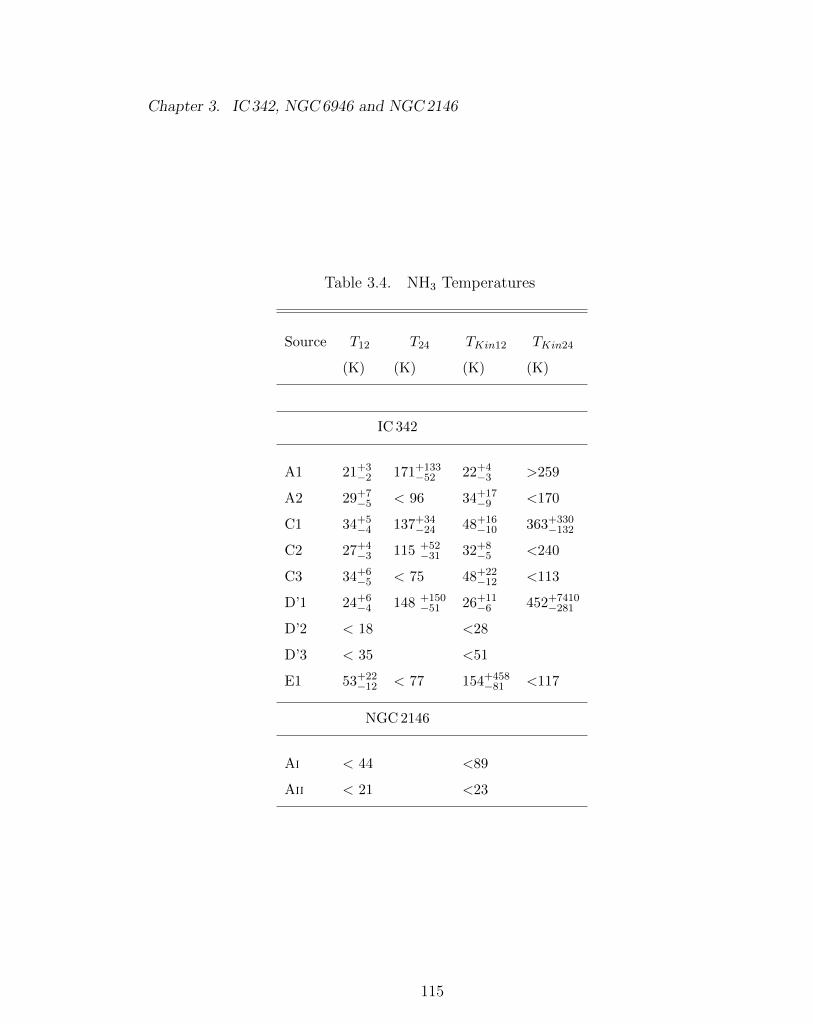
Chapter 3. IC 342, NGC6946 and NGC2146
Table 3.4. NH3 Temperatures
Source T12 T24 TKin12 TKin24
(K) (K) (K) (K)
IC 342
A1 21+3�2 171+133
�52 22+4�3 >259
A2 29+7�5 < 96 34+17
�9 <170
C1 34+5�4 137+34
�24 48+16�10 363+330
�132
C2 27+4�3 115 +52
�31 32+8�5 <240
C3 34+6�5 < 75 48+22
�12 <113
D’1 24+6�4 148 +150
�51 26+11�6 452+7410
�281
D’2 < 18 <28
D’3 < 35 <51
E1 53+22�12 < 77 154+458
�81 <117
NGC2146
AI < 44 <89
AII < 21 <23
115
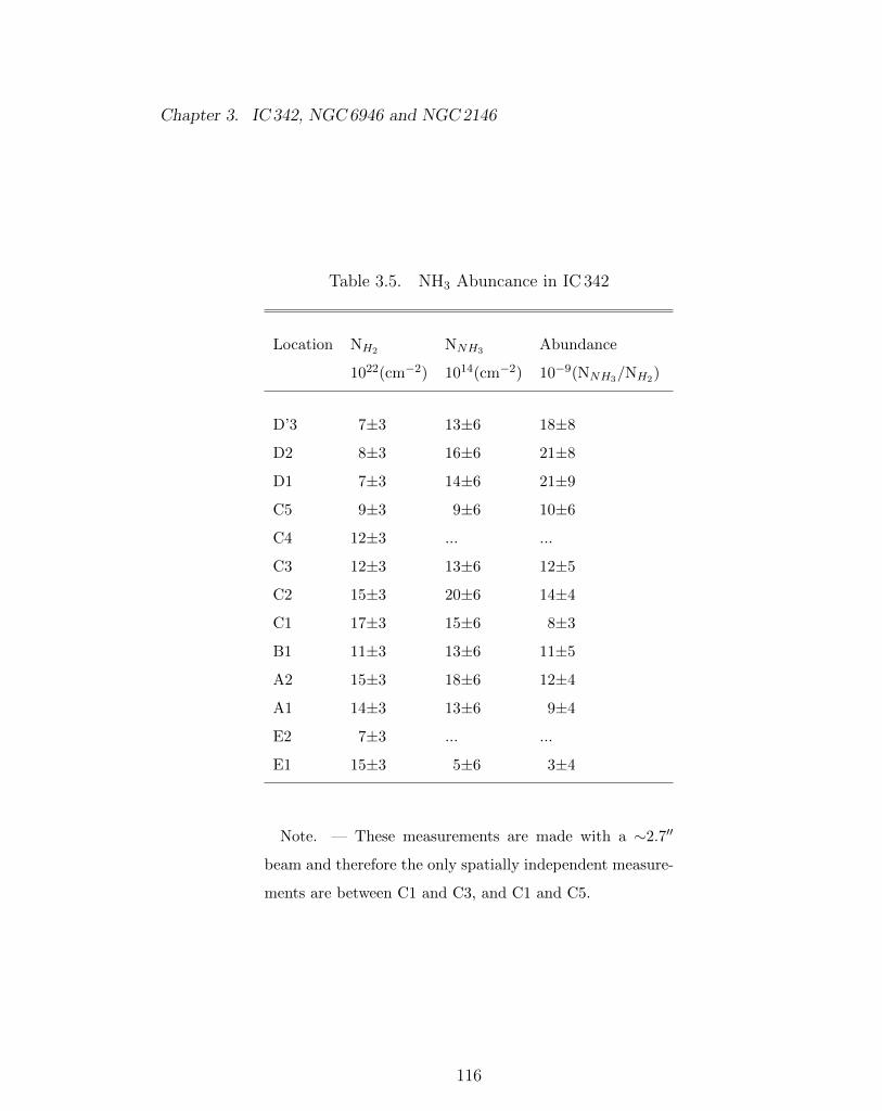
Chapter 3. IC 342, NGC6946 and NGC2146
Table 3.5. NH3 Abuncance in IC 342
Location NH2 NNH3 Abundance
1022(cm�2) 1014(cm�2) 10�9(NNH3/NH2)
D’3 7±3 13±6 18±8
D2 8±3 16±6 21±8
D1 7±3 14±6 21±9
C5 9±3 9±6 10±6
C4 12±3 ... ...
C3 12±3 13±6 12±5
C2 15±3 20±6 14±4
C1 17±3 15±6 8±3
B1 11±3 13±6 11±5
A2 15±3 18±6 12±4
A1 14±3 13±6 9±4
E2 7±3 ... ...
E1 15±3 5±6 3±4
Note. — These measurements are made with a ⇠2.700
beam and therefore the only spatially independent measure-
ments are between C1 and C3, and C1 and C5.
116
Chapter 4
Sub-arcsecond Maser Diagnostics
of NGC 253’s Nuclear Starburst
4.1 Overview
It is necessary to provide observationally motivated descriptions of the connection
between the ISM and star formation because the relationship is responsible for signif-
icant uncertainties in models of galaxy evolution. Specifically, feedback is necessary
to stifle star formation. We can best study this aspect in nearby galaxies such as
NGC 253. This galaxy has a nucleated starburst that is driving a strong ionized and
molecular outflow. To date it is the only extragalactic case known to host water,
ammonia, and 36 GHz methanol masers. The H2O masers have been shown to be
extended along the minor axis of the galaxy in the direction of the outflow. NGC 253
is one of three extragalactic sources with 36 GHz methanol maser detections, and it
is also one of two known extragalactic cases of ammonia masers. Chapter 2 left open
questions about the nature of the emission from these masers that can be addressed
with higher angular resolution. Therefore in this chapter we present analysis of sub-
117
Chapter 4. Sub-arcsecond Maser Diagnostics of NGC 253’s Nuclear Starburst
arcsecond resolution observations of H2O, NH3, and CH3OH masers in the central
500 pc of NGC 253.
4.2 Introduction
In evolutionary models feedback is necessary to impede star formation. This happens
in two ways, by preventing the ISM from accreting i.e., preventative feedback, and
by removing gas from the ISM i.e., ejective feedback (Somerville & Dave, 2015). In
the previous chapters we discussed both aspects of feedback at scales relevant to
GMCs. In this chapter we will discuss ejective feedback on sub-arcsecond scales in
NGC 253.
NGC 253’s outflow is a typical example of ejective feedback. A nuclear starburst
provides an overpressure in the center of the galaxy causing material to be ejected
perpendicular to the disk in an outflow. Strickland et al. (2002) provides four possible
scenarios relating the hot X-ray emitting gas, H↵ emitting cool (104 K) gas, halo gas,
and the disk ISM (Figure 4.1). Model (a) suggests interaction of the hot outflowing
material with cool-ambient halo clouds that are either accreting primordial material,
or cooled ejecta as in the galactic fountain model (Norman & Ikeuchi, 1989). Models
(b) and (c) suggest entrainment of dense gas from the disk. In model (b) the gas
is shocked and entrained. We do not expect to be able to distinguish between (b)
and (c) with maser observations. Last, model (d) shows an interaction with the
thick disk component from Rosen & Bregman (1995), creating a shell of cool and of
shocked material. For each of these scenarios we expect di↵erent maser morphologies
as shown in Figure 4.1. In this chapter we provide initial results regarding sub-
arcsecond imaging of the H2O, NH3, and CH3OH maser emission in the central
500 pc of NGC 253 and the relationship between masers, the outflow and nuclear
starburst. In the astronomical context masers are spectrally narrow point sources.
118
Chapter 4. Sub-arcsecond Maser Diagnostics of NGC 253’s Nuclear Starburst
High spatial resolution is necessary to resolve the maser distribution, and uncover
their relationship with galaxy structures.
In Chapter 2 we show that the H2O maser emission is extended ⇠ 100 pc perpen-
dicular to the major axis of the disk, and the spectrum shows evidence of multiple
H2O masers. There are three masers with velocities 25-109 km s�1, while the sys-
temic velocity of the galaxy is 235 km s�1 (Ott et al., 2005). These maser velocities
are inconsistent with the rotation of the molecular bar. In addition, there are a host
of faint unresolved maser candidates centered around the systemic velocity. Work
by Brunthaler et al. (2009) showed no AGN related component or activity, thus the
H2O masers are likely purely star formation related. With such a large o↵set from
the galaxy’s systemic velocity, Brunthaler et al. (2009) suggest that the dominant
maser component may be associated with the outflow or supernova remnants.
To date, outside of the Milky Way, 36 GHz methanol masers have been detected in
only NGC 253 (Ellingsen et al., 2014), IC 342 (Chapter 3), and Arp 220 (Chen et al.,
2015). Ellingsen et al. (2014) detected two regions where masers exist in NGC 253.
In Chapter 2 we split these two sites into several locations, but each is still spatially
unresolved. We suggest these masers exist where expanding superbubbles, discovered
by Sakamoto et al. (2006), interact with dense gas, in addition they are co-spatial
with the base of the molecular outflow (Bolatto et al., 2013). For comparison, the
most luminous 36 GHz CH3OHmaser in the Milky Way is M1 in GCM0.253+0.016
with a isotropic luminosity of ⇡ 8⇥10�4 L� (Mills et al., 2015). The total integrated
36 GHz CH3OHemission from NGC 253 is ⇠ 20 times more luminous than that from
the Milky Way CMZ (Ellingsen et al., 2014).
There are only two known extragalactic cases of NH3(3,3) masers to date: NGC
253 (Ott et al., 2005) and NGC 3079 (Miyamoto et al., 2015). In both galaxies
the masers are associated with the gas in the nuclear region. The NH3 masers are
identified by NH3(3,3) emission where all other NH3 metastable states are observed
119
Chapter 4. Sub-arcsecond Maser Diagnostics of NGC 253’s Nuclear Starburst
in absorption. It is suggested by Miyamoto et al. (2015) that the masers in NGC 3079
are due to the molecular outflow interacting with ambient molecular gas. In NGC 253
the position of the base of the outflow is likely the location of these masers. The two
velocity components in the spectra shown in Chapter 2 (NH3(3,3)a and NH3(3,3)b
at location C1) would represent gas in the approaching and receding side of the
bar. In the context of the Strickland et al. (2002) models we hypothesize that these
masers exist in the interaction region where the outflow meets the unperturbed disk.
We have marked these regions with circles on the Strickland models (Figure 4.1).
More precise positions will reveal the nature of these masers by probing the shocked
region’s density and kinematics.
In this chapter we discuss sub-arcsecond observations of the NH3(3,3), H2O, and
CH3OH masers in NGC 253. In §4.2 we discuss the observational setup and data
reduction. In §4.3 we show the first results from the observations. In §4.4 we discuss
the properties of the masers and their relationship to models of a starburst driven
outflow. Lastly, in §4.5 we summarize our findings.
4.3 Observations
We observed the 22.2351 GHz H2O maser, the NH3(3,3) maser at 23.8701 GHz, and
the class I 36.1693 GHz methanol maser in NGC 253 with the Karl G. Jansky Very
Large Array in the A configuration (project code: 16B-337). We acquired three hours
on source for the H2O and NH3 masers, and two hours on source for the CH3OH
masers. The total observing time was 13 hours and 43 minutes. The A configuration
of the VLA provides sub-arcsecond resolution, with a maximum baseline of 36.4 km,
suitable for localizing individual maser spots. The correlator was setup with 64 MHz
wide sub-bands centered at 23.849 GHz and 22.216 GHz over the NH3 and H2O maser
lines, and one 128 MHz sub-band centered at 36.131 GHz over the 36 GHz CH3OH
120
Chapter 4. Sub-arcsecond Maser Diagnostics of NGC 253’s Nuclear Starburst
maser. The H2O and NH3 sub-bands were divided into 4096 channels to provide
15.625 kHz (⇠ 0.2 km s�1) spectral resolution. The CH3OH sub-band was divided
into 6144 channels to provide 20.833 kHz (⇠ 0.17 km s�1) spectral resolution. All
velocities will be in the LSRK frame unless stated otherwise. We observed 3C48 as
the flux density calibrator, J2253+1608 as the bandpass calibrator, and J0120-2701
as the complex gain calibrator.
The data were reduced in CASA package 4.7.1 (McMullin et al., 2007). The data
were calibrated using the VLA scripted pipeline version 1.3.9, and then self cali-
brated on the continuum in the line free channels. The image cubes were CLEANed
to 3� rms noise with natural weighting. The NH3 and H2O cubes were gridded with
0.02500 pixels and the CH3OH cube was gridded with 0.01500 pixels. Continuum sub-
traction was performed in the (u, v) domain. The H2O image cubes were rebinned
to 0.5 km s�1 spectral resolution, and the NH3 and CH3OH image cubes were re-
binned to 1.0 km s�1 spectral resolution. The H2O, NH3, and CH3OH cubes have
respective rms noise values of 1.2 mJy beam�1 channel�1, 1.0 mJy beam�1 channel�1,
and 0.9 mJy beam�1 channel�1. The H2O maser image cubes were smoothed to a
common resolution per channel of 0.2300⇥0.1300 (position angle: 20.0�), the NH3 im-
age cubes were smoothed to 0.2100⇥0.1200 (position angle: 20.0�), and for CH3OH,
0.1300⇥0.1300 (position angle: 0.00�). So far we have not imaged the entire primary
beam. It takes several days to create an image cube, so we focused on the regions
where we see emission from Chapter 2. We created three cubes for CH3OH, one
for H2O, and one for NH3 (Figure 4.2). The three methanol cubes cover 1800⇥1800
centered around the two expanding shells seen in Chapter 2 and the galaxy cen-
ter. The phase centers are: RA(J2000): 00h47m33.890s, DEC: -25�17013.35000, RA:
00h47m33.043s DEC: -25�17018.35700, and RA: 00h47m32.090s DEC: -25�17025.57300.
The NH3 and H2O cubes cover 2000⇥2000 centered at RA: 00h47m33.130s, DEC: -
25�17019.60000. There remains the potential for many more interesting results in the
fields that have not yet been imaged.
121
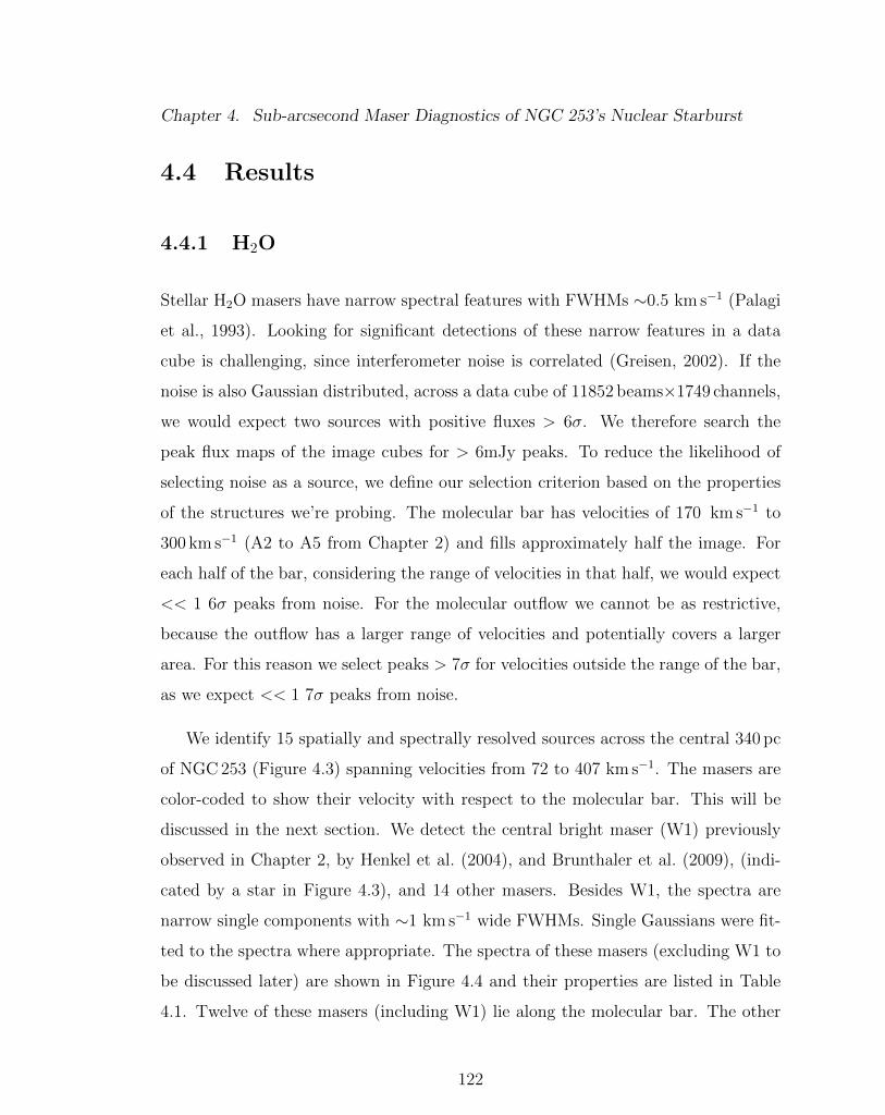
Chapter 4. Sub-arcsecond Maser Diagnostics of NGC 253’s Nuclear Starburst
4.4 Results
4.4.1 H2O
Stellar H2O masers have narrow spectral features with FWHMs ⇠0.5 km s�1 (Palagi
et al., 1993). Looking for significant detections of these narrow features in a data
cube is challenging, since interferometer noise is correlated (Greisen, 2002). If the
noise is also Gaussian distributed, across a data cube of 11852 beams⇥1749 channels,
we would expect two sources with positive fluxes > 6�. We therefore search the
peak flux maps of the image cubes for > 6mJy peaks. To reduce the likelihood of
selecting noise as a source, we define our selection criterion based on the properties
of the structures we’re probing. The molecular bar has velocities of 170 km s�1 to
300 km s�1 (A2 to A5 from Chapter 2) and fills approximately half the image. For
each half of the bar, considering the range of velocities in that half, we would expect
<< 1 6� peaks from noise. For the molecular outflow we cannot be as restrictive,
because the outflow has a larger range of velocities and potentially covers a larger
area. For this reason we select peaks > 7� for velocities outside the range of the bar,
as we expect << 1 7� peaks from noise.
We identify 15 spatially and spectrally resolved sources across the central 340 pc
of NGC 253 (Figure 4.3) spanning velocities from 72 to 407 km s�1. The masers are
color-coded to show their velocity with respect to the molecular bar. This will be
discussed in the next section. We detect the central bright maser (W1) previously
observed in Chapter 2, by Henkel et al. (2004), and Brunthaler et al. (2009), (indi-
cated by a star in Figure 4.3), and 14 other masers. Besides W1, the spectra are
narrow single components with ⇠1 km s�1 wide FWHMs. Single Gaussians were fit-
ted to the spectra where appropriate. The spectra of these masers (excluding W1 to
be discussed later) are shown in Figure 4.4 and their properties are listed in Table
4.1. Twelve of these masers (including W1) lie along the molecular bar. The other
122
Chapter 4. Sub-arcsecond Maser Diagnostics of NGC 253’s Nuclear Starburst
three are positioned a few 10’s of pc perpendicular to the major axis of the galaxy.
The W1 maser is the strongest source in our observations. It shows as many as 5
distinct velocity components (Figure 4.5).
123
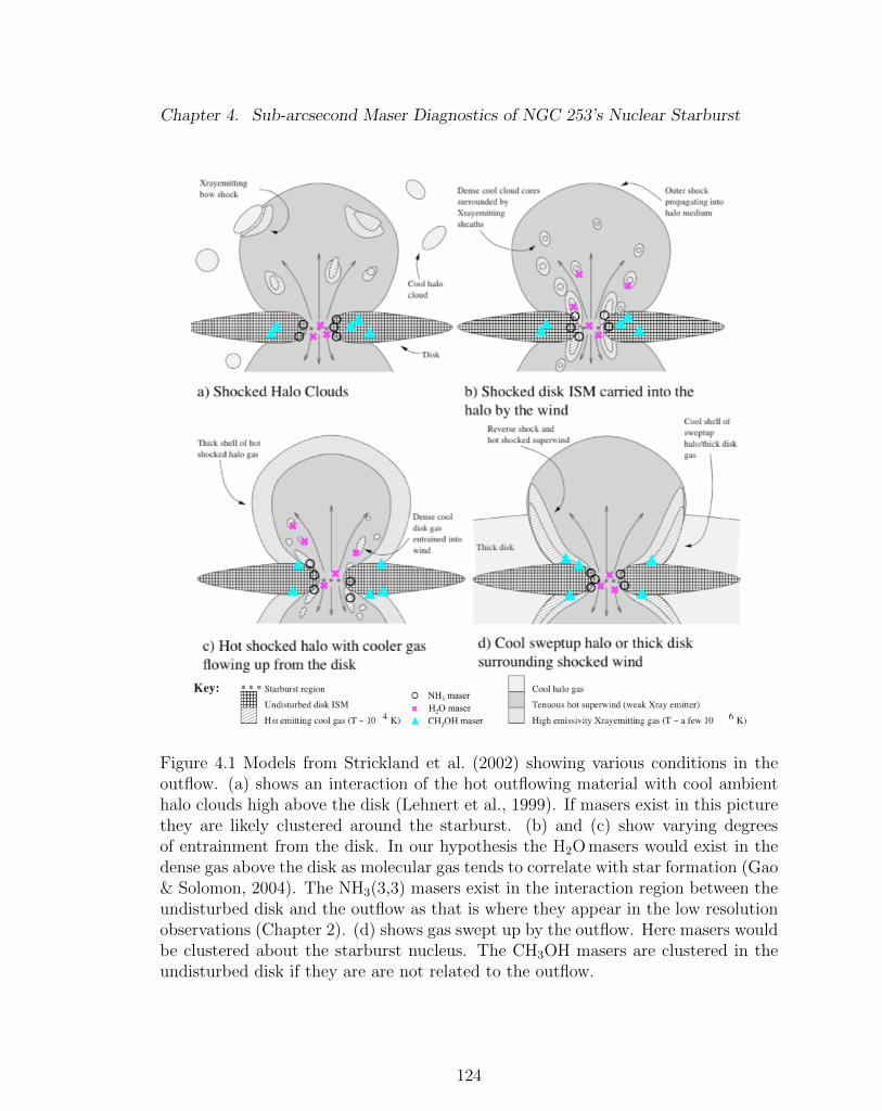
Chapter 4. Sub-arcsecond Maser Diagnostics of NGC 253’s Nuclear Starburst
Figure 4.1 Models from Strickland et al. (2002) showing various conditions in theoutflow. (a) shows an interaction of the hot outflowing material with cool ambienthalo clouds high above the disk (Lehnert et al., 1999). If masers exist in this picturethey are likely clustered around the starburst. (b) and (c) show varying degreesof entrainment from the disk. In our hypothesis the H2O masers would exist in thedense gas above the disk as molecular gas tends to correlate with star formation (Gao& Solomon, 2004). The NH3(3,3) masers exist in the interaction region between theundisturbed disk and the outflow as that is where they appear in the low resolutionobservations (Chapter 2). (d) shows gas swept up by the outflow. Here masers wouldbe clustered about the starburst nucleus. The CH3OH masers are clustered in theundisturbed disk if they are are not related to the outflow.
124
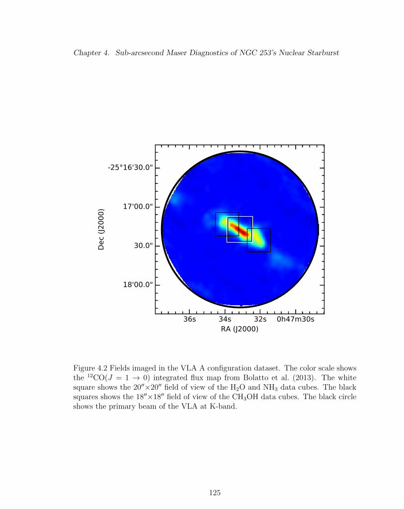
Chapter 4. Sub-arcsecond Maser Diagnostics of NGC 253’s Nuclear Starburst
Figure 4.2 Fields imaged in the VLA A configuration dataset. The color scale showsthe 12CO(J = 1 ! 0) integrated flux map from Bolatto et al. (2013). The whitesquare shows the 2000⇥2000 field of view of the H2O and NH3 data cubes. The blacksquares shows the 1800⇥1800 field of view of the CH3OH data cubes. The black circleshows the primary beam of the VLA at K-band.
125
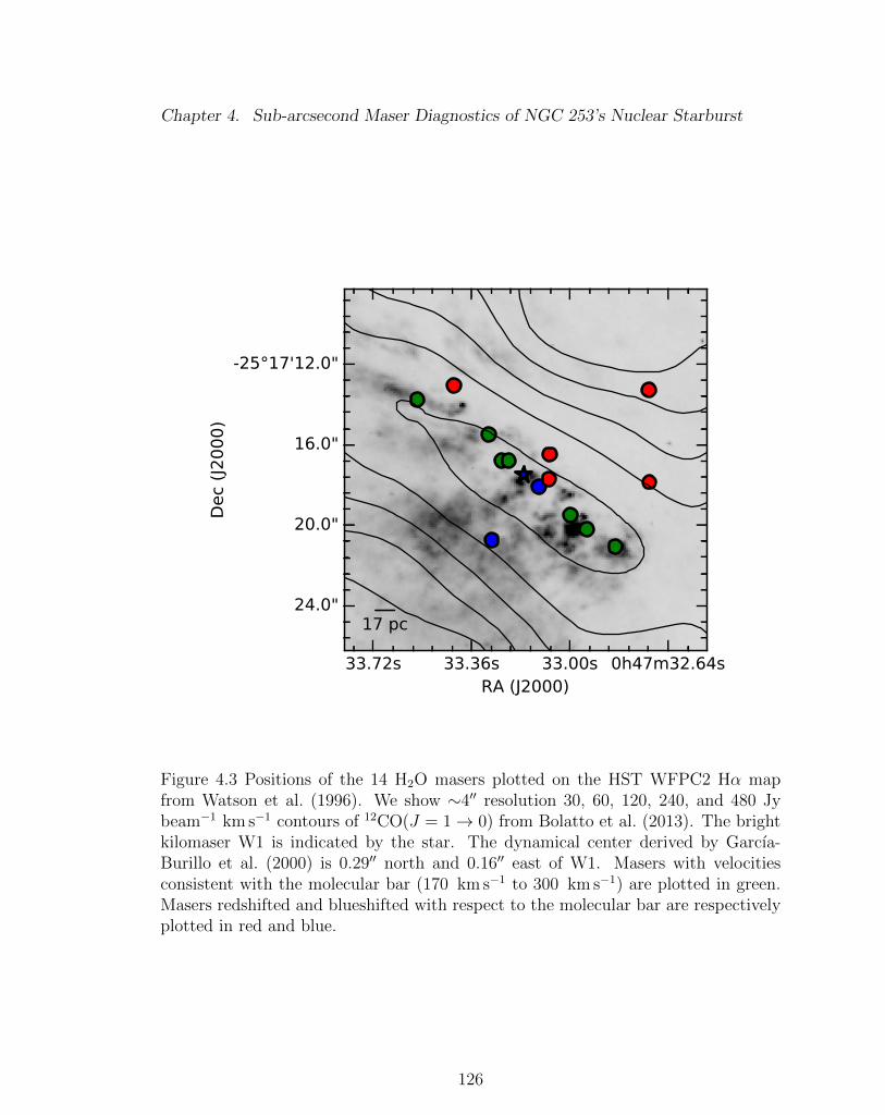
Chapter 4. Sub-arcsecond Maser Diagnostics of NGC 253’s Nuclear Starburst
Figure 4.3 Positions of the 14 H2O masers plotted on the HST WFPC2 H↵ mapfrom Watson et al. (1996). We show ⇠400 resolution 30, 60, 120, 240, and 480 Jybeam�1 km s�1 contours of 12CO(J = 1 ! 0) from Bolatto et al. (2013). The brightkilomaser W1 is indicated by the star. The dynamical center derived by Garcıa-Burillo et al. (2000) is 0.2900 north and 0.1600 east of W1. Masers with velocitiesconsistent with the molecular bar (170 km s�1 to 300 km s�1) are plotted in green.Masers redshifted and blueshifted with respect to the molecular bar are respectivelyplotted in red and blue.
126
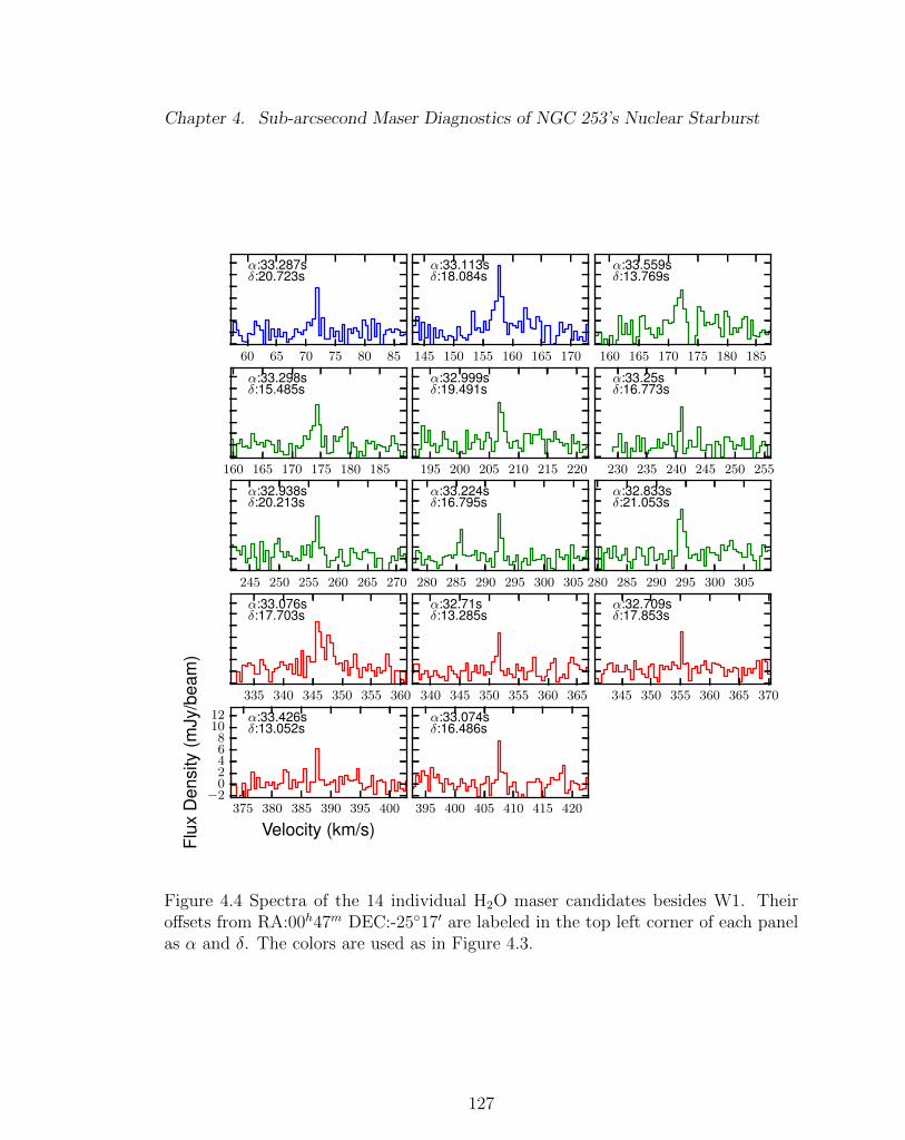
Chapter 4. Sub-arcsecond Maser Diagnostics of NGC 253’s Nuclear Starburst
60 65 70 75 80 85
�:33.287s�:20.723s
145 150 155 160 165 170
�:33.113s�:18.084s
160 165 170 175 180 185
�:33.559s�:13.769s
160 165 170 175 180 185
�:33.298s�:15.485s
195 200 205 210 215 220
�:32.999s�:19.491s
230 235 240 245 250 255
�:33.25s�:16.773s
245 250 255 260 265 270
�:32.938s�:20.213s
280 285 290 295 300 305
�:33.224s�:16.795s
280 285 290 295 300 305
�:32.833s�:21.053s
335 340 345 350 355 360
�:33.076s�:17.703s
340 345 350 355 360 365
�:32.71s�:13.285s
345 350 355 360 365 370
�:32.709s�:17.853s
375 380 385 390 395 400
Velocity (km/s)
�202468
1012
Flux
Den
sity
(mJy
/bea
m)
�:33.426s�:13.052s
395 400 405 410 415 420
�:33.074s�:16.486s
Figure 4.4 Spectra of the 14 individual H2O maser candidates besides W1. Theiro↵sets from RA:00h47m DEC:-25�170 are labeled in the top left corner of each panelas ↵ and �. The colors are used as in Figure 4.3.
127
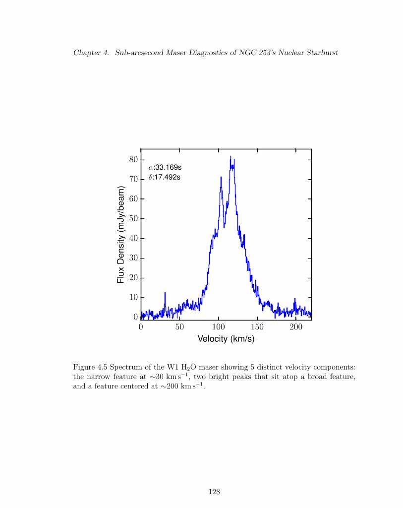
Chapter 4. Sub-arcsecond Maser Diagnostics of NGC 253’s Nuclear Starburst
0 50 100 150 200
Velocity (km/s)
0
10
20
30
40
50
60
70
80
Flux
Den
sity
(mJy
/bea
m)
↵:33.169s�:17.492s
Figure 4.5 Spectrum of the W1 H2O maser showing 5 distinct velocity components:the narrow feature at ⇠30 km s�1, two bright peaks that sit atop a broad feature,and a feature centered at ⇠200 km s�1.
128
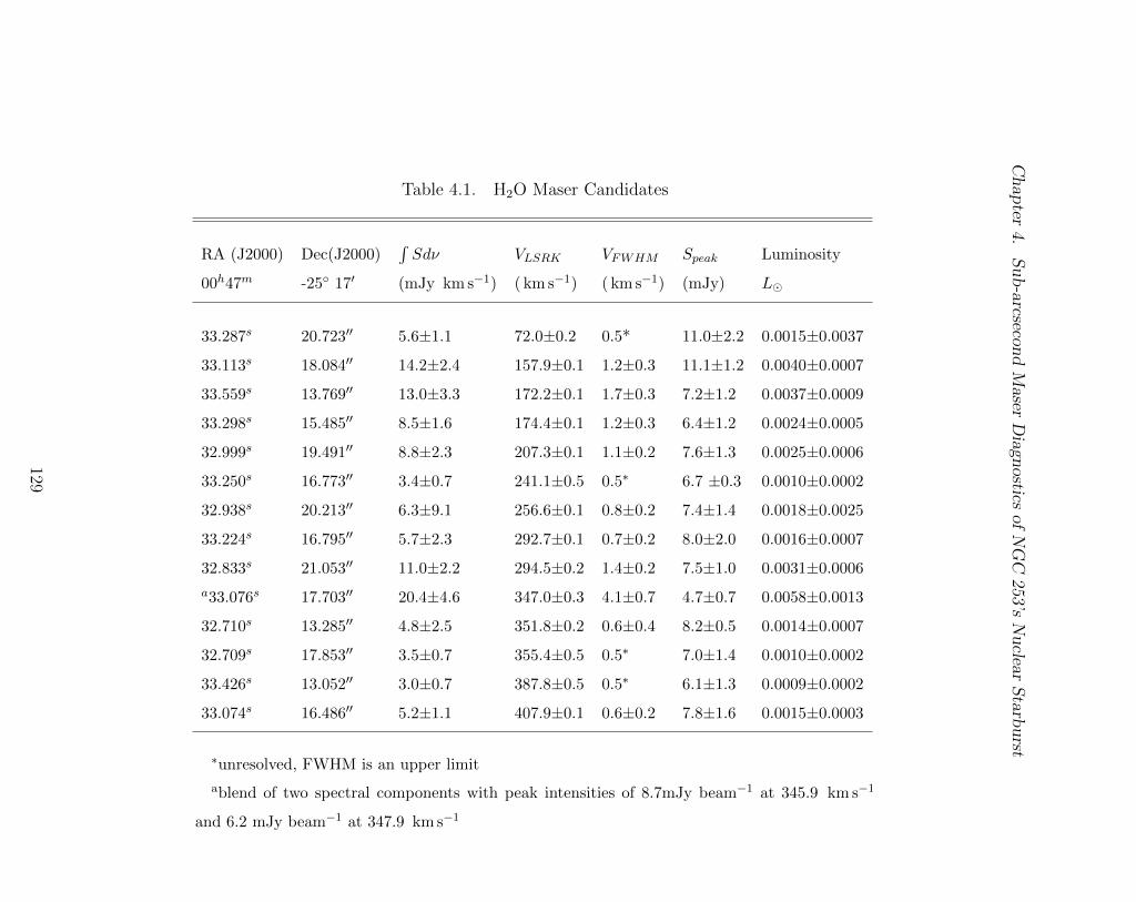
Chapter4.
Sub-arcsecondMaserDiagnosticsofNGC
253’sNuclearStarburst
Table 4.1. H2O Maser Candidates
RA (J2000) Dec(J2000)R
Sd⌫ VLSRK VFWHM Speak Luminosity
00h47m -25� 170 (mJy km s�1) ( km s�1) ( km s�1) (mJy) L�
33.287s 20.72300 5.6±1.1 72.0±0.2 0.5* 11.0±2.2 0.0015±0.0037
33.113s 18.08400 14.2±2.4 157.9±0.1 1.2±0.3 11.1±1.2 0.0040±0.0007
33.559s 13.76900 13.0±3.3 172.2±0.1 1.7±0.3 7.2±1.2 0.0037±0.0009
33.298s 15.48500 8.5±1.6 174.4±0.1 1.2±0.3 6.4±1.2 0.0024±0.0005
32.999s 19.49100 8.8±2.3 207.3±0.1 1.1±0.2 7.6±1.3 0.0025±0.0006
33.250s 16.77300 3.4±0.7 241.1±0.5 0.5⇤ 6.7 ±0.3 0.0010±0.0002
32.938s 20.21300 6.3±9.1 256.6±0.1 0.8±0.2 7.4±1.4 0.0018±0.0025
33.224s 16.79500 5.7±2.3 292.7±0.1 0.7±0.2 8.0±2.0 0.0016±0.0007
32.833s 21.05300 11.0±2.2 294.5±0.2 1.4±0.2 7.5±1.0 0.0031±0.0006
a33.076s 17.70300 20.4±4.6 347.0±0.3 4.1±0.7 4.7±0.7 0.0058±0.0013
32.710s 13.28500 4.8±2.5 351.8±0.2 0.6±0.4 8.2±0.5 0.0014±0.0007
32.709s 17.85300 3.5±0.7 355.4±0.5 0.5⇤ 7.0±1.4 0.0010±0.0002
33.426s 13.05200 3.0±0.7 387.8±0.5 0.5⇤ 6.1±1.3 0.0009±0.0002
33.074s 16.48600 5.2±1.1 407.9±0.1 0.6±0.2 7.8±1.6 0.0015±0.0003
⇤unresolved, FWHM is an upper limit
ablend of two spectral components with peak intensities of 8.7mJy beam�1 at 345.9 km s�1
and 6.2 mJy beam�1 at 347.9 km s�1
129
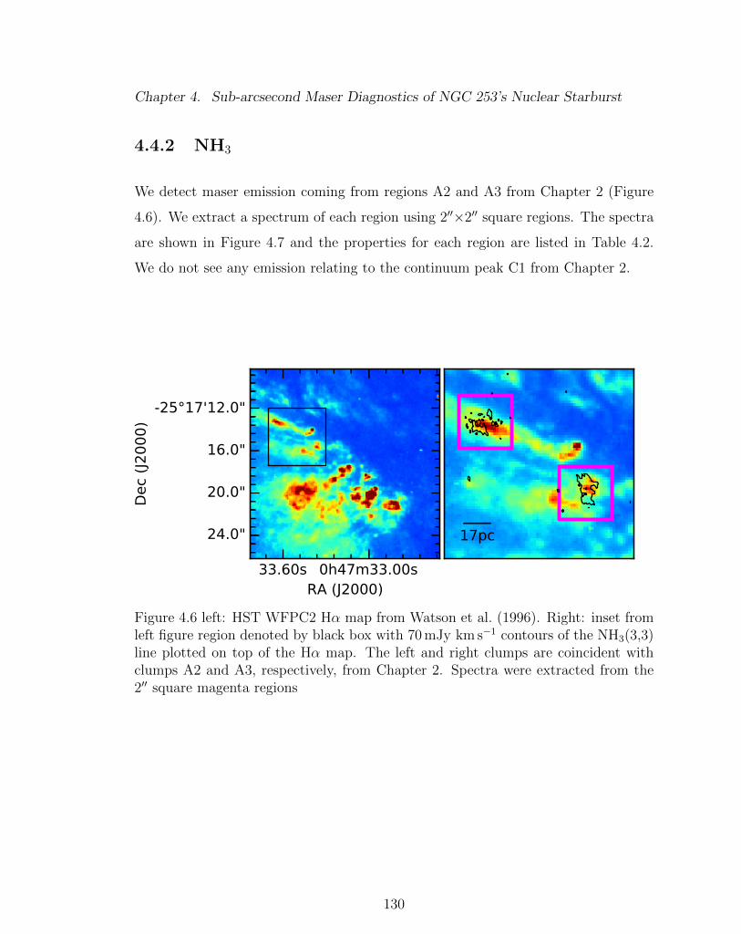
Chapter 4. Sub-arcsecond Maser Diagnostics of NGC 253’s Nuclear Starburst
4.4.2 NH3
We detect maser emission coming from regions A2 and A3 from Chapter 2 (Figure
4.6). We extract a spectrum of each region using 200⇥200 square regions. The spectra
are shown in Figure 4.7 and the properties for each region are listed in Table 4.2.
We do not see any emission relating to the continuum peak C1 from Chapter 2.
Figure 4.6 left: HST WFPC2 H↵ map from Watson et al. (1996). Right: inset fromleft figure region denoted by black box with 70 mJy km s�1 contours of the NH3(3,3)line plotted on top of the H↵ map. The left and right clumps are coincident withclumps A2 and A3, respectively, from Chapter 2. Spectra were extracted from the200 square magenta regions
130
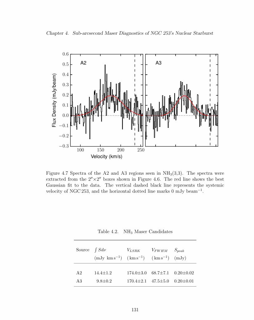
Chapter 4. Sub-arcsecond Maser Diagnostics of NGC 253’s Nuclear Starburst
100 150 200 250
Velocity (km/s)
�0.3
�0.2
�0.1
0.0
0.1
0.2
0.3
0.4
0.5
0.6Fl
uxD
ensi
ty(m
Jy/b
eam
)
A2 A3
Figure 4.7 Spectra of the A2 and A3 regions seen in NH3(3,3). The spectra wereextracted from the 200⇥200 boxes shown in Figure 4.6. The red line shows the bestGaussian fit to the data. The vertical dashed black line represents the systemicvelocity of NGC 253, and the horizontal dotted line marks 0 mJy beam�1.
Table 4.2. NH3 Maser Candidates
SourceR
Sd⌫ VLSRK VFWHM Speak
(mJy km s�1) ( km s�1) ( km s�1) (mJy)
A2 14.4±1.2 174.0±3.0 68.7±7.1 0.20±0.02
A3 9.8±0.2 170.4±2.1 47.5±5.0 0.20±0.01
131
Chapter 4. Sub-arcsecond Maser Diagnostics of NGC 253’s Nuclear Starburst
4.4.3 CH3OH
The first extragalactic 36 GHz CH3OH masers were seen by Ellingsen et al. (2014) in
NGC 253. They detected two sources with a spatial resolution of 8.000⇥4.200 using the
Australia Telescope Compact Array (ATCA)1. In Chapter 2 we resolved these sources
into five di↵erent sources with a 600⇥400 beam using the VLA. Since then, extragalactic
36 GHz CH3OH masers have been observed in IC 342, NGC 6946 (Chapter 3) and in
Arp 220 (Chen et al., 2015).
We detect nine 36 GHz CH3OH masers. We show the locations of the masers in
Figure 4.8. They are concentrated in and around sources M3 and M5 from Chapter
2. Spectra are extracted from the points shown in Figure 4.8 and the spectra are
shown in Figure 4.9. The extracted properties of the masers are shown in Table 4.3.
Six of the masers have FWHMs >10 km s�1 where the other three are narrow with
FWHMs of ⇠1 km s�1.
1The Australia Telescope Compact Array is part of the Australia Telescope, which isfunded by the Commonwealth of Australia for operation as a National Facility managedby CSIRO.
132
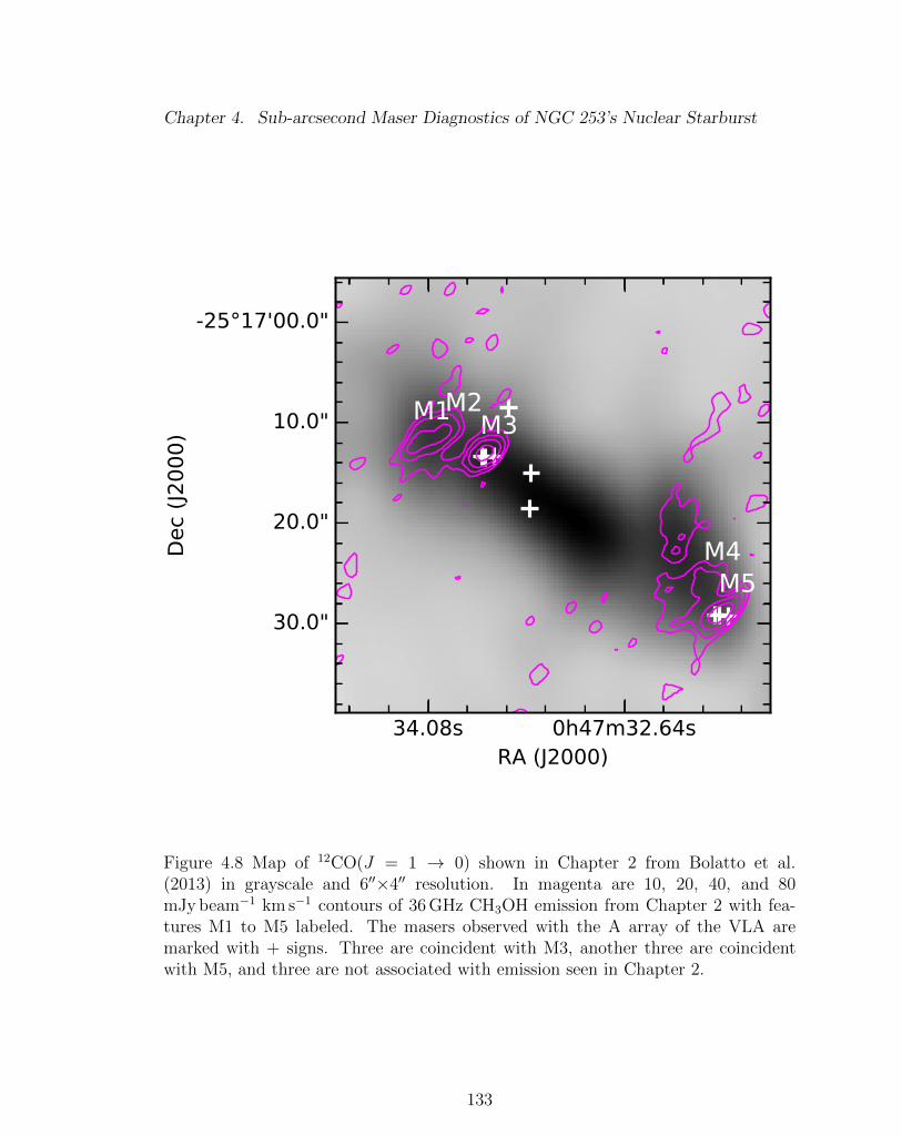
Chapter 4. Sub-arcsecond Maser Diagnostics of NGC 253’s Nuclear Starburst
Figure 4.8 Map of 12CO(J = 1 ! 0) shown in Chapter 2 from Bolatto et al.(2013) in grayscale and 600⇥400 resolution. In magenta are 10, 20, 40, and 80mJy beam�1 km s�1 contours of 36 GHz CH3OH emission from Chapter 2 with fea-tures M1 to M5 labeled. The masers observed with the A array of the VLA aremarked with + signs. Three are coincident with M3, another three are coincidentwith M5, and three are not associated with emission seen in Chapter 2.
133
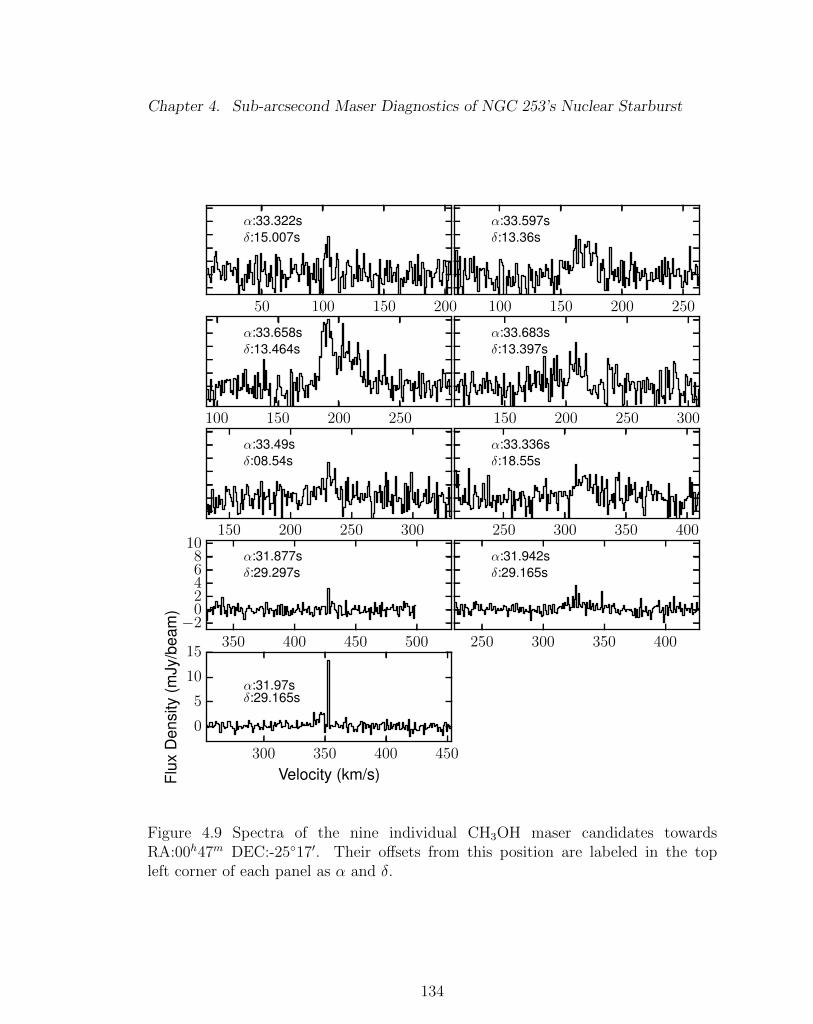
Chapter 4. Sub-arcsecond Maser Diagnostics of NGC 253’s Nuclear Starburst
50 100 150 200
↵:33.322s�:15.007s
100 150 200 250
↵:33.597s�:13.36s
100 150 200 250
↵:33.658s�:13.464s
150 200 250 300
↵:33.683s�:13.397s
150 200 250 300
↵:33.49s�:08.54s
250 300 350 400
↵:33.336s�:18.55s
350 400 450 500�2
02468
10↵:31.877s�:29.297s
250 300 350 400
↵:31.942s�:29.165s
300 350 400 450
Velocity (km/s)
0
5
10
15
Flux
Den
sity
(mJy
/bea
m)
↵:31.97s�:29.165s
Figure 4.9 Spectra of the nine individual CH3OH maser candidates towardsRA:00h47m DEC:-25�170. Their o↵sets from this position are labeled in the topleft corner of each panel as ↵ and �.
134
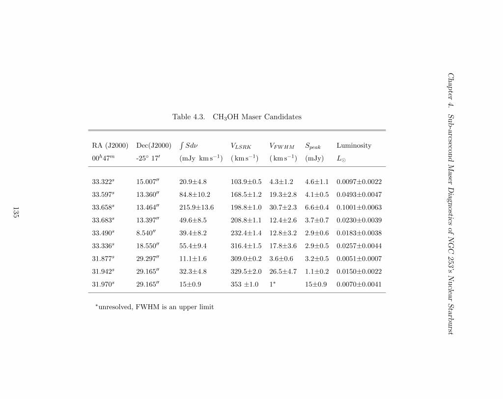
Chapter4.
Sub-arcsecondMaserDiagnosticsofNGC
253’sNuclearStarburst
Table 4.3. CH3OH Maser Candidates
RA (J2000) Dec(J2000)R
Sd⌫ VLSRK VFWHM Speak Luminosity
00h47m -25� 170 (mJy km s�1) ( km s�1) ( km s�1) (mJy) L�
33.322s 15.00700 20.9±4.8 103.9±0.5 4.3±1.2 4.6±1.1 0.0097±0.0022
33.597s 13.36000 84.8±10.2 168.5±1.2 19.3±2.8 4.1±0.5 0.0493±0.0047
33.658s 13.46400 215.9±13.6 198.8±1.0 30.7±2.3 6.6±0.4 0.1001±0.0063
33.683s 13.39700 49.6±8.5 208.8±1.1 12.4±2.6 3.7±0.7 0.0230±0.0039
33.490s 8.54000 39.4±8.2 232.4±1.4 12.8±3.2 2.9±0.6 0.0183±0.0038
33.336s 18.55000 55.4±9.4 316.4±1.5 17.8±3.6 2.9±0.5 0.0257±0.0044
31.877s 29.29700 11.1±1.6 309.0±0.2 3.6±0.6 3.2±0.5 0.0051±0.0007
31.942s 29.16500 32.3±4.8 329.5±2.0 26.5±4.7 1.1±0.2 0.0150±0.0022
31.970s 29.16500 15±0.9 353 ±1.0 1⇤ 15±0.9 0.0070±0.0041
⇤unresolved, FWHM is an upper limit
135
Chapter 4. Sub-arcsecond Maser Diagnostics of NGC 253’s Nuclear Starburst
4.5 Discussion
Strickland et al. (2002) provides four possible models to explain the relationship be-
tween outflows and nuclear starbursts (Figure 4.1). Here we will use our observations
of masers to better constrain the models. The models predict various degrees of en-
trainment of molecular gas and interactions between the hot outflowing material and
cooler ambient ISM. Scenario (a) shows only interactions between infalling cool halo
clouds suggesting no entrainment of the dense ISM from the disk, scenarios (b) and
(c) show varying degrees of entrainment of the dense ISM in the outflow, and (d)
shows radially pushed out, or swept up, dense gas at the edges of the outflow, as the
dense ISM collimates the outflow out of the disk. Here we will attempt to unify our
observations of masers with these pictures of the outflow.
4.5.1 H2O
We detect 14 H2O masers in the central 300 pc of NGC 253. All but one of these
masers (W1 from Chapter 2 or Brunthaler et al., 2009) have luminosities < 0.1 L�.
Their line widths are narrow, with VFWHM ⇠1 km s�1 making them all consistent
with stellar class AGB or YSO masers (Palagi et al., 1993). In Chapter 2 we showed
evidence for a H2O maser extension along the minor axis of the galaxy suggesting
either an AGN jet or entrainment of star forming material. We see no evidence for
an AGN, as we do not see a long jet-like structure and the nuclear maser W1 is
not luminous enough to be a megamaser (measured in Chapter 2). However, three
of our stellar H2O masers are not spatially coincident with the molecular bar (Fig-
ure 4.3). These masers have peculiarly high velocities for being associated with the
molecular bar. The molecular regions closest to the center have velocities spanning
⇠ 170 km s�1 to ⇠ 300 km s�1 (A3 and A5 from Chapter 2). Seven stellar masers
have velocities exceeding this range with extremes at 72 km s�1 and 406 km s�1.
136
Chapter 4. Sub-arcsecond Maser Diagnostics of NGC 253’s Nuclear Starburst
Westmoquette et al. (2011) shows the ionized gas in the approaching side of the out-
flow is blueshifted ⇠100± 50 km s�1 with respect to the systemic velocity of NGC 253
of 235 km s�1. Masers with measured velocities of 35 km s�1 to 185 km s�1 fall within
this velocity range. There is some overlap with the molecular bar velocities. To be
on the safe side we only consider masers with velocities less than 170 km s�1 to be
part of the approaching outflow. The nuclear kilomaser W1 sits almost at the mid-
point of this range at a velocity of 109 km s�1 (Chapter 2). We find that the masers
blueshifted with respect to the systemic velocity are in good agreement with this
model suggesting star formation in the outflow of NGC 253. This would suggest en-
trainment of dense molecular material suggested by Strickland et al. (2002) in models
(b) and (c).
If we consider all these masers with extraneous velocities to be part of the outflow,
then the five remaining masers with velocities greater than 300 km s�1 would be part
of the receding side of the outflow. The receding side has never been observed in
the center of the galaxy. Currently evidence for the receding side of the outflow is
limited to kpc scales (Strickland et al., 2002). The locations of the masers, northwest
of the molecular bar, also suggest that they are part of the receding outflow.
4.5.2 NH3(3,3) masers
We detect two regions of NH3(3,3) masers associated with clouds A2 and A3. How-
ever, from Chapter 2 we should also see masers about C1, where our lower resolution
measurements revealed two velocity components associated with the peak of the con-
tinuum C1. We make no detection of these components. It is likely that either the
emission is resolved out with the VLA in A configuration or the masers are variable.
It has a minimum resolution of ⇠2.400 in the K band, vs 6600 in the D configuration.
In the Milky Way NH3(3,3) masers are associated with high mass star forming
137
Chapter 4. Sub-arcsecond Maser Diagnostics of NGC 253’s Nuclear Starburst
regions (e.g., Mangum & Wootten, 1994, Kraemer & Jackson, 1995, Zhang et al.,
1999). The maser is likely collisionally excited. In Figure 4.6 the two clumps appear
to be coincident with H↵ filaments in the outflow. The lines are broad, with VFWHM
⇠50-70 km s�1. This is unusual for masers as they typically have narrow spectral
features. Admittedly we extract spectra over 200 (⇠34 pc) potentially broadening
the line by averaging over many velocity components. It is likely that the emission
results from many individual masers. We imagine two possibilities. First, the spatial
coincidence with H↵ filaments in the outflow, and broad linewidths, suggest possible
entrainment of molecular gas in the outflow. The masers are excited as molecular
material collides with the hot outflowing gas. Second, the alignment with the H↵
filaments could be coincidental, and we are seeing gas in the molecular bar. The
NH3 masers are then star forming masers nestled in molecular clouds in the disk.
4.5.3 36GHz CH3OH masers
We resolve the M1 and M5 masers from Chapter 2 into three masers each and uncover
three new CH3OH masers. We do not observe any masers associated with the M2,
M3 or M4 sources from Chapter 2. The total luminosity of the masers from Chapter
2 is 4.98 L�, whereas in A configuration we measure 0.46 L�. Approximately ⇠91%
of the flux from the previous D array observations is not seen.
Surveys of Class I methanol masers in supernova remnants (e.g., Pihlstrom et
al., 2014, McEwen et al., 2016) reveal line widths of ⇠ 1 km s�1 in collisions of
supernova remnants with molecular clouds. We observe a range of line widths from
⇠ 1 � 30 km s�1, either potentially suggesting a di↵erent generating mechanism, or
we are averaging over many masers within our 0.1200 (2 pc) beam.
Leurini et al. (2016) explains that Class I CH3OH masers are not typically variable
on time scales of . 15 yrs. As our D and A array observations were separated by only
138
Chapter 4. Sub-arcsecond Maser Diagnostics of NGC 253’s Nuclear Starburst
three years, we do not expect these masers to be variable. This suggests larger scale
structures generate the emission, and that most of the emission is likely resolved out.
From Chapter 2 we suggested that these masers are a result of the interaction between
expanding shells identified by Sakamoto et al. (2006) and Bolatto et al. (2013) and
the molecular bar. Perhaps it is possible that the expanding superbubbles, with
expansion kinetic energies of 1046 J, collide with molecular clouds generating the
larger scale shocks that give rise to extended CH3OH maser emission. This could
explain the resolved out flux and broader line widths. Surveys of CH3OH masers
about star forming regions (e.g., Kang et al., 2013, Voronkov et al., 2014) also reveal
narrow lines ⇠1 km s�1. This may explain the three narrow features we see, but does
not explain the broad spectral lines. This suggests a mechanism other than stellar
outflows for generating the maser.
There is a distinct lack of CH3OH maser emission from the center of the galaxy
(Chapter 2) despite there being ample evidence for shocks (Meier et al., 2015). It
may be that the class I CH3OH maser emission is quenched in regions of high density,
n> 106 cm�3 (e.g., Menten, 1991, McEwen et al., 2014). It is possible that this is
the reason why the masers are concentrated at the ends of the molecular bar as the
column density of molecular gas is lower (Leroy et al., 2015). Alternatively, Ellingsen
et al. (2014) suggested that these masers may indicate the edges of the outflow. The
measured velocities are consistent with the molecular bar and do not match the
velocity of the hot ionized gas from Westmoquette et al. (2011). For this reason we
do not think this explanation is likely. However these masers could be indicators of
swept up molecular material as suggested by Strickland et al. (2002) in model (d),
but the slightly inclined orientation of NGC 253 makes it di�cult to determine.
139
Chapter 4. Sub-arcsecond Maser Diagnostics of NGC 253’s Nuclear Starburst
4.6 Summary
In this chapter we have presented the first results from sub-arcsecond imaging of
masers in the nuclear starburst of NGC 253.
1. We detect 15 H2O masers across the central 300 pc of NGC 253. Seven of these
masers have velocities more consistent with the outflow than the molecular
bar, and three of these masers have large spatial o↵sets from the molecular
bar, suggesting star formation in the outflow of NGC 253 and entrainment of
molecular gas.
2. We do not detect the NH3(3,3) maser features seen in C1 from Chapter 2 at
the center of the galaxy. The emission is either resolved out or the masers are
variable. Instead we observe two sites of maser emission in regions A2 and
A3. These locations are coincident with H↵ filaments suggesting entrainment
of molecular gas in the outflow or buried star formation in the disk.
3. Most of the CH3OH emission from Chapter 2 is resolved out and the masers
have very broad line widths, suggesting large scale shocks and masing regions
are responsible for the emission seen in Chapter 2.
These are only the first results from this data set. Much more remains to be done,
as explained in the next chapter.
4.7 Acknowledgments
Mark Gorski acknowledges support from the National Radio Astronomy Observatory
in the form of a Reber Fellowship, and Student Observer support. This research has
made use of the NASA/IPAC Extragalactic Database (NED), which is maintained
140
Chapter 4. Sub-arcsecond Maser Diagnostics of NGC 253’s Nuclear Starburst
by the Jet Propulsion Laboratory, Caltech, under contract with the National Aero-
nautics and Space Administration (NASA) and NASA’s Astrophysical Data System
Abstract Service (ADS).
141
Chapter 5
Conclusions and Future Work
5.1 Conclusions
This dissertation is part of the Survey of Water and Ammonia in Nearby galaxies
(SWAN). The purpose is to explore the physical conditions related to feedback in
four nearby galaxies: NGC 253, IC 342, NGC 6946, and NGC 2146. All the galaxies
were observed with the VLA in K and Ka-bands. While there are potentially many
atomic and molecular lines to be studied, as shown in Chapter 2, we selected the
metastable NH3 lines, the 22 GHz H2O maser, and the 36 GHz CH3OH maser. These
were chosen because NH3 is an excellent temperature probe, the H2O masers are an
indicator of star formation, and the CH3OH maser is new in the extragalactic context.
We started with the iconic starburst galaxy NGC 253. Here we detected the
NH3(1,1), (2,2), (3,3), (4,4), (5,5), and (9,9) lines. Using NH3 as a temperature probe
we uncovered a uniform distribution of two temperatures: 130 K and 57 K. We did
not observe a correlation with any one feedback e↵ect, PDRs, weak shocks, or strong
shocks, suggesting that no single feedback e↵ect dominates the gas. In this galaxy
we also confirmed an earlier result from Ott et al. (2005) that suggests the existence
142
Chapter 5. Conclusions and Future Work
of NH3(3,3) masers in the nucleus of NGC 253. We also uncovered evidence for water
masers extended perpendicular to the major axis of the galaxy, a possible AGN jet.
This would be uncovered later to be entrainment of star forming molecular gas in the
outflow (Chapter 4). In this galaxy we also resolved the first detected extragalactic
methanol masers (Ellingsen et al., 2014) into five distinct sources. These masers
appear to be grouped around sites where expanding superbubbles are interacting
with molecular clouds. The morphology of the CH3OH masers is similar to HNCO
from Meier et al. (2015) suggesting that weak shocks generate the masers.
Moving on from NGC 253 we proceeded to the other three galaxies in the sample:
IC 342, NGC 6946, and NGC 2146. We detected the NH3(1,1) to (4,4) lines in IC 342,
only the NH3(3,3) line in NGC 6946, and only the NH3(1,1) line in NGC 2146. The
only galaxy where we could make precise temperature determinations is IC 342. Sim-
ilar to NGC 253, the temperature distribution is constant across the central kpc in
IC 342. The temperatures are 27 K and 308 K. There is no correlation with individ-
ual feedback e↵ects (e.g. supernovae, PDRs, shocks). The detection of the NH3(1,1)
line in NGC 2146 allowed us to put upper limits on the molecular gas temperature
of 89 K.
Over all the galaxies we built up a sample of nine H2O masers from the low
resolution data sets. The luminosity of these masers fits well into the established
classifications of stellar, kilomaser, and megamaser. The kilomasers are located in the
galaxies with strong star formation, whereas the stellar masers are more ubiquitously
distributed. Surprisingly, the luminosity of these masers correlates well with the
local star formation rate, given that H2O masers are an extremely local phenomenon
(scales .1 pc) whereas the star formation rate is measured from scales of & 100 pc.
The 36 GHz CH3OH maser was also detected in IC 342 and NGC 6946, expanding
the number of galaxies external to the Milky May to host these masers to four:
NGC 253 (Chapter2), IC 342 (Chapter 3), NGC 6946 (Chapter 3), and Arp220 (Chen
143
Chapter 5. Conclusions and Future Work
et al., 2015). The morphology of the masers from IC 342 and NGC 253 suggest that
weak shocks generate the masers, as it is similar to HNCO.
After we completed the analysis on IC 342, NGC 6946, and NGC 2146, we re-
turned to the unusual structures we saw in masers in NGC 253. In Chapter 2
we showed a possible extension related to the galactic nucleus in H2O masers,
broad NH3(3,3) masers at the continuum peak, and new 36 GHz CH3OH masers.
Since masers are usually point-like sources, we attempted to resolve them with sub-
arcsecond observations from the VLA in A configuration.
We’ve started to uncover the relationship these masers have with the environment.
We show evidence for star formation happening in the outflow with stellar class
H2O masers. The broad NH3(3,3) masers seen at the continuum peak in Chapter 2
disappeared in the high resolution data set. This is either due to the emission being
resolved out or variability in the masers. However, we see two sites with NH3(3,3)
masers near regions A2 and A3. It is possible these indicate entrainment of molecular
gas in the outflow or background gas in the disk. Lastly, we uncovered nine CH3OH
masers, three of which are associated with M3, three with M5, and three new sources.
The 36 GHz CH3OH maser is not variable on time scales of . 15 years (Leurini et
al., 2016). Therefore much of the maser emission from Chapter 3 (200 resolution)
is resolved out in the high resolution (0.200) data. This is evidence for large-scale
weak shocks in these regions either related to the molecular outflow or expanding
superbubbles interacting with molecular clouds. More remains to be done with this
data set as < 10% has been been imaged so far. What remains to be done is explained
in the next section.
Much may also be learned by applying our NH3 thermometry techniques to AGN.
So far the galaxies we’ve observed do not host AGN. In §5.3, we discuss such an
experiment proposed for the VLA.
144
Chapter 5. Conclusions and Future Work
5.2 Future Sub-Arcsecond Studies of NGC253
In Chapter 4 we started to reveal the properties of the outflow in NGC 253 using
H2O, NH3, and CH3OH masers. We have imaged the centermost 2000⇥2000 of the
galaxy in H2O, and NH3(3,3), masers. With a 20 primary beam . 5% has been
imaged (Figure 4.2). Much remains to be explored in the remainder of the field of
view. The molecular bar is approximately 1 kpc long, and the outflow extends to a
height of 9 kpc above the disk (Strickland et al., 2002). With the current data set
it is possible to image 1 kpc above the disk on the receding and approaching sides.
Approximately 800 pc remains to be imaged on each side. The approaching side of
the outflow has velocities up to -300 km s�1 within this region (Westmoquette et al.,
2011). There is potential for more masers to be discovered in the outflow at greater
heights from the disk. One particular region of interest is the molecular outflow from
Bolatto et al. (2013). There are two molecular ridges with outflowing gas seen in
12CO(J = 1 ! 0) with velocities 40-140 km s�1and 70-250 km s�1.
The water masers we’ve seen so far are concentrated in the center of the galaxy.
Our selection criterion is fairly conservative requiring a peak flux of 6 mJy in five
adjacent pixels. We expect there to be more faint sources in the disk. There are >60
compact radio sources located in the center consisting of supernova remnants and
H II regions (Ulvestad & Antonucci, 1997). This gives us the opportunity to test the
findings from Claussen et al. (1999) and Woodall & Gray (2007) that there are no
water masers in supernova remnants. To excite water masers in a supernova remnant
likely requires unusually high shock velocities or cloud densities (Woodall & Gray,
2007). With this sample of compact radio sources it will be possible to compare with
the H2O masers in the disk to see if there are any unusual supernova remnants that
excite H2O masers.
There is also the possibility that there are more NH3 masers to be discovered
145
Chapter 5. Conclusions and Future Work
either in the molecular bar or molecular outflow. So far we saw in Chapter 4 that
the masers look to be related to regions of H↵ emission. There are numerous other
H↵ sites that have not yet been imaged in the disk (Watson et al., 1996) and in the
outflow (Westmoquette et al., 2011). As the excitation of the NH3(3,3) maser in this
galaxy still remains mysterious, more detections will become extremely valuable.
We have also imaged three 1800⇥1800 regions, amounting to . 9% of the primary
beam (Figure 4.2), in 36 GHz CH3OH. From the low resolution (VLA D config-
uration) observations in Chapter 2 we do not expect more emission to be found.
However, we did observe three new masers not expected from the observations in
Chapter 2, and there may be more elsewhere that give us a handle on the excitation
of 36 GHz CH3OH from an extragalactic viewpoint.
5.3 NH3 Thermometry of AGN
5.3.1 Introduction
We have shown via NH3 thermometry that the distributions of kinetic temperatures,
in the dense molecular ISM, across kiloparsec scales, in galaxies IC 342 and NGC 253
are flat. The comparison with feedback tracers (e.g., photon dominated regions, and
shock tracers) show no correlation with the gas temperatures. While SWAN covers
star forming galaxies, and feedback e↵ects related to star formation, it does not cover
any galaxies with an active nucleus (AGN).
AGN are powerful sources of feedback. They power high velocity winds, generate
hot bubbles, suppress cooling and star formation, and ionize or dissociate gas. AGN
feedback has drastic e↵ects on the dense molecular gas in the disk on scales up to a
kpc. For example, in NGC 1068 star formation is largely quenched within the central
kpc due to feedback from the AGN (Romeo & Fathi, 2016). Miyamoto et al. (2015)
146
Chapter 5. Conclusions and Future Work
have detected hot molecular gas in the nucleus of NGC 3079 on pc scales using NH3
thermometry. They detect one temperature in each velocity component, T=270 K
for the systemic component and T>500 K for the blueshifted component, possibly
indicating hot gas entrained in the outflow driven by the AGN. These are much
warmer than temperatures measured from Ao et al. (2011) in NGC 1068 of 80 K and
140 K. This begs the questions: do all AGN couple to the surrounding ISM, and at
what scale does AGN heating dominate? The map of NGC 3079 from Miyamoto et
al. (2015) is only sensitive to small spatial scales because for the VLA in A array
the NH3 emission is resolved out. The single dish observations from Ao et al. (2011)
show evidence for a hot component, but their observations do not have the spatial
information to determine if hot gas arises from the AGN, or if the ISM has evenly
distributed kinetic temperatures as in NGC 253 and IC 342 (Chapter 2 and Chapter
3).
By probing the heating and cooling balance of these galaxies on arcsecond scales,
we will expose how AGN feedback thermally couples to the dense molecular ISM
on ⇠100 pc scales. On these scales we are sensitive to gas resolved out by pc scale
experiments and capable of resolving gas associated with various parts of a galaxy’s
anatomy (e.g nuclear starburst, molecular bars, AGN, spiral arms, outflows, etc.).
In addition Garcıa-Burillo et al. (2005) show that the torque on the gas is strong
within the central kpc of galaxies that host AGN. Close to the AGN (200-300 pc)
positive torques quench AGN feeding while further out strong negative torques feed
gas into the nuclear region. The torque on the gas is changing its angular momentum,
potentially heating the gas through large scale dynamics. The top row of Figure 5.1
shows the flat distribution of temperatures in NGC 253 from Chapter 2, and it shows
what we predict should AGN feedback and torqued gas be important for heating the
molecular gas. We adopt temperatures from the hot components in Miyamoto et al.
(2015) for our predicted model.
147
Chapter 5. Conclusions and Future Work
5.3.2 The Proposed Experiment
We have proposed to observe six spiral galaxies with AGN in K band of the VLA.
The goal is to probe the heating and cooling balance of the dense molecular ISM in
galaxies that host AGN. We aim for a systematic survey across an order of magnitude
in black hole mass, and select galaxies that are known to have large molecular gas
reservoirs in order to maximize the likelihood of detection of weak emission lines.
NGC 1068 and NGC 3079 are iconic Seyfert galaxies. NGC 1068 shows evidence for
feedback on kpc scales that quenches star formation in the center (Romeo & Fathi,
2016). NGC 3079 has a mild starburst but an AGN that is powering an outflow. The
other galaxies NGC 4258, NGC 5194, NGC 5033, and NGC 3627, were selected from
the BIMA (Helfer et al., 2003) or NUGA (Garcıa-Burillo et al., 2003) surveys and
have large columns of gas in the centermost 500pc so that the impact of the AGN
may be visible. The properties of these galaxies are listed in Table 5.1.
There are only two known extragalactic cases of NH3(3,3) masers to date: NGC
253 (Ott et al., 2005) and NGC 3079 (Miyamoto et al., 2015). In both galaxies the
masers are associated with the gas in the nuclear region. Both galaxies drive galactic
winds, though the driving mechanism is di↵erent. NGC 253’s wind is driven by a
starburst whereas NGC 3079’s is driven by an AGN. The NH3 masers are identified by
NH3(3,3) emission where all other NH3 metastable states are observed in absorption.
It is unknown how ubiquitous these masers are, and they are seen in galaxies with
extreme nuclear environments. By observing six galaxies with AGN we will explore
the possibility that AGN give rise to the conditions that excite NH3(3,3) masers.
Metastable NH3 transitions (1,1)-(7,7) will be used for thermometry (e.g., Ott et
al., 2005, Mangum et al., 2013, Chapter 2, and Chapter 3). We will also target a
number of non-metastable (J6=K) transitions. These are necessary to understand the
excitation in environments with strong IR backgrounds. For example, in Arp 220 it
148
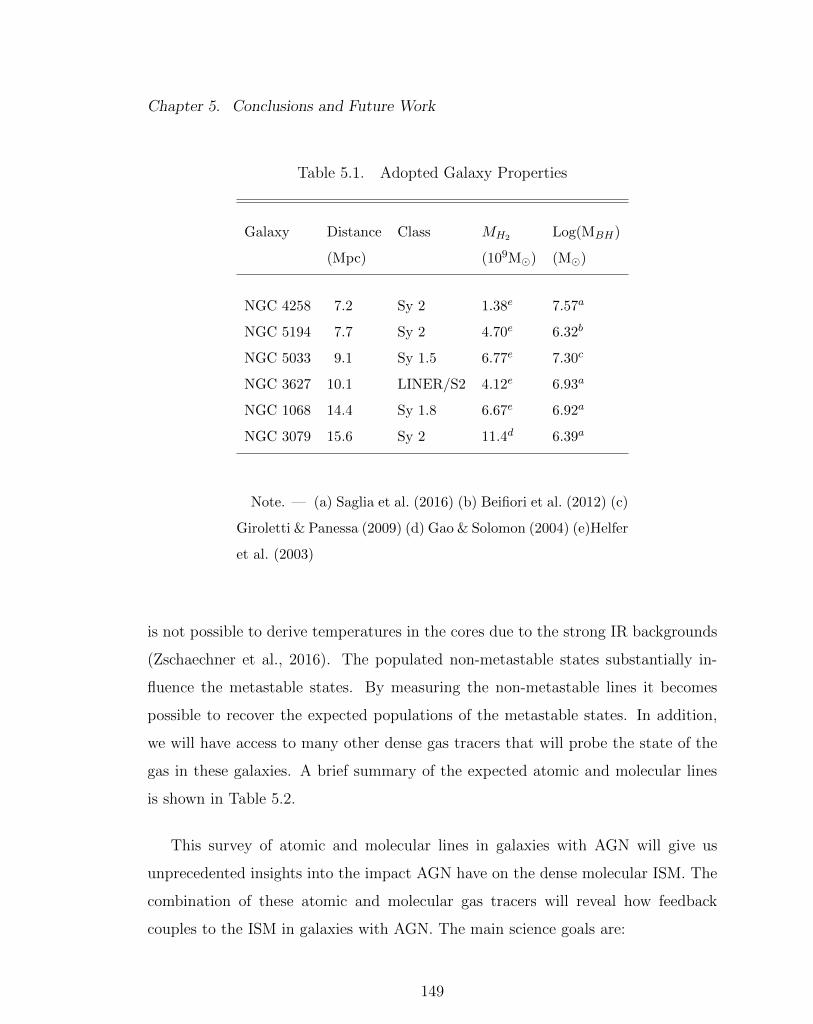
Chapter 5. Conclusions and Future Work
Table 5.1. Adopted Galaxy Properties
Galaxy Distance Class MH2 Log(MBH)
(Mpc) (109M�) (M�)
NGC 4258 7.2 Sy 2 1.38e 7.57a
NGC 5194 7.7 Sy 2 4.70e 6.32b
NGC 5033 9.1 Sy 1.5 6.77e 7.30c
NGC 3627 10.1 LINER/S2 4.12e 6.93a
NGC 1068 14.4 Sy 1.8 6.67e 6.92a
NGC 3079 15.6 Sy 2 11.4d 6.39a
Note. — (a) Saglia et al. (2016) (b) Beifiori et al. (2012) (c)
Giroletti & Panessa (2009) (d) Gao & Solomon (2004) (e)Helfer
et al. (2003)
is not possible to derive temperatures in the cores due to the strong IR backgrounds
(Zschaechner et al., 2016). The populated non-metastable states substantially in-
fluence the metastable states. By measuring the non-metastable lines it becomes
possible to recover the expected populations of the metastable states. In addition,
we will have access to many other dense gas tracers that will probe the state of the
gas in these galaxies. A brief summary of the expected atomic and molecular lines
is shown in Table 5.2.
This survey of atomic and molecular lines in galaxies with AGN will give us
unprecedented insights into the impact AGN have on the dense molecular ISM. The
combination of these atomic and molecular gas tracers will reveal how feedback
couples to the ISM in galaxies with AGN. The main science goals are:
149
Chapter 5. Conclusions and Future Work
• Reveal heating from AGN feedback in the molecular ISM. We aim
to answer three questions about the heating and cooling balance in galaxies:
Do AGN heat the gas compared to the rest of the galaxy? Do strong posi-
tive torques from large scale galactic structure heat the molecular gas? Does
feedback from AGN destroy cold gas in galaxy centers? We will answer these
questions by deriving kinetic temperatures via NH3 thermometry and analysis
of non-metastable transitions where appropriate, on ⇠100 pc scales across six
galaxies.
• Identify characteristics of NH3(3,3) masers. These masers are weakly
associated with star formation within the Milky Way and observed in galaxy
outflows. This project aims to expand the known list of galaxies with NH3(3,3)
masers, and uncover the conditions that give rise to these masers.
• Characterize the galactic environment via molecular tracers. We will
have access to many diagnostically important molecular tracers. Two examples
of molecules that will be useful are HNCO and H2O. HNCO is formed on grain
surfaces and remains until shocks liberate the molecule to the gas phase. Its
morphology is typically very similar to that of the commonly used shock tracer,
SiO, but a factor of ⇠3-4 brighter (e.g., Meier & Turner, 2005, Meier et al.,
2015). The 22 GHz H2O maser transition is used to trace AGN kinematics
(Reid et al., 2009), and is a useful indicator of star formation (Palagi et al.,
1993).
• Determine properties of the thermal gas via radio recombination
lines. RRLs provide an extinction free diagnostic of star forming regions. We
will be able to constrain the density of the thermal gas, the ionizing photon
rate, and electron temperatures.
150
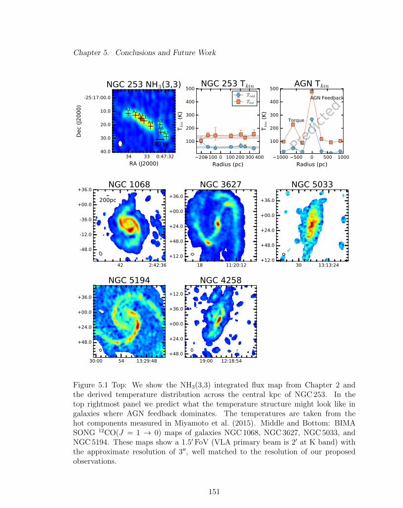
Chapter 5. Conclusions and Future Work
Figure 5.1 Top: We show the NH3(3,3) integrated flux map from Chapter 2 andthe derived temperature distribution across the central kpc of NGC 253. In thetop rightmost panel we predict what the temperature structure might look like ingalaxies where AGN feedback dominates. The temperatures are taken from thehot components measured in Miyamoto et al. (2015). Middle and Bottom: BIMASONG 12CO(J = 1 ! 0) maps of galaxies NGC 1068, NGC 3627, NGC 5033, andNGC 5194. These maps show a 1.50 FoV (VLA primary beam is 20 at K band) withthe approximate resolution of 300, well matched to the resolution of our proposedobservations.
151
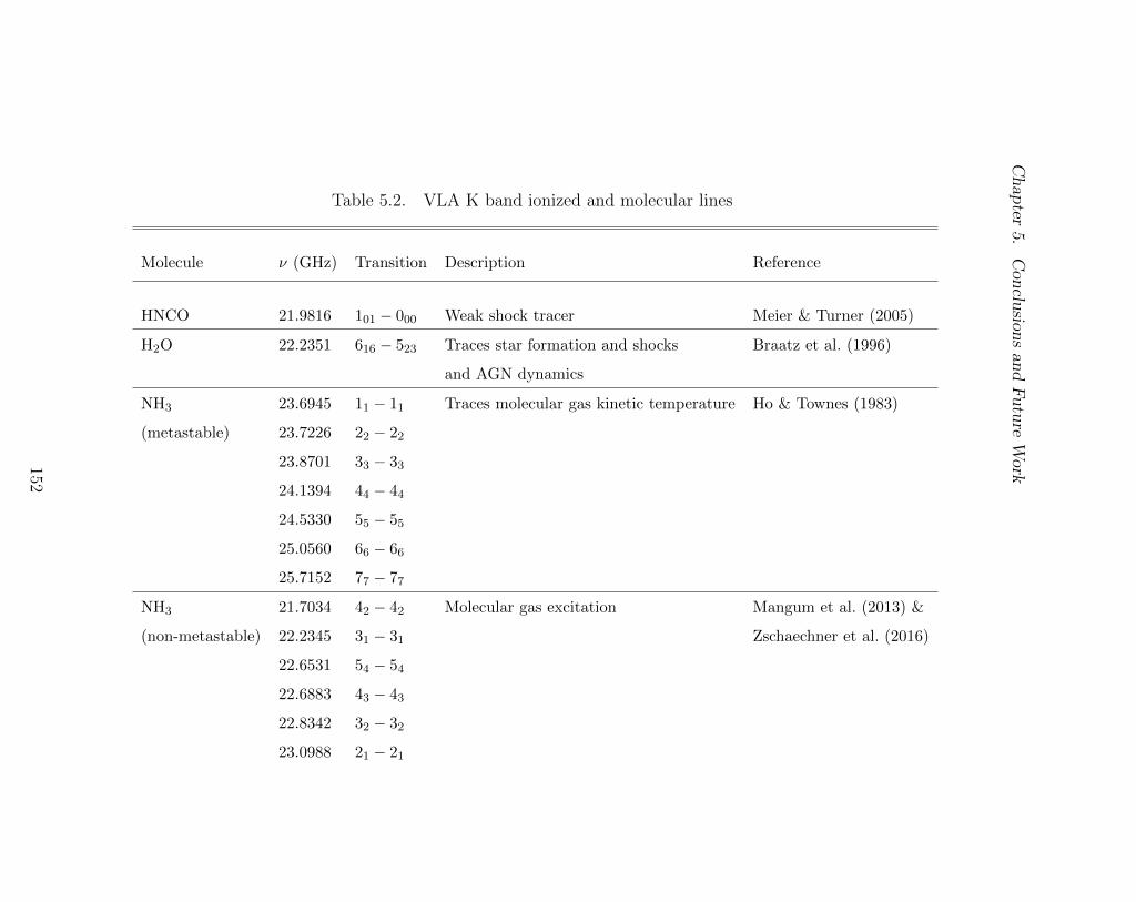
Chapter5.
ConclusionsandFutureWork
Table 5.2. VLA K band ionized and molecular lines
Molecule ⌫ (GHz) Transition Description Reference
HNCO 21.9816 101 � 000 Weak shock tracer Meier & Turner (2005)
H2O 22.2351 616 � 523 Traces star formation and shocks Braatz et al. (1996)
and AGN dynamics
NH3 23.6945 11 � 11 Traces molecular gas kinetic temperature Ho & Townes (1983)
(metastable) 23.7226 22 � 22
23.8701 33 � 33
24.1394 44 � 44
24.5330 55 � 55
25.0560 66 � 66
25.7152 77 � 77
NH3 21.7034 42 � 42 Molecular gas excitation Mangum et al. (2013) &
(non-metastable) 22.2345 31 � 31 Zschaechner et al. (2016)
22.6531 54 � 54
22.6883 43 � 43
22.8342 32 � 32
23.0988 21 � 21
152
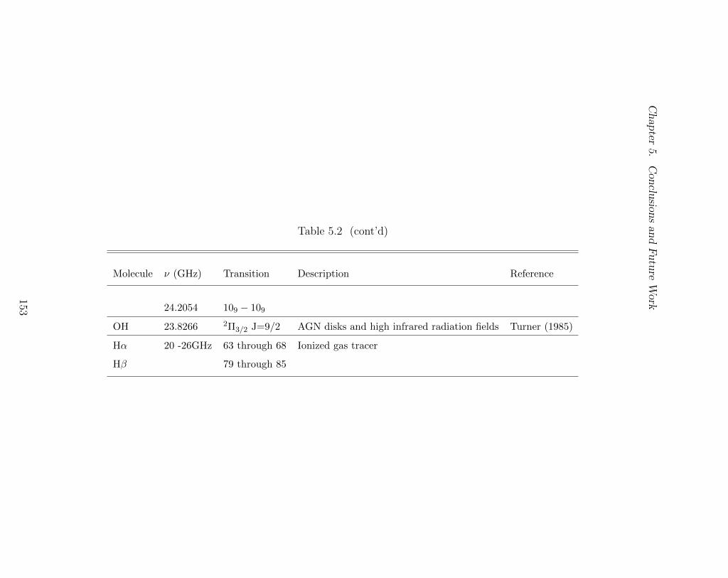
Chapter5.
ConclusionsandFutureWork
Table 5.2 (cont’d)
Molecule ⌫ (GHz) Transition Description Reference
24.2054 109 � 109
OH 23.8266 2⇧3/2 J=9/2 AGN disks and high infrared radiation fields Turner (1985)
H↵ 20 -26GHz 63 through 68 Ionized gas tracer
H� 79 through 85
153
References
Ao, Y., Henkel, C., Braatz, J. A., et al. 2011, A&A, 529, A154
Alonso-Herrero, A., Rieke, G. H., Rieke, M. J., & Kelly, D. M. 2003, AJ, 125, 1210
Bolatto, A. D., Warren, S. R., Leroy, A. K., et al. 2013, Nature, 499, 450
Beifiori, A., Courteau, S., Corsini, E. M., & Zhu, Y. 2012, MNRAS, 419, 2497
Braatz, J. A., Wilson, A. S., & Henkel, C. 1996, ApJS, 106, 51
Brogan, C. L., & Hunter, T. R. 2010, NRAO eNews, June 2010, volume 3, issue 6,
pages 5-6, 3,
Brunthaler, A., Castangia, P., Tarchi, A., et al. 2009, A&A, 497, 103
Caswell, J. L., Breen, S. L., & Ellingsen, S. P. 2011, MNRAS, 410, 1283
Chen, X., Ellingsen, S. P., Baan, W. A., et al. 2015, ApJ, 800, L2
Cheung, A. C., Rank, D. M., Townes, C. H., Thornton, D. D., & Welch, W. J. 1968,
Physical Review Letters, 21, 1701
Churchwell, E., Witzel, A., Huchtmeier, W., et al. 1977, A&A, 54, 969
Claussen, M. J., & Lo, K.-Y. 1986, ApJ, 308, 592
Claussen, M. J., Wilking, B. A., Benson, P. J., et al. 1996, ApJS, 106, 111
154
REFERENCES
Claussen, M. J., Goss, W. M., Frail, D. A., & Seta, M. 1999, AJ, 117, 1387
Crain, R. A., Schaye, J., Bower, R. G., et al. 2015, MNRAS, 450, 1937
Dale, D. A., Cohen, S. A., Johnson, L. C., et al. 2009, ApJ, 703, 517
Dougherty, S. M., & Perley, R. A. 2010, The Dynamic Interstellar Medium: A Cele-
bration of the Canadian Galactic Plane Survey, 438, 421
Downes, D., Radford, S. J. E., Guilloteau, S., et al. 1992, A&A, 262, 424
Elitzur, M., Hollenbach, D. J., & McKee, C. F. 1989, ApJ, 346, 983
Ellingsen, S. P., Chen, X., Qiao, H.-H., et al. 2014, ApJ, 790, L28
Ellingsen, S. P., Sobolev, A. M., Cragg, D. M., & Godfrey, P. D. 2012, ApJ, 759, L5
Engels, D., Schmid-Burgk, J., & Walmsley, C. M. 1986, A&A, 167, 129
Felli, M., Brand, J., Cesaroni, R., et al. 2007, A&A, 476, 373
Fuente, A., Martin-Pintado, J., Cernicharo, J., & Bachiller, R. 1993, A&A, 276, 473
Gao, Y., & Solomon, P. M. 2004, ApJ, 606, 271
Garcıa-Burillo, S., Martın-Pintado, J., Fuente, A., & Neri, R. 2000, A&A, 355, 499
Garcıa-Burillo, S., Combes, F., Eckart, A., et al. 2003, Active Galactic Nuclei: From
Central Engine to Host Galaxy, 290, 423
Garcıa-Burillo, S., Combes, F., Schinnerer, E., Boone, F., & Hunt, L. K. 2005, A&A,
441, 1011
Genzel, R., & Downes, D. 1977, A&AS, 30, 145
Giroletti, M., & Panessa, F. 2009, ApJ, 706, L260
155
REFERENCES
Goddi, C., & Moscadelli, L. 2006, A&A, 447, 577
Goddi, C., Henkel, C., Zhang, Q., Zapata, L., & Wilson, T. L. 2015, A&A, 573, A109
Gray, M. 2012, Maser Sources in Astrophysics, by Malcolm Gray, Cambridge, UK:
Cambridge University Press, 2012,
Greisen, E. W. 2002, Astronomical Data Analysis Software and Systems XI, 281, 260
Greve, A., Neininger, N., Sievers, A., & Tarchi, A. 2006, A&A, 459, 441
Haas, M. R., Schaye, J., Booth, C. M., et al. 2013, MNRAS, 435, 2931
Hagiwara, Y., Henkel, C., Menten, K. M., & Nakai, N. 2001, ApJ, 560, L37
Hartmann, L., Ballesteros-Paredes, J., & Bergin, E. A. 2001, ApJ, 562, 852
Helfer, T. T., Thornley, M. D., Regan, M. W., et al. 2003, ApJS, 145, 259
Henkel, C., Mauersberger, R., Peck, A. B., Falcke, H., & Hagiwara, Y. 2000, A&A,
361, L45
Henkel, C., Tarchi, A., Menten, K. M., & Peck, A. B. 2004, A&A, 414, 117
Ho, P. T. P., Martin, R. N., Henkel, C., & Turner, J. L. 1987, ApJ, 320, 663
Ho, P. T. P., & Townes, C. H. 1983, ARA&A, 21, 239
Hogbom, J. A. 1974, A&AS, 15, 417
Hopkins, P. F., Keres, D., Onorbe, J., et al. 2014, MNRAS, 445, 581
Hopkins, P. F., Quataert, E., & Murray, N. 2011, MNRAS, 417, 950
Hopkins, P. F., Quataert, E., & Murray, N. 2012, MNRAS, 421, 3488
Huettemeister, S., Wilson, T. L., Mauersberger, R., et al. 1995, A&A, 294, 667
156
REFERENCES
Jarrett, T. H., Masci, F., Tsai, C. W., et al. 2013, AJ, 145, 6
Johnston, K. J., Gaume, R., Stolovy, S., et al. 1992, ApJ, 385, 232
de Jong, T. 1973, A&A, 26, 297
Kang, M., Lee, J.-E., Choi, M., et al. 2013, ApJS, 209, 25
Karachentsev, I. D., Makarov, D. I., & Kaisina, E. I. 2013, AJ, 145, 101
Kau↵mann, G., Colberg, J. M., Diaferio, A., & White, S. D. M. 1999, MNRAS, 303,
188
Kennicutt, R. C., Jr. 1998, ARA&A, 36, 189
Kepley, A. A., Chomiuk, L., Johnson, K. E., et al. 2011, ApJ, 739, L24
Kraemer, K. E., & Jackson, J. M. 1995, ApJ, 439, L9
Krumholz, M. R., Klein, R. I., & McKee, C. F. 2011, ApJ, 740, 74
Lebron, M., Mangum, J. G., Mauersberger, R., et al. 2011, A&A, 534, A56
Lehnert, M. D., Heckman, T. M., & Weaver, K. A. 1999, ApJ, 523, 575
Leroy, A. K., Bolatto, A. D., Ostriker, E. C., et al. 2015, ApJ, 801, 25
Lo, K. Y. 2005, ARA&A, 43, 625
Leurini, S., Schilke, P., Menten, K. M., et al. 2004, A&A, 422, 573
Leurini, S., Menten, K. M., & Walmsley, C. M. 2016, A&A, 592, A31
Levine, D. A., Turner, J. L., & Hurt, R. L. 1994, IAU Colloq. 140: Astronomy with
Millimeter and Submillimeter Wave Interferometry, 59, 339
Norman, C. A., & Ikeuchi, S. 1989, ApJ, 345, 372
157
REFERENCES
Mangum, J. G., Darling, J., Henkel, C., et al. 2013, ApJ, 779, 33
Mangum, J. G., & Shirley, Y. L. 2015, Publications of the ASP, 127, 266
Mangum, J. G., & Wootten, A. 1994, ApJ, 428, L33
McCormick, A., Veilleux, S., & Rupke, D. S. N. 2013, ApJ, 774, 126
Martın, S. 2011, The Molecular Universe, 280, 351
Martın, S., Kohno, K., Izumi, T., et al. 2015, A&A, 573, A116
McEwen, B. C., Pihlstrom, Y. M., & Sjouwerman, L. O. 2014, ApJ, 793, 133
McEwen, B. C., Pihlstrom, Y. M., & Sjouwerman, L. O. 2016, ApJ, 826, 189
McMullin, J. P., Waters, B., Schiebel, D., Young, W., & Golap, K. 2007, Astronom-
ical Data Analysis Software and Systems XVI, 376, 127
Meier, D. S., Turner, J. L., & Hurt, R. L. 2000, ApJ, 531, 200
Meier, D. S., Walter, F., Bolatto, A. D., et al. 2015, ApJ, 801, 63
Meier, D. S., & Turner, J. L. 2001, ApJ, 551, 687
Meier, D. S., & Turner, J. L. 2005, ApJ, 618, 259
Meier, D. S., Turner, J. L., & Schinnerer, E. 2011, AJ, 142, 32
Meier, D. S., & Turner, J. L. 2012, ApJ, 755, 104
Menten, K. 1991, Atoms, Ions and Molecules: New Results in Spectral Line Astro-
physics, 16, 119
Mills, E. A. C., & Morris, M. R. 2013, ApJ, 772, 105
Mills, E. A. C., Butterfield, N., Ludovici, D. A., et al. 2015, ApJ, 805, 72
158
REFERENCES
Miyamoto, Y., Nakai, N., Seta, M., et al. 2015, PASJ, 67, 5
Muller, H. S. P., Schloder, F., Stutzki, J., & Winnewisser, G. 2005, Journal of
Molecular Structure, 742, 215
Murray, N., Quataert, E., & Thompson, T. A. 2010, ApJ, 709, 191
Okamoto, T., Eke, V. R., Frenk, C. S., & Jenkins, A. 2005, MNRAS, 363, 1299
Ott, J., Henkel, C., Braatz, J. A., & Weiß, A. 2011, ApJ, 742, 95
Ott, J., Weiss, A., Henkel, C., & Walter, F. 2005, ApJ, 629, 767
Palagi, F., Cesaroni, R., Comoretto, G., Felli, M., & Natale, V. 1993, A&AS, 101,
153
Peck, A. B., Henkel, C., Ulvestad, J. S., et al. 2003, ApJ, 590, 149
Perley, R. A., & Butler, B. J. 2013, ApJS, 206, 16
Perley, R. A., & Butler, B. J. 2017, ApJS, 230, 7
Pence, W. D. 1980, ApJ, 239, 54
Pickett, H. M., Poynter, R. L., Cohen, E. A., et al. 1998, Journal of Quantitative
Spectroscopy and Radiative Transfer, 60, 883
Pihlstrom, Y. M., Sjouwerman, L. O., Frail, D. A., et al. 2014, AJ, 147, 73
Pratap, P., Shute, P. A., Keane, T. C., Battersby, C., & Sterling, S. 2008, AJ, 135,
1718
Radburn-Smith, D. J., de Jong, R. S., Seth, A. C., et al. 2011, ApJS, 195, 18
Reid, M. J., Braatz, J. A., Condon, J. J., et al. 2009, ApJ, 695, 287
Rodriguez-Franco, A., Martin-Pintado, J., & Fuente, A. 1998, A&A, 329, 1097
159
REFERENCES
Romeo, A. B., & Fathi, K. 2016, MNRAS, 460, 2360
Rosenberg, M. J. F., Kazandjian, M. V., van der Werf, P. P., et al. 2014, A&A, 564,
A126
Rosen, A., & Bregman, J. N. 1995, ApJ, 440, 634
Saglia, R. P., Opitsch, M., Erwin, P., et al. 2016, ApJ, 818, 47
Sakamoto, K., Ho, P. T. P., Iono, D., et al. 2006, ApJ, 636, 685
Sakamoto, K., Mao, R.-Q., Matsushita, S., et al. 2011, ApJ, 735, 19
Schinnerer, E., Boker, T., Emsellem, E., & Lisenfeld, U. 2006, ApJ, 649, 181
Schoier, F. L., van der Tak, F. F. S., van Dishoeck, E. F., & Black, J. H. 2005, A&A,
432, 369
Somerville, R. S., & Dave, R. 2015, ARA&A, 53, 51
Strong, A. W., Bloemen, J. B. G. M., Dame, T. M., et al. 1988, A&A, 207, 1
Strickland, D. K., Heckman, T. M., Weaver, K. A., Hoopes, C. G., & Dahlem, M.
2002, ApJ, 568, 689
Suto, M., & Lee, L. C. 1983, JChPh, 78, 4515
Takano, S., Nakai, N., & Kawaguchi, K. 2002, PASJ, 54, 195
Takano, S., Hofner, P., Winnewisser, G., Nakai, N., & Kawaguchi, K. 2005, PASJ,
57, 549
Tarchi, A., Henkel, C., Peck, A. B., & Menten, K. M. 2002, A&A, 385, 1049
Tarchi, A., Henkel, C., Peck, A. B., & Menten, K. M. 2002b, A&A, 389, L39
Tarchi, A. 2012, IAU Symposium, 287, 323
160
REFERENCES
Tarchi, A., Castangia, P., Columbano, A., Panessa, F., & Braatz, J. A. 2011, A&A,
532, A125
Tsai, A.-L., Matsushita, S., Nakanishi, K., et al. 2009, PASJ, 61, 237
Turner, B. E. 1985, ApJ, 299, 312
Turner, B. E. 1995, ApJ, 449, 635
Turner, J. L., & Ho, P. T. P. 1985, ApJ, 299, L77
Turner, J. L., & Hurt, R. L. 1992, ApJ, 384, 72
Ulvestad, J. S., & Antonucci, R. R. J. 1997, ApJ, 488, 621
Ungerechts, H., Winnewisser, G., & Walmsley, C. M. 1986, A&A, 157, 207
Van der Tak, F.F.S., Black, J.H., Schier, F.L., Jansen, D.J., van Dishoeck, E.F.,
2007, A&A, 468, 627-635
van Dishoeck, E. F., Herbst, E., & Neufeld, D. A. 2013, Chemical Reviews, 113, 9043
Vazquez-Semadeni, E., Colın, P., Gomez, G. C., Ballesteros-Paredes, J., & Watson,
A. W. 2010, ApJ, 715, 1302
Voronkov, M. A., Caswell, J. L., Ellingsen, S. P., Green, J. A., & Breen, S. L. 2014,
MNRAS, 439, 2584
Walmsley, C. M., & Ungerechts, H. 1983, A&A, 122, 164
Watson, A. M., Gallagher, J. S., III, Holtzman, J. A., et al. 1996, AJ, 112, 534
Weiß, A., Neininger, N., Henkel, C., Stutzki, J., & Klein, U. 2001, ApJ, 554, L143
Westmoquette, M. S., Smith, L. J., & Gallagher, J. S., III 2011, MNRAS, 414, 3719
Whiting, A. B. 1999, AJ, 117, 202
161
REFERENCES
Wilson, T. L., Rohlfs, K., & Huttemeister, S. 2009, Tools of Radio Astronomy, by
Thomas L. Wilson; Kristen Rohlfs and Susanne Huttemeister. ISBN 978-3-540-
85121-9. Published by Springer-Verlag, Berlin, Germany, 2009.,
Wilson, T. L., & Mauersberger, R. 1990, A&A, 239, 305
Woodall, J. M., & Gray, M. D. 2007, MNRAS, 378, L20
Yamagishi, M., Kaneda, H., Ishihara, D., et al. 2010, PASJ, 62, 1085
Yusef-Zadeh, F., Cotton, W., Viti, S., Wardle, M., & Royster, M. 2013, ApJ, 764,
L19
Zhang, Q., Hunter, T. R., Sridharan, T. K., & Cesaroni, R. 1999, ApJ, 527, L117
Zschaechner, L. K., Ott, J., Walter, F., et al. 2016, ApJ, 833, 41
162


