MONITORING AND DIAGNOSIS OFCONTINUOUS DYNAMIC SYSTEMSUSING SEMIQUANTITATIVE SIMULATIONbyDANIEL LOUIS DVORAK, B.S., M.S.DISSERTATIONPresented to the Faculty of the Graduate School ofThe University of Texas at Austinin Partial Ful�llmentof the Requirementsfor the Degree ofDOCTOR OF PHILOSOPHY

THE UNIVERSITY OF TEXAS AT AUSTINMay, 1992

AcknowledgmentsI especially thank Prof. Benjamin Kuipers for his guidance in shaping this researchand his continuous encouragement; many times his insightful comments helped me to pressforward, and many times his encouraging words helped me believe that the work was worthdoing. I am indebted to Dan Berleant for his work on Q2/Q3 and to Bert Kay for hiswork on dynamic envelopes; both of these research e�orts provided important tools to buildupon. I sincerely appreciate the e�orts of Kee Kimbrell and Dan Clancy in porting Qsim tothe Macintosh. I value the many other friendships that I gained during this time, includingthose of Ray Bareiss, Jimi Crawford, Adam Farquhar, David Franke, Wan-Yik Lee, WoodLee, Raman Rajagopalan, David Throop, and Chris Walton.I sincerely appreciate the encouragement and support of Reid Watts and HaroldJackson of AT&T Bell Laboratories, and the �nancial assistance of the Doctoral SupportProgram at AT&T Bell Laboratories. I thank the Visionnaire Group at Bell Labs for theuse of their Symbolics machines.Finally, I thank my wife Waf�a for her patience and understanding during the lasttwo years as I toiled into the night. Daniel Louis DvorakThe University of Texas at AustinMay, 1992ii

MONITORING AND DIAGNOSIS OFCONTINUOUS DYNAMIC SYSTEMSUSING SEMIQUANTITATIVE SIMULATIONPublication No.Daniel Louis Dvorak, Ph.D.The University of Texas at Austin, 1992Supervisor: Benjamin J. KuipersOperative diagnosis, or diagnosis of a physical system in operation, is essential for systemsthat cannot be stopped every time an anomaly is detected, such as in the process industries,space missions, and medicine. Compared to maintenance diagnosis where the system is o�-line and arbitrary points can be probed, operative diagnosis is limited mainly to sensorreadings, and diagnosis begins while the e�ects of a fault are still propagating. Symptomschange as the system's dynamic behavior unfolds.This research presents a design for monitoring and diagnosis of deterministic con-tinuous dynamic systems based on the paradigms of \monitoring as model corroboration"and \diagnosis as model modi�cation" in which a semiquantitative model of a physicalsystem is simulated in synchrony with incoming sensor readings. When sensor readingsdisagree with predictions, variant models are created representing di�erent fault hypothe-ses. These models are then simulated and either corroborated or refuted as new readingsarrive. The set of models changes as new hypotheses are generated and as old hypothesesare exonerated. In contrast to methods that base diagnosis on a snapshot of behavior, thisiii

simulation-based approach exploits the system's time-varying behavior for diagnostic cluesand exploits the predictive power of the model to forewarn of imminent hazards.The design holds several other advantages over existing methods: 1) semiquan-titative models provide greater expressive power for states of incomplete knowledge thandi�erential equations, thus eliminating certain modeling compromises; 2) semiquantitativesimulation generates guaranteed bounds on variables, thus providing dynamic alarm thresh-olds and thus fewer fault detection errors than with �xed-threshold alarms; 3) the guaran-teed prediction of all valid behaviors eliminates the \missing prediction bug" in diagnosis;4) the branching-time description of behavior permits recognition of all valid manifestationsof a fault (and of interacting faults); 5) hypotheses based on predictive semiquantitativemodels are more informative because they show the values of unseen variables and can pre-dict future consequences; and 6) fault detection degrades gracefully as multiple faults arediagnosed over time.

iv

Table of ContentsAcknowledgments iiAbstract iiiTable of Contents v1. Introduction 11.1 The Problem: Monitoring Dynamic Systems : : : : : : : : : : : : : : : : : : 11.1.1 Background and Motivation : : : : : : : : : : : : : : : : : : : : : : : 11.1.2 Operative Diagnosis : : : : : : : : : : : : : : : : : : : : : : : : : : : 21.1.3 Operator Advisory Systems : : : : : : : : : : : : : : : : : : : : : : : 41.1.4 False Positives, False Negatives : : : : : : : : : : : : : : : : : : : : : 51.1.5 The Domain : : : : : : : : : : : : : : : : : : : : : : : : : : : : : : : 61.2 The Approach : : : : : : : : : : : : : : : : : : : : : : : : : : : : : : : : : : : 71.2.1 Goals and Non-Goals : : : : : : : : : : : : : : : : : : : : : : : : : : : 71.2.2 Diagnosis as Model Modi�cation : : : : : : : : : : : : : : : : : : : : 81.2.3 Semiquantitative Simulation : : : : : : : : : : : : : : : : : : : : : : : 81.2.4 Bene�ts : : : : : : : : : : : : : : : : : : : : : : : : : : : : : : : : : : 91.2.5 Architecture : : : : : : : : : : : : : : : : : : : : : : : : : : : : : : : 101.3 Scope : : : : : : : : : : : : : : : : : : : : : : : : : : : : : : : : : : : : : : : 101.3.1 Assumptions : : : : : : : : : : : : : : : : : : : : : : : : : : : : : : : 101.3.2 Non-requirements : : : : : : : : : : : : : : : : : : : : : : : : : : : : : 111.3.3 Modeling Issues : : : : : : : : : : : : : : : : : : : : : : : : : : : : : : 111.3.4 Implementation : : : : : : : : : : : : : : : : : : : : : : : : : : : : : : 121.3.5 Empirical Evaluation : : : : : : : : : : : : : : : : : : : : : : : : : : : 131.4 Claims : : : : : : : : : : : : : : : : : : : : : : : : : : : : : : : : : : : : : : : 13v

1.4.1 Modeling & Simulation : : : : : : : : : : : : : : : : : : : : : : : : : 131.4.2 Predictive Monitoring : : : : : : : : : : : : : : : : : : : : : : : : : : 141.4.3 Discrepancy Detection & Diagnosis : : : : : : : : : : : : : : : : : : : 141.4.4 Skepticism : : : : : : : : : : : : : : : : : : : : : : : : : : : : : : : : 151.5 Example: A Two-Tank Cascade : : : : : : : : : : : : : : : : : : : : : : : : : 171.5.1 Modeling : : : : : : : : : : : : : : : : : : : : : : : : : : : : : : : : : 171.5.2 Simulation : : : : : : : : : : : : : : : : : : : : : : : : : : : : : : : : 181.5.3 Discrepancy Detection : : : : : : : : : : : : : : : : : : : : : : : : : : 201.5.4 Hypothesis Generation : : : : : : : : : : : : : : : : : : : : : : : : : : 211.5.5 Hypothesis Testing : : : : : : : : : : : : : : : : : : : : : : : : : : : : 231.5.6 Forewarning : : : : : : : : : : : : : : : : : : : : : : : : : : : : : : : : 241.5.7 Summary : : : : : : : : : : : : : : : : : : : : : : : : : : : : : : : : : 241.6 Guide to the Dissertation : : : : : : : : : : : : : : : : : : : : : : : : : : : : 251.7 Terminology : : : : : : : : : : : : : : : : : : : : : : : : : : : : : : : : : : : : 252. Related Work 312.1 Symptom-Based Approaches : : : : : : : : : : : : : : : : : : : : : : : : : : : 312.1.1 Rule-Based Systems : : : : : : : : : : : : : : : : : : : : : : : : : : : 312.1.2 Fault Dictionaries : : : : : : : : : : : : : : : : : : : : : : : : : : : : 332.1.3 Decision Trees : : : : : : : : : : : : : : : : : : : : : : : : : : : : : : 332.2 Model-Based Approaches : : : : : : : : : : : : : : : : : : : : : : : : : : : : 342.2.1 PREMON/SELMON (Doyle et al.) : : : : : : : : : : : : : : : : : : : 342.2.2 DRAPHYS (Abbott) : : : : : : : : : : : : : : : : : : : : : : : : : : : 362.2.3 MIDAS (Finch, Oyeleye and Kramer) : : : : : : : : : : : : : : : : : 372.2.4 Inc-Diagnose (Ng) : : : : : : : : : : : : : : : : : : : : : : : : : : : : 392.2.5 Kalman Filters : : : : : : : : : : : : : : : : : : : : : : : : : : : : : : 41vi

2.2.6 KARDIO (Bratko et al.) : : : : : : : : : : : : : : : : : : : : : : : : : 452.2.7 Modeling for Troubleshooting (Hamscher) : : : : : : : : : : : : : : : 492.3 In uential Research : : : : : : : : : : : : : : : : : : : : : : : : : : : : : : : 512.3.1 Measurement Interpretation : : : : : : : : : : : : : : : : : : : : : : : 512.3.2 Generate, Test and Debug : : : : : : : : : : : : : : : : : : : : : : : : 522.3.3 STEAMER : : : : : : : : : : : : : : : : : : : : : : : : : : : : : : : : 543. The Design of Mimic 553.1 Design Overview : : : : : : : : : : : : : : : : : : : : : : : : : : : : : : : : : 553.2 Modeling : : : : : : : : : : : : : : : : : : : : : : : : : : : : : : : : : : : : : 583.2.1 Structural Model : : : : : : : : : : : : : : : : : : : : : : : : : : : : : 583.2.2 Behavioral Model : : : : : : : : : : : : : : : : : : : : : : : : : : : : : 623.2.3 Modeling Faults : : : : : : : : : : : : : : : : : : : : : : : : : : : : : 643.3 Simulation : : : : : : : : : : : : : : : : : : : : : : : : : : : : : : : : : : : : : 653.3.1 Qualitative-Quantitative Simulation : : : : : : : : : : : : : : : : : : 663.3.2 Feedback Loops : : : : : : : : : : : : : : : : : : : : : : : : : : : : : : 673.3.3 State-Insertion for Measurements : : : : : : : : : : : : : : : : : : : : 703.3.4 Dynamic Envelopes : : : : : : : : : : : : : : : : : : : : : : : : : : : 723.3.5 Pruned Envisionment : : : : : : : : : : : : : : : : : : : : : : : : : : 733.4 Monitoring : : : : : : : : : : : : : : : : : : : : : : : : : : : : : : : : : : : : 733.4.1 Monitoring Model : : : : : : : : : : : : : : : : : : : : : : : : : : : : 743.4.2 Limitations of Alarms : : : : : : : : : : : : : : : : : : : : : : : : : : 753.4.3 Discrepancy Detection : : : : : : : : : : : : : : : : : : : : : : : : : : 763.4.4 Tracking : : : : : : : : : : : : : : : : : : : : : : : : : : : : : : : : : : 793.4.5 Updating Predictions from Measurements : : : : : : : : : : : : : : : 813.4.6 Measurement Issues : : : : : : : : : : : : : : : : : : : : : : : : : : : 81vii

3.5 Diagnosis : : : : : : : : : : : : : : : : : : : : : : : : : : : : : : : : : : : : : 823.5.1 Hypothesis Generation : : : : : : : : : : : : : : : : : : : : : : : : : : 833.5.2 Hypothesis Testing : : : : : : : : : : : : : : : : : : : : : : : : : : : : 863.5.3 Resimulation : : : : : : : : : : : : : : : : : : : : : : : : : : : : : : : 883.5.4 Hypothesis Discrimination : : : : : : : : : : : : : : : : : : : : : : : : 893.5.5 Multiple-Fault Diagnosis : : : : : : : : : : : : : : : : : : : : : : : : : 903.6 Advising : : : : : : : : : : : : : : : : : : : : : : : : : : : : : : : : : : : : : : 903.6.1 Warning Predicates : : : : : : : : : : : : : : : : : : : : : : : : : : : 903.6.2 Forewarning : : : : : : : : : : : : : : : : : : : : : : : : : : : : : : : : 903.6.3 Ranking of Hypotheses : : : : : : : : : : : : : : : : : : : : : : : : : : 913.6.4 Defects vs. Disturbances : : : : : : : : : : : : : : : : : : : : : : : : : 923.7 Special Fault Handling : : : : : : : : : : : : : : : : : : : : : : : : : : : : : : 933.7.1 Intermittent Faults : : : : : : : : : : : : : : : : : : : : : : : : : : : : 933.7.2 Consequential Faults : : : : : : : : : : : : : : : : : : : : : : : : : : : 933.8 Controlling Complexity : : : : : : : : : : : : : : : : : : : : : : : : : : : : : 934. Experimental Results 974.1 Gravity-Flow Tank : : : : : : : : : : : : : : : : : : : : : : : : : : : : : : : : 974.1.1 Cycle 9: t = 0.9 : : : : : : : : : : : : : : : : : : : : : : : : : : : : : 994.1.2 Cycle 11: t = 1.1 : : : : : : : : : : : : : : : : : : : : : : : : : : : : : 1024.1.3 Cycle 12: t = 1.2 : : : : : : : : : : : : : : : : : : : : : : : : : : : : : 1034.1.4 Cycle 22: t = 2.2 : : : : : : : : : : : : : : : : : : : : : : : : : : : : : 1044.2 Two-Tank Cascade : : : : : : : : : : : : : : : : : : : : : : : : : : : : : : : : 1044.3 Open-Ended U-Tube : : : : : : : : : : : : : : : : : : : : : : : : : : : : : : : 1084.4 Vacuum Chamber : : : : : : : : : : : : : : : : : : : : : : : : : : : : : : : : 1114.5 The Dynamics Debate : : : : : : : : : : : : : : : : : : : : : : : : : : : : : : 113viii

5. Discussion and Conclusions 1155.1 Design Principles : : : : : : : : : : : : : : : : : : : : : : : : : : : : : : : : : 1155.2 Strengths : : : : : : : : : : : : : : : : : : : : : : : : : : : : : : : : : : : : : 1175.3 Limitations : : : : : : : : : : : : : : : : : : : : : : : : : : : : : : : : : : : : 1195.3.1 Temporal Abstraction : : : : : : : : : : : : : : : : : : : : : : : : : : 1195.3.2 Dependency Tracing : : : : : : : : : : : : : : : : : : : : : : : : : : : 1195.3.3 Spurious Behaviors : : : : : : : : : : : : : : : : : : : : : : : : : : : : 1205.3.4 Cascading Faults : : : : : : : : : : : : : : : : : : : : : : : : : : : : : 1205.3.5 Complexity and Real-Time Performance : : : : : : : : : : : : : : : : 1215.4 Appropriate Domains : : : : : : : : : : : : : : : : : : : : : : : : : : : : : : 1215.5 Future Work : : : : : : : : : : : : : : : : : : : : : : : : : : : : : : : : : : : 1225.5.1 Discrepancy Detection : : : : : : : : : : : : : : : : : : : : : : : : : : 1225.5.2 Perturbation Analysis : : : : : : : : : : : : : : : : : : : : : : : : : : 1225.5.3 Component-Connection Models : : : : : : : : : : : : : : : : : : : : : 1235.5.4 Hierarchical Representation and Diagnosis : : : : : : : : : : : : : : : 1235.5.5 Scale-Space Filtering : : : : : : : : : : : : : : : : : : : : : : : : : : : 1255.5.6 Speeding it Up : : : : : : : : : : : : : : : : : : : : : : : : : : : : : : 1255.5.7 Reconciling FDI and MBR : : : : : : : : : : : : : : : : : : : : : : : 1265.5.8 Real Applications : : : : : : : : : : : : : : : : : : : : : : : : : : : : : 1265.6 Epilogue : : : : : : : : : : : : : : : : : : : : : : : : : : : : : : : : : : : : : : 127A. Sample Execution History 129BIBLIOGRAPHY 149Vita ix

x

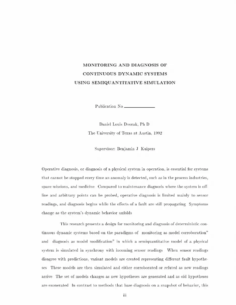
Chapter 1Introduction: : :computer technology allows more complex systems to be controlled but italso enables far more information about the system to be displayed. For exam-ple, process control and instrumentation systems such as those found in nuclearpower plants may have around 2000 alarms in a control room in addition to thedisplays of analogue plant data. When plant crises occur, these data can changevery rapidly. In one simulated loss-of-coolant accident, 500 lights went on or o�within the �rst minute, and 800 in the second.It is in these kinds of real-time problem-solving situations that many of thelimitations of humans are at their most apparent. Their tendency to overlookrelevant information, to respond too slowly and to panic when the rate of infor-mation ow is too great all contribute to lower than desired levels of performance.[SPT86]1.1 The Problem: Monitoring Dynamic Systems1.1.1 Background and MotivationNuclear power plant operations is but one example in which a human must mon-itor a physical system through sensor readings and interpret those readings, often undergrave time pressure, when unexpected behavior occurs. This task is prevalent in our modernworld | in operating a petroleum re�nery, in ying a commercial jet aircraft, in monitor-ing a patient in a surgical intensive care unit, and in monitoring spacecraft environmentalsystems. In all these cases the human's primary source of information is sensor readingsand alarms, and diagnosis must be performed while the system continues to operate.The hazards of performing this di�cult task incorrectly or too slowly can beseen in the records of notable accidents such as the 1979 Three Mile Island nuclear poweraccident, the 1977 New York City blackout, the near-tragedy of the Apollo 13 ight in 1970,and the 1969 Texas City explosion of a butadiene re�ning unit. As Perrow recognized whenhe analyzed these and other accidents, the characteristics that make a system more proneto accident are tight coupling and complex interactions [Per84]. Such systems are harderto understand when something goes wrong and allow less time to take corrective action.Perrow's interactions/coupling chart (Figure 1.1) shows examples of high-risk systems in the1

2 Linear Complex-�6?

InteractionsLooseTightCoupling �Nuclear plants�DNA�Aircraft �Chemical plants�Space missions �Military early warning�Military adventures�Mining �R&D �rms�Universities

�Dams �Power grids�Some continuousprocesses �Marine transport�Rail transport �Airways�Junior college�Assembly-line production�Most manufacturing�Post o�ceFigure 1.1: Perrow's Interactions/Coupling Chart. The systems most prone to accident arethose having tight coupling and complex interactions, as shown in the upper-right quadrant.upper right quadrant, such as nuclear plants, chemical plants, aircraft, and space missions.(Medical intensive care also belongs in this quadrant since human biology exhibits tightcoupling and complex interactions; Perrow did not include medical care because his focuswas on man-made organizations and technology.)1.1.2 Operative DiagnosisThis research focuses on the problem of operative diagnosis, or diagnosis of phys-ical systems in operation. As Abbott notes [Abb90, p. 135], operative diagnosis is distinctfrom \o�-line" or \maintenance" diagnosis in several respects. As Table 1.1 shows, the ob-jective of operative diagnosis is to facilitate continued safe operation of the system whereasthe objective of maintenance diagnosis is to determine which part to �x or replace. Oper-ative diagnosis arises in at least three situations: when it is impossible to shut down thephysical system (as in medicine), when faults are tolerated because it is too expensive tostop for every maintenance item (in industry), and when severe consequences may resultwithin seconds or minutes after a malfunction (as in space missions). Malko� [Mal87, p.98] describes well a root problem in operative diagnosis:

3Operative diagnosis Maintenance diagnosisContext System remains in operation. System is o�-line.Objective Continued safe operation. Fix or replace faulty compo-nent.Requirements Identify faulty component,identify speci�c fault, exposeits e�ects, and forewarn of pos-sible adverse e�ects. Localize fault to a �eld re-placeable unit.Observations Limited mainly to sensor read-ings. Can probe arbitrary points.Symptoms Diagnosis begins while e�ectsof fault are still propagating,so symptoms may change. Diagnosis usually done afterall e�ects have propagated.Hypothesis Consists of a mech-anism model embodying zeroor more faults, plus its state. Identi�es a suspected compo-nent.Testing Restricted to cautious inputperturbations. Can apply arbitrary input sig-nals.Table 1.1: Operative Diagnosis versus Maintenance Diagnosis. Much of the prior work inknowledge-based diagnosis is aimed at maintenance diagnosis. This report addresses thechallenges of operative diagnosis.

4 In process control systems, the detection and diagnosis of faults generallydepends upon two mechanisms:1. Large numbers of sensors are installed at key points in the plant. Rawparameter values transmitted from these sensors are monitored and com-pared with pre-speci�ed upper and lower range-limits of normal. Whenparameter range-limits are exceeded, alarms are activated to attract theattention of the operator.2. Human operators are responsible for performing (manually, and in realtime) the multisensor integration (i.e., the process of observing all the sen-sor data), particularly the occurrence of alarms, analyzing their signi�canceand correctly formulating a diagnosis.Herein lies the root of a serious problem in dealing with fault diagnosis:Design engineers and, to a lesser extent, plant operators, can reasonablywell anticipate the pattern of alarms that will be triggered by a known mal-function. To a lesser degree, this is the case even for multiple, simultaneousmalfunctions. On the other hand, they have great di�culty reasoning inthe reverse direction: that is, mapping from a complicated pattern of sensoralarms back to causative faults.1.1.3 Operator Advisory SystemsTo help the operator perform operative diagnosis, the \operator advisory system"has emerged as an extension to existing monitoring & control technology (see Figure 1.2),and has become an important area of application for expert systems. Escort [SPT86] (anexpert system for complex operations in real-time) and Realm [TC86] (a reactor emergencyaction level monitor) are two of many expert systems developed for process industries. (Forsurveys of this work, see Dvorak's study of monitoring & control expert systems [Dvo87]and La�ey et al.'s survey of real-time knowledge-based systems [LCS+88].) These systemsaim to reduce the cognitive load on operators, usually by helping to diagnose the cause ofalarms and possibly suggesting corrective actions. Most of these expert systems get theirknowledge of symptoms, faults, and corrective actions through the usual process of codifyinghuman expertise in rules or decision trees. But the problem, as with all expert systems, isreliability. As Denning observes,the trial-and-error process by which knowledge is elicited, programmed, andtested is likely to produce inconsistent and incomplete databases; hence, an expertsystem may exhibit important gaps in knowledge at unexpected times [Den86].These \gaps in knowledge" can lead to errors in fault detection and diagnosis, and can haveserious consequences in some applications.

5DynamicPhysicalSystem OperatorAdvisorySystem ������ AA��HH((((((((((((:status alarms������������9 controls -manual observations-sensor readings� control signalsFigure 1.2: Operating a physical system. The purpose of the operator advisory system isto assist the operator in interpreting sensor readings and determining appropriate controlactions. '& $%Expectedbehavior'& $%Correctbehavior '& $%FaultybehaviorA B CD FEG�����False positivesA [ B QQQQk False negativesE [ FFigure 1.3: Fault detection errors as a function of behavior. False positives arise whenexpected behavior fails to include all valid correct behaviors. False negatives arise whenfaulty behavior is indistinguishable from expected behavior.1.1.4 False Positives, False NegativesFault detection can be wrong in two ways: as false negatives, in which a real faultgoes undetected, and as false positives , in which an alarm is raised when no fault is present(see Figure 1.3). There are several fundamental reasons why a fault may be undetectable,and thus cause a false negative: the fault may be masked by a redundant spare; the faultmay not be exposed in the current operating mode (such as a burned-out light bulb withno power applied); the fault may not have a�ected any sensor yet, or the a�ected sensormay itself be defective; the fault manifestations may be buried in noise or may simply betoo small to distinguish from normal behavior, particularly in its early stages.Similarly, there are several reasons why a fault may be \detected" when none ispresent: readings from the fault-free mechanism may exceed a detection threshold, whetherdue to noise or to acceptable variations within the mechanism; thresholds designed for

6steady-state operation may be exceeded during other phases of operation, such as startupand shutdown; and normal-but-infrequent behavior may be neglected in threshold design.False positives (a.k.a. false alarms) might seem like a less serious problem since, in somecritical applications, it is better to be safe than sorry. However, the following caution isgiven in a book on fault detection:False alarms are generally indicative of poor performance in a fault detectionscheme. Even a small false alarm rate during normal operation of the moni-tored system is unacceptable because it quickly leads to lack of con�dence in thedetection scheme. [CFP89, p. 8]The design of alarm thresholds is usually viewed as a tradeo� in which narrowthresholds cause false positives and wide thresholds cause false negatives. The objective is tostrike a compromise where the rates of false positives and false negatives are acceptable forthe given monitoring situation. However, this view lumps together all sources of uncertaintyand assumes that limit-checking is the only way of detecting faults. Later in Chapter 3 wewill show how it is possible to eliminate (in a mathematical sense) some of the sources offalse positives.This research has been motivated both by need and by opportunity. The needclearly exists for improved methods of monitoring and diagnosis of continuous dynamicsystems; when something goes wrong in a complex system, the operator needs help inheeding all data and forming explanations that account for the data. Advances in the �eldof qualitative reasoning and semiquantitative reasoning have generated an opportunity toprovide a new foundation for operator advisory systems that o�ers distinct improvementsover current practice.1.1.5 The DomainThe technology described in this dissertation is applicable to deterministic, continuous-variable dynamic systems that can be modeled, at least approximately, with ordinary dif-ferential equations. This encompasses many physical phenomena that are well understoodthrough the laws of physics, such as thermodynamics, uid mechanics, and electricity. How-ever, a strength of this technology is that it enables modeling of real-world systems in whichknowledge of parameter values and functional relationships is imprecise, and for which an-alytic models are not solvable. Such incomplete knowledge occurs not only in �elds whereour understanding is incomplete (such as in human physiology) but also in real-world mech-anisms where device performance is expressed as being within a speci�ed tolerance range(such as a water pump). A sampling of potential applications for this technology includessystems such as thermal power plants, chemical re�neries, jet engines, intensive-care moni-toring, and spacecraft environmental systems.

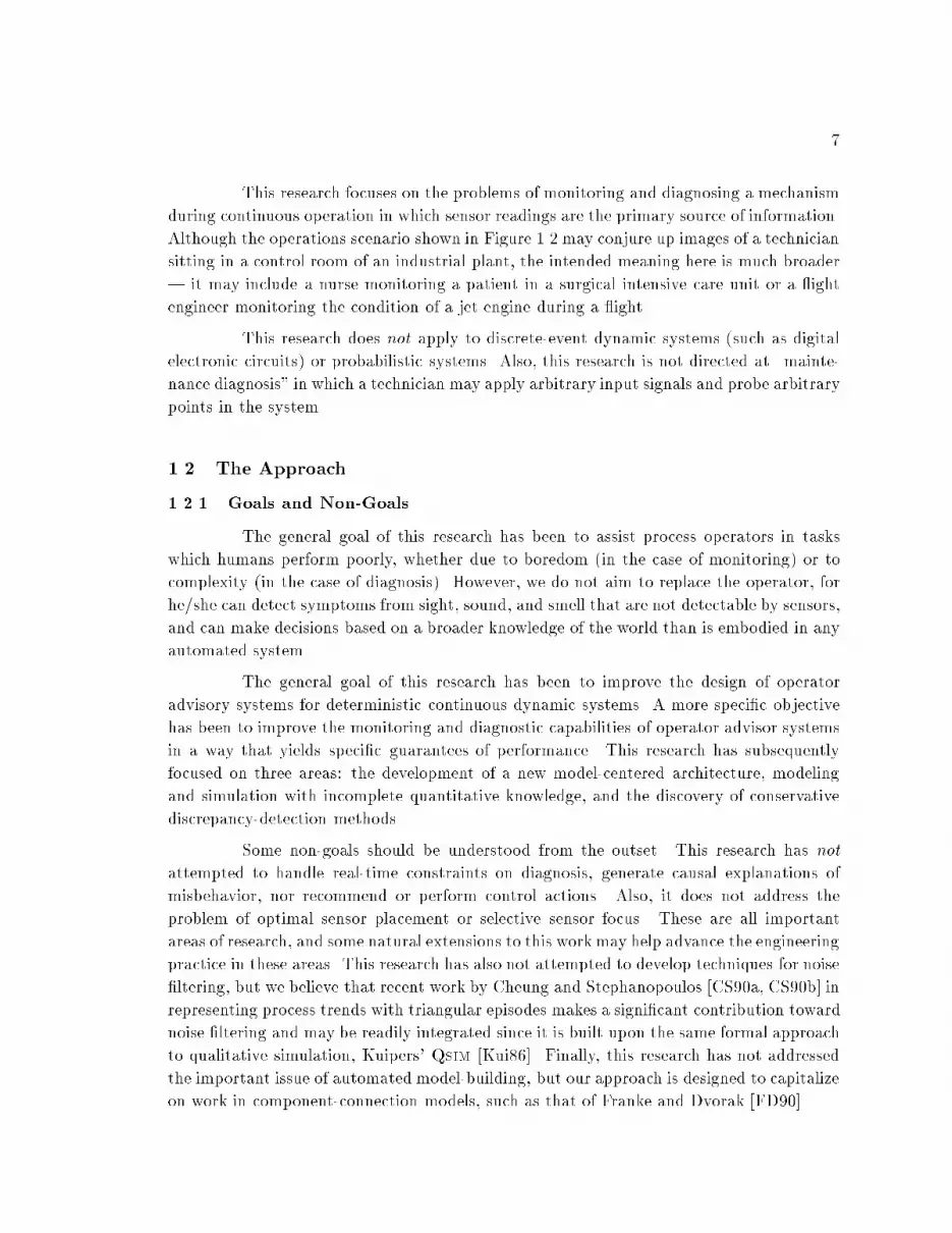
7This research focuses on the problems of monitoring and diagnosing a mechanismduring continuous operation in which sensor readings are the primary source of information.Although the operations scenario shown in Figure 1.2 may conjure up images of a techniciansitting in a control room of an industrial plant, the intended meaning here is much broader| it may include a nurse monitoring a patient in a surgical intensive care unit or a ightengineer monitoring the condition of a jet engine during a ight.This research does not apply to discrete-event dynamic systems (such as digitalelectronic circuits) or probabilistic systems. Also, this research is not directed at \mainte-nance diagnosis" in which a technician may apply arbitrary input signals and probe arbitrarypoints in the system.1.2 The Approach1.2.1 Goals and Non-GoalsThe general goal of this research has been to assist process operators in taskswhich humans perform poorly, whether due to boredom (in the case of monitoring) or tocomplexity (in the case of diagnosis). However, we do not aim to replace the operator, forhe/she can detect symptoms from sight, sound, and smell that are not detectable by sensors,and can make decisions based on a broader knowledge of the world than is embodied in anyautomated system.The general goal of this research has been to improve the design of operatoradvisory systems for deterministic continuous dynamic systems. A more speci�c objectivehas been to improve the monitoring and diagnostic capabilities of operator advisor systemsin a way that yields speci�c guarantees of performance. This research has subsequentlyfocused on three areas: the development of a new model-centered architecture, modelingand simulation with incomplete quantitative knowledge, and the discovery of conservativediscrepancy-detection methods.Some non-goals should be understood from the outset. This research has notattempted to handle real-time constraints on diagnosis, generate causal explanations ofmisbehavior, nor recommend or perform control actions. Also, it does not address theproblem of optimal sensor placement or selective sensor focus. These are all importantareas of research, and some natural extensions to this workmay help advance the engineeringpractice in these areas. This research has also not attempted to develop techniques for noise�ltering, but we believe that recent work by Cheung and Stephanopoulos [CS90a, CS90b] inrepresenting process trends with triangular episodes makes a signi�cant contribution towardnoise �ltering and may be readily integrated since it is built upon the same formal approachto qualitative simulation, Kuipers' Qsim [Kui86]. Finally, this research has not addressedthe important issue of automated model-building, but our approach is designed to capitalizeon work in component-connection models, such as that of Franke and Dvorak [FD90].

81.2.2 Diagnosis as Model Modi�cationThe key cognitive skill for a process operator is the formation of a mental modelthat not only accounts for current observations but also enables him/her to predict near-term behavior and predict the e�ect of possible control actions. This observation underliesour architecture for process monitoring, named Mimic [DK89, DK91]. The basic idea isquite simple: mimic the physical system with a predictive model, and when the systemchanges behavior due to a fault or repair, change the model accordingly so that it continuesto give accurate predictions of expected behavior.Intuitively, Mimic incrementally simulates a model of the physical system in stepwith incoming observations, making the state of the model track the state of the physicalsystem. This is the paradigm of \monitoring as model corroboration". (This is similar inprinciple to Kalman �ltering, but we will show in Chapter 2 that there are fundamentaldi�erences (and bene�ts) in our approach.) When observations disagree with predictions,model-based diagnosis determines the possible fault(s). When a fault is hypothesized, it isinjected into the model so that the model's predictions continue to track observations. Thisis the paradigm of \diagnosis as model modi�cation" or, as Simmons and Davis call it intheir Generate-Test-Debug approach [SD87], \debugging almost right models".1.2.3 Semiquantitative SimulationAny form of model-based reasoning is fundamentally empowered (and also lim-ited) by the type of model used. Mimic uses a qualitative-quantitative model, hereafterreferred to as a semiquantitative model, based on the work of Kuipers, Berleant, and Kay[Kui86, KB88, Ber91, Kay91]. Semiquantitative models provide a level of description thatis intermediate between abstract qualitative models and precise numerical models. Despitehaving less-than-precise information, semiquantitative models are capable of impressivepredictive power. For example, Widman showed that for a variety of cardiovascular disor-ders, a qualitative model with semiquantitative speci�cation for just a few key parameterswas able to correctly predict (qualitatively) the values of the measured variables [Wid89].Semi-quantitative modeling and simulation provides two key bene�ts for monitoring anddiagnosis:1. Reasoning with incomplete information. Most real-world information about mecha-nisms is imprecise, even when we know the exact design. A semiquantitative modelallows the modeler to express what is known without making inappropriate assump-tions or approximations, and simulation yields ranges rather than point values. Theseranges are guaranteed upper and lower bounds, enabling simple, unambiguous match-ing against physical measurements.2. Finding all behaviors automatically. Given incomplete information about a mech-anism, it is possible that the mechanism may exhibit more than one qualitatively

9PhysicalSystem ModelMonitoringDiagnosisAdvising-- -� -� ���� safety conditionsrecommended procedures� ���controlalarmsforewarningsFigure 1.4: In the Mimic architecture, three tasks mediate between the physical systemand its model.distinct behavior, such as a tank that either over ows or not. Semiquantitative simu-lation reveals all of the behaviors that are consistent with the incomplete information.This is especially important when trying to predict the e�ects of a fault or the e�ectsof interacting faults.1.2.4 Bene�tsA key bene�t of the model-based approach is that we can use the model as awindow into the physical system. Speci�cally, the model can be used to:� detect early deviations from expected behavior, much more quickly than with �xed-threshold alarms;� predict the values of unobserved variables to permit alarms or other inferences onunseen variables, and to assist the operator's understanding of process conditions;� discriminate among competing hypotheses by comparing the evolving e�ects of a faultagainst the predicted e�ects;� predict ahead in time, thus forewarning of near-term undesirable or hazardous condi-tions;� accumulate multiple faults over time and still give bounded behavior predictions forthe degraded system; and� predict the e�ect of proposed control actions to see if the control action will have thedesired e�ect | a valuable capability in complex systems.

101.2.5 ArchitectureThe basic architecture ofMimic is shown in Figure 1.4 in which a predictive modelmimics the physical system. Two tasks maintain the model. The monitoring task advancesthe state of the model in step with observations from the physical system, and detectsdiscrepancies between predictions and observations. The diagnosis task, upon getting adiscrepancy and hypothesizing a particular fault, injects that fault into the current modelto test it for consistency with current and future observations. Since a given misbehaviormight be caused by one of several faults, Mimic actually maintains a set of candidatemodels, called the tracking set. Each element of the tracking set represents a possiblecondition of the system, i.e., its state and faults.The end purpose of monitoring and diagnosis is advice | advice to the operatorabout what's happening and what to do about it. The role of the advising task is to apply theexpert knowledge of safety conditions, recommended operating procedures, and performanceobjectives to produce advice in the form of alarms, forewarnings, and recommended actions.The advising task is a major bene�ciary of the model-based approach in that the candidatemodels (and their tracked states) can provide a testbed for generating forewarnings and fortesting proposed control actions.1.3 ScopeThis section characterizes the scope of the dissertation in terms of assumptionsmade, modeling issues, and the implementation and evaluation of the ideas.1.3.1 AssumptionsThis section describes the assumptions made in the design and operation of themonitoring and diagnostic reasoning. These assumptions include:� The mechanism is deterministic in nature, not probabilistic.� The dynamics of the mechanism can be modeled with ordinary di�erential equations,at least as an approximation. Thus, the mechanism may have state and containfeedback.� The behavioral model of the mechanism is not invertible, in general. That is, themodel can predict from inputs to outputs, but not necessarily from outputs to inputs.� The mechanism can be described, both functionally and structurally, as a set of com-ponents and connections.� The behavioral model of a component should de�ne normal and fault modes which,collectively, cover the entire behavior space of the real component.

11� Automatic sensor readings are the primary source of information about the state ofthe mechanism. There is limited opportunity to measure other variables or to perturbinputs and observe e�ects.� Faults appear one-at-a-time with respect to the sampling rate for readings.� Diagnosis must be performed while the mechanism operates.� The mechanism may continue to operate in a degraded mode with multiple faults, sosingle-fault diagnosis is inadequate.� Sensor readings may contain random noise of known magnitude.� Incomplete knowledge of the mechanism does not imply random behavior within des-ignated bounds. A landmark value is constant; its exact value is known only within aspeci�ed range; it does not vary randomly within that range. Likewise, functional rela-tions are �xed, existing somewhere within the bounds speci�ed by envelope functions;the true relation does not vary within that space.1.3.2 Non-requirements� The Mimic approach is not restricted to near-equilibrium behavior of a mechanism.In fact, dynamic changes in behavior are a valuable source of clues for monitoring anddiagnosis.� Observations do not have to be periodic | they can vary in frequency.� The set of measured quantities does not have to be constant; it can change with everyset of readings. This permits focusing on a subset of sensors in one phase of operation,then shifting to other subsets during other phases. Sensors known to be bad can beexcluded at any time.� Manual observations can be supplied at any time; they do not have to synchronizedwith automatic observations.� Observations do not have to be supplied in temporal order. For example, in medicine,lab reports take much longer to arrive than direct monitor data applying to the sametime-point.1.3.3 Modeling IssuesTable 1.2 illustrates where this work stands with respect to several issues of mod-eling, simulation, fault detection, and diagnosis. Three issues require explanation:

12 Less Di�cult More Di�cult-�Discrete variables Continuous variablesQualitative information Numeric InformationDeterministic models Probabilistic modelsNo feedback Feedback presentNo internal state Device has internal stateApproximate predictions Guaranteed boundsSteady state Dynamic behaviorExpect complete data Tolerant of missing dataSingle fault Multiple faultsNormal model only Fault models usedAbsence of noise Presence of noisePersistent fault Intermittent faultO�ine diagnosis Operative diagnosisTable 1.2: Modeling issues addressed in this report. The black bars represent where Mimicstands.� On the issue of single-fault versus multiple-fault diagnosis, Mimic generates onlysingle-change hypotheses from a set of symptoms, but those changes are made tomodels that may already embody faults, so multiple-fault hypotheses are built incre-mentally over time, one fault at a time.� The e�ects of sensor noise are ignored in the initial presentation of discrepancy-detection methods in this report. Later, we show how random noise of known magni-tude weakens these discrepancy-detection methods, but does not cause false positives.� In our method of continuous monitoring, persistent faults (when diagnosed) are cor-roborated over time by a stream of compatible sensor readings. Although intermittentfaults cannot attain that kind of corroboration, the history of their being repeatedlyhypothesized and refuted can be collected as evidence of intermittent faults.1.3.4 ImplementationThe ideas for monitoring and operative diagnosis presented in this dissertation areimplemented in a computer program named Mimic, written in Common Lisp and testedon a Symbolics 3650 computer. Mimic builds upon four important pieces of research:Kuipers' Qsim for qualitative modeling and simulation [Kui86], Kuipers and Berleant's Q2for semiquantitative simulation with partial quantitative knowledge [KB88], Berleant's Q3

13for the technique of state insertion at measurement instants [Ber91], and Kay's Nsim fordynamic behavior envelopes [Kay91].1.3.5 Empirical EvaluationClaims made in this dissertation have been tested on a series of uid ow systemsof varying complexity. The uid ow systems were simulated in both normal and faultycon�gurations to produce simulated sensor readings. These readings were then given asinput toMimic to test its ability to detect and diagnose faults during continuous operation.Chapter 4 presents these results.1.4 ClaimsThis report describes a method for monitoring and diagnosis of process systemsbased on three foundational technologies: semi-quantitative simulation, measurement in-terpretation, and model-based diagnosis. Compared to existing methods based on �xed-threshold alarms, fault dictionaries, decision trees, and expert systems, several advantagesaccrue. The claims that follow divide into three principal categories: modeling and simula-tion, predictive monitoring, and discrepancy detection.1.4.1 Modeling & SimulationValidation. It is easier to acquire and validate a model of a mechanism than to acquireand validate a set of diagnostic rules. Although the latter approach typically yieldsan earlier demonstration of diagnostic capability, the knowledge base is never com-plete, there are no guarantees of diagnostic coverage, and performance degrades withmultiple faults.Expressive Power. Semiquantitative models provide greater expressive power for statesof incomplete knowledge than di�erential equations, and thus make it possible tobuild models without incorporating assumptions of linearity or speci�c values forincompletely known constants. The modeler can express incomplete knowledge of pa-rameter values and monotonic functional relationships (both linear and non-linear).By specifying conservative ranges for landmark values and conservative envelope func-tions for monotonic relationships, semiquantitative simulation generates guaranteedbounds for all state variables. This eliminates modeling approximations and compro-mises as a source of false positives during diagnosis.Soundness. Qualitative simulation generates all possible behaviors of the mechanism thatare consistent with the incomplete/imprecise knowledge. This is essential for dis-tinguishing misbehavior (which is due to a fault, and thus requires diagnosis) from

14 normal behavior, especially when there is more than one possible normal behavior.This eliminates \missing predictions" as a source of false positives during diagnosis.1.4.2 Predictive MonitoringOperating with Faults. Large complex systems almost always operate with faults, and itis not enough just to detect anomalous behavior. In order to continue safe operation,it is just as important to predict the e�ects of faults in order to forewarn of possibleundesirable states and to help determine appropriate control actions.Exploiting Dynamic Behavior. Observations of dynamic behavior over time enable strongermethods of fault detection and isolation than from a single snapshot of system out-put. This may seem obvious, but few fault detection schemes actually base theirconclusions on a sequence of sensor readings taken at di�erent times while the mech-anism operates. By tracking readings against model predictions, Mimic exploits thedynamic behavior of the mechanism to corroborate or refute hypotheses.Early Warning. By simulating ahead in time from the current state, an operator can beforewarned of nearby undesirable states that the plant might enter. Similarly, thee�ects of proposed control actions can be determined by simulating from the currentstate of every model being tracked.Updating the State. Sensor readings supply important information that can be used toupdate the state of the model. By unifying conservative reading ranges with conser-vative prediction ranges, the semiquantitative simulation continues to generate guar-anteed bounds using the latest available information.1.4.3 Discrepancy Detection & DiagnosisDynamic Alarm Thresholds. Incremental simulation of the semiquantitative model insynchrony with incoming sensor readings generates, in e�ect, dynamically changingalarm thresholds. Comparison of observations to model predictions permits earlierfault detection than with �xed-threshold alarms and eliminates false alarms duringperiods of signi�cant dynamic change, such as startup and shutdown.Temporal and Value Uncertainty. Because a given fault may manifest in di�erent waysunder di�erent circumstances, methods that identify faults based on speci�c subsetsof alarms or speci�cally-ordered sequences of alarms are insu�cient [Mal87]. SinceMimic matches observations against a branching-time description of predicted be-havior (a description that includes all valid orderings of events), and since it tests foroverlap of uncertain value ranges rather than whether or not an alarm is active, it candetect all of the valid ways in which a fault manifests.

15Hypothesis Discrimination. Discrimination among competing hypotheses is automaticinMimic. Whenever new readings arrive, every model in the tracking set is tested fordiscrepancies. Thus, incorrect hypotheses can be refuted either by the mechanism'snatural behavior or by its response to perturbation tests. (Mimic does not currentlygive advice on what inputs to perturb).Multiple-Fault Diagnosis Mimic supports continuous monitoring of a mechanism be-cause it updates the model as faults and repairs are diagnosed. This permits incre-mental creation of multiple-fault diagnoses over time and continues to provide validpredictions of behavior, even though multiple faults are present.1.4.4 SkepticismIt is reasonable, even wise, to be skeptical of new methods and the claims madefor them. This section attempts to answer some of the obvious questions that might occurto the skeptical reader.� Why this model-based approach? Does it have any fundamental theoretical advantagesover existing methods?Most of the advantages are a consequence of analytical redundancy | the use ofa process model to estimate the values of process state variables X(t) and processparameters �(t) based on measurable inputs U(t) and outputs Y (t). Compared torange-checking of output variables, Isermann [Ise89] notes several advantages to thisapproach:1. In terms of signal ow, the state variables X(t) or process parameters �(t) are,in many cases, closer to the process faults. Hence the process faults may bedetected earlier and localized more precisely than by range checking of Y (t).2. A process fault usually causes changes of several output variables �Yi(t) withdi�erent signs and dynamics. The model-based fault detection now takes intoaccount all these detailed changes, provides a data reduction and determines(theoretically) the state variable or process parameter which has been changeddirectly by the fault. Hence, it can be expected that a signi�cant change �Xj(t)or ��j(t) can be extracted and the fault detection selectivity will be improved.3. Closed loops generally compensate for changes �Yi(t) of the outputs by changingthe inputs U(t). Therefore deviations caused by faults cannot be recognized byrange-checking alone. Model-based fault detection methods automatically con-sider the relations between inputs and outputs and are therefore also applicableto closed-loop systems.4. Model-based fault detection methods need, in principle, only a few robust sensors.This lessens the need (in traditional methods) for numerous sensors that measure,

16 as directly as possible, all pertinent variables. The use of numerous sensors canbecome expensive.� If this is such a good idea, why hasn't it been done before?The overly simple answer is that it has been done before, though not in the sameway as described in this report. As we will see in Chapter 2, a few model-basedapproaches to operative diagnosis have arisen in the last few years, and they all lendsupport to the basic concept. However, these e�orts are too new to be in commonusage. Kitamura describes current practice this way:FDI [fault detection and isolation] techniques currently in use by the in-dustrial sector are conservative and traditional. Typical examples includecalibration against standards, limit checking, mutual consistency checking(majority voting), surveillance during periodic shutdown and perturbationtests before restart. [Kit89]Much of the engineering e�ort in the process industries has been directed not atfault detection but at automation and control, with many improvements in sensors,actuators, displays, feedforward and feedback control, and optimization. In describingthe current practice in alarm monitoring and protection, Isermann notes that:: : : the implemented methods are still rather simple and consist mainly oflimit-value checking of some easily available single signals. In contrast tothe �eld of control, methods based on modern dynamic systems theory arehardly applied. [Ise89, p. 254]� Surely there must be some drawbacks to your method, no?Yes. The bene�ts of our method come at a price: a substantial computational loadfrom simulating multiple models in real-time. Ten years ago this approach wouldhave been absurdly expensive and/or unreasonably slow, given the existing computertechnology. In the last ten years the price/performance ratio of computers has im-proved enormously and the emergence of qualitative and semiquantitative simulationtechnology has brought the approach into the realm of the possible. Of course, wedo not claim that the approach is practical in all cases. There are certainly existingprocesses and mechanisms whose complexity exceeds our current capabilities.There are other limitations which are discussed in Chapter 5. Some of these are dueto current limitations of the simulation technology; others concern issues that havealways been problematic, such as reasoning with noise and failing to detect subtlefaults.

17In ow ��x- ?� �� �� �� �� �� �� �� �� �� �� �� �� �� �� �� �? Tank AA� �� �� �� �� �� �� �� �� �� �� �� �� �� �� �� � Tank BB ?Out ow��level sensor�� ow sensor Di�erential equations:A0 = inflow � f(A)B0 = f(A) � g(B)

Figure 1.5: Two-tank cascade. Water ows into Tank-A at a measured rate, which thendrains into Tank-B, which drains to the outside. The level of water in Tank-B is measured,but the level in Tank-A is not.1.5 Example: A Two-Tank CascadeThis section illustratesMimic by example, demonstrating several important prop-erties and claims of this work. The intent here is to show what Mimic does, not necessarilyhow it does it. The ideas presented here will be developed more fully in Chapter 3. Webegin by describing a simple mechanism and show how it is modeled in Mimic. Then, weexamine what happens as a fault occurs, as Mimic monitors and diagnoses the mechanism.1.5.1 ModelingConsider the two-tank cascade shown in Figure 1.5. Water ows into the topof Tank-A at a measured rate; Tank-A drains into Tank-B, whose level is measured; andTank-B drains to the outside. If everything is working normally and a constant in ow isapplied, the level in each tank will reach equilibrium (assuming that no over ow occurs).Note that there is no sensor for the level in Tank-A; this state value is unmea-sured, so an operator has no way of knowing its level except through manual measurement.Likewise, there is no sensor on the out ow from Tank-B, so an operator cannot directlydetermine if out ow is normal.The scenario begins with both tanks empty. A constant in ow is applied and the

18Time, in seconds0 10 20 30 40 50 60 70 80 90 100 110 120010203040

5060Amount-Bin liters � � � � � � � � � � � � �Figure 1.6: Raw sensor readings from the two-tank cascade. The readings are a�ectedslightly by a partial obstruction in the drain of Tank-A at t = 50:01.tanks begin �lling toward equilibrium. Everything works normally until t = 50:01, at whichtime the drain of tank-A becomes partially clogged, reducing its ow rate by 20%. Notethat this fault does not alter the basic dynamics of the system; it still functions as a 2-tankcascade and the slight change in behavior is barely noticeable in the raw sensor readingsshown in Figure 1.6.The challenge, of course, is to detect and diagnose the fault. Using the paradigm of\monitoring as model corroboration", a semiquantitative model of the mechanism predictsthe mechanism's behavior, which is then compared to observations. Figure 1.7 shows themodel for the two-tank cascade, from which all predictions are made. Incomplete knowledgeof the physical two-tank cascade is expressed in this model as numeric ranges for landmarkvalues (see the initial-ranges clause). Incomplete knowledge can also take the form ofenvelope functions for monotonic relations, though none are required in this example.1.5.2 SimulationFigure 1.8 shows the actual behavior of our faulty two-tank cascade overlaidon the predicted behavior of a normal two-tank cascade. The short vertical lines showthe range of each reading. Sensors are not exact measuring devices, but are designed toyield a measurement correct to within a speci�ed tolerance, such as �3%. Thus, the sensorreading ranges result from applying the tolerance to the actual reading value. The rectanglesshow the predicted range of a variable (there is no temporal range in the prediction; therectangle has width only for display purposes). Here, the range results from the the partial

19(define-QDE TWO-TANK-CASCADE(quantity-spaces(Inflow-A (0 normal inf) "flow(out->A)")(Amount-A (0 full) "amount(A)")(Outflow-A (0 max) "flow(A->B)")(Netflow-A (minf 0 inf) "d amount(A)")(Amount-B (0 full) "amount(B)")(Outflow-B (0 max) "flow(B->out)")(Netflow-B (minf 0 inf) "d amount(B)" )(Drain-A (0 vlo lo normal))(Drain-B (0 vlo lo normal)))(constraints((MULT Amount-A Drain-A Outflow-A) (full normal max))((ADD Outflow-A Netflow-A Inflow-A))((D/DT Amount-A Netflow-A))((MULT Amount-B Drain-B Outflow-B) (full normal max))((ADD Outflow-B Netflow-B Outflow-A)) ; Outflow-A = Inflow-B((D/DT Amount-B Netflow-B)))(independent Inflow-A Drain-A Drain-B)(history Amount-A Amount-B)(unreachable-values(netflow-a minf inf) (netflow-b minf inf) (inflow-a inf))(initial-ranges((Inflow-A normal) (3.01 3.19)) ; +/- 3% of 3.1((Amount-A full) (99 101))((Amount-B full) (99 101))((Time T0) (0 0))((Drain-A normal) (0.0485 0.0515)) ; +/- 3% of .05((Drain-B normal) (0.0485 0.0515)) ; +/- 3% of .05((Drain-A lo) (0.020 0.0485))((Drain-B lo) (0.020 0.0485))((Drain-A vlo) (0 0.020))((Drain-B vlo) (0 0.020))))Figure 1.7: Semiquantitative model of the two-tank cascade. Incomplete quantitative knowl-edge is expressed in the form of ranges for landmark values, in initial-ranges. Whenmodels contain monotonic function constraints (this one does not), incomplete knowledgecan also be expressed in the form of envelope functions.

20Time, in seconds0 10 20 30 40 50 60 70 80 90 100 110 120010203040

5060Amount-Bin liters = predicted range= reading rangeFigure 1.8: Sensor readings and fault-free predictions from the two-tank cascade. Thesimple limit test fails to detect any discrepancy between observations and predictions.quantitative knowledge in the model; the semiquantitative simulation methods generateupper and lower bounds for each variable.The small \kink" in the predicted range at t = 70 is a consequence a unifyingreadings with predictions on each cycle. Speci�cally, the small intersection at t = 60properly altered the next prediction for t = 70, narrowing its range and lowering its value.1.5.3 Discrepancy DetectionThis dissertation will describe four methods for detecting a fault by detectingincompatibilities between predictions and observations. The �rst and most obvious methodis to test for overlap between a reading range and its predicted range. As Figure 1.8 showsfor this example, there is indeed overlap for every reading, so no fault is detected with thismethod. Note that at t = 60 (the �rst reading after the fault) the overlap is very small,but quickly returns to \normal" within about 30 seconds. This example illustrates twoimportant problems: for systems having compensatory response, some faults can only bedetected in their earliest moments, and simple range-checking is not always sensitive enoughto detect abnormal perturbations in behavior.Mimic uses three other methods of discrepancy detection, to be described laterin Chapter 3. In this particular case, the fault is detected as an analytic discrepancy,meaning that the assumptions, predictions, and observations are mutually incompatible,even though they are individually compatible. In this case, the analytic discrepancy wasdiscovered when the range of overlap for Amount-B at t = 60 was asserted back to the model

21variable mode value fault type probabilityDrain-A normal nil .95lo abrupt .04vlo abrupt .01Drain-B normal nil .95lo abrupt .04vlo abrupt .01Table 1.3: Some alternate operating modes in the two-tank cascade.and its e�ects propagated through the model; it was inconsistent for the upper bound ofAmount-B to be so low (47.30) given the predicted range for Amount-A ([55.79 62.19]) andthe assumed ranges for Drain-A ([.485 .515]) and Drain-B ([.485 .515]). This demonstratesan important strength of the model-based approach in general and the semiquantitativemethods in particular: by using constraint-like descriptions, the model can be used notonly to predict behavior from an initial state, but also to check the mutual consistency ofa set of readings that otherwise appear to agree with the model's predictions.1.5.4 Hypothesis GenerationUp until this time the tracking set has contained only the fault-free model. Thediscrepancy with Amount-B at t = 60 removes that model from the tracking set and initiateshypothesis generation via dependency tracing through a structural model of the mechanism.The structural model, shown in Figure 1.9, is essentially a declarative description of themechanism's components and connections, shown graphically in Figure 1.5. By tracingupstream from the site of the discrepancy (Amount-B), Mimic identi�es the componentsand parameters whose malfunction could have caused the discrepancy. In this case, thesuspects are Amount-B-sensor, Tank-B, Drain-B, Tank-A, Drain-A, and Inflow-A. Tokeep this example simple, we'll focus on two suspects: Drain-A and Drain-B.Having identi�ed the suspects, Mimic consults a table of alternate operatingmodes for each suspect in order to generate modi�cations of the current model. Table 1.3shows the possible mode values for Drain-A and Drain-B. These values are present in thesemiquantitative model (�gure 1.7) and can therefore be used to instantiate a modi�edversion of the current model. The fault type can be either abrupt or drift. All abruptfaults are always hypothesized since these faults can occur at any time. For drift faults,however, only the one or two drift fault values adjacent to the current value are hypothesized(because the fault represents drift from the normal value). The a priori probability of eachmode is used in ranking hypotheses (and as we will see in Chapter 3, hypotheses can alsobe ranked by age and by degree-of-match).

22Component de�nitions:(COMPONENTS(INFLOW-SENSOR(flow-in input icon1)(measured output i-obs))(TANK-A(inlet input icon1)(outlet 2-way tocon1)(drainrate input dr1))(TANK-B(inlet input tocon1)(outlet 2-way tocon2)(drainrate input dr2)(amount output acon))(AMOUNT-SENSOR(amount-in input acon)(measured output a-obs)))

Parameter to connection mappings.(PARAMETERS(Inflow-A icon1)(Drain-A dr1)(Drain-B dr2))Variable to connection mappings.(VARIABLES(Amount-B a-obs)(Inflow-obs i-obs))Figure 1.9: Structural model of the two-tank cascade. This model is used by the dependencytracer to trace upstream from the site of a discrepancy to identify all the components andparameters whose malfunction could have caused the discrepancy.

23Time, in seconds0 10 20 30 40 50 60 70 80 90 100 110 120010203040

5060Amount-Bin liters = predicted range= reading rangeFigure 1.10: Predictions for Amount-B showing agreement with the hypothesis that Drain-Ais partially clogged .1.5.5 Hypothesis TestingMimic assumes that faults occur one-at-a-time with respect to the sampling ratefor readings, so it hypothesizes single-changes to the existing model. One model is createdfor Drain-A = lo, another for Drain-B = lo. For each new model, Mimic attempts toinitialize it using the hypothesized modes, current readings, and latest predictions. Sincethere may have been some time elapsed between the moment that the fault occurred and themoment that it manifested as a symptom,Mimic performs a procedure termed resimulation.This procedure reattempts initialization at successively earlier reading moments, simulatingthe model up to the current time and quantifying the similarity between predictions andreadings. The initialization time that yields the strongest similarity during this hill-climbingsearch is taken as the probable time of failure. Resimulation is essential because it revisesthe values of unobserved state variables to re ect the e�ects of an earlier fault. Withoutresimulation, future predictions of behavior would be incorrect.In the case of Drain-B = lo, the model fails to initialize. Speci�cally, every at-tempt to initialize it results in an inconsistency, meaning that the fault hypothesis embodiedin this model is immediately falsi�able. In general, though, some incorrect fault models willinitialize and be carried in the tracking set until future readings show it to be incompatible.In the case of Drain-A = lo, the model initializes successfully and resimulation yields thetime-of-failure to be t = 50. Figure 1.10 shows the predicted ranges for this model. Thewider predicted ranges for this model versus the normal model are a consequence of thewider range for lo ([.02 .0485]) versus the narrow range for normal ([.0485 .0515]).

24Time, in seconds0 10 20 30 40 50 60 70 80 90 100 110 120010203040

5060Amount-Ain liters 70 Tank-A over ow threshold= predicted rangeFigure 1.11: Over ow prediction for Tank-A. The level in Tank-A is not observable and canonly be inferred using the model. Given the hypothesis that Drain-A is partially clogged,prediction shows that over ow can occur as early as t = 91:61.5.6 ForewarningFor monitoring, an important advantage of the model-based approach is thatit predicts ranges for unobserved state variables. In our two-tank cascade, there is nolevel sensor for Tank-A, so there is no way for the operator to know the amount in Tank-A.However, by simulating in parallel with the mechanism a model that embodies all diagnosedfaults, the operator can be kept informed of the values of unobserved variables. Furthermore,by simulating the model ahead in time, the operator can be forewarned of future undesirablestates. Figure 1.11 shows the predicted ranges for the amount in Tank-A. Let's assume thatthe capacity of Tank-A is 65 liters, as shown with the dashed line. After the diagnosis ofDrain-A = lo at t = 60 (and the corresponding change in the model), predictions showthat Tank-A could over ow as early as t = 91:6. In general, the tracking set may containmore than one model, so forewarnings are based on the earliest warnings from the set ofmodels.1.5.7 SummaryLet's summarize what has happened. Mimic began tracking the fault-free modelat t = 0, and as each new set of readings appeared, it tested for discrepancies betweenpredictions and readings using four distinct methods. It also uni�ed predictions with obser-

25vations, yielding tighter predictions of future behavior. At t = 50:01 the drain of Tank-Abecame partially obstructed, and the fault was detected at the next readings at t = 60 as ananalytic discrepancy. Two fault hypotheses were formed and instantiated as modi�cationsof the current fault-free model. One hypothesis was immediately discarded because it failedto initialize, but the other initialized successfully and was resimulated from successivelyearlier moments, localizing the time-of-failure to be t = 50. This adjusted the unobservedstate values (Amount-A, in this case) to re ect the e�ects of the fault between t = 50 andt = 60. Subsequent predictions from the fault model were corroborated by the readings andalso used to forewarn the operator of a possible Tank-A over ow at t = 91:6.1.6 Guide to the DissertationThis dissertation is organized into �ve chapters. This chapter has introduced theproblem of monitoring dynamic systems and brie y demonstrated a new approach and itsbene�ts. Chapter 2 describes existing methods for monitoring and diagnosis, showing theirsimilarities and di�erences with the Mimic approach. Chapter 3 presents our contributionsto the theory of fault detection in dynamic systems and to the engineering design of au-tomated process monitoring. Chapter 4 presents results from an implementation of thistheory, describing the diagnostic programMimic and its performance on a set of uid- owproblems. Chapter 5 discusses the implications of this work and presents ideas for futureresearch.1.7 TerminologyThis section de�nes some terms used throughout this report.abrupt fault An abrupt fault has a sudden e�ect on the mechanism, such as the suddenfailure of a pump. Sometimes called cataleptic fault. Contrast with incipient fault.accommodation As part of the task ofmonitoring, accommodation of a faulty mechanismto normal operation requires correcting or compensating for the e�ects of a fault.analytical redundancy The term analytical redundancy, also called functional redun-dancy, refers to the fault detection method of using known analytical relationshipsamong sets of signals, such as outputs from dissimilar sensors, to check for mutualconsistency. The method (and the phrase) emerged as an alternative to the earlierpractice of hardware redundancy, wherein 3 or 4 identical sensors and voting logic areused for fault tolerance.attainable envisionment An attainable envisionment of a mechanism is the set of allqualitatively distinct behaviors possible from a given initial state. As generated byQsim, an attainable envisionment is a tree whose root node is the initial state and

26 where each directed link represents a transition to a valid successor state node. Whena state has more than one valid successor state, the resulting branch indicates aqualitative distinction in behavior. Any single path through the tree is a behavior,represented as a sequence of states. Contrast with total envisionment.behavior The observed behavior of mechanism is its sequence of sensor readings. Thepredicted behavior of a mechanism is a sequence of states in which each state containsvalues for all state variables and is justi�ed as a valid successor of the preceding state.See attainable envisionment.candidate A candidate is a model of the mechanism whose predictions are compatiblewith the current readings. A candidate, therefore, embodies a hypothesis about theoperating mode of each component, whether normal or faulty.candidate generation When discrepancies are found between the observed behavior andthe behavior predicted by the mechanism model, candidate generation produces oneor more possible explanations for those discrepancies in the form of modi�cations ofthe mechanism model.component A component is any piece of a mechanism, such as the level sensor in the two-tank cascade. The concept of a component is hierarchical; an entire steam turbinemay be regarded as a component of a larger mechanism, just as the fan blades arecomponents of the steam turbine.consequential fault A consequential fault, sometimes called an induced fault, is a defectcaused by an earlier fault. For example, if a pump motor fails in a way that causes it todraw an excessive amount of current, that may cause a fuse to blow as a consequenceof the excessive current. Some consequential faults propagate rapidly, creating theappearance of multiple simultaneous failures.defect A defect is a fault whose cause is internal to the mechanism, such as a compo-nent that is broken or out of calibration, or a connection that is severed or blocked.Diagnosis of a defect calls for repair of the mechanism. Contrast with disturbance.diagnosis A diagnosis is a plausible explanation for an unexpected behavior. Note that be-havior which is undesirable but predictable (such as subjecting a fault-free mechanismto a known overload) does not need to be diagnosed.discrepancy A discrepancy is an incompatibility between an observation (whether director derived) and a prediction. For example, if the predicted range for x is [2.1 2.4] andthe reading range is [2.5 2.6], then there is a discrepancy. A discrepancy that cannotbe resolved (such as by advancing the simulation) becomes a symptom.

27discrepancy detection Sometimes called fault detection, discrepancy detection is thetask of detecting misbehavior in the mechanism, as in recognizing when observedbehavior di�ers from expected behavior. It does not include identifying the cause (seefault isolation).discrimination As diagnosis proceeds there are usually several candidates that could ex-plain all the discrepancies. Discrimination is the process of gathering additional ob-servations from the mechanism in order to refute incorrect candidates through dis-crepancy detection.disturbance A disturbance is a fault whose cause is external to the mechanism, such as anabnormally high ambient temperature. Diagnosis of a disturbance calls for changes inenvironmental conditions rather than repairs to the mechanism. Contrast with defect.drift fault Same as incipient fault.false negative In fault detection, a false negative is the failure to detect a fault when oneis present. There are several fundamental reasons why a fault may be undetectable:the fault may be masked by a redundant spare; the fault may not be exposed inthe current operating mode, such as a burned-out light bulb with no power applied;the fault may not have a�ected any sensor (yet), or the a�ected sensor may itself bedefective; the fault manifestations may be buried in noise or may simply be too smallto distinguish from normal behavior.false positive In fault detection, a false positive (sometimes called a false alarm) is the\detection" of a fault when none is present. This can occur in at least three ways: whenreadings from the fault-free mechanism exceed a detection threshold, whether due tonoise or to acceptable variations within the mechanism; when thresholds designed forsteady-state operation are triggered during other phases of operation, such as startupand shutdown; and when a normal-but-infrequent behavior is neglected in thresholddesign, such as the opening of a pressure-relief valve.fault A fault is an abnormality in a mechanism or its environment. A fault is either adefect in a component or a disturbance in an exogenous variable or parameter. Theonset of a fault may be abrupt (abrupt fault) or gradual (incipient fault). A faultdoes not necessarily manifest in a symptom; the fault may not be exposed in certainoperating modes (such as a burned-out light bulb with no power applied) or its e�ectsmay be masked by a redundant spare.fault detection Same as discrepancy detection.fault isolation Fault isolation is the task of localizing a fault to a speci�c component orexternal input of the mechanism.

28�delity A model has �delity when it does not support incorrect predictions about themechanism. Compare with precision.functional redundancy Same as analytical redundancy.incipient fault A small or slowly developing fault is often called an incipient or evolvingor drift fault. Such faults may be due to aging or drift. Contrast with abrupt fault.Kalman �lter The Kalman �lter can be thought of as a processor that produces threetypes of output, given a noisy measurement sequence and associated models. First, itcan be thought of as a state estimator or reconstructor, i.e., it reconstructs estimatesof the state x(t) from noisy measurements y(t). Second, the Kalman estimator canbe thought of as a measurement �lter which accepts the noisy sequence fy(t)g asinput and produces a �ltered measurement sequence fy(tjt)g. Third, the �lter canbe thought of as a whitening �lter that accepts noisy correlated measurements fy(t)gand produces uncorrelated or white-equivalent measurements fe(t)g, the innovationsequence. [Can88, p. 321]mechanism A mechanism is a physical system which has structure and whose behaviorand state is the object of operational attention. Speci�c application domains mayrefer to the mechanism as a \device" or \process" or \system" or \patient".mode A component may operate in one of several modes, such as a thermostat that iseither on or o�. A mode variable may change value automatically as speci�ed in themodel (such as when a thermostat changes from o� to on) or as a result of a faulthypothesis (such as a thermostat that is \stuck on").model In this report the noun model refers to an abstraction of the mechanism, usuallyas a model of structure (components and connections) or behavior (semiquantitativeconstraint equations). (This is di�erent from its meaning in logic in which an in-terpretation I is said to be a model of a sentence � if I satis�es � for all variableassignments.)monitoring Monitoring is the continuous real-time process of detecting anomalous behav-ior, tracking the e�ects of a fault, and determining control actions to continue safeoperation in the presence of faults. Monitoring includes discrepancy detection, faultisolation, and accommodation.operator An operator is a human responsible for the safe and e�cient operation of amechanism. An operator's duties include monitoring the mechanism's behavior, di-agnosing the possible cause(s) of misbehavior, and taking corrective action to controlthe mechanism.

29parameter A parameter is a �xed quantity in a mechanism or, analogously, a constant in amodel of the mechanism. For example, the electrical resistance of a heating element isa parameter. Some defects are termed \parameter faults" because a parameter valuehas changed to an abnormal value.precision A model has precision to the extent that the predictions it makes are strongenough to be falsi�able by observations of the actual mechanism. Compare with�delity.repair A repair is a change from faulty to normal. When talking about the mechanism,a repair means the disappearance of a fault, whether due to a �x or to spontaneousremission. When talking about a hypothesis, a repair is a change from a fault modelof some component to its normal model.structure The structure of a mechanism is its components and connections, usually rep-resented as a directed graph in which the vertices are components and the edges areconnections.suspect A suspect is a component or parameter of the mechanism whose malfunction couldaccount for a discrepancy. If the suspect is an input parameter of the mechanism, thenit identi�es a possible disturbance; if it is a component, then it identi�es a possibledefect.symptom A symptom is an incompatibility with expected behavior, as detected in anunresolved discrepancy. A symptom is a manifestation of one or more changes (faultsor repairs) in the assumed condition of the mechanism. There may be an arbitrarilylong time between the occurrence of a fault/repair and its manifestation as a symptom.Whether or not a symptom is detectable depends on the size of the perturbation, theprecision of the model, the placement and precision of sensors, the magnitude of noise,and the sensitivity of the discrepancy-detection methods.total envisionment A total envisionment is a representation of all behaviors inherent insome mechanism in some con�guration, for each possible initial state. Represented as agraph, each node is a possible state of the mechanism and each directed link representsa valid transition from one state to another. In design analysis, for example, a totalenvisionment can reveal whether there is any initial state that does not lead to thedesired behavior. Contrast with attainable envisionment.tracking set The tracking set is the set of models (and their states) that are being trackedat any given time. Candidate generation adds models to the tracking set; discrepancydetection removes models.

30

Chapter 2Related WorkThere is a vast amount of work published on the subjects of monitoring anddiagnosis | too much to cover adequately in the space of this chapter. Our objective hereis to focus on the most relevant work, which divides into three categories:� symptom-based approaches that have been applied in the past but have been rejectedin this research because of inherent limitations;� model-based approaches that deserve close comparison because of similarities toMimic;and� other research results that have been in uential in the design of Mimic.2.1 Symptom-Based ApproachesMuch of the literature on diagnosis describes methods of associational inferencethat relate symptoms directly to faults. This encompasses representations based on rules,decision trees, and fault dictionaries. Each of these methods has proven its worth in variousdiagnostic settings, but in the case of operative diagnosis, several limitations are shared tovarying degrees:� failure to exploit clues from the time-varying behavior of the mechanism;� limited ability to diagnose multiple faults;� no predictive power to reveal possible future e�ects of a fault or e�ects of compensatingcontrol actions.The following sections examine each of the three methods in more detail, describing speci�climitations for operative diagnosis.2.1.1 Rule-Based SystemsTraditional rule-based systems have been built by accumulating the experience ofexpert troubleshooters in the form of empirical associations | rules that associate symptomswith underlying faults [DH88]. The problem-solving strategy may be either data-driven31

32(forward-chaining) or goal-driven (backward-chaining) or a combination of both. The data-driven approach is most appropriate for the task of monitoring, where it is important torespond quickly to new readings and alarms, combining multiple pieces of evidence to assessthe likelihood and severity of a problem, providing the operator with an interpretation ofa possibly overwhelming amount of data. The goal-driven approach is most often usedin diagnosis where the goal is a diagnostic conclusion and the rules, through backwardchaining, seek supporting evidence for various intermediate and �nal conclusions.The rule-based approach became popular, in part, because it permitted easyconstruction of expert systems by encoding heuristic knowledge in the form of if-then andwhen-then rules. The technology permitted rather quick and impressive demonstrationsof diagnostic capability and promised that diagnostic coverage could be increased just byadding more rules. However, several limitations became apparent as rule-based systemswere applied to increasingly large and complex mechanisms:� The encoded knowledge is based on experience with the mechanism, and it may takea long time to accumulate the necessary experience before diagnostic patterns emerge.This is a particular problem for newly designed mechanisms.� The task of knowledge engineering (i.e., extracting experiential knowledge from ex-perts and representing it in an appropriate form) is widely acknowledged to be thebottleneck in the building of new expert systems. As the mechanism under studybecomes larger and more complex, so too does the task of knowledge engineering.� There is no guarantee that novel faults (i.e., faults not speci�cally considered duringknowledge engineering) will be detected, much less diagnosed. Likewise, two faultsthat are individually diagnosable may interact in ways that mask any or all of thesymptoms. A rule-based system may be validated on a set of test cases but still haveimportant gaps in its knowledge base.� Rule-based systems have little, if any, predictive power. They cannot show whatwill happen if a fault is left unrepaired or what will happen if some control action istaken to compensate. Similarly, it is di�cult to express and reason about temporalinformation, such as the evolution of symptoms of a fault.� Failed sensors is a problem for rule-based systems. If a rule depends on evidencefrom N sensors, it requires 2N � 1 rules to handle all combinations of failed sensors(assuming that none of the sensors are redundant).� Di�erent phases of operation (such as startup, normal operation, and shutdown) typ-ically require separate sets of rules because of large di�erences in system behavior.� Small changes in the design of the mechanism may necessitate revisions in a large partof the rule-base.

332.1.2 Fault DictionariesA fault dictionary is a list of symptom/fault pairs, indexed by symptom. Thedictionary is built by simulating a model of the mechanism for every kind and combinationof faults anticipated. Each simulation generates a description of how the entire mechanismwould behave if a speci�c component were broken in a speci�c way. The result is a list offault/symptom pairs, which is then inverted to form a dictionary of symptom/fault pairs.To an extent, fault dictionaries overcome some of the limitations associated withrule-based systems: the dictionary does not depend on experience (so it can be madeavailable quickly), it can expose the e�ects of interacting faults, it can be regeneratedmechanically if the design changes, and it is likely to cover more fault scenarios because ofits systematic (though not exhaustive) treatment of the kinds and combinations of faults.The idea behind fault dictionaries | systematic generation of symptom/faultassociations | is good, but the technique has some practical limitations:� To make the simulation task tractable, only the most likely failure modes of eachcomponent are considered, and simulation of combination faults is severely limited.Thus, the approach usually cannot guarantee detection of all single-faults, let alonemultiple faults.� In the case of continuous-variable dynamic systems, simulations must be performedwith nominal values, yielding symptoms that are only an approximation of whatmight be observed. Thus, there is an \approximate-matching problem" in deciding ifa mechanism actually exhibits a given set of symptoms.� In a single entry of the dictionary the symptoms are essentially a predicate on asnapshot of the observable variables of the mechanism. This kind of matching failsto exploit temporal continuity in the evolving manifestations of a fault (which can bevital in getting the right hypothesis and refuting incorrect hypotheses).2.1.3 Decision TreesDecision trees provide a guide to diagnosis in that they write down the sequenceof tests leading to a diagnostic conclusion. Decision trees used in process industries aretypically built manually by engineers using detailed knowledge of the plant's design and itsknown failure modes. Such decision trees may contain not only diagnostic steps but alsorecommended control actions to ensure plant safety, even before a diagnostic conclusion isreached. As Davis and Hamscher [DH88] point out, the simplicity and e�ciency that is astrength of decision trees is also an important weakness: they are a way of writing down adiagnostic strategy, but o�er no indication of the knowledge used to justify that strategy.Decision trees thus lack \transparency" and are therefore di�cult to update (a small change

34to the mechanism may require a major restructuring of the tree). Like the other methods,decision trees have no predictive power to reveal the propagating e�ects of a fault.2.2 Model-Based ApproachesModel-based diagnostic reasoning can be viewed as an interaction between pre-diction and observation [DH88]. By using a behavioral model of the mechanism and viewingmisbehavior as anything other than what the model predicts, model-based diagnosis coversa broader collection of faults than symptom-based approaches. By matching against pre-dictions rather than symptomatic patterns, model-based diagnosis also avoids combinatoricproblems in handling failed sensors and data that is for any reason unavailable [Sca89].Another virtue of the technique is its device-independence, enabling reasoning about a sys-tem as soon as a structural model and behavioral model is available. Also, constraint-likedescriptions of the mechanism allow both simulating its behavior and making inferencesabout the values of unmeasured variables.The principles of model-based diagnosis are well understood; the diversity of workin this �eld owes largely to the many types of models that can be used within this frame-work, representing many di�erent degrees of abstraction. Our coverage of this �eld thereforeattempts to be representative rather than exhaustive. In the �rst three sections, Mimic iscompared to three other monitoring systems: Premon, Draphys, and Midas. Interest-ingly, these four research e�orts arose at about the same time, apparently independently.The similarities are encouraging in that they lend support to a common set of concepts,and the di�erences are enlightening in terms of the distinct types and capabilities of modelsused.2.2.1 PREMON/SELMON (Doyle et al.)The concept of predictive monitoring is the inspiration behind Premon, a fo-cused context-sensitive approach to monitoring [DSA87, DSA89] and its successor Selmon[DF91]. Both Mimic and Premon take the position that a predictive simulation model isrequired for e�ective monitoring of a dynamic physical system. Both collect measurementsfrom sensors and interpret that data with respect to predictions from the model. Both usemodels that are fundamentally qualitative but may be augmented with partial quantitativeinformation.Because of di�erent objectives, Mimic and Premon turn out to be largely com-plementary. Premon focuses on two issues: how to adjust alarm thresholds to re ectthe changing operating context of the system, and how to utilize sensors selectively so thatnominal operation can be veri�ed reliably without processing a prohibitive amount of sensordata. Both issues depend on predicting the expected behavior of the system in a dynamicoperating context, and require only the single fault-free model of the physical system.

35#" !PhysicalSystem#" !DeviceModel

SensorInterpreterCausalSimulator SensorPlanner-readings ?alarms6systemstate-model

������������knownevents �?� �causal dependencies,predicted events

sensor plan,expected valuesFigure 2.1: Architecture of Premon.Premon uses a predict-plan-sense cycle using a causal simulator, a sensor plan-ner, and a sensor interpreter, as shown in Figure 2.1. The causal simulator takes as input acausal model of the system to be monitored, and a set of events describing the initial stateof the system and possibly some future scheduled events. The causal simulator produces asoutput a set of predicted events and a graph of causal dependencies among those events.The sensor planner takes as input that causal dependency graph and determines whichsubset of the predicted events should be veri�ed. Those events are then passed on to thesensor interpreter. The interpreter compares expected values as predicted by the causalsimulator with actual sensor readings. Alarms are raised when discrepancies occur. Finally,the most recent sensor readings are passed back to the causal simulator to contribute toanother predict-plan-sense cycle.In contrast, Mimic focuses on two di�erent issues: how to extract the mostinformation possible from observations and predictions in order to detect discrepancies, andhow to continue monitoring and continue safe operation in the presence of faults. WherePremon uses a single fault-free model, Mimic necessarily uses fault models in order topredict the e�ects of faults. Mimic uses all available sensor data; it does not focus on asubset as Premon and Selmon do.

362.2.2 DRAPHYS (Abbott)Of all the related work in this chapter, Abbott's work on operative diagnosis[Abb90] is the most similar in objective toMimic, but di�ers substantially in several aspects.Draphys uses three types of models: a numerical simulation model (as a pre-cise behavioral model), a component hierarchy (as a model of mechanism structure), anddirected graph of the paths of propagation (as an abstract, qualitative model of behavior).The numerical simulation model of the fault-free mechanism is used to generate predictionsof behavior. When a prediction di�ers signi�cantly from observations, Draphys generatesa qualitative symptom containing: the qualitative value of the sensor reading as positive(+), zero (0), or negative (�); the status of the reading compared to its prediction, as highor low; the qualitative value of the derivative, and the status of the derivative comparedto its predicted value. Abbott acknowledges that it is di�cult to determine when a signaldi�ers \signi�cantly" from its expected value. Two major reasons for this are sensor noiseand lack of model �delity. The approach in Draphys errs in favor of false positives.The next step is to localize the symptoms to a subsystem of the mechanism,which is done by inspecting the component hierarchy. For example, if all of the symptoms(e.g., Pressure-N2 and Fuel-flow) come from components within a common subsystem(such as Engine-B), then Draphys localizes the problem to the subsystem Engine-B. Eachcomponent in the engine subsystem is then proposed as the source of the fault.For each proposed faulty component, Draphys propagates the fault through thedirected graph of paths of propagation. Nodes in the graph represent components, and linksrepresent dependencies among the components. The links indicate only that one componentmay a�ect another; it does not say how soon, or in what direction, or in what amount.Draphys propagates the e�ect of the proposed fault to other components and checks thereal mechanism to see if symptoms have appeared at the predicted places. Propagationhalts on any path where the a�ected component is not yet symptomatic. Draphys retainshypotheses that account for all symptoms, extending the propagation as new symptomsappear. If a hypothesis cannot account for a symptom, the hypothesis is discarded. Theconcept of propagating the e�ects of a fault is exactly analogous to tracking the propagationbehavior of diseases in a causal network, as done in Casnet [WKAS78]. (Casnet isarguably the �rst major model-based reasoning program.)Draphys was evaluated on eight civil transport aircraft accident cases, and cor-rectly diagnosed seven of them. In explaining why Draphys worked so well, Abbott creditstwo aspects of her approach, both of which are also embodied in Mimic. The �rst creditgoes to the rapid detection of discrepancies by comparing sensor readings to expected valuescomputed from a numerical simulation model. In contrast to �xed-threshold alarms, thisapproach yields earlier detection of small deviations. The second credit goes to the model offault propagation which enables e�cient tracking of symptoms against hypothesis-speci�cexpectations.

37Although not a particular emphasis of her work, Draphys provides a separatemethod for diagnosis of well-known, commonly occurring faults. The approach embedstemporal predicates into a rule-based system using the temporal functions of Allen [All84](e.g., Starts, Meets, Overlaps, etc.). For example, one of the rules is triggered whenvariables EPR, EGT, and Fuel ow are uctuating simultaneously, and EPR uctuating isfollowed immediately by EPR decreasing, and EGT uctuating is followed immediately byEGT decreasing. This is essentially a fault signature expressed as a sequence of obser-vations, and allows for quick recognition of speci�c patterns. Although this approach iseasy to understand, Abbott points out two speci�c limitations. First, it is di�cult to getknowledge about faults and their propagation behavior at this level of detail. In particular,it is di�cult to predict all the di�erent manifestations that a particular fault can exhibit.A second problem is the choice of rule-based representation. When using rules, the entiresequence of symptoms must take place before the rule is satis�ed. However, it is sometimesimportant to identify those fault hypotheses whose initial temporal sequence is satis�ed,even if subsequent symptoms have not yet occurred. This capability is inherent in Mimic'stracking of multiple hypotheses over time, and Abbott's observation supports a basic prin-ciple in the design of Mimic: rather than trying to encode speci�c symptom patterns, it isbetter to use simulation to reveal all the possible patterns.Draphys can be viewed as performing much the same kind of monitoring anddiagnosis as Mimic, albeit at a higher level of abstraction. Both detect discrepancies bycomparing readings to predictions from a quantitative model, and both track the evolvingsymptoms against fault-speci�c expectations. There are, however, fundamental di�erencesin the models used, leading to signi�cant di�erences in approach. First, Mimic uses asemiquantitative model which generates upper and lower bounds on variable values. Thissimpli�es the problem of discrepancy detection | readings are checked to see if they arewithin the bounds rather than trying to decide if they are \close enough" to some averagevalue. Second, Mimic uses the semiquantitative model not only to detect initial symptomsbut also to verify agreement between readings and speci�c fault hypotheses. By injectingspeci�c faults into the semiquantitative model, Mimic can generate expectations that aremore detailed than those generated in a graph of propagation paths, and thus more likelyto be refuted if incorrect. Third, Mimic's semiquantitative predictions of (faulty) behaviorinclude time, whereas Draphys' graph of propagation paths does not. Mimic can use notonly the order in which e�ects occur but also the absolute time as a way to check hypotheses.2.2.3 MIDAS (Finch, Oyeleye and Kramer)The Model-Integrated Diagnostic Analysis System (Midas) is a program for di-agnosing abnormal transient conditions in chemical, re�nery, and utility systems [FOK90].Midas is similar to Mimic in that it continuously monitors the physical plant, updatingits hypotheses as new \events" appear. The basic design of Midas for on-line diagnosis isdepicted in Figure 2.2, as explained below.

38#" !EventInterpreter#" !ProcessModel #" !HypothesisModel #" !UserInterface#" !Monitors������� @@@I@@@R �������-� - HumanOperatorData from sensors?Qualitative events?EventGraphModel -

'&-InterrogationFigure 2.2: Design of Midas on-line diagnosis.Inference in Midas centers around the detection of \events" and search withinan event model. An event is any observable discrete occurrence that carries signi�cantdiagnostic information. An event is typically a change in the qualitative state or trend ofa process (e.g., level was normal and is now high), or the results of a diagnostic test (e.g.,pump test was performed with negative results), or a constraint equation residual (e.g.,mass balance was satis�ed and is now violated). Events are declared by monitors, with aseparate monitor for each sensor and each constraint equation. A disturbance detected byany monitor can initiate diagnosis.Diagnosis depends on the event model. The event model can be viewed as a graphin which nodes represent the di�erent qualitative states of the modeled process variables.For each variable there is a set of nodes, one for each of its qualitative states, only one ofwhich can be active at any given time. For each node which represents an abnormality, thereare associated root causes (malfunctions). For example, root causes associated with the node\level high" might be outlet blockage, high in ow, and level sensor high bias. Nodes canbe connected by precursor/successor links that depict causal relationships between nodes.For example, \level high" may have a successor link to \out ow high" indicating that theformer state can lead to the latter state. Conditions are often attached to such causal linksto restrict the propagation of a disturbance. For example, although \outlet blockage" isa potential root cause of \level high", it is not a potential cause of \out ow high" and istherefore not supported if \out ow high" is detected. Midas' event model is similar in

39purpose to Draphys' model of paths of fault propagation; both permit new observationsto be reconciled with existing hypotheses. Midas' event model contains more informationin that its links possess conditions under which disturbances can be transmitted.The event interpreter creates a diagnosis from event observations. For everydetected event the interpreter searches through the causal links in the process model forrelationships that might exist between the new event and previously detected events. It isassumed that events which can be clustered (i.e., causally related in the event graph) stemfrom a single root cause. The interpreter then either revises an existing diagnosis or createsa new one.Interestingly, four speci�c limitations ofMidas cited by the authors are addressedby Mimic:� Midas currently assumes that the process operates in a nominal steady state. Itdoes not simulate a dynamic process model in parallel with the plant to distinguishabnormal transients from normal dynamic behavior. Mimic is capable of monitoringa process throughout its full range of dynamic behavior.� Midas can explain events but it cannot predict them. Causal links mean \may cause"rather than \will cause". Although Mimic does not employ a \causal" model, it doesuse a behavioral model to predict future e�ects.� Midas assumes that the process remains within a single qualitative regime (with theexception of controller saturation). Malfunctions that add new causalities or reversesigns in the signed directed graph require other methods of diagnosis. In contrast,a process monitored by Mimic may exhibit [predictable] transitions among di�erentoperating modes, and Mimic may hypothesize and track faults that cause arbitrarychanges within components of the mechanism.� Semiquantitative information about the process can only be used in the quantitativeconstraints (used by the monitors); they cannot be used in the SDG and thereforecannot strengthen the event model. In Mimic, semiquantitative models are used notonly for detecting discrepancies but also for predicting what happens next, and inwhat order.2.2.4 Inc-Diagnose (Ng)In 1987 Reiter proposed a formal theory of diagnosis from �rst principles thatreasons from system descriptions and observations of system behavior [Rei87]. The algo-rithm computes all minimal diagnoses of a device, including multiple-fault diagnoses. Incontrast to an abductive approach to diagnosis in which the hypothesized faults must implyor explain the symptoms, Reiter's theory requires only that a diagnosis be consistent withthe system description and observations; no notion of causality is needed. However, the

40theory was applied only to diagnosis of digital circuits, which are representative only ofphysical devices having discrete, persistent states. Reiter's theory is not in con ict with thewell-known model-based diagnosis work of researchers such as Davis & Hamscher [DH88]and deKleer & Williams [dKW87]; rather, it lays a stronger theoretical foundation for thatwork. In 1990 Ng [Ng90] extended Reiter's algorithm to diagnose dynamic continuousdevices of the kind modeled by Qsim. Since Qsim represents continuous behavior as a �nitenumber of discrete qualitative states, it allows the diagnosis problem to be transformed froma continuous one to a discrete one. Ng's algorithm, named Inc-Diagnose, makes Reiter'sapproach incremental in that it permits measurement-taking at di�erent times, intermixedwith hypothesis generation. Like Reiter's approach, Inc-Diagnose can diagnose multiplefaults using only a correct model of the device (it does not use fault models).Although Inc-Diagnose and Mimic address the same basic problem | diag-nosis of continuous dynamic systems | they di�er fundamentally in what constitutes ahypothesis. In Inc-Diagnose a hypothesis is a set of components believed to be defective.InMimic a hypothesis includes the same thing but also speci�es a particular fault mode foreach device and the semiquantitative state of the entire mechanism. This leads to a funda-mental di�erence in the design of the two algorithms: Inc-Diagnose uses a model only forconsistency-checking of observations;Mimic uses a model not only for consistency-checkingbut also for prediction. This leads to several di�erences in capabilities:� Inc-Diagnose does not verify that measurements taken at time t + 1 are valid suc-cessors of measurements taken at time t, and therefore does not recognize an illegal\jump" in a mechanism's behavior.� Because Inc-Diagnose does not use fault models and does not do prediction, itcannot predict the e�ects of faults and thus cannot forewarn of undesirable futurestates.� Because Inc-Diagnose does not predict and track the evolving state of a hypothesismodel, it has no information about the possible value of an unobserved state variableother than what it can infer from the latest readings. This weakens its ability todetect inconsistencies.The problem of multiple-fault diagnosis is treated di�erently in the two algo-rithms. Inc-Diagnose addresses the more di�cult problem where symptoms of two ormore faults may appear simultaneously. Although the algorithm is relatively e�cient forcomputing all diagnoses, its performance is still exponential in the worst case. Mimicmakesa simplying assumption that faults (or more precisely, their symptoms) appear one-at-a-time with respect to frequent observations. This allows a restricted form of multiple-faultdiagnosis that spreads the exponential work over time.

412.2.5 Kalman FiltersThe �eld of control systems engineering has long been interested in on-line faultdetection in dynamic systems. Much of the early work (and much of the current engineeringpractice) centers around �xed-threshold alarm systems. However, with the declining costof digital computers and advances in model-based signal processing, the control engineeringcommunity has moved toward the idea of simulating a dynamic mathematical model inparallel with the physical system being monitored. The recent book Fault Diagnosis inDynamic Systems [PFC89] is the �rst multi-authored book on this subject from the controlengineering community, and it covers the state of the art in fault diagnosis from severalpoints of view. The book focuses to a large extent on fault detection and isolation (FDI)techniques that are based on a dynamic model of a process system | an approach that issimilar to Mimic.Analytical Redundancy The common theme in all of this work is analytical redundancy| a method of fault detection that uses known analytical relationships among di�erentsignals to check for mutual consistency. This approach depends on estimating the valuesof observed variables using a mathematical model of the system, and then updating thecurrent estimate as new measurement data become available. There are several di�erentforms of model-based algorithms depending on the models used and the manner in whichestimates are calculated. For example, there are process model-based algorithms (Kalman�lters), statistical model-based algorithms (Box-Jenkins �lters, Bayesian �lters), statistic-based algorithms (covariance �lters), and optimization-based algorithms (gradient �lters)[Can86, p. 12]. We will focus our comparison on Kalman �ltering since it is based on adeterministic dynamic process model and thus most nearly resembles the type of model usedin Mimic. We begin with a synopsis of the mathematical terminology and then examinewhat the FDI literature calls \observer-based fault detection". This is followed by a basicintroduction to Kalman �lters, which is then compared to Mimic.State-Space Models The \modern" approach to system analysis (in contrast to the\classical" approach prevalent prior to World War II) is based on state-space analysis.Sometimes called the state-variable method, it is simply the technique of representing annth-order di�erential equation as a set of n �rst-order equations. The state-space model ofa discrete-time process is given byx(t) = A(t� 1)x(t� 1) + B(t � 1)u(t� 1)with the corresponding output or measurement model asy(t) = C(t)x(t)where x is the Nx-state vector, u is the Nu-input vector, y is the Ny-output vector, A is the(Nx�Nx)-system matrix, B is the (Nx�Nu)-input matrix, and C is the (Ny�Nx)-output

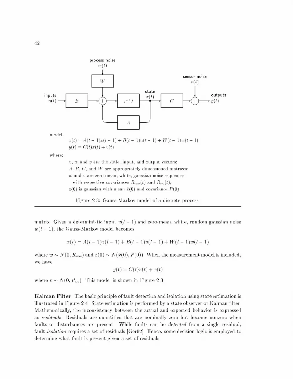
42B W Az�1I C� ��+ � ��+u(t)inputs - w(t)process noise??- - - - -?v(t)sensor noise y(t)outputsx(t)state� ��6model: x(t) = A(t� 1)x(t� 1) +B(t � 1)u(t� 1) +W (t� 1)w(t� 1)y(t) = C(t)x(t) + v(t)where: x, u, and y are the state, input, and output vectors;A, B, C, and W are appropriately dimensioned matrices;w and v are zero-mean, white, gaussian noise sequenceswith respective covariances Rww(t) and Rvv(t);x(0) is gaussian with mean x(0) and covariance P (0).Figure 2.3: Gauss-Markov model of a discrete process.matrix. Given a deterministic input u(t� 1) and zero-mean, white, random gaussian noisew(t� 1), the Gauss-Markov model becomesx(t) = A(t� 1)x(t� 1) +B(t � 1)u(t� 1) +W (t� 1)w(t� 1)where w � N(0; Rww) and x(0) � N(x(0); P (0)). When the measurement model is included,we have y(t) = C(t)x(t) + v(t)where v � N(0; Rvv). This model is shown in Figure 2.3.Kalman Filter The basic principle of fault detection and isolation using state estimation isillustrated in Figure 2.4. State estimation is performed by a state observer or Kalman �lter.Mathematically, the inconsistency between the actual and expected behavior is expressedas residuals. Residuals are quantities that are nominally zero but become nonzero whenfaults or disturbances are present. While faults can be detected from a single residual,fault isolation requires a set of residuals [Ger92]. Hence, some decision logic is employed todetermine what fault is present given a set of residuals.

43State estimatorNominalProcessModelPhysicalProcessFeedback�? ResidualGenerator DecisionLogic 12m���--- ?Alarms� ��� 6 -?-�- �+u yyeFigure 2.4: Fault detection and isolation using state estimation.The Kalman �lter can be thought of as an algorithm that produces two typesof output, given a noisy measurement sequence and associated models. First, it can bethought of as a state estimator or reconstructor, i.e., it reconstructs estimates of the statex(t) from noisy measurements y(t). In this view it is like an implicit solution of equationssince the state is not necessarily available (measurable) directly | the model can be thoughtof as the means to implicitly extract x(t) from y(t). Second, the Kalman estimator can bethought of as a measurement �lter which accepts the noisy sequence fy(t)g as input andproduces a �ltered measurement sequence fy(tjt)g. (The notation y(t2jt1) can be read as\the estimated value of y at time t2 given the measurements at time t1".)The Kalman �lter can be described as a predictor-corrector algorithm which al-ternates between a prediction phase and a correction phase. Candy [Can88, p. 322] gives asuccinct description of the algorithm:The operation of the Kalman �lter algorithm can be viewed as a predictor-corrector algorithm as in standard numerical integration. Referring to the algo-rithm in Table 2.1, we see the inherent timing in the algorithm. First, supposewe are currently at time t and have not received a measurement y(t) as yet. Wehave available to us the previous �ltered estimate x(t� 1jt� 1) and covariance~P (t � 1jt� 1) and would like to obtain the best estimate of the state based on[t� 1] data samples. We are in the \prediction phase" of the algorithm. We usethe state-space model to predict the state estimate x(tjt� 1) and associated er-ror covariance ~P (tjt� 1). Once the prediction based on the model is completed,we then calculate the innovation covariance Ree(t) and Kalman gain K(t). Assoon as the measurement at time t becomes available, that is, y(t), then wedetermine the innovation e(t). Now we enter the \correction phase" of the algo-rithm. Here we correct or update the state based on the new information in the

44 Prediction:x(tjt� 1) = A(t� 1)x(t� 1jt� 1) + B(t� 1)u(t� 1) (state prediction)~P (tjt� 1) = A(t� 1) ~P (t� 1jt� 1)A0(t� 1) +W (t� 1)Rww(t� 1)W 0(t� 1)(covariance prediction)Innovation:e(t) = y(t)� y(tjt� 1) = y(t)� C(t)x(tjt� 1) (innovation)Ree(t) = C(t) ~P (tjt� 1)C 0(t) + Rvv(t) (innovation covariance)Gain:K(t) = ~P (tjt� 1)C 0(t)R�1ee (t) (Kalman gain)Correction:x(tjt) = x(tjt� 1) +K(t)e(t) (state correction)~P (tjt) = [I �K(t)C(t)] ~P(tjt� 1) (covariance correction)Initial Conditions:x(0j0); ~P (0j0)Table 2.1: Kalman �lter algorithm (predictor-corrector form).measurement|the innovation. The old, or predicted, state estimate x(tjt � 1)is used to form the �ltered, or corrected, state estimate x(tjt) and ~P (tjt). Herewe see that the error, or innovation, is the di�erence between the actual mea-surement and the predicted measurement y(tjt� 1). The innovation is weightedby the gain K(t) to correct the old state estimate (predicted) x(tjt � 1); theassociated error covariance is corrected as well. The algorithm then awaits thenext measurement at time t+ 1.The operation of the Kalman estimator is pivoted around the values of the gainmatrix K. For small K the estimator \believes" the model; for large K it \believes" themeasurement. A Kalman estimator is not functioning properly when the gain becomessmall but the measurements still contain information necessary for the estimates. The �lteris said to diverge under these conditions [Can86, p. 94].Mimic and the Kalman �lter di�er fundamentally in the way that their respec-tive process models handle uncertainty. The semiquantitative model in Mimic expressesparameter uncertainty directly in the form of conservative ranges, where the true valuefalls within the range, and expresses functional uncertainty in the form of upper and lowerenvelope functions, where the true function is bounded by the envelopes. The philosophyhere is that uncertainty should be stated explicitly in the model and re ected in the model'spredictions. In contrast, the Kalman �lter uses a conventional numerical model in whichuncertain parameter values are approximated with mean values and uncertain functionalrelations are approximated with a \close" function. The numerical model gives precise pre-dictions which are then \corrected" to bring them into closer agreement with measurements.Candy summarizes a problem inherent in this approach:

45The process model is usually an approximation to the underlying physical phe-nomenology, and the model parameters and noise statistics are rarely exact; i.e.,the process model used for the estimator di�ers from the (real) process thatgenerates the measurements. Sometimes the approximation is intentional. Forinstance, using a reduced-order model in order to decrease computational com-plexity or linearizing a nonlinear model. It is clear that an imprecise estimatormodel degrades �lter performance : : : . In fact, these modeling errors or `modelmismatches' may even cause the estimator to diverge. In designing an estimatorit is therefore important to evaluate the e�ect of the approximations made inthe selection of the models. [Can86, p. 111]Kalman �lters do not perform diagnosis, of course, but they can determine howwell a given process model tracks the observations (by watching e(t)). Therefore, thecommon method is to use a bank of Kalman �lters in parallel, each one designed andtuned for a particular fault [FW89, MW89]. The �lter yielding the smallest error e(t)represents the best-matching hypothesis. One obvious problem with this approach is thecombinatorics | a potentially large number of �lters is needed to represent all the typesand combinations of faults to be diagnosed. Another problem is that tuning the Kalmanestimator is considered an art [Can86, p. 93]. Candy also notes that the Kalman �lter\is not a satisfactory (numerically) or e�cient algorithm to employ because of the errorcovariance equations".Epilogue One thing is very clear from a study of the literature: model-based approachesto monitoring and diagnosis are not unique to the AI community. The basic concept |that of using a model to predict expected behavior, and then using discrepancies betweenpredictions and observations as diagnostic clues | has evolved in two separate communi-ties: the model-based reasoning (MBR) specialty within the AI community and the faultdetection & isolation (FDI) specialty within the engineering community. Unfortunately,the two communities are largely unaware of each other, and each could pro�t from a betterunderstanding of the other's work. Certainly, the MBR community would pro�t from anunderstanding of model-based signal processing and the modern approach to system anal-ysis that it is based on, covering topics such as state estimation, parameter estimation,noise �ltering, observability, controllability, and stability. Likewise, the FDI communitywould bene�t from an understanding of qualitative constraint models, constraint suspen-sion, assumption-based truth maintenance, and semiquantitative simulation. An extremelyvaluable contribution to both communities would be a comprehensive article that comparesand contrasts the MBR and FDI methods on a sample problem, showing relative strengthsand weaknesses of each. This is an action item for future work.2.2.6 KARDIO (Bratko et al.)

46 �� ��Compressedsurface rules�� ��Experts,literature �� ��Causalmodel�� ��surfacerules6 - ?� SimulationInductionFigure 2.5: Knowledge acquisition cycle used in Kardio.Kardio is a medical expert system for diagnosis of cardiac arrhythmias [BML89].In contrast with most expert systems whose rules represent heuristics obtained from do-main experts, Kardio's rule base was mechanically generated in a 3-step process: build aqualitative model of the heart's electrical conduction; simulate the model for all interestingcombinations of faults; and learn diagnostic rules through induction over the simulationresults. The authors (Bratko, Mozeti�c and Lavra�c) expect that the Kardio \knowledgeacquisition cycle" (see Figure 2.5) will become a standard technique in the development ofpractical expert systems.It's interesting to note why the Kardio project used a predictive model, becauseit is for a di�erent reason than is commonly given for model-based diagnostic applications.Most applications, especially those based on engineered mechanisms, use a model partlybecause it is easily derived from the engineering design and partly because model-based di-agnosis overcomes a variety of limitations with symptom-based approaches (see Section 2.1).Kardio began in 1982 at a time when most diagnostic expert systems were based on expe-riential knowledge and before Davis had articulated the principles of model-based diagnosis[Dav84]. In the foreword to the Kardio book, Michie explains why the Kardio team builta causal model (and then induced diagnostic rules from its predictions):That part of existing cardiological knowledge which was explicitly repre-sented in Kardio was not the diagnostic part to be found in texts of clinicalpractice or in the heads of the authors of such texts. The role of consultantphysicians who collaborated in the project was to help the Kardio team todesign the logical model of the heart which was then used as a de novo genera-tor of diagnostic rules. Professor Bratko and his colleagues judged that existingclinical knowledge was not of an explicitness or completeness to support a usefulexercise of extraction from specialists and enhancement in the machine. Fromthe start, therefore, they had no other option but to construct the required cor-pus of knowledge from scratch | by machine derivation, that is to say, from acompact logical speci�cation. By doing so, Bratko, Lavra�c and Mozeti�c reaped

47the reward of guaranteed completeness and correctness in the �nally synthesizedexpert system. [BML89, Foreword]There is a lesson here that the model-based reasoning community has perhaps not suf-�ciently emphasized | that even for systems in which experience-based diagnosis is thenorm, it is often easier to acquire and validate a model of the system than to acquire andvalidate a set of symptom!fault associations, particularly where completeness and correct-ness are concerned. Koton's side-by-side comparison of two expert systems built for thesame domain | one using heuristic knowledge, the other using model-based reasoning |o�ers a good example of this lesson [Kot85].A fundamental di�erence in approach between Kardio and Mimic lies in themathematical foundations of the respective simulators. Mimic builds upon Qsim, a simula-tion algorithm that implements a qualitative mathematics and guarantees sound predictionsof all behaviors consistent with the semi-quantitative model. This soundness eliminates cer-tain sources of false positives during fault detection. Interestingly, the Kardio team madea deliberate choice to not use an available qualitative modeling technique, as they explain:The main feature in the Kardio approach is the use of logic as the rep-resentation formalism. Kardio is not rooted in any traditional theory usedin modeling, such as numerical techniques and di�erential equations. In com-parison with other approaches to qualitative modeling, the main advantage ofKardio applied to physiology lies in the potential power of the description lan-guage used. The model designer has the freedom to choose the most suitabledescription language and de�ne the laws of the domain in a most natural way.The description language is thus hardly constrained by any traditional mathe-matical notions. In general, this has of course, the disadvantage that no existingmathematical theory is assumed and automatically available to the model de-signer. Instead, if such a mathematical theory is useful it has to be explicitlystated in the model. It really depends on the problem of whether the freedom tochoose is more precious than the availability of some established mathematicaltheory. The latter is probably more important when the problem is susceptibleto some traditional approach, such as di�erential equations, but in physiologythe freedom is probably more valuable. [BML89, p. 49]The above statement is important but misleading. It is an important warningto modelers to choose a representation that is natural for the domain (wise advice forany project), but it is misleading in that it implies that the modeler must choose betweenmathematical rigor and expressive power. A more helpful view is that model-based reason-ing should be decomposed into two tasks: model building and simulation. The simulatorshould provide the mathematical rigor, guaranteeing the soundness of all predictions, andthe model-building language should make it easy to express what is known about the do-main using expressions that are grounded in physics and mathematics rather than ad hoc\laws of the domain".

48 Interestingly, the Kardio team did consider using Qsim, but rejected it becauseof two important limitations:First, it seems to be very di�cult to express in Qsim models which are notsusceptible to di�erential equations. This is often the case in medicine and itseems that a Qsim model of the heart that would correspond to the Kardiomodel would be extremely complex. Second, even when a Qsim model is de-rived from corresponding di�erential equations, the Qsim qualitative simulationalgorithm may nondeterministically generate numerous behaviors. Some of thegenerated behaviors can be justi�ed simply by lack of information in the model.Unfortunately, Qsim also generates unreal behaviors that are not justi�ed bylack of information. [BML89, p. 48].Although progress has been made on both limitations, it's not clear that the Kardio teamwould decide the question any di�erently today. Their model of cardiac electrical activityinvolves repetitive processes in time, some of which are asynchronous. While it is possibleto model repetitive processes in Qsim, the generated behavior would be large due to allthe qualitative distinctions arising from unsynchronized processes. In contrast, Kardiocan assert a simple domain law that says that the sum of two signals, one with regularand one with irregular rhythm, is a signal with irregular rhythm. This kind of abstractsymbolic description is suitable for Kardio's purpose, but is not expressible in Qsim'squalitative di�erential equations. This highlights the importance of using suitable temporalabstractions, as discussed in section 2.2.7.The Compilation Debate The Kardio project was seen as the �rst clear demonstrationthat large-scale automatic synthesis of human-type knowledge was technically feasible, ful-�lling a goal of the International School for the Synthesis of Expert Knowledge. As such, itwas driven by a di�erent research agenda than the other model-based systems described inthis chapter. The central approach in Kardio| that of performing exhaustive simulationsof the model and then compressing the predictions into diagnostic rules | has become atopic of debate in the model-based reasoning community. Davis has argued that this ap-proach, which has been employed in numerous other research e�orts, does not result infaster diagnostic performance and, more importantly, focuses attention away from the trulyimportant research issue: the creation of a sequence of increasingly approximate models foruse by a model-based reasoner [Dav89]. In one of the more spirited debates this author haswitnessed, Keller defends the attacks on \knowledge compilation" and argues that it is morefruitful to view associational reasoning and model-based reasoning as opposite endpointsalong a spectrum of approaches ranging from more compiled to less compiled [Kel90]. Thedebate is clearly not settled for there are strongly held views on both sides.

492.2.7 Modeling for Troubleshooting (Hamscher)Model-based diagnosis, as commonly described in the AI community [DH88], re-quires models of structure and behavior of the mechanism under study. One might assumethat an adequate structural model is simply a complete hierarchical description of sub-systems and components, and that an adequate behavioral model is a detailed simulationmodel that predicts all the time-varying events/changes in the mechanism. While suchmodels do support model-based diagnosis, they are also part of the problem. As Hamschernotes in a recent article about troubleshooting digital circuits [Ham91], \existing methodsfor model-based troubleshooting have not previously scaled up to deal with complex digitalcircuits, in part because traditional circuit models do not represent aspects of the devicethat troubleshooters consider important." As Hamscher emphasizes, the important thingabout developing a model for troubleshooting is not that it uses abstractions to deal withcomplexity (any representation does that), but that it embodies structural and behavioralabstractions appropriate to troubleshooting.What sort of abstractions are helpful in troubleshooting? Hamscher identi�eseight principles to guide a knowledge engineer in constructing a model that makes trou-bleshooting feasible. Although Hamscher's research concerns digital circuits (a form ofdiscrete-event dynamic systems), the principles are general enough to apply, in most cases,to the continuous-variable dynamic systems considered in this dissertation. We state theeight principles at the end of this section for interested readers, but here we focus on oneissue that may be of particular importance in the future development ofMimic| the issueof temporal abstractions.Consider the example of an oscillator in a digital circuit. In a clock-cycle-by-clock-cycle description of the oscillator's output, the output is a repeating sequence ofrising edge, stable value, falling edge, and stable value. A more abstract description is theoutput frequency, and an even more abstract description is simply the attribute \changing"(as opposed to \constant"). These temporally coarse descriptions of behavior hold twoadvantages: they are easier to generate because the model is simpler, and they are easier toobserve in the real mechanism, often providing su�cient diagnostic information to exoneratemany components without resort to the more temporally-detailed models. As Hamscheremphasizes:The important property of temporal abstractions is that they sacri�ce preci-sion without sacri�cing the ability to detect faulty behavior. In troubleshootingthe idea is to detect discrepancies between the observed behavior of the real deviceand an idealized model of it; thus the predictions of interest are those that canbe made e�ciently from what we have observed and that could be signi�cantlyviolated if the device were broken. [Ham91, p. 239]Temporal abstractions provide considerable leverage in the troubleshooting pro-cess, and just as they are important in certain types of digital circuits, they are also likely

50to be important in certain types of continuous-variable dynamic systems. Currently, Qsimcan describe a rhythmic signal in the temporally-detailed form of a time-varying magnitudeor in the less-detailed form of a frequency. However, to obtain coarser descriptions such as\regular vs. irregular rhythm" or \changing vs. constant", a di�erent modeling languagemust be used. The development of such a language to support temporally coarse descrip-tions of behavior in continuous-variable dynamic systems will enable systems like Mimic toexploit an important type of abstraction. Ideally, such a language will be built on a �rmfoundation of qualitative mathematics and will be able to make guarantees of soundness,as Qsim does. This is an important goal for future work.Eight modeling principles This section quotes Hamscher's eight principles for guidingknowledge engineers in the construction of models intended for troubleshooting. Theseprinciples divide into three categories: behavior, structure, and failures. We show the eightprinciples here to give interested readers a fuller understanding of Hamscher's insights, andwe recommend his article for explanations of each.Modeling of Behavior� The behavior of components should be represented in terms of features that are easyfor the troubleshooter to observe.� The behavior of components should be represented in terms that are stable over longperiods of time or that summarize much activity into a single parameter. This iseasiest for a component for which changes on its inputs always results in changes onits outputs.� A temporally coarse behavior description that only covers part of the behavior of acomponent is better than not covering any at all.� A sequential circuit should be encapsulated into a single component to enable thedescription of its behavior in a temporally coarse way.Modeling of Structure� Components in the representation of the physical organization of the circuit shouldcorrespond to the possible repairs of the actual device.� Components in the representation of the functional organization of the circuit shouldfacilitate behavioral abstraction.Modeling of Failures� An explicit representation of a given component failure mode should be used if theunderlying failure has high likelihood.

51� An explicit representation of a given component failure mode should be used if theresulting misbehavior is drastically simpler than the normal behavior of the compo-nent.2.3 In uential Research2.3.1 Measurement InterpretationAs Forbus explains in a 1986 paper:An unsolved problem in qualitative physics is generating a qualitative under-standing of how a physical system is behaving from raw data, especially numeri-cal data taken across time, to reveal changing internal state. Yet providing thisability to \read gauges" is a critical step towards building the next generation ofintelligent computer-aided engineering systems : : : [For86]This problem, called measurement interpretation, arises in Mimic and other systems thatattempt to translate observed behavior (including numerical data) into useful qualitativeterms. In this section we brie y review Forbus' theory of \across-time measurement in-terpretation" (ATMI) and then explain why and how Mimic takes a considerably di�erentapproach to the same problem. This comparison applies equally well to DeCoste's extensionto ATMI, named DATMI [DeC90].ATMI The ATMI theory requires two pieces of input: a total envisionment of the mecha-nism (a graph of all possible behaviors) and domain-speci�c criteria for quantizing numericaldata into an initial qualitative description. A measurement interpretation problem takesas input a set of measurement sequences, each consisting of a set of measurements for agiven variable, totally ordered by the times of the measurements. The output is a set ofone or more consistent interpretations of the data expressed as a �nite path through thetotal envisionment. In other words, given the measurements of a mechanism across time, aninterpretation is that the mechanism went through a speci�c sequence of qualitative statesS1, S2, : : :Sn.The ATMI theory interprets measurements in a manner analogous to AI modelsof speech understanding in which the speech signal is partitioned into segments, each ofwhich is explained in terms of phonemes and words, and where grammatical constraints areimposed between the hypothesized words to prune the possible interpretations. In ATMI,the initial signal sequence is partitioned into pieces which are interpreted as possible qual-itative states of the mechanism. The envisionment, by supplying information about statetransitions, plays the role of grammatical constraints, imposing compatibility conditionsbetween the hypotheses for adjacent partitions.

52 ATMI performs interpretation with respect to a total envisionment of a modelof the mechanism (normally, the fault-free model). In order to perform interpretations ofpossibly faulty behavior, ATMI would also require total envisionments of every type andcombination of fault to be diagnosed. For mechanisms of the scale and complexity foundin the process industries, computing the total envisionments is an enormous job. Forbusrecognizes this and proposes that the envisionments be pre-computed and preprocessed toprovide a set of state tables indexed by the possible values of measurements.Mimic Mimic's approach to measurement interpretation di�ers in two important ways.First, Mimic is continuously tracking observations against an incremental simulation. Ev-ery state S in the tracking set represents a test for new observations | they are eithercompatible with S or not. If not, tracking simply looks at the near successors of S fora match (this is explained more fully in Chapter 3). Mimic does not require the mas-sive precomputing of total envisionments, both normal and faulty. Instead, it generates anattainable envisionment, extending the simulation only as needed, and pruning behaviorbranches as soon as they fail to match observations. In e�ect, the simulation is focused bythe observations, and interpretation is reduced to local search in the unfolding attainableenvisionment.The second di�erence between Mimic and ATMI is in the interpretation of indi-vidual numerical measurements. In ATMI, a numerical measurement is converted into oneor more qualitative values based on pre-speci�ed conversion tables. This quantitative-to-qualitative conversion loses information. In Mimic, however, there is no such informationloss. Instead, the semiquantitative simulation generates numeric ranges for each variable,and the measurement is simply tested for overlap with the predicted range. In fact, thereis information gain because each new set of observations is uni�ed with the model's predic-tions to update the current state. Thus, by using the information in previous measurements,Mimic is able to generate tighter bounds on expected values.In a sense, the Mimic and ATMI approaches to measurement interpretation arecomplementary. ATMI is able to take an arbitrary sequence of measurements as input andproduce one or more possible interpretations, having no idea of the state of the mechanismwhen the �rst measurement was taken. Mimic, in contrast, begins with the initial state ofthe mechanism and so is able to build an interpretation as measurements arrive with lesssearch. Also, because of its diagnostic capabilities, Mimic is able to build interpretationsthat jump across models as faults and repairs are diagnosed.2.3.2 Generate, Test and DebugIn 1987 Simmons and Davis presented a problem-solving paradigm named \Gen-erate, Test and Debug" (GTD) that combines associational rules and causal models, pro-ducing a system with both the e�ciency of rules and the breadth of problem solving power

53DEBUGTESTGENERATE??HypothesisCausal Explanation����� --HypothesisFigure 2.6: Control ow in the GTD paradigm.of causal models [SD87]. GTD was explored primarily for planning and interpretation tasks.Both tasks are of the general form \given an initial state and a �nal (goal) state, �nd a se-quence of events which could achieve the �nal state." Admittedly, this is di�erent than thediagnosis task addressed by Mimic; we'll explain the in uence of GTD on Mimic followinga synopsis of GTD's three stages.Problem solving in GTD proceeds in three stages, as shown in Figure 2.6:1. Generate | the generator uses associational rules to map from e�ects to causes.The left-hand side of a rule is a pattern of observable e�ects and the right-hand sideis a sequence of events which could produce those e�ects. The rules are matchedagainst the �nal state and the resultant sequences are combined to produce an initialhypothesis | a sequence of events that is hypothesized to achieve the �nal state.2. Test | the tester tests the hypothesis by using a causal model to simulate the se-quence of events. If the test is successful (i.e., the results of the simulation matchthe �nal state) then the hypothesis is accepted as a solution. Otherwise, the testerproduces a causal explanation for why the hypothesis failed to achieve the �nal state.It then passes this explanation and the buggy hypothesis to the debugger.3. Debug | the debugger uses the causal explanation from the tester to track downthe source of the bugs in the hypothesis. It uses both domain-speci�c causal modelsand domain-independent debugging knowledge to suggest modi�cations which couldrepair the hypothesis. The modi�ed hypothesis is then submitted to the tester forveri�cation. Alternatively, the debugger has the option to invoke the generator toproduce a new hypothesis.The core idea in GTD is of \debugging almost right plans" whereas inMimic it isof \debugging almost right models". The interaction between GTD's tester and debugger is

54similar to the interaction between Mimic's discrepancy detector (as tester) and hypothesisgenerator (as debugger). The discrepancies are used by the hypothesis generator to decidehow to modify the model, which is then simulated to see if its predictions are corroboratedby future measurements. This is described in more detail in Chapter 3.2.3.3 STEAMERSteamer [HHW84] was a research e�ort concerned with exploring the use ofAI software and hardware technologies in the implementation of intelligent computer-basedtraining systems. The key idea is that of an interactive inspectable simulation. For example,Steamer's animation of a steam propulsion plant allows a student to see processes andconditions that are not visible in the physical system. This is felt to be an importantcontribution in the student's formation of a mental model. In a warning about increasingautomation in the control room, Perrow emphasizes how important it is for an operator tounderstand his/her system:This computerization has the e�ect of limiting the options of the operator, how-ever, and does not encourage broader comprehension of the system|a key re-quirement for intervening in unexpected interactions. [Per84, p. 122]Steamer's main contributions are in the areas of training and human interface.Although these are not the focus of our research, Steamer is important in that it highlightsthe importance of visualizing the system, even the parts that aren't visible. In a processmonitoring situation where a human operator is the �nal arbiter, it is very important topromote the operator's understanding of each hypothesis and the associated state of themechanism. Since Mimic predicts the values of unseen variables, it can show the operatorthe complete state of the mechanism for each hypothesis.

Chapter 3The Design of MimicMost medical expert systems diagnose by naming a disease rather than coher-ently describing what is happening in the world (a model) and causally relatingstates and processes. Perhaps because programs do not structurally simulatepathophysiological processes, researchers have not considered inference in termsof model construction. William J. Clancey [Cla89]Clancey's observation above suggests that a diagnostic program should simulatethe faulty process under observation, attempting to construct a model that tracks thephysical situation. This is, in fact, a succinct description of Mimic's operation.This chapter describes the design of Mimic. The objective here is to present thedesign in enough detail to enable a rational reconstruction. We proceed from general tospeci�c, starting with the high-level architecture and then elaborating on its components.3.1 Design OverviewMimic is a model-based design for monitoring and diagnosis of continuous-timedynamic systems. Its two basic paradigms are \monitoring as model corroboration" and\diagnosis as model modi�cation". Figure 3.1 presents an abstract view of the Mimicarchitecture in which three tasks mediate between the physical system and its models. Thethree tasks are summarized as follows:PhysicalSystem ModelsMonitoringDiagnosisAdvising-- -� -� ���� safety conditionsrecommended procedures� ���controlalarmsforewarningsFigure 3.1: Three tasks of an operator advisory system.55

56 Models:Behaviors: M1B11 B12������ BBBBBB M2B21 MnBn1 Bn2 Bn3 JJJJJJ� � �� �(discrep.) (discrep.)p p p pFigure 3.2: Each element of the tracking set is a model plus its tracked behavior(s). Abehavior is removed when it fails to match current observations, such as B11 and B21 . Amodel is removed from the set only when it has no remaining behaviors, such as model M2.Monitoring The purpose of the monitoring task is twofold: to update the state of themodel in synchrony with the mechanism's observed state, and to detect when di�er-ences between observations and predictions indicate a fault. This task is driven bythe arrival of new observations in a sense-simulate-compare-update cycle. When newobservations arrive, the model is simulated up to the time of the observations andobservations are compared to predictions. Any discrepancies indicate that the modelno longer re ects the mechanism, due to a fault or repair in the mechanism. If thereare no discrepancies, the state of the model is updated from the measurements.Diagnosis The purpose of the diagnosis task is to bring the model back into agreementwith the mechanism, and in so doing, identify the fault(s) present in the mechanism.Using discrepancies as clues, this task performs a hypothesize-build-test sequence thatcreates modi�cations of the discrepant model, where each modi�cation may add orremove a single fault. These newly hypothesized models are tested for compatibilitywith the current observations and then injected into the monitoring cycle for subse-quent testing as new observations arrive.Advising The purpose of the advising task is to inform the operator of the current stateof diagnosis. Each hypothesis consists of a model (possibly containing faults) and itscurrently tracked state(s). Hypotheses are ranked by probability, degree-of-match,age, and risk. Ranking by risk (future possible undesirable states) provides an earlywarning capability that takes advantage of the model's predictive power.The Tracking Set The set of candidate models maintained byMimic is called the trackingset. As depicted in Figure 3.2, each element of the tracking set is a model plus its currently

57'& $%StructuralModel'& $%BehavioralModels HypothesisGeneratorModelBuilder

TrackerIncrementalSimulatorPhysicalSystem

DiscrepancyDetector-operating inputs -� observations

?�6simulationcontrol6hypotheses-- -models predictions ?�6 unresolveddiscrepancies� � discrepancies �

6� updatesFigure 3.3: Architecture of Mimic. The rectangular boxes represent processing elementsand the labeled lines show information ow.tracked partial behavior(s). Each model is distinguished by the fault hypothesis it embodies.A given model may have more than one distinct behavior being tracked at a given time.As new readings are obtained and compared to behaviors in the tracking set,some behaviors may be corroborated (denoted with \p") while others are refuted (denotedwith \�"). As long as a model has at least one behavior corroborated up to the presenttime (such as M1 and Mn), the model remains in the tracking set with its corroboratedbehaviors. If all of a model's behaviors are refuted (as with M2), the model is refuted andremoved from the tracking set. The refuted model and its refuted behavior(s) become inputto the hypothesis generation function.Information Flow The ow of information within Mimic can be seen more clearly in thedetailed architecture of Figure 3.3. When observations arrive at time t, the incrementalsimulator advances the simulation of each model in the tracking set to time t. Predictionsare then compared to observations, and if no discrepancies are detected, the observationsare uni�ed with the predictions and propagated through the model's equations to updatethe ranges of variables and constants. If a discrepancy is detected, the tracker attempts toresolve it by determining if the observations are compatible with a successor of the current

58qualitative state. If so, the qualitative state of the model is updated; if not, the unresolveddiscrepancy triggers hypothesis generation.The hypothesis generator takes unresolved discrepancies as symptoms of an un-known fault or repair. By dependency tracing through the structural model, suspectedcomponents and parameters are identi�ed. For each suspect, single-change hypotheses areformed using a subset of the suspect's operating modes (the subset depends on the typeof fault | abrupt or gradual). For each hypothesis, a model is built and then initializedfrom current observations. If the model initializes successfully, it is added to the trackingset. Failure to initialize indicates a contradiction between model and observations, in whichcase the model is discarded as an incorrect hypothesis.Main Loop Mimic operates in a continuous loop, as shown in Figure 3.4, where each cyclebegins with a new set of sensor readings and ends with an updated set of hypotheses. Thealgorithm operates on the tracking-set, performing three basic actions: (1) it updates thestate of candidates that are consistent with the readings; (2) it removes candidates that areinconsistent with the readings; and (3) it creates new candidates based on the discrepanciesfound in inconsistent candidates.The remainder of this chapter describes each element of the design in more de-tail. The �rst two sections | modeling and simulation | describe the foundations thateverything else is built upon. The next three sections | monitoring, diagnosis and advising| correspond to the three main tasks shown in Figure 3.1. The last section describes howcomplexity is controlled.3.2 ModelingMimic depends on two distinct types of models: a structural model representingcomponents and connections, and a behavioral model that predicts possible behaviors givena fault hypothesis. This section describes both types of models using a two-tank cascade asan example (see Figure 3.5).3.2.1 Structural ModelThe structure of a mechanism is its components and connections. Figure 3.6shows the structure of the two-tank cascade. The structural information is used only duringdiagnosis to trace \upstream" from the site of a discrepancy along the paths of interactionto the components and parameters whose malfunction could have caused the discrepancy.As such, the structural model must contain components, parameters, connections, and thedirection of connections.The structural model used by Mimic is shown in Figure 3.7. This model is adeclarative representation of the preceding structure diagram. The model has three main

59Read sensors:Obtain next time-stamped set of sensor readings for time t.Track candidates:For each model in tracking-set:Simulate ahead to time t,Test for discrepancies between readings and predictions.If no discrepancies, update state from readings.Return two sets: retained-candidates and rejected-candidates.Generate hypotheses:Given the discrepancies in rejected-candidates,perform dependency tracing to create new single-changehypotheses in hypothesized-candidates.Test hypotheses:Attempt to initialize each member of hypothesized-candidates.Successful members are placed in new-candidates.Display candidates:Display candidates ranked by probability, similarity, age,and risk.Update tracking set:tracking-set new-candidates [ retained-candidatesGo to first step.Figure 3.4: Main loop of Mimic.

60 In ow ��x- ?� ������ �� �� �� �� �� �� �� �� �� �� �� �� �? Tank AA� ���� �� �� �� �� �� �� �� �� �� �� �� �� �� � Tank BB ?Out ow��level sensor�� ow sensor Di�erential equations:A0 = inflow � f(A)B0 = f(A) � g(B)

Figure 3.5: Two-tank cascade.Tank-BTank-A�� � Drain-B�� � Drain-A �� � In ow-A AmountSensorFlowSensor? - - In ow-obs(observable)-- ?? - - Amount-B-obs(observable)Out ow-BOut ow-A �� ��= parameter= componentFigure 3.6: Component-connection graph of the two-tank cascade. Rectangles representdiagnosable components/subsystems, ovals represent parameters (constants), and directedlinks represent connections and their direction of ow.

61Component de�nitions:(COMPONENTS(INFLOW-SENSOR(flow-in input icon1)(measured output i-obs))(TANK-A(inlet input icon1)(outlet 2-way tocon1)(drainrate input dr1))(TANK-B(inlet input tocon1)(outlet 2-way tocon2)(drainrate input dr2)(amount output acon))(AMOUNT-SENSOR(amount-in input acon)(measured output a-obs)))Parameter to connection mappings.(PARAMETERS(Inflow-A icon1)(Drain-A dr1)(Drain-B dr2))Variable to connection mappings.(VARIABLES(Amount-B-obs a-obs)(Inflow-obs i-obs))Figure 3.7: Structural description of the two-tank cascade. This is a declarative represen-tation of the component-connection graph in the previous �gure.clauses. The VARIABLES clause contains entries for each of the observable variables, typicallysensor outputs. The PARAMETERS clause contains entries for each of the constants that maybe identi�ed as a suspect during diagnosis. Likewise, the COMPONENTS clause contains entriesfor each of the components/subsystems that may be identi�ed as a suspect during diagnosis.In a component-connection representation of a mechanism it is assumed that allinteractions among components take place through explicit connections among the terminalsof the components. Each terminal of a component is described with a 3-tuple consisting of:(terminal-name direction connection-name)The direction of a terminal must be input, output, or 2-way. To be called an inputterminal, the component must not have any direct e�ect on the quantities transmitted intothat terminal. For example, the input of an infrared sensor does not a�ect the sourcesof infrared radiation that it measures. To be called an output terminal, the quantitiestransmitted by the component to its terminal must not be directly a�ected by whateverthat terminal is connected to. For example, the luminance at the surface of a light bulb'sglobe is not a�ected by the air or uid surrounding the globe. When a terminal is called2-way, it means that some or all of the quantities carried through that terminal can bea�ected not only by the component but also by what it is connected to it. For example, the

62amount of ow out of a water tank is a�ected by the downstream resistance of the pipingsystem it is connected to. These directions-of-e�ect are used in the dependency tracingalgorithm described in section 3.5.1.The other two elements of the 3-tuple | terminal name and connection name| are simply labels. Terminal names (such as inlet and outlet) exist only for humanunderstanding and play no role in dependency tracing. Connection names are arbitrarytags which, when repeated in another clause, designate a connection between the associatedterminals and/or variables and/or parameters.3.2.2 Behavioral ModelThe purpose of a behavioral model is to predict the possible behavior(s) of amechanism given a starting state and a fault hypothesis. Further, the predictions areto be based on \�rst principles", i.e., physical laws such as conservation of energy, massbalance, Ohm's law, etc. For the class of mechanisms considered in this report, the modelis a deterministic, continuous-time, dynamic model based on an abstraction of ordinarydi�erential equations. The qualitative di�erential equation (QDE) representation that weuse is based on Kuipers' formalism for qualitative simulation [Kui86] and further extendedby Kuipers and Berleant for simulation with incomplete quantitative knowledge [KB88].This section summarizes the QDE representation.Figure 3.8 shows a behavioral model for a two-tank cascade where there is aconstant in ow into the top of tank-A and an out ow from the bottom of tank-B. Thequantity-spaces clause de�nes the variables of the model and the ordered landmark valuesin each quantity space. The constraints clause contains the equations of the model,representing the physical laws of the domain. These two clauses de�ne the qualitativemodel, which can be simulated using only the symbolic non-numeric information shown.However, the model can be strengthened with partial quantitative knowledge intwo additional clauses. First, the initial-ranges clause de�nes numeric ranges for land-mark values, allowing the modeler to specify the lower and upper bounds for impreciselyknown constants. Second, the m-envelopes clause speci�es envelope functions for mono-tonic (M+ and M-) function constraints. This lets the modeler express uncertainty about theprecise function by bounding it with upper and lower \envelope" functions. In the exampleshown, the envelope functions express the basic square root relationship for drains, withuncertainty about the precise value of a factor.Where, exactly, does the partial quantitative knowledge come from? It is a formof domain knowledge which is sometimes given explicitly in the domain and sometimesrequires the judgement of a domain expert. As an example of the former, electrical resistorsare labeled as having a nominal value with a tolerance of, say, �2 percent. Thus, the initialrange for the resistor's nominal value is easily provided. As an example of the latter, in thehuman cardiovascular system the mathematical relation between central venous pressure

63(define-QDE Two-Tank-Cascade(quantity-spaces(Inflow-A (0 normal inf))(Amount-A (0 full))(Outflow-A (0 max))(Netflow-A (minf 0 inf))(Amount-B (0 full))(Outflow-B (0 max))(Netflow-B (minf 0 inf))(Drain-A (0 vlo lo normal))(Drain-B (0 vlo lo normal)))(constraints((M+ Amount-A Outflow-A) (full max))((ADD Outflow-A Netflow-A Inflow-A))((D/DT Amount-A Netflow-A))((M+ Amount-B Outflow-B) (full max))((ADD Outflow-B Netflow-B Outflow-A)) ; Outflow-A = Inflow-B((D/DT Amount-B Netflow-B)))(independent Inflow-A Drain-A Drain-B)(history Amount-A Amount-B)(unreachable-values(Netflow-A minf inf) (Netflow-B minf inf) (Inflow-A inf))(m-envelopes((M+ Amount-A Outflow-A)(upper-envelope (lambda (x) (* (ub 'Drain-A) (expt x 0.5))))(lower-envelope (lambda (x) (* (lb 'Drain-A) (expt x 0.5))))(upper-inverse (lambda (y) (expt (/ y (ub 'Drain-A)) 2)))(lower-inverse (lambda (y) (expt (/ y (lb 'Drain-A)) 2))))((M+ Amount-B Outflow-B)(upper-envelope (lambda (x) (* (ub 'Drain-B) (expt x 0.5))))(lower-envelope (lambda (x) (* (lb 'Drain-B) (expt x 0.5))))(upper-inverse (lambda (y) (expt (/ y (ub 'Drain-B)) 2)))(lower-inverse (lambda (y) (expt (/ y (lb 'Drain-B)) 2)))))(initial-ranges((Time t0) (0 0))((Inflow-A normal) (8.0 8.1))((Amount-A full) (45 46)) ((Amount-B full) (45 46))((Drain-A normal) (1.40 1.43)) ((Drain-B normal) (1.40 1.43))((Drain-A lo) (0.70 1.40)) ((Drain-B lo) (0.70 1.40))((Drain-A vlo) (0 0.70)) ((Drain-B vlo) (0 0.70))))Figure 3.8: Semiquantitative model of a two-tank cascade. Incomplete quantitative knowl-edge is expressed in the form of ranges for landmark values, in initial-ranges, and enve-lope functions for monotonic function constraints, in m-envelopes.

64and mean pulmonary arterial pressure is not precisely de�ned. However, a cardiologist canprovide reasonable bounds on this relation.3.2.3 Modeling FaultsThere are two separate properties of faults that are important in Mimic: howthe fault is represented in the model, and speed of onset of the fault. We examine eachproperty below.Parameter Faults vs. Mode Faults There are two basic ways of representing a faultin a model: by changing the value of a parameter (such as changing the ow resistance ofdrain because it has become clogged), or by changing the equations of a component (suchas changing a heater function that relates voltage input to heat output when the heaterburns out). In this section we will show how such faults are represented in the behavioralmodel. Later, in section 3.5, we will see how such faults are hypothesized.For faults that are represented as abnormal parameter values, the modeler needonly add appropriate landmarks in the parameter's quantity space and corresponding rangesin the initial-ranges clause. An example of this is shown in Figure 3.8, where parameterDrain-A can have one of four landmark values: 0, vlo, lo, or normal. Numeric ranges forthese values are de�ned in initial-ranges. Parameters are represented as independentvariables in the model, meaning that they are constants. Once a parameter's value is set,it stays that way unless Mimic changes it during diagnosis.For faults that change the set of equations in the model, we use the simple ideathat the appropriate set of equations for a component depends on the component's operatingmode. For example, the mode of an electric heating element may be normal or burned-out.In the former case it dissipates heat proportional to the square of the voltage applied, butin the latter case it dissipates no heat, regardless of the voltage. This di�erence in behavioris modeled by having two di�erent sets of equations, only one of which can be active at atime, as shown below in a fragment of a constraints clause:(mode (heater normal)((MULT V V V-SQUARED))((MULT HEAT R V-SQUARED)))(mode (heater burned-out)((ZERO-STD HEAT)))In this example, heater is called a mode variable, and its value determines which setof equations govern the behavior of the component. Like parameters, mode variables areconstants that can be changed during diagnosis. Although we don't explore it in this report,

65modes serve two other useful purposes: (1) they can be used to represent normal transitionswithin a component, such as a thermostat that changes between its on and o� modes, and(2) they can be used by a component to predict its own fault, such as a heater that burnsout when its power dissipation exceeds a threshold.Abrupt Faults vs. Gradual Faults Mimic partitions faults according to their speed-of-onset as abrupt or gradual. Abrupt faults cover discrete events (such as heater burn-out) andfailure of normal behavior transitions (such as a thermostat that fails to turn o� after thetemperature exceeds an upper limit). Gradual faults cover slowly developing abnormalitiescaused by aging, drift, contamination, etc (such as a pipe whose ow resistance graduallyrises due to lime deposits). Abrupt faults may be modeled as either parameter faults ormode faults, but gradual faults are ordinarily modeled as parameter faults. The distinctionbetween abrupt versus gradual is important during hypothesis generation, as explainedbelow. Suppose we are modeling an electric heating element in a water heater. Theheating element can exhibit two di�erent abrupt faults | short-circuit and open-circuit |which are modeled as mode faults that change the equations relating voltage, current, andheat output. If the heater becomes a suspect during diagnosis, it is proper to hypothesizeall of its abrupt faults since such faults can happen at any time, regardless of the currentoperating mode.Now suppose we are modeling a pipe which is known from experience to accu-mulate lime deposits over time, even to the point of becoming completely obstructed. Wemodel three levels of severity of this gradual fault by giving the ow-resistance parameterfour possible values: normal, high, very-high, and infinity. Each of these parametervalues will have an associated numeric range speci�ed in the initial-ranges clause. Ifthe pipe is operating in the normal range but becomes a suspect during diagnosis, then theonly appropriate hypothesis is high. Because of the fault's gradual nature, very-high andinfinity are not yet valid hypotheses. Thus, the bene�t of distinguishing gradual faultsfrom abrupt faults is that fewer hypotheses are generated during diagnosis.3.3 SimulationThe type of simulation used in Mimic enables several of the bene�ts describedearlier in section 1.4. Though it is called semiquantitative simulation, a more descriptivename is qualitative-quantitative simulation. The simulation is fundamentally qualitative,but strengthened with partial quantitative knowledge in the form of numeric ranges forlandmark values and envelope functions for monotonic function constraints. The resultingsimulation combines a key advantage of qualitative simulation | prediction of all behaviorsconsistent with the partial knowledge | with the ability to use incomplete quantitativeknowledge to re�ne the predictions.

66 �� ��Empty -t0 �� ��Filling(t0 t1) -������*HHHHHHj�� ��Equilibriumbefore full�� ��Equilibriumat full�� ��Over owt1Figure 3.9: Branching-time description of a bathtub's possible behaviors. In contrast to con-ventional numerical simulation, semiquantitative simulation reveals all behaviors consistentwith incomplete knowledge of the mechanism.This section describes semiquantitative simulation from a user's point of view,focusing on the simulation output and the inherent capabilities of the method. Readersinterested in a more complete description of these simulation methods should consult thepapers by Kuipers on Qsim [Kui86], by Kuipers and Berleant on Q2 [KB88], and by Kayon dynamic envelopes [Kay91].3.3.1 Qualitative-Quantitative SimulationA behavior, in Qsim parlance, is a sequence of states alternating between statesthat represent a point in time and states that represent an interval in time. Point statesare created when qualitative distinctions arise during simulation, such as a quantity thatreaches a landmark value or changes from increasing to steady. Interval states describebehavior between successive point states; the duration of an interval may range from veryshort to very long.Prediction of All Valid Behaviors Two properties of qualitative-quantitative behaviorare important in Mimic. On the qualitative side, the simulation yields a \behavior tree"which is a branching-time description of the possible behaviors of the mechanism. Figure 3.9shows a simple example of this for a bathtub �lling from empty. Initially, the bathtub isempty at time t0, then begins �lling in the time interval (t0 t1). Based on the availableinformation, the bathtub may end in one of three �nal states: equilibrium before full,equilibrium at full, or over ow. The key feature here is that the branching-time descriptionof behavior reveals all of the qualitatively distinct behaviors consistent with the availableinformation. This stands in contrast to conventional numerical simulation which replacesuncertainty with approximations and then generates a single, numerically-precise behavior.The precision is seductive, but it fails to provide a comprehensive description of the behavior

67space. The branching-time behavior description is important to Mimic in two ways.Monitoring in general is susceptible to a \missing prediction error" in which a model isrefuted because observations fail to match predicted behavior. The error arises becauseconventional numerical simulation generates a single behavior even though other behav-iors may be possible. This error can cause both false positives and false negatives duringdiscrepancy-detection (false positives when matching against the normal model and falsenegatives when matching against a fault model). Semiquantitative simulation eliminatesthis source of error because it guarantees that all valid behaviors are predicted.The second way that sound behavior prediction is important is in forewarning.When Mimic is monitoring a fault model, it is important to be able to look ahead intime to see if any undesirable states are imminent. Again, the semiquantitative simulationensures that all possible futures are predicted, so Mimic can guarantee that any potentialnear-future problems are reported to the operator.Use of Incomplete Quantitative Knowledge On the quantitative side, qualitative-quantitative simulation takes advantage of incomplete quantitative knowledge to constrainthe simulation, thereby eliminating some behaviors, and yielding numeric range predictionsfor every variable. Figure 3.10 shows an example of this for a two-tank cascade, �llingfrom empty. Every landmark value has an associated range. Importantly, the ranges areguaranteed to bound the valid possible values. This allows sensor readings to be compareddirectly to predicted ranges. This eliminates the \approximate matching problem" thatoccurs with conventional numerical models since they generate a precise value, thus requiringa decision as to whether the reading is close enough to the predicted value.3.3.2 Feedback LoopsFeedback is common in natural systems, but its presence has been problematicfor many diagnostic systems. As Widman and Loparo note in the introductory chapter ofa book on AI, simulation and modeling [WLN89]:Expert reasoning with symbolic models has not yet been widely used despite itsevident usefulness. The obstacles lie in two general types of models that arefrequently required to describe real-world physical systems: continuous modelscontaining interacting feedback loops, and discrete stochastic models containinginteracting probability distributions (conditional dependencies).Mimic works with the �rst type of model (continuous models containing feed-back), so it's important to show how semiquantitative simulation handles feedback. Wedemonstrate this with an example of negative feedback in an ampli�er, as shown in Fig-ure 3.11. For a linear ampli�er and linear feedback, the input-output relation can be solved

68Amount-At0 t1 t2* * b. . . . . . . . . . . . . . . . . . 0 [0 0]A-1 [58.4 65.8]Full [99 101] Amount-Bt0 t1 t2b * b. . . . . . . . . . . . . . . . . . 0 [0 0]A-2 [58.4 65.8]Full [99 101]Out ow-At0 t1 t2* * b. . . . . . . . . . . . . . . . . . 0 [0 0]O-1 [3.01 3.19]Max [4.8 5.2] Out ow-Bt0 t1 t2b * b. . . . . . . . . . . . . . . . . . 0 [0 0]O-2 [3.01 3.19]Max [4.8 5.2]Net ow-At0 t1 t2+ + b. . . . . . . . . . . . . . . . . . 0 [0 0]N-1 [3.01 3.19]In�nity Net ow-Bt0 t1 t2* b b. . . . . . . . . . . . . . . . . . 0 [0 0]N-2 [3.01 3.19]In�nityFigure 3.10: Semi-quantitative behavior of a two-tank cascade �lling from empty. Timepoint t0 represents the starting time and t2 represents the time when equilibrium is reached.Time t1 identi�es the time at which Net ow-B changes from increasing to decreasing. Theranges associated with each landmark value, such as A-1 [58.4 65.8], are guaranteed tobound the correct value.

69K = ampli�er gain = [100 101]F = feedback level = [0.10 0.11]u = input signal = [3.0 3.1]Ampli�er with feedback Constraint model����HHHHF- -���-u(t) K y(t)+� �� ��QQ��QQ �u(t) K y(t)F+ ��abEquation (linear case only):y(t) = K(u(t)� Fy(t))y(t) = Ku(t)(1+KF )By analytical solution:y = [25:0 28:2] Constraint equations:(ADD a b u)(MULT K a y)(MULT F y b)By constraint satisfaction:y = [24:7 28:6]Figure 3.11: Ampli�er with feedback. The ampli�er with linear gain K and linear feedbackF can be solved analytically, as shown. The semiquantitative constraint model is solvedthrough constraint-satisfaction, yielding a solution guaranteed to bound the correct value.Further, the constraint method works for non-linear models.

70analytically: y(t) = Ku(t)=(1+KF ). In general, though, we cannot assume that a mecha-nism is linear and that an analytical solution exists. Qsim/Q2 does not require an analyticalsolution. Rather, it solves the problem through constraint satisfaction, propagating rangesthrough the equations until converging on a �nal value. In the example shown, given rangesfor u, K and F , Q2 converges on a �nal range for y after eight iterations. Although thistechnique requires more computation than using an analytic solution, it works equally wellfor nonlinear systems and for multiple interacting feedback loops.3.3.3 State-Insertion for MeasurementsThe qualitative behavior tree of the bathtub, as shown in Figure 3.9, provides acomplete map of expected behavior, but it is a very imprecise map. The Filling state, forexample, covers the interval of time from the moment when �lling begins until the momentthat equilibrium is reached. Let's assume that the predicted value for the amount of waterin the tub at equilibrium is the range [47 49] liters. Therefore, the predicted value for theamount of water in the tub during �lling is [0 49]. If we are monitoring the amount of waterduring �lling, then any measurement in the range [0 49] will be accepted. Obviously, thisis as an extremely crude check on measurements and is not very useful in detecting subtlefaults.Time-Point Interpolation The basic problem here is that measurements represents aninstant in time, but the interval-state covering that instant covers a potentially long intervalof time, so its predictions are imprecise. To overcome this problem we adopt the technique oftime-point interpolation from Berleant's dissertation [Ber91, p. 40{50]. By inserting a time-point state into an interval-state (thus dividing it into two interval states) and specifyinga time value for the point-state, the Q2 range propagator can signi�cantly tighten thepredictions, not only for the newly inserted point-state but also for all succeeding point-states (and for preceding point-states, by propagation). Berleant uses the technique toprogressively re�ne a simulation to some desired precision by adaptively inserting statesinto wide time intervals.Mimic uses time-point interpolation in a slightly di�erent way, in behalf of mea-surement interpretation. By inserting a point-state for each measurement instant, Q2 isable to provide much more precise predictions at each measurement time. This results inmuch stronger tests of measurements, thus enabling detection of subtle faults. Figure 3.12shows an example of state insertion for the �rst �ve measurements of the two-tank cascade.The right-hand side shows the predicted ranges for Amount-B at each measurement instant,providing a strong test for those measurements. As we will see later in section 3.4.3, eachinserted state also enables an \analytical test" wherein Q2 checks the mutual consistencyof the measurements, assumptions, and model equations.

71

Amount-B 0 [0 0]? [5.22 5.98]? [15.27 17.54]? [25.60 29.32]? [34.43 39.36]? [41.43 47.19]A-2 [58.4 65.8]Full [99 101]t0 t1 t210 20 30 40 50b. . . . . . .*. . . . . . .*. . . . . . .*. . . . . . .*. . . . . . .*. . . . . . . . . . . . . . . . . bFigure 3.12: State-insertion for measurements. Initially, only the qualitative behavior isknown, designated by the qualitative time-point states at t0, t1, t2, and the interval statesbetween them. As new measurements arrive at times 10, 20, 30, 40, and 50, \measure-ment states" are created for those time points and inserted into the behavior to record thepredictions and observations at those instants (the ranges marked with \?" are predictionsfor those instants). This progressive discretization of the qualitative behavior tightens thepredictions for future measurements.

72Two Kinds of Time Figure 3.12 illustrates a novel aspect of Mimic's operation | itreconciles two kinds of time: qualitative and quantitative. Qualitative time is associatedwith the qualitatively distinct states generated by semiquantitative simulation. These statesreveal the space of possible behaviors but provide only weak predictions about actual time-of-occurrence of each event or the duration between successive events. Quantitative time isassociated with the passage of measurable time and is therefore associated with predictionsand observations for speci�c instants in time.In performing time-point interpolation,Mimicmust insert the measurement stateinto the appropriate qualitative time-interval (or on top of a qualitative time-point). Forexample, given the measurement at time 40 (see Figure 3.12), should the measurement statebe inserted in the time-interval (t0 t1) or on the time-point t1 or in the interval (t1 t2) oron t2? The simple answer is that the measurement state is inserted in the �rst qualitativestate that it is consistent with, where \consistent" means that there are no detectablediscrepancies. This is covered in more detail in section 3.4.The value of having two kinds of time will become apparent later, but the keybene�ts can be summarized here. Simulating in quantitative time is essential to generatingreasonably precise predictions for testing measurements. Simulating in qualitative timee�ciently reveals the space of possible behaviors, and is essential in forewarning the operatorof the possible consequences of a fault.3.3.4 Dynamic EnvelopesMimic depends on semiquantitative simulation for two things: prediction of allpossible behaviors, and prediction of variable values at each measurement instant. In thelatter category we want the most precise predictions consistent with the available knowledge.As we saw in the preceding section, Mimic uses time-point interpolation with Q2 to obtainmore precise predictions at measurement instants. However, range interval propagation inQ2 is still weak over time intervals, and the time between successive measurements can bearbitrarily long. Thus, Q2's predictions at measurement instants may still lack the desiredprecision. To overcome the weaknesses in range interval propagation, Mimic employs asecond semiquantitative simulation technique called \dynamic envelopes", developed by Kay[Kay91]. This method replaces the use of the mean value theorem in Q2's propagation withexplicit integration of a pair of bounding ordinary di�erential equations. These boundingODEs are derived from the QDE and numerically integrated, yielding upper and lowerbounds for state values. The method is implemented in a program named Nsim.Mimic uses the dynamic envelope method in the following way. When measure-ments arrive for time t, the bounding ODEs are simulated up to time t. Nsim's predictedranges for the state variables are then intersected with Q2's predicted ranges and the resultsare propagated through the measurement state. This ensures that the measurement state

73Sense:Obtain sensor readings for time t.Simulate:Advance simulation by inserting state for time t.Compare:Compare readings to predictions.If discrepancy detected, exit.Update:Update inserted state from readings.t t+ 1Go to first step.Figure 3.13: The Monitoring Cycle. This cycle is applied to every behavior in the trackingset.has the best available predictions, not only for state variables but also for all other variables(some of which are measured variables).3.3.5 Pruned EnvisionmentQsim ordinarily generates what is called an attainable envisionment, i.e., the set ofall possible behaviors attainable from an initial state. This simulation is potentially time-consuming due to the large number of behaviors that result with some models. Mimic,however, does not generate an attainable envisionment. Rather, it simulates incremen-tally, starting with the initial state and simulating only enough of the behavior to trackthe current measurements. As observations refute some behaviors, the behavior tree is ef-fectively pruned at that point. The e�ect, over time, is that Mimic generates a \prunedenvisionment" guided by the measurements, thus greatly reducing the amount of simulationrequired.3.4 MonitoringThe purpose of the monitoring task is fault detection. In Mimic, monitoringconsists of a sense-simulate-compare-update cycle, as shown in Figure 3.13. This cycle isapplied to every behavior in the tracking set. The end result is that the behavior is eitherupdated and corroborated by the measurements or else it is refuted, with the discrepanciesserving as input to the diagnosis task.

74 PredictedBehaviors��� @@@SpuriousGenuine��� @@@Desirable UndesirableFigure 3.14: Classi�cation of behaviors. The monitor wants to test observations againstdesirable behaviors, but Qsim generates the larger set of predicted behaviors, consistingof genuine and spurious behaviors. Genuine behaviors may include undesirable behaviorswhich, in Mimic, are distinguished from desirable behaviors by domain-speci�c criteriarepresented in \warning predicates". Spurious behaviors may arise due to inadequate phys-ical knowledge in the model or to current limitations of qualitative simulation; most aresuppressed through Qsim's global �lters.3.4.1 Monitoring ModelEarlier in section 3.2 we stated that Mimic requires two types of models |structural and behavioral | but in truth it also requires a third type: the monitoringmodel. Recall that the behavioral model is used during monitoring to compare observationsto predictions. One might assume that the fault-free behavioral model reveals exactlyand only the acceptable behaviors of the mechanism, but this is wrong on two counts,as shown in Figure 3.14. First, the behavioral model predicts all possible behaviors ofthe mechanism, whether or not they are desirable behaviors for normal operation. Forexample, it is predictable for a bathtub to over ow if a large enough in ow is sustainedfor long enough, but over ow is an undesirable outcome that should produce an alarm.Second, qualitative simulation can produce spurious behaviors that do not correspond tothe solution of any ODEs covered by the QDE. If a malfunction exhibits behavior thatcorresponds to a spurious behavior of the normal model, it will not be recognized as adiscrepancy.As Lackinger notes in his thesis [Lac91, p. 78], the role of monitoring is to checkif the purpose of the system is still ful�lled. Correct monitoring requires a model thatgenerates only the desirable behaviors. Such a teleologic monitoring model clearly requiresextra knowledge not found in the behavioral model, such as plant safety regulations andcost guidelines that might be violated in some genuine behaviors. InMimic such knowledgeis supplied through a set of warning predicates that return true if a state is undesirable in

75any way. These predicates are used not only to raise immediate alarms but also to forewarnof future undesirable states.In contrast to identifying undesirable behaviors, we wish to suppress spuriousbehaviors. A behavior is termed \spurious" if it is physically impossible. Spurious behaviorscan arise for several reasons, but two basic categories are: (1) de�ciencies in the model, suchas neglecting to include a conservation-of-energy constraint, and (2) current limitations inqualitative simulation. Considerable progress has been made in the elimination of spuriousbehaviors which, in Mimic, reduces a source of false negatives during fault detection.3.4.2 Limitations of AlarmsMuch of the current practice in process fault detection is based on alarms whichare triggered when a measured output exceeds its alarm threshold. Subsequent diagnosisis then based largely on the presence and absence of various alarms. This approach isfundamentally limited because of two forms of information loss. First, diagnosis is basedon a very crude quantitative-to-qualitative abstraction of the measured variables; variablesare either below normal, normal, or above normal, with no information about how far thealarm threshold has been exceeded and whether the variable is moving back toward normalor further away from it. Second, the sequence of alarms is ignored even though it maycontain important clues. As Malko� explains:Current systems ordinarily ignore data about the timing of alarms and otherevents. They depend on the detection of speci�c subsets of alarms or, in somecases, the detection of some pre-designated speci�cally-ordered sequences ofalarms. Because the occurrence of fan-in and fan-out, knowledge of only subsetmembership or sequential order is insu�cient for diagnosis. There is need tomake use of additional relevant information such as temporal data. But systemparameter values and signi�cant events such as alarms are subject to randomvariability and, therefore, the precise time of occurrence of each new alarm fol-lowing a malfunction is not fully predictable and is never the same even foridentically ordered alarm sequences. [Mal87, p. 99]Mimic overcomes both forms of information loss through its use of semiquantita-tive simulation. First, measurements do not require a quantitative-to-qualitative conversionsince predicted ranges are available for direct comparison. If there is a discrepancy, subse-quent testing and discrimination of fault hypotheses still uses the unmodi�ed measurementdata. Second, Mimic's diagnosis does not depend upon speci�c subsets or sequences ofalarms. Instead, when a fault occurs and an initial set of discrepancies appear, Mimic iden-ti�es the initial set of suspects through dependency tracing. Fault models are instantiatedand simulation begins to reveal, for each model, a branching-time description of behavior.As subsequent manifestations from the same fault appear, tracking will corroborate some

76 -6y time� � � � �= predicted= measuredFigure 3.15: The limit test checks each measurement to see if it is within acceptable limits.InMimic the limits change dynamically (dynamic thresholds), providing earlier fault detec-tion than with �xed-threshold alarms. This example is shown without noise, but in general,Mimic assumes that the e�ect of noise can be adequately modeled by putting intervalsaround predicted and measured values.models and refute others. The key point is that simulation predicts all valid orderings ofevents and tracking corroborates the [few] fault models (and their behaviors) that matchthe observations over time. Thus, there is no need for rules that attempt to recognize afault through a speci�c sequence or subset of alarms.3.4.3 Discrepancy DetectionDiscrepancy-detection is \where measurement meets prediction". The ability todetect disagreement between predictions and measurements is critically important inMimicbecause discrepancies not only detect the existence of a fault in the mechanism but alsorefute incorrect hypotheses in the tracking set. All additions to and deletions from thetracking set depend on discrepancy detection.Discrepancy-detection poses two challenges: to extract as much information aspossible from predictions and measurements in order to detect anomalies when they occur,and to ensure that a discrepancy is always due to a fault rather than to approximations inthe model or \missing predictions". This section describes four methods in the open-endedcategory of discrepancy-detection methods for continuous deterministic dynamic systems:the limit test, trend test, acceleration test, and analytic test. Examples of each test appearin Chapter 4. The tests are described here without noise but, in general, Mimic assumesthat the e�ects of noise can be adequately modeled by putting intervals around predictedand measured values.Limit Test The limit test is the simplest and most obvious test of a mechanism's behav-ior in which a measured value is checked to see if it falls within acceptable limits. Anymeasurement that goes out of range, as shown in Figure 3.15, is detected by the limit test,whether the divergence is abrupt or gradual.

77Measurementt1 t2y1y2 � �. . . . . . . . . .�y�t = y2�y1t2�t1 Predictiont1 t2_ya_yb range( _y) = [ _ya _yb]Figure 3.16: The trend test uses two consecutive measurements (t1, t2) to check the rate-of-change of a measured variable. The mean value of the measured rate-of-change must fallwithin the range predicted for the time interval (t1 t2).Many industrial systems, as noted earlier in section 1.4.4, check easily availablesignals against �xed limits. Mimic improves on this approach in two ways. First, the semi-quantitative model automatically computes the limits (bounds) for every variable basedon the partial quantitative knowledge in the model rather than on experimentally-set lim-its. Second, when measurements arrive for time t, Mimic advances the semi-quantitativesimulation to time t, changing all predicted bounds in accord with the model's dynamicbehavior. Generating dynamic thresholds in Mimic eliminates a disagreeable tradeo� thatmust be made with �xed-threshold alarms | the tradeo� between wide limits, which misssome faults and are slow to detect others, and narrow limits, which give too many falsealarms, especially during periods of wide dynamic change such as startup and shutdown.Trend Test The trend test checks the rate-of-change of a measured state variable. Thistest is able to detect some deviations in behavior more quickly than the limit test. Inindustry, the trend test is not used as frequently as the limit test, but when it does appear,it is usually a test against �xed thresholds. As with the limit test, Mimic improves on thistechnique by computing the bounds from the partial quantitative knowledge in the modeland by changing the bounds as the behavior evolves.As Figure 3.16 shows, the trend test depends on two consecutive measurements ofa variable. The slope between those measurements is the mean value of the rate-of-change.It's important to recognize that the mean value can be reached at any instant within thetime interval, depending on the dynamics of the mechanism. Thus, the predicted rate-of-change for the time interval must be conservatively stated as the range from the smallestvalue to the greatest value of the �rst derivative at the two time points. The dashed boxdepicts this conservative range.

78 Measurementt1 t2 t3y � � �. . . . . . . . . . . . . .m1 m2m1, m2 are mean values ofrate-of-change Predictionqdir( _y) t1 t2 t3+ + + + +If acc = inc, verify m2 > m1If acc = dec, verify m2 < m1Figure 3.17: The acceleration test uses three consecutive measurements (t1, t2, t3) to checkthe direction of change of a measured variable's rate-of-change. To apply this test, thepredicted qdir of the measured variable's �rst derivative must remain the same over theopen time interval (t1 t3).The trend test can only be applied over a time interval in which the sign of the �rstderivative remains the same. Otherwise, the mean value of the rate-of-change is not properlybounded by the predictions at the two time points. Fortunately, the qualitative behaviorgenerated by Qsim and tracked byMimic provides the needed information | as long as theqdir of the measured variable remains the same between the two measurements, then it isvalid to apply the trend test. This illustrates an important point that we will see again withthe acceleration test: a qualitative description of behavior provides a context that enablesa principled interpretation of measurements. A qualitative simulation guarantees that apredicted qdir is unchanging over a qualitative time interval. A conventional numericalsimulation cannot provide such a context because it cannot, in general, guarantee that thetrue behavior is \smooth" between two consecutive steps of simulation.Unlike the limit test, the trend test is a retrospective test. Given measurements attime tn, the trend test is really a test on the behavior immediately preceding tn, speci�callythe time interval [tn�1 tn].Acceleration Test The acceleration test, as the name suggests, checks the second deriva-tive of a measured state variable. This test is more sensitive than the trend test for certaintypes of misbehavior, but it uses only a qualitative description of acceleration. Speci�cally,in the semiquantitative model, only the sign of the acceleration of a state variable is known,i.e., the rate-of-change is either increasing, decreasing, or steady.As Figure 3.17 shows, three consecutive measurements are used in the acceler-ation test to compute the mean values of two consecutive rates-of-change. The predictedacceleration is the qdir of the �rst derivative of the measured variable, and the test is ap-

79Model & State:��+AB C[4 5][7 11] [11 16] Measurements:B = [7 8]C = [15 16](Violates A +B = C)Figure 3.18: The analytical test checks for mutual consistency among measurements andknown analytical relationships. Even though the two measurements are individually com-patible with the current predictions, they are mutually inconsistent with the equation andthe assumed value for A.plied only if the acceleration has remained the same (inc, dec, or std) from t1 to t3. Ifthe acceleration is inc then verify that m2 > m1; if the acceleration is dec then verify thatm2 < m1; if the acceleration is std then verify that m2 = m1.Analytical Test The analytical test checks the mutual consistency of a set of simultaneousmeasurements using the known analytical relationships expressed in the model and theassumed values of unmeasured parameters. Very simply, each measurement in a set maybe compatible with the model's predictions, but the set as a whole may be inconsistent.Figure 3.18 shows a simple example of this, where measured variables B and C are eachcompatible with their predicted range, but taken together with the assumed value of A,they violate the model's equation A+B = C.Interestingly, the analytical test is a byproduct of updating the model with eachset of measurements. After a set of measurements has passed the limit, trend and acceler-ation tests, Q2 intersects each measurement with its predicted range, and propagates theresulting range through the model to further narrow the ranges of related variables. If,at any time during this propagation, the range of a variable becomes empty, an analyticaldiscrepancy is declared.The analytical test subsumes the limit test for limits generated by Q2, since thesame predictive machinery is used in both cases. However, limits generated by Nsim aresometimes tighter than those of Q2, so the limit test is still performed.3.4.4 TrackingThe detection of a discrepancy does not necessarily mean that the current modelis incorrect. It may simply mean that the mechanism is operating in a di�erent regionof the qualitative behavior than had been assumed. For example, if we are monitoringthe temperature in a house during the winter and observe that the temperature is slowly

80 D E FGH IJKLM- - -�����>@@@@@R -�����:XXXXXz�����:XXXXXzFigure 3.19: Tracking through a behavior graph. As the observed behavior unfolds, Mimicmatches measurements against predictions in the behavior graph, advancing to successorstates as needed to track the observed behavior. Mimic expands only the paths that matchthe observations.dropping, it is compatible to assume that the system is operating in the region of qualitativebehavior where the furnace is o� and the house is slowly cooling. However, when we laterobserve that the temperature is rising, it does not necessarily mean that a fault has occurred,but rather that the system has \moved forward" in some predictable way. In this case, it ispredictable that the furnace turns on after the temperature drops below a threshold, andthen heats the house causing a rise in temperature. The procedure that Mimic uses forresolving such discrepancies is called tracking.Tracking is the continuous process of following a path through a behavior tree,as guided by observations. When a discrepancy is detected between observations O andstate S in behavior B, tracking examines the immediate successor(s) of S (by traversingthe behavior graph B) for compatibility with O. If a compatible successor state is found,then that state replaces S as the currently tracked state. For example, in Figure 3.19, ifMimic is currently at state E when a discrepancy is detected, tracking will advance to thesuccessor states F, G, and H, testing each one for compatibility with the observations. Ifonly state G is compatible, then it will replace E as the currently tracked state. In e�ect,discrepancies drive the qualitative simulation forward. In general there may be multipletracked states for a given model, as shown earlier in Figure 3.2; each state is considered aseparate tracking problem.Tracking may have to move forward by more than one state since measurementsmay not occur as frequently as events in the simulation. The obvious question arises: howfar forward should tracking go in trying to resolve a discrepancy? In Mimic the search islimited in two ways. First, the tracker checks the lower bound on the time of the state.If that lower bound is greater than the time of the latest measurements, then no furthersearch is attempted in that behavior. However, this method alone is often not enough to

81limit the search since some states have very conservative lower bounds on time, such asthe time of the latest measurements. Thus, a second method is used in which the searchis limited to a user-speci�ed number of steps. This number should be based on the longestexpected time between measurements and the shortest expected time between successivestates in the simulation.3.4.5 Updating Predictions from MeasurementsThe last step in the monitoring cycle is to update the current predicted statefrom the measurements. The principle involved here is that the measurements contain newinformation that can be used to reduce ambiguity in the state of the model.The basic computation performed in updating is that for some variable x, thepredicted range xp is intersected with the measured range xm and the resulting rangeis propagated through the equations of the model, possibly narrowing the range of othervariables and constants (this computation is performed by Q2). It's important to understandwhy xp is intersected with xm rather than replaced by it. The reason is that we believein a model only to the extent that its predictions overlap the measurements. For example,if xp = [3:1 3:7] and xm = [3:6 3:8], the intersected range [3:6 3:7] is the extent of theagreement, and should be the basis for any future predictions with this model. Of course,when the intersection is empty, there is no agreement, so a discrepancy is declared.Updating the state provides two bene�ts. First, and most obviously, it narrows therange of some variables and therefore tightens future predictions from this state. This makesit more likely that the behavior will be refuted if it is incorrect. Second, but no so obvious,updating may narrow the range of some constants (i.e., parameters), thus tightening themodel in a di�erent way. For example, consider the simple constraint C + y = z where Cis a constant with an assumed range of [7 9], and the values of y and z after intersectionwith their respective measurements are y = [1:5 1:7] and z = [8:5 10:0]. By propagatingranges through the equivalent constraint C = z � y, C's upper bound is lowered from 9 to8:5. All future predictions involving C will bene�t from its more precise value. In short,range propagation in Q2 does not distinguish between variables and constants (nor shouldit); if the measurements, predictions, and model are consistent with a narrower range forsome constant, that range will be updated.3.4.6 Measurement Issues� Measurements do not need to be periodic; all that Mimic needs to know with eachset of measurements is the time at which they were taken.� The set of measured variables can change at any time; there is no requirement that thesame variables be measured each time. This permits, for example, occasional manualmeasurements as well as selective sensor focus in large systems.

82 Identify Suspects:Given a set of discrepancies and the structural model,identify suspects via dependency tracing.Test:Test each suspect via constraint suspension.If the test fails, discard the suspect.Re�ne:Create fault models for each suspect,discarding any that already exist in the tracking set.Initialize:Attempt to initialize the fault model.If initialization fails, discard the model.Resimulate:Resimulate the model from successively earlier measurementtimes to identify the approximate time of fault.Figure 3.20: The diagnosis algorithm. Diagnosis takes as input a set of discrepancies andproduces as output a set of initialized fault models which are added to the tracking set.� Measurements do not have to appear in chronological order. A measurement takenat an earlier point in time but reported later may be retroactively applied to allbehaviors in the tracking set, updating some behaviors and possibly refuting others.One example of such an out-of-order measurement is a blood test, where the sampleis taken at time t but the lab results are not available until time t + 6.� Frequent measurements help in detecting faults having compensatory response. If alarge amount of time elapses between measurements, some fault manifestations candisappear within that time.� The more simultaneous measurements, the better. The analytical test is most ca-pable of detecting a discrepancy when it has the maximum number of simultaneousmeasurements.3.5 DiagnosisDiagnosis is the process of isolating a fault to a speci�c misbehavior of a speci�ccomponent or parameter. The diagnosis algorithm, as shown in Figure 3.20, takes as inputa discrepant model-behavior and generates a set of initialized fault models which are addedto the tracking set. These models are then tracked against future measurements to refuteincorrect models and corroborate valid models.

83Each model-behavior in the tracking set is a hypothesis about the state of themechanism and, as such, has two attributes: probability and similarity. These attributesare described more fully in section 3.6.3, but for now, simple de�nitions will su�ce. Amodel's probability estimates the likelihood of the model based on the a priori probabilitiesof its individual component operating modes. A behavior's similarity is a measure of howwell its current predictions match current observations.3.5.1 Hypothesis GenerationWhen to hypothesize? In conventional model-based diagnosis where only a single fault-free model is used, there is no question about when to generate hypotheses | the answer iswhenever there is a discrepancy between predictions and observations. However, in Mimicwhere there may be several di�erent models in the tracking set at any given time, whenis it appropriate to generate new hypotheses? The two extreme positions on this questionare \whenever any model has a discrepancy" and \when the last model is refuted". Weexamine these two positions below and show that a better approach is to base the decisionon the current state of the diagnosis.If hypotheses are generated whenever any model has a discrepancy, this can leadto the phenomenon of \chattering hypotheses". Consider the simple case of a tank whosedrain-rate is either normal, low, or very-low. Let's say that the tank drain is initiallynormal when it becomes partially obstructed, corresponding to a rate of low. When thediscrepancy with the normal model is �rst detected, two fault models are built: one for lowand one for very-low. Since the fault corresponds to a drain-rate of low, the model for lowwill be corroborated by future readings, and the model for very-low will eventually exhibita discrepancy. If, at that time, new hypotheses are generated based on a discrepancy withthe model for very-low, then two hypotheses will be proposed: normal and low. Since themodel for low already exists in the tracking set, it will not be built anew, but the modelfor normal will be built and added to the tracking set. The normal model will eventuallyexhibit a discrepancy, starting the cycle all over again. The net e�ect is that while thecorrect hypothesis (low) is tracked, there will be an endless chattering between normal andvery-low as alternate hypotheses. This is clearly undesirable, and the problem gets worsewith large numbers of alternate hypotheses.At the other extreme, hypothesis generation may be suppressed until the lastmodel in the tracking set is refuted. In other words, as long as there is at least oneother model in the tracking set, no new hypotheses will be generated when a model isrefuted. This approach eliminates the problem of chattering hypotheses, but it may discardvaluable clues. For example, suppose that there are two models in the tracking set | onerepresenting a high-probability fault with high similarity (which happens to be the correcthypothesis at the moment) and one representing a low-probability fault with low similarity.If discrepancies are suddenly detected with both models (because, say, a new fault has

84occurred) and they are refuted in the order listed above, then hypothesis generation will bebased on the incorrect model. The best clues | the discrepancies from the strongest model| will have been ignored, and the single-change hypotheses resulting from discrepancieswith the weak model will not contain the correct combination of faults.A better approach is to include the current state of the diagnosis in the decisionof when to generate hypotheses. Speci�cally, if after performing discrepancy-detection onall models in the tracking set, there is at least one \strong" model, then don't generatehypotheses. Otherwise, generate hypotheses using discrepancies from the strongest of therefuted hypotheses. In the current implementation, a hypothesis is \strong" if it exceedsuser-speci�ed minimum thresholds for similarity and probability. This may be improved inthe future to make the thresholds change dynamically based on the contents of the trackingset.Identifying Suspects via Dependency Tracing Given a set of discrepancies foundduring monitoring, the task of hypothesis generation is to identify all the components andparameters whose malfunction could have caused the discrepancies. Mimic accomplishesthis using the standard technique of dependency tracing, as shown in Figure 3.21.Dependency tracing is a simple graph-traversal procedure which starts from thesite of a discrepancy in the structural model and traces upstream from there, identifyingall the components and parameters whose malfunction could have contributed to the dis-crepancy. The structural model is a directed graph where directions indicate direction ofe�ect, so the algorithm only traces connections in an upstream direction. This means thata component can be entered through an output or 2-way terminal and exited through aninput or 2-way terminal. The algorithm must keep track of where it has been to avoid anendless loop when tracing feedback loops.When there is a set of simultaneous discrepancies, the sets of suspects resultingfrom individual discrepancies are intersected on the assumption that there is a single faultor repair responsible for those discrepancies. The �nal set of suspects becomes input to thecandidate generation process.Candidate Generation Given a set of suspects, the next task is to generate modi�cationsof the current model based on the possible fault modes of the suspects. Every componentand parameter has an associated set of fault modes. For a parameter, the modes cover allpossible value ranges in the parameter's quantity space. For a component, the modes coverall known faults of that type of component by determining which constraints are active (asdescribed earlier in section 3.2.3). Since a component may fail in a novel way, the modelermay include a fault mode that corresponds to no constraints (constraint-suspension), thuscovering all possible fault behaviors.A mode is basically a triple fF; T; Cg. F (fault-p) is a truth value indicating

85dependency-trace (discrepancies)z fall possible suspectsg8d 2 discrepancies:y �nd-suspects(d)z y \ zreturn z�nd-suspects (x)If x is traced, return nilelse mark x as traced.If x is a parameter, return fxg.If x is a connection or terminal, and the quantityat x is measured and not discrepant, return nil.y trace-upstream(x)If x is a component, return x [ yelse return ytrace-upstream (x)If x is a terminalIf x is an output or 2-way terminal,return �nd-suspects( component(x) )else return nilIf x is a componenty nil8t 2 terminals(x)If t is an input or 2-way terminaly y[ �nd-suspects(t)return yIf x is a connectiony nil8c 2 connected-to(x)y y[ �nd-suspects(c)return yFigure 3.21: Dependency tracing algorithm. Top-level function dependency-trace takesas input a set of discrepancies and returns a set of suspected components and parameters.The lower-level functions find-suspects and trace-upstream are mutually recursive; eachtakes an object as input (a terminal, component, connection, or parameter) and returns aset of suspects. The algorithm keeps track of where it has been to avoid endless loopsin feedback circuits, and takes advantage of non-discrepant measurements to halt furthertracing on some paths.

86�� ��From discrepant model:constants & history values ���������������1�� ��From hypothesis generator:operating modes -�� ��From mechanism:measurements PPPPPPPPPPPPPPPq'& $%Initial valuesfor new modelFigure 3.22: Three sources of information are used to initialize a new model: the mech-anism provides measurements, the hypothesis generator provides hypothesized operatingmodes, and the discrepant model provides quantities that cannot change instantaneously|constants and history values. Measurements take precedence over modes, constants, andhistory values.whether this mode is a fault mode or a normal operating mode. Mimic uses F only duringthe display of hypotheses to distinguish faults from non-faults; it does not use F duringdiagnosis since it hypothesizes repairs as well as faults. T (type) speci�es whether this modeoccurs abruptly or gradually. If it occurs abruptly, the mode is always hypothesized; if itoccurs gradually, the the mode is hypothesized only if it is adjacent to the current mode ofthe suspect. C (constraints) speci�es the constraints that are active in this mode. In thecase of a parameter, C is always nil.3.5.2 Hypothesis TestingWhen a modi�ed model has been hypothesized, the next step is to test the hy-pothesis by attempting to initialize the model. As Figure 3.22 shows, initial values are takenfrom three sources of information: the mechanism provides measurements, the hypothesisgenerator provides hypothesized operating modes, and the discrepant model provides con-stants and history values. Measurements take precedence over modes, constants, and historyvalues because they come from observations rather than assumptions or predictions.Since the occurrence of a fault may cause discontinuous changes in behavior,Mimicmust be careful about what values from the state of the old model it uses to initializethe new model. Initial values are taken in decreasing order of preference from the followinglist:1. Measurements. A symbolic measurement, such as whether a switch is on or o�, is used

87directly as an initial value. A quantitative measurement, however, is �rst converted toa qualitative value in order to initialize the qualitative part of the model. The qmagis constructed simply as the interval between the two landmarks that bound the rangeof the quantitative measurement.2. Modes. Mode variables are always set byMimic to specify a hypothesis. Hence, everymode variable is guaranteed to be initialized.3. Constants. A constant may be a \natural constant" used in the model, such as �,or a system parameter whose value is not considered open to suspicion (else it wouldhave been a mode variable). Not only is the qmag initialized but also the qdir sincethe qdir of a constant is always std.4. History variables. A history variable, sometimes called a state variable, is either anintegrated quantity or functionally related to an integrated quantity, and thereforecannot change magnitude instantaneously. Therefore, the qmag is inherited from theold model, but the qdir is not since a qdir can change instantaneously.All remaining variables in the new model are left uninitialized. Their values will be deter-mined through propagation and constraint satisfaction.In all cases, the qdir of an initial value is determined by the new model, never bythe old model. For example, a variable y might be a time-varying dependent variable in theold model but change to a constant in the new model, as in a \stuck-at" fault. The simplerule of qdir initialization is this: if the variable being initialized is a constant in the newmodel, then its qdir is set to std, otherwise it is set to nil. There is no special exemptionfor measured variables or history variables. Even though the trend of measured values fora variable z has clearly been increasing over the last two or more measurements, there is noguarantee that z is still increasing at the instant of the most recent measurement. Hence,the qdir of a measured value must be set to nil. Similarly, a history value cannot inheritits qdir from the state of the old model because a fault can cause an abrupt change in avariable's qdir. Hence, the qdir of a history value must be set to nil.After all initial values have been determined, Qsim/Q2 is invoked to form aninitial state through propagation and constraint satisfaction. Two outcomes are possible|initialization either succeeds or fails. If the model is overconstrained by the initial values,then no consistent initial state will be found. In this case, the hypothesis represented bythe model has failed the test, and is discarded. If initialization succeeds, the initial state(s)are added to the tracking set. It's important to note that there may be more than oneinitial state if the model is underconstrained by the initial values. This simply meansthat the hypothesis represented by the model has more than one possible behavior, givenincomplete knowledge of its initial state. In either case, tracking of the state(s) againstfuture measurements will determine if the hypothesis survives.

88- time30 40 50 60 70 806faultoccurs 6discrepancydetectedNormal model:Fault model: e e e e e �- - - - -e e- .63e e e- - .87e e e e- - - .94 � Chosen fortrackinge e e e e- - - - .83?� Similarityafterresimulation

Figure 3.23: Resimulation of a fault model. Tracking of the normal model proceeds untila discrepancy is detected. When a fault model is hypothesized, it is initialized from suc-cessively earlier measurement states and simulated up to the time of discrepancy until theending similarity stops improving. The initialization yielding the highest similarity to themeasurements provides the best estimate of time-of-fault and the best corrected state fortracking.3.5.3 ResimulationOperative diagnosis di�ers frommaintenance diagnosis in that the e�ects of a faultare still propagating through the mechanism. Thus, it's important to know when a faultoccurred in order to predict its current and future e�ects. There may be an arbitrary amountof time between the occurrence of a fault and its detection through a discrepancy. Thus, bythe time the fault is detected, the predicted values for an unmeasured state variable may besigni�cantly di�erent from its true value. Since unmeasured state variables are initializedby inheriting their last predicted value before the discrepancy, the fault model's initial statemay be signi�cantly di�erent than the true state.Mimic addresses this problem through a procedure called resimulation, depictedin Figure 3.23. The basic idea is simple: initialize the new model from successively earliermeasurement states, simulating each one up to the present time until the degree-of-matchwith the last set of measurements stops improving. The starting measurement state yieldingthe highest degree-of-match represents the best estimate of the time of fault, and the newmodel's resimulated state represents the best estimate of the mechanism's true values. Inshort, resimulation is a hill-climbing algorithm that seeks the best state for the new model.

89The algorithm is summarized below:1. Let tn be the time at which the discrepancy occurred with model Mx. Therefore, themeasurement state at tn�1 is the last consistent state of Mx.2. Let i (n � 1), e 0.3. Given a new model My to initialize and test, initialize My from the measurementstate of Mx at ti, simulate it up to time tn, updating its state along the way witheach intervening set of measurements, and compute its degree-of-match d with themeasurements at time tn.4. If d � e, done. Otherwise, set e d and i (i� 1).5. If i < 0, done. Otherwise, go to step 3.Resimulation is important not only to correct the state of the model but also toinform the operator of how long the hypothesized fault has existed. To an operator, there'sa big di�erence between knowing that a leak has just occurred versus learning that the leakstarted forty minutes ago. The operator can use the estimated time-of-fault to estimate theamount of damage and/or urgency of a �x.Resimulation requires Mimic to retain a lot of data. Let's examine an extremeexample to see if the storage requirements are reasonable. Assume that 100 readings aretaken every second and that each reading requires 8 bytes of memory, so storage is consumedat the rate of 800 bytes/second. Also, assume that the model has 100 state variables (itmay have many other non-state variables, but they don't need to be saved), and sincepredictions are made for each measurement instant, another 800 bytes/second is consumed.If measurements are to be retained for the last hour, they can be saved in less than 6 MBof storage. In short, resimulation does not demand an unreasonable amount of storage onmodern computers.3.5.4 Hypothesis DiscriminationHypothesis discrimination is the task of obtaining additional information in orderto discriminate among multiple hypotheses. In a continuous monitoring system such asMimic, new information is arriving all the time, so the task is accomplished in a natural way:each new set of measurements tests every hypothesis in the tracking set, and hypothesesthat fail the test are discarded.Two other techniques are available to help in hypothesis discrimination, both atthe discretion of the operator. The operator may manually measure an unsensed variableand supply that measurement toMimic, or the operator may perturb one or more measuredsystem inputs and let the resulting perturbations in sensor measurements serve as diagnostic

90clues. Mimic does not currently o�er advice about what variables to measure or whatinputs to perturb; the minimum-entropy method for measurement selection employed inGDE [dKW87] and Sherlock [dKW89] o�er guidance in this area of future work.3.5.5 Multiple-Fault DiagnosisMimic makes a simplifying assumption that faults occur one-at-a-time with re-spect to the sampling rate. For a system of n components, this assumption reduces thesize of the hypothesis space from O(2n) to O(n). Mimic is still able to form multiple-faulthypotheses, but does so one fault at a time. In each cycle of the main loop, Mimic mayhypothesize new faults or repairs, so models of varying numbers of faults may be found inthe tracking set.3.6 AdvisingThe purpose of the advising task is to interpret the state of diagnosis for theoperator. This task of interpretation has three parts: (1) warning of current undesirablebehavior, (2) forewarning of potential undesirable behavior in the near future, and (3)presentation of a ranked set of fault hypotheses.3.6.1 Warning PredicatesIn conventional alarm-based monitoring, an alarm draws the operator's attentionto an abnormal value, but it doesn't say whether the alarm was caused by a fault or is simplyundesirable behavior. This may seem like a subtle distinction, but the fact is that there is nodirect relation between faults and unacceptable behavior. A mechanism containing a fault,such as a tank with a minor obstruction in its drain, may still operate within an acceptablerange. Conversely, a fault-free mechanism may produce undesirable behavior, such as abathtub that over ows because the in ow rate is excessive, even though nothing is wrongwith the bathtub itself. In short, Mimic cannot draw conclusions about the acceptabilityof a behavior based on fault hypotheses; extra domain knowledge is required.Mimic distinguishes between desirable and undesirable behavior through a set ofwarning predicates, as noted earlier in Figure 3.14. Warning predicates can be applied toa set of measurements to identify current undesirable behavior of the mechanism, and theycan also be applied to a predicted state in order to forewarn of possible future undesirablebehavior. Unlike alarms, which are based on measured quantities, warning predicates canalso be based on unmeasured quantities in a model's state. Thus, warnings can be baseddirectly on the quantities of interest, regardless of their measurability.3.6.2 Forewarning

91Amount-At0[0 0] t1[127 inf]* * *. . . . . . . . . . . . . . . . . . 0 [0 0]A-0 [43.1 48.9]Full [99 101]?�over ow!

Figure 3.24: Forewarning of future undesirable behavior. By simulating ahead in qualitativetime, possible future undesirable states can be identi�ed along with an estimated time ofoccurrence. In this example, over ow of a tank is possible as early as t = 127 or as late asin�nity (meaning that it will not necessarily occur), based on current measurements.Mimic is capable of forewarning the operator of near-future undesirable states.This is done e�ciently by simulating ahead in qualitative time and testing the resultingstates with the warning predicates. Figure 3.24 shows a simple example where the possibilityof an over ow is predicted. Importantly, semiquantitative simulation computes bounds onthe time at which over ow is reached, so the operator can know how soon the problem mayoccur. Two important properties of the forewarning algorithm are that it is sound ande�cient:� The forewarning algorithm can guarantee that all near-term future states of a givenhypothesis are predicted because qualitative simulation is used.� The forewarning algorithm is e�cient because the lookahead is accomplished withqualitative simulation. In contrast, simulating ahead in quantitative time would re-quire hundreds or thousands of simulation steps.3.6.3 Ranking of HypothesesAt any given time the tracking set may contain multiple hypotheses. Each hy-pothesis is consistent with the most recent readings, of course, otherwise it would not be inthe tracking set. But there is additional information about each hypothesis that can helpthe operator focus attention on a subset of the hypotheses. In the following list we presentfour methods of ranking hypotheses:

92Age: A hypothesis \lives" in the tracking set from the moment it is hypothesized untilit exhibits a discrepancy. Since new hypotheses may be generated on any cycle ofthe main loop, the tracking set may contain hypotheses of varying age. The oldesthypothesis has the most corroborating evidence since it has survived the greatestnumber of tests (each set of observations is a test). Thus, the oldest hypothesis maybe favored over all others, but it must be remembered that this ranking strategy isbiased against new evidence.Probability: Given the a priori probability of each fault in a model and the assumptionthat faults are independent, Mimic computes the probability of the model as a whole.In situations where there are large di�erences in fault probabilities, this metric usefullyranks the hypotheses by likelihood. This is particularly useful when the hypothesesare ranked nearly equal by the other metrics.Similarity: The similarity value computed by Mimic is a measure of how well the pre-dictions of a model match the observations. The calculation produces a real numberbetween 0 and 1, where 1 occurs when the midpoint of the observed range equals themidpoint of the predicted range, and 0 occurs when there is no overlap between thetwo ranges. For multiple variables, overall similarity is the minimum of the individualsimilarities.It's important to remember that as long as similarity is greater than zero, the model(i.e., the hypothesis) cannot be discarded. For this reason, similarity itself is not agood metric for ranking hypotheses. However, a negative rate of change in similaritymeans that predictions are diverging away from observations, often foretelling theeventual refutation of the hypothesis. Thus, ranking by similarity's rate of change isinformative.Risk: By simulating ahead in qualitative time, Mimic is able to forewarn of undesirablenear-future states. The undesirable states are identi�ed by applying the warningpredicates, and are ranked by undesirability using domain knowledge.The choice of which ranking metric (or combination of metrics) to use is clearlydomain-dependent. For example, where safety is the overriding concern, the hypothesesshould be ranked �rst by risk and second by probability.3.6.4 Defects vs. DisturbancesA fault may be either a defect or a disturbance. A defect is a fault whose causeis internal to the mechanism, such as a component that is broken or out of calibration,or a connection that is severed or blocked. Diagnosis of a defect calls for repair of themechanism or, if that is not immediately feasible, for recon�guration or compensation. Adisturbance is a fault whose cause is external to the mechanism, such as an input that

93is abnormally high. Diagnosis of a disturbance calls for correction of the environmentalinputs rather than repairs to the mechanism. Thus, in order for the operator to know whatresponse is appropriate. the advising task must identify each hypothesized fault as a defector a disturbance. This is accomplished by simply annotating which parameters representinputs.3.7 Special Fault Handling3.7.1 Intermittent FaultsSince Mimic performs continuous monitoring and diagnosis, it has the potentialto identify intermittent faults. By keeping simple statistics on each possible fault, Mimicaccumulates evidence of intermittency. Speci�cally, two statistics are kept: the number oftimes that the fault has been hypothesized and refuted, and the average length of time thefault hypothesis survived. Faults that score high in either measure may be intermittent.3.7.2 Consequential FaultsSometimes a failure in one component predictably causes a failure in anothercomponent. For example, if two electrical heating elements are in series and one of themfails with a short-circuit across its terminals, the other element will draw much more currentand dissipate much more power than it was designed for, and will fail in a short time. Thisis an example of a consequential fault where the e�ects of one fault propagate to othercomponents, stressing them beyond their design limit.Consequential faults can be diagnosed in Mimic to the extent that the individualcomponent models can predict their own failure based on abnormal inputs. For example, aheating element might predict its own failure as a non-linear function of power dissipationand time, using envelope functions to represent upper and lower bounds on lifetime. Whenthe lifetime threshold is reach, the component would change its own mode from normalto burned-out. Thus, a new fault would be hypothesized not as a result of discrepancydetection but rather through prediction.3.8 Controlling ComplexityThere are two main sources of combinatoric explosion in Mimic: prediction of anexplosive number of behaviors during simulation and generation of an exponential numberof hypotheses during diagnosis. We examine each problem below and explain the practicalmethods used to control it.Semiquantitative simulation can generate a large tree of behaviors because thesimulation branches on every qualitative distinction. This problem of \intractable branch-ing" is partly a consequence of being able to simulate with incomplete knowledge and partly

94a consequence of the relatively early stage of development of semiquantitative mathematics.Since this problem doesn't exist in conventional numerical simulation, it is well to recall whywe are using semiquantitative simulation in the �rst place. Any real mechanism operatingwithin normal limits can exhibit an in�nite number of in�nitesimally di�erent behaviors.By using semiquantitative simulation we can cover an in�nite number of real behaviors witha single semiquantitative behavior. While mean-and-variance simulation can cover minorvariations in a real behavior, it does not guarantee to predict all possible behaviors of themechanism, such as whether or not a rocket achieves escape velocity.While some branching is unavoidable in semiquantitative simulation because ofincomplete knowledge, there are practical steps that the modeler can and should take toreduce the size of the behavior tree.� Many variables include inf and/or minf in their quantity spaces, but the landmarkitself is usually not reachable in a realistic system. By appropriately specifying un-reachable values in the QDE, some impossible behaviors will be eliminated.� The \qdir" (qualitative direction of change) of a derivative variable is often uncon-strained and can introduce unwanted distinctions in behavior. These distinctions canoften be eliminated through the use of higher-order derivative constraints or sup-pressed with ignore-qdirs.� Partial quantitative knowledge can substantially improve the precision of a modeland thereby eliminate behaviors inconsistent with that knowledge. The knowledge isexpressed in the form of initial ranges for landmark values and envelope functions formonotonic function constraints. The more precise that this knowledge is, the moree�ective it is in reducing the number of behaviors.� Qsim o�ers several global �lters to eliminate spurious behaviors, such as the analyticfunction �lter, the non-intersection �lter, and the energy �lter. All appropriate global�lters should be used during simulation.In addition to what the modeler can do, two aspects of Mimic's design help control theproliferation of behaviors:� Mimic simulates incrementally, advancing only as far as needed to check currentmeasurements and forewarn of imminent undesirable states. As measurements refutesome behaviors, they are pruned, thereby reducing the number of paths that Mimicwill expand and explore in the behavior tree.� Each time that measurements are uni�ed with predictions, the state of the model ismade more precise, potentially eliminating some branches in the behavior tree.

95Hypothesis generation and testing is inherently exponential in the number of faulthypotheses to consider. Given a mechanism of n components, each of which has an averageof m operating modes (of which m � 1 modes are considered fault modes), there are mnpossible fault combinations. Mimic reduces this complexity in the following ways:� The single-fault-at-a-time assumption reduces the number of hypotheses to (m� 1)n.� Constraint-suspension is used to test a suspect before instantiating and testing itsm� 1 fault modes. This provides early elimination of some suspects.� The distinction between abrupt faults and gradual faults reduces the number of faultmodes for a gradual-fault suspect from m� 1 to 1 or 2.� The four discrepancy-detection methods described earlier provide strong tests on newand existing hypotheses. Of course, these methods depend on good sensor placementand adequate model precision.

96

Chapter 4Experimental ResultsThe success of a paradigm|whether Aristotle's analysis of motion, Ptolemy'scomputations of planetary position, Lavoisier's application of the balance, orMaxwell's mathematization of the electromagnetic �eld|is at the start largely apromise of success discoverable in selected and still incomplete examples.The Structure of Scienti�c RevolutionsThomas S. Kuhn [Kuh70]The purpose of this chapter is to illustrate the operation of Mimic through ex-ample. Using simple uid- ow mechanisms, we show the ow of control and data duringmonitoring and diagnosis, and strive to \make visible" the computation of several key al-gorithms in Mimic.The preceding chapter has described the many elements of Mimic's design |semiquantitative simulation, state-insertion for measurements, discrepancy-detection, stateupdating, tracking, dependency-tracing, model modi�cation, initialization, resimulation,hypothesis ranking, forewarning | and this chapter illustrates each one in operation. Par-ticular attention is given to discrepancy-detection because of its central role in fault detec-tion, hypothesis discrimination, and control of complexity.4.1 Gravity-Flow TankWe begin with the simplest possible dynamic system in order to illustrateMimic'soperation without the distraction of domain complexity. The gravity- ow tank, as shown inFigure 4.1, is simply a tank that begins full and drains toward empty. The only measuredvariable is the amount of water in the tank. The purpose in monitoring the draining of thetank is to detect a possible obstruction in the drain.Figure 4.2 shows the semiquantitative model. To keep this example utterly simple,the out ow rate has been modeled as being linearly proportional to the amount of water inthe tank. In a more realistic model, out ow rate would be proportional to the square-rootof the drain pressure (as shown earlier in chapter 3).Our monitoring scenario begins at t = 0 with a full tank, when draining com-mences. Measurement of the amount of water in the tank is taken every 6 seconds (every97

98� �� �� �� �� �� �� �� �� �� �� �� �� �� �� �� �A ?Out ow��

level sensor Di�erential equation:A0 = inflow � f(A)Figure 4.1: Gravity- ow tank. The amount of water in the tank is monitored as the tankdrains due to gravitational ow.(define-QDE GRAVITY-FLOW-TANK(quantity-spaces(Amount (0 Full))(Outflow (0 Omax))(Netflow (minf 0 inf))(Drain (0 hi-blockage lo-blockage normal)))(constraints((MULT Amount Drain Outflow) (Full normal Omax))((MINUS Outflow Netflow))((D/DT Amount Netflow)))(history Amount)(independent Drain)(unreachable-values (Netflow minf inf))(initial-ranges ((Time T0) (0 0))((Amount Full) (99 101))((Drain normal) (0.8 1.0))((Drain lo-blockage) (0.4 0.8))((Drain hi-blockage) (0.0 0.4))))Figure 4.2: Semiquantitative model of the gravity- ow tank. Incomplete quantitative knowl-edge is expressed in the form of ranges for landmark values, in initial-ranges. The Drainvalues lo-blockage and hi-blockage are used in fault models to simulate a clogged drain.

99����S0 �� ��Sd ����Se- -Initialstate Drainingstate EndingstateFigure 4.3: Behavior tree for the gravity- ow tank. The initial state S0 and the endingstate Se represent instants in time, whereas the draining state Sd represents an interval oftime. During monitoring, measurement states are inserted into this time interval.0.1 minute). Immediately following the measurement at t = 1:0, the drain becomes par-tially obstructed, reducing its ow rate by a third. In the following narrative, we exam-ine three cycles of Mimic's main loop: one before the obstruction occurs, one when theanomaly is detected, and one when an incorrect hypothesis is refuted. The ninth cycle, att = 0:9, illustrates four basic procedures in monitoring: state-insertion for measurements,semiquantitative simulation, discrepancy-detection, and state updating. The eleventh cy-cle, at t = 1:1, which actually detects a fault, illustrates �ve more procedures: tracking,dependency-tracing, model modi�cation, initialization, and resimulation. The entire moni-toring history from which this narrative is derived is provided in Appendix A.4.1.1 Cycle 9: t = 0.9State-insertion for measurements The arrival of new measurements necessitates thecreation of a new state and its insertion into the behavior graph. Let's refer to theprevious measurement state as S0:8 and the new measurement state as S0:9. Further,let's refer to the three states in the attainable envisionment as S0 (initial state), Sd(draining state), and Se (empty state), as shown in Figure 4.3. To determine where toinsert S0:9 in the behavior tree,Mimic inspects the time range of the next point-statefollowing S0:8, which in this case is Se with a time range of [inf inf]. Hence, it istemporally compatible to insert S0:9 in the time interval between S0:8 and Se.Semiquantitative simulation Given the previous state of the model at t = 0:8 and thearrival of new measurements for t = 0:9, the purpose of semiquantitative simulationis to predict the values of all variables for t = 0:9. At the end of the previous cycle att = 0:8, amount was the range [47.21 50.13]. For t = 0:9 Q2 predicts [42.20 46.75] andNsim predicts [42.72 46.28]. These two ranges are intersected to obtain the tightest

100Time, in minutes0 0.2 0.4 0.6 0.8 1.0 1.2 1.4 1.6 1.8 2.0

Amountin liters 020406080100

���*discrepancy!= predicted (normal model)= measured

Figure 4.4: Gravity- ow tank: predictions from the normal model, plus measurements.After the drain becomes partially obstructed at t = 1:001, measurements start to divergefrom predictions until the limit test fails at t = 1:4. However, as the next �gure shows, thetrend test detects a discrepancy much sooner.prediction. In this case, Nsim provides the tightest prediction for both upper andlower bounds.Discrepancy-detection The new measurements at t = 0:9 are subjected to four discrepancy-detection tests. As Figure 4.4 shows, the limit test passes since there is overlap be-tween the predicted range of [42.72 46.28] and the measured range of [43.15 45.81].Likewise, as Figure 4.5 shows, the trend test passes since there is overlap betweenthe predicted range of [-50.13 -34.17] and the measured range of [-43.16 -40.64]. Also,the acceleration test passes since the predicted acceleration agrees with the measuredacceleration.State updating The last discrepancy test|the analytical test|is a byproduct of updat-ing state S0:9 with the measurements from t = 0:9. For each measured quantity, themeasured range is intersected with the corresponding predicted range, and the resultis propagated through the equations of the model, possibly updating other values. Inthis example, the only measured quantity is Amount. The state value for Amount in

101Time, in minutes0 0.2 0.4 0.6 0.8 1.0 1.2 1.4 1.6 1.8 2.0Net owin liters/sec 0-20-40-60-80-100

XXXy discrepancy!= predicted (normal model)= derived from measurementsFigure 4.5: Gravity- ow tank: measured and predicted trends. After the drain becomespartially obstructed at t = 1:001, the trend test detects a discrepancy on the next measure-ment, much sooner than the limit test. Notice that the trend predictions cover the intervalbetween two successive measurements, and the measured trend is really the mean-valuerange of the rate-of-change, as derived from the measurements.

102 S0:9 is replaced by the intersection of measurement and prediction (speci�cally, [43.1545.81]). The resulting propagation does not tighten any other values.4.1.2 Cycle 11: t = 1.1Discrepancy-detection Immediately after the tenth monitoring cycle at t = 1:0, the tankdrain became partially obstructed, reducing its ow rate by one-third. The resultingperturbation in behavior passes the limit test at t = 1:1 but fails the trend test,as shown in Figure 4.5. As Figure 4.4 shows, the limit test would have eventuallydetected a discrepancy at t = 1:4, but the trend test is more sensitive to this type offault and detects it sooner.Tracking Mimic's �rst reaction to a discrepancy is to attempt to resolve the discrepancy bymoving forward in the qualitative behavior tree. In this example, the only unexploredregion of behavior (besides the time interval preceding Se, which was being tracked) isthe �nal state Se. Accordingly, Mimic tries to create a measurement state S1:1 on topof Se but fails because the time range of S1:1 ([1.1 1.1]) has no overlap with the timerange of Se ([inf inf]). Hence, the discrepancy is not resolved and is thus assumed tobe due to a fault.Dependency-tracing The dependency tracing algorithm takes as input a set of one ormore simultaneous discrepancies and produces as output a set of suspects. In this casethe only discrepancy is for Amount. Tracing upstream from Amount in the structuralmodel identi�es three suspects: the tank, the drain, and the amount sensor. In thespirit of keeping this example utterly simple, the tank and amount sensor are assumedto be fault-free, so the only real suspect is the drain.Model modi�cation Given the drain as a suspect, the task of model modi�cation is tocreate single-change variations of the discrepant model. The drain parameter hasthree possible values: normal, lo-blockage, and hi-blockage. Since the value ofdrain in the discrepant model is normal, two new models are created, one for drain= lo-blockage and another for drain = hi-blockage.Initialization & Resimulation The purpose of initialization is to attempt to initializeeach new model from the last consistent state of the now-discrepant model usingobservations, modes, constants, and history variables, as described in section 3.5.2.Resimulation reattempts initialization at successively earlier times in a hill-climbingsearch for the time-of-fault. In this case, the model for drain = hi-blockage initial-izes with highest similarity of 0.492 from time 1.0; the model for drain= lo-blockageinitializes with highest similarity of 0.989 from time 1.0. Thus, although this cyclebegan with the single model for drain = normal, it ends by discarding that modeland replacing it with two tested fault models: drain = hi-blockage and drain =lo-blockage.

103Time, in minutes0 0.2 0.4 0.6 0.8 1.0 1.2 1.4 1.6 1.8 2.0

Amountin liters 020406080100

6�fault modelcreated & initialized= predicted (fault model)= measured

Figure 4.6: Gravity- ow tank: measurements and predictions. After a fault was detectedat t = 1:1, a fault model was initialized for Drain = lo-blockage. This graph shows thefault model's agreement with the subsequent measurements.4.1.3 Cycle 12: t = 1.2Hypothesis discrimination The measurements that arrive at the beginning of each cycleserve as a test for all models in the tracking set. In this cycle, the predictions from themodel drain = lo-blockage pass all discrepancy tests, but the predictions from themodel drain = hi-blockage fail the trend test. The subsequent e�ort to resolve thisdiscrepancy fails, so the model is refuted. No attempt is made to generate hypothesesfrom this discrepancy because there is another model in the tracking set that stronglymatches the current measurements (as described earlier in section 3.5.1).Corroboration After a fault model is created and successfully initialized, it is placed inthe tracking set. The model survives as long as its predictions are corroborated bysubsequent measurements. As Figure 4.6 shows, the model for Drain = lo-blockagewas created and initialized at t = 1:1 and then tested by subsequent measurements.This model emerged as the sole surviving hypothesis.

104 In ow ��x- ?� �� �� �� �� �� �� �� �� �� �� �� �� �� �� �� �? Tank AA� �� �� �� �� �� �� �� �� �� �� �� �� �� �� �� � Tank BB ?Out ow��level sensor�� ow sensor Di�erential equations:A0 = inflow � f(A)B0 = f(A) � g(B)

Figure 4.7: Two-tank cascade. Water ows into Tank-A at a measured rate, which thendrains into Tank-B, which drains to the outside. The level of water in Tank-B is measured,but the level in Tank-A is not.4.1.4 Cycle 22: t = 2.2Semiquantitative simulation On each monitoring cycle Mimic uses two di�erent meth-ods of semiquantitative simulation (Q2 and Nsim) in order to obtain the tightestpossible bounds on predicted values. In all cycles so far, the tightest predictions havebeen generated by Nsim. However, the last cycle in the execution history, at t = 2:2,shows an exception. Nsim predicted a range of [18.81 20.79] for Amount and Q2 pre-dicted a range of [19.00 20.88]. Thus, in this cycle, the greatest lower-bound camefrom Q2 (19.00) and the least upper-bound came from Nsim (20.79).4.2 Two-Tank CascadeThe two-tank cascade, as shown in Figure 4.7, represents the next step up incomplexity from the gravity- ow tank. Here, there are two state variables, Amount-A andAmount-B, where Amount-B is a�ected by Amount-A. The semiquantitative model, as shownin Figure 4.8, exhibits a more complex dynamic behavior than the gravity- ow tank (seeFigure 4.9). Since there is no sensor to measure Amount-A in this example, and since anobstructed drain in Tank-A could lead to over ow, the early warning capability of Mimicbecomes important.

105(define-QDE TWO-TANK-CASCADE(quantity-spaces(Inflow-A (0 normal inf) "flow(out->A)")(Amount-A (0 full) "amount(A)")(Outflow-A (0 max) "flow(A->B)")(Netflow-A (minf 0 inf) "d amount(A)")(Amount-B (0 full) "amount(B)")(Outflow-B (0 max) "flow(B->out)")(Netflow-B (minf 0 inf) "d amount(B)" )(Drain-A (0 vlo lo normal))(Drain-B (0 vlo lo normal)))(constraints((MULT Amount-A Drain-A Outflow-A) (full normal max))((ADD Outflow-A Netflow-A Inflow-A))((D/DT Amount-A Netflow-A))((MULT Amount-B Drain-B Outflow-B) (full normal max))((ADD Outflow-B Netflow-B Outflow-A)) ; Outflow-A = Inflow-B((D/DT Amount-B Netflow-B)))(independent Inflow-A Drain-A Drain-B)(history Amount-A Amount-B)(unreachable-values(netflow-a minf inf) (netflow-b minf inf) (inflow-a inf))(initial-ranges((Inflow-A normal) (3.01 3.19)) ; +/- 3% of 3.1((Amount-A full) (99 101))((Amount-B full) (99 101))((Time T0) (0 0))((Drain-A normal) (0.0485 0.0515)) ; +/- 3% of .05((Drain-B normal) (0.0485 0.0515)) ; +/- 3% of .05((Drain-A lo) (0.020 0.0485))((Drain-B lo) (0.020 0.0485))((Drain-A vlo) (0 0.020))((Drain-B vlo) (0 0.020))))Figure 4.8: Semiquantitative model of the two-tank cascade. This model is the next step upin complexity from the gravity- ow tank because it contains two state variables, Amount-Aand Amount-B, where Amount-B is a�ected by Amount-A, and Amount-A is not observable.

106Amount-At0 t1 t2* * b. . . . . . . . . . . . . . . . . . 0 [0 0]A-1 [58.4 65.8]Full [99 101] Amount-Bt0 t1 t2b * b. . . . . . . . . . . . . . . . . . 0 [0 0]A-2 [58.4 65.8]Full [99 101]Out ow-At0 t1 t2* * b. . . . . . . . . . . . . . . . . . 0 [0 0]O-1 [3.01 3.19]Max [4.8 5.2] Out ow-Bt0 t1 t2b * b. . . . . . . . . . . . . . . . . . 0 [0 0]O-2 [3.01 3.19]Max [4.8 5.2]Net ow-At0 t1 t2+ + b. . . . . . . . . . . . . . . . . . 0 [0 0]N-1 [3.01 3.19]In�nity Net ow-Bt0 t1 t2* b b. . . . . . . . . . . . . . . . . . 0 [0 0]N-2 [3.01 3.19]In�nityFigure 4.9: Semi-quantitative behavior of a two-tank cascade �lling from empty, with nofaults. In contrast with the previous example, in ow is greater than zero. Time point t0represents the starting time and t2 represents the time when equilibrium is reached. Timet1 identi�es the time at which Net ow-B changes from increasing to decreasing. The rangesassociated with each landmark value, such as A-1 [58.4 65.8], are guaranteed to bound thecorrect value.

107Time, in seconds0 10 20 30 40 50 60 70 80 90 100 110 120010203040

5060Amount-Bin liters ?Change from normal modelto fault model= predicted range= reading rangeFigure 4.10: Sensor readings and predictions for the two-tank cascade, with a fault att = 50:01. The normal model is tracked up to t = 60, when an analytical discrepancyis detected. From that discrepancy the hypothesis Drain-A = lo is proposed and thecorresponding fault model is initialized. Subsequent readings show agreement with thefault model's predictions. The reason why the predicted ranges are larger with the faultmodel than with the normal model is because the range associated with Drain-A = lo [.02.0485] is larger than the range associated with Drain-A = normal [.0485 .0515].The monitoring scenario for the two-tank cascade begins with both tanks emptywhen �lling begins with a constant in ow. At t = 50:01, just after the measurement att = 50, the drain for Tank-A becomes partially clogged. The highlights from Mimic'sexecution history are summarized below; the history is not included in the appendix.1. Before the failure at t = 50:01 occurs, Mimic �rst has to track past an in ection in theqdir of Netflow-B. The readings for t = 20, 30, and 40 show that the second derivativeof Amount-B decreases from about 0.050 to 0.002 to -0.017. A discrepancy is detectedat t = 40 since a second derivative of �0:017 is incompatible with Netflow-B's pre-dicted qdir of inc. Mimic resolves this discrepancy by �nding the successor state tobe compatible.2. At t = 50 the single state being tracked from the normal model has a very strongsimilarity to the readings (0.977). The partial clog in the upper drain then occurs att = 50:01.3. At t = 60 the single state remains compatible with readings, but just barely; theobserved value of Amount-B barely overlaps the predicted range (see Figure 4.10).

108 Similarity has dropped to 0.181, but in updating the state of the model from thereadings, an analytical discrepancy is detected by Q2. Thus, although the readingsare individually compatible with predictions, propagating these readings through themodel's equations reveals that the readings, parameters, and equations are mutuallyincompatible.4. The discrepancy with Amount-B at t = 60 prompts dependency tracing which resultsin two hypotheses: Drain-A = lo and Drain-B = lo. The new-hypothesis state forDrain-A = lo results in 3 completions di�ering only in the qdir of Netflow-B. Afterresimulation, the estimated time-of-fault for each of these 3 states is t = 50, which is\correct" since the failure occurred closer to t = 50 than to t = 60.The new-hypothesis state for Drain-B = lo results in 9 completions di�ering not onlyin the qdir of Netflow-B but also in the qmag. However, none of these states survivesresimulation because, in all cases, the upper bound of the reading for Amount-B att = 60 is less than the lower bound predicted by Q2/Nsim. Thus, the only survivingcandidate at t = 60 is Drain-A = lo, with 3 states.5. At t = 70 two of the three states for candidate Drain-A = lo have a discrepancy withthe qdir of Netflow-B. These two states are discarded without any attempt to formnew hypotheses because the candidate still has a valid state.6. At t = 90,Mimic has to get past the exact same in ection in Netflow-B's qdir that itencountered at t = 40. The reason that this has occurred again is because the failureat t = 50:01 e�ectively set us back to an earlier position in the qualitative behavior ofthe two-tank cascade. The three new-hypothesis states that were created at t = 60 forthis candidate actually represented all three possibilities with respect to the in ectionpoint (before, at, and after), but only the \before in ection" state survived to thispoint.There are seven successors to the state discarded at t = 90, but only two of them arefound to be compatible with the readings. Thus, the cycle at t = 90 ends with onemodel having two behaviors.7. In all remaining readings, the two behaviors of candidate Drain-A = lo survive. Thetwo behaviors di�er from each other in the value for Inflow-A because when theywere created at t = 90, the lower-bound of Inflow-A (an independent variable) wastightened from its initial value of 3.01 to 3.06 due to Q2 propagation of readings att = 90.4.3 Open-Ended U-TubeThe open-ended U-tube, as shown in Figure 4.11, is more complex than the two-tank cascade because the two tanks a�ect each other, whereas in the two-tank cascade, the

109�� �� �� �� �� �� �� �� �� �� �� �� �� �� �� �In ow ��x- ?�� ow sensor � �� �� �� �� �� �� �� �� �� �� �� �� �� �� �A B -Out ow�� level sensorDi�erential equations:A0 = inflow � f(A;B)B0 = f(A;B) � g(B)

Figure 4.11: Open-ended U-tube. Water ows into Tank-A at a measured rate, which then ows into Tank-B through the connecting pipe. The water in Tank-B drains to the outside.The level of water in Tank-B is measured, but the level in Tank-A is not.downstream tank does not a�ect the upstream tank. The semiquantitative model is shown inFigure 4.12. Experiments with this example motivated the development of the accelerationtest for discrepancy-detection because a particular [subtle] fault was undetectable with thelimit and trend tests.The monitoring scenario for the open-ended U-tube begins with both tanks emptywhen a constant in ow is applied to Tank-A. At t = 50:01, just after the measurement att = 50, a partial clog develops in the pipe connecting the two tanks. The e�ect of this faultwould be most visible in measuring the amount in Tank-A, but only Tank-B has an amountsensor in this example. The highlights from Mimic's execution history are summarizedbelow; the history is not included in the appendix.1. At t = 10 the �rst sensor readings appear and are tracked.2. At t = 20 Mimic tracks past an in ection in the qdir of Netflow-b.3. At t = 50:01 a partial clog develops in the pipe, but no discrepancy is detected withthe following reading at t = 60, although the similarity drops markedly.4. At t = 70 an acceleration discrepancy is detected. Why wasn't this discrepancydetected at t = 60? If the deviation had been larger, this would have been possible,but the deviation was small and the readings at t = 70 were the �rst chance tocompute a second derivative based on two consecutive �rst derivatives following thefailure.Two hypotheses are formed at this time: Conductance = lo, with 5 completions, andDrain-B = lo, with 15 completions. The high number of completions is a result of

110(define-QDE OPEN-U-TUBE(quantity-spaces(Inflow-A (0 normal inf))(Amount-A (0 full))(Pressure-A (0 max))(Pressure-B (0 max))(P-diff (minf 0 inf))(Flow-AB (minf 0 inf))(Netflow-A (minf 0 inf))(Amount-B (0 full))(Outflow-B (0 max))(Netflow-B (minf 0 inf))(Drain-B (0 vlo lo normal))(K-A (0 KA*))(K-B (0 KB*))(Conductance (0 vlo lo normal)))(constraints((MULT Amount-A K-A Pressure-A) (full KA* max))((MULT Amount-B K-B Pressure-B) (full KB* max))((ADD P-diff Pressure-B Pressure-A))((MULT P-diff Conductance Flow-AB))((ADD Netflow-A Flow-AB Inflow-A)) ; Netflow = Inflow - Outflow((D/DT Amount-A Netflow-A))((MULT Amount-B Drain-B Outflow-B) (full normal max))((ADD Netflow-B Outflow-B Flow-AB)) ; Netflow = Inflow - Outflow((D/DT Amount-B Netflow-B)))(independent Inflow-A K-A K-B Conductance Drain-B)(history Amount-A Amount-B)(unreachable-values (netflow-a minf inf) (netflow-b minf inf)(inflow-a inf) (P-diff minf inf) (flow-AB minf inf))(initial-ranges ((Drain-B normal) (0.0485 0.0515)) ; +/- 3% of .05((Drain-B lo) (0.020 0.0485))((Drain-B vlo) (0 0.020))((Inflow-A normal) (3.01 3.19))((Amount-A full) (99 101))((Amount-B full) (99 101))((K-A KA*) (0.97 1.03))((K-B KB*) (0.97 1.03))((Conductance normal) (.2425 .2575))((Conductance lo) (.125 .2425))((Conductance vlo) (0 .125))((Time T0) (0 0))))Figure 4.12: Semiquantitative model of the open-ended U-tube.

111two things: the lack of any readings for Amount-A and the [necessarily] conservativeapproach that Mimic takes in determining initial values for a new hypothesis. zzzz5. At t = 80, 2 of the 20 states being tracked exhibit an acceleration discrepancy, and ineach case tracking �nds two compatible successor states. From t = 90 until the end,a total of 22 states are being tracked.6. At the end, at t = 110, the two candidates still remain, with 22 states total. Thecorrect candidate (Conductance = lo) has a signi�cantly higher similarity than theother candidate (0.753 vs. 0.343). The similarity of the incorrect candidate (Drain-B= lo) has steadily decreased from its initial similarity of 0.531 to 0.343, but it hasremained compatible with observations because: (a) not enough time has elapsed forit to be detected by the limit test or analytical test, and (b) the near-equilibrium stateof the U-tube has not provided the kinds of dynamic changes in behavior that thetrend and acceleration tests depend on for discrepancy detection.The multiple states of a given candidate are due to di�erences between Netflow-A andNetflow-B, usually due to qdir di�erences. Since there are no readings for Amount-A orNetflow-A,Mimic cannot detect any discrepancies with Amount-A or its derivatives,so it must carry along all these states. Recent work by Fouch�e [Fou91] on aggregatingsuch \irrelevant distinctions" apply to this problem and may help substantially. Im-portantly, the Mimic framework allows this to be factored out as a distinct problem,so independent advances on this problem will bene�t Mimic.4.4 Vacuum ChamberThe most detailed practical example of fault detection using Mimic is given inKay's thesis on the dynamic envelope method [Kay91], as described earlier in section 3.3.4and implemented in Nsim. Kay illustrates the method through monitoring and diagnosisof a vacuum chamber using an early version of Mimic. The vacuum chamber presents acompelling application for monitoring, as Kay explains:The production of high vacuum is of great importance to semiconductor fab-rication as many of the steps (such as sputtering and molecular beam epitaxy)cannot be performed if there are foreign particles in the process chamber. Unfor-tunately, creating such ultra-high vacua can be expensive and time-consuming.To reach ultimate pressures of 10�9 torr1 can take several hours and somethingas innocuous as a �ngerprint left on the chamber during servicing can cause ahuge performance loss. Because of this risk, it is important to service vacuum1Torr (from Torricelli) is a unit of pressure equal to 1333.22 microbars, the pressure needed to support acolumn of mercury one millimeter high under standard conditions.

112 � �������@@ PumpAdsorbed gasin chamberwalls Chamber gas Virtual leakgasFigure 4.13: Vacuum chamber and vacuum pump. Gas is removed from the main chamberby pumping action; the adsorbed gas on the chamber walls \outgasses" as the pressuredrops and is then pumped out. This 3-tank model allows for a \virtual leak", which ispresent in some fault models.equipment only when there is a problem. This suggests a need for a monitoringsystem that can detect when the system goes out of tolerance. Of particularimportance is the time during which the chamber is being pumped down fromatmospheric pressure. If failures during this fairly short period (around 15 to30 minutes) can be detected, much time and expense can be avoided.The vacuum chamber is a particularly appropriate application for semiquantita-tive modeling and simulation because there is no practical theory for the sorption of gases.Speci�cally, the adsorption and desorption of gas from chamber walls is not understoodprecisely, so the model must account for this incomplete state of knowledge.Kay modeled the vacuum chamber as a U-tube in which one compartment con-tains the relatively large amount of chamber gas and the other compartment contains therelatively small amount of gas adsorbed on chamber walls (see Figure 4.13). The chambergas obeys the ideal gas law (PV = nRT ), but the adsorbed gas | or more speci�cally,its rate of adsorption and desorption | can only be approximated. Likewise, pump per-formance is approximated as a function of chamber pressure. Su�ce it to say that thereare several uncertain values and relations in the model, so the ability to express theseuncertainties directly in the simulation model is valuable.The earliest version ofMimic, which Kay used in his experiments, used only Q2 forsemiquantitative prediction and did not yet incorporate the technique of state-insertion formeasurements or other discrepancy-detection tests besides the limit test. Thus, Kay's testsprimarily illustrate the power of dynamic envelopes (Nsim) to detect abnormal behavior overlong time intervals. In one test, Mimic monitored measurements from a simulated vacuumchamber with a gasket leak of about 1.6 ml/sec. During the approximately 30-minute

113pump-down phase, Mimic without dynamic envelopes detected the fault after 9 minutes,but with dynamic envelopes it was able to detect the fault in only 4 minutes. Thus, Kay'sexperiment demonstrates the power of dynamic envelopes in semiquantitative simulationand it also demonstrates a practical application ofMimic in a signi�cant industrial process.4.5 The Dynamics DebateCritics may point out, correctly, that the four models presented in this chapter donot exhibit \interesting dynamics". The four systems are all �rst-order and mostly linear(the vacuum chamber contains some non-linear functions), and therefore do not representdi�cult problems for scientists and engineers. They argue that useful research addressesonly open problems, i.e., problems that scientists don't know how to do or �nd so di�cultthat it really isn't done.An alternate view, best expressed by Brian Falkenhainer and Johan de Kleer ina recent network discussion, is that useful research in Qualitative Physics encompasses awider range of issues. Scientists and engineers form a relatively small class of people; thereis a far larger class of people who have to operate, troubleshoot, and repair our technology.And there is probably more payo� to society in making these people more productive. Onegoal of Qualitative Physics is to build the technology needed for design and diagnosis toolsto enable the large class of technicians to do their jobs better.Towards this goal, the research issues aren't so much in the dynamics of thesystem but in the surrounding machinery. What are the sound inferences that can bedrawn from partial information? What kind of abstractions should be used in modelingthe system? Which faulty component may be causing the observed abnormality? Does themodel over-estimate or under-estimate? There are many \simple" systems out there whichwe don't know how to diagnose e�ciently. This dissertation speaks to the surroundingmachinery|the machinery that enables monitoring and diagnosis based on sound inferencefrom partial knowledge of a mechanism.

114

Chapter 5Discussion and ConclusionsAs a one-time engineer, Mott loved that word elegant, for it implied an entirescale of values: an elegant solution had to be simpler than its adversaries, it hadto be easily assembled, it had to be cost-e�cient, and it had to be instinctivelysatisfying to the engineering mind. Space, by James A. Michener [Mic82]This dissertation has presented a novel design for monitoring and diagnosis ofcontinuous-variable dynamic systems. This �nal chapter examines the design to identifyits main principles and the bene�ts that ensue. The importance of the two technologicalfoundations | semiquantitative simulation and model-based diagnosis | become apparentin the description of the design principles and strengths. The chapter ends with directionsfor future research.5.1 Design PrinciplesThe design ofMimic has evolved over time, driven by a growing understanding ofthe problem of monitoring & diagnosis and by an increasing recognition of the capabilitiesof semiquantitative simulation and model-based diagnosis. The resulting design embodies anumber of principles, some that guided the design from the beginning and some that wererecognized in retrospect. The list of principles described below should be combined withthe following section on strengths to gain a complete picture of the design's rationale andbene�ts.1. Shape inference in terms of model construction.Clancey's observation at the beginning of chapter 3 is telling | a diagnosis shoulddescribe what is happening in the world, causally relating states and processes. Hissuggestion to consider inference in terms of model construction requires a model ofthe world | a model that can be modi�ed to re ect alternate hypotheses about theworld. The purpose of diagnosis then becomes one of constructing the right modeland verifying its agreement with the world. In Mimic this is seen in the paradigmsof \monitoring as model corroboration" and \diagnosis as model modi�cation".115

1162. Integrate monitoring and diagnosis.The tasks of monitoring and diagnosis are integrated in Mimic in a natural way be-cause they work on exactly the same information: the models and behaviors in thetracking set. The same method for predicting normal behavior limits during monitor-ing is used again to predict fault behavior during diagnosis. The same discrepancy-detection methods used to detect the initial problem during monitoring are used againto discriminate among the resulting hypotheses during diagnosis. The same similaritymetric used to rank hypotheses during monitoring is used again to estimate the time-of-fault during the resimulation phase of diagnosis. The same warning predicates thatare used during monitoring to detect undesirable behavior are used again to forewarnof risk during diagnosis. In short, Mimic's design views monitoring and diagnosis astwo sides of the same coin, and this view enables an elegant sharing of techniques.3. Exploit dynamic behavior for clues.Observations of dynamic behavior over time provide stronger clues about faults thancan be obtained from a single snapshot of system output. This may seem obvious,but few fault detection schemes actually base their conclusions on a sequence of ob-servations. Most approaches to automated diagnosis have focused on maintenancediagnosis, where all the e�ects of a fault have propagated and the system is o�-line.In operative diagnosis, however, the e�ects are still propagating and the system re-mains in operation. The primary source of information in operative diagnosis is astream of sensor readings, andMimic uses this information to the fullest. This meanscomparing the time-varying observations to time-varying predictions, seeking to cor-roborate or refute behaviors that follow from the fault hypotheses, and updating thestate of a model with new measurements.4. Use semiquantitative simulation, not heuristics.Years of experience with �rst-generation expert systems have revealed serious weak-nesses in their ability to reliably detect and diagnose faults. The ways in which asingle fault can manifest are numerous, depending on the severity of the fault andthe state of the system. A fault does not necessarily trip the same alarms each time,nor does it always trip them in the same sequence. Add to this the possibility thatmultiple faults may interact and the fact that many large systems customarily operatewith at least one fault, and the limitations of the heuristic approach become clear.Given a system with complex interactions and tight coupling, the only practical wayto predict the possible manifestations of a fault is to simulate the fault model in away that reveals all behaviors consistent with incomplete knowledge of the mechanismand its observed state. Semiquantitative simulation is the enabling technology thatmakes this possible. Then, through model-based diagnosis we can infer the possiblefaults | all without resort to experience-based heuristics.

1175. Discrepancy-detection is key.The ability to detect discrepancies between measurements and predictions is the sin-gle most important factor in controlling the complexity of monitoring and diagnosis.This ability depends on well-placed sensors, adequate model precision, and sensitivediscrepancy-detection methods. The need for precision motivated the inclusion ofthe Nsim dynamic envelope method and the Q3 technique of state-insertion for mea-surements. Similarly, the need for sensitive discrepancy-detection methods drove thedevelopment of the trend, acceleration, and analytical tests | all aimed at extract-ing the most possible information from model and measurements. The continuingchallenge is to discover additional methods in this open-ended category that are con-servative (no false positives) yet sensitive.5.2 Strengths1. Expressive PowerSemiquantitative models provide greater expressive power for states of incompleteknowledge than di�erential equations, and thus make it possible to build models with-out incorporating assumptions of linearity or speci�c values for incompletely knownconstants. The modeler can express incomplete knowledge of parameter values andmonotonic functional relationships (both linear and non-linear). By specifying conser-vative ranges for landmark values and conservative envelope functions for monotonicrelationships, semiquantitative simulation generates guaranteed bounds for all statevariables. This eliminates modeling approximations and compromises as a source offalse positives during diagnosis.2. SoundnessQualitative simulation generates all possible behaviors of the mechanism that are con-sistent with the incomplete/imprecise knowledge. This is essential for distinguishingmisbehavior (which is due to a fault, and thus requires diagnosis) from normal behav-ior, especially when there is more than one possible normal behavior. This eliminatesthe \missing prediction error" as a source of false positives during diagnosis.3. Early WarningGiven the set of hypothesized models in the tracking set, Mimic can simulate thesemodels ahead in qualitative time to e�ciently predict the possible futures and forewarnof imminent harm (risk). Similarly, the e�ects of proposed control actions can bedetermined by simulating from the current state | a valuable capability in complexsystems. Both features take advantage of semiquantitative simulation's ability topredict all possible behaviors consistent with an incomplete state of knowledge.4. Dynamic Alarm ThresholdsIncremental simulation of the semiquantitative model in synchrony with incoming sen-sor readings generates, in e�ect, dynamically changing alarm thresholds. Comparison

118 of observations to model predictions permits earlier fault detection than with �xed-threshold alarms and eliminates false alarms during periods of signi�cant dynamicchange, such as startup and shutdown.5. Temporal UncertaintyBecause a given fault may manifest in di�erent ways under di�erent circumstances,methods that identify faults based on speci�c subsets of alarms or speci�cally-orderedsequences of alarms are insu�cient. Since Mimic matches observations against abranching-time description of predicted behavior (a description that includes all validorderings of events), and since it tests for overlap of uncertain value ranges ratherthan whether or not an alarm is active, it can detect all of the valid ways in which afault manifests.6. Graceful DegradationLarge mechanisms incorporating fault-tolerant design tend to degrade gracefully asunrepaired faults accumulate. Similarly, Mimic's predictions of faulty behavior tendto degrade (i.e., to be less precise, but still sound) as more faults are incorporatedinto a hypothesis. Such graceful degradation is preferable to the problem of \fallingo� the knowledge cli�" | the problem that occurs with heuristic-based systems whenthe combination of faults surpasses the system's ability to diagnose.7. Cognitive SupportDesign engineers and, to a lesser extent, plant operators, can reasonablywell anticipate the pattern of alarms that will be triggered by a known mal-function. To a lesser degree, this is the case even for multiple, simultaneousmalfunctions. On the other hand, they have great di�culty reasoning inthe reverse direction: that is, mapping from a complicated pattern of sen-sor alarms back to causative faults. [Mal87]Like any other operator advisory system, Mimic was designed from the outset toassist the operator in the di�cult task of diagnosis. However, unlike the methodsin current industrial practice, Mimic forms a fault-model that accounts for the ob-servations over time. As a result, Mimic can provide a more satisfying explanationof its hypothesis than a symptom-fault association based on experience; Mimic canshow that its hypothesis has accurately predicted the observed behavior over the lastn measurements. Mimic's model is also more informative because it shows the valuesof unseen variables and predicts future consequences. Thus, Mimic not only relievessome of the cognitive load but also provides results in a form that makes justi�ablesense to the operator.

1195.3 LimitationsThis section on limitations and the following section on future work should beconsidered as parts of a larger whole. To a great extent, the limitations listed here are areasfor future work, and the areas for future work reveal limitations of the current design.5.3.1 Temporal AbstractionIn the current work, Mimic uses a behavioral model based on qualitative di�er-ential equations, in the style of Qsim. Such a model gives predictions for each variableof magnitude and direction-of-change for time points and time intervals. This kind of de-scription of dynamic behavior is very useful in detecting and diagnosing faults, as shownin Chapter 4, but is undesirably detailed for some troubleshooting scenarios. Hamscherhas emphasized this point, showing the value of using a representation that makes explicitthe behavior at a high level of temporal abstraction [Ham91]. For example, although aninstruction-level simulation of a microprocessor explicitly represents the logic levels presenton the external bus at every clock edge, it does not reveal the simple fact that during normaloperation those bus signals should be very active.One form of temporal abstraction is achieved by shifting from the time domain tothe frequency domain, but Hamscher's example uses an even more abstract representation:a signal is either changing or constant. This aspect of a signal is easy to observe andstill supports e�ective troubleshooting. Similarly, as we saw in Chapter 2, Kardio uses atemporal abstraction that describes a signal as having a regular or irregular rhythm, anda model that determines that the sum of two signals | one with regular and one withirregular rhythm | is a signal with irregular rhythm.The use of temporal abstraction still �ts within the hypothesize-build-simulate-match architecture of Mimic; it just requires an appropriate model. However, in anymodeling language that might be created to express temporal abstractions, we want topreserve two key properties that Qsim provides: (1) the ability to predict all behaviors thatare consistent with the incomplete knowledge, and (2) the ability to bound the predictionsbased on the incomplete quantitative knowledge. This task | that of creating a modelingformalism for various types of temporal abstraction | is an important area for future work.5.3.2 Dependency TracingMimic currently uses a graph traversal procedure to trace upstream from discrep-ancies to identify suspects in the structural model of the mechanism. While this method isintuitively understandable and identi�es all appropriate suspects, it can also identify someunnecessary suspects. For example, given a multiplier that computes x � y = z and thediscrepancy z = 0 and the observation x 6= 0, the fault must either be in the multiplier orupstream of y; it cannot be upstream of x because no non-zero value of x can cause z = 0

120(assuming a functioning multiplier). Dependency tracing, however, will trace upstream ofx because it treats the multiplier as a black box.A better technique for identifying suspects is to have the simulator record depen-dencies for each predicted value (Sophie [BBd82] provided one of the earliest examples ofthis approach). Thus, when a discrepancy is detected for variable z, the set of componentsand parameters that participated in z's predicted value are available in the dependencytrail. This basic idea is used in assumption-based truth maintenance [dKW87].5.3.3 Spurious BehaviorsQualitative simulation can predict behaviors that do not correspond to the solu-tion of any ODE covered by the QDE. These are called spurious behaviors because they donot appear in any real mechanism that the QDE represents. Some spurious behaviors areeliminated by global �lters that check speci�c mathematical or physical properties of thebehavior, such as the analytic functions �lter, the curvature-at-steady �lter, and the energy�lter. However, some spurious behaviors may still survive.Spurious behaviors can be a source of false negatives during fault detection be-cause a faulty behavior observed in the real mechanism might coincidentally match a spu-rious behavior. Thus, misbehavior could go undetected. The solution, of course, is toeliminate spurious behavior predictions through the discovery of additional global �lterswhich are both mathematically and physically valid. This requires more research into thesources of incompleteness that leads to spurious behaviors.5.3.4 Cascading FaultsThe hypothesis-generation algorithm ofMimic makes the simplifying assumptionthat new symptoms are due to a single new fault or repair. For mechanisms that aremonitored with frequent periodic sensor readings, this is usually a correct assumption.However, there is a class of faults known as cascading faults or consequential faults inwhich one fault may cause another fault almost immediately, and another, and another.If the symptoms of two faults (A and B) initially appear at time t, Mimic will generatesingle-change hypotheses which include fAg and fBg individually, but not fA;Bg together.Unless symptoms of A or B persist until time t+1 or reappear at some future time, Mimicwill fail to diagnose the combination fA;Bg.There are two approaches to the multiple-simultaneous-fault problem. The sim-plest is to permit generation of multiple-change hypotheses up to some value N , where Nis the maximum number of multiple changes. This approach is likely to ensure that thecorrect hypothesis is generated, but it substantially increases the size of the hypothesisspace every time hypotheses are generated. An alternate approach is to exploit domain-speci�c knowledge of cascading faults. For example, if it is known that fault A usually

121causes an immediate fault B, then it is straightforward to hypothesize fAg and fA;Bg.This approach is much more computationally tractable, but is also vulnerable to gaps inthe domain-speci�c knowledge.5.3.5 Complexity and Real-Time PerformanceThe Mimic design makes no guarantees about real-time performance becausethe amount of work to be done on each cycle of the main loop is not predictable. As wenoted in Chapter 3, there is exponential complexity in behavior generation and hypothesisgeneration. Although this complexity is largely controlled through practical methods andsimplifying assumptions, the Mimic algorithm does not impose any upper limits on theamount of computation that may be consumed during behavior generation or hypothesisgeneration.5.4 Appropriate DomainsFor what types of applications is the Mimic design appropriate? As noted at thebeginning of this dissertation,Mimic is intended for deterministic continuous-time dynamicsystems that must be continually monitored from sensor readings and diagnosed duringsystem operation. This description applies to much of the process industries (chemicalprocessing, power generation, food processing, etc.) as well as medical intensive care. Ofcourse, there are methods already in place in these settings, and some of the settings imposedemands that Mimic does not meet. In particular, Mimic is:� not appropriate for hard real-time applications where reaching a diagnosis after adeadline is as bad as an incorrect diagnosis;� not appropriate in applications where multiple simultaneous faults or rapidly cascad-ing faults are common; and� not appropriate in applications where the most important clues are sensed only byhumans, such as through sight, sound, and smell.Outside of these inappropriate settings,Mimic is most appropriate in settings where existingmethods are inadequate in an area where Mimic provides an advantage. In particular,Mimic is:� appropriate where the mechanism is highly dynamic and therefore di�cult to diagnosewith existing methods;� appropriate where false positives are a problem during fault detection;� appropriate where early warning of the possible consequences of a fault are important;

122� appropriate where the failure to consider some hypothesis could be disastrous; and� appropriate where a precise theory is not available to predict behavior.5.5 Future Work5.5.1 Discrepancy DetectionDiscrepancy-detection is crucially important inMimic because it is used not onlyto detect anomalies and thus trigger hypothesis generation, but also to refute incorrectcandidates during tracking. One way to improve discrepancy-detection is to improve theprecision of the model's predictions, and this is the goal of two active lines of research.The �rst is the elimination of spurious behavior predictions in qualitative simulation, thuseliminating a source of false negatives during fault detection. The second line of research isthe discovery of increasingly stronger methods of semiquantitative reasoning. By generatingtighter bounds on variables and their derivatives, especially in the presence of noise, somemisbehaviors will either be detectable sooner or become detectable for the �rst time.5.5.2 Perturbation AnalysisMimic does not currently exploit some information that is in the model; thisis best described through example. Consider a simple one-tank system where the tank isdraining toward empty with a partially clogged drain, which Mimic has already properlydiagnosed. Speci�cally, the model has three possible values for the drain-rate (normal, low,and very-low), and has correctly diagnosed the value as low. Suddenly, the drain is clearedand the out ow rises. When Mimic detects the discrepancy and identi�es the drain as asuspect, it will generate hypotheses not only for normal but also for very-low. Of course,common sense tells us that, given the discrepancy of increased out ow, the drain-rate cannotbe less than what it was, i.e., it cannot be very-low.The problem is that Mimic treats the drain (and every other suspect) as a blackbox whose fault modes must be hypothesized. If Mimic knew the sign of the partial deriva-tive of out ow with respect to drain-rate (with everything else remaining the same), then itcould eliminate such nonsensical hypotheses. Weld's work on comparative analysis [Wel88a]and exaggeration [Wel88b] provides exactly what is needed | it determines how a mecha-nism will react to perturbations in a parameter. By adding such perturbation analysis athypothesis-generation time, Mimic can reduce the number of hypotheses to be modeled,tracked, and refuted. Further, the same information can be used to determine the initialqdirs of some variables when a new fault model is initialized, thereby reducing the numberof initial states. Both capabilities will help control complexity in Mimic.

1235.5.3 Component-Connection ModelsMimic requires two models of the mechanism being monitored: a behavioralmodel expressed in qualitative di�erential equations and a structural model expressed asa network of components and connections. The two models are built separately and caremust be taken to ensure that they are consistent with each other. Further, creation ofthe behavioral model is tedious because it is assembled as a set of equations | a level ofdescription that is unlike the mechanism itself, which is assembled from a set of standardcomponents.Ideally, a model builder could create a model by assembling it from a library ofstandard components, in much the same way that the physical mechanism is assembled. Inthis vein, Franke has developed CC, a model-building program that accepts a component-connection description of a physical system and translates it into the qualitative di�erentialequations of Qsim [FD90]. This permits a domain expert to specify the model in termsthat are more natural to the domain (components and connections) and ensures that thebehavioral model is always consistent with the structural model. CC provides facilities forcomponent abstraction and hierarchical component de�nition, raising the level of abstrac-tion for modeling via Qsim. Since a CC model is organized as a set of explicit componentsand connections, it contains the structural information needed by Mimic for hypothesisgeneration. A natural step then, in future work, is to modify the hypothesis-generationcode of Mimic to work directly with a CC model.5.5.4 Hierarchical Representation and DiagnosisTo handle larger, more complex systems, Mimic will need to add hierarchicaldiagnosis. Of course, this requires a hierarchical representation of the mechanism, andsuch a capability is now available in the CC component-connection language. Hierarchicalmodeling is independent of fault modeling, of course; fault models may appear at any levelof a hierarchy. A diagnostic system that has both has two separate methods for makinga diagnosis more speci�c: re�nement and decomposition. Given a suspect that has passedthe test of constraint suspension, re�nement is the process of instantiating and testingits fault models. Similarly, given a con�rmed suspect, decomposition is the process ofmoving to a more detailed description of the suspect's individual components in order toachieve a more localized identi�cation of the faulty unit. With both methods, the questionarises as to the proper control structure for choosing between re�nement and decomposition.Hamscher's diagnostic engine, XDE, always prefers re�nement over decomposition, as shownin Figure 5.1. However, he states that this is not ideal:Re�nement has priority over decomposition because, again heuristically, re�ne-ment is often able to rule out alternative diagnoses while decomposition oftenincreases the number of alternatives. Experience with XDE suggests the need forresearch into a more exible control structure. The program should not always

124?������PPPPPP PPPPPP ������FreeObservation?yes ?������PPPPPP PPPPPP ������DominantCandidate? - Doneyes?������PPPPPP PPPPPP ������Re�nements? -yes?������PPPPPP PPPPPP ������Decompositions? -yes?Choose Observation?Add Observation

Use a fault model -Descend intothe hierarchy -� �����

� -Figure 5.1: Control ow in XDE currently prefers re�nement over decomposition. Hamscherbelieves that the control can be improved by basing the decision of re�nement vs. decom-position vs. probes on the current state of the diagnosis.

125try re�nements before decompositions, nor decompositions before probes; peo-ple clearly make use of the current state of the diagnosis to make this decision,and so should the program. [Ham91]Future work in this area should be guided by Hamscher's insight.5.5.5 Scale-Space FilteringNoisy signals are a fact of life in process monitoring, but e�ective monitoring anddiagnosis depend on either �ltering out the noise or somehow accounting for noise whenreasoning with noisy sensor readings. One common method treats noise as a high-frequencycomponent on a low-frequency signal, and therefore removes noise using a low-pass �lter.Unfortunately, this method also removes transients indicative of certain faults. Anothercommon method models noise as a zero-mean gaussian function of known variance, as inthe Kalman �lter; the e�ect of noise is diminished by reconstructing an estimated signalbased partly on measurements and partly on model predictions. This method also tends tosuppress recognition of non-noise perturbations due to faults.A possibly promising approach to noise �ltering may exist in the method of scale-space �ltering, originally developed for image processing. This method enables the re-construction of the original signal from a noisy signal by characterizing the signal over avariety of time scales. Witken provides a very informative summary of the method [Wit87,p. 973{980].5.5.6 Speeding it UpA practical limitation of the current implementation is that it is slow. Qsim, Q2,and Nsim are research tools that were designed more for clarity and experimentation thanfor speed. However, as these tools are applied to increasingly large and complex models, thespeed of execution begins to become a practical limitation. Three areas for improvementstand out:1. Qsim's constraint-satisfaction algorithm is presently a simple chronological-backtrackingalgorithm. At a minimum it should be upgraded to use a dependency-directed back-tracking algorithm, a.k.a. backjumping. Also, it could be improved to check for \no-goods", especially if it can be shown to improve speed in the average case.2. Q2's range-propagation algorithm is slow, but not because the algorithm is naive.Rather, the representation that it manipulates consists of lists of symbols, with nu-merous associative searches to locate appropriate entries. This propagator can bespeeded up signi�cantly by changing to a representation in the form of a network ofpointers to appropriate objects that Lisp can manipulate through accessor functions.

1263. Much of the code in Qsim and Q2 and Mimic creates and abandons lists and otherobjects with no concern about the subsequent price to be paid in garbage collection.Probably the best approach here is to identify the few places that consume the mostmemory and rewrite them to either avoid consing altogether or at least manage theirown memory pools.5.5.7 Reconciling FDI and MBRAs noted earlier in Chapter 2 in examining Kalman �lters, there is a large bodyof work in the engineering specialty of \fault detection & isolation" (FDI). One thing that isclear from a study of the FDI literature is that model-based approaches to monitoring anddiagnosis are not unique to the AI community. The basic concept | that of using a modelto predict expected behavior, and then using discrepancies between predictions and obser-vations as diagnostic clues | has evolved in two separate communities: the model-basedreasoning (MBR) specialty within the AI community and the fault detection & isolation(FDI) specialty within the engineering community. Unfortunately, the two communitiesare largely unaware of each other, and each could pro�t from a better understanding ofthe other's work. Certainly, the MBR community would pro�t from an understanding ofmodel-based signal processing and the modern approach to system analysis that it is basedon, covering topics such as state estimation, parameter estimation, noise �ltering, observ-ability, controllability, and stability. Likewise, the FDI community would bene�t from anunderstanding of qualitative constraint models, constraint suspension, assumption-basedtruth maintenance, and semiquantitative simulation. An extremely valuable contributionto both communities would be a comprehensive article that compares and contrasts theMBR and FDI methods on a sample problem, showing relative strengths and weaknessesof each.5.5.8 Real ApplicationsWhen one takes an FDI scheme whose feasibility has been demonstrated (in-cluding a laboratory setting) and attempts to implement that scheme into a prac-tical operating device in a real system, numerous practical and unforeseen di�-culties present themselves. To overcome these di�culties one must understandthe FDI scheme as well as the nature of the practical problems. This usuallyrequires the FDI designer to follow his work into the speci�c engineering �eld,either doing the implementation himself or working closely with those who do it.For this reason we also call applications a legitimate area of research. [PFC89,pages 13{14]The research presented here has been tested only on relatively simple systemssimulated in the laboratory. The next logical step is to test our methods in an application

127of realistic complexity and scale. As the above quote warns, we can expect to see \numerouspractical and unforeseen di�culties", but these will serve to guide future research.5.6 EpilogueGiven the technologies of semiquantitative simulation and model-based diagnosisas a foundation to build upon, the design ofMimic is fairly simple and easy to understand.The bene�ts of the design, however, are almost surprising in extent and importance. In avery real sense, \the whole is greater than the sum of its parts."It would be dishonest to claim that the Mimic design is better in every respectthan existing methods, and it would be an exaggeration to say that the experimental resultspresented here \prove" that the design scales up to handle large systems. Rather, webelieve that this dissertation has demonstrated a promising approach to monitoring anddiagnosis, and that further research driven by real applications will help turn that promiseinto engineering practice.

128

Appendix ASample Execution HistoryThis appendix shows the unedited execution history of Mimic while monitoringthe gravity- ow tank, as described in chapter 4. The main events of interest in this historyare summarized below:� t = 0The tank is full, drain = normal, draining begins. Mimic creates the initial quali-tative state and Nsim creates the extremal equations that are used in its numericalsimulation.� t = 1:0001The drain becomes partially clogged, reducing its ow rate by one-third. (This iswhat occurred, but it isn't visible to Mimic until the next measurement.)� t = 1:1A trend discrepancy is detected. Hypotheses are generated for drain = lo-blockageand drain = hi-blockage. Both models initialize successfully.� t = 1:2A trend discrepancy is detected for the model drain = hi-blockage, but model drain= lo-blockage passes all discrepancy tests. Hence, the former is discarded and thelatter is retained.� t = 1:3 and beyond.Model drain = lo-blockage continues to be corroborated by subsequent measure-ments, emerging as the �nal hypothesis.� t = 2:2The very last PREDICTED entry shows a somewhat rare case where the lower-boundfor Amount comes from Q2 and the upper-bound comes from Nsim.Command: (mimic-draining-tank)initial-qvalues: ((AMOUNT (FULL NIL)) (DRAIN (NORMAL STD)) (TOLERANCE (NORMAL STD)))Run time: 0.030 seconds to initialize a state.Initial states: (S-0,.)Table is(OUTFLOW (M+ AMOUNT OUTFLOW))(NETFLOW (- OUTFLOW))(AMOUNT NETFLOW) 129

130State equations are((AMOUNT (- (FCTN (M+ AMOUNT OUTFLOW) AMOUNT))))Extremal Tables:::((AMOUNT LB (- (UB (M+ AMOUNT OUTFLOW) (LB AMOUNT))) T))((AMOUNT UB (- (LB (M+ AMOUNT OUTFLOW) (UB AMOUNT))) T))M-envelopes = (((M+ AMOUNT OUTFLOW) (UPPER-ENVELOPE UE1) (UPPER-INVERSE UI1)(LOWER-ENVELOPE LE1) (LOWER-INVERSE LI1)))env-set = ((UPPER-ENVELOPE UE1) (UPPER-INVERSE UI1)(LOWER-ENVELOPE LE1) (LOWER-INVERSE LI1))env = UE1Creating system function F0121(LAMBDA (TIN Y YP)(DECLARE (IGNORE TIN)) (SETF (SVREF YP 0) (- (FUNCALL #'UE1 (SVREF Y 0)))))M-envelopes = (((M+ AMOUNT OUTFLOW) (UPPER-ENVELOPE UE1) (UPPER-INVERSE UI1)(LOWER-ENVELOPE LE1) (LOWER-INVERSE LI1)))env-set = ((UPPER-ENVELOPE UE1) (UPPER-INVERSE UI1)(LOWER-ENVELOPE LE1) (LOWER-INVERSE LI1))env = LE1Creating system function F0122(LAMBDA (TIN Y YP)(DECLARE (IGNORE TIN)) (SETF (SVREF YP 0) (- (FUNCALL #'LE1 (SVREF Y 0)))))--------------------------------------------------------------------------------VARIABLE VALUE QDIRS 1st-DERIV 2nd-DERIV--------- ------------- --------- ------------- ---------------READINGS: Time 0.2 (inc)READINGS: Amount [81.02 86.04] (dec) [-80.958 -76.242]--------------------------------------------------------------------------------ADV1EXTENDING: S-0 to next time point stateCurvatures: NILSd3-constraints: NILSUCCESSORS: S-0 --> (S-1) [before global filters]SUCCESSORS: S-0 --> (S-1) [after global filters]SUCCESSORS: S-1 --> (S-2) [before global filters]SUCCESSORS: S-1 --> (S-2) [after global filters]TRACKING: S-0 at time = [0.00 0.00] does not cover time of readings 0.2SUCCESSORS: Point ---> Interval ---> PointSUCCESSORS: S-0,. --> S-1,- --> (S-2,.f)ADV2INSERTION: S-1,- ==> (S-3,- S-4,. S-5,-) [S-4,. will be reading state]UPDATING: S-4,. (updating Q2 values from Nsim predictions)PREDICTED: State Varname Q2 NsimPREDICTED: S-4,. AMOUNT [78.80 88.39] [81.05 86.07]------------------------------------------------------------------------------State Variable Observed Predicted Similarity----- --------- -------------- -------------- ----------SIMILARITY: S-4 Time [0.20 0.20] [0.20 0.20] 1.000SIMILARITY: S-4 Amount [81.02 86.04] [81.05 86.07] 0.994SIMILARITY: S-4 Amount' [-80.96 -76.24] [-101.00 -64.84] (range of Netflow)SIMILARITY: S-4,. ............................................ = 0.994------------------------------------------------------------------------------TRACKED: S-4,.

131UPDATING: S-4,. (updating Q2 values from readings)UPDATING: S-4,. (updating Nsim values from readings)UPDATING: S-4 Amount [81.05 86.04] <- [81.05 86.07] (updating nsim)==============================================================================CANDIDATES: 1 original, 1 retained, 0 rejected, 0 hypothesized, 0 new.1: Drain = normalstates = (S-4)similarity = 0.994 apriori probability = 0.90age = 0.20 [created at 0.00, highest similarity at 0.00]==============================================================================--------------------------------------------------------------------------------VARIABLE VALUE QDIRS 1st-DERIV 2nd-DERIV--------- ------------- --------- ------------- ---------------READINGS: Time 0.3 (inc)READINGS: Amount [74.05 78.63] (dec) [-74.057 -69.743] [64.990 69.010]--------------------------------------------------------------------------------TRACKING: S-4 --> already tracked; moving to its successorsSUCCESSORS: Point ---> Interval ---> PointSUCCESSORS: S-4,. --> S-5,- --> (S-2,.f)ADV3INSERTION: S-5,- ==> (S-6,- S-7,. S-8,-) [S-7,. will be reading state]UPDATING: S-7,. (updating Q2 values from Nsim predictions)PREDICTED: State Varname Q2 NsimPREDICTED: S-7,. AMOUNT [72.45 80.24] [73.34 79.42]------------------------------------------------------------------------------State Variable Observed Predicted Similarity----- --------- -------------- -------------- ----------SIMILARITY: S-7 Time [0.30 0.30] [0.30 0.30] 1.000SIMILARITY: S-7 Amount [74.05 78.63] [73.34 79.42] 0.992SIMILARITY: S-7 Amount' [-74.06 -69.74] [-86.04 -58.67] (range of Netflow)SIMILARITY: S-7 Amount'' [64.990 69.010] inc (qdir of Netflow)SIMILARITY: S-7,. ............................................ = 0.992------------------------------------------------------------------------------TRACKED: S-7,.UPDATING: S-7,. (updating Q2 values from readings)UPDATING: S-7,. (updating Nsim values from readings)UPDATING: S-7 Amount [74.05 78.63] <- [73.34 79.42] (updating nsim)==============================================================================CANDIDATES: 1 original, 1 retained, 0 rejected, 0 hypothesized, 0 new.1: Drain = normalstates = (S-7)similarity = 0.992 apriori probability = 0.90age = 0.30 [created at 0.00, highest similarity at 0.00]==============================================================================--------------------------------------------------------------------------------VARIABLE VALUE QDIRS 1st-DERIV 2nd-DERIV--------- ------------- --------- ------------- ---------------

132READINGS: Time 0.8 (inc)READINGS: Amount [47.21 50.13] (dec) [-57.000 -53.680] [53.544 56.856]--------------------------------------------------------------------------------TRACKING: S-7 --> already tracked; moving to its successorsSUCCESSORS: Point ---> Interval ---> PointSUCCESSORS: S-7,. --> S-8,- --> (S-2,.f)ADV3INSERTION: S-8,- ==> (S-9,- S-10,. S-11,-) [S-10,. will be reading state]UPDATING: S-10,. (updating Q2 values from Nsim predictions)PREDICTED: State Varname Q2 NsimPREDICTED: S-10,. AMOUNT [34.73 64.74] [44.91 52.71]------------------------------------------------------------------------------State Variable Observed Predicted Similarity----- --------- -------------- -------------- ----------SIMILARITY: S-10 Time [0.80 0.80] [0.80 0.80] 1.000SIMILARITY: S-10 Amount [47.21 50.13] [44.91 52.71] 0.974SIMILARITY: S-10 Amount' [-57.00 -53.68] [-78.63 -35.93] (range of Netflow)SIMILARITY: S-10 Amount'' [53.544 56.856] inc (qdir of Netflow)SIMILARITY: S-10,. ............................................ = 0.974------------------------------------------------------------------------------TRACKED: S-10,.UPDATING: S-10,. (updating Q2 values from readings)UPDATING: S-10,. (updating Nsim values from readings)UPDATING: S-10 Amount [47.21 50.13] <- [44.91 52.71] (updating nsim)==============================================================================CANDIDATES: 1 original, 1 retained, 0 rejected, 0 hypothesized, 0 new.1: Drain = normalstates = (S-10)similarity = 0.974 apriori probability = 0.90age = 0.80 [created at 0.00, highest similarity at 0.00]==============================================================================--------------------------------------------------------------------------------VARIABLE VALUE QDIRS 1st-DERIV 2nd-DERIV--------- ------------- --------- ------------- ---------------READINGS: Time 0.9 (inc)READINGS: Amount [43.15 45.81] (dec) [-43.157 -40.643] [43.456 46.144]--------------------------------------------------------------------------------TRACKING: S-10 --> already tracked; moving to its successorsSUCCESSORS: Point ---> Interval ---> PointSUCCESSORS: S-10,. --> S-11,- --> (S-2,.f)ADV3INSERTION: S-11,- ==> (S-12,- S-13,. S-14,-) [S-13,. will be reading state]UPDATING: S-13,. (updating Q2 values from Nsim predictions)PREDICTED: State Varname Q2 NsimPREDICTED: S-13,. AMOUNT [42.20 46.75] [42.72 46.28]------------------------------------------------------------------------------

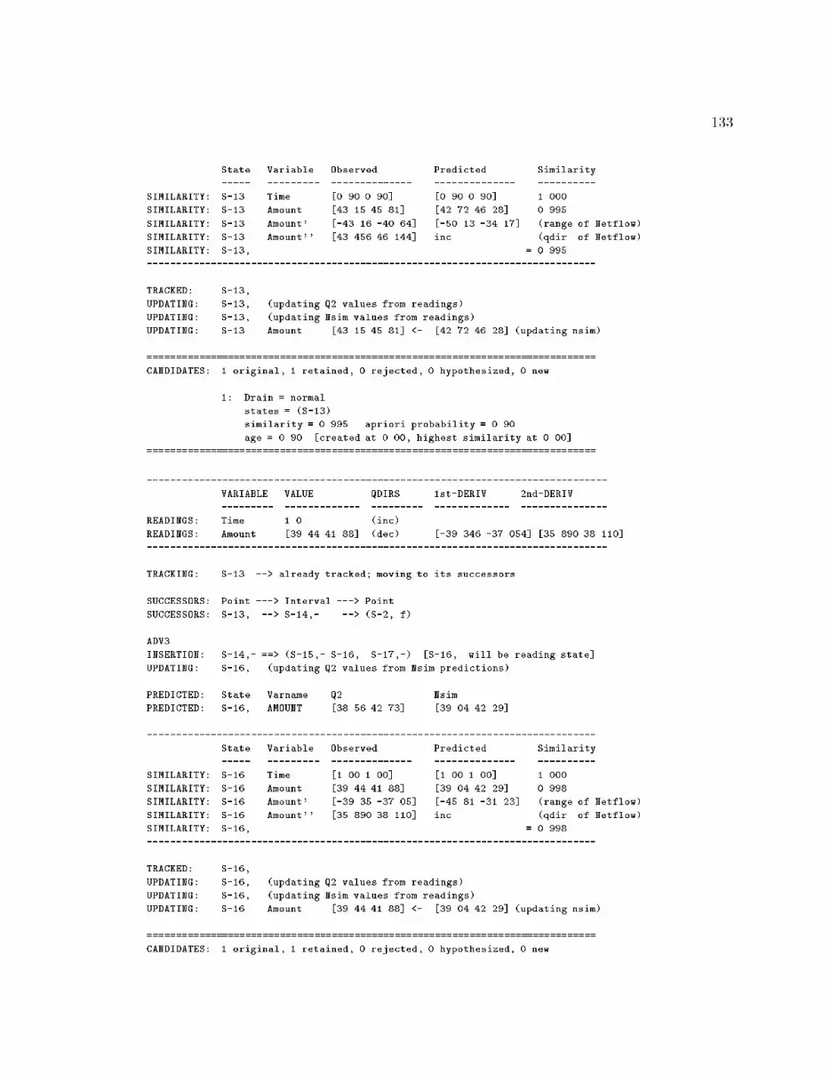
133State Variable Observed Predicted Similarity----- --------- -------------- -------------- ----------SIMILARITY: S-13 Time [0.90 0.90] [0.90 0.90] 1.000SIMILARITY: S-13 Amount [43.15 45.81] [42.72 46.28] 0.995SIMILARITY: S-13 Amount' [-43.16 -40.64] [-50.13 -34.17] (range of Netflow)SIMILARITY: S-13 Amount'' [43.456 46.144] inc (qdir of Netflow)SIMILARITY: S-13,. ............................................ = 0.995------------------------------------------------------------------------------TRACKED: S-13,.UPDATING: S-13,. (updating Q2 values from readings)UPDATING: S-13,. (updating Nsim values from readings)UPDATING: S-13 Amount [43.15 45.81] <- [42.72 46.28] (updating nsim)==============================================================================CANDIDATES: 1 original, 1 retained, 0 rejected, 0 hypothesized, 0 new.1: Drain = normalstates = (S-13)similarity = 0.995 apriori probability = 0.90age = 0.90 [created at 0.00, highest similarity at 0.00]==============================================================================--------------------------------------------------------------------------------VARIABLE VALUE QDIRS 1st-DERIV 2nd-DERIV--------- ------------- --------- ------------- ---------------READINGS: Time 1.0 (inc)READINGS: Amount [39.44 41.88] (dec) [-39.346 -37.054] [35.890 38.110]--------------------------------------------------------------------------------TRACKING: S-13 --> already tracked; moving to its successorsSUCCESSORS: Point ---> Interval ---> PointSUCCESSORS: S-13,. --> S-14,- --> (S-2,.f)ADV3INSERTION: S-14,- ==> (S-15,- S-16,. S-17,-) [S-16,. will be reading state]UPDATING: S-16,. (updating Q2 values from Nsim predictions)PREDICTED: State Varname Q2 NsimPREDICTED: S-16,. AMOUNT [38.56 42.73] [39.04 42.29]------------------------------------------------------------------------------State Variable Observed Predicted Similarity----- --------- -------------- -------------- ----------SIMILARITY: S-16 Time [1.00 1.00] [1.00 1.00] 1.000SIMILARITY: S-16 Amount [39.44 41.88] [39.04 42.29] 0.998SIMILARITY: S-16 Amount' [-39.35 -37.05] [-45.81 -31.23] (range of Netflow)SIMILARITY: S-16 Amount'' [35.890 38.110] inc (qdir of Netflow)SIMILARITY: S-16,. ............................................ = 0.998------------------------------------------------------------------------------TRACKED: S-16,.UPDATING: S-16,. (updating Q2 values from readings)UPDATING: S-16,. (updating Nsim values from readings)UPDATING: S-16 Amount [39.44 41.88] <- [39.04 42.29] (updating nsim)==============================================================================CANDIDATES: 1 original, 1 retained, 0 rejected, 0 hypothesized, 0 new.

134 1: Drain = normalstates = (S-16)similarity = 0.998 apriori probability = 0.90age = 1.00 [created at 0.00, highest similarity at 0.00]==============================================================================--------------------------------------------------------------------------------VARIABLE VALUE QDIRS 1st-DERIV 2nd-DERIV--------- ------------- --------- ------------- ---------------READINGS: Time 1.1 (inc)READINGS: Amount [37.14 39.44] (dec) [-24.411 -22.989] [140.650 149.350]--------------------------------------------------------------------------------TRACKING: S-16 --> already tracked; moving to its successorsSUCCESSORS: Point ---> Interval ---> PointSUCCESSORS: S-16,. --> S-17,- --> (S-2,.f)ADV3INSERTION: S-17,- ==> (S-18,- S-19,. S-20,-) [S-19,. will be reading state]UPDATING: S-19,. (updating Q2 values from Nsim predictions)PREDICTED: State Varname Q2 NsimPREDICTED: S-19,. AMOUNT [35.25 39.06] [35.69 38.66]------------------------------------------------------------------------------State Variable Observed Predicted Similarity----- --------- -------------- -------------- ----------SIMILARITY: S-19 Time [1.10 1.10] [1.10 1.10] 1.000SIMILARITY: S-19 Amount [37.14 39.44] [35.69 38.66] 0.576SIMILARITY: S-19 Amount' [-24.41 -22.99] [-41.88 -28.55] (range of Netflow) <--SIMILARITY: S-19 Amount'' [140.650 149.350] inc (qdir of Netflow)SIMILARITY: S-19,. ............................................ = RATE------------------------------------------------------------------------------TRACKING: S-19,. --> Rate discrepancy, is being discarded.DISCREP: S-19,. discrepancies (AMOUNT) saved on S-17,-REMOVAL: (S-18,- S-19,. S-20,-) ==> S-17,- [restoring S-17,-]SUCCESSORS: Point ---> Interval ---> PointSUCCESSORS: S-17,- --> S-2,.fADV2EXTENDING: S-2 is a quiescent/final state; cannot be extended.INSERTION: S-2,.f ==> S-21,.f [S-21,.f will be reading state]UPDATING: S-21,.f (updating Q2 values from Nsim predictions)PREDICTED: State Varname Q2 NsimPREDICTED: S-21,.# AMOUNT [19.00 20.00] [35.69 38.66]UPDATING: S-21,.# discrepancies = (TIME)TRACKING: S-21,.# being discarded because of inconsistency with Nsim values.DISCREP: S-21,.# discrepancies (TIME) saved on S-2,.fREMOVAL: S-21,.# ==> S-2,.f [restoring S-2,.f]SUCCESSORS: S-2,.f --> has no successors; status = (TRANSITION FINAL COMPLETE)TRACING: USE-DISCREPANCIES from S-17,-: (AMOUNT)TRACING: Amount evokes suspects (Drain tank tolerance amount-sensor)TRACING: Final suspects = (Drain tank tolerance amount-sensor)HYPOTHESES: Removing suspect TANK; it's not a mode variableHYPOTHESES: Removing suspect AMOUNT-SENSOR; it's not a mode variableTRACING: Tolerance is not a known mode variable.

135---------------------------------------------------------------------------HYPOTHESES: Single-change hypotheses:1: Drain = lo-blockage (prob = 0.0700)2: Drain = hi-blockage (prob = 0.0300)------------------------------------------------------------------------------------------------------------------------------------------------------HYPOTHESES: New (not old) hypotheses:1: Drain = lo-blockage (prob = 0.0700)2: Drain = hi-blockage (prob = 0.0300)-------------------------------------------------------------------------------------------------------------------------------------------------------INITIALIZE: Creating new state(s) from S-16 + hypothesized modes + readings.INITIALIZE: Drain = hi-blockageVar type Variable Qval Reading----------- ---------- ------------ -------------------time Time (t*-6 inc) (1.1 1.1)reading Amount (a-0 dec) (37.1413 39.4387)dependent Outflow (NIL nil)dependent Netflow (NIL nil)dependent Amount-obs (NIL nil)independent Tolerance (normal std)mode Drain (hi-blockage std)Run time: 0.025 seconds to initialize a state.INITIALIZE: S-22,. --completions--> (S-22,.)ZIP-UP (TIME t*-6): (-INF +INF) -> (0.9999999 +INF).Updating: (TIME t*-6) from (0.9999999 +INF) -> (1.0999999 1.1000001).Insignificant update ignored (TOLERANCE normal): (0.9799999 1.0200001) ~ (0.98 1.02).Updating: (OUTFLOW (AT S-22,.)) from (-INF +INF) -> (-INF 101).Updating: (OUTFLOW (AT S-22,.)) from (-INF 101) -> (0 101).Updating: (NETFLOW (AT S-22,.)) from (-INF +INF) -> (-101 0).Updating: (AMOUNT-OBS (AT S-22,.)) from (-INF +INF) -> (0 +INF).Updating: (OUTFLOW (AT S-22,.)) from (0 101) -> (0 17.06368).Updating: (NETFLOW (AT S-22,.)) from (-101 0) -> (-17.06368 0).Updating: (AMOUNT-OBS (AT S-22,.)) from (0 +INF) -> (37.792847 43.512386).ZIP-UP (TIME t1): (0.9999999 +INF) -> (1.0999999 +INF).Q2 assertions = (((TIME t*-6) (1.1 1.1)) ((AMOUNT a-0) (37.1413 39.4387)))Table is(OUTFLOW (M+ AMOUNT OUTFLOW))(NETFLOW (- OUTFLOW))(AMOUNT NETFLOW)State equations are((AMOUNT (- (FCTN (M+ AMOUNT OUTFLOW) AMOUNT))))Extremal Tables:::((AMOUNT LB (- (UB (M+ AMOUNT OUTFLOW) (LB AMOUNT))) T))((AMOUNT UB (- (LB (M+ AMOUNT OUTFLOW) (UB AMOUNT))) T))M-envelopes = (((M+ AMOUNT OUTFLOW) (UPPER-ENVELOPE UE1) (UPPER-INVERSE UI1)(LOWER-ENVELOPE LE1) (LOWER-INVERSE LI1)))env-set = ((UPPER-ENVELOPE UE1) (UPPER-INVERSE UI1)(LOWER-ENVELOPE LE1) (LOWER-INVERSE LI1))env = UE1Creating system function F0123(LAMBDA (TIN Y YP)(DECLARE (IGNORE TIN)) (SETF (SVREF YP 0) (- (FUNCALL #'UE1 (SVREF Y 0)))))M-envelopes = (((M+ AMOUNT OUTFLOW) (UPPER-ENVELOPE UE1) (UPPER-INVERSE UI1)(LOWER-ENVELOPE LE1) (LOWER-INVERSE LI1)))env-set = ((UPPER-ENVELOPE UE1) (UPPER-INVERSE UI1)(LOWER-ENVELOPE LE1) (LOWER-INVERSE LI1))

136env = LE1Creating system function F0124(LAMBDA (TIN Y YP)(DECLARE (IGNORE TIN)) (SETF (SVREF YP 0) (- (FUNCALL #'LE1 (SVREF Y 0)))))INITIALIZE: ---filtered----> (S-22,.)----------------------------------------------------------------------------UNDO: Created S-23,. from S-22,. by removing lmarks created for S-16,.-------------------------------------------------------------------------RESIMULATE: reading sequence = (S-4 S-7 S-10 S-13 S-16 S-22)RESIMULATE: resim sub-sequence = (S-16 S-22)RESIMULATE: starting from S-16 (time = 1.0)RESIMULATE: intersecting with readings from S-22 (time = 1.1)UPDATING: S-25 (updating Q2 values from readings)UPDATING: S-25 (updating Nsim values from readings)UPDATING: S-25 Amount [37.89 39.44] <- [37.89 41.88] (updating nsim)RESIMULATE: S-25 sim = 0.49175772RESIMULATE: resim sub-sequence = (S-13 S-16 S-22)RESIMULATE: starting from S-13 (time = 0.9)RESIMULATE: intersecting with readings from S-16 (time = 1.0)UPDATING: S-27 (updating Q2 values from readings)UPDATING: S-27 (updating Nsim values from readings)UPDATING: S-27 Amount [41.45 41.88] <- [41.45 45.81] (updating nsim)RESIMULATE: intersecting with readings from S-22 (time = 1.1)UPDATING: S-29 (updating Q2 values from readings)UPDATING: S-29 (updating Nsim values from readings)UPDATING: S-29 Amount [39.83 39.44] <- [39.83 41.88] (updating nsim)discarding because lower bound exceeds upper bound!RESIMULATE: S-29 sim = 0RESIMULATE: best-state = S-25, best-sim = 0.49175772, best-time = 1.0-------------------------------------------------------------------------EXTENDING: S-25 to next time point stateSUCCESSORS: S-25 --> (S-30) [before global filters]SUCCESSORS: S-25 --> (S-30) [after global filters]SUCCESSORS: S-30 --> (S-31) [before global filters]SUCCESSORS: S-30 --> (S-31) [after global filters]HYPOTHESES: (Drain = hi-blockage) ---> (S-25,.)----------------------------------------------------------------------------INITIALIZE: Creating new state(s) from S-16 + hypothesized modes + readings.INITIALIZE: Drain = lo-blockageVar type Variable Qval Reading----------- ---------- ------------ -------------------time Time (t*-10 inc) (1.1 1.1)reading Amount (a-0 dec) (37.1413 39.4387)dependent Outflow (NIL nil)dependent Netflow (NIL nil)dependent Amount-obs (NIL nil)independent Tolerance (normal std)mode Drain (lo-blockage std)Run time: 0.042 seconds to initialize a state.INITIALIZE: S-32,. --completions--> (S-32,.)ZIP-UP (TIME t*-10): (-INF +INF) -> (0.9999999 +INF).

137Updating: (TIME t*-10) from (0.9999999 +INF) -> (1.0999999 1.1000001).Insignificant update ignored (TOLERANCE normal): (0.9799999 1.0200001) ~ (0.98 1.02).Updating: (OUTFLOW (AT S-32,.)) from (-INF +INF) -> (-INF 101).Updating: (OUTFLOW (AT S-32,.)) from (-INF 101) -> (0 101).Updating: (NETFLOW (AT S-32,.)) from (-INF +INF) -> (-101 0).Updating: (AMOUNT-OBS (AT S-32,.)) from (-INF +INF) -> (0 +INF).Updating: (OUTFLOW (AT S-32,.)) from (0 101) -> (15.425653 34.12736).Updating: (NETFLOW (AT S-32,.)) from (-101 0) -> (-34.12736 -15.425653).Updating: (AMOUNT-OBS (AT S-32,.)) from (0 +INF) -> (37.792847 43.512386).ZIP-UP (TIME t1): (0.9999999 +INF) -> (1.0999999 +INF).Q2 assertions = (((TIME t*-10) (1.1 1.1)) ((AMOUNT a-0) (37.1413 39.4387)))Table is(OUTFLOW (M+ AMOUNT OUTFLOW))(NETFLOW (- OUTFLOW))(AMOUNT NETFLOW)State equations are((AMOUNT (- (FCTN (M+ AMOUNT OUTFLOW) AMOUNT))))Extremal Tables:::((AMOUNT LB (- (UB (M+ AMOUNT OUTFLOW) (LB AMOUNT))) T))((AMOUNT UB (- (LB (M+ AMOUNT OUTFLOW) (UB AMOUNT))) T))M-envelopes = (((M+ AMOUNT OUTFLOW) (UPPER-ENVELOPE UE1) (UPPER-INVERSE UI1)(LOWER-ENVELOPE LE1) (LOWER-INVERSE LI1)))env-set = ((UPPER-ENVELOPE UE1) (UPPER-INVERSE UI1)(LOWER-ENVELOPE LE1) (LOWER-INVERSE LI1))env = UE1Creating system function F0125(LAMBDA (TIN Y YP)(DECLARE (IGNORE TIN)) (SETF (SVREF YP 0) (- (FUNCALL #'UE1 (SVREF Y 0)))))M-envelopes = (((M+ AMOUNT OUTFLOW) (UPPER-ENVELOPE UE1) (UPPER-INVERSE UI1)(LOWER-ENVELOPE LE1) (LOWER-INVERSE LI1)))env-set = ((UPPER-ENVELOPE UE1) (UPPER-INVERSE UI1)(LOWER-ENVELOPE LE1) (LOWER-INVERSE LI1))env = LE1Creating system function F0126(LAMBDA (TIN Y YP)(DECLARE (IGNORE TIN)) (SETF (SVREF YP 0) (- (FUNCALL #'LE1 (SVREF Y 0)))))INITIALIZE: ---filtered----> (S-32,.)----------------------------------------------------------------------------UNDO: Created S-33,. from S-32,. by removing lmarks created for S-16,.-------------------------------------------------------------------------RESIMULATE: reading sequence = (S-4 S-7 S-10 S-13 S-16 S-32)RESIMULATE: resim sub-sequence = (S-16 S-32)RESIMULATE: starting from S-16 (time = 1.0)RESIMULATE: intersecting with readings from S-32 (time = 1.1)UPDATING: S-35 (updating Q2 values from readings)UPDATING: S-35 (updating Nsim values from readings)UPDATING: S-35 Amount [37.14 39.44] <- [36.41 40.24] (updating nsim)RESIMULATE: S-35 sim = 0.9893015RESIMULATE: resim sub-sequence = (S-13 S-16 S-32)RESIMULATE: starting from S-13 (time = 0.9)RESIMULATE: intersecting with readings from S-16 (time = 1.0)UPDATING: S-37 (updating Q2 values from readings)UPDATING: S-37 (updating Nsim values from readings)UPDATING: S-37 Amount [39.83 41.88] <- [39.83 44.02] (updating nsim)RESIMULATE: intersecting with readings from S-32 (time = 1.1)UPDATING: S-39 (updating Q2 values from readings)UPDATING: S-39 (updating Nsim values from readings)

138UPDATING: S-39 Amount [37.14 39.44] <- [36.77 40.24] (updating nsim)RESIMULATE: S-39 sim = 0.92651534RESIMULATE: best-state = S-35, best-sim = 0.9893015, best-time = 1.0-------------------------------------------------------------------------EXTENDING: S-35 to next time point stateSUCCESSORS: S-35 --> (S-40) [before global filters]SUCCESSORS: S-35 --> (S-40) [after global filters]SUCCESSORS: S-40 --> (S-41) [before global filters]SUCCESSORS: S-40 --> (S-41) [after global filters]HYPOTHESES: (Drain = lo-blockage) ---> (S-35,.)==============================================================================CANDIDATES: 1 original, 0 retained, 1 rejected, 2 hypothesized, 2 new.1: Drain = hi-blockagestates = (S-25)similarity = 0.492 apriori probability = 0.03age = 0.10 [created at 1.10, highest similarity at 1.00]2: Drain = lo-blockagestates = (S-35)similarity = 0.989 apriori probability = 0.07age = 0.10 [created at 1.10, highest similarity at 1.00]==============================================================================--------------------------------------------------------------------------------VARIABLE VALUE QDIRS 1st-DERIV 2nd-DERIV--------- ------------- --------- ------------- ---------------READINGS: Time 1.2 (inc)READINGS: Amount [34.98 37.14] (dec) [-22.969 -21.631] [13.580 14.420]--------------------------------------------------------------------------------ADV3EXTENDING: S-25 to next time point stateTRACKING: S-25 at time = [1.10 1.10] does not cover time of readings 1.2SUCCESSORS: Point ---> Interval ---> PointSUCCESSORS: S-25,. --> S-30,- --> (S-31,.f)ADV2INSERTION: S-30,- ==> (S-42,- S-43,. S-44,-) [S-43,. will be reading state]UPDATING: S-43,. (updating Q2 values from Nsim predictions)PREDICTED: State Varname Q2 NsimPREDICTED: S-43,. AMOUNT [35.56 39.44] [36.41 39.44]------------------------------------------------------------------------------State Variable Observed Predicted Similarity----- --------- -------------- -------------- ----------SIMILARITY: S-43 Time [1.20 1.20] [1.20 1.20] 1.000SIMILARITY: S-43 Amount [34.98 37.14] [36.41 39.44] 0.283SIMILARITY: S-43 Amount' [-22.97 -21.63] [-15.78 0.00] (range of Netflow) <--SIMILARITY: S-43 Amount'' [13.580 14.420] inc (qdir of Netflow)SIMILARITY: S-43,. ............................................ = RATE------------------------------------------------------------------------------TRACKING: S-43,. --> Rate discrepancy, is being discarded.DISCREP: S-43,. discrepancies (AMOUNT) saved on S-30,-

139REMOVAL: (S-42,- S-43,. S-44,-) ==> S-30,- [restoring S-30,-]SUCCESSORS: Point ---> Interval ---> PointSUCCESSORS: S-30,- --> S-31,.fADV2EXTENDING: S-31 is a quiescent/final state; cannot be extended.INSERTION: S-31,.f ==> S-45,.f [S-45,.f will be reading state]UPDATING: S-45,.f (updating Q2 values from Nsim predictions)PREDICTED: State Varname Q2 NsimPREDICTED: S-45,.# AMOUNT [19.00 20.00] [36.41 39.44]UPDATING: S-45,.# discrepancies = (TIME)TRACKING: S-45,.# being discarded because of inconsistency with Nsim values.DISCREP: S-45,.# discrepancies (TIME) saved on S-31,.fREMOVAL: S-45,.# ==> S-31,.f [restoring S-31,.f]SUCCESSORS: S-31,.f --> has no successors; status = (TRANSITION FINAL COMPLETE)ADV3EXTENDING: S-35 to next time point stateTRACKING: S-35 at time = [1.10 1.10] does not cover time of readings 1.2SUCCESSORS: Point ---> Interval ---> PointSUCCESSORS: S-35,. --> S-40,- --> (S-41,.f)ADV2INSERTION: S-40,- ==> (S-46,- S-47,. S-48,-) [S-47,. will be reading state]UPDATING: S-47,. (updating Q2 values from Nsim predictions)PREDICTED: State Varname Q2 NsimPREDICTED: S-47,. AMOUNT [33.99 38.08] [34.29 37.89]------------------------------------------------------------------------------State Variable Observed Predicted Similarity----- --------- -------------- -------------- ----------SIMILARITY: S-47 Time [1.20 1.20] [1.20 1.20] 1.000SIMILARITY: S-47 Amount [34.98 37.14] [34.29 37.89] 0.990SIMILARITY: S-47 Amount' [-22.97 -21.63] [-31.55 -13.71] (range of Netflow)SIMILARITY: S-47 Amount'' [13.580 14.420] inc (qdir of Netflow)SIMILARITY: S-47,. ............................................ = 0.990------------------------------------------------------------------------------TRACKED: S-47,.UPDATING: S-47,. (updating Q2 values from readings)UPDATING: S-47,. (updating Nsim values from readings)UPDATING: S-47 Amount [34.98 37.14] <- [34.29 37.89] (updating nsim)==============================================================================CANDIDATES: 2 original, 1 retained, 1 rejected, 0 hypothesized, 0 new.1: Drain = lo-blockagestates = (S-47)similarity = 0.990 apriori probability = 0.07age = 0.20 [created at 1.10, highest similarity at 1.00]==============================================================================--------------------------------------------------------------------------------VARIABLE VALUE QDIRS 1st-DERIV 2nd-DERIV--------- ------------- --------- ------------- ---------------READINGS: Time 1.3 (inc)READINGS: Amount [32.94 34.98] (dec) [-21.630 -20.370] [12.609 13.390]

140--------------------------------------------------------------------------------TRACKING: S-47 --> already tracked; moving to its successorsSUCCESSORS: Point ---> Interval ---> PointSUCCESSORS: S-47,. --> S-48,- --> (S-41,.f)ADV3INSERTION: S-48,- ==> (S-49,- S-50,. S-51,-) [S-50,. will be reading state]UPDATING: S-50,. (updating Q2 values from Nsim predictions)PREDICTED: State Varname Q2 NsimPREDICTED: S-50,. AMOUNT [32.01 35.86] [32.29 35.69]------------------------------------------------------------------------------State Variable Observed Predicted Similarity----- --------- -------------- -------------- ----------SIMILARITY: S-50 Time [1.30 1.30] [1.30 1.30] 1.000SIMILARITY: S-50 Amount [32.94 34.98] [32.29 35.69] 0.990SIMILARITY: S-50 Amount' [-21.63 -20.37] [-29.71 -12.92] (range of Netflow)SIMILARITY: S-50 Amount'' [12.609 13.390] inc (qdir of Netflow)SIMILARITY: S-50,. ............................................ = 0.990------------------------------------------------------------------------------TRACKED: S-50,.UPDATING: S-50,. (updating Q2 values from readings)UPDATING: S-50,. (updating Nsim values from readings)UPDATING: S-50 Amount [32.94 34.98] <- [32.29 35.69] (updating nsim)==============================================================================CANDIDATES: 1 original, 1 retained, 0 rejected, 0 hypothesized, 0 new.1: Drain = lo-blockagestates = (S-50)similarity = 0.990 apriori probability = 0.07age = 0.30 [created at 1.10, highest similarity at 1.00]==============================================================================--------------------------------------------------------------------------------VARIABLE VALUE QDIRS 1st-DERIV 2nd-DERIV--------- ------------- --------- ------------- ---------------READINGS: Time 1.4 (inc)READINGS: Amount [31.02 32.94] (dec) [-20.394 -19.206] [11.640 12.361]--------------------------------------------------------------------------------TRACKING: S-50 --> already tracked; moving to its successorsSUCCESSORS: Point ---> Interval ---> PointSUCCESSORS: S-50,. --> S-51,- --> (S-41,.f)ADV3INSERTION: S-51,- ==> (S-52,- S-53,. S-54,-) [S-53,. will be reading state]UPDATING: S-53,. (updating Q2 values from Nsim predictions)PREDICTED: State Varname Q2 NsimPREDICTED: S-53,. AMOUNT [30.14 33.77] [30.41 33.61]------------------------------------------------------------------------------State Variable Observed Predicted Similarity----- --------- -------------- -------------- ----------

141SIMILARITY: S-53 Time [1.40 1.40] [1.40 1.40] 1.000SIMILARITY: S-53 Amount [31.02 32.94] [30.41 33.61] 0.989SIMILARITY: S-53 Amount' [-20.39 -19.21] [-27.98 -12.16] (range of Netflow)SIMILARITY: S-53 Amount'' [11.640 12.361] inc (qdir of Netflow)SIMILARITY: S-53,. ............................................ = 0.989------------------------------------------------------------------------------TRACKED: S-53,.UPDATING: S-53,. (updating Q2 values from readings)UPDATING: S-53,. (updating Nsim values from readings)UPDATING: S-53 Amount [31.02 32.94] <- [30.41 33.61] (updating nsim)==============================================================================CANDIDATES: 1 original, 1 retained, 0 rejected, 0 hypothesized, 0 new.1: Drain = lo-blockagestates = (S-53)similarity = 0.989 apriori probability = 0.07age = 0.40 [created at 1.10, highest similarity at 1.00]==============================================================================--------------------------------------------------------------------------------VARIABLE VALUE QDIRS 1st-DERIV 2nd-DERIV--------- ------------- --------- ------------- ---------------READINGS: Time 1.5 (inc)READINGS: Amount [29.22 31.02] (dec) [-19.158 -18.042] [11.640 12.360]--------------------------------------------------------------------------------TRACKING: S-53 --> already tracked; moving to its successorsSUCCESSORS: Point ---> Interval ---> PointSUCCESSORS: S-53,. --> S-54,- --> (S-41,.f)ADV3INSERTION: S-54,- ==> (S-55,- S-56,. S-57,-) [S-56,. will be reading state]UPDATING: S-56,. (updating Q2 values from Nsim predictions)PREDICTED: State Varname Q2 NsimPREDICTED: S-56,. AMOUNT [28.39 31.80] [28.64 31.65]------------------------------------------------------------------------------State Variable Observed Predicted Similarity----- --------- -------------- -------------- ----------SIMILARITY: S-56 Time [1.50 1.50] [1.50 1.50] 1.000SIMILARITY: S-56 Amount [29.22 31.02] [28.64 31.65] 0.991SIMILARITY: S-56 Amount' [-19.16 -18.04] [-26.35 -11.45] (range of Netflow)SIMILARITY: S-56 Amount'' [11.640 12.360] inc (qdir of Netflow)SIMILARITY: S-56,. ............................................ = 0.991------------------------------------------------------------------------------TRACKED: S-56,.UPDATING: S-56,. (updating Q2 values from readings)UPDATING: S-56,. (updating Nsim values from readings)UPDATING: S-56 Amount [29.22 31.02] <- [28.64 31.65] (updating nsim)==============================================================================CANDIDATES: 1 original, 1 retained, 0 rejected, 0 hypothesized, 0 new.1: Drain = lo-blockagestates = (S-56)

142 similarity = 0.991 apriori probability = 0.07age = 0.50 [created at 1.10, highest similarity at 1.00]==============================================================================--------------------------------------------------------------------------------VARIABLE VALUE QDIRS 1st-DERIV 2nd-DERIV--------- ------------- --------- ------------- ---------------READINGS: Time 1.6 (inc)READINGS: Amount [27.51 29.21] (dec) [-18.128 -17.072] [9.700 10.300]--------------------------------------------------------------------------------TRACKING: S-56 --> already tracked; moving to its successorsSUCCESSORS: Point ---> Interval ---> PointSUCCESSORS: S-56,. --> S-57,- --> (S-41,.f)ADV3INSERTION: S-57,- ==> (S-58,- S-59,. S-60,-) [S-59,. will be reading state]UPDATING: S-59,. (updating Q2 values from Nsim predictions)PREDICTED: State Varname Q2 NsimPREDICTED: S-59,. AMOUNT [26.73 29.95] [26.97 29.81]------------------------------------------------------------------------------State Variable Observed Predicted Similarity----- --------- -------------- -------------- ----------SIMILARITY: S-59 Time [1.60 1.60] [1.60 1.60] 1.000SIMILARITY: S-59 Amount [27.51 29.21] [26.97 29.81] 0.987SIMILARITY: S-59 Amount' [-18.13 -17.07] [-24.82 -10.79] (range of Netflow)SIMILARITY: S-59 Amount'' [9.700 10.300] inc (qdir of Netflow)SIMILARITY: S-59,. ............................................ = 0.987------------------------------------------------------------------------------TRACKED: S-59,.UPDATING: S-59,. (updating Q2 values from readings)UPDATING: S-59,. (updating Nsim values from readings)UPDATING: S-59 Amount [27.51 29.21] <- [26.97 29.81] (updating nsim)==============================================================================CANDIDATES: 1 original, 1 retained, 0 rejected, 0 hypothesized, 0 new.1: Drain = lo-blockagestates = (S-59)similarity = 0.987 apriori probability = 0.07age = 0.60 [created at 1.10, highest similarity at 1.00]==============================================================================--------------------------------------------------------------------------------VARIABLE VALUE QDIRS 1st-DERIV 2nd-DERIV--------- ------------- --------- ------------- ---------------READINGS: Time 1.7 (inc)READINGS: Amount [25.91 27.51] (dec) [-16.995 -16.005] [10.670 11.330]--------------------------------------------------------------------------------TRACKING: S-59 --> already tracked; moving to its successorsSUCCESSORS: Point ---> Interval ---> PointSUCCESSORS: S-59,. --> S-60,- --> (S-41,.f)

143ADV3INSERTION: S-60,- ==> (S-61,- S-62,. S-63,-) [S-62,. will be reading state]UPDATING: S-62,. (updating Q2 values from Nsim predictions)PREDICTED: State Varname Q2 NsimPREDICTED: S-62,. AMOUNT [25.17 28.20] [25.39 28.07]------------------------------------------------------------------------------State Variable Observed Predicted Similarity----- --------- -------------- -------------- ----------SIMILARITY: S-62 Time [1.70 1.70] [1.70 1.70] 1.000SIMILARITY: S-62 Amount [25.91 27.51] [25.39 28.07] 0.991SIMILARITY: S-62 Amount' [-17.00 -16.01] [-23.37 -10.16] (range of Netflow)SIMILARITY: S-62 Amount'' [10.670 11.330] inc (qdir of Netflow)SIMILARITY: S-62,. ............................................ = 0.991------------------------------------------------------------------------------TRACKED: S-62,.UPDATING: S-62,. (updating Q2 values from readings)UPDATING: S-62,. (updating Nsim values from readings)UPDATING: S-62 Amount [25.91 27.51] <- [25.39 28.07] (updating nsim)==============================================================================CANDIDATES: 1 original, 1 retained, 0 rejected, 0 hypothesized, 0 new.1: Drain = lo-blockagestates = (S-62)similarity = 0.991 apriori probability = 0.07age = 0.70 [created at 1.10, highest similarity at 1.00]==============================================================================--------------------------------------------------------------------------------VARIABLE VALUE QDIRS 1st-DERIV 2nd-DERIV--------- ------------- --------- ------------- ---------------READINGS: Time 1.8 (inc)READINGS: Amount [24.41 25.91] (dec) [-15.965 -15.035] [9.700 10.300]--------------------------------------------------------------------------------TRACKING: S-62 --> already tracked; moving to its successorsSUCCESSORS: Point ---> Interval ---> PointSUCCESSORS: S-62,. --> S-63,- --> (S-41,.f)ADV3INSERTION: S-63,- ==> (S-64,- S-65,. S-66,-) [S-65,. will be reading state]UPDATING: S-65,. (updating Q2 values from Nsim predictions)PREDICTED: State Varname Q2 NsimPREDICTED: S-65,. AMOUNT [23.71 26.56] [23.92 26.43]------------------------------------------------------------------------------State Variable Observed Predicted Similarity----- --------- -------------- -------------- ----------SIMILARITY: S-65 Time [1.80 1.80] [1.80 1.80] 1.000SIMILARITY: S-65 Amount [24.41 25.91] [23.92 26.43] 0.993SIMILARITY: S-65 Amount' [-15.97 -15.04] [-22.01 -9.57] (range of Netflow)SIMILARITY: S-65 Amount'' [9.700 10.300] inc (qdir of Netflow)SIMILARITY: S-65,. ............................................ = 0.993------------------------------------------------------------------------------

144TRACKED: S-65,.UPDATING: S-65,. (updating Q2 values from readings)UPDATING: S-65,. (updating Nsim values from readings)UPDATING: S-65 Amount [24.41 25.91] <- [23.92 26.43] (updating nsim)==============================================================================CANDIDATES: 1 original, 1 retained, 0 rejected, 0 hypothesized, 0 new.1: Drain = lo-blockagestates = (S-65)similarity = 0.993 apriori probability = 0.07age = 0.80 [created at 1.10, highest similarity at 1.00]==============================================================================--------------------------------------------------------------------------------VARIABLE VALUE QDIRS 1st-DERIV 2nd-DERIV--------- ------------- --------- ------------- ---------------READINGS: Time 1.9 (inc)READINGS: Amount [22.98 24.40] (dec) [-15.141 -14.259] [7.760 8.240]--------------------------------------------------------------------------------TRACKING: S-65 --> already tracked; moving to its successorsSUCCESSORS: Point ---> Interval ---> PointSUCCESSORS: S-65,. --> S-66,- --> (S-41,.f)ADV3INSERTION: S-66,- ==> (S-67,- S-68,. S-69,-) [S-68,. will be reading state]UPDATING: S-68,. (updating Q2 values from Nsim predictions)PREDICTED: State Varname Q2 NsimPREDICTED: S-68,. AMOUNT [22.33 25.02] [22.53 24.90]------------------------------------------------------------------------------State Variable Observed Predicted Similarity----- --------- -------------- -------------- ----------SIMILARITY: S-68 Time [1.90 1.90] [1.90 1.90] 1.000SIMILARITY: S-68 Amount [22.98 24.40] [22.53 24.90] 0.987SIMILARITY: S-68 Amount' [-15.14 -14.26] [-20.73 -9.01] (range of Netflow)SIMILARITY: S-68 Amount'' [7.760 8.240] inc (qdir of Netflow)SIMILARITY: S-68,. ............................................ = 0.987------------------------------------------------------------------------------TRACKED: S-68,.UPDATING: S-68,. (updating Q2 values from readings)UPDATING: S-68,. (updating Nsim values from readings)UPDATING: S-68 Amount [22.98 24.40] <- [22.53 24.90] (updating nsim)==============================================================================CANDIDATES: 1 original, 1 retained, 0 rejected, 0 hypothesized, 0 new.1: Drain = lo-blockagestates = (S-68)similarity = 0.987 apriori probability = 0.07age = 0.90 [created at 1.10, highest similarity at 1.00]==============================================================================--------------------------------------------------------------------------------VARIABLE VALUE QDIRS 1st-DERIV 2nd-DERIV

145--------- ------------- --------- ------------- ---------------READINGS: Time 2.0 (inc)READINGS: Amount [21.64 22.98] (dec) [-14.214 -13.386] [8.730 9.270]--------------------------------------------------------------------------------TRACKING: S-68 --> already tracked; moving to its successorsSUCCESSORS: Point ---> Interval ---> PointSUCCESSORS: S-68,. --> S-69,- --> (S-41,.f)ADV3INSERTION: S-69,- ==> (S-70,- S-71,. S-72,-) [S-71,. will be reading state]UPDATING: S-71,. (updating Q2 values from Nsim predictions)PREDICTED: State Varname Q2 NsimPREDICTED: S-71,. AMOUNT [21.03 23.56] [21.21 23.44]------------------------------------------------------------------------------State Variable Observed Predicted Similarity----- --------- -------------- -------------- ----------SIMILARITY: S-71 Time [2.00 2.00] [2.00 2.00] 1.000SIMILARITY: S-71 Amount [21.64 22.98] [21.21 23.44] 0.990SIMILARITY: S-71 Amount' [-14.21 -13.39] [-19.52 -8.49] (range of Netflow)SIMILARITY: S-71 Amount'' [8.730 9.270] inc (qdir of Netflow)SIMILARITY: S-71,. ............................................ = 0.990------------------------------------------------------------------------------TRACKED: S-71,.UPDATING: S-71,. (updating Q2 values from readings)UPDATING: S-71,. (updating Nsim values from readings)UPDATING: S-71 Amount [21.64 22.98] <- [21.21 23.44] (updating nsim)==============================================================================CANDIDATES: 1 original, 1 retained, 0 rejected, 0 hypothesized, 0 new.1: Drain = lo-blockagestates = (S-71)similarity = 0.990 apriori probability = 0.07age = 1.00 [created at 1.10, highest similarity at 1.00]==============================================================================--------------------------------------------------------------------------------VARIABLE VALUE QDIRS 1st-DERIV 2nd-DERIV--------- ------------- --------- ------------- ---------------READINGS: Time 2.1 (inc)READINGS: Amount [20.38 21.64] (dec) [-13.390 -12.610] [7.760 8.240]--------------------------------------------------------------------------------TRACKING: S-71 --> already tracked; moving to its successorsSUCCESSORS: Point ---> Interval ---> PointSUCCESSORS: S-71,. --> S-72,- --> (S-41,.f)ADV3INSERTION: S-72,- ==> (S-73,- S-74,. S-75,-) [S-74,. will be reading state]UPDATING: S-74,. (updating Q2 values from Nsim predictions)PREDICTED: State Varname Q2 NsimPREDICTED: S-74,. AMOUNT [19.80 22.19] [19.98 22.08]

146------------------------------------------------------------------------------State Variable Observed Predicted Similarity----- --------- -------------- -------------- ----------SIMILARITY: S-74 Time [2.10 2.10] [2.10 2.10] 1.000SIMILARITY: S-74 Amount [20.38 21.64] [19.98 22.08] 0.990SIMILARITY: S-74 Amount' [-13.39 -12.61] [-18.38 -7.99] (range of Netflow)SIMILARITY: S-74 Amount'' [7.760 8.240] inc (qdir of Netflow)SIMILARITY: S-74,. ............................................ = 0.990------------------------------------------------------------------------------TRACKED: S-74,.UPDATING: S-74,. (updating Q2 values from readings)UPDATING: S-74,. (updating Nsim values from readings)UPDATING: S-74 Amount [20.38 21.64] <- [19.98 22.08] (updating nsim)==============================================================================CANDIDATES: 1 original, 1 retained, 0 rejected, 0 hypothesized, 0 new.1: Drain = lo-blockagestates = (S-74)similarity = 0.990 apriori probability = 0.07age = 1.10 [created at 1.10, highest similarity at 1.00]==============================================================================--------------------------------------------------------------------------------VARIABLE VALUE QDIRS 1st-DERIV 2nd-DERIV--------- ------------- --------- ------------- ---------------READINGS: Time 2.2 (inc)READINGS: Amount [19.19 20.37] (dec) [-12.669 -11.931] [6.790 7.210]--------------------------------------------------------------------------------TRACKING: S-74 --> already tracked; moving to its successorsSUCCESSORS: Point ---> Interval ---> PointSUCCESSORS: S-74,. --> S-75,- --> (S-41,.f)ADV3INSERTION: S-75,- ==> (S-76,- S-77,. S-78,-) [S-77,. will be reading state]UPDATING: S-77,. (updating Q2 values from Nsim predictions)PREDICTED: State Varname Q2 NsimPREDICTED: S-77,. AMOUNT [19.00 20.88] [18.81 20.79]------------------------------------------------------------------------------State Variable Observed Predicted Similarity----- --------- -------------- -------------- ----------SIMILARITY: S-77 Time [2.20 2.20] [2.20 2.20] 1.000SIMILARITY: S-77 Amount [19.19 20.37] [19.00 20.79] 0.922SIMILARITY: S-77 Amount' [-12.67 -11.93] [-17.31 -7.60] (range of Netflow)SIMILARITY: S-77 Amount'' [6.790 7.210] inc (qdir of Netflow)SIMILARITY: S-77,. ............................................ = 0.922------------------------------------------------------------------------------TRACKED: S-77,.UPDATING: S-77,. (updating Q2 values from readings)UPDATING: S-77,. (updating Nsim values from readings)UPDATING: S-77 Amount [19.19 20.37] <- [18.81 20.79] (updating nsim)==============================================================================CANDIDATES: 1 original, 1 retained, 0 rejected, 0 hypothesized, 0 new.

1471: Drain = lo-blockagestates = (S-77)similarity = 0.922 apriori probability = 0.07age = 1.20 [created at 1.10, highest similarity at 1.00]==============================================================================

148

BIBLIOGRAPHY[Abb90] Kathy Hamilton Abbott. Robust Fault Diagnosis of Physical Systems in Oper-ation. PhD thesis, Rutgers University, May 1990.[All84] James Allen. Towards a general theory of action and time. Arti�cial Intelli-gence, 23(2):123{154, 1984.[BBd82] J. S. Brown, R. R. Burton, and J. deKleer. Pedagogical, natural language, andknowledge engineering techniques in sophie i, ii, and iii. In D. Sleeman and J. S.Brown, editors, Intelligent Tutoring Systems, pages 227{282. Academic Press,1982.[Ber91] Jared Daniel Berleant. The Use of Partial Quantitative Information with Qual-itative Reasoning. PhD thesis, Department of Computer Sciences, The Univer-sity of Texas at Austin, August 1991. Also published as tech report AI 91-163.[BML89] Ivan Bratko, Igor Mozeti�c, and Nada Lavra�c. KARDIO: A Study in Deep andQualitative Knowledge for Expert Systems. MIT Press, 1989.[Can86] James V. Candy. Signal Processing: The Model-Based Approach. McGraw-HillSeries in Electrical Engineering. McGraw-Hill, 1986.[Can88] James V. Candy. Signal Processing: The Modern Approach. McGraw-Hill Seriesin Electrical Engineering. McGraw-Hill, 1988.[CFP89] R. N. Clark, P. M. Frank, and R. J. Patton. Fault Diagnosis in Dynamic Sys-tems: Theory and Applications, chapter 1: Introduction, pages 1{19. PrenticeHall, 1989. (editors: Ron Patton, Paul Frank, Robert Clark).[Cla89] William J. Clancey. Viewing knowledge bases as qualitative models. IEEEExpert, 4(2):9{23, summer 1989.[CS90a] J. T.-Y. Cheung and G. Stephanopoulos. Representation of process trends|part I. a formal representation framework. Computers Chem. Engng.,14(4/5):495{510, 1990.[CS90b] J. T.-Y. Cheung and G. Stephanopoulos. Representation of process trends|part II. the problem of scale and qualitative scaling. Computers Chem. Engng.,14(4/5):511{539, 1990. 149

150[Dav84] Randall Davis. Diagnostic reasoning based on structure and behavior. Arti�-cial Intelligence, 24(3):347{410, December 1984. Also in Qualitative Reasoningabout Physical Systems, pages 347{410, D. G. Bobrow (ed.), MIT Press, Cam-bridge, Massachusetts, 1985.[Dav89] Randall Davis. Form and content in model based reasoning. In Working Papersof the 1989 Workshop on Model Based Reasoning, pages 11{27, August 1989.Detroit, Michigan.[DeC90] Dennis DeCoste. Dynamic across-time measurement interpretation. In AAAI-90, pages 373{379. American Association for Arti�cial Intelligence, AAAI Press,July 1990.[Den86] P. J. Denning. Towards a science of expert systems. IEEE Expert, 1(2):80{83,1986.[DF91] Richard J. Doyle and Usama M. Fayyad. Sensor selection techniques in devicemonitoring. In Proceedings of the Second Annual Conference on AI, Simula-tion and Planning in High Autonomy Systems, pages 154{163. IEEE ComputerSociety Press, April 1991.[DH88] Randall Davis and Walter Hamscher. Exploring Arti�cial Intelligence, chapter8: Model-based Reasoning: Troubleshooting, pages 297{346. Morgan Kauf-mann Publishers, 1988.[DK89] Daniel Dvorak and Benjamin Kuipers. Model-based monitoring of dynamic sys-tems. In Proceedings of the Eleventh International Joint Conference on Arti�-cial Intelligence (IJCAI-89), pages 1238{1243, August 1989. Detroit, Michigan.[DK91] Daniel Dvorak and Benjamin Kuipers. Process monitoring and diagnosis: Amodel-based approach. IEEE Expert, 6(3):67{74, June 1991.[dKW87] Johan de Kleer and Brian C. Williams. Diagnosing multiple faults. Arti�cialIntelligence, 32(1):97{130, April 1987.[dKW89] Johan de Kleer and Brian C. Williams. Diagnosis with behavioral modes. InProceedings of the Eleventh International Joint Conference on Arti�cial Intel-ligence (IJCAI-89), pages 1324{1330, August 1989.[DSA87] R. J. Doyle, S. M. Sellers, and D. J. Atkinson. Predictive monitoring based oncausal simulation. In Proceedings of the Second Annual Research Forum, pages44{59. NASA Ames Research Center, 1987.

151[DSA89] Richard J. Doyle, Suzanne M. Sellers, and David J. Atkinson. A focused,context-sensitive approach to monitoring. In Proceedings of the Eleventh In-ternational Joint Conference on Arti�cial Intelligence (IJCAI-89), pages 1231{1237. International Joint Conferences on Arti�cial Intelligence, Inc., August1989.[Dvo87] Daniel L. Dvorak. Expert systems for monitoring and control. Technical ReportAI87-55, Department of Computer Sciences, The University of Texas at Austin,May 1987.[FD90] David Franke and Daniel Dvorak. CC: Component-connection models for qual-itative simulation { a user's guide. Technical Report AI 90-126, Department ofComputer Sciences, The University of Texas at Austin, January 1990.[FOK90] F. Eric Finch, O. O. Oyeleye, and Mark A. Kramer. A robust event-orientedmethodology for diagnosis of dynamic process systems. Computers & ChemicalEngineering, 14(12):1379{1396, 1990.[For86] Kenneth D. Forbus. Interpreting measurements of physical systems. In AAAI-86, pages 113{117, Los Altos, August 1986. American Association for Arti�cialIntelligence, Morgan Kaufmann Publishers, Inc.[Fou91] Pierre Fouch�e. Abstracting irrelevant distinctions in qualitative simulation. InWorking Papers of the Fifth International Workshop on Qualitative Reasoningabout Physical Systems, pages 232{244, May 1991.[FW89] Paul M. Frank and J�urgen W�unnenberg. Fault Diagnosis in Dynamic Systems:Theory and Applications, chapter 3: Robust fault diagnosis using unknowninput observer schemes, pages 47{98. Prentice Hall, 1989. (editors: Ron Patton,Paul Frank, Robert Clark).[Ger92] Janos Gertler. Structured residuals for fault isolation, disturbance decouplingand modelling error robustness. In Proceedings IFAC Symposium on On-LineFault Detection and Supervision in the Chemical Process Industries, April 1992.Newark, DE.[Ham91] Walter C. Hamscher. Modeling digital circuits for troubleshooting. Arti�cialIntelligence, 51:223{271, 1991.[HHW84] James D. Hollan, Edwin L. Hutchins, and Louis Weitzman. Steamer: An inter-active inspectable simulation-based training system. AI Magazine, V(2):15{27,Summer 1984.

152[Ise89] Rolf Isermann. Fault Diagnosis in Dynamic Systems: Theory and Applications,chapter 7: Process Fault Diagnosis Based on Dynamic Models and ParameterEstimation Methods, pages 253{291. Prentice Hall, 1989. (editors: Ron Patton,Paul Frank, Robert Clark).[Kay91] Herbert Kay. Monitoring and diagnosis of multi-tank ows using qualitativereasoning. Master's thesis, The University of Texas at Austin, May 1991.[KB88] Benjamin Kuipers and Daniel Berleant. Using incomplete quantitative knowl-edge in qualitative reasoning. In Proceedings of the Seventh National Conferenceon Arti�cial Intelligence (AAAI-88), pages 324{329. American Association forArti�cial Intelligence, August 1988.[Kel90] Richard M. Keller. In defense of compilation. In Working Papers of the SecondAAAI Workshop on Model Based Reasoning, pages 22{31, July 1990. Boston,Massachusetts.[Kit89] M. Kitamura. Fault Diagnosis in Dynamic Systems: Theory and Applications,chapter 9: Fault Detection in Nuclear Reactors with the Aid of ParametricModelling Methods, pages 311{360. Prentice Hall, 1989. (editors: Ron Patton,Paul Frank, Robert Clark).[Kot85] P. A. Koton. Empirical and model-based reasoning in expert systems. In Pro-ceedings of the Ninth International Joint Conference on Arti�cial Intelligence(IJCAI-85), pages 297{299, August 1985. Los Angeles, California.[Kuh70] Thomas S. Kuhn. The Structure of Scienti�c Revolutions. The University ofChicago Press, second edition, 1970.[Kui86] Benjamin Kuipers. Qualitative simulation. Arti�cial Intelligence, 29(3):289{338, 1986.[Lac91] Franz Lackinger. Model-Based Troubleshooting: Qualitative Reasoning and Im-pacts of Time. PhD thesis, Vienna University of Technology, December 1991.Christian Doppler Laboratory for Expert Systems.[LCS+88] Thomas J. La�ey, Preston A. Cox, James L. Schmidt, Simon M. Kao, andJackson Y. Read. Real-time knowledge-based systems. AI Magazine, 9(1):27{45, Spring 1988.[Mal87] Donald B. Malko�. A framework for real-time fault detection and diagnosisusing temporal data. Arti�cial Intelligence in Engineering, 2(2):97{111, 1987.[Mic82] James A. Michener. Space. Random House, Inc., 1982. This novel is a storyabout the American space program, �ction for the most part, but built aroundreal events.

153[MW89] Raymond C. Montgomery and Je�rey P. Williams. Fault Diagnosis in DynamicSystems: Theory and Applications, chapter 10: Analytic redundancy manage-ment for systems with appreciable structural dynamics, pages 361{386. PrenticeHall, 1989. (editors: Ron Patton, Paul Frank, Robert Clark).[Ng90] Hwee Tou Ng. Model-based, multiple-fault diagnosis of time-varying, continu-ous physical devices. In Proceedings of the Sixth IEEE Conference on AI Ap-plications, pages 9{15, 1990. Reprinted in IEEE Expert, 6(6):38{43, December1991.[Per84] Charles Perrow. Normal Accidents. Basic Books, Inc., New York, 1984.[PFC89] Ron Patton, Paul Frank, and Robert Clark, editors. Fault Diagnosis in Dy-namic Systems: Theory and Applications. International Series in Systems andControl Engineering. Prentice Hall, 1989.[Rei87] R. Reiter. A theory of diagnosis from �rst principles. Arti�cial Intelligence,32(1):57{95, 1987.[Sca89] Ethan Scarl. Sensor failure and missing data: further inducements for reason-ing with models. In Working Papers of the 1989 Workshop on Model BasedReasoning, pages 1{6, August 1989. Detroit, Michigan.[SD87] Reid Simmons and Randall Davis. Generate, test and debug: Combining as-sociational rules and causal models. In Proceedings of the Tenth InternationalJoint Conference on Arti�cial Intelligence (IJCAI-87), pages 1071{1078, Au-gust 1987. Milan, Italy.[SPT86] Paul A. Sachs, Andy M. Paterson, and Michael H. M. Turner. Escort { anexpert system for complex operations in real time. Expert Systems, 3(1):22{29,January 1986.[TC86] Robert A. Touchton and Mike Casella. Reactor emergency action level moni-tor: a real time expert system. In Instrument Society of America Convention,October 1986. [REALM].[Wel88a] Daniel S. Weld. Comparative analysis. Arti�cial Intelligence, 36(3):333{374,1988.[Wel88b] Daniel S. Weld. Exaggeration. In Proceedings of the Seventh National Confer-ence on Arti�cial Intelligence (AAAI-88), pages 291{295. American Associationfor Arti�cial Intelligence, August 1988. Saint Paul, Minnesota.[Wid89] L. E. Widman. Expert system reasoning about dynamic systems by semi-quantitative simulation. Computer Methods and Programs in Biomedicine,29(2):95{113, 1989.

154[Wit87] A. Witken. Scale-space methods. In Stuart C. Shapiro, editor, The Encyclo-pedia of Arti�cial Intelligence, Volume 2, pages 973{980. John Wiley & Sons,1987.[WKAS78] S. M. Weiss, C. Kulikowski, S. Amarel, and A. Sa�r. A model-based methodfor computer-aided medical decision making. Arti�cial Intelligence, 11:145{172,1978.[WLN89] Lawrence E. Widman, Kenneth A. Loparo, and Norman R. Nielsen, editors.Arti�cial Intelligence, Simulation & Modeling. John Wiley & Sons, 1989.

VITADaniel Louis Dvorak was born in Terre Haute, Indiana on July 24, 1950, the sonof John and Nona Dvorak. After graduating from Schulte High School, he entered RosePolytechnic Institute (now named Rose-Hulman Institute of Technology) and completed aBachelor of Science degree in electrical engineering in 1972. He then joined AT&T BellLaboratories as a Member of Technical Sta� and served in the Air National Guard. Heattended Stanford University, graduating in 1974 with a Master of Science degree in \Elec-trical Engineering: Computer Engineering", and returned to work at Bell Laboratories.His work over the years entailed a variety of design and programming projects inoperating systems, computer networking and distributed computing. In 1984 he receivedthe \Distinguished Technical Sta� Award for Sustained Achievement" and began doctoralstudies in September 1985 at The University of Texas at Austin.Permanent address: 2S 455 Barclay PlaceGlen Ellyn, IL 60137-6912This dissertation was typeset1 with LaTEX by the author.1LaTEX document preparation system was developed by Leslie Lamport as a special version of DonaldKnuth's TEX program for computer typesetting. TEX is a trademark of the American Mathematical Society.The LaTEX macro package for The University of Texas at Austin dissertation format was written by Khe-SingThe.