Motivating Knowledge Agents:

Can Incentive Pay Overcome Social Distance?∗

Erlend Berg (Oxford) Maitreesh Ghatak (LSE)

R Manjula (ISEC) D Rajasekhar (ISEC)

Sanchari Roy (Warwick)†

March 29, 2013

Abstract

This paper studies the interaction of incentive pay and social distance

in the dissemination of information. We analyse theoretically as well as

empirically the effect of incentive pay when agents have pro-social objec-

tives, but also preferences over dealing with one social group relative to

another. In a randomised field experiment undertaken across 151 villages

in South India, local agents were hired to spread information about a

public health insurance programme. Relative to flat pay, incentive pay

improves knowledge transmission to households that are socially distant

from the agent, but not to households similar to the agent.

JEL Codes: C93, D83, I38, M52, O15, Z13

Key words: public services, information constraints, incentive pay,

social proximity, knowledge transmission

∗We thank Oriana Bandiera, Arunish Chawla, Clare Leaver, Gerard Padro i Miquel, Vi-jayendra Rao, E. Somanathan and seminar participants at Bristol, IGC Growth Week 2011,IGC Patna meeting 2011, ISI Delhi, JNU, LSE, Oxford and Warwick for helpful comments.We gratefully acknowledge funding from Improving Institutions for Pro-Poor Growth (iiG), aresearch programme consortium funded by DFID, as well as the International Growth Centre.Any views expressed are the authors’ own and not necessarily shared by the funders.†Email addresses: erlend.berg@economics.ox.ac.uk; m.ghatak@lse.ac.uk;

manjula@isec.ac.in; raja@isec.ac.in; s.roy@warwick.ac.uk

1

1 Introduction

Economists tend to believe in the power of incentives and prices to achieve ef-

ficiency, whether the aim is to motivate workers or eliminate social ills such as

discrimination.1 Yet in the context of public goods and services, where output

is hard to measure and there is a risk of crowding out intrinsic motivation or

undermining voluntary provision, both theory and evidence suggest that there

are grounds for being cautious about the logic that seems so compelling for pri-

vate goods (e.g., Gneezy, Meier and Rey-Biel, 2011). For example, in jobs that

have some aspect of social service, workers are often perceived not to be ‘in it

only for the money’, and hence, it is thought, financial incentives may interfere

with or even ‘crowd out’ their intrinsic motivation (Benabou and Tirole, 2006).

Similarly, when group identity is salient, incentive pay ‘as the sole motivator can

be both costly and ineffective’ (Akerlof and Kranton, 2005).

In this paper we develop a theoretical model and provide empirical evidence

on the interaction of incentive pay and social distance in spreading information

about a public service. This allows us to shed light on the question of whether

incentive pay is effective in settings where output is noisy and crowding out is a

possibility, and whether it can ‘price out prejudice’.

A simple theoretical framework is developed which combines elements of a

motivated-agent framework (Besley and Ghatak, 2005) with the multi-tasking

model (Holmstrom and Milgrom, 1991). The framework predicts that when

there is a single task and the agent is intrinsically motivated, effort is always

weakly increasing in the part of the agent’s compensation that is dependent on

success (the ‘bonus’). But when there are two tasks, which differ in terms of

the agent’s intrinsic motivation to succeed and in the marginal cost of effort, the

effect of bonus pay will depend in part on the degree of substitutability in the

cost of effort across the two tasks. If substitutability is low, increasing bonus

pay will lead to an increase in the agent’s effort with respect to both tasks. But

if the two tasks are relatively substitutable in the cost function, an increase in

bonus may cause effort in one task to decrease while effort in the other increases.

This can be interpreted as incentive pay ‘crowding out’ intrinsic motivation for

one of the tasks.

We analyse data from a field experiment conducted across 151 villages in

Karnataka, India, in the context of a government-subsidized health insurance

scheme aimed at the rural poor. In a random subsample of the villages (the

1See Becker and Posner (2009) and Sandel (2012) for different perspectives on this issue.

2

treatment groups), one local woman per village was recruited to spread infor-

mation about the scheme. These ‘knowledge agents’ were randomly assigned to

either a flat-pay or an incentive-pay contract. Under the latter contract, the

agents’ pay depended on how a random sample of eligible households in their

village performed when they were surveyed and orally presented with a knowl-

edge test about the scheme. We examine the effect of incentive pay overall, but

also how the effect varies across task types. Specifically, the two tasks of the

model are mapped to the agents’ interaction with households that are socially

proximate (similar) to, respectively socially distant (different) from, themselves.

The main findings are as follows: First, hiring agents to spread information

has a positive impact on the level of knowledge about the programme. The effect

is entirely driven by agents on incentive-pay contracts. Households in villages

assigned an incentive-pay agent score 0.25 standard deviations higher on the

knowledge test than those in the control group.

Second, using the random assignment of incentivised agents as an instrument

for knowledge, it is found that improved knowledge increases programme take-up.

An increase of one standard deviation in knowledge score increases the likelihood

of enrolment by 39 percentage points.

Third, social distance between agent and beneficiary has a negative impact

on knowledge transmission. Putting agents on incentive-pay contracts appears

to increase knowledge transmission by cancelling (at our level of bonus pay) the

negative effect of social distance. Incentive pay has no impact on knowledge

transmission for socially proximate agent-beneficiary pairs.

Our preferred interpretation is that, with respect to their ‘own’ (socially

proximate) group, agents were already at a maximum effort level and hence,

introducing bonus pay has no impact. However, non-incentivised agents choose

a lower level of effort with respect to the ‘other’ (socially distant) group. With

incentive pay, effort goes up to the same level as for the agent’s own group. This

is what we refer to as ‘pricing out prejudice’. We do not observe crowding out

empirically, but it could still happen outside of the observed parameter values.

To the best of our knowledge, this paper presents the first randomized evalua-

tion of incentive pay for agents tasked with providing information about a public

service. It contributes to the growing literature on the importance of informa-

tion costs in economic decision-making and, in particular, the demand for public

services. Previous work has explored how information campaigns affect local

participation and educational outcomes in India (Banerjee et al., 2010b), how

3

providing information on measured returns increases years of schooling (Jensen,

2010) and how creating awareness about HIV prevalence reduces incidence of

risky sexual behaviour among Kenyan girls (Dupas, 2011).

Most existing work on the role of incentives in public services emphasises the

supply side. For example, a number of studies look at whether teacher and health

worker incentives can reduce problems of absenteeism and under-performance in

the public sector (Duflo, Hanna and Ryan, 2012; Glewwe, Holla and Kremer,

2009; Muralidharan and Sundararaman, 2011; Banerjee, Glennester and Duflo,

2008). But the importance of incentives in the context of demand for public

services is relatively under-studied.2

In developed countries, low take-up of welfare programmes has been linked to

information costs (Hernanz, Malherbet and Pellizzari, 2004). Aizer (2007) finds

that eligible children do not sign up for free public health insurance (Medicaid)

in the US because of high information costs, and Daponte, Sanders and Taylor

(1999) find that randomly allocating information about the Food Stamp Program

significantly increases participation amongst eligible households. The evidence

presented here suggests that information costs can act as a barrier to take-up

also in developing countries. This is in line with Keefer and Khemani (2004),

who argue that information constraints and social barriers, along with a lack

of credibility of political promises, are important reasons for inadequate social

services in India.

There is substantial evidence that ethnic heterogeneity is linked to poor eco-

nomic outcomes, including sub-optimal provision of public goods and poor gov-

ernance (Easterly and Levine, 1997; La Porta et al., 1999; Kimenyi, 2006). A

possible explanation for this is that people prefer to interact with those who are

similar to themselves, leading to fragmented markets and reduced gains from

trade (Anderson, 2011). In the context of awareness campaigns, if people prefer

to liaise with their own kind, information constraints on the demand for public

services may be more severe in socially heterogeneous settings. However, micro-

level evidence on the role of social distance in the spreading of awareness about

public services is scarce.

This paper is also related to the rich literature on the role of monetary and

non-monetary incentives on the performance of agents. This body of work en-

compasses studies in the ‘standard setting’ of firms in developed countries where

output or productivity is measurable but worker effort is not. Close to the theme

2Banerjee et al. (2010a) is a notable exception.

4

of this paper, Bandiera, Barankay and Rasul (2009) study the interplay of so-

cial connections and financial incentives in the context of worker productivity

in a private firm in the United Kingdom. They find that when managers are

paid fixed wages, they favour workers with whom they are socially connected;

but when incentive pay is introduced, managers’ efforts do not depend on social

connections. Our paper is related, but as Bandiera, Barankay and Rasul (2011)

point out, provision of incentives for pro-social tasks raise different issues com-

pared to private tasks for several reasons, including the possibility of crowding

out. This literature also includes studies on incentives for teachers and health

workers in developing countries, as surveyed by Kremer and Holla (2008) and

Glewwe, Holla and Kremer (2009). There are also studies looking at the role

of agents’ intrinsic motivation and identification with either the task at hand or

the intended beneficiaries in reducing the need for explicit incentives (Akerlof

and Kranton, 2005; Benabou and Tirole, 2003; Besley and Ghatak, 2005). In

a laboratory setting, Gneezy and Rustichini (2000) find non-monotonicities in

the effect of incentive pay on effort. However, as Bandiera, Barankay and Rasul

(2011) point out, there is little field-experimental evidence in this area, although

Ashraf, Bandiera and Jack (2012) is a recent exception.

The rest of the paper is organised as follows: In Section 2, a simple theoretical

framework is presented with the aim of analysing the impact of incentive pay

on agents’ effort and its interaction with social identity matching to guide our

empirical analysis. Section 3 describes the context, experimental design and data.

Section 4 presents the empirical evidence and Section 5 interprets it. Section 6

concludes.

2 Theoretical Framework

In this section we develop a simple model of motivated agents, as in Besley

and Ghatak (2005), extended to incorporate features of the multi-tasking model

(Holmstrom and Milgrom, 1991). The goal is to provide a theoretical framework

to generate predictions about the effects of incentive payment and how these

might interact with the effects of social distance.

Suppose agents exert unobservable effort in spreading awareness of a scheme

to potential beneficiaries. The goal may either be the transmission of knowledge

itself or it may be to increase programme enrolment. The principal can be

thought of as a planner (say, the relevant government agency) who values either

5

awareness of or enrolment in the programme among the eligible population. A

given agent can interact with a fixed number of beneficiaries which we take to

be exogenous.

2.1 A Single Task

First, assume there is a single task. This may correspond to a situation in which

the potential beneficiaries of the public service are relatively homogeneous. Let

e be the unobservable effort exerted by the agent. Let the outcome variable Y

be binary and of value 0 or 1, with the former denoting ‘bad performance’ or

‘failure’ and the latter, ‘good performance’ or ‘success’. For example, a group

of beneficiaries doing well in the knowledge test (say, scoring above a certain

threshold level), or enrolling in the programme, might be considered a success.

The agent’s effort stochastically improves the likelihood of a good outcome. To

keep things simple, assume that the probability of success is p(e) = e, so that

attention is restricted to values of e that lie between 0 and 1. Let us further

assume that the lowest value e can take is e ∈ (0, 1), and the highest value e

can take is e ∈ (e, 1). This means that there is some minimum effort that any

agent supplies and that even with this minimum effort, there is some chance

that the good outcome will happen. There is also a maximum level of effort,

but even at that level, the good outcome is not guaranteed to occur. Therefore,

as is standard in agency models, there is common support, i.e., any value of the

outcome is consistent with any value of effort in the feasible range. It is also

assumed that both the principal and the agent are risk-neutral.

Let the agent’s disutility of effort be c(e) = 12ce2. If the project succeeds, the

agent receives a non-pecuniary pay-off of θ —this is her intrinsic motivation for

the task—and the principal receives a pay-off of π, which may have a pecuniary

as well as a non-pecuniary component. The planner’s pay-off incorporates both

the direct benefit to the beneficiaries and how the rest of society values their

welfare. In the absence of incentive problems, the problem is

maxe

(θ + π) e− 1

2ce2,

subject to e ∈ [e, e]. The solution is

e∗∗ = max

{min

{θ + π

c, e

}, e

}.

6

If effort is contractible, the principal can simply stipulate e∗∗. For the problem

to be interesting, and for incentive pay to have an effect, assume that there is

moral hazard in the choice of effort. Also, agents have zero wealth and there is

limited liability: the agent’s income in any state of the world must be above a

certain minimum level, say, ω > 0. From the principal’s point of view, this creates

a tension between minimizing costs and providing incentives. In the absence of

a limited liability constraint, the principal could have achieved the first-best

outcome by imposing a stiff penalty or fine for failure. With limited liability, the

only way the principal can motivate the agent, beyond relying on her intrinsic

motivation, θ, is to pay her a bonus that is contingent on performance. In

choosing the bonus for the agent, the principal has to respect the limited-liability

constraint and the incentive-compatibility constraint (henceforth, ICC). There

is also a participation constraint (henceforth, PC) which requires the agent’s

expected pay-off to be at least as high as her outside option. To keep things

simple, assume that the outside option is relatively unattractive so that the

PC does not bind—the analysis is qualitatively unchanged if this assumption is

relaxed.

Let w be the pay the principal offers to the agent in the case of success, and

let w be the pay in the case of failure. Define b ≡ w−w, which can be interpreted

as bonus pay with w as the fixed wage component. Then the agent’s objective is

maxe

(θ + w)e+ w(1− e)− 1

2ce2

subject to e ∈ [e, e], which yields

e = max

{min{b+ θ

c, e}, e

}. (1)

This is the incentive compatibility constraint (ICC). Since b ≤ π, effort will, in

general, be lower than in the first-best scenario. This can be formally seen as

follows. The principal’s objective is3

maxw,w

(π − w) e− w(1− e),

3In the formulation presented here it is assumed that the principal does not put any directweight on the agent’s welfare but does take into account the welfare of the beneficiaries. Analternative formulation would be to put a weight λ on the welfare of the beneficiaries and aweight 1−λ on the welfare of the agents, which would lead to higher incentive pay and highereffort.

7

subject to the ICC (1), the limited liability constraints (LLC) w ≥ ω and w ≥ ω

and the participation constraint (PC)

(θ + w)e+ w(1− e)− 1

2ce2 ≥ u.

Since we ignore the PC (which is justified if u is small enough), the optimal

contract is easy to characterize (see Besley and Ghatak, 2005, for details). Since

the agent is risk-neutral, w will be at the lowest limit permitted by the LLC,

namely w = ω. The solution for optimal bonus then follows:

b = max

{π − θ

2, 0

}.

Note that optimal bonus is strictly smaller than π.

The effort response is only observed experimentally for two values of b, so the

focus here will be on the incentive constraint (1) rather than the optimal bonus.

If there is no bonus pay and the agent is not sufficiently intrinsically motivated,

we may get a lower corner solution, namely e = e. This will be the case for e ≥ θc.

At the other extreme, if the agent is sufficiently motivated (namely, θc≥ e), then

even without any bonus pay the agent chooses the maximum level of effort e.

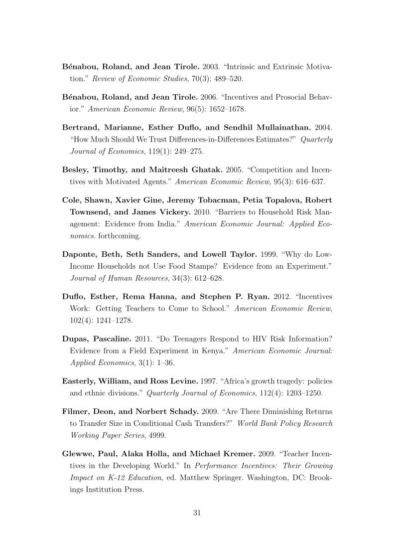
Otherwise, effort is increasing in bonus pay. The solution is illustrated in Figure

1 (see page 38 for all figures). The slope of the interior-solution segment (1c) is

positive and so is its intercept ( θc). However, depending on parameter values,

the value of e for any given value of b could range from e to e. For example,

the case of the relatively unmotivated agent is captured by the dashed vertical

line marked by ce > θ. In this case, the vertical axis (at which b = 0) intersects

the effort curve at a flat section where e = e. Similarly, the case where the

agent is sufficiently motivated is captured by the dashed vertical line marked by

θ > ce, and an intermediate level of motivation is captured by the line market

by ce < θ < ce. In the former case, the agent is at the minimum effort level for

b = 0 and initially the marginal effort with respect to bonus pay is zero. As bonus

pay increases further, the marginal effort becomes positive, before returning to

zero once the effort curve has hit the upper bound. If the vertical axis is at the

right-most dashed vertical line, then the agent is already at the maximum effort

level when b = 0 and effort will be unresponsive to incentive pay at any level. If

the vertical axis is at the middle dashed line, effort level is at an interior value

when b = 0 and the marginal effort with respect to bonus pay is positive.

8

2.2 Two Tasks

Assume now that the agent has two tasks, as in the multi-tasking model. The

tasks may be thought of as the agent transferring knowledge to, or enrolling, two

different types of beneficiary households. However, unlike in the classic multi-

tasking model, the outcomes associated with the two tasks are assumed to be

equally measurable. Instead, the differences between the two tasks will lie in

the agent’s intrinsic pay-off from success and her cost of effort. Extending the

notation from the previous section, let Y1 and Y2 be the binary outcomes for the

two tasks and e1 and e2, the corresponding effort levels.

It is assumed that the principal is constrained to offer the agent the same con-

ditional payments for the two tasks. That is, the payment in the case of success

must be the same for task 1 and 2, as must the payment in the case of failure.

This is justified if the principal is politically, socially or legally constrained to

offer the same pay rates for all tasks. The assumption is also justified if the rel-

evant characteristics of the households are not observable to the principal. For

example, a knowledge agent may be biased in favour of some social or economic

group or may have purely idiosyncratic biases, but if the principal does not the

relevant dimension, the remuneration scheme cannot be contingent on it.

Let e and e, where 0 < e < e < 1, define lower and upper bounds for both

e1 and e2, and let θ1 and θ2 denote the non-pecuniary pay-offs to the agent from

success in task 1 and 2, respectively. Let the agent’s cost of effort be given by

c(e1, e2) =1

2c1e

21 +

1

2c2e

22 + γe1e2.

The parameter γ can be thought of as a measure of the substitutability of effort

in tasks 1 and 2 in the cost function. To ensure that the marginal cost of effort

in each task is always positive, it is assumed that γ ≥ 0.

Note that if c1 = c2 = γ = c and θ1 = θ2 = θ, the set-up collapses to the

single-task model. Abstracting from the special case c1 = c2 we can, without loss

of generality, assume that c1 < c2 and refer to task 1 and 2 as the easier and the

harder task, respectively.

The principal values the tasks equally and so receives the same pay-off π from

success in both. Then the first-best is characterised by:

maxe1,e2

(θ1 + π) e1 + (θ2 + π) e2 −(

1

2c1e

21 +

1

2c2e

22 + γe1e2

).

9

The first-order conditions yield the following interior solutions:

e1(π) =(c2 − γ)π + c2θ1 − γθ2

c1c2 − γ2

e2 (π) =(c1 − γ) π + c1θ2 − γθ1

c1c2 − γ2.

For this to be a local maximum, the second-order condition requires

c1c2 > γ2.

As before, corner solutions may be possible. Also, if ei assumes a corner solution,

ej (j 6= i) would take a different form.

Define the pair:

e1(π) =

θ1+π−γe

c1if e2(π) ≤ e

e1(π) if e < e2(π) < e

θ1+π−γec1

if e2(π) ≥ e

e2(π) =

θ2+π−γe

c2if e1(π) ≤ e

e2(π) if e < e1(π) < e

θ2+π−γec2

if e1(π) ≥ e.

Now the complete first-best solution for the two-task model in is given by:

e∗1(π) = max{min{e1(π), e}, e}

e∗2(π) = max{min{e2(π), e}, e}.

The second-best is characterised as follows. Let w be the wage the principal

offers to the agent conditional on success in a task, let w be the wage conditional

on failure, and define b ≡ w − w. The agent’s objective is to maximize:

maxe1,e2

(θ1 + w)e1 + (θ2 + w)e2 + w(1− e1) + w(1− e2)− c(e1, e2).

The first-order conditions yield:

e1 (b) =(c2 − γ) b+ c2θ1 − γθ2

c1c2 − γ2

e2 (b) =(c1 − γ) b+ c1θ2 − γθ1

c1c2 − γ2.

10

As in the single-task model, we expect effort levels to be lower than first-best

because the participation constraint of the agent is assumed not to bind. As

in the case of the first-best, corner solutions may be possible, and following the

same steps as above, we can derive e1(b) and e2(b) :

e1(b) =

θ1+b−γe

c1if e2(b) ≤ e

e1(b) if e < e2(b) < e

θ1+b−γec1

if e2(b) ≥ e

e2(b) =

θ2+b−γe

c2if e1(b) ≤ e

e2(b) if e < e1(b) < e

θ2+b−γec2

if e1(b) ≥ e.

The complete second-best solution for the two-task model is given by:

e1(π) = max{min{e1(b), e}, e}

e2(π) = max{min{e2(b), e}, e}.

Several aspects of the solution are worth noting. First, e1 is always weakly

increasing in b.

Second, e2 is also non-decreasing in b, except when both tasks are at internal

solutions and c1 < γ < c2. The intuition for the negative slope is that when

effort in the two tasks are relatively substitutable and both effort curves are at

internal solutions, providing monetary incentives leads the agent to substitute

effort towards the easier task to a degree that causes effort in the harder task to

fall. We view this as a form of ‘crowding out’, as increasing incentive pay leads

the agent to work less in one of the tasks. However, this is not quite crowding

out in the sense of Benabou and Tirole (2006), where the term is taken to imply

a decrease in effort overall. In our case, the sum of effort across the two tasks is

always weakly increasing in b. This follows trivially from the above except when

both efforts are internal. But then,

e1 (b) + e2 (b) =(c2 + c2 − 2γ) b+ (c2 − γ) θ1 + (c1 − γ) θ2

c1c2 − γ2

and c1+c2−2γ > c1+c2−2√c1c2 =

(√c1 −

√c2)2> 0, where the first inequality

follows from the second-order condition, c1c2 > γ2.

Third, when both effort curves are internal, the slope of e1 is always greater

11

than the slope of e2.

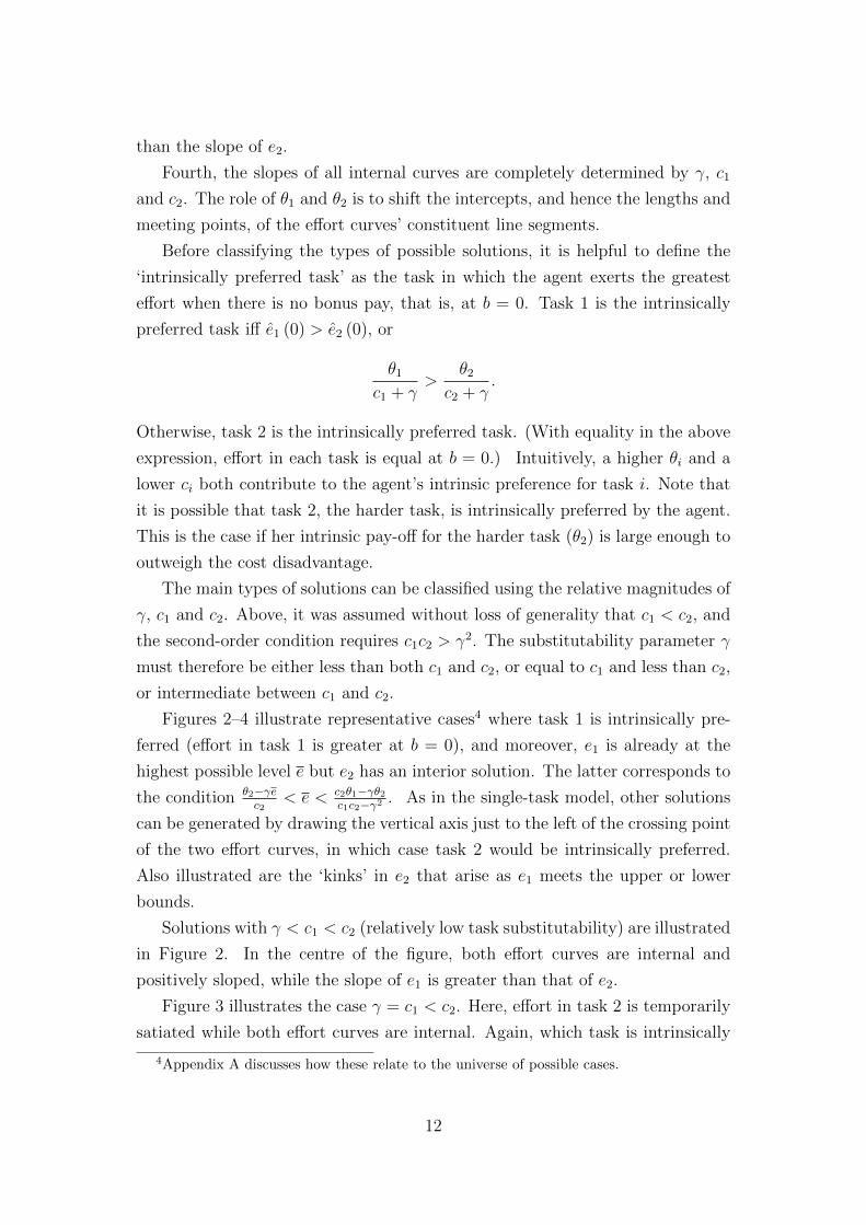
Fourth, the slopes of all internal curves are completely determined by γ, c1

and c2. The role of θ1 and θ2 is to shift the intercepts, and hence the lengths and

meeting points, of the effort curves’ constituent line segments.

Before classifying the types of possible solutions, it is helpful to define the

‘intrinsically preferred task’ as the task in which the agent exerts the greatest

effort when there is no bonus pay, that is, at b = 0. Task 1 is the intrinsically

preferred task iff e1 (0) > e2 (0), or

θ1c1 + γ

>θ2

c2 + γ.

Otherwise, task 2 is the intrinsically preferred task. (With equality in the above

expression, effort in each task is equal at b = 0.) Intuitively, a higher θi and a

lower ci both contribute to the agent’s intrinsic preference for task i. Note that

it is possible that task 2, the harder task, is intrinsically preferred by the agent.

This is the case if her intrinsic pay-off for the harder task (θ2) is large enough to

outweigh the cost disadvantage.

The main types of solutions can be classified using the relative magnitudes of

γ, c1 and c2. Above, it was assumed without loss of generality that c1 < c2, and

the second-order condition requires c1c2 > γ2. The substitutability parameter γ

must therefore be either less than both c1 and c2, or equal to c1 and less than c2,

or intermediate between c1 and c2.

Figures 2–4 illustrate representative cases4 where task 1 is intrinsically pre-

ferred (effort in task 1 is greater at b = 0), and moreover, e1 is already at the

highest possible level e but e2 has an interior solution. The latter corresponds to

the condition θ2−γec2

< e < c2θ1−γθ2c1c2−γ2 . As in the single-task model, other solutions

can be generated by drawing the vertical axis just to the left of the crossing point

of the two effort curves, in which case task 2 would be intrinsically preferred.

Also illustrated are the ‘kinks’ in e2 that arise as e1 meets the upper or lower

bounds.

Solutions with γ < c1 < c2 (relatively low task substitutability) are illustrated

in Figure 2. In the centre of the figure, both effort curves are internal and

positively sloped, while the slope of e1 is greater than that of e2.

Figure 3 illustrates the case γ = c1 < c2. Here, effort in task 2 is temporarily

satiated while both effort curves are internal. Again, which task is intrinsically

4Appendix A discusses how these relate to the universe of possible cases.

12

preferred depends on the position of the vertical axis.

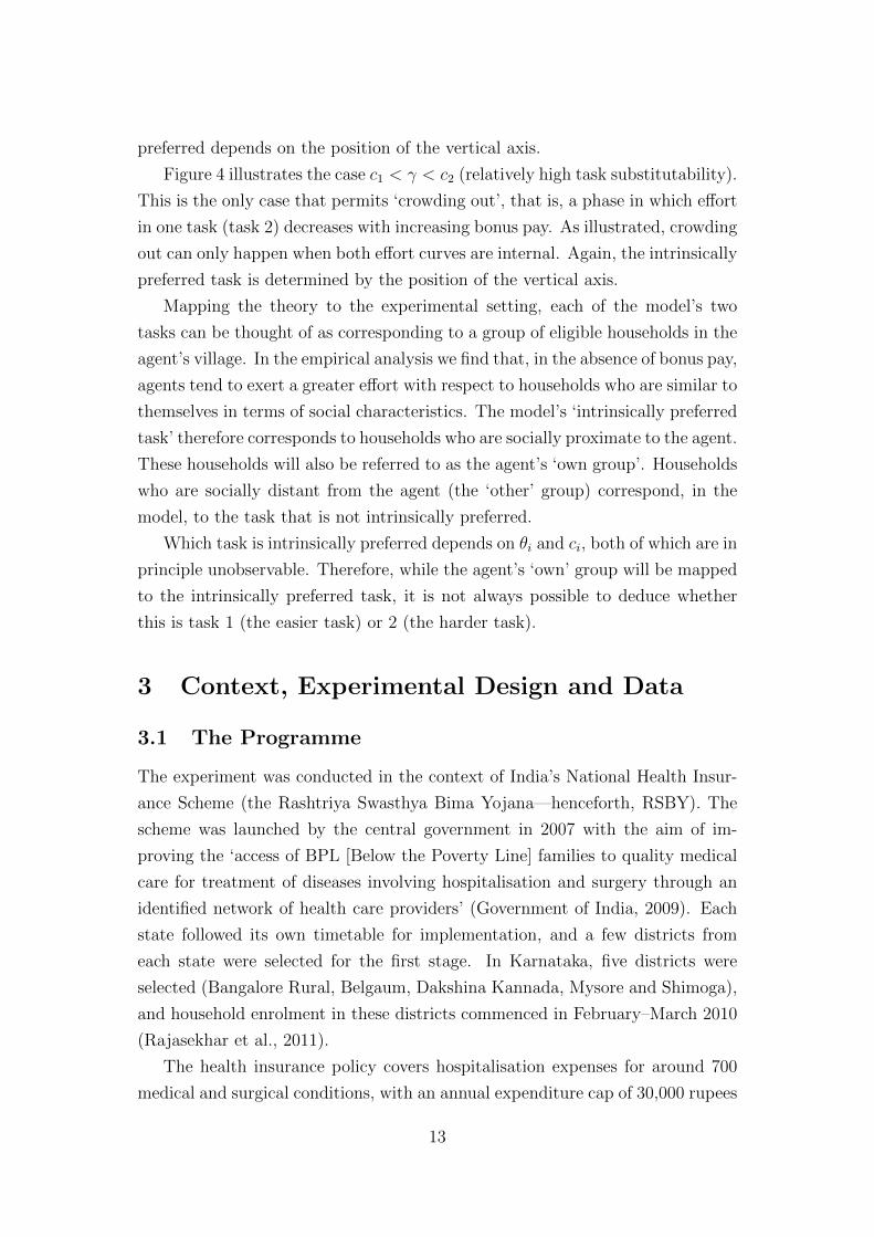
Figure 4 illustrates the case c1 < γ < c2 (relatively high task substitutability).

This is the only case that permits ‘crowding out’, that is, a phase in which effort

in one task (task 2) decreases with increasing bonus pay. As illustrated, crowding

out can only happen when both effort curves are internal. Again, the intrinsically

preferred task is determined by the position of the vertical axis.

Mapping the theory to the experimental setting, each of the model’s two

tasks can be thought of as corresponding to a group of eligible households in the

agent’s village. In the empirical analysis we find that, in the absence of bonus pay,

agents tend to exert a greater effort with respect to households who are similar to

themselves in terms of social characteristics. The model’s ‘intrinsically preferred

task’ therefore corresponds to households who are socially proximate to the agent.

These households will also be referred to as the agent’s ‘own group’. Households

who are socially distant from the agent (the ‘other’ group) correspond, in the

model, to the task that is not intrinsically preferred.

Which task is intrinsically preferred depends on θi and ci, both of which are in

principle unobservable. Therefore, while the agent’s ‘own’ group will be mapped

to the intrinsically preferred task, it is not always possible to deduce whether

this is task 1 (the easier task) or 2 (the harder task).

3 Context, Experimental Design and Data

3.1 The Programme

The experiment was conducted in the context of India’s National Health Insur-

ance Scheme (the Rashtriya Swasthya Bima Yojana—henceforth, RSBY). The

scheme was launched by the central government in 2007 with the aim of im-

proving the ‘access of BPL [Below the Poverty Line] families to quality medical

care for treatment of diseases involving hospitalisation and surgery through an

identified network of health care providers’ (Government of India, 2009). Each

state followed its own timetable for implementation, and a few districts from

each state were selected for the first stage. In Karnataka, five districts were

selected (Bangalore Rural, Belgaum, Dakshina Kannada, Mysore and Shimoga),

and household enrolment in these districts commenced in February–March 2010

(Rajasekhar et al., 2011).

The health insurance policy covers hospitalisation expenses for around 700

medical and surgical conditions, with an annual expenditure cap of 30,000 rupees

13

(652 USD) per eligible household.5 Each household can enrol up to five mem-

bers. Pre-existing conditions are covered, as is maternity care, but outpatient

treatment is excluded.

The policy is underwritten by insurance companies selected in state-wise ten-

der processes. The insurer receives an annual premium per enrolled household,6

paid by the central (75%) and state (25%) governments. The beneficiary house-

hold pays only a 30 rupees (0.65 USD) annual registration fee.

Biometric information is collected from all members on the day of enrolment

and stored in a smart card issued to the household on the same day.7 Beneficiaries

are entitled to cashless treatment at any participating (‘empanelled’) hospital

across India. Both public and private hospitals can be empanelled. Hospitals

are issued with card readers and software. The cost of treating patients under

RSBY are reimbursed to the hospital by the insurance company according to

fixed rates.

3.2 Experimental Design

151 villages were randomly selected from two of the first-phase RSBY districts in

Karnataka: Shimoga and Bangalore Rural. In the first stage of randomisation,

some villages in our sample (112 out of 151) were randomly selected to be part of

the treatment group, i.e. receive an agent, while the remaining form the control

group. In each treatment village, our field staff arranged a meeting with the

local Self-Help Groups (SHGs).8 All SHGs contacted were female-only. In the

meeting, SHG members were given a brief introduction to RSBY and told that

a local agent would be recruited to help spread awareness of the scheme in the

village over a period of one year. They were told that the agents would be paid,

but no further details on the payment were given at that time. In each case, an

agent was nominated by the group and recruited on the same day, most often

from the SHG itself; but in a small number of cases the selected agent was a non-

member recommended by the SHG. In about a third of the cases, the president

5Here and later, we use the currency exchange rate as per 1 July 2010 according towww.oanda.com (46 rupees/USD).

6The annual premium is determined at the state (and sometimes district) level, and iscurrently in the range of 400–600 rupees (9–13 USD). In Karnataka, the annual premium inthe first year of operation was 475 rupees.

7According to RSBY guidelines, smart cards should be issued at the time of registration,but this is often not adhered to. For more detail, see Rajasekhar et al. (2011).

8Self-Help Groups are savings and credit groups of about 15-20 individuals, often all women,that meet regularly. All government-sponsored SHGs in the village were invited to the meeting.

14

of the SHG became the agent. All agents were female.

Once the meeting was concluded and the agent selected, she was taken aside

and given a more thorough introduction to the scheme, including details on

eligibility criteria, enrolment, benefits and other relevant information. An agent

background questionnaire was also fielded at this time.

The payment scheme was revealed to the agent only after recruitment. Each

treatment village had been randomly allocated to a payment structure, but this

information was kept secret. Even our field staff did not know about the contract

type until after the agent had been selected. The day after recruitment, the agent

was called up and informed of her payment scheme. There were two payment

schemes, defining the two treatment groups. Flat-pay agents were told that they

would be paid 400 rupees every three months. Incentive-pay agents were told

that knowledge of RSBY would be tested in the eligible village population every

three months. The agent’s pay would depend on the results of these knowledge

tests. There would be a fixed payment of 200 rupees every three months, but

the variable component would depend entirely on the outcome of the knowledge

tests in the village.9

The bonus payments were determined as follows: A random sample of house-

holds eligible for RSBY in each village was surveyed and orally presented with

the knowledge test. A household was classified as having ‘passed’ the test if it

answered at least four out of eight questions correctly. The proportion of passing

households in a village was multiplied by the number of eligible households in

that village in order to estimate the number of eligible village households that

would have passed if everybody had taken the test. The bonus was calculated

as a fixed amount per eligible household estimated to pass the test in a village,

and set in such a manner that the average bonus payment across each of the two

study districts would be 200 rupees per agent. The households taking the tests

were not told how they scored, nor were they provided with the correct answers.

38 villages/agents were assigned to the flat-pay treatment group, and 74 to

the incentive-pay treatment group. Agents were told that there would be other

agents in other villages, but not that there was variation in the payment scheme.

The purpose of not revealing the payment scheme until after recruiting the

agent was to isolate the incentive effect of the payment structure from its poten-

9As part of the original experimental design, we also provided a second type of incentivepay to some agents based on programme utilisation by the beneficiaries in their village. Butbecause the scheme was hardly operational during the period of our study, overall utilisation ofRSBY across Karnataka was very low. See Rajasekhar et al. (2011) for details. These agentsand the corresponding villages are excluded from the analysis presented here.

15

tial selection effect. None of the agents pulled out after learning of the payment

scheme. However, four agents dropped out 6-12 months after recruitment. Three

of these were in incentive-pay villages, while the fourth was in a flat-pay village.

In each case, the reported reason was either childbirth or migration away from

the village. The agents were replaced, but the villages in question are excluded

from the analysis presented here. Hence, in the analysis presented here, there

are 37 villages with flat-pay agents and 71 villages with incentive-pay agents, for

a total of 108 agents in 108 treatment villages. The number of control villages

remains 39, so the total number of villages in our final sample is 147.

The original plan was to set the variable part of the pay scale for incentive-

pay agents in such a manner that average pay would equal 400 rupees in each

of the two treatment groups. The aim of equalising average pay across the

incentive-pay and flat-pay groups was to isolate the incentive effect of the contract

structure (‘incentive effect’) from that of the expected payment amount (‘income

effect’). The pay did in fact average 400 rupees for one district (Shimoga) in the

first survey round and for both districts in the second round. But due to an

administrative error, a majority of incentive-pay agents in Bangalore Rural were

overpaid in the first round of payments. In spite of the error, the rank ordering

of agents was preserved in the sense that better-performing agents were indeed

paid more. Nevertheless, we also present results only for Shimoga district, where

average pay in the knowledge group was equal to that of flat-pay agents (400

rupees) in both rounds.

3.3 Data

Following agent recruitment, three consecutive rounds of ‘mini-surveys’ were

fielded. For each wave, randomly selected households in each sample village

were interviewed to establish the state of their knowledge about the scheme,

along with enrolment status. One purpose of these surveys was to provide infor-

mation on agent performance so as to be able to pay the incentive-pay agents.

The households were drawn at random for the first and second survey rounds, so

that there was a partial overlap between the households in the first two rounds of

surveys. The first and second rounds of mini-surveys were based on face-to-face

interviews. For the third survey, the sample from the second survey was re-used,

but this time the agents were contacted by telephone. Although not everyone

could be reached by phone, the re-survey rate was significant. 2369 households

were interviewed in the first mini-survey wave, 1933 in the second and 1348 in

16

the third. In all, the mini-surveys cover 3296 households, of which 908 were

interviewed twice and 723 were interviewed three times. However, using each

household observation as an equally-weighted data point would give more weight

to households that were observed more than once. Observation weights were

introduced to take account of this, so that the total weight across observations

equals 1 for all households. All empirical results presented here are based on

weighted least squares regressions. In addition, standard errors are clustered at

the village level. Since serial correlation is probably more severe within a house-

hold than across households within a village, clustering at the village level yields

consistent, but not efficient, estimates.

After the completion of each mini-survey, the agents were revisited and paid.

At the same time, the agents’ knowledge of the scheme was refreshed and added

to.

Descriptive statistics on agents are presented in Table 1. Recall that all

agents are female. The average agent is 35 years old. 88% are married. 59%

of the agents’ household heads have completed primary school. 82% of agent

households have a ration card10, and 39% are from a forward or dominant caste.11

In 29% of the cases, the recruited agent was the president of a Self-Help Group.

The ‘female autonomy’ score was constructed on the basis of the following

question fielded to all agents after recruitment: ‘Are you usually allowed to go

to the following places? To the market; to the nearby health facility; to places

outside the village.’ The answer options were ‘Alone’, ‘Only with someone else’

and ‘Not at all’. For each of the three destinations, agents were given a score

of 0 if they were not allowed to visit it at all, 1 if they were allowed to visit it

only with someone else and 2 if they were allowed to visit it on their own. These

three scores were added up to give an autonomy score ranging from 0 (least

autonomous) to 6 (most autonomous). 82% of agents received the highest score,

6.

Table 2 presents summary statistics for households. The average household

has 4.6 members. 19% are from a forward/dominant caste. In 26% of households,

the household head has completed primary school. 93% have a ration card. It is

interesting to note that agents are more likely than the average eligible household

10These cards entitle the holders to purchase certain foods at subsidised rates. The cardsare intended for the poor, but because of mis-allocation issues they are an imperfect indicatorof poverty.

11In Karnataka, two castes officially classified as “backward”, Vokkaliga and Lingayath, tendto dominate public life. These two have therefore been classified together with the forwardcaste groups in one category.

17

to belong to the forward/dominant caste category. Agent households are also

more highly educated than the average eligible household.

The main outcome variable is the household ‘knowledge score’. A knowledge

test was fielded to all households interviewed in each of the three mini-surveys.

Each test consisted of eight questions about particulars of the RSBY scheme,

including eligibility, cost, cover, exclusions and how to obtain care. The exact

questions used in the knowledge tests are provided in Appendix B. Each answer

was recorded and later coded as being correct or incorrect. The number of correct

answers gives each interviewed household a score between 0 (least knowledgeable)

and 8 (most knowledgeable).12

The test questions asked in the three surveys were different, so although the

raw scores can be compared across households within a survey, they cannot easily

be compared across surveys, even for individual households. The scores on each

test were therefore standardised by subtracting the test-wise mean and dividing

by the standard deviation.

4 Evidence

4.1 The Impact of Agents on Knowledge

Consider first the impact of knowledge agents on household knowledge score.

The basic specification is

Yhv = α + βTv + εhv. (2)

The outcome variable Yhv is the test z-score for household h in village v. Tv

is a binary variable equal to 1 if the household lives in a treatment village (a

village with a knowledge agent of either type) and 0 otherwise. The coefficient

β captures the average effect on test score of being in a treated village, and α is

a constant reflecting the average test score in the control group. The standard

errors εhv are clustered at the village level to take account of possible serial

correlation and heteroscedasticity (Bertrand, Duflo and Mullainathan, 2004).

The results of regression (2) are presented in Table 3, column 1. Households

living in a treatment village score 0.18 standard deviations higher on the knowl-

12Question 8 on the third test is difficult to mark as correct or incorrect, as there are severalways in which an RSBY member might plausibly check whether a particular condition will becovered ahead of visiting a hospital. For this reason the question is omitted when computingthe overall score and the maximum score on the third test is taken to be 7.

18

edge test compared to households in the control villages. Column 2 indicates that

this effect is robust to the inclusion of fixed effects for taluk (the administrative

unit below district) and time (survey wave).

In column 3, the treatment effect is estimated separately for flat-pay and

incentive-pay agents, while still including taluk and time fixed effects. Flat-pay

agents have no significant impact on test scores. This is consistent with the

argument that, since these agents are paid a constant amount irrespective of

the outcome, they are not incentivised to exert any extra effort beyond some

minimum level which may be determined by their intrinsic motivation as in the

theoretical model. In contrast, households in villages assigned an incentive-pay

agent score 0.25 standard deviations higher on the knowledge test relative to

those in the control group. Hence, providing agents with financial incentives

leads to an improvement in knowledge about the scheme among beneficiaries.

Moreover, the equality of these two coefficients is rejected with a p-value of 0.06.

This suggests that the entire effect of knowledge-spreading agents in the village

is due to the agents that are on incentive-pay contracts.

As already mentioned, an administrative error caused incentive-pay agents in

one of the districts (Bangalore Rural) to be overpaid after the first survey. To

allay concerns that our findings are driven by these higher rates of pay, Table 4

presents results using data only from Shimoga district, where no error was made.

Overall, the qualitative findings concerning the main coefficients of interest are

similar to those obtained in Table 3. Hence it appears that the main findings

are not driven by the larger agent payments in Bangalore Rural in one of the

rounds.

4.2 The Impact of Knowledge on Enrolment

Does increased knowledge about the programme cause higher enrolment rates?

In order to estimate the causal impact of knowledge on enrolment we consider

the following equation:

Ehv = αE + γYhv + uhv, (3)

where Ehv captures the enrolment status of household h in village v. OLS es-

timation of equation (3) could lead to biased estimates of the causal impact

of knowledge, because of either unobserved factors (for example, ability) that

might influence both knowledge score and enrolment or reverse causality: being

enrolled in the programme may itself spur people to acquire more knowledge.

19

In order to address these concerns, we use the random assignment of our

experimental treatment as an instrument for knowledge. Since we find that

the households assigned a flat-pay agent did not exhibit a significantly different

impact on knowledge scores compared to those in the control group (Table 3,

column 3), we club these two groups together and use assignment to the incentive-

pay group, compared to either flat-pay or pure control, as the instrument for

knowledge.

The results are shown in Table 5. Column 1 presents the OLS estimate, which

is positive and highly significant. Column 2 reports the reduced-form estimates

obtained by regressing enrolment on the instrument, and the result indicates

that households assigned an incentive-pay agent are 8 percentage points more

likely to enrol in the programme compared to those assigned a flat-pay agent or

no agent. Column 3 reports the first stage of the IV regressions and indicates

that the instrument has good explanatory power. This regression is similar to

that reported in column 3 of Table 3, except that in this case the omitted group

consists of not only the pure control villages but also those that were assigned a

flat-pay agent.

Column 4 presents the second-stage regression, and the results indicate that

an increase of one standard deviation in knowledge score increases the likelihood

of enrolment by 39 percentage points. Hence, we find robust evidence that im-

proving knowledge about the welfare scheme had a positive impact on enrolment.

The fact that the co-efficient of interest nearly doubles between the OLS

and IV regressions suggests that the effect of knowledge on enrolment is par-

ticularly strong for those whose knowledge levels are influenced by the presence

of an incentivised agent (local average treatment effect). In other words, those

households for whom the knowledge transfer is the most successful are also the

households for whom increased knowledge is most likely to lead to take-up.

A concern with this instrumental variable analysis might be that, in addi-

tion to imparting knowledge, the agents are associated with an ‘endorsement

effect’. Having been selected by the Self-Help Group, the typical agent proba-

bly represents someone of considerable standing and respect among her peers.

Therefore, it may be argued that in addition to getting knowledge of the scheme,

the households perceive the agent’s involvement as a form of endorsement and

might therefore be more likely to enrol irrespective of their level of knowledge.

To address this concern, the above analysis was repeated while excluding the

pure control villages. Hence the comparison is now only between flat-pay and

20

incentive-pay village, and the instrument is ‘putting the agent on an incentive

contract’. Since the agents were selected before the contract type was revealed,

and there was very little attrition at any point, the flat-pay and incentive-pay

agents are drawn from the same distribution and should not differ on average.

In other words, if there is an endorsement effect associated with the agents, it

will be the same for both types, assuming that the households did not know

their agent’s payment type. Note that the difference between the two forms of

payment contract changes the incentives to impart knowledge, but neither type

is incentivised to enrol households into the scheme.

Dropping the control villages means that there is now only data on 71 incentive-

pay agents/villages and 37 flat-pay agents/villages. In spite of the reduced sam-

ple size, the results are qualitatively similar to the above, although the reduced-

form and first-stage estimates are significant only at the 10% level. The second-

stage estimate of the effect of knowledge on enrolment is 0.54 and highly signifi-

cant (not reported).

Another concern might be that the households learn of their agent’s payment

type and that it might somehow influence the enrolment decision. We believe it is

unlikely that the households will learn of the agent’s payment structure since this

was revealed to the agent in private and she has little incentive to discuss it with

the households. Even if she did, we believe that the most likely effect of such

information would be to trust the incentive-agent relatively less, since house-

holds might be suspicious of an agent who stands to gain personally from their

engagement with the scheme. If so, any ‘endorsement effect’ of the incentive-pay

scheme should actually be negative so that the regression co-efficients are under-

rather than over-estimates.

A final concern might be that the incentivised agent might try harder than

the flat-pay agent to get the household enrolled because she thinks that will make

it easier to boost their knowledge level. Although it is not possible to rule out

this possibility, we find it quite unlikely.

4.3 Agent Characteristics and Heterogeneous Treatment

Effects

The questionnaire that was administered to the agents at the time of their ap-

pointment collected information on some individual and household character-

istics including age, marital status, education of household head, caste, house

ownership and personal autonomy.

21

Table 6 looks at how the impact of knowledge agents on knowledge test scores

depends on agent characteristics. Column 1 replicates column 2 of Table 3 for

ease of reference. In column 2, the main treatment variable (whether or not

there is an agent in village) is interacted with variables on agent age, caste,

education, ration-card status, home ownership, whether the agent is president

of an SHG and her personal autonomy. None of these interacted effects are

significant except for the autonomy metric. (The autonomy variable is described

in the data section.) It seems intuitive that an important factor determining the

effectiveness of an agent is whether she is free to move around the village.

4.4 Pricing Out Prejudice: Financial Incentives and So-

cial Distance

The results so far suggest that monetary incentives matter for how effective

agents are at disseminating information about the scheme, and that improving

knowledge in turn increases enrolment. But previous work suggests that social

identity is also an important determinant of insurance take-up. For example,

Cole et al. (2010) find that demand for rainfall insurance is significantly affected

by whether the picture on the associated leaflet (a farmer in front of either a

Hindu temple or a mosque) matches the religion of the potential buyer.

This section asks whether matching agents with target households in terms of

social characteristics has an effect on knowledge scores that is independent of the

effect of incentive pay. Also, it investigates whether the effects of social distance

and incentive-pay are purely additive or whether they reinforce or weaken each

other.

A simple metric of social distance is constructed as follows: First, create four

binary variables which capture basic social dimensions and for which we have

data for both the agent and eligible households: forward/dominant caste status

(0/1), whether the household head has completed primary school (0/1), ration-

card status (0/1) and home ownership (0/1). In each of these four dimensions,

define the social distance between an agent and a household as the absolute

difference in the agent’s and the household’s characteristics. To take ration-card

status as an example, ration-card distance is set to 0 if either both have a ration

card or if neither of them does. Ration-card distance is 1 if any one of them has

a ration card and the other does not.

The composite social distance is the simple sum across the four individual

distance measures. The composite social distance metric is normalised to lie

22

between zero and one by dividing by four.

The empirical specification is of the following form:

Yhv = α + βDhv + γTv + δDhvTv + πX + uhv (4)

Dhv denotes social distance between household h in village v and the agent

in village v. Tv is a binary variable indicating whether the agent in village v

is on an incentive-pay contract. (The control villages are necessarily dropped

from this analysis.) X are control variables for each of the agent and house-

hold characteristics that are considered in the construction of the social distance

metrics.

The coefficient β captures the effect13 of social distance on knowledge when

the agent is not incentivised. The coefficient γ captures the effect of incentive pay

for socially proximate (non-distant) agent-household pairs. Finally, δ captures

the differential effect of incentive pay for socially distant agent-household pairs

relative to socially proximate ones.

The results are presented in Table 7. Column 1 confirms that incentive-pay

agents have a significant and positive impact on knowledge compared to flat-pay

agents, even when controlling for agent and household caste, education, ration-

card status and home-ownership as well as taluk and time fixed effects.

Column 2 presents results for the composite social distance metric. The

un-interacted treatment effect is not significant, while the coefficients on social

distance and the interaction of incentive pay with social distance are both highly

significant and roughly opposite in magnitude. We interpret this in three steps:

First, it confirms that social distance has a negative impact on knowledge trans-

mission. Second, putting agents on an incentive-pay contract has a positive effect

on knowledge transmission, but only for socially distant agent/household pairs.

And third, the effect of providing financial incentives (at our level of bonus pay)

is more or less exactly the level required to cancel out the negative effect due to

social distance. In other words, the effect of incentive pay seems to be to cancel

the negative effect of social distance, but no more.

In Indian villages, caste groups sometimes live in distinct sub-villages called

hamlets. This means that the social distance between a pair of households in the

village may be positively correlated with the physical distance between them. To

13The words ‘effect’ and ‘impact’ are used for ease of exposition, but we cannot make the sameclaims of causality in this part of the analysis since social characteristics were not randomlyallocated.

23

the extent that this is the case, it is possible that the results so far confound the

effect on knowledge transmission of social distance with that of physical distance.

After all, it seems natural that the cost of knowledge transmission increases with

the physical distance between the agent and a household.

While we do not have good measures of physical distance at the household

level, a rough test can be constructed for a subset of villages for which we know

whether caste groups tend to live apart or not. This information is available

for 107 out of the 147 villages. Based on this information, a binary indicator is

constructed which is equal to 1 if, in a given village, the settlements of the major

caste groups are physically separated, and 0 otherwise. This indicator is 1 for

26 out of 107 villages. In column 3, this indicator and its interaction with the

incentive-pay variable are included in the regression.

While the sample size drops, the results, in column 3, confirm that physical

separation does have a negative effect on knowledge transmission and that this

effect, like the one for social distance, is completely counter-acted by the intro-

duction of incentive pay. But the results also show that the social distance indi-

cator and its interaction with incentive-pay is still significant and qualitatively

unchanged. While the measure of physical distance is crude, and, therefore, it

is conceivable that the the social-distance measure still captures some physical-

distance effect, the fact that the coefficients on the social-distance measure and

its interaction with the treatment variable are virtually unchanged suggests that

this is not the case. Social distance matters, even after controlling for physical

distance.

Columns 4–7 repeat the exercise of column 2 for each of the sub-component

distance metrics. For distance in caste group, ration-card status and home own-

ership, the story appears to align with the findings for the overall distant metric

presented above. However, for education, there appears to be no significant

disadvantage due to social distance. In other words, agent–household commu-

nication appears to be hampered by differences in caste, ration-card status and

home ownership, but not by differences in education. Correspondingly, in this

specification, un-interacted incentive pay has a large and positive co-efficient,

though it is statistically significant only at the 10% level.

It is of interest to examine whether the impact of social distance and its in-

teraction with incentive pay is symmetric across the caste hierarchy. In other

words, is the impact of social distance between agent and beneficiary household

more severe when a lower-caste agent interacts with a higher-caste household

24

than vice versa? To test this, we compute differences-in-differences in mean ef-

fects by agent caste group. The results, presented in Table 8, suggest that the

qualitative findings are symmetric: irrespective of whether the agent is of the for-

ward/dominant caste group or not, non-incentivised agents are significantly more

effective at transmitting knowledge to their own group than to the cross-group,

while for incentivised agents there is no significant difference in performance be-

tween the agent’s own group and the cross-group. Moreover, irrespective of the

agent’s own caste group, the co-efficient representing the effect of introducing

incentive pay is greater with respect to the cross-group than to the own group.

4.5 Relating the Empirical Results to the Theoretical

Model

The aim of this section is to tie the empirical findings back to the model. It

should, however, be noted that what follows is subject to statistical inaccuracy.

That is, while we cannot reject the equality of certain quantities, it is also possible

that the true values of these quantities are different, but not different enough for

the differences to be detectable by our econometric tests. While for simplicity we

will proceed as if these equalities hold exactly, a full discussion would consider

a broader range of cases in which the effort curve is nearly flat, effort across the

two tasks nearly equal, etc.

Let es(b) denote the effort of a knowledge agent when dealing with her own

social group, and let eo(b) denote the effort with respect to dealing with the other

group. We observe four points empirically: es(0), es(b′), eo(0) and eo(b

′); that

is, the effort with respect to the agent’s own and cross-group, with and without

bonus. Given this notation, the empirical findings can be summarised as follows:

eo(0) < es(0) = es(b′) = eo(b

′)

In words, the task of transmitting information to the agent’s own group is

intrinsically preferred. The introduction of bonus pay induces no change in effort

in the intrinsically preferred task, but it does increase effort in the non-preferred

task, up to the same level as for the intrinsically preferred task.

The most straightforward interpretation is that with respect to their own

group, agents were already exerting the maximum effort, and, therefore, bonus

pay induces no additional effort. With respect to the other group, the agents

were choosing a sub-maximal effort level without bonus, but with bonus pay the

25

effort goes up to the maximum level. We do not observe crowding out, but we

cannot rule it out outside of the observed parameter values. Specifically, given

more variation in b, we might encounter a region in which effort with respect

to one of the groups decreases with b. Unfortunately, from the four points we

observe, we cannot tell whether or not we are in a ‘crowding-out’ world.

In Figures 2–4, the position of the vertical axes correspond to cases that are

consistent with the empirical findings. At b = 0, e1 has reached the maximum

effort level while e2 has not. A sufficiently high bonus b would bring e2 up to e

where it would be equal to e1. If this reflects the empirical reality, then task 1,

the easier task, corresponds to the agent’s own group.

However, another possibility is generated by shifting e in Figures 2–4 down

until it meets, or crosses, the meeting point of the internal solutions. The ver-

tical axis would now need to be placed to the left of the crossing point. This

configuration would generate a solution in which e2, the harder task, corresponds

to the agent’s own group. For this to be the case, θ2, the intrinsic motivation

for success in the own-group task would need to be not only greater than θ1 but

large enough to outweigh the cost disadvantage.

As an example of the latter, imagine that, irrespective of the agent’s own

identity, it is easier to transmit knowledge to high-caste than low-caste house-

holds, perhaps because high-caste households tend to be better educated. Then,

irrespective of the caste of the agent, task 1 (the easier task) corresponds to

high-caste households and task 2 to low-caste households. If so, for a low-caste

agent to intrinsically prefer the task of transmitting information to her own caste

group, which is what we observe, her intrinsic motivation for the own-group task,

θ2, needs to be large enough, relative to θ1, to outweigh the cost disadvantage.

It is also possible that the apparent convergence of the effort curves is not due

to having reached the maximum effort level as assumed above, but rather that

one of the effort curves is flat, as in Figure 3. If the vertical axis were to the left

of the crossing point, and the positive bonus pay observation b = b′ were exactly

at the crossing point, this could explain the empirical findings. However, we find

this possibility less likely than the two described above, because it would require

the arbitrarily chosen experimental value for bonus pay to have hit exactly the

‘sweet spot’ (the crossing point), which is unlikely.

Though the empirical findings are supportive of the model’s assumption of an

upper limit to agent effort, the theory does not explain why such an upper limit

should exist in the first place. One possibility is that households ‘max out’ on

26

the knowledge tests, thereby creating an upper bound on agent performance. If

households attain the maximum score, any further effort would be unobservable

and hence, from the point of view of incentive-pay, futile. However, a quick look

at the distribution of test scores reveals that the households are generally nowhere

near the level of test scores where such saturation could become important. In

particular, only 5% of households answered seven or eight out of eight questions

correctly.

Another, and in our view more likely, possibility is that the upper bound

e is not imposed by the test or the agent but by the household. The agent

might be willing to sit with the households for long periods of time to teach

them the intricacies of RSBY, especially if they are incentivised to do so, but

households may have limited time or patience for this. Field anecdotes suggest

that households think of the agent as a resource that can be used if the need

arises: if a household member falls ill or otherwise needs health care, they will

to turn to the agent and ask her advice on how to obtain treatment under

the scheme. If this perspective is widespread, it would not be surprising if the

households’ motivation for learning details about the insurance policy is limited.

They only need basic knowledge about the scheme, and for this reason their

patience with listening to details will probably ‘max out’ relatively quickly.

5 Discussion

It may seem that the effect of incentive pay is rather large compared to the rates

of pay that were offered to the agents. After all, an average payment of 400

rupees (9 USD) for work over a period of several months is not all that much,

even for India’s poor. However, whether the job was well-paid or not is also a

function of the hours put in. While we do not have survey data to back this

up, examining our field notes indicates that agents spend in the region of 4-5

days of full-time work equivalents per payment period. This is a very rough

estimate, and clearly there will be substantial variation around the mean, but

if reasonably accurate, it would suggest that the average pay per day of work

is around 100 rupees (2.17 USD), which is of the same order of magnitude as

what agricultural labourers earn. A hundred rupees per day is also the wage rate

that was offered by the government’s large-scale public-works programme, the

National Rural Employment Guarantee, in Karnataka at the time of the surveys.

In the experiment, the agents were paid a bonus of 8 rupees (0.17 USD) for

27

each household that answered at least four out of eight knowledge test questions

correctly. Since the average effect of incentive pay is to increase knowledge levels

by about 0.25 standard deviations or about 0.6 correctly answered questions on

the knowledge test, crude extrapolation would suggest that a bonus of 13 rupees

(0.28 USD) per household would suffice to increase by one the average number

of correctly answered questions.

The reduced-form estimate in column 2 of Table 5 suggests that a 8 rupees

(0.17 USD) bonus per household raises the enrolment rate by 8 percentage points.

Our findings concerning the relative importance of financial incentives and

social distance have implications for contexts in which strong own-group bias can

lead to adverse welfare effects. In India, caste and religious identities, in particu-

lar, have been found to create social divisions that impede the efficient function-

ing of markets (Anderson, 2011) and access to public goods (Banerjee, Iyer and

Somanathan, 2005; Banerjee and Somanathan, 2007). This creates inequities

and perpetuates disadvantage. In this context, our findings that incentive-pay

may reduce own-group bias may have significant implications for inequality and

welfare.

It is also interesting that even a modest amount of bonus pay (in our case,

8 rupees or 0.17 USD per household) to agents appears to completely wipe out

the knowledge gap between beneficiary groups that are socially proximate to the

agent and those that are not.

It would be hasty to extrapolate our findings from the current context of

information transmission about welfare schemes to the wider societal effects of

own-group bias, but our results do suggest that in this particular context, a

relatively small piece rate was sufficient to overcome the negative consequences of

entrenched social barriers. The interaction between social distance and financial

incentives in other contexts may also be a fruitful topic for future research.

Another possible reason, a more behavioural one, for the finding that rela-

tively small bonus rates can have large effects on outcomes is that agents may be

more sensitive to the fact that there is an incentive than to the size of the incen-

tive. This finding would correspond with results obtained in other recent work

on conditional cash transfers, where the size of transfer was not found to matter

beyond the fact that there is a positive transfer (Filmer and Schady, 2009) as

well as in the context of preventive health behaviour, where demand for services

were found to be sensitive to small incentives (Thornton, 2008; Banerjee et al.,

2010a).

28

6 Conclusion

This paper sheds light on the role of financial incentives and social proximity in

motivating local agents to transmit knowledge about a public service. The results

suggest, first, that hiring agents to spread knowledge about welfare programmes

has a positive impact on the level of knowledge, but that the entire effect is driven

by agents on incentive-pay contracts. Second, using the random assignment

of our experimental treatment as an instrument for knowledge, we find that

improved knowledge in turn increases programme take-up. An increase of one

standard deviation in knowledge score increases the likelihood of take-up by

39 percentage points. Third, we find that social distance between agent and

beneficiary has a negative impact on knowledge transmission, but putting agents

on incentive-pay contracts increases knowledge transmission by cancelling out (at

our level of bonus pay) the negative effect of social distance. On the other hand,

incentive pay has no impact on knowledge transmission for socially proximate

agent-beneficiary pairs.

Our results may have implications for public service delivery in developing

countries, where, in addition to common supply-side problems like staff absen-

teeism, corruption and red tape, a lack of awareness and knowledge regarding

available welfare schemes represents an important barrier to the take-up of gov-

ernment programmes. The experimental evidence presented here points to a key

mechanism that may in some circumstances alleviate this problem.

In future work, we hope to investigate the impact of spreading information

about the health insurance scheme on health outcomes of the beneficiaries. Al-

though utilisation of the scheme has been low so far, there are indications that it

might pick up over time, and we hope to capture this in future follow-up surveys

of our sample villages. In particular, we would like to know whether providing

incentives for information dissemination, which was found to improve knowledge

and enrolment of the programme, also leads to improved health outcomes for the

beneficiaries.

References

Aizer, Anna. 2007. “Public Health Insurance, Program Take-up and Child

Health.” Review of Economics and Statistics, 89(3): 400–415.

29

Akerlof, George, and Rachel Kranton. 2005. “Identity and the Economics

of Organizations.” Journal of Economic Perspectives, 19(1): 9–32.

Anderson, Siwan. 2011. “Caste as an Impediment to Trade.” American Eco-

nomic Journal: Applied Economics, 3(1): 239–263.

Ashraf, Nava, Oriana Bandiera, and Kelsey Jack. 2012. “No Margin, No

Mission? A Field Experiment on Incentives for Pro-Social Tasks.” Economic

Organisation and Public Policy Discussion Papers, 035.

Bandiera, Oriana, Iwan Barankay, and Imran Rasul. 2009. “Social Con-

nections and Incentives in the Workplace: Evidence from Personnel Data.”

Econometrica, 77(4): 1047–94.

Bandiera, Oriana, Iwan Barankay, and Imran Rasul. 2011. “Field Exper-

iments with Firms.” Journal of Economic Perspectives, 25(3): 63–82.

Banerjee, Abhijit, and Rohini Somanathan. 2007. “The Political Econ-

omy of Public Goods: Some Evidence from India.” Journal of Development

Economics, 82(2): 287–314.

Banerjee, Abhijit, Esther Duflo, Rachel Glennerster, and Dhruva

Kothari. 2010a. “Improving Immunisation Coverage in Rural India: Clus-

tered Randomised Controlled Evaluation of Immunisation Campaigns with

and without Incentives.” British Medical Journal, 340:c2220.

Banerjee, Abhijit, Lakshmi Iyer, and Rohini Somanathan. 2005. “His-

tory, Social Divisions, and Public Goods in Rural India.” Journal of the Eu-

ropean Economic Association, 3(2-3): 639–647.

Banerjee, Abhijit, Rachel Glennester, and Esther Duflo. 2008. “Putting

a Band-Aid on a Corpse: Incentives for Nurses in the Indian Public Health

Care System.” Journal of European Economic Association, 6(2-3): 487–500.

Banerjee, Abhijit, Rukmini Banerji, Esther Duflo, Rachel Glennerster,

and Stuti Khemani. 2010b. “Pitfalls of Participatory Programs: Evidence

from a Randomized Evaluation in Education in India.” American Economic

Journal: Economic Policy, 2(1): 1–30.

Becker, Gary S., and Richard A. Posner. 2009. Uncommon sense: Eco-

nomic Insights, from Marriage to Terrorism. Chicago:University of Chicago

Press.

30

Benabou, Roland, and Jean Tirole. 2003. “Intrinsic and Extrinsic Motiva-

tion.” Review of Economic Studies, 70(3): 489–520.

Benabou, Roland, and Jean Tirole. 2006. “Incentives and Prosocial Behav-

ior.” American Economic Review, 96(5): 1652–1678.

Bertrand, Marianne, Esther Duflo, and Sendhil Mullainathan. 2004.

“How Much Should We Trust Differences-in-Differences Estimates?” Quarterly

Journal of Economics, 119(1): 249–275.

Besley, Timothy, and Maitreesh Ghatak. 2005. “Competition and Incen-

tives with Motivated Agents.” American Economic Review, 95(3): 616–637.

Cole, Shawn, Xavier Gine, Jeremy Tobacman, Petia Topalova, Robert

Townsend, and James Vickery. 2010. “Barriers to Household Risk Man-

agement: Evidence from India.” American Economic Journal: Applied Eco-

nomics. forthcoming.

Daponte, Beth, Seth Sanders, and Lowell Taylor. 1999. “Why do Low-

Income Households not Use Food Stamps? Evidence from an Experiment.”

Journal of Human Resources, 34(3): 612–628.

Duflo, Esther, Rema Hanna, and Stephen P. Ryan. 2012. “Incentives

Work: Getting Teachers to Come to School.” American Economic Review,

102(4): 1241–1278.

Dupas, Pascaline. 2011. “Do Teenagers Respond to HIV Risk Information?

Evidence from a Field Experiment in Kenya.” American Economic Journal:

Applied Economics, 3(1): 1–36.

Easterly, William, and Ross Levine. 1997. “Africa’s growth tragedy: policies

and ethnic divisions.” Quarterly Journal of Economics, 112(4): 1203–1250.

Filmer, Deon, and Norbert Schady. 2009. “Are There Diminishing Returns

to Transfer Size in Conditional Cash Transfers?” World Bank Policy Research

Working Paper Series, 4999.

Glewwe, Paul, Alaka Holla, and Michael Kremer. 2009. “Teacher Incen-

tives in the Developing World.” In Performance Incentives: Their Growing

Impact on K-12 Education, ed. Matthew Springer. Washington, DC: Brook-

ings Institution Press.

31

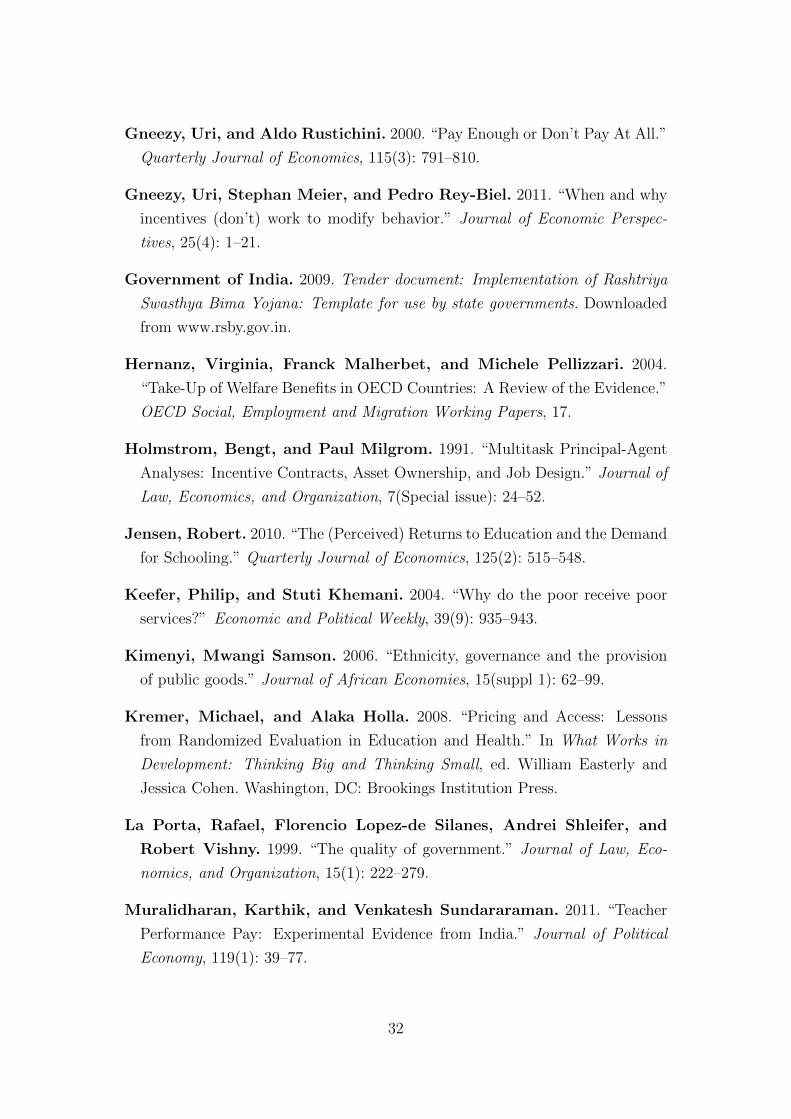
Gneezy, Uri, and Aldo Rustichini. 2000. “Pay Enough or Don’t Pay At All.”

Quarterly Journal of Economics, 115(3): 791–810.

Gneezy, Uri, Stephan Meier, and Pedro Rey-Biel. 2011. “When and why

incentives (don’t) work to modify behavior.” Journal of Economic Perspec-

tives, 25(4): 1–21.

Government of India. 2009. Tender document: Implementation of Rashtriya

Swasthya Bima Yojana: Template for use by state governments. Downloaded

from www.rsby.gov.in.

Hernanz, Virginia, Franck Malherbet, and Michele Pellizzari. 2004.

“Take-Up of Welfare Benefits in OECD Countries: A Review of the Evidence.”

OECD Social, Employment and Migration Working Papers, 17.

Holmstrom, Bengt, and Paul Milgrom. 1991. “Multitask Principal-Agent

Analyses: Incentive Contracts, Asset Ownership, and Job Design.” Journal of

Law, Economics, and Organization, 7(Special issue): 24–52.

Jensen, Robert. 2010. “The (Perceived) Returns to Education and the Demand

for Schooling.” Quarterly Journal of Economics, 125(2): 515–548.

Keefer, Philip, and Stuti Khemani. 2004. “Why do the poor receive poor

services?” Economic and Political Weekly, 39(9): 935–943.

Kimenyi, Mwangi Samson. 2006. “Ethnicity, governance and the provision

of public goods.” Journal of African Economies, 15(suppl 1): 62–99.

Kremer, Michael, and Alaka Holla. 2008. “Pricing and Access: Lessons

from Randomized Evaluation in Education and Health.” In What Works in

Development: Thinking Big and Thinking Small, ed. William Easterly and

Jessica Cohen. Washington, DC: Brookings Institution Press.

La Porta, Rafael, Florencio Lopez-de Silanes, Andrei Shleifer, and

Robert Vishny. 1999. “The quality of government.” Journal of Law, Eco-

nomics, and Organization, 15(1): 222–279.

Muralidharan, Karthik, and Venkatesh Sundararaman. 2011. “Teacher

Performance Pay: Experimental Evidence from India.” Journal of Political

Economy, 119(1): 39–77.

32

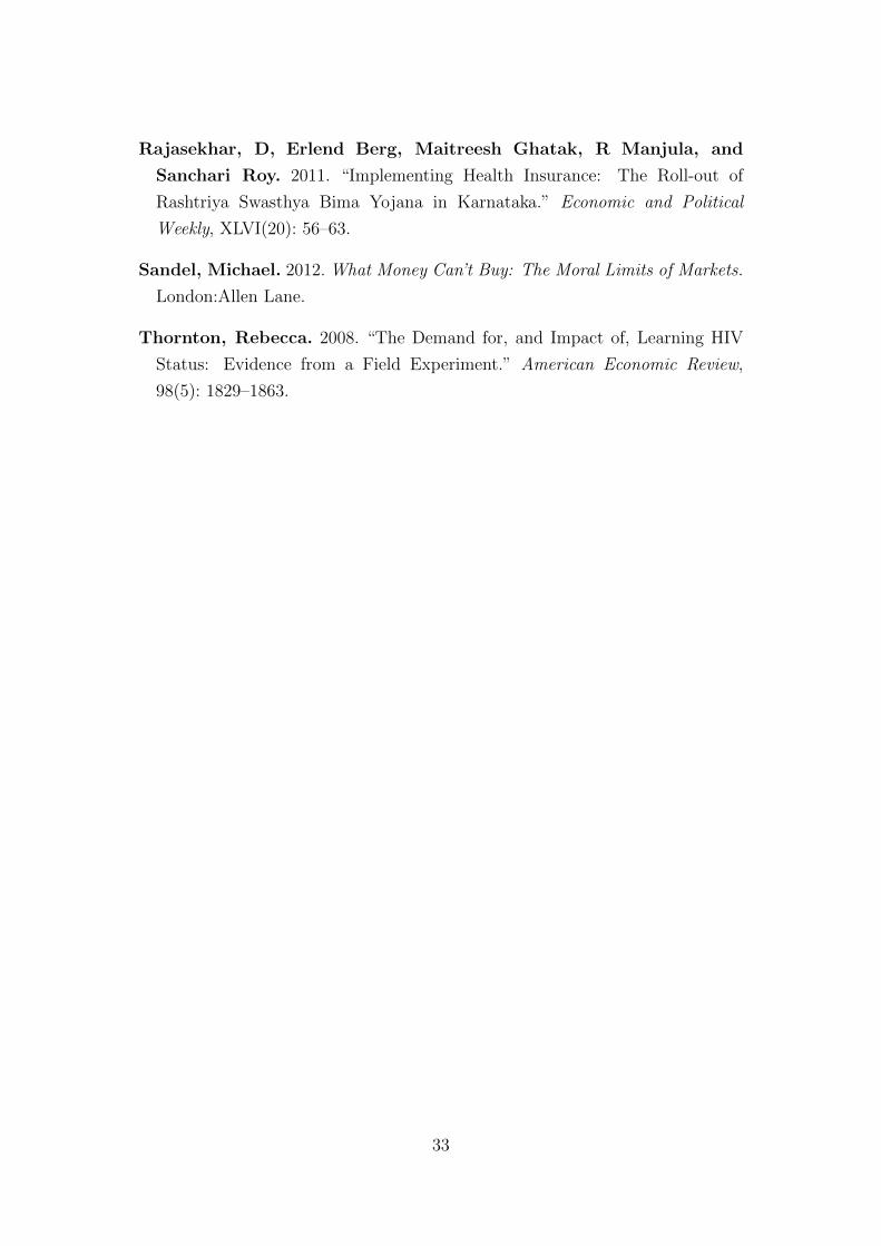
Rajasekhar, D, Erlend Berg, Maitreesh Ghatak, R Manjula, and

Sanchari Roy. 2011. “Implementing Health Insurance: The Roll-out of

Rashtriya Swasthya Bima Yojana in Karnataka.” Economic and Political

Weekly, XLVI(20): 56–63.

Sandel, Michael. 2012. What Money Can’t Buy: The Moral Limits of Markets.

London:Allen Lane.

Thornton, Rebecca. 2008. “The Demand for, and Impact of, Learning HIV

Status: Evidence from a Field Experiment.” American Economic Review,

98(5): 1829–1863.

33

e

e

b

e

θ < ce ce < θ < ce θ > ce

Figure 1: The one-task solution

e

e

b

e1

e2

Figure 2: A solution without crowding out (γ < c1 < c2).

e

e

b

e1

e2

Figure 3: A solution with temporary satiation in e2 (γ = c1 < c2)

34

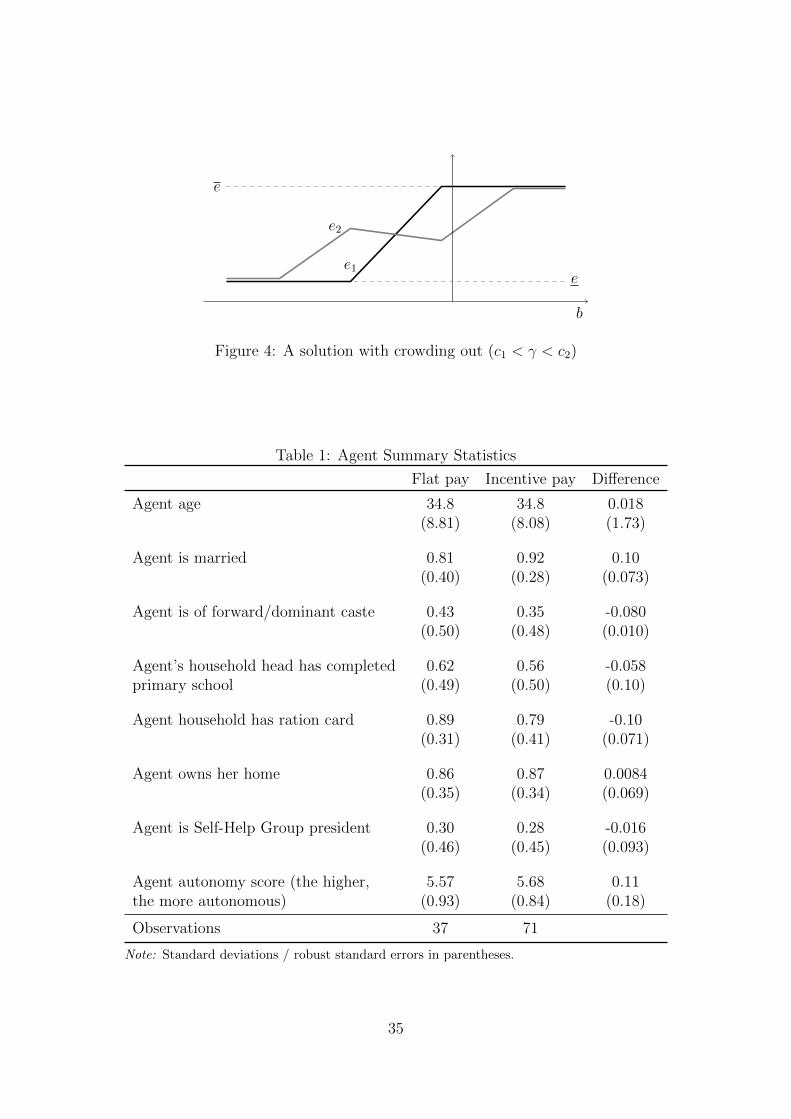
e

e

b

e1

e2

Figure 4: A solution with crowding out (c1 < γ < c2)

Table 1: Agent Summary Statistics

Flat pay Incentive pay Difference

Agent age 34.8 34.8 0.018(8.81) (8.08) (1.73)

Agent is married 0.81 0.92 0.10(0.40) (0.28) (0.073)

Agent is of forward/dominant caste 0.43 0.35 -0.080(0.50) (0.48) (0.010)

Agent’s household head has completed 0.62 0.56 -0.058primary school (0.49) (0.50) (0.10)

Agent household has ration card 0.89 0.79 -0.10(0.31) (0.41) (0.071)

Agent owns her home 0.86 0.87 0.0084(0.35) (0.34) (0.069)

Agent is Self-Help Group president 0.30 0.28 -0.016(0.46) (0.45) (0.093)

Agent autonomy score (the higher, 5.57 5.68 0.11the more autonomous) (0.93) (0.84) (0.18)

Observations 37 71

Note: Standard deviations / robust standard errors in parentheses.

35

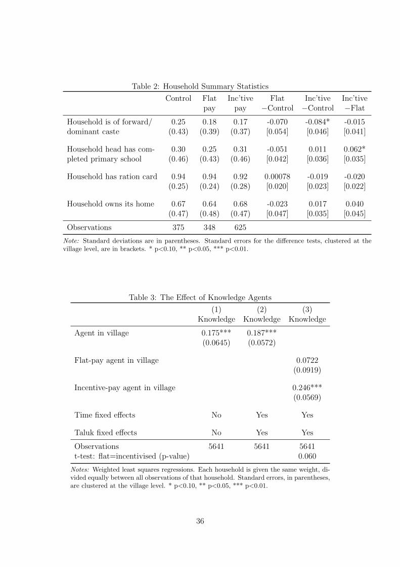
Table 2: Household Summary Statistics

Control Flat Inc’tive Flat Inc’tive Inc’tivepay pay −Control −Control −Flat

Household is of forward/ 0.25 0.18 0.17 -0.070 -0.084* -0.015dominant caste (0.43) (0.39) (0.37) [0.054] [0.046] [0.041]

Household head has com- 0.30 0.25 0.31 -0.051 0.011 0.062*pleted primary school (0.46) (0.43) (0.46) [0.042] [0.036] [0.035]

Household has ration card 0.94 0.94 0.92 0.00078 -0.019 -0.020(0.25) (0.24) (0.28) [0.020] [0.023] [0.022]

Household owns its home 0.67 0.64 0.68 -0.023 0.017 0.040(0.47) (0.48) (0.47) [0.047] [0.035] [0.045]

Observations 375 348 625

Note: Standard deviations are in parentheses. Standard errors for the difference tests, clustered at thevillage level, are in brackets. * p<0.10, ** p<0.05, *** p<0.01.

Table 3: The Effect of Knowledge Agents

(1) (2) (3)Knowledge Knowledge Knowledge

Agent in village 0.175*** 0.187***(0.0645) (0.0572)

Flat-pay agent in village 0.0722(0.0919)

Incentive-pay agent in village 0.246***(0.0569)

Time fixed effects No Yes Yes

Taluk fixed effects No Yes Yes

Observations 5641 5641 5641t-test: flat=incentivised (p-value) 0.060

Notes: Weighted least squares regressions. Each household is given the same weight, di-vided equally between all observations of that household. Standard errors, in parentheses,are clustered at the village level. * p<0.10, ** p<0.05, *** p<0.01.

36

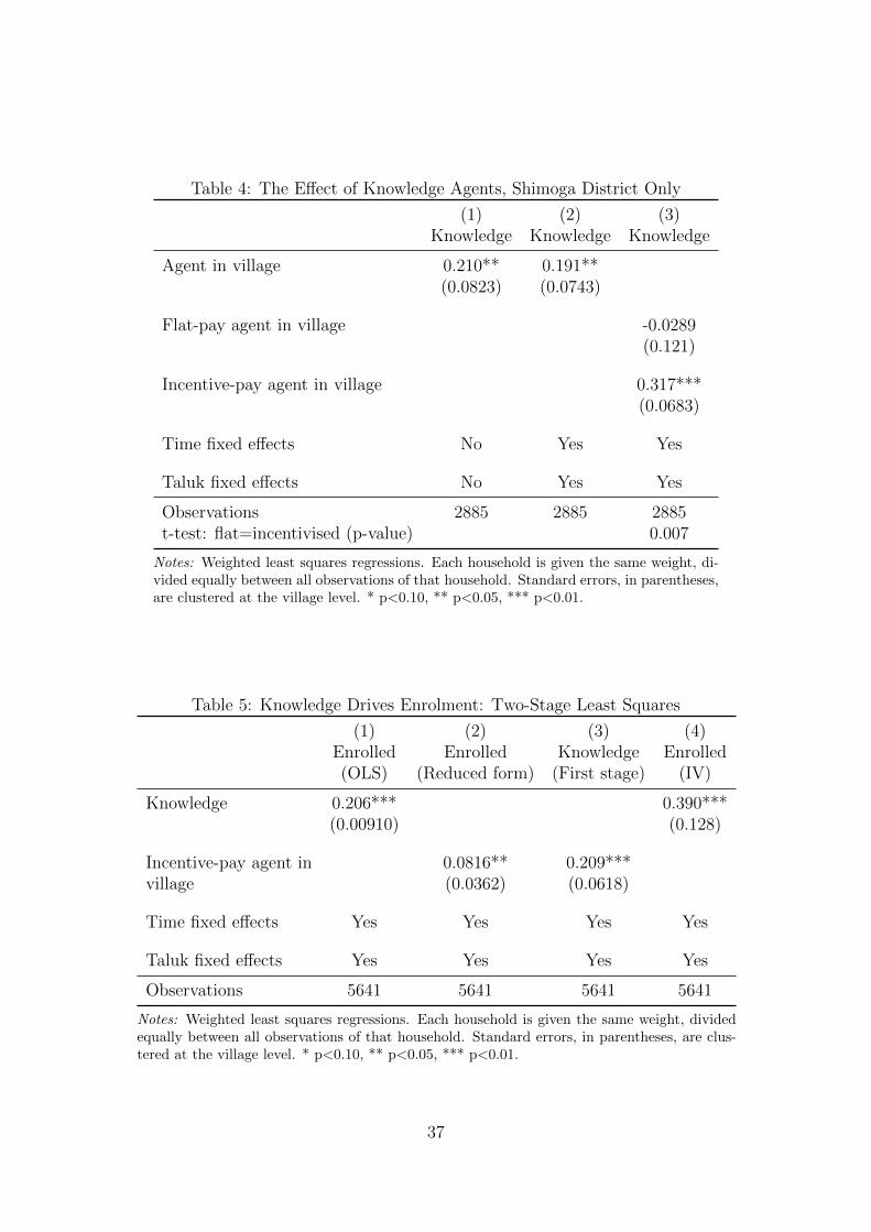
Table 4: The Effect of Knowledge Agents, Shimoga District Only

(1) (2) (3)Knowledge Knowledge Knowledge

Agent in village 0.210** 0.191**(0.0823) (0.0743)

Flat-pay agent in village -0.0289(0.121)

Incentive-pay agent in village 0.317***(0.0683)

Time fixed effects No Yes Yes

Taluk fixed effects No Yes Yes

Observations 2885 2885 2885t-test: flat=incentivised (p-value) 0.007

Notes: Weighted least squares regressions. Each household is given the same weight, di-vided equally between all observations of that household. Standard errors, in parentheses,are clustered at the village level. * p<0.10, ** p<0.05, *** p<0.01.

Table 5: Knowledge Drives Enrolment: Two-Stage Least Squares

(1) (2) (3) (4)Enrolled Enrolled Knowledge Enrolled(OLS) (Reduced form) (First stage) (IV)

Knowledge 0.206*** 0.390***(0.00910) (0.128)

Incentive-pay agent in 0.0816** 0.209***village (0.0362) (0.0618)

Time fixed effects Yes Yes Yes Yes

Taluk fixed effects Yes Yes Yes Yes

Observations 5641 5641 5641 5641

Notes: Weighted least squares regressions. Each household is given the same weight, dividedequally between all observations of that household. Standard errors, in parentheses, are clus-tered at the village level. * p<0.10, ** p<0.05, *** p<0.01.

37

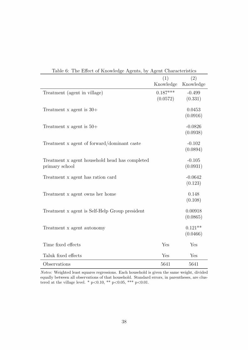
Table 6: The Effect of Knowledge Agents, by Agent Characteristics

(1) (2)Knowledge Knowledge

Treatment (agent in village) 0.187*** -0.499(0.0572) (0.331)

Treatment x agent is 30+ 0.0453(0.0916)

Treatment x agent is 50+ -0.0826(0.0938)

Treatment x agent of forward/dominant caste -0.102(0.0894)

Treatment x agent household head has completed -0.105primary school (0.0931)

Treatment x agent has ration card -0.0642(0.123)

Treatment x agent owns her home 0.148(0.108)

Treatment x agent is Self-Help Group president 0.00918(0.0865)

Treatment x agent autonomy 0.121**(0.0466)

Time fixed effects Yes Yes

Taluk fixed effects Yes Yes

Observations 5641 5641

Notes: Weighted least squares regressions. Each household is given the same weight, dividedequally between all observations of that household. Standard errors, in parentheses, are clus-tered at the village level. * p<0.10, ** p<0.05, *** p<0.01.

38

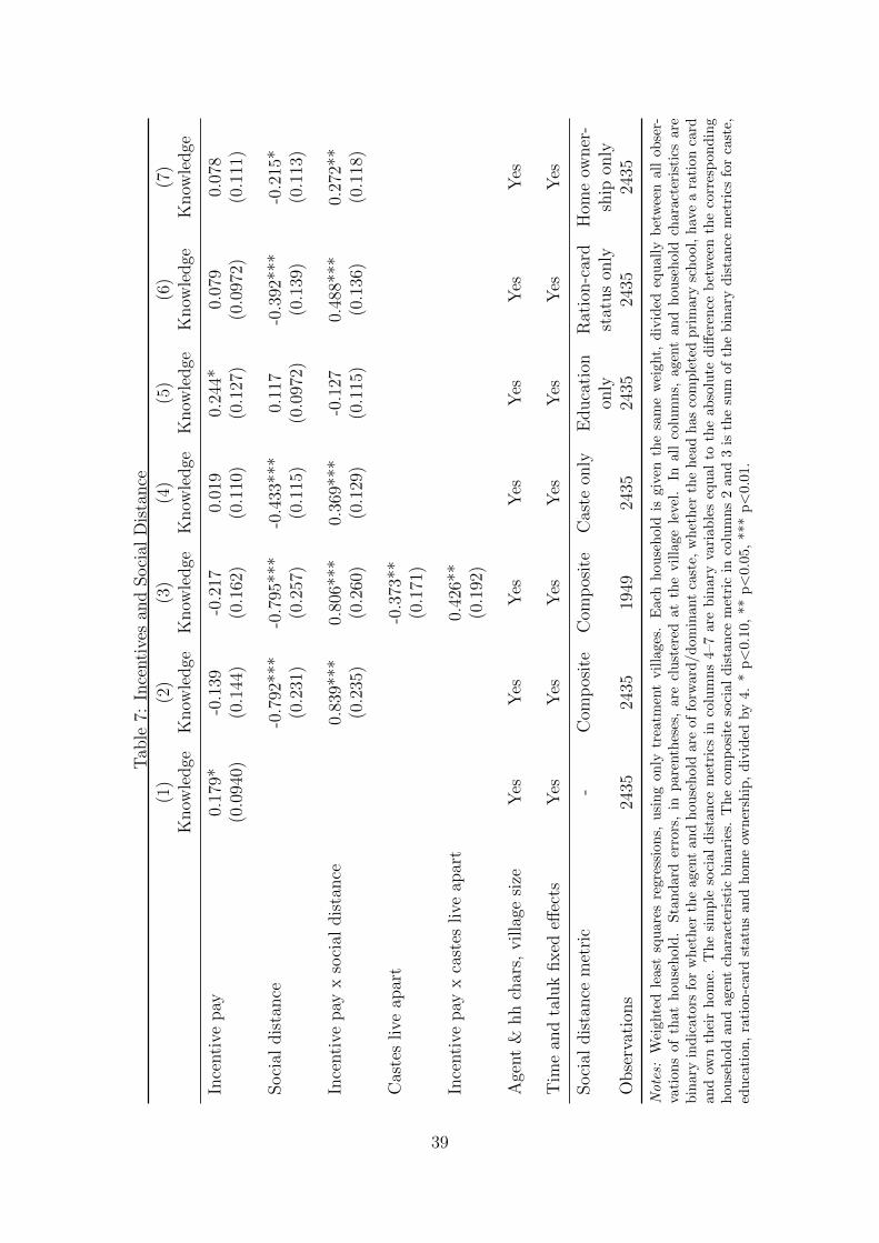
Tab

le7:

Ince

nti

ves

and

Soci

alD

ista

nce

(1)

(2)

(3)

(4)

(5)

(6)

(7)

Know

ledge

Know

ledge

Know

ledge

Know

ledge

Know

ledge

Know

ledge

Know

ledge

Ince

nti

vepay

0.17

9*-0

.139

-0.2

170.

019

0.24

4*0.

079

0.07

8(0

.094

0)(0

.144

)(0

.162

)(0

.110

)(0

.127

)(0

.097

2)(0

.111

)

Soci

aldis

tance

-0.7

92**

*-0

.795

***

-0.4

33**

*0.

117

-0.3

92**

*-0

.215

*(0

.231

)(0

.257

)(0

.115

)(0

.097

2)(0

.139

)(0

.113

)

Ince

nti

vepay

xso

cial

dis

tance

0.83

9***

0.80

6***

0.36

9***

-0.1

270.

488*

**0.

272*

*(0

.235

)(0

.260

)(0

.129

)(0

.115

)(0

.136

)(0

.118

)

Cas

tes

live

apar

t-0

.373

**(0

.171

)

Ince

nti

vepay

xca

stes

live

apar

t0.

426*

*(0

.192

)

Age

nt

&hh

char

s,villa

gesi

zeY

esY

esY

esY

esY

esY

esY

es

Tim

ean

dta

luk

fixed

effec

tsY

esY

esY

esY

esY

esY

esY

es

Soci

aldis

tance

met

ric

-C

omp

osit

eC

omp

osit

eC

aste

only

Educa

tion

Rat

ion-c

ard

Hom

eow

ner

-on

lyst

atus

only

ship

only

Obse

rvat

ions

2435

2435

1949

2435

2435

2435

2435

Notes:

Wei

ghte

dle

ast

squ

ares

regr

essi

ons,

usi

ng

only

trea

tmen

tvil

lages

.E

ach

hou

seh

old

isgiv

enth

esa

me

wei

ght,

div

ided

equ

all

yb

etw

een

all

ob

ser-

vati

ons

ofth

ath

ouse

hol

d.

Sta

nd

ard

erro

rs,

inp

aren

thes

es,

are

clu

ster

edat

the

vil

lage

level

.In

all

colu

mn

s,agen

tan

dh

ou

seh

old

chara

cter

isti

csare

bin

ary

ind

icat

ors

for

wh

eth

erth

eag

ent

and

hou

seh

old

are

of

forw

ard

/d

om

inant

cast

e,w

het

her

the

hea

dh

as

com

ple

ted

pri

mary

sch

ool,

hav

ea

rati

on

card

and

own

thei

rh

ome.

Th

esi

mp

leso

cial

dis

tan

cem

etri

csin

colu

mn

s4–7

are

bin

ary

vari

ab

les

equ

al

toth

eab

solu

ted

iffer

ence

bet

wee

nth

eco

rres

pon

din

gh

ouse

hol

dan

dag

ent

char

acte

rist

icb

inar

ies.

Th

eco

mp

osi

teso

cial

dis

tan

cem

etri

cin

colu

mn

s2

and

3is

the

sum

of

the

bin

ary

dis

tan

cem

etri

csfo

rca

ste,

edu

cati

on,

rati

on-c

ard

stat

us

and

hom

eow

ner

ship

,d

ivid

edby

4.

*p<

0.1

0,

**

p<

0.0

5,

***

p<

0.0

1.

39

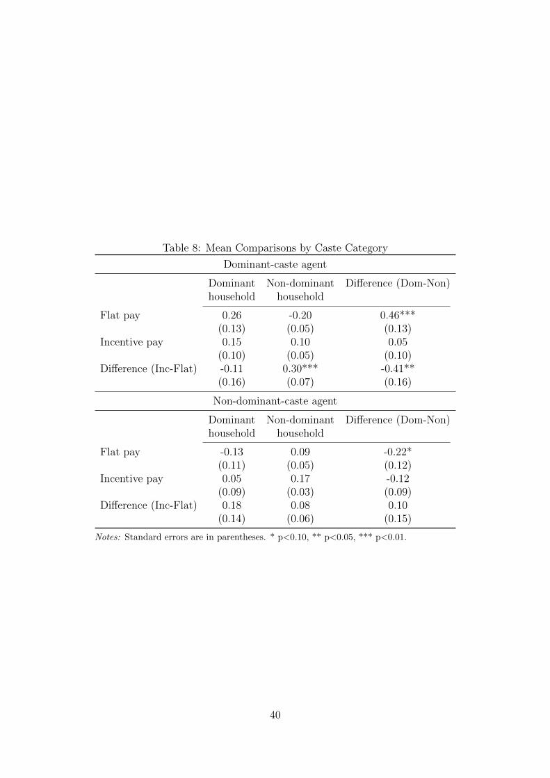
Table 8: Mean Comparisons by Caste Category

Dominant-caste agent

Dominant Non-dominant Difference (Dom-Non)household household

Flat pay 0.26 -0.20 0.46***(0.13) (0.05) (0.13)

Incentive pay 0.15 0.10 0.05(0.10) (0.05) (0.10)

Difference (Inc-Flat) -0.11 0.30*** -0.41**(0.16) (0.07) (0.16)

Non-dominant-caste agent

Dominant Non-dominant Difference (Dom-Non)household household

Flat pay -0.13 0.09 -0.22*(0.11) (0.05) (0.12)

Incentive pay 0.05 0.17 -0.12(0.09) (0.03) (0.09)

Difference (Inc-Flat) 0.18 0.08 0.10(0.14) (0.06) (0.15)

Notes: Standard errors are in parentheses. * p<0.10, ** p<0.05, *** p<0.01.

40

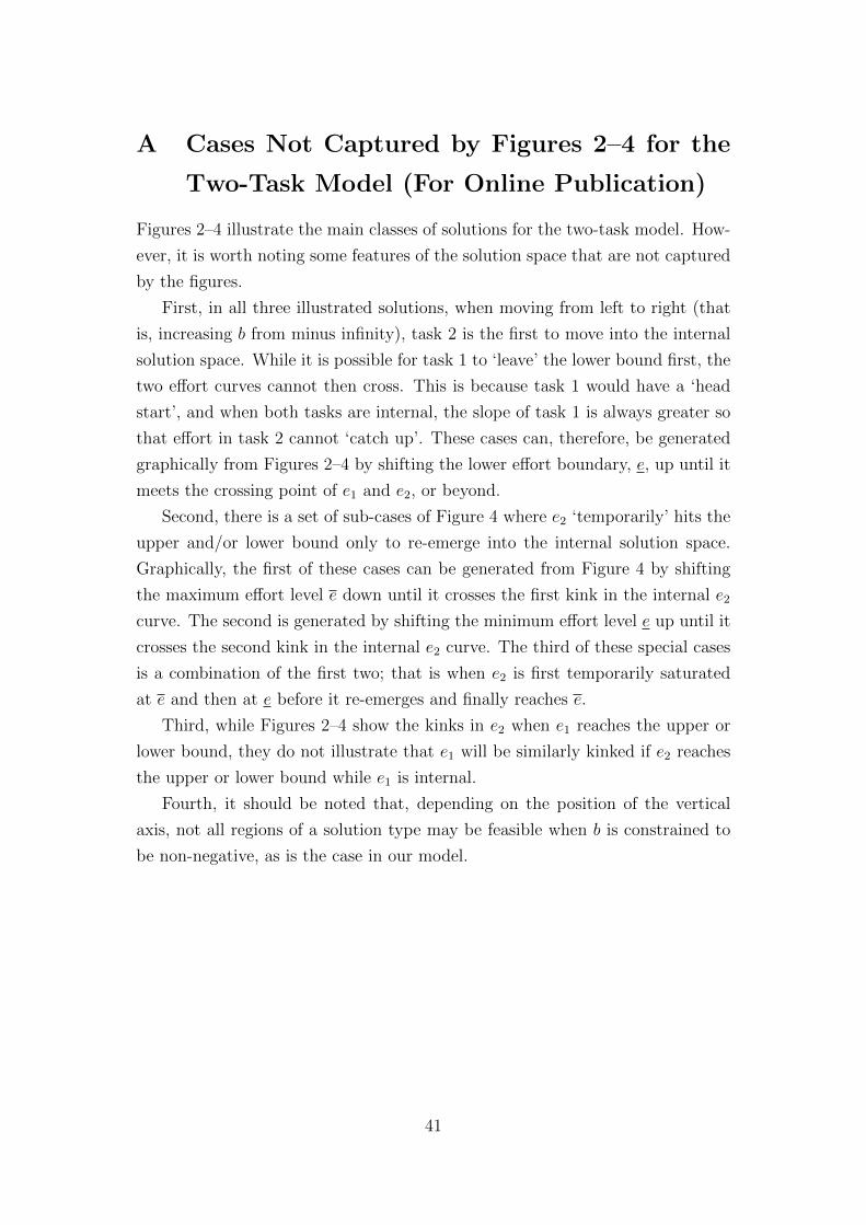
A Cases Not Captured by Figures 2–4 for the

Two-Task Model (For Online Publication)

Figures 2–4 illustrate the main classes of solutions for the two-task model. How-

ever, it is worth noting some features of the solution space that are not captured

by the figures.

First, in all three illustrated solutions, when moving from left to right (that

is, increasing b from minus infinity), task 2 is the first to move into the internal

solution space. While it is possible for task 1 to ‘leave’ the lower bound first, the

two effort curves cannot then cross. This is because task 1 would have a ‘head

start’, and when both tasks are internal, the slope of task 1 is always greater so

that effort in task 2 cannot ‘catch up’. These cases can, therefore, be generated

graphically from Figures 2–4 by shifting the lower effort boundary, e, up until it

meets the crossing point of e1 and e2, or beyond.

Second, there is a set of sub-cases of Figure 4 where e2 ‘temporarily’ hits the

upper and/or lower bound only to re-emerge into the internal solution space.

Graphically, the first of these cases can be generated from Figure 4 by shifting

the maximum effort level e down until it crosses the first kink in the internal e2

curve. The second is generated by shifting the minimum effort level e up until it

crosses the second kink in the internal e2 curve. The third of these special cases

is a combination of the first two; that is when e2 is first temporarily saturated

at e and then at e before it re-emerges and finally reaches e.

Third, while Figures 2–4 show the kinks in e2 when e1 reaches the upper or

lower bound, they do not illustrate that e1 will be similarly kinked if e2 reaches

the upper or lower bound while e1 is internal.

Fourth, it should be noted that, depending on the position of the vertical

axis, not all regions of a solution type may be feasible when b is constrained to

be non-negative, as is the case in our model.

41

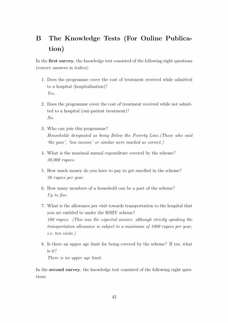
B The Knowledge Tests (For Online Publica-

tion)

In the first survey, the knowledge test consisted of the following eight questions

(correct answers in italics):

1. Does the programme cover the cost of treatment received while admitted

to a hospital (hospitalisation)?

Yes.

2. Does the programme cover the cost of treatment received while not admit-

ted to a hospital (out-patient treatment)?

No.

3. Who can join this programme?

Households designated as being Below the Poverty Line.(Those who said

‘the poor’, ‘low income’ or similar were marked as correct.)

4. What is the maximal annual expenditure covered by the scheme?

30,000 rupees.

5. How much money do you have to pay to get enrolled in the scheme?

30 rupees per year.

6. How many members of a household can be a part of the scheme?

Up to five.

7. What is the allowance per visit towards transportation to the hospital that

you are entitled to under the RSBY scheme?

100 rupees. (This was the expected answer, although strictly speaking the

transportation allowance is subject to a maximum of 1000 rupees per year,

i.e. ten visits.)

8. Is there an upper age limit for being covered by the scheme? If yes, what

is it?

There is no upper age limit.

In the second survey, the knowledge test consisted of the following eight ques-

tions:

42

1. What is the maximum insurance cover provided by RSBY per annum?

30,000 rupees.

2. Does the beneficiary have to bear the cost of hospitalisation under the

RSBY scheme up to the maximum limit?

No.

3. Are pre-existing diseases covered under RSBY?

Yes.

4. Are out-patient services covered under RSBY?

No.

5. Are day surgeries covered under RSBY?

Yes.

6. Does the scheme cover post-hospitalisation charges? If yes, up to how many

days?

Yes, up to 5 days. (Anyone who answered ‘yes’ was marked as correct.)

7. Are maternity benefits covered?

Yes.

8. If a female RSBY member has given birth to a baby during the policy

period, will the baby be covered under RSBY?

Yes.

In the third survey, the knowledge test consisted of the following eight ques-

tions:

1. Under RSBY, how many family members can be enrolled in the scheme?

Five.

2. What is the maximum insurance cover provided by RSBY per policy pe-

riod?

30,000 rupees.

3. If hospitalised, does an RSBY cardholder have to pay separately for his/her

medicines?

No.

43

4. If hospitalised, does an RSBY cardholder have to pay separately for his/her

diagnostic tests?

No.

5. Is it compulsory for an RSBY cardholder to carry the smart card while

visiting the hospital for treatment?

Yes.

6. If an RSBY cardholder is examined by a doctor for a health problem but

not admitted to the hospital, will the treatment cost be covered under

RSBY?

No.

7. What is the duration/tenure of the RSBY policy period?

1 year.

8. How can an RSBY cardholder check if a particular health condition is

covered under RSBY prior to visiting the hospital for treatment?

Multiple correct answers, see text.

44