Piecewise linear incentive scheme and participative budgeting

Review of Quantitative Finance and Accounting, 3 (1993): 149-169 0 1993 Kluwer Academic Publishers, Boston. Manufactured in The Netherlands.

Piecewise Linear Incentive Scheme and Participative Budgeting

SUNGSOO YEOM Kye Mvong University, Korea

KASHI R. BALACHANDRAN AND JOSHUA RONEN Stern School of Business, 40 West Fourth St., Rm. 434, New York, NY 10003

Abstract. This paper studies the economic incentives of participative budgeting through the design of incentive schemes within the agency theory framework. In particular, a piecewise linear incentive scheme (PLIS), an optimal version of Weitzman's New Soviet Incentive Scheme (NSIS), is derived.

The characteristics of PLIS are: first, unlike NSIS, the bonus (penalty) rates of the optimal PLIS vary according to the agent's type in order to improve the principal's welfare, second, a penalty may be imposed on the overfulfillment of the agent's performance in order to maintain incentive compatibility, and finally, it is shown that if the coefficients are constant as in NSIS, there is no need for participative budgeting.

Also, PLIS is compared with a quadratic incentive scheme. Both incentive schemes achieve the optimal solution, but each incentive scheme has its own advantage over the other depending on the situation.

I. Introduction

Since the Soviet Union announced economic reform in the early 1970s, many studies have investigated the truth-inducing property of the New Soviet Incentive Scheme (hereafter, NSIS). 1 Noting its similarity with the incentive problem in a decentralized capitalist firm, they focused on the informational and motivational advantages of NSIS when a divisional manager has local information. Under the incentive scheme, a manager is asked to set a target and is then paid depending on both the actual performance and the target. A basic compensation is adjusted by some proportion of difference between the target and the actual performance; a bonus is paid for overfulfillment and a penalty is charged otherwise. This process is consistent with participative budgeting system in a business organization.

This paper is concerned with the economic incentives of participative budgeting. In particular, this paper derives the optimal budget-based incentive scheme within the agency theory framework, taking into consideration both hidden information and hidden action coupled with uncertainty. Similar to Kirby, Reichelstein, Sen, and Paik (1991), who studied a different budget-based incentive scheme with a similar model, communication is interpreted as participation in this paper.

Demski and Feltham (1978) have pointed out the positive effects of a (mandatory) budgeting system on the agency relationship. Since then, participative incentives schemes (communication) were shown to achieve better risk sharing (see, for example, Christensen

150 s. YEOM, K.R. BALACHANDRAN AND J. RONEN

(1982) and Penno (1984)). This paper, as in Kirby et al. (1991), focuses on the effect of participation on the incentive structure and hence the principal and the agent are assumed to be risk neutral in money.

Laffont and Tirole (1986) derived an optimal incentive scheme which is linear in realized outcome for an agency model featuring both adverse selection and moral hazard. The advantages of a linear incentive scheme (hereafter, LIS) are its simplicity and robustness to uncertainty. Rogerson (1987), however, showed that LIS is not an optimal incentive scheme when the expected compensation is not convex in the expected outcome. In order to resolve this problem, a quadratic incentive scheme (hereafter, QIS), which is quadratic in realized outcome, was studied by Picard (1987) and derived directly by Kirby et al. (1991). They showed that QIS can be an optimal incentive scheme in cases where LIS fails to be optimal. The common feature of both schemes is that they are composed of a fixed component (determined by the agent's report) and a variable component (determined by the difference between the target and actual performance). Due to this feature, both are called budget-based incentive schemes.

Unlike Kirby et al. (1991), who focused on a quadratic incentive scheme, this paper examines a piecewise linear incentive scheme (hereafter, PLIS) 2 which is piecewise linear in realized outcome. PLIS weakly dominates LIS, as in the case of QIS, in the sense that a larger set of outcomes is feasible and thereby more efficient results become possible than under LIS. Both PLIS and QIS, however, depend on the nature of the uncertainty. QIS depends on the variance, and PLIS depends on the value of the density function around its expected value. The two schemes differ in their characteristics as well. The larger the variance is, the higher fixed payment is necessary in order to offset the penalty effect of the quadratic term. Also, under QIS, the agent may be subject to penalty if the overfulfillment is extremely high. On the other hand, if the value of the density function around its expected value is small, PLIS also has to guarantee high fixed payment and is likely to impose excessive penalty upon overfulfillment. The choice between QIS or PLIS depends on the nature of uncertainty.

PLIS is a generalized version of NSIS and shares several properties with it but there are basic differences. PLIS, in addition to inducing the manager to forecast an unbiased expected outcome, is designed to maximize the organizational objective (the principal's welfare in this paper) unlike NSIS. This seems trivial, but it turns out to have important implications as explained in section 4. The main objective of designing a good control system is neither truth-inducement nor the improvement of managerial performance per se. Rather, the system must coordinate managers' activities towards maximizing the organization's objective. In this framework, we show that NSIS is not an optimal incentive scheme at all even in our simple model, so that the principal may not wish to use it. Moreover, there exists a nonparticipative incentive scheme which performs equivalently to NSIS and is simpler than NSIS; hence, at the outset there is no rationale for using NSIS. Second, the bonus (penalty) rates of the optimal PLIS are not constant unlike NSIS but vary according to the agent's type in order to improve the principal's welfare. Also, a bonus is not necessary for the overfulf'dlment of the agent's performance, instead a penalty may be charged in order to maintain incentive compatibility.

PIECEWISE LINEAR INCENTIVE SCHEME AND PARTICIPATIVE BUDGETING 151

This paper is organized as follows. Section 2 provides a model where the principal and the agent are risk neutral in income and the agent has pre-contract private information. In section 3, the optimal PLIS is derived by using the direct revelation principle. This is reinterpreted in a participative budgeting framework in section 4. Among other things, it is shown that there exists a nonparticipative incentive scheme whose performance is equivalent to the Weitzman's scheme. Section 5 concludes the paper.

2. The Model

Let us consider a firm which consists of a principal and an agent. The agent produces .~ which is observed by both the principal and the agent ex post. s may be interpreted as a net profit or physical output with a normalized price. The variable e fi [e, ~] is a level of effort of the agent which increases s stochastically. 0 ~ [a, b] (a < b) represents the pre-contract private information of the agent (e.g., technology of production function or quality of raw materials), where higher 0 yields lower outcome. The center knows the probability density function of an agent's type or technology, f( . ) , which is continuous and strictly positive on its domain. Let F(.) be the corresponding cumulative distribution function. In particular, consider an outcome function, s = x + e and x = e - 0. x is the expected true outcome which is linearly determined by e and 0. 3 By the expected true outcome we mean that the agent is solely responsible to x. e is a random noise represented by the probability density function g(.) and its cumulative distribution function is G(') . Assume E(e) = 0, where E( ' ) is an expected operator. Let V(e) be a money equivalent measure of disutility of the agent. We assume that both the principal and agent are risk neutral in money, and the agent is work averse so that V(e) is increasing and convex in e. The principal's utility is .~ - t, where t is compensation to the agent. The agent's utility is t - V(e). We restrict our attention to the direct revelation mechanism (see Myerson (1979)) without any loss of generality.

Program 1 (Main Model)

max l ) (e(O) - 0 + e - t(O, e(O) - 0 + e))g(e)de f(O)dO t ( O , ~ ) . e ( O ) �9 a

s .L

f t(O, e(O) - 0 + e)g(e)de - V(e(O)) _> O, VO ~ 0 (1)

(O, e(O)) E arg max ( f t(O, e - O + e)g(e)de - V(e) ) , VO, O e (2)

(1) and (2) are the individual rationality and incentive compatibility constraints, respectively.

152 S. YEOM, K.R. BALACHANDRAN AND J. RONEN

Since the principal is unable to observe x, the agent has a degree of freedom in choosing his effort even when the agent sends a message. That is, if the incentive scheme is constant for a given message, the agent is willing to choose the lowest possible effort since the principal cannot infer the amount of effort even at optimum. Therefore, in spite of risk neutrality, bearing uncertainty becomes important not for risk sharing but for incentive purposes. So, once Y is realized and observed, the principal is likely to reward the agent based not only on 0 but also on ~. This uncertainty, however, may not cause any more inefficiency compared with the certainty case: When the principal and the agent are risk neutral in income, moral hazard does not entail welfare losses compared to the adverse selection case under some conditions. To exploit this result in our model, let us introduce a benchmark case where x is observed by the principal and hence contractible. In this benchmark case, has no information content beyond x and hence Y can be ignored in designing a mechanism unlike program 1. For this case, due to the works of Guesnerie and Laffont (1984) and Picard (1987), we have

Program 2 (Benchmark Case)

fa b

max {e(O) - 0 - V(e(O)) - V'(e(O))z(O)}f(O)dO e(O)

$.L

e ( O ) - 1 < 0 a.e.

where

F(O) z(O) -

f(O)"

Examining the relationship between program 1 and program 2 gives us an idea about how to get the optimal incentive scheme. Let {s (0), e (0)} be the optimal solution of program 2. The issue now becomes whether there exists t(O, ~) which preserves e(0) and gives the agent the expected payment of s(0). Resolving this requires solving the following integral equation for t(O, ~) that satisfies

s(O) = f , t(O, ~)g(e)de (3)

and implements the optimal effort under program 2. In order to answer this question, fix the agent's message for a moment. In program 2,

the observability of true outcome restricts the agent's choice of efforts. But, in program 1, the agent has more discretion over his choice of effort since the uncertainty prohibits the principal from inferring the agent's true type from the message alone unlike program 2. This makes the incentive compatibility constraints in program 1 more stringent than in program 2 and hence the set of implementable efforts in program 1 is restricted as sum- marized in lemma 1 without proof.


Lemma 1. Let e(0) be an implementable effort by t(0, 2?) in program 1. Then, the effort can be implemented in program 2.

Notice that once we have t(0, 2?) satisfying (3), program 1 becomes the same as program 2 except for the incentive compatibility constraints. Therefore, the value of program 2 is the upper bound of the value of program 1. This upper bound can be achieved if we find the t(O, 2?) that implements the optimal effort of program 2. This is formally stated in proposition 1.

Proposition 1. Let {s(0), e(0)} be the optimal solution in program 2. Then, e(0) is the optimal effort in program 1 if and only if there exists a t(O, 2?) such that

1. s(O) : j~ t(O, e(O) - 0 + e) g(e)de

2. (O, e(O)) ~ arg max ( f t(O, 2?)g(e)de - V(e) ) u O ~

Proof If e (0) is the optimal effort in program 1, it must be incentive compatible and hence proposition 1.2 is satisfied. Contrary to our argument, suppose that

s(O) < f~ t(O, e(O) - 0 + e)g(E)d~.

Since e(0) is implementable, the principal can reduce the compensation by some constant amount until the agent's expected payment reaches s(O).

Conversely suppose that the two conditions of the sufficiency part of proposition 1 hold. Then, e(0) is an implementable effort and the agent is paid the same amount as in program 2. Hence e(0) is optimal. []

Proposition 1 provides us with a useful framework to derive an optimal PLIS in the subse- quent section. Before proceeding with the derivation, the following technical issues must be discussed. First, in the case of bunching, there does not exist any compensation function satisfying conditions of proposition 1. 4 Even worse, there is no simple condition that characterizes the optimal effort (see Guesnerie and Laffont (1984)). Hence, we restrict our attention to the case wherein the optimal effort is not subject to bunching. Second, even though there exist compensation functions that satisfy the first condition in proposition 1, a subset of the functions cannot implement the optimal effort as in the case of LIS (see Rogerson (1987)). Finally, the number of incentive schemes may be infinite.

3. The Piecewise Linear Incentive Scheme

Weitzman (1976) considers the following incentive scheme where the actual payment is composed of basic compensation and an adjustment.


tW(x,.~) = /~(2) f f Kl" ('~ - 2) i f2 > .~

K= (2 2) i f2_< 2,

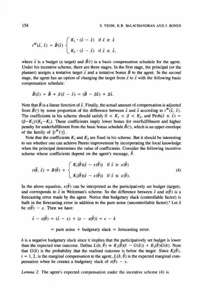
Where 2 is a budget (a target) and/~(') is a basic compensation schedule for the agent. Under his incentive scheme, there are three stages. In the first stage, the principal (or the planner) assigns a tentative target s and a tentative bonus/~ to the agent. In the second stage, the agent has an option of changing the target from s to 2 with the following basic compensation schedule:

B ( s = B + ~ ( ~ - s = (B - t~s + t32.

Note that/] is a linear function ofs Finally, the actual amount of compensation is adjusted from/~(.) by some proportion of the difference between s and s according to tw(s 2). The coefficients in his scheme should satisfy 0 < KI < ~ < K2, and Prob(s < 2) = (~-K1)/(K2-K1). These coefficients imply lower bonus for overfulfillment and higher penalty for underfulfillment from the basic bonus schedule/~(.), which is an upper-envelope of the family of {tw(')}.

Note that the coefficients K 1 and K2 are fixed in his scheme. But it should be interesting to see whether one can achieve Pareto improvement by incorporating the local knowledge when the principal determines the value of coefficients. Consider the following incentive scheme whose coefficients depend on the agent's message, /J.

f KI(/J)(2 - x(0)) if ~ ~ x(0) t(/J, ~) = B(~J) + (4)

Kz(/~)(J x(/J)) if.~ _< x(0).

In the above equation, x(tJ) can be interpreted as the participatively set budget (t,affget), and corresponds to 2 in Weitzman's scheme. So the difference between ~ and x(O) is a forecasting error made by the agent. Notice that budgetary slack (controllable factor) is built in the forecasting error in addition to the pure noise (uncontrollable factor). 5 Let 6 be x(0) - x. Then we have:

- x(~J) = (Y - x ) + (x - x ( ~ ) ) = e -

= pure noise + budgetary slack = forecasting error.

6 is a negative budgetary slack since it implies that the participatively set budget is lower than the expected true outcome. Define L(6; O) = KI(0)(I - G(6)) + K2(tJ)G(6). Note that G(6) is the probability that the realized outcome is below the target. Since Ki(~J), i = 1, 2, is the marginal compensation to the agent, L(b; 0) is the expected marginal compensation when he creates a budgetary slack of x(0) - x.

Lemma 2. The agent's expected compensation under the incentive scheme (4) is


f , t(0, .~)g(e)de = B(0 )+ fx0 )_x L(y; O ) d y - ( K 2 ( 0 ) - gl(0)),fO a(c)d~_. (5)

Proof See Appendix.

The second term of (5) is a function of budgetary slack and the message, and it captures the tendency of the agent to create the budgetary slack. Now consider the properties of L(6; O) which are useful in deriving the optimal PLIS.

Lemma 3. L(6; O) has the following properties:

1. Ll(tS; 0) = (K2(0) - Kl(O))g(6) >_ O.

2. L12(6; O) = (K2(O) - Kl(O))g(6).

Proof From the definition of L(& 0), lemma 3 is trivially proved.

Since 6 is a negative slack, lemma 3.1 captures the idea of diminishing marginal expected returns to slack. Consider the 0-agent's optimal choice of effort when he sends message t~. Let u(0, e; 8) be the agent's expected utility and e*(0, 0) be the optimal choice of effort given his message. For simplicity, let x* = e*(0, 0) - 0. The first order condition for the agent's choice of effort becomes:

Ou(O, e; O) Oe

= L(x(O) - x*; 0) - V'(e*(O, 0)) = O. (6)

e=e*(8,0)

The second order sufficient condition is satisfied by the convexity of V(e) and lemma 3.1; hence, e*(0, 0) is unique. Let e(0) = e*(/~, 0) be the effort expected by the principal for the message 0. Lemma 3 and the convexity of V(.) imply that the agent creates budgetary slack (x* > x(0)) if and only if he sends a worse message than the true one (0 > 0). As a result, his effort choice is smaller than the expected effort given message 0. On the other hand, he sends the true message if and only if he chooses the optimal action and there will be no budgetary slack. One immediate result is that the budgetary slack is bounded by: Ix(t~) - x*l < 1 0 - 0l -< b - a.

The next proposition obtains the sufficient conditions for the optimality of basic compensation and coefficients of PLIS. Unlike NSIS, the basic compensation is not a linear function of the budget, and the coefficients are not constant.

Proposition 2. Let {e(0), s(0)} be the optimal solution of program 2. Consider t(0, s such that

t(0, s = B(t~) + ~ KI(~)(y - x(0)) i f5 _> x(0)

L K2(0)(x x(/~)) if Y _< x(v),


where ~J is a message by the agent and Km(O) < K2(O). Then, truth-telling is an equilibrium so that t(O, ~) implements e(O) with an expected payment of s(O) if

f0 fo 1. B(O) = V(e(O)) + V'(e(v))dv + (K2(O) - KI(0)) G(e)de. - - O 0

2. The coefficients of PLIS satisfy the following conditions:

(7)

KI(0)(I - G(0)) + Kz(O)G(O) = V'(e(O)) (8)

K2(O) - KI(O) >- sup ~ V"(e(O))b(O) + lgz(o) - gl(O)] 1 O,lel<_O_a g(e)(1 - ~ ) "

(9)

Proof Since the proof is quite long, we will sketch it here (see Appendix for detail). Notice that the value of program 2 is an upperbound of that of program 1. Hence, if t(O, ~) implements the optimal efforts of program 2 with the same expected payment, then it is optimal for program 1. The proof consists of two parts. The first part derives the basic compensation guaranteeing the expected payment of s(O). The second part finds the sufficient conditions for coefficients in order to implement the optimal effort of program 2. Notice that we begin with a three-parameter problem, {B(0), KI(O), Kz(O)}, but end up with a two- parameter problem since (8) reduces one degree of freedom. Also notice that the conditions still allow to have a family of coefficients pairs. 6 []

Let us consider proposition 2.1. First, it is easy to show that the optimal PLIS satisfies proposition 1.1. Second, B(O) is nonlinear in e(0) and hence nonlinear in x(O), unlike in Weitzman's scheme. Finally, B (0) has an additional term other than s (0), the third term of (7). In light of the principal and the agent being risk neutral, uncertainty is averaged out when the incentive scheme is linear (see Laffont and Tirole (1986)). PLIS, however, is kinked so that the preference of the agent facing PLIS becomes concave with respect to the expected outcome. This induces the principal to give the agent a larger compensation (larger by the third term of (7) due to the induced risk aversion of the agent.)

Now consider proposition 2.2 which specifies the sufficient conditions of PLIS to implement the optimal effort. Note that L(0; 0) is the marginal expected payment of true outcome at 0 = 0. From (8) we have

L(0; 0) = V'(e(O)). (10)

V'(e(O)) is a convex combination of KI(O) and K2(0) weighted by G(0) at optimum. Therefore, by setting the proper coefficients, PLIS balances the bonus and the penalty in a way that equates marginal expected compensation with the marginal disutility of effort at optimum. Finally, consider (9). Weitzman (1976) reported that the magnitude of/(2 (0) might be twice of K1 (O). However, his observation is incomplete. The important thing is not only the relative magnitude of the coefficients but also the absolute difference betweeen them. Notice that bunching (e(O) = 1) requires the difference between K2(0) and KI(0) to be infinite. In this case, it is impossible to construct a PLIS (this impossibility also


applies to QIS). On the other hand, if e(0) < 0 for every 0 E O, we can construct a linear incentive scheme by setting KI(0) --- K2(0) as in Laffont and Tirole (1986).

There is another way of looking at the incentive compatibility requirement as in the following corollary.

Corollary 1. Consider a PLIS, t(0, ,~). Then, t(t~, 2) is an incentive compatible scheme if we have for every 0, 0 ~ O (0e*(0, 0 ) ) / 0 0 <_ O.

P r o o f See Appendix.

Budgetary slack is usually higher when the agent is able to set the budget as low as possible by sending a higher 0 than the true 0, and if he is able to simultaneously choose a higher effort than the one actually required. Corollary 1 says that incentive compatible mechanism must block this behavior. In other words, the optimal incentive scheme should make it^optimal for the agent to choose lower effort than e(0) when an agent reports a higher 0 than O, and vice versa.

As shown above, there could be infinite number of optimal PLIS. Notice that

f B(O) = V(e (O) ) + V ' ( e ( v ) ) d v + (K2(/~) - Kt(0) ) o G ( e ) d e . - - o o

The basic compensation becomes larger as the difference of coefficients increases. The large basic compensation, however, has at least three adverse effects on the agency relationship. First, from (8) and the fact that Kz(0 ) is greater than K l ( O ) , the very large difference between coefficients implies that the value of K~ (0) becomes negative. In this case, the principal has to impose a penalty on overfulfillment relative to the target; this is often viewed as being undesirable. Second, the large basic compensation may result in a small (even negative) residual return to the principal when the budget meets the realized outcome. The principal, in this case, may wish the realized outcome to deviate from the budget since the larger deviation makes his residual share larger. Hence, even if the principal devises a mechanism that extracts true information from the agent, the principal prefers a large deviation ex post. Finally, as/(2(0) becomes large, it is highly probable that any limited liability of the agent (not considered here) will be binding at low outcomes. (Notice that QIS imposes penalty on the high overfulfillment so that it also has the same adverse effects discussed above on the agency relationship.) Therefore, among the infinite number of the optimal PLIS, it is desirable to have a small difference between the two coefficients. This is accomplished by setting kl = K2.

Corollary 2. Among the class of optimal PLIS, the most desirable one is that

KI(O) = V ' (e (O)) - n �9 G(0); /<2(0) = V' (e (O) ) + n �9 (1 - G(0)),

where


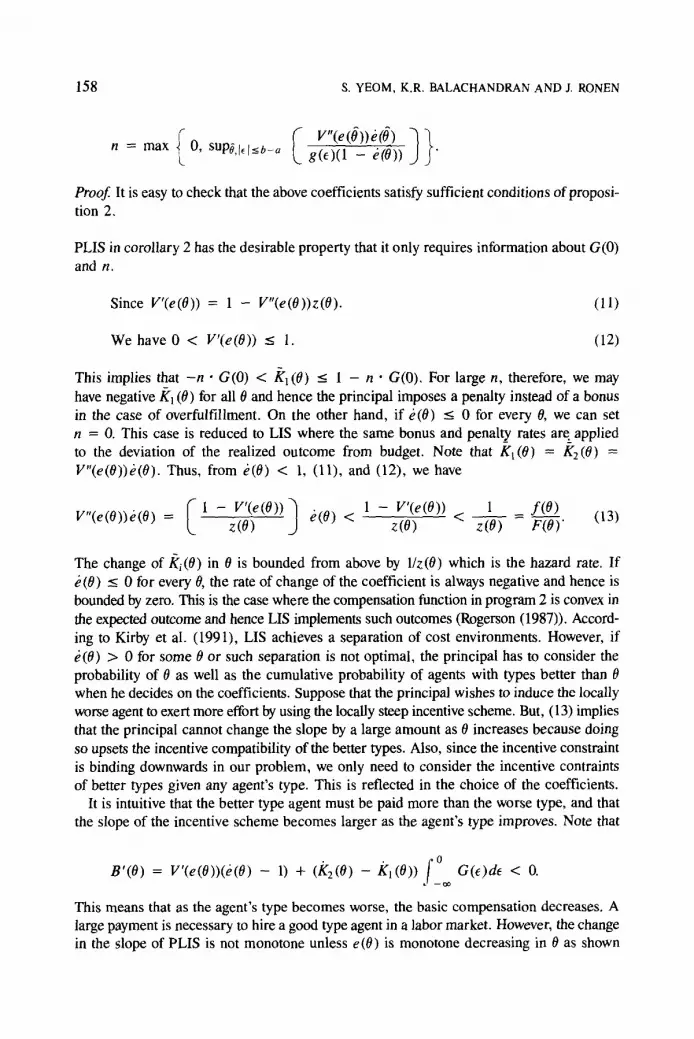
n = max ( 0, supg,/~[<0_a ~ g~.e)(1V"(e(0 _))e(0)_ b(0)) 1 ) "

Proof It is easy to check that the above coefficients satisfy sufficient conditions of proposition 2.

PLIS in corollary 2 has the desirable property that it only requires information about G O ) and n.

Since V'(e(O)) = 1 - V"(e(O))z(O). (11)

We have 0 < V'(e(O)) < 1. (12)

This implies that - n �9 G(0) < Kl (0) - 1 - n �9 G(0). For large n, therefore, we may have negative K1 (0) for all 0 and hence the principal imposes a penalty instead of a bonus in the case of overfulfillment. On the other hand, if e(O) <_ 0 for every 0, we can set n = 0. This case is reduced to LIS where the same bonus and penal~ rates are applied to the deviation of the realized outcome from budget. Note that Kt(0 ) = K2(0 ) = V"(e(O))e(O). Thus, from i,(O) < 1, (11), and (12), we have

('-1 - V'(e(O)) ~ 1 - V'(e(O)) 1 _ f ( O ) V"(e(O))e(O) = z(O) _3 e(O) < z(O) < z(O) F(O)" (13)

The change of Ki(O) in 0 is bounded from above by 1/z(O) which is the hazard rate. If e(0) ~ 0 for every 0, the rate of change of the coefficient is always negative and hence is bounded by zero. This is the case where the compensation function in program 2 is convex in the expected outcome and hence LIS implements such outcomes (Rogerson (1987)). Accord- ing to Kirby et al. (1991), LIS achieves a separation of cost environments. However, if ~(0) > 0 for some 0 or such separation is not optimal, the principal has to consider the probability of 0 as well as the cumulative probability of agents with types better than 0 when he decides on the coefficients. Suppose that the principal wishes to induce the locally worse agent to exert more effort by using the locally steep incentive scheme. But, (13) implies that the principal cannot change the slope by a large amount as 0 increases because doing so upsets the incentive compatibility of the better types. Also, since the incentive constraint is binding downwards in our problem, we only need to consider the incentive contraints of better types given any agent's type. This is reflected in the choice of the coefficients.

It is intuitive that the better type agent must be paid more than the worse type, and that the slope of the incentive scheme becomes larger as the agent's type improves. Note that

B'(O) = V'(e(O))(e(O) - 1) + (Kz(0) - KI(0)) e ]0 G(e)de < O. t - - o o

This means that as the agent's type becomes worse, the basic compensation decreases. A large payment is necessary to hire a good type agent in a labor market. However, the change in the slope of PLIS is not monotone unless e(0) is monotone decreasing in 0 as shown


in (13). The roles of the bonus (penalty) rates are mainly defined by the requirements of incentive compatibility. That is, in some cases, higher effort is not necessary for a better type agent in terms of the whole organization's objective. In other words, for some agents, it is too costly to induce higher effort than exerted by the worse type. This concern is also reflected in the choice of the coefficients.

Finally, PLIS will be compared with QIS. From Picard (1987) and Kirby et al. (1991), QIS can be written a s : tQ(o, x) = s(O) + V'(e(O))(Y - x(O)) - q[(.~ - x(0)) 2 - a2], where o 2 is the variance of uncertainty,

f b IV,,(e(O))e(O) ~ s(O) = V(e(O)) + V'(e(v))dv, and - 2 q _< in f0 ] - - - - ~ '

or q can be chosen as sup0 [V"(e(O))/2]. Notice that both QIS and PLIS are two-parameter incentive schemes. It is easy to see that the agent is paid extra fixed amount of o2V"(e(O))/2 when the realized outcome coincides with reported outcome. Hence, if variance is very large, the principal has to pay too high a fixed payment in order to offset the penalty effect from the quadratic term. Also the agent is likely to be punished for a very high overfulfillment, which may not be desirable. On the other hand, the extra payment under PLIS will be n f~ which could be very high if n is very large. This could happen if the value of g( ' ) is very small over ]EI < b - a. In this case, K 1 (0) is likely to be negative so that the agent is punished even under overfulfillment. In sum, the choice between QIS and PLIS depends on the situation.

Example. Consider a firm where the agent's disutility function is V(e) = ~e 2. Consider the following probability density function over the agent's type.

= % - % o

f(O)

= 4/30

1 i f 0 < 0 < -

2

1 i f ~ < 0 _ < 1.

From the first order condition of the principal's problem, we have e(0) = 4 - z(O). Since z'(O) > - 0 . 5 , the effort is implementable: ~(0) = -z'(O) <_ 0.5 < 1. Notice that ~(0) > 0 for some 0 implies that LIS fails to implement this optimal effort. Suppose e is uniformly distributed over [ - % , Co]. We then have

n = sup f V"(e(O))e(O) t o,l~j<_l g ( - ~ l ~ ~ ) = Co/2.

Consider k 1 (0) : V'(e(O)) - nG(O) = 1 - z(O)/4 - Co~4. Since 0 _< z(O) < 3/4, we have 1~6 - ~"/4 -< K'I(0) -< 1 - '~ . I f Co > 4, then/~l(0) < 0. This means that the_prin- cipal is willing to impose a penalty on overfulfillment. If r < 13/4, then we have KI (0) > 0; hence the principal pays bonus for overfulfillment. If, however, 13/4 < eo < 4,

160 s YEOM, K.R. BALACHANDRAN AND J. RONEN

then the sign of k I (0) is indeterminate; hence the principal pays a bonus for overfulfillment sometimes and imposes penalties otherwise.

This example, where noise is uniformly distributed, reflects a special case where overfulfillment becomes less desirable for incentive purposes as uncertainty increases. 7 As uncertainty increases, in this example, the realized outcome conveys less information about the agent's effort. This allows the agent to have greater discretion over his effort choice. Hence in order for the agent to choose optimal effort the principal must impose a stringent incentive scheme. This results in penalties even in the case of overfulfillment. Of course, as previously explained, the large value of n has undesirable effects on the agency relationship: An upper-bound of the compensation or limited liability may prevent the use of PLIS.

One more comment is helpful to understand the example. Note that e has a compact support so that the following incentive scheme, called knife-edged incentive scheme, would suffice to implement the optimal solution:

S = s(O) i f s > x(O) - ~o t(O, s

= M if.~ < x(O) - Co,

where M is a sufficiently small number. Such a dichotomous contract surely implements the optimal effort and does not detract from the principal's welfare. However, this dichotomous incentive scheme is discontinuous in the parameter of the distribution of e. With a small error in eo (or in the message), the resulting compensation changes dramatically even though actual performance stays constant; that is, it is not robust to small errors. On the other hand, PLIS is continuous in the parameters so that it is robust to small errors.

4. Participative Budgeting

Participative budgeting is usually implemented by the following steps. The principal devises a rule which specifies the procedures of participative budgeting and rewards: The agent sets the budget and communicates it to the principal. After observing the actual performance, the principal pays rewards based on a rule that is a function of the budget and actual performance. Thus, participative budgeting constitutes an indirect mechanism. In this section, we study such an indirect mechanism.

Let T(s s be participative budgeting system, where the agent sets budget s We showed that the optimal PLIS implements optimal effort. The property of the optimal effort is that e(0) - 0(= x(O)) is decreasing in 0; hence, x(O) has one-to-one correspondence with 0. Let ~b(-) be an inverse function defined by

dp(x) = {0 Ix(O) = x}. (14)

Now it is trivial to identify the incentive compatible participative budgeting system below.

Proposition 3. Suppose t(O, 2) is an optimal PLIS. Then, T(s s is an optimal participative budgeting system if T(s s = t(4~(s 2).


Proof

Note that t(O, ~) satisifies s(O) = j t(O, Y)g(E)de. (15)

Substitute (14) into (15).

s(~b(.~)) = f t (d~(~) ,x) ,g(e)de = f T(.~, x )g(e )de .

Since t(O, ~) is incentive compatible, for ~ = x(O), we have

J; T ( ~ , ~ ) g ( , ) d e - V(e(O)) = J ; t (O ' x )g (e )de - V(e(O)) >_ f , t (O ' ,Y)g(e)de - V(e')

= f t(c~(x'), e' - 0 + e)g(e)de - V(e3

= f T(x', Y )g (e )de - V(e').

Hence, T(s ~) implements e(0) with an expected payment of s(O). []

The underlying idea of proposition 3 is that observing the budget s plays the same role as communication in the direct revelation mechanism. Therefore, T(s s is an incentive compatible participative budgeting system, and is usually called a menu of contracts in- dexed by .~.

Example. Using the previous example, we can derive the optimal participative budgeting system. Let q~(x) be the solution of the followingequation: 4 - z(O) - 0 = x. Since e(0) = x(O) + O, we have e = x + q~(x). This gives Kl(X) = V'(x + 4~(x)) - %/4, and ~'2(x) = V'(x + r + %/4. These determine T(,~, Y).

The optimal solution may be implemented by a single reward scheme instead of a menu of incentive schemes (Melumad and Reichelstein (1989) and Guesnerie, Picard, and Rey (1988) in a general framework, and Kirby et al. (1991) in a participative budgeting framework). If so, a single reward scheme may have the advantage of renegotiation-proffness 8 over a menu of incentive schemes, and it avoids the cost of communiation if any. Defining the single reward function requires finding a t(s such that

f f ~o(x) = t (Y)g(e)de = t(x + e)g(e)de (16)


where r = s(~b(x)) andx is an expected outcome. If such a t(s exists, or if the integral equation (16) has a solution, the single reward incentive scheme may implement the optimal effort without any welfare loss and would render communication valueless. Guesnerie, Picard, and Rey (1988) summarize the sufficient conditions for the existence of t(s in (16) (see also "spanning" condition in Melumad and Reichelstein (1989)). One of the conditions is that if ~o (x) is a polynomial of degree n and if the distribution of noise has moments of order n, we can find a t(s which is also a polynomial of degree n. Applying this, we can show that there exists a nonparticipative incentive scheme which performs equivalently to Weitzman's scheme. Note that tw(~, ~) is a piecewise linear function of s and the first moment of noise exists. In this case, we can have a single reward function such that

t(.~) = (/~ - flY) + fix. (17)

Note that t(s = B(s where/~(.) is a basic bonus function in Weitzman's scheme. (17) can be reinterpreted in a budgeting framework. Rearranging (17) gives t(s = / ~ + /3(s - s The agent is paid a bonus (penalty) at some proportion of his over- (under-) achieve- ment of performance as well as the fixed compensation B. Since s can be interpreted as a mandatory budget, it is a nonparticipative (mandatory) budgeting system.

Proposi t ion 4. Let e(0) be an effort implemented by tw(j, ~). Consider t(,~) such that

t(.r) = (/? - flY) + fl.x.

Then, e(0) is also implemented by t(2) and is determined by V'(e(O)) = ft. The expected compensation under t(s is the same as that under tw(s s Moreover, the coefficients of tw(~, ~) will satisfy

fl - g 1 G(0) -

K2 - KI"

Proof See Appendix.

Proposition 4 says that t(s and tw(s ~) perform equivalently and implement the same effort. This, in turn, implies that Weitzman's type of incentive scheme is very restricted because it is optimal only if the optimal effort is constant. Notice that t(s is a profit sharing incentive scheme where the agent is paid/3s plus some constant.

Consider the effort implemented by tw(.~, 2). Suppose fl = 1. Then, V'(e(O)) = 1. From the solution of case 1, we can conclude that tw(s ~) implements the ex post optimal effort. In this case, a single reward incentive scheme t(s = (B - s + s This is a franchise type of incentive scheme, but it is too costly for the principal to guarantee nonnegative expected utility for all possible types of agents. Consider the case of/3 > 1. This implies that the marginal disutility of effort exceeds the marginal expected outcome so that there is no benefit in the agency relationship. Finally, consider the case of/3 < 1. Then, the optimal effort is determined by V'(e(O)) = /3 < 1. However, in this case, it is difficult to find a principal's objective function where such effort is optimal. This points to the


nontrivial problems associated with designing an incentive structure in an organization. In other words, even through NSIS induces truth-telling, we cannot evaluate the performance of the scheme without specifying a reasonable objective function of the organization. For example, if NSIS is not an optimal incentive scheme for the organization considered, the principal may not wish to use it. If NSIS is optimal, we have shown that there exists a nonparticipative incentive scheme which is a function of only actual outcome and pertbrms as well as NSIS. Therefore, participative budgeting by NSIS only makes the principal worse off either because NSIS is not optimal or because communication might be costly. So we believe that this should be examined in an experimental study in which not only the truth-inducing property is considered but also improvement in welfare.

Remark. At this moment, one may wonder if there always exists a single reward incentive scheme which performs equivalently to our optimal PLIS. Consider the previous example. It is easy to verify that

1 f9 r V'(x + (9(x))dx. : ( . r) = (x + ~(x))2/8 + ~ :~

Since the highest order of ~b(x) is a linear term, ,p(x) is at most quadratic in x. Consider the following density function:

G(~)

f l/6x 2 i fe < - 1

= 1/2 + 1/3x i f - 1 < e <- 1

1 - 1/6x 2 i fe _> 1.

This distribution has expectation of zero, but its variance does not exist. Hence there does not exist a single reward incentive scheme which implements the optimal solution because ~p(x) is a quadratic function ofx. On the other hand, if we restrict a priori the type of incentive schemes to NSIS, a single reward incentive scheme that performs equivalently to NSIS always exists since NSIS requires only the first moment of noise. Also note that a quadratic incentive scheme does not exist in this example because it requires the second moment of the distribution.

5. Conclusion

Designing a good budgetary system requires the design of an incentive structure within an organization. This paper derived the optimal PLIS under hidden information and hidden action coupled with uncertainty. The optimal PLIS has features that make it distinct from NSIS. For example, its coefficients vary depending on the budget set by the subor- dinates, and the bonus rate is not necessarily positive. More importantly, if the coefficients are constant like NSIS, we have no rationale for NSIS at the outset since there exists a nonparticipative incentive scheme which performs as well as NSIS.


This paper can be extended in a variety of ways. It is valuable to consider our problem in a more general setting. For example, risk sharing is an important aspect in an uncertain environment. Risk neutrality played a very crucial role in this paper in showing that program 1 achieves approximately the same welfare as in program 2. But in the case of a risk averse agent welfare losses due to hidden action will result, and hence the principal's welfare in program 1 could fall below that of program 2. Also note that PLIS is piecewise linear in the actual performance. If the agent is risk averse, PLIS may impose so much risk on the agent that it could cease to be optimal. In this case, budgetary slack may be a necessary buffer for uncertainty. Second, a decision variable could be introduced in our model to facilitate the analysis of planning along with control. Third, in our analysis, we assumed that precommitment by the principal is credible. But it may not be the case if the agency relationship is maintained over multiple periods. For example, suppose the principal is able to use the agent's past history (messages and performances) as the basis for performance evaluation. The agent will no longer be willing to tell the truth if he loses in the future by doing so. Due to this ratchet effect, PLIS derived in this paper may not be the optimal incentive scheme in a dynamic incentive framework. Finally, it will be instructive to consider the incentive problem under a multi-agents setting. In this case, one agent's evaluation may depend on the other's participatively set budget. Or, by devising competi- tion among the agents within an organization, the principal's welfare may be improved.

Appendix

Proof of Lemma 2

E[t(O, x)l = B(O) + f~>_x(O) KI(O)(s - x(O))g(elde

+ f;,<_x(O)K2(O)(.~ - x(Ol)g(e)de

= B(O) + Kt(O)(x - x(fi)) + (g2(o) - Kt(O))f2<_x~)

For simplicity, let us calculate the integral term only.

s f fx<o,--,- <_x(O) ('~ - x(O))g(elde = o-o~xfO)-x (x - x(O))g(e)de + 0 - ~ eg(e)de

x(~)-x = (x - x(O))G(x(O) - x) + f eg(e)de

. 1 - o o

f x(O)-x G( )d = - - ~_ 6 _ .

. 1 - o o

(,~ - x(0)) g(e)de (18)


= B ( 6 ) + I" 0)). J x(O)-x*

The last equality follows from integration by parts. Substituting this into (18) proves the lemma. Q.E.D.

Proof of Proposition 2

It suffices to derive (B(0); K1 (0); K2(0)) which satisfies the conditions of proposition 1.

Derivation of B (0):

Using lemma 2, if the agent tells the truth and takes the optimal effort (x(0) = x), we have

f , t(O, ;)g(e)de = B(O) - (K2(O) - KI(0)) f_~

In order for the principal to have the same expected utility as in case 2, we must have, from proposition I. 1,

fob T(O, 5)g(e)de = s(O) = V(e(O)) + V'(e(v))dv.

Proposition 2.1 follows.

Derivation of (Ki (0); K 2 (0)):

Note that e*(0, 0) is unique; hence, it suffices to show that truth-telling is optimal. Let 7r (0, 0) be the agent's utility when he sends a message 6 and takes effort e* (0, 0) given his true type of 0. Then

r (0 , 0) = u(0, e* (0, 0); 0)

L(e; O)de - (K,(O) - K2(O)) a-f~ G(e)de - V(e*(O,

By the envelope theorem and by differentiating (19) with respect to 6, we have:

(19)

It is easy to check that truth-telling satisfies the first order condition since e(O) = e*(O, O) and V'(e(O)) -- L(O, 0)). Now we need to characterize the condition that truth-telling is indeed the global optimum.

_ . s aTr(O, O) V'(e*(O, 0))(~(6) - 1) - L(x(O) - x ; 6)(e(/~) - 1) + L2(e; 0)dE

06 (0)-x*


Note that r (0 , 0) - r (0 , 0) = fo~ ~ (327r(v, t))/(OO00) dtdv. Hence, the sufficient condition for the mechanism to implement the optimal effort is

32~(0, O) _ L~(x(6) - x*; 6) O(x(O) - x*) (e(O) - 1) a6o0 oo

i.e.

I 0e*(0, 0) 30 1

-L2 (x (6 ) - x*; 6) a (x (6 ) - x* ) > 0. 30

( r g x ( O ) - x*; ~)(e(6) - 1) + r2(x(~J) - x*; ~)) _> 0

From (6), for every 0, 0 E O, L ( x ( O ) - x*; 6) - V'(e*(0, 0)) = 0. (20)

Since V(-) is convex and L~(6; 6) >_ O, we have 0 _< (0e*(0, 0))/(30) < 1.

This implies

Ll (x (O) - x*; 0)(e(6) - 1) + L2(x(0) - x*; 6) < 0. (22)

By lemma 3, for all 6, 0 E O

& ( x ( 6 ) - x*; 6)(e(6) - 1) + L2(x(6) - x*; 6)

< (K2(0) - K l ( O ) ) g ( x ( O ) - x*)(e(0) - 1) + L2(0; 0) + tKz (o ) - k~(0)]

= (K2(0) - K l ( 6 ) ) g ( x ( O ) - x*)(e(0) - 1) + V"(e(tg))e(0) + IK2(0) - R~(0)].

Therefore, it is sufficient for the global optimality to be ensured for all 6, 0 ~ O

V"(e(O))e (O) + IK2(0) - g , (0 ) l K2(0 ) - Kl(O ) >

g(x (O) - x * ) ( l - e(O))

Also note that Ix(tJ) - x*l --< 10 - 01 < b - a. Hence, (9) follows. QE.D.

Differentiating (20) with respect to 0,

L l ( x ( 6 ) - x*; 6) Q 30

i.e.

Oe*(O, O) L l (x (O) - x*; 0)

O0 v " ( e * ( 6 , 0)) + L~(x(6) - x*; 6)"

0e*(0, 0) + 1 I - V"(e*(0, 0)) 0e*(/J, 0) 30 - 0 , (21)


Proof of Corollary 1

Differentiating (6) with respect to 0 gives

Ll(x(O ) - x*; /J) I b(ff) - 1 Oe*(0,0 1/ j )

Rearranging the expression gives

( V"(e*(O,

0e*(0, 0) = 0. + G ( x ( 0 ) - x*; ~) - V"(e*(~, 0)) Og

0)) + Ll(x(O ) - x*; 0) ] Be*(0,00 ~- 0)

= Ll(x(O) - x*; 0)(e(/J) - 1) + L,2(x(/J) - x*; 0) < 0.

Since V"(.) + LI(~; 0) > 0, the corollary is proved.

Proof of Proposition 4

Under the single reward incentive scheme, the agent's utility is

u ( t ( ~ ) , e) = (B - [3~) + [3~ - V(e) .

The agent's choice of effort is represented by the first order condition such that

OU(t(s e) Be = [3 - V'(e(O)) = O.

e=e(O)

Under the Weitzman's scheme, the agent's expected utility is

u(~, e ; 0) = (t~ - [3~) + [3x(~) - ( x < 0 ~ - x L ( y ) d y - V(e) a0

where L(y) = KI(1 - G(y)) + K2G(y). Let e*(~J, 0) be an optimal effort given message and his true type 0. Then,

Ou(O, e; O) = L ( x ( O ) - x * ) - V ' ( e * ( O , 0 ) ) = O. Oe

e=e*(O.O)


Note that e*(0, 0) = e(0) at 0 = 0 gives

V'(e(O)) = L(0) = K~(I - G(0)) + K2G(0). (23)

Given his behavior, the requirement of truthful revelation is

Ou(O, e * ; 0 )

a6 = / 3 ( ~ ' ( 0 ) - 1) - L ( 0 ) ( e ( 0 ) - 1) = (/3 - V'(e (O)) ) (e (O) - 1) = O.

~=o

The local second order condition is satisfied as in the proof of proposition 2. Since e(0) < 1, we have V'(e(O)) =/3, which is the same effort implemented under t(s Also, it is easy to show that the expected compensations are same under both schemes. From (23), the coefficients of tw(s E) are determined by

G(0) - /3 - K1 K2 _ K l . Q.E.D.

N o t e s

1. ljiri, Kinard, and Putney (1968) observed that an essentially identical scheme was used in negotiated incentive contracts in Department of Defense procurement and claimed that the scheme could be used within an organization to facilitate planning. Gonik (1978) reported that a similar scheme was used to determine salesmen's compensations in IBM Brazil.

2. Paik (1993) has studied independently same incentive scheme with a different model and called "Kinked Linear Incentive Scheme"

3. Note that while a linear technology is assumed in this paper, Kirby et al. (1991) and Paik (1993) use a general technology with the monotone inverse hazard rate assumption. As an anonymous referee indicated, either linearity or monotone hazard rate could be relaxed in order to study a situation where LIS is not optimal. In particular, the monotone hazard rate is satisfied by many well-known probability functions. In this paper, however, the intuitive monotone hazard rate assumption is sacrificed because a linear technology enables us to get coefficients of PLIS explicitly. One may notice that our main results depend heavily on the analysis of coefficients in PLIS. Also the qualitative results do not change in either choice.

4. The typical result of bunching is that expected compensation and x(O) are constant. However, the effort is still increasing in 0; hence, marginal disutility of effort is also increasing. This leads to nondifferentiability of the compensation with respect to the expected outcome (see Picard (1987) for detail) and hence a solution does not exist.

5. Organizational slack refers to an excess of resources allocated over the minimum necessary to accomplish the task assigned. This concept of slack appeared in accounting literature; for example, Ronen and Balachan- dran (1988), Balachandran and Ronen (1989), and Kirby, Reichelstein, Sen, and Paik (1991). Budgetary slack in our paper refers to the understatement of the outcome (profit) in the budgeting process:

6. Kl(0 ) and K2(0) must be differentiable, otherwise Kt(o ) - /~2(0) does not exist. Paik (1990) also derived similar conditions in a different setting, but he restricted a priori the difference of the coefficients to be constant unlike proposition 2.


7. The principal is concerned with the degree to which the agent is able to deviate from his budget due to the noise of the realized outcome. This concern is captured in the value of n or

1 in( g(x(0) - x*) -

]xi0) x* I_<b-a 2% "

The variance of the distribution in the example is %/3 and hence we regard e o as the degree of uncertainty. 8. In a revelation game, the agent tells the truth at optimum. So, once communication is made, the principal

has an incentive to renegotiate the original contract; hence, the solution has to assume a strong commitment between them. Since, however, the single reward incentive scheme does not require any communication, there is no need for renegotiation in a single period framework. For a detailed discussion, see Demougin (1989).

References

Balachandmn, K.R. and J. Ronen, "Incentive Contracts When Production is Subcontracted." European Journal of Operational Research 40, 169-185, (May 1989).

Christensen, J.. "The Determination of Performance Standards and Participation." Journal of Accounting Research 20, 589-603, (Autumn 1982).

Demougin, D.M., "~ Renegotiation-Proof Mechanism for a Principal-Agent Model with Moral Hazard and Adverse Selection." RAND Journal of Economics 20, 256-267, (1988).

Demski, J. and G. Feltham, "Economic Incentives in Budgetary Control Systems." The Accounting Review 53, 336-359, (April 1978).

Gonik, J., "Tie Salesman's Bonuses to Their Forecasts." Harvard Business Review 116-123, (May-June 1978). Guesnerie, R. and J.-J. Laffont, "A Complete Solution to a Class of Principal-Agent Problems with an Applica-

tion to the Control of a Self-Managed Firm." Journal of Public Economics 25, 329-369, (December 1984). Guesnerie, R., P. Picard and E Rey, "Adverse Selection and Moral Hazard with Risk Neutral Agents." European

Economic Review 33, 807-823, (1988). Ijiri, Y., C. Kinard and EB. Putney, "An Integrated Evaluation System for Budget Forecasting and Operating

Performance with a Classified Budgeting Bibliography.'" Journal of Accounting Research 6, 1-28, (Spring 1968). Kirby, A.J., S. Reichelstein, EK. Sen and T. Paik. "Participation, Slack, and Budget-Based Performance Evaluation."

Journal of Accounting Research 29, 109-128, (Spring 1991). Laffont, J.-J. and J. Tirole, "'Using Cost Observation to Regulate Firms." Journal of Political Economy. 94, 614-64 l,

(June 1986). Melumad, N.D. and S. Reichelstein, "'Value of Communication in Agencies." Journal of Economic Theor3" 47,

334-368, (April 1989). Myerson, R.B., "'Incentive Compatibility and the Bargaining Problem." Econometrica 47, 61-73 (January, 1979). Paik, T., "Participative Budgeting with Kinked Linear Payment Schemes." Review of Quantitative Finance and

Accounting 3, 1993. Penno, M., '~symmetry of Pre-Decision Information and Managerial Accounting." Journal of Accounting Research

22, 177-191, (Spring 1984). Picard, E, "On the Design of Incentive Schemes under Moral Hazard and Adverse Selection.'" Journal of Public

Economics 33, 305-331, (1987).

Rogerson, W. "On the Optimality of Menus of Linear Contracts." mimeo, Northwestern University, (1987). Ronen, J. and K.R. Balachandran, "An Approach to Transfer Pricing under Uncertainty." Journal of Accounting

Research 26, 300-314, (Autumn, 1988). Weitzman, M.. "'The New Soviet Incentive Model." The Bell Journal of Economics 7.251-257, (Spring 1976).

Documents

Piecewise linear incentive scheme and participative budgeting