MSBRIDGE: OPENSEES PUSHOVER AND EARTHQUAKE

STRUCTURAL SYSTEMS

RESEARCH PROJECT

Report No.

SSRP–16/05

MSBRIDGE: OPENSEES

PUSHOVER AND EARTHQUAKE

ANALYSIS OF MULTI-SPAN

BRIDGES - USER MANUAL

by

ABDULLAH ALMUTAIRI

JINCHI LU

AHMED ELGAMAL

KEVIN MACKIE

Final Report Submitted to the California Department of

Transportation (Caltrans) under Contract No. 65A0530.

January 2019

Department of Structural Engineering

University of California, San Diego

La Jolla, California 92093-0085

ii



Structural Systems Research Project

Report No. SSRP-16/05

MSBridge: OpenSees Pushover and Earthquake Analysis

of Multi-span Bridges - User Manual

by

Abdullah Almutairi

Graduate Student Researcher, UC San Diego

Jinchi Lu

Associate Project Scientist, UC San Diego

Ahmed Elgamal

Professor of Geotechnical Engineering, UC San Diego

Kevin Mackie

Associate Professor of Structural Engineering,

University of Central Florida

Final Report Submitted to the California Department of

Transportation under Contract No. 65A0530



La Jolla, California 92093-0085

January 2019

iii

Technical Report Documentation Page 1. Report No.

2. Government Accession No.

3. Recipient’s Catalog No.

4. Title and Subtitle

MSBridge: OpenSees Pushover and Earthquake Analysis

of Multi-span Bridges - User Manual

5. Report Date

January 2019

6. Performing Organization Code

7. Author(s)

Abdullah Almutairi, Jinchi Lu, Ahmed Elgamal and

Kevin Mackie

8. Performing Organization Report No.

UCSD / SSRP-16/05

9. Performing Organization Name and Address

Department of Structural Engineering School of Engineering

10. Work Unit No. (TRAIS)

University of California, San Diego La Jolla, California 92093-0085

11. Contract or Grant No.

65A0530

12. Sponsoring Agency Name and Address

California Department of Transportation

13. Type of Report and Period Covered

Final Report

Division of Engineering Services 1801 30th St., MS-9-2/5i

Sacramento, California 95816

14. Sponsoring Agency Code

15. Supplementary Notes

Prepared in cooperation with the State of California Department of Transportation.

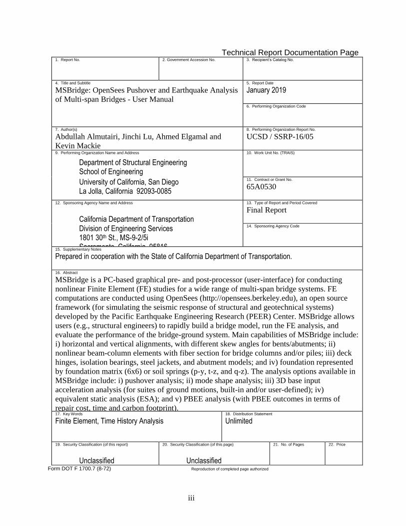
16. Abstract

MSBridge is a PC-based graphical pre- and post-processor (user-interface) for conducting

nonlinear Finite Element (FE) studies for a wide range of multi-span bridge systems. FE

computations are conducted using OpenSees (http://opensees.berkeley.edu), an open source

framework (for simulating the seismic response of structural and geotechnical systems)

developed by the Pacific Earthquake Engineering Research (PEER) Center. MSBridge allows

users (e.g., structural engineers) to rapidly build a bridge model, run the FE analysis, and

evaluate the performance of the bridge-ground system. Main capabilities of MSBridge include:

i) horizontal and vertical alignments, with different skew angles for bents/abutments; ii)

nonlinear beam-column elements with fiber section for bridge columns and/or piles; iii) deck

hinges, isolation bearings, steel jackets, and abutment models; and iv) foundation represented

by foundation matrix (6x6) or soil springs (p-y, t-z, and q-z). The analysis options available in

MSBridge include: i) pushover analysis; ii) mode shape analysis; iii) 3D base input

acceleration analysis (for suites of ground motions, built-in and/or user-defined); iv)

equivalent static analysis (ESA); and v) PBEE analysis (with PBEE outcomes in terms of

repair cost, time and carbon footprint). 17. Key Words

Finite Element, Time History Analysis

18. Distribution Statement

Unlimited

19. Security Classification (of this report)

Unclassified

20. Security Classification (of this page)

Unclassified

21. No. of Pages

22. Price

Form DOT F 1700.7 (8-72) Reproduction of completed page authorized

iv

DISCLAIMER This document is disseminated in the interest of information exchange. The contents of this

report reflect the views of the authors who are responsible for the facts and accuracy of the data

presented herein. The contents do not necessarily reflect the official views or policies of the

State of California or the Federal Highway Administration. This publication does not constitute

a standard, specification or regulation. This report does not constitute an endorsement by the

California Department of Transportation of any product described herein.

For individuals with sensory disabilities, this document is available in Braille, large print,

audiocassette, or compact disk. To obtain a copy of this document in one of these alternate

formats, please contact Division of Research and Innovation, MS-83, California Department of

Transportation, P.O. Box 942873, Sacramento, CA 94273-0001.

v

ACKNOWLEDGMENTS

The research described in this report was primarily supported by the California Department of

Transportation (Caltrans) with Dr. Charles Sikorsky as the project manager. Additional funding

was provided by the Pacific Earthquake Engineering Research Center (PEER). These supports

are most appreciated. In addition, we are grateful for the valuable technical suggestions,

comments, and contributions provided by Caltrans engineers, particularly Dr. Charles

Sikorsky, Dr. Toorak Zokaie, Mr. Yeo (Tony) Yoon, Dr. Mark Mahan, Dr. Anoosh

Shamsabadi, and Mr. Steve Mitchell.

vi

ABSTRACT

MSBridge is a PC-based graphical pre- and post-processor (user-interface) for conducting

nonlinear Finite Element (FE) studies for a wide range of multi-span bridge systems. FE

computations are conducted using OpenSees (http://opensees.berkeley.edu), an open source

framework (for simulating the seismic response of structural and geotechnical systems)

developed by the Pacific Earthquake Engineering Research (PEER) Center. MSBridge allows

users (e.g., structural engineers) to rapidly build a bridge model, run the FE analysis, and

evaluate the performance of the bridge-ground system. Main capabilities of MSBridge include: i)

horizontal and vertical alignments, with different skew angles for bents/abutments; ii) nonlinear

beam-column elements with fiber section for bridge columns and/or piles; iii) deck hinges,

isolation bearings, steel jackets, and abutment models; and iv) foundation represented by

foundation matrix (6x6) or soil springs (p-y, t-z, and q-z). The analysis options available in

MSBridge include: i) pushover analysis; ii) mode shape analysis; iii) 3D base input acceleration

analysis (for suites of ground motions, built-in and/or user-defined); iv) equivalent static analysis

(ESA); and v) PBEE analysis (with PBEE outcomes in terms of repair cost, time and carbon

footprint).

vii

TABLE OF CONTENTS

DISCLAIMER............................................................................................................................. IV

ACKNOWLEDGMENTS ............................................................................................................ V

ABSTRACT ................................................................................................................................. VI

TABLE OF CONTENTS ..........................................................................................................VII

LIST OF FIGURES .................................................................................................................... XI

LIST OF TABLES ................................................................................................................... XIX

1 INTRODUCTION......................................................................................................1

1.1 Overview ......................................................................................................................... 1

1.2 What’s New in Current Updated Version ....................................................................... 1

1.3 Units ................................................................................................................................ 2

1.4 Coordinate Systems ........................................................................................................ 2

1.5 System Requirements...................................................................................................... 3

1.6 Acknowledgment ............................................................................................................ 3

2 GETTING STARTED ...............................................................................................4

2.1 Start-Up ........................................................................................................................... 4

2.2 Interface .......................................................................................................................... 5

2.2.1 Menu Bar .................................................................................................................... 7

2.2.2 Model Input Region .................................................................................................... 7

2.2.3 FE Mesh Region ......................................................................................................... 7

3 BRIDGE MODEL ....................................................................................................10

3.1 Spans ............................................................................................................................. 11

3.1.1 Straight Bridge .......................................................................................................... 11

3.1.2 Curved Bridge ........................................................................................................... 12

3.2 Deck Sections................................................................................................................ 17

3.3 Bentcap Sections ........................................................................................................... 19

3.4 Column Cross Sections ................................................................................................. 21

3.4.1 Cross-section Shapes ................................................................................................ 21

3.4.2 Cross Section Properties ........................................................................................... 22

3.5 Foundation .................................................................................................................... 34

3.5.1 Rigid Base ................................................................................................................. 34

viii

3.5.2 Soil Springs ............................................................................................................... 34

3.5.3 Foundation Matrix .................................................................................................... 41

3.6 Abutment....................................................................................................................... 44

3.7 Bridge Model ................................................................................................................ 45

3.7.1 Uniform Column Layout........................................................................................... 45

3.7.2 Non-uniform Column Layout ................................................................................... 47

3.8 Advanced Options ......................................................................................................... 48

3.8.1 Deck Hinges .............................................................................................................. 48

3.8.2 Isolation Bearings ..................................................................................................... 51

3.8.3 Steel Jackets .............................................................................................................. 53

3.8.4 Skew Angles ............................................................................................................. 54

3.8.5 Pilecap Mass ............................................................................................................. 55

3.8.6 OpenSees Parameters ................................................................................................ 55

3.9 Mesh Parameters ........................................................................................................... 57

4 ABUTMENT MODELS ..........................................................................................58

4.1 Elastic Abutment Model ............................................................................................... 58

4.2 Roller Abutment Model ................................................................................................ 63

4.3 SDC 2004 Abutment Model ......................................................................................... 64

4.3.1 Longitudinal Response.............................................................................................. 64

4.3.2 Transverse Response ................................................................................................. 67

4.3.3 Vertical Response ..................................................................................................... 69

4.3.4 Definition of the SDC 2004 Abutment Model .......................................................... 71

4.4 SDC 2010 Sand Abutment Model ................................................................................ 73

4.5 SDC 2010 Clay Abutment Model ................................................................................. 74

4.6 ElasticPP-Gap Model .................................................................................................... 74

4.7 HFD Model ................................................................................................................... 76

5 COLUMN RESPONSES & BRIDGE RESONANCE ..........................................78

5.1 Bridge Natural Periods .................................................................................................. 78

5.2 Column Gravity Response ............................................................................................ 78

5.3 Column & Abutment Longitudinal Responses ............................................................. 78

5.4 Column & Abutment Transverse Responses ................................................................ 78

ix

6 PUSHOVER & EIGENVALUE ANALYSES .......................................................82

6.1 Pushover Analysis ......................................................................................................... 82

6.1.1 Input Parameters ....................................................................................................... 82

6.1.2 Output for Pushover Analysis ................................................................................... 84

6.2 Mode Shape Analysis ................................................................................................... 90

7 GROUND SHAKING ..............................................................................................92

7.1 Definition/specification of input motion ensemble (suite) ........................................... 92

7.1.1 Available Ground Motions ....................................................................................... 92

7.1.2 Specifications of Input Motions ................................................................................ 93

7.2 Rayleigh Damping ...................................................................................................... 100

7.3 Save Model and Run Analysis .................................................................................... 100

8 TIME HISTORY OUTPUT ..................................................................................103

8.1 Time History Output Quantities.................................................................................. 103

8.1.1 Deck Response Time Histories ............................................................................... 104

8.1.2 Column Response Profiles ...................................................................................... 104

8.1.3 Column Response Time Histories .......................................................................... 105

8.1.4 Column Response Relationships ............................................................................. 107

8.1.5 Abutment Responses Time Histories ...................................................................... 109

8.1.6 Soil Spring Responses Time Histories .................................................................... 111

8.1.7 Deck Hinge Responses Time Histories................................................................... 112

8.1.8 Isolation Bearing Responses Time Histories .......................................................... 114

8.2 Deformed Mesh and Animation.................................................................................. 115

8.3 Maximum Output Quantities ...................................................................................... 117

8.3.1 Bridge Peak Accelerations & Displacements for All Motions ............................... 117

8.3.2 Maximum Column & Abutment Forces for All Motions ....................................... 119

9 EQUIVALENT STATIC ANALYSIS..................................................................120

9.1 Bridge Longitudinal Direction .................................................................................... 120

9.2 Bridge Transverse Direction ....................................................................................... 121

10 ANALYSIS OF IMPOSED DISPLACEMENTS ................................................124

10.1 Imposed Soil Displacement ........................................................................................ 124

10.2 Pile Analysis ............................................................................................................... 131

x

11 PBEE ANALYSIS (GROUND SHAKING) ........................................................135

11.1 Theory and Implementation of PBEE Analysis .......................................................... 135

11.2 Input Necessary for User-defined PBEE Quantities ................................................... 138

11.3 Definition/specification of PBEE input motion ensemble (suite) ............................... 139

11.4 Save Model and Run Analysis .................................................................................... 139

11.5 PBEE Analysis ............................................................................................................ 140

11.5.1 PBEE Quantities ................................................................................................. 140

11.5.2 Compute PBEE outcomes ................................................................................... 144

11.5.3 Compute Hazard Curves ..................................................................................... 146

11.5.4 Compute Disaggregation .................................................................................... 147

12 TIME HISTORY AND PBEE OUTPUT .............................................................148

12.1 Time History Output Quantities.................................................................................. 148

12.2 PBEE Output Quantities ............................................................................................. 150

12.3 PBEE Outcomes.......................................................................................................... 155

12.3.1 Repair Cost, Repair Time, and Carbon Footprint ............................................... 155

12.3.2 Hazard Curves ..................................................................................................... 159

12.3.3 Disaggregation .................................................................................................... 164

APPENDIX A CAPABILITIES ADDED IN THE CURRENT UPDATED VERSION

167

APPENDIX B CALCULATION OF STEEL AND CONCRETE MATERIAL

PROPERTIES 171

APPENDIX C HOW TO INCORPORATE USER-DEFINED MOTIONS ..................175

APPENDIX D COMPARISON WITH SAP2000 FOR REPRESENTATIVE BRIDGE

CONFIGURATIONS ................................................................................................................180

xi

LIST OF FIGURES

Fig. 1. Global coordinate system employed in MSBridge ................................................. 2

Fig. 2. MSBridge main window .......................................................................................... 4

Fig. 3. Toolbar and file-related submenus: a) toolbar; b) submenu File; c) submenu Execute

...................................................................................................................................... 5

Fig. 4. Result-related submenus: a) submenu Display; b) submenu Report; and c) submenu Help

...................................................................................................................................... 6

Fig. 5. MSBridge copyright and acknowledgment window ............................................... 8

Fig. 6. Buttons available in the FE Mesh window ............................................................. 9

Fig. 7. Model builder buttons ............................................................................................ 10

Fig. 8. MSBridge main window (bridge model with soil springs and a deck hinge included)

.................................................................................................................................... 10

Fig. 9. Bridge span definition ........................................................................................... 11

Fig. 10. Varied span lengths ............................................................................................. 12

Fig. 11. Straight bridge with different span lengths .......................................................... 12

Fig. 12. Horizontal alignment ........................................................................................... 13

Fig. 13. Horizontal and vertical alignments: a) horizontal alignment (plan view); b) vertical

alignment (side view) ................................................................................................. 14

Fig. 14. Vertical alignment ............................................................................................... 14

Fig. 15. Examples of horizontally curved bridges (horizontal alignment): a) single horizontal

curve; b) multiple horizontal curves. ......................................................................... 15

Fig. 16. Examples of vertically curved bridges (vertical alignment): a) single slope; b) begin and

end slopes; c) multiple slopes. ................................................................................... 16

Fig. 17. Deck material and section properties ................................................................... 17

Fig. 18. Box girder shape employed for a bridge deck section ......................................... 18

Fig. 19. Bentcap material and section properties .............................................................. 19

Fig. 20. Rectangular shape employed for a bentcap section ............................................. 20

Fig. 21. Column section properties ................................................................................... 21

Fig. 22. Definition of linear column ................................................................................. 23

Fig. 23. Column elastic material properties ...................................................................... 23

Fig. 24. Column section properties ................................................................................... 23

xii

Fig. 25. Nonlinear Fiber Section window ......................................................................... 24

Fig. 26. Rebar material properties: a) Steel02 material; b) ReinforcingSteel material ..... 25

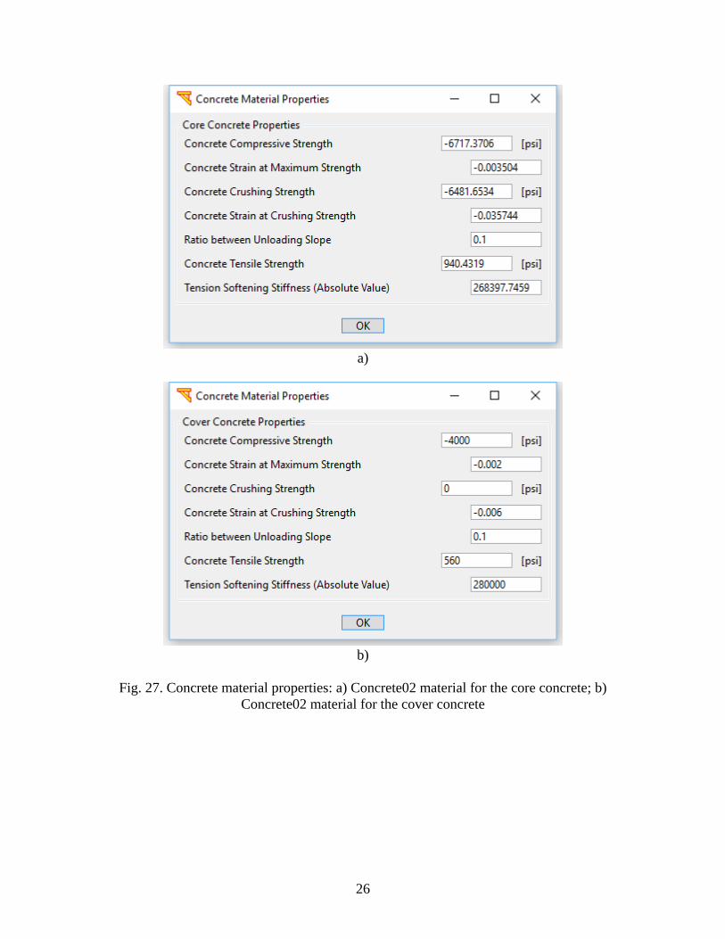
Fig. 27. Concrete material properties: a) Concrete02 material for the core concrete; b)

Concrete02 material for the cover concrete ............................................................... 26

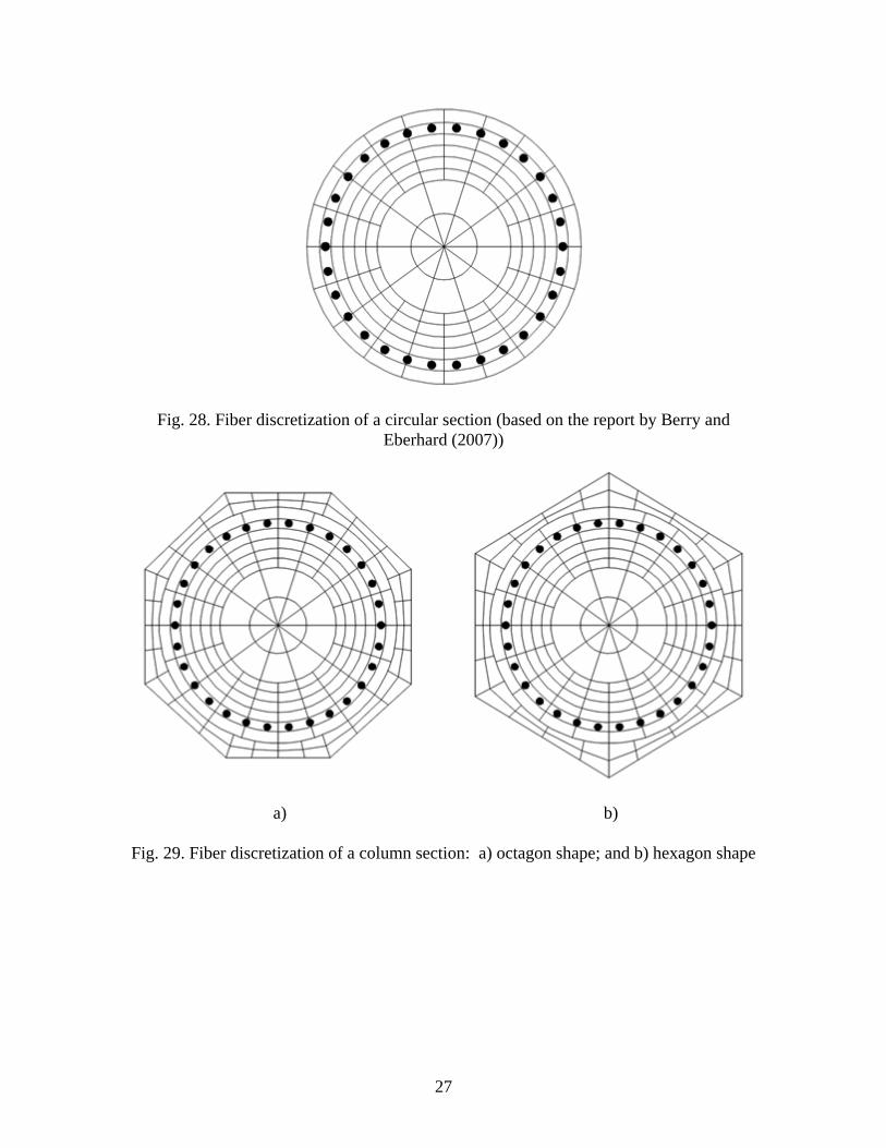
Fig. 28. Fiber discretization of a circular section (based on the report by Berry and Eberhard

(2007)) ........................................................................................................................ 27

Fig. 29. Fiber discretization of a column section: a) octagon shape; and b) hexagon shape27

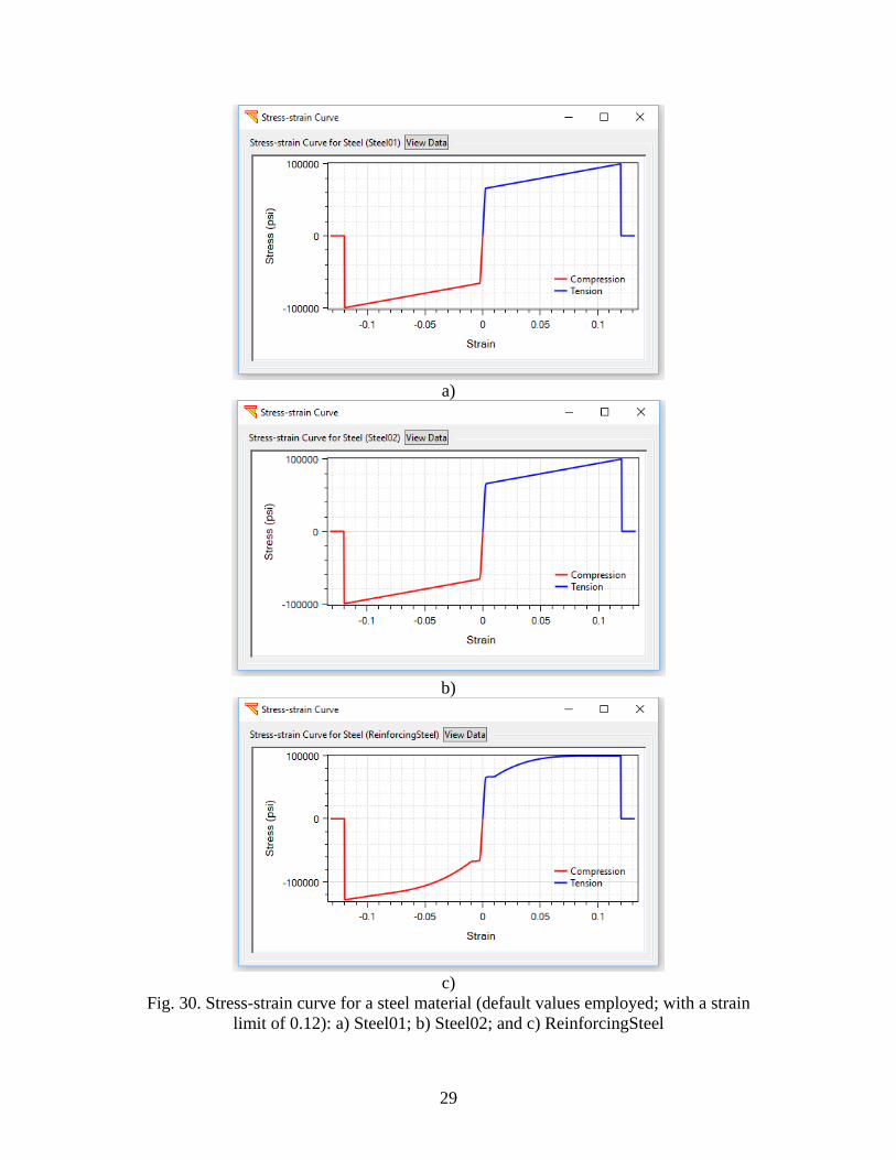
Fig. 30. Stress-strain curve for a steel material (default values employed; with a strain limit of

0.12): a) Steel01; b) Steel02; and c) ReinforcingSteel ............................................... 29

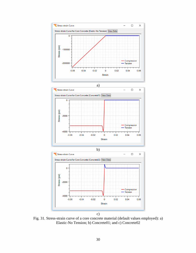
Fig. 31. Stress-strain curve of a core concrete material (default values employed): a) Elastic-No

Tension; b) Concrete01; and c) Concrete02 ............................................................... 30

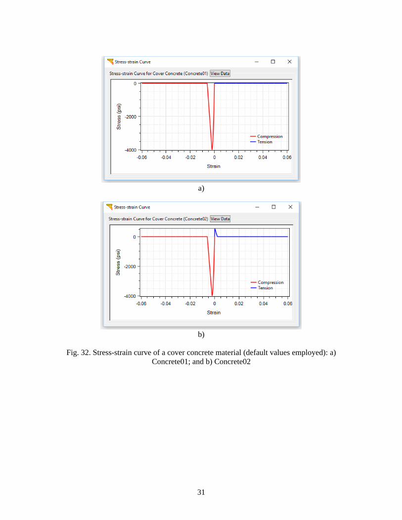
Fig. 32. Stress-strain curve of a cover concrete material (default values employed): a)

Concrete01; and b) Concrete02 .................................................................................. 31

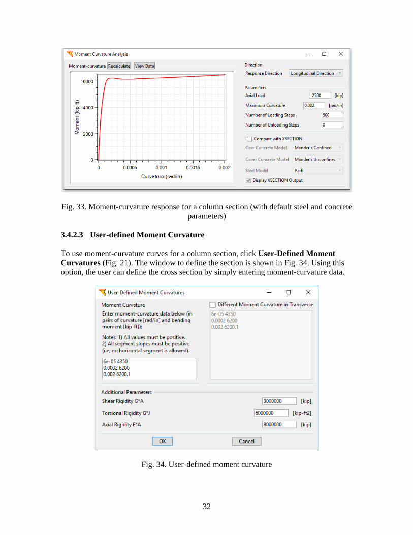
Fig. 33. Moment-curvature response for a column section (with default steel and concrete

parameters) ................................................................................................................. 32

Fig. 34. User-defined moment curvature .......................................................................... 32

Fig. 35. User-defined Tcl script for nonlinear fiber section ............................................. 33

Fig. 36. Foundation types available in MSBridge ........................................................... 34

Fig. 37. Shaft foundation for abutments and bents ........................................................... 35

Fig. 38. Pile foundation model for an abutment ............................................................... 36

Fig. 39. Soil springs .......................................................................................................... 36

Fig. 40. Soft Clay (Matlock) p-y model ............................................................................ 37

Fig. 41. Stiff Clay without Free Water (Reese) p-y model ............................................... 37

Fig. 42. Sand (Reese) p-y model ....................................................................................... 38

Fig. 43. Liquefied Sand (Rollins) p-y model .................................................................... 38

Fig. 44. Soil spring definition window after using the soil spring data calculated based on p-y

equations .................................................................................................................... 39

Fig. 45. FE mesh of a bridge model with soil springs included ........................................ 39

Fig. 46. User-defined p-y curves ....................................................................................... 40

Fig. 47. User-defined t-z curves ........................................................................................ 40

Fig. 48. User-defined q-z soil springs ............................................................................... 41

xiii

Fig. 49. Local coordination system for a foundation matrix ............................................. 42

Fig. 50. Foundation matrix definition ............................................................................... 42

Fig. 51. Multi-linear material definition ........................................................................... 43

Fig. 52. Definition of pile foundations (for PBEE analysis only) .................................... 43

Fig. 53. Definition of an abutment model ......................................................................... 44

Fig. 54. Definition of a bridge model ............................................................................... 45

Fig. 55. Uniform column layout ....................................................................................... 45

Fig. 56. Column heights .................................................................................................... 46

Fig. 57. Column boundary conditions............................................................................... 46

Fig. 58. Bridge configuration: a) general options; b) column layout definition ............... 47

Fig. 59. Advanced options ................................................................................................ 48

Fig. 60. Definition of deck hinges .................................................................................... 50

Fig. 61. FE mesh of a 4-span model with 2 deck hinges included ................................... 51

Fig. 62. OpenSees zeroLength elements for deck hinges (plan view) ............................. 51

Fig. 63. Definition of isolation bearings ........................................................................... 52

Fig. 64. FE mesh of a 4-span bridge model with two isolation bearings included on each bent cap

.................................................................................................................................... 52

Fig. 65. OpenSees zeroLength elements for isolation bearings (side view of bentcap cut-plan)

.................................................................................................................................... 53

Fig. 66. Definition of steel jackets .................................................................................... 53

Fig. 67. Sketch of a steel jacket ........................................................................................ 54

Fig. 68. Definition of skew angles .................................................................................... 54

Fig. 69. Definition of pilecap mass ................................................................................... 55

Fig. 70. Parameters for OpenSees analysis ....................................................................... 56

Fig. 71. Mesh parameters .................................................................................................. 57

Fig. 72. Definition of an abutment model ......................................................................... 59

Fig. 73. General scheme of the Elastic Abutment Model: a) longitudinal component; b)

transverse component; c) vertical component ............................................................ 60

Fig. 74. Definition of the Elastic Abutment Model .......................................................... 61

Fig. 75. Parameters of the Elastic Abutment Model ......................................................... 61

xiv

Fig. 76. Longitudinal components of the Elastic Abutment Model in a curved bridge: a) left

abutment; b) right abutment ....................................................................................... 62

Fig. 77. Bridge model with multiple distributed springs and a positive skew angle: a) straight

bridge; b) curved bridge ............................................................................................. 63

Fig. 78. General scheme of the Roller Abutment Model .................................................. 64

Fig. 79. Selection of the Roller Abutment Model ............................................................. 64

Fig. 80. Longitudinal response of the SDC 2004 Abutment Model: a) general scheme; b)

longitudinal response of a bearing pad; c) total longitudinal response ...................... 66

Fig. 81. Longitudinal response of the SDC 2004 Abutment Model for a curved bridge with a

(positive) skew angle .................................................................................................. 67

Fig. 82. Transverse response of the SDC 2004 Abutment Model: a) general scheme; b) response

of a bearing pad and shear keys (curve with a higher peak value is the shear key response); c)

total transverse response ............................................................................................ 68

Fig. 83. Vertical response of the SDC 2004 Abutment Model: a) general scheme; b) vertical

response of a bearing pad; c) total vertical response .................................................. 70

Fig. 84. Definition of the SDC 2004 Abutment Model: a) main parameters; b) bearing pad

properties .................................................................................................................... 71

Fig. 85. Definition of the SDC 2004 Abutment Model: a) shear key properties; b) SDC abutment

properties; c) embankment properties ........................................................................ 72

Fig. 86. Backfill horizontal properties for the SDC 2010 Sand Abutment Model ........... 73

Fig. 87. Backfill horizontal properties of the SDC 2010 Clay Abutment Model ............. 74

Fig. 88. Backfill horizontal properties of the EPP-Gap Abutment Model ........................ 75

Fig. 89. Definition of the HFD Abutment Model: a) HFD abutment model; and b) HFD

parameters for abutment backfills suggested by Shamsabadi et al. (2007); and c) backfill

properties of the HFD Model ..................................................................................... 77

Fig. 90. Buttons to view column & abutment responses and bridge resonance ............... 78

Fig. 91. Natural periods and frequencies of bridge ........................................................... 79

Fig. 92. Column internal forces and bending moments after application of own weight . 79

Fig. 93. Column longitudinal response ............................................................................. 80

Fig. 94. Abutment longitudinal response .......................................................................... 80

Fig. 95. Column transverse response ................................................................................ 81

xv

Fig. 96. Abutment transverse response ............................................................................. 81

Fig. 97. Pushover analysis option ..................................................................................... 82

Fig. 98. Load pattern for monotonic pushover analysis .................................................... 83

Fig. 99. Load pattern for cyclic pushover analysis ........................................................... 83

Fig. 100. User-defined pushover (U-Push) ....................................................................... 84

Fig. 101. Column response profiles .................................................................................. 85

Fig. 102. Column response time histories ......................................................................... 86

Fig. 103. Response relationships for column .................................................................... 87

Fig. 104. Abutment response time histories...................................................................... 88

Fig. 105. Deformed mesh and contour fill ........................................................................ 89

Fig. 106. Visualization of Plastic hinges (red dots represent plastic hinges developed) .. 90

Fig. 107. Steps to perform a mode shape analysis ............................................................ 90

Fig. 108. Mode shape analysis: a) first mode; b) second mode; c) third mode ................ 91

Fig. 109. Group shaking analysis ...................................................................................... 94

Fig. 110. Definition of input motions ............................................................................... 95

Fig. 111. Importing a user-defined motion ....................................................................... 96

Fig. 112. Ground motion: a) time histories; and b) response spectra ............................... 97

Fig. 113. Intensity measures of a ground motion.............................................................. 98

Fig. 114. Histogram and cumulative distribution for a motion set: a) histogram; b) cumulative

distribution ................................................................................................................. 99

Fig. 115. Rayleigh damping ............................................................................................ 101

Fig. 116. Simultaneous execution of analyses for multiple motions .............................. 102

Fig. 117. Selection of an input motion ............................................................................ 104

Fig. 118. Deck longitudinal displacement response time histories ................................. 105

Fig. 119. Displacement profile in the longitudinal plane ................................................ 106

Fig. 120. Bending moment profile in the longitudinal plane .......................................... 106

Fig. 121. Response time histories and profiles for column (and pile shaft): displacement is shown

at the nodes. .............................................................................................................. 107

Fig. 122. Load-displacement curve at the column top .................................................... 108

Fig. 123. Moment-curvature curve at the column top .................................................... 109

xvi

Fig. 124. Abutment longitudinal force-displacement relationship: a) left abutment; and b) right

abutment ................................................................................................................... 110

Fig. 125. Soil spring response time histories .................................................................. 111

Fig. 126. Deck hinge response time histories: a) cable element; b) edge element ......... 113

Fig. 127. Isolation bearing response time histories ......................................................... 114

Fig. 128. Deformed mesh................................................................................................ 115

Fig. 129. Visualization of plastic hinges ......................................................................... 116

Fig. 130. Bridge peak accelerations for all motions: a) maximum bridge accelerations; b)

maximum bridge displacements ............................................................................... 118

Fig. 131. Maximum column & abutment forces for all motions .................................... 119

Fig. 132. Equivalent Static Analysis for the bridge longitudinal & transverse directions121

Fig. 133. Longitudinal ESA: a) pushover load; b) elastic displacement demand ........... 122

Fig. 134. Comparison of displacements from ESA and THA ........................................ 122

Fig. 135. Transverse ESA: a) pushover load and bent number; b) elastic displacement demand

.................................................................................................................................. 123

Fig. 136. Imposed displacement window ....................................................................... 125

Fig. 137. Schematic abutment configuration and soil properties (not to scale) .............. 126

Fig. 138. Imposed displacement: (a) displacement time history functions; and (b) displacement

profile layout ............................................................................................................ 128

Fig. 139. Imposed displacement factors: (a) input motions factors; and (b) bents factors;129

Fig. 140. An output of imposed displacement for the longitudinal bridge direction: a) deformed

shape; and b) pile response profile ........................................................................... 130

Fig. 141. Pile Analysis window ...................................................................................... 131

Fig. 142. Pile Analysis inputs: (a) Pile loading; and (b) Pile Analysis options .............. 132

Fig. 143. Pile Analysis outputs: (a) Pile Response; and (b) Soil Spring Response ........ 134

Fig. 142. Schematic procedure of the LLRCAT methodology for a single bridge component

.................................................................................................................................. 136

Fig. 143. PBEE analysis window .................................................................................... 140

Fig. 144. Damage states window .................................................................................... 141

Fig. 145. Repair quantities window ................................................................................ 141

Fig. 146. Unit Costs window .......................................................................................... 142

xvii

Fig. 147. Production Rates window ................................................................................ 143

Fig. 148. Emission Factors window ................................................................................ 144

Fig. 149. Post-processing capabilities (menu options) available in a base shaking analysis149

Fig. 150. Code snippet to calculate the tangential drift ratio of column ......................... 151

Fig. 151. Menu items to access the PG quantities for all motions .................................. 153

Fig. 152. PG quantities for all motions ........................................................................... 154

Fig. 153. Contribution to expected repair cost ($) from each performance group ......... 155

Fig. 154. Total repair cost ratio (%) as a function of intensity ....................................... 156

Fig. 155. Contribution to expected repair cost ($) from each repair quantity ................ 156

Fig. 156. Contribution to repair cost standard deviation ($) from each repair quantity . 157

Fig. 157. Total repair time (CWD: Crew Working Day) as a function of intensity measure157

Fig. 158. Contribution to expected repair time (CWD) from each repair quantity ........ 158

Fig. 159. Contribution to expected carbon footprint (Mg CO2 equivalent) from each performance

group ........................................................................................................................ 158

Fig. 160. Contribution to expected carbon footprint (Mg CO2 equivalent) from each repair

quantity ..................................................................................................................... 159

Fig. 161. Mean annual frequency of exceedance (ground motion) ................................ 160

Fig. 162. Return period against total repair cost ratio ..................................................... 161

Fig. 163. Mean annual frequency of exceedance (loss) against total repair cost ratio ... 162

Fig. 164. Return period against total repair time ............................................................ 163

Fig. 165. Mean annual frequency of exceedance (loss) against total repair time ........... 164

Fig. 166. Disaggregation of expected cost by performance group ................................. 165

Fig. 167. Disaggregation of expected repair cost by repair quantities ............................ 165

Fig. 168. Disaggregation of expected repair time by repair quantities ........................... 166

Fig. 169. Choosing a motion set ..................................................................................... 177

Fig. 170. The directory structure of a motion set ............................................................ 178

Fig. 171. Sample .info file .............................................................................................. 178

Fig. 172. Sample .data file .............................................................................................. 179

Fig. 173. Example of user-defined motion ..................................................................... 179

Fig. 174. Bridge Type 1 model: a) MSBridge; b) SAP2000 ......................................... 181


xviii


Fig. 177. Bridge Type 10 model: a) MSBridge; b) SAP2000 ....................................... 184

xix

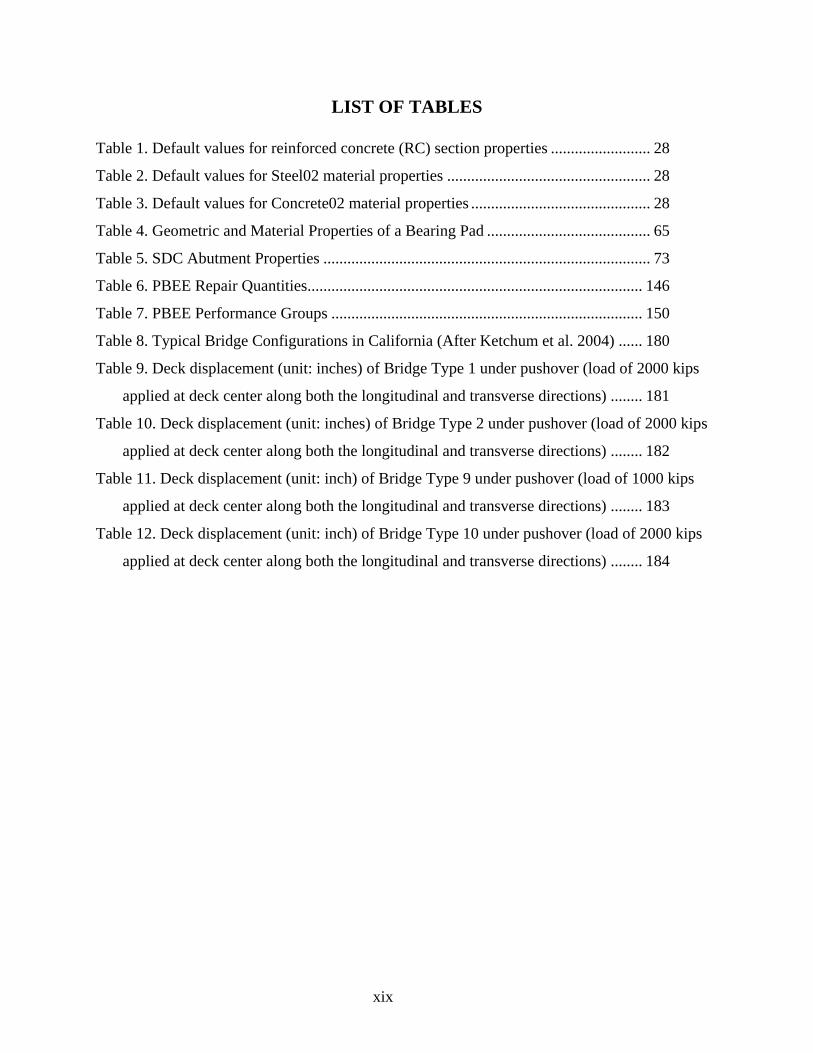
LIST OF TABLES

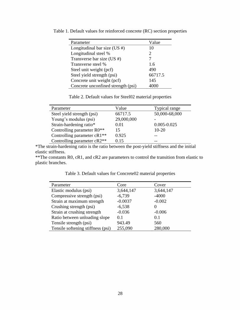
Table 1. Default values for reinforced concrete (RC) section properties ......................... 28

Table 2. Default values for Steel02 material properties ................................................... 28

Table 3. Default values for Concrete02 material properties ............................................. 28

Table 4. Geometric and Material Properties of a Bearing Pad ......................................... 65

Table 5. SDC Abutment Properties .................................................................................. 73

Table 6. PBEE Repair Quantities.................................................................................... 146

Table 7. PBEE Performance Groups .............................................................................. 150

Table 8. Typical Bridge Configurations in California (After Ketchum et al. 2004) ...... 180

Table 9. Deck displacement (unit: inches) of Bridge Type 1 under pushover (load of 2000 kips

applied at deck center along both the longitudinal and transverse directions) ........ 181

Table 10. Deck displacement (unit: inches) of Bridge Type 2 under pushover (load of 2000 kips


Table 11. Deck displacement (unit: inch) of Bridge Type 9 under pushover (load of 1000 kips


Table 12. Deck displacement (unit: inch) of Bridge Type 10 under pushover (load of 2000 kips


1

1

1 INTRODUCTION

1.1 Overview

MSBridge is a PC-based graphical pre- and post-processor (user-interface) for

conducting nonlinear Finite Element (FE) studies for multi-span bridge systems. Main

capabilities include:

i) Horizontal and vertical alignments, with different skew angles for

bents/abutments

ii) Nonlinear beam-column element with fiber section for bridge columns and

piles

iii) Deck hinges, isolation bearings, and steel jackets

iv) Foundation represented by Foundation matrix or soil springs (p-y, t-z and

q-z)

v) Advanced abutment models (Elgamal et al. 2014; Aviram 2008a, 2008b)

vi) Automatic mesh generation of multi-span bridge systems

vii) Management of ground motion suites

viii) Simultaneous execution of nonlinear Time History Analysis (THA) for

multiple motions

ix) PBEE outcomes in terms of repair cost, time and carbon footprint

x) Visualization and animation of response time histories

FE computations in MSBridge are conducted using OpenSees (currently ver. 2.5.0 is

employed). OpenSees is an open source software framework (McKenna et al. 2010;

Mazzoni et al. 2009) for simulating the seismic response of structural and geotechnical

systems. OpenSees has been developed as the computational platform for research in

performance-based earthquake engineering (PBEE) at the Pacific Earthquake

Engineering Research (PEER) Center. For more information about OpenSees, please visit

http://opensees.berkeley.edu/.

The analysis options available in MSBridge include:

i) Pushover Analysis

ii) Mode Shape Analysis

iii) Single and Multiple 3D Base Input Acceleration Analysis

iv) Equivalent Static Analysis (ESA)

v) PBEE Analysis

1.2 What’s New in Current Updated Version

A number of capabilities and features have been added in the current version of

MSBridge. These added features mainly allow MSBridge to address possible variability

in the bridge deck, bent cap, column, foundation, or soil configuration/properties (on a

bent-by-bent basis). For the complete list of the added capabilities and features, please

see Appendix A.

2

1.3 Units

MSBridge supports analysis in both the US/English and SI unit systems, and the default

system is US/English units. This unit option can be interchanged during model creation,

and MSBridge will convert all input data to the desired unit system. For conversion

between SI and English Units, please check:

http://www.unit-conversion.info/

Some commonly used quantities can be converted as follows:

1 kPa = 0.14503789 psi

1 psi = 6.89475 kPa

1 m = 39.37 in

1 in = 0.0254 m

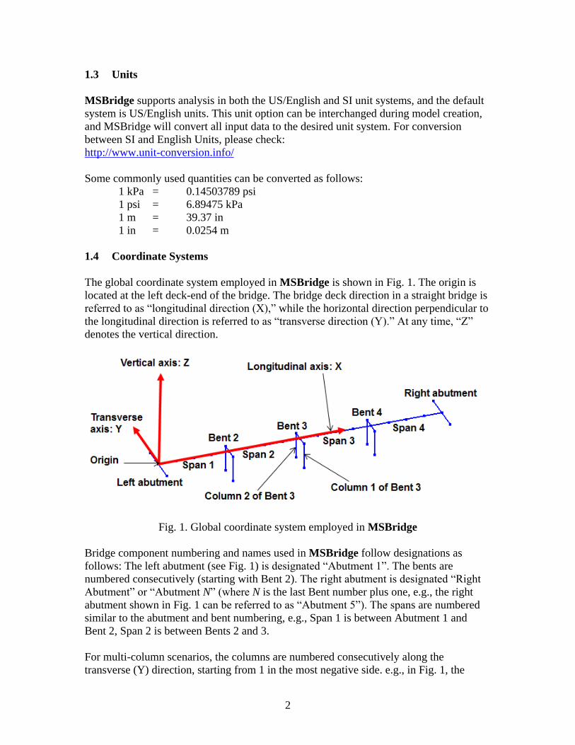
1.4 Coordinate Systems

The global coordinate system employed in MSBridge is shown in Fig. 1. The origin is

located at the left deck-end of the bridge. The bridge deck direction in a straight bridge is

referred to as “longitudinal direction (X),” while the horizontal direction perpendicular to

the longitudinal direction is referred to as “transverse direction (Y).” At any time, “Z”

denotes the vertical direction.

Fig. 1. Global coordinate system employed in MSBridge

Bridge component numbering and names used in MSBridge follow designations as

follows: The left abutment (see Fig. 1) is designated “Abutment 1”. The bents are

numbered consecutively (starting with Bent 2). The right abutment is designated “Right

Abutment” or “Abutment N” (where N is the last Bent number plus one, e.g., the right

abutment shown in Fig. 1 can be referred to as “Abutment 5”). The spans are numbered

similar to the abutment and bent numbering, e.g., Span 1 is between Abutment 1 and

Bent 2, Span 2 is between Bents 2 and 3.

For multi-column scenarios, the columns are numbered consecutively along the

transverse (Y) direction, starting from 1 in the most negative side. e.g., in Fig. 1, the

http://www.unit-conversion.info/

3

column at the negative side of the transverse (Y) direction is referred to as Column 1

while the one at the positive side is called Column 2. For Bent 3, there are “Column 1 of

Bent 3” and “Column 2 of Bent 3” (Fig. 1).

Local coordinate systems will also be used in this document to describe certain

components, e.g., deck hinges, isolation bearings, distributed spring abutment models

with a skew angle, etc. In that case, labels of “1”, “2” and “3” (or lower case “x,” “y” and

“z”) will be used. Please refer to the appropriate section for the corresponding

description.

In MSBridge, maximum response quantities (e.g., displacement, acceleration) are

reported in the local coordinate system. For a straight bridge, the local coordinate system

is parallel to the global one. For a curved bridge, the local coordinate system is defined in

such a way that the local longitudinal axis (x) is tangent to the bridge curve at a given

superstructure location while the transverse axis (y) is another horizontal direction that is

perpendicular to the longitudinal axis (x). The z-axis in a local coordinate system is

perpendicular to the x- and y-axes and positive upwards.

1.5 System Requirements

MSBridge runs on PC-compatible systems running Windows (7, 8, 10 or Server). The

system should have a minimum hardware configuration appropriate to the particular

operating system. For best results, the system’s video should be set to 1024 by 768 or

higher.

1.6 Acknowledgment

Development of MSBridge was funded primarily by the California Department of

Transportation (Caltrans). Additional funding was provided by the Pacific Earthquake

Engineering Research Center (PEER), a multi-institutional research and education center

with headquarters at the University of California, Berkeley.

MSBridge was written in Microsoft .NET Framework (Windows Presentation

Foundation or WPF). OpenTK (OpenGL) library (https://opentk.github.io/) was used for

visualization of FE mesh and OxyPlot package (https://github.com/oxyplot) was

employed for x-y plotting. In addition, 3D extruded view of a bridge model was

implemented by using Helix Toolkit (https://github.com/helix-toolkit).

For questions or remarks about MSBridge, please send email to Dr. Ahmed Elgamal

([email protected]), or Dr. Jinchi Lu ([email protected]).

https://opentk.github.io/

https://github.com/oxyplot

https://github.com/helix-toolkit

4

2 GETTING STARTED

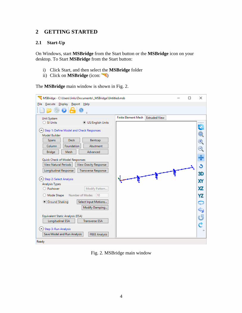
2.1 Start-Up

On Windows, start MSBridge from the Start button or the MSBridge icon on your

desktop. To Start MSBridge from the Start button:

i) Click Start, and then select the MSBridge folder

ii) Click on MSBridge (icon: )

The MSBridge main window is shown in Fig. 2.

Fig. 2. MSBridge main window

5

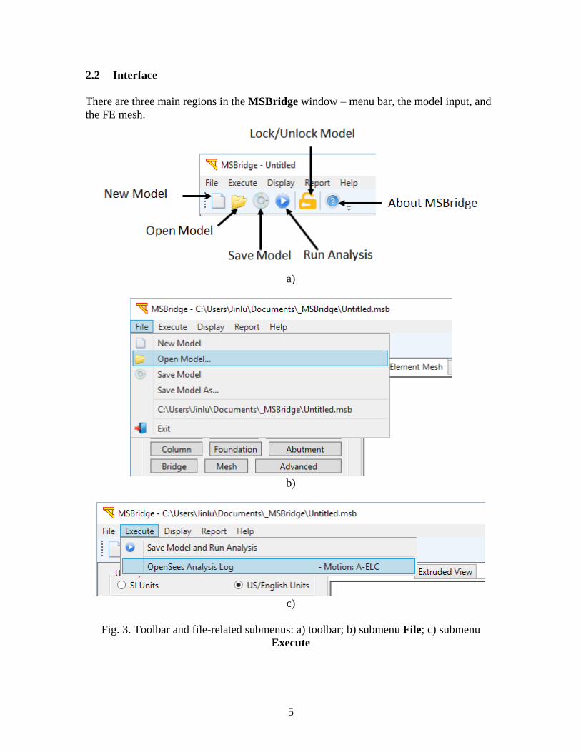
2.2 Interface

There are three main regions in the MSBridge window – menu bar, the model input, and

the FE mesh.

a)

b)

c)

Fig. 3. Toolbar and file-related submenus: a) toolbar; b) submenu File; c) submenu

Execute

6

a)

b)

c)

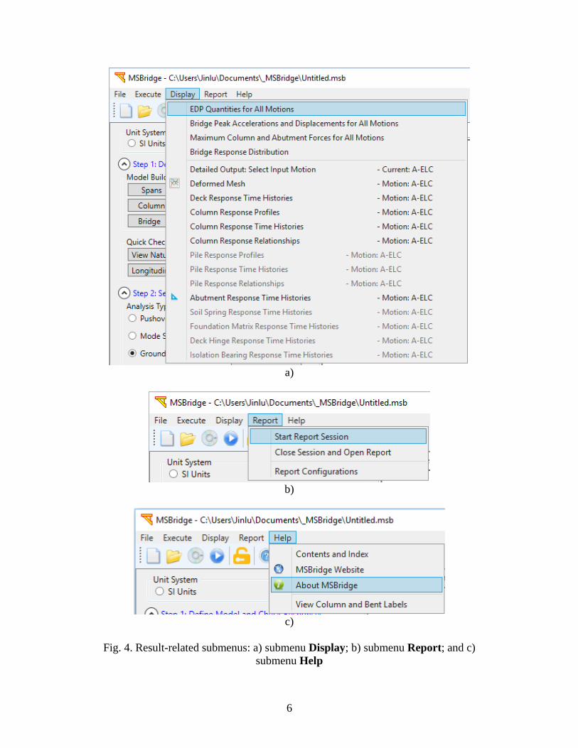
Fig. 4. Result-related submenus: a) submenu Display; b) submenu Report; and c)

submenu Help

7

2.2.1 Menu Bar

The menu bar, shown in Fig. 3 and Fig. 4, offers rapid access to most MSBridge main

features. The main features in MSBridge are organized into the following submenus:

• File: Controls opening, saving of model definition parameters, and exiting MSBridge.

• Execute: Controls running analyses and displaying OpenSees analysis log.

• Display: Controls displaying analysis results.

• Report: Controls creating an analysis report in Microsoft Word format

• Help: Visit the MSBridge website and display the copyright/acknowledgment message

(Fig. 5).

Note that Fig. 3a shows a “Lock Model” button which is a toggle button that prevents

from overwriting analysis results after an analysis is done. If the model is in “Locked

Mode,” the OK buttons (and Apply buttons) in all dialog windows in MSBridge are

disabled, and users cannot make changes to the current model. To unlock the model,

users need to click the “Lock Model” button. If the model is in “Unlocked Mode,” any

result will be overwritten if a new analysis is launched.

2.2.2 Model Input Region

The model input region controls definitions of the model and analysis options, which are

organized into three regions (Fig. 2):

Step 1: Define Model & Check Responses: Controls definitions of bridge parameters

including material properties. Meshing parameters are also defined in this step.

Step 2: Select an Analysis Option: Controls analysis types (pushover analysis, mode

shape analysis or ground shaking). Equivalent Static Analysis (ESA) option is also

available.

Step 3: Run FE Analysis: Controls execution of the FE analysis and displaying of the

analysis progress bar.

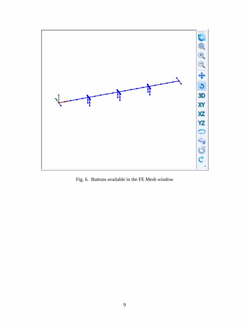
2.2.3 FE Mesh Region

The FE mesh region (Fig. 2) displays the generated mesh. In this window, the mesh can

be manipulated by clicking buttons shown in Fig. 6.

The FE mesh shown in MSBridge is automatically generated. The user can also click the

button at the top-right corner (shown in Fig. 6) to re-draw FE mesh (based on the input

data entered).

8

Fig. 5. MSBridge copyright and acknowledgment window

9

Fig. 6. Buttons available in the FE Mesh window

10

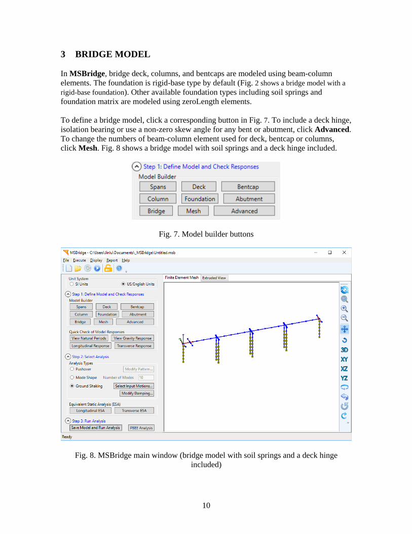
3 BRIDGE MODEL

In MSBridge, bridge deck, columns, and bentcaps are modeled using beam-column

elements. The foundation is rigid-base type by default (Fig. 2 shows a bridge model with a

rigid-base foundation). Other available foundation types including soil springs and

foundation matrix are modeled using zeroLength elements.

To define a bridge model, click a corresponding button in Fig. 7. To include a deck hinge,

isolation bearing or use a non-zero skew angle for any bent or abutment, click Advanced.

To change the numbers of beam-column element used for deck, bentcap or columns,

click Mesh. Fig. 8 shows a bridge model with soil springs and a deck hinge included.

Fig. 7. Model builder buttons

Fig. 8. MSBridge main window (bridge model with soil springs and a deck hinge

included)

11

3.1 Spans

To change the number of spans, click Spans in the main window (Fig. 7 and Fig. 9).

Number of Spans: The total number of spans for a multi-span bridge. The

minimum is 2, and the maximum is 100.

MSBridge supports models for both straight bridge and curved bridge options.

3.1.1 Straight Bridge

If the bridge has equal span lengths, click Equal Span Length and specify the span

length (Fig. 9).

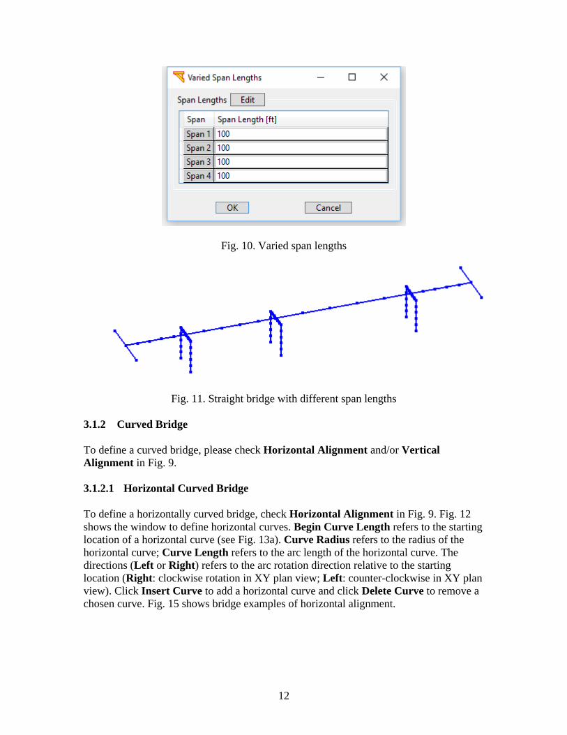
If the bridge has varied span lengths, click Varied Span Length and then Modify Span

Lengths to specify span lengths (Fig. 10). Fig. 11 shows a straight bridge model with

varied span lengths.

Fig. 9. Bridge span definition

12

Fig. 10. Varied span lengths

Fig. 11. Straight bridge with different span lengths

3.1.2 Curved Bridge

To define a curved bridge, please check Horizontal Alignment and/or Vertical

Alignment in Fig. 9.

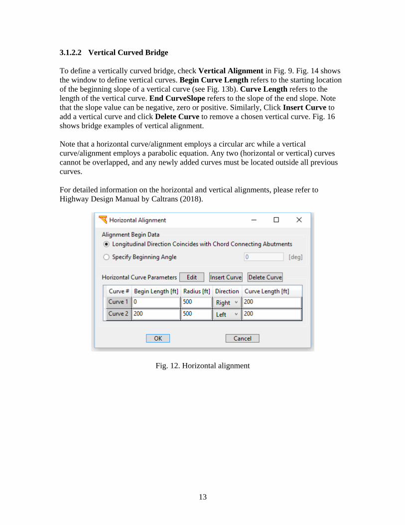
3.1.2.1 Horizontal Curved Bridge

To define a horizontally curved bridge, check Horizontal Alignment in Fig. 9. Fig. 12

shows the window to define horizontal curves. Begin Curve Length refers to the starting

location of a horizontal curve (see Fig. 13a). Curve Radius refers to the radius of the

horizontal curve; Curve Length refers to the arc length of the horizontal curve. The

directions (Left or Right) refers to the arc rotation direction relative to the starting

location (Right: clockwise rotation in XY plan view; Left: counter-clockwise in XY plan

view). Click Insert Curve to add a horizontal curve and click Delete Curve to remove a

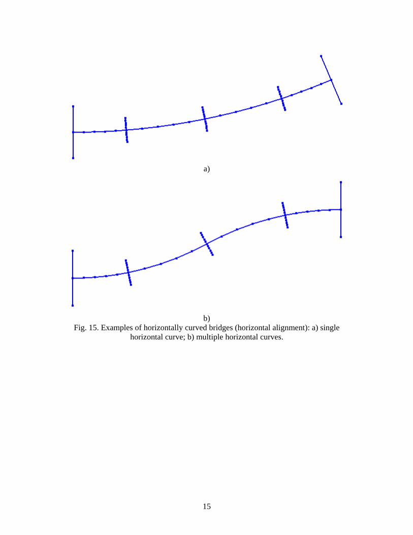
chosen curve. Fig. 15 shows bridge examples of horizontal alignment.

13

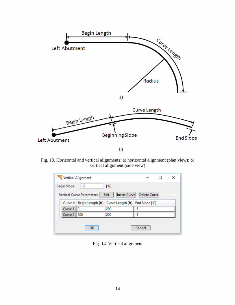
3.1.2.2 Vertical Curved Bridge

To define a vertically curved bridge, check Vertical Alignment in Fig. 9. Fig. 14 shows

the window to define vertical curves. Begin Curve Length refers to the starting location

of the beginning slope of a vertical curve (see Fig. 13b). Curve Length refers to the

length of the vertical curve. End CurveSlope refers to the slope of the end slope. Note

that the slope value can be negative, zero or positive. Similarly, Click Insert Curve to

add a vertical curve and click Delete Curve to remove a chosen vertical curve. Fig. 16

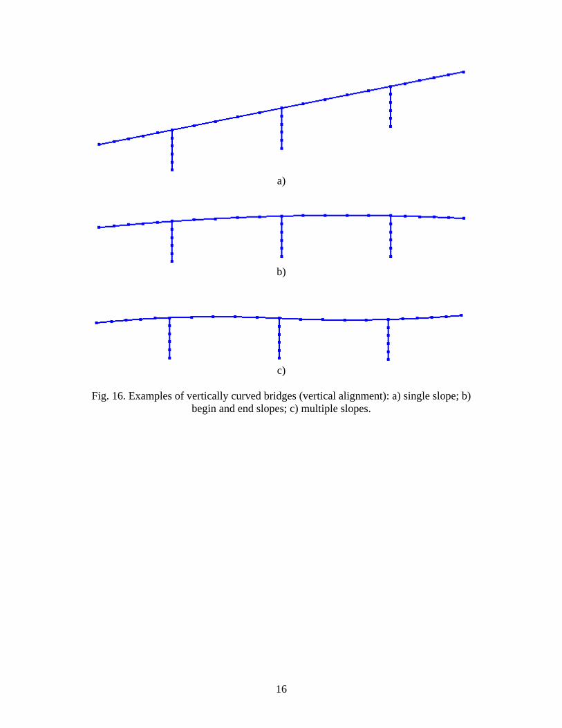
shows bridge examples of vertical alignment.

Note that a horizontal curve/alignment employs a circular arc while a vertical

curve/alignment employs a parabolic equation. Any two (horizontal or vertical) curves

cannot be overlapped, and any newly added curves must be located outside all previous

curves.

For detailed information on the horizontal and vertical alignments, please refer to

Highway Design Manual by Caltrans (2018).

Fig. 12. Horizontal alignment

14

a)

b)

Fig. 13. Horizontal and vertical alignments: a) horizontal alignment (plan view); b)

vertical alignment (side view)

Fig. 14. Vertical alignment

15

a)

b)

Fig. 15. Examples of horizontally curved bridges (horizontal alignment): a) single

horizontal curve; b) multiple horizontal curves.

16

a)

b)

c)

Fig. 16. Examples of vertically curved bridges (vertical alignment): a) single slope; b)

begin and end slopes; c) multiple slopes.

17

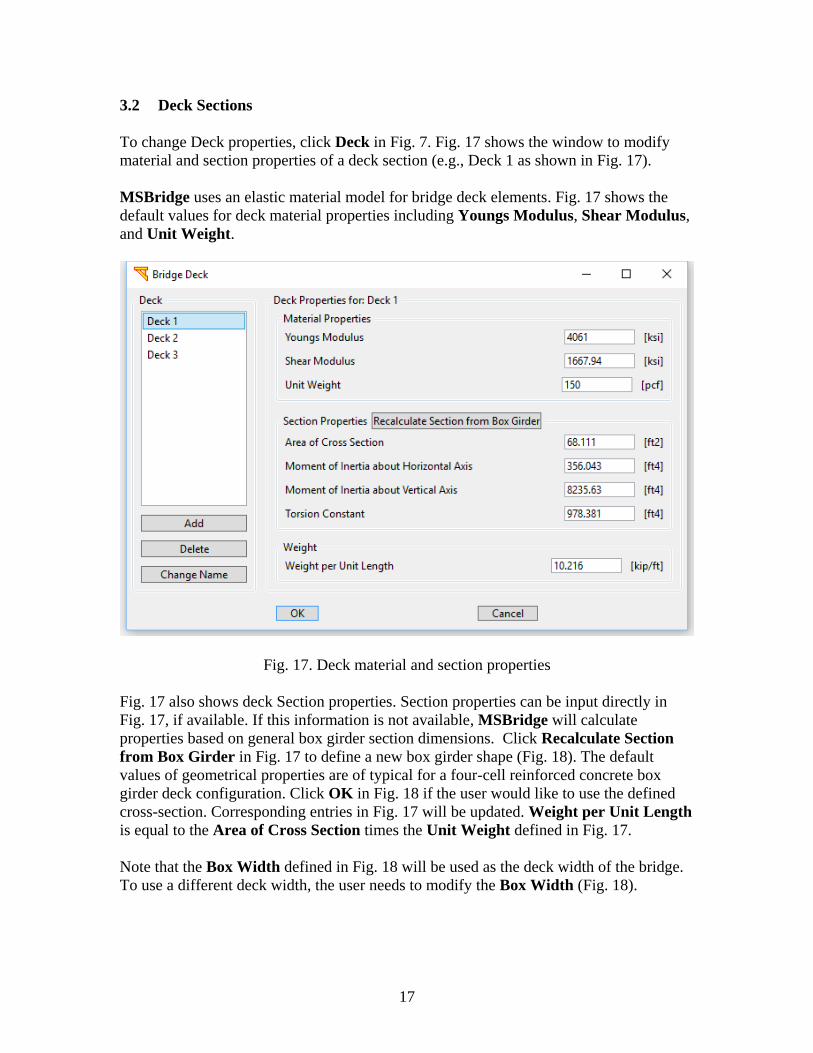
3.2 Deck Sections

To change Deck properties, click Deck in Fig. 7. Fig. 17 shows the window to modify

material and section properties of a deck section (e.g., Deck 1 as shown in Fig. 17).

MSBridge uses an elastic material model for bridge deck elements. Fig. 17 shows the

default values for deck material properties including Youngs Modulus, Shear Modulus,

and Unit Weight.

Fig. 17. Deck material and section properties

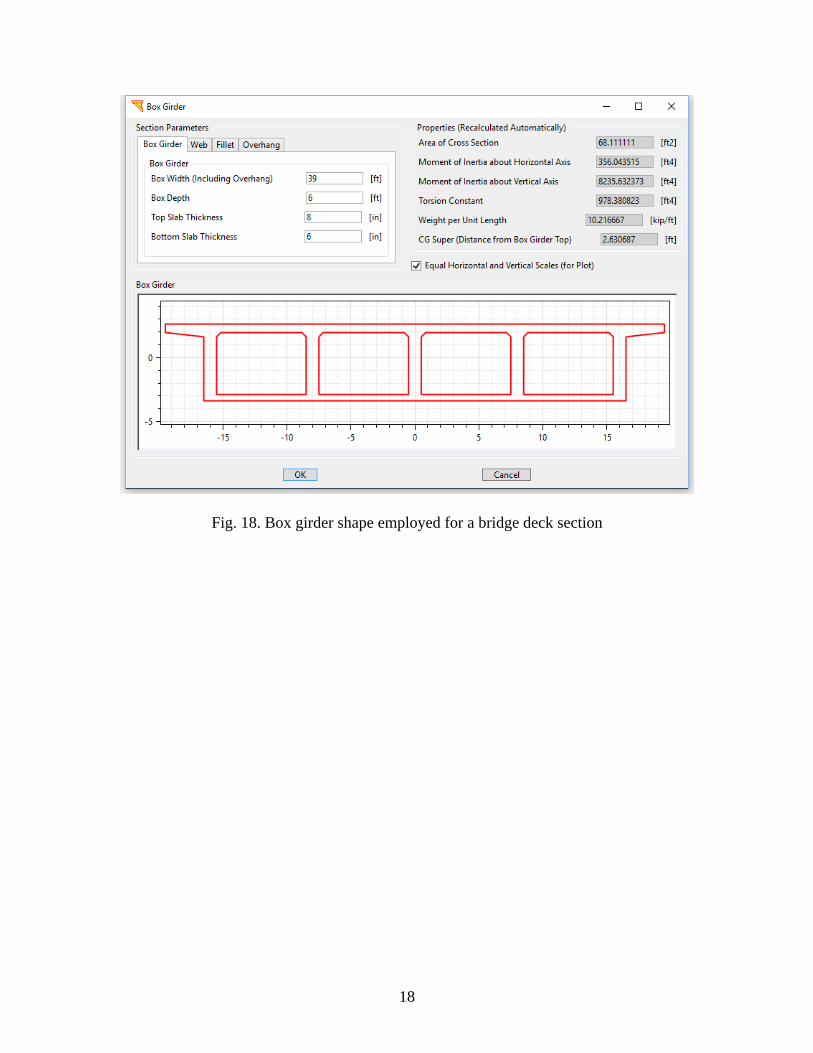
Fig. 17 also shows deck Section properties. Section properties can be input directly in

Fig. 17, if available. If this information is not available, MSBridge will calculate

properties based on general box girder section dimensions. Click Recalculate Section

from Box Girder in Fig. 17 to define a new box girder shape (Fig. 18). The default

values of geometrical properties are of typical for a four-cell reinforced concrete box

girder deck configuration. Click OK in Fig. 18 if the user would like to use the defined

cross-section. Corresponding entries in Fig. 17 will be updated. Weight per Unit Length

is equal to the Area of Cross Section times the Unit Weight defined in Fig. 17.

Note that the Box Width defined in Fig. 18 will be used as the deck width of the bridge.

To use a different deck width, the user needs to modify the Box Width (Fig. 18).

18

Fig. 18. Box girder shape employed for a bridge deck section

19

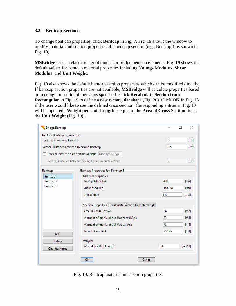
3.3 Bentcap Sections

To change bent cap properties, click Bentcap in Fig. 7. Fig. 19 shows the window to

modify material and section properties of a bentcap section (e.g., Bentcap 1 as shown in

Fig. 19)

MSBridge uses an elastic material model for bridge bentcap elements. Fig. 19 shows the

default values for bentcap material properties including Youngs Modulus, Shear

Modulus, and Unit Weight.

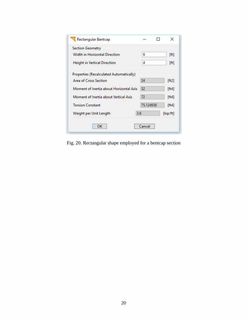
Fig. 19 also shows the default bentcap section properties which can be modified directly.

If bentcap section properties are not available, MSBridge will calculate properties based

on rectangular section dimensions specified. Click Recalculate Section from

Rectangular in Fig. 19 to define a new rectangular shape (Fig. 20). Click OK in Fig. 18

if the user would like to use the defined cross-section. Corresponding entries in Fig. 19

will be updated. Weight per Unit Length is equal to the Area of Cross Section times

the Unit Weight (Fig. 19).

Fig. 19. Bentcap material and section properties

20

Fig. 20. Rectangular shape employed for a bentcap section

21

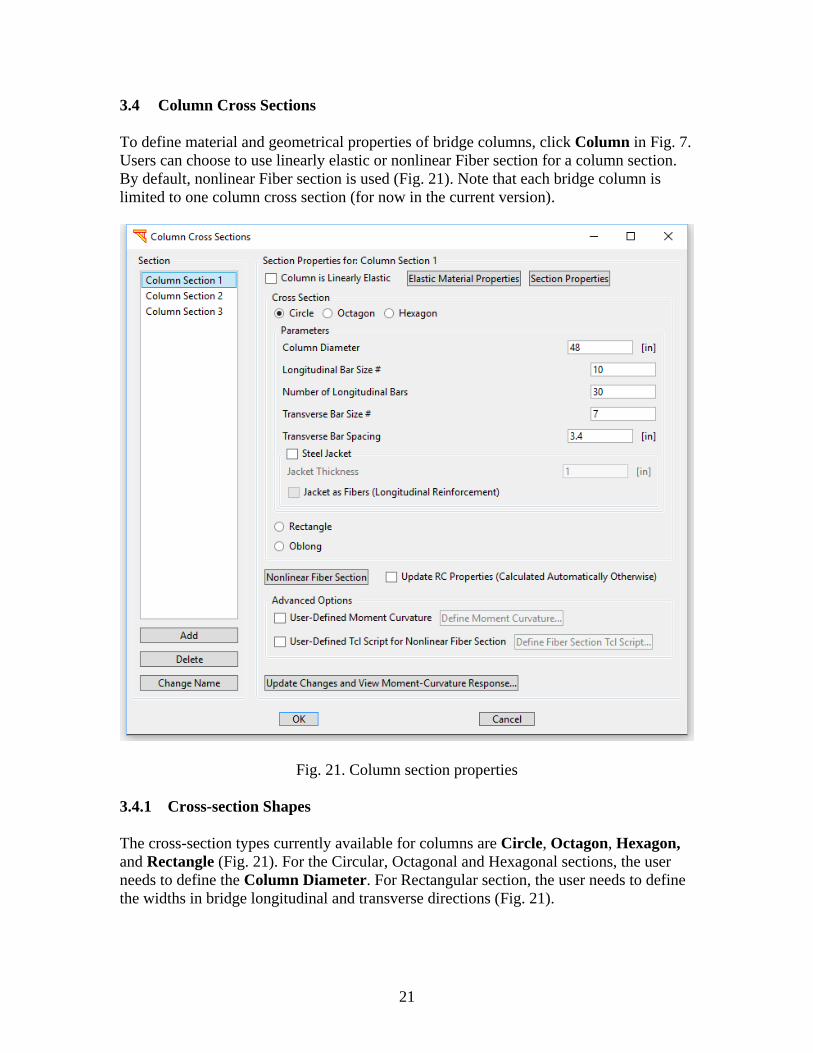
3.4 Column Cross Sections

To define material and geometrical properties of bridge columns, click Column in Fig. 7.

Users can choose to use linearly elastic or nonlinear Fiber section for a column section.

By default, nonlinear Fiber section is used (Fig. 21). Note that each bridge column is

limited to one column cross section (for now in the current version).

Fig. 21. Column section properties

3.4.1 Cross-section Shapes

The cross-section types currently available for columns are Circle, Octagon, Hexagon,

and Rectangle (Fig. 21). For the Circular, Octagonal and Hexagonal sections, the user

needs to define the Column Diameter. For Rectangular section, the user needs to define

the widths in bridge longitudinal and transverse directions (Fig. 21).

22

3.4.2 Cross Section Properties

Four options available to define a bridge column section: i) linear elastic, ii) nonlinear

Fiber Section, iii) user-defined moment curvature, and iv) user-defined Tcl script for

nonlinear Fiber section.

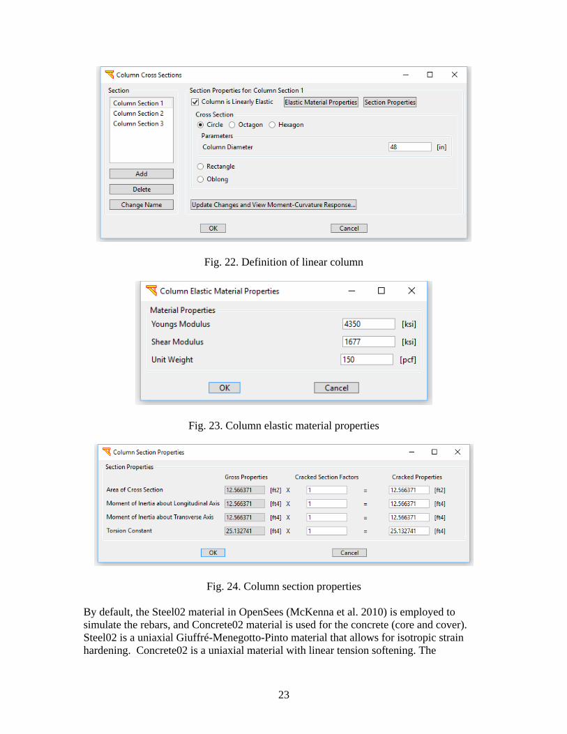
3.4.2.1 Linearly Elastic

To activate the linearly elastic option for a column section, check the checkbox Column

is Linearly Elastic (Fig. 22). Elastic beam-column element (elasticBeamColumn,

McKenna et al. 2010) is used for the column section in this case. Click Elastic Material

Properties to define Youngs Modulus, Shear Modulus and Unit Weight of the column

section (Fig. 23). Click Section Properties to change the column section properties (by

changing cracked section factors) as shown in Fig. 24.

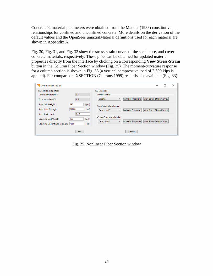
3.4.2.2 Nonlinear Fiber Section

To use nonlinear Fiber section for a column section, click Nonlinear Fiber Section (Fig.

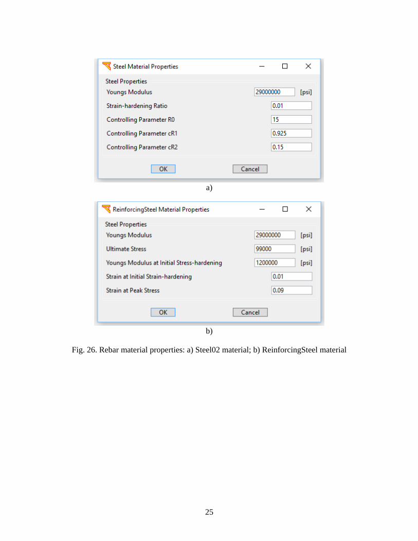
21). The window for defining the Fiber section is shown in Fig. 25. Click Material

Properties buttons to display or modify the material properties for the rebars (Fig. 26),

the core and the cover concrete (Fig. 27).

Nonlinear beam-column elements with fiber section (Fig. 28) are used to simulate the

column in this case. The fiber layout for the octagonal and hexagonal cross sections are

similar to that of the circular cross section except for the cover. Fig. 29 shows a slight

treatment of the fiber layout for the octagonal and hexagon cross sections. For

Rectangular section, the number of rebars refers to the number of reinforcing bars around

the section perimeter (equal spacing).

The material options available for the rebars include Elastic, Steel01, Steel02, and

ReinforcingSteel. The material options available for the concrete include Elastic, ENT

(Elastic-No Tension), Concrete01, and Concrete02. The default material properties of a

column section are shown in Tables 1-3.

23

Fig. 22. Definition of linear column

Fig. 23. Column elastic material properties

Fig. 24. Column section properties

By default, the Steel02 material in OpenSees (McKenna et al. 2010) is employed to

simulate the rebars, and Concrete02 material is used for the concrete (core and cover).

Steel02 is a uniaxial Giuffré-Menegotto-Pinto material that allows for isotropic strain

hardening. Concrete02 is a uniaxial material with linear tension softening. The

24

Concrete02 material parameters were obtained from the Mander (1988) constitutive

relationships for confined and unconfined concrete. More details on the derivation of the

default values and the OpenSees uniaxialMaterial definitions used for each material are

shown in Appendix A.

Fig. 30, Fig. 31, and Fig. 32 show the stress-strain curves of the steel, core, and cover

concrete materials, respectively. These plots can be obtained for updated material

properties directly from the interface by clicking on a corresponding View Stress-Strain

button in the Column Fiber Section window (Fig. 25). The moment-curvature response

for a column section is shown in Fig. 33 (a vertical compressive load of 2,500 kips is

applied). For comparison, XSECTION (Caltrans 1999) result is also available (Fig. 33).

Fig. 25. Nonlinear Fiber Section window

25

a)

b)

Fig. 26. Rebar material properties: a) Steel02 material; b) ReinforcingSteel material

26

a)

b)

Fig. 27. Concrete material properties: a) Concrete02 material for the core concrete; b)

Concrete02 material for the cover concrete

27

Fig. 28. Fiber discretization of a circular section (based on the report by Berry and

Eberhard (2007))

a) b)

Fig. 29. Fiber discretization of a column section: a) octagon shape; and b) hexagon shape

28

Table 1. Default values for reinforced concrete (RC) section properties

Parameter Value

Longitudinal bar size (US #) 10

Longitudinal steel % 2

Transverse bar size (US #) 7

Transverse steel % 1.6

Steel unit weight (pcf) 490

Steel yield strength (psi) 66717.5

Concrete unit weight (pcf) 145

Concrete unconfined strength (psi) 4000

Table 2. Default values for Steel02 material properties

Parameter Value Typical range

Steel yield strength (psi) 66717.5 50,000-68,000

Young’s modulus (psi) 29,000,000 -

Strain-hardening ratio* 0.01 0.005-0.025

Controlling parameter R0** 15 10-20

Controlling parameter cR1** 0.925 --

Controlling parameter cR2** 0.15 --

*The strain-hardening ratio is the ratio between the post-yield stiffness and the initial

elastic stiffness.

**The constants R0, cR1, and cR2 are parameters to control the transition from elastic to

plastic branches.

Table 3. Default values for Concrete02 material properties

Parameter Core Cover

Elastic modulus (psi) 3,644,147 3,644,147

Compressive strength (psi) -6,739 -4000

Strain at maximum strength -0.0037 -0.002

Crushing strength (psi) -6,538 0

Strain at crushing strength -0.036 -0.006

Ratio between unloading slope 0.1 0.1

Tensile strength (psi) 943.49 560

Tensile softening stiffness (psi) 255,090 280,000

29

a)

b)

c)

Fig. 30. Stress-strain curve for a steel material (default values employed; with a strain

limit of 0.12): a) Steel01; b) Steel02; and c) ReinforcingSteel

30

a)

b)

c)

Fig. 31. Stress-strain curve of a core concrete material (default values employed): a)

Elastic-No Tension; b) Concrete01; and c) Concrete02

31

a)

b)

Fig. 32. Stress-strain curve of a cover concrete material (default values employed): a)

Concrete01; and b) Concrete02

32

Fig. 33. Moment-curvature response for a column section (with default steel and concrete

parameters)

3.4.2.3 User-defined Moment Curvature

To use moment-curvature curves for a column section, click User-Defined Moment

Curvatures (Fig. 21). The window to define the section is shown in Fig. 34. Using this

option, the user can define the cross section by simply entering moment-curvature data.

Fig. 34. User-defined moment curvature

33

3.4.2.4 User-defined Tcl Script for Nonlinear Fiber Section

To use used-defined Fiber section for a column section, click User-Defined Fiber

Section (Fig. 21). The window for defining the Fiber section is shown in Fig. 35. Using

this option, the user can use a Tcl code snippet to define a complex cross section.

Fig. 35. User-defined Tcl script for nonlinear fiber section

34

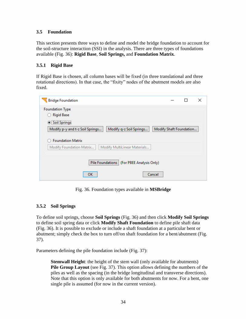
3.5 Foundation

This section presents three ways to define and model the bridge foundation to account for

the soil-structure interaction (SSI) in the analysis. There are three types of foundations

available (Fig. 36): Rigid Base, Soil Springs, and Foundation Matrix.

3.5.1 Rigid Base

If Rigid Base is chosen, all column bases will be fixed (in three translational and three

rotational directions). In that case, the “fixity” nodes of the abutment models are also

fixed.

Fig. 36. Foundation types available in MSBridge

3.5.2 Soil Springs

To define soil springs, choose Soil Springs (Fig. 36) and then click Modify Soil Springs

to define soil spring data or click Modify Shaft Foundation to define pile shaft data

(Fig. 36). It is possible to exclude or include a shaft foundation at a particular bent or

abutment; simply check the box to turn off/on shaft foundation for a bent/abutment (Fig.

37).

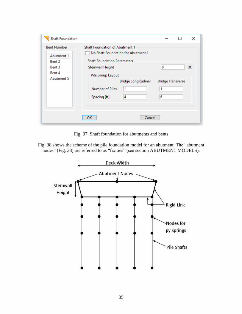
Parameters defining the pile foundation include (Fig. 37):

Stemwall Height: the height of the stem wall (only available for abutments)

Pile Group Layout (see Fig. 37). This option allows defining the numbers of the

piles as well as the spacing (in the bridge longitudinal and transverse directions).

Note that this option is only available for both abutments for now. For a bent, one

single pile is assumed (for now in the current version).

35

Fig. 37. Shaft foundation for abutments and bents

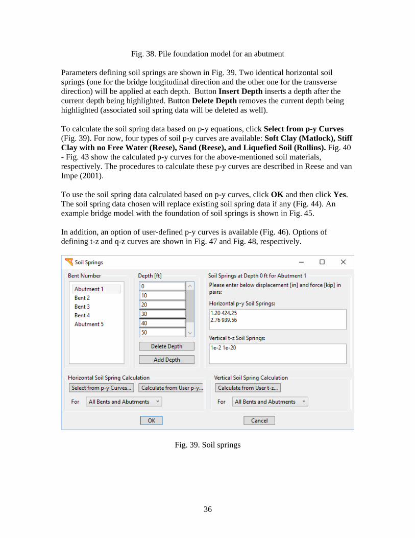
Fig. 38 shows the scheme of the pile foundation model for an abutment. The “abutment

nodes” (Fig. 38) are referred to as “fixities” (see section ABUTMENT MODELS).

36

Fig. 38. Pile foundation model for an abutment

Parameters defining soil springs are shown in Fig. 39. Two identical horizontal soil

springs (one for the bridge longitudinal direction and the other one for the transverse

direction) will be applied at each depth. Button Insert Depth inserts a depth after the

current depth being highlighted. Button Delete Depth removes the current depth being

highlighted (associated soil spring data will be deleted as well).

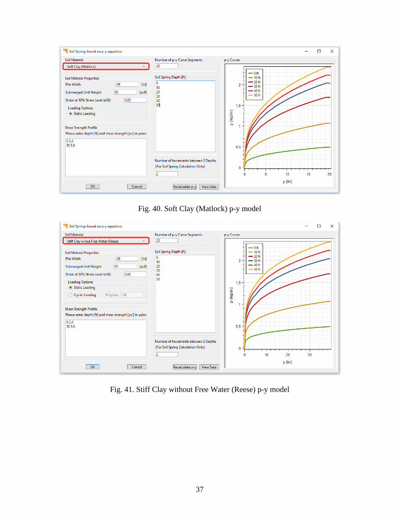
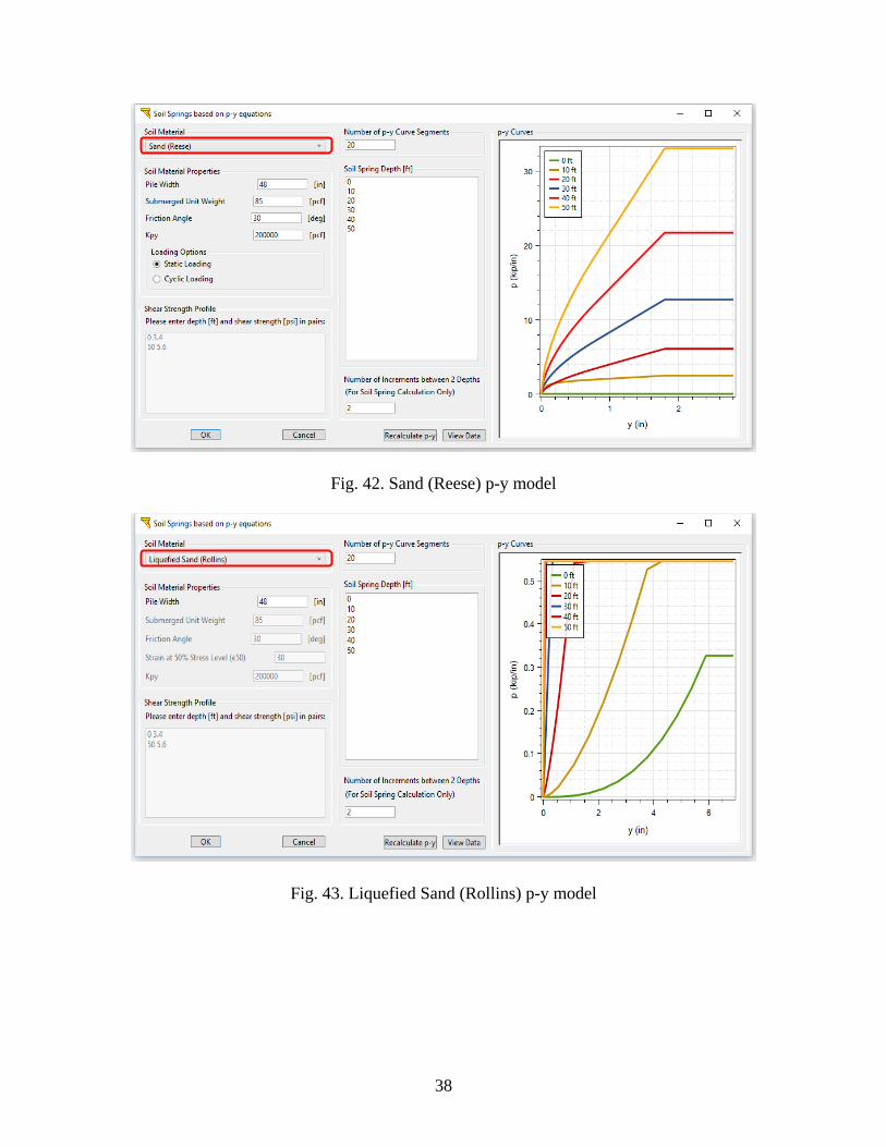
To calculate the soil spring data based on p-y equations, click Select from p-y Curves

(Fig. 39). For now, four types of soil p-y curves are available: Soft Clay (Matlock), Stiff

Clay with no Free Water (Reese), Sand (Reese), and Liquefied Soil (Rollins). Fig. 40

- Fig. 43 show the calculated p-y curves for the above-mentioned soil materials,

respectively. The procedures to calculate these p-y curves are described in Reese and van

Impe (2001).

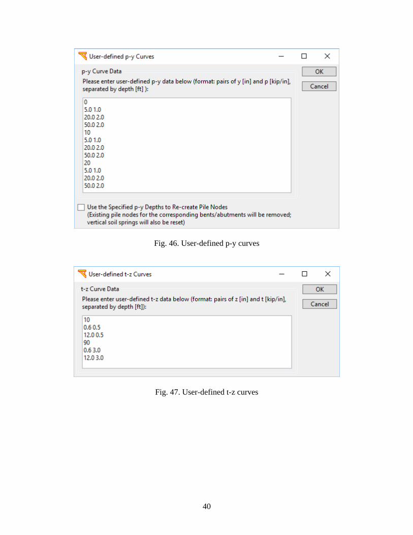
To use the soil spring data calculated based on p-y curves, click OK and then click Yes.

The soil spring data chosen will replace existing soil spring data if any (Fig. 44). An

example bridge model with the foundation of soil springs is shown in Fig. 45.

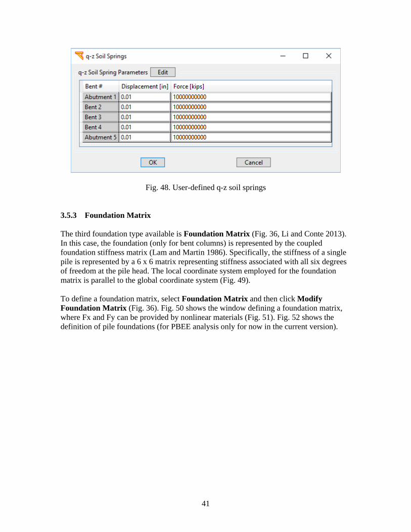
In addition, an option of user-defined p-y curves is available (Fig. 46). Options of

defining t-z and q-z curves are shown in Fig. 47 and Fig. 48, respectively.

Fig. 39. Soil springs

37

Fig. 40. Soft Clay (Matlock) p-y model

Fig. 41. Stiff Clay without Free Water (Reese) p-y model

38

Fig. 42. Sand (Reese) p-y model

Fig. 43. Liquefied Sand (Rollins) p-y model

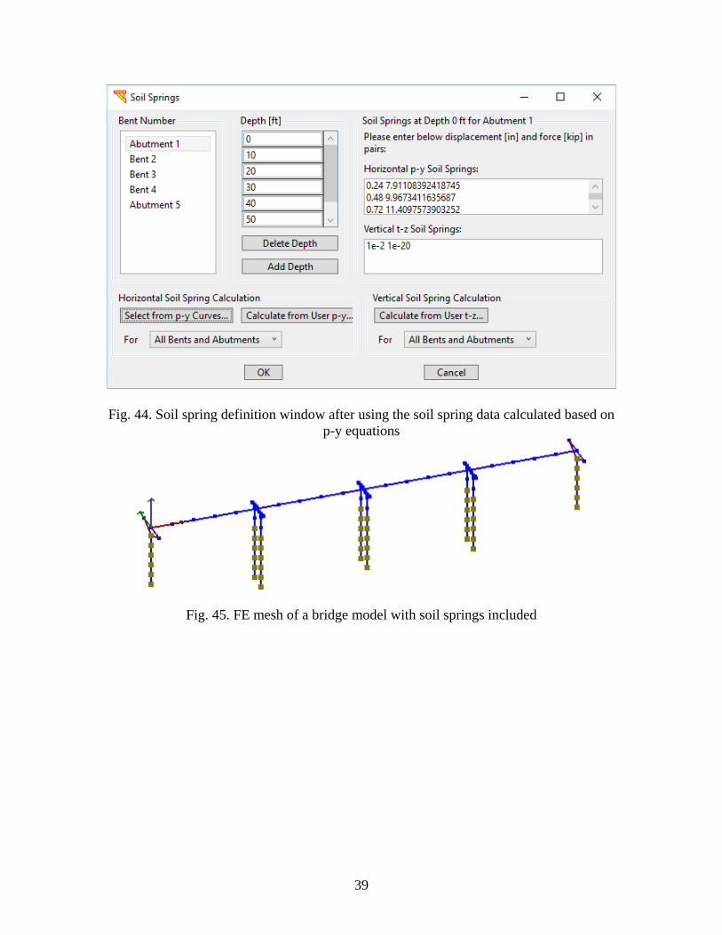
39

Fig. 44. Soil spring definition window after using the soil spring data calculated based on

p-y equations

Fig. 45. FE mesh of a bridge model with soil springs included

40

Fig. 46. User-defined p-y curves

Fig. 47. User-defined t-z curves

41

Fig. 48. User-defined q-z soil springs

3.5.3 Foundation Matrix

The third foundation type available is Foundation Matrix (Fig. 36, Li and Conte 2013).

In this case, the foundation (only for bent columns) is represented by the coupled

foundation stiffness matrix (Lam and Martin 1986). Specifically, the stiffness of a single

pile is represented by a 6 x 6 matrix representing stiffness associated with all six degrees

of freedom at the pile head. The local coordinate system employed for the foundation

matrix is parallel to the global coordinate system (Fig. 49).

To define a foundation matrix, select Foundation Matrix and then click Modify

Foundation Matrix (Fig. 36). Fig. 50 shows the window defining a foundation matrix,

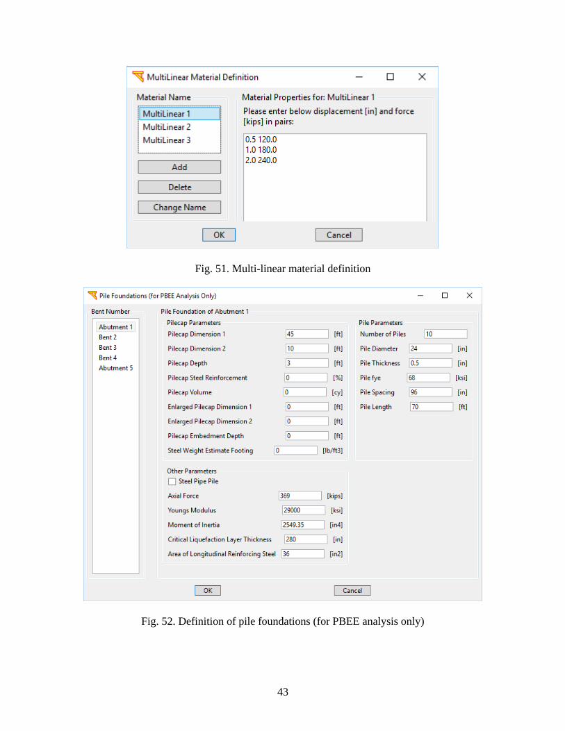
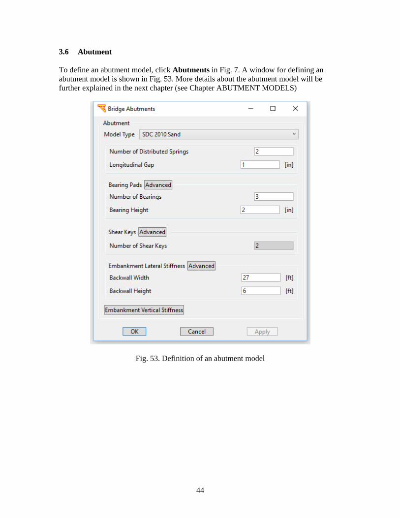
where Fx and Fy can be provided by nonlinear materials (Fig. 51). Fig. 52 shows the

definition of pile foundations (for PBEE analysis only for now in the current version).

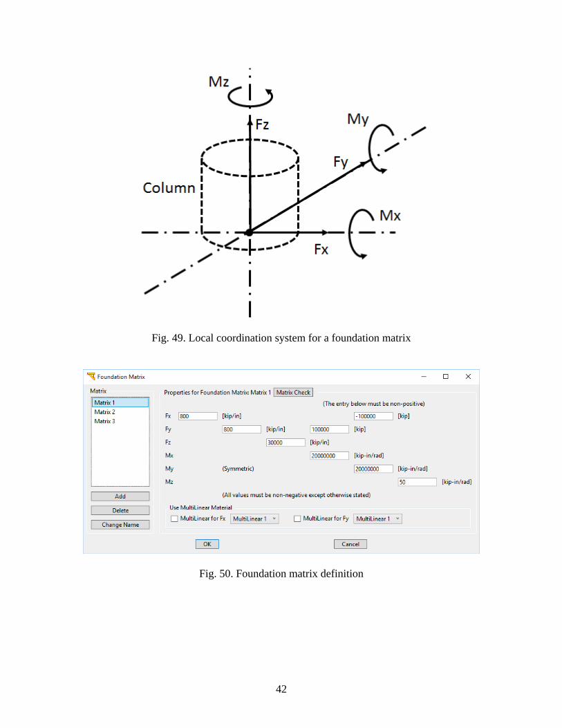
42

Fig. 49. Local coordination system for a foundation matrix

Fig. 50. Foundation matrix definition

43

Fig. 51. Multi-linear material definition

Fig. 52. Definition of pile foundations (for PBEE analysis only)

44

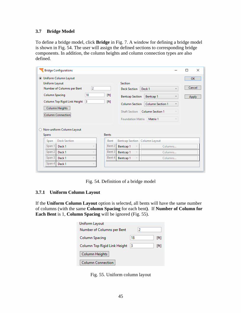
3.6 Abutment

To define an abutment model, click Abutments in Fig. 7. A window for defining an

abutment model is shown in Fig. 53. More details about the abutment model will be

further explained in the next chapter (see Chapter ABUTMENT MODELS)

Fig. 53. Definition of an abutment model

45

3.7 Bridge Model

To define a bridge model, click Bridge in Fig. 7. A window for defining a bridge model

is shown in Fig. 54. The user will assign the defined sections to corresponding bridge

components. In addition, the column heights and column connection types are also

defined.

Fig. 54. Definition of a bridge model

3.7.1 Uniform Column Layout

If the Uniform Column Layout option is selected, all bents will have the same number

of columns (with the same Column Spacing for each bent). If Number of Column for

Each Bent is 1, Column Spacing will be ignored (Fig. 55).

Fig. 55. Uniform column layout

46

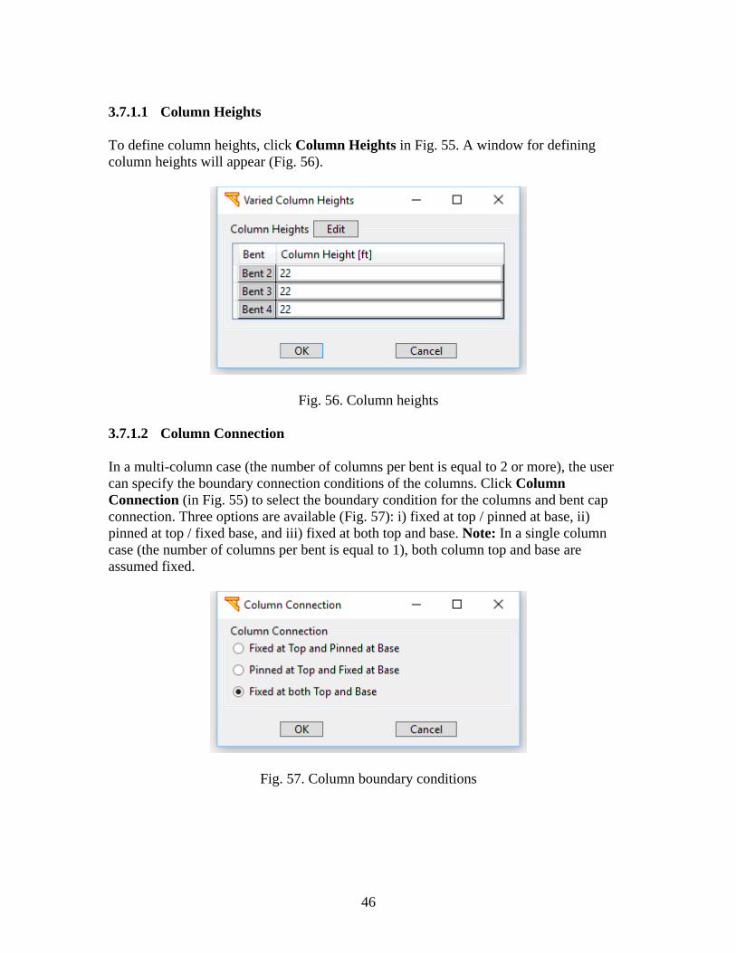
3.7.1.1 Column Heights

To define column heights, click Column Heights in Fig. 55. A window for defining

column heights will appear (Fig. 56).

Fig. 56. Column heights

3.7.1.2 Column Connection

In a multi-column case (the number of columns per bent is equal to 2 or more), the user

can specify the boundary connection conditions of the columns. Click Column

Connection (in Fig. 55) to select the boundary condition for the columns and bent cap

connection. Three options are available (Fig. 57): i) fixed at top / pinned at base, ii)

pinned at top / fixed base, and iii) fixed at both top and base. Note: In a single column

case (the number of columns per bent is equal to 1), both column top and base are

assumed fixed.

Fig. 57. Column boundary conditions

47

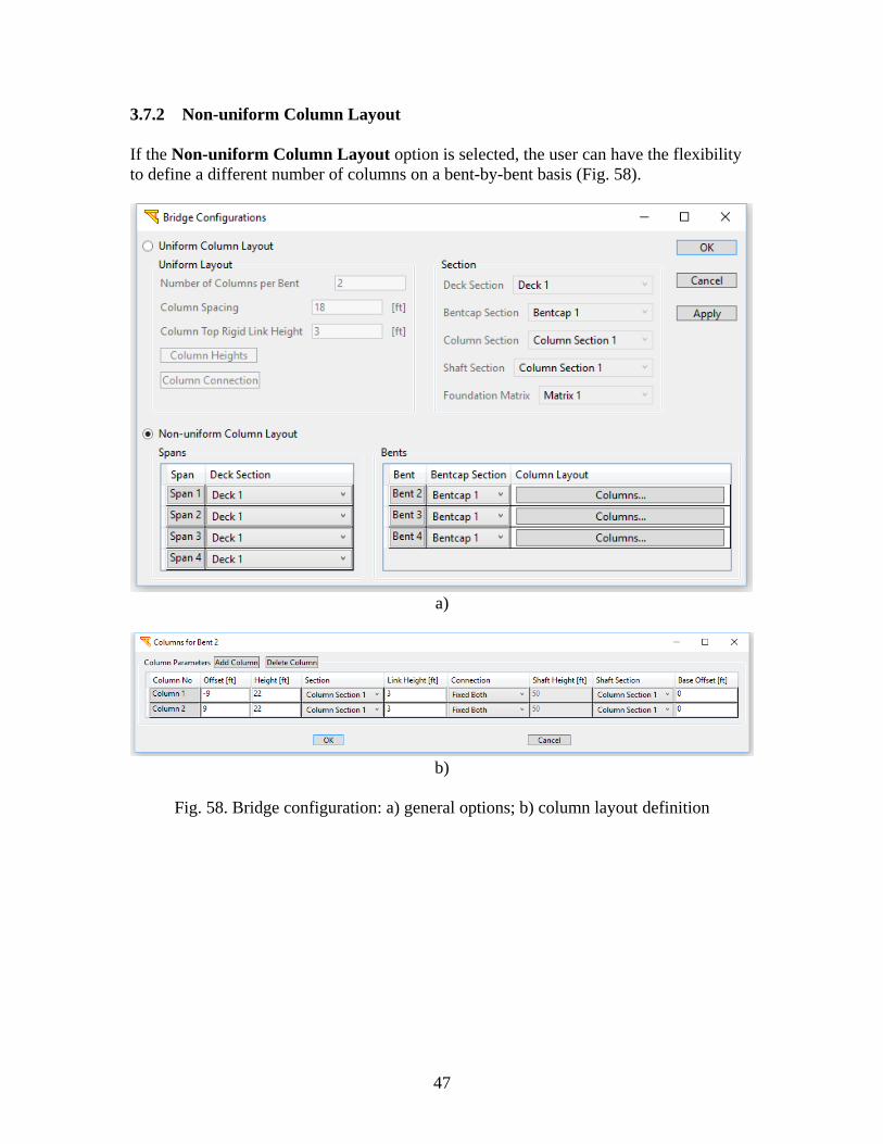
3.7.2 Non-uniform Column Layout

If the Non-uniform Column Layout option is selected, the user can have the flexibility

to define a different number of columns on a bent-by-bent basis (Fig. 58).

a)

b)

Fig. 58. Bridge configuration: a) general options; b) column layout definition

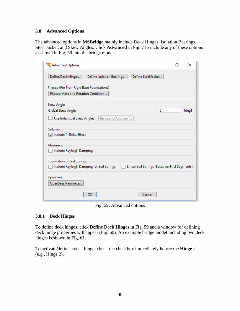
48

3.8 Advanced Options

The advanced options in MSBridge mainly include Deck Hinges, Isolation Bearings,

Steel Jacket, and Skew Angles. Click Advanced in Fig. 7 to include any of these options

as shown in Fig. 59 into the bridge model.

Fig. 59. Advanced options

3.8.1 Deck Hinges

To define deck hinges, click Define Deck Hinges in Fig. 59 and a window for defining

deck hinge properties will appear (Fig. 60). An example bridge model including two deck

hinges is shown in Fig. 61.

To activate/define a deck hinge, check the checkbox immediately before the Hinge #

(e.g., Hinge 2).

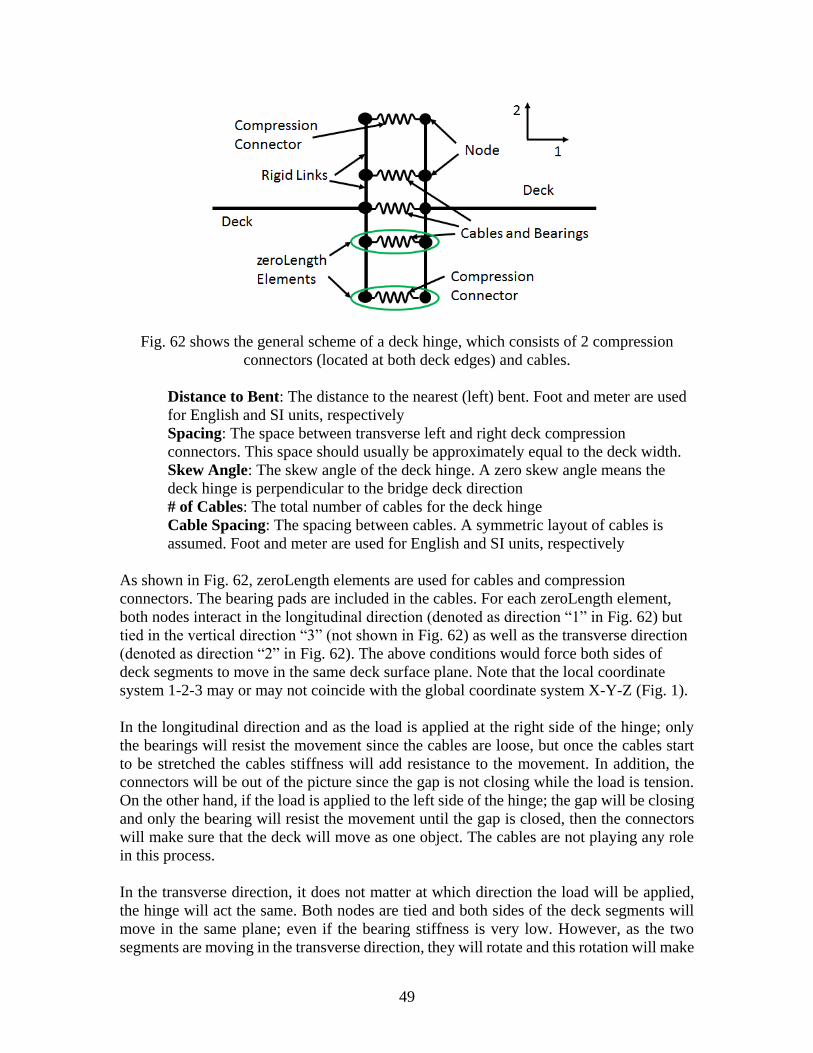
49

Fig. 62 shows the general scheme of a deck hinge, which consists of 2 compression

connectors (located at both deck edges) and cables.

Distance to Bent: The distance to the nearest (left) bent. Foot and meter are used

for English and SI units, respectively

Spacing: The space between transverse left and right deck compression

connectors. This space should usually be approximately equal to the deck width.

Skew Angle: The skew angle of the deck hinge. A zero skew angle means the

deck hinge is perpendicular to the bridge deck direction

# of Cables: The total number of cables for the deck hinge

Cable Spacing: The spacing between cables. A symmetric layout of cables is

assumed. Foot and meter are used for English and SI units, respectively

As shown in Fig. 62, zeroLength elements are used for cables and compression

connectors. The bearing pads are included in the cables. For each zeroLength element,

both nodes interact in the longitudinal direction (denoted as direction “1” in Fig. 62) but

tied in the vertical direction “3” (not shown in Fig. 62) as well as the transverse direction

(denoted as direction “2” in Fig. 62). The above conditions would force both sides of

deck segments to move in the same deck surface plane. Note that the local coordinate

system 1-2-3 may or may not coincide with the global coordinate system X-Y-Z (Fig. 1).

In the longitudinal direction and as the load is applied at the right side of the hinge; only

the bearings will resist the movement since the cables are loose, but once the cables start

to be stretched the cables stiffness will add resistance to the movement. In addition, the

connectors will be out of the picture since the gap is not closing while the load is tension.

On the other hand, if the load is applied to the left side of the hinge; the gap will be closing

and only the bearing will resist the movement until the gap is closed, then the connectors

will make sure that the deck will move as one object. The cables are not playing any role

in this process.

In the transverse direction, it does not matter at which direction the load will be applied,

the hinge will act the same. Both nodes are tied and both sides of the deck segments will

move in the same plane; even if the bearing stiffness is very low. However, as the two

segments are moving in the transverse direction, they will rotate and this rotation will make

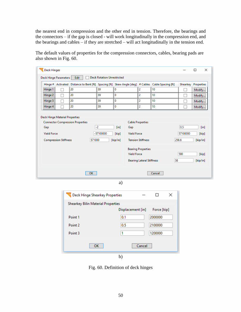
50

the nearest end in compression and the other end in tension. Therefore, the bearings and

the connectors – if the gap is closed - will work longitudinally in the compression end, and

the bearings and cables – if they are stretched – will act longitudinally in the tension end.

The default values of properties for the compression connectors, cables, bearing pads are

also shown in Fig. 60.

a)

b)

Fig. 60. Definition of deck hinges

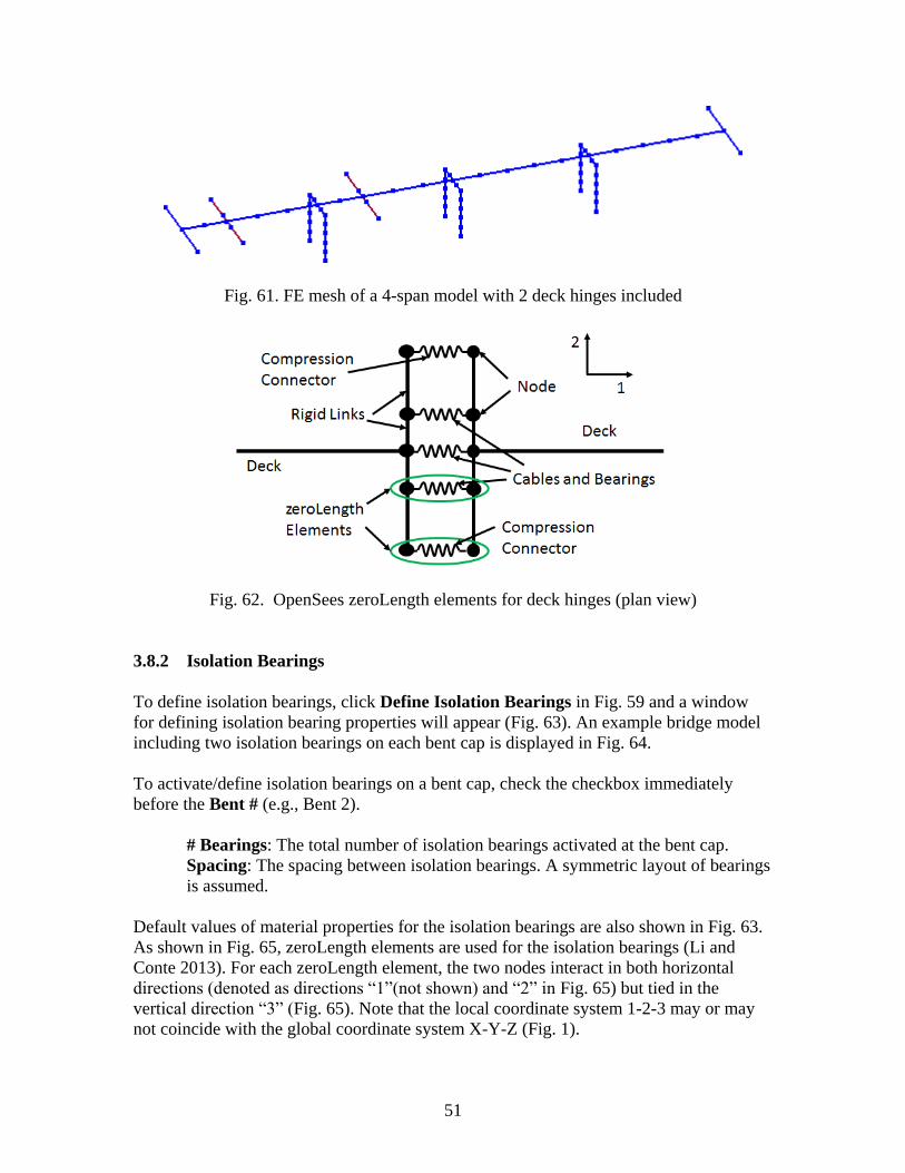
51

Fig. 61. FE mesh of a 4-span model with 2 deck hinges included

Fig. 62. OpenSees zeroLength elements for deck hinges (plan view)

3.8.2 Isolation Bearings

To define isolation bearings, click Define Isolation Bearings in Fig. 59 and a window

for defining isolation bearing properties will appear (Fig. 63). An example bridge model

including two isolation bearings on each bent cap is displayed in Fig. 64.

To activate/define isolation bearings on a bent cap, check the checkbox immediately

before the Bent # (e.g., Bent 2).

# Bearings: The total number of isolation bearings activated at the bent cap.

Spacing: The spacing between isolation bearings. A symmetric layout of bearings

is assumed.

Default values of material properties for the isolation bearings are also shown in Fig. 63.

As shown in Fig. 65, zeroLength elements are used for the isolation bearings (Li and

Conte 2013). For each zeroLength element, the two nodes interact in both horizontal

directions (denoted as directions “1”(not shown) and “2” in Fig. 65) but tied in the

vertical direction “3” (Fig. 65). Note that the local coordinate system 1-2-3 may or may

not coincide with the global coordinate system X-Y-Z (Fig. 1).

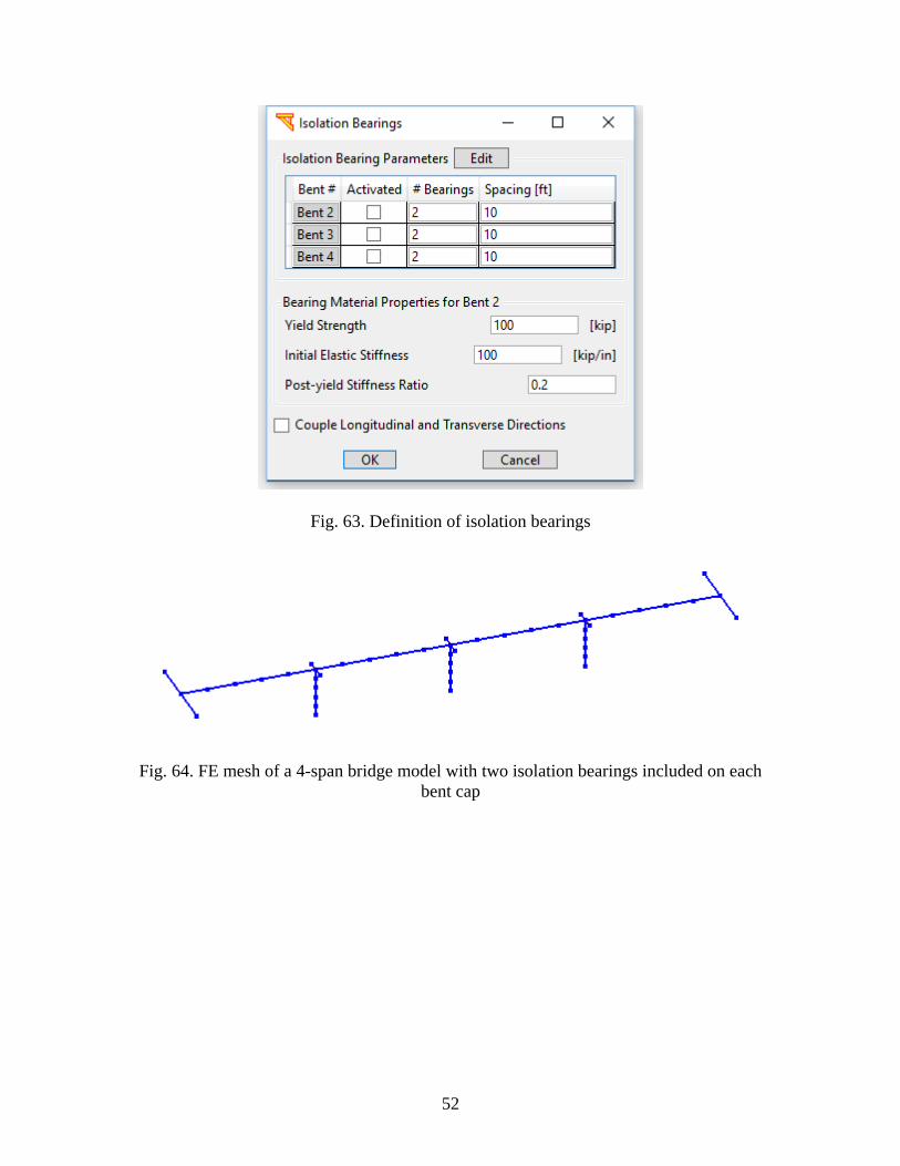
52

Fig. 63. Definition of isolation bearings

Fig. 64. FE mesh of a 4-span bridge model with two isolation bearings included on each

bent cap

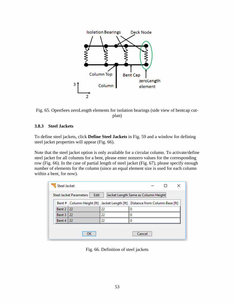
53

Fig. 65. OpenSees zeroLength elements for isolation bearings (side view of bentcap cut-

plan)

3.8.3 Steel Jackets

To define steel jackets, click Define Steel Jackets in Fig. 59 and a window for defining

steel jacket properties will appear (Fig. 66).

Note that the steel jacket option is only available for a circular column. To activate/define

steel jacket for all columns for a bent, please enter nonzero values for the corresponding

row (Fig. 66). In the case of partial length of steel jacket (Fig. 67), please specify enough

number of elements for the column (since an equal element size is used for each column

within a bent, for now).

Fig. 66. Definition of steel jackets

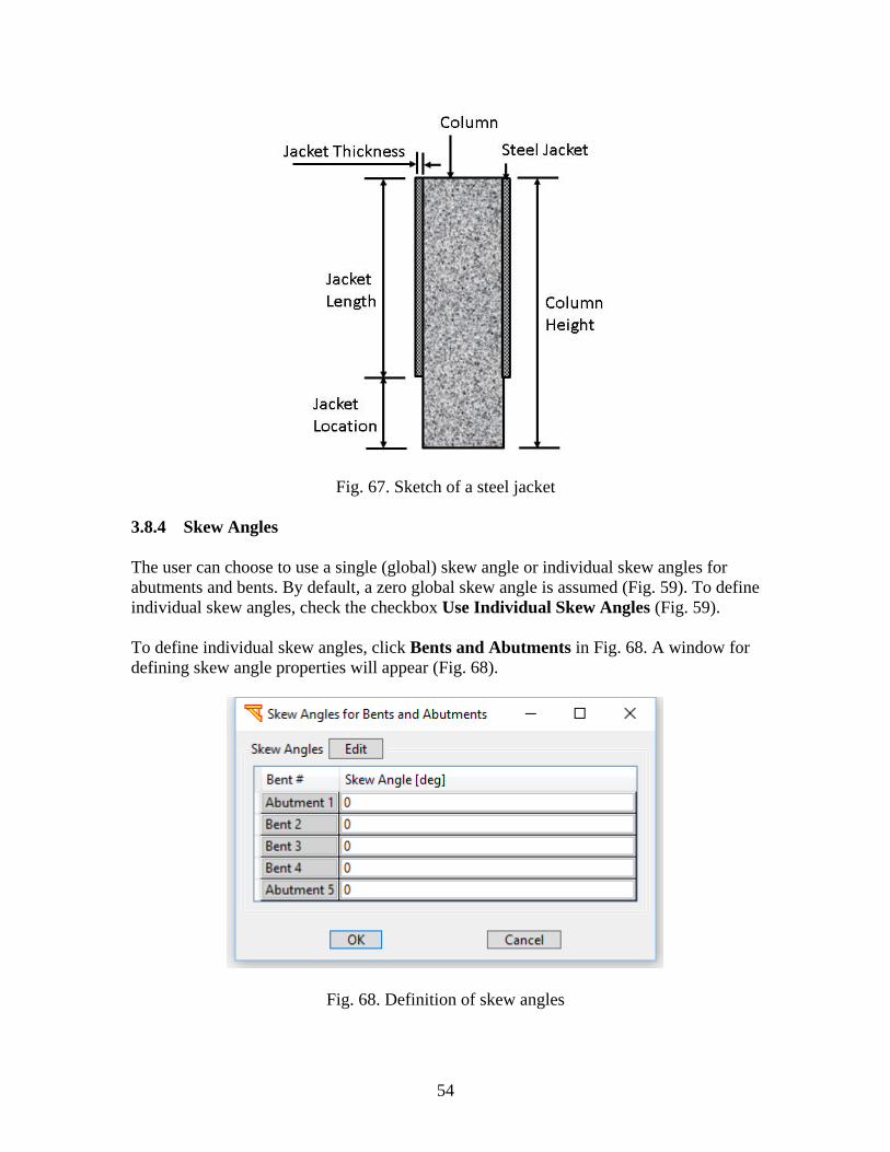
54

Fig. 67. Sketch of a steel jacket

3.8.4 Skew Angles

The user can choose to use a single (global) skew angle or individual skew angles for

abutments and bents. By default, a zero global skew angle is assumed (Fig. 59). To define

individual skew angles, check the checkbox Use Individual Skew Angles (Fig. 59).

To define individual skew angles, click Bents and Abutments in Fig. 68. A window for

defining skew angle properties will appear (Fig. 68).

Fig. 68. Definition of skew angles

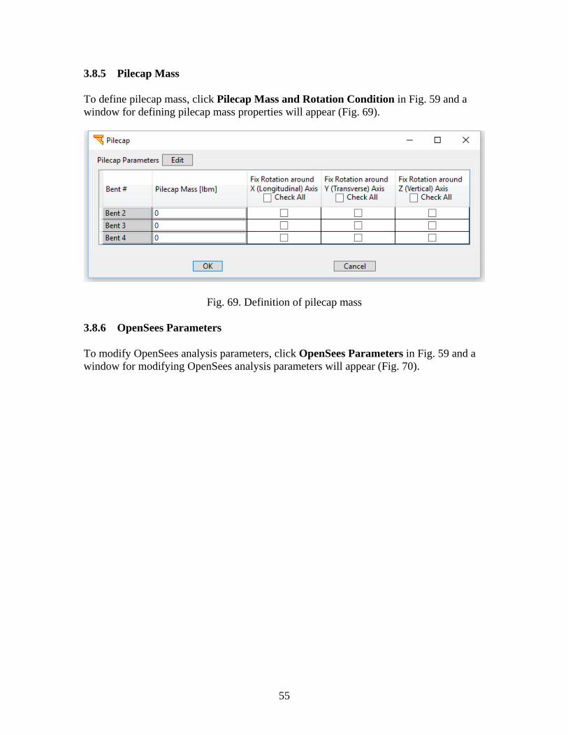
55

3.8.5 Pilecap Mass

To define pilecap mass, click Pilecap Mass and Rotation Condition in Fig. 59 and a

window for defining pilecap mass properties will appear (Fig. 69).

Fig. 69. Definition of pilecap mass

3.8.6 OpenSees Parameters

To modify OpenSees analysis parameters, click OpenSees Parameters in Fig. 59 and a

window for modifying OpenSees analysis parameters will appear (Fig. 70).

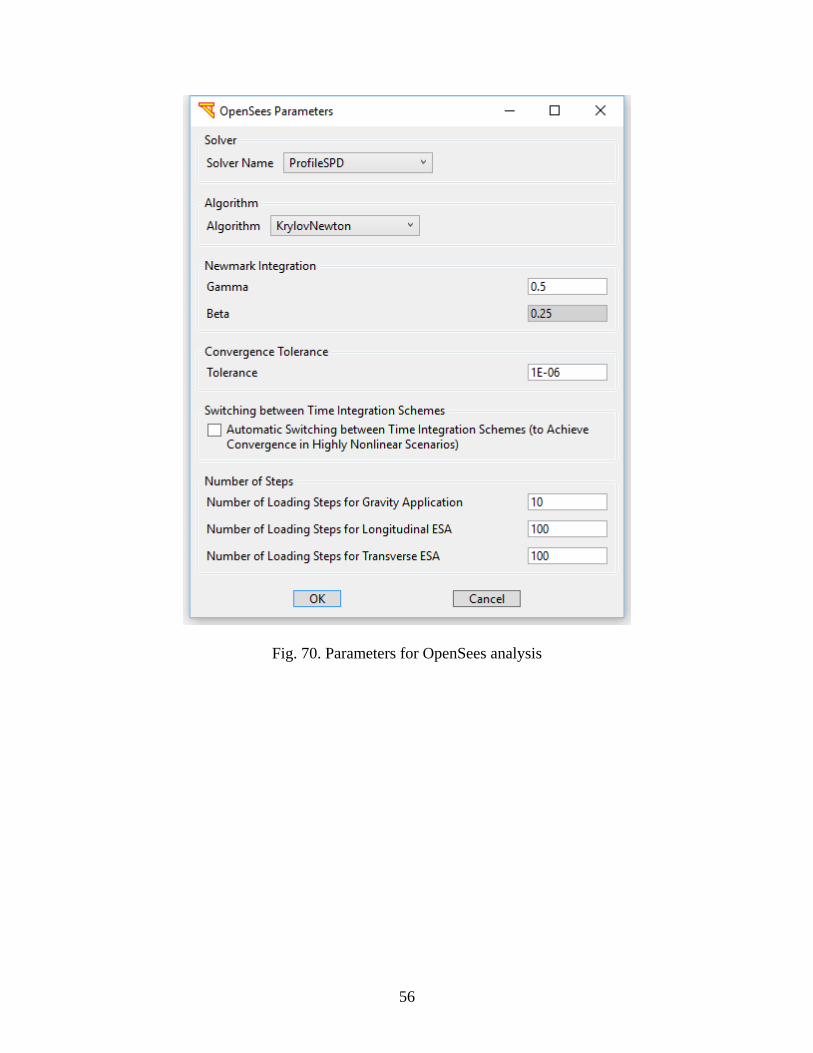
56

Fig. 70. Parameters for OpenSees analysis

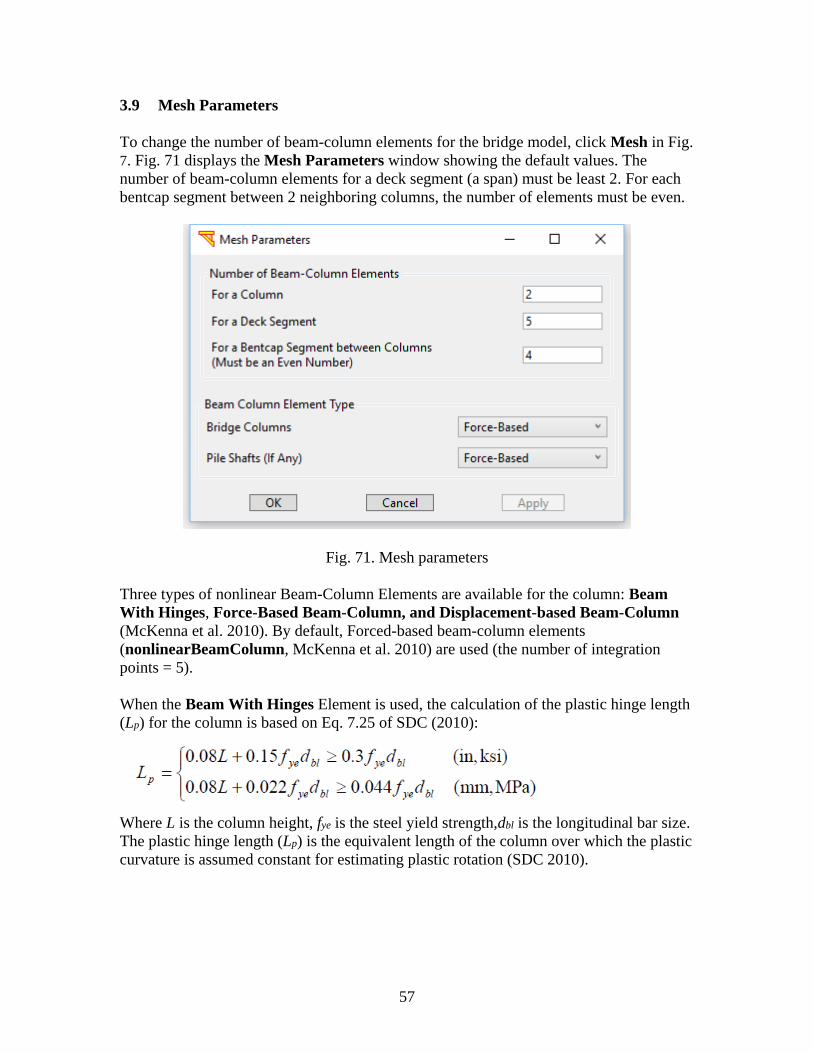
57

3.9 Mesh Parameters

To change the number of beam-column elements for the bridge model, click Mesh in Fig.

7. Fig. 71 displays the Mesh Parameters window showing the default values. The

number of beam-column elements for a deck segment (a span) must be least 2. For each

bentcap segment between 2 neighboring columns, the number of elements must be even.

Fig. 71. Mesh parameters

Three types of nonlinear Beam-Column Elements are available for the column: Beam

With Hinges, Force-Based Beam-Column, and Displacement-based Beam-Column

(McKenna et al. 2010). By default, Forced-based beam-column elements

(nonlinearBeamColumn, McKenna et al. 2010) are used (the number of integration

points = 5).

When the Beam With Hinges Element is used, the calculation of the plastic hinge length

(Lp) for the column is based on Eq. 7.25 of SDC (2010):

Where L is the column height, fye is the steel yield strength,dbl is the longitudinal bar size.

The plastic hinge length (Lp) is the equivalent length of the column over which the plastic

curvature is assumed constant for estimating plastic rotation (SDC 2010).

58

4 ABUTMENT MODELS

Abutment behavior, soil-structure interaction, and embankment flexibility have been

found by post-earthquake reconnaissance reports to significantly influence the response

of the entire bridge system under moderate to strong intensity ground motions.

Specifically, for Ordinary Standard bridge structures in California with short spans and

relatively high superstructure stiffness, the embankment mobilization and the inelastic

behavior of the soil material under high shear deformation levels dominate the response

of the bridge and the intermediate column bents (Kotsoglu and Pantazopoulou 2006;

Shamsabadi et al. 2007, 2010). Seven abutment models have been implemented in

MSBridge. The abutment models are defined as Elastic, Roller, SDC 2004, SDC 2010

Sand, SDC 2010 Clay, EPP-Gap and HFD abutment models.

To define an abutment model, click Abutment in Fig. 7. A window for defining an

abutment model is shown in Fig. 72.

4.1 Elastic Abutment Model

The Elastic Abutment Model consists of a series of 6 elastic springs (3 translational and 3

rotational) at each node at the end of the bridge (Fig. 73). To choose the Elastic

Abutment Model, select Elastic for the Model Type in Fig. 72 (Fig. 74).The main

window to define the Elastic Abutment Model is shown in Fig. 75. By default, no

additional rotational springs are specified but can be added by the user.

As shown in Fig. 73 - Fig. 75, MSBridge allows the user to define multiple distributed

springs (equal spacing within deck width). The values specified in Fig. 75 are the overall

stiffness for each direction (translational or rotational). For the longitudinal direction

(translational and rotational), each of the distributed (Elastic) springs carries its tributary

amount.

e.g., Fig. 73 shows a case of 4 distributed springs. Each of the both end springs carries

one-sixth of the load, and each of the middle springs carries one-third (Fig. 73a). The

vertical components (translational and rotational) are similar to the longitudinal ones. i.e.,

each of the distributed springs carries its tributary amount in the vertical direction.

However, the transverse component is different: only the both end-springs carry the load.

In other words, each of the end springs carries half of the load along the transverse

direction (translational and rotational).

By default, the number of distributed springs is 2. In this case, these two springs are

located at the both ends of the Rigid element (the length of which is equal to deck width)

shown in Fig. 73. However, due to the coupling of the longitudinal, and vertical

translational springs, the option of using a single node at each abutment is possible, this

gives the user full control over the true rotational stiffness apart from the translational

stiffness.

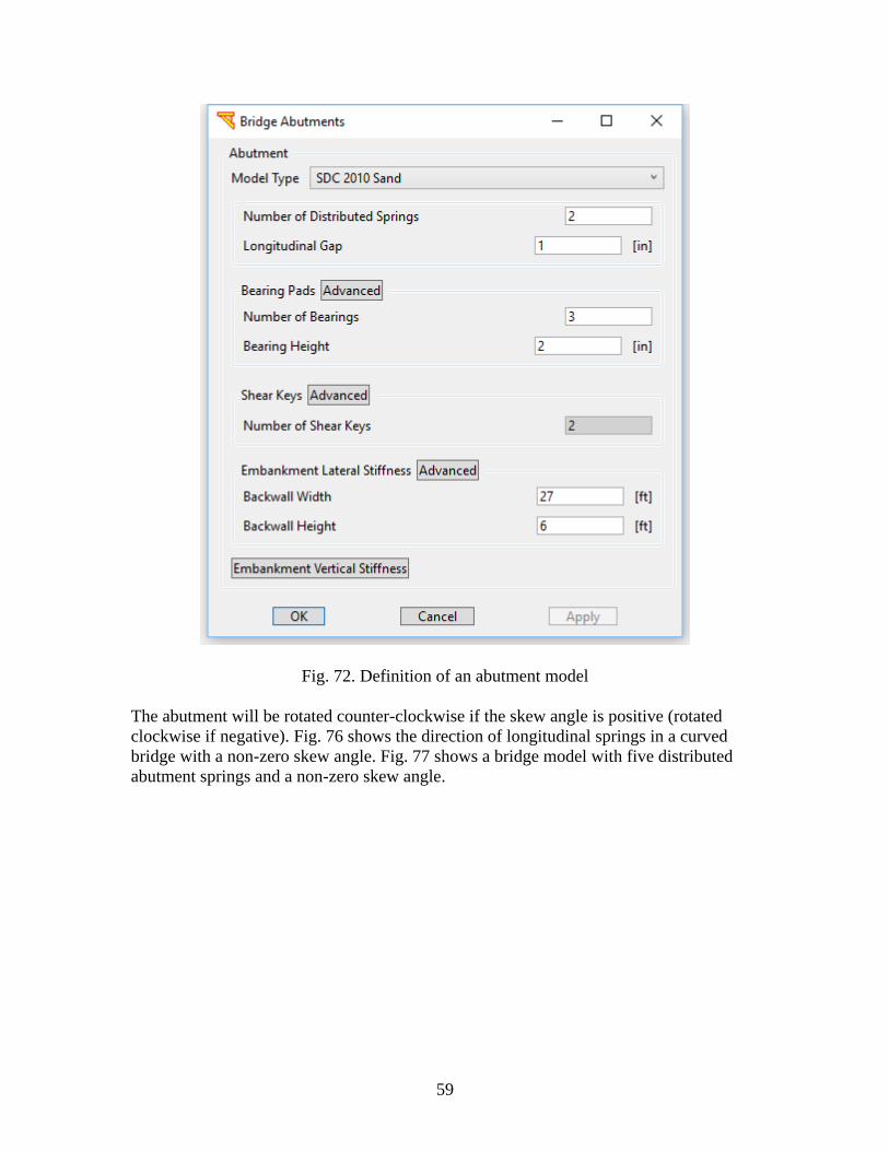
59

Fig. 72. Definition of an abutment model

The abutment will be rotated counter-clockwise if the skew angle is positive (rotated

clockwise if negative). Fig. 76 shows the direction of longitudinal springs in a curved

bridge with a non-zero skew angle. Fig. 77 shows a bridge model with five distributed

abutment springs and a non-zero skew angle.

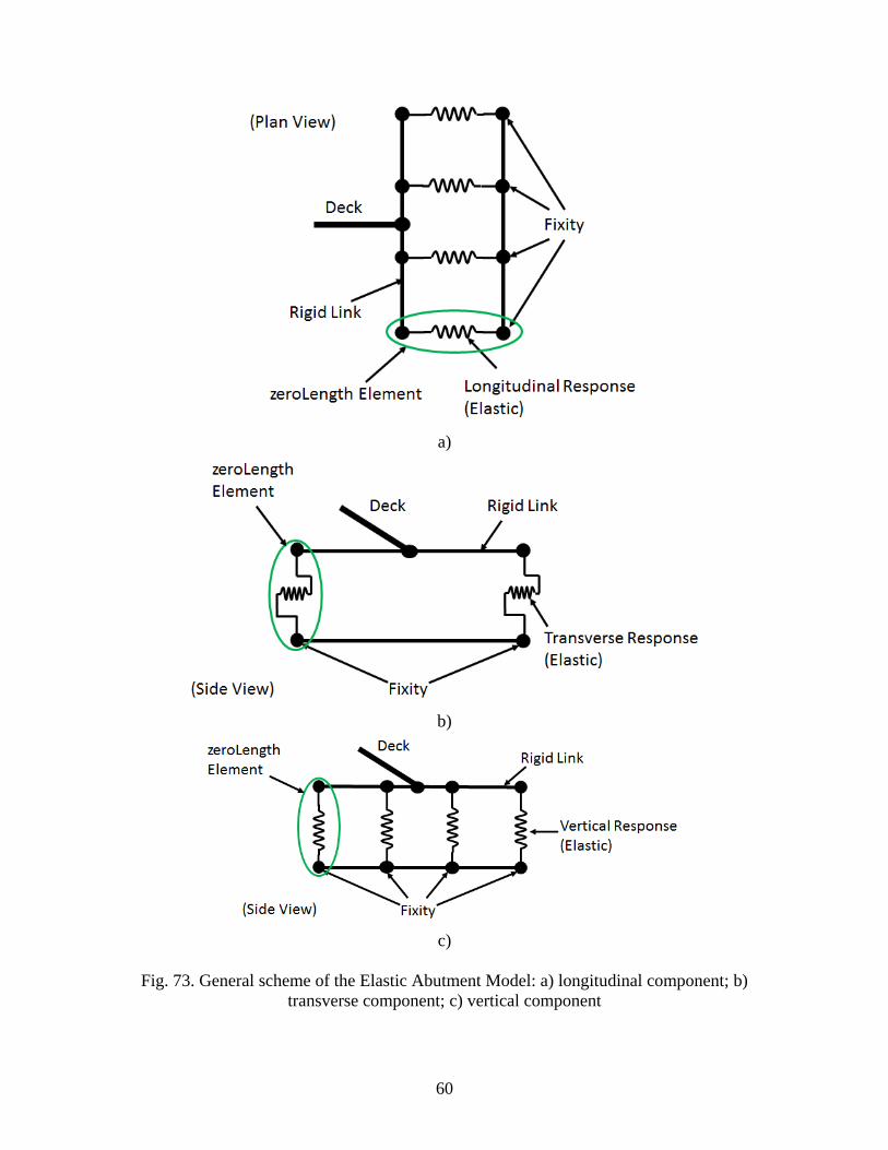
60

a)

b)

c)

Fig. 73. General scheme of the Elastic Abutment Model: a) longitudinal component; b)

transverse component; c) vertical component

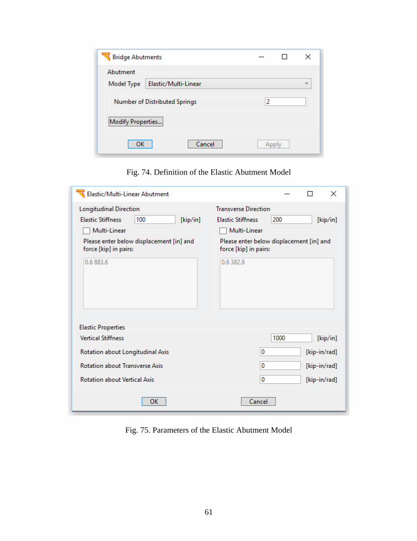
61

Fig. 74. Definition of the Elastic Abutment Model

Fig. 75. Parameters of the Elastic Abutment Model

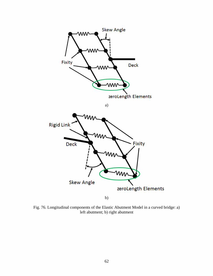
62

a)

b)

Fig. 76. Longitudinal components of the Elastic Abutment Model in a curved bridge: a)

left abutment; b) right abutment

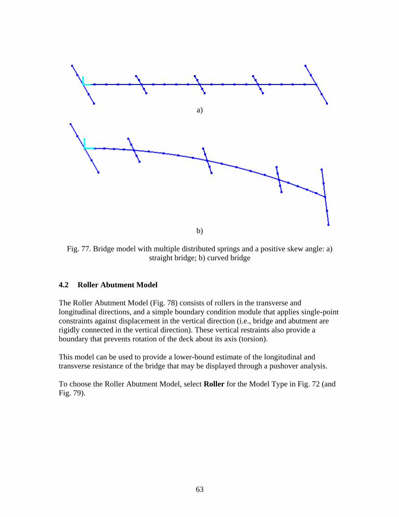
63

a)

b)

Fig. 77. Bridge model with multiple distributed springs and a positive skew angle: a)

straight bridge; b) curved bridge

4.2 Roller Abutment Model

The Roller Abutment Model (Fig. 78) consists of rollers in the transverse and

longitudinal directions, and a simple boundary condition module that applies single-point

constraints against displacement in the vertical direction (i.e., bridge and abutment are

rigidly connected in the vertical direction). These vertical restraints also provide a

boundary that prevents rotation of the deck about its axis (torsion).

This model can be used to provide a lower-bound estimate of the longitudinal and

transverse resistance of the bridge that may be displayed through a pushover analysis.

To choose the Roller Abutment Model, select Roller for the Model Type in Fig. 72 (and

Fig. 79).

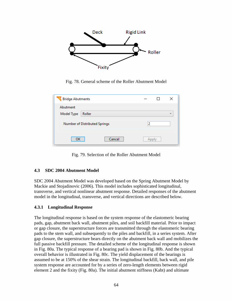
64

Fig. 78. General scheme of the Roller Abutment Model

Fig. 79. Selection of the Roller Abutment Model

4.3 SDC 2004 Abutment Model

SDC 2004 Abutment Model was developed based on the Spring Abutment Model by

Mackie and Stojadinovic (2006). This model includes sophisticated longitudinal,

transverse, and vertical nonlinear abutment response. Detailed responses of the abutment

model in the longitudinal, transverse, and vertical directions are described below.

4.3.1 Longitudinal Response

The longitudinal response is based on the system response of the elastomeric bearing

pads, gap, abutment back wall, abutment piles, and soil backfill material. Prior to impact

or gap closure, the superstructure forces are transmitted through the elastomeric bearing

pads to the stem wall, and subsequently to the piles and backfill, in a series system. After

gap closure, the superstructure bears directly on the abutment back wall and mobilizes the

full passive backfill pressure. The detailed scheme of the longitudinal response is shown

in Fig. 80a. The typical response of a bearing pad is shown in Fig. 80b. And the typical

overall behavior is illustrated in Fig. 80c. The yield displacement of the bearings is

assumed to be at 150% of the shear strain. The longitudinal backfill, back wall, and pile

system response are accounted for by a series of zero-length elements between rigid

element 2 and the fixity (Fig. 80a). The initial abutment stiffness (Kabt) and ultimate

65

passive pressure (Pabt) are obtained from equations 7.43 and 7.44 of SDC 2004. Fig. 81

shows the directions of zeroLength elements for a curved bridge with a skew angle.

Each bearing pad has a default height (h) of 0.0508 m (2 in) which can be modified by

users and a side length (square) of 0.508 m (20 in). The properties of a bearing pad are

listed in Table 4.

The abutment is assumed to have a nominal mass proportional to the superstructure dead

load at the abutment, including a contribution from structural concrete as well as the

participating soil mass. An average of the embankment lengths obtained from Zhang and

Makris (2002) and Werner (1994) is included in the calculation of the participating mass

due to the embankment of the abutment. The user can modify the lumped mass through

the soil mass. For design purposes, this lumped mass can be ignored and set to be zero.

Table 4. Geometric and Material Properties of a Bearing Pad

Shear Modulus G 1034.2 kPa (0.15 ksi)

Young’s Modulus E 34473.8 kPa (5 ksi)

Yield Displacement 150% shear strain

Lateral Stiffness (where A is the cross-section area, and h is the

height)

Longitudinal gap 4 in

hardening ratio 1%

Vertical Stiffness

Vertical Tearing Stress

Longitudinal gap

15513.2 kPa (2.25 ksi)

2 in

h

GA

h

EA

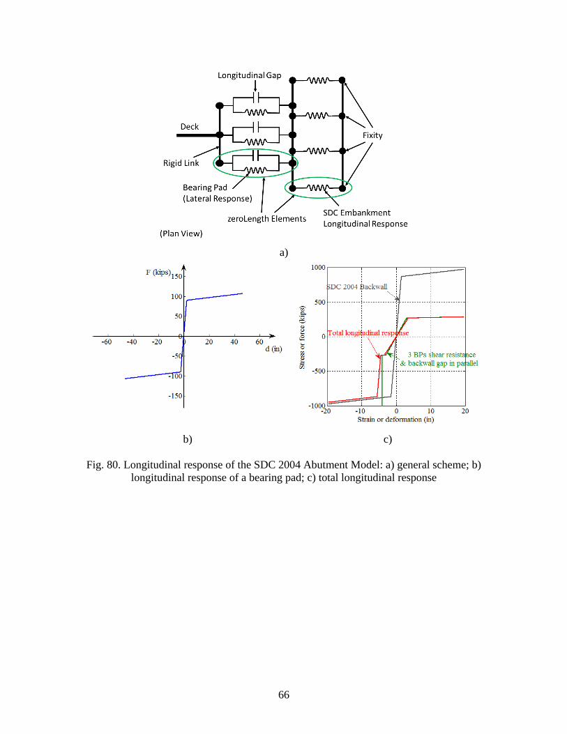
66

a)

b) c)

Fig. 80. Longitudinal response of the SDC 2004 Abutment Model: a) general scheme; b)

longitudinal response of a bearing pad; c) total longitudinal response

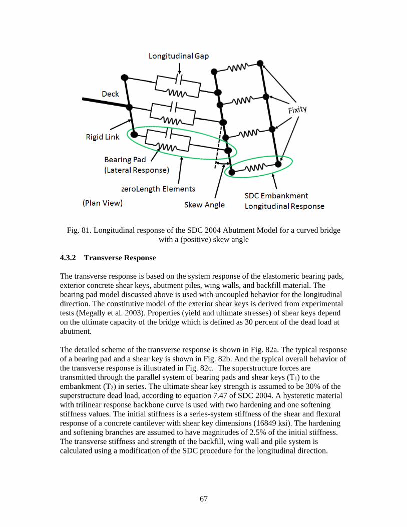
67

Fig. 81. Longitudinal response of the SDC 2004 Abutment Model for a curved bridge

with a (positive) skew angle

4.3.2 Transverse Response

The transverse response is based on the system response of the elastomeric bearing pads,

exterior concrete shear keys, abutment piles, wing walls, and backfill material. The

bearing pad model discussed above is used with uncoupled behavior for the longitudinal

direction. The constitutive model of the exterior shear keys is derived from experimental

tests (Megally et al. 2003). Properties (yield and ultimate stresses) of shear keys depend

on the ultimate capacity of the bridge which is defined as 30 percent of the dead load at

abutment.

The detailed scheme of the transverse response is shown in Fig. 82a. The typical response

of a bearing pad and a shear key is shown in Fig. 82b. And the typical overall behavior of

the transverse response is illustrated in Fig. 82c. The superstructure forces are

transmitted through the parallel system of bearing pads and shear keys (T1) to the

embankment (T2) in series. The ultimate shear key strength is assumed to be 30% of the

superstructure dead load, according to equation 7.47 of SDC 2004. A hysteretic material

with trilinear response backbone curve is used with two hardening and one softening

stiffness values. The initial stiffness is a series-system stiffness of the shear and flexural

response of a concrete cantilever with shear key dimensions (16849 ksi). The hardening

and softening branches are assumed to have magnitudes of 2.5% of the initial stiffness.

The transverse stiffness and strength of the backfill, wing wall and pile system is

calculated using a modification of the SDC procedure for the longitudinal direction.

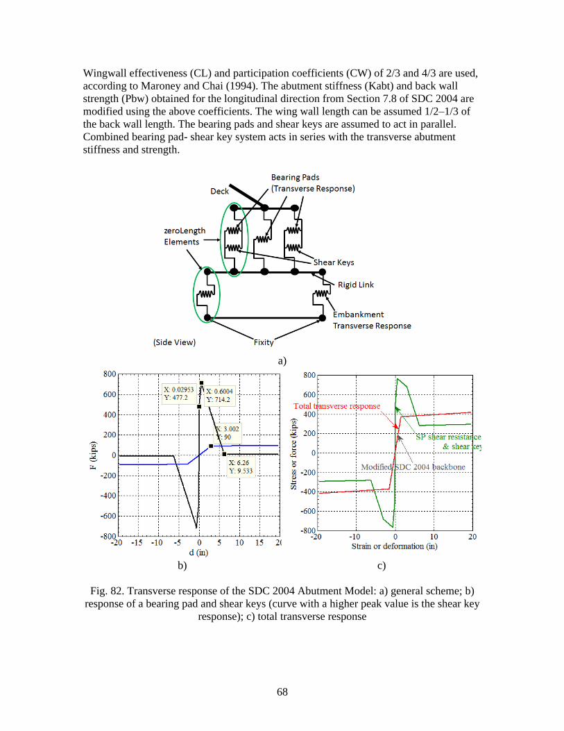
68

Wingwall effectiveness (CL) and participation coefficients (CW) of 2/3 and 4/3 are used,

according to Maroney and Chai (1994). The abutment stiffness (Kabt) and back wall

strength (Pbw) obtained for the longitudinal direction from Section 7.8 of SDC 2004 are

modified using the above coefficients. The wing wall length can be assumed 1/2–1/3 of

the back wall length. The bearing pads and shear keys are assumed to act in parallel.

Combined bearing pad- shear key system acts in series with the transverse abutment

stiffness and strength.

a)

b) c)

Fig. 82. Transverse response of the SDC 2004 Abutment Model: a) general scheme; b)

response of a bearing pad and shear keys (curve with a higher peak value is the shear key

response); c) total transverse response

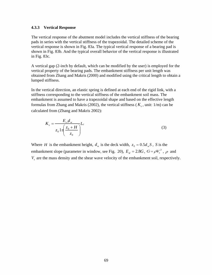
69

4.3.3 Vertical Response

The vertical response of the abutment model includes the vertical stiffness of the bearing

pads in series with the vertical stiffness of the trapezoidal. The detailed scheme of the

vertical response is shown in Fig. 83a. The typical vertical response of a bearing pad is

shown in Fig. 83b. And the typical overall behavior of the vertical response is illustrated

in Fig. 83c.

A vertical gap (2-inch by default, which can be modified by the user) is employed for the

vertical property of the bearing pads. The embankment stiffness per unit length was

obtained from Zhang and Makris (2000) and modified using the critical length to obtain a

lumped stiffness.

In the vertical direction, an elastic spring is defined at each end of the rigid link, with a

stiffness corresponding to the vertical stiffness of the embankment soil mass. The

embankment is assumed to have a trapezoidal shape and based on the effective length

formulas from Zhang and Makris (2002), the vertical stiffness ( , unit: 1/m) can be

calculated from (Zhang and Makris 2002):

Lc

(3)

Where is the embankment height, is the deck width, , is the

embankment slope (parameter in window, see Fig. 20), , , and

are the mass density and the shear wave velocity of the embankment soil, respectively.

vK

+=

0

0

0 l nz

Hzz

dEK ws l

v

H wd Sdz w5.00 = S

GEsl 8.2=2

sVG =

sV

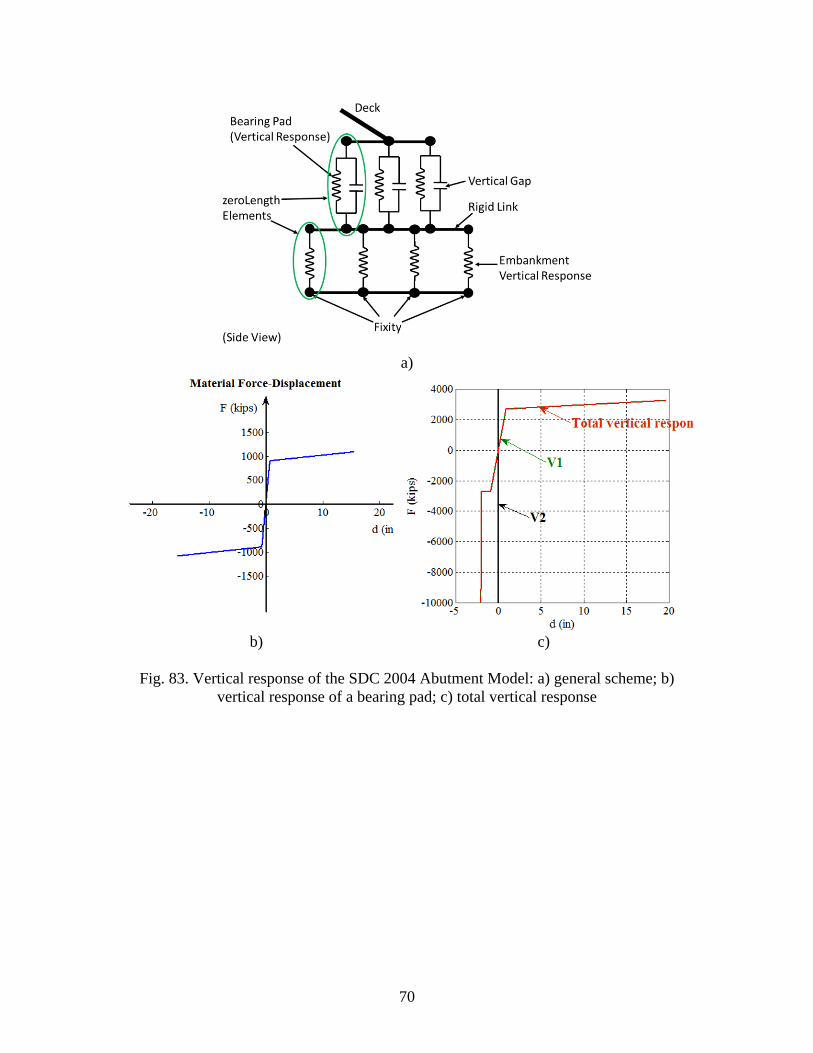
70

a)

b) c)

Fig. 83. Vertical response of the SDC 2004 Abutment Model: a) general scheme; b)

vertical response of a bearing pad; c) total vertical response

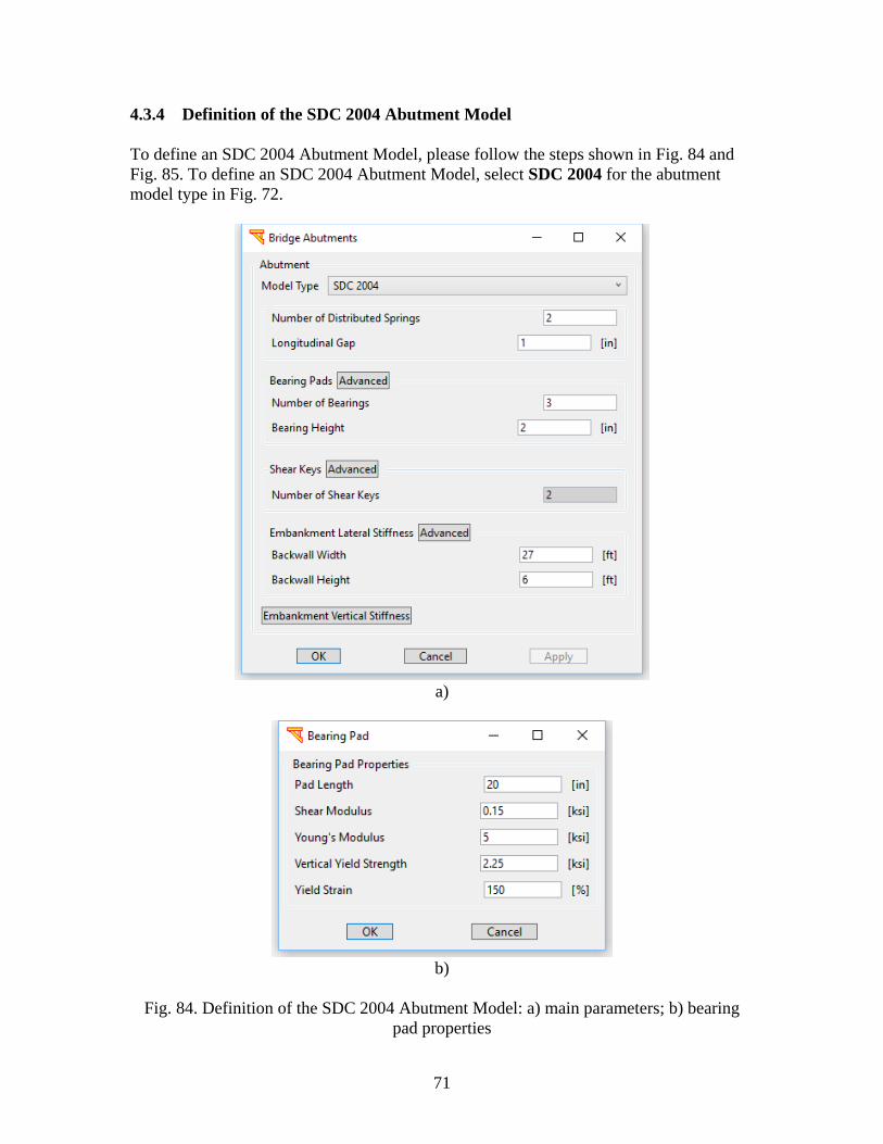
71

4.3.4 Definition of the SDC 2004 Abutment Model

To define an SDC 2004 Abutment Model, please follow the steps shown in Fig. 84 and

Fig. 85. To define an SDC 2004 Abutment Model, select SDC 2004 for the abutment

model type in Fig. 72.

a)

b)

Fig. 84. Definition of the SDC 2004 Abutment Model: a) main parameters; b) bearing

pad properties

72

a)

b)

c)

Fig. 85. Definition of the SDC 2004 Abutment Model: a) shear key properties; b) SDC

abutment properties; c) embankment properties

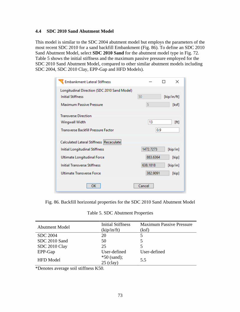
73

4.4 SDC 2010 Sand Abutment Model

This model is similar to the SDC 2004 abutment model but employs the parameters of the

most recent SDC 2010 for a sand backfill Embankment (Fig. 86). To define an SDC 2010

Sand Abutment Model, select SDC 2010 Sand for the abutment model type in Fig. 72.

Table 5 shows the initial stiffness and the maximum passive pressure employed for the

SDC 2010 Sand Abutment Model, compared to other similar abutment models including

SDC 2004, SDC 2010 Clay, EPP-Gap and HFD Models).

Fig. 86. Backfill horizontal properties for the SDC 2010 Sand Abutment Model

Table 5. SDC Abutment Properties

Abutment Model Initial Stiffness

(kip/in/ft)

Maximum Passive Pressure

(ksf)

SDC 2004 20 5

SDC 2010 Sand 50 5

SDC 2010 Clay 25 5

EPP-Gap User-defined User-defined

HFD Model *50 (sand);

25 (clay) 5.5

*Denotes average soil stiffness K50.

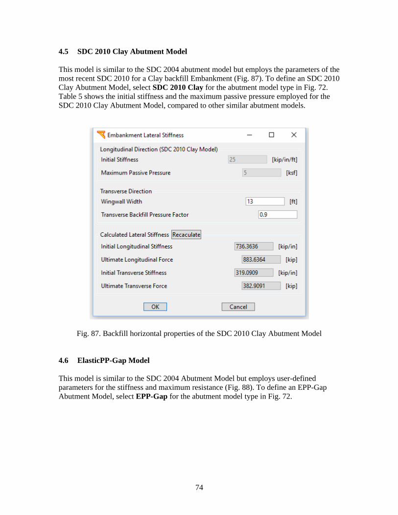
74

4.5 SDC 2010 Clay Abutment Model

This model is similar to the SDC 2004 abutment model but employs the parameters of the

most recent SDC 2010 for a Clay backfill Embankment (Fig. 87). To define an SDC 2010

Clay Abutment Model, select SDC 2010 Clay for the abutment model type in Fig. 72.

Table 5 shows the initial stiffness and the maximum passive pressure employed for the

SDC 2010 Clay Abutment Model, compared to other similar abutment models.

Fig. 87. Backfill horizontal properties of the SDC 2010 Clay Abutment Model

4.6 ElasticPP-Gap Model

This model is similar to the SDC 2004 Abutment Model but employs user-defined

parameters for the stiffness and maximum resistance (Fig. 88). To define an EPP-Gap

Abutment Model, select EPP-Gap for the abutment model type in Fig. 72.

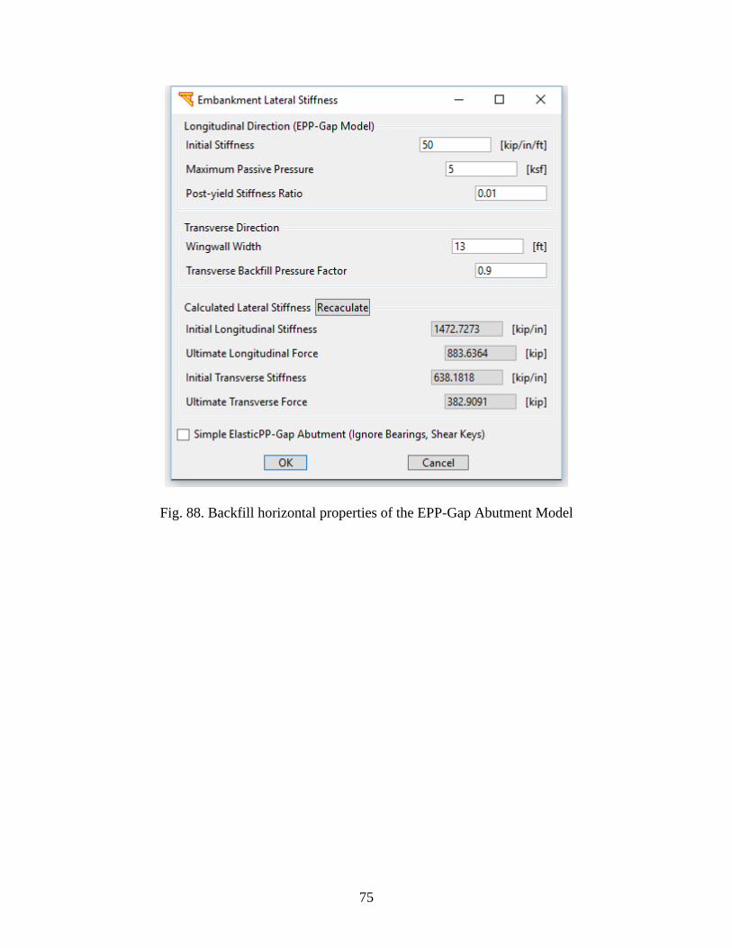
75

Fig. 88. Backfill horizontal properties of the EPP-Gap Abutment Model

76

4.7 HFD Model

As suggested by Shamsabadi et al. (2007, 2010), a Hyperbolic Force-Displacement

(HFD) relationship is employed to represent abutment resistance to bridge displacement

in the longitudinal direction (Fig. 89).

𝐹(𝑦) =𝐹𝑢𝑙𝑡(2𝐾50𝑦𝑚𝑎𝑥 − 𝐹𝑢𝑙𝑡)𝑦

𝐹𝑢𝑙𝑡𝑦𝑚𝑎𝑥 + 2(𝐾50𝑦𝑚𝑎𝑥 − 𝐹𝑢𝑙𝑡)𝑦

Where F is the resisting force, y is the longitudinal displacement, Fult is the ultimate

passive resistance and K50 is the secant stiffness at Fult/2.

𝐹(𝑦) =(2𝐾50 −

𝐹𝑢𝑙𝑡

𝑦𝑚𝑎𝑥) 𝑦

1 + 2 (𝐾50

𝐹𝑢𝑙𝑡−

1

𝑦𝑚𝑎𝑥) 𝑦

In this HFD model, resistance appears after a user-specified gap is traversed, and the

bridge thereafter gradually mobilizes the abutment’s passive earth pressure strength.

Herein, this strength is specified according to Shamsabadi et al. (2007, 2010) at 5.5 ksf

(for a nominal 5.5 ft bridge deck height), with full resistance occurring at a passive lateral

displacement of 3.6 in (the sand structural backfill scenario). Similarly, abutment

resistance to the transverse bridge displacement is derived from the longitudinal

hyperbolic force-displacement relationship according to the procedure outlined in Aviram

et al. (2008).

To define an HFD abutment model, select HFD Model for the abutment model type.

Click Advanced in Embankment Lateral Stiffness box to define the horizontal backfill

properties (Fig. 89c). Parameters of the backfill soil are defined based on soil types (sand,

clay, or User-defined), and the overall abutment stiffness/ or maximum passive pressure

resist are calculated using the SDC equations.

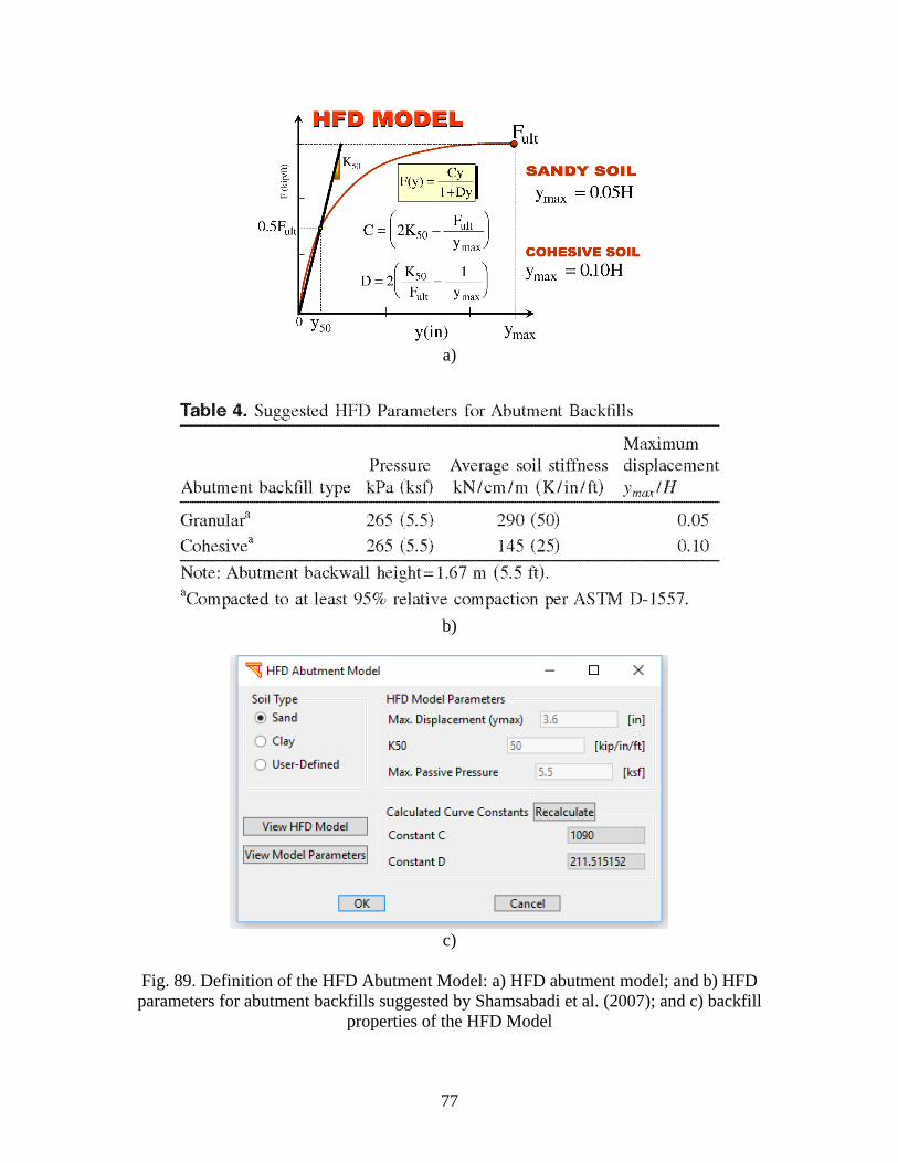
77

a)

b)

c)

Fig. 89. Definition of the HFD Abutment Model: a) HFD abutment model; and b) HFD

parameters for abutment backfills suggested by Shamsabadi et al. (2007); and c) backfill

properties of the HFD Model

78

5 COLUMN RESPONSES & BRIDGE RESONANCE

MSBridge provides features to view column lateral responses, abutment responses and

bridge natural periods (Fig. 8 and Fig. 90).

Fig. 90. Buttons to view column & abutment responses and bridge resonance

5.1 Bridge Natural Periods

Click View Natural Periods (Fig. 90) to view the natural periods and frequencies of the

bridge (Fig. 91). A mode shape analysis is conducted in this case.

The user can copy and paste the values to their favorite text editor such as MS Excel (in

Fig. 91, right-click and then click Select All (ctrl-a) to highlight, and then right-click and

then click Copy (ctrl c) to copy to the clipboard).

5.2 Column Gravity Response

Click View Gravity Response (Fig. 90) to view the column internal forces and bending

moments after application of own weight (Fig. 92).

5.3 Column & Abutment Longitudinal Responses

Click Longitudinal Response (Fig. 90) to view the column longitudinal responses (Fig.

93) and the abutment longitudinal responses (Fig. 94). A pushover up to 5% of drift ratio

in the longitudinal direction is conducted in this case.

5.4 Column & Abutment Transverse Responses

Click Transverse Response (Fig. 90) to view the transverse column responses (Fig. 95)

and the abutment transverse responses (Fig. 96). A pushover up to 4% of drift ratio in the

transverse direction is conducted in this case.

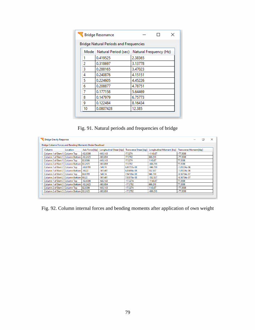
79

Fig. 91. Natural periods and frequencies of bridge

Fig. 92. Column internal forces and bending moments after application of own weight

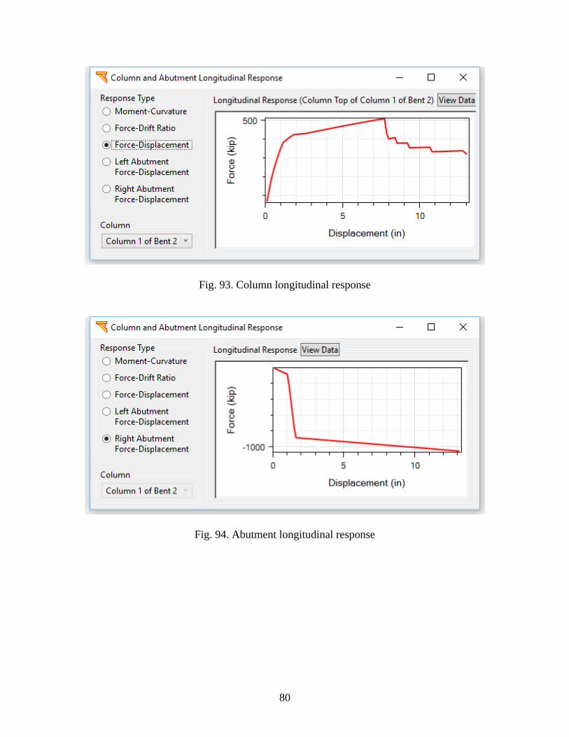
80

Fig. 93. Column longitudinal response

Fig. 94. Abutment longitudinal response

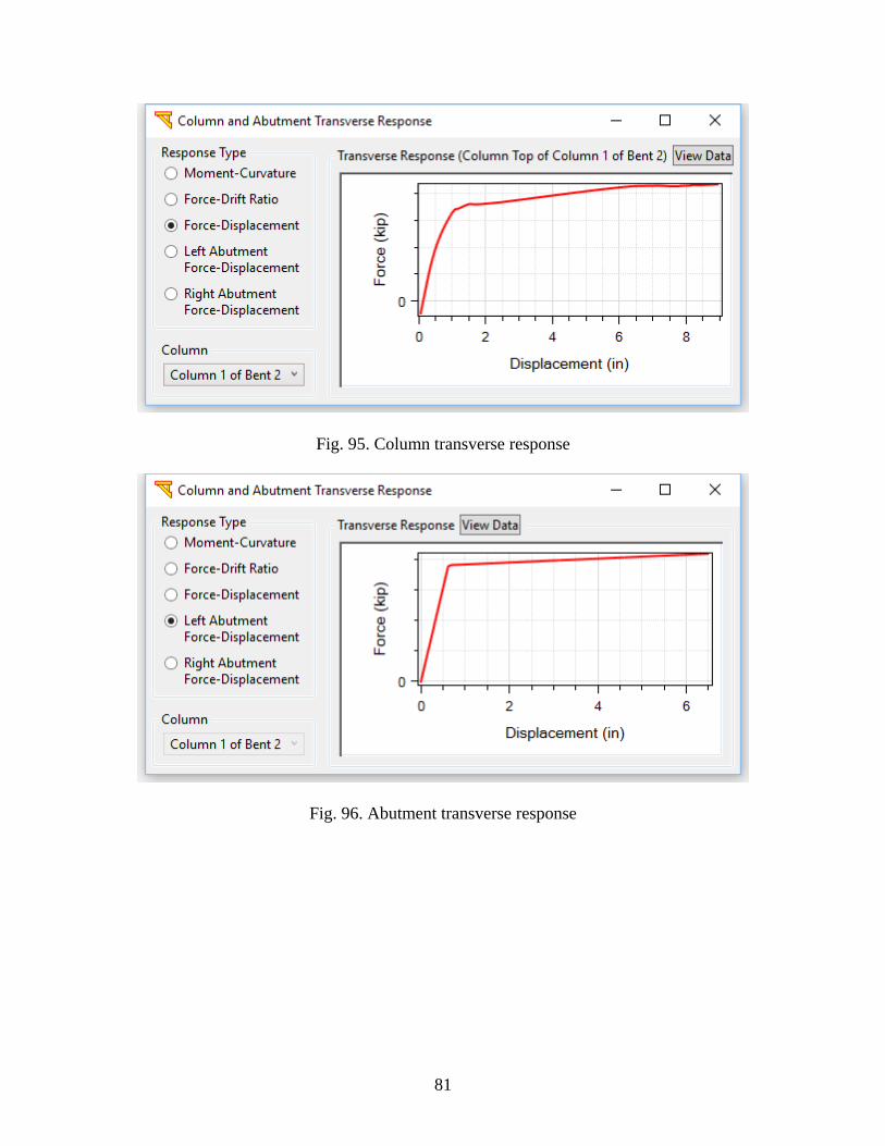
81

Fig. 95. Column transverse response

Fig. 96. Abutment transverse response

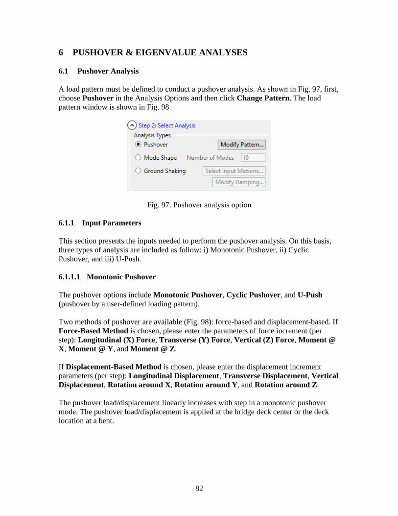
82

6 PUSHOVER & EIGENVALUE ANALYSES

6.1 Pushover Analysis

A load pattern must be defined to conduct a pushover analysis. As shown in Fig. 97, first,

choose Pushover in the Analysis Options and then click Change Pattern. The load

pattern window is shown in Fig. 98.

Fig. 97. Pushover analysis option

6.1.1 Input Parameters

This section presents the inputs needed to perform the pushover analysis. On this basis,

three types of analysis are included as follow: i) Monotonic Pushover, ii) Cyclic

Pushover, and iii) U-Push.

6.1.1.1 Monotonic Pushover

The pushover options include Monotonic Pushover, Cyclic Pushover, and U-Push

(pushover by a user-defined loading pattern).

Two methods of pushover are available (Fig. 98): force-based and displacement-based. If

Force-Based Method is chosen, please enter the parameters of force increment (per

step): Longitudinal (X) Force, Transverse (Y) Force, Vertical (Z) Force, Moment @

X, Moment @ Y, and Moment @ Z.

If Displacement-Based Method is chosen, please enter the displacement increment

parameters (per step): Longitudinal Displacement, Transverse Displacement, Vertical

Displacement, Rotation around X, Rotation around Y, and Rotation around Z.

The pushover load/displacement linearly increases with step in a monotonic pushover

mode. The pushover load/displacement is applied at the bridge deck center or the deck

location at a bent.

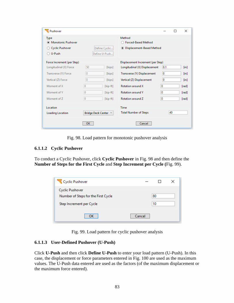
83

Fig. 98. Load pattern for monotonic pushover analysis

6.1.1.2 Cyclic Pushover

To conduct a Cyclic Pushover, click Cyclic Pushover in Fig. 98 and then define the

Number of Steps for the First Cycle and Step Increment per Cycle (Fig. 99).

Fig. 99. Load pattern for cyclic pushover analysis

6.1.1.3 User-Defined Pushover (U-Push)

Click U-Push and then click Define U-Push to enter your load pattern (U-Push). In this

case, the displacement or force parameters entered in Fig. 100 are used as the maximum

values. The U-Push data entered are used as the factors (of the maximum displacement or

the maximum force entered).

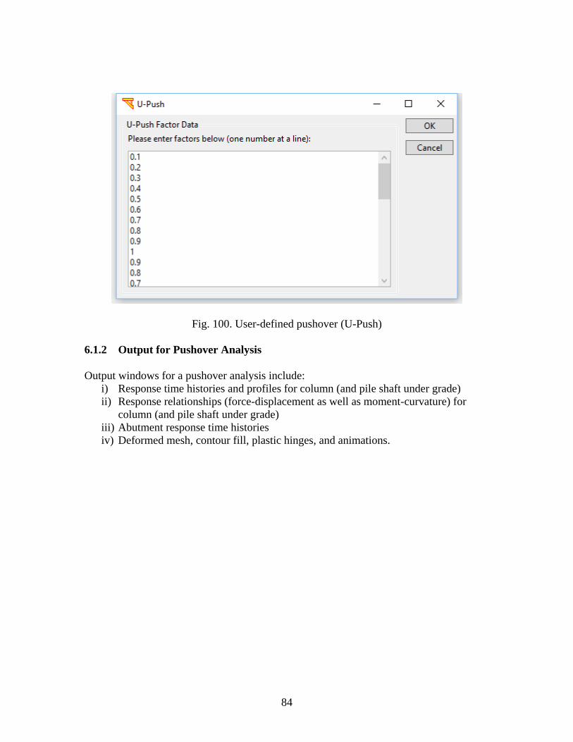
84

Fig. 100. User-defined pushover (U-Push)

6.1.2 Output for Pushover Analysis

Output windows for a pushover analysis include:

i) Response time histories and profiles for column (and pile shaft under grade)

ii) Response relationships (force-displacement as well as moment-curvature) for

column (and pile shaft under grade)

iii) Abutment response time histories

iv) Deformed mesh, contour fill, plastic hinges, and animations.

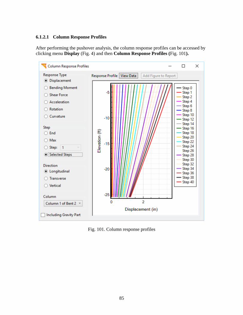
85

6.1.2.1 Column Response Profiles

After performing the pushover analysis, the column response profiles can be accessed by

clicking menu Display (Fig. 4) and then Column Response Profiles (Fig. 101).

Fig. 101. Column response profiles

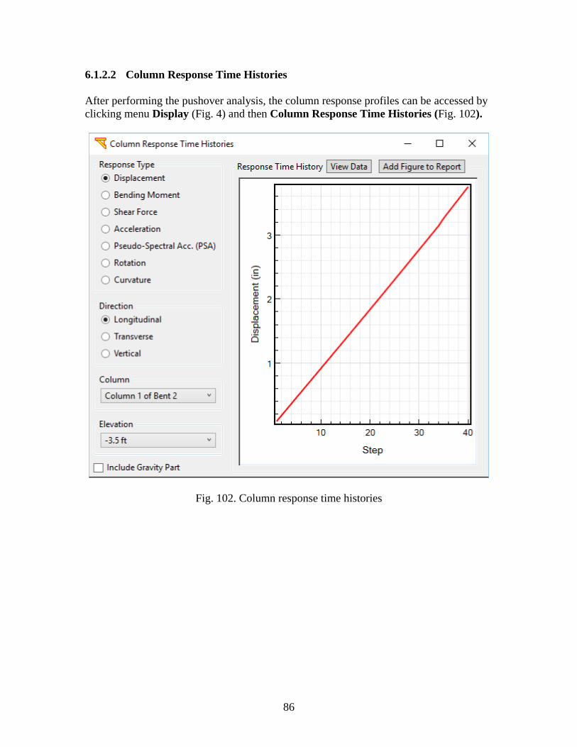
86

6.1.2.2 Column Response Time Histories


clicking menu Display (Fig. 4) and then Column Response Time Histories (Fig. 102).

Fig. 102. Column response time histories

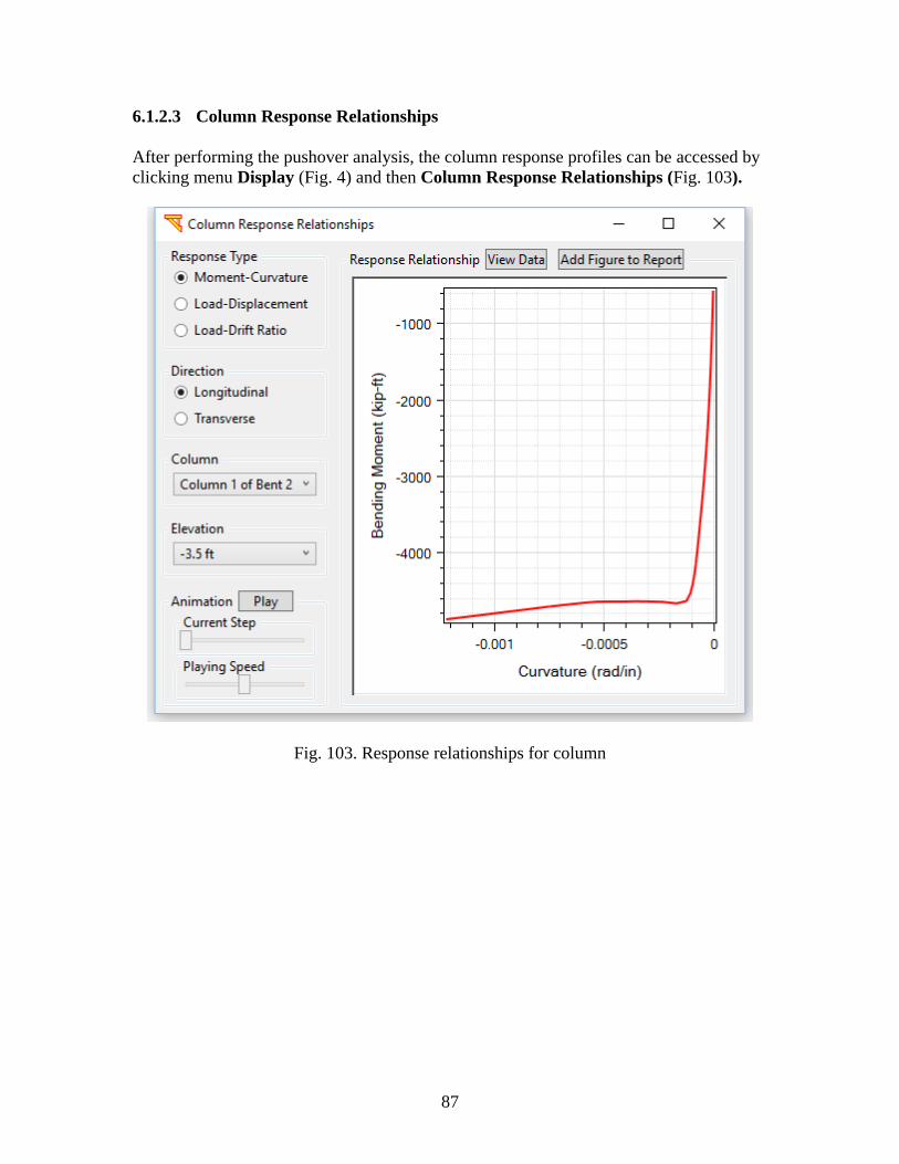
87

6.1.2.3 Column Response Relationships


clicking menu Display (Fig. 4) and then Column Response Relationships (Fig. 103).

Fig. 103. Response relationships for column

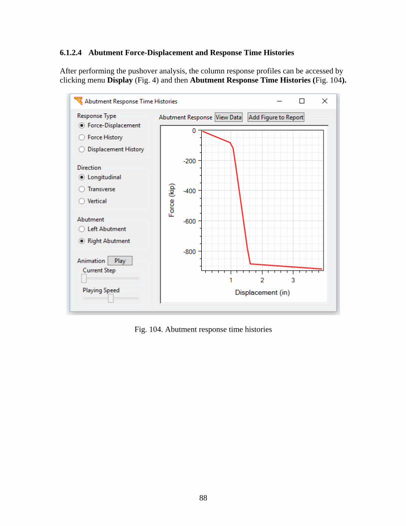
88

6.1.2.4 Abutment Force-Displacement and Response Time Histories


clicking menu Display (Fig. 4) and then Abutment Response Time Histories (Fig. 104).

Fig. 104. Abutment response time histories

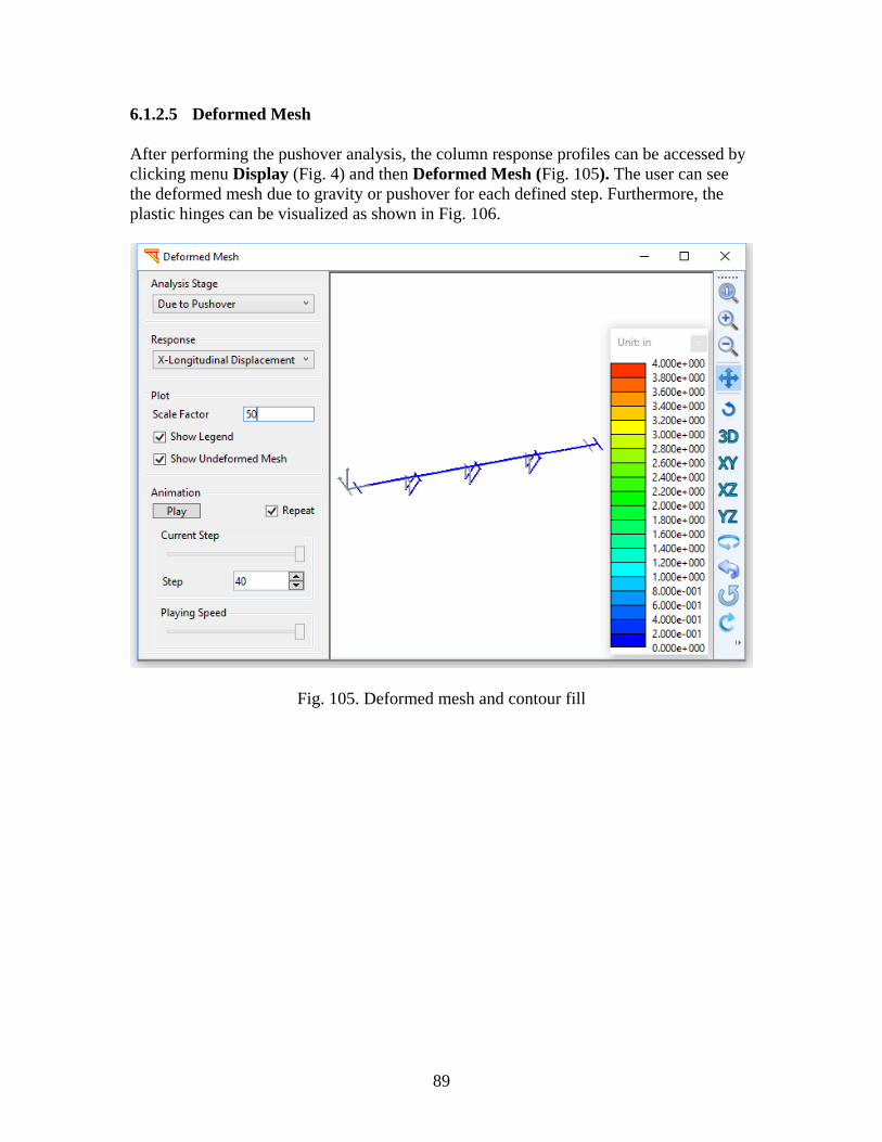
89

6.1.2.5 Deformed Mesh


clicking menu Display (Fig. 4) and then Deformed Mesh (Fig. 105). The user can see

the deformed mesh due to gravity or pushover for each defined step. Furthermore, the

plastic hinges can be visualized as shown in Fig. 106.

Fig. 105. Deformed mesh and contour fill

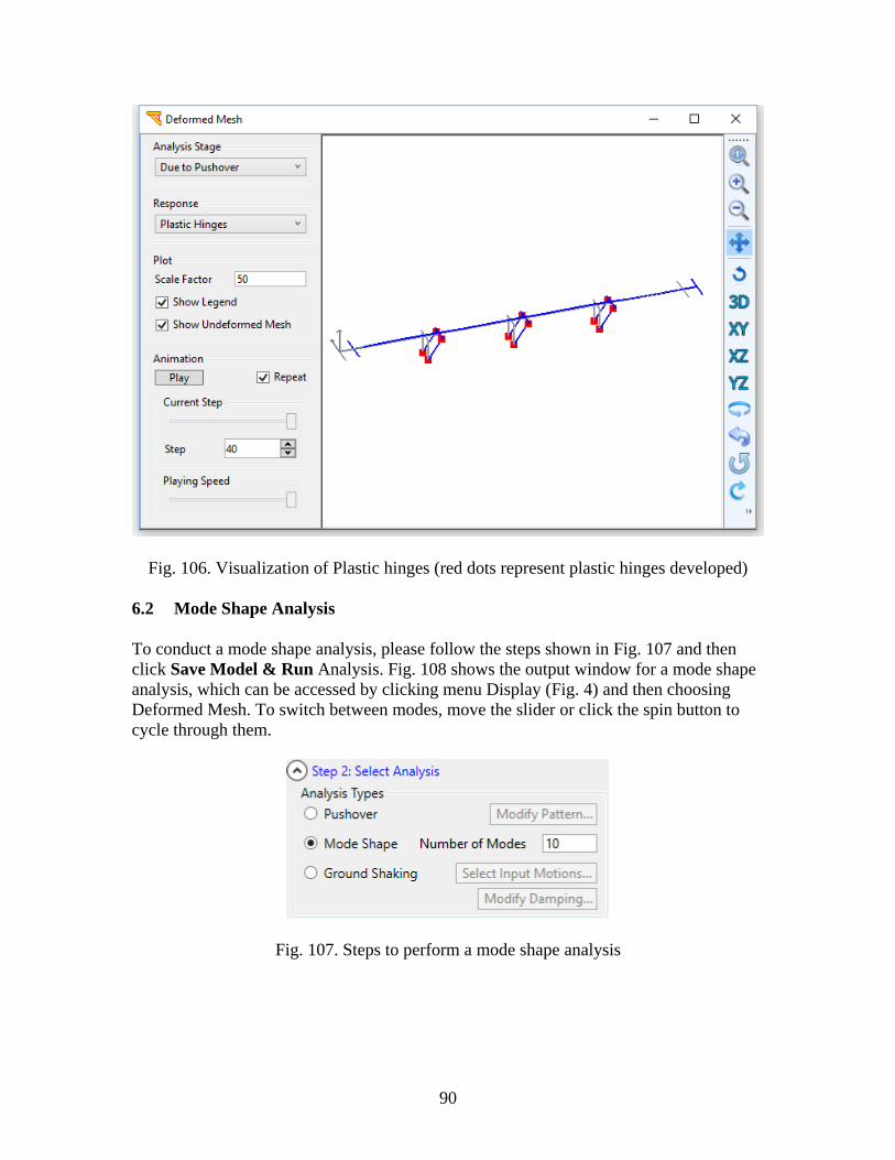
90

Fig. 106. Visualization of Plastic hinges (red dots represent plastic hinges developed)

6.2 Mode Shape Analysis

To conduct a mode shape analysis, please follow the steps shown in Fig. 107 and then

click Save Model & Run Analysis. Fig. 108 shows the output window for a mode shape

analysis, which can be accessed by clicking menu Display (Fig. 4) and then choosing

Deformed Mesh. To switch between modes, move the slider or click the spin button to

cycle through them.

Fig. 107. Steps to perform a mode shape analysis

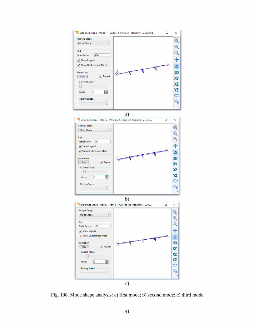
91

a)

b)

c)

Fig. 108. Mode shape analysis: a) first mode; b) second mode; c) third mode

92

7 GROUND SHAKING

To conduct a single earthquake analysis or multiple earthquake analyses, the “Ground

Shaking” option under Analysis Options (Fig. 2 and Fig. 109) is used. For that purpose,

the input earthquake excitation(s) must be specified. If only one earthquake record is

selected out of a specified ensemble (suite) of input motions, then a conventional single

earthquake analysis will be performed.

7.1 Definition/specification of input motion ensemble (suite)

This section presents the definition and specification of the input motions that represent a

wide range of intensity measures to perform the analysis.

7.1.1 Available Ground Motions

A set of 10 motions are provided as the default input motion suite. The above ground

motion data sets were resampled to a sampling frequency of 50 Hz (regardless of whether

initial sampling frequency was 100 or 200 Hz) due to the computational demands of

running full ground-structure analyses for an ensemble of motions. Standard interpolation

methods were used to resample the time domain signals (so that the signal shape is

preserved). The resampled records were then baselined to remove any permanent velocity

and displacement offsets. Baselining was accomplished using a third order polynomial

fitted to the displacement record.

In addition, four sets of input motions are also available (can be downloaded from the

website: http://www.soilquake.net/msbridge):

Motion Set 1: These 100 motions were obtained directly from the PEER NGA database,

and all files have been re-sampled to a time step of 0.02 seconds. This PBEE motion

ensemble (Medina and Krawinkler 2004) obtained from the PEER NGA database

(http://peer.berkeley.edu/nga/) consists of 100 3D input ground motions. Each motion is

composed of 3 perpendicular acceleration time history components (2 lateral and one

vertical). These motions were selected through earlier efforts (Gupta and Krawinkler,

2000; Mackie et al., 2007) to be representative of seismicity in typical regions of

California. The moment magnitudes (Mw) of these motions range from 5.8-7.2 (distances

from 0-60 km). The engineering characteristics of each motion and the ensemble overall

may be viewed directly within MSBridge. The provided ground motions are based on

earlier PEER research (Mackie and Stojadinovic 2005).

Motion Set 2: These motions (160 in total) were developed by Dr. Kevin Mackie from

the 80 motions of Set1 (excluding the 20 motions of Set1 in the bin NEAR), to account

for site classification.

Motion Set 3: These motions (80 in total) were developed by Dr. Jack Baker for PEER.

Additional information about these motions is available at the website:

http://www.soilquake.net/msbridge

93

http://peer.berkeley.edu/transportation/projects/ground-motion-studies-for-transportation-

systems/

Motion Set 4: These motions (260 in total) include the above Set2 and Set3 as well as

the additional Bin NEAR of Set1.

Once an input motion data set is specified, the user interface will extract/calculate

Intensity Measures (IMs) for each of these motions. In total, 11 different Intensity

Measures are defined for each motion (and presented to the user in table and graphical

formats), including quantities such as Peak Ground Acceleration (PGA), Peak Ground

Velocity (PGV), Arias Intensity (AI), and so forth.

7.1.2 Specifications of Input Motions

To conduct a ground shaking analysis, input motions must be defined (Fig. 109). The

window to define input motions is shown in Fig. 110. To select all motions, click Select

All. To un-select all motions, click De-select All. To remove one motion, select the

motion by clicking on it and then click Delete. To remove all motions, click Remove All.

To add a user-defined motion, click Import and then follow the simple steps to import a

new motion (Fig. 111). The resulting motion will be added to the current suites of input

motion. To obtain a completely new set of input motions, use Delete All to remove all

existing input motions, and then use Import to add new motions.

To import a ground motion file, first, save the ground acceleration time history (easy in a

notepad .txt file) with each new line being the next acceleration time step. This data in

this file should have the acceleration units of g.

The finite element computations can be conducted for several earthquakes at a time. This

is employed by specifying the Number of Motions Running Simultaneously (Fig. 110).

You can select as many as eight records to be run at the same time to reduce the overall

run time (for dual core machines or better).

Click View Motion to view the intensity measures and response spectra of the input

motion being highlighted (Fig. 112). SRSS stands for Square Root of the Sum of the

Squares of the two horizontal components. Click Display Intensity Measures to view

the intensity measures of the input motion being highlighted (Fig. 113). The user can

copy and paste the intensity measures to their favorite text editor such as MS Excel (in

Fig. 113, right-click and then click Select All (ctrl-a) to highlight, and then right-click

and then click Copy (ctrl c) to copy to the clipboard).

Click View Histograms & Cumulative Distribution to view the histogram and

cumulative distribution plots for the whole input motion set (Fig. 114). The intensity

measures include:

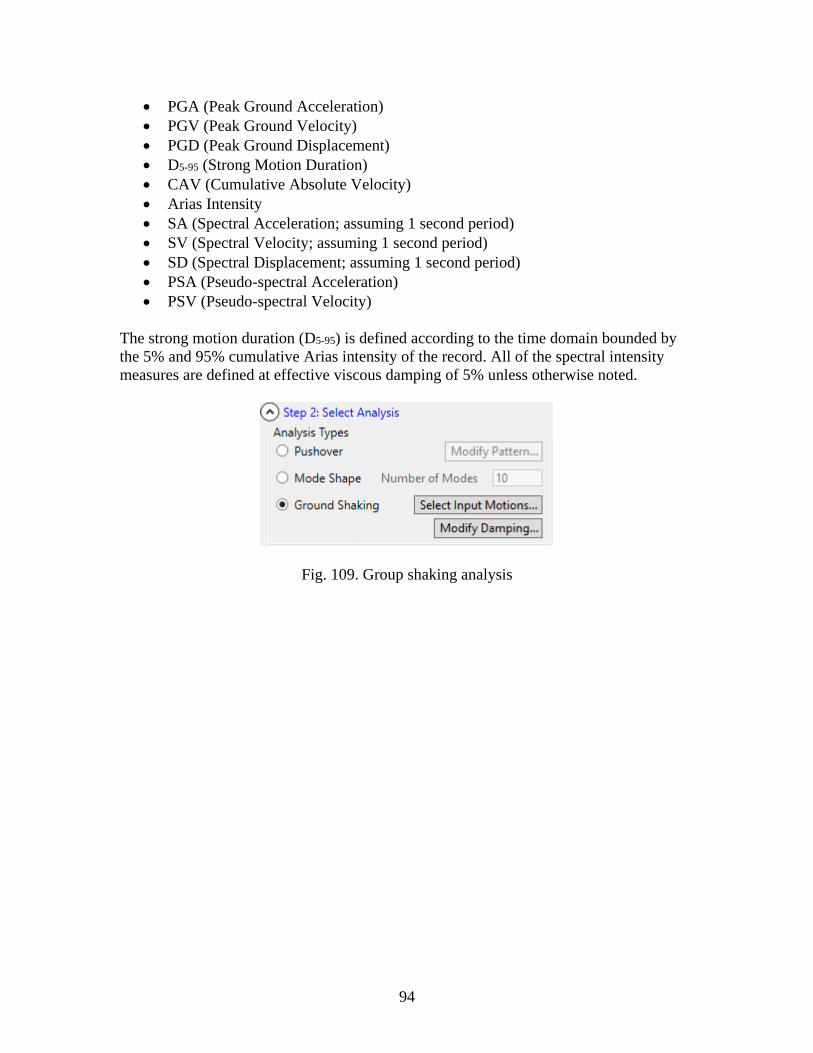
http://peer.berkeley.edu/transportation/projects/ground-motion-studies-for-transportation-systems/

http://peer.berkeley.edu/transportation/projects/ground-motion-studies-for-transportation-systems/

94

• PGA (Peak Ground Acceleration)

• PGV (Peak Ground Velocity)

• PGD (Peak Ground Displacement)

• D5-95 (Strong Motion Duration)

• CAV (Cumulative Absolute Velocity)

• Arias Intensity

• SA (Spectral Acceleration; assuming 1 second period)

• SV (Spectral Velocity; assuming 1 second period)

• SD (Spectral Displacement; assuming 1 second period)

• PSA (Pseudo-spectral Acceleration)

• PSV (Pseudo-spectral Velocity)

The strong motion duration (D5-95) is defined according to the time domain bounded by

the 5% and 95% cumulative Arias intensity of the record. All of the spectral intensity

measures are defined at effective viscous damping of 5% unless otherwise noted.

Fig. 109. Group shaking analysis

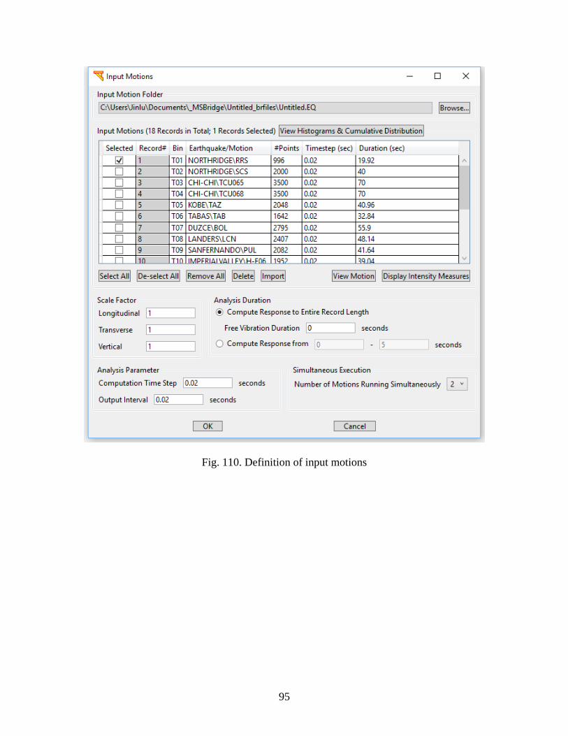
95

Fig. 110. Definition of input motions

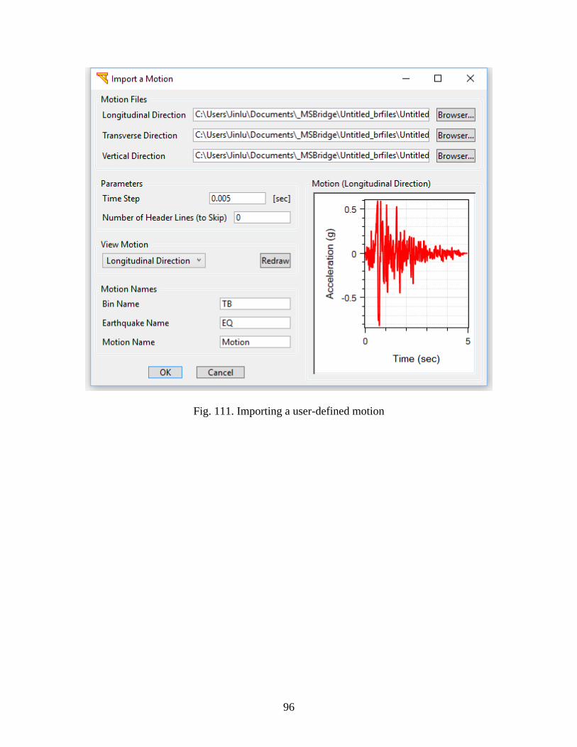
96

Fig. 111. Importing a user-defined motion

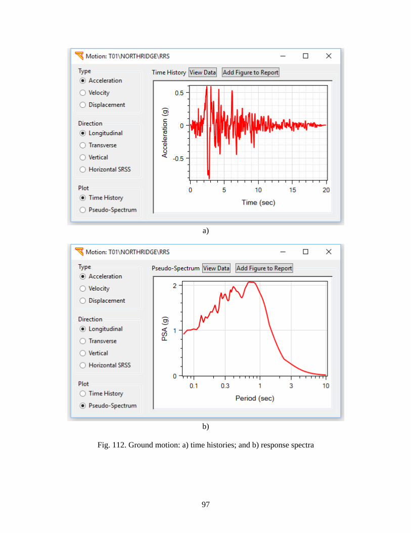
97

a)

b)

Fig. 112. Ground motion: a) time histories; and b) response spectra

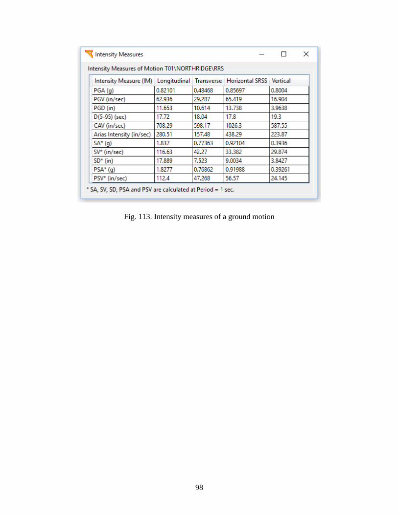
98

Fig. 113. Intensity measures of a ground motion

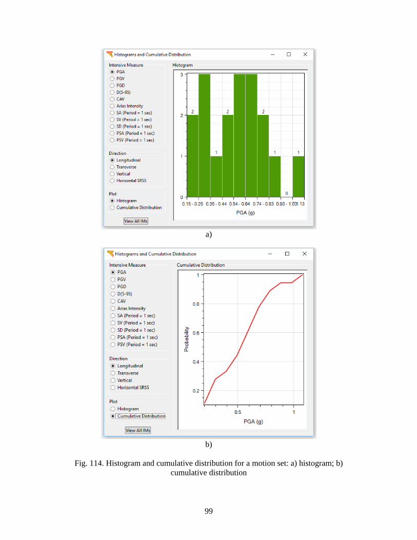
99

a)

b)

Fig. 114. Histogram and cumulative distribution for a motion set: a) histogram; b)

cumulative distribution

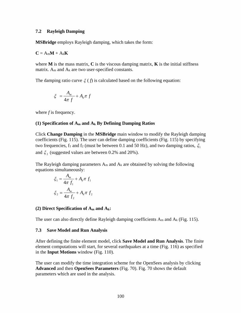
100

7.2 Rayleigh Damping

MSBridge employs Rayleigh damping, which takes the form:

C = AmM + AkK

where M is the mass matrix, C is the viscous damping matrix, K is the initial stiffness

matrix. Am and Ak are two user-specified constants.

The damping ratio curve ( f) is calculated based on the following equation:

fAf

Ak

m

+=4

where f is frequency.

(1) Specification of Am and Ak By Defining Damping Ratios

Click Change Damping in the MSBridge main window to modify the Rayleigh damping

coefficients (Fig. 115). The user can define damping coefficients (Fig. 115) by specifying

two frequencies, f1 and f2 (must be between 0.1 and 50 Hz), and two damping ratios, 1

and 2 (suggested values are between 0.2% and 20%).

The Rayleigh damping parameters Am and Ak are obtained by solving the following

equations simultaneously:

1

1

14

fAf

Ak

m

+=

2

2

24

fAf

Ak

m

+=

(2) Direct Specification of Am and Ak:

The user can also directly define Rayleigh damping coefficients Am and Ak (Fig. 115).

7.3 Save Model and Run Analysis

After defining the finite element model, click Save Model and Run Analysis. The finite

element computations will start, for several earthquakes at a time (Fig. 116) as specified

in the Input Motions window (Fig. 110).

The user can modify the time integration scheme for the OpenSees analysis by clicking

Advanced and then OpenSees Parameters (Fig. 70). Fig. 70 shows the default

parameters which are used in the analysis.

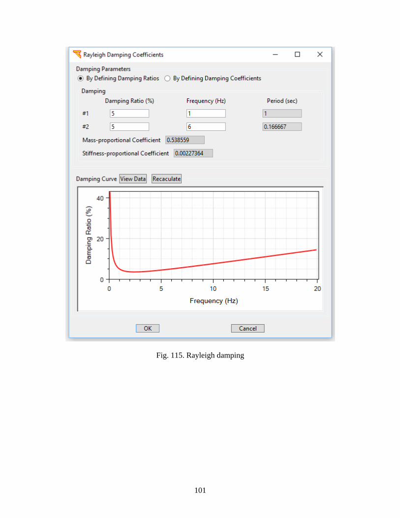
101

Fig. 115. Rayleigh damping

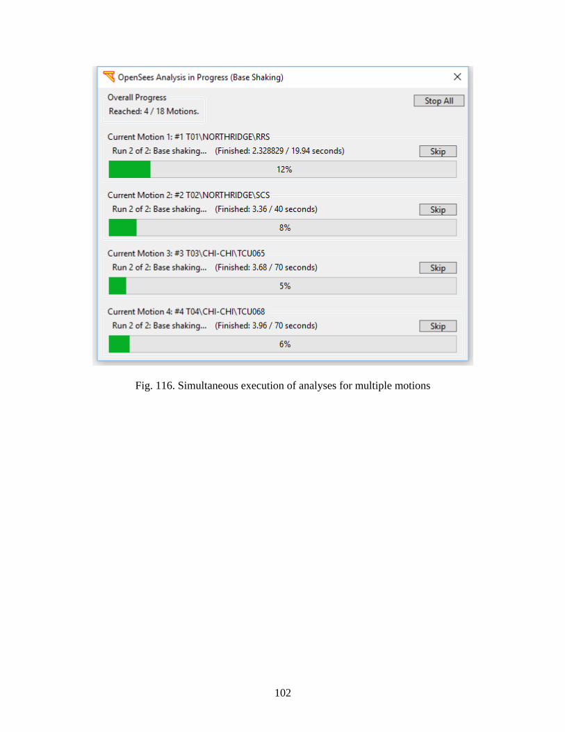
102

Fig. 116. Simultaneous execution of analyses for multiple motions

103

8 TIME HISTORY OUTPUT

This section presents the time history outputs after the FE analysis phase. The outputs are

time history output quantities for each bridge element, the deformed mesh, and the

maximum output quantities for all input motions.

8.1 Time History Output Quantities

At the end of the FE analysis phase, time histories and bridge responses will be available

of the form:

i) Column Response Time Profiles

ii) Column Response Time Histories

iii) Column Response Relationships

iv) Abutment Responses

v) Deformed Mesh

In addition, for multiple earthquake analysis scenarios, Intensity Measures (IMs) and

response spectra for each input motion are calculated and are available for display in

Table and Figure formats. Engineering Demand Parameter (EDP) Quantities and Bridge

peak accelerations for all employed shaking motions are also available for display against

any of the computed IMs.

The post-processing capabilities can be accessed from Menu Display (Fig. 4). To display

output for a different input motion, click Menu Display and then Detailed Output:

Please Select Input Motion (Fig. 4d). The name of the selected input motion will also

appear on the menu items (Fig. 4d).

104

Fig. 117. Selection of an input motion

8.1.1 Deck Response Time Histories

The deck response time histories can be accessed by clicking menu Display (Fig. 4) and

then Deck Response Time Histories. Fig. 118 shows the window for displaying the deck

longitudinal displacement time histories.

8.1.2 Column Response Profiles

The column response profiles can be accessed by clicking menu Display (Fig. 4) and

then Column Response Profiles. The column response window is shown in Fig. 119.

The columns are labeled as:

i) Column 1 of Bent 2 (see Fig. 1., the first bent starting after left abutment is

denoted as “Bent 2”, the second as “Bent 3”, and so on)

ii) Column 2 of Bent 2

iii) (more if any)

Fig. 120 shows the bending moment in the longitudinal plane. The horizontal axis of the

plot is the response name (e.g., displacement, bending moment, etc.) and the vertical axis

is the elevation of the column. Zero elevation means the column base.

105

8.1.3 Column Response Time Histories

The column response time histories can be accessed by clicking menu Display (Fig. 4)

and then Column Response Time Histories. Fig. 121 shows the window for displaying

the column longitudinal displacement time histories.

Fig. 118. Deck longitudinal displacement response time histories

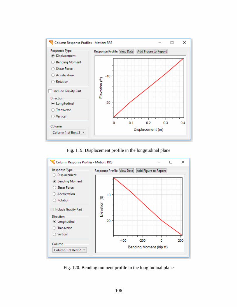
106

Fig. 119. Displacement profile in the longitudinal plane

Fig. 120. Bending moment profile in the longitudinal plane

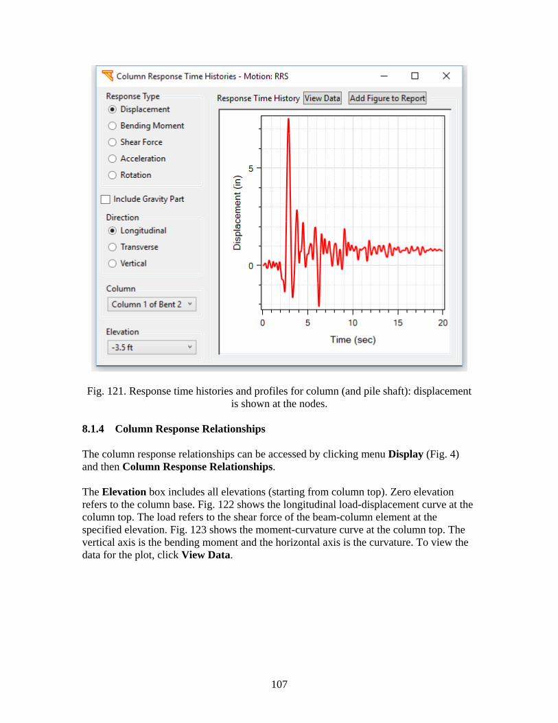
107

Fig. 121. Response time histories and profiles for column (and pile shaft): displacement

is shown at the nodes.

8.1.4 Column Response Relationships

The column response relationships can be accessed by clicking menu Display (Fig. 4)

and then Column Response Relationships.

The Elevation box includes all elevations (starting from column top). Zero elevation

refers to the column base. Fig. 122 shows the longitudinal load-displacement curve at the

column top. The load refers to the shear force of the beam-column element at the

specified elevation. Fig. 123 shows the moment-curvature curve at the column top. The

vertical axis is the bending moment and the horizontal axis is the curvature. To view the

data for the plot, click View Data.

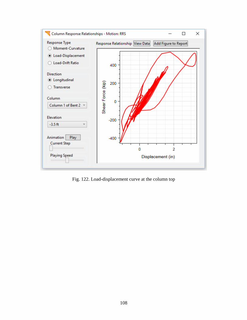
108

Fig. 122. Load-displacement curve at the column top

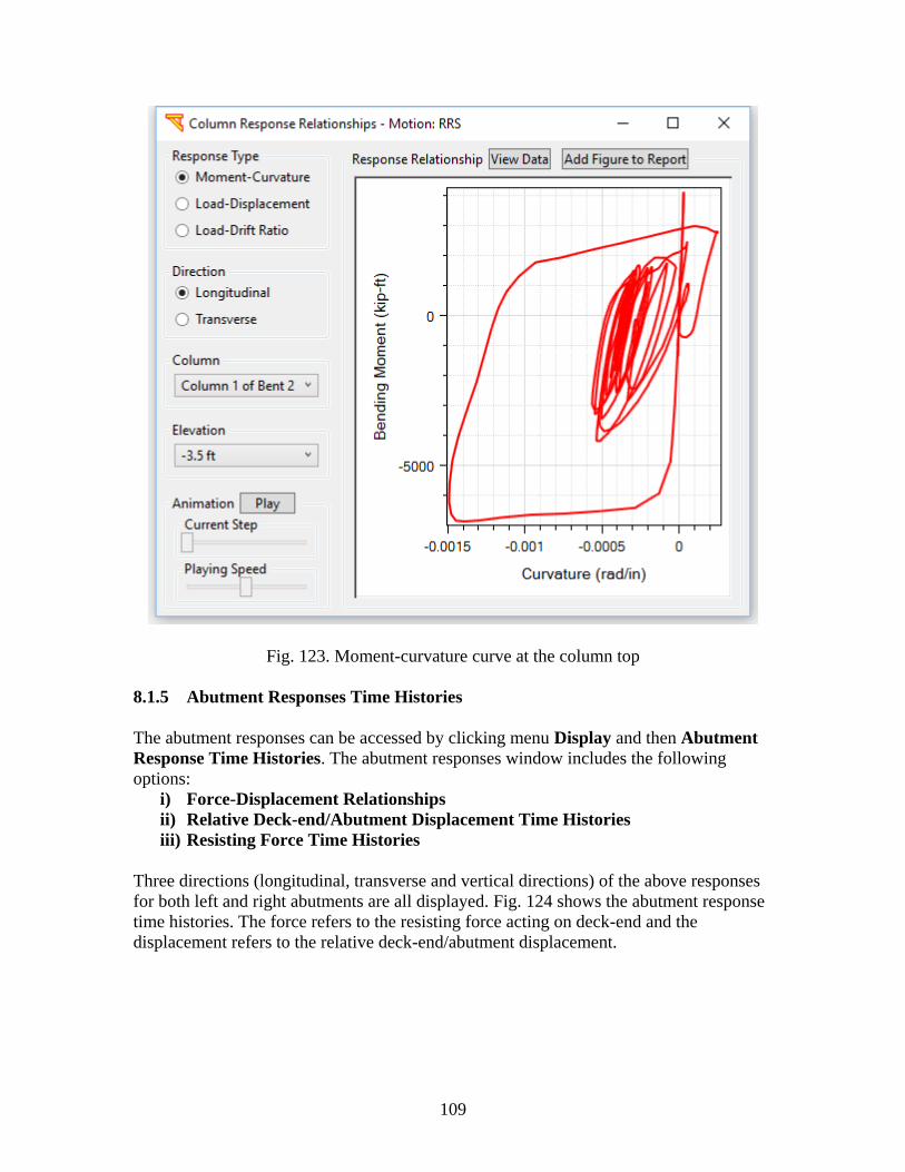
109

Fig. 123. Moment-curvature curve at the column top

8.1.5 Abutment Responses Time Histories

The abutment responses can be accessed by clicking menu Display and then Abutment

Response Time Histories. The abutment responses window includes the following

options:

i) Force-Displacement Relationships

ii) Relative Deck-end/Abutment Displacement Time Histories

iii) Resisting Force Time Histories

Three directions (longitudinal, transverse and vertical directions) of the above responses

for both left and right abutments are all displayed. Fig. 124 shows the abutment response

time histories. The force refers to the resisting force acting on deck-end and the

displacement refers to the relative deck-end/abutment displacement.

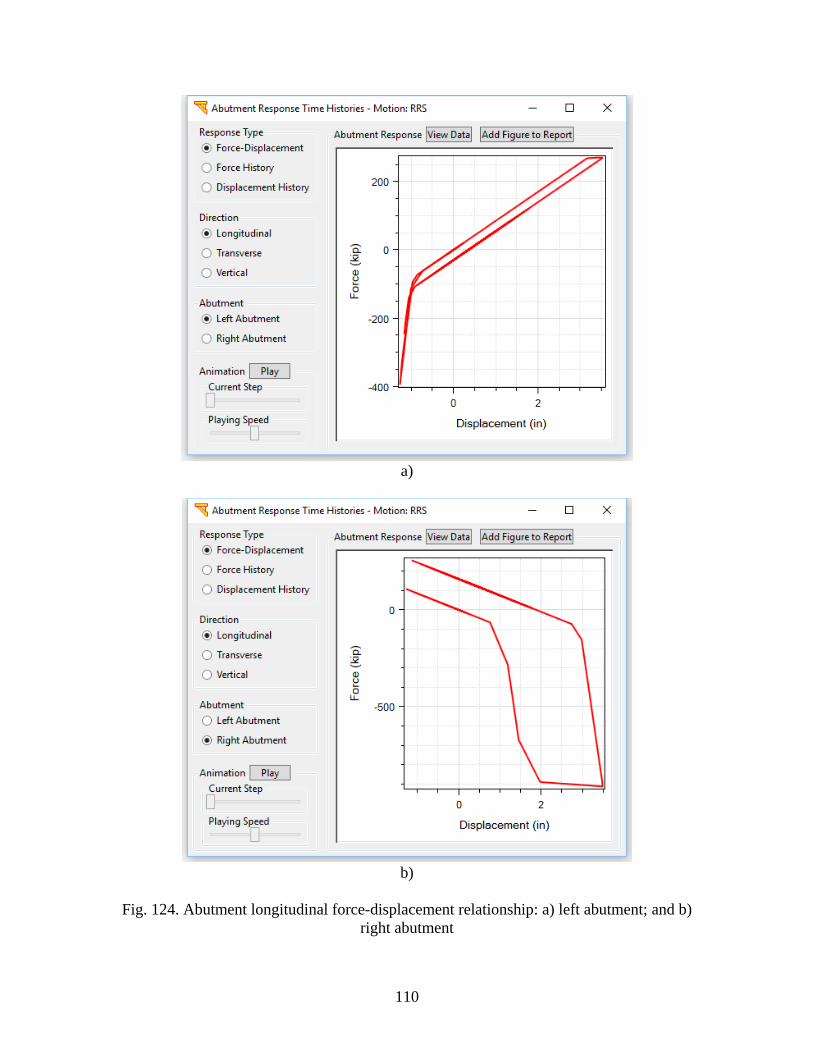
110

a)

b)

Fig. 124. Abutment longitudinal force-displacement relationship: a) left abutment; and b)

right abutment

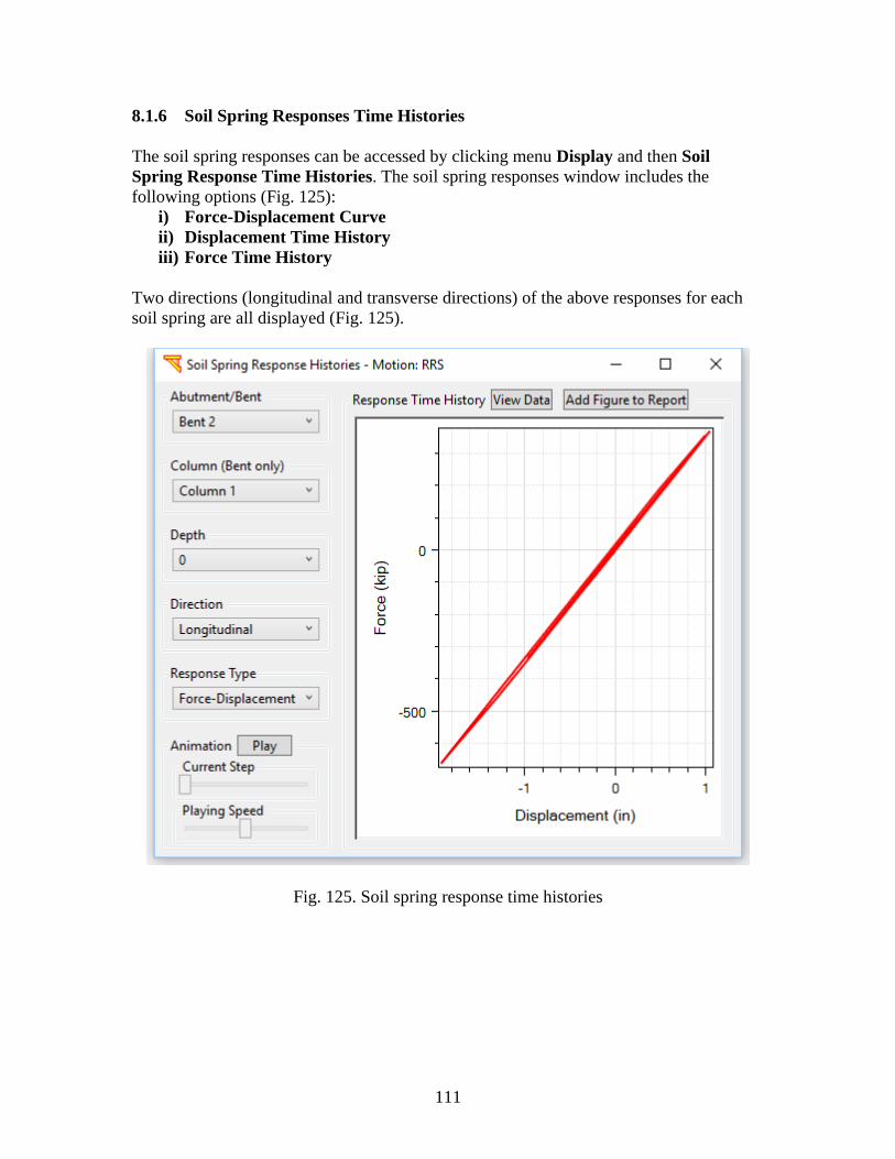
111

8.1.6 Soil Spring Responses Time Histories

The soil spring responses can be accessed by clicking menu Display and then Soil

Spring Response Time Histories. The soil spring responses window includes the

following options (Fig. 125):

i) Force-Displacement Curve

ii) Displacement Time History

iii) Force Time History

Two directions (longitudinal and transverse directions) of the above responses for each

soil spring are all displayed (Fig. 125).

Fig. 125. Soil spring response time histories

112

8.1.7 Deck Hinge Responses Time Histories

The deck hinge responses can be accessed by clicking menu Display and then Deck

Hinge Response Time Histories. The deck hinge responses window includes the

following options (Fig. 126):




Response time histories are shown for the cable and edge hinge elements for each hinge

(Fig. 126).

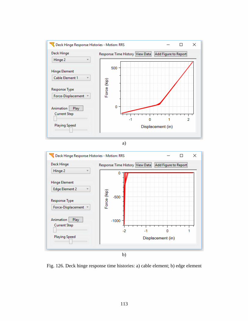
113

a)

b)

Fig. 126. Deck hinge response time histories: a) cable element; b) edge element

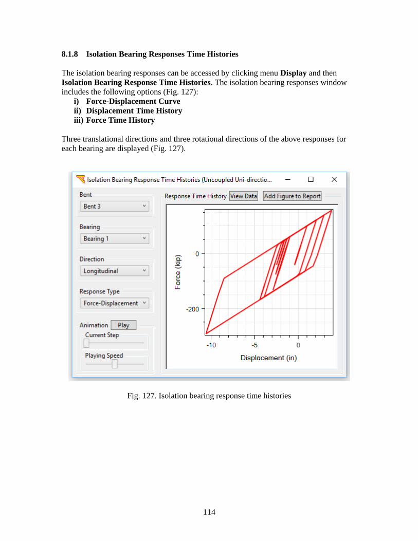
114

8.1.8 Isolation Bearing Responses Time Histories

The isolation bearing responses can be accessed by clicking menu Display and then

Isolation Bearing Response Time Histories. The isolation bearing responses window

includes the following options (Fig. 127):




Three translational directions and three rotational directions of the above responses for

each bearing are displayed (Fig. 127).

Fig. 127. Isolation bearing response time histories

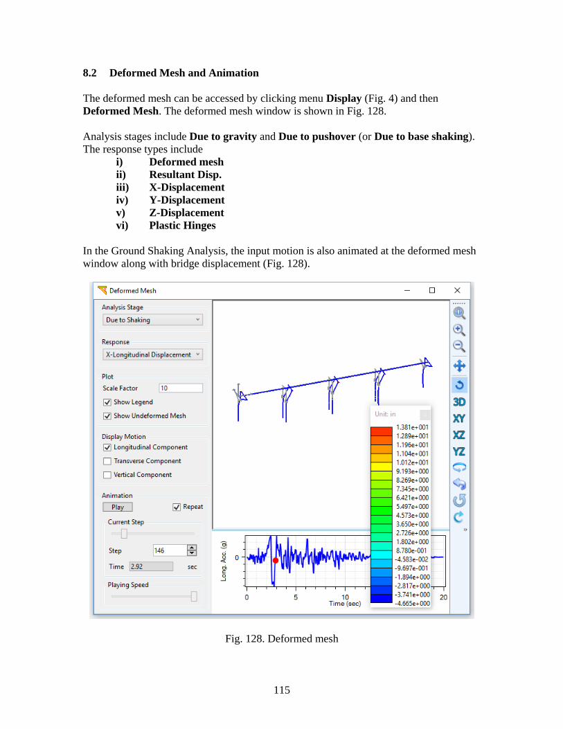
115

8.2 Deformed Mesh and Animation

The deformed mesh can be accessed by clicking menu Display (Fig. 4) and then

Deformed Mesh. The deformed mesh window is shown in Fig. 128.

Analysis stages include Due to gravity and Due to pushover (or Due to base shaking).

The response types include

i) Deformed mesh

ii) Resultant Disp.

iii) X-Displacement

iv) Y-Displacement

v) Z-Displacement

vi) Plastic Hinges

In the Ground Shaking Analysis, the input motion is also animated at the deformed mesh

window along with bridge displacement (Fig. 128).

Fig. 128. Deformed mesh

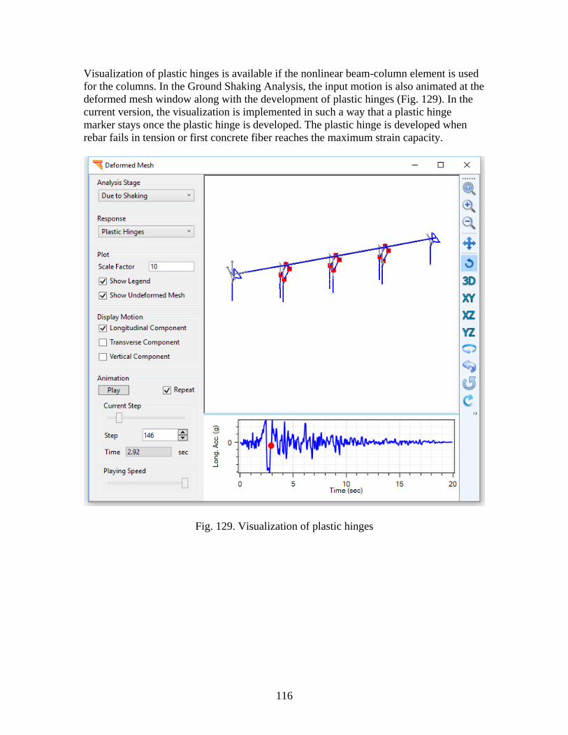
116

Visualization of plastic hinges is available if the nonlinear beam-column element is used

for the columns. In the Ground Shaking Analysis, the input motion is also animated at the

deformed mesh window along with the development of plastic hinges (Fig. 129). In the

current version, the visualization is implemented in such a way that a plastic hinge

marker stays once the plastic hinge is developed. The plastic hinge is developed when

rebar fails in tension or first concrete fiber reaches the maximum strain capacity.

Fig. 129. Visualization of plastic hinges

117

8.3 Maximum Output Quantities

This section presents the maximum acceleration and displacements for all motions after

performing time history analysis. In addition, the maximum column and abutments

forces.

8.3.1 Bridge Peak Accelerations & Displacements for All Motions

The bridge peak accelerations and displacements for all input motions can be accessed by

clicking menu Display (Fig. 4) and then Bridge Peak Accelerations& Displacements

for All Motions. The window to display the bridge peak accelerations for all motions is

shown in Fig. 130. The responses are available in the longitudinal and transverse

directions as well as for the SRSS of the two horizontal directions (Fig. 130).

The figures in this window include:

i) Maximum bridge acceleration

ii) Maximum bridge displacement

iii) Bridge peak acceleration/input peak acceleration

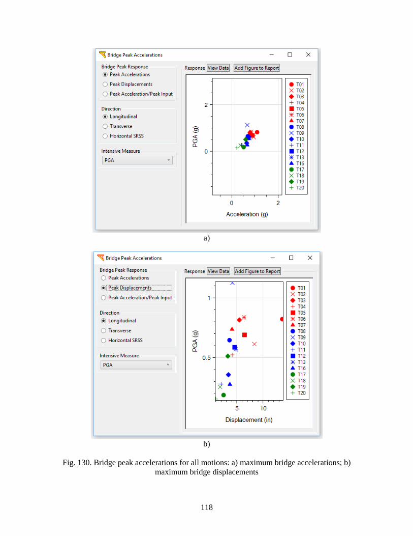
118

a)

b)

Fig. 130. Bridge peak accelerations for all motions: a) maximum bridge accelerations; b)

maximum bridge displacements

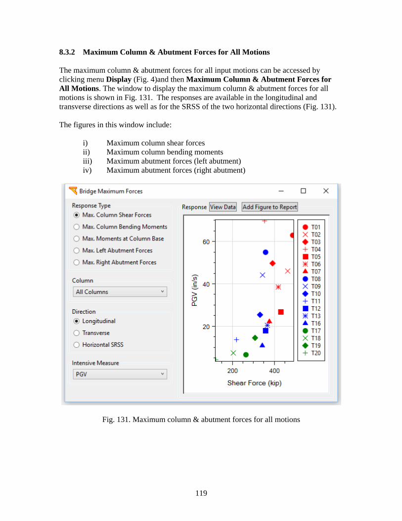
119

8.3.2 Maximum Column & Abutment Forces for All Motions

The maximum column & abutment forces for all input motions can be accessed by

clicking menu Display (Fig. 4)and then Maximum Column & Abutment Forces for

All Motions. The window to display the maximum column & abutment forces for all

motions is shown in Fig. 131. The responses are available in the longitudinal and

transverse directions as well as for the SRSS of the two horizontal directions (Fig. 131).

The figures in this window include:

i) Maximum column shear forces

ii) Maximum column bending moments

iii) Maximum abutment forces (left abutment)

iv) Maximum abutment forces (right abutment)

Fig. 131. Maximum column & abutment forces for all motions

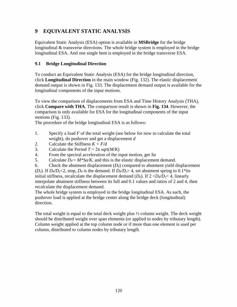
120

9 EQUIVALENT STATIC ANALYSIS

Equivalent Static Analysis (ESA) option is available in MSBridge for the bridge

longitudinal & transverse directions. The whole bridge system is employed in the bridge

longitudinal ESA. And one single bent is employed in the bridge transverse ESA.

9.1 Bridge Longitudinal Direction

To conduct an Equivalent Static Analysis (ESA) for the bridge longitudinal direction,

click Longitudinal Direction in the main window (Fig. 132). The elastic displacement

demand output is shown in Fig. 133. The displacement demand output is available for the

longitudinal components of the input motions.

To view the comparison of displacements from ESA and Time History Analysis (THA),

click Compare with THA. The comparison result is shown in Fig. 134. However, the

comparison is only available for ESA for the longitudinal components of the input

motions (Fig. 133).

The procedure of the bridge longitudinal ESA is as follows:

1. Specify a load F of the total weight (see below for now to calculate the total

weight), do pushover and get a displacement d

2. Calculate the Stiffness K = F/d

3. Calculate the Period T = 2π sqrt(M/K)

4. From the spectral acceleration of the input motion, get Sa

5. Calculate Dd = M*Sa/K, and this is the elastic displacement demand.

6. Check the abutment displacement (Dd) compared to abutment yield displacement

(Dy). If Dd/Dy<2, stop, Dd is the demand. If Dd/Dy> 4, set abutment spring to 0.1*its

initial stiffness, recalculate the displacement demand (Dd). If 2 <Dd/Dy< 4, linearly

interpolate abutment stiffness between its full and 0.1 values and ratios of 2 and 4, then

recalculate the displacement demand.

The whole bridge system is employed in the bridge longitudinal ESA. As such, the

pushover load is applied at the bridge center along the bridge deck (longitudinal)

direction.

The total weight is equal to the total deck weight plus ½ column weight. The deck weight

should be distributed weight over span elements (or applied to nodes by tributary length).

Column weight applied at the top column node or if more than one element is used per

column, distributed to column nodes by tributary length.

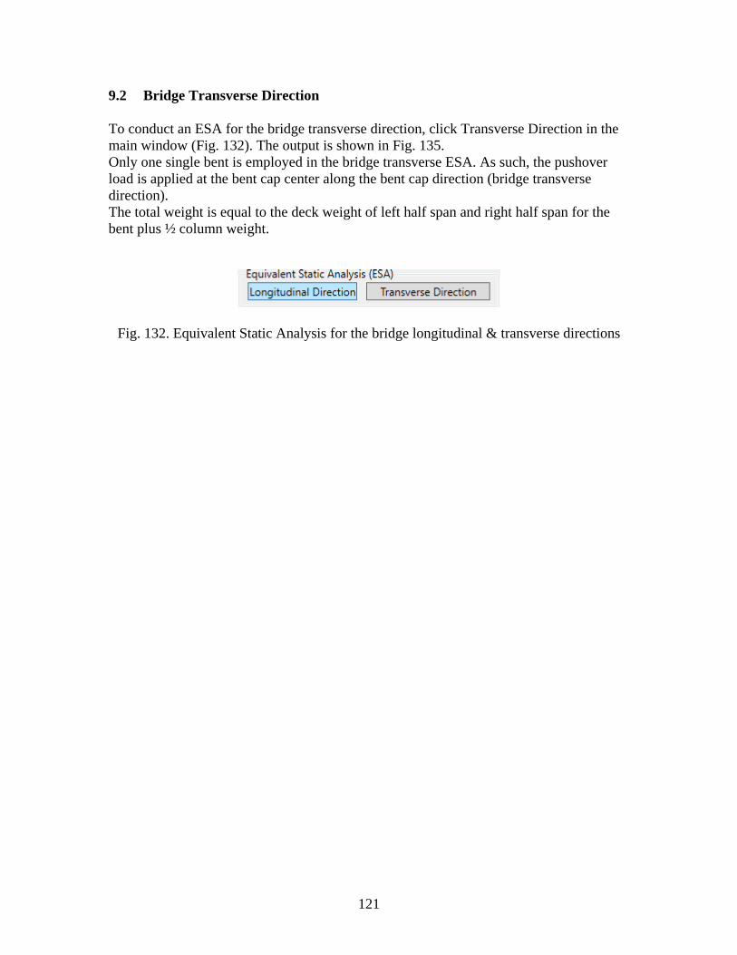
121

9.2 Bridge Transverse Direction

To conduct an ESA for the bridge transverse direction, click Transverse Direction in the

main window (Fig. 132). The output is shown in Fig. 135.

Only one single bent is employed in the bridge transverse ESA. As such, the pushover

load is applied at the bent cap center along the bent cap direction (bridge transverse

direction).

The total weight is equal to the deck weight of left half span and right half span for the

bent plus ½ column weight.

Fig. 132. Equivalent Static Analysis for the bridge longitudinal & transverse directions

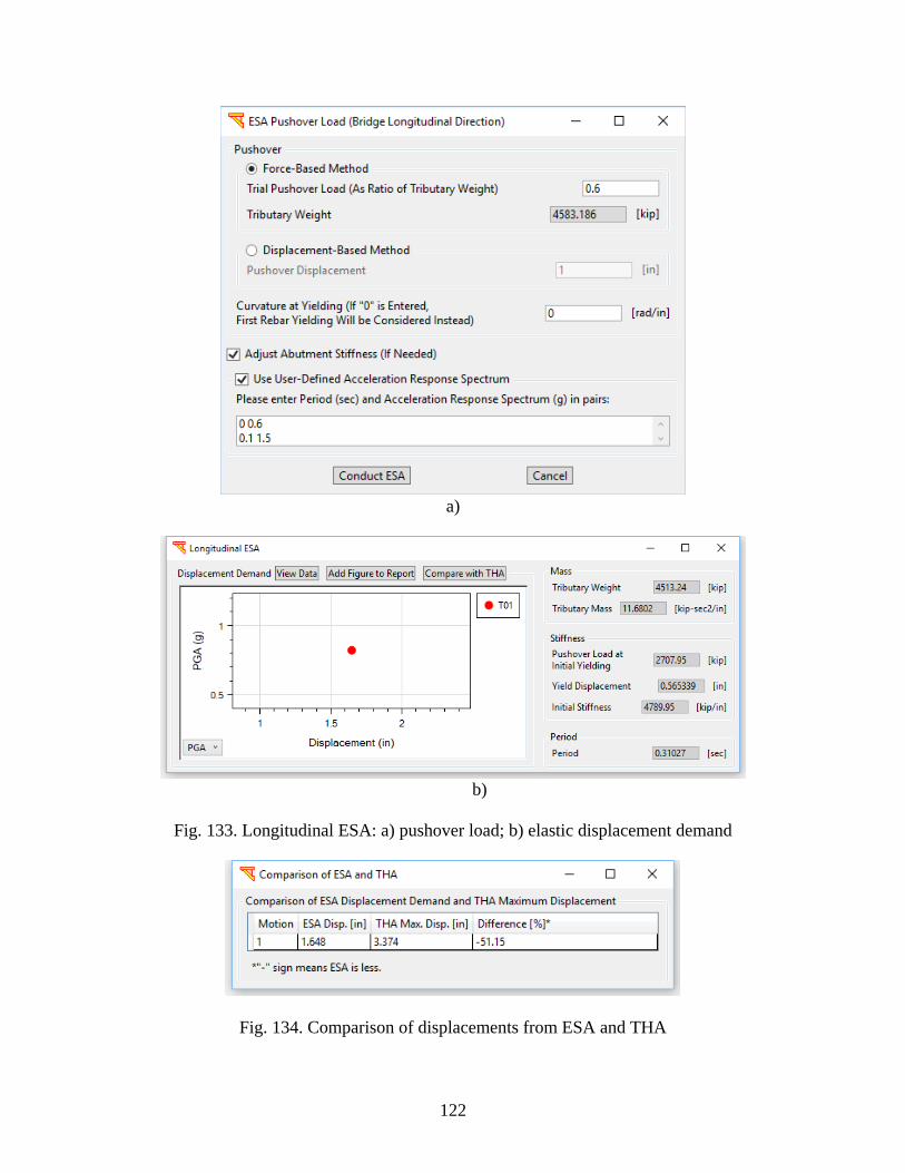
122

a)

b)

Fig. 133. Longitudinal ESA: a) pushover load; b) elastic displacement demand

Fig. 134. Comparison of displacements from ESA and THA

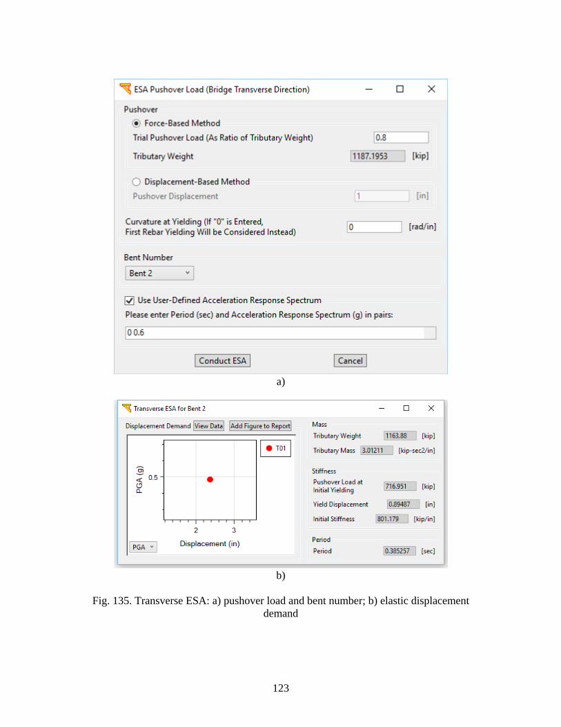
123

a)

b)

Fig. 135. Transverse ESA: a) pushover load and bent number; b) elastic displacement

demand

124

10 ANALYSIS OF IMPOSED DISPLACEMENTS

10.1 Imposed Soil Displacement

Imposed displacement option is available in MSBridge to study the soil movement for the

bridge longitudinal, transverse and vertical directions. This option has been added to

perform the pushover analysis with varying displacements along the pile height.

Therefore, soil springs foundation model must be selected to activate this option. As

such, the deformation due to liquefaction-induced lateral spreading can be applied as per

Caltrans guidelines found in MTD 20-15 (Caltrans 2017).

To conduct the pushover analysis of soil movements, click Imposed Displacement in the

main window (Fig. 2). The soil displacement profile layout is shown in Fig. 136.

According to the simplified procedure (Caltrans 2017), application of the permanent

lateral ground displacement follows the pattern displayed in Fig. 137, where the soil

above the liquefied layer moves as a rigid block (constant displacement) and the

displacement decreases constantly in the liquefied layer, with zero displacement below.

To define the normalized displacement profile, the displacement time history functions

should be first defined, click Define Time History Functions. As such, each function

corresponds to a value in the normalized displacement profile that will be reached after a

certain number of steps (Fig. 138a). By default, Function 1 and Zero Displacement are

defined for the values of unity and zero, respetively, then the user should define the

linearly interpolated functions along the thickness of the liquefied layer as according to

the existing soil spring nodes. After that, the functions should be assigned at different

nodes along the pile height (Fig. 138b). To do that, click Define Layout.

To account for a wide range of displacement values that resulted from applying different

input motions and different values for each bent. Click Define Displacement to enter the

displacement factors as according to the corresponding input motion (Fig. 139a) and click

Modify Displacement Factor to enter the bent location factors (Fig. 139b). Fig. 140

shows the output in terms of the bridge deformed shape and pile response profile.

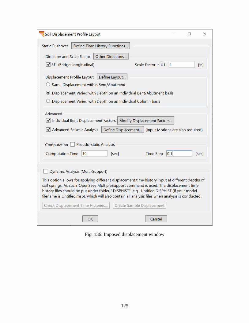
125

Fig. 136. Imposed displacement window

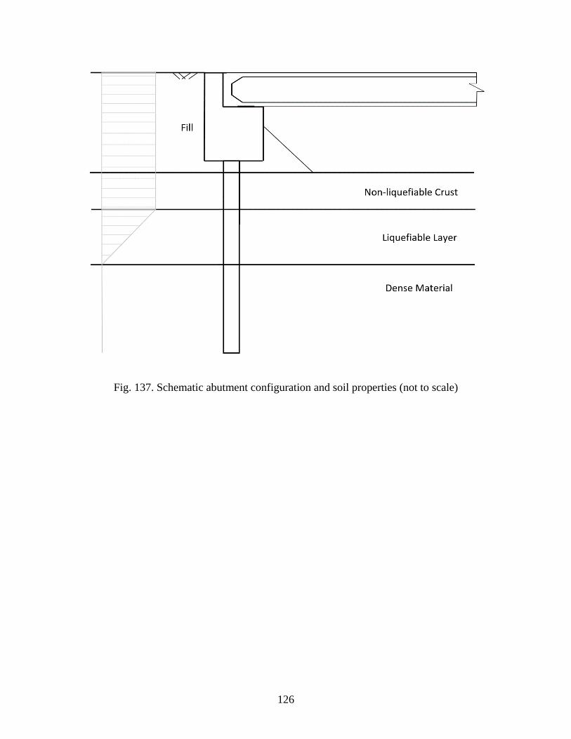
126

Fig. 137. Schematic abutment configuration and soil properties (not to scale)

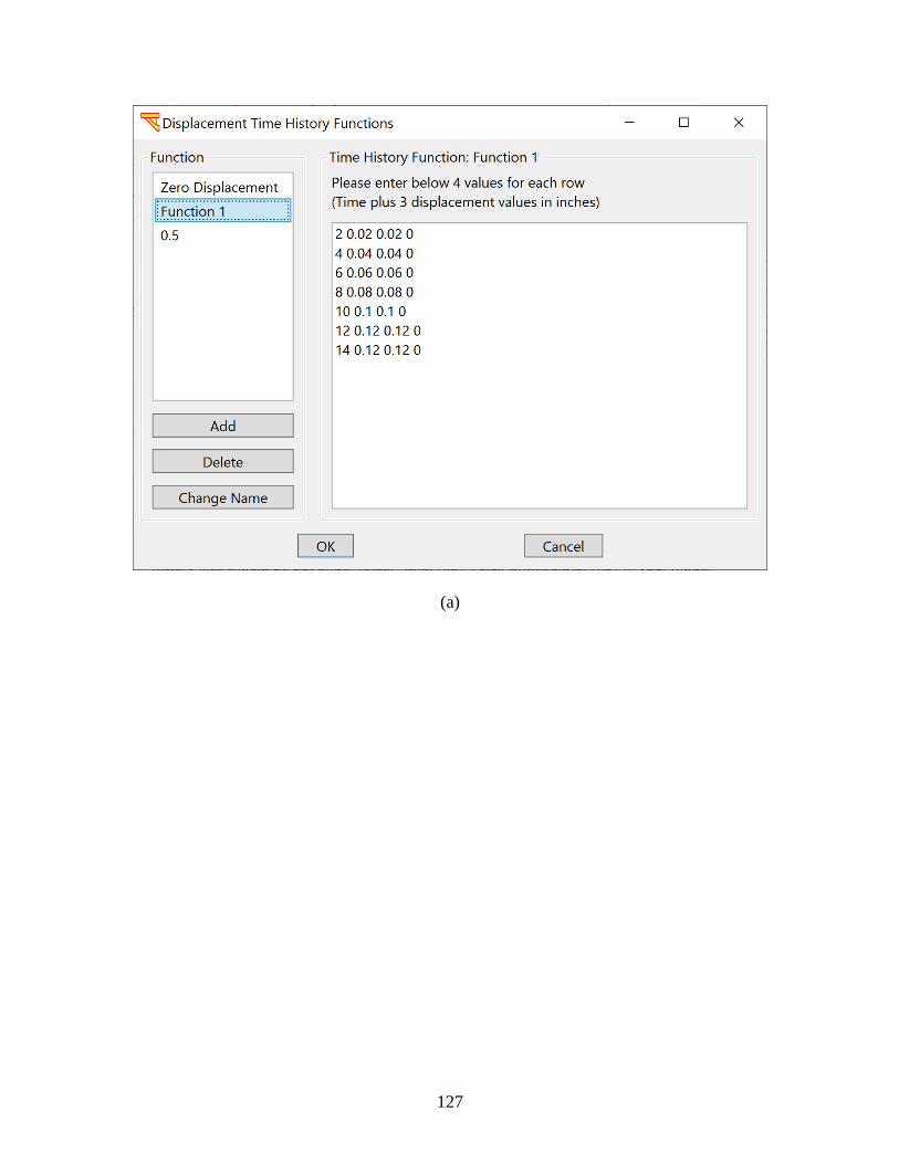
127

(a)

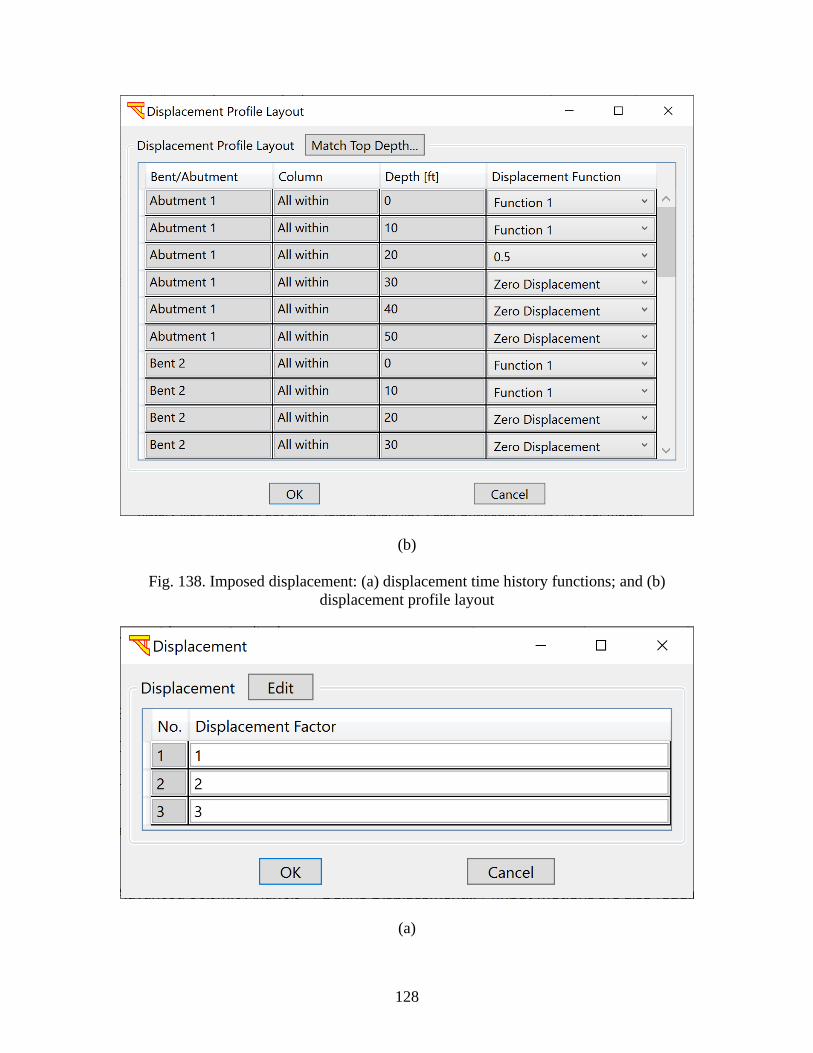
128

(b)

Fig. 138. Imposed displacement: (a) displacement time history functions; and (b)

displacement profile layout

(a)

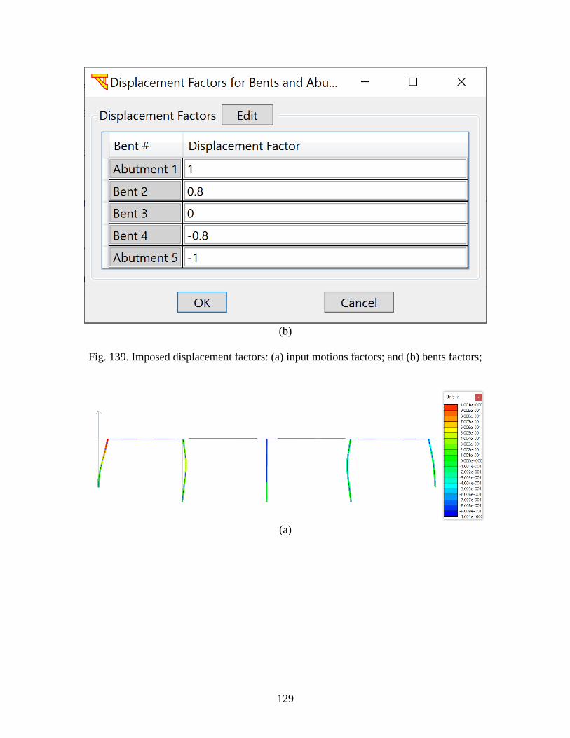
129

(b)

Fig. 139. Imposed displacement factors: (a) input motions factors; and (b) bents factors;

(a)

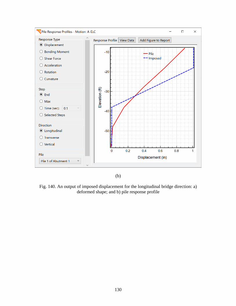
130

(b)

Fig. 140. An output of imposed displacement for the longitudinal bridge direction: a)

deformed shape; and b) pile response profile

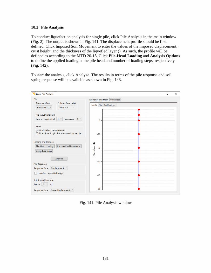
131

10.2 Pile Analysis

To conduct liquefaction analysis for single pile, click Pile Analysis in the main window

(Fig. 2). The output is shown in Fig. 141. The displacement profile should be first

defined. Click Imposed Soil Movement to enter the values of the imposed displacement,

crust height, and the thickness of the liquefied layer (). As such, the profile will be

defined as according to the MTD 20-15. Click Pile-Head Loading and Analysis Options

to define the applied loading at the pile head and number of loading steps, respectively

(Fig. 142).

To start the analysis, click Analyze. The results in terms of the pile response and soil

spring response will be available as shown in Fig. 143.

Fig. 141. Pile Analysis window

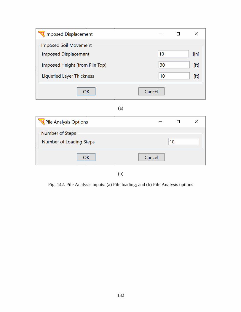
132

(a)

(b)

Fig. 142. Pile Analysis inputs: (a) Pile loading; and (b) Pile Analysis options

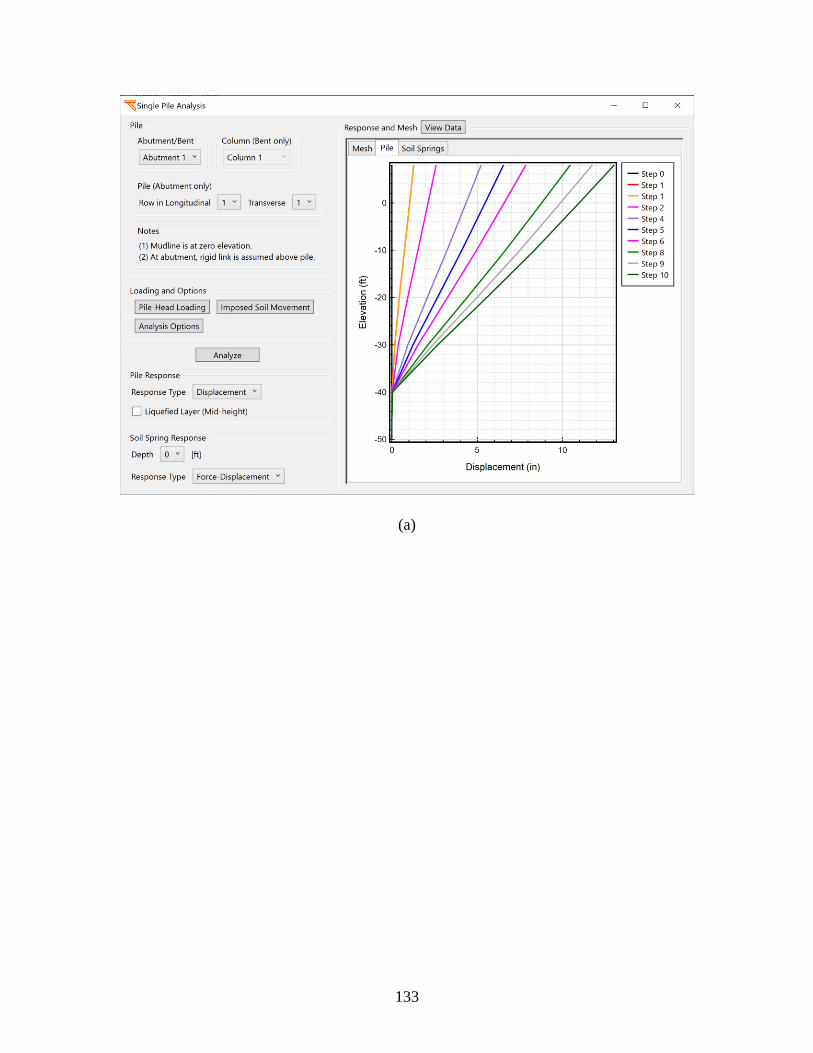
133

(a)

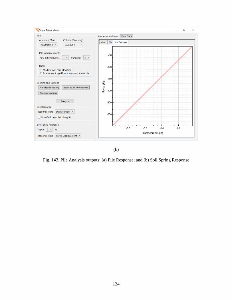
134

(b)

Fig. 143. Pile Analysis outputs: (a) Pile Response; and (b) Soil Spring Response

135

11 PBEE ANALYSIS (GROUND SHAKING)

To conduct a single earthquake analysis or a full PBEE analysis, click on the “Ground

Shaking” option under Analysis Type (Fig. 2). For that purpose, the input earthquake

excitation(s) must be specified. Input files at http://soilquake.net/msbridge that exercise

this option include Examples 2 and 4. If only one earthquake record is selected out of a

specified ensemble (suite) of input motions, then a conventional single earthquake

analysis will be performed.

11.1 Theory and Implementation of PBEE Analysis

In the user interface, an implementation of the Pacific Earthquake Engineering Research

(PEER) Center’s performance-based earthquake engineering framework (Cornell and

Krawinkler, 2000) is used to generate probabilistic estimates of repair cost and repair

time. The PEER PBEE framework utilizes the total probability theorem to compute the

desired probability distributions by disaggregating the task into several intermediate

probabilistic models with different sources of randomness and uncertainty. The hazard

model uses earthquake ground motion data to determine an intensity measure (IM). The

demand model uses response from dynamic analysis to determine an engineering demand

parameter (EDP). The damage model connects the EDP to a damage measure (DM).

Then, the DM is linked to consequences that are termed the decision variables (DV).

Repair cost and repair time can be thought of as two possible decision variable (DV)

outcomes characterized probabilistically by the framework.

The complete analysis is accomplished using the local linearization repair cost and time

methodology (LLRCAT), described by Mackie et al. (2010) and depicted conceptually in

Fig. 144. In the LLRCAT methodology, each bridge system is disaggregated into

independent structural or non-structural components or subassemblies defined as

performance groups (PGs) that are damaged, assessed, and repaired together using a

specific combination of different repair methods. Demands on the bridge system (and

components) are determined using 3D nonlinear time history analysis under multiple-

component earthquake excitation. The damage in each of the PGs is characterized

according to several discrete damage states (DSs) that are defined by distributions of

critical EDPs.

A feature of the LLRCAT implementation used is the introduction of a repair model

between the original PEER abstraction of DM and DV. Jumping directly from DMs to

repair costs is difficult to accomplish because it skips over the details of repair design and

the variability of cost and time estimating. Creating these two additional models makes it

easier to implement a step-by-step procedure for defining the models. The repair model

and cost model are created through the process of schematic design of repairs and

estimating the costs of those designs. Different repair methods are employed for the

various damage states of each PG or bridge component. The repair methods for each PG

require a combination of several repair quantities (Qs). Repair quantities for all PGs are

then combined with due consideration of the correlation between components. Repair

costs (RC) are obtained through a unit cost (UC). Repair times (RT) are obtained through

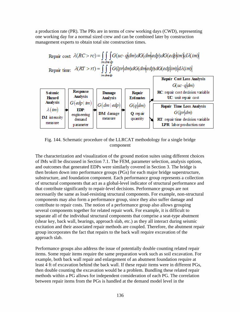
136

a production rate (PR). The PRs are in terms of crew working days (CWD), representing

one working day for a normal sized crew and can be combined later by construction

management experts to obtain total site construction times.

Fig. 144. Schematic procedure of the LLRCAT methodology for a single bridge

component

The characterization and visualization of the ground motion suites using different choices

of IMs will be discussed in Section 7.1. The FEM, parameter selection, analysis options,

and outcomes that generated EDPs were similarly covered in Section 3. The bridge is

then broken down into performance groups (PGs) for each major bridge superstructure,

substructure, and foundation component. Each performance group represents a collection

of structural components that act as a global-level indicator of structural performance and

that contribute significantly to repair-level decisions. Performance groups are not

necessarily the same as load-resisting structural components. For example, non-structural

components may also form a performance group, since they also suffer damage and

contribute to repair costs. The notion of a performance group also allows grouping

several components together for related repair work. For example, it is difficult to

separate all of the individual structural components that comprise a seat-type abutment

(shear key, back wall, bearings, approach slab, etc.) as they all interact during seismic

excitation and their associated repair methods are coupled. Therefore, the abutment repair

group incorporates the fact that repairs to the back wall require excavation of the

approach slab.

Performance groups also address the issue of potentially double counting related repair

items. Some repair items require the same preparation work such as soil excavation. For

example, both back wall repair and enlargement of an abutment foundation require at

least 4 ft of excavation behind the back wall. If these repair items were in different PGs,

then double counting the excavation would be a problem. Bundling these related repair

methods within a PG allows for independent consideration of each PG. The correlation

between repair items from the PGs is handled at the demand model level in the

137

methodology. A total of 11 PGs are considered: PG1: Max column drift ratio; PG2:

Residual column drift ratio; PG3: Max relative deck-end/abutment displacement (left);

PG4: Max relative deck-end/abutment displacement (right); PG5: Max bridge-abutment

bearing displacement (left); PG6: Max bridge-abutment bearing displacement (right);

PG7: Approach residual vertical displacement (left); PG8: Approach residual vertical

displacement (right); PG9: Abutment residual pile cap displacement (left); PG10:

Abutment residual pile top displacement (right); PG11: Column residual pile

displacement at ground surface.

Discrete DSs are defined for each PG. Damage states are numbered sequentially in order

of increasing severity. The DS0 damage state corresponds to the onset of damage when

repair costs begin to accumulate. An upper limit to the quantities and costs is called DS∞

because it corresponds to the most severe possible damage state for the elements in a PG.

DS∞ usually corresponds to complete failure and replacement of all the elements in the

entire PG. The DSs are connected to structural demands obtained from finite element

analysis results by way of an EDP specific to each PG. The repair quantities associated

with each DS are developed more fully in the definition of the damage scenarios. All the

PGs and DSs are linked to a single EDP in this implementation.

Based on previous work, the methodology was calibrated for defining the post-

earthquake performance of select bridges that fall within the class of ordinary post-

tensioned, box girder, reinforced concrete highway overpasses (Mackie et al. 2011). The

three major components required for this calibration were damage scenarios that describe

particular instances of earthquake damage, schematic design of bridge repairs to address

the state of damage in the scenarios, and the link between repair design, methods and

procedures, and subsequent quantities. There is a direct link between damage scenarios

and the repair, i.e., there is a single repair procedure for a single state of damage. The

repair quantity results were parameterized in terms of basic bridge geometry and

properties so that they can be used to extrapolate loss modeling for other bridges in the

same class (such as those that can be built within the user interface).

Data for time and monetary repair costs were obtained by estimating the costs of the

damage and loss scenarios using published Caltrans construction estimation data, case

studies from previous earthquakes, and interviews with Caltrans bridge engineers.

Monetary costs were adjusted to 2007 values based on Caltrans cost index data. Repair

costs are estimated for each damage scenario based on quantities of each repair item.

Cost estimates accounted for variations in unit cost, and the details involved in estimating

a combination of repairs together. The benefit of separating the Qs from costs is that the

unit cost model is easily updated for new years of data, local economic conditions, site

accessibility, and incentives.

Normalized costs of repair are obtained by using the repair cost ratio (RCR) between the

cost of repair and the cost of replacement cost (does not include demolition). It is shown

in %, and it can range between 0 and some number higher than 100% (there is no reason

why it is bounded by replacement cost; this is purely an owner/operator decision). This

ratio is useful for comparing the performance of different bridge design options for new

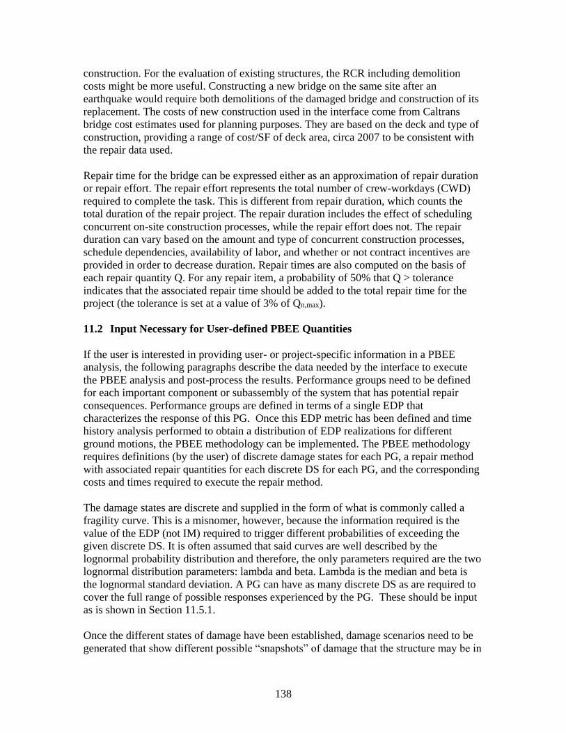
138

construction. For the evaluation of existing structures, the RCR including demolition

costs might be more useful. Constructing a new bridge on the same site after an

earthquake would require both demolitions of the damaged bridge and construction of its

replacement. The costs of new construction used in the interface come from Caltrans

bridge cost estimates used for planning purposes. They are based on the deck and type of

construction, providing a range of cost/SF of deck area, circa 2007 to be consistent with

the repair data used.

Repair time for the bridge can be expressed either as an approximation of repair duration

or repair effort. The repair effort represents the total number of crew-workdays (CWD)

required to complete the task. This is different from repair duration, which counts the

total duration of the repair project. The repair duration includes the effect of scheduling

concurrent on-site construction processes, while the repair effort does not. The repair

duration can vary based on the amount and type of concurrent construction processes,

schedule dependencies, availability of labor, and whether or not contract incentives are

provided in order to decrease duration. Repair times are also computed on the basis of

each repair quantity Q. For any repair item, a probability of 50% that Q > tolerance

indicates that the associated repair time should be added to the total repair time for the

project (the tolerance is set at a value of 3% of Qn,max).

11.2 Input Necessary for User-defined PBEE Quantities

If the user is interested in providing user- or project-specific information in a PBEE

analysis, the following paragraphs describe the data needed by the interface to execute

the PBEE analysis and post-process the results. Performance groups need to be defined

for each important component or subassembly of the system that has potential repair

consequences. Performance groups are defined in terms of a single EDP that

characterizes the response of this PG. Once this EDP metric has been defined and time

history analysis performed to obtain a distribution of EDP realizations for different

ground motions, the PBEE methodology can be implemented. The PBEE methodology

requires definitions (by the user) of discrete damage states for each PG, a repair method

with associated repair quantities for each discrete DS for each PG, and the corresponding

costs and times required to execute the repair method.

The damage states are discrete and supplied in the form of what is commonly called a

fragility curve. This is a misnomer, however, because the information required is the

value of the EDP (not IM) required to trigger different probabilities of exceeding the

given discrete DS. It is often assumed that said curves are well described by the

lognormal probability distribution and therefore, the only parameters required are the two

lognormal distribution parameters: lambda and beta. Lambda is the median and beta is

the lognormal standard deviation. A PG can have as many discrete DS as are required to

cover the full range of possible responses experienced by the PG. These should be input

as is shown in Section 11.5.1.

Once the different states of damage have been established, damage scenarios need to be

generated that show different possible “snapshots” of damage that the structure may be in

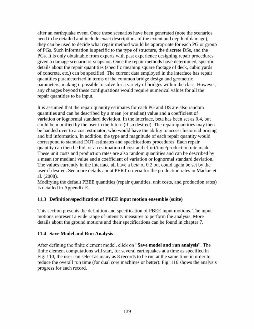
139

after an earthquake event. Once these scenarios have been generated (note the scenarios

need to be detailed and include exact descriptions of the extent and depth of damage),

they can be used to decide what repair method would be appropriate for each PG or group

of PGs. Such information is specific to the type of structure, the discrete DSs, and the

PGs. It is only obtainable from experts with past experience designing repair procedures

given a damage scenario or snapshot. Once the repair methods have determined, specific

details about the repair quantities (specific meaning square footage of deck, cubic yards

of concrete, etc.) can be specified. The current data employed in the interface has repair

quantities parameterized in terms of the common bridge design and geometric

parameters, making it possible to solve for a variety of bridges within the class. However,

any changes beyond these configurations would require numerical values for all the

repair quantities to be input.

It is assumed that the repair quantity estimates for each PG and DS are also random

quantities and can be described by a mean (or median) value and a coefficient of

variation or lognormal standard deviation. In the interface, beta has been set as 0.4, but

could be modified by the user in the future (if so desired). The repair quantities may then

be handed over to a cost estimator, who would have the ability to access historical pricing

and bid information. In addition, the type and magnitude of each repair quantity would

correspond to standard DOT estimates and specifications procedures. Each repair

quantity can then be bid, or an estimation of cost and effort/time/production rate made.

These unit costs and production rates are also random quantities and can be described by

a mean (or median) value and a coefficient of variation or lognormal standard deviation.

The values currently in the interface all have a beta of 0.2 but could again be set by the

user if desired. See more details about PERT criteria for the production rates in Mackie et

al. (2008).

Modifying the default PBEE quantities (repair quantities, unit costs, and production rates)

is detailed in Appendix E.

11.3 Definition/specification of PBEE input motion ensemble (suite)

This section presents the definition and specification of PBEE input motions. The input

motions represent a wide range of intensity measures to perform the analysis. More

details about the ground motions and their specifications can be found in chapter 7.

11.4 Save Model and Run Analysis

After defining the finite element model, click on “Save model and run analysis”. The

finite element computations will start, for several earthquakes at a time as specified in

Fig. 110, the user can select as many as 8 records to be run at the same time in order to

reduce the overall run time (for dual core machines or better). Fig. 116 shows the analysis

progress for each record.

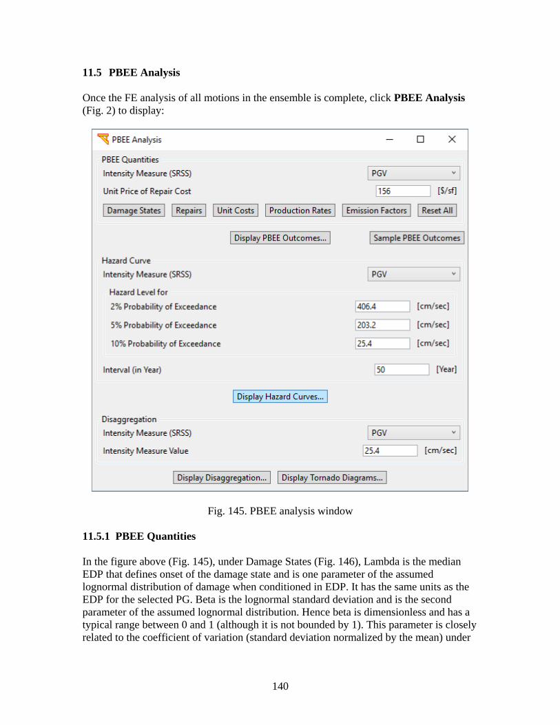
140

11.5 PBEE Analysis

Once the FE analysis of all motions in the ensemble is complete, click PBEE Analysis

(Fig. 2) to display:

Fig. 145. PBEE analysis window

11.5.1 PBEE Quantities

In the figure above (Fig. 145), under Damage States (Fig. 146), Lambda is the median

EDP that defines onset of the damage state and is one parameter of the assumed

lognormal distribution of damage when conditioned in EDP. It has the same units as the

EDP for the selected PG. Beta is the lognormal standard deviation and is the second

parameter of the assumed lognormal distribution. Hence beta is dimensionless and has a

typical range between 0 and 1 (although it is not bounded by 1). This parameter is closely

related to the coefficient of variation (standard deviation normalized by the mean) under

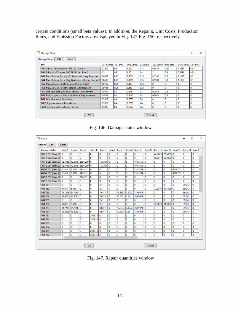
141

certain conditions (small beta values). In addition, the Repairs, Unit Costs, Production

Rates, and Emission Factors are displayed in Fig. 147-Fig. 150, respectively.

Fig. 146. Damage states window

Fig. 147. Repair quantities window

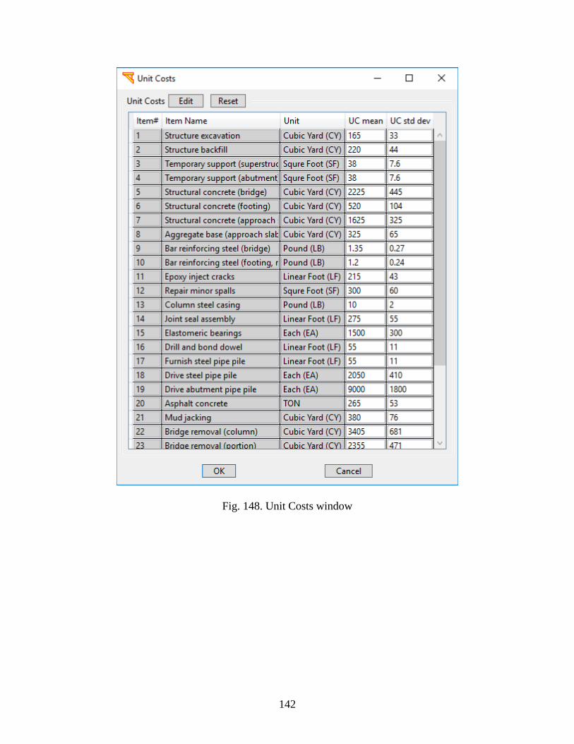
142

Fig. 148. Unit Costs window

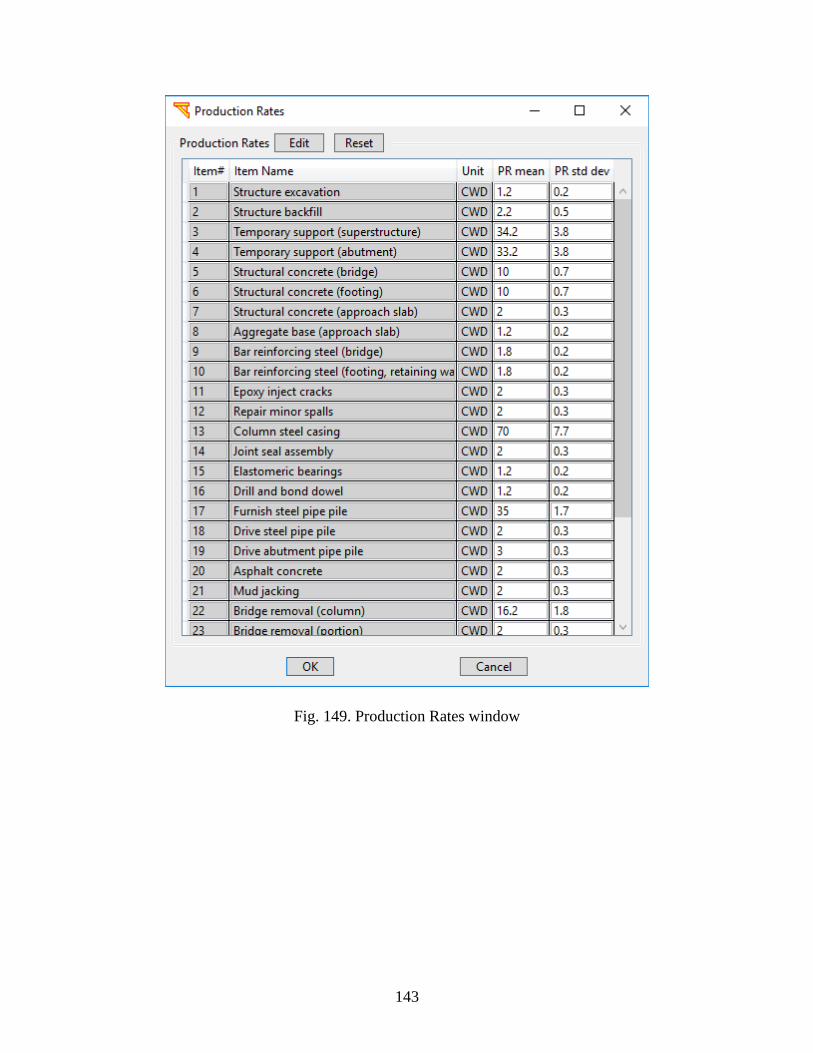
143

Fig. 149. Production Rates window

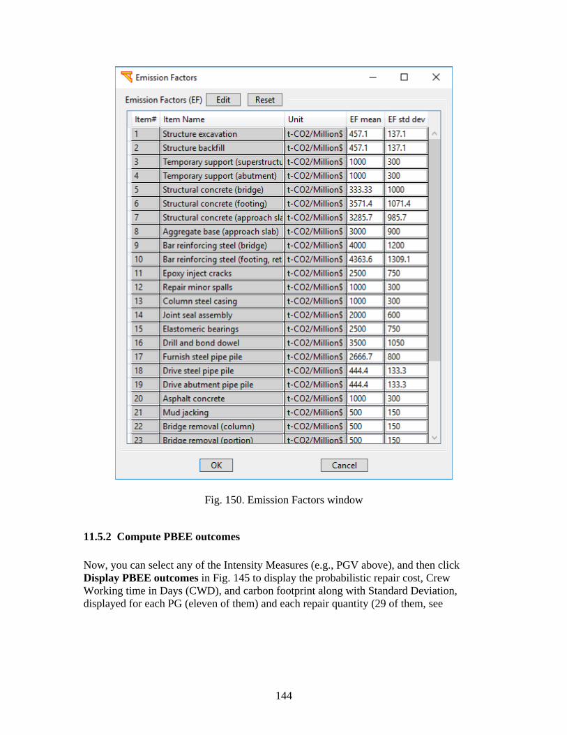
144

Fig. 150. Emission Factors window

11.5.2 Compute PBEE outcomes

Now, you can select any of the Intensity Measures (e.g., PGV above), and then click

Display PBEE outcomes in Fig. 145 to display the probabilistic repair cost, Crew

Working time in Days (CWD), and carbon footprint along with Standard Deviation,

displayed for each PG (eleven of them) and each repair quantity (29 of them, see

145

Table 6), as shown below. See Section 12.3.1 for the detailed output.

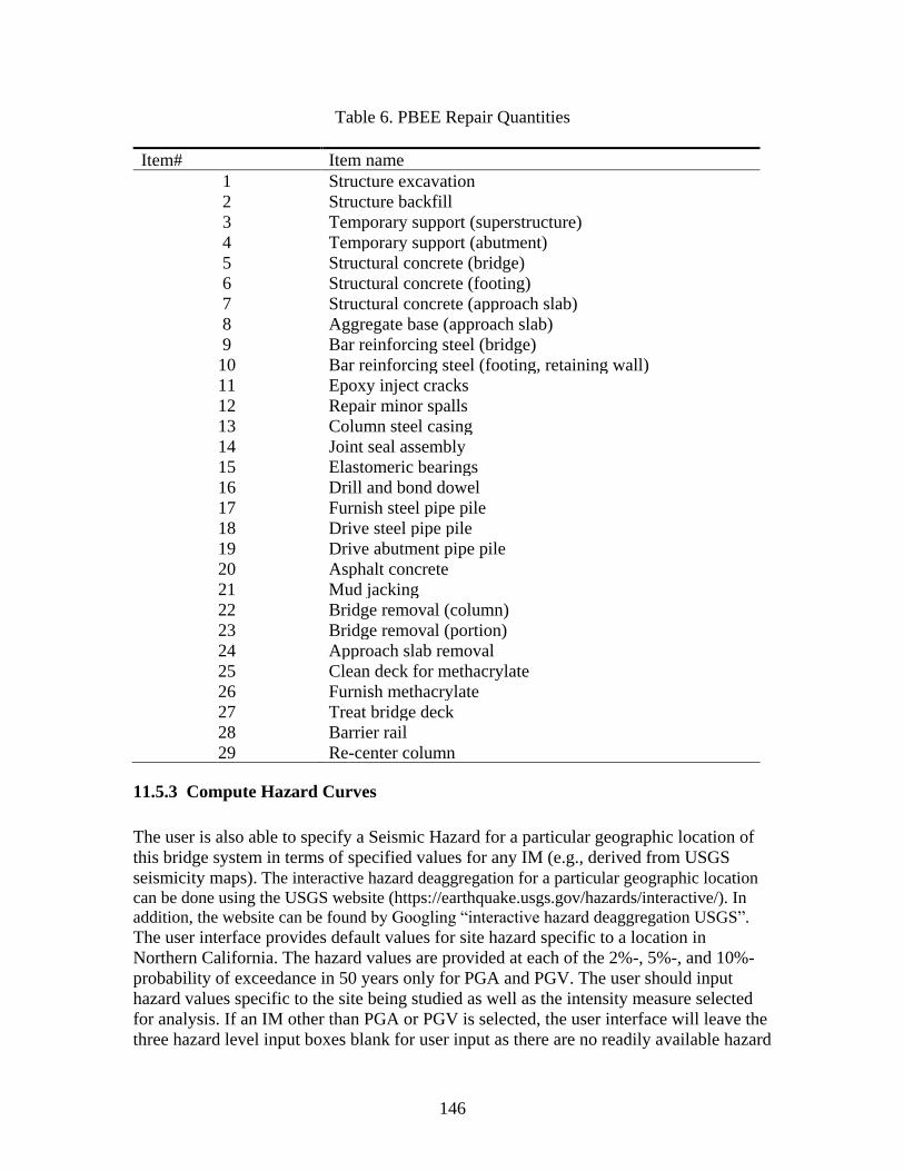
146

Table 6. PBEE Repair Quantities

Item# Item name

1 Structure excavation

2 Structure backfill

3 Temporary support (superstructure)

4 Temporary support (abutment)

5 Structural concrete (bridge)

6 Structural concrete (footing)

7 Structural concrete (approach slab)

8 Aggregate base (approach slab)

9 Bar reinforcing steel (bridge)

10 Bar reinforcing steel (footing, retaining wall)

11 Epoxy inject cracks

12 Repair minor spalls

13 Column steel casing

14 Joint seal assembly

15 Elastomeric bearings

16 Drill and bond dowel

17 Furnish steel pipe pile

18 Drive steel pipe pile

19 Drive abutment pipe pile

20 Asphalt concrete

21 Mud jacking

22 Bridge removal (column)

23 Bridge removal (portion)

24 Approach slab removal

25 Clean deck for methacrylate

26 Furnish methacrylate

27 Treat bridge deck

28 Barrier rail

29 Re-center column

11.5.3 Compute Hazard Curves

The user is also able to specify a Seismic Hazard for a particular geographic location of

this bridge system in terms of specified values for any IM (e.g., derived from USGS

seismicity maps). The interactive hazard deaggregation for a particular geographic location

can be done using the USGS website (https://earthquake.usgs.gov/hazards/interactive/). In

addition, the website can be found by Googling “interactive hazard deaggregation USGS”.

The user interface provides default values for site hazard specific to a location in

Northern California. The hazard values are provided at each of the 2%-, 5%-, and 10%-

probability of exceedance in 50 years only for PGA and PGV. The user should input

hazard values specific to the site being studied as well as the intensity measure selected

for analysis. If an IM other than PGA or PGV is selected, the user interface will leave the

three hazard level input boxes blank for user input as there are no readily available hazard

147

maps or conversions from PGA for an arbitrary IM. The default PGA hazard values were

obtained from USGS hazard maps. These PGA values were converted to PGV values

using the firm ground conversion of 48 in./sec/g. It is not meant to imply that switching

between PGA and PGV (or any other IM) will yield equal hazard.

Once a desired local site seismicity is defined, users can click Display Hazard Curves

(Fig. 145) to display the mean annual frequency of exceedance and return period. Please

see Section 12.3.2 for the detailed output.

11.5.4 Compute Disaggregation

Users can also click Display Disaggregation (Fig. 145) to display the disaggregation by

performance groups and repair quantities. Please see Section 12.3.3 for the detailed

output. Only the disaggregation of the expected repair cost/time by performance group is

possible due to the LLRCAT formulation. However, both expected, and variance

disaggregation plots are available when disaggregating by repair quantity. The user can

select the intensity measure and value on which to disaggregate. The default value is a

PGV value equal to the 10% probability of exceedance in 50 years specified in the

previous section.

148

12 TIME HISTORY AND PBEE OUTPUT

This section presents the time history results after the FE analysis phase that are used to

calculate the EDP values needed for the PBEE outcomes.

12.1 Time History Output Quantities

At the end of the FE analysis phase, time histories and bridge responses will be available

of the form:

v) Column Response Time Histories and Profiles

vi) Column Response Relationships

vii) Abutment Responses

viii) Deformed Mesh

In addition, for PBEE analysis scenarios, Intensity Measures (IMs) and response spectra

for each input motion are calculated and are available for display in Table and Figure

formats. Performance Group (PG) Quantities and Bridge peak accelerations for all

employed shaking motions are also available for display against any of the computed

IMs.

The post-processing capabilities can be accessed from Menu Display (Fig. 4). Fig. 151

shows the post-processing capabilities available in a base shaking analysis, respectively.

More details about the time history outputs can be found in chapter 8.

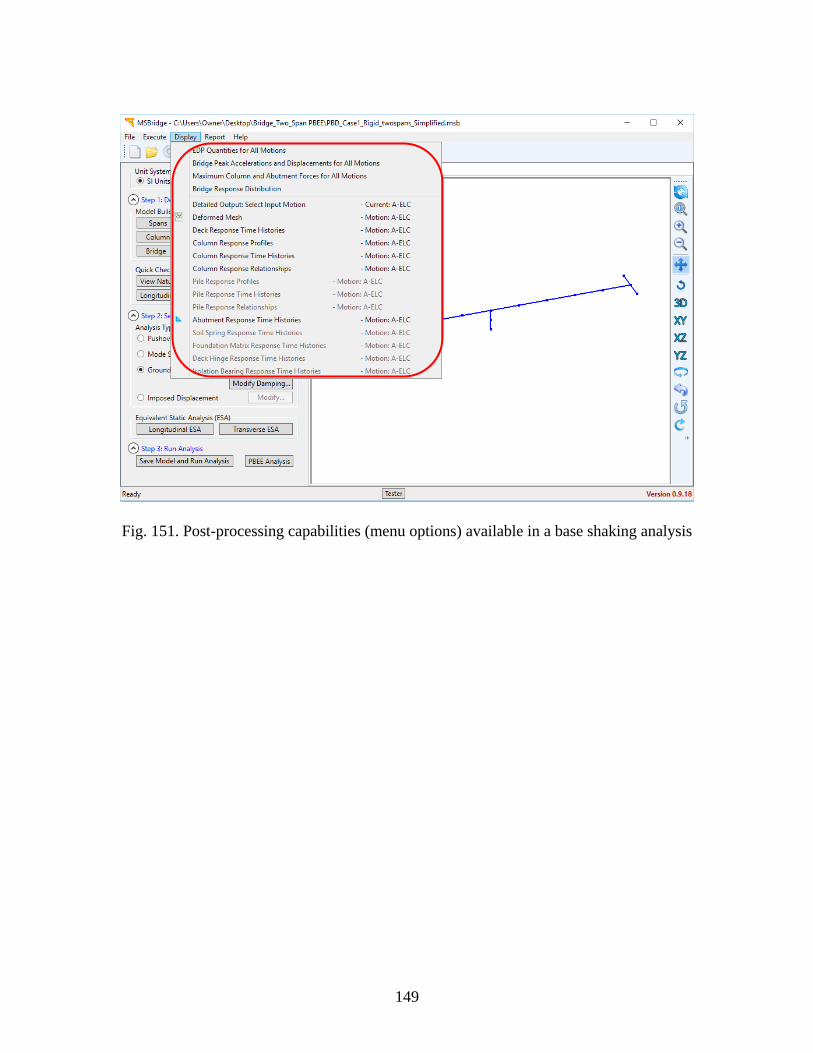
149

Fig. 151. Post-processing capabilities (menu options) available in a base shaking analysis

150

12.2 PBEE Output Quantities

At the end of the finite element analysis phase, the following output performance group

quantities (for each earthquake record) are used in the next phase of PBEE analysis:

Table 7. PBEE Performance Groups

Performance Group

(PG) # Performance group names

1 Maximum column drift ratio

2 Residual column drift ratio

3 Maximum relative deck-end/abutment displacement (left)

4 Maximum relative deck-end/abutment displacement (right)

5 Maximum bridge-abutment bearing displacement (left)

6 Maximum bridge-abutment bearing displacement (right)

7 Approach residual vertical displacement (left)

8 Approach residual vertical displacement (right)

9 Abutment residual pile cap displacement (left)

10 Abutment residual pile top displacement (right)

11 Column residual pile displacement at ground surface

To account for the multi-span extension for the framework, the following notation (Eq. 4)

is used for PG1, PG2, and PG11:

𝑃𝐺𝑖 − 𝑗 (4)

where i refers to the PG # as defined in Table 7, and j refers to column #.

In addition, Intensity Measures for the computed Free Field ground surface acceleration

records are computed, so that outcomes can be either shown against the input base

shaking IMs or the computed ground surface IMs (noted as Free-Field in the user

interface). The sections below detail how the response quantities are obtained for each

PG.

PG1: Maximum tangential drift ratio SRSS (column)

PG2: Residual tangential drift ratio SRSS (column)

The tangential drift ratio is defined as the maximum of a) displacement above the

inflection point divided by the length of this distance, and b) displacement below the

inflection point divided by the length of this distance. This takes care of rotation at the

base, different boundary conditions, etc., so that the results are consistent when

computing damage. The Square Root of Sum of Squares (SRSS) values of the two

horizontal components are used. The tangential drift ratios are combined separately at

each time step (to obtain SRSS).

151

PG1 (Max tangential drift ratio SRSS) is the maximum of the SRSS values of all time

steps. PG2 (Residual tangential drift ratio SRSS) is the SRSS value at the last time step.

The tangential drift ratio is in percentage.

To calculate the tangential drift ratio, the following 2 lines were added into the tcl file:

recorder Element -file A-ELC.dft -time -ele $columnEle tangentDrift

recorder Element -file A-ELC.ifp -time -ele $columnEle inflectionPoint

where $columnEle is the element # of the column (Only one forced-based beam-column

element nonlinearBeamColumn is used for the column). In the .dft file, there will be

five columns of data for each time step, and the first column is time. In the .ifp file, there

will be three columns for each time step, and the first column is also time.

Subsequently, the tangential drift ratio is calculated using the code snippet shown in Fig.

152. For the tangential drift ratio in the longitudinal direction (X-direction or bridge

longitudinal direction), the tdx1 and tdx2 variables are the second and third column (the

first column is time), respectively, of the tangential drift recorder file (e.g., A-ELC.dft).

The tdxi variable is the second column (the first column is time) of the inflection point

recorder file (e.g., A-ELC.ifp).

For the transverse tangential drift ratio, the tdx1 and tdx2 variables are the fourth and

fifth column of the .dft file and the tdxi variable is the third column of the .ifp file.

Fig. 152. Code snippet to calculate the tangential drift ratio of column

PG3: Maximum longitudinal relative deck-end/abutment displacement (left)

PG4: Maximum longitudinal relative deck-end/abutment displacement (right)

// tdx1 & tdx2 -- the tangent drift recorder file at time step i

// tdxi -- the inflection point recorder at time step i

// tdx – tangential drift ratio

if( fabs(tdxi) < 1e-20 ) {

tdx = -tdx2/(H - tdxi);

}

else if ( fabs(H-tdxi) < 1e-20 ) {

tdx = -tdx1 / tdxi;

}

else {

tdx = __max(fabs(tdx1/tdxi), fabs(tdx2/(H-tdxi)));

//tdx = -tdx*sgn(tdx2/(H-tdxi));

if( fabs(tdx2/(H-tdxi)) < 1e-20 )

tdx = 0;

else if( (tdx2/(H-tdxi)) > 0)

tdx = -tdx;

}

return tdx;

152

These two PGs are intended to address the issue of abutment impact into the backwall, so

they are defined as only the motion of the deck into the abutment. Maximum absolute

values in the longitudinal direction are used.

For example, for the right abutment, it is the relative longitudinal displacement of node B

(deck-end node) in the direction of node C (abutment top node). A zero value is used for

the times during which the deck-end node moves away from the abutment top node.

PG5: Maximum absolute bearing displacement (left abutment)

PG6: Maximum absolute bearing displacement (right abutment)

These two PGs are intended to address bearing damage whether or not an explicit

representation of the bearings is included in the user-selected abutment model. Therefore,

the EDP for the PG is based on the relative displacements of the deck-end node to the

abutment top node. The SRSS values of the resulting two relative horizontal

displacements are used, and both motions into the backwall and away from the backwall

are considered.

PG7: Residual vertical displacement (left abutment)

PG8: Residual vertical displacement (right abutment)

This PG is used to gauge immediate repairs for rideability and is not a measure of the

permanent slumping of the embankment (for example). Therefore, the EDP is calculated

as the vertical displacement of the abutment top node relative to the deck-end node. The

residual value is used (value at the final time step).

PG9: Residual pile cap displacement SRSS (left abutment)

PG10: Residual pile cap displacement SRSS (right abutment)

These PGs address possible damage below grade due to lateral translation of the piles and

pile caps. While not a direct measure, pile cap displacement was selected as it would not

require knowledge or observations of piles below grade. The EDP is defined by

calculating the SRSS value of the 2 horizontal displacements of the abutment pile cap

node. The residual is obtained from the value at the final time step.

PG11: Residual pile cap displacement SRSS (column)

This quantity is analogous to the two previous PG but is representative of response and

damage at the abutment foundations. The EDP is obtained by calculating the SRSS value

of the 2 horizontal displacements of the column pile cap node and taking the value at the

final time step.

The PG (Performance Group) quantities for all input motions can be accessed by clicking

menu Display (Fig. 4) and then PG Quantities for All Motion (Fig. 153). The window

to display PG quantities is shown in Fig. 154.

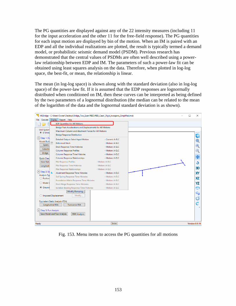
153

The PG quantities are displayed against any of the 22 intensity measures (including 11

for the input acceleration and the other 11 for the free-field response). The PG quantities

for each input motion are displayed by bin of the motion. When an IM is paired with an

EDP and all the individual realizations are plotted, the result is typically termed a demand

model, or probabilistic seismic demand model (PSDM). Previous research has

demonstrated that the central values of PSDMs are often well described using a power-

law relationship between EDP and IM. The parameters of such a power-law fit can be

obtained using least squares analysis on the data. Therefore, when plotted in log-log

space, the best-fit, or mean, the relationship is linear.

The mean (in log-log space) is shown along with the standard deviation (also in log-log

space) of the power-law fit. If it is assumed that the EDP responses are lognormally

distributed when conditioned on IM, then these curves can be interpreted as being defined

by the two parameters of a lognormal distribution (the median can be related to the mean

of the logarithm of the data and the lognormal standard deviation is as shown).

Fig. 153. Menu items to access the PG quantities for all motions

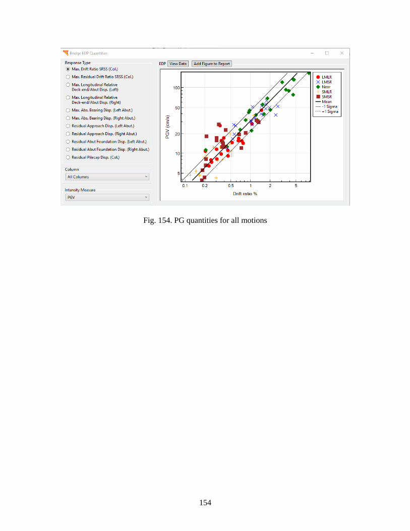
154

Fig. 154. PG quantities for all motions

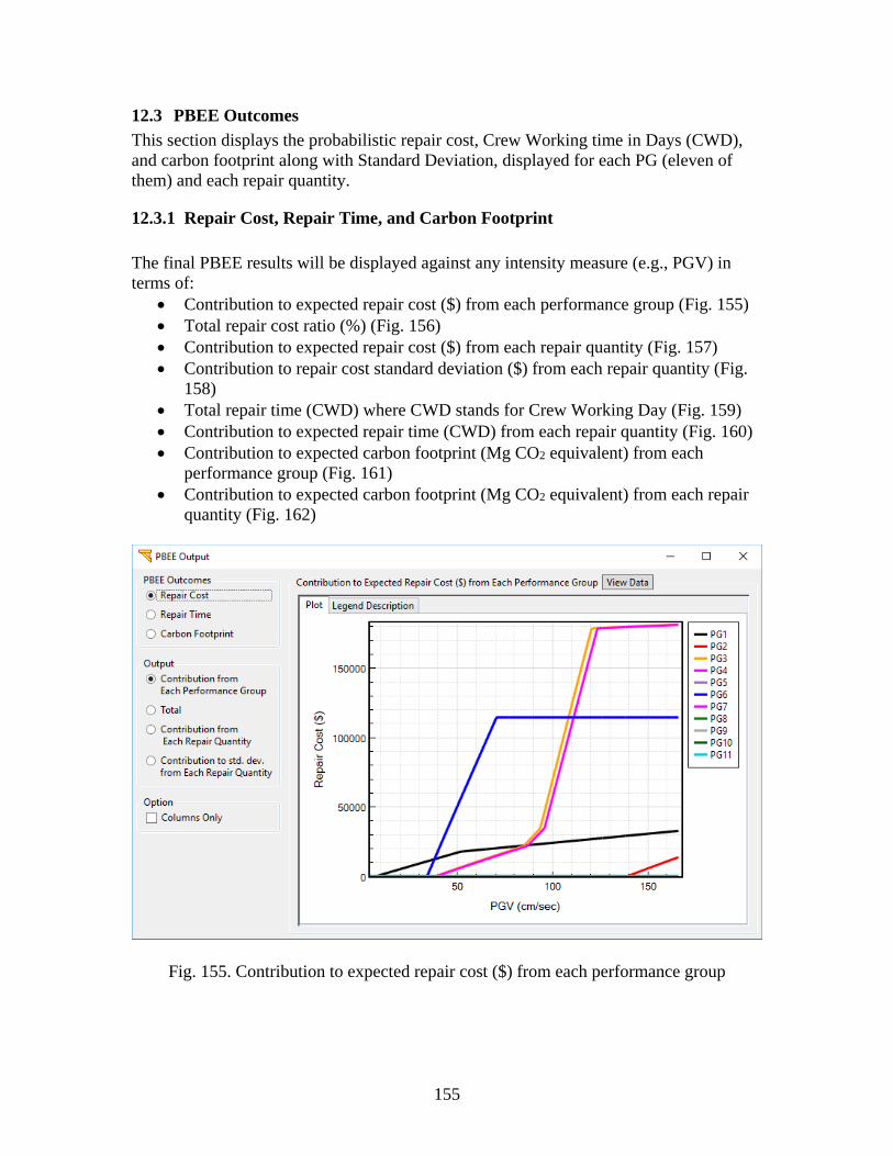
155

12.3 PBEE Outcomes

This section displays the probabilistic repair cost, Crew Working time in Days (CWD),

and carbon footprint along with Standard Deviation, displayed for each PG (eleven of

them) and each repair quantity.

12.3.1 Repair Cost, Repair Time, and Carbon Footprint

The final PBEE results will be displayed against any intensity measure (e.g., PGV) in

terms of:

• Contribution to expected repair cost ($) from each performance group (Fig. 155)

• Total repair cost ratio (%) (Fig. 156)

• Contribution to expected repair cost ($) from each repair quantity (Fig. 157)

• Contribution to repair cost standard deviation ($) from each repair quantity (Fig.

158)

• Total repair time (CWD) where CWD stands for Crew Working Day (Fig. 159)

• Contribution to expected repair time (CWD) from each repair quantity (Fig. 160)

• Contribution to expected carbon footprint (Mg CO2 equivalent) from each

performance group (Fig. 161)

• Contribution to expected carbon footprint (Mg CO2 equivalent) from each repair

quantity (Fig. 162)

Fig. 155. Contribution to expected repair cost ($) from each performance group

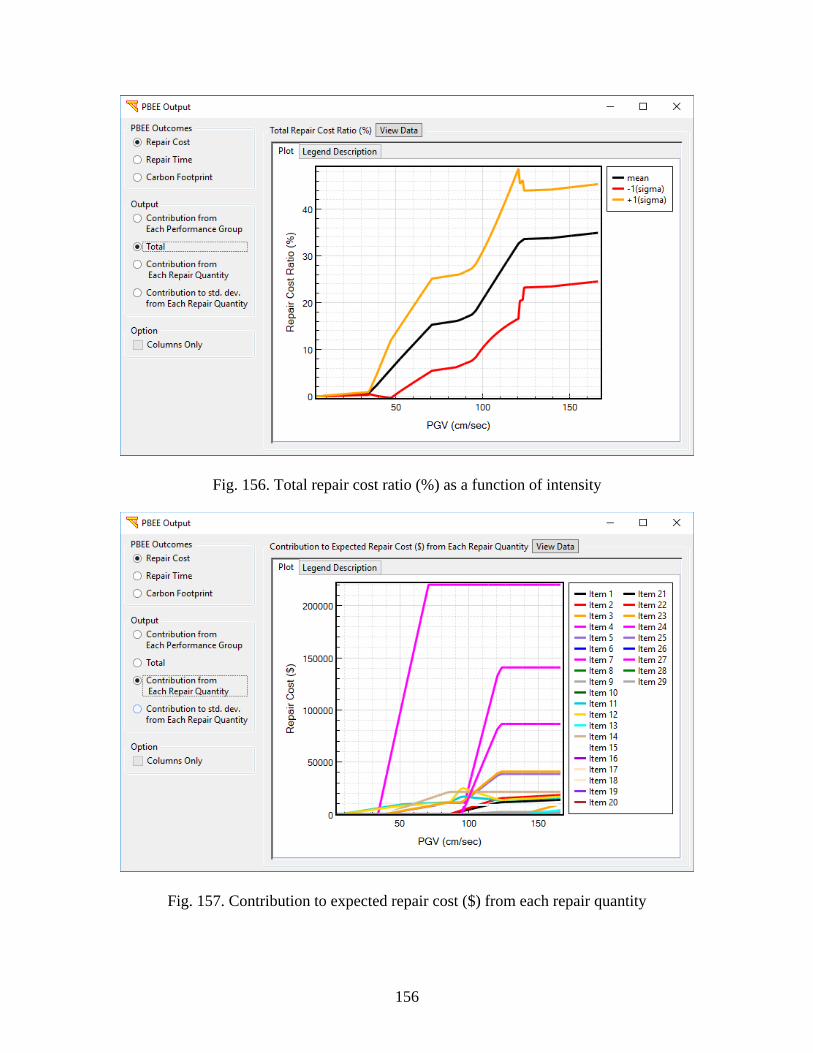
156

Fig. 156. Total repair cost ratio (%) as a function of intensity

Fig. 157. Contribution to expected repair cost ($) from each repair quantity

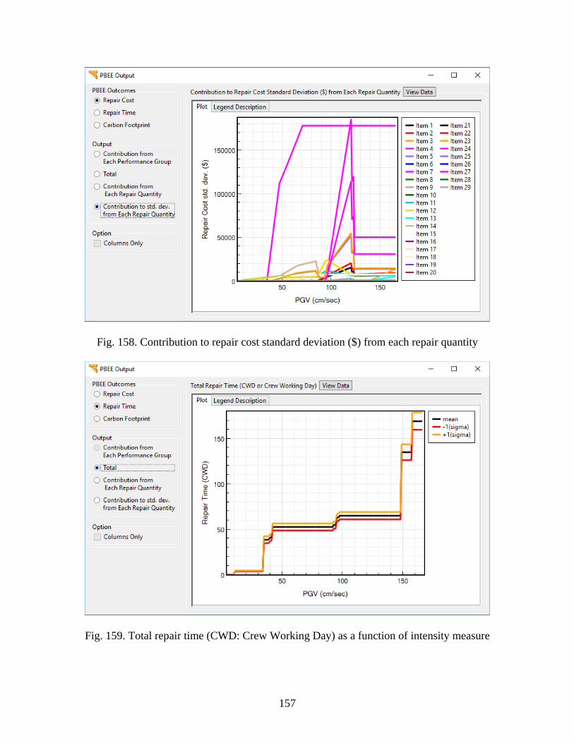
157

Fig. 158. Contribution to repair cost standard deviation ($) from each repair quantity

Fig. 159. Total repair time (CWD: Crew Working Day) as a function of intensity measure

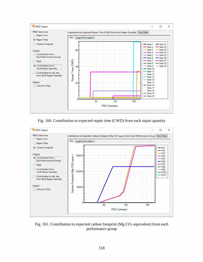
158

Fig. 160. Contribution to expected repair time (CWD) from each repair quantity

Fig. 161. Contribution to expected carbon footprint (Mg CO2 equivalent) from each

performance group

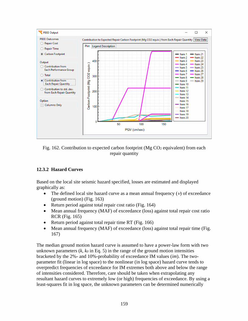
159

Fig. 162. Contribution to expected carbon footprint (Mg CO2 equivalent) from each

repair quantity

12.3.2 Hazard Curves

Based on the local site seismic hazard specified, losses are estimated and displayed

graphically as:

• The defined local site hazard curve as a mean annual frequency () of exceedance

(ground motion) (Fig. 163)

• Return period against total repair cost ratio (Fig. 164)

• Mean annual frequency (MAF) of exceedance (loss) against total repair cost ratio

RCR (Fig. 165)

• Return period against total repair time RT (Fig. 166)

• Mean annual frequency (MAF) of exceedance (loss) against total repair time (Fig.

167)

The median ground motion hazard curve is assumed to have a power-law form with two

unknown parameters (k, k0 in Eq. 5) in the range of the ground motion intensities

bracketed by the 2%- and 10%-probability of exceedance IM values (im). The two-

parameter fit (linear in log space) to the nonlinear (in log space) hazard curve tends to

overpredict frequencies of exceedance for IM extremes both above and below the range

of intensities considered. Therefore, care should be taken when extrapolating any

resultant hazard curves to extremely low (or high) frequencies of exceedance. By using a

least-squares fit in log space, the unknown parameters can be determined numerically

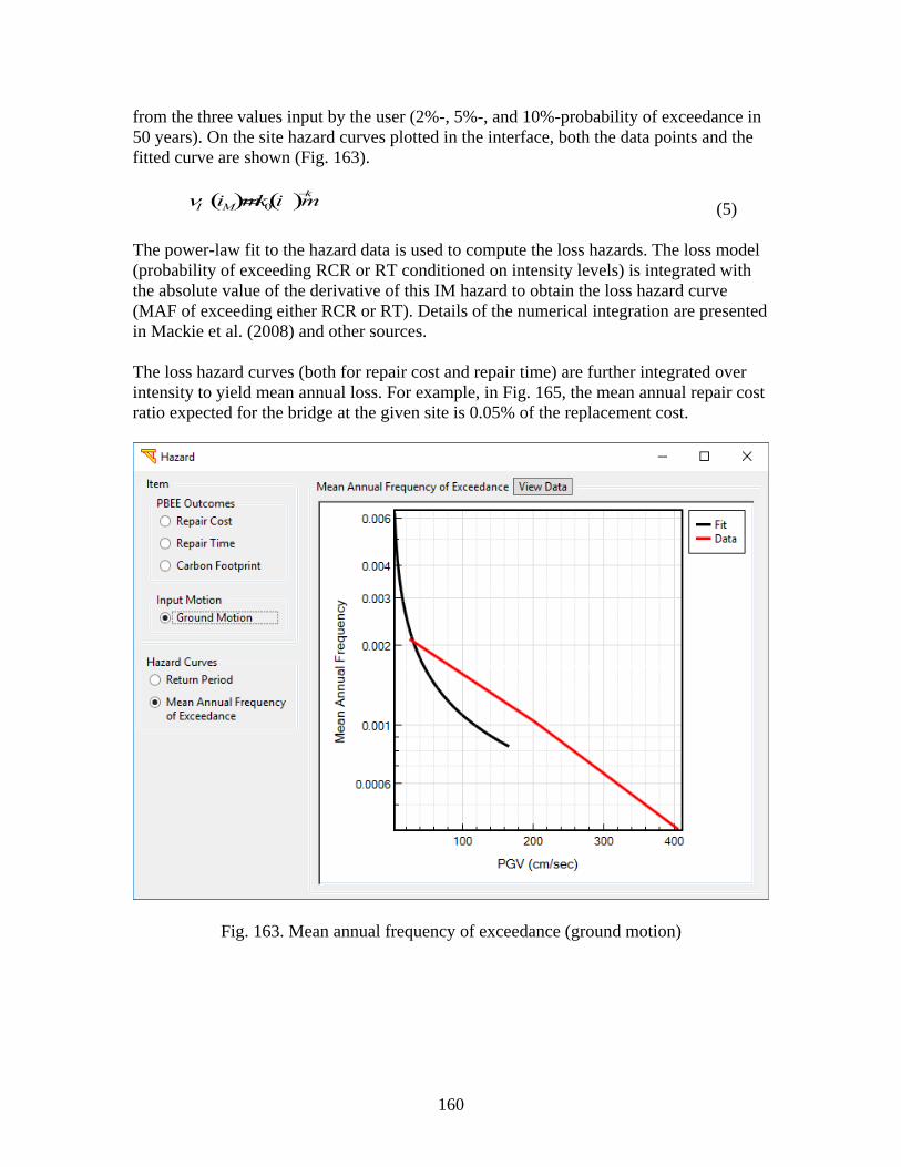
160

from the three values input by the user (2%-, 5%-, and 10%-probability of exceedance in

50 years). On the site hazard curves plotted in the interface, both the data points and the

fitted curve are shown (Fig. 163).

(5)

The power-law fit to the hazard data is used to compute the loss hazards. The loss model

(probability of exceeding RCR or RT conditioned on intensity levels) is integrated with

the absolute value of the derivative of this IM hazard to obtain the loss hazard curve

(MAF of exceeding either RCR or RT). Details of the numerical integration are presented

in Mackie et al. (2008) and other sources.

The loss hazard curves (both for repair cost and repair time) are further integrated over

intensity to yield mean annual loss. For example, in Fig. 165, the mean annual repair cost

ratio expected for the bridge at the given site is 0.05% of the replacement cost.

Fig. 163. Mean annual frequency of exceedance (ground motion)

I Mi m( )=k0 i m( )−k

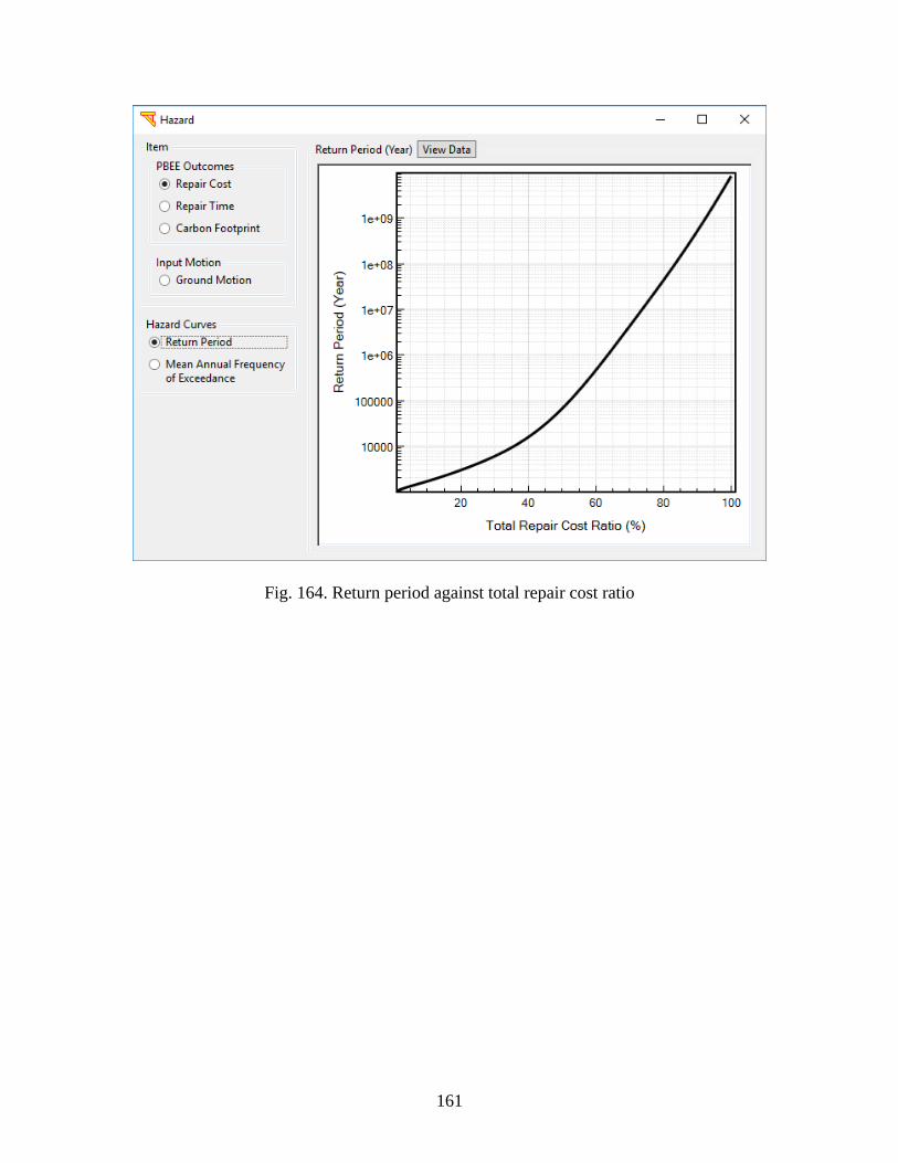
161

Fig. 164. Return period against total repair cost ratio

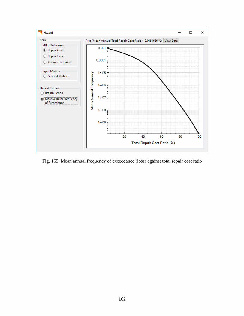
162

Fig. 165. Mean annual frequency of exceedance (loss) against total repair cost ratio

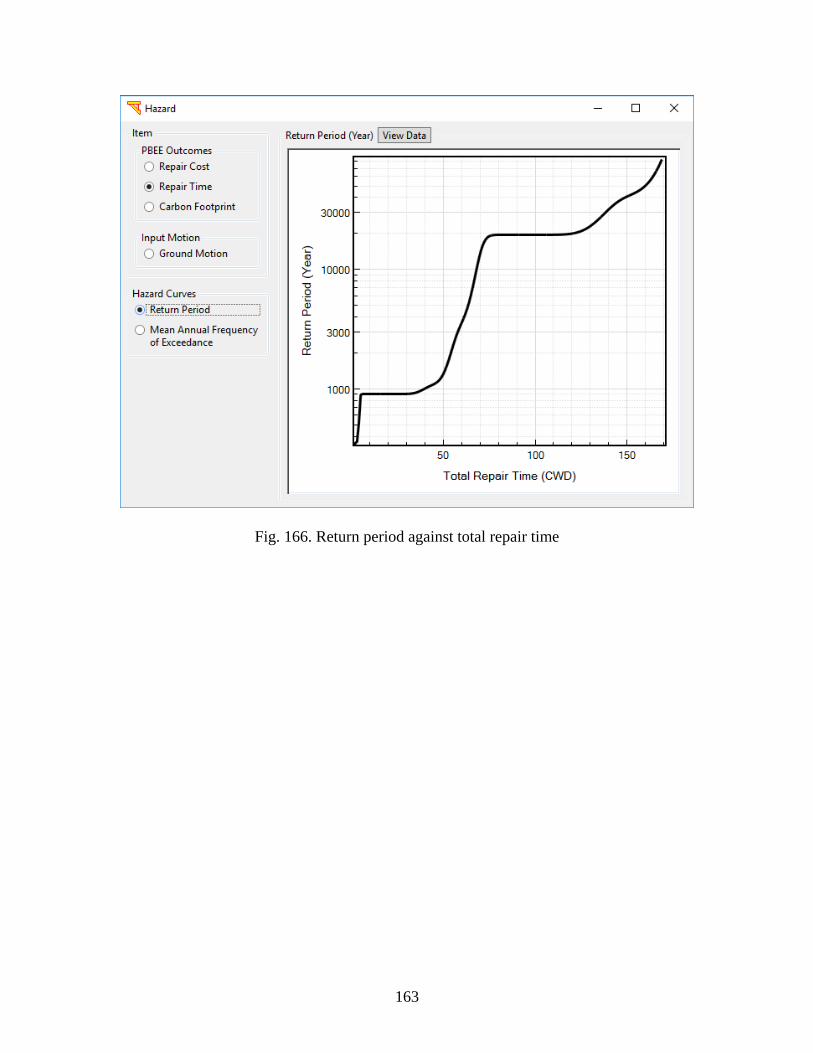
163

Fig. 166. Return period against total repair time

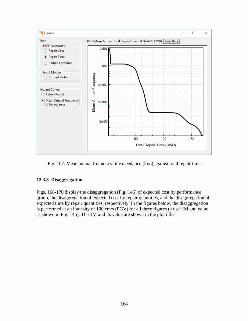
164

Fig. 167. Mean annual frequency of exceedance (loss) against total repair time

12.3.3 Disaggregation

Figs. 168-170 display the disaggregation (Fig. 145) of expected cost by performance

group, the disaggregation of expected cost by repair quantities, and the disaggregation of

expected time by repair quantities, respectively. In the figures below, the disaggregation

is performed at an intensity of 100 cm/s (PGV) for all three figures (a user IM and value

as shown in Fig. 145). This IM and its value are shown in the plot titles.

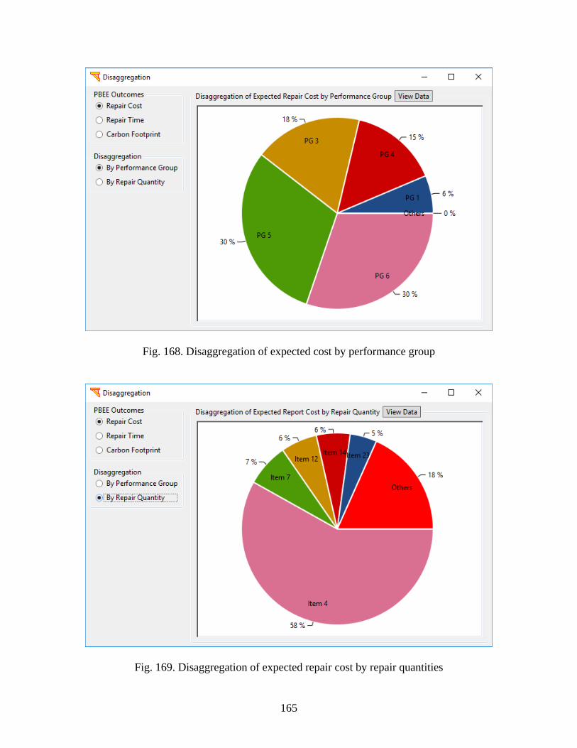
165

Fig. 168. Disaggregation of expected cost by performance group

Fig. 169. Disaggregation of expected repair cost by repair quantities

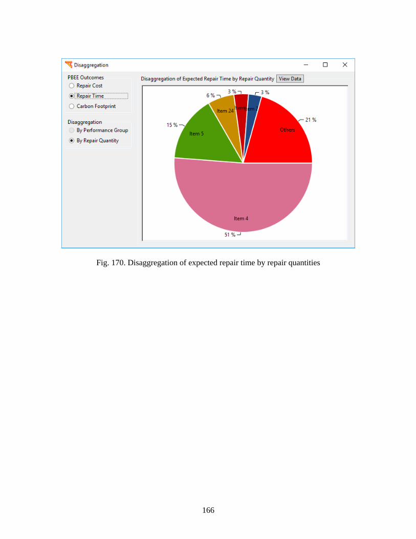
166

Fig. 170. Disaggregation of expected repair time by repair quantities

167

APPENDIX A CAPABILITIES ADDED IN THE CURRENT

UPDATED VERSION

A number of capabilities and features have been added in the current version of MSBridge.

These added features mainly allow MSBridge to address possible variability in the bridge

deck, bent cap, column, foundation, and soil configuration/properties (on a bent-by-bent

basis). Specifically, the capabilities implemented are:

(a) A different skew angle can be defined for each individual bent/abutment (in

MSBridge, from main window -> Advanced -> check Use Individual Skew

Angles -> Bent and Abutments).

(b) A different skew angle can be defined for each individual deck hinge (from main

window -> Advanced -> Define Deck Hinges).

(c) Shear key option (using OpenSees Bilin material) is included in the deck hinge

model. The shear key is not activated by default (From main window -> Advanced

-> Define Deck Hinges -> Modify).

(d) Deck and bentcap are now connected by a rigid link (deck offset is activated in this

case). A hinge with 6 Degrees of freedom (DOF’s) of linear springs can be activated

at the rigid link, at the location that the user specifies (From main window ->

Bentcap).

(e) Box girder section graphical representation has been added (for efficient

incorporation of the user-defined properties). (From main window -> Deck ->

Recalculate Section from Box Girder)

(f) Option to couple longitudinal and transverse directions of isolation bearing

nonlinear response has been added (From main window -> Advanced -> Define

Isolation Bearings -> Couple Longitudinal and Transverse Directions).

(g) Definition of the bent cap properties is now allowed on a bent by bent basis (From

main window -> Bentcap).

(h) Definition of the column properties is allowed for each individual column. This

option gives the user great flexibility and control over assigning different nonlinear

fiber sections to columns and pile shafts (Types I & II), (From main window ->

Column).

(i) Oblong column cross-section with two circular steel cages has been added (From

main window -> Column -> Oblong).

(j) For the circular cross-section, options for Bonded and Un-bonded Column Jackets

(i.e., Casing as Fibers in the Bonded case) have been added (From main window ->

Column -> Circle -> check Activate Steel Jacket).

168

(k) Option to improve computational analysis schemes has been added. Specifically,

this option is mainly to allow automatic switching between time integration

schemes to achieve convergence in highly nonlinear scenarios (From menu

Execute -> Advanced Option: OpenSees Parameters -> check Automatic

Switching between Time Integration Schemes).

Furthermore, the following options have been implemented:

(a) Concrete properties can be manually specified (instead of automatically calculated

from the column geometry and reinforcement information) (From main window ->

Column -> check Update RC Properties and click Nonlinear Fiber Section).

(b) Option to enter user-defined moment curvature (from main window -> Column ->

check User-Defined Moment Curvature and click Define Moment Curvature).

(c) A separate steel material can be used for the steel jacket (From main window ->

Column -> Nonlinear Fiber Section).

(d) Option to include the vertical soil springs for the Soil Springs foundation type

(From main window -> Foundation -> click Soil Springs and then Modify Soil

Springs).

(e) Option to calculate the vertical soil springs (for the Soil Springs foundation type)

based on user-defined T-z and Q-z data (From main window -> Foundation ->

click Soil Springs and then Modify Soil Springs -> click Calculate from User T-

z and Q-z).

(f) Option to specify a yielding curvature as the yielding criterion for Longitudinal and

Transverse ESA (From main window -> click Longitudinal Direction (or

Transverse Direction).

(g) A different number of columns can be specified for each individual bent, with

locations defined by column offsets (From main window -> Bridge -> check Non-

uniform Column Layout -> Columns).

(h) Column base offset (zero by default) can also be defined, for modeling inclined

columns (From main window -> Bridge -> check Non-uniform Column Layout

-> Columns -> specify Base Offset).

(i) Different deck properties can be specified on a span-by-span basis (From main

window -> Deck; from main window -> Bridge -> check Non-uniform Column

Layout).

(j) For Horizontal Alignment, the global coordinate system can be rotated at the angle

specified; or the bridge longitudinal direction can be chosen to coincide with the

169

chord connecting the two abutments (From main window -> Spans -> check

Horizontal Alignment -> Modify Horizontal Curve).

(k) Option to include the bentcap overhang (the portion of the bent cap outside the

columns) has been added (From main window -> Bentcap).

(l) Option to include the user-defined TCL code snippet for the nonlinear Fiber section

has been added. This is an advanced option and the users must proceed with caution

(From main window -> Column -> check User-Defined Tcl Script for Nonlinear

Fiber Section -> Define Fiber Section Tcl Script).

(m) Different Foundation Matrix parameters can be assigned to each column base

(From main window -> Foundation -> check Foundation Matrix -> Modify

Foundation Matrix).

(n) Option to include pile cap masses and fixity conditions has been added, available

only in the foundation types “Soil Springs” and “Foundation Matrix” (From main

window -> Advanced -> Pilecap Mass and Rotation Condition).

(o) Option to include column P-Delta effect (included by default) has been added

(From main window -> Advanced -> check/uncheck Include P-Delta Effect).

(p) Option to include Rayleigh (stiffness proportional component) damping for the

abutments has been added, with no Rayleigh damping for the abutment stiffness as

the default (From main window -> Advanced -> check/uncheck Include Rayleigh

Damping).

(q) Deck-end fixity conditions can be directly applied (From main window ->

Advanced -> Deckend Fixity)

(r) Visualization of pile response (profiles, time histories and relationships) has been

added, available for the foundation type “Soil Springs” (From menu Display ->

Pile Response Profiles/Pile Response Time Histories/Pile Response

Relationships).

(s) Option to view OpenSees analysis log (From main menu -> Execute -> OpenSees

Analysis Log).

(t) Multi-Linear abutment model has been added (From main window -> Abutment

-> select Elastic/Multi-Linear Abutment -> Modify Properties).

(u) Option to include Rayleigh (stiffness proportional component) damping for the soil

springs has been added, with no Rayleigh damping for the soil springs as the default

(From main window -> Advanced -> check/uncheck Include Rayleigh Damping).

170

(v) Option to activate the linear behavior for the soil springs (From main window ->

Advanced -> Linear Soil Springs).

(w) Option to choose a beam column element type for pile shafts (From main window

-> Mesh).

171

APPENDIX B CALCULATION OF STEEL AND CONCRETE

MATERIAL PROPERTIES

Steel Bars

By default, the Steel02 material is used to simulate steel bars. The format of the Steel02

command is as follows (McKenna et al. 2010):

uniaxialMaterial Steel02 $matTag $fy $E0 $b $R0 $cR1 $cR2

Where $fy is the steel yield strength, $E0 is Young’s modulus of steel, and $b is the

strain-hardening ratio (ratio between post-yield tangent and initial elastic tangent), $R0,

$cR1, and $cR2 are parameters to control the transition from elastic to plastic branches.

The number of longitudinal bars is calculated as follows:

(6)

Where is the longitudinal steel percentage, Ac the column cross-section area, Ab is the

cross-section area of the steel bar.

If the number of longitudinal bars is known, the longitudinal steel percentage

(reinforcement ratio) can be calculated:

(7)

Where As is the area of longitudinal steel, which is equal to the area of each bar times the

number of bars. For example, the diameter of a #18 bar is 2.257 inches, so the area is four

in2. If there are 10 bars in a 36-inch diameter circular column, then

or 3.9%.

The transverse steel percentage (reinforcement ratio) for a spirally confined circular

column, currently the only type of column supported in the interface, is

(8)

Where dbt is the diameter of the transverse spiral (always smaller than the diameter of the

longitudinal bars). The spacing between transverse bars is s. The diameter of the confined

core is dcc which is the gross diameter minus twice the cover and minus the diameter of

b

cs

A

Abars

=#

s

c

s

sA

A=

039.0

364

)4(10

2

==

s

)(

)(2

c c

dbt

ds

d =

172

the transverse bars (see Eq. 11). So for a #5 spiral spaced at 3 inches on center in the

same column mentioned above.

or 1.3%. (9)

Currently, the transverse reinforcement does affect the shear response (through changes

in the uniaxial constitutive model for the concrete core). However, the columns are

modeled considering only flexurally dominated response (i.e., there is no accounting for

shear flexibility or shear degradation directly). Additional relevant details on the

parameters used in both the Cover and Core Concrete are included below.

Cover concrete

The Concrete02 material is used to simulate the concrete (for both cover and core). The

format of the Concrete02 command is as follows:

uniaxialMaterial Concrete02 $matTag $fpc $epsc0 $fpcu $epsu $lambda $ft $Ets

Where $fpc is the concrete compressive strength, $epsc0 is the concrete strain at

maximum strength, $fpcu is the concrete crushing strength, $epsu is the concrete strain at

crushing strength (all of the above values are entered as negative), $lambda is the ratio

between unloading slope at $epsu and initial slope, $ft is the tensile strength, and $Ets is

tension softening stiffness (absolute value) (slope of the linear tension softening branch).

For cover concrete, $fpc is equal to the concrete unconfined strength, $epsc0 = 0.002,

$fpcu = 0.0, $epscu = 0.006, $lambda = 0.1, $ft = (0.14)$fpc, and $Ets = $ft / $epsc0.

Core concrete

i) For core concrete of circular column cross-sections according to the Mander model, the

procedure to calculate the confined concrete strength $fpc(= ) is as follows:

(10)

Where is the unconfined compressive strength and can be obtained from the

following equation:

(11)

0 1 3.0

)8

5)2(23 6(3

)8

5( 2

=

−−

=

t

ccf

)29 4.712 5 4.22 5 4.1('

'

'

''

c

e

c

ecc c

f

f

f

fff −++−=

'

cf '

ef

ytee fKf 2

1'=

173

Where is the steel yield strength, t is the transverse steel percentage, and can be

obtained from the following equation for circular columns confined by hoops:

(12)

Where:

(13)

An assumed value of the area of the confined core is used for default values. This area

should be modified based on the expected compressive block in the column during lateral

loading.

(14)

(15)

Where dbt is the transverse bar diameter

(16)

Where c is the clear cover (c = 1.5”)

ii) $epsc0

(17)

Where:

(18)

Where w is the concrete unit weight (unit: kg/m3)

iii) $epsu (= )

yf eK

)1(

)2

'1( 2

cc

cce

d

S

K−

−

=

4

)( 2

c c

c c

dA

=

cct

bt

d

dS

2

' =

b tLc c dcDd −−= 2

c

c c

E

fepsc

20 =

'5.1043.0 cfwEc =

e p s c u

cc

s cc

A

A =

174

(19)

Where is the ultimate steel strain ( )

iv) $fpcu (= )

(20)

Where:

(21)

(22)

_____________________________________________

Notes:

1. The information above is specific to the Steel02 and Concrete02 models of the Fiber

section. Other options include (Fig. 25), Steel01 and Concrete01 (for more information

please see the OpenSees documentation), and Elastic properties for the fibers. These

options can be activated by clicking on the default Steel02 or Concrete02 sections (Fig.

25) and changing these options.

2. A different property may be specified for the Column below grade (for instance to

roughly represent a large pile group as a large single column). If this option is selected

(Fig. 7), the column below grade will have linear properties as specified by its diameter

and Young’s Modulus).

3. All the equations presented in this Appendix are based on the Mander model for spiral-

reinforced circular concrete columns. The user may want to use their constitutive model

or parameters. In this case, these parameters can be defined directly in Fig. 25.

t

c

y

sf

fepscu

'004.0 +=

s 12.0=s

cuf

)

))(

)((1)(

)((

)(

)(

)(ep scr

cc

cu

epsc

epscuepscr

epscr

epsc

epscuff

+−

=

))1(51)(0('

−+=c

cc

f

fepscepsc

)(eps c

fE

Eeps cr

c c

c

c

−

=

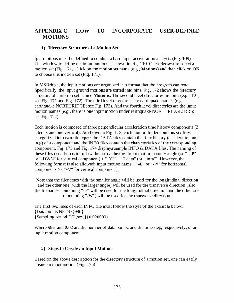
175

APPENDIX C HOW TO INCORPORATE USER-DEFINED

MOTIONS

1) Directory Structure of a Motion Set

Iput motions must be defined to conduct a base input acceleration analysis (Fig. 109).

The window to define the input motions is shown in Fig. 110. Click Browse to select a

motion set (Fig. 171). Click on the motion set name (e.g., Motions) and then click on OK

to choose this motion set (Fig. 171).

In MSBridge, the input motions are organized in a format that the program can read.

Specifically, the input ground motions are sorted into bins. Fig. 172 shows the directory

structure of a motion set named Motions. The second level directories are bins (e.g., T01;

see Fig. 171 and Fig. 172). The third level directories are earthquake names (e.g.,

earthquake NORTHRIDGE; see Fig. 172). And the fourth level directories are the input

motion names (e.g., there is one input motion under earthquake NORTHRIDGE: RRS;

see Fig. 172).

Each motion is composed of three perpendicular acceleration time history components (2

laterals and one vertical). As shown in Fig. 172, each motion folder contains six files

categorized into two file types: the DATA files contain the time history (acceleration unit

in g) of a component and the INFO files contain the characteristics of the corresponding

component. Fig. 173 and Fig. 174 displays sample INFO & DATA files. The naming of

these files usually has to follow the format below: Input motion name + angle (or "-UP"

or "-DWN" for vertical component) + ".AT2" + ".data" (or “.info"). However, the

following format is also allowed: Input motion name + "-E" or "-W" for horizontal

components (or "-V" for vertical component).

Note that the filenames with the smaller angle will be used for the longitudinal direction

and the other one (with the larger angle) will be used for the transverse direction (also,

the filenames containing "-E" will be used for the longitudinal direction and the other one

(containing "-W") will be used for the transverse direction.

The first two lines of each INFO file must follow the style of the example below:

{Data points NPTS}{996}

{Sampling period DT (sec)}{0.020000}

Where 996 and 0.02 are the number of data points, and the time step, respectively, of an

input motion component.

2) Steps to Create an Input Motion

Based on the above description for the directory structure of a motion set, one can easily

create an input motion (Fig. 175):

176

Step 1: create a folder and rename to your motion set name (e.g. MotionSet1; see Fig.

175).

Step 2: create a folder under the motion set folder and rename to your bin name (e.g.,

bin1).

Step 3: create a folder under the bin folder and rename to your earthquake name (e.g.,

Quake1).

Step 4: create a folder under the earthquake name and rename to your input motion name

(e.g., MOTION1).

Step 5: create the six files (3 INFO files and 3 DATA files) for this input motion (Fig.

175).

Note: If you download the input motion files from the PEER NGA Database, there is no

need to re-format the data into one column as shown in Fig. 174. Just copy the data points

into the corresponding DATA files. And then make the INFO files containing the number

of data points and the sampling period DT (2 lines) according to the header information.

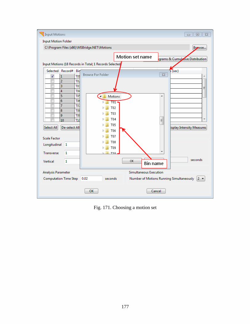
177

Fig. 171. Choosing a motion set

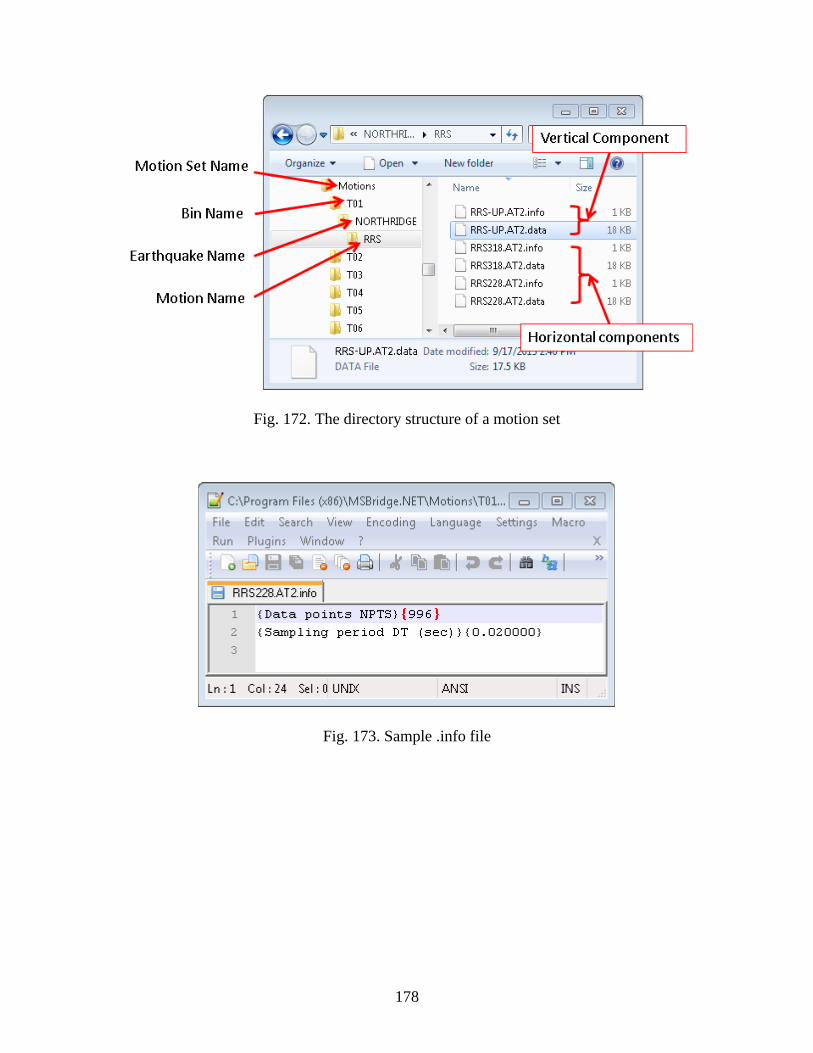
178

Fig. 172. The directory structure of a motion set

Fig. 173. Sample .info file

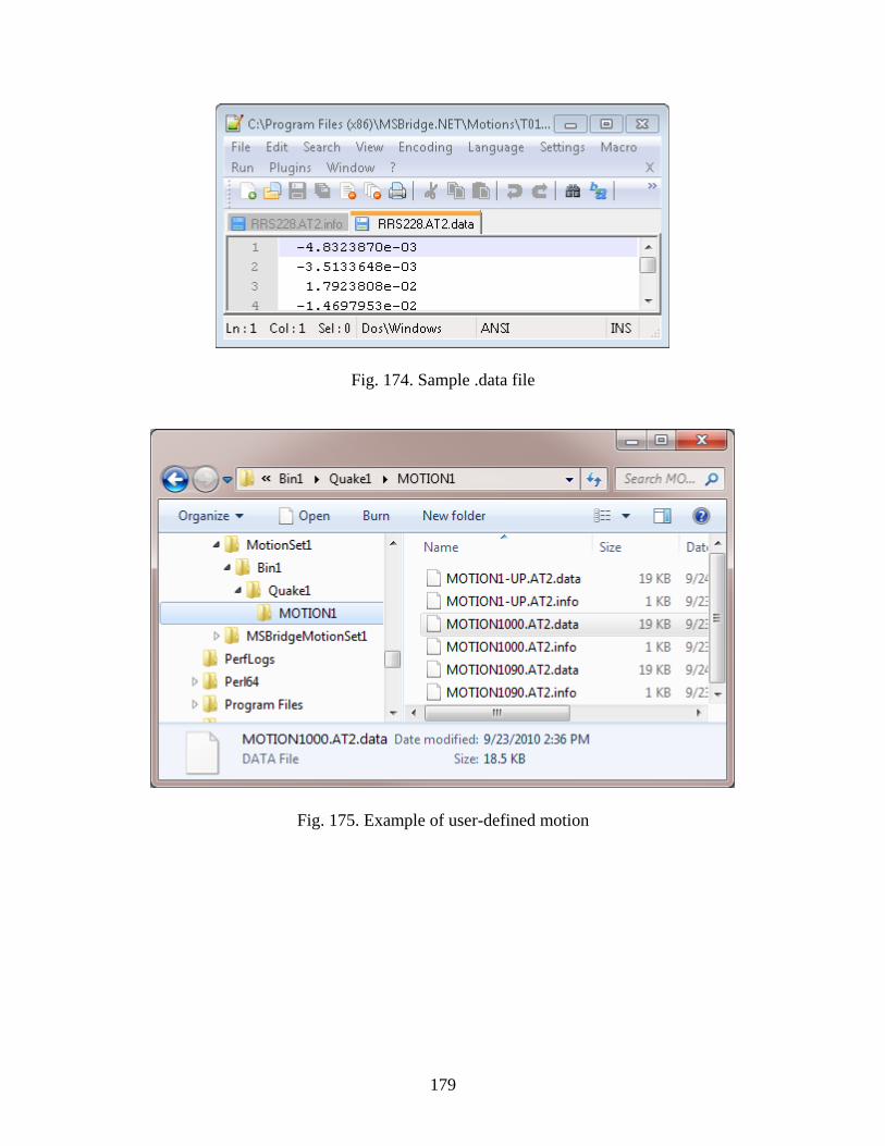
179

Fig. 174. Sample .data file

Fig. 175. Example of user-defined motion

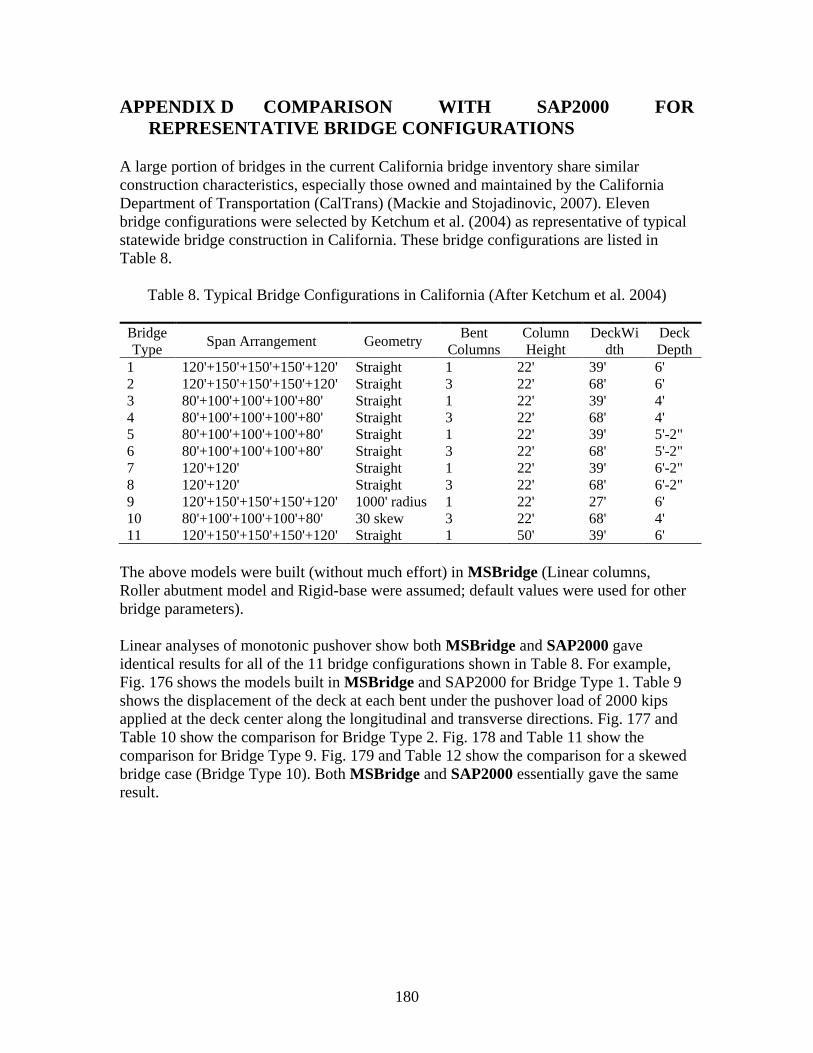
180

APPENDIX D COMPARISON WITH SAP2000 FOR

REPRESENTATIVE BRIDGE CONFIGURATIONS

A large portion of bridges in the current California bridge inventory share similar

construction characteristics, especially those owned and maintained by the California

Department of Transportation (CalTrans) (Mackie and Stojadinovic, 2007). Eleven

bridge configurations were selected by Ketchum et al. (2004) as representative of typical

statewide bridge construction in California. These bridge configurations are listed in

Table 8.

Table 8. Typical Bridge Configurations in California (After Ketchum et al. 2004)

Bridge

Type Span Arrangement Geometry

Bent

Columns

Column

Height

DeckWi

dth

Deck

Depth

1 120'+150'+150'+150'+120' Straight 1 22' 39' 6'

2 120'+150'+150'+150'+120' Straight 3 22' 68' 6'

3 80'+100'+100'+100'+80' Straight 1 22' 39' 4'

4 80'+100'+100'+100'+80' Straight 3 22' 68' 4'

5 80'+100'+100'+100'+80' Straight 1 22' 39' 5'-2"

6 80'+100'+100'+100'+80' Straight 3 22' 68' 5'-2"

7 120'+120' Straight 1 22' 39' 6'-2"

8 120'+120' Straight 3 22' 68' 6'-2"

9 120'+150'+150'+150'+120' 1000' radius 1 22' 27' 6'

10 80'+100'+100'+100'+80' 30 skew 3 22' 68' 4'

11 120'+150'+150'+150'+120' Straight 1 50' 39' 6'

The above models were built (without much effort) in MSBridge (Linear columns,

Roller abutment model and Rigid-base were assumed; default values were used for other

bridge parameters).

Linear analyses of monotonic pushover show both MSBridge and SAP2000 gave

identical results for all of the 11 bridge configurations shown in Table 8. For example,

Fig. 176 shows the models built in MSBridge and SAP2000 for Bridge Type 1. Table 9

shows the displacement of the deck at each bent under the pushover load of 2000 kips

applied at the deck center along the longitudinal and transverse directions. Fig. 177 and

Table 10 show the comparison for Bridge Type 2. Fig. 178 and Table 11 show the

comparison for Bridge Type 9. Fig. 179 and Table 12 show the comparison for a skewed

bridge case (Bridge Type 10). Both MSBridge and SAP2000 essentially gave the same

result.

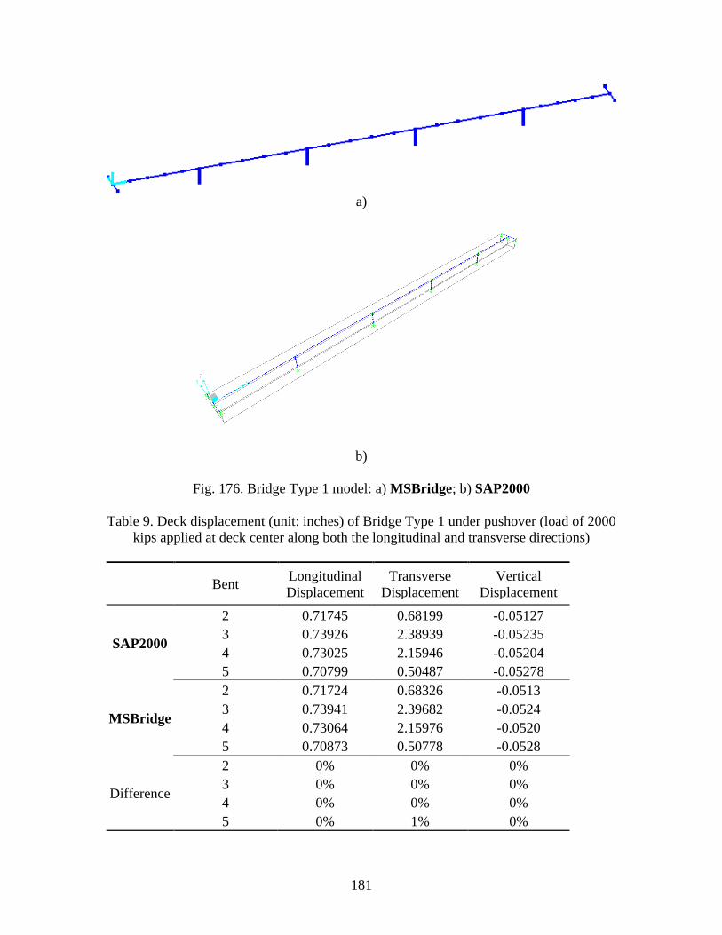
181

a)

b)

Fig. 176. Bridge Type 1 model: a) MSBridge; b) SAP2000

Table 9. Deck displacement (unit: inches) of Bridge Type 1 under pushover (load of 2000

kips applied at deck center along both the longitudinal and transverse directions)

Bent Longitudinal

Displacement

Transverse

Displacement

Vertical

Displacement

SAP2000

2 0.71745 0.68199 -0.05127

3 0.73926 2.38939 -0.05235

4 0.73025 2.15946 -0.05204

5 0.70799 0.50487 -0.05278

MSBridge

2 0.71724 0.68326 -0.0513

3 0.73941 2.39682 -0.0524

4 0.73064 2.15976 -0.0520

5 0.70873 0.50778 -0.0528

Difference

2 0% 0% 0%

3 0% 0% 0%

4 0% 0% 0%

5 0% 1% 0%

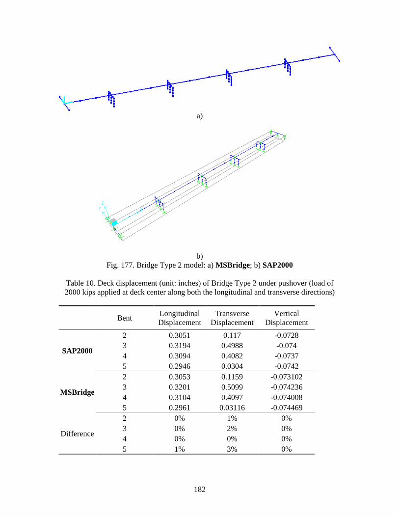
182

a)

b)


Table 10. Deck displacement (unit: inches) of Bridge Type 2 under pushover (load of

2000 kips applied at deck center along both the longitudinal and transverse directions)

Bent Longitudinal

Displacement

Transverse

Displacement

Vertical

Displacement

SAP2000

2 0.3051 0.117 -0.0728

3 0.3194 0.4988 -0.074

4 0.3094 0.4082 -0.0737

5 0.2946 0.0304 -0.0742

MSBridge

2 0.3053 0.1159 -0.073102

3 0.3201 0.5099 -0.074236

4 0.3104 0.4097 -0.074008

5 0.2961 0.03116 -0.074469

Difference

2 0% 1% 0%

3 0% 2% 0%

4 0% 0% 0%

5 1% 3% 0%

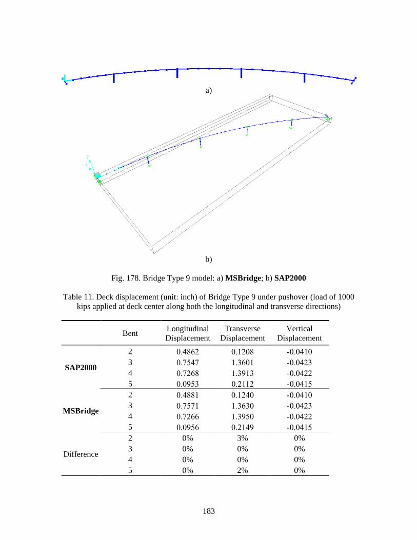
183

a)

b)


Table 11. Deck displacement (unit: inch) of Bridge Type 9 under pushover (load of 1000

kips applied at deck center along both the longitudinal and transverse directions)

Bent Longitudinal

Displacement

Transverse

Displacement

Vertical

Displacement

SAP2000

2 0.4862 0.1208 -0.0410

3 0.7547 1.3601 -0.0423

4 0.7268 1.3913 -0.0422

5 0.0953 0.2112 -0.0415

MSBridge

2 0.4881 0.1240 -0.0410

3 0.7571 1.3630 -0.0423

4 0.7266 1.3950 -0.0422

5 0.0956 0.2149 -0.0415

Difference

2 0% 3% 0%

3 0% 0% 0%

4 0% 0% 0%

5 0% 2% 0%

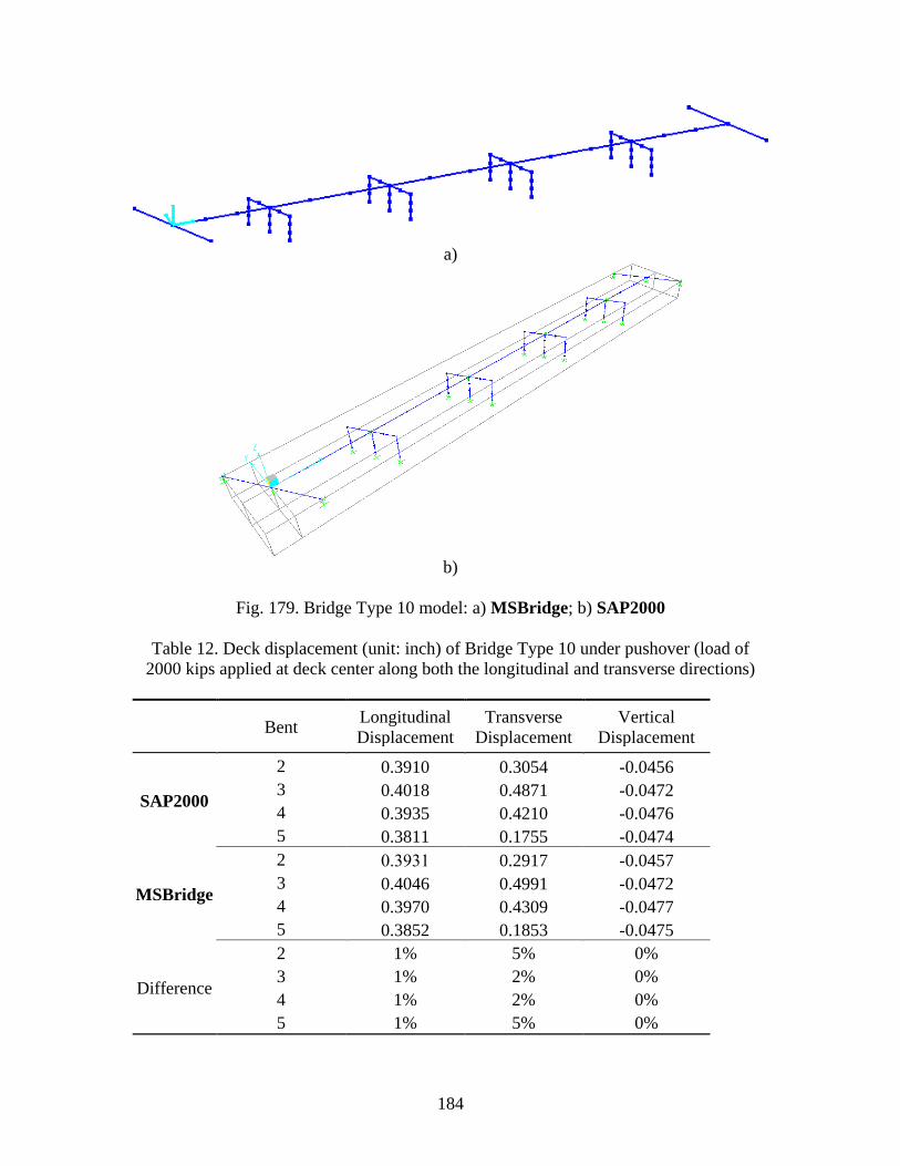
184

a)

b)


Table 12. Deck displacement (unit: inch) of Bridge Type 10 under pushover (load of

2000 kips applied at deck center along both the longitudinal and transverse directions)

Bent Longitudinal

Displacement

Transverse

Displacement

Vertical

Displacement

SAP2000

2 0.3910 0.3054 -0.0456

3 0.4018 0.4871 -0.0472

4 0.3935 0.4210 -0.0476

5 0.3811 0.1755 -0.0474

MSBridge

2 0.3931 0.2917 -0.0457

3 0.4046 0.4991 -0.0472

4 0.3970 0.4309 -0.0477

5 0.3852 0.1853 -0.0475

Difference

2 1% 5% 0%

3 1% 2% 0%

4 1% 2% 0%

5 1% 5% 0%

185

REFERENCES

Aviram, A., Mackie, K.R., and Stojadinovic, B. (2008).Effect of Abutment Modeling on

the Seismic Response of Bridge Structures, Earthquake Engineering and Engineering

Vibration 7(4), 395-402.

Berry, M.P., and Eberhard, M.O. (2007). Performance Modeling Strategies for Modern

Reinforced Concrete Bridge Columns, Report No. 2007/07, Pacific Earthquake

Engineering Research Center, University of California, Berkeley, California.

Kotsoglu, A., and Pantazopoulou, S. (2006). Modeling of Embankment Flexibility and

Soil-structure Interaction in Integral Bridges, Proceedings of First European

Conference on Earthquake Engineering and Seismology, September 3-8, Geneva,

Switzerland.

Caltrans, 1999, xSection User Manual, California Department of Transportation,

Sacramento, California.

Caltrans SDC, 2004. Caltrans Seismic Design Criteria, Version 1.3, California

Department of Transportation, Sacramento, California.





Caltrans, 2017. Bridge Memo to Designer (MTD) 20-15: “Lateral Spreading Analysis for

New and Existing Bridges.” California Department of Transportation, Sacramento, CA

95816.

Caltrans, 2018. Highway Design Manual, 6th Edition, California Department of

Transportation, Sacramento, California.

Elgamal, A., Yang, Z., Parra, E., and Ragheb, A. 2003.Modeling of cyclic mobility in

saturated cohesionless soils. International Journal of Plasticity, 19(6), 883-905.

Elgamal, A., and Lu, J. 2009. A Framework for 3D finite element analysis of lateral pile

system response, Proceedings of the 2009 International Foundation Congress and

Equipment Expo, Contemporary Topics in In Situ Testing, Analysis, and Reliability of

Foundations, ASCE GSP 186, M. Iskander, D. F. Laefer, and M. H. Hussein, Editors,

Orlando, Florida, March 15-19, pp. 616-623.

Elgamal, A., Jinchi Lu, J., and Forcellini, D. 2009a. Mitigation of liquefaction-induced

lateral deformation in a sloping stratum: 3D numerical simulation, Journal of

186

geotechnical and geoenvironmental engineering, ASCE, Vol. 135, No. 11, November,

1672-1682.

Elgamal, A., Lu, J., Yang, Z. and Shantz, T. 2009b. Scenario-focused three-dimensional

computational modeling in geomechanics, Alexandria, Egypt, October 3-5, 4

iYGEC'09 - 4th International Young Geotechnical Engineers' Conference, 2 - 6

October, ISSMGE.

Elgamal, A. (2010). Calibrated 3D computational modeling of soil-structure systems and

liquefaction scenarios, Proc. Fifth Intl. Conf. on Recent Advances in Geotechnical

Earthquake Engineering and Soil Dynamics, May 24-29, San Diego, CA.

Lam, I. P., and Martin, G. R. (1986), "Seismic Design of Highway Bridge Foundations,

FHWA Report," Federal Highway Administration, Washington D.C.

Lu J., 2006. Parallel finite element modeling of earthquake site response and liquefaction,

Ph.D. Thesis, Department of Structural Engineering, University of California, San

Diego, La Jolla, CA.

Mackie, K.R., and Stojadinovic, B. (2005). "Fragility basis for California highway

overpass bridge seismic decision making." PEER Report No. 2005/02, Pacific

Earthquake Engineering Research Center, University of California, Berkeley.

Mackie, K. and Stojadinovic, B. (2006). Seismic Vulnerability of Typical Multi-span

California Highway Bridges, Proceedings of the Fifth National Seismic Conference on

Bridges and highways, September 18-20, San Francisco.

Mackie, K.R., Wong, J-M., and Stojadinovic, B. (2008)."Integrated probabilistic

performance-based evaluation of benchmark reinforced concrete bridges." PEER

Report No. 2007/09, Pacific Earthquake Engineering Research Center, University of

California, Berkeley.

Mackie, K.R., Wong, J-M., and Stojadinovic, B. (2010). Post-earthquake bridge repair

cost and repair time estimation methodology. Earthquake Engineering and Structural

Dynamics, 39(3): 281-301.

Mackie, K.R., Wong, J-M., and Stojadinovic, B. (2011). Bridge damage and loss

scenarios calibrated by schematic design and cost estimation of repairs. Earthquake

Spectra, 27: 1127-1145.

Maroney, B.H., and Chai, Y.H. (1994). Seismic Design and Retrofitting of Reinforced

Concrete Bridges, Proceedings of 2nd International Workshop, Earthquake

Commission of New Zealand, Queenstown, New Zealand.

187

Mander, J.B., Priestley, M.J.N., and Park, R. (1988). Theoretical Stress-Strain Model for

Confined Concrete, Journal of the Structural Division ASCE, 114, pp. 1804-1826.

Mazzoni, S., McKenna, F., Scott, M. H., Fenves, G. L., et al. (2009). Open System for

Earthquake Engineering Simulation, User Command-Language Manual, Pacific

Earthquake Engineering Research Center, University of California, Berkeley,

OpenSees version 2.0, May.

Megally, S.H., Seible, F., Bozorgzadeh, A., Restrepo, J. and Silva, P.F. (2003). Response

of Sacrificial Shear Keys in Bridge Abutments to Seismic Loading, Proceedings of the

FIB Symposium on Concrete Structures in Seismic Regions, May 6-9, Athens, Greece.

Shamsabadi, A., Rollins, K.M, and Kapuskar, M. (2007).Nonlinear Soil-Abutment-

Bridge Structure Interaction for Seismic Performance-Based Design, Journal of

Geotechnical and Geoenvironmental Engineering, 133(6), 707-720, June.

Shamsabadi, A., Khalili-Tehrani, P., Stewart, J.P., and Taciroglu, E. (2010).Validated

Simulation Models for Lateral Response of Bridge Abutments with Typical Backfills,

J. Bridge Eng., 15(3), 302-311, May.

Werner, S.D. (1994). Study of Caltrans' Seismic Evaluation Procedures for Short

Bridges, Proceedings of the 3rd Annual Seismic Research Workshop, Sacramento,

California.

Yang, Z., Elgamal, A., and Parra, E. 2003.A computational model for cyclic mobility and

associated shear deformation, Journal of Geotechnical and Geoenvironmental

Engineering, 129 (12), 1119-1127.

Zhang, J., and Makris, N. (2002). Kinematic Response Functions and Dynamic

Stiffnesses of Bridge Embankments, Earthquake Engineering & Structural Dynamics,

31(11), pp. 1933-1966.

Documents

MSBRIDGE: OPENSEES PUSHOVER AND EARTHQUAKE