Embed Size (px)
Citation preview
applied sciences
Article
Application of Mode-Adaptive Bidirectional Pushover Analysisto an Irregular Reinforced Concrete Building Retrofitted viaBase Isolation
Kenji Fujii 1,* and Takumi Masuda 2
�����������������
Citation: Fujii, K.; Masuda, T.
Application of Mode-Adaptive
Bidirectional Pushover Analysis to an
Irregular Reinforced Concrete
Building Retrofitted via Base
Isolation. Appl. Sci. 2021, 11, 9829.
https://doi.org/10.3390/app11219829
Academic Editors: Pier Paolo Rossi
and Melina Bosco
Received: 25 September 2021
Accepted: 19 October 2021
Published: 21 October 2021
Publisher’s Note: MDPI stays neutral
with regard to jurisdictional claims in
published maps and institutional affil-
iations.
Copyright: © 2021 by the authors.
Licensee MDPI, Basel, Switzerland.
This article is an open access article
distributed under the terms and
conditions of the Creative Commons
Attribution (CC BY) license (https://
creativecommons.org/licenses/by/
4.0/).
1 Department of Architecture, Faculty of Creative Engineering, Chiba Institute of Technology,Chiba 275-0016, Japan
2 Graduate School of Creative Engineering, Chiba Institute of Technology, Chiba 275-0016, Japan;[email protected]
* Correspondence: [email protected]
Featured Application: Seismic response evaluation of a base-isolated buildings: Seismic rehabil-itation design for reinforced concrete buildings using the base-isolation technique.
Abstract: In this article, the applicability of mode-adaptive bidirectional pushover analysis (MABPA)to base-isolated irregular buildings was evaluated. The point of the updated MABPA is that thepeaks of the first and second modal responses are predicted considering the energy balance during ahalf cycle of the structural response. In the numerical examples, the main building of the former UtoCity Hall, which was severely damaged in the 2016 Kumamoto earthquake, was investigated as acase study for the retrofitting of an irregular reinforced concrete building using the base-isolationtechnique. The comparisons between the predicted peak response by MABPA and nonlinear time-history analysis results showed that the peak relative displacement can be properly predicted byMABPA. The results also showed that the performance of the retrofitted building models wassatisfactory for the ground motion considered in this study, including the recorded motions in the2016 Kumamoto earthquake.
Keywords: seismic isolation; asymmetric building; mode-adaptive bidirectional pushover analysis(MABPA); seismic retrofit; momentary energy input
1. Introduction1.1. Background
Seismic isolation is widely applied to buildings for earthquake protection in earthquake-prone countries [1]. Unlike in the case of traditional (non-isolated) earthquake-resistantstructures, seismic isolation ensures that the behaviors of building structures are within theelastic range and reduces acceleration in buildings during large earthquakes [2]. Therefore,this technique is applied to not only new buildings, but also existing reinforced concreteand masonry buildings, including historical structures [3–14]. The isolation layer consistsof isolators and dampers. Isolators support the gravity loads of the superstructure. Thehorizontal flexibility and centering capability of seismically isolated buildings is also achievedby isolators [1]. Dampers provide the energy dissipation capacity for reducing the seismicresponses. Although it is very common to use hysteresis dampers (e.g., steel dampers) and/oroil dampers in the isolation layer, there are several studies about the innovative seismicisolation systems in recent years, e.g., [15–22].
In general, there is some degree of irregularity in building structures, whether theyare newly designed or preexisting. Therefore, the problem of torsional response due toplan irregularities needs to be studied for base-isolated structures, as well as non-isolatedstructures. Several researchers have investigated the seismic behavior of base-isolated
Appl. Sci. 2021, 11, 9829. https://doi.org/10.3390/app11219829 https://www.mdpi.com/journal/applsci
Appl. Sci. 2021, 11, 9829 2 of 41
buildings with plan irregularities [23–36]; these include fundamental parametric studiesusing idealized models [23–27], as well as studies using more realistic frame buildingmodels [28–36]. Most of these studies are based on nonlinear time-history analyses [23–35].However, there are a few investigations that examine the applicability of nonlinear staticprocedures to base-isolated buildings with asymmetry. Kilar and Koren [36] examinedthe applicability of the extended N2 method [37,38], which is one of the variants of thenonlinear static procedures, to the base-isolated asymmetric buildings. They found thenonlinear peak response of base-isolated asymmetric building can be predicted by theextended N2 method. However, they examined only those whose superstructure wasregular in elevation. Therefore, further investigations are needed for the applicabilityof the nonlinear static procedures, especially for base-isolated building with plan andelevation irregularities.
1.2. Motivation
There were two main motivations for this study. The first was to extend nonlinearstatic analyses to base-isolated buildings with irregularities, and the second was to pre-dict the nonlinear peak responses of base-isolated buildings according to the concept ofenergy input.
With respect to the first motivation, the authors proposed mode-adaptive bi-directionalpushover analysis (MABPA) [39–44]. This is a variant of nonlinear static analysis and wasoriginally proposed for the seismic analysis of non-isolated asymmetric buildings subjectedto horizontal bidirectional excitation. The first version of MABPA was proposed for non-isolated asymmetric buildings with regular elevation [39]; it was then updated followingthe development of displacement-based mode-adaptive pushover (DB-MAP) analysis [40].This version has been applied to reinforced concrete asymmetric frame buildings withbuckling-restrained braces [41] and to building models with bidirectional setbacks [42].The applicability of MABPA has been discussed and evaluated based on the effective modalmass ratio of the first two modes [43]. The seismic capacity of an existing irregular buildingseverely damaged in the 2016 Kumamoto earthquake (the former Uto City Hall) has beenevaluated using MABPA [44]. Looking back on the development of MABPA, the logicalnext step should be to extend the method to base-isolated buildings with irregularities.Considering the case in which the seismic isolation period is well separated from thenatural period of a superstructure, the behavior of the superstructure may be that of arigid body, as discussed by several researchers, e.g., [27]. In such cases, the effective modalmass ratio of the first and second modes is close to unity, provided that the torsionalresistance at the isolation layer is sufficient. It is expected that the seismic response of sucha base-isolated building with plan irregularities will be accurately predicted by MABPA.
In the nonlinear static analysis shown in the American Society of Civil EngineersASCE/SEI 41-17 document [3], the reduced spectrum considering the effective dampingis used to predict the target displacement for a nonlinear static analysis. Similarly, asshown in Notification No. 2009 of the Ministry of Construction of Japan [45], the equivalentlinearization technique can be used for target displacement evaluations of base-isolatedbuildings. However, several researchers have examined the responses of long-period build-ing structures subjected to pulse-like ground motions, e.g., Mazza examined a base-isolatedbuilding [29,31] and Günes and Ulucan studied a tall reinforced concrete building [46].Because the effective damping is calculated based on a steady response having the same dis-placement amplitude in the positive and negative directions, the use of effective dampingfor the prediction of the peak responses of base-isolated structures subjected to pulse-likeground motion is questionable. From this viewpoint, an alternative concept for predictingthe peak response is required. Accordingly, the second motivation of this study was toinvestigate the use of the energy concept.
The concept of energy input was introduced by Akiyama in the 1980 s [47] and isimplemented in the design recommendation for seismically isolated buildings presented bythe Architectural Institute of Japan [2]. In Akiyama’s theory, the total input energy is a suit-
Appl. Sci. 2021, 11, 9829 3 of 41
able seismic intensity parameter to access the cumulative response of a structure. Instead ofthe total input energy, Inoue et al. proposed the maximum momentary input energy [48–50] asan intensity parameter related to peak displacement; nonlinear peak displacement can bepredicted by equating the maximum momentary input energy and the cumulative hystere-sis energy during a half cycle of the structural response. Following the work of Inoue et al.,the authors investigated the relationship between the maximum momentary input energyand the total input energy of an elastic single-degree-of-freedom (SDOF) model [51]. In ad-dition, the concept of the momentary input energy was extended to consider bidirectionalhorizontal excitation [52,53]. Specifically, the time-varying function of the momentaryenergy input has been formulated for unidirectional [51] and bidirectional [52] excitation:This function can be calculated from the transfer function of the model and the complexFourier coefficients of the ground acceleration. Using the time-varying function, bothenergy parameters, the total and maximum momentary input energy, can be accuratelycalculated. In a previous study [53], it was shown that the nonlinear peak displacementand the cumulative energy of the isotropic two-degree-of-freedom model representinga reinforced concrete building can be properly predicted using a time-varying function.Therefore, the use of a time-varying function of the momentary energy input is promisingfor seismic response predictions for base-isolated buildings.
1.3. Objectives
Based on the above discussion, the following questions were addressed in this paper.
• Is MABPA capable of predicting the peak response of irregular base-isolated buildings?• The prediction of the peak equivalent displacement of the first two modal responses
is an essential step in MABPA. For this, the relationship between the maximummomentary input energy and the peak displacement needs to be properly evaluated.How can this relationship be evaluated from the pushover analysis results?
• In the prediction of the maximum momentary input energy of the first two modalresponses, the effect of simultaneous bidirectional excitation needs to be considered.Can the upper bound of the peak equivalent displacement of the first two modalresponses be predicted using the bidirectional maximum momentary input energyspectrum [52]?
In this study, the applicability of mode-adaptive bidirectional pushover analysis(MABPA) to base-isolated irregular buildings was evaluated. The point of the updatedMABPA is that the peaks of the first and second modal responses are predicted consideringthe energy balance during a half cycle of the structural response. In the numerical examples,the main building of the former Uto City Hall [44], which was severely damaged in the2016 Kumamoto earthquake, was investigated as a case study for the retrofitting of anirregular reinforced concrete building using the base-isolation technique. The nonlinearpeak responses of two retrofitted building models subjected to bidirectional excitationwere investigated via a time-history analysis using artificial and recorded ground motiondatasets. Then, their peak responses were predicted by MABPA to evaluate its accuracy.Note that of the many types of dampers used nowadays in base-isolated buildings, onlyhysteresis dampers were considered in this study; this is because they are easily imple-mented in nonlinear static analysis. The applicability of MABPA to base-isolated buildingswith other types of dampers, such as oil and tuned viscous mass dampers [18], will be thenext phase of this study.
The rest of paper is organized as follows. Section 2 presents an outline of MABPA,followed by the prediction procedure of the maximum equivalent displacement conductedusing the maximum momentary input energy. Section 3 briefly presents informationconcerning the original building. Then, two retrofitted building models using the base-isolation technique are presented, as well as the ground motion data used in the nonlineartime-history analysis. The validation of the prediction of the peak response is discussedin Section 4. Discussions focused on (i) the relationship between the maximum equiva-lent displacement and the maximum momentary input energy, (ii) the predictability of
Appl. Sci. 2021, 11, 9829 4 of 41
the largest maximum momentary input energy from the bidirectional momentary inputenergy spectrum, and (iii) the accuracy of the upper bound of the maximum equivalentdisplacement of the first two modes are presented in Section 5. The conclusions and futuredirections of the study are discussed in Section 6.
2. Description of MABPA2.1. Outline of MABPA
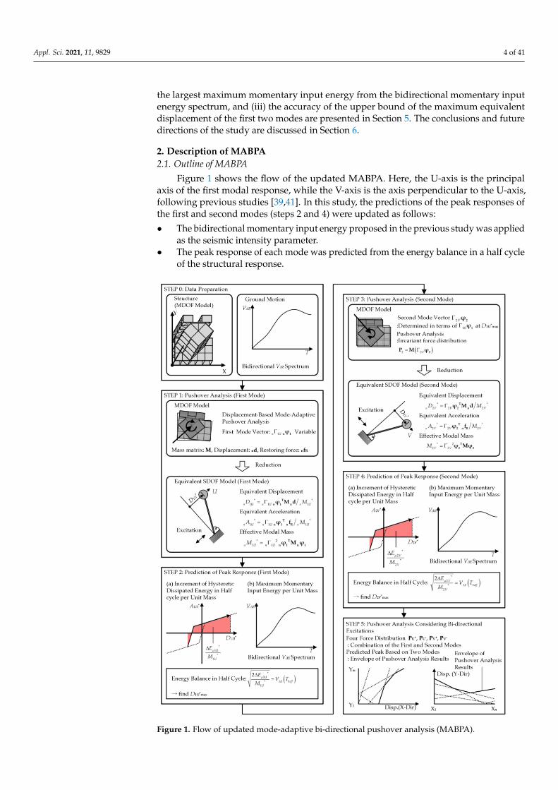
Figure 1 shows the flow of the updated MABPA. Here, the U-axis is the principalaxis of the first modal response, while the V-axis is the axis perpendicular to the U-axis,following previous studies [39,41]. In this study, the predictions of the peak responses ofthe first and second modes (steps 2 and 4) were updated as follows:
• The bidirectional momentary input energy proposed in the previous study was appliedas the seismic intensity parameter.
• The peak response of each mode was predicted from the energy balance in a half cycleof the structural response.
Figure 1. Flow of updated mode-adaptive bi-directional pushover analysis (MABPA).
Appl. Sci. 2021, 11, 9829 5 of 41
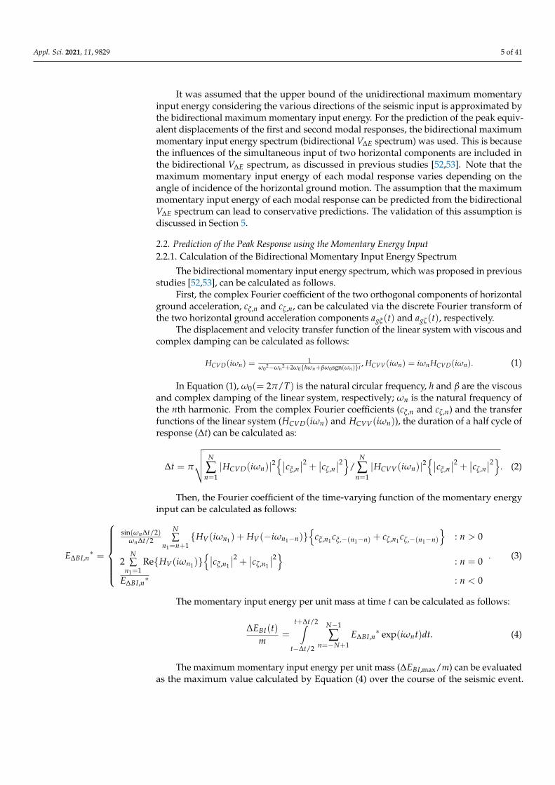
It was assumed that the upper bound of the unidirectional maximum momentaryinput energy considering the various directions of the seismic input is approximated bythe bidirectional maximum momentary input energy. For the prediction of the peak equiv-alent displacements of the first and second modal responses, the bidirectional maximummomentary input energy spectrum (bidirectional V∆E spectrum) was used. This is becausethe influences of the simultaneous input of two horizontal components are included inthe bidirectional V∆E spectrum, as discussed in previous studies [52,53]. Note that themaximum momentary input energy of each modal response varies depending on theangle of incidence of the horizontal ground motion. The assumption that the maximummomentary input energy of each modal response can be predicted from the bidirectionalV∆E spectrum can lead to conservative predictions. The validation of this assumption isdiscussed in Section 5.
2.2. Prediction of the Peak Response using the Momentary Energy Input2.2.1. Calculation of the Bidirectional Momentary Input Energy Spectrum
The bidirectional momentary input energy spectrum, which was proposed in previousstudies [52,53], can be calculated as follows.
First, the complex Fourier coefficient of the two orthogonal components of horizontalground acceleration, cξ,n and cζ,n, can be calculated via the discrete Fourier transform ofthe two horizontal ground acceleration components agξ(t) and agζ(t), respectively.
The displacement and velocity transfer function of the linear system with viscous andcomplex damping can be calculated as follows:
HCVD(iωn) =1
ω02−ωn2+2ω0{hωn+βω0sgn(ωn)}i
, HCVV(iωn) = iωn HCVD(iωn). (1)
In Equation (1), ω0(= 2π/T) is the natural circular frequency, h and β are the viscousand complex damping of the linear system, respectively; ωn is the natural frequency ofthe nth harmonic. From the complex Fourier coefficients (cξ,n and cζ,n) and the transferfunctions of the linear system (HCVD(iωn) and HCVV(iωn)), the duration of a half cycle ofresponse (∆t) can be calculated as:
∆t = π
√√√√ N
∑n=1|HCVD(iωn)|2
{∣∣cξ,n∣∣2 + ∣∣cζ,n
∣∣2}/N
∑n=1|HCVV(iωn)|2
{∣∣cξ,n∣∣2 + ∣∣cζ,n
∣∣2}. (2)
Then, the Fourier coefficient of the time-varying function of the momentary energyinput can be calculated as follows:
E∆BI,n∗ =
sin(ωn∆t/2)ωn∆t/2
N∑
n1=n+1{HV(iωn1) + HV(−iωn1−n)}
{cξ,n1 cξ,−(n1−n) + cζ,n1 cζ,−(n1−n)
}: n > 0
2N∑
n1=1Re{HV(iωn1)}
{∣∣cξ,n1
∣∣2 + ∣∣cζ,n1
∣∣2} : n = 0
E∆BI,n∗ : n < 0
. (3)
The momentary input energy per unit mass at time t can be calculated as follows:
∆EBI(t)m
=
t+∆t/2∫t−∆t/2
N−1
∑n=−N+1
E∆BI,n∗ exp(iωnt)dt. (4)
The maximum momentary input energy per unit mass (∆EBI,max/m) can be evaluatedas the maximum value calculated by Equation (4) over the course of the seismic event.
Appl. Sci. 2021, 11, 9829 6 of 41
The bidirectional maximum momentary input energy spectrum (the bidirectional V∆Espectrum) can be calculated as:
V∆E =√
2∆EBI,max/m. (5)
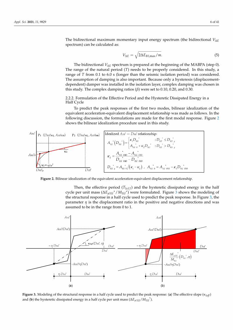
The bidirectional V∆E spectrum is prepared at the beginning of the MABPA (step 0).The range of the natural period (T) needs to be properly considered. In this study, arange of T from 0.1 to 6.0 s (longer than the seismic isolation period) was considered.The assumption of damping is also important. Because only a hysteresis (displacement-dependent) damper was installed in the isolation layer, complex damping was chosen inthis study. The complex damping ratios (β) were set to 0.10, 0.20, and 0.30.
2.2.2. Formulation of the Effective Period and the Hysteretic Dissipated Energy in aHalf Cycle
To predict the peak responses of the first two modes, bilinear idealization of theequivalent acceleration-equivalent displacement relationship was made as follows. In thefollowing discussion, the formulations are made for the first modal response. Figure 2shows the bilinear idealization procedure used in this study.
Figure 2. Bilinear idealization of the equivalent acceleration-equivalent displacement relationship.
Then, the effective period (T1e f f ) and the hysteretic dissipated energy in the halfcycle per unit mass (∆Eµ1U
∗/M1U∗) were formulated. Figure 3 shows the modeling of
the structural response in a half cycle used to predict the peak response. In Figure 3, theparameter η is the displacement ratio in the positive and negative directions and wasassumed to be in the range from 0 to 1.
Figure 3. Modeling of the structural response in a half cycle used to predict the peak response: (a) The effective slope (κ1eff )and (b) the hysteretic dissipated energy in a half cycle per unit mass (∆Eµ1U/M1U
*).
Appl. Sci. 2021, 11, 9829 7 of 41
In this study, the effective period of the first mode corresponding to D1U∗ was calcu-
lated as:T1e f f (D1U
∗) = 2π/√
κ1e f f (D1U∗). (6)
In addition, the equivalent velocity of the hysteretic dissipated energy in a half cyclecorresponding to D1U
∗ was calculated as:
V∆Eµ1U∗(D1U
∗) =
√2∆Eµ1U
∗
M1U∗ (D1U
∗). (7)
The effective slope corresponding to D1U∗ was calculated as:
κ1e f f (D1U∗) =
1∫0
κ1e f f (D1U∗, η)dη
=
{κ1 : D1U
∗ ≤ D1U∗
y
(2 ln 2) A1U∗
0D1U
∗ + κ2 −{
ln(
1 + D1U∗
yD1U
∗
)}(A1U
∗0
D1U∗ + κ1 − κ2
)+
D1U∗
yD1U
∗ (κ1 − κ2) : D1U∗ > D1U
∗y
(8)
The hysteretic dissipated energy in a half cycle per unit mass corresponding to D1U∗
was calculated as:
∆Eµ1U∗
M1U∗ (D1U
∗) =1∫
0
∆Eµ1U∗
M1U∗ (D1U
∗, η)dη
=
13 κ1D1U
∗2 : D1U∗ ≤ D1U
∗y
13 κ2D1U
∗2 + 32 A1U
∗0D1U
∗{(
1− D1U∗
yD1U
∗
)2+ 2
3D1U
∗y
D1U∗
(1− 2
3D1U
∗y
D1U∗
)}: D1U
∗ > D1U∗
y
. (9)
The predicted peak response D1U∗
max was obtained from the following equation:
V∆Eµ1U∗{
T1e f f (D1U∗
max)}= V∆E
{T1e f f (D1U
∗max)
}. (10)
Note that no viscous damping was considered because the isolation layer was assumedto have no viscous damping.
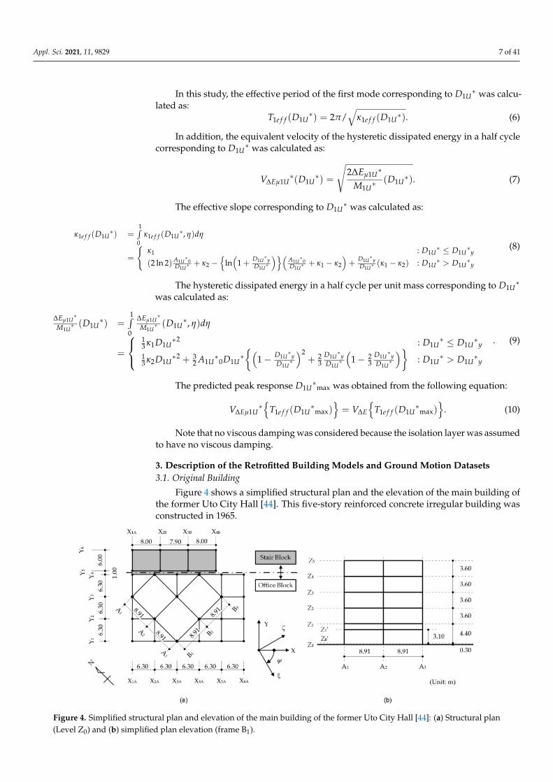
3. Description of the Retrofitted Building Models and Ground Motion Datasets3.1. Original Building
Figure 4 shows a simplified structural plan and the elevation of the main building ofthe former Uto City Hall [44]. This five-story reinforced concrete irregular building wasconstructed in 1965.
Figure 4. Simplified structural plan and elevation of the main building of the former Uto City Hall [44]: (a) Structural plan(Level Z0) and (b) simplified plan elevation (frame B1).
Appl. Sci. 2021, 11, 9829 8 of 41
Figure 5 shows the former Uto City Hall after the 2016 Kumamoto earthquake. Afterthe 2016 Kumamoto earthquake, this building was demolished. Details concerning thisbuilding can be found in the literature [44].
Figure 5. View of the former Uto City Hall after the 2016 Kumamoto earthquake [44]. Photographs were taken from (a) thesouth, (b) the southwest, and (c) the north.
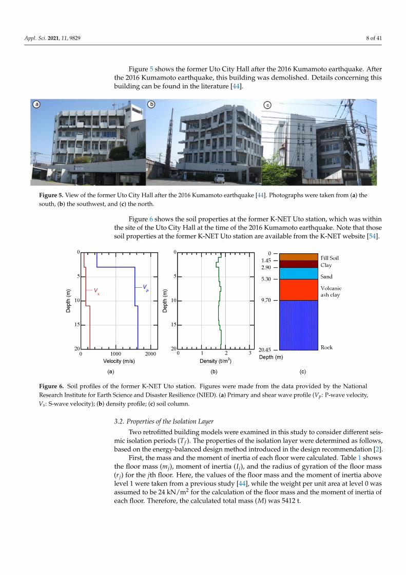
Figure 6 shows the soil properties at the former K-NET Uto station, which was withinthe site of the Uto City Hall at the time of the 2016 Kumamoto earthquake. Note that thosesoil properties at the former K-NET Uto station are available from the K-NET website [54].
Figure 6. Soil profiles of the former K-NET Uto station. Figures were made from the data provided by the NationalResearch Institute for Earth Science and Disaster Resilience (NIED). (a) Primary and shear wave profile (Vp: P-wave velocity,Vs: S-wave velocity); (b) density profile; (c) soil column.
3.2. Properties of the Isolation Layer
Two retrofitted building models were examined in this study to consider different seis-mic isolation periods (Tf ). The properties of the isolation layer were determined as follows,based on the energy-balanced design method introduced in the design recommendation [2].
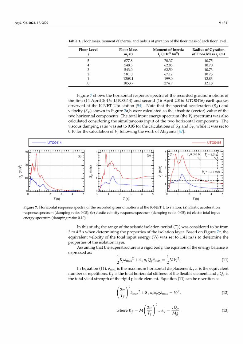
First, the mass and the moment of inertia of each floor were calculated. Table 1 showsthe floor mass (mj), moment of inertia (Ij), and the radius of gyration of the floor mass(rj) for the jth floor. Here, the values of the floor mass and the moment of inertia abovelevel 1 were taken from a previous study [44], while the weight per unit area at level 0 wasassumed to be 24 kN/m2 for the calculation of the floor mass and the moment of inertia ofeach floor. Therefore, the calculated total mass (M) was 5412 t.
Appl. Sci. 2021, 11, 9829 9 of 41
Table 1. Floor mass, moment of inertia, and radius of gyration of the floor mass of each floor level.
Floor Levelj
Floor Massmj (t)
Moment of InertiaIj (×103 tm2)
Radius of Gyrationof Floor Mass rj (m)
5 677.8 78.37 10.754 548.5 62.85 10.703 543.0 62.50 10.732 581.0 67.12 10.751 1208.1 199.0 12.830 1853.7 274.9 12.18
Figure 7 shows the horizontal response spectra of the recorded ground motions ofthe first (14 April 2016: UTO0414) and second (16 April 2016: UTO0416) earthquakesobserved at the K-NET Uto station [54]. Note that the spectral acceleration (SA) andvelocity (SV) shown in Figure 7a,b were calculated as the absolute (vector) value of thetwo horizontal components. The total input energy spectrum (the VI spectrum) was alsocalculated considering the simultaneous input of the two horizontal components. Theviscous damping ratio was set to 0.05 for the calculations of SA and SV , while it was set to0.10 for the calculation of VI following the work of Akiyama [47].
Figure 7. Horizontal response spectra of the recorded ground motions at the K-NET Uto station: (a) Elastic accelerationresponse spectrum (damping ratio: 0.05); (b) elastic velocity response spectrum (damping ratio: 0.05); (c) elastic total inputenergy spectrum (damping ratio: 0.10).
In this study, the range of the seismic isolation period (Tf ) was considered to be from3 to 4.5 s when determining the properties of the isolation layer. Based on Figure 7c, theequivalent velocity of the total input energy (VI) was set to 1.41 m/s to determine theproperties of the isolation layer.
Assuming that the superstructure is a rigid body, the equation of the energy balance isexpressed as:
12
K f δmax2 + 4 s nsQyδmax =
12
MVI2. (11)
In Equation (11), δmax is the maximum horizontal displacement, s n is the equivalentnumber of repetitions, K f is the total horizontal stiffness of the flexible element, and s Qy isthe total yield strength of the rigid plastic element. Equation (11) can be rewritten as:(
2π
Tf
)2
δmax2 + 8 s nsαygδmax = VI
2, (12)
where K f = M
(2π
Tf
)2
, s αy =s Qy
Mg. (13)
Appl. Sci. 2021, 11, 9829 10 of 41
In Equation (13), g is the acceleration due to gravity, assumed to be 9.8 m/s2, and s αyis the yielding shear strength coefficient. In this study, the design-allowable horizontaldisplacement (δa) was set to 0.40 m, while the value of s n was set to 2 following the designrecommendation [2]. Then, the two parameters of the isolation layer, Tf and s αy, wereadjusted, such that the following condition was satisfied:(
2π
Tf
)2
δa2 + 16 s αygδa ≥ VI
2. (14)
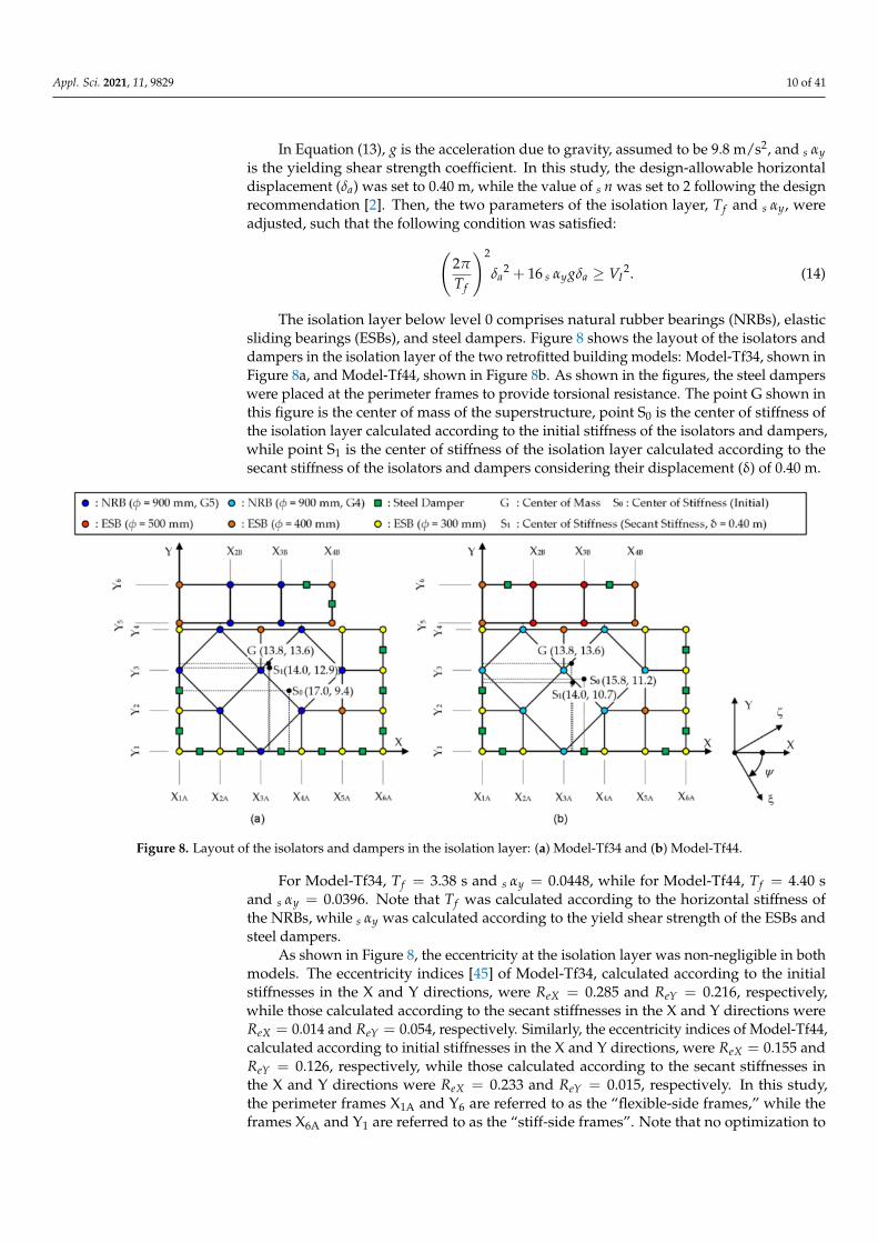
The isolation layer below level 0 comprises natural rubber bearings (NRBs), elasticsliding bearings (ESBs), and steel dampers. Figure 8 shows the layout of the isolators anddampers in the isolation layer of the two retrofitted building models: Model-Tf34, shown inFigure 8a, and Model-Tf44, shown in Figure 8b. As shown in the figures, the steel damperswere placed at the perimeter frames to provide torsional resistance. The point G shown inthis figure is the center of mass of the superstructure, point S0 is the center of stiffness ofthe isolation layer calculated according to the initial stiffness of the isolators and dampers,while point S1 is the center of stiffness of the isolation layer calculated according to thesecant stiffness of the isolators and dampers considering their displacement (δ) of 0.40 m.
Figure 8. Layout of the isolators and dampers in the isolation layer: (a) Model-Tf34 and (b) Model-Tf44.
For Model-Tf34, Tf = 3.38 s and s αy = 0.0448, while for Model-Tf44, Tf = 4.40 sand s αy = 0.0396. Note that Tf was calculated according to the horizontal stiffness ofthe NRBs, while s αy was calculated according to the yield shear strength of the ESBs andsteel dampers.
As shown in Figure 8, the eccentricity at the isolation layer was non-negligible in bothmodels. The eccentricity indices [45] of Model-Tf34, calculated according to the initialstiffnesses in the X and Y directions, were ReX = 0.285 and ReY = 0.216, respectively,while those calculated according to the secant stiffnesses in the X and Y directions wereReX = 0.014 and ReY = 0.054, respectively. Similarly, the eccentricity indices of Model-Tf44,calculated according to initial stiffnesses in the X and Y directions, were ReX = 0.155 andReY = 0.126, respectively, while those calculated according to the secant stiffnesses inthe X and Y directions were ReX = 0.233 and ReY = 0.015, respectively. In this study,the perimeter frames X1A and Y6 are referred to as the “flexible-side frames,” while theframes X6A and Y1 are referred to as the “stiff-side frames”. Note that no optimization to
Appl. Sci. 2021, 11, 9829 11 of 41
minimize the torsional response was made to choose the dampers in this study, becausesuch optimization was beyond the scope of this study.
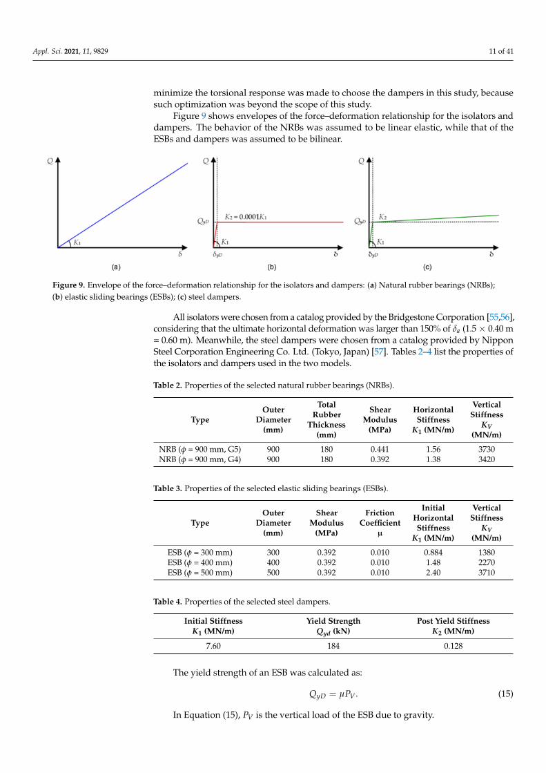
Figure 9 shows envelopes of the force–deformation relationship for the isolators anddampers. The behavior of the NRBs was assumed to be linear elastic, while that of theESBs and dampers was assumed to be bilinear.
Figure 9. Envelope of the force–deformation relationship for the isolators and dampers: (a) Natural rubber bearings (NRBs);(b) elastic sliding bearings (ESBs); (c) steel dampers.
All isolators were chosen from a catalog provided by the Bridgestone Corporation [55,56],considering that the ultimate horizontal deformation was larger than 150% of δa (1.5× 0.40 m= 0.60 m). Meanwhile, the steel dampers were chosen from a catalog provided by NipponSteel Corporation Engineering Co. Ltd. (Tokyo, Japan) [57]. Tables 2–4 list the properties ofthe isolators and dampers used in the two models.
Table 2. Properties of the selected natural rubber bearings (NRBs).
TypeOuter
Diameter(mm)
TotalRubber
Thickness(mm)
ShearModulus
(MPa)
HorizontalStiffness
K1 (MN/m)
VerticalStiffness
KV(MN/m)
NRB (φ = 900 mm, G5) 900 180 0.441 1.56 3730NRB (φ = 900 mm, G4) 900 180 0.392 1.38 3420
Table 3. Properties of the selected elastic sliding bearings (ESBs).
TypeOuter
Diameter(mm)
ShearModulus
(MPa)
FrictionCoefficient
µ
InitialHorizontalStiffness
K1 (MN/m)
VerticalStiffness
KV(MN/m)
ESB (φ = 300 mm) 300 0.392 0.010 0.884 1380ESB (φ = 400 mm) 400 0.392 0.010 1.48 2270ESB (φ = 500 mm) 500 0.392 0.010 2.40 3710
Table 4. Properties of the selected steel dampers.
Initial StiffnessK1 (MN/m)
Yield StrengthQyd (kN)
Post Yield StiffnessK2 (MN/m)
7.60 184 0.128
The yield strength of an ESB was calculated as:
QyD = µPV . (15)
In Equation (15), PV is the vertical load of the ESB due to gravity.
Appl. Sci. 2021, 11, 9829 12 of 41
3.3. Structural Modeling
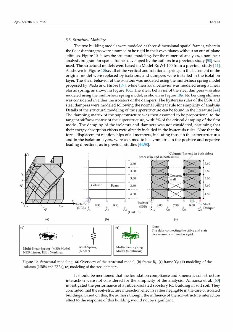
The two building models were modeled as three-dimensional spatial frames, whereinthe floor diaphragms were assumed to be rigid in their own planes without an out-of-planestiffness. Figure 10 shows the structural modeling. For the numerical analyses, a nonlinearanalysis program for spatial frames developed by the authors in a previous study [58] wasused. The structural models were based on Model-RuW4-100 from a previous study [44].As shown in Figure 10b,c, all of the vertical and rotational springs in the basement of theoriginal model were replaced by isolators, and dampers were installed in the isolationlayer. The shear behavior of the isolators was modeled using the multi-shear spring modelproposed by Wada and Hirose [59], while their axial behavior was modeled using a linearelastic spring, as shown in Figure 10d. The shear behavior of the steel dampers was alsomodeled using the multi-shear spring model, as shown in Figure 10e. No bending stiffnesswas considered in either the isolators or the dampers. The hysteresis rules of the ESBs andsteel dampers were modeled following the normal bilinear rule for simplicity of analysis.Details of the structural modeling of the superstructure can be found in the literature [44].The damping matrix of the superstructure was then assumed to be proportional to thetangent stiffness matrix of the superstructure, with 2% of the critical damping of the firstmode. The damping of the isolators and dampers was not considered, assuming thattheir energy absorption effects were already included in the hysteresis rules. Note that theforce–displacement relationships of all members, including those in the superstructuresand in the isolation layers, were assumed to be symmetric in the positive and negativeloading directions, as in previous studies [44,58].
Figure 10. Structural modeling: (a) Overview of the structural model; (b) frame B1; (c) frame Y6; (d) modeling of theisolators (NRBs and ESBs); (e) modeling of the steel dampers.
It should be mentioned that the foundation compliance and kinematic soil–structureinteraction were not considered for the simplicity of the analysis. Almansa et al. [60]investigated the performance of a rubber-isolated six-story RC building in soft soil. Theyconcluded that the soil–structure interaction effect is rather negligible in the case of isolatedbuildings. Based on this, the authors thought the influence of the soil–structure interactioneffect to the response of this building would not be significant.
Appl. Sci. 2021, 11, 9829 13 of 41
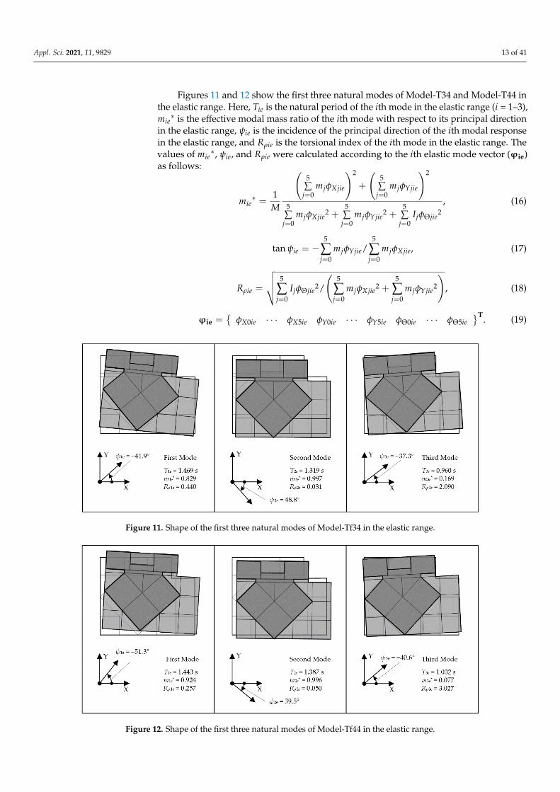
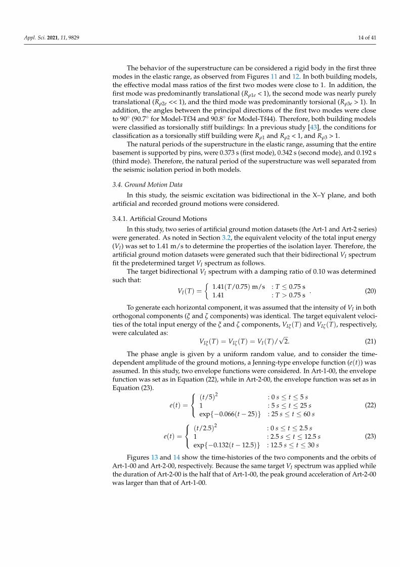
Figures 11 and 12 show the first three natural modes of Model-T34 and Model-T44 inthe elastic range. Here, Tie is the natural period of the ith mode in the elastic range (i = 1–3),mie∗ is the effective modal mass ratio of the ith mode with respect to its principal direction
in the elastic range, ψie is the incidence of the principal direction of the ith modal responsein the elastic range, and Rρie is the torsional index of the ith mode in the elastic range. Thevalues of mie
∗, ψie, and Rρie were calculated according to the ith elastic mode vector (ϕie)as follows:
mie∗ =
1M
(5∑
j=0mjφXjie
)2
+
(5∑
j=0mjφYjie
)2
5∑
j=0mjφXjie
2 +5∑
j=0mjφYjie
2 +5∑
j=0IjφΘjie
2, (16)
tan ψie = −5
∑j=0
mjφYjie/5
∑j=0
mjφXjie, (17)
Rρie =
√√√√ 5
∑j=0
IjφΘjie2/
(5
∑j=0
mjφXjie2 +
5
∑j=0
mjφYjie2
), (18)
ϕie ={
φX0ie · · · φX5ie φY0ie · · · φY5ie φΘ0ie · · · φΘ5ie}T. (19)
Figure 11. Shape of the first three natural modes of Model-Tf34 in the elastic range.
Figure 12. Shape of the first three natural modes of Model-Tf44 in the elastic range.
Appl. Sci. 2021, 11, 9829 14 of 41
The behavior of the superstructure can be considered a rigid body in the first threemodes in the elastic range, as observed from Figures 11 and 12. In both building models,the effective modal mass ratios of the first two modes were close to 1. In addition, thefirst mode was predominantly translational (Rρ1e < 1), the second mode was nearly purelytranslational (Rρ2e << 1), and the third mode was predominantly torsional (Rρ3e > 1). Inaddition, the angles between the principal directions of the first two modes were closeto 90◦ (90.7◦ for Model-Tf34 and 90.8◦ for Model-Tf44). Therefore, both building modelswere classified as torsionally stiff buildings: In a previous study [43], the conditions forclassification as a torsionally stiff building were Rρ1 and Rρ2 < 1, and Rρ3 > 1.
The natural periods of the superstructure in the elastic range, assuming that the entirebasement is supported by pins, were 0.373 s (first mode), 0.342 s (second mode), and 0.192 s(third mode). Therefore, the natural period of the superstructure was well separated fromthe seismic isolation period in both models.
3.4. Ground Motion Data
In this study, the seismic excitation was bidirectional in the X–Y plane, and bothartificial and recorded ground motions were considered.
3.4.1. Artificial Ground Motions
In this study, two series of artificial ground motion datasets (the Art-1 and Art-2 series)were generated. As noted in Section 3.2, the equivalent velocity of the total input energy(VI) was set to 1.41 m/s to determine the properties of the isolation layer. Therefore, theartificial ground motion datasets were generated such that their bidirectional VI spectrumfit the predetermined target VI spectrum as follows.
The target bidirectional VI spectrum with a damping ratio of 0.10 was determinedsuch that:
VI(T) ={
1.41(T/0.75) m/s : T ≤ 0.75 s1.41 : T > 0.75 s
. (20)
To generate each horizontal component, it was assumed that the intensity of VI in bothorthogonal components (ξ and ζ components) was identical. The target equivalent veloci-ties of the total input energy of the ξ and ζ components, VIξ(T) and VIζ(T), respectively,were calculated as:
VIξ(T) = VIζ(T) = VI(T)/√
2. (21)
The phase angle is given by a uniform random value, and to consider the time-dependent amplitude of the ground motions, a Jenning-type envelope function (e(t)) wasassumed. In this study, two envelope functions were considered. In Art-1-00, the envelopefunction was set as in Equation (22), while in Art-2-00, the envelope function was set as inEquation (23).
e(t) =
(t/5)2 : 0 s ≤ t ≤ 5 s1 : 5 s ≤ t ≤ 25 sexp{−0.066(t− 25)} : 25 s ≤ t ≤ 60 s
(22)
e(t) =
(t/2.5)2 : 0 s ≤ t ≤ 2.5 s1 : 2.5 s ≤ t ≤ 12.5 sexp{−0.132(t− 12.5)} : 12.5 s ≤ t ≤ 30 s
(23)
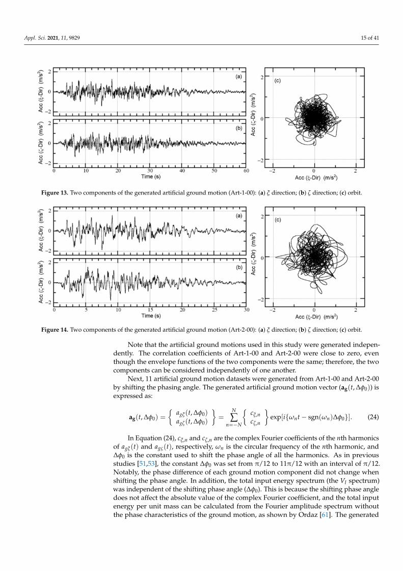
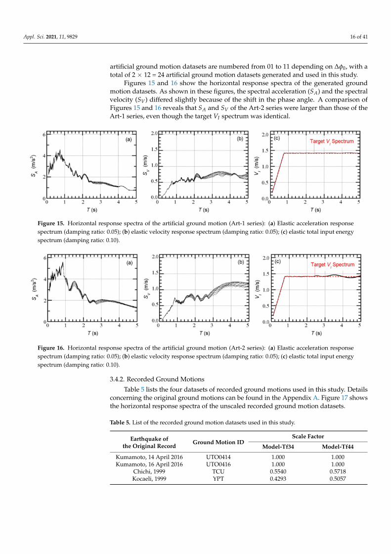
Figures 13 and 14 show the time-histories of the two components and the orbits ofArt-1-00 and Art-2-00, respectively. Because the same target VI spectrum was applied whilethe duration of Art-2-00 is the half that of Art-1-00, the peak ground acceleration of Art-2-00was larger than that of Art-1-00.
Appl. Sci. 2021, 11, 9829 15 of 41
Figure 13. Two components of the generated artificial ground motion (Art-1-00): (a) ξ direction; (b) ζ direction; (c) orbit.
Figure 14. Two components of the generated artificial ground motion (Art-2-00): (a) ξ direction; (b) ζ direction; (c) orbit.
Note that the artificial ground motions used in this study were generated indepen-dently. The correlation coefficients of Art-1-00 and Art-2-00 were close to zero, eventhough the envelope functions of the two components were the same; therefore, the twocomponents can be considered independently of one another.
Next, 11 artificial ground motion datasets were generated from Art-1-00 and Art-2-00by shifting the phasing angle. The generated artificial ground motion vector (ag(t, ∆φ0)) isexpressed as:
ag(t, ∆φ0) =
{agξ(t, ∆φ0)agζ(t, ∆φ0)
}=
N
∑n=−N
{cξ,ncζ,n
}exp[i{ωnt− sgn(ωn)∆φ0}]. (24)
In Equation (24), cξ,n and cζ,n are the complex Fourier coefficients of the nth harmonicsof agξ(t) and agς(t), respectively, ωn is the circular frequency of the nth harmonic, and∆φ0 is the constant used to shift the phase angle of all the harmonics. As in previousstudies [51,53], the constant ∆φ0 was set from π/12 to 11π/12 with an interval of π/12.Notably, the phase difference of each ground motion component did not change whenshifting the phase angle. In addition, the total input energy spectrum (the VI spectrum)was independent of the shifting phase angle (∆φ0). This is because the shifting phase angledoes not affect the absolute value of the complex Fourier coefficient, and the total inputenergy per unit mass can be calculated from the Fourier amplitude spectrum withoutthe phase characteristics of the ground motion, as shown by Ordaz [61]. The generated
Appl. Sci. 2021, 11, 9829 16 of 41
artificial ground motion datasets are numbered from 01 to 11 depending on ∆φ0, with atotal of 2 × 12 = 24 artificial ground motion datasets generated and used in this study.
Figures 15 and 16 show the horizontal response spectra of the generated groundmotion datasets. As shown in these figures, the spectral acceleration (SA) and the spectralvelocity (SV) differed slightly because of the shift in the phase angle. A comparison ofFigures 15 and 16 reveals that SA and SV of the Art-2 series were larger than those of theArt-1 series, even though the target VI spectrum was identical.
Figure 15. Horizontal response spectra of the artificial ground motion (Art-1 series): (a) Elastic acceleration responsespectrum (damping ratio: 0.05); (b) elastic velocity response spectrum (damping ratio: 0.05); (c) elastic total input energyspectrum (damping ratio: 0.10).
Figure 16. Horizontal response spectra of the artificial ground motion (Art-2 series): (a) Elastic acceleration responsespectrum (damping ratio: 0.05); (b) elastic velocity response spectrum (damping ratio: 0.05); (c) elastic total input energyspectrum (damping ratio: 0.10).
3.4.2. Recorded Ground Motions
Table 5 lists the four datasets of recorded ground motions used in this study. Detailsconcerning the original ground motions can be found in the Appendix A. Figure 17 showsthe horizontal response spectra of the unscaled recorded ground motion datasets.
Table 5. List of the recorded ground motion datasets used in this study.
Earthquake ofthe Original Record
Ground Motion IDScale Factor
Model-Tf34 Model-Tf44
Kumamoto, 14 April 2016 UTO0414 1.000 1.000Kumamoto, 16 April 2016 UTO0416 1.000 1.000
Chichi, 1999 TCU 0.5540 0.5718Kocaeli, 1999 YPT 0.4293 0.5057
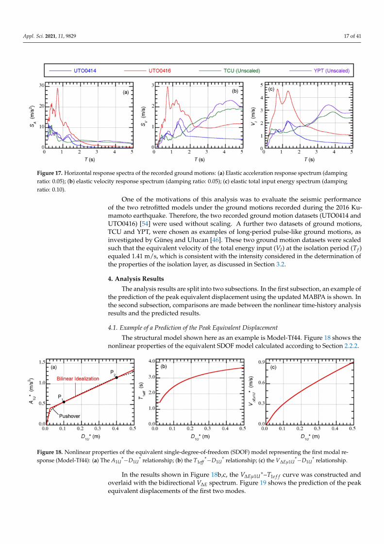
Appl. Sci. 2021, 11, 9829 17 of 41
Figure 17. Horizontal response spectra of the recorded ground motions: (a) Elastic acceleration response spectrum (dampingratio: 0.05); (b) elastic velocity response spectrum (damping ratio: 0.05); (c) elastic total input energy spectrum (dampingratio: 0.10).
One of the motivations of this analysis was to evaluate the seismic performanceof the two retrofitted models under the ground motions recorded during the 2016 Ku-mamoto earthquake. Therefore, the two recorded ground motion datasets (UTO0414 andUTO0416) [54] were used without scaling. A further two datasets of ground motions,TCU and YPT, were chosen as examples of long-period pulse-like ground motions, asinvestigated by Günes and Ulucan [46]. These two ground motion datasets were scaledsuch that the equivalent velocity of the total energy input (VI) at the isolation period (Tf )equaled 1.41 m/s, which is consistent with the intensity considered in the determination ofthe properties of the isolation layer, as discussed in Section 3.2.
4. Analysis Results
The analysis results are split into two subsections. In the first subsection, an example ofthe prediction of the peak equivalent displacement using the updated MABPA is shown. Inthe second subsection, comparisons are made between the nonlinear time-history analysisresults and the predicted results.
4.1. Example of a Prediction of the Peak Equivalent Displacement
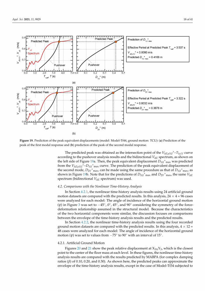
The structural model shown here as an example is Model-Tf44. Figure 18 shows thenonlinear properties of the equivalent SDOF model calculated according to Section 2.2.2.
Figure 18. Nonlinear properties of the equivalent single-degree-of-freedom (SDOF) model representing the first modal re-sponse (Model-Tf44): (a) The A1U
*−D1U* relationship; (b) the T1eff
*−D1U* relationship; (c) the V∆Eµ1U
*−D1U* relationship.
In the results shown in Figure 18b,c, the V∆Eµ1U∗–T1e f f curve was constructed and
overlaid with the bidirectional V∆E spectrum. Figure 19 shows the prediction of the peakequivalent displacements of the first two modes.
Appl. Sci. 2021, 11, 9829 18 of 41
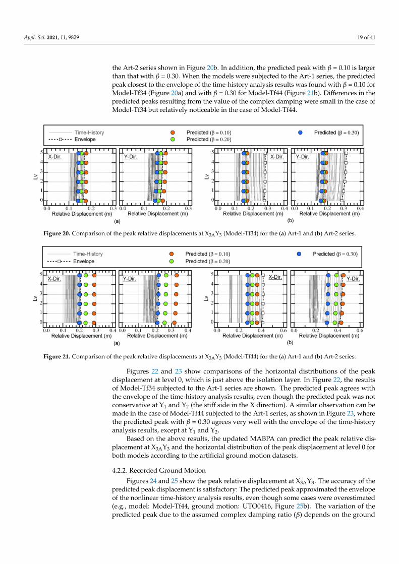
Figure 19. Prediction of the peak equivalent displacements (model: Model-Tf44, ground motion: TCU): (a) Prediction of thepeak of the first modal response and (b) prediction of the peak of the second modal response.
The predicted peak was obtained as the intersection point of the V∆Eµ1U∗–T1e f f curve
according to the pushover analysis results and the bidirectional V∆E spectrum, as shown onthe left side of Figure 19a. Then, the peak equivalent displacement D1U
∗max was predicted
from the V∆Eµ1U∗–D1U
∗max curve. The prediction of the peak equivalent displacement of
the second mode, D2V∗
max, can be made using the same procedure as that of D1U∗
max, asshown in Figure 19b. Note that for the predictions of D1U
∗max and D2V
∗max, the same V∆E
spectrum (bidirectional V∆E spectrum) was used.
4.2. Comparisons with the Nonlinear Time-History Analysis
In Section 4.2.1, the nonlinear time-history analysis results using 24 artificial groundmotion datasets are compared with the predicted results. In this analysis, 24 × 4 = 96 caseswere analyzed for each model: The angle of incidence of the horizontal ground motion(ψ) in Figure 3 was set to −45◦, 0◦, 45◦, and 90◦ considering the symmetry of the force-deformation relationship assumed in the structural model. Because the characteristicsof the two horizontal components were similar, the discussion focuses on comparisonsbetween the envelope of the time-history analysis results and the predicted results.
In Section 4.2.2, the nonlinear time-history analysis results using the four recordedground motion datasets are compared with the predicted results. In this analysis, 4 × 12 =48 cases were analyzed for each model: The angle of incidence of the horizontal groundmotion (ψ) was set to values from −75◦ to 90◦ with an interval of 15◦.
4.2.1. Artificial Ground Motion
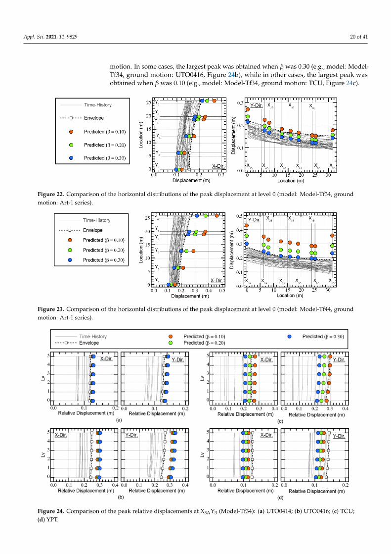
Figures 20 and 21 show the peak relative displacement at X3AY3, which is the closestpoint to the center of the floor mass at each level. In these figures, the nonlinear time-historyanalysis results are compared with the results predicted by MABPA (for complex dampingratios (β) of 0.10, 0.20, and 0.30). As shown here, the predicted peaks can approximate theenvelope of the time-history analysis results, except in the case of Model-Tf34 subjected to
Appl. Sci. 2021, 11, 9829 19 of 41
the Art-2 series shown in Figure 20b. In addition, the predicted peak with β = 0.10 is largerthan that with β = 0.30. When the models were subjected to the Art-1 series, the predictedpeak closest to the envelope of the time-history analysis results was found with β = 0.10 forModel-Tf34 (Figure 20a) and with β = 0.30 for Model-Tf44 (Figure 21b). Differences in thepredicted peaks resulting from the value of the complex damping were small in the case ofModel-Tf34 but relatively noticeable in the case of Model-Tf44.
Figure 20. Comparison of the peak relative displacements at X3AY3 (Model-Tf34) for the (a) Art-1 and (b) Art-2 series.
Figure 21. Comparison of the peak relative displacements at X3AY3 (Model-Tf44) for the (a) Art-1 and (b) Art-2 series.
Figures 22 and 23 show comparisons of the horizontal distributions of the peakdisplacement at level 0, which is just above the isolation layer. In Figure 22, the resultsof Model-Tf34 subjected to the Art-1 series are shown. The predicted peak agrees withthe envelope of the time-history analysis results, even though the predicted peak was notconservative at Y1 and Y2 (the stiff side in the X direction). A similar observation can bemade in the case of Model-Tf44 subjected to the Art-1 series, as shown in Figure 23, wherethe predicted peak with β = 0.30 agrees very well with the envelope of the time-historyanalysis results, except at Y1 and Y2.
Based on the above results, the updated MABPA can predict the peak relative dis-placement at X3AY3 and the horizontal distribution of the peak displacement at level 0 forboth models according to the artificial ground motion datasets.
4.2.2. Recorded Ground Motion
Figures 24 and 25 show the peak relative displacement at X3AY3. The accuracy of thepredicted peak displacement is satisfactory: The predicted peak approximated the envelopeof the nonlinear time-history analysis results, even though some cases were overestimated(e.g., model: Model-Tf44, ground motion: UTO0416, Figure 25b). The variation of thepredicted peak due to the assumed complex damping ratio (β) depends on the ground
Appl. Sci. 2021, 11, 9829 20 of 41
motion. In some cases, the largest peak was obtained when β was 0.30 (e.g., model: Model-Tf34, ground motion: UTO0416, Figure 24b), while in other cases, the largest peak wasobtained when β was 0.10 (e.g., model: Model-Tf34, ground motion: TCU, Figure 24c).
Figure 22. Comparison of the horizontal distributions of the peak displacement at level 0 (model: Model-Tf34, groundmotion: Art-1 series).
Figure 23. Comparison of the horizontal distributions of the peak displacement at level 0 (model: Model-Tf44, groundmotion: Art-1 series).
Figure 24. Comparison of the peak relative displacements at X3AY3 (Model-Tf34): (a) UTO0414; (b) UTO0416; (c) TCU;(d) YPT.
Appl. Sci. 2021, 11, 9829 21 of 41
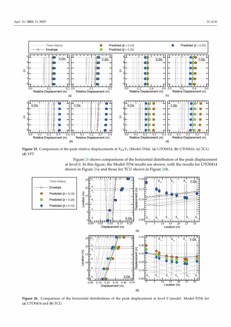
Figure 25. Comparison of the peak relative displacements at X3AY3 (Model-Tf44): (a) UTO0414; (b) UTO0416; (c) TCU;(d) YPT.
Figure 26 shows comparisons of the horizontal distribution of the peak displacementat level 0. In this figure, the Model-Tf34 results are shown, with the results for UTO0414shown in Figure 26a and those for TCU shown in Figure 26b.
Figure 26. Comparison of the horizontal distributions of the peak displacement at level 0 (model: Model-Tf34) for(a) UTO0414 and (b) TCU.
Appl. Sci. 2021, 11, 9829 22 of 41
The predicted horizontal distribution of the peak displacement in the Y direction wasnotably different from the envelope of the time-history analysis in the case of UTO0414, asshown in Figure 26a. In the predicted distribution, the largest displacement occurred at X1A(the flexible side in the Y direction); meanwhile, in the envelope of the time-history analysisresults, the displacement at X1A was the smallest. Conversely, the predicted horizontaldistribution of the peak displacement in the Y direction fits the envelope of the time-historyanalysis in the case of TCU very well, as shown in Figure 26b. In the predicted distribution,the largest displacement occurred at X1A, which is consistent with the envelope of thetime-history analysis results. The modal displacement responses at X1A and X6A (the stiffside in the Y direction) are compared and discussed further in Section 5.5.
One of the motivations of this analysis was to evaluate the seismic performance ofthe retrofitted building models under the recorded motions from the 2016 Kumamotoearthquake. It has already been reported in a previous study [44] that the seismic capacityevaluation of the main building of the former Uto City Hall indicate that the structure wasinsufficient to withstand the earthquake that occurred on 14 April 2016. Therefore, the driftof the superstructure was examined as follows.
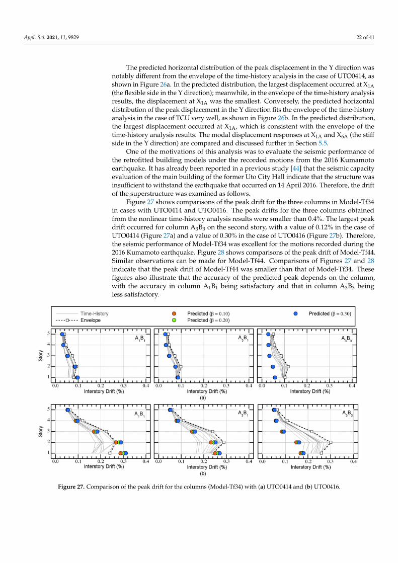
Figure 27 shows comparisons of the peak drift for the three columns in Model-Tf34in cases with UTO0414 and UTO0416. The peak drifts for the three columns obtainedfrom the nonlinear time-history analysis results were smaller than 0.4%. The largest peakdrift occurred for column A3B3 on the second story, with a value of 0.12% in the case ofUTO0414 (Figure 27a) and a value of 0.30% in the case of UTO0416 (Figure 27b). Therefore,the seismic performance of Model-Tf34 was excellent for the motions recorded during the2016 Kumamoto earthquake. Figure 28 shows comparisons of the peak drift of Model-Tf44.Similar observations can be made for Model-Tf44. Comparisons of Figures 27 and 28indicate that the peak drift of Model-Tf44 was smaller than that of Model-Tf34. Thesefigures also illustrate that the accuracy of the predicted peak depends on the column,with the accuracy in column A1B1 being satisfactory and that in column A3B3 beingless satisfactory.
Figure 27. Comparison of the peak drift for the columns (Model-Tf34) with (a) UTO0414 and (b) UTO0416.
Appl. Sci. 2021, 11, 9829 23 of 41
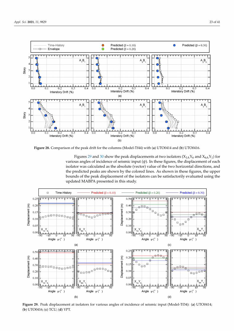
Figure 28. Comparison of the peak drift for the columns (Model-Tf44) with (a) UTO0414 and (b) UTO0416.
Figures 29 and 30 show the peak displacements at two isolators (X1AY6 and X6AY1) forvarious angles of incidence of seismic input (ψ). In these figures, the displacement of eachisolator was calculated as the absolute (vector) value of the two horizontal directions, andthe predicted peaks are shown by the colored lines. As shown in these figures, the upperbounds of the peak displacement of the isolators can be satisfactorily evaluated using theupdated MABPA presented in this study.
Figure 29. Peak displacement at isolators for various angles of incidence of seismic input (Model-Tf34): (a) UTO0414;(b) UTO0416; (c) TCU; (d) YPT.
Appl. Sci. 2021, 11, 9829 24 of 41
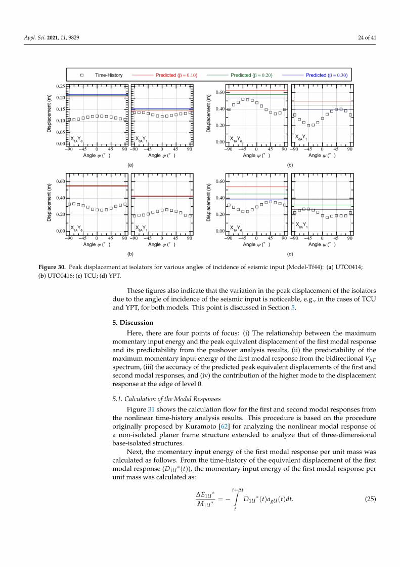
Figure 30. Peak displacement at isolators for various angles of incidence of seismic input (Model-Tf44): (a) UTO0414;(b) UTO0416; (c) TCU; (d) YPT.
These figures also indicate that the variation in the peak displacement of the isolatorsdue to the angle of incidence of the seismic input is noticeable, e.g., in the cases of TCUand YPT, for both models. This point is discussed in Section 5.
5. Discussion
Here, there are four points of focus: (i) The relationship between the maximummomentary input energy and the peak equivalent displacement of the first modal responseand its predictability from the pushover analysis results, (ii) the predictability of themaximum momentary input energy of the first modal response from the bidirectional V∆Espectrum, (iii) the accuracy of the predicted peak equivalent displacements of the first andsecond modal responses, and (iv) the contribution of the higher mode to the displacementresponse at the edge of level 0.
5.1. Calculation of the Modal Responses
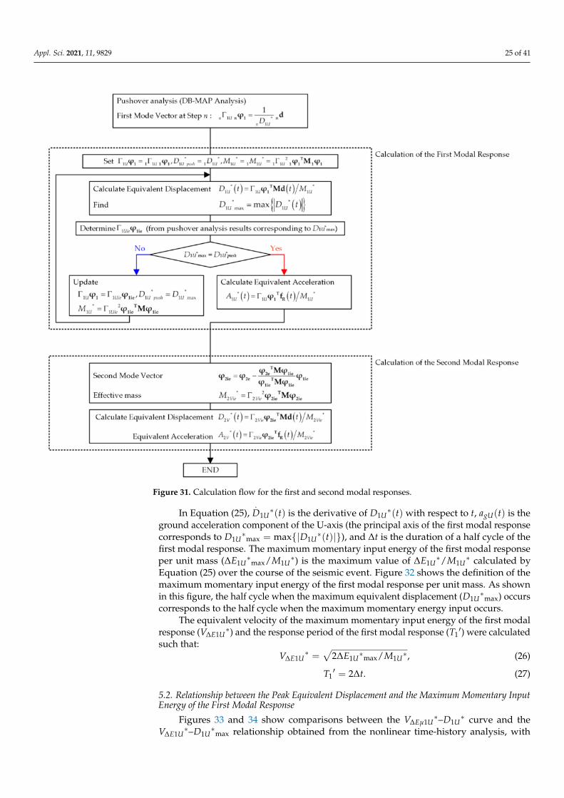
Figure 31 shows the calculation flow for the first and second modal responses fromthe nonlinear time-history analysis results. This procedure is based on the procedureoriginally proposed by Kuramoto [62] for analyzing the nonlinear modal response ofa non-isolated planer frame structure extended to analyze that of three-dimensionalbase-isolated structures.
Next, the momentary input energy of the first modal response per unit mass wascalculated as follows. From the time-history of the equivalent displacement of the firstmodal response (D1U
∗(t)), the momentary input energy of the first modal response perunit mass was calculated as:
∆E1U∗
M1U∗ = −
t+∆t∫t
.D1U
∗(t)agU(t)dt. (25)
Appl. Sci. 2021, 11, 9829 25 of 41
Figure 31. Calculation flow for the first and second modal responses.
In Equation (25),.
D1U∗(t) is the derivative of D1U
∗(t) with respect to t, agU(t) is theground acceleration component of the U-axis (the principal axis of the first modal responsecorresponds to D1U
∗max = max{|D1U
∗(t)|}), and ∆t is the duration of a half cycle of thefirst modal response. The maximum momentary input energy of the first modal responseper unit mass (∆E1U
∗max/M1U
∗) is the maximum value of ∆E1U∗/M1U
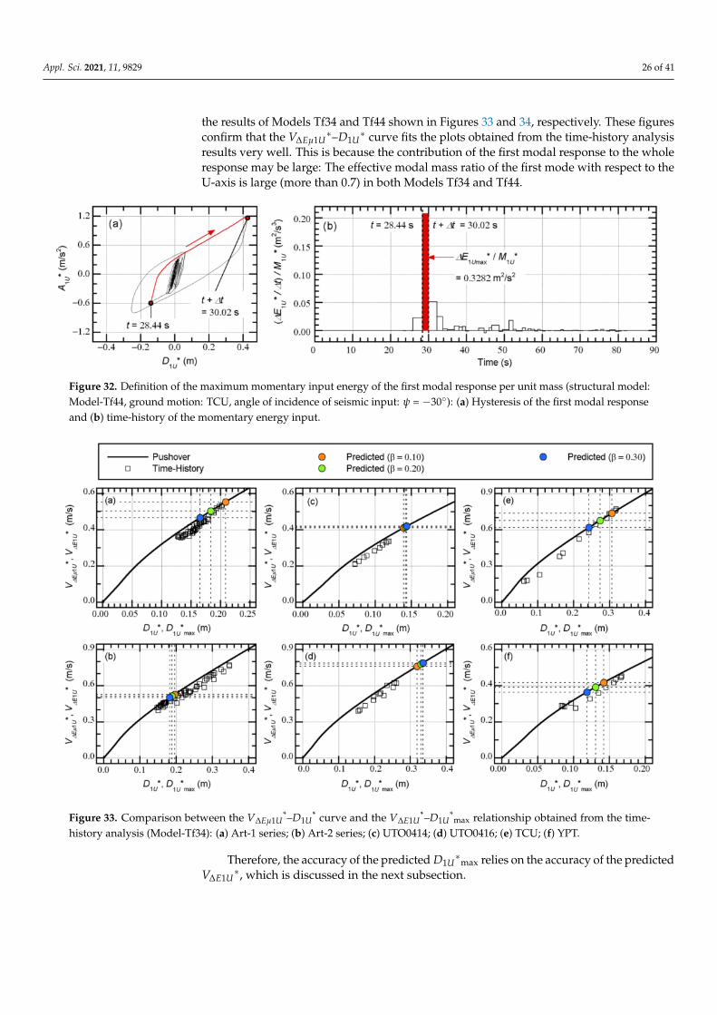
∗ calculated byEquation (25) over the course of the seismic event. Figure 32 shows the definition of themaximum momentary input energy of the first modal response per unit mass. As shownin this figure, the half cycle when the maximum equivalent displacement (D1U
∗max) occurs
corresponds to the half cycle when the maximum momentary energy input occurs.The equivalent velocity of the maximum momentary input energy of the first modal
response (V∆E1U∗) and the response period of the first modal response (T1
′) were calculatedsuch that:
V∆E1U∗ =
√2∆E1U
∗max/M1U∗, (26)
T1′ = 2∆t. (27)
5.2. Relationship between the Peak Equivalent Displacement and the Maximum Momentary InputEnergy of the First Modal Response
Figures 33 and 34 show comparisons between the V∆Eµ1U∗–D1U
∗ curve and theV∆E1U
∗–D1U∗
max relationship obtained from the nonlinear time-history analysis, with
Appl. Sci. 2021, 11, 9829 26 of 41
the results of Models Tf34 and Tf44 shown in Figures 33 and 34, respectively. These figuresconfirm that the V∆Eµ1U
∗–D1U∗ curve fits the plots obtained from the time-history analysis
results very well. This is because the contribution of the first modal response to the wholeresponse may be large: The effective modal mass ratio of the first mode with respect to theU-axis is large (more than 0.7) in both Models Tf34 and Tf44.
Figure 32. Definition of the maximum momentary input energy of the first modal response per unit mass (structural model:Model-Tf44, ground motion: TCU, angle of incidence of seismic input: ψ = −30◦): (a) Hysteresis of the first modal responseand (b) time-history of the momentary energy input.
Figure 33. Comparison between the V∆Eµ1U*–D1U
* curve and the V∆E1U*–D1U
*max relationship obtained from the time-
history analysis (Model-Tf34): (a) Art-1 series; (b) Art-2 series; (c) UTO0414; (d) UTO0416; (e) TCU; (f) YPT.
Therefore, the accuracy of the predicted D1U∗
max relies on the accuracy of the predictedV∆E1U
∗, which is discussed in the next subsection.
Appl. Sci. 2021, 11, 9829 27 of 41
5.3. Comparison of the Maximum Momentary Input Energy and the Bidirectional MomentaryInput Energy Spectrum
Figure 35 shows the prediction of V∆E1U∗ from the bidirectional V∆E spectrum for Model-
Tf34. The plots shown in this figure indicate the nonlinear time-history analysis results.
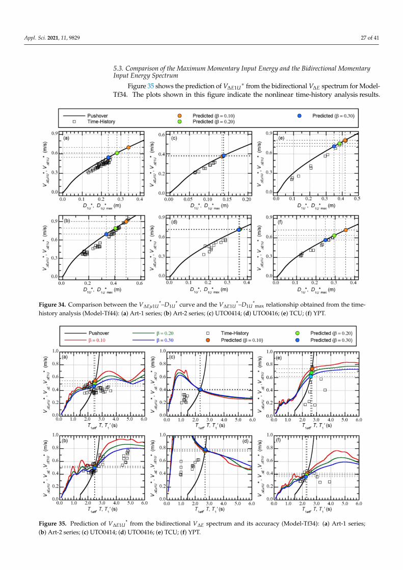
Figure 34. Comparison between the V∆Eµ1U*–D1U
* curve and the V∆E1U*–D1U
*max relationship obtained from the time-
history analysis (Model-Tf44): (a) Art-1 series; (b) Art-2 series; (c) UTO0414; (d) UTO0416; (e) TCU; (f) YPT.
Figure 35. Prediction of V∆E1U* from the bidirectional V∆E spectrum and its accuracy (Model-Tf34): (a) Art-1 series;
(b) Art-2 series; (c) UTO0414; (d) UTO0416; (e) TCU; (f) YPT.
Appl. Sci. 2021, 11, 9829 28 of 41
In most cases, the bidirectional V∆E spectrum with complex damping β = 0.10 ap-proximated the upper bound of the plot of the time-history analysis results, as shownin Figure 35a,b,e,f. However, in the other cases shown in Figure 35c,d, the plots of thetime-history analysis results were below those of the bidirectional V∆E spectrum.
From the comparisons between the predicted V∆E1U∗ and that obtained from the
time-history analysis results, the predicted V∆E1U∗ provided a conservative estimation,
except in the case of the Art-2 series shown in Figure 35b. This is because the predictedresponse points correspond to the “valley” of the bidirectional V∆E spectrum, thereforemaking the predicted V∆E1U
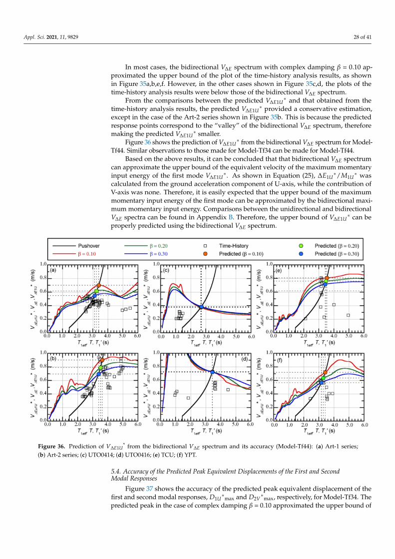
∗ smaller.Figure 36 shows the prediction of V∆E1U
∗ from the bidirectional V∆E spectrum for Model-Tf44. Similar observations to those made for Model-Tf34 can be made for Model-Tf44.
Based on the above results, it can be concluded that that bidirectional V∆E spectrumcan approximate the upper bound of the equivalent velocity of the maximum momentaryinput energy of the first mode V∆E1U
∗. As shown in Equation (25), ∆E1U∗/M1U
∗ wascalculated from the ground acceleration component of U-axis, while the contribution ofV-axis was none. Therefore, it is easily expected that the upper bound of the maximummomentary input energy of the first mode can be approximated by the bidirectional maxi-mum momentary input energy. Comparisons between the unidirectional and bidirectionalV∆E spectra can be found in Appendix B. Therefore, the upper bound of V∆E1U
∗ can beproperly predicted using the bidirectional V∆E spectrum.
Figure 36. Prediction of V∆E1U* from the bidirectional V∆E spectrum and its accuracy (Model-Tf44): (a) Art-1 series;
(b) Art-2 series; (c) UTO0414; (d) UTO0416; (e) TCU; (f) YPT.
5.4. Accuracy of the Predicted Peak Equivalent Displacements of the First and SecondModal Responses
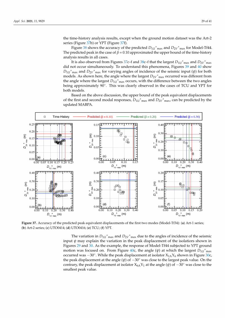
Figure 37 shows the accuracy of the predicted peak equivalent displacement of thefirst and second modal responses, D1U
∗max and D2V
∗max, respectively, for Model-Tf34. The
predicted peak in the case of complex damping β = 0.10 approximated the upper bound of
Appl. Sci. 2021, 11, 9829 29 of 41
the time-history analysis results, except when the ground motion dataset was the Art-2series (Figure 37b) or YPT (Figure 37f).
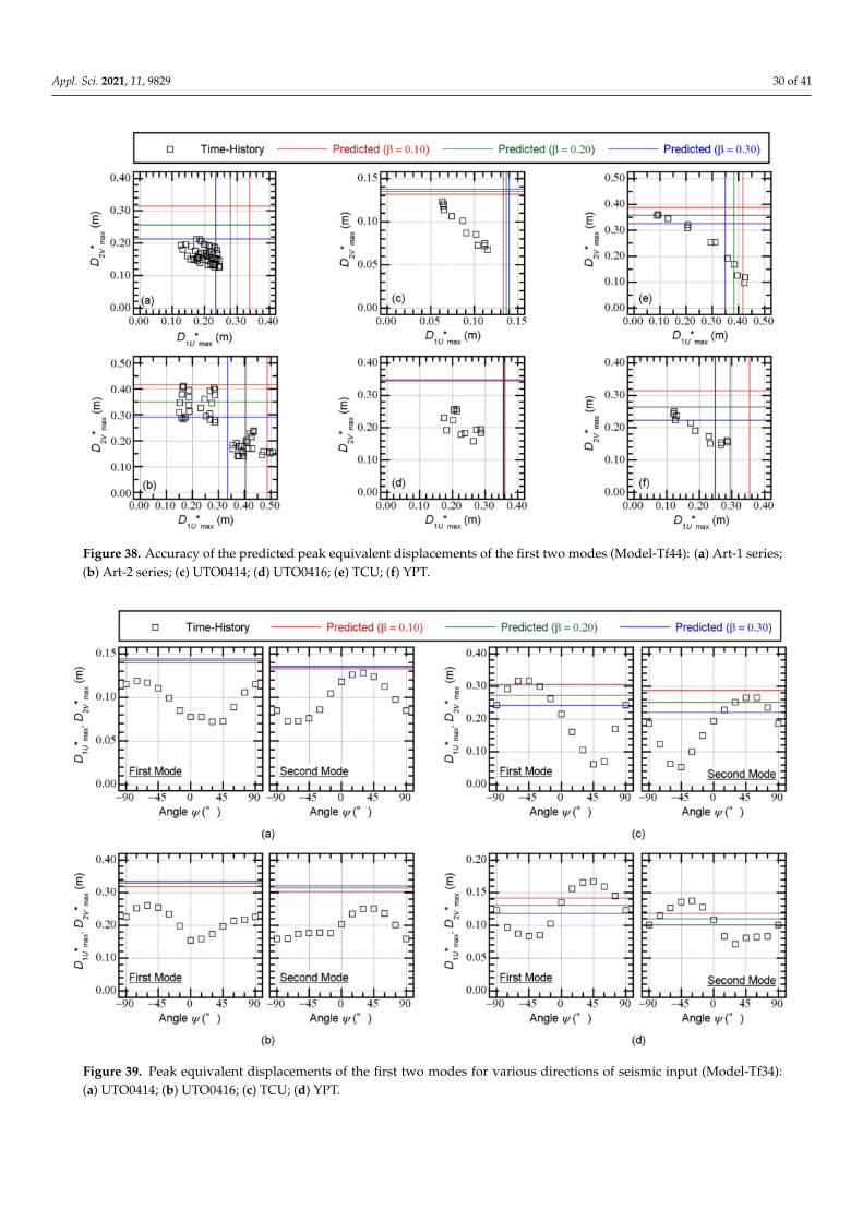
Figure 38 shows the accuracy of the predicted D1U∗
max and D2V∗
max for Model-Tf44.The predicted peak in the case of β = 0.10 approximated the upper bound of the time-historyanalysis results in all cases.
It is also observed from Figures 37c–f and 38c–f that the largest D1U∗
max and D2V∗
maxdid not occur simultaneously. To understand this phenomena, Figures 39 and 40 showD1U
∗max and D2V
∗max for varying angles of incidence of the seismic input (ψ) for both
models. As shown here, the angle where the largest D2V∗
max occurred was different fromthe angle where the largest D1U
∗max occurs, with the difference between the two angles
being approximately 90◦. This was clearly observed in the cases of TCU and YPT forboth models.
Based on the above discussion, the upper bound of the peak equivalent displacementsof the first and second modal responses, D1U
∗max and D2V
∗max, can be predicted by the
updated MABPA.
Figure 37. Accuracy of the predicted peak equivalent displacements of the first two modes (Model-Tf34): (a) Art-1 series;(b) Art-2 series; (c) UTO0414; (d) UTO0416; (e) TCU; (f) YPT.
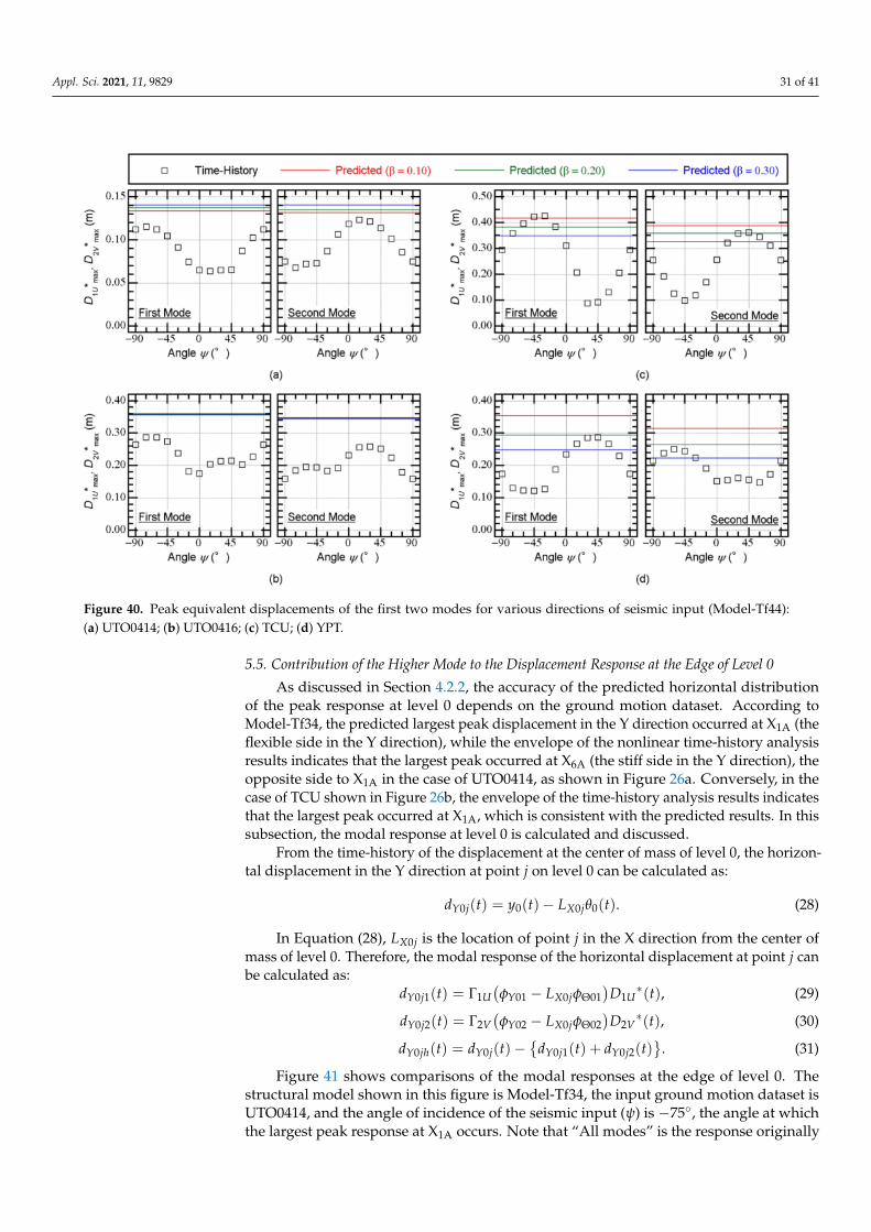
The variation in D1U∗
max and D2V∗
max due to the angles of incidence of the seismicinput ψ may explain the variation in the peak displacement of the isolatiors shown inFigures 29 and 30. As the example, the response of Model-Tf44 subjected to YPT groundmotion was focused on. From Figure 40c, the angle (ψ) at which the largest D1U
∗max
occurred was −30◦. While the peak displacement at isolator X1AY6 shown in Figure 30c,the peak displacement at the angle (ψ) of −30◦ was close to the largest peak value. On thecontrary, the peak displacement at isolator X6AY1 at the angle (ψ) of −30◦ was close to thesmallest peak value.
Appl. Sci. 2021, 11, 9829 30 of 41
Figure 38. Accuracy of the predicted peak equivalent displacements of the first two modes (Model-Tf44): (a) Art-1 series;(b) Art-2 series; (c) UTO0414; (d) UTO0416; (e) TCU; (f) YPT.
Figure 39. Peak equivalent displacements of the first two modes for various directions of seismic input (Model-Tf34):(a) UTO0414; (b) UTO0416; (c) TCU; (d) YPT.
Appl. Sci. 2021, 11, 9829 31 of 41
Figure 40. Peak equivalent displacements of the first two modes for various directions of seismic input (Model-Tf44):(a) UTO0414; (b) UTO0416; (c) TCU; (d) YPT.
5.5. Contribution of the Higher Mode to the Displacement Response at the Edge of Level 0
As discussed in Section 4.2.2, the accuracy of the predicted horizontal distributionof the peak response at level 0 depends on the ground motion dataset. According toModel-Tf34, the predicted largest peak displacement in the Y direction occurred at X1A (theflexible side in the Y direction), while the envelope of the nonlinear time-history analysisresults indicates that the largest peak occurred at X6A (the stiff side in the Y direction), theopposite side to X1A in the case of UTO0414, as shown in Figure 26a. Conversely, in thecase of TCU shown in Figure 26b, the envelope of the time-history analysis results indicatesthat the largest peak occurred at X1A, which is consistent with the predicted results. In thissubsection, the modal response at level 0 is calculated and discussed.
From the time-history of the displacement at the center of mass of level 0, the horizon-tal displacement in the Y direction at point j on level 0 can be calculated as:
dY0j(t) = y0(t)− LX0jθ0(t). (28)
In Equation (28), LX0j is the location of point j in the X direction from the center ofmass of level 0. Therefore, the modal response of the horizontal displacement at point j canbe calculated as:
dY0j1(t) = Γ1U(φY01 − LX0jφΘ01
)D1U
∗(t), (29)
dY0j2(t) = Γ2V(φY02 − LX0jφΘ02
)D2V
∗(t), (30)
dY0jh(t) = dY0j(t)−{
dY0j1(t) + dY0j2(t)}
. (31)
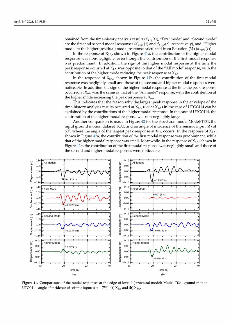
Figure 41 shows comparisons of the modal responses at the edge of level 0. Thestructural model shown in this figure is Model-Tf34, the input ground motion dataset isUTO0414, and the angle of incidence of the seismic input (ψ) is −75◦, the angle at whichthe largest peak response at X1A occurs. Note that “All modes” is the response originally
Appl. Sci. 2021, 11, 9829 32 of 41
obtained from the time-history analysis results (dY0j(t)), “First mode” and “Second mode”are the first and second modal responses (dY0j1(t) and dY0j2(t), respectively), and “Highermode” is the higher (residual) modal response calculated from Equation (31) (dY0jh(t)).
In the response of X1A, shown in Figure 41a, the contribution of the higher modalresponse was non-negligible, even though the contribution of the first modal responsewas predominant. In addition, the sign of the higher modal response at the time thepeak response occurred at X1A was opposite to that of the “All mode” response, with thecontribution of the higher mode reducing the peak response at X1A.
In the response of X6A, shown in Figure 41b, the contribution of the first modalresponse was negligibly small and those of the second and higher modal responses werenoticeable. In addition, the sign of the higher modal response at the time the peak responseoccurred at X6A was the same as that of the “All mode” response, with the contribution ofthe higher mode increasing the peak response at X6A.
This indicates that the reason why the largest peak response in the envelope of thetime-history analysis results occurred at X6A (not at X1A) in the case of UTO0414 can beexplained by the contributions of the higher modal response. In the case of UTO0414, thecontribution of the higher modal response was non-negligibly large.
Another comparison is made in Figure 42 for the structural model Model-Tf34, theinput ground motion dataset TCU, and an angle of incidence of the seismic input (ψ) of60◦, where the angle of the largest peak response at X1A occurs. In the response of X1A,shown in Figure 42a, the contribution of the first modal response was predominant, whilethat of the higher modal response was small. Meanwhile, in the response of X6A, shown inFigure 42b, the contribution of the first modal response was negligibly small and those ofthe second and higher modal responses were noticeable.
Figure 41. Comparisons of the modal responses at the edge of level 0 (structural model: Model-Tf34, ground motion:UTO0414, angle of incidence of seismic input: ψ = −75◦): (a) X1A and (b) X6A.
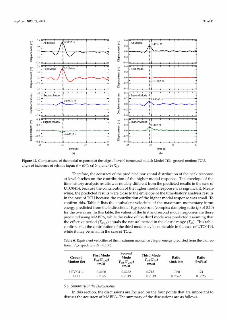
Appl. Sci. 2021, 11, 9829 33 of 41
Figure 42. Comparisons of the modal responses at the edge of level 0 (structural model: Model-Tf34, ground motion: TCU,angle of incidence of seismic input: ψ = 60◦): (a) X1A and (b) X6A.
Therefore, the accuracy of the predicted horizontal distribution of the peak responseat level 0 relies on the contribution of the higher modal response. The envelope of thetime-history analysis results was notably different from the predicted results in the case ofUTO0414, because the contribution of the higher modal response was significant. Mean-while, the predicted results were close to the envelope of the time-history analysis resultsin the case of TCU because the contribution of the higher modal response was small. Toconfirm this, Table 6 lists the equivalent velocities of the maximum momentary inputenergy predicted from the bidirectional V∆E spectrum (complex damping ratio (β) of 0.10)for the two cases. In this table, the values of the first and second modal responses are thosepredicted using MABPA, while the value of the third mode was predicted assuming thatthe effective period (T3e f f ) equals the natural period in the elastic range (T3e). This tableconfirms that the contribution of the third mode may be noticeable in the case of UTO0414,while it may be small in the case of TCU.
Table 6. Equivalent velocities of the maximum momentary input energy predicted from the bidirec-tional V∆E spectrum (β = 0.100).
GroundMotion Set
First ModeV∆E(T1eff )
(m/s)
SecondMode
V∆E(T2eff )(m/s)
Third ModeV∆E(T3e)
(m/s)
Ratio(2nd/1st)
Ratio(3rd/1st)
UTO0414 0.4108 0.4232 0.7151 1.030 1.741TCU 0.7575 0.7319 0.2519 0.9662 0.3325
5.6. Summary of the Discussions
In this section, the discussions are focused on the four points that are important todiscuss the accuracy of MABPA. The summary of the discussions are as follows.
Appl. Sci. 2021, 11, 9829 34 of 41
The relationship between the maximum momentary input energy and the peak equiv-alent displacement of the first modal response was discussed in Section 5.2. The resultsconfirmed that the V∆Eµ1U
∗–D1U∗ curve obtained from pushover analysis results fit the
plots obtained from the time-history analysis results very well. This is because the contri-bution of the first modal response to the whole response may be large in both Models Tf34and Tf44.
Then, the predictability of the maximum momentary input energy of the first modal re-sponse was discussed in Section 5.3. The results confirmed that bidirectional V∆E spectrumcan approximate the upper bound of the equivalent velocity of the maximum momentaryinput energy of the first mode V∆E1U
∗. This is because that the maximum momentary inputenergy of the first mode was calculated from the unidirectional input in U-axis, while theeffect of simultaneous bidirectional input was included in the calculation of bidirectionalV∆E spectrum automatically.
Since (a) the V∆Eµ1U∗–D1U
∗ curve can be properly predicted from the pushover analy-sis results, and (b) the upper bound of the equivalent velocity of the maximum momentaryinput energy can be predicted via the bidirectional V∆E spectrum, the largest peak equiva-lent displacement should be predicted accurately. The accuracy of the predicted equivalentdisplacements of the first and second modal responses was discussed in Section 5.4. Theresults confirmed that the upper bound of the peak equivalent displacement of the firstand second modal responses can be predicted accurately.
Although the upper bound of the peak equivalent displacement of the first and secondmodal responses can be predicted accurately, the accuracy of the predicted horizontaldistributions of the peak displacement at level 0 depends on the ground motion dataset.Section 5.5 discussed the contribution of the higher mode to the displacement response atthe edge of level 0. The results showed that higher modal responses may not be negligiblefor the prediction of the peak displacement at the edge of level 0. In the MABPA prediction,only the contributions of the first and second modal responses were considered. Therefore,a discrepancy of the predicted results from the time-history analysis may occur because ofthe lack of a contribution from the higher modal responses.
6. Conclusions
In this study, the main building of the former Uto City Hall was investigated as a casestudy of the retrofitting of an irregular reinforced concrete building using the base-isolationtechnique. The nonlinear peak responses of two retrofitted building models subjected tohorizontal bidirectional ground motions were predicted by MABPA, and the accuracy ofthe method was evaluated. The main conclusions and results are as follows:
• The predicted peak response according to the updated MABPA agreed satisfactorilywith the envelope of the time-history analysis results. The peak relative displacementat X3AY3 at each floor can be satisfactorily predicted. The predicted distribution of thepeak displacement at level 0 (just above the isolation layer) approximated the envelopeof the nonlinear time-history analysis results, even though in some cases, the predicteddistributions differed from the envelope of the nonlinear time-history analysis. Adiscrepancy between the predicted results and nonlinear time-history analysis mayoccur because of the lack of a contribution from the higher modal responses.
• The relationship between the equivalent velocity of the maximum momentary inputenergy of the first modal response (V∆E1U
∗) and the peak equivalent displacementof the first modal response (D1U
∗max) can be properly evaluated from the pushover
analysis results. The plots obtained from the nonlinear time-history analysis results fitthe evaluated curve from the pushover analysis results well.
• The upper bound of the peak equivalent displacements of the first two modal re-sponses can be predicted using the bidirectional V∆E spectrum [52]. Comparisonsbetween the predicted peak equivalent displacements and those calculated from thenonlinear time-history analysis results showed that the predicted peak approximated
Appl. Sci. 2021, 11, 9829 35 of 41
the upper bound of the nonlinear time-history analysis results. The upper bound ofV∆E1U
∗ can be approximated by the bidirectional V∆E spectrum.
Based on the above findings, the updated MABPA appears to predict the peak re-sponses of irregular base-isolated buildings with accuracy. However, MABPA still has twoshortcomings. The first shortcoming is the limitation of the applicability of MABPA. Asdiscussed in a previous study [43], the application of MABPA is limited to buildings classi-fied as torsionally stiff buildings. The current (updated) MABPA has the same restriction.This limitation can be avoided if the torsional resistance of the isolation layer is sufficientlyprovided, as shown in this study. The second shortcoming involves the contributions ofthe higher modal responses. In the original MABPA for non-isolated buildings, only thefirst two modes were considered for the prediction. Therefore, the prediction was lessaccurate for cases when the response in the stiff-side perimeter was larger than that in theflexible-side perimeter. The contributions of the third and higher modal responses need tobe investigated.
Another aspect of this study to be emphasized is the application of the bidirectionalV∆E spectrum for the prediction of the peak response of a base-isolated building. Theresults shown in this study imply that the bidirectional V∆E spectrum [52] is a promisingcandidate for a seismic intensity parameter for the peak response. As discussed in aprevious study [53], one of the biggest advantages of the bidirectional momentary inputenergy is that it can be directly calculated from the Fourier amplitude and phase angle ofthe ground motion components using a time-varying function of the momentary energyinput, without knowing the time-history of the ground motion. This means that researcherscan eliminate otherwise unavoidable fluctuations from the nonlinear time-history analysisresults. Therefore, the pushover analysis and the bidirectional V∆E spectrum are an optimalcombination to understand the fundamental characteristics of both base-isolated andnon-isolated asymmetric buildings.
The optimal distribution of the hysteresis dampers according to the design of theisolation layer needed to minimize the torsional response was not discussed in this study.However, the updated MABPA presented here can help in the optimization of the damperdistribution. The next update of MABPA for base-isolated irregular buildings with otherkinds of dampers (e.g., linear and nonlinear oil dampers, viscous mass dampers, and otherkings of “smart passive dampers” [19]) is also an important issue that will be investigatedin subsequent studies.
Author Contributions: Conceptualization, K.F. and T.M.; data curation, K.F. and T.M.; formalanalysis, K.F. and T.M.; funding acquisition, K.F.; investigation, K.F. and T.M.; methodology, K.F.;project administration, K.F.; resources, K.F. and T.M.; software, K.F.; supervision, K.F.; validation,K.F.; visualization, K.F.; writing—original draft, K.F.; writing—review and editing, K.F. All authorshave read and agreed to the published version of the manuscript.
Funding: This research received no external funding.
Institutional Review Board Statement: Not applicable.
Informed Consent Statement: Not applicable.
Data Availability Statement: The data presented in this study are available on request from the cor-responding author. The data are not publicly available because they are not part of ongoing research.
Acknowledgments: The ground motions used in this study were obtained from the website of theNational Research Institute for Earth Science and Disaster Resilience (NIED) (http://www.kyoshin.bosai.go.jp/kyoshin/, last accessed on 14 December 2019) and the Pacific Earthquake EngineeringResearch Center (PEER) (https://ngawest2.berkeley.edu/, last accessed on 14 December 2019). Thecontributions during the beginning stage of this study made by Ami Obikata, a former undergraduatestudent at the Chiba Institute of Technology, are greatly appreciated.
Conflicts of Interest: The authors declare no conflict of interest.
Appl. Sci. 2021, 11, 9829 36 of 41
Appendix A. Time-Histories of the Recorded Ground Motions Used in This Study
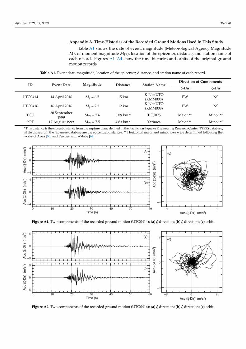
Table A1 shows the date of event, magnitude (Meteorological Agency MagnitudeMJ , or moment magnitude MW), location of the epicenter, distance, and station name ofeach record. Figures A1–A4 show the time-histories and orbits of the original groundmotion records.
Table A1. Event date, magnitude, location of the epicenter, distance, and station name of each record.
ID Event Date Magnitude Distance Station NameDirection of Components
ξ-Dir ζ-Dir
UTO0414 14 April 2016 MJ = 6.5 15 km K-Net UTO(KMM008) EW NS
UTO0416 16 April 2016 MJ = 7.3 12 km K-Net UTO(KMM008) EW NS
TCU 20 September1999 MW = 7.6 0.89 km * TCU075 Major ** Minor **
YPT 17 August 1999 MW = 7.5 4.83 km * Yarimca Major ** Minor **
* This distance is the closest distance from the rupture plane defined in the Pacific Earthquake Engineering Research Center (PEER) database,while those from the Japanese database are the epicentral distances. ** Horizontal major and minor axes were determined following theworks of Arias [63] and Penzien and Watabe [64].
Figure A1. Two components of the recorded ground motion (UTO0414): (a) ξ direction; (b) ζ direction; (c) orbit.
Figure A2. Two components of the recorded ground motion (UTO0416): (a) ξ direction; (b) ζ direction; (c) orbit.
Appl. Sci. 2021, 11, 9829 37 of 41
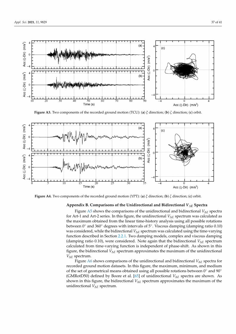
Figure A3. Two components of the recorded ground motion (TCU): (a) ξ direction; (b) ζ direction; (c) orbit.
Figure A4. Two components of the recorded ground motion (YPT): (a) ξ direction; (b) ζ direction; (c) orbit.
Appendix B. Comparisons of the Unidirectional and Bidirectional V∆E Spectra
Figure A5 shows the comparisons of the unidirectional and bidirectional V∆E spectrafor Art-1 and Art-2 series. In this figure, the unidirectional V∆E spectrum was calculated asthe maximum obtained from the linear time-history analysis using all possible rotationsbetween 0◦ and 360◦ degrees with intervals of 5◦. Viscous damping (damping ratio 0.10)was considered, while the bidirectional V∆E spectrum was calculated using the time-varyingfunction described in Section 2.2.1. Two damping models, complex and viscous damping(damping ratio 0.10), were considered. Note again that the bidirectional V∆E spectrumcalculated from time-varying function is independent of phase-shift. As shown in thisfigure, the bidirectional V∆E spectrum approximates the maximum of the unidirectionalV∆E spectrum.
Figure A6 shows comparisons of the unidirectional and bidirectional V∆E spectra forrecorded ground motion datasets. In this figure, the maximum, minimum, and mediumof the set of geometrical means obtained using all possible rotations between 0◦ and 90◦
(GMRotD50) defined by Boore et al. [65] of unidirectional V∆E spectra are shown. Asshown in this figure, the bidirectional V∆E spectrum approximates the maximum of theunidirectional V∆E spectrum.
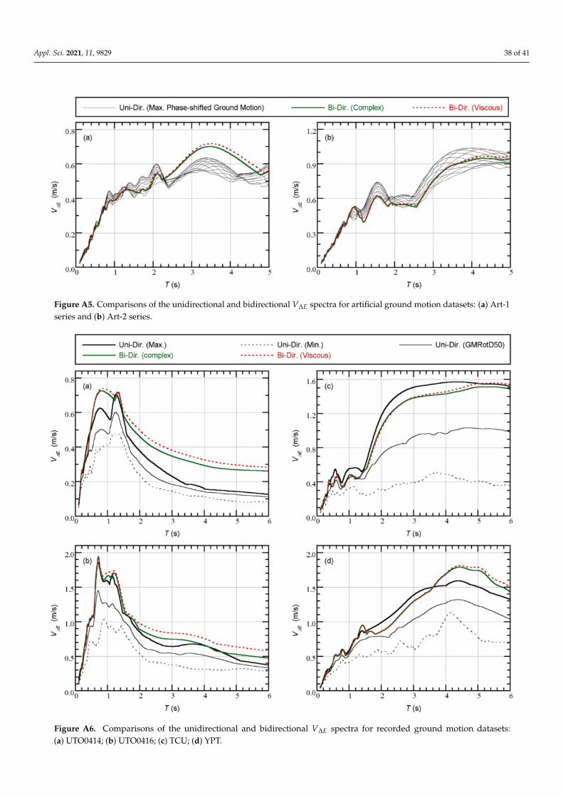
Appl. Sci. 2021, 11, 9829 38 of 41
Figure A5. Comparisons of the unidirectional and bidirectional V∆E spectra for artificial ground motion datasets: (a) Art-1series and (b) Art-2 series.
Figure A6. Comparisons of the unidirectional and bidirectional V∆E spectra for recorded ground motion datasets:(a) UTO0414; (b) UTO0416; (c) TCU; (d) YPT.

Appl. Sci. 2021, 11, 9829 39 of 41
References1. Charleson, A.; Guisasola, A. Seismic Isolation for Architects; Routledge: London, UK; New York, NY, USA, 2017.2. Architectural Institute of JAPAN (AIJ). Design Recommendations for Seismically Isolated Buildings; Architectural Institute of Japan:
Tokyo, Japan, 2016.3. ASCE. Seismic Evaluation and Retrofit of Existing Buildings; ASCE Standard, ASCE/SEI41-17; American Society of Civil Engineering:
Reston, VA, USA, 2017.4. Seki, M.; Miyazaki, M.; Tsuneki, Y.; Kataoka, K. A Masonry school building retrofitted by base isolation technology. In Proceedings
of the 12th World Conference on Earthquake Engineering, Auckland, New Zealand, 30 January–4 February 2000.5. Kashima, T.; Koyama, S.; Iiba, M.; Okawa, I. Dynamic behaviour of a museum building retrofitted using base isolation system. In
Proceedings of the 14th World Conference on Earthquake Engineering, Beijing, China, 12–17 October 2008.6. Clemente, P.; De Stefano, A. Application of seismic isolation in the retrofit of historical buildings. Earthquake Resistant Engineering
Structures VIII; WIT Press: Southampton, UK, 2011; Volume 120, pp. 41–52.7. Gilani, A.S.; Miyamoto, H.K. Base isolation retrofit challenges in a historical monumental building in Romania. In Proceedings of
the 15th World Conference on Earthquake Engineering, Lisbon, Portugal, 24–28 September 2012.8. Nakamura, H.; Ninomiya, T.; Sakaguchi, T.; Nakano, Y.; Konagai, K.; Hisada, Y.; Seki, M.; Ota, T.; Yamazaki, Y.; Mochizuki, S.; et al.
Seismic isolation retrofit of Susano City Hall situated above lava tubes. In Proceedings of the 15th World Conference on EarthquakeEngineering, Lisbon, Portugal, 24–28 September 2012.
9. Sorace, S.; Terenzi, G. A viable base isolation strategy for the advanced seismic retrofit of an r/c building. Contemp. Eng. Sci. 2014,7, 817–834. [CrossRef]
10. Ferraioli, M.; Mandara, A. Base isolation for seismic retrofitting of a multiple building structure: Evaluation of equivalentlinearization method. Math. Probl. Eng. 2016, 2016, 8934196. [CrossRef]
11. Terenzi, G.; Fuso, E.; Sorace, S.; Costoli, I. Enhanced seismic retrofit of a reinforced concrete building of architectural interest.Buildings 2020, 10, 211. [CrossRef]
12. Vailati, M.; Monti, G.; Bianco, V. Integrated solution-base isolation and repositioning-for the seismic rehabilitation of a preservedstrategic building. Buildings 2021, 11, 164. [CrossRef]
13. Usta, P. Investigation of a base-isolator system’s effects on the seismic behavior of a historical structure. Buildings 2021, 11, 217.[CrossRef]
14. Nishizawa, T.; Suekuni, R. Outline of structural design for Kyoto City Hall. In Proceedings of the 17th World Conference onEarthquake Engineering, Sendai, Japan, 20 September–2 November 2021.
15. Hashimoto, T.; Fujita, K.; Tsuji, M.; Takewaki, I. Innovative base-isolated building with large mass-ratio TMD at basement forgreater earthquake resilience. Future Cities Environ. 2015, 1, 9. [CrossRef]
16. Ikenaga, M.; Ikago, K.; Inoue, N. Development of a displacement-dependent damper for base isolated structures. In Proceedingsof the Tenth International Conference on Computational Structures Technology, Valencia, Spain, 14–17 September 2010.
17. Ikenaga, M.; Ikago, K.; Inoue, N. Seismic displacement control design of base isolated structures by magneto-rheologicaldampers based on a pseudo-complex-damping rule. In Proceedings of the Thirteenth International Conference on ComputationalStructures Technology, Crete, Greece, 6–9 September 2011.
18. Nakaminami, S.; Ikago, K.; Inoue, N.; Kida, H. Response characteristics of a base-isolated structure incorporated with a force-restricted viscous mass damper. In Proceedings of the 15th World Conference on Earthquake Engineering, Lisbon, Portugal,24–28 September 2012.
19. Inoue, N.; Ikago, K. Displacement control design concept for long-period structures. In Proceedings of the 16th World Conferenceon Earthquake Engineering, Santiago, Chile, 9–13 January 2017.
20. Anajafi, H.; Medina, R.A. Comparison of the seismic performance of a partial mass isolation technique with conventional TMDand base-isolation systems under broad-band and narrow-band excitations. Eng. Struct. 2018, 158, 110–123. [CrossRef]
21. Luo, H.; Ikago, K.; Chong, C.; Keivan, A.; Phillips, B.M. Performance of low-frequency structures incorporated with rate-independent linear damping. Eng. Struct. 2019, 181, 324–335. [CrossRef]
22. Tariq, M.A.; Usman, M.; Farooq, S.H.; Ullah, I.; Hanif, A. Investigation of the structural response of the MRE-based MDOFisolated structure under historic near- and far-fault earthquake loadings. Appl. Sci. 2021, 11, 2876. [CrossRef]
23. Nagarajaiah, S.; Reinhorn, A.M.; Constantinou, M.C. Torsion in base-isolated structures with elastomeric isolation systems. J.Struct. Eng. ASCE 1992, 119, 2932–2951. [CrossRef]
24. Tena-Colunga, A.; Gómez-Soberón, L. Torsional response of base-isolated structures due to asymmetries in the superstructure.Eng. Struct. 2002, 24, 1587–1599. [CrossRef]
25. Tena-Colunga, A.; Zambrana-Rojas, C. Dynamic torsional amplifications of base-isolated structures with an eccentric isolationsystem. Eng. Struct. 2006, 28, 72–83. [CrossRef]
26. Tena-Colunga, A.; Escamilla-Cruz, J.L. Torsional amplifications in asymmetric base-isolated structures. Eng. Struct. 2008, 29,237–247. [CrossRef]
27. Seguín, C.E.; De La Llera, J.C.; Almazán, J.L. Base–structure interaction of linearly isolated structures with lateral–torsionalcoupling. Eng. Struct. 2008, 30, 110–125. [CrossRef]
28. Di Sarno, L.; Chioccarelli, E.; Cosenza, E. Seismic response analysis of an irregular base isolated building. Bull. Earthq. Eng. 2011,9, 1673–1702. [CrossRef]
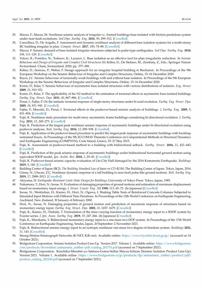
Appl. Sci. 2021, 11, 9829 40 of 41
29. Mazza, F.; Mazza, M. Nonlinear seismic analysis of irregular r.c. framed buildings base-isolated with friction pendulum systemunder near-fault excitations. Soil Dyn. Earthq. Eng. 2016, 90, 299–312. [CrossRef]
30. Cancellara, D.; De Angelis, F. Assessment and dynamic nonlinear analysis of different base isolation systems for a multi-storeyRC building irregular in plan. Comput. Struct. 2017, 180, 74–88. [CrossRef]
31. Mazza, F. Seismic demand of base-isolated irregular structures subjected to pulse-type earthquakes. Soil Dyn. Earthq. Eng. 2018,108, 111–129. [CrossRef]
32. Volcev, R.; Postolov, N.; Todorov, K.; Lazarov, L. Base isolation as an effective tool for plan irregularity reduction. In SeismicBehaviour and Design of Irregular and Complex Civil Structures III; Köber, D., De Stefano, M., Zembaty, Z., Eds.; Springer NatureSwitzerland: Cham, Switzerland, 2020; pp. 377–389.
33. Köber, D.; Semrau, P.; Weber, F. Design approach for an irregular hospital building in Bucharest. In Proceedings of the 9thEuropean Workshop on the Seismic Behaviour of Irregular and Complex Structures, Online, 15–16 December 2020.
34. Reyes, J.C. Seismic behaviour of torsionally-weak buildings with and without base isolators. In Proceedings of the 9th EuropeanWorkshop on the Seismic Behaviour of Irregular and Complex Structures, Online, 15–16 December 2020.
35. Koren, D.; Kilar, V. Seismic behaviour of asymmetric base isolated structures with various distributions of isolators. Eng. Struct.2009, 31, 910–921.
36. Koren, D.; Kilar, V. The applicability of the N2 method to the estimation of torsional effects in asymmetric base-isolated buildings.Earthq. Eng. Struct. Dyn. 2011, 40, 867–886. [CrossRef]
37. Perus, I.; Fajfar, P. On the inelastic torsional response of single-storey structures under bi-axial excitation. Earthq. Eng. Struct. Dyn.2005, 34, 931–941. [CrossRef]
38. Fajfar, P.; Marušic, D.; Perus, I. Torsional effects in the pushover-based seismic analysis of buildings. J. Earthq. Eng. 2005, 9,831–854. [CrossRef]
39. Fujii, K. Nonlinear static procedure for multi-story asymmetric frame buildings considering bi-directional excitation. J. Earthq.Eng. 2011, 15, 245–273. [CrossRef]
40. Fujii, K. Prediction of the largest peak nonlinear seismic response of asymmetric buildings under bi-directional excitation usingpushover analyses. Bull. Earthq. Eng. 2014, 12, 909–938. [CrossRef]
41. Fujii, K. Application of the pushover-based procedure to predict the largest peak response of asymmetric buildings with buckling-restrained braces. In Proceedings of the 5th ECCOMAS Thematic Conference on Computational Methods in Structural Dynamicsand Earthquake Engineering (COMPDYN), Crete Island, Greece, 25–27 May 2015.
42. Fujii, K. Assessment of pushover-based method to a building with bidirectional setback. Earthq. Struct. 2016, 11, 421–443.[CrossRef]
43. Fujii, K. Prediction of the peak seismic response of asymmetric buildings under bidirectional horizontal ground motion usingequivalent SDOF model. Jpn. Archit. Rev. 2018, 1, 29–43. [CrossRef]
44. Fujii, K. Pushover-based seismic capacity evaluation of Uto City Hall damaged by the 2016 Kumamoto Earthquake. Buildings2019, 9, 140. [CrossRef]
45. Building Center of Japan (BCJ). The Building Standard Law of Japan on CD-ROM; The Building Center of Japan: Tokyo, Japan, 2016.46. Günes, N.; Ulucan, Z.Ç. Nonlinear dynamic response of a tall building to near-fault pulse-like ground motions. Bull. Earthq. Eng.
2019, 17, 2989–3013. [CrossRef]47. Akiyama, H. Earthquake–Resistant Limit–State Design for Buildings; University of Tokyo Press: Tokyo, Japan, 1985.48. Nakamura, T.; Hori, N.; Inoue, N. Evaluation of damaging properties of ground motions and estimation of maximum displacement
based on momentary input energy. J. Struct. Constr. Eng. AIJ 1998, 513, 65–72. (In Japanese) [CrossRef]49. Inoue, N.; Wenliuhan, H.; Kanno, H.; Hori, N.; Ogawa, J. Shaking Table Tests of Reinforced Concrete Columns Subjected to
Simulated Input Motions with Different Time Durations. In Proceedings of the 12th World Conference on Earthquake Engineering,Auckland, New Zealand, 30 January–4 February 2000.
50. Hori, N.; Inoue, N. Damaging properties of ground motion and prediction of maximum response of structures based onmomentary energy input. Earthq. Eng. Struct. Dyn. 2002, 31, 1657–1679. [CrossRef]
51. Fujii, K.; Kanno, H.; Nishida, T. Formulation of the time-varying function of momentary energy input to a SDOF system byFourier series. J. Jpn. Assoc. Earthq. Eng. 2019, 19, 247–266. (In Japanese) [CrossRef]
52. Fujii, K.; Murakami, Y. Bidirectional momentary energy input to a one-mass two-DOF system. In Proceedings of the 17th WorldConference on Earthquake Engineering, Sendai, Japan, 20 September–2 November 2021.
53. Fujii, K. Bidirectional seismic energy input to an isotropic nonlinear one-mass two-degree-of-freedom system. Buildings 2021,11, 143. [CrossRef]
54. Strong-Motion Seismograph Networks (K-NET, KiK-net). Available online: https://www.kyoshin.bosai.go.jp/ (accessed on 14October 2021).
55. Bridgestone Corporation. Seismic Isolation Product Line-Up. Version 2017. Volume 1. Available online: https://www.bridgestone.com/products/diversified/antiseismic_rubber/pdf/catalog_201710.pdf (accessed on 7 September 2021).
56. Bridgestone Corporation. Kenchiku-Menshin-yo Sekisou-Gomu-Seihin Shiyou-Ichiran (Seismic Isolation Product Line-Up).Version 2021. Volume 1. Available online: https://www.bridgestone.co.jp/products/dp/antiseismic_rubber/product/pdf/product_catalog_202106.pdf (accessed on 7 September 2021).

Appl. Sci. 2021, 11, 9829 41 of 41
57. Nippon Steel Engineering Co. Ltd. Men-Shin NSU Damper Line-Up. Available online: https://www.eng.nipponsteel.com/steelstructures/product/base_isolation/damper_u/lineup_du/ (accessed on 3 August 2019). (In Japanese)
58. Fujii, K. Prediction of the Maximum Seismic Member Force in a Superstructure of a Base-Isolated Frame Building by UsingPushover Analysis. Buildings 2019, 9, 201. [CrossRef]
59. Wada, A.; Hirose, K. Elasto-plastic dynamic behaviors of the building frames subjected to bi-directional earthquake motions. J.Struct. Constr. Eng. AIJ 1989, 399, 37–47. (In Japanese)
60. Almansa, F.L.; Weng, D.; Li, T.; Alfarah, B. Suitability of seismic isolation for buildings founded on soft soil. Case study of a RCbuilding in Shanghai. Buildings 2020, 10, 241. [CrossRef]
61. Ordaz, M.; Huerta, B.; Reinoso, E. Exact Computation of Input-Energy Spectra from Fourier Amplitude Spectra. Earthq. Eng.Struct. Dyn. 2003, 32, 597–605. [CrossRef]
62. Kuramoto, H. Earthquake response characteristics of equivalent SDOF system reduced from multi-story buildings and predictionof higher mode responses. J. Struct. Constr. Eng. AIJ 2004, 580, 61–68. (In Japanese) [CrossRef]
63. Arias, A. A measure of seismic intensity. In Seismic Design for Nuclear Power Plant; MIT Press: Cambridge, MA, USA, 1970;pp. 438–483.
64. Penzien, J.; Watabe, M. Characteristics of 3-dimensional earthquake ground motions. Earthq. Eng. Struct. Dyn. 1975, 3, 365–373.[CrossRef]
65. Boore, D.M.; Watson-Lamprey, J.; Abrahamson, N.A. Orientation-Independent Measures of Ground Motion. Bull. Seismol. Soc.Am. 2007, 96, 1502–1511. [CrossRef]


