sensors

Article

Human–Machine Interface: Multiclass Classification byMachine Learning on 1D EOG Signals for the Control of anOmnidirectional Robot

Francisco David Pérez-Reynoso 1 , Liliam Rodríguez-Guerrero 2,* and Julio César Salgado-Ramírez 3,*and Rocío Ortega-Palacios 3,*

Citation: Pérez-Reynoso, F.D.;

Rodríguez-Guerrero, L.;

Salgado-Ramírez, J.C.;

Ortega-Palacios, R. Human–Machine

Interface: Multiclass Classification by

Machine Learning on 1D EOG Signals

for the Control of an Omnidirectional

Robot. Sensors 2021, 21, 5882.

https://doi.org/10.3390/s21175882

Academic Editors: Rezia Molfino and

Francesco Cepolina

Received: 29 July 2021

Accepted: 26 August 2021

Published: 31 August 2021

Publisher’s Note: MDPI stays neutral

with regard to jurisdictional claims in

published maps and institutional affil-

iations.

Copyright: © 2021 by the authors.

Licensee MDPI, Basel, Switzerland.

This article is an open access article

distributed under the terms and

conditions of the Creative Commons

Attribution (CC BY) license (https://

creativecommons.org/licenses/by/

4.0/).

1 Mechatronic Engineering, Universidad Politécnica de Pachuca (UPP), Zempoala 43830, Mexico;david_perez@upp.edu.mx

2 Research Center on Technology of Information and Systems (CITIS), Electric and Control Academic Group,Universidad Autónoma del Estado de Hidalgo (UAEH), Pachuca de Soto 42039, Mexico

3 Biomedical Engineering, Universidad Politécnica de Pachuca (UPP), Zempoala 43830, Mexico* Correspondence: liliam_rodriguez@uaeh.edu.mx (L.R.-G.); csalgado@upp.edu.mx (J.C.S.-R.);

rortega@upp.edu.mx (R.O.-P.)

Abstract: People with severe disabilities require assistance to perform their routine activities; aHuman–Machine Interface (HMI) will allow them to activate devices that respond according to theirneeds. In this work, an HMI based on electrooculography (EOG) is presented, the instrumenta-tion is placed on portable glasses that have the task of acquiring both horizontal and vertical EOGsignals. The registration of each eye movement is identified by a class and categorized using theone hot encoding technique to test precision and sensitivity of different machine learning classifica-tion algorithms capable of identifying new data from the eye registration; the algorithm allows todiscriminate blinks in order not to disturb the acquisition of the eyeball position commands. Theimplementation of the classifier consists of the control of a three-wheeled omnidirectional robot tovalidate the response of the interface. This work proposes the classification of signals in real timeand the customization of the interface, minimizing the user’s learning curve. Preliminary resultsshowed that it is possible to generate trajectories to control an omnidirectional robot to implement inthe future assistance system to control position through gaze orientation.

Keywords: EOG; one hot encoding; machine learning; omnidirectional robot

1. Introduction

The EOG signal is generated by the potential difference between the retina and thecornea of the eye by means of superficial electrodes; the horizontal (left–right) and vertical(up–down) eye movements can be detected [1–3]. In recent years, HMI has been imple-mented using EOG since its acquisition is less invasive compared to electroencephalog-raphy (EEG) [4–6]. In addition, artificial intelligence algorithms have been used whichallow the classification of EOG signals for the control of wheelchairs, orthotics, assistancerobots and HMI [7–9]. In [10], for example, the horizontal EOG channel is used to generatecontrol commands for a lower limb orthosis, these commands are detected in a three-secondsampling window to avoid false activations of the system and the processing is done inmachine language. In [11], an Internet search engine was developed using horizontal andvertical EOG signals, the user’s impulses are obtained by deriving the signal and using aprediction algorithm of words, getting a response time of between 80 and 100 s. In [12], ahybrid brain–computer interface (hBCI) is carried out, through the union of EOG and EEG.Classification is done using the EEG signal with a Support Vector Machine (SVM) and theEOG signal is used to eliminate noise on EEG acquisition. In [13], an interface methodis proposed to improve the letter selection on a virtual keyboard, where an EOG-guidedmouse points to interactive buttons with audio; click is controlled by blinking.

Sensors 2021, 21, 5882. https://doi.org/10.3390/s21175882 https://www.mdpi.com/journal/sensors

Sensors 2021, 21, 5882 2 of 29

Other systems classifying EOG signals using fuzzy logic and a database that storewaveform information from different users have been developed [14–18] in order for theinterface to compare the parameters of each user with previously established commands.One of the most representative works is presented in [19]; Fuzzy PD control is appliedto the horizontal EOG channel that generates a wheelchair’s rotation to the right or leftand the vertical EOG indicates forward or reverse. In [20], a writing system for peoplewith disabilities is designed; the similarity of the trajectories generated by the movementof the eye and the shape of the letters is determined by fuzzy Gaussian membershipfunctions. The training generates a database, which is the input to a multilayer neuralnetwork determining the letter that the user wants to write using EOG signals. In addition,the EOG has been applied in other fields such as industrial robotics; for example, in [21]a speed control system of a FANUC LR Mate 200iB industrial robot is developed usingEOG. The signal amplitude is classified; the voltage value is previously divided into threethresholds; the user must reach the defined amplitude, otherwise the robot will not activate.The authors in [22] also developed a portable EOG acquisition system, which generatesposition control commands for an industrial robot using a nine-state machine, concerningwhich it was tested whether making the end effector followed five points; the obtainedresponse time was of 220 s with trained users. In [23] a review of EOG based human–computer interface systems is presented; the work of 41 authors is explained, where theinterfaces used to move a device always generate points in coordinates X-Y, as is the casefor control of wheelchairs, Mohd et al [19]. In this paper, research did not generate a three-dimensional workspace; unlike the one presented in [24] where the EOG signals activate arobot with three degrees of freedom in 3D Cartesian space, the Cartesian coordinates X, Y,Z are generated by a fuzzy classifier that is automatically calibrated using optimizationalgorithms. The system response time, from the user’s eye movement until the robotreaches the desired position, is 118 s. This is less than that reported in the works presentedin [23]; however, in this research it was found that to control a device that moves in aCartesian space a state machine is insufficient to describe all the points in the workspaceand does not allow track trajectories.

Some authors have as an alternative method the hybrid Brain–Computer Interfaces(BCIs) using eye-tracking to control robot models. Reference [25] presents the motionof an industrial robot controlled with eye movement and eye tracking via Ethernet.Reference [26] presents a hybrid wearable interface using eye movement and mental focusto control a quadcopter in three-dimensional space. Reference [27] developed a hybrid BCIto manipulate a Jaco robotic arm using natural gestures and biopotentials. Reference [28]presented a semi-autonomous hybrid brain–machine interface using human intracranialEEG, eye tracing and computer vision to control an upper limb prosthetic robot.

In regards to the EOG work related to classifiers, Fang et al. published in their pa-per advances about visual writing for Japanese Katakana [20]. Since Katakana is mainlycomposed of straight lines, researchers developed a system to recognize 12 basic types ofhits. By recognizing these strokes, the proposed system was able to classify all Katakanacharacters (48 letters). For six participants, Katakana recognition accuracy was 93.8%.In this study, a distinguishing feature implemented was the continuous eye writing. Byignoring small eye movements, the system could recognize the eye writing of multipleletters continuously without discrete sessions. The average entry rate was 27.9 letters permin. Another work related to eye movement is [29]. There, character classifiers written bythe eyes were implemented using an artificial neural network (quantification of learningvectors) for eye writing recognition. The average accuracy in character detection was 72.1%.In works of Fang and Tsai, eye movement is applied to writing; we use them to create com-plex trajectories of a robot’s movements; in addition, machine learning classifiers are usedto analyze eye movement. Computational models were developed to identify antioxidantsin the laboratory and machine learning was used for this purpose. The validation methodused in this study is 10-fold cross validation, whereas in Fang and Tsai, the followingvalidation metrics were used: Sensitivity of 81.5%, specificity of 85.1% and accuracy of

Sensors 2021, 21, 5882 3 of 29

84.6%. In [30], the random forest classification algorithm is used to validate the efficiencyof the computational method. Genes are the subject of study in computational biology andmodels of classification algorithms have been proposed to determine essential genes andsequencing problems. The metrics used for the validation method were: Sensitivity 60.2%,specificity 84.6%, accuracy 76.3%, area of Receiver Operating Characteristic (ROC) curves,also called AUC with a value of 0.814 [31]. The aforementioned study demonstrated theimportance of supervised classification and the metrics used, metrics that are determinativeand recognized by researchers in machine learning, are reliable metrics to measure theaccuracy of classifiers.

Three contributions are presented in this work: First, the designed acquisition systemallows to obtain the EOG signal, which is free from interference induced noise, by applyinga digital filter which is tuned analyzing the EOG frequency spectrum in real time, forselecting its cutoff frequency; the second contribution is the verification of the performanceof different classifiers to choose the best algorithm for the EOG signal model and to controla robotic system, based on the result of precision, accuracy and computational cost for thedevelopment of the model in an embedded system; the third contribution proposed is thediscrimination of the involuntary potentials model such as blinking; this characteristic doesnot affect the operation of the classifier, taking this property as a total stop of the system.The assistance system implements modeling through a Multilayer Neural Network (MNN)to generalize the classification of EOG signals. So, if there is an amplitude variation of thesignal due to user change or clinical problems, the algorithm must search the dataset foran entry for the classifier and thus assign a response to the system. The system presentedin this work customizes the classification system and adapts to the individual propertiesof the user.

Section 2.1 describes in detail each of the classifiers implemented to choose the best onefor identifying the eye registration of both EOG channels and introduces the basics of theEOG signal. Section 2.3 details the design of the HMI. In Section 2.4 using machine learningand the horizontal and vertical EOG signal, the Cartesian coordinates are generated toposition a robot using a PID control. In Section 3 a test is presented to evaluate the responsetime of the proposed system and a discussion of the contributions of the developed interfaceis made.

2. Materials and Methods2.1. Classifiers2.1.1. Multilayer Perceptron (MLP)

MLP is a neural network that aims to solve classification problems when classes cannotbe separated linearly. This neural network mainly consists of three types of layers whichare the input layer, the intermediate or hidden layers and the output layer [32]. Researchersin machine learning consider this classifier to be a good pattern classifier. The classifierworks as follows: Neurons whose output values belong to the corresponding class are inthe output layer. Neurons in the hidden layer, as a propagation rule, use the weighted sumof the inputs with the synaptic weights and a sigmoid transfer function is applied to thissum. The backpropagation error uses the root mean square error as a cost function.

2.1.2. Tree-Type Classifiers

There are tree-type classifiers such as C4.5, ID3, random forest and random tree andJ48 [33,34]. These decision tree algorithms can be explained as follows: For iteration n andtaking as a criterion an already established variable, the predictor variable is searched todecide the cut that was made as well as the exact cut point where the mistake made isminor. This would happen when the confidence levels are higher than those established.After the cutoff, the algorithm will execute if the predictor variables are above the definedhigher confidence level. The level of confidence is important since given too many subjectsand variables, the tree will result in a large one. To avoid this situation, the size of the tree

Sensors 2021, 21, 5882 4 of 29

is limited by assigning a minimum number of instances per node. These algorithms are themost used in the classification of patterns.

2.1.3. Naïve Bayes (NB)

Naïve Bayes classifier is widely used in machine learning. It is based on Bayes’theorem [35]. Bayes proposed that we learn from the world by approximations and that theworld is neither probabilistic nor uncertain, which allows us to get very close to the truth themore evidence there is. This classifier assumes that the presence or absence of an attributeis not probabilistically related to the presence or absence of other attributes, different fromwhat happens in the real world. The Naïve Bayes classifier consists of converting the dataset into a frequency table. In addition, a probability table is created for the various eventsto occur. Naïve Bayes is applied to calculate the posterior probability of each class and theprediction class is the class with the highest probability. The classifier, due to its simplicity,allows to easily build probability-based models with very good performance.

2.1.4. The K Nearest Neighbors (K-NN)

The K-Nearest Neighbor (K-NN) classifier is a widely used algorithm in supervisedlearning [36]. The concept of the classifier is intuitive. Each new attribute that is presentedto the K-NN is classified to the class of its closest neighbor. The algorithm calculates thedistance of the new attribute with respect to each of the existing attributes, the distancesare ordered from least to greatest and the class with the highest frequency and the shortestdistance is selected [37–40].

2.1.5. Logistic Classifier (Logistic)

This classifier is based on logistic regression [41]. Logistic regression, because itdoes not require many computing resources, is widely used in machine learning as itturns out to be very efficient. The most common models of logistic regression are theclassification of a binary value (yes or no; true or false) and the logistic regression model isthe multinomial (more than two possible outcomes). The Logistic classifier, to classify orpredict, assigns actual values based on the probability that the input belongs to an existingclass. Probability is calculated using a sigmoid function, where the exponential functionplays a very important role.

2.1.6. Support Vector Machines (SVM)

The concept of SVM is based on finding the hyperplane to separate the classes inthe data space [42–44]. This algorithm is born from the theory of statistical learning.Optimization of analytical functions serves as the basis for the design and operation ofSVM algorithms.

2.1.7. Performance Measures

Within the supervised classification there are two processes or phases; one phase isthe learning phase and the other phase is the classification phase [45]. A classifier shouldalways have one data set for the training phase (P_train), which is also called a trainingclass and another data set for testing the performance of the class, which is called a testclass (P_test). Once the classifier learns, it is presented with a test class and as a resultthe presented pattern sets will be assigned to the corresponding classes. Patterns will notalways be classified correctly, indicating that this is acceptable according to the no freelunch theorem [46,47].

As the data acquired is stored in a set of data or attributes, a partition of the totaldata set must be performed through a validation method. The method used in this paperis the cross-validation method. This method guarantees that the classes are distributedproportionally in each fold. The cross-validation method consists of dividing the total dataset into k folds. k must be a positive integer and the most used values for k in the state of

Sensors 2021, 21, 5882 5 of 29

the art are k = 5 and k = 10 [48,49]. For this paper, the cross-validation method used will bek = 10.

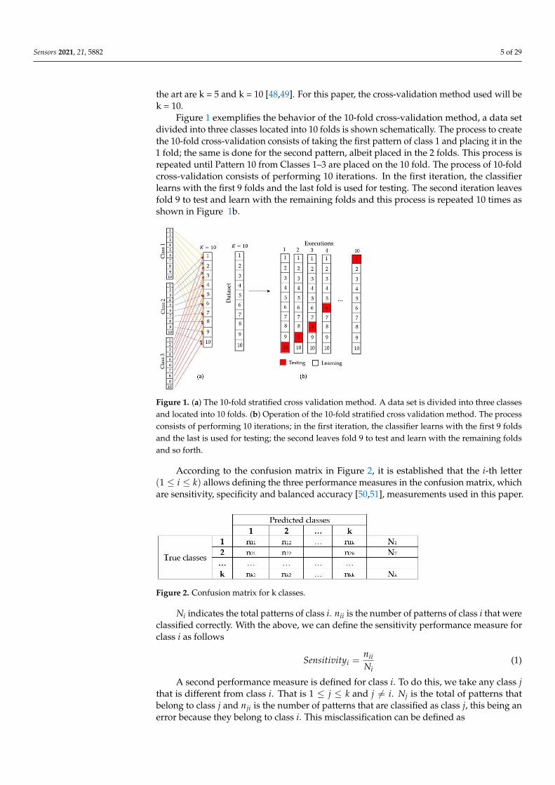
Figure 1 exemplifies the behavior of the 10-fold cross-validation method, a data setdivided into three classes located into 10 folds is shown schematically. The process to createthe 10-fold cross-validation consists of taking the first pattern of class 1 and placing it in the1 fold; the same is done for the second pattern, albeit placed in the 2 folds. This process isrepeated until Pattern 10 from Classes 1–3 are placed on the 10 fold. The process of 10-foldcross-validation consists of performing 10 iterations. In the first iteration, the classifierlearns with the first 9 folds and the last fold is used for testing. The second iteration leavesfold 9 to test and learn with the remaining folds and this process is repeated 10 times asshown in Figure 1b.

Figure 1. (a) The 10-fold stratified cross validation method. A data set is divided into three classesand located into 10 folds. (b) Operation of the 10-fold stratified cross validation method. The processconsists of performing 10 iterations; in the first iteration, the classifier learns with the first 9 foldsand the last is used for testing; the second leaves fold 9 to test and learn with the remaining foldsand so forth.

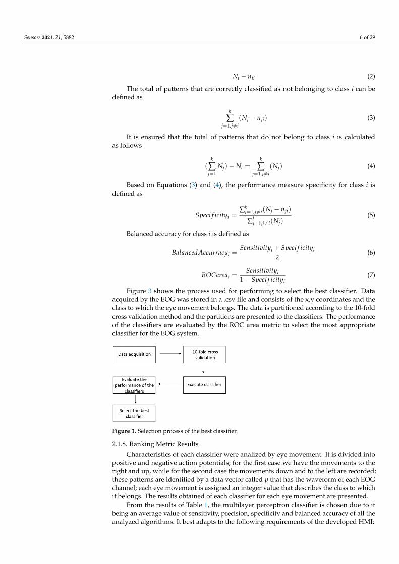
According to the confusion matrix in Figure 2, it is established that the i-th letter(1 ≤ i ≤ k) allows defining the three performance measures in the confusion matrix, whichare sensitivity, specificity and balanced accuracy [50,51], measurements used in this paper.

Figure 2. Confusion matrix for k classes.

Ni indicates the total patterns of class i. nii is the number of patterns of class i that wereclassified correctly. With the above, we can define the sensitivity performance measure forclass i as follows

Sensitivityi =niiNi

(1)

A second performance measure is defined for class i. To do this, we take any class jthat is different from class i. That is 1 ≤ j ≤ k and j 6= i. Nj is the total of patterns thatbelong to class j and nji is the number of patterns that are classified as class j, this being anerror because they belong to class i. This misclassification can be defined as

Sensors 2021, 21, 5882 6 of 29

Ni − nii (2)

The total of patterns that are correctly classified as not belonging to class i can bedefined as

k

∑j=1,j 6=i

(Nj − nji) (3)

It is ensured that the total of patterns that do not belong to class i is calculatedas follows

(k

∑j=1

Nj)− Ni =k

∑j=1,j 6=i

(Nj) (4)

Based on Equations (3) and (4), the performance measure specificity for class i isdefined as

Speci f icityi =∑k

j=1,j 6=i(Nj − nji)

∑kj=1,j 6=i(Nj)

(5)

Balanced accuracy for class i is defined as

BalancedAccurracyi =Sensitivityi + Speci f icityi

2(6)

ROCareai =Sensitivityi

1− Speci f icityi(7)

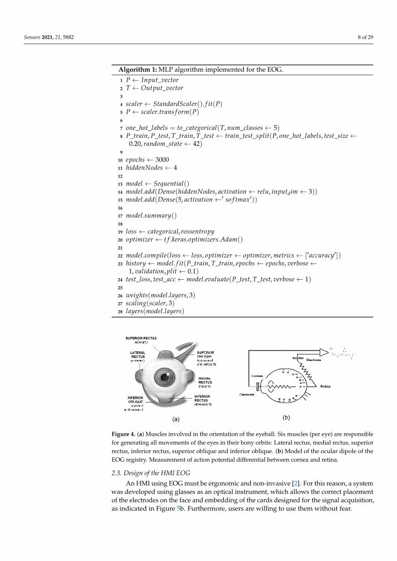
Figure 3 shows the process used for performing to select the best classifier. Dataacquired by the EOG was stored in a .csv file and consists of the x,y coordinates and theclass to which the eye movement belongs. The data is partitioned according to the 10-foldcross validation method and the partitions are presented to the classifiers. The performanceof the classifiers are evaluated by the ROC area metric to select the most appropriateclassifier for the EOG system.

Figure 3. Selection process of the best classifier.

2.1.8. Ranking Metric Results

Characteristics of each classifier were analized by eye movement. It is divided intopositive and negative action potentials; for the first case we have the movements to theright and up, while for the second case the movements down and to the left are recorded;these patterns are identified by a data vector called p that has the waveform of each EOGchannel; each eye movement is assigned an integer value that describes the class to whichit belongs. The results obtained of each classifier for each eye movement are presented.

From the results of Table 1, the multilayer perceptron classifier is chosen due to itbeing an average value of sensitivity, precision, specificity and balanced accuracy of all theanalyzed algorithms. It best adapts to the following requirements of the developed HMI:

Sensors 2021, 21, 5882 7 of 29

• A newly created dataset of each individual;• The model resulting from the classifier implemented in an embedded system with

memory characteristics lower than those of a personal computer;• To determine the most appropriate classifier, the computational cost and the time

required for each classifier were considered. Since these are higher the more accuratethe classifier is, the multilayer perceptron classifier represents a balance betweencomputational resources and accuracy.

Table 1. Description of performance measures (sensitivity, specificity, balanced accuracy and preci-sion) in different classifiers.

Classifier Sensitivity Specificity Balanced Precision ROC AreaAccuracy

Random 0.986 0.982 0.984 0.986 0.999ForestRandom 0.986 0.982 0.984 0.986 0.996Tree

J48 0.977 0.973 0.975 0.977 0.996KNN-1 0.979 0.975 0.977 0.979 0.997KNN-2 0.966 0.960 0.963 0.966 0.997KNN-3 0.958 0.952 0.955 0.958 0.996Logistic 0.683 0.805 0.744 0.683 0.889

Multilayer 0.755 0.836 0.795 0.755 0.889PerceptionSupport

0.669 0.853 0.761 0.669 0.882VectorMachine

Naive 0.714 0.849 0.782 0.714 0.905Bayes

The configuration of the MLP was: Adam optimizer, W synaptic weights and bpolarization values, with 3000 epochs, four hidden nodes and two layers. W synapticweights and b polarization values are found in the results section.

MLP classifier was implemented in Python and the code is shown in Algorithm 1.

2.2. EOG Signal

The human eye is the anatomical organ that makes the vision process possible. It isa uniform organ located on both sides of the sagittal plane, within the bony cavity of theorbit. The eyeball is set in motion by the oculomotor muscles that support it (Figure 4a).The EOG measures the action potential differential between the cornea and the retina,called eye dipole, which is generated with each eye movement. A change in the orientationof the dipole reflects a change in the amplitude and polarity of the EOG signal, as seen inFigure 4b, from which the movement of the eyeball can be determined [21].

Six silver/silver chloride (Ag/AgCl) electrodes are used for obtaining two channelsrecording horizontal and vertical eye movements. Two pairs are positioned close to theeyes, one on the earlobe and the other on the forehead, as shown in Figure 5a. EOG signalshave amplitudes of 5 µV to 20 µV per degree of displacement, with a bandwidth of 0 to50 Hz [13]. Eye movements useful for generating commands are saccadic movements, rapidmovements of the eyes between two fixation points, which can be performed voluntarilyor in response to visual stimulation. They reach a maximum displacement of ±45°, whichcorresponds to the ends of the eye position [21].

Sensors 2021, 21, 5882 8 of 29

Algorithm 1: MLP algorithm implemented for the EOG.

1 P← Input_vector2 T ← Output_vector3

4 scaler ← StandardScaler(). f it(P)5 P← scaler.trans f orm(P)6

7 one_hot_labels = to_categorical(T, num_classes← 5)8 P_train, P_test, T_train, T_test← train_test_split(P, one_hot_labels, test_size←

0.20, random_state← 42)9

10 epochs← 300011 hiddenNodes← 412

13 model ← Sequential()14 model.add(Dense(hiddenNodes, activation← relu, inputdim← 3))15 model.add(Dense(5, activation←′ so f tmax′))16

17 model.summary()18

19 loss← categoricalcrossentropy20 optimizer ← t f .keras.optimizers.Adam()21

22 model.compile(loss← loss, optimizer ← optimizer, metrics← [′accuracy′])23 history← model. f it(P_train, T_train, epochs← epochs, verbose←

1, validations plit← 0.1)24 test_loss, test_acc← model.evaluate(P_test, T_test, verbose← 1)25

26 weights(model.layers, 3)27 scaling(scaler, 3)28 layers(model.layers)

Figure 4. (a) Muscles involved in the orientation of the eyeball. Six muscles (per eye) are responsiblefor generating all movements of the eyes in their bony orbits: Lateral rectus, medial rectus, superiorrectus, inferior rectus, superior oblique and inferior oblique. (b) Model of the ocular dipole of theEOG registry. Measurement of action potential differential between cornea and retina.

2.3. Design of the HMI EOG

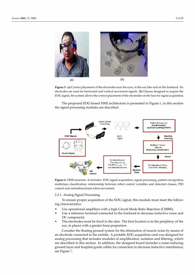
An HMI using EOG must be ergonomic and non-invasive [2]. For this reason, a systemwas developed using glasses as an optical instrument, which allows the correct placementof the electrodes on the face and embedding of the cards designed for the signal acquisition,as indicated in Figure 5b. Furthermore, users are willing to use them without fear.

Sensors 2021, 21, 5882 9 of 29

Figure 5. (a) Correct placement of the electrodes near the eyes, in the ear lobe and on the forehead. Sixelectrodes are used for horizontal and vertical movement signals. (b) Glasses designed to acquire theEOG signal, the system allows the correct placement of the electrodes on the face for signal acquisition.

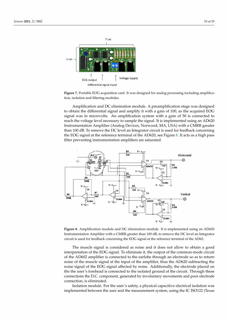
The proposed EOG-based HMI architecture is presented in Figure 6, in this sectionthe signal processing modules are described.

Figure 6. HMI structure. It includes: EOG signal acquisition, signal processing, pattern recognition,multiclass classification, relationship between robot control variables and detected classes, PIDcontrol and ominidirectional robot movement.

2.3.1. Analog Signal Processing

To ensure proper acquisition of the EOG signal, this module must meet the follow-ing characteristics:

• Use operational amplifiers with a high Circuit Mode Ratio Rejection (CMRR);• Use a reference terminal connected to the forehead to decrease inductive noise and

DC component;• The electrodes must be fixed to the skin. The best location is in the periphery of the

eye, in places with a greater bone proportion.

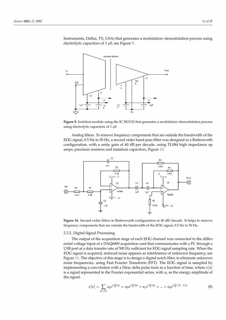
Consider the floating ground system for the elimination of muscle noise by means ofan electrode connected to the earlobe. A portable EOG acquisition card was designed foranalog processing that includes modules of amplification, isolation and filtering, whichare described in this section. In addition, the designed board includes a noise-reducingground layer and hospital-grade cables for connection to decrease inductive interference,see Figure 7.

Sensors 2021, 21, 5882 10 of 29

Figure 7. Portable EOG acquisition card. It was designed for analog processing including amplifica-tion, isolation and filtering modules.

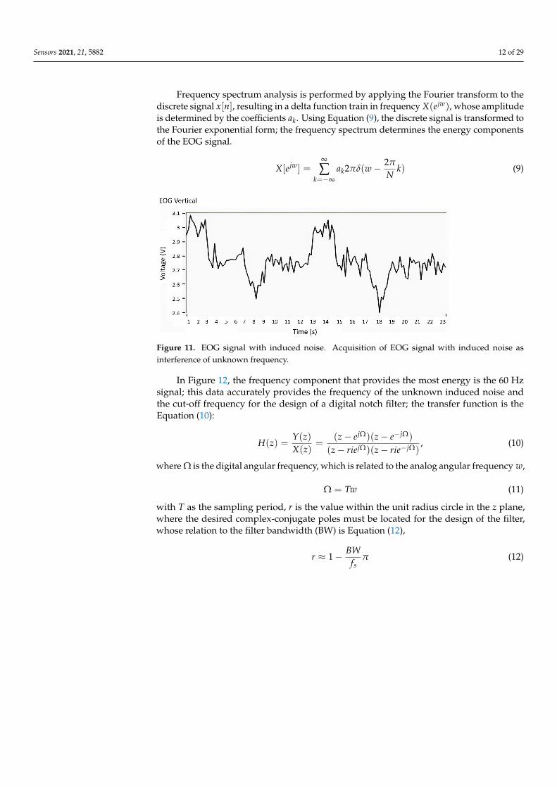
Amplification and DC elimination module. A preamplification stage was designedto obtain the differential signal and amplify it with a gain of 100, as the acquired EOGsignal was in microvolts. An amplification system with a gain of 50 is connected toreach the voltage level necessary to sample the signal. It is implemented using an AD620Instrumentation Amplifier (Analog Devices, Norwood, MA, USA) with a CMRR greaterthan 100 dB. To remove the DC level an Integrator circuit is used for feedback concerningthe EOG signal at the reference terminal of the AD620, see Figure 8. It acts as a high passfilter preventing instrumentation amplifiers are saturated.

Figure 8. Amplification module and DC elimination module. It is implemented using an AD620Instrumentation Amplifier with a CMRR greater than 100 dB, to remove the DC level an Integratorcircuit is used for feedback concerning the EOG signal at the reference terminal of the AD62.

The muscle signal is considered as noise and it does not allow to obtain a goodinterpretation of the EOG signal. To eliminate it, the output of the common-mode circuitof the AD602 amplifier is connected to the earlobe through an electrode so as to returnnoise of the muscle signal at the input of the amplifier, thus the AD620 subtracting thenoise signal of the EOG signal affected by noise. Additionally, the electrode placed onthe the user’s forehead is connected to the isolated ground of the circuit. Through theseconnections the D.C. component, generated by involuntary movements and poor electrodeconnection, is eliminated.

Isolation module. For the user’s safety, a physical capacitive electrical isolation wasimplemented between the user and the measurement system, using the IC ISO122 (Texas

Sensors 2021, 21, 5882 11 of 29

Instruments, Dallas, TX, USA) that generates a modulation–demodulation process usingelectrolytic capacitors of 1 µF, see Figure 9.

Figure 9. Isolation module using the IC ISO122 that generates a modulation–demodulation processusing electrolytic capacitors of 1 µF.

Analog filters. To remove frequency components that are outside the bandwidth of theEOG signal, 0.5 Hz to 50 Hz, a second order band-pass filter was designed in a Butterworthconfiguration, with a unity gain of 40 dB per decade, using TL084 high impedance opamps, precision resistors and tantalum capacitors, Figure 10.

Figure 10. Second order filters in Butterworth configuration at 40 dB/decade. It helps to removefrequency components that are outside the bandwidth of the EOG signal, 0.5 Hz to 50 Hz.

2.3.2. Digital Signal Processing

The output of the acquisition stage of each EOG channel was connected to the differ-ential voltage input of a DAQ6009 acquisition card that communicates with a PC through aUSB port at a data transfer rate of 500 Hz sufficient for EOG signal sampling rate. When theEOG signal is acquired, induced noise appears as interference of unknown frequency, seeFigure 11. The objective of this stage is to design a digital notch filter, to eliminate unknownnoise frequencies, using Fast Fourier Transform (FFT). The EOG signal is sampled byimplementing a convolution with a Dirac delta pulse train as a function of time, where x[n]is a signal represented in the Fourier exponential series, with ak as the energy amplitude ofthe signal.

x[n] = ∑k=N

akej eπN kn = a0ej eπ

N 0n + a1ej eπN 1n + ... + a0ej eπ

N (N−1)n (8)

Sensors 2021, 21, 5882 12 of 29

Frequency spectrum analysis is performed by applying the Fourier transform to thediscrete signal x[n], resulting in a delta function train in frequency X(ejw), whose amplitudeis determined by the coefficients ak. Using Equation (9), the discrete signal is transformed tothe Fourier exponential form; the frequency spectrum determines the energy componentsof the EOG signal.

X[ejw] =∞

∑k=−∞

ak2πδ(w− 2π

Nk) (9)

Figure 11. EOG signal with induced noise. Acquisition of EOG signal with induced noise asinterference of unknown frequency.

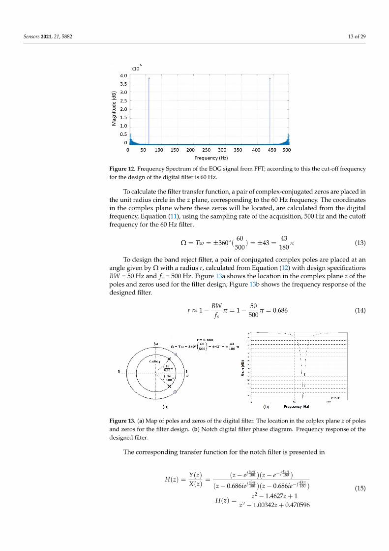
In Figure 12, the frequency component that provides the most energy is the 60 Hzsignal; this data accurately provides the frequency of the unknown induced noise andthe cut-off frequency for the design of a digital notch filter; the transfer function is theEquation (10):

H(z) =Y(z)X(z)

=(z− ejΩ)(z− e−jΩ)

(z− riejΩ)(z− rie−jΩ), (10)

where Ω is the digital angular frequency, which is related to the analog angular frequency w,

Ω = Tw (11)

with T as the sampling period, r is the value within the unit radius circle in the z plane,where the desired complex-conjugate poles must be located for the design of the filter,whose relation to the filter bandwidth (BW) is Equation (12),

r ≈ 1− BWfs

π (12)

Sensors 2021, 21, 5882 13 of 29

Figure 12. Frequency Spectrum of the EOG signal from FFT; according to this the cut-off frequencyfor the design of the digital filter is 60 Hz.

To calculate the filter transfer function, a pair of complex-conjugated zeros are placed inthe unit radius circle in the z plane, corresponding to the 60 Hz frequency. The coordinatesin the complex plane where these zeros will be located, are calculated from the digitalfrequency, Equation (11), using the sampling rate of the acquisition, 500 Hz and the cutofffrequency for the 60 Hz filter.

Ω = Tw = ±360(60

500) = ±43 =

43180

π (13)

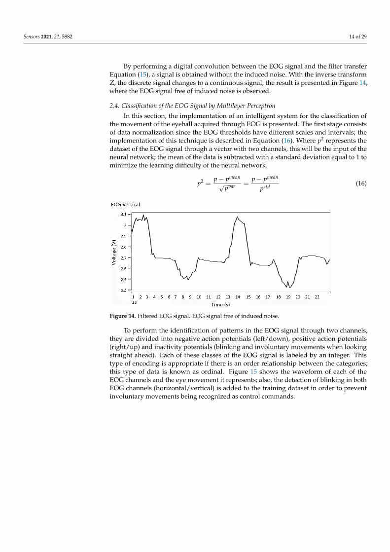
To design the band reject filter, a pair of conjugated complex poles are placed at anangle given by Ω with a radius r, calculated from Equation (12) with design specificationsBW = 50 Hz and fs = 500 Hz. Figure 13a shows the location in the complex plane z of thepoles and zeros used for the filter design; Figure 13b shows the frequency response of thedesigned filter.

r ≈ 1− BWfs

π = 1− 50500

π = 0.686 (14)

Figure 13. (a) Map of poles and zeros of the digital filter. The location in the colplex plane z of polesand zeros for the filter design. (b) Notch digital filter phase diagram. Frequency response of thedesigned filter.

The corresponding transfer function for the notch filter is presented in

H(z) =Y(z)X(z)

=(z− ej 43π

180 )(z− e−j 43π180 )

(z− 0.686iej 43π180 )(z− 0.686ie−j 43π

180 )

H(z) =z2 − 1.4627z + 1

z2 − 1.00342z + 0.470596

(15)

Sensors 2021, 21, 5882 14 of 29

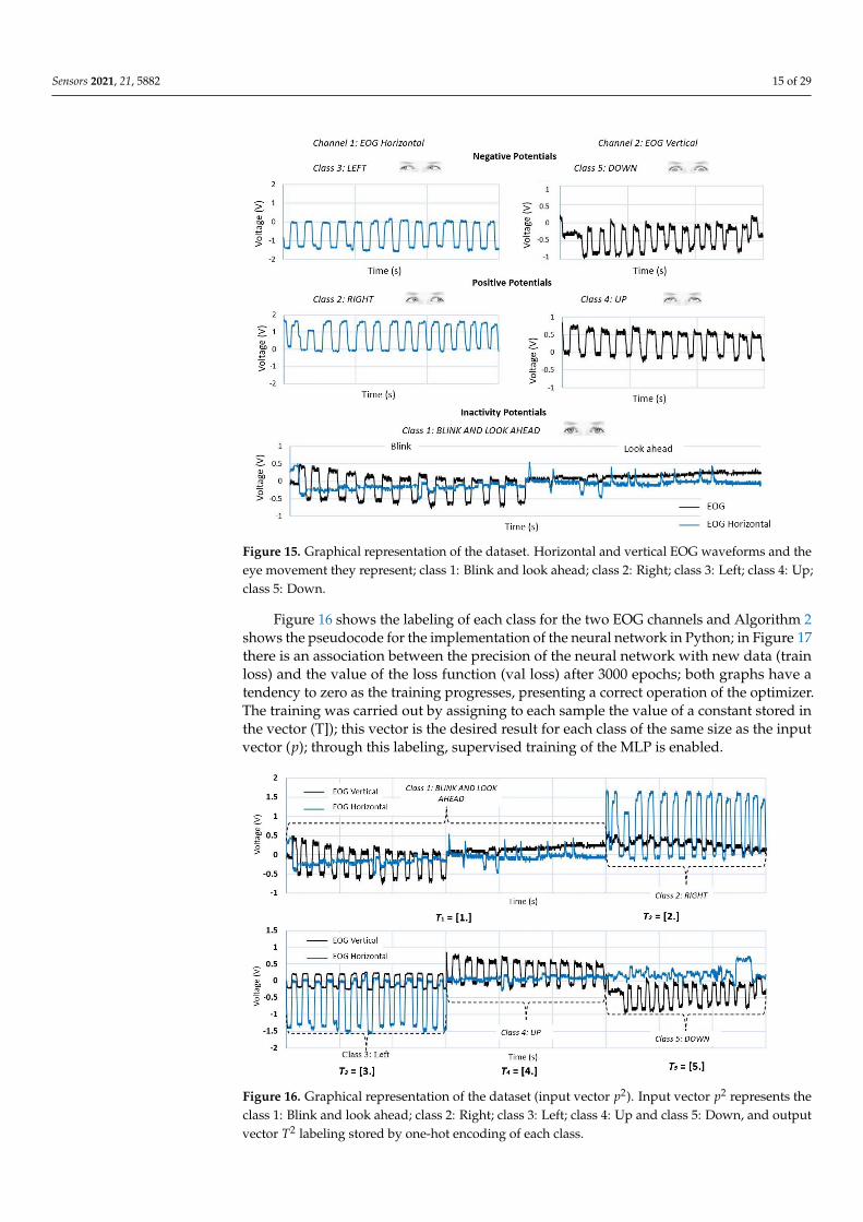
By performing a digital convolution between the EOG signal and the filter transferEquation (15), a signal is obtained without the induced noise. With the inverse transformZ, the discrete signal changes to a continuous signal, the result is presented in Figure 14,where the EOG signal free of induced noise is observed.

2.4. Classification of the EOG Signal by Multilayer Perceptron

In this section, the implementation of an intelligent system for the classification ofthe movement of the eyeball acquired through EOG is presented. The first stage consistsof data normalization since the EOG thresholds have different scales and intervals; theimplementation of this technique is described in Equation (16). Where p2 represents thedataset of the EOG signal through a vector with two channels, this will be the input of theneural network; the mean of the data is subtracted with a standard deviation equal to 1 tominimize the learning difficulty of the neural network.

p2 =p− pmean√

pvar =p− pmean

pstd (16)

Figure 14. Filtered EOG signal. EOG signal free of induced noise.

To perform the identification of patterns in the EOG signal through two channels,they are divided into negative action potentials (left/down), positive action potentials(right/up) and inactivity potentials (blinking and involuntary movements when lookingstraight ahead). Each of these classes of the EOG signal is labeled by an integer. Thistype of encoding is appropriate if there is an order relationship between the categories;this type of data is known as ordinal. Figure 15 shows the waveform of each of theEOG channels and the eye movement it represents; also, the detection of blinking in bothEOG channels (horizontal/vertical) is added to the training dataset in order to preventinvoluntary movements being recognized as control commands.

Sensors 2021, 21, 5882 15 of 29

Figure 15. Graphical representation of the dataset. Horizontal and vertical EOG waveforms and theeye movement they represent; class 1: Blink and look ahead; class 2: Right; class 3: Left; class 4: Up;class 5: Down.

Figure 16 shows the labeling of each class for the two EOG channels and Algorithm 2shows the pseudocode for the implementation of the neural network in Python; in Figure 17there is an association between the precision of the neural network with new data (trainloss) and the value of the loss function (val loss) after 3000 epochs; both graphs have atendency to zero as the training progresses, presenting a correct operation of the optimizer.The training was carried out by assigning to each sample the value of a constant stored inthe vector (T]); this vector is the desired result for each class of the same size as the inputvector (p); through this labeling, supervised training of the MLP is enabled.

Figure 16. Graphical representation of the dataset (input vector p2). Input vector p2 represents theclass 1: Blink and look ahead; class 2: Right; class 3: Left; class 4: Up and class 5: Down, and outputvector T2 labeling stored by one-hot encoding of each class.

Sensors 2021, 21, 5882 16 of 29

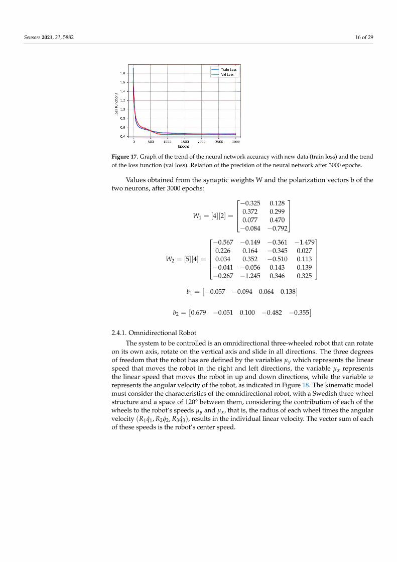
Figure 17. Graph of the trend of the neural network accuracy with new data (train loss) and the trendof the loss function (val loss). Relation of the precision of the neural network after 3000 epochs.

Values obtained from the synaptic weights W and the polarization vectors b of thetwo neurons, after 3000 epochs:

W1 = [4][2] =

−0.325 0.1280.372 0.2990.077 0.470−0.084 −0.792

W2 = [5][4] =

−0.567 −0.149 −0.361 −1.4790.226 0.164 −0.345 0.0270.034 0.352 −0.510 0.113−0.041 −0.056 0.143 0.139−0.267 −1.245 0.346 0.325

b1 =

[−0.057 −0.094 0.064 0.138

]b2 =

[0.679 −0.051 0.100 −0.482 −0.355

]2.4.1. Omnidirectional Robot

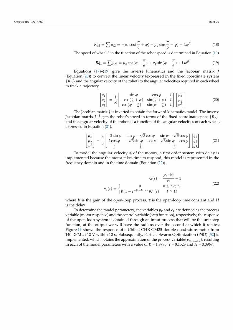
The system to be controlled is an omnidirectional three-wheeled robot that can rotateon its own axis, rotate on the vertical axis and slide in all directions. The three degreesof freedom that the robot has are defined by the variables µy which represents the linearspeed that moves the robot in the right and left directions, the variable µx representsthe linear speed that moves the robot in up and down directions, while the variable wrepresents the angular velocity of the robot, as indicated in Figure 18. The kinematic modelmust consider the characteristics of the omnidirectional robot, with a Swedish three-wheelstructure and a space of 120° between them, considering the contribution of each of thewheels to the robot’s speeds µy and µx, that is, the radius of each wheel times the angularvelocity (R1q1, R2q2, R3q3), results in the individual linear velocity. The vector sum of eachof these speeds is the robot’s center speed.

Sensors 2021, 21, 5882 17 of 29

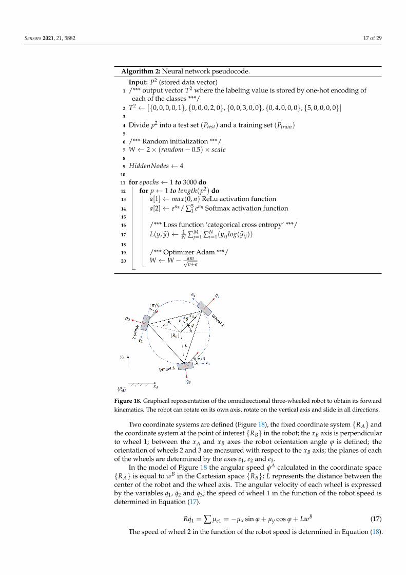
Algorithm 2: Neural network pseudocode.

Input: P2 (stored data vector)1 /*** output vector T2 where the labeling value is stored by one-hot encoding of

each of the classes ***/2 T2 ← [0, 0, 0, 0, 1, 0, 0, 0, 2, 0, 0, 0, 3, 0, 0, 0, 4, 0, 0, 0, 5, 0, 0, 0, 0]3

4 Divide p2 into a test set (Ptest) and a training set (Ptrain)5

6 /*** Random initialization ***/7 W ← 2× (random− 0.5)× scale8

9 HiddenNodes← 410

11 for epochs← 1 to 3000 do12 for p← 1 to length(p2) do13 a[1]← max(0, n) ReLu activation function14 a[2]← en5 / ∑5

1 en5 Softmax activation function15

16 /*** Loss function ‘categorical cross entropy’ ***/17 L(y, y)← 1

N ∑Mj=1 ∑N

i=1(yijlog(yij))

18

19 /*** Optimizer Adam ***/20 W ←W − αm√

v+ε

Figure 18. Graphical representation of the omnidirectional three-wheeled robot to obtain its forwardkinematics. The robot can rotate on its own axis, rotate on the vertical axis and slide in all directions.

Two coordinate systems are defined (Figure 18), the fixed coordinate system RA andthe coordinate system at the point of interest RB in the robot; the xB axis is perpendicularto wheel 1; between the xA and xB axes the robot orientation angle ϕ is defined; theorientation of wheels 2 and 3 are measured with respect to the xB axis; the planes of eachof the wheels are determined by the axes e1, e2 and e3.

In the model of Figure 18 the angular speed ϕA calculated in the coordinate spaceRA is equal to wB in the Cartesian space RB; L represents the distance between thecenter of the robot and the wheel axis. The angular velocity of each wheel is expressedby the variables q1, q2 and q3; the speed of wheel 1 in the function of the robot speed isdetermined in Equation (17).

Rq1 = ∑ µe1 = −µx sin ϕ + µy cos ϕ + LwB (17)

The speed of wheel 2 in the function of the robot speed is determined in Equation (18).

Sensors 2021, 21, 5882 18 of 29

Rq2 = ∑ µe2 = −µx cos(π

6+ ϕ)− µy sin(

π

6+ ϕ) + LwB (18)

The speed of wheel 3 in the function of the robot speed is determined in Equation (19).

Rq3 = ∑ µe3 = µx cos(ϕ− π

6) + µy sin(ϕ− π

6) + LwB (19)

Equations (17)–(19) give the inverse kinematics and the Jacobian matrix J(Equation (20)) to convert the linear velocity (expressed in the fixed coordinate systemRA and the angular velocity of the robot) to the angular velocities required in each wheelto track a trajectory.q1

q2q3

=1R

− sin ϕ cos ϕ L− cos(π

6 + ϕ) sin(π6 + ϕ) L

cos(ϕ− π6 ) sin(ϕ− π

6 ) L

µxµywB

(20)

The Jacobian matrix J is inverted to obtain the forward kinematics model. The inverseJacobian matrix J−1 gets the robot’s speed in terms of the fixed coordinate space RAand the angular velocity of the robot as a function of the angular velocities of each wheel,expressed in Equation (21).µx

µywB

=R3

−2 sin ϕ sin ϕ−√

3 cos ϕ sin ϕ +√

3 cos ϕ

2 cos ϕ −√

3 sin ϕ− cos ϕ√

3 sin ϕ− cos ϕ1L

1L

1L

q1q2q3

(21)

To model the angular velocity qi of the motors, a first order system with delay isimplemented because the motor takes time to respond; this model is represented in thefrequency domain and in the time domain (Equation (22)).

G(s) =Ke−Hs

τs+ 1

pv(t) =

0 0 ≤ t < HK(1− e−(t−H)/τ)Cv(t) t ≥ H

(22)

where K is the gain of the open-loop process, τ is the open-loop time constant and His the delay.

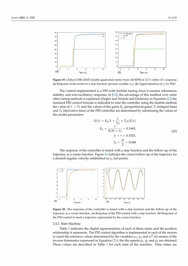
To determine the model parameters, the variables pv and cv are defined as the processvariable (motor response) and the control variable (step function), respectively; the responseof the open-loop system is obtained through an input process that will be the unit stepfunction; at the output we will have the radians over the second at which it rotates;Figure 19 shows the response of a Chihai CHR-GM25 double quadrature motor from140 RPM at 12 V within 10 s. Subsequently, Particle Swarm Optimization (PSO) [52] isimplemented, which obtains the approximation of the process variable(pvestimated), resultingin each of the model parameters with a value of K = 1.8795, τ = 0.1523 and H = 0.0967.

Sensors 2021, 21, 5882 19 of 29

Figure 19. Chihai CHR-GM25 double quadrature motor from 140 RPM at 12 V within 10 s response.(a) Response of the motor to a step function (process variable vp). (b) Approximation of vp by PSO.

The control implemented is a PID with lambda tuning since it ensures robustness,stability and non-oscillatory response; in [53], the advantage of this method over someother tuning methods is explained (Ziegler and Nichols and Haalman); in Equation (23) thestandard PID control formula is indicated to tune the controller using the lambda method;the value of λ = 3τ and the values of the gains Kp (proportional gain), Ti (integral time)and Td (derivative time) of the PID controller are determined by substituting the values ofthe model parameters.

U(s) = Kp(1 +1

Tis+ Tds)E(s)

Kp =τ

K(H + λ)= 0.1463,

ti = τ = 0.1523,

Td =H2

= 0.048

(23)

The response of the controller is tested with a step function and the follow-up of thetrajectory as a cosine function. Figure 20 indicates the correct follow-up of the trajectory fora desired angular velocity established as sp (set point).

Figure 20. The response of the controller is tested with a step function and the follow-up of thetrajectory as a cosine function. (a) Response of the PID control with a step function. (b) Response ofthe PID control to track a trajectory represented by the cosine function.

2.4.2. State Machine

Table 2 indicates the digital representation of each of these states and the positionrelationship it represents. The PID control algorithm is implemented in each of the motorsto reach the reference values determined by the variables µx, µy and wB; by means of theinverse kinematics expressed in Equation (21), the the speeds q1, q2 and q3 are obtained.These values are described in Table 3 for each state of the machine. Nine states are

Sensors 2021, 21, 5882 20 of 29

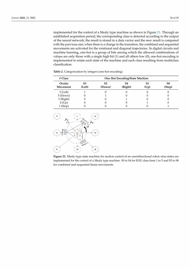
implemented for the control of a Mealy type machine as shown in Figure 21. Through anestablished acquisition period, the corresponding class is detected according to the outputof the neural network; the result is stored in a data vector and the new result is comparedwith the previous one; when there is a change in the transition, the combined and sequentialmovements are activated for the rotational and diagonal trajectories. In digital circuits andmachine learning, one-hot is a group of bits among which the allowed combinations ofvalues are only those with a single high bit (1) and all others low (0), one-hot encoding isimplemented to relate each state of the machine and each class resulting from multiclassclassification.

Table 2. Categorization by integers (one-hot encoding).

# Class One Hot Encoding/State Machine

Ocular S3 S2 S4 S1 S0Movement (Left) (Down) (Right) (Up) (Stop)

3 (Left) 1 0 0 0 05 (Down) 0 1 0 0 02 (Right) 0 0 1 0 0

4 (Up) 0 0 0 1 01 (Stop) 0 0 0 0 1

Figure 21. Mealy-type state machine for motion control of an omnidirectional robot; nine states areimplemented for the control of a Mealy type machine. S0 to S4 for EOG class from 1 to 5 and S5 to S8for combined and sequential linear movements.

Sensors 2021, 21, 5882 21 of 29

Table 3. Description of each of the movements in the state machine.

State Class Desired Value DesiredEOG (µx, µy, wB) Movement

S3 3 (−0.15 m/s, 0 m/s, 0 rad/s) LeftS2 5 (0 m/s, −0.15 m/s, 0 rad/s) DownS4 2 (0.15 m/s, 0 m/s, 0 rad/s) RightS1 4 (0 m/s, 0.15 m/s, 0 rad/s) UpS0 1 (0 m/s, 0 m/s, 0 rad/s) Stop

Combined and sequential linear movements

S5 3, 4 (−0.15 m/s, 0.15 m/s, 0 rad/s) Upper-LeftDiagonal

S6 2, 4 (0.15 m/s, 0.15 m/s, 0 rad/s) Upper-RightDiagonal

S7 3, 5 (−0.15 m/s, −0.15 m/s, 0 rad/s) Lower-LeftDiagonal

S8 2, 5 (0.15 m/s, −0.15 m/s, 0 rad/s) Lower-RightDiagonal

Combined and sequential rotational movements

4, 2, 5, 3 (0 m/s, 0 m/s, 0.8 rad/s) Counterclockwiserotation

3, 5, 2, 4 (0 m/s, 0 m/s, −0.8 rad/s) Clockwiserotation

3. Results and Discussion

To evaluate the operation of the HMI, tests were developed in digital evaluationsystems and simulations. First, the response of the EOG acquisition system to interferencewas evaluated experimentally. Later, by means of the graphic interface, simulation testswere performed to evaluate the performance of the classifier.

3.1. EOG Acquisition System Evaluation

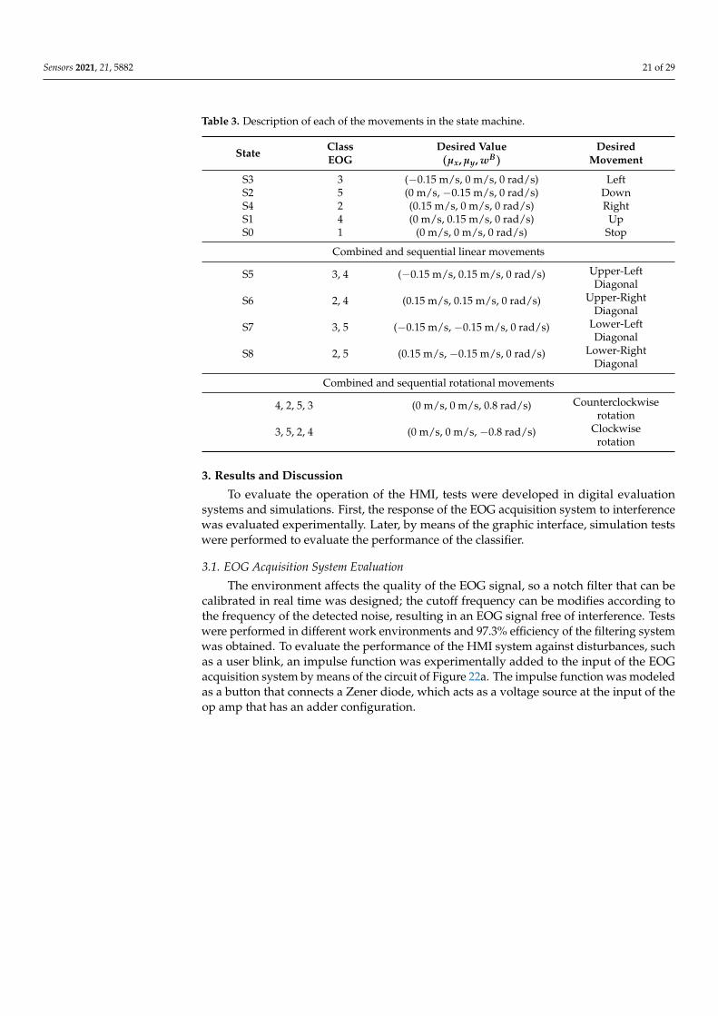
The environment affects the quality of the EOG signal, so a notch filter that can becalibrated in real time was designed; the cutoff frequency can be modifies according tothe frequency of the detected noise, resulting in an EOG signal free of interference. Testswere performed in different work environments and 97.3% efficiency of the filtering systemwas obtained. To evaluate the performance of the HMI system against disturbances, suchas a user blink, an impulse function was experimentally added to the input of the EOGacquisition system by means of the circuit of Figure 22a. The impulse function was modeledas a button that connects a Zener diode, which acts as a voltage source at the input of theop amp that has an adder configuration.

Sensors 2021, 21, 5882 22 of 29

Figure 22. Experimental impulse function added to the input of the EOG acquisition system toevaluate the performance of the HMI system against disturbances. (a) System to test interferenceelimination. (b) Signal obtained with perturbation.

The signal obtained is seen in Figure 22b; the disturbance does not affect the classifierbecause the experimental tests determined that, even with this induced noise, the neu-ronal network model is capable of classifying the movement according to the class thatcorresponds to it.

Virtual Test

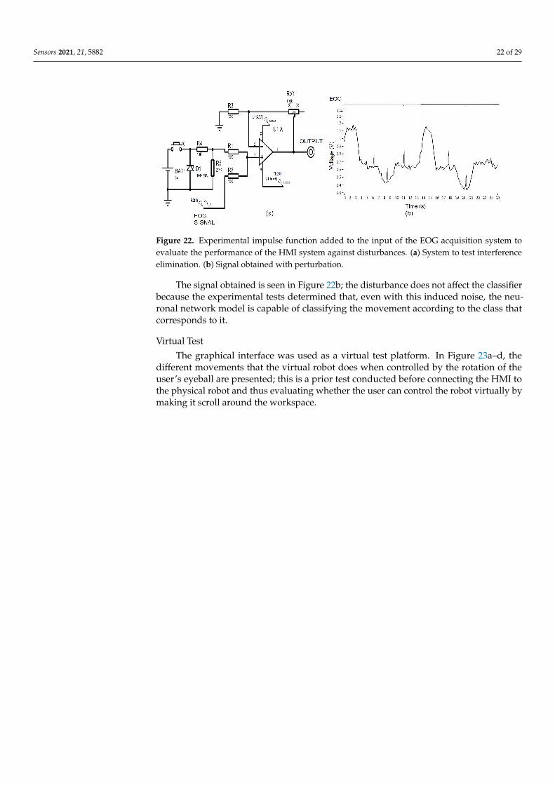
The graphical interface was used as a virtual test platform. In Figure 23a–d, thedifferent movements that the virtual robot does when controlled by the rotation of theuser’s eyeball are presented; this is a prior test conducted before connecting the HMI tothe physical robot and thus evaluating whether the user can control the robot virtually bymaking it scroll around the workspace.

Sensors 2021, 21, 5882 23 of 29

Figure 23. Virtual robot movements when controlled by the rotation of the eyeball. (a) Eye movementlooking up and tracking the robot’s trajectory forward. (b) Eye movement looking down and trackingthe robot’s trajectory backwards. (c) Eye movement looking to the right and tracking the robot’strajectory to the right. (d) Eye movement looking to the left and tracking the robot’s trajectoryto the left.

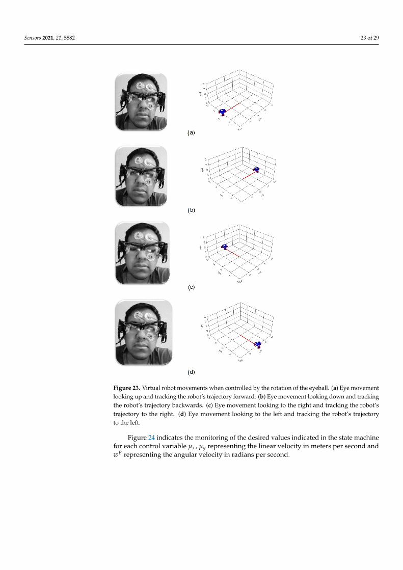
Figure 24 indicates the monitoring of the desired values indicated in the state machinefor each control variable µx, µy representing the linear velocity in meters per second andwB representing the angular velocity in radians per second.

Sensors 2021, 21, 5882 24 of 29

Figure 24. Desired values indicated in the state machine and the PID control responses for eachvariable µx, µy and wB.

3.2. Performance Test

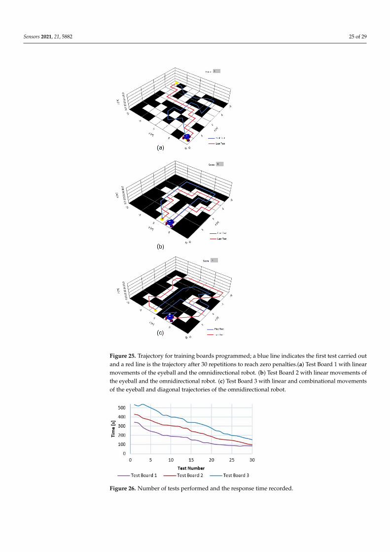
Three game and training boards are programmed; the ability of the user to arrive froma starting point and an end point colored in yellow is evaluated; each black square on thegame board corresponds to a penalty, which means there are points in the workspace wherethe user must not place the mobile robot; the only valid points to move the robot are thewhite squares. The test consists of recording the number of penalties and the time it takesfor the user to place the robot on the assigned points, marking the generated trajectory inred. In Figure 25a,b, Boards 1 and 2 are shown; only linear movements are recorded. InFigure 25c, Test Board 3 is presented; linear and sequential movements are recorded, whichare combinations of the eyeball to move the robot diagonally or rotationally.

The interface has the property of detecting involuntary movements such as blinkingand looking forward; in Figure 25 there is also a trajectory marked in blue that indicatesthe first test carried out; the tests on different boards indicate that 30 repetitions is enoughto reach zero penalties.

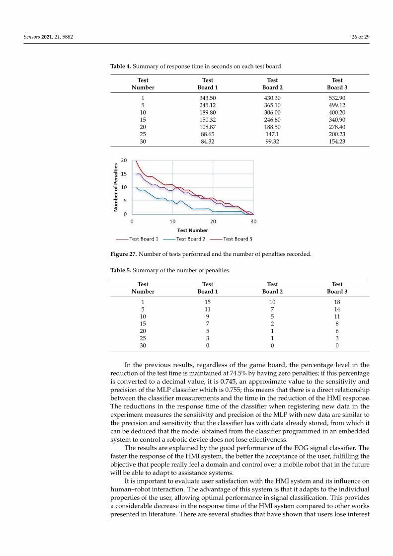
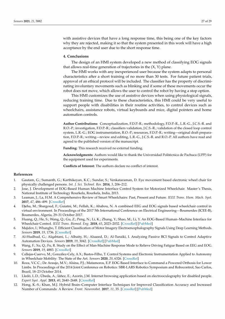
In Figure 26, the trend graph of Table 4 is presented, which records the response timeof each of the repetitions performed. It is observed that after 30 repetitions the time isdecreased by 71.1% to perform the task on Test board 3; on Test Board 2 the time is reducedby 76.9% when executing the task and finally on Test Board 1 there is a response timereduction of 75.4%. The experiment ends after 30 repetitions since there were 0 penaltiesdecreasing after each repetition. This result can be seen in Figure 27, which indicates thedownward trend in the number of penalties recorded in Table 5. Therefore, a conclusion canbe obtained where, regardless of the test board, the user has a mastery after 30 repetitionswith an average of 74.5% reduction of learning time.

Sensors 2021, 21, 5882 25 of 29

Figure 25. Trajectory for training boards programmed; a blue line indicates the first test carried outand a red line is the trajectory after 30 repetitions to reach zero penalties.(a) Test Board 1 with linearmovements of the eyeball and the omnidirectional robot. (b) Test Board 2 with linear movements ofthe eyeball and the omnidirectional robot. (c) Test Board 3 with linear and combinational movementsof the eyeball and diagonal trajectories of the omnidirectional robot.

Figure 26. Number of tests performed and the response time recorded.

Sensors 2021, 21, 5882 26 of 29

Table 4. Summary of response time in seconds on each test board.

Test Test Test TestNumber Board 1 Board 2 Board 3

1 343.50 430.30 532.905 245.12 365.10 499.1210 189.80 306.00 400.2015 150.32 246.60 340.9020 108.87 188.50 278.4025 88.65 147.1 200.2330 84.32 99.32 154.23

Figure 27. Number of tests performed and the number of penalties recorded.

Table 5. Summary of the number of penalties.

Test Test Test TestNumber Board 1 Board 2 Board 3

1 15 10 185 11 7 1410 9 5 1115 7 2 820 5 1 625 3 1 330 0 0 0

In the previous results, regardless of the game board, the percentage level in thereduction of the test time is maintained at 74.5% by having zero penalties; if this percentageis converted to a decimal value, it is 0.745, an approximate value to the sensitivity andprecision of the MLP classifier which is 0.755; this means that there is a direct relationshipbetween the classifier measurements and the time in the reduction of the HMI response.The reductions in the response time of the classifier when registering new data in theexperiment measures the sensitivity and precision of the MLP with new data are similar tothe precision and sensitivity that the classifier has with data already stored, from which itcan be deduced that the model obtained from the classifier programmed in an embeddedsystem to control a robotic device does not lose effectiveness.

The results are explained by the good performance of the EOG signal classifier. Thefaster the response of the HMI system, the better the acceptance of the user, fulfilling theobjective that people really feel a domain and control over a mobile robot that in the futurewill be able to adapt to assistance systems.

It is important to evaluate user satisfaction with the HMI system and its influence onhuman–robot interaction. The advantage of this system is that it adapts to the individualproperties of the user, allowing optimal performance in signal classification. This providesa considerable decrease in the response time of the HMI system compared to other workspresented in literature. There are several studies that have shown that users lose interest

Sensors 2021, 21, 5882 27 of 29

with assistive devices that have a long response time, this being one of the key factorswhy they are rejected, making it so that the system presented in this work will have a highacceptance by the end user due to the short response time.

4. Conclusions

The design of an HMI system developed a new method of classifying EOG signalsthat allows real-time generation of trajectories in the (X, Y) plane.

The HMI works with any inexperienced user because the system adapts to personalcharacteristics after a short training of no more than 30 tests. For future patient trials,approval of an ethical protocol will be included. The classifier has the property of discrimi-nating involuntary movements such as blinking and if some of these movements occur therobot does not move, which allows the user to control the robot by having a stop option.

This HMI customizes the use of assistive devices when using physiological signals,reducing training time. Due to these characteristics, this HMI could be very useful tosupport people with disabilities in their routine activities, to control devices such aswheelchairs, assistance robots, virtual keyboards and mice, digital pointers and homeautomation controls.

Author Contributions: Conceptualization, F.D.P.-R.; methodology, F.D.P.-R., L.R.-G., J.C.S.-R. andR.O.-P.; investigation, F.D.P.-R.; classifiers validation, J.C.S.-R.; validation of the closed loop controlsystem, L.R.-G.; EOG instrumentation, R.O.-P.; resources, F.D.P.-R.; writing—original draft prepara-tion, F.D.P.-R.; writing—review and editing, L.R.-G., J.C.S.-R. and R.O.-P. All authors have read andagreed to the published version of the manuscript.

Funding: This research received no external funding.

Acknowledgments: Authors would like to thank the Universidad Politécnica de Pachuca (UPP) forthe equipment used for experiments.

Conflicts of Interest: The authors declare no conflict of interest.

References1. Gautam, G.; Sumanth, G.; Karthikeyan, K.C.; Sundar, S.; Venkataraman, D. Eye movement based electronic wheel chair for

physically challenged persons. Int. J. Sci. Technol. Res. 2014, 3, 206–212.2. Jose, J. Development of EOG-Based Human Machine Interface Control System for Motorized Wheelchair. Master’s Thesis,

National Institute of Technology Rourkela, Rourkela, India, 2013.3. Leaman, J.; La, H.M. A Comprehensive Review of Smart Wheelchairs: Past, Present and Future. IEEE Trans. Hum. Mach. Syst.

2017, 47, 486–499. [CrossRef]4. Djeha, M.; Sbargoud, F.; Guiatni, M.; Fellah, K.; Ababou, N. A combined EEG and EOG signals based wheelchair control in

virtual environment. In Proceedings of the 2017 5th International Conference on Electrical Engineering—Boumerdes (ICEE-B),Boumerdes, Algeria, 29–31 October 2017.

5. Huang, Q.; He, S.; Wang, Q.; Gu, Z.; Peng, N.; Li, K.; Zhang, Y.; Shao, M.; Li, Y. An EOG-Based Human–Machine Interface forWheelchair Control. IEEE Trans. Biomed. Eng. 2018, 65, 2023–2032. [CrossRef] [PubMed]

6. Majidov, I.; Whangbo, T. Efficient Classification of Motor Imagery Electroencephalography Signals Using Deep Learning Methods.Sensors 2019, 19, 1736. [CrossRef]

7. Al-Hudhud, G.; Alqahtani, L.; Albaity, H.; Alsaeed, D.; Al-Turaiki, I. Analyzing Passive BCI Signals to Control AdaptiveAutomation Devices. Sensors 2019, 19, 3042. [CrossRef] [PubMed]

8. Wang, F.; Xu, Q.; Fu, R. Study on the Effect of Man-Machine Response Mode to Relieve Driving Fatigue Based on EEG and EOG.Sensors 2019, 19, 4883. [CrossRef]

9. Callejas-Cuervo, M.; González-Cely, A.X.; Bastos-Filho, T. Control Systems and Electronic Instrumentation Applied to Autonomyin Wheelchair Mobility: The State of the Art. Sensors 2020, 20, 6326. [CrossRef]

10. Roza, V.C.C.; De Araujo, M.V.; Alsina, P.J.; Matamoros, E.P. EOG Based Interface to Command a Powered Orthosis for LowerLimbs. In Proceedings of the 2014 Joint Conference on Robotics: SBR-LARS Robotics Symposium and Robocontrol, Sao Carlos,Brazil, 18–23 October 2014.

11. Lledó, L.D.; Úbeda, A.; Iáñez, E.; Azorín, J.M. Internet browsing application based on electrooculography for disabled people.Expert Syst. Appl. 2013, 40, 2640–2648. [CrossRef]

12. Hong, K.-S.; Khan, M.J. Hybrid Brain–Computer Interface Techniques for Improved Classification Accuracy and IncreasedNumber of Commands: A Review. Front. Neurorobot. 2017, 11, 35. [CrossRef] [PubMed]

Sensors 2021, 21, 5882 28 of 29

13. Ülkütas, H.Ö.; Yıldız, M. Computer based eye-writing system by using EOG. In Proceedings of the 2015 Medical TechnologiesNational Conference (TIPTEKNO), Bodrum, Turkey, 15–18 October 2015.

14. Chang, W.-D. Electrooculograms for Human-Computer Interaction: A Review. Sensors 2019, 19, 2690. [CrossRef]15. Rim, B.; Sung, N.-J.; Min, S.; Hong, M. Deep Learning in Physiological Signal Data: A Survey. Sensors 2020, 20, 969. [CrossRef]

[PubMed]16. Martínez-Cerveró, J.; Ardali, M.K.; Jaramillo-Gonzalez, A.; Wu, S.; Tonin, A.; Birbaumer, N.; Chaudhary, U. Open Soft-

ware/Hardware Platform for Human-Computer Interface Based on Electrooculography (EOG) Signal Classification. Sensors 2020,20, 2443. [CrossRef]

17. Laport, F.; Iglesia, D.; Dapena, A.; Castro, P.M.; Vazquez-Araujo, F.J. Proposals and Comparisons from One-Sensor EEG and EOGHuman–Machine Interfaces. Sensors 2021, 21, 2220. [CrossRef] [PubMed]

18. Lee, K.-R.; Chang, W.-D.; Kim, S.; Im, C.-H. Real-Time “Eye-Writing” Recognition Using Electrooculogram. IEEE Trans. NeuralSyst. Rehabil. Eng. 2017, 25, 37–48. [CrossRef]

19. Mohd Noor, N.M.; Ahmad, S.; Sidek, S.N. Implementation of Wheelchair Motion Control Based on Electrooculography UsingSimulation and Experimental Performance Testing. App. Mech. Mater. 2014, 554, 551–555. [CrossRef]

20. Fang F.; Shinozaki T. Electrooculography-based continuous eye-writing recognition system for efficient assistive communicationsystems. PLoS ONE 2018, 13.

21. Iáñez, E.; Azorín, J.M.; Fernández, E.; Úbeda, A. Interface Based on Electrooculography for Velocity Control of a Robot Arm. Appl.Bionics Biomech. 2010, 7, 199–207. [CrossRef]

22. Ubeda, A.; Iañez, E.; Azorin, J.M. Wireless and Portable EOG-Based Interface for Assisting Disabled People. IEEE/ASME Trans.Mechatron. 2011, 16, 870–873. [CrossRef]

23. Ramkumar, S.; Sathesh Kumar, K.; Dhiliphan Rajkumar, T.; Ilayaraja, M.; Shankar, K. A review-classification of electrooculogrambased human computer interfaces. Biomed. Res. 2018, 29, 1078–1084. [CrossRef]

24. Reynoso, F.D.P.; Suarez, P.A.N.; Sanchez, O.F.A.; Yañez, M.B.C.; Alvarado, E.V.; Flores, E.A.P. Custom EOG-Based HMI UsingNeural Network Modeling to Real-Time for the Trajectory Tracking of a Manipulator Robot . Front. Neurorobot. 2020, 14, 578834.[CrossRef] [PubMed]

25. Kubacki, A.; Jakubowski, A. Controlling the industrial robot model with the hybrid BCI based on EOG and eye tracking. AIPConf. Proc. 2018, 2029, 020032.

26. Kim, B.H.; Kim, M.; Jo, S. Quadcopter flight control using a low-cost hybrid interface with EEG-based classification and eyetracking. Comput. Biol. Med. 2014, 51, 82–92. [CrossRef] [PubMed]

27. Postelnicu, C.-C.; Girbacia, F.; Voinea, G.-D.; Boboc, R. Towards Hybrid Multimodal Brain Computer Interface for Robotic ArmCommand. In Augmented Cognition; Schmorrow D., Fidopiastis C., Eds.; Springer: Cham, Switzerland, 2019; Volume 11580,pp. 461–470.

28. McMullen, D.; Hotson, G.; Katyal, K.D.; Wester, B.A.; Fifer, M.S.; McGee, T.G.; Harris, A.; Johannes, M.S.; Vogelstein, R.J.;Ravitz, A.D.; et al. Demonstration of a semi-autonomous hybrid brain-machine interface using human intracranial EEG, eyetracking and computer vision to control a robotic upper limb prosthetic. IEEE Trans. Neural Syst. Rehabil. Eng. 2014, 22, 784–792.[CrossRef]

29. Sai, J.-Z.; Lee, C.-K.; Wu, C.-M.; Wu, J.-J.; Kao, K.-P. A feasibility study of an eye-writing system based on electro-oculography.J. Med. Biol. Eng. 2008, 28, 39–46.

30. Luu, T.; Ngoc, H.; Le, V.; Ho, T.; Truong, N.; Ngan, T.; Luong H.; Nguyen Q. Machine Learning Model for Identifying AntioxidantProteins Using Features Calculated from Primary Sequences. Biology 2020, 9, 325.

31. Nguyen, Q.; Duyen, T.; Truong, K.; Luu, T.; Tuan-Tu, H.; Ngan, K.A Computational Framework Based on Ensemble Deep NeuralNetworks for Essential Genes Identification. Int. J. Mol. Sci. 2020, 21, 9070.

32. Daqi, G., Yan, J. Classification methodologies of multilayer perceptrons with sigmoid activation functions. Pattern Recognit. 2005,38, 1469–1482. [CrossRef]

33. Quinlan, J.R. Improved use of continuous attributes in C4.5. J. Artif. Intell. Res. 1996, 4, 77–90. [CrossRef]34. Quinlan, J.R. Induction of decision trees. Mach. Learn. 1986, 1, 81–106. [CrossRef]35. Otneim, H.; Jullum, M.; Tjøstheim, D. Pairwise local Fisher and Naïve Bayes: Improving two standard discriminants. J. Econom.

2020, 216, 284–304. [CrossRef]36. Cover, T.; Hart, P. Nearest neighbor pattern classification. IEEE Trans. Inf. Theory 1967, 13, 21–27. [CrossRef]37. Yamashita, Y.; Wakahara, T. Affine-transformation and 2D-projection invariant k-NN classification of handwritten characters via

a new matching measure. Pattern Recognit. 2016, 52, 459–470. [CrossRef]38. Noh, Y.-K.; Zhang, B.-T.; Lee, D.D. Generative Local Metric Learning for Nearest Neighbor Classification. IEEE Trans. Pattern

Anal. Mach. Intell. 2018, 40, 106–118. [CrossRef]39. Stoklasa, R.; Majtner, T.; Svoboda, D. Efficient k-NN based HEp-2 cells classifier. Pattern Recognit. 2014, 47, 2409–2418. [CrossRef]40. Pernkopf, F. Bayesian network classifiers versus selective k-NN classifier. Pattern Recognit. 2005, 38, 1–10. [CrossRef]41. Le Cessie, S.; van Houwelingen, J.C. Ridge Estimators in Logistic Regression. Appl. Stat. 1992, 41, 191–201. [CrossRef]42. Paranjape, P.; Dhabu, M.; Deshpande, P. A novel classifier for multivariate instance using graph class signatures. Front. Comput.

Sci. 2020, 14, 144307. [CrossRef]

Sensors 2021, 21, 5882 29 of 29

43. Hall, M.; Frank, E.; Holmes, G.; Pfahringer, B.; Reutemann, P.; Witten, I.H. The WEKA data mining software: An update. ACMSIGKDD Explor. Newsl. 2009, 11, 10–18. [CrossRef]

44. Lindberg, A. Developing Theory Through Integrating Human and Machine Pattern Recognition. J. Assoc. Inf. Syst. 2020, 21, 7.[CrossRef]

45. Schwenker, F.; Trentin, E. Pattern classification and clustering: A review of partially supervised learning approaches. PatternRecognit. Lett. 2014, 37, 4–14. [CrossRef]

46. Wolpert, D.H.; Macready, W.G. No free lunch theorems for optimization. IEEE Trans. Evol. Comput. 1997, 1, 67–82. [CrossRef]47. Adam, S.P.; Alexandropoulos, S.A.N.; Pardalos, P.M.; Vrahatis, M.N. No free lunch theorem: A review. In Approximation and

Optimization; Springer Optimization and Its Applications Series; Springer: Cham, Switzerland, 2019; Volume 145, pp. 57–82.48. Stock, M.; Pahikkala, T.; Airola, A.; Waegeman, W.; De Baets, B. Algebraic shortcuts for leave-one-out cross-validation in

supervised network inference. Brief. Bioinform. 2020, 21, 262–271. [CrossRef] [PubMed]49. Jiang, G.; Wang, W. Error estimation based on variance analysis of k-fold cross-validation. Pattern Recognit. 2017, 69, 94–106.

[CrossRef]50. Soleymani, R.; Granger, E.; Fumera, G. F-measure curves: A tool to visualize classifier performance under imbalance. Pattern

Recognit. 2020, 100, 107–146. [CrossRef]51. Moreno-Ibarra, M-A.; Villuendas-Rey, Y.; Lytras, M.; Yañez-Marquez, C.; Salgado-Ramirez, J-C. Classification of Diseases Using

Machine Learning Algorithms: A Comparative Study. Mathematics 2021, 9, 1817. [CrossRef]52. Cogollo, M.R.; Velásquez, J.D.; Patricia, A. Estimation of the nonlinear moving model Parameters using the DE-PSO Meta-

Heuristic. Rev. Ing. Univ. Medellín 2013, 12, 147–156. [CrossRef]53. Pruna, E.; Sasig, E.R.; Mullo S. PI and PID controller tuning tool based on the lambda method. In Proceedings of the 2017

CHILEAN Conference on Electrical, Electronics Engineering, Information and Communication Technologies (CHILECON),Pucon, Chile, 18–20 October 2017; pp. 1–6.