The effects of randomness in asynchronous 1D cellular automata

Seediscussions,stats,andauthorprofilesforthispublicationat:https://www.researchgate.net/publication/2337791

TheEffectsofRandomnessinAsynchronous1DCellularAutomata

ARTICLE·OCTOBER1997

Source:CiteSeer

CITATIONS

19

READS

19

1AUTHOR:

YasusiKanada

Hitachi,Ltd.

87PUBLICATIONS285CITATIONS

SEEPROFILE

Availablefrom:YasusiKanada

Retrievedon:09February2016

https://www.researchgate.net/publication/2337791_The_Effects_of_Randomness_in_Asynchronous_1D_Cellular_Automata?enrichId=rgreq-45d45265-de12-47c6-978d-d16f3943dbc6&enrichSource=Y292ZXJQYWdlOzIzMzc3OTE7QVM6MTg4NDcxMDE2Njk3ODU2QDE0MjE5NDY0MDAyNDU%3D&el=1_x_2

https://www.researchgate.net/publication/2337791_The_Effects_of_Randomness_in_Asynchronous_1D_Cellular_Automata?enrichId=rgreq-45d45265-de12-47c6-978d-d16f3943dbc6&enrichSource=Y292ZXJQYWdlOzIzMzc3OTE7QVM6MTg4NDcxMDE2Njk3ODU2QDE0MjE5NDY0MDAyNDU%3D&el=1_x_3

https://www.researchgate.net/?enrichId=rgreq-45d45265-de12-47c6-978d-d16f3943dbc6&enrichSource=Y292ZXJQYWdlOzIzMzc3OTE7QVM6MTg4NDcxMDE2Njk3ODU2QDE0MjE5NDY0MDAyNDU%3D&el=1_x_1

https://www.researchgate.net/profile/Yasusi_Kanada2?enrichId=rgreq-45d45265-de12-47c6-978d-d16f3943dbc6&enrichSource=Y292ZXJQYWdlOzIzMzc3OTE7QVM6MTg4NDcxMDE2Njk3ODU2QDE0MjE5NDY0MDAyNDU%3D&el=1_x_4


https://www.researchgate.net/institution/Hitachi_Ltd?enrichId=rgreq-45d45265-de12-47c6-978d-d16f3943dbc6&enrichSource=Y292ZXJQYWdlOzIzMzc3OTE7QVM6MTg4NDcxMDE2Njk3ODU2QDE0MjE5NDY0MDAyNDU%3D&el=1_x_6


97.9.22 7:24 PM

1

Asynchronous 1D Cellular Automataand the Effects of Fluctuation and Randomness

— Extended version —

Yasusi KanadaTsukuba Research Center, Real World Computing Partnership

Tsukuba, Ibaraki 305, [email protected]

Abstract

Cellular automata are used as models of emergent computation and artificial life.They are usually simulated under synchronous and deterministic conditions. Thus,they are evolved without existence of noise, i.e., fluctuation or randomness. However,noise is unavoidable in real world. The target of the present paper is to show thefollowing two effects and several other phenomena caused by existence or nonex-istence of noise in the computation order in one-dimensional asynchronous cellularautomata (1D-ACA) experimentally. One major effect is that certain properties of 2-neighbor 1D-ACA are fully expressed in their patterns if certain level of noise exists,though they are only partially expressed if no noise exists. The patterns generated by1D-ACA may have characteristics, such as mortality of domains of 1’s or splittingdomains of 0’s into two. These characteristics, which are coded in the “chromosome”of the automata, i.e., the look-up table, are fully expressed only when the computationorder is random. The other major effect is that phantom phenomena, which almostnever occurs in real world, sometimes occur when there is no noise. Thecharacteristics of patterns generated by several 1D-ACA are drastically changed fromuniform patterns to patterns with multiple or chaotic phases when only low level ofnoise is added. Another observed phenomenon is that randomized 1D-ACAgenerates patterns that are similar to those generated by coupled map lattices(CMLs). This phenomenon suggests that the chaos built into CMLs works similarlyto random numbers in 1D-ACA.

97.9.22 7:24 PM

2

1. Introduction

Artificial life [Lan 89, 91, 93] is a research domain, in which biological-life-like emergentbehavior of complex systems in real world is studied. Fluctuation or randomness, or noise, isunavoidable and sometimes plays positive roles in real world. Living objects, as autopoieticsystems [Mat 79], continuously receive environmental noise. Thus, I believe, the maintarget of artificial life is to reveal complex system behavior under environmental noise.However, cellular automata, which are often used as models of artificial life, are usuallyexperienced under deterministic and noise-less environment. Although cellular automatawith local or internal randomness, i.e., with probabilistic state transitions, have been studied[Vic 89, Kau 84], effects of non-local or environmental noise have not been deeply studied.Ingerson and Bavel [Ing 84] compares patterns of synchronous automata and those ofrandomized asynchronous automata. However, their observation and discussion is limited,and they do not distinguish the effects of randomness from those of asynchronism.

Prigogine [Pri 77] and Haken [Hak 78] pointed out that both determinacy and nondetermi-nacy are necessary for generating behavior of complex continuous physical systems, such a sBénard convection or Belusov-Zhabotinsky reaction system. I intend to show that thisstatement is also true in artificial life or complex discrete computing systems. Emergentcomputation without randomness in the computation process, such as that in synchronouscellular automata, sometimes causes phantoms, which are phenomena that are so fragile thatthey almost never occur in real world where noise or randomness exists. Such a case mayeasily occur in a continuous dynamical system, as illustrated in Figure 1. If the potential of asystem takes the minimal value, the system is stable. If the potential takes a value betweenthe minimal and maximal value, the state of the system changes. However, if the potentialtakes the maximal value and no noise exists or the temperature is zero, the system continuesto stay in the unstable state. This does not happen in real world. Emergent computationwithout randomness may also fail to show their important features, which almost alwaysoccur in real world, in their behavior.

Parameter

Pote

ntia

l

unstable statestable states

Figure 1. Bifurcation and unstable equilibrium state

The type of CA, which is most widely used, is synchronous deterministic CA(e.g., [Wol 84]) as mentioned above. In this type of automata, randomness exists only in theinitial state. However, there are two types of CA, in which randomness is introduced to theircomputation processes. The first type is CA with probabilistic (or randomized) state transi-

97.9.22 7:24 PM

3

tions (e.g., [Vic 89]). In this type of automata, the major source of randomness except theinitial state lies in each cell. Thus, they can be called CA with local (or internal) noise. Thistype of automata has also been widely studied, because they are useful for simulating naturalphenomena.1 The second type is random asynchronous CA [Ing 84, Lub 87, Hof 87]. In thistype of automata, the major source of randomness lies in the order of state transitions of thecells, and thus, the noise is non-local or environmental to each cell.2 Ingerson and Buvel[Ing 84] compared patterns of synchronous automata and those of two types of random asyn-chronous automata, and found several interesting features of the latters. However, theirobservation and discussion is limited, and they do not distinguish the effects of randomnessfrom those of asynchronism. Effects of non-local or environmental noise have not been deeplystudied.

… [Ber 94], [Lum 94] …

The objective of the present paper is to show examples that support the above state-ments. A definition of one-dimensional asynchronous cellular automata (1D-ACA) is given inSection 2. Example patterns generated by 1D-ACA, in which the order of computation israndomized, and those generated by deterministic ones are compared in Section 3. The look-up table of 1D-ACA is interpreted and their properties, which are fully expressed only whenstronger noise exists, is argued in Section 4. Very noise-sensitive (thus, phantom) patternsgenerated by 1D-ACA are discussed in Section 5. Conclusions are given in Section 6.

2. Definition of 1D Asynchronous Cellular Automata

Wolfram [Wol 84] analyzes a type of one-dimensional cellular automata. Time is discrete inthis model. The state of each cell is determined by the states of itself and the two neighborcells in the previous time step. Wolfram’s model is synchronous, as same as most othermodels. The states of all the cells are changed at the same time. However, an asynchronousmodel, which is called 1D-ACA, is used in the present paper. Many variations of asyn-chronous cellular automata can be devised, but a basically sequential model, which hassimilarity to the asynchronous Hopfield neural networks, is used in the present paperbecause of simplicity.

1D-ACA is defined as follows. The state of i-th cell at time t is binary and expressed a ss(i; t) (i.e., k = 2 and s(i; t) ∈ {0, 1}). The initial states of cells, s(i; 0), are given, and thestate of a cell is computed from the previous states of itself and two neighbor cells (i.e., r = 1)using the following rule when t > 0 (where function f is mentioned later).

1 However, this type of CA is probably not very useful for engineering or designing purpose, because this type ofrandomness does not reveal the microscopic structures of systems, which are relevant to design. Understanding isnot enough for making.2 This type of CA is suitable for engineering or designing purpose. They are more suitable for large-scale parallelcomputers than the first type, which requires global synchronization.

97.9.22 7:24 PM

4

s(i; t) = f(s(i – 1; t – 1), s(i; t – 1), s(i + 1; t – 1)) when i = ic(t), ands(i; t) = s(i; t – 1) when i ≠ ic(t),

where s(–1; t) = s(N – 1; t) and s(N; t) = s(0; t)(periodic boundary condition holds.)(i = 0, 1, …, N – 1, and t = 1, 2, …).

State transitions are sequential, i.e., for each time step t, there is only one value of i (= ic(t) )where the value of s(i; t) is updated. The order of computation, i.e., sequence ic(1), ic(2), …is defined by one of the following three methods.

(1) Random order: The elements of the sequence is uniform random numbers between 0 andN – 1.

(2) Fixed random order: The first N elements of the sequence is uniform random numbers,and these values are repeated in the sequence. Thus, the sequence is periodic. Thisorder is used only in Section 5.

(3) Interlaced order: ic(t) = C t mod N, where C is a parameter and prime to N (gcd(C, N) =1).

Interlaced orders have the maximum possible parallelism when C = ( N – 1) / 2 or ( N + 1) /2 . An example of interlaced orders is shown in Figure 2. Cells 0, 3 and 6 can be computedin parallel (i.e., the parallel computation makes no difference in the results), and cells 1, 4 and7 can be computed in parallel in the next step, and so on.

0 1 2 3 4 5 6 7

0 1 2 3 4 5 6 7

Cells

The order ofcomputation

Figure 2. An example of interlaced orders (N = 8, C = 3)

Function f is defined using eight parameters or look-up table elements, the values of f0 =f(0, 0, 0), f1 = f(0, 0, 1), f2 = f(0, 1, 0), …, f7 = f(1, 1, 1). This table can be regarded as a setof genes, or a chromosome. The genes determine the behavior of, or the patterns generatedby the automata. An automaton is identified using binary number f7 f6 f5 f4 f3 f2 f1 f0 [Wol 84].For example, the identifier is #3 (in decimal) if the table elements are 1, 1, 0, 0, 0, 0, 0, 0.

3. Patterns Generated by the Automata

Examples of spatiotemporal patterns generated by 1D-ACA are shown in the presentsection. They are classified into mostly noise-insensitive patterns, fluctuated patterns,merging and/or splitting patterns, and chaotic or partially chaotic patterns. Many newobservation results, which Ingerson and Bavel [Ing 84] do not mention, are included.

97.9.22 7:24 PM

5

3.1 Mostly noise-insensitive patterns

Mostly noise-insensitive patterns generated by 1D-ACA are shown and explained here.Patterns generated by automata #32, #160 and #100 are shown for example in Figure 3 toFigure 5. Black means 1, and white means 0 in these figures. The number of cells is 152.The cells are arrayed horizontally. Time goes in downward direction. Figure 5 and thefollowing figures show range 0 ≤ t < 152 ⋅ 152 / 2. The order of computation is random, orinterlaced with C = 75. These conditions are the same for following examples too. Bothpatterns using random orders and those using an interlaced order are shown for eachautomaton. The results can be summarized as follows.

#32: Patterns A1 and A2, shown in Figure 3, are generated by automata #32. Pattern A1 isgenerated using a random order, and pattern A2 is generated using an interlaced order.These automata generate patterns that die out almost immediately These patterns arequite similar to those generated by synchronous automata classified to Class I(homogeneous) by Wolfram [Wol 84]. However, the randomized automaton generateslonger patterns.

A1. Random order A2. Interlaced order

Figure 3. Patterns generated by automata #32 (= 001000002)

#160: […]

Random order Interlaced order


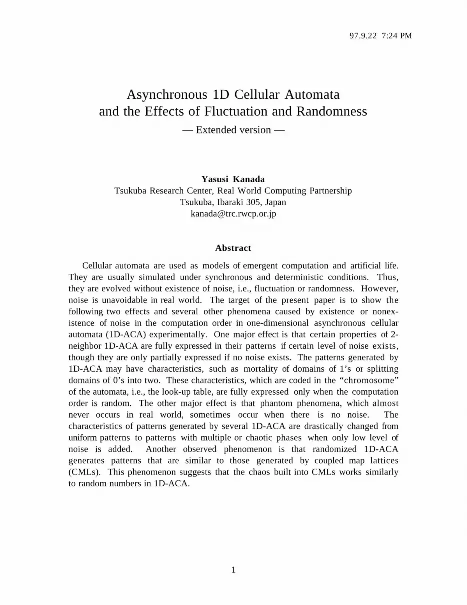
#100: There are no significant differences between both patterns, B1 and B2 (shown inFigure 5), generated by automata #100. However, the randomized automaton generateslonger transient patterns. These patterns are similar to those generated by synchronousautomata of Class II (periodic) [Wol 84].

97.9.22 7:24 PM

6

B1. Random order B2. Interlaced order


3.2 Fluctuated patterns

Patterns, which are fluctuated by randomization but whose major characteristics arepreserved, are shown and their properties, such as their life-time, are argued here. Patternsgenerated by automata #226, #146 and #22 (See [Ing 84]) are shown for example in Figure 6to Figure 11.

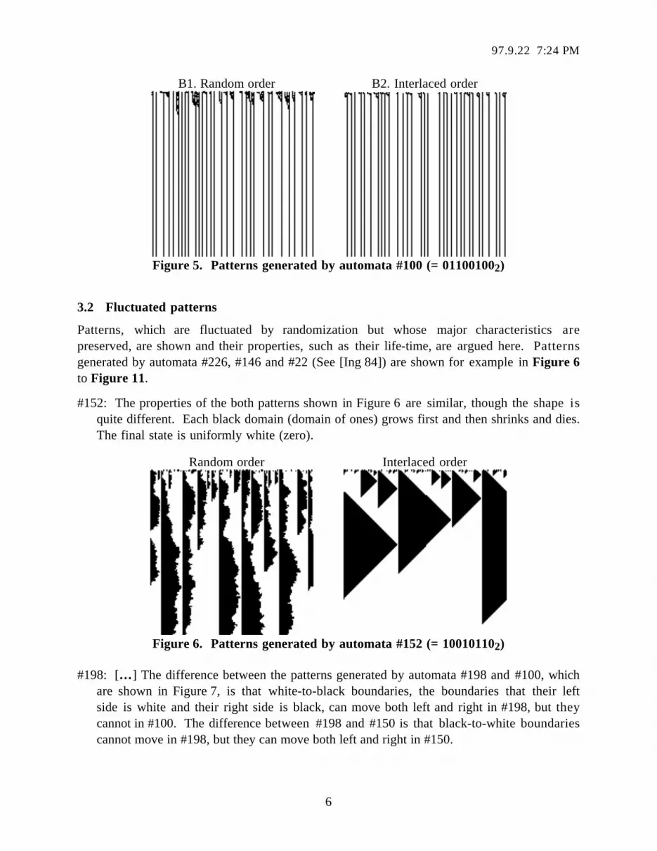
#152: The properties of the both patterns shown in Figure 6 are similar, though the shape isquite different. Each black domain (domain of ones) grows first and then shrinks and dies.The final state is uniformly white (zero).



#198: […] The difference between the patterns generated by automata #198 and #100, whichare shown in Figure 7, is that white-to-black boundaries, the boundaries that their leftside is white and their right side is black, can move both left and right in #198, but theycannot in #100. The difference between #198 and #150 is that black-to-white boundariescannot move in #198, but they can move both left and right in #150.

97.9.22 7:24 PM

7



#150: The number of black domains (and thus, the number of white domains) are invariant intime in the patterns shown in Figure 8. This is the same as in #100. However, theboundaries go left and right in #150, but it does not move in #100. The major differencebetween the random and deterministic cases are that waves go left and those go right canbe seen in latter, but they cannot be seen in former.



#226: Patterns C1 and C2, which are shown in Figure 9, are generated by automata #226.The shapes of black or white domains in pattern C1 and those in pattern C2 are quitedifferent. However, these patterns have the same characteristic. Many black domains(domain of 1’s) grow first, then shrink and die in both patterns. However, the white-to-black borders, i.e., the borders whose left side is 0 and right side is 1, move like Brownianparticles in the random case. The randomized automaton generates longer transientpatterns. The final state of the interlaced case is determined solely by the initial state (byfate), but that of the random case is determined by both the initial state and the randomnumbers.

97.9.22 7:24 PM

8

C1. Random order C2. Interlaced order


#146: Both patterns, D1 and D2 shown in Figure 10, are different in several points. First,black domains are mortal in the random case, i.e., the final state is always uniformly white(0’s). However, black domains or the slanting lines exist forever in the interlaced case,unless those move right and those move left exactly cross out each other. Second, aborder between a black domain and a white domain goes left or goes right at a constantspeed in the interlaced case, but one can move left or right freely, depending on the orderof computation, in the random case.

D1. Random order D2. Interlaced order


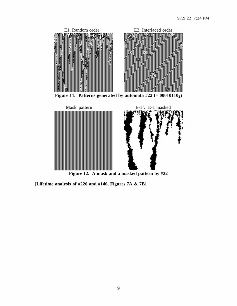
#22: Both patterns, E1 and E2 shown in Figure 11, generated by automata #22 have stripesas their background. Particles or lattice defects moving left or right can be seen in bothcases. Particles can move in both directions, such as Brownian particles, in the randomcase. This pattern is very similar to a pattern generated by a (deterministic) CML(coupled map lattice) in “diffusion of defect” phase [Kan 89]. Particles can move eitherleft or right in the interlaced case. If two particles crash, they always seem to disappearin the random case, but they often cross or reflect each other in the interlaced case.Particles can also crash and disappear in the latter case, but this type of reaction canoccur only in the early stage.

97.9.22 7:24 PM

9

E1. Random order E2. Interlaced order


Mask pattern E-1’. E-1 masked

Figure 12. A mask and a masked pattern by #22

[Lifetime analysis of #226 and #146, Figures 7A & 7B]

97.9.22 7:24 PM

10

1E+00 1E+01 1E+02 1E+03 1E+04 1E+05 1E+06

Time

1

10

100

Num

ber

of b

ound

arie

s

RandomDeterministicexp(logT^-0.49)exp(logT^-0.82)

Figure 13. Lifetime of domains in patterns generated by automata #226 (N = 256) * 1.2Average of 10 times

1E+00 1E+01 1E+02 1E+03 1E+04 1E+05 1E+06

Time

1

10

100

Num

ber

of b

ound

arie

s

RandomDeterministicexp(logT^-0.60)

Figure 14. Lifetime of domains in patterns generated by automata #146 (N = 256) * 1.2Average of 10 times

Relation to fractal dimensions (?)

97.9.22 7:24 PM

11

3.3 Merging and/or splitting patterns

Patterns, in which domains are merging and/or splitting, generated by asynchronous automataare shown here. Patterns generated by automata #166, #58 and #38 are shown for example inFigure 15 to Figure 18.

#166: The differences between the random and interlaced cases, F1 and F2 shown inFigure 15, are as follows. First, two black domains sometimes merge into one in theformer, but they do not in the latter. The final state is uniformly black (not white!) in theformer. Second, black domains move left in both cases, but the speed of this motion ismuch slower in the former. However, they never move right.

F1. Random order F2. Interlaced order


#58: The characteristics of both patterns, G1 and G2 shown in Figure 16, are completelydifferent in this case. The differences are as follows. The two points described for #146are the same for #58. Third, a black domain sometimes splits into two, and two blackdomains sometimes merge into one in the random case. Patterns generated by a randomautomaton is similar to some of those generated by synchronous automata of Class IV(complex) with more neighbors (a larger value of r) [Wol 84]. However, similar patternsare never generated in the interlaced case.

G1. Random order G2. Interlaced order

97.9.22 7:24 PM

12


#74: The both patterns shown in Figure 17 are similar to those generated by #58 automata.An important diffrence between these cases are that the borders between black and whitedomains can go left or right in #58, but they cannot go right in #74. This condition holdsboth for the random and deterministic cases.

D-1. Random order D-2. Interlaced order


#38: Patterns H1 and H2, shown in Figure 18, have similarity to those shown in Figure 15.However, pattern L1 is more complicated than pattern F1 because the black domains notonly merge but also sometimes split into two domains.

H1. Random order H2. Interlaced order


[Lifetime analysis of #166, #58 and #74]

97.9.22 7:24 PM

13

1E+00 1E+01 1E+02 1E+03 1E+04 1E+05 1E+06

Time

1

10

100

Num

ber

of b

ound

arie

s


Figure 19. Lifetime of domains in patterns generated by automata #166

1E+00 1E+01 1E+02 1E+03 1E+04 1E+05 1E+06

Time

1

10

100

Num

ber

of b

ound

arie

s



97.9.22 7:24 PM

14

1E+00 1E+01 1E+02 1E+03 1E+04 1E+05 1E+06

Time

1

10

100

Num

ber

of b

ound

arie

s



3.4 Chaotic and partially chaotic patterns

Chaotic and partially chaotic patterns generated by 1D-ACA are shown here. Some 1D-ACAgenerate chaotic patterns, some of which is very similar to patterns generated bysynchronous automata, and others are quite different from them. Patterns generated byautomata #105 and #57 are shown for example in Figure 22 to Figure 24.

#1: No structure can be seen in pattern A-1 shown in Figure 22, which is generated by therandomized automata. Thus, this is classified into chaotic patterns. However, in patternA-2 shown in Figure 22, which is generated by the deterministic automata, white particlescan be seen in dotted background. Thus, this is orderly.



97.9.22 7:24 PM

15

#105: No significant structure can be seen in pattern I1 shown in Figure 23, which isgenerated by the randomized automaton. Thus, this is classified into chaotic patterns.However, in pattern I2 shown in Figure 23, which is generated by the interlacedautomaton, waves moving to the left or right can be seen. Thus, this is orderly.

I1. Random order I2. Interlaced order


#57: The patterns generated by automata #57, which are shown in Figure 24, are morecomplex, but they are similar to those of #1. The pattern is chaotic in the random case, J1.The pattern seems to be more orderly but still chaotic in the interlaced case, J2. Thecomplex structure seen in the interlaced case and its noise-sensitivity is analyzed inSection 5.

J1. Random order J2. Interlaced order


#54: Pattern C-1 shown in Figure 25, which is generated by randomized automata #54, isless chaotic than those generated by #1 and #43. White holes can be observed in C-1.Black particles can be seen in pattern C-2 shown in Figure 25, which is generated bydeterministic automata. This structure has similarity to that in A-2, though their back-grounds are different.

97.9.22 7:24 PM

16



#60: Pattern D-1 in Figure 26, which is generated by randomized automata #60, seems tohave similarity to pattern C-1. However, pattern D-2 in Figure 26, which is generated bydeterministic automata #60, is quite different from pattern C-2. Pattern D-2 is similar tothat generated by synchronous automata classified to Class III (chaotic automata) byWolfram.



Some automata generate partially chaotic patterns, such as those shown in Figure 27 toFigure 28.

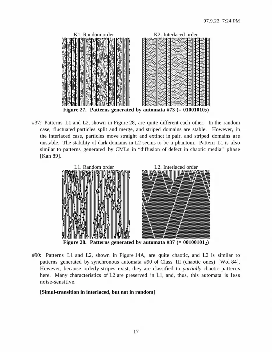
#73: The thick black stripes in patterns K1 and K2 shown in Figure 27 do not change normove. The patterns between these stripes are chaotic in the randomized case, and whiteparticles moving left or right can be seen in the interlaced case.

97.9.22 7:24 PM

17

K1. Random order K2. Interlaced order


#37: Patterns L1 and L2, shown in Figure 28, are quite different each other. In the randomcase, fluctuated particles split and merge, and striped domains are stable. However, inthe interlaced case, particles move straight and extinct in pair, and striped domains areunstable. The stability of dark domains in L2 seems to be a phantom. Pattern L1 is alsosimilar to patterns generated by CMLs in “diffusion of defect in chaotic media” phase[Kan 89].

L1. Random order L2. Interlaced order


#90: Patterns L1 and L2, shown in Figure 14A, are quite chaotic, and L2 is similar topatterns generated by synchronous automata #90 of Class III (chaotic ones) [Wol 84].However, because orderly stripes exist, they are classified to partially chaotic patternshere. Many characteristics of L2 are preserved in L1, and, thus, this automata is lessnoise-sensitive.

[Simul-transition in interlaced, but not in random]

97.9.22 7:24 PM

18

L1. Random order L2. Interlaced order


4. Interpretation of the Chromosome and Patterns

Some characteristics of the patterns shown in the previous section can be explained by thechromosomes of the automata. The chromosome, or the look-up table, contains eight genes,f0, f1, …, f7, each of which is one-bit length. These genes can be interpreted as follows.

f0: If its value is 1, white domains may split into two. Otherwise, they do not split.

f7: If its value is 0, black domains may split into two. Otherwise, they do not split.

f2: If its value is 0, black domains are mortal (may die). Otherwise, they are immortal.

f5: If its value is 1, white domains are mortal. Otherwise, they are immortal.

f1: If its value is 1, WB borders (white-to-black borders) may move left. Otherwise, they donot move left.

f6: If its value is 0, BW borders (black-to-white borders) may move right. Otherwise, theydo not move right.

f3: If its value is 0, WB borders may move right. Otherwise, they do not move right.

f4: If its value is 1, BW borders may move left. Otherwise, they do not move left.

Detailed explanations on the gene functions are omitted because of page limitations.However, the functions can be understood intuitively by Figure 30. This figure shows thecurrent state of a cell to be updated, those of the neighbor cells, and the updated state of thecell. For example, the leftmost part of the figure shows the case that all three cells are white.The next state is specified by gene f0 . If the updated state is black as shown, this is thebeginning of a black domain, and the white domain splits into two. Other parts of the figurecan be interpreted in the same way.

Several examples shown in the previous section are analyzed using the interpretationabove.

97.9.22 7:24 PM

19

Next state

f(0, 0, 0) = 1 f(1, 1, 1) = 0f(0, 1, 0) = 1 f(1, 0, 1) = 1f(1, 0, 0) = 1f(0, 1, 1) = 0

The chromosome(reversed order)

f0 f1 f2 f3 f4 f5 f6 f7

f(0, 0, 1) = 1 f(1, 1, 0) = 0

Notation: Current state

White areassplitting

B-W bordersmoving right

Black areasmortal

B-W bordersmoving left

W-B bordersmoving left

White areasmortal

W-B bordersmoving right

Black areassplitting

Leftneighbor

Rightneighbor

Figure 30. Interpretation of the chromesome

Several examples shown in the previous section are analyzed using the interpretationabove.

#226 (= 111000102): First, gene f0 is 0 and gene f7 is 1. Thus, both white and black domainsin patterns C1 and C2 do not split. Second, f2 is 0 and f5 is 1. Thus, both white and blackdomains are mortal. Actually, black domains die in C1 and C2. All the black domains dieif the random order is used. However, some black domains continue to exist if theinterlaced order is used, because gene f7 is not used for the state transitions of suchdomains. Thus, the properties of the automaton are only partially expressed when nonoise exists. Third, f1 is 1 and f3 is 0. Thus, WB borders can move in both directions.The WB borders actually move in both directions in C1. However, they move in singledirection in a period in C2. This is another example of partial expression of genes undernoise-free situations. Fourth, f6 is 1 and f4 is 0. Thus, BW borders do not move. Thisproperty is expressed both in C1 and C2.

#166 (= 101001102): f0 is 0 and f7 is 1. Thus, both white and black domains in patterns F1and F2 do not split. Both f2 and f5 are 1. Thus, black domains are immortal and whitedomains are mortal. White domains die in C1, but they continue to exist after theautomaton comes into a limit cycle in C2. This is another example of partial expression ofgenes. Expression and suppression of other genes can easily be observed.

#58 (= 001110102): Black domains can split because f0 is 0, but white domains do not splitbecause f7 is 0. Expression of gene f7 can easily be seen in G1, but this property is alsosuppressed in G2. Expression and suppression of other genes can easily beobserved.

Other patterns, such as those shown in Sections 3.1 to 3.3, can be understood in the sameway.

The above simpler relation between the look-up table values and the property of patternsexist only if the computation is sequential. Synchronous or partially synchronous automatacannot be analyzed using the above interpretation. It is much more difficult to analyze theseautomata.

97.9.22 7:24 PM

20

5. Very Noise-sensitive Patterns

Automata #105 and #57, whose example patterns have been shown in Figure 23 andFigure 24, are very sensitive to noise, though not all chaotic automata generate very noise-sensitive patterns. There are two “fluctuations” in the interlaced order with C = ( N – 1) / 2or ( N + 1) / 2 . If N = 8 and C = 3 (see Figure 2), cells 1 and 5 are “fluctuated.” In the firstscan of cells, the computations on cells 0, 3 and 6 refer to the initial values of the neighborcells, those of cells 7, 2 and 5 refer to the new values of the neighbors, and those of cells 1and 4 refer to the initial value of the right neighbor and the new value of the left neighbor.These differences in the order of computation cause no significant differences in most of 1D-ACA. However, there are significant differences in automata #105, #57 and several others.

These differences are shown in Figure 31. Figure 31 a and b show patterns generated byautomata #105 and #37 (See also Figure 23 and Figure 24). The initial state is almost black,but there are two white points. It is easy to see the two different effects caused both by thefluctuation on the order of computation and by the noise in the initial state. The former noiseworks near the left edge of the patterns and near the center (at cells 1 and 76). It is not easyto see the propagation of the latter noise in this figure. To clarify the non-local structure, thetime-scale is reduced by half in Figure 31 c and d. Figure 31 c shows the pattern generatedwhen there is no initial noise. Many domains with different textures, or locally repetitivestructures, can be seen in this figure. No such phenomena occur, if the order of computation isalternate, i.e., even cells are computed first and then odd cells are computed. Although thelong-scale pattern is periodical, the cycle is so long that it is not possible to show a wholecycle in the figure. Figure 31 d shows a pattern with a small initial noise. The propagation ofthe noise can be tracked in this figure. They refract when they go into a different domain, andsometimes cause new waves. Detailed analysis of these phenomena is a future work.

(a) #105, interlaced order, (b) #57, interlaced order,with small initial noise with small initial noise

97.9.22 7:24 PM

21

(c) #57, interlaced order, without (d) #57, interlaced order, withinitial noise, doubled time scale small initial noise, doubled time scale

97.9.22 7:24 PM

22

(e) #105, fixed random order, (f) #146, fixed random order,with initial noise with initial noise

Figure 31. Patterns generated by very noise-sensitive automata #105 and #57 (N = 152)

Figure 32. Patterns generated by very noise-sensitive automata #123 (= 100110012)

Figure 31 e shows a pattern generated by automata #57 using a fixed random order. Theinitial state is uniformly white. This pattern is chaotic and completely different from thatshown in Figure 31 b. However, the characteristics of most other patterns are not destroyedby this computation order. An example, a pattern generated by automata #146, is shown inFigure 31 f. There are no significant differences between this and pattern D2.

[Figure 32]

6. Conclusions

Two major effects caused by adding noise, i.e., randomness or fluctuation, to the order ofcomputation in 1D-ACA are shown in the present paper. One major effect is that propertiesof 1D-ACA embedded in their “chromosomes” are fully expressed in their patterns whenstronger noise exists, i.e., when the order of computation is random. However, the propertiesare only partially expressed when no noise or weaker noise exists. The other major effect isthat very fragile particles and domains, which may be regarded as phantom phenomena

97.9.22 7:24 PM

23

because they are almost never seen if noise exists, are sometimes observed in noise-lessenvironments (in Sections 3.4 and 4). The characteristics of patterns generated by several1D-ACA are drastically changed from uniform patterns to patterns with multiple or chaoticdomains even if low level of noise is added. Several other effects, such as delay of patternmotion under existence of noise, are observed. Although 1D-ACA are simpler systems, Ibelieve the results of this research contribute to research of emergent computation, such a sCCM (chemical casting model) [Kan 94], and artificial life.

One important direction of future work is to analyze the statistics, such as entropies, ofpatterns generated by 1D-ACA to support the hypotheses quantitatively. Another directionis to analyze or develop mechanisms of controlling partial expression and suppression of theproperties embedded in the chromosomes, because partial expression is the usual case inbiological life.

7. References[Ber 94] Bersini, H., and Detours, V.: Asynchrony Induces Stability in Cellular Automata

Based Models, Artificial Life IV, 382–387, MIT Press, 1994.[Hak 78] Haken, H.: Synergetics — An Introduction, Springer-Verlag GmbH & Co. KG,

1978.[Hof 87] Hofmann, M. I.: A Cellular Automaton Model Based on Cortical Physiology,

Complex Systems, 1, 187–202, 1987.[Ing 84] Ingerson, T. E., and Buvel, R. L.: Structure in Asynchronous Cellular Automata,

Physica D, Vol. 10, pp. 59–68, 1984.[Kan 89] Kaneko, K.: Pattern Dynamics in Spatiotemporal Chaos, Physica D, Vol. 34, pp. 1–

41, 1989.[Kan 94] Kanada, Y., and Hirokawa, M.: Stochastic Problem Solving by Local Computation

based on Self-organization Paradigm, 27th Hawaii International Conference onSystem Sciences, 1994.

[Kan 94b] Kanada, Y.: The Effects of Randomness in Asynchronous 1D Cellular Automata,Artificial Life IV Poster/Demo Session, 1994.

[Kau 84] Kauffman, S. A.: Emergent Properties in Random Complex Automata, Physica D,Vol. 10, pp. 145–156, 1984.

[Lan 90] Langton, C. G. et al. eds.: Artificial Life, Addison Wesley, 1989.[Lan 92] Langton, C. G. et al. eds.: Artificial Life II, Addison Wesley, 1991.[Lan 93] Langton, C. G. et al. eds.: Artificial Life III, Addison Wesley, 1993.[Lum 94] Lumer, E. D., and Nicolis, G.: Synchronous versus Asynchronous Dynamics in

Spatially Distributed Systems, Physica D, 71, 440–452, 1994.[Mat 79] Maturana, H. R., and Varela, F. J.: Autopoiesis and Cognition: The Realization of

the Living, Reidel, 1979.[Par 86] Park, J. K., Steiglitz, K., and Thurston, W.: Soliton-Like Behavior in Automata,

Physica D, 19, 423–432, 1986.

97.9.22 7:24 PM

24

[Pri 77] Nicolis, G., and Prigogine, I.: Self-organization in Nonequilibrium Systems — FromDissipative Structures to Order through Fluctuations, John Wiley & Sons, Inc.,1977.

[Vic 89] Vicsek, T.: Fractal Growth Phenomena, World Scientific, 1989.[Wol 83] Wolfram, S.: Statistical Mechanics of Cellular Automata, Reviews of Modern

Physics, 55, 601–, 1983.[Wol 84] Wolfram, S.: Universality and Complexity in Cellular Automata, Physica D,

Vol. 10, pp. 1–35, 1984.

Documents

The effects of randomness in asynchronous 1D cellular automata