Multicue HMM-UKF for Real-Time Contour Tracking

Yunqiang Chen�, Yong Rui

�and Thomas S. Huang

�

Abstract

We propose an HMM model for contour detection based on multiple visual cues in spatial domain

and improve it by joint probabilistic matching to reduce background clutter. It is further integrated with

unscented Kalman filter to exploit object dynamics in nonlinear systems for robust contour tracking.

Keywords: Parametric contour, HMM, unscented Kalman filters, joint probabilistic matching

1 Introduction

Reliable visual object tracking in complex environments is of great importance. Its applications in-

clude human computer interaction, teleconferencing, and visual surveillance, among many others. Un-

fortunately, after years of research, robust and efficient object tracking is still an open problem. Two of

the major challenges are:

1. Various visual cues have been used to discriminate objects from background clutter (e.g., object

contour [7] or color distribution [5]). However, none are robust individually. Multiple cues are

combined recently (e.g. [3]). The major difficulty, however, is how to efficiently integrate multiple

cues with spatial constraints and model the uncertainties of the detection in a principled way.�Yunqiang Chen is with Siemens Corporate Research, Princeton, NJ 08540. yunqiang.chen@siemens.com�Yong Rui is with Microsoft Research, Redmond, WA 98052. yongrui@microsoft.com�Thomas Huang is with University of Illinois at Urbana Champaign, Urbana, IL 61801. huang@ifp.uiuc.edu

2. Object dynamics is a useful constraint in temporal domain, but difficult to enforce when the states

of the object are nonlinearly related to the observations. How to effectively integrate the dynamics

with the uncertain contour detection result in a nonlinear dynamic system is critical for robust

real-time object tracking.

The Hidden Markov Model (HMM) [11] provides a potential tool to solve the first difficulty. Tradi-

tional HMM usually works in 1D time domain. In this paper, we propose a new HMM in 2D spatial

domain to detect object contour, where the contour is modeled by a parametric shape and the true con-

tour points are searched along a set of normal lines along the shape. In the new HMM, multiple visual

cues can be effectively integrated as well as various spatial constraints. Furthermore, the HMM provides

probabilistic contour detection results with confidence measurement, based on which the more confi-

dently detected contour segments contribute more and the cluttered contour segments contribute less in

the final estimation of the object states. To reduce the background clutter, we further develop an efficient

joint probabilistic matching (JPM) scheme to consider the contexture information when enforcing the

contour smoothness. More accurate spatial constraints can be enforced by the proposed HMM.

To address the second difficulty, particle filter [7, 13] and extended Kalman filter (EKF) [2] have

been proposed before. However, the particle filter requires random sampling in the state space and the

computation grows exponentially with the state space dimension. The EKF is more efficient than the

particle filter but only approximates the nonlinearity to the first order. The newly proposed unscented

Kalman filter (UKF) can approximate the nonlinearity up to the second order without explicit calculation

of the Jacobians. It provides a better alternative and is very efficient for real-time object tracking [8].

We then integrate the new HMM and the UKF seamlessly into a powerful parametric contour tracking

framework in nonlinear dynamic systems. At each time frame � , the HMM provides probabilistic contour

detection with confidence measurement, which are then passed to the UKF to estimate a more accurate

object trajectory based on the nonlinear system dynamics. Furthermore, a robust online adaptation

process is designed based on the probabilistic contour detection of the HMM to handle possible changes

of object appearance or background for long-turn tracking in non-stationary environments.

The rest of the paper is organized as follows. In Section 2, we present our HMM for contour de-

tection. In Section 3, a more accurate contour smoothness term is designed based on JPM in cluttered

environments. In Section 4, parametric contour tracking is achieved by combining the UKF with the

HMM. In Section 5, adaptive learning is further developed to handle appearance changes or dynamic

environments. Experiments and concluding remarks are given in Section 6 and 7 respectively.

2 Contour Tracking Using HMM

Active contour methods (e.g. [1, 6]) have been proposed to track nonrigid objects by efficient dynamic

programming. However, they provide only one ‘optimal’ solution with no alternatives and is not ideal for

further refinement by object dynamics. HMM, on the other hand, can utilize the forward-backward algo-

rithm ([11]) to provide probabilistic detection for each contour points, which allows further integration

with UKF (in Section 4) and the online adaptation scheme (in Section 5) for better object tracking.

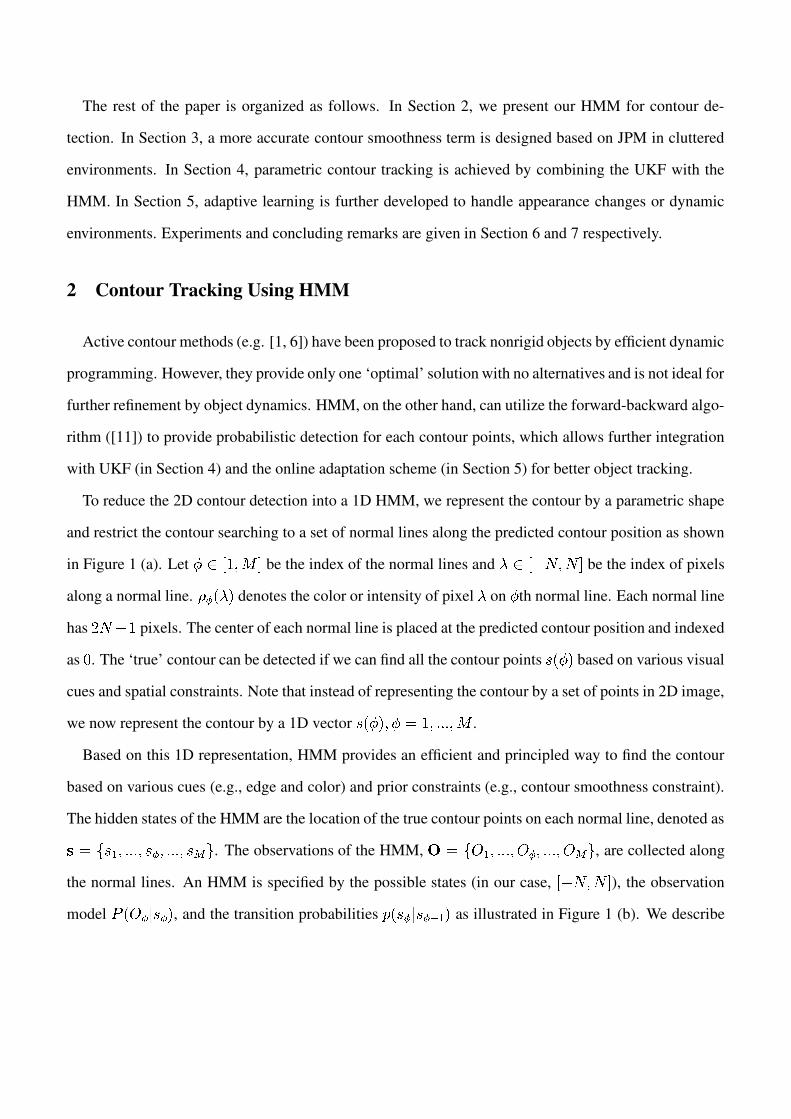
To reduce the 2D contour detection into a 1D HMM, we represent the contour by a parametric shape

and restrict the contour searching to a set of normal lines along the predicted contour position as shown

in Figure 1 (a). Let ��� ������� be the index of the normal lines and ���� ��������� be the index of pixels

along a normal line. ��� �!�#" denotes the color or intensity of pixel � on � th normal line. Each normal line

has $%�'&� pixels. The center of each normal line is placed at the predicted contour position and indexed

as ( . The ‘true’ contour can be detected if we can find all the contour points )��!�*" based on various visual

cues and spatial constraints. Note that instead of representing the contour by a set of points in 2D image,

we now represent the contour by a 1D vector )��+�,"-���/.0���2131314�5� .

Based on this 1D representation, HMM provides an efficient and principled way to find the contour

based on various cues (e.g., edge and color) and prior constraints (e.g., contour smoothness constraint).

The hidden states of the HMM are the location of the true contour points on each normal line, denoted as6 .879)9:-�2131314�5)2�;�2131314�5)=<?> . The observations of the HMM, @A.87CBD:5�2131413��BE�;�2131314��BF<G> , are collected along

the normal lines. An HMM is specified by the possible states (in our case, �����H�I� ), the observation

model J?�+BE�LKM)2�C" , and the transition probabilities NO�+)P�QKR)2�PST:U" as illustrated in Figure 1 (b). We describe

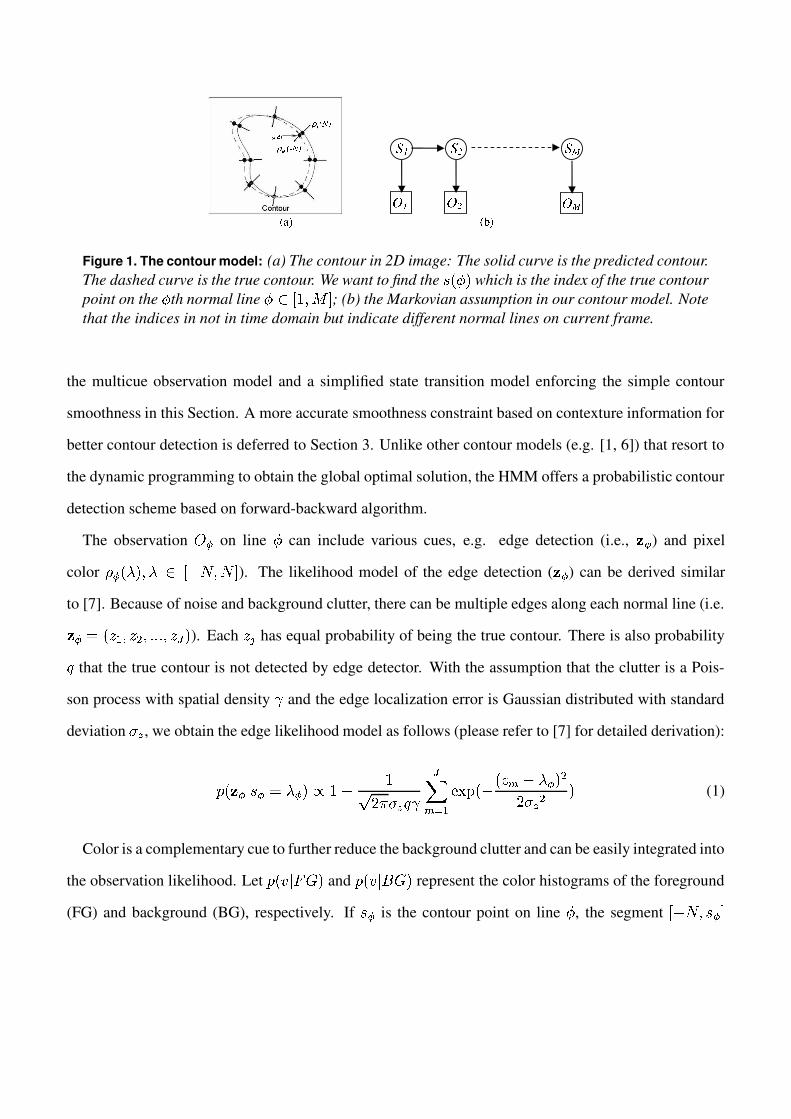
Figure 1. The contour model: (a) The contour in 2D image: The solid curve is the predicted contour.The dashed curve is the true contour. We want to find the )V�+�," which is the index of the true contourpoint on the � th normal line ��W ������� ; (b) the Markovian assumption in our contour model. Notethat the indices in not in time domain but indicate different normal lines on current frame.

the multicue observation model and a simplified state transition model enforcing the simple contour

smoothness in this Section. A more accurate smoothness constraint based on contexture information for

better contour detection is deferred to Section 3. Unlike other contour models (e.g. [1, 6]) that resort to

the dynamic programming to obtain the global optimal solution, the HMM offers a probabilistic contour

detection scheme based on forward-backward algorithm.

The observation BF� on line � can include various cues, e.g. edge detection (i.e., XY� ) and pixel

color ��� �+�*"5�5�Z�A[�\�I���I� ). The likelihood model of the edge detection ( XV� ) can be derived similar

to [7]. Because of noise and background clutter, there can be multiple edges along each normal line (i.e.X;�E.]�+^9:���^2_=�2131413��^P`�" ). Each ^5a has equal probability of being the true contour. There is also probabilityb that the true contour is not detected by edge detector. With the assumption that the clutter is a Pois-

son process with spatial density c and the edge localization error is Gaussian distributed with standard

deviation dQe , we obtain the edge likelihood model as follows (please refer to [7] for detailed derivation):

NO�fX;�TKM)2�g.h�Q�9"jiZ�k& �l $CmndTe b c`oprq :�s5t u �v� �+^ p �w�T�9" _$9dTe _ " (1)

Color is a complementary cue to further reduce the background clutter and can be easily integrated into

the observation likelihood. Let NO�yxzK {}|}" and NO�fxnK ~D|�" represent the color histograms of the foreground

(FG) and background (BG), respectively. If )C� is the contour point on line � , the segment [�\�I�5)C�P�

belongs to the foreground and the segment �)P��&����H�I� belongs to the background. Combining the edge

likelihood model and the color (i.e. x ) of the foreground and background, we can have the following

multicue observation likelihood model:

J��fBE�LKM)2�9"�.�NO�fX;�TKR)=�9"r�0�+��� q S � J��yx�.��;�Y�f��"PK {}|}"�� ��� q �f� � :J?�fxD.h�;� �f��"=KR~D|}" (2)

If more cues are available, they can be integrated similarly. As shown in Section 5, the HMM also

allows us to update the color model (i.e. NO�fxnKR{�|}" and NO�yxzK ~D|}" ) in a probabilistic way to accommodate

the lighting or object appearance changes and hence more robust in dynamic environments.

To complete the HMM model, the transition probability is discussed here to enforce the spatial con-

straint of the contour (e.g., contour smoothness). We defer a more complete smoothness constraint based

on contextual information to Section 3. To exploit the contour smoothness in the HMM, it needs to be

in a causal form. In Figure 1 (a), we can see that when the normal lines are dense (30 lines in our

experiments) and the contour is smooth, the true contour points on adjacent normal lines tend to have

similar amounts of displacement from the predicted contour position (center of each normal line). This

correlation is causal and can be captured by transition probabilities Nz�!)9�TKM)2�=ST:�" defined as follows:

NO�!)2�TKM)2�=ST:v"j.����P� ST� � � S � �5�9� �4�������� (3)

where � is a normalization constant and d � regulates the strength of the smoothness constraint. This

transition probability penalizes discontinuity of the contour and results in a smoother contour.

Given the observation @ . 7CBg���5�A��[���5���f> , the multicue based likelihood model and transi-

tion probabilities, we can obtain probabilistic contour detection results based on the efficient forward-

backward algorithm. Let  �� �!)P"\.hNz�+B}:5�2131314��BE�;��)=�?.¡)P" and ¢T� �!)P"�.hNO�+BE� � :5�2131413��BF<£�5)2��.¡)P" (please

refer to [11] for details), we have:

J?�!)2�E.¤)YK�@?"�.  O� �!)P"U¢T�Y�+)P"¥ �¦�q S �  O� �f§*"U¢T�Y�y§*" � )g�w[�\�I���I� (4)

Instead of returning one single solution as traditional active contour methods, HMM provides proba-

bilistic contour detection results, based on which we can estimate the confidence of the detected contour

points on each normal line. This information can be effectively integrated with the UKF in Section

4, where the confidently detected contour points contribute more to the object state estimation. It is

worth noting that the HMM cannot enforce the smoothness between the beginning and ending points of

a closed contour. For strict smoothness constraint on closed contour, loopy belief propagation [9] can be

used instead of forward-backward algorithm.

3 Improving Transition Probability

The transition probability in Eq. (3) only considers the contour points themselves with no contexture

information. It is especially dangerous when strong background clutter is close to the tracked contour,

e.g. the dark rectangle in Fig 2 (a). A more robust contour smoothness constraint should consider all

pixels on the neighboring normal lines jointly similar to the joint data association technique in [12]. We

propose joint probabilistic matching (JPM) of the neighboring normal lines for more accurate smooth-

ness constraint and design an efficient dynamic programming technique to calculate the matching.

Since all the pixels along the normal lines could be the true contour (edge detector might miss the

true contour), we have to track the transition between all the pixels. Let )%� and )=� � : be the true contour

points on normal line � and ��&'� , respectively. These two contour points segment the two normal lines

into foreground (FG) and background (BG) segments. If the object is opaque, the edges on FG cannot

transit to BG, which means the edges on FG/BG on line � should match to the FG/BG on line �/&0�respectively. A more accurate transition probability can be designed based on this constraint.

Let ¨}©��f�ª��« " and ¨}¬k�y�ª��«V" be the matching errors between edge points on the neighboring foreground

segments (i.e., segment [�\�I�H�+� on line � and [������«�� on line �I&Z� ) and background segments (i.e.,

segment R�n&��%���I� on line � and «g&­�%���I� on line �?&�� ), respectively. Let ®Y�y��"¯.�« be a mapping of

pixel � on line � to pixel « on line ��&�� . Then, the matching costs are defined as follows:

¨ © �f�ª��« "j.±°/�!²,³ o´�µ9¶ S �O· �¹¸ K4K �;�V�+ºL"r�W�;� � :»�f®Y�+ºL"ª"=K¼K _ � ® �!ºY"½�W ������«��¨ ¬ �y�ª��«V"j.�°/�+²,³ o´�µ9¶ � � :�· � ¸ K4K �;� �!ºL"r�¾�;� � :»�f®Y�+ºL"ª"=K¼K _ � ® �!ºL"��w «F&±�����I� (5)

A more accurate transition probability can then be defined as follows (compare with Eq. (3)):

��¿fÀ=Á,� NO�+)2_%KM)9:�"�"Â.F¨ © �!)9:-�5)2_5"n&�¨ ¬ �!)9:5��)=_�"n&��!)2_Â�w)9:ª" _5à d _� (6)

The effect of this new transition probability can be illustrated by a synthesized image in Figure 2 (a).

The dark rectangle on the background is very close to the tracked object (gray region). Along the two

normal lines shown in Figure 2 (a), two edges can be detected, i.e., ‘ Ä ’ and ‘ Å ’ on line 1 and ‘ � ’ and

‘ Æ ’ on line 2, which is distracting to the contour detection. The measurements on these two lines are

shown in Figure 2 (b). Based on the simple contour smoothness in Eq. (3), the transition from ‘ Ä ’ to ‘ � ’and from ‘ Å ’ to ‘ � ’ have almost the same transition probabilities because KRÄG�'��KÈÇÉKRů�'��K . However,

if we consider all the edges together, we can see that ‘ ÄV� ’ is not a good contour candidate because ‘ Å ’and ‘ Æ ’ are now on foreground and background respectively and they have no matching edges on the

neighboring lines. The contour candidates ‘ Ä�Æ ’ and ‘ Å5� ’ are better contour candidates. (The best choice

between these two should be further decided based on all the normal lines.)

Figure 2. JPM based smoothness constraint: (a) Synthesized image. (b) The intensity along line 1and 2. ‘ ÄV� ’ is a bad contour candidate and separates the two lines into unmatched FG and BG. (c)Without JPM, the contour is distracted by background edges. (d) With JPM, the contour is correct.

The comparison between JPM based contour smoothness and the simple contour smoothness is shown

in Figure 2 (c) and (d). Without JPM, the contour is distracted by the strong edges from the dark rectangle

in Figure 2 (c). In Figure 2 (d), correct contour is obtained by utilizing the JPM term, which has large

penalty for the contour to jump to background clutter and then jump back.

To use the JPM, we need to calculate �+$%�Ê&¤�P" _ transition probabilities for one pair of neighboring

normal lines and for each possible transition we should consider the deformable matching between two

normal lines. The computation is very expensive. We design a dynamic programming method similar to

the forward-backward algorithm by assuming the edges do not cross each other. The new method only

costs $E�V�!$%�Ë&±�P" _ to calculate the transition probabilities for all �!$%�8&��P" _ possible transitions. Given

observation on lines 1 and 2, the joint matching can be calculated in the following recursive manner:

¨ © �y�ª��«V"j.�̣ͼÎÈ�+¨ © �f�z�Ï�%��«V"n&�ÆT��¨ © �f����«}�'�P"n&�ÆT��¨ © �f�n�'����«g�'�P"�"n&����f����«V" (7)

where Æ is the penalty of shifting one pixel in the matching and ���U14�»1Ð" is the matching cost between two

pixels. ¨}©j�y�ª��«V" is the minimal matching cost between segment [�����H�f� on line 1 and segment [������«��on line 2. We start from ¨�©��v������«V"�.ɨ}©Ñ�f���2�\�Ò"�.Ó( , where �ª��«��Ô ��������� and use the above

recursion to obtain the matching cost ¨ © �f�ª��« " from �r.0�\� to � and «�.Õ�\� to � . A similar process

is used to calculate ¨ ¬ �f����«V" . After obtaining all matching costs, the more comprehensive state transition

probability can be easily computed as in Eq. (6) and plugged into the HMM in Section 2.

4 Parametric Contour Tracking by UKF

Previously, we have described the JPM-HMM model for detecting the contour using multiple cues

and spatial constraints. In the temporal domain, there is also object dynamics, based on which we can

combine the contour detection results on consecutive frames to achieve more robust tracking. Kalman

filter is a typical method for linear systems [2]. But in visual tracking systems, the object states (e.g.,

head position and orientation) usually cannot be measured directly but are nonlinearly related to the

measurements (e.g., contour points of the object). This problem can be formulated as follows.

Let Ö?×ªØ Ù and ÚQ×ªØ Ù represent the state trajectory and measurement history of a system from time ( to � .With the assumption that the state sequence is a Markov chain and the measurements are independent

given the states, tracking can be achieved by obtaining NO�yÖ�ÙHK ÖGÙÛST:-��ÚTÙf" . In our case, Ö£Ù is the parametric

shape of the head, and Ú#Ù is the detected contour on all normal lines. The two key components in

the tracking system are object dynamics (i.e. Ö?ÙD.ÝÜÑ�ÞÖ£ÙÛST:-�ª°ßÙf" ) and observation model (i.e. Ú#Ù�.à �ÞÖ£Ù��H²*Ù+" ). The terms °ßÙ and ²*Ù are process noise and measurement noise, respectively. With the

Gaussian distribution assumption, it has an analytical solution which is the well-known Kalman filter

[2]. Unfortunately, the linearity is usually not satisfied in the real world.

For tracking human’s head (see Section 6), we define the object state, system dynamics, and measure-

ments in this section. We model human’s head by an ellipse, áÔ.âã�»ä����5åC�� Â�H¢j�5æk� ç , where �f�5ä;����å»" is

the center of the ellipse,   and ¢ are the lengths of the major and minor axes of the ellipse, and æ is

the orientation of the ellipse. The object states at frame � include the shape parameters and the velocity:ÖGÙÈ.Zãá\Ù èáEÙ¼� ç . We adopt the Langevin process [14] to model the head dynamics:

éÖGÙyê ÙÛST:Â.�Ür�yÖGÙÛST:-�H°ßÙf"j.ëìí � î( Ä

ï[ðñ

ëìí á\ÙÛST:èá\ÙÛST:

ï[ðñ &

ëìí ( Å

ï[ðñ °ßÙ (8)

where Ä and Å are constants and ° is Gaussian noise �¾�+(Y�Hò�" . î is the discretization time step. The object

states cannot be measured directly but are nonlinearly related to the observed object contour. As shown in

Figure 1, we restrict the contour detection along the normal lines of the predicted object position. Based

on the probabilistic detection result in Eq. (4), the contour position on each normal line can be estimated

by )=ó� . ¥ � S � )�ô¯J?�!)2�G.¡)YKRB�" . Then, we have ÚQÙj. 6 óF.õã)=ó : �5)=ó_ �2131413�5)=ó< � ç as the measurement of the

contour position. We can also estimate the uncertainty of the measurements based on the probabilistic

detection results of the HMM so that the more confidently detected contour points contribute more to

object state trajectory estimation in the UKF. Since the UKF assumes Gaussian distributed noise (i.e. ²OÙ ),the contour detection confidence is modeled by measurement variance d _� . ¥ � S � ) _ ôöJ��+)2�F.¤)YKRB�" .

The )=� is the intersection of the ellipse áEÙ¯.÷ã��ä;����åC�� k�ª¢Â��æk� (i.e. the object states) and the normal

line � (represented by its center point ø*� �ªù%�2� and its angle ú2� ). We first perform a coordinate translation

and rotation to make the ellipse upright, centered at the origin. In the new coordinate, the normal line is

represented by the new center ( ø#û� �Hù�û� � ç ) and the angle ú9û� . )=� can be calculated as follows:

ü)2�E. à �yÖGÙU�H²*Ùy"Â.ý þ ä�ÿ��� ����� ÿ�� � & å�ÿ� ����� ÿ�� � _ � þ

���� � � ÿ�� � & ���� � � ÿ�� �

þ ä�ÿ ��� � & å�ÿ ��� � �Ï� � þ ä ÿ � � ����� ÿ�� � & å ÿ� ����� ÿ�� � þ���� � � ÿ�� � & ��� � � ÿ�� � &E²#Ù

(9)

From the above equation, we can see that the relations between the measurements and the object states

are highly nonlinear. The Unscented Kalman filter (UKF) provides a superior alternative [8] than EKF.

Rather than linearizing the system, the UKF generates sigma points (i.e. hypotheses) in the object state

space and applies the system dynamics and observation models to these sigma points. Then it uses the

weighted sigma points to estimate the posterior mean and covariance of the predicted measurements.

Compared with the EKF, the UKF does not need to explicitly calculate the Jacobians. It therefore

not only outperforms the EKF in accuracy (second-order vs. first-order approximation), but also is

computationally efficient. The UKF is implemented using the Unscented Transformation by expanding

the state space to include the noise component: ø��Ù .÷ øLçÙ °�çÙ ²#çÙ � ç . Let � � .õ�gäE&�� p &h��� be the

dimension of the expanded state space, where � p and ��� are the dimensions of noise °/Ù and ²*Ù , and letò and � be the covariance of noise °�Ù and ²*Ù . The UKF can be summarized as follows (refer to [8]):

1. Initialization: éø �× .] éÖ ç× ( ( � ç and J �× .Z JO×Éò � �2. Iterate for each time instance � :

(a) Generate $9� � &�� scaled symmetric sigma points based on the state mean and variance;

(b) Pass all the generated sigma points through the system dynamics in Eq. (8) and observation

model in Eq. (9). Compute the mean and covariance of the predicted object stateséÖ Ùyê ÙÛST: and

predicted contour positionéÚQÙyê ÙÛST: using the weighted sigma points;

(c) Calculate the innovation Ú#ÙT� éÚQÙyê ÙÛST: based on the measurement Ú#Ùn. �)=ó : �5)=ó_ �»141314��)Pó< � ç and the

variance of the measurement on current frame (obtained by the JPM-HMM in Sections 2 and

3). Update the mean and covariance of the states (i.e. J�������� , J������� ) and the Kalman gain� ÙÈ.�J�� � � � J ST:������ based on the sigma points and get the final estimation;

With respect to the computational cost, UKF is better than the EKF in our case. Remember that we

use ellipse to model the object and Langevin process to model the dynamics and use 30 normal lines to

detect the contour (i.e. �}ä�.]$�� ��. �2( , � p .!� and ����.]� .#"�( ). To calculate Jacobian matrix

for EKF, we need to compute $ ü)P� à $Lø � for ���� �%�5��� and �Ñ.0���2131413����ä (i.e. ��ä%� � . �2(Eô&"�( terms).

For UKF, it is very straight forward and only need to propagate $'���U�=(j& ��&("�(;"Y&w�ö.*)Y� sigma points

through the Eq (8) and Eqs (9), which is much easier than calculating $ ü)9� Ã $Lø � . The UKF is also much

more efficient than the particle filter because the number of the sigma points increases linearly with the

number of dimension.

5 Online Adaptation

In a dynamic environment, both the objects and background may gradually change their appearances.

An online adaptation is therefore necessary to update the observation likelihood models dynamically.

However, adaptation might be adversely affected by tracking inaccuracy or partial occlusion. Fortu-

nately, the probabilistic detection results from HMM (i.e. J?�!)C��. )LKã@?" ) in Eq. (4) allows us to update

the observation models based on the tracking confidence on each normal line.

Based on the probabilistic detection results, the probability of pixel �,� belonging to the foreground

object can be computed by integration: J?�!�#��� {}|}". ¥ � q �� q,+ � Nz�!)2�Ï. )YK�@?" (i.e. sum of all the

probabilities that the true contour point on line � is outside of pixel �,� ). Based on this, we can weight

the importance of each pixel when updating the color histograms of the foreground and background. In

this way, the more confidently classified pixels will contribute more to the color model.

The adaptation makes the tracking system much more robust to the error caused by rough initialization

or the changing lighting or appearance. Since the color close to the contour is more important than the

color in the middle in helping us locate the contour, we use the pixels on the normal lines to update the

color model. It is then plugged back into Eq. (2) during the contour searching on the next frame.

6 Experiments

To validate the robustness of the proposed framework, we apply it in various real-world video se-

quences captured by a pan/tilt/zoom video camera in a typical office environment. The sequences simu-

late various tracking conditions, including appearance changes, quick movement, out-of-plane rotation,

shape deformation, background clutter, camera pan/tilt/zoom, and partial occlusion. In the experiments,

we use the parametric ellipse áFÙö. M�5ä;�H�5åC�� Â�H¢j�5æk� to model human heads and we adopt the Langevin

process as the object dynamics, as discussed in Section 4. For all the testing sequences, we use the

same algorithm configuration, e.g., object dynamics, state transition probability calculation. For each

ellipse, 30 normal lines are used, i.e., � .-"�( . Each line has 21 observation locations, i.e., � .Ô�=( .

The tracking algorithm is implemented in C++ on Windows XP platform. No attempt is made on code

optimization and the current system can run at 60 frames/sec comfortably on a standard Dell PIII 1G

machine. It is worth noting that we derive the HMM-UKF tracking framework based on ellipse. But it

can be extended to other parametric contour if a corresponding observation model can be derived. Three

set of comparisons are conducted to demonstrate the strength of the new method.

6.1 Multiple cues vs. single cue

First, we compare our tracker with the CAMSHIFT algorithm [4], which tracks ellipsoid objects

based on color histogram. In both algorithms, H and S channels in the HSV color space are used and

each color has 32 bins. Two sequences (i.e. Seq A and Seq B, captured at 30 frames/sec) are tested.

While CAMSHIFT is one of the best single cue trackers, it loses track when the user rotates her head

or when other objects of similar color (e.g. the door, the cardboard box or other faces) are close to the

tracked face. The result of CAMSHIFT tracker is shown in the top row compared with our method on

the bottom row in Fig. 3.

The CAMSHIFT tracker is quite robust when the object color remains the same and there is no sim-

ilar color in the background. But it is easily distracted when patches of similar color appear in the

background near the target because it ignores contour information and object dynamics. Also, there is

Figure 3. CAMSHIFT vs. JPM HMM Figure 4. Plain HMM (top) vs. JPM-HMM (bottom)

no principled way to update the color histogram of the object. When the person turns her head and the

face is not visible (Seq A, Frame 187), CAMSHIFT tracker loses track.

On the other hand, the proposed HMM probabilistically integrates multiple cues into the HMM model

and successfully tracks the user through the sequence. It is worth noting that some other algorithms can

also track the object in the sequence by fusing color and edge together, but require potentially more

difficult initialization (e.g. a side view of the head including both skin and hair is needed to train a color

model in [3]). In our algorithm, both foreground and background color histograms are probabilistically

updated during tracking by the HMM. It only requires a rough initialization (e.g. an automatic face

detector) and can effectively handles initialization error or object appearance change due to head rotation.

6.2 JPM-HMM vs. plain HMM

As we have described in Section 3, the traditional contour smoothness constraint only takes into ac-

count the contour points but ignores all other edge points. This can be dangerous in a cluttered environ-

ment. To show the strength of this JPM energy term, we compare the JPM-HMM (using the improved

transition probability proposed in Eq. (6)) against the plain HMM model (using the traditional contour

smoothness constraint in Eq. (3)).

The comparisons on sequence A and B are shown in Figure 4, where the top row is the result from

the plain HMM and the bottom row is the result from the JPM-HMM. In the plain HMM, tracking

is gradually distracted by the strong edges on the background clutter nearby. Because JPM tracks the

contour points more accurately when estimating the contour smoothness by considering all edges jointly,

the JPM-HMM is much more robust against sharp edges on the background.

6.3 UKF vs. Kalman Filter

In this subsection, we evaluate HMM-UKF’s ability to handle large distractions, e.g., partial occlu-

sions, on Sequence C, which has 225 frames captured at 30 frames/second (see Figure 5). Note that the

observation model in Eq. (9) of the tracking system is highly nonlinear. It is therefore quite difficult to

calculate the Jacobians as required by the EKF. An ad hoc method to get around this situation is not to

model the nonlinearity explicitly. For example, one can first obtain the best contour positions and then

use least-mean-square (LMS) to fit a parametric ellipse followed by a Kalman filter. Although simple

to implement, it does not take full advantage of the object dynamics. The UKF, on the other hand, not

only exploits system dynamics in Eq. (8) and observation model in Eq. (9), but also avoids computing

the complicated Jacobians. The comparison between the UKF and Kalman filter is shown in Figure 5.

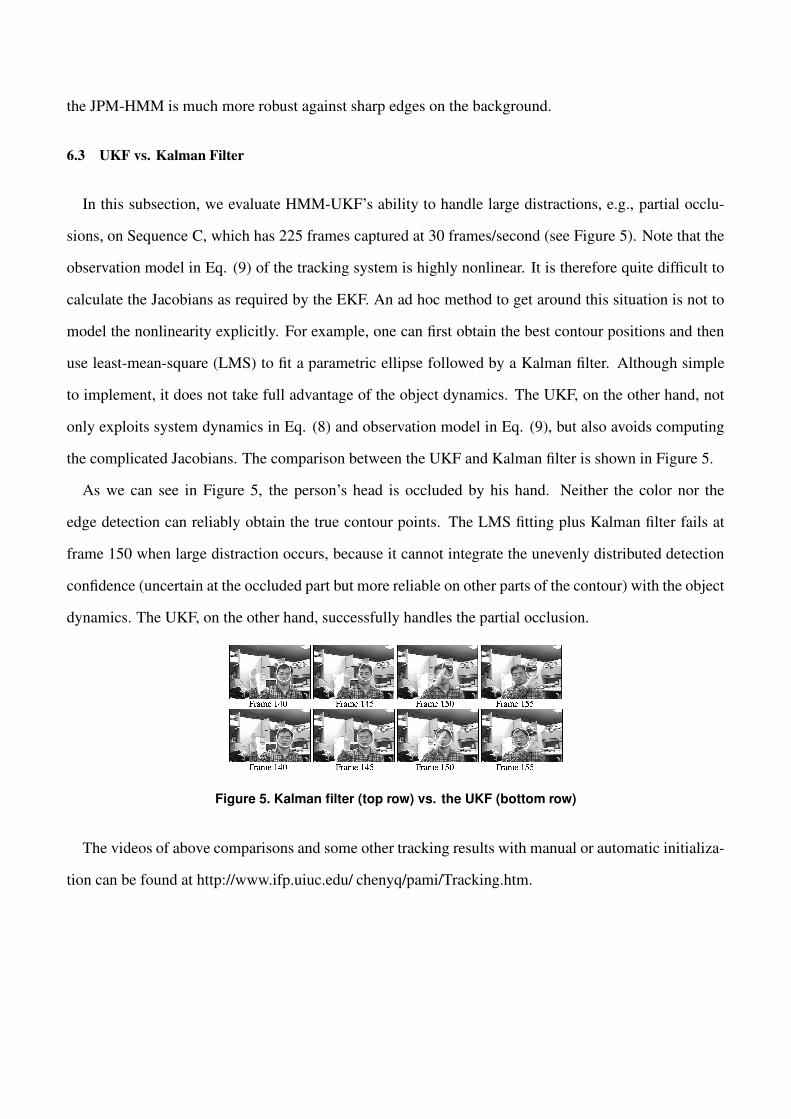
As we can see in Figure 5, the person’s head is occluded by his hand. Neither the color nor the

edge detection can reliably obtain the true contour points. The LMS fitting plus Kalman filter fails at

frame 150 when large distraction occurs, because it cannot integrate the unevenly distributed detection

confidence (uncertain at the occluded part but more reliable on other parts of the contour) with the object

dynamics. The UKF, on the other hand, successfully handles the partial occlusion.

Figure 5. Kalman filter (top row) vs. the UKF (bottom row)

The videos of above comparisons and some other tracking results with manual or automatic initializa-

tion can be found at http://www.ifp.uiuc.edu/ chenyq/pami/Tracking.htm.

7 Conclusion

In this paper, we propose a new HMM-UKF framework for real-time multicue object tracking. Several

important features distinguish the proposed HMM-UKF from other approaches: (1) Integrating multiple

visual cues in a principled probabilistic way; (2) Better contour smoothness constraint based on joint

probabilistic matching; (3) Exploiting object dynamics in nonlinear systems; (4) Online adaptation al-

lowing rough initialization and robustness to lighting/appearance changes. As further improvement, we

are investigating multiple hypothesis tracking based on the proposed algorithm. Also, verification step

based on the prior knowledge of the object is necessary to automatically evaluate the tracking perfor-

mance.

References

[1] A. Amini, T. Weymouth, and R. Jain. Using dynamic programming for solving variational problems in

vision. IEEE Trans. Pattern Anal. Machine Intell., 12(9):855–867, September 1990.

[2] B. Anderson and J. Moore. Optimal Filtering. Englewood Cliffs, NJ: Prentice-Hall, 1979.

[3] S. Birchfield. Elliptical head tracking using intensity gradients and color histograms. In Proc. IEEE Int’l

Conf. on Comput. Vis. and Patt. Recog., pages 232–237, 1998.

[4] G. R. Bradski. Computer video face tracking for use in a perceptual user interface. Intel Technology Journal,

Q2, 1998.

[5] D. Comaniciu, V. Ramesh, and P. Meer. Real-time tracking of non-rigid objects using mean shift. In Proc.

IEEE Int’l Conf. on Comput. Vis. and Patt. Recog., pages II 142–149, 2000.

[6] D. Geiger, A. Gupta, L. Costa, and J. Vlontzos. Dynamic-programming for detecting, tracking, and matching

deformable contours. IEEE Trans. Pattern Anal. Machine Intell., 17(3):294–302, 1995.

[7] M. Isard and A. Blake. CONDENSATION - conditional density propagation for visual tracking. Int. J.

Computer Vision, 29(1):5–28, 1998.

[8] S. Julier and J. Uhlmann. Unscented filtering and nonlinear estimation. Proceeding of the IEEE, 92(3):401–

422, 2004.

[9] M. K., W. Y., and J. M. Loopy belief propagation for approximate inference: an empirical study. In Proc. of

the 15th Conf. on Uncertainty in Artificial Intelligence, 1999.

[10] J. Lafferty, A. McCallum, and F. Pereira. Conditional random fields: Probabilistic models for segmenting

and labeling sequence data. In Int. Conf. on Machine Learning, 2001.

[11] L. R. Rabiner and B. H. Juang. An introduction to hidden Markov models. IEEE Trans. Acoust., Speech,

Signal Processing, 3(1):4–15, January 1986.

[12] C. Rasmussen and G. Hager. Joint probabilistic techniques for tracking multi-part objects. In Proc. IEEE

Int’l Conf. on Comput. Vis. and Patt. Recog., pages 16–21, 1998.

[13] J. Sullivan, A. Blake, M. Isard, and J. MacCormick. Bayesian object localisation in images. Int. J. Computer

Vision, 44(2):111–135, 2001.

[14] J. Vermaak and A. Blake. Nonlinear filtering for speaker tracking in noisy and reverberant environments. In

Proc. IEEE Int’l Conf. Acoustic Speech Signal Processing, pages V:3021–3024, 2001.