Embed Size (px)
Citation preview
Physica A xx (xxxx) xxx–xxx
Contents lists available at ScienceDirect
Physica A
journal homepage: www.elsevier.com/locate/physa
Multidimensional aspects of nonlinear electromagneticsolitary pulses
Q1 A. Bonatto a,b,∗, R.P. Nunes c, C. Bonatto d, R. Pakter a, S.R. Lopes b, F.B. Rizzato a
a Instituto de Física, Universidade Federal do Rio Grande do Sul, Caixa Postal 15051, 91501-970 Porto Alegre, RS, Brazilb Departamento de Física, Universidade Federal do Paraná, 81531-990 Curitiba, PR, Brazilc Departamento de Engenharia Elétrica, Universidade Federal do Rio Grande do Sul, Campus Central, 90035-190 Porto Alegre, RS, Brazild Departamento de Física, Universidade Federal de Pelotas, Campus Capão do Leão, Caixa Postal 354, 96010-900 Pelotas, RS, Brazil
h i g h l i g h t s
• A study of EM pulses and space-charge waves in laser-plasmas settings is presented.• The role of transverse effects on trains of EM pulses in plasmas is studied.• Space-charge modes are studied in resonant and nonresonant regimes.• Estimates allow to predict how far can trains of pulses propagate before distortion.
a r t i c l e i n f o
Article history:Received 21 February 2014Available online xxxx
Keywords:SolitonsLaser-plasmaSpace-chargeNonlinear
a b s t r a c t
Thiswork is devoted to the study of the interaction between pulses of electromagnetic radi-ation and space-chargewaves in laser-plasmas settings.We analysemodes depending onlyon the co-moving coordinate of the beam frame, but make no a priori assumption on thelongitudinal-to-transverse aspect ratio of the pulses. The model thus constructed allowsus to investigate regimes where transverse and longitudinal length scales of the pulses arecomparable. Resonant and nonresonant excitations of space-charge modes are analyzedand the endurance of trains of solitons against transverse effects is clarified.
© 2014 Elsevier B.V. All rights reserved.
1. Introduction 1
Formation and propagation of solitary pulses have been drawing attention over the years in a variety of areas involved 2
with statistical and nonlinear physics. Solitary pulses appear indeed in systems as distinct as statistical Toda lattices [1] or 3
laser-plasma settings [2], for instance. The key ingredient is the presence of the correct nonlinearities capable of entrapping 4
free energy into tightly localized structures. 5
Under certain circumstances, solitary waves are weakly interacting among themselves. This fact allows to describe the 6
corresponding nonlinear system as a gas of freely moving quasiparticles whose role is played by the solitary structures 7
themselves [3]. This is the case of integrable systems, where the solitary structures aremore precisely referred to as solitons. 8
Of course, not always one deals with integrable systems. A very typical behavior in nonintegrable cases is the following. One 9
starts off with extended modes which self-modulates into solitary modes. The solitary modes survive as such for a while, 10
∗ Corresponding author at: Departamento de Física, Universidade Federal do Paraná, 81531-990 Curitiba, PR, Brazil. Tel.: +55 15106465318.E-mail addresses: [email protected], [email protected] (A. Bonatto), [email protected] (R.P. Nunes), [email protected]
(C. Bonatto), [email protected] (R. Pakter), [email protected] (S.R. Lopes), [email protected] (F.B. Rizzato).
http://dx.doi.org/10.1016/j.physa.2014.02.0650378-4371/© 2014 Elsevier B.V. All rights reserved.

2 A. Bonatto et al. / Physica A xx (xxxx) xxx–xxx
but are eventually annihilated due to the presence of the nonintegrable terms of the governing nonlinear equations. It is1
therefore of interest to investigate how long can a solitary mode survive in a general nonintegrable environment.2
In addition to the aforementioned question on the endurance against nonintegrable effects, the propagation of localized3
radiation pulses in plasmas is of extreme technological interest. Among several examples, one can cite nonlinear wave4
excitation [2,4], particle and photon acceleration [5–9], and laser fusion [10], to mention but a few exemplifying cases.5
In the present paper we thus focus our efforts to investigate the case of solitary modes in a laser plasma nonintegrable6
system.7
Asmentioned earlier, pulses are formed as large amplitude electromagnetic waves self-modulate in the plasma, breaking8
up into a series localized lumps. This is a typical behavior seen in strong soliton turbulence [11] and in self-modulated laser9
accelerators [12].10
As the pulses move into the plasma, the associated ponderomotive potential creates charge displacement, which results11
in the generation of space-charge fields. The full dynamics is therefore defined by the self-consistent interaction of electro-12
magnetic and space-charge waves, with further account of the relativistic mass variations of particles. As opposed to sim-13
pler equations as the Nonlinear Schrödinger Equation, for instance, the full dynamics cannot be shown to be integrable [13],14
which remits to our original intention of studying nonintegrable effects on solitary modes.15
The one dimensional (1D) solitary dynamics in laser plasma systems has been investigated in co-moving frames, where16
fields depend solely on combined coordinates of the type ξ ≡ vg t − x. Here, x denotes the propagation axis, t the time,17
and vg the pulse velocity [14,15]. The simple dependence of the electromagnetic and space-charge fields on the co-moving18
coordinate ξ allows to look at the system as two-degrees-of-freedom system, amenable therefore to the use of nonlinear19
dynamics tools. Analysis in the co-moving beam frame is of particular relevance for propagation over large distances since,20
after initial transients, the radiation beams are attracted towards these co-moving regimes [16]. This is what happens with21
relativistic laser pulses injected in plasmas. After a self-modulational transient stage, the injected pulses typically decay into22
trains of solitons which can be described with help of the co-moving coordinates.23
Full solutions to 1D co-moving models indicate the presence of solitary pulses [4,10], whose underlying nonlinear dy-24
namics and bifurcation sequences have been further exploredmore recently [17]. In particular one observes that resonantly25
excited space-charge waves, which arise when the pulse sizes equal the plasmawavelength, are responsible for introducing26
nonintegrable features in the system. On the other hand, in nonresonant regimes the system remains integrable. Space-27
charge-like potentials have a similar role in the closely related subject of the Ginzburg–Landau equations. The overall dy-28
namics has been shown to largely differ depending on whether the potentials are resonantly excited [18], or noresonantly29
excited [19].30
In 1D models the transverse coordinates are completely neglected. Several papers analyze the opposite, paraxial limit,31
where transverse effects dominate the dynamics. The approach is appropriate to study very long pulses for which the32
transverse extension is much smaller than the extension along the propagation axis. This is particularly suitable to study33
the process of self-focusing of laser beams with smooth longitudinal modulations [20].34
There are several occasions, however, where the transverse and longitudinal sizes of a laser beam are similar [21,22].35
When this happens, both effects (longitudinal and transverse) should be treated on the same footing in order to evaluate36
the laser-plasma dynamics accurately.37
In thisworkwe analyze the nonlinear coupleddynamics of electromagnetic and space-chargewaves in a plasma, avoiding38
the use of 1D models and paraxial approximations [20,23]. We accompany the dynamics after transients have damped out,39
when fields can be described as functions of co-moving coordinates along the propagation axis. On the other hand, full40
effects of transverse derivatives in both the equations for the space-charge and laser fields shall be kept. Our objective is to41
determine how a train of solitons – usually formed when a pulse injected breaks up due to self-modulation effects [24] – is42
affected by the transverse structure. In order to examine the problem we develop a simple way to estimate the magnitude43
and characteristic time scales of transverse effects, which compares well with simulations.44
The paper is organized as it follows. In Section 2 we present the model, discuss its geometrical settings and review some45
analytical results. In Section 3 we investigate the model in several instances, examining the roles of plasma wave excitation46
and of the transverse structure of the fields. Estimates are made and compared with simulations. In Section 4 we draw our47
conclusions.48
2. The model49
In this section, for the comfort of the reader, we derive the model used to investigate our physical system. Although50
(besides minor changes) we have used this model in a previous work [25], it is important to emphasize that we are now51
dealing with very different initial conditions: while previously we had a laser beam, distributed along the direction of its52
propagation, now we start from a sequence of solitons.53
2.1. Governing equations in the weakly nonlinear approximation54
In thisworkwedescribe theplasmaas consisting of amobile cold electronic fluid in a neutralizing, fixed ionic background,55
and the laser field by the associated vector potential A in the form of a slowly modulated high-frequency carrier of wave56

A. Bonatto et al. / Physica A xx (xxxx) xxx–xxx 3
vector k0 and frequency ω0: 1
A = ea(x⊥, vg t − x)ei(ω0t−k0x) + c.c. (1) 2
We adopt circular polarization with the polarization vector given by e = (y + iz)/√2, and introduce the variable a as 3
the slowly varying real amplitude. Following the previous comments on the field structure, in addition to the co-moving 4
coordinate ξ ≡ vg t − x we allow for the presence of the transverse structure, represented by the transverse coordinate x⊥ 5
in the argument of the scalar amplitude a. The interdependence of the carrier’s frequency and wave vector, with the group 6
velocity vg , shall be elucidated as soon as one solves the wave equation for the vector potential A. 7
As the frequency of the carrier is always higher than the frequency of modulation, there are two distinct scales in the 8
evolution of our system: a fast one, associatedwith the jitter of the electrons in response to the high frequency laser field, and 9
a slow one, associated with the wake that follows the laser pulse in response to its low frequency ponderomotive potential. 10
The fast dynamics can be described by the laser wave equation in the Coulomb gauge, which (neglecting the low- 11
frequency terms) reads as follows: 12
1c2
∂2A∂t2
− ∇2A = µ0j, (2) 13
where µ0 is the magnetic vacuum permeability and j is the high-frequency current, which can be written in terms of the 14
electron density n, mass m, charge q and relativistic factor γ as j = −(q2/m) nA/γ [26]. Then, from Eq. (2) one can write 15
the governing equation for the weakly relativistic amplitude a in the form 16
− (k20 − ω20 + 1)a − 2i(ω0vg − k0)
∂a∂ξ
− (v2g − 1)
∂2a∂ξ 2
+ ∇2⊥a =
n −
a2
2
a. (3) 17
We point out that in Eq. (3) we have migrated to dimensionless quantities defined in the form ωpx/c → x, ωpx⊥/c → x⊥, 18
ωpt → t, qa/√2mc2 → a, vg/c → vg , and (n − n0)/n0 → n. The parameter n0 is the equilibrium density, ωp = n0q2/ϵ0m 19
denotes the plasma frequency and ϵ0 is the electric vacuum permeability. We note that the frequency and the wave vector 20
of the carrier are normalized accordingly, and that the weakly nonlinear (or weakly relativistic) field magnitudes satisfy the 21
condition |a| ≪ 1. 22
On the right-hand-side of Eq. (3) the nonlinear features of the theory can be devised: the ponderomotive nonlinearity, 23
represented by the coupling involving density and vector potential, and the cubic relativistic nonlinearity, which has its 24
origins in the weakly relativistic expansion of the relativistic factor γ . 25
One can advance with the analysis, as one recalls that a is real. Then, if one separates Eq. (3) into its real and imaginary 26
parts, the following expressions are obtained: 27
−δa + κ∂2a∂ξ 2
+ ∇2⊥a =
n −
a2
2
a, (4) 28
vg =k0ω0
, (5) 29
with κ ≡ 1 − v2g as the coefficient of the nonparaxial term involving the second derivative with respect to the co-moving 30
coordinate ξ . The detuning parameter, introduced as δ ≡ k20 − ω20 + 1, is thus seen to be part of a nonlinear equation. As we 31
shall elaborate better in the coming sections, this indicates that wave frequency and wave vector are related through a non- 32
linear dispersion relation, and that vg is thus a nonlinear group velocity. The nonparaxial term is occasionally neglected for 33
smooth modulations along the propagation axis. Following previous comments, it will be fully kept in the present analysis, 34
since we are precisely interested on sharp solitary structure along that axis. In what follows, we consider ω0 > 0, k0 > 0, 35
and thus vg > 0. 36
As for the low-frequency density fluctuations, we start from the ponderomotive-driven low-frequencymomentumequa- 37
tion for the electrons. Using the Lorentz force in Newton’s second law, expressing the electric and magnetic fields as func- 38
tions of the scalar and vector potentials and considering the relation between the fast component of the momentum and 39
the vector potential [26], we can write the following equation: 40
∂p∂t
= e∇φ −1
2mγ∇a2, (6) 41
where the nonlinear terms related to the low frequencies are absent, since they have a higher order in the laser potential. 42
Here, φ is the electrostatic potential. If one takes the divergence of (6), the first term of its right-hand side becomes the 43
Laplacian of the electrostatic potential, ∇2φ, which can be rewritten as a function of the electron density perturbation n 44
using the Poisson equation. After that, one can use the continuity equation to obtain the following governing equation (for 45
a weakly nonlinear regime and under the same set of normalizations previously employed): 46
v2g∂2n∂ξ 2
+ n =12
∂a2
∂ξ 2+
12∇
2⊥a2. (7) 47
For convenience we split the derivatives of the ponderomotive term on the right-hand-side into longitudinal and perpen- 48
dicular components. 49

4 A. Bonatto et al. / Physica A xx (xxxx) xxx–xxx
We now proceed to reduce Eqs. (4) and (7) into simpler and more amenable forms for numerical and analytical investi-1
gations, avoiding underdense approximations where the velocity of the laser pulse is approximated by the speed of light.Q22
Eq. (7) suggests a convenient combination of fields a2 and n into a new quantity ϕ ≡ v2gn − a2/2, which we call the3
space-charge potential. Accordingly, regrouping of terms in Eqs. (3) and (5) so as to replace v2gn − a2/2 with ϕ, yields the4
following coupled equations for the laser field and for the space-charge potential, respectively:5
κ∂2a∂ξ 2
= δa +1v2gϕ a +
κ
2v2ga3 − ∇
2⊥a, (8)6
∂2ϕ
∂ξ 2+
1v2gϕ = −
12v2
ga2 +
12∇
2⊥a2. (9)7
The pair of Eqs. (8) and (9) is cast into the convenient format wewere looking for. If the transverse structure is neglected,8
the set becomes similar to models analyzed in the past [15]. Under this planar condition one can think of Eqs. (8) and (9)9
as describing the coupled nonlinear dynamics of fields a and ϕ as a function of the co-moving coordinate ξ , which plays10
the role of time. With the transverse structure included, the set of Eqs. (8)–(9) describes the weakly nonlinear, spatio-11
temporal interaction of laser and space-charge field. Coordinate ξ can still be seen as time, and space is associated with12
the transverse structure itself. We also point out that, in the present regime where fields depend on time through the co-13
moving coordinates, the presence of the nonparaxial derivative with respect to ξ in Eq. (8) is responsible for advancing the14
laser field in the real time t as well.15
2.2. Beam geometry, boundary conditions and initial conditions16
We first of all observe that due to the transverse terms, solutions to the nonlinear equations Eqs. (8) and (9) depend on the17
geometry of the beam. In the present investigation we adopt the use of a slab geometry where the system is uniform along18
one transverse Cartesian axis, say x, and is localized along the other one which we call x⊥. This option avoids issues related19
to the inherent singularities at the axis of a cylindrical beam, but is nevertheless qualitatively similar to the cylindrical case20
if one looks at the half space x⊥ ≥ 0, provided that the beam is symmetrical with respect to x⊥ = 021
In summary, we require that all fields are even functions of the transverse coordinate x⊥, vanishing as |x⊥| → ∞.22
With the geometry and boundary conditions thus defined, we can introduce the initial conditions based on the fact23
that the front end of the soliton train is a region not yet perturbed by the passage of the electromagnetic pulses. We shall24
therefore require vanishing small fields at the front end, whichwe place at ξ = 0. On the grounds of causality, the physically25
meaningful region lies behind the front end, where ξ > 0.26
In more specific terms, we shall take for the initial laser field27
a(0, x⊥) = a0e−λx2⊥ (10)28
and∂a∂ξ
ξ=0
= 0, (11)29
and for the initial space-charge field30
ϕ(0, x⊥) = −a(0, x⊥)2/2 (12)31
and∂ϕ
∂ξ
ξ=0
= 0. (13)32
The initially null derivative of both fields puts in effect the idea that, at the front end, fields are slowly rising due to the33
approaching wave train. Condition (12), on its turn, expresses the fact that during this initial stage where derivatives with34
respect to ξ are small, ϕ becomes adiabatically enslaved to a2, as can be seen from Eq. (9) when ∂2ϕ/∂ξ 2≈ 0.35
Aswe examine the set (8)–(13)we first recall that, while in the longitudinal direction the pulse formation has a time scale36
given by (δ/κ)−1/2, the growth of transverse effects is given by (λ/κ)−1/2. Comparing both time scales we can see that the37
relativemagnitudes of δ andλ dictatewhether or not pulses can be observed: if δ ≫ λ, theywill be formed before transverse38
effects become appreciable; otherwise, if δ ≪ λ, the transverse term will be subjected to a instability and a ∼ eλξ2/κ as39
shown in a previous work [25].40
The task ahead is basically to make use of the initial condition at the wave front end, and integrate the pair of Eqs. (8)41
and (9) investigating the dynamics for ξ > 0. We shall proceed along this line, exploring the characteristics of the nonlinear42
system in order to derive relatively accurate estimates on its behavior.43
3. Evolution of the train of pulses44
Asmentioned, the task now is to see how the electromagnetic pulses evolve as theymove into the plasma. Ifwe temporar-45
ily neglect the transverse terms, our dynamics can be divided into nonresonant regimes, where the adiabatic approximation
A. Bonatto et al. / Physica A xx (xxxx) xxx–xxx 5
remains always valid and pulses evolve keeping their shapes, and resonant ones, where this approximation is broken and 1
waves are excited in the plasma. In nonresonant regimes, pulses are strongly distorted and destroyed even without the 2
transverse effects. 3
Our program, therefore, will proceed as follows. We first neglect the transverse derivatives and examine the transition 4
from nonresonant to resonant regimes. With the results obtained this way, we shall produce estimates on the critical 5
magnitude of the transverse term beyond which it can no longer be neglected from the dynamics. 6
The transition from nonresonant to resonant regimes is thus studied as we neglect the transverse derivatives, ∇2⊥a 7
and ∇2⊥a2, in Eqs. (8) and (9) respectively. Under this circumstance, the wave system converts into a low-dimensional 8
conservative system with two degrees of freedom, which can be obtained from the following Hamilton function 9
H =P2a
2κ−
P2ϕ
2−
δa2
2−
κa4
8v2g
−a2ϕ2v2
g−
ϕ2
2v2g, (14) 10
where the variables Pa and Pϕ are the canonical momenta respectively associated with fields a and ϕ. As in our model the 11
co-moving coordinate ξ plays the role of time, the canonical equations can be written as 12
∂a/∂ξ = ∂H/∂Pa, −∂Pa/∂ξ = ∂H/∂a, 13
∂ϕ/∂ξ = ∂H/∂Pϕ, −∂Pϕ/∂ξ = ∂H/∂ϕ. 14
As expected, using the canonical equations one can recover the original forms embodied by Eqs. (8) and (9) without the 15
terms containing transverse derivatives. The solutions of the canonical system based on the Hamiltonian (Eq. (14)) can be 16
displayed in the standard form of Poincaré plots. Since we are interested to investigate the behavior of space-charge modes, 17
the natural variables defining the Poincaré section shall be chosen as ϕ and Pϕ . In addition, we need to define the plotting 18
condition on the Poincaré section. In order to do that, a little digression is necessary. 19
We first recall that in the nonresonant or adiabatic regimes the pulse dynamics evolves in a much longer time scale than 20
the plasma one. Then, looking at Eq. (9) one can say that the terms that contain 1/v2g are much larger than the term with 21
the second derivative of ξ . Under this condition, we can approximately write ϕ = −a2/2, which means that the evolution 22
of the space-charge potential ϕ is enslaved to the laser field a, and Eq. (8) can be used to obtain the governing equation for 23
the laser envelope in this regime: 24
κ∂2a∂ξ 2
= δa −a3
2. (15) 25
This equation represents a nonlinear oscillator with stable and unstable equilibria. For an active medium as a plasma for 26
example, the laser group velocity is lower than the speed of light (vg < 1), which implies that κ ≡ 1 − v2g < 1. In this Q3 27
case, the condition δ < 0 is sufficient to ensure the existence of both equilibria. Since the stable equilibria are located at 28
a = ±√2 δ andwe shall launch our initial conditions in the positive a sector, we choose as our plotting condition the instant 29
where a = +√2 δ, with the proviso that Pa > 0. In the truly adiabatic regimes we will see the adiabatic orbit as a fixed 30
point in the Poincaré plane, because each time the plane is crossed, the enslaved ϕ will take the very same value. 31
It is true, however, that we will be exploring other than the adiabatic regimes. We shall nevertheless keep our choices 32
on the surface of the section and plotting conditions, because we expect that the lingering attracting quality of the adiabatic 33
orbit can still generate a sufficient number of plane crossings. We will see that this is indeed the case. Q4 34
Our first figure, Fig. 1, represents the transition from a typical adiabatic regime to a resonant regime.We choose δ = 10−235
and a(ξ = 0) = 10−3 – small values to comply with the weak nonlinearity condition – representing fields rising from noise 36
level. Keeping those two parameters, the transition is examined as vg is varied. 37
In panel (a) of Fig. 1we take v2g = 0.2,which, according to previous comments, places the system into an adiabatic regime 38
due to the large value of 1/v2g . One indeed sees that the phase space is definitely regular, with awell established central fixed 39
point representing the adiabatic orbit. As one advances to larger values of vg , as in panel (b) where v2g = 0.55, one already 40
sees the presence of resonant islands surrounding the central fixed point, which nevertheless still holds as the adiabatic 41
orbit. Lastly, for larger values of vg , as in panel (c) where v2g = 0.66, one notices that the central fixed point is no longer 42
seen, whichmeans that the adiabatic orbit is no longer present. Previous investigationswith this type of system showed that 43
the central fixed point disappears through a tangent bifurcation [17], where it collides with one of the unstable points of the 44
surrounding resonances seen in panel (b). Amore detailed examination reveals that the transition occurs nearly at v2g = 0.65. 45
We point out that our coupled system formed by the laser and space-charge waves is investigated under conditions 46
where solitary pulses are formed. In this case, the laser dynamics evolves close to the separatrix defined by the nonlinear 47
equation (15). 48
Separatrix chaos is a subject of notorious difficulty [27], remaining as one of the not yet fully solved problems in non- 49
linear dynamics. Analytical estimates of the width of chaotic layers near the separatrix, which involve calculation of the 50
Melnikov–Arnold integrals, are lengthy and often inaccurate, and not quite within the scope of the present analysis. The 51
simple numerical estimate outlined here allows us to see that, while for small values of vg the normalized plasma frequency 52
is too large (which favors adiabatic dynamics), larger values of vg reduce both the plasma frequency and κ , which reduces 53
the pulse time scale and favorsmore efficient resonant (and eventually chaotic) interaction between pulses and space charge 54
fluctuations. 55

6 A. Bonatto et al. / Physica A xx (xxxx) xxx–xxx
Fig. 1. Series of Poincaré plots displaying the transition from the regular nonresonant regime, to the nonintegrable resonant regime. We take δ = 10−2
along with v2g = 0.2 in (a), v2
g = 0.55 in (b), and v2g = 0.66 in (c).
Given the behavior of the system in the absence of transverse derivatives, our next step is to investigate the role of the1
transverse derivatives both in the adiabatic and resonant regimes. We now proceed to analyze the two cases separately.2
3.1. Nonresonant regimes3
In nonresonant regimes, the dynamics with transverse derivatives turned off was seen to be entirely governed by the4
single Eq. (15). There is, however, a distinct initial condition for each value of x⊥, which follows from the initial beam pro-5
file expressed in Eq. (10). Since Eq. (15) represents a nonlinear oscillator, the frequencies associated with different initial6
conditions are likewise different. In other words, at each value of x⊥ the laser oscillates with a distinct nonlinear frequency7
Ω = Ω(x⊥). Under these conditions of nonuniform transverse profiles, the gradient of the phase Ω(x⊥) ξ thus continually8
grows as the time ξ evolves. It is not possible to avoid impact of this behavior on the dynamics: even for initially small and9
smooth pulses the magnitude of transverse derivatives will grow and, at some point, affect the dynamics. For the nonreso-10
nant regime we can use Eq. (15) to estimate the value of ξ for which the transverse term becomes comparable with the oth-11
ers. If we start fromnoise-like conditions, the right-hand-side of this equation remains oscillatingwithin a regionR, defined12
A. Bonatto et al. / Physica A xx (xxxx) xxx–xxx 7
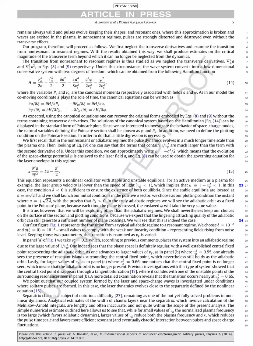
Fig. 2. Magnitude of the transverse Laplacian as a function of x⊥ and ξ . At ξ = 35 the Laplacian touches the boundary of region R, which signals theinstant where its corresponding effects become noticeable.
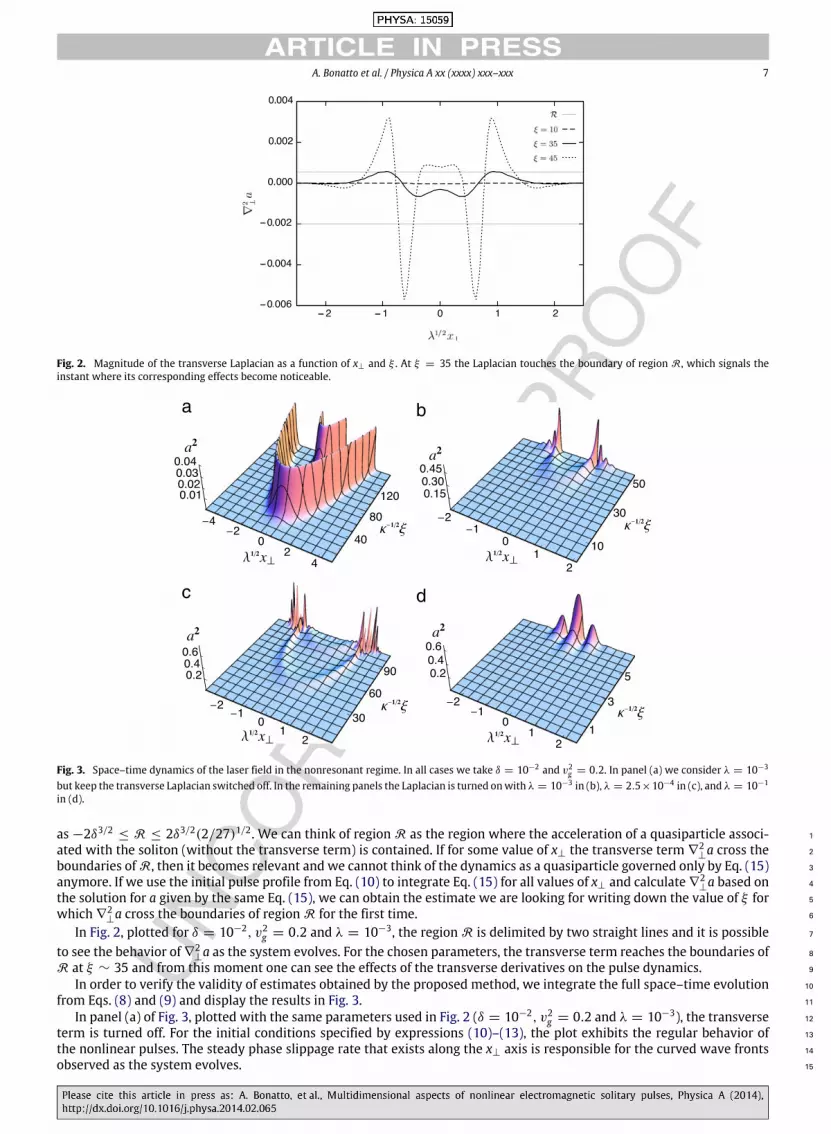
Fig. 3. Space–time dynamics of the laser field in the nonresonant regime. In all cases we take δ = 10−2 and v2g = 0.2. In panel (a) we consider λ = 10−3
but keep the transverse Laplacian switched off. In the remaining panels the Laplacian is turned onwith λ = 10−3 in (b), λ = 2.5×10⁻⁴ in (c), and λ = 10−1
in (d).
as −2δ3/2≤ R ≤ 2δ3/2(2/27)1/2. We can think of region R as the region where the acceleration of a quasiparticle associ- 1
ated with the soliton (without the transverse term) is contained. If for some value of x⊥ the transverse term ∇2⊥a cross the 2
boundaries of R, then it becomes relevant and we cannot think of the dynamics as a quasiparticle governed only by Eq. (15) 3
anymore. If we use the initial pulse profile from Eq. (10) to integrate Eq. (15) for all values of x⊥ and calculate ∇2⊥a based on 4
the solution for a given by the same Eq. (15), we can obtain the estimate we are looking for writing down the value of ξ for 5
which ∇2⊥a cross the boundaries of region R for the first time. 6
In Fig. 2, plotted for δ = 10−2, v2g = 0.2 and λ = 10−3, the region R is delimited by two straight lines and it is possible 7
to see the behavior of ∇2⊥a as the system evolves. For the chosen parameters, the transverse term reaches the boundaries of 8
R at ξ ∼ 35 and from this moment one can see the effects of the transverse derivatives on the pulse dynamics. 9
In order to verify the validity of estimates obtained by the proposed method, we integrate the full space–time evolution 10
from Eqs. (8) and (9) and display the results in Fig. 3. 11
In panel (a) of Fig. 3, plotted with the same parameters used in Fig. 2 (δ = 10−2, v2g = 0.2 and λ = 10−3), the transverse 12
term is turned off. For the initial conditions specified by expressions (10)–(13), the plot exhibits the regular behavior of 13
the nonlinear pulses. The steady phase slippage rate that exists along the x⊥ axis is responsible for the curved wave fronts 14
observed as the system evolves. 15

8 A. Bonatto et al. / Physica A xx (xxxx) xxx–xxx
Fig. 4. Space–time dynamics of the laser field in the resonant regime. In panel (a) we take δ = 10−2 and v2g = 0.9, along with λ = 10−4 . Panel (b) is
plotted for the same parameters, but with the transverse term switched off.
Fig. 3(b) is plotted with the same parameters of the previous panel, but with the transverse term turned on. Here we can1
see sharp spikes emerging from the train of pulses a little before ξ = 50, agreeing with our previous estimates. These spikes2
result from the action of the second derivatives along ξ , as we can see looking back to Fig. 2, and thus are the transverse3
effectswehave beenmentioning so far. Soon after the spikes, the dynamics exhibits a chaotic pattern that cannot be followed4
for long, since the fields grow beyond the validity of our weakly nonlinear approximation. We point out that although the5
model cannot provide a detailed description in the large amplitude regimes, it is perfectly capable to indicate how far the6
trains of solitons can move into the plasma before being distorted by transverse effects.7
In panel (c) of Fig. 3 we set a smaller λ, λ = 2.5 × 10⁻⁴, to extend the beam width and keep the same previous values8
for the remaining parameters. Here, as expected, the solitary pulse goes further before being affected by the transverse9
term, and the critical time ξ ∼ 70 (again obtained when ∇2⊥a crosses the boundaries of region R) is in good agreement10
with the curves of this panel. For larger values of λ, the transverse term is dominant and generates the exponential growth11
commented before [25]. Fig. 3(d), plotted for λ = 10−1 (≫ δ), displays this behavior. It is worth to note that, for these12
situations, the maximum of ∇2⊥a is already out of the region R at ξ = 0.13
3.2. Resonant regimes14
Our final topic refers to the resonant regime, where, even in the absence of the transverse term, space-charge plasma15
waves are strongly excited. In nonresonant regimes,where nonintegrable behavior is present evenwhen the transverse term16
is neglected, the estimates obtained from the integrable Eq. (15) are no longer accurate. Still, we are tempted to associate17
the time scales (δ/κ)−1/2 and (λ/κ)−1/2 with the longitudinal and transverse dynamics respectively. In order to investigate18
a nonresonant regime, we set v2g = 0.9 and choose δ = 10−2 and λ = 10−4. Here, as λ ≪ δ, pulses have time enough to19
be formed even if irregularly. This is basically what happens in the panel (a) of Fig. 4. Comparing this panel and panel (b),20
plotted with the same parameters but with the transverse term turned off, we can realize that the effect of the transverse21
structure on the laser amplitude is perceptible even for such a small value of λ. Essentially, the characteristic time scale of22
oscillation is shortened by the presence of the transverse term. This shortening becomes stronger as we increase λ, what is23
expected from the enhancement of the instability in these circumstances [25].24
For larger values of λ, as λ = 10−1, the transverse instability takes over and the tridimensional plot with scaled axes25
become almost identical to that of Fig. 3(d).26

A. Bonatto et al. / Physica A xx (xxxx) xxx–xxx 9
4. Conclusions 1
We have studied the role of transverse effects on the formation and existence of trains of electromagnetic pulses in 2
laser-plasma interactions. 3
Pulse shape depends on the co-moving coordinate of the beam frame and also on the transverse coordinate, and no a 4
priori assumption is made on the longitudinal-to-transverse aspect ratio of the pulses. 5
Space-charge modes are present and are analyzed in two distinct regimes of excitation: resonant and nonresonant. Ac- 6
curate estimates are possible in the nonresonant case, where space-charge modes are described under adiabatic approxi- 7
mations. However, fairly good estimates can be also obtained in the resonant case, where typical scales of the space-charge 8
modes become comparable to the ones of the laser pulses and adiabatic approximations fail. 9
It is possible to estimate the number of unperturbed pulses in a train as (δ/λ)1/2 which, considering that the pulse ampli- 10
tude ap is proportional to δ1/2, can be rewritten as ap λ−1/2. Here, λ−1/2 itself is a measure of the transverse length expressed 11
in units of the plasma wavelength. From this estimate one can see that, for a laser beam with a wide transverse profile 12
(λ−1/2≫ 1), a finite number of pulses can be formed even if its amplitude ap is small. However, for larger values of λ (as in 13
the case with λ ∼ 10−1), no pulses are formed at all. 14
All in all, estimates allow to predict how far can trains of pulses move into the plasma before distortion due to the finite 15
beam’s cross section sets in.We believe that a key point here is that both our estimates and simulations show that evenwhen 16
the cross section of the radiation beam is fairly larger than longitudinal pulse size, transverse effects may still noticeably 17
affect the pulses. From that point on the very concept of the soliton gas, as discussed in the introductory part of the paper, 18
is somewhat weakened. Q5 19
Acknowledgments 20
We acknowledge support from CNPq, Brasil, and from AFOSR, USA, under research grant FA9550-12-1-0438. 21
References 22
[1] M. Toda, Theory of Nonlinear Lattices, Springer, Berlin, 1989. 23
[2] P.K. Shukla, N.N. Rao, M.Y. Yu, N.L. Tsintsadze, Phys. Lett. 138 (1986) 1. 24
[3] T. Tsuzuki, K. Sasaki, Progr. Theoret. Phys. Suppl. (94) (1988) 73. 25
[4] D. Farina, S.V. Bulanov, Phys. Rev. Lett. 86 (2001) 5289. 26
[5] T. Tajima, J.M. Dawson, Phys. Rev. Lett. 43 (1979) 267. 27
[6] J.T. Mendonça, Theory of Photon Acceleration, IOP Publishing, Bristol, 2001. 28
[7] E. Esarey, B. Hafizi, R. Hubbard, A. Ting, Phys. Rev. Lett. 80 (1998) 5552. 29
[8] R. Bingham, Nature 424 (2003) 258. 30
[9] C. Joshi, T. Katsouleas, Phys. Today 56 (2003) 47. 31
[10] S. Poornakala, A. Das, A. Sen, P.K. Kaw, Phys. Plasmas 9 (2002) 1820. 32
[11] P.A. Robinson, G.I. de Oliveira, Phys. Plasmas 6 (1999) 3057. 33
[12] C. Kamperidis, C. Bellei, N. Bourgeois, M.C. Kaluza, K. Krushelnick, S.P.D. Mangles, J.R. Marques, S.R. Nagel, Z. Najmudin, J. Plasma Phys. 78 (2012) 433. 34
[13] G.I. de Oliveira, F.B. Rizzato, A.C.-L. Chian, Phys. Rev. E 52 (1995) 2025. 35
[14] V.A. Kozlov, A.G. Litvak, E.V. Suvorov, Zh. Eksp. Teor. Fiz. 76 (1979) 148. 36
[15] U.A. Mofiz, U. de Angelis, J. Plasma Phys. 33 (1985) 107. 37
[16] B.S. Azimov, M.M. Sagatov, A.P. Sukhorukov, Sov. J. Quantum Electron. 21 (1991) 93. 38
[17] A. Bonatto, R. Pakter, F.B. Rizzato, J. Plasma Phys. 72 (2006) 179. 39
[18] R. Erichsen, L.G. Brunnet, F.B. Rizzato, Phys. Rev. E 60 (1999) 6566. 40
[19] L.E. Guerrero, J.A. González, Physica A 257 (1998) 390. 41
[20] B.J. Duda, W.B. Mori, Phys. Rev. E 61 (2000) 1925. 42
[21] S.-C. Tang, H.-B. Jiang, Y. Liu, Q.-H. Gong, Chin. Phys. Lett. 25 (2008) 3268. 43
[22] E. Miura, in: A. Andreev (Ed.), Femtosecond-Scale Optics, in: Electron Acceleration using an Ultra-short Ultra-intense Laser Pulse, ISBN: 978-953-307-769-7, 2011, p. 11.
44
[23] E. Esarey, C.B. Schroeder, B.A. Shadwick, J.S. Wurtele, W.P. Leemans, Phys. Rev. Lett. 84 (2000) 3081. 45
[24] Lj. Hadžievski, M.S. Jovanovič, M.M. Skorič, K. Mima, Phys. Plasmas 9 (2002) 2569. 46
[25] A. Bonatto, R. Pakter, F.B. Rizzato, C. Bonatto, Laser Part. Beams 30 (2012) 583. 47
[26] P. Gibbon, Short Pulse Laser Interactions with Matter, Imperial College Press, London, 2007. 48
[27] A.J. Lichtenberg, M.A. Lieberman, Regular and Chaotic Dynamics, Springer-Verlag, New York, 1992. 49


