Embed Size (px)
Citation preview

Multilinear Algebra
and Its Applications
Ana Cannas, Ozlem Imamoglu, Alessandra Iozzi
March 2021


Contents
Introduction 1
Chapter 1. Review of Linear Algebra 71.1. Vector Spaces 71.2. Bases 91.3. The Einstein Convention 141.4. Linear Transformations 18
Chapter 2. Multilinear Forms 272.1. Linear Forms 272.2. Bilinear Forms 352.3. Multilinear Forms 41
Chapter 3. Inner Products 453.1. Definitions and First Properties 453.2. Reciprocal Basis 543.3. Relevance of Covariance and Contravariance 63
Chapter 4. Tensors 654.1. Towards General Tensors 654.2. Tensors of Type (p, q) 694.3. Tensor Product 71
Chapter 5. Applications 775.1. Inertia Tensor 775.2. Stress Tensor (Spannung) 895.3. Strain Tensor (Verzerrung) 985.4. Elasticity Tensor 1025.5. Conductivity Tensor 104
Solutions to Exercises 107


Introduction
This text deals with physical or geometric entities, known as tensors, which can bethought of as a generalization of vectors. The quantitative description of tensors, i.e.,their description in terms of numbers, changes when we change the frame of reference,a.k.a. the basis in linear algebra. Tensors are central in Engineering and Physics, becausethey provide the framework for formulating and solving problems in areas such as Me-chanics (inertia tensor, stress tensor, elasticity tensor, etc.), Electrodynamics (electricalconductivity and electrical resistivity tensors, electromagnetic tensor, magnetic suscep-tibility tensor, etc.), or General Relativity (stress–energy tensor, curvature tensor, etc.).
Just like the main protagonists in Linear Algebra are vectors and linear maps, the mainprotagonists in Multilinear Algebra are tensors and multilinear maps. Tensors describelinear relations among objects in space, and are represented – once a basis is chosen –by multidimensional arrays of numbers:
T1 . . . . . . Tn
1. A tensor of order 1, Tj .
T11
...
...
. . . . . . T1n
...
...
Tn1 . . . . . . Tnn
2. A tensor of order 2, Tij .
T111 . . . . . . . . .
...
...
T1n1
...
...
Tn11 . . . . . . . . . Tnn1
T1nn
. . . . . . . . .
...
...
Tnnn
T11n . . . . . . . . .
Tn1n
3. A tensor of order 3, Tijk.
In the notation, the indices can be upper or lower. For tensors of order at least2, some indices can be upper and some lower. The numbers in the arrays are calledcomponents of the tensor and give the representation of the tensor with respect to agiven basis.
1
2 INTRODUCTION
Two natural questions arise:
(1) Why do we need tensors?(2) What are the important features of tensors?
(1) Scalars are not enough to describe directions, for which we need to resort tovectors. At the same time, vectors might not be enough, in that they lack the ability to“modify” vectors.
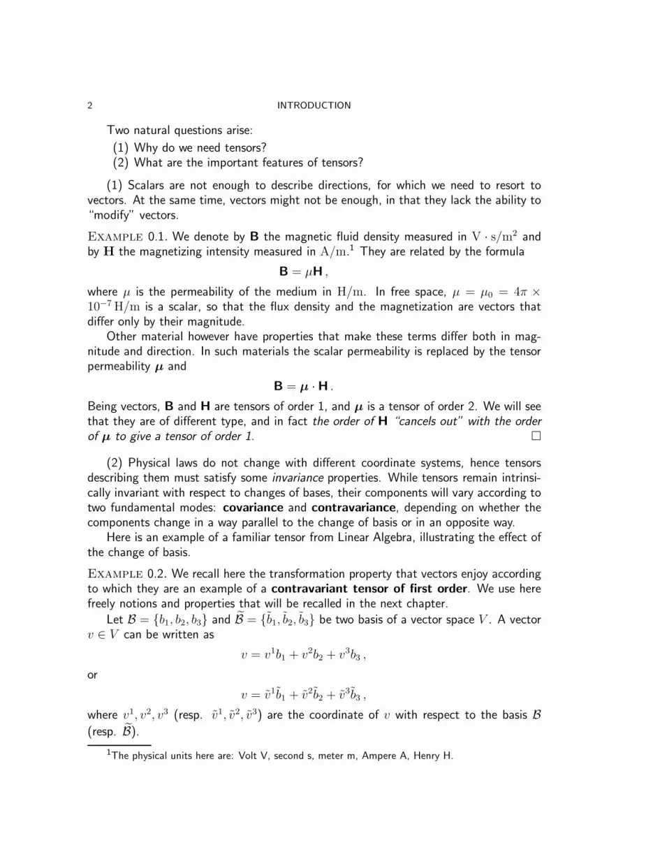
Example 0.1. We denote by B the magnetic fluid density measured in V · s/m2 andby H the magnetizing intensity measured in A/m.1 They are related by the formula
B = µH ,
where µ is the permeability of the medium in H/m. In free space, µ = µ0 = 4π ×10−7H/m is a scalar, so that the flux density and the magnetization are vectors thatdiffer only by their magnitude.
Other material however have properties that make these terms differ both in mag-nitude and direction. In such materials the scalar permeability is replaced by the tensorpermeability µ and
B = µ ·H .
Being vectors, B and H are tensors of order 1, and µ is a tensor of order 2. We will seethat they are of different type, and in fact the order of H “cancels out” with the orderof µ to give a tensor of order 1. �
(2) Physical laws do not change with different coordinate systems, hence tensorsdescribing them must satisfy some invariance properties. While tensors remain intrinsi-cally invariant with respect to changes of bases, their components will vary according totwo fundamental modes: covariance and contravariance, depending on whether thecomponents change in a way parallel to the change of basis or in an opposite way.
Here is an example of a familiar tensor from Linear Algebra, illustrating the effect ofthe change of basis.
Example 0.2. We recall here the transformation property that vectors enjoy accordingto which they are an example of a contravariant tensor of first order. We use herefreely notions and properties that will be recalled in the next chapter.
Let B = {b1, b2, b3} and B = {b1, b2, b3} be two basis of a vector space V . A vectorv ∈ V can be written as
v = v1b1 + v2b2 + v3b3 ,
or
v = v1b1 + v2b2 + v3b3 ,
where v1, v2, v3 (resp. v1, v2, v3) are the coordinate of v with respect to the basis B(resp. B).
1The physical units here are: Volt V, second s, meter m, Ampere A, Henry H.

INTRODUCTION 3
Warning: Please keep the lower indices as lower indices and the upper ones as upperones. You will see later that there is a reason for it!
We use the following notation:
[v]B =
v1
v2
v3
and [v]B =
v1
v2
v3
,(0.1)
and we are interested in finding the relation between the coordinates of v in the twobases.
The vectors bj , j = 1, 2, 3, in the basis B can be written as a linear combination ofvectors in B as follows:
bj = L1jb1 + L2
jb2 + L3jb3 ,
for some Lij ∈ R. We consider the matrix of the change of basis from B to B,
L := LBB =
L11 L1
2 L13
L21 L2
2 L23
L31 L3
2 L33
whose jth-column consists of the coordinates of the vectors bj with respect to the basisB. The equalities
b1 = L11b1 + L2
1b2 + L31b3
b2 = L12b1 + L2
2b2 + L32b3
b3 = L13b1 + L2
3b2 + L33b3
can simply be written as(b1 b2 b3
)=(b1 b2 b3
)L .(0.2)
(Check this symbolic equation using the rules of matrix multiplication.) Analogously,writing basis vectors in a row and vector coordinates in a column, we can write
v = v1b1 + v2b2 + v3b3 =(b1 b2 b3
)v1
v2
v3
(0.3)
and
v = v1b1 + v2b2 + v3b3 =(b1 b2 b3
)
v1
v2
v3
=(b1 b2 b3
)L
v1
v2
v3
,(0.4)
4 INTRODUCTION
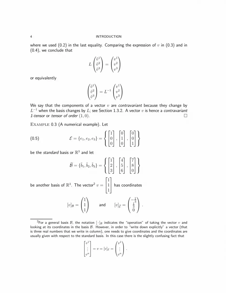
where we used (0.2) in the last equality. Comparing the expression of v in (0.3) and in(0.4), we conclude that
L
v1
v2
v3
=
v1
v2
v3
or equivalently
v1
v2
v3
= L−1
v1
v2
v3
We say that the components of a vector v are contravariant because they change byL−1 when the basis changes by L; see Section 1.3.2. A vector v is hence a contravariant1-tensor or tensor of order (1, 0). �
Example 0.3 (A numerical example). Let
E = {e1, e2, e3} =
100
,
010
,
001
(0.5)
be the standard basis or R3 and let
B = {b1, b2, b3} =
123
,
456
,
780
be another basis of R3. The vector2 v =
111
has coordinates
[v]B =
111
and [v]E =
−1
3130
.
2For a general basis B, the notation [ · ]B indicates the “operation” of taking the vector v andlooking at its coordinates in the basis B. However, in order to “write down explicitly” a vector (thatis three real numbers that we write in column), one needs to give coordinates and the coordinates areusually given with respect to the standard basis. In this case there is the slightly confusing fact that
v1
...
vn
= v = [v]E =
v1
...
vn
.
INTRODUCTION 5
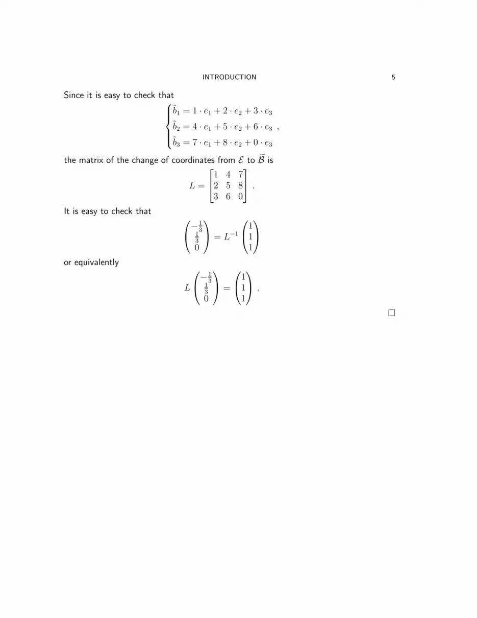
Since it is easy to check that
b1 = 1 · e1 + 2 · e2 + 3 · e3b2 = 4 · e1 + 5 · e2 + 6 · e3b3 = 7 · e1 + 8 · e2 + 0 · e3
,
the matrix of the change of coordinates from E to B is
L =
1 4 72 5 83 6 0
.
It is easy to check that
−1
3130
= L−1
111
or equivalently
L
−1
3130
=
111
.
�


CHAPTER 1
Review of Linear Algebra
1.1. Vector Spaces
A vector space (or linear space) is a set of objects where addition and scaling aredefined in a way that satisfies natural requirements for such operations, such as theproperties listed in the definition below.
1.1.1. Vectors and Scalars.
In this text, we will only consider real vector spaces, a.k.a. vector spaces over R,where the scaling is by real numbers.
Definition 1.1. A vector space V over R is a set V equipped with two operations:
(1) Vector addition: V × V → V , (v, w) 7→ v + w, and(2) Multiplication by a scalar: R× V → V , (α, v) 7→ αv ,
satisfying the following properties:
(1) (associativity) (u+ v) + w = u+ (v + w) for every u, v, w ∈ V ;(2) (commutativity) u+ v = v + u for every u, v ∈ V ;(3) (existence of the zero vector) There exists 0 ∈ V such that v+0 = v for every
v ∈ V ;(4) (existence of additive inverse) For every v ∈ V , there exists wv ∈ V such that
v + wv = 0. The vector wv is denoted by −v.(5) α(βv) = (αβ)v for every α, β ∈ R and every v ∈ R;(6) 1v = v for every v ∈ V ;(7) α(u+ w) = αu+ αv for all α ∈ R and u, v ∈ V ;(8) (α + β)v = αv + βv for all α, β ∈ R and v ∈ V .
An element of the vector space is called a vector and, mostly in the context of vectorspaces, a real number is called a scalar.
Example 1.2 (Prototypical example). The Euclidean space Rn, n = 1, 2, 3, . . . , is avector space with componentwise addition and multiplication by scalars. Vectors in Rn
are denoted by
v =
x1...xn
,
7

8 1. REVIEW OF LINEAR ALGEBRA
with x1, . . . , xn ∈ R. Addition component-by-component translates geometrically to theparallelogram law for vector addition, well-known in R2 and R3. �
Examples 1.3 (Other examples). The operations of vector addition and scalar multi-plication are usually inferred from the context.
(1) The set of real polynomials of degree ≤ n is a vector space, denoted by
V = R[x]n := {anxn + an−1xn−1 + · · ·+ a1x+ a0 : aj ∈ R}
with the usual (degreewise) sum of polynomials and scalar multiplication.(2) The set of real matrices of size m× n,
V =Mm×n(R) :=
a11 . . . a1m...
...an1 . . . anm
: aij ∈ R
with componentwise addition and scalar multiplication.(3) The space {f : W → R} of all real-valued functions on a vector space W .(4) The space of solutions of a homogeneous linear (ordinary or partial) differential
equation.
�
Exercise 1.4. Are the following vector spaces?
(1) The set V of all vectors in R3 perpendicular to the vector
123
.
(2) The set of invertible 2× 2 matrices, that is
V :=
{[a bc d
]: ad− bc = 6= 0
}.
(3) The set of polynomials of degree exactly n, that is
V := {a0xn + a1xn−1 + · · ·+ an−1x+ an : aj ∈ R, an 6= 0} .
(4) The set V of 2× 4 matrices with last column zero, that is
V :=
{[a b c 0d e f 0
]: a, b, c, d, e, f ∈ R
}
(5) The set of solutions f : R→ R of the equation f ′ = 5, that is
V := {f : R→ R : f(x) = 5x+ C, C ∈ R} .Definition 1.5. A function T : V → W between real vector spaces V and W is alinear transformation if it satisfies the property
T (αv + βw) = αT (v) + βT (w) ,
for all α, β ∈ R and all v, w ∈ V .

1.2. BASES 9
Exercise 1.6. Show that the set of all linear transformations T : R2 → R3 forms avector space.
1.1.2. Subspaces.
Definition 1.7. A subset W of a vector space V that is itself a vector space is asubspace.
By reviewing the properties in the definition of vector space, we see that a subsetW ⊆ V is a subspace exactly when the following conditions are verified:
(1) The 0 element is in W ;(2) W is closed under addition, that is v + w ∈ W for every v, w ∈ W ;(3) W is closed under multiplication by scalars, that is αv ∈ W for every α ∈ R
and every v ∈ W .
Condition (1) in fact follows from (2) and (3) under the assumption that W 6= ∅.Yet it is often an easy way to check that a subset is not a subspace.
Recall that a linear combination of vectors v1, . . . , vn ∈ V is a vector of the formα1v1 + · · ·+ αnvn for α1, . . . , αn ∈ R. With this notion, the above three conditions fora subspace are equivalent to the following ones:
(1)’ W is nonempty;(2)’ W is closed under linear combinations, that is αv + βw ∈ W for all α, β ∈ R
and all v, w ∈ W .
Definition 1.8. If T : V → W is a linear transformation between real vector spacesV and W , then:
• the kernel (or null space) of T is the set ker T := {v ∈ V : T (v) = 0};• the image (or range) of T is the set imT := {T (v) : v ∈ V }.
Exercise 1.9. Show that, for a linear transformation T : V → W , the kernel ker T isa subspace of V and the image imT is a subspace of W .
1.2. Bases
The key to study and to compute in vector spaces is the concept of basis, which inturn relies on the fundamental notions of linear independence/dependence and of span.
1.2.1. Definition of Basis.
Definition 1.10. The vectors b1, . . . , bn ∈ V are linearly independent if α1b1+ · · ·+αnbn = 0 implies that α1 = · · · = αn = 0. In other words, if the only linear combinationof these vectors that yields the zero vector is the trivial one. We then also say that thevector set {b1, . . . , bn} is linearly independent.
Example 1.11. The vectors
100
,
010
,
001

10 1. REVIEW OF LINEAR ALGEBRA
are linearly independent in R3. In fact,
µ1
100
+ µ2
010
+ µ3
001
= 0⇐⇒
µ1
µ2
µ3
=
000
⇐⇒ µ1 = µ2 = µ3 = 0 .
�
Example 1.12. The vectors
b1 =
123
, b2 =
456
, b3 =
780
are linearly independent in R3. In fact,
µ1b1 + µ2b2 + µ3b3 = 0⇐⇒
µ1 + 4µ2 + 7µ3 = 0
2µ1 + 5µ2 + 8µ30
3µ1 + 6µ2 = 0
⇐⇒ · · · ⇐⇒ µ1 = µ2 = µ3 = 0 .
(If you are unsure how to fill in the dots look at Example 1.21.) �
Example 1.13. The vectors
b1 =
123
, b2 =
456
, b3 =
789
are linearly dependent in R3, i.e., not linearly independent. In fact,
µ1b1 + µ2b2 + µ3b3 = 0⇐⇒
µ1 + 4µ2 + 7µ3 = 0
2µ1 + 5µ2 + 8µ30
3µ1 + 6µ2 + 9µ3 = 0
⇐⇒ · · · ⇐⇒{µ1 = µ2
µ2 = −2µ3 ,
so
b1 − 2b2 + b3 = 0
and b1, b2, b3 are not linearly independent. For instance, we say that b1 = 2b2 − b3 is anon-trivial linear relation between the vectors b1, b2 and b3. �
Definition 1.14. The vectors b1, . . . , bn ∈ V span V , if every vector v ∈ V can bewritten as a linear combination v = α1b1 + · · · + αnbn, for some α1, . . . , αn ∈ R. Wethen also say that the vector set {b1, . . . , bn} spans V .Examples 1.15.
(1) The vectors
100
,
010
,
001
span R3.
(2) The vectors
100
,
010
,
001
,
111
also span R3.

1.2. BASES 11
(3) The vectors
100
,
010
span the xy-coordinate plane (i.e., the subspace given
by the equation z = 0) in R3.
�
Exercise 1.16. The set of all linear combinations of b1, . . . , bn ∈ V is denoted byspan {b1, . . . , bn}. Show that span {b1, . . . , bn} is a subspace of V .
Definition 1.17. The vectors b1, . . . , bn ∈ V form a basis of V , if:
(1) they are linearly independent and(2) they span V .
We then denote this basis as an ordered set B := {b1, . . . , bn}, where we fix the orderof the vectors.
Warning: In this text, we only consider bases for so-called finite-dimensional vectorspaces, that is, vector spaces that admit bases consisting of a finite number of elements.
Example 1.18. The vectors
e1 :=
100
, e2 :=
010
, e3 :=
001
form a basis ofR3. This is called the standard basis of R3 and denoted E := {e1, e2, e3}.For Rn, the standard basis E := {e1, . . . , en} is defined similarly. �
Example 1.19. The vectors in Example 1.12 span R3, while the vectors in Example 1.13do not span R3. To see this, we recall the following facts about bases. �
1.2.2. Facts about Bases.
Let V be a vector space; as stated above, V is finite-dimensional. Then we have:
(1) All bases of V have the same number of elements. This number is called thedimension of V and denoted dim V .
(2) If B = {b1, . . . , bn} is a basis of V , there is a unique way of writing any v ∈ Vas a linear combination
v = v1b1 + . . . vnbn
of elements in B. The numbers v1, . . . , vn are the coordinates of v withrespect to the basis B and we denote by
[v]B =
v1
...vn
the coordinate vector of v with respect to B.

12 1. REVIEW OF LINEAR ALGEBRA
(3) If we know that dimV = n, then:(a) More than n vectors in V must be linearly dependent;(b) Fewer than n vectors in V cannot span V ;(c) Any n linearly independent vectors span V ;(d) Any n vectors that span V must be linearly independent;(e) If k vectors span V , then k ≥ n and some subset of those k vectors must
be a basis of V ;(f) If a set of m vectors is linearly independent, then m ≤ n and we can
always complete that set to form a basis of V .
Example 1.20. The vectors b1, b2, b3 in Example 1.12 form a basis of R3 since they arelinearly independent and they are exactly as many as the dimension of R3. �
Example 1.21 (Gauss-Jordan elimination). We are going to compute here the coordi-
nates of v =
111
with respect to the basis B := {b1, b2, b3} from Example 1.12. The
seeked coordinates [v]B =
v1
...vn
must satisfy the equation
v1
123
+ v2
456
+ v3
780
=
111
,
so to find them we have to solve the following system of linear equations:
v1 + 4v2 + 7v3 = 1
2v1 + 5v2 + 8v3 = 1
3v1 + 6v2 = 1.
For that purpose, we may equivalently reduce the following augmented matrix
1 4 7 12 5 8 13 6 0 1
to echelon form, using the Gauss–Jordan elimination method. We are going to performboth calculations in parallel, which will also point out that they are indeed seeminglydifferent incarnations of the same method.
By multiplying the first equation/row by 2 (resp. 3) and subtracting it from thesecond (reps. third) equation/row we obtain
v1 + 4v2 + 7v3 = 1
− 3v2 − 6v3 = −1− 6v2 − 21v3 = −2
!
1 4 7 1
0 −3 −6 −10 −6 −21 −2
.

1.2. BASES 13
By multiplying the second equation/row by −13and by adding to the first (resp. third)
equation/row the second equation/row multiplied by −43(resp. 2) we obtain
v1 − v3 = −13
v2 + 2v3 = 13
− 9v3 = 0
!
1 0 −1 −1
3
0 1 2 13
0 0 −9 0
.
The last equation/row shows that v3 = 0, hence by backward substitution we obtainthe solution
v1 = −13
v2 = 13
v3 = 0
!
1 0 0 −1
3
0 1 0 13
0 0 1 0
.
�
Example 1.22. When V = Rn and B = E is the standard basis, the coordinate vectorv ∈ Rn coincides with the vector itself! In this very special case, we have [v]E = v. �
Exercise 1.23. Let V be the vector space consisting of all 2 × 2 matrices with tracezero, namely
V :=
{[a bc d
]: a, b, c, d ∈ R and a + d = 0
}.
(1) Show that
B :=
{[1 00 −1
]
︸ ︷︷ ︸b1
,
[0 10 0
]
︸ ︷︷ ︸b2
,
[0 01 0
]
︸ ︷︷ ︸b3
}
is a basis of V .(2) Show that
B :=
{[1 00 −1
]
︸ ︷︷ ︸b1
,
[0 −11 0
]
︸ ︷︷ ︸b2
,
[0 11 0
]
︸ ︷︷ ︸b3
}
is another basis of V .(3) Compute the coordinates of
v =
[2 17 −2
]
with respect to B and with respect to B.

14 1. REVIEW OF LINEAR ALGEBRA
1.3. The Einstein Convention
1.3.1. A Convenient Summation Convention.
We start by setting a notation that will turn out to be useful later on. Recall that ifB = {b1, b2, b3} is a basis of a vector space V , any vector v ∈ V can be written as
v = v1b1 + v2b2 + v3b3(1.1)
for appropriate v1, v2, v3 ∈ R.
Notation. From now on, expressions like the one in (1.1) will be written as
v =✭✭
✭✭✭✭✭✭✭✭❤
❤❤❤❤❤❤❤❤❤
v1b1 + v2b2 + v3b3 = vjbj .(1.2)
That is, from now on when an index appears twice – once as a subscript and once asa superscript – in a term, we know that it means that there is a summation over allpossible values of that index. The summation symbol will not be displayed.
On the other hand, indices that are not repeated in expressions like aijxkyj are free
indices not subject to summation.
Examples 1.24. For indices ranging over {1, 2, 3}, i.e. n = 3:
(1) The expression aijxiyk means
aijxiyk = a1jx
1yk + a2jx2yk + a3jx
3yk ,
and could be called Rkj (meaning that Rk
j and aijxiyk both depend on the
indices j and k).(2) Likewise,
aijxkyj = ai1x
ky1 + ai2xky2 + ai3x
ky3 =: Qki .
(3) Further
aijxiyj = a11x
1y1 + a12x1y2 + a13x
1y3
+ a21x2y1 + a22x
2y2 + a23x2y3
+ a31x3y1 + a32x
3y2 + a33x3y3 =: P
(4) An expression like
AiBjkℓC
ℓ =: Dijk
makes sense. Here the indices i, j, k are free (i.e. free to range in {1, 2, . . . , n})and ℓ is a summation index.
(5) On the other hand an expression like
EijFℓjkGℓ = Hjk
i
does notmake sense because the expression on the left has only two free indices,i and k, while j and ℓ are summation indices and neither of them can appearon the right hand side.
1.3. THE EINSTEIN CONVENTION 15
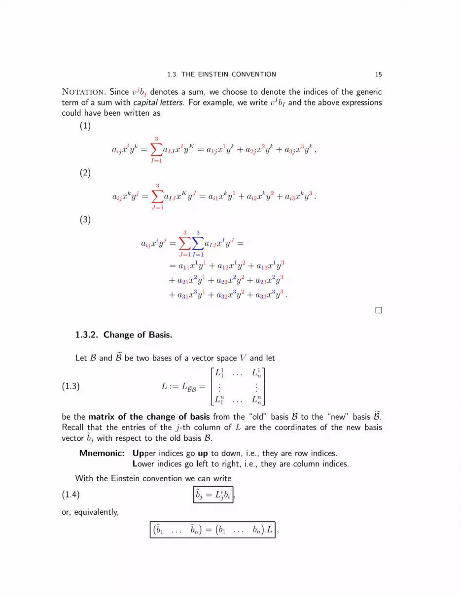
Notation. Since vjbj denotes a sum, we choose to denote the indices of the genericterm of a sum with capital letters. For example, we write vIbI and the above expressionscould have been written as
(1)
aijxiyk =
3∑
I=1
aIJxIyK = a1jx
1yk + a2jx2yk + a3jx
3yk ,
(2)
aijxkyj =
3∑
J=1
aIJxKyJ = ai1x
ky1 + ai2xky2 + ai3x
ky3 .
(3)
aijxiyj =
3∑
J=1
3∑
I=1
aIJxIyJ =
= a11x1y1 + a12x
1y2 + a13x1y3
+ a21x2y1 + a22x
2y2 + a23x2y3
+ a31x3y1 + a32x
3y2 + a33x3y3 .
�
1.3.2. Change of Basis.
Let B and B be two bases of a vector space V and let
L := LBB =
L11 . . . L1
n...
...Ln1 . . . Ln
n
(1.3)
be the matrix of the change of basis from the “old” basis B to the “new” basis B.Recall that the entries of the j-th column of L are the coordinates of the new basisvector bj with respect to the old basis B.
Mnemonic: Upper indices go up to down, i.e., they are row indices.Lower indices go left to right, i.e., they are column indices.
With the Einstein convention we can write
bj = Lijbi ,(1.4)
or, equivalently,(b1 . . . bn
)=(b1 . . . bn
)L ,

16 1. REVIEW OF LINEAR ALGEBRA
where we use some convenient formal notation: The multiplication is to be performedwith the usual rules for vectors and matrices, though, in this case, the entries of the rowvectors
(b1 . . . bn
)and
(b1 . . . bn
)are not real numbers but vectors themselves.
If Λ = L−1 denotes the matrix of the change of basis from B to B, then, using thesame formal notation as above, we have
(b1 . . . bn
)=(b1 . . . bn
)Λ .
Equivalently, this can be written in compact form using the Einstein notation as
bj = Λij bi .
Analogously, the corresponding relations for the vector coordinates are
v1
...vi
...vn
=
L11 . . . . . . L1
n...
...Li1 . . . . . . Li
n...
...Ln1 . . . . . . Ln
n
v1
...
...
...vn
and
v1
...vi
...vn
=
Λ11 . . . . . . Λ1
n...
...Λi
1 . . . . . . Λin
......
Λn1 . . . . . . Λn
n
v1
...
...
...vn
and these can be written with the Einstein convention respectively as
vi = Lij v
j and vi = Λijv
j ,(1.5)
or, in matrix notation,
[v]B = LBB[v]B and [v]B = (LBB)−1[v]B = LBB[v]B .
Important: Note how the coordinate vectors change in a way opposite to the basischange. Hence, we say that the coordinate vectors are contravariant3 because theychange by L−1 when the basis changes by L.
Example 1.25. We consider the following two bases of R2
B =
{ [10
]
︸︷︷︸b1
,
[21
]
︸︷︷︸b2
}
B =
{ [31
]
︸︷︷︸b1
,
[−1−1
]
︸ ︷︷ ︸b2
}(1.6)
and we look for the matrix of the change of basis. Namely we look for a matrix L suchthat [
3 −11 −1
]=(b1 b2
)=(b1 b2
)L =
[1 20 1
]L .
3In Latin contra means “contrary” or “against”.

1.3. THE EINSTEIN CONVENTION 17
There are two alternative ways of finding L:
(1) With matrix inversion: Recall that[a bc d
]−1
= 1D
[d −b−c a
],(1.7)
where D = det
[a bc d
]is the determinant. Thus
L =
[1 20 1
]−1 [3 −11 −1
]=
[1 −20 1
] [3 −11 −1
]=
[1 11 −1
].
(2) With Gauss-Jordan elimination:[1 2 3 −10 1 1 −1
]!
[1 0 1 10 1 1 −1
]
�
1.3.3. The Kronecker Delta Symbol.
Notation. The Kronecker delta symbol δij is defined as
δij :=
{1 if i = j
0 if i 6= j .(1.8)
Examples 1.26. If L is a matrix, the (i, j)-entry of L is the coefficient in the i-th rowand j-th column, and is denoted by Li
j .
(1) The n× n identity matrix
I =
1 . . . 0...
. . ....
0 . . . 1
has (i, j)-entry equal to δij .(2) Let L and M be two square matrices. The (i, j)-th entry of the product
ML =
M11 . . . . . . M1
n......
M i1 . . . . . . M i
n......
Mn1 . . . . . . Mn
n
L11 . . . L
1j . . . L
1n
......
......
......
Ln1 . . . L
nj . . . L
nn
equals the dot product of the i-th row of M and j-th column of L,
(M i
1 . . . M in
)·
L1j...Lnj
=M i
1L1j + · · ·+M i
nLnj ,

18 1. REVIEW OF LINEAR ALGEBRA
or, using the Einstein convention,
M ikL
kj .
Notice that, since in general ML 6= LM , it follows that
M ikL
kj 6= Li
kMkj =Mk
j Lik .
However, in the special case where M = Λ = L−1, we have ΛL = LΛ = I andhere we can write
ΛikL
kj = δij = Li
kΛkj .
�
Remark 1.27. Using the Kronecker delta symbol we can check that the notations in(1.5) are all consistent. In fact, from (1.2) we should have
vibi = v = vibi ,(1.9)
and, in fact, using (1.5),
vibi = Λijv
jLki bk = δkj v
jbk = vjbj ,
where we used that ΛijL
ki = δkj since Λ = L−1.
Two words of warning:
• The two expressions vjbj and vkbk are identical, as the indices j and k aredummy indices, that is, can be replaced by other symbols throughout, withoutchanging the meaning of the expression (as long as the symbols do not collidewith other symbols already used in the expression).• When multiplying two different expressions in Einstein notation, you shouldbe careful to distinguish by different letters different summation indices. Forexample, if vi = Λi
jvj and bi = Lj
i bj , in order to perform the multiplication
vibi we have to make sure to replace one of the dummy indices in the twoexpressions. So, for example, we can write bi = Lk
i bk, so that vibi = Λijv
jLki bk.
1.4. Linear Transformations
1.4.1. Linear Transformations as (1, 1)-Tensors.
Recall that a linear transformation from V to itself, T : V → V , is a function (ormap or transformation) that satisfies the property
T (αv + βw) = αT (v) + βT (w) ,
for all α, β ∈ R and all v, w ∈ V . Once we choose a basis B = {b1, . . . bn} of V ,the transformation T is represented by a matrix A, called the matrix of the lineartransformation with respect to that basis. The columns of A are the coordinatevectors of T (b1), . . . , T (bn) with respect to B. Then that matrix A gives the effect of

1.4. LINEAR TRANSFORMATIONS 19
T on coordinate vectors as follows: If T (v) is the value of the transformation T on thevector v, with respect to a basis B we have that
[v]B 7−→ [T (v)]B = A[v]B .(1.10)
If B is another basis, we have also
[v]B 7−→ [T (v)]B = A[v]B ,(1.11)
where now A is the matrix of the transformation T with respect to the basis B.We want to find now the relation between A and A. Let L := LBB be the matrix of
the change of basis from B to B. Then, for any v ∈ V ,
[v]B = L−1[v]B .(1.12)
In particular the above equation holds for the vector T (v), that is
[T (v)]B = L−1[T (v)]B .(1.13)
Using (1.12), (1.11), (1.13) and (1.10) in this order, we have
AL−1[v]B = A[v]B = [T (v)]B = L−1[T (v)]B = L−1A[v]B
for every vector v ∈ V . If follows that AL−1 = L−1A or equivalently
A = L−1AL ,(1.14)
which in Einstein notation reads
Aij = Λi
kAkmL
mj .
We say that the linear transformation T is a tensor of type (1, 1).
Example 1.28. Let V = R2 and let B and B be the bases in Example 1.25. Thematrices corresponding to the change of coordinates are
L := LBB =
[1 11 −1
]and L−1 = 1
−2
[−1 −1−1 1
]=
[12
12
12−1
2
],
where in the last equality we used the formula for the inverse of a matrix in (1.7).Let T : R2 → R2 be the linear transformation that in the basis B takes the form
A =
[1 32 4
].
Then according to (1.14) the matrix A of the linear transformation T with respect
to the basis B is
A = L−1AL =
[12
12
12−1
2
] [1 32 4
] [1 11 −1
]=
[5 −2−1 0
].
�

20 1. REVIEW OF LINEAR ALGEBRA
Example 1.29. We now look for the standard matrix of T , that is, the matrix Mthat represents T with respect to the standard basis of R2, which we denote by
E :=
{ [10
]
︸︷︷︸e1
,
[01
]
︸︷︷︸e2
}.
We want to apply again the formula (1.14) and hence we first need to find the matrixS := LBE of the change of basis from E to B. Recall that the columns of S are thecoordinates of bj with respect to the basis E , that is
S =
[1 20 1
].
According to (1.14),
A = S−1MS ,
from which, using again (1.7), we obtain
M = SAS−1 =
[1 20 1
] [1 32 4
] [1 −20 1
]=
[1 20 1
] [1 12 0
]=
[5 12 0
].
�
Example 1.30. Let T : R3 → R3 be the orthogonal projection onto the plane P ofequation
2x+ y − z = 0 .
This means that the transformation T is characterized by the fact that
– it does not change vectors in the plane P, and– it sends vectors perpendicular to P to the zero vector in P.
We want to find the standard matrix for T .
Idea: First compute the matrix of T with respect to a basis B of R3 well adapted to theproblem, then use (1.14) after having found the matrix LBE of the change of basis.
To this purpose, we choose two linearly independent vectors in the plane P and athird vector perpendicular to P. For instance, we set
B :=
{102
︸︷︷︸b1
,
011
︸︷︷︸b2
,
21−1
︸ ︷︷ ︸b3
},
where the coordinates of b1 and b2 satisfy the equation of the plane, while the coordinatesof b3 are the coefficients of the equation describing P. Let E be the standard basis ofR3.
Since
T (b1) = b1, T (b2) = b2 and T (b3) = 0 ,
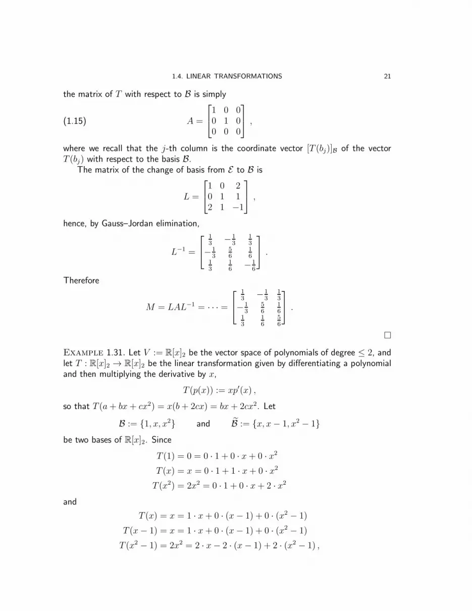
1.4. LINEAR TRANSFORMATIONS 21
the matrix of T with respect to B is simply
A =
1 0 00 1 00 0 0
,(1.15)
where we recall that the j-th column is the coordinate vector [T (bj)]B of the vectorT (bj) with respect to the basis B.
The matrix of the change of basis from E to B is
L =
1 0 20 1 12 1 −1
,
hence, by Gauss–Jordan elimination,
L−1 =
13−1
313
−13
56
16
13
16−1
6
.
Therefore
M = LAL−1 = · · · =
13−1
313
−13
56
16
13
16
56
.
�
Example 1.31. Let V := R[x]2 be the vector space of polynomials of degree ≤ 2, andlet T : R[x]2 → R[x]2 be the linear transformation given by differentiating a polynomialand then multiplying the derivative by x,
T (p(x)) := xp′(x) ,
so that T (a+ bx+ cx2) = x(b+ 2cx) = bx+ 2cx2. Let
B := {1, x, x2} and B := {x, x− 1, x2 − 1}be two bases of R[x]2. Since
T (1) = 0 = 0 · 1 + 0 · x+ 0 · x2
T (x) = x = 0 · 1 + 1 · x+ 0 · x2
T (x2) = 2x2 = 0 · 1 + 0 · x+ 2 · x2
and
T (x) = x = 1 · x+ 0 · (x− 1) + 0 · (x2 − 1)
T (x− 1) = x = 1 · x+ 0 · (x− 1) + 0 · (x2 − 1)
T (x2 − 1) = 2x2 = 2 · x− 2 · (x− 1) + 2 · (x2 − 1) ,

22 1. REVIEW OF LINEAR ALGEBRA
then
A =
0 0 00 1 00 0 2
and A =
1 1 20 0 −20 0 2
.
One can check that indeed AL = LA or, equivalently A = L−1AL, where
L =
0 −1 −11 1 00 0 1
is the matrix of the change of basis. �
1.4.2. Conjugate Matrices.
The above calculations can be summarized by the commutativity of the followingdiagram. Here, the vertical arrows correspond to the operation of change of basis from Bto B (recall that the coordinate vectors are contravariant tensors, that is, they transformas [v]B = L−1[v]B) and the horizontal arrows correspond to the operation of applyingthe transformation T with respect to the two different basis:
[v]B✤ A
//❴
L−1
��
[T (v)]B❴
L−1
��
[v]B✤
A
// [T (v)]B .
Saying that the diagram is commutative is saying that if one starts from the upper lefthand corner, reaching the lower right hand corner following either one of the two pathshas exactly the same effect. In other words, changing coordinates first then applying thetransformation T yields exactly the same affect as applying first the transformation T
and then the change of coordinates, that is, L−1A = AL−1 or, equivalently,
A = L−1AL .
In this case we say that A and A are conjugate matrices. This means that A and Arepresent the same transformation with respect to different bases.
Definition 1.32. We say that two matrices A and A are conjugate if there exists andinvertible matrix L such that A = L−1AL.
Example 1.33. The three matrices from Example 1.28 and Example 1.29
A =
[1 32 4
]M =
[5 12 0
]and A =
[5 −2−1 0
]
are all conjugate. Indeed, we have
A = L−1AL , A = S−1MS and A = R−1MR ,

1.4. LINEAR TRANSFORMATIONS 23
where L and S may be found in those examples and where R := SL. �
We now review some facts about conjugate matrices. Recall that the characteristicpolynomial of a square matrix A is the polynomial
pA(λ) := det(A− λI) .
Let us assume that A and A are conjugate matrices, that is A = L−1AL for someinvertible matrix L. Then
pA(λ) = det(A− λI) = det(L−1AL− λL−1IL)
= det(L−1(A− λI)L)=
✘✘✘✘✘
(detL−1) det(A− λI)✘✘✘✘(detL) = pA(λ) ,
(1.16)
which means that any two conjugate matrices have the same characteristic polynomial.Recall that the eigenvalues of a matrix A are the roots of its characteristic poly-
nomial and we here usually allow complex roots. Then, by the so-called fundamentaltheorem of Algebra, each n×n matrix has n (real or complex) eigenvalues counted withmultiplicities as polynomial roots. Recall also the definitions of determinant and traceof a square matrix. By analysing the characteristic polynomial, we see that
(1) the determinant of a matrix is equal to the product of its eigenvalues (multi-plied with multiplicities), and
(2) the trace of a matrix is equal to the sum of its eigenvalues (added with multi-plicities).
From (1.16) if follows that, if the matrices A and A are conjugate, then:
• A and A have the same size;• the eigenvalues of A (as well as their multiplicities) are the same as those of A;
• detA = det A;• trA = tr A;• A is invertible if and only if A is invertible.
Example 1.34. The matrices A =
[1 32 4
]and A′ =
[1 22 4
]are not conjugate. In fact,
A is invertible, as detA = −2 6= 0, while detA′ = 0, so that A′ is not invertible. �
1.4.3. Eigenbases.
The possibility of choosing different bases is very important and often simplifies thecalculations. Example 1.30 is such an example, where we choose an appropriate basisaccording to the specific problem. Other times, a basis can be chosen according to thesymmetries and, completely at the opposite side, sometime there is just not a basis thatis a preferred one. In the context of a linear transformation T : V → V , a basis that isparticularly convenient, when it exists, is an eigenbasis for that linear transformation.

24 1. REVIEW OF LINEAR ALGEBRA
Recall that an eigenvector of a linear transformation T : V → V is a vector v 6= 0such that T (v) is a multiple of v, say T (v) = λv and, in that case, the scaling numberλ is called an eigenvalue of T .
An eigenbasis is a basis of V consisting of eigenvectors of a linear transformationT : V → V . The point of having an eigenbasis is that, with respect to this eigenbasis, thelinear transformation is representable by a diagonal matrix, D. Hence, the initial matrixrepresentative A is actually conjugate to a diagonal matrix D. A linear transformationT : V → V for which an eigenbasis exists is then called diagonalizable.4
Given a linear transformation T : V → V , in order to find an eigenbasis of T , wefirst represent T by some matrix A (with respect to some chosen basis of V ), and thenperform the following steps:
(1) We find the eigenvalues by determining the roots of the characteristic polyno-mial of A (often allowing complex roots).
(2) For each eigenvalue λ, we find the corresponding eigenvectors by looking forthe nonzero vectors in the so-called eigenspace
Eλ := ker(A− λI) .
When considering complex eigenvalues, the eigenspaces are determined as sub-spaces of the complex vector space Cn. However, in this text, we concentrateon real cases.
(3) We determine whether there exists an eigenbasis.
We will illustrate this in the following examples.
Example 1.35. Let T : R2 → R2 be the linear transformation given by the matrix
A =
[3 −4−4 −3
]with respect to the standard basis of R2.
(1) The eigenvalues are the roots of the characteristic polynomial pλ(A). Since
pA(λ) = det(A− λI) = det
[3− λ −4−4 −3− λ
]
= (3− λ)(−3− λ)− 16 = λ2 − 25 = (λ− 5)(λ+ 5) ,
hence λ = ±5 are the eigenvalues of A.(2) If λ is an eigenvalue of A, the eigenspace corresponding to λ is given by Eλ =
ker(A− λI). Note that
v ∈ Eλ ⇐⇒ Av = λv .
4In general, when an eigenbasis does not exist, it is still possible to find a basis, with respect towhich the linear transformation is as simple as possible, i.e., as close as possible to being diagonal.Such a best matrix representative of T : V → V is called a Jordan canonical form and is, of course,conjugate to the first matrix representative A. In this text, we will not address such more generalcanonical forms.

1.4. LINEAR TRANSFORMATIONS 25
With our choice of A and with the resulting eigenvalues, we have
E5 = ker(A− 5I) = ker
[−2 −4−4 −8
]= span
[2−1
]
E−5 = ker(A+ 5I) = ker
[8 −4−4 2
]= span
[12
].
(3) The following is an eigenbasis for this linear transformation:
B =
{b1 =
[2−1
], b2 =
[12
]}
and
T (b1) = 5b1 = 5 · b1 + 0 · b2T (b2) = −5b2 = 0 · b1 − 5 · b2 ,
so that A =
[5 00 −5
].
x+ 2y = 0
b1
b2
Notice that the eigenspace E5 consists of vectors on the line x + 2y = 0and these vectors get scaled by the transformation T by a factor of 5. On theother hand, the eigenspace E−5 consists of vectors perpendicular to the linex+2y = 0 and these vectors get flipped by the transformation T and then alsoscaled by a factor of 5. Hence T is just the reflection across the line x+2y = 0followed by multiplication by 5.
�
Example 1.36. Now let T : R2 → R2 be the linear transformation given by the matrix
A =
[1 24 3
]with respect to the standard basis of R2.
(1) The eigenvalues are the roots of the characteristic polynomial:
pA(λ) = det(A− λI) = det
[1− λ 24 3− λ
]
= (1− λ)(3− λ)− 2 · 4 = λ2 − 4λ− 5 = (λ+ 1)(λ− 5) ,
hence λ = −1 and λ = 5 are the eigenvalues of A.
26 1. REVIEW OF LINEAR ALGEBRA
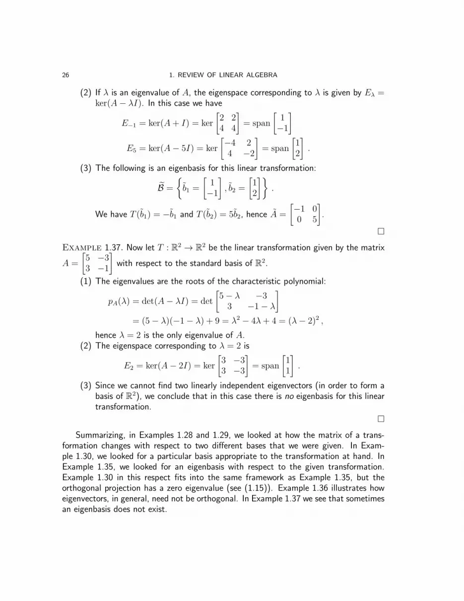
(2) If λ is an eigenvalue of A, the eigenspace corresponding to λ is given by Eλ =ker(A− λI). In this case we have
E−1 = ker(A+ I) = ker
[2 24 4
]= span
[1−1
]
E5 = ker(A− 5I) = ker
[−4 24 −2
]= span
[12
].
(3) The following is an eigenbasis for this linear transformation:
B =
{b1 =
[1−1
], b2 =
[12
]}.
We have T (b1) = −b1 and T (b2) = 5b2, hence A =
[−1 00 5
].
�
Example 1.37. Now let T : R2 → R2 be the linear transformation given by the matrix
A =
[5 −33 −1
]with respect to the standard basis of R2.
(1) The eigenvalues are the roots of the characteristic polynomial:
pA(λ) = det(A− λI) = det
[5− λ −33 −1− λ
]
= (5− λ)(−1− λ) + 9 = λ2 − 4λ+ 4 = (λ− 2)2 ,
hence λ = 2 is the only eigenvalue of A.(2) The eigenspace corresponding to λ = 2 is
E2 = ker(A− 2I) = ker
[3 −33 −3
]= span
[11
].
(3) Since we cannot find two linearly independent eigenvectors (in order to form abasis of R2), we conclude that in this case there is no eigenbasis for this lineartransformation.
�
Summarizing, in Examples 1.28 and 1.29, we looked at how the matrix of a trans-formation changes with respect to two different bases that we were given. In Exam-ple 1.30, we looked for a particular basis appropriate to the transformation at hand. InExample 1.35, we looked for an eigenbasis with respect to the given transformation.Example 1.30 in this respect fits into the same framework as Example 1.35, but theorthogonal projection has a zero eigenvalue (see (1.15)). Example 1.36 illustrates howeigenvectors, in general, need not be orthogonal. In Example 1.37 we see that sometimesan eigenbasis does not exist.
CHAPTER 2
Multilinear Forms
2.1. Linear Forms
Linear forms on a vector space V are defined as linear real-valued functions on V .We will see that linear forms behave very much like vectors, only that they are elementsnot of V , but of a different, yet related, vector space. Whereas we represent regularvectors (from V ) by column vectors once a basis is fixed, we will represent linear forms(on V ) by row vectors. Then the value of a linear form on a specific vector is simplygiven by by the matrix product with the row vector (linear form) on the left and thecolumn vector (actual vector) on the right.
2.1.1. Definition and Examples.
Definition 2.1. Let V be a vector space. A linear form on V is a map α : V → R
such that for every a, b ∈ R and for every v, w ∈ V
α(av + bw) = aα(v) + bα(w) .
Alternative terminologies for “linear form” are tensor of type (0, 1), 1-form, linearfunctional and covector.
Exercise 2.2. If V = R3 , which of the following are linear forms?
(1) α(x, y, z) := xy + z;(2) α(x, y, z) := x+ y + z + 1;(3) α(x, y, z) := πx− 7
2z.
Exercise 2.3. If V is the infinite dimensional vector space of continuous functionsf : R→ R, which of the following are linear forms?
(1) α(f) := f(7)− f(0);(2) α(f) :=
∫ 33
0exf(x)dx;
(3) α(f) := ef(4).
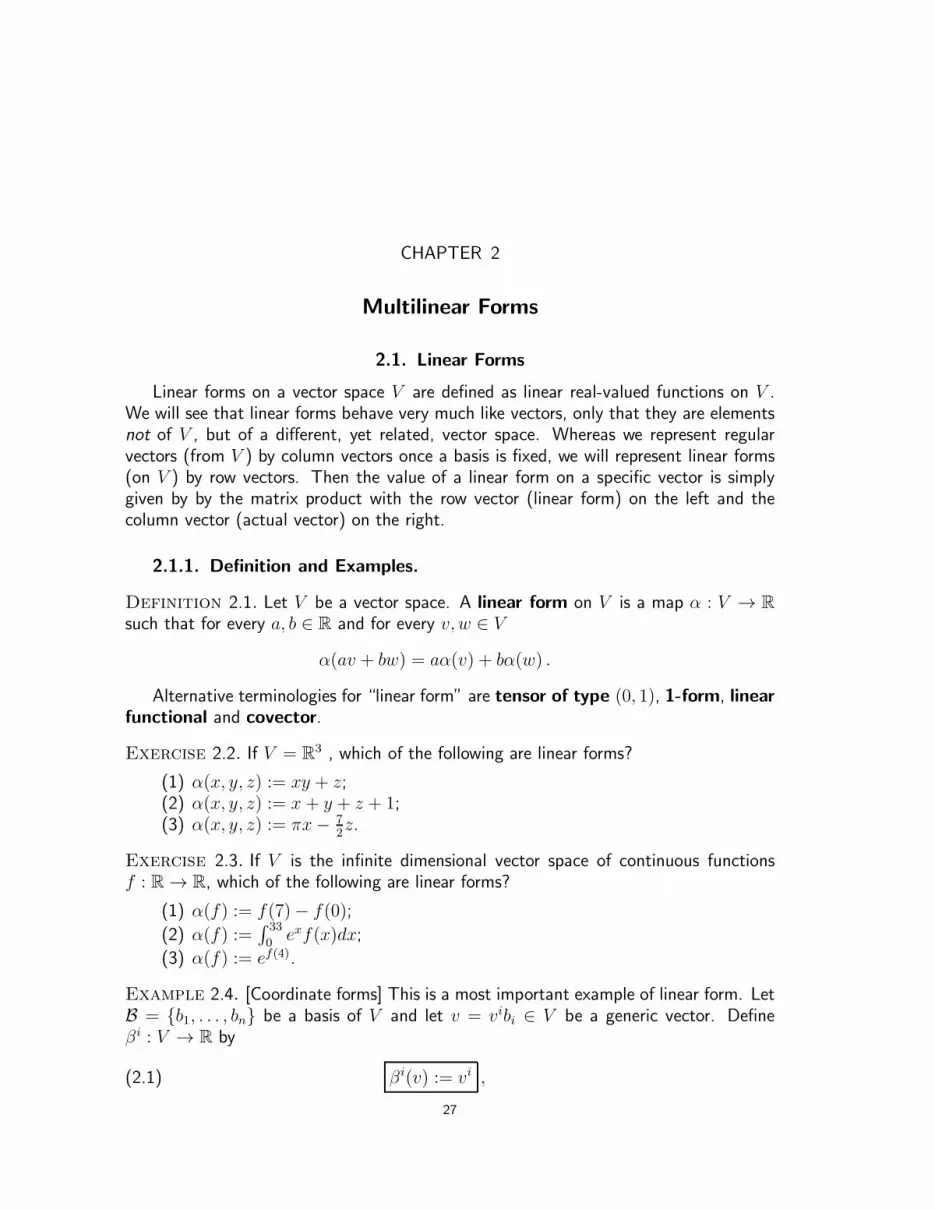
Example 2.4. [Coordinate forms] This is a most important example of linear form. LetB = {b1, . . . , bn} be a basis of V and let v = vibi ∈ V be a generic vector. Defineβi : V → R by
βi(v) := vi ,(2.1)
27

28 2. MULTILINEAR FORMS
that is βi will extract the i-th coordinate of a vector with respect to the basis B. Thelinear form βi is called coordinate form. Notice that
βi(bj) = δij ,(2.2)
since the i-th coordinate of the basis vector bj with respect to the basis B is equal to 1if i = j and 0 otherwise. �
Example 2.5. Let V = R3 and let E be its standard basis. The three coordinate forms
are defined by
β1
xyz
:= x , β2
xyz
:= y , β3
xyz
:= z .
�
Example 2.6. Let V = R2 and let B :=
{ [11
]
︸︷︷︸b1
,
[1−1
]
︸ ︷︷ ︸b2
}. We want to describe the
elements of B∗ := {β1, β2}, in other words we want to find
β1(v) and β2(v)
for a generic vector v ∈ V .To this purpose we need to find [v]B. Recall that if E denotes the standard basis of
R2 and L := LBE the matrix of the change of coordinate from E to B, then
[v]B = L−1[v]E = L−1
(v1
v2
).
Since
L =
[1 11 −1
]
and hence
L−1 = 12
[1 11 −1
],
then
[v]B =
( 12(v1 + v2)
12(v1 − v2)
).
Thus, according to the definition (2.1), we deduce that
β1(v) = 12(v1 + v2) and β2(v) = 1
2(v1 − v2) .
�

2.1. LINEAR FORMS 29
2.1.2. Dual Space and Dual Basis.
We define
V ∗ := {all linear forms α : V → R} ,and call this the dual (or dual space) of V .
Exercise 2.7. Check that V ∗ is a vector space whose null vector is the linear formidentically equal to zero.
Remark 2.8. Just like any function, two linear forms on V are equal if and only if theirvalues are the same when applied to each vector in V . However, because of the definingproperties of linear forms, to determine whether two linear forms are equal, it is enoughto check that they are equal on each element of a basis of V . In fact, let α, α′ ∈ V ∗,let B = {b1, . . . , bn} be a basis of V and suppose that we know that
α(bj) = α′(bj)
for all 1 ≤ j ≤ n. We verify that this implies that they are the same when applied toeach vector v ∈ V . In fact let v = vjbj its representation with respect to the basis B.Then we have
α(v) = α(vjbj) = vjα(bj) = vjα′(bj) = α′(vjbj) = α′(v) .
�
Proposition 2.9. Let B = {b1, . . . , bn} be a basis of V and β1, . . . , βn the correspond-ing coordinate forms. Then B∗ := {β1, . . . , βn} is a basis of V ∗. As a consequence
dimV = dimV ∗ .
Proof. According to Definition 1.17, we need to check that the linear forms in B∗
(1) are linearly independent and(2) span V ∗.
(1) We need to check that the only linear combination of β1, . . . , βn that yields the zerolinear form is the trivial linear combination. Let ciβ
i = 0 be a linear combination of theβi. Then for every basis vector bj , with j = 1, . . . , n,
0 = (ciβi)(bj) = ci(β
i(bj)) = ciδij = cj ,
thus showing the linear independence.
(2) To check that B∗ spans V we need to verify that any α ∈ V ∗ is a linear combinationof β1, . . . , βn, that is that we can find αi ∈ R such that
α = αiβi(2.3)
To find such αi we apply both sides of (2.3) to the j-th basis vector bi, and we obtain
α(bj) = αiβi(bj) = αiδ
ij = αj ,(2.4)

30 2. MULTILINEAR FORMS
which identifies the coefficients in (2.3).By hypothesis α is a linear form and, since V ∗ is a vector space, also α(bi)β
i is alinear form. Moreover, we have just verified that these two linear form coincide on thebasis vectors. By Remark 2.8 the two linear forms are the same and, hence, we havewritten α as a linear combination of the coordinate forms. This completes the proofthat the coordinate forms form a basis of the dual. �
The basis B∗ of V ∗ is called the basis of V ∗ dual to B. We emphasize that thecomponents (or coordinates) of a linear form α with respect to B∗ are exactly the valuesof α on the elements of B, as we found in the above proof:
αi = α(bi) .
We build with these the coordinate-vector of α as a row-vector:
[α]B∗ :=(α1 . . . αn
).
Example 2.10. Let V = R[x]2 be the vector space of polynomials of degree ≤ 2, letα : V → R be the linear form given by
α(p) := p(2)− p′(2)(2.5)
and let B be the basis {1, x, x2} of V . In this example, we want to:
(1) find the components of α with respect to B∗;(2) describe the basis B∗ = {β1, β2, β3};
(1) Since
α1 = α(b1) = α(1) = 1− 0 = 1
α2 = α(b2) = α(x) = 2− 1 = 1
α3 = α(b3) = α(x2) = 4− 4 = 0 ,
then
[α]B∗ =(1 1 0
).(2.6)
(2) The generic element p(x) ∈ R[x]2 written as combination of basis elements 1, x andx2 is
p(x) = a+ bx+ cx2 .
Hence B∗ = {β1, β2, β3}, is given by
β1(a+ bx+ cx2) = a
β2(a+ bx+ cx2) = b
β3(a+ bx+ cx2) = c .
(2.7)
�

2.1. LINEAR FORMS 31
Remark 2.11. Note that we have to be careful when referring to a “dual basis” of V ∗,as for every basis B of V there is going to be a basis B∗ of V ∗ dual to the basis B. Inthe next section we are going to see how a dual basis transforms with a change of basis.
2.1.3. Covariance of Linear Forms.
We want to examine how a linear form α : V → R behaves with respect to a changea basis in V . To this purpose, let
B = {b1, . . . , bn} and B := {b1, . . . , bn}be two bases of V and let
B∗ := {β1, . . . , βn} and B∗ := {β1, . . . , βn}be the corresponding dual bases. Let
[α]B∗ =(α1 . . . αn
)and [α]B∗ =
(α1 . . . αn
)
be the coordinate vectors of α with respect to B∗ and B∗, that is
α(bi) = αi and α(bi) = αi .
Let L := LBB be the matrix of the change of basis in (1.3)
bj = Lijbi .
Then
αj = α(bj) = α(Lijbi) = Li
jα(bi) = Lijαi = αiL
ij ,(2.8)
so that
αj = αiLij .(2.9)
Exercise 2.12. Verify that (2.9) is equivalent to saying that
[α]B∗ = [α]B∗L .(2.10)
Note that we have exchanged the order of αi and Lij in the last equation in (2.8) to
respect the order in which the matrix multiplication in (2.10) has to be performed. Thiswas possible because both αi and L
ij are real numbers.
We say that a linear form α is covariant because its components change by L whenthe basis changes by L.5 A linear form α is hence a covariant tensor or a tensor oftype (0, 1).
5In Latin, the prefix co means “joint”.

32 2. MULTILINEAR FORMS
Example 2.13. We continue with Example 2.10. We consider the bases as in Exam-ple 1.31, that is
B := {1, x, x2} and B := {x, x− 1, x2 − 1}and the linear form α : V → R as in (2.5). We will:
(1) find the components of α with respect to B∗;(2) describe the basis B∗ = {β1, β2, β3};(3) find the components of α with respect to B∗;
(4) describe the basis B∗ = {β1, β2, β3};(5) find the matrix of change of basis L := LBB and compute Λ = L−1;(6) check the covariance of α;(7) check the contravariance of B∗.
(1) This is done in (2.6).
(2) This is done in (2.7).
(3) We proceed as in (2.6). Namely,
α1 = α(b1) = α(x) = 2− 1 = 1
α2 = α(b2) = α(x− 1) = 1− 1 = 0
α3 = α(b3) = α(x2 − 1) = 3− 4 = −1 ,so that
[α]B∗ =(1 0 −1
).
(4) Since βi(v) = vi, to proceed as in (2.7) we first need to write the generic polynomial
p(x) = a + bx + cx2 as a linear combination of elements in B, namely we need to find
a, b and c such that
p(x) = a+ bx+ cx2 = ax+ b(x− 1) + c(x2 − 1) .
By multiplying and collecting the terms, we obtain that
− b− c = a
a+ b = b
c = c
that is
a = a+ b+ c
b = −a− cc = c .
Hence
p(x) = a + bx+ cx2 = (a+ b+ c)x+ (−a− c)(x− 1) + c(x2 − 1) ,
so that it follows that
β1(p(x)) = a+ b+ c
β2(p(x)) = −a− cβ3(p(x)) = c ,

2.1. LINEAR FORMS 33
(5) The matrix of the change of basis is given by
L := LBB =
0 −1 −11 1 00 0 1
,
since for example b3 can be written as a linear combination with respect to B as b3 =x2 − 1 = −1b1 + 0b2 + 1b3, and these coordinates −1, 0, 1 build the third column of L.
To compute Λ = L−1 we can use the Gauss–Jordan elimination process0 −1 −1 1 0 01 1 0 0 1 00 0 1 0 0 1
! . . . !
1 0 0 1 1 10 1 0 −1 0 −10 0 1 0 0 1
Therefore, we have
Λ =
1 1 1−1 0 −10 0 1
.
(6) The linear form α is indeed covariant, since
(α1 α2 α3
)L =
(1 1 0
)0 −1 −11 1 00 0 1
=
(1 0 −1
)=(α1 α2 α3
).
(7) The dual basis B∗ is contravariant, since
β1
β2
β3
= Λ
β1
β2
β3
,
as it can be verified by evaluating both sides on an arbitrary vector p(x) = a+ bx+ cx2:
Λ
β1(p)β2(p)β3(p)
=
1 1 1−1 0 −10 0 1
abc
=
a+ b+ c−a− cc
=
β1(p)
β2(p)
β3(p)
.
�
2.1.4. Contravariance of Dual Bases.
In fact, statement (7) in Example 2.10 holds in general, namely:
Proposition 2.14. Dual bases are contravariant.
Proof. We will check that when bases B and B are related by
bj = Lijbi

34 2. MULTILINEAR FORMS
V real vector space V ∗ = {linear forms α : V → R}with dimV = n dual vector space to V
B = {b1, . . . , bn} B∗ = {β1, . . . , βn}basis of V dual basis of V ∗ w.r.t. B
B := {b1, . . . , bn} B∗ = {β1, . . . , βn}another basis of V dual basis of V ∗ w.r.t. B∗
L := LBB =matrix of the change Λ = L−1 =matrix of the change
of basis from B to B of basis from B to BThen we have bj = Li
jbi or Then we have βi = Λijβ
j or
(b1 . . . bn
)=(b1 . . . bn
)L
β1
...
βn
= L−1
β1
...βn
covariance of a basis contravariance of the dual basis
If v is any vector in V , If α is any linear form in V ∗,
then v = vibi = vibi, where then α = αjβj = αj β
j, where
vi = Λijv
j i.e. [v]B = L−1[v]B or αj = Lijαi i.e. [α]B∗ = [α]B∗L or
v1...vn
= L−1
v1...vn
(α1 . . . αn
)=(α1 . . . αn
)L
contravariance of the coordinate vectors covariance of linear forms components
→ vectors are (1, 0)-tensors → linear forms are (0, 1)-tensors
Table 1. Summary regarding duality
the corresponding dual bases B∗ and B∗ of V ∗ are related by
βj = Λjiβ
i .(2.11)
It is enough to check that the Λjiβ
i are dual to the bj . In fact, since ΛL = I, then
(Λkℓβ
ℓ)(bj) = (Λkℓβ
ℓ)(Lijbi) = Λk
ℓLijβ
ℓ(bi) = ΛkℓL
ijδ
ℓi = Λk
iLij = δkj = βj(bj) .
�
In Table 1, you can find a summary of the properties that bases and dual bases,coordinate vectors and components of linear forms satisfy with respect to a changeof basis and hence whether they are covariant or contravariant. Moreover, Table 2summarizes the characteristics of covariance and contravariance.

2.2. BILINEAR FORMS 35
covariance contravariaceof a tensor of a tensor
is denoted by lower indices upper indicescoordinate-vectors are indicated as row vectors column vectorsthe tensor transforms w.r.t. a change of
basis from B to B by multiplication with L on the right L−1 on the left(for later use)a tensor of type (p, q) has covariant order q contravariant order p
Table 2. Covariance vs. contravariance
2.2. Bilinear Forms
2.2.1. Definition and Examples.
Definition 2.15. A bilinear form on V is a function ϕ : V × V → R that is linear ineach variable, that is
ϕ(u, λv + µw) = λϕ(u, v) + µϕ(u, w)
ϕ(λv + µw, u) = λϕ(v, u) + µϕ(w, u) ,
for every λ, µ ∈ R and for every u, v, w ∈ V .
Examples 2.16. Let V = Rn.
(1) If v, w ∈ Rn, the dot product (or scalar product) defined as
ϕ(v, w) := v · w = |v| |w| cos θ ,where θ is the angle between v and w is a bilinear form.
(2) Let n = 3. Choose a vector u ∈ R3 and for any two vectors v, w ∈ R
3, denoteby v × w their cross product. The scalar triple product
ϕu(v, w) := u · (v × w) = det
uvw
(2.12)
is a bilinear form in v and w, where
uvw
denotes the matrix with rows u, v and
w. The quantity ϕu(v, w) calculates the signed volume of the parallelepipedspanned by u, v, w: the sign of ϕu(v, w) depends on the orientation of the tripleu, v, w.
Since the cross product is defined only in R3, in contrast with the scalarproduct, the scalar triple product cannot be defined in R
n with n 6= 3 (thoughthere is a formula for an n dimensional parallelediped involving some “general-ization” of it).
�

36 2. MULTILINEAR FORMS
Exercise 2.17. Verify the equality in (2.12) using the Leibniz formula for the determi-nant of a 3× 3 matrix. Recall that
det
a11 a12 a13a21 a22 a23a31 a32 a33
=a11a22a33 − a11a23a32 + a12a23a31
−a12a21a33 + a13a21a32 − a13a22a31
=∑
σ∈S3
sign(σ)a1σ(1)a2σ(2)a3σ(3) ,
where
σ = (σ(1), σ(2), σ(3)) ∈ S3 := {permutations of 3 elements}= {(1, 2, 3), (1, 3, 2), (2, 3, 1), (2, 1, 3), (3, 1, 2), (3, 2, 1)} ,
and the corresponding signs flip each time two elements get swapped:
sign(1, 2, 3) = 1 , sign(1, 3, 2) = −1 , sign(3, 1, 2) = 1 ,
sign(3, 2, 1) = −1 , sign(2, 3, 1) = 1 , sign(2, 1, 3) = −1 .An even permutation is a permutation σ with sign(σ) = 1; an odd permutation isa permutation σ with sign(σ) = −1.Examples 2.18. Let V = R[x]2.
(1) Let p, q ∈ R[x]2. The function ϕ(p, q) := p(π)q(33) is a bilinear form.(2) Likewise,
ϕ(p, q) := p′(0)q(4)− 5p′(3)q′′(12)
is a bilinear form.
�
Exercise 2.19. Are the following functions bilinear forms?
(1) V = R2 and ϕ(u, v) := det
[uv
];
(2) V = R[x]2 and ϕ(p, q) :=∫ 1
0p(x)q(x)dx;
(3) V = M2×2(R), the space of real 2 × 2 matrices, and ϕ(L,M) := L11 trM ,
where L11 it the (1,1)-entry of L and trM is the trace of M ;
(4) V = R3 and ϕ(v, w) := v × w;(5) V = R2 and ϕ(v, w) is the area of the parallelogram spanned by v and w.(6) V =Mn×n(R), the space of real n× n matrices with n > 1, and ϕ(L,M) :=
trL detM , where trL is the trace of L and detM is the determinant of M .
Remark 2.20. We need to be careful about the following possible confusion. A bilinearform on V is a function on V × V that is linear in each variable separately. But V × Vis also a vector space and one might wonder whether a bilinear form on V is also a linear

2.2. BILINEAR FORMS 37
form on the vector space V × V . But this is not the case. For example consider thecase in which V = R, so that V × V = R2 and let ϕ : R× R→ R be a function:
(1) If ϕ(x, y) := 2x− y, then ϕ is not a bilinear form on R, but is a linear form on(x, y) ∈ R2;
(2) If ϕ(x, y) := 2xy, then ϕ is a bilinear form on R (hence linear in x ∈ R
and linear in y ∈ R), but it is not a linear form on R2, as it is not linear in
(x, y) ∈ R2.
So a bilinear form is not a form that it is “twice as linear” as a linear form, but a formthat is defined on the product of twice the vector space.
�
Exercise 2.21. Verify the above assertions in Remark 2.20 to make sure you understandthe difference.
2.2.2. Tensor Product of Two Linear Forms on V .
Let α, β ∈ V ∗ be two linear forms, α, β : V → R, and define ϕ : V × V → R, by
ϕ(v, w) := α(v)β(w) .
Then ϕ is bilinear, is called the tensor product of α and β and is denoted by
ϕ = α⊗ β .Note 2.22. In general α ⊗ β 6= β ⊗ α, as there could be vectors v and w such thatα(v)β(w) 6= β(v)α(w).
Example 2.23. Let V = R[x]2, let α(p) = p(2)− p′(2) and β(p) =∫ 4
3p(x)dx be two
linear forms. Then
(α⊗ β)(p, q) = (p(2)− p′(2))∫ 4
3
q(x)dx
is a bilinear form. �
Remark 2.24. The bilinear form ϕ : R×R→ R defined by the formula ϕ(x, y) := 2xyis the tensor product of two linear forms on R, for instance, ϕ(x, y) = (α ⊗ α)(x, y)where α : R→ R is the linear form given by α(x) :=
√2x.
On the other hand, not every bilinear form is simply the tensor product of two linearforms. As we will see below, the first such examples are found for bilinear forms onvector spaces of dimension at least 2. �
2.2.3. A Basis for Bilinear Forms.
Let
Bil(V × V,R) := {all bilinear forms ϕ : V × V → R} .

38 2. MULTILINEAR FORMS
Exercise 2.25. Check that Bil(V ×V,R) is a vector space with the zero element equalto the bilinear form identically equal to zero.Hint: It is enough to check that if ϕ, ψ ∈ Bil(V ×V,R), and λ, µ ∈ R, then λϕ+µψ ∈Bil(V × V,R). Why? (Recall Example 1.3(3) on page 8 and Exercise 2.7 on page 29.)
Assuming Exercise 2.25, we are going to find a basis of Bil(V ×V,R) and determineits dimension. Let B = {b1, . . . , bn} be a basis of V and let B∗ = {β1, . . . , βn} be thedual basis of V ∗ (that is βi(bj) = δij).
Proposition 2.26. The bilinear forms βi⊗βj , i, j = 1, . . . , n form a basis of Bil(V ×V,R). As a consequence, dimBil(V × V,R) = n2.
Notation. We denote
Bil(V × V,R) = V ∗ ⊗ V ∗
and call this vector space the tensor product of V ∗ and V ∗. A justification for thisnotation will appear in §4.3.2.
Remark 2.27. Just as it is for linear forms, to verify that two bilinear forms on V arethe same it is enough to verify that they are the same on every pair of elements of abasis of V . In fact, let ϕ, ψ be two bilinear forms, let B = {b1, . . . , bn} be a basis of V ,and assume that
ϕ(bi, bj) = ψ(bi, bj)
for all 1 ≤ i, j,≤ n. Let v = vibi, w = wjbj ∈ V be arbitrary vectors. We now verifythat ϕ(v, w) = ψ(v, w). Because of the linearity in each variable, we have
ϕ(v, w) = ϕ(vibi, wjbj) = viwjϕ(bi, bj) = viwjψ(bi, bj) = ψ(vibi, w
jbj) = ψ(v, w) .
�
Proof of Proposition 2.26. The proof will be similar to the one of Proposi-tion 2.9 for linear forms. We first check that the set of bilinear forms {βi ⊗ βj, i, j =1, . . . , n} consists of linearly independent vectors, then that it spans Bil(V × V,R).
For the linear independence we need to check that the only linear combination ofthe βi ⊗ βj that gives the zero bilinear form is the trivial linear combination. Letcijβ
i⊗βj = 0 be a linear combination of the βi⊗βj. Then for all pairs of basis vectors(bk, bℓ), with k, ℓ = 1, . . . , n, we have
0 = cijβi ⊗ βj(bk, bℓ) = cijδ
ikδ
jℓ = ckℓ ,
thus showing the linear independence.To check that span{βi ⊗ βj, i, j = 1, . . . , n} = Bil(V × V,R), we need to check
that if ϕ ∈ Bil(V × V,R), there exists Bij ∈ R such that
ϕ = Bijβi ⊗ βj .
Because of (2.2) on page 28, we obtain
ϕ(bk, bℓ) = Bijβi(bk)β
j(bℓ) = Bijδikδ
jℓ = Bkℓ ,

2.2. BILINEAR FORMS 39
for every pair (bk, bℓ) ∈ V × V . Hence, we set Bkℓ := ϕ(bk, bℓ). Now both ϕ andϕ(bk, bℓ)β
i ⊗ βj are bilinear forms and they coincide on B × B. Because of the aboveRemark 2.27, the two bilinear forms coincide. �
Example 2.28. We continue with the study of the scalar triple product ϕu : R3×R3 →
R, that was defined in Example 2.16 for a fixed given vector u =
u1
u2
u3
. We now want
to find the components Bij of ϕu with respect to the standard basis of R3.Recall the cross product in R3 is defined on the elements of the standard basis by
ei × ej :=
0 if i = j
ek if (i, j, k) is a cyclic permutation of (1, 2, 3)
−ek if (i, j, k) is a noncyclic permutation of (1, 2, 3) ,
that is
cyclic
e1 × e2 = e3
e2 × e3 = e1
e3 × e1 = e2
and
noncyclic
e2 × e1 = −e3e3 × e2 = −e1e1 × e3 = −e2
Since u · ek = uk, then
Bij = ϕu(ei, ej) = u · (ei × ej) =
0 if i = j
uk if (i, j, k) is a cyclic permutation of (1, 2, 3)
−uk if (i, j, k) is a noncyclic permutation of (1, 2, 3)
Thus
B12 = u3 = −B21
B31 = u2 = −B13
B23 = u1 = −B32
B11 = B22 = B33 = 0 (that is, the diagonal components are zero) ,
which can be written as a matrix
B =
0 u3 −u2−u3 0 u1
u2 −u1 0
.
The components Bij of B are the components of this bilinear form with respect to thebasis βi ⊗ βj (i, j = 1, . . . , n), where βi(ek) = δik. Hence, we can write
ϕu = Bijβi ⊗ βj = u1
(β2 ⊗ β3 − β3 ⊗ β2
)
+u2(β3 ⊗ β1 − β1 ⊗ β3
)+ u3
(β1 ⊗ β2 − β2 ⊗ β1
).
�

40 2. MULTILINEAR FORMS
2.2.4. Covariance of Bilinear Forms.
We have seen that, once we choose a basis B = {b1, . . . , bn} of V , we automaticallyhave a basis B∗ = {β1, . . . , βn} of V ∗ and a basis {βi⊗βj , i, j = 1, . . . , n} of V ∗⊗V ∗.This implies, that any bilinear form ϕ : V ×V → R can be represented by its components
Bij = ϕ(bi, bj) ,(2.13)
in the sense that
ϕ = Bijβi ⊗ βj .
Moreover, these components can be arranged in a matrix6
B :=
B11 . . . B1n
......
Bn1 . . . Bnn
called the matrix of the bilinear form ϕ with respect to the chosen basis B. Thenatural question of course is: how does the matrix B change when we choose a differentbasis of V ?
So, let us choose a different basis B := {b1, . . . , bn} and corresponding bases B∗ =
{β1, . . . , βn} of V ∗ and {βi⊗ βj , i, j = 1, . . . , n} of V ∗⊗ V ∗, with respect to which ϕ
will be represented by a matrix B, whose entries are Bij = ϕ(bi, bj).
To see the relation between B and B, due to the change of basis from B to B, westart with the matrix of the change of basis L := LBB, according to which
bj = Lijbi .(2.14)
Then
Bij = ϕ(bi, bj) = ϕ(Lki bk, L
ℓjbℓ) = Lk
iLℓjϕ(bk, bℓ) = Lk
iLℓjBkℓ ,
where the first and the last equality follow from (2.13), the second from (2.14) (afterhaving renamed the dummy indices to avoid conflicts) and the remaining one from thebilinearity of σ. We conclude that
Bij = LkiL
ℓjBkℓ .
Exercise 2.29. Show that the formula of the transformation of the component of abilinear form in terms of the matrices of the change of coordinates is
B = tLBL ,(2.15)
where tL denotes the transpose of the matrix L.
6Note that, contrary to the matrix that gives the change of coordinates between two basis of thevector space, here we have only lower indices. This is not by chance and reflects the type of tensor abilinear form is.

2.3. MULTILINEAR FORMS 41
We hence say that a bilinear form ϕ is a covariant 2-tensor or a tensor of type(0, 2).
2.3. Multilinear Forms
2.3.1. Definition, Basis and Covariance.
We saw in §2.1.3 that linear forms are covariant 1-tensors – or tensors of type (0, 1)– and in §2.2.4 that bilinear forms are covariant 2-tensors – or tensors of type (0, 2).
Analogously to what was done until now, one can define trilinear forms on V , thatis functions T : V × V × V → R that are linear with respect to each of the threearguments. The space of trilinear forms on V is denoted
V ∗ ⊗ V ∗ ⊗ V ∗ ,
has basis
{βj ⊗ βj ⊗ βk, i, j, k = 1, . . . , n}and, hence, has dimension n3. The tensor product ⊗ is defined as above.
Since the components of a trilinear form T : V × V × V → R satisfy the followingtransformation with respect to a change of basis
Tijk = LℓiL
pjL
qkTℓpq ,
a trilinear form is a covariant 3-tensor or a tensor of type (0, 3).Of course, there is nothing special about k = 1, 2 or 3:
Definition 2.30. A k-linear form or multilinear form of order k on V is a functionf : V × · · ·× V → R from k-copies of V into R, that is linear in each of its arguments.
A k-linear form is a covariant k-tensor (or a covariant tensor of order k or atensor of type (0, k)). The vectors space of k-linear forms on V , denoted
V ∗ ⊗ · · · ⊗ V ∗︸ ︷︷ ︸
k factors
,
has basis
βi1 ⊗ βi2 ⊗ · · · ⊗ βik , i1, . . . , ik = 1, . . . , n
and, hence, dim(V ∗ ⊗ · · · ⊗ V ∗) = nk .
2.3.2. Examples of Multilinear Forms.
Example 2.31. We once more address the scalar triple product,7 discussed in Exam-ples 2.16 and 2.28. This time we want to find the components Bij of ϕu with respect
7The scalar triple product is called Spatprodukt in German.

42 2. MULTILINEAR FORMS
to the (nonstandard) basis
B :=
{010
︸︷︷︸b1
,
101
︸︷︷︸b2
,
001
︸︷︷︸b3
}.
The matrix of the change of coordinates from the standard basis to B is
L =
0 1 01 0 00 1 1
,
so that
B =
0 1 01 0 10 0 1
︸ ︷︷ ︸tL
0 u3 −u2−u3 0 u1
u2 −u1 0
︸ ︷︷ ︸B
0 1 01 0 00 1 1
︸ ︷︷ ︸L
=
0 1 01 0 10 0 1
︸ ︷︷ ︸tL
u3 −u2 −u20 u1 − u3 u1
−u1 u2 0
︸ ︷︷ ︸BL
=
0 u1 − u3 u1
u3 − u1 0 −u2−u1 u2 0
.
It is easy to check that B is antisymmetric just like B is, and to check that the compo-
nents of B are correct by using the formula for ϕ. In fact
B12 = ϕ(b1, b2) = u · (e2 × (e1 + e3)) = u1 − u3
B13 = ϕ(b1, b3) = u · ((e2)× e3) = u1
B23 = ϕ(b2, b3) = u · ((e1 + e3)× e3) = −u2
B11 = ϕ(b1, b1) = u · (e2 × e2) = 0
B22 = ϕ(b2, b2) = u · ((e1 + e3)× (e1 + e3)) = 0
B33 = ϕ(b3, b3) = u · (e3 × e3) = 0
�
Example 2.32. If, in the definition of the scalar triple product, instead of fixing a vectora ∈ R, we let the vector vary, we have a function ϕ : R3 × R
3 × R3 → R, defined by
ϕ(u, v, w) := u · (v × w) = det
uvw
.
One can verify that such function is trilinear, that is linear in each of the three variablesseparately.

2.3. MULTILINEAR FORMS 43
The components Tijk of this trilinear form are simply given by the sign of the corre-sponding permutation:
ϕ = sign(i, j, k)βi ⊗ βj ⊗ βk = β1 ⊗ β2 ⊗ β3 − β1 ⊗ β3 ⊗ β2 + β3 ⊗ β1 ⊗ β2
−β3 ⊗ β2 ⊗ β1 + β2 ⊗ β3 ⊗ β1 − β2 ⊗ β1 ⊗ β3 ,
where the sign of the permutation is given by
sign(i, j, k) :=
+1 if (i, j, k) = (1, 2, 3), (2, 3, 1) or (3, 1, 2)
(even permutations of (1, 2, 3))
−1 if (i, j, k) = (1, 3, 2), (2, 1, 3) or (3, 2, 1)
(odd permutations of (1, 2, 3))
0 otherwise.
�
Example 2.33. In general, the determinant defines an n-linear form in Rn by
ϕ : Rn × . . .× Rn
︸ ︷︷ ︸n factors
−→ R , ϕ(v1, . . . , vn) := det
v1...vn
,
where we compute the determinant of the square matrix with rows (equivalently, columns)given by the n vectors. Multilinearity is a fundamental property of the determinant.
In this case, the components of this multilinear form are also given by the permutationsigns:
ϕ = sign(i1, . . . , in)βi1 ⊗ . . .⊗ βin ,
where
sign(i1, . . . , in) :=
+1 if (i1, . . . , in) is an even permutation of (1, . . . , n)
−1 if (i1, . . . , in) is an odd permutation of (1, . . . , n)
0 otherwise.
A permutation of (1, 2, . . . , n) is called an even permutation, if it is obtained from(1, 2, . . . , n) by an even number of two-element swaps; otherwise it is called an oddpermutation. �
2.3.3. Tensor Product for Multilinear Forms.
Let
T : V × · · · × V︸ ︷︷ ︸k times
→ R and U : V × · · · × V︸ ︷︷ ︸ℓ times
→ R

44 2. MULTILINEAR FORMS
be, respectively, a k-linear and an ℓ-linear form. Then the tensor product of T and Uis the function
T ⊗ U : V × · · · × V︸ ︷︷ ︸k+ℓ times
→ R
defined by
T ⊗ U(v1, . . . , vk+ℓ) := T (v1, . . . , vk)U(vk+1, . . . , vk+ℓ).
This is a (k + ℓ)-linear form. Equivalently, this is saying that the tensor product of atensor of type (0, k) and a tensor of type (0, ℓ) is a tensor of type (0, k + ℓ). Later wewill see how this product extends to more general tensors.

CHAPTER 3
Inner Products
3.1. Definitions and First Properties
Inner products are a special case of bilinear forms. They add an important structureto a vector space, as for example they allow to compute the length of a vector and theyprovide a canonical identification between the vector space V and its dual V ∗.
3.1.1. Inner Products and their Related Notions.
Definition 3.1. An inner product g : V × V → R on a real vector space V is abilinear form on V that is
(1) symmetric, that is g(v, w) = g(w, v) for all v, w ∈ V and(2) positive definite, that is g(v, v) ≥ 0 for all v ∈ V , and g(v) = 0 if and only if
v = 0.
Exercise 3.2. Let V = R3. Verify that the dot product ϕ(v, w) := v · w, defined as
v · w = viwi ,
where v =
v1
v2
v3
and w =
w1
w2
w3
is an inner product. This is called the standard inner
product.
Exercise 3.3. Determine whether the following bilinear forms ϕ : Rn × R
n → R
are inner products, by verifying whether they are symmetric and positive definite (theformulas are troughout defined for all v, w ∈ Rn):
(1) ϕ(v, w) := −v · w;(2) ϕ(v, w) := v · w + 2v1w2;(3) ϕ(v, w) := v1w1;(4) ϕ(v, w) := v · w − 2v1w1;(5) ϕ(v, w) := v · w + 2v1w1;(6) ϕ(v, w) := v · 3w.
Exercise 3.4. Let V := R[x]2 be the vector space of polynomials of degree ≤ 2.Determine whether the following bilinear forms are inner products, by verifying whetherthey are symmetric and positive definite:
45

46 3. INNER PRODUCTS
(1) ϕ(p, q) :=∫ 1
0p(x)q(x)dx;
(2) ϕ(p, q) :=∫ 1
0p′(x)q′(x)dx;
(3) ϕ(p, q) :=∫ π
3exp(x)q(x)dx;
(4) ϕ(p, q) := p(1)q(1) + p(2)q(2);(5) ϕ(p, q) := p(1)q(1) + p(2)q(2) + p(3)q(3).(6) ϕ(p, q) := p(1)q(2) + p(2)q(3) + p(3)q(1).
Definition 3.5. Let g : V × V → R be an inner product on V .
(1) The norm ‖v‖ of a vector v ∈ V is defined as
‖v‖ :=√g(v, v) .
(2) A vector v ∈ V is unit vector if ‖v‖ = 1;(3) Two vectors v, w ∈ V are orthogonal (that is, perpendicular denoted v ⊥ w),
if g(v, w) = 0;(4) Two vectors v, w ∈ V are orthonormal if they are orthogonal and ‖v‖ =‖w‖ = 1;
(5) A basis B of V is an orthonormal basis if b1, . . . , bn are pairwise orthonormalvectors, that is
g(bi, bj) = δij :=
{1 if i = j
0 if i 6= j ,(3.1)
for all i, j = 1 . . . , n. The condition for i = j implies that an orthonormalbasis consists of unit vectors, while the one for i 6= j implies that it consists ofpairwise orthogonal vectors.
Example 3.6.
(1) Let V = Rn and g the standard inner product. The standard basis B ={e1, . . . , en} is an orthonormal basis with respect to the standard inner product.
(2) Let V = R[x]2 and let g(p, q) :=∫ 1
−1p(x)q(x)dx. Check that the basis
B = {p1, p2, p3} ,
where
p1(x) :=1√2, p2(x) :=
√32x, p3(x) :=
√58(3x2 − 1) ,
is an orthonormal basis with respect to the inner product g. Up to scaling,p1, p2, p3 are the so-called first three Legendre polynomials.
�

3.1. DEFINITIONS AND FIRST PROPERTIES 47
An inner product g on a vector space V induces a metric8 on V , where the distancebetween vectors v, w ∈ V is given by
d(v, w) := ‖v − w‖ .
3.1.2. Symmetric Matrices and Quadratic Forms.
Recall that a matrix S ∈Mn×n(R) is symmetric if S = tS, that is if
S =
∗ a b . ..
a ∗ c . ..
b c ∗ . ..
. ... .. ∗
.
Moreover, if S is symmetric, then
(1) S is positive definite if tvSv > 0 for all v ∈ Rn \ {0};(2) S is negative definite if tvSv < 0 for all v ∈ Rn \ {0};(3) S is positive semidefinite if tvSv ≥ 0 for all v ∈ Rn;(4) S is positive semidefinite if tvSv ≤ 0 for all v ∈ Rn;(5) S is indefinite if vtSv takes both positive and negative values for different
v ∈ Rn.
Definition 3.7. A quadratic form Q : Rn → R is a homogeneous quadratic polyno-mial in n variables:
Q(x1, . . . , xn) = Qijxixj , where Qij ∈ R .
To any symmetric matrix S corresponds a quadratic form QS : Rn → R definedby
QS(v) =tvSv =
[v1 . . . vn
]S
v1
...vn
︸ ︷︷ ︸matrix notation
= vivjSij︸ ︷︷ ︸Einstein notation
.(3.2)
Note that Q is not linear in v.Let S be a symmetric matrix and QS be the corresponding quadratic form. The
notion of positive definiteness, etc. for S can be translated into corresponding propertiesfor QS, namely:
(1) Q is positive definite if Q(v) > 0 for all v ∈ Rn \ {0};(2) Q is negative definite if Q(v) < 0 for all v ∈ Rn \ {0};
8An inner product induces a norm and a norm induces a metric on a vector space. However, theconverses do not hold.

48 3. INNER PRODUCTS
(3) Q is positive semidefinite if Q(v) ≥ 0 for all v ∈ Rn;(4) Q is negative semidefinite if Q(v) ≤ 0 for all v ∈ Rn;(5) Q is indefinite if Q(v) takes both positive and negative values.
Example 3.8. We consider R2 with the standard basis E and the quadratic form9
Q(v) := v1v1 − v2v2, where v =
[v1
v2
]. The symmetric matrix corresponding to Q is
S :=
[1 00 −1
]. If v =
[v1
0
], then Q(v) = 1 > 0, if v =
[0v2
], then Q(v) = −1 < 0,
but any vector for which v1 = v2 has the property that Q(v) = 0. �
To find out the type of a symmetric matrix S (or, equivalently of a quadratic formQS) it is enough to look at the eigenvalues of S, namely:
(1) S and QS are positive definite when all eigenvalues of S are positive:(2) S and QS are negative definite when all eigenvalues of S are negative;(3) S and QS are positive semidefinite when all eigenvalues of S are non-negative;(4) S and QS are negative semidefinite when all eigenvalues of S are non-positive;(5) S and QS are indefinite when S has both positive and negative eigenvalues.
The reason this makes sense is the same reason for which we need to restrict ourattention to symmetric matrices and lies in the so-called Spectral Theorem:
Theorem 3.9. [Spectral Theorem] Any n × n symmetric matrix S has the followingproperties:
(1) it has only real eigenvalues;(2) it is diagonalizable;(3) it admits an orthonormal eigenbasis, that is, a basis {b1, . . . , bn} of Rn such
that the bj are orthonormal and are eigenvectors of S.
3.1.3. Inner Products vs. Symmetric Positive Definite Matrices.
Let B = {b1, . . . , bn} be a basis of V and g an inner product. The components ofg with respect to B are
gij := g(bi, bj) .(3.3)
Let G be the matrix with entries gij
G =
g11 . . . g1n...
. . ....
gn1 . . . gnn
.(3.4)
We claim that G is symmetric and positive definite. In fact:
9Here, we avoid the usual notation for squares, because of the possible confusion with upper indices.

3.1. DEFINITIONS AND FIRST PROPERTIES 49
(1) Since g is symmetric, then for 1 ≤ i, j ≤ n,
gij = g(bi, bj) = g(bj, bi) = gji =⇒ G is a symmetric matrix;(3.5)
(2) Since g is positive definite, then G is positive definite as a symmetric matrix.In fact, let v = vibi, w = wjbj ∈ V be two vectors. Then, using the bilinearityof g, the definition (3.3) and Einstein notation, we have:
g(v, w) = g(vibi, wjbj) = viwj g(bi, bj)︸ ︷︷ ︸
gij
= viwjgij
or, in matrix notation,
g(v, w) = t[v]BG[w]B =[v1 . . . vn
]G
w1
...wn
.
Conversely, if S is a symmetric positive definite matrix and B = {b1, . . . , bn} is abasis of V , then the assignment
V × V −→ R , (v, w) 7−→ t[v]BS[w]B
defines a map that is seen to be bilinear, symmetric and positive definite, hence an innerproduct.
3.1.4. Orthonormal Bases.
Suppose that there is a basis B = {b1, . . . , bn} of V consisting of orthonormal vectorswith respect to g, so that
gij = δij ;
cf. Definitions 3.5(5) and (3.3). In other words the symmetric matrix corresponding tothe inner product g in the basis consisting of orthonormal vectors is the identity matrix.Moreover
g(v, w) = viwjgij = viwjδij = viwi ,
so that, if v = w,
‖v‖2 = g(v, v) = vivi = v1v1 + · · ·+ vnvn .
We thus deduce that:
Fact 3.10. Any inner product g can be expressed in the standard form
g(v, w) = viwi ,
as long as [v]B =
v1...vn
and [w]B =
w1
...wn
are the coordinates of v and w with respect
to an orthonormal basis B for g.

50 3. INNER PRODUCTS
Example 3.11. Let g be an inner product of R3 with respect to which
B :=
{
100
︸︷︷︸b1
,
110
︸︷︷︸b2
,
111
︸︷︷︸b3
}
is an orthonormal basis. We want to express g with respect to the standard basis E ofR3
E :=
{100
︸︷︷︸e1
,
010
︸︷︷︸e2
,
001
︸︷︷︸e3
}.
The matrices of the change of basis are
L := LBE =
1 1 10 1 10 0 1
and Λ = L−1 =
1 −1 00 1 −10 0 1
.
Since g is a bilinear form, we saw in (2.15) that its matrices with respect to the basesB and E are related by the formula
G = tLGL .
Since the basis B is orthonormal with respect to g, the associated matrix G is the identitymatrix, so that
G =tΛGΛ = tΛΛ
=
1 0 0−1 1 00 −1 1
1 −1 00 1 −10 0 1
=
1 −1 0−1 2 −10 −1 2
.(3.6)
It follows that, with respect to the standard basis, g is given by
g(v, w) =(v1 v2 v3
)
1 −1 0−1 2 −10 −1 2
w1
w2
w3
= v1w1 − v1w2 − v2w1 + 2v2w2
−v2w3 − v3w2 + 2v3w3 .
(3.7)
�
Exercise 3.12. Verify the formula (3.7) for the inner product g in the coordinates of
the basis B by applying the matrix of the change of coordinate directly on the coordinatesvectors [v]E .

3.1. DEFINITIONS AND FIRST PROPERTIES 51
Remark 3.13. The norm and the value of the inner product of vectors depend only onthe choice of g, but not on the choice of basis: different coordinate expressions yield thesame result:
g(v, w) = t[v]BG[v]B = t[v]BG[v]B
Example 3.14. We verify the assertion of the previous remark with the inner productin Example 3.11. Let v, w ∈ R3 such that
[v]E =
v1
v2
v3
=
321
and [v]B =
v1
v2
v3
= L−1
v1
v2
v3
=
111
and
[w]E =
w1
w2
w3
=
123
and [w]B =
w1
w2
w3
= L−1
w1
w2
w3
=
−1−13
.
Then with respect to the basis B we have that
g(v, w) = 1 · (−1) + 1 · (−1) + 1 · 3 = 1 ,
and also with respect to the basis Eg(v, w) = 3 · 1− 3 · 2− 2 · 1 + 2 · 2 · 2− 2 · 3− 1 · 2 + 2 · 1 · 3 = 1 .
�
Exercise 3.15. Verify that ‖v‖ =√3 and ‖w‖ =
√11, when computed with respect
to either basis.
Let B = {b1, . . . , bn} be an orthonormal basis and let v = vibi be a vector in V .Then the coordinates vi of v can be obtained from the inner product g and the elementsof the basis. In fact, we have
g(v, bj) = g(vibi, bj) = vig(bi, bj) = viδij = vj ,
that is, the coordinates of a vector with respect to an orthonormal basis are the innerproduct of the vector with the basis vectors. This is particularly nice, so that we haveto make sure that we remember how to construct an orthonormal basis from a givenarbitrary basis.
Recall. The Gram-Schmidt orthogonalization process is a recursive process thatallows us to obtain an orthonormal basis starting from an arbitrary one. Let B ={b1, . . . , bn} be an arbitrary basis, let g : V × V → R be an inner product and ‖ · ‖ thecorresponding norm.
We start by recalling that the orthogonal projection of a vector ∈ V onto bk is definedas

52 3. INNER PRODUCTS
projbk v =g(v, bk)
g(bk, bk)bk .(3.8)
bk
v
projbk v
In fact, projbk v is clearly parallel to bk and the following exercises shows that thecomponent v − projbk v is orthogonal to bk.
Exercise 3.16. With projbk v defined as in (3.8), check that we have
v − projbk v ⊥ bk ,
where the orthogonality is meant with respect to the inner product g.
Given the basis B = {b1, . . . , bn} of V , we will find an orthonormal basis. We startby defining
u1 :=1
‖b1‖b1 .
Next, observe that g(b2, u1)u1 is the projection of the vector b2 in the direction of u1.It follows that
b⊥2 := b2 − g(b2, u1)u1is a vector orthogonal to u1, but not necessarily of unit norm. Hence we set
u2 :=1
‖b⊥2 ‖b⊥2 .
Likewise g(b3, u1)u1+(b3, u2)u2 is the projection of b3 on the plane generated by u1 andu2, so that
b⊥3 := b3 − g(b3, u1)u1 − g(b3, u2)u2is orthogonal both to u1 and to u2. Set
u3 :=1
‖b⊥3 ‖b⊥3 .
Continuing until we have exhausted all elements of the basis B, we obtain an orthonormalbasis {u1, . . . , un}.
u3
b1
b2 b2
b3b3 b3
u1u1u1
u2 u2

3.1. DEFINITIONS AND FIRST PROPERTIES 53
Example 3.17. Let V be the subspace of R4 spanned by
b1 =
11−1−1
b2 =
2200
b3 =
1110
.
(One can check that b1, b2, b3 are linearly independent and hence form a basis of V .) Welook for an orthonormal basis of V with respect to the standard inner product 〈 · , · 〉.Since
‖b1‖ = (11 + 12 + (−1)2 + (−1)2)1/2 = 2 ,
we find
u1 :=1
2b1 .
Moreover,
〈b2, u1〉 = 12(1 + 1) = 2 =⇒ b⊥2 := b2 − 〈b2, u1〉u1 =
1111
,
so that ‖b⊥2 ‖ = 2 and
u2 :=1
2
1111
.
Finally,
〈b3, u1〉 = 12(1 + 1− 1) = 1
2and 〈b3, u2〉 = 1
2(1 + 1 + 1) = 3
2
imply that
b⊥3 := b3 − 〈b3, u1〉u1 − 〈b3, u2〉u2 =
0012−1
2
.
Since ‖b⊥3 ‖ =√22, we have
u3 :=
√2
2
001−1
.
�

54 3. INNER PRODUCTS
3.2. Reciprocal Basis
3.2.1. Definition and Examples.
Let g : V ×V → R be an inner product and B = {b1, . . . , bn} any basis of V . Fromg and B we can define another basis of V , denoted by
Bg = {b1, . . . , bn}and satisfying
g(bi, bj) = δij .(3.9)
The basis Bg is called the reciprocal basis of V with respect to g and B.Note that, strictly speaking, we are very imprecise here. Indeed, while it is certainly
possible to define a set of n = dimV vectors as in (3.9), we should justify the fact thatwe call it a basis. This will be done in Claim 3.21.
Remark 3.18. In general, Bg 6= B and in fact, because of Definition 3.5(5),
B = Bg ⇐⇒ B is an orthonormal basis.
Example 3.19. Let g be the inner product in (3.7) in Example 3.11 and let E thestandard basis of R3. We want to find the reciprocal basis Eg, that is we want to findEg := {e1, e2, e3} such that
g(ei, ej) = δij .
If G is the matrix of the inner product in (3.6), using the matrix notation and consideringej as a row vector and ei as a column vector for i, j = 1, 2, 3, we have
[–– tei ––
]G
|ej|
= δij .
Letting i and j vary from 1 to 3, we obtain–– te1 –––– te2 –––– te3 ––
1 −1 0−1 2 −10 −1 2
| | |e1 e2 e3| | |
=
1 0 00 1 00 0 1
,
from which we conclude that
–– te1 –––– te2 –––– te3 ––
=
| | |e1 e2 e3| | |
−1
1 −1 0−1 2 −10 −1 2
−1
=
| | |e1 e2 e3| | |
3 2 12 2 11 1 1
=
3 2 12 2 11 1 1
.

3.2. RECIPROCAL BASIS 55
Therefore,
e1 =
321
, e2 =
221
, e3 =
111
.(3.10)
Observe that in order to compute G−1 we used the Gauss–Jordan elimination method
1 −1 0 1 0 0−1 2 −1 0 1 00 −1 2 0 0 1
!
1 −1 0 1 0 00 1 −1 1 1 00 −1 2 0 0 1
!
1 0 −1 2 1 00 1 −1 1 1 00 0 1 1 1 1
!
1 0 0 3 2 10 1 0 2 2 10 0 1 1 1 1
�
Exercise 3.20. We put ourselves in the situation of Examples 3.19 and 3.11. Namely,let g be an inner product on R3, let E = {e1, e2, e3} be the standard basis and let
B :=
{
100
︸︷︷︸b1
,
110
︸︷︷︸b2
,
111
︸︷︷︸b3
}
be an orthonormal basis with respect to g.
(1) Compute [b1]B, [b2]B and [b3]B.
(2) Compute the matrix GB associated to g with respect to the basis B, and thematrix GE associated to g with respect to the basis E , .
(3) We denote by Eg = {e1, e2, e3} and Bg = {b1, b2, b3} the reciprocal bases
respectively of E and B. By Remark 3.13,
g(bi, bj) = δij and g(ei, ej) = δij
are independent of the choice of the basis. It follows that:(a) δij = g(bi, bj) = [tbi]BGB[bj ]B;
(b) δij = g(bi, bj) = [tbi]EGE [bj ]E ;
(c) δij = g(ei, ej) = [tei]BGB[ej ]B;
(d) δij = g(ei, ej) = [tei]EGE [ej ]E .Using (1), (2) and the appropriate formula among (a), (b), (c) and (d), compute
[bi]B, [bi]E , [e
i]E and [ei]B. For some of these, you will probably want to applythe same technique as in Example 3.19.

56 3. INNER PRODUCTS
3.2.2. Properties of Reciprocal Bases.
Claim 3.21. Given a vector space V with a basis B and an inner product g : V ×V → R,a reciprocal basis exists and is unique.
As we pointed out right after the definition of reciprocal basis, what this claim reallysays is that there is a set of vectors {b1, . . . , bn} in V that satisfy (3.9), that form abasis and that this basis is unique.
Proof. Let B = {b1, . . . , bn} be the given basis. Any other basis {b1, . . . , bn} isrelated to B by the relation
bi =M ijbj(3.11)
for some invertible matrix M . We want to show that there exists a unique matrix Msuch that, when (3.11) is plugged into g(bi, bj), we have
g(bi, bj) = δij .(3.12)
From (3.11) and (3.12) we obtain
δij = g(bi, bj) = g(M ikbk, bj) =M ikg(bk, bj) =M ikgkj ,
which, in matrix notation becomes
I =MG ,
where G is the matrix of g with respect to B whose entries are gij as in (3.4). Since Gis invertible because it is positive definite, then M = G−1 exists and is unique. �
Remark 3.22. Note that in the course of the proof we have found that, since M =LBgB, then
G = (LBgB)−1 = LBBg .
We denote with gij the entries of M = G−1. From the above discussion, it followsthat with this notation
gikgkj = δij(3.13)
as well as
bi = gijbj ,(3.14)
or10
(b1 . . . bn
)=(b1 . . . bn
)G−1 .(3.15)
10Note that the following, like previously remarked, is a purely symbolic expression that has theonly advantage of encoding the n expressions in (3.15).

3.2. RECIPROCAL BASIS 57
(you need to understand why G−1 has to be multiplied on the right). Note that this isconsistent with the findings in §1.3.2. We can now compute g(bi, bj)
g(bi, bj)(3.14)= g(gikbk, g
jℓbℓ) = gikgjℓg(bk, bℓ)
= gikgjℓgkℓ(3.5)= gikgjℓgℓk
(3.13)= gikδjk = gij ,
where we used in the second equality the bilinearity of g. Thus, similarly to (3.1), wehave
gij = g(bi, bj) .(3.16)
Exercise 3.23. In the setting of Exercise 3.20, verify (3.15) in the particular cases of
E and Eg and of B and Bg, that is verify that
(1)(e1 e2 e3
)=(e1 e2 e3
)G−1
E , and
(2)(b1 b2 b3
)=(b1 b2 b3
)G−1
B .
Recall in fact that in (3.15), because of the way it was obtained, G is the matrix of gwith respect to the basis B.
Given that we just proved that reciprocal bases are unique, we can talk about thereciprocal basis (of a fixed vector space V associated to a basis and an inner product).
Claim 3.24. The reciprocal basis is contravariant.
Proof. Let B and B be two bases of V and L := LBB be the corresponding matrixof the change of basis, with Λ = L−1. Recall that this means that
bi = Lji bj .
We have to check that if Bg = {b1, . . . , bn} is a reciprocal basis for B, then the basis
{b1, . . . , bn} defined by
bi = Λikb
k(3.17)
is a reciprocal basis for B. Then the assertion will be proven, since {b1, . . . , bn} iscontravariant by construction.
To check that {b1, . . . , bn} is the reciprocal basis, we need with check that with the
choice of bi as in (3.17), the property (3.1) of the reciprocal basis is verified, namelythat
g(bi, bj) = δij .
But in fact,
g(bi, bj)(3.17)= g(Λi
kbk, Lℓ
jbℓ) = ΛikL
ℓjg(b
k, bℓ)(3.12)= Λi
kLℓjδ
kℓ = Λi
kLkj = δij ,
where the second equality comes from the bilinearity of g, the third from the property(3.9) defining reciprocal basis and the last from the fact that Λ = L−1. �

58 3. INNER PRODUCTS
Suppose now that V is a vector space with a basis B and that Bg is the reciprocalbasis of V with respect to B and to a fixed inner product g : V × V → R. Then thereare two ways of writing a vector v ∈ V , namely
v = vibi︸︷︷︸with respect to B
= vjbj
︸︷︷︸with respect to Bg
.
Recall that the (ordinary) coordinates of v with respect to B are contravariant (seeExample 0.2).
Claim 3.25. Vector coordinates with respect to the reciprocal basis are covariant.
Proof. This will follow from the fact that the reciprocal basis is contravariant andthe idea of the proof is the same as in Claim 3.24.
Namely, let B, B be two bases of V , L := LBB the matrix of the change of basis and
Λ = L−1. Let Bg and Bg be the corresponding reciprocal bases and v = vjbj a vector
with respect to Bg.It is enough to check that the numbers
vi := Ljivj
are the coordinates of v with respect to Bg, because in fact these coordinates arecovariant by definition. But in fact, using this and (3.17), we obtain
vibi = (Lj
ivj)(Λikb
k) = LjiΛ
ik︸ ︷︷ ︸
δjk
vjbk = vjb
j = v
�
Definition 3.26. The coordinates vi of a vector v ∈ V with respect to the reciprocalbasis Bg are called the covariant coordinates of v.
3.2.3. Change of Basis from a Basis B to its Reciprocal Basis Bg.
We want to look now at the direct relationship between the covariant and the con-travariant coordinates of a vector v. Recall that we can write
vibi︸︷︷︸with respect to B
= v = vjbj
︸︷︷︸with respect to Bg
.
from which we obtain
(vigij)bj = vi(gijb
j) = vibi = v = vjbj ,
and hence, by comparing the coefficients of bj ,
vj = vigij or t[v]Bg = G[v]B , .(3.18)
Likewise, from
vibi = v = vjbj = vj(g
jibi) = (vjgji)bi ,

3.2. RECIPROCAL BASIS 59
follows that
vi = vjgji or [v]B = G−1t[v]Bg .(3.19)
Example 3.27. Let E = {e1, e2, e3} be the standard basis of R3 and let
G =
1 −1 0−1 2 −10 −1 2
be the matrix of g with respect to E . In (3.10) Example 3.19, we saw that
Eg ={b1 =
321
, b2 =
221
, b3 =
111
}
is the reciprocal basis. We find the covariant coordinates of v =
456
with respect to
Eg using (3.18), namely
[v]Eg = G[v]E =
1 −1 0−1 2 −10 −1 2
456
=(−1 0 7
).
The following computation double checks this result:
vibi = (−1)
321
+ 0
221
+ 7
111
=
456
.
�
Example 3.28. Let V := R[x]1 be the vector space of polynomials of degree ≤ 1 (thatis, “linear” polynomials of the form a+ bx). Let g : V × V → R be defined by
g(p, q) :=
∫ 1
0
p(x)q(x)dx ,
and let B := {1, x} be a basis of V . Determine:
(1) the matrix G;(2) the matrix G−1;(3) the reciprocal basis Bg;(4) the contravariant coordinates of p(x) = 6x (that is the coordinates of p(x)
with respect to B);(5) the covariant coordinates of p(x) = 6x (that is the coordinates of p(x) with
respect to Bg).
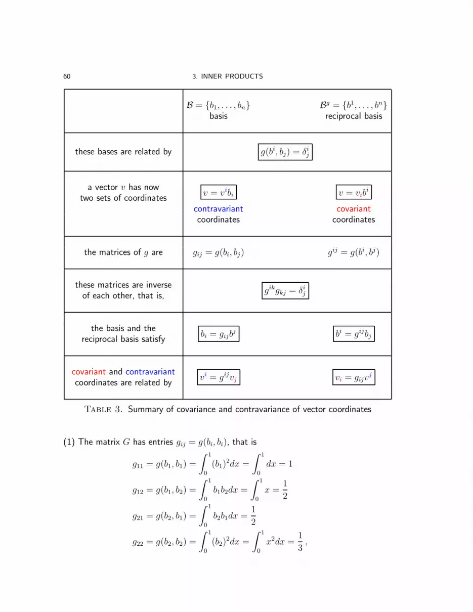
60 3. INNER PRODUCTS
B = {b1, . . . , bn} Bg = {b1, . . . , bn}basis reciprocal basis
these bases are related by g(bi, bj) = δij
a vector v has nowtwo sets of coordinates
v = vibi v = vibi
contravariant covariantcoordinates coordinates
the matrices of g are gij = g(bi, bj) gij = g(bi, bj)
these matrices are inverseof each other, that is,
gikgkj = δij
the basis and thereciprocal basis satisfy
bi = gijbj bi = gijbj
covariant and contravariantcoordinates are related by
vi = gijvj vi = gijvj
Table 3. Summary of covariance and contravariance of vector coordinates
(1) The matrix G has entries gij = g(bi, bi), that is
g11 = g(b1, b1) =
∫ 1
0
(b1)2dx =
∫ 1
0
dx = 1
g12 = g(b1, b2) =
∫ 1
0
b1b2dx =
∫ 1
0
x =1
2
g21 = g(b2, b1) =
∫ 1
0
b2b1dx =1
2
g22 = g(b2, b2) =
∫ 1
0
(b2)2dx =
∫ 1
0
x2dx =1
3,

3.2. RECIPROCAL BASIS 61
so that
G =
(1 1
2
12
13
).
(2) Since detG = 1 · 13− 1
2· 12= 1
12, then by using (1.7), we get
G−1 =
(4 −6−6 12
), .
(3) Using (3.15), we obtain that
(b1 b2
)=(1 x
)G−1 =
(1 x
)( 4 −6−6 12
)=(4− 6x −6 + 12x
),
so that Bg = {4− 6x,−6 + 12x}.
(4) p(x) = 6x = 0 ·1+6 ·x, so that p(x) has contravariant coordinates [p(x)]B =
(06
).
(5) From (3.18) it follows that if v = p(x), then(v1v2
)= G
(v1
v2
)=
(1 1
212
13
)(06
)=
(32
).
We can check this result:
v1b1 + v2b
2 = 3 · (4− 6x) + 2 · (−6 + 12x) = 6x .
�
3.2.4. Isomorphisms Between a Vector Space and its Dual.
We saw already in Proposition 2.9, that if V is a vector space and V ∗ is its dual,then dimV = dim V ∗. In particular, this means that V and V ∗ can be identified, oncewe choose a basis B of V and a basis B∗ of V ∗. In fact, the basis B∗ of V ∗ is givenonce we choose the basis B of V , as the dual basis of V ∗ with respect to B. Then thereis the following correspondence:
v ∈ V ! α ∈ V ∗ ,
exactly when v and α have the same coordinates, respectively with respect to B andB∗. However, this correspondence depends on the choice of the basis B and hence notcanonical.
If however V is endowed with an inner product, then there is a canonical identifi-cation of V with V ∗ that is, an identification that does not depend on the basis B ofV . In fact, let g : V × V → R be an inner product and let v ∈ V . Then
g(v, · ) : V −→ R
w 7−→ g(v, w)

62 3. INNER PRODUCTS
is a linear form and hence we have the following canonical identification given by themetric
V ←→ V ∗
v ←→ v∗ := g(v, · ) .(3.20)
Note that the isomorphism11 sends the zero vector to the linear form identically equalto zero, since g(v, · ) ≡ 0 if and only if v = 0 by positive definiteness of g.
So far, we have two bases of the vector space V , namely the basis B and thereciprocal basis Bg and we have also the dual basis of the dual vector space V ∗. It turnsout that, under the isomorphism (3.20), the reciprocal basis of V and the dual basis ofV ∗ correspond to each other. This follows from the fact that, under the isomorphism(3.20) an element of the reciprocal basis bi corresponds to the linear form g(bi, · )
bi ←→ g(bi, · )and the linear form g(bi, · ) : V → R has the property that
g(bi, bj) = δij .
We conclude that
g(bi, · ) ≡ βi ,
so under the canonical identification between V and V ∗ the reciprocal basis of V corre-sponds to the dual basis of V ∗.
3.2.5. Geometric Interpretation.
Let g : V × V → R be an inner product and B = {b1, . . . , bn} a basis of V withreciprocal basis Bg. Let v = vib
i ∈ V be a vector written in terms of its covariantcoordinates (that is, the coordinates with respect to the reciprocal basis). Then
g(v, bk) = g(vibi, bk) = vi g(b
i, bk)︸ ︷︷ ︸δik
= vk ,
so that (3.8) becomes
projbk v =vk
g(bk, bk)bk .
If we assume that the elements of the basis B = {b1, . . . , bn} are unit vectors, then(3.8) further simplifies to give
projbk v = vkbk .(3.21)
This equation shows the following:
Fact 3.29. The covariant coordinates of v give the orthogonal projection of v ontob1, . . . , bn.
11Recall that an isomomorphism T : V →W is an invertible linear transformation.

3.3. RELEVANCE OF COVARIANCE AND CONTRAVARIANCE 63
Likewise, the following holds basically by definition:
Fact 3.30. The contravariant coordinates of v give the “parallel” projection of v ontob1, . . . , bn.
b1
b2
︸ ︷︷ ︸
︸ ︷︷ ︸
︸
︷︷
︸
︸
︷︷
︸
v2
v2
v1
v1
v
3.3. Relevance of Covariance and Contravariance
Why do we need or care for covariant and contravariant components?
3.3.1. Physical Relevance.
Consider the following physical problem: Calculate the work performed by a force Fon a particle to move the particle by a small displacement dx, in the Euclidean plane. Thework performed should be independent of the choice of the coordinate system (i.e choiceof basis) used. For the work to remain independent of choice of basis we will see that,if the components of the displacement change contravariantly, then the components ofthe force should change covariantly.
To see this let B = {b1, b2} be a basis of the Euclidean plane. Suppose the forceF = (F1, F2) is exerted on a particle that moves with a displacement dx = (dx1, dx2).Then the work done is given by
dW = F1dx1 + F2dx
2 .
Suppose we are given another coordinate system B := {b1, b2} and let F = (F1, F2)and dx = (dx1, dx2). Then
dW = F1dx1 + F2dx
2 .
Now assume that the coordinates of dx change contravariantly;
dxi = Λijdx
j ,
or, equivalently,
dxi = Lijdx
j ,

64 3. INNER PRODUCTS
where Λ = L−1 and L = (Lij) is the change of basis matrix from B to B.
dW =F1dx1 + F2dx
2
=F1[L11dx
1 + L12dx
2] + F2[L21dx
1 + L22dx
2]
=(F1L11 + F2L
21)dx
1 + (F1L12 + F2L
22)dx
2
Since the work performed is independent of basis chosen we also have
dW = F1dx1 + F2dx
2 .
This gives thatF1 = F1L
11 + F2L
21
F2 = F1L12 + F2L
22 .
Hence the coordinates of F transform covariantly; Fi = LjiFj . Using matrices this can
be written as (F1, F2) = (F1, F2)L.
3.3.2. Distinction Vanishes when Restricting to Orthonormal Bases.
In the presence of an inner product g : V × V → R and if we restrict ourselves toorthonormal bases, the distinction between covariance and contravariance vanishes! Infact, it all becomes a matter of transposition: writing vectors as columns or as rows.
Why is that?First, as we saw, the reciprocal of an orthonormal basis is equal to itself, so covariant
and contravariant coordinates are equal in this special case.Moreover, when we change from one orthonormal basis to another by a change of
basis matrix L, the inverse change is given simply by the transpose of L. Here is a proof.
Let B = {b1, . . . , bn} and B = {b1, . . . , bn} be two orthonormal bases of V and letL := LBB be the corresponding matrix of the change of basis. This means, as always,that
bi = Lji bj .
Since B and B are orthonormal, we have g(bi, bj) = δij = g(bi, bj). Therefore, we have
δij = g(bi, bj) = g(Lki bk, L
ℓjbℓ) = Lk
iLℓjg(bk, bℓ) = Lk
iLℓjδkℓ == Lk
iLkj ,
showing that LtL = I, that is, L−1 = tL. Such a matrix L is called an orthogonalmatrix.
We conclude that, in this special case, we see no distinction between covariant andcontravariant behaviour, it is simply a matter of transposition.

CHAPTER 4
Tensors
4.1. Towards General Tensors
Let V be a vector space. Up to now, we saw several objects related to V , which wecalled tensors. We summarize them in Table 4. From these, we infer the definition ofa tensor of type (0, q) for all q ∈ N, but we cannot say the same for a tensor of type(p, 0) for all p ∈ N, even less of general type (p, q). The next discussion will lead us totensors of type (p, 0), and in the meantime we will discuss an important isomorphism.
4.1.1. Canonical Isomorphism between V and (V ∗)∗.
We saw in §3.2.4 that any vector space is isomorphic to its dual, though in generalthe isomorphism is not canonical, that is, it depends on the choice of a basis. We alsosaw that, if there is an inner product on V , then there is a canonical isomorphism. Thepoint of this section is to show that, even without an inner product, there is always acanonical isomorphism between V and its bidual (V ∗)∗, that is the dual of its dual.
To see this, let us observe first of all that
dim V = dim(V ∗)∗ .(4.1)
Tensor Components Behavior under a change of basis Type
vectorin V
vi contravariant tensor (1, 0)
linear formV → R
αj covariant tensor (0, 1)
linear transformationV → V
Aij
tensor of mixed character:contravariant and covariant
(1, 1)
bilinear formV × V → R
Bij covariant 2-tensor (0, 2)
k-linear formV × · · · × V → R
Fi1i2...ik covariant k-tensor (0, k)
Table 4. Covariance and contravariance of earlier tensors
65

66 4. TENSORS
In fact, for any vector space W , we saw in Proposition 2.9 that dimW = dimW ∗. Ifwe apply this equality both to W = V and to W = V ∗, we obtain
dimV = dimV ∗ and dim V ∗ = dim(V ∗)∗ ,
from which (4.1) follows immediately. We deduce (for instance, using §3.2.4) that Vand (V ∗)∗ are isomorphic, and we only have to see that there is a canonical isomorphism.
To this end, observe that a vector v ∈ V gives rise to a linear form on V ∗ defined by
ϕv : V∗ −→ R
α 7−→ α(v) .
Then we can define a linear map as follows:
Φ : V −→ (V ∗)∗
v 7−→ ϕv .(4.2)
Since, for any linear map T : V → W between vector spaces, we have the dimensionformula (known as the rank-nullity theorem in Linear Algebra):
dimV = dim im (T ) + dimker(T ) ,
it will be enough to show that ker Φ = {0}, because then
dimV = dim im (Φ) = dim(V ∗)∗ ,
and we can conclude that im (Φ) = (V ∗)∗, hence Φ is an isomorphism. Notice that wehave not chosen a basis to define the isomorphism Φ.
To see that ker Φ = {0}, observe that this kernel consists of all vectors v ∈ V suchthat α(v) = 0 for all α ∈ V ∗. We want to see that the only vector v ∈ V for whichthis happens is the zero vector. In fact, if v ∈ V is nonzero and B = {b1, . . . , bn} isany basis of V , then we can write v = vibi, where at least one coordinate, say v
j , is notzero. In that case, if B∗ = {β1, . . . , βn} is the dual basis, we have βj(v) = vj 6= 0, thuswe have found an element in V ∗ not vanishing on this v. We record this fact as follows:
Fact 4.1. Let V be a vector space and V ∗ its dual. The dual (V ∗)∗ of V ∗ is canonicallyisomorphic to V . The canonical isomorphism Φ : V → (V ∗)∗ takes v ∈ V to the linearform on the dual ϕv : V
∗ → R, ϕv(α) := α(v).
4.1.2. (2, 0)-Tensors.
Recall that the dual of a vector space V is the vector space
V ∗ := {linear forms α : V → R} = {(0, 1)-tensors} .Taking now the dual of the vector space V ∗, we obtain
(V ∗)∗ := {linear forms ϕ : V ∗ → R} .

4.1. TOWARDS GENERAL TENSORS 67
Using the canonical isomorphism Φ : V → (V ∗)∗ and the fact that coordinate vectorsare contravariant, we conclude that
{linear forms ϕ : V ∗ → R} = (V ∗)∗ ∼= V = {(1, 0)-tensors} .So, changing the vector space from V to its dual V ∗ seems to have had the effect
of converting covariant tensors of type (0, 1) into contravariant ones of type (1, 0).We are going to apply the above principle to convert covariant tensors of type (0, 2)
into contravariant ones of type (2, 0). Recall that
{(0, 2)-tensors} ={bilinear maps ϕ : V × V → R}
and consider now
{bilinear maps σ : V ∗ × V ∗ → R} .Anticipating the contravariant character of such bilinear maps (to be proven in §4.1.4),we advance the following definition:
Definition 4.2. A tensor of type (2, 0) is a bilinear form on V ∗, that is, a bilinearfunction σ : V ∗ × V ∗ → R.
Then we have
{(2, 0)-tensors} = {bilinear maps σ : V ∗ × V ∗ → R}and we denote this set Bil(V ∗ × V ∗,R).
Exercise 4.3. Check that Bil(V ∗ × V ∗,R) is a vector space. Just like in the caseof Bil(V × V,R) (cf. Exercise 2.25), it is enough to show that the zero map is inBil(V ∗ × V ∗,R) and that if σ, τ ∈ Bil(V ∗ × V ∗,R) and c, d ∈ R, then the linearcombination cσ + dτ is also in Bil(V ∗ × V ∗,R).
4.1.3. Tensor Product of Two Linear Forms on V ∗.
If v, w ∈ V are two vectors (i.e., are two (1, 0)-tensors), we define
σv,w : V ∗ × V ∗ → R
by
σv,w(α, β) := α(v)β(w) ,
for any two linear forms α, β ∈ V ∗. Then σv,w is indeed bilinear, i.e., linear in eachvariable, α and β, so is indeed a (2, 0)-tensor. We denote
σv,w =: v ⊗ w
and call this the tensor product of v and w.

68 4. TENSORS
Note 4.4. In general, we have
v ⊗ w 6= w ⊗ v ,as there can be linear forms α, β such that α(v)β(w) 6= α(w)β(v).
Similar to what we saw in §2.2.3, we find a basis for the space of (2, 0)-tensors byconsidering the (2, 0)-tensors defined by bi⊗ bj , where B = {b1, . . . , bn} is a basis of V .
Proposition 4.5. The elements bj⊗bj , i, j = 1, . . . , n form a basis of Bil(V ∗×V ∗,R).Thus dimBil(V ∗ × V ∗,R) = n2.
The proof of this proposition is analogous to the one of Proposition 2.26 and wewill not write it here. However, we state the crucial remark for the proof, analogous toRemark 2.27.
Remark 4.6. As for linear forms and bilinear forms on V , in order to verify that twobilinear forms on V ∗ are the same, it is enough to verify that they are the same onevery pair of elements of a basis of V ∗. In fact, let σ, τ be two bilinear forms on V ∗, let{γ1, . . . , γn} be a basis of V ∗ and let us assume that
σ(γi, γj) = τ(γi, γj)
for all 1 ≤ i, j,≤ n. Let α = αiγi and β = βjγ
j be arbitrary elements of V ∗. We nowverify that σ(α, β) = τ(α, β). Because of the linearity in each variable, we have
σ(α, β) = σ(αiγi, βjγ
j) = αiβjσ(γi, γj) = αiβjτ(γ
i, γj) = τ(αiγi, βjγ
j) = τ(α, β) .
�
4.1.4. Contravariance of (2, 0)-Tensors.
Let σ : V ∗ × V ∗ → R be a bilinear form on V ∗, that is, a so-called (2, 0)-tensor.We want to verify that it behaves as we expect with respect to a change of basis. Afterchoosing a basis B = {b1, . . . , bn} of V , we have the dual basis B∗ = {β1, . . . , βn} ofV ∗ and the basis {bi ⊗ bj : i, j = 1, . . . , n} of the space of (2, 0)-tensors.
The (2, 0)-tensor σ is represented by its components
Sij = σ(βi, βj) ,
in the sense that
σ = Sijbj ⊗ bj ,and the components Sij can be arranged into a matrix12
S =
S11 . . . S1n
.... . .
...Sn1 . . . Snn
12Once again, contrary to the change of basis matrix L, here we have only upper indices. Thisreflects the contravariance of the underlying tensor, σ.

4.2. TENSORS OF TYPE (p, q) 69
called the matrix of the (2, 0)-tensor σ with respect to the chosen basis of V .We look now at how the components of a (2, 0)-tensor change with a change of basis.
Let B = {b1, . . . , bn} and B = {b1, . . . , bn} be two basis of V and let B∗ := {β1, . . . , βn}and B∗ := {β1, . . . , βn} be the corresponding dual bases of V ∗. Let σ : V ∗ × V ∗ → R
be a (2, 0)-tensor with components
Sij = σ(βi, βj) and Sij = σ(βi, βj)
with respect to B∗ and B∗, respectively. Let L := LBB be the matrix of the change of
basis from B to B, and let Λ := L−1. Then, as seen in (1.4) and (2.11), we have that
bj = Lijbi and βi = Λi
jβj .
It follows that
Sij = σ(βi, βj) = σ(Λikβ
k,Λjℓβ
ℓ) = ΛikΛ
jℓσ(β
k, βℓ) = ΛikΛ
jℓS
kℓ ,
where the first and the last equalities follow from the definition of Sij and of Skℓ,respectively, the second from the change of basis and the third from the bilinearity of σ.We conclude that
Sij = ΛikΛ
jℓS
kℓ .(4.3)
Hence, the bilinear form σ is a contravariant 2-tensor.
Exercise 4.7. Verify that, in terms of matrices (4.3) translates into
S = ΛSΛt .
Compare with (2.15).
4.2. Tensors of Type (p, q)
In general, a (p, q)-tensor (with p, q = 0, 1, 2, . . .) is defined to be a real-valuedfunction of p covectors and of q vectors, which is linear in each of its arguments:
Definition 4.8. A tensor of type (p, q) or (p, q)-tensor is a multilinear form (or(p+ q)-linear function)
T : V ∗ × . . . V ∗︸ ︷︷ ︸
p
×V × · · · × V︸ ︷︷ ︸q
−→ R .
By convention, a tensor of type (0, 0) is a real number, a.k.a. scalar (a constant funtionof no arguments).
The order of a tensor is the number of arguments that it takes: a tensor of type(p, q) has, thus, order p+ q.13
13The order of a tensor is sometimes also called rank. However, rank of a tensor is often reservedfor another notion closer to the notion of rank of a matrix and related to decomposability of tensors(see §4.3.1 and §4.3.2).

70 4. TENSORS
Earlier tensor Viewed as multilinear function Type
vectorv ∈ V
V ∗ −→ R
β 7−→ β(v)(1, 0)
linear formα ∈ V ∗
V −→ R
w 7−→ α(w)(0, 1)
linear transformationF : V → V
V ∗ × V −→ R
(β, w) 7−→ β(F (w))(1, 1)
bilinear formϕ ∈ Bil(V × V,R)
V × V −→ R
(v, w) 7−→ ϕ(v, w)(0, 2)
k-linear formϕ on V
V × · · · × V −→ R
(v1, . . . , vk) 7−→ ϕ(v1, . . . , vk)(0, k)
bilinear form on V ∗
σ ∈ Bil(V ∗ × V ∗,R)V ∗ × V ∗ −→ R
(α, β) 7−→ σ(α, β)(2, 0)
Table 5. Earlier tensors viewed within general definition
If all the arguments of a tensor are vectors, i.e. p = 0, the tensor is said to be(purely) covariant. If the arguments are all linear forms, i.e. q = 0, the tensor is said tobe (purely) contravariant. Otherwise, a (p, q)-tensor is of mixed character, p being itsorder of contravariance and q its order of covariance. Purely covariant tensors are whatwe earlier called multilinear forms. Purely contravariant tensors are sometimes calledpolyadics.14
Table 5 gives an overview of how the earlier examples of tensors fit in the abovegeneral definition.
Let T be a (p, q)-tensor, B = {b1, . . . , bn} a basis of V and B∗ = {β1, . . . , βn} thecorresponding dual basis of V ∗. The components of T with respect to these bases are
Ti1,...,ipj1,...,jq
:= T (βi1, . . . , βip, bj1, . . . , bjq) .
If, moreover, B = {b1, . . . , bn} is another basis, B∗ = {β1, . . . , βn} the correspondingdual basis of V ∗ and L := LBB the matrix of the change of basis with inverse Λ := L−1,then the components of T with respect to these new bases are
Ti1,...,ipj1,...,jq
= Λi1k1. . .Λ
ipkpLℓ1j1. . . L
ℓqjqT
k1,...,kpℓ1,...,ℓq
.
The above formula displays the p-fold contravariant character and the q-fold covariantcharacter of T .
14Whereas Latin roots are used for covariant tensors, like in bilinear form, Greek roots are used forcontravariant tensors, like in dyadic.

4.3. TENSOR PRODUCT 71
The set of all tensors of type (p, q) on a vector space V with the natural operationsof addition and scalar multiplication on tensors is itself a vector space denoted by
T pq (V ) := {all (p, q)-tensors on V } .
4.3. Tensor Product
We saw already in §2.2.3 and §2.3.3 the tensor product of two multilinear forms.Since multilinear forms are covariant tensors, we said that this corresponds to the tensorproduct of two covariant tensors. We can now define the tensor product of two tensorsin general. This will further lead us to the tensor product of vector spaces.
4.3.1. Tensor Product for Tensors.
Definition 4.9. Let
T : V ∗ × · · · × V ∗︸ ︷︷ ︸
p
×V × · · · × V︸ ︷︷ ︸q
−→ R
be a (p, q)-tensor and
U : V ∗ × · · · × V ∗︸ ︷︷ ︸
k
×V × · · · × V︸ ︷︷ ︸ℓ
−→ R
a (k, ℓ) tensor. The tensor product T ⊗ U of T and U is the (p + k, q + ℓ)-tensor
T ⊗ U : V ∗ × · · · × V ∗︸ ︷︷ ︸
p+k
×V × · · · × V︸ ︷︷ ︸q+ℓ
−→ R
defined by
(T ⊗ U)(α1, . . . , αp+k, v1, . . . , vq+ℓ) :=T (α1, . . . , αp, v1, . . . , vq)U(αp+1, . . . , αp+k, vq+1, . . . , vq+ℓ) .
Although both T ⊗ U and U ⊗ T are tensors of the same type, in general we have
T ⊗ U 6= U ⊗ T .So we say that the tensor product is not commutative. On the other hand, the tensorproduct is associative, since we always have
(S ⊗ T )⊗ U = S ⊗ (U ⊗ T ) .Analogously to how we proceeded in the case of (0, 2)-tensors, we compute the
dimension of the vector space T pq (V ). Let B = {b1, . . . , bn} be a basis of V and B∗ :=
{β1, . . . , βn} the corresponding dual basis of V ∗. Just like we saw in Proposition 4.5in the case of (0, 2)-tensors, we form a basis of T p
q (V ) by collecting all elements of theform
bi1 ⊗ bi2 ⊗ · · · ⊗ bip ⊗ βj1 ⊗ βj2 ⊗ · · · ⊗ βjq

72 4. TENSORS
where the indices i1, . . . , ip and j1, . . . , jq take all values between 1 and n. Since thereare npnq = np+q elements in the above basis (corresponding to all possible choices ofbik and βjℓ), we deduce that
dim T pq (V ) = np+q .
If T is a (p, q)-tensor with components
Ti1,...,ipj1,...,jq
:= T (βi1, . . . , βip, bj1, . . . , bjq) ,
then we have, with a (p+ q)-fold application of the Einstein convention, that
T = Ti1,...,ipj1,...,jq
bi1 ⊗ bi2 ⊗ · · · ⊗ bip ⊗ βj1 ⊗ βj2 ⊗ · · · ⊗ βjq .
A simple tensor (also called a tensor of rank 1 or pure tensor or decomposabletensor or elementary tensor) of type (p, q) is a tensor T that can be written as atensor product of the form
T = a⊗ b⊗ . . .︸ ︷︷ ︸p
⊗α⊗ β ⊗ . . .︸ ︷︷ ︸q
where a, b, . . . ∈ V and α, β, . . . ∈ V ∗. The rank of a tensor T is then the minimumnumber of simple tensors that sum to T .15 By convention, the zero tensor has rank 0and a nonzero tensor of order zero, i.e., a nonzero scalar, has rank 1. A nonzero tensorof order 1 always has rank 1. Already among tensors of order 2 (and when dimV ≥ 2)there are tensors of rank greater than 1. Example 4.11 provides such an instance.
4.3.2. Tensor Product for Vector Spaces.
To complement the previous exposition and justify the notation V ∗ ⊗ V ∗ for thevector space of all bilinear forms on V (cf. §2.2.3), we aim in this section to give anidea of what the tensor product for finite-dimensional vector spaces should mean and ofhow the tensor product for vector spaces relates to the tensor product for tensors.
Let V and W be two vector spaces with dim V = n and dimW = m. Choose{b1, . . . , bn} a basis of V and {a1, . . . , am} a basis of W .16
Definition 4.10. The tensor product of V and W is the (n ·m)-dimensional vectorspace V ⊗W with basis
{bi ⊗ aj : 1 ≤ i ≤ n, 1 ≤ j ≤ m} .15This notion of rank of a tensor extends the notion of rank of a matrix, as can be seen by
considering tensors of order two and their corresponding matrices of components.16There is a way of defining the tensor product for vector spaces without involving bases, but we
will not do it here. That other, more abstract way shows elegantly that the tensor product of vectorspaces does not depend on the choice of bases.

4.3. TENSOR PRODUCT 73
Elements of V ⊗W are naturally referred to as tensors; further below we address theconnection to the previous notion of tensor. By definition, they are linear combinationsof the bi ⊗ aj. By viewing bi ∈ V as a linear map (cf. Table 5)
bi : V∗ −→ R , β 7−→ β(bi) ,
and similarly for aj ∈ W as
aj :W∗ −→ R , α 7−→ α(aj) ,
we may regard the symbol bi ⊗ aj as a bilinear map
V ∗ ×W ∗ −→ R , (β, α) 7−→ β(bi)α(aj) .
The tensor product V ⊗W is endowed with a bilinear map from the cartesian productV ×W
Ψ : V ×W −→ V ⊗Wdefined as follows. If
v = vibi ∈ V and w = wjaj ∈ W ,
then Ψ(v, w) =: v ⊗ w is the element of V ⊗W with coordinates viwj with respect tothe basis {bi ⊗ aj : 1 ≤ i ≤ n, 1 ≤ j ≤ m}, so that the following holds:
v ⊗ w =(vibi)⊗(wjaj
)=(viwj
)bi ⊗ aj .
Notice that the ranges for the indices are different: 1 ≤ i ≤ n, 1 ≤ j ≤ m. The numbersviwj may be viewed as obtained by the so-called outer product of the coordinate vectorsof v and w yielding an n×m matrix:
[v]Bt[w]A =
v1...vn
(w1 . . . wm)=
v1w1 . . . v1wm
......
vnw1 . . . vnwm
.
An element of V ⊗W that is in the image of the map Ψ, that is, an element ofV ⊗W that can be written as v ⊗ w for some v ∈ V and w ∈ W is called a simpletensor (or tensor of rank 1 or pure tensor or decomposable tensor or elementarytensor). Yet keep in mind, that the map Ψ is usually by far not surjective. In particular,one can show that, if v1, v2 ∈ V are linearly independent and w1, w2 ∈ W are alsolinearly independent, then the sum v1⊗w1+ v2⊗w2 is not a pure tensor. Checking thefirst instance of this phenomenon is left as the next exercise. The proof in general goesalong somewhat similar lines, but gets sophisticated.17
Exercise 4.11. Check that if both V and W are 2-dimensional with respective bases{b1, b2} and {a1, a2}, then b1 ⊗ a1 + b2 ⊗ a2 is not a pure tensor.
The following proposition gives some useful identifications.
17If you are interested in learning more, look up the Segre embedding from Algebraic Geometry.

74 4. TENSORS
Proposition 4.12. Let V and W be vector spaces with dimV = n and dimW = mand let
Lin(V,W ∗) := {linear maps V →W ∗} .Then
Bil(V ×W,R) ∼= Lin(V,W ∗)∼= Lin(W,V ∗)∼= V ∗ ⊗W ∗
∼= (V ⊗W )∗
= Lin(V ⊗W,R) .
Proof. Here is the idea behind this chain of identifications. Let f ∈ Bil(V ×W,R),that is, f : V ×W → R is a bilinear function, in particular it takes two vectors, v ∈ Vand w ∈ W , as input and gives a real number f(v, w) ∈ R as output. If, however,we only feed f one vector v ∈ V as input, then there is a remaining spot waiting fora vector w ∈ W to produce a real number. Since f is linear in V and in W , the mapf(v, · ) : W → R is a linear form, so f(v, · ) ∈ W ∗, hence f gives us an element inLin(V,W ∗). There is then a linear map
Bil(V ×W,R) −→ Lin(V,W ∗)
f 7−→ Tf ,
where
Tf (v)(w) := f(v, w) .
Conversely, any T ∈ Lin(V,W ∗) can be identified with a bilinear map fT ∈ Bil(V ×W,R) defined by
fT (v, w) := T (v)(w) .
Since fTf= f and TfT = T , we have proven the first identification in the proposition.
Analogously, if the input is only a vector w ∈ W , then f( · , w) : V → R is a linearmap and we now see that f ∈ Bil(V ×W,R) defines a linear map Uf ∈ Lin(W,V ∗). Thesame reasoning as in the previous paragraph, shows that Bil(V ×W,R) ∼= Lin(W,V ∗).
To proceed with the identifications, observe that, because of our definition of V ∗ ⊗W ∗, we have
Bil(V ×W,R) ∼= V ∗ ⊗W ∗ ,
since these spaces both have basis
{βi ⊗ αj : 1 ≤ i ≤ n, 1 ≤ j ≤ m} ,where {b1, . . . , bn} is a basis of V with corresponding dual basis {β1, . . . , βn} of V ∗,and {a1, . . . , an} is a basis of W with corresponding dual basis {α1, . . . , αn} of W ∗.

4.3. TENSOR PRODUCT 75
Finally, an elementDijβi⊗αj ∈ V ∗⊗W ∗ may be viewed as a linear map V⊗W → R,
that is as an element of (V ⊗W )∗ by
V ⊗W −→ R
Ckℓbk ⊗ aℓ 7−→ DijCkℓ βi(bk)︸ ︷︷ ︸
δik
αj(aℓ)︸ ︷︷ ︸δjℓ
= DijCkℓ .
�
Because of the identification Bil(V ×W,R) ∼= Lin(V ⊗W,R), we can say that
the tensor product linearizes what was bilinear (or multilinear).
There is no reason to restrict oneself to the tensor product of only two factors.One can equally define the tensor product V1 ⊗ · · · ⊗ Vk, and obtain a vector space ofdimension dimV1 × · · · × dimVk. Note that we do not need to use brackets, since thetensor product is associative: (V1 ⊗ V2)⊗ V3 = V1 ⊗ (V2 ⊗ V3).
We have
T pq (V ) = V ⊗ · · · ⊗ V︸ ︷︷ ︸
p
⊗V ∗ ⊗ · · · ⊗ V ∗︸ ︷︷ ︸
q
,
since both spaces have the same basis. An element T of T pq (V ) was first regarded
according to Definition 4.8 as a multilinear map
T : V ∗ × . . . V ∗︸ ︷︷ ︸
p
×V × · · · × V︸ ︷︷ ︸q
−→ R .
Now, with respect to bases B = {b1, . . . , bn} of V and B∗ = {β1, . . . , βn} of V ∗, thecomponents of T are
Ti1,...,ipj1,...,jq
:= T (βi1, . . . , βip, bj1, . . . , bjq) ,
hence we may view T as
Ti1,...,ipj1,...,jq
bi1 ⊗ . . .⊗ bip ⊗ βj1 ⊗ . . .⊗ βjq ∈ V ⊗ · · · ⊗ V︸ ︷︷ ︸p
⊗V ∗ ⊗ · · · ⊗ V ∗︸ ︷︷ ︸
q
.
In particular, the pth tensor power of a vector space is
V ⊗p := V ⊗ · · · ⊗ V︸ ︷︷ ︸p
= T p0 (V ) .
Therefore, we may write
Bil(V ∗ × V ∗,R) = V ⊗ V = V ⊗2 , Bil(V × V,R) = V ∗ ⊗ V ∗ = (V ∗)⊗2
and
T pq (V ) = V ⊗p ⊗ (V ∗)⊗q .


CHAPTER 5
Applications
Mathematically-speaking, a tensor is a real-valued function of some number of vec-tors and some number of covectors (a.k.a. linear forms), which is linear in each of itsarguments. On the other hand, tensors are most useful in connection with concrete phys-ical applications. In this chapter, we borrow notions and computations from Physics andCalculus to discuss important classical tensors.
5.1. Inertia Tensor
5.1.1. Physical Preliminaries.
We consider a rigid bodyM fixed at a point O and rotating about an axis through Owith angular velocity ω. Denoting the time variable t and an angle variable θ aroundthe axis of rotation, the angular velocity will be viewed as a vector18 with magnitude
‖ω‖ =∥∥∥∥dθ
dt
∥∥∥∥ ,
with direction given by the axis of rotation and with orientation given by the right-handrule. The position vector of a point P in the body M relative to the origin O is
x :=−→OP
while the linear velocity of that point P is
v := ω × x .
The linear velocity v has, hence, magnitude
‖v‖ = ‖ω‖︸︷︷︸‖ dθ
dt‖‖x‖ sinα︸ ︷︷ ︸
=:r
,
where α is the angle between ω and x, and has direction tangent at P to the circle ofradius r perpendicular to the axis of rotation.
18Warning: The angular velocity is actually only what physicists call a pseudovector because itdoes not follow the usual contravariance of a vector in case of orientation flip. Luckily, this issue doesnot affect the inertia tensor, since the sign flip cancels out thanks to squaring.
77

78 5. APPLICATIONS
..
α
r
O
P
x
v
ω
The kinetic energy of an infinitesimal region dM of M around P is
dE =1
2‖v‖2dm ,
where ‖v‖2 = v · v is the square of the norm of the linear velocity and dm is the massof dM . The total kinetic energy of M is
E =1
2
∫
M
‖v‖2dm =1
2
∫
M
‖ω × x‖2dm .
Actually, depending on the type of rigid body, we might take here a sum instead ofintegral, or some other type of integral (line integral, surface integral, etc) such as:
(1) If M is a solid in 3-dimensional space, then
E =1
2
∫∫∫
M
‖ω × xP‖2ρ
Pdx1dx2dx3 ,
where the norm squared ‖ω × xP‖2 and the density ρ
Pare functions of the
point P with coordinates (x1, x2, x3).(2) If M is a flat sheet, then
E =1
2
∫∫
M
‖ω × xP‖2ρ
Pdx1dx2 ,
where the integrand only depends on two cartesian coordinates.

5.1. INERTIA TENSOR 79
(3) If M is a (curvy) surface in 3-dimensional space, then
E =1
2
∫∫
M
‖ω × xP‖2ρ
Pdσ ,
where dσ is the infinitesimal element of the surface for a surface integral.(4) If M is a wire in 3-dimensional space, then
E =1
2
∫
M
‖ω × xP‖2ρ
Pds ,
where ds is the infinitesimal element of length for a line integral.(5) If M is a finite set of N point masses mi with rigid relative positions, then
E =1
2
N∑
i=1
‖ω × xi‖2mi .
We will keep writing our formulas for the first case (with a volume integral); these shouldbe adjusted for situations of the other types.
In any case, we need to work out the quantity
‖ω × x‖2
for vectors ω and x in 3-dimensional space.To this purpose, we use the Lagrange identity19, according to which
(a× b) · (c× d) = det
[a · c a · db · c b · d
].(5.1)
Applying (5.1) with a = c = ω and b = d = x, we obtain
‖ω × x‖2 = (ω × x) · (ω × x) = det
[ω · ω ω · x
x · ω x · x
]= ‖ω‖2‖x‖2 − ‖ω · x‖2 .
Let now B = {e1, e2, e3} be an orthonormal20 basis of R3, so that
ω = ωiei and x = xiei .
Then
‖ω‖2 = ω · ω = δijωiωj = ω1ω1 + ω2ω2 + ω3ω3
‖x‖2 = x · x = δkℓxkxℓ = x1x1 + x2x2 + x3x3
ω · x = δikωixk = ω1x1 + ω2x2 + ω3x3
19The Lagrange identity can be patiently proven in coordinates.20We could use any basis of R3. Then, instead of the δij , the formulas would have involved the
components of the metric tensor gij . However, computations with orthonormal bases are simpler; inparticular, the inverse of an orthonormal basis change L is simply tL. Moreover, the inertia tensor issymmetric, hence admits an orthonormal eigenbasis.

80 5. APPLICATIONS
so that
‖ω × x‖2 = ‖ω‖2‖x‖2 − ‖ω · x‖2
= (δijωiωj)(δkℓx
kxℓ)− (δikωixk)(δjlω
jxℓ)
= (δijδkℓ − δikδjℓ)ωiωjxkxℓ .
Therefore, the total kinetic energy is
E =1
2(δijδkℓ − δikδjℓ)ωiωj
∫∫∫
M
xkxℓdm
and it depends only on ω1, ω2, ω3 (since we have integrated over the x1, x2, x3).
5.1.2. Moments of Inertia.
Definition 5.1. The inertia tensor is the covariant 2-tensor whose components withrespect to an orthonormal basis B are
Iij = (δijδkℓ − δikδjℓ)∫∫∫
M
xkxℓdm .
Then the kinetic energy of the rotating rigid body is
E =1
2Iijω
iωj
which in matrix notation amounts to
E =1
2ω · Iω =
1
2tωIω .
Remark 5.2. If, instead of an orthonormal basis, we had used any basis of R3, wewould have gotten
Iij = (gijgkℓ − gikgjℓ)∫∫∫
M
xkxℓdm .
where gij are the components of the metric tensor. This formula also makes apparentthe covariance and the symmetry of I inherited from the metric: Iij = Iji for all i andj.
We will see that the inertia tensor is a convenient way to encode all moments ofinertia of an object in one quantity and we return now to the case of an orthonormalbasis. The first component of the inertia tensor is
I11 = (δ11δkℓ︸ ︷︷ ︸=0
unlessk=ℓ
− δ1kδ1ℓ︸ ︷︷ ︸=0
unlessk=ℓ=1
)
∫∫∫
M
xkxℓdm .
5.1. INERTIA TENSOR 81
If k = ℓ = 1, then δ11δ11− δ11δ11 = 0, so that the non-vanishing terms have k = ℓ 6= 1.In this way, one can check that
I11 =
∫∫∫
M
(x2x2 + x3x3) dm
I22 =
∫∫∫
M
(x1x1 + x3x3) dm
I33 =
∫∫∫
M
(x1x1 + x2x2) dm
I23 = I32 = −∫∫∫
M
x2x3 dm
I31 = I13 = −∫∫∫
M
x1x3 dm
I12 = I21 = −∫∫∫
M
x1x2 dm ,
so that with respect to an orthonormal basis B, the inertia tensor is represented by thesymmetric matrix
I =
I11 I12 I13I21 I22 I23I31 I32 I33
.
The diagonal components I11, I22, I33 are the moments of inertia of the rigid bodyM with respect to the coordinate axes Ox1, Ox2, Ox3, respectively. The off-diagonalcomponents I12, I23, I31 are the polar moments of inertia or the products of inertiaof the rigid body M .
Example 5.3. We want to find the inertia tensor of a homogeneous rectangular platewith sides a and b and total mass m, assuming that the rotation preserves the centerof mass O. We choose a coordinate system (corresponding to an orthonormal basis)with origin at the center of mass O, with x-axis parallel to the side of length a, y-axisparallel to the side of length b, z-axis perpendicular to the plate, and adjust our previousformulas to double integrals. Since the plate is assumed to be homogeneous, it has aconstant mass density equal to
ρ =total mass
area=m
ab.

82 5. APPLICATIONS
.e1
e2
a
b
Then
I11︸︷︷︸Ixx
=
∫ a2
− a2
∫ b2
− b2
(y2 + z2︸︷︷︸=0
) ρ︸︷︷︸mab
dy dx
=m
aba
∫ b2
− b2
y2 dy
=m
b
[y3
3
] b2
− b2
=m
12b2 .
Similarly,
I22︸︷︷︸Iyy
=m
12a2 ,
and
I33︸︷︷︸Izz
=
∫ a2
− a2
∫ b2
− b2
(x2 + y2)ρ dy dx =m
12(a2 + b2)
turns out to be just the sum of I11 and I22.Furthermore,
I23 = I32 = −∫ a
2
− a2
∫ b2
− b2
y z︸︷︷︸=0
ρ dy dx = 0 ,
and, similarly, I31 = I13 = 0. Finally, we have
I21 = I21 = −∫ a
2
− a2
∫ b2
− b2
xy ρ dy dx = −mab
(∫ a2
− a2
x dx
)
︸ ︷︷ ︸=0
(∫ b2
− b2
y dy
)
︸ ︷︷ ︸=0︸ ︷︷ ︸
because the integral of an odd functionon a symmetric interval is 0
.

5.1. INERTIA TENSOR 83
We conclude that the inertia tensor is given by the matrix
m
12
b2 0 00 a2 00 0 a2 + b2
.
�
Exercise 5.4. Compute the inertia tensor of the same plate, but now with center ofrotation O coinciding with a vertex of the rectangular plate.
5.1.3. Moment of Inertia About any Axis.
We compute the moment of inertia of the body M about an axis through the pointO and defined by the unit vector p.
. .αr
OP x
p
The moment of inertia of an infinitesimal region of M around P is
dI = r2︸︷︷︸r is the distancefrom P to the axis
dm︸︷︷︸infinitesimal
mass
= ‖p× x‖2 dm ,
where the last equality follows from the fact that ‖p× x‖ = ‖p‖ ‖x‖ sinα = r, since pis a unit vector. Hence, the total moment of inertia of M with respect to the axisgiven by p is
Ip :=
∫∫∫
M
‖p× x‖2 dm ≥ 0 .
This is very similar to the total kinetic energy E: just replace ω by p and omit the factor12. By the earlier computations, we conclude that
I = Iijpipj ,
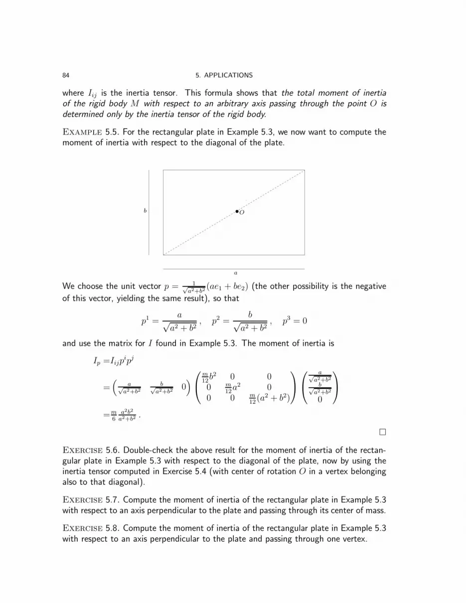
84 5. APPLICATIONS
where Iij is the inertia tensor. This formula shows that the total moment of inertiaof the rigid body M with respect to an arbitrary axis passing through the point O isdetermined only by the inertia tensor of the rigid body.
Example 5.5. For the rectangular plate in Example 5.3, we now want to compute themoment of inertia with respect to the diagonal of the plate.
.O
a
b
We choose the unit vector p = 1√a2+b2
(ae1 + be2) (the other possibility is the negative
of this vector, yielding the same result), so that
p1 =a√
a2 + b2, p2 =
b√a2 + b2
, p3 = 0
and use the matrix for I found in Example 5.3. The moment of inertia is
Ip =Iijpipj
=(
a√a2+b2
b√a2+b2
0)
m12b2 0 00 m
12a2 0
0 0 m12(a2 + b2)
a√a2+b2b√
a2+b2
0
=m6
a2b2
a2+b2.
�
Exercise 5.6. Double-check the above result for the moment of inertia of the rectan-gular plate in Example 5.3 with respect to the diagonal of the plate, now by using theinertia tensor computed in Exercise 5.4 (with center of rotation O in a vertex belongingalso to that diagonal).
Exercise 5.7. Compute the moment of inertia of the rectangular plate in Example 5.3with respect to an axis perpendicular to the plate and passing through its center of mass.
Exercise 5.8. Compute the moment of inertia of the rectangular plate in Example 5.3with respect to an axis perpendicular to the plate and passing through one vertex.

5.1. INERTIA TENSOR 85
5.1.4. Angular Momentum.
Let M be a body rotating with angular velocity ω about an axis through the point
O. Let x =−→OP be the position vector of a point P and v = ω × x the linear velocity
of P .
..
α O
P
x
v
ω
Then the angular momentum of an infinitesimal region of M around P is
dL = (x× v) dm ,
so that the total angular momentum21 of M is
L =
∫∫∫
M
(x× (ω × x)) dm .
21Just like the angular velocity, the angular momentum is not an honest vector, but only a pseu-
dovector, since there is an issue with orientation. In this subsection, we should thus assume that wework with an oriented orthonormal basis {e1, e2, e3} of R3, so that e1 × e2 = e3 (and not −e3). Thisamounts to assuming that the change of basis matrix L from the standard basis has detL = 1 (andnot −1).

86 5. APPLICATIONS
We need to work out x× (ω × x) for vectors x and ω in 3-dimensional space. Weapply the following identity22 for the triple vector product:
x× (ω × x) = (x · x)ω − (ω · x)x .(5.2)
Let B = {e1, e2, e3} be an orthonormal basis of R3. Then, replacing the following
equalities
ω = ωiei = δijωjei(5.3)
x = xiei = δikxkei(5.4)
x · x = δkℓxkxℓ(5.5)
ω · x = δjℓωjxℓ(5.6)
into (5.2), we obtain
x× (ω × x) = (δkℓxkxℓ︸ ︷︷ ︸
(5.5)
) δijωjei︸ ︷︷ ︸
(5.3)
−(δjℓωjxℓ︸ ︷︷ ︸(5.6)
) δikxkei︸ ︷︷ ︸
(5.4)
= (δijδkℓ − δikδjℓ)ωjxkxℓei .
Therefore, the total angular momentum is
L = Liei ,
where the components Li are
Li = (δijδkℓ − δikδjℓ)ωj
∫∫∫
M
xkxℓ dm .
Since we have always
δij = δij = δij =
{1 if i = j
0 if i 6= j,
if we violate index balance for one instance, the above expression for Li can be writtenin terms of the inertia tensor Iij as
Li = Iijωj ,
which corresponds to the matrix form L = Iω. We see that the angular momentum Lis proportional (or parallel) to the angular velocity ω only when ω is an eigenvector ofthe inertia tensor I.
Example 5.9. Suppose the rectangular plate in the previous examples is rotating aboutan axis through the center of mass O with angular velocity
ω = e1 + 2e2 + 3e3 , or
ω1
ω2
ω3
=
123
.
We want to compute its angular momentum.
22To prove this vector equality use coordinates, consider only the case in which ω is a standardbasis vector and then use the linearity in ω.
5.1. INERTIA TENSOR 87
The inertia tensor is given by the matrix Iij found in Example 5.3:
m12b2 0 00 m
12a2 0
0 0 m12(a2 + b2)
.
The total angular momentum has components given byL1
L2
L3
=
m12b2 0 00 m
12a2 0
0 0 m12(a2 + b2)
123
=
m12b2
m6a2
m4(a2 + b2)
,
so that
L =m
12b2e1 +
m
6a2e2 +
m
4(a2 + b2)e3 .
�
5.1.5. Principal Moments of Inertia.
Observe that the inertia tensor of a rigid bodyM is symmetric and recall the spectraltheorem (Theorem 3.9). Then we know that an orthonormal eigenbasis {e1, e2, e3}exists for the inertia tensor. Let I1, I2, I3 be the corresponding eigenvalues. The matrixrepresenting the inertia tensor with respect to this eigenbasis is
I1 0 00 I2 00 0 I3
.
The orthonormal eigenbasis gives a preferred coordinate system in which to formulatea problem pertaining to rotation of this body. The axes of the eigenvectors are calledthe principal axes of inertia of the rigid body M . The eigenvalues Ii are called theprincipal moments of inertia.
For instance, if a homogeneous body is symmetric with respect to the xy-plane, thenthe polar moments of inertia I23 = I32 and I13 = I31 vanish, thus the z-axis is necessarilya principal axis (because of the block-form of I).
The principal moments of inertia are the moments of inertia with respect to theprincipal axes of inertia, hence they are non-negative
I1, , I2, , I3 ≥ 0 .
A rigid body is called
(1) an asymmetric top if I1 6= I2 6= I3 6= I1;(2) a symmetric top if exactly two eigenvalues are equal, say I1 = I2 6= I3: any
axis passing through the plane determined by e1 and e2 is then a principal axisof inertia;
(3) a spherical top if I1 = I2 = I3: any axis passing through O is a principal axisof inertia.

88 5. APPLICATIONS
With respect to the eigenbasis {e1, e2, e3} the kinetic energy is
E =1
2(I1(ω
1)2 + I2(ω2)2 + I3(ω
3)2) ,
where ω = ωiei, with ωi the components of the angular velocity with respect to the
basis {e1, e2, e3}. In particular, we see that the kinetic energy can be conserved, even ifthe angular velocity ω changes, as long as the above combination of squares is preserved.This is related to the phenomenon of precession.
The surface determined by the equation (with respect to the coordinates x, y, z)
I1x2 + I2y
2 + I3z2 = 1(5.7)
is called the ellipsoid of inertia. The symmetry axes of the ellipsoid coincide with theprincipal axes of inertia. Note that for a spherical top, the ellipsoid of inertia is actuallya sphere.
The ellipsoid of inertia gives the moment of inertia with respect to any axis as follows:Consider an axis given by the unit vector p and let q = cp be a vector of intersection ofthe axis with the ellipsoid of inertia, where c is (±) the distance to O of the intersectionof the axis with the ellipsoid of inertia.
O
q
p
axis
The moment of inertia with respect to this axis is
I = Iijpipj =
1
c2Iijq
iqj =1
c2,
where the last equality follows from the fact that, since q is on the ellipsoid, thenIijq
iqj = 1 by equation (5.7).
Example 5.10. The principal axes of inertia for the rectangular plate in Example 5.3 arethe axes parallel to the sides and the axis perpendicular to the plate. The correspondingprincipal moments of inertia are
I11 =m
12b2 , I22 =
m
12a2 and I33 =
m
12(a2 + b2) .
If a = b, that is, if the rectangle is a square, we have a symmetric top. �

5.2. STRESS TENSOR (SPANNUNG) 89
5.2. Stress Tensor (Spannung)
5.2.1. Physical Preliminaries.
Let us consider a rigid bodyM acted upon by external forces but in static equilibrium,and let us consider an infinitesimal region dM around a point P . There are two typesof external forces:
(1) The body forces, that is forces whose magnitude is proportional to the vol-ume/mass of the region. For instance, gravity, attractive force or the centrifugalforce.
(2) The surface forces, that is forces exerted on the surface of the element by thematerial surrounding it. These are forces whose magnitude is proportional tothe area of the region in consideration.
The surface force per unit area is called the stress. We will concentrate on homoge-neous stress, that is stress that does not depend on the location of the element inthe body, but depends only on the orientation of the surface given by its tangent plane.Moreover, we assume that the body in consideration is in static equilibrium.
Remark 5.11. It was the concept of stress in mechanics that originally led to theinvention of tensors
tenseur
%%▲▲▲
▲▲▲▲
▲▲▲
stress
99ssssssssss
%%❑❑❑
❑❑❑❑
❑❑tensor
tension
99rrrrrrrrr
Choose an orthonormal basis {e1, e2, e3} and the plane Π through P parallel to thee2e3 coordinate plane. The vector e1 is normal to this plane. Let ∆A1 be the area ofthe slice of the infinitesimal region around P cut by the plane and let ∆F be the forceacting on that slice. We write ∆F in terms of its components
∆F = ∆F 1e1 +∆F 2ee +∆F 3e3
and, since the stress is the surface force per unit area, we define
σ1j := lim∆A1→0
∆F j
∆A1
, for j = 1, 2, 3 .
Similarly, we can consider planes parallel to the other coordinate planes
e1 e2
e3
P
PP
Π1
Π2
Π3

90 5. APPLICATIONS
and define
σij := lim∆Ai→0
∆F j
∆Ai.
It turns out that the resulting nine numbers σij are the components of a contravariant2-tensor called the stress tensor, as we will see in §5.2.5. The stress tensor encodesthe mechanical stresses on an object.
We now compute the stress across other slices through P , that is, across other planeswith other normal vectors. Let Π be a plane passing through P , n a unit vector throughP perpendicular to the plane Π, ∆s = Π∩ dM the area of a small element of the planeΠ containing P and ∆F the force acting on that element.
Π∆s
n
P
Claim 5.12. The stress at P across the surface perpendicular to n is
σ(n) := lim∆s→0
∆F
∆s= σij(n · ei)ej .
It follows from the claim that the stress σ is a vector-valued function that dependslinearly on the normal n to the surface element.
Proof. Consider the tetrahedron OA1A2A3 bound by the triangular slice on theplane Π having area ∆s and three triangles on planes parallel to the coordinate planes
e1
e2
e3
O
n
A1
A2
A3
Consider all external forces acting on this tetrahedron, which we regard as a volumeelement of the rigid body:
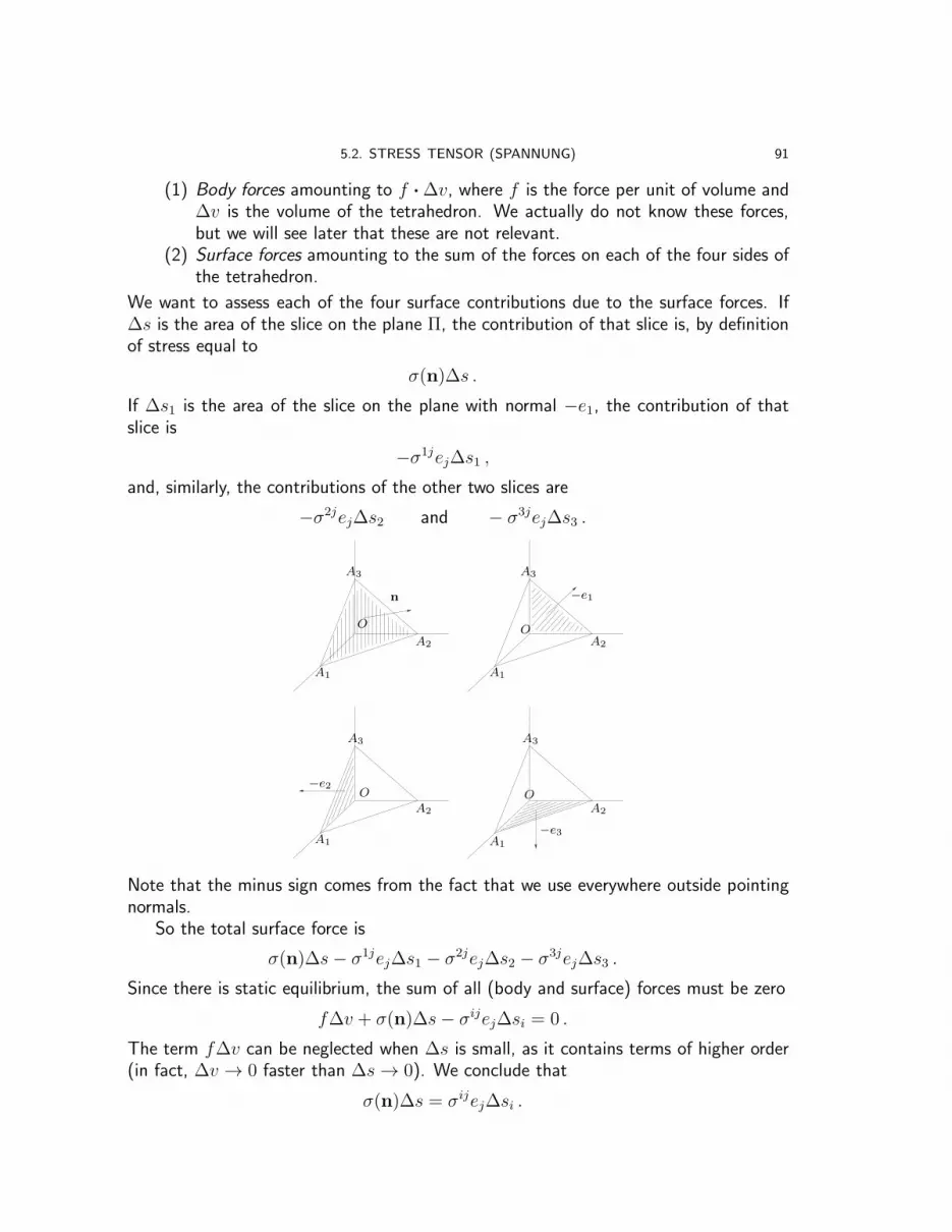
5.2. STRESS TENSOR (SPANNUNG) 91
(1) Body forces amounting to f ·∆v, where f is the force per unit of volume and∆v is the volume of the tetrahedron. We actually do not know these forces,but we will see later that these are not relevant.
(2) Surface forces amounting to the sum of the forces on each of the four sides ofthe tetrahedron.
We want to assess each of the four surface contributions due to the surface forces. If∆s is the area of the slice on the plane Π, the contribution of that slice is, by definitionof stress equal to
σ(n)∆s .
If ∆s1 is the area of the slice on the plane with normal −e1, the contribution of thatslice is
−σ1jej∆s1 ,
and, similarly, the contributions of the other two slices are
−σ2jej∆s2 and − σ3jej∆s3 .
−e1
−e2
−e3
O
O O
O
n
A1 A1
A1A1
A2
A2A2
A2
A3 A3
A3A3
Note that the minus sign comes from the fact that we use everywhere outside pointingnormals.
So the total surface force is
σ(n)∆s− σ1jej∆s1 − σ2jej∆s2 − σ3jej∆s3 .
Since there is static equilibrium, the sum of all (body and surface) forces must be zero
f∆v + σ(n)∆s− σijej∆si = 0 .
The term f∆v can be neglected when ∆s is small, as it contains terms of higher order(in fact, ∆v → 0 faster than ∆s→ 0). We conclude that
σ(n)∆s = σijej∆si .

92 5. APPLICATIONS
It remains to relate ∆s to ∆s1,∆s2,∆s3. The side with area ∆si is the orthogonalprojection of the side with area ∆s onto the plane with normal ei. The scaling factorfor the area under projection is cosαi, where αi is the convex angle between the planenormal vectors
ei
n
αi
∆si∆s
= cosαi = cosαi‖n‖ ‖ei‖ = n · ei .
Therefore ,
σ(n)∆s = σijej(n · ei)∆s
or, equivalently,
σ(n) = σij(n · ei)ej .
Note that, in the above formula, the quantities n · ei are the coordinates of n withrespect to the orthonormal basis {e1, e2, e3}, namely
n = (n · e1)e1 + (n · e2)e2 + (n · e3)e3 = n1e1 + n2e2 + n3e3 .
�
Remark 5.13. For homogeneous stress, the stress tensor σij does not depend on thepoint P . However, when we flip the orientation of the normal to the plane, the stresstensor changes sign. In other words, if σ(n) is the stress across a surface with normaln, then
σ(−n) = −σ(n) .
The stress considers orientation as if the forces on each side of the surface have tobalance each other in static equilibrium.
σ(n)
σ(−n)
−n
n
�

5.2. STRESS TENSOR (SPANNUNG) 93
5.2.2. Principal Stresses.
Claim 5.14. The stress tensor is a symmetric tensor, that is σij = σji.
Proof. Consider an infinitesimal cube of side ∆ℓ surrounding P and with facesparallel to the coordinate planes.
e1
e2
e3
A B
CD
A′B′
C′D′
The force acting on each of the six faces of the cube are:
• σ1j∆A1ej and −σ1j∆A1ej , respectively for the front and the back faces,ABB′A′ and DCC ′D′;• σ2j∆A2ej and−σ2j∆A2ej, respectively for the right and the left faces BCC
′B′
and ADD′A′;• σ3j∆A3ej and −σ3j∆A3ej , respectively for the top and the bottom facesABCD and A′B′C ′D′,
where ∆A1 = ∆A2 = ∆A3 = ∆s = (∆ℓ)2 is the common face area. We compute nowthe torque µ, assuming the forces are applied at the center of each face, whose distanceto the center point P is 1
2∆ℓ. Recall that the torque is the tendency of a force to twist
or rotate an object. It is given by the cross product of the distance vector and the forcevector.
µ =∆ℓ2e1 × σ1j∆s ej +
(−∆ℓ
2e1)× (−σ1j∆s ej )
+ ∆ℓ2e2 × σ2j∆s ej +
(−∆ℓ
2e2)× (−σ2j∆s ej )
+ ∆ℓ2e2 × σ3j∆s ej +
(−∆ℓ
2e3)× (−σ3j∆s ej )
=∆ℓ∆s (ei × σijej)
=∆ℓ∆s((σ23 − σ32)e1 + (σ31 − σ13)e2 + (σ12 − σ21)e3
).
Since the equilibrium is static, then µ = 0, so that σij = σji. �

94 5. APPLICATIONS
We can hence write
σ =
σ11 σ12 σ13
σ12 σ22 σ23
σ13 σ23 σ33
,
where the diagonal entries σ11, σ22 and σ33 are the normal components, that is thecomponents of the forces perpendicular to the coordinate planes and the remainingentries σ12, σ13 and σ23 are the shear components, that is the components of theforces parallel to the coordinate planes.
Since the stress tensor is symmetric, again by the spectral theorem (Theorem 3.9),it can be orthogonally diagonalized, that is
σ =
σ1 0 00 σ2 00 0 σ3
,
where now σ1, σ2 and σ3 are the principal stresses, that is the eigenvalues of σ. Theeigenspaces of σ are the principal directions and the shear components disappear forthe principal planes, i.e., the planes orthogonal to the principal directions.
5.2.3. Special Forms of the Stress Tensor.
We consider the stress tensor with respect to an orthonormal eigenbasis or anotherspecial basis, so that the corresponding matrix has a simpler form. We use the followingterminology:
• Uniaxial stress for a stress tensor given by
σ 0 00 0 00 0 0
Example 5.15. This is the stress tensor in a long vertical rod loaded by hang-ing a weight on the end. �
• Plane stressed state or biaxial stress for a stress tensor given byσ1 0 00 σ2 00 0 0
Example 5.16. This is the stress tensor in plate on which forces are appliedas in the picture.
�

5.2. STRESS TENSOR (SPANNUNG) 95
• Pure shear for a stress tensor given by−σ 0 00 σ 00 0 0
or
0 σ 0σ 0 00 0 0
.(5.8)
This is special case of the biaxial stress, in the case where σ1 = −σ2. In(5.8) the first is the stress tensor written with respect to an eigenbasis, whilethe second is the stress tensor written with respect to an orthonormal basisobtained by rotating an eigenbasis by 45◦ about the third axis. In fact0 σ 0σ 0 00 0 0
=
√22
√22
0
−√22
√22
00 0 1
︸ ︷︷ ︸tL
−σ 0 00 σ 00 0 0
√22−
√22
0√22
√22
00 0 1
︸ ︷︷ ︸L
where L is the matrix of the change of coordinates.
• Shear deformation for a stress tensor given by
0 σ12 σ13
σ12 0 σ23
σ13 σ23 0
(with respect to some orthonormal basis).It turns out that the stress tensor σ is equivalent to a shear deformation if
and only if its trace is zero.
Example 5.17. The stress tensor
2 −4 0−4 0 40 4 −2
represents a shear deformation. In fact, one can check that
√22
0√22
0 1 0
−√22
0√22
︸ ︷︷ ︸tL
2 −4 0−4 0 40 4 −2
√22
0 −√22
0 1 0√22
0√22
︸ ︷︷ ︸L
=
0 0 −20 0 4
√2
−2 4√2 0
�

96 5. APPLICATIONS
• Hydrostatic pressure with stress tensor given by−p 0 00 −p 00 0 −p
,
where p 6= 0 is the pressure. Here all eigenvalues are equal to −p.Example 5.18. Pressure of a fluid on a bubble. �
Exercise 5.19. Any stress tensor can be written as the sum of a hydrostatic pressureand a shear deformation. Hint: look at the next section.
5.2.4. Invariants.
Let A be a 3× 3 matrix with entries aij . The characteristic polynomial pA(λ) of Ais invariant under conjugation (see §1.4.2), so its coefficients remain unchanged.
pA(λ) =det(A− λI) = det
a11 − λ a12 a13
a21 a22 − λ a23
a31 a32 a33 − λ
=− λ3 + trAλ2
−(a11a22 + a11a33 + a22a33 − a12a21 − a23a32 − a13a31
)︸ ︷︷ ︸
quadratic expressionin the entries of A
λ+ detA .
Applying this to the stress tensor σ = A, we obtain some stress invariants, namely:
I1 := tr σ = σ11 + σ22 + σ33
I2 :=(σ12)2 + (σ23)2 + (σ13)2 − σ11σ22 − σ22σ33 − σ33σ11
I3 := det σ .
That means, that the above quantities I1, I2 and I3 are invariant when we change theorthonormal basis.23
The stress tensor can be expressed as the sum of 2 other stress tensors;
• The hydrostatic stress tensor
πδij =
π 0 00 π 00 0 π
,
where π := I1/3 = (σ11 + σ22 + σ33)/3. This relates to volume change.
23By contravariance, when we change basis via a matrix L, the matrix of the stress tensor changesfrom σ to σ = tΛσΛ, where Λ = L−1. But since we are restricting to orthonormal bases, we have thatthe change of basis matrix is orthogonal, i.e., Λ = tL, so this is in fact a conjugation: σ = LσL−1.

5.2. STRESS TENSOR (SPANNUNG) 97
• The deviatoric stress tensor
sij := σij − πδij =
σ11 − π σ12 σ13
σ12 σ22 − π σ23
σ13 σ23 σ33 − π
.
This relates to shape change.
Remark 5.20. The hydrostatic pressure is generally defined as the negative one thirdof the stress invariant I1, i.e. p = −πRemark 5.21. The stress deviator tensor is a shear deformation since
tr(sij) = σ11 + σ22 + σ33 − 3π = 0.
Clearly
σij = sij + πδij
and hence the stress tensor is a sum of a shear deformation and a hydrostatic pressureas claimed in Exercise 5.19.
5.2.5. Contravariance of the Stress Tensor.
Let B = {e1, e2, e3} and B = {e1, e2, e3} be two orthonormal bases, and let
ei = Ljiej and ei = Λj
i ej ,(5.9)
where L := LBB is the matrix of the change of basis and Λ := L−1 is the inverse. Letn be a given unit vector and σ the stress across a surface perpendicular to n. Then σ
can be expressed in two ways, respectively with respect to B and to B,σ = σij(n · ei)ej and σ = σij(n · ei)ej ,(5.10)
and we want to relate σij to σij . We start with the first expression for S in (5.10) andrename the indices for later convenience:
σ = σkm(n · ek)em = σkm(n · Λikei)(Λ
jmej) = σkmΛi
kΛjm(n · ei)ej ,
where in the second equality we used (5.9), and in the third we used linearity. Comparingthe last expression with the second expression in (5.10) we obtain
σij = σkmΛikΛ
jm ,
thus showing that σ is a contravariant 2-tensor or a tensor of type (0, 2).Heuristically, we may think that the stress at each point takes one plane, thought
of as the kernel of a linear form, and gives a vector, thus is a linear map V ∗ → V or,equivalently, a bilinear map V ∗ × V ∗ → R, i.e., a tensor of type (0, 2).

98 5. APPLICATIONS
5.3. Strain Tensor (Verzerrung)
5.3.1. Physical Preliminaries.
Consider a slight deformation of a body, where we compare the relative positions oftwo particles before and after the deformation:
.
.
.
.
P
P
P1
P1
P
P
P1
P1
∆x ∆x
displacement of P1
displacement of P
∆u
We have
∆x = ∆x+∆u ,
where ∆x is the old relative position of P and P1, ∆x is their new relative position and∆u is the displacement difference, which hence measures the deformation.
Assume that we have a small homogeneous deformation, that is
∆u = f(∆x) ,
in other words, f is a small linear function independent of the point P . If we writethe components of ∆u and ∆x with respect to an orthonormal basis {e1, e2, e3}, thefunction f will be represented by a matrix with entries that we denote by fij,
∆ui = fij∆xj .

5.3. STRAIN TENSOR (VERZERRUNG) 99
The matrix (fij) can be written as a sum of a symmetric and an antisymmetric matrixas follows:
fij = ǫij + ωij ,
where
ǫij =1
2(fij + fji)
is a symmetric matrix and is called the strain tensor or deformation tensor and
ωij =1
2(fij − fji)
is an antisymmetric matrix called the rotation tensor. We will next try to understandwhere these names come from.
Remark 5.22. First we verify that a (small) antisymmetric 3 × 3 matrix represents a(small) rotation in 3-dimensional space.
Fact 5.23. Let V be a vector space with orthonormal basis B = {e1, e2, e3}, and let
ω =
abc
. The matrix Rω of the linear map V → V defined by v 7→ ω×v with respect
to the basis B is
Rω =
0 −c bc 0 −a−b a 0
.
Indeed, we have
ω × v =
abc
×
xyz
= det
e1 e2 e3a b cx y z
=
bz − cycx− azay − bx
=
0 −c bc 0 −a−b a 0
xyz
.
Note that the matrix Rω = (ωij) :=
0 ω12 −ω31
−ω12 0 ω23
ω31 −ω23 0
corresponds to the cross
product with the vector ω =
−ω23
−ω31
−ω12
. �

100 5. APPLICATIONS
5.3.2. The Antisymmetric Case: Rotation.
Suppose that the matrix (fij) was already antisymmetric, so that
ωij = fij and ǫij = 0 .
Note that
ωii =1
2(fii − fii) = 0.
By the Fact 5.23, if ω =
−ω23
−ω31
−ω12
, then
Rω∆x = ω ×∆x
and the relation
∆ui = fij∆xj(5.11)
is equivalent to
∆u = ω ×∆x ,
so that
∆x = ∆x+∆u = ∆x+ ω ×∆x .
When ω is small, this represents an infinitesimal rotation of an angle ‖ω‖ about the axisOω.
∆x ∆x
α
r
O
ω

5.3. STRAIN TENSOR (VERZERRUNG) 101
In fact, since ω × ∆x is orthogonal to the plane determined by ω and by ∆x, itis tangent to the circle with center along the axis Oω and radius determined by ∆x.Moreover,
‖∆u‖ = ‖ω ×∆x‖ = ‖ω‖ ‖∆x‖ sinα︸ ︷︷ ︸r
,
and hence, since the length of an arc of a circle of radius r corresponding to an angle θis rθ, infinitesimally this represents a rotation by an angle ‖ω‖.
5.3.3. The Symmetric Case: Strain.
The opposite extreme case is when the matrix fij was already symmetric, so that
ǫij = fij and ωij = 0 .
We will see that it is ǫij that encodes the changes in the distances: in fact,
‖∆x‖2 = ∆x ·∆x = (∆x+∆u) · (∆x+∆u)
= ∆x ·∆x+ 2∆x ·∆u+∆u ·∆u
≃ ‖∆x‖2 + 2ǫij∆xi∆xj ,
(5.12)
where in the last step we neglected the term ‖∆u‖2 since it is small compared to ∆uwhen ∆u→ 0 and used (5.11).
Remark 5.24. Even when fij is not purely symmetric, only the symmetric part ǫij isrelevant for the distortion of the distances. In fact, since ωij is antisymmetric, the term2ωij∆x
i∆xj = 0, so that
‖∆x‖2 ≃ ‖∆x‖2 + 2fij∆xi∆xj = ‖∆x‖2 + 2ǫij∆x
i∆xj .
�
Recall that a metric tensor (or inner product) encodes the distances among points.It follows that a deformation changes the metric tensor. Let us denote by g the metricbefore the deformation and by g the metric after the deformation. By definition, wehave
‖∆x‖2 def= g(∆x,∆x) = gij∆x
i∆xj = gij(∆xi +∆ui)(∆xj +∆uj)(5.13)
and
‖∆x‖2 def= g(∆x,∆x) = gij∆x
i∆xj .(5.14)
For infinitesimal deformations (that is, if ∆u ∼ 0), (5.13) becomes
‖∆x‖2 = gij∆xi∆xj .
This, together with (5.14) and (5.12), leads to
gij∆xi∆xj ≃ gij∆x
i∆xj + 2ǫij∆xi∆xj

102 5. APPLICATIONS
and hence
ǫij ≃1
2(gij − gij) ,
that is, ǫij measures the change in the metric.By definition the strain tensor ǫij is symmetric
E =
ǫ11 ǫ12 ǫ13ǫ12 ǫ22 ǫ23ǫ13 ǫ23 ǫ33
,
where the terms on the diagonal (in green) determine the elongation or the contractionof the body along the coordinate directions e1, e2, e3, and the terms above the diagonal(in orange) are the shear components of the strain tensor; that is ǫij is the movementof a line element parallel to Oej towards Oei. Since it is a symmetric tensor, it can beorthogonally diagonalized (cf. Theorem 3.9), so we can find an orthonormal basis withrespect to which E is given by
ǫ1 0 00 ǫ2 00 0 ǫ3
,
The eigenvalues of E are the principal coefficients of the deformation and the eigenspacesare the principal directions of the deformation.
5.3.4. Special Forms of the Strain Tensor.
We use the following terminology:
(1) Shear deformation when E is traceless
tr E = ǫ11 + ǫ22 + ǫ33 = 0 .
(2) Uniform compression when the principal coefficients of E are equal (andnonzero)
k 0 00 k 00 0 k
Exercise 5.25. Any strain tensor can be written as the sum of a uniformcompression and a shear deformation.
5.4. Elasticity Tensor
The stress tensor represents an external exertion on the material, while the straintensor represents the material reaction to that exertion. In crystallography these arecalled field tensors because they represent imposed conditions, opposed to mattertensors, that represents material properties.

5.4. ELASTICITY TENSOR 103
Hooke’s law says that, for small deformations, stress is related to strain by a mattertensor called elasticity tensor or stiffness tensor E:
σij = Eijkℓǫkl ,
while the tensor relating strain to stress is the compliance tensor S:
ǫkℓ = Sijkℓσij .
The elasticity tensor has order 4, and hence in 3-dimensional space it has 34 = 81components. Luckily, symmetry reduces the number of independent components forEijkℓ.
(1) Minor symmetries: The symmetry of the stress tensor
σij = σji
implies that
Eijkℓ = Ejikℓ for each k, ℓ ;
it follows that for each k, ℓ fixed there are only 6 independent components Eijkℓ
E11kℓ E12kℓ E13kℓ
E12kℓ E22kℓ E23kℓ
E13kℓ E23kℓ E33kℓ .
Having taken this in consideration, the number of independent componentsdecreases to 6 × 32 at the most. Moreover, the symmetry also of the straintensor
ǫkℓ = ǫℓk
implies that
Eijkℓ = Eijℓk for each i, j .
This means that for each i, j fixed there are also only 6 independent componentsEijkℓ, so that Eijkℓ has at most 62 = 36 independent components.
(2) Major symmetries: Since (under appropriate conditions) partial derivativescommute, if follows from the existence of a strain energy density functional Usatisfying
∂2U
∂ǫij∂ǫkℓ= Eijkℓ
that
Eijkℓ = Ekℓij ,
that means the matrix with rows labelled by (i, j) and columns labelled by (k, ℓ)is symmetric. Since, from (1), there are only 6 entries (i, j) for a fixed (k, ℓ),

104 5. APPLICATIONS
Eijkℓ can be written in a 6× 6 matrix with rows labelled by (i, j) and columnslabelled by (k, ℓ)
∗ ∗ ∗ ∗ ∗ ∗∗ ∗ ∗ ∗ ∗∗ ∗ ∗ ∗∗ ∗ ∗∗ ∗∗
so that Eijkℓ has in fact only 6 + 5 + 4 + 3 + 2 + 1 = 21 components.
5.5. Conductivity Tensor
Consider a homogeneous continuous crystal. Its properties can be divided into twoclasses:
• Properties that do not depend on a direction, and are hence described by scalars.Examples are density and heat capacity.• Properties that depend on a direction, and are hence described by tensors.Examples are elasticity, electrical conductivity and heat conductivity. Wesay that a crystal is anisotropic when it has such tensorial properties.
5.5.1. Electrical Conductivity.
Let E be the electric field and J the electrical current density. We assume thatthese are constant throughout the crystal. At each point of the crystal:
(1) E gives the electric force (in Volts/m) that would be exerted on a positivetest charge (of 1 Coulomb) placed at the point;
(2) J (in Amperes/m2) gives the direction the charge carriers move and the rate ofelectric current across an infinitesimal surface perpendicular to that direction.
The electrical current density J is a function of the electric field E,
J = f(E) .
Consider a small increment ∆J in J caused by a small increment ∆E in E, and writethese increments in terms of their components with respect to a chosen orthonormalbasis {e1, e2, e3}.
∆J = ∆J iei and ∆E = ∆Eiei .
By Calculus, the increments are related by
∆J i =∂f i
∂Ej∆Ej + higher order terms in (∆Ej)2, (∆Ej)3, . . .

5.5. CONDUCTIVITY TENSOR 105
If the quantities ∆Ej are small, we can assume that
∆J i =∂f i
∂Ej∆Ej(5.15)
If we assume that ∂f i
∂Ej is independent of the point of the crystal,
∂f i
∂Ej= κij ∈ R
we obtain the relation
∆J i = κij∆Ej
or simply
∆J = κ∆E ,
where κ if the electrical conductivity tensor. This is a (1, 1)-tensor and may depend24
on the initial value of E, that is the electrical conductivity may be different for small andlarge electric forces. If initially E = 0 and κ0 is the corresponding electrical conductivitytensor, we obtain the relation
J = κ0E
that is called the generalized Ohm law. This is always under the assumption that ∆Eand ∆J are small and that the relation is linear.
The electrical resistivity tensor is the inverse of κ:
ρ := κ−1 ,
that is, it is the (1, 1)-tensor such that
ρjiκℓj = δℓi .
The electrical conductivity measures the material’s ability to conduct an electrical cur-rent, while the electrical resistivity quantifies the ability of the material to oppose theflow of the electrical current.
For an isotropic crystal, all directions are equivalent and these tensors are spherical,meaning
κji = kδji and ρji =1
kδji ,(5.16)
where k is a scalar, called the electrical conductivity of the crystal. Equation (5.16)can also be written as
k 0 00 k 00 0 k
and
1k
0 00 1
k0
0 0 1k
.
24Typically, if the dependence between E and J is linear for any value, and not only for small ones,the tensor κ will not depend on the initial value of E.
106 5. APPLICATIONS
In general, κji is neither symmetric nor antisymmetric (and actually symmetry does noteven make sense for a (1, 1) tensor unless a metric is fixed, since it does require acanonical identification of V with V ∗).
5.5.2. Heat Conductivity.
Let T be the temperature and H the heat flux vector. For a homogeneous crystaland constant H and for a constant gradient of T , Fourier heat conduction law says that
H = −K gradT .(5.17)
At each point of the crystal:
(1) gradT points in the direction of the highest ascent of the temperature and mea-sures the rate of increase of T in that direction. The minus sign in (5.17) comesfrom the fact that the heat flows in the direction of decreasing temperature.
(2) H measure the amount of heat passing per unit area perpendicular to its direc-tion per unit time.
Here, K is the heat conductivity tensor or thermal conductivity tensor. In termsof components with respect to a chosen orthonormal basis, we have
H i = −Kij(gradT )j .
Exercise 5.26. Verify that the gradient of a real function is a covariant 1-tensor.
The heat conductivity tensor is a contravariant 2-tensor and experiments show that itis symmetric and hence can be orthogonally diagonalized. The heat resistivity tensoris its inverse:
r := K−1 ,
and hence is also symmetric. With respect to an orthonormal basis, K is represented byK1 0 00 K2 00 0 K3
,
where the eigenvalues of K are called the principal coefficients of heat conductivity.The fact that heat flows always in the direction of decreasing temperature shows
that the eigenvalues are positive
Ki > 0 .
The eigenspaces of K are called the principal directions of heat conductivity.

Solutions to Exercises
Exercise 1.4: (1) yes; (2) no, (3) no, (4) yes, (5) no.
Exercise 1.23:
(1) The vectors in B span V , since any element of V is of the form[a bc −a
]= a
[1 00 −1
]+ b
[0 10 0
]+ c
[0 01 0
].
Moreover, the vectors in B are linearly independent since
a
[1 00 −1
]+ b
[0 10 0
]+ c
[0 01 0
]=
[0 00 0
]
if and only if[a bc −a
]=
[0 00 0
],
that is, if and only if a = b = c = 0.(2) We know that dimV = 3, as B is a basis of V and has three elements. Since
B also has three elements, it is enough to check either that it spans V or thatit consists of linearly independent vectors. We will check this last condition.Indeed,
a
[1 00 −1
]+ b
[0 −11 0
]+ c
[0 11 0
]=
[0 00 0
]⇐⇒
[a c− b
b+ c −a
]=
[0 00 0
],
that is,
a = 0
b+ c = 0
c− b = 0
⇐⇒
a = 0
b = 0
c = 0.
(3) Since[2 17 −2
]= 2
[1 00 −1
]+ 1
[0 10 0
]+ 7
[0 01 0
],
we have
[v]B =
217
.
107

108 SOLUTIONS TO EXERCISES
To compute the coordinates of v with respect to B we need to find a, b, c ∈ R
such that[2 17 −2
]= a
[1 00 −1
]+ b
[0 −11 0
]+ c
[0 11 0
].
Solving the corresponding system of linear equations as above yields
[v]B =
234
.
Exercise 2.2: (1) no; (2) no; (3) yes.
Exercise 2.3: (1) yes; (2) yes; (3) no.
Exercise 2.7: We show that V ∗ is a subspace of the vector space of all real-valuedfunctions on V (cf. Example 1.3(3) on page 8), by checking the three conditions:
(1) The 0-function 000 associating the number zero to each vector in V is linearbecause 0 + 0 = 0 and k0 = 0 for every k ∈ R, so 000 ∈ V ∗;
(2) V ∗ is closed under addition since, if α : V → R and β : V → R are linear, thenα+ β : V → R defined by (α+ β)(v) = α(v) + β(v) is also linear (in v ∈ V );
(3) V ∗ is closed under multiplication by scalars since, if α : V → R is linear andk ∈ R, then kα : V → R defined by (kα)(v) = k (α(v)) is also linear.
Exercise 2.12: In fact:
[α]B∗L =(α1 . . . αn
)L11 . . . L1
n...
...Ln1 . . . Ln
n
=(αiL
i1 . . . αiL
in
)
=(α1 . . . αn
)
=[α]B∗
Exercise 2.17: By the Leibniz formula, we have
det
uvw
= det
u1 u2 u3
v1 v2 v3
w1 w2 w3
= u1(v2w3 − v3w2
)+ u2
(v3w1 − v1w3
)+ u3
(v1w2 − v2w1
)
=
u1
u2
u3
·
v2w3 − v3w2
v3w1 − v1w3
v1w2 − v2w1
= u · (v × w) .

SOLUTIONS TO EXERCISES 109
Exercise 2.19: (1) yes; (2) yes; (3) yes; (4) no, because v × w is not a real number;(5) no, because it fails linearity (the area of the parallelogram spanned by v and w isthe same as that of the parallelogram spanned by −v and w); (6) no, because becauseit fails linearity in the second argument (the determinant of a matrix with n > 1 is notlinear in that matrix).
Exercise 2.29: In fact,
tLBL =
L11 . . . Ln
1...
...L1n . . . Ln
n
B11 . . . B1n
......
Bn1 . . . Bnn
L11 . . . L1
n...
...Ln1 . . . Ln
n
=
L11 . . . Ln
1...
...L1n . . . Ln
n
B1iL
i1 . . . B1iL
in
......
BniLi1 . . . BniL
in
=
Lk1BkiL
i1 . . . Lk
1BkiLin
......
LknBkiL
i1 . . . Lk
nBkiLin
=B .
Exercise 3.3:
(1) no, as ϕ is negative definite, that is ϕ(v, v) < 0 if v ∈ V , v 6= 0;(2) no, as ϕ is not symmetric;(3) no, as ϕ is not positive definite;(4) no, as ϕ is not positive definite;(5) yes;(6) yes.
Exercise 3.4:
(1) Yes, in fact:
(a)∫ 1
0p(x)q(x)dx =
∫ 1
0q(x)p(x)dx because p(x)q(x) = q(x)p(x);
(b)∫ 1
0(p(x))2dx ≥ 0 for all p ∈ R[x]2 because (p(x))
2 ≥ 0, and∫ 1
0(p(x))2dx =
0 only when p(x) = 0 for all x ∈ [0, 1], that is only if p ≡ 0.
(2) No, since∫ 1
0(p′(x))2dx = 0 implies that p′(x) = 0 for all x ∈ [0, 1], but such
p is not necessarily the zero polynomial.(3) Yes.(4) No. Is there p ∈ R[x]2, p 6= 0 such that (p(1))2 + (p(2))2 = 0?(5) Yes. Is there a non-zero polynomial of degree 2 with 3 distinct zeros?(6) No, since this is not symmetric.

110 SOLUTIONS TO EXERCISES
Exercise 3.12: We write
[v]B =
v1
v2
v3
and [w]B =
w1
w2
w3
.
We know that g with respect to the basis B has the standard form g(v, w) = viwi andwe want to verify (3.7) using the matrix of the change of coordinates L−1 = Λ. If
[v]B =
v1
v2
v3
and [w]B =
w1
w2
w3
then we have that v1
v2
v3
= Λ
v1
v2
v3
=
v1 − v2v2 − v3v3
and w1
w2
w3
= Λ
w1
w2
w3
=
w1 − w2
w2 − w3
w3
It follows that
g(v, w) = viwi = (v1 − v2)(w1 − w2) + (v2 − v3)(w2 − w3) + v3w3
= v1w1 − v1w2 − v2w1 + 2v2w2 − v2w3 − w3v2 + 2v3w3 .
Exercise 3.15: With respect to B, we have
‖v‖ = (12 + 12 + 12)1/2 =√3
‖w‖ = ((−1)2 + (−1)2 + 32)1/2 =√11
and with respect to E‖v‖ = (3 · 3− 3 · 2− 2 · 3 + 2 · 2 · 2− 2 · 1− 1 · 2 + 2 · 1 · 1)1/2 =
√3
‖w‖ = (1 · 1− 1 · 2− 2 · 1 + 2 · 2 · 2− 2 · 3− 3 · 2 + 2 · 3 · 3)1/2 =√11 .
Exercise 3.16: Saying that the orthogonality is meant with respect to g, means thatwe have to show that g(v − projbkv, bk) = 0. In fact,
g(v − projbkv, bk) = g(v − g(v, bk)
g(bk, bk)bk, bk) = g(v, bk)−
g(v, bk)
✘✘✘✘✘g(bk, bk)
✘✘✘✘✘g(bk, bk) = 0
Exercise 3.20:
SOLUTIONS TO EXERCISES 111
(1) The coordinate vectors of basis vectors with respect to that same basis aresimply standard vectors, in this case:
[b1]B =
100
, [b2]B =
010
and [b3]B =
001
.
(2) As in Example 3.11, we have GB = I and GE =
1 −1 0−1 2 −10 −1 2
.
(3) In parts (a) and (b), note that, for an orthonormal basis B, we have Bg = B.In parts (c) and (d), we use the computations in Example 3.19 and the factthat [v]E = LBE [v]B.
(a) [b1]B = [b1]B =
100
, [b2]B = [b2]B =
010
and [b3]B = [b3]B =
001
.
(b) [b1]E = [b1]E =
100
, [b2]E = [b2]E =
110
and [b3]E = [b3]E =
111
.
(c) [e1]B =
111
, [e2]B =
011
and [e3]B =
001
.
(d) [e1]E =
321
, [e2]E =
221
and [e3]E =
111
.
Exercise 3.23:
(1) The assertion in the case of the bases E and Eg follows from
G−1E = (LEEg)−1 =
| | |e1 e2 e3
| | |
=
3 2 12 2 11 1 1
.
(2) Since bj = bj , we have G−1
B = LBBg = I and (3.15) is immediately verified.
Exercise 4.7: We first use upper indices for rows and lower indices for columns andAssume that A and B are square matrices of the same size. If A has (i, j)-entry (wherei labels the row and j the column) Ai
j and B has (i, j)-entry Bij , then by the definition
of matrix product the matrix C := AB has (i, j)-entry
AikB
kj
and the transpose of A has (i, j)-entry Aji , so C
tA has (i, j)-entry
C iℓA
jℓ

112 SOLUTIONS TO EXERCISES
and ABtA has (i, j)-entry
AikB
kℓA
jℓ .
We obtain the formula (4.3) by replacing A by Λ and Bkℓ by Skℓ.
Exercise 4.11: The coordinates of b1 ⊗ a1 + b2 ⊗ a2 with respect to the basis bi ⊗ ajare δij . So the task amounts to showing that there is no solution to the equation
(v1
v2
)(w1 w2
)=
(1 00 1
)
where the vi and wj are the coordinates of arbitrary vectors v ∈ V and w ∈ W w.r.t.the given bases. Indeed, the system
v1w1 = 1
v1w2 = 0
v2w1 = 0
v2w2 = 1
has no solution, since the first two equations force that w2 be zero, yet this is impossiblefor the last equation.
Exercise 5.4: We choose a coordinate system with origin at the vertex O, with x-axisalong the side of length a, y-axis along the side of length b and z-axis perpendicular tothe plate. We already know that the mass density is constant equal to ρ = m
ab. Then
I11︸︷︷︸Ixx
=
∫ a
0
∫ b
0
(y2 + z2︸︷︷︸=0
) ρ︸︷︷︸mab
dy dx
=m
aba
∫ b
0
y2 dy
=m
b
[y3
3
]b
0
=m
3b2 .
Similarly,
I22︸︷︷︸Iyy
=m
3a2 ,
and
I33︸︷︷︸Izz
=
∫ a
0
∫ b
0
(x2 + y2)ρ dy dx =m
3(a2 + b2)
is again just the sum of I11 and I22.
SOLUTIONS TO EXERCISES 113
Furthermore,
I23 = I32 = −∫ a
0
∫ b
0
y z︸︷︷︸=0
ρ dy dx = 0 ,
and, similarly, I31 = I13 = 0. Finally, we have
I21 = I21 = −∫ a
0
∫ b
0
xy ρ dy dx = −mab
[x2
2
]a
0
[y2
2
]b
0
= −mab4
.
We conclude that the inertia tensor is given by the matrix
m12
4b2 −3ab 0−3ab 4a2 00 0 4(a2 + b2)
.
Exercise 5.6: We again choose the unit vector
p =
a√
a2+b2b√
a2+b2
0
= 1√a2+b2
ab0
defining the axis of rotation, but now use the inertia tensor computed in Exercise 5.4,
m12
4b2 −3ab 0−3ab 4a2 00 0 4(a2 + b2)
,
thus obtaining
Ip =Iijpipj
= m12(a2+b2)
(a b 0
)
4b2 −3ab 0−3ab 4a2 00 0 4(a2 + b2)
ab0
=m6
a2b2
a2+b2,
necessarily the same result as in Example 5.5.
Exercise 5.7: We use the inertia tensor calculated in Example 5.3, where the originof the coordinate system is at the center of mass, and choose p = e3. The moment ofinertia is then
Ip =Iijpipj
=m12
(0 0 1
)b2 0 00 a2 00 0 a2 + b2
001
=I33 =m12(a2 + b2) .
114 SOLUTIONS TO EXERCISES
Exercise 5.8: We use the inertia tensor calculated in Exercise 5.4, where the origin ofthe coordinate system is at a vertex of the plate, and choose p = e3. The moment ofinertia is then
Ip =Iijpipj
=m12
(0 0 1
)
4b2 −3ab 0−3ab 4a2 00 0 4(a2 + b2)
001
=I33 =m3(a2 + b2) .


