Multinomial Approximating Models for Options

Multinomial Approximating Models for Options

Hemantha S. B. Herath* and Pranesh Kumar**

Business Program* and Mathematics and Computer Science**

University of Northern British Columbia, 3333 University Way, Prince George, British Columbia, Canada, V2N 4Z9

[email protected] ; Tel: (250) 960-6459

[email protected]; Tel: (250) 960-6671

2

Multinomial Approximating Models for Options

Abstract. We ensure non-negative probabilities for the Kamrad and Ritchken (1991)

multinomial approximating model by bounding the stretch parameter, which parameterizes the

size of the up- and down- jumps in the lattice. Next, we propose the inclusion of an omitted

second order term and derive analytical bounds in order to reduce errors. We establish

theoretical bounds and mathematical expressions to determine the number of nodes generated by

the approximation process. Numerical examples are presented to illustrate our findings.

3

Key Words: Real Options; Contingent Claims; Option Pricing; Project Evaluation; Multinomial

Lattice.

4

1. Introduction

Contingent claim models whose value depends on multiple sources of uncertainty have been

developed for stock options in the finance literature (Kamrad and Ritchken 1991, Boyle 1988,

Boyle Evnine and Gibbs 1989, Johnson 1987, and Stulz 1982). These models are useful for

valuing real options having multiple sources of uncertainty. Often numerical procedures are

used to approximate the stochastic process when there are multiple sources of uncertainties

because analytical solutions are unavailable. Numerical procedures can handle early exercise

features of American options. Such numerical procedures include finite difference schemes,

lattice approaches and simulation.

Several researchers have developed lattice models to value multivariate contingent claims

on stock. Boyle (1988) uses a trinomial lattice where he equates the first two moments to obtain

jump probabilities. In order to ensure that jump probabilities are non-negative he introduces a

stretch parameter, λ which need to be constrained. Boyle considers values of λ ≥ 1 but does not

provide ways to select a suitable stretch parameter. Boyle, Evnine and Gibbs (BEG) (1989)

consider an alternative approximation procedure that allows them to generalize the model for n

state variables. Boyle et al. (1989) uses a binomial lattice that gives a four-jump model when

there are two state variables. The problem of negative probability is overcome by selecting a

time step that is sufficiently small. Both these models do not however allow for horizontal jumps

and do not provide the means to choose the value of time step that is sufficiently small. Nelson

and Ramaswamy (1990) show how to construct computationally simple binomial processes that

converge weakly to commonly employed diffusions in financial models. The method is based on

the volatility stabilization transformation.

5

Kamrad and Ritchken (1991) propose a general multinomial approximation model for

valuing claims on one or more state variables. KR model is mathematically elegant. Their

research extends previous literature on multinomial approximating models by allowing for

horizontal jumps. The basis of KR model is similar to BEG model in that a multinomial lattice

approximates the logarithmic return process. KR model also uses a stretch parameter λ. The

authors claim their model with horizontal jumps yields a feasible set of probabilities for any λ

≥1. Kamrad and Ritchken (1991) show that when λ = 1, the binomial model is a special case of

their one state model and BEG model is a special case of their two state model. They generalize

their model for k state variables and illustrate the model using three-state variables.

Kamrad and Ritchken (1991) model has several limitations. KR model ignores higher

order terms of time step in the approximation process when calculating jump probabilities. As a

result the probability expressions for estimating jump probabilities introduce an error when

pricing an option. Furthermore, the stretch parameter λ required to obtain a feasible set of

probabilities is chosen arbitrarily. Arbitrary selection may impose an additional problem since

the probability values depend on λ. Although Kamrad and Ritchken (1991) argue that any λ ≥1

yields a feasible set of probabilities, we find that negative probabilities can occur when λ ≥ 1

thus severely limiting model applicability.

Our work is motivated by an imprecision in the KR model to value a compound option.

The imprecision is due to (i) the stretch parameter, which parameterizes the up- and down- jump

in the tree and (ii) omission of the second order terms of the time step. We suggest including

the omitted second order terms in the probability expressions for the KR model. Then using the

new probability expressions we develop bounds which condition the stretch parameter to ensure

that probabilities are non-negative. We prove theoretical results for the bounds and provide

6

numerical examples to illustrate model results. The new probability expression are referred to

as modified KR (MKR) model in this paper. In order to illustrate the computational advantage

of proposed MKR model over KR model we present a general formula for the number of nodes

generated by the approximating process for a 2k +1 jumps and 2k jumps.

In the next sections we develop new probability expressions for a single state model,

two-state model and a k-state model using a three-state model as an illustration. We provide

numerical examples under each case that show how negative probabilities may occur when λ ≥ 1

for the KR model and illustrate the relative errors. Next, in order to obtain a feasible set of

probabilities for any time step we derive analytical bounds for the stretch parameter and

correlation coefficients. We illustrate though an example the gain in accuracy of the MKR

model. Finally, we show the computational advantage of the MKR model over the KR model in

terms of computational effort measured using the number of nodes generated by the process.

Section 6 provides a conclusion.

2. Probability Expressions for One State Model

Kamrad and Ritchken (1991) multinomial approximation approach is as follows. We assume an

underlying asset S follows a diffusion process with a drift rate µ = r - σ 2/2 where, r is the risk-

free rate, and σ is the instantaneous standard deviation. Then for the asset over time interval [ t ,

t + ∆t ] we have:

, )()(ln)(ln ttSttS ζ+=∆+ (1)

where the normal random variable ζ (t) has mean µ∆t and variance σ2 ∆t. Since we need to

approximate the distribution for ζ (t) over the period [ t , t + ∆t ], we consider a discrete random

variable ζ a(t) such that

7

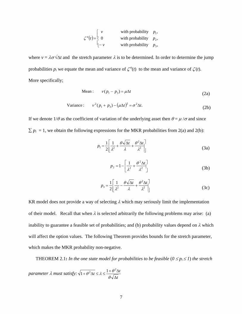
( ),y probabilit with ,y probabilit with ,y probabilit with

0

3

2

1

ppp

v

vta

⎪⎩

⎪⎨

⎧

−=ζ

where v = λσ √∆t and the stretch parameter λ is to be determined. In order to determine the jump

probabilities pi we equate the mean and variance of ζ a(t) to the mean and variance of ζ (t).

More specifically;

tpp ∆=− µν )( :Mean 31 (2a)

( ) .)( :Variance 2231

2 ttpp ∆=∆−+ σµν (2b)

If we denote 1/θ as the coefficient of variation of the underlying asset then θ = µ /σ and since

∑ pi = 1, we obtain the following expressions for the MKR probabilities from 2(a) and 2(b):

⎥⎥⎦

⎤

⎢⎢⎣

⎡ ∆+

∆+= 2

2

211

21

λθ

λθ

λttp

(3a)

⎥⎦

⎤⎢⎣

⎡ ∆+−= 2

2

2211

λθ

λtp

(3b)

1

21

2

2

23⎥⎥⎦

⎤

⎢⎢⎣

⎡ ∆+

∆−=

λθ

λθ

λttp

(3c)

KR model does not provide a way of selecting λ which may seriously limit the implementation

of their model. Recall that when λ is selected arbitrarily the following problems may arise: (a)

inability to guarantee a feasible set of probabilities; and (b) probability values depend on λ which

will affect the option values. The following Theorem provides bounds for the stretch parameter,

which makes the MKR probability non-negative.

THEOREM 2.1: In the one state model for probabilities to be feasible (0 ≤ pi ≤ 1) the stretch

parameter λ must satisfy: 112

2

ttt

∆∆+

≤≤∆+θθλθ

8

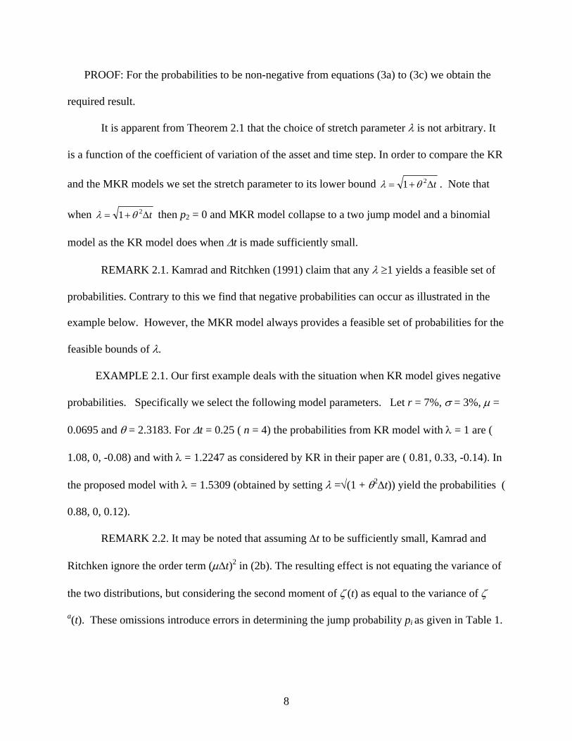
PROOF: For the probabilities to be non-negative from equations (3a) to (3c) we obtain the

required result.

It is apparent from Theorem 2.1 that the choice of stretch parameter λ is not arbitrary. It

is a function of the coefficient of variation of the asset and time step. In order to compare the KR

and the MKR models we set the stretch parameter to its lower bound t∆+= 21 θλ . Note that

when t∆+= 21 θλ then p2 = 0 and MKR model collapse to a two jump model and a binomial

model as the KR model does when ∆t is made sufficiently small.

REMARK 2.1. Kamrad and Ritchken (1991) claim that any λ ≥1 yields a feasible set of

probabilities. Contrary to this we find that negative probabilities can occur as illustrated in the

example below. However, the MKR model always provides a feasible set of probabilities for the

feasible bounds of λ.

EXAMPLE 2.1. Our first example deals with the situation when KR model gives negative

probabilities. Specifically we select the following model parameters. Let r = 7%, σ = 3%, µ =

0.0695 and θ = 2.3183. For ∆t = 0.25 ( n = 4) the probabilities from KR model with λ = 1 are (

1.08, 0, -0.08) and with λ = 1.2247 as considered by KR in their paper are ( 0.81, 0.33, -0.14). In

the proposed model with λ = 1.5309 (obtained by setting λ =√(1 + θ2∆t)) yield the probabilities (

0.88, 0, 0.12).

REMARK 2.2. It may be noted that assuming ∆t to be sufficiently small, Kamrad and

Ritchken ignore the order term (µ∆t)2 in (2b). The resulting effect is not equating the variance of

the two distributions, but considering the second moment of ζ (t) as equal to the variance of ζ

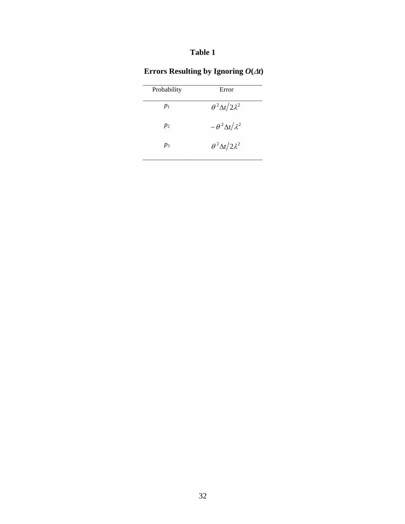
a(t). These omissions introduce errors in determining the jump probability pi as given in Table 1.

9

Insert Table 1 here

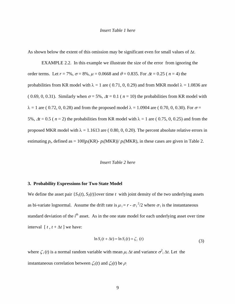
As shown below the extent of this omission may be significant even for small values of ∆t.

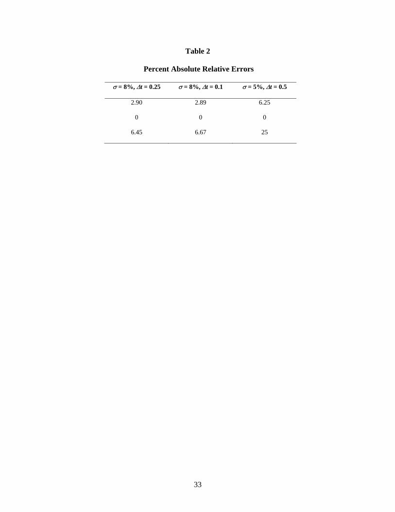
EXAMPLE 2.2. In this example we illustrate the size of the error from ignoring the

order terms. Let r = 7%, σ = 8%, µ = 0.0668 and θ = 0.835. For ∆t = 0.25 ( n = 4) the

probabilities from KR model with λ = 1 are ( 0.71, 0, 0.29) and from MKR model λ = 1.0836 are

( 0.69, 0, 0.31). Similarly when σ = 5%, ∆t = 0.1 ( n = 10) the probabilities from KR model with

λ = 1 are ( 0.72, 0, 0.28) and from the proposed model λ = 1.0904 are ( 0.70, 0, 0.30). For σ =

5%, ∆t = 0.5 ( n = 2) the probabilities from KR model with λ = 1 are ( 0.75, 0, 0.25) and from the

proposed MKR model with λ = 1.1613 are ( 0.80, 0, 0.20). The percent absolute relative errors in

estimating pi, defined as = 100|pi(KR)- pi(MKR)|/ pi(MKR), in these cases are given in Table 2.

Insert Table 2 here

3. Probability Expressions for Two State Model

We define the asset pair {S1(t), S2(t)}over time t with joint density of the two underlying assets

as bi-variate lognormal. Assume the drift rate is µ i = r - σ i 2/2 where σ i is the instantaneous

standard deviation of the ith asset. As in the one state model for each underlying asset over time

interval [ t , t + ∆t ] we have:

)()(ln)(ln ttSttS iii ζ+=∆+ (3)

where ζ i (t) is a normal random variable with mean µi ∆t and variance σ2i ∆t. Let the

instantaneous correlation between ζ1(t) and ζ2(t) be ρ.

10

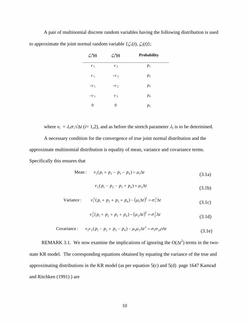
A pair of multinomial discrete random variables having the following distribution is used

to approximate the joint normal random variable {ζ1(t), ζ2(t)};

ζ1a(t) ζ2

a(t) Probability

ν 1 ν 2 p1

ν 1 -ν 2 p2

-ν 1 -ν 2 p3

-ν 1 ν 2 p4

0 0 p5

where vi = λiσ i√∆t (i= 1,2), and as before the stretch parameter λi is to be determined.

A necessary condition for the convergence of true joint normal distribution and the

approximate multinomial distribution is equality of mean, variance and covariance terms.

Specifically this ensures that

tpppp ∆=−−+ 143211 )( :Mean µν (3.1a)

tpppp ∆=+−− 243212 )( µν (3.1b)

( ) ttpppp ∆=∆−+++ 21

214321

21 )( :Variance σµν (3.1c)

( ) ttpppp ∆=∆−+++ 22

224321

22 )( σµν (3.1d)

ttpppp ∆=∆−−+− ρσσµµνν 212

21432121 )( :Covariance (3.1e)

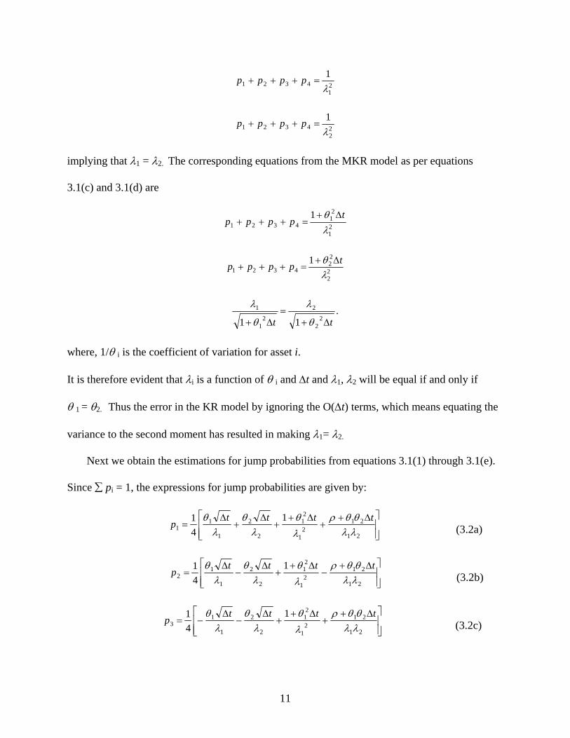
REMARK 3.1. We now examine the implications of ignoring the O(∆t2) terms in the two-

state KR model. The corresponding equations obtained by equating the variance of the true and

approximating distributions in the KR model (as per equation 5(c) and 5(d) page 1647 Kamrad

and Ritchken (1991) ) are

11

21

43211λ

=+++ pppp

22

43211λ

=+++ pppp

implying that λ1 = λ2. The corresponding equations from the MKR model as per equations

3.1(c) and 3.1(d) are

21

21

43211

λθ t

pppp∆+

=+++

22

22

43211

λθ tpppp ∆+

=+++

.11 2

2

2

21

1

tt ∆+=

∆+ θ

λ

θ

λ

where, 1/θ i is the coefficient of variation for asset i.

It is therefore evident that λi is a function of θ i and ∆t and λ1, λ2 will be equal if and only if

θ 1 = θ2. Thus the error in the KR model by ignoring the O(∆t) terms, which means equating the

variance to the second moment has resulted in making λ1= λ2.

Next we obtain the estimations for jump probabilities from equations 3.1(1) through 3.1(e).

Since ∑ pi = 1, the expressions for jump probabilities are given by:

⎥⎥⎦

⎤

⎢⎢⎣

⎡ ∆++

∆++

∆+

∆=

21

212

1

21

2

2

1

11

141

λλθθρ

λθ

λθ

λθ tttt

p (3.2a)

⎥⎥⎦

⎤

⎢⎢⎣

⎡ ∆+−

∆++

∆−

∆=

21

212

1

21

2

2

1

12

141

λλθθρ

λθ

λθ

λθ tttt

p (3.2b)

⎥⎥⎦

⎤

⎢⎢⎣

⎡ ∆++

∆++

∆−

∆−=

21

212

1

21

2

2

1

13

141

λλθθρ

λθ

λθ

λθ tttt

p (3.2c)

12

⎥⎥⎦

⎤

⎢⎢⎣

⎡ ∆+−

∆++

∆+

∆−=

21

212

1

21

2

2

1

14

141

λλθθρ

λθ

λθ

λθ tttt

p (3.2d)

⎥⎥⎦

⎤

⎢⎢⎣

⎡ ∆+−= 2

1

21

51

1λθ t

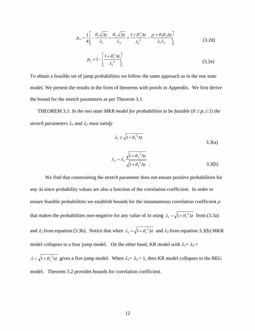
p (3.2e)

To obtain a feasible set of jump probabilities we follow the same approach as in the one state

model. We present the results in the form of theorems with proofs in Appendix. We first derive

the bound for the stretch parameters as per Theorem 3.1.

THEOREM 3.1: In the two state MKR model for probabilities to be feasible (0 ≤ pi ≤ 1) the

stretch parameters λ1 and λ2 must satisfy

1 2

11 t∆+≥ θλ 3.3(a)

t

t

∆+

∆+=

21

22

121

1

θ

θλλ

. 3.3(b)

We find that constraining the stretch parameter does not ensure positive probabilities for

any ∆t since probability values are also a function of the correlation coefficient. In order to

ensure feasible probabilities we establish bounds for the instantaneous correlation coefficient ρ

that makes the probabilities non-negative for any value of ∆t using t∆+= 211 1 θλ from (3.3a)

and λ2 from equation (3.3b). Notice that when t∆+= 211 1 θλ and λ2 from equation 3.3(b) MKR

model collapses to a four jump model. On the other hand, KR model with λ1= λ2 =

t∆+= 211 θλ gives a five jump model. When λ1= λ2 = 1, then KR model collapses to the BEG

model. Theorem 3.2 provides bounds for correlation coefficient.

13

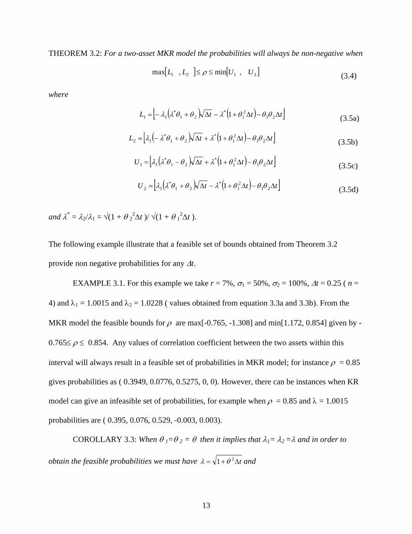
THEOREM 3.2: For a two-asset MKR model the probabilities will always be non-negative when

[ ] [ ]2121 , min , max UULL ≤≤ ρ

(3.4)

where

( ) ( )[ ]tttL ∆−∆+−∆+−= 21

21

*21

*11 1 θθθλθθλλ

(3.5a)

( ) ( )[ ]tttL ∆−∆++∆+−= 21

21

*21


(3.5b)

( ) ( )[ ]tttU ∆−∆++∆−= 21

21

*21


(3.5c)

( ) ( )[ ]tttU ∆−∆+−∆+= 21

21

*21


(3.5d)

and λ* = λ2/λ1 = √(1 + θ 22∆t )/ √(1 + θ 12∆t ).

The following example illustrate that a feasible set of bounds obtained from Theorem 3.2

provide non negative probabilities for any ∆t.

EXAMPLE 3.1. For this example we take r = 7%, σ1 = 50%, σ2 = 100%, ∆t = 0.25 ( n =

4) and λ1 = 1.0015 and λ2 = 1.0228 ( values obtained from equation 3.3a and 3.3b). From the

MKR model the feasible bounds for ρ are max[-0.765, -1.308] and min[1.172, 0.854] given by -

0.765≤ ρ ≤ 0.854. Any values of correlation coefficient between the two assets within this

interval will always result in a feasible set of probabilities in MKR model; for instance ρ = 0.85

gives probabilities as ( 0.3949, 0.0776, 0.5275, 0, 0). However, there can be instances when KR

model can give an infeasible set of probabilities, for example when ρ = 0.85 and λ = 1.0015

probabilities are ( 0.395, 0.076, 0.529, -0.003, 0.003).

COROLLARY 3.3: When θ 1=θ 2 = θ then it implies that λ1= λ2 =λ and in order to

obtain the feasible probabilities we must have t∆+= 21 θλ and

14

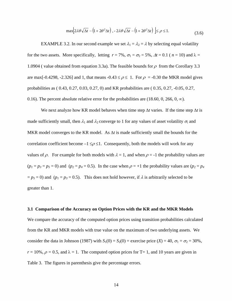
( ) ( )[ ] .1 212- , 212max 22 ≤≤∆+−∆∆+−∆ ρθλθθλθ tttt

(3.6)

EXAMPLE 3.2. In our second example we set λ1 = λ2 = λ by selecting equal volatility

for the two assets. More specifically, letting r = 7%, σ1 = σ2 = 5%, ∆t = 0.1 ( n = 10) and λ =

1.0904 ( value obtained from equation 3.3a). The feasible bounds for ρ from the Corollary 3.3

are max[-0.4298, -2.326] and 1, that means -0.43 ≤ ρ ≤ 1. For ρ = -0.30 the MKR model gives

probabilities as ( 0.43, 0.27, 0.03, 0.27, 0) and KR probabilities are ( 0.35, 0.27, -0.05, 0.27,

0.16). The percent absolute relative error for the probabilities are (18.60, 0, 266, 0, ∞).

We next analyze how KR model behaves when time step ∆t varies. If the time step ∆t is

made sufficiently small, then λ1 and λ2 converge to 1 for any values of asset volatility σi and

MKR model converges to the KR model. As ∆t is made sufficiently small the bounds for the

correlation coefficient become –1 ≤ρ ≤1. Consequently, both the models will work for any

values of ρ. For example for both models with λ = 1, and when ρ = -1 the probability values are

(p1 = p3 = p5 = 0) and (p2 = p4 = 0.5). In the case when ρ = +1 the probability values are (p2 = p4

= p5 = 0) and (p1 = p3 = 0.5). This does not hold however, if λ is arbitrarily selected to be

greater than 1.

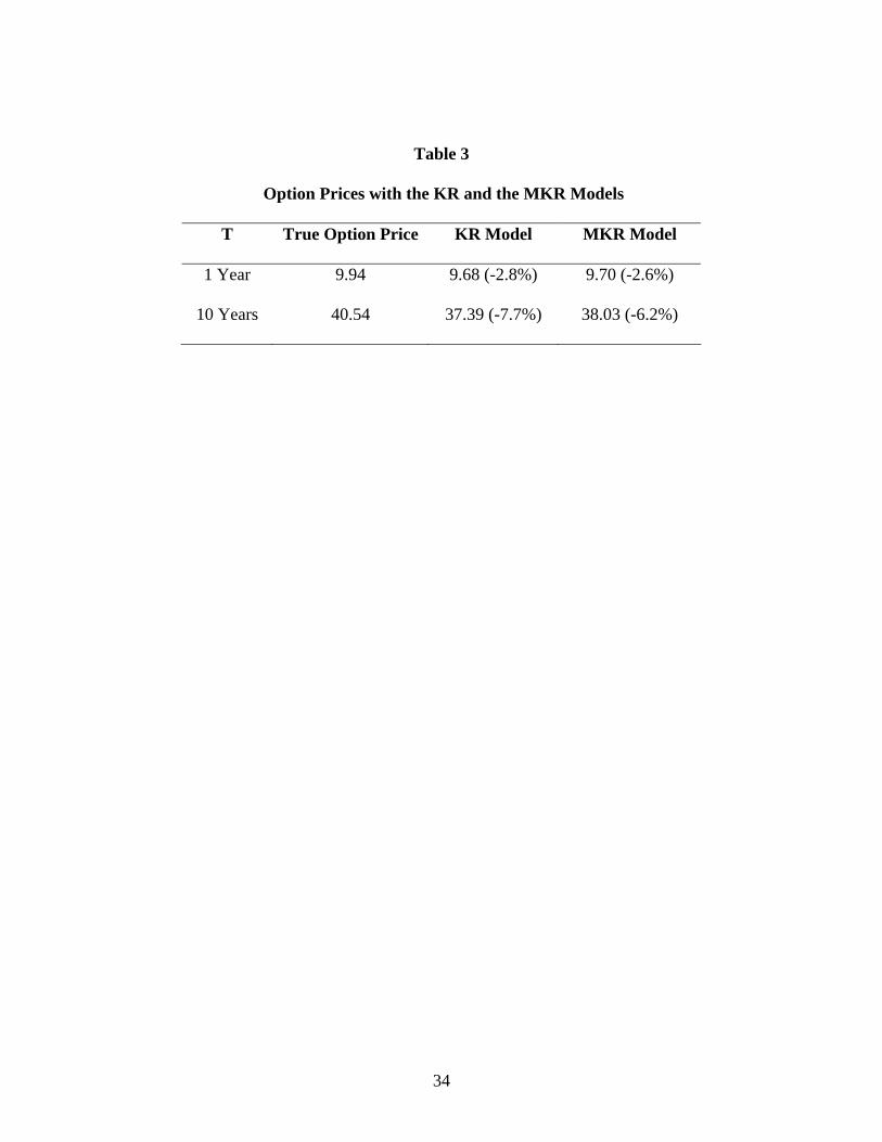
3.1 Comparison of the Accuracy on Option Prices with the KR and the MKR Models

We compare the accuracy of the computed option prices using transition probabilities calculated

from the KR and MKR models with true value on the maximum of two underlying assets. We

consider the data in Johnson (1987) with S1(0) = S2(0) = exercise price (X) = 40, σ1 = σ2 = 30%,

r = 10%, ρ = 0.5, and λ = 1. The computed option prices for T= 1, and 10 years are given in

Table 3. The figures in parenthesis give the percentage errors.

15

Insert Table 3 here

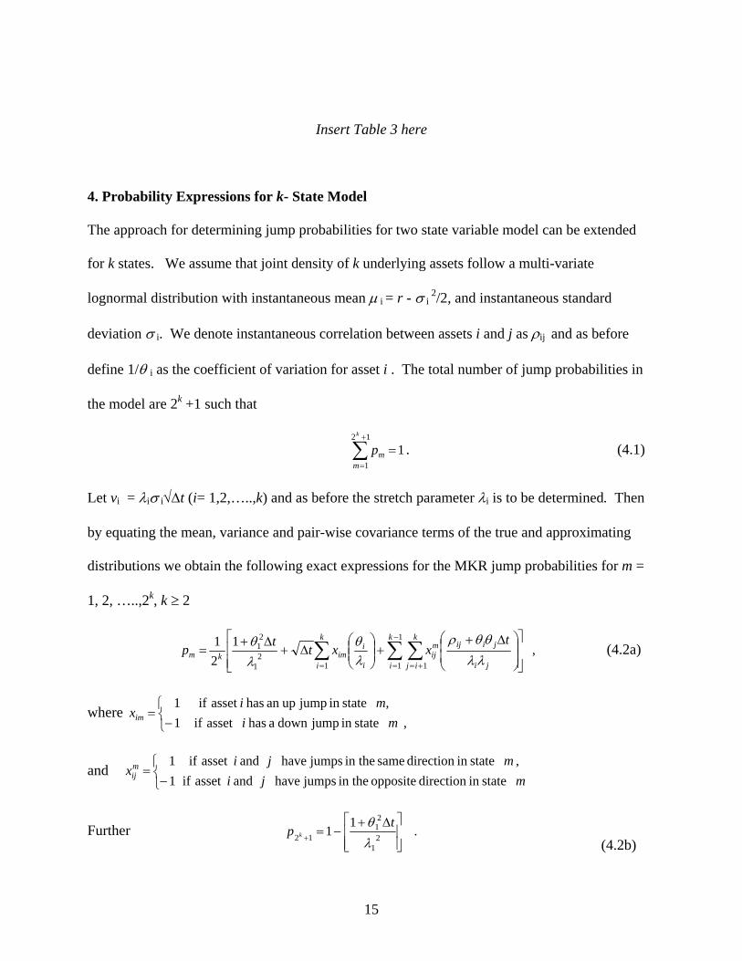
4. Probability Expressions for k- State Model

The approach for determining jump probabilities for two state variable model can be extended

for k states. We assume that joint density of k underlying assets follow a multi-variate

lognormal distribution with instantaneous mean µ i = r - σ i 2/2, and instantaneous standard

deviation σ i. We denote instantaneous correlation between assets i and j as ρij and as before

define 1/θ i as the coefficient of variation for asset i . The total number of jump probabilities in

the model are 2k +1 such that

112

1

=∑+

=

k

mmp . (4.1)

Let vi = λiσ i√∆t (i= 1,2,…..,k) and as before the stretch parameter λi is to be determined. Then

by equating the mean, variance and pair-wise covariance terms of the true and approximating

distributions we obtain the following exact expressions for the MKR jump probabilities for m =

1, 2, …..,2k, k ≥ 2

, 121

1

1

1 12

1

21

⎥⎥⎦

⎤

⎢⎢⎣

⎡⎟⎟⎠

⎞⎜⎜⎝

⎛ ∆++⎟⎟

⎠

⎞⎜⎜⎝

⎛∆+

∆+= ∑ ∑ ∑

=

−

= +=

k

i

k

i ji

jiijk

ij

mij

i

iimkm

txxttp

λλθθρ

λθ

λθ (4.2a)

where , statein jumpdown a has asset if

, statein jump upan has asset if 11

mimi

xim⎩⎨⎧−

=

and mji

mjixm

ij statein direction opposite in the jumps have and asset if , statein direction same in the jumps have and asset if

11

⎩⎨⎧−

=

Further . 1

1 21

21

12 ⎥⎥⎦

⎤

⎢⎢⎣

⎡ ∆+−=

+ λθ t

p k

(4.2b)

16

Notice that as in the previous cases when t∆+= 211 1 θλ , the MKR model collapses to a 2k

jump model.

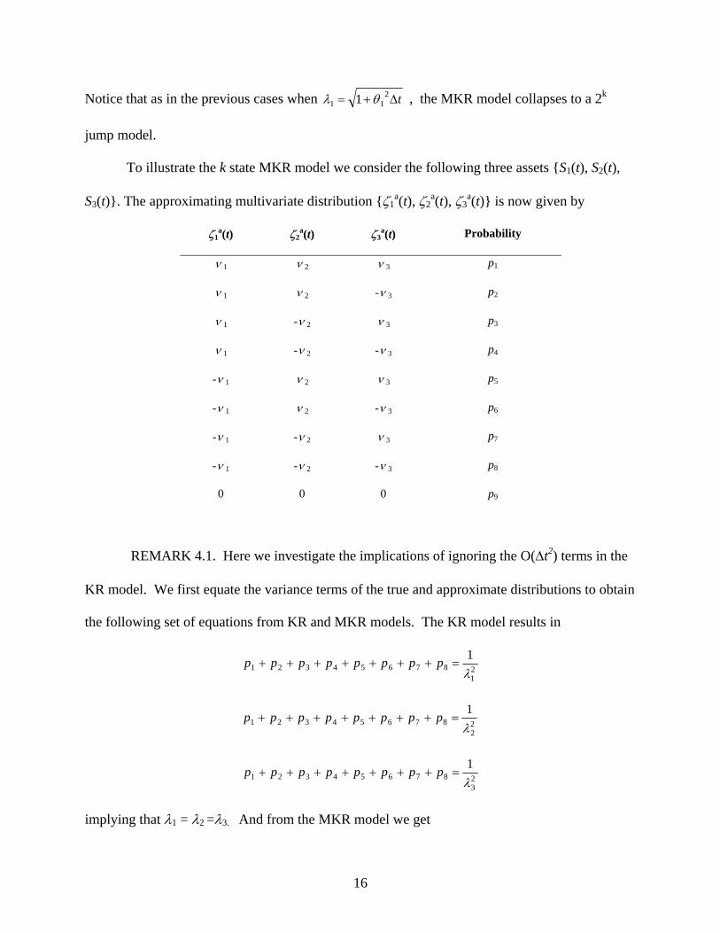
To illustrate the k state MKR model we consider the following three assets {S1(t), S2(t),

S3(t)}. The approximating multivariate distribution {ζ1a(t), ζ2

a(t), ζ3a(t)} is now given by

ζ1a(t) ζ2

a(t) ζ3a(t) Probability

ν 1 ν 2 ν 3 p1

ν 1 ν 2 -ν 3 p2

ν 1 -ν 2 ν 3 p3

ν 1 -ν 2 -ν 3 p4

-ν 1 ν 2 ν 3 p5

-ν 1 ν 2 -ν 3 p6

-ν 1 -ν 2 ν 3 p7

-ν 1 -ν 2 -ν 3 p8

0 0 0 p9

REMARK 4.1. Here we investigate the implications of ignoring the O(∆t2) terms in the

KR model. We first equate the variance terms of the true and approximate distributions to obtain

the following set of equations from KR and MKR models. The KR model results in

21

876543211λ

=+++++++ pppppppp

22

876543211λ

=+++++++ pppppppp

23

876543211λ

=+++++++ pppppppp

implying that λ1 = λ2 =λ3. And from the MKR model we get

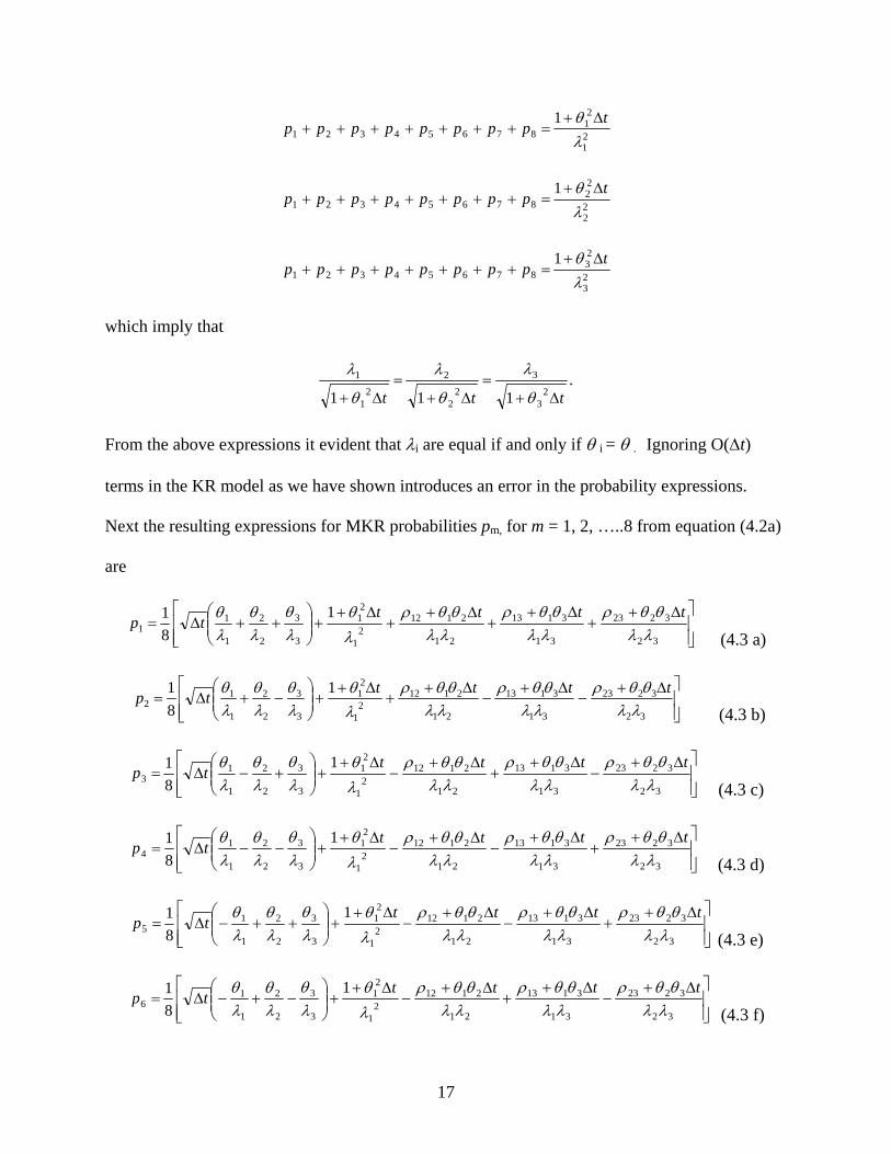
17

21

21

876543211

λθ t

pppppppp∆+

=+++++++

22

22

876543211

λθ t

pppppppp∆+

=+++++++

23

23

876543211

λθ t

pppppppp∆+

=+++++++

which imply that

.111 2

3

3

22

2

21

1

ttt ∆+=

∆+=

∆+ θ

λ

θ

λ

θ

λ

From the above expressions it evident that λi are equal if and only if θ i = θ . Ignoring O(∆t)

terms in the KR model as we have shown introduces an error in the probability expressions.

Next the resulting expressions for MKR probabilities pm, for m = 1, 2, …..8 from equation (4.2a)

are

⎥⎥⎦

⎤

⎢⎢⎣

⎡ ∆++

∆++

∆++

∆++⎟⎟

⎠

⎞⎜⎜⎝

⎛++∆=

32

3223

31

3113

21

21122

1

21

3

3

2

2

1

11

181

λλθθρ

λλθθρ

λλθθρ

λθ

λθ

λθ

λθ tttt

tp (4.3 a)

⎥⎥⎦

⎤

⎢⎢⎣

⎡ ∆+−

∆+−

∆++

∆++⎟⎟

⎠

⎞⎜⎜⎝

⎛−+∆=

32

3223

31

3113

21

21122

1

21

3

3

2

2

1

12

181

λλθθρ

λλθθρ

λλθθρ

λθ

λθ

λθ

λθ tttttp

(4.3 b)

⎥⎥⎦

⎤

⎢⎢⎣

⎡ ∆+−

∆++

∆+−

∆++⎟⎟

⎠

⎞⎜⎜⎝

⎛+−∆=

32

3223

31

3113

21

21122

1

21

3

3

2

2

1

13

181

λλθθρ

λλθθρ

λλθθρ

λθ

λθ

λθ

λθ tttt

tp (4.3 c)

⎥⎥⎦

⎤

⎢⎢⎣

⎡ ∆++

∆+−

∆+−

∆++⎟⎟

⎠

⎞⎜⎜⎝

⎛−−∆=

32

3223

31

3113

21

21122

1

21

3

3

2

2

1

14

181

λλθθρ

λλθθρ

λλθθρ

λθ

λθ

λθ

λθ tttt

tp (4.3 d)

⎥⎥⎦

⎤

⎢⎢⎣

⎡ ∆++

∆+−

∆+−

∆++⎟⎟

⎠

⎞⎜⎜⎝

⎛++−∆=

32

3223

31

3113

21

21122

1

21

3

3

2

2

1

15

181

λλθθρ

λλθθρ

λλθθρ

λθ

λθ

λθ

λθ tttt

tp (4.3 e)

⎥⎥⎦

⎤

⎢⎢⎣

⎡ ∆+−

∆++

∆+−

∆++⎟⎟

⎠

⎞⎜⎜⎝

⎛−+−∆=

32

3223

31

3113

21

21122

1

21

3

3

2

2

1

16

181

λλθθρ

λλθθρ

λλθθρ

λθ

λθ

λθ

λθ tttt

tp (4.3 f)

18

⎥⎥⎦

⎤

⎢⎢⎣

⎡ ∆+−

∆+−

∆++

∆++⎟⎟

⎠

⎞⎜⎜⎝

⎛+−−∆=

32

3223

31

3113

21

21122

1

21

3

3

2

2

1

17

181

λλθθρ

λλθθρ

λλθθρ

λθ

λθ

λθ

λθ tttt

tp (4.3 g)

⎥⎥⎦

⎤

⎢⎢⎣

⎡ ∆++

∆++

∆++

∆++⎟⎟

⎠

⎞⎜⎜⎝

⎛−−−∆=

32

3223

31

3113

21

21122

1

21

3

3

2

2

1

18

181

λλθθρ

λλθθρ

λλθθρ

λθ

λθ

λθ

λθ tttt

tp (4.3 h)

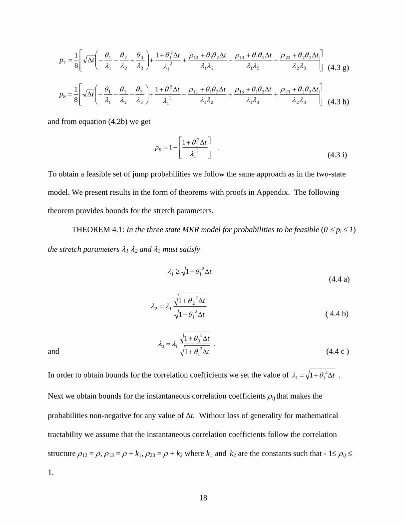
and from equation (4.2b) we get

.

11 2

1

21

9⎥⎥⎦

⎤

⎢⎢⎣

⎡ ∆+−=

λθ t

p (4.3 i)

To obtain a feasible set of jump probabilities we follow the same approach as in the two-state

model. We present results in the form of theorems with proofs in Appendix. The following

theorem provides bounds for the stretch parameters.

THEOREM 4.1: In the three state MKR model for probabilities to be feasible (0 ≤ pi ≤ 1)

the stretch parameters λ1 λ2 and λ3 must satisfy

1 211 t∆+≥ θλ

(4.4 a)

1

12

1

22

12t

t

∆+

∆+=

θ

θλλ

( 4.4 b)

and .

1

12

1

23

13t

t

∆+

∆+=

θ

θλλ

(4.4 c )

In order to obtain bounds for the correlation coefficients we set the value of t∆+= 211 1 θλ .

Next we obtain bounds for the instantaneous correlation coefficients ρij that makes the

probabilities non-negative for any value of ∆t. Without loss of generality for mathematical

tractability we assume that the instantaneous correlation coefficients follow the correlation

structure ρ12 = ρ, ρ13 = ρ + k1, ρ23 = ρ + k2 where k1, and k2 are the constants such that - 1≤ ρij ≤

1.

19

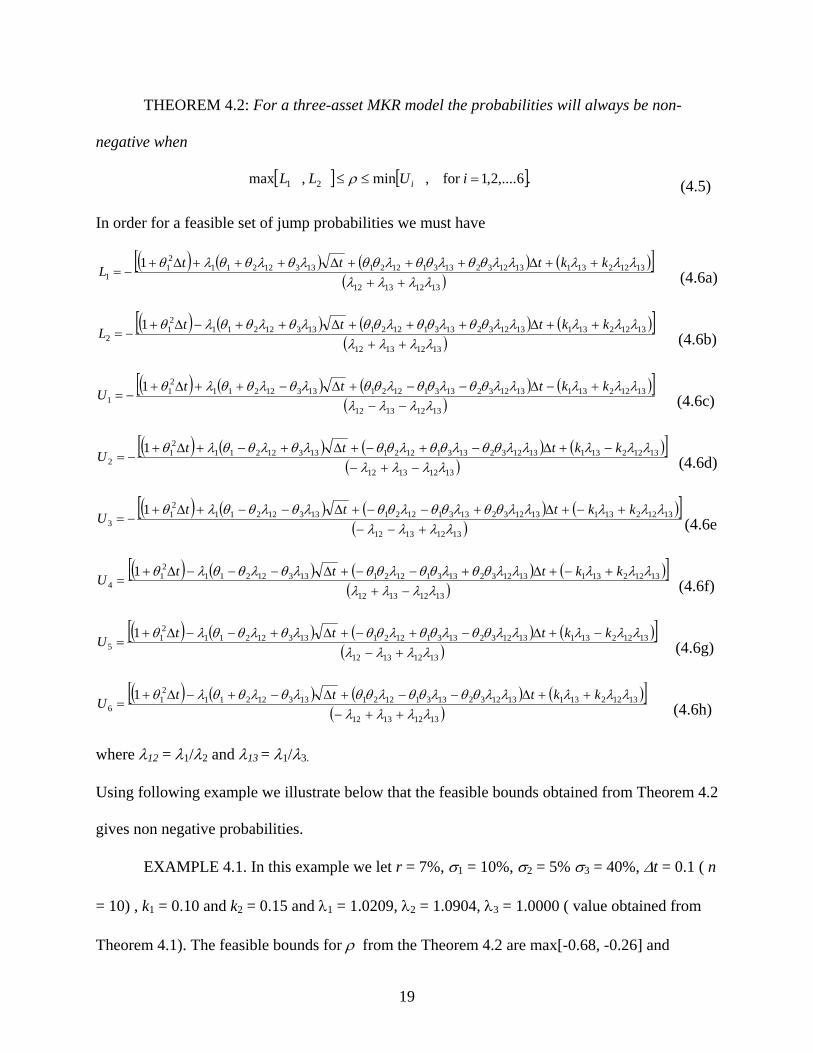
THEOREM 4.2: For a three-asset MKR model the probabilities will always be non-

negative when

[ ] [ ].6,....2,1for , min , max 21 =≤≤ iULL iρ

(4.5)

In order for a feasible set of jump probabilities we must have

( ) ( ) ( ) ( )[ ]( )13121312

1312213113123213311221133122112

11

1λλλλ

λλλλλθθλθθλθθλθλθθλθ++

++∆+++∆+++∆+−=

kktttL

(4.6a)

( ) ( ) ( ) ( )[ ]( )13121312

1312213113123213311221133122112

12

1λλλλ

λλλλλθθλθθλθθλθλθθλθ++

++∆+++∆++−∆+−=

kktttL

(4.6b)

( ) ( ) ( ) ( )[ ]( )13121312

1312213113123213311221133122112

11

1λλλλ

λλλλλθθλθθλθθλθλθθλθ−−

+−∆−−+∆−++∆+−=

kktttU (4.6c)

( ) ( ) ( ) ( )[ ]( )13121312

1312213113123213311221133122112

12

1λλλλ

λλλλλθθλθθλθθλθλθθλθ−+−

−+∆−+−+∆+−+∆+−=

kktttU

(4.6d)

( ) ( ) ( ) ( )[ ]( )13121312

1312213113123213311221133122112

13

1λλλλ

λλλλλθθλθθλθθλθλθθλθ+−−

+−+∆+−−+∆−−+∆+−=

kktttU (4.6e

( ) ( ) ( ) ( )[ ]( )13121312

1312213113123213311221133122112

14

1λλλλ

λλλλλθθλθθλθθλθλθθλθ−+

+−+∆+−−+∆−−−∆+=

kktttU

(4.6f)

( ) ( ) ( ) ( )[ ]( )13121312

1312213113123213311221133122112

15

1λλλλ

λλλλλθθλθθλθθλθλθθλθ+−

−+∆−+−+∆+−−∆+=

kktttU

(4.6g)

( ) ( ) ( ) ( )[ ]( )13121312

1312213113123213311221133122112

16

1λλλλ

λλλλλθθλθθλθθλθλθθλθ++−

++∆−−+∆−+−∆+=

kktttU (4.6h)

where λ12 = λ1/λ2 and λ13 = λ1/λ3.

Using following example we illustrate below that the feasible bounds obtained from Theorem 4.2

gives non negative probabilities.

EXAMPLE 4.1. In this example we let r = 7%, σ1 = 10%, σ2 = 5% σ3 = 40%, ∆t = 0.1 ( n

= 10) , k1 = 0.10 and k2 = 0.15 and λ1 = 1.0209, λ2 = 1.0904, λ3 = 1.0000 ( value obtained from

Theorem 4.1). The feasible bounds for ρ from the Theorem 4.2 are max[-0.68, -0.26] and

20

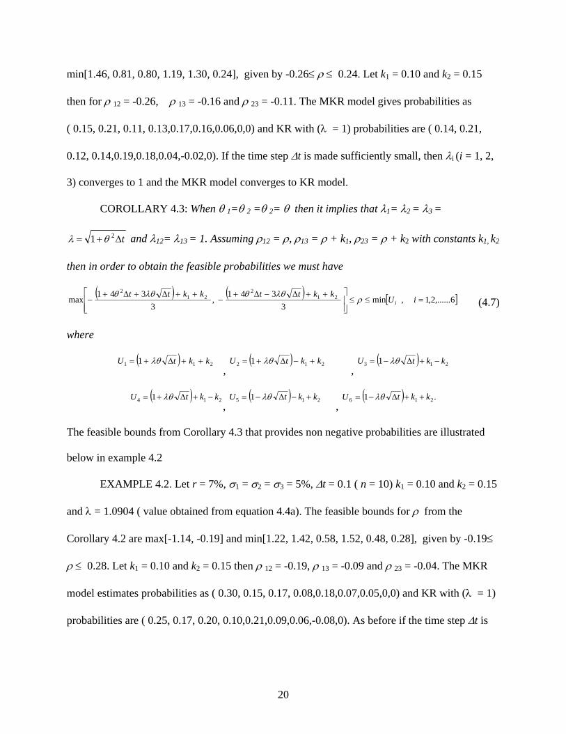
min[1.46, 0.81, 0.80, 1.19, 1.30, 0.24], given by -0.26≤ ρ ≤ 0.24. Let k1 = 0.10 and k2 = 0.15

then for ρ 12 = -0.26, ρ 13 = -0.16 and ρ 23 = -0.11. The MKR model gives probabilities as

( 0.15, 0.21, 0.11, 0.13,0.17,0.16,0.06,0,0) and KR with (λ = 1) probabilities are ( 0.14, 0.21,

0.12, 0.14,0.19,0.18,0.04,-0.02,0). If the time step ∆t is made sufficiently small, then λi (i = 1, 2,

3) converges to 1 and the MKR model converges to KR model.

COROLLARY 4.3: When θ 1=θ 2 =θ 2= θ then it implies that λ1= λ2 = λ3 =

t∆+= 21 θλ and λ12= λ13 = 1. Assuming ρ12 = ρ, ρ13 = ρ + k1, ρ23 = ρ + k2 with constants k1, k2

then in order to obtain the feasible probabilities we must have

( ) ( ) [ ]6,......2,1 , min 3

341 ,

3 341

max 212

212

=≤≤⎥⎥⎦

⎤

⎢⎢⎣

⎡ ++∆−∆+−

++∆+∆+− iU

kkttkkttiρ

λθθλθθ

(4.7)

where

( ) 211 1 kktU ++∆+= λθ ,

( ) 212 1 kktU +−∆+= λθ ,

( ) 213 1 kktU −+∆−= λθ

( ) 214 1 kktU −+∆+= λθ,

( ) 215 1 kktU +−∆−= λθ ,

( ) .1 216 kktU ++∆−= λθ

The feasible bounds from Corollary 4.3 that provides non negative probabilities are illustrated

below in example 4.2

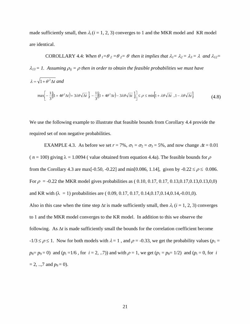
EXAMPLE 4.2. Let r = 7%, σ1 = σ2 = σ3 = 5%, ∆t = 0.1 ( n = 10) k1 = 0.10 and k2 = 0.15

and λ = 1.0904 ( value obtained from equation 4.4a). The feasible bounds for ρ from the

Corollary 4.2 are max[-1.14, -0.19] and min[1.22, 1.42, 0.58, 1.52, 0.48, 0.28], given by -0.19≤

ρ ≤ 0.28. Let k1 = 0.10 and k2 = 0.15 then ρ 12 = -0.19, ρ 13 = -0.09 and ρ 23 = -0.04. The MKR

model estimates probabilities as ( 0.30, 0.15, 0.17, 0.08,0.18,0.07,0.05,0,0) and KR with (λ = 1)

probabilities are ( 0.25, 0.17, 0.20, 0.10,0.21,0.09,0.06,-0.08,0). As before if the time step ∆t is

21

made sufficiently small, then λi (i = 1, 2, 3) converges to 1 and the MKR model and KR model

are identical.

COROLLARY 4.4: When θ 1=θ 2 =θ 2= θ then it implies that λ1= λ2 = λ3 = λ and λ12=

λ13 = 1. Assuming ρij = ρ then in order to obtain the feasible probabilities we must have

t∆+= 21 θλ and

( )[ ] ( )[ ] [ ].1 , 1min 341

31 , 341

31max 22 tttttt ∆−∆+≤≤⎥⎦

⎤⎢⎣⎡ ∆−∆+−∆+∆+− λθλθρλθθλθθ

(4.8)

We use the following example to illustrate that feasible bounds from Corollary 4.4 provide the

required set of non negative probabilities.

EXAMPLE 4.3. As before we set r = 7%, σ1 = σ2 = σ3 = 5%, and now change ∆t = 0.01

( n = 100) giving λ = 1.0094 ( value obtained from equation 4.4a). The feasible bounds for ρ

from the Corollary 4.3 are max[-0.50, -0.22] and min[0.086, 1.14], given by -0.22 ≤ ρ ≤ 0.086.

For ρ = -0.22 the MKR model gives probabilities as ( 0.10, 0.17, 0.17, 0.13,0.17,0.13,0.13,0,0)

and KR with (λ = 1) probabilities are ( 0.09, 0.17, 0.17, 0.14,0.17,0.14,0.14,-0.01,0).

Also in this case when the time step ∆t is made sufficiently small, then λi (i = 1, 2, 3) converges

to 1 and the MKR model converges to the KR model. In addition to this we observe the

following. As ∆t is made sufficiently small the bounds for the correlation coefficient become

-1/3 ≤ ρ ≤ 1. Now for both models with λ = 1 , and ρ = -0.33, we get the probability values (p1 =

p8= p9 = 0) and (pi =1/6 , for i = 2, ..7)) and with ρ = 1, we get (p1 = p8= 1/2) and (pi = 0, for i

= 2, ..,7 and p9 = 0).

22

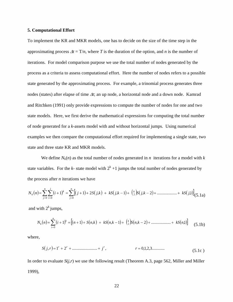
5. Computational Effort

To implement the KR and MKR models, one has to decide on the size of the time step in the

approximating process ∆t = T/n, where T is the duration of the option, and n is the number of

iterations. For model comparison purpose we use the total number of nodes generated by the

process as a criteria to assess computational effort. Here the number of nodes refers to a possible

state generated by the approximating process. For example, a trinomial process generates three

nodes (states) after elapse of time ∆t; an up node, a horizontal node and a down node. Kamrad

and Ritchken (1991) only provide expressions to compute the number of nodes for one and two

state models. Here, we first derive the mathematical expressions for computing the total number

of node generated for a k-assets model with and without horizontal jumps. Using numerical

examples we then compare the computational effort required for implementing a single state, two

state and three state KR and MKR models.

We define Nk(n) as the total number of nodes generated in n iterations for a model with k

state variables. For the k- state model with 2k +1 jumps the total number of nodes generated by

the process after n iterations we have

( ) ( ) ( ) ( ) ( ) ( ) ( ) ( )[ ]∑∑ ∑= = =

++−+−+++=+=n

j

j

i

n

j

kkk j, kSj,kS j,k kS j,kSjinN

0 0 02 1...................21211 (5.1a)

and with 2k jumps,

( ) ( ) ( ) ( ) ( ) ( ) ( ) ( )[ ]∑=

++−+−+++=+=n

i

kkk n, kSn,kS n,k kS n,kSninN

02 1...................2111 (5.1b)

where,

( ) ............3,2,1,0 ,........................21, =+++= rjrjS rrr (5.1c )

In order to evaluate S(j,r) we use the following result (Theorem A.3, page 562, Miller and Miller

1999),

23

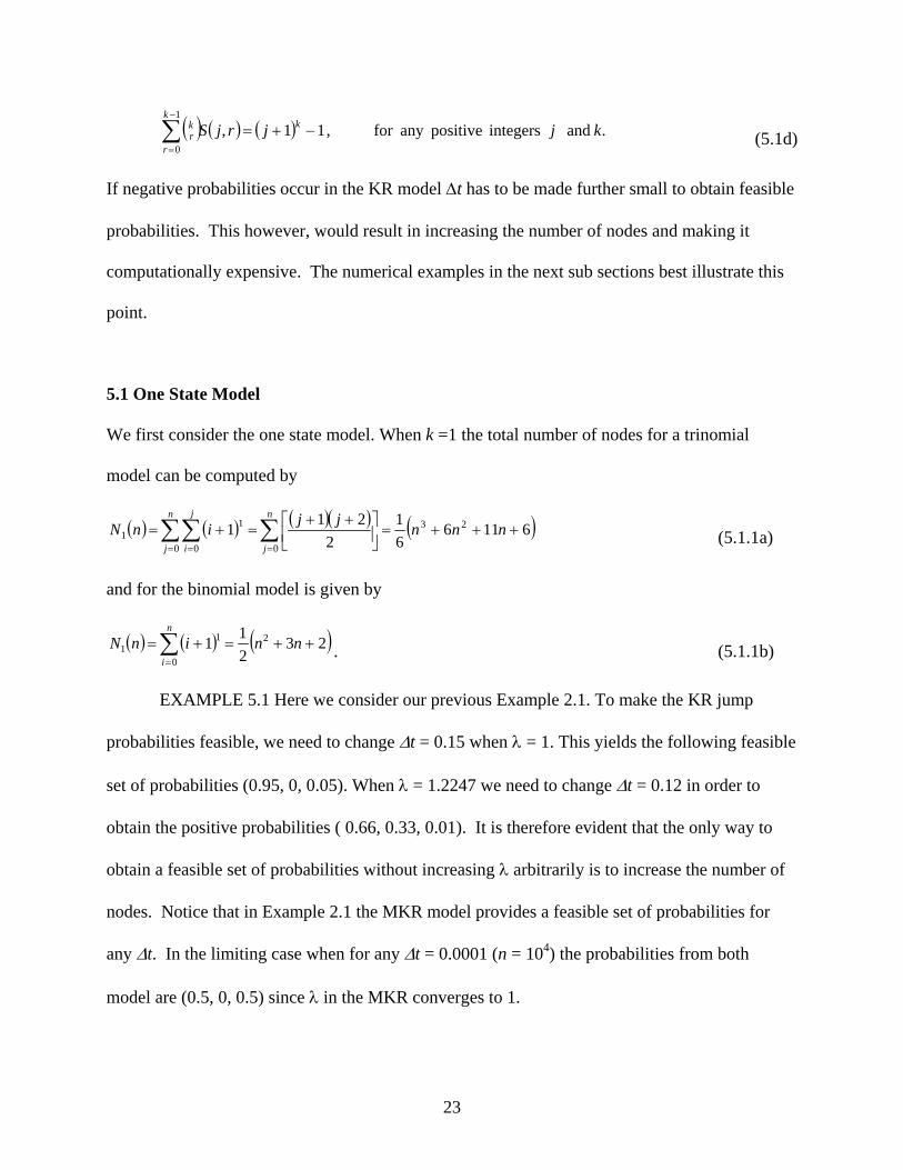
( ) ( ) ( ) . and integers positiveany for , 11,1

0

kjjrjS kk

r

kr −+=∑

−

= (5.1d)

If negative probabilities occur in the KR model ∆t has to be made further small to obtain feasible

probabilities. This however, would result in increasing the number of nodes and making it

computationally expensive. The numerical examples in the next sub sections best illustrate this

point.

5.1 One State Model

We first consider the one state model. When k =1 the total number of nodes for a trinomial

model can be computed by

( ) ( ) ( )( ) ( )611661

2211 23

0 0 0

11 +++=⎥⎦

⎤⎢⎣⎡ ++

=+=∑∑ ∑= = =

nnnjjinNn

j

j

i

n

j (5.1.1a)

and for the binomial model is given by

( ) ( ) ( )23211 2

0

11 ++=+=∑

=

nninNn

i. (5.1.1b)

EXAMPLE 5.1 Here we consider our previous Example 2.1. To make the KR jump

probabilities feasible, we need to change ∆t = 0.15 when λ = 1. This yields the following feasible

set of probabilities (0.95, 0, 0.05). When λ = 1.2247 we need to change ∆t = 0.12 in order to

obtain the positive probabilities ( 0.66, 0.33, 0.01). It is therefore evident that the only way to

obtain a feasible set of probabilities without increasing λ arbitrarily is to increase the number of

nodes. Notice that in Example 2.1 the MKR model provides a feasible set of probabilities for

any ∆t. In the limiting case when for any ∆t = 0.0001 (n = 104) the probabilities from both

model are (0.5, 0, 0.5) since λ in the MKR converges to 1.

24

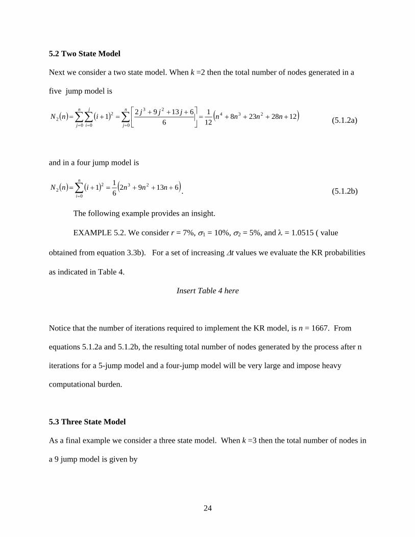
5.2 Two State Model

Next we consider a two state model. When k =2 then the total number of nodes generated in a

five jump model is

( ) ( ) ( )1228238121

6613921 234

0 0 0

232

2 ++++=⎥⎦

⎤⎢⎣

⎡ +++=+=∑∑ ∑

= = =

nnnnjjjinNn

j

j

i

n

j (5.1.2a)

and in a four jump model is

( ) ( ) ( )61392611 23

0

22 +++=+=∑

=

nnninNn

i. (5.1.2b)

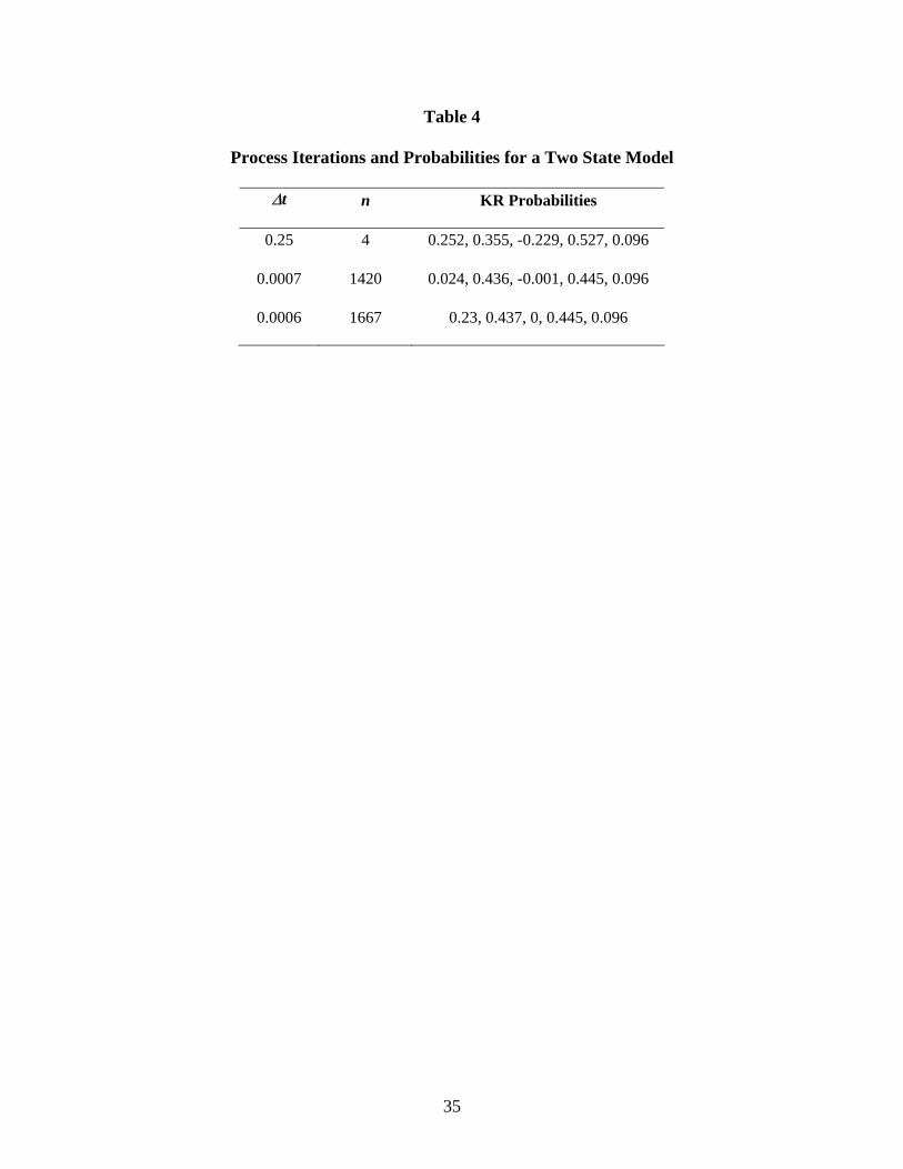
The following example provides an insight.

EXAMPLE 5.2. We consider r = 7%, σ1 = 10%, σ2 = 5%, and λ = 1.0515 ( value

obtained from equation 3.3b). For a set of increasing ∆t values we evaluate the KR probabilities

as indicated in Table 4.

Insert Table 4 here

Notice that the number of iterations required to implement the KR model, is n = 1667. From

equations 5.1.2a and 5.1.2b, the resulting total number of nodes generated by the process after n

iterations for a 5-jump model and a four-jump model will be very large and impose heavy

computational burden.

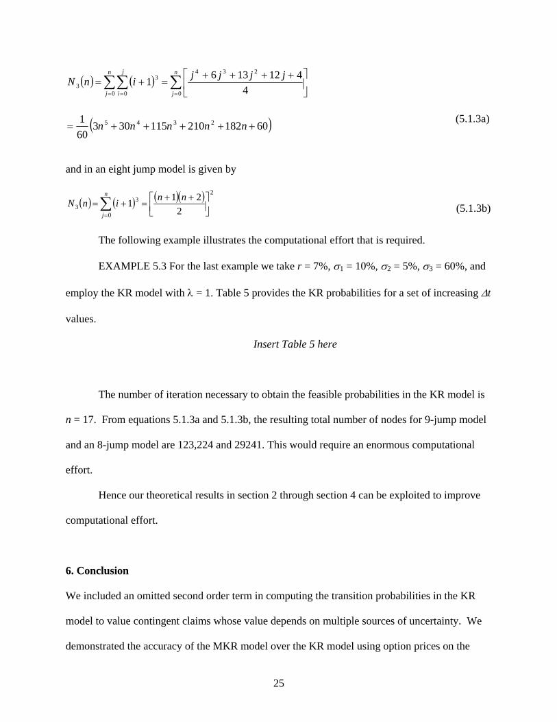
5.3 Three State Model

As a final example we consider a three state model. When k =3 then the total number of nodes in

a 9 jump model is given by

25

( )60182210115303601 2345 +++++= nnnnn

( ) ( )∑∑ ∑= = =

⎥⎦

⎤⎢⎣

⎡ ++++=+=

n

j

j

i

n

j

jjjjinN0 0 0

2343

3 44121361

(5.1.3a)

and in an eight jump model is given by

( ) ( ) ( )( ) 2

0

33 2

211 ⎥⎦⎤

⎢⎣⎡ ++

=+=∑=

nninNn

j (5.1.3b)

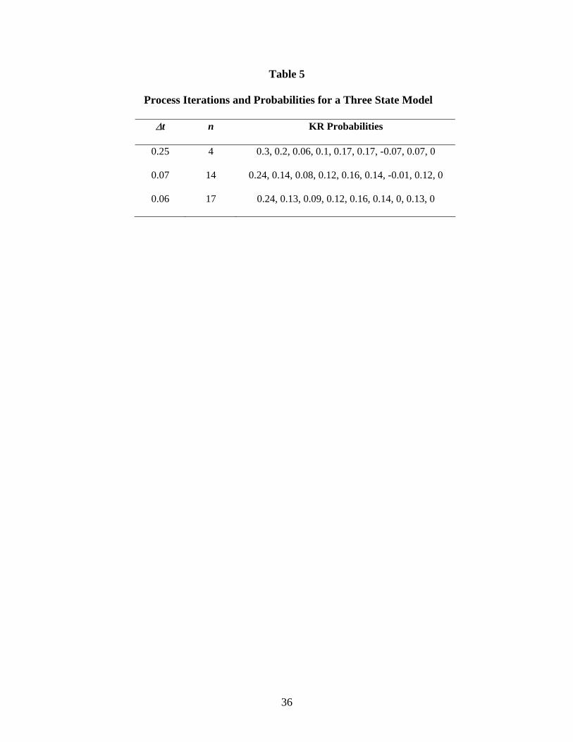
The following example illustrates the computational effort that is required.

EXAMPLE 5.3 For the last example we take r = 7%, σ1 = 10%, σ2 = 5%, σ3 = 60%, and

employ the KR model with λ = 1. Table 5 provides the KR probabilities for a set of increasing ∆t

values.

Insert Table 5 here

The number of iteration necessary to obtain the feasible probabilities in the KR model is

n = 17. From equations 5.1.3a and 5.1.3b, the resulting total number of nodes for 9-jump model

and an 8-jump model are 123,224 and 29241. This would require an enormous computational

effort.

Hence our theoretical results in section 2 through section 4 can be exploited to improve

computational effort.

6. Conclusion

We included an omitted second order term in computing the transition probabilities in the KR

model to value contingent claims whose value depends on multiple sources of uncertainty. We

demonstrated the accuracy of the MKR model over the KR model using option prices on the

26

maximum of two assets. Our analysis suggest that the KR model should be used when the time

step is very small and when there are fewer state variables implying it is only then the model

becomes computationally inexpensive. We proved that bounds for the stretch parameter and the

correlation coefficient could be exploited to obtain a feasible set of probabilities without

imposing heavy computational burden. In addition, we developed general expressions to

determine the number of nodes generated in the approximation process when there are k state

variables.

The probability estimates from the MKR model are more accurate than the probability

estimates based on the KR model which ignore the second order terms of the time step. We have

however shown that the two models provide identical probability estimates when the time step is

very small. The previous research including Kamrad and Ritchken (1991) do not provide an

objective way of selecting the stretch parameter. The examples that we selected show that

negative probabilities may occur limiting the usefulness of the KR model. Also, option values

may be different for different stretch parameters. Adapting the framework that we suggested as

we have shown reduces the computational effort. More importantly it provides a model where

positive probabilities are guaranteed by constraining the correlation coefficient. Knowing the

feasible range of the correlation coefficient indicates when the multinomial approximation model

can be applied.

27

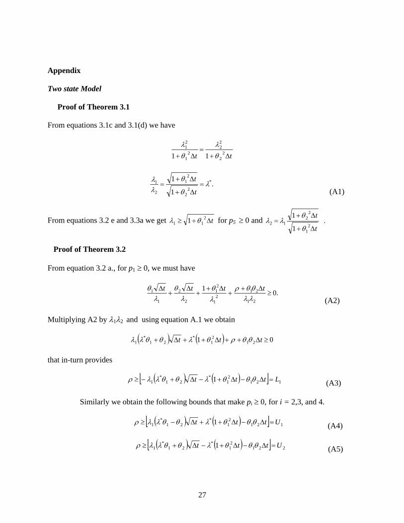
Appendix

Two state Model

Proof of Theorem 3.1

From equations 3.1c and 3.1(d) we have

tt ∆+=

∆+ 22

22

21

21

11 θλ

θλ

.

1

1 *

22

21

2

1 λθ

θλλ

=∆+

∆+=

t

t

(A1)

From equations 3.2 e and 3.3a we get t∆+≥ 211 1 θλ for p5 ≥ 0 and .

1

12

1

22

12t

t

∆+

∆+=

θ

θλλ


From equation 3.2 a., for p1 ≥ 0, we must have

.01

21

212

1

21

2

2

1

1 ≥∆+

+∆+

+∆

+∆

λλθθρ

λθ

λθ

λθ tttt

(A2)

Multiplying A2 by λ1λ2 and using equation A.1 we obtain

( ) ( ) 01 212

1*

21*

1 ≥∆++∆++∆+ ttt θθρθλθθλλ

that in-turn provides

( ) ( )[ ] 121

21

*21

*1 1 Lttt =∆−∆+−∆+−≥ θθθλθθλλρ

(A3)

Similarly we obtain the following bounds that make pi ≥ 0, for i = 2,3, and 4.

( ) ( )[ ] 121

21

*21

*1 1 Uttt =∆−∆++∆−≥ θθθλθθλλρ

(A4)

( ) ( )[ ] 221

21

*21

*1 1 Uttt =∆−∆+−∆+≥ θθθλθθλλρ

(A5)

28

( ) ( )[ ] 2.21

21

*21

*1 1 Lttt =∆−∆++∆+−≥ θθθλθθλλρ

(A6)

Therefore, in the two asset model the probabilities will always be non negative when

[ ] [ ]. , min , max 2 121 UULL ≤≤ ρ

Three State Model


By equating the pair-wise covariance terms we obtain

.111 2

3

23

22

22

21

21

ttt ∆+=

∆+=

∆+ θλ

θλ

θλ

Then

122

2

21

2

1

1

1λ

θ

θλλ

=∆+

∆+=

t

t

(A7)

.1

1132

3

21

3

1 λθ

θλλ

=∆+

∆+=

t

t

(A8)

From equation (4.3i) for p9 ≥ 0 we get

t∆+≥ 211 1 θλ

(A9)

t

t

∆+

∆+=

21

22

121

1

θ

θλλ

(A10)

.

1

12

1

23

13t

t

∆+

∆+=

θ

θλλ

(A11)

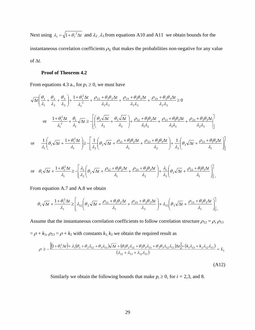
29

Next using t∆+= 211 1 θλ and λ2 , λ3 from equations A10 and A11 we obtain bounds for the

instantaneous correlation coefficients ρij that makes the probabilities non-negative for any value

of ∆t.


From equations 4.3 a., for p1 ≥ 0, we must have

01

32

3223

31

3113

21

21122

1

21

3

3

2

2

1

1 ≥∆+

+∆+

+∆+

+∆+

+⎟⎟⎠

⎞⎜⎜⎝

⎛++∆

λλθθρ

λλθθρ

λλθθρ

λθ

λθ

λθ

λθ tttt

t

⎥⎥⎦

⎤

⎢⎢⎣

⎡ ∆++

∆++

∆++⎟

⎟⎠

⎞⎜⎜⎝

⎛ ∆+

∆−≥∆+

∆+

32

3223

31

3113

21

2112

3

3

2

2

1

12

1

211or

λλθθρ

λλθθρ

λλθθρ

λθ

λθ

λθ

λθ ttttttt

⎥⎥⎦

⎤

⎢⎢⎣

⎡⎟⎟⎠

⎞⎜⎜⎝

⎛ ∆++∆+⎟⎟

⎠

⎞⎜⎜⎝

⎛ ∆++

∆++∆−≥⎟⎟

⎠

⎞⎜⎜⎝

⎛ ∆++∆

1

31133

33

3223

1

21122

21

21

11

1111or λθθρ

θλλ

θθρλθθρ

θλλ

θθ

λttttttt

⎥⎥⎦

⎤

⎢⎢⎣

⎡⎟⎟⎠

⎞⎜⎜⎝

⎛ ∆++∆+⎟⎟

⎠

⎞⎜⎜⎝

⎛ ∆++

∆++∆−≥

∆++∆

1

31133

3

1

3

3223

1

21122

2

1

1

21

11or

λθθρ

θλλ

λθθρ

λθθρ

θλλ

λθ

θttttttt

.

From equation A.7 and A.8 we obtain

⎥⎥⎦

⎤

⎢⎢⎣

⎡⎟⎟⎠

⎞⎜⎜⎝

⎛ ∆++∆+⎟⎟

⎠

⎞⎜⎜⎝

⎛ ∆++

∆++∆≥

∆++∆

1

3113313

3

3223

1

2112212

1

21

11

λθθρ

θλλ

θθρλθθρ

θλλθ

θt

ttt

tt

t.

Assume that the instantaneous correlation coefficients to follow correlation structure ρ12 = ρ, ρ13

= ρ + k1, ρ23 = ρ + k2 with constants k1, k2 we obtain the required result as

( ) ( ) ( )[ ] ( )( ) 1

13121312

1312213113123213311221133122112

11L

kkttt=

++++∆+++∆+++∆+

−≥λλλλ

λλλλλθθλθθλθθλθλθθλθρ

(A12)

Similarly we obtain the following bounds that make pi ≥ 0, for i = 2,3, and 8.

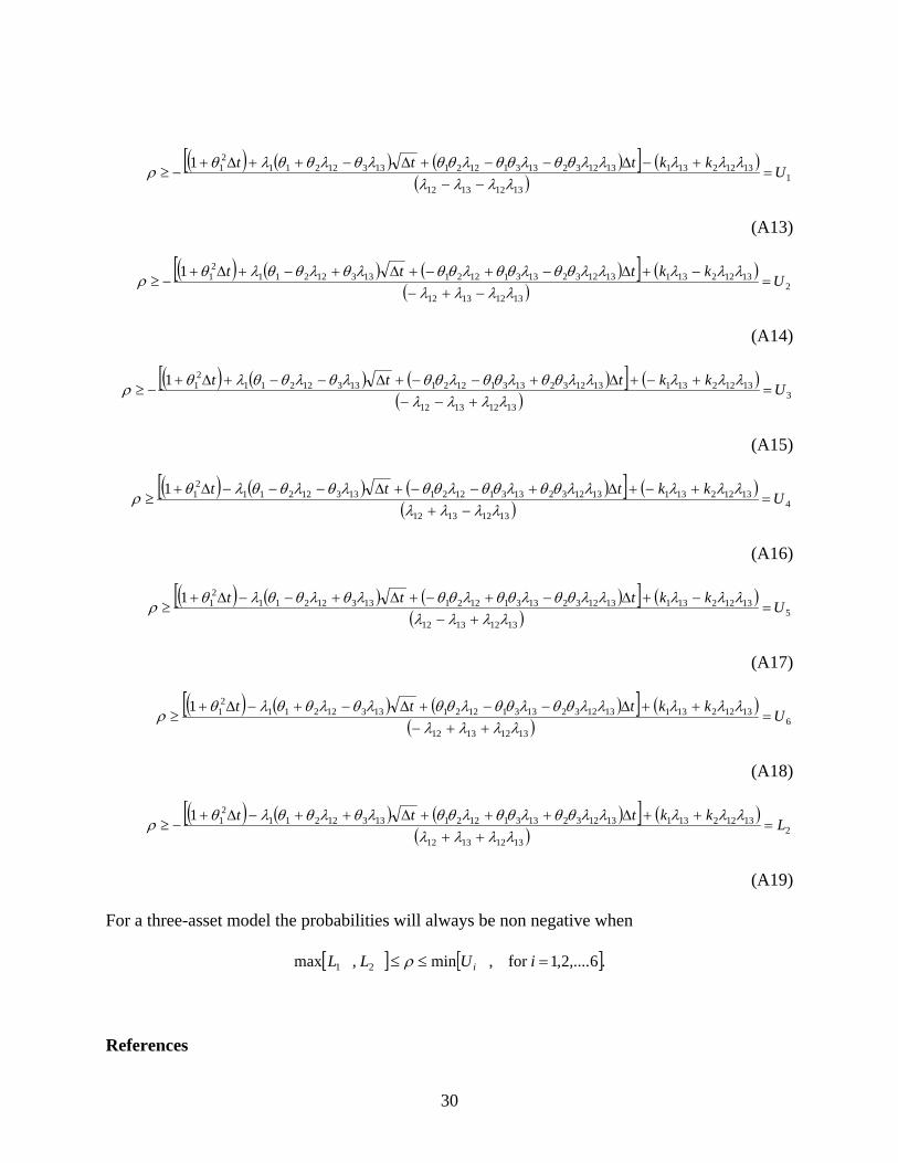
30

( ) ( ) ( )[ ] ( )( ) 1

13121312

1312213113123213311221133122112

11 Ukkttt=

−−+−∆−−+∆−++∆+

−≥λλλλ


(A13)

( ) ( ) ( )[ ] ( )( ) 2

13121312

1312213113123213311221133122112

11 Ukkttt=

−+−−+∆−+−+∆+−+∆+

−≥λλλλ


(A14)

( ) ( ) ( )[ ] ( )( ) 3

13121312

1312213113123213311221133122112

11 Ukkttt=

+−−+−+∆+−−+∆−−+∆+

−≥λλλλ


(A15)

( ) ( ) ( )[ ] ( )( ) 4

13121312

1312213113123213311221133122112

11 Ukkttt=

−++−+∆+−−+∆−−−∆+

≥λλλλ


(A16)

( ) ( ) ( )[ ] ( )( ) 5

13121312

1312213113123213311221133122112

11 Ukkttt=

+−−+∆−+−+∆+−−∆+

≥λλλλ


(A17)

( ) ( ) ( )[ ] ( )( ) 6

13121312

1312213113123213311221133122112

11 Ukkttt=

++−++∆−−+∆−+−∆+

≥λλλλ


(A18)

( ) ( ) ( )[ ] ( )( ) 2

13121312

1312213113123213311221133122112

11 Lkkttt=

++++∆+++∆++−∆+

−≥λλλλ


(A19)

For a three-asset model the probabilities will always be non negative when

[ ] [ ].6,....2,1for , min , max 21 =≤≤ iULL iρ

References

31

Boyle, P. P., "A Lattice Framework for Option Pricing with Two State Variables", Journal of

Financial and Quantitative Analysis, 23(1), 1 -12, (March 1988).

Boyle, P. P., J Evnine and S. Gibbs, "Numerical Evaluation of Multivariate Contingent Claims",

The Review of Financial Studies, 2(2) 241-250, 1989.

Johnson H, "Options on the Maximum or the Minimum of Several Assets", Journal of Financial

and Quantitative Analysis, 22(3), 277- 283, (September 1987).

Kamrad B., and Ritchken P., "Multinomial Approximating Model for Options with k-State

Variables", Management Science, 37(12), 1640-1652, (December 1991).

Miller I. and Miller M., "John E. Freund's Mathematical Statistics", Sixth ed., New Jersey:

Prentice Hall, 1999.

Nelson D. B., and Ramaswamy K., "Simple Binomial Processes as Diffusion Approximations in

Financial Models", The Review of Financial Studies, 3(3), 393-430, 1990.

Stulz R. M., "Options on the Minimum or the Maximum of Two Risk Assets: Analysis and

Applications", Journal of Financial Economics, 10, 161-185, (July 1982).

32

Table 1

Errors Resulting by Ignoring O(∆t)

Probability Error

p1 22 2λθ t∆

p2 22 λθ t∆−

p3 22 2λθ t∆

33

Table 2

Percent Absolute Relative Errors

σ = 8%, ∆t = 0.25 σ = 8%, ∆t = 0.1 σ = 5%, ∆t = 0.5

2.90 2.89 6.25

0 0 0

6.45 6.67 25

34

Table 3

Option Prices with the KR and the MKR Models

T True Option Price KR Model MKR Model

1 Year 9.94 9.68 (-2.8%) 9.70 (-2.6%)

10 Years 40.54 37.39 (-7.7%) 38.03 (-6.2%)

35

Table 4

Process Iterations and Probabilities for a Two State Model

∆t n KR Probabilities

0.25 4 0.252, 0.355, -0.229, 0.527, 0.096

0.0007 1420 0.024, 0.436, -0.001, 0.445, 0.096

0.0006 1667 0.23, 0.437, 0, 0.445, 0.096

36

Table 5

Process Iterations and Probabilities for a Three State Model

∆t n KR Probabilities

0.25 4 0.3, 0.2, 0.06, 0.1, 0.17, 0.17, -0.07, 0.07, 0

0.07 14 0.24, 0.14, 0.08, 0.12, 0.16, 0.14, -0.01, 0.12, 0

0.06 17 0.24, 0.13, 0.09, 0.12, 0.16, 0.14, 0, 0.13, 0

Documents

Multinomial Approximating Models for Options