Embed Size (px)
Citation preview

Multiple-Output Production WithUndesirable Outputs: An Application to
Nitrogen Surplus in Agriculture
Carmen Fern�andez, Gary Koop and Mark F.J. Steel
Many production processes yield both good outputs and undesirableones (e.g. pollutants). In this paper, we develop a generalization ofa stochastic frontier model which is appropriate for such technologies.We discuss eÆciency analysis and, in particular, de�ne technical andenvironmental eÆciency in the context of our model. Methods for car-rying out Bayesian inference are developed and applied to a panel dataset of Dutch dairy farms, where excess nitrogen production constitutesan important environmental problem.
Keywords: Dairy farm, EÆciency, Environment, Longitudinal data, Stochastic frontier
Carmen Fern�andez is Lecturer, School of Mathematics and Statistics, University of St. An-drews, KY16 9SS, UK (E-mail: [email protected]), Gary Koop is Professor, Depart-ment of Economics, University of Glasgow, G12 8RT, UK (E-mail: [email protected])and Mark F.J. Steel is Professor, Institute of Mathematics and Statistics, University of Kentat Canterbury, CT2 7NF, UK (E-mail: [email protected]). Carmen Fern�andez was af-�liated to the Department of Mathematics, University of Bristol when the �rst version ofthis paper was completed. Financial support from ESRC under grant number R34515 isgratefully acknowledged. We would like to thank Stijn Reinhard and the Dutch AgriculturalEconomics Research Institute (LEI-DLO) for kindly providing the data and we are gratefulto the current and the previous Editor, an Associate Editor, three referees and David Ulphfor stimulating comments.

1 Nitrogen Pollution and Dairy Farming
The environmental problems posed by excess nitrogen produced in the farming sector form a
major concern of the European Union (EU), and have led to the 1992 Common Agricultural
Policy reform and the Nitrates Directive. The share of agriculture in the total runo� of
nitrogen discharge is estimated to be as large as 60% (EEA 1995). Animal density within the
EU is highest in the Netherlands, which also has the highest measured nitrogen surplus per
unit area (see Brouwer, Hellegers, Hoogeveen and Luesink 1999). The environmental impact
is substantial. Nitrates pollute the surface waters and leach into groundwater aquifers,
contaminating the drinking water supply. In addition, the evaporation of ammonia is a
major contributor to acid rain. The main external nitrogen inputs to dairy farms are the
application of chemical fertilizers used in roughage production (mainly grass and green maize)
and the purchase of external roughage and concentrate used in animal production. Part of
this input is absorbed in the production of marketable outputs (milk, meat, livestock and
roughage sold), but most of it (over 75% in the dataset used here, according to Reinhard,
Lovell and Thijssen 1999) is released into the environment as nitrogen surplus. The nitrogen
surplus largely stems from the application of excess fertilizer and manure produced by the
livestock (leading to nitrogen exchange with the soil and ammonia evaporation from land),
and also contains ammonia emission from stables and manure sold.
We shall focus on specialized dairy farms in the Netherlands, which are quite intensive
and lead to a substantial nitrogen surplus (in our dataset the average was 416 kg nitrogen
per hectare per year). Including beef and veal production, the dairy sector is reported to be
responsible for 72% of manure production in the Netherlands, and 62% of the agricultural
ammonia emmision (CBS 1995). Various restrictions have recently been put in place to curb
the nitrogen problem. For example, as of 1998 the more intensive farms need to keep accounts
of their mineral balances, and a levy has to be paid for every kg of nitrogen surplus above
a certain threshold. Pricing this surplus and setting the threshold are key policy issues.
Before policy decisions in this context can be discussed, however, it is crucial to be able
to �rst de�ne and then measure the success (eÆciency) of farms in minimizing the release
of nitrogen into the environment. Recently, the Commission of the European Communities
(2000) has stressed the need for developing environmental eÆciency indicators in this context
to formally introduce environmental concerns into the Common Agricultural Policy.
1

There are many applications in economics where an agent (e.g. a farm, �rm, country or
individual) produces undesirable outputs such as pollution, in addition to desirable ones. In
the application considered in this paper, Dutch dairy farms produce not only good outputs
(which we will informally call \goods"), such as milk, but also undesirable outputs (or
\bads"), such as excessive nitrogen. It is thus important to understand the nature of the
best-practice technology available to farmers for turning inputs into good and bad outputs.
Furthermore, it is important to see how individual farms measure up to this technology.
In other words, evaluation of farm eÆciency, both in producing as many good outputs and
as few undesirable outputs as possible, is crucial. Whereas there is a longer tradition of
measuring technical eÆciency, related to production of goods, the question of how to de�ne
and measure environmental eÆciency has only been considered much more recently. In this
paper, we propose a de�nition of environmental eÆciency along with a statistical framework
for conducting inference. Currently, there is no generally accepted methodology to address
these important questions. The state of the art in this emerging �eld is provided by Reinhard
et al. (1999), who use a stochastic frontier approach, and Reinhard and Thijssen (2000), who
base their analysis on a system of estimated shadow costs.
Thus, we deal with de�ning and estimating environmental (and technical) eÆciencies. A
third important issue is how to explain di�erences of measured eÆciencies across farms. We
shall provide a theoretical framework for doing so, by incorporating explanatory variables
(e.g. farm characteristics) into the eÆciency distribution. Such e�ects are typically explored
through a second stage regression of estimated eÆciencies on certain variables (see Hallam
and Machado 1996, and Reinhard 1999, chap. 6). In contrast, we follow Kumbhakar, Ghosh
and McGuckin (1991) and Koop, Osiewalski and Steel (1997) and make the dependence of
the eÆciency distribution on explanatory variables an integral part of our model.
This paper uses Bayesian methods, which automatically and formally allow for the cal-
culation of �nite sample measures of uncertainty (e.g. 95% posterior credible intervals) for
all parameters and the eÆciencies themselves. This is very diÆcult to do reliably using
non-Bayesian statistical methods (see, e.g., Horrace and Schmidt 1996). We have found
substantial spread in the posterior distribution of eÆciencies. Taking this uncertainty into
account is crucial if we want to base policy decisions on di�erences in eÆciencies.
The next section will outline the basic theoretical model we will use, while Section 3
2

formally describes the sampling model used in this paper. In the fourth section we look at
various implications of our sampling model in terms of the underlying economic theory. The
prior and the algorithm used for posterior inference are described in Section 5, while Section
6 presents our empirical application. The �nal section contains some policy conclusions.
2 Stochastic Frontiers
Stochastic frontier models are commonly used in the empirical study of eÆciency and
productivity (see Bauer 1990 for a survey). Such models are used to analyse the eÆciency of
dairy farms in e.g. Kumbhakar et al. (1991) and Ahmad and Bravo-Ureta (1995) for the USA
and in Hallam and Machado (1996) for Portuguese data. All of these papers assume that a
single good output is produced and ignore the possible presence of undesirable by-products.
In the single output case, a sensible de�nition of eÆciency can easily be found: the ratio
of actual output produced to the maximum that could have possibly been produced with
the inputs used. The extension to the case of multiple good outputs is more complicated
since multivariate distributions must be used and various ways of de�ning eÆciency exist.
Fern�andez, Koop and Steel (2000a) provide a solution to these complications, and the present
paper builds on this approach to allow for some of the outputs to be bad. We will distinguish
between technical and environmental eÆciency. The former is the standard eÆciency concept
which compares actual to maximum possible output, extended to a multi-output setting. Our
de�nition of environmental eÆciency aims to answer the question \How much could pollution
be reduced, without sacri�cing good outputs, by adopting best-practice technology?".
To �x ideas, y, b and x will, throughout, denote vectors of good outputs, bad outputs and
inputs, respectively. The best-practice technology for turning inputs into outputs is given
by a relationship between the inputs and best-practice vectors of good and bad outputs:
f(ybp; bbp; x) = 0: (1)
In the simplest case of a single good output and no bads, the relationship above is
typically assumed to allow for expressing ybp = h(x). The function h(x) is known as the
production frontier and corresponds to the maximum output level that can be obtained with
input vector x. The technical eÆciency of a �rm producing y with inputs x is then de�ned as
3

� � y=h(x) 2 [0; 1]. Statistical estimation of eÆciency can be done by adding measurement
error to the model and making appropriate distributional and functional form assumptions.
In the multiple good outputs case, still without bads, Fern�andez et al. (2000a) also
assume that the relationship in (1) is separable, in the sense that there exist non-negative
functions �(�) and h(�) such that �(ybp) = h(x), where ybp is now a vector. �(y) = constant
maps out the output combinations that are technologically equivalent, and is thus de�ned
as the production equivalence surface. By analogy with the single output case, h(x) de�nes
the maximum output [as measured by �(y)] that can be produced with inputs x and is
referred to as the production frontier. For a �rm producing y, technical eÆciency is de�ned
as � � �(y)=h(x). Fern�andez et al. (2000a) provide a detailed justi�cation for this eÆciency
de�nition. Alternative de�nitions are examined in Fern�andez, Koop and Steel (2000b).
In the general multiple output case with both goods and bads, the present paper argues
for a relationship in (1) that can be written as:
�(ybp) = h1(x) and �(bbp) = h2(ybp); (2)
for non-negative functions �(�), h1(�), �(�) and h2(�). In other words, the general relationship
can be broken down into two equations involving the \aggregate goods" �(y), the \goods'
production frontier" h1(x), the \aggregate bads" �(b), and the \bads' production frontier"
h2(y). The assumption that the frontier for the goods depends only on the inputs, whereas
the frontier for the bads is determined by the amount of good outputs produced is likely to
be reasonable in many cases. For a �rm producing (y; b) with inputs x, we can now de�ne
�1 ��(y)
h1(x)and �2 �
h2(y)
�(b); (3)
where �1 is technical eÆciency and �2, environmental eÆciency, is de�ned as the minimum
possible bad aggregate output divided by the actual one. Both �1 and �2 are in [0,1].
Alternatively, one could start with the transformation function in (1) and de�ne, e.g., the
frontier for the goods as the maximal combinations of y given x and b, and the frontier for
the bads as the minimal combinations of b given y and x. Under a separability assumption
on the transformation function, this approach essentially reduces to treating the two types of
output di�erently in the same aggregator, thus e�ectively reducing the problem to having a
single frontier. This is pursued in Fern�andez et al. (2000b) and this basic idea also underlies
4
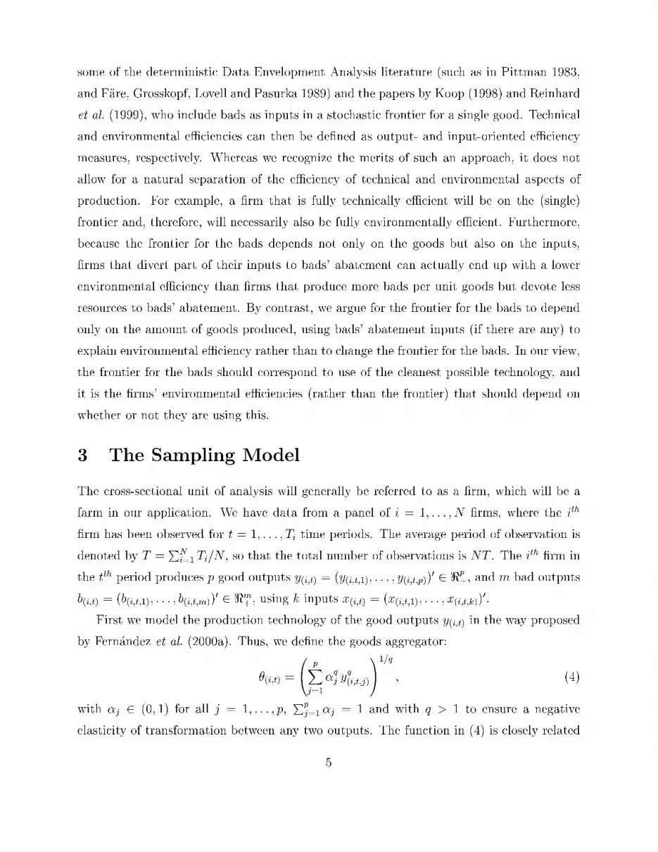
some of the deterministic Data Envelopment Analysis literature (such as in Pittman 1983,
and F�are, Grosskopf, Lovell and Pasurka 1989) and the papers by Koop (1998) and Reinhard
et al. (1999), who include bads as inputs in a stochastic frontier for a single good. Technical
and environmental eÆciencies can then be de�ned as output- and input-oriented eÆciency
measures, respectively. Whereas we recognize the merits of such an approach, it does not
allow for a natural separation of the eÆciency of technical and environmental aspects of
production. For example, a �rm that is fully technically eÆcient will be on the (single)
frontier and, therefore, will necessarily also be fully environmentally eÆcient. Furthermore,
because the frontier for the bads depends not only on the goods but also on the inputs,
�rms that divert part of their inputs to bads' abatement can actually end up with a lower
environmental eÆciency than �rms that produce more bads per unit goods but devote less
resources to bads' abatement. By contrast, we argue for the frontier for the bads to depend
only on the amount of goods produced, using bads' abatement inputs (if there are any) to
explain environmental eÆciency rather than to change the frontier for the bads. In our view,
the frontier for the bads should correspond to use of the cleanest possible technology, and
it is the �rms' environmental eÆciencies (rather than the frontier) that should depend on
whether or not they are using this.
3 The Sampling Model
The cross-sectional unit of analysis will generally be referred to as a �rm, which will be a
farm in our application. We have data from a panel of i = 1; : : : ; N �rms, where the ith
�rm has been observed for t = 1; : : : ; Ti time periods. The average period of observation is
denoted by T =PN
i=1 Ti=N , so that the total number of observations is NT . The ith �rm in
the tth period produces p good outputs y(i;t) = (y(i;t;1); : : : ; y(i;t;p))0 2 <p
+, and m bad outputs
b(i;t) = (b(i;t;1); : : : ; b(i;t;m))0 2 <m
+ , using k inputs x(i;t) = (x(i;t;1); : : : ; x(i;t;k))0.
First we model the production technology of the good outputs y(i;t) in the way proposed
by Fern�andez et al. (2000a). Thus, we de�ne the goods aggregator:
�(i;t) =
0@ pXj=1
�qj yq(i;t;j)
1A1=q
; (4)
with �j 2 (0; 1) for all j = 1; : : : ; p,Pp
j=1 �j = 1 and with q > 1 to ensure a negative
elasticity of transformation between any two outputs. The function in (4) is closely related
5

to the \constant elasticity of transformation" speci�cation of Powell and Gruen (1968),
and implies an elasticity of transformation equal to 1=(1 � q). The role of the p unknown
parameters in � and q is further discussed in Fern�andez et al. (2000a). The particular choice
of (4) for the aggregator function (albeit quite exible) is a key element of our model, and
di�erent aggregators may well lead to di�erent results.
Interpreting �(i;t) as aggregate good output, we de�ne a production equivalence surface
as the (p� 1)-dimensional surface with a constant value for �(i;t). Now that we have reduced
the problem to a unidimensional aggregate, we de�ne the NT -dimensional vector
log � = (log �(1;1); log �(1;2); : : : ; log �(1;T1); : : : ; log �(N;TN ))0; (5)
and we model log � through the usual stochastic frontier
log � = V � �Dz + "g: (6)
In (6), the matrix V = (v(x(1;1)); : : : ; v(x(N;TN )))0 consists of exogenous regressors, where
each v(x(i;t)) is a function of the inputs x(i;t). The particular choice of v(�) de�nes the
speci�cation of the production frontier (e.g. Cobb-Douglas, translog, etc.). Typically, we
impose regularity conditions on the coeÆcients �, which assign an economic meaning to the
surface V � in (6) as a frontier (e.g. monotonicity conditions ensuring that production does
not decrease as inputs increase). In our farms application we use a Cobb-Douglas frontier
(i.e. it contains an intercept and is linear in the logs of the inputs) and, accordingly, all the
elements of � except for the intercept are restricted to be non-negative.
Another key element of (6) is the vector of technical ineÆciencies Dz 2 <NT+ , where the
matrix D gives some structure to the ineÆciencies. In this paper we follow the usual practice
in assuming that ineÆciencies for each �rm are constant over time. In our application Ti � 4
years, which makes this a reasonable assumption in our view. For balanced panels (where
Ti = T for all i) this corresponds to D = IN �T , where denotes the Kronecker product
and �T a vector of T ones, with the obvious generalization for unbalanced panels (where Ti
varies with i). In both cases, z 2 <N+ becomes a vector of �rm-speci�c ineÆciencies. Since
the dependent variable in (6) has been transformed to logarithms, technical eÆciency for
the ith �rm is de�ned as �1i = exp(�zi). Extensions to more general D are straightforward.
Now we turn to the analysis of the bads, b(i;t), for which we specify a very similar model.
6

First we aggregate the m components of b(i;t) into
�(i;t) =
0@ mXj=1
rj br(i;t;j)
1A1=r
; (7)
with j 2 (0; 1) for all j = 1; : : : ; m and such thatPm
j=1 j = 1 and now with 0 < r < 1. In
the case of bads a positive elasticity of transformation is more appropriate on the basis of
economic theory considerations. We de�ne log � analogously to log � in (5) and model this
through the following stochastic frontier:
log� = UÆ +Mv + "b; (8)
where U = (u(y(1;1)); : : : ; u(y(N;TN )))0, i.e. the matrix U is a function of the good outputs.
This re ects our idea that the frontier for the bads should be measured relative to the
amount of goods produced. Note that U is a function of the p-variate y(i;t) rather than of
the aggregated scalar �(i;t) alone, since the aggregation in (4) relates only to the production
of the good outputs, and it may well be that the in uence of the various components of y(i;t)
on the production of bads is very di�erent from how they appear in (4). It is quite likely
that di�erent technologically equivalent y(i;t) vectors, i.e. situated on the same production
equivalence surface corresponding to a particular value of �(i;t), can have very di�erent con-
sequences for the minimal amount of aggregated bads we can achieve. We impose regularity
conditions on Æ, so that a larger amount of goods cannot be commensurate with a smaller
amount of bads. In the application we use a Cobb-Douglas speci�cation and, accordingly,
all the elements of Æ except for the intercept are restricted to be non-negative.
UÆ will de�ne the smallest feasible (frontier) production of the aggregate undesirable
outputs for a given amount of desirable outputs. If there is any systematic (positive) devia-
tion, this is labelled environmental ineÆciency, which is grouped in the vector Mv 2 <NT+ .
Generally, we can impose di�erent structures through choosing the �xed matrix M . In this
paper we assume that �rms have a constant environmental ineÆciency over time (i.e. indi-
vidual e�ects), so that M = D is as described above, and the vector v 2 <N+ groups the
environmental ineÆciencies. The environmental eÆciency of �rm i is, thus, �2i = exp(�vi).
Again, extensions to more general M , not necessarily equal to D, are straightforward.
In the microeconomic theory of production (see, e.g. Varian 1984), the production tech-
nology of a �rm that uses input x to produce output y is de�ned in terms of the production
7

possibilities set, that is, the set of all feasible input-output combinations. For a �xed value of
the output y, the input requirement set, de�ned as the collection of input vectors x for which
(x; y) belongs to the production possibilities set, is assumed to be convex [i.e. if (x1; y) and
(x2; y) are feasible input-output combinations, so is ((1� a)x1 + ax2; y) for any a 2 (0; 1)].
The regularity conditions imposed on the frontier parameters � and Æ ensure that the input
requirement sets corresponding to (6) and (8) separately have this property, where \input"
for bads production are the goods produced. From (6) and (8) it is easy to prove that
if (x1; y0; b0) and (x2; y0; b0) are feasible input-goods-bads combinations (where b0 is on or
above the bads' frontier corresponding to y0), so is ((1�a)x1+ax2; y0; b0) for any a 2 (0; 1),
and thus convexity also holds when we consider goods and bads jointly.
We still need to introduce stochastics into the sampling model. The terms "g in (6) and
"b in (8) capture the usual measurement error and model imperfections, and as such will
be assigned a symmetric distribution. We allow for the two error terms to be correlated
for the same �rm and time period, and assume a bivariate Normal distribution. That is, if
we let fRN ("ja; A) denote the R-variate Normal p.d.f. with mean a and covariance matrix A,
evaluated at ", we can write:
p("g; "bj�) = f 2NTN
"g"bj0;� INT
!(9)
where � is a 2� 2 positive de�nite symmetric matrix.
Through (4)-(9) we have speci�ed a joint distribution for the aggregated goods and bads
(�(i;t); �(i;t)). Since our aggregators contain unknown parameters, (�(i;t); �(i;t)) is not available
for use as a suÆcient statistic for the frontier parameters and ineÆciencies. Thus, we need
to add further stochastic assumptions in order to have a sampling model for (y(i;t); b(i;t))
leading to a full likelihood. From a non-Bayesian viewpoint, one could consider limited-
information approaches which do not require the full likelihood and could dispense with the
distributions that we next specify. For example, in a context without bads, Adams, Berger
and Sickles (1999) consider a linear aggregator for the goods and normalize the coeÆcient
of one of the outputs to be one, while putting the remaining outputs on the right hand
side. Problems which arise due to the correlation of the remaining outputs with the error
term are resolved through semiparametric eÆcient methods. See also L�othgren (1997) for
an alternative approach based on a polar transformation of the outputs.
8

We now complete the speci�cation of the sampling model along the lines suggested by
Fern�andez et al. (2000a). For the goods, when p > 1 we de�ne the weighted output shares:
�(i;t;j) =�qjy
q(i;t;j)Pp
l=1 �ql y
q(i;t;l)
; j = 1; : : : ; p; (10)
group them into �(i;t) = (�(i;t;1); : : : ; �(i;t;p))0, and assume independent sampling from
p(�(i;t)js) = f p�1D (�(i;t)js); (11)
where s = (s1; : : : ; sp)0 2 <p
+ and f p�1D (�js) is the p.d.f. of a Dirichlet distribution with
parameter s. Similarly, if m > 1 we de�ne a weighted vector of shares for the bads:
�(i;t;j) = rj b
r(i;t;j)Pm
l=1 rl b
r(i;t;l)
; j = 1; : : : ; m; (12)
stack them to form �(i;t) = (�(i;t;1); : : : ; �(i;t;m))0, and assume independent sampling from
p(�(i;t)jh) = fm�1D (�(i;t)jh); (13)
where h = (h1; : : : ; hm)0 2 <m
+ .
Now (4)� (13) lead to a sampling distribution for Y;B which are matrices of dimensions
NT �p and NT �m, respectively, with elements ordered in the same manner as log � in (5).
Taking into account the Jacobian of the transformation, we obtain the sampling density:
p(Y;Bj�; z; Æ; v;�; �; ; q; r; s; h) = f 2NTN
log �log �
jV � �DzUÆ +Mv
;� INT
!(14)
Yi;t
24 f p�1D (�(i;t)js)
0@ pYj=1
q1�1
p�(i;t;j)y(i;t;j)
1A35Yi;t
24fm�1D (�(i;t)jh)
0@ mYj=1
r1�1
m�(i;t;j)b(i;t;j)
1A35 :
4 Implications of the Sampling Model
It is important to relate the statistical model speci�ed in the previous section to the underly-
ing economic theory. Given the independent sampling assumption, we will consider a single
observation and suppress the (i; t) subscripts, and we will not explicitly indicate conditioning
on model parameters in this section.
Economic intuition relates largely to the stochastic frontiers of equations (6) and (8),
which only involve log � and log � instead of the entire vectors y and b. This suggests
9

focussing on the marginal and conditional distributional properties of log � and log �. Using
(14) with a Cobb-Douglas structure for the bads' frontier [i.e. U = (1; log y1; : : : ; log yp)] and
changing variables from y to (log �; �) and from b to (log �; �), we obtain:
p(log �; �; log�; �) = f 2N
log �log�
jV � � zÆ(V � � z) + l(�) + v
;W
!f p�1D (�js)fm�1D (�jh); (15)
where Æ �Pp+1
j=2 Æj, l(�) � Æ1+Pp
j=1 Æj+1 log(��1j �1=qj ) and, denoting by �ij the (i; j)
th element
of �, the elements of W are w11 = �11; w12 = �11 + �12; w22 = [det(�) + w212]=�11:
The marginal distributions of y and b correspond to modelling the goods ignoring the bads
and modelling the bads ignoring the goods. From (15) it is immediate that, in the marginal
distribution, log � and � are independent, with p.d.f.'s respectively given by f 1N(log �jV � �
Dz; �11) and fp�1D (�js). This is the speci�cation in Fern�andez et al. (2000a), who consider
the problem with multiple goods and no bads. Marginally, log � and � are also independent,
with log � distributed as a location mixture of Normals with expectation E[log �] = Æ1 +Ppj=1 Æj+1E[log yj] + v. Clearly, the economic regularity conditions imposed previously on �
and Æ exactly correspond to regularity on the marginal distributions.
We now consider the conditional distributions of log � given (�; b) and of log� given (�; y).
From (15), it is immediate that both these distributions are Normal with means given by:
E[log �j�; b] = V ��1� Æ
w12
w22
�+w12
w22[ log �� l(�)]�
��1� Æ
w12
w22
�z +
w12
w22v�; (16)
E[log �j�; y] =�Æ �
w12
w11
�E[log �] +
w12
w11log � + l(�) + v:
Note that the conditional mean of log � given (�; b) depends on log �, similarly to analyses
where bads are treated as inputs (e.g. Koop 1998, or Reinhard et al. 1999). Thus, the treat-
ment of pollutants as inputs arises naturally in our framework if we focus on the conditional
distribution of y given b. In order to interpret the means in (16) as frontiers with ineÆcien-
cies, we need to impose regularity conditions, so that aggregate goods increase with inputs
and log �� l(�), and aggregate bads increase with E[log �] and goods. When V corresponds
to a Cobb-Douglas speci�cation, these conditions amount to
�min��11;
�22Æ
�� �12 � 0: (17)
We will impose this regularity condition in addition to those discussed in Section 3.
10
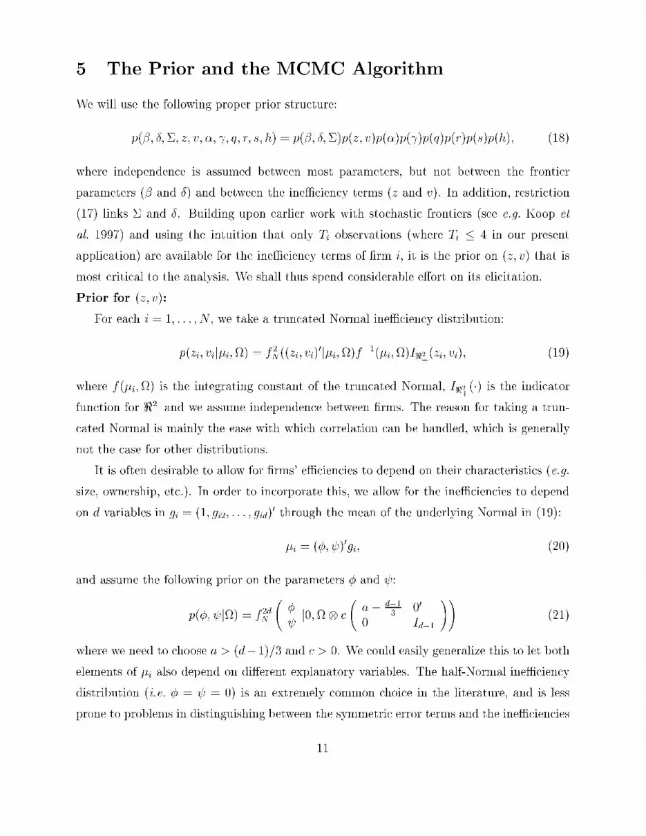
5 The Prior and the MCMC Algorithm
We will use the following proper prior structure:
p(�; Æ;�; z; v; �; ; q; r; s; h) = p(�; Æ;�)p(z; v)p(�)p( )p(q)p(r)p(s)p(h); (18)
where independence is assumed between most parameters, but not between the frontier
parameters (� and Æ) and between the ineÆciency terms (z and v). In addition, restriction
(17) links � and Æ. Building upon earlier work with stochastic frontiers (see e.g. Koop et
al. 1997) and using the intuition that only Ti observations (where Ti � 4 in our present
application) are available for the ineÆciency terms of �rm i, it is the prior on (z; v) that is
most critical to the analysis. We shall thus spend considerable e�ort on its elicitation.
Prior for (z; v):
For each i = 1; : : : ; N , we take a truncated Normal ineÆciency distribution:
p(zi; vij�i;) = f 2N((zi; vi)0j�i;)f
�1(�i;)I<2+(zi; vi); (19)
where f(�i;) is the integrating constant of the truncated Normal, I<2+(�) is the indicator
function for <2+ and we assume independence between �rms. The reason for taking a trun-
cated Normal is mainly the ease with which correlation can be handled, which is generally
not the case for other distributions.
It is often desirable to allow for �rms' eÆciencies to depend on their characteristics (e.g.
size, ownership, etc.). In order to incorporate this, we allow for the ineÆciencies to depend
on d variables in gi = (1; gi2; : : : ; gid)0 through the mean of the underlying Normal in (19):
�i = (�; )0gi; (20)
and assume the following prior on the parameters � and :
p(�; j) = f 2dN
� j0; c
a� d�1
300
0 Id�1
!!(21)
where we need to choose a > (d�1)=3 and c > 0. We could easily generalize this to let both
elements of �i also depend on di�erent explanatory variables. The half-Normal ineÆciency
distribution (i.e. � = = 0) is an extremely common choice in the literature, and is less
prone to problems in distinguishing between the symmetric error terms and the ineÆciencies
11

than a general truncated Normal (see Ritter and Simar 1997, for a related discussion of
Gamma ineÆciency distributions). By keeping the prior centered over � = = 0, we allow
some exibility relative to this well-known benchmark. The prior ineÆciency distribution is
now completed by an Inverted Wishart prior on :
p() = f 2IW (j0; �0) ; (22)
which has expectation equal to the matrix 0=(�0 � 3) if �0 > 3.
Our aim is to obtain a prior for (�i;) (and, thus, for the ineÆciencies), which is ap-
proximately the same for a range of choices of d and gi. This is achieved by standardization
of the variable gi so that 0 � gij � 1 for j = 2; : : : ; d. Then we have
p(�ij) = f 2N
0@�ij0; c
24a� d� 1
3+
dXj=2
g2ij
35
1A � f 2N(�ij0; ac); (23)
where the approximation is based on the fact that if the gij's were independent and uniformly
distributed on [0; 1] then E[Pd
j=2 g2ij] = (d� 1)=3. This approximation should be reasonably
accurate if a is large with respect to jPd
j=2 g2ij �(d� 1)=3j and is exact when d = 1. For
(empirically relevant) situations with d � 4 we �nd that choosing a = 3 gives reasonable
results. From (21), the variance for the �rst elements of � and is then two to three times
larger than for the others, which re ects a moderate prior belief that �rm characteristics
in uence the eÆciency distributions less than the common intercept. The ratio of the prior
variance of the last d � 1 components of � and to that of the underlying Normal on
ineÆciencies in (19) is given by c. We choose c = 1 as a reasonable value which allows for
suÆcient uncertainty on � and , given a realistic prior eÆciency distribution.
In (22), we choose a diagonal 0 and set �0 = 6 which is the smallest (and hence
least informative) integer value for which the prior covariance of exists. For the diagonal
elements of 0 we take 0:65, on the basis of extensive simulations of the resulting distributions
of technical eÆciency �1i = exp(�zi) and environmental eÆciency �2i = exp(�vi). Figures 1-
4 graph the resulting marginal prior density function (which is the same for both eÆciencies)
computed using the approximation in (23). Prior median eÆciency is 0.72 with a 95%
credible interval of (0.11, 0.99) and the correlation between both eÆciencies is 0.09. The
exact prior was found to be very similar for a range of values of d and gi. Experimentation
with simulated data revealed the resulting prior to be easily dominated by data.
12

Prior for other parameters:
All other parameters of the model are assigned relatively at priors. In selecting these,
we base ourselves on the experience gained with the multiple good output analysis with no
bads of Fern�andez et al. (2000a). In particular, we adopt the following structure:
p(�; Æ;�) / fN
�Æjb0; H
�10
!f 2IW (�j�0; �0)IRR(�; Æ;�); (24)
where IRR(�) is the indicator function for the region where regularity conditions are met,
p(�) = f p�1D (�ja0); p( ) = fm�1D ( jg0) (25)
p(q) / fG(qj1; q0)I(1;1)(q); p(r) / fG(rj1; r0)I(0;1)(r); (26)
where fG(:ja; b) denotes a Gamma density function with shape parameter a and mean a=b,
p(s) =pY
j=1
fG(sjjdj; kj); p(h) =mYj=1
fG(hjjlj; nj): (27)
We make the relatively noninformative choices of b0 = 0, H0 equal to 0.0001 times the
identity matrix of the appropriate dimension, �0 = I2 and �0 = 2. In the previous sections
we have shown the form of IRR(�; Æ;�) when V and U are chosen to imply Cobb-Douglas
frontiers. For the Dirichlet priors in (25) we set a0 and g0 to appropriately dimensioned
vectors of ones. For the truncated exponential priors in (26) we choose r0 = q0 = 0:1. In
(27) we set dj = kj = lj = nj = 0:1, thus centering �(i;t) and �(i;t) at the equal output share
values. In Section 6 we will comment on the e�ect of departures from this base prior.
The Posterior MCMC Algorithm:
We use a Markov chain Monte Carlo (MCMC) algorithm on the space of the parameters in
(14) and the ineÆciencies (z; v), augmented with �; ; [from the hierarchical prior of (z; v)
in (19)-(22)]. The Markov chain will be constructed from Gibbs steps for (z; v); (�; Æ);�,
where we can draw immediately from the conditionals, and Normal random walk Metropolis
samplers (see e.g. Chib and Greenberg 1995) for ; �; ; �; ; q; r; s; h.
6 Application to Nitrogen Surplus in Dairy Farms
6.1 The data
The data set used in this paper was compiled by the Agricultural Economics Research
Institute in the Netherlands using data on highly specialized dairy farms that were in the
13

Dutch Farm Accountancy Data Network, a strati�ed random sample. Reinhard et al. (1999)
and Reinhard (1999) describe the data in detail. The latter papers use a deterministic linear
aggregator (based on prices) to aggregate the two types of good outputs mentioned below
into one. The panel is unbalanced and we have NT = 1; 545 observations on N = 613 dairy
farms in the Netherlands for some or all of 1991-94. We assume Cobb-Douglas forms for
both frontiers. The dairy farms produce three outputs, p = 2 of these are good and m = 1
is bad, using k = 3 inputs:
� Good outputs: Milk (millions of kg) and Non-milk (millions of 1991 Guilders).
� Bad output: Nitrogen surplus (thousands of kg).
� Inputs: Family labor (thousands of hours), Capital (millions of 1991 Guilders) and
Variable input (thousands of 1991 Guilders).
Non-milk output contains meat, livestock and roughage sold. Nitrogen surplus is the
emission of nitrogen into the environment, i.e. the di�erence between nitrogen inputs (such
as fertilizer) and its incorporation in marketable outputs (milk, meat etc.). In particular,
nitrogen surplus takes the form of nitrogen exchange with the soil, ammonia emmission
from land and stables and manure sold. Variable input includes hired labor, concentrates,
roughage and fertilizer. Capital includes land, buildings, equipment and livestock.
As explanatory variables for the ineÆciency distributions we use:
� Labor quality: agricultural education of the farmer (a dummy variable).
� Nitrogen content of inputs: kg of nitrogen fertilizer per hectare.
� Capital composition: number of cows per unit capital.
We tried most of the explanatory variables mentioned in Reinhard (1999, Chapter 6),
with the exception of time dummies (since we have time-invariant eÆciencies) and variables
that can not be assumed exogenous with respect to our sampling model. In the end, we
only retained the three explanatory variables above, since the others were found to be either
unimportant in explaining eÆciencies or strongly correlated with the inputs in the frontiers.
6.2 Posterior results
We present results based on retaining every 3rd value from a Markov chain of 105,000 draw-
ings after discarding the �rst 20,000. Convergence of the sampler as well the length of the
chain were found to be adequate following the method of Raftery and Lewis (1992).
14

It should be understood that our model requires many assumptions for the de�nition of
the key concepts and its stochastic implementation. Thus, our results are inevitably depen-
dent on e.g. the speci�cation of the frontiers, the output aggregators and the ineÆciency
prior. However, we feel the particular assumptions made were reasonable from an economic
point of view. Unreported results with various sets of arti�cial data show that the resulting
model allows us to extract useful information on key concepts, such as eÆciencies, from
practically relevant sample sizes. In addition, by considering prior assumptions on eÆcien-
cies at odds with the data, it was revealed that the prior is easily dominated by data. The
results presented here are obtained with the base prior described in Section 5. However,
careful elicitation was only conducted for the prior on the ineÆciency terms (z; v) and the
only other real prior information comes from economic theory in the form of the regularity
conditions and the indicator functions in (26). The other aspects of the prior are much more
arbitrarily chosen, and aim at re ecting the absence of real prior information. In order to
assess whether we have not inadvertently introduced prior information, we have tried various
alternative prior assumptions, which attempt to be even less informative than the base prior.
To this end, we have divided H0; a0; q0; dj and kj by 100 and changed �0 to 1.01 (it needs to
be larger than one for a proper prior). Recall that we only have one bad in our application,
i.e. m = 1. An even further deviation from the base prior was achieved by also changing the
prior on q and s from Gamma priors to inverted Beta (or Beta prime) priors with density
function fIB(xj1; 1) = (1 + x)�2. This prior has zero mode and no mean. Neither of the
alternative priors resulted in any appreciable change in results (changes in posterior medians
were typically less than one tenth of the interquartile ranges).
Table 1 shows that most of the parameters are reasonably precisely estimated. It is
interesting to note the relative magnitudes of the coeÆcients Æ in the production frontier
for nitrogen surplus. These coeÆcients can be interpreted as elasticities, and the elasticity
of bad output production with respect to milk production is much greater than the elas-
ticity with respect to non-milk production. Thus, it is the milk side of dairy farming that
is most associated with the production of excess nitrogen. \RTS" denotes returns to scale,
which re ects the relative e�ect of a proportionate change in all inputs on attainable good
(aggregate) output or the e�ects of such a change in goods on attainable bads. The produc-
tion frontier for goods shows increasing RTS, while the production frontier for bads shows
15

decreasing RTS, indicating advantages of large farms, both technically and environmentally.
The shape of the production equivalence surface for the good outputs depends on � and
q. The values �1 = �2 = 1=2 and q = 1, imply a linear production equivalence surface
with a one-for-one tradeo� (in the units of measurement mentioned above) between the two
outputs (see Fern�andez et al. 2000a). Table 1 indicates that we are close to this case.
With stochastic frontier models, interest typically centers on the eÆciencies. Space pre-
cludes the presentation of results on environmental and technical eÆciency for each individual
farm, but Table 2 presents results for ten farms with a wide range of eÆciencies. Based on
an earlier run, we select these as the �ve farms with the minimum, 25th percentile, median,
75th percentile and maximum mean technical eÆciency and similarly for environmental ef-
�ciency (these are not the same farms for both types of eÆciencies). The information in
Table 2 about the posterior technical and environmental eÆciencies is supplemented by Fig-
ures 1 and 2 which plot the posterior eÆciency distributions of the minimum, median and
maximum eÆciency farms. Table 2 also presents results on the e�ect that the explanatory
variables have on the ineÆciency distributions. Education is found to be quite unimportant
for environmental eÆciency, but the amount of nitrogen fertilizer per hectare has a large neg-
ative e�ect on environmental eÆciency, while being conducive to technical eÆciency. This
is in line with our expectations and these results are not inconsistent with the �ndings of
Reinhard (1999, chap. 6), who uses a second-stage regression of his measure of environmental
eÆciency on some of the same variables. Interestingly, as cows constitute a larger fraction
of total capital, both types of eÆciencies tend to decrease substantially. The latter may well
be related to less investment in new technology. An alternative explanation for the e�ect
on environmental eÆciency is that this characteristic is a proxy for the degree of intensity
of the dairy farm (usually measured as number of cows per hectare, which is unavailable to
us). LEI (2001) comments on the fact that more intensive farms have a far higher nitrogen
surplus (1999-2000 data). Our model will account for this by the fact that these intensive
farms will tend to have a larger production share of milk, which has a much higher weight
(Æ2) than non-milk output in de�ning the environmental frontier. Nevertheless, it is possible
that aspects of the degree of intensity of dairy farming remain that are not totally captured
in our frontier, and that these are now recovered in the eÆciency distribution.
The posteriors for technical and environmental eÆciency for the observed farms are fairly
16

dispersed. A key advantage of Bayesian methods is that they lead to �nite sample measures
of uncertainty (e.g. 95% posterior credible intervals) for farm-speci�c eÆciencies. In empir-
ical work, it often turns out that such 95% posterior credible intervals are quite wide and
the present application is no exception. Ranking farms in terms of their eÆciencies could
be of interest for policy purposes. A naive ranking based on point estimates could be highly
misleading, in view of the posterior uncertainty in farm eÆciencies. Perhaps a more realistic
use of eÆciency results is to see whether di�erent groups of farms can be statistically distin-
guished on the basis of their entire posterior distributions (e.g. can the best and worst farms
be reliably di�erentiated in terms of their 95% posterior credible intervals?). Figures 1 and 2
indicate that this is possible, since the eÆciency distributions of the minimum, median and
maximum farms do not overlap much. Tables 3 and 4 present additional evidence on this
issue, in the form of the probability that, e.g., the farm we label the minimum eÆcient one
really is less eÆcient than the farm that we label as median eÆcient. The tables indicate
that we are able to distinguish well between the various quartiles.
6.3 Predictive results
It might be illuminating to conduct eÆciency inference for an unobserved farm, rather than
for farms we actually observe. Technical and environmental eÆciencies for an unobserved
farm are de�ned as out-of-sample predictive eÆciencies, obtained by integrating out (19)
with the posterior distribution on (�; ;) and transforming to eÆciencies. If we denote the
ineÆciency of an unobserved farm, say f , by (zf ; vf ), we have �1f = exp(�zf ) as technical
eÆciency and �2f = exp(�vf ) as environmental eÆciency. Since the eÆciency distributions
depend on a set of farm characteristics, we have to specify which combination of regressors
gf we wish to consider. We choose one farm (labelled \type A") as having the following
con�guration: educated farmer, nitrogen fertilizer at the 90th percentile of the observed
sample and median cows/capital. Another type of farm (\type B") is chosen to have a farmer
without agricultural education, and uses both nitrogen fertilizer and cows/capital at the 10th
percentile. In addition, we consider the analysis without explanatory variables for eÆciencies
(labelled \d = 1"), and from that we compute the predictive eÆciency distribution. Figures 3
and 4 display the predictive (out-of-sample) eÆciency distributions for these three basic types
of farms. These distributions exhibit a high variance, indicating a great degree of spread in
17

eÆciencies across farms. Clearly, if we have not actually observed the farm, our inference
on its eÆciency is bound to be less precise than for the observed farms in Figures 1 and 2.
Some farms are much more eÆcient than others, even if they have the same characteristics,
and this is re ected in the spread of the predictive distribution. If, in addition, we do not
use any information on farm characteristics (i.e. d = 1), we lose even more precision. In any
case, these predictives are very di�erent from the prior eÆciency distribution, so we have
learned something from the data. From Table 2, we also see that the predictive correlation
between the two types of eÆciencies is always moderately positive, indicating that there is a
tendency for farms which are technically ineÆcient to also be environmentally ineÆcient. A
similar �nding was reported by Reinhard et al. (1999). Note that this correlation is stronger
when we take into account explanatory variables.
In order to get a more direct interpretation of the e�ect of the explanatory variables, we
also consider the predictive eÆciencies of a number of �rms with characteristics that di�er
only in one explanatory variable from the �rm with median characteristics (denoted by
\median gi" in Table 2). In particular, we consider �rms with nitrogen fertilizer at the 25th
and 75th sample percentiles, and similarly for the cows per capital variable. A �nal �rm has a
farmer without agricultural education. Note that these are all reasonable con�gurations for
the farms in this industry, and thus provide important indications as to the e�ects of di�erent
policy initiatives. The eÆciency distributions display a shift in location with respect to the
�rm with median gi. Here we brie y summarize the main �ndings. Even moderate changes
can have appreciable e�ects on the median predictive eÆciencies: reducing nitrogen fertilizer
from the median (about 256 kg per hectare) to the 25th percentile (about 197 kg) increases
environmental eÆciency by 0.038 or 3.8%, while only reducing technical eÆciency by 1.1%.
Reducing the number of cows per unit capital from the median of 32.9 cows per million
guilders of capital to 29.3 cows leads to a median increase in technical and environmental
eÆciency of 2.1% and 1.3%. For both variables, changing to the 75th percentile has roughly
the same e�ect, but with opposite signs. Education improves technical eÆciency by 2.6%,
but leaves environmental eÆciency virtually unchanged. The latter could re ect a focus of
agricultural education on technical rather than environmental issues (maybe partly because
many farmers in the sample were educated some time ago, their median age being 47 years).
It is apparent throughout that environmental eÆciency tends to be lower than technical
18

eÆciency. If we take d = 1 (to abstract from the in uence of explanatory variables), the
predictive median of the environmental eÆciency is only 0.39, corresponding to the \typical"
farm being only 39% as eÆcient as the (hypothetical) best-practice farm in terms of pollution
control. Thus, the typical farm is producing two to three times as much nitrogen surplus
than is consistent with best practice! This result seems to be driven by a minority of farms
who are leading the way in minimizing nitrogen surplus with a majority of farms falling
far behind this lead. This �nding is consistent with the incentives farmers face: there are
economic incentives to eliminate technical ineÆciencies (i.e. pro�t maximization). However,
there were, at the time this data was collected, no �nancial incentives for farms to improve
their environmental eÆciency, since no levy for nitrogen surplus was imposed. Note that
Reinhard et al. (1999) also �nd lower environmental eÆciencies than technical ones.
7 Policy Conclusions
In this paper we have introduced a framework for measuring environmental and technical
eÆciency in the context of a model for multiple good and bad outputs. A Markov chain
Monte Carlo algorithm is used to conduct Bayesian statistical inference. Results using
arti�cial (not reported) and real data show that this algorithm is computationally practical
and our model yields reasonable results.
An application to Dutch dairy farms indicates that:
� Farms tend to be more eÆcient technically than environmentally. Without taking into
account farm characteristics, we expect an unobserved dairy farm to have a median
technical eÆciency of 67% and a median environmental eÆciency of only 39%.
� However, there is a large spread of eÆciencies. This manifests itself in large di�erences
between the 2:5th and 97:5th percentiles of the predictive eÆciencies of unobserved
farms: technical eÆciency ranges from 48% to 92%, and for environmental eÆciency
these percentiles are 23% and 63%.
� The (moderate) positive correlations between eÆciencies indicate that farms which
tend to be less eÆcient technically also tend to be less eÆcient environmentally.
� Agricultural education has a positive impact on technical eÆciency, but virtually none
on environmental eÆciency. A large proportion of livestock in capital a�ects both
eÆciencies negatively, whereas nitrogen fertilizer has a positive e�ect on technical, but
19

a large negative e�ect on environmental eÆciency.
� Milk output has a much larger e�ect on the nitrogen frontier than non-milk output. In
particular, increasing milk output by 10% increases the minimum attainable nitrogen
production by 8.5-9%, whereas a 10% increase of non-milk production only raises the
eÆcient nitrogen production by 0.8-1.1%.
� Increasing returns to scale seem to exist for good output production, while slightly
decreasing returns exists for bad output production.
We hesitate to draw �rm policy conclusions based solely on this one set of empirical
results for one model speci�cation. However, to illustrate the types of issues that our model
can be used to address, we o�er the following comments. The relatively large degree of
environmental ineÆciency indicates that pollution can be reduced in many farms at no
cost in terms of foregone good output. That is, if ineÆcient farms were to adopt best-
practice technology and move towards their environmental production frontiers, production
of pollutants could be reduced at no cost to milk or non-milk production. The positive
correlation between the two types of eÆciencies indicates that improving environmental
eÆciency could be associated with improvements in technical eÆciency. Whereas farms can
theoretically reach their environmental (and technical) frontiers, we have tried to model
some of the pathways along which improvement could occur. Firstly, we observe that the
amount of nitrogen fertilizer per hectare has a large negative impact on the environmental
eÆciency distribution. As could be expected, this variable a�ects technical eÆciency in
the opposite way (albeit less importantly), so that policy initiatives towards reducing the
application of nitrogen fertilizer could (and probably should) take place, but may meet with
some resistance. Altering the composition of capital away from livestock, though, could
have a large bene�cial e�ect on both types of eÆciencies. For environmental eÆciency
this could partly re ect the fact that more land will be able to take up more nitrogen,
but we think this is also linked with investment in new and more eÆcient technologies.
Thus, subsidies for such investments might well be very bene�cial, both on technical and
environmental grounds. Finally, the pattern of returns to scale results indicate that larger
farms have advantages, both technically and environmentally. Hence, policies which promote
rationalization of farms (e.g. encouraging larger farms to purchase smaller farms) could result
both in more production of milk and non-milk outputs (due to increasing returns in the good
20

production frontier) and less pollution (due to decreasing returns in the bads' frontier).
As mentioned in Section 1, a levy on nitrogen surplus above a certain threshold was
introduced in the Netherlands in 1998 for intensive farms. There is currently an active
debate concerning this issue, both at Dutch national (see LEI 2001) and EU level (Brouwer
et al. 1999, CLM 2001). Our present framework feeds directly into this issue. In setting
the levy-free surplus, i.e. the threshold up to which nitrogen pollution is not priced, the
regulatory agency can now directly take account of the production of good outputs. It is,
in our view, much less desirable to take into account other characteristics of the farm, such
as the presence of pollution-abatement technologies, since it is exactly the responsibility of
the farmer to introduce the latter and the environmental target should not depend on the
e�orts made towards reducing pollution. Thus, it seems quite natural to make the threshold
proportional to the bads' frontier (for the amount of goods produced). If the government
would set it at l% above the bads' frontier, it would implicitly start taxing nitrogen surplus
if environmental eÆciency fell below (1 + l=100)�1. In contrast, current government policy
is formulated in terms of absolute values of nitrogen surplus per hectare, without taking
into account the production of goods. Clearly, this latter policy does not take into account
that the production of certain goods inevitably leads to polluting side-e�ects, and risks
introducing unwanted shifts in economic activities (such as from the production of milk
to non-milk outputs, i.e. towards less intensive farming). Basing the levy-free surplus on
the environmental frontier would avoid penalizing (necessary) economic activities with high
unavoidable bad output, but would rather penalize production activities that fail to stay
close to the relevant environmental best-practice.
References
Adams, R., Berger, A., and Sickles, R. (1999), \Semiparametric Approaches to Stochastic
Panel Frontiers With Applications in the Banking Industry," Journal of Business and
Economic Statistics, 17, 349-358.
Ahmad, M., and Bravo-Ureta, B.E. (1995), \An Econometric Decomposition of Dairy Output-
Growth," American Journal of Agricultural Economics, 77, 914-921.
Bauer, P. (1990), \Recent Developments in the Econometric Estimation of Frontiers," Jour-
nal of Econometrics, 46, 39-56.
Brouwer, F., Hellegers, P., Hoogeveen, M., and Luesink, H. (1999), \Managing Nitrogen
21

Pollution from Intensive Livestock Production in the EU," Report 2.99.04, Agricultural
Economics Research Institute, The Hague.
CBS (1995), Monthly Statistics of Agriculture, October 1995, Voorburg: Statistics Nether-
lands.
CLM (2001), Towards a European Levy on Nitrogen, Utrecht: Centre for Agriculture and
Environment.
Commission of the European Communities (2000), Indicators for the Integration of Envi-
ronmental Concerns into the Common Agricultural Policy, Brussels: Author.
Chib, S., and Greenberg, E. (1995), \Understanding the Metropolis-Hastings Algorithm,"
The American Statistician, 49, 327-335.
EEA (1995), Environment in the European Union 1995: Report for the Review of the Fifth
Environmental Action Programme, Copenhagen: European Environment Agency.
F�are, R., Grosskopf, S., Lovell, C.A.K., and Pasurka, C. (1989), \Multilateral Productiv-
ity Comparisons When Some Outputs Are Undesirable: A Nonparametric Approach,"
Review of Economics and Statistics, 71, 90-98.
Fern�andez, C., Koop, G., and Steel, M.F.J. (2000a), \A Bayesian Analysis of Multiple-output
Production Frontiers," Journal of Econometrics, 98, 47-79.
Fern�andez, C., Koop, G., and Steel, M.F.J. (2000b), \Alternative eÆciency measures for
multiple-output production," Discussion Paper 00-06, University of Edinburgh.
Hallam, D., and Machado, F. (1996), \EÆciency Analysis with Panel Data: A Study of
Portuguese Dairy Farms," European Review of Agricultural Economics, 23, 79-93.
Horrace, W., and Schmidt, P. (1996), \Con�dence Statements for EÆciency Estimates From
Stochastic Frontier Models," Journal of Productivity Analysis, 7, 257-282.
Koop, G. (1998), \Carbon Dioxide Emissions and Economic Growth: A Structural Ap-
proach," Journal of Applied Statistics, 25, 489-515.
Koop, G., Osiewalski, J., and Steel, M.F.J. (1997), \Bayesian EÆciency Analysis Through
Individual E�ects: Hospital Cost Frontiers," Journal of Econometrics, 76, 77-105.
Kumbhakar, S.C., Ghosh, S., and McGuckin, J.T. (1991), \A Generalized Production Fron-
tier Approach for Estimating Determinants of IneÆciency in U.S. Dairy Farms," Journal
of Business and Economic Statistics, 9, 279-286.
LEI (2001), Landbouw Economisch Bericht 2001, The Hague: Agricultural Economics Re-
22

search Institute.
L�othgren, M. (1997), \Generalized Stochastic Frontier Production Models," Economics Let-
ters, 57, 255-259.
Pittman, R. (1983), \Multilateral Productivity Comparisons With Undesirable Outputs,
Economic Journal, 93, 883-891.
Powell, A., and Gruen, F. (1968), \The Constant Elasticity of Transformation Production
Frontier and Linear Supply System," International Economic Review, 9, 315-328.
Raftery, A.E., and Lewis, S.M. (1992), \How Many Iterations in the Gibbs Sampler?," in
Bayesian Statistics 4, eds. J.M. Bernardo, J.O. Berger, A.P. David and A.F.M. Smith,
Oxford: Oxford University Press, pp. 765-776.
Reinhard, S. (1999), \Econometric Analysis of Economic and Environmental EÆciency of
Dutch Dairy Farms," Ph.D. dissertation, Wageningen University.
Reinhard, S., Lovell, C.A.K., and Thijssen, G. (1999), \Econometric Application of Tech-
nical and Environmental EÆciency: An Application to Dutch Dairy Farms," American
Journal of Agricultural Economics, 81, 44-60.
Reinhard, S., and Thijssen, G. (2000), \Nitrogen EÆciency of Dutch Dairy Farms: A Shadow
Cost System Approach," European Review of Agricultural Economics, 27, 167-186.
Ritter, C., and Simar, L. (1997), \Pitfalls of Normal-Gamma Stochastic Frontier Models,"
Journal of Productivity Analysis, 8, 167-182.
Varian, H.R. (1984), Microeconomic Analysis (2nd ed.), New York: Norton.
Table 1: Posterior Median and Percentiles for Parameters
2.5% Median 97.5%�1(Intercept) -3.31 -3.17 -2.99�2(Labor) 0.08 0.10 0.13�3(Capital) 0.53 0.55 0.58�4(Variable) 0.40 0.42 0.44RTS Goods 1.05 1.08 1.10Æ1(Intercept) 2.45 2.67 2.86Æ2(Milk) 0.84 0.87 0.90Æ3(Non-milk) 0.08 0.09 0.11RTS Bads 0.93 0.96 0.99q 1.00 1.00 1.02�1 0.56 0.59 0.61
23

Table 2: Posterior and Predictive Results for EÆciencies. The �rst �ve farms are ob-
served farms selected on basis of their posterior mean eÆciencies (for each eÆciency type).
The following four rows present predictive eÆciency results for �rms with various con�g-
urations of characteristics (\d = 1" corresponds to the analysis without any explanatory
variables in the ineÆciency distribution). The last column reports the predictive correlation
between both types of eÆciencies. The last four rows present posterior quantiles of the
coeÆcients of explanatory variables (�; ).
Tech. e�. Env. e�.2.5% Median 97.5% 2.5% Median 97.5% Corr
Min 0.30 0.36 0.41 0.14 0.18 0.2325th 0.49 0.60 0.69 0.25 0.33 0.43Med 0.56 0.67 0.74 0.29 0.38 0.4875th 0.61 0.72 0.80 0.33 0.42 0.54Max 0.79 0.94 1.00 0.61 0.82 0.99Type A 0.52 0.69 0.89 0.22 0.32 0.46 0.40d = 1 0.48 0.67 0.92 0.23 0.39 0.63 0.24Type B 0.49 0.65 0.85 0.33 0.48 0.69 0.39Median gi 0.51 0.67 0.87 0.26 0.38 0.55 0.40Intercept 0.05 0.15 0.31 -0.06 0.15 0.35Education -0.08 -0.04 -0.01 -0.06 -0.01 0.03N fertilizer -0.23 -0.16 -0.09 0.82 0.91 1.01Cows/capital 0.72 0.82 0.93 0.74 0.89 1.04
Table 3: Probability that Farm in Column is Less Technically EÆcient than Farm
in Row
Farm Min 25th Median 75th25th 1.00Median 1.00 0.9375th 1.00 1.00 0.96Max 1.00 1.00 1.00 1.00
Table 4: Probability that Farm in Column is Less Environmentally EÆcient than
Farm in Row
Farm Min 25th Median 75th25th 1.00Median 1.00 0.8775th 1.00 0.98 0.86Max 1.00 1.00 1.00 1.00
24

Figure labels
Figure 1. Technical eÆciency for Dutch dairy farms observed in the sample. Prior
density based on the approximation in (23) (dotted line) and posterior densities for three
farms, chosen on the basis of their mean technical eÆciency: minimum (short dashes),
median (solid line) and maximum (long dashes)
Figure 2. Environmental eÆciency for Dutch dairy farms observed in the sample. Prior
density based on the approximation in (23) (dotted line) and posterior densities for three
farms, chosen on the basis of their mean environmental eÆciency: minimum (short dashes),
median (solid line) and maximum (long dashes)
Figure 3. Technical eÆciency for Dutch dairy farms not observed in the sample. Prior
density based on the approximation in (23) (dotted line) and predictive densities for two types
of farms, corresponding to type A: educated farmer, high nitrogen fertilizer and median
cows/capital (short dashes), and type B: farmer without agricultural education, and low
nitrogen fertilizer and cows/capital (long dashes). In addition, the solid line represents the
predictive of a typical farm without taking into account any explanatory variables for the
ineÆciencies.
Figure 4. Environmental eÆciency for Dutch dairy farms not observed in the sample.
Prior density based on the approximation in (23) (dotted line) and predictive densities for
two types of farms, corresponding to type A: educated farmer, high nitrogen fertilizer and
median cows/capital (short dashes), and type B: farmer without agricultural education, and
low nitrogen fertilizer and cows/capital (long dashes). In addition, the solid line represents
the predictive of a typical farm without taking into account any explanatory variables for
the ineÆciencies.
25

26


