Entropy 2013, 15, 1-x manuscripts; doi:10.3390/e150x000x

entropy ISSN 1099-4300

www.mdpi.com/journal/entropy

Article

Multiple solutions of nonlinear boundary value problems of

fractional order: new analytic iterative technique

Omar Abu Arqub 1, Ahmad El-Ajou

1, Zeyad Al Zhour

2, and Shaher Momani

3,*

1 Department of Mathematics, Faculty of Science, Al Balqa Applied University, Salt 19117, Jordan;

E-Mails: o.abuarqub@bau.edu.jo (O.A.A.); ajou44@bau.edu.jo (A.E.-A.) 2 Department of Basic Sciences and Humanities, College of Engineering, University of Dammam,

Dammam 31451, KSA; E-Mail: zalzhour@ud.edu.sa 3 Department of Mathematics, Faculty of Science, The University of Jordan, Amman 11942, Jordan

* Author to whom correspondence should be addressed; E-Mail: s.momani@ju.edu.jo;

Tel.: +962 799774979; Fax:. +962 6 5355 522

Received: / Accepted: / Published:

Abstract. The purpose of this paper is to present a new kind of analytical method so-called

residual power series to predict and represent the multiplicity of solutions to nonlinear

boundary value problems of fractional order. The present method is capable to calculate all

branches of solutions simultaneously, even if these multiple solutions are very close and

thus rather difficult to distinct even by numerical techniques. To verify the computational

efficiency of the designed proposed technique, two nonlinear models are performed, one of

them arises in mixed convection flows and the other one arises in heat transfer, which both

admits multiple solutions. The results reveal that the method is very effective,

straightforward, and powerful for formulating the multiple solutions.

Keywords: Multiple solutions; Fractional differential equations; Rower series

AMS Subject Classification: 32A05; 41A58; 26A33

1. Introduction

Multiple or dual solutions of nonlinear boundary value problems (BVPs) of fractional order are an

interesting subject in the area of mathematics, physics, and engineering. In fact, it is more

consequential not to lose any solution of nonlinear BVPs of fractional order due to its wide application

in scientific and engineering research. Based on this important fact, the present paper is going to

present an analytical method, so-called residual power series (RPS), so that, it enables us to predict the

OPEN ACCESS

Entropy 2013, 15 2

multiplicity of solutions which nonlinear BVP of fractional order admits and furthermore to calculate

the multiple solutions analytically at the same time.

BVPs of fractional order have received considerable attention in the recent years due to their wide

applications in the areas of physics and engineering. Many important phenomena in electromagnetic,

acoustics, viscoelasticity, electrochemistry, and material science are well described by fractional BVP

[1-4]. It is well known that the fractional order differential and integral operators are non-local

operators. This is main reason why differential operators of fractional order provide an excellent

instrument for description of memory and hereditary properties of various physical and engineering

processes. For example, half-order derivatives and integrals proved to be more useful for the

formulation of certain electrochemical problems than the classical models [5-9]. Indeed, for example,

applying fractional calculus theory to entropy theory has become a significant part and a hotspot

research domain [10-19]; since, the fractional entropy could be used in the formulation of algorithms

for image segmentation where traditional Shannon entropy has presented limitations [13] and in the

analysis of anomalous diffusion processes and fractional diffusion equation [14-19].

In general, most of BVPs of fractional order do not have exact solutions. Particularly, there is no

known method for solving these types of equations in closed form solution. As a result, numerical and

analytical techniques have been used to study such problems. The reader is asked to refer to [20-27] in

order to know more details about the fractional BVPs, including their history and kinds, their existence

and uniqueness of solution, their applications and methods of solutions, etc.

Series expansions are a very important aid in numerical calculations, especially for quick estimates

made in hand calculation, for example, in evaluating functions, integrals, or derivatives. Solutions to

differential equations can often be expressed in terms of series expansions. Since, the advent of

computers, it has, however, become more common to treat differential equations directly, using

different approximation method instead of series expansions. But in connection with the development

of automatic methods for formula manipulation, one can anticipate renewed interest for series

methods. These methods have some advantages, especially in multidimensional and multiple solutions

for BVPs of fractional order.

The RPS method was developed by the first author [28] as an efficient method for determine values

of coefficients of the power series solution for the first and the second-order fuzzy differential

equations. It has been successfully applied in the numerical solution of generalized Lane-Emden

equation, which is a highly nonlinear singular differential equation [29] and in the numerical solution

of higher-order regular differential equations [30]. The RPS method is effective and easy to construct

power series solution for strongly linear and nonlinear equations without linearization, perturbation, or

discretization [28-30]. Different from the classical power series method, the RPS method does not

need to compare the coefficients of the corresponding terms and a recursion relation is not required.

This method computes the coefficients of the power series by a chain of equations of one or more

variables. In fact, the RPS method is an alternative procedure for obtaining analytic solution for BVPs

of fractional order that admits multiple solutions. By using residual error concept, we get a series

solution, in practice a truncated series solution. Moreover, the multiple solutions and all their fractional

derivatives are applicable for each arbitrary point in the given interval. On the other aspect as well, the

RPS method does not require any converting while switching from the low-order to the higher-order;

as a result the method can be applied directly to the given problem by choosing an appropriate initial

guess approximation.

In the present paper, the RPS method will investigate to construct new algorithm for predicting and

finding multiple solutions for those nonlinear BVPs of fractional order whose admit multiple solutions.

Entropy 2013, 15 3

Furthermore, we will adapt a new generalization of Taylor's series formula that involving Caputo

fractional derivatives in order to apply the RPS method.

The results dealing with multiple solutions of BVPs of fractional order are relatively scarce.

Recently, many authors have discussed the multiple solutions to some problems using some of the

well-known methods. However, the reader is asked to refer to [31-35] in order to know more details

about these methods, including their types and history, their motivation for use, their characteristics,

and their applications. On the other hand, the numerical solvability of other version of differential

equations and other related equations can be found in [36- 43] and references therein.

The outline of the paper is as follows. In the next section, we utilize some necessary definitions and

results from fractional calculus theory. In Section 3, the general form of generalized Taylor's formula

is mentioned and proved. In Section 4, basic idea of the RPS method is presented in order to construct

and predict multiple solutions for BVPs of fractional order. In Section 5, two nonlinear models are

performed in order to illustrate the capability and simplicity of proposed method. Finally, conclusions

are presented in Section 6.

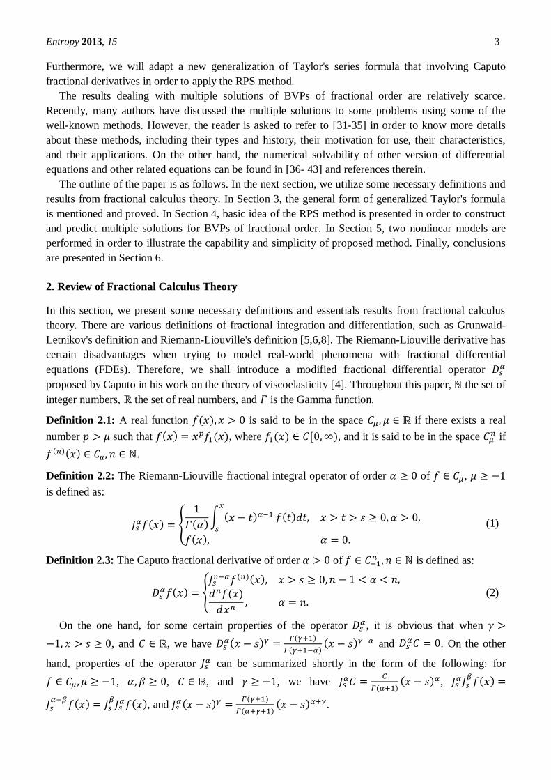
2. Review of Fractional Calculus Theory

In this section, we present some necessary definitions and essentials results from fractional calculus

theory. There are various definitions of fractional integration and differentiation, such as Grunwald-

Letnikov's definition and Riemann-Liouville's definition [5,6,8]. The Riemann-Liouville derivative has

certain disadvantages when trying to model real-world phenomena with fractional differential

equations (FDEs). Therefore, we shall introduce a modified fractional differential operator

proposed by Caputo in his work on the theory of viscoelasticity [4]. Throughout this paper, the set of

integer numbers, the set of real numbers, and is the Gamma function.

Definition 2.1: A real function is said to be in the space if there exists a real

number such that , where , and it is said to be in the space if

.

Definition 2.2: The Riemann-Liouville fractional integral operator of order of ,

is defined as:

(1)

Definition 2.3: The Caputo fractional derivative of order of is defined as:

(2)

On the one hand, for some certain properties of the operator , it is obvious that when

, and , we have

and

. On the other

hand, properties of the operator can be summarized shortly in the form of the following: for

, , , and , we have

,

, and

.

Entropy 2013, 15 4

Theorem 2.1: If , , , and , then

and

, where .

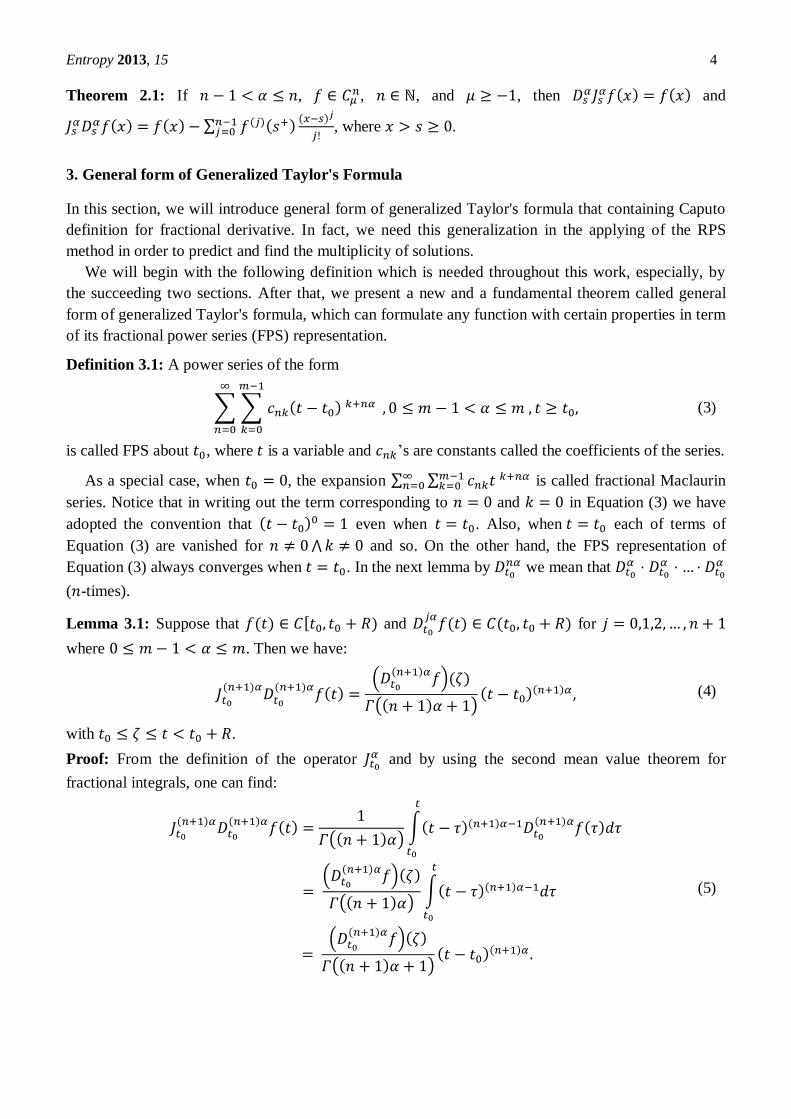
3. General form of Generalized Taylor's Formula

In this section, we will introduce general form of generalized Taylor's formula that containing Caputo

definition for fractional derivative. In fact, we need this generalization in the applying of the RPS

method in order to predict and find the multiplicity of solutions.

We will begin with the following definition which is needed throughout this work, especially, by

the succeeding two sections. After that, we present a new and a fundamental theorem called general

form of generalized Taylor's formula, which can formulate any function with certain properties in term

of its fractional power series (FPS) representation.

Definition 3.1: A power series of the form

(3)

is called FPS about , where is a variable and ’s are constants called the coefficients of the series.

As a special case, when , the expansion

is called fractional Maclaurin

series. Notice that in writing out the term corresponding to and in Equation (3) we have

adopted the convention that even when . Also, when each of terms of

Equation (3) are vanished for and so. On the other hand, the FPS representation of

Equation (3) always converges when . In the next lemma by

we mean that

( -times).

Lemma 3.1: Suppose that and

for

where . Then we have:

(4)

with .

Proof: From the definition of the operator

and by using the second mean value theorem for

fractional integrals, one can find:

(5)

Entropy 2013, 15 5

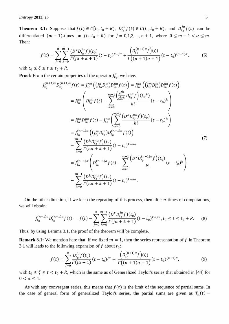
Theorem 3.1: Suppose that ,

, and

can be

differentiated -times on for , where .

Then:

(6)

with .

Proof: From the certain properties of the operator

, we have:

(7)

On the other direction, if we keep the repeating of this process, then after -times of computations,

we will obtain:

(8)

Thus, by using Lemma 3.1, the proof of the theorem will be complete.

Remark 3.1: We mention here that, if we fixed , then the series representation of in Theorem

3.1 will leads to the following expansion of about :

(9)

with , which is the same as of Generalized Taylor's series that obtained in [44] for

.

As with any convergent series, this means that is the limit of the sequence of partial sums. In

the case of general form of generalized Taylor's series, the partial sums are given as

Entropy 2013, 15 6

. In general, is the sum of its general form of generalized

Taylor's series if . But on the other aspect as well, if we set

, then is the remainder of general form of generalized Taylor's series. That is,

.

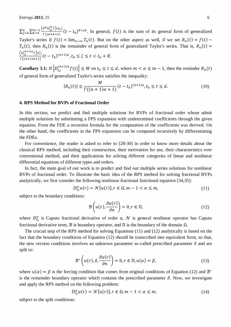
Corollary 3.1: If

on , where , then the reminder

of general form of generalized Taylor's series satisfies the inequality:

(10)

4. RPS Method for BVPs of Fractional Order

In this section, we predict and find multiple solutions for BVPs of fractional order whose admit

multiple solutions by substituting a FPS expansion with undetermined coefficients through the given

equation. From the FDE a recursion formula for the computation of the coefficients was derived. On

the other hand, the coefficients in the FPS expansion can be computed recursively by differentiating

the FDEs.

For convenience, the reader is asked to refer to [28-30] in order to know more details about the

classical RPS method, including their construction, their motivation for use, their characteristics over

conventional method, and their applications for solving different categories of linear and nonlinear

differential equations of different types and orders.

In fact, the main goal of our work is to predict and find out multiple series solutions for nonlinear

BVPs of fractional order. To illustrate the basic idea of the RPS method for solving fractional BVPs

analytically, we first consider the following nonlinear fractional functional equation [34,35]:

(11)

subject to the boundary conditions:

(12)

where is Caputo fractional derivative of order , is general nonlinear operator has Caputo

fractional derivative term, is boundary operator, and is the boundary of the domain .

The crucial step of the RPS method for solving Equations (11) and (12) analytically is based on the

fact that the boundary conditions of Equation (12) should be transcribed into equivalent form, so that,

the new version conditions involves an unknown parameter so-called prescribed parameter and are

split to:

(13)

where is the forcing condition that comes from original conditions of Equation (12) and

is the remainder boundary operator which contains the prescribed parameter . Now, we investigate

and apply the RPS method on the following problem:

(14)

subject to the split conditions:

Entropy 2013, 15 7

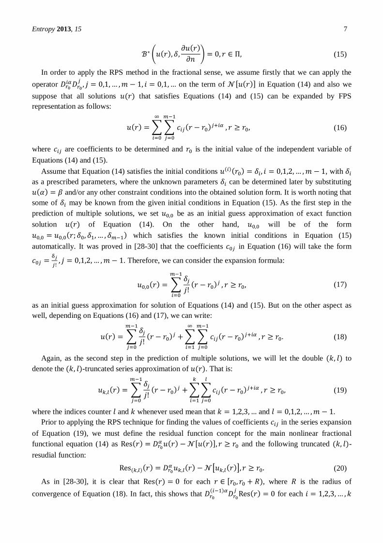
(15)

In order to apply the RPS method in the fractional sense, we assume firstly that we can apply the

operator

on the term of in Equation (14) and also we

suppose that all solutions that satisfies Equations (14) and (15) can be expanded by FPS

representation as follows:

(16)

where are coefficients to be determined and is the initial value of the independent variable of

Equations (14) and (15).

Assume that Equation (14) satisfies the initial conditions , with

as a prescribed parameters, where the unknown parameters can be determined later by substituting

and/or any other constraint conditions into the obtained solution form. It is worth noting that

some of may be known from the given initial conditions in Equation (15). As the first step in the

prediction of multiple solutions, we set be as an initial guess approximation of exact function

solution of Equation (14). On the other hand, will be of the form

which satisfies the known initial conditions in Equation (15)

automatically. It was proved in [28-30] that the coefficients in Equation (16) will take the form

. Therefore, we can consider the expansion formula:

(17)

as an initial guess approximation for solution of Equations (14) and (15). But on the other aspect as

well, depending on Equations (16) and (17), we can write:

(18)

Again, as the second step in the prediction of multiple solutions, we will let the double to

denote the -truncated series approximation of . That is:

(19)

where the indices counter and whenever used mean that and .

Prior to applying the RPS technique for finding the values of coefficients in the series expansion

of Equation (19), we must define the residual function concept for the main nonlinear fractional

functional equation (14) as and the following truncated -

resudial function:

(20)

As in [28-30], it is clear that for each , where is the radius of

convergence of Equation (18). In fact, this shows that

for each

Entropy 2013, 15 8

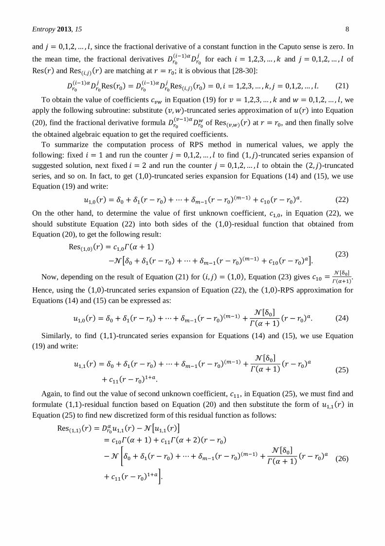
and , since the fractional derivative of a constant function in the Caputo sense is zero. In

the mean time, the fractional derivatives

for each and of

and are matching at ; it is obvious that [28-30]:

(21)

To obtain the value of coefficients in Equation (19) for and , we

apply the following subroutine: substitute -truncated series approximation of into Equation

(20), find the fractional derivative formula

of at , and then finally solve

the obtained algebraic equation to get the required coefficients.

To summarize the computation process of RPS method in numerical values, we apply the

following: fixed and run the counter to find -truncated series expansion of

suggested solution, next fixed and run the counter to obtain the -truncated

series, and so on. In fact, to get -truncated series expansion for Equations (14) and (15), we use

Equation (19) and write:

(22)

On the other hand, to determine the value of first unknown coefficient, , in Equation (22), we

should substitute Equation (22) into both sides of the -residual function that obtained from

Equation (20), to get the following result:

(23)

Now, depending on the result of Equation (21) for , Equation (23) gives

.

Hence, using the -truncated series expansion of Equation (22), the -RPS approximation for

Equations (14) and (15) can be expressed as:

(24)

Similarly, to find -truncated series expansion for Equations (14) and (15), we use Equation

(19) and write:

(25)

Again, to find out the value of second unknown coefficient, , in Equation (25), we must find and

formulate -residual function based on Equation (20) and then substitute the form of in

Equation (25) to find new discretized form of this residual function as follows:

(26)

Entropy 2013, 15 9

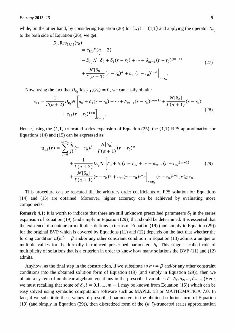
while, on the other hand, by considering Equation (20) for and applying the operator

to the both side of Equation (26), we get:

(27)

Now, using the fact that , we can easily obtain:

(28)

Hence, using the -truncated series expansion of Equation (25), the -RPS approximation for

Equations (14) and (15) can be expressed as:

(29)

This procedure can be repeated till the arbitrary order coefficients of FPS solution for Equations

(14) and (15) are obtained. Moreover, higher accuracy can be achieved by evaluating more

components.

Remark 4.1: It is worth to indicate that there are still unknown prescribed parameters in the series

expansion of Equation (19) (and simply in Equation (29)) that should be determined. It is essential that

the existence of a unique or multiple solutions in terms of Equation (19) (and simply in Equation (29))

for the original BVP which is covered by Equations (11) and (12) depends on the fact that whether the

forcing condition and/or any other constraint condition in Equation (13) admits a unique or

multiple values for the formally introduced prescribed parameters . This stage is called rule of

multiplicity of solutions that is a criterion in order to know how many solutions the BVP (11) and (12)

admits.

Anyhow, as the final step in the construction, if we substitute and/or any other constraint

conditions into the obtained solution form of Equation (19) (and simply in Equation (29)), then we

obtain a system of nonlinear algebraic equations in the prescribed variables (Here,

we must recalling that some of may be known from Equation (15)) which can be

easy solved using symbolic computation software such as MAPLE or MATHEMATICA . In

fact, if we substitute these values of prescribed parameters in the obtained solution form of Equation

(19) (and simply in Equation (29)), then discretized form of the -truncated series approximation

Entropy 2013, 15 10

of of Equations (11) and (12) (and simply -truncated series approximation of as given

by Equation (26)) will be obtained.

5. Applications and Numerical Discussions

The application problems are carried out using the proposed RPS method, which is one of the modern

analytical techniques because of it's iteratively nature; it can handle any kind of boundary conditions

and other constraints. The RPS method doesn't have mathematical requirements about the multiple

solutions of fractional BVPs to be solved; also the RPS method is very effective in performing global

predicted solutions, and provides a great flexibility in choosing the initial guess approximations.

However, in order to verify the computational efficiency of the designed RPS method, two nonlinear

models are performed, one of them arises in mixed convection flows and the other one arises in heat

transfer, which both admits multiple solutions. In the process of computation, all the symbolic and

numerical computations were performed by using MATHEMATICA software package.

Throughout this section, we will try to give the results of the two applications; however, in some

cases we will switch between the results obtained for the applications in order not to increase the

length of the paper without the loss of generality for the remaining application and results. However,

by easy calculations we can collect further results and discussion for the desire application.

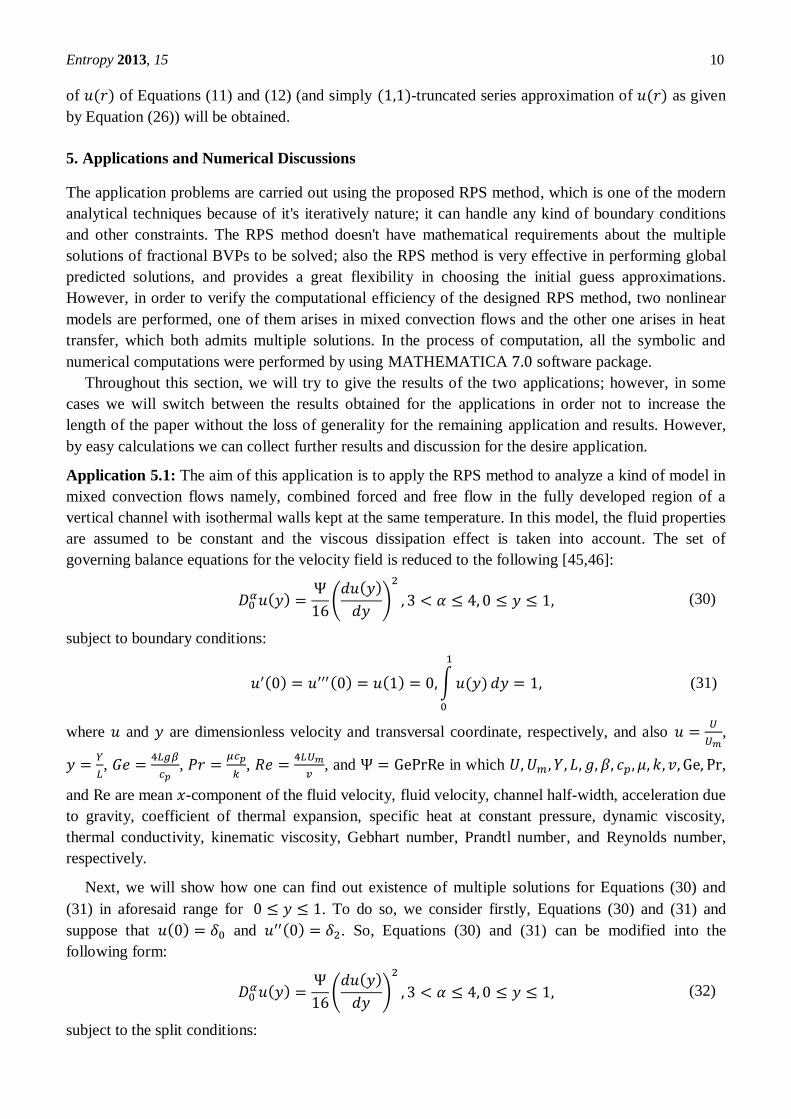
Application 5.1: The aim of this application is to apply the RPS method to analyze a kind of model in

mixed convection flows namely, combined forced and free flow in the fully developed region of a

vertical channel with isothermal walls kept at the same temperature. In this model, the fluid properties

are assumed to be constant and the viscous dissipation effect is taken into account. The set of

governing balance equations for the velocity field is reduced to the following [45,46]:

(30)

subject to boundary conditions:

(31)

where and are dimensionless velocity and transversal coordinate, respectively, and also

,

,

,

,

, and in which ,

and are mean -component of the fluid velocity, fluid velocity, channel half-width, acceleration due

to gravity, coefficient of thermal expansion, specific heat at constant pressure, dynamic viscosity,

thermal conductivity, kinematic viscosity, Gebhart number, Prandtl number, and Reynolds number,

respectively.

Next, we will show how one can find out existence of multiple solutions for Equations (30) and

(31) in aforesaid range for . To do so, we consider firstly, Equations (30) and (31) and

suppose that and . So, Equations (30) and (31) can be modified into the

following form:

(32)

subject to the split conditions:

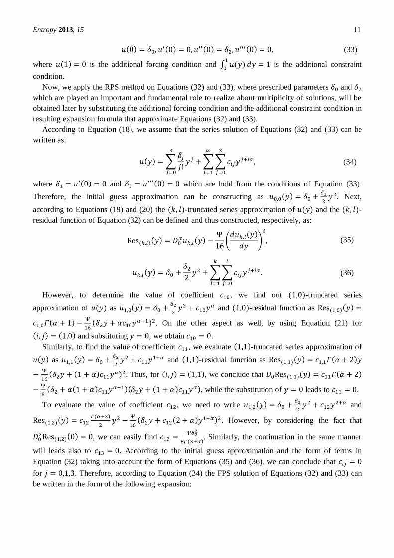
Entropy 2013, 15 11

, (33)

where is the additional forcing condition and

is the additional constraint

condition.

Now, we apply the RPS method on Equations (32) and (33), where prescribed parameters and

which are played an important and fundamental role to realize about multiplicity of solutions, will be

obtained later by substituting the additional forcing condition and the additional constraint condition in

resulting expansion formula that approximate Equations (32) and (33).

According to Equation (18), we assume that the series solution of Equations (32) and (33) can be

written as:

(34)

where and which are hold from the conditions of Equation (33).

Therefore, the initial guess approximation can be constructing as

. Next,

according to Equations (19) and (20) the -truncated series approximation of and the -

residual function of Equation (32) can be defined and thus constructed, respectively, as:

(35)

(36)

However, to determine the value of coefficient , we find out -truncated series

approximation of as

and -residual function as

. On the other aspect as well, by using Equation (21) for

and substituting , we obtain .

Similarly, to find the value of coefficient , we evaluate -truncated series approximation of

as

and -residual function as

. Thus, for , we conclude that

, while the substitution of leads to .

To evaluate the value of coefficient , we need to write

and

. However, by considering the fact that

, we can easily find

. Similarly, the continuation in the same manner

will leads also to . According to the initial guess approximation and the form of terms in

Equation (32) taking into account the form of Equations (35) and (36), we can conclude that

for . Therefore, according to Equation (34) the FPS solution of Equations (32) and (33) can

be written in the form of the following expansion:

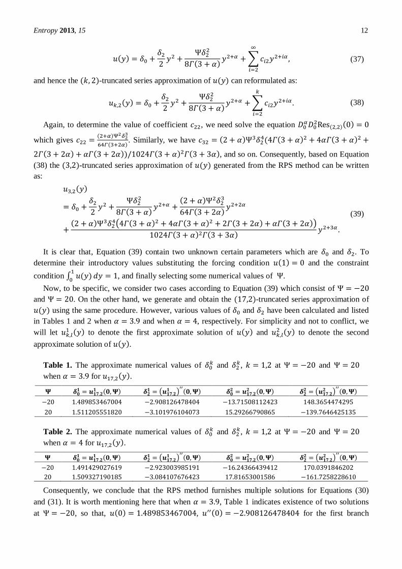
Entropy 2013, 15 12

(37)

and hence the -truncated series approximation of can reformulated as:

(38)

Again, to determine the value of coefficient , we need solve the equation

which gives

. Similarly, we have

, and so on. Consequently, based on Equation

(38) the -truncated series approximation of generated from the RPS method can be written

as:

(39)

It is clear that, Equation (39) contain two unknown certain parameters which are and . To

determine their introductory values substituting the forcing condition and the constraint

condition

, and finally selecting some numerical values of .

Now, to be specific, we consider two cases according to Equation (39) which consist of

and . On the other hand, we generate and obtain the -truncated series approximation of

using the same procedure. However, various values of and have been calculated and listed

in Tables 1 and 2 when and when , respectively. For simplicity and not to conflict, we

will let to denote the first approximate solution of and

to denote the second

approximate solution of .

Table 1. The approximate numerical values of and

, at and

when for .

Table 2. The approximate numerical values of and

, at and

when for .

Consequently, we conclude that the RPS method furnishes multiple solutions for Equations (30)

and (31). It is worth mentioning here that when , Table 1 indicates existence of two solutions

at , so that, , for the first branch

Entropy 2013, 15 13

solution and , for the second branch solution.

In fact, these results answer the question how many solutions the nonlinear BVP (30) and (31) admits?

The same procedure has been done at the case . As we see from Table 1, there exist multiple

solutions namely , for the first branch

solution and , for the second branch solution.

Similar conclusion can be achieved when as shown in Table 2.

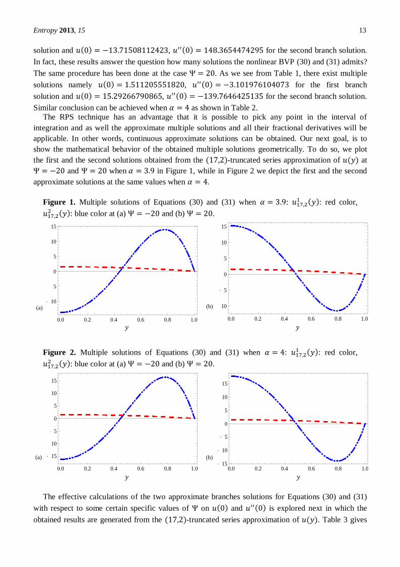
The RPS technique has an advantage that it is possible to pick any point in the interval of

integration and as well the approximate multiple solutions and all their fractional derivatives will be

applicable. In other words, continuous approximate solutions can be obtained. Our next goal, is to

show the mathematical behavior of the obtained multiple solutions geometrically. To do so, we plot

the first and the second solutions obtained from the -truncated series approximation of at

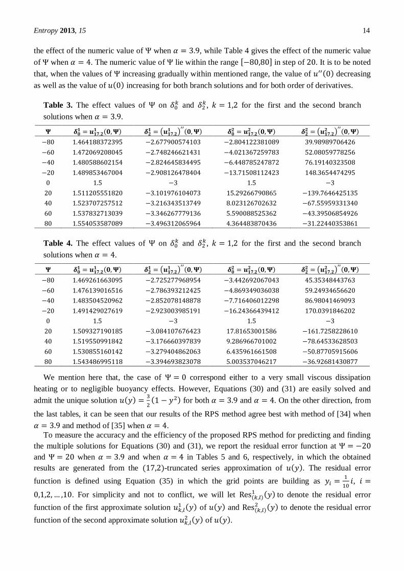
and when in Figure 1, while in Figure 2 we depict the first and the second

approximate solutions at the same values when .

Figure 1. Multiple solutions of Equations (30) and (31) when : : red color,

: blue color at (a) and (b) .

Figure 2. Multiple solutions of Equations (30) and (31) when : : red color,

: blue color at (a) and (b) .

The effective calculations of the two approximate branches solutions for Equations (30) and (31)

with respect to some certain specific values of on and is explored next in which the

obtained results are generated from the -truncated series approximation of . Table 3 gives

0.0 0.2 0.4 0.6 0.8 1.0

10

5

0

5

10

15

0.0 0.2 0.4 0.6 0.8 1.0

10

5

0

5

10

15

0.0 0.2 0.4 0.6 0.8 1.0

15

10

5

0

5

10

15

0.0 0.2 0.4 0.6 0.8 1.015

10

5

0

5

10

15

(a) (b)

(a) (b)

Entropy 2013, 15 14

the effect of the numeric value of when , while Table 4 gives the effect of the numeric value

of when . The numeric value of lie within the range in step of . It is to be noted

that, when the values of increasing gradually within mentioned range, the value of decreasing

as well as the value of increasing for both branch solutions and for both order of derivatives.

Table 3. The effect values of on and

, for the first and the second branch

solutions when .

1

5

Table 4. The effect values of on and

, for the first and the second branch

solutions when .

1

We mention here that, the case of correspond either to a very small viscous dissipation

heating or to negligible buoyancy effects. However, Equations (30) and (31) are easily solved and

admit the unique solution

for both and . On the other direction, from

the last tables, it can be seen that our results of the RPS method agree best with method of [34] when

and method of [35] when .

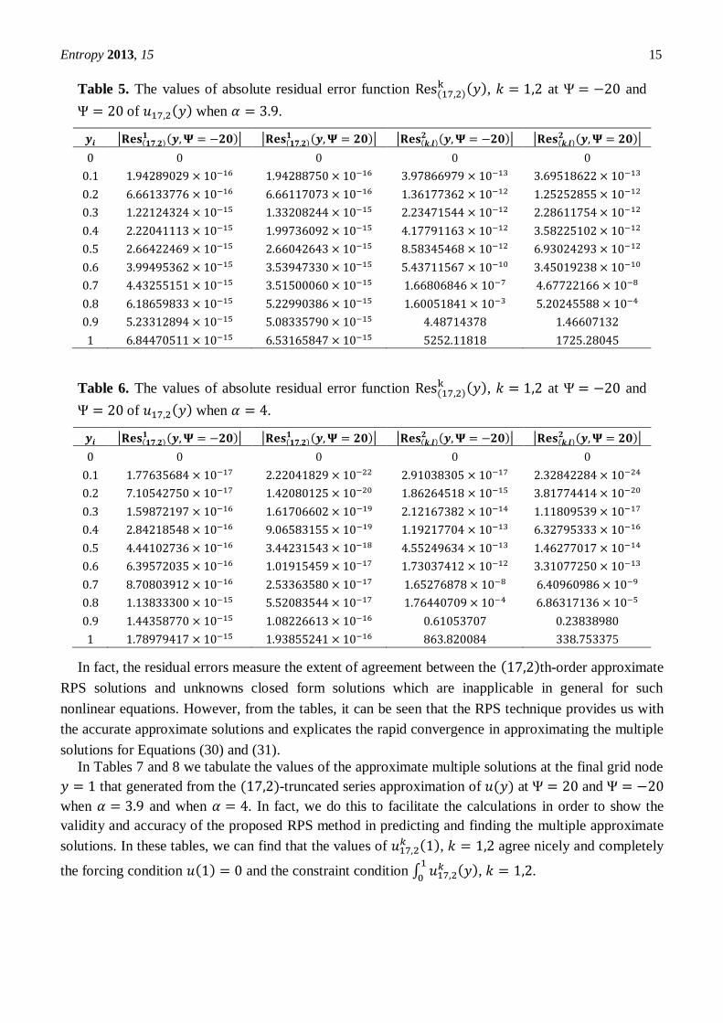
To measure the accuracy and the efficiency of the proposed RPS method for predicting and finding

the multiple solutions for Equations (30) and (31), we report the residual error function at

and when and when in Tables 5 and 6, respectively, in which the obtained

results are generated from the -truncated series approximation of . The residual error

function is defined using Equation (35) in which the grid points are building as

,

. For simplicity and not to conflict, we will let to denote the residual error

function of the first approximate solution of and

to denote the residual error

function of the second approximate solution of .

Entropy 2013, 15 15

Table 5. The values of absolute residual error function , at and

of when .

0 0 0 0

Table 6. The values of absolute residual error function , at and

of when .

0 0 0 0

5

In fact, the residual errors measure the extent of agreement between the th-order approximate

RPS solutions and unknowns closed form solutions which are inapplicable in general for such

nonlinear equations. However, from the tables, it can be seen that the RPS technique provides us with

the accurate approximate solutions and explicates the rapid convergence in approximating the multiple

solutions for Equations (30) and (31).

In Tables 7 and 8 we tabulate the values of the approximate multiple solutions at the final grid node

that generated from the -truncated series approximation of at and

when and when . In fact, we do this to facilitate the calculations in order to show the

validity and accuracy of the proposed RPS method in predicting and finding the multiple approximate

solutions. In these tables, we can find that the values of , agree nicely and completely

the forcing condition and the constraint condition

, .

Entropy 2013, 15 16

Table 7. The approximate value of forcing condition and constraint condition

, at and when .

Table 8. The approximate value of forcing condition and constraint condition

, at and when .

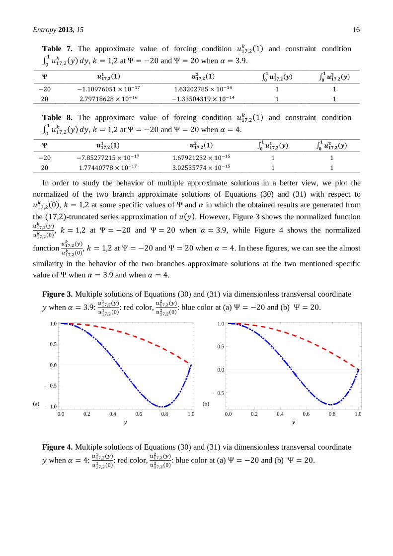
In order to study the behavior of multiple approximate solutions in a better view, we plot the

normalized of the two branch approximate solutions of Equations (30) and (31) with respect to

, at some specific values of and in which the obtained results are generated from

the -truncated series approximation of . However, Figure 3 shows the normalized function

, at and when , while Figure 4 shows the normalized

function

, at and when . In these figures, we can see the almost

similarity in the behavior of the two branches approximate solutions at the two mentioned specific

value of when and when .

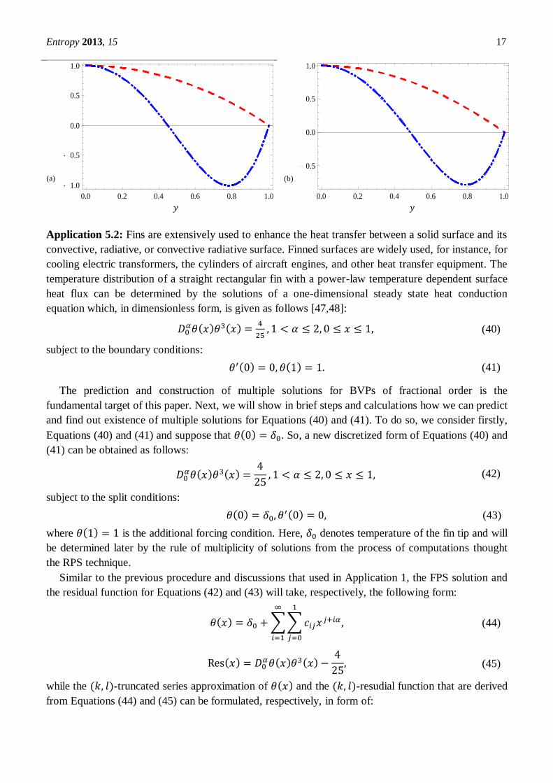
Figure 3. Multiple solutions of Equations (30) and (31) via dimensionless transversal coordinate

when :

: red color,

: blue color at (a) and (b) .

Figure 4. Multiple solutions of Equations (30) and (31) via dimensionless transversal coordinate

when :

: red color,

: blue color at (a) and (b) .

0.0 0.2 0.4 0.6 0.8 1.0

1.0

0.5

0.0

0.5

1.0

0.0 0.2 0.4 0.6 0.8 1.0

0.5

0.0

0.5

1.0

(b) (a)

Entropy 2013, 15 17

Application 5.2: Fins are extensively used to enhance the heat transfer between a solid surface and its

convective, radiative, or convective radiative surface. Finned surfaces are widely used, for instance, for

cooling electric transformers, the cylinders of aircraft engines, and other heat transfer equipment. The

temperature distribution of a straight rectangular fin with a power-law temperature dependent surface

heat flux can be determined by the solutions of a one-dimensional steady state heat conduction

equation which, in dimensionless form, is given as follows [47,48]:

(40)

subject to the boundary conditions:

(41)

The prediction and construction of multiple solutions for BVPs of fractional order is the

fundamental target of this paper. Next, we will show in brief steps and calculations how we can predict

and find out existence of multiple solutions for Equations (40) and (41). To do so, we consider firstly,

Equations (40) and (41) and suppose that . So, a new discretized form of Equations (40) and

(41) can be obtained as follows:

(42)

subject to the split conditions:

(43)

where is the additional forcing condition. Here, denotes temperature of the fin tip and will

be determined later by the rule of multiplicity of solutions from the process of computations thought

the RPS technique.

Similar to the previous procedure and discussions that used in Application 1, the FPS solution and

the residual function for Equations (42) and (43) will take, respectively, the following form:

(44)

(45)

while the -truncated series approximation of and the -resudial function that are derived

from Equations (44) and (45) can be formulated, respectively, in form of:

0.0 0.2 0.4 0.6 0.8 1.0

1.0

0.5

0.0

0.5

1.0

0.0 0.2 0.4 0.6 0.8 1.0

0.5

0.0

0.5

1.0

(b) (a)

Entropy 2013, 15 18

(46)

(47)

It is to be noted that the -truncated series solution of Equations (42) and (43) is

and the -residual function is

. Thus, using

Equation (21) for , we get

. Similarly, the -truncated series solution

is

and the -residual function is:

(48)

More precisely, according to Equation (21) the solution of equation will gives

. Thus, based on the initial guess approximation and the form of terms of Equation (42) taking

into account the form of Equations (46) and (47), it easy to see that , . Therefore,

according to Equation (44) a new discretized form of FPS solution for Equations (42) and (43) can be

obtained and expressed as:

(49)

and hence the -truncated series approximation of can formulated as:

(50)

In the shape of shapes by continuing in this procedure and using Equations (46) and (47) taking into

account Equation (21), we can easily obtained that

,

,

and so on. Consequently, based on Equation (50) the -truncated series approximation of

generated from the RPS method can be written as:

Entropy 2013, 15 19

(51)

It is clear that, all the terms in Equation (51) contain an unknown certain parameter and to

determine its introductory values we must substitute the boundary condition 1 back into

Equation (51) to obtain a nonlinear algebraic equation in one variable, which can be easy solved using

symbolic computation software. But on the other aspect as well, if we generate and obtain -

truncated series approximation of by using the same procedure discussed, then two various

values of have been calculated and listed in Table 9 when and when .

Table 9. The approximate numerical values of , when and when for

.

0.447213595446

It is clear from the table that two -plateaus can be identified and consequently we conclude that the

RPS method furnishes multiple solutions to Equations (40) and (41). It is worth mentioning here that

Equation (46) (and simply in Equation (51)) indicates existence of two solutions. On the other hand,

the existence of a unique or multiple solutions in terms of Equation (46) (and simply in Equation (51))

for the original BVP which is covered by Equations (40) and (41) depends on the fact that whether the

forcing condition admits a unique or multiple values for the formally introduced prescribed

parameters .

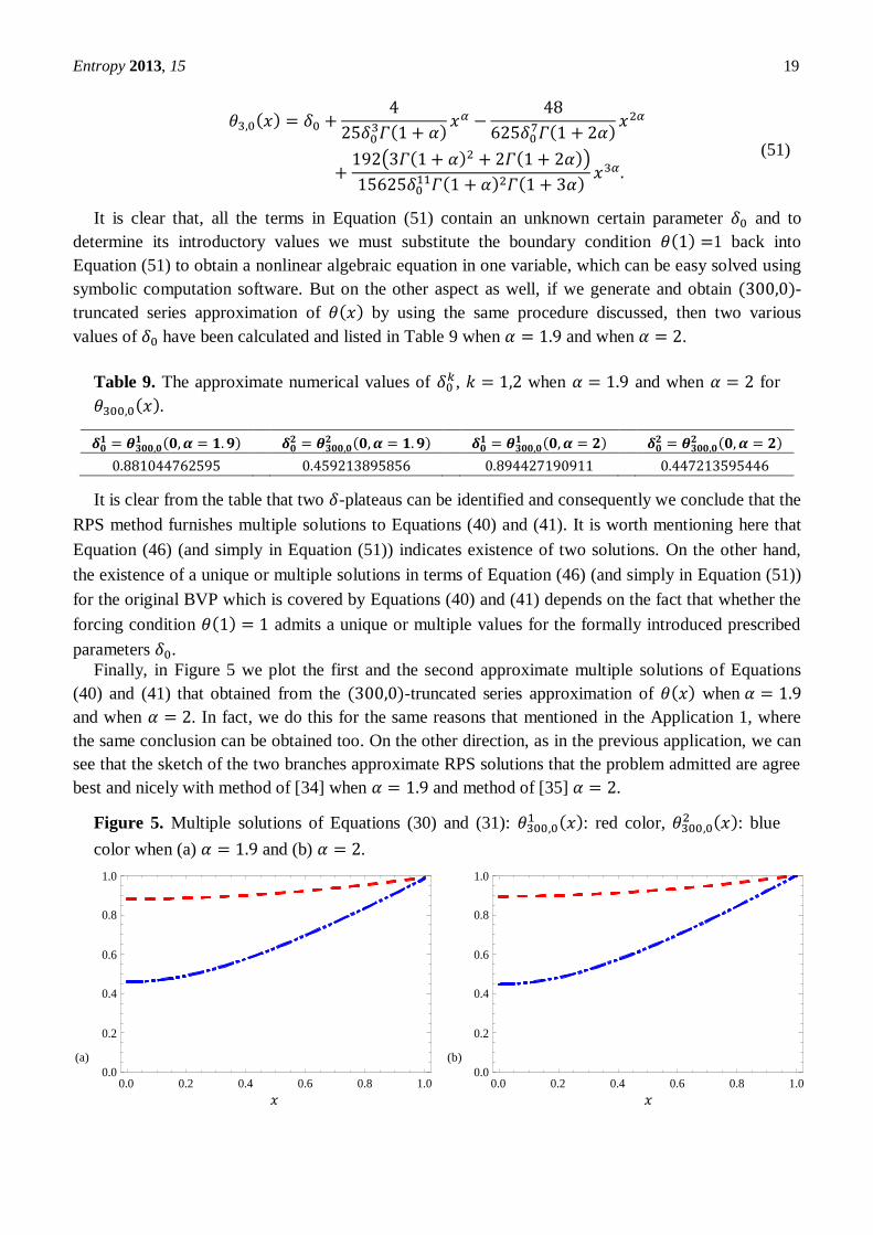
Finally, in Figure 5 we plot the first and the second approximate multiple solutions of Equations

(40) and (41) that obtained from the -truncated series approximation of when

and when . In fact, we do this for the same reasons that mentioned in the Application 1, where

the same conclusion can be obtained too. On the other direction, as in the previous application, we can

see that the sketch of the two branches approximate RPS solutions that the problem admitted are agree

best and nicely with method of [34] when and method of [35] .

Figure 5. Multiple solutions of Equations (30) and (31): : red color,

: blue

color when (a) and (b) .

0.0 0.2 0.4 0.6 0.8 1.00.0

0.2

0.4

0.6

0.8

1.0

0.0 0.2 0.4 0.6 0.8 1.00.0

0.2

0.4

0.6

0.8

1.0

(a) (b)

Entropy 2013, 15 20

6. Conclusions

It is very important not to lose any solution of nonlinear FDEs with boundary conditions in

engineering and physical sciences. In this regard, the present paper has introduced a new methodology

namely the RPS method to prevent this, so that, the presented method is not only to predict existence

of multiple solutions, but also to calculate all branches of solutions effectively at the same time by

using an appropriate initial guess approximation. We also noted that the RPS solutions were computed

via a simple algorithm without any need for perturbation techniques, special transformations, or

discretization. The validity of this method has been checked by two nonlinear models, one of them

arises in mixed convection flows and the other one arises in heat transfer, which both admits multiple

or dual solutions.

References

1. Beyer, H.; Kempfle, S. Definition of physical consistent damping laws with fractional

derivatives. Zeitschrift für Angewandte Mathematik und Mechanik 1995, 75, 623-635.

2. He, J.H. Approximate analytic solution for seepage flow with fractional derivatives in porous

media. Computer Methods in Applied Mechanics and Engineering 1998, 167, 57-68.

3. He, J.H. Some applications of nonlinear fractional differential equations and their

approximations. Bulletin of Science and Technology 1999, 15, 86-90.

4. Caputo, M. Linear models of dissipation whose Q is almost frequency independent: part II.

Geophysical Journal International 1967, 13, 529-539.

5. Miller, K.S.; Ross, B. An Introduction to the Fractional Calculus and Fractional Differential

Equations; John Willy and Sons, Inc. New York, 1993.

6. Mainardi, F. Fractional Calculus: Some Basic Problems in Continuum and Statistical Mechanics.

In Fractals and Fractional Calculus in Continuum Mechanics, Carpinteri, A., Mainardi, F. Eds.,

Springer-Verlag, Wien and New York, 1997, pp. 291-348.

7. Podlubny, I. Fractional Differential Equations; Academic Press, New York, 1999.

8. Oldham, K.B.; Spanier, J. The Fractional Calculus; New York: Academic Press, 1974.

9. Luchko, Y.; Gorenflo, R. The Initial-Value Problem for Some Fractional Differential Equations

with Caputo Derivative; Preprint Series A08-98, Fachbereich Mathematik und Informatic, Berlin,

Freie Universitat, 1998.

10. Ubriaco, M.R. Entropies based on fractional calculus. Physics Letters A 2009, 373, 2516–2519.

11. Li, H.; Haldane, F.D.M. Entanglement spectrum as a generalization of entanglement entropy:

Identification of topological order in non-abelian fractional quantum hall effect states. Physical

Review Letters 2008, 101, 010504.

12. Hoffmann, K.H.; Essex, C.; Schulzky, C. Fractional diffusion and entropy production. Journal of

Non-Equilibrium Thermodynamics 1998, 23, 166–175.

13. Machado, J.A.T. Entropy analysis of integer and fractional dynamical systems. Nonlinear

Dynamics 2010, 62, 371–378.

14. Essex, C.; Schulzky, C.; Franz, A.; Hoffmann, K.H. Tsallis and Rényi entropies in fractional

diffusion and entropy production. Physica A: Statistical Mechanics and its Applications 2000,

284, 299–308.

Entropy 2013, 15 21

15. Cifani, S.; Jakobsen, E.R. Entropy solution theory for fractional degenerate convection–diffusion

equations. Annales de l'Institut Henri Poincare (C) Non Linear Analysis 2011, 28, 413–441.

16. Prehl, J.; Essex, C.; Hoffmann, K.H. Tsallis relative entropy and anomalous diffusion. Entropy

2012, 14, 701–706.

17. Prehl, J.; Boldt, F.; Essex, C.; Hoffmann, K.H. Time evolution of relative entropies for

anomalous diffusion. Entropy 2013, 15, 2989–3006.

18. Prehl, J.; Essex, C.; Hoffmann, K.H. The superdiffusion entropy production paradox in the

space-fractional case for extended entropies. Physica A: Statistical Mechanics and its

Applications 2010, 389, 215–224.

19. Magin, R.L.; Ingo, C.; Colon-Perez, L.; Triplett, W.; Mareci, T.H. Characterization of anomalous

diffusion in porous biological tissues using fractional order derivatives and entropy. Microporous

and Mesoporous Materials 2013, 178, 39–43.

20. Doha, E.H.; Bhrawy, A.H.; Ezz-Eldien, S.S. A Chebyshev spectral method based on operational

matrix for initial and boundary value problems of fractional order. Computers and Mathematics

with Applications 2011, 62, 2364-2373.

21. Al-Mdallal, Q.M.; Syam, M.I.; Anwar, M.N. A collocation-shooting method for solving

fractional boundary value problems. Commun Nonlinear Sci Numer Simulat 2010, 15, 3814-

3822.

22. Al-Refai, M.; Hajji, M.A. Monotone iterative sequences for nonlinear boundary value problems

of fractional order. Nonlinear Analysis 2011, 74, 3531-3539.

23. Pedas, A.; Tamme, E. Piecewise polynomial collocation for linear boundary value problems of

fractional differential equations. Journal of Computational and Applied Mathematics 2012, 236,

3349-3359.

24. Ahmad, B.; Nieto, J.J. Existence of solutions for nonlocal boundary value problems of higher-

order nonlinear fractional differential equations. Abstract and Applied Analysis 2009, Article ID

494720, pages 9. doi:10.1155/2009/494720.

25. Shuqin, Z. Existence of solution for boundary value problem of fractional order. Acta

Mathematica Scentia 2006, 26B, 220-228.

26. Bai, Z. On positive solutions of a nonlocal fractional boundary value problem. Nonlinear

Analysis: Theory, Methods & Applications 2010, 72, 916-924.

27. El-Ajou, A.; Abu Arqub, O.; Momani, S. Solving fractional two-point boundary value problems

using continuous analytic method. Ain Shams Engineering Journal-engineering physics and

mathematics 2013, 4, 539-547.

28. Abu Arqub, O. Series solution of fuzzy differential equations under strongly generalized

differentiability. Journal of Advanced Research in Applied Mathematics 2013, 5, 31-52.

29. Abu Arqub, O.; El-Ajou, A.; Bataineh, A.; Hashim, I. A representation of the exact solution of

generalized Lane-Emden equations using a new analytical method. Abstract and Applied Analysis

2013, Article ID 378593, 10 pages. doi:10.1155/2013/378593.

30. Abu Arqub, O.; Abo-Hammour, Z.; Al-badarneh, R.; Momani, S. A reliable analytical method for

solving higher-order initial value problems. Discrete Dynamics in Nature and Society 2014, in press.

31. Liao, S.J. An analytic approach to solve multiple solutions of a strongly nonlinear problem.

Applied Mathematics and Computation 2005, 69, 854-65.

32. Xu, H.; Liao, S.J. Dual solutions of boundary layer flow over an upstream moving plate.

Commun Nonlinear Sci Numer Simulat 2008, 13, 350-358.

Entropy 2013, 15 22

33. Xu, H.; Lin, Z.L.; Liao, S.J.; Wu, J.Z.; Majdalani, J. Homotopy based solutions of the Navier-

Stokes equations for a porous channel with orthogonally moving walls. Phys Fluids 2010, 22,

053601. doi:10.1063/1.3392770.

34. Alomari, A.K.; Awawdeh, F.; Tahat, N.; Bani Ahmad, F.; Shatanawi, W. Multiple solutions for

fractional differential equations: Analytic approach. Applied Mathematics and Computation 2013,

219, 8893-8903.

35. Abbasbandy, S.; Shivanian, E. Predictor homotopy analysis method and its application to some

nonlinear problems. Commun Nonlinear Sci Numer Simulat 2011, 16, 2456-2468.

36. Abu Arqub, O.; Al-Smadi, M.; Momani, S. Application of reproducing kernel method for solving

nonlinear Fredholm-Volterra integrodifferential equations. Abstract and Applied Analysis 2012,

Article ID 839836, 16 pages. doi:10.1155/2012/839836.

37. Abu Arqub, O.; Al-Smadi, M.; Shawagfeh, N. Solving Fredholm integro-differential equations

using reproducing kernel Hilbert space method. Applied Mathematics and Computation 2013,

219, 8938-8948.

38. Al-Smadi, M.; Abu Arqub, O.; Momani, S. A computational method for two-point boundary

value problems of fourth-order mixed integrodifferential equations. Mathematical Problems in

Engineering 2013, Article ID 832074, 10 pages. doi.10.1155/2013/832074.

39. Shawagfeh, N.; Abu Arqub, O.; Momani, S. Analytical solution of nonlinear second-order

periodic boundary value problem using reproducing kernel method. Journal of Computational

Analysis and Applications, In press.

40. Abu Arqub, O.; El-Ajou, A.; Momani, S.; Shawagfeh, N. Analytical solutions of fuzzy initial

value problems by HAM. Applied Mathematics and Information Sciences 2013, 7, 1903-1919.

41. El-Ajou, A.; Abu Arqub, O.; Momani, S. Homotopy analysis method for second-order boundary

value problems of integrodifferential equations. Discrete Dynamics in Nature and Society 2012,

Article ID 365792, 18 pages. doi:10.1155/2012/365792.

42. Abu Arqub, O.; Abo-Hammour, Z.S.; Momani, S. Application of continuous genetic algorithm

for nonlinear system of second-order boundary value problems. Applied Mathematics and

Information Sciences. In press.

43. Abu Arqub, O.; Abo-Hammour, Z.S.; Momani, S.; Shawagfeh, N. Solving singular two-point

boundary value problems using continuous genetic algorithm. Abstract and Applied Analysis

2012, Article ID 205391, 25 page. doi.10.1155/2012/205391.

44. Odibat, Z.; Shawagfeh, N. Generalized Taylor’s formula. Applied Mathematics and Computation

2007, 186, 286-293.

45. Barletta, A. Laminar convection in a vertical channel with viscous dissipation and buoyancy

effects. International Journal of Heat and Mass Transfer 1999, 26, 153-64.

46. Barletta, A.; Magyari, E.; Keller, B. Dual mixed convection flows in a vertical channel.

International Journal of Heat and Mass Transfer 2005, 48, 4835-45.

47. Kern, Q.D.; Kraus, D.A. Extended surface heat transfer; New York: McGraw-Hill; 1972.

48. Chang, M.H. A decomposition solution for fins with temperature dependent surface heat flux.

International Journal of Heat and Mass Transfer 2005, 48, 1819-24.