Embed Size (px)
Citation preview

�����������������
Citation: Chachuła, K.; Słojewski,
T.M.; Nowak, R. Multisensor Data
Fusion for Localization of Pollution
Sources in Wastewater Networks.
Sensors 2022, 22, 387. https://
doi.org/10.3390/s22010387
Academic Editors: Charalampos
Konstantopoulos and Annie Lanzolla
Received: 19 October 2021
Accepted: 30 December 2021
Published: 5 January 2022
Publisher’s Note: MDPI stays neutral
with regard to jurisdictional claims in
published maps and institutional affil-
iations.
Copyright: © 2022 by the authors.
Licensee MDPI, Basel, Switzerland.
This article is an open access article
distributed under the terms and
conditions of the Creative Commons
Attribution (CC BY) license (https://
creativecommons.org/licenses/by/
4.0/).
sensors
Article
Multisensor Data Fusion for Localization of Pollution Sourcesin Wastewater NetworksKrystian Chachuła * , Tomasz Michał Słojewski and Robert Nowak
Faculty of Electronics and Information Technology, Warsaw University of Technology, 00-665 Warsaw, Poland;[email protected] (T.M.S.); [email protected] (R.N.)* Correspondence: [email protected]
Abstract: Illegal discharges of pollutants into sewage networks are a growing problem in largeEuropean cities. Such events often require restarting wastewater treatment plants, which cost upto a hundred thousand Euros. A system for localization and quantification of pollutants in utilitynetworks could discourage such behavior and indicate a culprit if it happens. We propose anenhanced algorithm for multisensor data fusion for the detection, localization, and quantificationof pollutants in wastewater networks. The algorithm processes data from multiple heterogeneoussensors in real-time, producing current estimates of network state and alarms if one or many sensorsdetect pollutants. Our algorithm models the network as a directed acyclic graph, uses adaptive peakdetection, estimates the amount of specific compounds, and tracks the pollutant using a Kalmanfilter. We performed numerical experiments for several real and artificial sewage networks, andmeasured the quality of discharge event reconstruction. We report the correctness and performanceof our system. We also propose a method to assess the importance of specific sensor locations.The experiments show that the algorithm’s success rate is equal to sensor coverage of the network.Moreover, the median distance between nodes pointed out by the fusion algorithm and nodes wherethe discharge was introduced equals zero when more than half of the network nodes contain sensors.The system can process around 5000 measurements per second, using 1 MiB of memory per 4600measurements plus a constant of 97 MiB, and it can process 20 tracks per second, using 1.3 MiB ofmemory per 100 tracks.
Keywords: sensors; data fusion; tracking; peak detection; sewage network; IoT
1. Introduction
Due to industrialization, society must take care of waste disposal and the efficientoperation of sewage treatment plants. Breakdowns in these areas are a growing threat,so it is crucial to continuously monitor utility networks and react as soon as possible.It is achievable to design pollutant tracking systems that use a very simplified modelof substance flow. An appropriate detection accuracy is obtained by fusing data frommany sensors of different types. Sensor technology constantly improves and, due todevelopments in the Internet of Things (IoT) space, provided measurements are easier toaccess for processing than ever.
Researchers’ interest in exploring methods for the detection, localization, and quantifica-tion of pollutants in wastewater networks (WWNs) and water distribution systems (WDSs)has grown considerably in recent years, especially regarding sensor technology [1–16]. Ques-tionable policies regarding waste disposal are prevalent in today’s industry [17,18]. This iswhy we see more and more incidents connected to WWNs [13,19–21].
The characteristics of WWNs and the volatility of pollutants make localization andquantification immensely challenging. The reasons for the difficulty of this task come fromthe randomness of the injection process involving the type of pollutants, the injection point,the injection amount, time, duration, etc. [22] Moreover, some physical properties of thewastewater are less predictable or more difficult to measure precisely than others.
Sensors 2022, 22, 387. https://doi.org/10.3390/s22010387 https://www.mdpi.com/journal/sensors

Sensors 2022, 22, 387 2 of 19
The need for data fusion in this field is supported by the fact that a simple monitoringsystem where anomalies are detected independently for each sensor would be lacking atleast four desirable features. The first one is marking discharges observed by multiplesensors as more significant than those detected by only a single sensor. The second is thequantification of pollutants by considering the sum of deviations in measurement seriesconnected to a single discharge event. Another one would be the deduplication of alarmsby clustering similar observations. The last one is discovering the flow path of the pollutantthat leads to easier source localization. Data fusion has also proved to be a viable techniquefor knowledge discovery in other fields such as bearing fault identification [23].
We propose an enhanced data fusion algorithm for the detection, localization, and quantifi-cation of pollutants in WWNs. This article extends the system depicted in Chachuła et al. [24],where we proposed the preliminary and very limited version of the data fusion algorithm.The algorithm presented in Chachuła et al. [24] represents the sewage network as a directedtree. In this structure, there is one and only one path from any point of the sewage networkto sink. Our new algorithm represents the sewage network by a directed acyclic graph(DAG), which corresponds to the structure of real WWNs. Therefore, we can now performfusion in sewage networks presented in the literature.
Related Work
In the previous algorithm ([24]), pollutant quantification was based on a fixed per-quantity threshold. This assumption is not valid if we observe sensor calibration drift, orthe water level in the network changes. Both of these phenomena occur in real sewagenetworks. In our new algorithm, we use adaptive peak detection.
We also improved our implementation. Even though the current algorithm is morecomplex than the previous one, we can process 5000 measurements and 20 tracks persecond, which is 50 times faster than previously.
Presented improvements broaden possible use cases of the algorithm and bring itcloser to being ready for deployment in real scenarios.
Buras and Solano Donado [25] used random forest classifiers to detect and identifypollutants in wastewater and the XGBoost algorithm for predicting the distance from thesource to the sensor. However, the proposed models did not quantify the pollutants.
In 2021, Yan et al. [22] proposed an improved genetic algorithm for the pollutionsource localization in water supply networks. They formulated assumptions about thebehavior of pollutants in water, which are also used in this article. Those assumptions were:
• The pollutant does not react with other substances.• The pollutant gradually dilutes with the water flow.• The running speed of the pollutant is consistent with the flow velocity of the pipe segment.• Pollutants are injected into the network only through the nodes.• The probability of injection for all nodes is equal.• The sensors can monitor water properties in real-time.
The second assumption does not mean that we estimate the dilution of pollutants.We consider this phenomenon by considering the sum of deviations of samples from thebackground value in the measurement series. This way, we account for highly dilutedtargets causing low, long deviations and concentrated ones, high, short deviations.
The assumption about equal discharge probability in every node does not come with-out drawbacks. There are areas in networks of real cities, such as industrial districts orresidential areas known for illegal activities, with higher probabilities of polluting dis-charges. However, this information may be difficult to access, as it is connected to lawenforcement or simply nonexistent, as is the case in artificial networks used in simula-tions. This article considers a worst-case scenario, where such knowledge is unavailable,and assumes an identical probability of discharge in every node.
In 2013, Sidhu et al. [26] experimented with using microbial and chemical sourcetracking for the detection of viruses and chemical compounds in urban stormwater runoff.

Sensors 2022, 22, 387 3 of 19
They state the benefits of monitoring the network for human enteric viruses and drugs,which include more reliable public health risk assessments.
In 2016, Yang et al. [27] focused on combating drug abuse by developing a novelsewage sensor for use in wastewater-based epidemiology. They demonstrated that this sen-sor could be used for the on-site real-time monitoring of wastewater by unskilled personnel.
Varon et al. [28] localized and quantified a large, persistent methane source usingcoarse and fine satellite instruments. They used a fusion strategy, where the coarse imageswere used for localization and fine images—for quantification.
Macas and Wu [29] introduced a framework based on an autoencoder for the detectionof anomalies in water treatment systems.
In 2020, Montalvo-Cedillo et al. [30] highlighted the significance of combined seweroverflow events in the contamination of receiving bodies such as rivers. They analyzed mul-tiple wastewater parameters to evaluate the behavior of three different sewage dischargesinto a river.
Jalal and Ezzedine [31] built and compared two models, a support vector machine anda decision tree, to detect anomalies in WDSs. Their evaluation was based on a real datasetretrieved from a water treatment station.
This article’s goal is to describe the improved multisensor data fusion framework,present the results of various evaluation methods, and interpret them to assess the algo-rithm’s applicability in real-world scenarios.
2. Methods
We represent the sewage network by a directed acyclic graph (DAG) G(V, E). Edgese ∈ E represent wastewater pipes, and nodes v ∈ V represent buildings and junctions. Thedirection of edges corresponds with the direction of the water flow. In some nodes, thereare sensors measuring different properties of wastewater. The sensors could be the sametype (measure the same property) or different types. Measured properties of wastewaterare referred to as entities. Introducing some amount of a pollutant (target) to a node iscalled a discharge event. Such an event could cause peaks in measurement series providedby sensors along the flow paths if the event refers to the compound that changes a propertythat is being measured by the sensor.
Edges have two variable attributes: oe, the time needed for the water to flow throughthe whole pipe, and ge, which is the dispersion factor. The dispersion factor is calculatedby dividing the expected peak height at the end of the pipe by the expected peak height atthe start of the pipe.
The data fusion algorithm is a loop of six steps: resampling, peak detection, pollutionquantification, downstream propagation, tracking, and event generation. See Figure 1. Itprocesses measurements in real-time, and the steps presented in Figure 1 are repeated forsuccessive, equally spaced points in time as dictated by the sampling period.
Our algorithm supports sensors located in different places and sampling at differentrates. The algorithm’s first step (resampling) converts sensor output (measurements) into aunified discrete-time domain. This conversion is achieved either by mean aggregation (ifthere are several sensor samples in the single algorithm period) or linear interpolation (if asensor samples slower than the algorithm period). This step’s details and mathematicalformulas were presented in Chachuła et al. [24].
The peak detection algorithm classifies measurements into either peaks or background.This step filters sensor output (measurements), to reduce the amount of needed computa-tion. We present the details of this step in Section 2.1.
In the pollution quantification step, measurements marked by peak detection assignificant are analyzed further to approximate amounts of pollutants. This step transformsobservations in the measurement domain (sensor, entity, time, value, uncertainty) intoobservations in the target domain (target, node, time, amount, confidence) called detections.Our method, that extends the approach presented in Chachuła et al. [24], is shown in detailin Section 2.3.

Sensors 2022, 22, 387 4 of 19
Downstream propagation approximates the amount of substance (pollutant) in everynode, even if the node has no sensor. This step also smooths out the tracks, which are ourestimation of the state of a pollutant flowing through the network. The tracking algorithm,uses the Kalman filter, which finds tracks’ state by clustering detections. Downstreampropagation was explained in Chachuła et al. [24], and tracking is extended as presented inSection 2.2.
Event generation creates potential events based on tracks. It is the final step ofthe algorithm, and its primary purpose is to report only tracks with a large number ofsupporting (associated) detections. For such tracks, an event represents the discharge of acompound into a graph node. This step focuses the user on essential changes in the sewagenetwork. Event generation is depicted in detail in Chachuła et al. [24].
Resampling
Interpolating and aggregating measurements to form observations at regular
intervals
Adaptivepeak detection
Classifying measurements
Pollutant Quantification
Calculating possible amounts of compounds
Downstreampropagation
Predicting
the compound flow
Tracking
Clustering observations and tracking the compounds
Event generation
Reconstructing the discharge event
Figure 1. The data fusion algorithm.
2.1. Adaptive Peak Detection
The peak detection module classifies measurements into three classes: background, uppeaks, down peaks. The background class contains measurements of value similar to othermeasurements from the same series. The up peak class is a set of consecutive measurementsof value that stands out from the background in the positive direction and down peaks—inthe negative direction.
The module’s task is to detect measurements that belong to peaks. Detected peaks areused to determine the time of discharge events, and the amount of substance discharged iscalculated from the peak area. The implemented algorithm is a modification of an algorithmcreated by Palshikar [32]. We modified it to work with streams of measurements and todetect both up peaks and down peaks.
In our previous solution [24], we did not use adaptive peak detection. The pollutantswere detected by comparing measured values to a fixed background level. If the deviationfrom the background was greater than a fixed threshold, target presence observations(detections) were created based on this measurement. Such an approach works only ifthe background level is constant and signal to noise ratio is very high. However, in realconditions, the background level varies with time, and currently available sensor technologyproduces measurements with high noise levels [1]. Using such fixed thresholds in realscenarios was difficult, as the characteristics of real measurements are complex. We createdan adaptive peak detection module to enable the data fusion algorithm to produce correctresults in real cases.
We denote the set of measurements belonging to a single series as M = {x1, x2, . . . , xN},where xi is a value measured at the discrete time i. The module works with streams ofmeasurements. This means that, at the moment of analyzing a measurement from time j,we only know the values of the measurements Mj = {x1, x2, . . . , xj}. Palshikar’s algorithmis based on assigning a peak score to each of the measurements. This score is the value offunction S(Mj). In this algorithm, it is proposed that each point for which S(Mj) > θ isconsidered a peak, where θ is some predetermined or calculated threshold.
However, we are looking for both positive and negative peaks and only store a limitednumber of measurements from the past. The assumption that for S(Mj) 6 θ the point ispart of up peak and for S(Mj) > −θ it is part of a down peak, could in many cases causedetection of a false up peak after the occurrence of a true down peak or detection of afalse down peak after the occurrence of true up peak. For this reason, we calculate twofunctions S+(Mj) and S−(Mj). The first one is the score of an up peak, and the second oneis the score of a down peak. It may happen that at the same time, both S+(Mj) > θ+ andS−(Mj) 6 θ−. In such a case, such a point could be classified as a component of both an uppeak and a down peak.

Sensors 2022, 22, 387 5 of 19
To solve this problem, it is not enough to take the greater of |S+(Mj)| and |S−(Mj)|.If such a solution was used, a similar problem would be as in the case of using oneS(Mj) function. Therefore, each of the measurements is given the attribute p ∈ {−1, 0, 1}(Algorithm 1 lines 5–11).
p(xj) =
−1, if S−(Mj) > θ− and S+(Mj) < S−(Mj)
1, if S+(Mj) > θ+ and S+(Mj) > S−(Mj)
0, otherwise
(1)
If we divide the set of all measurements into subsets Tl = {xi, xi+1, . . . , xi+m} such thatp(xi) = p(xi+1) = . . . = p(xi+m) and at the same time p(xi−1) 6= p(xi), p(xi+m+1) 6= p(xi).As the peak consists of two slopes, we merge two consecutive sets of points Tl , Tl+1 suchthat t(Tl) = {−1, 1} and t(Tl+1) = {−1, 1} in such a way that each of the sets Tl is linkedto at most one other set.
So if the currently analyzed measurement xj belongs to Tl and Tl−1 has not beencombined with Tl−2, then if r(Tl) = 1, and r(Tl−1) = −1, then the set Tl−1 ∪ Tl is classifieda down peak, because there is a descending slope first and then a rising slope, and ifr(Tl) = −1, r(Tl−1) = 1, then the set Tl−1 ∪ Tl is classified as an up peak because it containsthe rising slope first and then the descending slope. Function r(Tl) is value of functionp(xi) for each xi ∈ Tl .
Algorithm 1: Peak detection.Input: set of measurements MOutput: set of peaks PParameters : thresholds θ− for down peaks, thresholds θ+ for up peaks
1 for m in M do2 M’ := M’ + m;3 ai+ := S+(M′);4 ai− := S−(M′);5 if ai− > θ− ∧ ai+ < ai− then6 pi := -17 else if ai+ > θ+ ∧ ai+ < ai− then8 pi := 1;9 else
10 pi := 0;11 end
// sets of measurements in previous and current slope12 T’ := [];13 T := [];14 if pi 6= 0 then15 if pi−1 = pi then16 T := T + pi;17 else18 if T’ = [] then19 T’ := T;20 else21 P := P + (T’ ∪ T);22 T’ = [];23 end24 T = [];25 end26 end

Sensors 2022, 22, 387 6 of 19
The value of the thresholds θ+ and θ− could be constant. However, we applied asolution in which they adapt to measurement values. Their values depend on the standarddeviation of the function values S+(Mj) and S−(Mj). We used thresholds [32] adapted tothe problem of detecting both up peaks and down peaks.
θ+ = (h · s′+) + m′+ (2)
θ− = (h · s′−) + m′− (3)
s′+ is the standard deviation of function S+(Mj), and m′− is the mean of this function.Similarly, s′− and m′− are the standard deviation and the mean of function S−(Mj). h is auser-specified positive constant that determines the sensitivity of detection. The smaller his, the more sensitive the algorithm is.
Our solution works with stream measurements. We calculate the standard deviationand mean using only a limited number of past measurements. To calculate the standarddeviation, we used the Welford algorithm [33], designed to calculate the approximatevalue of the standard deviation for data streams.
sn = sn−1 +
(n− 1
n
)(xn − xn−1)
2 (4)
An important element of the entire algorithm is the peak score function. The functionwe use is the maximum difference between the value of the analyzed measurement [32]and the values of the previous k measurements, where k is a user-specified parameter ofthe detection algorithm.
S+(Mj) = max(
xj − xj−1, xj − xj−2, . . . , xj − xj−k
)(5)
S−(Mj) = max(
xj−1 − xj, xj−2 − xj, . . . , xj−k − xj
)(6)
A low value of the parameter k favors the detection of peaks of short duration.
2.2. Tracking in DAGs
The aim of tracking is to follow the state of pollutants. When a pollutant is dischargedinto the network, it starts flowing in the direction of edges starting in the discharge node.During tracking, detections along the flow paths are clustered so that these caused by asingle discharge event are part of a single track cluster.
We use the Kalman filter in the tracking algorithm. The Kalman filter is typically usedin metric space, such as R3. Our algorithm does not use geographical positions of sensorsand pollution because we represent sewage networks by DAGs. The average positionof pollution used in tracking is a real number (one-dimensional position), defined as thedistance from the start point of the track. We cannot use the distance to a sink node becausethere is no guarantee that a single sink exists in a DAG. Therefore we represent the targetposition as a pair of two values: the starting node and time offset. The starting node is thenode where the track was created. The time offset is the sum of time offsets on the pathbetween the starting node and the node where the target was last observed.
In our previous algorithm [24], when we only considered networks that are directedtrees, we represented positions as a single number, the distance from the sink. The currentsolution allows representing all possible flow paths from the starting node. This is necessaryin DAGs that can contain nodes with more than one outgoing edge. The Kalman filter statecontains position and the first derivative of the position. The filter is two-dimensional andhas improved the precision of track modeling.
First, let us focus on modeling a track as a linear dynamic system. We assume velocityd of the track is constant with the possibility of correction via measurements. The decisionto model this velocity as a constant is supported by the fact that pollutants are observedonly in network nodes. This results in short bursts of observations separated by long

Sensors 2022, 22, 387 7 of 19
periods with no observations. The constant velocity with high observation noise covarianceresults in linear interpolation of the track’s position between nodes.
The position d changes according to the wastewater velocity. This relationship ispresented in Equation (7).
dk+1 = dk (7)
dk+1 = dk + dk (8)
A general equation representing the state of a linear dynamic object without inputor offsets but with transition and observation noise is presented in Equation (9). zk is theobject’s output, or in this case, the position d of the track as mentioned above. Q and R aretransition covariance and observation noise covariance, respectively.
xk+1 = Axk + ε1k+1 (9)
zk = Cxk + ε2k (10)
ε1k+1 ∼ N (0, Q) (11)
ε2k ∼ N (0, R) (12)
Let xk be the state of a track.
xk =
[dd
](13)
Then Equation (7) can be rewritten as Equation (9) with the following transitionmatrix A (Equation (14)) and observation matrix C (Equation (15)). The observation matrixindicates that only d can be directly observed.
A =
[1 10 1
](14)
C =[1 0
](15)
We propose that the state vector is extended by adding first-order derivatives to thisvector (Equation (13)). The track’s state is not constant. Its position changes at a constantrate equal to the velocity of wastewater. Such a modification causes the filter to representthe state of tracks more accurately.
2.3. Better Amount Approximation with Flow Rate
The flow rate of wastewater has an impact on detected amounts of pollutants. Due todispersion [25], in high flow rate conditions, the peaks are smaller and wider. This meansthat a larger part of the peaks is indistinguishable from noise, causing quantification error toincrease. We wanted to take this effect into account when approximating amounts of detectedtargets. We introduced an additional dynamic property of the network’s nodes—attenuation.Attenuation c is a real number that indicates how much smaller detected amountsa in thisnode are in comparison to the real expected amounts a. This relationship is presented inEquation (16).
a = c · a; c ∈ (0, 1] (16)
The equation can be rearranged to calculate actual amounts based on detected amountslike in Equation (17) This is used in the quantification step after applying the amountfunction [24].
a =ac
(17)
3. Results
In order to evaluate our improved algorithm, we conducted a set of experiments.Those experiments were based on three different sewage networks. First one we called
Sensors 2022, 22, 387 8 of 19
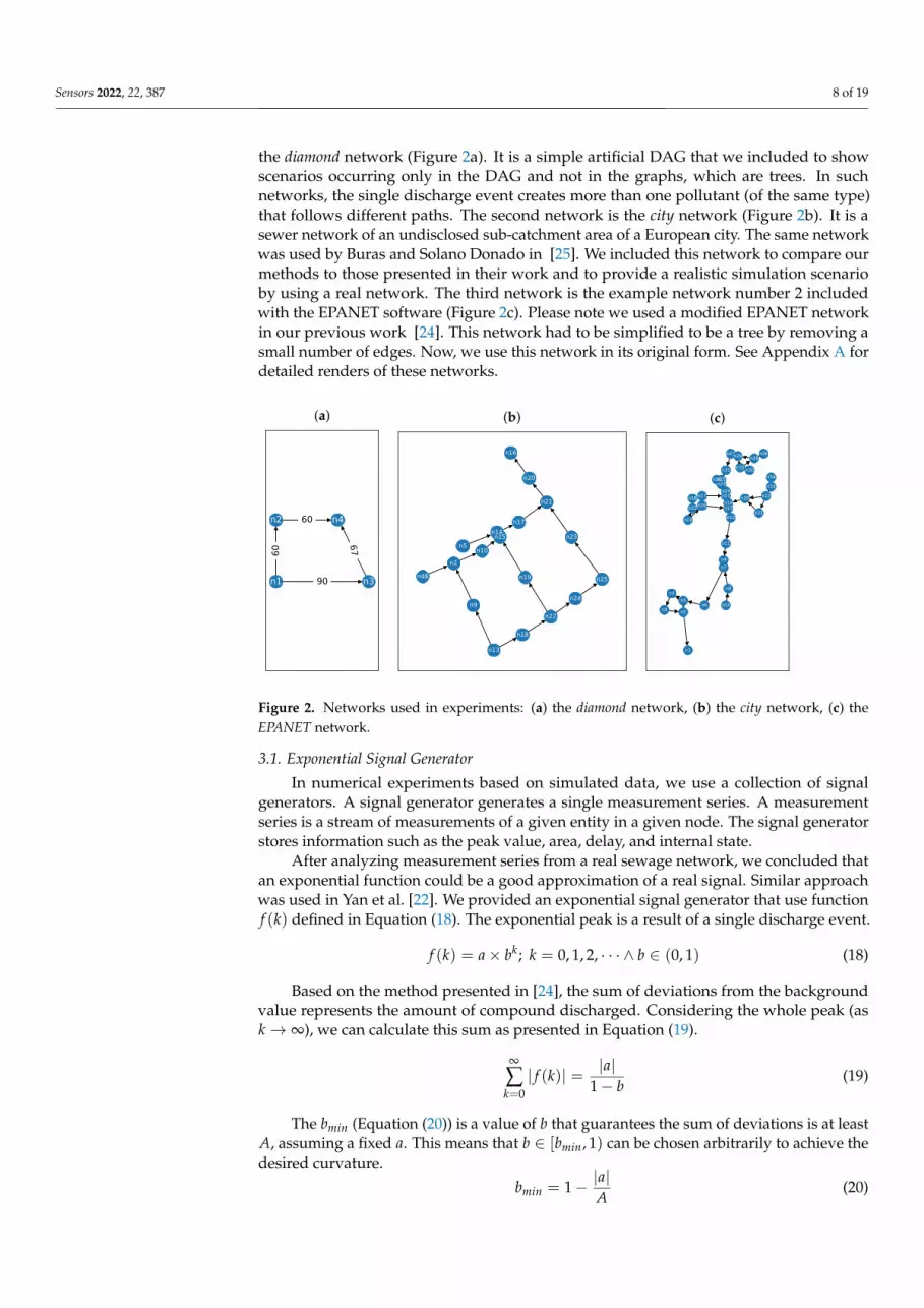
the diamond network (Figure 2a). It is a simple artificial DAG that we included to showscenarios occurring only in the DAG and not in the graphs, which are trees. In suchnetworks, the single discharge event creates more than one pollutant (of the same type)that follows different paths. The second network is the city network (Figure 2b). It is asewer network of an undisclosed sub-catchment area of a European city. The same networkwas used by Buras and Solano Donado in [25]. We included this network to compare ourmethods to those presented in their work and to provide a realistic simulation scenarioby using a real network. The third network is the example network number 2 includedwith the EPANET software (Figure 2c). Please note we used a modified EPANET networkin our previous work [24]. This network had to be simplified to be a tree by removing asmall number of edges. Now, we use this network in its original form. See Appendix A fordetailed renders of these networks.
(a)
60
90
60
67n1
n2
n3
n4
(b)
n48
n2
n5
n9
n10
n13
n14n15
n16
n17
n18
n19
n20
n21
n22
n23
n24
n25
(c)
n2
n1
n5
n3
n4
n6
n7
n8
n9
n10
n11
n12
n13n14
n15
n16
n17n18
n32
n19
n20
n21
n22
n23n24
n25n26
n31
n27n29 n28
n33
n34
n35 n30
n36
Figure 2. Networks used in experiments: (a) the diamond network, (b) the city network, (c) theEPANET network.
3.1. Exponential Signal Generator
In numerical experiments based on simulated data, we use a collection of signalgenerators. A signal generator generates a single measurement series. A measurementseries is a stream of measurements of a given entity in a given node. The signal generatorstores information such as the peak value, area, delay, and internal state.
After analyzing measurement series from a real sewage network, we concluded thatan exponential function could be a good approximation of a real signal. Similar approachwas used in Yan et al. [22]. We provided an exponential signal generator that use functionf (k) defined in Equation (18). The exponential peak is a result of a single discharge event.
f (k) = a× bk; k = 0, 1, 2, · · · ∧ b ∈ (0, 1) (18)
Based on the method presented in [24], the sum of deviations from the backgroundvalue represents the amount of compound discharged. Considering the whole peak (ask→ ∞), we can calculate this sum as presented in Equation (19).
∞
∑k=0| f (k)| = |a|
1− b(19)
The bmin (Equation (20)) is a value of b that guarantees the sum of deviations is at leastA, assuming a fixed a. This means that b ∈ [bmin, 1) can be chosen arbitrarily to achieve thedesired curvature.
bmin = 1− |a|A
(20)
Sensors 2022, 22, 387 9 of 19
After choosing b, the generator needs a number of samples N, after which the desiredsum A is achieved. Using Equation (21), we can calculate N as seen in Equation (22).
A =N
∑k=0| f (k)| =
|a|(bN+1 − 1
)b− 1
(21)
N = logb
[Aa(b− 1) + 1
]− 1 (22)
3.2. Success Rate
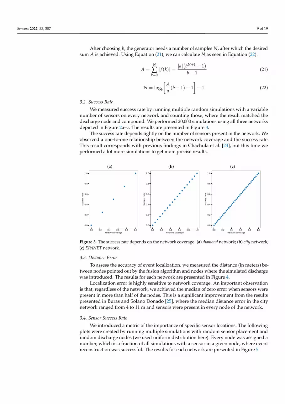
We measured success rate by running multiple random simulations with a variablenumber of sensors on every network and counting those, where the result matched thedischarge node and compound. We performed 20,000 simulations using all three networksdepicted in Figure 2a–c. The results are presented in Figure 3.
The success rate depends tightly on the number of sensors present in the network. Weobserved a one-to-one relationship between the network coverage and the success rate.This result corresponds with previous findings in Chachuła et al. [24], but this time weperformed a lot more simulations to get more precise results.
(a)
0.0 0.2 0.4 0.6 0.8 1.0Relative coverage
0.0
0.2
0.4
0.6
0.8
1.0
Succ
ess r
ate
(b)
0.0 0.2 0.4 0.6 0.8 1.0Relative coverage
0.0
0.2
0.4
0.6
0.8
1.0
Succ
ess r
ate
(c)
0.0 0.2 0.4 0.6 0.8 1.0Relative coverage
0.0
0.2
0.4
0.6
0.8
1.0
Succ
ess r
ate
Figure 3. The success rate depends on the network coverage. (a) diamond network; (b) city network;(c) EPANET network.
3.3. Distance Error
To assess the accuracy of event localization, we measured the distance (in meters) be-tween nodes pointed out by the fusion algorithm and nodes where the simulated dischargewas introduced. The results for each network are presented in Figure 4.
Localization error is highly sensitive to network coverage. An important observationis that, regardless of the network, we achieved the median of zero error when sensors werepresent in more than half of the nodes. This is a significant improvement from the resultspresented in Buras and Solano Donado [25], where the median distance error in the citynetwork ranged from 4 to 11 m and sensors were present in every node of the network.
3.4. Sensor Success Rate
We introduced a metric of the importance of specific sensor locations. The followingplots were created by running multiple simulations with random sensor placement andrandom discharge nodes (we used uniform distribution here). Every node was assigned anumber, which is a fraction of all simulations with a sensor in a given node, where eventreconstruction was successful. The results for each network are presented in Figure 5.

Sensors 2022, 22, 387 10 of 19
(a)
0.3 0.4 0.5 0.6 0.7 0.8 0.9 1.0Relative coverage
0
20
40
60
80
100
120
Abso
lute
dist
ance
erro
r [m
]
(b)
0.0 0.1 0.2 0.3 0.4 0.5 0.6 0.7 0.8 0.9 1.0Relative coverage
0
50
100
150
200
250
300
Abso
lute
dist
ance
erro
r [m
]
(c)
0.0 0.1 0.2 0.3 0.4 0.5 0.6 0.7 0.8 0.9 1.0Relative coverage
0.0
0.2
0.4
0.6
0.8
1.0
1.2
1.4
Abso
lute
dist
ance
erro
r [m
]1e4
Figure 4. Distance error depends on the network coverage. (a) diamond network; (b) city network;(c) EPANET network.
(a)
0.86
0.88
0.90
0.92
0.94
0.96
0.98
1.00
Success rate
(b)
0.93
0.94
0.95
0.96
0.97
0.98
0.99
1.00
Success rate
(c)
0.90
0.92
0.94
0.96
0.98
1.00
Success rate
Figure 5. The success rate of sensors. (a) diamond network; (b) city network; (c) EPANET network.
For the diamond network (Figure 5a) 100% success rate is achieved when a sensor ispresent in node n4 (node labels are presented in Figure 2a) because all of the wastewaterflows through this node. Sensor readings in nodes n2 and n3 are not influenced by dis-charges into node n4, as they are upstream. The consequence of this is that sensors in nodesn2 and n3 have around 90% success rate. Sensors in node n1 have lowest success rate equalto 84%. The reason for this is that sensors in this location are able to detect discharges onlyin node n1.
In other networks we can see similar trends. The final sink–nodes are able to detectall of the discharges. The further upstream, the lower the success rate, because of the factthat sensors can only observe discharges that happen upstream from them. Looking atFigure 5a,b we can see irregularities, which are caused by the greater number of nodes

Sensors 2022, 22, 387 11 of 19
requiring more random simulations to achieve smooth and clear results. An importantremark is that in these two networks, sensor importance never dropped below 88% and itsdispersion is low. This result means that in real networks, decisions about sensor placementshould rely on additional knowledge such as the probability of discharge in different nodes.
3.5. Sensor Distance Error
An additional sensor importance metric is the sensors’ share in the overall distanceerror. This was measured by computing the average non-zero distance between the actualdischarge node and the reconstructed discharge node. The average was calculated for everysensor that was present in a given simulation. The results for each network are presentedin Figure 6.
(a)
1.00
1.02
1.04
1.06
1.08
1.10
Average non-zero distance [m]
(b)
1.5
1.6
1.7
1.8
1.9
2.0
Average non-zero distance [m]
(c)
1.25
1.50
1.75
2.00
2.25
2.50
2.75
3.00
Average non-zero distance [m]
Figure 6. Sensors’ share in localization error. (a) diamond network; (b) city network; (c) EPANETnetwork.
The maps of sensor importance and distance error highlight the preferred location ofsensors. In reality, it is practical to deploy only a few sensors in the network. Extensivesimulations can hint at important locations to aid in optimal sensor placement. Oursimulations indicate that sensor placement is always a trade-off between success rate anddistance error. Sensors placed far downstream have a large chance of detecting discharges,as they are more often on the flow path of the pollutants. Sensors placed further upstreamminimize distance error with a cost of success rate.
3.6. Peak Detection
We ran the peak detection on a variety of measurement series. We tested the module’soperation on both real data (Figure 7) and simulated data (Figures 8–10). Real measure-ments were taken by Micromole sensors [1], and simulated measurements were generatedby the aforementioned exponential signal generator.
0 2000 4000 6000 8000 10000 12000Time
1.0
10.0
Mea
sure
men
t val
ue
1e3measurementup peakdown peak
Figure 7. The output of the peak detection algorithm for real measurements taken by Micromole sensors.

Sensors 2022, 22, 387 12 of 19
In Figure 8, we can see that the algorithm correctly classifies imperfect peaks withemerging outliers. Moreover, the module can cope with different peak heights (Figure 10a)and when both types of peaks are present in a single series of measurements, as is presentedin Figure 10b.
0 20 40 60 80 100 120Time
7.50
7.75
8.00
8.25
8.50
8.75
9.00
9.25
9.50M
easu
rem
ent v
alue
1e3measurementup peakdown peak
Figure 8. The resistance of the peak detector to the occurrence of outliers.
0 20 40 60 80 100 120 140 160Time
1
2
3
4
5
6
7
8
9
Mea
sure
men
t val
ue
1e3measurementup peakdown peak
Figure 9. Correctness of peak detection for a measurement series with large variance.
0 20 40 60 80 100 120Time
7.50
7.75
8.00
8.25
8.50
8.75
9.00
9.25
9.50
Mea
sure
men
t val
ue
1e3measurementup peakdown peak
(a)
0 100 200 300 400 500 600Time
0.0
0.5
1.0
1.5
2.0
2.5
Mea
sure
men
t val
ue
1e3measurementup peakdown peak
(b)
Figure 10. Detection of different types of peaks. (a) Different heights of up peaks; (b) Both up peaksand down peaks.
The peak detection module adapts to the characteristics of the measurements. Thesensitivity of the peak detection is lower when the variance of the measurements is greater.Moreover, we observed that the peak detector could not cope with outliers when they arein the initial phase of a peak. In this case, a single peak is treated as two separate peaks.

Sensors 2022, 22, 387 13 of 19
We developed the presented algorithm to work online and analyze current data fromsensors. The algorithm represents the state of the sewage network for a given time pointand produces the most probable events. Such assumption eliminates the possibility ofanalyzing the time series from sensors offline (using historical data) and then finding theevents using optimization algorithms, e.g., by simulating many times the network statesand comparing the simulation results with measured values ([22]).
3.7. Attenuation in Quantification
To assess how errors in attenuation data influence the pollutant amount error, weran multiple random simulations with Gaussian disturbance to the attenuation attribute.Figure 11 depicts this relationship. We can observe that the greater the disturbance,the greater the error, which is expected. Looking at the scale of the error, we concluded thatthe accuracy of target amounts is very sensitive to errors in attenuation. However, the ap-proximation of detected amounts is rough in the first place, as the behavior of compoundsin wastewater is hard to model. For the purposes of this study, achieving quantificationerror within an order of magnitude is considered a success.
0.0 0.1 0.2 0.3 0.4 0.5 0.6 0.7 0.8 0.9 1.0Standard deviation of attenuation disturbance
0.5
0.0
0.5
1.0
1.5
2.0
2.5
Rela
tive
amou
nt e
rror
Figure 11. Amount error versus attenuation disturbance.
3.8. Multipath Tracking
The characteristics of directed acyclic graphs can cause an apparent doubling of eventsin certain cases. If the diamond network (Figure 2a) is considered, there are two paths ofdifferent lengths between nodes n1 and n4. The first path: n1→ n2→ n4, has length equalto 120 and the second path: n1→ n3→ n4 has length equal to 157. This means that if adischarge event happens in n1 at time k, then five peaks will be observed in the network: inn1 at t, in n2 at t + 60, in n3 at t + 90, in n4 at t + 120 and in n4 at t + 157. An example ofthis behavior can be seen in Figure 12.
25 50 75 100 125 150 175Time [s]
0
20
40
60
80
100
120
140
160
Posit
ion
[s]
track positionobservations
Figure 12. Doubling of signals. The target flows through two different paths of different lengths, thusproducing five peaks in a 4-node network.

Sensors 2022, 22, 387 14 of 19
This event doubling can make tracking difficult if two events happen in succession.In such cases, choosing a correct clustering threshold is crucial. See Figure 13, where athreshold of 20 s was used.
25 50 75 100 125 150 175 200Time [s]
0
25
50
75
100
125
150
175
200
Posit
ion
[s]
track position 1track position 2observations
Figure 13. Two discharge events are correctly separated by the data fusion algorithm.
In our opinion, working online and generating the most probable set of events usingavailable information main advantage is allowing to react and alarm as soon as possible.However, there is a risk of false alarms. Moreover, the set of events can change when newinformation is available.
In the literature, the flow in sewage and water network is modeled by Poisson distri-bution [22]. Such distribution is achieved when we assume the single household uses thenetwork as a rectangular pulse process with random time and intensity. In the real dataavailable for as this is true, we also observe Poisson distribution in our systems; however,in our algorithm, we decide not to model the flow in the network. We just use measureddata from sensors and we assume that the flow is provided by the sensors on an ongoingbasis and is constant within the calculation cycle. This assumption simplifies the model.We consider this assumption as valid because the measuring cycle is short.
3.9. Resource Usage
The performance and resource usage were evaluated by running a simulation witha variable number of significant measurements and a constant number of tracks. Theseexperiments show how quickly and efficiently the algorithm processes measurements.Tests were run on a fourth-generation Intel Core processor. In Figure 14a, we can see that,on average, the system can process around 5000 significant measurements per second witha constant component of 1 s. We also measured the maximum resident memory of theprocess (Figure 14b), which stabilizes at around 1 MiB per 4600 significant measurementsplus a constant of 97 MiB.
0 2000 4000 6000 8000 10000 12000 14000 16000Number of detections
1
2
3
4
CPU
time
[s]
0 2000 4000 6000 8000 10000 12000 14000 16000Number of detections
96
97
98
99
100
101
Mem
ory
[MiB
]
Figure 14. CPU time and memory usage depend on detection count.

Sensors 2022, 22, 387 15 of 19
We also repeated these experiments with a constant number of significant measure-ments and a variable number of tracks. In Figure 15, we presented the results. The relation-ship between the number of tracks and CPU time is linear. In this scenario, the CPU timerequired for processing additional 20 tracks is approximately 5 s. Memory requirementsfor additional tracks are approximately 1.3 MiB per 100 tracks.
0 20 40 60 80 100Number of tracks
0
5
10
15
20
25
CPU
time
[s]
0 20 40 60 80 100Number of tracks
94.6
94.8
95.0
95.2
95.4
95.6
95.8
96.0
Mem
ory
[MiB
]
Figure 15. CPU time and memory usage depend on track count.
Resource usage was significantly improved compared to the previous iteration of thealgorithm in Chachuła et al. [24]. Adjusting implementation details caused the system to beable to process measurements 50 times faster. The memory requirements were previouslynot measured directly, but we consider the result of 1 MiB per 4600 significant measure-ments a success for a proof-of-concept system. The constant 97 MiB overhead is notable butpractical compared to the memory available in modern systems. We calculated and thenobserved that the time and memory complexity of the proposed data fusion algorithm islinear with respect to the number of detections and tracks. However, memory complexitywith respect to the number of tracks is problematic to observe, as each track introduces avery small memory overhead. At this scale, processes such as garbage collection play asignificant role.
4. Discussion
Resampling introduces sampling error if measurements are not periodic or the periodis different from the sampling period. We developed our algorithm to detect pollution inthe sewage network, and according to domain experts, we should process the changesof measured values every minute. Our system calculates the sewage network state everysecond. Therefore, the resampling error is negligible. We assume that the period will besmall enough to introduce a minimal error in real scenarios. Moreover, we used simulateddata, and we assumed that the generated measurements are periodic, and the period isequal to the sampling period.
All data included in the measurement domain are provided by sensors. We do notuse uncertainty in the current version of the algorithm. However, such information can beused in future work to calculate the detection confidence coefficient that we already use inthe event generation step of the algorithm.
In our approach, we do not model pollutant spreading. We require a short list of allpossible pollutants. In the quantification process, each pollutant is considered for everymeasurement. Finally, the best pollutant is reported. In recent years, especially for airpollutants, hierarchical methods that model spatio-temporal processes and measurementnoise were popular [34,35]. We plan to apply such models in the future to make our resultsmore accurate.
The success rate and distance error of specific sensors indicate that there is a trade-offbetween those two metrics when considering sensor placement. However, the correctness ofthe results still strongly depends on how many sensors are present in the network and theirplacement. Another limitation of the proposed solution is the reliance on high-quality data.

Sensors 2022, 22, 387 16 of 19
Simulated measurements are the best-case scenario. Data from real sensors are of varyingquality because of the sensor technology and the characteristics of the wastewater networks.
Further research should focus on evaluating the data fusion algorithm in real-worldscenarios, which means running fusion using data from real sensors in live wastewaternetworks. This will require defining a procedure for choosing the best values of the param-eters of the algorithm. Parallel processing techniques could be applied to the proposedsolution in case current performance is not enough in large networks with many sensors.Investigation of the influence of sensor placement and discharge amount on the uncertaintyof reconstructed events could improve the calculation of event confidence coefficients.Similarly, the uncertainty of measurements, as reported by sensors, could be consideredwhen calculating these coefficients.
5. Conclusions
The proposed improvements to the data fusion algorithm significantly broadened itsapplicability. The new, adaptive peak detection algorithm can adapt to changing back-ground values as presented in Section 3.6. It is a milestone for testing this system inreal-world networks. Implementing tracking in DAGs poses a significant improvementfrom previous achievements as real-world networks no longer have to be modified toperform fusion in as shown in Section 3.8. Results in Section 3.7 suggest that accountingfor flow rate by introducing the attenuation coefficient helps when detected pollutantamounts are consistently low because of a high flow rate. Unlike the previous iteration,these improvements make the proposed multisensor data fusion algorithm applicable inreal-world scenarios.
Moreover, the development mentioned above did not negatively influence the cor-rectness of the results. This was verified by measuring success rate the same way as inour previous study, using the same network, this time unmodified, in Section 3.2. Weperformed more simulations to clearly show the linear relationship between the number ofsensors and the success rate. In order to evaluate the algorithm in more depth, additionalmetrics were calculated.
The applicability was not the only aspect of the algorithm that was improved. Simpli-fying the implementation caused it to be able to process measurements 50 times faster thanthe previous one as presented in Section 3.9. The measured processing speed and memoryrequirements show that such a system could run on a regular computer and monitor thenetwork in real-time.
Author Contributions: All authors developed the concept and methodology, prepared manuscriptand agreed to the published version. K.C. and T.M.S. developed software and performed numericalexperiments, R.N. supervised their work and provided resources. All authors have read and agreedto the published version of the manuscript.
Funding: This research was funded by Priority Research Area Cyber&DS Research Center at WarsawUniversity of Technology under contract number 1820/18/2021 and the H2020 SYSTEM [2] project,which has received funding from the European Union’s Horizon 2020 research and innovationprogramme under Grant Agreement No. 787128 and Institute of Computer Science Warsaw Universityof Technology statutory research grant.
Institutional Review Board Statement: Not applicable.
Informed Consent Statement: Not applicable.
Data Availability Statement: Restrictions apply to the availability of these data. Data were obtainedfrom Steffen Krause and Christoph Wöllgens of the Universität der Bundeswehr München and areavailable from the authors with the permission of Universität der Bundeswehr München.
Acknowledgments: The manuscript was improved by the anonymous reviewers. We would alsolike to thank Norbert Niderla, Fernando Solano and other colleagues from SYSTEM for their valu-able comments.

Sensors 2022, 22, 387 17 of 19
Conflicts of Interest: The authors declare no conflict of interest. The funders had no role in the designof the study; in the collection, analyses, or interpretation of data; in the writing of the manuscript, orin the decision to publish the results.
Appendix A. Detailed Renders of Networks Used in Experiments
43
39
4759
29
42
63
31
7
44
43
61
40
38
39
60
55
42
66
n48
n2
n5
n9
n10
n13
n14n15
n16
n17
n18
n19
n20
n21
n22
n23
n24
n25
Figure A1. Detailed render of the city network.
2400800
1000
1300
1200 1200
2700
1200400
1000
700
1900
600400
300
1500
1500
600
700
350
1400
500
1100
1300 1300
1300
600
250
300
200
600
400
400700
1000
400
500 700
1000
300
n2
n1
n5
n3
n4
n6
n7
n8
n9
n10
n11
n12
n13
n14
n15
n16
n17n18
n32
n19
n20
n21
n22
n23
n24
n25n26
n31
n27n29
n28
n33
n34
n35n30
n36
Figure A2. Detailed render of the EPANET network.

Sensors 2022, 22, 387 18 of 19
References1. Micromole. Micromole—Sewage Monitoring System for Tracking Synthetic Drug Laboratories. Available online: http:
//www.micromole.eu (accessed on 17 October 2019).2. SYSTEM. H2020 SYSTEM—SYnergy of Integrated Sensors and Technologies for Urban Secured Environment. Fact Sheet
Available at EC Website. Under Project ID 787128. Available online: https://cordis.europa.eu/project/rcn/220304/factsheet/en(accessed on 12 October 2021).
3. De Vito, S.; Fattoruso, G.; Esposito, E.; Salvato, M.; Agresta, A.; Panico, M.; Leopardi, A.; Formisano, F.; Buonanno, A.; Veneri,P.D.; et al. A distributed sensor network for waste water management plant protection. In Convegno Nazionale Sensori; Springer:Cham, Switzerland, 2016; pp. 303–314.
4. Lepot, M.; Makris, K.F.; Clemens, F.H. Detection and quantification of lateral, illicit connections and infiltration in sewers withInfra-Red camera: Conclusions after a wide experimental plan. Water Res. 2017, 122, 678–691. [CrossRef]
5. Tan, F.H.S.; Park, J.R.; Jung, K.; Lee, J.S.; Kang, D.K. Cascade of one class classifiers for water level anomaly detection. Electronics2020, 9, 1012. [CrossRef]
6. Tashman, Z.; Gorder, C.; Parthasarathy, S.; Nasr-Azadani, M.M.; Webre, R. Anomaly detection system for water networks innorthern ethiopia using bayesian inference. Sustainability 2020, 12, 2897. [CrossRef]
7. Zhang, D.; Heery, B.; O’Neil, M.; Little, S.; O’Connor, N.E.; Regan, F. A low-cost smart sensor network for catchment monitoring.Sensors 2019, 19, 2278. [CrossRef] [PubMed]
8. Perfido, D.; Messervey, T.; Zanotti, C.; Raciti, M.; Costa, A. Automated leak detection system for the improvement of waternetwork management. In Proceedings of the Multidisciplinary Digital Publishing Institute Proceedings, Online, 15–30 November2016; Volume 1, p. 28.
9. Rojek, I.; Studzinski, J. Detection and localization of water leaks in water nets supported by an ICT system with artificialintelligence methods as a way forward for smart cities. Sustainability 2019, 11, 518. [CrossRef]
10. Ji, H.W.; Yoo, S.S.; Lee, B.J.; Koo, D.D.; Kang, J.H. Measurement of wastewater discharge in sewer pipes using image analysis.Water 2020, 12, 1771. [CrossRef]
11. Kuchmenko, T.A.; Lvova, L.B. A perspective on recent advances in piezoelectric chemical sensors for environmental monitoringand foodstuffs analysis. Chemosensors 2019, 7, 39. [CrossRef]
12. Pisa, I.; Santín, I.; Vicario, J.L.; Morell, A.; Vilanova, R. ANN-based soft sensor to predict effluent violations in wastewatertreatment plants. Sensors 2019, 19, 1280. [CrossRef] [PubMed]
13. Emke, E.; Vughs, D.; Kolkman, A.; de Voogt, P. Wastewater-based epidemiology generated forensic information: Amphetaminesynthesis waste and its impact on a small sewage treatment plant. Forensic Sci. Int. 2018, 286, e1–e7. [CrossRef]
14. Ma, J.; Meng, F.; Zhou, Y.; Wang, Y.; Shi, P. Distributed water pollution source localization with mobile UV-visible spectrometerprobes in wireless sensor networks. Sensors 2018, 18, 606. [CrossRef]
15. Desmet, C.; Degiuli, A.; Ferrari, C.; Romolo, F.S.; Blum, L.; Marquette, C. Electrochemical sensor for explosives precursors’detection in water. Challenges 2017, 8, 10. [CrossRef]
16. Kumar, P.M.; Hong, C.S. Internet of things for secure surveillance for sewage wastewater treatment systems. Environ. Res. 2022,203, 111899. [CrossRef]
17. Hammond, P.; Suttie, M.; Lewis, V.T.; Smith, A.P.; Singer, A.C. Detection of untreated sewage discharges to watercourses usingmachine learning. NPJ Clean Water 2021, 4, 1–10. [CrossRef]
18. Aguiar-Oliveira, M.d.L.; Campos, A.; R Matos, A.; Rigotto, C.; Sotero-Martins, A.; Teixeira, P.F.; Siqueira, M.M. Wastewater-BasedEpidemiology (WBE) and Viral Detection in Polluted Surface Water: A Valuable Tool for COVID-19 Surveillance—A Brief Review.Int. J. Environ. Res. Public Health 2020, 17, 9251. [CrossRef] [PubMed]
19. Nine Days, Ten Finds of Drug Waste. Available online: https://vaaju.com/netherlandseng/nine-days-ten-finds-of-drug-waste/(accessed on 6 October 2021).
20. Treatment Plant almost Failed after Illegal Waste Discharge. Available online: https://www.rnz.co.nz/news/regional/222633/treatment-plant-almost-failed-after-illegal-waste-discharge (accessed on 12 October 2021).
21. Department of Social Communication Panstwowe Gospodarstwo Wodne Wody Polskie. Failure in the ‘Czajka’ Sewage TreatmentPlant. Available online: https://www.apgw.gov.pl/en/news/show/96 (accessed on 5 November 2021).
22. Yan, X.; Gong, J.; Wu, Q. Pollution source intelligent location algorithm in water quality sensor networks. Neural Comput. Appl.2021, 33. [CrossRef]
23. Saucedo-Dorantes, J.J.; Arellano-Espitia, F.; Delgado-Prieto, M.; Osornio-Rios, R.A. Diagnosis Methodology Based on DeepFeature Learning for Fault Identification in Metallic, Hybrid and Ceramic Bearings. Sensors 2021, 21, 5832. [CrossRef] [PubMed]
24. Chachuła, K.; Nowak, R.; Solano, F. Pollution Source Localization in Wastewater Networks. Sensors 2021, 21, 826. [CrossRef][PubMed]
25. Buras, M.P.; Solano Donado, F. Identifying and Estimating the Location of Sources of Industrial Pollution in the Sewage Network.Sensors 2021, 21, 3426. [CrossRef]
26. Sidhu, J.; Ahmed, W.; Gernjak, W.; Aryal, R.; McCarthy, D.; Palmer, A.; Kolotelo, P.; Toze, S. Sewage pollution in urban stormwaterrunoff as evident from the widespread presence of multiple microbial and chemical source tracking markers. Sci. Total Environ.2013, 463, 488–496. [CrossRef]

Sensors 2022, 22, 387 19 of 19
27. Yang, Z.; Castrignanò, E.; Estrela, P.; Frost, C.G.; Kasprzyk-Hordern, B. Community sewage sensors towards evaluation of druguse trends: Detection of cocaine in wastewater with DNA-directed immobilization aptamer sensors. Sci. Rep. 2016, 6, 21024.[CrossRef]
28. Varon, D.; McKeever, J.; Jervis, D.; Maasakkers, J.; Pandey, S.; Houweling, S.; Aben, I.; Scarpelli, T.; Jacob, D. Satellite discovery ofanomalously large methane point sources from oil/gas production. Geophys. Res. Lett. 2019, 46, 13507–13516. [CrossRef]
29. Macas, M.; Wu, C. An unsupervised framework for anomaly detection in a water treatment system. In Proceedings of the 201918th IEEE International Conference On Machine Learning And Applications (ICMLA), Boca Raton, FL, USA, 16–19 December2019; pp. 1298–1305.
30. Montalvo-Cedillo, C.; Jerves-Cobo, R.; Domínguez-Granda, L. Determination of pollution loads in spillways of the combinedsewage network of the city of Cuenca, Ecuador. Water 2020, 12, 2540. [CrossRef]
31. Jalal, D.; Ezzedine, T. Decision Tree and Support Vector Machine for Anomaly Detection in Water Distribution Networks. InProceedings of the 2020 International Wireless Communications and Mobile Computing (IWCMC), Limassol, Cyprus, 15–19 June2020; pp. 1320–1323.
32. Palshikar, G.K. Simple Algorithms for Peak Detection in Time-Series. In Proceedings of the 1st IIMA International Conference onAdvanced Data Analysis, Business Analytics and Intelligence, Ahmedabad, India, 6–7 June 2009.
33. Welford, B.P. Note on a Method for Calculating Corrected Sums of Squares and Products. In Technometrics; American StatisticalAssociation and American Society for Quality: Cheshire, UK, 1962; pp. 419–420.
34. Blangiardo, M.; Pirani, M.; Kanapka, L.; Hansell, A.; Fuller, G. A hierarchical modelling approach to assess multi pollutant effectsin time-series studies. PLoS ONE 2019, 14, e0212565. [CrossRef] [PubMed]
35. Li, L.; Wu, J.; Ghosh, J.K.; Ritz, B. Estimating spatiotemporal variability of ambient air pollutant concentrations with a hierarchicalmodel. Atmos. Environ. 2013, 71, 54–63. [CrossRef] [PubMed]


