Embed Size (px)
Citation preview
HAL Id: hal-01770948https://hal.archives-ouvertes.fr/hal-01770948
Submitted on 17 Feb 2022
HAL is a multi-disciplinary open accessarchive for the deposit and dissemination of sci-entific research documents, whether they are pub-lished or not. The documents may come fromteaching and research institutions in France orabroad, or from public or private research centers.
L’archive ouverte pluridisciplinaire HAL, estdestinée au dépôt et à la diffusion de documentsscientifiques de niveau recherche, publiés ou non,émanant des établissements d’enseignement et derecherche français ou étrangers, des laboratoirespublics ou privés.
Robust multisensor time-frequency signal processing: Atutorial review with illustrations of performance
enhancement in selected application areasBoualem Boashash, Abdeldjalil Aissa El Bey
To cite this version:Boualem Boashash, Abdeldjalil Aissa El Bey. Robust multisensor time-frequency signal processing:A tutorial review with illustrations of performance enhancement in selected application areas. DigitalSignal Processing, Elsevier, 2018, 77, pp.153-186. 10.1016/j.dsp.2017.11.017. hal-01770948
Multisensor Time-Frequency Signal Processing:A tutorial review with illustrations in selected
application areas
Boualem Boashasha,∗, Abdeldjalil Aıssa-El-Beya,b
aQatar University, Department of Electrical Engineering, Doha, QatarbIMT Atlantique, UMR CNRS 6285 Lab-STIC, Universite Bretagne Loire, Brest, France
Abstract
This tutorial review presents high-resolution multisensor time-frequency distri-
butions (MTFDs) and their application to the analysis of multichannel non-
stationary signals. The approach involves combining time-frequency analysis
and array signal processing methods. To demonstrate the benefits of MTFDs,
this study considers several applications including source localization based on
direction of arrival (DOA) estimation and automated component separation
(ACS) of non-stationary sources, with particular attention on blind source sep-
aration which is a particular case of ACS. The MTFD approach is further il-
lustrated by a new application to EEG signals that specifically uses ACS and
DOA estimation methods for artifacts removal and source localization. Supple-
mentary material with code is provided to allow readers to reproduce all the
results and apply these methods to their own data.
Keywords: Quadratic TFDs, High-resolution TFDs, Multisensor TFDs,
Direction of arrival, Blind source separation, EEG signals, Lead field matrix,
Non-stationary array processing, EEG abnormality source localization,
Time-frequency analysis
∗Corresponding author
Preprint submitted to Digital Signal Processing May 10, 2017
Contents
1 Introduction 4
1.1 Objectives and motivations . . . . . . . . . . . . . . . . . . . . . 5
1.1.1 Multichannel systems condition monitoring . . . . . . . . 5
1.1.2 Motivation and organization of the paper . . . . . . . . . 7
1.2 Main Objectives . . . . . . . . . . . . . . . . . . . . . . . . . . . 7
2 Extension of single sensor TFDs to multisensor TFDs 9
2.0 Background and motivation . . . . . . . . . . . . . . . . . . . . . 9
2.1 Problem statement . . . . . . . . . . . . . . . . . . . . . . . . . . 10
2.1.1 Formulation . . . . . . . . . . . . . . . . . . . . . . . . . . 10
2.1.2 Multisensor Time-Frequency Distributions MTFDs . . . . 12
2.1.3 Two types of cross-terms in MTFDs . . . . . . . . . . . . 12
2.2 Mixing models in array processing . . . . . . . . . . . . . . . . . 13
2.2.1 Instantaneous mixing model . . . . . . . . . . . . . . . . . 14
2.2.2 Convolutive mixing model . . . . . . . . . . . . . . . . . . 16
2.3 Non-stationary case array signal model . . . . . . . . . . . . . . . 17
2.3.1 Defining multisensor TFDs . . . . . . . . . . . . . . . . . 17
2.3.2 High resolution MTFDs . . . . . . . . . . . . . . . . . . . 19
2.3.3 Advantages of MTFDs over the Covariance matrix approach 22
2.3.4 Four key properties of MTFDs . . . . . . . . . . . . . . . 22
2.3.5 Cross-term issues in MTFD . . . . . . . . . . . . . . . . . 25
2.3.6 Examples . . . . . . . . . . . . . . . . . . . . . . . . . . . 26
3 Blind source separation (BSS) 26
3.0 Background and motivation . . . . . . . . . . . . . . . . . . . . . 26
3.1 BSS of instantaneous mixtures based on MTFDs . . . . . . . . . 30
3.1.1 Data whitening preprocessing . . . . . . . . . . . . . . . . 31
3.1.2 Source separation by joint diagonalization (JD) . . . . . . 31
3.1.3 Source separation by joint off-diagonalization (JOD) . . . 33
3.1.4 Experiment: Separation of Instantaneous Mixtures . . . . 35
2
3.2 BSS of convolutive mixtures based on MTFDs . . . . . . . . . . 35
3.2.1 Signal Model in the convolutive mixture case . . . . . . . 35
3.2.2 BSS using MTFD matrices for convolutive mixtures . . . 38
3.2.3 Experiment: Separation of Convolutive Mixtures . . . . . 40
3.3 Under-determined blind source separation (UBSS) . . . . . . . . 41
3.3.1 Data model and assumptions . . . . . . . . . . . . . . . . 42
3.3.2 UBSS using Vector Clustering . . . . . . . . . . . . . . . . 44
3.3.3 UBSS for non-disjoint sources in the (t, f) domain . . . . 49
3.3.4 Experiment: Underdetermined blind source separation . . 51
3.4 Discussion . . . . . . . . . . . . . . . . . . . . . . . . . . . . . . . 51
3.4.1 Auto-term selection . . . . . . . . . . . . . . . . . . . . . 52
3.4.2 Number of sources for UBSS clustering step . . . . . . . . 52
3.4.3 Number of overlapping sources . . . . . . . . . . . . . . . 53
3.4.4 Separation quality versus number of sources . . . . . . . . 54
3.4.5 Overdetermined case . . . . . . . . . . . . . . . . . . . . . 55
3.4.6 Improved BSS using high-resolution MTFDs . . . . . . . 55
4 Direction of arrival estimation using MTFDs 56
4.0 Background and motivation . . . . . . . . . . . . . . . . . . . . . 56
4.1 Time domain DOAs estimation . . . . . . . . . . . . . . . . . . . 58
4.1.1 Time Domain MUSIC Algorithm . . . . . . . . . . . . . . 59
4.1.2 Time Domain ESPRIT Algorithm . . . . . . . . . . . . . 60
4.2 Time-frequency DOAs estimation . . . . . . . . . . . . . . . . . . 61
4.2.1 Time-Frequency MUSIC Algorithm . . . . . . . . . . . . . 61
4.2.2 Time-Frequency ESPRIT Algorithm . . . . . . . . . . . . 62
4.3 Examples . . . . . . . . . . . . . . . . . . . . . . . . . . . . . . . 63
4.4 Underdetermined DOAs estimation using MTFDs . . . . . . . . 64
4.5 Discussion . . . . . . . . . . . . . . . . . . . . . . . . . . . . . . . 66
4.5.1 Signal subspace dimension . . . . . . . . . . . . . . . . . . 66
4.5.2 Spatial resolution . . . . . . . . . . . . . . . . . . . . . . . 67
4.5.3 Improved DOA estimation using high-resolution MTFDs . 69
3
5 Cross Channel Causality Analysis 70
5.0 Background and motivation . . . . . . . . . . . . . . . . . . . . . 70
5.1 Cross-channel causality and phase synchrony . . . . . . . . . . . 71
5.1.1 Phase synchrony estimation using a complex TFD . . . . 73
5.1.2 Phase synchrony estimation using MTFDs . . . . . . . . . 75
5.2 Illustrative examples . . . . . . . . . . . . . . . . . . . . . . . . . 76
5.2.1 Experiment 1 . . . . . . . . . . . . . . . . . . . . . . . . . 77
5.2.2 Experiment 2 . . . . . . . . . . . . . . . . . . . . . . . . . 77
6 Application: multisensor time-frequency analysis of EEG sig-
nals 83
6.1 Data model . . . . . . . . . . . . . . . . . . . . . . . . . . . . . . 84
6.1.1 Lead Field Matrix . . . . . . . . . . . . . . . . . . . . . . 84
6.1.2 Formulation . . . . . . . . . . . . . . . . . . . . . . . . . . 85
6.2 Application of BSS to EEG artifacts removal . . . . . . . . . . . 86
6.2.0 Background and motivation . . . . . . . . . . . . . . . . . 86
6.3 TF-MUSIC applied to source localization of brain EEG abnor-
malities . . . . . . . . . . . . . . . . . . . . . . . . . . . . . . . . 87
6.3.0 Background and motivation . . . . . . . . . . . . . . . . . 87
6.3.1 Source localization of EEG abnormality using TF-MUSIC 87
6.4 Results and discussion . . . . . . . . . . . . . . . . . . . . . . . . 88
6.4.1 Experiment: application of BSS to EEG artifacts removal 88
6.4.2 Experiment: TF-MUSIC applied to source localization of
EEG signals . . . . . . . . . . . . . . . . . . . . . . . . . . 89
7 Summary and conclusions 92
1. Introduction
Recent studies have reported significant advances in both array signal pro-
cessing for non-stationary signals and mutichannel high resolution time-frequency
signal processing [1, 2, 3, 4]. The main idea of this paper is to combine, extend
4
and report these advances in a tutorial review framework and provide corre-
sponding code to allow for reproducible research [5] and application to other
areas where multisensor/multichannel data are collected for analysis and deci-
sion making.
1.1. Objectives and motivations
1.1.1. Multichannel systems condition monitoring
In a wide range of engineering applications, a collection or array of mea-
surement sensors is used to solve the problem at hand. The type of sensors
depends on the application context. For example, antennas measuring an elec-
trical field are used in telecommunications, while sensors for measuring pressure
fluctuations are utilized in acoustic applications such as sonar, ultrasound and
speech processing. Regardless of the type of sensor used, by using more than
one sensor, one may acquire more information about the measured phenomena.
Typically, the placement of sensors in different physical locations is per-
formed to exploit any spatial diversity present in the signal being measured,
and to potentially infer spatial characteristics about the underlying process.
For example, in a radar or sonar application, one may wish to determine from
which direction an echo is returning, and thus infer the position of a target.
In speech processing, it may be desirable to extract the speech signal from
a speaker standing in a known position, while suppressing any “noise” com-
ing from other locations, in order to improve intelligibility of the speech in
hands-free communications or improve the performance of a speech recognition
program. Furthermore, signals can be collected from multisensor systems with
a large number of sensors and under several conditions such as low signal to
noise ratio [6, 7], high interference [8, 9], missing data [10] ... etc). Multichan-
nel systems (multi-sensor, sensor array) are used in many applications, such
as: biomedical signal processing [11], wireless communications [8, 9], and au-
dio/speech processing [12, 13]. In such applications, the general objective is to
extract critical discriminatory information from the multidimensional signal in
order to achieve and/or improve change detection and classification processes
5
[14]. Thus, the general approach involves several processing stages such as: ac-
quisition, transformation (time-frequency, time-scale...), information extraction
(features, denoising ...etc), clustering, detection and decision.
In many real-life problems, the spectral characteristics of the signals acquired
by the multichannel systems are varying with time. This may be a character-
istic of the originating process, such as with speech, or due to the surrounding
environment, as when the measurement system is in motion with respect to the
source of interest. On the one hand, estimation of parameters linked to the
time-varying nature of a signal can be enhanced through the use of multiple
sensors. This may be relevant, for example, if one wishes to infer the velocity
of a moving target with a radar system. On the other hand, if the time-varying
nature of the process is known, this property can be used to enhance the estima-
tion of spatial parameters related to the physical location of the signal source;
An example is the position of an observed target using radar. It is specifically
the synergical combined consideration of both the time-varying characteristics
of a measured signal and the spatial information provided by an array of mea-
surement sensors, which is the focus of this paper. A particular formal field
of signal processing was motivated by the existence of non-stationary signals,
i.e. signals with time-varying spectral characteristics; it is often called joint
time-frequency analysis.
Therefore, by combining array signal processing for non-stationary signals
and multichannel high resolution time-frequency signal processing, one can pro-
vide generic methodologies to a wide field of new applications, such as:
• Abnormalities detection in biomedical signal processing (EEG, ECG...etc)
in order to improve early detection of diseases [14, 15, 16, 17, 18, 19].
• Structural health monitoring of strategic assets such as bridges, dams, for
the early detection or prevention of faults [20, 21, 22, 23].
• Energy monitoring for industrial applications, such as electrical consump-
tion monitoring of units in a factory where the objective is to optimize
the performance (production versus electrical consumption) [24, 25].
6
1.1.2. Motivation and organization of the paper
Previous studies have found that the performance of communication systems,
radar, sonar and EEG processing systems could be enhanced by simultaneously
taking into account (1) the non-stationary characteristics of measured signals
using time-frequency distributions (TFDs) and (2) the spatial information pro-
vided by an array of measuring sensors [1]. This results in the development of
new methods born from the marriage of these two advanced specialized signal
processing fields: hence, the collective name “multisensor time-frequency sig-
nal processing”. Furthermore, newly developed high-resolution quadratic TFDs
have led to improved performance in a wide range of situation [1, 2, 14]. Hence,
this study presents a tutorial review on the use of multisensor high-resolution
TFDs in the optimal processing of multisensor data e.g. the context of solving
array processing problems such as automated component separation (ACS) and
direction of arrival estimation (DOA); one key aim being improved resolution,
when signals are non-stationary. In addition to resolution, another key aim is
the signal causality analysis across sensors/channels and/or signals which allows
us to track the time varying location of moving sources by combining spatial
and time-frequency information obtained by a multisensor array. For example,
(1) in biomedical signal processing, the cross channel causality characterizes the
propagation of a seizure location across EEG channels and therefore providing
a key information about the time-varying information flow in scalp EEG sig-
nals [26]. Combing ACS and DOA should therefore improve decision making
from scalp EEG measurements and allow more knowledge about brain activity.
(2) In wireless communication, it characterizes the varying spatial location of a
moving user (mobile) in cell by exploiting the multiantenna array of the base
station. Determining the position and velocity of mobiles in cell is an important
issue for cellular networks since the efficient resource allocation depends on it.
1.2. Main Objectives
This study aims at presenting and extending past findings in a step by step
tutorial review with focus on:
7
• Showing the mathematical and physical relationship between the founda-
tions of single variable TFDs and multichannel time-frequency distribu-
tions (MTFDs).
• Extending conventional stationary array processing techniques to the non-
stationary (time-frequency) array processing case in a step by step tutorial
presentation.
• Using advanced algorithms based on multisensor high-resolution TFDs to
enhance the capability of multisensor systems in areas such as direction
of arrival estimation or separation of non-stationary sources.
• Finally, illustrating the methods developed for multisensor TFDs on new
applications such as source localization of brain EEG abnormalities, and
propagation path of seizures on the scalp.
The rest of the paper is organized as follows: The extension of single sensor
TFDs to multisensor TFDs is discussed in Section 2. Blind source separation
methods based on MTFDs are described in Section 3. Then, Section 4 presents
a review on direction of arrival estimation algorithms using MTFDs. In Section
5, cross channel causality analysis is introduced with extension to MTFDs. An
application of mutisensor time-frequency analysis for EEG signals is provided in
Section 6. Finally, Section 7 concludes the paper. In 7, symbols frequently used
in this paper are listed in alphabetical order. The meaning in this list should
be assumed unless the symbol is otherwise defined in context.
The terminology MTFD is preferred as sensors and therefore channels pro-
vide a spatial dimension which is originally discrete, while the t and f variables
are naturally continuous. In addition, “M” in “MTFD” can refer to either
multisensors or multichannels as the former generates the latter.
8
2. Extension of single sensor TFDs to multisensor TFDs
2.0. Background and motivation
This section aims at reviewing the fundamentals of array processing from
a non-stationary perspective in order to establish the mathematical and phys-
ical foundation for multisensor TFDs. Next, the advantages of multisensor or
multichannel TFDs are discussed.
Multisensor or multichannel TFDs are also called Spatial Time Frequency
Distributions (STFDs) in other works. In this study, the terminology MTFD
is preferred as discussed in Section 1.2. These techniques can solve array pro-
cessing problems such as direction of arrival (DOA) estimation with improved
resolution, using spatial information for the (t, f) processing of multichannel
non-stationary signals.
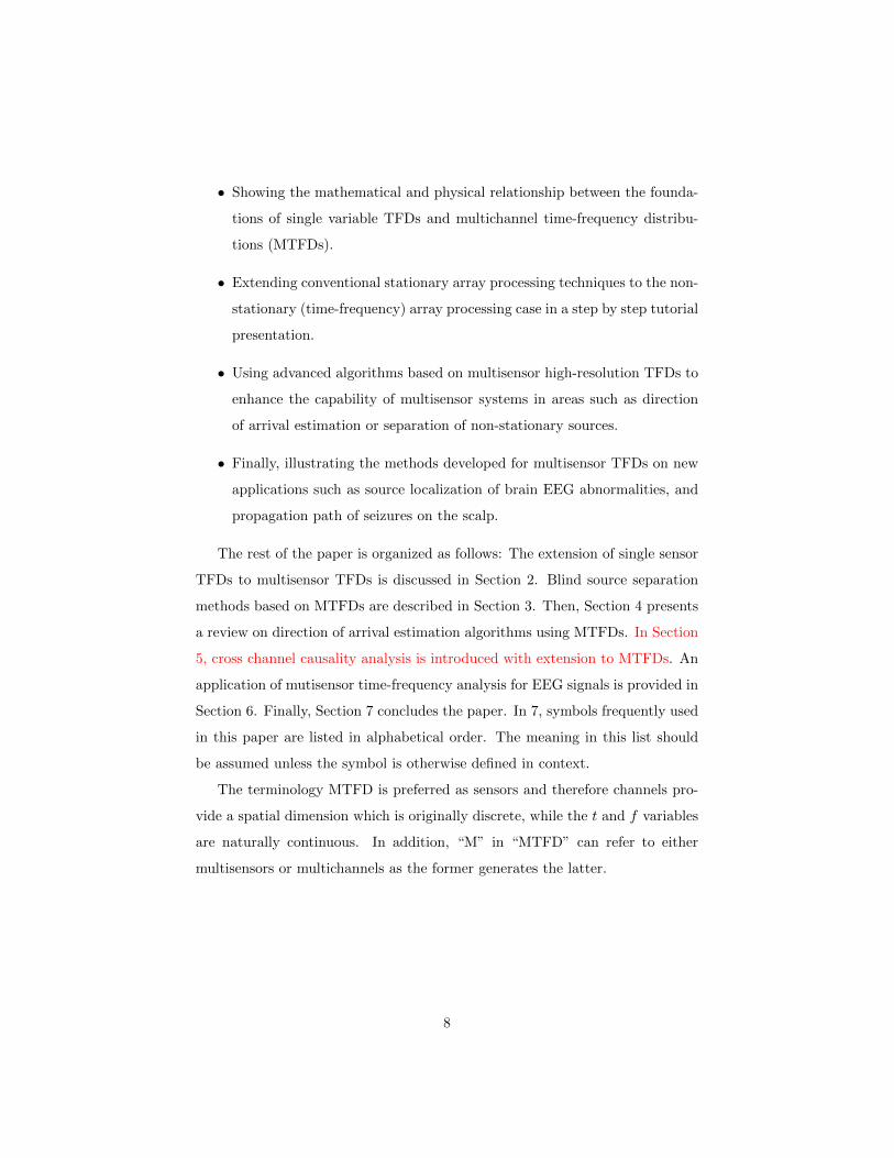
Many signal processing approaches focus on the case where non-stationary
signals are recorded by a single sensor. In fact, in some cases, only one source
produces a mono-component signal received by the sensor. However, a single
source can also generate a multicomponent signal. In other cases, a different
situation arises where several sources generate different components that merge
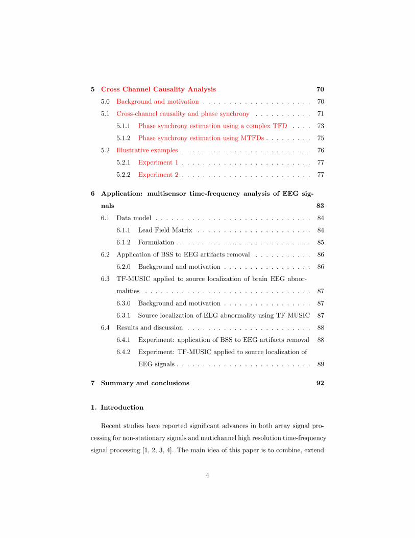
into one signal recorded by one sensor. (See Fig. 1). These two cases are known
as “Single Input and Single Output (SISO)” and “Multiple Input and Single
Output (MISO)”. The TF problem of analyzing multicomponent signals then
reduces to a problem of source separation in the case of just one sensor [27].
The traditional field of multisensor (array processing) deals effectively both with
this case “Single Input Multiple Output (SIMO)” and the more complex case of
multisource and Multi-sensor “Multiple Input and Multiple Output (MIMO)”.
This section formalized the problem statement for the extension of single sensor
TFDs to multisensor TFDs.
9
Source
Sensor
(a)
Sensor
Sources
𝑆1 𝑆2 𝑆𝑛 …
(b)
Figure 1: a) Single-Input Single-Output (SISO) b) Multiple-Input Single-Output (MISO).
2.1. Problem statement
Let us consider a non-stationary zero-mean1 real signal vector x (t) =
[x1 (t) , x2 (t) , . . . , xm (t)]T
and z(t) = [z1 (t) , z2 (t) , . . . , zm (t)]T
is the analytic
signal associated with the original real signal x (t) obtained using the Hilbert
transform such that:
zi (t) = xi (t) + jHxi (t) , i = 1, . . . ,m. (1)
where H · represents the Hilbert transform operator defined by:
Hxi (t) = F−1
f→t
(−j sgn f) F
t→f
xi (t)
. (2)
In the next section, we introduce the formulation of monochannel time-frequency
distributions and its extension to the multichannel case.
2.1.1. Formulation
In order to introduce the class of multichannel TFDs, we start this section
by presenting the foundation of TFDs in the monosensor case2. Let us consider
a non-stationary monosensor real signal x(t) and its analytic associate z(t).
1It is assumed, without loss of generality, that xi (t) has zero mean for i = 1, . . . ,m.2For greater clarity, convenience, and without loss of generality, we focus on the use of
quadratic TFDs (QTFDs) as they form a class that encompass most of the useful TFDs used
in practice, including the spectrogram and standard filterbank (also called sonogram). Note
also that the spectrogram is the square modulus of the short time Fourier transform.
10
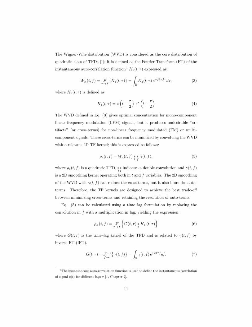
The Wigner-Ville distribution (WVD) is considered as the core distribution of
quadratic class of TFDs [1]; it is defined as the Fourier Transform (FT) of the
instantaneous auto-correlation function3 Kz(t, τ) expressed as:
Wz (t, f) = Fτ→fKz(t, τ) =
∫RKz(t, τ) e−j2πfτdτ, (3)
where Kz(t, τ) is defined as
Kz(t, τ) = z(t+
τ
2
)z∗(t− τ
2
)(4)
The WVD defined in Eq. (3) gives optimal concentration for mono-component
linear frequency modulation (LFM) signals, but it produces undesirable “ar-
tifacts” (or cross-terms) for non-linear frequency modulated (FM) or multi-
component signals. These cross-terms can be minimized by convolving the WVD
with a relevant 2D TF kernel; this is expressed as follows:
ρz(t, f) = Wz(t, f) ∗t∗fγ(t, f), (5)
where ρz(t, f) is a quadratic TFD, ∗t∗f
indicates a double convolution and γ(t, f)
is a 2D smoothing kernel operating both in t and f variables. The 2D smoothing
of the WVD with γ(t, f) can reduce the cross-terms, but it also blurs the auto-
terms. Therefore, the TF kernels are designed to achieve the best trade-off
between minimizing cross-terms and retaining the resolution of auto-terms.
Eq. (5) can be calculated using a time–lag formulation by replacing the
convolution in f with a multiplication in lag, yielding the expression:
ρz (t, f) = Fτ→f
G (t, τ) ∗
tKz (t, τ)
(6)
where G(t, τ) is the time–lag kernel of the TFD and is related to γ(t, f) by
inverse FT (IFT).
G(t, τ) = F−1
f→τ
γ(t, f)
=
∫Rγ(t, f) ej2πτfdf. (7)
3The instantaneous auto-correlation function is used to define the instantaneous correlation
of signal z(t) for different lags τ [1, Chapter 2].
11
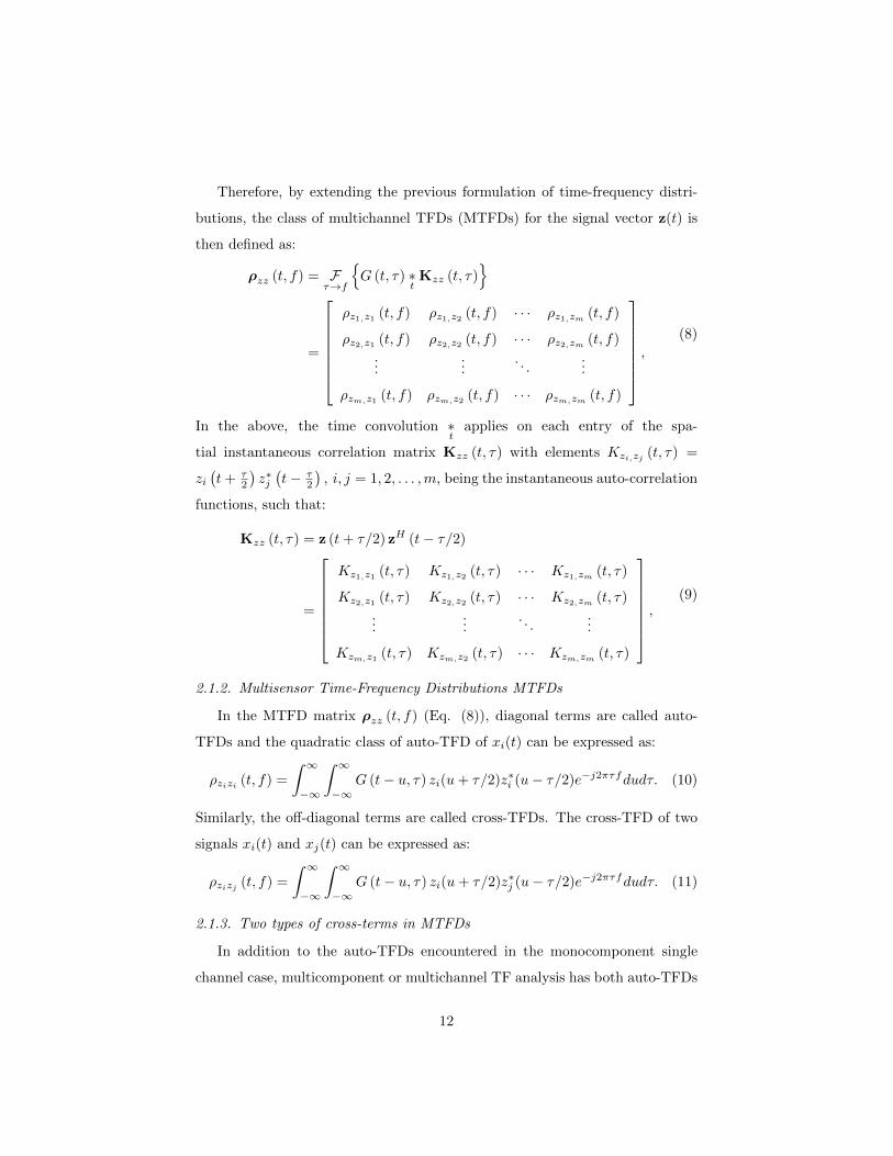
Therefore, by extending the previous formulation of time-frequency distri-
butions, the class of multichannel TFDs (MTFDs) for the signal vector z(t) is
then defined as:
ρzz (t, f) = Fτ→f
G (t, τ) ∗
tKzz (t, τ)
=
ρz1,z1 (t, f) ρz1,z2 (t, f) · · · ρz1,zm (t, f)
ρz2,z1 (t, f) ρz2,z2 (t, f) · · · ρz2,zm (t, f)...
.... . .
...
ρzm,z1 (t, f) ρzm,z2 (t, f) · · · ρzm,zm (t, f)
,(8)
In the above, the time convolution ∗t
applies on each entry of the spa-
tial instantaneous correlation matrix Kzz (t, τ) with elements Kzi,zj (t, τ) =
zi(t+ τ
2
)z∗j(t− τ
2
), i, j = 1, 2, . . . ,m, being the instantaneous auto-correlation
functions, such that:
Kzz (t, τ) = z (t+ τ/2) zH (t− τ/2)
=
Kz1,z1 (t, τ) Kz1,z2 (t, τ) · · · Kz1,zm (t, τ)
Kz2,z1 (t, τ) Kz2,z2 (t, τ) · · · Kz2,zm (t, τ)...
.... . .
...
Kzm,z1 (t, τ) Kzm,z2 (t, τ) · · · Kzm,zm (t, τ)
,(9)
2.1.2. Multisensor Time-Frequency Distributions MTFDs
In the MTFD matrix ρzz (t, f) (Eq. (8)), diagonal terms are called auto-
TFDs and the quadratic class of auto-TFD of xi(t) can be expressed as:
ρzizi (t, f) =
∫ ∞−∞
∫ ∞−∞
G (t− u, τ) zi(u+ τ/2)z∗i (u− τ/2)e−j2πτfdudτ. (10)
Similarly, the off-diagonal terms are called cross-TFDs. The cross-TFD of two
signals xi(t) and xj(t) can be expressed as:
ρzizj (t, f) =
∫ ∞−∞
∫ ∞−∞
G (t− u, τ) zi(u+ τ/2)z∗j (u− τ/2)e−j2πτfdudτ. (11)
2.1.3. Two types of cross-terms in MTFDs
In addition to the auto-TFDs encountered in the monocomponent single
channel case, multicomponent or multichannel TF analysis has both auto-TFDs
12
𝑥
𝑦
𝑧
𝝓
𝜽
Source
Sensor 1 Sensor 2
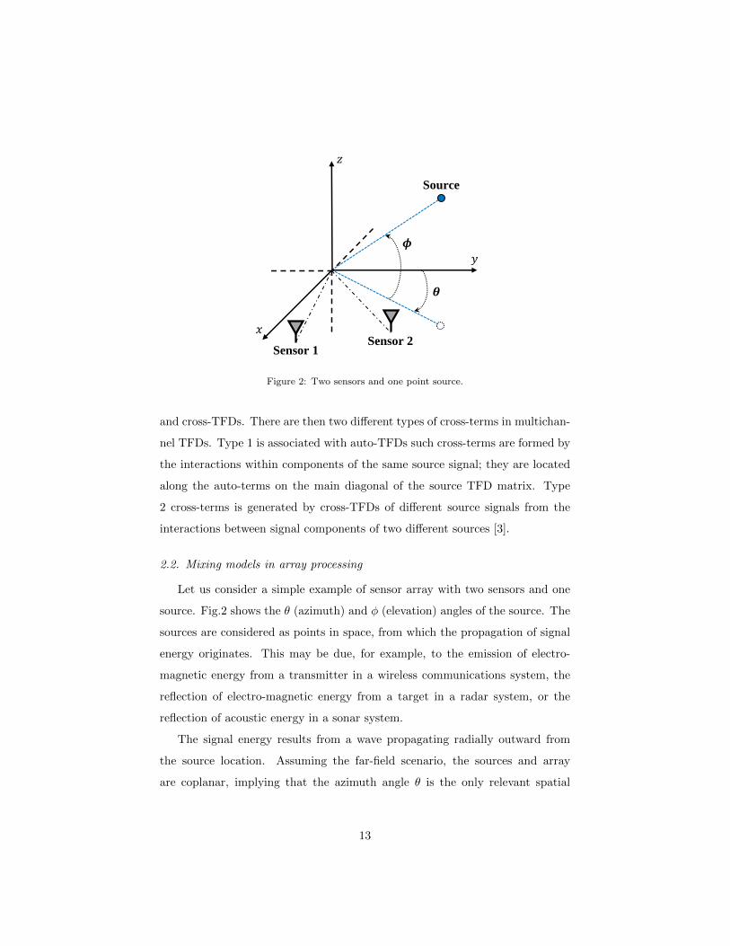
Figure 2: Two sensors and one point source.
and cross-TFDs. There are then two different types of cross-terms in multichan-
nel TFDs. Type 1 is associated with auto-TFDs such cross-terms are formed by
the interactions within components of the same source signal; they are located
along the auto-terms on the main diagonal of the source TFD matrix. Type
2 cross-terms is generated by cross-TFDs of different source signals from the
interactions between signal components of two different sources [3].
2.2. Mixing models in array processing
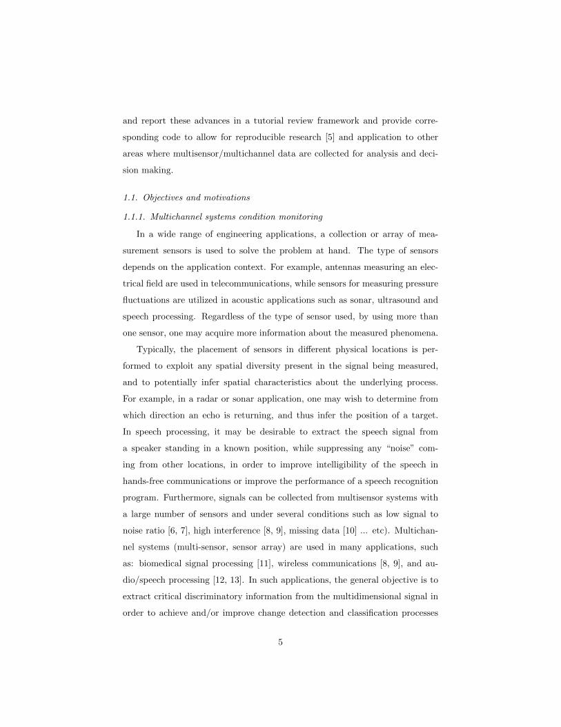
Let us consider a simple example of sensor array with two sensors and one
source. Fig.2 shows the θ (azimuth) and φ (elevation) angles of the source. The
sources are considered as points in space, from which the propagation of signal
energy originates. This may be due, for example, to the emission of electro-
magnetic energy from a transmitter in a wireless communications system, the
reflection of electro-magnetic energy from a target in a radar system, or the
reflection of acoustic energy in a sonar system.
The signal energy results from a wave propagating radially outward from
the source location. Assuming the far-field scenario, the sources and array
are coplanar, implying that the azimuth angle θ is the only relevant spatial
13
𝒅
𝜃1
. . .
Sources
𝜃2 𝜃𝑛 . . . Multi-sensor antenna
𝑥1 𝑥2 𝑥𝑚
𝑠1 𝑠2
𝑠𝑛
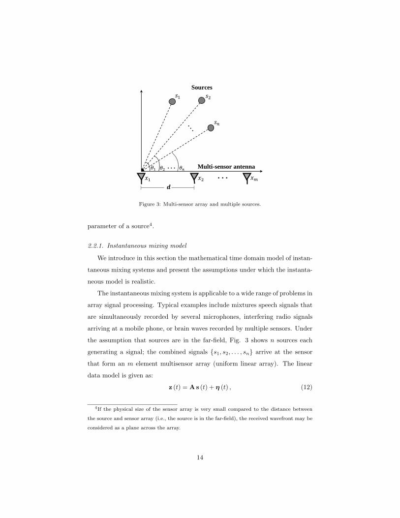
Figure 3: Multi-sensor array and multiple sources.
parameter of a source4.
2.2.1. Instantaneous mixing model
We introduce in this section the mathematical time domain model of instan-
taneous mixing systems and present the assumptions under which the instanta-
neous model is realistic.
The instantaneous mixing system is applicable to a wide range of problems in
array signal processing. Typical examples include mixtures speech signals that
are simultaneously recorded by several microphones, interfering radio signals
arriving at a mobile phone, or brain waves recorded by multiple sensors. Under
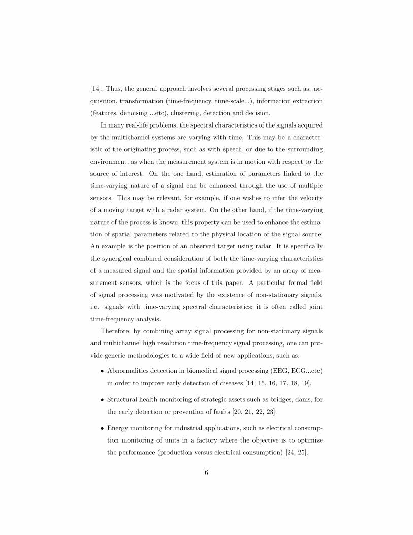
the assumption that sources are in the far-field, Fig. 3 shows n sources each
generating a signal; the combined signals s1, s2, . . . , sn arrive at the sensor
that form an m element multisensor array (uniform linear array). The linear
data model is given as:
z (t) = A s (t) + η (t) , (12)
4If the physical size of the sensor array is very small compared to the distance between
the source and sensor array (i.e., the source is in the far-field), the received wavefront may be
considered as a plane across the array.
14
𝒙𝟏
𝑺𝟏 𝑺𝟐
𝑺𝒏
𝒙𝟐
𝒙𝒎
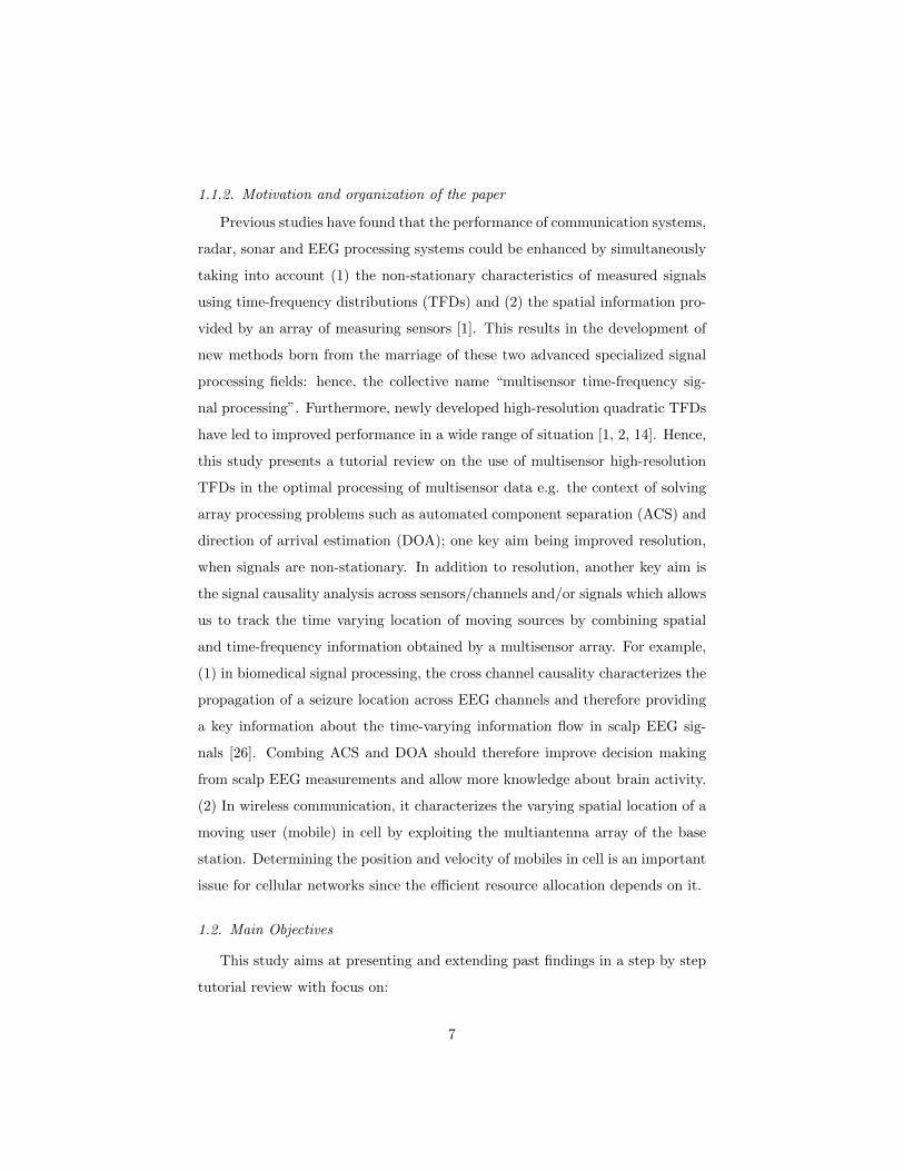
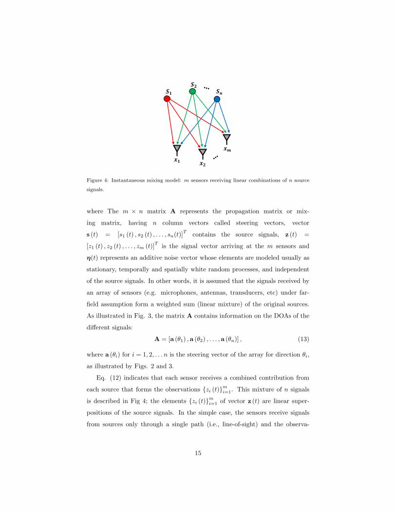
Figure 4: Instantaneous mixing model: m sensors receiving linear combinations of n source
signals.
where The m × n matrix A represents the propagation matrix or mix-
ing matrix, having n column vectors called steering vectors, vector
s (t) = [s1 (t) , s2 (t) , . . . , sn(t)]T
contains the source signals, z (t) =
[z1 (t) , z2 (t) , . . . , zm (t)]T
is the signal vector arriving at the m sensors and
η(t) represents an additive noise vector whose elements are modeled usually as
stationary, temporally and spatially white random processes, and independent
of the source signals. In other words, it is assumed that the signals received by
an array of sensors (e.g. microphones, antennas, transducers, etc) under far-
field assumption form a weighted sum (linear mixture) of the original sources.
As illustrated in Fig. 3, the matrix A contains information on the DOAs of the
different signals:
A = [a (θ1) ,a (θ2) , . . . ,a (θn)] , (13)
where a (θi) for i = 1, 2, . . . n is the steering vector of the array for direction θi,
as illustrated by Figs. 2 and 3.
Eq. (12) indicates that each sensor receives a combined contribution from
each source that forms the observations zi (t)mi=1. This mixture of n signals
is described in Fig 4; the elements zi (t)mi=1 of vector z (t) are linear super-
positions of the source signals. In the simple case, the sensors receive signals
from sources only through a single path (i.e., line-of-sight) and the observa-
15
𝒙𝟏
𝑺𝟏 𝑺𝟐
𝑺𝒏
𝒙𝟐
𝒙𝒎
Re
fle
cto
r
multi-path
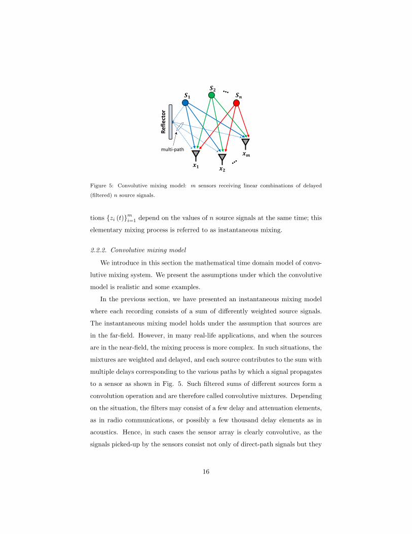
Figure 5: Convolutive mixing model: m sensors receiving linear combinations of delayed
(filtered) n source signals.
tions zi (t)mi=1 depend on the values of n source signals at the same time; this
elementary mixing process is referred to as instantaneous mixing.
2.2.2. Convolutive mixing model
We introduce in this section the mathematical time domain model of convo-
lutive mixing system. We present the assumptions under which the convolutive
model is realistic and some examples.
In the previous section, we have presented an instantaneous mixing model
where each recording consists of a sum of differently weighted source signals.
The instantaneous mixing model holds under the assumption that sources are
in the far-field. However, in many real-life applications, and when the sources
are in the near-field, the mixing process is more complex. In such situations, the
mixtures are weighted and delayed, and each source contributes to the sum with
multiple delays corresponding to the various paths by which a signal propagates
to a sensor as shown in Fig. 5. Such filtered sums of different sources form a
convolution operation and are therefore called convolutive mixtures. Depending
on the situation, the filters may consist of a few delay and attenuation elements,
as in radio communications, or possibly a few thousand delay elements as in
acoustics. Hence, in such cases the sensor array is clearly convolutive, as the
signals picked-up by the sensors consist not only of direct-path signals but they
16
are also supplemented by their delayed (reflected) and attenuated versions in
the presence of noise. The received signal at the ith sensor under the convolutive
mixing model can be expressed as:
zi(t) =
n∑j=1
K∑k=0
aij(k)sj(t− k) + ηi(t), (14)
The received signal is a linear mixture of filtered versions of each source signals,
and aij(k) represents filter coefficients between the ith sensor and the jth source
signal. The filters may be of infinite length with K →∞ (and implemented as
recursive infinite impulse response systems); in practice it is in general sufficient
to assume K < ∞. The convolutive model can be formulated in matrix form
as:
z (t) =
K∑k=0
A (k) s (t− k) + η(t), (15)
where the elements of the matrix A (k) are given by (A (k))i,j = aij(k).
2.3. Non-stationary case array signal model
Conventional stationary array processing methods are based on the covari-
ance matrix of the received observation at the array of sensors. For non-
stationary signals, their spectral content is time varying, and assuming sta-
tionarity would be inappropriate and reduce performance. There is therefore
a need to extend array processing methods to the non-stationary case in with
rigorous formulation of precise relevant models.
2.3.1. Defining multisensor TFDs
Multisensor TFDs represent a vector signal corresponding to the number of
channels (the space variable). The three dimensions, namely space, time and
frequency, are used to construct a matrix called Multisensor Time-Frequency
Distribution Matrix as given in Eq. (8). This approach may be called “Space-
Time-Frequency Processing” or more simply “Multisensor Time-Frequency Pro-
cessing” to account for the fact that the sensor/channel variable is naturally
discrete while the t and f variables are naturally continuous at the stage of mea-
surement and prior to sampling. It uses (t, f) domain information across sensors
17
located at different spatial locations to characterize the set of non-stationary sig-
nals, and their interrelationship. By removing the stationarity assumption, the
covariance matrix becomes time-dependent, and is expressed as:
Rzz (t, τ) = E Kzz(t, τ) = Ez (t+ τ/2) zH (t− τ/2)
, (16)
where E · denotes expected value. By assuming the instantaneous mixing
model given by Eq. (12) the previous equation can be rewritten as:
Rzz (t, τ) = ARss (t, τ) AH + σ2η δ(τ) Im. (17)
where Rss (t, τ) = Es (t+ τ/2) sH (t− τ/2)
represents the signal sources
covariance matrix. The additive noise vector η(t) is assumed to be a sta-
tionary, temporally and spatially white zero mean random process, such that
Rηη (t, τ) = Eη (t+ τ/2)ηH (t− τ/2)
= σ2
η δ(τ) Im where δ(t) is the Dirac
delta function and Im is the m×m identity matrix.
In such case, using the extended Wiener–Khintchine theorem, the time-
varying power spectrum of a non-stationary signal z (t) can be estimated as the
FT of the filtered time-dependent covariance matrix Rzz (t, τ),
ρzz (t, f) = Fτ→f
G (t, τ) ∗
tRzz (t, τ)
. (18)
Replacing the matrix Rzz (t, τ) by its expression Eq. (17) yields:
ρzz (t, f) = Fτ→f
G (t, τ) ∗
t
(A Rss (t, τ) AH + σ2
η δ(τ) Im). (19)
By exploiting the linearity of the Fourier transform and convolution operations,
we can rewrite the previous equation as:
ρzz (t, f) = A Fτ→f
G (t, τ) ∗
tRss (t, τ)
AH + σ2
η Im Fτ→f
G (t, τ) ∗
tδ(τ)
.
(20)
Finally, the time-varying power spectrum of a non-stationary signal z (t) can be
given by:
ρzz (t, f) = Aρss (t, f) AH + σ2 Im, (21)
18
where ρss (t, f) = Fτ→f
G (t, τ) ∗
tRss (t, τ)
is the signal TFD, σ2 = σ2
η g(0, 0)5.
By replacing the covariance matrices with Rzz (t, τ) and defining ρzz (t, f), then
the multisensor TFD (i.e., MTFD) matrices, Eq. (17) and Eq. (21) have a sim-
ilar structure. In Eq. (21), the auto-source TFDs (diagonal entries of ρss (t, f))
and the cross-source TFDs (off-diagonal entries of ρss (t, f)) play an analogous
role to the signal auto- and cross-correlations, respectively. This important ob-
servation allows one to apply many of the conventional second-order based array
processing methods to nonstationary signals by replacing the covariance matrix
with the MTFD matrix [3, 28, 29].
2.3.2. High resolution MTFDs
This section discusses the use of high resolution TFDs as a basis for designing
high-resolution MTFDs and their role in enhancing their performance.
i) Design principle.
The multisensor MWVD of the multisensor analytic signal z(t) is defined as the
FT of the instantaneous auto-correlation function.
Wzz (t, f) = Fτ→fKzz (t, τ) . (22)
Despite its many desirable properties, the MWVD has some drawbacks that re-
quire a precise handling. It may assume large negative values. Furthermore, it
is quadratic in the signal; hence, it exhibits cross-terms. Such cross-terms may
be useful in some applications like classification but are undesirable in other
applications, including analysis and interpretation as well as multicomponent
IF estimation. As in the single sensor case, cross-terms can be reduced by con-
volving the MWVD with a 2D TF kernel designed specifically for this purpose.
By extension of Eq.(5) most quadratic MTFDs, including the Multisensor Spec-
trogram (MS), can be interpreted as smoothed versions of the MWVD i.e. all
5g(ν, τ) is defined in Eq.(28). For some standard QTFDs g(0, 0) = 1, but this is not always
the case. It is a requirement for the marginal property to hold [1].
19
MTFDs can be written as:
ρzz(t, f) = Wzz(t, f) ∗t∗fγ(t, f), (23)
where ∗t∗f
indicates a double convolution and γ(t, f) is a TF kernel filter related
to G(t, τ) by Eq.(7) or equivalently defined by:
γ(t, f) = Fτ→f
G(t, τ)
=
∫RG(t, τ) e−j2πfτdτ. (24)
By extending of monosensor case, one obtains an approach for designing and
implementing high-performance quadratic MTFDs which is to apply the speci-
fication constraints in the dual domain expression i.e. [1, 14]:
ρzz(t, f) = Fτ→f
F−1
ν→t
g(ν, τ)Azz(ν, τ)
, (25)
where Azz(ν, τ) is the spatial ambiguity function such that:
Azz (ν, τ) = Ft→ν
Kzz(t, τ)
=
Az1,z1 (ν, τ) Az1,z2 (ν, τ) · · · Az1,zm (ν, τ)
Az2,z1 (ν, τ) Az2,z2 (ν, τ) · · · Az2,zm (ν, τ)...
.... . .
...
Azm,z1 (ν, τ) Azm,z2 (ν, τ) · · · Azm,zm (ν, τ)
,(26)
with
Azi,zj (ν, τ) =
∫Rzi
(t+
τ
2
)z∗j
(t− τ
2
)e−j2πνtdt (27)
and g(ν, τ) is a Doppler-lag kernel defined by:
g(ν, τ) = Ft→ν
G(t, τ)
. (28)
ii) Formulation.
Separable kernel methods can overcome the resolution limitation of the multisen-
sor spectrogram because they add an additional degree of freedom that controls
smoothing along both axes [1, Section 5.7] such that g(ν, τ) = G1(ν)g2(τ). The
S-method [30], extended modified B-distribution (EMBD) [2], compact kernel
distribution (CKD) [31] and multidirectional distribution (MDD) [2] are four ex-
amples of high resolution separable kernel TFDs used earlier in the single sensor
20
case. Previous studies showed that the CKD and the MDD give promising re-
sults [1, 2, 14]. For this reason we focus on them for the purpose of illustrating
the capability of the MTFD approach. The CKD is defined as:
g(ν, τ) =
exp(
2c+ cD2
ν2−D2 + cE2
τ2−E2
)if |ν| < D, |τ | < E
0 otherwise(29)
The parameters D and E specify the cut-off of the ambiguity domain filters
along the ν and τ axes. The parameter c controls the shape of the smoothing
kernel.
To account for the fact that real signals are multicomponent and can have several
directions of energy concentration in the (t, f) domain, the multidirectional
kernel (MDK) was formulated as [1, Section 5.9]:
gβ(ν, τ) =1
P
P∑i=1
χβi(ν, τ)hβi(ν, τ) , (30)
where P represents the number of branches and the factor 1/P in front of the
summation is a normalization coefficient and βi is related to the frequency rate
αi by αi = tan(βi). The term gβi(ν, τ) is the ith branch of the MDK, which is
rotated in the ambiguity domain by an angle βi ,
χβi(ν, τ) =
exp(c0 +
cD2i
Fβi (ν,τ)2−D2i
), |Fβi(ν, τ)| < Di
0, otherwise
where Fβi(ν, τ) = cos(βi)ν−sin(βi)τ , c0 and c are slope-adjustment parameters,
and Di is the half-support of gβi(ν, τ) along the direction perpendicular to the
ith branch of the MDK, and hβi(ν, τ) is the Doppler lag window for the ith
branch of the MDK; that is,
hβi(ν, τ) =
exp(c+
c0 E2i
Gβi (ν,τ)2−E2i
), |Gβi(ν, τ)| < Ei
0, otherwise
where Gβi(ν, τ) = sin(βi)ν + cos(βi)τ and Ei is related to either the time dura-
tion of the LFM components or the bandwidth of spike components.
21
2.3.3. Advantages of MTFDs over the Covariance matrix approach
This MTFD-based approach is in essence designed to increase the effective
SNR. It provides improved robustness with respect to noise by spreading the
noise power while simultaneously localizing the source signal power in the (t, f)
domain [3]. More precisely, the TFD of white noise is spread over the whole
(t, f) plane, while the TFDs of FM like sources are in general confined to much
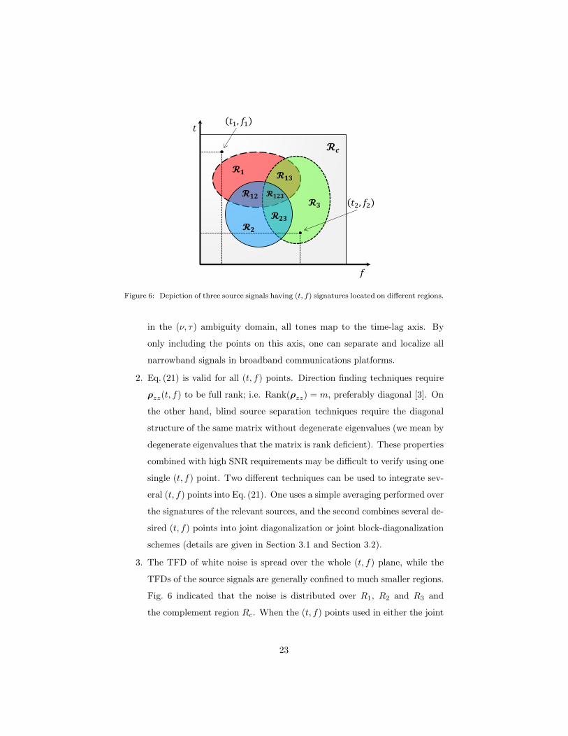
smaller regions, as illustrated in Fig. 6. Let us consider three sources 1, 2
and 3 arriving on a multisensor array. Source 1 occupies the (t, f) region R1,
Source 2 the (t, f) region R2 and Source 3 the (t, f) region R3. The (t, f) region
characteristics (signatures) of the three sources intersect (i.e., region R12, R13,
R23 and region R123), but each source still has its own particular (t, f) region
that has no overlap with other sources. On the other hand, the noise is spread
over R1, R2 and R3, as well as the complement region Rc. When we select (t, f)
points for averaging that are within the noise only region Rc (such as (t1, f1)),
then no useful information about the sources is available. But, if we constrain
the selection of (t, f) points to R1, R2 or R3, such as (t2, f2), then only the noise
contribution in these regions is counted. The effect of removing the (t, f) points
that are outside the (t, f) signatures region of the signal arrivals is to increase
the SNR. To be more specific, the MTFDs property of concentrating the input
signal energy in its instantaneous bandwidth (IB) and around its instantaneous
frequency (IF) while distributing the noise over the whole (t, f) plane improves
the effective SNR which is important in many applications. A key point is
therefore the selection of (t, f) points in the region of interest.
2.3.4. Four key properties of MTFDs
Four key advantages results from using array signal processing with MTFD.
To explain these advantages, let us use the example presented in the previous
section and illustrated by Fig. 6.
1. The prior knowledge about any time-domain parameters or the type of
time-varying frequency behavior of the sources of interest can allow us to
directly select the (t, f) regions used in Eq. (21). For example, recall that,
22
𝓡𝒄
𝓡𝟏
𝓡𝟐
𝓡𝟑 𝓡𝟏𝟐
𝓡𝟐𝟑
𝓡𝟏𝟑
𝓡𝟏𝟐𝟑
(𝑡1, 𝑓1)
(𝑡2, 𝑓2)
𝑓
𝑡
Figure 6: Depiction of three source signals having (t, f) signatures located on different regions.
in the (ν, τ) ambiguity domain, all tones map to the time-lag axis. By
only including the points on this axis, one can separate and localize all
narrowband signals in broadband communications platforms.
2. Eq. (21) is valid for all (t, f) points. Direction finding techniques require
ρzz(t, f) to be full rank; i.e. Rank(ρzz) = m, preferably diagonal [3]. On
the other hand, blind source separation techniques require the diagonal
structure of the same matrix without degenerate eigenvalues (we mean by
degenerate eigenvalues that the matrix is rank deficient). These properties
combined with high SNR requirements may be difficult to verify using one
single (t, f) point. Two different techniques can be used to integrate sev-
eral (t, f) points into Eq. (21). One uses a simple averaging performed over
the signatures of the relevant sources, and the second combines several de-
sired (t, f) points into joint diagonalization or joint block-diagonalization
schemes (details are given in Section 3.1 and Section 3.2).
3. The TFD of white noise is spread over the whole (t, f) plane, while the
TFDs of the source signals are generally confined to much smaller regions.
Fig. 6 indicated that the noise is distributed over R1, R2 and R3 and
the complement region Rc. When the (t, f) points used in either the joint
23
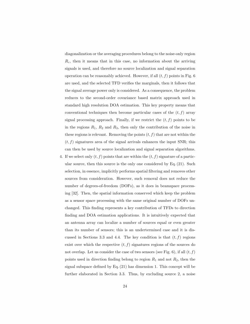
diagonalization or the averaging procedures belong to the noise-only region
Rc, then it means that in this case, no information about the arriving
signals is used, and therefore no source localization and signal separation
operation can be reasonably achieved. However, if all (t, f) points in Fig. 6
are used, and the selected TFD verifies the marginals, then it follows that
the signal average power only is considered. As a consequence, the problem
reduces to the second-order covariance based matrix approach used in
standard high resolution DOA estimation. This key property means that
conventional techniques then become particular cases of the (t, f) array
signal processing approach. Finally, if we restrict the (t, f) points to be
in the regions R1, R2 and R3, then only the contribution of the noise in
these regions is relevant. Removing the points (t, f) that are not within the
(t, f) signatures area of the signal arrivals enhances the input SNR; this
can then be used by source localization and signal separation algorithms.
4. If we select only (t, f) points that are within the (t, f) signature of a partic-
ular source, then this source is the only one considered by Eq. (21). Such
selection, in essence, implicitly performs spatial filtering and removes other
sources from consideration. However, such removal does not reduce the
number of degrees-of-freedom (DOFs), as it does in beamspace process-
ing [32]. Then, the spatial information conserved which keep the problem
as a sensor space processing with the same original number of DOFs un-
changed. This finding represents a key contribution of TFDs to direction
finding and DOA estimation applications. It is intuitively expected that
an antenna array can localize a number of sources equal or even greater
than its number of sensors; this is an undertermined case and it is dis-
cussed in Sections 3.3 and 4.4. The key condition is that (t, f) regions
exist over which the respective (t, f) signatures regions of the sources do
not overlap. Let us consider the case of two sensors (see Fig. 6), if all (t, f)
points used in direction finding belong to region R1 and not R2, then the
signal subspace defined by Eq. (21) has dimension 1. This concept will be
further elaborated in Section 3.3. Thus, by excluding source 2, a noise
24
subspace is established. This allows us to proceed with high resolution
techniques for localization of source 1. In a general context, one can local-
ize one source at a time or a set of selected sources, depending on the array
size, overlapping and distinct (t, f) regions, and the dimension of the noise
subspace necessary to achieve the required resolution performance. The
same concepts and advantages of (t, f) point selection discussed above for
direction finding can be applied to blind source separation problems.
2.3.5. Cross-term issues in MTFD
In the case of a single sensor, there are two sources of crossterms. The
first type are crossterms that result from the interactions between components
of the same source signal. The second type of crossterms are produced from
interactions between pairs of signal components belonging to different sources.
This second category of crossterms originates from cross-TFDs of the source
signals and, at any given (t, f) point, it constitutes the off-diagonal entries of
the source TFD matrices ρzz(t, f) defined in Eq.(21). Although the off-diagonal
elements do not necessarily affect the full-rank matrix property required for
direction-finding [28], they violate the key assumption in the problem of source
separation regarding the diagonal structure of the source TFD matrix. One
needs therefore to select the (t, f) points that are in autoterm regions where
crossterm contributions are at minimum, e.g., by using a priori information
from the source signals.
Note that the method of spatial averaging of the MTFD described in [29] does
not reduce the crossterms as in the case with reduced-interference distribution
kernels (see Section 2.3.2). Instead, it moves them from their locations on the
off-diagonal matrix entries to be part of the matrix diagonal elements. The other
parts of the matrix diagonal elements represent the contribution of autoterms
at the same point. Therefore, one can set the off-diagonal elements of the source
TFD matrix to zeros, and also improve performance by selecting the (t, f) points
of peak values, whether these points belong to autoterm or crossterm regions.
25
2.3.6. Examples
In this illustration, three synthetic signals are generated with sampling fre-
quency 1 Hz such that:
z1(t) = exp (−j2π (0.25 t+ 0.012 cos (3.8πt))) ,
z2(t) = exp (−j2π(0.3) t) ,
z3(t) = exp
(−j2π
(0.4 t− 0.3
256t2))
.
Two MTFDs for the three generated signals are computed using the MWVD
and the CKD distributions respectively, as depicted in Figs. 7 and 8. The auto-
MTFDs in the MWVD diagonal plots in Fig. 7 illustrate the ideal representa-
tion of the WVD for mono-component LFM signals, and the deleterious effect
of inner cross-terms when representing nonlinear FM signals. Furthermore, the
cross-MTFDs in the MWVD off-diagonal plots in Fig. 7 do not represent the
intersections between the synthetic signals time-frequency signatures. On the
other hand, auto-MTFDs in the CKD, diagonal plots in Fig. 8, illustrate the
tradeoff between resolution and cross-terms suppression, when representing dif-
ferent classes of signals. In addition, the cross-MTFD in the CKD off-diagonal
plots in Fig. 8 successfully represent the intersections between the synthetic
signals time-frequency signatures.
The above results can be reproduced using the codes provided in [5].
3. Blind source separation (BSS)
3.0. Background and motivation
The aim of automated component separation (ACS) methods is to process
the observation acquired by multisensor arrays in such a way that the original
unknown source signal can be extracted. The scientific community used the
word “blind” to denote all identification or inversion methods that are based
on output observations only. Therefore, in the following, we use blind source
separation (BSS) to introduce the presented algorithm.
26
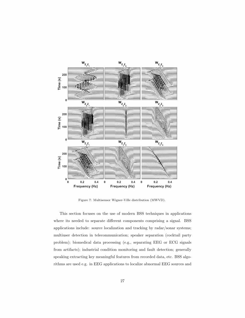
Figure 7: Multisensor Wigner-Ville distribution (MWVD).
This section focuses on the use of modern BSS techniques in applications
where its needed to separate different components comprising a signal. BSS
applications include: source localization and tracking by radar/sonar systems;
multiuser detection in telecommunication; speaker separation (cocktail party
problem); biomedical data processing (e.g., separating EEG or ECG signals
from artifacts); industrial condition monitoring and fault detection; generally
speaking extracting key meaningful features from recorded data, etc. BSS algo-
rithms are used e.g. in EEG applications to localize abnormal EEG sources and
27
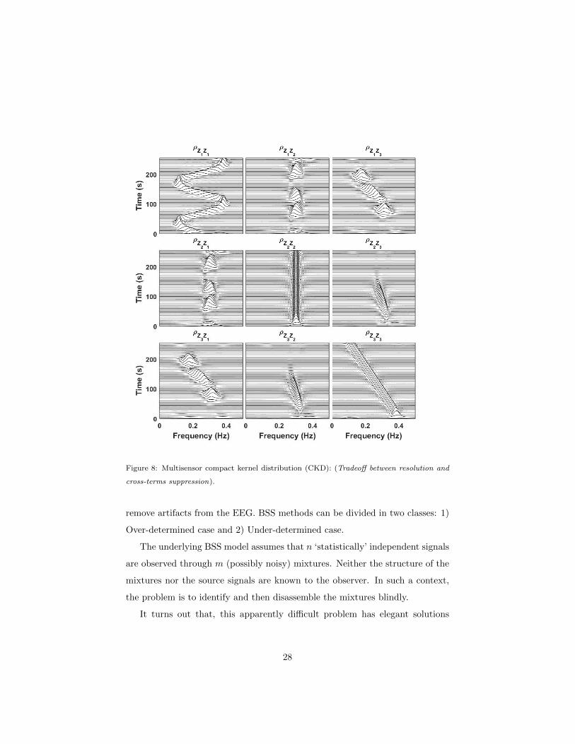
Figure 8: Multisensor compact kernel distribution (CKD): (Tradeoff between resolution and
cross-terms suppression).
remove artifacts from the EEG. BSS methods can be divided in two classes: 1)
Over-determined case and 2) Under-determined case.
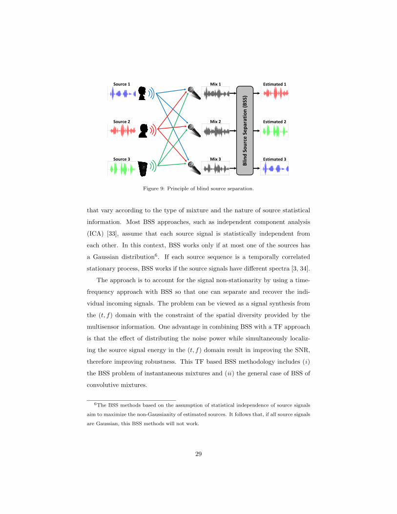
The underlying BSS model assumes that n ‘statistically’ independent signals
are observed through m (possibly noisy) mixtures. Neither the structure of the
mixtures nor the source signals are known to the observer. In such a context,
the problem is to identify and then disassemble the mixtures blindly.
It turns out that, this apparently difficult problem has elegant solutions
28
Blin
d S
ou
rce
Se
par
atio
n (
BSS
)
Source 1
Source 2
Source 3
Mix 1
Mix 2
Mix 3
Estimated 1
Estimated 2
Estimated 3
Figure 9: Principle of blind source separation.
that vary according to the type of mixture and the nature of source statistical
information. Most BSS approaches, such as independent component analysis
(ICA) [33], assume that each source signal is statistically independent from
each other. In this context, BSS works only if at most one of the sources has
a Gaussian distribution6. If each source sequence is a temporally correlated
stationary process, BSS works if the source signals have different spectra [3, 34].
The approach is to account for the signal non-stationarity by using a time-
frequency approach with BSS so that one can separate and recover the indi-
vidual incoming signals. The problem can be viewed as a signal synthesis from
the (t, f) domain with the constraint of the spatial diversity provided by the
multisensor information. One advantage in combining BSS with a TF approach
is that the effect of distributing the noise power while simultaneously localiz-
ing the source signal energy in the (t, f) domain result in improving the SNR,
therefore improving robustness. This TF based BSS methodology includes (i)
the BSS problem of instantaneous mixtures and (ii) the general case of BSS of
convolutive mixtures.
6The BSS methods based on the assumption of statistical independence of source signals
aim to maximize the non-Gaussianity of estimated sources. It follows that, if all source signals
are Gaussian, this BSS methods will not work.
29
Although BSS algorithms exist in great profusion, the underdetermined case
(with number of sensors smaller than number of sources) is less addressed than
the overdetermined case (with number of sensors greater than or equal to num-
ber of sources). In the underdetermined BSS (UBSS) case, one way to deal with
the lack of information is to exploit the assumption that the non-stationary
sources are disjoint in the time-frequency domain in order to solve the UBSS
problem without prior knowledge on the source distribution.
3.1. BSS of instantaneous mixtures based on MTFDs
In this section, we review the BSS technique based on multisensor time-
frequency analysis for instantaneous mixing system. Let us consider an n-
dimensional vector s(t) = [s1(t), . . . , sn(t)]T that represents n non-stationary
source signals si(t), i = 1, . . . , n. The si(t) propagate through a medium and
arrives at an array of m sensors which records a mixture of signals described
by an m-dimensional vector z(t) = [z1(t), . . . , zm(t)]T . Therefore, the data
model given in Section 2.2.1 by Eq.(12) is applicable in this situation so that
z (t) = A s (t) + η (t).
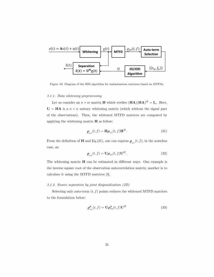
A number of BSS algorithms have been developed for the instantaneous
mixing case, which make use of the MTFD matrices discussed in the previous
section. [35, 36]. The various approches all exploit the underlying diagonal or
off-diagonal structure of MTFD matrices at some locations in the (t, f) domain.
BSS is achieved by first constructing a set of MTFD matrices, followed by joint
diagonalization (JD), joint off-diagonalization (JOD) or combined JD/JOD, to
estimate the mixing matrix. The optimization of JD/JOD criteria is based on
both orthogonal [35] and non-orthogonal [37] constraints. Such an algorithm is
illustrated in Fig. 10.
The principle of BSS based on orthogonal JD/JOD of MTFDs matrices is
outlined below [3]. This approach constrains the mixing matrix to be orthogonal,
but this is not the case in general. A whitening step needs therefore to be applied
to the signals, to verify the orthogonality constraint.
30
MTFD 𝑧(𝑡) = 𝐀𝑠(𝑡) + 𝜂(𝑡) Auto-term
Selection
(𝑡𝑎, 𝑓𝑎)
𝜌𝑧𝑧(𝑡, 𝑓) Whitening
𝑧(𝑡)
JD/JOD
Algorithm
Separation
(𝒕) = 𝐔𝚮𝒛(𝒕) U
(𝑡)
Figure 10: Diagram of the BSS algorithm for instantaneous mixtures based on MTFDs.
3.1.1. Data whitening preprocessing
Let us consider an n×m matrix H which verifies (HA)(HA)H = In. Here,
U = HA is a n × n unitary whitening matrix (which whitens the signal part
of the observations). Then, the whitened MTFD matrices are computed by
applying the whitening matrix H as follow:
ρzz
(t, f) = Hρzz(t, f)HH . (31)
From the definition of H and Eq.(21), one can express ρzz
(t, f), in the noiseless
case, as:
ρzz
(t, f) = Uρss(t, f)UH . (32)
The whitening matrix H can be estimated in different ways. One example is
the inverse square root of the observation autocorrelation matrix; another is to
calculate it using the MTFD matrices [3].
3.1.2. Source separation by joint diagonalization (JD)
Selecting only auto-term (t, f) points reduces the whitened MTFD matrices
to the formulation below:
ρazz
(t, f) = Uρass(t, f)UH (33)
31
where ρass(t, f) is diagonal7. Eq.(33) shows that any whitened MTFD matrix
is diagonal in the basis formed by the columns of the matrix U (given that the
eigenvalues of ρazz
(t, f) are the diagonal entries of ρss(t, f)).
In the case where, for a given (t, f) point, the diagonal elements of ρass(t, f)
are all different, the missing unitary matrix U may be uniquely retrieved by
computing the eigendecomposition of ρazz
(t, f), up to permutation and scaling
ambiguity. Indeed, the BSS problem has an inherent ambiguity concerning the
order and amplitudes of the sources. In the case of degenerate eigenvalues in-
determinacy occurs, where we mean by degenerate eigenvalues that the matrix
ρazz
(t, f) is rank deficient. Formally, this occurs when ρsisi(t, f) = ρsjsj (t, f),
i 6= j. One cannot see how to a priori choose the (t, f) point such that the
diagonal entries of ρass(t, f) are all different. Furthermore, if some eigenvalues
of ρazz
(t, f) are degenerate, the robustness of determining U from the eigen-
decomposition of a single whitened MTFD matrix suffers. The situation is
more appropriate if one considers the joint diagonalization of a combined set
ρazz
(ti, fi)|i = 1,. . . , p of p (source auto-term) MTFD matrices. This is equiv-
alent to including several (t, f) points in the source separation problem which
decreases the probability of selecting only degenerate eigenvalues. Therefore,
by considering a combined set ρazz
(ti, fi)|i = 1,. . . , p one can improve the ro-
bustness of the joint diagonalization procedure. Note that if two source signals
have identical (t, f) signatures, it is expected intuitively that they cannot be
separated even if one includes all information available in the (t, f) domain.
The joint diagonalization of a set Mk|k = 1,. . . , p of p matrices is formu-
lated as the maximization of the following cost function [3]:
C(V) ,p∑k=1
n∑i=1
|vHi Mkvi|2 (34)
over the set of unitary matrices V = [v1, . . . ,vn] [3]. One way to get an efficient
7Given that the off-diagonal elements of ρass(t, f) are actually cross-terms, the source TFD
matrix is quasi-diagonal for the (t, f) points that correspond to a true component power
concentration, i.e. a source auto-term.
32
joint approximate diagonalization algorithm is to generalize the Jacobi technique
[38] for the exact diagonalization of a single normal matrix [3].
3.1.3. Source separation by joint off-diagonalization (JOD)
The effect of selecting cross-term (t, f) points is that the whitened MTFD
matrices formulation becomes:
ρczz
(t, f) = Uρcss(t, f)UH (35)
where ρcss(t, f) is off-diagonal. As the diagonal of ρc
ss(t, f) are formed by el-
ements that are auto-terms, the source TFD matrix is then quasi off-diagonal
(i.e., diagonal entries are negligible i.e. ' 0) for each (t, f) point that corre-
sponds to a cross-term. The required unitary matrix U is estimated by joint
off-diagonalization (JOD) of a combined set ρczz
(ti, fi)|i = 1,. . . , q of q source
cross-term MTFD matrices [3].
Such JOD procedure is justified by realizing that the off-diagonalization of
a single n× n matrix N means maximizing
C(N,V) , −n∑i=1
|vHi Nvi|2 (36)
over the set of unitary matrices V=[v1, . . . ,vn]. This is because the Frobenius
norm of a matrix is constant under unitary transform, i.e., ‖N‖F = ‖VHNV‖F .
Hence, the JOD of a set Nk|k=1,. . . , q of n×n matrices is formulated as the
maximization of the JOD cost function:
C(V) ,q∑
k=1
C(Nk,V) = −q∑
k=1
n∑i=1
|vHi Nkvi|2 (37)
under the same unitary constraint.
Then, in order to improve the robustness of separation procedure and take
advantage of both auto-terms and cross-terms, one can combine joint diag-
onalization and joint off-diagonalization of two sets Mk|k = 1,. . . , p and
Nk|k = 1,. . . , q of n× n matrices by maximizing the JD/JOD cost function:
C(V) ,n∑i=1
(p∑k=1
|vHi Mkvi|2 −q∑
k=1
|vHi Nkvi|2)
(38)
33

over the set of unitary matrices V = [v1, . . . ,vn]. Then, the combined JD/JOD
criterion can be applied to a combined set of p (source auto-term) MTFD matri-
ces and q (source cross-term) MTFD matrices in order to estimate the unitary
matrix U.
Notes:
(1) The performance of the JD or JOD of MTFD matrices in retrieving the
unitary matrix U depends strongly on correctly selecting auto-term and cross-
term points [3]. Therefore, it is critical to define a selection method that can
discriminate between auto-term and cross-term points based only on the MTFD
observations matrices. One possible solution is to exploit the off-diagonal struc-
ture of the source cross-term MTFD matrices and the invariance of Trace oper-
ation under a unitary transformation. More specifically, for a source cross-term
MTFD matrix, we have
Trace(ρczz
(t, f))
= Trace(Uρc
ss(t, f)UH)
Then, knowing that the source cross-term MTFD matrices are off-diagonal (i.e.
the diagonal elements are equal to zero), and that Trace(U M UH
)= Trace
(M)
if U is a unitary matrix, then:
Trace(Uρc
ss(t, f)UH)
= Trace(ρcss(t, f)
)≈ 0.
Based on this observation, the following testing procedure applies:
1) ifTrace(ρ
zz(t,f))
‖ρzz
(t,f)‖ < ε,−→ then, allocate the (t, f) point as cross-term;
2) ifTrace(ρ
zz(t,f))
‖ρzz
(t,f)‖ > ε,−→ then, allocate the (t, f) point as auto-term;
where ε is a ‘small’ positive real scalar (typically, ε = 0.05) [3].
(2) In effect, the source cross-term MTFD matrices are not totally off-diagonal,
given that some auto-terms main lobes or side lobes overlap with the areas
where cross-terms are dominant. This is like the case of joint diagonalization
of MTFD matrices selecting auto-term points [3], where the source auto-term
MTFD matrices are not totally diagonal because of cross-term overlap. This
34
weakness is compensated by the joint approximation and robustness properties
of the JD/JOD algorithm.
(3) The above results suggest that other classes of TFDs and related methods
may also benefit from BSS; e.g. a cumulant-based 4th order WVD or time-
varying trispectrum can be utilized for source separation [39]. Blind separation
of more sources than sensors (underdetermined BSS) is solved using a (t, f)
disjoint concept [40] (see Section 3.3).
Implementation details and the corresponding MATLAB code of the above
algorithm are described in [5].
3.1.4. Experiment: Separation of Instantaneous Mixtures
In this example, three synthetic signals are generated with sampling fre-
quency 1 Hz such that:
s1(t) = exp
(−j2π 0.5
256t2),
s2(t) = exp
(−j2π
(0.5 t− 0.5
256t2))
,
s3(t) = exp (−j2π(0.3 t)) ,
as depicted in the first row of Fig. 11. The generated signals are mixed using an
instantaneous noisy uniform linear array model, to be received on m = 6 sensors
with an SNR of 30 dB (Fig. 12). The received mixtures are whitened, and
their MTFD using WVD is computed for the selection of auto and cross-terms.
Finally, the un-mixing matrix is estimated, using a joint diagonalization/joint
off-diagonalization algorithm, and estimated sources are classified using their
time-frequency correlation with the original signals, as depicted in the second
row of Fig. 11. The results presented in this section can be reproduced using
the codes provided in [5].
3.2. BSS of convolutive mixtures based on MTFDs
3.2.1. Signal Model in the convolutive mixture case
The convolutive case involves delayed elements caused e.g. by a multi-path
propagation. The multiple input multiple output (MIMO) linear time invariant
35
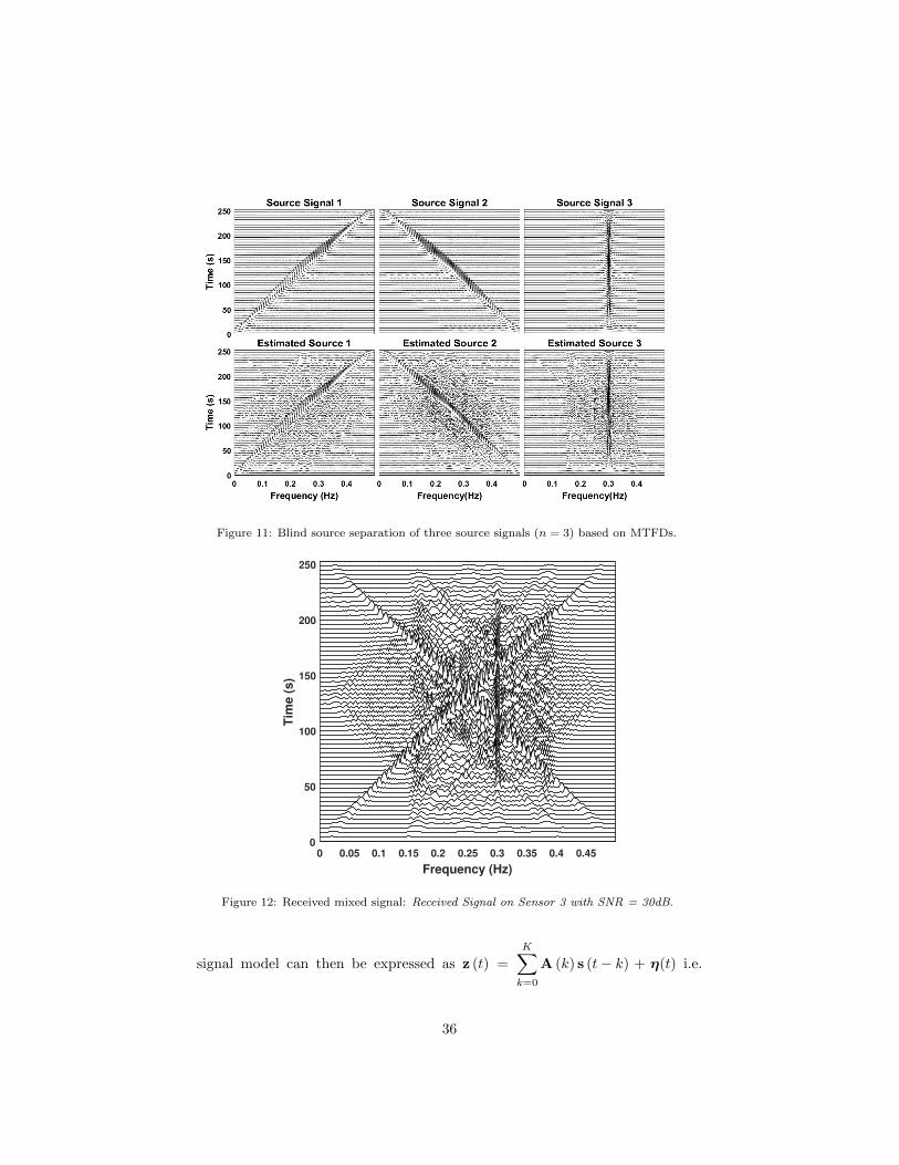
Figure 11: Blind source separation of three source signals (n = 3) based on MTFDs.
0 0.05 0.1 0.15 0.2 0.25 0.3 0.35 0.4 0.45
Frequency (Hz)
0
50
100
150
200
250
Tim
e (
s)
Figure 12: Received mixed signal: Received Signal on Sensor 3 with SNR = 30dB.
signal model can then be expressed as z (t) =
K∑k=0
A (k) s (t− k) + η(t) i.e.
36
Eq.(15). As discussed earlier, two assumptions are made; (1) that the sources
have different sparse (t, f) signatures and (2) the channel matrix A formulated
in (40) is full column rank; this means that all the filters aij(k)Kk=0 are stable
[41]. Eq. (15) can be rewritten in matrix form as:
z(t) = A s(t) + η(t), (39)
where s(t), z(t), η(t) and A are further described below:
s(t) = [s1(t), . . . , s1(t− (K +K ′) + 1), . . . , sn(t− (K +K ′) + 1)]T ,
z(t) = [z1(t), . . . , z1(t−K ′ + 1), . . . , zm(t−K ′ + 1)]T ,
η(t) = [η1(t), . . . , η1(t−K ′ + 1), . . . , ηm(t−K ′ + 1)]T ,
A =
A11 · · · A1n
.... . .
...
Am1 · · · Amn
, (40)
with
Aij =
aij(0) · · · aij(K) · · · 0
. . .. . .
. . .
0 · · · aij(0) · · · aij(K)
, (41)
where A is an mK ′ × n(K +K ′) matrix and Aij are K ′ × (K +K ′) matrices.
The parameter K ′ is a slide window size chosen such that mK ′ ≥ n(K+K ′) to
ensure that the matrix A is invertible.
The formalism is similar to the instantaneous mixture case. The data MTFD
matrices still have the same expression as in Eq. (21). But the source auto-
term matrices ρss(t, f) are no longer diagonal, but block-diagonal8 where each
diagonal block is of size (K +K ′)× (K +K ′). Similarly, the source cross-term
matrices are no longer off-diagonal but block off-diagonal. This block-diagonal
8The block diagonal characteristic comes from the property that cross-terms between si(t)
and si(t−d) are not zero as they relate to the local correlation structure of the signal.
37
or block off-diagonal property enables BSS to work in this case; as discussed in
the next section.
3.2.2. BSS using MTFD matrices for convolutive mixtures
Let us now generalize the BSS method for the instantaneous case presented
in Section 3.1 to the case of convolutive mixtures.
i) Data whitening preprocessing.
For BSS of instantaneous mixtures, this approach constrains the mixing matrix
A to be orthogonal, which is not the case in general. To match assumptions
with reality, the first step of the procedure is to then whiten the data vector
z(t) to fulfill the orthogonality constraint. This is done by processing z(t) with
a whitening matrix H, which is an n(K ′+K)×mK ′ matrix verifying:
H Rzz HH =(HAR
12
ss
)(HAR
12
ss
)H= In(K′+K), (42)
where Rzz and Rss denote the covariance matrices of z(t) and s(t), respectively.
Eq. (42) shows that if H is a whitening matrix and if R12
ss (Hermitian square
root matrix of Rss) is block diagonal, then the following matrix
U = HAR12
ss (43)
is an n(K ′ +K)× n(K ′ +K) unitary matrix. The whitening matrix H can be
determined from the eigendecomposition of the data covariance matrix Rzz as
its inverse square root [3].
ii) Separation using matrix joint block diagonalization.
Recall the whitened MTFD matrices ρzz
(t, f) = Hρzz(t, f)HH as defined in
(31). Combining Eq.(39) and Eq.(43) leads to:
ρzz
(t, f) = UR− 1
2
ss ρss(t, f)R− 1
2
ss UH (44)
Let us denote ρ(t, f) = R− 1
2
ss ρss(t, f)R− 1
2
ss . This then results in
ρzz
(t, f) = Uρ(t, f)UH (45)
38
As ρ(t, f) is block diagonal and the matrix U is unitary, the following property
holds: any whitened MTFD matrix is then block diagonal on the basis formed
by the column vectors of matrix U. As a consequence, the unitary matrix U can
be determined by estimating the block diagonalization of the matrix ρzz
(t, f).
As for the joint diagonalization approach presented in Section 3.1.2, one can use
the joint block diagonalization of a set ρzz
(ti, fi); i = 1,. . . , p of p whitened
MTFD matrices in order to reduces the probability of selecting only degenerate
eigenvalues, and then improve the robustness of the joint block-diagonalization.
A similar procedure can be used with the joint block off-diagonalization of the
source cross-term MTFD matrices.
This joint block-diagonalization (JBD) is obtained by maximizing the fol-
lowing criterion under unitary transform:
C(U) ,p∑k=1
n∑l=1
(K′+K)l∑i,j=(K′+K)(l−1)+1
∣∣∣u∗i ρzz(tk, fk) uj
∣∣∣2 , (46)
over the set of unitary matrices U = [u1, . . . ,un(K′+K)]. To perform the above,
one can use an efficient Jacobi-like algorithm for joint block diagonalization
algorithm such as [38, 42].
After the unitary matrix U is retrieved (up to a block diagonal unitary
matrix P due to the inherent JBD problem indeterminacy [43]), the estimated
signals are then estimated up to a filter by:
s(t) = UH H z(t). (47)
By “up to a filter” we mean that the separated sources correspond to filtered
versions of the original ones, i.e. si(t) = si(t) ∗ hi(t) where hi(t) is an unknown
filter and ∗ stands for the convolution. According to (39) and (43), the estimated
signals verify, s(t) = PR− 1
2
ss s(t) (48)
where, the matrix R− 1
2
ss is block diagonal and P is a block diagonal unitary
matrix.
39
iii) Assumptions and reality.
The performance of the above algorithms may be affected by a few points.
(1) In practice, it is sufficient that only n signals among the n(K ′+K) recovered
ones are selected. One chooses the signals resulting in the smallest cross-terms
coefficients. This result is obtained as a byproduct of the joint block diagonal-
ization procedure with no additional required computations.
(2) The algorithm yields a source separation up to a filter, instead of the full
MIMO deconvolution procedure. An alternative is to apply a SIMO (Single In-
put Multiple Output) deconvolution/equalization [44] to the separated sources.
3.2.3. Experiment: Separation of Convolutive Mixtures
In this experiment, two synthetic signals (n = 2) are generated with sampling
frequency 1 Hz as:
s1(t) = exp
(−j2π
(0.5 t− 0.5
256t2))
,
s2(t) = exp(−j2π 10−5 t3
),
as depicted in the first row of Fig. 13. The generated signals are passed through
a noisy convolutive invariant filter with length K = 1 representing the mixing
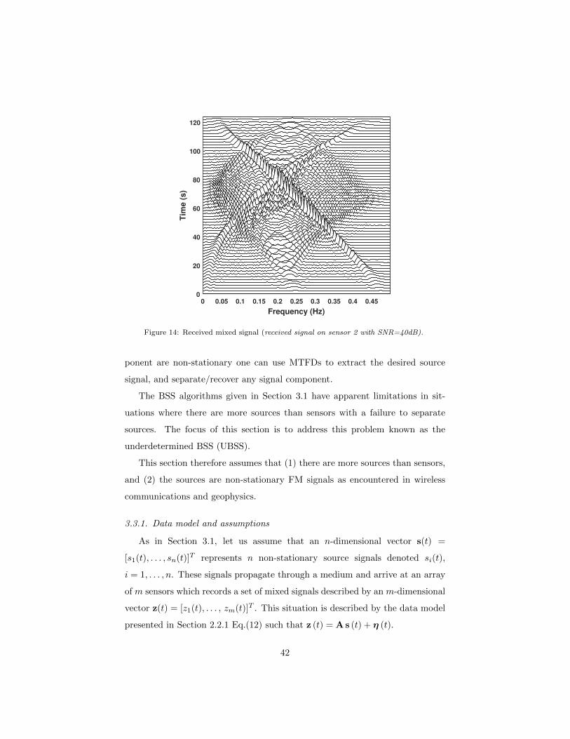
model and then received on four sensors (m = 4) with 40 dB SNR (Fig. 14).
The received mixtures are whitened, and their MTFD is computed using WVD
for the selection of auto-terms. The estimated sources are obtained by applying
a separation matrix given by the joint block diagonalization of selected auto-
terms with window size K ′ = 2. Estimated filtered sources are then classified
using their TF correlation with the original signals, as depicted in the last three
rows of Fig. 13.
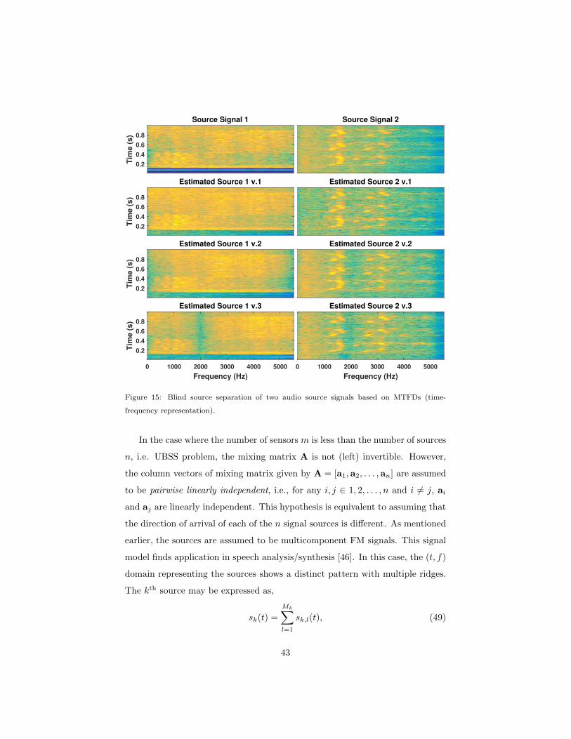
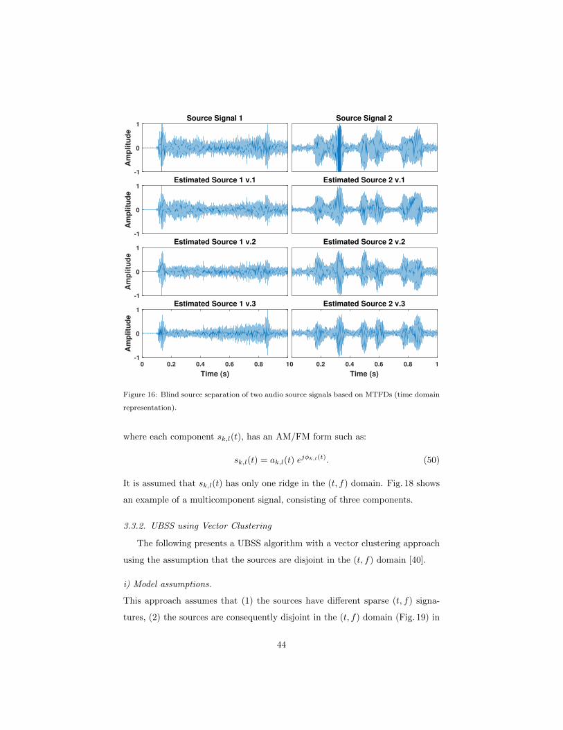
In the second experiment, a pair of one seconds soundtracks (n = 2), car
start-up and seagull sounds, are used as illustrated in the first row of Figs. 15
and 16. Other one seconds soundtracks can be obtained from [5], while their
original full length can be downloaded from [45]. The used sounds are passed
through a noisy convolutive invariant filter, describing the mixing model, to be
received on three sensors (m = 3), as shown in Fig. 17. The received mixtures
40
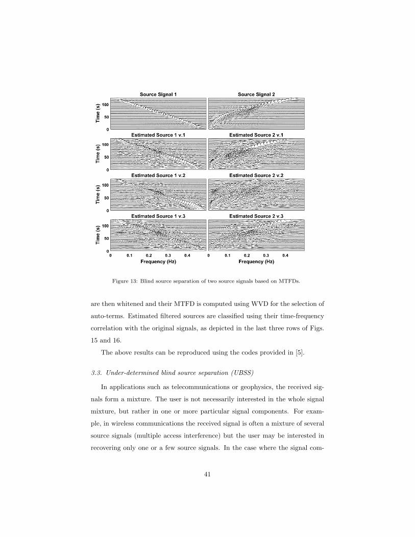
Figure 13: Blind source separation of two source signals based on MTFDs.
are then whitened and their MTFD is computed using WVD for the selection of
auto-terms. Estimated filtered sources are classified using their time-frequency
correlation with the original signals, as depicted in the last three rows of Figs.
15 and 16.
The above results can be reproduced using the codes provided in [5].
3.3. Under-determined blind source separation (UBSS)
In applications such as telecommunications or geophysics, the received sig-
nals form a mixture. The user is not necessarily interested in the whole signal
mixture, but rather in one or more particular signal components. For exam-
ple, in wireless communications the received signal is often a mixture of several
source signals (multiple access interference) but the user may be interested in
recovering only one or a few source signals. In the case where the signal com-
41
0 0.05 0.1 0.15 0.2 0.25 0.3 0.35 0.4 0.45
Frequency (Hz)
0
20
40
60
80
100
120
Tim
e (
s)
Figure 14: Received mixed signal (received signal on sensor 2 with SNR=40dB).
ponent are non-stationary one can use MTFDs to extract the desired source
signal, and separate/recover any signal component.
The BSS algorithms given in Section 3.1 have apparent limitations in sit-
uations where there are more sources than sensors with a failure to separate
sources. The focus of this section is to address this problem known as the
underdetermined BSS (UBSS).
This section therefore assumes that (1) there are more sources than sensors,
and (2) the sources are non-stationary FM signals as encountered in wireless
communications and geophysics.
3.3.1. Data model and assumptions
As in Section 3.1, let us assume that an n-dimensional vector s(t) =
[s1(t), . . . , sn(t)]T represents n non-stationary source signals denoted si(t),
i = 1, . . . , n. These signals propagate through a medium and arrive at an array
of m sensors which records a set of mixed signals described by an m-dimensional
vector z(t) = [z1(t), . . . , zm(t)]T . This situation is described by the data model
presented in Section 2.2.1 Eq.(12) such that z (t) = A s (t) + η (t).
42
Source Signal 1
0.2
0.4
0.6
0.8T
ime
(s
)
Source Signal 2
Estimated Source 1 v.1
0.2
0.4
0.6
0.8
Tim
e (
s)
Estimated Source 2 v.1
Estimated Source 1 v.2
0.2
0.4
0.6
0.8
Tim
e (
s)
Estimated Source 2 v.2
Estimated Source 1 v.3
0 1000 2000 3000 4000 5000
Frequency (Hz)
0.2
0.4
0.6
0.8
Tim
e (
s)
Estimated Source 2 v.3
0 1000 2000 3000 4000 5000
Frequency (Hz)
Figure 15: Blind source separation of two audio source signals based on MTFDs (time-
frequency representation).
In the case where the number of sensors m is less than the number of sources
n, i.e. UBSS problem, the mixing matrix A is not (left) invertible. However,
the column vectors of mixing matrix given by A = [a1,a2, . . . ,an] are assumed
to be pairwise linearly independent, i.e., for any i, j ∈ 1, 2, . . . , n and i 6= j, ai
and aj are linearly independent. This hypothesis is equivalent to assuming that
the direction of arrival of each of the n signal sources is different. As mentioned
earlier, the sources are assumed to be multicomponent FM signals. This signal
model finds application in speech analysis/synthesis [46]. In this case, the (t, f)
domain representing the sources shows a distinct pattern with multiple ridges.
The kth source may be expressed as,
sk(t) =
Mk∑l=1
sk,l(t), (49)
43
-1
0
1A
mp
litu
de
Source Signal 1 Source Signal 2
-1
0
1
Am
plitu
de
Estimated Source 1 v.1 Estimated Source 2 v.1
-1
0
1
Am
pli
tud
e
Estimated Source 1 v.2 Estimated Source 2 v.2
0 0.2 0.4 0.6 0.8 1
Time (s)
-1
0
1
Am
plitu
de
Estimated Source 1 v.3
0 0.2 0.4 0.6 0.8 1
Time (s)
Estimated Source 2 v.3
Figure 16: Blind source separation of two audio source signals based on MTFDs (time domain
representation).
where each component sk,l(t), has an AM/FM form such as:
sk,l(t) = ak,l(t) ejφk,l(t). (50)
It is assumed that sk,l(t) has only one ridge in the (t, f) domain. Fig. 18 shows
an example of a multicomponent signal, consisting of three components.
3.3.2. UBSS using Vector Clustering
The following presents a UBSS algorithm with a vector clustering approach
using the assumption that the sources are disjoint in the (t, f) domain [40].
i) Model assumptions.
This approach assumes that (1) the sources have different sparse (t, f) signa-
tures, (2) the sources are consequently disjoint in the (t, f) domain (Fig. 19) in
44
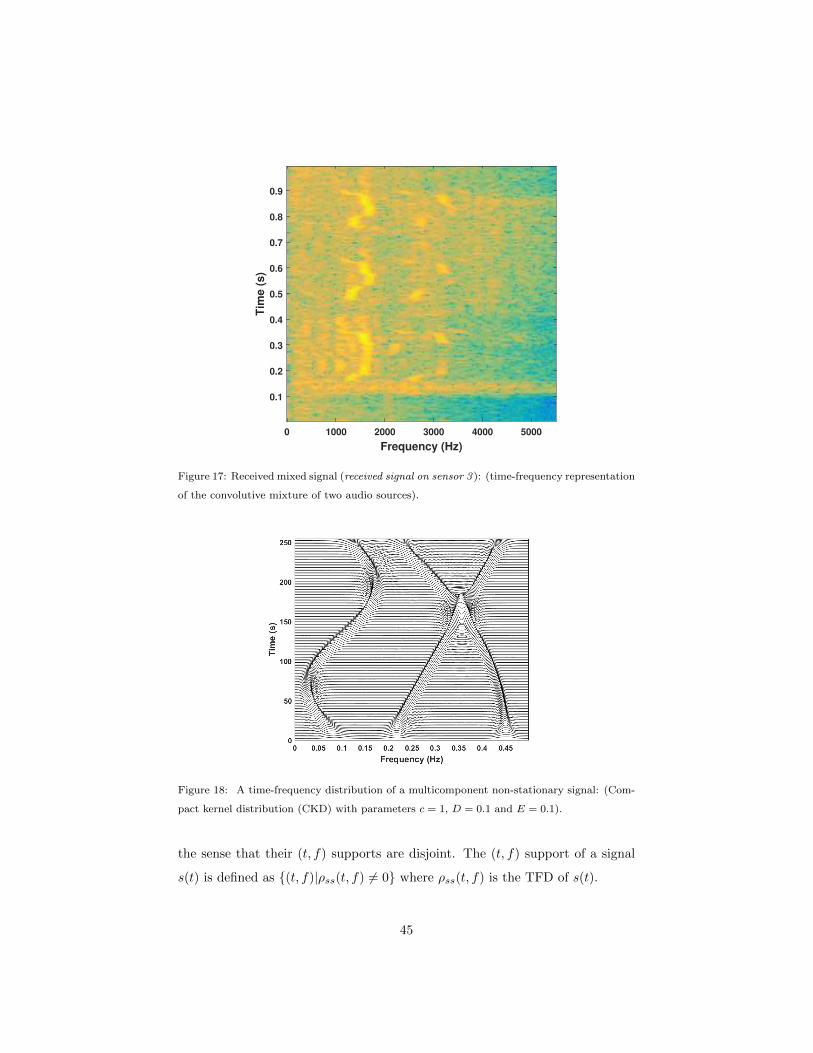
0 1000 2000 3000 4000 5000
Frequency (Hz)
0.1
0.2
0.3
0.4
0.5
0.6
0.7
0.8
0.9
Tim
e (
s)
Figure 17: Received mixed signal (received signal on sensor 3 ): (time-frequency representation
of the convolutive mixture of two audio sources).
Figure 18: A time-frequency distribution of a multicomponent non-stationary signal: (Com-
pact kernel distribution (CKD) with parameters c = 1, D = 0.1 and E = 0.1).
the sense that their (t, f) supports are disjoint. The (t, f) support of a signal
s(t) is defined as (t, f)|ρss(t, f) 6= 0 where ρss(t, f) is the TFD of s(t).
45
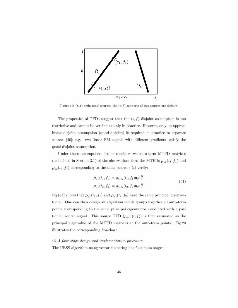
Figure 19: (t, f) orthogonal sources; the (t, f) supports of two sources are disjoint.
The properties of TFDs suggest that the (t, f) disjoint assumption is too
restrictive and cannot be verified exactly in practice. However, only an approx-
imate disjoint assumption (quasi-disjoint) is required in practice to separate
sources [40]; e.g. two linear FM signals with different gradients satisfy the
quasi-disjoint assumption.
Under these assumptions, let us consider two auto-term MTFD matrices
(as defined in Section 3.1) of the observation; then the MTFDs ρzz(t1, f1) and
ρzz(t2, f2) corresponding to the same source si(t) verify:
ρzz(t1, f1) = ρsisi(t1, f1)aiaHi ,
ρzz(t2, f2) = ρsisi(t2, f2)aiaHi .
(51)
Eq.(51) shows that ρzz(t1, f1) and ρzz(t2, f2) have the same principal eigenvec-
tor ai. One can then design an algorithm which groups together all auto-term
points corresponding to the same principal eigenvector associated with a par-
ticular source signal. This source TFD (ρsisi(t, f)) is then estimated as the
principal eigenvalue of the MTFD matrices at the auto-term points. Fig.20
illustrates the corresponding flowchart.
ii) A four stage design and implementation procedure.
The UBSS algorithm using vector clustering has four main stages:
46
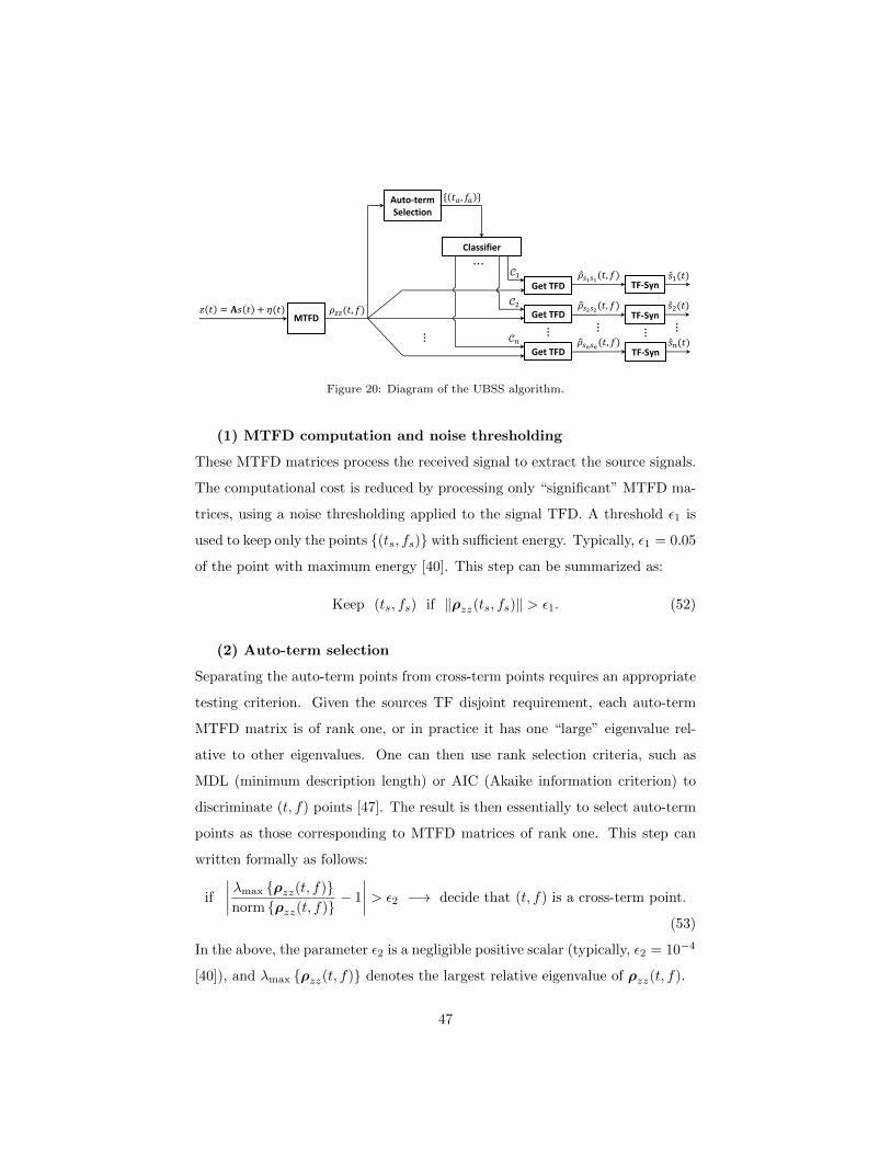
MTFD
Auto-term Selection
𝑡𝑎, 𝑓𝑎
Classifier
⋯
⋮
𝜌𝑧𝑧 𝑡, 𝑓
Get TFD
Get TFD
Get TFD
𝒞1
𝒞2
𝒞𝑛
𝜌 𝑠1𝑠1 𝑡, 𝑓 TF-Syn
𝑠 1 𝑡
𝜌 𝑠2𝑠2 𝑡, 𝑓 TF-Syn
𝑠 2 𝑡
𝜌 𝑠𝑛𝑠𝑛 𝑡, 𝑓 TF-Syn
𝑠 𝑛 𝑡 ⋮ ⋮ ⋮ ⋮
𝑧 𝑡 = 𝐀𝑠 𝑡 + 𝜂 𝑡
Figure 20: Diagram of the UBSS algorithm.
(1) MTFD computation and noise thresholding
These MTFD matrices process the received signal to extract the source signals.
The computational cost is reduced by processing only “significant” MTFD ma-
trices, using a noise thresholding applied to the signal TFD. A threshold ε1 is
used to keep only the points (ts, fs) with sufficient energy. Typically, ε1 = 0.05
of the point with maximum energy [40]. This step can be summarized as:
Keep (ts, fs) if ‖ρzz(ts, fs)‖ > ε1. (52)
(2) Auto-term selection
Separating the auto-term points from cross-term points requires an appropriate
testing criterion. Given the sources TF disjoint requirement, each auto-term
MTFD matrix is of rank one, or in practice it has one “large” eigenvalue rel-
ative to other eigenvalues. One can then use rank selection criteria, such as
MDL (minimum description length) or AIC (Akaike information criterion) to
discriminate (t, f) points [47]. The result is then essentially to select auto-term
points as those corresponding to MTFD matrices of rank one. This step can
written formally as follows:
if
∣∣∣∣ λmax ρzz(t, f)norm ρzz(t, f)
− 1
∣∣∣∣ > ε2 −→ decide that (t, f) is a cross-term point.
(53)
In the above, the parameter ε2 is a negligible positive scalar (typically, ε2 = 10−4
[40]), and λmax ρzz(t, f) denotes the largest relative eigenvalue of ρzz(t, f).
47
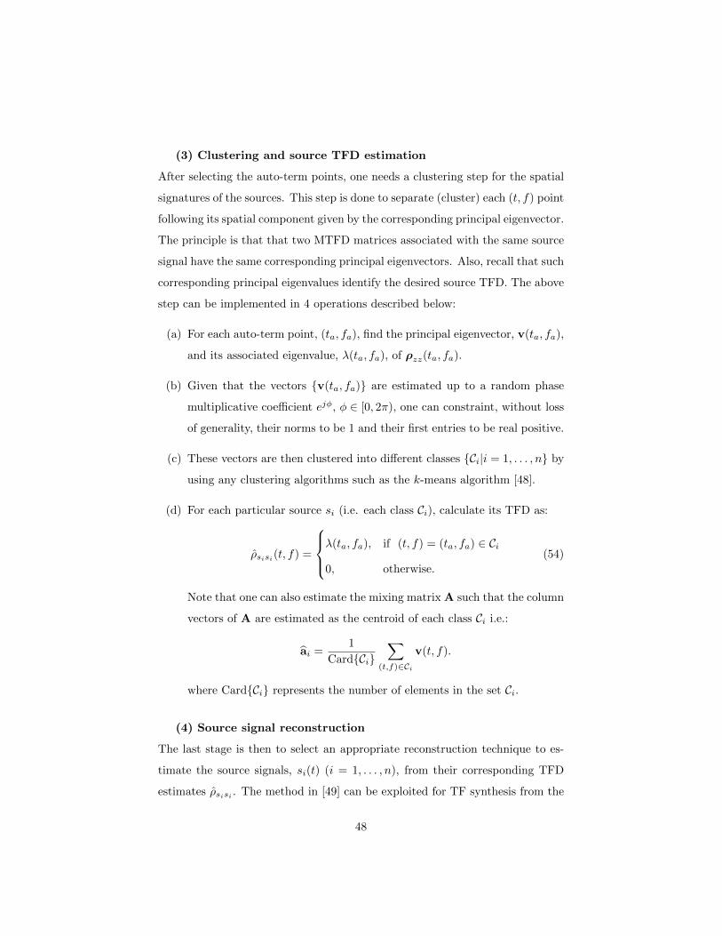
(3) Clustering and source TFD estimation
After selecting the auto-term points, one needs a clustering step for the spatial
signatures of the sources. This step is done to separate (cluster) each (t, f) point
following its spatial component given by the corresponding principal eigenvector.
The principle is that that two MTFD matrices associated with the same source
signal have the same corresponding principal eigenvectors. Also, recall that such
corresponding principal eigenvalues identify the desired source TFD. The above
step can be implemented in 4 operations described below:
(a) For each auto-term point, (ta, fa), find the principal eigenvector, v(ta, fa),
and its associated eigenvalue, λ(ta, fa), of ρzz(ta, fa).
(b) Given that the vectors v(ta, fa) are estimated up to a random phase
multiplicative coefficient ejφ, φ ∈ [0, 2π), one can constraint, without loss
of generality, their norms to be 1 and their first entries to be real positive.
(c) These vectors are then clustered into different classes Ci|i = 1, . . . , n by
using any clustering algorithms such as the k-means algorithm [48].
(d) For each particular source si (i.e. each class Ci), calculate its TFD as:
ρsisi(t, f) =
λ(ta, fa), if (t, f) = (ta, fa) ∈ Ci
0, otherwise.
(54)
Note that one can also estimate the mixing matrix A such that the column
vectors of A are estimated as the centroid of each class Ci i.e.:
ai =1
CardCi∑
(t,f)∈Ci
v(t, f).
where CardCi represents the number of elements in the set Ci.
(4) Source signal reconstruction
The last stage is then to select an appropriate reconstruction technique to es-
timate the source signals, si(t) (i = 1, . . . , n), from their corresponding TFD
estimates ρsisi . The method in [49] can be exploited for TF synthesis from the
48
WVD of separated sources, based on the following inversion property of the
WVD [1, Chapter 3]:
z(t) =1
z(0)∗
∫RWz
(t
2, f
)ej2πtf df (55)
In the next section, the TF-disjoint condition is relaxed by allowing the
sources to be nondisjoint in the (t, f) plane. This is to overcome the drawback
of the BSS method presented above. Although this method worked well under
the TF-almost-disjoint condition, it did not explicitly process the TF regions
where the sources overlap. A point in the overlap area of two sources was
assigned “by chance” to only one of the sources. As a result, the source that is
allocated this point gets information about another source while the latter loses
some of its own information. If the number of overlapping points increases (i.e.,
the TF-almost-disjoint condition is not met), the performance of the separation
tends to reduce unless the overlapping points are processed correctly.
3.3.3. UBSS for non-disjoint sources in the (t, f) domain
In most real life applications, the (t, f) disjoint assumption is a restrictive
condition that is not precisely and rigourously applicable. When this condition
is not met, the separation performance degrades greatly at those overlapped
(t, f) points. In order to remedy this weakness, a subspace projection based
separation method, with sparsity assumption relaxed, can be used [4, 50]. In this
algorithm, the (t, f) representations of different sources are allowed to overlap,
but only to the extent that there are less active sources at any (t, f) point than
the number of sensors. As this sparsity condition is more relaxed than the
(t, f) disjoint assumption so that the sources are allowed to overlap in the (t, f)
domain, it will be called TF nondisjoint.
Under the (t, f) nondisjoint assumption, consider a particular (t, f) point
at which there are K sources s`1(t), . . . , s`K(t) present, with K < m where
`1, . . . , `K ∈ 1, 2, . . . , n denote the indexes of the sources present at the point
(t0, f0). The goal is to identify the sources that are present at the point (t0, f0),
i.e. `1, . . . , `K, and to estimate the TFD of each of these contributing sources.
49
In order to model the received signal under this assumption, let us define
the following sub-vector and sub-matrix:
s(t) = [s`1(t), . . . , s`K(t)]T , (56a)
A` = [a`1 , . . . ,a`K ]. (56b)
Then, under the (t, f) nondisjoint assumption the instantaneous model reduces
to the following
ρzz(t, f) = A` ρss(t, f) AH` . (57)
Consequently, given that ρss(t, f) is of full rank, we obtain
Range ρzz(t, f) = Range
A`
(58)
Let Q = Im −VVH be the orthogonal projection matrix onto the noise sub-
space of ρzz(t, f), where V is the matrix formed by the K principal singular
eigenvectors of ρzz(t, f). Then, from Eq. (58), we obtain:Q ai = 0, i ∈ `1, . . . , `K,
Q ai 6= 0, otherwise.
. (59)
Assuming that the mixing matrix A has been estimated by methods such as
the clustering based method presented in Section 3.3.2, the observation in Eq.
(59) can be used to identify the indexes `1, . . . , `K and therefore, the sources
present at (t0, f0). To implement this and account for the additive noise,
one can detect these indexes by selecting the K smallest values from the set
‖Q ai‖|i = 1, . . . , n, as mathematically expressed by:
`1, . . . , `K = arg mini;K‖Q ai‖ . (60)
The MTFD values of the K sources at (t0, f0) are calculated as the diagonal
elements of the following matrix:
ρss(t0, f0) ≈ A#` ρzz(t0, f0) A#H
` , (61)
where (#) represents the Moore-Penrose’s pseudo-inversion operator [51].
50
3.3.4. Experiment: Underdetermined blind source separation
In the first experiment, four TF disjoint source signals (n = 4) are generated
with sampling frequency 1 Hz such that:
s1(t) = exp
(−j2π 0.2
256t2)
+ exp
(−j2π
(0.2 t− 0.2
256t2))
,
s2(t) = exp (−j2π(0.25 t)) ,
s3(t) = exp
(−j2π
(0.3 t+
0.1
256t2))
,
s4(t) = exp
(−j2π
(0.4 t+
0.1
256t2))
,
as depicted in the first row of Fig. 21. The generated signals are then mixed
using an instantaneous noisy uniform linear array model, to be received on three
sensors (m = 3) with an SNR of 30 dB. The MTFDs of the received mixtures
are computed and the separation is achieved by using a clustering method as
depicted in the second row of Fig. 21.
In the second experiment, four non-disjoint source signals (n = 4) are gener-
ated using crossing LFMs. The first two signals are crossing LFMs interchange-
ably changing from 0.05 Hz to 0.2 Hz, while the third and fourth signals are
LFMs interchangeably changing from 0.3 Hz to 0.45 Hz, as depicted in the first
row of Fig. 22. The generated signals are then mixed using an instantaneous
noisy uniform linear array model, to be received on three sensors (m = 3) with
an SNR of 40 dB (Fig. 23). From Fig. 22, we can observe that the overlapping
points are randomly allocated for one source, when utilizing the cluster-based
algorithm. However, by using the subspace-based algorithm, the intersection
points are redistributed to their corresponding two sources. In general, overlap-
ping points in the non-disjoint case have been explicitly treated. This provides
a visual performance comparison.
The above results can be reproduced using the codes provided in [5].
3.4. Discussion
The performance and limitations of BSS algorithms and their applications
are further reviewed below.
51
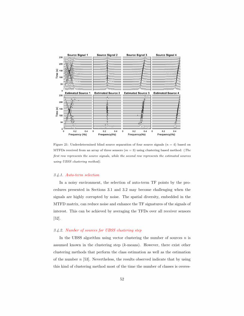
Figure 21: Underdetermined blind source separation of four source signals (n = 4) based on
MTFDs received from an array of three sensors (m = 3) using clustering based method: (The
first row represents the source signals, while the second row represents the estimated sources
using UBSS clustering method).
3.4.1. Auto-term selection
In a noisy environment, the selection of auto-term TF points by the pro-
cedures presented in Sections 3.1 and 3.2 may become challenging when the
signals are highly corrupted by noise. The spatial diversity, embedded in the
MTFD matrix, can reduce noise and enhance the TF signatures of the signals of
interest. This can be achieved by averaging the TFDs over all receiver sensors
[52].
3.4.2. Number of sources for UBSS clustering step
In the UBSS algorithm using vector clustering the number of sources n is
assumed known in the clustering step (k-means). However, there exist other
clustering methods that perform the class estimation as well as the estimation
of the number n [53]. Nevertheless, the results observed indicate that by using
this kind of clustering method most of the time the number of classes is overes-
52
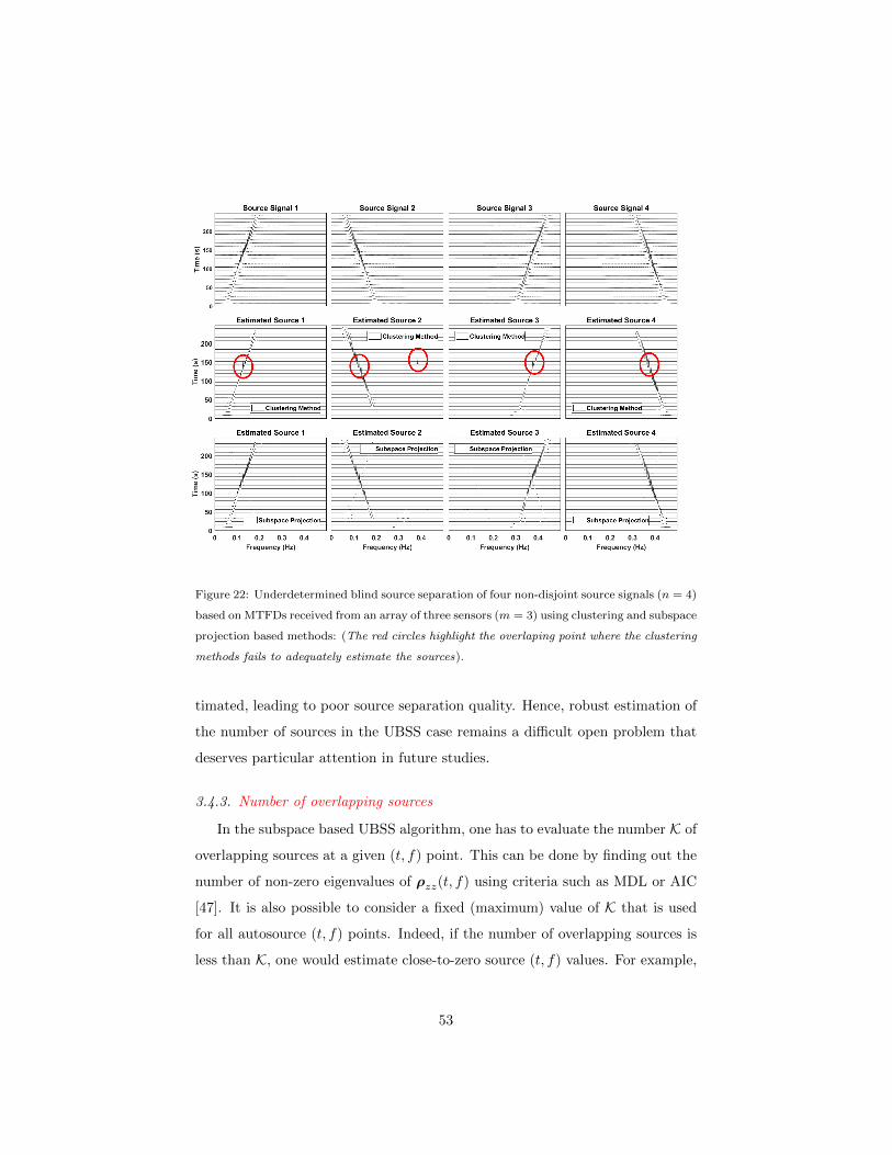
Figure 22: Underdetermined blind source separation of four non-disjoint source signals (n = 4)
based on MTFDs received from an array of three sensors (m = 3) using clustering and subspace
projection based methods: (The red circles highlight the overlaping point where the clustering
methods fails to adequately estimate the sources).
timated, leading to poor source separation quality. Hence, robust estimation of
the number of sources in the UBSS case remains a difficult open problem that
deserves particular attention in future studies.
3.4.3. Number of overlapping sources
In the subspace based UBSS algorithm, one has to evaluate the number K of
overlapping sources at a given (t, f) point. This can be done by finding out the
number of non-zero eigenvalues of ρzz(t, f) using criteria such as MDL or AIC
[47]. It is also possible to consider a fixed (maximum) value of K that is used
for all autosource (t, f) points. Indeed, if the number of overlapping sources is
less than K, one would estimate close-to-zero source (t, f) values. For example,
53
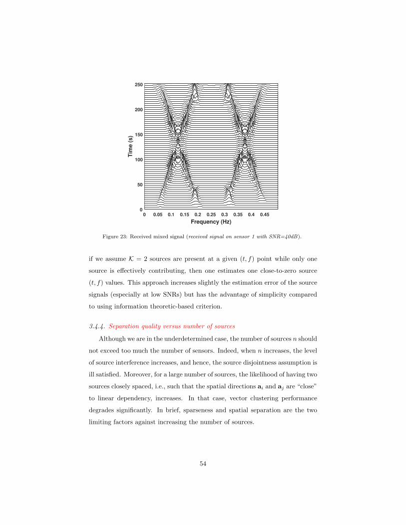
0 0.05 0.1 0.15 0.2 0.25 0.3 0.35 0.4 0.45
Frequency (Hz)
0
50
100
150
200
250
Tim
e (
s)
Figure 23: Received mixed signal (received signal on sensor 1 with SNR=40dB).
if we assume K = 2 sources are present at a given (t, f) point while only one
source is effectively contributing, then one estimates one close-to-zero source
(t, f) values. This approach increases slightly the estimation error of the source
signals (especially at low SNRs) but has the advantage of simplicity compared
to using information theoretic-based criterion.
3.4.4. Separation quality versus number of sources
Although we are in the underdetermined case, the number of sources n should
not exceed too much the number of sensors. Indeed, when n increases, the level
of source interference increases, and hence, the source disjointness assumption is
ill satisfied. Moreover, for a large number of sources, the likelihood of having two
sources closely spaced, i.e., such that the spatial directions ai and aj are “close”
to linear dependency, increases. In that case, vector clustering performance
degrades significantly. In brief, sparseness and spatial separation are the two
limiting factors against increasing the number of sources.
54
3.4.5. Overdetermined case
The class of UBSS algorithms presented in Section 3.3 can be further sim-
plified in the overdetermined case where m ≥ n. In that context, the algorithm
can be reduced to the mixing matrix estimation step, the noise thresholding
then source estimation using the mixing matrix pseudo-inversion.
3.4.6. Improved BSS using high-resolution MTFDs
In the case where the received multisensor signal presents high cross-terms,
the BSS may become a challenging. Therefore, in order to improve the robust-
ness against cross-terms of separation procedure based on joint diagonalization
(JD, JOD and JBD), we can use the hight resolution TFDs introduced in Sec-
tion 2.3.2 instead of MWVD. Indeed, despite its many desirable properties, the
MWVD has some drawbacks that require a precise handling such as cross-terms.
Such cross-terms are undesirable in BSS application. Then, cross-terms can be
reduced by using high resolution TFDs such as EMBD, CKD or MDD.
To support this claim, let us consider the same three source signals pre-
sented in Section 3.1.4 as depicted in the first row of Fig. 24. The generated
signals are mixed using an instantaneous noisy uniform linear array model, to
be received on m = 6 sensors with an SNR of 30 dB (Fig. 25). The received
mixtures are whitened, and their MTFD using CKD is computed with param-
eters c = 1, D = 0.1 and E = 0.1 for the selection of auto and cross-terms.
Finally, the un-mixing matrix is estimated, using a joint diagonalization/joint
off-diagonalization algorithm, and estimated sources are classified using their
time-frequency correlation with the original signals, as depicted in the second
row of Fig. 24. The main objective of this simulation is to illustrate the trade-
off between resolution and cross-terms suppression, when representing different
classes of signals such as CKD. Indeed, one can observe from Figs. 12 and 25
that the cross-terms have been significantly reduced with keeping a good time-
frequency resolution which improve the robustness of TF BSS algorithms against
auto-terms and cross-terms selection. This robustness against auto-terms and
cross-terms selection will improve the performance of joint diagonalization al-
55
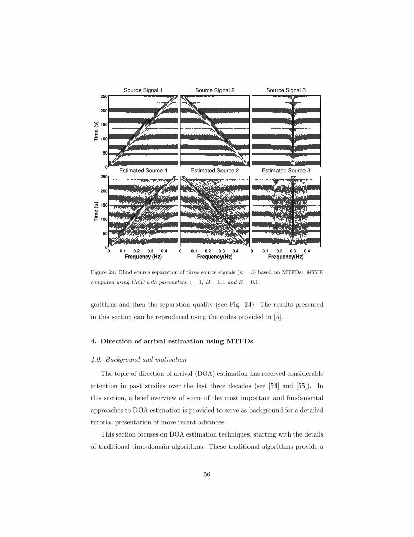
0
50
100
150
200
250
Source Signal 1T
ime
(s)
0 0.1 0.2 0.3 0.40
50
100
150
200
250
Estimated Source 1
Tim
e (
s)
Frequency (Hz)
Source Signal 2
0 0.1 0.2 0.3 0.4
Estimated Source 2
Frequency(Hz)
Source Signal 3
0 0.1 0.2 0.3 0.4
Estimated Source 3
Frequency(Hz)
Figure 24: Blind source separation of three source signals (n = 3) based on MTFDs: MTFD
computed using CKD with parameters c = 1, D = 0.1 and E = 0.1.
gorithms and then the separation quality (see Fig. 24). The results presented
in this section can be reproduced using the codes provided in [5].
4. Direction of arrival estimation using MTFDs
4.0. Background and motivation
The topic of direction of arrival (DOA) estimation has received considerable
attention in past studies over the last three decades (see [54] and [55]). In
this section, a brief overview of some of the most important and fundamental
approaches to DOA estimation is provided to serve as background for a detailed
tutorial presentation of more recent advances.
This section focuses on DOA estimation techniques, starting with the details
of traditional time-domain algorithms. These traditional algorithms provide a
56
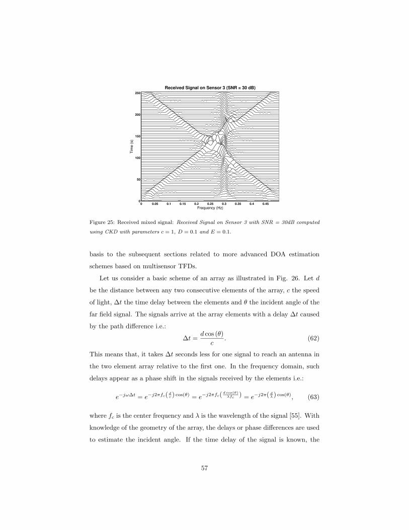
0 0.05 0.1 0.15 0.2 0.25 0.3 0.35 0.4 0.450
50
100
150
200
250
Tim
e (
s)
Frequency (Hz)
Received Signal on Sensor 3 (SNR = 30 dB)
Figure 25: Received mixed signal: Received Signal on Sensor 3 with SNR = 30dB computed
using CKD with parameters c = 1, D = 0.1 and E = 0.1.
basis to the subsequent sections related to more advanced DOA estimation
schemes based on multisensor TFDs.
Let us consider a basic scheme of an array as illustrated in Fig. 26. Let d
be the distance between any two consecutive elements of the array, c the speed
of light, ∆t the time delay between the elements and θ the incident angle of the
far field signal. The signals arrive at the array elements with a delay ∆t caused
by the path difference i.e.:
∆t =d cos (θ)
c. (62)
This means that, it takes ∆t seconds less for one signal to reach an antenna in
the two element array relative to the first one. In the frequency domain, such
delays appear as a phase shift in the signals received by the elements i.e.:
e−jω∆t = e−j2πfc(dc ) cos(θ) = e−j2πfc(
d cos(θ)λfc
) = e−j2π( dλ ) cos(θ), (63)
where fc is the center frequency and λ is the wavelength of the signal [55]. With
knowledge of the geometry of the array, the delays or phase differences are used
to estimate the incident angle. If the time delay of the signal is known, the
57
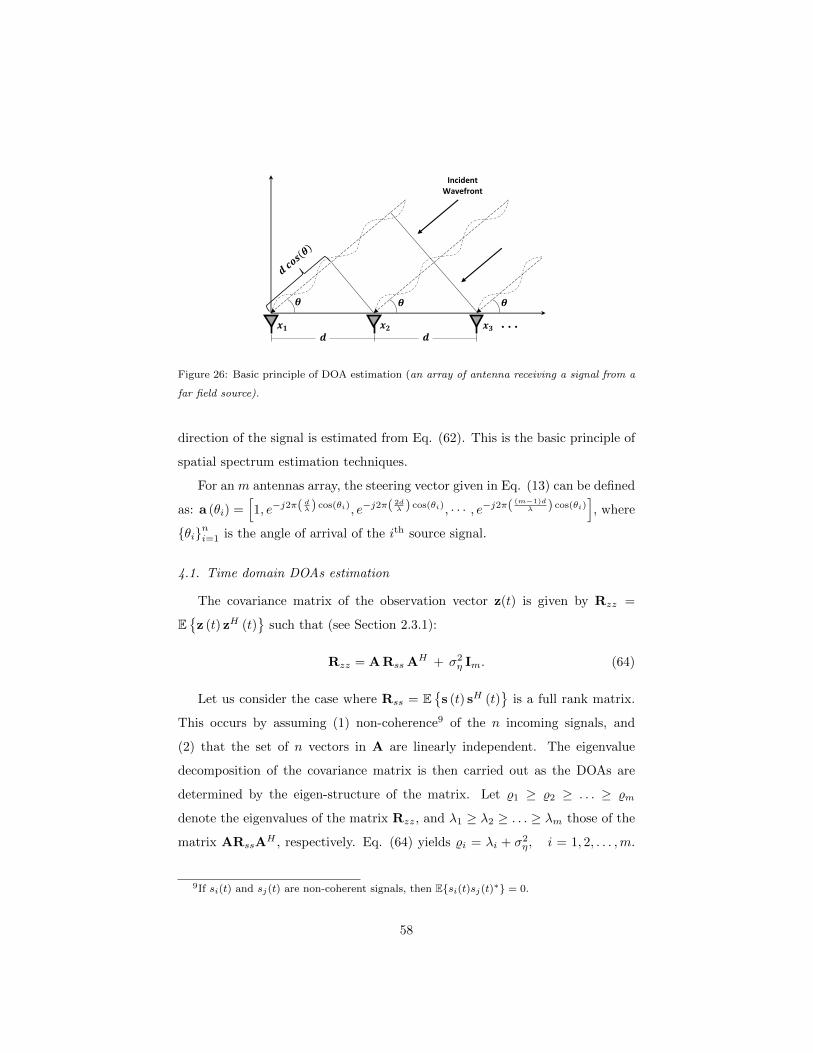
𝒅 𝒅
𝜽 𝜽 𝜽
. . .
Incident Wavefront
𝒙𝟏 𝒙𝟐 𝒙𝟑
Figure 26: Basic principle of DOA estimation (an array of antenna receiving a signal from a
far field source).
direction of the signal is estimated from Eq. (62). This is the basic principle of
spatial spectrum estimation techniques.
For an m antennas array, the steering vector given in Eq. (13) can be defined
as: a (θi) =[1, e−j2π( dλ ) cos(θi), e−j2π( 2d
λ ) cos(θi), · · · , e−j2π( (m−1)dλ ) cos(θi)
], where
θini=1 is the angle of arrival of the ith source signal.
4.1. Time domain DOAs estimation
The covariance matrix of the observation vector z(t) is given by Rzz =
Ez (t) zH (t)
such that (see Section 2.3.1):
Rzz = A Rss AH + σ2η Im. (64)
Let us consider the case where Rss = Es (t) sH (t)
is a full rank matrix.
This occurs by assuming (1) non-coherence9 of the n incoming signals, and
(2) that the set of n vectors in A are linearly independent. The eigenvalue
decomposition of the covariance matrix is then carried out as the DOAs are
determined by the eigen-structure of the matrix. Let %1 ≥ %2 ≥ . . . ≥ %m
denote the eigenvalues of the matrix Rzz, and λ1 ≥ λ2 ≥ . . . ≥ λm those of the
matrix ARssAH , respectively. Eq. (64) yields %i = λi + σ2
η, i = 1, 2, . . . ,m.
9If si(t) and sj(t) are non-coherent signals, then Esi(t)sj(t)∗ = 0.
58
Since, the matrix A is full column rank n, the (m− n) smallest eigenvalues of
Rzz equal σ2η:
%i =
λi + σ2η i = 1, 2, . . . , n,
σ2η i = n+ 1, n+ 2, . . . ,m.
(65)
The eigenvalue decomposition of the covariance matrix Rzz then reduces to:
Rzz =
n∑i=1
(λi + σ2
η
)viv
Hi +
m∑i=n+1
σ2ηviv
Hi , (66)
where vHi vj = δi,j are the orthogonal eigenvectors of the matrix Rzz (i.e.,
Rzzvi = %ivi for i = 1, 2, . . . ,m). Eq.(66) will then simplify to Rzzvi =
σ2ηvi, i = n+ 1, n+ 2, . . . ,m or, equivalently,
(Rzz − σ2
ηIm)vi = 0, i = n+ 1, n+ 2, . . . ,m. (67)
Eq.(64) can be rewritten as Rzz − σ2ηIm = ARssA
H ; Eq.(67) then becomes:
ARssAHvi = 0, i = n+ 1, n+ 2, . . . ,m, which yields:
AHvi = 0, i = n+ 1, n+ 2, . . . ,m. (68)
Eq.(68) shows that the subspace spanned by the eigenvectors
vn+1,vn+2, . . . ,vm is orthogonal to the complement subspace spanned
by the steering vectors in matrix A. Therefore, from the eigenvectors of Rzz,
one can obtain the signal DOAs by finding those steering vectors that are
orthogonal to the noise subspace.
4.1.1. Time Domain MUSIC Algorithm
Spectral-based DOA estimation methods are based on maximizing the power
of signal projected on the signal subspace. One of the standard DOA techniques,
MUSIC (Multiple SIgnal Classification) [56], performs an eigenvalue decompo-
sition of the unknown covariance matrix Rzz estimated as:
Rzz =1
T
∫ T
0
z (τ) zH (τ) dτ, (69)
59
where T is the signal duration. Let use express the eigenvector estimates as
v1, v2, . . . , vm such that the singular value decomposition of Rzz is given by:
Rzz = V Λ VH , (70)
with V = [v1, v2, . . . , vm]. Using Eq.(68), MUSIC then estimates the signal
directions as the peaks of the spatial spectrum estimate expressed by [55]:
PMUSIC (θ) =1
m∑i=n+1
|a (θ) vi|2, (71)
where a (θ) is a column vector of the steering matrix defined by Eq.(13). The
MUSIC spectrum is estimated from a single realization of the random process
represented by the observations z (t) for t = 1, 2, . . . , T . MUSIC estimates were
shown to be consistent and they converge to the true source bearings as the
number of observations increases to infinity [57].
4.1.2. Time Domain ESPRIT Algorithm
ESPRIT stands for Estimation of Signal Parameters via Rotational Invari-
ance Techniques [58, 54]. The aim of the ESPRIT algorithm is to exploit the
rotational invariance in the signal subspace which is created by two arrays with
a translational invariance structure. ESPRIT inherently assumes narrowband
signals so as to know the translational phase relationship between the multi-
ple arrays to be used. The ESPRIT algorithm is more robust with respect to
array imperfections than MUSIC [59, 60]. Computation complexity and stor-
age requirements are lower than MUSIC as it does not perform an extensive
search throughout all possible steering vectors [54]. The ESPRIT algorithm is
summarized as follows:
• Estimate the correlation matrix Rzz by using Eq. (69) and compute its
eigendecomposition in order to get the eigenvector v1, v2, . . . , vm.
• From the n principal eigenvectors v1, v2, . . . , vn, representing the signal
subspace, form the matrix Vs = [v1, v2, . . . , vn]. Then, from the matrix
60
Vs form the matrices V1 and V2 such that:
Vs =
V1
last row
=
first row
V2
. (72)
• Solve in a least square sense the relation V2 = V1Ψ in order to estimate
the matrix Ψ.
• Find the eigenvalues ψ1, ψ2, . . . , ψn of the matrix Ψ. Then, DOA esti-
mates are obtained by [55]:
θi = arccos
(jλ logψi
2πd
)(73)
4.2. Time-frequency DOAs estimation
4.2.1. Time-Frequency MUSIC Algorithm
As noted in Section 2.3.1, the linear model given in Eq. (21) has the same
structure as the covariance matrix based on the linear model given in Eq. (64).
This similarity suggests that the MUSIC algorithm can be simply extended
for direction finding using the subspace decomposition of an averaged MTFD
matrix. The steps needed to find the averaged MTFD matrix ρzz are given
in Table 1. After estimating the averaged MTFD matrix ρzz, TF-MUSIC can
therefore simply extend Eq.(71) to get:
PTF-MUSIC (θ) =1
M∑i=n+1
|a (θ) vTFi |2
, (77)
where vTFi is the ith eigenvector of the averaged MTFD matrix ρzz. A differ-
ence between the averaged MTFD matrix ρzz and the sample covariance Rzz is
that the former is obtained by averaging selected high signal energy points by
rejecting noise contributions while the later is obtained by averaging all avail-
able points including noise contributions. Hence, the averaged MTFD matrix
ρzz based directional estimation technique PTF-MUSIC (θ) is expected to im-
prove performance. In addition, the TF approach allows the estimation of the
covariance matrix of each source separately (e.g. by using a multi-component IF
61
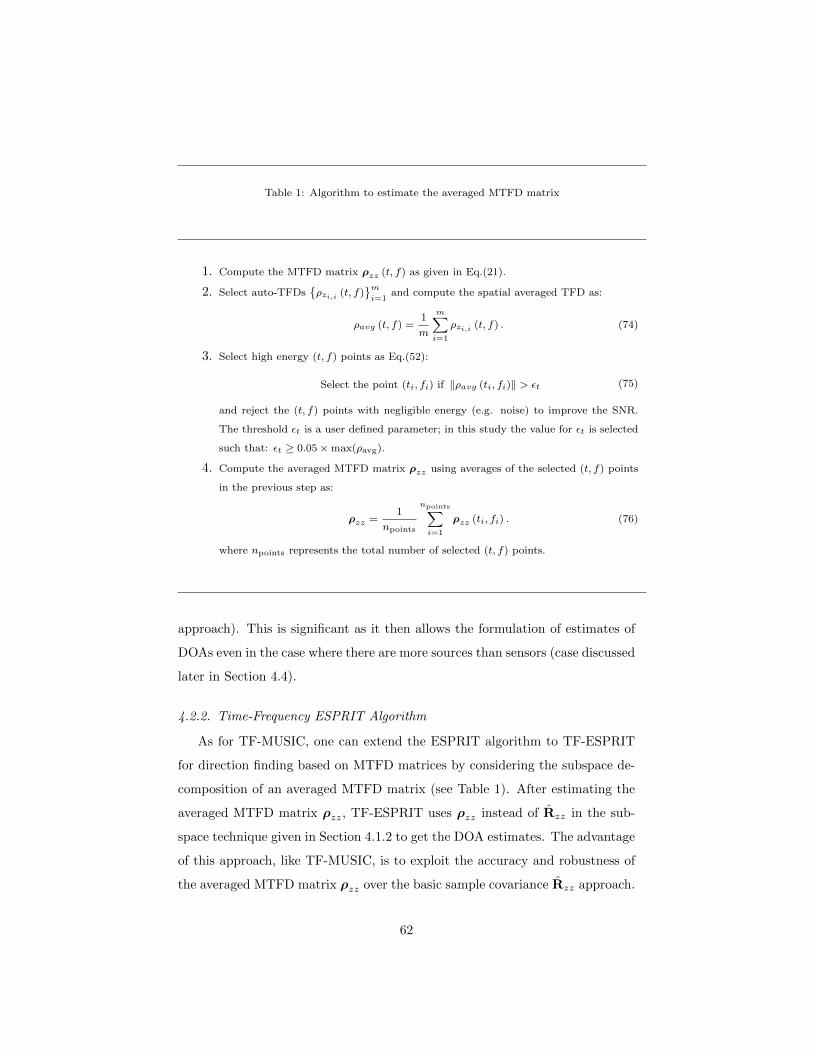
Table 1: Algorithm to estimate the averaged MTFD matrix
1. Compute the MTFD matrix ρzz (t, f) as given in Eq.(21).
2. Select auto-TFDsρzi,i (t, f)
mi=1
and compute the spatial averaged TFD as:
ρavg (t, f) =1
m
m∑i=1
ρzi,i (t, f) . (74)
3. Select high energy (t, f) points as Eq.(52):
Select the point (ti, fi) if ‖ρavg (ti, fi)‖ > εt (75)
and reject the (t, f) points with negligible energy (e.g. noise) to improve the SNR.
The threshold εt is a user defined parameter; in this study the value for εt is selected
such that: εt ≥ 0.05×max(ρavg).
4. Compute the averaged MTFD matrix ρzz using averages of the selected (t, f) points
in the previous step as:
ρzz =1
npoints
npoints∑i=1
ρzz (ti, fi) . (76)
where npoints represents the total number of selected (t, f) points.
approach). This is significant as it then allows the formulation of estimates of
DOAs even in the case where there are more sources than sensors (case discussed
later in Section 4.4).
4.2.2. Time-Frequency ESPRIT Algorithm
As for TF-MUSIC, one can extend the ESPRIT algorithm to TF-ESPRIT
for direction finding based on MTFD matrices by considering the subspace de-
composition of an averaged MTFD matrix (see Table 1). After estimating the
averaged MTFD matrix ρzz, TF-ESPRIT uses ρzz instead of Rzz in the sub-
space technique given in Section 4.1.2 to get the DOA estimates. The advantage
of this approach, like TF-MUSIC, is to exploit the accuracy and robustness of
the averaged MTFD matrix ρzz over the basic sample covariance Rzz approach.
62
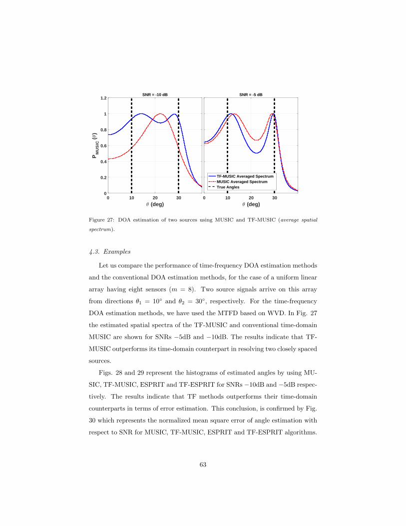
0 10 20 30
3 (deg)
0
0.2
0.4
0.6
0.8
1
1.2P
MU
SIC
(3
)SNR = -10 dB
0 10 20 30
3 (deg)
SNR = -5 dB
TF-MUSIC Averaged SpectrumMUSIC Averaged SpectrumTrue Angles
Figure 27: DOA estimation of two sources using MUSIC and TF-MUSIC (average spatial
spectrum).
4.3. Examples
Let us compare the performance of time-frequency DOA estimation methods
and the conventional DOA estimation methods, for the case of a uniform linear
array having eight sensors (m = 8). Two source signals arrive on this array
from directions θ1 = 10 and θ2 = 30, respectively. For the time-frequency
DOA estimation methods, we have used the MTFD based on WVD. In Fig. 27
the estimated spatial spectra of the TF-MUSIC and conventional time-domain
MUSIC are shown for SNRs −5dB and −10dB. The results indicate that TF-
MUSIC outperforms its time-domain counterpart in resolving two closely spaced
sources.
Figs. 28 and 29 represent the histograms of estimated angles by using MU-
SIC, TF-MUSIC, ESPRIT and TF-ESPRIT for SNRs −10dB and −5dB respec-
tively. The results indicate that TF methods outperforms their time-domain
counterparts in terms of error estimation. This conclusion, is confirmed by Fig.
30 which represents the normalized mean square error of angle estimation with
respect to SNR for MUSIC, TF-MUSIC, ESPRIT and TF-ESPRIT algorithms.
63
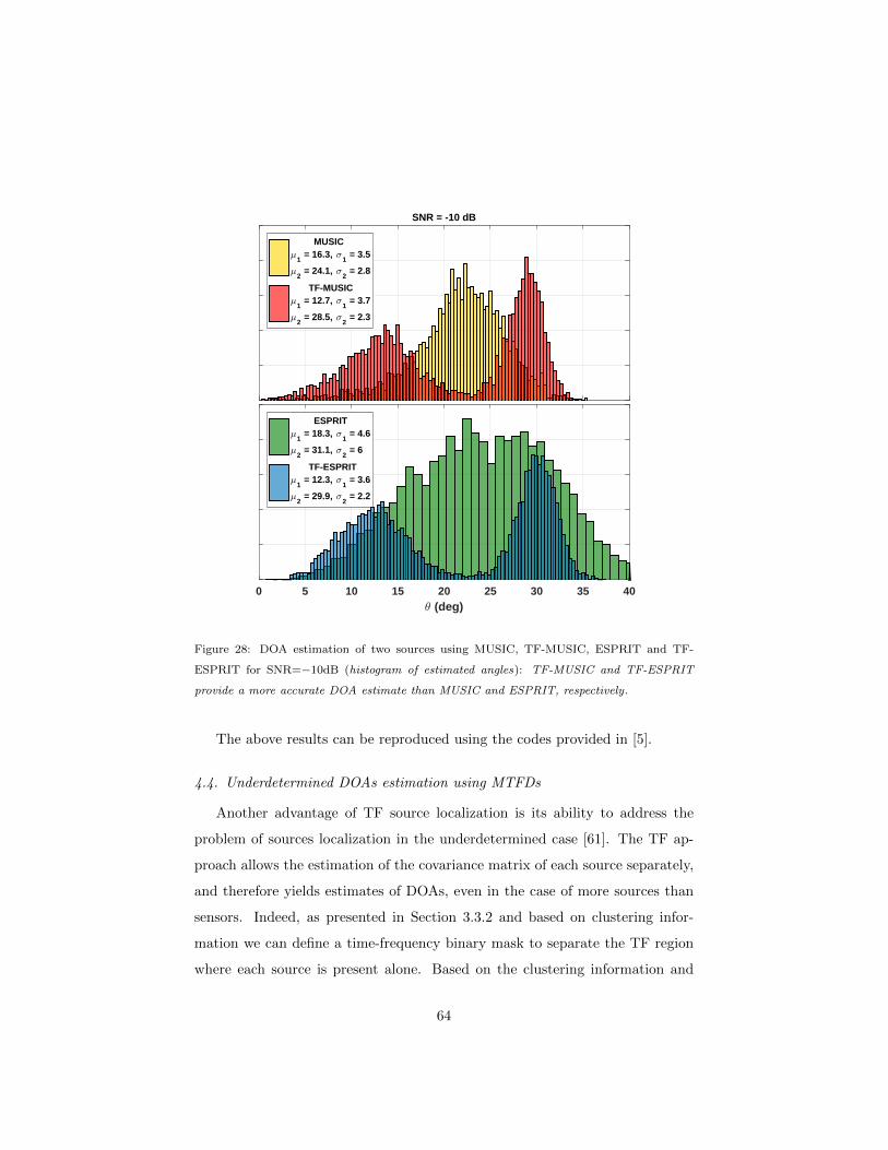
SNR = -10 dB
MUSIC7
1 = 16.3, <
1 = 3.5
72 = 24.1, <
2 = 2.8
TF-MUSIC7
1 = 12.7, <
1 = 3.7
72 = 28.5, <
2 = 2.3
0 5 10 15 20 25 30 35 403 (deg)
ESPRIT7
1 = 18.3, <
1 = 4.6
72 = 31.1, <
2 = 6
TF-ESPRIT7
1 = 12.3, <
1 = 3.6
72 = 29.9, <
2 = 2.2
Figure 28: DOA estimation of two sources using MUSIC, TF-MUSIC, ESPRIT and TF-
ESPRIT for SNR=−10dB (histogram of estimated angles): TF-MUSIC and TF-ESPRIT
provide a more accurate DOA estimate than MUSIC and ESPRIT, respectively.
The above results can be reproduced using the codes provided in [5].
4.4. Underdetermined DOAs estimation using MTFDs
Another advantage of TF source localization is its ability to address the
problem of sources localization in the underdetermined case [61]. The TF ap-
proach allows the estimation of the covariance matrix of each source separately,
and therefore yields estimates of DOAs, even in the case of more sources than
sensors. Indeed, as presented in Section 3.3.2 and based on clustering infor-
mation we can define a time-frequency binary mask to separate the TF region
where each source is present alone. Based on the clustering information and
64
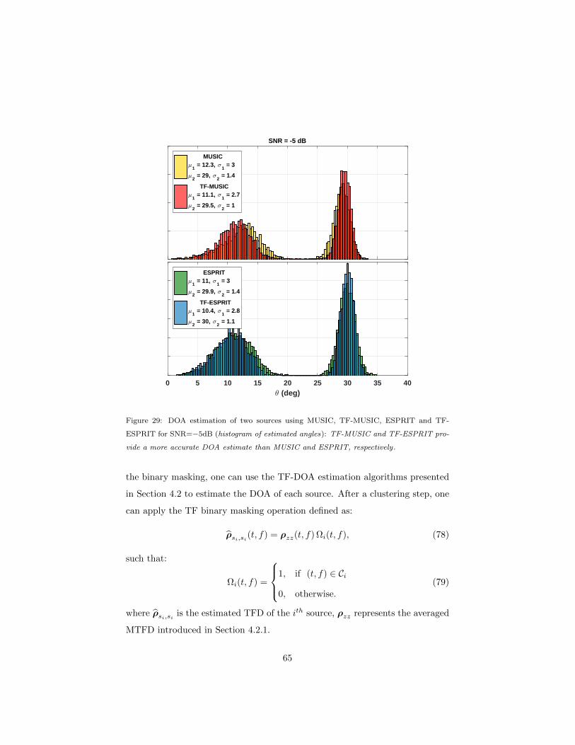
SNR = -5 dB
MUSIC7
1 = 12.3, <
1 = 3
72 = 29, <
2 = 1.4
TF-MUSIC7
1 = 11.1, <
1 = 2.7
72 = 29.5, <
2 = 1
0 5 10 15 20 25 30 35 403 (deg)
ESPRIT7
1 = 11, <
1 = 3
72 = 29.9, <
2 = 1.4
TF-ESPRIT7
1 = 10.4, <
1 = 2.8
72 = 30, <
2 = 1.1
Figure 29: DOA estimation of two sources using MUSIC, TF-MUSIC, ESPRIT and TF-
ESPRIT for SNR=−5dB (histogram of estimated angles): TF-MUSIC and TF-ESPRIT pro-
vide a more accurate DOA estimate than MUSIC and ESPRIT, respectively.
the binary masking, one can use the TF-DOA estimation algorithms presented
in Section 4.2 to estimate the DOA of each source. After a clustering step, one
can apply the TF binary masking operation defined as:
ρsi,si(t, f) = ρzz(t, f) Ωi(t, f), (78)
such that:
Ωi(t, f) =
1, if (t, f) ∈ Ci
0, otherwise.
(79)
where ρsi,si is the estimated TFD of the ith source, ρzz represents the averaged
MTFD introduced in Section 4.2.1.
65
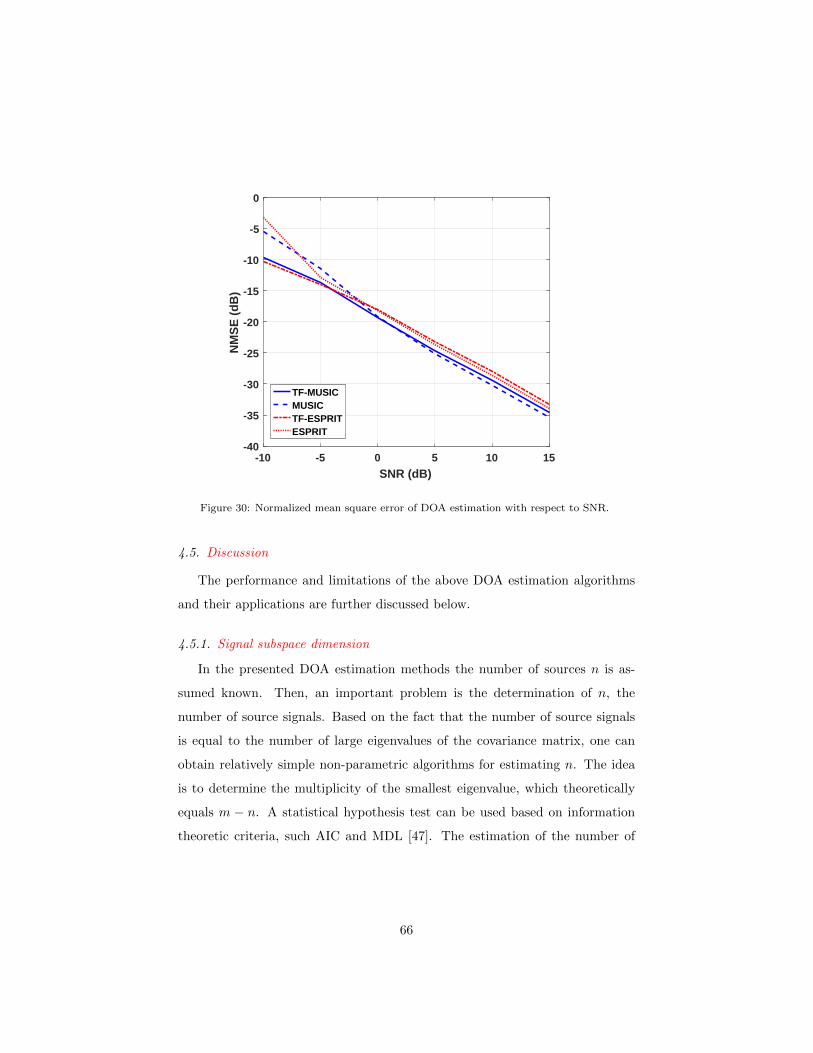
-10 -5 0 5 10 15
SNR (dB)
-40
-35
-30
-25
-20
-15
-10
-5
0
NM
SE
(d
B)
TF-MUSICMUSICTF-ESPRITESPRIT
Figure 30: Normalized mean square error of DOA estimation with respect to SNR.
4.5. Discussion
The performance and limitations of the above DOA estimation algorithms
and their applications are further discussed below.
4.5.1. Signal subspace dimension
In the presented DOA estimation methods the number of sources n is as-
sumed known. Then, an important problem is the determination of n, the
number of source signals. Based on the fact that the number of source signals
is equal to the number of large eigenvalues of the covariance matrix, one can
obtain relatively simple non-parametric algorithms for estimating n. The idea
is to determine the multiplicity of the smallest eigenvalue, which theoretically
equals m − n. A statistical hypothesis test can be used based on information
theoretic criteria, such AIC and MDL [47]. The estimation of the number of
66
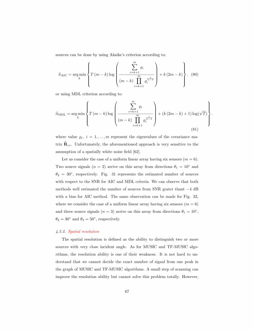
sources can be done by using Akaike’s criterion according to:
nAIC = arg mink
T (m− k) log
m∑
i=k+1
%i
(m− k)
m∏i=k+1
%1
m−ki
+ k (2m− k)
. (80)
or using MDL criterion according to:
nMDL = arg mink
T (m− k) log
m∑
i=k+1
%i
(m− k)
m∏i=k+1
%1
m−ki
+ (k (2m− k) + 1) log(√T )
.
(81)
where value %i, i = 1, . . . ,m represent the eigenvalues of the covariance ma-
trix Rzz. Unfortunately, the aforementioned approach is very sensitive to the
assumption of a spatially white noise field [62].
Let us consider the case of a uniform linear array having six sensors (m = 6).
Two source signals (n = 2) arrive on this array from directions θ1 = 10 and
θ2 = 30, respectively. Fig. 31 represents the estimated number of sources
with respect to the SNR for AIC and MDL criteria. We can observe that both
methods well estimated the number of sources from SNR grater thant −4 dB
with a bias for AIC method. The same observation can be made for Fig. 32,
where we consider the case of a uniform linear array having six sensors (m = 6)
and three source signals (n = 3) arrive on this array from directions θ1 = 10,
θ2 = 30 and θ3 = 50, respectively.
4.5.2. Spatial resolution
The spatial resolution is defined as the ability to distinguish two or more
sources with very close incident angle. As for MUSIC and TF-MUSIC algo-
rithms, the resolution ability is one of their weakness. It is not hard to un-
derstand that we cannot decide the exact number of signal from one peak in
the graph of MUSIC and TF-MUSIC algorithms. A small step of scanning can
improve the resolution ability but cannot solve this problem totally. However,
67
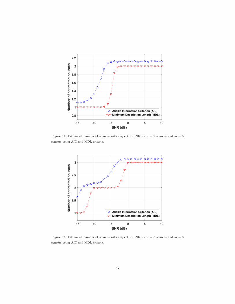
-15 -10 -5 0 5 10
SNR (dB)
0.8
1
1.2
1.4
1.6
1.8
2
2.2
Nu
mb
er
of
es
tim
ate
d s
ou
rce
s
Akaike Information Criterion (AIC)
Minimum Description Length (MDL)
Figure 31: Estimated number of sources with respect to SNR for n = 2 sources and m = 6
sensors using AIC and MDL criteria.
-15 -10 -5 0 5 10
SNR (dB)
1
1.5
2
2.5
3
Nu
mb
er
of
es
tim
ate
d s
ou
rce
s
Akaike Information Criterion (AIC)
Minimum Description Length (MDL)
Figure 32: Estimated number of sources with respect to SNR for n = 3 sources and m = 6
sensors using AIC and MDL criteria.
68
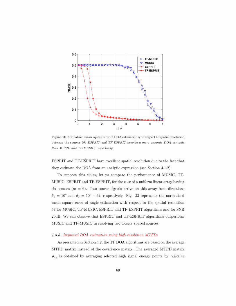
0 1 2 3 4 5 6 7
δ θ
0
0.1
0.2
0.3
0.4
0.5
0.6
NM
SE
TF-MUSIC
MUSIC
ESPRIT
TF-ESPRIT
Figure 33: Normalized mean square error of DOA estimation with respect to spatial resolution
between the sources δθ: ESPRIT and TF-ESPRIT provide a more accurate DOA estimate
than MUSIC and TF-MUSIC, respectively.
ESPRIT and TF-ESPRIT have excellent spatial resolution due to the fact that
they estimate the DOA from an analytic expression (see Section 4.1.2).
To support this claim, let us compare the performance of MUSIC, TF-
MUSIC, ESPRIT and TF-ESPRIT, for the case of a uniform linear array having
six sensors (m = 6). Two source signals arrive on this array from directions
θ1 = 10 and θ2 = 10 + δθ, respectively. Fig. 33 represents the normalized
mean square error of angle estimation with respect to the spatial resolution
δθ for MUSIC, TF-MUSIC, ESPRIT and TF-ESPRIT algorithms and for SNR
20dB. We can observe that ESPRIT and TF-ESPRIT algorithms outperform
MUSIC and TF-MUSIC in resolving two closely spaced sources.
4.5.3. Improved DOA estimation using high-resolution MTFDs
As presented in Section 4.2, the TF DOA algorithms are based on the average
MTFD matrix instead of the covariance matrix. The averaged MTFD matrix
ρzz is obtained by averaging selected high signal energy points by rejecting
69
noise contributions. However, in the case where the received signal presents
high cross-terms, the averaged MTFD matrix ρzz can be disturbed by these
cross-terms and then degrade the performance of DOA estimations. Therefore,
in order to improve the robustness against cross-terms of TF DOA algorithms,
we can use the hight resolution TFDs introduced in Section 2.3.2 instead of
MWVD. Indeed, the high resolution TFDs provide a good compromise between
resolution and cross-terms reduction which improve the robustness of TF DOA
algorithms against cross-terms.
To support this claim, let us compare the performance of the conventional
MUSIC algorithm, TF-MUSIC algorithm using different TFDs, for the case
of a uniform linear array having eight sensors (m = 4). Two source signals
arrive on this array from directions θ1 = −5 and θ2 = 5, respectively. For
the TF-MUSIC algorithm, we have used the MTFD based on WVD and MDD
respectively. In Fig. ??a the estimated spatial spectra of the TF-MUSIC based
on MDD is shown, while Fig. ??b shows the estimated spatial spectra of the for
conventional MUSIC (red) and TF-MUSIC based on the MWVD (black). The
results indicate that, when the SNR is set to -10 dB both standard TF-MUSIC
based on the MWVD and conventional MUSIC fail to estimate the 2 angles
accurately (see Fig. ??b), while the TF-MUSIC based on MDD gives sharp
peaks at the incident angles as shown in Fig. ??a. In the second experiment,
keeping the same setup with an SNR of 10 dB, all the algorithms appear to give
sharp peaks at estimated incident angles as illustrated in Fig. ??c for the TF-
MUSIC based on MDD and Fig. ??d for the TF-MUSIC based on the MWVD
and conventional MUSIC algorithms.
5. Cross Channel Causality Analysis
5.0. Background and motivation
Previous sections have shown that by combining array signal processing for
non-stationary signals and multichannel high resolution time-frequency signal
processing methods, one can enhance the performance of several standard meth-
70
ods and techniques (such as BSS and DOA estimation) for a wide field of appli-
cations by simultaneously taking into account (1) the non-stationary character-
istics of measured signals using TFDs and (2) the spatial information provided
by an array of measuring sensors.
In addition to such improvements, another key capability of the MTFSP
approach is to allow a signal causality analysis across sensors/channels and/or
signals; new information is then gained e.g. by tracking the time varying location
of moving sources propagating through the system. Combining spatial and time-
frequency information obtained by a multisensor array results then in improved
precision. Examples are:
(1) in brain studies, the concept of cross channel causality can be used to
characterize the propagation of a seizure location across EEG channels, therefore
providing a key information about the time-varying information flow scalp [26];
(2) In wireless communication, it characterizes the varying spatial location
of a moving user (mobile) in cell by exploiting the multi-antenna array of the
base station;
(3) In aeronautics, a primary design goal for helicopter engineers is to uti-
lize vibrations measured from a multichannel system to identify the excitation
sources or faults of a rotating system [63].
5.1. Cross-channel causality and phase synchrony
The cross channel causality describes the dependence relationship between
multichannel signals. This dependence can be quantified using various ap-
proaches, from simple linear correlation to more advanced TF based approaches.
Cross-correlation between two zero mean signals xi(t) and xj(t) under the weak-
sense stationarity assumption is defined as:
rij(τ) =Exi(t)xj(t+ τ)∗
√Exi(t)2
Exj(t+ τ)2
such that − 1 ≤ rij(τ) ≤ 1. (82)
The cross-correlation is typically utilized to assess the linear relationship be-
tween different signals; however, a simple correlation coefficient at the zeroth
71
lag is limited in its ability to assess the interactions of these signals, as it can
only quantify the linear relationships and capture mostly the amplitude-based
relationships.
Another useful measure between multichannel signals is the coherence func-
tion defined as:
Cij(f) =Sij(f)√Sii(f)Sjj(f)
such that 0 ≤ |Cij(f)| ≤ 1. (83)
where Sij(f) is the cross-spectral density between xi(t) and xj(t) given by:
Sij(f) = Fτ→f
Exi(t)xj(t+ τ)∗
(84)
and Sii(f) and Sjj(f) the auto-spectral density of xi(t) and xj(t) respectively.
The coherence function provides a measure that quantifies linear relationships
in the frequency domain between two wide sense stationary signals [64, 65]. The
magnitude squared coherence function measures the degree to which one signal
can be represented as the output of a linear filter operating on the other signal
and varies from 0 for two statistically independent signals to 1, when one signal is
the result of linear filtering performed on the other. The coherence function finds
many useful applications but the results based on coherence depend on several
factors like stationarity of the signal, segment length, number of segments, etc.
[66]. A short but broad review that includes linear as well as non-linear measures
is given in [67, 68].
In order to mitigate these limitations and address the analysis of non-
stationary signal, phase synchrony analysis can be used [69]. Phase synchrony
analysis is a useful measure of linear dependence between multichannel signals.
This approach is based on the concept of phase synchronization of chaotic os-
cillators [70, 71]. The phase synchrony (coefficient) takes on values between 0,
for two signals at different frequencies, and 1, for signals that exhibit a constant
difference in instantaneous phase (representing the situation where a signal and
its time-shifted version are observed). So, phase synchrony refers to the inter-
dependence between the instantaneous phases of two signals; the instantaneous
72
phases may be strongly synchronized even when the amplitudes of the two sig-
nals are statistically independent [70, 71].
The degree of synchrony between two signals is usually assessed via esti-
mation of instantaneous phase around a particular frequency, which is usually
accomplished via the Hilbert transform such that [72]:
ϕ(t) = arg [z(t)] = arg [x (t) + jHx (t)] (85)
Then, in the case of non-stationary signals, TF methods become naturally more
suitable for the calculation of synchrony between two signals [73, 74]. Several
approaches exist. A Morlet wavelet-based method was used in [75], but here for
continuity with above sections, we present a recently proposed method based
on quadratic TFDs [73] [1, Section 16.4].
5.1.1. Phase synchrony estimation using a complex TFD
Let us consider the QTFD of a signal based on the reduced-interference
Rihaczek TFD, defined for a monosensor signal z(t) as:
ρz(t, f) =
∫ ∫R2
e−ν2τ2
σ e−jπντAz(ν, τ) e−j2π(fτ−νt) dνdτ (86)
where Az(ν, τ) is the ambiguity function defined in Section 2.3.2 and given by:
Az (ν, τ) =
∫Rz(t+
τ
2
)z∗(t− τ
2
)e−j2πνtdt (87)
The factor e−jπντ is the kernel for the Rihaczek distribution, and e−ν2τ2
σ is an
exponential kernel used to reduce the effect of the cross-terms. Other kernels
can be used as long as they remove the cross-terms in the Rihaczek amplitude
spectrum.
Therefore, by extending the previous formulation of Rihaczek distributions,
the Rihaczek MTFD for the signal vector z(t) can be defined as:
ρzz(t, f) = Fτ→f
F−1
ν→t
g(ν, τ)Azz(ν, τ)
, (88)
where Azz(ν, τ) is the spatial ambiguity function defined by Eq.(26) and g(ν, τ)
is the Doppler-lag kernel defined by:
g(ν, τ) = e−ν2τ2
σ e−jπντ (89)
73
Since the TFD localizes spectral components in the (t, f) domain, the cross
correlation of specific events on two spatially separated TFDs gives the phase
difference and hence the phase synchrony can be estimated. The amplitude of
the cross TFD indicates coincident or partly overlapped signals. The phase of
the cross TFD at local maxima indicates the phase difference between them.
The phase of the TFD product of two signals zi(t) and zj(t) is then defined as
follows [73] [1, Section 16.4]:
ϕij(t, f) = arg[ρzi,zi(t, f)ρ∗zj,zj (t, f)
](90)
Based on the estimate of a time-varying phase spectrum as shown above, a syn-
chrony measure still needs to be defined. For this, the phase-locking value (PLV)
is considered. The PLV between two signals, averaged across realizations/trials,
can be defined as [73]:
Pij(t, f) =1
Tr
∣∣∣∣∣Tr∑k=1
ej ϕ(k)ij (t,f)
∣∣∣∣∣ (91)
where Pij(t, f) is the ijth element of the matrix P(t, f), Tr is the number of tri-
als/realizations, and ϕ(k)ij (t, f) is the time-varying phase estimate between zi(t)
and zj(t) for the kth trial. The PLV measures the intertrial/interrealization vari-
ations of phase differences at time t and frequency f . A PLV close to 1 indicates
a small phase difference across trials/realizations. For a single trial, a so-called
single-trial PLV is calculated, denoting the consistency of the phase across time.
Lastly, the described phase synchrony measure assesses the instantaneous phase
differences between signals in the (t, f) domain using the complex Rihaczek dis-
tribution [76]. In some applications, such as biomedical signal processing, one
would expect to have a ”number” which shows whether the channels are syn-
chronized. Then, based on the PLV definition, the channel synchronization can
be quantified by using the mean value over time and frequency, such that:
Pij =1
CardΩ
∣∣∣∣∣∣∑
(t,f)∈Ω
ej ϕij(t,f)
∣∣∣∣∣∣ , (92)
where Pij is the ijth element of the mean PLV matrix P which quantifies the
synchronization between the ith and the jth sensors.
74
5.1.2. Phase synchrony estimation using MTFDs
The above derivation shows that we can use the cross spectral property to
estimate the PLV between two signals as a function of t and f . Therefore, a
similar attempt can be made by taking advantage of MTFDs definition and
using the cross TFD terms to define the phase of the cross TFD as:
ϕij(t, f) = arg[ρzi,zj (t, f)2
](93)
This definition, calculates the phase of the square of cross TFD in order to
remain homogeneous with respect to the phase definition given by Eq. (90)
and to avoid the sign indeterminacy in the real case. Then, the PLV can be
estimated from this new definition of phase of cross TFD and following the
definition given in Eq. (91).
The method of a time-varying phase estimation presented in Eq. (90) re-
quires the use of the Rihaczek distribution, due to the fact that the Rihaczek
distribution is a complex distribution. However, one of the disadvantages of the
Rihaczek distribution is the existence of cross-terms for multicomponent signals.
These cross-terms are located at the same time and frequency locations as the
original signals and will lead to biased energy and phase estimates. To get rid
of these cross-terms a reduced interference version of the Rihaczek distribution
is used in Eq. (86) by applying a kernel function to filter the cross-terms in
the ambiguity domain. On the other hand, the method of a time-varying phase
estimation presented in Eq. (93) allows us to exploit the whole class of TFDs
which is the fact that the cross TFDs are intrinsically complex and convey a
phase information. Therefore, this time-varying phase estimation method en-
ables to choose the best TFD according to the used signals in order to optimize
the trade-off between cross-terms reduction and resolution.
In order to assess the behaviour of phase synchrony and PLV, let consider a
simple case of two phase locked signals zi(t) and zj(t) such that zj(t) = zi(t) ejφ.
In this case, one can observe that ρzi,zi(t, f) = ρzj,zj (t, f). Then, the phase of
the TFD product of the two signals zi(t) and zj(t) define in Eq. (90) will be:
ϕij(t, f) = arg[ρzi,zi(t, f)ρ∗zj,zj (t, f)
]= 0
75
Therefore, the PLV defined by Eq. (92) tends to 1 which is consistent under
phase locked signal assumption. In other hand, the cross TFD of zi(t) and zj(t)
can be expressed as:
ρzi,zj (t, f) = ρzi,zi(t, f) e−jφ
Then, knowing that ρzi,zi(t, f) is real, the phase of cross TFD defined in Eq.
(93) is given by:
ϕij(t, f) = arg[ρzi,zj (t, f)2
]= −2φ
In the same way the resulting PLV also tends to 110. One can conclude that
the two methods of time-varying phase estimation lead to the same theoretical
behavior of the PLV for the phase locked signals. However, the method defined
by Eq. (93) makes it possible to extract additional information on the phase
shift of the two signals where the method defined by Eq. (90) is invariant with
respect to the phase shift.
5.2. Illustrative examples
This simulation uses a forward model11 generated from an atlas of neonatal
MRI data. The relevant surfaces, a 3D cortex mesh, and the coregistration of
the Electrical Geodesics, Inc (EGI) hydrocell caps orientation on the infants
head are generated by using the MATLAB software, Brainstorm [77, 78]. Once
these surfaces are generated, OpenMEEG is then used to generate the lead-field
matrix from this model [79, 80]. A simulator then takes the lead-field matrix and
generates virtual sources centered on a single cortical volume. To do so, a virtual
source signal is given, along with a cortical volume and dipole orientation for
m = 64 electrodes. The signal is then propagated through the lead-field matrix,
and additive noise is included. To establish brain connectivity matrices, the
definitions given by Eqs. (90) and (93) are used to calculate the time-varying
phase spectra and the corresponding PLV values for all EEG channels.
10By replacing ϕij(t, f) = −2φ for ∀(t, f) in Eq. (92) the PLV tends to 1.11The forward model is a conduction model describing how signals originating from partic-
ular locations within the brain traverse the tissues of the head and are received at the EEG
electrodes (see Section 6.1.1).
76
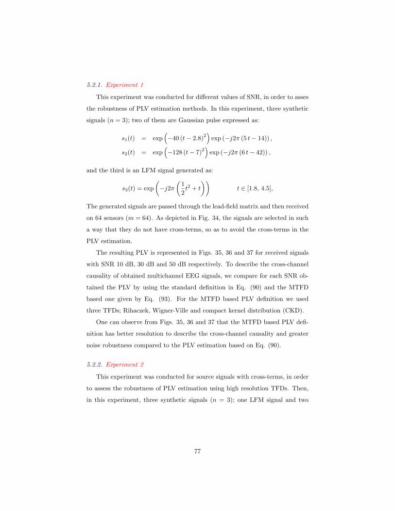
5.2.1. Experiment 1
This experiment was conducted for different values of SNR, in order to asses
the robustness of PLV estimation methods. In this experiment, three synthetic
signals (n = 3); two of them are Gaussian pulse expressed as:
s1(t) = exp(−40 (t− 2.8)
2)
exp (−j2π (5 t− 14)) ,
s2(t) = exp(−128 (t− 7)
2)
exp (−j2π (6 t− 42)) ,
and the third is an LFM signal generated as:
s3(t) = exp
(−j2π
(1
2t2 + t
))t ∈ [1.8, 4.5],
The generated signals are passed through the lead-field matrix and then received
on 64 sensors (m = 64). As depicted in Fig. 34, the signals are selected in such
a way that they do not have cross-terms, so as to avoid the cross-terms in the
PLV estimation.
The resulting PLV is represented in Figs. 35, 36 and 37 for received signals
with SNR 10 dB, 30 dB and 50 dB respectively. To describe the cross-channel
causality of obtained multichannel EEG signals, we compare for each SNR ob-
tained the PLV by using the standard definition in Eq. (90) and the MTFD
based one given by Eq. (93). For the MTFD based PLV definition we used
three TFDs; Rihaczek, Wigner-Ville and compact kernel distribution (CKD).
One can observe from Figs. 35, 36 and 37 that the MTFD based PLV defi-
nition has better resolution to describe the cross-channel causality and greater
noise robustness compared to the PLV estimation based on Eq. (90).
5.2.2. Experiment 2
This experiment was conducted for source signals with cross-terms, in order
to assess the robustness of PLV estimation using high resolution TFDs. Then,
in this experiment, three synthetic signals (n = 3); one LFM signal and two
77
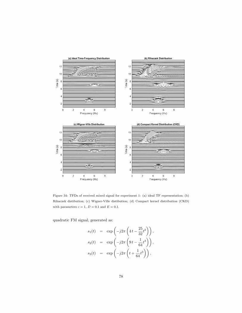
Figure 34: TFDs of received mixed signal for experiment 1: (a) ideal TF representation; (b)
Rihaczek distibution; (c) Wigner-Ville distibution; (d) Compact kernel distribution (CKD)
with parameters c = 1, D = 0.1 and E = 0.1.
quadratic FM signal, generated as:
s1(t) = exp
(−j2π
(4 t− 25
32t2))
,
s2(t) = exp
(−j2π
(9 t− 1
64t3))
,
s3(t) = exp
(−j2π
(t+
1
64t3))
,
78
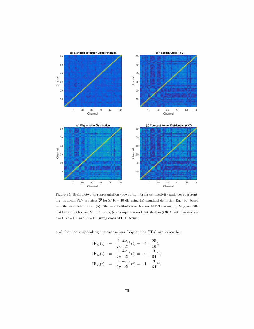
(a) Standard definition using Rihaczek
10 20 30 40 50 60
Channel
10
20
30
40
50
60C
ha
nn
el
(b) Rihaczek Cross TFD
10 20 30 40 50 60
Channel
10
20
30
40
50
60
Ch
an
ne
l
(c) Wigner-Ville Distribution
10 20 30 40 50 60
Channel
10
20
30
40
50
60
Ch
an
ne
l
(d) Compact Kernel Distribution (CKD)
10 20 30 40 50 60
Channel
10
20
30
40
50
60
Ch
an
ne
l
Figure 35: Brain networks representation (newborne): brain connectivity matrices represent-
ing the mean PLV matrices P for SNR = 10 dB using (a) standard definition Eq. (90) based
on Rihaczek distribution; (b) Rihaczek distibution with cross MTFD terms; (c) Wigner-Ville
distibution with cross MTFD terms; (d) Compact kernel distribution (CKD) with parameters
c = 1, D = 0.1 and E = 0.1 using cross MTFD terms.
and their corresponding instantaneous frequencies (IFs) are given by:
IFs1(t) =1
2π
dϕs1dt
(t) = −4 +25
16t,
IFs2(t) =1
2π
dϕs2dt
(t) = −9 +3
64t2,
IFs3(t) =1
2π
dϕs3dt
(t) = −1− 3
64t2,
79
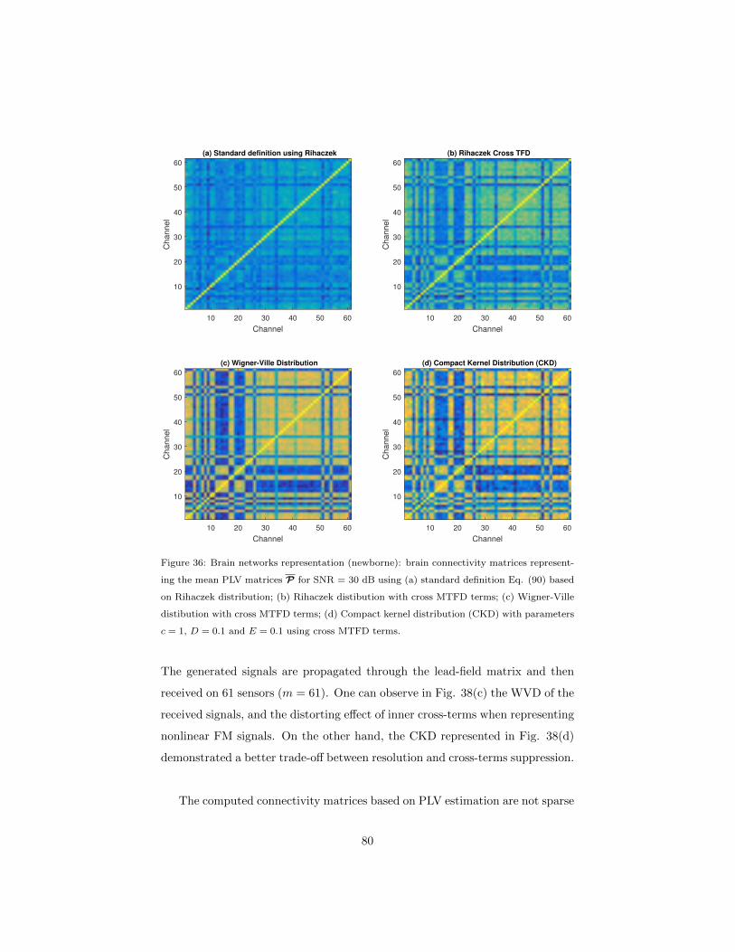
(a) Standard definition using Rihaczek
10 20 30 40 50 60
Channel
10
20
30
40
50
60C
ha
nn
el
(b) Rihaczek Cross TFD
10 20 30 40 50 60
Channel
10
20
30
40
50
60
Ch
an
ne
l
(c) Wigner-Ville Distribution
10 20 30 40 50 60
Channel
10
20
30
40
50
60
Ch
an
ne
l
(d) Compact Kernel Distribution (CKD)
10 20 30 40 50 60
Channel
10
20
30
40
50
60
Ch
an
ne
l
Figure 36: Brain networks representation (newborne): brain connectivity matrices represent-
ing the mean PLV matrices P for SNR = 30 dB using (a) standard definition Eq. (90) based
on Rihaczek distribution; (b) Rihaczek distibution with cross MTFD terms; (c) Wigner-Ville
distibution with cross MTFD terms; (d) Compact kernel distribution (CKD) with parameters
c = 1, D = 0.1 and E = 0.1 using cross MTFD terms.
The generated signals are propagated through the lead-field matrix and then
received on 61 sensors (m = 61). One can observe in Fig. 38(c) the WVD of the
received signals, and the distorting effect of inner cross-terms when representing
nonlinear FM signals. On the other hand, the CKD represented in Fig. 38(d)
demonstrated a better trade-off between resolution and cross-terms suppression.
The computed connectivity matrices based on PLV estimation are not sparse
80
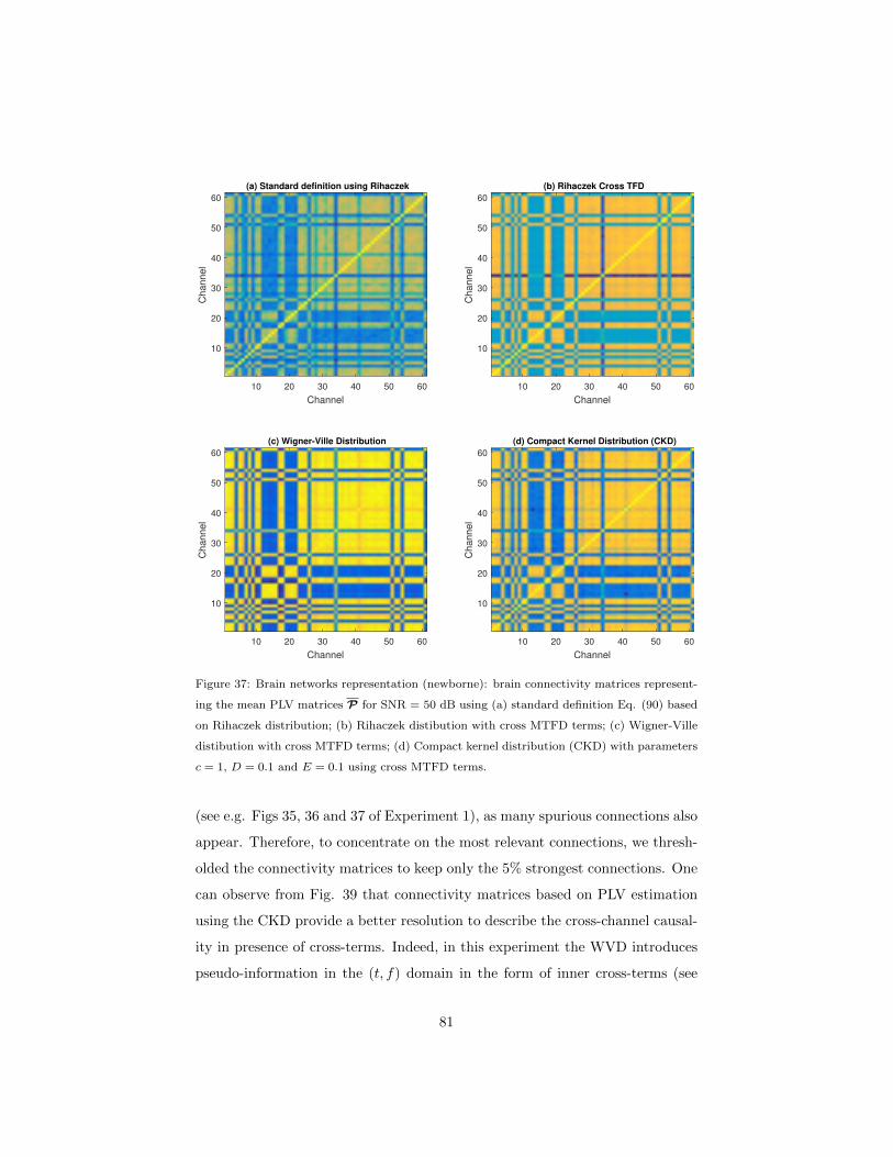
(a) Standard definition using Rihaczek
10 20 30 40 50 60
Channel
10
20
30
40
50
60C
ha
nn
el
(b) Rihaczek Cross TFD
10 20 30 40 50 60
Channel
10
20
30
40
50
60
Ch
an
ne
l
(c) Wigner-Ville Distribution
10 20 30 40 50 60
Channel
10
20
30
40
50
60
Ch
an
ne
l
(d) Compact Kernel Distribution (CKD)
10 20 30 40 50 60
Channel
10
20
30
40
50
60
Ch
an
ne
l
Figure 37: Brain networks representation (newborne): brain connectivity matrices represent-
ing the mean PLV matrices P for SNR = 50 dB using (a) standard definition Eq. (90) based
on Rihaczek distribution; (b) Rihaczek distibution with cross MTFD terms; (c) Wigner-Ville
distibution with cross MTFD terms; (d) Compact kernel distribution (CKD) with parameters
c = 1, D = 0.1 and E = 0.1 using cross MTFD terms.
(see e.g. Figs 35, 36 and 37 of Experiment 1), as many spurious connections also
appear. Therefore, to concentrate on the most relevant connections, we thresh-
olded the connectivity matrices to keep only the 5% strongest connections. One
can observe from Fig. 39 that connectivity matrices based on PLV estimation
using the CKD provide a better resolution to describe the cross-channel causal-
ity in presence of cross-terms. Indeed, in this experiment the WVD introduces
pseudo-information in the (t, f) domain in the form of inner cross-terms (see
81
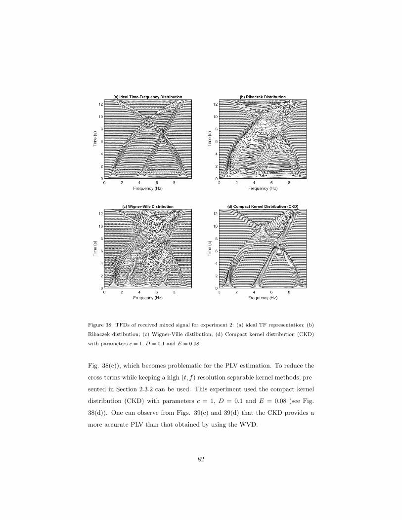
Figure 38: TFDs of received mixed signal for experiment 2: (a) ideal TF representation; (b)
Rihaczek distibution; (c) Wigner-Ville distibution; (d) Compact kernel distribution (CKD)
with parameters c = 1, D = 0.1 and E = 0.08.
Fig. 38(c)), which becomes problematic for the PLV estimation. To reduce the
cross-terms while keeping a high (t, f) resolution separable kernel methods, pre-
sented in Section 2.3.2 can be used. This experiment used the compact kernel
distribution (CKD) with parameters c = 1, D = 0.1 and E = 0.08 (see Fig.
38(d)). One can observe from Figs. 39(c) and 39(d) that the CKD provides a
more accurate PLV than that obtained by using the WVD.
82
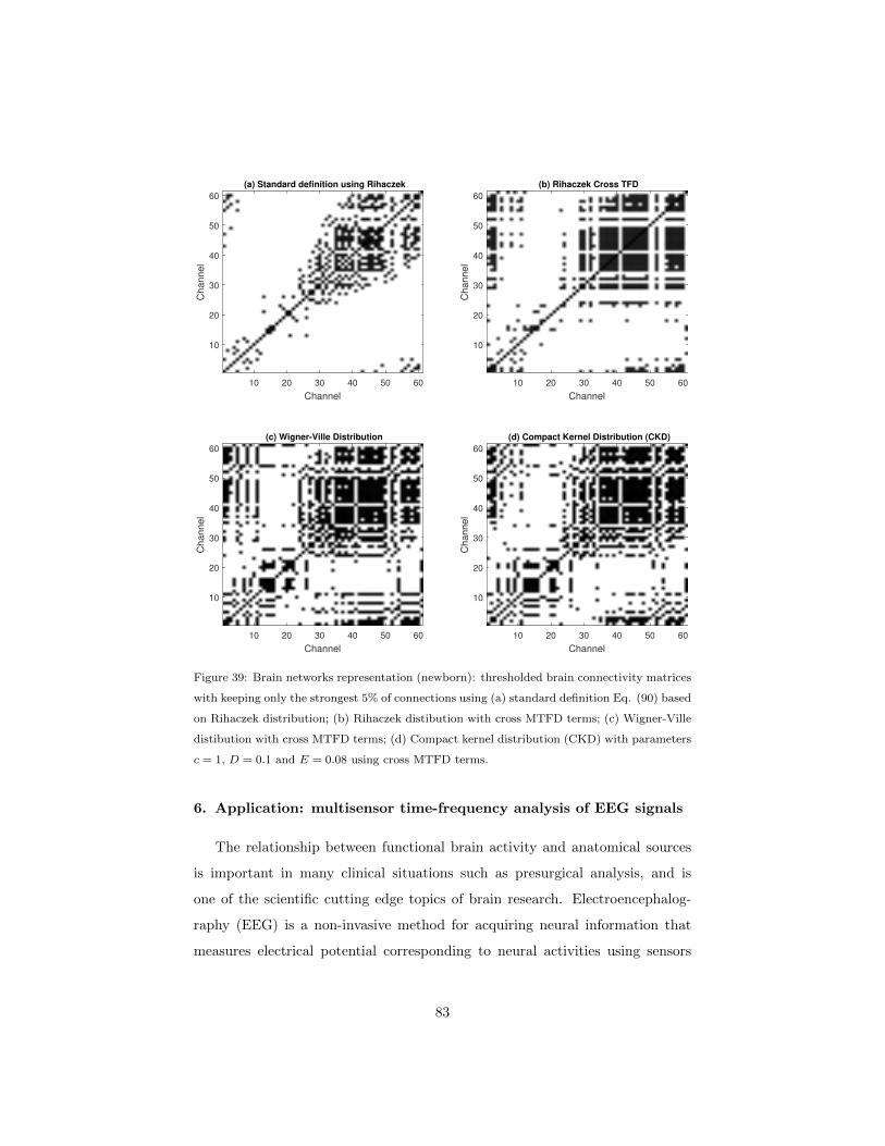
(a) Standard definition using Rihaczek
10 20 30 40 50 60
Channel
10
20
30
40
50
60C
ha
nn
el
(b) Rihaczek Cross TFD
10 20 30 40 50 60
Channel
10
20
30
40
50
60
Ch
an
ne
l
(c) Wigner-Ville Distribution
10 20 30 40 50 60
Channel
10
20
30
40
50
60
Ch
an
ne
l
(d) Compact Kernel Distribution (CKD)
10 20 30 40 50 60
Channel
10
20
30
40
50
60
Ch
an
ne
l
Figure 39: Brain networks representation (newborn): thresholded brain connectivity matrices
with keeping only the strongest 5% of connections using (a) standard definition Eq. (90) based
on Rihaczek distribution; (b) Rihaczek distibution with cross MTFD terms; (c) Wigner-Ville
distibution with cross MTFD terms; (d) Compact kernel distribution (CKD) with parameters
c = 1, D = 0.1 and E = 0.08 using cross MTFD terms.
6. Application: multisensor time-frequency analysis of EEG signals
The relationship between functional brain activity and anatomical sources
is important in many clinical situations such as presurgical analysis, and is
one of the scientific cutting edge topics of brain research. Electroencephalog-
raphy (EEG) is a non-invasive method for acquiring neural information that
measures electrical potential corresponding to neural activities using sensors
83
directly attached to the scalp. Despite its superior temporal resolution, the
spatial resolution of EEG is less than other functional brain imaging methods
such as fMRI. This is due to the separation between EEG electrodes and the
current sources inside the head, i.e. neurons, by several layers with different
conductivity profiles [81]. In addition, since various source arrangements inside
the brain or cortex can result in a similar potential distribution on the scalp,
the visual interpretation of EEG cannot provide an accurate location of neural
generators [82].
Some of the well-documented methods are based on the convenient but inac-
curate assumption that EEG signals are stationary or at least quasi-stationary
[83, 84, 85]. To account for the non-stationary characteristic EEG seizure, a
number of time-frequency methods have been proposed [86, 69, 87]. Most stud-
ies have focused on only single channel EEG or on single channels at a time when
using multichannel EEGs. However, to improve precision and performance, the
problem of analyzing multichannel EEGs should be approached more precisely
using recently developed TF methods for analyzing multisensor data in the con-
text of array signal processing [87, 88]. Once an abnormality has been detected
and classified in multichannel EEG, the solution of the inverse problem can be
used to locate the sources of that abnormality in the brain.
The following extends the MTFD concepts presented earlier to an application
dealing with EEG signals enhancement and diagnosis; specifically, we use TF-
BSS and TF-MUSIC methods for artifacts removal and source localization.
6.1. Data model
6.1.1. Lead Field Matrix
The EEG forward problem aims at predicting the scalp potentials that re-
sult from the hypothetical dipoles, or more generally from current distributions
inside the head at any location, orientation and amplitude values [89]. Because
most studies of EEG deal with frequencies between 0.1 Hz and 100 Hz [90],
the forward model can be described by the quasi-static versions of Maxwell’s
equations [91]. In this condition Poisson’s equation gives the potentials at any
84
position in a volume conductor due to current source distribution as [92, 93]:
∇. (µ∇ϑ) = ∇.Js, in Ω, (94)
where ∇ is a partial differential vector operator, Ω denotes ohm (unit of the
resistance of a conductor), µ is the electrical conductivity, ϑ are the electrical
potentials and Js are the electric current sources. Eq. (94) indicates that for
a given configuration of electric sources, the mapping from the electric sources
within the head to the scalp recordings on the outside of the scalp can be
represented by a lead field matrix [89].
There are two main numerical methods for solving the forward model and
obtaining the lead field matrix, namely; boundary element method (BEM) [94,
95] and finite element method (FEM) [96, 97, 98]. Boundary element methods
assume that each layer is homogeneous and isotropic in conductivity. Finite
element methods can be extended to model anisotropic and inhomogeneous
tissues such as skull and white matter. However, It has been shown that when
piecewise constant conductivity is used (instead of a spatially varying anisotropic
conductivity model), both methods perform similar in terms of the accuracy of
the solution [99].
6.1.2. Formulation
Let us define zi (t) as the electric field measured at sensor i at time instant t.
The vector z (t) = [z1 (t) , z2 (t) , . . . , zm(t)]T
then presents the set of measure-
ments collected by m sensors. Let’s assume n current dipole sources generate
the electric field. The magnitude of the ith dipole source movement is si (t) and
the source magnitude vector is defined as: s (t) = [s1 (t) , s2 (t) , . . . , sn(t)]T
. For
m sensors and n dipole sources, the relationship between z (t) and s (t) can be
expressed by Eq.(12) using matrix A such that z (t) = A s (t) + η (t), where A
represents the lead-field matrix of dimension m× n [89] that includes both the
effect of location Λ and orientation Φ of the dipoles as A = ΛΦ. Each column
of the lead-field matrix is called a lead field and it defines the current flow for a
given sensor through each dipole position [89].
85
Hence, the above model can be used to solve the problem of EEG source
localization and artifacts removal using the approaches presented earlier.
6.2. Application of BSS to EEG artifacts removal
6.2.0. Background and motivation
In this section, the advanced BSS algorithms discussed earlier in the text
are applied to the analysis of multichannel EEG signals for artifacts removal.
Artifacts cause a major problem in the implementation of fully automated
EEG signal classification systems; e.g. respiratory artifacts look like seizures
and can be misinterpreted by the automatic abnormality detection system thus
resulting in false alarms. One option is to apply machine learning algorithms
to first detect and then reject EEG segments corrupted by artifacts, but this
approach results in a loss of EEG data [2, 14]. Another approach for removing
artifacts is to correct EEG signals without discarding any EEG segments. Some
artifacts can be corrected by simple frequency domain filtering, e.g. band pass
filtering can remove low-frequency movement related artifacts or a notch filter
can remove 50 Hz noise. This approach does not require any reference signals.
For more complex cases, when the spectrum of artifacts overlaps with the spec-
trum of EEG signals, BSS algorithms can be used. In this approach, signals
that are corrupted by artifacts are identified either manually or automatically
using correlation from a reference signal [100]. The artifact free signal is then
synthesized by combining only artifact free components.
Based on the model presented in Section 6.1.1 the instantaneous BSS meth-
ods can be considered to tackle the problem of artifacts removal. Therefore, an
EEG artifact removal algorithm can be designed by using the BSS algorithm
presented in Section 3 with a selected high resolution time-frequency distribu-
tion to extract close signal components (see results in Section 6.4).
86
6.3. TF-MUSIC applied to source localization of brain EEG abnormalities
6.3.0. Background and motivation
In this section, the advanced DOA estimation algorithms discussed above
are applied to the analysis of multichannel EEG signals.
EEG source localization (ESL) is an important tool used to estimate the
intracerebral generators of the potentials observed on the scalp in both clinical
and research in cognitive neuroscience. While there is an increasing interest in
studying motor evoked potentials (EVP) by means of ESL, epilepsy has been the
main focus of the clinical application of ESL in neurology [101]. Similarly, cog-
nitive neuroscience studies have used ESL to investigate temporal information
in the event related potentials (ERP), and psychiatry and psychopharmacology
has employed ESL to study sources in specific frequency bands [101].
6.3.1. Source localization of EEG abnormality using TF-MUSIC
In the context of the brain application, where the aim is to estimate the loca-
tions of EEG abnormalities, localization algorithms (such as MUSIC, ESPRIT)
exploit the fact that the lead-field matrix A = ΛΦ is orthogonal to the noise
subspace of the received covariance matrix [89]. To find the locations of ab-
normalities, the covariance matrix is estimated from the received multichannel
EEG signals, and instead of using steering vectors, in Eq.(71) the eigenvectors
are projected on the columns of the lead field matrix A.
More precisely, the TF-MUSIC algorithm, as indicated in Section 4.2.1,
starts with calculating the MTFD of the processed EEG data ρzz(t, f), fol-
lowed by the average procedure described in Table 1. To estimate the loca-
tions of the sources, the TF-MUSIC algorithm takes advantage of the fact that
span (A) = span (Vs) (where Vs is the signal subspace of ρzz(t, f)) and the or-
thogonality of signal subspace and noise subspace. These can thus be obtained
by checking the orthogonality between the lead field matrix and the noise sub-
space projector. Then, the final TF-MUSIC metric is derived as a measure of
87
orthogonality between the noise subspace and the lead-field matrix [102]:
J =1
λmin (AH V VH A, AHA)(95)
where λmin is the minimum generalized eigenvalue of the matrix pair
AH V VH A and AHA, and V is the noise subspace defined as V =
[vn+1, . . . ,vm] in which vi is the ith eigenvector of the averaged MTFD ma-
trix. Calculating this metric over all grid points (source space) then results in
a map with a peak at or near the location of the source.
6.4. Results and discussion
In this section, numerical and experimental results will be discussed where
we apply the concepts of TF BSS and TF-MUSIC on EEG signals for artifacts
removal and source localization.
6.4.1. Experiment: application of BSS to EEG artifacts removal
In order to illustrate the application of BSS to EEG artifacts removal we
propose the following experiment. A 5 seconds segment of clean multichannel
EEG was obtained from a publicly available database described in [103]. The
obtained EEG segment is recorded using nineteen electrodes, which were placed
according to the 10-20 International System. The extracted EEG segment is
down-sampled to 100 Hz, and then combined with synthetic multichannel EEG
artifacts as depicted in Fig. 40. The TFDs of clean EEG signal and corrupted
EEG signal are represented in Figs 42a and 42b respectively. The multichan-
nel contaminated signals are whitened, and their MTFDs are computed for the
selection of auto and cross-terms. After that, two independent sources are es-
timated using the joint diagonalization/joint off-diagonalization algorithm, and
artifactual components are identified using a maximum likelihood detector that
utilizes an independent template. Finally, clean multichannel EEG is estimated
and compared with the original clean EEG, as depicted in Fig. 41 (TFD of the
estimated EEG signal is given in Fig. 42c).
88
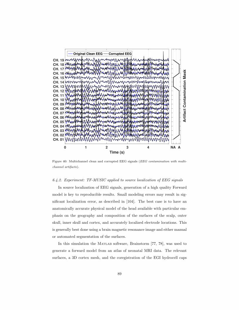
0 1 2 3 4
Time (s)
CH. 01
CH. 02
CH. 03
CH. 04
CH. 05
CH. 06
CH. 07
CH. 08
CH. 09
CH. 10
CH. 11
CH. 12
CH. 13
CH. 14
CH. 15
CH. 16
CH. 17
CH. 18
CH. 19
Original Clean EEG Corrupted EEG
NA A
Art
ifa
ct
Co
nta
min
ati
on
Ma
sk
Figure 40: Multichannel clean and corrupted EEG signals (EEG contamination with multi-
channel artifacts).
6.4.2. Experiment: TF-MUSIC applied to source localization of EEG signals
In source localization of EEG signals, generation of a high quality Forward
model is key to reproducible results. Small modeling errors may result in sig-
nificant localization error, as described in [104]. The best case is to have an
anatomically accurate physical model of the head available with particular em-
phasis on the geography and composition of the surfaces of the scalp, outer
skull, inner skull and cortex, and accurately localized electrode locations. This
is generally best done using a brain magnetic resonance image and either manual
or automated segmentation of the surfaces.
In this simulation the MATLAB software, Brainstorm [77, 78], was used to
generate a forward model from an atlas of neonatal MRI data. The relevant
surfaces, a 3D cortex mesh, and the coregistration of the EGI hydrocell caps
89
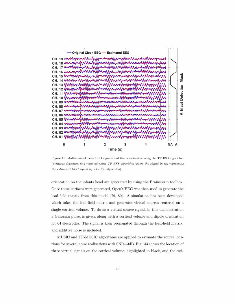
0 1 2 3 4
Time (s)
CH. 01
CH. 02
CH. 03
CH. 04
CH. 05
CH. 06
CH. 07
CH. 08
CH. 09
CH. 10
CH. 11
CH. 12
CH. 13
CH. 14
CH. 15
CH. 16
CH. 17
CH. 18
CH. 19
Original Clean EEG Estimated EEG
NA A
Art
ifa
ct
De
tec
tio
n M
as
k
Figure 41: Multichannel clean EEG signals and theirs estimates using the TF BSS algorithm
(artifacts detection and removal using TF BSS algorithm where the signal in red represents
the estimated EEG signal by TF-BSS algorithm).
orientation on the infants head are generated by using the Brainstorm toolbox.
Once these surfaces were generated, OpenMEEG was then used to generate the
lead-field matrix from this model [79, 80]. A simulation has been developed
which takes the lead-field matrix and generates virtual sources centered on a
single cortical volume. To do so a virtual source signal, in this demonstration
a Gaussian pulse, is given, along with a cortical volume and dipole orientation
for 64 electrodes. The signal is then propagated through the lead-field matrix,
and additive noise is included.
MUSIC and TF-MUSIC algorithms are applied to estimate the source loca-
tions for several noise realisations with SNR=3dB. Fig. 43 shows the location of
three virtual signals on the cortical volume, highlighted in black, and the esti-
90
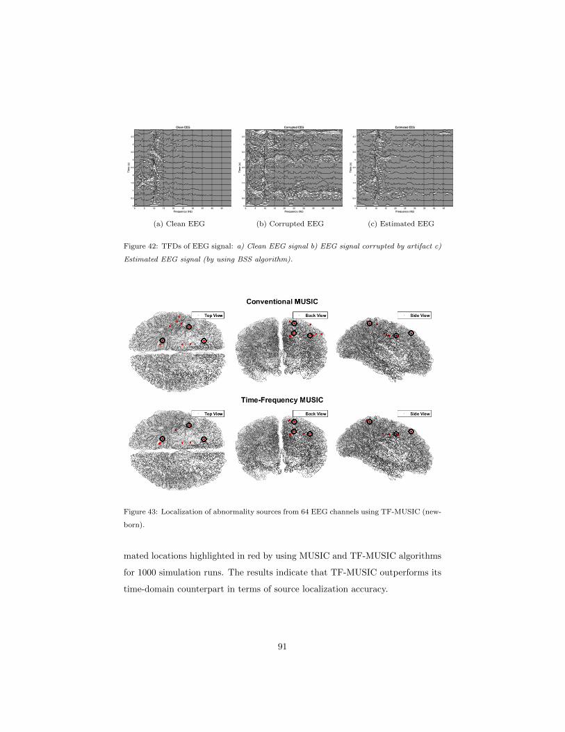
0 5 10 15 20 25 30 35 40 45
Frequency (Hz)
0
0.5
1
1.5
2
2.5
3
3.5
4
4.5
Tim
e (
s)
Clean EEG
(a) Clean EEG
0 5 10 15 20 25 30 35 40 45
Frequency (Hz)
0
0.5
1
1.5
2
2.5
3
3.5
4
4.5
Tim
e (
s)
Corrupted EEG
(b) Corrupted EEG
0 5 10 15 20 25 30 35 40 45
Frequency (Hz)
0
0.5
1
1.5
2
2.5
3
3.5
4
4.5
Tim
e (
s)
Estimated EEG
(c) Estimated EEG
Figure 42: TFDs of EEG signal: a) Clean EEG signal b) EEG signal corrupted by artifact c)
Estimated EEG signal (by using BSS algorithm).
Figure 43: Localization of abnormality sources from 64 EEG channels using TF-MUSIC (new-
born).
mated locations highlighted in red by using MUSIC and TF-MUSIC algorithms
for 1000 simulation runs. The results indicate that TF-MUSIC outperforms its
time-domain counterpart in terms of source localization accuracy.
91
7. Summary and conclusions
This study presents a rigorous tutorial review of multisensor high-resolution
time-frequency distributions (MTFDs) and a discussion of their area of appli-
cation, with a special EEG feasibility case study. MTFDs effectively combine
time-frequency analysis and array signal processing and are formulated by:
• Extending the principles of single-variable TFDs to multisen-
sor/multichannel TFDs,
• Extending conventional stationary array processing to the non-stationary
case using time-frequency methods.
• Using principles of high-resolution TFD design [105].
To demonstrate the benefits of MTFDs, this study considered several appli-
cations including source localization based on direction of arrival (DOA) es-
timation and blind source separation (BSS) of non-stationary sources. One
key aspect of this study is to illustrate clearly that, in these two applications,
the incorporation of time-frequency (TF) concepts enhances the attributes of
multisensor receivers. The key reason for this enhancement is the possible ex-
ploitation of the signal power localization properties in the (t, f) domain by
expressing the multisensor data in terms of the source TF signatures. By doing
so, enhancement of signal to noise ratio (SNR) is obtained prior to performing
subspace decomposition for source localization and source separation. Analyt-
ical reasoning also indicates that distinction in the TF signatures of closely
spaced sources allows reducing the number of sources in the field to a single
source. This enables processing more sources than sensors and further enhances
the performance of the techniques for DOA estimation and BSS.
In the second part of the study, time-frequency DOA estimation approaches
(such as the TF-MUSIC and the TF-ESPRIT algorithms) are discussed and
compared with the conventional time domain DOA estimation approaches in
the context of localizing the sources of EEG abnormalities. The findings indi-
cate that compared to traditional DOA estimation algorithms, when properly
92
used, MTFDs perform better for the localization of the sources of EEG abnor-
malities. It is because; 1) EEG signals are non-stationary in nature, 2) TF
DOA estimation algorithms exploit the signal signature localization properties
of MTFDs through the selection of the high energy (t, f) points.
However, this detailed presentation of MTFDs indicates that there is a
lot of potential for extracting additional useful information from multisen-
sor/multichannel data sets in a wide range of fields, such as feature extraction
for change detection in biomedical signal processing or to detect early struc-
tural problem in structural health monitoring. Also, key methodologies have
been provided and illustrated on selected examples with applications to audio
and EEG signals. The MTFSP toolbox [5] needed to reproduce the results pre-
sented in this paper is provided as Supplementary Material and outlined in a
companion paper [5].
Acknowledgements
This research was funded by Qatar Foundation grants NPRP 6-885-2-364
and NPRP 6-680-2-282. The authors thank Mohamed Fathi Al-Sad for his
valuable technical help. The first author thanks Prof. Paul Colditz for providing
the EEG data and the lead-field matrix as part of the grant NPRP 6-885-2-364.
Appendix A. Definitions, Terminology and Notations
Symbols frequently used in this paper are listed below in alphabetical order.
The meaning in the list below should be assumed unless the symbol is otherwise
defined in context.
Az(ν, τ) symmetrical ambiguity function (SAF) of z(t)
=∫∞−∞ z(t+ τ
2 ) z∗(t− τ2 ) e−j2πνt dt
f frequency
Ft→f
x(t)
Fourier transform (FT) of x(t), to f domain
93

F−1
f→t
X(f)
inverse Fourier transform (IFT) of X(f), back to t domain
G(t, τ) time-lag kernel =∫∞−∞ g(ν, τ) ej2πνt dν
g(ν, τ) Doppler-lag kernel
In n× n identity matrix
Kz(t, τ) instantaneous auto-correlation function (IAF) of z(t)
= z(t+ τ2 ) z∗(t− τ
2 )
Kzz(t, f) represents spatial instantaneous autocorrelation function (SIAF)
T duration of signal
t time
w(t) window function
Wz(t, f) Wigner-Ville distribution (WVD) of z(t)
=∫∞−∞ z(t+ τ
2 ) z∗(t− τ2 ) e−j2πfτdτ
γ(t, f) time-frequency kernel =∫∞−∞G(t, τ) e−j2πfτdτ
η(t) additive noise with mean µη and variance σ2η
ν Doppler (frequency shift)
ρz(t, f) quadratic time-frequency distribution (TFD) of signal z(t)
=∫∞−∞
∫∞−∞
∫∞−∞ ej2πν(t−u)g(ν, τ) z(u+ τ
2 ) z∗(u− τ2 ) e−j2πfτdν du dτ
ρzz(t, f) represents multisensor time-frequency distributions
τ lag (delay, time shift)
∗t
convolution in time
∗t∗f
2D convolution in both time and frequency
, equal by definition, or defined as
∝ proportional to∫R≡∫ ∞−∞∫
R2
≡∫ ∞−∞
∫ ∞−∞
94
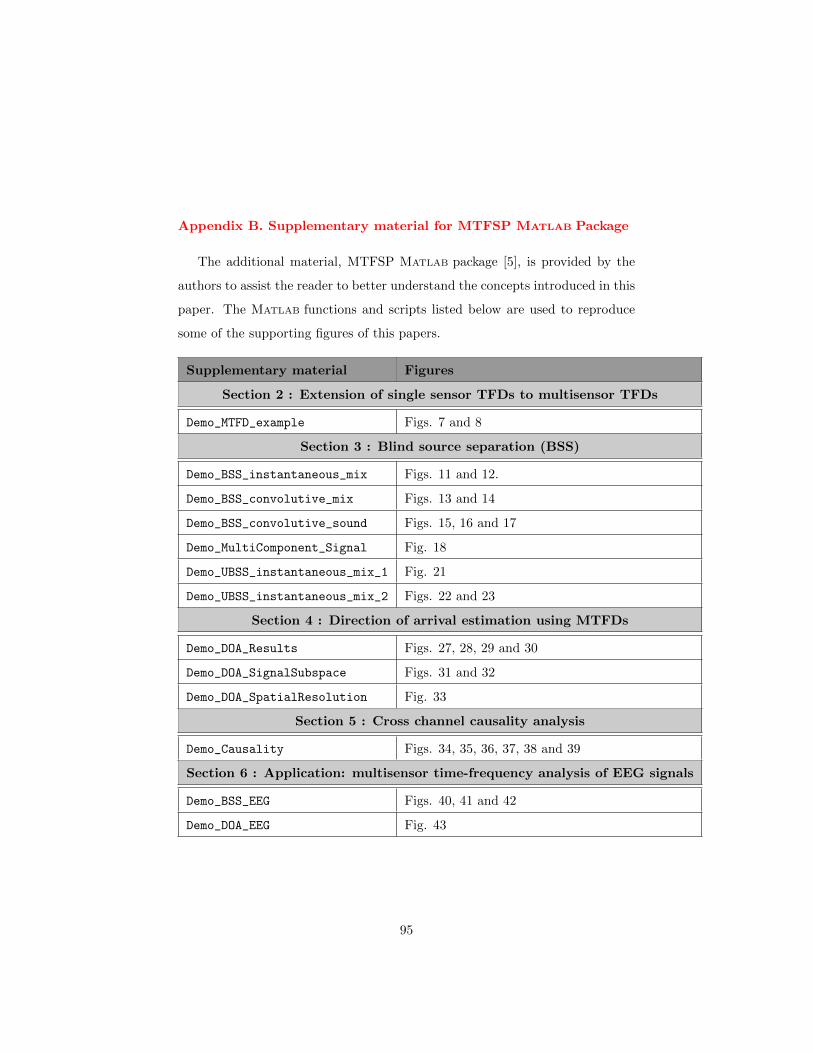
Appendix B. Supplementary material for MTFSP MATLAB Package
The additional material, MTFSP MATLAB package [5], is provided by the
authors to assist the reader to better understand the concepts introduced in this
paper. The MATLAB functions and scripts listed below are used to reproduce
some of the supporting figures of this papers.
Supplementary material Figures
Section 2 : Extension of single sensor TFDs to multisensor TFDs
Demo_MTFD_example Figs. 7 and 8
Section 3 : Blind source separation (BSS)
Demo_BSS_instantaneous_mix Figs. 11 and 12.
Demo_BSS_convolutive_mix Figs. 13 and 14
Demo_BSS_convolutive_sound Figs. 15, 16 and 17
Demo_MultiComponent_Signal Fig. 18
Demo_UBSS_instantaneous_mix_1 Fig. 21
Demo_UBSS_instantaneous_mix_2 Figs. 22 and 23
Section 4 : Direction of arrival estimation using MTFDs
Demo_DOA_Results Figs. 27, 28, 29 and 30
Demo_DOA_SignalSubspace Figs. 31 and 32
Demo_DOA_SpatialResolution Fig. 33
Section 5 : Cross channel causality analysis
Demo_Causality Figs. 34, 35, 36, 37, 38 and 39
Section 6 : Application: multisensor time-frequency analysis of EEG signals
Demo_BSS_EEG Figs. 40, 41 and 42
Demo_DOA_EEG Fig. 43
95
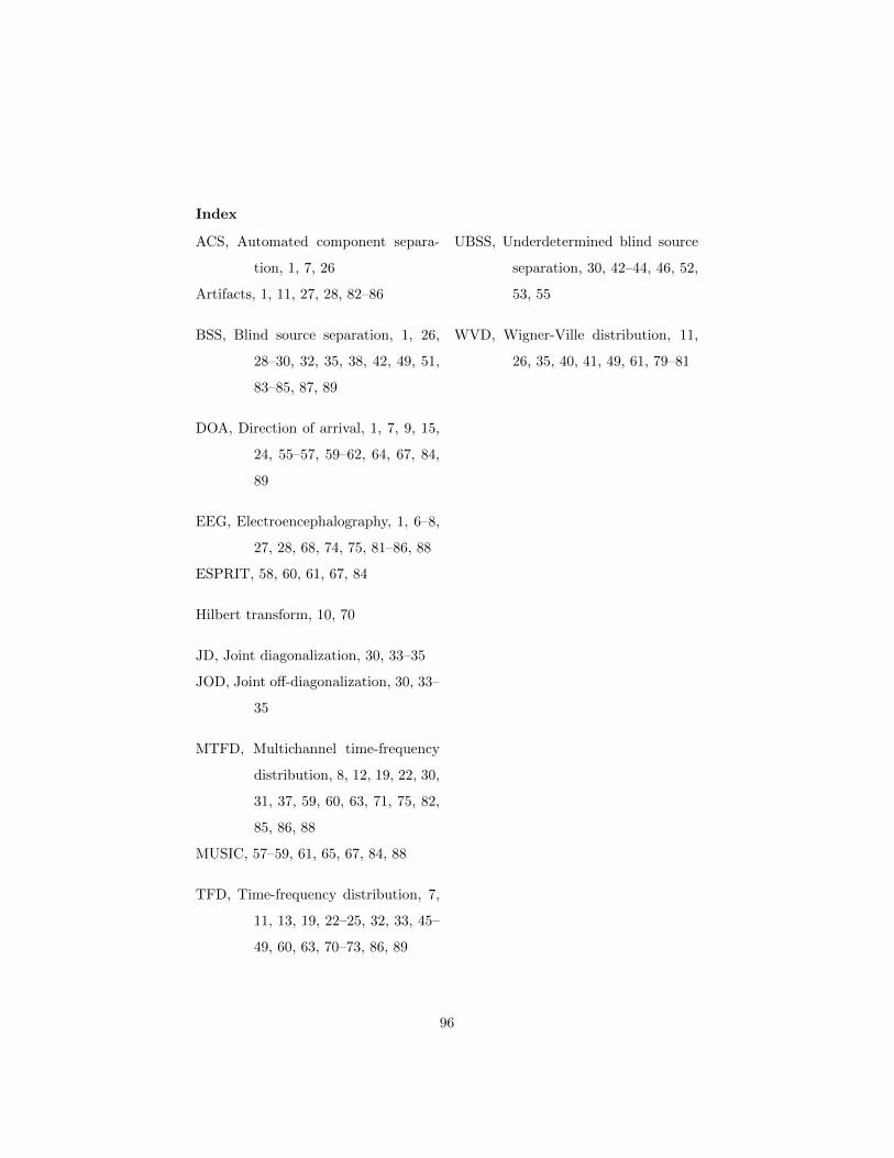
Index
ACS, Automated component separa-
tion, 1, 7, 26
Artifacts, 1, 11, 27, 28, 82–86
BSS, Blind source separation, 1, 26,
28–30, 32, 35, 38, 42, 49, 51,
83–85, 87, 89
DOA, Direction of arrival, 1, 7, 9, 15,
24, 55–57, 59–62, 64, 67, 84,
89
EEG, Electroencephalography, 1, 6–8,
27, 28, 68, 74, 75, 81–86, 88
ESPRIT, 58, 60, 61, 67, 84
Hilbert transform, 10, 70
JD, Joint diagonalization, 30, 33–35
JOD, Joint off-diagonalization, 30, 33–
35
MTFD, Multichannel time-frequency
distribution, 8, 12, 19, 22, 30,
31, 37, 59, 60, 63, 71, 75, 82,
85, 86, 88
MUSIC, 57–59, 61, 65, 67, 84, 88
TFD, Time-frequency distribution, 7,
11, 13, 19, 22–25, 32, 33, 45–
49, 60, 63, 70–73, 86, 89
UBSS, Underdetermined blind source
separation, 30, 42–44, 46, 52,
53, 55
WVD, Wigner-Ville distribution, 11,
26, 35, 40, 41, 49, 61, 79–81
96
References
[1] B. Boashash (Ed.), Time-frequency signal analysis and processing, 2nd
Edition, Academic Press, Oxford, 2016.
[2] B. Boashash, G. Azemi, J. M. O’Toole, Time-frequency processing of non-
stationary signals: Advanced TFD design to aid diagnosis with highlights
from medical applications, IEEE Signal Processing Magazine 30 (6) (2013)
108–119. doi:10.1109/MSP.2013.2265914.
[3] A. Belouchrani, M. G. Amin, N. Thirion-Moreau, Y. D. Zhang,
Source separation and localization using time-frequency distributions:
An overview, IEEE Signal Processing Magazine 30 (6) (2013) 97–107.
doi:10.1109/MSP.2013.2265315.
[4] A. Aıssa-El-Bey, N. Linh-Trung, K. Abed-Meraim, A. Belouchrani,
Y. Grenier, Underdetermined blind separation of nondisjoint sources in
the time-frequency domain, IEEE Transactions on Signal Processing 55 (3)
(2007) 897–907. doi:10.1109/TSP.2006.888877.
[5] B. Boashash, A. Aıssa-El-Bey, Multisensor time-frequency signal process-
ing software MATLAB package: An analysis tool for multichannel non-
stationary data, SoftwareX (in press) (2017) .
[6] D. E. Carlson, J. T. Vogelstein, Q. Wu, W. Lian, M. Zhou, C. R. Stoet-
zner, D. Kipke, D. Weber, D. B. Dunson, L. Carin, Multichannel elec-
trophysiological spike sorting via joint dictionary learning and mixture
modeling, IEEE Transactions on Biomedical Engineering 61 (1) (2014)
41–54. doi:10.1109/TBME.2013.2275751.
[7] C. Weiss, A. M. Zoubir, A sparse regularization technique for source
localization with non-uniform sensor gain, in: IEEE 8th Sensor Array
and Multichannel Signal Processing Workshop (SAM), 2014, pp. 93–96.
doi:10.1109/SAM.2014.6882346.
97
[8] Y. Fadlallah, A. Aıssa-El-Bey, K. Amis, D. Pastor, R. Pyndiah, New
iterative detector of MIMO transmission using sparse decomposition,
IEEE Transactions on Vehicular Technology 64 (8) (2015) 3458–3464.
doi:10.1109/TVT.2014.2360687.
[9] A. Aıssa-El-Bey, D. Pastor, S. M. A. Sbaı, Y. Fadlallah, Sparsity-based
recovery of finite alphabet solutions to underdetermined linear systems,
IEEE Transactions on Information Theory 61 (4) (2015) 2008–2018.
doi:10.1109/TIT.2015.2399914.
[10] P. Langley, S. King, K. Wang, D. Zheng, R. Giovannini, M. Bojarnejad,
A. Murray, Estimation of missing data in multi-channel physiological time-
series by average substitution with timing from a reference channel, in:
Computing in Cardiology, 2010, pp. 309–312.
[11] M. R. Mowla, S.-C. Ng, M. S. Zilany, R. Paramesran, Artifacts-matched
blind source separation and wavelet transform for multichannel EEG de-
noising, Biomedical Signal Processing and Control 22 (2015) 111–118.
doi:10.1016/j.bspc.2015.06.009.
[12] I. Bayram, A multichannel audio denoising formulation based on spec-
tral sparsity, IEEE/ACM Transactions on Audio, Speech, and Language
Processing 23 (12) (2015) 2272–2285. doi:10.1109/TASLP.2015.2479042.
[13] S. Mirzaei, H. V. Hamme, Y. Norouzi, Blind audio source count-
ing and separation of anechoic mixtures using the multichan-
nel complex NMF framework, Signal Processing 115 (2015) 27–37.
doi:10.1016/j.sigpro.2015.03.006.
[14] B. Boashash, S. Ouelha, Automatic signal abnormality detection
using time-frequency features and machine learning: A newborn
EEG seizure case study, Knowledge-Based Systems 106 (2016) 38–50.
doi:10.1016/j.knosys.2016.05.027.
98
[15] B. Boashash, G. Azemi, A review of time–frequency matched filter de-
sign with application to seizure detection in multichannel newborn EEG,
Digital Signal Processing 28 (2014) 28–38. doi:10.1016/j.dsp.2014.02.007.
[16] P. Shen, S. Liu, W. Zhou, F. Lin, A. Lam, H. Sung, W. Chen,
J. Lin, M. Chiu, M. Pan, J. Kao, F. Lai, A physiology-based seizure
detection system for multichannel EEG, PLoS ONE 8 (6), e65862.
doi:10.1371/journal.pone.0065862.
[17] K. Fu, J. Qu, Y. Chai, T. Zou, Hilbert marginal spectrum analysis for
automatic seizure detection in EEG signals, Biomedical Signal Processing
and Control 18 (2015) 179–185. doi:10.1016/j.bspc.2015.01.002.
[18] M. Varanini, G. Tartarisco, R. Balocchi, A. Macerata, G. Pioggia, L. Bil-
leci, A new method for QRS complex detection in multichannel ECG:
Application to self-monitoring of fetal health, Computers in Biology and
Medicine (2016) –doi:10.1016/j.compbiomed.2016.04.008.
[19] V. Ionescu, Fetal ECG extraction from multichannel abdominal ECG
recordings for health monitoring during labor, Procedia Technology 22
(2016) 682–689. doi:10.1016/j.protcy.2016.01.143.
[20] X. Wang, A. Mortazawi, Medium wave energy scavenging for
wireless structural health monitoring sensors, IEEE Transactions
on Microwave Theory and Techniques 62 (4) (2014) 1067–1073.
doi:10.1109/TMTT.2014.2304918.
[21] Z. Zou, Y. Bao, H. Li, B. F. Spencer, J. Ou, Embedding compressive
sensing-based data loss recovery algorithm into wireless smart sensors for
structural health monitoring, IEEE Sensors Journal 15 (2) (2015) 797–808.
doi:10.1109/JSEN.2014.2353032.
[22] Z. Herrasti, I. Val, I. Gabilondo, J. Berganzo, A. Arriola, F. Martınez,
Wireless sensor nodes for generic signal conditioning: Application to struc-
99
tural health monitoring of wind turbines, Sensors and Actuators A: Phys-
ical 247 (2016) 604–613. doi:10.1016/j.sna.2016.06.027.
[23] D. Liang, S. Yuan, Structural health monitoring system based on multi-
agent coordination and fusion for large structure, Advances in Engineering
Software 86 (2015) 1–12. doi:10.1016/j.advengsoft.2015.03.008.
[24] W.-T. Sung, H.-Y. Chung, A distributed energy monitoring network sys-
tem based on data fusion via improved PSO, Measurement 55 (2014)
362–374. doi:10.1016/j.measurement.2014.05.007.
[25] F. Doyle, M.-J. R. Duarte, J. Cosgrove, Design of an embed-
ded sensor network for application in energy monitoring of com-
mercial and industrial facilities, Energy Procedia 83 (2015) 504–514.
doi:10.1016/j.egypro.2015.12.170.
[26] A. Omidvarnia, G. Azemi, B. Boashash, J. M. O’Toole, P. B.
Colditz, S. Vanhatalo, Measuring time-varying information flow in
scalp EEG signals: Orthogonalized partial directed coherence, IEEE
Transactions on Biomedical Engineering 61 (3) (2014) 680–693.
doi:10.1109/TBME.2013.2286394.
[27] J. Lerga, V. Sucic, B. Boashash, An efficient algorithm for instanta-
neous frequency estimation of nonstationary multicomponent signals in
low SNR, EURASIP Journal on Advances in Signal Processing 2011 (1)
(2011) 725189. doi:10.1155/2011/725189.
[28] M. G. Amin, Y. Zhang, Direction finding based on spatial time-frequency
distribution matrices, Digital Signal Processing 10 (4) (2000) 325–339.
doi:10.1006/dspr.2000.0374.
[29] Y. Zhang, M. G. Amin, Spatial averaging of time-frequency distributions
for signal recovery in uniform linear arrays, IEEE Transactions on Signal
Processing 48 (10) (2000) 2892–2902. doi:10.1109/78.869043.
100
[30] L. Stankovic, A method for time-frequency analysis, IEEE Transactions
on Signal Processing 42 (1) (1994) 225–229. doi:10.1109/78.258146.
[31] M. Abed, A. Belouchrani, M. Cheriet, B. Boashash, Time-frequency dis-
tributions based on compact support kernels: Properties and performance
evaluation, IEEE Transactions on Signal Processing 60 (6) (2012) 2814–
2827. doi:10.1109/TSP.2012.2190065.
[32] G. M. Kautz, M. D. Zoltowski, Beamspace DOA estimation featuring
multirate eigenvector processing, IEEE Transactions on Signal Processing
44 (7) (1996) 1765–1778. doi:10.1109/78.510623.
[33] A. Hyvarinen, J. Karhunen, E. Oja, Independent component analysis, 1st
Edition, Adaptive and learning systems for signal processing, communi-
cations, and control, John Wiley, New York, Chichester, Weinheim, 2001.
[34] L. Parra, C. Spence, Convolutive blind separation of non-stationary
sources, IEEE Transactions on Speech and Audio Processing 8 (3) (2000)
320–327. doi:10.1109/89.841214.
[35] A. Belouchrani, K. Abed-Meraim, M. G. Amin, A. M. Zoubir, Blind sep-
aration of nonstationary sources, IEEE Signal Processing Letters 11 (7)
(2004) 605–608. doi:10.1109/LSP.2004.830119.
[36] L. Giulieri, H. Ghennioui, N. Thirion-Moreau, E. Moreau, Nonorthogo-
nal joint diagonalization of spatial quadratic time-frequency matrices for
source separation, IEEE Signal Processing Letters 12 (5) (2005) 415–418.
doi:10.1109/LSP.2005.843760.
[37] A. Yeredor, Non-orthogonal joint diagonalization in the least-squares sense
with application in blind source separation, IEEE Transactions on Signal
Processing 50 (7) (2002) 1545–1553. doi:10.1109/TSP.2002.1011195.
[38] G. Chabriel, M. Kleinsteuber, E. Moreau, H. Shen, P. Tichavsky, A. Yere-
dor, Joint matrices decompositions and blind source separation: A survey
101
of methods, identification, and applications, IEEE Signal Processing Mag-
azine 31 (3) (2014) 34–43. doi:10.1109/MSP.2014.2298045.
[39] A. R. Leyman, Z. M. Kamran, K. Abed-Meraim, Higher-order time
frequency-based blind source separation technique, IEEE Signal Process-
ing Letters 7 (7) (2000) 193–196. doi:10.1109/97.847366.
[40] N. Linh-Trung, A. Belouchrani, K. Abed-Meraim, B. Boashash, Sep-
arating more sources than sensors using time-frequency distributions,
EURASIP Journal on Advances in Signal Processing 2005 (17) (2005)
845079. doi:10.1155/ASP.2005.2828.
[41] M. Castella, A. Chevreuil, J.-C. Pesquet, Chapter 8 - convolutive mix-
tures, in: P. Comon, C. Jutten (Eds.), Handbook of Blind Source Sepa-
ration, Academic Press, Oxford, 2010, pp. 281–324. doi:10.1016/B978-0-
12-374726-6.00013-8.
[42] A. Belouchrani, M. G. Amin, K. Abed-Meraim, Direction finding in corre-
lated noise fields based on joint block-diagonalization of spatio-temporal
correlation matrices, IEEE Signal Processing Letters 4 (9) (1997) 266–268.
doi:10.1109/97.623045.
[43] H. Bousbia-Salah, A. Belouchrani, K. Abed-Meraim, Jacobi-like algorithm
for blind signal separation of convolutive mixtures, Electronics Letters
37 (16) (2001) 1049–1050. doi:10.1049/el:20010698.
[44] K. Abed-Meraim, W. Qiu, Y. Hua, Blind system identification, Proceed-
ings of the IEEE 85 (8) (1997) 1310–1322. doi:10.1109/5.622507.
[45] [link].
URL http://www.wavsource.com/
[46] N. C. Geckını, T. Gungen, H. Gungen, M. Etıskol, Speech synthesis using
am/fm sinusoids and band-pass noise, Signal Processing 8 (3) (1985) 339–
361. doi:10.1016/0165-1684(85)90111-2.
102
[47] M. Wax, T. Kailath, Detection of signals by information theoretic criteria,
IEEE Transactions on Acoustics, Speech, and Signal Processing 33 (2)
(1985) 387–392. doi:10.1109/TASSP.1985.1164557.
[48] J. MacQueen, Some methods for classification and analysis of multivari-
ate observations, in: Proceedings of the Fifth Berkeley Symposium on
Mathematical Statistics and Probability, Volume 1: Statistics, University
of California Press, Berkeley, Calif., 1967, pp. 281–297.
URL http://projecteuclid.org/euclid.bsmsp/1200512992
[49] G. Boudreaux-Bartels, T. Parks, Time-varying filtering and signal esti-
mation using Wigner distribution synthesis techniques, IEEE Transac-
tions on Acoustics, Speech, and Signal Processing 34 (3) (1986) 442–451.
doi:10.1109/TASSP.1986.1164833.
[50] A. Aıssa-El-Bey, K. Abed-Meraim, Y. Grenier, Blind separation of un-
derdetermined convolutive mixtures using their time-frequency represen-
tation, IEEE Transactions on Audio, Speech, and Language Processing
15 (5) (2007) 1540–1550. doi:10.1109/TASL.2007.898455.
[51] E. H. Moore, On the reciprocal of the general algebraic matrix, Bul-
letin of the American Mathematical Society 26 (9) (1920) 394–395.
doi:10.1090/S0002-9904-1920-03322-7.
[52] W. Mu, M. G. Amin, Y. Zhang, Bilinear signal synthesis in array pro-
cessing, IEEE Transactions on Signal Processing 51 (1) (2003) 90–100.
doi:10.1109/TSP.2002.806577.
[53] I. E. Frank, R. Todeschini, The data analysis handbook, Vol. 14, Elsevier,
1994.
[54] H. Krim, M. Viberg, Two decades of array signal processing research:
the parametric approach, IEEE Signal Processing Magazine 13 (4) (1996)
67–94. doi:10.1109/79.526899.
103
[55] H. L. Van Trees, Detection, Estimation, and Modulation Theory, Vol. IV:
Optimum Array Processing, John Wiley & Sons, Inc., 2002.
[56] R. Schmidt, Multiple emitter location and signal parameter estimation,
IEEE Transactions on Antennas and Propagation 34 (3) (1986) 276–280.
doi:10.1109/TAP.1986.1143830.
[57] J. F. Cardoso, E. Moulines, Asymptotic performance analysis of direction-
finding algorithms based on fourth-order cumulants, IEEE Transactions
on Signal Processing 43 (1) (1995) 214–224. doi:10.1109/78.365301.
[58] A. Paulraj, R. Roy, T. Kailath, A subspace rotation approach to signal
parameter estimation, Proceedings of the IEEE 74 (7) (1986) 1044–1046.
doi:10.1109/PROC.1986.13583.
[59] P. Stoica, A. Nehorai, Performance comparison of subspace rotation and
music methods for direction estimation, IEEE Transactions on Signal Pro-
cessing 39 (2) (1991) 446–453. doi:10.1109/78.80828.
[60] B. Ottersten, M. Viberg, T. Kailath, Performance analysis of the total
least squares esprit algorithm, IEEE Transactions on Signal Processing
39 (5) (1991) 1122–1135. doi:10.1109/78.80967.
[61] S. Ouelha, A. Aıssa-El-Bey, B. Boashash, Improving DOA estimation al-
gorithms using high-resolution time-frequency distributions, IEEE Trans-
actions on Signal Processing (accepted) (2017) .
[62] X. L. Xu, K. M. Buckley, Bias analysis of the music location estima-
tor, IEEE Transactions on Signal Processing 40 (10) (1992) 2559–2569.
doi:10.1109/78.157296.
[63] T. Ning, F.-S. Wei, Multichannel coherence analysis of helicopter vibra-
tions, in: 6th International Conference on Signal Processing, Vol. 2, 2002,
pp. 1774–1777. doi:10.1109/ICOSP.2002.1180146.
104
[64] L. Koopmans (Ed.), The Spectral Analysis of Time Series, Vol. 22 of Prob-
ability and Mathematical Statistics, Academic Press, San Diego, 1995.
doi:10.1016/B978-0-12-419250-8.
[65] L. B. White, B. Boashash, Cross spectral analysis of nonstationary pro-
cesses, IEEE Transactions on Information Theory 36 (4) (1990) 830–835.
doi:10.1109/18.53742.
[66] J. S. Bendat, A. G. Piersol (Eds.), Random Data, 4th Edition, Analysis
and Measurement Procedures, John Wiley & Sons, Inc., New Jersey, 2012.
doi:10.1002/9781118032428.
[67] E. Pereda, R. Q. Quiroga, J. Bhattacharya, Nonlinear multivariate analy-
sis of neurophysiological signals, Progress in Neurobiology 77 (1–2) (2005)
1–37. doi:10.1016/j.pneurobio.2005.10.003.
[68] K. J. Blinowska, Review of the methods of determination of directed con-
nectivity from multichannel data, Medical & Biological Engineering &
Computing 49 (5) (2011) 521—529. doi:10.1007/s11517-011-0739-x.
[69] S. Assous, B. Boashash, Evaluation of the modified s-transform for time-
frequency synchrony analysis and source localisation, EURASIP Journal
on Advances in Signal Processing 2012 (1) (2012) 49. doi:10.1186/1687-
6180-2012-49.
[70] M. Rosenblum, A. Pikovsky, J. Kurths, Phase synchronization of
chaotic oscillators, Physical Review Letters 76 (1996) 1804–1807.
doi:10.1103/PhysRevLett.76.1804.
[71] A. Pikovsky, M. Rosenblum, J. Kurths, Phase synchronization in regu-
lar and chaotic systems, International Journal of Bifurcation and Chaos
10 (10) (2000) 2291–2305. doi:10.1142/S0218127400001481.
[72] B. Boashash, Estimating and interpreting the instantaneous frequency of
a signal. i. fundamentals, Proceedings of the IEEE 80 (4) (1992) 520–538.
doi:10.1109/5.135376.
105
[73] S. Aviyente, E. M. Bernat, W. S. Evans, S. R. Sponheim, A
phase synchrony measure for quantifying dynamic functional inte-
gration in the brain, Human Brain Mapping 32 (1) (2011) 80–93.
doi:10.1002/hbm.21000.
[74] A. Omidvarnia, G. Azemi, P. B. Colditz, B. Boashash, A time–frequency
based approach for generalized phase synchrony assessment in nonstation-
ary multivariate signals, Digital Signal Processing 23 (3) (2013) 780 – 790.
doi:10.1016/j.dsp.2013.01.002.
[75] J.-P. Lachaux, E. Rodriguez, J. Martinerie, F. J. Varela, Measuring phase
synchrony in brain signals, Human Brain Mapping 8 (4) (1999) 194–208.
[76] S. Aviyente, A. Y. Mutlu, A time-frequency-based approach to phase
and phase synchrony estimation, IEEE Transactions on Signal Process-
ing 59 (7) (2011) 3086–3098. doi:10.1109/TSP.2011.2144589.
[77] F. Tadel, S. Baillet, J. Mosher, D. Pantazis, R. Leahy, Brainstorm: A user-
friendly application for MEG/EEG analysis, Computational Intelligence
and Neuroscience 2011 (879716) (2011) 13. doi:10.1155/2011/879716.
[78] Brainstorm toolbox.
URL http://neuroimage.usc.edu/brainstorm
[79] A. Gramfort, T. Papadopoulo, E. Olivi, M. Clerc, OpenMEEG: open-
source software for quasistatic bioelectromagnetics, BioMedical Engineer-
ing OnLine 9 (1) (2010) 45. doi:10.1186/1475-925X-9-45.
[80] J. Kybic, M. Clerc, T. Abboud, O. Faugeras, R. Keriven, T. Papadopoulo,
A common formalism for the integral formulations of the forward EEG
problem, IEEE Transactions on Medical Imaging 24 (1) (2005) 12–28.
doi:10.1109/TMI.2004.837363.
[81] R. Srinivasan, Methods to improve the spatial resolution of EEG, Inter-
national Journal of Bioelectromagnetism 1 (1) (1999) 102–111.
106
[82] C. Grova, J. Daunizeau, J.-M. Lina, C. Benar, H. Benali, J. Got-
man, Evaluation of EEG localization methods using realistic sim-
ulations of interictal spikes, NeuroImage 29 (3) (2006) 734–753.
doi:10.1016/j.neuroimage.2005.08.053.
[83] A. Liu, J. Hahn, G. Heldt, R. Coen, Detection of neonatal seizures through
computerized EEG analysis, Electroencephalography and Clinical Neuro-
physiology 82 (1) (1992) 30–37. doi:10.1016/0013-4694(92)90179-L.
[84] J. Gotman, D. Flanagan, B. Rosenblatt, A. Bye, E. Mizrahi, Evaluation
of an automatic seizure detection method for the newborn EEG, Elec-
troencephalography and Clinical Neurophysiology 103 (3) (1997) 363–369.
doi:10.1016/S0013-4694(97)00005-2.
[85] S. Faul, G. Boylan, S. Connolly, L. Marnane, G. Lightbody, An evaluation
of automated neonatal seizure detection methods, Clinical Neurophysiol-
ogy 116 (7) (2005) 1533–1541. doi:10.1016/j.clinph.2005.03.006.
[86] H. Hassanpour, M. Mesbah, B. Boashash, Time-frequency based newborn
EEG seizure detection using low and high frequency signatures, Physio-
logical Measurement 25 (4) (2004) 935. doi:10.1088/0967-3334/25/4/012.
[87] B. Boashash, L. Boubchir, G. Azemi, A methodology for time-frequency
image processing applied to the classification of non-stationary multichan-
nel signals using instantaneous frequency descriptors with application to
newborn EEG signals, EURASIP Journal on Advances in Signal Process-
ing 2012 (1) (2012) 117. doi:10.1186/1687-6180-2012-117.
[88] M. A. Latif, S. Sanei, J. Chambers, L. Spyrou, Partially constrained
blind source separation for localization of unknown sources exploiting non-
homogeneity of the head tissues, The Journal of VLSI Signal Processing
Systems for Signal, Image, and Video Technology 49 (2) (2007) 217–232.
doi:10.1007/s11265-007-0075-4.
107
[89] R. Grech, T. Cassar, J. Muscat, K. P. Camilleri, S. G. Fabri, M. Zervakis,
P. Xanthopoulos, V. Sakkalis, B. Vanrumste, Review on solving the in-
verse problem in EEG source analysis, Journal of NeuroEngineering and
Rehabilitation 5 (1) (2008) 25. doi:10.1186/1743-0003-5-25.
[90] S. Baillet, J. C. Mosher, R. M. Leahy, Electromagnetic brain
mapping, IEEE Signal Processing Magazine 18 (6) (2001) 14–30.
doi:10.1109/79.962275.
[91] M. Hamalainen, R. Hari, R. J. Ilmoniemi, J. Knuutila, O. V. Lounasmaa,
Magnetoencephalography: theory, instrumentation, and applications to
noninvasive studies of the working human brain, Reviews of Modern
Physics 65 (1993) 413–497. doi:10.1103/RevModPhys.65.413.
[92] J. C. de Munck, B. W. van Dijk, H. Spekreijse, Mathematical dipoles
are adequate to describe realistic generators of human brain activity,
IEEE Transactions on Biomedical Engineering 35 (11) (1988) 960–966.
doi:10.1109/10.8677.
[93] M. A. Latif, S. Sanei, J. Chambers, L. Shoker, Localization of abnormal
EEG sources using blind source separation partially constrained by the
locations of known sources, IEEE Signal Processing Letters 13 (3) (2006)
117–120. doi:10.1109/LSP.2005.862622.
[94] P. K. Banerjee, R. Butterfield, Boundary element methods in engineering
science, Vol. 17, McGraw-Hill, London, UK, 1981.
[95] N. G. Gencer, I. O. Tanzer, Forward problem solution of electromagnetic
source imaging using a new BEM formulation with high-order elements,
Physics in Medicine and Biology 44 (9) (1999) 2275–2287.
[96] O. C. Zienkiewicz, R. L. Taylor, R. L. Taylor, The finite element method,
Vol. 3, McGraw-Hill, London, UK, 1977.
108
[97] Y. C. Zhang, S. A. Zhu, B. He, A second-order finite element algorithm for
solving the three-dimensional EEG forward problem, Physics in Medicine
and Biology 49 (13) (2004) 2975–2987.
[98] A. P. Bagshaw, A. D. Liston, R. H. Bayford, A. Tizzard, A. P. Gibson,
A. Tidswell, M. K. Sparkes, H. Dehghani, C. D. Binnie, D. S. Holder, Elec-
trical impedance tomography of human brain function using reconstruc-
tion algorithms based on the finite element method, NeuroImage 20 (2)
(2003) 752–764. doi:10.1016/S1053-8119(03)00301-X.
[99] F. Darvas, D. Pantazis, E. Kucukaltun-Yildirim, R. Leahy, Mapping hu-
man brain function with MEG and EEG: methods and validation, Neu-
roImage 23, Supplement 1 (2004) S289–S299, mathematics in Brain Imag-
ing. doi:10.1016/j.neuroimage.2004.07.014.
[100] M. D. Vos, W. Deburchgraeve, P. Cherian, V. Matic, R. Swarte, P. Go-
vaert, G. Visser, S. V. Huffel, Automated artifact removal as preprocess-
ing refines neonatal seizure detection, Clinical Neurophysiology 122 (12)
(2011) 2345 – 2354. doi:10.1016/j.clinph.2011.04.026.
[101] C. M. Michel, M. M. Murray, G. Lantz, S. Gonzalez, L. Spinelli, R. G.
de Peralta, EEG source imaging, Clinical Neurophysiology 115 (10) (2004)
2195 – 2222. doi:10.1016/j.clinph.2004.06.001.
[102] K. Sekihara, S. S. Nagarajan, D. Poeppel, S. Miyauchi, N. Fu-
jimaki, H. Koizumi, Y. Miyashita, Estimating neural sources from
each time-frequency component of magnetoencephalographic data,
IEEE Transactions on Biomedical Engineering 47 (5) (2000) 642–653.
doi:10.1109/10.841336.
[103] M. A. Klados, C. L. Papadelis, P. D. Bamidis, REG-ICA: A new hybrid
method for EOG artifact rejection, in: 2009 9th International Conference
on Information Technology and Applications in Biomedicine, 2009, pp.
1–4. doi:10.1109/ITAB.2009.5394295.
URL http://www.mklados.com/regica.html
109
[104] Z. Akalin Acar, S. Makeig, Effects of forward model errors on
EEG source localization, Brain Topography 26 (3) (2013) 378–396.
doi:10.1007/s10548-012-0274-6.
[105] B. Boashash, S. Ouelha, An improved design of high-resolution quadratic
time-frequency distributions for the analysis of nonstationary multicompo-
nent signals using directional compact kernels, IEEE Transactions on Sig-
nal Processing 65 (10) (2017) 2701–2713. doi:10.1109/TSP.2017.2669899.
110


