Multistep Predictions from Multivariate ARMA-GARCH

Models and their Value for Portfolio Management

Jaroslava Hlouskova Kurt Schmidheiny

Martin Wagner

02-12

November 2002

Dis

kuss

ions

schr

iften

Universität Bern Volkswirtschaftliches Institut Gesellschaftstrasse 49 3012 Bern, Switzerland Tel: 41 (0)31 631 45 06 Web: www-vwi.unibe.ch

Multistep Predictions from Multivariate ARMA-GARCH

Models and their Value for Portfolio Management∗

Jaroslava HlouskovaDepartment of Economics and Finance

Institute for Advanced StudiesStumpergasse 56A-1060 Vienna

Kurt SchmidheinyDepartment of Economics

University of BernGesellschaftsstrasse 49

CH-3012 Bern

Martin WagnerDepartment of Economics

University of BernGesellschaftsstrasse 49

CH-3012 Bern

Abstract

In this paper we derive the closed form solution for multistep predictions of the conditionalmeans and their covariances from multivariate ARMA-GARCH models. These are usefule.g. in mean variance portfolio analysis when the rebalancing frequency is lower than thedata frequency. In this situation the conditional mean and covariance matrix of the sumof the higher frequency returns until the next rebalancing period is required as input inthe mean variance portfolio problem. The closed form solution for this quantity is derivedas well. We assess the empirical value of the result by evaluating and comparing theperformance of quarterly and monthly rebalanced portfolios using monthly MSCI indexdata across a large set of ARMA-GARCH models. The results forcefully demonstrate thesubstantial value of multistep predictions for portfolio management.

JEL Classification: C32, C61, G11Keywords: Multivariate ARMA-GARCH models, volatility forecasts, portfolio optimiza-tion, minimum variance portfolio

∗This work has been supported by OLZ and Partners Asset and Liability Management AG.

1

I Introduction

In this paper we derive the closed form solution for multistep predictions of the conditional

means and covariances from multivariate ARMA-GARCH models. These are useful e.g. in

mean variance portfolio analysis, when the rebalancing frequency is lower than the data fre-

quency. We assess the empirical value of this result by evaluating the performance of quarterly

rebalanced portfolios using monthly MSCI index data and compare their performance with

the performance of the corresponding monthly rebalanced portfolios. Additionally we also

consider the importance of transaction costs.

Multistep prediction in GARCH models has been considered previously in e.g. Baillie and

Bollerslev (1992), who derive the minimum mean squared error forecasts for the conditional

mean and the conditional variance of univariate ARMA-GARCH processes. We extend their

results to the multivariate case and derive closed form representations for the conditional mean

and the conditional covariances h-steps ahead. In addition we derive the explicit formula for

the conditional covariance of the sum of the conditional means up to h-steps ahead. This

corresponds, when modelling asset returns, to the conditional variance of the cumulative

returns over an h-period horizon.

The above result may be useful for mean variance portfolio analysis, when portfolio re-

allocations take place at a lower frequency than the data used in estimating the underlying

GARCH models. Mean variance portfolio analysis (see Section 2) requires estimates of ex-

pected returns and their covariances. If the rebalancing frequency is lower than the data

frequency, the expected returns over the rebalancing interval are given by the cumulative ex-

pected returns at the higher data frequency. Hence, the need for the conditional variance of

cumulative returns. If the portfolio is, as in our empirical application, adjusted quarterly, and

one estimates GARCH models using monthly data, one needs predictions for the conditional

means and covariances up to 3-months. The empirical part of our study is closely related

to Nilsson (2002) and Polasek and Pojarliev (2001a, 2001b), who use 1-step predictions from

multivariate GARCH models for portfolio selection using - as we do - MSCI regional indices.

Our study differs in the use of multistep predictions and also our empirical results are based

on a larger set of GARCH models.1

1Contrary to Nilsson (2002), we exclude GARCH-in-Mean models, whose multistep predictions are notcovered by our result and are a subject of further research. Polasek and Pojarliev (2001a) use a Bayesianapproach to GARCH modelling.

2

The value of the derived multistep predictions for portfolio management is evaluated

on monthly data for six regional MSCI indices over the evaluation period January 1992 to

December 2001. The empirical investigation is performed from the perspective of a Swiss

investor, hence all indices are converted to Swiss Francs.2 For a large number, 66 to be

precise, of ARMA-GARCH models the corresponding global minimum variance portfolios

are tracked, both for monthly and quarterly rebalancing. In the latter case the quarterly

rebalanced portfolios correctly based on multistep predictions and incorrectly based on 1-step

predictions are evaluated. For the quarterly adjusted portfolios based on correct predictions

the following results are obtained. The best performing portfolio, in terms of gross return,

outperforms the MSCI world index by 2.9 % per annum. A vast majority of ARMA-GARCH

based portfolios has higher gross return than the benchmark, the over-performance being on

average 1.05 % per annum. Also for net returns after deducting transaction costs the quarterly

rebalanced ARMA-GARCH portfolios show favorable performance. It is remarkable to note

that a majority of the ARMA-GARCH portfolios result in higher (gross and net) return

than the naive portfolio based on the sample mean and covariance. The performance of

quarterly rebalanced portfolios that are incorrectly based on 1-step predictions from the

ARMA-GARCH models is computed in order to focus on the effect of correct multistep

predictions on portfolio performance. It turns out that multistep prediction is of considerable

value. For 79 % of the models the portfolios based on the correct prediction outperform the

corresponding ”incorrect” portfolio. The average over-performance is 0.34 % gross return

per annum. Monthly rebalanced portfolios are evaluated for the same set of models in order

to quantify the effect of lower-frequency portfolio rebalancing (based on correct multistep

predictions) compared to rebalancing at the data frequency. Surprisingly, even for net returns

after deducting transaction costs, the correct and also the incorrect quarterly rebalanced

portfolios outperform the monthly rebalanced portfolios. These results forcefully demonstrate

the substantial value of multistep predictions for portfolio management.

The paper is organized as follows: In Section 2 the portfolio optimization problem, the

ARMA-GARCH models considered as well as the multistep prediction problem are briefly dis-

cussed. In Section 3 the data are described and the empirical results are presented. Section 4

briefly summarizes and concludes. In the Appendix we explain in detail the computation

of multistep predictions of the conditional means and covariances for multivariate ARMA-2This feature is e.g. shared by Hamelink (2000).

3

GARCH models and present detailed results for all implemented models.

II Portfolio Optimization and ARMA-GARCH Models

In this section we introduce the portfolio optimization problem, describe the implemented

multivariate GARCH models and discuss the main features of multistep prediction of condi-

tional means and covariances from multivariate ARMA-GARCH models.

II.A Portfolio Optimization

This study is performed within the framework of mean-variance (MV) portfolio analysis

(Markowitz (1952) and (1956)). MV analysis assumes that the investor’s decision and hence

the optimal portfolio only depends on the expected return and the conditional variance of the

portfolio return, the latter measuring risk.3 Having a universe of n risky assets and investment

horizon of one period the investor faces the following decision problem at time t:

Minxt

σ2pt+1 =

n∑i,j=1

xitxjtcov(rit+1, rjt+1|It)

s.t. E(rpt+1|It) =n∑

i=1

xitE(rit+1|It) = r,n∑

i=1

xit = 1, xit ≥ 0

where rpt+1 and σ2pt+1 denote the portfolio return and portfolio variance, respectively. Given

a fixed value of the expected return, E(rpt+1|It) = r, the fractions, xit, of wealth invested

in an individual asset i are chosen to minimize the risk of the portfolio return. In this

study, we additionally assume nonnegative xit, i.e. short sales are prohibited. E(rit+1|It) and

cov(rit+1, rjt+1|It) are approximated by predictions (e.g. from GARCH models) of individual

asset returns and their covariances over the period from t to t + 1, given the information

set at t denoted by It. The above optimization problem leads, by varying r̄, to the well-

known efficient frontier. The optimal portfolio choice from the set of mean-variance efficient

portfolios depends on the investor’s preferences and also on the consideration of a potential

risk free asset. Omitting the constraint E(rpt+1|It) = r leads to the global minimum variance

portfolio, which is independent of expected returns.

It is well-known that MV optimization is very sensitive to errors in the estimated E(rpt+1|It)

and cov(rit+1, rjt+1|It), see Chopra, Hensel and Turner (1993) or Best and Grauer (1991).

3MV analysis is consistent with von Neumann-Morgenstern utility maximization if either the asset returnsare multivariate normally distributed or the investor’s preferences can be described by a quadratic utilityfunction.

4

Chopra and Ziemba (1997) point out that the asset allocations of efficient portfolios are more

sensitive to uncertainty in the expected returns than to uncertainty in their conditional covari-

ances. By focusing on the global minimum variance portfolio only, we eliminate the impact

of the imprecision in the prediction of the returns.

II.B Multivariate ARMA-GARCH Models

The required predictions for both the returns and the conditional covariances of the returns

are derived from multivariate ARMA-GARCH models. Since the seminal contribution of

Engle (1982), ARCH and GARCH type models have become standard tools to model financial

market data. Modelling and predicting financial data has to take into account the widespread

phenomenon of volatility clustering, i.e. that periods of sustainedly high volatility and periods

of sustainedly low volatility are present. This volatility clustering can e.g. be modelled by

ARCH or GARCH type models.4 During the last two decades an enormous variety of GARCH

models has been developed, see e.g. Bollerslev, Engle and Nelson (1994) or Gourieroux (1997)

for overviews of some of the developed models.

Multivariate ARMA-GARCH models consist of two equations. The first one is an ARMA

equation for the returns, rt say. Thus, the mean equation is of the form rt = c+A1rt−1+ · · ·+Aprt−p+ εt+B1εt−1+ · · ·+Bqεt−q with Ai, Bj ∈ R

n×n. The innovation εt is allowed to have

time-varying conditional covariance, denoted by Σt = cov(εt, εt|It−1). The second equation

is, appropriately parameterized, an ARMA equation for the conditional covariance matrix Σt

and is used to model time dependance structure. More precisely, the variance equation is an

ARMA equation in Σt and εt. If the variance equation is only modelled as an autoregression

in Σt, the model is termed an ARCH model.

Preliminary model selection shows that for our application the lag lengths required in

both the mean and the variance equation are at most equal to 1. For this reason the following

description of the implemented models is in terms of the ARMA(1,1)-GARCH(1,1) case. This

simplifies the mean equation to

rt = c+Art−1 + εt +Bεt−1

using for simplicity A = A1 and B = B1. We allow for two possible distributions of εt in the

empirical part of the paper. Normally distributed innovations and t-distributed innovations,4An alternative model class is given by stochastic volatility models, see e.g. Harvey, Shephard and Ruiz

(1994).

5

A B εt

AR(1) diag diagonal 0 N(0,Σt)MA(1) diag 0 diagonal N(0,Σt)AR(1) full unrestr. 0 N(0,Σt)

AR(1) diag t diagonal 0 t-distr.MA(1) diag t 0 diagonal t-distr.

ARMA(1,1) full t unrestr. unrestr. t-distr.naive 0 0 –

Table 1: Specifications of the mean equation.

where in the latter case the degree of freedom of the innovation distribution is estimated

itself. The latter possibility is included in order to allow for stronger leptokurtic behavior.

The unrestricted ARMA(1,1) formulation of the mean equation results in most cases in a

large number of insignificant parameters. Therefore, in more parsimonious specifications of

the mean equation, either A or B or both matrices are restricted to be either diagonal or

0-matrices. See Table 1 for a list of all implemented mean equations. The performance of the

portfolios based on the estimated ARMA-GARCH models is compared to the naive portfolio,

where both the return and covariance predictions are given by the sample mean and the

sample covariance, respectively, over the estimation period.

In the estimation of multivariate GARCH models two aspects have to be considered.

Firstly, positive semi-definiteness and symmetry of the estimated conditional covariance ma-

trix has to be guaranteed. Secondly, the number of parameters to be estimated grows rapidly

with the number of assets. For circumventing the first problem the literature proposes a vari-

ety of multivariate GARCH models that guarantee positive semi-definiteness and symmetry

of the estimate of Σt, some of them discussed below.

The unrestricted GARCH or diagonal-vecmodel (Bollerslev, Engle andWooldridge (1988))

constitutes the natural starting point for the discussion and is therefore described first. The

variance equation of the diagonal-vec model is given by:

Σt = P0 + P1 � (εt−1ε′t−1) +Q1 � Σt−1

where � denotes the Hadamard product and P0 ∈ Rn×n, P1 ∈ R

n×n and Q1 ∈ Rn×n for

an application with n assets. Taking the symmetry restriction into account, the diagonal-

vec model leads to 63 parameters to be estimated in our application with six index returns

series. However, in this formulation it additionally has to be ensured that the resulting

6

estimated Σt is positive semi-definite, which complicates the likelihood optimization problem.

For this reason we focus on the estimation of alternative formulations of GARCH(1,1) models

that incorporate the restrictions that the estimated Σt has to be positive semi-definite and

symmetric and do not consider the diagnonal-vec model further. One popular formulation

in the empirical literature is known as BEKK model (see Engle and Kroner, 1995). The

BEKK(1,1) model’s variance equation is

Σt = P0P′0 + P1(εt−1ε

′t−1)P

′1 +Q1Σt−1Q

′1

with P0, P1, Q1 given as above. The BEKK model results in more parameters than the

diagonal-vec model, however its formulation incorporates symmetry and positive semi-definite-

ness of Σt and its estimate.

The second implemented version of GARCH(1,1) models is the vector-diagonal model

Σt = P0P′0 + p1p

′1 � (εt−1ε

′t−1) + q1q

′1 � Σt−1

with vectors p1, q1 ∈ Rn and P0 as above. It is obvious that this formulation reduces the

number of estimated parameters whilst symmetry and positive semi-definiteness of Σt remain

ensured.

An alternative strategy for parameter reduction consists in transforming the multivariate

problem into a set of (essentially) univariate problems. This means that after appropriate

transformations the components of the conditional variance series are modelled with standard

univariate GARCH type models. We have implemented three variance equations following

this strategy: the CCC, the PC and the pure diagonal models.

In the constant conditional correlation (CCC) model (Bollerslev (1990)), the conditional

covariance matrix is modelled as

Σt = DtRDt

where R ∈ Rn×n is the constant conditional correlation matrix and Dt = diag(σ1t, . . . , σnt)

denotes the diagonal matrix of the conditional standard deviations of the individual returns

series. The series σit are then modelled in our application with univariate GARCH, EGARCH

or PGARCH models (see the description below).

Related in spirit to the CCC model is the principal components (PC) model,5 which is

based on a singular value decomposition of Σt as its first step

Σt = NtΛtN′t

5The implementation of principal components models in S-PLUS GARCH 1.3 Release 2 is flawed.

7

with Nt denoting the matrix of singular vectors corresponding to the singular value decom-

position of Σt and Λt = diag(σ21t, . . . , σ

2nt), where σ2

it are the conditional variances of the

individual series (as well as the singular values of Σt). Again, the individual series σ2it are

modelled with univariate GARCH models.

Assuming that the returns are conditionally uncorrelated, i.e. that Σt is diagonal for all t,

one can directly model the individual volatility series with univariate GARCH models. This

approach is often termed pure diagonal GARCH model. However, one should note that the

residuals used in this univariate modelling of the volatilities are derived from the multivariate

specification of the mean equation. Hence, the results differ from a completely univariate

GARCH analysis, where also the mean equations are specified for each of the return series

separately.

Let us finally turn to a brief description of the underlying univariate GARCH models

used. Hence, from now on we deal only with one volatility series σit and one residual or

innovation series εit. The basic model is the GARCH model of Bollerslev (1986), which in its

GARCH(1,1) form is given by

σ2it = pi + pi1ε

2it−1 + qi1σ

2it−1

with pi, pi1, qi1 ∈ R. Here, the condition pi1+qi1 < 1 is necessary for covariance stationarity of

the underlying return series. In order to be able to model asymmetric behavior of volatility in

response to positive or negative shocks, the standard GARCH specification has been extended

in various ways. Two of these extensions have been used in this study, the exponentialGARCH

(EGARCH) model introduced by Nelson (1991) and the power GARCH (PGARCH) model,

see e.g. Ding, Engle and Granger (1993). The univariate EGARCH(1,1) model has the

following variance equation

lnσ2it = pi + pi1

|εit−1|+ γiεit−1

σit−1+ qi1 lnσ2

it−1

Finally the variance equation of the PGARCH(1,1) model is given by

σdit = pi + pi1 (|εit−1|+ γiεit−1)

di + qi1σdiit−1

with γi, pi, pi1, qi1 ∈ R and where the parameter di ∈ R can be estimated as well.

8

II.C Prediction of Conditional Mean and Covariance of ARMA-GARCHModels

For the portfolio optimization problem introduced above, predictions for both the returns as

well as the conditional covariances of the returns are computed from all described ARMA-

GARCH models. If the investment horizon is larger than one period, multistep predictions

are needed. Consider, as is the case in our empirical application, that rebalancing takes place

every 3 months, but data are available on a monthly frequency. In this case one needs to

cumulate the one-period returns over the longer investment horizon. Denote by

r[t+1:t+3] = rt+1 + · · ·+ rt+3

the cumulative returns over 3 periods.6 Then it follows that the conditional covariance matrix

of the cumulative return vector r[t+1:t+3] is given by

cov(r[t+1:t+3], r[t+1:t+3]|It) = cov(rt+1 + rt+2 + rt+3, rt+1 + rt+2 + rt+3|It)

=3∑

i=1

cov(rt+i, rt+i|It) +3∑

i,j=1,i�=j

cov(rt+i, rt+j |It)(1)

Thus, we see that estimates of the conditional variances and covariances of the returns rt+i

for i = 1, 2, 3 are required. In the context of ARMA-GARCH models it is important to note

that these predictions for the conditional covariances of rt+i differ from the predictions for the

conditional variances of the residuals εt+i. The general formula for computing h−step aheadpredictions of the conditional variances of rt+h from multivariate ARMA(p,q)-GARCH(k,l)

models is presented in the Appendix.7 The predictions for the conditional variances of εt+i

can be easily computed for specified variance equation, thus we focus on the computation

of the conditional variances and covariances of rt+h only. To illustrate the issue consider a

model with an AR(1) mean equation, i.e.

rt = c+Art−1 + εt

where, as above, εt has the conditional covariance matrix Σt = cov(εt, εt|It−1). Now denote

by Σrt+1,t the conditional covariance matrix of rt+1 given It. Then, it immediately follows that

Σrt+1,t = cov(rt+1, rt+1|It) = cov(Art + εt+1, Art + εt+1|It) = cov(εt+1, εt+1|It) = Σt+1. We

6This follows directly from the definition of the 1-period returns, calculated as the logarithmic difference ofasset prices.

7Multistep prediction in univariate GARCH models is presented in Baillie and Bollerslev (1992).

9

introduce the notation Σt+h,t to denote the conditional variance matrix of εt+h with h ≥ 1

given It. Hence, with this notation Σt+1 = Σt+1,t. Thus, the conditional variance of rt+2

given It, denoted by Σrt+2,t can be computed as:

Σrt+2,t = cov(rt+2, rt+2|It)

= cov(Art+1 + εt+2, Art+1 + εt+2|It)

= cov(Art+1, Art+1|It) + cov(Art+1, εt+2|It) + cov(εt+2, Art+1|It)

+ cov(εt+2, εt+2|It)

= Acov(rt+1, rt+1|It)A′ +Acov(rt+1, εt+2|It) + cov(εt+2, rt+1|It)A′

+ cov(εt+2, εt+2|It)

= Acov(εt+1, εt+1|It)A′ + cov(εt+2, εt+2|It)

= AΣt+1,tA′ +Σt+2,t

as cov(rt+1, εt+2|It) = 0. Along the same lines the recursion can be continued to obtain Σrt+3,t:

Σrt+3,t = cov(rt+3, rt+3|It)

= cov(Art+2 + εt+3, Art+2 + εt+3|It)

= cov(Art+2, Art+2|It) + cov(Art+2, εt+3|It)

+ cov(εt+3, Art+2|It) + cov(εt+3, εt+3|It)

= Acov(rt+2, rt+2|It)A′ +Acov(rt+2, εt+3|It)

+ cov(εt+3, rt+2|It)A′ + cov(εt+3, εt+3|It)

= A(Acov(εt+1, εt+1|It)A′ + cov(εt+2, εt+2|It))A′

+ cov(εt+3, εt+3|It),

= A2cov(εt+1, εt+1|It)(A′)2 +Acov(εt+2, εt+2|It)A′ + cov(εt+3, εt+3|It)

= A2Σt+1,t(A′)2 +AΣt+2,tA′ +Σt+3,t

= AΣrt+2,tA

′ +Σt+3,t

using the result for Σrt+2,t and cov(rt+2, εt+3|It) = 0. It can be shown that the recursion noted

in the last line of the above derivation also holds for larger prediction horizons, hence, for the

AR(1) mean equation one obtains Σrt+h,t = AΣr

t+h−1,tA′+Σt+h,t for h ≥ 1 and Σr

t+1,t = Σt+1.

In order to compute cov(r[t+1:t+3], r[t+1:t+3]|It), the covariances have to be calculated along

similar lines as the variance terms. Then summing up all required variance and covariance

10

terms delivers the result, see equation (1). In the Appendix the expression for the conditional

covariance matrix of the cumulative h-period returns from ARMA(p,q)-GARCH(k,l) models

is derived. This formula for the conditional variance forms the basis for actual predictions by

replacing the theoretical quantities by their estimates.

III Data and Results

In the previous section we have illustrated how multistep predictions are obtained for ARMA-

GARCH models. These become potentially useful for portfolio management if the data fre-

quency is higher than the rebalancing frequency. In this section we assess the practical

implications of this result for portfolio selection by comparing the portfolio performance with

higher frequency rebalancing (1-month) to lower frequency (3-month) rebalancing using higher

frequency (1-month) data. Consequently, the former portfolio selection has to be based on 1-

step predictions and the latter on 3-step predictions. The quantitative importance of correct

multistep predictions is evaluated by additionally computing several performance measures of

portfolios rebalanced at a 3-month frequency but ”incorrectly” based on 1-step predictions.

In the course of this procedure a large number of multivariate ARMA-GARCH models

are implemented, see Table 3 in the Appendix for the list of 66 implemented models. This

allows us to identify the set of models leading to the best portfolio performance, according

to optimality criteria such as gross return, net return or the Sharpe ratio. Furthermore the

impact of transaction costs on the portfolio performance of the three described approaches

is computed. This is done to evaluate the trade-off between higher transaction costs and

faster adjustment to new information, when rebalancing occurs monthly. When considering

transaction costs, these are assumed to equal 0.3 % of the portfolio turnover.

In the comparison we track an internationally diversified portfolio denominated in Swiss

francs over the 1990ies. The portfolio wealth is invested in six world regions. The Mor-

gan Stanley Capital International (MSCI) indices for the U.S., Switzerland, Great Britain,

Japan, Europe (excluding Great Britain) and Pacific (excluding Japan) are the investment

instruments.8 We use monthly return data from February 1972 to December 2001 for the six

indices. The MSCI world index denominated in Swiss Francs is used as benchmark.

The evaluation with quarterly (respectively monthly) rebalancing proceeds in the following8Note that we do not include a risk free asset in order to focus on the effect of ARMA-GARCH predicted

correlation structures on portfolio performance.

11

time

rebalancing interval: 3 months

last investment decision: 10/2001

2nd investment decision: 4/1992

1st investment decision: 1/1992

1st estimation period

2nd estimation period

sample: 2/1971 – 12/2001

evaluation: 1/1992 – 12/2001

Figure 1: Timing of the evaluation (quarterly rebalancing).

steps (see the timing illustrated in Figure 1):

(1) The monthly return data from February 1972 up to the date of the investment decision

are used to predict the returns and the covariances of the six regional indices. 67 different

predictions are computed: From 66 ARMA-GARCH models and the naive predictions.

(2) The corresponding global minimum variance portfolios are calculated.

(3) The realized 3- and 1-month returns are calculated.

(4) The investment decision is repeated every 3 (1) months from January 1, 1992 to October

1, (December 1) 2001 and the portfolios are rebalanced accordingly.

Table 2 exhibits a summary of the results presented in detail in Table 3 in the Appendix.

The latter table shows the detailed results from the evaluation and juxtaposes the results from

monthly rebalancing and quarterly rebalancing for both the ”correct” 3-step prediction and

the ”incorrect” 1-step prediction method. In Table 3 we report the gross and net return as well

as the Sharpe ratio of the portfolios based on 66 ARMA-GARCH models. For comparison,

the results obtained from the naive portfolio, based on sample means and covariances, and

the MSCI world index as benchmark portfolio are displayed too. Gross return denotes the

mean annualized return of the portfolio computed over the evaluation period, net return

denotes the mean annualized return of the portfolio after deducting transaction costs and the

Sharpe ratio is given by net excess return (i.e. net return minus riskfree rate9) divided by9The 3-month (respectively 1-month) deposit rate is used as riskfree rate. Before December 1996 the deposit

rate is approximated by the LIBOR minus five basis points.

12

Table 2: Main Results of Performance ComparisonGross Net Sharpereturn return ratio

3-monthAverage return across ARMA-GARCH portfolios- monthly rebalancing 10.48 9.80 0.171- quarterly rebalancing with 3-step prediction 10.78 10.37 0.195- quarterly rebalancing with 1-step prediction 10.44 10.11 0.185Best return of ARMA-GARCH portfolios- monthly rebalancing 12.01 11.05 0.209- quarterly rebalancing with 3-step prediction 12.63 12.14 0.248- quarterly rebalancing with 1-step prediction 12.40 11.95 0.244Return of naive prediction- monthly rebalancing 10.23 10.19 0.177- quarterly rebalancing with 3-step prediction 10.55 10.50 0.183- quarterly rebalancing with 1-step prediction 10.20 10.17 0.176Benchmark 9.73 0.155Number of GARCH models 66 66 66- monthly rebal.: GARCH better than naive prediction 49 38 40- quarterly rebal.: 3-step GARCH better than 3-step naive prediction 34 31 43- quarterly rebal.: 3-step better than 1-step GARCH prediction 52 49 51- quarterly rebal.: 1-step GARCH better than 1-step naive prediction 47 44 49- quarterly rebal. (3-step prediction) better than monthly rebalancing 44 50 53This table summarizes the results presented in Table 3 in the Appendix. Gross return denotesthe mean annualized return of the portfolio. Net return denotes the mean annualized return ofthe portfolio after deducting transaction costs. Sharpe ratio (3-step) denotes the mean net excessreturn (i.e. net return minus riskfree rate) divided by the portfolio’s standard deviation basedon quarterly returns. 3-step (1-step) indicates the use of the correct multi-step (incorrect 1-step)predictions in quarterly rebalanced portfolios.

the portfolio’s standard deviation.10 We report the 1-month Sharpe ratio using the standard

deviation computed from monthly returns and the 3-month Sharpe ratio based on quarterly

returns.11

We need to clarify at this point how we derive multistep predictions for the naive portfolio

strategy, which is based on sample means and covariances. Since in the quarterly rebalancing

the investor is interested in the prediction of the 3-month returns and their covariances, we

base our naive predictions for the 3-month return on the sample mean and covariance matrix

of the monthly return series aggregated to 3-month returns.12

10More detailed tables including further risk adjusted performance measures such as Jensen’s alpha, Treynor’smeasure as well as shortfall are available from the authors upon request.

11The Sharpe ratio of the annualized monthly returns cannot directly be compared to the Sharpe ratio ofannualized quarterly returns, as the latter have lower volatility almost by construction. We therefore comparethe 3-month Sharpe ratios of quarterly and monthly rebalanced portfolios. For monthly rebalanced portfolios,Table 3 in the Appendix shows both, the 1- and 3-month Sharpe ratios.

12This seems to be more natural than to simply use the empirical mean and covariance matrix of the returnsseries at the monthly frequency. The latter are used as ”incorrect” forecasts for the quarterly rebalancing of

13

Let us start by discussing the performance of ARMA-GARCH predictions used for monthly

adjusted portfolios, which requires only 1-step predictions. The best performing portfolio in

terms of gross return (12.01%), net return (11.05%) as well as Sharpe ratio (1-month 0.159,

3-month 0.209) is the ARMA(1,1)-BEKK(1,1) portfolio with t-distributed innovations. Note

already here that t-distributed innovations only lead to superior portfolio performance for

monthly adjusted portfolios. The best quarterly adjusted portfolio is based on a model

estimated under the assumption of normality. The ARMA(1,1)-BEKK(1,1) portfolio with

t-distributed innovations substantially outperforms the naive portfolio, with gross return of

10.23%, net return of 10.19% and 1-month Sharpe ratio of 0.124. Considering e.g. gross re-

turns, 49 of the 66 ARMA-GARCH models result in portfolio strategies which outperform the

naive portfolio. The average annualized gross return (10.48%) across all 66 ARMA-GARCH

portfolios is 75 basis points higher than the mean return of the benchmark but only 25 basis

points above the return of the naive portfolio. However, the average net return over ARMA-

GARCH portfolios is below the naive portfolio (-39 basis points) and only marginally (7 basis

points) above the benchmark.

Let us now turn to the quarterly portfolio rebalancing. The AR(1)-full-Diag-GARCH(1,1)

yields the best portfolio: gross return of 12.63%, net return of 12.14% and 3-month Sharpe ra-

tio of 0.248. This compares to the corresponding naive portfolio’s performance of 10.55% gross

return, 10.50% net return and 3-month Sharpe ratio equal to 0.183. For illustration, the asset

allocations of these two portfolio strategies are displayed in Figure 2. From this figure a typi-

cal feature of portfolios based on GARCH models becomes visible: The larger amount of asset

reallocations compared to e.g. the naive portfolio. This difference of course is important when

comparing net returns, see below. Again, a majority, now 34 out of the 66 ARMA-GARCH

portfolios, show higher gross returns than the corresponding naive portfolio. This lower pro-

portion, compared to monthly rebalancing (with 49 out of 66), can mainly be attributed to the

poor performance of quarterly rebalanced principal components-GARCH portfolios.13 The

average annualized gross return across all ARMA-GARCH portfolios (10.78%) is now 105 ba-

sis points above the benchmark and 23 basis points above the naive portfolio. Again, as with

monthly rebalanced portfolios, the average net return across all ARMA-GARCH portfolios

is lower than the net return of the naive portfolio. Note, however, that despite this lower

the naive portfolio.13Principal components models perform poor even though we use a corrected algorithm supplied by Insightful

Corporation after pointing out the errors in the released version. See Footnote 2.

14

1992 2001

0.2

0.4

0.6

0.8

1AR(1)-full-Diag-GARCH(1,1)

1992 2001

0.2

0.4

0.6

0.8

1Naive

USACHUKJapanEuropePacific

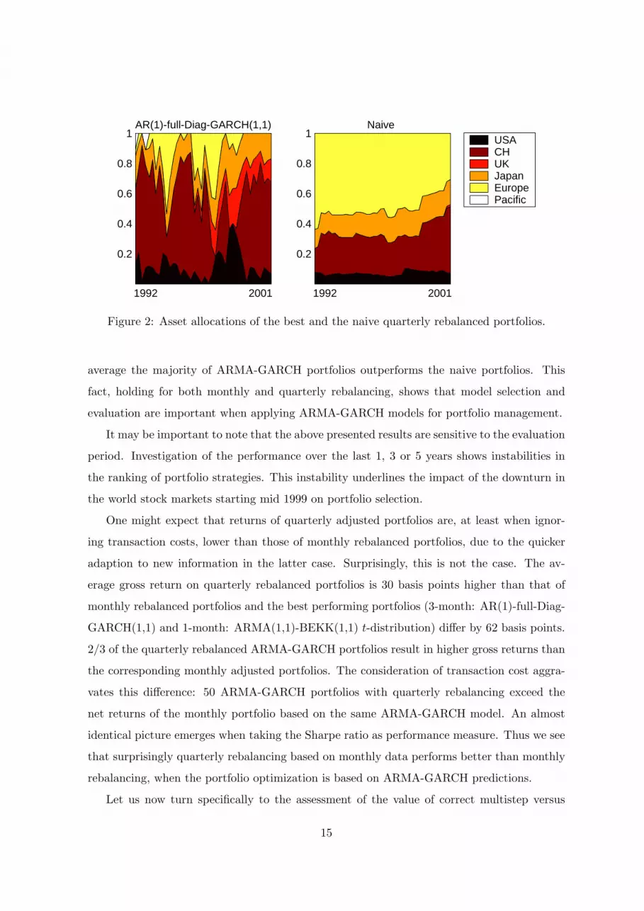
Figure 2: Asset allocations of the best and the naive quarterly rebalanced portfolios.

average the majority of ARMA-GARCH portfolios outperforms the naive portfolios. This

fact, holding for both monthly and quarterly rebalancing, shows that model selection and

evaluation are important when applying ARMA-GARCH models for portfolio management.

It may be important to note that the above presented results are sensitive to the evaluation

period. Investigation of the performance over the last 1, 3 or 5 years shows instabilities in

the ranking of portfolio strategies. This instability underlines the impact of the downturn in

the world stock markets starting mid 1999 on portfolio selection.

One might expect that returns of quarterly adjusted portfolios are, at least when ignor-

ing transaction costs, lower than those of monthly rebalanced portfolios, due to the quicker

adaption to new information in the latter case. Surprisingly, this is not the case. The av-

erage gross return on quarterly rebalanced portfolios is 30 basis points higher than that of

monthly rebalanced portfolios and the best performing portfolios (3-month: AR(1)-full-Diag-

GARCH(1,1) and 1-month: ARMA(1,1)-BEKK(1,1) t-distribution) differ by 62 basis points.

2/3 of the quarterly rebalanced ARMA-GARCH portfolios result in higher gross returns than

the corresponding monthly adjusted portfolios. The consideration of transaction cost aggra-

vates this difference: 50 ARMA-GARCH portfolios with quarterly rebalancing exceed the

net returns of the monthly portfolio based on the same ARMA-GARCH model. An almost

identical picture emerges when taking the Sharpe ratio as performance measure. Thus we see

that surprisingly quarterly rebalancing based on monthly data performs better than monthly

rebalancing, when the portfolio optimization is based on ARMA-GARCH predictions.

Let us now turn specifically to the assessment of the value of correct multistep versus

15

incorrect 1-step predictions of returns and covariances based on ARMA-GARCH models. The

above favorable results of quarterly rebalanced portfolios, based on correct 3-step predictions,

are possibly driven by two factors: The use of monthly data and the use of correct multistep

predictions. In order to single out the value of the correct predictions, we compare the results

next with quarterly rebalanced portfolios based on (incorrect) 1-step predictions. These

results are again contained in Table 3 in the Appendix and summarized in Table 2. 52 out

of the 66 ARMA-GARCH portfolios exhibit higher gross returns with the correct multistep

method than with the incorrect 1-step prediction. The mean difference is 32 basis points.

Note that the generally poor performing principal components models account for most of

the cases where the incorrect predictions perform better. Excluding these models, the correct

method leads in 46 out of 48 cases to better performance. The average over-performance

is then 69 basis points. Again, an almost identical picture emerges for net returns and the

Sharpe ratio. The substantial advantage of using the correct multistep prediction is also

present for the naive portfolio strategy.

The results are briefly summarized as follows: Considering gross returns the correctly

predicted quarterly rebalanced portfolios perform best, followed by the monthly rebalanced

portfolios and the incorrectly predicted quarterly rebalanced portfolios. This ranking holds in

particular for both the average across all ARMA-GARCH portfolios and the respective best

ARMA-GARCH portfolios. This is striking as one expects for gross returns, i.e. where trans-

action costs are ignored, monthly rebalanced portfolios to outperform quarterly rebalanced

portfolios. Looking at the average net return across all ARMA-GARCH models, the correctly

predicted quarterly rebalanced portfolios perform again best, now followed by the incorrectly

predicted quarterly rebalanced portfolios and the monthly rebalanced portfolios. The inferior

performance of the monthly rebalanced portfolios, even compared to the quarterly rebalanced

portfolios based on incorrect multistep predictions, is explained by the higher transaction costs

due to the higher rebalancing frequency. The naive portfolio is, both in terms of gross and

net returns, outperformed by the majority of ARMA-GARCH portfolios. This holds even

when the latter are based on incorrect predictions. Basing the quarterly portfolio decision on

correct multistep predictions leads in virtually all cases to performance gains.

16

IV Summary and Conclusions

In this paper we have derived the closed form solution for multistep predictions of the con-

ditional mean and covariance for ARMA-GARCH models and have illustrated their value

for portfolio management. Multistep predictions of the conditional means and covariances

are e.g. needed for mean-variance portfolio analysis when the rebalancing frequency is lower

than the data frequency. In order to deal with this problem we have in addition derived the

explicit formula for the conditional covariance matrix of the corresponding cumulative higher

frequency returns. The closed form solution for the general ARMA(p,q)-GARCH(k,l) case is

provided in the Appendix along with a convenient recursive representation.

The practical relevance of these results has been assessed empirically with an application to

six regional MSCI indices using a large variety of ARMA-GARCH models. Based on monthly

data the portfolio performance of monthly and quarterly rebalanced portfolios is investigated.

The quarterly rebalancing decision is based on either the (model consistent) correct 3-step

predictions or is incorrectly based on 1-step predictions. The evaluation period is January

1992 to December 2001. Some observations emerge: The first observation is that basing

the quarterly rebalancing decision on correct multistep predictions is for almost all portfolios

advisable. I.e. for almost all ARMA-GARCH models the return of the corresponding portfolio

is higher when the rebalancing decision is based on the correct multistep predictions. This

holds for gross returns, net returns and also the Sharpe ratio. The second main observation

is the fact that for gross returns, i.e. when neglecting transaction costs, quarterly rebalanced

portfolios based on multistep predictions lead to better performance than monthly adjusted

portfolios. The latter in general outperform quarterly adjusted portfolios based on 1-step

predictions. For net returns, even the quarterly adjusted portfolios based on 1-step predictions

outperform (on average) the monthly adjusted portfolios. This is a surprising result, as a priori

one would expect - at least for gross returns - that monthly rebalanced portfolios outperform

quarterly adjusted portfolios. This conjecture, based on the argument that monthly adjusted

portfolios incorporate new information faster, is not validated for our empirical example.

The third observation is that by basing the portfolio decision on (predictions from) ARMA-

GARCH models one can substantially outperform the naive portfolio and the benchmark.

This fact that portfolios that rely upon volatility models can outperform naive (or static)

portfolios is also found for daily data e.g. by Fleming et al. (2001). Fourthly, we have observed

17

that no particular class of GARCH models leads to superior performance and we have finally

seen that models with t-distributed innovations lead to better portfolio performance for the

monthly adjusted portfolios only.

An important theoretical question that is left open for future research is the derivation

of multistep predictions for multivariate GARCH-in-Mean models. See Karanasos (2001) or

Nilsson (2002) for some results concerning prediction for this model class. An important

empirical issue that requires further exploration is to assess the value of multistep predictions

at higher data frequencies, to explore e.g. the performance of weekly portfolio allocation based

on daily data. This might lead to interesting results as the volatility effects are stronger at

higher frequencies which should increase the value of correct conditional multistep predictions

of conditional covariances.

18

Appendix: Multistep ARMA-GARCH Predictions

In this appendix we derive multistep predictions for the conditional means and covariances of mul-tivariate ARMA(p,q)-GARCH(k,l) models. We derive both the mean squared error (MSE) predictorand the conditional MSE. Related to the portfolio optimization problem in the main text we alsoderive the predictions for the conditional variance of the forecast of the sum of the variable (in ourcase returns) h-steps ahead. These are required in the portfolio optimization problem where the datafrequency is higher than the rebalancing frequency, see the discussion in Section 2.

In the discussion we abstain from deriving also the multistep prediction formula for the conditionalvariance of the innovations εt. Obtaining these is a standard prediction problem for the ARMAtype variance equation. Thus, this result is dependent of the precise formulation of the varianceequation and easily available if the variance equation is specified. Furthermore note also that multisteppredictions of the conditional variances of the innovations εt are directly available in various softwarepackages, whereas the conditional variances of multistep predictions of the returns themselves are toour knowledge not implemented in software packages.

Note that the limits for h → ∞ of the derived results for the minimum MSE predictor of themean and variance are finite only for stationary processes. Also note that the derivations do notapply to ARCH-in-Mean models, where by construction the prediction of the mean is coupled withthe prediction of the conditional variance.

To facilitate the actual implementation of the results we also derive a recursive representation ofthe result, compare the AR(1) example in Section 2.3.

In relation to the empirical application presented in the main text we finally derive in detail theclosed form representation of the conditional variance matrix of the returns over 3 periods ahead forall mean equations implemented empirically, i.e. for ARMA(1,1), AR(1), and MA(1) mean equations.

The cumulative returns over an h−period horizon, henceforth denoted as r[t+1:t+h], are straight-forwardly calculated from the single period returns, rt+i, as follows

r[t+1:t+h] = rt+1 + · · ·+ rt+h

Thus, the conditional covariance matrix of the cumulated returns r[t+1:t+h] is

cov(r[t+1:t+h], r[t+1:t+h]|It) = cov(rt+1 + · · ·+ rt+h, rt+1 + · · ·+ rt+h|It)

=h∑

i=1

cov(rt+i, rt+i|It) +h∑

i,j=1,i �=j

cov(rt+i, rt+j |It)(2)

where It denotes again the information set at time t. One clearly sees from this equation thatthe conditional variance matrix of r[t+1:t+h] is composed of the (conditional) variances and covari-ances of the one-period returns in rt+i for i = 1, . . . , h. We thus see that for the calculatingcov(r[t+1:t+h], r[t+1:t+h]|It) it is necessary to derive the MSE predictor of rt+i and the correspond-ing conditional variances and covariances.

General Case

Let rt be an n-dimensional ARMA(p, q), p, q ∈ N, process with GARCH errors

rt = c+p∑

i=1

Airt−i +q∑

i=1

Biεt−i + εt(3)

where c ∈ Rn, εt ∼ WN(0,Σt), with Σt = cov(εt, εt|It−1) and A1, . . . , Ap, B1, . . . , Bq ∈ R

n×n matri-ces. In the derivation of the minimum MSE predictors of rt+i and their conditional covariances it is

19

convenient to express the model (3) in the following format:

rt

rt−1

...rt−p+1

εt

εt−1

...εt−q+1

=

c0...000...0

+

A1 . . . Ap B1 . . . Bq

I 0 . . . 0 0 . . . 0... . . .

...... . . .

...0 . . . I 0 0 . . . 00 . . . 0 0 . . . 00 . . . 0 I . . . 0... . . .

...... . . .

...0 . . . 0 0 . . . I 0

rt−1

rt−2

...rt−p

εt−1

εt−2

...εt−q

+

εt

0...0εt

0...0

(4)

or more compactly as

Rt = E1c+ΦRt−1 + Eεt(5)

where I ∈ Rn×n is the identity matrix and Rt ∈ R

(p+q)n, Φ ∈ R(p+q)n×(p+q)n, E1, E ∈ R

(p+q)n×n aredefined as follows

Rt = (r′t, . . . , r′t−p+1, ε

′t, . . . , ε

′t−q+1)

′(6)

Φ =

A1 . . . Ap B1 . . . Bq

I 0 . . . 0 0 . . . 0... . . .

...... . . .

...0 . . . I 0 0 . . . 00 . . . 0 0 . . . 00 . . . 0 I . . . 0... . . .

...... . . .

...0 . . . 0 0 . . . I 0

(7)

and

E = E1 + Ep+1(8)

The matrices Ej , j = 1, . . . , p + q denote (p + q)n × n matrices of 0n×n sub-matrices except for thej-th sub-matrix, which is the n× n identity matrix. From (4) or (5) it follows that

cov(rt+i, rt+j |It) = E′1cov(Rt+i, Rt+j |It)E1(9)

where E1 ∈ R(p+q)n×n is defined as above for j = 1. Iterating equation (5) (i− 1)-times leads to

Rt =i−1∑j=0

ΦjE1c+ΦiRt−i +i−1∑j=0

ΦjEεt−j(10)

where i = 1, . . . , t− 1. For the sake of brevity we introduce the following notation for i, j ∈ N

ΣRt+i,t = cov(Rt+i, Rt+i|It)

ΣRt+i,t+j,t = cov(Rt+i, Rt+j |It)

where ΣRt+i,t and Σ

Rt+i,t+j,t ∈ R

(p+q)n×(p+q)n. Note that ΣRt+i,t = Σ

Rt+i,t+i,t.

From (6) it directly follows that

Rt =p−1∑i=0

Ei+1rt−i +q−1∑i=0

Ei+p+1εt−i(11)

20

It then follows from (6), (10) and (11) that

rt+h =h−1∑i=0

E′1Φ

iE1c+p−1∑i=0

(E′1Φ

hEi+1)rt−i +q−1∑i=0

(E′1Φ

hEi+p+1)εt−i +h−1∑i=0

(E′1Φ

iE)εt+h−i(12)

From this, the minimum MSE h-step ahead predictor for rt+h is readily seen to be

E(rt+h|It) =h−1∑i=0

E′1Φ

iE1c+p−1∑i=0

(E′1Φ

hEi+1)rt−i +q−1∑i=0

(E′1Φ

hEi+p+1)εt−i(13)

Furthermore, (12) and (13) imply that the forecast error for the h−step ahead predictor in (13) isgiven by

et,h =h−1∑j=0

(E′1Φ

jE)εt+h−j(14)

which directly leads to the conditional MSE given by:

E(et,he′t,h|It) = cov(rt+h, rt+h|It) = E′

1

h−1∑j=0

ΦjE Σt+h−j,t(ΦjE)′E1(15)

In expression (15) the conditional covariances Σt+i,t for i = 0, . . . , h − 1 show up. For an evaluation,respectively estimation, of this expression therefore the expected values of the conditional i-step aheadcovariances of the innovations εt have to be computed. These obviously depend upon the precisespecification of the variance equation of the ARMA-GARCH model. Computation of the requiredmatrices Σt+i,t is, as already mentioned also at the beginning of this appendix, straightforward for aspecified variance equation. For all implemented variance equations the required results are containedin the output of the used GARCH software.

Using (9) and (10) we obtain

cov(rt+i, rt+j |It) = E′1Σ

Rt+i,t+j,tE1

= E′1cov(Φ

iRt +i−1∑k=0

ΦkEεt+i−k,ΦjRt +j−1∑l=0

ΦlEεt+j−l|It)E1

= E′1

i−1∑k=max{0,i−j}

ΦkE Σt+i−k,t(Φj−i+kE)′E1(16)

An estimate of quantity (16) is obtained, as already mentioned above, by inserting estimates for thematrices Σt+i,t in this expression. From (2) and (16) we now obtain the result for the conditionalcovariance matrix of the aggregated h-period returns:

cov(r[t+1:t+h], r[t+1:t+h]|It) = cov(rt+1 + · · ·+ rt+h, rt+1 + · · ·+ rt+h|It)

= E′1

h∑i=1

[i−1∑k=0

ΦkE Σt+i−k,t(ΦkE)′]E1

+E′1

h∑i,j=1,i �=j

i−1∑

k=max{0,i−j}ΦkE Σt+i−k,t(Φj−i+kE)′

E1

(17)

Thus, we see again that the expression for cov(r[t+1:t+h], r[t+1:t+h]|It) depends upon the mean equationand the conditional covariances of the innovations. An estimate of equation (17) is given by subsitutingall parameters with estimates and by inserting the predictions of the conditonal variances of εt+i.

21

When rewriting the ARMA model in companion form (5) caution has to be taken in the definitionof the quantities Rt, Φ and E (see equations (6)−(8)), when either the autoregressive order p or themoving average order q are equal to 0. See the following remark:

Remark 1 If q = 0, i.e. we consider an AR(p) mean equation, it is more convenient to use (5) withRt, Φ and E defined by

Rt = (r′t, . . . , r′t−p+1)

′

Φ =

A1 . . . Ap

I 0 . . . 0... . . .

...0 . . . I 0

and E = E1.If we consider an MA(q) mean equation, i.e. the case p = 0, it is more convenient to use repre-

sentation (5) with the following quantities:

Rt = (r′t, ε′t, . . . , ε

′t−q+1)

′

Φ =

0 B1 . . . Bq

0 0 . . . 00 I . . . 0...

... . . ....

0 0 . . . I 0

and E = E1 + E2.

Note that ΣRt+i,t+j,t can also be calculated recursively. Consider i = j first, then (5) implies

ΣRt+i,t = cov(Rt+i, Rt+i|It) = cov(ΦRt+i−1 + Eεt+i,ΦRt+i−1 + Eεt+i|It)

= ΦΣRt+i−1,tΦ

′ + EΣt+i,tE′(18)

as cov(Eεt+i, Rt+i−1|It) = 0. Consider next the case i > j, then (10) implies

ΣRt+i,t+j,t = cov(Rt+i, Rt+j |It) = cov(Φi−jRt+j +

i−j−1∑k=0

ΦkEεt+i−k, Rt+j |It)

= Φi−jΣRt+j,t(19)

as cov(Eεt+i−k, Rt+j |It) = 0 for k = 0, . . . , i− j − 1. Finally, let i < j. Then using (5) we obtain

ΣRt+i,t+j,t = cov(Rt+i, Rt+j |It) = cov(Rt+i,Φj−iRt+i +

j−i−1∑k=0

ΦkEεt+j−k|It)

= ΣRt+i,t(Φ

j−i)′(20)

as cov(Rt+i, Eεt+j−k|It) = 0 for k = 0, . . . , j − i − 1. Taking equations (2), (9) (18)−(20) and thedefinition of ΣR

t+i,t+j,t we obtain the result:

cov(r[t+1:t+h], r[t+1:t+h]|It) = E′1

h∑

i=1

ΣRt+i,t +

h∑i=2

i−1∑j=1

Φi−jΣRt+j,t

E1 +

+ E′1

h−1∑

i=1

h∑j=i+1

ΣRt+i,t(Φ

j−i)′

E1(21)

22

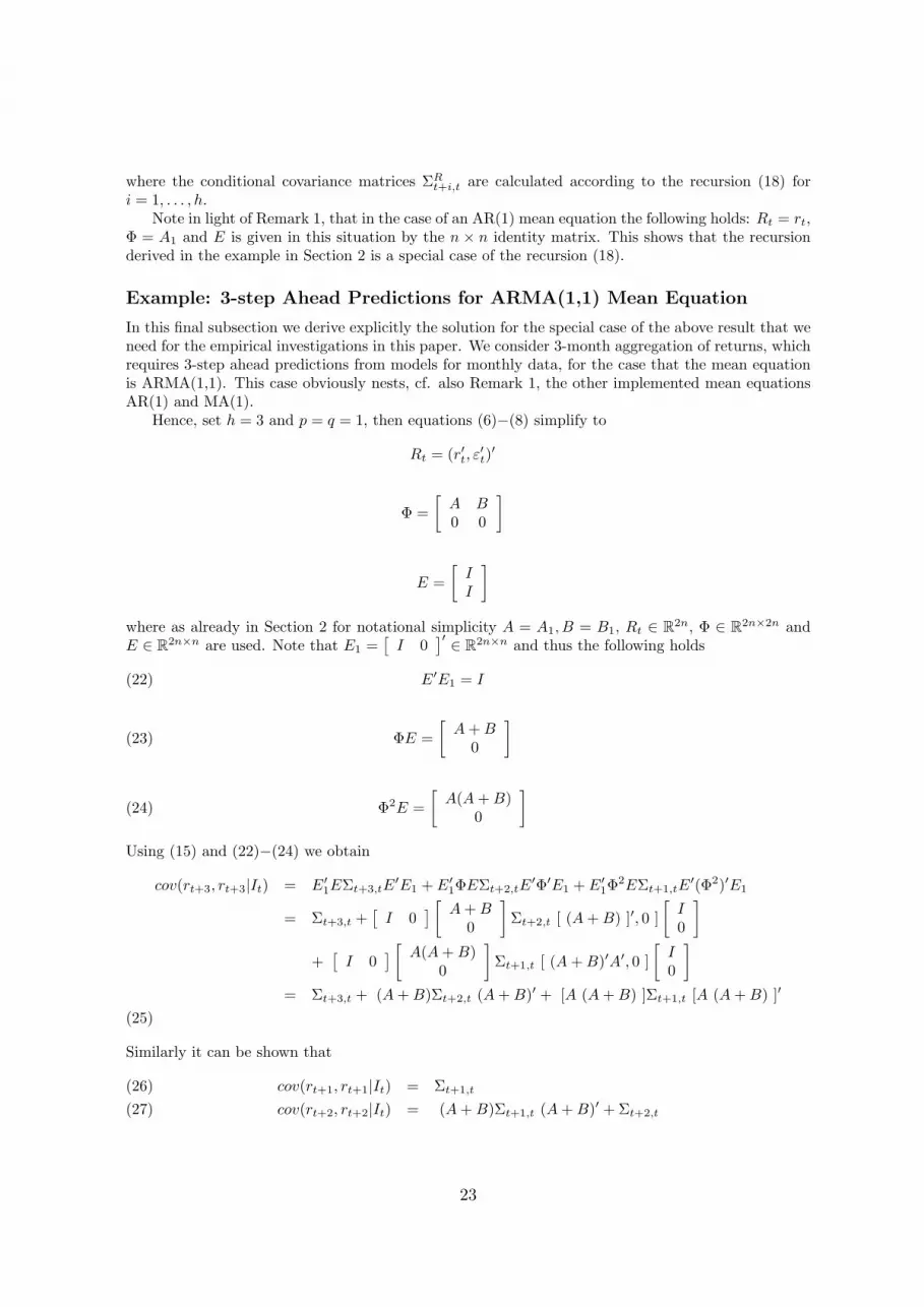
where the conditional covariance matrices ΣRt+i,t are calculated according to the recursion (18) for

i = 1, . . . , h.Note in light of Remark 1, that in the case of an AR(1) mean equation the following holds: Rt = rt,

Φ = A1 and E is given in this situation by the n × n identity matrix. This shows that the recursionderived in the example in Section 2 is a special case of the recursion (18).

Example: 3-step Ahead Predictions for ARMA(1,1) Mean Equation

In this final subsection we derive explicitly the solution for the special case of the above result that weneed for the empirical investigations in this paper. We consider 3-month aggregation of returns, whichrequires 3-step ahead predictions from models for monthly data, for the case that the mean equationis ARMA(1,1). This case obviously nests, cf. also Remark 1, the other implemented mean equationsAR(1) and MA(1).

Hence, set h = 3 and p = q = 1, then equations (6)−(8) simplify to

Rt = (r′t, ε′t)

′

Φ =[

A B0 0

]

E =[

II

]

where as already in Section 2 for notational simplicity A = A1, B = B1, Rt ∈ R2n, Φ ∈ R

2n×2n andE ∈ R

2n×n are used. Note that E1 =[

I 0]′ ∈ R

2n×n and thus the following holds

E′E1 = I(22)

ΦE =[

A+B0

](23)

Φ2E =[

A(A+B)0

](24)

Using (15) and (22)−(24) we obtain

cov(rt+3, rt+3|It) = E′1EΣt+3,tE

′E1 + E′1ΦEΣt+2,tE

′Φ′E1 + E′1Φ

2EΣt+1,tE′(Φ2)′E1

= Σt+3,t +[

I 0] [

A+B0

]Σt+2,t [ (A+B) ]′, 0 ]

[I0

]

+[

I 0] [

A(A+B)0

]Σt+1,t [ (A+B)′A′, 0 ]

[I0

]= Σt+3,t + (A+B)Σt+2,t (A+B)′ + [A (A+B) ]Σt+1,t [A (A+B) ]′

(25)

Similarly it can be shown that

cov(rt+1, rt+1|It) = Σt+1,t(26)cov(rt+2, rt+2|It) = (A+B)Σt+1,t (A+B)′ +Σt+2,t(27)

23

Equations (16), (22)−(24) imply

cov(rt+3, rt+2|It) = E′1ΦEΣt+2,tE

′E1 + E′1Φ

2EΣt+1,t(ΦE)′E1

=[

I 0] [

A+B0

]Σt+2,t

+[

I 0] [

A(A+B)0

]Σt+1,t [ (A+B)′, 0 ]

[I0

]= (A+B)Σt+2,t +A (A+B)Σt+1,t (A+B)′(28)

Along the same lines it also directly follows that

cov(rt+2, rt+1|It) = (A+B)Σt+1,t(29)cov(rt+3, rt+1|It) = A (A+B)Σt+1,t(30)

and cov(rt+1, rt+2|It) = cov(rt+2, rt+1|It)′, cov(rt+1, rt+3|It) = cov(rt+3, rt+1|It)′, cov(rt+2, rt+3|It)= cov(rt+3, rt+2|It)′. Thus, from (2), (25)−(30) after some algebraic modifications we arrive at thefollowing result:

cov(r[t+1:t+3], r[t+1:t+3]|It)

= [I + (I +A) (A+B) ]Σt+1,t [I + (I +A)(A+B)]′

+ (I +A+B)Σt+2,t (I +A+B)′ +Σt+3,t(31)

The required predictions for Σt+1,t,Σt+2,t and Σt+3,t and the estimates for A and B are in our

application for all implemented models directly obtained from the GARCH Module in SPLUS.

In the AR(1) case the above result holds with B = 0 and for the MA(1) case only A = 0 has to be

inserted.

24

Tab

le3:

Mea

nR

eturn

sov

erEva

luat

ion

Per

iod

1992

/1to

2001

/12

Estimatedmodel

monthlyrebalancing

quarterlyrebalancing

Meaneq.

Varianceeq.

1-stepprediction

3-stepprediction(correct)

1-stepprediction(”incorrect”)

Gross

Net

Sharpe

Sharpe

Gross

Net

Sharpe

Gross

Net

Sharpe

return

return

ratio

ratio

return

return

ratio

return

return

ratio

1-month

3-month

3-month

3-month

AR(1)

BEKK(1,1)

11.16

10.40

0.143

0.190

11.43

11.04

0.210

11.22

10.77

0.206

MA(1)

BEKK(1,1)

10.99

10.25

0.141

0.187

11.20

10.84

0.205

10.95

10.52

0.199

AR(1)full

BEKK(1,1)

11.11

10.32

0.143

0.189

11.49

11.09

0.215

11.28

10.82

0.210

AR(1)t

BEKK(1,1)

11.47

10.68

0.149

0.199

12.24

11.80

0.242

11.67

11.22

0.219

MA(1)t

BEKK(1,1)

11.42

10.52

0.151

0.196

12.47

12.10

0.247

12.40

11.95

0.244

ARMA(1,1)t

BEKK(1,1)

12.01

11.05

0.159

0.209

12.59

12.11

0.245

12.20

11.66

0.235

AR(1)

CCCGARCH(1,1)

10.32

8.77

0.132

0.154

10.24

9.87

0.188

9.72

9.10

0.170

MA(1)

CCCGARCH(1,1)

10.75

9.18

0.138

0.165

10.20

9.85

0.186

9.65

9.04

0.167

AR(1)full

CCCGARCH(1,1)

9.94

8.38

0.124

0.141

10.22

9.86

0.186

9.49

8.86

0.164

AR(1)t

CCCGARCH(1,1)

10.86

9.83

0.140

0.184

11.04

10.62

0.208

10.44

9.93

0.191

MA(1)t

CCCGARCH(1,1)

10.67

9.50

0.135

0.173

10.30

9.86

0.189

9.90

9.36

0.176

ARMA(1,1)t

CCCGARCH(1,1)

11.53

10.42

0.146

0.192

11.81

11.37

0.223

11.26

10.68

0.205

AR(1)

CCCPGARCH(1,1)

9.02

7.69

0.103

0.113

9.31

8.83

0.156

8.81

8.23

0.142

MA(1)

CCCPGARCH(1,1)

9.07

7.75

0.104

0.117

8.75

8.25

0.141

8.18

7.57

0.125

AR(1)full

CCCPGARCH(1,1)

9.59

8.62

0.114

0.144

10.37

9.97

0.191

9.79

9.31

0.175

AR(1)t

CCCPGARCH(1,1)

9.21

7.76

0.105

0.118

10.86

10.29

0.198

10.31

9.61

0.182

MA(1)t

CCCPGARCH(1,1)

8.31

6.77

0.088

0.088

9.28

8.67

0.153

9.11

8.36

0.148

ARMA(1,1)t

CCCPGARCH(1,1)

9.86

8.43

0.115

0.139

11.36

10.82

0.214

10.89

10.22

0.198

AR(1)

CCCEGARCH(1,1)

10.35

8.66

0.128

0.146

10.45

10.05

0.190

9.85

9.19

0.170

MA(1)

CCCEGARCH(1,1)

10.35

8.66

0.128

0.146

10.45

10.06

0.191

9.85

9.19

0.170

AR(1)full

CCCEGARCH(1,1)

9.92

8.29

0.121

0.137

10.34

9.91

0.186

9.64

8.94

0.166

AR(1)t

CCCEGARCH(1,1)

10.97

10.06

0.140

0.186

11.54

11.14

0.222

11.18

10.71

0.211

MA(1)t

CCCEGARCH(1,1)

11.04

10.14

0.142

0.189

11.44

11.07

0.218

11.09

10.65

0.207

ARMA(1,1)t

CCCEGARCH(1,1)

11.33

10.52

0.144

0.192

11.45

11.10

0.216

11.07

10.67

0.204

AR(1)

DiagGARCH(1,1)

10.69

10.44

0.132

0.186

12.48

12.03

0.246

10.65

10.52

0.189

MA(1)

DiagGARCH(1,1)

10.76

10.52

0.133

0.187

12.50

12.04

0.245

10.62

10.49

0.188

AR(1)full

DiagGARCH(1,1)

10.78

10.52

0.133

0.187

12.63

12.14

0.248

10.76

10.62

0.191

AR(1)t

DiagGARCH(1,1)

10.74

10.51

0.133

0.186

12.15

11.78

0.243

10.62

10.51

0.188

MA(1)t

DiagGARCH(1,1)

10.73

10.50

0.133

0.186

12.10

11.72

0.242

10.61

10.50

0.188

ARMA(1,1)t

DiagGARCH(1,1)

10.66

10.34

0.132

0.183

10.27

9.62

0.182

10.54

10.38

0.185

25

Tab

le3

(con

tinued

):M

ean

Ret

urn

sov

erEva

luat

ion

Per

iod

1992

/1to

2001

/12

Estimatedmodel

monthlyrebalancing

quarterlyrebalancing

Meaneq.

Varianceeq.

1-stepprediction

3-stepprediction(correct)

1-stepprediction(”incorrect”)

Gross

Net

Sharpe

Sharpe

Gross

Net

Sharpe

Gross

Net

Sharpe

return

return

ratio

ratio

return

return

ratio

return

return

ratio

1-month

3-month

3-month

3-month

AR(1)

DiagPGARCH(1,1)

10.03

9.59

0.118

0.161

9.91

9.22

0.167

9.98

9.77

0.170

MA(1)

DiagPGARCH(1,1)

9.84

9.44

0.115

0.157

10.33

9.60

0.177

10.04

9.83

0.171

AR(1)full

DiagPGARCH(1,1)

9.92

9.59

0.118

0.162

10.91

10.35

0.203

10.01

9.84

0.172

AR(1)t

DiagPGARCH(1,1)

10.35

10.06

0.125

0.173

11.31

10.80

0.214

10.40

10.26

0.182

MA(1)t

DiagPGARCH(1,1)

10.37

10.08

0.125

0.174

11.38

10.89

0.218

10.34

10.20

0.180

ARMA(1,1)t

DiagPGARCH(1,1)

10.24

9.97

0.122

0.171

12.00

11.49

0.220

10.24

10.10

0.177

AR(1)

DiagEGARCH(1,1)

10.52

10.28

0.129

0.181

12.22

11.78

0.239

10.59

10.47

0.187

MA(1)

DiagEGARCH(1,1)

10.53

10.29

0.129

0.181

12.21

11.77

0.239

10.58

10.46

0.187

AR(1)full

DiagEGARCH(1,1)

10.54

10.31

0.129

0.181

12.05

11.61

0.234

10.65

10.53

0.188

AR(1)t

DiagEGARCH(1,1)

10.49

10.22

0.128

0.179

11.56

11.08

0.223

10.45

10.31

0.183

MA(1)t

DiagEGARCH(1,1)

10.48

10.21

0.128

0.178

11.55

11.06

0.224

10.44

10.31

0.183

ARMA(1,1)t

DiagEGARCH(1,1)

10.62

10.25

0.130

0.180

10.78

9.90

0.191

10.65

10.49

0.188

AR(1)

VectorDiagModel

9.63

8.73

0.116

0.147

10.07

9.68

0.178

9.79

9.30

0.170

MA(1)

VectorDiagModel

9.58

8.68

0.115

0.145

9.97

9.60

0.176

9.69

9.21

0.168

AR(1)full

VectorDiagModel

9.76

8.86

0.118

0.150

10.36

9.96

0.185

10.12

9.62

0.179

AR(1)t

VectorDiagModel

9.36

8.50

0.111

0.144

10.06

9.69

0.178

9.77

9.32

0.170

MA(1)t

VectorDiagModel

9.51

8.62

0.114

0.148

10.12

9.73

0.182

9.85

9.38

0.174

ARMA(1,1)t

VectorDiagModel

10.19

9.21

0.123

0.160

11.34

10.87

0.211

10.89

10.35

0.199

AR(1)

PCGARCH(1,1)

10.69

10.36

0.132

0.179

9.96

9.61

0.165

10.45

10.28

0.181

MA(1)

PCGARCH(1,1)

10.70

10.38

0.132

0.180

10.00

9.67

0.166

10.48

10.30

0.182

AR(1)full

PCGARCH(1,1)

10.70

10.36

0.132

0.180

10.41

10.03

0.176

10.40

10.22

0.180

AR(1)t

PCGARCH(1,1)

10.65

10.39

0.131

0.180

9.18

8.89

0.142

10.50

10.37

0.184

MA(1)t

PCGARCH(1,1)

10.75

10.48

0.134

0.184

9.16

8.70

0.141

10.51

10.37

0.183

ARMA(1,1)t

PCGARCH(1,1)

10.90

10.61

0.135

0.186

9.87

9.37

0.165

10.87

10.72

0.193

AR(1)

PCPGARCH(1,1)

10.79

10.42

0.134

0.182

10.03

9.85

0.164

10.58

10.38

0.186

MA(1)

PCPGARCH(1,1)

10.70

10.35

0.132

0.180

9.92

9.55

0.159

10.49

10.30

0.183

AR(1)full

PCPGARCH(1,1)

10.56

10.22

0.129

0.175

8.79

8.69

0.134

10.47

10.30

0.182

AR(1)t

PCPGARCH(1,1)

10.96

10.65

0.137

0.188

8.90

8.73

0.135

10.87

10.71

0.193

MA(1)t

PCPGARCH(1,1)

10.91

10.59

0.136

0.186

8.74

8.40

0.131

10.60

10.44

0.186

ARMA(1,1)t

PCPGARCH(1,1)

11.03

10.71

0.138

0.189

10.53

10.08

0.169

10.83

10.67

0.192

26

Tab

le3

(con

tinued

):M

ean

Ret

urn

sov

erEva

luat

ion

Per

iod

1992

/1to

2001

/12

Estimatedmodel

monthlyrebalancing

quarterlyrebalancing

Meaneq.

Varianceeq.

1-stepprediction

3-stepprediction(correct)

1-stepprediction(”incorrect”)

Gross

Net

Sharpe

Sharpe

Gross

Net

Sharpe

Gross

Net

Sharpe

return

return

ratio

ratio

return

return

ratio

return

return

ratio

1-month

3-month

3-month

3-month

AR(1)

PCEGARCH(1,1)

10.90

10.53

0.136

0.184

10.95

10.79

0.193

10.64

10.46

0.186

MA(1)

PCEGARCH(1,1)

10.87

10.52

0.135

0.183

10.88

10.72

0.191

10.60

10.42

0.185

AR(1)full

PCEGARCH(1,1)

10.86

10.50

0.135

0.182

10.77

10.58

0.186

10.55

10.37

0.183

AR(1)t

PCEGARCH(1,1)

10.85

10.59

0.135

0.185

10.77

10.65

0.190

10.63

10.49

0.187

MA(1)t

PCEGARCH(1,1)

10.85

10.58

0.135

0.185

10.78

10.66

0.190

10.62

10.48

0.186

ARMA(1,1)t

PCEGARCH(1,1)

10.81

10.44

0.134

0.181

10.54

10.29

0.182

10.85

10.68

0.192

Naive

10.23

10.19

0.124

0.177

10.55

10.50

0.183

10.20

10.17

0.176

Riskfree

3.21

3.38

Benchmark

9.73

0.106

0.155

9.73

0.155

Remarks:

Thereturnandcovariancepredictionsusedinthemean-varianceoptimizationarebasedonmonthlydata.

Theportfoliocompositionisadjustedevery3months(1month)from

January1992toOctober(December)2001.

Theresultsreportedcorrespondtotheevaluationof

glob

alm

inim

umva

rian

ceportfolios.

Est

imat

edm

odelspecifiesthe

mea

neq

uationandthe

vari

ance

equa

tionoftheestimatedARMA-GARCHmodel.

Gro

ssre

turndenotesthemeanannualizedreturnoftheportfolio.

Net

retu

rndenotesthemeanannualizedreturnoftheportfolioafterdeductingtransactioncosts(seeSection3).

Shar

pera

tioisgivenbynetexcessreturn(i.e.netreturnminusriskfreerate)dividedbytheportfolio’sstandarddeviation.

1-m

onth

Shar

pera

tiousesthestandarddeviationbasedonmonthlyreturns.

3-m

onth

Shar

pera

tiousesstandarddeviationbasedonquarterlyreturns.

3-st

eppr

edic

tionmeansthatthemodelconsistent3-steppredictionsfortheconditionalmeansandcovariancesareused.

1-st

eppr

edic

tionmeansthatthe1-steppredictionsfortheconditionalmeansandcovariancesareused.

27

References

Baillie, R.T. and T. Bollerslev. ”Prediction in dynamic models with time-dependent condi-

tional variances.” Journal of Econometrics, 52 (1992), 91–113.

Best, M.J. and R.R. Grauer. ”On the sensitivity analysis of mean-variance-efficient portfo-

lios to changes in asset means: Some analytical and computational results.” Review of

Financial Studies, 4 (1991), 315–342.

Bollerslev, T. ”Generalized autoregressive conditional heterocedasticity.” Journal of Econo-

metrics, 31 (1986), 307–327.

Bollerslev, T. ”Modeling the coherence of short-run nominal exchange rates: a multivariate

generalized ARCH model.” Review of Economics and Statistics, 72 (1990), 498–505.

Bollerlsev, T., R.F. Engle and D.B. Nelson. ”ARCH models.” In Handbook of Econometrics,

Vol. 4, R.F. Engle and D.L. McFadden, eds. Amsterdam: Elsevier (1994).

Bollerslev, T., R.F. Engle and J.M. Wooldridge. ”A capital asset pricing model with time-

varying covariance.” Journal of Political Economy, 96 (1988), 116–131.

Chopra, V.K., C.R. Hensel and A.L. Turner. ”Massaging mean-variance inputs: Returns from

alternative global investment strategies in the 1980s.” Management Science, 39 (1993),

845–855.

Chopra, V.K. and W.T. Ziemba. ”The effect of errors in means, variances, and covariances

on optimal portfolio choice.” Journal of Portfolio Management, 24 (1997), 6–11.

Ding, Z., R.F. Engle and C.W.J. Granger. ”Long memory properties of stock market returns

and a new model.” Journal of Empirical Finance, 1 (1993), 83–106.

Engle, R.F. ”Autoregressive conditional heteroscedasticity with estimates of the variance of

U.K. inflation.” Econometrica, 50 (1982), 987–1008.

Engle, R.F. and K.F. Kroner. ”Multivariate simultaneous generalized ARCH.” Econometric

Theory, 11 (1995), 122–150.

Fleming, J., C. Kirby and B. Ostdiek. ”The economic value of volatility timing.” The Journal

of Finance, 56 (2001), 329–352.

28

Gourieroux, C. ARCH models and financial applications. New York: Springer (1997).

Hamelink, F. ”Optimal International Diversification: Theory Investor’s Perspective and Prac-

tice from a Swiss Investor’s Perspective.” FAME Research Papers, 21 (2000).

Harvey, A.C., N. Shephard and E. Ruiz. ”Multivariate stochastic variance models.” Review

of Economic Studies, 61 (1994), 247–64.

Karanasos, M. ” Prediction in ARMA models with GARCH in mean effects.” Journal of Time

Series Analysis, 22 (2001), 555-576.

Markowitz, H. M. ”Portfolio selection.” The Journal of Finance, 7 (1952), 77–91.

Markowitz, H. M. ”The optimization of a quadratic function subject to linear constraints.”

Naval Research Logitstics Quarterly, 3 (1956), 111–133.

Nelson, D. ”Conditional heteroskedasticity in asset returns: a new approach.” Econometrica,

59 (1991), 347–370.

Nilsson, B. ”International Asset Pricing and the Benefits from World Market Diversification.”

Lund University Working Papers, 1 (2002).

Polasek, W. and M. Pojarliev. ”Portfolio construction with Bayesian GARCH forecasts.” In

Operations Research Proceedings 2000, Fleischmann, B. et al., eds. Heidelberg: Springer

(2001a).

Polasek, W. and M. Pojarliev. ”Applying multivariate time series forecasts for active portfolio

management.” Financial Markets and Portfolio Analysis, 15 (2001b), 201–211.

29