Sector Volatility Prediction Performance Using GARCH ... - arXiv

Sector Volatility Prediction Performance Using GARCH

Models and Artificial Neural Networks

October 1, 2020

Curtis Nybo

University of London

[email protected]

Abstract

Recently neural networks (ANNs) have seen success in volatility prediction, but the

literature is divided on where an ANN should be used rather than the common GARCH

model. The purpose of this study is to compare the volatility prediction performance of

ANN and GARCH models when applied to stocks with low, medium, and high volatility

profiles. This approach intends to identify which model should be used for each case. The

volatility profiles comprise of five sectors that cover all stocks in the U.S stock market

from 2005 to 2020. Three GARCH specifications and three ANN architectures are

examined for each sector, where the most adequate model is chosen to move on to

forecasting. The results indicate that the ANN model should be used for predicting

volatility of assets with low volatility profiles, and GARCH models should be used when

predicting volatility of medium and high volatility assets.

1 Introduction

A prominent feature of capital markets is the uncertainty around price movements. This is referred to as

volatility, which measures the dispersion of an assets returns around its average, which in turn acts as a

measure of risk. Volatility is a latent variable that cannot be observed at an instantaneous point in time.

Therefore, we resort to using averaging methods as a proxy for the true volatility value such as the common

variance or standard deviation measure. Riskier assets often have large differences between the current and

average price over a period of time, while less risky asset prices tend to remain closer to their average price.

Since an increase in volatility leads to an increase in risk, it similarly leads to an increase in potential profits

given by the larger dispersion of returns. This phenomenon makes volatility a popular topic of study in the

finance literature.

Sector Volatility Prediction Performance Using GARCH Models and Artificial Neural Networks

2

The importance of volatility as a risk measure is the main reason for incorporating it into financial analysis.

Every stock faces unique risks that pertain to its own operations or line of business, and this risk is visible

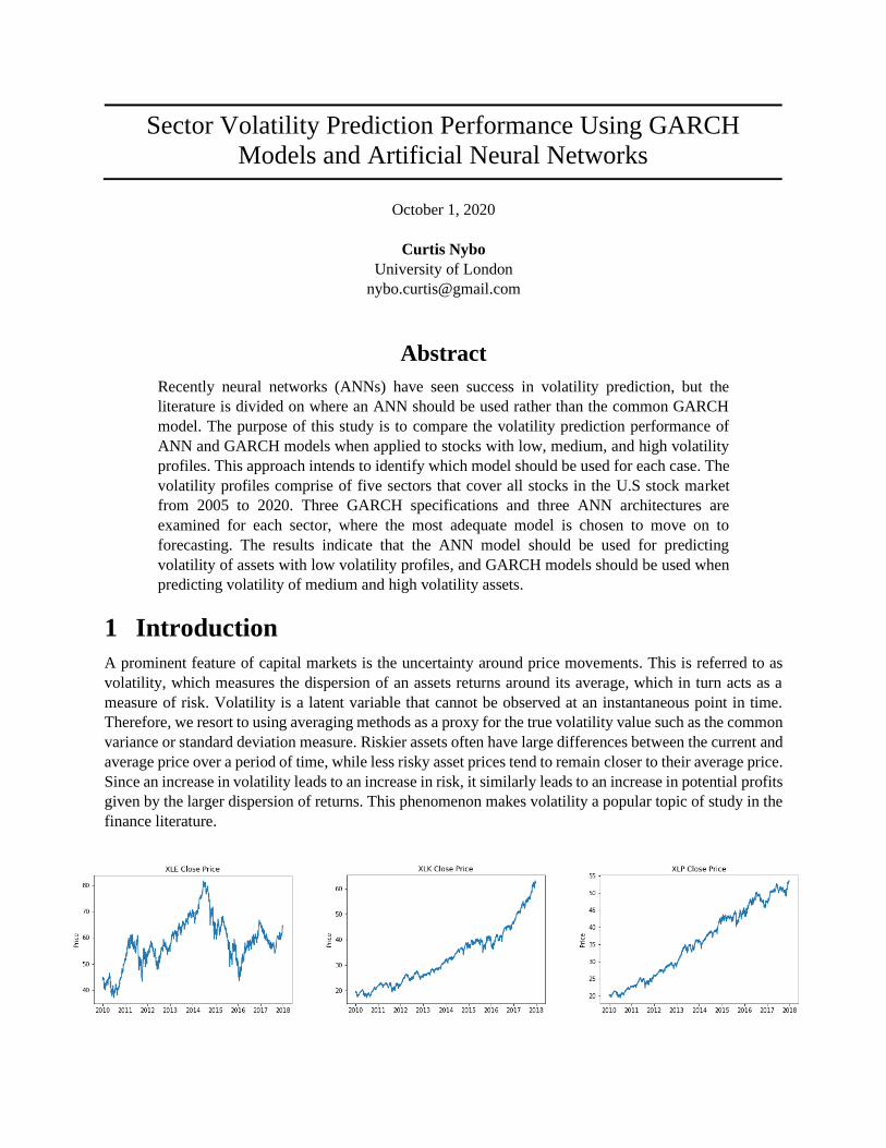
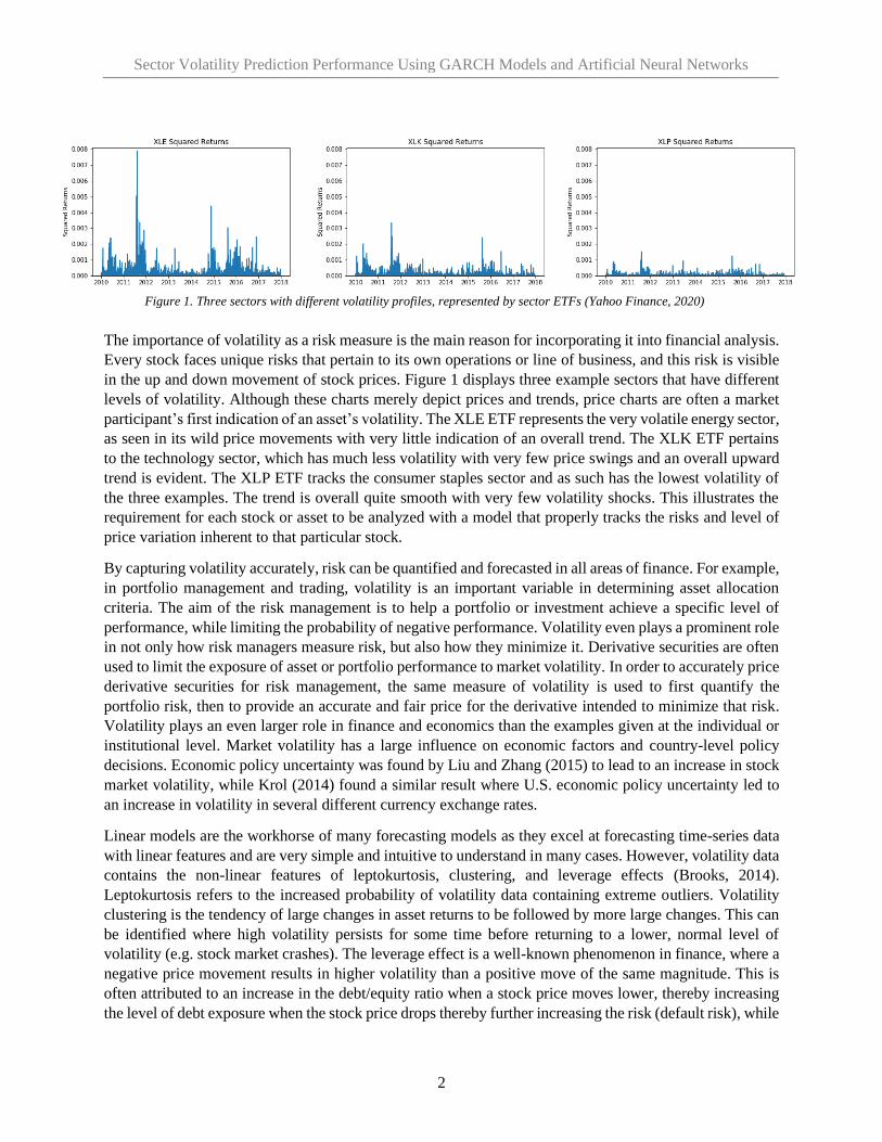
in the up and down movement of stock prices. Figure 1 displays three example sectors that have different

levels of volatility. Although these charts merely depict prices and trends, price charts are often a market

participant’s first indication of an asset’s volatility. The XLE ETF represents the very volatile energy sector,

as seen in its wild price movements with very little indication of an overall trend. The XLK ETF pertains

to the technology sector, which has much less volatility with very few price swings and an overall upward

trend is evident. The XLP ETF tracks the consumer staples sector and as such has the lowest volatility of

the three examples. The trend is overall quite smooth with very few volatility shocks. This illustrates the

requirement for each stock or asset to be analyzed with a model that properly tracks the risks and level of

price variation inherent to that particular stock.

By capturing volatility accurately, risk can be quantified and forecasted in all areas of finance. For example,

in portfolio management and trading, volatility is an important variable in determining asset allocation

criteria. The aim of the risk management is to help a portfolio or investment achieve a specific level of

performance, while limiting the probability of negative performance. Volatility even plays a prominent role

in not only how risk managers measure risk, but also how they minimize it. Derivative securities are often

used to limit the exposure of asset or portfolio performance to market volatility. In order to accurately price

derivative securities for risk management, the same measure of volatility is used to first quantify the

portfolio risk, then to provide an accurate and fair price for the derivative intended to minimize that risk.

Volatility plays an even larger role in finance and economics than the examples given at the individual or

institutional level. Market volatility has a large influence on economic factors and country-level policy

decisions. Economic policy uncertainty was found by Liu and Zhang (2015) to lead to an increase in stock

market volatility, while Krol (2014) found a similar result where U.S. economic policy uncertainty led to

an increase in volatility in several different currency exchange rates.

Linear models are the workhorse of many forecasting models as they excel at forecasting time-series data

with linear features and are very simple and intuitive to understand in many cases. However, volatility data

contains the non-linear features of leptokurtosis, clustering, and leverage effects (Brooks, 2014).

Leptokurtosis refers to the increased probability of volatility data containing extreme outliers. Volatility

clustering is the tendency of large changes in asset returns to be followed by more large changes. This can

be identified where high volatility persists for some time before returning to a lower, normal level of

volatility (e.g. stock market crashes). The leverage effect is a well-known phenomenon in finance, where a

negative price movement results in higher volatility than a positive move of the same magnitude. This is

often attributed to an increase in the debt/equity ratio when a stock price moves lower, thereby increasing

the level of debt exposure when the stock price drops thereby further increasing the risk (default risk), while

Figure 1. Three sectors with different volatility profiles, represented by sector ETFs (Yahoo Finance, 2020)


3

the opposite is true for a rise in the stock price. These features are inherent in stock volatility data and

require specific non-linear methods to accurately model and forecast volatility values.

The Autoregressive Conditional Heteroscedastic (ARCH) model was developed to deal with these non-

linear issues (Engle, 1982). The model can accommodate autoregressive behaviour such as volatility

clustering. Since autoregressive behaviour results in a variance that is dependant, or conditional, on the

prior period variance, these variances are then non-constant over a period of time. This condition is known

as heteroscedasticity, which causes imprecise confidence intervals and therefore poses a challenge for

common statistical forecasting techniques. Given the labels in the ARCH acronym, this model was

developed to address these issues. The ARCH model is widely used in practice but suffers from issues such

as determining the appropriate number of lags and non-negativity constraints. Bollerslev (1986) built upon

the work of Engle and developed the Generalized ARCH (GARCH) model, which addresses many issues

of and improves upon the ARCH model. This has led to the GARCH model often being chosen as the

appropriate model to describe volatility in academics and industry.

The advancements in data science research in the last two decades combined with the decreasing cost of

computing power has led artificial intelligence and machine learning models to see widespread applications

in finance. The study of volatility prediction has been one of these focuses. The artificial neural network

(ANN) has proven effective in solving various prediction problems, from regression and classification to

anomaly detection. The application of ANN models to volatility predictions has proven to be promising

since earlier studies in the field from researchers such as Donaldson and Kamstra (1997). More recently,

ANNs have proven to be effective in modelling non-linear data due to their reduced dependence on the

assumptions placed on the classical methods. This makes ANNs well suited for volatility prediction and

has led to increased research in this area.

The forecasting performance comparisons between GARCH and ANN models in the existing literature

focus mainly on prediction of stock market indexes covering all stocks from a certain country (e.g. NYSE,

DAX) or a specific stock or commodity. Both models have been shown to outperform one another in

different forecasting experiments, with little work completed in the sense of understanding which specific

situations each model may be better suited. The approach in this study aims to understand these specific

situations where each model may perform best by predicting volatility in specific market sectors with

varying levels of volatility.

The objective of this study is twofold. First, we develop a suitable GARCH and ANN model to compare

the forecasting performance of each model when applied to specific volatility profiles to identify the

conditions where one model may outperform the other. Second, we demonstrate the potential usefulness of

ANNs for volatility prediction within these volatility profiles. The volatility profiles are made up of five

sector portfolios that contain all stocks traded on the U.S stock exchanges, sorted into their appropriate

sector grouping. Examining ANN prediction performance of volatility at the sector level expands upon the

existing literature as it narrows down specifically where an ANN model may be most useful in predicting

volatility. This study contributes to the current body of knowledge around the circumstances required for

ANNs to outperform GARCH models.

The results of this study show that the ANN models outperform the GARCH models when predicting the

volatility of low volatility sectors (consumer durables and health). The GARCH models outperform the

ANN model when predicting volatility in the medium (technology) and high volatility sectors

(manufacturing, and other). This indicates that the ANNs are better suited at predicting volatility in assets

with low volatility profiles, while GARCH models are better suited for assets with medium and high

volatility profiles.


4

The paper is structured with a literature review in section 2 detailing the current research in the area of

volatility forecasting with GARCH and ANN models. Section 3 provides specifics of the methodology and

relevant theories used in the GARCH and ANN model specifications and predictions. The sector data used

to represent distinct volatility profiles is detailed in section 4. Section 5 contains the results of the model

specification and prediction performance. A discussion of these results and their implications follows in

section 6. Section 7 presents a conclusion and suggestions for further research.

2 Literature Review

The challenge of developing accurate predictive models has long been a top priority for researchers. The

earlier works of the ARCH (Engle, 1982) and GARCH (Bollerslev, 1986) models spearheaded the research

of volatility prediction by developing the models specifically to handle the non-linear features of stock

return data. The research into the feasibility of these models to predict volatility in practice and academics

has since greatly expanded.

Liu, et al. (2018) demonstrated the use of a GARCH model to deliver accurate volatility values for

derivative valuation. The GARCH framework used was found to provide lower premiums for a put option

on a bank’s assets (known more commonly as deposit insurance), in comparison to the common Black-

Scholes model. Liu found that since the Black-Scholes model assumes constant volatility resulting in over-

estimating the bank default risk during higher risk periods, a GARCH model addresses this issue and results

in more accurate derivative premium calculations. Kim and Enke (2016) provide another example where a

GARCH(1,1) model was shown to decrease risk in a stock portfolio following a target-volatility asset

allocation strategy. The GARCH model is used to predict a level of volatility at a given time, and the

proportion of risky vs risk-free assets is adjusted based on whether the predicted volatility value is higher

or lower than the target value. This approach resulted in a lower maximum drawdown while maintaining a

similar Sharpe ratio when compared to the common fixed asset allocation strategy of 60/40 in risky and

risk-free assets, respectively.

GARCH-type models have mainly been studied and applied to predict corporate stock, country stock index,

or commodity price volatility. Much research has been completed in testing the various GARCH-type

models in these markets using linear vs nonlinear and symmetric vs asymmetric GARCH models. Wei, et

al. (2010) built upon prior work to use GARCH models to capture the volatility characteristics of the Brent

and West Texas Intermediate (WTI) oil markets. Of the eight GARCH-type models tested, no single model

was found to be superior to the rest in all situations. However, the non-linear (e.g. GJR-GARCH,

FIGARCH) models in general were found to provide better forecasting accuracy compared to the linear

models (e.g. GARCH, IGARCH). This is due to the ability to capture the asymmetry and memory effects

of oil prices. A similar approach was applied to the gold market by Bentes (2015), where GARCH(p,q),

IGARCH(p,q), FIGARCH(p,d,q) models are applied to gold spot prices. Once again, the non-linear

FIGARCH(1,d,1) model was determined to be the optimal model for gold volatility forecasts, indicating

that long memory of volatility shocks exist in gold market volatility. Asymmetric models were again found

to be superior when predicting stock index returns on Romania’s BET index, where Gabriel (2012) found

the asymmetric TGARCH specification to outperform the standard symmetric GARCH(1,1) model in terms

of forecast performance.

While GARCH models have long been the standard volatility prediction framework, new advances in data

science and statistical methods paired with increased accessibility to high-performance computing, artificial

neural networks (ANNs) have also been investigated and utilized for this purpose. ANNs have seen success

in various fields including prediction, classification, and anomaly detection. The potential of ANNs for


5

volatility prediction is highlighted in earlier works such as Donaldson and Kamstra (1997), where they

demonstrated that an ANN could capture the asymmetric volatility effects of four large stock indexes

around the world that were not captured by the GARCH models. Arnerić, et al. (2014) utilized a Jordan

neural network (JNN), a type of recurrent neural network that is more complicated than a feedforward

neural network but is known to excel in sequence prediction. Squared daily returns of the Croatian

CROBEX index were used as inputs into the JNN model, as well a GARCH(1,1) model for comparison.

The JNN model demonstrated superior performance in volatility prediction compared to the GARCH(1,1)

model. Similar conclusions where ANNs have provided superior volatility predictions are seen when

compared to implied volatility from S&P 500 Index futures options. Hamid and Iqbal (2004) found that the

predicted volatility values from the ANN were not significantly different from the realized volatility, while

the opposite was found for implied volatility as a prediction tool.

On the other hand, there are several examples where the ANN models have failed to outperform the

GARCH-type models. Laily, et al. (2018) used an Elman Recurrent neural network (ERNN), which is

functionally similar to the JNN discussed earlier. The authors found that the GARCH(1,1) model had a

smaller mean squared error value than the ERNN model when forecasting volatility of stock prices.

Likewise, Hossain, et al. (2009) also found the GARCH(1,1) model and the Support Vector Machine (SVM)

machine learning model to both outperform a feedforward ANN in three of four markets. The authors also

note that the GARCH and SVM models are more parsimonious than the ANN model, and require less data

to accurately train.

Other works have created hybrid approaches to volatility prediction using hybrid GARCH-ANN models

with promising results at the expense of parsimony. Kristjanpoller, et al. (2014) used an ANN to predict

volatility on three South American stock exchanges, where the GARCH(1,1) output was used as an input

into the ANN model. The hybrid ANN model realized a lower MAPE value when compared to the

performance of the stand-alone GARCH model. Kristjanpoller and Hernández (2017) again applied this

same GARCH-ANN hybrid approach to the metals markets, specifically prices of gold, silver, and copper.

The study concluded again that the hybrid GARCH-ANN model improved forecasting performance when

compared to the forecasts of the standalone GARCH models. When comparing the performance of hybrid

GARCH-ANN models to each other, Lu, et al. (2016) found the EGARCH-ANN model to outperform other

GARCH-ANN model hybrids.

This study builds upon this work in the current literature of comparing the volatility prediction performance

of ANN models to GARCH models. However, the approach used in this study is different from the

approaches in the literature as it focuses on identifying specific volatility profiles where the ANN or

GARCH model outperforms the other. This study uses industry sector data as a proxy for unique volatility

profiles.

3 Methodology

In order to determine the best fit GARCH and ANN models, we will estimate three GARCH specifications

and three ANN architectures to determine which fit each sector’s volatility profile best. The goal is to ensure

the most appropriate specification or architecture is chosen for each model in order to identify if either

model outperforms for a given sector.


6

3.1 GARCH Models

3.1.1 GARCH(p,q) Model

The inability of linear models to explain features inherent to financial data such as volatility clustering,

leverage effects, and leptokurtosis has forced the adoption of non-linear models to account for these

features. The most common non-linear models used to forecast volatility in financial data are the ARCH

family of models. The Autoregressive Conditional Heteroscedastic (ARCH) model is capable of modeling

non-linear features such as the non-constant variances inherent in market time series data. The ARCH

model is well suited for handling features such as volatility shocks, periods of volatility followed by

continued volatility.

To develop the ARCH model mathematically, we begin with stock returns (𝑟𝑡):

𝑟𝑡 = 𝜇 + 𝑢𝑡 where 𝑢𝑡 = 𝑣𝑡𝜎𝑡 and 𝑣𝑡~ 𝑁(0,1)

The returns in equations 1 are derived from the mean (𝜇) plus a stochastic error term (𝑢𝑡), where 𝑣𝑡 is a

white-noise process following a normal distribution. The conditional variance is the variance of stock

returns assumed to be dependant on the past stock return behaviour. The error term (𝑢𝑡) can now be used

to estimate the conditional variance (often referred to as conditional volatility) using the ARCH model in

equation 2 (Engle, 1982).

𝜎𝑡2 = 𝑎0 + 𝑎1𝑢𝑡−1

2

Equation 2 is referred to as an ARCH(1) model, where the conditional variance (𝜎𝑡2) depends only on one

squared lagged value of 𝑢𝑡 in equation 1. This ARCH(1) model can be modified into an ARCH(q) model

as in equation 3, where the conditional variance depends on 𝑞 number of lags (Brooks, 2014).

𝜎𝑡2 = 𝑎0 + 𝑎1𝑢𝑡−1

2 + ⋯ + 𝑎𝑞𝑢𝑡−𝑞2

The ARCH model can quickly become unwieldy as one needs to determine the appropriate number of lags

(𝑞), which may result in a large number of lags and therefore a more complicated, less parsimonious model.

The ARCH model also adheres to a non-negativity constraint, where all coefficients (𝑎) are required to be

non-negative. As the number of lags increase, it becomes more likely that this non-negativity constraint

will be violated (Brooks, 2014).

A more parsimonious approach was developed by Bollerslev (1986), who built upon the ARCH model to

develop a Generalized ARCH (GARCH) model. The GARCH model is similar to the ARCH model above,

but the conditional variance is allowed to be dependant upon its own previous lags. Equation 4 formulates

this approach:

𝜎𝑡2 = 𝑎0 + 𝑎1𝑢𝑡−1

2 + 𝛽1𝜎𝑡−12

This is known as the GARCH(1,1) model. This model adheres to the conditions 𝑎0 > 0, 𝑎1 > 0, 𝐵1 > 0,

and 𝑎1 + 𝛽1 < 1. The coefficients provide valuable insight into the behaviour of the conditional volatility.

Coefficient 𝑎1 indicates that volatility is sensitive to market shocks when the value is large (close to 1) and

a large 𝛽1 value indicates that the volatility persists and takes more time to die out.

The unconditional volatility (𝜎2), or the long-term average variance, can also be calculated using the

coefficients from equation 4. Conditional volatility will converge to the unconditional volatility over long

timeframes. If the GARCH conditions above remain fulfilled, unconditional volatility can be calculated

using equation 5.

Eq. 1

Eq. 2

Eq. 4

Eq. 3


7

𝜎2 = 𝑎0

1 − (𝑎1 + 𝛽1)

The coefficients from equation 4 can be used to measure the rate of convergence of conditional to

unconditional volatility by simply summing 𝑎1 + 𝛽1.

Similar to the ARCH(q) model, the GARCH model can be expanded to include more than one timestep.

This extends the model to the GARCH(p, q) version, which calculated conditional variance based on q lags

of the error variance and p lags of the conditional variance term. This is identified in equation 6:

𝜎𝑡2 = 𝑎0 + ∑ 𝑎𝑖𝑢𝑡−𝑖

2 +

𝑞

𝑖=1

∑ 𝛽𝑗𝜎𝑡−𝑗2

𝑝

𝑗=1

The GARCH(p,q) model adheres to the same constraints above, but now applies to all 𝑎𝑖 and 𝛽𝑗 terms.

GARCH models require an alternative estimation method than those used for ordinary least squares (OLS)

or other linear models. Since they are non-linear in form, the maximum likelihood (MLE) approach is used.

MLE is a method that can identify the most likely values given a set of data, usually via finding the values

that maximize a log-likelihood function. Once the mean equation (equation 1) and the appropriate GARCH

model is identified (equation 4 or equation 6), then we can use the log-likelihood function under normality

assumptions to find the appropriate parameter values in equation 7 (Brooks, 2014).

𝑙 = −𝑇

2ln (2𝜋) −

1

2∑ 𝑙𝑛(𝜎𝑡

2) −1

2∑

𝑢𝑡2

𝜎𝑡2

𝑇

𝑡=1

𝑇

𝑡=1

GARCH models provide a solution to the issues of the ARCH model listed above. The GARCH model is

more parsimonious, than that of its predecessor, and much less likely to breach the non-negativity

constraints (Brooks, 2014). A GARCH(1,1) model for example, is equivalent to a ARCH(∞) model. With

a GARCH(1,1) model, one does not need to estimate the number of lags and only needs to estimate a small

number of parameters. The question often then arises of which GARCH model is appropriate to use. Brooks

(2014) notes that a GARCH(1,1) model is sufficient to capture important features such as volatility

clustering in financial data. This is backed up by the literature, where researchers often elect to use the

GARCH(1,1) model in academics and industry. However, there are uses for higher order GARCH(p,q)

models as well. Engle (2001) states that a higher order model (p > 1 and/or q > 1) is often more useful than

a GARCH(1,1) model when using a long timeframe of data. In sum, it is important to test different

specifications for each dataset to see which specification provides the most appropriate fit and accurately

describes the volatility behaviour.

For the purposes of this study, all GARCH modelling is completed using the Python programming language

and the ARCH library (Sheppard, et al., 2019).

3.1.2 Asymmetric GARCH Model

Volatility is assumed to follow a symmetric response to volatility shocks in ARCH models. This assumption

is often violated in the real world, as a negative market shock during a time of crisis will usually cause

volatility to rise more than a similar positive shock. This results in an asymmetric response to volatility

shocks, usually caused by leverage effects as initially identified by Black (1976) or the volatility-feedback

Eq. 5

Eq. 6

Eq. 7


8

hypothesis. We can improve the GARCH specification and forecasts by accounting for volatility asymmetry

if it is identified in the data.

There are many asymmetric GARCH models in use today. One of the most popular models is the

exponential GARCH (EGARCH) model derived by Nelson (1991). The EGARCH conditional variance

equation has several formulations, and this study will follow the formulation used in the Python ARCH

library in equation 8 for an EGARCH(p,q) model:

ln(𝜎𝑡2) = 𝜔 + ∑ 𝛽𝑘ln (𝜎𝑡−𝑘

2 )

𝑝

𝑘=1

+ ∑ 𝛾𝑗

𝑢𝑡−𝑗

𝜎𝑡−𝑗

𝑜

𝑗=1

+ ∑ 𝑎𝑖 [|𝑢𝑡−𝑖|

𝜎𝑡−𝑖− √

2

𝜋 ]

𝑞

𝑖=1

The EGARCH model has the additional advantage of relaxing the non-negativity constraints imposed in

the original GARCH models due to the inclusion of ln(𝜎𝑡2). The indication of the level of asymmetry is

also given via the gamma (𝛾) term. A significant gamma term indicates that asymmetry exists, and a

negative gamma term indicates that the relationship between volatility and the returns are negative.

The EGARCH unconditional variance (𝜎2) can be calculated by equation 9 (MathWorks, 2020).

𝜎2 = exp {𝜔

1 − ∑ 𝛽𝑖𝑝𝑖=1

}

3.2 Artificial Neural Networks (ANN)

ANN models have seen success in the areas of market forecasting, equity trading, fraud detection, and more.

By emulating the architecture of the neurons and their interconnections of the human brain, ANNs are

renowned for their flexibility and capacity to find hidden patterns in noisy or incomplete data. This

flexibility makes them a good candidate for forecasting volatility.

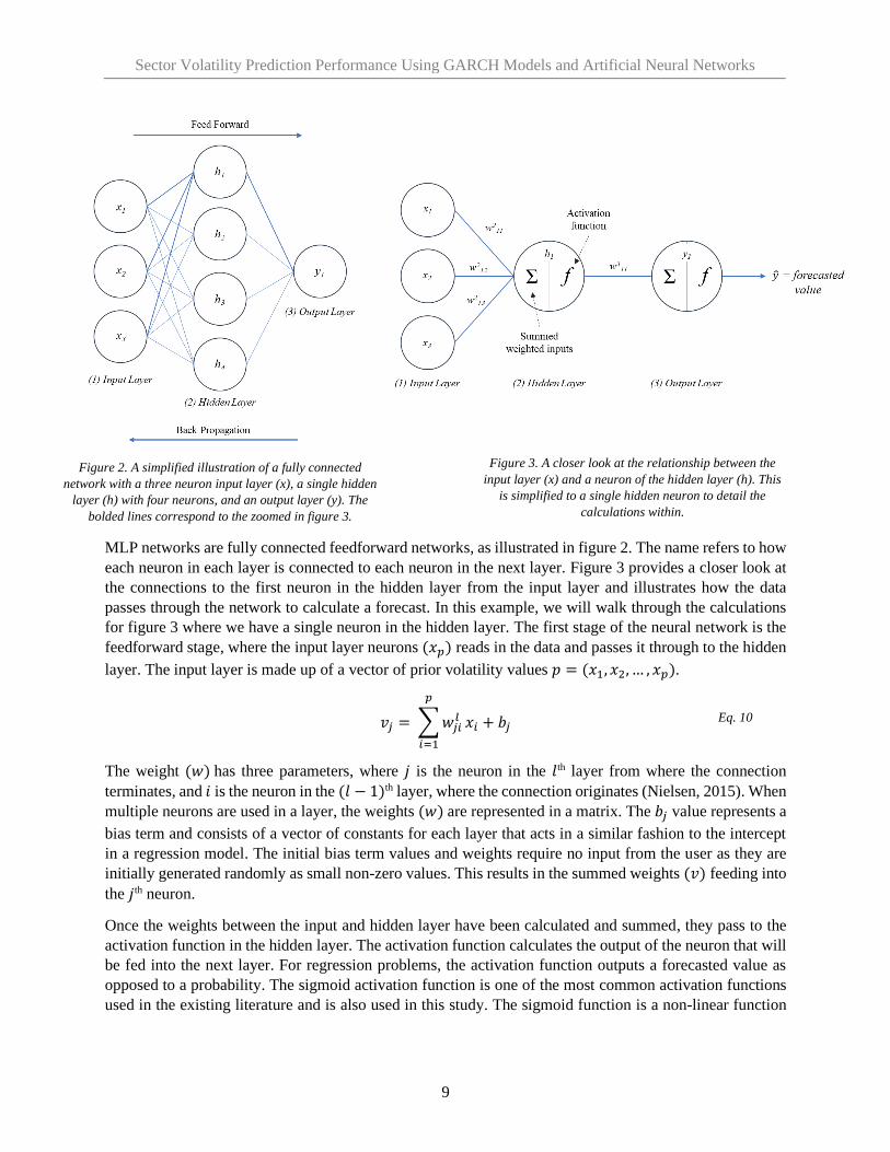
The ANN model used in this study is the Multi-Layer Perceptron (MLP). MLPs are widely used in industry

and academics thanks to their simplicity. The MLP comprises of three main parameters: layers, neurons,

and activation functions. The layers are made up of an input layer which reads in the data, a custom number

of hidden layers which perform a deciding calculation, and an output layer that provides the forecasted

output. Each layer is made up of a certain number of neurons, and the neurons utilize an activation function

to make the calculations resulting in the predictions in the output layer. This is visualized in figures 2 and

3 for an arbitrary example network with one input layer with three neurons, one hidden layer with four

neurons, and one output layer with one neuron to retrieve the final forecasted value.

Eq. 8

Eq. 9


9

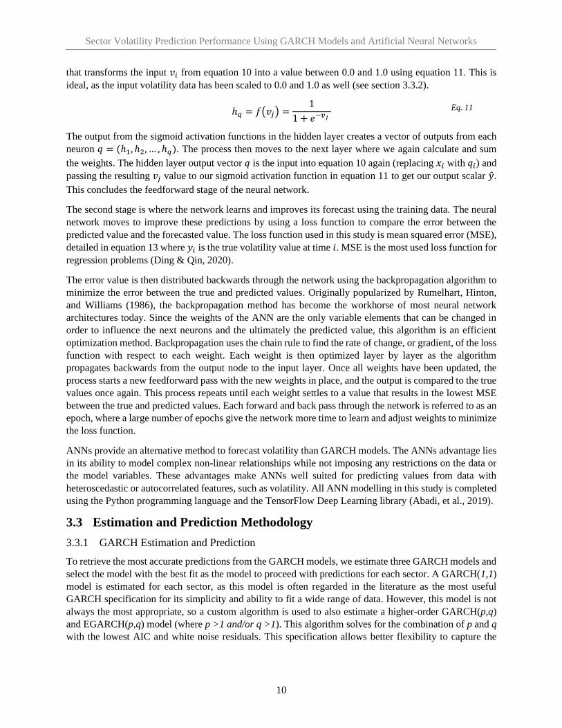
MLP networks are fully connected feedforward networks, as illustrated in figure 2. The name refers to how

each neuron in each layer is connected to each neuron in the next layer. Figure 3 provides a closer look at

the connections to the first neuron in the hidden layer from the input layer and illustrates how the data

passes through the network to calculate a forecast. In this example, we will walk through the calculations

for figure 3 where we have a single neuron in the hidden layer. The first stage of the neural network is the

feedforward stage, where the input layer neurons (𝑥𝑝) reads in the data and passes it through to the hidden

layer. The input layer is made up of a vector of prior volatility values 𝑝 = (𝑥1, 𝑥2, … , 𝑥𝑝).

𝑣𝑗 = ∑ 𝑤𝑗𝑖𝑙

𝑝

𝑖=1

𝑥𝑖 + 𝑏𝑗

The weight (𝑤) has three parameters, where 𝑗 is the neuron in the 𝑙th layer from where the connection

terminates, and 𝑖 is the neuron in the (𝑙 − 1)th layer, where the connection originates (Nielsen, 2015). When

multiple neurons are used in a layer, the weights (𝑤) are represented in a matrix. The 𝑏𝑗 value represents a

bias term and consists of a vector of constants for each layer that acts in a similar fashion to the intercept

in a regression model. The initial bias term values and weights require no input from the user as they are

initially generated randomly as small non-zero values. This results in the summed weights (𝑣) feeding into

the 𝑗th neuron.

Once the weights between the input and hidden layer have been calculated and summed, they pass to the

activation function in the hidden layer. The activation function calculates the output of the neuron that will

be fed into the next layer. For regression problems, the activation function outputs a forecasted value as

opposed to a probability. The sigmoid activation function is one of the most common activation functions

used in the existing literature and is also used in this study. The sigmoid function is a non-linear function

Figure 2. A simplified illustration of a fully connected

network with a three neuron input layer (x), a single hidden

layer (h) with four neurons, and an output layer (y). The

bolded lines correspond to the zoomed in figure 3.

Figure 3. A closer look at the relationship between the

input layer (x) and a neuron of the hidden layer (h). This

is simplified to a single hidden neuron to detail the

calculations within.

Eq. 10


10

that transforms the input 𝑣𝑖 from equation 10 into a value between 0.0 and 1.0 using equation 11. This is

ideal, as the input volatility data has been scaled to 0.0 and 1.0 as well (see section 3.3.2).

ℎ𝑞 = 𝑓(𝑣𝑗) =1

1 + 𝑒−𝑣𝑗

The output from the sigmoid activation functions in the hidden layer creates a vector of outputs from each

neuron 𝑞 = (ℎ1, ℎ2, … , ℎ𝑞). The process then moves to the next layer where we again calculate and sum

the weights. The hidden layer output vector 𝑞 is the input into equation 10 again (replacing 𝑥𝑖 with 𝑞𝑖) and

passing the resulting 𝑣𝑗 value to our sigmoid activation function in equation 11 to get our output scalar �̂�.

This concludes the feedforward stage of the neural network.

The second stage is where the network learns and improves its forecast using the training data. The neural

network moves to improve these predictions by using a loss function to compare the error between the

predicted value and the forecasted value. The loss function used in this study is mean squared error (MSE),

detailed in equation 13 where 𝑦𝑖 is the true volatility value at time 𝑖. MSE is the most used loss function for

regression problems (Ding & Qin, 2020).

The error value is then distributed backwards through the network using the backpropagation algorithm to

minimize the error between the true and predicted values. Originally popularized by Rumelhart, Hinton,

and Williams (1986), the backpropagation method has become the workhorse of most neural network

architectures today. Since the weights of the ANN are the only variable elements that can be changed in

order to influence the next neurons and the ultimately the predicted value, this algorithm is an efficient

optimization method. Backpropagation uses the chain rule to find the rate of change, or gradient, of the loss

function with respect to each weight. Each weight is then optimized layer by layer as the algorithm

propagates backwards from the output node to the input layer. Once all weights have been updated, the

process starts a new feedforward pass with the new weights in place, and the output is compared to the true

values once again. This process repeats until each weight settles to a value that results in the lowest MSE

between the true and predicted values. Each forward and back pass through the network is referred to as an

epoch, where a large number of epochs give the network more time to learn and adjust weights to minimize

the loss function.

ANNs provide an alternative method to forecast volatility than GARCH models. The ANNs advantage lies

in its ability to model complex non-linear relationships while not imposing any restrictions on the data or

the model variables. These advantages make ANNs well suited for predicting values from data with

heteroscedastic or autocorrelated features, such as volatility. All ANN modelling in this study is completed

using the Python programming language and the TensorFlow Deep Learning library (Abadi, et al., 2019).

3.3 Estimation and Prediction Methodology

3.3.1 GARCH Estimation and Prediction

To retrieve the most accurate predictions from the GARCH models, we estimate three GARCH models and

select the model with the best fit as the model to proceed with predictions for each sector. A GARCH(1,1)

model is estimated for each sector, as this model is often regarded in the literature as the most useful

GARCH specification for its simplicity and ability to fit a wide range of data. However, this model is not

always the most appropriate, so a custom algorithm is used to also estimate a higher-order GARCH(p,q)

and EGARCH(p,q) model (where p >1 and/or q >1). This algorithm solves for the combination of p and q

with the lowest AIC and white noise residuals. This specification allows better flexibility to capture the

Eq. 11


11

heteroscedasticity and autocorrelation effects in the data at the risk of a more complicated model. Lastly,

an EGARCH model will be estimated to evaluate if the model needs to account for asymmetry in the data.

The evaluation of each model will be based on how well the heteroscedasticity and autocorrelation (referred

to as ARCH effects) are captured in the data, provided no constraints are violated. The use of statistical

tests such as the Ljung-Box Q statistic will provide this information. Forecasting ability will be measured

by the Akaike Information Criteria (AIC). The AIC allows for a direct comparison between GARCH

specifications, and has been shown to work well with GARCH(1,1) as well as higher-order models (Naik,

et al., 2020).

Once the appropriate specification has been determined, a rolling window forecast will be used to predict

the conditional volatility value one step ahead (𝜎𝑡+12 ). The rolling window forecast initially uses a fixed

sample length, then forecasts the value one step ahead from the final observation. The next forecast then

drops the first value of the fixed sample and includes the true value of the prior forecasted value as the final

value, and so on.

3.3.2 ANN Estimation and Prediction

The example network given in section 3.2 differs slightly from the ANNs used in this study. The ANN

architecture used in this study has an input layer with five neurons, as we will be inputting a vector of prior

volatility values from a five day look back period. Several lookback windows were examined, with the five-

day lookback period producing the best results. The hidden layer has a varying number of neurons, and the

output layer always has a single neuron where we retrieve the forecasted value.

The ANN estimation and prediction follows the same process as the GARCH model, where we choose the

best fit ANN model from three different architectures. The architectures differ in the number of neurons in

the hidden layer, ranging from 1, 12, or 50 neurons. Choosing the correct number of neurons is a difficult

task as there is less consensus on a standard procedure to do so. ANN users usually resort to trial and error

and experimentation to find the optimal number of neurons, so that is what we have done here.

The prediction process begins with the data being read into an auto-scaler that transforms each prior

volatility data point to a range between 0.0 and 1.0. This preprocessing step is important as it speeds up the

training process and allows for more robust weights that will be learned when training the network, further

stabilizing the model. The vector of transformed prior volatility values is then fed into the input layer, where

the process in section 3.2 takes over. The ANN models use the vector of five prior volatility values to

predict the next single volatility value (𝜎𝑡+12 ) one step ahead. This is the same process as outlined for

GARCH prediction in section 3.3.1, where the same rolling window method is used.

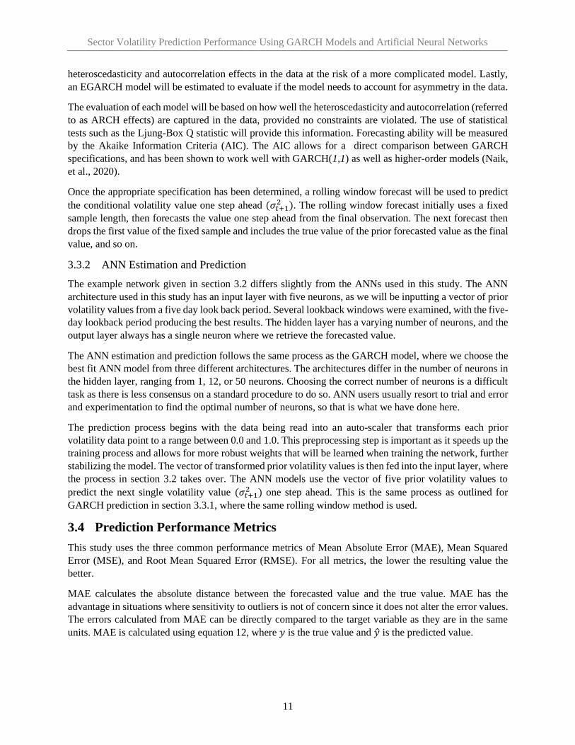
3.4 Prediction Performance Metrics

This study uses the three common performance metrics of Mean Absolute Error (MAE), Mean Squared

Error (MSE), and Root Mean Squared Error (RMSE). For all metrics, the lower the resulting value the

better.

MAE calculates the absolute distance between the forecasted value and the true value. MAE has the

advantage in situations where sensitivity to outliers is not of concern since it does not alter the error values.

The errors calculated from MAE can be directly compared to the target variable as they are in the same

units. MAE is calculated using equation 12, where 𝑦 is the true value and �̂� is the predicted value.


12

𝑀𝐴𝐸 =1

𝑁∑ |𝑦𝑖 − �̂�𝑖|

𝑁

𝑖=1

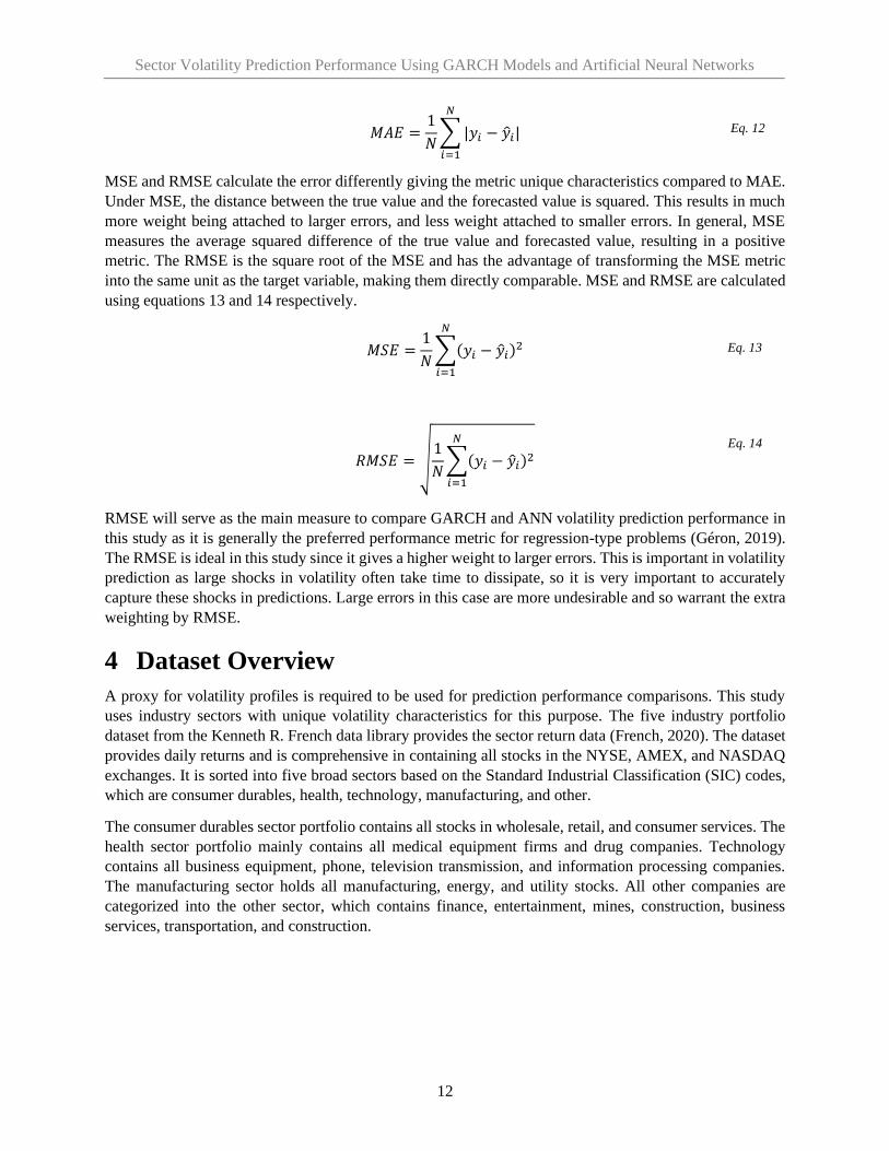
MSE and RMSE calculate the error differently giving the metric unique characteristics compared to MAE.

Under MSE, the distance between the true value and the forecasted value is squared. This results in much

more weight being attached to larger errors, and less weight attached to smaller errors. In general, MSE

measures the average squared difference of the true value and forecasted value, resulting in a positive

metric. The RMSE is the square root of the MSE and has the advantage of transforming the MSE metric

into the same unit as the target variable, making them directly comparable. MSE and RMSE are calculated

using equations 13 and 14 respectively.

𝑀𝑆𝐸 =1

𝑁∑(𝑦𝑖 − �̂�𝑖)2

𝑁

𝑖=1

𝑅𝑀𝑆𝐸 = √1

𝑁∑(𝑦𝑖 − �̂�𝑖)2

𝑁

𝑖=1

RMSE will serve as the main measure to compare GARCH and ANN volatility prediction performance in

this study as it is generally the preferred performance metric for regression-type problems (Géron, 2019).

The RMSE is ideal in this study since it gives a higher weight to larger errors. This is important in volatility

prediction as large shocks in volatility often take time to dissipate, so it is very important to accurately

capture these shocks in predictions. Large errors in this case are more undesirable and so warrant the extra

weighting by RMSE.

4 Dataset Overview

A proxy for volatility profiles is required to be used for prediction performance comparisons. This study

uses industry sectors with unique volatility characteristics for this purpose. The five industry portfolio

dataset from the Kenneth R. French data library provides the sector return data (French, 2020). The dataset

provides daily returns and is comprehensive in containing all stocks in the NYSE, AMEX, and NASDAQ

exchanges. It is sorted into five broad sectors based on the Standard Industrial Classification (SIC) codes,

which are consumer durables, health, technology, manufacturing, and other.

The consumer durables sector portfolio contains all stocks in wholesale, retail, and consumer services. The

health sector portfolio mainly contains all medical equipment firms and drug companies. Technology

contains all business equipment, phone, television transmission, and information processing companies.

The manufacturing sector holds all manufacturing, energy, and utility stocks. All other companies are

categorized into the other sector, which contains finance, entertainment, mines, construction, business

services, transportation, and construction.

Eq. 13

Eq. 14

Eq. 12


13

4.1 Sector Statistics

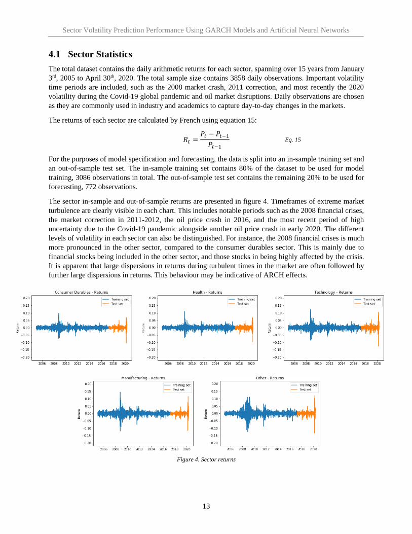
The total dataset contains the daily arithmetic returns for each sector, spanning over 15 years from January

3rd, 2005 to April 30th, 2020. The total sample size contains 3858 daily observations. Important volatility

time periods are included, such as the 2008 market crash, 2011 correction, and most recently the 2020

volatility during the Covid-19 global pandemic and oil market disruptions. Daily observations are chosen

as they are commonly used in industry and academics to capture day-to-day changes in the markets.

The returns of each sector are calculated by French using equation 15:

𝑅𝑡 =𝑃𝑡 − 𝑃𝑡−1

𝑃𝑡−1

For the purposes of model specification and forecasting, the data is split into an in-sample training set and

an out-of-sample test set. The in-sample training set contains 80% of the dataset to be used for model

training, 3086 observations in total. The out-of-sample test set contains the remaining 20% to be used for

forecasting, 772 observations.

The sector in-sample and out-of-sample returns are presented in figure 4. Timeframes of extreme market

turbulence are clearly visible in each chart. This includes notable periods such as the 2008 financial crises,

the market correction in 2011-2012, the oil price crash in 2016, and the most recent period of high

uncertainty due to the Covid-19 pandemic alongside another oil price crash in early 2020. The different

levels of volatility in each sector can also be distinguished. For instance, the 2008 financial crises is much

more pronounced in the other sector, compared to the consumer durables sector. This is mainly due to

financial stocks being included in the other sector, and those stocks in being highly affected by the crisis.

It is apparent that large dispersions in returns during turbulent times in the market are often followed by

further large dispersions in returns. This behaviour may be indicative of ARCH effects.

Eq. 15

Figure 4. Sector returns


14

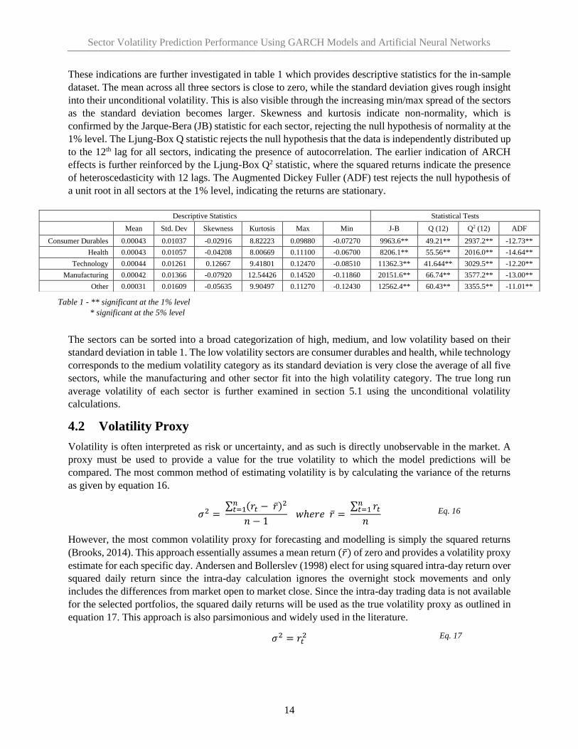
These indications are further investigated in table 1 which provides descriptive statistics for the in-sample

dataset. The mean across all three sectors is close to zero, while the standard deviation gives rough insight

into their unconditional volatility. This is also visible through the increasing min/max spread of the sectors

as the standard deviation becomes larger. Skewness and kurtosis indicate non-normality, which is

confirmed by the Jarque-Bera (JB) statistic for each sector, rejecting the null hypothesis of normality at the

1% level. The Ljung-Box Q statistic rejects the null hypothesis that the data is independently distributed up

to the 12th lag for all sectors, indicating the presence of autocorrelation. The earlier indication of ARCH

effects is further reinforced by the Ljung-Box Q2 statistic, where the squared returns indicate the presence

of heteroscedasticity with 12 lags. The Augmented Dickey Fuller (ADF) test rejects the null hypothesis of

a unit root in all sectors at the 1% level, indicating the returns are stationary.

The sectors can be sorted into a broad categorization of high, medium, and low volatility based on their

standard deviation in table 1. The low volatility sectors are consumer durables and health, while technology

corresponds to the medium volatility category as its standard deviation is very close the average of all five

sectors, while the manufacturing and other sector fit into the high volatility category. The true long run

average volatility of each sector is further examined in section 5.1 using the unconditional volatility

calculations.

4.2 Volatility Proxy

Volatility is often interpreted as risk or uncertainty, and as such is directly unobservable in the market. A

proxy must be used to provide a value for the true volatility to which the model predictions will be

compared. The most common method of estimating volatility is by calculating the variance of the returns

as given by equation 16.

𝜎2 = ∑ (𝑟𝑡 − �̅�)2𝑛

𝑡=1

𝑛 − 1 𝑤ℎ𝑒𝑟𝑒 �̅� =

∑ 𝑟𝑡𝑛𝑡=1

𝑛

However, the most common volatility proxy for forecasting and modelling is simply the squared returns

(Brooks, 2014). This approach essentially assumes a mean return (�̅�) of zero and provides a volatility proxy

estimate for each specific day. Andersen and Bollerslev (1998) elect for using squared intra-day return over

squared daily return since the intra-day calculation ignores the overnight stock movements and only

includes the differences from market open to market close. Since the intra-day trading data is not available

for the selected portfolios, the squared daily returns will be used as the true volatility proxy as outlined in

equation 17. This approach is also parsimonious and widely used in the literature.

𝜎2 = 𝑟𝑡2

Descriptive Statistics Statistical Tests

Mean Std. Dev Skewness Kurtosis Max Min J-B Q (12) Q2 (12) ADF

Consumer Durables 0.00043 0.01037 -0.02916 8.82223 0.09880 -0.07270 9963.6** 49.21** 2937.2** -12.73**

Health 0.00043 0.01057 -0.04208 8.00669 0.11100 -0.06700 8206.1** 55.56** 2016.0** -14.64**

Technology 0.00044 0.01261 0.12667 9.41801 0.12470 -0.08510 11362.3** 41.644** 3029.5** -12.20**

Manufacturing 0.00042 0.01366 -0.07920 12.54426 0.14520 -0.11860 20151.6** 66.74** 3577.2** -13.00**

Other 0.00031 0.01609 -0.05635 9.90497 0.11270 -0.12430 12562.4** 60.43** 3355.5** -11.01**

Eq. 16

Eq. 17

Table 1 - ** significant at the 1% level

* significant at the 5% level


15

5 Results

5.1 GARCH Estimation: In-Sample Data

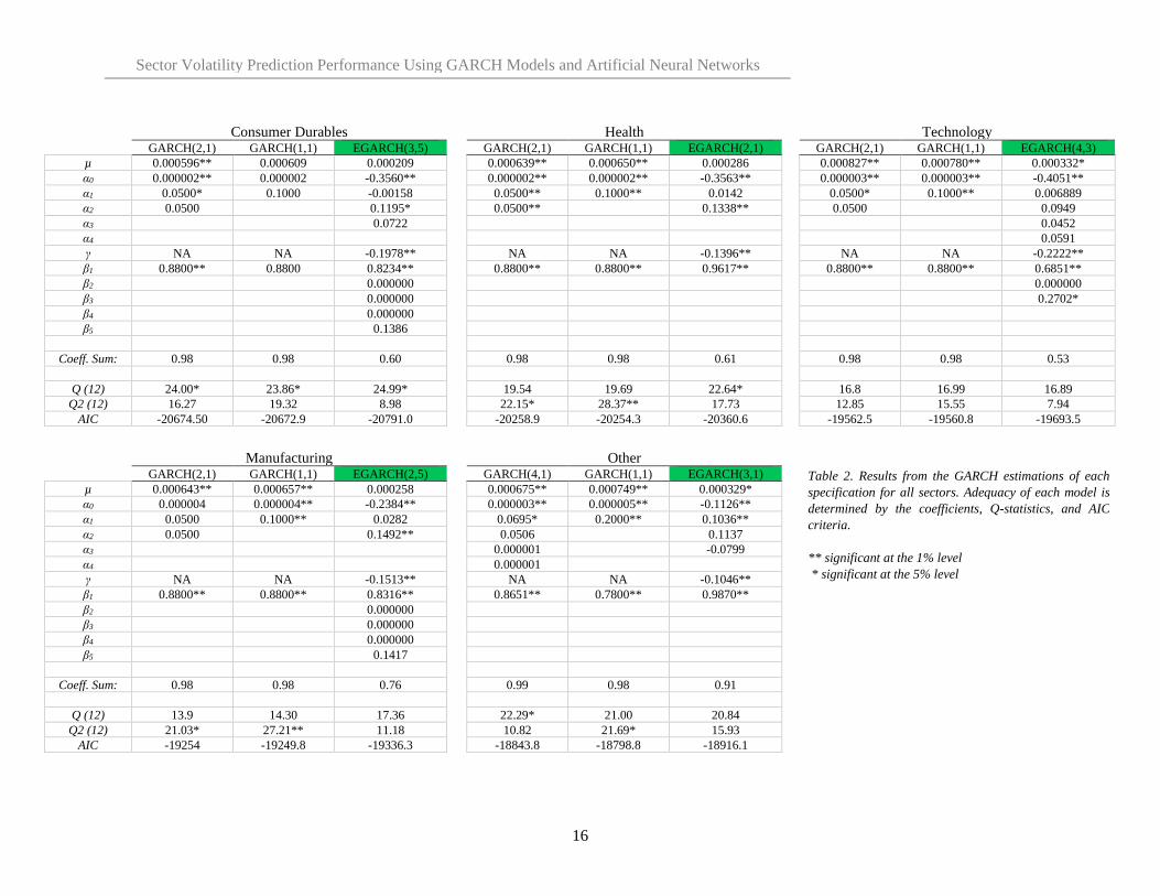
For each sector, the three GARCH specifications outlined in section 3.1 are estimated, namely the

GARCH(p,q), GARCH(1,1), and EGARCH(p,q) models. The best specification is chosen for forecasting

based on the adequacy of fit and AIC criterion. Each GARCH model is estimated using the in-sample

portion of the daily return data to prevent look-ahead bias in the estimations. Results for all sectors are

displayed in Table 2.

Of the three GARCH models estimated, the EGARCH(p,q) model is the most adequate model to proceed

with forecasting for all five sectors. These EGARCH specifications are highlighted in table 2. Each

EGARCH specification results in a conditional mean equation that is not significantly different from zero

at least at the 1% level, while the conditional volatility equations result in varying numbers of significant

coefficients. The EGARCH models adequately capture all ARCH effects in the returns as given by the

insignificant Q-statistics at least at the 1% level. This indicates that the resulting residuals and squared

residuals are a white noise process. Although the EGARCH model relaxes the non-negativity constraints,

the 𝛽 terms must be positive and less than one to remain stationary, which is the case in all EGARCH

models (Ezzat, 2012).

The main benefit of the EGARCH model is the ability to account for potential asymmetries in the response

to volatility shocks via the gamma term. Each EGARCH model has a negative gamma term that is

significantly different from zero at the 1% level, which implies that volatility asymmetry exists and the

relationship between volatility and returns is negative. This relationship indicates that leverage effects exist

in the data of each sector, where a negative shock has a greater effect on volatility than a similar positive

shock (Brooks, 2014). Once asymmetry have been identified, it is important to account for it when

forecasting future volatility values. The forecasting potential for each model is also given by the AIC value,

where the EGARCH models provide a lower value than the other GARCH models across all sectors. This

indicates the EGARCH specification have the best forecasting ability for this study.

The GARCH(p,q) and GARCH(1,1) model estimations for each sector resulted in varying levels of model

adequacy. The GARCH(p,q) models, despite having differing p and q values, and GARCH(1,1) models

resulted in very similar coefficients for all sectors except other. This shows that the unconditional volatility

of each sector when estimated by these specifications is very similar across four sectors. Both models satisfy

the non-negativity constraints imposed by the standard GARCH models, and all have coefficients that sum

to less than one. The large 𝛽 coefficients in these GARCH models of each sector indicate that volatility

persists for a long time after a shock. Similarly, since the coefficients sum to a number close to one, the

conditional volatility reverts to the unconditional (long term average) volatility very slowly. However, in

all sectors except Other, the low 𝛼 coefficients indicate that the initial reaction of conditional volatility to

market shocks is quite minimal in the first place.

Despite the insights the GARCH(p,q) and GARCH(1,1) models provide into the volatility characteristics

of the sectors, they are not as adequate as the EGARCH specifications for forecasting. The GARCH(p,q)

and GARCH(1,1) models fail to capture ARCH effects in several sectors as indicated by the significant Q

statistics at the 1% level, while both models have much higher AIC values than the EGARCH

specifications.


16

Consumer Durables Health Technology GARCH(2,1) GARCH(1,1) EGARCH(3,5) GARCH(2,1) GARCH(1,1) EGARCH(2,1) GARCH(2,1) GARCH(1,1) EGARCH(4,3)

µ 0.000596** 0.000609 0.000209 0.000639** 0.000650** 0.000286 0.000827** 0.000780** 0.000332*

α0 0.000002** 0.000002 -0.3560** 0.000002** 0.000002** -0.3563** 0.000003** 0.000003** -0.4051**

α1 0.0500* 0.1000 -0.00158 0.0500** 0.1000** 0.0142 0.0500* 0.1000** 0.006889

α2 0.0500 0.1195* 0.0500** 0.1338** 0.0500 0.0949

α3 0.0722 0.0452

α4 0.0591

γ NA NA -0.1978** NA NA -0.1396** NA NA -0.2222**

β1 0.8800** 0.8800 0.8234** 0.8800** 0.8800** 0.9617** 0.8800** 0.8800** 0.6851**

β2 0.000000 0.000000

β3 0.000000 0.2702*

β4 0.000000

β5 0.1386

Coeff. Sum: 0.98 0.98 0.60 0.98 0.98 0.61 0.98 0.98 0.53

Q (12) 24.00* 23.86* 24.99* 19.54 19.69 22.64* 16.8 16.99 16.89

Q2 (12) 16.27 19.32 8.98 22.15* 28.37** 17.73 12.85 15.55 7.94

AIC -20674.50 -20672.9 -20791.0 -20258.9 -20254.3 -20360.6 -19562.5 -19560.8 -19693.5

Manufacturing Other

GARCH(2,1) GARCH(1,1) EGARCH(2,5) GARCH(4,1) GARCH(1,1) EGARCH(3,1)

µ 0.000643** 0.000657** 0.000258 0.000675** 0.000749** 0.000329* α0 0.000004 0.000004** -0.2384** 0.000003** 0.000005** -0.1126** α1 0.0500 0.1000** 0.0282 0.0695* 0.2000** 0.1036** α2 0.0500 0.1492** 0.0506 0.1137 α3 0.000001 -0.0799 α4 0.000001 γ NA NA -0.1513** NA NA -0.1046** β1 0.8800** 0.8800** 0.8316** 0.8651** 0.7800** 0.9870** β2 0.000000 β3 0.000000 β4 0.000000 β5 0.1417

Coeff. Sum: 0.98 0.98 0.76 0.99 0.98 0.91

Q (12) 13.9 14.30 17.36 22.29* 21.00 20.84

Q2 (12) 21.03* 27.21** 11.18 10.82 21.69* 15.93 AIC -19254 -19249.8 -19336.3 -18843.8 -18798.8 -18916.1

Table 2. Results from the GARCH estimations of each

specification for all sectors. Adequacy of each model is

determined by the coefficients, Q-statistics, and AIC

criteria.

** significant at the 1% level

* significant at the 5% level


17

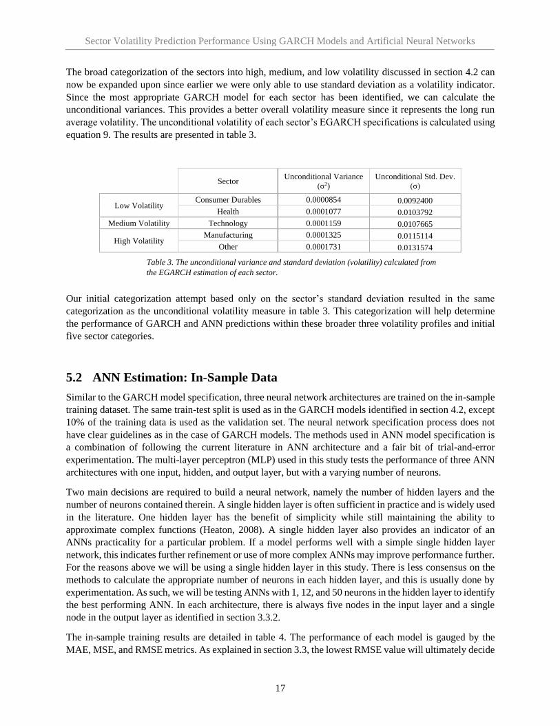
The broad categorization of the sectors into high, medium, and low volatility discussed in section 4.2 can

now be expanded upon since earlier we were only able to use standard deviation as a volatility indicator.

Since the most appropriate GARCH model for each sector has been identified, we can calculate the

unconditional variances. This provides a better overall volatility measure since it represents the long run

average volatility. The unconditional volatility of each sector’s EGARCH specifications is calculated using

equation 9. The results are presented in table 3.

Sector Unconditional Variance

(σ2)

Unconditional Std. Dev.

(σ)

Low Volatility Consumer Durables 0.0000854 0.0092400

Health 0.0001077 0.0103792

Medium Volatility Technology 0.0001159 0.0107665

High Volatility Manufacturing 0.0001325 0.0115114

Other 0.0001731 0.0131574

Our initial categorization attempt based only on the sector’s standard deviation resulted in the same

categorization as the unconditional volatility measure in table 3. This categorization will help determine

the performance of GARCH and ANN predictions within these broader three volatility profiles and initial

five sector categories.

5.2 ANN Estimation: In-Sample Data

Similar to the GARCH model specification, three neural network architectures are trained on the in-sample

training dataset. The same train-test split is used as in the GARCH models identified in section 4.2, except

10% of the training data is used as the validation set. The neural network specification process does not

have clear guidelines as in the case of GARCH models. The methods used in ANN model specification is

a combination of following the current literature in ANN architecture and a fair bit of trial-and-error

experimentation. The multi-layer perceptron (MLP) used in this study tests the performance of three ANN

architectures with one input, hidden, and output layer, but with a varying number of neurons.

Two main decisions are required to build a neural network, namely the number of hidden layers and the

number of neurons contained therein. A single hidden layer is often sufficient in practice and is widely used

in the literature. One hidden layer has the benefit of simplicity while still maintaining the ability to

approximate complex functions (Heaton, 2008). A single hidden layer also provides an indicator of an

ANNs practicality for a particular problem. If a model performs well with a simple single hidden layer

network, this indicates further refinement or use of more complex ANNs may improve performance further.

For the reasons above we will be using a single hidden layer in this study. There is less consensus on the

methods to calculate the appropriate number of neurons in each hidden layer, and this is usually done by

experimentation. As such, we will be testing ANNs with 1, 12, and 50 neurons in the hidden layer to identify

the best performing ANN. In each architecture, there is always five nodes in the input layer and a single

node in the output layer as identified in section 3.3.2.

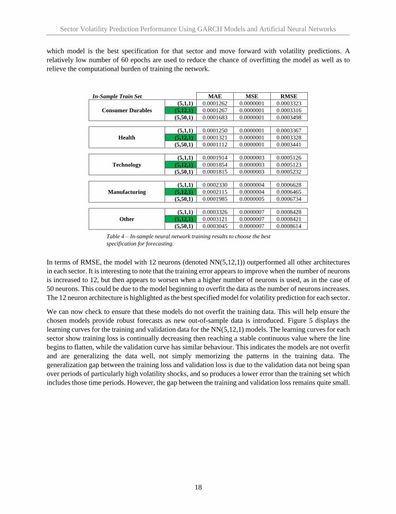
The in-sample training results are detailed in table 4. The performance of each model is gauged by the

MAE, MSE, and RMSE metrics. As explained in section 3.3, the lowest RMSE value will ultimately decide

Table 3. The unconditional variance and standard deviation (volatility) calculated from

the EGARCH estimation of each sector.


18

which model is the best specification for that sector and move forward with volatility predictions. A

relatively low number of 60 epochs are used to reduce the chance of overfitting the model as well as to

relieve the computational burden of training the network.

In-Sample Train Set MAE MSE RMSE

Consumer Durables

(5,1,1) 0.0001262 0.0000001 0.0003323

(5,12,1) 0.0001267 0.0000001 0.0003316

(5,50,1) 0.0001683 0.0000001 0.0003498

Health

(5,1,1) 0.0001250 0.0000001 0.0003367

(5,12,1) 0.0001321 0.0000001 0.0003328

(5,50,1) 0.0001112 0.0000001 0.0003441

Technology

(5,1,1) 0.0001914 0.0000003 0.0005126

(5,12,1) 0.0001854 0.0000003 0.0005123

(5,50,1) 0.0001815 0.0000003 0.0005232

Manufacturing

(5,1,1) 0.0002330 0.0000004 0.0006628

(5,12,1) 0.0002115 0.0000004 0.0006465

(5,50,1) 0.0001985 0.0000005 0.0006734

Other

(5,1,1) 0.0003326 0.0000007 0.0008428

(5,12,1) 0.0003121 0.0000007 0.0008421

(5,50,1) 0.0003045 0.0000007 0.0008614

In terms of RMSE, the model with 12 neurons (denoted NN(5,12,1)) outperformed all other architectures

in each sector. It is interesting to note that the training error appears to improve when the number of neurons

is increased to 12, but then appears to worsen when a higher number of neurons is used, as in the case of

50 neurons. This could be due to the model beginning to overfit the data as the number of neurons increases.

The 12 neuron architecture is highlighted as the best specified model for volatility prediction for each sector.

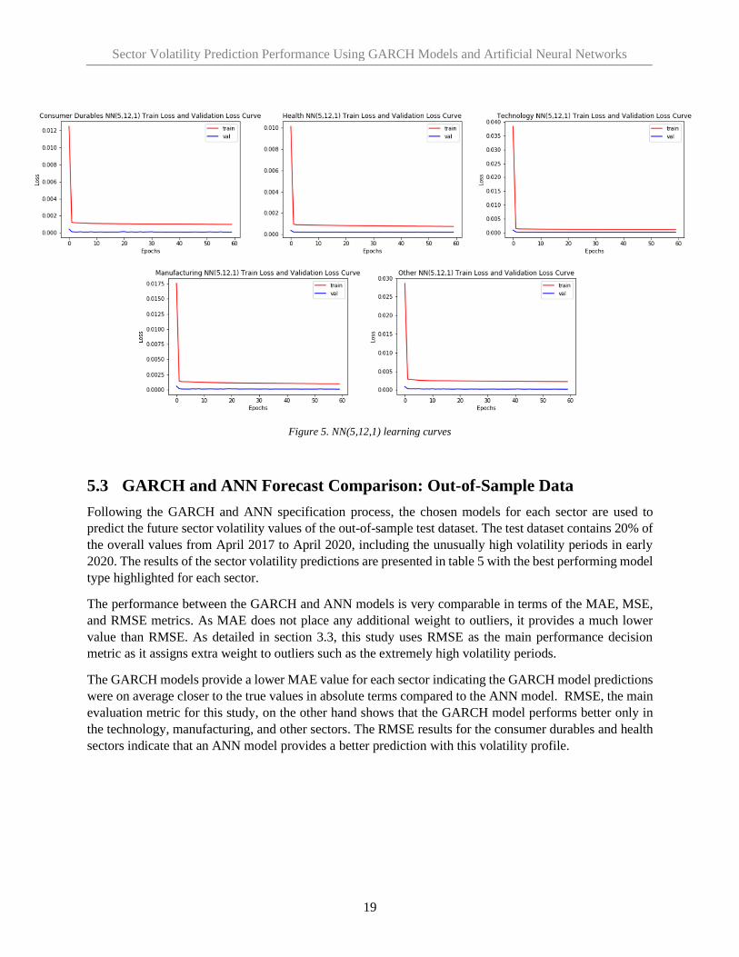
We can now check to ensure that these models do not overfit the training data. This will help ensure the

chosen models provide robust forecasts as new out-of-sample data is introduced. Figure 5 displays the

learning curves for the training and validation data for the NN(5,12,1) models. The learning curves for each

sector show training loss is continually decreasing then reaching a stable continuous value where the line

begins to flatten, while the validation curve has similar behaviour. This indicates the models are not overfit

and are generalizing the data well, not simply memorizing the patterns in the training data. The

generalization gap between the training loss and validation loss is due to the validation data not being span

over periods of particularly high volatility shocks, and so produces a lower error than the training set which

includes those time periods. However, the gap between the training and validation loss remains quite small.

Table 4 – In-sample neural network training results to choose the best

specification for forecasting.


19

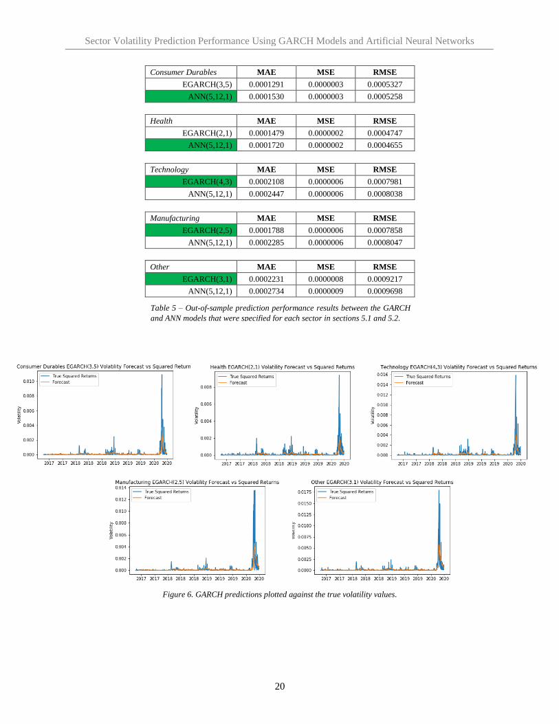
5.3 GARCH and ANN Forecast Comparison: Out-of-Sample Data

Following the GARCH and ANN specification process, the chosen models for each sector are used to

predict the future sector volatility values of the out-of-sample test dataset. The test dataset contains 20% of

the overall values from April 2017 to April 2020, including the unusually high volatility periods in early

2020. The results of the sector volatility predictions are presented in table 5 with the best performing model

type highlighted for each sector.

The performance between the GARCH and ANN models is very comparable in terms of the MAE, MSE,

and RMSE metrics. As MAE does not place any additional weight to outliers, it provides a much lower

value than RMSE. As detailed in section 3.3, this study uses RMSE as the main performance decision

metric as it assigns extra weight to outliers such as the extremely high volatility periods.

The GARCH models provide a lower MAE value for each sector indicating the GARCH model predictions

were on average closer to the true values in absolute terms compared to the ANN model. RMSE, the main

evaluation metric for this study, on the other hand shows that the GARCH model performs better only in

the technology, manufacturing, and other sectors. The RMSE results for the consumer durables and health

sectors indicate that an ANN model provides a better prediction with this volatility profile.

Figure 5. NN(5,12,1) learning curves


20

Consumer Durables MAE MSE RMSE

EGARCH(3,5) 0.0001291 0.0000003 0.0005327

ANN(5,12,1) 0.0001530 0.0000003 0.0005258

Health MAE MSE RMSE

EGARCH(2,1) 0.0001479 0.0000002 0.0004747

ANN(5,12,1) 0.0001720 0.0000002 0.0004655

Technology MAE MSE RMSE

EGARCH(4,3) 0.0002108 0.0000006 0.0007981

ANN(5,12,1) 0.0002447 0.0000006 0.0008038

Manufacturing MAE MSE RMSE

EGARCH(2,5) 0.0001788 0.0000006 0.0007858

ANN(5,12,1) 0.0002285 0.0000006 0.0008047

Other MAE MSE RMSE

EGARCH(3,1) 0.0002231 0.0000008 0.0009217

ANN(5,12,1) 0.0002734 0.0000009 0.0009698

Table 5 – Out-of-sample prediction performance results between the GARCH

and ANN models that were specified for each sector in sections 5.1 and 5.2.

Figure 6. GARCH predictions plotted against the true volatility values.


21

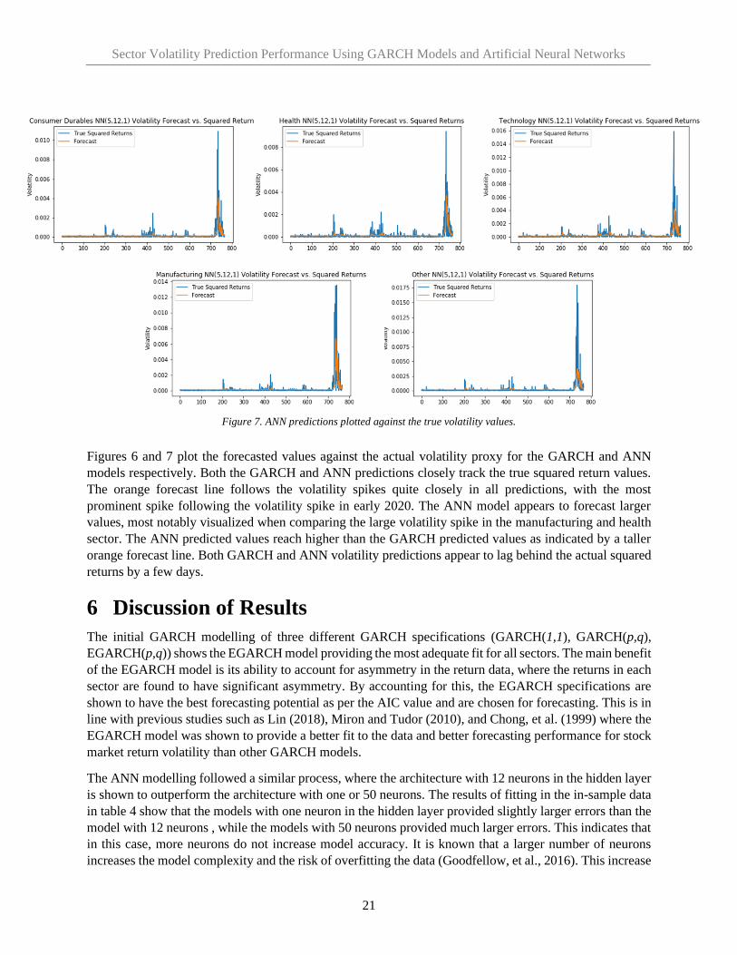
Figures 6 and 7 plot the forecasted values against the actual volatility proxy for the GARCH and ANN

models respectively. Both the GARCH and ANN predictions closely track the true squared return values.

The orange forecast line follows the volatility spikes quite closely in all predictions, with the most

prominent spike following the volatility spike in early 2020. The ANN model appears to forecast larger

values, most notably visualized when comparing the large volatility spike in the manufacturing and health

sector. The ANN predicted values reach higher than the GARCH predicted values as indicated by a taller

orange forecast line. Both GARCH and ANN volatility predictions appear to lag behind the actual squared

returns by a few days.

6 Discussion of Results

The initial GARCH modelling of three different GARCH specifications (GARCH(1,1), GARCH(p,q),

EGARCH(p,q)) shows the EGARCH model providing the most adequate fit for all sectors. The main benefit

of the EGARCH model is its ability to account for asymmetry in the return data, where the returns in each

sector are found to have significant asymmetry. By accounting for this, the EGARCH specifications are

shown to have the best forecasting potential as per the AIC value and are chosen for forecasting. This is in

line with previous studies such as Lin (2018), Miron and Tudor (2010), and Chong, et al. (1999) where the

EGARCH model was shown to provide a better fit to the data and better forecasting performance for stock

market return volatility than other GARCH models.

The ANN modelling followed a similar process, where the architecture with 12 neurons in the hidden layer

is shown to outperform the architecture with one or 50 neurons. The results of fitting in the in-sample data

in table 4 show that the models with one neuron in the hidden layer provided slightly larger errors than the

model with 12 neurons , while the models with 50 neurons provided much larger errors. This indicates that

in this case, more neurons do not increase model accuracy. It is known that a larger number of neurons

increases the model complexity and the risk of overfitting the data (Goodfellow, et al., 2016). This increase

Figure 7. ANN predictions plotted against the true volatility values.


22

in model complexity may increase performance of ANNs in some applications, but this result indicates that

increased model complexity decreases performance when predicting volatility. Given these results, we can

be confident that the ideal of parsimony applies here, where a simpler 12 neuron model has outperformed

more complicated models.

The resulting out-of-sample forecasting performance of the EGARCH(p,q) specifications and the

ANN(5,12,1) models is compared in table 5. As discussed in section 3.4, the RMSE measure is chosen as

the deciding metric to evaluate model prediction performance in this study. The results show the ANN

model provides more accurate volatility predictions in the consumer durables and health sectors, while the

GARCH model outperforms the ANN model in the technology, manufacturing, and other sectors. The

classification of these sectors into high, medium, and low volatility profiles in sections 4.1 and 5.1 reveals

that the ANN model outperforms the GARCH model when predicting volatility in low volatility sectors

(consumer durables and health), while the GARCH model outperforms the ANN model in the medium

(technology) and high volatility sectors (manufacturing and other).

The RMSE performance of both models is very close in the medium volatility sector. However, the ANN

underperformed the GARCH model in the high volatility sectors by a much larger RMSE margin. As

visualized in figure 4, the high volatility sectors have larger volatility shocks (manufacturing) or the shocks

take longer to dissipate (other). This indicates that the EGARCH specifications are better at forecasting

volatility over time periods with larger and longer volatility shocks than the ANN models. This result aligns

with the results from Lim and Sek (2013),where an asymmetric GARCH model is found to be most

preferred during a high volatility period.

The actual and forecasted values plotted in figures 6 and 7 for both models deliver further insight into these

results. The ANN forecasted values track the actual volatility values more closely in the two low volatility

sectors than the GARCH model. Both models provide a similar range of forecasted values for the

technology (medium volatility) and the manufacturing sector (high volatility), but the figures show the

ANN model failing to accurately forecast volatility in the highest volatility sector, other, while the GARCH

forecast was quite accurate. The learning curves in figure 5 provide evidence that this is not due to the ANN

model overfitting the data. A possible reason for the ANN outperformance in the low volatility sectors and

underperformance in the medium and high volatility sectors is due to the noise sensitivity of the

backpropagation ANNs used in this study (Sharma, et al., 2017). In a lower volatility sector there is less

noise in the data due to less price fluctuations, which the ANN can model and forecast quite accurately. In

sectors with higher levels of volatility and therefore price fluctuations, the ANN loses accuracy when fitting

the data and forecasting.

These results are subject to some limitations of this study that should be considered in future research. The

most significant limitation is the small number of model-type specifications tested due to the document size

constraints of this study. A future comprehensive study would include a greater number of GARCH-type

models and ANN types and architectures. This would expand the evidence provided in this study to include

an even greater guideline of model types to use and to which volatility profiles they should be applied for

best forecasting results. Other factors that would expand upon this research include using larger timeframes

(perhaps decades of return data) or using a different volatility proxy such as squared intra-day returns

instead of squared daily returns.

Overall, this study demonstrates the applicability for ANN models to produce more accurate forecasts than

the standard GARCH models when applied to specific volatility profiles. By examining the usefulness of

the ANN model in comparison to the GARCH model, we have shown that the ANN parameters have the

needed flexibility to improve performance. The GARCH models suffer from less flexibility as they are


23

required to adhere to often strict constraints. Overall, the results are promising for ANN applications in

volatility prediction, and with further refinement in the architecture performance can be improved.

7 Conclusion

The objective of this study is to evaluate the volatility prediction performance of an ANN model compared

to the common GARCH-type models when applied to specific volatility profiles. This will identify specific

volatility profiles where each model outperforms the other. Through this approach, the study will also

demonstrate the usefulness of ANNs for the volatility prediction of assets within these specific volatility

profiles. Three GARCH specifications and three ANN architectures are examined using the stock return

data from 2005 to 2020 of all publicly traded companies in the United States. Each company is sorted into

one of five sectors: consumer durables, health, technology, manufacturing, and other. A single best

performing GARCH and ANN model is then chosen as the optimal model to move forward with the

forecasting of volatility for each individual sector.

Based on the model AIC value, adherence to constraints, and other metrics, the EGARCH(p,q) specification

is chosen as the most adequate fit model over the GARCH(1,1) and GARCH(p,q) specifications for each

sector. For consistency, the same approach is used for the ANN architecture selection, where the

ANN(5,12,1) architecture is chosen over the ANN(5,1,1) and ANN(5,50,1) architectures based mainly on

in-sample fit. By examining three distinct specifications, this approach helps ensure that the best GARCH

specification and ANN architecture is chosen for volatility prediction performance comparisons.

The out-of-sample results clearly identify volatility profiles where each model outperforms the other. Using

the RMSE metric as the main performance measuring criteria, the ANN model provides more accurate

volatility forecasts for the low volatility sectors (consumer durables and health). This indicates that ANN

models are a better choice than GARCH-type models when forecasting volatility in stocks with a low

volatility profile. Meanwhile, the GARCH-type model outperformed the ANN model in the medium

(technology) and high volatility (manufacturing and other) sectors. This indicates that GARCH-type models

are more suitable and provide more accurate volatility forecasts for stocks with a medium or high volatility

profile.

The results of this study have important implications in both industry and academics. By identifying the

volatility profiles where each model will perform best, this study further solidifies the ANNs place in the

volatility forecasters toolbox. The benefits of this study to industry is two-fold. First it gives economists,

traders, and other market participants an additional volatility forecasting tool to the common GARCH

model. Second, it provides evidence of the asset volatility profiles where each model type should be used.

It is standard industry practice to never solely rely on a single type of model (Zhang, 2012). This study

directly expands the types of models available to market participants. The study also furthers the academic

literature in this area by expanding upon the existing work of volatility prediction models and adding further

evaluation of the applicability of the ANN model in financial forecasting. Prior studies conducted focused

on performance of ANN and GARCH models when applied to specific indexes and stocks, where this study

has taken a broader view by grouping all stocks into volatility profiles and determining where each model

performs best.

By using less complex ANN architectures and GARCH-type models, this study provides a foundation for

further research in this context. Future research is required to examine more complex ANN architectures

such as Long-Short Term Memory (LSTM) or Recurrent Neural Network (RNN), as well as GARCH-type

models such as the TGARCH or GJR-GARCH. Broadening the set of models examined contributes to the


24

literature by further identifying the specific scenarios where an ANN model or GARCH model should be

used and gives market participants more choice of available models in both industry and academics.

8 References

The Python code developed for this study and the datasets can be found at:

https://github.com/curtnybo/MSc-Dissertation-Code

Abadi, M. et al., 2019. TensorFlow White Papers - Large-Scale Machine Learning on Heterogeneous

Distributed Systems. [Online]

Available at: https://www.tensorflow.org/about/bib

Andersen, T. G. & Bollerslev, T., 1998. Answering the Skeptics: Yes, Standard Volatility Models do

Provide Accurate Forecasts. International Economic Review, 39(4), pp. 885-905.

Arnerić, J., Poklepović, T. & Aljinović, Z., 2014. GARCH based artificial neural networks in forecasting

conditional variance of stock returns. CRORR Journal Regular Issue, 5(2), pp. 329-343.

Bentes, S. R., 2015. Forecasting volatility in gold returns under the GARCH, IGARCH and FIGARCH

frameworks: New evidence. Physica A: Statistical Mechanics and its Applications, 438(15), pp. 355-364.

Black, F., 1976. Studies of Stock Price Volatility Changes. Proceedings of the 1976 Meetings of the

Business and Economics Statistics Section American Statistical Association, pp. 177-181.

Bollerslev, T., 1986. Generalized autoregressive conditional heteroskedasticity. Journal of Econometrics,

31(3), pp. 307-327.

Brooks, C., 2014. Introductory Econometrics for Finance. 3rd ed. Cambridge: Cambridge University

Press.

Chong, C. W., Ahmad, M. I. & Abdullah, M. Y., 1999. Performance of GARCH models in forecasting

stock market volatility. Journal of Forecasting, 18(5), pp. 333-343.

Ding, G. & Qin, L., 2020. Study on the prediction of stock price based on the associated network model

of LSTM. International Journal of Machine Learning and Cybernetics, Volume 11, pp. 1307-1317.

Donaldson, G. R. & Kamstra, M., 1997. An artificial neural network-GARCH model for international

stock return volatility. Journal of Empirical Finance, 4(1), pp. 17-46.

Engle, R., 2001. GARCH 101: The Use of ARCH/GARCH Models in Applied Econometrics. Journal of

Economic Perspectives, 15(4), pp. 157-168.

Engle, R. F., 1982. Autoregressive Conditional Heteroscedasticity with Estimates of the Variance of

United Kingdom Inflation. Econometrica, 50(4), pp. 987-1007.

Ezzat, H., 2012. The Application of GARCH and EGARCH in Modeling the Volatility of Daily Stock

Returns During Massive Shocks: The Empirical Case of Egypt. International Research Journal of

Finance and Economics, Volume 96, pp. 143-154.

French, K. R., 2020. Kenneth R. French - Data Library. [Online]

Available at: https://mba.tuck.dartmouth.edu/pages/faculty/ken.french/data_library.html

[Accessed June 2020].


25

Gabriel, A. S., 2012. Evaluating the Forecasting Performance of GARCH Models. Evidence from

Romania. Procedia - Social and Behavioral Sciences, 62(24), pp. 1006-1010.

Géron, A., 2019. Hands-On Machine Learning with Scikit-Learn, Keras, and TensorFlow. 2nd ed.

Sebastopol, CA: O'Reilly Media, Inc.

Goodfellow, I., Bengio, Y. & Courville, A., 2016. Deep Learning. s.l.:The MIT Press.

Hamid, S. A. & Iqbal, Z., 2004. Using neural networks for forecasting volatility of S&P 500 Index futures

prices. Journal of Business Research, 57(10), pp. 1116-1125.

Heaton, J., 2008. Introduction to Neural Networks for Java. 2nd ed. s.l.:Heaton Research, Inc.

Hossain, A., Zaman, F., Nasser, M. & Mufakhkharul Islam, M., 2009. Comparison of GARCH, Neural

Network and Support Vector Machine in Financial Time Series Prediction. Pattern Recognition and

Machine Intelligence. PReMI 2009. Lecture Notes in Computer Science, Volume 5909, pp. 597-602.

Kim, Y. & Enke, D., 2016. Using Neural Networks to Forecast Volatility for an Asset Allocation Strategy

Based on the Target Volatility. Procedia Computer Science, Volume 95, pp. 281-286.

Kristjanpoller, W., Fadic, A. & Minutolo, M. C., 2014. Volatility forecast using hybrid Neural Network

models. Expert Systems with Applications, 41(5), pp. 2437-2442.

Kristjanpoller, W. & Hernández, E. P., 2017. Volatility of main metals forecasted by a hybrid ANN-

GARCH model with regressors. Expert Systems with Applications, 84(30), pp. 290-300.

Krol, R., 2014. Economic Policy Uncertainty and Exchange Rate Volatility. International Finance, 17(2),

pp. 241-256.

Laily, V. O. N., Warsito, B. & Asih, M. D., 2018. Comparison of ARCH / GARCH model and Elman

Recurrent Neural Network on data return of closing price stock. Journal of Physics: Conference Series,

Volume 1025.

Lim, C. M. & Sek, S. K., 2013. Comparing the Performances of GARCH-type Models in Capturing the

Stock Market Volatility in Malaysia. Procedia Economics and Finance, Volume 5, pp. 478-487.

Lin, Z., 2018. Modelling and forecasting the stock market volatility of SSE Composite Index using

GARCH models. Future Generation Computer Systems, 79(3), pp. 960-972.

Liu, H., Li, R. & Yuan, J., 2018. Deposit insurance pricing under GARCH. Finance Research Letters,

Volume 26, pp. 242-249.

Liu, L. & Zhang, T., 2015. Economic policy uncertainty and stock market volatility. Finance Research

Letters, Volume 15, pp. 99-105.

Lu, X., Que, D. & Cao, G., 2016. Volatility Forecast Based on the Hybrid Artificial Neural Network and

GARCH-type Models. Procedia Computer Science, Volume 91, pp. 1044-1049.

MathWorks, 2020. EGARCH conditional variance time series model - MATLAB. [Online]

Available at: https://www.mathworks.com/help/econ/egarch.html

[Accessed July 2020].

Miron, D. & Tudor, C., 2010. Asymmetric Conditional Volatility Models: Empirical Estimation and

Comparison of Forecasting Accuracy. Romanian Journal of Economic Forecasting, Volume 3.


26

Naik, N., Mohan, B. R. & Jha, R. A., 2020. GARCH-Model Identification based on Performance of

Information Criteria. Procedia Computer Science, Volume 171, pp. 1935-1942.

Nelson, D. B., 1991. Conditional Heteroskedasticity in Asset Returns: A New Approach. Econometrica,

59(2), pp. 347-370.

Nielsen, M. A., 2015. Neural Networks and Deep Learning. s.l.:Determination Press.

Rumelhart, D. E., Hinton, G. E. & Williams, R. J., 1986. Learning Internal Representations by Error

Propagation. In: Parallel Distributed Processing: Explorations in the Microstructure of Cognition:

Foundations. s.l.:MIT Press, pp. 318-362.

Sharma, A., Bhuriya, D. & Singh, U., 2017. Survey of stock market prediction using machine learning

approach. Coimbatore, India, IEEE.

Sheppard, K. et al., 2019. ARCH Python - Release 4.13. [Online]

Available at: https://github.com/bashtage/arch/tree/4.13

Wei, Y., Wang, Y. & Huang, D., 2010. Forecasting crude oil market volatility: Further evidence using

GARCH-class models. Energy Economics, 32(6), pp. 1477-1484.

Yahoo Finance, 2020. Yahoo Finance - Stock Market, Live Quotes, Business and Finance News -

Historical Prices. [Online]

Available at: https://ca.finance.yahoo.com/

[Accessed April 2020].

Zhang, P. G., 2012. Neural Networks for Time-Series Forecasting. In: Handbook of Natural Computing.

Berlin, Heidelberg: Springer, pp. 461-477.

This dissertation is submitted in partial fulfilment of the requirements for the degree of

MSc Quantitative Finance of the University of London

Documents

Sector Volatility Prediction Performance Using GARCH ... - arXiv