N-gram based text categorization

COMENIUS UNIVERSITY

FACULTY OF MATHEMATICS, PHYSICS AND INFORMATICS

INSTITUTE OF INFORMATICS

Peter Náther

N-gram based Text Categorization

Diploma thesis

Thesis advisor: Mgr. Ján Habdák

BRATISLAVA 2005

By this, I declare that I wrote this diploma thesis by oneself, only with the help of the refer-

enced literature, under the careful supervision of my thesis advisor.

Bratislava, 2005 Peter Náther

I would like to express sincere appreciation to Mr. Jan Habdák for his assistance and insight

throughout the development of this project. Thanks also to my family and friends their support

and patience.

Contents

1 Introduction 3

2 Text Categorization 52.1 Feature Construction and Feature Selection . . . . . . . . . . . . . . . . . . . . 5

2.2 Learning Phase . . . . . . . . . . . . . . . . . . . . . . . . . . . . . . . . . . . 6

2.3 Performance Measures . . . . . . . . . . . . . . . . . . . . . . . . . . . . . . . 8

3 N-gram based Text Categorization 103.1 N-grams . . . . . . . . . . . . . . . . . . . . . . . . . . . . . . . . . . . . . . . 10

3.2 N-gram frequency statistics . . . . . . . . . . . . . . . . . . . . . . . . . . . . . 11

3.3 Document representation . . . . . . . . . . . . . . . . . . . . . . . . . . . . . . 11

3.4 Comparing . . . . . . . . . . . . . . . . . . . . . . . . . . . . . . . . . . . . . 12

3.5 Observations . . . . . . . . . . . . . . . . . . . . . . . . . . . . . . . . . . . . 12

3.6 Possible improvements . . . . . . . . . . . . . . . . . . . . . . . . . . . . . . . 13

4 Clusterization and Categorization of Long Texts 144.1 Feature Selection . . . . . . . . . . . . . . . . . . . . . . . . . . . . . . . . . . 15

4.1.1 N-gram Selection . . . . . . . . . . . . . . . . . . . . . . . . . . . . . . 15

4.1.2 IDF table . . . . . . . . . . . . . . . . . . . . . . . . . . . . . . . . . . 15

4.2 Document and Category Representation . . . . . . . . . . . . . . . . . . . . . . 16

4.3 Measure of Similarity . . . . . . . . . . . . . . . . . . . . . . . . . . . . . . . . 17

4.4 Clusterization . . . . . . . . . . . . . . . . . . . . . . . . . . . . . . . . . . . . 17

4.5 Categorization . . . . . . . . . . . . . . . . . . . . . . . . . . . . . . . . . . . . 18

5 Experiments 205.1 Corpus . . . . . . . . . . . . . . . . . . . . . . . . . . . . . . . . . . . . . . . . 20

5.2 IDF’s Threshold . . . . . . . . . . . . . . . . . . . . . . . . . . . . . . . . . . . 20

5.3 Clusterization . . . . . . . . . . . . . . . . . . . . . . . . . . . . . . . . . . . . 21

5.4 Categorization . . . . . . . . . . . . . . . . . . . . . . . . . . . . . . . . . . . . 23

6 Conclusions and Further Work 25

1

CONTENTS 2

Bibliography 28

A Tables 28

B Implementation 30

Chapter 1

Introduction

We live in the world where information have a great value and the amount of available information

(mostly on internet) has been expansively growing during last years. There are so much informa-

tion around us, that it becomes a problem to find those that are relevant for us. Because of this,

there are many databases and catalogues of information divided into categories, helping the user

to navigate to the information he would like to obtain. Most of these information are texts and

here the text categorization comes to the scene. Text categorization is the problem of choosing

a category from the catalogue or database that has common characteristics with the selected text.

Usually these catalogs are made by people. However, creating such a database consumes a lot of

time, because you have to read each text (or its part) to assign a correct category to it. That is why

there is a lot of research in the area of automatic text categorization. Usually text categorization

tries to categorize documents according to two characteristics - the language and the subject (or

topic) of the text.

These tasks are usually solved within the machine learning framework. Such a learning algo-

rithm is trained on the set of texts with assigned categories. Trained system we can use to assign

category(ies) to the previously unseen documents. Used methods vary from simple methods to

very complex ones. Usually the text is represented as the sequence of words and to find a correct

category for it you have to use a lot of information about the text (number of words, relations

between them, etc.). Because of this, the automatic text categorization is a hard problem, which

consumes a lot of resources and computational time and the results are often not so good to be

used.

The inspiration for this work comes from the article N-gram Based Text Categorization by J.

Trenkle and W. Cavnar [1]. They introduced a very simple method based on statistical principles,

with the usage of sequences of characters. Usually whole words or sequences of words are used in

text categorization. First, this method was designed for categorization by a language, and solved

this problem with the accuracy of 99.8%. This is an excellent number and I think that it is easy to

increase it even more. They tested it also on the problem of categorization by a subject, but with

lower achievement and some other restrictions. The main problem of the designed system was

3

CHAPTER 1. INTRODUCTION 4

that it was working only for short texts. I wanted to find a way to improve this method to make it

more general and obtain better results. Especially to change this system in the way that it will be

working well for long texts.

As I have written, text categorization used to be solved with learning methods. In addition,

the one introduced in [1] is not an exception, even if the “learning phase” is so simple that we

can say there is almost no learning. Nevertheless, we need the mentioned training set. What I

needed was the database of documents (articles, books ...) with the categories assigned to each

of these documents. To provide sufficient experiments we needed a large set of long documents.

This means articles or books. I asked forthe Reuter’s corpus, which is often used for training

and testing automatic text categorization, unfortunately I got no answer. I have tried many other

resources and finally I tried to build up my own database from the books (E-texts) available on

the Project Gutenberg’s site 1 with the help of the database of publication on the database located

on the web site of the Library of Congress 2, where the numbers of Dewey Decimal Classification

for some publications were. This Classification was developed early, in 1873, and has more levels

of categories. Therefore, I extracted names of authors and titles from the E-texts. Than I tried to

match them with the entries in this database, but this also does not work well enough to build and

categorized database.

After all these unsuccessful attempts, I gave it up and decided to build my database automat-

ically. It means that before the text categorization I have to perform a text clusterization. This

means to divide the training set (in this case E-texts) into the groups according to some common

characteristics of the documents in one of such groups. Of course, these categories may not cor-

respond to categories that people use, but it is a nice experiment, which can tell us whether the

documents in the categories we used had something common. In my work, I suggested a method

for the text clusterization and I have made some implementation to be able to run some tests of

clusterization and categorization.3

1http://www.gutebberg.org2http://www.loc.gov3In this thesis I use some standard terminology from the graph theory. You can find all definitions in the book -

Diestel, R. Graph Theory, Springer-Verlag New York 1997.

Chapter 2

Text Categorization

Text categorization or classification can be defined as a content-based assignment of one or more

predefined categories to free texts. In the 80’s mainly knowledge-based systems were imple-

mented and used for the text categorization. Nowadays statistical pattern recognition and neural

networks are used to construct text classifiers. The goal of a classifier is to assign a category(ies)

to given documents. Of course, each classifier needs some set of data as an input for each sin-

gle computation. The most frequently used input is the vector of weighted characteristics. Often

very complicated and sophisticated methods are used to construct these inputs, also called feature

vectors.

Text categorization or the process of learning to classify texts can be divided into two main

tasks: Feature Construction and Feature Selection 2.1, Learning Phase 2.2. The first one serves

to prepare data for learning machines, in the second task we train the classification machine on

features (feature vectors) obtained from documents from the training data set. Usually each text

categorization system is then tested according to texts from outside of the training set. The best

would be to make various measurements of performance and compare them to the results of other

systems. Unfortunately, there were made only few such comparisons. The problem is that many

authors used their own measures, and almost each system was tested with different data sets. How-

ever, for more complete overview in section 2.3, I described mainly used performance measures.

2.1 Feature Construction and Feature Selection

As I have mentioned above, learning and classification techniques work with vectors or sets of fea-

tures. The reason is that classifiers use some computations algorithms and these work with some

measurable characteristics and not the plain text. Therefore, we have to extract some features from

the document, which will represent it. Some of already used features are simple words (or strings

separated by blanks) with the number of occurrences in documents as the value of the feature.

Other possibilities are the context of word w - set of words, that must co occur in the document

with w(used in RIPPER [2]) or spare phrases, which is a sequence of nearby, not necessarily

5

CHAPTER 2. TEXT CATEGORIZATION 6

consecutive words (used in Sleeping Experts [2]). Also word N-grams (ordered sequences of

words)[3] and morphemes [4] were used. Last but not least I have to mention character N-grams

that are very efficient and easy to be used in various text categorization tasks [1] [4] [5]. Let me

note, that all these features where parts of the given text. Nevertheless, the feature of the document

can be any characteristics you can observe and describe (e.g. the length of the text). However, I

have not seen any solution that would use anything else as parts of the text.

All these features have a common disadvantage. The dimension of the features is very high,

what can lead to overfitting of classification machine. For this reason, the feature selection plays

an important reason in the text categorization. Feature selection methods are designed to reduce

the dimension of the feature, with the smallest possible influence on the information represented

by feature vector. There are many methods for dimensionality reduction in statistical literature.

Usually the simple threshold cut off method is used. In this case, there are some possibilities

of term-goodness criteria, examined in more details in [6]. These are: document frequency -

number of documents in which a feature occurs, information gain - measures the number of bits of

information obtained from category prediction by knowing the presence or absence of a feature in

a document, χ2 - statistic measure of the lack of independence between the term and the category,

term strength - measures how commonly a term is likely to appear in "closely related" documents.

In addition, some other feature selection methods were designed. E.g. FuCe and Autofeatures [4].

These work with previous results of classification machines. Generally, all these selections have a

positive impact on the performance of text categorization.

2.2 Learning Phase

We can divide classifiers into two main types. These are binary classifiers and m-ary (m > 2) clas-

sifiers. The difference between these two types is following. Binary classifiers assign YES/NO for

a given category and document, independently from its decisions on other categories. m-ary clas-

sifiers use the same classifier for all categories and produce a ranked list of candidate categories for

each document, with a confidence score for each candidate. Per-category binary decisions can be

obtained by thresholding on ranks or scores of candidate categories. There are several algorithms

for converting m-ary classification output into per-category binary decisions. See [7] for details.

In principle, to use independent binary classifier to produce category ranking is also possible, but

it is still not well understood and can be an object of future research. Usually, algorithms of classi-

fiers are closely related to machine learning algorithms, used for their training. Now I will shortly

describe some classifiers and machine learning frameworks, which are commonly used in the text

categorization. Some experiments and more details about most of the following can be found in

[8].

Distances of vectors are the simplest classifiers. For each category and document represen-


tative vectors are produced. Some measure of the distance must be defined. We count all these

distances between vectors of categories and a document’s vector and the category closest to the

document is chosen. Often the dot product cosin value of vectors is used instead of the distance.

Decision Trees are algorithms that are used to select informative words based on an informa-

tion gain criterion and predict categories of document according to occurrences of word combina-

tions

Naive Bayes are probabilistic classifiers using joint probabilities of words and categories to

calculate the category of a given document. Naive Bayes approach is far more efficient than many

other approaches with the exponential complexity. Naive Bayes based systems are probably the

most frequently used systems in text categorization.

kNN is the k-nearest neighbors classification. This system ranks k-nearest documents from the

training set and use categories of these documents to predict a category of a given document. kNN

belongs to m-ary classifiers

Rocchio algorithm uses vector-space model for document classification. The basic idea uses

summing vectors of document and categories with positive or negative weights, which depends on

belonging of a document to a given category. The weakness of this method is the assumption of

one centroid (a group of vectors) per category. This brings problems, when documents with very

different vectors belong to the same category.

RIPPER is a nonlinear rule learning algorithm. It uses a statistical data to create simple rules

for each category and then uses conjunctions of these rules do determine whether the given docu-

ment belongs to the given category [2].

Sleeping experts are based on the idea of combining predictions of several classifiers. It is

important to obtain a good classifier, the master algorithm, which combines results of these classi-

fiers. Empirical evidence shows, that multiplicative updates of weights of classifiers are the most

efficient [2].

Neural networks were also used to solve this task. Simple more-layered networks were de-

signed and tested.

Support Vector Machines(SVM) is a learning method introduced by Vapnik [9]. This method

is based on the Structural Risk Minimization principle and mapping of input vectors in high-

dimensional feature space. Experimental results show, that SVM is good method for text catego-


rization. It reaches very good results in the high-dimensional feature space, avoids overfitting and

does not need a feature selection. SVM method has also one of best results in efficiency of text

categorization [10].

Similarity Measure

All these techniques are well-known machine learning algorithms that can be used to solve many

other problems. However, the essential part of the text categorization is the “similarity measure” of

two documents or a document and a category. To count this measure the feature sets or vectors are

used. There are many possibilities how to define such a measure. Often the probability measure

is used. Some systems work also with the dot product of some feature vectors. The goal of the

machine learning is then to train all parameters and thresholds of the algorithm to obtain best

similarities for documents that belong to the same category.

2.3 Performance Measures

Now I would like to show some measures that are used to evaluate classifiers. Again, we can

divide measures for category ranking and binary classification. Two basic measures for a given

document, in ranking based systems, are recall and precision. These are computed as follows:

recall =categoriesfoundandcorrect

totalcategoriescorrect

precision =categoriesfoundandcorrect

totalcategoriesfound

Very popular method for global evaluation of a classifier is an 11-point average precision measure.

It can be computed using following algorithm:

- For each document, compute the recall and precision at each position for the ranked list.

- For each interval between recall values (0%-10%,10%-20%,...,90%-100% - therefore 11-

point), use the highest precision value as the representative precision.

- For each interval between recall values compute average precision over all test documents.

- Average eleven precision obtained from previous step to obtain a single number - 11-point

average precision.

For evaluation of binary classifiers four are values important (for a given category):

a - number of documents correctly assigned to the category.


b - number of documents incorrectly assigned to the category.

c - number of documents incorrectly rejected from the category.

d - number of documents correctly rejected from the category.

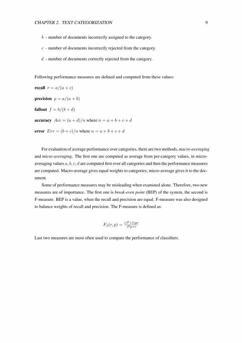
Following performance measures are defined and computed from these values:

recall r = a/(a + c)

precision p = a/(a + b)

fallout f = b/(b + d)

accuracy Acc = (a + d)/n where n = a + b + c + d

error Err = (b + c)/n where n = a + b + c + d

For evaluation of average performance over categories, there are two methods, macro-averaging

and micro-averaging. The first one are computed as average from per-category values, in micro-

averaging values a, b, c, d are computed first over all categories and then the performance measures

are computed. Macro-average gives equal weights to categories; micro-average gives it to the doc-

ument.

Some of performance measures may be misleading when examined alone. Therefore, two new

measures are of importance. The first one is break-even point (BEP) of the system, the second is

F-measure. BEP is a value, when the recall and precision are equal. F-measure was also designed

to balance weights of recall and precision. The F-measure is defined as:

Fβ(r, p) = (β2+1)prβ2p+r

Last two measures are most often used to compare the performance of classifiers.

Chapter 3

N-gram based Text Categorization

From all possible features presented in the previous chapter, I chose the solution based on N-

grams. I would like to explore possible improvements of methods described in [1] and [5]. In the

second article, some improvements were introduced, but used methods are also more complicated.

In this chapter, I would like to more deeply introduce these works.

3.1 N-grams

N-gram is a sequence of terms, with the length of N. Mostly words are taken as terms. Neverthe-

less, Trenkle and Cavnar chose N-grams based on characters for their work. In literature, you can

find the definition of N-gram as any co-occurring set of terms, but for this work, only contiguous

sequences were used. One word from the document was represented as the set of overlapping N-

grams. Here also leading and trailing spaces were considered as the part of the word. For example,

the word "TEXT" would be composed of following N-grams:

bi-grams _T, TE, EX, XT, T_

tri-grams _TE, TEX, EXT, XT_, T__

quad-grams _TEX, TEXT, EXT_, XT__, T___

In the first of the mentioned texts, N-grams with various lengths were used (from 1 to 5-grams).

In the second one only N-grams of the length of four were used. We can build such N-gram

representation for the whole document. This representation is then used for comparing documents.

The benefit of the N-gram based matching is derived form its nature. Every string is decomposed

into small parts, so any errors that are presented, affects only a limited number of N-grams, leaving

the remainder intact. The measure, counted as the number of N-grams, that are common for two

strings, is resistant to various textual errors.

10

CHAPTER 3. N-GRAM BASED TEXT CATEGORIZATION 11

3.2 N-gram frequency statistics

Each word occurs in human languages with a different frequency. The most common observation

of some regularity is known as Zipf’s Law. If f is the frequency of the word and r is the rank of

the word in the list ordered by the frequency, Zipf’s Law states, that:

f =k

r(3.1)

Later some modifications, were suggested, but they are only small deviations from original Zipf’s

observations. From this we get, that there is always a set of words, which dominates most of the

other words, in terms of frequency of use. This is true for languages, but also for words, that are

specific for the particular subject. As N-grams are components, which carry meanings, the idea of

Zipf’s law can be applicable also on frequencies of N-grams. The main idea of the categorization

used by Trenkle and Cavnar is that if we are comparing documents from the same category, they

should have similar N-gram frequency distribution [1].

In [5] Cavnar uses another helpful characterization and that is the inverse document frequency

(IDF). IDF was used to help to choose most significant N-grams for the subject identification. The

IDF for a specific N-gram is counted as the ratio of documents in the collection to the number

of documents in which the given N-gram occurs. IDF strongly corresponds to the importance of

the N-gram for the text categorization. If N-gram can be founded in all documents, it gives us no

information about difference between contexts, on the other side, if it will occur only in part of the

documents, these have something incommon (at least this N-gram).

3.3 Document representation

In the first article, documents were represented, by their N-gram frequency profiles. It is the list

of N-grams ordered by the number of occurrences in the given document. It simply describes

the Zipfian distribution of N-grams in the document. For the categorization by subject, N-grams

starting at rank 300 were used. This number was obtained by several experiments.

In the second article, they used representation that was more sophisticated. Each document

was represented as a vector, with values of term weights for each N-gram. As the vectors for each

document would have a very high dimension and would be very sparse, IDF was used to reduce

the dimension of the vector space. The weight for the terms was defined like:

wj =(log2(tfj) + 1) · IDFj√∑

iwi

(3.2)

where tfj is the term frequency and the IDFj is the inverse document frequency of the jth N-gram

in the document.

In both cases, the same representation as for documents was used also for categories.


3.4 Comparing

For the comparison of the two profiles, a very simple method was used, in the first work. The

similarity measure of two profiles was defined as a sum of differences between the rank of the

N-grams in one profile and the rank in the other profile. If an N-gram was not present in one of

the profiles, a maximum value was used.

In the second article, the similarity of two documents or categories was defined as the angle

between the representation vectors. Cosine of this angle can be computed as a dot product of these

two vectors.

When we want to choose a category for the document, we have to count distances (angles)

from all the categories profiles. Than we choose the category with the smallest distance (angle)

from the document profile. As we have the list of distances from all categories, we can order

them and with the help of some threshold, we can choose most relevant categories for the given

document. This means that the suggested classifier belongs to m-ary classifiers. In their work,

they used only the first category as the winner, so they assigned exactly one category to each

document.

3.5 Observations

In the first case, categorization was tested on the Usenet newsgroups. They have chosen five

closely related categories, from the computer science. For counting profiles of categories, they

used the FAQs of the given newsgroups. They used 778 articles from the Usenet and tested them

again the 7 selected FAQs. Their system achieved 80% correct classification rate. I tried to make

same computation of recall and precision (Cavnar and Trenkle have mentioned only the numbers

of documents correctly/incorrectly assigned) and from these computation I assumed that recall

and precision of this system are both about 60%. It is not a very high number, but I think, that this

classifier would obtain a pretty good score in the BEP measure.

Unfortunately, Usenet newsgroups messages articles are quite short and the system was not

giving such a good results for longer texts. The problem is, that in short texts, N-grams in first 300

ranks are mostly language specific, and from the rank of 300, they are more subject specific, so

we can use them to determine the subject of the text. The problem of longer texts is that there is

a higher amount of language specific N-grams in the text and these have usually high frequencies.

This leads to the fact that subject specific N-grams start on higher ranks than 300.

In the newer article, to eliminate this problem, inverse document frequency was used. This

helped to reduce the dimension of N-gram vectors and thus increase the speed of computation,

only with a low loss of performance. The system was tested on the TREC competition, against

different data sets. Very popular performance measures like Average Precision, Precision @ 100


docs and R-precision were used, to see how good the results are. The values of all measures were

somewhat lower, than median performance of all system in the TREC93 competition.

Both articles show, that it is possible to implement an N-gram based retrieval system. Such a

system has some very nice advantages.

As it was already mentioned, it is resistant to various textual errors. Of course, we suppose

that the same errors occur with a low probability. So such an error does not affect final results,

because the frequency of such an “invalid” N-gram will be so low that we will never calculate with

it.

The suggested systems are language independent, without any additional effort, because we

do not do any linguistic computation on the data. Language independence was also verified on a

set of Spanish documents.

Other advantage, but I think a very important one, is the simplicity of suggested methods. It

is easy to implement them. We can say that the “learning phase” of these systems does not exist

(all you need to do is to count the profiles of categories and they can be easily updated). The first

system also consumes very little resources. The other one has a little problem with the table of

IDF’s.

3.6 Possible improvements

There are some possibilities, how to improve the systems suggested in these works. We can use

more sophisticated term weighting, larger amount of N-grams to represent the text, use N-grams

with larger N, find a clever function to appoint the correct number to replace the magical ’300’,

with a most precise value for a various documents, etc.

In my work, I would like to explore some of these possibilities, to find some way how to apply

these methods to large texts, but I would like to keep it as simple as possible, because I think, it is

a very important benefit of these systems.

Chapter 4

Clusterization and Categorization ofLong Texts

The first inspiration to this project was the article [1]. The suggested system is very easy and has

good results. As the main problem of this system is the fact, that in the way it was described in [1]

it can be used only for short texts (Usenet newsgroups articles). I wanted to find some way how

to improve this system to obtain better results also for longer texts, to make it more general. In

their experiment they say, that in the sequence of N-grams ranked by the number of occurrences,

the subject specific N-grams are starting at the rank of 300. The first idea was to try to find such

a function, that will for each text return the most precise starting rank of the subject specific N-

grams. Nevertheless, I wanted to find some relationship between the length of the text and this

special rank. To do this, I needed a train set of long texts with assigned categories. Unfortunately,

I did find any resource of this kind.

But I still wanted to discover the power of N-grams, so I decided to build categories by my

own. Before the text categorization, I had to deal with the text clusterization. I decided to use

the information given by comparing two texts - “similarity”, to build up clusters of documents,

from the unknown set of documents (we can look at this as on the reinforcement learning). This

means I will try automatically to divide the set of documents, to subsets according some common

signs, in this case N-grams. I hoped that created subsets would have common subjects and would

correspond to categories, as a man would set up. For this purposes I used the collection of books

form Project Gutenberg 1. It is a large collection of free books (almost 10 000) and it was easy to

get it.

I made following tests: I chouse the train and the test set from the whole collection. Then

I counted profiles of all documents. Next step was the clusterization phase, in which I selected1http://www.gutebberg.org

14

CHAPTER 4. CLUSTERIZATION AND CATEGORIZATION OF LONG TEXTS 15

documents to categories and counted profiles for them. The last phase was categorization phase. In

this part, I compared documents from the test set to profiles of categories and chose one category

for each document. These tests are described in the chapter 5. Now I will describe the suggested

methods.

4.1 Feature Selection

In the first article [1], N-grams with the length from 1 to 5 were used, in the second article [5],

quad-grams were used. In the first article the N-grams selected as features, were determined by

its rank, in the second article, IDF (see 3.2) was used to determine appropriate N-grams. As I

have already written, to determine the correct rank of important N-grams we need a categorized

database of documents. I did not have it, so I also used IDF to select representative N-grams.

4.1.1 N-gram Selection

As I had already written, I used the N-gram with the length of 4. As an input, I took a plain text

with a single space between words, without tabulators or new line characters. In [5] they worked

with each word separately, so they did not take a care about N-grams, overlapping two words. I

think this has two disadvantages. N-grams that interfere with two words, give us some information

about relations between these words. For example, N-grams “ew Y” and “w Yo” fror words “New

York”, will be often together. The second disadvantage against the system, that completely treats

input as a single word is, that we have to search for word boundaries, to split the text to words.

Because of this, I decided to use also N-grams that interfere with more than one word. I was

working with the text as one single word and include spaces between words into N-grams.

4.1.2 IDF table

The first task was to build up the table of inverse document frequencies. For each N-gram, I

counted the number of documents, in which it occurs. The IDF of an N-gram t is defined as

IDF (t) =nt

N(4.1)

where nt is the number of documents in which the N-gram t occurs and N is the number of all

documents in the collection.

The table was very huge, so I decided to use N-grams with the length of 4, in tests. Even after

this, the table was too huge to store in memory so I threw out N-grams with lowest frequencies.

In this, I suppose these were mistakes, or it were very specific N-grams, that would give us no

help by categorization. Zipf’s law (see 3.1) helps us see that we can cut off quite a large part of

N-grams with a low influence on the final distribution. From (3.1) we have r = kf , where r is the

rank of N-gram, f is its frequency and k is constant. Let a be N-gram with the lowest rank (ra)


from N-grams with the frequency β (number of documents in witch it is present) and b the N-gram

with the lowest rank (rb) from N-grams with the frequency β + 1. Than the number of N-grams

with the frequency β is:

ra − rb ≈k

β− k

(β + 1)=

k

β(β + 1)(4.2)

The highest rank of an N-gram in the collection is approximately:

rmax ≈k

1= k (4.3)

Now if we want to determine the fraction of N-grams with the frequency of β we have 1β(β+1) .

From this, the portion of N-grams, which occurs only once, is 12 . Clearly, such N-grams have no

influence on the categorization, but we can highly reduce the number of N-grams we have to hold

in the table (If an N-gram is not in the table, it means it was only in few documents, so do not use

him for representation).

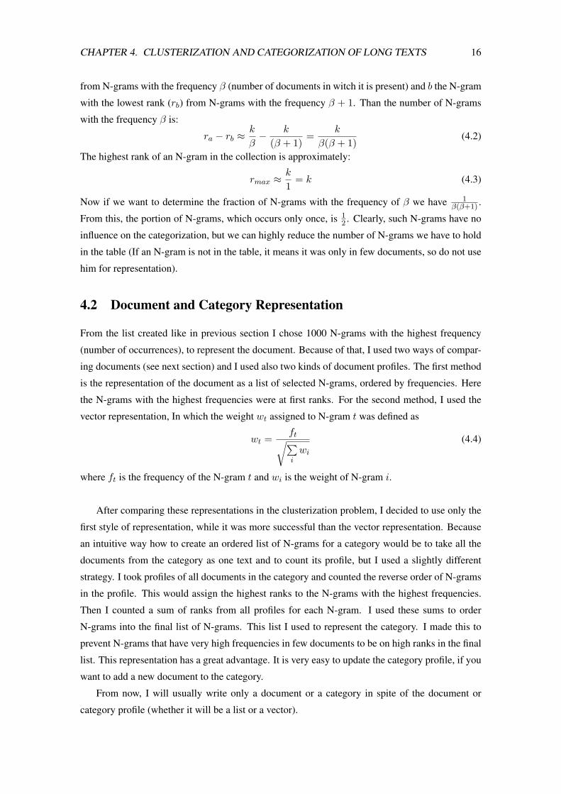
4.2 Document and Category Representation

From the list created like in previous section I chose 1000 N-grams with the highest frequency

(number of occurrences), to represent the document. Because of that, I used two ways of compar-

ing documents (see next section) and I used also two kinds of document profiles. The first method

is the representation of the document as a list of selected N-grams, ordered by frequencies. Here

the N-grams with the highest frequencies were at first ranks. For the second method, I used the

vector representation, In which the weight wt assigned to N-gram t was defined as

wt =ft√∑i

wi

(4.4)

where ft is the frequency of the N-gram t and wi is the weight of N-gram i.

After comparing these representations in the clusterization problem, I decided to use only the

first style of representation, while it was more successful than the vector representation. Because

an intuitive way how to create an ordered list of N-grams for a category would be to take all the

documents from the category as one text and to count its profile, but I used a slightly different

strategy. I took profiles of all documents in the category and counted the reverse order of N-grams

in the profile. This would assign the highest ranks to the N-grams with the highest frequencies.

Then I counted a sum of ranks from all profiles for each N-gram. I used these sums to order

N-grams into the final list of N-grams. This list I used to represent the category. I made this to

prevent N-grams that have very high frequencies in few documents to be on high ranks in the final

list. This representation has a great advantage. It is very easy to update the category profile, if you

want to add a new document to the category.

From now, I will usually write only a document or a category in spite of the document or

category profile (whether it will be a list or a vector).


4.3 Measure of Similarity

To make a clusterization or categorization we have to define some measure of similarity between

the two documents or the category and the document. The measures I used are normalized to the

interval 〈0, 1〉, and are build in such a way, that the lower values mean higher similarity. First is the

mentioned “out-of-place” measure. To count this measure we need the ordered list of N-grams.

Now I will define this measure. Let v and w be lists of N-grams, with the same length l. The

“out-of-place” measure s(v, w) can be defined as following:

s(v, w) = 1−

∑a

d(a) +∑b

d(b)+

2 · l2(4.5)

where a (b) goes through all N-grams from v (w) and d(i, j) is defined as

d(x) =

{|rvx − rwx| x ∈ v ∧ x ∈ w

l x /∈ v ∨ x /∈ w(4.6)

where rvx is the rank of the N-gram x in the list v and rwx is the rank in list w. This measure

gains values from the interval 〈0, 1〉. When we have this measure, we say that the similarity of two

documents or categories v and w increases with increasing value of s(v, w).

The second measure uses the dot product of two vectors. I used this measure for the second

type of the document profile. As we know, the dot product of two vectors corresponds to the cosine

value of the angle between these two vectors. This gives us the number from the interval〈−1, 1〉.After this, I used a transformation to get values into the interval 〈0, 1〉.

I compared both methods for comparing documents (“out-of-place” measure [1] and the vector

processing [5]). Surprisingly, results of the first method were better. It seems like the “out-of-

place” measure is creating categories that are more similar to categories created by people). This

is why I did not use the vector processing method for the text categorization.

4.4 Clusterization

The task of clusterization is to divide the set of documents to groups (clusters), so that similar

documents will be in the same group (cluster). If we want to define this problem, we can say that

the measure, defined in the previous section between two documents from the same group will

be higher, than similarities between these documents and any other document outside this group.

More formally:

Let T be the set of all documents. C ⊂ S is the cluster of similar documents, if and only if

holds, that for any a, b ∈ C and c ∈ T ∧ c /∈ C s(a, b) > s(a, c).

So I had the set of N documents and the table of N × N with values of similarity measures

between all these documents (we do not need the whole table, the upper triangle is sufficient,


because s(v, w) = s(w, v)). We can look at this table as at the complete graph, where documents

can be mapped to nodes and the weight of an edge between nodes v and w is s(v, w). Now we can

transform our problem to split components of this graph, so that weights of edges inside of these

components will be bigger than outgoing edges of these components. To do this, we need to set

up a threshold, which says that edges with the lower weight than this threshold will be outgoing

edges of components. This will split up the graph to “unconnected” components (it is something

like deleting these edges from the graph). In the meaning of similarity, this threshold is saying that

documents with the lower similarity should not be in the same cluster. This does not mean they

will really be in different clusters, because they both can be similar to the third document, which

will bind them together.

I made some experiments with clusterization and I came to the problem. The split graph looked

like one big component of many independent documents and few small components that could be

considered as categories. With increasing of the threshold, new components were cut form the big

one, but the previous small components felt apart to single documents (or very small components

from two or three documents). I was really disappointed, but now it seems, that I have found

the solution. The problem was that the similarity of documents in one category (or cluster) was

different and could be much higher or lower than the similarity of documents in other category.

The idea of the improving the clusterization was as followed:

1. Set up an low threshold t

2. Split the graph using this threshold

3. If the clusters with the “good” size are present, mark them as clusters and remove them

from the graph. The “good” size depends on the size of the graph and on your belief in your

similarity measurement (if it is very good, then two documents can be a base for a cluster).

4. Increase t and repeat from the step 1., until there is a component with more than t nodes.

With this system, I was able to create clusters from the training set. There was quite a big junk - the

clusters of a very small size or single documents, but some of created categories were “man-like”

(see 5.3 for more details).

4.5 Categorization

The main goal was to find a good method for text categorization. The task of categorization as-

sumes that we have the profile of the document we would like to categorize and the profiles of

categories from which we chose the one that is most suitable to be the category of the document.

Creating profiles of documents and categories was discussed in 4.2. The algorithm of the catego-

rization is very simple and has only two steps.

1. First, count similarities (4.5) between the selected document and all categories.


2. Than choose the category with the highest similarity as the category of the document.

In reality, one document can be a member of more categories and this method of categorization

(but not the clusterization from previous section) can handle this. All we need to do is to order

the categories according to similarities with the document and then the categories with the highest

similarity are the most probable categories of this document. For this work, I used only the first

one as the category of the document.

Now if our test set contained documents with assigned categories, we can compare it with the

chosen category and use it to tune up the system (all thresholds, sizes, etc. ...). Unfortunately, I do

not have it. I checked results manually and made some statistical observations. They are described

in chapter 5.

Chapter 5

Experiments

5.1 Corpus

For the training and testing text categorization, we need a corpus. As I have already written, I was

not able to get a corpus sorted into categories. The set of documents, which I used in experiments

with suggested methods of text clusterization and categorization, were E-texts of books freely

available on the website of the Project Gutenberg1. The whole collection contains about 11 000

books. I did not use the whole collection, because my implementation was not able to work with

such a great amount of data. I used only plain text files smaller than 2MB’s (because of memory

consumption). Of course I cut off headers of E-texts.

5.2 IDF’s Threshold

First, I counted the table of IDF’s. For this, I used the set of 8189 documents and the final table

(without the N-grams with the lowest frequencies - see section 4.1.2) contained 346 305 unique

N-grams.

I started measuring the similarity on a small set of 30 documents. I knew the subjects of these

documents, so I was able to say whether the results are clever or not. Later I made some tests with

500 documents. I came to the threshold of 2.75. I do not say that it is the best value, but obtained

results were giving best results. There is something strange about this value. In [5] they also used

the value 2.75 as a threshold for IDF, but they defined IDF as log2(Nnt

but I defined it without a

logarithm. So this threshold corresponds to the threshold of 1.46 in their system. Their threshold

corresponds to the threshold of 6,72 in my system. In spite of this, it looks like that the threshold

of 2.75 gives much better results. I think this can be due to different creation of N-grams in their

and my system (see 4.1.1).1http://www.gutebberg.org

20

CHAPTER 5. EXPERIMENTS 21

5.3 Clusterization

Dividing documents into categories depends on their similarity, the size of cluster we want and of

course the clusterization algorithm. As clusters are created in iterations, it is possible, that the last

created cluster will be only the rest of documents that had not fit anywhere but are slightly similar.

First tests with clusterization were made on a set of 500 books randomly chosen from the set of

11 0000 books I had.2 I was satisfied with these results. Only 246 books where used to create

categories, so there was a big junk (60%). This set of 197 books was divided into 9 categories.

Each category has the size from 10 to 35 documents. The best thing about these tests was that some

of the created categories where “man-like”. In category1 were memories of people, in category2

poems and theatre, in category5 political documents. I do not know whether documents in other

categories would be in similar categories as in the “man-like” categorization, because they were

created from more “common books” and I had not read all these books to determine their subjects.

In table A.1 are some examples of categories and documents from which they were created. In

figure 5.1 you can se how 197 books were divided into categories.

cat0 cat1 cat2 cat3 cat4 cat5 cat6 cat7 cat80

50

100

150

20 1914 10

1626 30 29 33

Figure 5.1: Distribution of documents among categories. “500 test”, only 197 were divided into

categories

I ran next test with the set of 3,000 documents. 3 I was expecting that if in the previous test

categories had the size between 10 and 30, here I chose the size from 50 to 200. The results

were following: 739 books were divided into 7 categories. But the junk was very big (75.3%).

In the figure 5.2 you can see the distribution of books among categories. I think that one the

reasons for this may be that the threshold for IDF with the value 2.75 is too high. The effect of

this is that similar measures between documents are very low (it is under 0.2) and so only very

similar documents create categories. Here I must say that there is nothing wrong with the fact that2I will refer to all tests connected with this set of documents as the “500 test”3I will refer to all tests connected with this set of documents as the “3,000 test”


distributions in figures 5.2 and 5.1 are completely different. There were used different train sets

and numbers of categories does not say that these must have something common.

cat0 cat1 cat2 cat3 cat4 cat5 cat60

100

200

300

400

500

600

9378 73

54

182

64

196

Figure 5.2: Distribution of documents among categories. “3,000 test”, only 739 were divided into

categories

The problem in clusterization is that I assigned one or none category to each document. But in

reality, each document can belongs to many categories, an so there are connections between cat-

egories which abuses the clusterization. This could be solved with more complicated algorithms

that will split the graph, also when there is a small set off documents creating a cut between two

sets of documents, but for the tests I used only a simple version, that was creating categories from

standalone components, that had no connections to the rest of the graph.

In spite of all these problems, the results are quite interesting. First, in spite of the fact, that

I threw out all frequent N-grams (this is because of usage IDF) documents from other languages

than English created their own categories. For example in the “500 test” German books where

in category0, in the “3,000 test” they where in category4. French books created catgory1 in the

“3,000 test”. Furthermore, I was able to describe some other categories too, e.g. in the “500 test”:

category1 - contained books somehow connected with Netherlands

category2 - books about theology and psychology

category3 - some philosophical books about people, their knowledge and senses

category4 - memories, diaries and life stories of famous people mainly from England and the

USA

category5 - memories of famous French people from the times of Napoleon, together with novels

from A. Dumas and H. Balzac (both were writing about these times)

category8 - theatre - plays


About categories from the “3,000 test”:

category0 - mainly some scientific books

category2 - memories and books about famous French people from the times of Napoleon

category3 - theatre - plays - except two, all by Shakespeare.

category4 - German literature, together with books about Greek mythology and antic times -

maybe the reason is that some of German’s books were also from Greek mythology.

category5 - poetry

As you can see, I was not able to say anything about categories 6 and 7 from the first test and

category6 from the second test. One of the reasons can be following. The clusterization, in the

way I implemented cutting components from one large graph. At the end there is a component,

which is the rest of the graph, but it is enough small to fulfill the conditions to become a category.

This can lead to categories that are giving no sense.

5.4 Categorization

The categorization tests consist of comparing set of documents with created categories. Results

are lists of documents assigned to each category and the count of documents assigned to each

category. With both sets of categories, I made two such tests. In the first test, I took the “junk

files” - the files from train set that were not chosen to any category and ran the categorization

test on them. In the second test I randomly chose 1,000 documents from the Project Gutenberg’s

books (different from the train set). You can see the distribution of documents among categories

in figures 5.3 and 5.4. Slightly disappointing is that these distributions do not correspond to the

distribution of categories (fig 5.1, 5.2), but it is easy to see that distributions in figure 5.4 are

similar. This can mean that there is a characteristics of this collection of books, which divides

the whole collection to created categories. But this means that these categories are feasible, what

would be a great success of the suggested method. This means that they really describe the whole

collection of books.

I checked these results also manually. It seems, that almost all documents that should belong to

some category, where assigned to this category. However, to each category, there where assigned

also documents that do not belong to it. Except the failure, the reason can be the fact, that this

document should not belong to any of created categories, but the chosen category had the most

similar characteristics. Tests with “junk files” are giving interesting results. Many of these files

had something common with the categories in which they were assigned and I did not know why

they do not become part of this category during clusterization.


There is also an example, that it is possible that this method will reach good results with only

few documents in a category (some categories had only ten documents), but also when these docu-

ments are very similar. To be more concrete, category3 from the “3,000 test” consists of the plays

written by Shakespeare (only two texts where by other authors). Then in the tests with “junk files”

and the 1,000 randomly chosen files, much other theatre plays by various authors were assigned

to this category.

Unfortunately, I was not able to make any classical measurements, because I did not have the

set of correctly and incorrectly categorized documents as it used to be common.


50

100

150

200

250

300

3

3423

65

4661

1732

22


200

400

600

800

1000

5399 121

96

166 151

92124

98

“junk” 1,000 documents

Figure 5.3: Distributions of documents in “500 tests”


300

600

900

1200

1500

1800

2100

606

27

581

10426

232

685


200

400

600

800

1000

232

41

229

51 52

140

255

“junk” 1,000 documents

Figure 5.4: Distributions of documents in “3,000 tests”

Chapter 6

Conclusions and Further Work

In this work, I have implemented the system for text categorization. Used ideas are mainly the

mixture of ideas from articles [1] and [5]. Unfortunately, I did not have the necessary database to

train this method with some classical machine-learning algorithm. That was the reason I did not

fulfill the goal stated at the beginning of the work completely.

Nevertheless, I had found a method for the text clusterization. It is a method, which helps us

to build categories from the set of documents, without previous knowledge of given texts. We can

look at text clusterization as at the reinforcement learning method of text categorization, because

we do not know whether created categories are feasible or not. Obtained results are not so good

that I could use this system to solve some real problems, but they are not so bad and we should not

throw them into the bin. I was able to find some “real” similarities among documents in created

categories and I do not say that there is no similarity among books from other categories, but I do

not know every book, so I did not find it. The implemented system showed also some ability of

generalization, when it correctly categorized previously unseen documents. I think that the system

with a good ability of text clusterization in unknown environment will be very valuable for prob-

lems of information retrieval. Other very useful advantage of N-gram based systems, mentioned

already by Trenkle and Cavnar [1] is the language independency. Of course, it is possible to make

many improvements, which will for sure bring much better results, but I think that now we can

see, that the N-gram based system has its meaning and it can be valuable for future research.

Here I would like to sketch some possible suggestions for improvements. The first thing what

should be done is to find some database of categorized texts. With such a database, we can tune

up the system for much better results. This would especially help to find better threshold for IDF’s

values. Furthermore, I believe that it is possible that with such a database we will be able to find

“ranks of important N-grams” in the complete list of N-grams from a document without the help

of IDF values. This would help us to reduce computational resources we need.

As I said, the text clusterization can be very useful and there are some possibillities how to

25

CHAPTER 6. CONCLUSIONS AND FURTHER WORK 26

make it better. One problem of the implemented method was that each document was assigned

only to one category. The suggested improvement is the question of algorithms in the graph of

documents and their similarities. The idea is not to split the graph only when there are unconnected

components. We can split the graph also when there are two sets of nodes, with the cut containing

only few documents. In this case, we have to include these nodes in both sets. This will ensures

that one document can be in more categories.

The last improvement is a slightly different view of the problem. If you think how the people

do the text categorization, they usually do not read the whole book to determine its subject. They

usually read only short parts. This means that these parts must contain the sufficient information

for the text categorization. But we have the text categorization of short texts that reaches quite

good results [1]. So why not split the long text into small parts, categorize them and from the

results choose the category of the whole document? For the last part, the k-NN algorithm can be

useful.

Bibliography

[1] W. B. Cavnar and J. M. Trenkle. N-gram-based text categorization. Proceedings of SDAIR-

94, 3rd Annual Symposium on Document Analysis and Information Retrieval, 1994.

[2] W. W. Cohen and Y. Singer. Context-sensitive learning methods for text categorization. Pro-

ceedings of SIGIR-96, 19th ACM International Conference on Research and Development in

Information Retrieval, 1996.

[3] D. Peng, F.; Schuurmans and S. Wang. Language and task independent text categorization

with simple language models. Proceedings of the 2003 Human Language Technology Con-

ference of the North American Chapter of the Association for Computational Linguistics,

2003.

[4] J.; Will T. Goller, C.; Loning and W. Wolff. Automatic document classification: A thorough

evaluation of various methods. In Internationales Symposium f ur Informationswissenschaft,

2000.

[5] W. B. Cavnar. Using an n-gram-based document representation with a vector processing

retrieval model. In Proceedings of the Third Text REtrieval Conference (TREC-3), 1994.

[6] Y. Yang and J. 0. Pedersen. A comparative study on feature selection in text categorization.

Proceedings of ICML-97, 14th International Conference on Machine Learning, 1997.

[7] Y. Yang and J. 0. Pedersen. A study on thresholding strategies for text categorization. Pro-

ceedings of SIGIR-01, 24th ACM International Conference on Research and Development in

Information Retrieval, 2001.

[8] Y. Yang. An evaluation of statistical approaches to text categorization. Technical Report

CMU-CS-97-127, Computer Science Department, Carnegie Mellon University, 1997.

[9] V. Vapnik and C. Cortes. Support-vector networks. AT&T Labs-Research, USA, 1995.

[10] T. Joachims. Text categorization with support vector machines: Learning with many relevant

features. Proceedings of the European Conference on Machine Learning (ECML), 1998.

27

Appendix A

Tables

Following tables show results of my experiments. There are lists of books from each category.

This is no a complete list. All titles and authors were retrieved from the books by a small utility I

made and some of them where not parsed correctly.

category0 Wilhelm Busch , Hans Huckebein; Johann Wolfgang Goethe, Wilhelm Meisters Lehrjahre–Buch 2; Johann Wolfgang von Goethe, Reineke Fuchs;

Heinrich Heine, Buch der Lieder; Theodor Mommsen, Römische Geschichte Book 8; Meyer, Die Versuchung des Pescara;

Ferdinand Raimund, Der Verschwender; Jacob Michael Reinhold Lenz, Der Hofmeister; Friedrich Schiller, Kabale und Liebe; Johanna Spyri

category1 G. A. Henty, By England’s Aid; Schiller, Book I., IV, Revolt of Netherlands; Georg Ebers, Vol. 1.,6.,9., Barbara Blomberg;

Georg Ebers, v4, The Bride of the Nile; John Lothrop Motley, Rise of the Dutch Republic, 1564-65, 1573-1574;

John Lothrop Motley, History of the United Netherlands, The Life of John of Barneveld,

category2 Michel de Montaigne, The Essays of Montaigne, V4; J. J. Thomas, Froudacity; Walter Pater, Marius the Epicurean, Vol. I;

John Edgar McFadyen, Introduction to the Old Testament; Charlotte Mary Yonge, The Chosen People; Ethel D. Puffer, The Psychology of Beauty;

Spinoza A Theologico-Political Treatise; William James, The Varieties of Religious Experience; Abraham Myerson, The Foundations of Personality

category3 Speeches and Writings of Edmund Burke; Joseph Butler, Human Nature & Other Sermons; William James, The Meaning of Truth

Thomas Paine, Common Sense; Henry Handel Richardson, The Getting of Wisdom; James Gillman, The Life of Samuel Taylor Coleridge;

D. Jerrold, Mrs. Caudle’s Curtain Lectures; George Berkeley, A Treatise Concerning the Principles of Human Knowledge;

category4 General Philip Henry Sheridan, Memoirs of General P. H. Sheridan, v1; William T. Sherman, Memoirs of General W. T. Sherman, v1;

Gardner, The Life of Stephen A. Douglas; David Widger, Quotations from Diary of Samuel Pepys; Matthew L. Davis, Memoirs of Aaron Burr;

Stephen Gwynn, The Life of the Rt. Hon. Sir Charles W. Pepys The Diary of Samuel Pepys; Jacques Casanova, Old Age and Death;

category5 Tommaso Campanells, The City of the Sun; Louis Antoine Fauvelet de Bourrienne, the Memoirs of Napoleon; Constant, the Private Life of Napoleon

La Marquise De Montespan, The Memoirs of Madame de Montespan; Elizabeth-Charlotte, Duchesse d’Orleans, Memoirs of Louis XIV. and the Regency

Jean Jacques Rousseau, The Confessions of J. J. Rousseau; Charles Eastman, Indian Boyhood; Honore de Balzac, The Deputy of Arcis;

category6 Anthony Trollope, The Prime Minister; Irving Bacheller, Eben Holden; Charlotte M. Yonge, The Heir of Redclyffe;

Guy de Maupassant Original Maupassant Short Stories.; Louisa May Alcott , Jo’s Boys; Kate Douglas Wiggin, A Summer in a Canyon;

Anonymous, The Book Of The Thousand Nights And One Night, I-III; Charles Dickens, A Christmas Carol; George Meredith, v6, Beauchamps Career;

category7 Trevelyan, Life and Letters of Lord Macaulay; The Earl of Chesterfield, Letters to His Son; Voltaire, Le Blanc et le Noir; Emile Zola, La Bete Humaine;

Victor Hugo, L’homme qui rit; Thomas de Quincey, Memorials and Other Papers; Frederick Niecks, Frederick Chopin as a Man and Musician;

Mary Schweidler, The Amber Witch; Emile Zola, Nana; Jean-Baptiste Poquelin, L’Avare; Arsene Houssaye, Les grandes dames;

category8 John Galsworthy , The Pigeon; Shakespeare, The Merchant of Venice; Upton Sinclair, The Second-Story Man;

Bernard Shaw, Augustus Does His Bit; George Bernard Shaw, Heartbreak House; Tom Taylor, Our American Cousin

Voltaire, Candido, o El Optimismo; Richard Hakluyt, The Principal Navigations, Voyages; Leonardo Da Vinci, The Notebooks of Leonardo Da Vinci

ongreve, The Way of the World; Tullia d’Aragona, Rime;Ben Jonson., The Alchemist; James M. Barrie, What Every Woman Knows

Dante Alighieri, "Divina Commedia di Dante: Inferno"; Dante Alighieri, Dante’s Inferno; Shakespeare, Love’s Labour’s Lost;

Table A.1: Categories and assigned documents. “500 test”

28

APPENDIX A. TABLES 29

category0 Trollope, The Courtship of Susan Bell; Trollope, George Walker At Suez; John Burroughs, Time and Change; Trollope, The House of Heine Brothers;

Robert Chambers, Vestiges of the Natural History of Creation; Trollope, O’Conors of Castle Conor; Simon Newcomb, Side-Lights On Astronomy;

Thomas Henry Huxley, The Rise and Progress of Palaeontology; Charles Darwin, Literary Archive Foundation; Huxley, Lectures on Evolution;

Elizabeth Gaskell, Doom of the Griffiths; Andrew Lang, How to Fail in Literature Elizabeth Gaskell, The Half-Brothers; James Joyce , Chamber Music;

Williams, A History of Science; Darwin, On the Origin of Species; Darwin, The Voyage of the Beagle; Stallman, The Right to Read;

category1 Hippolyte A. Taine, The Origins of Contemporary France; Marcel Proust, A L’Ombre Des Jeunes Filles en Fleur; Alexandre Dumas, Henri III et sa Cour;

Jules Verne, Tour Du Mond 80 Jours ; Huguette Bertrand, Espace perdu, poesie; Pierre Loti, Pecheur d’Islande; Jules Renard, Poil De Carotte;

Jules Verne, Voyage au Centre de la Terre; Huguette Bertrand, Les Visages du temps, poesie; Moliere , L’Etourdi, par Moliere; Voltaire, Candide;

Emile Zola, La Bete Humaine; Robert de Boron, Li Romanz de l’estoire dou Graal; Victor Hugo, Le Dernier Jour d’un Condamne; Boileau, Le Lutrin;

Frederic Mistral, Mes Origines. Memoires et Recits; Anatole France, Thais; Victor Hugo, Actes et Paroles; Alexandre Dumas, Les Quarante-Cinq

category2 The Duc de Saint-Simon, Memoirs Louis XIV, Madame Hausset, Memoirs of Louis XV./XVI; Louise Muhlbach, Napoleon And Blucher;

S. Baring-Gould, In Troubador-Land; Dumas, The Man in the Iron Mask; Dumas, Louise de la Valliere; John K. Bangs, Mr. Bonaparte of Corsica;

Eugene Sue, The Wandering Jew; Muhlbach, Frederick The Great And His Family; Constant, Private Life of Napoleon;

Madam Campan, Memoirs of Marie Antoinette; Stewarton, Gentleman at Paris, to Nobleman in London; Alfred de Vigny, Cinq Mars;

Eugene Sue, The Mysteries of Paris; Dumas, The Three Musketeers; Dumas, Twenty Years After; Honore de Balzac, Catherine de Medici

category3 William Shakespeare, The Merry Devil; Schiller, The Maid of Orleans (play); William Hazlitt, Characters of Shakespeare’s Plays;

Thomas Kyd, The Spanish Tragedie; Shakespeare, King Henry VI, Part 1; Shakespeare, Titus Andronicus; Shakespeare, The Two Gentlemen of Verona;

Shakespeare, King John ; Shakespeare, Romeo and Juliet; Shakespeare, Twelfth Night; Shakespeare, Measure for Measure;

Shakespeare, King Lear; Shakespeare, Pericles; Shakespeare, The Tempest; Shakespeare, Much Ado About Nothing;

category4 Goethe, Reineke Fuchs; Friedrich Schiller, Die Piccolomini; Johann Wolfgang Goethe, Novelle; Goethe, Briefe aus der Schweiz;

Georg Büchner, Dantons Tod; Franz Grillparzer, Die Argonauten; AEschylus, The House of Atreus; Franz Grillparzer, Der Traum ein Leben;

Goethe, Iphigenie auf Tauris, Herodotus, The History of Herodotus; Hermann Hesse, Siddhartha; Theodor Mommsen, Römische Geschichte;

Friedrich Hebbel, Schnock Andrew Lang, M.A., Walter Leaf, Litt.D.„ The Iliad of Homer; Friedrich Hebbel, Agnes Bernauer;

William Shakespeare, Wie es euch gefällt William Shakespeare, Was ihr wollt Suetonius, The Lives Of The Caesars Michael Clarke, Story of Aeneas

category5 Nora Pembroke, Verses and Rhymes by the way; Thomas Hardy, Late Lyrics and Earlier; William Wordsworth, Lyrical Ballads, With Other Poems;

Alexander Pope, Essay on Man Charles Swinburne, Two Nations; Edgar Allan Poe, The Works of Edgar Allan Poe; George Borrow, Romantic Ballads et al;

Burton Stevenson, The Home Book of Verse; Emily Dickinson, Poems; William Makepeace Thackeray, Ballads; Thomas Hardy, Moments of Vision;

William Morris, The Pilgrims of Hope William Morris, Poems by the Way Ella Wheeler Wilcox, Poems of Progress Hardy, Wessex Poems and Other Verses

C. Patmore, The Angel in the House Esaias Tegne’r, Fridthjof’s Saga Swinburne, Songs before Sunrise Jean de La Fontaine, The Fables of La Fontaine

category6 Kate Langley Bosher, Miss Gibbie Gault; Elizabeth Cleghorn Gaskell, Cousin Phillis; Robert Alexander Wason, Happy Hawkins;

Anthony Trollope, Barchester Towers ; Zane Grey, The Border Legion; Kipling , Captains Courageous; D.H. Lawrence, The Trespasser;

Rudyard Kipling, Kim; Joseph Conrad , A Set of Six; George MacDonald , Sir Gibbie; Louisa M. Alcott , Eight Cousins;

George MacDonald, Robert Falconer Hardy, Romantic Adventures of a Milkmaid Bentley, Trent’s Last Case F.W. Moorman, Yorkshire Dialect Poems

George Meredith, Vittoria; Elizabeth Gaskell, Sylvia’s Lovers; Charles Dickens , Hard Times Sir Walter Scott, Waverley;

Table A.2: Categories and assigned documents. “3000 test”

Appendix B

Implementation

I have made an implementation of the described methods of clusterization and categorization. To

try the categorization again the categories form the “3000 test”, you can use the TextCat demo,

which is a part of the implementation. Manual, complete source cod and compiled classes are

on the CD. I implemented the solution in Java. Used algorithms are not optimized. I made the

implementation only for the tests. Here are the most important parts from the source code.

First is the source code of the NgramSequence class. It was used for the representation of

documents and categories. It implements the addition of N-gram and the counting of ranks.package org . t e x t c a t . ngram ;

i m p o r t j a v a . u t i l . A r r a y L i s t ;i m p o r t j a v a . u t i l . A r r a ys ;i m p o r t j a v a . u t i l . Compara tor ;i m p o r t j a v a . u t i l . HashMap ;i m p o r t j a v a . u t i l . HashSet ;i m p o r t j a v a . u t i l . I t e r a t o r ;i m p o r t j a v a . u t i l . L i s t ;i m p o r t j a v a . u t i l . Map ;i m p o r t j a v a . u t i l . S e t ;

/∗∗∗ Thi s c l a s s r e p r e s e n t s t h e s e t of p a i r s N−gram and v a l u e .∗ I t imp lemen t s add in g N−grams t o t h e sequence ,∗ o r d e r i n g and r a n k i n g of N−grams by t h e a s s i g n e d v a l u e s .∗ Ranks from od e re d l i s t or f r e q u e n c i e s t h a t where a s s i g n e d t o N−grams∗ a r e h e r e f o r v a l u e s .∗ @author pna∗∗ /

p u b l i c c l a s s NgramSequence {

p r o t e c t e d double l o w e s t V a l u e = Double .MAX_VALUE;p r i v a t e L i s t f L i s t ;p r i v a t e S e t f S e t ;p r o t e c t e d Map map = new HashMap ( ) ;

/∗∗∗ R e t u r n s t h e l i s t of N−grams∗∗ /

p r i v a t e L i s t g e t L i s t ( ) {i f ( f L i s t = = n u l l ) f L i s t = new A r r a y L i s t ( map . ke ySe t ( ) ) ;re turn f L i s t ;

}

/∗∗∗ R e t u r n s t h e s e t of a l l N−grams i n t h e s e q u e n c e∗ /

p u b l i c S e t g e t S e t ( ) {i f ( f S e t = = n u l l ) f S e t = new HashSet ( map . ke ySe t ( ) ) ;re turn f S e t ;

}

30

APPENDIX B. IMPLEMENTATION 31

/∗∗∗ Order N−grams by v a l u e s a s s i g n e d t o them .∗ R e t u r n s t h e f i n a l l i s t∗ /

p u b l i c L i s t o r d e r L i s t ( ) {L i s t l i s t = g e t L i s t ( ) ;O b j e c t [ ] a r r a y = l i s t . t o A r r a y ( ) ;Ar r ay s . s o r t ( a r r a y , new Compara tor ( ) {

p u b l i c i n t compare ( O b j e c t a , O b j e c t b ) {double d1 = g e t V a l u e ( a ) ;double d2 = g e t V a l u e ( b ) ;i f ( d1>d2 ) re turn −1;i f ( d1<d2 ) re turn 1 ;re turn 0 ;

}

} ) ;f L i s t = new A r r a y L i s t ( Ar r a ys . a s L i s t ( a r r a y ) ) ;re turn f L i s t ;

}

/∗∗∗ Add an N−gram t o t h e s e q u e n c e . I t means i n c r e a s e t h e v a l u e a s s i g n e d t o∗ N−gram by one∗ I f t h e r e i s no such N−gram i n s e r t i t t o s e q u e n c e wi th t h e v a l u e o f 1 .∗∗ /

p u b l i c vo id add ( O b j e c t i d ) {add ( id , 1 ) ;

}

/∗∗∗∗ Add an N−gram t o t h e s e q u e n c e . I t means i n c r e a s e t h e v a l u e a s s i g n e d t o N−gram by < code > va lue < / code >∗ I f t h e r e i s no such N−gram i n s e r t i t t o s e q u e n c e wi th t h e v a l u e o f < code > va lue < / code > .∗∗ /

p u b l i c vo id add ( O b j e c t id , double v a l u e ) {Double d = ( Double ) map . g e t ( i d ) ;i f ( d = = n u l l ) p u t ( id , v a l u e ) ;e l s e p u t ( id , d . doub leVa lue ( ) + v a l u e ) ;

}

/∗∗∗ P u t s N−gram wi th t h e g i v e n v a l u e t o t h e s e q u e n c e . I f t h e r e i s a l r e a d y such N−gram ,∗ i t w i l l be r e p l a c e d .∗ /

p u b l i c vo id p u t ( O b j e c t id , double v a l u e ) {i f ( va lue < l o w e s t V a l u e ) l o w e s t V a l u e = v a l u e ;map . p u t ( id , new Double ( v a l u e ) ) ;

}

/∗∗∗ R e t u r n s t h e v a l u e a s s i g n e d t o N−gram .∗ U s u a l l y i t i s a f r e q u e n c y or a rank∗ @param i d∗ @return∗ /

p u b l i c double g e t V a l u e ( O b j e c t i d ) {Double d = ( Double ) map . g e t ( i d ) ;re turn ( d = = n u l l ) ? − 1 : d . doub leVa lue ( ) ;

}

/∗∗∗ R e t u r n s new < code >NgramSequence < / code > . Ngrams i n t h i s s e q u e n c e w i l l be s u b s e t o f t h e N−grams∗ from c u r r e n t s e q u e n c e . Oders o f N−grams i s g i v e n by t h e < code > l i s t <code >∗ /

p u b l i c NgramSequence ge tSubSequence ( i n t s t a r t , i n t end ) {L i s t l i s t = g e t L i s t ( ) ;NgramSequence r e s = new NgramSequence ( ) ;i n t e = end ;i f ( end> s i z e ( ) ) e = s i z e ( ) ;f o r ( i n t i = s t a r t ; i < e ; i + + ) {

O b j e c t o = l i s t . g e t ( i ) ;r e s . p u t ( o , g e t V a l u e ( o ) ) ;

}re turn r e s ;

}

/∗∗∗ Rep lace t h e v a l u e s a s s i g n e d t o N−grams wi th t h e i r rank i n an o r d e r e d l i s t .∗ The l i s t i s o r d e r e d form h i g h e s t t o l o w e s t v a l u e s .∗∗ /

p u b l i c vo id coun tRanks ( ) {l o w e s t V a l u e = Double .MAX_VALUE;L i s t l i s t = o r d e r L i s t ( ) ;f o r ( i n t i = 0 ; i < l i s t . s i z e ( ) ; i + + ) {


S t r i n g e l e m e n t = ( S t r i n g ) l i s t . g e t ( i ) ;p u t ( e lement , i ) ;

}}

/∗∗∗ D e c r e a s e v a l u e s o f a l l N−grams , by t h e l o w e s t v a l u e .∗ So z e r o u w i l l be t h e l o w e s t v a l u e h e r e∗∗ /

p u b l i c vo id normRanks ( ) {double lw = l o w e s t V a l u e ;f o r ( I t e r a t o r i t = map . k ey Se t ( ) . i t e r a t o r ( ) ; i t . hasNext ( ) ; ) {

O b j e c t e l e m e n t = i t . n e x t ( ) ;p u t ( e lement , g e t V a l u e ( e l e m e n t)−lw ) ;

}}

}

Here is the source code of method that implements the creation of the sequence of N-grams from

the plain text. During the creation, the filter of N-grams is used. It checks the value of the IDF. If

it is greater than the given threshold (2.75 in this case), it will not use this N-gram.

p u b l i c NgramSequence b u i l d R a n k e d F i l t e r e d S e q u e n c e ( S t r i n g sou rce , i n t l ength , F i l t e r f i l t e r ) {s o u r c e = s o u r c e . r e p l a c e A l l ( " [ \ t \ n \ f \ r ] " , " " ) . r e p l a c e A l l ( " {2 ,}+ " , " " ) ;NgramSequence r e s = new NgramSequence ( ) ;i n t i =0 ;whi le ( i + l e n g t h < = s o u r c e . l e n g t h ( ) ) {

S t r i n g s = s o u r c e . s u b s t r i n g ( i , i + l e n g t h ) ;i f ( f i l t e r . a c c e p t ( s ) )

r e s . add ( s ) ;i ++;

}r e s . coun tRanks ( ) ;re turn r e s ;

}

/∗∗ C r e a t e d on 2 0 . 4 . 2 0 0 5∗∗ /

package org . t e x t c a t . ngram ;

i m p o r t o rg . t e x t c a t . common . F i l t e r ;

/∗∗∗ Thi s i s a f i l t e r , which a c c e p t s N−grams wi th t h e IDF v a l u e∗ h i g h e r t h a n 2 . 7 5∗∗ @author pna∗ /

p u b l i c c l a s s I D F F i l t e r imp lemen t s F i l t e r {

/∗ ( non−Javadoc )∗ @see org . t e x t c a t . common . F i l t e r # a c c e p t ( j a v a . l a n g . O b j e c t )∗ /

p u b l i c boolean a c c e p t ( O b j e c t o ) {i f ( IDFTable . i n s t a n c e ( ) . documents / IDFTable . i n s t a n c e ( ) . ns . g e t V a l u e ( o ) > 2 . 7 5 )

re turn t r u e ;re turn f a l s e ;

}

}


Here is the method, which updates the representation of a category with the new NgramSequence.

/∗∗∗ Updates t h e v a l u e s i n < code > c a t e g o r i e . ns < / code > wi th t h e v a l u e s from < code >seq < / code >∗ Values a r e u p d a t e d wi th t h e v a l u e o f t h e rank from t h e end of t h e l i s t .∗ So t h e N−grams on t h e f i r s t r a n k s w i l l have h i g h e s t v a l u e s∗ /

p u b l i c vo id j o i n ( NgramSequence seq ) {f o r ( I t e r a t o r i t = seq . g e t S e t ( ) . i t e r a t o r ( ) ; i t . hasNext ( ) ; ) {

O b j e c t e l e m e n t = i t . n e x t ( ) ;c a t e g o r y . ns . add ( e lement , seq . s i z e ()−1−seq . g e t V a l u e ( e l e m e n t ) ) ;

}}

This is the implementation of the similarity measure. The measure is described in 4.3.

/∗∗∗ R e t u r n s t h e " out−of−p l a c e−measure " ( s i m i l a r i t y ) o f∗ < code >a1 </ code > and < code >b1 </ code > .∗ /

p u b l i c double compare ( NgramSequence a1 , NgramSequence b1 ) {NgramSequence a = a1 , b=b1 ;i f ( a . s i z e ( ) > b . s i z e ( ) ) a = a . ge tSubSequence ( 0 , b . s i z e ( ) ) ;i f ( b . s i z e ( ) > a . s i z e ( ) ) b = b . ge tSubSequence ( 0 , a . s i z e ( ) ) ;S e t c = new HashSet ( a . g e t S e t ( ) ) ;c . a dd Al l ( b . g e t S e t ( ) ) ;double r e s = 0 ;f o r ( I t e r a t o r i t = c . i t e r a t o r ( ) ; i t . hasNext ( ) ; ) {

r e s += d i s t a n c e ( a , b , i t . n e x t ( ) ) ;}re turn 1 − r e s / ( c . s i z e ( )∗ a . s i z e ( ) ) ;

}

/∗∗∗ R e t u r n s d i s t a n c e between an N−gram ( < code > id < / code > i n two s e q u e n c e s .∗ /

p r i v a t e double d i s t a n c e ( NgramSequence a , NgramSequence b , O b j e c t i d ) {double av = a . g e t V a l u e ( i d ) ;double bv = b . g e t V a l u e ( i d ) ;i f ( av = = − 1 | | bv == −1) re turn a . s i z e ( ) ;re turn Math . abs ( av−bv ) ;

}

}

This is the implementation of the clusterization. Concretely it counts the components of given

graph. For more details, see comments in the code. I chose only the most important parts of the


source code.

∗ Thi s c l a s s computes t h e components when t h e { @link org . t e x t c a t . ngram . CompareTab lePa r t CompareTab lePa r t }∗ i s g i v e n . Th i s t a b l e p r o v i d e s t h e a c c e s t o t h e s i m i l a r i t y be tween two documents .∗ Only t h e components o f r e l e v a n t f i l e s a r e choosen . I t s t a r t s a t t r e s h o l d o f 0 . 1 and∗ i t e r a t e s u n t i l l a r g e r a s < code > maxsize < / code > components a r e p r e s e n t . I f t h e v a l u e o f s i m i l a r i t y i s lower∗ t h a n t h e t r e s h o l d we c o n s i d e r i t a s non e x i s t i n g edge .∗ Arguments i s t h e i n i f i l e . Here i s an example :∗∗ t a b l e = j o i n e d t a b l e∗ c a t = c a t∗ max = 3 5∗ min = 1 0∗ s t e p = 0 . 0 0 1∗∗ where t a b l e i s input f i l e c o n t a i n i n g t h e { @link org . t e x t c a t . ngram . CompareTab lePa r t CompareTab lePa r t } ,∗ c a t i s t h e o u t p u t used f o r s t o r i n g l i s t of c a t e g o r i e s and c r e a t e t h e names of c a t e g o r i e s ,∗ max and min a r e t h e maximal and minimal s i z e of c r e a t e d c l u s t e r s and t h e s t e p i s a i t e r a t i o n v a l u e f o r t h e∗ s i m i l a r i t y t r e s h o l d .∗∗ @author pna∗ /

p u b l i c c l a s s S p l i t T a b l e {

CompareTab lePa r t t a b l e ;p r i v a t e L i s t components ;L i s t f i l e N a m e s ;p r i v a t e i n t [ ] h ;p r i v a t e i n t [ ] p ;p r i v a t e i n t m i n s i z e ;p r i v a t e i n t maxs ize ;p r i v a t e double s t e p ;

/∗∗∗ R e t u r n s t h e s i m i l a r i t y o f two documents∗ /

p u b l i c double g e t D i f f e r e n c e ( S t r i n g id1 , S t r i n g i d 2 ) {re turn t a b l e . g e t D i f f e r e n c e ( id1 , i d 2 ) ;

}

/∗∗∗ Counts t h e components . I n c r e a s e s t h e t r e s h o l d u n t i l t h e r e a r e on ly s m a l l e r t h a n r e l e v a n t∗ components∗ /

p u b l i c L i s t s p l i t ( ) {components = new A r r a y L i s t ( ) ;

double v a l u e = 0 . 0 1 ;i f ( s t e p > = 1 )

s t e p = 0 . 9 9 ;i f ( s t e p < = 0 )

s t e p = 0 . 0 1 ;L i s t comp = new A r r a y L i s t ( ) ;whi le ( v a l u e < 1 && hasLargerComponent ( comp , maxs ize ) ) {

comp = getComponents ( f i l eNames , v a l u e ) ;v a l u e = v a l u e + s t e p ;h a n d l e F i n i s h e d ( f i l eNames , comp ) ;l o g . p r i n t l n ( v a l u e +" "+components . s i z e ( ) + " "+comp . s i z e ( ) + " " + f i l e N a m e s . s i z e ( ) ) ;l o g . f l u s h ( ) ;

}l o g . c l o s e ( ) ;re turn components ;

}

/∗∗∗ Removes t h e node from t h e s m a l l compopnents from t h e graph and∗ adds r e l e v a n t components t o t h e r r e s u l t∗ /

p r i v a t e vo id h a n d l e F i n i s h e d ( L i s t nodes , L i s t comp ) {f o r ( I t e r a t o r i t = comp . i t e r a t o r ( ) ; i t . hasNext ( ) ; ) {

L i s t e l e m e n t = ( L i s t ) i t . n e x t ( ) ;i f ( e l e m e n t . s i z e ( ) < = maxs ize ) {

nodes . removeAl l ( e l e m e n t ) ;i f ( e l e m e n t . s i z e ( ) > = m i n s i z e ) {

components . add ( e l e m e n t ) ;}

}}

}

/∗∗∗ R e t u r n s t r u e i f t h e g raph c o n t a i n s component l a r g e r t h a n t h e < code >maxsize2 <code >∗ /

p r i v a t e boolean hasLargerComponent ( L i s t comp , i n t maxs ize2 ) {i f ( comp . s i z e ( ) < 1 )

re turn t r u e ;f o r ( I t e r a t o r i t = comp . i t e r a t o r ( ) ; i t . hasNext ( ) ; ) {

L i s t e l e m e n t = ( L i s t ) i t . n e x t ( ) ;


i f ( e l e m e n t . s i z e ( ) > = maxs ize2 )re turn t r u e ;

}re turn f a l s e ;

}

/∗∗∗ R e t u r n s components o f t h e g raph r e p r e s e n t e d by < code >nodes2 < / code > as t h e v e r t i c e s and∗ t h e s i m i l a r i t i e s a s edge v a l u e s . Edges wi th lower v a l u e s t h a n < code > va lue < / code >∗ a r e c o n s i d e r e d as i f t h e y do n o t e x i s t .∗∗ F i n d i n g components i s impelmented wi th t h e help of < code >union </ code >/ < code > f i n d S e t < / code > methods∗ which g i v e s t h e c o m p l e x i t y o f O(m + n . l o g (m ) ) where m = n . ( n−1) /2 i s t h e number o f edges and n number o f nodes∗ /

p r o t e c t e d L i s t ge tComponents ( L i s t nodes2 , double v a l u e ) {p = new i n t [ nodes2 . s i z e ( ) ] ;h = new i n t [ nodes2 . s i z e ( ) ] ;S e t c = new HashSet ( ) ;f o r ( i n t i =0 ; i <p . l e n g t h ; i + + ) { p [ i ]= i ; c . add ( new I n t e g e r ( i ) ) ; }f o r ( i n t i = 0 ; i < nodes2 . s i z e ()−1; i ++){

f o r ( i n t j = i +1 ; j < nodes2 . s i z e ( ) ; j ++){i f ( g e t D i f f e r e n c e ( ( S t r i n g ) nodes2 . g e t ( i ) , ( S t r i n g ) nodes2 . g e t ( j ) ) > v a l u e ) {

i n t k1= f i n d S e t ( i ) ;i n t k2= f i n d S e t ( j ) ;i f ( k1 ! = k2 ) {

i n t p1 = union ( k1 , k2 ) ;c . remove ( ( new I n t e g e r ( k1 ) ) ) ;c . remove ( ( new I n t e g e r ( k2 ) ) ) ;c . add ( new I n t e g e r ( p1 ) ) ;

}}

}i f ( c . s i z e ( ) < 2 ) break ;i f ( i%20 ==0){

l o g . p r i n t l n ( i +" "+c . s i z e ( ) ) ;l o g . f l u s h ( ) ;

}}L i s t [ ] comps = new L i s t [ nodes2 . s i z e ( ) ] ;f o r ( i n t i = 0 ; i < p . l e n g t h ; i + + ) {

i n t k = f i n d S e t ( i ) ;i f ( comps [ k ] = = n u l l ) comps [ k ] = new A r r a y L i s t ( ) ;comps [ k ] . add ( nodes2 . g e t ( i ) ) ;

}L i s t r e s u l t = new A r r a y L i s t ( ) ;f o r ( i n t i = 0 ; i < comps . l e n g t h ; i + + ) {

i f ( comps [ i ] ! = n u l l ) r e s u l t . add ( comps [ i ] ) ;}

re turn r e s u l t ;}

/∗∗∗ Dete rmine t h e r e p e r e s e n t a t i o n ( p a r e n t ) o f t h e component i n t o∗ which < code > i < / code > b e l o n g s t o .∗ /

p r i v a t e i n t f i n d S e t ( i n t i ) {i f ( p [ i ] ! = i ) p [ i ]= f i n d S e t ( p [ i ] ) ;re turn p [ i ] ;

}

/∗∗∗ J o i n s two components t o g e h t e r∗ @param i∗ @param j∗ @return∗ /

p r i v a t e i n t union ( i n t i , i n t j ) {i f ( h [ i ] < h [ j ] ) {

p [ i ]= p [ j ] ;h [ j ]= h [ i ]+ h [ j ] + 1 ;re turn p [ j ] ;

} e l s e {p [ j ]= p [ i ] ;h [ i ]= h [ i ]+ h [ j ] + 1 ;re turn p [ i ] ;

}

}

}

Documents

N-gram based text categorization