NBER WORKING PAPER SERIES

HE WHO COUNTS ELECTS:DETERMINANTS OF FRAUD IN THE 1922 COLOMBIAN PRESIDENTIAL ELECTION

Isaías N. ChavesLeopoldo FergussonJames A. Robinson

Working Paper 15127http://www.nber.org/papers/w15127

NATIONAL BUREAU OF ECONOMIC RESEARCH1050 Massachusetts Avenue

Cambridge, MA 02138July 2009

We are particularly grateful to Eduardo Posada-Carbó for telling us about the data on the 1922 electionin the National Archive in Bogotá. We also thank Daron Acemoglu, James Alt, Jeffry Frieden, andDaniel Ziblatt for their comments and María Angélica Bautista, Camilo García, María Alejandra Palacio,and Olga Lucía Romero for their invaluable help with the data. All translations from Spanish textsare our own. We thank the Canadian Institute for Advanced Research for their financial support. Theviews expressed herein are those of the author(s) and do not necessarily reflect the views of the NationalBureau of Economic Research.

NBER working papers are circulated for discussion and comment purposes. They have not been peer-reviewed or been subject to the review by the NBER Board of Directors that accompanies officialNBER publications.

© 2009 by Isaías N. Chaves, Leopoldo Fergusson, and James A. Robinson. All rights reserved. Shortsections of text, not to exceed two paragraphs, may be quoted without explicit permission providedthat full credit, including © notice, is given to the source.

He Who Counts Elects: Determinants of Fraud in the 1922 Colombian Presidential ElectionIsaías N. Chaves, Leopoldo Fergusson, and James A. RobinsonNBER Working Paper No. 15127July 2009, Revised December 2012JEL No. H0

ABSTRACT

This paper constructs measures of the extent of ballot stuffing (fraudulent votes) and electoral coercionat the municipal level using data from Colombia's 1922 Presidential elections. Our main findings arethat the presence of the state reduced the extent of ballot stuffing, but that of the clergy, which wasclosely imbricated in partisan politics, increased coercion. We also show that landed elites to someextent substituted for the absence of the state and managed to reduce the extent of fraud where theywere strong. At the same time, in places which were completely out of the sphere of the state, andthus partisan politics, both ballot stuffing and coercion were relatively low. Thus the relationship betweenstate presence and fraud is not monotonic.

Isaías N. ChavesStanford UniversityDepartment of Political ScienceEncina Hall West616 Serra St.Stanford, CA 94305isa.chaves.v@gmail.com

Leopoldo FergussonDepartment of EconomicsMIT, E52-37150 Memorial Drive Cambridge, MA 02142-1347leopoldo@mit.edu

James A. RobinsonHarvard UniversityDepartment of GovernmentN309, 1737 Cambridge StreetCambridge, MA 02138and NBERjrobinson@gov.harvard.edu

“What the conservatives won with arms cannot be taken away by a few slips

of paper.”1

1 Introduction

The preponderance of the literature on democracy in political science has focused on the

origins and timing of the introduction of universal suffrage (e.g., Rueschemeyer, Stephens

and Stephens, 1992, Collier, 1999, Acemoglu and Robinson, 2006). While this approach is

surely justified in many cases, it also leaves aside many puzzles. For instance, Argentina had

universal male suffrage after the promulgation of the 1853 constitution, as did Mexico after

its 1857 constitution, but neither country is typically counted as a democracy in the 19th

century. In fact, the typical date for the introduction of democracy in Argentina is the passing

of the Saenz Pena Law in 1914 whose main aim was to eliminate electoral corruption and

fraud, things which had previously negated the effects of universal male suffrage. This law

had profound consequences, destabilizing the political status quo and allowing the Radical

Party to assume power, a process ultimately leading to the coup of 1930 (Smith, 1978). This

example, and others like it, such as the introduction of the secret ballot in Chile in 1957

(Baland and Robinson, 2008, 2012), suggest that the consequences of variation in electoral

fraud are possibly as large as that of the variation in the formal institutions of democracy.

In this paper we develop a theoretical model of one type of electoral fraud, ballot stuffing,

or creating fake votes. We study the trade-off between using fraud and offering standard

policy concessions, specifically providing public goods and we study the determinants of

fraud and public good provision. In the model two political parties compete for votes in

a national election. Both offer a policy vector, but the incumbent party also has local

political agents that can stuff ballots to inflate the national incumbent’s vote totals relative

to the opposition. We assume that ballot stuffing is costly and destroys income, but that

the stronger is the state the more it can penalize such illegal activities. The incumbent

rewards the local politicians with transfers in exchange for stuffed ballots. In the model we

distinguish between economic elites, who own assets such as land, and political elites who

run the local parties, but we also parameterize the extent to which these groups coincide,

or ‘overlap’. This creates a conflict of interest between these different sorts of elites since

1In Spanish: “lo que los conservadores han ganado con las armas no se puede perder con papelitos.” ElEspectador, February 10, 1922, quoted on Blanco et al. (1922) p. 306.

1

economic elites suffer from the consequences of fraud, but do not necessarily benefit from it,

except to the extent that they overlap with the political elite. We therefore allow such elites

to lobby (influence) the local politicians to reduce fraud.

The model generates three main testable results for the incidence of fraud. First, the

extent of ballot stuffing should be negatively correlated with the strength of the state. This

is because greater state strength makes stuffing more costly, reducing the extent of it in

equilibrium. Second, higher land inequality should be correlated with less ballot stuffing.

This is because when inequality is higher, local economic elites suffer greater losses from the

chaos that goes along with fraudulent elections and they oppose it more. Third, the greater

is the extent of overlap, the more ballot stuffing there is, other things equal. Greater overlap

means that local economic and political elites coincide more, implying that economic elites

put more weight on the rents generated by supplying votes to national politicians and they

therefore prefer more of it. These results have intuitive corollaries for the provision of public

goods. Public good provision is higher, the greater is the strength of the state, the higher is

land inequality, and the lower is overlap.

To test the implications of the model we construct a unique, though necessarily imperfect,

measure of the extent of fraudulent voting or ‘ballot stuffing’ at the municipal level in the

1922 Colombian presidential election. We do this by combining data collected on the vote

totals reported by municipal electoral boards (Jurados Electorales) to the central government

with estimates of the maximum potential franchise from the 1918 population census. This

gives us at least a lower bound on the extent of ballot stuffing. For 508 out of the total

755 municipalities of Colombia for which we have data we find the reported vote totals to

be larger than the maximum number of people who could possibly have voted. In such

municipalities there was obvious ballot stuffing and this was consequential. The ratio of

stuffed ballots to total votes is very large, reaching over 35% on average. Indeed, according

to this methodology the total number of stuffed ballots was 230,007 which was larger than the

winning margin of 188,502 by which the Conservative candidate Pedro Nel Ospina defeated

the Liberal loser Benjamın Herrera.

Table 1 shows some of the basic data from this exercise by Colombian department. One

can see here that there is a lot of variation in our estimated number of stuffed ballots. For

instance in Antioquia, traditionally a bastion of the Conservative party, the total number of

votes cast was 76,420 of which we calculate close to 11,000 were fraudulent. On the other

hand, in the Liberal stronghold of Santander of the 55,492 votes ‘cast’ almost 24,000 were

fake, a far greater proportion. Generally, ballot stuffing is larger in the eastern Andean

2

region (Boyaca, Cundinamarca and the Santanderes) as well as in the Coast (Bolivar and

Magdalena).

Though we have data on ballot stuffing for most departments, to test the predictions of

the model we focus solely on the department of Cundinamarca. The reason for this is that we

have detailed historical information of land inequality from Acemoglu, Bautista, Querubın

and Robinson (2008) who also collected the names of the mayors in each municipality over the

period 1875 to 1895. By matching these data on the names of landowners we can construct a

measure of the extent to which politicians were large landowners, our measure of overlap. We

measure the extent of state capacity by the number of state officials and soldiers who were

present in a municipality from the 1918 Colombian Census which also gives us data on one

type of public good, the vaccination rate. We also use richer data on public goods available

from the next reliable Colombian census (1937) as a check on the basic results. Finally, we

also use various sources of information, particularly the proceedings of a conference held in

the Colombian city of Ibague after the election, to code a variable measuring incidents of

electoral violence or coercion (Blanco, Solano and Rodrıguez, 1922). This conference, held

by the Liberal party in the wake of the 1922 election contains numerous accounts of both

ballot stuffing, fraud and coercion. This data suffers from being constructed from probably

biased reports, so is much less objective than our data on ballot stuffing.

Our empirical work finds robust evidence which is consistent with all the predictions

made by our model. Nevertheless, we are cautious in giving the correlations we uncover a

causal interpretation since we use ordinary least squares (OLS) regressions and we proceed

by assuming that our main explanatory variables, land inequality, overlap and the strength

of the state, are all econometrically exogenous.

Our theoretical results and empirical findings in Cundinamarca, Colombia, contrast with

and complement the existing literature on electoral fraud. Most related is the seminal re-

search of Lehoucq and Molina (2002) who studied the intensity and spatial distribution of

over a thousand legal accusations of ballot rigging in Costa Rica between 1901 and 1946.

They find that fraud accusations were more prevalent in the three poorest and least popu-

lated provinces of the country where social differentiation was more pronounced and it was

harder to protect civil liberties. Ziblatt (2009) using data on complaints of electoral mis-

conduct from pre-1914 Germany finds that electoral fraud was greater in areas with high

land concentration. His interpretation of this is that strong local elites captured local state

institutions and used these to commit fraud and sustain their power. Finally, Baland and

Robinson (2008, 2012) find that traditional landed elites in Chile coerced workers into voting

3

for conservative parties prior to 1958.2

We make several contributions to this literature. First, our model suggests that a key

determinant of the extent of ballot stuffing and coercion is the strength (here measured by

the presence) of the central state, which appears not to have been directly tested before.

Second, unlike Ziblatt or Baland and Robinson, we allow for political elites and economic

elites to be different actors. Though it is often assumed in the study of Latin America that

they are always the same, there is a lot of variation in this.3 Our model allows us to vary

land inequality and the political participation of the landed elite (overlap) independently,

while Ziblatt and Baland and Robinson interpret an increase in inequality to imply both

higher inequality and greater landed power. Though their assumption is probably a good

one for late 19th century Germany or 1950s Chile, it is not a good one for Colombia where

a large historical literature emphasizes that political elites were distinct from landed elites.4

Our unique dataset allows us to actually measure the extent to which this is true. Quite

tellingly, in our data our measure of overlap between political and economic elites on the

one hand, and land inequality on the other, are not significantly correlated (they exhibit a

correlation coefficient of -7.26% with associated p-value of 0.5).

We find that holding constant landed political power, higher land inequality is correlated

with less electoral fraud, at least in the sense of ballot stuffing. We believe that the reason

for this is that local economic elites in Colombia were not closely associated with political

parties. Therefore, they were not in a position to ‘capture’ local institutions in the way

Ziblatt (2009) describes. Moreover, the central state was much weaker. Unlike Prussian

Junkers or the Hacendados of Chile’s Central Valley, Colombian landowners could not rely

on basic things such as social order and they had little interest in encouraging the anarchy

that went along with electoral fraud.5 Third, unlike Lehoucq and Molina, but similar to

Ziblatt (2009), we do not find a lot of evidence that ‘modernization’ reduced fraud.6

2Other related work is that of Cox and Kousser (1981) and there is also a rich case study literature onelectoral fraud in the United States, see Bensel (2004). See also Posada-Carbo (2000) on Latin America andLehoucq (2003) for a conceptual overview.

3Historians of Latin America have rebelled against the simplistic assumption that landed elites necessarilydominated politics (see Brading, 1973, Safford, 1985, Schwartz, 1996, Hora, 2001). Nevertheless, it was truein some cases, see Bauer (1975) and Ratcliff and Zeitlin (1988) on Chile.

4See the seminal work of Safford (1972, 1974) and Delpar (1981) and Uribe-Uran (2000), the latter bookemphasizing that Colombia politics after independence was dominated by lawyers not landowners.

5Hirst (2006), in his study of the origins of the secret ballot in the Australian state of Victoria, arguesthat it was economic elites who suffered from the anarchy created by fraud and coercion in elections whopushed for the introduction of effective secret ballots.

6Unfortunately it is not possible to investigate in Colombia several of the issues which the literatureraises. For instance, it is impossible to collect meaningful data on either turnout or political competition

4

Our approach also has the advantage that for our measure of ballot stuffing we have

actual data on the extent of fraud as opposed to complaints about fraud. Since accusations

of fraud may be used strategically, it is useful to have a relatively objective source (though

our data on coercion does come from such accusations).

There are clearly many ways to undermine the true outcome of elections. In a more

general model one could choose whether or not to use coercion to keep voters from the polls

or instead to force them to turn out and vote in a particular way. In addition instead of

using sticks, political parties can use carrots, buying votes or rewarding people for turning

out (see Stokes, 2005, Baland and Robinson, 2008, 2012, Dekel, Jackson and Wolinsky, 2008,

Dunning and Stokes, 2008, Nichter, 2008, Gans-Morse, Mazzuca, and Nichter, 2011, Diaz-

Cayeros, Estevez and Magaloni, 2012, for models of some of these strategies). Which strategy

is optimal will depend on the institutional details. For example, ballot stuffing, if it can be

used, is obviously a cheaper strategy than buying votes or turnout. In situations where the

rule of law is very weak, as in the case of Colombia in 1922, the focus of our empirical study,

or many other Latin American countries, vote or turnout buying will therefore be dominated

by other strategies. Moreover, if there is a reasonably secret ballot, it may be difficult to

check how a coerced person votes, in which case it may be more reliable to keep people away,

which is observable, and stuff ballots. Coercing people at a voting table may also be more

likely to cause a riot. The ability to coerce people to vote in a particular way depends on the

extent of political competition and socioeconomic control over voters. For example, Baland

and Robinson (2008) shows that economic elites brought their workers to the polls and told

them how to vote. In comparison to Colombia, these Chilean elites had much greater control

over their workers and also did not face opposition from other parties locally. Our focus on

ballot-stuffing is partially because the historical and case study literature suggests it was of

salient importance historically in Colombia and partially for the practical reason that we

were able to construct a unique measure of the extent of ballot stuffing and we are also able

to measure public good provision. It is no doubt true that coercion also took place but

rather than model the extent of coercion endogenously we use this variable as a covariate in

the empirical analysis.

Finally, our paper builds on the work of the political economy of Colombia by Acemoglu,

during this period since elections were either very fraudulent, or were uncontested. Wilkinson (2004) forinstance, finds that electoral violence is more likely in close elections in India and Ziblatt (2009) also findsmore fraud in more competitive elections. Since we have no way to know if an election is close, we cannotinvestigate this claim with our data. Moreover, since we are examining data for a national election, it is notclear if these ideas are relevant in our setting.

5

Bautista, Querubın and Robinson (2008). We borrow heavily from their data construction

for Cundinamarca and several of our findings are very consistent with theirs.

The paper proceeds as follows. In the next section we develop our model of ballot stuffing

and coercion whose comparative statics capture the key hypotheses we test. Section 3 gives

some historical background to the 1922 presidential election, describes the institutional set-

up and contemporary accounts of fraud. Section 4 discussed the data construction and some

descriptive statistics. Section 5 presents our econometric results and section 6 concludes.

2 The Model

2.1 Setup

We consider a simple probabilistic voting model (Lindbeck and Weibull, 1987) of political

competition between two parties, the incumbent (I) and his opponent (O). While real

ballots will be cast, the incumbent can also stuff ballots. More specifically, we assume the

incumbent party has two types of politicians, local and national. If he wins the elections,

the national incumbent politician gives a transfer t to the local politician. In exchange, the

local politician provides the ballot stuffing (S) that will favor the incumbent party during

national elections.

National politicians must also offer a policy platform to voters. For simplicity, we will

assume that the tax rate on income is fixed at τ, and thus the policy platform is simply a

level of public goods G from which voters derive some utility. National politicians get some

exogenous rents (R) from power, and they choose policy to maximize their probability of

winning and obtain these rents. The local incumbent politicians, on the other hand, want

to maximize the rents t they obtain from national politicians.

Turning to voters, we introduce inequality and assume that y, the average income, is the

weighted sum of the income yr of a mass of λ rich individuals and yp of a mass (1− λ) of

poor individuals. To capture inequality in the simplest possible way, we assume that the rich

hold a share θ of total income, that is λyr = θy. We assume that, θ > λ so that yr > yp and

define θ = (θ/λ) to be the ratio of the rich’s share of income to its share in total population,

which is our measure of inequality.

The utility that each voter i in group j ∈ {p, r} derives from policy is given by

uj (G) = (1− τ) yj + u (G) , (1)

6

where u (G) is the utility from the public good which is increasing and strictly concave with

derivatives denoted u′ > 0 and u′′ < 0. Aside from the utility from policy, we introduce

a parameter (σi) to capture the underlying “ideological” bias of individual i towards the

opponent party, as well as a “popularity” shock (δ) for the opponent party. We assume that

each σi is independent and uniformly distributed with density 1 and centered at 0; δ is also

uniformly distributed with density 1 and centered at 0.

We also assume that ballot stuffing comes at a cost. In particular, it generates disruption

and disorder which reduces income. When stuffing is S, a fraction γ S2

2of income is destroyed,

such that net income is: (1− γS

2

2

)y.

In the theoretical analysis below we think of the parameter γ, the marginal cost of stuffing,

as a reduced form way of measuring the strength of the state. The stronger is the state, the

higher is γ and the more costly it is to stuff ballots.

We think of the rich individuals in this setup as the local economic elite. They are in-

fluential in local politics to the extent that they can act collectively and lobby the local

politician to stop coercion and ballot stuffing. The rationale for this lobbying is that local

economic elites suffer from the disruption caused by ballot stuffing, while local politicians

only care about rents. We follow the approach of Grossman and Helpman (2001) and in their

setup the lobby, here the economic elite, offers a transfer of income to the local politicians

in exchange for a reduction in the extent of ballot stuffing. Grossman and Helpman’s as-

sumptions imply in our context that the local politician’s objective function ends up being a

weighted function of his utility and that of the economic elite in society. Moreover, to allow

for some “overlap” between the local politician and the local elite, we posit that a fraction µ

of the rents from the national politician are obtained directly by the local elites, with (1− µ)

going to the local politician. With these assumptions in place, the local incumbent politician

maximizes,

ulocal = (1− µ) t+ α [ur (G) + µt] (2)

where ur (G) is the utility of a representative member of the rich elite as given by (1) and

α > 17. Following this lobbying game between the local politicians and elite, the following

7More specifically, to derive (2) suppose that the local politician has a utility of the following form

ulocal = Cnp + Celite + a · uelite

where Cnp = t is the contribution that he gets from the national politician. Celite, on the other hand, is thecontribution that the elite can make as a ”lobby” to the local politician. Finally, a captures to what extent

7

electoral game is played.

1. The incumbent politician promises rents t to the local politician if he wins.

2. The opponent and incumbent national politicians promise GO and GI , respectively, to

voters.

3. The local politician chooses ballot stuffing S.

4. Shocks are realized and elections take place.

5. Politicians fulfill their promises.

2.2 Probability of winning

A citizen i in group p will vote for I only if

(1− τ) yp + up(GI)> (1− τ) yp + up

(GO)

+ σi + δ.

This defines a critical value of σi, σp, such that all poor voters with σi < σp vote for the

incumbent party. This critical level is defined by σp = u(GI)− u

(GO)− δ. In the case of

the rich, recall that they obtain a fraction µ of the transfers from the national incumbent

politician. Assuming that such transfer is distributed evenly among rich individuals, the

corresponding critical value for the rich is σr = u(GI)− u

(GO)

+ µ tλ− δ. Using these

critical values and the distribution of σi, we can find the share of real votes in each group

for party I, bjI , as:

bpI =1

2+ u

(GI)− u

(GO)− δ,

and

brI =1

2+ u

(GI)

+ µt

λ− u

(GO)− δ.

Let vI and vO be the number of votes for the incumbent and his opponent. These totals

are made up of ballots cast (bP = λbrP + (1− λ) bpP for P ∈ {I, O}), but also in the case of

the local politician cares directly about the elite’s utility.As in Grossman and Helpman (2001) it can be shown that the resulting policy can be found as the solution

to the following welfare function,Cnp + (1 + a)uelite.

Therefore, in (2) α = 1 + a. Thus our assumption that α > 1 can be restated as saying that the localpolitician is not completely indifferent about the elite’s utility.

8

the incumbent of ballots stuffed. Hence, vI = bI + S. The probability that party I wins,

π = Pr [vI − vO ≥ 0] , is then computed using the distribution of δ as

π =1 + S

2+ u

(GI)− u

(GO)

+ µt (3)

2.3 The local incumbent politician

Recall that the local politician wants to maxS ulocal = maxS (1− µ) t + α (ur (G) + µt) .

Substituting the utility of a representative member of the rich elite, recognizing that the

transfers are only obtained when the incumbent wins, and rearranging, we have:

maxS

[1 + µ (α− 1)] πt+ α

[(1− τ) θy

(1− γS

2

2

)+ πu

(GI)

+ (1− π)u(GO)]

where π is given by (3). The first order condition of this problem gives the following solution

for stuffing as a function of t, GI , and GO:

S =1

2γθ

[1 + µ (α− 1)] t− α[u(GO)− u

(GI)]

α (1− τ) y(4)

Note that ballot stuffing is decreasing in inequality(θ)

and increasing in national politician

transfers (t). However, this is for a fixed level of public good platforms, GO and GI , which

also depend on parameters and will be determined below. Also notice that when µ = 1, the

full overlap case, α as expected plays no role in the solution, as we can think of the local

elite and local politician as the same player. Also notice that since α > 1, more overlap

as captured by an increase in µ increases the saliency of transfers t and therefore increases

ballot stuffing. In addition a higher marginal cost of the instrument of fraud, captured by

γ, reduces the use of such an instrument. Finally, ballot stuffing is smaller the larger is the

gap between the level of public good offered by the opponent and the incumbent.

2.4 The national politicians

To find the equilibrium of the game, we now continue by backwards induction and examine

the national politicians’ problems. The opponent has a trivial problem, as it maximizes

(1− π)R subject to τy = GO. Since his election probability (1− π) is increasing in GO, he

chooses

GO = τy.

9

The national incumbent politician, in turn, will solve

maxGI ,t

πR

subject to

τy = GI + t

The first-order conditions for an interior optimum are, using the expressions for S and π,

and with λg the Lagrange multiplier for the government budget constraint,[1

4θ

1

(1− τ) y

1

γ+ 1

]u′(GI)R = λg(

1

4θ

[1 + µ (α− 1)]

α (1− τ) y

1

γ+ µ

)R = λg

Combining, and summarizing, we find that in the interior solution the equilibrium vector of

promised policies is{(GI , t

),(GO)}

that satisfies:

u′(GI)

=1

1γ

+ 4θ (1− τ) y

(1 + µ (α− 1)

α

1

γ+ 4µθ (1− τ) y

)(5)

t = τy −GI (6)

GO = τy (7)

Note from this solution that the incumbent promises less public goods than the oppo-

nent, because the opponent is not passing on transfers in exchange for ballot stuffing and

coercion. Moreover, it can be shown that the incumbent’s public good offer is increasing

in the parameter that captures the marginal cost of ballot stuffing, γ . More interesting,

GI is also increasing in inequality θ8. Of course, the transfers to the local politician have

the opposite comparative statics in these parameters, namely they are decreasing in γ and

θ. Regarding overlap, (5) shows that an increase in overlap µ reduces the provision of the

public good and thus increases transfers.

8To see these results, let x = 1γ , z = 4θ (1− τ) y, then (5) is: u′

(GI)

= 1x+z

(1+µ(α−1)

α x+ µz). Taking

the derivative of the right hand side with respect to x, and simplifying, one can show that the condition forit to be positive (and thus for GI to fall when γ increases) is just z (1− µ) > 0, which is clearly satisfiedsince µ ∈ (0, 1). Similarly, taking the derivative of the right hand side with respect to z, the condition for itto be negative (and thus for GI to increase when θ rises) is found to be x (1− µ) > 0, which is also triviallysatisfied.

10

As for stuffing, it will be given by (4) evaluated at the equilibrium values (5)-(7). With

some algebra, it can be shown that the indirect effects that the equilibrium values of t and

GI as given by (5)-(7) have on such expression do not change our conclusions on the effects

of inequality, overlap, and marginal costs derived before. We can therefore summarize our

results in the following Proposition.

Proposition 1 Consider the electoral game described before between the incumbent national

politician, his opponent, the local incumbent politician and the local economic elite. Then,

the unique subgame perfect equilibrium of the game features a set of policies{(GI , t

),(GO)}

given by (5)-(7), and ballot stuffing S given by (4). Moreover, these equilibrium quantities

satisfy:

∂GI

∂θ> 0,

∂GI

∂γ> 0, and

∂GI

∂µ< 0;

∂t

∂θ< 0,

∂t

∂γ< 0, and

∂t

∂µ> 0;

∂S

∂θ< 0,

∂S

∂γ< 0, and

∂S

∂µ> 0.

Proof. In the text and Appendix A

Proposition 1 captures the main results of interest. Consider first inequality. It says that

higher inequality is associated with more public good provision and less electoral fraud. The

intuition for this is that since more inequality implies a richer economic elite, they care more

about the costs of disruption and put a check on the local politician’s stuffing and coercion,

who now puts less effort into committing electoral fraud. In addition, the national politician

observes this and is less willing to give transfers to the local politician, focusing instead on

increasing public goods to increase its election probability. This strategic effect also reduces

the local politicians incentive to commit fraud in search of rents.

The increase in the marginal cost of fraud, which we associate with state strength, has

a similar effect on public good provision, transfers, and electoral fraud. Intuitively, buying

votes from local politicians becomes more expensive when the marginal cost of ballot stuffing

increases. This reduces the transfers that national politicians send to local politicians in

exchange for fraud, reducing the equilibrium level of fraud, and enticing politicians to focus

on public good provision instead to attract votes.

Finally, greater overlap means that local economic and political elites coincide more,

11

implying that economic elites put more weight on the rents generated by supplying votes to

national politicians. Hence, they are willing to tolerate more of it in spite of the disorder

that it brings. In this case, the emphasis for getting electoral support is shifted from public

good provision to ballot stuffing. For these reasons, with more overlap we expect more ballot

stuffing, more transfers to from national to local politicians, and less public good provision.

3 Historical Background and Context

3.1 Context of the 1922 Election9

Colombia has had a long history of elections (Deas, 1993). However, if elections have been

traditional in Colombia, fraud has been an electoral tradition. In 1879, the following de-

scription could be found in the Diario de Cundinamarca:

“elections in Colombia are ... terrible confrontations of press, agitation, in-

trigue, letters, bribes, weapons, incentives for vengeance, politics, choler, men-

ace” (Guerra, 1922, p. 608).

The data we use to measure ballot stuffing comes from the 1922 presidential elections

which pitted the Conservative Pedro Nel Ospina against the Liberal Benjamın Herrera. The

election was unique in the period for featuring an open, competitive contest between the

Liberals and Conservatives. Prior to 1914 the election of the President was indirect. In

1914, the first direct elections of President since 1857 “took place with ‘an entire absence of

party strife and feeling”’ (Posada-Carbo, 1997, p. 261). For the 1918 elections, the Liberals,

led by Benjamın Herrera, decided to “try again the old tactic of supporting a Conservative

candidate, to promote divisions within the ruling party, which seemed impossible to beat

in open confrontation” (Melo, 1995). By 1922, however, Liberals were convinced that their

party had good chances of gaining office with fair elections, and fraud accusations were

widely publicized in the Liberal press. Finally, the 1926 elections “could be described as the

‘private act of a few public employees”’ (Posada-Carbo, 1997, p. 260). This leaves the 1922

elections to examine.

9This section draws mainly from Bushnell (1993), Mazzuca and Robinson (2009), Melo (1995) and Posada-Carbo (1997).

12

3.2 Electoral Legislation and State Strength

Legislative activity between the 1890s and 1916 reveals the ongoing concern of politicians

to control fraud and reflects the weakness of the state (see Montoya, 1938). The content

of the numerous reform proposals shows that irregularities in the making of voting lists,

vote buying, the strategic allocation of voting tables, double-voting, and participation of

the armed forces in elections were among the elements that, in the views of politicians,

corrupted elections. An indication of the extent of this fraud comes from the fact that in

despair at its inability of to stop local party officials and supporters from defrauding the

Liberals in congressional elections Conservative elites shared power with the Liberals via the

“incomplete vote.” (Mazzuca and Robinson, 2009).10 This system gave Liberals one third of

the seats in legislature, no matter how many votes they received.

3.2.1 Laws and Main Reforms, 1888-191611

There were persistent efforts to control or eliminate electoral fraud for the simple reason that

it threatened political stability. Law 7 of 1888 attempted to draft a comprehensive Electoral

Code to organize electoral institutions. Though its scope was more limited than that of the

Electoral Code to be adopted in 1916, Law 7 established the main electoral institutions and

their functions. For our purposes the most important feature of these laws were the Jurados

Electorales (electoral juries). One such jury was elected for each electoral district by the

departmental Junta de Distrito Electoral. It compiled the lists of voters, elected the Jurados

de Votacion (voting overseers) to be allocated at each voting table, and counted the votes.

The Jurados Electorales, therefore, had a great deal of influence over the final vote tallies in

a municipality: they could decide whom to exclude from the voter rolls or, if they so chose,

they could create official voting tallies that suited their political alliances. Also, since the

lower rungs of this bureaucracy (e.g. the Jurados de Votacion) were political appointees

of higher ones, this meant that if a party dominated the national legislature it ultimately

controlled the entire electoral system.

An important reform was Law 85 of December 31 of 1916, proposed by the government

to counter a Liberal project, was opposed by Liberal senator Fabio Lozano on the basis that

10Other scholars have emphasized as well the unruliness of these political bosses. Deas (1993, p. 213)notes “A conservative governor admitted in 1854 that though these [caciques] were ‘friends’ he could haveno control over them” and Reyes (1978) concurs, and argues that, in the early twentieth Century, “it wasstill hard for the Central government to confront a regional cacique” (p. 118).

11This section draws mainly from Montoya (1938) and Registradurıa Nacional del Estado Civil (1991).

13

it would not stop

“the outrageous scandal of the prodigious multiplication of Conservative votes

to drown the Liberal majorities in the most important centers of the country ...

In election time we will still have what specialists call chocorazos in Magdalena;

canastadas in Boyaca and Cundinamarca; milagros de Santa Isabel in Tolima”

(AS, 1917: 1117).

In spite of its deficiencies, Law 85 included several clauses aimed at reducing electoral

corruption. Apart from stipulating that voting lists should be published, article 179 declared

null elections in which the number of voters exceeded the number of those inscribed in the

electoral census. Fines were also established for Police and Army officials influencing their

subordinates in electoral matters, and imprisonment was established as the punishment for

some electoral practices such as falsification of electoral documents and violence against

electoral authorities.

Before the 1922 elections, two Laws were adopted that reformed some aspects of Law 85

of 1916: Law 70 of 1917 and Law 96 of 1920. A very illustrative article in Law 70 in terms

of the politicians’ concern about ballot stuffing was added over the course of the debate

by Senator Arango and other senators (AS, 1917: 386, 392). The article disenfranchised

municipalities where the number of votes exceeded one third of the total population of the

respective municipality.12 To this end, the municipalities’ population would have to be

computed from the latest civil census available or, in its absence, from the latest national

census available.13

In 1920, a group of Liberal politicians proposed a new modification of the Electoral Code

of 1916, which included the introduction of a cedula, an electoral ID, and a lowered threshold

for disenfranchising municipalities. The proposed threshold was 15% of the municipality’s

population for elections of members of Local Councils and Departmental Assemblies (in

which all males older than 21 years old could participate) and 10% of the population for

presidential and congressional elections (in which male citizens had to fulfill the age require-

ment plus one of the following: being literate, owning property of $1,000 pesos or more,

or earning a yearly income of over $300 pesos). Most of these modifications were derailed

by Conservatives, but Law 96 of 1920 ultimately did include measures such as mandating

12As will be shown below, this rule became a binding constraint on the behavior of politicians riggingthe election. In spite of the record magnitude of ballot-stuffing across the country, only six municipalitiesexceeded this upper bound.

13Unfortunately, there are no records of the debates on these articles in the Anales del Congreso.

14

publication of the electoral census in a visible place and within time frames that facilitated

protests from citizens.14

It was against the backdrop of this institutional framework and ongoing debate on the

electoral organization that the 1922 elections took place. We now review some key aspects

of the 1922 presidential election and fraud episode.

3.3 The 1922 Episode and the Convencion de Ibague

The presidential contest between Ospina and Herrera in 1922 was very competitive. Herrera

won in every major city. Ospina obtained high vote shares in the countryside. The elections

were obscured, however, by fraud accusations, which were so widespread that they led Liberal

elites to actively challenge the result. As Deas (1993) puts it, “In 1922 the Conservative

divisions were exploited by an independent Liberal coalition, and the situation was saved by

the use of force at the local level and a general reliance on fraud” (p. 218).

Liberal representative to the national electoral council, Luis de Greiff, demanded upon

completion of vote counting that the following be added to the record: “the Liberal repre-

sentative’s ... conviction [is] that such verdict is not the genuine expression of popular will,

but the result of the most scandalous fraud, tolerated by authorities and facilitated, in many

cases, by government agents” (quoted in Blanco et al, 1922, p. 403). The Conservative

majority rejected the proposition and proclaimed Ospina as President without any mention

of the fraud denunciations.

Following the elections, Herrera decided to call for an extraordinary Liberal convention

in the city of Ibague, to decide, among other things, on the posture that the party would

take regarding the new government. According to Pedro Juan Navarro, after the 1922

elections and with the Convencion de Ibague “the nation’s horizon was tragically obscured

by the possibility of a Civil War” (Navarro, 1935, p. 46). The threat gradually disappeared,

however, and General Herrera’s motto at the time “The Nation before the parties” became

famous. The Convencion de Ibague left a very complete record of Liberal complaints both

in the official summary of the convention and in a book commissioned by the convention to

demonstrate Conservative abuses.15

14The debate over each of the elements of the reform was extremely animated. The spirit of the discussionmay be illustrated with Conservative congressman Sotero Penuela’s closing comment in one of his interven-tions: “When you in a family find an unruly young man, arrogant, vicious, if he is not Liberal, sooner orlater he ends in that party. Doctor Tirado Macıas once told us in the House that the women of certain lifeare all Liberal: the reason is clear” (ACR, 1920: 500).

15Several Conservative commentators attacked the Liberal claims (e.g. Guerra,1922, Penuela, 1922, p. 4).

15

The irregularities denounced include the alteration of the electoral registry, the political

activity of the clergy, and the homicide of Liberals. It is worth reproducing the following

passage from Los Partidos Polıticos en Colombia, where Liberals summarized their view on

the tools that Conservatism used to remain in power:

“Conservatism takes shelter in a castle of illegal strengths ... The electoral

law, interpreted and executed by an ad-hoc power of eminently political origin,

autonomous only in appearance, yet docile mirror in reality of the executive will.

It has been impossible to introduce, into this law, the reforms that Liberalism

has requested over and over, except when those reforms are innocuous and do

not effectively threaten the Conservative hegemony ... if we add the combative

and at times implacable attitude of priests it is clear that we find ourselves, as a

nation, witnessing maybe a unique problem in the world” (Blanco et al, 1922, p.

15, 17).

Even considering some degree of exaggeration in the Liberal discourse, it is clear that

Conservatives used diverse fraudulent methods during the elections. Ballot-stuffing and

coercion seemed to follow regional patterns. Regarding ballot stuffing, Liberals accusations

claimed that the “fraudulent multiplication” of votes was largest in Cundinamarca and the

Santanderes (the departments of Santander and Norte de Santander), where there were

Liberal majorities and hence

“it was necessary ... to rely on the greatest fraud ever registered. The multi-

plication of votes caused vertigo” (Blanco et al, 1922, p. 27).

Regarding other departments, Liberals claimed that in Valle, Antioquia and Caldas,

fraud consisted mostly of inscribing Conservatives in the voting lists even when they did

not meet the legal requirements, and obstructing the registration of Liberals. Apparently,

fraud was less widespread there, “where, if there were irregularities, at least the scandalous

‘chocorazos’ of other departments were not observed” (Blanco et al, 1922, p. 399). In

Atlantico and Magdalena, the substitution of voting lists with fake ones is regarded as the

most common fraud, and finally in Narino and Boyaca, where Conservatism was the norm

amongst “illiterate farmers,” Conservatism “multiplied votes appallingly, and hence the two

illiterate Departments lead the number of voters” (Blanco et al, 1922, p. 27). These claims

are basically consistent with our data in Table 1. We indeed find very high levels of ballot

stuffing in Cundinamarca and the Santanderes, but much less in Antioquia, Valle and Caldas.

16

3.4 Corroborating the Mechanism16

Having described the background, context, and immediate aftermath of the election, we now

turn to a more detailed discussion of fraud itself.

3.4.1 The Rewards of Fraud

Though we cannot directly observe the political kickbacks received by politicians who helped

the Conservative party carry the election, the historical record has circumstantial but com-

pelling evidence that those who stuffed the ballot dramatically benefited from a greater share

of the economic rents.

As late as the end of 1921, Ospina lacked any significant political presence in Cundina-

marca.17 At the same time, local Conservative Alfredo Vasquez Cobo controlled five of six

representatives to the department’s assembly (Colmenares, 1984, p. 38). Using this power,

Vasquez Cobo had granted himself a monopoly over the department’s liquor rents and with

those funds had created a formidable electoral machine in the region (Velez, 1921, p. 17,

41, 75). Vasquez seems to have used his machine to support Pedro Nel Ospina in 1922,

so Cundinamarca was ultimately one of the provinces that delivered the greatest number

of fraudulent votes to Ospina’s election. Tellingly, the first foreign loan processed by the

Ospina administration (for five million dollars or one fifth of the entire indemnity payment)

was destined to Vasquez’s pet public works project: the Pacific railroad, in Vasquez’s home

region.

Probably the most apparent instance of Ospina’s political indebtedness was toward the

Boyaca caciques. Boyaca, an impoverished, fervently Catholic, rural department, was an-

other epicenter of Conservative ballot stuffing in 1922. Ospina appointed several of these

caciques to important political jobs for which they were not qualified. One, Aristobulo

Archila, was made the Treasury Minister, even though he was “as slow in financial matters

and economic science, as he was experienced, sagacious, and domineering in the intricate

small-town politicking of the Conservative party” (Navarro, 1935, p. 103). Moreover, Ospina

appointed him in spite of well-founded rumors that the person could not speak English.18

16This section draws largely from Chaves (2008).17In a last ditch effort to court Cundinamarca voters, Ospina started appearing in public dressed in the

traditional garb of Cundinamarques peasants, a move that earned him repeated mockery from the nationalpress (Colmenares, 1984, p. 102).

18Political cartoonist Ricardo Rendon gave the sharpest commentary on naming an unprepared, if po-litically powerful, rural boss for this office. Rendon’s cartoon shows Archila talking to Edwin Kemmerer,the Princeton economist who advised and supervised Colombia’s financial transformations during Ospina’s

17

3.4.2 Ballot-stuffing and Jurados Electorales

As we discussed above, ballot-stuffing was generally the work of Conservative-dominated

Jurados Electorales. Liberals filed thousands of complaints detailing the many delays and

irregularities in the formation of voting lists. A couple of examples, from Barranquilla,

Atlantico (a historically Liberal city) and from Chiquinquira, Cundinamarca, suffice to il-

lustrate the type of legal and bureaucratic maneuvering used to tamper with vote tallies.

Liberals in Barranquilla griped that “Here, all sorts of obstructions are being placed in front

of Liberal voters, and the [electoral] census record has been distorted, once sealed and signed,

to inflate it in the last minute with nine hundred additional names, and in spite of protests, it

appears that this scandal will not be rectified” (Paz and Solano, 1922, p. 54, from a telegram

by the Liberal Committee in Barranquilla). Similarly, reports surfaced from Chiquinquira

claiming that “In this city inscription activity involved only Liberals, who are the majority

and reached one thousand names. However, in the definite lists six thousand Conservatives

appeared also, filling the allowed legal space” (quoted in Paz and Solano, 1922, p. 65, from

Liberal Committee in Chiquinquira).

4 The Data

4.1 Dependent Variables

4.1.1 Ballot Stuffing

Our measure of ballot stuffing - the extent of fraudulent votes - relies on the comparison of

the total number of votes cast in each municipality with a reasonable estimate of the size of

the franchise from information of the 1918 National Census. This measure is imprecise since

we do not have accurate data on the real level of turnout. The arbitrary exclusion of voters

from the electoral registries, which historical evidence suggests was common, is especially

problematic, as several of the municipalities that reveal no ballot stuffing in our database

might have experienced stuffing nonetheless. In spite of this caveat, that should be kept in

mind, ballot stuffing was perhaps one of the most prevalent forms of fraud (indeed, it was

so common that there were colloquial names for the practice of it, as shown in the quote

from Lozano above). Finally, our measure of ballot stuffing is not likely to be influenced

tenure. Instead of discussing bonds, interest rates, or money supply, Kemmerer is giving a primary schoolEnglish lesson: “Pencil, book, ruler, paper, box pen,” he says, pointing at the objects on the desk (quotedon Colmenares, 1984, p. 197).

18

by the strategic effects of other measures of electoral fraud based on testimonies of party

followers.19

To estimate ballot stuffing we proceed as follows. As explained above, under the 1916

Electoral Code, suffrage rights were restricted to adult males (over 21 years of age), and

for presidential elections male citizens had to fulfill the age requirement plus one of the

following: being literate, owning property of $1,000 pesos or more, or earning a yearly

income of over $300 pesos. The income and wealth requirements implied by these thresholds

are fairly restrictive. For example, nominal GDP per-capita in Colombia in 1922 was about

$84 (GRECO, 2002) so that to qualify to vote using the income criterion an illiterate person

would have had to earn almost 3 times average income. Given that around 50% of adult

males were literate in 1918, it is plausible that very few illiterates could have earned such high

incomes. Using data on land ownership for the department of Cundinamarca in 1890 (see

below) and adjusting for prices suggests that if one owned $1,000 worth of land one would

be in the top 21% of landowners. Hence, it seems very unlikely that an illiterate male would

have been able to qualify to vote on the basis of wealth holdings either. In consequence we

assume that everyone who could qualify to vote on the basis of land ownership and income

were also literate. This assumption implies that landowners and earners of income over $300

are subsets of the literate males, and that the number of adult literate males is a reasonable

estimate of the franchise.

We therefore use the 1918 National Census to compute the number of males over 20 years

of age in every municipality (the census does not report males over 21), and multiply this

number by the literacy rate of men in each municipality. Since the presidential election was

held in 1922 and the Census was made in 1918, we may be underestimating the franchise.

Hence, assuming a rate of population growth consistent with the information from the 1918

and 1928 National Censuses, we also adjust our estimate of the adult literate male population

to allow for population growth. This constitutes our measure of the size of the franchise in

each municipality. It is clear that this measure of the franchise is an overestimate since it

assumes a 100% voter turnout and since only people older than 21 could vote. This will

19The idea of constructing a measure of ballot stuffing based on reasonable estimates of the real size of thefranchise is not new. As soon as the 1922 elections were over and the official count was relased, Liberals soonnoticed that General Benjamın Herrera obtained around one thousand more votes than the ones obtainedby Marco Fidel Suarez, the winning conservative candidate, in the 1918 elections (see, e.g., Navarro, 1935, p.37). In Los Partidos Polıticos en Colombia, where Liberal complaints were summarized, Liberals used theavailable statistics to draw some calculations in the spirit of the ones we construct in this section showingresults for each department and the country as a whole, and attributing the “multiplication of votes” to theconservative party (see Rodrıguez, 1922).

19

therefore tend to create relatively conservative measures of electoral fraud.

We combine our estimate of the franchise with the total number of votes cast in each

municipality according to the official electoral registries sent by local authorities to the Gran

Consejo Electoral.

4.1.2 Public Goods

We used two measures of public goods. Unfortunately the 1918 census only has one such

measure, the percentage of people vaccinated. We supplement this with data from the 1937

census. This records for each municipality the total number of buildings and also the number

of buildings which lack access to electricity, water and sewage. We therefore constructed the

fraction of buildings without access to all public services by combining these two pieces of

information, which provides us with another interesting measure of public good provision.

4.2 Explanatory Variables

4.2.1 State Strength

One of the most important hypotheses we wish to investigate in our paper is that the state

of the state reduced the extent of ballot stuffing and coercion. The simplest proxy for this is

a measure of the presence of the state in different dimensions and for this we use data from

the 1918 population census on the number of public employees and the number of agents

of the armed forces in each municipality. Ideally, we would like to examine the impact of

the police and the army separately. Unfortunately, the 1918 Census does not distinguish

between the two.

4.2.2 Land Inequality

Data on land inequality comes from Acemoglu et al. (2008). These authors collected cadas-

tral (land census) data collected by the state of Cundinamarca in 1879 and 1890. We use

a very standard measure of land inequality from their paper - the land gini coefficient,

which measures land inequality among landowners. For each municipality at each date, we

construct the gini coefficient using the standard formula

gmt =1

n2t yt

nt∑i=1

nt∑j=1

|yi,t − yj,t| (8)

20

where i = 1, ..., nt denotes the total number of land owners at time t, yi,t is the value of land

owned by individual i at time t, and and yt = 1nt

nt∑i=1

yi,t is the average value of land at time

t. Throughout most of our analysis, we average the gini coefficients across the two dates for

each municipality to arrive to our measure of (average) land gini. The average gini over this

entire period was 0.65 (see Table 2 below).

4.2.3 Overlap

We constructed a measure of the overlap between political officeholding and landed wealth.

To do this we classified the individuals in our sample according to whether they were politi-

cians, rich, or both. We define an individual as being both rich and a politician if we can

find an exact match of the first and last name in the Cundinamarca cadastral surveys and in

the list of mayors within each municipality. Acemoglu et. al. (2008) collected data on 2300

politician (mayor) names between 1875 and 1895 from the Registro del Estado and Gaceta

de Cundinamarca, official newspapers which published the names of principal and substitute

mayors appointed in each municipality. Naturally, this procedure may lead to an overstate-

ment of overlap if we match two different persons with the same first and last name, though

this appears to be unlikely within a municipality. On the other hand, there are various

reasons for understating overlap, since rich landowners may be politicians in neighboring

municipalities or they may have substantial political influence without becoming mayor’s

themselves.

To construct our measure of overlap, let us introduce some notation. Let Nmt be the

set of adult males living in municipality m at time t, Lmt be the set of adult males without

any substantial landholdings or political power, Rmt be the rich, i.e. those with substantial

landholdings and finally let Pmt be those with political power (mayors). It is clear that:

Nmt = Lmt ∪Rmt ∪ Pmt.

Let #Rmt be the number of individuals in the setRmt, and define #Nmt, #Pmt, # (Rmt ∪ Pmt)and #Lmt similarly. Since we can directly compute #Pmt and #Rmt, and observe #Nmt,

the number of individuals who are neither rich nor politicians can be computed as

#Lmt = #Nmt −# (Rmt ∪ Pmt) .

For the purposes of our analysis, we define individuals whose land plots are in the top 25%

21

most valuable plots as “rich landowners”. In these calculations, we compute the thresholds

for the entire region (and not for each municipality separately) so as to exploit the variation

in the presence of big landowners driven by inequality across regions which we want to take

into account.20 In calculating the number of rich landowners in each municipality, we use

the cadastral surveys for 1879 and 1890. For politicians, we use neighboring dates to these,

so that for 1879, any individual who is a mayor between 1877 and 1882 is considered a

politician, and for 1890, we look at the window from 1888 to 1892.

Our measure of overlap in municipality m at time t is computed as

omt =# (Rmt ∩ Pmt)# (Rmt ∪ Pmt)

.

Our main measure of overlap is the average of this index for the two dates 1879 and 1890.

4.2.4 Coercion

To measure coercion we coded the information from the proceedings of the Convencion de

Ibague. In the book there are many accusations of coercion which we sorted into different

types of coercion using dummy variables to capture whether or not a particular type of

violence was present in a municipality. These are

1. Violence=1 if the municipality had reports of actual violence breaking out: brawls,

gun-shots which hit their target, confrontations with injured or casualties.

2. Intimidation/Harassment=1 for reports of incarcerating Liberals, subjecting them to

random searches and detainment, coercive measures to prevent Liberal propagandizing

or activism.

3. Arms distribution/paramilitary activity=1 for reports of organized armed Conserva-

tives who are not police or army or distribution of arms for these bodies. Reports of

intimidation by these bodies.

4. Coercion=1 indicator for the union of violence, intimidation, arms etc. 1 if any of the

above happened.

In the empirical work we investigate only Coercion.

20We have also computed an alternative measure where individuals whose land plots are in the top 50%most valuable plots are counted as “rich landowners,” with very similar results. We do not report theseresults to save space.

22

4.2.5 Other Covariates

In addition to our main explanatory variables we try to control for other factors which may

be correlated with these. We consider three types of controls: geographical, historical, and

contemporaneous.

As geographical controls we use the distance (in kilometers) of each municipality to Bo-

gota and to the Magdalena river (both from Instituto Geografico Agustın Codazzi). The

literature suggests that there may be large differences between core and peripheral munici-

palities, hence it is desirable to control for this directly. Distance to Bogota is crucial since

the city was both the political and economic center of Cundinamarca (and the country),

whereas the Magdalena river was key for transportation and trade.

Our historical controls include: state functionaries in 1794, distance to royal roads (in

kilometers), percent of slaves in 1843, a dummy variable for whether the municipality was a

colonial city, and the earliest foundation date. These variables are from a number of primary

sources, originally compiled and used by Garcıa-Jimeno (2005). State functionaries are from

Guıa de Forasteros del Nuevo Reino de Granada by Joaquın Duran y Dıaz. Duran y Dıaz

constructed a full account of the Colonial State bureaucracy and fiscal accounts for 1794,

coding all the crown employees in each city, and allowing us also to code the dummy variable

for colonial city. Percent of slaves are from the 1843 census published by the Secretarıa del

Interior in the Estadıstica General de la Nueva Granada. The earliest foundation date of

the municipality is from Bernard and Zambrano (1993). Like our geographical variables,

some of these controls allow us to take into account how peripheral each area was. Older

municipalities with more state functionaries historically, like municipalities closer to Bogota,

could exhibit different levels of fraud, as the presence of the state is likely to be stronger in

such municipalities. The percent of slave population in 1843, on the other hand, may capture

other important dimensions, like differences in the types of economic activities historically

important and in the social structure of municipalities.

Turning to contemporaneous controls, unfortunately we do not have a good control for

the level of economic development at the municipality level. Though the censuses do report

data on literacy and schooling we do not use this as a control variable for ballot stuffing since

they are mechanically related to our measure of ballot stuffing given that we use the literate

male population to construct the number of stuffed ballots. However, the 1918 census does

have information on the proportion of the population in skilled occupations and since this

is very likely related to income per-capita we use this variable as an imperfect control for

income per-capita. In addition, to control for differences stemming from variation in ethnic

23

composition, we control for the percent of indigenous people and black (Afro-Colombian)

population in 1918, also from the 1918 census.

4.3 Descriptive Statistics

Table 2 reports the descriptive statistics. The first row reports the ratio of stuffed ballots

to adult males for the 91 municipalities for which we have data. The first row shows that

the mean number of stuffed ballots was 29% of the total adult male population. We then

split the sample into those municipalities with below median levels of ballot stuffing and

those with above median levels. This shows that the average stuffed ballots as a percentage

of the adult population was 5% in below median, and 54% in above median municipalities.

Rows 3 and 4 then looks at our other main dependent variable, public goods provision. In

all municipalities on average 35% of adults were vaccinated. This number is 37% for low

ballot stuffing municipalities and 33%, over 10% lower, in municipalities with high amounts

of stuffing. Access to public services in 1937 appears little different however across these two

groups.

The next panel of Table 2 then looks at out main explanatory variables. There are some

quite interesting patterns here. First, average overlap is over 20% higher in municipalities

with high levels of ballot stuffing (0.076 as opposed to 0.061). Here the number 0.076 implies

that of the entire economic and political elite, meaning rich landowners and people who have

been mayor, 7.6% of them are both rich and political office holders. The land gini however

is about 5% higher in low ballot stuffing municipalities. The last two rows here show the

average number of armed forces or bureaucrats relative to the population of the municipality,

so that, for example, on average 0.4% of the population were bureaucrats. These numbers

do not seem to be different between high and low ballot stuffing municipalities.

The final panel of the tables examines some of the covariates we use. Most interesting

perhaps is our measure of coercion. We see here that this is significantly higher in municipal-

ities with low ballot stuffing, as one might conjecture from a theoretical point of view since it

seems likely that coercion and stuffing are strategic substitutes (rather than complements).

There are a few other patterns of interest. Surprisingly low ballot stuffing municipalities

seem to be further from Bogota and they also had a larger presence of the state in late

colonial times. Otherwise, the two types of municipalities seem quite comparable.

24

5 Econometric Analysis

5.1 Ballot Stuffing

5.1.1 Basic Results

Having presented the main features of our data we now proceed to the econometric analysis.

To do so we estimate simple ordinary least squares regressions. The basic model we estimate

is

ym = αgm + βom + γpm + X′mζ + εm. (9)

In (9) ym is our explanatory variable of interest, either ballot stuffing or some measure of

public goods provision. Throughout we measure ballot stuffing as log(

1 + smnm

)where sm

represents the number of stuffed ballots in municipality m and nm the adult male population

of the municipality. In (9) gm is the land gini in municipality m, and om is our measure of the

overlap between the economic and the political elite and pm is one of our measures of state

presence (which we use to proxy strength). Finally, X′m is a vector of covariates, such as our

measure of coercion, the proportion of skilled workers in the labor force, or the foundation

date of the municipality which also includes a constant. The error term εm captures all

omitted influences, including any deviations from linearity. Equation (9) will consistently

estimate the parameters of interest if Cov(gm, εm) =Cov(om, εm) =Cov(pm, εm) = 0. Nev-

ertheless, we emphasize that these covariance restrictions are unlikely to hold in practice,

since the presence of the state and political outcomes, such as ballot stuffing are all jointly

determined and this is why we are cautious in interpretations our findings as causal.

Table 3 presents the basic results of estimating (9). We split the table into two panels,

where the only difference is that in the bottom panel, B, we control for coercion. In this

table there are no covariates other than our main explanatory variables. The top panel

A starts in column 1 with the most parsimonious model where we regress the dependent

variable log(

1 + smpm

)on the land gini. Here α = −0.615 with a standard error of 0.205 and

highly significant statistically (at the 1% level). This suggests that higher land inequality is

correlated with lower ballot stuffing. In column 2 we again run a parsimonious specification

where the only explanatory variable is the extent of overlap. Here β = 1.282 (s.e.=0.662)

which is significant at the 10% level. This suggests a positive correlation between the extent

of overlap in a municipality and the amount of ballot stuffing. Column 3 then uses the

presence of the armed forces as a measure of pm. Here γ = −3.135 (s.e.=1.504). Column

4 instead uses the presence of government bureaucrats as a measure of state strength. In

25

both cases the estimated coefficient is statistically significant at the 5% level though the

quantitative effect of bureaucracy is 5 times larger. In both cases more state presence, which

we interpret as strength, is correlated with less ballot stuffing. In column 5 we add both

of these measures of state presence at the same time and in this case only bureaucracy is

statistically significant. Finally in column 6 we add all of the main explanatory variables

together. The coefficients on the land gini and overlap hardly change and they both remain

statistically significant. The coefficients of both measures of state presence drop a lot however

and neither is significant at standard confidence levels. The evidence on state presence then

is less strong and it is possible that the results in columns (3)-(5) are being driven by the

fact that state presence is correlated with land inequality and/or overlap.

Panel B reproduces all these regressions with the addition of coercion in all columns.

The basic patterns from panel A are very robust to this. Adding coercion does little to

change the size of the estimated coefficients or the statistical significance, the one exception

being overlap in column 6 when we add all of the explanatory variables, which just loses

significance. Coercion itself has a negative sign, as we anticipated, but it is only significant

in column 3.

5.1.2 Robustness

We now examine the robustness of the results in Table 3 by controlling for the covariates

we discussed above. In Table 4 we focus on the robustness of land inequality and overlap.

Table 5 focuses instead on state presence.

In Table 4 panel A examines the robustness of land inequality, while panel B focuses on

the robustness of overlap. The different columns are distinguished by the different control

variables which they use on the right side of (9). Thus in panel A column 1 the coefficient

on Control is the coefficient on the distance from the centroid of the municipality to Bogota.

In column 2 control is the distance to the Magdalena River etc. The main point of panel

A is to notice that with the single exception of the distance to Royal Roads, the estimated

effect of land inequality on ballot stuffing is very robust. The coefficient changes little and

it is usually significant at the 1% level.

Panel B likewise shows that the estimated coefficient and significance level of overlap is

similarly robust to the addition of all these different covariates. The one time it just loses

significance is in column 8 when we add the proportion of the labor force that is skilled.

The general message here is that the correlations we found in Table 3 between land

inequality, overlap and ballot stuffing are very robust to the inclusion of our three sets of

26

controls: geographic, historical, and contemporaneous variables.

Table 5 then moves to examine the robustness of our two measures of state presence.

Panel A focuses on the presence of armed forces and panel B on the presence of state

bureaucracy. Both panels again show that the negative correlation between state presence

and ballot stuffing presented in Table 3 is very robust. The coefficient changes little and it

is usually significant at the 1% level. The single exception occurs in panel B when, while

still negative, the correlation between bureaucracy and ballot stuffing is not significant when

controlling for distance to Royal Roads.

Table 5 thus reassures the findings of Acemoglu et al. (2008) and our earlier observations

about the Colombian state, though subject to the caveats we discussed when analyzing the

results from Table 3. Though the Colombian state may have been weak in 1922, where it was

present it served to reduce the extent of fraud. Bureaucrats and the armed forces reduced

ballot stuffing. This is certainly different from what some have argued. For instance Pinzon

(1994) claims that “the official bias of the police during the campaign was clear. On January

13 of 1922, a political demonstration of liberals in Bogota was violently crashed by armed

conservatives with police support (...) For a long time there had been little discussion over

the electoral participation of the army, but precisely some of the accusations of corruption

in these elections referred to that” (p. 78, 79). Yet Montoya (1935, p. 42) argues, referring

to the role of the army,

“It is undeniable that for long time and under different political regimes, the

Colombian government used the armed forces as an instrument for fraud, and that

members of the army were docile and at times eager agents of such condemnable

system; but it is not less evident, to the honor and joy of our Nation, that those

practices have disappeared”

Taken together with the results for land inequality and overlap, these results may be

interpreted with our theoretical model and contrasted with existing findings. In Cundi-

namarca landed elites were not competing with the state, as they may have been in 19th

century Germany (Ziblatt, 2009) or Chile in the 1950s (Baland and Robinson, 2008, 2012).

Instead, they were substituting for it and in doing so reduced the extent of fraud. This

explains why high land inequality is negatively correlated with ballot stuffing. Not all elites

were traditional however and some had used their political offices and connections to acquire

wealth. In these places, municipalities of high overlap, elites needed to supply fraudulent

ballots to national politicians to guarantee their power and newly found wealth.

27

5.2 Public Goods

Tables 3 to 5 are therefore largely supportive of our theory of the interaction between eco-

nomic elites, political elites, and electoral fraud. Yet to further examine the validity of

our framework, we can examine its implications for public good provision. The same logic

underlying the positive correlation between overlap and ballot stuffing implies a negative

correlation with public goods. Similarly, the negative correlation between inequality and

state capacity with ballot stuffing mirrors an expected positive correlation with public good

provision.

Tables 6-8 examine this by looking at the vaccination rate in 1918 as our key dependent

variable. Table 6 has the same structure as Panel A of Table 3, with columns 1 to 4 running

a parsimonious specification for each one of our key determinants of fraud and public good

provision: inequality, overlap, and state presence (armed forces and bureaucracy). In column

1, we regress the vaccination rate on land inequality and find, as predicted, a positive and

highly significant positive coefficient. The correlation with the extent of overlap, in column 2,

is also of the expected negative sign, albeit significant only at the 10% level. Columns 3 and 4

examine the role of state presence measured with armed forces (column 3) and bureaucrats

(column 4). Both are positive and significant at the 1% level. Moreover, the coefficients

retain significance when both dimensions of the state are included together as regressors,

in column 5. Finally in column 6 we add all of the main explanatory variables together.

The coefficients on the land gini and armed forces fall slightly but both remain statistically

significant. Overlap, which was marginally significant, is still negative but smaller and no

longer significant in this fuller specification. The coefficient on bureaucracy also falls, to half

its size in columns 4 and 5, and is not significant either.

Hence, Table 6 falls largely in line with the predictions of our model. Where inequality

is high, ballot stuffing is not only smaller; we also find that public good provision is higher.

While the evidence is somewhat weaker, we also find that more overlap, if anything, is

correlated with less public good provision. Finally, and perhaps less surprising, there is

more public good provision in places with more state presence.

In Tables 7 and 8 we perform the same robustness tests on our regressions for the vacci-

nation rate as we did for ballot stuffing in Tables 4 and 5. In Panel A of Table 7, we find

that the positive correlation between inequality and public goods is very robust to our ge-

ographic, historical, and contemporaneous controls. In columns 1-10 the coefficient on land

gini is very stable, and typically significant at the 1% level. In Panel B, showing regressions

for the vaccination rate on overlap, we constantly find a negative coefficient, yet it is less

28

stable and is not significant when controlling for state functionaries (column 3), distance

to royal roads (column 4), or the percent of the population who are skilled (column 8) or

black (column 10). In the remaining 6 columns overlap is significantly correlated with the

vaccination rate, typically at the 10% level.

Table 8 examines the robustness of state presence. Both Panel A for armed forces and

Panel B for bureaucracy send a very clear message. The positive correlation between both

measures of state presence and the vaccination rate is robust to all our controls. Indeed, the

coefficient on state presence is significant at the 1% level with a single exception, in column

4 of panel B where significance is at the 10% level.

Finally, Tables 9-11 complement our results on public goods by using an alternative

measure of public good delivery. As noted before, while we have no other good measure of

public goods in 1918, from the 1937 census we constructed the fraction of buildings without

access to all public services (hence a measure of public good underprovision). In Tables

9-11 we repeat the same specifications as in Tables 6-8, using 1 minus such fraction as our

measure of public good provision. Reassuringly, the results fall in line with those of Tables

6-8.

6 Conclusions

In this paper we have developed a model to investigate the circumstances in which politicians

would use electoral fraud, specifically ballot stuffing, as opposed to making policy concessions,

which we measured as public good provision. The model predicted that fraud should be

higher and public good provision lower, the weaker is the state, lower in land inequality and

the higher is the extent to which economic and political elites coincide (overlap). We tested

these predictions using a unique measure of ballot stuffing we constructed from Colombia’s

1922 presidential elections. Our findings, summarized above, are quite distinct from existing

studies. For one, our focus is very much on the role of the state. Though politics in Colombia

was highly partisan, our results suggest that by 1922 some element of a ‘Weberian state’ had

emerged in Colombia and that at least some state officials were focused on reducing, not

implementing fraud. For another, we found that land inequality is negatively correlated with

ballot stuffing. Contrary to other studies which have found evidence suggesting that landed

elites are implicated in fraud, the data from Colombia suggests the opposite. We argue that

this is a consequence of state weakness. Though the state might have fought against fraud,

its ability to do so was highly limited. Consequently, landed elites in Colombia found it in

29

their interests to substitute for the state, not undermine it, and as such fought against the

chaos and illegality that went along with electoral fraud.

Nevertheless, one should keep in mind the problems with the data sources which we have

used to draw these conclusions. Though we have real data on recorded vote totals from the

1922 election we had to estimate the franchise because we have no objective information on

turnout. We believe that this means that our estimates are a lower bound on the extent

of ballot stuffing, but this obviously introduces potential biases into our estimates that are

hard to evaluate because we do not know what influenced the extent of turnout across

municipalities or the extent to which it might have been correlated with our explanatory

variables. This measure of fraud is complementary to existing measures which only rely

on accusations of fraud. Indeed, we used accusations ourselves to construct a measure of

electoral coercion. Exploring the determinants of variation in such ballot stuffing is obviously

a fascinating research agenda.

30

References

Acemoglu, Daron, Marıa Angelica Bautista, Pablo Querubın and James A.

Robinson (2008) “Economic and Political Inequality in Development: The Case of Cun-

dinamarca, Colombia,” in Elhanan Helpman ed. Institutions and Economic Performance,

Cambridge: Harvard University Press.

Acemoglu, Daron and James A. Robinson (2006) Economic Origins of Dictator-

ship and Democracy, New York: Cambridge University Press.

Anales de la Camara de Representantes (ACR), Various numbers.

Anales del Senado (AS), Various numbers.

Bauer, Arnold J. (1975) Chilean rural society from the Spanish conquest to 1930, New

York: Cambridge University Press.

Blanco, Pedro, Armando Solano, and Jorge Rodrıguez et al. (1922) Los Par-

tidos Polıticos en Colombia, Bogota: Aguila Negra.

Baland, Jean Marie and James A. Robinson (2008) “Land and Power: Theory

and Evidence from Chile,” American Economic Review, 98, 1737–65.

Baland, Jean Marie and James A. Robinson (2012) “The Political Value of Land:

Political Reform and Land Prices in Chile,” American Journal of Political Science, 56(3),

601-619.

Bensel, Richard F. (2004) The American ballot box in the mid-nineteenth century,

New York: Cambridge University Press.

Bernard, Olivier and Fabio Zambrano (1993) Ciudad y Territorio: El Proceso de

Poblamiento en Colombia, Bogota: Academia de Historia de Bogota.

Brading, David A. (1973) “Government and Elite in Late Colonial Mexico,” Hispanic

American Historical Review, 53(3), 389-414.

Bushnell, David (1993) The Making of Modern Colombia: A Nation in Spite of Itself.

Berkeley: University of California Press.

Chaves, Isaıas (2008) “Ballots, Bullets, and American Money: Explaining the Inci-

dence of Electoral Fraud in Colombia, 1921-1925,” Unpublished Senior Thesis, Department

of History, Harvard University.

Collier, Ruth Berins (1999) Paths Towards Democracy: The Working Class and

Elites n Westrn Europe and South America, New York: Cambridge University Press.

Colmenares, German (1984) Ricardo Rendon, Una Fuente Para la Historia de la

Opinion Publica, Bogota: Fondo Cultural Cafetero.

31

Cox, Gary W. and J. Morgan Kousser (1981) “Turnout and Rural Corruption:

New York as a Test Case,” American Journal of Political Science, 25, 646-663.

Deas, Malcolm (1993) “Algunas notas sobre el caciquismo en Colombia,” In Del poder

y la gramatica y otros ensayos sobre historia, polıtica y literatura colombianas, Bogota: Ter-

cer Mundo Editores.

Dekel, Eddie, Matthew Jackson and Asher Wolinsky (2008) “Vote Buying: Gen-

eral Elections,” Journal of Political Economy, 116, 351-380.

Delpar, Helen (1981) Red against blue: the Liberal Party in Colombian politics, 1863-

1899, Tuscaloosa: University of Alabama Press.

Diaz-Cayeros, Alberto, Federico Estevez and Beatriz Magaloni (2012) Forth-

coming. Strategies of Vote-Buying: Poverty, Democracy, and Social Transfers in Mexico.

Typescript, Stanford University.

Dunning, Thad and Susan C. Stokes (2008) “Persuasion vs. Mobilization.” Paper

Prepared for Presentation at the Annual Meeting of the American Political Science Associ-

ation, Boston, MA.

Gans-Morse, Jordan, Sebastian Mazzuca, and Simeon Nichter (2011) “Varieties

of Clientelism: Machine Politics During Elections,”

http://faculty.wcas.northwestern.edu/˜jlg562/documents/VarietiesofClientelism December2011.pdf

Garcıa-Jimeno, Camilo (2005), “Colonial Institutions And Long-Run Economic Per-

formance In Colombia: Is there Evidence of Persistence?,” Documentos Cede 2152, Univer-

sidad de los Andes.

GRECO (2002) El Crecimiento Economico Colombiano en el Siglo XX, Bogota: Fond

de Cultura Economica.

Grossman, Gene M. and Elhanan Helpman (2001) Special Interest Politics, Cam-

bridge: MIT Press.

Guerra, Jose Joaquın (1922) Viceversas Liberales. Documentos Relativos a la Histo-

ria del Liberalismo Colombiano, Bogota: Editorial La Cruzada.

Hirst, John (2006) Making Votes Secret: Victoria’s introduction of a new method of

voting that has spread around the world, Melbourne: Victoria Electoral Commission.

Hora, Roy (2001) The Landowners of the Argentine Pampas: A Social and Political

History 1860-1945, New York: Oxford University Press.

Lehoucq, Fabrice E. and Ivan Molina (2002) Stuffing the Ballot Box. Fraud, Elec-

toral Reform, and Democratization in Costa Rica, New York: Cambridge University Press.

Lehoucq, Fabrice (2003) “Electoral Fraud: Causes, Types, and Consequences,” An-

32

nual Review of Political Science, 6, 233-256.

Lindbeck, Assar and Jorgen Weibull (1987) “Balanced Budget Redistribution as

the Outcome of Political Competition,” Public Choice, LII, 272-297.

Mazzuca, Sebastian and James A. Robinson (2009) “Political Conflict and Power-

sharing in the Origins of Modern Colombia,” Hispanic American Historical Review, 89, 285-

321.

Melo, Jorge Orlando (1995) “La Republica Conservadora,” in Melo, Jorge Orlando

(ed), Colombia Hoy: Perspectivas Hacia el Siglo XXI, Bogota: Tercer Mundo.

Montoya, Hernan (1938) La Cedula y el Sufragio, Bogota: Republica de Colombia,

Ministerio de Gobierno.

Navarro, Pedro Juan (1935) El Parlamento en Pijama. Este libro tambien podrıa

llamarse Aguafuerte del Partido Conservador, Bogota: Mundo al Dıa.

Nichter, Simeon (2008) “Vote Buying or Turnout Buying? Machine Politics and the

Secret Ballot,” American Political Science Review, 102, 19-31.

Paz, Felipe and Armando Solano (1922) La Convencion de Ibague, Bogota: Edito-

rial de Cromos.

Penuela, Sotero (1922) El Liberalismo: lo que ha sido y lo que es, Bogota: Casa

Editorial de La Cruzada.

Pinzon, Patricia (1994) El ejercito y las elecciones: ensayo historico, Bogota: Cerec.

Posada-Carbo, Eduardo (1997) “Limits of Power: Elections Under the Conservative

Hegemony in Colombia, 1886-1930,” The Hispanic American Economic Review, 77, 245-279.

Posada-Carbo, Eduardo (2000) “Electoral Juggling: A Comparative History of the

Corruption of Suffrage in Latin America, 1830-1930,” Journal of Latin American Studies,

32, 611-644.

Ratcliff, Richard E. and Maurice Zeitlin (1988) Landlords and Capitalists: The

Dominant Class of Chile, Princeton: Princeton University Press.

Registradurıa Nacional del Estado Civil (1991) Historia Electoral Colombiana,

Bogota: Imprenta Nacional de Colombia.

Reyes, Alejandro (1978) Latifundio y Poder Polıtico. La Hacienda Ganadera en

Sucre. Bogota: Editorial CINEP.

Rodrıguez, Jorge (1922) “Prestidigitacion Electoral,” In Blanco, Pedro et al., Los

Partidos Polıticos en Colombia, Bogota: Aguila Negra.

Rueschemeyer, Dietrich, Evelyn H. Stephens and John D. Stephens (1992)

Capitalist Development and Democracy, Chicago: University of Chicago Press.

33

Safford, Frank R (1972) “Social Aspects of Politics in Nineteenth Century Spanish

Amer-ica: New Grenada, 1825-1850,” Journal of Social History, 5, 344-370.

Safford, Frank R (1974) “Bases of Political Alignments in Early Republican Spanish

America,” in Richard Graham and Peter Smith, eds., New Approaches to Latin American

History, Austin: University of Texas Press.

Safford, Frank R (1985) “Politics, Ideology and Society in Post-Independence Spanish

America,” in Leslie Bethel ed. Cambridge History of Latin America, vol. 3, New York:

Cambridge University Press.

Schwartz, Stuart B. (1996) “The Landed Elite,” in Louisa Schell Hoberman and Susan

Migden Socolow eds. The countryside in colonial Latin America, Albuquerque: University

of New Mexico Press.

Smith, Peter H. (1978) “The Breakdown of Democracy in Argentina, 1916-1930,” in

Juan J. Linz and Alfred Stepan eds. The Breakdown of Democratic Regimes: Latin America,

Baltimore: Johns Hopkins University Press.

Stokes, Susan C. (2005) “Perverse Accountability: A Formal Model of Machine Poli-

tics with Evidence from Argentina,” American Political Science Review, 99, 315-325.

Uribe-Uran, Victor M. (2000) Honorable lives: lawyers, family, and politics in

Colombia, 1780-1850, Pittsburgh: University of Pittsburgh Press.

Velez L., Antonio (1921) Alfredo Vasquez Cobo, El Candidato Reo, Bogota: Aguila

Negra Editorial.

Wilkinson, Steven I. (2004) Votes and violence: electoral competition and ethnic riots

in India, New York: Cambridge University Press.

Ziblatt, Daniel (2009) “Shaping Democratic Practice and the Causes of Electoral

Fraud: Theory and Evidence from pre-1914 Germany,” American Political Science Review,

103, 1-21.

34

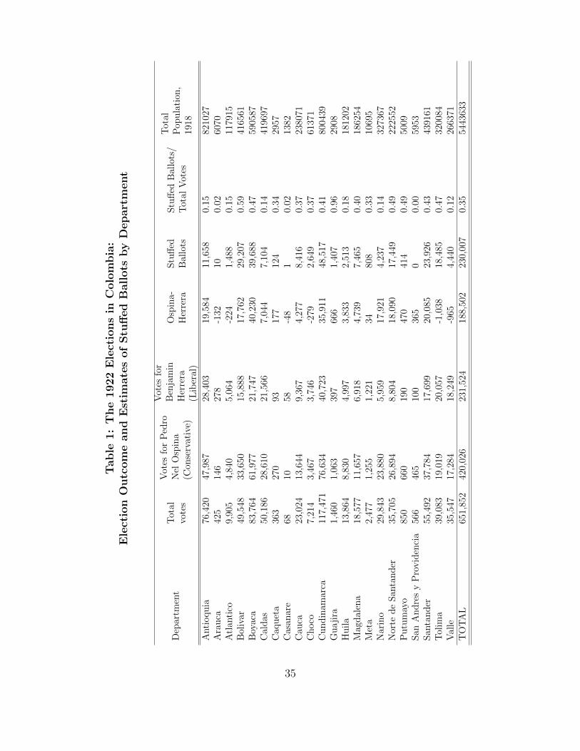
Tab

le1:

The

1922

Ele

ctio

ns

inC

olo

mbia

:E

lect

ion

Outc

om

eand

Est

imate

sof

Stu

ffed

Ball

ots

by

Depart

ment

Dep

artm

ent

Tot

alvo

tes

Vot

esfo

rP

edro

Nel

Osp

ina

(Con

serv

ativ

e)

Vot

esfo

rB

enja

min

Her

rera

(Lib

eral

)

Osp

ina-

Her

rera

Stu

ffed

Bal

lots

Stu

ffed

Bal

lots

/T

otal

Vot

es

Tot

alP

opu

lati

on,

1918

Anti

oqu

ia76

,420

47,9

8728

,403

19,5

8411

,658

0.15

8210

27A

rau

ca42

514

627

8-1

3210

0.02

6070

Atl

anti

co9,

905

4,84

05,

064

-224

1,48

80.

1511

7915

Bol

ivar

49,5

4833

,650

15,8

8817

,762

29,2

070.

5941

6561

Boy

aca

83,7

6461

,977

21,7

4740

,230

39,6

880.

4759

0587

Cal

das

50,1

8628

,610

21,5

667,

044

7,10

40.

1441

9697

Caq

uet

a36

327

093

177

124

0.34

2957

Cas

anar

e68

1058

-48

10.

0213

82C

auca

23,0

2413

,644

9,36

74,

277

8,41

60.

3723

8071

Ch

oco

7,21

43,

467

3,74

6-2

792,

649

0.37

6137

1C

un

din

amar

ca11

7,47

176

,634

40,7

2335

,911

48,5

170.

4180

0439

Gu

aji

ra1,

460

1,06

339

766

61,

407

0.96

2908

Hu

ila

13,8

648,

830

4,99

73,

833

2,51

30.

1818

1202

Mag

dal

ena

18,5

7711

,657

6,91

84,

739

7,46

50.

4018

6254

Met

a2,

477

1,25

51,

221

3480

80.

3310

695

Nar

ino

29,8

4323

,880

5,95

917

,921

4,23

70.

1432

7367

Nor

ted

eS

anta

nd

er35

,705

26,8

948,

804

18,0

9017

,449

0.49

2225

52P

utu

may

o85

066

019

047

041

40.

4950

09S

anA

nd

res

yP

rovid

enci

a56

646

510

036

50

0.00

5953

San

tan

der

55,4

9237

,784

17,6

9920

,085

23,9

260.

4343

9161

Tol

ima

39,0

8319

,019

20,0

57-1

,038

18,4

850.

4732

0084

Val

le35

,547

17,2

8418

,249

-965

4,44

00.

1226

6371

TO

TA

L65

1,85

242

0,02

623

1,52

418

8,50

223

0,00

70.

3554

4363

3

35

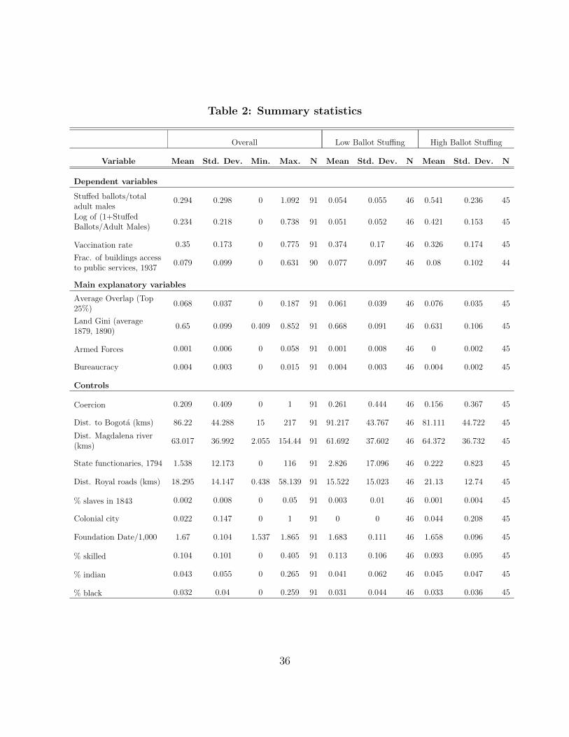
Table 2: Summary statistics

Overall Low Ballot Stuffing High Ballot Stuffing

Variable Mean Std. Dev. Min. Max. N Mean Std. Dev. N Mean Std. Dev. N

Dependent variables

Stuffed ballots/totaladult males

0.294 0.298 0 1.092 91 0.054 0.055 46 0.541 0.236 45

Log of (1+StuffedBallots/Adult Males)

0.234 0.218 0 0.738 91 0.051 0.052 46 0.421 0.153 45

Vaccination rate 0.35 0.173 0 0.775 91 0.374 0.17 46 0.326 0.174 45

Frac. of buildings accessto public services, 1937

0.079 0.099 0 0.631 90 0.077 0.097 46 0.08 0.102 44

Main explanatory variables

Average Overlap (Top25%)

0.068 0.037 0 0.187 91 0.061 0.039 46 0.076 0.035 45

Land Gini (average1879, 1890)

0.65 0.099 0.409 0.852 91 0.668 0.091 46 0.631 0.106 45

Armed Forces 0.001 0.006 0 0.058 91 0.001 0.008 46 0 0.002 45

Bureaucracy 0.004 0.003 0 0.015 91 0.004 0.003 46 0.004 0.002 45

Controls

Coercion 0.209 0.409 0 1 91 0.261 0.444 46 0.156 0.367 45

Dist. to Bogota (kms) 86.22 44.288 15 217 91 91.217 43.767 46 81.111 44.722 45

Dist. Magdalena river(kms)

63.017 36.992 2.055 154.44 91 61.692 37.602 46 64.372 36.732 45

State functionaries, 1794 1.538 12.173 0 116 91 2.826 17.096 46 0.222 0.823 45

Dist. Royal roads (kms) 18.295 14.147 0.438 58.139 91 15.522 15.023 46 21.13 12.74 45

% slaves in 1843 0.002 0.008 0 0.05 91 0.003 0.01 46 0.001 0.004 45

Colonial city 0.022 0.147 0 1 91 0 0 46 0.044 0.208 45

Foundation Date/1,000 1.67 0.104 1.537 1.865 91 1.683 0.111 46 1.658 0.096 45

% skilled 0.104 0.101 0 0.405 91 0.113 0.106 46 0.093 0.095 45

% indian 0.043 0.055 0 0.265 91 0.041 0.062 46 0.045 0.047 45

% black 0.032 0.04 0 0.259 91 0.031 0.044 46 0.033 0.036 45

36

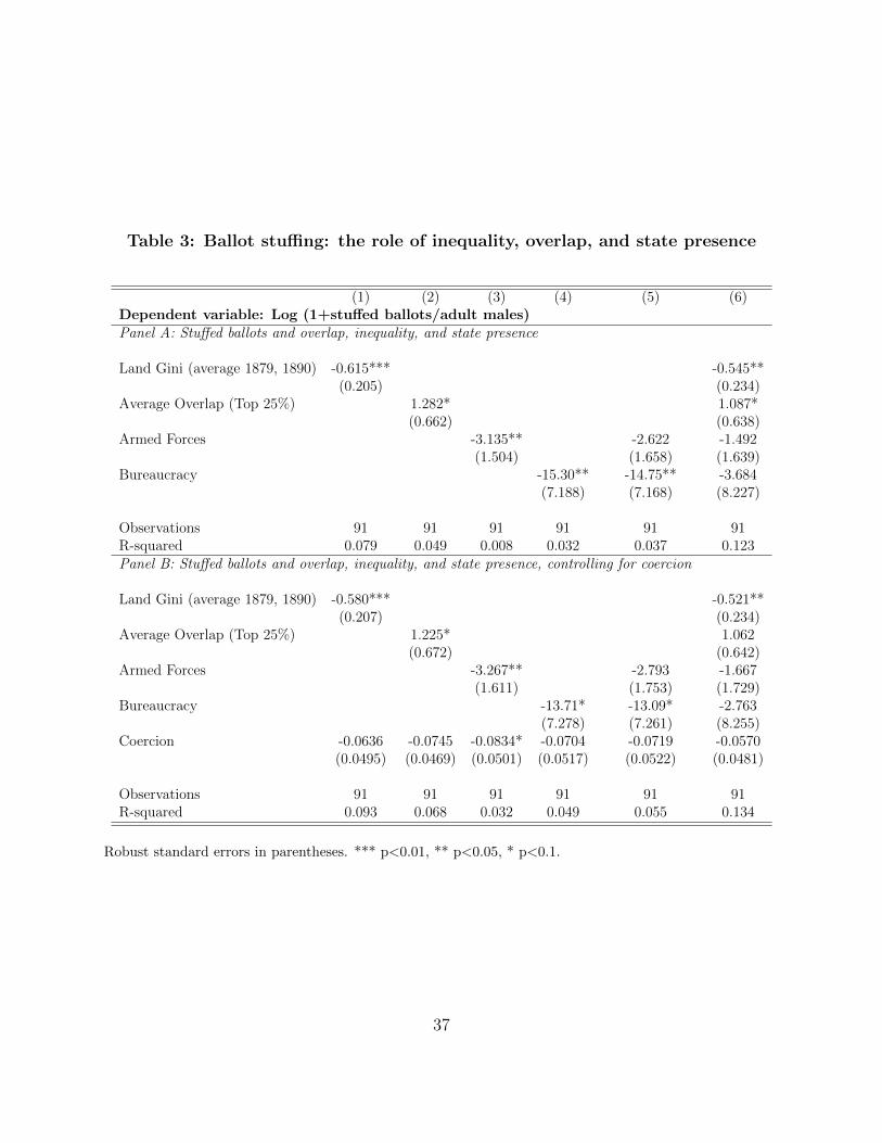
Table 3: Ballot stuffing: the role of inequality, overlap, and state presence

(1) (2) (3) (4) (5) (6)Dependent variable: Log (1+stuffed ballots/adult males)Panel A: Stuffed ballots and overlap, inequality, and state presence

Land Gini (average 1879, 1890) -0.615*** -0.545**(0.205) (0.234)

Average Overlap (Top 25%) 1.282* 1.087*(0.662) (0.638)

Armed Forces -3.135** -2.622 -1.492(1.504) (1.658) (1.639)

Bureaucracy -15.30** -14.75** -3.684(7.188) (7.168) (8.227)

Observations 91 91 91 91 91 91R-squared 0.079 0.049 0.008 0.032 0.037 0.123Panel B: Stuffed ballots and overlap, inequality, and state presence, controlling for coercion

Land Gini (average 1879, 1890) -0.580*** -0.521**(0.207) (0.234)

Average Overlap (Top 25%) 1.225* 1.062(0.672) (0.642)

Armed Forces -3.267** -2.793 -1.667(1.611) (1.753) (1.729)

Bureaucracy -13.71* -13.09* -2.763(7.278) (7.261) (8.255)

Coercion -0.0636 -0.0745 -0.0834* -0.0704 -0.0719 -0.0570(0.0495) (0.0469) (0.0501) (0.0517) (0.0522) (0.0481)

Observations 91 91 91 91 91 91R-squared 0.093 0.068 0.032 0.049 0.055 0.134

Robust standard errors in parentheses. *** p<0.01, ** p<0.05, * p<0.1.

37

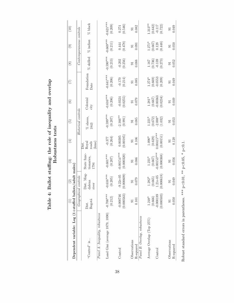
Tab

le4:

Ball

ot

stuffi

ng:

the

role

of

inequali

tyand

overl

ap

Robust

ness

test

s

(1)

(2)

(3)

(4)

(5)

(6)

(7)

(8)

(9)

(10)

Dep

endent

vari

ab

le:

Log

(1+

stuff

ed

ball

ots

/adu

ltm

ale

s)

Geo

grap

hica

lco

ntr

ols

His

tori

cal

con

trol

sC

onte

mpo

ran

eou

sco

ntr

ols

“Con

trol

”is

...

Dis

t.B

ogot

a

Dis

t.M

ag-

dal

ena

rive

r

Sta

tefu

nc-

tion

arie

s,17

94

Dis

t.R

oyal

road

s(k

ms)

%sl

aves

,18

43

Col

onia

lci

tyF

oundat

ion

Dat

e%

skille

d%

india

n%

bla

ck

Pan

elA

:In

equ

alit

y,ro

bust

nes

s

Lan

dG

ini

(ave

rage

1879

,18

90)

-0.7

00**

*-0

.616

***

-0.6

01**

*-0

.377

-0.5

99**

*-0

.616

***

-0.6

41**

*-0

.590

***

-0.6

69**

*-0

.621

***

(0.2

12)

(0.2

05)

(0.2

07)

(0.2

64)

(0.2

07)

(0.2

06)

(0.2

06)

(0.2

13)

(0.2

11)

(0.2

09)

Con

trol

-0.0

0074

6-9

.22e

-05

-0.0

0154

***

0.00

305

-2.1

66**

-0.0

324

-0.1

70-0

.202

0.44

40.

274

(0.0

0056

3)(0

.000

609)

(0.0

0032

0)(0

.001

85)

(0.9

91)

(0.0

255)

(0.2

14)

(0.2

56)

(0.4

78)

(0.5

46)

Obse

rvat

ions

9191

9191

9191

9191

9191

R-s

quar

ed0.

101

0.07

90.

086

0.10

60.

085

0.07

90.

085

0.08

80.

091

0.08

2P

anel

B:

Ove

rlap

,ro

bust

nes

s

Ave

rage

Ove

rlap

(Top

25%

)1.

248*

1.28

2*1.

231*

1.09

0*1.

221*

1.28

1*1.

274*

1.16

71.

271*

1.31

3**

(0.6

66)

(0.6

65)

(0.6

67)

(0.6

29)

(0.6

72)

(0.6

67)

(0.6

69)

(0.7

36)

(0.6

67)

(0.6

42)

Con

trol

-0.0

0018

91.

21e-

05-0

.001

53**

*0.

0041

5***

-2.0

08*

-0.0

0363

-0.0

553

-0.1

390.

128

-0.1

17(0

.000

503)

(0.0

0061

8)(0

.000

368)

(0.0

0151

)(1

.032

)(0

.023

4)(0

.209

)(0

.273

)(0

.448

)(0

.722

)

Obse

rvat

ions

9191

9191

9191

9191

9191

R-s

quar

ed0.

050

0.04

90.

056

0.12

00.

053

0.04

90.

049

0.05

20.

050

0.04

9

Rob

ust

stan

dar

der

rors

inp

aren

thes

es.

***

p<

0.01,

**

p<

0.0

5,

*p<

0.1

.

38

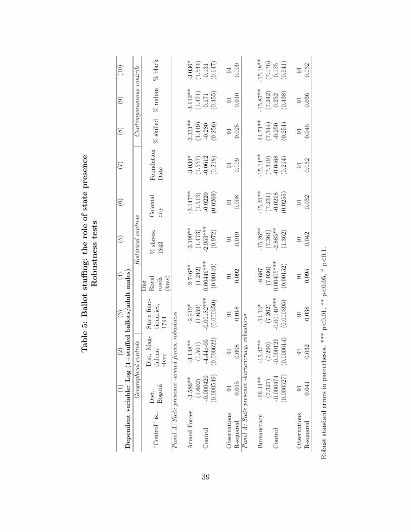
Table

5:

Ball

ot

stuffi

ng:

the

role

of

state

pre

sence

Robust

ness

test

s

(1)

(2)

(3)

(4)

(5)

(6)

(7)

(8)

(9)

(10)

Dep

endent

vari

able

:L

og

(1+

stuff

ed

ballots

/adult

male

s)

Geo

grap

hica

lco

ntr

ols

His

tori

cal

con

trol

sC

onte

mpo

ran

eou

sco

ntr

ols

“Con

trol

”is

...

Dis

t.B

ogot

a

Dis

t.M

ag-

dal

ena

rive

r

Sta

tefu

nc-

tion

arie

s,17

94

Dis

t.R

oyal

road

s(k

ms)

%sl

aves

,18

43

Col

onia

lci

tyF

oundat

ion

Dat

e%

skille

d%

india

n%

bla

ck

Pan

elA

:S

tate

pres

ence

-arm

edfo

rces

,ro

bust

nes

s

Arm

edF

orce

s-3

.586

**-3

.148

**-2

.915

*-2

.746

**-3

.199

**-3

.147

**-3

.039

*-3

.331

**-3

.112

**-3

.036

*(1

.602

)(1

.501

)(1

.659

)(1

.212

)(1

.473

)(1

.513

)(1

.537

)(1

.449

)(1

.471

)(1

.544

)C

ontr

ol-0

.000

420

-4.4

4e-0

5-0

.001

82**

*0.

0044

6***

-2.9

53**

*-0

.022

0-0

.061

2-0

.280

0.17

10.

131

(0.0

0054

9)(0

.000

622)

(0.0

0035

0)(0

.001

49)

(0.9

72)

(0.0

269)

(0.2

18)

(0.2

56)

(0.4

55)

(0.6

47)

Obse

rvat

ions

9191

9191

9191

9191

9191

R-s

quar

ed0.

015

0.00

80.

018

0.09

20.

019

0.00

80.

009

0.02

50.

010

0.00

9P

anel

A:

Sta

tepr

esen

ce-b

ure

aucr

acy,

robu

stn

ess

Bure

aucr

acy

-16.

44**

-15.

47**

-14.

13*

-8.6

87-1

5.26

**-1

5.31

**-1

5.14

**-1

4.71

**-1

5.87

**-1

5.18

**(7

.327

)(7

.290

)(7

.262

)(7

.036

)(7

.361

)(7

.231

)(7

.319

)(7

.344

)(7

.242

)(7

.176

)C

ontr

ol-0

.000

474

-0.0

0012

1-0

.001

40**

*0.

0040

5***

-2.8

85**

-0.0

218

-0.0

468

-0.2

500.

252

0.13

5(0

.000

527)

(0.0

0061

4)(0

.000

395)

(0.0

0152

)(1

.362

)(0

.025

5)(0

.214

)(0

.251

)(0

.438

)(0

.641

)

Obse

rvat

ions

9191

9191

9191

9191

9191

R-s

quar

ed0.

041

0.03

20.

038

0.09

50.

042

0.03

20.

032

0.04

50.

036

0.03

2

Rob

ust

stan

dar

der

rors

inp

aren

thes

es.

***

p<

0.01,

**

p<

0.0

5,

*p<

0.1

.

39

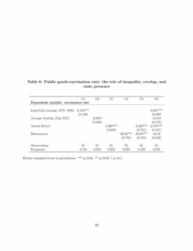
Table 6: Public goods-vaccination rate: the role of inequality, overlap, andstate presence

(1) (2) (3) (4) (5) (6)Dependent variable: vaccination rate

Land Gini (average 1879, 1890) 0.743*** 0.627***(0.169) (0.169)

Average Overlap (Top 25%) -0.858* -0.513(0.488) (0.478)

Armed Forces 4.260*** 3.562*** 2.574***(0.629) (0.551) (0.551)

Bureaucracy 20.82*** 20.08*** 10.19(6.758) (6.739) (6.826)

Observations 91 91 91 91 91 91R-squared 0.183 0.034 0.023 0.093 0.109 0.235

Robust standard errors in parentheses. *** p<0.01, ** p<0.05, * p<0.1.

40

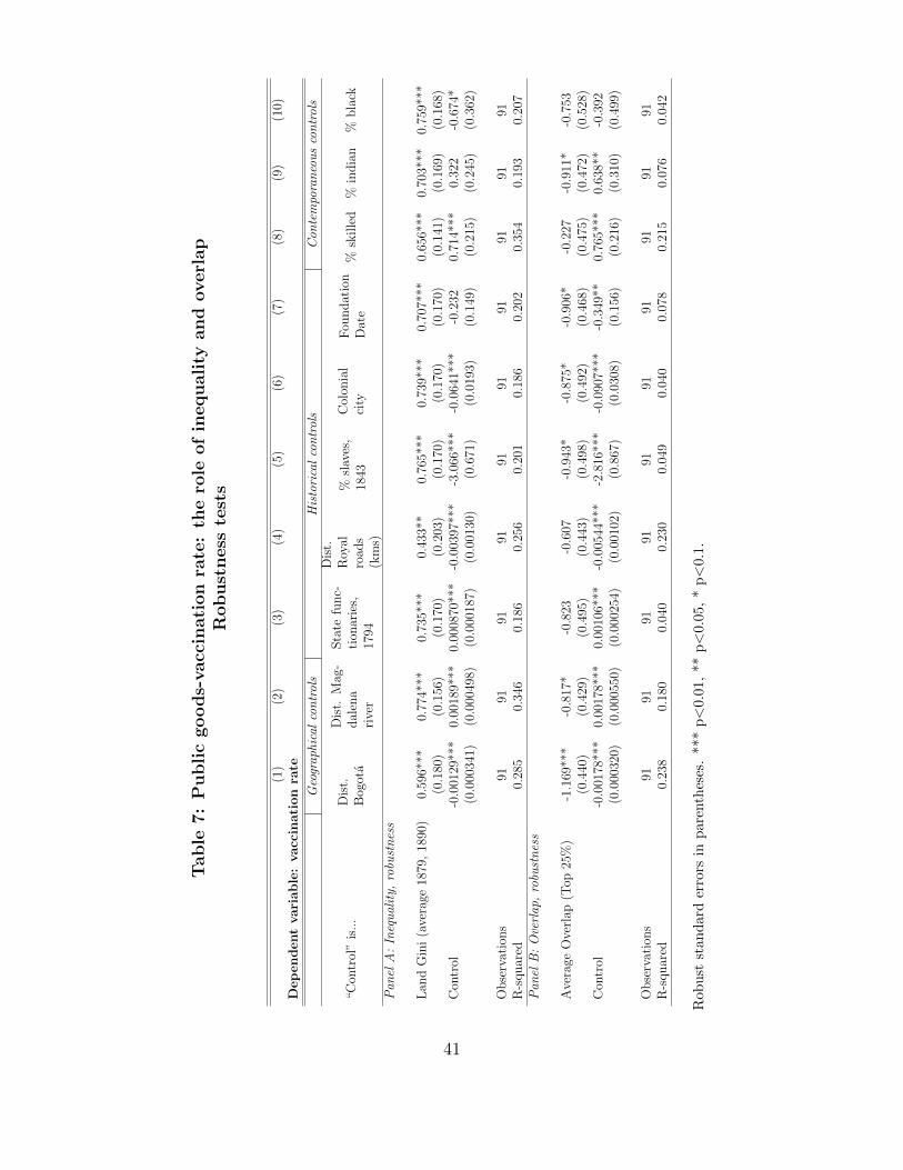
Tab

le7:

Pu

blic

goods-

vacc

inati

on

rate

:th

ero

leof

inequali

tyand

overl

ap

Robust

ness

test

s

(1)

(2)

(3)

(4)

(5)

(6)

(7)

(8)

(9)

(10)

Dep

endent

vari

ab

le:

vacc

inati

on

rate

Geo

grap

hica

lco

ntr

ols

His

tori

cal

con

trol

sC

onte

mpo

ran

eou

sco

ntr

ols

“Con

trol

”is

...

Dis

t.B

ogot

a

Dis

t.M

ag-

dal

ena

rive

r

Sta

tefu

nc-

tion

arie

s,17

94

Dis

t.R

oyal

road

s(k

ms)

%sl

aves

,18

43

Col

onia

lci

tyF

oundat

ion

Dat

e%

skille

d%

india

n%

bla

ck

Pan

elA

:In

equ

alit

y,ro

bust

nes

s

Lan

dG

ini

(ave

rage

1879

,18

90)

0.59

6***

0.77

4***

0.73

5***

0.43

3**

0.76

5***

0.73

9***

0.70

7***

0.65

6***

0.70

3***

0.75

9***

(0.1

80)

(0.1

56)

(0.1

70)

(0.2

03)

(0.1

70)

(0.1

70)

(0.1

70)

(0.1

41)

(0.1

69)

(0.1

68)

Con

trol

-0.0

0129

***

0.00

189*

**0.

0008

70**

*-0

.003

97**

*-3

.066

***

-0.0

641*

**-0

.232

0.71

4***

0.32

2-0

.674

*(0

.000

341)

(0.0

0049

8)(0

.000

187)

(0.0

0130

)(0

.671

)(0

.019

3)(0

.149

)(0

.215

)(0

.245

)(0

.362

)

Obse

rvat

ions

9191

9191

9191

9191

9191

R-s

quar

ed0.

285

0.34

60.

186

0.25

60.

201

0.18

60.

202

0.35

40.

193

0.20

7P

anel

B:

Ove

rlap

,ro

bust

nes

s

Ave

rage

Ove

rlap

(Top

25%

)-1

.169

***

-0.8

17*

-0.8

23-0

.607

-0.9

43*

-0.8

75*

-0.9

06*

-0.2

27-0

.911

*-0

.753

(0.4

40)

(0.4

29)

(0.4

95)

(0.4

43)

(0.4

98)

(0.4

92)

(0.4

68)

(0.4

75)

(0.4

72)

(0.5

28)

Con

trol

-0.0

0178

***

0.00

178*

**0.

0010

6***

-0.0

0544

***

-2.8

16**

*-0

.090

7***

-0.3

49**

0.76

5***

0.63

8**

-0.3

92(0

.000

320)

(0.0

0055

0)(0

.000

254)

(0.0

0102

)(0

.867

)(0

.030

8)(0

.156

)(0

.216

)(0

.310

)(0

.499

)

Obse

rvat

ions

9191

9191

9191

9191

9191

R-s

quar

ed0.

238

0.18

00.

040

0.23

00.

049

0.04

00.

078

0.21

50.

076

0.04

2

Rob

ust

stan

dar

der

rors

inp

aren

thes

es.

***

p<

0.01,

**

p<

0.0

5,

*p<

0.1

.

41

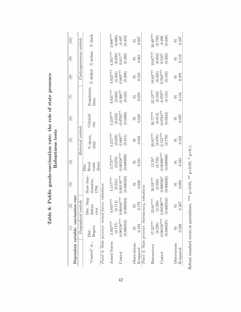
Tab

le8:

Pu

blic

goods-

vacc

inati

on

rate

:th

ero

leof

state

pre

sence

Robust

ness

test

s

(1)

(2)

(3)

(4)

(5)

(6)

(7)

(8)

(9)

(10)

Dep

endent

vari

able

:vacc

inati

on

rate

Geo

grap

hica

lco

ntr

ols

His

tori

cal

con

trol

sC

onte

mpo

ran

eou

sco

ntr

ols

“Con

trol

”is

...

Dis

t.B

ogot

a

Dis

t.M

ag-

dal

ena

rive

r

Sta

tefu

nc-

tion

arie

s,17

94

Dis

t.R

oyal

road

s(k

ms)

%sl

aves

,18

43

Col

onia

lci

tyF

oundat

ion

Dat

e%

skille

d%

india

n%

bla

ck

Pan

elA

:S

tate

pres

ence

-arm

edfo

rces

,ro

bust

nes

s

Arm

edF

orce

s2.

563*

**4.

810*

**4.

117*

**3.

774*

**4.

215*

**4.

219*

**4.

821*

**4.

823*

**4.

341*

**3.

888*

**(0

.717

)(0

.714

)(0

.531

)(0

.678

)(0

.628

)(0

.634

)(0

.694

)(0

.564

)(0

.650

)(0

.696

)C

ontr

ol-0

.001

58**

*0.

0018

4***

0.00

119*

**-0

.005

58**

*-2

.060

**-0

.076

2**

-0.3

60**

0.80

3***

0.61

1**

-0.4

97(0

.000

352)

(0.0

0056

4)(0

.000

220)

(0.0

0099

9)(0

.911

)(0

.036

9)(0

.162

)(0

.200

)(0

.286

)(0

.453

)

Obse

rvat

ions

9191

9191

9191

9191

9191

R-s

quar

ed0.

184

0.17

80.

030

0.23

10.

032

0.02

80.

070

0.24

30.

061

0.03

7P

anel

A:

Sta

tepr

esen

ce-b

ure

aucr

acy,

robu

stn

ess

Bure

aucr

acy

17.2

2***

23.6

1***

20.3

3***

12.7

0*20

.85*

**20

.77*

**22

.13*

**19

.03*

**19

.67*

**20

.40*

**(6

.228

)(5

.326

)(6

.928

)(6

.758

)(6

.676

)(6

.814

)(6

.542

)(6

.345

)(6

.652

)(6

.798

)C

ontr

ol-0

.001

50**

*0.

0019

6***

0.00

0586

*-0

.004

98**

*-2

.152

***

-0.0

764*

*-0

.379

**0.

763*

**0.

510*

-0.4

98(0

.000

337)

(0.0

0051

6)(0

.000

296)

(0.0

0098

6)(0

.770

)(0

.033

4)(0

.153

)(0

.183

)(0

.293

)(0

.440

)

Obse

rvat

ions

9191

9191

9191

9191

9191

R-s

quar

ed0.

238

0.26

70.

095

0.24

50.

102

0.09

70.

144

0.29

10.

119

0.10

7

Rob

ust

stan

dar

der

rors

inp

aren

thes

es.

***

p<

0.01,

**

p<

0.0

5,

*p<

0.1

.

42

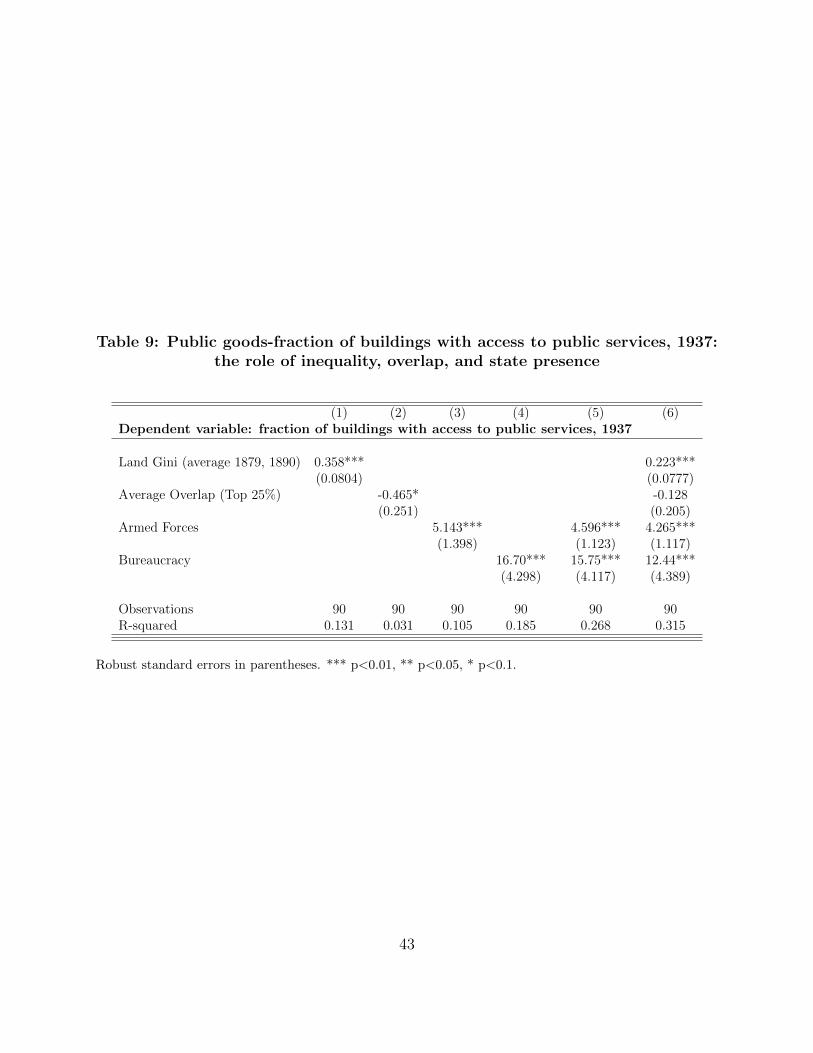
Table 9: Public goods-fraction of buildings with access to public services, 1937:the role of inequality, overlap, and state presence

(1) (2) (3) (4) (5) (6)Dependent variable: fraction of buildings with access to public services, 1937

Land Gini (average 1879, 1890) 0.358*** 0.223***(0.0804) (0.0777)

Average Overlap (Top 25%) -0.465* -0.128(0.251) (0.205)

Armed Forces 5.143*** 4.596*** 4.265***(1.398) (1.123) (1.117)

Bureaucracy 16.70*** 15.75*** 12.44***(4.298) (4.117) (4.389)

Observations 90 90 90 90 90 90R-squared 0.131 0.031 0.105 0.185 0.268 0.315

Robust standard errors in parentheses. *** p<0.01, ** p<0.05, * p<0.1.

43

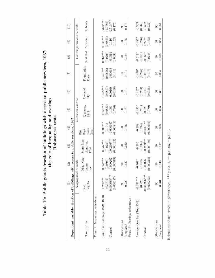
Table

10:

Pu

blic

goods-

fract

ion

of

buil

din

gs

wit

hacc

ess

topubli

cse

rvic

es,

1937:

the

role

of

inequali

tyand

overl

ap

Robust

ness

test

s

(1)

(2)

(3)

(4)

(5)

(6)

(7)

(8)

(9)

(10)

Dep

endent

vari

ab

le:

fract

ion

of

bu

ildin

gs

wit

hacc

ess

topu

bli

cse

rvic

es,

1937

Geo

grap

hica

lco

ntr

ols

His

tori

cal

con

trol

sC

onte

mpo

ran

eou

sco

ntr

ols

“Con

trol

”is

...

Dis

t.B

ogot

a

Dis

t.M

ag-

dal

ena

rive

r

Sta

tefu

nc-

tion

arie

s,17

94

Dis

t.R

oyal

road

s(k

ms)

%sl

aves

,18

43

Col

onia

lci

tyF

oundat

ion

Dat

e%

skille

d%

india

n%

bla

ck

Pan

elA

:In

equ

alit

y,ro

bust

nes

s

Lan

dG

ini

(ave

rage

1879

,18

90)

0.28

0***

0.35

4***

0.33

7***

0.30

4***

0.36

5***

0.35

8***

0.35

7***

0.36

4***

0.34

4***

0.37

0***

(0.0

735)

(0.0

806)

(0.0

789)

(0.1

04)

(0.0

830)

(0.0

807)

(0.0

876)

(0.0

796)

(0.0

865)

(0.0

789)

Con

trol

-0.0

0068

5***

-0.0

0020

70.

0023

0***

-0.0

0069

7-1

.006

0.00

168

-0.0

0668

-0.0

514

0.11

6-0

.519

***

(0.0

0018

7)(0

.000

319)

(0.0

0013

2)(0

.000

845)

(0.7

26)

(0.0

266)

(0.1

41)

(0.0

696)

(0.1

52)

(0.1

75)

Obse

rvat

ions

9090

9090

9090

9090

9090

R-s

quar

ed0.

220

0.13

70.

212

0.13

80.

137

0.13

10.

131

0.13

40.

135

0.17

6P

anel

B:

Ove

rlap

,ro

bust

nes

s

Ave

rage

Ove

rlap

(Top

25%

)-0

.631

***

-0.4

67*

-0.3

85-0

.388

-0.4

93*

-0.4

67*

-0.4

76*

-0.5

17*

-0.4

87*

-0.3

63(0

.225

)(0

.253

)(0

.244

)(0

.244

)(0

.261

)(0

.254

)(0

.246

)(0

.261

)(0

.246

)(0

.268

)C

ontr

ol-0

.000

926*

**-0

.000

260

0.00

239*

**-0

.001

75**

-0.9

20-0

.011

8-0

.067

3-0

.066

70.

272*

-0.3

82(0

.000

202)

(0.0

0031

8)(0

.000

160)

(0.0

0066

9)(0

.789

)(0

.035

5)(0

.137

)(0

.074

6)(0

.155

)(0

.237

)

Obse

rvat

ions

9090

9090

9090

9090

9090

R-s

quar

ed0.

201

0.04

00.

117

0.09

30.

036

0.03

10.

036

0.03

50.

054

0.05

4

Rob

ust

stan

dar

der

rors

inp

aren

thes

es.

***

p<

0.01,

**

p<

0.0

5,

*p<

0.1

.

44

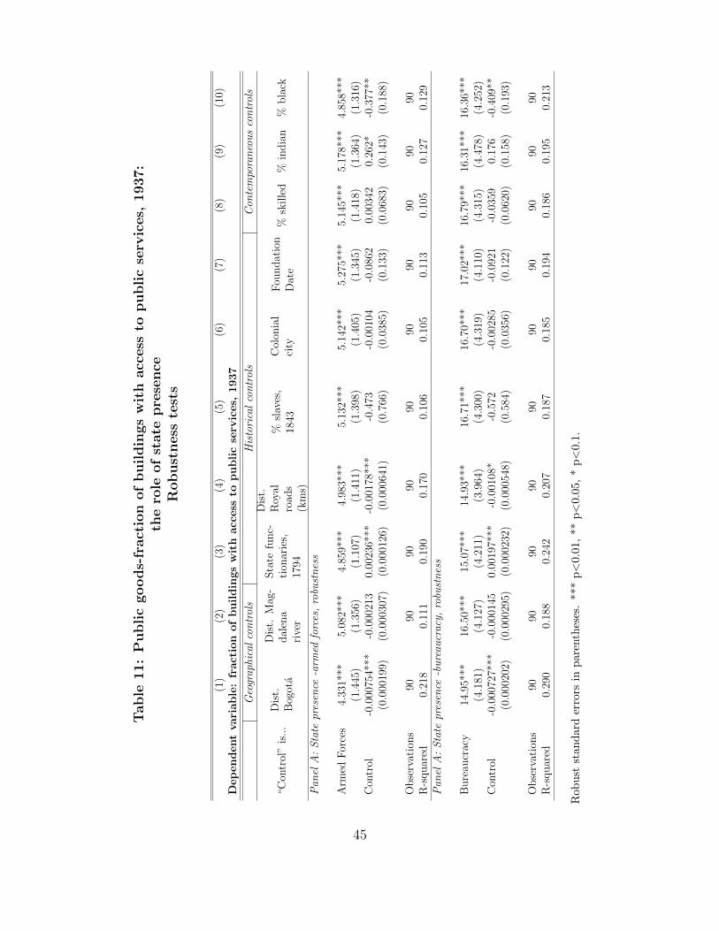
Table

11:

Pu

blic

goods-

fract

ion

of

buil

din

gs

wit

hacc

ess

topubli

cse

rvic

es,

1937:

the

role

of

state

pre

sence

Robust

ness

test

s

(1)

(2)

(3)

(4)

(5)

(6)

(7)

(8)

(9)

(10)

Dep

endent

vari

able

:fr

act

ion

of

buildin

gs

wit

hacc

ess

topublic

serv

ices,

1937

Geo

grap

hica

lco

ntr

ols

His

tori

cal

con

trol

sC

onte

mpo

ran

eou

sco

ntr

ols

“Con

trol

”is

...

Dis

t.B

ogot

a

Dis

t.M

ag-

dal

ena

rive

r

Sta

tefu

nc-

tion

arie

s,17

94

Dis

t.R

oyal

road

s(k

ms)

%sl

aves

,18

43

Col

onia

lci

tyF

oundat

ion

Dat

e%

skille

d%

india

n%

bla

ck

Pan

elA

:S

tate

pres

ence

-arm

edfo

rces

,ro

bust

nes

s

Arm

edF

orce

s4.

331*

**5.

082*

**4.

859*

**4.

983*

**5.

132*

**5.

142*

**5.

275*

**5.

145*

**5.

178*

**4.

858*

**(1

.445

)(1

.356

)(1

.107

)(1

.411

)(1

.398

)(1

.405

)(1

.345

)(1

.418

)(1

.364

)(1

.316

)C

ontr

ol-0

.000

754*

**-0

.000

213

0.00

236*

**-0

.001

78**

*-0

.473

-0.0

0104

-0.0

862

0.00

342

0.26

2*-0

.377

**(0

.000

199)

(0.0

0030

7)(0

.000

126)

(0.0

0064

1)(0

.766

)(0

.038

5)(0

.133

)(0

.068

3)(0

.143

)(0

.188

)

Obse

rvat

ions

9090

9090

9090

9090

9090

R-s

quar

ed0.

218

0.11

10.

190

0.17

00.

106

0.10

50.

113

0.10

50.

127

0.12

9P

anel

A:

Sta

tepr

esen

ce-b

ure

aucr

acy,

robu

stn

ess

Bure

aucr

acy

14.9

5***

16.5

0***

15.0

7***

14.9

3***

16.7

1***

16.7

0***

17.0

2***

16.7

9***

16.3

1***

16.3

6***

(4.1

81)

(4.1

27)

(4.2

11)

(3.9

64)

(4.3

00)

(4.3

19)

(4.1

10)

(4.3

15)

(4.4

78)

(4.2

52)

Con

trol

-0.0

0072

7***

-0.0

0014

50.

0019

7***

-0.0

0108

*-0

.572

-0.0

0285

-0.0

921

-0.0

359

0.17

6-0

.409

**(0

.000

202)

(0.0

0029

5)(0

.000

232)

(0.0

0054

8)(0

.584

)(0

.035

6)(0

.122

)(0

.062

0)(0

.158

)(0

.193

)

Obse

rvat

ions

9090

9090

9090

9090

9090

R-s

quar

ed0.

290

0.18

80.

242

0.20

70.

187

0.18

50.

194

0.18

60.

195

0.21

3

Rob

ust

stan

dar

der

rors

inp

aren

thes

es.

***

p<

0.01,

**

p<

0.0

5,

*p<

0.1

.

45

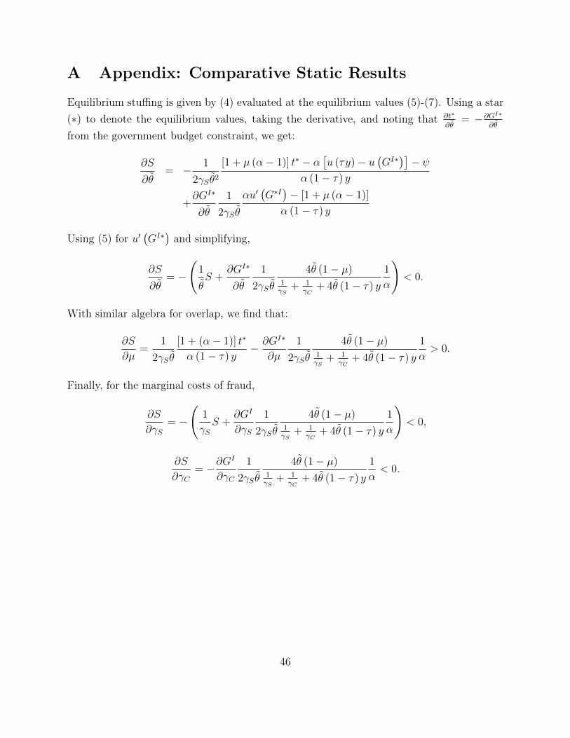
A Appendix: Comparative Static Results

Equilibrium stuffing is given by (4) evaluated at the equilibrium values (5)-(7). Using a star

(∗) to denote the equilibrium values, taking the derivative, and noting that ∂t∗

∂θ= −∂GI∗

∂θ

from the government budget constraint, we get:

∂S

∂θ= − 1

2γS θ2

[1 + µ (α− 1)] t∗ − α[u (τy)− u

(GI∗)]− ψ

α (1− τ) y

+∂GI∗

∂θ

1

2γS θ

αu′(G∗I)− [1 + µ (α− 1)]

α (1− τ) y

Using (5) for u′(GI∗) and simplifying,

∂S

∂θ= −

(1

θS +

∂GI∗

∂θ

1

2γS θ

4θ (1− µ)1γS

+ 1γC

+ 4θ (1− τ) y

1

α

)< 0.

With similar algebra for overlap, we find that:

∂S

∂µ=

1

2γS θ

[1 + (α− 1)] t∗

α (1− τ) y− ∂GI∗

∂µ

1

2γS θ

4θ (1− µ)1γS

+ 1γC

+ 4θ (1− τ) y

1

α> 0.

Finally, for the marginal costs of fraud,

∂S

∂γS= −

(1

γSS +

∂GI

∂γS

1

2γS θ

4θ (1− µ)1γS

+ 1γC

+ 4θ (1− τ) y

1

α

)< 0,

∂S

∂γC= −∂G

I

∂γC

1

2γS θ

4θ (1− µ)1γS

+ 1γC

+ 4θ (1− τ) y

1

α< 0.

46