NBER WORKING PAPER SERIES

INDIVIDUAL RISK AND INTERGENERATIONALRISK SHARING IN AN INVESTMENT-BASED SOCIAL SECURITY SYSTEM

Martin FeldsteinElena Ranguelova

Working Paper 6839http://www.nber.org/papers/w6839

NATIONAL BUREAU OF ECONOMIC RESEARCH1050 Massachusetts Avenue

Cambridge, MA 02138December 1998

The views expressed here are those of the author and do not reflect those of the National Bureau ofEconomic Research.

© 1998 by Martin Feldstein and Elena Ranguelova. All rights reserved. Short sections of text, notto exceed two paragraphs, may be quoted without explicit permission provided that full credit,including © notice, is given to the source.

May 1998

Individual Risk and Intergenerational Risk Sharing in an Investment-Based Social Security System

Martin Feldstein and Elena Ranguelova

ABSTRACT

This paper examines the risk aspects of a fully phased-in investment-based defined contributionSocial Security plan. Individuals save a fraction of wages in a Personal Retirement Account (PRA)invested in a 60:40 equity-debt mix and receive a similarly invested variable annuity from age 67. Thevalue of the portfolio follows a random walk with historic (1946-1995) mean log real return of 5.5percent and standard deviation of 12.5 percent. We study 10,000 stochastic distributions of this processfor the 80 year experience from 1998 to 2077.

With a nonstochastic 5.5 percent rate of return, individuals could purchase the future benefitspromised in the current Social Security law ( the “benchmark” level of benefits) by saving 3.1 percent ofearnings, just one-sixth of the payroll tax that Social Security actuaries project will be needed in thepaygo system. A higher saving rate provides a “cushion” that reduces the risk of unacceptably lowbenefits. For example, saving 6 percent implies a median annuity at age 67 of 2.1 times the benchmarkbenefits and only a 17 percent chance that the annuity is less than the benchmark. In 95 percent of thepotential investment experience the annuity exceeds 61 percent of the benchmark benefit. With a 9percent saving rate (half of the tax rate required in a pay-as-you-go system), there is only a 6 percentchance that the annuity is less than the benchmark and in 95 percent of the potential investmentexperience the annuity exceeds 92 percent of the benchmark benefit.

We also study a modified plan in which retirees face no risk of receiving less than the benchmarkbenefit because the government provides a conditional pension transfer to any retiree whose annuity isless in any year than the benchmark level of benefits. With a six percent saving rate, a conditionaltransfer is required in only about 40 percent of the simulations. The expected value of the transfers issubstantially less than the expected incremental corporate tax revenue that results from the PersonalRetirement Account saving. Additional tax revenue is needed in fewer than one percent of thesimulations.

In short, a pure defined contribution plan, with a saving rate equal to one third of the long-runprojected payroll tax, invested in a 60:40 equity-debt Personal Retirement Account could provide aretirement annuity that is likely to be substantially more than the benchmark benefit while exposing theretiree to relatively little risk that the annuity will be less than the benchmark. Even this risk can becompletely eliminated by a conditional guarantee plan that imposes only a very small risk on futuretaxpayers.

Martin Feldstein (feldstein@nber.org)Elena Ranguelova (elena@nber.org)National Bureau of Economic Research1050 Massachusetts AvenueCambridge, MA 02138

*Martin Feldstein is Professor of Economics, Harvard University, and President of theNational Bureau of Economic Research. Elena Ranguelova is a doctoral candidate HarvardUniversity and a Research Assistant at the NBER. We are grateful for discussions about thissubject with Andrew Abel, John Biggs, John Campbell, Jeff Liebman, Gilbert Metcalf, JamesPoterba, Antonio Rangel, Andrew Samwick, Kent Smetters, and Larry Summers and forcomments from participants in the 1998 NBER Summer Institute meeting on Social Securityreform. The current paper updates the earlier version to the actuarial assumptions in the 1998Trustees Report and recognizes the shift in normal retirement age for Social Security

1A “defined contribution” plan is one in which individuals contribute a fixed portion ofwage income each year and receive benefits based on the accumulated value in those accounts.The existing Social Security system is a “defined benefit” plan in which individuals’ retirementbenefits are based on a formula relating to years of service and past earnings but not to anaccumulated total of past contributions. A defined contribution plan is “investment-based” if thefunds are actually invested in a portfolio of stocks and bonds. Some countries maintain“notional” defined contribution systems in which retirement benefits depend on pastcontributions but in which contributions receive an accounting or notional rate of return becausethe funds are not actually invested.

2In the United States, the use of such defined contribution accounts has been proposed bymembers of the 1997 Social Security Advisory Council, by the more recent NationalCommission on Retirement Policy, and by a number of prominent legislators in both parties. Several countries have already adopted such systems.

1May 1998

Individual Risk and Intergenerational Risk Sharing in an Investment-Based Social Security System

Martin Feldstein and Elena Ranguelova*

The rapid aging of the population creates substantial financing problems for existing pay-

as-you-go Social Security programs. Governments around the world are therefore considering

shifting completely or partially to investment-based defined contribution plans.1,2 In such plans,

employees contribute a fraction of their wages to individual accounts, invest the funds in a

3See, for example, Aaron (1998), Diamond (1997, 1998).

4There have however been a number of more general discussions about the role of risk insocial security pension systems, including Bohn (1998), Merton (1983), Shiller (1998), andSmetters (1997, 1997b).

2May 1998

combination of stocks and bonds, and use the accumulated assets to finance a retirement annuity.

Such prefunded programs offer the prospect of financing future retirement benefits with

substantially smaller sacrifices during working years than the taxes that would be required in

traditional unfunded pay-as-you-go (“paygo”) programs. They have the potential disadvantage,

however, of exposing retirees to the uncertainty associated with the variable returns on stocks

and bonds.

Some critics of the proposals to transform Social Security to a system of individually

invested accounts argue that the reduced financing burden does not justify exposing retirees to

such increased investment risk.3 They advocate retaining the existing unfunded program or

shifting to a system in which existing defined benefits are financed in part by a government trust

fund invested in stocks and bonds.

Despite the importance of this issue, there has been no analysis of the magnitude of the

risk to which retirees would be exposed in a system of individual defined contribution accounts.4

A primary purpose of this paper is to present an explicit estimate of that risk.

In earlier papers on the transition from the existing U.S. system to one that uses

individual defined contribution accounts to finance retirement income, Feldstein and Samwick

(1997, 1998a) suggested that the problem of risk might be dealt with by requiring individuals to

save more than the amount that would be needed to fund the target level of benefits at the

expected rate of return. The extra saving would provide a margin of safety to compensate for

5A conditional pension of this type is not the same as a means tested benefit. Because itrelates only to the shortfall of the defined contribution annuity, it does not penalize other savingor work after the eligible retirement age.

3May 1998

returns that are lower than the expected value. The present paper evaluates the extent to which

such incremental saving can reduce retirees’ risk of inadequate retirement income while still

permitting a lower financing cost during working years than a paygo program with the same

benefits.

The retirees’ risk that the investment-based annuities in a defined contribution system

will be less than the currently promised future Social Security benefits can be eliminated

completely if the government makes up any shortfall with a conditional pension payment funded

with general revenue.5 This shifts all of the risk of poor investment experience to future taxpayers

while leaving future retirees with the ability to benefit from better investment performance. A

third purpose of this paper is to study such a conditional pension plan. We assess the extent of

the risk that future taxpayers would bear in such a program and evaluate the extent to which the

conditional pension benefits could be funded with the additional corporate tax revenue that

would be generated by the increased investment in plant and equipment that would result from

shifting to a defined contribution program.

Section 1 of the paper discusses the basic issues in the choice between defined benefit

and defined contribution plans. The second section describes the system of personal retirement

accounts and the risk properties of stock and bond investments in such accounts with variable

annuity retirement benefits. Section 3 then presents our estimates of the risks borne by retirees in

alternative plans with different saving rates. The fourth section analyzes the conditional pension

program that shifts the risk from retirees to future taxpayers. Section 5 presents explicit expected

4May 1998

utility calculations of the alternative options. There is a brief concluding section.

The results presented in this paper use the future Social Security benefits promised in

current law (essentially a continuation of current replacement rates) as the benchmark for judging

defined contribution plans. Our analysis shows that the risk of receiving less than the

“benchmark” level of benefits in a pure defined contribution system would be relatively small at

saving rates that are substantially less than the future paygo tax rate required to fund that level of

benefits. If these risks are completely shifted to future taxpayers, their required rate of saving-

plus-taxes is also substantially lower than the tax rate required in a paygo defined benefit system.

1. Defined Contributions vs. Defined Benefits

Although the practice of unfunded paygo social security pensions can be traced back to

Bismarck in 1889, it was Samuelson (1958) who first showed the economic properties of such a

system. Samuelson showed how, without any capital investment, individuals can earn an implicit

rate of return on their social security tax payments. In steady state equilibrium, this implicit rate

of return is equal to the real rate of growth of the social security tax base, i.e., the sum of the

growth rates of the labor force and real wages.

The introduction of a new paygo pension plan provides an immediate windfall to those

who are already retired or who will soon retire because they receive benefits with little or no

previous contributions. Subsequent increases in benefit-wage ratios financed by increases in tax

rates provide similar windfalls to those who are then retired or soon to be retired. The U.S.

Social Security system began providing benefits in 1940 and has increased the relative level and

the scope of benefits a number of times. Those who have retired under the existing program have

received quite high implicit rates of return on the taxes that they and their employer paid.

6See Board of Trustees (1998). As recently as 1996, the Social Security actuariesestimated that the 18 percent rate would not be needed until after 2055.

5May 1998

When program expansions can no longer provide such windfall gains, the implicit rate of

return of a paygo program eventually decreases to the Samuelsonian rate of growth of aggregate

wages. For the United States, this has averaged 2.5 percent over the past 30 years. The rate of

return for any particular birth cohort will vary from the steady state rate in response to changes in

the ratio of retirees to workers caused by changes in labor force participation, birth rates and

death rates, and the ratio of wages to total compensation including fringe benefits. Caldwell et.

al. (1998) estimate that current Social Security rules imply that the real rate of return on Social

Security contributions will be 2.4 percent for the generation born right after World War II but

only about 1 percent for those born in the 1970s and essentially zero for those born at the end of

the 1990s.

The aging of the population that is now occurring in virtually every country implies that

maintaining the current ratio of benefits to preretirement wages will require substantial increases

in paygo tax rates. For the United States, the Social Security actuaries estimate that the current

12.4 percent tax rate will have to increase to more than 18 percent by the year 2035 to maintain

the current benefit-wage replacement rates.6

The combination of the low implied rate of return for current and future taxpayers and the

prospect of a substantial increase in future Social Security tax rates has stimulated the search for

alternatives to the current pay-as-you-go system. Several countries have already shifted

completely or partially to an investment-based (i.e., prefunded) defined contribution system

7Chile was the first of these but it has been followed by other countries including Mexico,Argentina, Australia, Great Britain and, more recently, Sweden and China. Feldstein (1998a)contains essays describing the systems in Chile, Mexico, Argentina, Australia and Great Britain.On China, see Feldstein (1998b).

8See also Feldstein (1997 and 1998d) and Feldstein and Samwick (1998b).

6May 1998

based on employer-employee contributions to Personal Retirement Accounts (PRAs).7 In such

plans, individuals invest these assets in stock and bond funds and receive annuity benefits based

on the returns earned in these accounts. In some countries, the government complements these

annuities with a supplementary defined benefit pension or a minimum unfunded pension.

In the United States, the official 1997 Social Security Advisory Council presented three

alternative plans for Social Security reform, all of which involved some substitution of

investment-based funding for the existing paygo system. More recently, the Congressionally

appointed National Commission on Retirement Policy unanimously recommended that two

percent of payroll taxes be diverted from the Social Security system to individual investment

accounts, offsetting that revenue reduction by reductions in existing paygo benefits. Several

individual members of Congress have presented plans to use the surpluses in the government

budget that are projected for the next decade to fund such accounts.8

The fundamental difference between a paygo program and an investment-based program

is that the investment-based system involves an initial reduction of national consumption and a

concurrent increase in the national capital stock. The rate of return in an investment-based plan

is therefore the marginal product of capital, a number substantially greater than the rate of growth

of aggregate wages. Poterba (1997), using recently revised national income and product account

data, estimates that the marginal product of capital in the U.S. nonfinancial corporate sector

9Poterba estimates the marginal product of capital by dividing the sum of profits, interestand capital taxes by the capital stock at replacement cost. These estimates relate to the domesticcapital stock and corresponding capital income flows. This method will overstate the national gain from incremental saving to the extent that some of the additional saving is invested abroador in owner-occupied housing. It may also understate the marginal product of capital to theextent that the additional saving is used to finance new expenditures on research anddevelopment that, because of externalities, have a higher national rate of return than investmentsin plant and equipment. For a further discussion of these issues, see Feldstein (1998c).

7May 1998

averaged 8.5 percent between 1959 and 1996.9 This relatively high rate of return on incremental

capital makes it possible to finance any level of benefits at a much lower cost in an investment-

based program than in a paygo program. Note in particular that it is the overall return on capital

relative to the growth rate of wages that matters and not the return on equity investments relative

to the return on government bonds, as some have suggested (e.g., Aiyagari, 1997).

A simplified calculation will indicate the magnitude of the effect of this difference in

rates of return on the cost of funding retirement benefits. Assume an overlapping generations

framework in which there are T years between generations. In the paygo system, individuals

receive benefits T years after they pay tax; in the investment-based system, individuals spend

their accumulated assets T years after they make the savings deposit. If the implicit rate of return

in a paygo system is denoted c = n + g where n is the growth rate of the labor force and g is the

rate of growth of average wages, the Samuelson (1958) analysis implies that each dollar of

retirement income at time T requires a tax payment of e−γ T dollars at the contribution date

during the working years. Similarly, if ρ is the marginal product of capital, each dollar of

retirement income at T requires a contribution to the personal retirement account of e−ρ T at the

contribution date. The ratio of the PRA contribution to the paygo tax payment to finance the

same benefit T years later is e (γ − ρ) Τ. With γ = 0.025, ρ = 0.085 and T = 30 years, e (γ − ρ) Τ

10There are also a number of very important practical issues about the administrativestructure and costs of individual accounts, the supervision of investment mangers, etc. that liebeyond the scope of this paper. See Shoven (1999).

8May 1998

= 0.165, i.e., each dollar of tax payment required in a paygo system can be replaced by just 16.5

cents in a funded program with an 8.5 percent rate of return. The 18 percent future payroll tax

rate projected by the Social Security Administration could in principle be replaced by a funded

program with mandatory contributions equal to 3.0 percent of earnings.

This comparison of the potential long-run gains from switching to an investment-based

system ignores three important conceptual issues: (1) financing the transition, (2) the riskiness of

defined benefit and defined contribution plans, and (3) the distributional consequences of shifting

to a defined contribution plan from a defined benefit plan.10 We now comment briefly on each of

these before turning to a full analysis of the risk issue.

The transition problem is often summarized by the statement that workers in the

transition generation must “pay double” (paying to finance the paygo benefits to existing retirees

while also contributing to the Personal Retirement Accounts that will finance their own

retirement), implying that the existing 12.4 percent payroll tax would rise to more than 24

percent. Taken literally, this is wrong for two reasons: first, the required PRA contributions are

very much less than the existing paygo tax payments; second, the future paygo tax payments

would gradually decline as new retirees begin to receive PRA annuities and therefore become

less dependent on paygo benefits. Feldstein and Samwick (1997) showed that a gradual transition

from the existing paygo program to a fully funded system could be achieved without raising the

combined total of the paygo tax and the PRA saving deposit by more than 2.0 percent of wages,

i.e., from the 12.4 percent existing payroll tax to a combined total of 14.4 percent of wages in the

11Kotlikoff (1996, 1998) examined alternative transition arrangements based on givingexisting retirees and current employees “recognition bonds” with an actuarial value of the futurepaygo benefits to which they are currently entitled and showed the consequences of financing theinterest and principal of these “recognition bonds” with different tax structures.

12This investment is equivalent to repaying the national debt implicit in the unfundedSocial Security obligations. Repaying this debt involves accumulating an equal amount ofnational capital stock.

13We ignore issues of risk here and return to them below.

9May 1998

first year of the transition and to lower combined rates in future years. Within 20 years, the

combination of the reduced paygo tax and the PRA deposits would be less than the initial 12.4

percent payroll tax. These calculations, based on the detailed demographic projections and

mortality assumptions of the Social Security Administration, assumed a marginal product of

capital of 9 percent (the historic average before the recent data revision). But even with a very

much lower 5.5 percent rate of return, the maximum combined total of paygo tax and PRA

contribution was only 15 percent and the cross-over time to a reduced total payment was 28 years

(Feldstein and Samwick, 1998a).11

The transition from the paygo system to the funded system can be seen as a process of

national investment. National consumption is reduced (and the capital stock is increased) during

the early decades of the transition (by the higher combination of the paygo tax and the PRA

deposits) in order to achieve a lower cost of funding the same benefits in the more distant

future.12 Since the retirement income is designed to stay the same in both systems, the present

value depends only on the consumption changes implied by the changes in taxes and PRA

deposits.13 There is of course no gain in present value if the discount rate used to evaluate the

variations in consumption is the marginal product of capital, i.e., if the discount rate is the same

14This appears to be the reason that Murphy and Welch (1998) and Geanakoplos , Mitchell and Zeldes (1998) find no net present value gain.

15For a more extensive discussion of these issues, see Feldstein (1964, 1996, and 1998a,pp. 13-14).

10May 1998

as the rate of return earned on this “investment.”14 But in a second best economy in which the

corporate income tax and personal income tax reduce the net rate of return to individuals, the

appropriate net-of-tax rate for discounting changes in consumption is less than the marginal

product of capital. Moreover, since the reduced consumption affects the current generation of

employees while much of the benefit accrues to the future generations, the appropriate discount

rate for aggregating the consumption changes over the multi-generation horizon is not a market

based interest rate but a rate that reflects the decline in the marginal utility of consumption as per

capita consumption grows over time. With expected growth of per capita consumption of about

one percent a year, any plausible elasticity of the social marginal utility function implies a social

discount rate for consumption that is substantially less than the 8.5 percent marginal product of

capital.15

This comparison ignores the change in risk associated with the shift from a defined

benefit paygo system to an investment-based defined contribution system. Both types of system

subject retirees to a risk that benefits will be less than their expected value when the individual

retires. For a defined benefit program, the risk is that the government will respond to fiscal

pressures by reducing benefits. This has already happened in the United States in the 1980s

when benefits were first subject to income tax and the future age of retirement was increased.

Several current legislative proposals would reduce benefits further for some or all current

16See McHale (1998) for evidence on the magnitude of the benefit reductions in theUnited States and other major industrial countries.

17The actual extent of redistribution is less than commonly believed; see Boskin, Shovenand Hurd (1987) and Liebman (1998).

11May 1998

retirees.16 The level of the retirement annuity is also uncertain in a pure investment-based

defined-contribution system because it depends on the returns earned on stocks and bonds during

the individual’s lifetime. If the government provides some form of minimum guarantee or risk

sharing, the level of paygo taxes (as well as the reliability of the government’s commitment)

becomes uncertain. For some analysts of Social Security policy, this uncertainty is the

fundamental objection to shifting to an investment-based system of individual accounts. The

present paper analyzes the magnitude of these risks to retirees and the potential cost to taxpayers

of reducing the retirees’ uncertainty by a conditional supplementary government pension.

A final issue that requires attention in a full analysis of the effects of shifting to an

investment-based system is the effect on the distribution of income among retirees and surviving

dependents. The current defined benefit system provides a higher ratio of retirement benefits to

past income for low wage workers than for those who have had higher earnings. This

redistributive effect of the defined benefit pensions, together with the Supplemental Security

Income program, is designed to protect the standard of living in old age of individuals with low

or sporadic lifetime earnings, including widows and divorced individuals.17 Some preliminary

calculations reported in Feldstein and Samwick (1997, 1998a) indicate that transfers to prevent

poverty in old age can be achieved in an investment-based system by relatively small taxes on

accumulated retirement balances. Although a much more thorough analysis of this issue is

18Kotlikoff et al (1998) have extended the Auerbach-Kotlikoff overlapping generationsmodel to examine the general equilibrium effects of Social Security reform in an economy withten income classes. See also Huggett and Ventura (1998) for a related general equilibriumanalysis. Feldstein and Liebman (1999) use detailed long-term panel data to compare theannuities paid to a variety of income and demographic groups under existing Social Securitydefined benefit rules and alternative defined contribution rules.

19We assume that the assets of individuals who die before retirement remain in theannuity pool. On the effect of various bequest rules, see Feldstein and Ranguelova (1999).

12May 1998

warranted, the subject lies beyond the scope of the current paper.18

2. An Investment-Based Defined Contribution Plan with Variable Annuity Benefits

This section describes the system of Personal Retirement Accounts in which a

representative individual accumulates assets and uses those assets to purchase a variable rate

annuity at the time of retirement.19 The representative individual enters the labor force at age 21

and retires at age 67 (if he or she is still alive). For the sake of concreteness, we use the

economic and demographic projections of the Social Security Administration (Board of Trustees,

1998) for the cohort reaching age 21 in 1998. We assume that the representative individual has

his birth cohort’s average earnings at each age and experiences the cohort’s age-specific

mortality rates.

In the defined benefit plan specified in the current Social Security law, the individual with

such average earnings experience would receive a benefit at age 67 for himself equal to 40

percent of his immediate preretirement wage. The full amount of the defined benefit in our

simulations is a multiple of this individual benefit (known as the “primary insurance amount”)

that reflects possible benefits for a spouse or other dependants as well as disability benefits.

Instead of modeling such additional benefits explicitly, we use a multiple of the individual

benefit such that the implied aggregate Social Security benefits in each year beginning in 2030 is

20This ratio is selected to correspond approximately to the debt-equity ratio of U.S.corporations so that the rate of return on capital at the corporate level can correspond to thereturn to these portfolio investments without considerations of the relative yields on debt andequity.

13May 1998

equal to the aggregate benefit projected by the Social Security Administration. The aggregate

benefits projected in this way together with the aggregate wage income projected by the Social

Security Administration (Board of Trustees, 1998) imply that the tax rate required to pay current

benefits will be 18.4 percent when the cohort that we study retires (in contrast to the current tax

rate of 12.4 percent). These assumptions about future defined benefits do not affect the projected

behavior of the defined contribution annuities but provide a benchmark for comparing the

relative costs of defined benefit and defined contribution programs.

With a defined contribution plan, the individual contributes a fixed percentage of wages

in each year to a Personal Retirement Account (PRA); we will examine the implications of

different saving rates from 4 percent to 9 percent (i.e., up to half of the long-run paygo tax rate of

18.4 percent). The individual invests these savings in a portfolio that is continually rebalanced to

maintain 60 percent equities and 40 percent debt.20 At retirement, these accumulated assets are

used to finance a variable annuity in which annual benefits vary with portfolio performance in a

way described below.

We use the S&P500 index and a Salomon Brothers corporate bond index as proxies for

the stock and bond investments. Both indices are assumed to follow a geometric random walk

with drift. This implies that the log returns for each type of asset are serially independent and

identically distributed with given mean and variance. Thus if pe (s) and pb (s) are the log levels of

the equity and bond indices at time s, we assume

21The value of the PRA portfolio is also increased by the annual savings of 2 percent ofthe individual’s wage plus the distributed share of the PRA balances of all those members of theage cohort who die during the previous year; the explicit evolution is shown below.

14May 1998

pe (s) = pe (s-1) + µe + ue (s)

and

pb (s) = pb (s-1) + µb + ub (s)

where ue ~ iid N (0, σ2e ) and u b ~ iid N (0, σ2

b ). The covariance between the stock and bond

returns is σ e b .

With a continuously compounded 60:40 equity-debt portfolio, the log level of the overall

portfolio would satisfy the following random walk if there were no additions or payments:21

p (s) = p (s-1) + µ + u (s)

with u ~ iid N (0, σ2 ). To derive the values of µ and σ2 we use the lognormal property of

the returns.

More specifically, if µ∗ i is the mean return on asset i in level form, the mean return on

the 60:40 portfolio is the weighted average µ∗ = 0.6 µe ∗ + 0.4 µb * . Because we assume the

log returns to be normally distributed, µ∗ i = µ i + .5 σ2i . This implies that

µ + 0.5 σ2 = 0.6 ( µe + 0.5 σ2e ) + 0.4 ( µb + 0.5 σ2

b )

where

σ2 = 0.36 σ2e + 0.16 σ2

b + 0.48 σ e b.

From these two equations and the measured mean and variance of the log returns on stocks and

bonds we can derive the log return on the portfolio and the variance of that return.

22 The bond rate of return is based on the Salomon Brothers AAA bond returns adjustedto a more typical corporate bond yield by adding two percentage points.

23The portfolio return is essentially unchanged if we use a longer time period from 1926to 1997.

24This estimate of the administrative cost may be compared with the cost of about 0.2percent charged now in indexed equity funds by mutual fund companies like Vanguard andFidelity. Bond funds generally have lower administrative charges.

15May 1998

The CRSP data for the postwar period from 1946 through 1995 imply that for stocks and

bonds the mean real log rates of return were 7.0 percent and 3.3 percent.22 The corresponding

standard deviations are 16.6 percent for stocks and 10.4 percent for bonds. The covariance of the

stock and bond returns is σe b = 0.0081. Taken together, these parameters imply a logarithmic

rate of return on the 60:40 portfolio of 5.9 percent with a standard deviation of 12.5 percent.23

We reduce the mean return from 5.9 percent to 5.5 percent to reflect potential

administrative costs. 24

In the analysis that follows, we recognize that the adjusted mean real log return of 5.5

percent for the portfolio during the period from 1946 through 1995 is only an estimate of the

relevant mean for future years. Our stochastic simulation therefore uses a two step procedure to

simulate the uncertain future annual returns. For each of 10,000 simulations, we begin by

generating a mean real log return on the portfolio from a normal distribution with a mean of

0.055 and a standard deviation of 0.0175 which is equal to the standard error of the estimated

mean based on the number of years in the sample. We then use this estimated realization of the

mean and the standard deviation of 0.125 to generate a 71 year sequence of portfolio returns from

the year 2000 to 2070. We repeat this 10,000 times.

Although the equation for p(s) describes the way that the logarithmic value of the PRA

25Note that E[r(s)] = 0.055 and the standard deviation of r(s) = 0.125 imply that E[1+R(s)]= E[er(s)] = eEr(s)+0.5F2 = 1.065.

16May 1998

account would evolve during the accumulation years if there were no external additions, in

practice the actual individual PRA account is also augmented by the fraction α of the

individual’s wage and by the distributed share of the PRA balances of those members of the

cohort who die during the year. We simulate this evolution at the level of the birth cohort (rather

than of the individual) by:

M(s) = [ 1 + R (s-1) ] M(s-1) + α w(s) N(s)

where M(s) is the aggregate PRA balance for the cohort as a whole, R(s) is the rate of return in

period s, N(s) is the number of living members of the cohort, w(s) is average wage and α is the

share of wages that are saved and contributed to the PRA accounts. Since this equation is in

level rather than logarithmic form, the value of 1 +R(s) = exp [r(s)] where r(s) is the logarithmic

rate of return in period s implied by r(s) = p(s) - p (s-1) = µ + u(s).25

2.1 The Variable Annuity

We assume that this same stock-bond portfolio is used to finance the variable annuity

during retirement. A variable annuity adjusts the annual benefit according to the changes in the

value of the accumulation account. More specifically, the initial annuity benefit that is paid at

age 67 (on an annuity purchased at age 66) reflects the PRA assets at the beginning of the

individual’s 66th year, the expected mortality rates at all future ages, and the assumption that the

future return will be equal to the expected log return of 5.5 percent. No adjustment is needed for

the uncertainty because the individual retiree bears all the risk of fluctuations in the rate of return.

One year later, the size of the variable annuity payment is increased or decreased from the

17May 1998

initial value in proportion to the change in the market value of the PRA assets relative to the

market value that would have prevailed if the expected 5.5 percent log return had actually

occurred. A similar revision of the annual annuity payment occurs in each subsequent year.

To derive the explicit value of the variable annuity, consider the individuals in a

particular birth cohort. Let the time index coincide with the age of the cohort so that Nt is the

number of individuals alive at age t. Let A66 be the be the value of the PRA assets at the

beginning of the 66th year and let R be the expected annual real rate of return on the portfolio of

assets used to finance the retirement annuity. The first annuity benefit is paid at the beginning of

the individual’s 67th year and annually thereafter. The cost at age 66 of a fixed real annuity of $1

for life (i.e., an annuity that starts with $1 and grows in proportion to the level of consumer

prices) is the actuarial present value (APV) of that dollar with the discount rate equal to the

expected real rate of return on the investment portfolio:t = 100

APV = 3 (Nt / N66 ) (1 + R) - (t - 66) t = 67

where we assume that all individuals alive at age 99 die at the end of the 100th year.

Since the PRA account has assets equal to A66 when the annuity is established, the annual

annuity that the individual would receive in the 67th year is a67 = A66 / APV if the expected return

of R is actually realized in the 66th year. More generally, if the expected return R is realized in

every future year, the individual would continue to receive that same annuity and the

accumulated assets at age 66 of all members of that birth cohort would be exhausted when the

last member of the cohort dies at age 100.

In practice, of course, the actual rate of return varies from year to year. The annuity

payments are adjusted in proportion to the annual changes in the asset value in such a way that

26See Poterba (1997). These rates of return are not logarithmic. Poterba’s method ofestimation is described in footnote 9 above.

27On the general importance of taking into account the corporate tax revenue that resultsfrom fiscal saving incentives, see Feldstein (1995).

18May 1998

the birth cohort’s accumulated fund is still exhausted over the 34 year retirement period. If Rt is

the actual rate of increase of the asset value during year t, the asset value at the beginning of the

cohort’s 67th year is A66 = A66 (1 + R66). The annuity paid in that year is therefore

a67 = ( A66/ APV) (1 + R66)/(1+R). Similarly the annuity at age 68 reflects the changes in the

market value of the assets during the 66th and 67th years: a67 = a66 (1 + R67/(1+R)= ( A66/ APV)

[(1 + R67)/(1+R)][(1 + R66)/(1+R)]. The last payment to those who are 100 years old is a100 = a99

(1 + R99)/(1+R). Note that if the rate of return in each period is equal to the expected rate of

return the annuity remains constant at a67 .

2.2 The Role of Corporate Tax Payments

The 5.9 percent rate of return that tax exempt portfolio investors have received during the

half century ending in 1995 is substantially less than the 8.5 percent marginal product of capital

estimated by Poterba for the year’s 1959 through 1996.26 The primary reason for the difference is

the corporate taxes on capital and capital income collected by federal, state and local

governments.27 The national income and product account data analyzed by Poterba imply that

property taxes and corporate profit taxes took 3.4 percentage points of the 8.5 percent pretax rate

of return, leaving a net-of-tax return to capital of 5.1 percent during those years. The difference

between this 5.1 percent net return to capital at the corporate level and the return earned by

investors in a balanced portfolio of stocks and bonds is due primarily to fluctuations in the ratio

of the market value of stocks and bonds to the reproduction value of the underlying assets (i.e.,

28Some part of the difference may reflect the difference in the periods since Poterba’sanalysis refers to the years since 1959.

29Note that a federal tax of 2.2 percent on a pretax yield of 8.5 percent is a 26 percenteffective tax rate, substantially less than the statutory corporate profits tax rate which is now 35percent and which has had a higher average during the sample years. The difference reflects thededuction of state and local property and income taxes in the calculation of federal tax liabilityand the combination of depreciation allowances and interest deductions.

19May 1998

to fluctuations in Tobin’s q).28

The funds saved in the Personal Retirement Accounts of a defined contribution Social

Security system should in principle receive the full 8.5 percent marginal product of the

incremental capital that they accumulate. Making this effective in practice would require the

government to use the additional tax revenues generated by the incremental capital to supplement

the income of the Personal Retirement Accounts. Although the calculations in Feldstein and

Samwick (1997, 1998a) assumed that the entire incremental tax revenue would be available for

this purpose, it is unlikely that the taxes collected by state and local governments could be used

in this way. Poterba estimates that of the 3.4 percentage points of tax, 0.9 percent is property tax

and the remaining 2.5 percentage points is corporate profits taxes. Since state and local

governments have collected about 13 percent of total corporate profits taxes in the postwar

period, the federal corporate profits tax is about 2.2 percent of capital.29

In the next section of this paper, we present two sets of calculations: the first assumes

that the PRAs receive only the net portfolio return with a mean log return of 5.5 percent (i.e., the

historic 5.9 percent portfolio return reduced by an allowance for administrative costs) while the

second assumes that this return is augmented by federal tax collections of 2.0 percent, raising the

mean log return to 7.5 percent.

30Poterba reports that the ratio of total federal, state and local corporate tax accruals bynonfinancial corporations to their tangible assets had a mean of 2.87 percent (slightly higher thanthe previously noted estimate of 2.5 percent because of small differences in data definitions) anda standard deviation of 1.03 percent, implying a coefficient of variation of 1.03/2.87 = 0.36. Incontrast, the market stock-bond portfolio had a mean yield of 5.9 percent and a standarddeviation of 12.47 percent, implying a coefficient of variation of 2.26 or more than six times aslarge as the coefficient of variation of the tax-capital ratio.

20May 1998

The two percentage points of this 7.5 percent return that correspond to the crediting of

the incremental federal tax receipts is not subject to the same market fluctuations as the portfolio

returns on stocks and bonds. Because the uncertainty of this income is so much less than the

uncertainty of the portfolio income, we treat the incremental two percent as non-stochastic.30

2.3 An Equivalent Riskless Asset

In the next section we analyze the probability distribution of annuity payments associated

with different saving rates and assess the risks to retirees that their benefits would be

unacceptably low. Before turning to that analysis and the further extensions in section 4, we now

consider a quite different approach (which we reject for reasons discussed below) to evaluating

the defined contribution plan by replacing the uncertain yield on the stock-bond portfolio with a

so-called “equivalent riskless asset.”

The logic of this approach is as follows: Since individuals hold a riskless asset (Treasury

bills) as well as stocks and bonds in their portfolios, they are indifferent at the margin among

these assets. The yield on the Treasury bills is therefore equivalent from the individual’s point of

view to the risk-adjusted yield on stocks or bonds. Instead of studying the risk characteristics of

the higher yielding stock-bond portfolio, why not just replace that risky yield with the yield on

the riskless Treasury bills and evaluate the defined contribution plan using that riskless yield so

that it can be compared directly to the defined benefits of the existing pay-as-you-go plan?

31If we wanted to identify a riskless asset for pension investment we would look instead tothe recently created Treasury Inflation Protected Securities in which the promised interest andprincipal are stated as real values and the actual payments are indexed to consumer prices. Theseare now available in a variety of maturities up to 30 years. It is noteworthy that the real interestrates that they offer are now slightly higher than 3.5 percent, substantially greater than theimplicit yield on Social Security taxes. Applying a 3.5 percent real interest rate to PersonalRetirement Account savings of a representative individual who is 21 in 1998 shows that thefuture Social Security benefits provided in current law could be obtained with a saving rate ofonly 7.5 percent of earnings.

21May 1998

One false presumption in such an analysis is that the defined benefit plan is riskless when,

in fact, current and future retirees face substantial risks that defined benefits will be reduced by

legislation (e.g., postponing the age of retirement) or administrative actions (e.g., changes in the

measurement of the inflation index.) A further weakness in this approach is the assumption that

Treasury bills are a riskless asset. Although they are free of default risk and subject to little

market fluctuation, they are a very imperfect asset for a long-term investor concerned with real

retirement income. The nominal yield on Treasury bills has generally moved with inflation but

not in a way that provides a complete inflation hedge. Moreover, Treasury bills and similar

assets are often held as a source of liquidity so that the interest rate understates the value to the

holder.31

More fundamentally, however, we do not believe an “equivalent riskless asset” approach

is suitable for evaluating defined contribution plans because about half of all households do not

hold any stocks or bonds at all. Feldstein (1996) noted that while this could reflect extreme risk

aversion on their part, a more plausible assumption is that these households do not want to take

the time and effort to learn how to invest in such securities because the size of their financial

assets is too small to justify this “fixed cost” of investment. Since the majority of households

22May 1998

have financial assets that are less than six months of income even as they approach retirement

age, the prospect of an incremental three or four percentage points of after-tax yield is equivalent

to less than two percent of income. It is not possible to make any judgement from their observed

behavior about their attitude to the risks involved in an investment-based pension plan.

Similarly, to the extent that retirees are guaranteed a minimum benefit and the risk of a

sub-par portfolio performance is transferred to taxpayers (a plan we discuss in section 4 of this

paper), it is significant that the majority of taxpayers hold little or no stock and bond assets. The

risk entailed in providing the guarantee to retirees is therefore likely to have a low correlation

with the other income of most taxpayers. Combining this observation with the fact that the

taxpayers’ risk associated with the pension guarantee represents only a very small fraction of

wage income (something we show in section 4) implies that relatively little adjustment for risk is

needed.

These statements depend of course on the magnitude of the risks that retirees and

taxpayers would face under different arrangements. We now turn to evaluating those risks.

3. Individual Risk in a Defined Contribution Plan

In this section we assess the risk that an individual will receive an unacceptably low

retirement annuity in an investment-based defined contribution plan. More specifically, we

estimate the distribution of annuity values associated with different PRA saving rates and relate

those annuity levels to the benefits currently promised in the Social Security defined benefit

paygo system. We refer to this level of future benefits promised in current law as the

“benchmark Social Security benefits,” mindful of the fact that these benefits could only be

provided in a paygo system by increasing taxes substantially and that there are many proposals to

23May 1998

reduce actual future benefits.

We use these calculations to assess the extent to which individuals can reduce the risk of

receiving a low annuity by using a higher saving rate while still saving less than the amount that

would be paid in taxes in a pure paygo system. The next section shows how the risk of a low

annuity can be eliminated completely by a conditional pension benefit that transfers the risk to

future workers and calculates the extent of the risk that such workers would bear.

Before examining the implications of the uncertain portfolio returns, it is useful to note

the saving rate that would be required to fund the future benchmark Social Security benefits if the

representative individual received the mean log return of 5.5 percent or the augmented return of

7.5 percent. This return is assumed to apply to both the preretirement accumulation and the

retirement annuity. The annuity is calibrated to correspond not only to the benefit of the

individual retiree but also to include dependents’ benefits and disability benefits in a way that

matches the projected aggregate OASDI benefits (as described above). The payroll tax required

to finance these benefits in a pure paygo program is projected to rise to 18.4 percent of earnings

as the ratio of retirees to employees increases.

In contrast, the savings rate (as a percentage of the same total earnings) that is required to

provide the same benefits in a defined contribution plan does not depend on the future

demographic changes. With a 5.5 percent log rate of return, the required PRA saving rate is 3.1

percent of earnings. With a 7.5 percent log rate of return, the benchmark benefits could be

financed by saving just 1.4 percent of earnings.

The variability of portfolio returns implies that saving exactly these amounts will produce

a retirement annuity that may either exceed or fall short of the benchmark Social Security benefit.

32We take the path of earnings to be nonstochastic. Although there is uncertainty andvariability of the projected cohort earnings, the degree of uncertainty is small relative to theuncertainty of portfolio returns.

24May 1998

To assess the probability distribution of annuities in the defined contribution plan, we generate

10,000 simulations of the 80 year sequence of portfolio returns corresponding to the years when

the members of the birth cohort are aged 21 through 100. For each of these 10,000 time series,

we generate the path of PRA assets and variable annuity payments corresponding to different

saving rates from 4 percent of earnings to 9 percent of earnings.32

Consider, for example, the implication of a mean log return of 5.5 percent, a standard

deviation of 12.5 percent, and a saving rate equal to 4 percent of earnings. In the 10,000

simulations, the median annuity at age 67 is 41 percent more than the benchmark Social Security

benefit. See column one of Table 1. In 66 percent of the simulations the annuity at age 67 (a67 )

exceeds the benchmark Social Security benefit. In the worst 10 percent of the simulations,

however, the annuity is less than 52 percent of the benchmark Social Security benefit. Because

of this risk of a low annuity, it would be prudent to require that the individual save a higher

fraction of earnings.

Before looking at the implication of increasing the saving rate, consider the

corresponding annuity distributions for older retirees. The median ratio of the defined

contribution annuity to the benchmark Social Security declines gradually as the cohort ages: 1.41

at age 67, 1.30 at age 77, and 1.22 at age 87. Similarly, the fraction of times that the annuity

would exceed the benchmark Social Security benefit decreases monotonically with age: from 66

percent at age 67 to 56 percent at age 87. The annuity level at the tenth percentile also becomes

lower as the cohort ages, declining from 52 percent of the benchmark Social Security benefit at

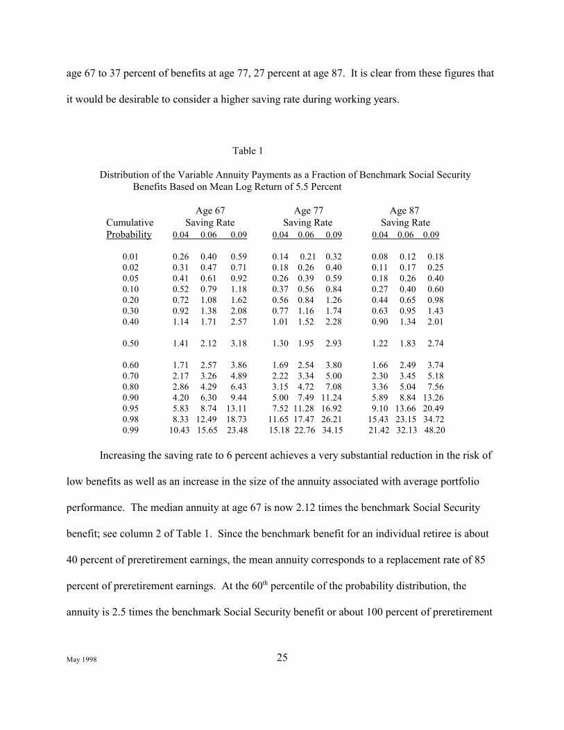
25May 1998

age 67 to 37 percent of benefits at age 77, 27 percent at age 87. It is clear from these figures that

it would be desirable to consider a higher saving rate during working years.

Table 1

Distribution of the Variable Annuity Payments as a Fraction of Benchmark Social Security Benefits Based on Mean Log Return of 5.5 Percent

Age 67 Age 77 Age 87 Cumulative Saving Rate Saving Rate Saving Rate Probability 0.04 0.06 0.09 0.04 0.06 0.09 0.04 0.06 0.09

0.01 0.26 0.40 0.59 0.14 0.21 0.32 0.08 0.12 0.18 0.02 0.31 0.47 0.71 0.18 0.26 0.40 0.11 0.17 0.25 0.05 0.41 0.61 0.92 0.26 0.39 0.59 0.18 0.26 0.40 0.10 0.52 0.79 1.18 0.37 0.56 0.84 0.27 0.40 0.60 0.20 0.72 1.08 1.62 0.56 0.84 1.26 0.44 0.65 0.98 0.30 0.92 1.38 2.08 0.77 1.16 1.74 0.63 0.95 1.43 0.40 1.14 1.71 2.57 1.01 1.52 2.28 0.90 1.34 2.01

0.50 1.41 2.12 3.18 1.30 1.95 2.93 1.22 1.83 2.74

0.60 1.71 2.57 3.86 1.69 2.54 3.80 1.66 2.49 3.74 0.70 2.17 3.26 4.89 2.22 3.34 5.00 2.30 3.45 5.18 0.80 2.86 4.29 6.43 3.15 4.72 7.08 3.36 5.04 7.56 0.90 4.20 6.30 9.44 5.00 7.49 11.24 5.89 8.84 13.26 0.95 5.83 8.74 13.11 7.52 11.28 16.92 9.10 13.66 20.49 0.98 8.33 12.49 18.73 11.65 17.47 26.21 15.43 23.15 34.72 0.99 10.43 15.65 23.48 15.18 22.76 34.15 21.42 32.13 48.20

Increasing the saving rate to 6 percent achieves a very substantial reduction in the risk of

low benefits as well as an increase in the size of the annuity associated with average portfolio

performance. The median annuity at age 67 is now 2.12 times the benchmark Social Security

benefit; see column 2 of Table 1. Since the benchmark benefit for an individual retiree is about

40 percent of preretirement earnings, the mean annuity corresponds to a replacement rate of 85

percent of preretirement earnings. At the 60th percentile of the probability distribution, the

annuity is 2.5 times the benchmark Social Security benefit or about 100 percent of preretirement

26May 1998

earnings. At these and higher annuity levels, retirees might want to make gifts to their children

or set some funds aside for future bequests.

The six percent saving rate reduces the probability that the annuity at age 67 is less than

the benchmark Social Security benefit to 17 percent. There is only a 5 percent chance that the

age 67 annuity is less than 61 percent of the benchmark Social Security benefit.

Increasing the saving rate to 9 percent (still less than half of the projected pay-as-you-go

tax rate) raises the distribution of benefits substantially. There is less than a 10 percent chance

that the benfit is less than 1.1 times the benchmark level and less than a 5 percent chance that it is

less than 92 percent of the benchmark benefit.

This favorable performance continues at older ages. The median annuity is nearly twice

the benchmark Social Security benefit at age 77, and 1.83 times the benchmark at age 87. The

probability of receiving an annuity that is less than the benchmark benefit remains low, rising

from 17 percent at age 67 to less than 31 percent at 87.

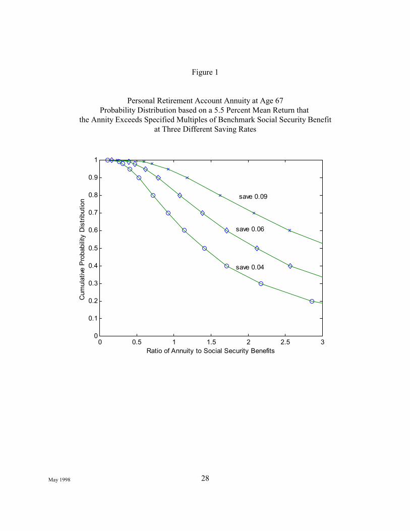
Figure 1 shows the cumulative distributions for the ratio of the annuities at age 67 to the

benchmark Social Security benefit for saving rates of four percent, six percent and nine percent.

Similar cumulative distributions of the annuity ratios are shown for four age levels in Table 1.

In considering these favorable distributions, it is worth emphasizing that the paygo tax

required to finance the benchmark Social Security benefits that are used as the standard of

comparison will rise to more than 18 percent during the next 40 years. Thus individuals could

achieve much higher expected benefits and face only a very small risk of lower benefits while

saving substantially less than the long-run paygo tax rate.

Although a nine percent saving rate is still less than half of the long-term tax rate required

27May 1998

in the paygo program, such a relatively high saving rate requires reducing consumption during

working years to transfer funds to retirement years when the annuity would be likely to provide a

substantially higher level of income than the individuals had consumed in preretirement years.

Individuals would probably prefer not to reduce consumption during working years by as much

as 9 percent to transfer funds to a time when the expected marginal value of income was

significantly lower.

An explicit evaluation of these alternative saving rates would depend on individuals’ time

preference as well as their attitudes toward risk. We do not pursue this further here but turn

instead to an alternative strategy: a conditional tax-financed pension payment to retirees in those

states of nature in which the annuities would otherwise be unacceptably low. We develop this

approach in the next section of the paper.

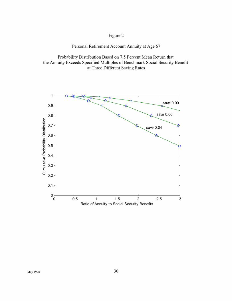
Before looking at the way that such intergenerational risk sharing might work, we present

estimates of the individual risk distribution if the expected rate of log return is increased by the

corporate income tax revenues from 5.5 percent to 7.5 percent. The results for this case are

presented in Figure 2 and Table 2, parallel to those for Figure 1 and Table 1 but with saving rates

of 3 percent, 5 percent and 9 percent.

28May 1998

0 0.5 1 1.5 2 2.5 30

0.1

0.2

0.3

0.4

0.5

0.6

0.7

0.8

0.9

1

Ratio of Annuity to Social Security Benefits

Cum

ulat

ive P

roba

bilit

y D

istri

butio

n

save 0.04

save 0.06

save 0.09

Figure 1

Personal Retirement Account Annuity at Age 67Probability Distribution based on a 5.5 Percent Mean Return that

the Annity Exceeds Specified Multiples of Benchmark Social Security Benefitat Three Different Saving Rates

33It is possible that without such a publicly provided minimum pension guarantee theprivate market would develop such a product. While a public program has the advantage that itcan use mandatory intergenerational transfers, the private market could use a series of forwardput options to transfer risk from retirees and employees to a broader population of investors,including high income individuals, institutions, and foreign investors. Such a potential marketbased system deserves further analysis.

29May 1998

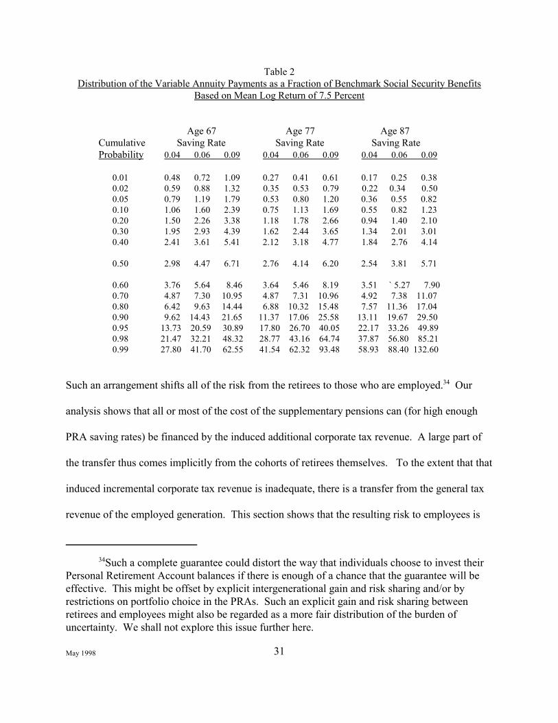
The results are obviously even more favorable with the 7.5 percent rate of return than

with the 5.5 percent rate of return. With a six percent saving rate, the median annuity at age 67 is

4.47 times the benchmark Social Security benefits and therefore nearly 180 percent of

preretirement income. In fewer than 3 percent of the simulations is the annuity less than the

benchmark Social Security benefit. Only in the one percent of simulations with the least

favorable performance is the annuity less than 72 percent of the benchmark Social Security

benefit.

4. Intergenerational Risk Sharing

The risk that retirees may receive less as a defined contribution annuity than they would

have received from Social Security can be eliminated completely by a relatively low cost

intergenerational government guarantee.33 In this section, we study a plan in which the

government provides an additional pension financed out of general tax revenue to make up any

deficiency between the benchmark Social Security benefit and the actual defined contribution

annuity.

30May 1998

0 0.5 1 1.5 2 2.5 30

0.1

0.2

0.3

0.4

0.5

0.6

0.7

0.8

0.9

1

Ratio of Annuity to Social Security Benefits

Cum

ulat

ive P

roba

bilit

y D

istri

butio

n

save 0.04

save 0.06

save 0.09

Figure 2

Personal Retirement Account Annuity at Age 67

Probability Distribution Based on 7.5 Percent Mean Return that the Annuity Exceeds Specified Multiples of Benchmark Social Security Benefit

at Three Different Saving Rates

34Such a complete guarantee could distort the way that individuals choose to invest theirPersonal Retirement Account balances if there is enough of a chance that the guarantee will beeffective. This might be offset by explicit intergenerational gain and risk sharing and/or byrestrictions on portfolio choice in the PRAs. Such an explicit gain and risk sharing betweenretirees and employees might also be regarded as a more fair distribution of the burden ofuncertainty. We shall not explore this issue further here.

31May 1998

Table 2Distribution of the Variable Annuity Payments as a Fraction of Benchmark Social Security Benefits

Based on Mean Log Return of 7.5 Percent

Age 67 Age 77 Age 87 Cumulative Saving Rate Saving Rate Saving Rate

Probability 0.04 0.06 0.09 0.04 0.06 0.09 0.04 0.06 0.09

0.01 0.48 0.72 1.09 0.27 0.41 0.61 0.17 0.25 0.38 0.02 0.59 0.88 1.32 0.35 0.53 0.79 0.22 0.34 0.50 0.05 0.79 1.19 1.79 0.53 0.80 1.20 0.36 0.55 0.82

0.10 1.06 1.60 2.39 0.75 1.13 1.69 0.55 0.82 1.23 0.20 1.50 2.26 3.38 1.18 1.78 2.66 0.94 1.40 2.10 0.30 1.95 2.93 4.39 1.62 2.44 3.65 1.34 2.01 3.01 0.40 2.41 3.61 5.41 2.12 3.18 4.77 1.84 2.76 4.14

0.50 2.98 4.47 6.71 2.76 4.14 6.20 2.54 3.81 5.71

0.60 3.76 5.64 8.46 3.64 5.46 8.19 3.51 ` 5.27 7.90 0.70 4.87 7.30 10.95 4.87 7.31 10.96 4.92 7.38 11.07 0.80 6.42 9.63 14.44 6.88 10.32 15.48 7.57 11.36 17.04 0.90 9.62 14.43 21.65 11.37 17.06 25.58 13.11 19.67 29.50 0.95 13.73 20.59 30.89 17.80 26.70 40.05 22.17 33.26 49.89 0.98 21.47 32.21 48.32 28.77 43.16 64.74 37.87 56.80 85.21 0.99 27.80 41.70 62.55 41.54 62.32 93.48 58.93 88.40 132.60

Such an arrangement shifts all of the risk from the retirees to those who are employed.34 Our

analysis shows that all or most of the cost of the supplementary pensions can (for high enough

PRA saving rates) be financed by the induced additional corporate tax revenue. A large part of

the transfer thus comes implicitly from the cohorts of retirees themselves. To the extent that that

induced incremental corporate tax revenue is inadequate, there is a transfer from the general tax

revenue of the employed generation. This section shows that the resulting risk to employees is

35We abstract from the effect of the guarantee on the portfolio choice that individualswould make by assuming that they must hold this standard 60:40 portfolio. A practical planmight allow more choice but provide a more complex form of risk-sharing.

32May 1998

quite small. Moreover, the combination of the amount that individuals save in their PRA

accounts and the amount that they may be called upon to pay to supplement the defined

contribution annuities of all cohorts of retirees is substantially less than the amount that they

would be required to pay in tax in a pure paygo program with the same benefit levels.

Our analysis is again based on the economic and demographic projections of the Social

Security actuaries and the underlying Census Bureau estimates of future birth and death rates. We

assume that the transition to the defined contribution system begins in 1998. The cohort of

individuals who are 21 years old in 1998 does not accrue any paygo benefits but contributes to

the defined contribution Personal Retirement Accounts throughout its working life. All

subsequent cohorts also participate exclusively in the defined contribution plan.

We look ahead to the year 2077 when the individuals who were 21 in 1998 are 100 years

old, the oldest age to which individuals are assumed to survive. This is the first year for which

we have such information from the Social Security actuaries’ projections and also the last year to

which their data can be extended. In that year, there are 34 cohorts of retirees ranging in age

from 67 to 100. The individuals in each cohort experienced the wage growth projected for that

cohort by the Social Security Administration (approximately a one percent annual rate of real

wage increase), saved a specified percentage or their wage income in the PRAs, and invested

those funds in the 60:40 equity-debt portfolio.35

We use 10,000 simulations of the return in each year from 1998 to 2077. All cohorts

experience the same portfolio rate of return in each calender year. On the basis of these returns,

33May 1998

we calculate the variable annuities of the 34 different cohorts that are retired in the year 2077.

Cohorts that are close in age have quite similar investment experiences while cohorts that are

further apart in age have less closely correlated investment experiences.

The 34 retiree cohorts that are alive in 2077 have cohort sizes Nt with t = 67, 68, ... 100.

For each of the 10,000 simulations, we calculate for each cohort the PRA annuity (at ) that

reflects its own investment experience, earnings history, and projected mortality rates. The

projected benchmark Social Security benefit in that year for each cohort is denoted ssben t . If the

PRA annuity of a cohort exceeds the cohort’s projected benchmark Social Security benefits,

there is no transfer. But if the PRA annuity is less than the benchmark benefit, each member of

the cohort receives a transfer equal to the shortfall: ssben t - at .

The aggregate transfer in the year 2077 is therefore T = Σ max (0, ssben t - at ) for t = 67,

68, ... 100. We summarize the probability distribution of such aggregate transfers in 2077

relative to the aggregate wage income in that year. If wt is the average wage earned by

individuals at age t for t = 21, 22, ...., 66 and Nt is the corresponding number of workers, the

aggregate wage income in that year is W = Σ wt Nt . The tax revenue required in 2077 to finance

the aggregate transfer to all retirees with annuity shortfalls is therefore 2 = T/W. We take the

distribution of 2 to represent the distribution of relative transfers needed in a fully phased-in

system. Although this transfer is stated as a percentage of wages, part or all of this transfer can

be financed with the corporate income tax revenue generated by the incremental capital in the

PRA accounts (if the accounts themselves are only credited with the 5.5 percent portfolio return.)

To illustrate the distribution of the aggregate cost of the conditional pensions, consider a

specific combination of saving rate and rate of return: a 4 percent saving rate and 5.5 percent

36The conditional transfer is thus a much lower cost way of preventing an inadequateretirement annuity than the universal flat benefit that is frequently advocated as a complement toa defined contribution plan.

34May 1998

mean log portfolio rate of return. We do 10,000 simulations of the 80 year investment

experience of those over age 20 in the year 2077. Of these 10,000 simulations, there is a

probability of 0.56 that some transfer to at least one generation of retirees will be needed. In the

remaining 44 percent of the simulations, the PRA annuities of every retired generation exceed the

benchmark Social Security benefits.

The mean transfer payment among all 10,000 simulations (including the zero transfers

when the annuity exceeds the benchmark) is 3.9 percent of the aggregate wage bill.36 With a four

percent saving rate and a 5.5 percent mean log portfolio rate of return, the aggregate of the PRA

balances of everyone over age 20 (including the retirees) has an expected value of 5.2 times the

aggregate wage bill. The corporate income tax of 2.0 percent of these balances implies corporate

tax revenue equal to 10.5 percent of the wage bill. Thus, on average, the corporate income tax

revenue generated by the PRA accounts is sufficient to finance the transfers needed to keep the

income of retirees at or above the benchmark Social Security benefit (i.e., 3.9 percent of payroll)

and to have a substantial residual left to reduce other taxes or finance other government

spending.

In summary, in the defined contribution plan with a four percent saving rate and an

intergenerational guarantee, the retiree income in a fully phased-in program is on average more

than 40 percent greater than the benchmark Social Security benefit and is never less than the

benchmark Social Security benefit. The four percent saving rate required to finance these

benefits is less than one fourth of the paygo tax that would be required to finance the benchmark

35May 1998

Social Security benefits. Employees are required to finance any shortfall to guarantee that the

retiree pension income is at least the benchmark Social Security benefit, but on average there is

no tax needed to do this since the extra corporate income tax receipts generated by the additional

capital in the Personal Retirement Accounts is more than enough to pay the expected transfers.

Although the induced corporate income tax is sufficient to finance the average

conditional pension transfers, there are cases in which the employed population would be

required to pay taxes to finance some of the conditional pension transfers. With a 4 percent

saving rate and a 5.5 percent mean log rate of return, the conditional transfers exceed the induced

corporate income tax revenue (10.5 percent of aggregate wages) in only 17 percent of the

simulations, i.e., the amount required to finance the transfers is less than 10.5 percent of wages in

about 83 percent of simulations. In the least favorable 5 percent of simulations the net revenue

required (in excess of the 10.5 percent from individual corporate taxes) would be 3.7 percent of

aggregate wages, bringing the total of PRA saving and the tax to 7.7 percent of earnings, still less

than half of the projected paygo tax rate.

Although the retirees have no risk of receiving less retirement income than the benchmark

Social Security benefits, they have the opportunity to receive substantially more when the

investment experience is favorable. Shown in Table 1, median retirement income at age 67 of

the cohort that was 21 in 1998 with the 4 percent saving rate is 1.41 times the benchmark Social

Security benefits. In the most favorable 20 percent of the simulations, the annuity exceeds 2.9

times the benchmark Social Security benefit.

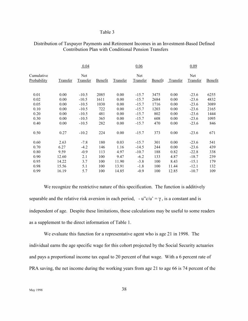
Table 3 summarizes the key results of the pension guarantee plan. Column 1 shows, for

the saving rate of 4 percent, the cumulative probability distribution of the required transfers as a

36May 1998

percentage of the aggregate wage income at the time. In more than 40 percent of the simulations,

no transfer is required. In 80 percent, the transfer is less than 9.6 percent of payroll. Column 2

presents the same transfers net of the incremental corporate tax revenue associated with the PRA

capital. These figures differ from the figures in column 1 by 10.5 percent of wages, the mean

incremental corporate tax revenue. Column 3 shows the cumulative distribution of the retiree

income of the cohort that was 21 in 1998 as a multiple of the benchmark Social Security benefit.

The retiree income is equal to the benchmark in those cases reported as 1.00. Beyond that, the

annuity exceeds the benchmark and the guarantee is irrelevant.

These three distributions are repeated in columns 4 through 9 for saving rates of 6 percent

and 9 percent. Note that with a 6 percent saving rate the incremental corporate tax is 15.7

percent of covered earnings while in the 9 percent case it is 23.6 percent of earnings. With a 6

and 9 percent saving rates, the incremental corporate income tax is sufficient to finance the

required transfer in more than 99 percent of simulations.

A final word of caution is appropriate. The ability to shift risk from retirees to taxpayers

with the type of conditional guarantee analyzed in this section assumes that taxpayers would be

willing to tax themselves when necessary. A risk averse individual who fears that future

taxpayers might not be willing to do so might prefer to make his own provision by a high rate of

saving, as indicated in the previous section.

5. A CRRA Expected Utility Evaluation

Although we believe that displaying the probability distributions of possible outcomes, as

we do in Tables 1, 2 and 3, is the best way to indicate the risks and rewards of the alternative

investment-based options, in this section we present explicit summary calculations based on

37May 1998

expected values of constant relative risk aversion (CRRA) utility functions.

To evaluate the PRA options presented in Table 1, we consider a representative individual with

expected utility function E = E [ Σ pt β t-21 u (Ct ) ] where the summation is from t = 21 to t = 100

and u ( Ct ) = ( Ct 1−γ - 1)/ (1 - γ). Ηere E is the expectation operator, pt is the probability of

surviving to age t from age 21, β is the time discount factor at which utility is discounted, and γ

is the coefficient of relative risk aversion. We do the analysis with a time discount factor of 0.98;

alternative calculations with a greater time discount (β = 0.96) and with no time discount factor

(β = 1) have very little effect on the results that we report below.

38May 1998

Table 3

Distribution of Taxpayer Payments and Retirement Incomes in an Investment-Based DefinedContribution Plan with Conditional Pension Transfers

0.04 0.06 0.09

Cumulative Net Net NetProbability Transfer Transfer Benefit Transfer Transfer Benefit Transfer Transfer Benefit

0.01 0.00 -10.5 2085 0.00 -15.7 3475 0.00 -23.6 6255 0.02 0.00 -10.5 1611 0.00 -15.7 2684 0.00 -23.6 4832 0.05 0.00 -10.5 1030 0.00 -15.7 1716 0.00 -23.6 3089 0.10 0.00 -10.5 722 0.00 -15.7 1203 0.00 -23.6 2165 0.20 0.00 -10.5 481 0.00 -15.7 802 0.00 -23.6 1444 0.30 0.00 -10.5 365 0.00 -15.7 608 0.00 -23.6 1095 0.40 0.00 -10.5 282 0.00 -15.7 470 0.00 -23.6 846 0.50 0.27 -10.2 224 0.00 -15.7 373 0.00 -23.6 671 0.60 2.63 -7.8 180 0.03 -15.7 301 0.00 -23.6 541 0.70 6.27 -4.2 146 1.16 -14.5 244 0.00 -23.6 439 0.80 9.59 -0.9 113 4.97 -10.7 188 0.82 -22.8 338 0.90 12.60 2.1 100 9.47 -6.2 133 4.87 -18.7 239 0.95 14.22 3.7 100 11.90 -3.8 100 8.43 -15.1 179 0.98 15.56 5.1 100 13.91 -1.8 100 11.44 -12.1 132 0.99 16.19 5.7 100 14.85 -0.9 100 12.85 -10.7 109

We recognize the restrictive nature of this specification. The function is additively

separable and the relative risk aversion in each period, - u”c/u’ = γ , is a constant and is

independent of age. Despite these limitations, these calculations may be useful to some readers

as a supplement to the direct information of Table 1.

We evaluate this function for a representative agent who is age 21 in 1998. The

individual earns the age specific wage for this cohort projected by the Social Security actuaries

and pays a proportional income tax equal to 20 percent of that wage. With a 6 percent rate of

PRA saving, the net income during the working years from age 21 to age 66 is 74 percent of the

37This represents a simplification in several ways. Although we are looking at wages forthe years beginning in 1998, we are ignoring the transition problem and comparing a fully phasedin PRA system with the paygo system that would also exist in the more distant future. We dothis to avoid the complexities of modeling the transition. We also simplify by treating theprojected wages as the marginal product of capital from which all taxes and saving aresubtracted.

38The lack of other saving reduces the individual’s level of retirement consumption andtherefore makes the individual’s utility more sensitive to fluctuations in the return to PRAsaving.

39We also present some results that focus exclusively on the income during retirement,abstracting from the difference between the 18 percent tax in preretirement years and the lowerPRA saving rate.

40See for example Mehra and Prescott (1985) and Kocherlakota (1996). The differencebetween the equity yield and the yield on Treasury bills has of course declined in recent years,implying a lower measure of risk aversion. If the “riskless” security is taken to be an asset withno credit risk and with a guaranteed long-term real return, the comparison should be the recently

39May 1998

gross wage.37 The individual is assumed to do no other saving, making the consumption in each

preretirement year the same 74 percent of pretax wages.38 During retirement the individual’s

consumption is the variable annuity that is generated by the PRA savings, as described in section

2.1 above. Similar simulations are done also for PRA plans with saving rates of 4 percent and 9

percent. We contrast each of these to the paygo system in which the tax rate is 18 percent ,

making the net consumption during the preretirement years equal to 62 percent of preretirement

income. This paygo system is assumed to provide the benchmark level of benefits prescribed in

current law during each retirement year with no uncertainty.39

The coefficient of relative risk aversion is the key parameter in this expected utility

evaluation. The values of γ inferred in the finance literature from the difference between the

yields on stocks and on “risk free” treasury bills are implausibly high, giving rise to the label

“equity premium puzzle.”40 Instead of using these implausibly high values as a guide to policy,

created Treasury Inflation Protected Securities. These TIPS now have a yield of about 3.6percent, not that different from the earnings-price ratio on equities.

40May 1998

we use the following mental experiment to help decide on appropriate CRRA values.

The representative individual in our example will reach age 67 in the year 2044 and will

be retired during the decades that follow. The level of retirement consumption that the PRA will

provide at that time might be conservatively approximated to be $40,000 in today’s prices; the

precise level does not matter for our example. Consider two equally probable states of nature. In

the good state the retiree has income and consumption of $40,000. In the bad state, it is only

$20,000. In the mental experiment, we give the individual the opportunity to increase

consumption in the bad state by one dollar by agreeing to reduce consumption if the good state

occurs. We can infer the individual’s CRRA γ coefficient by observing how much the

individual would be willing to give up in the good state to increase consumption in the bad state

by one dollar.

Any risk averse individual ( γ > 0) would be willing to give up more than a dollar in the

good state for a dollar in the bad state. If the individual would give up two dollars in the good

state, but no more, to increase consumption in the bad state by one dollar, we infer that

u (20,000) = 2 u’(40,000). Since the CRRA form noted above implies u’(c) = C − γ , the

condition that u’ (20,000) = 2 u’(40,000) implies that 2 γ = 2 or γ = 1.

Similarly, we can infer that if the representative individual is willing to give up four

dollars of consumption in the good state (when consumption would otherwise be $40,000) to

have an additional dollar of consumption in the bad state when consumption would otherwise be

$20,000, the coefficient of CRRA becomes γ = 2. And a representative individual who would

41May 1998

give up eight dollars in the good state to have one extra dollar in the bad state has a CRRA value

of γ = 3.

Readers can decide for themselves how much is reasonable to assume that someone

would give up when income is $40,000 for a dollar when the income would otherwise be

$20,000. Without choosing a specific value, we believe that the plausible sacrifice amount

would be less than eight dollars and probably less than four dollars.

We drew 10,000 independent histories of the 80 year sequence (from age 21 in 1998 to

age 100 in 2077) of returns on the PRA savings of the representative individual and calculated

the expected utility value associate with each value of γ . Our calculations show that the PRA

with a 6 percent mandatory saving rate is preferable to the paygo for the relative risk aversion

coefficient up to γ = 3.4. With a 4 percent saving rate the critical value of γ is 2.95 while with

a 9 percent saving rate the PRA system is preferred to paygo for all values of γ less than 3.85.

The comparison of the expected lifetime utilities of the PRA and the paygo systems

reflects time preference as well as risk preference. During the individuals’ working years, the

paygo requires an 18 percent tax while the PRA only involves a saving rate of between 4 percent

and 9 percent. Differences in time preference (β in our analysis) therefore influence the relative

desirability of the two options. To abstract from this and focus just on the difference between the

presumed-certain paygo benefit and the stochastic PRA annuity, we apply the expected utility

calculation just to the incomes in the retirement years. In other words, we disregard the PRA

system’s advantage of requiring much lower contributions during working years than the 18

percent paygo tax. With a saving rate of 6 percent, we note that the median PRA annuity is

42May 1998

substantially greater than the benchmark benefit; table 1 shows that the median PRA annuity at

age 67 is 2.12 times the benchmark benefit. Although there is a 17 percent chance that the PRA

annuity will fall below the benchmark benefit at age 67 (and a greater chance at higher ages), the

explicit utility evaluation starting at age 67 shows that the stochastic PRA annuity is preferred to

the “certain” paygo benefit for all CRRA coefficients up to 2.4. With a four percent saving rate

this critical value of γ becomes 1.6 while with a saving rate of 9 percent the PRA option is

preferred for all values of γ up to 3.1. In short, for plausible CRRA risk aversion parameters, the

preference for the PRA option does not depend on the lower contribution during the working

years.

5.1 Evaluating Government Guarantee Plans with CRRA Expected Utility

When we turn from the pure individualistic PRA system to one with a government

guarantee, we can no longer focus on a single age cohort but must consider the benefits received

by all retirees aged 67 through 100 and the taxes paid by employees of all ages (as we do in Table

3). We therefore examine the situation during a representative year after the PRA system is fully

phased in. We compare the possible outcomes of the PRA system (for alternative possible

saving rates) with the paygo system in the long-run with an 18 percent tax rate.

More specifically, we calculate the expected value of a social welfare function in the first

year in which the PRA system is fully phased in. This is the year 2077 when the youngest

workers in 1998 (those who are then 21 years old) have reached 100, the oldest age that we

consider in our analysis. The value of the social welfare function in that year is the sum of the

expected utilities of the employed taxpayers and the retirees: SWF = E [ Σ Νj u(Cj ) ] where the

summation is now over the 80 cohorts identified by age (from j = 21 to j = 100), E is again the

41This expected social welfare function value for a single year is of course different fromthe expected lifetime utility that we used to evaluate the choice between PRA and paygo plans. Itwould be desirable to use a framework in which for each of the 80 cohorts we evaluated theexpected present value of lifetime utility. Unfortunately, the data requirements for thatcalculation stretch further into the future than the projections of the Social Security actuaries andthe Census bureau.

43May 1998

expectations operator, Νj is the number of individuals in cohort j in the year 2077, and u (Cj )

is the utility of the consumption of the representative individual in cohort j in that year. The form

of the utility function is the same CRRA function specified above. In each of the 10,000

simulations that we do, we simulate the PRA accumulation of each cohort over the 80 year

horizon from 1998 until 2077 and then calculate the associated PRA annuity in that year for each

retiree cohort. We then specify that the individuals in each retiree cohort consume the greater of

the benchmark benefit and the PRA annuity of that cohort in that year.41

Retirees thus face no risk of consuming less than the benchmark benefit. All of the

potential adverse uncertainty is focused on the taxpayers who must pay an uncertain tax bill. In

particular, with a 6 percent mandatory saving rate and a 20 percent income tax, the consumption

of workers in cohort j is 74 percent of the cohort specific wage unless they are called upon to

pay a supplementary tax to fill the gap between a low PRA annuity and the benchmark benefit.

As we noted above, the first source of revenue to fill this gap would be the incremental corporate

tax revenue that results from the PRA capital. In approximately 15 percent of the outcomes with

the 4 percent saving rate, it is necessary for the employees to pay a supplementary tax, reducing

their consumption. In our analysis we assume that employees make annual adjustments to their

consumption when needed to fill the retiree income gap even though some form of smoothing

behavior would reduce the adverse utility effects of these uncertain extra tax burdens.

44May 1998

We contrast this PRA evaluation with a fully mature non-stochastic paygo system with an

18 percent tax (reducing consumption in working years to 62 percent of the pretax wage) and

with the benchmark benefits during retirement. We find that the PRA system with the

government guarantee dominates the paygo system for each of the three saving rates (4 percent, 6

percent and 9 percent) and for every CRRA parameter value the we considered (up to ( = 40).

These simulations tell us that a CRRA individual with any degree of risk aversion that we have

considered would prefer the PRA system with government guarantees to the current paygo

system.

We can also use this framework to compare the expected utility in a representative year of

the PRA plans with and without government guarantees. Although retirees obviously prefer the

guarantee, it is not clear ex ante which will be preferred when the expected utilities of all cohorts

of workers and retirees are taken into account. Our analysis shows that for each saving rate

between four percent and nine percent the guarantee is preferred for individuals with all of the

risk aversion coefficients that we have considered (up to ( = 40).

At this point our earlier warning about the risk of government promises is worth

repeating. These calculations assume that the paygo system and the government guarantee have

no risk when in fact there is the risk that the taxpayers will not provide the benefits called for by

either system. Individuals who regard the government payment as sufficiently risky might prefer

a PRA system with a higher saving rate to both the paygo system and the PRA system with a

government guarantee.

6. Concluding Remarks

This paper has examined the risk aspects of an investment-based defined contribution

42This 7.5 percent is less than the real marginal product of capital because the state andlocal governments also collect tax of one percent through property and profits taxes.

45May 1998

Social Security plan. We focus on the risks after the plan is fully phased in so that all employees

and retirees are participants in the plan. To be concrete, we base our calculations on the detailed

projections of economic and demographic variables by the Social Security Administration and

the Census Bureau for the 80 year period beginning in 1998. We therefore assume that the new

defined contribution program begins with the birth cohort that is 21 in 1998 and look at the

experience of the individuals of all cohorts who are alive in the year 2077.

In this plan, individuals are required to deposit a specified fraction of wages to a Personal

Retirement Account, invest these funds in a 60:40 equity-debt mix, and receive a similarly

invested variable annuity at age 67. The value of the assets in the Personal Retirement Accounts

follows a random walk with the mean and variance of a 60:40 equity-debt portfolio over the

period from 1946 to 1995, a mean log return of 5.5 percent (net of administrative costs of 0.4

percent) and a standard deviation of 12.5 percent. We study stochastic distributions of this

process by doing 10,000 simulations of the 80 year experience from 1998 to 2077. We examine

also the implications of using federal corporate income tax collections of an additional 2.0

percent of assets, bringing the total available return to 7.5 percent.42

The resulting annuities are compared to the future defined benefits promised in the

current Social Security law, a level that we refer to as the “benchmark” Social Security benefits.

The Social Security actuaries calculate that the aging of the population and increased longevity

imply that the future Social Security payroll tax required to finance the benchmark benefits on a

pay-as-you-go basis would be greater than 18 percent.

46May 1998

If the 5.5 percent mean log rate of return were known with certainty, individuals could

purchase the benchmark level of benefits by saving 3.1 percent of earnings, just one-sixth of the

required tax in the pay-as-you-go plan. But the uncertain nature of the rate of return implies that

saving 3.1 percent of wages is likely to provide an annuity that is either less than or greater than

the benchmark benefits.

Saving a higher share of wages provides a “cushion” that protects the individual from the

risk of an unacceptably low level of benefits. For example, an individual who saves 6 percent of

his earnings during his working years from 21 to 66 (with a 5.5 percent mean log return) has a 50

percent chance of receiving an annuity at age 67 that is at least 2.1 times the benchmark level of

Social Security benefits (and therefore about 70 percent of preretirement pretax wages) and only

a 17 percent chance that that annuity is less than benchmark Social Security benefit. In 95

percent of the investment experience the annuity exceeds 61 percent of the benchmark benefit.

We also study a modified defined contribution plan in which retirees face no risk of

receiving less than the benchmark benefit because the government provides a conditional pension

transfer to any retiree whose annuity is less in any year than the benchmark level of benefits. We

show that with a four percent saving rate and a 5.5 percent mean log rate of return, a conditional

transfer is required in only about half of the simulations. The expected value of the transfers is

substantially less than the expected incremental corporate tax revenue that results from the

Personal Retirement Account saving. In only about 15 percent of the simulations is it necessary

to use additional tax revenue to finance the transfers. In 95 percent of simulations, the net

revenue required (in excess of the incremental corporate tax) would be less than 3.7 percent of

earnings, implying that the combination of PRA saving and the conditional transfer tax is still

47May 1998

less than half of the projected pay-as-you-go tax.

A pure defined contribution plan with a 6 percent saving rate invested in a 60:40 equity-

debt Personal Retirement Account can cut the individual’s cost of providing a retirement annuity

to one-third of the projected 18 percent pay-as-you go tax while leaving the retiree exposed to

relatively little risk that the resulting annuity will be less than the benchmark level of Social

Security benefits projected in current law. Even this risk can be completely eliminated by a

conditional government transfer from employees when the defined contribution annuities are less

than the benchmark benefits. The risk to employees in this arrangement is extremely small,

again implying that a defined contribution Social Security plan can achieve the benchmark level

of benefits with a much lower burden on employees and little or no risk to retirees.

Cambridge, MAJuly 1998, December 1998Revised: April 1999

48May 1998

References

Aaron, Henry, “Social Security: Tune It Up, Don’t Trade It In,” The Brookings Institution, May

1998, Washington, DC.

Advisory Council on Social Security, (1997), Report of the 1994-1996 Advisory Council on

Social Security, Washington, DC.

Aiyagari, S. Rao, Comment on “The Economics of Prefunding Social Security and Medicare

Benefits, NBER Macroeconomics Annual 1997, The MIT Press, Cambridge, MA, pp

148-58.

Board of Trustees (1998), The 1998 Annual Report of the Social Security Trustees, Washington,

DC.

Bohn, Henning, “Risk Sharing in a Stochastic Overlapping Generations Economy,” June 1997.

Bohn, Henning, “Social Security Reform and Financing Markets,” in Social Security Reform,

Boston, MA: Federal Reserve Bank of Boston, 1998.

M. Boskin, J. Shoven and M. Hurd., "Social Security: A Financial Appraisal Across and Within

Generations." National Tax Journal, Vol. XL, No. 1, March 1987, pp. 19-34.

Caldwell, Steven, et al., “Social Security’s Treatment of Postwar America,” in Tax Policy

and the Economy (1998), James Poterba (ed.) Cambridge: MIT Press, 1998.

Diamond, Peter, “Macroeconomic Aspects of Social Security Reform,” Brookings Papers on

Economic Activity 2, 1997, Brookings Institution, Washington, DC, pp 1-88.

Diamond, Peter, “The Economics of Social Security Reform,” presented at the NASI Conference,

Framing the Social Security Debate: Values, Politics, and Economics, January 1998.

49May 1998

Feldstein, Martin, “The Social Time Preference Discount Rate in Cost-Benefit Analysis,” The

Economic Journal, 1964

Feldstein, Martin, “The Effects of Tax Based Incentives on National Saving and Government

Revenue,” Quarterly Journal of Economics, May 1995, pp 475-94.

Feldstein, Martin, “The Missing Piece in Policy Analysis: Social Security Reform,” The Richard

T. Ely Lecture, in American Economic Review, Vol. 86, No. 2, May 1996, pp 1-4.

Feldstein, Martin, “Don’t Waste the Budget Surplus,” The Wall Street Journal, November 4,

1997.

Feldstein, Martin, (ed.), Privatizing Social Security, (Chicago: University of Chicago Press,

1998a.

Feldstein, Martin, “Social Security Reform in China”, address to the Chinese Economists

Society, Beijing, China (June 1998), (mimeo), 1998b.

Feldstein, Martin, “Transition to a Fully Funded Pension System: Five Economic Issues,” in

Horst Siebert, (ed.), Rediscovering Social Security, Kiel Institute, University of Michigan

Press, 1998c.

Feldstein, Martin, “Let’s Really Save Social Security,” The Wall Street Journal, February 10,

1998d.

Feldstein, Martin and J. Liebman, “Distributional Effects of an Investment-Based Social Security

System,” forthcoming.

Feldstein, Martin and E. Ranguelova. “The Economics of Bequests in pensions and Social

Security,” NBER Working Paper No. 7065, April 1999.

50May 1998

Feldstein, Martin and A. Samwick, “The Economics of Prefunding Social Security and Medicare

Benefits, NBER Macroeconomics Annual 1997, The MIT Press, Cambridge, MA, pp

115-147.

Feldstein, Martin and A. Samwick, “The Transition Path in Privatizing Social Security, in M.

Feldstein (ed.) Privatizing Social Security, (Chicago: University of Chicago Press),

1998a, pp 215-60.

Feldstein, Martin and A. Samwick, “Potential Effects of Two Percent Personal Retirement

Accounts,” Tax Notes, Vol. 79, No. 5, May 4, 1998b, pp 615-20.

Geanakoplos, John, O.S. Mitchell and S.P. Zeldes, “Would a Privatized Social Security System

Really Pay a Higher Rate of Return?”, Pension Research Council Working Paper No. 98-

6, June 1998, University of Pennsylvania, Philadelphia, PA.

Huggett, Mark, and G. Ventura, “On the Distributional Effects of Social Security Reform,”

Discussion Paper 9801, January 1998, Centro do Investigacion Economia, Mexico.

Kocherlakota, N, “The Equity Premium Puzzle: It’s Still a Puzzle,” Journal of Economic

Literature, Volume 34, 1996, pp 42-71

Kotlikoff, Laurence, “Privatization of Social Security: How It Works and Why It Matters,” Tax

Policy and the Economy, 1996.

Kotlikoff, Laurence, “Simulating the Privatization of Social Security in General Equilibrium,” in

M. Feldstein (ed.), Privatizing Social Security, (Chicago: University of Chicago Press,

1998).

Kotlikoff, et. al., “Social Security: Privatizing and Progessivity”, NBER Working Paper No.

6428, February 1998.

51May 1998

Liebman, Jeffrey, “The Distribution of Social Security Benefits”, mimeo, 1998

McHale, John, “The Risk of Reduction in Social Security Benefits: An International

Comparison,” (mimeo), 1998.

Mehra, R and E. Prescott, “The Equity Premium Puzzle,” Journal of Monetary Economics,

volume 15, 1985, page 145-161.

Merton, Robert, “On the Role of Social Security as a Means for Efficient Risk Sharing in an

Economy Where Human Capital Is Not Tradable,” in Financial Aspects of the U.S.

Pension System, Z. Bodie and J. Shoven (eds.), Chicago: University of Chicago Press,

1983.

Murphy, Kevin and F. Welch, “Perspectives on the Social Security Crisis and Proposed

Solutions,” The American Economic Review, Vol. 88, No. 2, May 1998, pp 142-50.

National Commission on Retirement Policy,” The 21st Century Retirement Security Plan,”

Washington, DC: 1998

Poterba, James, “The Rate of Return to Corporate Capital and Factor Shares,” NBER Working

Paper No. 6263, 1997.

Samuelson, Paul, “An Exact Consumption Loan Model of Interest With or Without the Social

Contrivance of Money, Journal of Political Economy, December 1958.

Shiller, Robert, “Social Security and Institutions for Intergenerational, Intragenerational and

International Risk Sharing,” presented at Carnegie-Rochester Conference, April 1998.

Shoven, John, Administrative Aspects of Social Security Reform, 1999 (forthcoming)

Smetters, Kent, “Investing the Social Security Trust Fund in Equities: An Option Pricing

Approach,” Congressional Budget Office, August 1997.

52May 1998

Smetters, Kent, “Privatizing Social Security in the Presence of a Performance Guarantee,”

Congressional Budget Office, December 1997.