Nodal Analysis

3.1

PMcL Contents Index

2019 3 - Nodal Analysis

3 Nodal Analysis

Contents

Introduction ..................................................................................................... 3.2

3.1 Nodal Analysis .......................................................................................... 3.3

3.1.1 Circuits with Resistors and Independent Current Sources Only .. 3.6

3.1.2 Nodal Analysis Using Branch Element Stamps ........................... 3.9 3.1.3 Circuits with Voltage Sources .................................................... 3.12 3.1.4 Summary of Nodal Analysis ....................................................... 3.14

3.2 Summary .................................................................................................. 3.15

3.3 References ............................................................................................... 3.15

Exercises ........................................................................................................ 3.16

3.2

Index Introduction PMcL

3 - Nodal Analysis 2019

Introduction

After becoming familiar with Ohm’s Law and Kirchhoff’s Laws and their

application in the analysis of simple series and parallel resistive circuits, we

must begin to analyse more complicated and practical circuits.

Physical systems that we want to analyse and design include electronic control

circuits, communication systems, energy converters such as motors and

generators, power distribution systems, mobile devices and embedded systems.

We will also be confronted with allied problems involving heat flow, fluid

flow, and the behaviour of various mechanical systems.

To cope with large and complex circuits, we need powerful and general

methods of circuit analysis. Nodal analysis is a method which can be applied to

any circuit. This method is widely used in hand design and computer

simulation.

3.3

PMcL Nodal Analysis Index


3.1 Nodal Analysis

In general terms, nodal analysis for a circuit with N nodes proceeds as follows:

1. Select one node as the reference node, or common (all nodal voltages

are defined with respect to this node in a positive sense).

2. Assign a voltage to each of the remaining 1N nodes.

3. Write KCL at each node, in terms of the nodal voltages.

4. Solve the resulting set of simultaneous equations.

EXAMPLE 3.1 Nodal Analysis with Independent Sources

We apply nodal analysis to the following 3-node circuit:

23 A -2 A

5

1

Following the steps above, we assign a reference node and then assign nodal

voltages:

23 A -2 A

5

1

1v v2

We chose the bottom node as the reference node, but either of the other two

nodes could have been selected. A little simplification in the resultant

equations is obtained if the node to which the greatest number of branches is

connected is identified as the reference node.

The general principle of nodal analysis

3.4

Index Nodal Analysis PMcL


In many practical circuits the reference node is one end of a power supply

which is generally connected to a metallic case or chassis in which the circuit

resides; the chassis is often connected through a good conductor to the Earth.

Thus, the metallic case may be called “ground”, or “earth”, and this node

becomes the most convenient reference node.

To avoid confusion, the reference node will be called the “common” unless it

has been specifically connected to the Earth (such as the outside conductor on a

digital storage oscilloscope, function generator, etc.).

Note that the voltage across any branch in a circuit may be expressed in terms

of nodal voltages. For example, in our circuit the voltage across the 5

resistor is 21 vv with the positive polarity reference on the left:

( )

51v v2

- v21v

We must now apply KCL to nodes 1 and 2. We do this be equating the total

current leaving a node to zero. Thus:

0215

0352

212

211

vvv

vvv

Simplifying, the equations can be written:

22.12.0

32.07.0

21

21

vv

vv

The distinction between “common” and “earth”

3.5



Rewriting in matrix notation, we have:

2

3

2.12.0

2.07.0

2

1

v

v

These equations may be solved by a simple process of elimination of variables,

or by Cramer’s rule and determinants. Using the latter method we have:

V 5.28.0

2

8.0

6.04.1

8.0

22.0

37.0

V 58.0

4

04.084.0

4.06.3

2.12.0

2.07.0

2.12

2.03

2

1

v

v

Everything is now known about the circuit – any voltage, current or power in

the circuit may be found in one step. For example, the voltage at node 1 with

respect to node 2 is V 5.221 vv , and the current directed downward

through the 2 resistor is A 5.221 v .

3.6



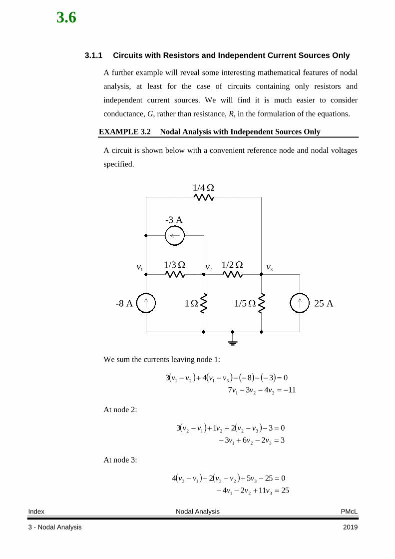
3.1.1 Circuits with Resistors and Independent Current Sources Only

A further example will reveal some interesting mathematical features of nodal

analysis, at least for the case of circuits containing only resistors and

independent current sources. We will find it is much easier to consider

conductance, G, rather than resistance, R, in the formulation of the equations.

EXAMPLE 3.2 Nodal Analysis with Independent Sources Only

A circuit is shown below with a convenient reference node and nodal voltages

specified.

-8 A 25 A

1/3

1

1v v2

-3 A

1/2

1/5

v3

1/4

We sum the currents leaving node 1:

11437

03843

321

3121

vvv

vvvv

At node 2:

3263

03213

321

32212

vvv

vvvvv

At node 3:

251124

025524

321

32313

vvv

vvvvv

3.7



Rewriting in matrix notation, we have:

25

3

11

1124

263

437

3

2

1

v

v

v

For circuits that contain only resistors and independent current sources, we

define the conductance matrix of the circuit as:

1124

263

437

G

It should be noted that the nine elements of the matrix are the ordered array of

the coefficients of the KCL equations, each of which is a conductance value.

Thr first row is composed of the coefficients of the Kirchhoff current law

equation at the first node, the coefficients being given in the order of 1v , 2v

and 3v . The second row applies to the second node, and so on.

The major diagonal (upper left to lower right) has elements that are positive.

The conductance matrix is symmetrical about the major diagonal, and all

elements not on this diagonal are negative. This is a general consequence of the

systematic way in which we ordered the equations, and in circuits consisting of

only resistors and independent current sources it provides a check against

errors committed in writing the circuit equations.

We also define the voltage and current source vectors as:

25

3

11

3

2

1

iv

v

v

v

The conductance matrix defined

3.8



Our KCL equations can therefore be written succinctly in matrix notation as:

iGv

The solution of the matrix equation is just:

iGv1

Computer programs that do nodal analysis use sophisticated numerical

methods to efficiently invert the G matrix and solve for v . When solving the

equations by hand we resort to matrix reduction techniques, or use Cramer’s

rule (up to 3 x 3). Thus:

1124

263

437

11225

263

4311

1

v

To reduce work, we expand the numerator and denominator determinants by

minors along their first columns to get:

V 1191

191

120123434

750123682

304413627

30254136211

26

434

112

433

112

267

26

4325

112

433

112

2611

1

v

Similarly:

V 2191

11254

233

4117

2

v V 3191

2524

363

1137

3

v

Nodal analysis expressed in matrix notation

3.9



3.1.2 Nodal Analysis Using Branch Element Stamps

The previous example shows that nodal analysis leads to the equation iGv .

We will now develop a method whereby the equation iGv can be built up

on an element-by-element basis by inspection of each branch in the circuit.

Consider a resistive element connected between nodes i and j:

vv

vv

( )

Gi j

- ji

(a)

vv

vv

( )

Gi j

- ij

(b)

Figure 3.1

Suppose that we are writing the ith KCL equation because we are considering

the current leaving node i (see Figure 3.1a). The term that we would write in

this equation to take into account the branch connecting nodes i and j is:

0 ji vvG (3.1)

This term appears in the ith row when writing out the matrix equation.

If we are dealing with the jth KCL equation because we are considering the

current leaving node j (see Figure 3.1b) then the term that we would write in

this equation to take into account the branch connecting nodes j and i is:

0 ij vvG (3.2)

This term appears in the jth row when writing out the matrix equation.

3.10



Thus, the branch between nodes i and j contributes the following element

stamp to the conductance matrix, G :

GG

GG

j

i

ji

(3.3)

If node i or node j is the reference node, then the corresponding row and

column are eliminated from the element stamp shown above.

For any circuit containing only resistors and independent current sources, the

conductance matrix can now be built up by inspection. The result will be a G

matrix where each diagonal element iig is the sum of conductances connected

to node i, and each off-diagonal element ijg is the total conductance between

nodes i and j but with a negative sign.

Now consider a current source connected between nodes i and j:

vvI

i j

Figure 3.2

In writing out the ith KCL equation we would introduce the term:

0 I (3.4)

In writing out the jth KCL equation we would introduce the term:

0 I (3.5)

The element stamp for a conductance

3.11



Thus, a current source contributes to the right-hand side (rhs) of the matrix

equation the terms:

I

I

j

i

(3.6)

Thus, the i vector can also be built up by inspection – each row is the addition

of all current sources entering a particular node. This makes sense since

iGv is the mathematical expression for KCL in the form of “current leaving

a node = current entering a node”.

EXAMPLE 3.3 Nodal Analysis Using the “Formal” Approach

We will analyse the previous circuit but use the “formal” approach to nodal

analysis.

-8 A 25 A

1/3

1

1v v2

-3 A

1/2

1/5

v3

1/4

By inspection of each branch, we build the matrix equation:

25

3

38

24524

22313

4343

3

2

1

3

2

1

321

v

v

v

This is the same equation as derived previously.

The element stamp for an independent current source

3.12



3.1.3 Circuits with Voltage Sources

Voltage sources present a problem in undertaking nodal analysis, since by

definition the voltage across a voltage source is independent of the current

through it. Thus, when we consider a branch with a voltage source when

writing a nodal equation, there is no way by which we can express the current

through the branch as a function of the nodal voltages across the branch.

There are two ways around this problem. The more difficult is to assign an

unknown current to each branch with a voltage source, proceed to apply KCL

at each node, and then apply KVL across each branch with a voltage source.

The result is a set of equations with an increased number of unknown variables.

The easier method is to introduce the concept of a supernode. A supernode

encapsulates the voltage source, and we apply KCL to both end nodes at the

same time. The result is that the number of nodes at which we must apply KCL

is reduced by the number of voltage sources in the circuit.

EXAMPLE 3.4 Nodal Analysis with Voltage Sources

Consider the circuit shown below, which is the same as the previous circuit

except the 21 resistor between nodes 2 and 3 has been replaced by a 22 V

voltage source:

-8 A 25 A

1/3

1

1v v2

-3 A

22 V

1/5

v3

1/4

supernode

The concept of a supernode

3.13



KCL at node 1 remains unchanged:

11437

03843

321

3121

vvv

vvvv

We find six branches connected to the supernode around the 22 V source

(suggested by a broken line in the figure). Beginning with the 31 resistor

branch and working clockwise, we sum the six currents leaving this supernode:

2894701525433

321

231312

vvvvvvvvv

We need one additional equation since we have three unknowns, and this is

provided by KVL between nodes 2 and 3 inside the supernode:

2223 vv

Rewriting these last three equations in matrix form, we have:

22

28

11

110

947

437

3

2

1

v

v

v

The solution turns out to be V 5.41 v , V 5.152 v and V 5.63 v .

Note the lack of symmetry about the major diagonal in the G matrix as well as

the fact that not all of the off-diagonal elements are negative. This is the result

of the presence of the voltage source. Note also that it does not make sense to

call the G matrix the conductance matrix, for the bottom row comes from the

equation 2232 vv , and this equation does not have any terms that are

related to a conductance.

A supernode can contain any number of independent or dependent voltage

sources. In general, the analysis procedure is the same as the example above –

one KCL equation is written for currents leaving the supernode, and then a

KVL equation is written for each voltage source inside the supernode.

The presence of a dependent source destroys the symmetry in the G matrix

3.14



3.1.4 Summary of Nodal Analysis

We perform nodal analysis for any resistive circuit with N nodes by the

following method:

1. Make a neat, simple, circuit diagram. Indicate all element and source

values. Each source should have its reference symbol.

2. Select one node as the reference node, or common. Then write the node

voltages 1v , 2v , …, 1Nv at their respective nodes, remembering that

each node voltage is understood to be measured with respect to the

chosen reference.

3. If the circuit contains dependent sources, express those sources in terms

of the variables 1v , 2v , …, 1Nv , if they are not already in that form.

4. If the circuit contains voltage sources, temporarily modify the given

circuit by replacing each voltage source by a short-circuit to form

supernodes, thus reducing the number of nodes by one for each voltage

source that is present. The assigned nodal voltages should not be

changed. Relate each supernode’s source voltage to the nodal voltages.

5. Apply KCL at each of the nodes or supernodes. If the circuit has only

resistors and independent current sources, then the equations may be

built using the “element stamp” approach.

6. Solve the resulting set of simultaneous equations.

The technique of nodal analysis described here is completely general and can

always be applied to any electrical circuit.

The general procedure to follow when undertaking nodal analysis

3.15

PMcL Summary Index


3.2 Summary

Nodal analysis can be applied to any circuit. Apart from relating source

voltages to nodal voltages, the equations of nodal analysis are formed from

application of Kirchhoff’s Current Law.

In nodal analysis, a supernode is formed by short-circuiting a voltage

source and treating the two ends as a single node.

3.3 References

Hayt, W. & Kemmerly, J.: Engineering Circuit Analysis, 3rd Ed., McGraw-

Hill, 1984.

3.16

Index Exercises PMcL


Exercises

1.

(a) Find the value of the determinant:

1003

2304

1011

3012

(b) Use Cramer’s rule to find 1v , 2v and 3v if:

0283

56432

03352

312

123

321

vvv

vvv

vvv

Documents

Nodal Analysis