THE NODAL BOUNDARY CONDITION METHOD

WAVE FUNCTIONS AND TRANSITION PROBABILITIES

FOR ATOMS WlTH TWO VALENCE ELECTRONS

Thesis by

Thomas M. HeUlwell

In Partlal FulfUlment of the Requirements

F or the Degree of

Doctor of P hUosophy

Callfornla lnatitute of Technology

Pasadena. CalUornia

1963

ACKNOWLEDGMENTS

The author ls particularly grateful to Professor R. F . Christy

for continued help and encouragement in the preparation of tbio thesis.

Several conversations with Professor R. B. King on experimental

results were very useful. Numerous dlscuoslons on astroph yslcal

applications with Professors J. L. Greenstein and W. A . Fowler.

and also with Dr. w. L . W. Sargent and Dr. J . Jugaku. provided one

of the chief motivations for this work.

A BSTR .ACT

A method is presented for com puting valence atomic wave

functions and transition probabilities. T his method, called the

"nodal boundary condition method", is a modified self-consistent-field

approach which makes some uee of experimental term -values in

order to eliminate the need for calculating wave functions for the

core electrons. Ae an application, the method is used to compute

eigenvalues, wave functions, and tranoition probabilities for several

atoms and ions having two valence electrons.

Various other approaches to the problem of calculating

atomic wave functions are reviewed, eo that the assumptionG and

approximations of the nodal boundary condition method may be

placed in perspective. The results of the present calculations are

compared in detail with "previous reaults whenever possible.

Finally, possible applications and extensions of the method are

briefly diocussed.

TABLE 0~ CONTENTS

I. INTRODUCTION

II. DEFINITIONS AND PROPER TIES OF OSCILLATOR

STRENGTHS

1

5

IU. METHODS OF CALCULATI NG ATOMIC WA VE FUNCTIONS 9

A. Atom ic Wave Functions 9

n. The Ha.rtree-F ock Method lS

c. P olarization of the Core 19

D. Analytic Variational Methods 24

E . The Nuclear Charge - Expansion .M:ethod 27

I V. THE COULOMB AFPROXI~1ATION 31

A. The Method of B ates and Damga.a.rd 31

B . Valence Wave Functions 35

C. Coulomb, SCF, and Experimental OocUlator

Strengths 3 9

V. THE NODAL BOUNDARY CONDI TI ON METHOD 43

A. Nodal StabUity 4S

B . Coulomb Nodes 52

1. Hydrogen and Ionized Helium 56

2.. Alkali Atoms and Ions 59

3. d 10sz Atoms and Ions 75

z 4. s p Atoms a.nd Ions SS

c. The Method with Calcium as an Example 92

1. Location of the Coulomb Nodes 92.

z. The 3Z Ground-State E nergy and Wave

Function 93

3. The Excited sp 1P 1 State

4. Calculation of OscUlator Strengths

D. Intercombination Lines

VI. RESULTS AND APP LICA TlONS

A . The S- Squared Calculations

B . E igenvalues and Oscillator Strengths

c . Comparison with the Coulomb Approximations

and with Experimental Results of the National

94

95

96

105

105

106

Bureau of Standards 163

D. General Conclusions 169

E . Astrophysical Appllcatlon£J 171

F . Extensions and F urther Applications of the Nodal

Boundary Condition Method 176

1. Configuration Interactions 176

2. Additional E lectron Coniiguratlons 178

3. Other Applications 179

REFERENCES 18 2

APPENDIX A : Numerical Solution of the E quations 186

A. The SchrOdinger Equation in a Coulom b F ield 186

2 1 B. The a s0 Hartree- F ock Equation 188

C. Th e s .t 1

L and 3 L IIartree• F ock E quations 189

APPENDIX B : The Computer P rograms 195

Input Data Cards 197

The Subroutines 205

T he F ortran P rograms 223

-1-

I. INTRODUCTION

At the present time, there is an increasing need for reasonably

accurate atomic transition probabilities, or "oscillator strengths. 11

In contrast to atomic energy levels, which have been measured with

great accuracy for most important atoms and ions, and which can often

be well predicted theoretically, transition probabilities are usually only

poorly known. Both experiments and theoretical calculations are rather

difficult to perform.

From the very incomplete existing knowledge of oscillator

strengths, it is clear that more effort is required, both experimentally

and theoretically. Aside from the valuable comparisons between

measurements and calculation&, in some important cases only one

method may be practicable. Experiments can be carried out on very com­

plex atoms which may be nearly impossible to compute. On the other

hand, ionized atoms are no more difficult to understand theoretically

than neutral ones, while there are numerous experimental difficulties in

making measurements with ions, because of the high temperatures in­

volved. In addition, there are a number of neutral atoms, having

inconvenient properties in the laboratory, which may be calculable.

This thesis will present a method fo·r computing radial atomic

wave functions which are often suitable for the calculation of oscillator

strengths. The method, which is essentially a simplified self-consistent­

field approach, will be called the "nodal boundary condition method." New

approaches to the computation of trana ition probabilities are a practical

necessity. In all but the simplest atoms, accurate calculations of atomic

-2-

wave functions are generally difficult and tedious. In Section III,

varioua approaches to the problem of computing accurate transition

probabilities will be discussed in aome detail. It is appropriate here

to mention two of these, which serve as a background to the introduction

of the nodal boundary condition method.

The most generally accurate practical method for calculating

atomic wave functions is the variational self-consistent-field (SCF)

method. This general approach may assume many forms. In any cave,

computations are lengthy and the work proceeds atom by atom, some­

times only for the ground state, but seldom for more than two or three

excited states. Thus only a limited number of SCF transition proba­

bilities are available.

In 1949, the problem of computing accurate oscillator strengths

for atoms with one valence electron was effectively and simply solved

by Bates and Damgaard (1 ). Their method has been extenaively applied

to many kinds of atoms, but can only be consistently trustworthy for those

with one valence particle. The great advantage of their approach is that

the inner electron shells can be eliminated from the problem by the use

of experimental term values. Results obtained by thio simple method

are aa good or better than full self-consistent-field calculations for the

appropriate atoms.

An important class of atoms and ions are those having two

electrons outside closed shells, such ao magnesium and calcium. Com­

pared to our knowledge of atoms with one valence electron, data for two­

electron atoms is rather meagre. A few experiments have been per-

-3-

formed. Also a handful of SCF calculations have been completed, parti­

cularly on the resonance lines.

The nodal boundary condition method was devised in an effort

to obtain a large number of oscillator strengths for atoms and ions

having two valence electrons. The method invol~es a technique for

making some use of experimental energies in order to simplify the

problem, principally by making unnecessary the calculation of wave

functions for the inner electron shells. Although considerably more

complicated than the one-electron situation, in a sense this new method

can be viewed as an extenaion of the Bates-Damgaard method to a more

complex system.

Among the most important application of oscillator strengths

are various problems in astrophysics. Spectrographic measurements

of line intensities, from stars or other objects, can reveal a great deal

about the physical conditions under which the line was formed. Also,

a considerable amount of work is currently being done on the element

abundances in stars. Accurate cosmic abundances can provide detailed

knowledge of stellar evolution, by comparison with theories of element

formation. A crucial stage in the reduction of the observed line inten­

sities of an element to an abundance value is the use of appropriate

oscillator strengths. There are a number of approximate steps in this

reduction, such as the use of model solar atmospheres and often difficult

line intensity measurements, but particularly as the analysis improves,

there will be a growing need for accurate transition probabilities.

The application of these oscillator strengths to the element

-4-

abundance problem will be discussed further in Section VL Also, there

are a number of extensions and other applications of the nodal boundary

method which will be briefly outlined.

The remaining sections are organized as follows: In Section n.

various important definitions and properties of oscillator strengths wUl

be reviewed. The n, in Section III, several methods of computing atomic

wave functions and transition probabilities will be discussed. Section IV

will deal entirely with the coulomb approximation and atoms with one

valence electron. The nodal boundary condition method will be explained

and justified in Section V. Finally, the results of applying the method

wUl be presented in Section VL This will include eigenvalues and oscil­

lator strengths for atoms and ions with two valence electrons. Appen­

dices A and B will discuss the numerical methods and computer programs

.used in the solution of the Hartree-Fock equations.

-5-

II. DEFINITIONS AND PROPER TIES OF OSCILLATOR STRENGTHS

The oscillator strength, or "£-value, " for a transition from

an initial state i to a final state f, is given by the formula

.; ~ 1 ~ I < .T.mf I 1-; I _..,.rnt. > 12 1n = .) T (2J. +1) 6 'if 'i' · 1 m,m'

where w is the frequency of transition, ._., is the electron mass, J. 1

is the total angular momentum of the initial state, and e<~1

1-; I ~> is the dipole moment matrix element connecting the initial and final wave

functions of the atom. The subscripts of f are usually suppressed.

It is convenient to introduce the line -streng th S, defined a s

t, = -~ I < .V7 I 1-; I "Ill~ > I 2

m,m'

If we also define the quantity .& by

g = ZJ. + 1 1

the product gf can be written

~E gf = ,.- s

where ~E is the transition energy in Rydbe r gs, and the line-strength

S is expressed in units of the first Bohr radius squared . The product

gf has the advantage of being symmetrical between the initial and final

states.

In terms of the oscillator strength, the transition probability,

or Einstein "A, " is written

2 2 A= 2e w f

3 me

-6-

It has become a wide-spread custom to speak of the £-value, rather . than the transition probability, because the oscillator strength is a

dimensionless quantity, often of order unity, obeying a number of s um-

rules.

The re are alternative definitions of the oscillator strength, in

terms of the so-called dipole "velocity" and dipole "acceleration"

matrix elements. These definitions are related to the dipole moment

form by the expressions

and

- ~E < wf I z . I w.> J 1

respectively. V is the p otential energy acting on the electron making

the transition, and ~E = Ef- Ei. These definitions are all equivalent

if the wave functions used are exact solutions of the Schrodinger equa-

tion, but the thre e forms for the matrix element may give quite different

results using approximate functions. It is evident that in g oing from

the dipole moment through the dipole velocity to the dipole acceleration

forms, the parts of the radial wave functions at small radii become

successively more important. The wave functions developed in this

thesis are most accurate at medium-to-large radii, so we shall use the

dipole moment forrn exclusively.

-7-

The most irr.portant sum-rule obeyed by oscillator strengths is

the Thomas - Reiche-Kuhn sum-rule, or "f sum-rule,"

2 f n'n =N

n'

which maintains that the sum of £-values from any one state to all

others allowed by the dipole selection rules (including transitions to

the continuum) is equal to the number of electrons in the atom. Oscil-

lator strengths for transitions to lower energy are to be taken with a

minus sign. This rule is of rather limited usefulness in the analysis of

atomic spectra. In p ractice it is necessary to write the approximate

relation

where N is the number of valence electrons, and we include only v

transitions of these particles. Unfortunately, we must include jumps

down into the core which are allowed by the selection rules, but for-

bidden by the exclusion principle. For example, an approximate sum­

rule for neutral sodium is '\' f 1 3 = 1. 0 which involves the £-values L n, s n '

for the valence 3s electron. It is necessary to include the £-value for

the 3s-2p transition, which cannot actually occur. Nevertheless, in

order to apply the rule, we must formally calculate this quantity.

The f sum-rule has been used to check the accuracy of calcu-

lated values, and also to normalize a set of oscillator strengths whose

relative values are known. These applications are generally unreliable

-8-

except in the roughest sense . Unfortunately, it does not follow that

the better of two calculated sets of oscillator strengths is that which

most nearly satisfies the sum-rule. For example, Green, Weber,

and Krawitz (2) have calculated f-valuea for transitions involving the

3d level of Ca II. This was done using both SCF functions with and

without exchange (see Section III) , giving thereby two sets of !-values .

Although the individual oscillator strengths were quite different in the

two cases , the sum- rule was about equally satisfied for both seta .

F u rther sum-rules and other properties of !-values are re­

viewed and proveo.l in (for example) "C.uantum Mechanics of One and

Two E lectron Atoms " by Bethe and Sal peter.

III. METHODS OF CALCULATING ATOMIC '.JtAVE FUNCTIONS

In thia section, several approaches to the p roblem of calculating

atomic wave functions will be reviewed. Part A outlines the problem

and discusses various properties of wave functions . The Hartree-

Fock self-consistent-field method is summarized in Part B . Part C

discusses the way in which polarization of the atomic core can be

taken into account. Part D reviews briefly various "analytic vari-

ational " methods for computing accurate wave functions . Finally,

the nuclear charge-expansion method. of Layzer is discussed in Part ~ .

A . Atomic VI ave Functions

The Schrodinger equation for a many-electron atom,

N

r h2

' 2 -~ ) 'V-1 Gm L.J i

i=l

N

Z 2 \' e 6

i=l

1 ') 1 "1 +e ... L - Ji((l, ... , N) = 2"'(1, •.• ,N),

ri i<j rij

cannot be separated exactly into the sum of simpler equations; the

electrons are all coupled to one another. Therefore , the correspond-

ing wave function depends on the variables of all the electrons , and

cannot be written as the product of several functions, each i nvolving

only a small number of variables .

E:xcept in the case of very few electrons, it appears that in

order to make any progress at all , separable wave functions must be

used. In fact , it is generally not only necessary to assume that the

total wave function canbe approximately wri tten as a product or sum

of products of one-electron functions, but also that each one-electron

-10-

function is a product of radial, angular, and spin functions . It has

been shown ( .3) that for clooed shells of electrons in the Hartree -Fock

SCF theory, the requirement that the total function be a product or

anti- symmetric product of one -electron functions also implies that

each one-electron function is a product of radial, angular, and apin

functions .

Some very important work with non-separable variational wave

functions has been carried out by Hylleraas (4) and others , mostly for

helium-like ions . This wo rk is mentioned briefly in part D of thie

section. Sinc e calculations of the Hylleraas type appear to be too

complicated to extend beyond ions with 3 or 4 electrons, a great deal

of effort has been expended to develop accurate methods of computinr,

separable functions . In general, these are written as finite sums of

products of a radial function, a spin function , and an angular function .

The latter is invariably taken to be a spherical harmonic possessing

a definite orbital ang ular 1nomentum quantum number I , or a simple

trigonometric function.

The Schrodinger equation as written on the previous page in­

cludes in the potential energy only the electrostatic interaction between

all the atomic particles. There is another term in the Hamiltonian

which sometimes becomes important enough, for our purposes , to treat

as a first-order perturbation. This i s the spin-orbit effect, caused by

the relativistic Thomo.B precession, and by the action of an effective

magnetic field on the electron ' s Dpin. U the spin-orbit interaction io

negligible for a given atom , that atom is aaid to obey Russell-Saunders

(or LS) coupling, for which the total orbital angular momentum L and

-11-

the total spin S (or multiplicity 2S + 1) are good quantum numbers .

It is found experimentally that light atoms are described very well by

LS-coupling, but that heavier atoms often show marked deviations . If

the spin-orbit interaction is large , it may be that an atom obeys more

nearly the so-called jj coupling, for which the total angular momentum

j_ of each electron is a good quantum number. Since the majority of

atoms show only small or moderate deviations from LS coupling, it

is common to label a particular state by the Russell-Saunders notation:

ZS+lLJ where L is written as S, P , D , F • . • for L = 0 , 1, 2 , 3 ,

respectively. In actual fact , particularly for heavy atoms , we must

apply intermediate coupling, which mixes the functions of different L

and S , but which have the same total angular momentum J . Thus for

1 example a state wri tten " P1

11 for an sp-configuration may contain an

appreciable amount of the 3P1

function for the same configuration.

This effect gives rise to the '' intercombination 11 lines , involving a

change in multiplicity between the i nitial and final states . Transitions

2 1 3 of the type (s ) s0

- (sp) P1

could not occur if both wave functions

were purely LS-coupl~d. but in many atoms these transitions are ob­

served, and are caused by an admixture of a 1P1

function in the 3P 1

function . Oscillator strengths for a number of intercombination linee

are calculated and listed in Section V I.

The spin-orbit interaction produces a splitting of the energy

levels for different values of J Within the same multiplet. Therefore

a qualitative criterion for judging whether st~ong intercombination linea

might exist for a particular change of configuration is to compare this

splitting with the difference i n term values between the multiplets of

-12-

the initial or final configuration. For example, if the splitting among

3 the etatee P O,l, 2 is very small compared to the energy difference

3 1 between the states P 1 and P 1, all in the sp-configuration, the

lntercombination line (s2

)1s0 -(sp) 3P 1 must be very weak.

A number of methods for obtaining approximate product wave

functions will be discussed in the following pages of this section. It is

appropriate first to define the complete probl em, and how these various

methods can approach the exact solution. \: e wish to obtain the solu­

tion of the non·separable Schrodinger equation neglecting spin effects,

the finite nuclear size, relativity, and all interactions except the

point-charge non- relativistic electrosta tic Coulomb pot.~ntial between

all the particle11. U needed, some other effects may be included at the

end by perturbation theory, but the initial problem can be restricted,

without necessarily reducing the difficulties to reasonable proportions,

to the non-relativistic Schrodinger equation with Coulomb forces. The

exact wave - function W can be expanded in terms of an infinite com-

plete set of orthonormal N-electron basis functions , and the total

energy for this state lit proceeds from the diagonalization of the energy

matrix

H=

<~P 1 1 HI~\> <~\ I HI <!I 2> ... <<P z I H ~ ~~> <<Pzl H 141 z>

•

where the 9 i are the basis functions, and .. H is the Hamiltonian

-13-

2 .~

H =- ~m l 1 -i=l

The moat extensive work baa been carried out using the Hartree

and the Hartree-Fock SCF methods , with or without exchange forces .

The goal of this method i s to find those separated functions tJ> which

minimize the off-diagonal elemento in the energy matrix. These

wave functions are then the moat accurate single - function approxi-

mations to a given state ae far as the variational procedure is con-

cerned. It should be emphasized that this does not imply that variational

functions are necessarily superior for computing matrix elements of

operators other than the Hamiltonian, but in practice they are used for

the lack of better criteria. The inclusion of off-diagonal elements is

known as "configuration interaction" or " superposition of configura-

tions. " This matter will be reviewed in part B of this section.

Other methods relinquish the requirement that the off-diagonal

elements be as small as possible for general product functions , but

require only that they be ae small as possible for product functions

of a definite algebraic~· While these off-diagonal elements are

larger in thia case, it may be that both they and also the diagonal

elements can be more easily calculated, ~hereupon a diagonalization

of a finite block of the energy matrix can be performed. This ie the

viewpoint of various analytic variational methods reviewed in part D .

TJte use of approximate w~ve functions, whose N-electron

eigenvalues are only an approximation to the true state energies, has

-14-

raised an interesting and important question in the calculation of !-

values. The dipole-moment definition of the oscillator strength in­

volves the product of the transition energy and the matrix element

squared:

m',m

Is it better to use the experimental value of A E , or the difference in

the calculated et'lergies corresponding to the approximate functions

~ f and l{!i 1 Hartree and Hartree (5) have suggested that there is no

reason to expect the calculated value to compensate for errors in the

wave functions, so they use the experimental AE. On the other hand,

Trefftz (6) has computed £-values in neutral calcium by both the

dipole -moment and dipole -velocity definitions, and fin us that the agree-

mentis improved if calculate d values are used for A £ . Green, \V ebber,

and Krawitz (2) have analyze d !-values in the ion Ca 11 in some detail,

and find that more consistent results are obtained if the calculated

6 £ 1s are used. In particular, the approximate f sum-rules seem

to be better satisfied in this case. The question has still not been

satisfactorily answere d and deserves further study. The nodal boundary

condition method to be presented in Section V wUl employ experimental

transition energies. This is consistent with its semi-empirical nature

and the relative inaccuracy of energies calculated by this approach.

-15-

B. The Hartree-Fock Method

In 1928, Hartree (7) first introduced the self-consistent-field

(SCF) method. This method, with·its later refinements, has pro-

vided most of our knowledge of accurate atomic wave functions. We

begin by assuming that each electron moves in a potential caused by

the nucleus and a spherically symmetrized charge density of other

electrons. Then from classical electrostatics

zz 2 , ).ri 2 I roo V.= -- + - } drjP. (r.) + 2 dr. 1 ri r. w . 0 J J . J

1 j:~i #i ri

where Vi is the potential acting on the i 'th electron (ln Hartree 's

atomic units, with radii in terms of the first Bohr radius, and energies

in Rydbergs), Pj(rj) is the radial wave function of the j 'th electron,

and Pf( rj) is its charge density. Therefore Schrodinger's equation

for one of the electrons in helium (for example) becomes approximately

2 " r zz 1(121) 2 sr 2 f 00 pt ,(

2) J

pi (1) = t £1- r + r + r 0 dr P1,(2) + 2Jr dr r pl (1)

which is the Hartree equation.

It was shown somewhat later that this equation follows from the

variational procedure, if it is assumed that the many-particle wave

function of an atom may be approximately written as a product of one-

electron functions.

subject to the condition of orthonormality of all distinct orbitals u1•

-16-

Therefor-a the Hartree function represents the beat wave function

possible as far al! the variational procedure is concerned, as long as a

simple product form is assumed. In addition, we have also required

that each one-electron function be separable into products of radial

and angular parts.

Subsequently Fock (S) added the i mportant condi tion that the

wave funct ions should obey the P auli princ.ple , i . e . that they should

be written in the form of antisymmetric products or Slater determi-

nants . v, e then apply the variational method to these functions 'W:

6 [ < ~ I HI 'AI > - ) ~ .. < ui I u. > ] = 0 ~ lJ J

i, j

where H is the "exact" Hamiltonian (neglecting spi n forces)

H =- )~ - t - + -·~ ' 2Z L 2 ~ t ~ ri ri. i i iq J

and the ~ij are Lagrange multipliers constraining the one-electron

orbitals lli to be normalized (d iagonal ~ ' s) and orthogonal (off-diagonal

~ ' s) . fhe Hartree - Fock equatione t hen become

- ~) 6(m .m j) rr d'r v~ ~ vl ] u. = ·'-;' s t a J J r 12 J

- '\' ~1 . o(m .m .)V. L J St 8J J J

The Kronecker delta

jections of functions

J

o(m im .) contains as arguments the spin pro­s SJ

vl and vr

-17-

These equations are sometimes referred to as the "SCF equations with

exchange," in contrast to the Hartret:! ~quations , or "SCF equations

without ,_xchange." The inclusion of exchange effects produces a sub­

stantial lowering of the total energy, indicating that the wave functions

are definitely superior to those calculated without exchange.

Two other assumptions have been made in the SCF methods :

first , that each state corresponds to a definite electron configuration,

and second, that L.3 coupling holds. Departures from these assump­

tions can be accounted for approximately at the end of a calculation.

The intluence of other configurations is included by the so-called " super­

position of configurations. 11 The Hartree-Fock functions form a com­

plete orthonormal set, so the true wave function can be expanded in

terms of them. This i s accomplished by diagonalizing the energy

matrix using wave functions of all configurations which can contribute

to a particular state, having the correct parity, orbital ,• spin, and total

angular momenta. The process appears to converge slowly, however,

so in order to obtain functions a great deal better than the single­

configuration approxi mation, a large number of configurations o hould

be included. I t is apparently more practical to follow an analytic

variational method for this expansion, as discussed in part D .

Deviations from L S coupling may be accounted for by mixing two

or more pure LS states for a particular configuration, so that the ob­

served spin-orbit splittingo are reproduced. This procedure will be

treated in detail in Section V .

Also in Section V we will need the Hartree-F·ock radial equati ons

-18-

we wri te the one- e l ectron o rbitals as products of radial , angular , and

spin func tions , we are lef t with an integrodifferential equation for the

radi al func ti on P ( r) . 2 For an a s tate, thh is

P "(r) = [E: -~ +! rr dr P 2 ( r) + 2500

dr P2

(r) ]P(r) r r J0 r r

which is identical wi th the Hartree equation (without exchange) for this

state, since the antisymmetry of the s2 1s0 function is provided by

the sln_glet spinor. For the el. configuration, we obtain

and

2 r 2Z 2 rr 2 J'00 pl. (r) J P "(r)= e--+- drP1 (r)+2 dr P

8(r)

a , s r 1". 0 r r

r 2 J r 1 : I 21+1 I r1+1

r.r 1 leo P Pl J drP8

r P 1 +.;. dr ~ Ps(r) · 0 r r

where the + and - signs refe r to the singlet and triplet states,

respectively. The off- diagonal Lagrange· multipliers have not been

included in these equati ons , so there is no aaeurance that all functions

are orthogonal. It has been found that the off-diagonal terms are small ,

so that for example the ls and 2s radial functions for the states

(ls2s)1s or 3s are nearly orthogonal. The departures are often n e g-

lected, since their systematic inclusion may take much more effort

-19-

without making appreciable difference.

For much more thorough and lucid accounts of the SCF theory,

the reader is referred to recent books by Hartree (9) and by Slater (10).

C. Polarization of the Co1·e

The Hartree-Fock method as described in part B assumes among

other things that the closed shells of an atom are spherically symmetric.

Aside from exchange effects , one pictures a valence electron as moving

in a spherical potential produced by a stationary spherical charge dis­

tribution. There b at least one physical effect of importance which is

neglected by this approximation, and this ia the polarization of the core

by the valence electrons . An electron in the valence shell will attract

the nucleus and repel the core electrons, causing a polarization effect

which in turn produces an additional attractive potential on the valence

particle. Classically, this potential is given for large radii by

V = ne 2/r4 , where n is the polarizability.

The influence of core polarization on atomic energy levels and

transition probabilities has been studied particularly by Biermann and

his collaborators. In a series of articles in the Journal Zeitschrift

fur Astrophysik (11, 12, B) , the method bas been developed and applied

to a number of atoms and ions with one or two valence electrons.

The procedure as set forth in the original article of Biermann

(11) can be briefly summarized. It is assumed that the polarization

potential can be written (in Hartree units)

-20-

2 - (r/r )5

26V=~(l-e 0)

r

This. is correct at large radii, and the exponential term is included

in order to cut off the potential inside some radius r 0

, which is

taken to be the outer turning-point of the outermost shell of the core.

The polarizability .! is taken from experiment. Using this potential

and known SCF wave-functions , the energy correction due to polariza-

tion can be estimated from first-order perturbation theory. This wae

done for Ca II, K I , Si IV, and Na I , and the results added to the

previously calculated Hartree-Fock eigenvalues . It is clear that the

change ia in the right direction to approach the experimental results ,

since the variational method must underestimate the one-electron

binding energies , at least for monovalent ions with nearly stationary

cores . In fact the final predicted energies agree with experiment

within 1 o/'o, except in two or three of the states examined.

New valence wave-functions wer~ then found by integrating

Schrodinger ' s equation

P " + (2V - € - l (.22 + l) )P = 0 r

using experimental term valueo for € , and the potential

- ( r/ro)S c - ( r / ro)s 2V = 2VHa t (1 + ~l3re ) +4 (l- e )

r ree r

The parameter 613 is determined from the solution, 'since the bound­

ary conditions must be satisfied. Oscillator strengths for a few

transitions in Na I , K I , and Mg II were calculated from these func-

tions, and were pronounced in good agreement with experimental valuea.

-21-

After the war, Biermann and Lubeck (12) published some

further work on core polarization, including calculations on both the

alkalis Na I, KI, and Mg II, and also the ions C II, Al I, and :3i II,

which have an s 2p configuration in the valence shell. The polariza-

tion corrections were calculated by perturbation theory as before ,

but it was found that to get sensible results a new polarization potential

was necessary:

2 -(r/r )8

2 6 V :: .,_ (1 - e 0 )

r

which differs from Biermann's original potential in that the eighth

power rather than the ~ power is used in the exponent. The change

made little difference in the alkalis , but was quite important in the

2 s p ions.

A large number of wave functions were computed using the

same method as in the original article, except that (r/r0

)8 was used.

Oscillator strengths were found from these functions . The lack of

experiments on the s 2p ions preclude& any check on the reliability

of the calculated values , but the alkali results agreed well with ex-

per iment.

The core polarization method was subsequently extended to

atoms with two electron• outside closed shells, in particular Mg I

and Ca I. Biermann and Trefftz (13) calculated wave functions for

seve1·al states in Mg I, and oscillator strengths for the transitions

(3s2

) 1s - (3o3p)1P

(3s3p) 3P - (3s3d) 3D

).2852,

)..383 2,

-22-

and

(3s 3d) 3D - (3s4f) 3F U4877.

Z - (r/r )8 o.e o

The polarization potential --:q (1 - e ) was included in the r

Hartree-Fock equations , which were then aolved by usual methods .

The oscillator strength derived in this way for the r e sonance line

~2852 wav f = Z. 21.

A more detailed analysts of Mg I was undertaken by Trefft z (14),

by the inclusion of tarm mixing or superposition of configurations as

well as core polarization. In particular, the effects of the conJ'lgurati1;>n

(3p2)1D on the terms (3s , nd)1D were calculated, and also the influence

of (3p2)1S on the ground-state (3s 2)1S was investigated. Thio partial

diagonalization of the energy matrix brought the calculated and ob-

served energies into better agreement than with the usual single-

configuration approximation. The term mixing also exercised a sub-

stantial effect on the oscillator strengths . The resonance line was

computed to give an f-value of 1. 606, considerably different than the

value 2. 21 found without term mixing.

T refftz has also treated Ca I (15) by the same kind of calcu-

1 1 3 3 lation, for the states 4 S , 4 P , 4 ~. and 3 D . Oscillator strengths

were found for the resonance line ~4227 (f c 1. 458) and for the transi­

tion 4 3P - 3 3D U9310 (f =·o. 010) . Both the dipole moment and dipole

velocity matrix elements were evaluated, and f-values derived from

each. It was discovered that the use of calculated rather than observed

transi tion frequencies in the f-value formulas improved the agreement

between the two results , so the calculated values were used. This io

-23-

in contrast to the previous work on magnesium, and on the majority

of other SCF £-value calculations , for which the e::w.perimental fre-

quencies are employed (and in which the dipole moment fonn is

almost universal). It is not clear that the greater consistency in

the calc ium result should serve ae a valid criterion for the use of

calculated frequencies. In thie particular instance the experimental

frequency (in Rydbergs) ls 0 . 2155, while the calculated value is

0 . 2305. In other calculations the discrepancies are sometimes much

larger, so the question of which to use is important and deserves

• consideration. The oscillator strengths for the resonance lines of

Mg and Ca obtained by Trefftz agree very well with the latest

experiments , as given in Section VI. It should be emphasized that this

agreement is probabl y more the result of using ,.superposition of con-

figurations " than of including polarization effects.

The result of this work on core polarization has undoubtedly

demonstrated its importance, and has provided one of the most im-

portant physical mechanisms neglected in the standard SCF approach.

The question of exactly how this effect should be included is a difficult

question, since there remain ambiguities . Some elements, as pointed

out by Biermann and L~beck, seem to be sensitive to the fo nn of the

polarization potential cut-off inside the core, and also the way in which

polarizabilities are to be chosen is not very clear. It seems likely

that in the (perhaps somewhat distant) future calculations will run

more along the line of the analytic variational methods described in

part D , which are not as physically appealing, but are very well defined.

i See Section IDA.

-24-

By the use of a large number of configurations involving the core as

well as the valence electrons , the polarization phenomenon should be

taken into account.

D. Analytic Variational Methods

In contrast to the Hartree-Fock method, which requires the

eolution of a set of coupled non-linear differential-integral equatiolls ,

a variety of analytic methods have been introduced which assume

definite algebraic forme for the wave- functions . Most of these methods

use finite sums of products of one-electron functions , but for very

light atoms , with only two o'r three 'electrons , considerable work has

been done with functions depending explicitly on rij ' the distance be­

tween electrons i and j . It is clear that the inclusion of such a term

should bring about a substantial lowering of the energy, since it can

describe very efficiently the electrostatic correlation between the two

e lectrons. The first calculations of the type were made by Hylleraa&

(4), but since that time various authors (16) have expanded and improved

the method, dete rmi ntng the ionization potential of helium to within

-1 0 . 01 em • A di scussion of the efforts in this direction, along with an

extensive bibliography, is contained in Chapter 18 of the Quantum

Theory of Atomic Structure by J . C . Slater.

Since the number of terms involving rij ' s rises quadratically

with the number of electrons , the work involved with finding Hylleraas-

type functions for many-electron atoms is prohibitive, so we must have

recourse to other methods. The first simple analytic product wave

-25-

functions were published by Zener (17) , E ckart (18), and by Morse,

Young and Haurwitz (19). They have the same structure (product

of single-particle radial and angular functions) as the Hartree-Fock

functions with exchange, so ca~.,..ot be as a c c urate , since the analytic

functions are restricted to a particular algebraic form. They are

neverthele3 !3 useful, b~cause they .are relatively easy to find, and

because integrals over them can be explicitly performed. The Morse

function for the l5 level, for example, is (~3a2/v)l/le-...,ar , where

a. is to be varied. Other orbitals are in general products of exponen-

tials and polynomials in the radius , and are similar in form to the

hydrogenic functions .

Within the past few years it has become gen~rally recognized

that analytic variational methods may be the best way of obtab.ing

wave-functions of arbitrary accuracy. Several superposition-of-

configuration calculations have been performed with the Hartree-Fock

equations , as reviewed briefly in part B , but the calculations for each

configuration are lengthy, and the process converges slowly. An

advantage of using analytic wave functions is that the solution for each

configuration involves an algebraic expansion, :rather than the numeri-

cal integration of a differential equation. By clever choi ce of the

functions the results may converge more rapidly , but the principal

advantage is the facility with which algebraic functions can be manipu-

lated.

Such a configuration interaction calculation baa been performed

for the ground state of helium by Nesbet and Watson (20) , who used 20

-26-

configurations. The one-electron orbitals were of the form

AH -ar m '1!1 = r e Y.i. (9, ¢)v(m

9) , where A is an integer, and v(m

8) is

a spinor. While their results are not as accurate atJ those using

Hylleraas-type wave functions, it is clear that they are superior to

a single-configuration approximation, and that in principle any atom

can be solved to arbitrary accuracy by this procedure. w ate on (21)

has made a 37- configuration calculation for the ground state of

beryllium by the same method.

A large Dl.lmber of papers have been published by Boys and

collaborators (22), who use a roughly similar approach. They have

investigated the mathematical framework very thoroughly. and the

steps toward obtaining highly accurate functions have been set forth

in detail. The complete calculation is separated into eight distinct

stages , each of which can be precisely defined. Tentative estimates

can be given of the effect involved in programming and performing the

computation of each stage. The best source for these 'developments

is an article by Boys in the Reviews of Modern Physics (23) which

reviews all his procedures. The results for only a few atoms treated

by this method have been published thus far , notably beryllium, boron

and carbon.

Several other authors have made contributions to the analytic

methods for both atoms and molecules, much of which was presentec;l

at a conference on molecular quantum mechanics as reported in the

Reviews of Modern Physics, Vol. 32. It is apparent that procedures

are being developed which will substantially increase our knowledge

-27-

of atomic wave-functions, although at th is point comparatively few

individual atoms h a ve been calculated •

.8 . The Nuclear Charge- E xpansion Method

In 1959, Layzer (24) proposed a new formulation of the atomic

structure problem. He noted that w hile the conventional SCF method

generally gives satisfactory eigenvalues and trt..n sition probabilities,

it is unable to reproduce certain observed regularities in spectra. In

SCF theory, there is no simple way to get wave functions and eigen-

values for N elect r ons around a nucleus Z in terms of those for

N electrons around a nucleus Z +1. Each a tom and ion must be indi-

vidually treated. There are some well-known regularities in the spectra

of isoelectronic sequences which are left unexplained in the usual theory,

since the calculations do not follow the experimental data in some

respects. In particular, there are two experimental "laws" which

state that along a'n isoelectronic sequence

1) the square root of the ionization potential varies linearly

with Z (the generalized Moseley's Law)

2) the difference in energy between two terms in the same con-

1 3 2 . figuration (e. g . D and P in the p configuration) varies

linearly with Z . (the generalized "screening doublet law " )

Layzer ' s theory ie specifically designed to explain these approximate

experimental regularities , and this is accomplished by retaining the

nuclear charge Z as a dynamical variable.

Beginning with the Hamiltonian for N electrons (in atomic

units)

we can write

where

and

H(N, Z)

H(N, Z }

-28-

2 \' pi z

= L ( T- ri) i

::: .t:( N , Z) + V(N)

N 2

,~ 1 + J

!....J rij i<j

E (N, Z) \~ pi z

= 0 <z --) r. i=l

V(N) = ) l :.......; riJ' i<j

1

If a new unit of length is adopted, equal to the Bohr radius divided by

Z , we have

H(N, Z) = z 2 { E (N,l) + z-lV(N)}

which may be treated by perturbation theory if Z is sufficiently large

so that the second term is small. The result is that the eigenvalues

of H can be written in the form

H' = w z 2 + w z + w + o{z -l> 2 1 0

wh~re N

W2= -) :......J

i=l

and w1 are eigenvalues of the matrices V whose elements are npSL

taken between terms having the same radial quantum number, parity,

total spin and total orbital angular mome·ntum. These matrices are

to be evaluated using hydrogenic wave-functions with Z = 1, and the

\ 1 operator V = !_;

T he fact that such simple functions are used

i<j

-29-

follows from the fact that the zero-order Hamiltonian Z 28(N, 1)

is a sum of single-particle hydrogenic Hamiltonians. The notation

O(Z -l) means that the product Z • O(Z -l) remains smaller than

some fixed constant !or arbitrarily large Z.

From the above expression for H', the ionization potential

can be written

l.P. c: (Z-cr)z + C + O(Z-l) 2n2

2 if W

0 is defined to be ~ + C. The theory of Layzer does not

ln . _1 predict the size of the last term O(Z ), so the usefulness of the ex-

pression for the ionization potential rests on the fact that this term

seem.s to be small expe rimentally. Both the generalized Mos eley's

Law and the screening doublet law then follow immediately from the

equation. The screening constants cr can be found from the vari-

ational principle, using hydro genic functions. The wave functions used

in this method are therefore these screened hydrogen wave-functions.

It should. be mentioned that the screening theory has recently been

extended to include the effects of relativity (25).

Varsavsky (26) has attacked the problem of calculating £-values

from the standpoint of Layzer 's theory. Since the work was of an ex-

ploratory nature, only the first-order wave-functions were used, and

it was further assumed that each state belonged to a definite configura-

tion. The full first-order theory takes account of some effects of con-

figuration mixing, because all configurations for a given set of radial

quantum numbers are included. The results are not uniformly success-

ful, and often disagree with experiment by large factors (almoet all

-30-

f-value theoriei!J do 1). Transitions in which there is no change in the

radial quantum numbers seem to be fairly well predicted. This is

probably principally due to the fact that there is usually a good "over­

lap" of the initial and final wave functions for such a transition so

the matrix element is not highly sensitive to the details of the functions.

Oscillator strengths usually require very accurate functions,

so one expects that the use of screened hydrogenic functions would be

inadequate for most transitions . The method does have the great

advantage of simplicity, so it might be feasible to include higher per­

turbations. However, the theory was not designed for the purpose of

obtaining accurate wave functions , and the addition of higher orders

in the perturbation expansion becomes difficult.

-31-

IV. THE COUL OMB APPROXIMATION

In this section we will be concerned with atoms having only

one electron outside closed shells. This configuration provides the

least complicated situation for the c alculation of £-values, and in

fact very simple theories give excellent results. We will concen­

trate on a description and evaluation of the Coulomb approximation,

or method of Bates and Damgaard. It is interesting to explore the

assumptions in this app roach, since its success for monovalent atoms

is quite striking. The analysis w ill provide much of the motivation

for the nodal boundary condition method for more complex atoms.

Part A of this section discusses the Coulomb approximation, part B

relates these Coulomb wave functions to the more sophisticated

SCF functions, and part C compares various computed and laboratory

£-values.

A . The Method of Bates and Damgaard

In 1949, Sates and Damgaard (1) effectively solved the prob-

lem of calculating transition probabilities for atoms with one valen-ce

electron. The results are probably the most accurate so far obtained

for fairly light atoms or ions having a ground state with an .!.. electron

outside a closed .!. or · .e shell, such as neutral lithium, sodium, or

potassium. This fact is somewhat surprising at first, since the method

is very simple.

Bates and Damgaard use a Coulomb approximation: that is,

the valence electron is assumed to move in a pure Coulomb field.

-32-

Therefore, this method is expected to supply a satisfactory wave

function outside the electron core, but to deviate strongly for small

radii. Fortunately, the greatest part of the valence function is out-

side the core for alkali atoms. Coupling this with the fact that the di ·

pole moment matrix element stresses the parts of the initial and final

wave functions at large radii, we have one reason for the success of

the Bates-Damgaard method with these atoms. Another reason has

to do with the eigenvalues chosen for the valence electron. From SCF

theory, K oopman ' s theorem (27) states that the eigenvalue of an elec.-

tron in the Hartree-Fock equation will be equal to its ionization energy

if and only if the wa.ve functions of all other electrons are constrained

not to change (i . e . " settle") in the process of removing the electron

in question. Now in an actual SCF problem, the other wave function

~ change , more or less , as evidenced by many calculations. The

removal of one electron reduces the shielding for all the others,

causing them to be pulled in toward smaller radii. However, this

effect is usually negligible for the inner shells , which are all that

remain for alkali atoms , aside from the valence particle . Hartree

and Hartree (28), for example , have computed wave functions for

neutral, first-ionized, and negatively ionized sodium. The eigen·

2 2 6 values of the i nner shells lB , 2s , and 2p are all affected some-

what by the presence of valence electrons , but the core wave functions

themselves are essentially the same in all three cases.

In c ontrast to the stability shown for the inner shells , we can

present the results of Hartree and Hartree (28 ) for neutral and first-

-33-

ionized calciwn. Neutral calcium has a one-electron eigenvalue

£ = 0 . 3891 Ryd. for the 4s 2 ground state, while the s ingle 4a

electron of ionized calcium haa an eigenvalue £ = 0 . 8295 Ryd. The

removal of one of the s -electrons has a large effect on the second,

causing it to collapse toward the nucleus.

As exemplified by the sodi um calculation, the inner shell wave

functions of alkali atoms are negligibly affected by the presence of

the valence particle . K oopman ' e theorem then testifies that for these

atoms, SCF e i genvalues are also SCF ionization energies. In addition,

calculated values agree fairly well with experi mental results. For

example,

e- Li(Zs) = O. 3964 I. P . = O. 3965

£Na (3s) = 0 . 361 1. P . = O. 3778

The remaining discrepancy may be due princi pally to core polariza­

tion, as suggested by Bi ermann (11). For the&e reasono i t is per-

missible, and perhaps better, to use experimental term values rather

than the (usually unknown) SCF energi es as the eigenvalues for the

Coulomb wave functions of Bates and Damgaard.

The actual wave functions ueed are asymptotic series repre­

sentations of Coulomb functions , dependi ng on several parameters.

They depend upon the effective charge £ acting on the valence

electron, which i s equal to the degree of ionization lf the active

-34-

electron is removed. The functions also depend on the angular momen­

tum. I., and on the effective radial quantum. nwnber n • = Cj..fE, where

E is the ionization energy of the level, in Rydbergs. The radial

functions are:

• 2 c ) n•r • J \ : • L exp (- rC /n )

P(r) =

+Ur(n•- 1 )/C) l/Z

where

• a,_ = R ( I. (I. + 1) - n •(n •- 1)]

and

• at= at-l ~~ [l{l + 1)- (n•- t)(n*- t + l)J)

Batee and Damgaard evaluate the dipole-moment matrix ele­

ments by forming the integral r dr p fr pi and then interchanging the

awns and integral. The integral is then simple. Finally, the double

sums can be (laboriously) computed as a function of n; and n~, and

tabulated.

The relative simplicity of the Bates-Damgaard method has come

about because the inner shells have been separated from the problem

by making use of experimental energies. These core wave functions

have not had to be computed, since there has been no need to apply the

usual boundary condition that the valence function gCI to zero at the origin.

There are several typographical errors in these formula• in the Batee­Damgaard article.

-35-

Unfortunately, the method cannot be confidently used for atoms

with more than one valence electron, for two reasons. First, the

active electron no longer moves in a Coulomb field, becauae of the

presence of other valence particles. Second, it is not sufficiently

accurate to use experimental term energies for the one-electron eigen-

values, since the other valence electrons are strongly affected by the .

motion of the active one. The Coulomb approach has been used rather

extensively for complex atom• for want of something better. The

results are often rather good, but in other cases are wrong , so appli-

cation of the Bates-Damgaard tables to atome with more than a single

valence particle muet be viewed with caution.

3 . Valence Wave Functions

It is interesting to compare the Coulomb functions with the

more sophbticated results of a SCF calculation, to see exactly where

the differences become important. The Coulomb functions are expected

to be correct at large raclH, but to become inaccurate as they move

through the inner electron shells toward the nucleua. The one-electron

eigenvalues ln the Bates-Damgaard method are taken from experiment,

ao we do not expect the Coulomb functions to agree perfectly with the

usual SCF results even for large radii, since the latter have different

(purely theoretical) eigenvalues. According to the work of Biermann

and collaborators, the energy discrepancy may be largely due to the

neglect (in SCF theory) of the polarization of inner electron shells by

the valence electron.

-36-

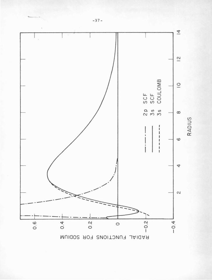
Figures IV-Aand IV- B illustrate the similarities and

differences of the Coulomb and SCF radial functions. Figure IV-A

shows the 3s valence function for sodium as computed by the Coulom.b

approximation using the experimental term value as an eigenvalue,

superimposed on the SCF function of Hartree (28). The SCF Zp

function is drawn also to indicate the position of the core electrons.

It is apparent that SP.rious deviations of the Coulomb function do not

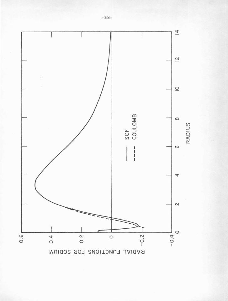
occur until the valence particle is well within the core. Figu1•e IV- B

shows the same 3s function of sodium in the Coulomb approximation

and in the SCF calculation of Biermann (11), which includes polarization

of the core. The agreement is somewhat better in this case, since

the eigenvalues are the same for each function. The polarization

potential in itself only slightly changes the shape of the SCF radial

function, but the associated change in eigenvalue draws the electron

into smaller radii, agreeing more closely with the Coulomb function.

The Coulomb functions used in these comparisons were cal­

culated by the computer program described ln the Appendices. It

should be noted that they are computed numerically from Schrodinger ' •

equation, while Bates and Damgaard use the series representation

given in part A. The result• are the same within the accuracy of the

two methods.

Figure IV-.A

Comparison of the Coulomb with the SCF radial function for the

3 s state of Na I.

- -·

<.0

0 v 0

C\J

0

- 37 -

. J .

I

0

V\lniOOS ~0.:1 SNOil:>Nn.:l

-

l.J... l.J... u u (f) (f)

0. "' C\JJ"{)

C\J

0 I

l'i:tiO 'i1 H

CD ~ 0 ....J :::> 0 u

"' J"()

v 0 I

C\J

0

00

(f)

:::> 0 <t 0::

<.0

C\J

Figure IV-B

Comparison of the .coulomb with the SCF radial function (including

core polarization) for the 3s state of Nal.

w 0

C\J

0

-38-

0

LL u en

(I)

2 0 _J

=> 0 u

C\J

0 I

~n I OOS ~0.:1 SNOil.:)Nn.:l l'itlOtt ~

C\J

0

CX)

w

C\1

0 ..;t

0 I

en => -Cl <t a::

-39-

C. Coulomb, SCF, and Experimental Oscillator Strengtl?e

The Bates-Damgaard approximation should g ive accurate £­

value results for atoms with one valence electron, particularly the alkali

metals , for which the stationary core approximation is moat nearly

satisfied. A great deal of effort, both experimental and theoretical ,

has been expended in the determination of transition probabilities for

some of these .atoms . It will therefore be particularly instructive to

compare the results of experiment and of self-consistent field calcula­

tions with the simple Coulomb approximation. As examples, we will

list and discus s oscillator strengths for Li I, Na I, and Ca II.

1) Li I

M ore than 25 papers dealing with t.heoretical and experimental

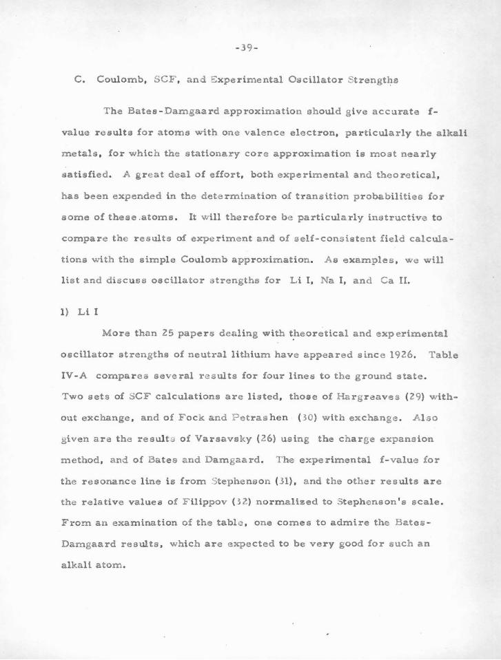
oscillator strengths of neutral lithium have appeared since 1926. Table

IV-A compares several results for four lines to the ground state.

Two sets of SCF calculations are listed, those of Hargraaves (29) with­

out exchange , and of Fock and P etras hen ( 30) with exchange. Also

given are the results of Varsavsky {26) using the charge expansion

method, and of Bates and Damgaard. The experimental £-value for

the resonance line is from Stephenson (31) , and the other results are

the relative values of F ilippov 02) normalized to Stephenson ' s scale .

From an examination of the table , one comes to admire the Bates­

Damgaard results, which are expected to be very good for such an

alkali atom.

-40-

TABLE IV-A

F ock and Bates and Transition Harsreaves Varsavsk:l Petras hen Damsaard Exfe riment

2s-2p 0. 700 0.619 0. 769 o. 750 o. 72 :i. 0 . 03

2s-3p 0.014 0.0358 0.0037 0.00565 0.0055

2s-4p 0.0147 0.0177 0.0035 o. 00501 0 . 0047

2e-5p 0.0051 0.0015 0.00245 0 . 00253

2) Na I

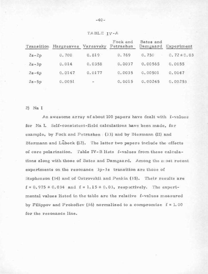
An awesome array of about 100 papers have dealt with £-values

for Na I. Self-consistent-field calculations have been made, for

example, by Fock and Petraehen (3 3) and by Biermann (11) and

Biermann and L;ibeck (12). The latter two papers include the effects

of core polarization. fable IV- B lists £-values from these calcula-

tions along with those of Bates and Damgaard. Among the n ost recent

experiments on the resonance 3p-3s transition are those of

Stephenson (34) and of Ostrovekii and Penldn 05). Their results are

f = 0 . 975 :* 0. 034 and f = 1.15 :t 0 . 03 , respectively. The experi-

mental values listed in the table are the relative £-values measured

by Filippov and Prokofiev (36) normalized to a compromise f = 1. 00

for the resonance line.

Transition

3p-3s

4p-3s

Sp-3s

6p-3s

3) Ca U

-41-

TABLE IV-B

Fock-Petraschen Length .Velocity Biermann

1. 04

0.014

0.97

0.010

0 . 99

0.014

Bates­Damgaard

0 .94

0 . 014

0.0021

0.00064

Experiment

1.0

0 . 0144

0 . 0021

o. 000645

A discussion and analysis of much of the work on Ca II is con-

tained in the thesis of Varsavsky (26). Oscillator strengths for

several lines have been computed in many different ways: by SCF

with exchange, SCF with exchange and core polarization, by the

Coulomb approximation, and by the nuclear charge expansion method.

Studies have been made of the effect of using the dipole length, velocity,

and acceleration forms of the matrix element. The result of using

experimental or calculated transition energies has also been investi-

gated.

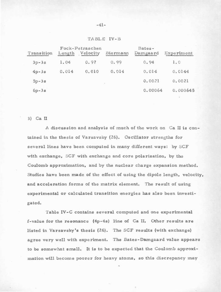
T able IV -C contains several computed and one experimental

£-value for the resonance (4p-4s) line of Ca 11. Other results are

listed in Vareavsky'e thesis (26). The SCF results (with exchange)

agree very well with experiment. The Bates-Damgaard value appears

to be somewhat small. lt ia to be expected that the Coulomb approxi-

mation will become poorer for heavy atoms, so this discrepancy may

-42-

indicate that the method is beginning to fail .

Hartree and Hartree

Green and Weber

Biermann and Trefftz

Vareaveky

Bates and Damgaard

Ostrovskii and Penkin

TABLE IV-C

SCF SCF Other without exchange with exchange Calculations Experiment

1. 42 1.19

1. 3 6 1. 19

1.10

1. 25

0. 93

1. 27

-4J-

V. THS NODAL BOUNDARY CONDITION METHOD

In thi.s section we will introduce a method for calculating wave

:functions , eigenvalues , and transition probabilities. It is·here applied

to atoms and ions with two valence electrons, but the general approach

has wider applications , which will be discussed in Section VI.

The purpose of the previous two sections was partly to review

various theoretical attacks on the atomic structure and !-value prob­

lems , but was also intended to serve as an introduction to some aspects

of the present method. The nodal boundary condition method uses

some of the simplifying assumptions of the Bates -Damgaard approach so

that the calculation of wave functions for the core electrons becomes

· unnecessary. It also uses the Hartree-Fock equations to calculate the

valence wave functions .

Two of the basic assumptions of the Bates-Damgaard method are

that the valence electron m oves in a Coulomb field and that ita eigen­

value is the experimental term value. These two approximations are

very good for the alkali atoms , and are often adequate for other mono­

valent atoms . The support for the assumptions comes from comparison

of Bates - Damgaard Coulomb functions w i th SCF functions, from com­

pari son of experi mental ionization energies with SCF eigenvalues for

such atoms, and from the agreement between Bates-Damgaard !-values

wi th experiment. Neither approximation is valid, however, for more

complex atoms . A valence particle then doe~:~ not move in a Coulomb

field , and its eigenvalues are not necessarily close to experimental

term values, due to the adjustment in position of other valence

-44-

elect rona. Nevertheless the implications of the two assumptions for

monovalent atoms is important for the treatment of more complicated

situationEJ. The Coulomb field approximation means that the valence

electron spends most of the time outside the core. The eigenvalue

approximation implies that the core is nearly unaffected by the position

of the valence electron. These facts are about equally valid for atoms

with two or more electrons outside closed shelle. When combined

with the effect of a deep core potential , they provide the motivation for

the nodal boundary condition method.

In part C of this section the method will be described in detail,

including particular examples . It will be useful at this point to give

a brief outline of the pri n cipal features.

It will first be established that the inner nodes of many valence

radial wave functions are insensitive to their eigenvalues. ThiS is

here called "nodal stability, " and is explained and verified in parts A

and B . The positions of these nodes can be found for any atom with

two electrons outside closed shells by a study of the correoponding

ion with a single valence particle, for which the two Bates -Damgaard

assumptions are valid. Nodal positions are then used as the inner

boundary conditions on the wave functions of the Hartree-Fock equations

for the two-electron situation. This provides s ufficient information to

determine eigenvalues and wave functions. Just as in the Bates­

Damgaard method, these wave functions are adequate outside the core,

but are incorrect at small radii because of our neglect of the true core

potential . Many atomic processes depend almost entirely on the main

-45-

part of th~ valence functions at intermediate and large radii, and this

is the caae with oscillator strengths , if the dipole-moment matrix

element is employed.

A. Nodal Stability

The nodal boundary condition method depends on the near­

independence of node positions w ith energy. For example , the 3s

ground-state radial wave function of sodium has two nodes . "" e will

make use of the fact that the 4a, Ss , • • • excited states of sodium

have nearly the same two inner nodes , the higher levels merely adding

on additional loopo and node a at large radii.

There i m nothing special about using the node positions ; the

slope - to-value ratio of any part of the valence wave .function inaide

the electron core could be used i nstead. The wave functions inside

the core (except for normalization) are almost the same for any degree

of excitation of electrons wi th a given angular momentum. Specifying

the node position is particularly appropriate bec ause it is easily

visualized, and because it ie convenient to use in calculations, involv­

ing a change in s i g n of the wave function.

The i dea of nodal stability can be understood in several ways .

The kinetic energy of a valence electron when it falls into the deep

potential withi n the core is so large that it "forgets " how much it had

when i t was out on the limb of the potential , where i t spends most of ito

time. Looked at in terms of Schrodinger ' s equation

P "(r) = ( V(r) - C) P (r)

-46-

it is seen that if the potential V(r) is large compared to the eigenvalue

.E , t he wave function is nearly independent of E. A small change in

energy of the valence electron, due to excitation, the presence of other

electrons, external fields , or other causes, may radically alter the

outer parte of the valence function, but the inner nodes remain quite

stable . The nodal boundary condition method leans heavily on this

stability. Vv e will use in particular the fact that (for example) the nodes

for the single valence a-electron of Ca II are very close to those for

the two valence s -electrons in Ca I. That is, an atom and its ion

have almost identical core potentials.

U the nodes for a particular atom are found to be stable, two

things are implied. First, that the potential inside the core is large

compared to the eigenvalue. Second, it must be true that the positions

of the core electrons are not much affected by the condition of the

valence particle •

.8efore presenting the evidence for nodal stability, it is neces­

sary to consider just~ much stability is required. For no atom are

the nodes absolutely stable for the whole range of energies for which

data is available. The criterion which will be used is that we should

be able to determine the nodes sufficiently accurately so that varying

their position within the range of possible error produces only a small

change in the calculated .oscillator strength. This means also that the

change in calculated eigenvalues for a two-electron function will be

small.

The first line of evidence for nodal stability comes from all

previoualy calculated !iartree and Hartree-Fock functions. Many

-47-

atoms and ions, both ground and excited states, have been solved by

the full self-consistent field method. Vi e may investigate the positions

of the nodes for such an atom for electrons of a particular angular

momentum ( :~ , p , d , •.. ) . The known results for several atoms and

ions having one or two ground-state ."s " or "p" electrons are given

in Table V-A. In brief, one finds that atoms or ions having one or two

"s" or "p " electrons outside closed "p " shells are particularly stable.

Because of the large centrifugal potential which tends to reduce the

deep central potential well, "d" electrons and those of higher angular

momentum do not usually have sufficiently stable nodes. It is only for

heavy atoms that the method can be used for "d" electrons, since in

this case the potential is large enough. Atoms with "s" or "p " electrons

outside closed "d" shells are not as stable as those outside closed "p"

shells. This i s due to the fact that t h e "d'' shell is quite sensitive

(owing to the shallow potential in which it moves) to movements of the

valence electrons. This in turn changes somewhat the potential acting

on the valence particle, thus changing their nodes.

Vv e can leave to experimental term-values (and the criterion

previously mentioned) whether a given d10

s or d10

s2

atom (e . g. Cu I,

Zn II) can be treated by the nodal boundary condition method. One or

two electrons outside a closed " s " shell (e. g . AlI, SiR) are rather un­

stable, probably due to the influence of the valence particle s on this

a-shell. In this case the important influence i s not due to the potential

in which the inner shell moves, which in the case of an a-shell is very

deep, but is due rather to there being only two particlee in the shell ,

-48-

so that a perturbation in the potential can have a relatively large

effect. For an inner p-shell , a small change in potential is less ef­

fecti ve in moving the electrons , as a change in one of the six tends to

shield the others from further change.

The second line of evidence for stable nodes, which serves to

find the atoms for which the method can be used, and also the "Coulomb

node " positions , comes from experimental term values for atoms and

ions with one valence electron. This procedure will be discussed in

part B.

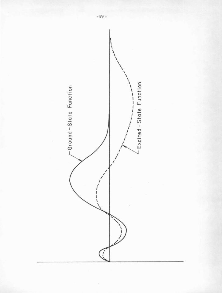
From the available SCF data and the Coulomb node results to

be given in part B , it is apparent that for most atoms the shift of

inner nodes i s small , if an electron is excited or i£ another valence

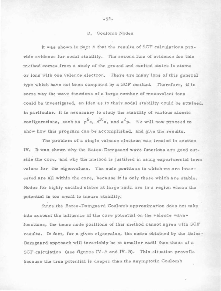
electron is added. The direc tion of these shifts are easily understood.

For a monovalent ion, the greater the degree of excitation, the more

the n odes shift inward (see figure V-A ). For smaller binding energies ,

the quantity IV - E I becomes larger, increasing t h e curvature of the

radial function for small radii, and decreasing it for large radii past

the classical turning point V = E . Therefore for smaller binding

energi es, the nodes move inward. The addition of another electron

produces two eff~cts . Firat of all , the valence binding energies are

different, and less than that of the single electron in the ion ground­

state; therefore the nodes will shift inward slightly. Secondly, the

introduction of another electron, particularly an " s " electron, produces

an added shielding on the original electron which was not present in the

ion. That is, a certain amount of the wave function of the new electron

F igure V -.A

A schematic diagram showing a ground -state and an e xcited-state

(.t = 0) radial wave function for a monova lent ion. T he figure

illustrates the near -independence of the node positions with

excitation energy, and also the direction in which deviations occur.

-49-

\ \ \ \ \ \

\

' \ \ \

' c \ 0 c

0 \ -- \ (.)

' c ::l

(.)

I u.. c ::l

u.. , Q) I -I 0

Q) - I -(f) 0

I -I I (f)

-,:J I I Q)

I --,:J c

I (.) ::l

I >< 0

/~ "-

(.!)

I I

I /

/ /

I I

I I , I \

' '

-50-

is inside the core. which means that the first electron docs not move

in exactly the same core potential as before. In turn. the original

electron shields the added electron more than one would expect from

the ionic situation. The effect of this shielding is to reduce the net

core potential a certain amount. which will be small for the medium-

to-heavy atoms possessing nodal stability. But the reduction in core

potential pushes the nodes outward slightly. Therefore the correct

nodes for a neutral atom are somewhat further out (about 1 %) than what

one would deduce from an interpolation of the energy versus node curve

obtained from the ionic functions. For example. Hartree and Hartree

(37) have calculated wave functions for Ca II (3p64s) and for Ca I

(3p64e2

). As taken from Table V-A. the outermost s-node for Ca II

(4e) is at r = 1. 433 corresponding to an energy £ = 0. 8295 Ryd,

while the node of Ca I (4s 2) is at r = 1. 442 for £ = 0. 3891. If

there were no added shielding, the s 2 node would have shifted inward

slightly.

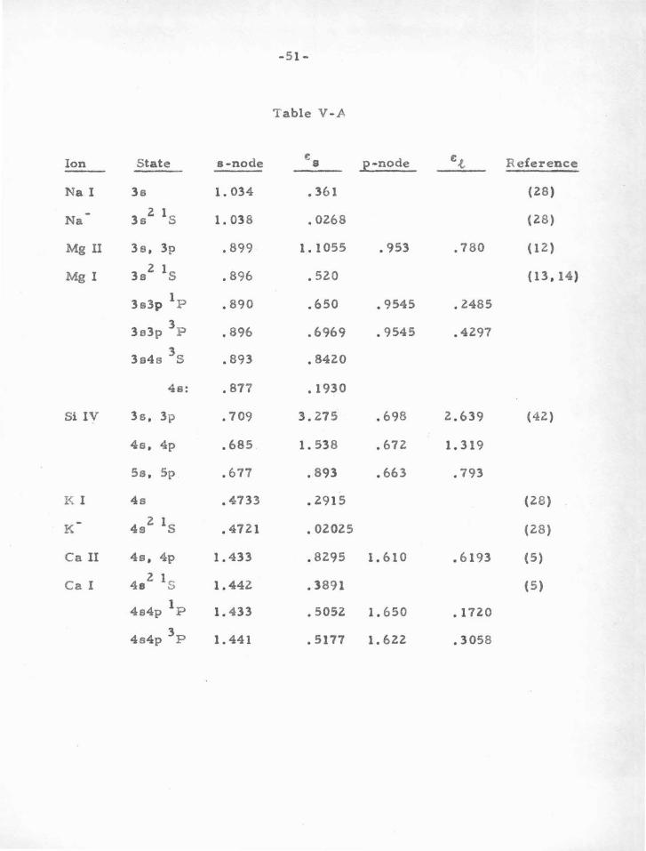
Table V-.A presents the SCF node positions for Na I, Na-.

Mg I. Si IV, K I, K -. Ca II, and Ca I. as taken from the wave functions

published by various investigators. These results provide an idea of

the nodal stability to be expected when moving from the ground state

to excited states of atoms with one or two valence electrons, and also

indicate the expected stability when passing from ionized to neutral

atoms.

-51-

Table V-A

Ion State a-node .:8 p-node f;.t Reference

Na I 3s 1. 034 .361 (28)

Na 3s2 1s 1. 038 • 0268 ( 28)

Mg n 3e, 3p .899 1. 1055 • 953 .780 ( 1 z.)

Mg I 3s2 1s .896 • 520 (13, 14)

1 3s3p P .890 .650 • 9545 .2485

3 3e3p P .896 .6969 • 9545 .4297

3 3s4s S .893 .8420

4s: .877 .1930

Si IV 3s, 3p • 709 3.275 .698 2.639 (42)

4s, 4p .685 1. 538 .672 1. 319

Ss, 5p .677 .893 .663 .793

K l 4s • 4733 .2915 (28)

K 4s2 1s • 4721 • 02025 (28)

Ca II 4s, 4p 1. 433 .8295 1. 610 .6193 (5)

Ca I 4e2 1s 1. 442 .3891 (5)

1 4s4p P 1. 4 33 • 5052 1.650 .1720

3 4s4p P 1. 441 • 5177 1. 622 • 3058

-52-

B . Coulomb Nodes

It was shown in pa,rt .A that the results of SCF calculations pro-

vide evidence for nodal stability. The second line of evidence for this

method comes from a study of the ground and excited states in atoms

or ions with one valence electron. There are many ions of thie general

type which have not been computed by a SCF method. Therefore , if in

some way the wave functions of a large number of monovalent ions

could be investigated, an idea as to their nodal stability could be attained.

In particular, it is necessary to study the stability of various atomic

6 10 2 configura tione, such ao p s , d s , and a p . We will now proceed to

show how this program can be accomplished, and give the resulto .

The problem of a oingle valence electron was treated in section

IV. It was shown why t!le Batee -Damgaard wave functions aro good out-

side the core, and why the method is justified in using experimental term

values for the eigenvalues. The node positions in which we are inter-

ested are all within the core , because it ie only these which are stable.

Nodes for highly excited states at large radii are in a region where the

potential is too small to insure stability.

Since the Batee - Damgaard Coulomb approximation does not take

into account the influence of the core potential on the valence wave-

functions , the inner node positions of this method cannot agree with SCF

results . In fact , for a given eigenvalue, the nodes obtained by the Bates-

Damgaard approach will invariably be at smaller radii than those of a

SCF calculation (see figures IV - A and IV- B) . This situation prevaih

because the true potential is deeper than the asymptotic Coulomb

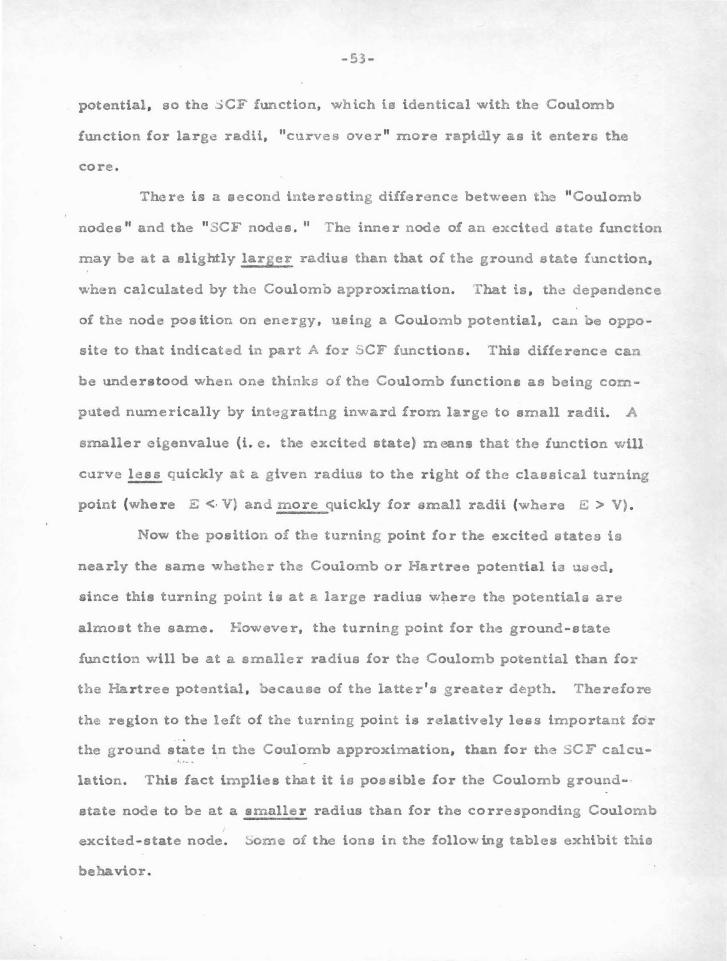
-53-

potential, so the .:)CF function, which is identical with the Coulomb

function for large radii, "curves over" more rapidly as it entera the

core.

There is a second interesting difference between t~ "Coulomb

nodes " and the " SCF nodes . 11 The inner node of an excited state function

may be at a slightly larger radius than that of the ground etate function,

when calculated by the Coulomb approximation. That is , the dependence

of the node position on energy, using a Coulomb potential, can be oppo­

site to that indicated in part A for SCF functions . This difference can

be underatood when one thinks of the Coulomb functions as being com­

puted numerically by integrating inward from large to small radii. A

smaller eigenvalue (i.e. the excited state) mean• that the function will

curve !!:.!.!, quickly at a g iven radius to the right of the classical turning

point (whe r e E <· V} and more quickly for small radii (where E > V) .

Now the position of the turning point for the excited statea is

nearly the same whether the Coulomb or Hartree potential i a used,

since this turning point is at a large radius wl;lere the potentials are

almost the same. However, the turning point for the ground-state

function will be at a smaller radius for the C oulomb potential than for

the Hart ree potential , because of the latter ' s greater depth. Therefore

the region to the left of the turning point is relatively less important for

the ground state in the Coulomb approximation, than for the SCF calcu­

lation. This fact implies that it is possible for the Coulomb ground­

state node to be at a smaller radius than for the corresponding Coulomb

excited-state node. ~me of the ions in the following tables exhibit thio

behavior.

-54-

One of the purposes of these calculations wao to investigate the

validity of the nodal stability approximation for various kinds of atoms

10 6 2 . (i. e. d s, p s, s p configurations). The second purpose was to find

the nodes to be used in a subsequent two-electron calculation. There

is an apparent ambiguity in the eigenvalue to be used for "p" and "d"

electrons, since there are two states for each c:onfiguration, corre-

sponding to j = I :t 1/2. For example, the splitting of the p - wave

2P

1; 2 and

2P 3; 2 states, caused by the spin-orbit interaction, is small

for the lightest atoms, but becomes very significant for heavier atoms .

U we were only interested in testing nodal stability, we could merely

conoietently use just one function, e . g . 2Pl/Z' and use the experimental

term values for this state. However, since we wUl use the nodes for

two-electron calculations, the absolute values of the nodes are needed.

So it ia an important mattcar to find the right choice of p - and d-wave

eigenvalues .

This problem is not difficult to solve, because evidently we

should use the energy corresponding to the absence of the spin•orbit

interaction. That ie, the correct zero-order valence radial function

would be an eigenfunction of the Hamiltonian including only the central

potential . A better wave-function and eigenvalue could then be obtained

by using the spin-orbit interaction in perturbation theory. This new

wave function, however, would no longer be the product of radial and

angular parts, but would be a mixture of many such functions. It there-

fore only makes sense to find a particular radial function from an eigen-

value corresponding to the purely central potential. This e i genvalue is

-55-

the "center-of-mass" of the experimental en~ rgics of th~ etat~s

2 2 P l/Z, "J/2. for a p-electron, or D 3; 2 , S/l for a d-electron.

The well-known relation for computing the spin-orbit matrix

element between eta tee of definite L, S, and J is

from which one finds

2 -- 2 3 < D3/2 I i . 8 I D3/?. > = - '!

2 -- 2 < '(" S/2 I .t • 8 I DS/2 > = 1 •

These matrix ele~nts are proportional to the firot-order energy

splittin g . Therefore the eigenvalue for a p-electron in the abs~nce of

a spin-orbit interact ion will be

where E ( ~) and ....:. ( ~) are the experimental 2Pl/Z and

2P 3; 2

energies. The eiJenvalue for a d-dectron is

The following tables present eigenvalues and Coulomb nodes for

32 monovalent atoms and ions. The nodes were found for the lowest

-=~-

three or four s, p, and d states except v•hen P.xperimental energies

were lacking. r:xcited states in general have more than one Coulomb

node : in thiD case the innermoflt node position is given first. \\ henever

there is a significant p- o r d-wave spin-orbit splitting, three energies

are quoted: that cot·responding to j = 1 + 1/2, the "center of mass"

energy, and that corresponding to j = t - 1/2, in order. In every caoe

the center-of-mass energy was used for the eigenvalue in the calcula-

tion. The first table gives the results for hydrogen and ionized helium.'

Since these wave functions are known exactly, a comparison with the

computed nodes givea an indication of the accuracy of the numerical inta -

gration. For convenience of analysis, the remaininG atoms and ions are

collected into three g roupo : those whose ground states have the configura-

6 2 10 2 . tions p s (or s s ' ) , d s , and s p respectively. At the beginmng of

each group, a discus s ion will be given of the reoults obtained.

1. Hydrogen and Ionized Helium

\V ave functions for hydrogen and ionized helium were computed

in order to test the accuracy of the numerical method used in the com-

puter program. As evidenced by the cloee agreement between exact and

calculated nodes , as given in the next table , the method is sufficiently

accurate for s- and p-wave ele ctrons . The only significant discrep-

ancies occur for d-wave nodes close to the origin, where the rapidly

varying centrifugal potential l ( .t +l)/r2

introduces considerable truncation

error. Therefore d-electron wave functions must be computed with

caution, and small-radii Coulomb nodea considered unreliable .

-57-

Calculations were performed for a variety of spacings and

maxim urn radii, but the node positions for s- and p-wave fWlctions

varied a negligible amoWlt unlesa the spacing became so large that

trWlcation error was important (h c spacing ;:; 0 . 1) .

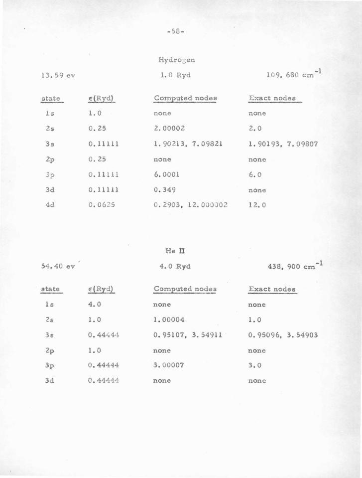
-58-

Hydroeen

13. 59 ev 1. 0 Ryd 109. 680 em ·1

state €~R:X:d) ComEuted nodes Exact nodes

ls 1.0 none none

2s 0.25 2.00002 2. 0

3s 0.11111 1. 90213. 7.09821 1. 90193. 7.09807

2p 0.25 none none

3p 0.1 1111 6.0001 6. 0

3d 0.11l.ll 0.349 none

4d 0.0625 o. 2903 . 12. 00JJ02 12. 0

He II

54.40 ev 4. 0 Ryd 438. 900 em -1

state E'~R:x:d2 ComEuted node.~ Exact nodes

1s 4.0 none none

ls 1.0 1.00004 1.0

3s 0.444-44 0.95107. 3. 54911 o. 95096. 3.54903

2p 1.0 none none

3p 0.44444 3.00007 3.0

3d 0 . 44444 none none

-5') -

7 ./.lkc:.li J. torr.o

:1) L i I, •. h II, ..;. III (1./? s confi., uration)

_'her,~e thrc~ i onu bave fa irly atabh, s.-noc.lcs , out the p - ancl

d - wave Coulomb nodet: are n o t Duffi cicntly sta~lc to uoe for a tv.o -

electron calcula tio._. fhis instability i s c aus'3d ..JY th.:! fa c t that t he -.

ir.ncrmo iJt p - and .:1 - v.eve nod.':Js c.r.:: far outsi.J...! th_. tirty l sL core.

2 .i-1s a r~:;ult , t!'l...: 2o eround- atate enerziea end wave f u nctions of B.-! I

U41cL .iJ II C<.!:l b.; computed, but C' 1Y tranli i t ion proi:,)co oilit iev calc ulated

!:>y the n odal boun-1<:: ry condition metnod would be t.mrcliabla .

b) Na. I, • ~6 II, ~.t III 2

(?I, ... ~s)

K I, Ca II, _c III 6 ( 5 t') tls)

r~ b 1, ~ r II, Y III (4p 6- • :;a I

Cs I, ba II, La III 6

(5p 6!:i)

Theol.! i ons ~xnibit great~r nodal stability than any other troup.

h 1 g~neral the stability i s gr.!ater for ti1~ heavbr than for the lighter

....Jem·~nta , ao that even th.:: d - utat~::J bec ome fa i r ly stabl e by th~ t ime

one reaches b ariuJn . The r efore , in pri n ciple , o.;Jcillator strengths

can be c ompated for :; - p transit~onfl of nll the corresponding two-

c L::c tron atoms. :-Io,·.over, the experimental term v alu.no are not suf-

! i cier tly c omplste for .... c III, Y III, o r La III, bO that Coul o mb nodes

cannot be a ccurately dctcrrr~inecl for these ions . f r aneitior.. probuoilitiev

v.. ~r-:! computed for !\~!; I , i\::. II, Ca I, "r I , and Ba I.

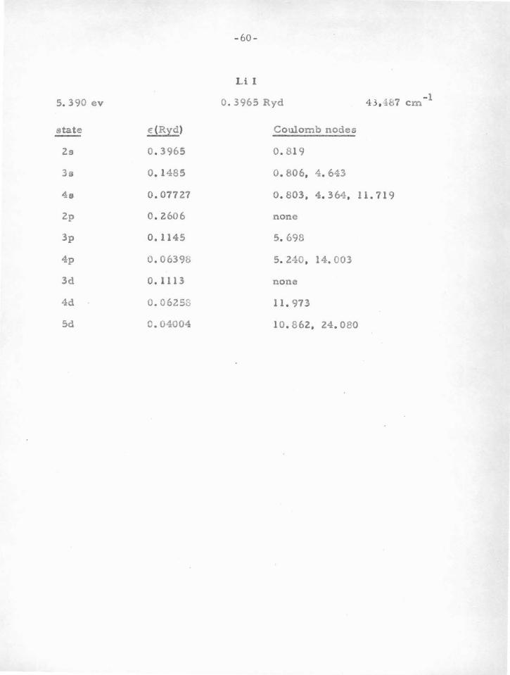
-60-

Lil

5. 390 ev 0. 3965 Ryd 43, H~7 em - 1

state € (Ryd) Coulomb nodes

ls 0 . 3965 0 . 819

3s 0 .1485 o. 806, 4 . 643

4 s 0.0772.7 o. 803, 4 . 364, 11.719

2p o. 2606 none

3p 0.1145 5 . 698

4p 0 . 06398 5 . 240, 14. 003

3d o. 1113 none

4d o. 06253 11. 973

5d 0.04004 10.862, 24. 080

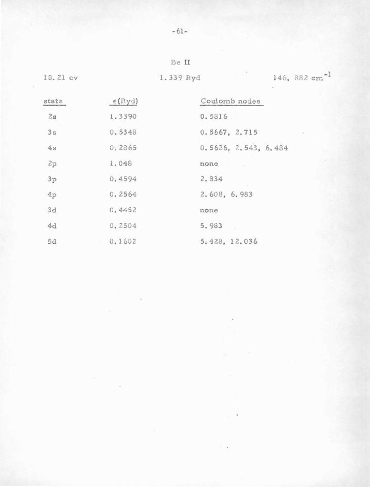
-61-

Be II

18. 21 ev 1. 339 Ryd 146, 882 em -1

state dRx.J> Coulomb nodes

2s l. 3390 0.5816

3s 0.5348 o. 5667. 2. 715

4s 0.2865 o. 5626, 2. 543, 6.484

2p 1.048 none

3p 0.4594 2.834

4p 0 . 2564 2. 608, 6.983

3d 0 . 4452 none

4d 0. 2504 5.983

5d 0 . 1602 5. 428 , 12. 036

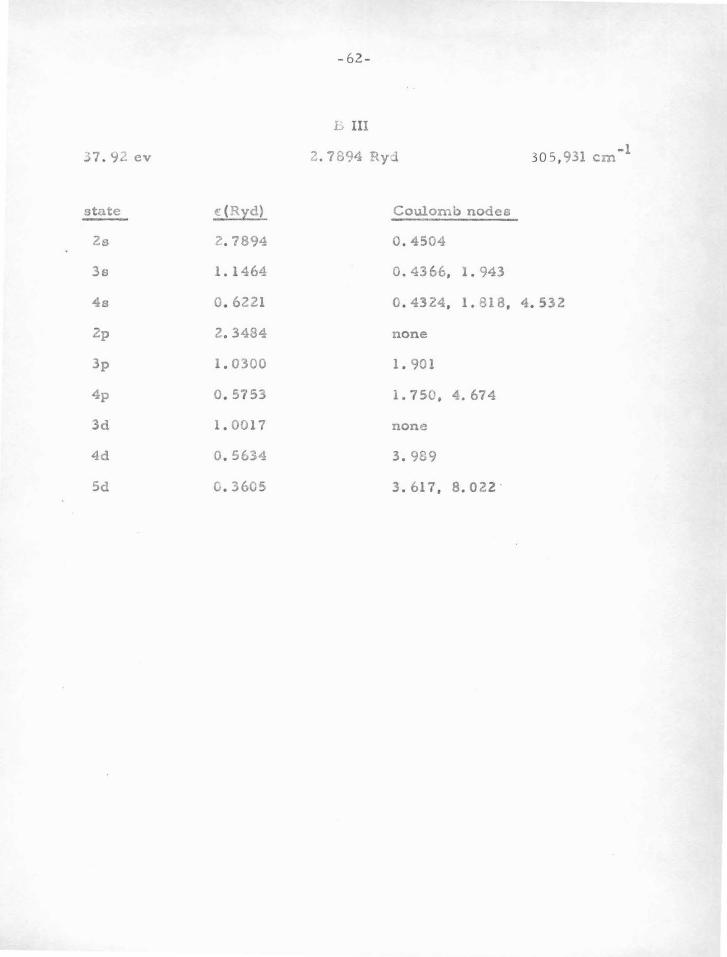
- 62-

L III

37 . 92 ev 2. 7894 Ry:i 30 5, 931 em - 1

state dRX:d) Coulomb nodes

2s 2. 7894 0 . 4504

3s 1. 1464 o. 4366, 1 . 943

4s o. 6221 o. 4324, 1. 818, 4 . 532

2p 2. 3484 n one

3p 1. 0300 1 . 901

4p o. 57 53 1. 7 so, 4. 674

3d 1. 0017 none

4d 0 . 5634 3. 989

Sd o. 3605 3 . 617 , 8 . 022

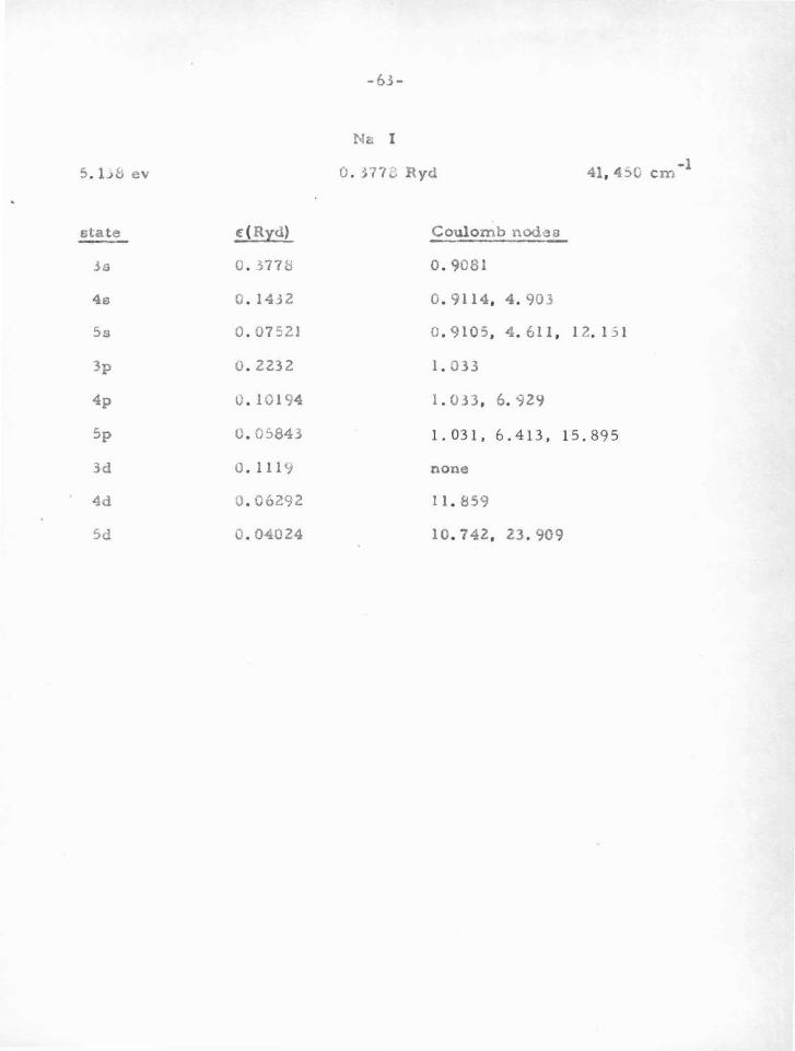
-63-

Na I

5 . 1->8 ev 0 . j77& Ryd 41 , 4:,0 em -1

state t:( Ryd) Coulomb nodeo

3s 0 . 377S 0 . 9081

4s 0 . 1432 o. 9114, 4 . 903

Sa 0 . 07521 o. 9105, 4 . 611 , 12. 1 51

3p 0 . 2232 1. 033

4p u. 10194 1.033, 6. 929

Sp O. OS843 1. 031, 6.413, 15.895

3d O.lll <J none

4d 0 . 06292 11. 859

Sd 0 . 04024 10. 742 , 23.909

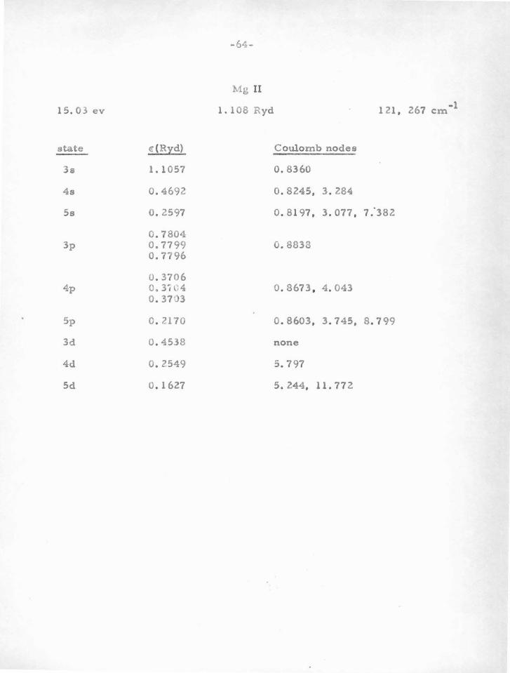
-64-

Mg II

15.03 ev 1. 108 Ryd 121 , 267 em -1

state €(Rid) Coulomb nodes

3s 1. 1057 0.8360

4s 0.4692 o. 8245, 3. 284

5s 0.2597 0.8197, 3.077, 7."382

0 .7804 3p 0.7799 0.8638

0 .7796

0 . 3706 4p o. 3i l 4 o. 3673 . 4 . 043

0 . 3703

5p 0 . 2170 o. 8603, 3. 745, s. 7 99

3d 0.4538 none

4d 0 . 2549 s. 797

5d o. 1627 5. 244, 11. 77 2

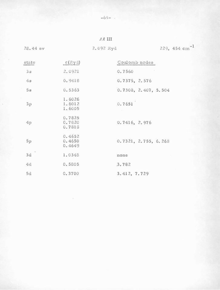
- 65- .

A £ III

28. 44 ev 2. 092 Ryd 229, 454 em -1

state c ( .P.}::l) Coulomo nodes

3s 2. 0921 0 . 7560

4s 0 . 9418 o. 7375, z. 576

Ss o. 5363 o. 7 308, 2 . 407 , 5. 504

1. 60 26 3p 1. 6012 o. 7651

1. 6005

0 . 7825 4p o. 7820 o. 7416, 2 . 976

0 . 7818

0.4652 5p 0 . 4650 o. 7321 , 2 . 7 55, 6 . 268

0 . 4649

3d 1. 0348 none

4d 0 . 5805 .3 . 782

5d 0 . 3700 3 . 4 1 2, 7 . 729

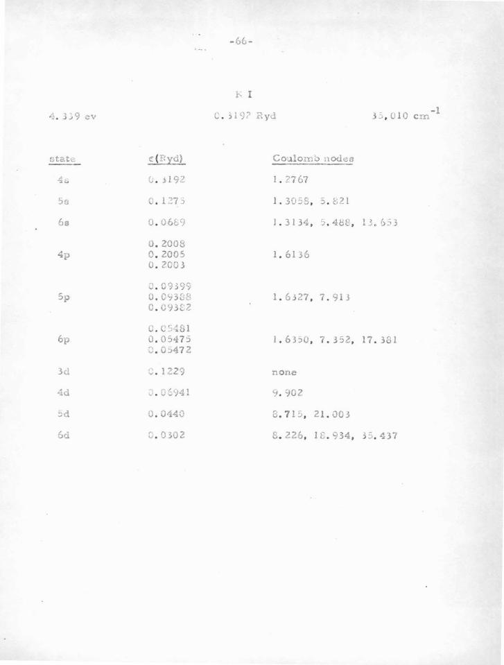
.. '1 . J~9ev

stat-.:: ~ ( Ryd)

4 :.. t.: . >192.

5s 0 . l ?.7 5

6s j . 06&')

o. 2008 4p 0 . 2005

0 . 2003

v. C'H99 5p O. C73G8

0 . 0)3[:2

C. C S-~8 1

6p 0 . 05475 :., . Qj472

3d ., . 1229

4..:1 : . ~~)41

5d J . 0140

6d 0 . 0302

-66-

1·, I

c . ) 19? ~yd

Co;.1lorr.~ .1od~e

I • ""'7 67

1 . 3Q.JS . :, . C.21

1.3134. .;; . 4~e .

1. 61 .36

1. 6J27 . 7 . 91 3

1.63:>0. 7 . 3 ~2.

none

9. 902

c. 7l .J . 21. 001

s. 226. 1£.934.

-1 .L . • LlO em

1;. 6.53

17 . 3G 1

E . ~37

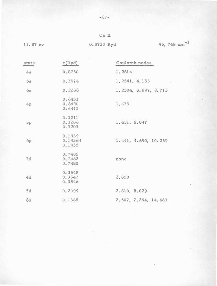
11 . 87 ev

state E{Ryd)

4s 0. 8730

Ss 0. 3974

6s 0. 2286

0. 6433 4p o. 6420

0. 6413

o. 3211 5p 0. 3206

0. 3203

0. 1939 6p 0. 19364

o. 1935

0. 7485 3d 0. 7482

0. 7480

0. 3548 4d 0. 3547

0 . 3546

5d 0. 2099

6d 0 . 1388

- 67 -

Ca II

0 . 8730 Ryd

Coulomb nodes

1. 2614

1. 2541, 4.155

1. 2504, 3. 897 ,

1. 473

1. 451 , 5. 047

-1 95, 748 e m

8. 7 15

1. 441 , 4.690 , 10 . 259

none

2. 850

2. 610, 8.029

2. 507 . 7 . 294, 14.683

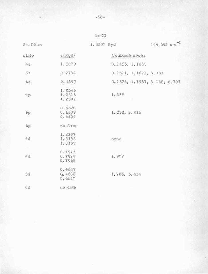
-68-

..;C III

24. 7 5 ev 1. 8207 Ryd 199, S93 ern -1

state E:(Ryd) C oulomb nodes

4:a 1. 5579 o. 1355, 1. 1869

::-,s 0 . 7734 0 .1 511 , 1.1621, 3.383

6s 0 . 4599 0 .157 6, 1.1 553 , 3. 168, 6.707

1. 2545 4p 1. 2516 1.328

1. 2502

0 . 6520 Sp o. 6509 1. 292, 3. 916

0 . 6504

6p no data

1. 8207 3d 1. 8196 none

l.S1C9

o. 7972 4d o. 7970 1. 907

o. 7968

0 . 4:689 Sd <+ 4680 1. 785, s. 414

0 . 4:687

6d no dv.ca

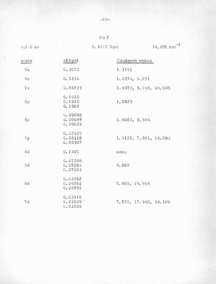
-69-

Rb 1

4.1• 6 ev 0. 3072 Ryd 33, 691 em -1

s late e! ( Ryd) Coulomb nodeo

Se 0. 3072 1. 3741

6a 0. 1236 1. 4274, 6.091

7s o. 06729 1. 4376, 5. 746, 14. 085

0. 1925 5p 0 . 1910 1. 8829

o. 1903

u. 09096 6p 0 . 09049 1. 9083 , 8 . 384

0.09025

0. 05339 7p o. 05318 1. 9121 , 7. 801 , 18. 083

0. 05307

4d 0. 1307 none

o. 01286 5d 0. 07284 9. 007

0 . 07283

o . 04562 6d 0. 04561 7. 955, 19. 914

0. 04561

0 . 03110 7d o. 03109 ' 7. 521 , 17 . 968, 34. 100

C. 03108

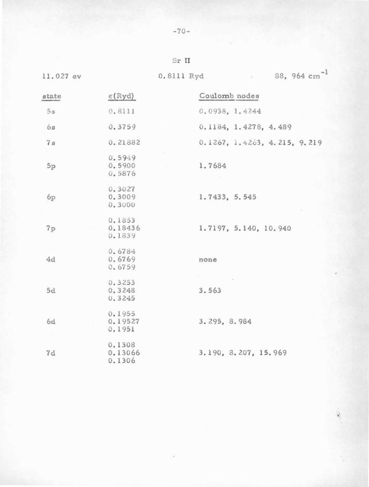
-70-

Sr II

11.027 ev 0. 8111 Ryd 88, 964 em -1

a tate €(Rid) Coulomb nodes

Ss 0. 8111 o. 0938, 1. 4244

6s 0. 375-J o. 1184, 1. 4278, 4.489

7a 0.21882 0.1267, L 4263 , 4. 215, 9. 219

0. 594.9 Sp 0.5900 1. 7684

u.E>876

0. 3U27 6p 0. 3009 1. 7433, 5. 545

0.3UOU

0.1853 7p 0. 18436 1. 7197. 5.140, 10. 940

0 .1 839

o. 6784 4d 0.6769 none

o. 6759

0.3253 5d 0.3248 3.563

0.3245

0.1955 6d 0.19527 3. 295, 8. 984

0 . 1951

0.1308 7d 0.1 3066 3. 190, 8. 207' 15. 969

0.1306

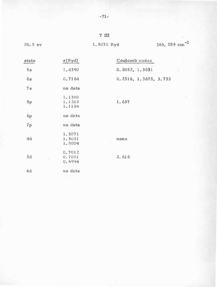
-71-

Y .Ill

20. 5 ev 1. 5070 Ryd 165p 289 em -1

state E(Ryd) Coulomb nodes

5e 1 . 4390 o. 2052, 1. 3831

6s o. 7164 o. 2316, 1. 3678, 3.753

78 no data

1. 1300 5p l. 1203 1. 637

1.1154

6p no data

7p no data

1. 5071 4d 1. 5031 none

1.5004

0.7012 5d 0.7001 2.616

0 . 6994

6d no data

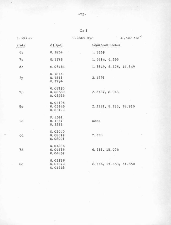
-7Z-

Cs I

3. 893 ev 0. Z864 Ryd 31,407 ern -1

state ~ (Ryd) Coulomb nodes -6s 0. 2864 1. 5669

7a o. 1175 . 1. 6414, 6. 553

Sa 0.06464 1. 6649, 6. 205, 14. 849

0.1844 6p o. 1811 2. 1897

0.1794

o. 08790 7p 0.08680 z. Z327, 8. 943

0. 08625

0. 05195 Bp 0. 05145 2. 2387, 8. 333 , 18.910

0. 05120

0 .1542 5d 0.1537 none

0. 1533

0.08040 6d 0. 08017 7.338

0 . 08001

0.04886 7d 0.04875 6. 617 , 18.006

o. 04867

o. 03279 Sd 0. 03272 6. 336, 17. 353, 31 . 850

0. 03268

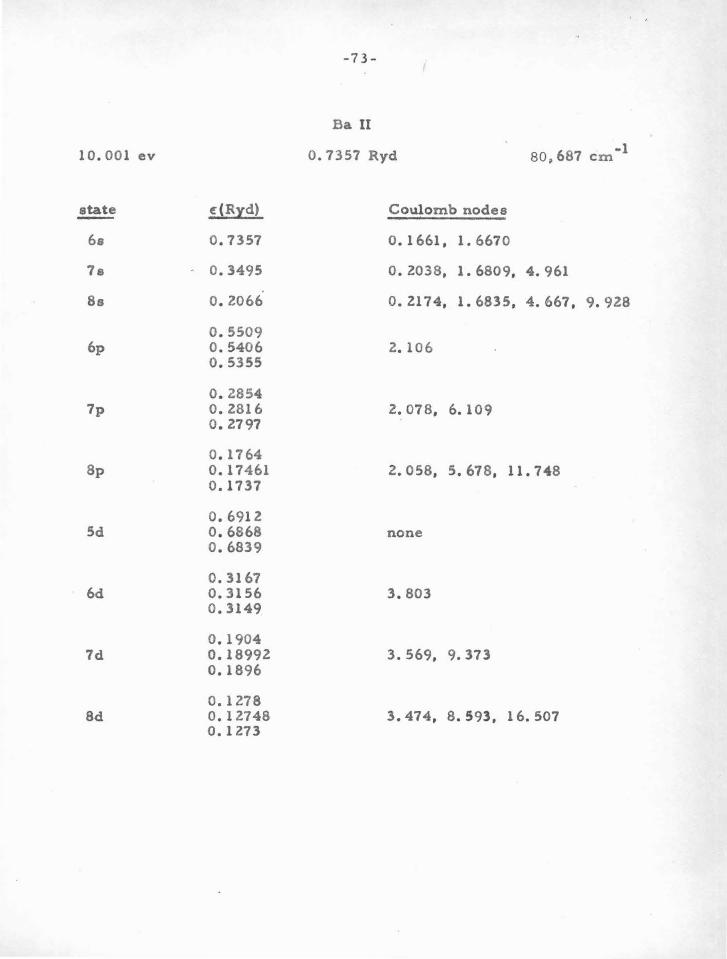
-7 3-

Ba II

10.001 ev O. 7357 Ryd 80,687 em -1

state ~~Rid) Coulomb nodes

6s 0.7357 o. 1661, 1. 6670

7s . 0.3495 o. 2038, 1. 6809, 4. 961

8s 0.2066 o. 2174, 1. 6835, 4. 667. 9.928

0.5509 6p 0.5406 2. 106

0.5355

0.2854 7p 0.2816 2. 078, 6. 109

o. 2797

o. 1764 8p o. 17461 2.058, 5.678, 11.748

0.1737

0.6912 Sd o. 6868 none

o. 6839

o. 3167 6d 0.3156 3.803

0.3149

0.1904 7d 0.18992 3. 569, 9. 373

0.1896

0.1278 8d 0.12748 3.474, 8.593, 16.507

o. 1273

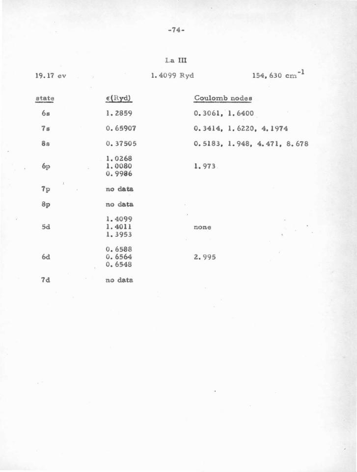
L a Ill

19.17 ev 1. 4099 Ryd 154,630 e m -1

state E(Ryd) Coulomb nodes

6s l.Z859 o. 3061 f . 1. 6400

7s 0.65907 0.3414, 1.6ZZO, 4.1974

8s 0.37505 o. 5183, 1.948, 4.471, 8.678

1. OZ68 6p 1.0080 1. 973

0.9986

7p no data

8p no data

1. 4099 5d 1. 4011 none

1.3953

0.6588 6d 0.6564 Z.995

0.6548

7d no data

-75-

3. CuI, Zn U, Ga III (3d104s)

Ag I, Cd II, In III (4d10ss)

Au I, Hg II, Tliii (Sd10 6s)

On the whole, the Coulomb nodes for this group of ions are not

6 aa stable as those for the alkali methals with the p s ground-state

configuration. As previously explained, this i8 due to the sensitivity

of the d10 shell to the excitation energy of the valence electron. Some

wave functions and/or transition probabilities were calculated for all

of the following two-electron ions: Zn I, Ga II, Cd I, In U, Hg I, and

Tl II. In some cases, either the p- or d-wave states were unstab~e

or the experimental term-values inadequate.

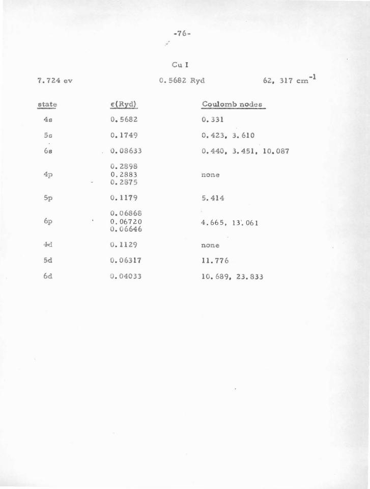
- 76-

Cu I

7. 724 ev 0. 5682 Ryd 62, 317 ern - 1

state E(Ryd) Coulomb nodes

4s o. 5682 0 . 331

Ss 0.1749 o. 423, 3. 610

6s 0 . 08633 o. 440, 3. 451 . 10.087

0 . 2898 4p 0.2883 none

0 . 2875

5p o. 1179 5. 414

o. 06868 6p o. 067 20

0 . 06646 4. 665, 13 ·. 061

4d o. 1129 none

5d o. 06317 11.776

6d 0 . 04033 10. 689, 23.833

-77-

Zn II

17. 96 ev 1. 3211 Ryd 144, 891 em -1

state dRyd} Coulomb nodes

4s 1. 3211 0.5972

5s 0.5147 o. 6356, 2. 812

6s o. 2771 o. 6429, 2. 715, 6. 778

0.8790 4p 0.8737 0.5756

0.8710

0.3969 Sp 0.3954 o. 6286, 3. 643

0.3946

0.2280 6p O. 2Z75 o. 6407. 3. 396. 8. 248

O. ZZ73

0.4375 4d o. 437 2 0.9457

0.4370

O.Z455 Sd o. Z4534 0. 9853, 6. ZOl

O.Z452

o. 1574 6d 0.15731 o. 9878, 5. 649. 1 z. 351

0.1573

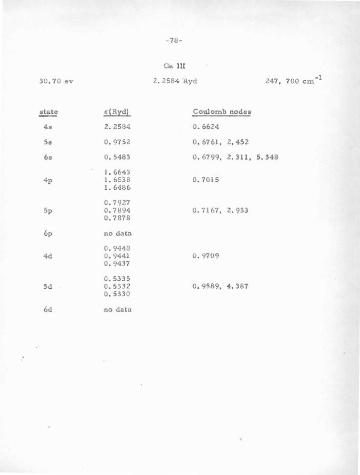
30. 70 ev

state €(Ryd)

4s 2.2584

5s 0 . 9752

6s 0.5483

1. 6643 4p 1. 6538

1. 6486

o. 7927 Sp 0.7894

o. 7 878

6p no data

0 . 9443 4d 0 . 9441

0 . 9437

0 .5335 5d 0 .5332

0 .5330

6d no data

-78-

Ga III

2. 2584 Ryd

Coulomb nodes

0.6624

o. 6761. 2.452

o. 6799, 2. 311.

0.7015

0.7167. 2. 933

o. 9709

o. 9589. 4. 387

c

-1 247 . 700 em

5.348

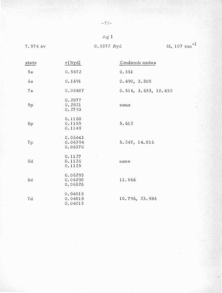
-79 -

Ag I

7. 574 ev 0. 5572 Ryd 61, 107 em -1

state €(Rid) Coulomb nodes

Ss o. 557 2 0. 351

6s o. 1691 o. 490, 3.805

7s 0.08407 o. 516, 3. 655, 10.458

0.2877 5p o. 2821 none

o. 2793

o. 1168 6p o. 1155 5. 612

o. 1149

0.06443 7p 0.06394 5. 24 7, 1 4. 0 1 6

0 .06370

0. 1127 Sd o. 1126 none

o. 1125

0.06295 6d o. 06290 11. 866

0.06826

0 .04018 7d 0.04015 1 o. 796, 23. 986

0.04013

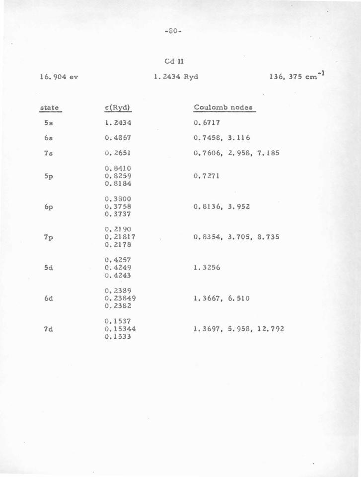
16. 904 ev

state €(Ryd)

Ss 1. 2434

6s o. 4867

7s o. 2651

0.8410 5p 0.8259

0.8184

0 .3800 6p o. 3758

0.3737

0.2190 7p 0.21817

0.2178

0 .4257 Sd 0.4249

0 .4243

0 . 2389 6d 0 .23849

0 .2382

0 .1537 7d 0 .15344

0.1533

-80-

Cd II

1. 2434 Ryd ·1 136, 375 em

Coulomb nodes

o. 6717

o. 7458, 3. 116

o. 7606, 2. 958, 7.185

o. 7 271

o. 8136, .3. 952

o. 8354, 3. 705, 8. 735

1. 3256

1. 3667, 6. 510

1.3697, 5.958, 12.792

28. 03 ev

state €(Ryd)

5s 2. 061S

6s 0 . 9047

7s o. 5167

1. 5401 5p 1. 5138

1.5006

0.7432 6p 0. 7351

0.7310

0.4153 7p o. 4116

0.4098

0.8903 Sd 0.8887

0 . 8877

o. 5067 6d 0.5057

0 . 5050

0. 3288 7d 0 . 3283

o. 3279

-81-

In III

2. 0615 Ryd -1 226, 100 em

Coulomb nodes

0.7752

o. 8130, 2. 725

o. 8219, 2. 577' 5. 776

0 . 880

0 . 912, 3. 270

1.180, 3.480 , 7.375

1. 329

l. 314, 4. 792

1.311, 4.409, 9.150

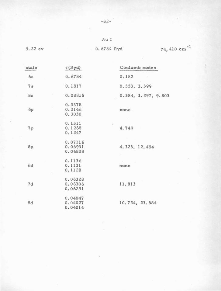
9. 22 ev

state ~(Ryd)

6s o. 6784

7s 0.1817

8s 0.08815

0.3378 6p 0.3146

0.3030

0. 1311 7p 0.1268

0.1247

0.07116 8p o. 06931

0.06838

o. 1136 6d o. 1131

o. 1128

0.06328 7d 0. 06306

0.06291

0.04047 8d 0.04027

0.04014

-82-

J\ u I

0. 6784 Ryd

Coulomb nodee

0.182

o. 353, 3.399

o. 384, 3. 297'

none

4.749

4. 323, 12. 494

none

11. 813

-1 74. 410 em

9.803

10.724, 23.884

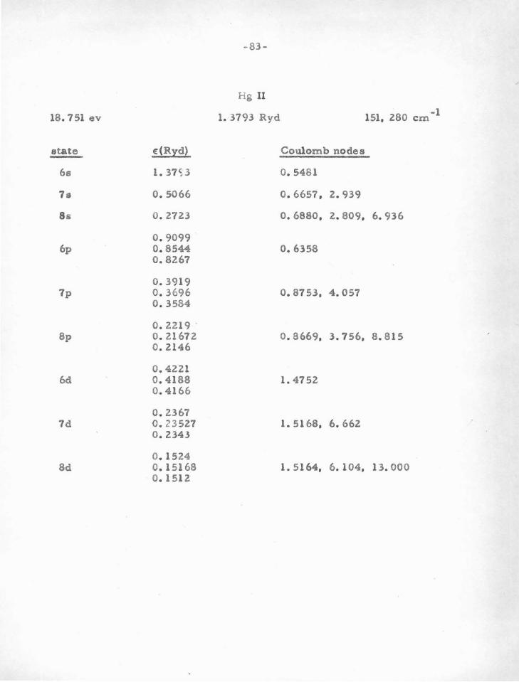
-83 -

Hg II

18. 751 ev 1. 3793 Ryd 151, Z80 em -1

state ~(Ryd) Coulomb nodes

68 1.37~3 0. 5481

7• o. 5066 o. 6657 . Z. 939

8& O. Z7Z3 o. 6880 , z. 809. 6.936

0. 9099 6p 0.8544 o. 6358

0 . 8267

0. 3919 7p 0. 3696 0. 8753, 4.057

0 . 3584

O. Z219 · 8p O. Z167Z 0. 8669. 3.756, 8.815

O.Z146

0. 42Zl 6d 0. 4188 1. 475Z

0. 4166

o. 2367 7d 0. 23527 1. 5168, 6. 66Z

O. Z343

0.15Z4 8d 0.1 5168 1.5164, 6.104, 13.000

0. 1512

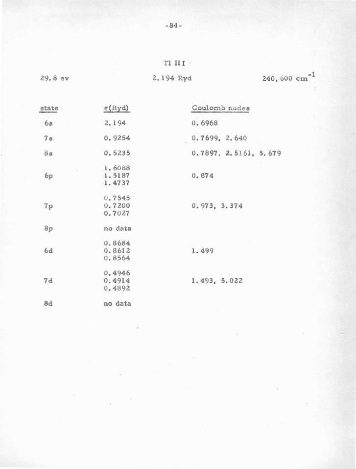
29. 8 ev

state ~(Ryd)

6s 2.194

7s 0 . 9254

8s 0 . 5235

1. 6088 6p 1 . 5187

1 . 4737

0 . 75~5

7p 0 . 7200 o. 7027

8p no data

0.8684 6d o. 8612

0.8564

0 . 4946 7d 0.4914

0 . 4892

8d no data

-84-

T1 II I ·

2. 194 Ryd

Coulomb nodes

0.6968

o. 7699, 2. 640

o. 7897, 2. 51 61·,

0 . 874

o. 973 , 3 . 374

1 . 499

1. 493, 5. ozz

- 1 240, 600 em

5. 679

4 . Bl, en

Al I, Si 11

Ga I, Ge 11

-85-

( Zs2Zp)

(3s2 3p)

(4s24p)

The Coulomb nodes for this group o! ions are found to be lees

stable than for either of the previous groups, except for the •- and

p•wave state a of Al I, Ga 1, and Ge II, and the a-wave state a of Si 11.

Therefore the only reasonably rellab~e transition probabilities that

could be computed for a two-electron situation are those for Ge I. As

a result, no two-electron calculation& at all were made for this group,

because previous theoretical and experimental results are almost ·

entirely lacking. No basis for reliability can be eatablhhed within the

group. There is also evidence that there i s strong interaction betwean

various configurations involving all three of the outer electrons, so

that lt t.s probably not a good approximation to treat these {one as having

z a stationary s shell and one valence electron.

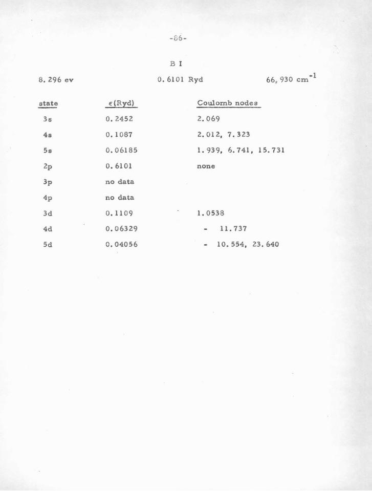
- 86-

B I

8. 296 ev 0.6101 Ryd 66.930 em -1

state dRid) Coulomb nodes

3s 0.2452 2.069

4s 0.1087 2.012, 7.323

5s 0.06185 1. 939, 6. 7 41, 15.731

2p o. 6101 none

3p no data

4p no data

3d o. 1109 1. 0538

4d 0.06329 11. 737

5d 0.04056 10. 554, 23.640

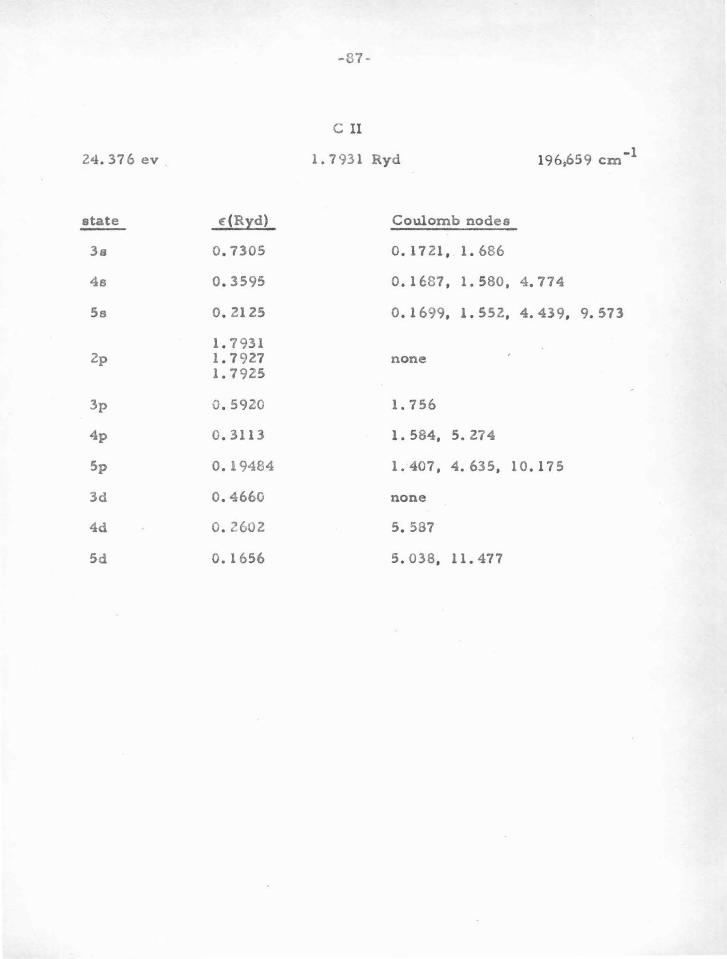
-87-

C II

24.376 ev 1. 7931 Ryd 196,659 em - 1

state £(Ryd) Coulomb nodes

3s 0 .7305 0.1721, 1. 686

4s 0.3595 o. 1687. 1. 580, 4 .774

5s 0.2125 o. 1699, 1. 552, 4. 439, 9.573

1. 7931 2p 1. 7 927 none

1. 7925

3p 0 . 5920 1. 756

4p o. 3 113 1. 584, 5.274

5p 0.19484 1. 407. 4. 635, 10.175

3d 0 . 4660 none

4d 0 . 2602 5. 587

5d 0.1656 5. 038, 11. 477

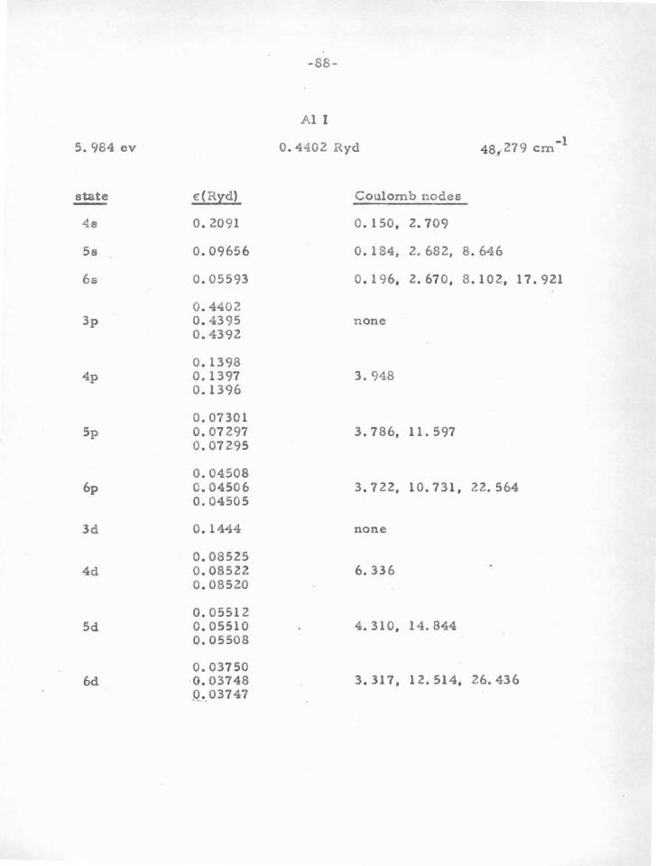
-88-

Al I

5. 984 ev 0. 4402 Ryd 48,-27 9 em -1

state €(Rid) Coulomb nodes

4s o. 2091 o. 150, 2.709

5s 0.09656 o. 184, 2. 682, 8 . 646

6s 0.05593 o. 196, 2. 670, 8. 102, 17.921

0.4402 3p 0.4395 none

0.4392

0.1398 4p 0.1397 3.948

0.1396

0.07301 5p o. 07 297 3. 786, 11. 597

o. 07 295

0.04508 6p 0. 04506 3. 7 22, 10.731, 22.564

0.04505

3d 0.1444 none

0.08525 4d 0 .08522 6.336

0.08520

0.05512 Sd 0.05510 4. 310, 14. 844

0.05508

0.03750 6d 0.03748 3.317, 12.514, 26.436

,Q_._ 03747

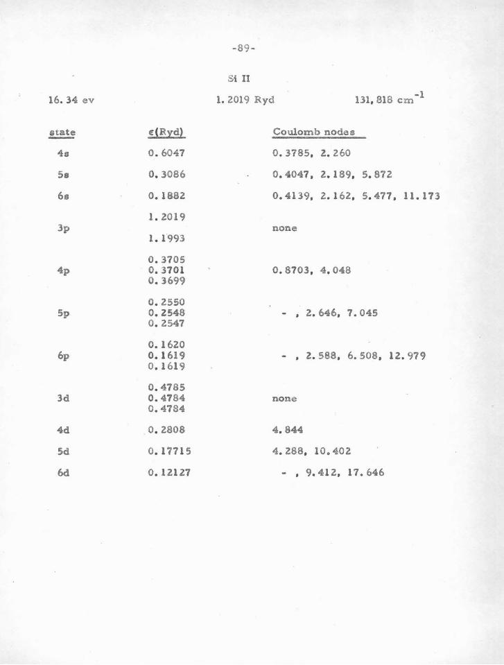
16. 34 ev

4&

Sa

6s

3p

4p

Sp

6p

3d

4d

Sd

6d

~(Ryd)

o. 6047

0. 3086

0. 1882

1.2019

1. 1"993

0. 3705 0. 3701 0. 3699

0. 2550 0.2548 o. 2547

0.1 620 o. 1619 0 . 1619

0. 4785 0 . 4784 0. 4784

0. 2808

0. 17715

0 . 12127

-89-

Si II

1. 2019 Ryd -1 131, 818 em

Coulomb nodes

o. 3785, 2. 260

0. 4047 , 2. 189, 5. 872

0. 4139, 2. 162, 5. 477 , 11 . 173

none

0 . 8703, 4 . 048

- • 2. 646, 7. 045

- • 2. 588, 6. 508, 12.979

none

4. 844

4. Z88, 10o 402

- • 9. 41 2, 17. 646

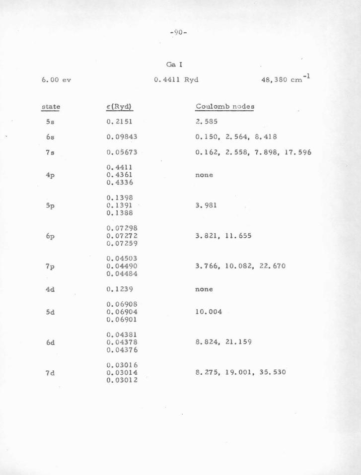
- 90-

Ga I

6. 00 ev 0. 4411 Ryd 48,380 em -1

state t:(Ryd) Coulomb n odes

5s o. 2151 2.585

6s 0.09843 o. 150, 2. 564, 8.418

7s o. 05673 0. 162, 2. 558, 7. 898, 17.596

0.4411 4p o. 4361 none

0.4336

0.1398 5p 0.1391 3. 981

0.1388

0.07298 6p 0.07272 3. 821, 11.655

0.07259

0.04503 7p 0.04490 3. 766, 10.082, 22. 670

0.04484

4d 0.1239 none

o. 06908 5d o. 06904 10.004

o. 06901

0.04381 6d 0.04378 8. 824, 21.159

0.04376

0.03016 7d 0.03014 8. 275, 19.001, 35.530

0.03012

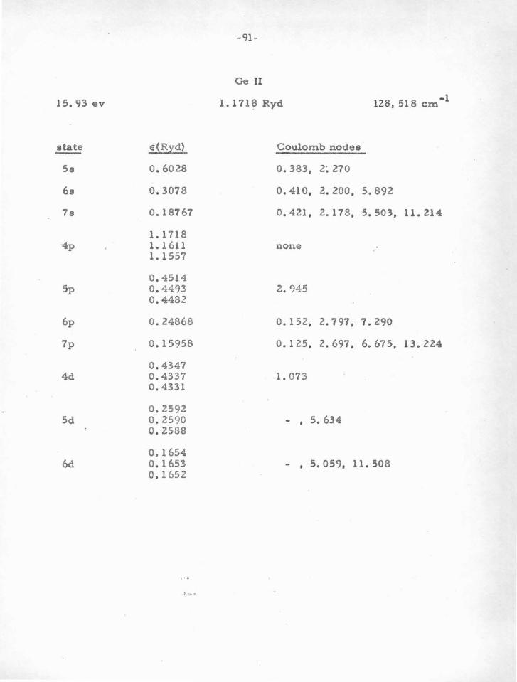
15. 93 ev

state e(Ryd)

5s o. 6028

6s 0.3078

7e 0.18767

1.1718 ·4p 1.1611

1. 1557

0.4514 5p 0.4493

0.4482

6p 0.24868

7p 0.15958

0.4347 4d 0.4337

0.4331

0.2592 5d 0.2590

0.2588

0.1654 6d 0.1653

0.1652

-91-

Geii

1.171 ~ Ryd

Coulomb nodes

o. 383, 2~ 270

0.410, 2. zoo.

o. 421, 2. 17 8,

none

2.945

o. 152, 2. 797.

o. 125, 2. 697.

1. 073

- • 5. 634

-1 128, 518 ern

5.892

5. 503, 11. 214

7.290

6. 67 5, 13.224

- • 5. 059, 11. 508

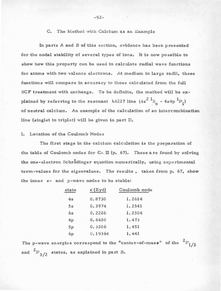
-92-

C. The Method with Calcium as an Example

In parts A and B of this s e ction, evidence has been presented

for the nodal stability of several types of ions. It is now posatble to

show how this property can be used to calculate radial wave functions

for atoms with two valence electrons. At medium to large radii, these

functions will compare in accuracy to those calculated from the full

SCF treatment with exchange. To be definite, the method will be ex­

plained by referring to the resonant ~4227 line (4s2 1s - 4s4p 1P1

) . 0

of neutral calcium. An example of the calculation of an intercombinatton

line (singlet to triplet) will be given in part D.

1. Location of the Coulomb Nodes

The first stage in the calcium calculation is the preparation of

the table of Coulomb nodes for Ca U (p. 67). These are found by solving

the one-electron Schrodinger equation numerically, using experimental

term-values for the eigenvalues. The results , taken from p. 67, show

the inner s- and p-wave nodes to be stable:

state E: (Rid) Coulomb node

4e 0.8730 1. 2614

5s 0.3974 1. 2541

6s 0.2286 1.2504

4p 0.6420 1. 473

5p o. 3206 1. 451

6p o. 19364 1. 441

2 The p-wave energies correspond to the "center-of-mae a" of the P 1; 2 2 and P 3; 2 states, as explained in part B.

-93-

Z. The s 2 Ground-State E nergy and Wave Function

The second stage in the calculation of the calcium resonance line

2 is the determination of the 4s ground-state energy, using the Ca II

s-wave Coulomb node data just quoted, and also the e 2 energy-node

table on p. 107. The latter table was prepared with the assistance of

the a -squared program discussed in the appendices. z Nodes for a

states were found as a function of the eigenvalue e, by solving the

Hartree • Foc k equation

P "(r) = ~ e - ~ + ! \r dr P 2 + 2 \QO dr ~ -J P(r) r r j 0 J r r

Therefore we have available two curves of energy vs . node: that from

2 the e-states of Ca II, and also the s curve. If we neglect the effects

of the small change in core potential as another a-electron is added to

2 Ca II, then the correct s energy and node for the ground state of Ca I

can be read from the intersection of the two curves.

In practice this was accomplished in the following way: The

Ca n energies 0. 8730 and 0 . 3974 with corresponding nodes 1. 2614 and

1. 2541 define a linear variation of node with energy. Using also a

linear interpolation between the s 2 energies 0. 40 and 0 •. 41 from p . I 01

one finds the intersection at e 2 = o. 4093 with node at 1. 2542. Another 8

linear relation for Ca I1 comes !rom using the two energies 0. 3974 and

0. 2286 with nodes 1. 2541 and 1. 2504. This line has a somewhat different

slope than that used before, but not enough to change the point of inter­

section with the s 2 curve by an appreciable amount. liv e t he refore

conclude that e 2 = 0. 4093 with a Coulomb node at 1. 2542. s

-94-

The result d e rive d by Hartre e and Hartree (37) from a full SCF

calculation is e- 2 = 0. 3891. The SCF electrons are thus not quite so s

tightly bound. Part of this diffe rence is due to the neglect of core

polarization in the usual SCF method. Core polarization is roughly

accounted for in the nodal boundary condition method by the use of

empirical nodes . Another part of the difference is due. in the nodal

boundary condition method, to a neglect of the slight reduction in core

potential when a second valence electron is added to a monovalent ion.

The order of magnitude of the influence of this effect on the node positions

can be estimated from the SCF node data of table V-A. This table sug­

gests that the radius of the node should be increased by about l o/o when

passing from the monovalent to the divalent situation. Using then a

Coulomb node of 1. 266 instead of 1. 254Z, the one electron energy is

found to decrease from 0. 4093 to 0. 4070. This change is small, amount­

ing to only 1/Z %. Therefore it is likely that the full SCF calculation,

perhaps because of the neglect of core polarization, underestimates the

binding energy by 3 to 4o/o.

3 . 1 The Excited sp p1 State

The most difficult calculation ls that for the sp-configuration.

Tl is involves solvint:; simultaneously the two non-linear Hart~ee-Fock

equations given l n Section III-B and Appendix A . Coulomb nodes are

extracted from the Ca 11 data. assuming a linear relation between

energy and node. A fair guess can be made of the s- and p-wave

eigenvalues expected, so that for a preliminary run. nodea correspond-

ing to these energies are used as inner boundary condttiorw on the wave

-95-

functions. U the derived eigenvalues differ significantly from those

guessed, the nodes are readjusted and the whole calculation repeated.

In the case of calcium, the i nitial 4s and

were chosen to be 1. 263 and 1. 438, r~spectively.

4p Coulomb nodes

1 The 4s4p P 1 calcu·

lation resulted in the eigenvalues € s = O. 555 and €p = 0.180. From

these energies , better nodes can be found by interpolating the Ca II

data. These are: a-node 1. 256; p-node 1. 440 . The final resulting

en~rgies are € = 0 . 533 and € = 0 . 1792. s p

Hartree and Hartree (37) have calculated the 4s4p 1P1

state

oi Ca t by the full SCF method with exchange, and obtained € 9

= 0 . 5052 and € = 0 .1720. As with the s 2 configuration, these eigen­

p

values are less than those obtained by the nodal boundary conditiol\

method. It is again our contention that the discrepancy ie due larg ely

to the neglect of core polarization or other correlation effects in the

SCF method, which are implicitly accounted for roughly in the nodal

boundary condition method by the use of experimental energies .

4 . Calculation of Oscillator Strengths

Once the initial and final wave functions have been determined,

the calculation of the dipole moment matrix element require s only the

evaluation of two numerical integrals by Simpson's rule. The com·

puter program calculates both of the two electron functions, the radial

integrals, the line strengths, and the gf-value.

-96-

D. lntercombinatton Lines

The effects o! a deviation from LS-coupUng were reviewed in

section Ill-A. The resulting m ixture of the LS bas t s functions provides

a meane by which the so-called '.'intercombination lines" can occur.

These are tran•itions involving a change of multiplicity or total spin S,

which means for two - electron functions that triplet to singlet transitions

are possible. For the configurations s 2, ss '• and ep, which we have

been considering, the followi ng intercombination lines can occur:

(s z) l s o - (ep)3Pl

1 3 (se ' ) S

0- (sp) P

1

(se') 3~ .. (sp) l pl

To find oscillator strengths for these transitions, it i s first

necessary to calcufate the amount of m ixing from observed spin-orbit

splltti.ngs. These wave functions can then be inserted in the d ipol e

moment matrix element. For example, if the experimentally des ignated

(sp) " 3P 1 " state i s actually

- 3 1 - 1 1 -1 < + f I r I '~~ i> = <a P t + b P t I r I so > • b < P 1 I r I so>

Condon and Shortley (38) give a complete d iscussion of intermediate

coupling. The energy matrix for the sp- configuration i s

3.,... r' 2

31.., - 1

'A( I '{2

where a 1 and <: denote electrostatic and apln- orbit m atrix elemente.

Following ~ing and Van Vleck (39), the parameter \ baa been in­

serted to try to account empirically for the ratio of t,.;.e off- Uiagonal to

tho diagonal radial matrlx e l emcmto of the opln- orbU: interaction. In

the more co:mmon approximation (as ln Condon and Shortley), ), is

set ec~ual to unity, but King and Van \'lecl~ point out that the r atio

(> 3 ° 2 3 A. = ~J d r (R 3R 1 /r )/ ,_' dr (R 3 /r } (where R 3 and R 1 are the

triplet and singlet radial £unctions) is unlikely to be unity, becauoc of

imperfect overlap of R 1 and R 3 • The 1/r3 factor welght o sm::ill

radii so hcavUy t11at only the inm ost p arts of the wave fWlctiono con•

tribute to t he integrals. But in this rcc..J'f.on t ho overlap is alm ost per­

fect (ln the SCF approxim ation) l>otween tho singlet and triple t functions,

i . e . , the nodeo coincide. However, the normalization dlffero con-

siderably betwee n t h e t-wo, the oinciet function belnr; s m alle1· £or omall

radii, so that the ratio X should be less than one.

By dlagonalizing the matrix e xactly. one find s the following

enere{es for t he four states (apart from a single additive constant):

3p 2

3:F 1

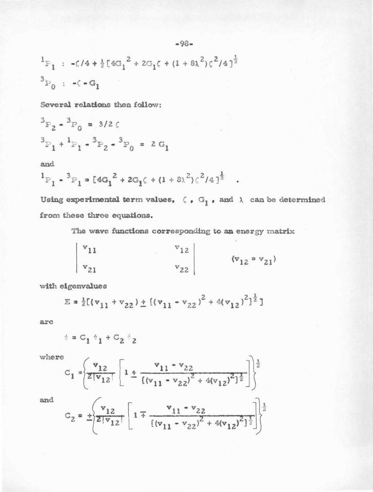
- 98-

· C/4 + j [ 4G12 + 2G1C + (1 + 8X 2)C 2/4]"~·

• ( ... Gl

Several rel ations then follow:

3 3 F 2 - P 0 = 3/2 c

3n + 1.,_ 3p 3p = •. 1 .o:- 1 - 2 - 0

and

l p l • 3 P l = (401 Z + ZGl C + (1 + 8>..2) ( 2/4 ]t

Using experimental term values, C , o1 , and >.. can be determined

from these three equations.

The wave functions corresponding to aa energy m atrix

with eigenvalues

E = i((vll + vzz) .± {(vll - vzz )z + 4(vlZ )z}t)

are

''' =C ·~ +C ;. . 1 ' 1 2 z

where t v c ::c 12 1 +

I Z(v1z! [ -

and

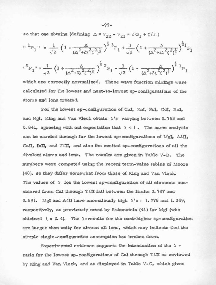
- 99-

so that ooe obtains (deftnlng ~ 5 v 22 - v 21 = 2 o 1 + C I z ) 1 1

" 1 P " = ....!.... ( 1 - /:) 1 )a 3 P + __!_ ( 1 + A )1f 1 P 1 ..J z. (A Z +Z.>. 2~ Zpr 1 ..J z. (A 2 +l). ZC Z)t 1

which are C<»:"l:'ectly normalized. Theae wave function mlxtngs were

calculated for the lowest and next- to.loweet sp- cODflguratiOQS of the

atoms and ions treated.

For the lowest sp• conftgurat!cm of Cat, Zul, Srl, Cdl, Bal,

and Hgl. F"..lng and Van Vleck obtain ). •s varying between 0. 758 and

0. 841, agreeb:ag with out expectation that ). < 1 • The same analysis

can be earned through for the lowest ep• configura.tlons of Mgt, AtU,

Gall, lnlL and TUI, and aloo the excU:ed ap- cotlfiguratlons o! aU the

divalent atoms and tons. The results at-e glven ln Table V- B. The

numbers were computed uoing the recent term-value tables of Moore

(40), eo they differ somewhat from those of King and Van Vleck.

The values of ). fo~ the lowest sp- conflguration of aU elements con­

sidered from Cal through T·UI fall between the ltmits o. 747 and

0. 891. Mgl aDd A~,n have anomalously hlgh X ' s : 1. 778 and 1. 349,

respectively, a.s previously noted by Rubenstein (41) for Mgl (who

obtalned ). = ~ 4). The J..•results for the next- higher ep- con!lguratlon

are larger than unity for almost all ions, which may indicate that the

sl.mple s lngle- conflguratlon assumption has broken down.

E xperimental evidence supports the lntroductic:m of the >.. -

ratio for the lowest sp- ccmflgurations of Cal through T.tU as reviewed·

by I<lng and Van Vleck, and as displayed in Table v- c , which gives

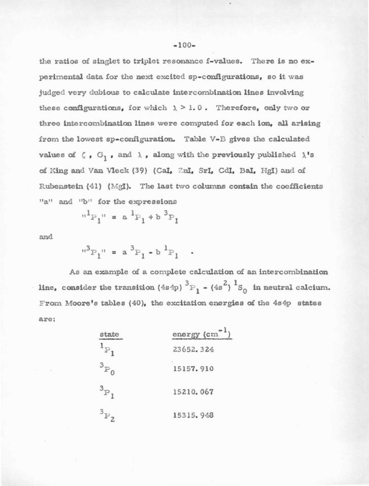
- 100-

the ratios of singlet to triplet resonance £- values. "'fhere is no ex­

perimental data for the next ex.cited sp- ccmfigurations, so it was

judged very dubiOUD to calculate lntercomblnation lines involving

these cc:mfigura.tions, for which ~ > 1. 0 • Therefore, only t-v.ro or

three intercombination lines were computed for each lon. all arising

from the lowest sp- configuration. Table V- B gives the calculated

values of C , a 1 , and X , along with the previously published ~ 'o

oi King and Van Vleck (39) (Cal, Znl, Sri, Cdl, Bal, Hgl) and o£

Rubenstein (41) (Mgl). The last two columns contain the coefficients

"a" and "b" for the expressions

1 1 3 II Pt" =a. pl -+b pl

and

As an example o£ a complete calculation o! an intercombination

3 2 1 line, consider the transition (4s~p) P 1 - (4s ) s0 in neutral calcium.

From Moore ' s tables (40), the excitation energies of the 4s4.p states

are :

state - 1 energy (em )

l p 1

23652. 324

3p 0 15157. 910

3p 1

15210.067

3p 2 15315. 94.-8

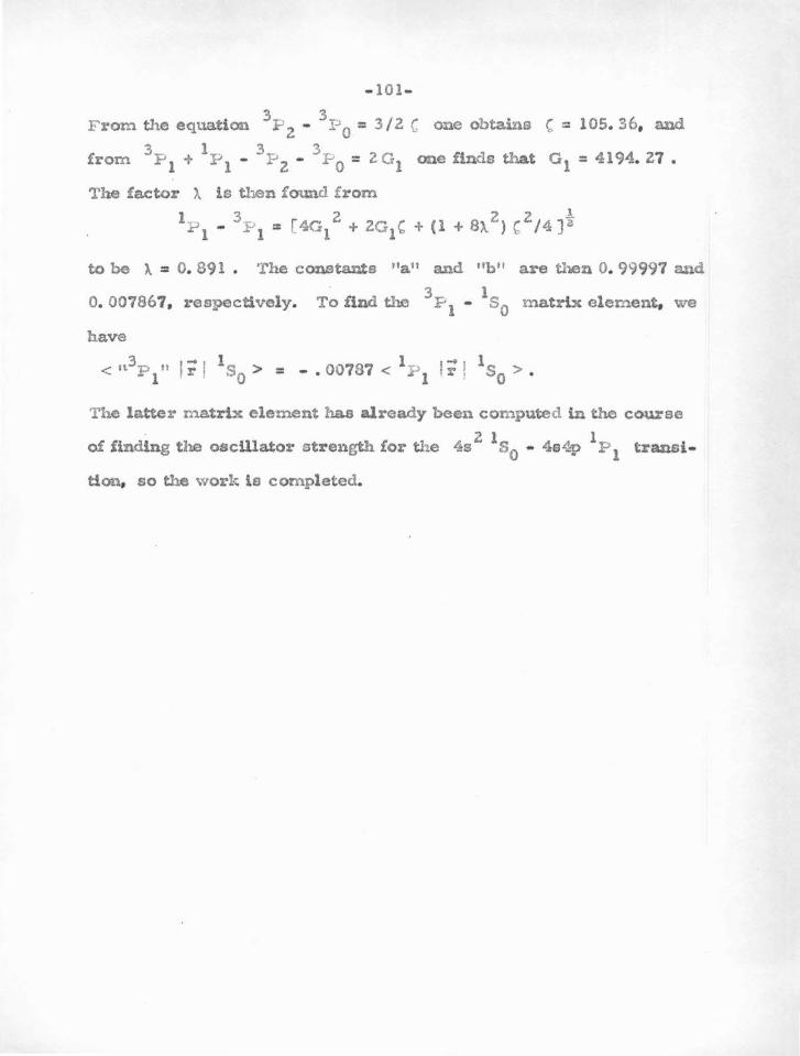
- 101-

From the equation 3:P2 -3

P 0 = 3/2 G one obtains C = 105. 36, and

3 1 . 3 3 from P 1 + P 1 .. P 2 .. P 0 = ZG1 one finds that G 1 = 4194. 27 .

The factor ).. is then found from

1 p 1 - 3 .P 1 = [ 4G 1 2 + ZG 1 C + ( 1 + 8).. 2) C z /4 ] t

to be ).. = 0. 891 • The constants "a." and "b" are then 0. 99997 and

0. 007867, 1·espectively. To find the 3

P 1 -1s0 matrix element, we

have

< n3

p 1" l i I 1s0 > = -. 00787 < 1.P1 1;! 1s0 > .

The latter matrix element has already been computed in tho course

z 1 1 of finding the oscillator stre1"igth !or the 4s s0 - 4e4p P 1 transi-

tion, so the work is completed.

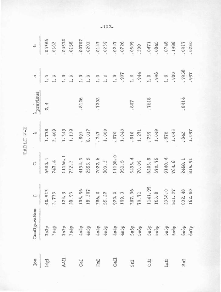
TA

BL

E V

-B

Ion

C

on

fig

ura

tio

n

( G

~

X_e~vious

a b

Mg

l 3

s3p

4

0.

513

65

80

. 1

l. 7

78

2

.4

1.0

.

00

38

6

3s4

p

2. 7

33

74

7.4

3

.40

9

1. 0

.

03

02

A-t

il

3s3

p

12

4. 9

1

11

66

. 1

l. 3

49

1

.0

. 0

05

32

3s4

p

2.8.

93

73

2.

3 1.

139

1.

0

. 01

58

Cal

4

s4p

1

05

.36

4

19

4.

3 . 8

91

• 81

26

1

.0

. 0

07

87

4s5

p

18

.30

7

25

55

.5

8.

017

1.0

.

0203

Zn

l 4

s4p

3

86.

0 7

02

2.6

•

74

7

. 77

02

1

.0

. 01

43

•

4s5

p

55.

27

803

.3

1. 0

00

1

.0

• O

Z39

-0 N

Gal

l 4

s4p

9

20

.0

11

19

8.

0 . 8

70

1

.0

. 02

47

•

4s5

p

19

9.3

95

1.

5 1.

04

0

. 99

7 .

07Z

6

Sri

5

s5p

3

87

.36

3

49

3.4

. 81

0

• 80

7

1. 0

.

03

09

5s6

p

79

.71

7

0.0

9

1. Z

71

.94

4

. 3

30

Cd

l 5

s5p

11

41.

99

6

20

3.8

• 7

59

. 7

61

8

1. 0

.

0471

Ss6

p

16

3.8

6

70.

75

1. 0

49

• 99

6

. 0

84

5

lnil

5

s5p

2

36

8.0

9

14

0. 4

• 8

76

1

.0

• 07

48

5s6

p

511

. 7

7

76

4.6

1.

043

.9

80

.

19

88

Ba

i 6

s6p

83

2-.

48

Z45

8. 1

• 8

4Z

• 84

14

. 9

95

8

. 0

91

7

6s7

p

16

2.5

0

81

5. 9

1 1.

09

7

. 99

7

. 0

73

0

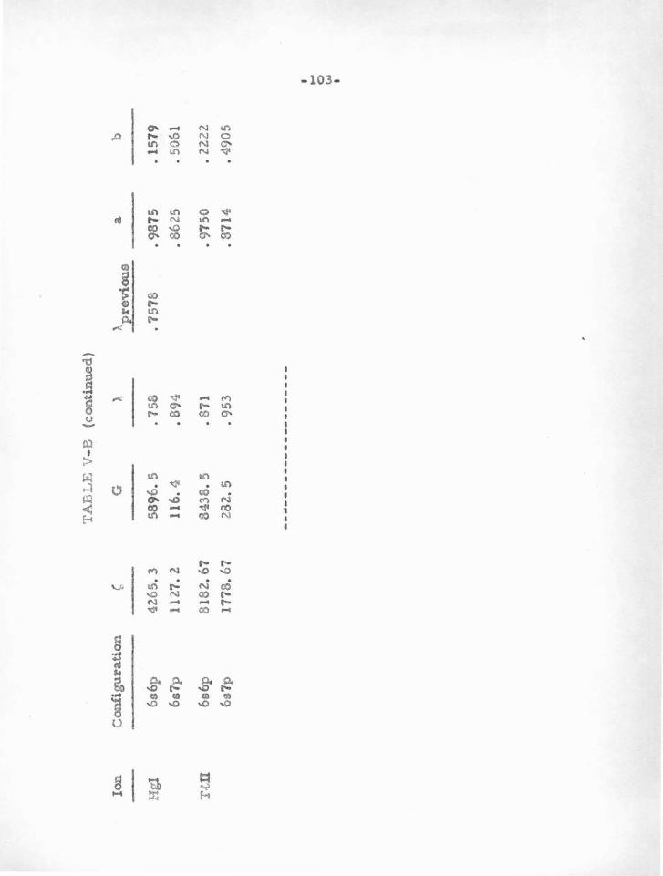
TA

BL

E V

-B

(co

nti

nu

ed)

Ion

Co

nfi

gu

rati

on

'

G

>.

Hg

l 6

s6p

4

26

5.3

589

6. 5

. 7

58

6s7

p

1127

. 2

11

6.4

• 8

94

Ttl

l 6

s6p

8

18

2.

67

84

38

.5

. 871

6s7

p

17

78

.67

2

82.

5

. 95

3

----

----

----

----

----

-

~rev

ious

a

.75

78

• 9

87

5

. 86

25

. 9

75

0

. 87

14

b

. 15

79

. 50

61

• 2

22

2

• 49

05

I ~

0 ~ •

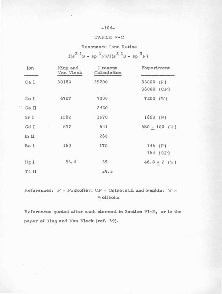
- 104-

TA B L E V- C

Resonance L ine Ratios

2 1 1 2 1 3 f(e S - s p P )/f(s S - sp P )

Ion King and I--resent Experiment Van Vleck Calculation

Ca I 301 '30 25200 33000 (P )

36000 (OP)

z.n I 6757 7000 7200 (W )

Gan 2420

51" I 1582 1570 1660 (P )

Cd I 6 37 641 680 + 100 (W )

Inn 260

:Sa 1 169 170 146 (P )

164 (OP)

Hg 1 53. 4 55 46. 8 + 2 (W )

T.t U 29. 3

References: P = P rokofiev; OP = Oatl"ovsl--• .U and P enkln; W = Wolfsohn

References quoted after each e l ement in Section VI- B . or in the

paper of Klng and Van Vleck (ref. 39).

-105-

VI. RESULTS AND APPLICATIONS

Evidence for nodal stabUity and the details ol applyin{l the

nodal boWldary condition method have been given in Section V . Cal-

cium was used as an example, and the eigenvalues, eigenfunctiona,

and oscillator strengths were compared with those found from a com-

plete SCF calculatlo~ In this section, the entire results of calcu-

2 lating with the method wUl be tabulated. In Part A , the e

configuration is discussed, and tables ol the variation in Coulomb

node with energy are given. Part B coll ects together eigenvalueo

and oscillator strengths for transitiono in thirteen atoms and lone

with two valence electrons. The application of these results to as-

tronomlcally observed lines, and to the problem of element abundances,

is treated briefly in Part c. Finally, ln Part D, possible extensions

of the technique are outlined, along with other uses o! the nodal

boundary condition method.

A. The S- Squared Calculations

The s - squared program discussed in the appendices computes

wave functions for given one-electron eigenvalues. Therefore, a

table of energy versus node can be constructed for this configuration.

From this table, if the Coulomb nodes are knoWn for a particular

atom, the s 2 one- electron energy can be interpolated. The detaUo

of making this interpolation were treated in Section v-c . If one sub­

sequently wishes to compute a transition probabUlty involving this

s 2 ground- state, the eigenvalue is known, so tha.t the wave- function

is determined.

-106-

The eigenvalues found from these .calculations ca.n be compared

with SCF results for various atoms. For example, the Coulomb S•

node for magnesium (from the data of Section V• B) is at r = . 82.5 •

2 From the node versus energy curve for the s configuration of

neutral atoms (Table Vl·A), one finds a one-electron energy for the

ground-state valence function of magnesium to be • 5194 RycL This

is close to the result(. 520) of Biermann a.nd Trefftz (13) using SCF

with core polarization. The case of the ground state of neutral cal-

cium was discussed in Section V -c. A systematic comparison with

previous results is given atom by atom in Part B of thi8 section.

B . Eigenvalues and OscUlator Strengths

The following tables contain the results of all the computations

made for atoms with two valence electrons. Altogether, some calcu­

lations were carried out for thirteen atoms and ions:

Ion Configuration

He I, L i II (ls 2)

Mg I, At U (2p63s 2 )

Ca I (3p64s 2 )

Zn I , Gall (3d104s 2 )

SrI (4p6ss 2 )

Cd I, Inn (4d 1058 2)

Ba 1 (Sp66s 2 )

Hg I, Tt II (Sd 106s 2 )

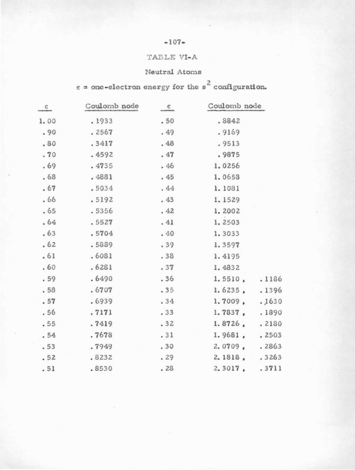
- 107-

TAFILE VI- A

Neutral Atoms

E: = one- electron energy for the s 2 configuration.

€ Coulomb node ~ Coulomb node -1. 00 • 1933 • 50 . 8842

• 90 • 2567 . 49 . 9169

• 80 • 3417 • 48 . 9513

.70 • 4592 • 47 • 9875

• 69 • 4735 • 46 1. 0256

• 68 • 4881 • 45 1. 0653

• 67 • 5034 . 44 1. 1081

• 66 • 5192 • 43 1. 1529

• 65 • 5356 • 42 1. 2002

• 64 • 5527 • 41 1. Z503

• 63 • 5704 • 40 1. 3033

• 6Z • 5889 • 39 1. 3597

• 61 • 6081 . 38 1. 4195

. 60 • 6281 . 37 1. 4832

• 59 • 6490 • 36 1. 5510 • • 1186

• 58 • 6707 • 35 1. 6235 • • 1396

• 57 . 6939 . 34 1. 7009 , . J630

• 56 • 7171 • 33 1. 7837 , . 1890

• 55 • 7419 • 32 1. 8726 , • 2180

• 54 • 7678 . 31 1. 9681 , • 2503

• 53 • 7949 • 30 2. 0709 , • 2863

• 52 • 8232 • 29 2. 1818 , • 3263

• 51 • 8530 • 28 2. 3017 , • 3711

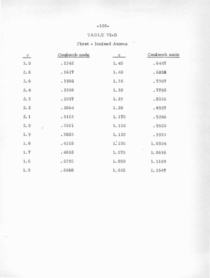
- 108-

TABLE Vl· B

F irst - Ionized Atoms

€ Coulomb node e Coulomb node

3. 0 • 1342 1. 45 • 6447

2. 8 • 1617 1. 40 • 6858

2. 6 • 1950 1. 35 • 7307

2. 4 • Z358 1. 30 .7798

2. 3 • 2597 1. 25 • 8336

2. 2 • 2864 1. 20 • 8927

2.1 • 3163 1. 17 5 • 9246

2. 0 • 3501 • 1. 150 • 9500

1. 9 • 3883 1. 125 • 9933

1.8 • 4318 l : 100 1. 0304

1. 7 • 48 18 1. 075 1. 0696

1. 6 • 5395 1. 050 1. 1109

1. 5 • 6068 1. 025 1. 1547

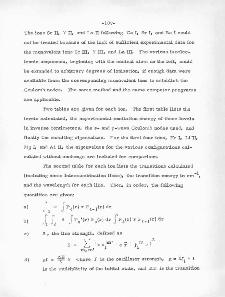
- 109-

The ions Sc n. Y II, and La n following Ca I, Sr I , and Ba 1 could

not be treated because of the lack of sufficient experimental data for

the monovalent ions Sc m , Y Ill, and Lam. The various isoelec-

tronic sequences, beginning with the neutral atom on the left, could

be extended to arbitrary degrees of ionization. if enough data were

avaUable from the correspondlng monovalent ions to establish the

Coulomb nodes. The same method and the same computer programs

are applicable.

Two tables are given for each ton. The first table lists the

levels calculated, the experimental excitation energy of these levels

in inverse centimeters, the s - and p - wave Coulomb nodes used, and

finally the resulting eigenvalues. For the firet four ions, He I, Li 11,

Mg I, and At U, the eigenvalues for the various configurations cal­

culated \vithout exchange are included for comparison.

The second table for each lon liDts the transitions calculated

- 1 (including some intercombination lines), the transition energy ln em ,

and the wavelength for each line. Then. in order, the following

quantities are given:

(I

a) j Pt(r) r Pt_ 1(r) dr

b) = J P 8 ' (r) P 8 (1•) dr J Pt(r) r P,e .• 1(r) dr

c) S , the line strength, defined as

s = L I<"' fm' I e r m , m '

d) gf = '\E S where f le the oscUlator strength. g = 2J1 + 1

is the m Ultiplicity of the initial state, and AE is the transition

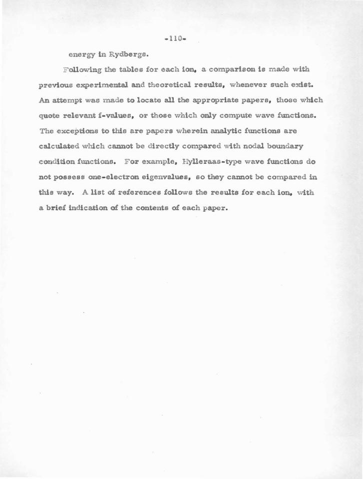
-110 ..

energy in Rydbergs.

F ollowing the tables for each ion, a comparison is made with

previous experimental and theoretical results, whenever such exist.

An attempt was made to locate all the appropriate papers, those wblch

quote relevant f .. values, or those which only compute wave functions.

The exceptions to this are papers wherein analytic functions are

calculated which cannot be directly compared with nodal boundary

condition functions. For example, Hylleraas - type wave functions do

not possess one- electron eigenvalues, so they cannot be compared in

this way. A list o! references follows the results for each ion. with

a brie! indication of the contents of each paper.

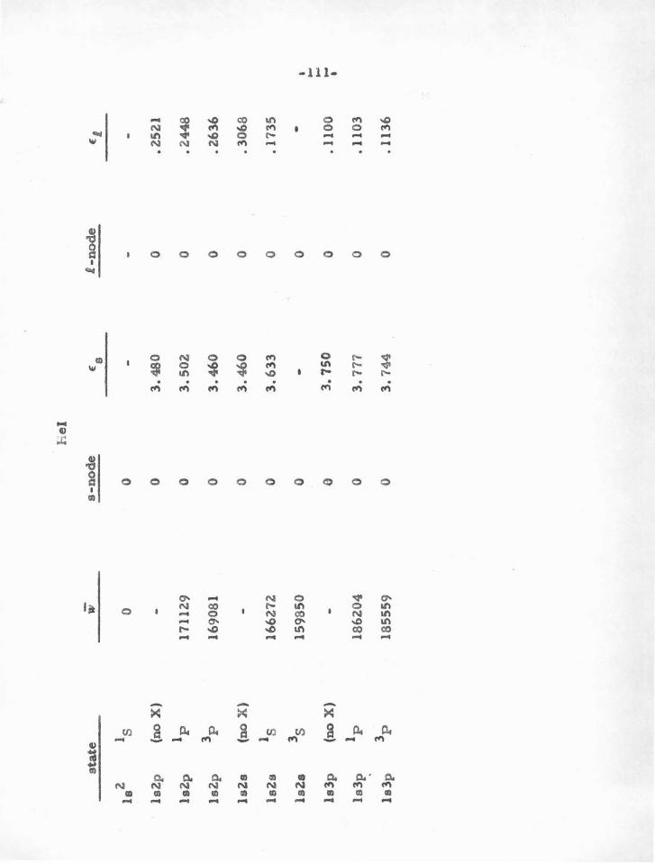
he

I

state

,.,

s-n

od

e £

8

1-n

od

e £

l

lsz

1s

0 0

lsZ

p (n

o X

) -

0 3

.48

0

0 .2

.52.

1

lsZ

p

1p

17

112.

9 0

3.50

2.

0 .2

448

lsZ

p

3p

16

9081

0

3.4

60

0

.2.6

36

lsZ

s (n

o X

) -

0 3

.46

0

0 .3

068

lsZ

s 1s

16

6272

. 0

3.6

33

0

.173

5

ls2.

a 35

15

9850

0

-0

-I .....

3

.75

0

.....

1s3p

(n

o X

) -

0 0

.11

00

- •

ls3

p

1p

18

62.0

4 0

3.7

77

0 .1

103

ls3

p

3p

18

5559

0

3.7

44

0

.11

36

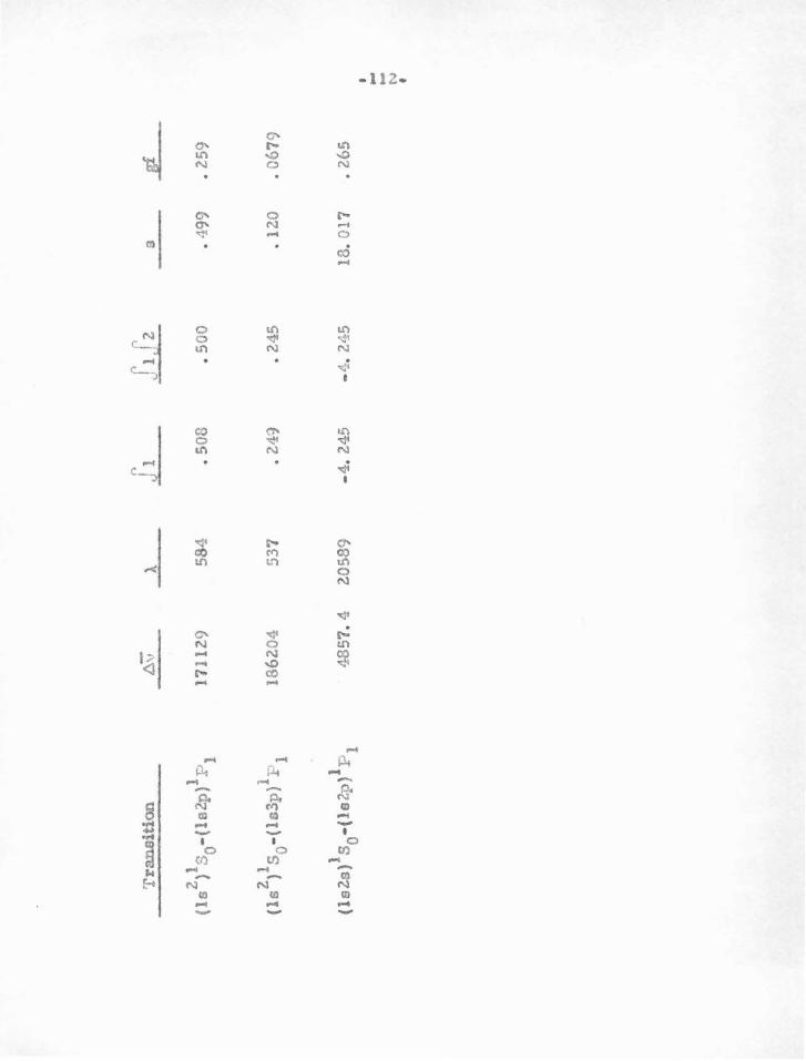
,... J

1J

2 T

ran

siti

on

6

\1

X

j 1

a .R

. 2

1 1

(ls

) s 0-

(le2

p)

P1

17

11

29

5

84

• 5

08

• 50

0 •

499

• 25

9

2 1

1 (l

s )

s 0-(lc

3p)

P1

18

62

04

53

7 •

249

• 24

5 •

12

0

• 0

67

9

1 1

(ls2

s) s

0-(

le2

p)

P1

4857

.4

20

58

9

-4

.24

5 -~

. 2•

.1-5

18.

017

•

265

• .... .... N •

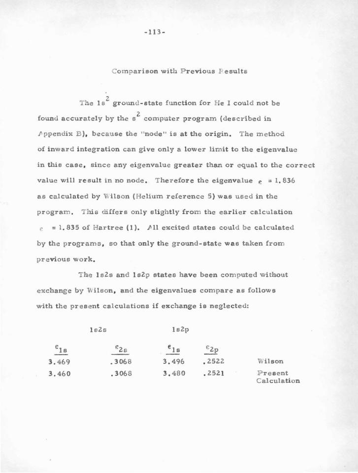
-113-

Comparison with Previous I' esults

The 1 s 2

ground · state function for He I could not be

2 found accurately by the s computer program {descr'ibed in

.r ppendix B ), because the "node" is at the origin. The method

of inward integration can give only a lower limit to the eigenvalue

in thie case, since any eigenvalue greater than or equal to the correct

value will result in no node. Therefore the eigenvalue f.': = 1. 836

as calculated by Wilson (Helium reference 5) was used in the

program . Thi s differs only slightly from the earlier calculation

;. = 1. 835 of Hartree ( 1 ). Pll excited states could be calculated

by the programs , so that only the ground-state was taken from

previous work.

The 1 s2s and 1 s2p states have been computed without

exchange by 'W ilson, and the eigenvalues compare as follows

with the present calculations if exchange is neglected:

1s2s ls2p

ele e2s e1s c 2p

3.469 • 3068 3.496 • 2522 Wilson

3.460 • 3068 3.480 . 2521 P resent Calculation

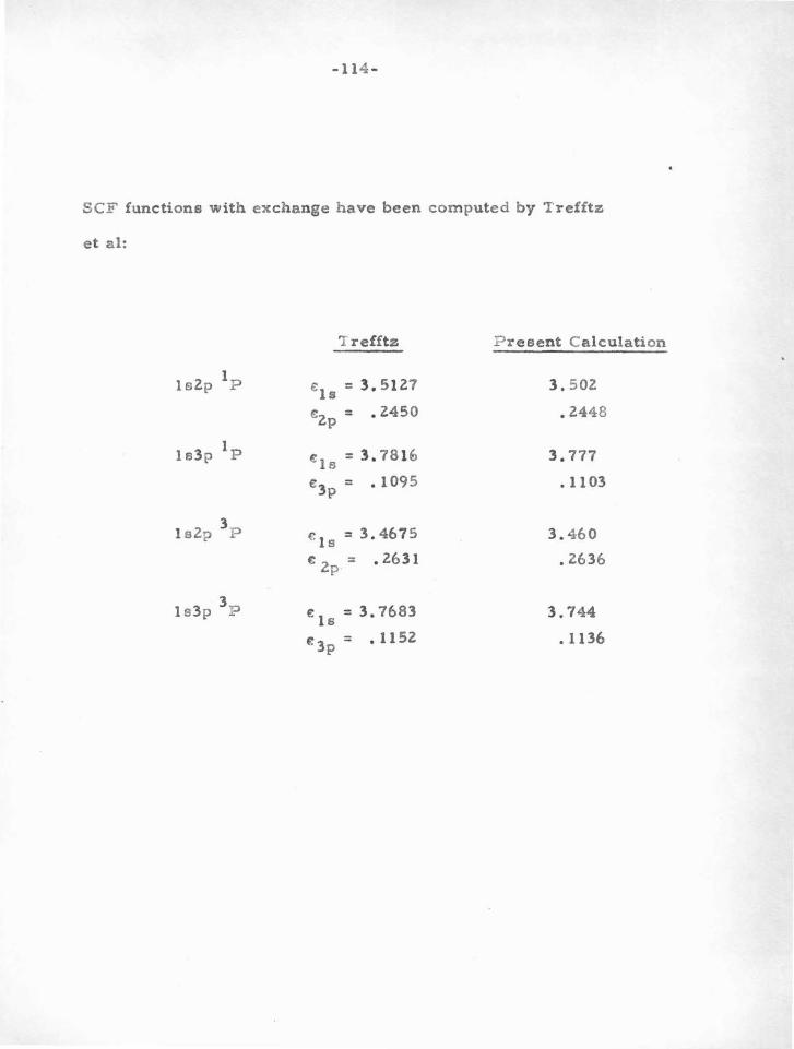
-114 -

SCF functions with exchange have been computed by Trefftz

et al:

'I refftz P resent Calculation

1 ls2p P e 18 = 3.5127 3. 502

€2p = .2450 .2448

1 1e3p P e 18 = 3. 781€> 3.777

€3p = • 1095 . 1103

3 1s2p P € 1 s = 3. 4675 3. 460

c 2p = .2631 .2636

3 = 3. 7683 3.744 1s 3p P E:ls

~3p = • 1152 .1136

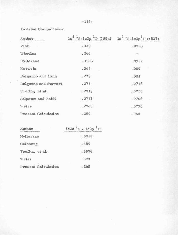
· 115-

F - Value Comparisons:

Author l 1 1

ls S-lslE P p.584~ 1s2 1

s - 1a3E 1P ().537)

Vinti . 349 • 092.8

Wheeler • 2.66

Hylleraae • 3555 • 0722.

Korweln . 365 . 089

Dalgarno and Lynn • 2.39 • 081

Dalgarno and Stewart • 2.75 • 0746

Tref!tz, et al. . 2719 • 0720

Salpeter and Zaidi • 2.717 . 0706

Welae • 2760 • 0730

Present Calculation • 259 • 068

Author ls2e 1 S • 1S 2f l p

Hylleraao • 3918

Goldberg . 389

Trefftz, et al. • 3578

Weise • 377

P t>esent Calculation • 2.65

-116-

Referenceo for Hallum

A great deal of work has been done on heUum by analytic

variational methods and by Hylleraas-type wave functions (depending

explleitly on r 12 ). We refer here (and also for all other atoms) only

to SC:! calculatiODS and other theoretical or experimental results wlth

which our eigenfunctions, eigenvalues, or tra.nsitlao probabUitieo can

be directly compared.

1) 1-Iartree, D . R .

Proc. Ca.mb. P hil. Soc. 24, 111, 127

Computes the ground-state function and one-electron eisen­

value.

Z) Vlntl, 1. P .

Phys. Rev. 42, 632, ' 32

Calculates £-values for single-excited. doubly-excited, and

continuum states from screened wave functions.

3) Wheeler, J. A.

Phys. Rev. 43, 258, '33

Computee the 1s2-ls2p £-value using variational functions.

4 ) K orwein, H.

7 . P hysik 91, 1, ' 34 2 . 2

Computes ls - lsZp and ls -la3p f·vslues from variational

functions .

5) WUscm. W. S. , and Lindsay, R . B.

Phys. Rev. 47, 681, '35

Computes SCF functions without exchange for the configuratlaa.o

(ls)2, (lsZo). (le2p), (2s2 ), (Zp2), and (2s2p). Wa.ve functiono

and eigenvalues are given.

6) WUson. W. S.

Fhys. R.ev. 43, 536, 135

The total atomic energies are computed for the states of ref·

erence 5).

7) Morse, P . M. , Young, L . A., and Haurwttz, E . s. Phys. Rev. 48, 948, 135

Analytic wave functions. used by Veaelov for f·value calcu•

latloos (ref. 10).

8) Hylleraas, E. A.

z. Physik 106, 395, ' 37

Computes oscllla.tor strengths for many bellum traneltlons

using previously calculated wave functions.

9) Goldberg. L .

Ap. J. 90, 414, ' 39

Uses simple variational analytic-type wave functions to obtain

£-values !or the series Zs-np and Zp-nd.

10) Veselov, M. G.

Jour. Ex. and Theo. Phys. (USSR) 1 <), 959, '49

Computeo £-values for the transitions ls•l!p and Za-Zp using

Morse wave functions (from ref. 7 ).

11) Vlzbaratte, Ya. 1, Ka.ntserevtc:hyua. A. I. , and Yutsi s , A. P .

OpttlQ l Spek. 1, 9, 156

Computes the lsZs, 183s, ls4p states by SCF with exchange.

lZ) Herem. S., McWhirter, R. W. ? . , and Rhoderick, E. H.

Nature Z34. 565, ' S6

Measures lifetime ol. the 3 1:;;:- state.

13) Dalgarno, A. , and L ynn, N.

P roc. Fhys. Soc. London A 10, SOZ, '57

Modlfles previously calculated f-valuee to satisfy the £sum­

rule.

14) Trefftz, E . , Scblb~r, A. , Dettrn.ar, K. • rL , and .nlrgens, K.

z. f. Ap. 44. 1, ' 58

Calculates eigenvalues and eiaenfWlctions by an extended

Hartree- F ock schem e. Oscillator strengths are given for

many t~ansltlons.

-118-

15) Oeb.erovlch. A. L., and Savich. L G.

Optika l Spek. 4, 715, • 58

Measures llfetlmes of 3 3P and 3 1F states.

16) Dalga.rno, A. , and Stewart, A. L .

P roc. Phy.s. Soc. London A 76, 49, ' 60

Gives £-values for ls2-ls2p a.nd lo 2-ls3p transitions.

17) Salpeter, E . E. , and Zaidi, M. H.

Phys. Rev. 125, 248, 162

Calculates £-values using many-pa.ram~ter functions.

18) Weiss, A. W.

National But"eau ol. Standards (private communication).

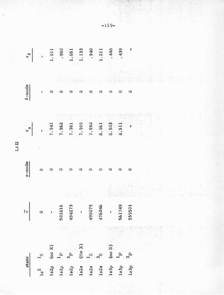
LiU

-s-

no

de

l-n

od

e

stat

e v

EB

£1.

-ls

2

1s

0 0

h2

p

(no

X)

-0

7.94

1 0

1.0

11

lsZ

p lp

50

1816

0

7.96

Z

0 .9

80

leZ

p 3

p

494Z

73

0 7.

961

0 1.

051

lsZ

s (N

o X

) -

0 7

.98

9

0 1.

133

lsZ

s •s

49

0079

0

7.5

50

0

.94

0

lsZ

a 35

47

6046

0

8.0

61

0

l.Z

ll

• .... h

3p

(n

o X

) . '

0

8. 5

03 .

0

.... -

.44

8

..0

• lp

"

5617

49

8. 5

11

.. , ls

3p

0

0 . 4

39

....

-. '

' '

' .

:, ...

. '

' .

.,,. 3

p

' .·

ls3

p

5595

01

0 0

~

:; .

.:':.

' •·

-

. ··

-.;,.

'

' '

' '

·"

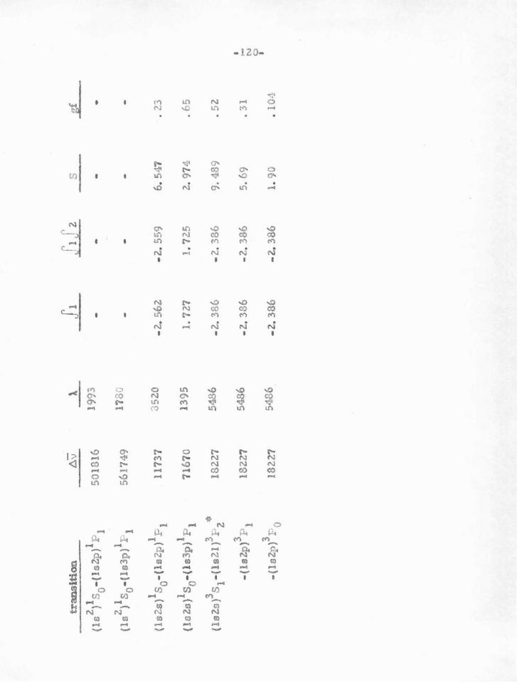
tran

siti

on

6

\)

). -Jl

n r

._! 1

X

l s

.2:

z 1

1 5

01

81

6

1993

(l

s )

s 0-

(Is2

p)

P1

-•

-•

2 1

1 (l

s )

s 0-(ls

3p}

P1

561"

'/49

178

0

1 1

(ls2

s) s

0-

(ls2

p)

F1

1173

7 J

520

-2.

56

2

.z. 5

59

6. 5

47

. 23

1 1

(ls2

s) s

0-(l

s3p

) P

1 7

16

70

13

95

1. 7

27

1.

7 2.

5 2.

97~~

. 65

3 3

* (l

sZs)

s1-

(ls2

.l)

P2

1822

.7

5486

-z

.3a6

.. z

. 38

6

9.48

9 •

52

3 1

82

27

54

86

-z. 3

86

-2

. 3

86

5.

69

• -(l

slp

) p

l •

31

-N 0

-(l

sZp

)3P

0 54

86

• 1

82

27

-z

. 38

6

-2.

38

6

1. 9

0

• 1

04

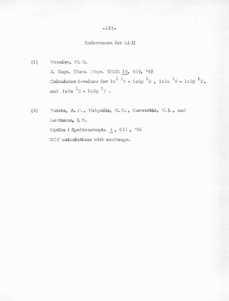
- 121-

Rcfe renee a for L i II

(1) Veselov, ~.1. G.

J . .Exl)t. Theo. ::Jhya. USSR 19, 959, ' 49 - -Calculates f-values for ls

2 1s - le2p 1

:t-· , lo2s 1s - le2p 1P ,

3 3 and lo2s S - lo2p P •

(2) Yutais, A. ? . • Ushpalis, r<:. K., Kavetakis, V. I ., and

Levinson. I. B .

OptUta i Spcktroskopia ! • 6 0 1 • '56

SCF calculationo with exchange.

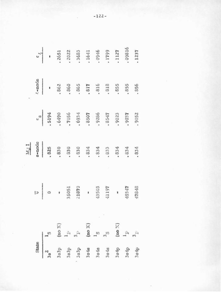
M"T

I .:

:.;Q

Sta

te

- v s-

node

e

s

..t-n

ode

£.{.

--

3s2

ls

0 •

825

• 5

194

-

-3

s3p

(n

o X

) -

• 8

30

• 6

49

0

• 86

2

• Z

651

3s3

p

lp

3505

1 •

83

0

.7

05

6

• 86

0

• 2

02

2

3s3

p

3p

~1870

• 83

0

• 6

93

4

. 86

5

• 36

83

3s4

s (n

o X

) -

• 83

4

• 8

507

• 8

17

• 16

41

ls

I

3s4

s 43

503

. 83

4

• 92

86

• 81

6

. 094

6 -N

3s

N

3s4

s 41

197

• 83

3 • 8

54

7

• 8

18

•

1799

I

3s4

p

(no

X)

-• 8

34

•

9023

•

85

5

• 11

27

3s4

p

lp

49

347

•

83

4

• 90

37

• 85

5

. 098

16

3s4

p

3F

47

84

8

• 83

4

• 90

52

.85

6

• 12

37

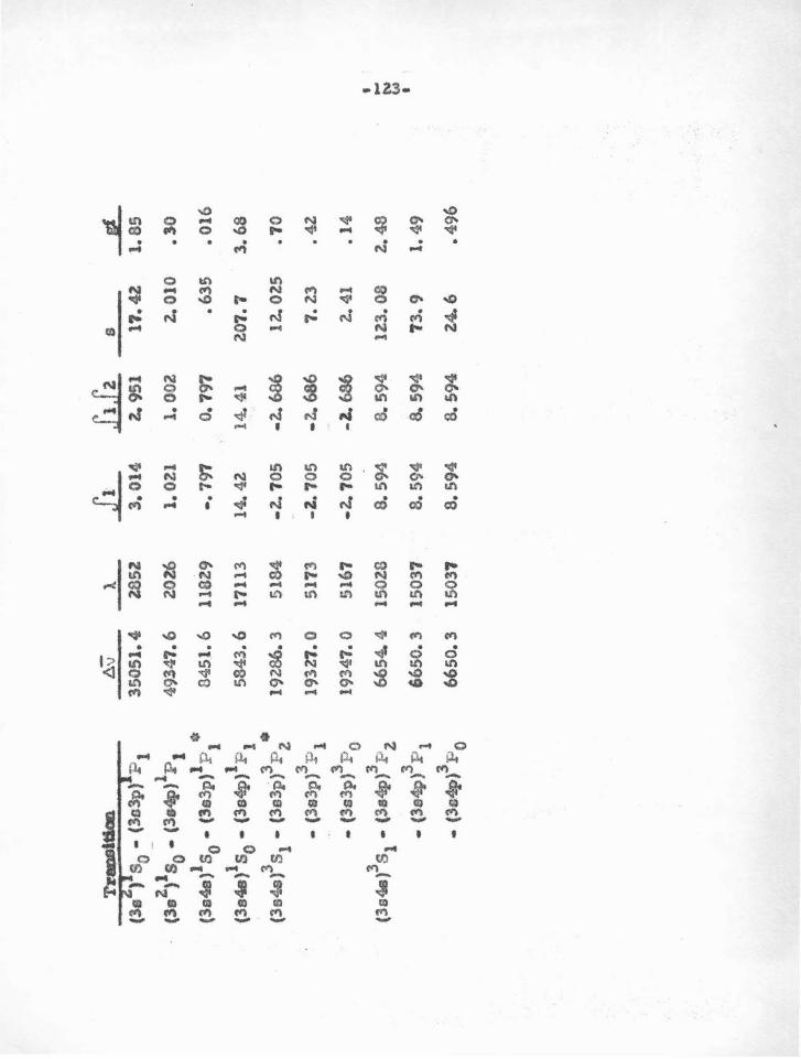
Tra

o&ltl

ca.

~-v

l.

.1L

.J

ll!_

s --

R.

(3s2

)1S

o -

(3s3

p)I

P1

3

50

51

.4

zasz

3

. 01

4

z. 95

1 17

.42

1. 8

5

2 1

-1

(Je

) s 0

• (3~)

P1

4934

'7. 6

zo

u 1

. OZ

l 1.

00

2

2. 0

10

.J

O

(3s4

s)1 s 0

• (3

.s3p

)1P

1 °

84

51

.6

11SZ

9 -.

79

7

0.7

97

• 6

35

• 0

16

(3s4

e)1 s 0

-(3

e4p)

1P

1 5

84

3.6

17

113

14

.42

1

4.4

1

20

1.7

3.

6S

• 3

. 3

(3s4

s) s

1 -

(3s3

p)

P2

19

28

6.3

5

18

4

-2.'

70

5

.. z_

686

12. 0

25

.70

3

-(3

s3p

) P

1 1

9lZ

1.0

51

73

-2.'

70

5

-z. 6

86

1. 2

3 • 4

Z

. 3

-(3

s3p

) P

0 1

93

47

.0

5167

-2

.70

5

-1.6

86

z.

41

• 1

4

3 3

I

(3s4

s) s

1 -

(.3s

4p)

P2

66

54

.4

1502

8 8.

594

8

.59

4

1Z3.

08

Z

.-48

~

~

3 -

(3s4

p)

P1

66

50

.3

1503

'7

8. 5

94

8.5

94

7

3.9

1.

49

• 3

• (3

s4p

) P

0 6

65

0.3

15

03.,

8

.59

4

8. 5

94

2

4.6

.4

96

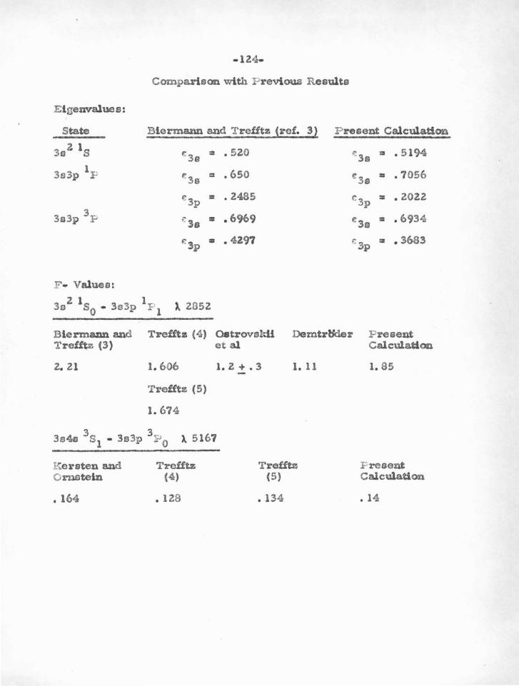
-124-

Comparison with P revious Results

Eigenvalues:

State

3a~ 1s Biermann and Trefftz (ref. 3) P resent Calculation

e 38 = .520 ~ 38 = . 5194

1 3a3p P fl! 38 = • 650 e 38 • • 7056

F · Values:

€3p •• 2485

~ 38 • • 6969

€3p •• 4297

2 1 1 3o s0

... 3s3p P1

). 2B5Z

{';3p = • 2022

e: 38 :a • 6934

f': 3p :1 • 3683

BiermaDn and Trefftz (4) O.trovsl-..U Demtrl'kler P resent Trefftz (3) et a1 Calcula.tlon

z. Zl 1. 606

Trefftz (5)

1. 674

1. 2 + . 3 1. 11

3 3 3s4o s1 .. 3s3p Po ~ 5167

Kersten and Ornstein

• 164

Trefftz (4)

• 128

Trefftz (5)

• 134

1. 85

F resant Calculation

• 14

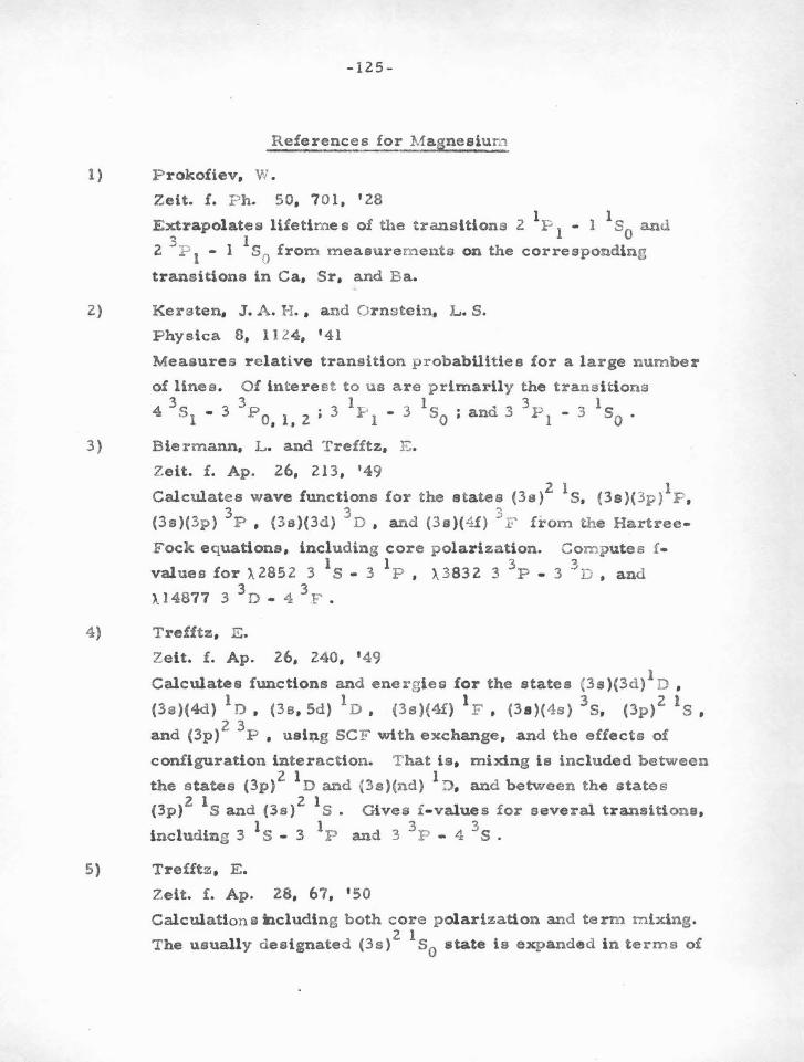
-125-

References for Magnesiurtl

1) P rokofiev, W.

Zeit. !. Ph. 50, 701, '28

Extrapolates lifetimes of the transitions 2 1P 1 - 1

1s0

and 3 1

Z. P 1 - 1 s0 from measurem ents on the corresponding

transitions in Ca, Sr, and Ba.

2) Kersten, J. A . H., and Ornstein, L . S .

Physica 8, 1124, 14 1

Measures relative transition probabilities for a large number

o! lines. Of interest to us are primarily the transitions

4 3Sl • 3 3PO, 1, 2; 3 11-' 1 - 3 ISO; and 3 3pl - 3 ISO .

3) Biermann, L . and Trefftz, E .

Zeit. £. Ap. 26, 213, '49 2 1 1 Calculates wave !unctions !or the states (3s) S , (3e)(3p) F ,

3 3 3 (3s)(3p) P , {3s)(3d) D , and (3s)(4f) F from the Hartree-

Fock equations, including core polarization. Com pute s f ·

values for ).2852 3 1s- 3

1P , ).3832 3

3p . 3 3 n , and

U4877 3 3n • 4

3F •

4) Trefftz, E.

Zeit. f. Ap. 26, 240, ' 49

Calculates functions and energies for the states (3s)(3d)1 D ,

(3e)(4d) 1n, (3e , Sd) 1n , (3s)(4f) 1F , (3 s)(4 s) 3s, (3p) 2 1s,

2 3 and (3p) P , usl~g SC F with exchange, and the effects of

configuration interaction. T hat is, mixing is included between 2 1 1 the states (3p) D and (3s)(nd) D, and between the states

z 1 2 1 (3p) S and (3s) S • Gives £-value s for several transition s, 1 1 3 3

including 3 S - 3 P and 3 P - 4 S .

5) Trefftz, E .

Zei t . £. Ap. 28, 6 7, ' 50

Calculations bcluding both core p olarization and term m ixing.

The usually designated (3s) 2 1s0 state is expanded l n terms of

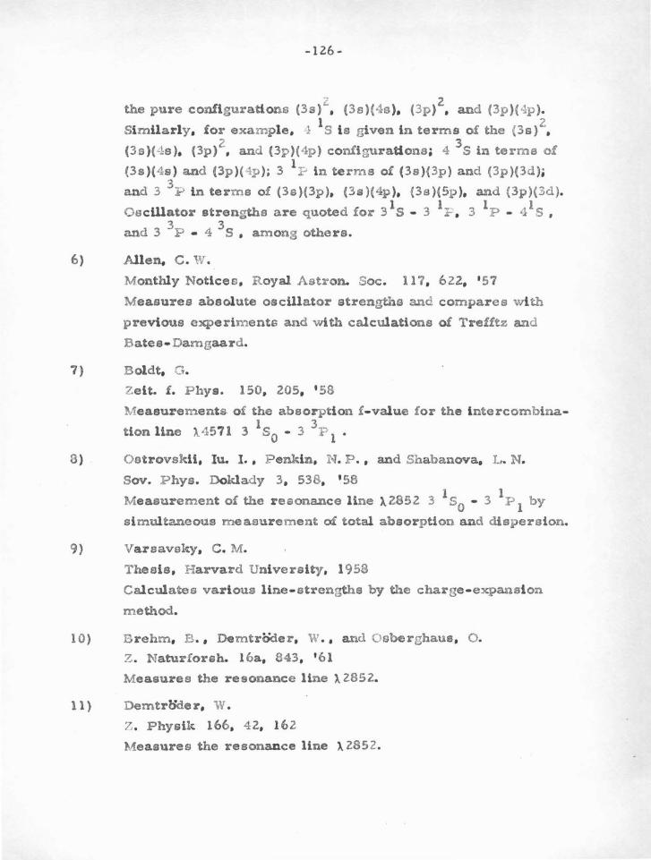
- 126-

z 2 the pure confi gurations (3a) , (3s)(4s), (3p) , and (3p)(4p).

1 2 Sl m Ua rly , for examp l e , -1 S i s given in terms of the (3 s) , 2 3 (3s)(-.l:s), (3p) , and (3p )(4p) configurations; 4 S in terms of

(3s)(4s ) and (3p)( 4p ); 3 11=- i n term s of (3s)(3p ) and (3p )(3d);

and 3 3P in t e r m s of (3s)(3p), (3s)(4p), (3s)(5p ), and (3p)(3d). 1 L 1 1 Os cWator str engths are quoted for 3 S - 3 .r , 3 P - 4 S ,

3 3 and 3 P - 4 S , among others.

6) All en. C . W.

Monthly Notices, R oyal Astron. Soc. 117, 622., ' 57

Me a sures ab solute oscillator s trengths and comparee wi th

previous experim ents and with calcula tions oi Trefftz and

Bates- Da mgaard.

7) B ol dt, G.

Ze lt. f . P hys. 150, 205, ' 58

Measurem ents. of the absorption £- value for the l ntercomblna-1 3

tion line ). 457 1 3 s0 - 3 P 1 •

3) Ostrovsldi, Iu. I . , P enldn, N. P . , and Shabanova, I .... N.

Sov. P hys. Doklady 3, 538 , ' 58 1 1 Measurement of the resonance line ). 2852 3 s0 • 3 P 1 by

s imultaneous measurement of total absorption and dispersion .

9) Va rsavaky, C. M.

Theflis, Harva rd Un iversi ty, 1958

Calculates vari ous line- strengths by the charge - expansi on

m ethod.

10) Drehm, B., Dem trOder, W., and Osberghaue , 0 .

z. Naturforsh. 16a, 843, ' 6 1

Mea sures the resona nc e llne ). 2852.

11) Demtr&ler, W .

7 . Physik 166, 42, 162

Mea sures the resonance Une ). 285 2.

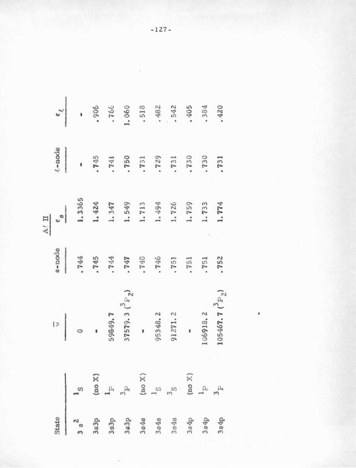
Afl

l

Sta

te

-s-

no

de

t-n

ode

" e

tt

8 --

3 s z

•s

0 •

74

4

1. 3

36

5

3s3

p (n

o X

) -

• 74

5

1.4

Z4

.74

5

• 906

3s3

p

lp

59

84

9.7

• 7

44

1.

347

•

741

• 76

6

3a3

p

3p

37

579

. 3

(3 P z>

• 74

7

1. 5

49

•

75

0 1.

06

0

3s4

e (n

o X

) -

• 748

1.

713

• 7

31

• 5

13

lc

I

3s4

s 95

348.

Z

• 746

1.

49

4

• 7Z

9 .4

82

-

i:)

N

-J

3s4

s 3

s 91

271.

2

• 751

1.

72

6

• 73

1 •

54Z

I

3s4

p

(no

X)

-• 7

51

1. 7

59

•

73

0

• 4

05

3s4

p

1p

10

691

8. z

. 7

51

1. 7

33

• 7

30

•

38

4

3s4

p

3p

1054

67. 7

(3 P

zl

• 75Z

1

.77

4

• 73

1 •

42

0

(">

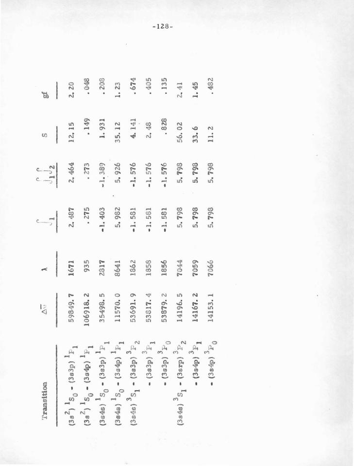
,... r

Tra

nsi

tio

n

6";

; ).

i J

ljl

s g

f ...

1 -

-2

1 1

. (3

e )

s 0 -

(3s3

p)

r--1

59

84

9.7

16

71

2. 4

87

2.4

64

12

. 15

2.

20

2 1

1 (3

s )

s 0 -

(3s4

p)

P 1

10

69

18

. 2

93

5

• 27

5 .

273

• 14

9 •

048

1 1

(3s4

s)

s 0 -

(3s3

p)

P 1

35

49

8. 5

28

17

-1.

40

3

-1.3

89

1.

931

•

208

1 1

(3e4

s)

s 0 •

(3s4

p)

P1

11

57

0. 0

8

64

1

s. 9

82

5.

92

6

35

. 1

2

1. 2

3

3 3

(3s4

o)

s 1 •

(3s3

p)

F 2

5369

1.

9 1

86

2

-1.

581

-1.

576

4. 1

41

• 67

4

3 5

38

17

. 4

1858

-1

. 58

1 -

1. 5

76

2.

48

•

40

5

• (3

s3p

) P

1 I

3 -

• (3

s3p

) 1-

' 0 5

38

79

.2

1856

-1

. 58

1 -1

. 57

6 . 8

28

•

13

5

N

())

I

3 3

(3s4

s)

s 1 -

(3sr

p)

P2

14

19

6. 5

7

044

5.

79

8

5.'7

98

5

6.0

2

2. 4

1

-(3

s4p

) 3 P

1 1

41

67

. 2

70

59

5.

79

3 5

.79

8

33

.6

1. 4

5

• (3

s4p

) 3:

p 0

1415

3. 1

7

06

6

5.7

93

5

. 79

8

11.

2 •

48

2

-129-

Biermann and Harting have computed the ground state of

At ll by SCF without exchange, obtaining c38

:a 1. 212, compared

w ith our result t:" 38 = 1. 336 •

Reference:

Ble rma.nn, L . and Harting, H.

Z. f. Ap. 22., 81. 143

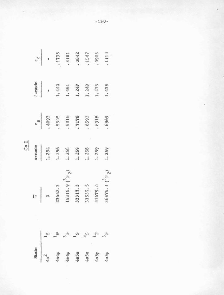
Ca

I -

Sta

te

-a-

node

.f·

no

de

'.1

ee

c .t.

-4

s2

Is

0 1.

25

4

• 4

09

3

4s4

p

1p

2

36

52

. 3

1. 2

56

• 53

05

1. 4

40

•

17

95

4s4

p

3!'

1

53

15

.9 (

3P

2)

1. 2

56

• 5

31

5

1. 4

51

• 31

81

4s5

s Is

3

33

17

.3

1. 2

59

• 7

17

8

1. 2

47

• 0

84

2

4s5

e 3

5

31

53

9. 5

1

. 2

58

•

65

93

1.

24

9

• 1

54

7

4s5

p

lp

41

67

9.0

1

. 2

59

.

69

15

1.

43

3

• 0

90

3

I -3]

? 3

65

75

. 1

(3 P 2

>

y.J

4s5

p

1.

25

9

. 696

9 1.

43

5

• 1

11

4

0 I

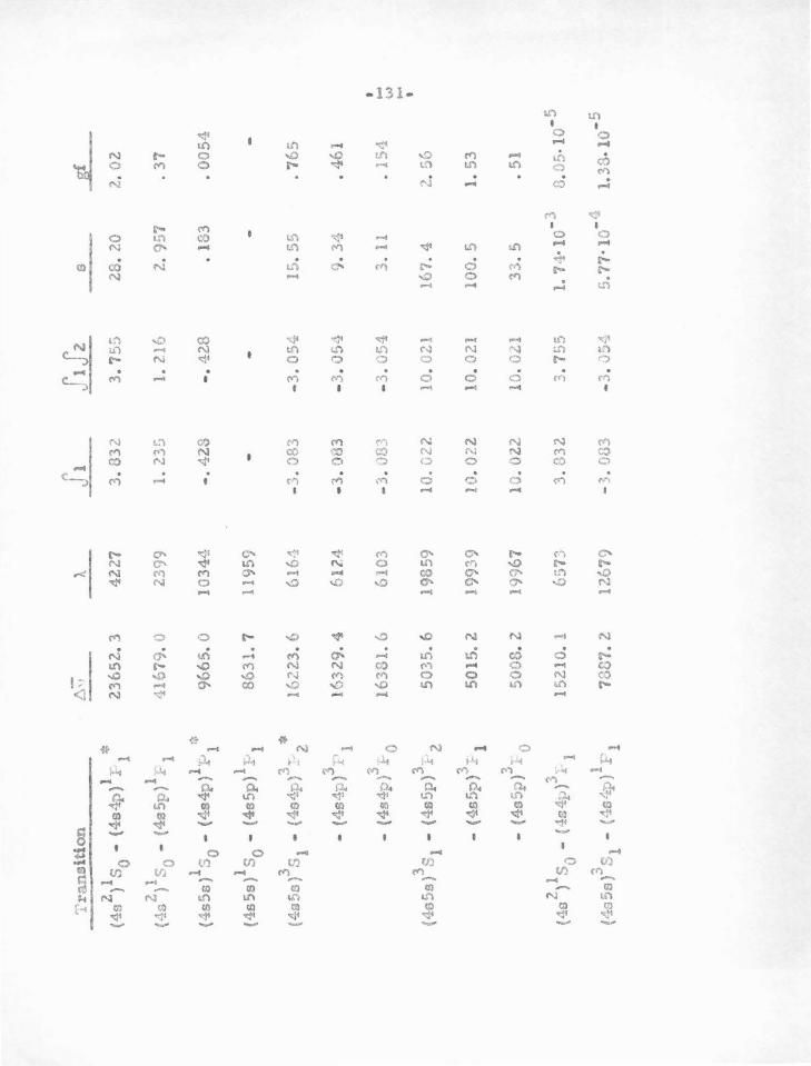
Tra

nsi

tio

n

t.:;;

>. Jl

J1

Jz

9 J!

2 1

1 *

(4s

) s 0

-(4

s4

p)

r 1

23

65

2.

3 4

22

7

3.8

32

3

.75

5

28

. 2

0

2.02

2 1

1 (4

s

) s 0

-(4

s5

p)

F 1

4167

9.0

2399

1

. 23

!j

1. 2

16

2.

957

.

37

1 1

:i'

(4s5

s)

s 0 -

(4s4

p)

1:.- 1

9665

.0

10

34

4

-.42

3 -.

42

8

• 18

3 .

00

54

(4s5

s)1 s

0-

{4s5

p)1 l-

' 1 8

63

1.

7 1

19

59

(4s5

a}3

s1

-(4

s4

p)3

: 2 $

16

22

3.

6 61

6-1

-3.0

83

-3

.05

4 1

5. 5

5

. 7

65

?.

-(4

s4p

)..)I\

16

32

9.4

61

24

-3

.08

3 •

3, {)

5L1

9.34

•

461

-(4

s4p

)3 .f-

0 •

1638

1. 6

6

10

3

-3.

08

3

-3.v

54

3.

11

. 1

54

-w -

(4a

5s)

3 s1

-(4

s5p

)3 I 2

• 5

03

5.

6 19

359

10

.G

2Z

10.

021

16·/

. 4

2. :

)6

-(4

s5p

}3}

1 5

01

5. z

1993

9 1

0.0

22

10

. 0

21

1

00

. 5

1.

53

?

-(4

s5p

f'l·

0 5

00

8. 2

19

967

10.

02

2

10.

0.21

33

.5

. 51

( •1s

2) 1 S

0 -

( 4s 4

!J) \

:. 1

15

21

0. 1

6

57

3

3.8

32

3

.75

5

1. 7

·1·1

0 -3

G.

05

·10

-5

., 1

(4o

5sr

's1

-(4

s4

p)

F 1

73D

7.2

12

67

? -

3.03

3 -

3.0

54

5.

77

·10 -

4 1.

33

-10 -5

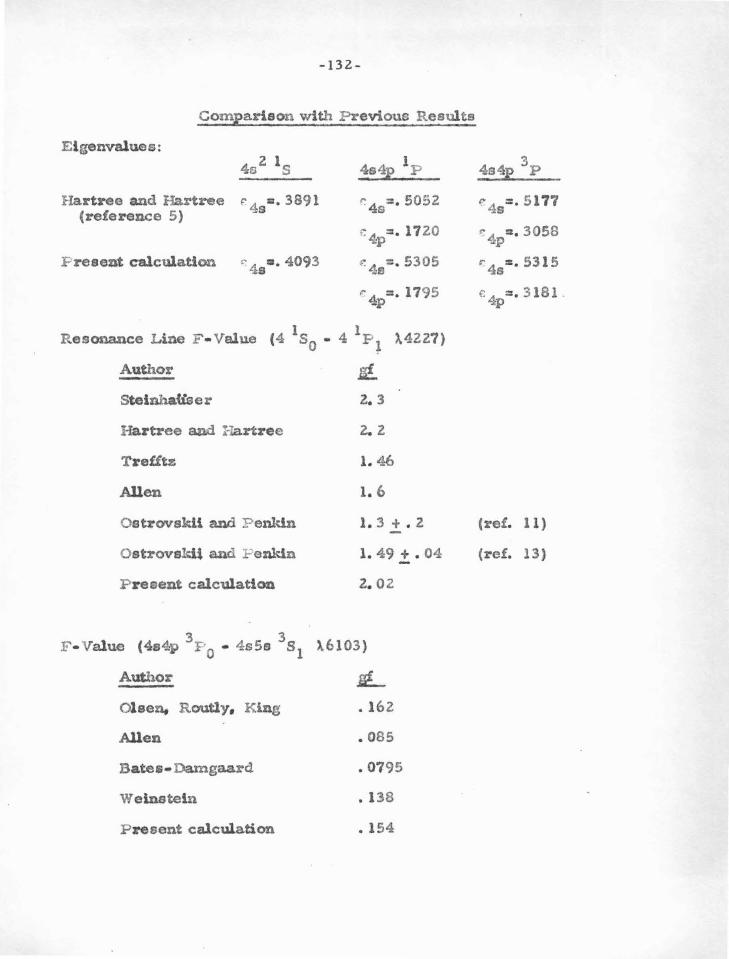
-132-

Comparison with Previous Results

E igenvalues:

4a2 1s 4s 4E

1P

Hartree and H.artree f' 48=. 3891 r. 46=.5052 (reference 5 )

c4 =· 1720 ·p

P resent calculation c: 48.-. 4093 +': 4. =. 5305 ~1!1

f!' 4p=· 1795

1 1 Resonance L ine F • Value (4 s0 • 4 P~ ).4227)

Author

Stelnha«ser

Hartree and Ha.rtree 2. 2

Trefitz 1. 46

Allen 1. 6

OstrovskU a.nd P enkln 1. 3 + • 2

Ostrovsldl and P enkln 1. 49 +. 04 -P resent calculation z. 0 2

3 3 F - Value (4s4p Po • 4s5s s1 ).6103)

Author

Olsen, R outly. King

Allen

Bate&• Damgaard

Weinstein

P resent calculation

• 162

• 085

• 0795

• 138

• 154

3 4a4f P

r- 48=. 5 177

~ 4p=· 3058

r 48

:. 531 5

£ 4 :::. 3 18 1 . p

(ref. 11)

(ref. 13)

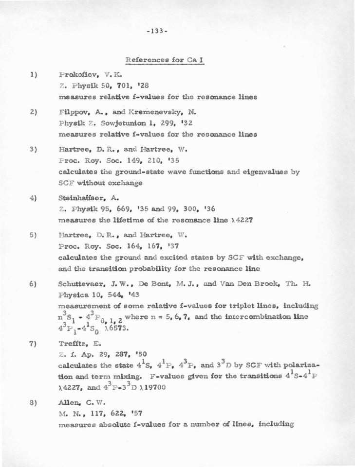
-133-

References for Ca. 1

1 ) :F->rokofiev, V. K .

z . P hysik 50, 7 01, '28

measures relative £-values for the resonance linea

2) F Uppov, A. , and Kremenevsky, N.

Physik z. Sowjetunion 1, 299, 132

measures relative £-values for the resonance liMe

3) Hanree, D. R. , and Hartree, W.

~Proc. Roy. Soc. 149, 210, ' 35

calculates the ground-state wave functions and e i genvalues by

SCF without exchange

4 ) SteinhaUser, A.

z. PhysUt 95, 669, 135 and 99, 300, '36

measures tl1.e lifetime of the r esonance line >.. 4227

5) Hartree, D. R . , and Hartree, W.

Proc. R oy. Soc. 164, 167, '37

calculates the ground and excited states by SCF with exchange,

and the transition probabUity for the resonance line

6) Schuttevaer, J. W., De Bont, M. J ., and Van Den Broe!<. Th. H.

P hyslca. 1 O, 544, ' 43

measurement of some rel ative £-values for triplet Unes, lncludlng 3 3

n3 s1 · t P 0, 1, 2 where n:: 5, 6, 7, and the lntercombtnation line

4 :P1

- 4 s0

>.. 65'73.

7) Trefftz, E .

z. £. Ap. 29, 287, ' 50 1 1 3 3 calculates the state 4 S, 4 P , 4 P , and 3 D by SCF with polariza-

1 1 tlon and term mixing. F •values given for the transitions 4 5· 4 P

>..4227, and 43 P - 3

3D >.. 19700

8) Allen, c . W.

M. N., 117, 62Z.. ' 57

measures absolute £-values for a llUmber of lines, including

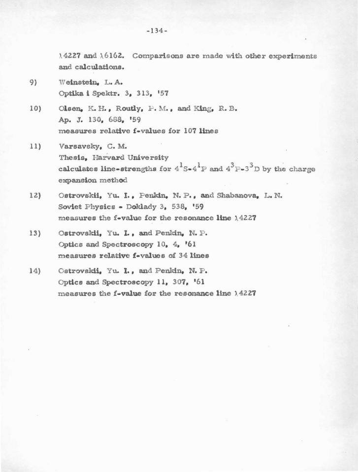
-134-

>..4227 and ).6162. Comparisons are made with other experiments

and calculations.

9) Weinstein. L.A.

Optlka 1 Spektr. 3, 313, 157

10) Ol sen. K. H. , Routly, r . M. , and King, R. B .

Ap. J. 130, 688, ' 59 measures relative !·values £or 107 lines

11) Varsavsky. c. M.

Thesis, HarVard University 1 1 3 _ 3 .

calculates line- strengths for 4 5 · 4 P and 4 l-'•3 D by the charge

expansion method

12) Ostrovskii, Yu. I. , P enldn. N. P ., and Shabanova. L. N.

Soviet Physics - Doklady 3, 538, '59 measures the f · value !or the resonance line >.. 4 227

13) Ostrovsk.U, Yu. L , and Penkin. N. P.

Optics and Spectroscopy 10, 4, '61

measures relative f · values o£ 341ines

14) Ostrovak.U, Yu. I., and P enkln, N. P .

Optics and Spectroscopy 11, 307, ' 61

measures the £-value for the resonance line ). 4227

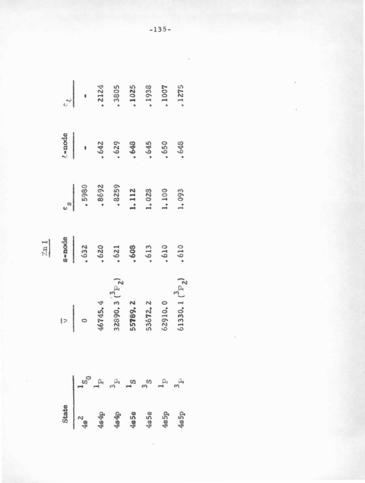
Zn

I

-S

tate

-

s•n

od

e

!•n

od

e \1

e

rt

s -

-4

82

•s 0

0 •

63

2

• 59

80

4a4

p

lp

46

74

5.4

• 6

2.0

• 869

2.

• 64

2.

• 2.

124

4s4

p

3F

3Z

S90

. 3 (

lp 2

) •

621

• 82.

59

• 62

.9

• 3

80

5

4e5

s ls

5

51

89

.2

• 60

8

1.1

12

• 6

48

.10

25

4s5

s 3

8

5367

2.. z

• 6

13

1.

02.

8 .6

45

•

1938

I .....

4

s5p

lp

62

.910

.0

• 61

0

I. 1

00

• 6

50

•

1007

U

)

1.11

I

4&5p

31

-6

13

30

. 1

(3 P2)

• 610

1.

093

•

648

• 1

27

5

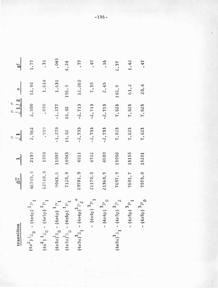
tran

siti

on

(4s2

) ls

o

-(4

s4

p)

lp 1

(4s2

) 1 s 0

-(4

s5p

) 1 P

1

1 1

(4e5

s) s

0 -

(4s4

p)

P 1

1 1

(4s5

s) s

0 -

(4sS

p)

P 1

Av

l --

46

74

5.4

2

13

9

62

91

0.0

1

59

0

90

43

.8

11

05

7

71

20

.8

14

04

3

3 3

* (4

s5s)

s1

-(4

e4p

) P

2 2

07

81

.9

48

11

3 -

(4s4

p)

P 1

21

17

0.8

4

72

2

3 -

(4s4

p)

P 0

21

36

0.9

4

68

0

3 3

(4s5

s)

s 1 -

(4s5

p)

P2

3 -(

4s5

p)

P1

3 -

(4s5

p)

P 0

76

57

.9

13

05

8

76

01

.7

13

15

5

75

75

.0

13

20

1

n r

n

1.L

J

1,1

2 s

_£

2. 5

62

2

. 50

0

12

. so

1. 7

7

• 91

9

• 89

6

1.6

14

•

31

-1.2

78

-1

.27

7

1.6

31

•

04

5

14

.02

1

4.0

2

19

6.5

4

.24

-2.7

33

-2

.71

3

12

.26

5

.77

-2.7

33

-2

.71

3

7,3

5

• 47

-2.7

33

-2

.71

3

2.4

5

• 16

7.8

23

7

. 8

23

1

02

.0

2.3

7

7.8

23

7

. 8

23

6

1.2

1

.42

7.8

23

7

.82

3

20

.4

• 47

I .... w

0'

I

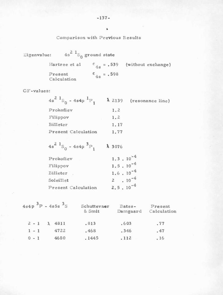
-137-

• Comparison with Pre v ious R esults

.t:;igenvalue:

Hartree et al

Present Calculation

c 46 = • 539

E: 48

= • 598

(without exchange)

GF - values:

3 4s4p P

2 - 1

1 - 1

0 - 1

482 I S O 4 4 l p - s p 1

Prokofiev

Filippov

Billeter

Present Calculation

482 ISO 4 4 3 p - s p 1

Prol<ofiev

F ilippov

B illeter

Soleillet

P resent Calculation

).

"

3 - 4e5s S Schut tevaer

& Smit

"' 4811 . 813

4722 . 468

4680 . 1445

2139 (resonance line)

1.2

1.2

1. 17

1. 77

3076

1. 3 • 10·- 4

1. 5 . 10-4

1.6. 10-4

2 • 10-4

2 . 5 • 10- 4

Bates-Damgaard

• 603

. 346

. 112

P resent Calculation

. 77

. 47

• 16

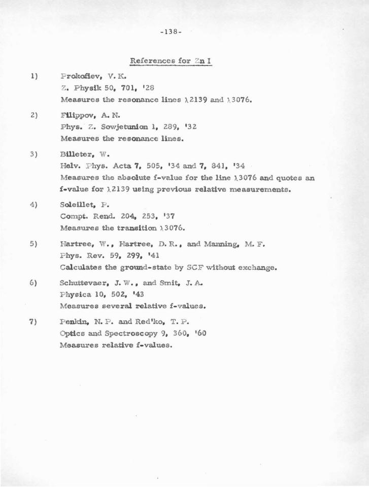
-138-

References for Zn I

1) P rokofiev, V . K.

z. Physik so, 701, '28

Measures the resonance lines >._2139 and ;.. 3076.

2) Ftllppov, A. N.

Phys. z. Sowjetunlon 1, 289, •32

Measures the resonance lines.

3) BUleter, W.

Helv. P hys. Acta 7, 505, '34 and 7, 841, ' 34

Measures the absolute £- value for the line >._3076 and quotes an

f·va.lue for >..2139 using previous relative measurements.

4 ) SoleWet, F .

Compt. R end. 204, 253, '37

Measures the transition >..3076.

5) Ha.rtree, W. , Hartree, D. R. , and Manning. M. F .

P hys. Rev. 59, 299, 141

Calculates the ground-state by SCF without exchange.

6) Schutteva.er, J . W., and Smit, J . A.

P hyelca 10, 502, ' 43

Measures several relative f - values.

7) Penkin, N. P . and Red 'l~o, T. P .

Optics and Spectroscopy 9, 360, 160

Measu1•es relative f·values.

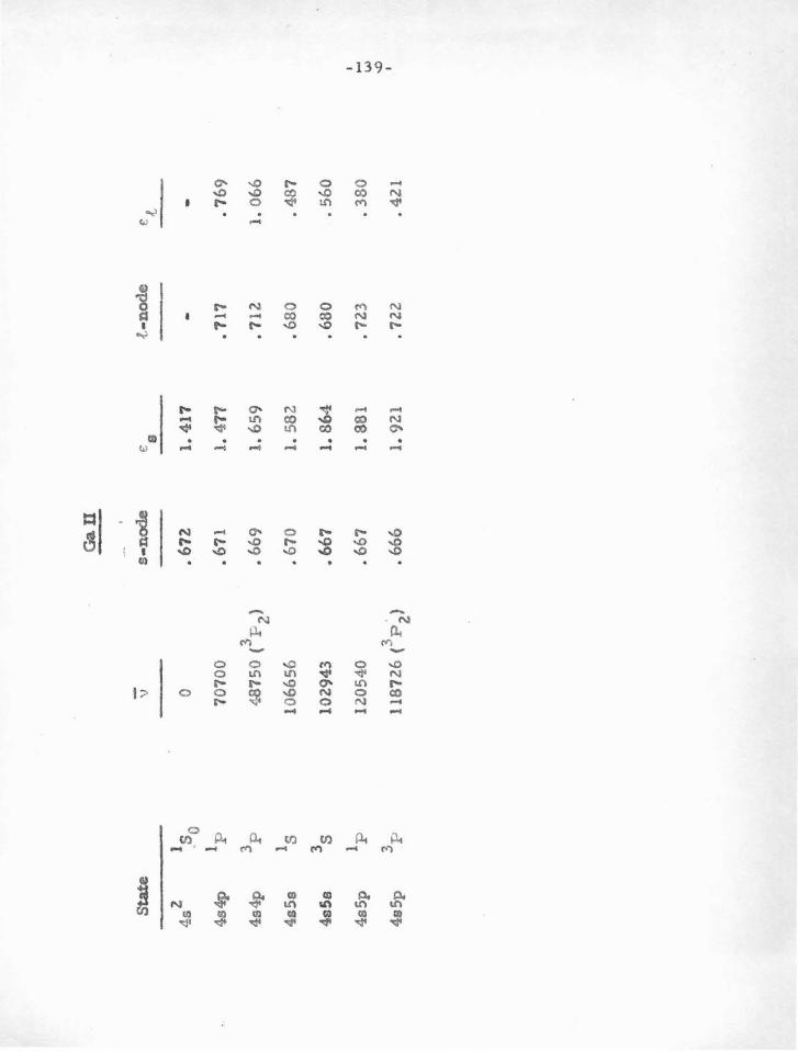
Ga.

U

-l

·-·~

Sta

te

- v s-

node

e

s .f.-n

ode

E:

t -

4 l

_s

Is

. 0

0 • 6

72

1.

41

7

4s4

p

lp

70

70

0

• 671

1.

477

.7

17

• 7

69

4s4

p

3p

48

75

0 (

3F

2)

• 6

69

1

.65

9

.71

2

1. 0

66

4s5

e

Is

106

65

6

• 6

70

1.

58

2

• 68

0

. 4

87

4s5

s 3s

10

2943

•

66

7

1. 8

64

• 6

80

.

560

lp

I

4s5

p

1205

40

• 66

7 1.

88

1

• 723

.

38

0

-v.> 3p

11

8726

(3P~)

..

0

4s5

p

• 66

6 1.

921

• 7

22

•

421

I

,'

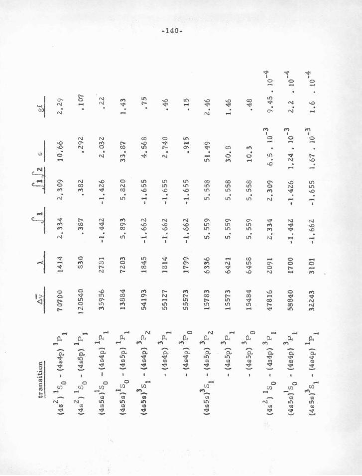
tran

siti

on

2 1

1 (4

s )

s 0 -

(4s4

p)

P 1

2 1

1 (4

s )

s 0 -

(4s5

.p)

P 1

1 1

(4s5

s)

s 0 -

(4s4

p)

P 1

1 1

(4s5

s) s

0 -

(4s5

p)

P 1

3 3

(4s5

s)

51

-(4

s4

p)

p2

3 -

(4s4

p)

P 1

3 -

(4s4

p)

P 0

3 3

(4s5

s)

s 1 -

(4s5

p)

P2

2 1

(4s

) so

3 -

(4s5

p)

P 1

3 -

(4s5

p)

P 0

3 -

( 43

4p

) p

1

1 3

(4s5

s) s

0 -

(4s4

p)

P 1

3 1

(4e

5s)

s 1 -

(4s4

p)

P 1

6v

-70

7!)0

1205

40

3595

6

1388

4

5419

3

5512

7

5557

3

1578

3

1557

3

1548

4

4781

6

5884

0

3224

3

! __

ji_

..1.!1

! _s

_

1414

2

.33

4

2.3

09

10

.66

830

.38

7

.38

2

.292

2781

-1

.442

-1

.42

6

2.0

32

7203

5

.89

3

5.8

20

3

3.8

7

1845

-1

.66

2

-1.6

55

4

. 5

68

1814

-1

.66

2

-1.6

55

2

.74

0

1799

-1

.66

2

-1.6

55

.9

15

6336

5

.55

9

5.5

58

5

1.4

9

6421

5

.55

9

5.55

8 30

.8

6458

5

.55

9

5.5

58

10

.3

2091

2

.33

4

2.3

09

6

. 5 •

10-

3

17

00

-1

.44

2

-1.4

26

1.

24

• 10

-3

3101

-1

.66

2

-1.6

55

1

.67

• 1

0-3

~

2.2

9

.10

7

• 22

1.4

3

.75

• 46

• 15

2.4

6

1.4

6

.48

9.4

5 •

10

-4

2. 2

•

10

-4

1. 6

•

10-4

I .....

.a:.

0 I

-141-

Hartree, Hartree, and Manning have calculated the

ground-state functions of Ga II by SCF without exchange. T hey

2 1 obtain £ = 1.28 for the 4s S state , compared to our e = 1. 417,

Reference:

Hartree, W ., Hartree, D. R ., and Manning. M. F .

P hys. R ev. 59 . 299 '41

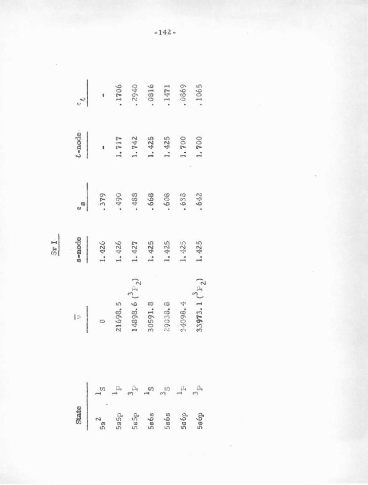
Sr

1 -

Sta

te

-s•

no

de

t-no

de·

\)

eQ

et

--

5s2

ts

0 1.

42

6

• 379

5s5

p

lp

21

69

8.5

1. 4

26

•

49

0

1. 7

17

• 17

06

Ss5

p

3p

14

89

8. 6

(3

P 2

) 1.

42

7 •

48

8

1. 7

42

•

29

40

Ss6

s 1s

30

591

.8

1. 4

25

• 6

68

1.

42

5

• 08

16

I

35

.....

S

s6s

2903

8.8

1. 4

25

•

60

8

1. 4

Z5

• 14

71

.;::.

N

I

5s6

p

lF

34

09

8.4

1.4

25

• 6

38

1.

700

•

08

69

5s6p

3p

33

.97

3.

1 (3

P 2>

1.

4Z

5 . 6

42

1.7

00

. 1

06

5

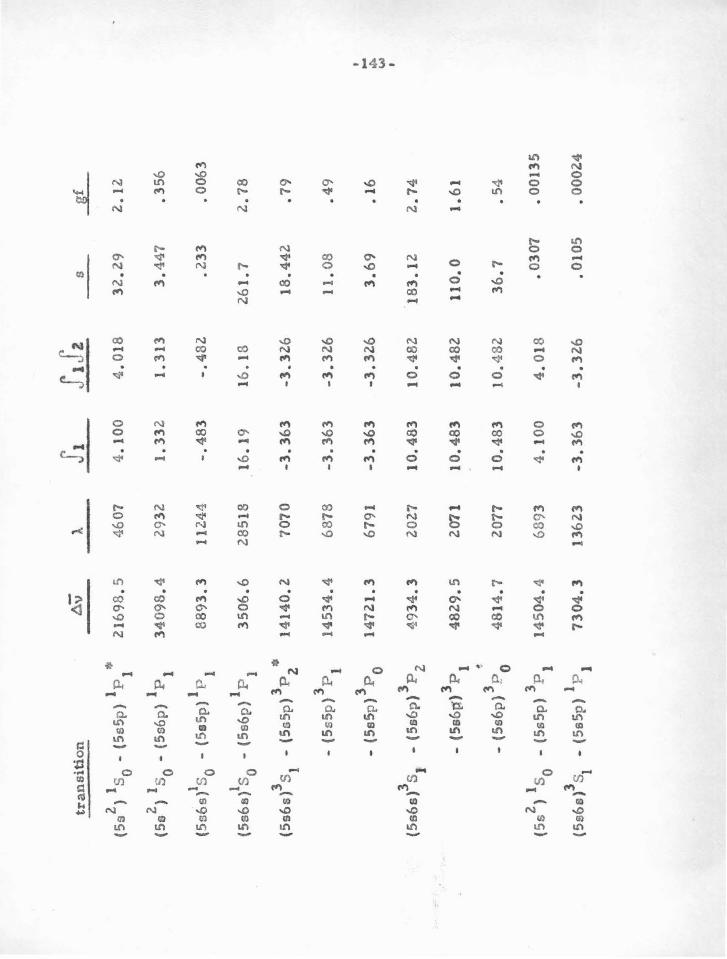
tran

siti

on

A"

V ).

J1

Jt

fz

s J.f

2 1

1 (S

a )

s 0 -

(SsS

p)

P 1 •

21

69

8.5

46

07

4.1

00

4

.01

8 3

2.2

9

2.1

2

2 1

1 (5

s )

s 0 -

(Ss6

p)

P 1

34

09

8.4

29

32

1.3

32

1

.31

3

3.4

47

• 356

1 1

(5s6

s) s

0 -

(5s5

p)

P 1

88

93

.3

1124

4 -.

483

-.

48

2

.23

3

. 006

3

1 1

(5s6

s) s

0 -

(5s6

p)

P 1

35

06

.6

2851

8 1

6.1

9

16.

13

26

1.7

2

.78

3 3

* (5

s6s)

s1

-(5

s5p)

P

2 1

41

40

.2

7070

-3

.36

3

-3.3

26

1

8.4

42

.7

9

3 -(

5s5

p)P

1 1

45

34

.4

6878

-3

.36

3

-3.3

26

1

1.0

8

.49

3 I

14

72

1.3

67

91

-3.3

63

-3

.32

6

3.6

9

• 16

--

(5s5

p)

P 0

~

w

I

3 3

(5s6

s) s

1 -

(Ss6

p)

P 2

493

4.3

20

27

10

.48

3

10

.48

2

18

3.1

2

2.7

4

3 -(5s6~)

P 1

48

29

.5

2071

1

0.4

83

1

0.4

82

1

10

.0

1. 6

1

-3

. -

(5s6

p)

P 0

48

14

.7

2077

1

0.4

83

1 o

. 482

3

6.7

•

54

2 1

3 (S

s )

s 0 -

(5s5

p)

P 1

14

50

4.4

68

93

4.1

00

4.0

18

• 0

307

• 001

35

3 1

(5s6

s) s

1 •

(SsS

p)

P l

73

04

.3

1362

3 -3

.36

3

-3.3

26

• 0

105

• 000

24

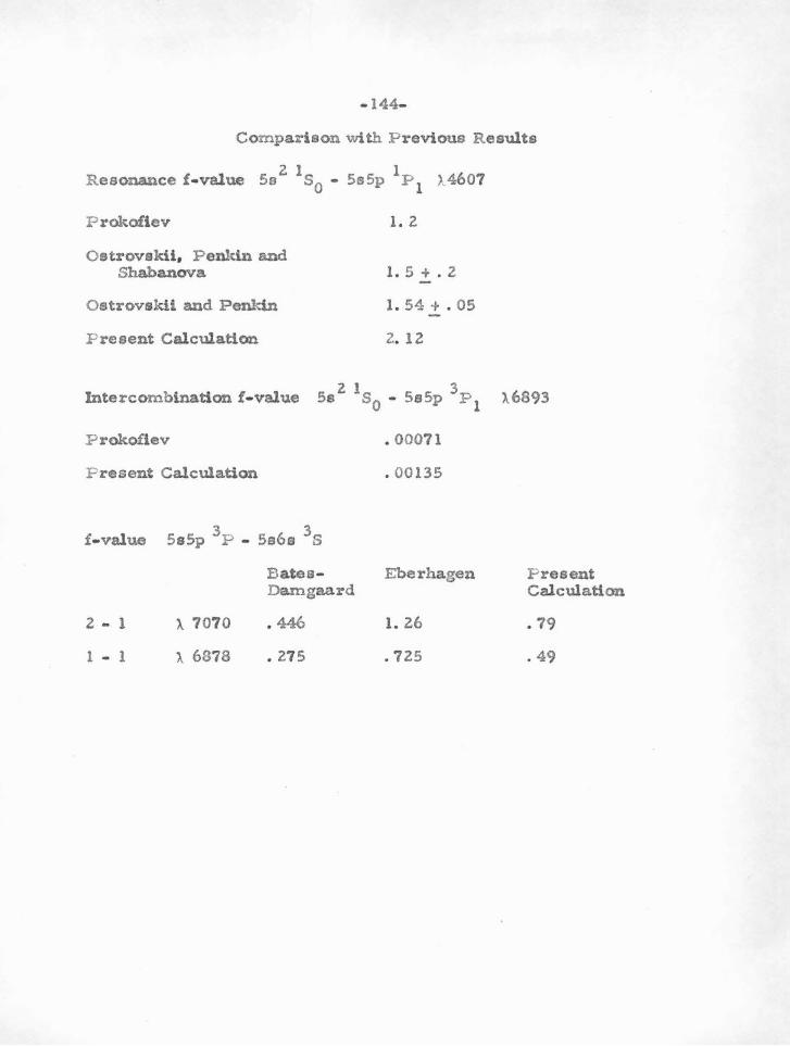
- 144-

Comparison with Previous Results

2 1 1 Resonance £- value Sa s0 .. 5s5p P 1 )A607

P rokofiev

Ostrovakii, Penldn and Shahan ova

Ostrovskii and Penldn

Present Calculation

1.2

1. 5 + • 2

1. 54+ • 05

2. 12

2 1 3 Intercombination f · value Ss s0 - Ss5p P 1 ).6893

P rokofiev • 00071

P resent Calculation • 00135

£- value 3 3 5s5p P - 5a6s S

Bates- Eberhagen P resent Damgaard Calculation

2- 1 ). 7070 • 446 1. 26 • 79

1 - 1 A 6878 • 275 . 725 . 49

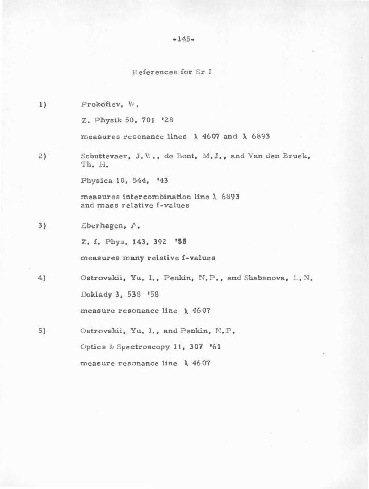
1)

2)

3)

4)

5)

-1~5-

R eferencee for S r I

Prokofiev, VV •

Z. Physik SO, 701 '28

measures resonance linea "- 4607 and ~ 6893

Schuttevaer, J. V . • , de Bont, M . J. , and Van den B ruek, T h. H .

Physica 10, 544, '43

measures intercombination line >.. 6893 and mass relative £-values

.Eberhagen. P.

z. f. Phys. 143, 392 '5!

measures many relative £-values

Ostrovekii, Yu. I., P enkin, N. P., and Shabanova, L . N .

Doklady 3, 538 '58

measure resonance line ~ 4607

O strovekii,. Yu. I., and Penkin, N . P .

Optics & Spectroscopy ll, 307 '61

measure resonance line l. 4607

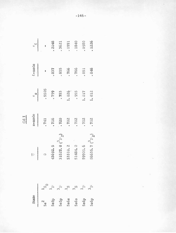
Cd

I

-S

tate

-

s-n

od

e t-

nocl

e \I

€

c.t

9 -

-5

s2 Is

0 0

• 741

•

5505

5s5

p

1p

4369

2.. 5

.7

16

• 79

9

• 83

7

• 20

48

5s5

p

3p

31

827

. o

(3 P2)

• 12.

0 •

75

3

. 81

5

. 3

62

1

5s6

s .1

s 5

33

10

. 2

.70

2 1.

02

6

• 76

6

. 09

91

5e6

s 35

5

14

84.

0

• 70

2

• 95

5 • 7

66

.

1840

I ....

lp

~

5s6

p

5990

5.6

. 70

2

1.

017

•

851

• 098

0 0

' I

5s6

p

3p

5063

5. 1

(3 P

2>

• 7

0Z

1. 0

12

• 84

8

• 12

.26

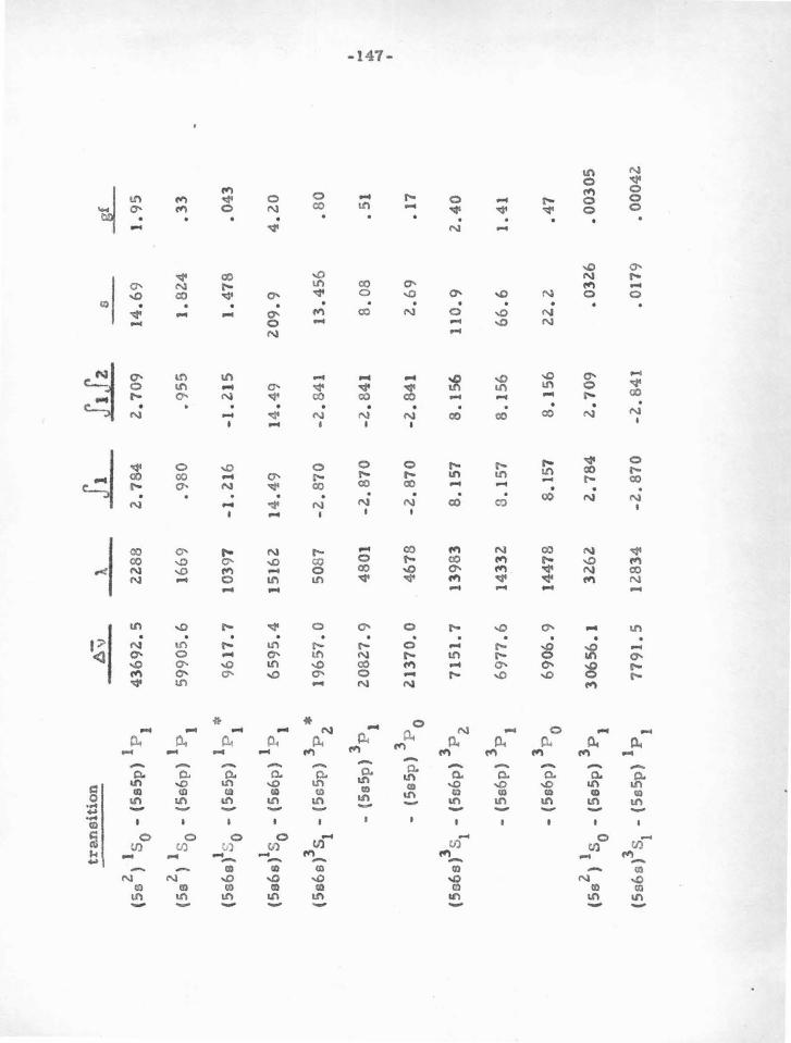
tran

siti

on

Av

~

.1!_

.M

_

a g£

-

----

2 1

1 ( S

s )

s 0 -

(5s5

p)

P 1

43

69

2.5

2

28

8

2. 7

84

2

.70

9

14.6

9 1

.95

2 1

1 (S

a )

s 0 -

(5s6

p)

P 1

59

90

5.6

16

69

.9

80

.9

55

1

.82

4

.33

1 1

* (5

s6s

) s 0

-(5

s5p

) P

1 96

17

.7

1039

7 -1

.21

6 -1

.21

5 1

.47

8

• 043

1 1

(5s6

s) s

0 -

(5s6

p)

P 1

65

95

.4

1516

2

14.4

9

14.4

9

20

9.9

4

.20

3 3

(5s6

s) s

1 -

(5s5

p)

P2 *

19

65

7.0

50

87

-2.8

70

-2

.84

1 1

3.4

56

.8

0

3 I

-(S

sSp

) P

1 2

08

27

.9

48

01

-2

.87

0

-2.8

41

8.0

8 • 5

1 -Ml- -.a

I

3 -

(Ss5

p)

PO

2

13

70

.0

46

78

-2

.87

0

-2.8

41

2.6

9

.17

3 3

(5s6

s) 8

1-

(5s6

p)

p2

7

15

1.7

1

398

3 8

.15

7

8.1

56

1

10

.9

2.4

0

3 -

(5s6

p)

P 1

69

77

.6

14

33

2

8.1

57

8.1

56

6

6.6

1

.41

3 -(

5s6

p)

P0

69

06

.9

1447

8 8

.157

8

.15

6

22.2

• 4

7

2 1

3 (S

s )

s 0 -

(5s5

p)

P 1

30

65

6.1

3Z

6Z

2.7

84

z.

70

9

• 032

6 •

00

30

5

3 1

(Ss6

s) s

1 -

(5s5

p)

PI

77

91

.5

12

83

4

-2.

87

0

-2.8

41

• 017

9 •

0004

.2

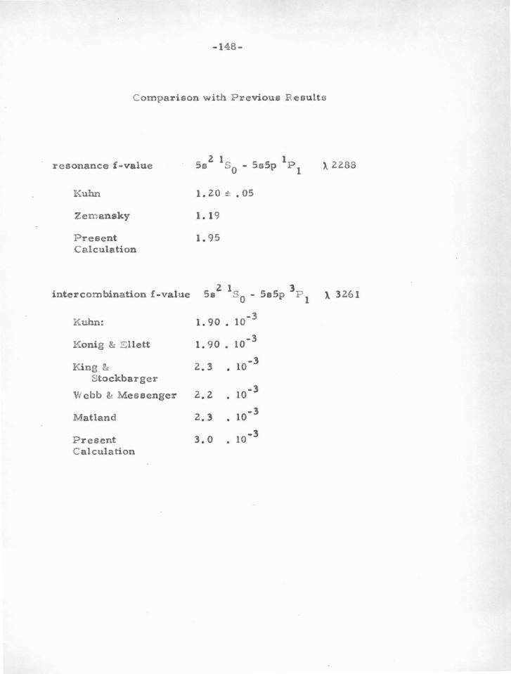
-148-

Comparison with Previous Results

resonance f -value

l<uhn

Zemansky

Present Calculation

intercombination £-value

Kuhn:

Konig & .Ellett

King & Stockbarger

Webb & Messenger

Matland

Present Calculation

). 2288

1. 20 :!: • 05

1. 19

1. 95

5 1. l eo 5 5 3p s ~0 - 8 p 1 ~ 3261

1. 90 • 10-3

1. 90 • 10-3

2.3 • 10-l

2.2 • 10-3

2.3 • 10-3

3.0 • 10-3

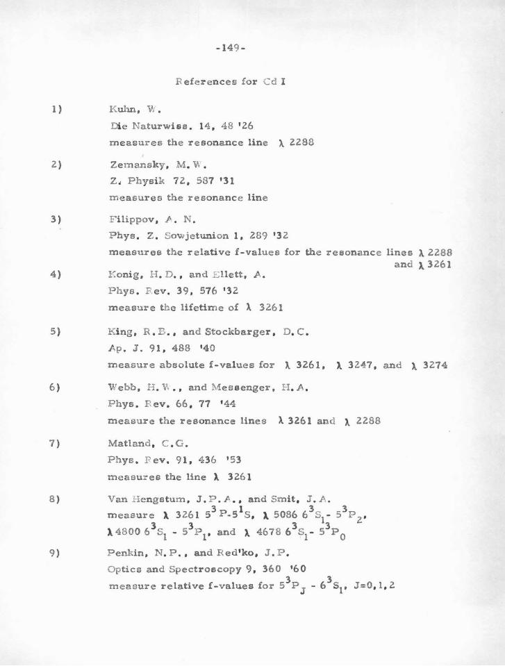
1)

2)

3)

4)

5)

6)

7)

8)

9)

-149 -

F eferences for Cd I

Kuhn , ·w . Die Naturwiss. 14 , 48 '26

measures the resonance line ). 2288

Zemansky, M . 'II\ •

z4 Physik 72, 587 '31

measures the resonance line

F ilippov, J> . N .

Phys . z. Sowjetun.ion 1, 289 '32

measures the relative f-values for the resonance lines A. 2288 and ). 3261

Konig, H . D., and E llett, A.

Phys . R ev. 39, 576 '32

measure t h e lifetime of ). 3261

Ki ng, R . B . , and Stockbarger , D. C .

Ap. J. 91,488 '40

measure absolute £-values for ). 3261, l. 3247, and ). 3274

Webb, H . V. ., and Messenger, H . A .

Phye. R ev. 66 , 77 ' 44

measure the resonance lines >.. 3261 and l. 2288

Matland, C . G .

Phye . F ev. 91 , 436 '53

measures the line ). 3261

Van H engetum , J. P . P. .• , and Smit, J . A . 3 1 3 3

measure ). 3261 5 P-5 S , ). 5086 6 s1- 5 P 2 , 3 3 3 3

). 4800 6 s1 - 5 P 1, and l. 4678 6 s1- 5 P 0

Penldn, N . P ., and R ed'ko, J.P.

Optics and Spectroscopy 9, 360 '60 3 3

measure relative £-values for 5 P J - 6 s1, J=O, 1, 2

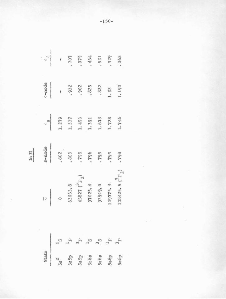
Inn

-

Sta

te

- \J s-

no

de

t-no

de

€ e ~

-9

-ss

2 Is

0

• 80

2

1. 2

79

Ss5

p

lp

~3033

.8

• 80

3 1.

33

7

• 9

32

.

707

5s5

p

\-'

458

27 (

3 P2)

• 79

5 1.

496

•

90

2

• 97

9

5s6

s ls

97

025.

4 • 7

96

1. 3

91

• 82

3

• 4

54

Ss6

s 3s

9

39

19

.0

• 79

3 1.

67

8

• B

lZ

• 52

1 I .....

·1

1.1

1 S

s6p

p

1097

75.4

• 7

()3

1. 7

28

1. 2

2 •

32

9

0 I

5e6

p

3p

10

8425

. s

(3 P2

) •

793

1. 7

46

1.

193

~

36

3

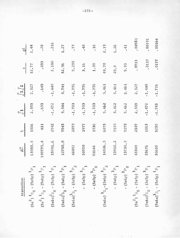
tran

siti

on

A

\i

,.,. ft

]t

J~

s __

_&£

2 1

1 (S

s )

s 0 -

(5sS

p)

P 1

63

03

3.8

15

86

2.5

53

2

.52

7

12

.77

2

.44

2 1

1 (S

s )

s 0 -

(5s6

p)

P 1

10

97

75

.4

41

1

.65

3

.64

5

.83

3

.28

(5s6

s)1 s 0

-(5

e5p

) 1 P

1 3

39

91

.6

29

42

-1

.47

2

-1.4

49

2

.10

0 • 2

16

1 1

(Ss6

s) s 0

-(S

s6p

) P

1 1

27

50

.0

78

43

5

.84

4

5.7

41

3

2.9

6

1.2

7

3 3

(5s6

s) s

1 -

(Ss5

p)

P2

48

09

2

20

79

-1

.78

3 -1

.77

6

5.2

55

.7

7

3 5

05

70

1

977

-1

.78

3

-1.7

76

3.1

6 .4

8 -

(5s5

p)

P 1

I ... Ul ....

3 5

164

4

1936

-1

.78

3 -1

.77

6

1. O

S •

16

I -

{SsS

p)

PO

3 3

(Ss6

s)

s 1-

(Ss6

p)

P2

1 45

06

.5

68

93

5

.46

2

5.4

61

49

.70

2

.19

3 -

(5s6

p)

P1

13

91

8.2

7

18

5

5.4

62

5

.461

29

.8

1. 2

6

3 -

(Ss6

p)

P 0

13

73

8.9

7

27

9

5.4

62

5

.46

1

9.9

5

.41

2 1

3 (S

s )

s 0 -

(5s5

p)

P 1

43

349

2

30

7

2.5

53

2

.52

7

• 0

71

3

• 00

93

8

1 3

(Se6

s) s

0 -

(SsS

p)

P 1

53

67

6

1863

-1

.47

2

-1.4

49

• 0

117

• 00

191

3 1

(Ss6

s) s

1 -

(5s5

p)

P1

30

88

5

32

38

-1

.78

3

-1.7

76

•

0177

.

00

164

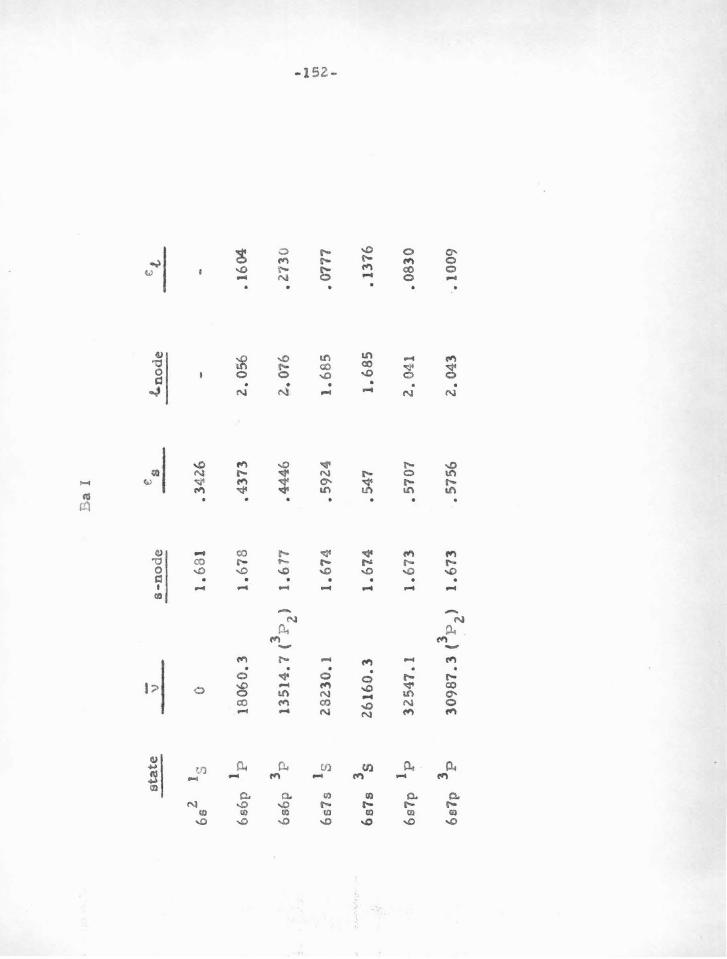
Ea

I

state

-

es

c.,

'\)

s-n

od

e

.(.n

ode

-6

s2 Is

0

1.6

81

.3

42

6

1 6

s6p

P

18

06

0.3

1

.67

8

.43

73

2

. 05

6 .1

60

4

3 1

35

14

.7 (

3 P 2

) 1

.61

7

.44

46

z..

076

.2

73

0

6s6

p

P I ....

1 \S

l 6

s7s

S 2

82

30

.1

1.6

74

•

59

24

1

.68

5

• 0

77

7

N

I

3 6

s7s

S 2

61

60

.3

1. 6

14

• 5

47

1

.68

5

.13

76

1 6

s7p

P

32

54

7.

1 1

.67

3

• 5

70

7

2.

041

• 08

30

3 6

s7p

P

30

98

7.3

(3 P

2)

1.6

73

•

57

56

2

. 04

3 ·.1

00

9

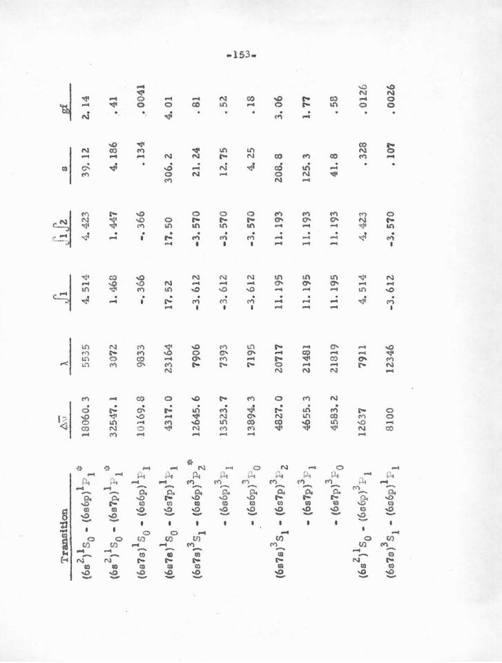
Tra

nsi

Uo

n

~'V

A. ji_

a

s g

f

2 1

1 l)

{6

s )

s 0 -

(6s6

p)

P 1

1806

0. 3

55

35

4. 5

14

4. 4

Z3

39

. 12

2.

14

2 1

1 *

(6a

) s 0

-(6

s7p)

P 1

3254

7. 1

30

72

1.

468

1.

44

7

4. 1

86

• 41

1 1

(6s7

s) s

0 •

(6s6

p)

P1

1016

9. 8

98

33

-.3

66

-.

366

•

134

• 00

41

1 1

(6s7

s) s

0 •

(6s7

p)

P 1

43

17

.0

23

16

4

17

.52

1

7.5

0

30

6.2

4.

01

3 3

* (6

a7s)

s1

• (6

s6p

) P

z 1

26

45

.6

79

06

-3

.61

2

-3.

57

0

21.

24

• 81

-(6

s6p

}3P

1 1

35

23

.7

7393

-3

.61

2

-3.

570

12

.75

•

52

' ....

3 .

Ul

1389

4. 3

71

95

-3.6

12

-3

. 5

70

4.

25

• 1

8

vv

-(6

s6p

) :r:-

0 •

(6s7

s)3 s 1

-(6

s7p

)3 P 2

48

27

.0

2011

7 11

. 19

5 11

. 19

3 2

08

.8

3.0

6

-(6

s7p)

3 P1

4655

. 3

2148

1 11

. 19

5 11

. 19

3 12

5. 3

1.

77

3 -

(6s7

p)

P0

45

83

.2

218

19

11.

195

11.

193

41

.8

• 58

2 1

3 (6

s )

s 0 -

(6a6

p}

P1

1263

7 79

11

4. 5

14

4.

42.

3 •

328

• 0

126

3 1

(6a7

s) 5

1 -

(6s6

p}

pl

810

0 12

346

-3.6

12

. -3

.57

0

• 10

7 •

00

26

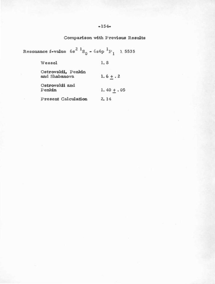
-154-

Comparison with Previous Results

z 1 1 Resonance f·value 6s s0 - 6s6p P 1 ). 5535

Wessel

Ostrovskll. Penkln and Shabanova

Ostrovekll and Penkln

Present Calculatloo

1. 8

1. 6 + • 2

1. 40 + • 05

z. 14

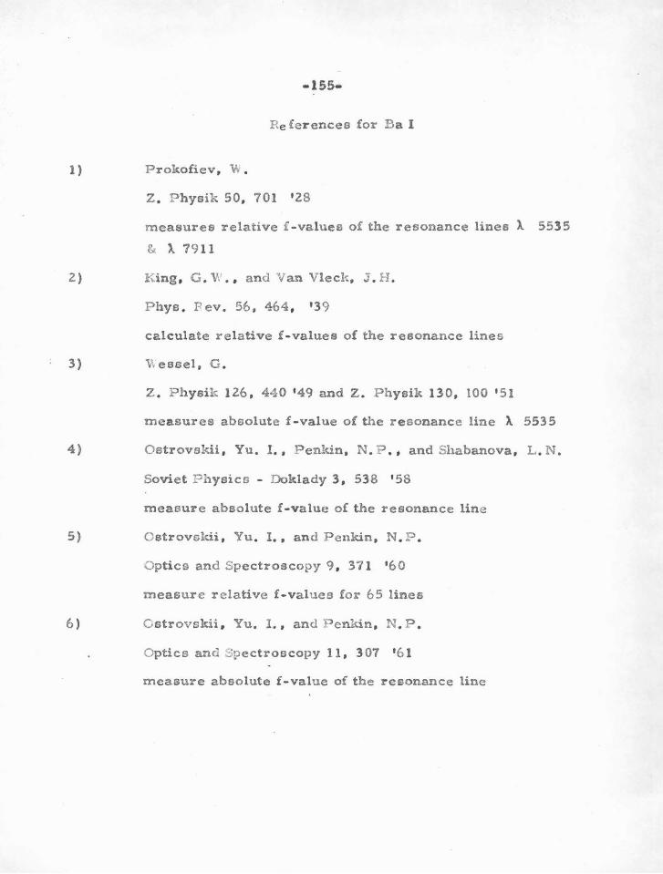
1)

2)

3)

4)

5)

6)

Re !erences for B a I

Prokofiev, W .

z. Physik 50, 701 '28

measures relative f -value a of the resonance lines l 5535

& ). 7911

King, G . V.' ., and V an Vleck , J . H .

P hys. F ev. 56, 464, 139

calculate relative £-values of the resonance lines

\\ easel, G .

z. Physik 126, 440 '49 and Z. Physik 130, 100 ' 51

measures absolute £-value o£ the resonance line l 5535

Ostrovskii, Yu. I., Penkin, N . P ., and Shabanova, L . N .

Soviet Physics - Doklady 3, 538 1 58

measure absolute £-value of the resonance line

Ostrovskii, Yu. I. , and Penkin, N . P .

Optics and Spectroscopy 9 , 371 160

measure r elative £-values for 65 lines

Ostrovekii , Yu. l ., and Penkin, N . P .

Optics and Spectroscopy 11, 307 ' 6 1

measure absolute £-valu e of the resonance line

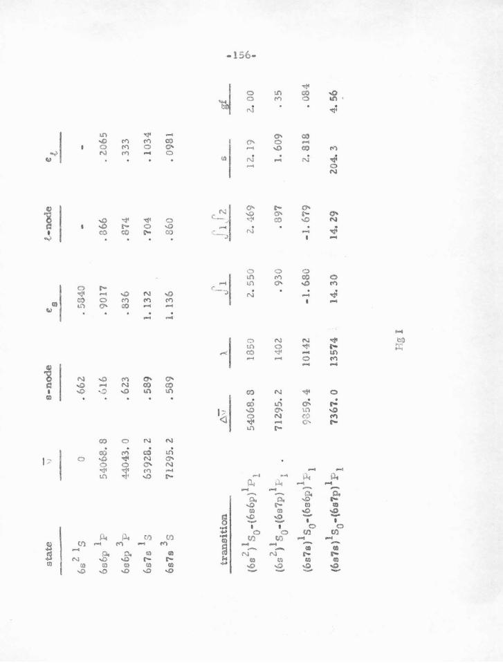
-s-

no

de

t-no

de

state

'I

es

et -

6s

2 1 s

0 •

66

2

• 5

84

0

6s6

p 1 F·

5

40

68.

8 . (

J16

. 9

01

7

.866

.

2.06

5

3 6

s6p

P

44

04

3.0

•

62.3

•

83

6

. 87

4

. 3

33

6s7

s 1 S

6392

8. z

•

58

9

1. 1

32

.7

04

.

103

4

3 6

s7s

S 7

12

95

. 2

• 5

89

1.

13

6

• 8

60

•

09

81

.....

,_i\ /z

tr

an

siti

on

A7

7 A

J 1

s

gf

• ... 2

1 1

01

(6s

} s 0

-(6

s6p

) P

1 5

40

68

.8

18

50

2. 5

50

2.

-16

9 12

. 19

2.

00

0' •

2. 1

1 7

12

95

.2.

140

2

(6s

) s 0-(

6s7

p}

11

. •

93

0

. 8

97

1. 6

09

. 35

1 1

(6s7

s) s

0-(

6a6

p)

F-1

93

59.

4

10

14

2

-1.6

80

-1

.67

9

2. 8

18

.

08

4

(6s7

s) 1 s 0

-(6

s7p

) 1 P 1

73

67

. 0

1357

4 14

. 3

0

14

.29

20

4. 3

4

. 5

6

Hg

I

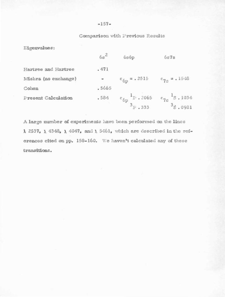
-157-

Compa.rioon with ?revious Resulto

Eigenvalues:

6s2 6s6p 6s7s

Hartree and Hartrec • 471

Mtshra (no exchange) c6p = • 251S e :: lS•.l:B 7o •

Cohen • 5665

P resent Calculation • 584 e6 1 r~ . ;.065 ·p F:?e

1s . 1034 3

F • 333 35.0981

A large number ol. experf.mente have been periortned on the lines

1 2537, ~ 4348, l. 4047, and )., 5461, which are described in t he zaof­

erencss cited on pp. 15S·160. ·we haven't calcula~ed any of these

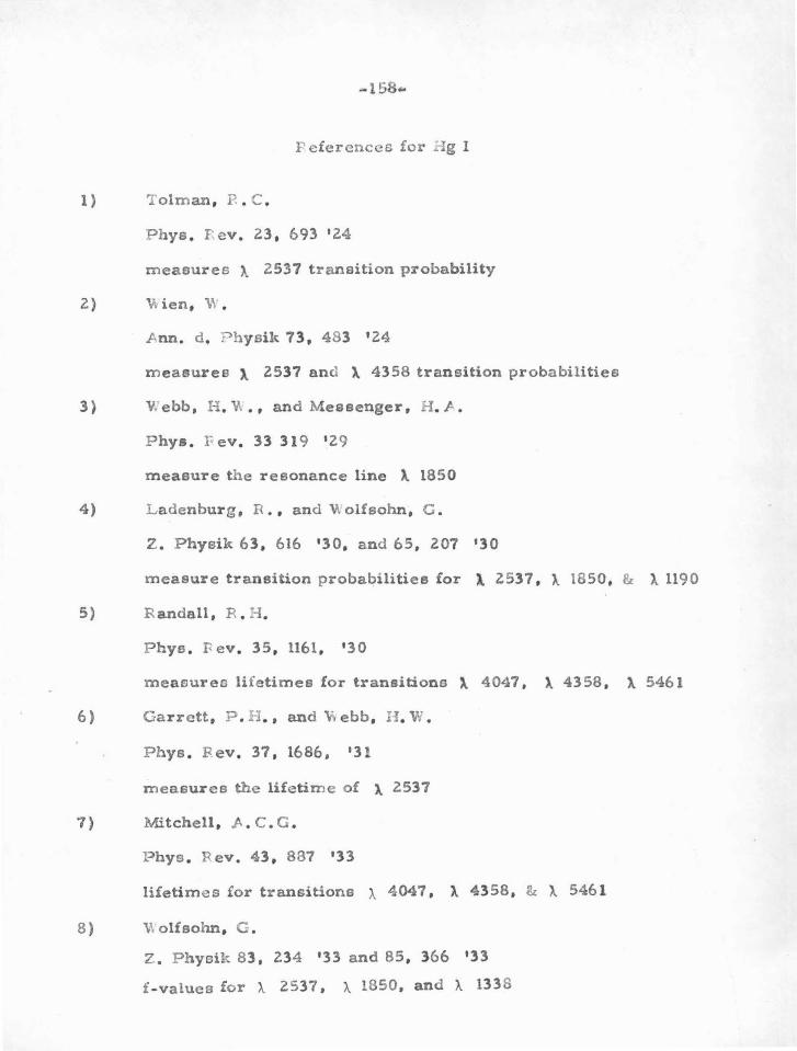
-158·

F eferences for Hg I

1) T olman, P. • C .

Phys . f'ev. 23 , 693 '24

measures ).. 2537 transition probability

2) \\ ien, W .

Ann. d . Physik 73, 483 124

measures ~ 2537 and ~ 4358 transition probabilities

3) Webb, H . "!A ., and Messenger, H . J..

Phys . F ev. 33 319 '29

measure the resonance line ~ 1850

4) L aden burg , R . , and V. olfaohn, G .

Z. Physik 63 , 616 '30, and 65, 207 130

measure transition probabilities for l. 2537, ~ 1850, & ~ 1190

5) R andall, R . :I.

Phye . F ev. 35, 1161, '3 0

meaeureo lifetimes for transitions ~ 4047, ~ 4358 , X 5461

6) Garrett, P . H ., and ¥. ebb, H . W.

Phys . F ev. 37, 1686, '31

measures the lifetime of X 2537

7) Mitchell , .A . C . G .

Phys . R ev. 43 , 887 '33

lifetimes for transitions A 4047 , ~ 4 3 58, & ).. 5461

8) \ \ olfsohn, G .

z. Phyoik 83, 234 '33 and 85 , 366 '33

£-values for A 2537, A 1850, and A 1338

·159-

9) Hartree , D. R ., and Hartree , \\ .

Proc . R oy. Soc . London P 149, 210 '35

calculate the ground - state by SCF with out exch ange

1 0) King, G . v •• , and Van Vleck, J . H .

Phye . Pev. 56 , 464 '39

calculate relative £-va lues for the resonance lines

11) Schouten, J. ' \ • , and Smi t, J . .fl. .

P hysica 10 , 661 '43

give a bsolute transition p robabilities for ~ 2537 , )., 4078 ,

).. 546 1 , 1 4358 , and l. 4047

12) L ennuier, F. . , and C oj an, J . L.

Compt. R end. 231, 1450 •so

meas ure lifetime of fi rst 3

P level for t hree differ ent H g

isoto pes

13) ~shra, B.

Phys . F: ev. 77 , 153 150

cal c u lates 6 s6p state by S C F , and combines with Hartree ' e

ground- state to g et the resonanc e line f-va.lue

14) E ros eel , J .

Phys . R ev. 83 , 210 ' 5 1

mea sures lifetime o f f irst 3

P level fo r Hg iso topes

15) B rossel , J ., and Bitt er , F .

P hys . R ev. 86, 3 08 ' 52

3 mea s ure lifetim e of f i rst P level for H g isotope

16) Mi shr a , B .

Proc . Camb. Phil . So c. 48, 511 ' 52

calculates SCF excited states for Hg without exchange:

6s6p, 6s6d, 6s7s , 6s7p, and 6s7d s t a t es

17) Brannen , C . , Hunt, F . R ., .Adlington, R . H ., and Nicholls , R . W .

Natur e 175, 810 ' 55

measure A 4358 transi tion probability

18) Cohen, S .

P esearch }..1emorandum-Rand Corporation ' 59

relativistic SCF with exch ange for the ground - state

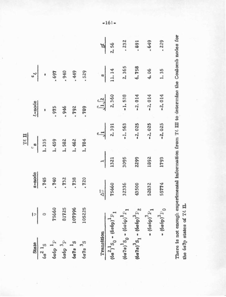
TtU

Sta

te

-s-

no

de

£8

t-n

od

e

&t

\)

-6

s2 1 s

0

.74

5

1. 3

35

-

-6&

6p1 P

75

66

0

• 74

0

1. 4

59

•

97

5

• 697

6s6

p 3 p

81

12

5

• 73Z

1

. 58Z

• 9

46

• 94

0

6e7

s 1 s

10

79

96

• 1

38

1.

46

2

• 792

• 4

49

6a7

s 3 s

105~25

• 12

0

1. 7

84

• 7

89

• 5

29

Tra

nslU

OD

. Av

).

_1

!_

l!1L

8 2

• -z

1 1

75

66

0

1321

z.

36

0

2..5

6 c-

(6s

) s 0

-(6

a6p)

P1

z. 39

1 11

. 14

.....

. • 1

1 (6

s7a)

s0

• (6

a6p)

P1

3233

6 30

95

-1.5

63

-1

. 53

8 2

. 36

5

• 23

2

3 3

(6s7

s) s

1 •

(6e6

p) P

z 43

500

2299

-2

. 02

5 -2

.01

4

6 .. 7

58

• 8

91

3 •

(6s6

p)

P1

5l9

3Z

18

9Z

-2.0

25

-2

. 0

14

4.

06

.6

49

3 •

(6s6

p)

P0

557'

74

1793

.z

. o2

s -~014

1. 3

5

• 22

9

Th

ere

ls

no

t en

ou

gh e

xp

erlm

enta

lln

form

aUo

n f

rom

Tt m

to d

ete

rmin

e t

he

Co

ulo

mb

no

des

f~

the

6s7

p s

tate

s o

f T

t U

.

·16Z·

Douglas, Hanree, and Runciman have calculated the ground­

state f\mctlcms of T.t D without exchange. They obtain an eigenvalue

c • 1. 054 for the 6s electrcms.

Reference'

.DoQglas, A. s. , Hartree, D. R. , and Runctmaa. W. A.

P .-oc. Camb. P hll. soc. 21• 486, •ss

- 163-

C . Comparison with the Coulomb f ,pproximation, and with

· ._.xpe rimental Results of the National Bureau of Standard s

.P lthough th e Bates- Damgaard method , as discussed in

Section IV , is not expected to be justified for divalent atom s , it i s

useful to system atically compare r e sults . T able VI - C contrasts

the absolute values of the r adial integrals J P f r P i dr of t he

C oulom b approximation with those of the nodal boundary condition

(NBC ) m ethod. The Coulomb values were calculated directly from

the tables of B ates and Da m gaard ( 1 ). F or the most part , transitions

of the types e2 1s - sp 1P (lowest) , sa' 1s - sp 1P (excited) , and

es ' 3s - s p 3

P (ex cited), are not in bad disagreement. T hese

2 1 1 1 1 transitions include (for exampl e) Ss S - SeSp P , Ss6a S - Ss6p P ,

and Ss 6 e 3s - Ss6p

3P , all in S r I . Howeve r , transitions s 2 1s - sp 1P

. 1 1 3 3 (exc1ted}, sa ' S - sp P (low est) , and ss ' S - sp P (low est}, often

disag ree by a factor of four, corresponding to a factor o f 16 i n th e

2 1 f - value . Theee latter transitions include , for example , Ss S -

1 1 1 3 3 . Ss6p P , .ss6s S - SsSp P , and Ss6s S - SsSp P 1n SrI.

T he explanation of w h y one group is in fair agr e e ment, and

why the other ia not, undoubtedly stems from the amount of can-

cellation in the ra,dial matrix elements. Cancellation is small for

the first group, but larger for the second. This implies that

calculations made with transitions of the second group are m ore

sensitive to the detailed shape of the wave functions used .

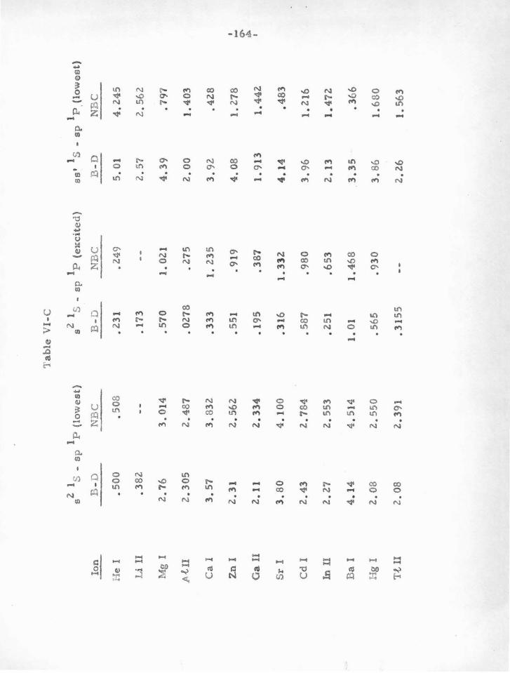
Tab

le V

I-C

2 1

1 s

S -

sp

P (l

ow

est)

a

2 1 s

-sp

1 P (e

1::c

ited}

1

1 ss

' S

-sp

P

. (lo

wes

t)

Ion

B-D

N

BC

B

-D

NB

C

B-D

N

BC

-

He

I • 5

00

• 508

.2

31

.24

9

5.0

1 4

.245

Li

II

.382

--

• 173

--

2. 5

7 2

.56

2

Mg

I 2.

76

3. 0

14

• 570

1.

02

1 4

.39

• 7

97

ft-L

II 2.

30

5 2

.487

• 0

278

.275

2

.00

1.

403

Ca

I 3

. 57

3.8

32

.33

3

1.

235

3.9

2

.42

8

Zn

I 2

.31

2.56

2 .5

51

.91

9 4

.08

1.

278

I -0' ~

Ga

II

2.1

1

2.3

34

.1

95

• 3

87

1. 9

13

1.4

42

I

SrI

3.8

0

4.1

00

.31

6

1.3

32

4

.14

.4

83

Cd

I 2

.43

2.

784

• 5

87

.980

3

.96

1

. 216

In I

I 2

.27

2.5

53

.2

51

• 653

2

.13

1

.47

2

Ba

I 4

.14

4.5

14

1. 0

1 1

.468

3

.35

.3

66

Hg

I 2

.08

2.5

50

• 565

.9

30

3.86

1

.68

0

T.t

II

2.0

8

2.3

91

.31

55

--2

.26

1.

563

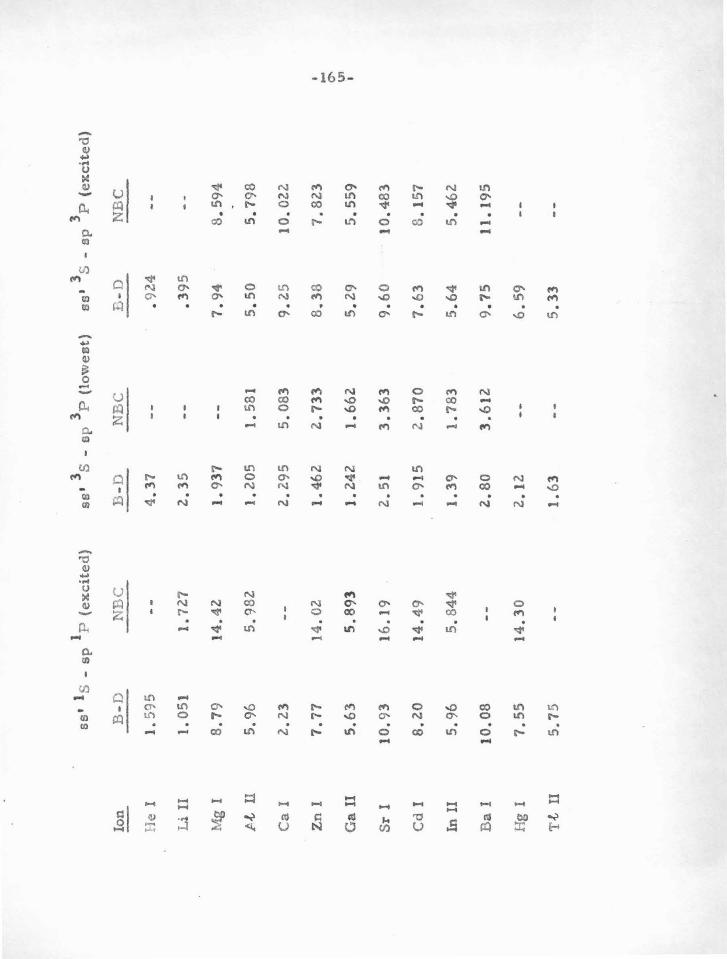
ss'

ls -

sp 1 P

(ex

cite

d)

3 3

ss'

S -

op

P (l

ow

est)

ss'

3 s -

ap 3 P

(ex

cite

d)

Ion

B

-D

N

BC

B

-D

N

BC

B

-D

N

BC

-

--

He

I 1.

59

5 --

4.3

7

--.9

24

Li

II

1. 0

51

1. 7

27

2.3

5

--.3

95

Mg

i 8.

79

1

4.4

2

1.9

37

--

7.9

4 8

. 594

P..f.-

II

5.96

5

.98

2

1.2

05

1

. 581

5.

50

5.7

98

Ca

I 2.

23

--2

.29

5

5.0

83

9

.25

1

0.0

22

Zn

I

7.7

7

14

.02

1

.46

2

2.7

33

8

.38

7

.82

3

• -0' G

a II

5

.63

5

.89

3

1. 2

42

1.6

62

5

.29

5

.55

9

Ul

I

Sr

I 1

0.9

3

16

.19

2

.51

3

.36

3

9.6

0

10

.48

3

Cd

I

8.2

0

14

.49

1

. 915

2

.87

0

7.6

3 8

.15

7

lnll

5.

96

5.8

44

1

. 39

1. 7

83

5.64

5

.46

2

Ba

I 1

0.0

8

--2

.80

3

.61

2

9. 7

5 11

. 195

Hg

I 7

.55

1

4.3

0

2.1

2

--6

. 59

T.f.-

II

5. 7

5 --

1. 6

3 --

5.3

3

-166-

The National Bureau of Standards has recently published a

volume of tables entitled " Z xperimental T ransition Probabilities for

Spectral L ines of Seventy E lements" (NBS Monograph 53, 1962) •

.Actually, relative £-values were measured, but the results were

normalized by previously measured (or calculated) abeolute £-values

for several elements . As stated in the Monograph. relative

gf-values within the spectrum of a single ion may deviate from

correct values by a factor of 1. 5 . ..Absolute values may deviate by

up to a factor z. 0.

All linea in common with our results are compa:ted in

Table VI- D. Some agree well. others not at all. For example.

the resonance £-value of Ca I ( ).. 4227), from at least aix previous

experiments and calculatio ns, is almost certainly at least 1. 45

(see p. 132), which is a factor of £ive greater than the NBS value

0. 28. Therefore £-values from these tables should be used with

some caution, unless only fairly rough values are needed.

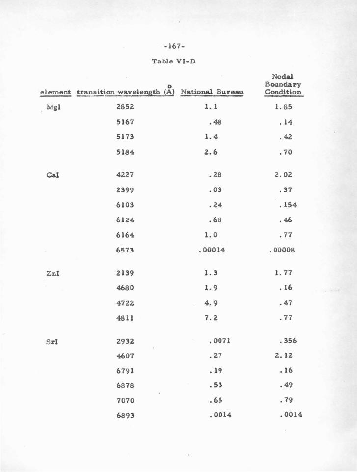
-167-

Table Vl-D

Nodal 0 Boundary

element transition wavele~th (A} National Bureau Condition

Mgl 2852 1.1 1. 85

5167 .48 .14

5173 1.4 • 42

5184 2.6 .70

Cal 4227 • 28 2.02

2399 .03 . 37

6103 .24 .154

6124 • 68 • 46

6164 1.0 .77

6573 .00014 .00008

Znl 2139 1.3 1. 77

4680 1.9 • 16

4722 4.9 . 47

4811 7.2 . 77

Sri 2932 • 0071 • 356

4607 • 27 2.12

6791 • 19 • 16

6878 .53 • 49

7070 .65 • 79

6893 .0014 • 0014

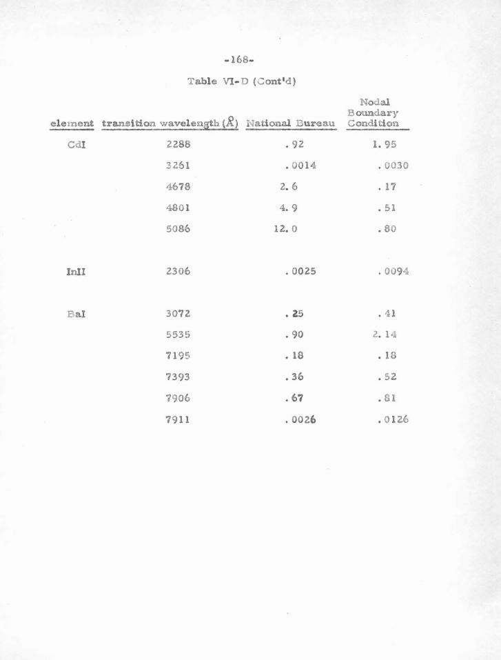
-168-

Table VI- D (Cont'd)

element transition wavele11gth (.R) National Dureau

Cdl 2288

3261

4678

4801

5086

I nil 2306

Bal 3072

5535

7195

7393

7906

7911

• 92

• 0014

2. 6

4.9

12. 0

. 0025

• as

. 90

• 18

. 36

. 67

. 0026

Nodal Boundary Condition

1. 95

. 0030

. 17

• 51

• 80

. 0094

. 11

2. 14

. 18

• 52

. 81

• 0 126

-169-

D. GENERAL CONCLUSIOl'S

In Section B , eigenvalues and transition probabili·

ties have been compared atom by atom with previous experimental

and theoretical results. Some generalizations can be inferred from

the detaUed comparisons:

1) Eigenvalues

The one-electron eigenvalues can only be compared with

previous SCF single-configuration calculations. The nodal boundary

condition electrons are almost invariably more tightly bound than

those of the usual SCF approach. As explained in Section V -C, this

is to be expected. The use of experimental information roughly

takes into account polarization of the core electrons, which provides

an additional attractive force on the valence particle.

Z) Transition Probabilities

OscUlator strengths can be compared with several sources:

experimental val-, standard SCF calculations (with and without

exchange), and SCF calculations including core polarization and

configuration interaction. In the special case of Hel, comparisons

can be made with highly .accurate Hylleraas•type calculations. The

latter comparisons are listed on p. 115, showing surprisingly good

agreement for moat transitions. For this case, the nodal boundary

condition method reduces to the usual single-configuration SCF

approximation with exchange. The only other SCF f-value calcula­

tions which have been made among the atoms we've been treating

are for Mgl and Cal. For the resonance lines, both have been done

-170-

by single-configuration and by configuration-interaction methods.

The nodal boundary condition f-values in each case are less than

the single-configuration, but greater than the configuration-inter­

action results. For the resonance line of Mgl, these are respec­

tively gf • 2. 21, 1. 85, and 1. 67. For Cal, they are gf = 2. 2, 2. 02,

and 1. 46. Experimental results favor the lower values. According

to Ostrovskii et al, the resonance gf-values are 1. 2 ::!: • 3 for Mgl,

and 1. 49 ::!: • 04 for Cal. Although resonance-line f-values have

not been calculated by SCF methods for other atom• of this type,

there are experimental measurements for Znl, Sri, Cell, Bal,

and Hgl. These are all lower than our results by about the same

cunount as for Mgl and Cal. The•e comparisons therefore strongly

indicate that the calculation of resonance f·valuee to better than

Z!S% accuracy will require configuration-interaction methods.

Also, future ordinary SCF single-configuration results will prob­

ably be slightly larger than those quoted here, and in poorer agree­

ment with experiment·.

There i• another reason for believing that our resonance

f-value results are up to 2So/o too large. The relative f-values be­

tween the triplet and singlet resonance lines (as listed in Section

V -D) agree very well with experiment. But absolute measurements

on f·values of the triplet (lntercombination) resonance lines are

generally smaller than what is found by applying our theoretical

ratios to the calculated singlet £-value.

Further experimental results will be very useful in deter­

mining the accuracy of the nodal boundary condition method and

-171-

single-configuration SCF calculations in general. It ehowd be em­

phasized that a measurement of a line in a particular element will

help in calibrating similar transitions in all the atoms and ions of

thia group.

E. ASTROPHYSICAL APPLICATIONS

A number of transitions computed by the nodal boundary

condition method are Hated in Charlotte Moore's 11 A Multiplet

Table of Astrophysical Interest" (43 ). Table VI-E collects these

transitions along with our f-values. Very likely there are other

linea in our tables which are now, or soon will be, of use in astro­

physics. Stars of unusual abundances are being increasingly stud­

ied, so that transitions which are usually too weak may be observed.

Also it may soon be possible to view a wider range of the spectrum.

Aside from observations of spectra, transition probabilities are

required for detaUed investigation of stellar opacities.

It is of interest to compare our f-value results with those

used by Goldberg, Mtuler, and Aller (44) in their recent analysis

of element abundances in the sun. Among lines we have computed,

there are surprisingly few of use in their investigations. These

include two lines in Cal, three in Zni, and three in Sri. Table Vl-F

lists these transitions, the f-values quoted by Goldberg, MtUler,

and Aller, along with the nodal boundary condition results. It is

evident from a comparison that the use of our f-values would make

no substantial changes in the abundance analysis for these three

elements.

·17Z-

Thorough abundance investigations have also been carried

out on B stars, for example by Aller and Jugaku (45). Among our

£-values, the only ones of interest in tha t analysis are those for He 1.

They use values calculated by 'l'refftz, et al.. (Helium reference 14),

whlc:h are in fair a greement "vith the few we have done (seep. 115).

The m ost i mportant d1££1iculty for He I was the uncertainty of meas­

ured equivalent widths, because the lines were so strong.

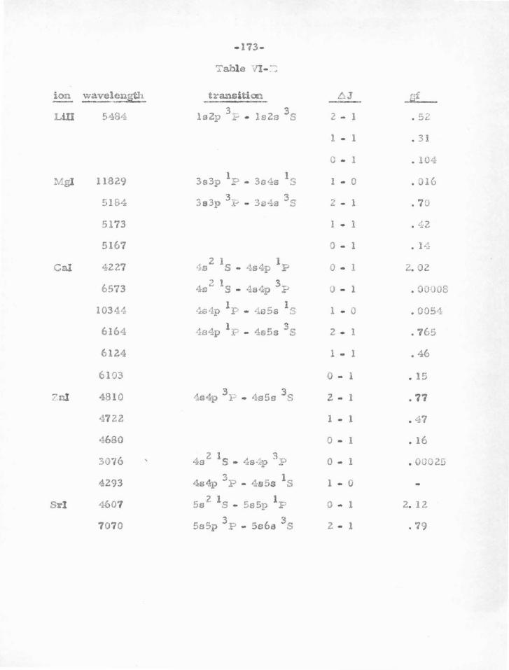
- 173-

Tabl e n - :-:

ion wavelensth transition D.J g£

LlD 548<',!, ls2p 3

:F • lsZs 3s 2 - 1 • 52

1 .. 1 • 31

0 .. 1 • 104

11829 1 1 ~ 1 - 0 • 016 Mgl 3s3p P - 3o4s ..,

5184 3 3 3s3p I-- - 3a4e S 2 - 1 . 70

5173 1 • 1 • 42

5167 0 - 1 . 14

Cal 4227 2 l l

4s S - 4s4p P 0 - 1 2. 02

6573 2 1 3

4s S - 4s4p P 0 - l • OOIJ08

10344 1 1 4s•lp P .. 4o5s S 1 - 0 • 00~4

6164 ·1s4p 1

P - 4s5s 3s 2 - 1 . 765

6124 1 - 1 • 46

6103 0 - 1 • 15

Z.nl 4810 4s4p 3

P - 4a5a 3s 2 - 1 • 77

4~722 1 - 1 • 47

4680 0 - 1 • 16

3076 4a 2 1s .. 4s~p 3p 0 - 1 • 00025

4293 3 1 4s4p P - 4s5s S 1 .. 0

Sri 4607 2 1 1 5s S - 5s5p P 0 - 1 2. 12

7070 3 3 5s5p P - 5s6s S 2 - 1 . 79

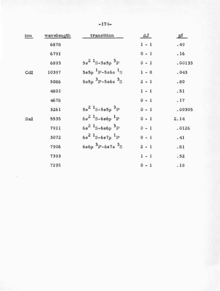
-174-

ion wavelength transition AJ ..sL -6878 1 - 1 .49

6791 0 - 1 • 16

6893 5sz 1s-Ss5p 3P 0 ... 1 .00135

Cdl 10397 5s5p 1P-So6s 1s 1 - 0 .043

5086 3 3 5s5p P-5s6s S ' - 1 .80

4801• 1 ... 1 .51

4678 0 - 1 • 17

3Z61 Ssz 1s-Ss5p 3P 0 .. 1 .00305

Bal 5535 6sz 1s-6e6p 1P 0 - 1 Z.14

7911 z 1 3 6s s-6s6p p 0 ... 1 .01Z6

307Z z 1 1 6s s-6s7p p 0 .. 1 • 41

7906 6s6p 3P-6s7s 3s z .. 1 .81

7393 1 - 1 .5Z

7195 0 - 1 .18

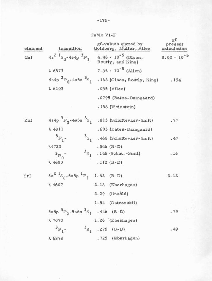
-175-

Table VI-F gf

gf-values quoted by present element transition Goldbers, MUller , Aller calculation

Cal z 1 3 6 -5 8. oz . 10-5 4s s0 -4e4p P 1 4. 4 • 10 (Olsen, Routly, and King )

~ 6573 -5 7. 95 • 10 (Allen)

3 3 4s4p P 0-4s5s s 1 . 16Z (Olsen , Routly, King) .154

~ 6103 . 085 (Allen)

• 0795 (Bates-Damgaard)

• 138 (Weinstein)

Znl 3 3 4s4p P

2-4s5s s 1 • 81 3 (Schuttevaer -Smit) .77

~4811 • 603 (Bates-Damgaard)

3p -1

38 1 . 468 (Schuttevaer-Smit) • 47

~47Z2 • 346 (B-D)

3p - 35 . 145 (Schut . -Smit) . 16 0

1

~ 468 0 . liZ (B-D)

Sri z 1 1 5s s0 -ss5p P 1 1. 8Z (B-D) Z. 1Z

~ 4607 Z.l8 (Eberhagen )

Z.Z9 (Unso'ld)

1. 54 (Ostrovskii)

3 3 5s5p P 2 -Ss6e s 1 . 446 (B-D) .79

~ 7070 1. Z6 · (Ebe r hagen)

3 35 .Z75 (B-D) • 49 pl . 1

~ 6878 • 7Z5 (Eberhagen)

F. ,..;xtensions and Further . .Applications of the Nodal Boundary

Condition Method

1. Configurationlnteraction

The nodal boundary condition method has been used to find

approximate SCF wave functions corresponding to a single Slater

determinant. That is, we have found a good approximation to those

functions which ar e the best possible functions (from an energy

standpoint), having a definite electron configuration. l ' rbitrarily

accurate wave functions can be obtained by relaxing the latter

restriction, or in other words by carrying out a configuration

interaction calculation. This process was described in section III-P

for SCF functions. The question of interest now is whether the nodal

boundary condition functions can be used in such an expansion.

There are two general practical approaches toward the

goal of finding exact functions. The fir at is to calculate the beet wave

functions (SCF) for each configuration. Then the matrix elements

< .!, I HI " > A . B can be evaluated , and the energy matrix

diagonalized . The second approach io to use a complete set of simple

analytic variational basis functions, which have larger off-diagonal

elemento than the SCF functions, but offer the advantage of ease of

manipulation and calculation. Both these methoda involve a great deal

of labor , but it is clear from calculations performed that substantially

better wave functions a!"e obtained. Since even single - configuration

-177-

SCF functions are not simple to compute anyway, it is logical that

one might as well proceed to do the whole problem through , super-

imposing aeveral configurations .

Unfortunately, the nodal boundary condition method cannot

be accurately ufled for such a com plete configuration-interaction

calculation, The reas on is this: we have found nodal stability to a ppl y

usually only for s- and p-wave functions . Therefore only w ave

func tions for configurations involving s and p electrons can be

computed with any accuracy. B ut it ia usually the case that configur ­

ations involving d electrons mix appreciably with the (e2

)1S , (sp)

1P ,

and (sp)3

P configurations in which we are interested. F or examp le ,

Trefft z (15) has found that for calcium,

= • 9480 d· (4 e-4p)- • 3184 '• (3d4p)

th(43P) c: • 9967 :'• (4e4p) + . 08125 11

1 (3d4p ).

T o obtain better wave functions and transition probabilities , the nex t

step would have to be the inclusion of such competing configurations .

B ut the problem in a configuration interaction treatment i & our

inability to obtain accurate d-wave functions . This trouble affects

both of the genera l methods of obtaining accurate functions . 1o apply

the a nalytic function a pproach via the nodal boundary condition

method, one can imagine choosing a set of analytic a-functions ,

-178-

p-functions, d-functions, e tc., each of which is constrained to

vanish at the appropriate coulomb node position, but which can be

varied in other ways. But again, the proper nodes for the d-wave

functions and those for higher angular momenta are not known.

V. e conclude that the nodal boundary condition method may

be a good approximation to the full S C F calculation as long as we are

satisfied with a single Slater determinant, but cannot be accurately

used in the more ambitious program.

2 . P.dditional E lectron Con figurations

The fir ot obvious extension of the method is to apply it to

th f. . 2 d I

c con 1gurat1ons p an pp T he Hartree-Fock equations are more

complicated, but the same general method can be used. These con-

figurations all involve t h e excitation of both valence electrons, so are

usually less important than thos e we have calculated.

Perhaps more important would be the extension to atoms

with three valence ele ctrons. Ions having an s2

p valence ground-state

configuration are very interesting. These include the ieoelectronic

sequences DI (CII, NIII , • • ), P.ll (Sill, P ill, .• ), and G a I (Gell, /lslll, .. ).

The coulomb nodes for some of the s e ions were computed and listed

in section V-B . These calculations assumed that ions of this typ e had

2 only a sing le valence electron: i.e., the s subshell was kep t

-179-

stationary. The coulomb nodes show a good deal of instability for

som e of the states, which indicates that probably the participation of

2 the s electrons should be accounted for. It would therefore be quite

interesting to calculate states with configurations s2p, s

2s•, and s

2d

2 ·to see how much the s subshell is influenced by the position of the

outermost electron. The coulomb nodes for these ions would be

calculated from experimental term values for the p6

s (or d10

s) ion:

e . g., ..Al Ill, Si IV, • • • • The Hartree - F ock equations are not

difficult, because of the two identical s -electrons. T he extension to

doubly-excited states, such as ss'p , is more complicated because

three functions must be computed.

If energy prevails , work can be done on the important atoms

2 2 with an s p ground state. These include CI , Sil , Gel , Snl, and Pbi.

If calculations on s2

-t configurations indicate that the s2

electrons

actually remain quite stable , the four -electron problem reduces

essentially to a two-electron p roblem. However, this simplification

is probably not sufficiently valid. In any case, excitations of the

inner s-electrons are unimportant, so that the four -electron calculations

b . d . 1 h f" . 2 2 d 2 can e restr1cte ma1n y to t e con 1gurat1ons s p an s ps '.

3. Ot her .Ppplications

There are several oth er possible applications of nodal

boundary condition wave functions. F or any situation in which the

usual S C F valence wave functions (with out configuration interaction)

-180·

are adequate, and where also the behavior of the functions at small

radii is unimportant, one may use nodal boundary condition functions.

For example, in the calculation of quadrupole transition probabilities.

one is interested in the matrix element < Rf I r2

IRi > • which

certainly depends only on the parts of the radial functions at large radii.

The inelastic scattering cross-section of a fast charged

particle by an atom is computed in the Born approximation via the

matrix element

Here ( and f

~ . are the final and initial wave functions of the atom, l .. ..... .. .....

and K = Ki - Kf is the momentum transfer (Ki and Kf are the initial

and final momenta of the scattered particle). This expression reduceo

to the single integral

If we are interested in collisions involving only small momentum

transfer , then in first approximation

l M = ~ i K ·

K

-181-

which is the same dipole moment integral needed for oscillator

strengths. Then if only transitions of valence electrons are required,

and if we restrict ourselves to small momentum transfer (ka < < 1,

where a is the atomic diameter) , nodal boundary condition functions

can be used.

There are also physical situations where the outer parts of

the valence wave functions are distorted, while the inner parte , locked

in the deep central potential , remained undisturbed. For example ,

nodal boundary condition functions might be useful in calculating wave

functions for molecules or for electrons in a crystal lattice. In both

of these cases , the outer parts of the valence functions are greatly

distorted, but if the interaction energy is not too large , the inner

coulomb nodes would be the same as for a single atom. .Again a

problem is the instability of nodes for orbital angular momenta of two

{d-wave) or greater , so that calculating SCF functions using the nodal

boundary condition would be generally inaccurate unless s- and p-waves

formed the only significant contributions to the total wave function,

-182-

General References

1. Bates, D. R. , and Damgaard. A.

PhU. Trans. R. Soc. London A242, 101, ' 49

2. Green, L . c. , Weber, N. E . , and Krawitz, E.

Ap. J. 113, 690 , ' 51

3. Delbriick, M .

P roc. Roy. Soc . London Al29, 686, ' 30

4. Hylleraas, E . A.

z. P hyslk 54. 347, ' 39

See also Blbllography ln reference 10.

5. Hartree, D. R.. , and Hartree, W.

P roc. Roy. Soc. London Al64, 167, '38

6. Trefftz, E .

z. l. Ap. 29, 287, '50

7. Hartree, D. R .

f>roc. Carob. P hU. Soc. !!• 89, 111, 426, ' 28

8. Foclt, V.

z . P hysik 62, 795, '30

9. Hartree, D. R .

The Calculation of Atomic Structures (VIUey, 1957)

10. Slater, J. C .

Quantum Theory of Atomic Structure (McGraw-HUl, 1960)

11. Biermann, L.

z . !. Ap. zz. 157, 143

12. Dlerrn.a.rm. L., and Lb.'beck. K.

z. f. Ap. 25, 325, '48

13. Biermann, L ., and Trefftz, E .

7.. £. Ap. 26, 213, '49

·183 -

14. Trefitz, E .

z. f. Ap. 26, Z40, ' 49 and 28, 67. •so

15. Trefitz, E .

z. f. Ap. 29, 287, • 50

16. See footnote p . 36, Vol. U of reference 10.

17. Zener, C.

P hys. Rev. 36, 51, '30

18.

P hys. Rev. 36, 878, '30

19. Morse, P . M. , Young, L.A., and Haurwitz, E . s. P hys. Rev. 48, 948, '35

zo. Nesbet, R . K. , and Watson, R. E.

Phya. Rev. 110, 1073, 158

21. Watson, R. E . Phys. Rev. 119, 170, '60

22. Boys, S. F . P roc. Roy. Soc. 217, 235, '53 and refs. listed ln this article

23. Boys, S. F .

Revs. Mod. Physics 32, 285, '60

24. Layzer, D.

Ann. Phys. 8, Z71, '59

25. Layzer, D. , and Btilicall, J.

Ann. Phya. 17, 177, '62

26. Varsareky, C. M.

Thesia, Harvard University, 1958

- 184-

27. Koopmans, T . A .

Physica 1, 104, ' 33

28. F...artree, D. R . , and Hartree, \'!.

Proc. Roy. Soc. London Al93, 299 , '48

and Proc. Camb. P hU. Soc. 34, 550, '38

29. Hargreaves, J .

Proc. Camb. Phil. Soc. 25, 75, 128

30. Fock, V. , and P etrashen, M.

Phys. z . Sowjetunion 8 , 547, 135

31 . Stephenson, G.

Nature 167, 156, '51

32. F Uippov, A.

Zeit. f. Ph. 69, 526, '31

33. Fock, V., and Petrashen, M.

P hys. z. Sowjetunion 6, 368, '34

34. Stephenson, G.

Proc. P bys . Soc. 64A, 458, ' 51

35. OstrovskU, Yu. I ., and Penkin, N. P .

Optics and Spectroscopy 1, 1, '61

36. F Uippov, A., and l- rokofiev, \i.i .

Zeit. f . P h. 56, 458, '29

3 7. Hartree, D. R . , and Hartree, W.

P roc. Roy. Soc. London Al64, 167, ' 38

38. Condon, E . U. , and Shortley, G. H.

The Theory o! Atomic Spectra (Cambridge University Press,

1951, Cambridge)

· 185-

39. King, G. W. , and Van Vleck, J . &

P hys. Rev. 56, 464, '39

40. Moore, c . Atomic Energy Levels

National Bureau of Standards Cir~ular 467 ( ' 49)

41 . Rubenstein, P . J.

Phye. Rev. 58, 1007, '40

4 2. Hartree, D. R . , Hartree, W. , and Manning, M. F .

P hys. Rev. 60, 857, ' 41

43. Moore, C .

A Multlplet Table of Astrophysical Interest

National Bureau of Standards

44. Goldberg, L. , Miille r , E. A . , and Aller, L . H.

Ap. J. Supplement, Vol. 5, ' 60

45. Aller, L . H. , and Jugaku, J .

Ap. J . SUpplement, Vol. 4, ' 59

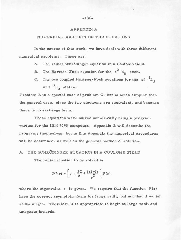
-186-

APPENDIX A

NUMERICAL SOLUTION OF THE EQUATIONS

In the course of this work, we have dealt with three different

numerical problems. These are:

A. The radial Schrodinge r equation in a Coulomb field.

B. 2 1 The Hartree-Fock equation for the s s0 state.

c. The two coupled Hartree-Fock equations for the sl

and 3LJ states.

Problem B is a special case of problem C, but is much simpler than

the general case, since the two electrons are equivalent, and because

there is no exchange term.

These equations were solved numerically using a program

wirtten for the IBM 7090 computer. Appendix B will describe the

programs themselves, but in this Appendix the numerical procedures

will be described, as well as the general method of solution.

A. THE SCHRODINGER EQUATION IN A COULOMB FIELD

The radial equation to be solved is

P "( ) f 2C + l (1 +1) J P ( ) r = L € - r- rz r

where the eigenvalue E" is given. We require that the function P (r)

have the correct asymptotic form for large radii, but not that it vanish

at the origin. Therefore it is appropriate to begin at large radii and

integrate inwards.

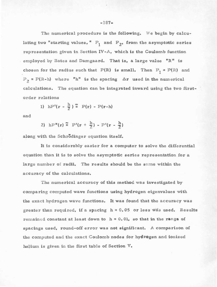
... 187-

The numerical procedure is the following. We begin by calcu-

lating two "starting values," P 1 and P 2, from the asymptotic series

representation given in Section IV-A, which is the Coulomb function

employed by Bates and Damgaard. That is, a large value "R" is

chosen for the radius such that P(R) is small. Then P 1 = P(R) and

P 2 = P(R-h) where "h " is the spacing ~r used in the numerical

calculations . The equation can be integrated inward using the two first-

order relations

h -1) hP '(r - ~ ) = P (r) - P(r-h)

and

2) hP"(r) ; P'(r + ~) - P'(r - ~)

along with the Schrodinge r equation itself.

It is considerably easier for a computer to solve the differential

equation than it i s to solve the asymptotic series representation for a

large number of radii. The results should be the s a me within the

acc uracy of the calculations.

The numerical accuracy of this methocl was investigated by

comparing computed wave functions using hydrogen eigenvalues with

the exact hydrogen wave functions. It was found that the accuracy was

g reater than required, if a spacing h = 0 . 05 or less w'as used. Results

remaine-d constant at least down to h = 0. 01, so that in the range of

spacings used, round-off error was not significant. A comparison of

the computed and t he exact Coulomb nodes for hyd~ogen and ionized

helium is given in the first table of Section V.

.B.

-138·

THE s 2 1s HARTRE.C-FOCK Ef_UATION 0

The equation to be solved is

P"(r) = Zc 2 ).

r 2 f'OO P2( ) J - - + - dr P (r) + 2 \J dr r r P (r) r r . 0 r

where C is the net atomic charge if both valence electrons are re-

moved. Here again, the eigenvalue € is to be specified at the otart. (' 2

.::iince -~ P (r) dr = 1, we can write

P"(r) = l € - Z(C-l) -! roo dr P 2(r) + 2 roo dr Pz(r) lj P (r) L r r) ' r r r

This is a more convenient expression for inward integration. The

same basic numerical method used to solve the Coulomb pote ntial

.Schrodinger equation can be used to solve this equation. Ci nce the

last two terms in the brackets are tJmall for large radii (and their sum

even smaller), Coulomb starting values are again appropriate. After

integrating inwards three or four steps, the terms

roo roo z -! ) dr P 2(r) + 2 ) dr p (r) r . r r r

can be evaluated by Simpson's rule, and included in eubsequent calcu-

lations of P "(r) from the known P (r) at each step.

There is an important difference between this equation and the

Schrodinger equation with Coulomb potential. The Hartree-Fock equation

2 is non-linear, so that if the computed s function P (r) ia found to be

unnormalized, the correct function is not P (r) divided by the square

-189-

root of the normalization integral. The procedure used is to calculate (>00 z

P (r), evaluate N = i dr P (r), and define new starting values ., 0

new old/~. . new old/_~:. . P1

= P 1 VN and P 2 = P 2 v.N and try again. This p rocedure

is repeated until the computed function ia correctly normalized to

w ithin 0 . 05%, which usually requires 6 to 8 iterations.

C . TH..& s~ 1L AND 3 L HARTREE:-FOCI< EC.UATION!:>

These ~quations are

2 ('r s ex> p l !£ + ! \ dr P 2 + 2 dr ..!_ j P

r r ,, 0 1 r r s

and

p"" = 'L~ ~ il - lE + 1<.e;u + £ \rdr pz + zS(X)dr p! ]p~. .o: x r r r ... 0 s r r

where the p lus and m inus signa refer to the singlet and triplet ctates,

respectively, and £ = 0 , 1, 2, ••• The s olution of these equations is

by far the m ost d ifficult of all t he calculations. An almost completely

d ifferent procedure from t he p revious methods is necessary.

For these equations, i n contrast to the 2 1 s s0 Hartree-Fock

equation, both outer and i nner boundary conditions are specified for

each function, so that we can solve for the wave functions and eigenvalues.

'.

, . .

-190-

The outer boundary cond ition is the usual requirement that each function

approach zero asymptotically for large rad ii. The inner boundary con·

dition is the node positi on ae found by the method described in Section V.

and

where

and

The equations can be written

II

P = HART ( r ) P :t FOCl< (r) s 8 8 s

II

P 1 =.HART1(r) P 1 :t FOCK1 (r)

HART (r) s

2

[ 2C 2 r r 2 r•CD pi J

= E' ., - - + - \ dr P l + 2 j dr -_ .., r r , 0 r r

The overall procedure of solution i s to first specify tri a l e i genvalues

E' 6

and ~ .{', , and compute trial Coulomb functions P 8

and P l ' cor ­

responding to these eigenvalues. If these e i ganvalues and functions are

" used to evaluate HART1 (r) and FOCK1 (r), the equation for Pl. can

be solved, resulting in a new function P 1 , and eigenvalue £I. . The

new El will in general be different from the trial value because the

function P 1 is forced to satisfy the inner and outer boundary conditions

-191-

by varying £c Then HART0(r) and FOCK

8(r) can be found by using

the initial trial values for £9

and P 9(r), but the new computed P 1 (r).

" Solving the equation for P , a new P and E are obtained. This 6 s s

ite rative procedure is continued until the eigenfunctions and eigenvalues

(hopefully) converge.

With these equations, it is best to integrate starting from the

(given) Coulomb node position, rather than from large radii inward.

That is, beginning at the Coulomb node "r ", we can first integrate c

outwards to large radii to see if the function is approaching zero asymp­

tot ically. If it does not, the eigenvalue is varied until this outer boundary

condition ia satisfied. Then we can integrate inward from r to small c

values of r to obtain the remainder of the function. There are several

a d vantages to this procedure over the inward integration used for the

one-ele ctron Schrodinger equation and the s 2 configuration Hartree-

Fock equation. With the advent of exchange terrns, it is no longer true

that Coulomb-approximation starting values are adequate at large radii.

The entire functions are sensitive to the starting values, so that this

difficulty is important. Another advantage of beginning at the Coulomb

node is related to the fact that some rather odd behavior can occur at

large radii for ss' or sp singlet functions. Sometimes an "anomalou&

node " can appear at large radii for the most tightly bound s -electron,

e. fact clielcovered by Hartree in the calculation of wave functions for

Mg I. The wave function appears ordinary for small and m edium radii,

but instead of gradually approaching zero as the radius is increased, lt

barely dips under the axis, has a minimum, and then approaches the

- 192-

axi s from bel ow. This behavior is not hard to understand. The s i nglet

equation i s wri tten

" P = HART ( r) P + FOCK8

(r) 8 B 8

At large radii, HARTs (r) is positive, and also FOCK6

(r) is p ositive

and quite large , s ince it contains as a factor the other wave function

P l ( r) , which is an excited state and therefore i s m o stly at fairly large II

radii. 5o if P 8

is s lightly negati ve, P 8

can etill be pos itive, causing

the function t o curve up toward the axi s . Therefore an extra n ode can

occur at a large radius for the singlet func t ion . This effect cannot occur

for triplet functions because of the m i nus sign in t he triplet equati on

II

P8

= HAR r ( r) P - FOCK ( r) • s a s

Il we integrate outwards starting at the Coul omb node r c ' one

of the two starting values is already known (P 1 = 0) , s o the s l ope-to­

value ratio i n the i mmediate vicini ty of thi s poi nt i s determined. A m i e-

take in the c h oice of the other starti ng value w i ll then r esult i n the com-

puted function being unnormalized, whi ch can be corrected in succeeding

i terations. For example, if the Coulomb node for the a-functi on of an

sp 1P state i s at r c = 1. 00 ~ we may begin by setting P 2 = 0 . 01. Then

in general the normalizati on integral \ P 2 (r) dr = N ¢ 1. 0 , so that in .) 8

the next i teration for P s ' we choose a starting value P 2 = O. 01/""N •

The equations are non-linear, so that this substitution does not guarantee

that the new P ( r) will be normalized, but the proce6s i s fo und to con­s

verge.

-193-

Because of the "anomalous node 11 difficulty, it is more con-

venient to integrate outwards from small radii, rather than inwards

from large radii. \o~ ithin a particular iteration, a wave function is cal-

culated several times with different eigenvalues until the boundary con-

ditions are satisfied. For slightly different eigenvalues, the main parts

of the wave !unction at intermediate radii vary in a smooth way. B ut a

slightly different eigenvalue can mean the appearance or disappearance

of an "anomalous 11 node at larger radii, which can only be easily handled

from outward integration. U one starts at large radii and integrates

inward, the whole character of the calculation depends upon whether or

not an anomalous node is present. The log ic and convergence problems

become very difficult.

The method of solving these two coupled equations can now be

summarized. From trial eigenvalues and eigenfunctions, the subsidiary

functions HART I. (r) and FoCK1 (r) are computed. Then, using the

e t.J uation

II

Pt = HAR T 1 (r) P 1 ::i: FOCK1 (r) ,

the function P 1 is evaluated by integrating outwards from the Coulomb

node. If the asymptotic boundary condition io not satisfied, the e:igen­

value E: 1

within the function HART 1 (r) is varied until the boundary

condition ia satisfied. This may or may not involve the appearance of

an "anomalous node". Using the original P and E: , and the new com-a s

puted P P. , the equation

-1 94-

II

P = HART (r) P :t: FOCK (r) s s s a

can be solved for a new P eJ The eigenvalue e: 8

is varied until the

boundary conditions are satisfied. Then a better P 1 is computed

using the new P • This iterative procedure is continued until conver-s

gence ie obtained. It is necessary that for the final iteration, the initial

eigenvalues for that iteration be within 0 . 05 o/o of those eigenvalues

needed to satisfy the boundary conditions. Also the functions as com­

puted must be normalized w ithin O.lo/o.

The exact description of how each of these steps is accomplished

w ould be very lengthy. These details can be gleaned from a study of

the F ortran program reproduced at the end of Appendix B .

-1 95-

APPENDI X B

THE COMPUTZR PROGRAMS

The programs were designed to do almost all of the numerical

work required in the calculation of wave functions and transition proba-

bili t ies. They were written i n the Fortran language, suitable for the

IBM 7090 computing machi ne.

Si x principal types of calculation can be perfo nned w ith the·se

programs for atoms or ions with one or two electrons outside closed

shells. These include :

1) Coulomb-approximation valence functions (wi th gi ven eigen-

value and angular momentum) for a single valence electron

2) Valence ground-state 2

s

3) Valence excited-state s l

electrons)

1s0 functions (two valence electrons)

1L or 3 L functions (two valence

4) Oscillator strengths for J. - 1 1 transi t ions (one valence

electron)

5) Oscillator strengths for s 2 1s0 - sp 1P 1 t r ansitions (two

valence electrons)

6) Oscillator strengths for sl 1L- sl 1 1

L 1 transitions or

sl 3 L - s~ 1 3 L 1 transi t ions (tw o valence electrons) . In

practice, I. i s limited to 0 or 1.

The principal purpose of this work was to calculate valence wave

fun..:tions and trans i tion probabilities for atoma and ions w i th two elec-

trons outside closed shells. In carrying out this project, i t was

-1 96-

necessary for two reasons t o compute Coulomb-approximation single-

electron functions. They were employed in finding Coulomb nodes

for two-electron situations, and also as first trial functions for sl-

configuration calculations. Since s ingle-electron functions had to be

computed anyway, it was deemed useful and convenient to have the

option of computing them for their own sake, which accounts for

calculation types (1) and (4). These functions should be the same as

the results of using the aaytnptotic series representation of Bates and

Damgaard (Section IV - A) , and the corresponding transition probabilities

should agree with the Bates-Damgaard tables. Results were com-

pared in several cases , substantiating this expectation.

In general, for a particular day ' s "run ", calculations can

be performed with one or several of the s ix basi c types of problem.

E ach calculation requires two or more input data cards. The number

of input cards can be reduced if the whole "run" consists only of one­

electron function calculations , or if i t consists only of a2

-configuration

calculations. These are called the "efficient" one-electron mode, and 2 .

the "efficient" a mode, in contrast to the "general " mode. These

modes were defined by the first data card for the run, which contains

-1, +1, or 00 in the first two spaces, depending upon whether one wishes

to use the efficient one-electron, efficient a-squared, or general mode.

The necessary data-cards for the various kinds of calculation will now

be listed.

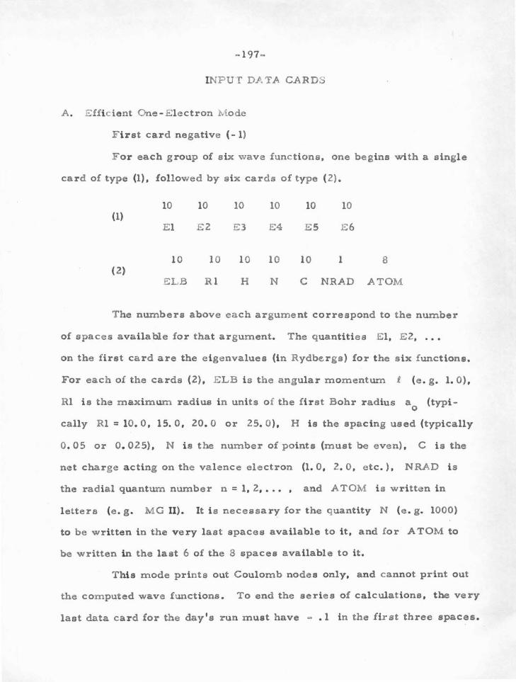
~197~

INP U f DATA CARDS

A. E fficient One- E lectron Mode

First card negative (-1)

For each group of six wave functions, one begins with a single

card of type (1), followed by six cards of type (2) .

10 10 10 (1)

E l E 2 E 3

10 10 10 (2)

10

E4

10

10

E S

10

10

E6

1 8

ELB Rl H N C NRAD ATOM

The numbers above each argument correspond to the number

of spaces available for that argument. The quantities El, E 2, .••

on the first card are the eigenvalues (in Rydbergs) for the six functions.

For each of the cards (2), E LB is the angular momentum .t (e. g. 1. 0),

Rl is the maximum radius in units o f the first Bohr radius a (typi­o

cally Rl = 10. 0, 15. 0, 20.0 or 25. 0), H is the spacing used (typically

0. 05 or 0. 025), N is the number of points (must be even), C is the

net charg e acting on the valence electron (1. 0, 2. 0, etc.), NRAD is

the radial quantum number n = 1, 2, •.• , and ATOM is written in

letters (e. g. M G II). It is necessary for the quantity N (e. g. 1000)

to be written in the very last spaces available to it, and for A TOM to

be written in the last 6 of the 8 spaces available to it.

This mode prints out Coulomb nodes only, and cannot print out

the com puted wave functions. To end the series of calculations, the very

last data card for the day's run must have ~ .1 in the first three spaces.

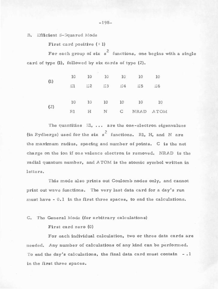
-198-

B. Efficient S-3quared Mod~

F i rst card positive ( t 1)

F o r each group of six a2

functions, one begins with a single

card of type (1), followed by s ix cards of type (2).

10 10 10 10 10 10 (1)

El E 2 £3 £4 ES

10 10 10 ( 2)

10

Rl H

10

N

10

c NRAD ATOM

The quantities El , • • • are the one-electron eigenvalues

(in Rydbergs) used for the s ix s2

functions . Rl, H, and N are

the maximum radius, spacing and number of poi nts . C is the net

charge on the ion if one val ence electron is removed. NRAD i s the

radial quantum number, and ATOM is the atomi c symbol wri tten in

letters.

This mode also pri nts out Coulomb nodes only, and cannot

pri nt out wave functions . The very last data card for a day ' s run

rnust have - 0 . 1 in the first three spaces , to end the calculations.

C . The General M ode (for arbi trary calculations)

F i rst card zero (0)

F o r each individual calculati on, two or three data cards are

needed. Any number of cal culations of any k i nd can be performed.

To end the day ' s calculations, the final data card must contai n - • 1

in the first three spaces.

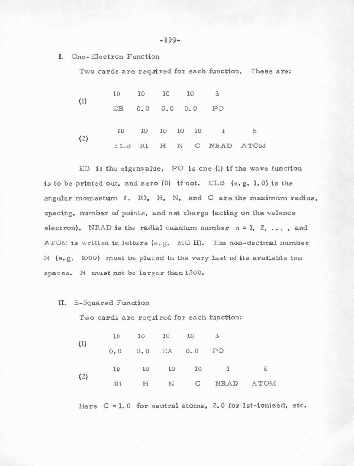
-199-

I. One-f.iectron Function

Two cards are required for each function. These are:

(1)

(2)

10

EB

10

10

o. o

10

ELB Rl

10 10

o. 0 o. 0

10 10 10

3

PO

1 8

H N C NRAD ATOM

EB is t he e i genvalue , PO i s one (1) if the wave function

i s to be printed out , and zero (0) if not. ELB (e. g . 1. 0) is the

angular momentum 1 . Rl, H , N , and C are the maximum r adi us ,

spaci ng, number of poi nts , and net charge (acting on the valence

electron) . NRAD i s the radial quantum number n = 1, 2, ... , and

A TOM i s written in letters (e . g . MG II). The non- decimal number

N (e . g. 1000) must be placed in the very last of i ts available ten

spaces . N must not be larger than 1200.

II. S- Squared F unction

. Two cards are required for each function :

10 10 10 10 3 (1)

0.0 0 . 0 EA 0 . 0 PO

10 10 10 10 1 8 ( 2)

Rl H N c NRAD ATOM

Here C = 1. 0 for neutral atoms , 2. 0 for 1st-ioni zed, etc .

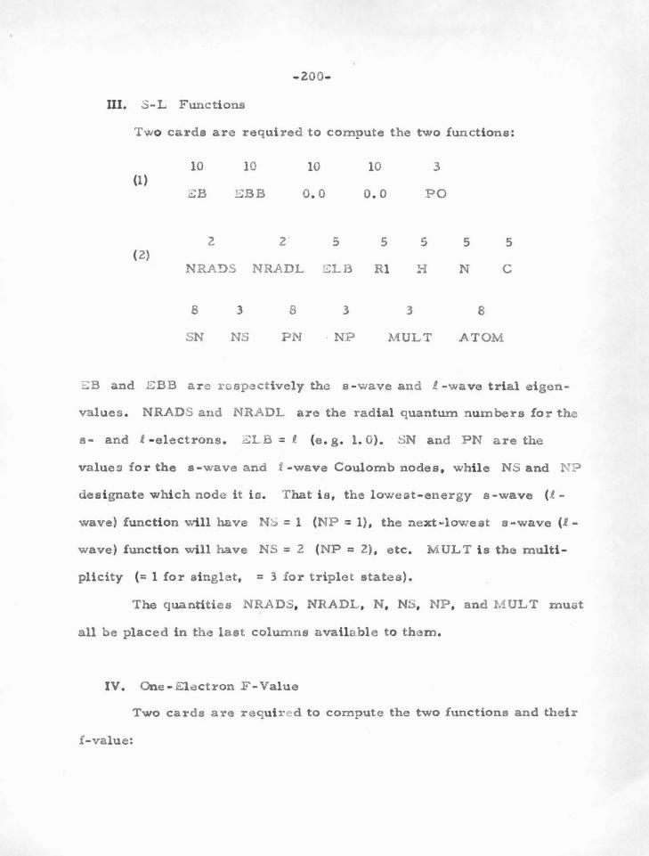
-200-

DI. S-L Functions

Two cards are required to compute the two functions:

(1)

(2)

10 10

BBB

2

10

o. o

5

NRADS NRADL l!:LB

8

SN

3

NS

8

PN

3

NP

3 10

0 . 0 PO

5

Rl

5

H

3

MULT

5

N

5

c

8

ATOM

EB and EBB are respectively the a-wave and I. -wave trial eigen­

values . NRAD.S and NRADL are the radi al quantum n umbers for the

s- and t • electrons. ZLB = l (e. g . 1. 0). SN and PN are the

values for the s-wave and t -wave Coulomb nodes , while NS and NP

des i gnate which node it is. That i s , the lowest-energy s - wave (1-

wave) function will have N~ = 1 (NP = 1) , the nex twlowest s - wave (1-

wave) function will have NS = 2 (NP = 2) , etc. MULT is the multi­

plicity (= 1 for s i nglet, = 3 for triplet states).

The quantities N~ADS, NRADL, N , NS, NP, and M ULT must

all be placed in the last columns availa ble to them.

IV. One - Electron F -Value

Two cards are requir e d to compute the two functions and their

:£-value:

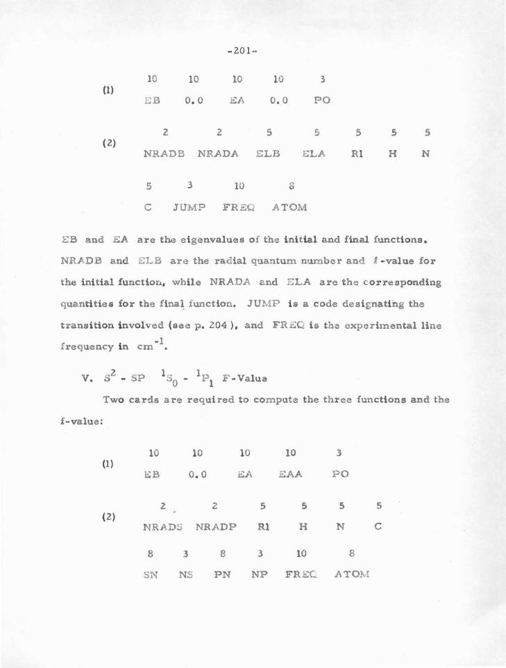
-201 ~

10 10 10 10 3 (1)

8B o. 0 EA o. o PO

2 2 5 5 5 5 5 (2)

NRADB NRADA ELB ELA Rl H N

5 3 10 8

c JUMP FREQ ATOM

EB and EA are the eigenvalues of the init ial and final functions .

NR.ADB and ELB are the radial quantum number and 1-value for

the init ial function, while NRADA and ELA are the corresponding

quantitiea for the ftna~ function. JUMP i s a code designating the

transition involved (see p . 204 ) , and FR.t,;Q is the experimental line

-1 frequency i n em •

V . s2 - SP 1s0 - 1P 1 F-Value

Two cards are required to compute the three functions and the

f-value :

10 10 (1)

EB o. o

2 2 (2)

NRADS NRADP

8 3 8

SN NS PN

10

EA

5

Rl

3

NP

10

EAA

5

H

10

FREC.

3

PO

5 5

N c

8

AT01vi

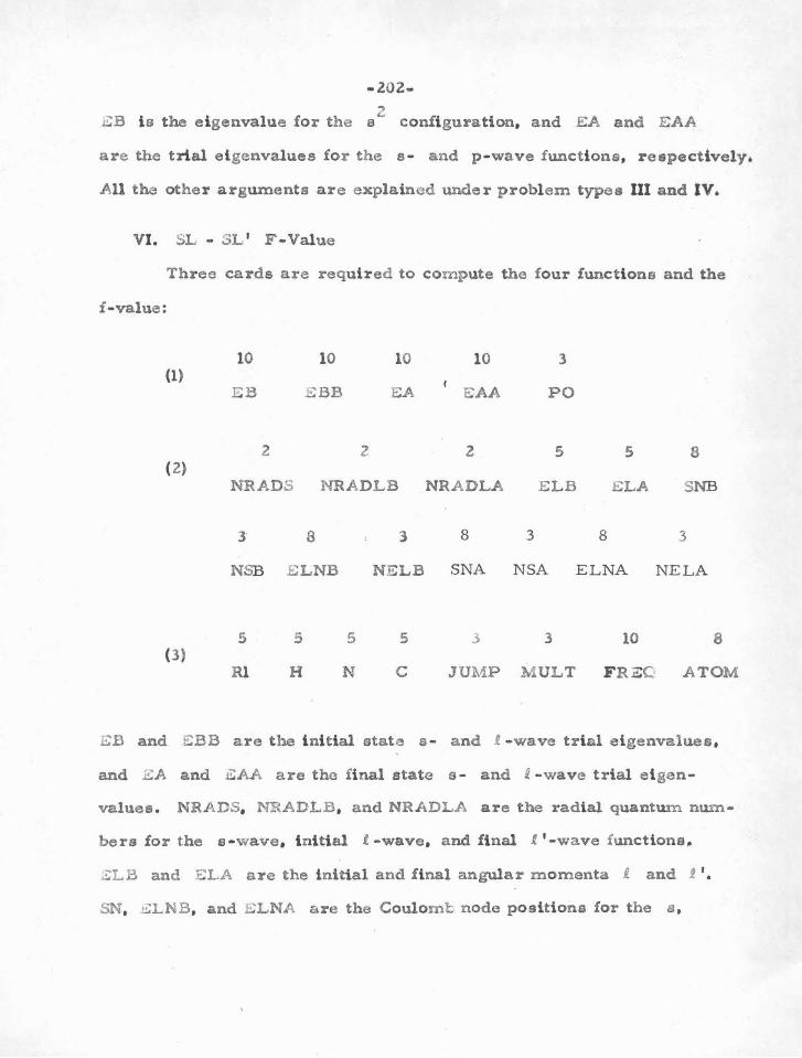
-zoz-2

EB i s the e i genvalue for the a configuration, and EA and EAA

are the trial eigenvalues for the s- and p-wave functions , respectively.

All the other arguments are explained under problem types III and IV.

VI. SL - SL ' F-Value

Three cards are required to compute the four functions and the

f-value:

10 10 (1)

EB E BB

2 2 (2)

10 10

EA EAA

2

3

PO

5 5 8

NRADS NRADLB NRADLA ELB ELA SNB

3 8 3 8 3 8 3

NSB E LNB NELB SNA NSA ELNA NELA

5 5 5 3 3 10 8 (3)

Rl

5

H N c JUM P MULT FR:a=C ATOM

EB and EBB are the initial state s- and 1 -wave trial eigenvalues,

and E A and EAA are the final state s- and t -wave trial elgen-

values. NRADS, NRADLB, and NRADLA are t he radial quantum num-

bers for the s-wave, i nitial I. -wave, and final l '-wave functions~

.ZLB and ELA are the initial and final angular momenta i. and t 1•

SN, ELNB, and ELNA are the Coulomt n ode positions for the s,

- 203-

initlal 2 , and final I. ' states. while N S, N E L.B, and N E L A designate

which node i s involved (as explai ned under problem type Ill). JUMP

is the transition code given on p. 204. M ULT = 1 or 3 for singlet or

triplet functions , and F REQ is the experimental line frequency in

em- 1.

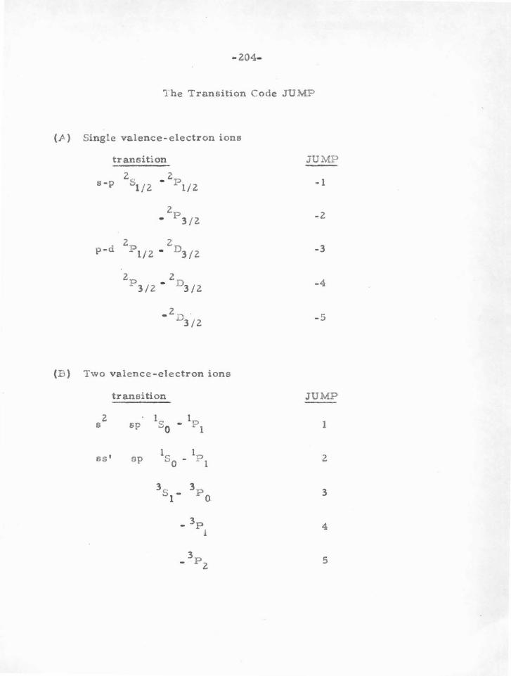
-204-

The Transition Code JUMP

(/I) Single valence-electron ions

transition

2 2 s-p 5

112 - pl/2

2 - p 3/2

p-d 2 2

p l/2 • D3/2

2 2 p 3/2 • D3/2

. 2 n 3·/ 2

(B) Two valence -electron ions

2 s

ss'

transition

sp

sp

JUMP

-1

-2

-3

-4

- 5

JUMP

1

2

3

4

5

.zos.

THE SUBROUTIN:::.3

The computer program is rep roduced in full (in the FORTRAN

language) on pp. 223-239 • It is necessary first to d i scuss the pur ­

pose and contents of each subroutine, supplemented with block dia­

grams of those requiring a detailed description.

DIRECTOR - MAIN PROGRAM

All calculations begin wHh the Director. From the fi rst data

card for a complete "run ," the Director determines what "mode" of

computations w ill be carried out -- whether

1) efficient one-ele ctron,

2) efficient a-squared, or

3) general

as defined on p. 197· If the "general " mode il!l to be used (which i s

usually the case), the Director finds from the first data card for each

calculation what kind of calculation is to be perfo rmed, and transfers

to the appropriate Sub-program (one-electron, a-squared, si, one­

electron £-value , or two- electron f-value).

- 206-

ONE- ELECTRON (MAIN PROGRAM)

SUBROUTINE O!!;MP(EB, PO)

This p:Dog ram reads input data, calls Subroutine ON.ELEC (which

computes a monovalent wave function), and prints out input data and

computed nodes, along with the wave function, if desired.

A r guments

EB: e i genvalue

PO: p rint -out code

S- SC.UARED (MAIN PROGRAM)

SUBROUTINE SS! .. i P (EA, PO)

This subroutine ls similar to Subroutine OEMP except that l t

z calls Subroutine SSQRD (to compute an e wav e function) instead of

calling ONELEC.

A r gu ments

EA: e i genvalue

PO: print-out cod e

S-L (MAIN PROGRAM)

SUBROUTI NE SLMP(EB, E B D, PO)

Calls Subroutine SL (which computes s - and l - functions for

1L or 3 L states), but is othe rwise s im ilar to the previous subroutine.

Arguments

EB: s - wave trial e i genvalue

...;BB: 1 -wave t rial eigenvalue

PO: p rint-out code

ONE - E L E CTRON F-VA LU.2 (t.A.AIN P ROGRA M )

SUBROUTINE OE FVMP( EB, EA, PO)

This subroutine reads input data, calls the ONE L E C subroutine

twice (to compute the initial and final wave functions), uses the OVLP

function to calculate the radial integral \ PfrPi dr and the FVALUE v

Subroutine to compute the line-strength and g f-value. Formats,

inp ut data, and final r e sults are p rinted, along with the wave functions,

if desired.

A r guments

E B: initial eigenvalue

J.!.A : final eigenvalue

PO: print-out code

TWO- ELBC T RON F-VALUE (MAIN PROGRAM )

.SUBROUTINE TEFVM P( E B, E BB, E A, EAA, PO)

2 This Subroutine consists of two parts, one to compute s -sp

£-values, and one to compute s1 - sl.' !-values. In each case, input

data is read, and formats are printed. 2 For an s -sp £-value,

Subroutines SSURD and SL are called. For an s.t - s i ' !-value,

Subroutine SL is called twice. The overlap integrals \ P P ,dr j s 8

and .\ P 1 rP 1 ,dr are computed from the OVLP function, and the

line strength and gf-value are computed by calling Subroutine FVALUE .

Finally, wave functions are printed out, if desired.

-208-

Arguments

~B:

E BB:

i n i tial s - wave e i genvalue

2 zero (0) for s -sp £-val ue , i ni t i al l - wave e i genval ue for

s i. -at' £-value

CA: fi nal s - wave e i genvalue

SAA: final 2 -wave e i genvalue

PO: print- out code

THE ON£ -..i:L£ CTRON SUBROUTIN E

SUBROUTINE ONBLBC( Z , EL, Rl, H , C , N , P , Z )

Computes normalized one-electron functions from the Coulomb­

potential Schrodinger equati on with g i ven e igenvalue E .

Input arguments

..;: e i genvalue

E L : angular momentum ~

Rl: maxi mum (starti ng) radi us

H: spacing (Ar)

C : charge (C = 1 for neut r al, C = 2 for first i onized, etc.)

N: number of poi nts

Output A rguments

P : wave functi on

Z : node posi tions

- 209·

fHE S· SOUAREL> SUBRC"UTlN:S

SUBROUTIN1 SS0RD(E, R l , H, C , N, E , Z, 1-0, ETC' T)

Computes normalized s 2

functions from the Hartrec-F ock

equation. fhe eigenvalUG E must be specified. The subroutine also

calculates the electrostatic interaction enermr

and the total energy of the two electrons

E TOT :: ZE + r o

Input Argum ents

E :

R l:

H:

C :

eigenvalue

m aximum (starting) radius

spacing

charge (C = 1 for neutral,

C = 2 for let ionized, etc. )

N: number of points

THE SL OUT SUBROUTINE

Output Arguments

PO:

wave fWlctlon

node position

electrostatic integral

ETOT: 2E + F 0

SUBR.OUTINE SL(E l, E 2, EL, H, C , RB, NN, SND, PND, NS, NF,

~·fU, PS, PP }

In p rinciple, the m ethod of solution used in this subroutine (see

1 3 Appendix A) can be used for any L or L s ·t • con!tguration two-

electron state. In practice, partly because the nodal boundary condition

m ethod becomes invalid for ..f, > 2., and partly because of convergence

-210·

1 3 difficulties, the program can be used only for se 1 :::; or S and

1 3 sp P or P states. Also only states of fairly low excitation energy

were actually computed, as listed in Section VI. The program may

work correctly for more highly excited statee, but convergence prob-

lema may be expected to require some alteration in the procedure .

The SL subroutine is quite lengthy and complicated. It begins

by using the s and t trial eigenvalues El and .:-:!:: 2 to compute trial

Coulomb functions via the ONE L E C ~ubroutine. It i s necessary to

force the trial s-wave function to approach zero at the given Coulomb

s -node, so that it looks roughly like the final result.

At this point, the first iteration begins. Subroutines MAR.3

and VENUS are called to help in the tabulation of the HART; and

FOCK1 functions for the equation

Subroutine BEGI N is called to provide starting values for the calcu-

lation. The equation is then integrated outward numerically. At each

new point, it ie determined whether or not one of the following "events"

has taken place:

0) function "blows up" (P(r) > 10. 0)

1) inflection point

2) maximum or minimum

3) node

4) end of calculation (r = r ) max

5) function "blows down 11 (P (r) < - 1. O)

U none of these six events have occurred, the integration is continued.

-211-

U one of them _2!! taken place, the program is routed to Subroutine

E VENT, which analyzes what is going on. U the function is not be-

having properly, EVENT chooses a new eigenvalue which should

improve the sit uation. For example, lf the function (while being tntc-

grated outward from the Coulomb node) has passed through an inflection

point, maxlmwn, inflection point and minimum, the function will blow

up instead of approaching the axis asymptotically. E V ENT lowers the

eigenvalue and directs the SL program to start over again with this

new eigenvalue. The process is continued until the function passes

through the correct sequence of events: a) inflection point, b) maxi­

mwn, c) inflection point, and d) end. The correct eigenvalue for the

iteration has then been found.

As explained in Appendix A, sometimes an extra node is

required at large radii for the inner a-function for singlet states.

The program determines whether such a node is necessary by

finding the difference in energy between an eigenvalue which causes

the function to reach a minimum (above the axis) and then blow up,

and an eigenvalue which causes the function to cross the axis and then

blow "down." I! this energy difference is small (lees than 0. 05%) ,

and if the radius at which the second function bas crossed the axis is

not too large (r < r /Z), then an extra node is required. The max

functions obtained for various eigenvalues in such a case are repre-

sented in figure B-1. Subroutine EXND ie employed to guide the pro-

gram in case such an extra node is required.

When the correct eigenvalue has been obtained, the function

· 212-

i a completed by integrating i nward from the Coulomb node . The

function is finally normalized us ing func tion .::>IMP to compute the

integral.

The fi rst s-wavc calculation i s them begun, usi ng the ao.me

basi c procedure. The iterations are continued until both functions

converge, meaning then they maintai n co nstant energi es and are

correctly no r malized w ithi n lim i ts gi ven i n Appendix A . All major

steps in the c a l culations are printed out as c ompleted.

Input A r guments

E l. E2: t ria l s - and l -wave e igenvalues

i:L: l

H: spacing (Ar}

C: charge

RB: maxi mum r adius

NN: number of points

SND. PND: s - and p - C oulomb n odes

NS. NP: number of nodes

MU: m ult ip licity (1 or 3)

Output Arguments

?S, PP: radi al wave functions

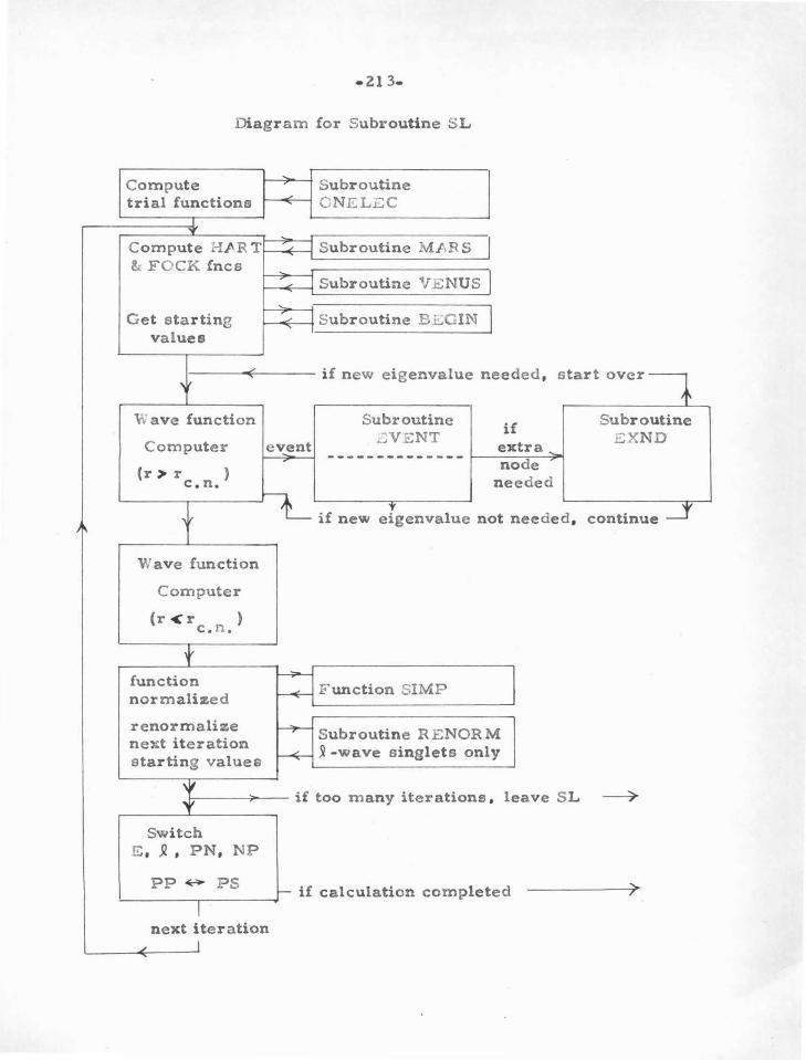
·213.

Diagram for Subroutine S L

Compute Subroutine trial functions CNEL.LC

v Compute H /IRT Subroutine M.l\RS l & FOCK fncs

Subroutine VENUS ....

I Get starting / Subroutine B C.:GIN I.

values

/ if new eigenvalue needed, start over+

" Wave function Subroutine

if Subroutine

Computer event .:VENT

extra .... EXND

-------------- node (r > r )

c. n. needed

if new eigenvalue not needed, continue _j' I~

Wave function

Computer

(r < r c. n .

)

t function H F unction SIMP normalized

renormalize ~ Subroutine R E NOR M next iteration

f.--+- ~-wave singlets only starting values

'f f

if too many iterations , leave S L ~

Switch E , .R , PN, NP

PP ~ PS r- if calculation completed ~

I next iteration

J

F igure B -1

Schematic diagram Ulustrating the appearance of an extra

node at large radii for s · wave singlet functione .

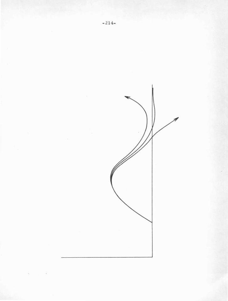
-214-

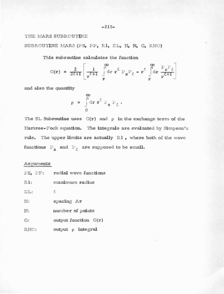
-21 5-

THE lV.t.ARS SUBROUTINE

SUBROUTINE W..ARS (P S, PP. R l. E L , H, N, G1 RHO)

Thls subroutine calculates the function

and also the quantity (l)

p = rd {., . ~ ,J rr .-s .:t . 0

The SL Subroutine uses G(r) and p in the exchange term of the

Hartrce-F ock equation. The Integrals are evaluated by Simp son's

rule. The upper limits are actually R l , where both of the wave

functions P s and P .t are supposed to be small.

Arguments

P S, :=:P: radial wave functions

R l: maximum radius

EL: .f_

H : spacing Ar

N: nwnber of pointa

G: output functi on G(r)

RHO: output p integral

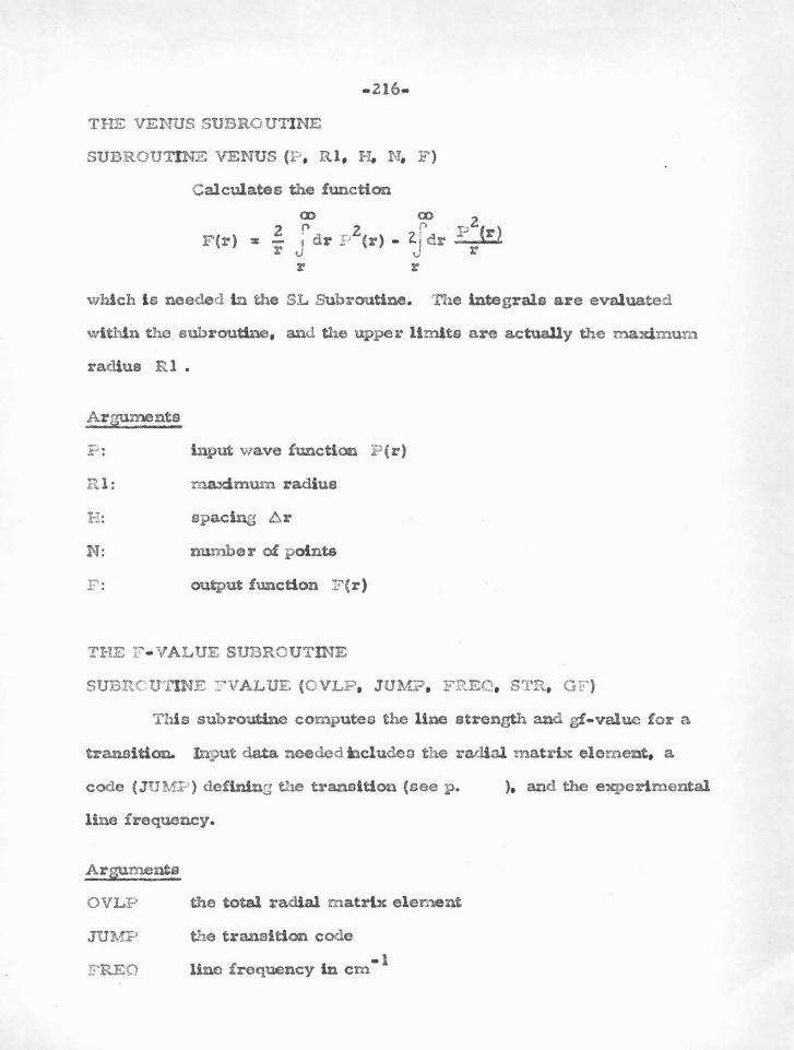
-216-

THE VEl\TUS SUBROUTINE

SUBRO UTINE VENUS (P , Rl , H. N, F )

Calculates the function

Q) co 2 1'\ l r p 2( )

F(r) s r j dr P (r) • 2.j d:r r r

r r

which l e needed ln the SL Subroutine. The integrals are evaluated

within the subroutine, and the upper llmlte are actually the maximum

radius Rl •

Arguments

? : input wave function P (r)

R l: ma.ximwn radius

H : spac~ 6.r

N: number of points

F : output function F (r)

THE F · VALUE SUBRO UTINE

SUBRC' UTINE FVALUE (O VLP , JUM?, FR.EQ, STR. GF}

This subroutine computes the line strength and gf- value for a.

transition. Input data needed bcludes the radial matrix elem ent, a

code (JUMP) defining the transition (see p .

line frequency.

Arguments

OVLP

JUMP

FREO

the total radial m atrix e l en'l.ent

the transition code

- 1 line frequency ln em

), and the experimental

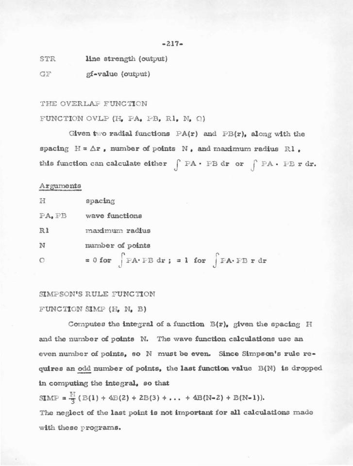
-217-

STR line strength (output)

GF gf-value (output)

THE OVERLA.F FUNCTION

FUNCTION OVLP (I-I. F A. 1-'B, R l, N, Q )

Glven t wo radlal functions P A(r) and PB(r), along with the

spacing H = t!J..r , number of points N, and maximum radius R l,

this function can calculate either J P A • P B dr or J P A . I-B r dr.

Arguments

P A, PD

Rl

N

0

spacing

wave functions

maximum radius

number of pointe

= 0 for r l-'A• f-B dr ; = u

SIMP SON' S R ULE FUNC '!10N

FUNCTION SI MP {H. N, B )

r 1 for J F A• FB r dr

Computes the integral of a functiou B (r), gtven the spacing H

and the number of points N. The wave function calculations use an

even number of points, eo N must be even. Since Simpson's rule re•

quires an~ number of points, the last functloa. value B(N) ls dropped

in computing the integral, eo that

SIMP = ~ ( B (l) + 4:6(2 ) + 2B(3) + ••• + 4B(N·2} + B(N•l )).

T he neglect of the last point le not important for all calculations made

wlth these p rograms.

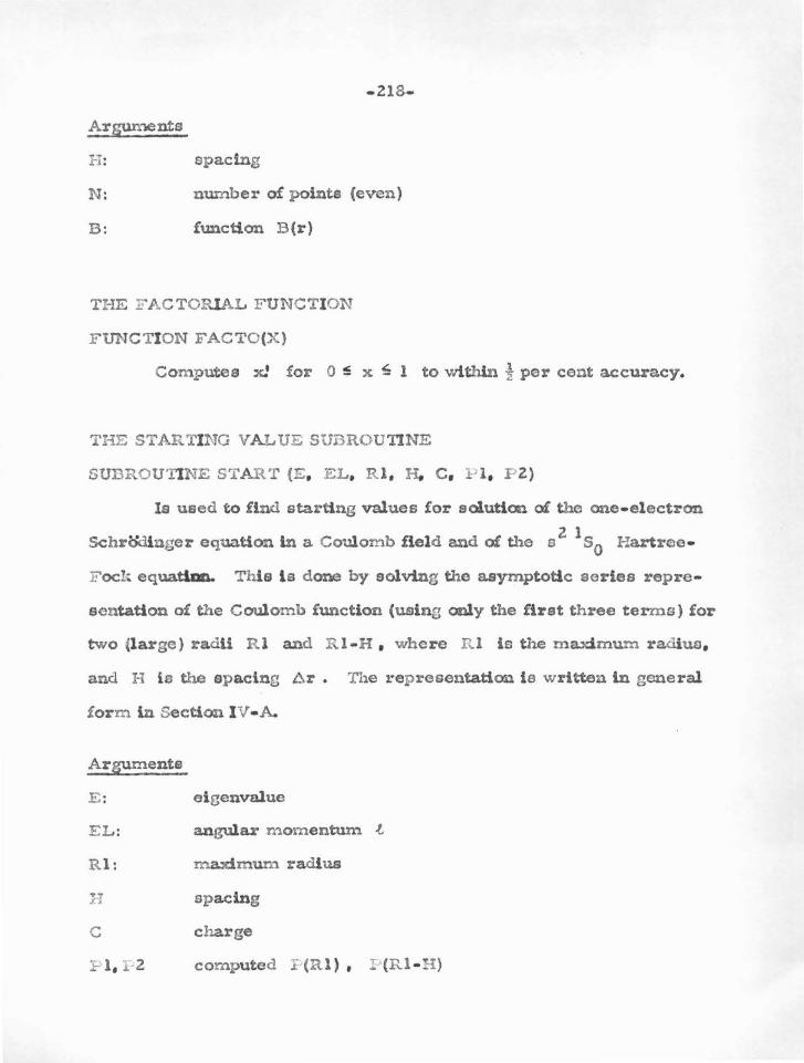
Arguments

H:

N:

B:

-218-

spacing

nwnber of points (even)

function B(r)

THE F AC TORlAL F UNC TION

F UNCTION F ACTO(}{)

Computes x! for 0 ~ x ~ 1 to within i per cent accuracy.

THE STARTI NG VALUE SUBROUTINE

SUDROU'I1NE STAR'£ (E, EL, R l, H. C, 1->1, P l)

Is used to find starting values for solution of the one-electron

Sch r()dinger equation in a Coulom b field and of the s 2 1s0 Hartree­

Foc!~ equatlDD. This ls done by solving the asymptotic series repre­

sentation of the Coulomb function (using only the first three terms) for

two (large) radii R l and R l·H , where R l is the maximum radius,

and H ia the s pacing Ar • The rep resentation le w ritten in general

form in Section I V·A.

Arguments

E :

EL:

R l:

c

J:-·1, 1 2

eigenvalue

angular m omentum t

ma::dmum radius

s p acing

charge

com puted :r (R l) , I=-•(R l·H )

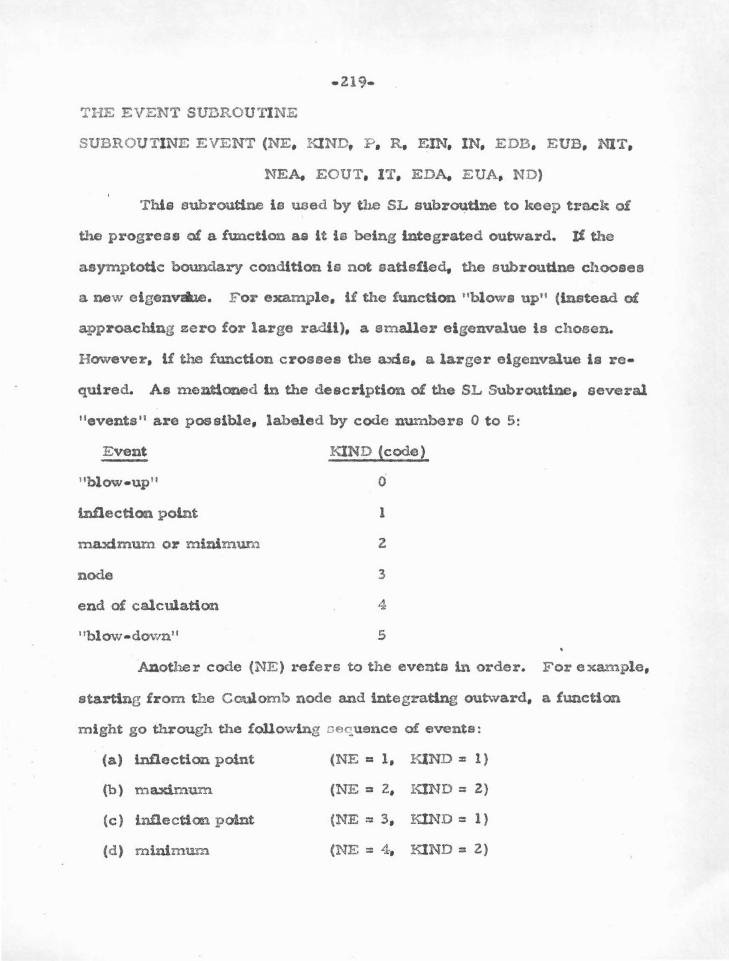
·219-

THE EVENT SUDROUTINE

SUBROUTINE EVENT (NE, KIND, P , R. ElN, IN, EDB, EUB, NIT,

NEA. EOUT, IT, EDA. EUA, ND)

This subroutine ls uaed by the SL subr~tlne to keep track of

the progress of a function aa lt is being integrated outward. If the

asymptotic boundary condition ls not satisfied, the subroutine chooses

a new eigenvabe. For example, if the function "blows up" (instead of

approaching zero for large ra.dU), a smaller eigenvalue is chosen.

However, if the function crosses the axis, a larger eigenvalue ls re•

qulred. As mentioned ln the description of the SL Subroutine, several

"events'' are possible, labeled by code numbers 0 to 5:

Event

"blow-up"

bUlection polnt

maximum or minimum

node

end of calculation

''blow-down''

KIND (code)

0

1

2

3

4

5

Another code (NE) refers to the events in order. For example,

startina from the Coulomb node and integrating outward, a function

might go through the following ce<!uence of events:

(a) lntlection point (NE = 1, KIND= 1)

(b) maximum (NE = Z, KIND= 2)

(c) inflection point (NE := 3, KIND= 1)

(d) minimum (NE = 4, KIND= 2)

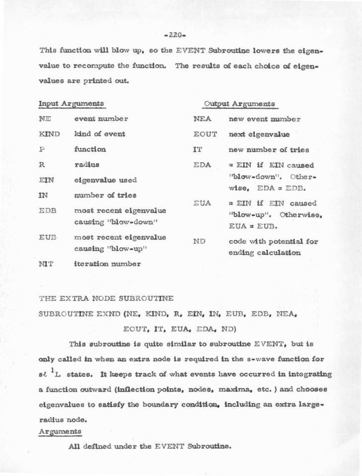
-220-

This function wUl blow up, so the EVENT Subroutine lowers the eigen­

value to recompute the function. The results of each cholce ot elgen•

values are printed out.

Input Ar~ents

NE

KIND

p

R

EIN

event number

ldnd of event

function

radius

eigenvalue used

IN number of trlee

EDB

EUB

most recent eigenvalue

causing ''blow-down''

most recent eigenvalue

causing "blow-up"

NIT iteration number

THE EXTRA NODE SUBROUTINE

2utput Arguments

NEA new event number

EOUT next eigenvalue

IT new number of tries

EDA = EIN U ElN caused

.,blov.r·down". Other•

wise, EDA : EDB.

EUA = EIN if EIN caused

"blow-up". Otherwise,

EUA ::a EUB.

ND code wt th potential for

ending calculation

SUBROUTINE EXND (NE, KIND, R., ElN, IN, EUB, EDB, NEA.

ECUT, IT, EUA, E DA. ND}

Thle subroutine is quite slm.Uar to subroutine EVENT; but ts

c:mly called In when an extra node is required ln the s-wave function for

a.t 1 L states. It lteepe track of what events have occurred in integrating

a. function outward (inflection points, nodes, maxima. etc. ) and chooses

eigenvalues to satisfy the boundary condltlQD. including an extra large•

radius node.

Arguments

All defined under the EVENT Subroutine.

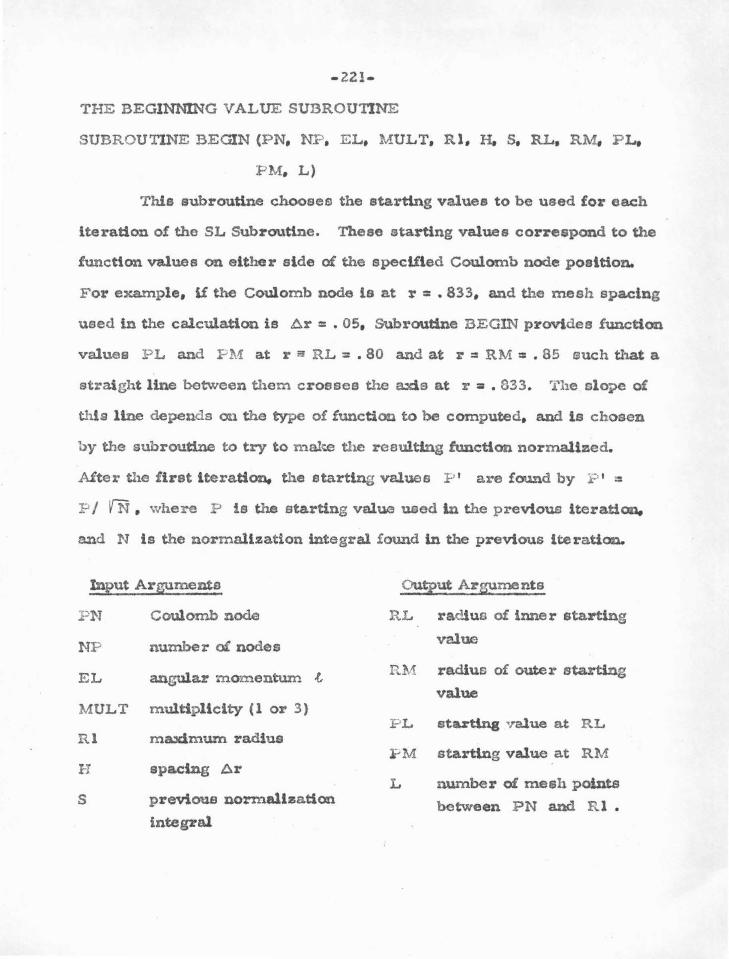
-221-

THE BEGINNING VALUE SUBROUnNE

SUBROUTINE BEGIN (PN, NP, E L, MULT, Rl, H. S, RL. R.M, FL,

PM, L)

This subroutine chooses the starting values to be used for each

iteration of the SL Subroutine. These starting values correspond to the

function values on elthe r side of the speclfled Coulomb node position.

For example, lf the Coulomb node ls at r = • 833, and the mesh spacing

used in the calculation is Ar = • 05, Subroutine BEGIN provides function

values P L and PM at r a RL = . 80 and at r = RM = • 85 such that a

straight line between them crosses the axis at r = • 833. The elope of

this line depends on the type of !unction to be computed, and ts chosen

by the subroutine to try to ma.lte the resulting function normalized.

Alter the !tret lteraticm, the starting values P ' are found by P ' ~

PI YN , where P is the starting value used ln the previous iteration.

and N ls the normalization integral found in the previous lte ration.

Input Ar~ments Output Arguments

PN Coulomb node RL radius of lnne r starting

NP number of nodes value

EL angular momentum .(, P..M r~us~o~re~

value MULT multiplicity ( 1 or 3)

P L staztlna •ralue at RL Rl maximum radius

:FM starting value at RM H spacing Ar

L number of mesh points s previous normalization between PN and Rl •

integral

-zzz-THE RENORMALlZATlON SUBROUTINES (NOS. 1 AND Z)

SUBROUTINE RENORM (51, SZ, 53, DENOM)

Two subroutines called RENORM were used lD the course of

these calculations. Their purpose is to speed convergence of the

ss' 1s0 functions. The majority of these functions converge using

no. 1, but some require no. 2. In practice, RENORM no. Z was com­

pUed only lf convergence was not achieved wtth no. 1.

The iterative calculations for these se' 1s0 functions are

found to be overdamped, so convergence is slow. A fairly effective

way to overcome this difficulty is to choose proper, or "renormallzed"

staztlng values. The usual procedure is to choose a starting value by I

the prescription P = PI ffi, where P is the starting value used

tn the previous iteration, and N ls the normalization integral obtained

tn the previous iteration. 1 For ss 1 S states, this method does not auf•

flciently improve the normalization for the s' function, so instead,

• • the formulae P s• = P 8

, I ¥ 1. 7 N or P s' = P 8

, I r.SN are used in

RENORM no. 1, depending on whether the normalization integrals tend

to be consistently too large or consistently too small. The RenormaU­

zattoc Subroutine decides which denominator is needed. and supplies lt

to the SL Subl'outine. RENORM no. Z usee dlfferent dtvldlng factors,

which depend on bow fast the functtan is approaching the correct nor­

malization.

Arguments

Sl, SZ, S3

DE NOM

thzee successive normalization lntegrale lor s• functlons

denominator ebosen

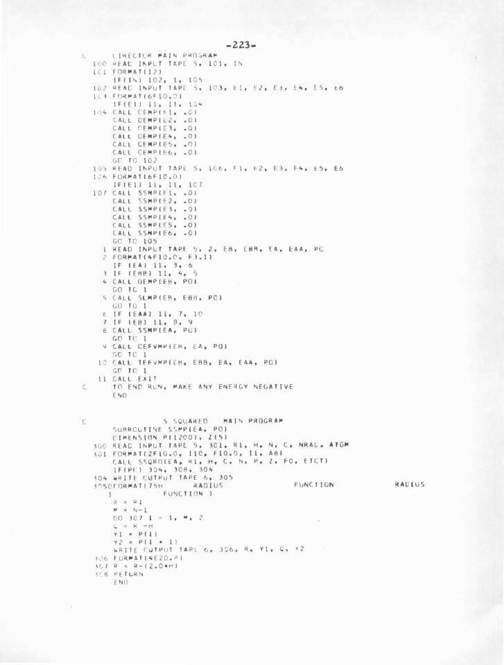
-223-L l I'<EC I LR "A I " P~O .... R A"

1! •0 Qf AC lii.P L T To!.P ( 'J , 1 C !, !" l C I r OR I" A T I I 2 )

IFCI"l 102 , 1, 10"> I Ul l'!fAC lfii PIJ T lAP ( ' • 10 3, tl , fl , (j , £ 4, (5 , tb I \ i r ()~ ,.A T I 6 F 1 0 . ~ )

IF IE I l 1 I , 1 I, I j <,

I 4 (A LL C( " Pitl , . Cl C ALL OE I'!PI L2 , .OJ CALL C'E I'! P t [J , . OJ C ALL GEHPIE4, .OJ CALL CE I'!PI E5 , . 01 CALL CE I'! PIE6, . OJ Gr r c 102

10? RFAO 11\.Pu T TAP ( S , lG6 , Fl , ~2 , E3 , F 4, t~ , E6 l'h FUR,.ATibFl O.Ol

IFIEll 11, 11, l C7 l OT CAL L SS HPIFl , . OJ

CALL ~S ... P i f2 , . OJ C ALL SS ,.. PIEJ , . I) J C ALL SS MP I E 4, . O J (ALL SS ,..PI ES , .OJ CALL 5SHPI E6 , . O J Gf' TC 10~ RE AD !"'P UT TAP E S , 2 , EB , EB~ , ( A, EAA, PC

? fOR,..ATI4Fl0. 0 , F3.ll IF l EAl 11, 3 , 6 It- I EHBl 11, 4, S

4 CALL OE MP IE ~ , P O l GO TC l

'> CAL L SU4PI Efl , EBH, P O l GO TO l

1:. If I E A.AI 11, 7, 10 7 IF IEBI 11, 8 , 9 e CALL SSHPIEA, P O l

GO TC l ~ CALL CEFVMPi f~ , E A, POl

r;c TC l I C' CALL TEFVMPI [ H, EBB , EA, EA A, POl

GO TC l 11 CALL EXIT

C TO EfliO RL~ , ,.AK E ANY ENERG Y NEG ATIV E (NO

C ~ \OU ARtO MAl ~ PRQGRA,. \UA R CU II ~E S~ ,.PI E A, POl l iM E,.. S I ON P(l200l, ll5l

100 READ lr-.P UT IA PE 5 , 301, R t, H. N, C , NRA L . ATGI'I 301 FOR ,.ATI2F1 0 . 0 , 110, flO. O , 11, AB I

C ALL S~OROIE A, Rl , H, C , N , P , l, FO, E TC TJ l F I Pf l 3:J4, 308, 30 4

~04 OI R IT E CUTP U T TA PE 6 , 305 lnS0fOR ,.AT I7SH RAD I US FUNCTION

1 FU"'CTI ON l ~ ~ R I " 2 ~-1 00 307 I 1.. ; I< - H Yl • Pill

1 .... 2

Y2•P( l+l l -.. R ilE r ulP lJ l ! AP t 6 , 306 , R , Yt, C, Y2

IJ6 T URMAI(4 (20 . ~l

\CT R : R-(2.0 • ~1

1'8 Pt li..RN ( Nil

RA C( US

l ONl ELEC TR ON MAI N PR r GR AM \U~RLU TI NE OF ~PltB, POl f'I MfNSION Pll 2f)Ol , liSl

-224-

.:C'O IlEAC lloiPUT TAP E 5 , .10 1, flt' , R1, H, N, C , NRA O, A{ CII lC I F~R ~ATI3F1 0 . 0 , 11 0 , Fl 0 . 0 , 11, A8l

CALl 01\iELE C IEB, ELB, Rl , H, C, N, ~. ll "RITE CUTPUT TAP E 6, 20?

:ul FORMAT 1 22H ONE ELEC T RO~ FUNC TI ON/ ) l 1 • ll 1 ) l2 ll 2) n & zt3l l4 : Zl 4 l l'> • ll 5 ) toi RI TE CU TPUT TAPE 6 , 2() ), AT OM, NR AC , fltl , £R, Rl o H, 1.1 , C

lC\O FOR ,.ATIA 8 , 6H N =II, bli L "' f 3 .l, llH ENERGY • Fl 0 . 8 , 113H RYO R l ~ F'S .l, 6H H s f5.3, 6H "• 15, 611 C • fS.J//1 "RIT E CUTP UT TAP~ 6 , 209 , l1, l 2 , l3, l~, l5

lO'l FOR MATil Ot-< '-j QQ[S AT F1 0 . 6 , 4F1 0 . 6 //!l IFIPC l 204, 208 , ?0 4

/J4 ,; RifE CU TP UT TAP E 6, 205 ~0'>0FOR MAT17 5H ~ AO I U S FUNCTION RADIU S

1 FUNCTI ON l R • R l "' = ,.._ 1 DO 207 I • 1, M, 2 0 s k-~

Yl • Pill Y2 • Pll+ll W R IT ~ OUTPUT TAP E 6 , 206, R, Yl , C, Y2

2C6 F ORMATI~E20. 8 l

20 7 R • R - I 2 . 0 • H I lOB RETUR~

C ~ L ~AI N PROGRA"' SUHROUT l NF Sl~PI EB , EBB, POl DIMENSI ON 1-' S il200 ), PPll200 l

4 000R EAO INI-' Uf TAP E 5, 401, NRAOS, NRAOL, ELB, Rl, H, N, Co l ">N , l-IS , PN, NP , MUll, AT O~

4 0 1 FOR IIATI21 2 , 3FS . O, IS, FS.O, F8.0, 13, F8. 0 , 13, JJ, ASI wRITE OU TP UT TAP E 6, ~03, AT O~. NRA OS , NRAOL, ELBt NS . SN, NP, PN

4u30FORMATI13H Sl FUNCTIONS//A8, 7H NS • 11, 7H Nl • fl, 16H L • F3.l, 9 H "'UMBE~ ll, ll H S NODE Al Fl5.8, 9H NUMBER 11, ?l lH L NODE AT Fl5. 8 ///)

WRITE CUTP UT TAP E 6 , 409, Rl, H, Ill, C 4 01 FORIIATI6~ Rl • F S.2, 6H H • FS.3, 6H N • 1'>, bH C " FS.3///l

CALL SLI[B, EB!i , ELB, H, C , Rl, N, SN , PN, NS, NP, NUllo P,, PP) IFIPO l 4 0 4, 4 08 , 404

404 ~RIT E OUTPUT TAP E 6 , 405 4~5 FORMAT155H RADI US S FUNCTION P FUNCTION)

~ • R l

CU 40 7 I % l, 'N Q % P S11l y % P PI I ) wRIT E CUTP t., T TAP [ 6 , 4 06 , R, O. Y

4C6 FOR.-ATI3F1 8 . 8 l 4"1 7 P = R- t-4 (l ll RE TURN

f N (')

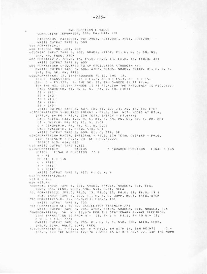
-225-

C T~G ELECTRfN F-VAL~E ~UHRCUTINE TE FVMPIEB, E8R , E A, EAA , PC)

O IMEI'o'iiO II< PAI1200l , P8112'10l~ PCI1200J, l1~>l, POI12 00 ) ~RITE CUTPUT TA PE 6, S99

'>'I q FOR" A T I 1 ~ 1 l b OG IF!EB~l 700, 601 , 7Ci0 I, •Jl ORE AO I,P u T TAP E'>, 602 , NRAOS, NRA n P, R1, H, N, C , SN, NS,

lPN, l'oP , F~E:O, AT O" hOl FORMA T1 212 , 2 FS.O, 15, F S . O , FB. O , 13, F 8 . 0 o 13, JlO.O, A8)

WRIT E CUTPU T TAPE 6, 60S nOS F OR,.ATI3 6 H S-SOUARE O TO S P O~C ILLAT OR STRE~TH //I

OwRIT t C UTP U T TAI>t 6 , 606, AT OM, fljRAOS , NRAO,, NRACP, Rl t H, N, C , 1NS, ') llj, NP, PN , FREQ

b'JbOFUR ,.ATIA il , 1 2 , 1JHS- S OUAf.IEO TO 1 2 , H~S 12 , 1 22H P TRAN S ITI ON Rl = FS. 2 , SH H ~ F S .J, 6H l'o c IS, 26 H C a FS.J/1, qH THE NO. 12, l4H S-NO C E I S AT f1.4~

JqH T~ E NO . 1 2 ,!4H P-NOOE IS <\T F7 .4,1 8H THE FREOU&NCY IS F1 0 . 0 ///l ( ALL SSORDIER, ~1, H, ( , "'• PA, l, FO, E TOTl ll a [(})

l2 & ll2l l3 • Zl3l [4 c ll4l IS ~ ZISl ~RIT E C UTP L T TAP t 6 , 607 , t b , l1, l2, l3, l4, l S , fO, ET G T

">0 7 0 F C:R I"Alt2 0 H S-SC.UARE O EN ERGY = Fq.6, l6H wiTH NODES AT f7.4, l4F7.4, 6~ FO c F7.4, 1 5H TO TAL ENERGY= F7.4///l

C ALL 'iL I E A, EAA , 1. 0 , H , C , R l, N , SN , PN , NS, NP, 1, PB, P C l u l • OVL P IH, PA , PC, Rl, ~ . 1.01 0 c C l•OVLPIH, PA, P b , Rl , N, 0 . 01 C ALL FVAL UE i r , l, FRFQ, ~ T R , GFI "RITE C uTP U T TAPE 6, 60'1 , 0 1, 0 , S TR, GF

h'J40FOR ,.ATI1 8H RAD IAL INTEGRAL c F 9 . S, l7H TCTAL OVERlAP '" F9.S, 11 2H STRE:II<G TH = fq.s, 7H Gf = Fq.SIIIIl

IFIP (; l 61 0 , 614 , 610 ~ I' ~ R tf [ G UTP U T TAP [ 6 , 6 11 bi 10 F-Of.I,.A T t81H RADI US S S CUAREO FUNC TI ON FINAL S f t.;N

1 C TI C"' Fl~AL P F UNCT I ON II l R = R 1 ro 611 1 = 1, N L • PA I I l X = PB I I l Y • PCI t l wRITE (U TPUT TAPE h , h 1 2 , R , C , X, Y

~ 1 2 FO~ NATI4 E20 . A l

•, I 3 K ~ R -~ '"> 14 f.IETURN 1 , 0 () ~ 1:: A C I 1\ ~ U T T A I>~ '> , 7 C I ~ 1\ R ADS , N R AD L6 , N R A Dl A • ELl! , t l A t

1 S NA , N\8 , E LN A , 'lEU! , '> ~A, N S A, E lNA, N ELA / G 1 F OR" A T I } I 2 , 2 F 'l . :) , f 8. 0 , l 3, F 8 . 0, 11, F 8. 0 t I 3 • f 8. 0 ~ I )

.{f: AC INP Li T TAPE '> , 7 02 , Rl , H , N, C , JUMP, NULl . fREO~ Al("' 1~2 ~OR ,. A lt2 FS . Q , I S , FS. 0 , 2 l 3 , FlO.O , AS )

loR I Tl C UT P U T TAI> E o , 7 0 3 / O l UR MATI31H 5 ll TO S L 2 CSC ILlAT OR S TRENG TH Ill

~!li TE C UTP U T TAP [ b , 7 0 4, AT O"• l'oRA C S, lltR ADlbo Ell, NRAOLA, EL A / 0 <. 0F0R "ATIA R, ~ H ~ = !2, 6 7~ F n R THE STATI ONARY 5-w AV E ELECTRON.

llt-< f TIIAN S JT! ON I S FR O ,. ~ ~ !2, C,H l "' Fl.1, 8H 10 N • 12~

l '>t-< L c F 3 . 1 Ill l OwRIH C UTP U T TAP ( 6 , 70S , R1, H, lit, C , NSB , '>N6 , ii>El. B . ELH8, 1 ~F LA, E LNA, " Ul T, JUI'P, FREQ

I C ">O F UR"'<\TI6~ .{1 "' FS. 2 , 6H H • F5.}, oH WITH (4, 1bH POINTS C • !FS .3, ll H THf I';UMAER l 2 ,17H S-NODE I S AT R • F7.4 II, llt- THE NV"'6

-226-2Ek J2,2"H L-NUOt: 8EfORI: I ~ AIR • f7,4, ISH A._O IKf NUI'I6ER 12, 1;' ) H l-NODE ArTER I S AT R. • f1,4//, l9H TH6 IIULTIPUCITY • 12, 4\bH TH( JU•P CPOE • 12 ,2 0 H AND THE fREQ UENCY • flt.l// I

( Al l ~liEB,E l' B,El8,H,C, Rl, N, SN8, f lNB, NS8, NELS, "'Ulf, PA,II'61 ( All StiEA, EAA, ELA,t<,C, R l, H, SNA, El "' A, NSA, NILA, 10\Jlf,PC,POI C \ • U~LPCH, P~, PC, R\, N, 1. 0 1 u • r i• O ~lPI H , PA, PC, R.\, N, 0 . 0 1 ( All FVALU ECO, JU"'P• FRE O, S T~, ~ FI lo RIT F C' UIPUT TAPE 6, 70 6, 0 1, O, ~ Ill, GF

l (l t>O f OR. ,..ATI1 9H ~AO IAl INTEGIIAL • F 'l . '"> , 17H TOTAL OVERLAP " F4.S//, 11 2H S TRE '<G TH = F 1.5, 6H Gr • F 'l . ~ ///./1

IFCP u l 1C 1, 711, 707 10 7 WRITE CUT PUT I AP E 6, 7013 7080fOR,..Afll 0 1H RA DIU S

! UNCTION FINAl S FU,( J! UN R • Rl 110 710 I • I, N 0 • PAIII II • PBI I I X • P( C I I Y • POCII

IN I I I A l S FUNC I tON FINAl l FUNCTION II I

wRITE OUIPUI TA PE 6, 70 9, R, O, lo, X, Y / Oq FORI'IATC5E20 . 8 1 11 0 R • R. - 1-< 7 11 REIURH

END

( ONE ElECTRCN F- YAlUE SUBR OU IINE OEFV,..PIE8, EA, POl OI114E,.SION P8112001, PAII 2 001 , l151

INIJIAL l f

'>OOO REAC INPUI TAPE 5, ~01, NRA08, NRAOA, El8o ELA, Rl, H, N, C, IJU•P, FREO, AT O"'

'">0 1 FOR,..ATill2, 4F5, 0 , 15, F5.0, 13, FlO.O, A81 WRIT E OUTPUT JAP E 6, 503

SO l FORMAT(lt-<1 32HONE ELECTRON OSCILLATOR STRENGTH /1 WRI 11: OUTPUI TAPE 6 , 504, AT O,.,, NRA08 , El8 , E8, NRAOA,. ElA , EA

~0 4 0 F OR,..ATIA8, 6H N • 11, bH l • F3 .1, l3H WITH ENERGf F15.8, 113H RY D TU N • 11, 6H L • F3.1, 13H WITH ENERGY fl5.8, "H RY0/1 CAll CNELECIEB, ELB, Rl, t<, C, N, PB, Zl WRIT E CUIPUT JAPE&, 515, Rl, H, N, Co JU"'II'~ FREO

5 1 S OFOR~AIC7H ~I & F5.2, 6H H • F5.3, bH N • 15, 6H C • f5.1, 110H JU"P • 13, 15H FRE CUENCY IS FB.l//1 ll • ZC11 l'2 • ZC21 l3 . 1(31 l4 • lC"I l"> • lCSI ~RITE CUTPUT JAPE 6, 50S, ll, Z2, ZJ, Z4, 15

~OS F OR~AT1l4H THE F1R S I HAS NUDE S AT FlO,& . ~Fl0.6//l

( All Ot-~ELE C C ~ A. ELA, Rl, t-<, ( , N, PA, ll ll • ZC11 Z2 • Zl2 1 n • z c J 1 Z4 • l!"l l 5 • 1151 WRIT E CUTPUT TAP E b, SOb. l1, Z2, lJ, l4, l5

~J~ F OR~ATC25H IHE S EC ON D HA S NODES AT FlO.&, 4FIO.b//l U • LVlPIH, PA, PB, 11.1, N, 1.01 CALL FVALU ECO, JU"'P• F~EO. STR, Gfl wR IT E OUTP UT IAPt: b, 507, O, SIR, GF

~f 7 0 f 0~"ATI1 H0 1AHRADIAL lNI EGRAl • F12.8, 14H S IRINGI H • F9.5, 16 H GF • F9.5////l

lFIPOI 506, 512, SOb ~O H loRlfE CUIP u f TAP ( 6, 5Q q ~~~ F OR~Afi5 5H RAOiu S INIIIAl FUNCTION fiNAl FUHCTIOHI

R. • Rl DO S 11 I • I , Ill 1.. • PEl Cl I Y • PAIII wRIT E CUI PU I TAP E 6 , 51 0 , R. Q, Y

~ 1 0 FOR •ATCJE20 .61 •, II ~ = 1<-~

~11 IH I URN ENO

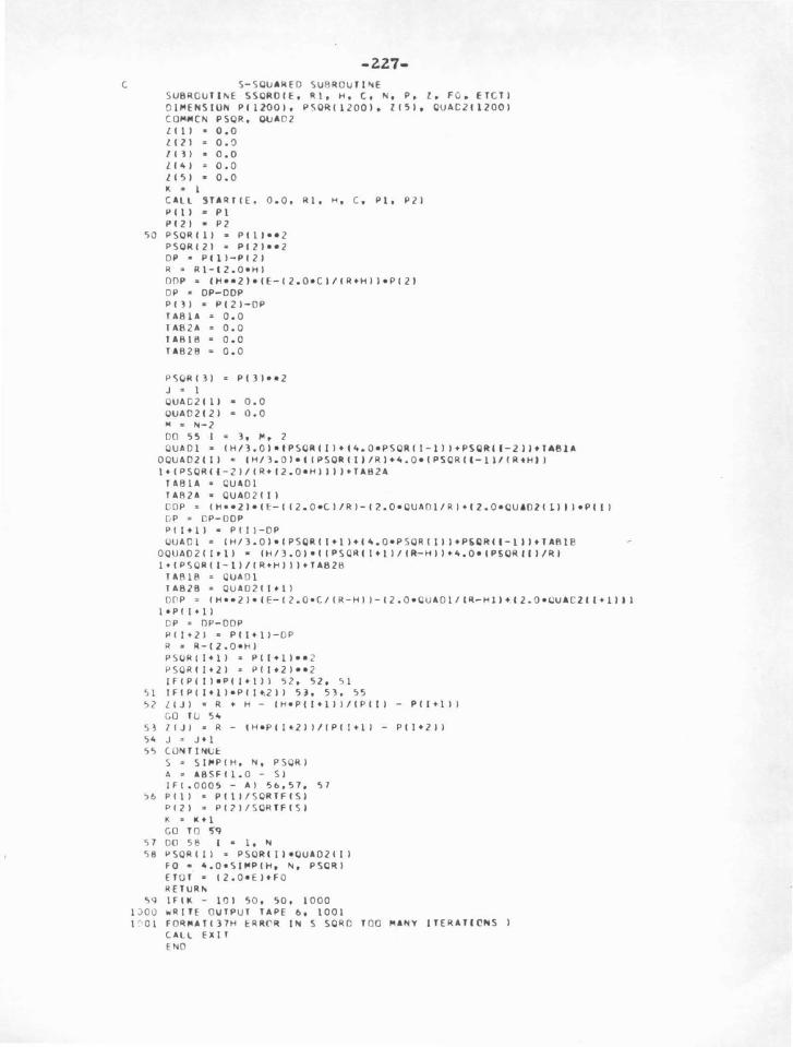
-Z.Z7-C S-SCVAREO S UB ROV TI~f

SV8ROUTI~E SSCROIE, Rl, H, C, N, P, l, FO, ETCTI OIMENSIUN Pll2001, PSORI1 2001, Zl51, 0UAC2112001 COMMCN PSCR, OUA02 llll • o.o liZI • 0.0 1(11 • o.o l I 4 I ~ 0. 0 ll51 • 0.0 1\ • 1 CALL STARTlE, 0 . 0 , Rl , H, C, P(, P21 Pill • Pl PIZI • P2

'iO P SCR I 1 I • PI ll • • 2 PSCRI21 • PIZI••Z DP • Pill-Pill II. • 11.1-IZ.O •HI OOP • IH••2l•IE-12.0•CI/tR+HII•P121 0 1' • OP-DDP PI 11 • PI 2 l-OP TABlA ~ O . 0 I A11 2A 2 0. 0 TA8t8 • 0 .0 TA828 • 0 . 0

P <;OR I 3 l • PI 3 l• • 2 J • l OUAC2t 11 • 0 .0 OUA02121 • 0 .0 M • N-2 DO 55 I • 3, "• 2 OU ADl • IHil.OI•tPSORtll+t4.0•P SORII - lll+PSCilRil-2li+TA6U

00U A02111 • tH/ 3 . 0 l•tiPSORIII/11.)+4. 0 •IPSORII-ll/lll.tHII l+IP SOR II -2l /IR+t2.0•HIIll+TAB2A

TABlA • CU AOl TAR2A • OUA02 111 COP • IH••21•11::-I 12 . 0 • CliRl- 12.0 •0UAOl/Rl+t2.0•0U 60 21 ~l l i •PI II DP • CP-OOP Pll+ll • Plll-OP OUAOl • (H/3,0I •IPSQRII+ll+t4.0 •P SORIIll+P,QRil-tii+TA8lB

OOUA0 2 11+ll • IH/3.0l•IIPSORII+ll/IR-Hll•4.0•tP!iORIIl/Rl l+IPSORII- II/I R•Hlii•TA82B

TA 61R • ()UA Ol TA828 • OUAD21 1+1 1 OP P • IH ••2l •I E-12.0•C/IR-HI I- 12. 0 • 0UA01/IR-Hll+t2.0 • CU AC211+llll

l•PCI+Il DP • OP- OOP P1 1+ 21 • Pll+li-OP R • 11.-IZ . O• HI PS<II'III+ll • 1'11+11•• 2 PSOR II+21 • PC1+21 •• 2 IFIPIII •P il+lll 52 , 52 , 5 1

~l IFIPCI+ll • PC1+:21l 5}, 53, 55 ~2 LIJI • R • H- IH • PII+lii/(Pill- Pll+l I I

GO TCJ 54 51 ZIJI • R- IH•PII+2li/IPII+ll- P 11+ 211 54 J • J. 1 ';5 CONTitfl.Jt:

S • Sl ~P IH, N, PSORl A • A8SF1l. O- S l IFI .OOOS - AI 56 , 57, 57

~6 P I 1 I • PI 11/ SORT F I S I Pt2 1 • PI21/ SORTFISI K • K+l GO TO ~q

S 7 DO 5 8 I • 1 , ~

'; 8 ~>SORIII • PS0R tll•OUA0 2111 FO • 4,0•SIMPIH, N, PSCRI ET OT • 12.0•EI+FO RETUR~

.-,q IFill. - 10 1 50 , 50, 1000 l JOO •RITE OUTP UT TAPE 6, 1001 1 ~ 01 FOR MATI37H tRRrR IN S SORD TOO "ANY ITERATICNS l

CALL EXI I ENO

-ZZ8-c O~f ELECTqQ~ SU8R0Uli~E

SUBROUTI~ E ONE LE C I E , Elo Rt, H, ( , N , P, ll O IME~SIO~ P112001, P\ORII2001, Zl!il CQ!'IIICN P S QR Zlll•O. O 1121 • o.o llll. o.o l c 4ol • 0. 0 Zl!il • 0.0 ( All START IE, ( l , R I , H, ( , P I • P 2 I P 11 I 2 PI P12l • P 2 P SOR I I I • PI I I• • 2 PSORI21 • P1 2 1•• 2 OP • P I l I - P I 2 I R • R 1-H J • I >4 • lo-1

00 4ol I • 2 , " OOP • IH••21 • 1 1 E •I~•I EL •l.Oil /IR •• 2 1l -12.0• C I/ Ri tPIIl

OP • OP-OOP Pll•ll • PIII-OP P SOR I I • 1 I • PI I • 1 I • • 2 R • R-t-IF IPII•li•PIIII 4 0 , ., 0 , 4ol

43 l iJI = R- I H•PIL• lii /IPII I- PII+lll J • J•l

41 CONT I"'U£ S • SI ~P(H, N, PSORI 00 4o 2 I • t, H

42 Pill ~ PIII/SORTFISI RETURN EIII O

( TH E ll'AR S SUBROU TINE SUBROUT INE MA~S IPS, PP, Rl, E L, H, Ill, G, RHCI

OO I!'EIII S IO~ PSI1200I, PPI1200 1, 81112001, 82112001, G111ZOOI, lG2112001, Gll 200 1 (~IIICN 81, 82 R • Rl 00 18 I • 1, N f\ 1111 • I R•• ELI •P SIII•PPIII

18 R • R-t-R • R l OOl'll•l , N A 2 II I • PSI II •P PI I II I It • • I E l• 1 • 0 I I

1'1 R • R- ... TABlA • 0 . 0 TA818 • 0.0 Gll\1 • 0 . 0 G21 11 • 0 . 0 Gll21 • 0.0 G2 121 • 0 . 0 TA82A • 0 . 0 TAII 2 B • 0 . 0 M • N-1 DO 20 I • l , ", 2 Gllll • I H/l.OI•IB1111+4o. 0 •8111-11+8111-21,.1A81A TABlA~ Gl l ll Glll•ll • IH/J.Ol•18lll+ll+4o.O•Bllll+8lll-lli+JA8l8 T A8 11 • G 11 I • II G2 111 • IH/J.OI•IBZC I l+4o.0•8211-11+1121 l-2 lltfA82A TA82A • G21 ll G 2 I I • 1 I • I HI l • 0 I • I 8 2 I 1 • 1 I • 4o • 0 • 8 2 I 1 I + B2 I I -1 II "T A 8 28

10 TA82 8 • G2 11+ll R • Rl-12.0•HI C • 1 .0/1 2 . 0 • EL •l. O I Gill • 0. 0 Gill • 0.0 00 2 1 I • l , N, 1 . Gi ll • C•I1Gliii/IR••I EL+l.Oili-IR••ELI•G2 CI II

2 1 R • R-H RHO • TABlA RE TUR~

f~O

c

-2.29-C THE VENUS SUBROuTINE

(.

SUBR OIJJINE VENUS IP. Rl, ~. N , Fl O I"'ENSIO'I Pll200), Flll200 ), F2112001, F11200l CC.-M CN Fl, F 2 fA lilA • 0. 0 TA818 0 , 0 TA82A • 0.0 14.8211 • o.o Fl Ill • 0.0 Fl 121 • 0.0 f-2 Ill • 0.0 F2 121 • 0.0 "" • N-l on 22 1 • 3, ""· 2 Fll ll • IHil. OI•IIPII 1•• 2 1 l+I~. O •IPI I- 11••211 2 + IPII- 21••211 +TABlA

TABlA • F ll I l Fl 11•11 • IH/3.01 • HPII+II •• 21

l+'-.0 • IPil l ••21 + IPil-11••211 + TA818 TA8ll • Fl 11+11 y " 1 F2 I II • IHI3.01 • IIIPil 1••21 I IRl - IY-1.01 • HII

l+ 4.0 • IIP1l-11••2l I IRl-IY-2.01 •Hll 2 + IIPII-21••21 I IRl-IY-l.Ol•Hlll + Tl82A

1AB2A • F2 Ill F2 ll+lJ " IHil.Ol • IHPII+ll••2l I IRI-Y•tOl

l+ 4.0 • 11Pill••2l I CRI-IY-l.Ol•Hll 2+ IIPII-11••21 I IR1-IY-2.0l•Hll I + TA828

22 TA828 • F211+1l R • Rl - 12. n •HI Fill • 0.0 F12l = 0.0 00 23 I . 3, .... 1 f-Ill " l.O • IIF11ll ' R l . - F211l l

n R . R-t< RETURN END

FACTOR IAL FUNCTION FUNCTION FACT O Ul y . IO.It6l•X•IX - 1. 0 I I • 1. 0 A . AASF I X-0. lobi l IFU - 0. 15) 94' 91t, 9 0

90 IF I A - 0 .... 61) 91, 'H, 94 91 IF IX- 0 .4611 92, 93 , •n qz FA( TO = Y-0.005

GO TC 'lS •n FACT L . y • 0.005

(,0 TC 'l5 9 4 FACT C " y

'lS RE TLRN ENO

THE OVERLAP FUNCTION fUNCTICN OVLPIH, PA, ~8, 111, N, 01 OII'U',., SION PA11200 l, P811200l, 8112001 (QM .. CN 8 IFIOl 13, 13, IS

11 DO 1'- I • I, N 1'- Bill • PAIIl•PBill

GO TC I 7 l') R • R1

no 16 1 • 1, N IH il • R•PAill•PBIIl

16 R = R-t< 17 OVLP • 'II"'PIH, N, 81

RETURI\j [ l'fO

-Z30-

C STARTING VALUE SURRO~TlNE SUBRCuTINE START CE, El, Rl, H, C , Pl, P21 E~ • Cl SORTF lEI y = l. 0 A " l. 0

~0 lr IEN+El-AI 32, 32, ll 31 Y z Y•IEN+EL-A+1.01

A z A+l.O GO TO 30

32 X EN+EL-A+l.O F Y•FACTOIXl l = 1 • 0 H 1. 0 IFCEN- EL - 2.Cl 36, 36, 33

33 IF IEN-EL-B-l.Ol 35 , 35, 34 ~4 l = l• CEN-EL-Bl

B = B + 1. 0 (,0 TC 33

3<; X = EI'-4-EL-~ G = F • l • FACT O IXl GO TC 39

3 6 I F I EN-E L + B- 2 • 0 I 3 7 • 1 8, 3 8 37 l = l • IEN-EL- 1. 0 +81

H = S+I.C Go r c 36

~8 X • [N-EL+R-2.0 IFill 70, 11, 70

10 G F•FACTOIXl/l 39 <; = EN • LOGF 12.0•C/E~I

T = IEXPFI S l• SQRTFICll/IEN • SOR TFIGll til • Eh •II EL•IEL + 1.011- IEN•IEN- l.OJLI/12.0•Cl f\2 • EN • 81 • tiel • IE:L +l. Oll- IIEN-1.01 • I EN-2 .0111/ 14.0•CI 83 Eh • 82 • tiEl• IEL+l.Oli-IIEN-2.01•1EN-3.011l/16.0•CI Ul "'EN • LOC.F IRll Pl T • ltXPFIUl-C•RL/tNII•Il.O+IBl/R11

1+182/IR1••2l l + IR3/IR1••31l l R2 • R1 - H

U2 • E" • LOGF IR 21 P2 • T • I EX PF I 02-C •R 2 /FN)) • 11.0+1Bl/R2l

1+ IB2/lR2 •• 2l l + CB3/IR2••311l RETURN

71 wRITE CUTPUf TAPE 6 , 72 72 FORMATl26H ERROR !~ START, l IS lER Cl

CALl EXIT END

( S LMPSCNS RULE FUNCTI ON FUNCTICN SIMP ( H, N, 81 OIMENSION B 11200) s s o.o ,.. = ~-2 uo 80 l 2, ~. 2

80 S S + B I l l <; • 2.C • s K " N-3 DO 81 I 3, K, 2

tl tSzS+RIIl SIMP= t~/3.0l•Cl2.0•SI +Bill + BIN-111 RETURN (NO

-231-

C THE EVENT SUBROUTINE 0SUBRCUT I~ E EVENTINE , KIN O, P, R, El~. IN, ECB . EU I, NlTo 1NEA, EC VT, IT, EOA, FU A, NO I ENIT-"IHT EOA s EOB EUA & EUB EOU T • EI N NO • 0 lFIN E - 21 1, 10, 20

1 IFIKIND- ll 2 , 5 8, 5 2 IT • IN + 1

F OU T "" E IN I I 1 • 0 +. 0. 2 • E IN I

s 6

10 12 1 1

15

20 21

GO TO 59 IFIKINO - 3 I I T "' 1 "'E A = 2 GO TO 60 IFIKIN C - 1 I IFIKINO- 3) IT . IN • 1 EOU T . I 1 . 0 GO TC 59 IT . 1 NE A ., 3 (,0 TO 60 IFIKINC t.~E A % 3 IT • I" GO TC 60

- ll

6, 2 . 2

11 • 15 , 12 11 • 1 1 • 2

• 0 . 2 • E LN l

21 , 2 1. 2 3

l3 IFIKlNO - 31 30 , 40, 2':1

• EI N

2 5 WRITE OUTPUT TAPE 6 , 26, E IN, P, R 260FORHATIFB. 5 , 44H HAXI~U~ INFLECT ION P T HONOTON tC TO P • F7.5t

1 10H AT R = F8 . 5 1111 '40 • 1 IT " I N NEA • 4 GO TC 60

~ C IT • IN + EU A = F IN IFilCRI 31 , 11, 35

3 1 E OU T • E I N I I 1 • 0 + I 0 • 1 I I I E N I T - 1 • 0 I • • 2 l l l GO TO 36

35 EOU T • I EUA + EDR I/ 2 . 0 36 WRIT( CUTP UT TAPE 6 , 3 7, E IN, P , R 370FOR~ATIF 8 .5, 44H MAX!MU~ INFLECTI ON PT HINLHUH WIT H P • F7.5,

110H AT R • f8. 5 l GO H. 59

40 I T • I N + 1 41 EOA = E l N

IFIE UBI 42, 42, 45 4 2 EOU T • 11. 0 + t0.1/t t EN il - 1 . 0 1 •• 211 l • ElN

GO TC 46 45 (OU T • I EUB + EOAI/2.0 4 6 WRITE CUTPUT TAPE 6 , 47, ElN , R 47 FORHATIF B.S, 43H MAXIM UM INFLE CTI ON PT AND NODI AT R • F8.5 l

GO TO 59 58 IT • IN r,q NEA • 1 60 RETURN

(NO

-232-

( EX TRA NODE SUBR OUTINE OSU8R~UTI~E f XNr t ~E . KINO , R, ElN, 1 ~ , EU~ , EOB, ~f A,

I f: 0\J T , I T , 1: U A , ED A , ~ 0 l fUA = EUB Er'A = ECH ~D • 0 [OUT = EIN 'j[A : 1 IT " I~ !FIN E - 51 1, 10, 30

I IF I I< I ND - 2 l 2 • 8 , 4 2 WRITE CVTPUT TAP E 6 , 3 , l iN, R 3 FOR~ATIF8 . 5 , 37H FKTRA NUCE !NFLECTICN PCfhT AT R • F8.5 l

E OA = E I "4 I T " I I. + I fCU T • IEIN + EU~l/2.0 1;c T c. 45

4 WRIT E CUTP UT TAPE 6 , S, R S FOR~ATI47H fXTRA NODE FCLLOWE C BY BL OW UP Ck ENU AT R • f8.S l

1 r " 20 GO TC 45

B 1\j E A = NE + 1 Gfl Tr 45

10 !Fit< INC - ll 11, 20 , 1 2 II NE A s NE + I

t ,L Tl! 45 12 w~ITt OUTP UT TAP E 6 , 13, EIN, R 13 F nR~ATIFB . S , l8H EXTRA NUO E ~lNI~U~ MGNO JONLC IC R ~ FB.SI

1110 " 1 t.r r r 45

?0 "RITE CU TPUT TAP E 6 , 21 , [ IN, R 2 1 f('lRMATIFB . ~. 34H EXTRA 1\j QOE M[ N I~U~ NODE AT R FB.S )

f-U A " E l "' I T = IN + 1 ((U T = I E IN + EOH I/2. 0 t.O TO 45

1') !FIK!Nr - 31 3 1, 35 , 4 () 11 wRITE CU TPUT TAPE 6 , 32 , EIN , R ~ 2 FORMATIF8 . 5 , 38 H EX TRA "4 0D F MI N I"'FL EC ~AX(HU~ AT R f8.5 l

I T c I"' + 1 CIJU I : I EIN + EUH I/ 2 . 0 en TC -45

~') WR(Tf CU TP UT TAP t 6 , )b , f iN, R 36 FnR .. ATIFB . S, 3SH EXTR A Nr:CE ~IN INFL EC NCOE AT R " FB.S l

r.o = 2 l, U TC 45

4 0 wRIT [ CUTP UT TAP [ 6 , 41 , E I N, R 41 rnR~AT(fP . S , 40H ( XT R A "4LOE MI N I"'FL EC ~ C NO T CN I( l O R • F8.5 I

•.o = 1 GO TO 45

4':> Rt:TU RN fNf'

-Z33-l ~-II AI. Ul ';U81!0U I l>j f

SUP RLU TI~ < FVAlUEI C IILP, J UNP , f~ E C, S~ A, ~FI

l fiJU ,. PI '100 , '100 , 'IC I 1(. 0 JUI'I P • - JOJfOP

~0 Tl 1'102 o '101 , ~03 , 'liH , 'l"~ • '1 0 ~, 90!> , '1071, Jt.f'f> IOIOGO TL 1 ~08, 4 0 4 , '110 , 'I l l. '1 12, 'I ll, '114 , 'II,, 'II ., '1 11,

1~18, 9 1'11 , J u ,.P 102 C • 7 . 0 /L J

C.O I f.. '12 0 •ol c • •.on. o

f~U rc. q z ~

10 4 C • 4, 0 /I">. C GO TL 9 2 0

• ..; ~ ( • 17.015. 0 viJ r r 920

~c 6 r • 6 . 0 / J"> . O (,0 T(l 920

<IC7 C : 2 4. 0/7 . 0 ,;o r r '12 0

•c e c • 2 . o en r o '12 0

•10 <1 C , I . C GU TC 920

n o c • l.OI.l. u 1,0 T(J '12 0

Ill c • 1.0 GO TC 92 0

9 1 7 c • "> . on . o A' TC 920

I I) ( • .I . C ,(1 TL '1 2 0

1!4 C • 2 . 011. 0 C,P H 920

" I ~ C • I. 0 / 2 . :J GC I f 'l20

-lib c • l. 0/2 . 0 GO Tl.. 'llC

•II C • 1.011 0 . 0 t.u ru 92 0

•I~ C • I. C/1.J cr r c 'l 2 0

n<~ c • 1•.ot~. c 1 2(1 ~ TR • C•l 011 lP•• 21 171 C,f • . 0 0 0003') l 7 4o FRtt.. • S TR

IH TuR" FND

< l~lh. !l l f"' l .,.(.. I " IP '- • .. w, fl. " ULI, lASt R l; t' ; S ;4CII,.R.,.,.. lJ ~; Ul

"I I • I . I v I .

l • •

J lo-l q - ~" ) .>' ,> , .... . .. : l f- l"'- ~'"I • , • •

" "" • c.. t t

' ... C J C ~ 'l ..( ... . (,;,

'u . ~ - " I ~ I P ~ - -• 'i ) 14 . I 4, l c I • IF I bl l I 1- ' I ' ' L • h 1 F I T 6 H I I t> , 1':; . ) 1 ( • 1 v . -.. ~

'0 If I J ,7 ' I~ . r • ; 1

f) h ll I r !Pl,.\Jll - I I ' . ,,. L 3

' IV , I.) • ..,

.I' I f 1 j I IHHl21 I j • II , I ' II lF t•H - II . ' . L 2 , I ! u It . r ., ;'\ ll >'L . , ( I • L"L - '"'IIL h • C J~ • SCQ f f l "> l l

.. .. . . c I . I ' " - POll I/ U• • " IV • S C'IIf l ~ll

"'P f\!lo(" 'Ill

-234~

C THE REN.O~M4uJl/d)C~ SURRCLTINE N0. 1 ~U~~GU1}~8 qE~OH ~(Sl~ 52~ 53~ CBNC~J

G'"' 1.; 0 ' 1 ~ Sl- l.; C' Q2 ~ S2- 1.:n ~3 .,. $3 - 1 .. [) IFlQl t C2I ~i 8• 1

1 IRl02 • C3 > a , e. 3 ] lfil-Q3- . 05) "• 5.1 5 4 IF,<J3 t . 03 ) 6• tr .8 5 CENC III "' 1.: 5

GO lC! <; 6 CB'IJO,. :: 'J ,7

GO lC S ? CBNOIP "' I.: G 9 H6TO~N

[-~[)

C fH~ Rfi~~RMAL,ZATICN SOBqCUTI~E NO. t SUBRCU1t~8 ~ENOR~lSlJ S2 , S3, DB~C~J G :a l.:C C l :a 51 - l.:C C2 ::11 52 - l. C (,3 2 s~ - 1.: .:. , .. ,,1;1 ~ <02l • '-<.12 ~ Q3)) 8~ ~. 1

l IRlQl t ~3} A• 8r 2 2 JFl.AIISFL ClJ - ARSPlG2JJ 8• a, 3 3 lP(A~S~lC3l - .;Jil a. 8~ 4 4 C 4 'Y • ( ~ W l I C. 2 ) +. t 0 2 f c:n J ) I 2 . : 0

i .. 1 5 ~ "' 1.;0 t ~ ~3 /LGA'Y••J))

l~(A8SFLF- l.Ol - ,C5J 7r 7; 6 c G "' F • G

f =- I t 1 GC lL 5

1 CEI\cC I' "' SQHJFLGJ GO lC 9

8 [81\10 11' •

S RE1UR ~

~i'fr:

1 ' "' • '-'

-235-

U-8 Sl OU T SU~RGU TI 'IE

L'r,U tiRt!l..li~E SLlEl~ E2 ; cl,. Ht~ C~ Re; ,_,N,. Sf\C t~ PN U ~ NS -' N'fl; flU; li'Sr PP) c.rJI"Elr. SI<J•, PSt120 J I; PP~1 ?C C: ), G Ll£ uC H FCCI<.I.l20 0 l.; PL12v C ir l t-~ A k H12(JC ), 11'iQRll20C); l'itSloi lP('5) CO ~fp.j ·PSO R CE NC, ., 1.:0 Sl "' 1.0 "2 .. 1 .:o '5 3 .. }~(,

;(t-0 1 • (}. C Rt--02 "' 0.:0 R l • RH ... "' .. ,.. s~ .. s~ PI'< ., Pl\0

I"IUL 1 a foiL "- li{Y ., G

"IT "' 1 su • 1 .a 'i l"lf$ .. l.:. t:. TAFJ .. 1.:. c NRtW ., C. EL2 • 8l: Ud " c.:.c C AL~ CI\EL6Gt El, ~ .: a ; R1; ~. C ; N, P 'S oi 1Sl CALu U~6l6Ct =2 r f l; Rlt H t~ C, ~; fP~ ZPl lFif\ • 0 R ., 1-l 1 I~G l 2 1 " l" \ IFlH- S"l 12,. l ) ~ 'i. C

lG IFlR- .5~- J.:. t". J 11-r lloJ 1 2 1 l P S l I I ., { I ~ - 5 II. I • P S L I I ll~aR-h

'4 IRlll~) 61; t 1; 55 )) • Q}l! UUTRL.l TAP l 6-' 56-' ~ IT

>t FUR~llll7H tT eK AIION NU~BE k 1 2 111/1 N ff a lOT + 1 lFt tH2 -c x.: o 1 6 1,. ,.,_ :; 9

' 1 aRila ~TPL.J TAP E 6 -' Se; ~ ~ ; e FC~~Af(34H ~-Wl~ c FUf\CTiuN WitH ~CO~ AT k "' FB.:.~r.Ll

GO lC: 61 ~q wRllf aurPuJ tAP~ 6; 6 0 ; P~

(;J FORMAH34H 0 -IIIAVc FUt-.CT ILl\ wl TH ;,CCI:! AT K "' F8.:51.'Ll GO J O 63

61 -~llE QljfRUl TAP E 6 ~ 62~ PN c2 FOR~AT~3~H 5-W AV E FU~ClJON WitH ~OC8 AT R "' Fe.:~r./l

6 ~ TA8 • - T48

f '- a )

t C" 1. ' t U~' ~ - 1 . " .. e~ ~ -d

'-'> TRAr " ·"

-236-

rALll I"AR ~ l ~ <; ,Ill'~ -<1~ El , ti , .. ., \: ~ >< HC l > r, l a H 2 U I P ~ C u • R 1 IPl~~ll- 11 2 ~ , 2 8~ I ~

15 l~lBl21 t~r 16 , 2 P 16 IPlRHfll I er 17t I M 11 ·H· C l • kHJ

; r JC 2 8 l>' lfO(~t'(;?) 2'1 , 1 .... . :;:; I G l( ~f2 .. 1n-o

'• ll TC ze 2 . .oo< IH ClJTP lJ J lA~ F. 6 r 21~ ~ f-'li ~ I F () R "' ~ Tt 1 e t-< V . 4 V F ,, 6 (, [ [ K ~ C a F e • ~ I I IJ

< ~u l • LHh C 1 • ~HC 2 • KHLJ I 3.u -< ~C 1 • ttH12 I{ ~L2 a R~ lJI

--~ c • Hf-o C T ;; ... 1 0 1Cl I " l r I'<

rcC KI II • P ~ lll~lll 2 . C • I{t-'Ll /llt 2 . L ~I!LI~l. Gl-.(~••LillJ+l.: O lllHG41-ll •} s J.< ... t-

? ( llLt; V 6'1t..<; t~J <; r R l , H - "~ ~~

•< • R 1 r o lC3 1 • 1• ., t• 4 k J ( I I ~ - ! 2 • (J • r /K J ~ I l E L 2 ,. I f L 2 • 1 • G 1 J I l k 41 • :< 1 1 - f l i I

I I 1 ~ • k - ~

L .\ L L It I! 0 I N ( P "< " 1\ " r b l 2 r I" L. L T " TAP ~ R 1 ~ H ~ SU t ll ll "R M.4 flu ~I" t1 l.I.Jl ! 1 ~ ~ llE ClJTP~J T4• E 6 ~ 6 4 r ""'~ RW~ RHO t ~ F U~~AT121H <; tA I{f l ~~ VA LLt P • Fl 0 .7~7 H Al K • Fd.:5~S~ MH O•F e .:5r//l

:•; l ~ : c .... .n 1 .. v •o<IJe OUl~ u l IAP L t r 6 5

< ) t- lJ.{ I'All4 C' h '~E< G Y

1 4 1'o £l ,a 1

l .. f. rc ,., • - I.· .. , ~ • PI" - IlL -< • Rio J • 1

1-' Rll.Jl) a "l P I' llll - I l " 1-'"'

l I t,t_, 1 5 ~ l " J , L L l .. Ll ~ I • L

rr "R • cr ., •' P ~ • C R

IF(,.blll 11~• 11~ , 111 ll Jf'l,.IHl - ll ! 14, ll 7 r 1 1 3

ll ... rr p , ~h•• 2 l • lllE"i £ • t1 Ad1Lll t PPllll • FCC: KU.II G '; J C 1 l ':

l l 1 Cr. P • l 1- t 41 i J • l I l 6 "- < t t· A ~ T I l l I • P 1-' l l l ) - F f1 C K U I I Ct , l t.. l l ~

l l 4 r:r· ll • ~ ~ t t 2 I • ~ ~ f "<.: • •• A~ 1 L L l I • P I' ll I I ll"l < a ~ t~

~ .. • r: I' t ·:r- " >- U ( L - lJ ~ 1-> t>( L ) • r P

II I

-237-l~(fCPC • cr PI 12~ , 12~, 11 h

11~ l~tc•e • n~l : 26 . 1~ ! . 11 1 117 IF(PP(l.- 11 • Pv(LJl 1 2 7, 1 2 7, 118 1 1 .~ 1 F l 4 It S ~ L P II llJ - 1 I l ~ 2 C • , l l l <; r 1 2 ~ ~ 1 2 R 1h lfl(''H- tl 1:' • • 1~ :: .. 1 21 1 2 v JF(~PlL - 11 + 1. 2 1 12~tl 1 ? ~, 121 1~1 IPl ~ t L ~/2 . I- R1l 1§), 1~3, 1 2 2 122 1<. H•C • 4

CC J t.. l3 C I 2 'i I( I 'lr • 1

Cl l J C 1 H' ! , f. I( I "'C • 2

, _L) J•, 1 L ' 1 2 T II I ~C " 3

Gl.l l C 1 F 1 2i' 1(}'\K: " :)

t,(" H , l 3 ':' 12., "'INC • 'i

C.,f' J ( 13 13.' JFl~P- J l 1' 3 , l~l, lll 131 IF-lKI H - ~1 151'1, 132 .o 1 5~

13 2 J • J .. l w ~ I J E C u T ~ ll l I A P :: 6 " 1 3 6, ·<

1~ ( F[l ~ I"Afl 2CH F t o-~. <;1 ~UfE 4T '< • R!:.'J) IFl~l~ ~ 1 ~ 1 ~J ~ , qGf t~ 31 (

~ r, ,: \ I X " "- I ( t 1 CC H 1'l'

I ? ; \1 '" PP ( 1..: l !FtlA~ l 137, 1 '1 / , 134

l~'i IFlX-'HSf.l,..L.LTl ~ 11 13'it~ 1 ; 5, 137 I ~'i IF (PH - 11 1' f r O, r G r 5C2 ') t JFlKAI\ C 'l '1(' 4 , 501 ,. 5 C '< ._,, 1 ~ . , r = P

o( ., "' 3 cr: H ' -; o:

~<: J f'lli\E~ l 117, ; q, Slt, l' 4 .J\ 'i : (, T

·~e

'c ' ) 1 ·~

I( ~ " c JF(IH- ~~ 1'/, ':.~ 7.,. 137 IFlG~HI 1 3 7, 1 11 0 ~~ F

lflciC81 117 , !31 , 'i C '> JFl~~SFl c u~ En ~l - L. r cc: • !:C ~ ll

!F( IH.C ~ l C . • >l lll 511 , 137t 137 ': 1 l ',(: A • ]

.\ ~ ~ " .,I I J L 1 :; >

5 1(1 .. 131,1 l)l

' 1 4 "'- A L L F :l"' t: p, •. , ' I , L • _. ,. F. 1\ .C. , II\ " t t.f~ ~ E G t4 , r, [ A , '1 0.1.. 1 ,o liT• !:LA, ::~ . ·r l

1 • ~ I T IFt•H l 31' . I., r ~ zc.

~ !• IFllf- "I : - 1, ~ 17, 5l c c I t. "N • Kl'll li

.,( ' c 1 1" ~ 11 o~ '1 11 F (l.fP \.., 1 lA~ · t. '31~

· l~ ~ ~1 ~1" All ! ~ t-< '-t '- ~'~ lll l R II:-<; illH- Aile EX TRA N(C!~ 11-111- ,, , 1 71', 5 1 '1; 1H

'd ., ~ • '<II; [

2 . 'I J f . 1 7 I' lf.l 'cC - ll oe: ', lH

-2.38-l,EAi eGu T- IT, 8~ &~ FU &~ ~ n I

!' r. u ~ • E" 2 I rot " ll JFtr-.r - IJ 1 ,. ~ .:-3r; ,. 230

I S C I F l I I - 2 0 I 1 ) l ,. 1 S l , ~ G '-1)1 JPI E*'2 - ECL TI 15 ') ,. 15 2 ,o l':l'l

152 "' il " "e~ l':l f' Jrii<II\ G- 11 iSJ ,. Il l. ,o 1 ~1

l)J CLI.II IIl'IIU E l~INP ~ JJ 23~ ~ ~ ~ o , 1S4

lS4 ~~2 • ~212. r

l.f' I C 1(}4 l':l 'l tN2 • 60Ll

'IJATI "I'UJT t

I P (,.,Afl - ~ Jl 14S ,. 14 5 ,1 > I L l't':l fUR - EU A

cr.H = flO-' IPI ~f Jl 15 q , 15G~ l ~(

1 5<; IFIIH- 21 I r 4, 1C4r~ 1 6C l eU IFl BO Hl 162 ,o ~ t2 , lcl 1 6 1 lf<I Cl!BI 162" 162t 1H lt2 LOP = ~OP ~ 1 163 lfolL C P ~ 21 1 .. 4t 1 6:J J 1 6~

165 ~ N2 ~ 8 ~2 t 2 . C ' 1 6 1\2 - E ~B ~ l

GO JG 111 4 17 ( 1\ S TR& C ~ NS, ~ A C t

I~I I\3TR 4 C - 1(.] l C' "" li'J, 1 7~

1 7 ) '- Ill 2 = !:(; ~ CO J L 10 4

1 7 ;; ~ "" " f(

I 1 <; P " ~ 1 L:O 1~3 II " 1, N !f( R - Rl\1 ! " ~ • U!2,r 11~2

1e£ ~>Q tlll" .: : II'~ -< " R - I-

" R I H Gl, f P ll l T A P :: f> ~ l ~ 5 , >{ I'!

11"'i ; ~ C~ " ~ll 6~'"' A'\'t li P f C ll C rC'.[l iTJ UI\ t-<O T lf ET 1 :.~_ ·Fe . ~ Ill!

(, t: l c 2 "'~ ·:

1 •; ,; ". ) T q A [ " I ~ <; l .J '\ [' t 1 !Flto. 'l TRt'll'- lei I ! 4 r l C'i• 1 7 5

~ • J I D " 1-' ~ - "'L .., ~ R L

C't ;: ~ 1 L " L l , ~

r!f'- lt-•• 21 ttlt E'-. 2 t h At-' T l LIJ•P P ILII : P -. CP - CC» ~~ I L + II • ~-' '"'IL l -[~

I P I H - l' • 'i l , 4 '> r :2 4 'I ~ 2 '> I ! 4 , I F I R I 24° ~ :4~ - ~ S G

_')_ !>' t-i lL~ ~I 3 2 . l tt ~ •~f'(L io ll ~~ ! .J • .I - ....

:4, I U 2:2 } · 3 1,. •\

i ~ 2 ~<; ~~ ''' . l> ~tll~• 2

' . ' . ')

, • S I~Pi h , " ~ ~ ;~K l

r IJ ~ ~ ~ t "' l , ~.

f ' f-1 I I J • I' R t I l I <: \J r< 1 F I. 5 I "'-'IH C~TIJ!.l PP ! A ~ 2'1 4, <,

P:UNO J t<CM ~tHCeO PA-S I

_ '; '• I .1 K "' A T l 2 t t- ' ' 1 ' -'< " 4 l f l A r ) 0 \ I ·~ r E ; R II L • F 8 • ~ I I I I I I Fl TA f< l ?55 - ,' -, <;, 2'J'..

~ ~~ ~J~Pl • 5 • ~L

'iU • S JJIIP <; 4 i.: 1 I R t N I T ~ J I 7 6 '- ~ 4 (' l J '! 0 1 401 JPtSI- 1. 0 1 4 • 1,. 4C<t' ~ C~

4<l2 Sl • S

-Jl IPl S~ - I. ~ l q t ,. 4J4,. 4 (6 4()<4 52 • s

(,C ll 2t.-: 4V6 JFlS !- _ Cl 4 t 1,. 40r't~ '1(7 401 H • s;

c;z • s~

4Cle 53 • s

-239-

(AkU R&NrR~L~lo' ~£ • <;3,. CCNO~I GO lt. 26C'

2 S(. <;Ji'•P'i • q • <;t · SU • SI~~L ~ CE~C ~

2Cll IPlAt'SPLEN;::- 1:2 1- .GC2 ':> • [2 1 L6 1J 27CJ £ 1 (;

2tl WPili GUT~~J TAP e 6; 262 2620FOR~All~6H ~EblS CO~Oill~~ W}IH A ~ E~ERLV ~If~}~ ~2 P EROE~ J OF 1

1HJ~ ITeRIITf1 )'\<; POJfAII E\2~u'l' /Ill I IPtB~J 268• ? 6~ . 268

26e IPtAeSFl'i- l.L l - . O:C'>I 2D l, 2h7~ 265 269 lfltAIISFl.S- l . L J- . C3 1 267 t~ 2t7 , 2 74 i 14 WRITE C~TPUf lAgt 6 , 27~ 2H FORIUH52h Fl~CflCN ~01 NCR I'Ul!H l ~diHi i\ ~ l' !iRr:B~J..: PRO OEE'C .: Ill

GO l C 21C 26~ •Rllf O~TPUl TAPt 6 ; 266 266 FORI"AHS2H Rli\C II LN ~CT "( ·< M,\ LilF C lolTHJ I\ ..:':>PERON"..: PRCCEEO ~ Ill

GC l~ 2lC 26 1 ~tRV • ~1RV t I

IPt~IR'I' - 21 2 7S , 26? ; 2t~

£63 wRJlf ~TPLJ IA~ E 6 , 26~ 2 6 4 FOR~~Tl2~H FU~CTILN<; fSIA~ li 5~6U /Ill

GO lC 3QP £ 7 0 "- lR'I " U

JPt~IT ~ 251 271 IIRilli C4JTitUT 272 FOR,.HL-'t41~

<.,O IC !l : z n u" E:~~o2 2 7<; .\ • F.2

:2 • E I [ l • ' t. " El 2 I'IJ2 • ELl tiJl • A A ~ 1'1\ P"4 • ~~

S"i " t. I " ~" lo.l' • 1\S t.. S • I

21lt 2 1~ .. 271 lAPc &, 212

10 C "A~'( I T[RA T I LJI\ \

3• ' '1 !:'0 2 ~ 1.. I , 1 , <;

A • I'P~}I

PPttl • P S lll J•C PSLII • ~

lllLUI'lll.l '14, .-,,, 'lli

I P L J A It I ~ l ) , ~ I .; ,. ' J •; l:J ,. f{ llli Oo\:IPI l IAR!: 6r ~ C l

CN 1 1. ~E H PR(BU 8,.. I

h.l H'RI'Atl'l _; t-> J. ,_ ... IY I~J C:<; .. lltlfUI "R[QL{E<;S Ll\ IL 'II:JCl P f{ L !JLE P<' I ' I ,· R 8 T L' u f,

e'c