arX

iv:1

209.

3595

v2 [

mat

h.A

G]

6 M

ar 2

013

Noncommutative complex differential geometry

Edwin Beggs and S. Paul Smith

March 7, 2013

Abstract

This paper defines and examines the basic properties of noncommutative analoguesof almost complex structures, integrable almost complex structures, holomorphic cur-vature, cohomology, and holomorphic sheaves. The starting point is a differential struc-ture on a noncommutative algebra defined in terms of a differential graded algebra.This is compared to current ideas on noncommutative algebraic geometry.

1 Introduction

1.1 Philosophy

This paper is about noncommutative complex analytic manifolds and holomorphicsheaf cohomology theory. The classical theory of complex manifolds begins with asmooth manifold of even dimension endowed with an ‘almost complex structure’. TheNewlander-Nirenberg condition [39] says when this almost complex structure actuallycomes from a complex coordinate system.

Every smooth complex algebraic variety is a complex manifold. Kodaira’s embed-ding theorem characterizes the compact complex manifolds that may be embedded inCPn. Chow’s Theorem shows that every compact complex submanifold of CPn is asmooth complex projective algebraic variety. Serre’s GAGA, the abbreviation of thetitle Geometrie algebrique et geometrie analytique of [43], shows that the algebraicand analytic properties of a smooth complex subvariety of CPn are “the same”.

In sum, these results show that the basic definitions in complex differential and com-plex algebraic geometry are compatible. This harmony confirms the appropriatenessof the basic definitions in the two fields. Hodge theory provides further compatibilitiesbetween complex differential and complex algebraic geometry.

There is nothing like this in noncommutative geometry. There is much less cer-tainty about the ‘correct’ definitions. This is entirely reasonable: there are morenoncommutative algebras than commutative ones, and some noncommutative algebrascan be really horrible. There are many ways in which ideas from commutative geome-try might be carried over into the noncommutative world, and there have been manyattempts to do this. But which ideas correspond to ‘geometry’ rather than the generaltheory of noncommutative algebras?

1

These ideas, whatever they are, must have a large and diverse collection of ex-amples. They should usually reduce to the corresponding classical structures, but weshould not exclude ideas that only have non-trivial meaning in the noncommutativeworld. And most classical geometric ideas should have noncommutative analogues.Certainly, in mathematical physics, it would make no sense if we were to say thatjust because the real world should be noncommutative because of quantum theory,we should no longer be allowed to teach general relativity because the concepts in itcannot really work. If the universe really is ‘noncommutative’, then there probablyare ideas in noncommutative geometry which reduce to, for example, geodesics andparallel transport in a classical limit.

This, then, is the philosophy of the paper: There ought to be a concept of non-commutative complex analytic manifolds within which one should be able to carry outmany of the classical operations. To be meaningful, there should be a good number ofexamples. And, for the future, there should be the possibility of using this as a bridgebetween noncommutative complex analytic manifolds and noncommutative complexalgebraic varieties.

1.2 Overview of the paper

This paper deals with non-commutative analogues of almost complex structures, inte-grable almost complex structures, holomorphic curvature, cohomology, and holomor-phic sheaves. We attempt to give minimal conditions for a noncommutative complexstructure that allow the cohomology of holomorphic sheaves to be constructed. We willalways refer to smooth or differentiable manifolds as real manifolds so as to distinguishthem from complex manifolds.

An almost complex structure on a non-commutative real manifold having a non-commutative ∗-algebraA of “C-valued differentiable functions” and a de Rham complex(Ω

q

A, d, ∗) with complex coefficients (a differential graded algebra) will be defined asan A-module homomorphism J : Ω1A → Ω1A whose square is minus the identity, andsatisfies a reality condition. This data, together with an extension of J to a derivationon Ω

q

A, leads to an A-bimodule decomposition Ωq

A = ⊕p,qΩp,qA into J-eigenspaces

such that (Ωp,qA)∗ = Ωq,pA and

ΩnA =⊕

p+q=n

Ωp,qA

for all n, and to associated operators

∂ : Ωp,qA → Ωp+1,qA and ∂ : Ωp,qA → Ωp,q+1A .

Motivated by the Newlander-Nirenberg condition we say that the almost complexstructure is integrable if dΩ1,0A ⊂ Ω2,0A ⊕ Ω1,1A. If the almost complex structureis integrable we show that

d = ∂ + ∂, ∂2 = 0, ∂∂ + ∂∂ = 0, ∂2= 0.

Suppose (Ωq

A, d, ∗, J) is an integrable almost complex structure on A. A holomor-phic A-module is a pair (E,∇) where E is a left A-module and ∇ : E → Ω0,1A ⊗A E

2

is a ∂-connection/operator. If ∇2= 0 we call (E,∇) a holomorphic left A-module.

We define a category Hol(A) of such modules. Associated to each (E,∇) ∈ Hol(A) is acomplex from which we define cohomology groups H

•

(E,∇). Elements of E play therole of continuous sections of a sheaf on the underlying non-commutative geometricobject and elements of H0(E,∇) = ker∇ play the role of holomorphic sections.

This category Hol(A) is abelian if Ω1,0A is flat as a right A-module. If all Ωp,qA areflat right A-modules every short exact sequence in Hol(A) yields a long exact sequenceof the cohomology groups (Proposition 4.6).

1.3 Relation to non-commutative complex projective algebraic

geometry

Let R be a finitely generated connected graded C-algebra of Gelfand-Kirillov dimen-sion n + 1. We assume R is left and right noetherian, Artin-Schelter regular, anda domain. We think of R as a homogeneous coordinate ring (hcr) of an irreduciblenon-commutative smooth complex projective variety, ProjncR, of dimension n, that isdefined implicitly by declaring that the category of “quasi-coherent sheaves” on it is

Qcoh(ProjncR) := QGr(R) =GrR

FdimR

where GrR is the category of Z-graded R-modules and FdimR is its full subcategoryof modules that are the sum of their finite dimensional submodules and QGr(R) is thequotient category.

ProjncR is a purely algebraic construct. In order to treat ProjncR as a non-commutative differential geometric object on which one can do calculus one first needsan underlying real structure on ProjncR, presumably defined in terms of a ∗-algebraA of Gelfand-Kirillov dimension 2n and a de Rham complex (Ω

q

A, d) which is also a∗-algebra.

1.3.1

Stafford and Van den Bergh’s survey article [47] shows that many ideas, tools, andresults, of projective algebraic geometry extend to the non-commutative setting in aseamless and satisfying way.

However, there are no non-commutative analogues of Chow’s Theorem, the Kodairaembedding Theorem, or Serre’s GAGA principle. In the classical commutative settingthose results allow the application of complex-analytic, Hodge-theoretic, and Kahlergeometric, methods to complex projective varieties, and conversely the methods ofalgebraic geometry apply to appropriate complex manifolds.

1.3.2

Until this gap, or chasm, is bridged non-commutative geometry will be without a unionof algebraic and analytic methods. If the gap were bridged non-commutative geometrywould be greatly enhanced. Such a development might also lead to a deep connectionbetween non-commutative algebraic geometry and non-commutative geometry as con-ceived of by Connes, i.e., based on operator algebras. At present there are few links

3

between the two subjects. The main contacts between the two schools include thefollowing: the work of Connes and Dubois-Violette on the non-commutative 3-spheresrelated to the 4-dimensional Sklyanin algebra; the work of Polishchuk and Schwarz onholomorphic bundles on the non-commutative 2-torus; the work of several people onhomogeneous spaces for quantum groups.

1.3.3

Part of the problem is that non-commutative complex projective algebraic geometrydeals only with holomorphic aspects of geometry and the objects appearing in non-commutative complex projective algebraic geometry have no underlying real structure:although many of these objects behave like smooth complex projective varieties, withfew exceptions, there is no underlying smooth non-commutative real manifold on whicha complex structure is then imposed.

Polishchuk and Schwarz’s work on holomorphic structures on non-commutative tori[41] is the great exception to the last statement and their work illustrates the advantagesof being able to impose a complex structure on a non-commutative real manifold.

1.3.4 Examples of complex structures on some non-commutativeprojective varieties

We end this paper by showing how the ideas in this paper apply to some particularnon-commutative projective algebraic varieties. The simplest of these examples, in§7.2, is CPnθ := ProjncRθ where θ is a skew-symmetric (n+1)× (n+1) matrix over R,Rθ is the free algebra C〈z0, . . . , zn〉 modulo relations zµzν = λµνzνzµ and λµν = eiθµν .

More substantial examples, in §7.3, are the quantum group analogues of irreduciblegeneralized flag manifolds studied by Heckenberger and Kolb, [26] and [27].

Further specializing, the quantizations CPnq have been examined in detail by varioussubsets of F. D’Andrea, L. Dabrowski, M. Khalkhali, G. Landi, A. Moatadelro, andW.D. van Suijlekom ([17], [18], [30], [31], [32]). The point of view of framed andassociated bundles is discussed in [40].

The reader should be aware that the notation CPnq is used in different ways bydifferent communities. Although there is a feeling that the same object is being dis-cussed the object called CPnq by one community belongs to a different category thanthe object called CP

nq by the other community.

Based on these examples we make some speculations in §7 about how one mightimpose integrable almost complex structures on the kinds of non-commutative projec-tive varieties that appear in the “Artin-Tate-Van den Bergh-Zhang” version of non-commutative projective algebraic geometry.

1.4 Relation to other work

Non-commutative differential geometry began with Connes’s 1985 IHES paper of thatname [14]. That paper, the birth of quantum groups, and Woronowicz’s 1987 and 1989papers, [53] and [54], in which he developed a ∗-differential calculus for quantum groups,were the beginning of a quarter-century development of non-commutative calculus.

4

Non-commutative calculus is an algebraic creation based on a non-commutativealgebra that plays the role of, and is viewed as, either the smooth or holomorphicfunctions on an imaginary non-commutative real manifold or complex manifold. Mostof this work has focused on developing either an analogue of the classical de Rhamcomplex of smooth forms or an analogue of the holomorphic de Rham complex.

Less has been done to develop a non-commutative calculus modeled on that for acomplex manifold, i.e., one that begins with the de Rham complex (Ω

q

A, d) of smoothforms, extends the scalars to C, and then using a non-commutative analogue of acomplex structure obtains a decomposition d = ∂+∂ and an associated decompositionΩq

CA = ⊕p,qΩ

p,qA into (p, q)-forms.A recent paper along these lines by Khalkali, Landi, and van Suijklekom [30] begins

with a short history of non-commutative complex geometry. That paper and others,for example, [11], [13], [17], [18], [19], [31], [33], [37], [41], [44], examine a range ofinteresting examples. Most of those examples fit into our framework.

Here we develop a fairly robust framework for a calculus of (p, q)-forms based onan almost complex structure J . Absent the J-operator, the definition of the (p, q)-forms in any particular example appears somewhat ad hoc although because the non-commutative examples that have been examined are closely modeled on classical com-mutative examples the guidance provided by the classical case has suggested what the(p, q)-forms should be.

The completely different approach by twisting in [10] is an example of the currenttheory, as the classical integrability condition twists into the noncommutative one.

1.5 Acknowledgement

The authors would like to thank the Isaac Newton Institute, where this work began dur-ing the program Noncommutative Geometry, 24 July - 22 December 2006. The authorsare also grateful to the Milliman Fund of the University of Washington’s Mathemat-ics Department for funding the first author’s visit there in September 2007. EdwinBeggs would also like to thank the Royal Society for a grant to allow him to givea lecture on this material ‘Noncommutative sheaves and complex structures’ at theInternational Conference on K-theory, C*-algebras and topology of Manifolds, ChernInstitute of Mathematics, Tianjin, 1-5 June, 2009. The second author is grateful forsupport from the NSF (grant DMS-0602347). The authors would like to thank StefanKolb for providing notes relating to the papers [25, 26, 27], which were used in writingSection 7.3.

2 Almost complex structures on ∗-algebras

In this paper we develop the rudiments of a non-commutative complex differentialgeometry based on the notion of ∗-algebras that applies to some non-commutativealgebraic varieties. Several issues must be addressed in doing this. First, most non-commutative projective varieties are defined globally in terms of their homogeneouscoordinate rings. They have no underlying topological space, and there is no patchingtogether of affine pieces. Second, complex differential geometry is developed by im-posing additional structure on an underlying real manifold but most non-commutative

5

projective varieties do not seem to have an underlying non-commutative analogue of areal manifold. This forces us to develop a formalism based on algebraic data that takesthe place of the underlying real manifold. That underlying algebraic data consists ofan algebra with a ∗-structure.

2.1 ∗-algebras

Definition 2.1 A ∗-structure on an associative C-algebra A is a map A → A, a 7→ a∗

such that a∗∗ = a, (ab)∗ = b∗a∗, and (λa + µb)∗ = λa∗ + µb∗ for all a, b ∈ A and allλ, µ ∈ C. We then call A a ∗-algebra. We call an element a ∈ A self-adjoint or hermitian

if a∗ = a. A ∗-homomorphism between ∗-algebras is a C-algebra homomorphism f suchthat f(a∗) = f(a)∗ for all a.

Throughout this paper A denotes an associative not-necessarily-commutative C-algebra. If the ∗-structure is ignored, elements of A should be thought of as playingthe role of holomorphic functions on a “non-commutative complex manifold” or regularfunctions on a “non-commutative quasi-affine variety”. With the ∗-structure, elementsof (A, ∗) should be thought of as C-valued functions on a “non-commutative real man-ifold” or “non-commutative real algebraic variety”. Often (A, ∗) plays the role of adense subalgebra of a C∗-algebra.

For example, elements of the Hopf algebraOq(SL(2,C)) can be thought of as regularfunctions on the non-commutative complex algebraic quantum group SLq(2,C) or,when a suitable ∗-Hopf structure is considered, as C-valued polynomial functions onits compact real form SUq(2).

The matrix algebra Mn(C) is always given the ∗-structure that sends a matrixto its conjugate transpose. An n-dimensional ∗-representation of a ∗-algebra A is a∗-homomorphism ϕ : A → Mn(C).

The free algebra F = C〈x1, . . . , xn, x∗1, . . . , x

∗n〉 on 2n variables is a ∗-algebra with

(xi)∗ = x∗

i , and λ∗ = λ for λ ∈ C. If A is a finitely generated ∗-algebra there is asurjective ∗-homomorphism F → A for a suitable n.

If B is a commutative R-algebra A := C⊗RB becomes a ∗-algebra by declaring that(λ ⊗ b)∗ := λ⊗ b for λ ∈ C and b ∈ B. We recover B as the subalgebra of self-adjointelements. A ∗-homomorphism f : A → C restricts to a homomorphism of R-algebrasB → R and, conversely, every R-algebra homomorphism B → R extends to a unique∗-homomorphism A → C. Every ∗-homomorphism is obtained by such an extensionso extension and restriction are mutually inverse bijections between ∗-homomorphismsA → C and R-algebra homomorphisms B → R.

These considerations apply when B is the coordinate ring of a real algebraic variety.Suppose X ⊂ Rn is the zero locus of a set of polynomials with real coefficients. LetB = R[x1, . . . , xn]/I where I consists of the polynomials that vanish on X . ThenA := C ⊗ B is a ∗-algebra and X may be recovered as the set of ∗-homomorphismsA → C. We will write C[X ] for A with this ∗-structure. We may think of C[X ] as thering of C-valued polynomial functions on X with ∗-structure defined by f∗(x) := f(x).

For example, if S1 is the unit circle x2 + y2 = 1 then C[S1] is C[x, y]/(x2 + y2 − 1)with x∗ = x and y∗ = y. Thus, if z = x + i y, then z∗ = x − i y and zz∗ = 1 soC[S1] ∼= C[z, z∗]/(zz∗ − 1). The unit circle is recovered as the R-valued points for thesubalgebra of self-adjoint elements R[z + z∗, i (z − z∗)] ∼= R[x, y]/(x2 + y2 − 1).

6

When B is an R-algebra that is not commutative the identity map on B is not a C-algebra anti-homomorphism so C⊗RB can’t be given a ∗-structure by defining (λ⊗b)∗

to be λ⊗ b. A standard example is provided by the algebra B = R[x, x∗] generated bythe annihilation and creation operators x and x∗ with relation xx∗ − x∗x = 1. NowA = C ⊗R B is the Weyl algebra. The momentum and position operators p and q arethe self-adjoint elements satisfying the equations

x = 12 (q + ip) and x∗ = 1

2 (q − ip).

Then pq − qp = −2i, illustrating the fact that the self-adjoint elements in a non-commutative ∗-algebra need not form a subalgebra.

2.2 Conjugate bimodules

This mixing of differential geometry and ∗-structures must be done with a little care innoncommutative geometry - the reader is referred to [8] for some of the details, mostof which will not be necessary in this paper.

Let A be a ∗-algebra and E an A-bimodule. We define the conjugate bimodule Eby declaring that

1. E = E as an abelian group;

2. we write e for an element e ∈ E when we consider it as an element of E;

3. the bimodule operations for E are a.e = e.a∗ and e.a = a∗.e.

If θ : E → F is any map we define θ : E → F by θ(e) := θ(e).If θ : E → F is a homomorphism of A-bimodules, so is θ. In this way the bar

operation E 7→ E is a functor from the category AMA of A-bimodules to itself.We make A an associative algebra by defining the multiplication ab := ba. As an

R-algebra, A is isomorphic to Aop via the map a 7→ a. We make A a C-algebra throughthe algebra homomorphism C → A, λ 7→ λ∗. We now define

⋆ : A → A, a 7→ a∗. (2-1)

Then ⋆ is a homomorphism of C-algebras and an isomorphism in AMA.

2.3 The universal differential calculus

We adopt the standard notation and terminology for non-commutative differentialcalculus. The reader can find more details in [23, Ch. 8], [34, Ch. 12], and [14].

Let A be an arbitrary C-algebra. Let Ω1univA denote the kernel of the multiplication

map µ : A ⊗ A → A. Following Cuntz and Quillen [16], we define the universaldifferential graded algebra over A to be the tensor algebra

Ωq

univA = TA(Ω1univA)

endowed with the unique degree one superderivation such that

d(a) := 1⊗ a− a⊗ 1

for a ∈ A.

7

Definition 2.2 A differential calculus or differential structure on A is a differentialgraded algebra (Ω

q

A, d) that is a quotient of (Ωq

univA, d) by a differential graded idealwhose degree-zero component is zero. The cohomology of (Ω

q

A, d) is called the complex-valued de Rham cohomology and denoted by H

q

dR(A).

Warning: We will denote the product in Ωq

A by wedge ∧ although ξ ∧ η will notusually equal (−1)|ξ| |η|η ∧ ξ when A is not commutative.

It follows from the definition that Ω0A = A; that Ωn+1A = A.d(ΩnA) for all n ≥ 1;that the multiplication map A⊗ d(ΩnA) → Ωn+1A is surjective for all n ≥ 0; and

d(ξ ∧ η) = dξ ∧ η + (−1)|ξ| ξ ∧ dη.

By hypothesis, Ωq

A is generated by A and Ω1A, and ΩnA is the C-span of

a0 da1 ∧ · · · ∧ dan | a0, . . . , an ∈ A.

Let (Ωq

A, d) and (Ωq

B, d) be differential calculi. An algebra homomorphism φ :A → B is differentiable if it extends to a homomorphism φ : Ω

q

A → Ωq

B of dgas. Inparticular, d(φ(a)) = φ(da) for all a ∈ A.

2.4 Differential ∗-calculus

Non-commutative ∗-calculus first appears in Woronowicz’s papers [54] and [53] and[54, Defn. 1.4] has been extended to higher degree forms as follows.

Definition 2.3 [34, p.462] A differential calculus (Ωq

A, d) on a ∗-algebra A is com-

patible with the star operation on A if the star operation on Ω0A = A extends toan involution ξ 7→ ξ∗ on Ω

q

A that preserves the grading and has the property that(dξ)∗ = d(ξ∗) and (ξ ∧ η)∗ = (−1)|η||ξ|η∗ ∧ ξ∗ for all homogeneous η, ξ ∈ ΩA.

When these conditions hold we call (Ωq

A, d, ∗) a differential ∗-calculus on A.

Remark. The definition implies (aξb)∗ = b∗ξ∗a∗ for all a, b ∈ A and ξ ∈ Ωq

A.We can rephrase the definition of a differential ∗-calculus using the notion of a

conjugate bimodule in §2.2 and the fact that the product

ξ ∧ η := (−1)|ξ| |η| η ∧ ξ

makes (Ω qA, d) a differential graded algebra.

Proposition 2.4 Suppose (Ωq

A, d, ∗) is a differential ∗-calculus on A.

1. If∑

ai.dbi = 0 in Ω1A, then∑

i db∗i .a

∗i = 0.

2. The map ⋆ : Ωq

A → Ω qA, ⋆ξ := ξ∗, is an A-bimodule homomorphism and ahomomorphism of differential graded algebras.

Conversely, if ξ 7→ ξ+ on Ωq

A is an involution that extends the ∗ on A and preservesthe grading and has the property that (dξ)+ = d(ξ+), then (Ω

q

A, d,+) is a differential∗-calculus on A.

8

Proof. We leave this to the reader.

The map ⋆ : Ωq

A → Ω qA is a morphism in the category of A-bimodules. The mapΩq

A → Ωq

A, ξ 7→ ξ∗ is not.Our ⋆ has nothing to do with the Hodge star operation in Riemannian geometry,

which in general changes the degree of the form. Our ⋆ is a notational device thatdepends only on the fact that A is a ∗-algebra. In the context of real classical geometry⋆ is the identity.

Proposition 2.5 Let F = C〈x1, . . . , xn, x∗1, . . . , x

∗n〉 be the free ∗-algebra. Then there

is a differential ∗-calculus (Ωq

univF, d, ∗) defined by (da)∗ = d(a∗) for a ∈ F and

(a0da1 · · ·dan)∗ := εn(da

∗n) · · · (da

∗1)a

∗0 (2-2)

where εn = (−1)12n(n−1); i.e., εn = 1 if n is 0 or 1 modulo 4, and -1 otherwise.

Proof. If ξ = a0da1 . . .dan, then

(dξ)∗ = (da0da1 . . .dan)∗

= εn+1da∗n · · · da

∗1da

∗0

= εn(−1)nda∗n · · ·da∗1da

∗0

= εnd(da∗n · · · da

∗1a

∗0)

= d(ξ∗).

Every element in ΩnunivF is a sum of terms of the form a0da1 . . . dan so (dξ)∗ = d(ξ∗)for all ξ ∈ ΩnunivF .

If a ∈ F and ξ ∈ Ωq

univF it follows at once that (aξ)∗ = ξ∗a∗ = aξ∗ so ⋆ : Ωq

F →Ω qF is a homomorphism of left F -modules.

A straightforward calculation shows that

da0da1 . . . dan−1an = (−1)na0da1 · · · dan

+n−1∑

i=0

(−1)n−i+1da0 · · · d(aiai+1) · · · dan.

It follows that (da0da1 . . . dan−1an)∗ is equal to

(−1)nεnda∗n · · · da

∗1a

∗0 +

n−1∑

i=0

(−1)n−i+1εnda∗n · · ·d(aiai+1)

∗ · · · da∗0.

= (−1)nεn

(

(−1)na∗nda∗n−1 · · ·da

∗0 +

n−1∑

i=0

(−1)n−i+1da∗n · · · d(a∗n−ia

∗n−i−1) · · · da

∗0

)

+

n−1∑

i=0

(−1)n−i+1εnda∗n · · · d(a

∗i+1a

∗i ) · · ·da

∗0

The two sums cancel so we obtain

(da0da1 . . .dan−1an)∗ = a∗nda

∗n−1 · · · da

∗0

9

which shows that ⋆ : Ωq

F → Ω qF is a homomorphism of right F -modules.

We note that εn is the sign of the permutation(

1n

2n−1 · · ·

n1

)

and (2-2) therefore

agrees with the formula in [53, (3.3)].

2.5 Almost complex structures

An almost complex structure on a real manifold is an endomorphism J of its tangentbundle such that J2 = −1. A complex manifold, when viewed as a real manifold,has a natural almost complex structure [29, Prop. 2.6.2]. Since we are working with(non-commutative analogues of) differential forms rather than the tangent bundle wemust express the notion of an almost complex structure in terms of differential forms.

Definition 2.6 Let (Ωq

A, d, ∗) be a differential ∗-calculus on A. An almost complex

structure on (Ωq

A, d, ∗) is a degree zero derivation J : Ωq

A → Ωq

A such that

1. J is identically 0 on A and hence an A-bimodule endomorphism of Ωq

A;

2. J2 = −1 on Ω1A; and

3. J(ξ∗) = (Jξ)∗ for ξ ∈ Ω1A (or, equivalently, J ⋆ = ⋆ J on Ω1A).

At this stage, there is no requirement on how J interacts with d. Such a requirementwill appear later when we define what it means for an almost complex structure to beintegrable.

Because J2 = −1 on Ω1A, there is an A-bimodule decomposition

Ω1A = Ω1,0A⊕ Ω0,1A (2-3)

where Ω1,0A = ω ∈ Ω1A | Jω = iω and Ω0,1A = ω ∈ Ω1A | Jω = −iω. Condition(3) in the definition implies (Ω0,1A)∗ = Ω1,0A.

The next result is analogous to the trivial fact that a differentiable manifold with analmost complex structure has even dimension, or, equivalently, the rank of its cotangentbundle is even.

Lemma 2.7 Let (Ωq

A, d, ∗) be a differential ∗-calculus on A. Suppose there is a func-tion

rank : some A-bimodules → Z

defined on a class of A-bimodules that is closed under finite direct sums and directsummands and contains A and all ΩnA and has the property that rankM = rank Mand rank (M ⊕ N) = rankM + rankN . If A has an almost complex structure, thenrankΩ1A is even.

Proof. The map ⋆ : Ω1,0A → Ω0,1A is an isomorphism of A-bimodules so Ω1,0A andΩ0,1A have the same rank. Therefore rankΩ1A = 2 rankΩ0,1A.

10

Remark 2.8 The hypothesis in Lemma 2.7 is mild. Sometimes there will be a finiteset that is a basis for Ω1A as both a left and right A-module and when Ω1A is not freeit is often a finitely generated projective A-module on the left and on the right, andbecomes free after a suitable localization.

It would be desirable to consider examples having the following additional properties:A is a finitely presented C-algebra, a domain, and noetherian, or coherent; Ω1A is afinitely generated projective A-module of rank 2r on both the left and the right; Ωp,qA,which we define in Lemma 2.10 below, is a finitely generated projective A-module ofrank

(

rp

)(

rq

)

on both the left and the right; there is a left A-module isomorphism∫

ℓ:

Ω2rA → A and a right A-module isomorphism∫

r: Ω2rA → A.

Proposition 2.9 Let F = C〈x1, . . . , xn, x∗1, . . . , x

∗n〉 be the free ∗-algebra endowed with

the differential ∗-calculus (Ωq

univF, d, ∗) in Proposition 2.5. Then there is a uniquealmost complex structure on (Ω

q

univF, d, ∗) such that

J(dxk) = −dx∗k and J(dx∗

k) = dxk

for k = 1, . . . , n

Proof. Since Ω1univF is the free F -bimodule with basis dxk, dx

∗k | 1 ≤ k ≤ n any

action of J on the basis extends in a unique way to an F -bimodule automorphism ofΩ1

univF . Then, because Ωq

univF is the tensor algebra over F on Ω1univF , the action of J

on Ω1univF extends in a unique way to an action of J as a derivation of Ω

q

univF .

Warning. When n > 1 the map J : ΩnA → ΩnA does not satisfy the equationJ2 = −1. For example, because J is a derivation J(da∧ db) = J(da)∧ db+da∧ J(db)for all a, b ∈ A and therefore

J2(da ∧ db) = J2(da) ∧ db+ 2J(da) ∧ J(db) + da ∧ J2(db)

= 2(

J(da) ∧ J(db)− da ∧ db)

.

More succinctly,J2 = 2(J ∧ J − 1) : Ω2A → Ω2A. (2-4)

2.5.1 (p, q)-forms

Let C[h] denote the commutative polynomial ring viewed as the enveloping algebra ofthe 1-dimensional Lie algebra. Thus, if V and W are C[h]-modules, V ⊗C W is giventhe C[h]-module structure h · (v ⊗ w) = v ⊗ hw + hv ⊗ w.1 In particular, the tensoralgebra T (V ) becomes a C[h]-module and h acts on T (V ) as a derivation.

Lemma 2.10 Let V be a C[h]-module annihilated by h2 + 1. Let n ≥ 1. Suppose Ωn

is a C[h]-module quotient of V ⊗n. Then there is a C[h]-module decomposition

Ωn =⊕

p+q=n

Ωp,q

1Equivalently, if ∆ : C[h] → C[h]⊗C[h] is the C-algebra homomorphism defined by ∆(h) := 1⊗h+h⊗1,then V ⊗ W is naturally a C[h]⊗C[h]-module and is made into a C[h]-module via ∆. Alternatively, Vand W can be viewed as representations of the trivial Lie algebra Ch and V ⊗r

⊗W⊗n is then made into arepresentation of Ch in the standard way.

11

whereΩp,q = ξ ∈ Ω⊗n | h.ξ = (p− q)iξ.

Furthermore, if Ωq

=⊕∞

n=0 Ωn is a quotient algebra of T (V ) by a C[h]-stable graded

ideal, then the multiplication in Ωq

is such that Ωp,q⊗Ωp′,q′ → Ωp+p

′,q+q′ . In particular,Ω0, q and Ω

q,0 are subalgebras of Ωq

.

Proof. By hypothesis, there is a C[h]-module direct sum decomposition V = V 1,0 ⊕V 0,1 where h acts as multiplication by i on V 1,0 and as multiplication by −i on V 0,1.

If W and W ′ are C[h]-modules annihilated by h − λ and h − λ′ respectively, thenW ⊗ W ′ is annihilated by h − (λ + λ′). Applying this observation inductively to(V 1,0 ⊕ V 0,1)⊗n it follows that

V ⊗n =⊕

p+q=n

V p,q

where V p,q = ξ ∈ V ⊗n | h.ξ = (p−q) iξ. This proves the lemma for Ωn = V ⊗n. SinceV ⊗n is a semisimple C[h]-module, so is every quotient of it, and the set of h-eigenvaluesfor a quotient of V ⊗n is a subset of the set of h-eigenvalues for V ⊗n.

This completes the proof of the first part of the lemma. The second part involvingΩq

is equally easy.

2.5.2

Let J be an almost complex structure on (Ωq

A, d, ∗).By hypothesis the multiplication Ω1A⊗AΩnA → Ωn+1A is surjective for all n ≥ 1.

Therefore C ⊕ Ω≥1A is a quotient of the tensor algebra TC(Ω1A) where the tensor is

taken over C.We may apply Lemma 2.10 with V = Ω1A and h acting as J does because J2ξ = −ξ

for all ξ ∈ Ω1A. Because TC(Ω1A) is generated by Ω1A as a C-algebra there is a unique

extension of h to a derivation on TC(Ω1A). Since J is a derivation of Ω

q

A the actionof J on ΩnA is induced by the action of h on (Ω1A)⊗n.

For all p, q ≥ 0 we define

Ωp,qA := ξ ∈ Ωp+qA | Jξ = (p− q)i ξ.

Elements in Ωp,qA are called (p, q)-forms. Because J is a derivation on Ωq

A it followsfrom Lemma 2.10 that

ΩnA =⊕

p+q=n

Ωp,qA

for all n. Because J vanishes on A, it is a homomorphism of A-bimodules and thereforeeach Ωp,qA is an A-bimodule. By the last part of Lemma 2.10,

Ωp,qA ∧ Ωp′,q′A ⊂ Ωp+p

′,q+q′A (2-5)

and Ω0, qA and Ωq,0A are subalgebras.

12

2.5.3 The ∂ and ∂ operators.

For all pairs of non-negative integers (p, q), let

πp,q : Ωp+qA → Ωp,qA

be the projections associated to the direct sum decomposition ΩnA = ⊕p+q=nΩp,qA.

Definition 2.11 Let∂ : Ωp,qA → Ωp+1,qA

be the composition πp+1,qd : Ωp,qA → Ωp+1,qA. Let

∂ : Ωp,qA → Ωp,q+1A

be the composition πp,q+1d : Ωp,qA → Ωp,q+1A.

Because Ω1A is generated as a left A-module by da | a ∈ A, Ω1,0A is generatedas a left A-module by ∂a | a ∈ A; likewise, Ω0,1A is generated as a left A-module by∂a | a ∈ A.

Proposition 2.12 Let J be an almost complex structure on (Ωq

A, d, ∗). Then for allξ ∈ Ω

q

A and for all p, q:J(ξ∗) = (Jξ)∗ (2-6)

(Ωp,qA)∗ = Ωq,pA (2-7)

Proof. Certainly (2-6) holds when ξ ∈ A ⊕ Ω1A. We now argue by induction ondegree. Suppose (2-6) holds when ξ ∈ ΩnA. Every n + 1 form is a sum of elementsξ ∧ η where ξ ∈ ΩnA and η ∈ Ω1A. Because J is a derivation on Ω

q

A,

(J(ξ ∧ η))∗ = (Jξ ∧ η + ξ ∧ Jη)∗

= (−1)n(

η∗ ∧ (Jξ)∗ + (Jη)∗ ∧ ξ∗)

= (−1)n(

η∗ ∧ J(ξ∗) + J(η∗) ∧ ξ∗)

= (−1)n J(η∗ ∧ ξ∗)= J((ξ ∧ η)∗).

Hence (2-6) holds when ξ ∈ Ωn+1A, and therefore holds for all ξ ∈ Ωq

A. Finally, asimple calculation shows that (2-7) follows from (2-6).

3 Integrable complex structures

3.1 The Newlander-Nirenberg integrability condition

By definition, an almost complex structure J on a smooth manifoldX is a vector bundleisomorphism J : TX → TX such that J2 = −1. Such a J leads to a decompositionT 1,0X ⊕T 0,1X of the complexified tangent bundle TX⊗C into the ±i-eigenspaces forJ . A complex manifold has a canonical almost complex structure and one says that(X, J) is integrable if there is a complex structure on X such that J is the canonicalalmost complex structure.

13

The Newlander-Nirenberg theorem says J is integrable if and only if

[T 0,1X,T 0,1X ] ⊂ T 0,1X.

In terms of differential forms, the Newlander-Nirenberg theorem says J is integrable ifand only if

dΩ1,0X ⊂ Ω2,0

X ⊕ Ω1,1X

(see, e.g., [29, Prop. 2.6.15] or [51, p. 54]). Furthermore, J is integrable if and only if

dω = ∂ω + ∂ω for all ω ∈ Ωq

[29, Prop. 2.6.15] if and only if ∂2= 0 on A [29, Cor.

2.6.18].

Definition 3.1 An almost complex structure J on (Ωq

A, d, ∗) is integrable if any ofthe equivalent conditions in Lemma 3.2 hold (cf., [29, Prop. 2.6.15 and Defn. 2.6.16]).

Lemma 3.2 Let J be an almost complex structure on (Ωq

A, d, ∗). The following con-ditions are equivalent:

1. ∂2= 0 as an operator A → Ω2A;

2. ∂2 = 0 as an operator A → Ω2A;

3. d = ∂ + ∂ as operators Ω1A → Ω2A;

4. dΩ1,0A ⊂ Ω2,0A⊕ Ω1,1A;

5. dΩ0,1A ⊂ Ω1,1A⊕ Ω0,2A.

Proof. If a ∈ A, then d2a = 0 so

π2,0d(∂a+ ∂a) = π1,1d(∂a+ ∂a) = π0,2d(∂a+ ∂a) = 0.

In other words,

∂2a+ π2,0d∂a = ∂∂a+ ∂∂a = π0,2d∂a+ ∂2a = 0. (3-8)

(1) ⇒ (4) Suppose (1) holds. Since ∂2a = 0, (3-8) implies π0,2d∂a = 0, i.e.,

d(∂a) ∈ Ω2,0A⊕ Ω1,1A. If b ∈ A, then

d(b.∂a) = db ∧ ∂a+ b.d(∂a) ∈ Ω1A ∧ Ω1,0A ⊂ Ω2,0A⊕ Ω1,1A .

Since Ω1,0A is generated as a left A-module by b.∂a | a, b ∈ A the last calculationshows that dΩ1,0A ⊂ Ω2,0A⊕ Ω1,1A.

(4) ⇒ (1) If dΩ1,0A ⊂ Ω2,0A⊕ Ω1,1A, then π0,2 d(∂a) = 0 for all a ∈ A so ∂2a = 0

by (3-8).(2) ⇔ (5) This is proved by the same kind of argument as was used to prove the

equivalence of (1) and (4).(4) ⇔ (5) Suppose (4) holds. Then

(

dΩ1,0A)∗

⊂(

Ω2,0A)∗

⊕(

Ω1,1A)∗. Condition

(5) now follows by applying (2-6) and (2-7). The implication (5) ⇒ (4) is proved in asimilar way.

(3) ⇒ (4) If d = ∂ + ∂ on Ω1A, then

dΩ1,0A ⊂ ∂Ω1A+ ∂Ω1,0A ⊂ Ω2,0A+Ω1,1A .

14

(4) ⇒ (3) Let ω ∈ Ω1,0A and η ∈ Ω0,1A. Then

dω ∈ dΩ1,0A ⊂ Ω2,0A+Ω1,1A

so dω = ∂ω+ ∂ω. Since (4) holds so does (5), and (5) implies that dη ∈ Ω1,1A+Ω0,2Aso dη = ∂η + ∂η. Thus d(ω + η) = (∂ + ∂)(ω + η).

Lemma 3.3 Let J be almost complex structure on (Ωq

A, d, ∗). The following condi-tions are equivalent:

1. J is integrable;

2. (1 − J ∧ J)dJ = Jd : Ω1A → Ω2A;

3. J2dJ = −2Jd : Ω1A → Ω2A;

4. J2d = 2JdJ : Ω1A → Ω2A;

5. JdJd = 0 : A → Ω2A.

Proof. (1) ⇒ (3) and (4). Because Ω1,0A = (J+i)Ω1A and because Ω2,0A, Ω1,1A, andΩ0,2A are the 2i-, 0-, and −2i-eigenspaces for J acting on Ω2A, Lemma 3.2(4) impliesthat (J − 2i)Jd(J + i) = 0 on Ω1A. Lemma 3.2(5) implies that (J + 2i)Jd(J − i) = 0on Ω1A. But

(J − 2i)Jd(J + i) = J2dJ + iJ2d− 2iJdJ + 2Jd = 0

and(J + 2i)Jd(J − i) = J2dJ − iJ2d + 2iJdJ + 2Jd = 0.

It is now clear that (3) and (4) hold.(2)⇔ (3) We already showed (2-4) that as endomorphisms of Ω2A, J2 = 2(J∧J−1).

Hence(1− J ∧ J)dJ − Jd = − 1

2 (J2dJ + 2Jd). (3-9)

The equivalence of (2) and (3) now follows.(3) ⇔ (4) Since J : Ω1A → Ω1A is an invertible map, (3) holds if and only if (4)

holds (multiply on the right by J).(4) ⇒ (1) Assume (4) holds. Then (3) holds too.A 2-form ξ belongs to Ω2,0A⊕ Ω1,1A if and only if (J + 2i)Jξ = 0. Since Ω1,0A =

(J + i)Ω1A it follows that Lemma 3.2(4) holds if and only if (J +2i)Jd(J + i) vanishesidentically on Ω1A. But

(J + 2i)Jd(J − i) =(

J2dJ + 2Jd)

− i(

J2d− 2JdJ)

and this is zero by (3) and (4).(4) ⇒ (5) Since J2d = 2JdJ , 0 = J2dd = 2JdJd.(5) ⇒ (4) Let a, b ∈ A. Then

J2d(adb) = 2(J ∧ J − 1)(da ∧ db) = 2(Jda ∧ Jdb− da ∧ db).

On the other hand 2JdJ(adb) = 2J(da ∧ Jdb+ adJdb) and J(adJdb) = aJdJdb = 0,so

2JdJ(adb) = 2J(da ∧ Jdb) = 2(Jda ∧ Jdb+ da ∧ J2db).

But da ∧ J2db = −da ∧ db, so J2d = 2JdJ : Ω1A → Ω2A.

15

Proposition 3.4 The operators

(1− J ∧ J)dJ − Jd, J2dJ + 2Jd, J2d− 2JdJ

are left A-module homomorphisms Ω1A → Ω2A. Hence J is integrable if any one ofthese homomorphisms vanishes on a set of left A-module generators for Ω1A. (Similarlychanging right for left everywhere.)

Proof. Let us show that the first of these three operators is a left A-module homo-morphism. Let aξ ∈ Ω1A. Then

(

(1 − J ∧ J)dJ − Jd)

(aξ) = (1− J ∧ J)d(aJξ)− J(da ∧ ξ + adξ)= (1− J ∧ J)(da ∧ Jξ + adJξ)− J(da ∧ ξ + adξ)= da ∧ Jξ + Jda ∧ ξ + a(1− J ∧ J)dJξ − J(da ∧ ξ + adξ)= a(1− J ∧ J)dJξ − aJdξ.

Hence (1 − J ∧ J)dJ − Jd is a left A-module homomorphism. It then follows from(3-9) that the second operator is also a left A-module homomorphism. The thirdoperator is obtained from the second one by composing on the right with the A-modulehomomorphism J so it too is a left A-module homomorphism. (The right module proofis similar.)

Proposition 3.5 Suppose (Ωq

A, d, ∗) is a differential ∗-calculus with an integrablealmost complex structure J . Then for all p and q,

d(

Ωp,qA)

⊂ Ωp+1,qA⊕ Ωp,q+1A.

Proof. We argue by induction on p+ q. The case p+ q = 1 is true by the definitionof integrability. Suppose n ≥ 2 and that the result is true for all p′ + q′ = n− 1.

Let p+ q = n. Then

ΩnA = Ω1A ∧ Ωn−1A =(

Ω1,0A⊕ Ω0,1A)

∧Ωn−1A

It therefore follows from (2-5) that

Ωp,qA = Ω1,0A ∧ Ωp−1,qA+Ω0,1A ∧ Ωp,q−1A .

However, dΩ1,0A ⊂ Ω2,0A ⊕ Ω1,1A and dΩ0,1A ⊂ Ω1,1A ⊕ Ω0,2A so, in conjunctionwith the induction hypothesis applied to dΩp−1,qA and dΩp,q−1A, we obtain

dΩp,q = dΩ1,0A ∧ Ωp−1,qA + Ω1,0A ∧ dΩp−1,qA + dΩ0,1A ∧Ωp,q−1A + Ω0,1A ∧ dΩp,q−1A⊂ Ωp+1,qA+Ωp,q+1A ,

as claimed.

Proposition 3.6 Suppose (Ωq

A, d, ∗) is a differential ∗-calculus with an integrablealmost complex structure J . Then d = ∂ + ∂ and

∂2 = 0, ∂∂ + ∂∂ = 0, ∂2 = 0. (3-10)

16

Proof. By Proposition 3.5, d = ∂ + ∂. We have

0 = d2Ωp,qA⊂ ∂2Ωp,qA+

(

∂∂ + ∂∂)

Ωp,qA+ ∂2Ωp,qA

⊂ Ωp+2,qA⊕ Ωp+1,q+1A⊕ Ωp,q+2A .

The equalities in (3-10) follow from the direct sum decomposition of ΩnA.

Proposition 3.7 Suppose (Ωq

A, d, ∗) is a differential ∗-calculus with an integrablealmost complex structure J . Both ∂ and ∂ are super-derivations.

Proof. Let πr,s : Ωr+sA → Ωr,sA denote the obvious projection (and its restrictions)for the direct sum decomposition of Ωr+sA onto the direct sum of its subspaces of(p, q)-forms.

Let ξ ∈ Ωp,qA and η ∈ Ωp′,q′A. Then

∂(ξ ∧ η) = πp+p′+1,q+q′d(ξ ∧ η)

= πp+p′+1,q+q′

(

dξ ∧ η + (−1)|ξ|ξ ∧ dη)

=(

πp+1,qdξ)

∧ η + (−1)|ξ|ξ ∧(

πp′+1,q′dη

)

= ∂ξ ∧ η + (−1)|ξ|ξ ∧ ∂η

as required. The proof for ∂ is essentially the same.

Proposition 3.8 For all ξ ∈ Ω∗A,

∂(ξ)∗ = ∂(ξ∗) and ∂(ξ)∗ = ∂(ξ∗).

Proof. Since it suffices to prove the proposition when ξ ∈ Ωp,qA we make that as-sumption. Since d(ξ∗) = (dξ)∗,

(∂ξ)∗ + (∂ξ)∗ = ∂(ξ∗) + ∂(ξ∗).

But ξ∗ ∈ Ωq,pA by Proposition 2.12, so = ∂(ξ∗) ∈ Ωq+1,pA and ∂(ξ∗) ∈ Ωq,p+1A.The result now follows from the fact that (∂ξ)∗ ∈

(

Ωp+1,qA)∗

= Ωq,p+1A and (∂ξ)∗ ∈(

Ωp,q+1A)∗

= Ωq+1,pA.

3.2 Holomorphic forms and holomorphic elements of A

Let J be an integrable almost complex structure on a differential ∗-calculus (Ωq

A, d, ∗).An element f ∈ A is holomorphic if ∂f = 0. We define

Ahol := f ∈ A | ∂f = 0 (3-11)

andΩp

holA := ω ∈ Ωp,0A | ∂ω = 0. (3-12)

Elements in Ahol are called holomorphic (functions) and elements in ΩpholA are called

holomorphic p-forms.

17

Elements in Ahol play the role of “holomorphic functions on a non-commutativecomplex variety” and elements in A play the role of “C-valued differentiable functionson an underlying real variety”.

As some reassurance, we check the analogue of the fact that the only R-valued holo-morphic functions on a connected complex manifold are the constants. The analogueof an R-valued function is a self-adjoint element of A. Suppose then that f = f∗ and∂f = 0. Then df ∈ Ω1,0A so (df)∗ ∈ Ω0,1A. However, (df)∗ = d(f∗) = df ∈ Ω1,0A sodf ∈ Ω0,1A ∩ Ω1,0A. Hence df = 0. The analogue of connectedness for a differentialcalculus is that d : A → Ω1A vanishes only on C; we therefore deduce that f ∈ C, i.e.,f is constant.

Proposition 3.9 Ahol is a C-subalgebra of A and every ΩpholA is a bimodule over Ahol.

Proof. Since ∂ is a C-linear derivation, Ahol is a C-subalgebra of A. If f ∈ Ahol andω ∈ Ωp

holA, then ∂(fω) = ∂f.ω + f∂ω = 0 so fω ∈ Ωp

holA. Similarly, ωf ∈ Ωp

holA.

The holomorphic de Rham complex for A is the complex

0 −→ Ahol∂

−→ Ω1holA

∂−→ Ω2

holA∂

−→ · · · .

3.2.1

Omitting some crucial definitions, consider a non-commutative projective algebraicvariety X := ProjncR. For F ∈ QcohX , one defines Hq(X,F) := Extq(OX ,F).There is no general definition of objects ΩpX in QcohX though in some cases whereR is a Koszul algebra with properties like a polynomial ring there are reasonablecandidates for such ΩpX defined in terms of the Koszul resolution of the trivial R-module. It would be very interesting to examine whether there are situations in whichHp,q

∂(A) is isomorphic to Hq(X,ΩpX) or the qth cohomology group of the holomorphic

de Rham complex for an appropriate A endowed with a suitable integrable almostcomplex structure on (Ω

q

A, d, ∗).

4 Holomorphic modules

4.1 The Koszul-Malgrange theorem

Throughout this section J is an integrable almost complex structure on a differential∗-calculus (Ω

q

A, d, ∗). In this section we will write Ωp,qA for the A-bimodules Ωp,qA.Holomorphic A-modules are defined in Definition 4.3 below. The justification for

our definition is the Koszul-Malgrange Theorem as we now explain.Let E be a complex vector bundle on a complex manifold M . A holomorphic

structure on E is a complex manifold structure on the total space of E such that thetransition functions are holomorphic. Although there is no natural exterior derivativeon a general complex vector bundle a holomorphic bundle E does have a naturallydefined C-linear ∂-operator

∂ : Ωp,qA⊗A E → Ωp,q+1A⊗A E

18

satisfying ∂2= 0 and the Leibniz rule ∂(f · α) = ∂(f) ∧ α+ f∂(α) (see, e.g., [24, p.70]

and [29, Lem. 2.6.23]).Let E be a complex vector bundle with a connection ∇ : E → Ω1A⊗A E. We can

write ∇ = ∇1,0+∇0,1 where ∇p,q : E → Ωp,qA⊗AE. The Koszul-Malgrange Theorem,which is analogous to the Newlander-Nirenberg criterion, says that if the composition

E∇0,1

// Ω0,1A⊗A E∇0,2

// Ω0,2A⊗A E

is zero, in which case ∇0,1 is said to be integrable, then there is a unique holomorphicstructure on E with respect to which the natural ∂-operator is ∇0,1.

A given complex vector bundle E might have many holomorphic structures eachof which determines a natural ∂-operator which, in turn, determines the holomorphicstructure on E. Moreover, every C-linear operator ∇ : E → Ω1,0A⊗A E satisfying theconditions in Definition 4.3 is the ∂-operator for a unique holomorphic structure on E(see, e.g., [29, Thm. 2.6.26]).

4.2 ∂-operators on modules

Definition 4.1 Let (Ωq

A, d, ∗) be a differential ∗-calculus with an integrable almostcomplex structure J . A ∂-operator on a left A module E is a C-linear map

∇ : E → Ω0,1A⊗A E

such that

∇(a.e) = ∂a⊗ e+ a.∇e

for all a ∈ A and e ∈ E. For q ≥ 1 we define

∇ : Ω0,qA⊗A E → Ω0,q+1A⊗A E

by∇(ξ⊗ e) := ∂ξ⊗ e+ (−1)q ξ ∧ ∇(e) . (4-13)

The holomorphic curvature of ∇ is defined to be

∇2: E → Ω0,2A⊗E.

It is easy to check that

1. ∇ : Ω0,qA⊗A E → Ω0,q+1A⊗A E is a homomorphism of left Ahol-modules and

2. ∇2is a left A-module map.

Lemma 4.2 Let (E,∇) be a module with a ∂-operator. Then

∇2: Ω0,∗A⊗A E −→ Ω0,∗+2A⊗A E

is a homomorphism of left Ω0,∗A-modules. In fact, for ξ ∈ Ω0,∗A and e ∈ E,

∇2(ξ ⊗ e) = ξ ∧ ∇

2(e).

19

Proof. An easy computation shows that ∇2(ξ ⊗ e) = ξ ∧ ∇

2e. Hence for every

η ∈ Ω0,∗A,

∇2(η ∧ ξ ⊗ e) = η ∧ ξ ∧∇

2e = η ∧ ∇

2(ξ ⊗ e).

In other words, ∇2commutes with “left multiplication by η” so is a homomorphism of

left Ω0,∗A-modules.

4.3 Holomorphic modules

Definition 4.3 Let (Ωq

A, d, ∗) be a differential ∗-calculus with an integrable almostcomplex structure J . A holomorphic structure on a left A-module E is a ∂-operator∇ on E whose holomorphic curvature vanishes. We then call (E,∇) a holomorphic

A-module and an element e ∈ E such that ∇e = 0 is said to be holomorphic.

Definition 4.4 The holomorphic modules (E,∇) are the objects in a category Hol(A).A morphism φ : (E1,∇1) → (E2,∇2) in Hol(A) is an A-module homomorphism φ :E1 → E2 such that ∇2φ = (id⊗ φ)∇1.

Proposition 4.5 If Ω0,1A is a flat right A-module, then Hol(A) is an abelian category.

Proof. Let f : (E1,∇1) → (E2,∇2) be a morphism in Hol(A). Let K be the kerneland C the cokernel of f in the category of right A-modules. The hypothesis that Ω0,1Ais flat implies the second row in the diagram

0 // K // E1

∇1

f// E2

//

∇2

C // 0

0 // Ω0,1A⊗A K // Ω0,1A⊗A E11⊗f

// Ω0,1A⊗A E2// Ω0,1A⊗A C // 0

is exact. There are unique maps ∇K : K → Ω0,1A ⊗A K and ∇C : C → Ω0,1A ⊗A Cmaking the diagram commute. Since ∇K is, in effect, the restriction of ∇1 it is a∂-operator. Likewise, ∇C is a ∂-operator because it is induced by the ∂-operator ∇2.

It is easy to check that (K,∇K) and (C,∇C) are a kernel and cokernel for f inHol(A).

If (E,∇) is a holomorphic module Lemma 4.2 implies that

0 −→ E∇−→ Ω0,1A⊗A E

∇−→ Ω0,2A⊗A E

∇−→ · · ·

is a complex. The cohomology groups of the complex Ω0, qA⊗A E will be denoted by

Hq

(E,∇).

If φ : (E1,∇1) → (E2,∇2) is a homomorphism between holomorphic modules, thenid⊗φ is a map of cochain complexes so induces a map in cohomology

φq

: Hq

(E1,∇1) → Hq

(E2,∇2).

20

Proposition 4.6 Suppose every ΩnA is flat as a right A-module. Then every exactsequence

0 // (E,∇E)φ

// (F,∇F )ψ

// (G,∇G) // 0

of holomorphic modules gives rise to a long exact sequence

0 // H0(E,∇E)φ∗

// H0(F,∇F )ψ∗

// H0(G,∇G)δ //

H1(E,∇E)φ∗

// H1(F,∇F )ψ∗

// · · ·

of left Ahol-modules.

Proof. A direct summand of a flat module is flat so each Ω0,nA is flat as a rightA-module. It follows that

0 // Ω0, qA⊗A E // Ω0, qA⊗A F // Ω0, qA⊗A G // 0

is an exact sequence of cochain complexes. The existence of the long exact sequencefollows in the usual way (see, e.g., [52, Thm. 1.3.1]).

A Question. Let R be one of the non-commutative homogeneous coordinaterings that appears in non-commutative projective algebraic geometry over C. LetX = ProjncR. Let M be a finitely generated graded left R-module that correspondsto an OX -module M. Is there a relation between Ext

q

(OX ,M) and Hq

(E,∇) forsome holomorphic module (E,∇) over some ∗-calculus (Ω

q

A, d, ∗) having an integrablestructure J?

4.4 A connection whose (0, 2)-curvature component vanishes in-

duces a holomorphic structure

A connection on a left A-module E is a C-linear map ∇ : E → Ω1A⊗A E such that

∇(a.e) = da⊗ e+ a.∇e

for all a ∈ A and e ∈ E. Because Ω1A = Ω1,0A ⊕ Ω0,1A we write ∇ = ∇1,0 + ∇0,1

where ∇p,q : E → Ωp,qA⊗A E. We define higher covariant exterior derivatives

∇ : ΩnA⊗A E → Ωn+1A⊗A E by ∇(ξ⊗ e) := dξ⊗ e+ (−1)n ξ ∧ ∇e

for ξ ∈ ΩnA and e ∈ E. The curvature of the connection ∇ is

R := ∇ ∇ : E → Ω2A⊗A E.

It can be shown that

∇ ∇ = id ∧R : ΩnA⊗A E → Ωn+2A⊗A E

21

so, if the curvature vanishes, there is a complex (Ωq

A ⊗A E,∇) and an associatedcohomology theory [9].

Now we show how, in parallel with the Koszul-Malgrange Theorem, a connectioninduces a holomorphic structure if the (0, 2) part of its curvature vanishes. The van-ishing of the holomorphic curvature is a weaker condition than the vanishing of thecurvature for a standard covariant derivative, as shall be explained.

As before, πp,q : Ωp+qA → Ωp,qA are the orthogonal projections.

Proposition 4.7 Let (E,∇) be a left A-module with a connection. Then the map

∇ := (π0,1 ⊗ idE)∇ : E → Ω0,1A⊗A E

is a ∂-operator. Its holomorphic curvature in terms of the curvature ∇2 is given by theformula

∇2= (π0,2 ⊗ idE)∇

2 : E → Ω0,2A⊗A E. (4-14)

Hence if the (0, 2) component of the curvature ∇2 vanishes, then (E,∇) is a holomor-phic left A-module.

Proof. First we check that ∇ is a ∂-operator, i.e., that the left Leibniz rule holds. Leta ∈ A and e ∈ E. Because π0,1 is a left A-module homomorphism

(π0,1 ⊗ idE)∇(a.e) = (π0,1 ⊗ idE) (da⊗ e + a.∇(e))= π0,1(da)⊗ e+ a.(π0,1 ⊗ idE)∇(e)= ∂a⊗ e + a.∇(e) .

Thus ∇ is a ∂-operator.If ω ∈ Ωp+qA we will write ωp,q for πp,q(ω), i.e., for the component of ω ∈ Ωp,qA.Let e ∈ E and suppose that ∇e = ω⊗ f (or, more correctly, a sum of such terms).

Then ∇2(e) = ∇(ω ⊗ f) = dω ⊗ f − ω ∧ ∇f so

(π0,2 ⊗ idE)∇2(e) = π0,2(dω)⊗ f − (π0,2 ⊗ idE)(ω ∧ ∇f)

= π0,2(dω1,0 + dω0,1)⊗ f − ω0,1 ∧ (π0,1 ⊗ idE)(∇f)= ∂ω0,1 ⊗ f − ω0,1 ∧∇f= ∇(ω0,1 ⊗ f)= ∇

(

(π0,1 ⊗ idE)(ω⊗ f))

= ∇∇(e)

so proving the formula in (4-14). The second line of the calculation used the fact thatif ω, η ∈ Ω1A, then π0,2(ω ∧ η) = ω0,1 ∧ η0,1; see (2-5).

The last sentence of the proposition follows at once.

5 Dolbeault cohomology

Let (Ωq

A, d, ∗) be a differential ∗-calculus with an integrable almost complex structureJ .

22

5.1

Definition 5.1 For each integer p we call

0 −→ Ωp,0A∂

−→ Ωp,1A∂

−→ Ωp,2A −→ · · · (5-15)

the pth Dolbeault complex and call its cohomology groups

Hp,q

∂(A)

the (p, q)-Dolbeault cohomology of A.

The q = 0 case of the classical theorem that the Dolbeault cohomology of a complexmanifold X computes the cohomology of the sheaf ΩpX , i.e., Hp,q(X) ∼= Hq(X,ΩpX),

becomes a tautology here: ΩpholA is equal to Hp,0

∂(A) because we defined Ωp

holto be

ω ∈ Ωp,0 | ∂ω = 0 in (3-12).

5.2

More generally, if (E,∇) is a holomorphic A-module we define Dolbeault complexes

0 −→ Ωp,0A⊗A E∇−→ Ωp,1A⊗A E

∇−→ Ωp,2A⊗A E −→ · · · (5-16)

by∇(ξ ⊗ e) := ∂ξ ⊗ e+ (−1)|ξ|ξ ∧ ∇e

and Dolbeault cohomology groups

Hp,q(E,∇).

Let M be a complex manifold and ΩM its sheaf of holomorphic 1-forms, i.e., theholomorphic sections of the cotangent bundle. Then the sheaf of holomorphic p-formson M is ΩpM :=

∧pΩM . If A is the C-valued differentiable functions on M , then

Hp,q

∂(A) ∼= Hq(M,ΩpM )

the qth sheaf cohomology group of the sheaf ΩM ; see e.g., [29, Sect. 2.6] and [51, Cor.4.38 and Defn. 2.37]. The dimensions hp,q of Hp,q

∂(A) are the Hodge numbers.

Similarly, Hp,q(E,∇) ∼= Hq(M,E ⊗ ΩpM )

6 The Hodge to de Rham spectral sequence

The Hodge to de Rham spectral sequence for a complex manifold can be used to statesome of the results of Hodge theory without assuming the underlying analysis andintegrals that underpin Hodge theory (see [51]).

Let (Ωq

A, d, ∗) be a differential ∗-calculus with integrable almost complex structureJ .

23

The Hodge-Frolicher, or Hodge to de Rham, spectral sequence is the spectral sequenceassociated to the double complex Ω

q, qA with its total differential d = ∂ + ∂. Thecomplex-valued de Rham complex (Ω

q

, d)A has a decreasing filtration F pΩq

A where

F pΩnA :=⊕

p≤r

Ωr,n−rA .

Since the quotient F pΩA/F p+1ΩA is the pth Dolbeault complex

Ωp,0A∂

−→ Ωp,1A∂

−→ Ωp,2A∂

−→ . . . (6-17)

the terms on the first page of the spectral sequence associated to this filtration are theDolbeault cohomology groups,

Ep,q1 = Hp,q

∂(A),

and the differential on Eq, q

1 is given by restricting ∂ : Ωp,qA → Ωp+1,qA to the kernelof ∂. This spectral sequence converges to the cohomology of the total complex (i.e.H

q

dR(A)) in the sense that

Ep,q∞

∼=F pHp+q

dR (A)

F p+1Hp+qdR (A)

,

where F pHq

dR(A) is the image of the map Hq

(F pΩA, d) → Hq

dR(A) induced by theinclusion F pΩA → ΩA.

Proposition 6.1 Suppose the integrable almost complex structure on A satisfies thefollowing condition:

for all p, q ∈ N, the map ∧ : Ω0,qA⊗A Ωp,0A → Ωp,qAis an isomorphism with inverse Θp,q.

Then each Ωp,0A is a holomorphic left A-module with respect to the ∂-operator

∇ := Θp,1∂ : Ωp,0A → Ω0,1A⊗A Ωp,0A.

Furthermore, the terms on the first page of the Frolicher, or Hodge to de Rham, spectralsequence are

Ep,q1 = Hp,q

∂(A) ∼= Hq(Ωp,0A,∇)

and this spectral sequence converges to the de Rham cohomology of A.2

Proof. We need to check that the holomorphic curvature vanishes. By (4-13), the

holomorphic curvature ∇2is the composition

Ωp,0A∇ // Ω0,1A⊗A Ωp,0A

∂⊗ id−id∧∇// Ω0,2A⊗A Ωp,0A .

2Classically, if the conditions for Hodge theory are satisfied, this spectral sequence has all derivativeszero, and thus converges at the first page.

24

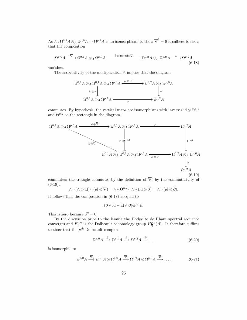
As ∧ : Ω0,2A⊗A Ωp,0A → Ωp,2A is an isomorphism, to show ∇2= 0 it suffices to show

that the composition

Ωp,0A∇ // Ω0,1A⊗A Ωp,0A

∂⊗ id−id∧∇// Ω0,2A⊗A Ωp,0A

∧ // Ωp,2A(6-18)

vanishes.The associativity of the multiplication ∧ implies that the diagram

Ω0,1A⊗A Ω0,1A⊗A Ωp,0A∧⊗ id

//

id⊗∧

Ω0,2A⊗A Ωp,0A

∧

Ω0,1A⊗A Ωp,1A∧

// Ωp,2A

commutes. By hypothesis, the vertical maps are isomorphisms with inverses id⊗Θp,1

and Θp,2 so the rectangle in the diagram

Ω0,1A⊗A Ωp,0Aid⊗∂

//

id⊗∇

((PPP

PPPP

PPPP

PPPP

PPPP

PPPP

PPPP

Ω0,1A⊗A Ωp,1A

id⊗Θp,1

∧ // Ωp,2A

Θp,2

Ω0,1A⊗A Ω0,1A⊗A Ωp,0A∧⊗ id

// Ω0,2A⊗A Ωp,0A

∧

Ωp,2A(6-19)

commutes; the triangle commutes by the definition of ∇; by the commutativity of(6-19),

∧ (∧ ⊗ id) (id⊗∇) = ∧ Θp,2 ∧ (id⊗ ∂) = ∧ (id⊗ ∂).

It follows that the composition in (6-18) is equal to

(∂ ∧ id− id ∧ ∂)Θp,1∂.

This is zero because ∂2 = 0.By the discussion prior to the lemma the Hodge to de Rham spectral sequence

converges and Ep,q1 is the Dolbeault cohomology group Hp,q

∂(A). It therefore suffices

to show that the pth Dolbeault complex

Ωp,0A∂

−→ Ωp,1A∂

−→ Ωp,2A∂

−→ . . . (6-20)

is isomorphic to

Ωp,0A∇−→ Ω0,1A⊗ Ωp,0A

∇−→ Ω0,2A⊗ Ωp,0A

∇−→ . . . . (6-21)

25

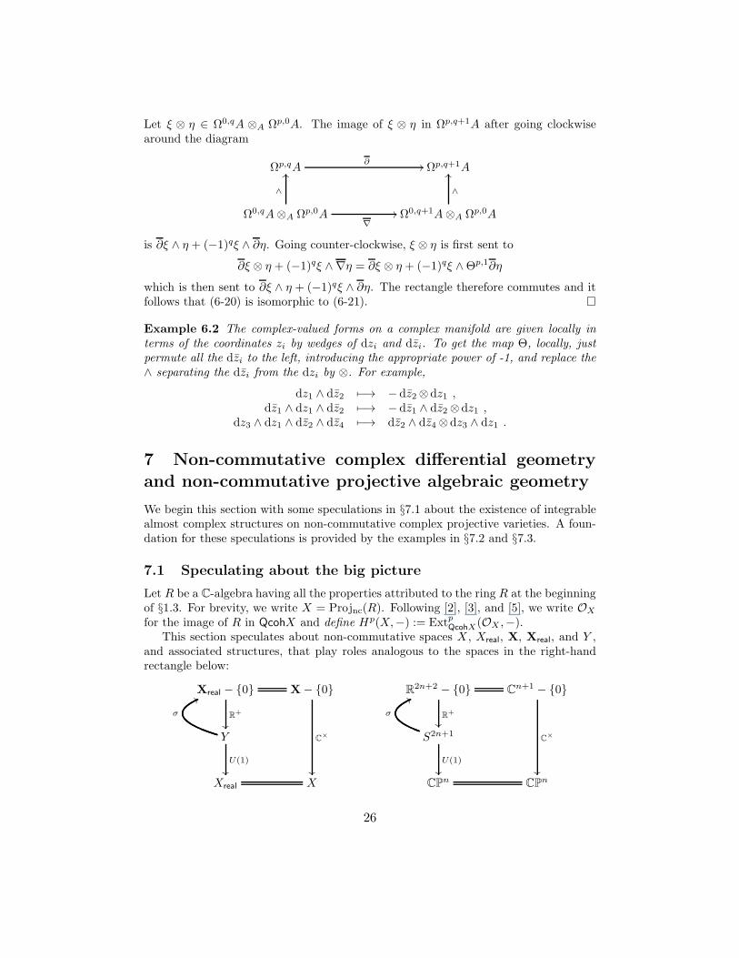
Let ξ ⊗ η ∈ Ω0,qA ⊗A Ωp,0A. The image of ξ ⊗ η in Ωp,q+1A after going clockwisearound the diagram

Ωp,qA∂ // Ωp,q+1A

Ω0,qA⊗A Ωp,0A

∧

OO

∇

// Ω0,q+1A⊗A Ωp,0A

∧

OO

is ∂ξ ∧ η + (−1)qξ ∧ ∂η. Going counter-clockwise, ξ ⊗ η is first sent to

∂ξ ⊗ η + (−1)qξ ∧ ∇η = ∂ξ ⊗ η + (−1)qξ ∧Θp,1∂η

which is then sent to ∂ξ ∧ η + (−1)qξ ∧ ∂η. The rectangle therefore commutes and itfollows that (6-20) is isomorphic to (6-21).

Example 6.2 The complex-valued forms on a complex manifold are given locally interms of the coordinates zi by wedges of dzi and dzi. To get the map Θ, locally, justpermute all the dzi to the left, introducing the appropriate power of -1, and replace the∧ separating the dzi from the dzi by ⊗. For example,

dz1 ∧ dz2 7−→ − dz2⊗dz1 ,dz1 ∧ dz1 ∧ dz2 7−→ − dz1 ∧ dz2 ⊗dz1 ,

dz3 ∧ dz1 ∧ dz2 ∧ dz4 7−→ dz2 ∧ dz4 ⊗dz3 ∧ dz1 .

7 Non-commutative complex differential geometry

and non-commutative projective algebraic geometry

We begin this section with some speculations in §7.1 about the existence of integrablealmost complex structures on non-commutative complex projective varieties. A foun-dation for these speculations is provided by the examples in §7.2 and §7.3.

7.1 Speculating about the big picture

Let R be a C-algebra having all the properties attributed to the ring R at the beginningof §1.3. For brevity, we write X = Projnc(R). Following [2], [3], and [5], we write OX

for the image of R in QcohX and define Hp(X,−) := ExtpQcohX(OX ,−).

This section speculates about non-commutative spaces X , Xreal, X, Xreal, and Y ,and associated structures, that play roles analogous to the spaces in the right-handrectangle below:

Xreal − 0

R+

X− 0

C×

R2n+2 − 0

R+

Cn+1 − 0

C×

Y

σ

66

U(1)

S2n+1

σ

66

U(1)

Xreal X CPn CPn

26

The left-hand columns represent the underlying real varieties of the complex varietiesin the right-hand columns.

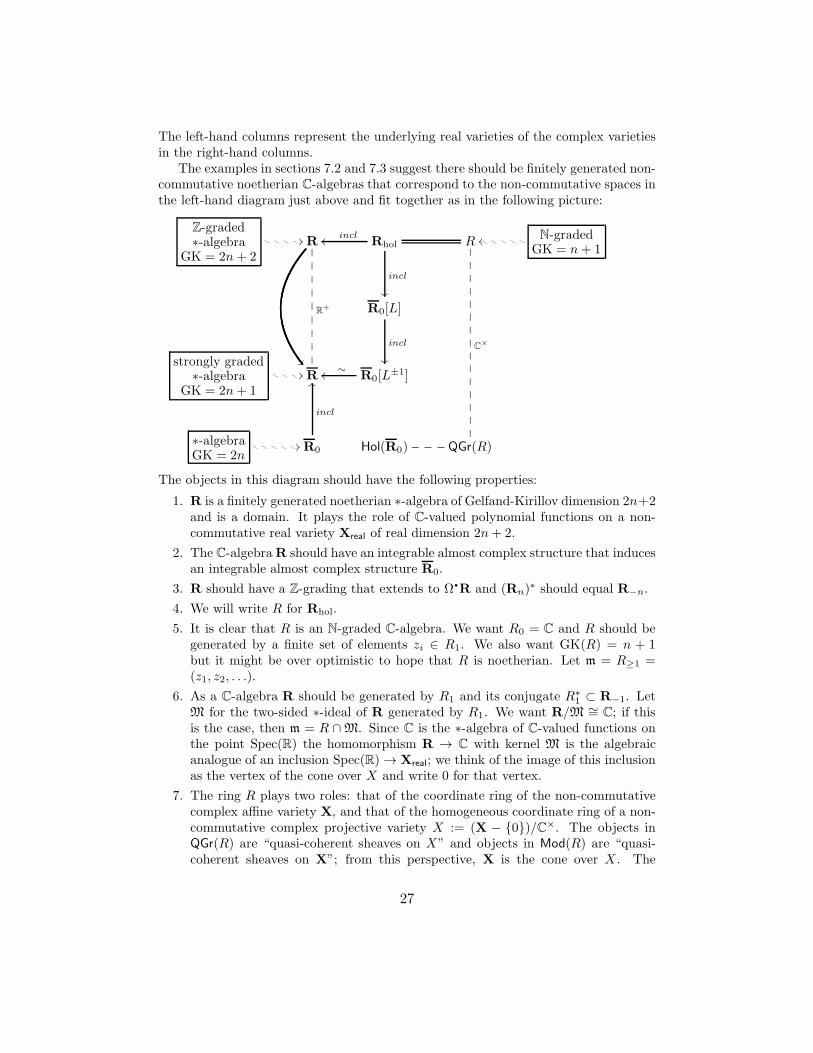
The examples in sections 7.2 and 7.3 suggest there should be finitely generated non-commutative noetherian C-algebras that correspond to the non-commutative spaces inthe left-hand diagram just above and fit together as in the following picture:

Z-graded∗-algebra

GK = 2n+ 2

///o/o/o/o R

Rholincloo

incl

R

C×

N-gradedGK = n+ 1

oo o/ o/ o/ o/ o/

R0[L]

incl

strongly graded∗-algebra

GK = 2n+ 1

///o/o/o R

R+

R0[L±1]

∼oo

∗-algebraGK = 2n

///o/o/o/o/o R0

incl

OO

Hol(R0) ❴❴❴ QGr(R)

The objects in this diagram should have the following properties:

1. R is a finitely generated noetherian ∗-algebra of Gelfand-Kirillov dimension 2n+2and is a domain. It plays the role of C-valued polynomial functions on a non-commutative real variety Xreal of real dimension 2n+ 2.

2. The C-algebraR should have an integrable almost complex structure that inducesan integrable almost complex structure R0.

3. R should have a Z-grading that extends to Ωq

R and (Rn)∗ should equal R−n.

4. We will write R for Rhol.

5. It is clear that R is an N-graded C-algebra. We want R0 = C and R should begenerated by a finite set of elements zi ∈ R1. We also want GK(R) = n + 1but it might be over optimistic to hope that R is noetherian. Let m = R≥1 =(z1, z2, . . .).

6. As a C-algebra R should be generated by R1 and its conjugate R∗1 ⊂ R−1. Let

M for the two-sided ∗-ideal of R generated by R1. We want R/M ∼= C; if thisis the case, then m = R ∩M. Since C is the ∗-algebra of C-valued functions onthe point Spec(R) the homomorphism R → C with kernel M is the algebraicanalogue of an inclusion Spec(R) → Xreal; we think of the image of this inclusionas the vertex of the cone over X and write 0 for that vertex.

7. The ring R plays two roles: that of the coordinate ring of the non-commutativecomplex affine variety X, and that of the homogeneous coordinate ring of a non-commutative complex projective variety X := (X − 0)/C×. The objects inQGr(R) are “quasi-coherent sheaves on X” and objects in Mod(R) are “quasi-coherent sheaves on X”; from this perspective, X is the cone over X . The

27

“quasi-coherent sheaves” on the punctured cone X − 0 are the objects in thequotient category Mod(R)/Mod0(R) where Mod0(R) is the full subcategory ofMod(R) consisting of the R-modules that are the sum of their finite dimensionalsubmodules and those submodules are annihilated by mn for n ≫ 0.

8. Let Mod0(R) be the full subcategory of Mod(R) consisting of the modules Msuch that each element of M is annihilated by some power of M. Let us writeMod(Xreal − 0) for the quotient category Mod(R)/Mod0(R).

9. There should be a central element c ∈ R0 that is an R-linear combination ofthe elements ziz

∗i and also an R-linear combination of the elements z∗i zi. The

requirement that the coefficient of ziz∗i belongs to R ensures that c, and hence

c− 1, is self-adjoint which implies that R/(c− 1) is a ∗-algebra. We think of c asplaying the the role of the “norm-squared” function.

10. R = R/(c−1) is the algebra of C-valued polynomial functions on Y , the norm=1part of Xreal − 0, and Xreal − 0 behaves like Y × R+.

11. Because c− 1 is homogeneous, R inherits a grading from R. Its degree-zero com-ponent R0 is the U(1)-invariant subalgebra, of R and plays the role of C-valuedpolynomial functions on Xreal, the non-commutative real variety underlying thenon-commutative complex projective varietyX whose category of “quasi-coherentsheaves” is QGr(R).

12. The solid arrows in the previous diagram represent C-algebra homomorphismsand those labeled incl are injective. The dashed lines −− should correspond toadjoint pairs of functors between certain abelian categories attached to the rings.

13. Hol(R0) is the category of holomorphic R0-modules defined in section 4.3 andshould be related to QGr(R) in such a way that the cohomology groups H

q

(E,∇)for (E,∇) ∈ Hol(R0) coincide with appropriate cohomology groups Hq(X,−) inQGr(R).

14. L is an invertible R0-bimodule, hence a rank one projective R0-module on boththe left and the right,

R0[L±1] =

∞⊕

m=−∞

L⊗m and R0[L] =

∞⊕

m=0

L⊗m.

7.1.1 Complex line bundles on Xreal

A closed subvariety X of CPn has a homogeneous coordinate ring R whose homoge-neous components are (holomorphic) sections of complex line bundles on Xreal. In thesituation we are considering, invertible bimodules over R0 play the role of complex linebundles on Xreal.

Each Rm is an R0-bimodule.From now on we will assume that R, and hence R0, is a domain. This is a mild

hypothesis that roughly corresponds to Y and Xreal being irreducible varieties.Because R0 has finite Gelfand-Kirillov dimension, it has a division ring of fractions,

D say. The rank of a finitely generated projective right R-module P is dimD(P ⊗R0

D).

In particular, if P is isomorphic to a non-zero right ideal of R0, then rankP = 1.

28

If conditions (9) and (10) above hold, then 1 ∈ R1R−1 whence R0 = R1R−1.Likewise, 1 ∈ R−1R1 and R0 = R−1R1.

Proposition 7.1 Suppose that R is a domain and that conditions (6), (9), and (10)above hold. Then each Rm is an invertible R0-bimodule and a finitely generated rankone projective R0-module on both the left and the right.

Proof. For each integer m, the multiplication in R gives an R0-bimodule homomor-phism

µm : Rm ⊗R0

R−m → R0.

Claim: µm is surjective. Proof: This is a triviality when m = 0. The image of µmis a two-sided ideal of R so it suffices to show that 1 is in the image. The image ofµ1 contains zjz

∗j for all j and hence the element c in (9); but c = 1 in R0 so µ1 is

surjective. Similarly, µ−1 is surjective.Suppose m ≥ 1. Because R is generated as a C-algebra by the image of z∗j , zj | 0 ≤

j ≤ n, R≥0 is generated as an algebra by R0 and R1. Hence, if m ≥ 1, Rm = (R1)m

by which we mean that Rm is spanned by the products of m elements belongingto R1. Likewise, R−m = (R−1)

m. The image of µm is therefore (R1)m(R−1)

m =R1(Rm−1R1−m)R1. The truth of the claim for m ≥ 1 now follows by induction.

A similar argument shows µm is surjective when m ≤ −1. ♦By the dual basis lemma, Rm is a projective right R0-module if the identity map

is in the image of the map

Ψ : Rm ⊗R0

HomR0

(Rm, (R0)R0) −→ End

R0(Rm), Ψ(s⊗ φ)(s′) := sφ(s′),

Given a ∈ R−m define φa ∈ HomR0

(Rm, (R0)R0) by φa(s

′) = as′. By the claim, there

are elements si ∈ Rm and ai ∈ R−m such that∑

siai = 1. Hence

Ψ(

∑

i

si ⊗ φai

)

= idR0

so Rm is a projective right R0-module. A similar argument shows that Rm is aprojective left R0-module.

Because R is a domain, left multiplication by a fixed non-zero element in R−m isan injective homomorphism Rm → R0 of right R0-modules. Hence rankRm = 1 onthe right. As similar argument shows that Rm has rank 1 as a left R0-module.

The invertibility of Rm as an R0-bimodule is part (3) of the next corollary.

Corollary 7.2 Suppose that R is a domain and that conditions (6), (9), and (10)above hold. Then

1. R is a strongly graded C-algebra.

2. There is an equivalence of categories Mod(R0) ≡ Gr(R).

3. The multiplication map Rk⊗R0Rm → Rk+m is an isomorphism of R0-bimodules

for all k,m ∈ Z.

4. Condition (14) holds.

29

Proof. (1) By definition, a Z-graded ring A is strongly graded if AiA−i = A0 for alli. The proof of Proposition 7.1 shows that 1 ∈ R−mRm for all m ∈ Z so R is stronglygraded.

(2), (3), and (4), are standard facts about strongly graded rings.

Given Proposition 7.1, the philosophy of non-commutative geometry says that ele-ments of Rm are smooth sections of a complex line bundle on the real algebraic varietyXreal. After we give Xreal, equivalently R0, an integrable almost complex structurethere should be a ∂-operator ∇ on each Rm such that Rm consists of the elements ofRm on which ∇ vanishes.

7.1.2 The (punctured) affine cone over X

As in algebraic geometry, there is a non-commutative complex affine variety X that isa cone over X defined implicitly by saying that the category of quasi-coherent sheaveson X is ModR. We then think of R as a ring of “holomorphic functions” on X.

The Artin-Schelter regularity conditions require R to have good homological prop-erties that one should probably think of as saying X is smooth, so not quite whatmost people would think of when they say “cone”. If necessary, one could weaken thehypothesis on R by allowing it to be a quotient of an Artin-Schelter regular ring bya central regular sequence such that the vertex of the cone is the only singular point,i.e., the “deviation” of R from being Artin-Schelter regular is “concentrated” at themodule R/R≥1. Formally, one would ask that the quotient category (ModR)/S, whereS is the smallest localizing subcategory containing R/R≥1, has finite global dimension,i.e., Ext2n+1 vanishes on (ModR)/S. In such a case it is more appropriate to think ofR as a ring of “holomorphic functions” on X− 0.

7.1.3 The action of C× on X

The homogeneous components of R are the eigenspaces for an action of C× as auto-morphisms of R. If we think of this as being inherited from an action of C× on X,then GrR is, in effect, the category of C×-equivariant (i.e., constant along orbits) quasi-coherent modules on X. The vertex 0 ∈ X is, by definition, the unique point fixed byC×; formally, 0 = Spec(R/R≥1). By quotienting out FdimR we are removing thosemodules supported at the vertex. Thus X behaves as the orbit space (X− 0)/C×.

7.1.4 Viewing X as a non-commutative real algebraic variety withan almost complex structure

Viewed through the lens of the ring R, X is a non-commutative complex variety ofcomplex dimension n + 1. If we wish to treat X as a real algebraic variety of realdimension 2(n+ 1) we need a ∗-algebra R of GK-dimension 2n+ 2 that will play therole of C-valued differentiable functions on Xreal − 0.

An appropriate almost complex structure on Xreal would be an almost complexstructure (Ω

q

R, d, ∗, J) such that

1. Rhol = R,

30

2. there is a Z-grading on R that is compatible with that on R, and

3. (Rn)∗ = R−n.

Because we want to retain the underlying real structure on X we use the factoriza-tion C× = R+×U(1) to pass down the left-hand sides of the diagrams at the beginningof section 7.1. §§7.1.5 and 7.1.6 address this.

7.1.5 Xreal − 0 as a trivial R+-bundle over Y

Let S2n+1 be the sphere of radius 1 in R2n+2 centered at the origin. Then R2n+2−0is diffeomorphic to R+×S2n+1. A non-commutative analogue of the inclusion S2n+1 →R2n+2 is a surjective homomorphism

R → R :=R

(c− 1)

where c − 1 is a self-adjoint central element in R0. Since R is to play the role of C-valued polynomials on a non-commutative real algebraic variety Y of dimension 2n+1we want the GK-dimension of R to be 2n+ 1. By [36, Prop. 3.15] GK(R) ≤ 2n+ 1.

The homomorphism R → R induces a closed immersion σ : Y → Xreal − 0 andthere should be a non-commutative map π : Xreal −0 → Y such that πσ = idY . Theexistence of such π and σ can be phrased in terms of the associated module categoriesby using the ideas and language in [50] and [45]. A closed immersion is a triple offunctors (σ∗, σ∗, σ

!) such that σ∗ : Mod(

R/(c−1))

→ Mod(Xreal−0) is fully faithful,the essential image of σ∗ is closed under subquotients, and σ∗ has a left adjoint σ∗ anda right adjoint σ∗.

For example, the functor β∗ : Mod(

R/(c− 1))

→ Mod(R) that sends an R/(c− 1)module M to M viewed as an R-module determines a closed immersion β : Y → Xreal.Similarly, The homomorphism R → R/M ∼= C corresponds to a closed immersionα : 0 → Xreal.

The localization functor j∗ : Mod(R) → Mod(Xreal − 0) and its right adjoint j∗implicitly define an open immersion j : Xreal − 0 → X.

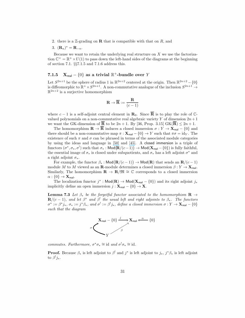
Lemma 7.3 Let β∗ be the forgetful functor associated to the homomorphism R →R/(c − 1), and let β∗ and β! the usual left and right adjoints to β∗. The functorsσ∗ := β∗j∗, σ∗ := j∗β∗, and σ! := β!j∗, define a closed immersion σ : Y → Xreal − 0such that the diagram

Xreal − 0j

// Xreal 0αoo

Y

σ

66

β

99rrrrrrrrrrr

commutes. Furthermore, σ∗σ∗∼= id and σ!σ∗

∼= id.

Proof. Because β∗ is left adjoint to β! and j∗ is left adjoint to j∗, j∗β∗ is left adjoint

to β!j∗.

31

To key step in showing β∗j∗ is left adjoint to σ∗ := j∗β∗ is to show that HomR(M,N) =Ext1R(M,N) = 0 for all R/(c− 1)-modules N and all R/M-modules M (see [45, Prop.7.1] for example). Since every R/M-module is a direct sum of copies of R/M it sufficesto show that HomR(R/M, N) = Ext1

R(R/M, N) = 0 for all R/(c− 1)-modules N .

Since c belongs toM, R/M is not annihilated by c−1, whence HomR(R/M, N) = 0.Now consider an exact sequence 0 → N → E → R/M → 0 of left R-modules

such that (c − 1)N = 0. Since c is central multiplication by c − 1 gives an R-modulehomomorphism E → (c − 1)E. Hence (c − 1)E ∼= R/M. Since (c − 1)N = 0, E =N ⊕ (c− 1)E and this leads to a splitting of the sequence 0 → N → E → R/M → 0.

We now show σ∗ is left adjoint to σ∗. Let N be an R-module. It is a standard fact[22] about localizing subcatgeories that there is an exact sequence

0 → lim−→n

HomR(R/Mn, N) → N → j∗j∗N → lim

−→n

Ext1R(R/Mn, N) → 0.

From this sequence and what we proved above we see that the natural map N → j∗j∗N

is an isomorphism for allR/(c−1)-modulesN . Hence j∗j∗β∗

∼= β∗. It is also a standardfact about localizations that j∗j∗ ∼= id. Let N be an R/(c− 1)-module. Then

Hom(β∗j∗M,N) ∼= Hom(j∗M, j∗j∗β∗N) ∼= Hom(j∗j∗M, j∗β∗N) ∼= Hom(M, j∗β∗N).

Thus σ∗ is left adjoint to σ∗. It is easy to check that σ∗σ∗∼= id and σ!σ∗

∼= id.

For this to be compatible with the principal C×-bundle on the right-hand sides ofthe diagrams at the beginning of section 7.1 it should be the case that Rm = L⊗m.

As mentioned before the previous result we would like a non-commutative mapπ : Xreal − 0 → Y such that πσ = idY . Since σ∗σ∗

∼= id one might define π∗ = σ∗.However, we do not know whether this is appropriate since it doesn’t appear that sucha π∗ has a left adjoint.

7.1.6 The action of U(1) on Y

There is an action of U(1) as ∗-algebra automorphisms of R and R/(c − 1) given byξ · r = ξmr if r ∈ L⊗m. If x ∈ Rm and ξ ∈ U(1), then ξ · x∗ = (ξ · x)∗ = (ξmx)∗ =ξmx∗ = ξ−mx∗ so x∗ ∈ R−m.

7.1.7 Analogues of the sheaves ΩpX

Even for those non-commutative projective varieties X that are well understood andhave excellent homological properties one knows no objects in Qcoh(X) that deservebeing denoted ΩpX . There is no effective general theory of exterior powers in non-commutative ring theory so it is unwise to seek objects ΩpX that are exterior powers ofΩ1X .An alternative is to ask that R, which is connected graded, be a twisted Calabi-

Yau algebra of dimension n, i.e., the projective dimension of R as an R-bimodule is nand the shifted Hochschild cohomology HH

q

(R,R⊗R)[n] is an invertible R-bimodule.Over a connected graded algebra the only invertible graded bimodules are of the form1Rσ for some graded algebra automorphism σ of R. Because R is connected graded

32

it has a unique minimal projective resolution as an R-bimodule. The wished for ΩpXmight be defined in terms of this resolution. Beilinson’s resolution of the diagonal isthe motivation for this approach.

A test as to whether these ideas are promising is to ask if, after proceeding asabove, for some X ’s that we understand, Hp,q

∂(R) is isomorphic to Hq(X,ΩpX) where

the latter is defined as ExtqQcohX(OX ,ΩpX).

7.1.8 Testing these ideas on non-commutative analogues of PnC

Let R be an Artin-Schelter regular algebra [1] such that the minimal resolution of thetrivial module C = R/R≥1 is

0 → R(−n) → R(−n+ 1)n → · · · → R(−1)n → R → C → 0.

For such an R it is generally accepted that X is a good non-commutative analogue ofPnC. The image in Qcoh(X) of the resolution is an exact sequence

0 → O(−n) → O(−n+ 1)n → · · · → O(−1)n → OX → 0.

When X is PnC,

ker(

O(−p)(np) → O(−p+ 1)(

np−1)

)

= Ωphol (7-22)

and Bott’s Vanishing Theorem (see, e.g., [12, Thm. 7.2.3]) says Hq(Pn−1C

,Ωphol(k))vanishes except for

1. p = q and k = 0;

2. q = 0 and k > p;

3. q = n− 1 and k < −n+ 1 + p.

The object Ωphol in (7-22) is not the same as the object called Ωphol

in (3-12); thelatter was defined to be ω ∈ Ωp,0R | ∂ω = 0. However, if ω ∈ Ωp,0R | ∂ω = 0 isa graded R-module it would have an image in the quotient category Qcoh(X) and wecould ask if that image is isomorphic to the kernel in (7-22). If so, Bott’s VanishingTheorem would hold for X : because R is Gorenstein, which is part of the definition ofArtin-Schelter regularity, the cohomology for OX(k) is the same as that for OPn−1(k).

For Ωphol, as defined in (3-12), to be a graded R-module the C×-action on R must

extend to a suitable C×-action on Ωq

R.

7.2 An example: θ-deformed Cn+1 and CPn

There is a large physics literature on the subject of θ-deformed spaces, or Moyal prod-ucts. This has been used in quantisation, gauge theory, string theory, cosmology andintegrable systems. We will quote the relations for the algebra and differential calculusfrom [38].

33

7.2.1 The noncommutative (2n + 2)-plane R2n+2

θ

Let θ be a real skew-symmetric (n+ 1)× (n+ 1) matrix, and set λµν = eiθµν .The algebra of complex-valued polynomial functions on R

2n+2θ is the ∗-algebra

C[

R2n+2θ

]

generated by zµ, zµ | 0 ≤ µ ≤ n with relations

zµzν = λµνzνzµ , zµzν = λµν zν zµ , zµzν = λνµzν zµ (7-23)

and (zµ)∗ = zµ. The elements

(z0)i0 . . . (zn)in (z0)j0 . . . (zn)jn , (i0, . . . , in, j0, . . . , jn) ∈ N2n+2

are a C-vector space basis for C[

R2n+2θ

]

.

There is an action of C× as algebra automorphisms of C[

R2n+2θ

]

defined by ξ ·zµ =

ξ zµ and ξ · zµ = ξ zµ. Its subgroup U(1) acts as ∗-algebra automorphisms of C[

R2n+2θ

]

.

The C×-action induces a Z-grading on C[

R2n+2θ

]

with deg zµ = 1 and deg zµ = −1.

Since C[

R2n+2θ

]

is a quadratic algebra having a PBW basis it is a Koszul algebraby Priddy’s Theorem [42, Thm. 5.3].

7.2.2 A differential ∗-calculus on R2n+2

θ

A ∗-differential calculus (Ωq

, d, ∗) on C[

R2n+2θ

]

is defined in [38]: Ωq

C[

R2n+2θ

]

hasgenerators zµ, zµ ∈ Ω0 and dzµ, dzµ ∈ Ω1 with relations (7-23) and

zµdzν = λµνdzνzµ ,zµdzν = λµνdzν zµ ,zµdzν = λνµdzν zµ ,zµdzν = λνµdzνzµ , (7-24)

and

dzµ ∧ dzν + λµνdzν ∧ dzµ = 0 ,dzµ ∧ dzν + λµνdzν ∧ dzµ = 0 ,dzµ ∧ dzν + λνµdzν ∧ dzµ = 0, (7-25)

and ∗-structure defined by

(zµ)∗ = zµ and (dzµ)∗ = dzµ

and extended to Ωq

C[

R2n+2θ

]

by (ωη)∗ := (−1)mnη∗ω∗ for ω ∈ ΩmC[

R2n+2θ

]

and

η ∈ ΩnC[

R2n+2θ

]

.

The C×-action extends to Ωq

C[

R2n+2θ

]

by ξ · dzµ = ξ dzµ and ξ · dzµ = ξ dzµ.

7.2.3 An integrable almost complex structure on R2n+2

θ

There is a unique degree-preserving map J : Ωq

C[

R2n+2θ

]

→ Ωq

C[

R2n+2θ

]

that is

1. an A-bimodule endomorphism, and

2. a derivation, and satisfies

34

3. J(dzµ) := i dzµ and J(dzµ) := −i dzµ.

In other words, J is an almost complex structure on R2n+2θ . We therefore have spaces

Ωp,qC[

R2n+2θ

]

and derivations ∂ and ∂ defined as in §2.5.2 and §2.5.3.

The C×-action extends with ξ · ω = ξp ξq ω for ω ∈ Ωp,qC[

R2n+2θ

]

.

Lemma 7.4 J is integrable.

Proof. Every element in Ω1,0C[

R2n+2θ

]

can be written in the form fµ.dzµ for some fµ ∈

C[

R2n+2θ

]

. Applying d to this gives dfµ∧dzµ, which is in Ω2,0C

[

R2n+2θ

]

⊕Ω1,1C[

R2n+2θ

]

.Hence d satisfies condition (4) in Lemma 3.2.

The subalgebra C[

R2n+2θ

]

holis generated by the zµ, 0 ≤ µ ≤ n. We denote it by

O(Cn+1θ ) and think of it as the coordinate ring of a non-commutative affine variety

Cn+1θ . The algebra O(Cn+1

θ ) has all the properties attributed to the ring R at thebeginning of §1.3. It is well-known that ProjncO(Cn+1

θ ) behaves very much like CPn.

7.2.4 The noncommutative sphere S2n+1

θ

For each µ, the element zµzµ = zµzµ is central. We define the C-valued polynomialfunctions on S2n+1

θ to be

C[

S2n+1θ

]

:=C[

R2n+2θ

]

(∑

µ zµzµ − 1

) .

Since∑

µ zµzµ−1 is self-adjointC

[

S2n+1θ

]

inherits a ∗-algebra structure fromC[

R2n+2θ

]

.

Since∑

µ zµzµ−1 is invariant under the C×-action the unit circle U(1) acts as ∗-algebra

automorphisms of C[

S2n+1θ

]

.Differentiating the relation

∑

µ zµzµ = 1 gives

∑

µ dzµzµ +

∑

µ zµdzµ = 0, so we

define Ωq

C[

S2n+1θ

]

to be the quotient of Ωq

C[

R2n+2θ

]

by the relations∑

µ zµzµ = 1

and∑

µ dzµzµ +

∑

µ zµdzµ = 0.

7.2.5 CPnθ

We define C[

CPnθ

]

to be the U(1)-invariant subalgebra of C[

S2n+1θ

]

. Since U(1) acts

as ∗-algebra automorphisms, C[

CPnθ

]

is a ∗-algebra.

We define Ωq

C[

CPnθ

]

to be the U(1)-invariant subalgebra of Ωq

C[

S2n+1θ

]

, with theadditional relations

∑

µ dzµzµ = 0 and

∑

µ zµdzµ = 0.

These relations∑

µ dzµzµ = 0 in Ω1,0C

[

CPnθ

]

and∑

µ zµdzµ = 0 in Ω0,1C

[

CPnθ

]

correspond to the following projection matrices for finitely generated projective mod-ules:

Pµν = δµν − zµzν , Qµν = δµν − zµzν .

The complex structure is given by J from Section 7.2.3, i.e. J(dzµ) := i dzµ andJ(dzµ) := −i dzµ. A brief check shows that this is consistent with the additionalrelations given here.

35

7.2.6 Complex line bundles on CPnθ

The U(1)-action on C[

S2n+1θ

]

corresponds to a Z-grading on C[

S2n+1θ

]

and C[

CPnθ

]

is

its degree-zero component. The homogeneous components of C[

S2n+1θ

]

are therefore

C[

CPnθ

]

-bimodules.

They are, in fact, invertible C[

CPnθ

]

-bimodules, hence finitely generated rank one

projective C[

CPnθ

]

-modules on both the right and left so should be thought of aspolynomial sections of complex line bundles on CP

nθ . The holomorphic sections should

be thought of as the global sections of invertible OCPnθ-modules.

7.3 A complex structure on quantum irreducible flag varieties

In [25], [26], [27], Kolb and Heckenberger construct an integrable almost complex struc-ture on the quantum group analogues of irreducible flag varieties. Stefan Kolb kindlyprovided us with some notes about that work and has allowed us to use them in writingthis section. We thank him. Of course, any inaccuracies below are due to the presentauthors.

7.3.1 Generalized flag varieties

Let g be a finite dimensional, complex, simple Lie algebra, p ⊂ g a parabolic subalgebra,p = l⊕ n its Levi decomposition, and pop := l⊕ n− the opposite parabolic.

Let G be the connected, simply connected, affine algebraic group with Lie algebrag, P ⊂ G the connected subgroup with Lie algebra p, and L the Levi factor of P . Thequotients G/L and G/P are affine and projective algebraic varieties, respectively.

We make the additional assumption that g/p is irreducible as a p-moduleunder the adjoint action. In this situation G/P is called an irreducibleflag manifold.3 Irreducible flag manifolds coincide with compact Hermitiansymmetric spaces [28, Sect. X.6.3].

Suppose that µ is a dominant integral weight, V (µ) is the finite dimensional simpleU(g)-module with highest weight µ, and vµ is a highest weight vector in V (µ).

For each parabolic subgroup P ⊂ G there is a weight λ such that G/P is isomorphicto the G-orbit in P

(

V (λ))

of vλ, the image of vλ.4 The vector space

S[G/P ] :=

∞⊕

n=0

V (nλ)∗

endowed with the Cartan multiplication and Z-grading given by deg V (λ)∗ = +1 isa homogeneous coordinate ring of G/P . It coincides with the subalgebra of O(G)generated by the matrix coefficients cλf,vλ | f ∈ V (λ)∗ where

cµf,v(u) := f(uv), f ∈ V (µ)∗, v ∈ V (µ), u ∈ U(g).

There are invertible OG/P -modules Lnλ such that H0(G/P,Lnλ) ∼= V (nλ)∗.

3For a classification of such pairs (g, p) see [6, Sect. 3.1].4The weight λ is not unique but there is a “smallest” such λ, the one that is a sum of fundamental

weights with coefficients 0 or 1. From now on it is that λ which we will use.

36

7.3.2 Quantum group analogues

Let q ∈ R− 0.Let Uq(g) be the quantized enveloping algebra of g defined at [34, 6.1.2]. The

quantum group Gq is defined implicitly by declaring that its coordinate ring, O(Gq),is the linear span of the matrix coefficients cµf,v ∈ Uq(g)

∗,

cµf,v(u) := f(uv), f ∈ V (µ)∗, v ∈ V (µ), u ∈ Uq(g),

as µ ranges over the dominant integral weights and V (µ) is the simple Uq(g)-modulewith highest weight µ.

Following Soibelman [46], and subsequent authors, let S[Gq/P ] be the subalgebraof O(Gq) generated by cλf,vλ | f ∈ V (λ)∗. There is an isomorphism

S[Gq/P ] ∼=

∞⊕

n=0

V (nλ)∗

of vector spaces that becomes an algebra isomorphism when the right-hand side isgiven a quantized analogue of the Cartan product. We view S[Gq/P ] as a homogenouscoordinate ring of a non-commutative analogue of G/P .5 In this setting, S[Gq/P ] isthe algebra denoted R in section 7.1, and the non-commutative analogue of G ·vλ playsthe role of X .

So far we are only thinking of Gq/P as a non-commutative complex projective vari-ety, Projnc(S[Gq/P ]) where S[Gq/P ] is thought of as holomorphic polynomial functionson the “punctured cone” over Gq/P , i.e., the non-commutative space X− 0 in §7.1.To give Gq/P , or, more precisely, X − 0, an underlying real structure we need a∗-algebra that plays the role played by R in section 7.1.4.

At a minimum, we need an algebra to play the role of anti-holomorphic polynomialfunctions onX−0. The G-orbit in P(V (λ)∗) of a lowest weight vector f−λ ∈ V (λ)∗ ∼=V (−w0λ) is isomorphic to G/P op so, following the classical case (e.g., [25, §§2-3]), wedefine the ring of anti-holomorphic polynomial functions on Gq/P to be the subalgebra

S[Gq/Pop] ⊂ O(Gq) generated by c−w0λ

v,f−λ| v ∈ V (−w0λ)

∗ ∼= V (λ). It is isomorphicto

∞⊕

n=0

V (nλ)

endowed with the quantized Cartan multiplication. We consider S[Gq/Pop] as a Z-

graded algebra concentrated in degree ≤ 0 with deg V (λ) = −1.

7.3.3 The underlying real structure on Gq/P

First, we need an underlying real structure on Gq by viewing it as the complexificationof a non-commutative real algebraic variety. Recall, G is the complexification of itscompact connected real form, U ⊂ G and, if K = U ∩P , the natural inclusion U/K →G/P is a diffeomorphism.

5We are writing S[Gq/P ] for the algebra denoted Sq[G/P ] by Heckenberger and Kolb [26, Sect. 3.1.1]and, later, will write S[Gq/P

op] for the algebra they denote by Sq[G/P op].

37

The Hopf ∗-algebra structure on Uq(g) induces a Hopf ∗-algebra structure onO(Gq).The explicit form of ∗ appears at [48, (3.5)]. We write C[Uq] for O(Gq) viewed as a ∗-algebra; as a ∗-algebra C[Uq] behaves as C-valued polynomial functions on the quantumgroup analogue Uq of the compact real form U . The involution ∗ is an anti-isomorphismbetween S[Gq/P ] and S[Gq/P

op] (see [49, Defn.2.2]).LetR be the Z-graded vector space S[Gq/P ]⊗S[Gq/P

op] with the following algebrastructure: let v1, . . . , vN and f1, . . . , fN be dual bases for V (λ) and V (λ)∗ consistingof weight vectors; declare that the subalgebra of R generated by f1, . . . , fN (resp.,v1, . . . , vN ) is isomorphic to S[Gq/P ] (resp., S[Gq/P

op]), and declare that (1⊗vi)(fi⊗1)is the linear combination of the elements fk ⊗ vℓ given by [26, (28)].

The degree-zero component, R0, can also be described in the following alternativeways:

1. R0 = Aqλ, the unital ∗-subalgebra of C[Uq] generated by the products f ·g∗ | f, g ∈ V (λ)∗ ([49, Defn. 2.3(b)]);

2. R0 = C[Uq/L ∩ Uq] = C[Gq/L], the subalgebra φ ∈ C[Uq] | u.φ = ε(u)φ ∀u ∈Uq(l) of C[Uq] ([48, (4.4)]).

Equality of the algebras in (1) and (2) is proved at [48, Thm. 4.10] and [49, Thm. 2.5]by passing to C∗-algebra completions, and at [25, Prop. 2] without using C∗-algebras.

Following Heckenberger and Kolb [26, §3.1.2] there is a central element and anassociated quotient algebra,

c :=N∑

i=1

vi ⊗ fi ∈ R0 and R :=R

(c− 1).

Because deg(c) = 0, R inherits the Z-grading on R. Because c is self-adjoint it also

inherits the ∗-algebra structure on R. The algebra R is denoted Sq[G/P ]c=1

Cby Heck-

enberger and Kolb in [26, §3].

7.3.4 The de Rham complex for C[Gq/L]

By [25, Thm.2, p.483], there are exactly two non-isomorphic finite dimensional irre-ducible left covariant first order differential calculi, C[Gq/L] → Γ+ and C[Gq/L] → Γ−,in the sense of Woronowicz [34, Sect. 12.1.2]. In [27, Sect. 7.1], Heckenberger andKolb relabel these (Γ∂ , ∂) and (Γ∂ , ∂). To conform with our notation we label them

(Ω1,0C[Gq/L], ∂) and (Ω0,1C[Gq/L], ∂). Heckenberger and Kolb now define

(Ω1C[Gq/L], d) := (Ω1,0

C[Gq/L]⊕ Ω0,1C[Gq/L], ∂ ⊕ ∂).

Thus, Ω1C[Gq/L] and the derivation d : C[Gq/L] → Ω1C[Gq/L] provide a non-commutative analogue of the module of Kahler differentials for the affine variety G/L.

Associated to each first order calculus (Ω1C[Gq/L], d), (Ω1,0C[Gq/L], ∂), and (Ω0,1C[Gq/L], ∂),

is a unique universal higher order differential calculus (see, e.g., [34, 12.2.3]) that wedenote by (Ω

q

C[Gq/L], d), (Ωq,0C[Gq/L], ∂), and (Ω0, qC[Gq/L], ∂), respectively.

6

6These are denoted (Γd,d), (Γ∂ , ∂), and (Γ∂ , ∂), in the sentence before [27, Thm.7.1].

38

For example, (Ωq

C[Gq/L], d) is the differential graded algebra that is the quotientof the tensor algebra TC[Gq/L](Ω

1) by the ideal generated by

∑

i

dai ⊗ dbi

∣

∣

∣

∣

∣

∑

i

aidbi = 0

(7-26)

with differential defined by d(a0da1 ∧ . . . ∧ dan) = da0 ∧ da1 ∧ . . . ∧ dan.7 It follows

from the definition of Ωq

C[Gq/L] and d : Ωq

C[Gq/L] → Ωq+1C[Gq/L] that d

2 = 0.Heckenberger and Kolb call (Ω

q

C[Gq/L], d) the de Rham complex for Cq[G/L]. Byconstruction, Ω0C[Gq/L] = Cq[G/L] and d : Cq[G/L] → Ω1C[Gq/L] is, as above, ∂⊕∂.

The main results in [26], Propositions 3.6, 3.7, and 3.11, show that the homogeneouscomponents of (Ω

q

C[Gq/L], d), (ΩqC[Gq/L],0, ∂), and (Ω0, qC[Gq/L], ∂), have the same

dimensions as their classical counterparts. In particular, Ω2 dim(g/p)C[Gq/L] is a freeleft and right C[Gq/L]-module of rank one, a generator being interpreted as a volumeform on Gq/P .

7.3.5 (p, q)-forms on Gq/P

In [27], it is shown that (Ωq

C[Gq/P ], d) may be constructed in terms of the Bernstein-Gelfand-Gelfand resolution and that that construction [27, above Theorem 7.14] givesa decomposition of (Ω

q

C[Gq/P ], d) as a direct sum of covariant Cq[G/L]-bimodules

ΩnC[Gq/P ] =⊕

p+q=n

Ωp,qC[Gq/P ] (7-27)

where Ω1,0C[Gq/P ] and Ω0,1C[Gq/P ] are as in section 7.3.4 and d : ΩnC[Gq/P ] →Ωn+1

C[Gq/P ] satisfies d = ∂+∂ with ∂(Ωp,qC[Gq/P ]) ⊂ Ωp+1,qC[Gq/P ] and ∂(Ωp,qC[Gq/P ]) ⊂

Ωp,q+1C[Gq/P ]. The differentials ∂ and ∂ coincide with those defined in [26, Proposi-tion 3.8, Remark 3.10]. Proceeding as in [27, Lemmata 7.6, 7.17], one shows that themultiplication maps

∧ : Ω1,0C[Gq/P ] : Ωp,qC[Gq/P ] → Ωp+1,q

C[Gq/P ]

∧ : Ω0,1C[Gq/P ] : Ωp,qC[Gq/P ] → Ωp,q+1

C[Gq/P ]

are surjective, and hence

Ωp,qC[Gq/P ] ∧ Ωp′,q′

C[Gq/P ] = Ωp+p′,q+q′

C[Gq/P ] . (7-28)

7.3.6 Definition of J

Let J : Ω1C[Gq/P ] → Ω1

C[Gq/P ] be the unique C-linear map such that J2 = −1and Ω1,0 is the +1-eigenspace and Ω0,1 is the −1-eigenspace. It is clear that J isa Cq[G/L]-bimodule automorphism of both Ω1,0C[Gq/P ] and Ω0,1C[Gq/P ] hence aCq[G/L]-bimodule automorphism of Ω1C[Gq/P ].

7Here, as throughout this paper, ∧ is used to denote the multiplication and is not assumed to be skew-commutative.

39

Using the direct sum decomposition (7-27) we can extend J to a bimodule isomor-phism J : Ω

q

C[Gq/P ] → Ωq

C[Gq/P ] by

J(ω) = (p− q)iω for all ω ∈ Ωp,qC[Gq/P ].

By (7-28), J is a derivation: if ω ∈ Ωp,qC[Gq/P ] and τ ∈ Ωp′,q′C[Gq/P ], then

J(ω ∧ τ) = (p+ p′ − (q + q′))iω ∧ τ

= (p− q)iω ∧ τ + (p′ − q′)iω ∧ τ

= J(ω) ∧ τ + ω ∧ J(τ).

References

[1] M. Artin and W. Schelter, Graded algebras of global dimension, 3. Adv.Math., 66 (1987) 171-216.

[2] M. Artin, J. Tate and M. Van den Bergh, Some algebras related to auto-morphisms of elliptic curves, in The Grothendieck Festschrift, Vol.1, 33-85,Birkhauser, Boston 1990.

[3] M. Artin, J. Tate and M. Van den Bergh, Modules over regular algebras ofdimension 3, Invent. Math., 106 (1991) 335-388.

[4] M. Artin, W. Schelter and J. Tate, Quantum deformations of GLn, Comm.Pure Appl. Math., 64 (1991) 879-895.

[5] M. Artin and J.J. Zhang, Non-commutative Projective Schemes, Adv. Math.,109 (1994) 228-287.

[6] R. J. Baston and M. G. Eastwood, The Penrose transform, Oxford UniversityPress, Oxford, 1989.

[7] V. Chari and A. Pressley, A guide to quantum groups, Cambridge UniversityPress, Cambridge, 1994.

[8] E.J. Beggs and S. Majid, Bar categories and star operations, Algebras andRepresentation Theory, 12 (2009) 103-152.

[9] E.J. Beggs and T. Brzezinski, The Serre spectral sequence of a noncommu-tative fibration for de Rham cohomology, Acta Math., 195 (2005), 155-196

[10] S.J. Brain and S. Majid, Quantisation of twistor theory by cocycle twist,Commun. Math. Phys., 284 (2008) 713-774.

[11] T. Brzezinski, H. Dabrowski, and J. Rembielinski, On the quantum differen-tial calculus and the quantum holomorphicity, Jour. Math. Phys., 33 (1992)19-24.

[12] J. Carlson, S. Muller-Stach, and C. Peters, Period Mappings and PeriodDomains, Camb. Studies in Adv. Math., vol. 85, Camb. Univ. Press., 2003.

[13] C.-S. Chu, P.-M. Ho, and B. Zumino, Some complex quantum manifolds andtheir geometry. Quantum fields and quantum space time (Cargse, 1996),281–322, NATO Adv. Sci. Inst. Ser. B Phys., 364, Plenum, New York, 1997.

40

[14] A. Connes, Non-commutative differential geometry, Publ. I.H.E.S., tome 62,no. 2, (1985) 41-144.

[15] A. Connes, Noncommutative Geometry, Academic Press 1994.

[16] J. Cuntz and D. Quillen, Algebra extensions and nonsingularity, Jour. Amer.Math. Soc., 8 (1995) 251-289.

[17] F. D’Andrea, L. Dabrowski, and G. Landi, The non-commutative geome-try of the quantum projective plane, Rev. Math. Phys. 20 (2008) 979-1006,arXiv:0712.3401v2.

[18] F. D’Andrea and G. Landi, Anti-selfdual connections on the quantumprojective plane: monopoles, Comm. Math. Phys., 297 (2010) 841-893.arXiv:0903.3551v1.

[19] M. Dieng and A. Schwarz, Differential and complex geometry of two-dimensional noncommutative tori, Lett. in Math. Phys., 61 (2002) 263-270.arXiv:math.QA/0203160v3

[20] M.J. Dijkhuizen and M. Noumi, A family of quantum projective spaces andrelated q-hypergeometric orthogonal polynomials, Trans. Amer. Math. Soc.,350 (1998) 3269-3296.

[21] P.G.A. Floris, Addition formula for q-disk polynomials, Compositio Math.,108 (1997) 123-149.

[22] P. Gabriel, Des Categories Abeliennes, Bull. Soc. Math. Fr., 90 (1962) 323-448.

[23] J.M. Gracia-Bondıa, J.C. Varailly and H. Figueroa, Elements of Noncommu-tative Geometry, Birkhauser, 2000.

[24] P.Griffiths and J.Harris, Principles of Algebraic Geometry, Wiley, New York,1978.

[25] I. Heckenberger and S. Kolb, The locally finite part of the dual coalgebraof quantized irreducible flag manifolds, Proc. London Math. Soc., 89 (2004),no. 2, 457-484.

[26] I. Heckenberger and S. Kolb, De Rham complex for quantized irreducible flagmanifolds, J. Algebra, 305 (2006), no. 2, 704-741.

[27] I. Heckenberger and S. Kolb, De Rham complex via the Bernstein-Gelfand-Gelfand resolution for quantized irreducible flag manifolds, 57 J. Geom.Phys., (2007), 2316-2344.

[28] S. Helgason, Differential geometry, Lie groups and symmetric spaces, Pureand Appl. Math., vol. 80, Academic Press, New York, 1978.

[29] D. Huybrechts, Complex Geometry: An Introduction, Universitext, Springer-Verlag, 2004.

[30] M. Khalkhali, G. Landi, and W.D. van Suijlekom, Holomorphic structureson the quantum projective line, Int. Math. Res. Not., 4 (2011) 851-884.arXiv:0907.0154

41

[31] M. Khalkhali and A. Moatadelro, The homogeneous coordinate ring of thequantum projective plane, J. Geom. Phys., 61 (2011) 276-289.

[32] M. Khalkhali and A. Moatadelro, Noncommutative complex geometry ofthe quantum projective space, J. Geom. Phys., 61 (2011) 2436-2452.arXiv:1105.0456

[33] S. Klimyk, A note on noncommutative holomorphic and harmonic functionson the unit disk, in Analysis, geometry and topology of elliptic operators,383400, World Sci. Publ., Hackensack, NJ, 2006. arXiv 0409040v1

[34] A. Klimek and K. Schmudgen, Quantum Groups and their representations,Texts and Monog. in Physics, Springer-Verlag, Berlin, 1997.

[35] L.I. Korogodsky and L.L. Vaksman, Quantum G-spaces and Heisenberg al-gebra, in Quantum Groups (P.P. Kulish, ed.), Lecture Notes in Math. 1510,Springer-Verlag, Berlin, 1992, pp. 5666. MR 93k:17031.

[36] G. Krause and T. H. Lenagan, Growth of algebras and Gelfand-Kirillov di-mension, Revised ed., Grad. Studies in Math., 22. Amer. Math. Soc., Provi-dence, RI, 2000.

[37] S. Majid, Noncommutative Riemannian and Spin Geometry of the standardq-Sphere, Comm. Math. Phys., 256 (2005) 255-285.

[38] P.J. Martınez, J.L. Pena, F. Panaite, and F. Van Oystaeyen, On IteratedTwisted Tensor Products of Algebras, International Journal of Mathematics,19 (9) (2008) 1053-1101.

[39] A. Newlander and L. Nirenberg, Complex Analytic Coordinates in AlmostComplex Manifolds, Annals of Mathematics, 65 (1957) 391-404.

[40] R. O Buachalla, Quantum Bundles and Noncommutative Complex Struc-tures, arXiv:1108.2374

[41] A. Polishchuk and A. Schwarz, Categories of holomorphic vector bundles onnon-commutative two-tori, Comm. Math. Phys., 236 (2003), no. 1, 135–159.

[42] S. Priddy, Koszul resolutions, Trans. Amer. Math. Soc.,152 (1970) 39-60.

[43] J. P. Serre, Geometrie algebrique et geometrie analytique, Annales del’Institut Fourier, 6 (1956) 1-42.

[44] S. Sinel’shchikov and L. Vaksman, Quantum groups and non-commutativecomplex analysis, arXiv 0410396v1

[45] S.P. Smith, Subspaces of non-commutative spaces, Trans. Amer. Math. Soc.,354 (2002) 2131-2171.

[46] Ya.S. Soibelman, On quantum flag manifolds, Funct. Anal. Appl., 26 (1992)225-227.

[47] J. T. Stafford and M. Van den Bergh, Noncommutative curves and noncom-mutative surfaces, Bull. Amer. Math. Soc., 38 (2001) 171-216.

[48] J.V. Stokman and M. Dijkhuizen, Quantized flag manifolds and irreducible∗-representations, Comm. Math. Phys., 203 (1999) 297-324.

42

[49] J.V. Stokman, The quantum orbit method for generalized flag manifolds,Math. Res. Lett., 10 (2003) 469-481.

[50] M. Van den Bergh, Blowing up on non-commutative smooth surfaces, Mem.Amer. Math. Soc., 154 (2001) no. 734.

[51] C. Voisin, Hodge Theory and Complex Algebraic Geometry I, Camb. Studiesin Adv. Math., No. 76, 2002.

[52] C. Weibel, An introduction to homological algebra, Camb. Studies in Adv.Math., no. 38, Camb. Univ. Press, 1994.

[53] S.L. Woronowicz, Twisted SU(2)group. An example of a noncommutativedifferential calculus, Publ. Res. Inst. Math. Sci., Kyoto Univ., 23 (1987)117-181.

[54] S.L. Woronowicz, Differential calculus on compact matrix pseudogroups(quantum groups). Comm. Math. Phys., 122 (1989), no. 1, 125-170.

43