arX

iv:h

ep-t

h/05

1103

6v2

16

Dec

200

5

Preprint typeset in JHEP style. - PAPER VERSION DFTT-35/2005

Non-commutative (D)-instantons ∗

Marco Billo , Marialuisa Frau , Stefano Sciuto, Giuseppe Vallone

Dipartimento di Fisica Teorica, Universita di Torino

and Istituto Nazionale di Fisica Nucleare - sezione di Torino

via P. Giuria 1, I-10125 Torino, Italy

Alberto Lerda†

Dipartimento di Scienze e Tecnologie Avanzate

Universita del Piemonte Orientale, I-15100 Alessandria, Italy

and Istituto Nazionale di Fisica Nucleare - sezione di Torino

via P. Giuria 1, I-10125 Torino, Italy

Abstract: We study systems of D3 and D(−1) branes in a NS-NS magnetic back-

ground and show that, when the brane configuration is stable, the physical degrees

of freedom of the open strings with at least one end-point on the D-instantons de-

scribe the ADHM moduli of instantons for non-commutative gauge theories. We

also prove that disk diagrams with mixed boundary conditions are the sources for

the classical profile of the non-commutative gauge instantons in the singular gauge.

We finally compare the string theory description in a large distance expansion with

the non-commutative ADHM construction in the singular gauge and find complete

agreement at perturbative level in the non-commutativity parameter.

Keywords: D-branes, Non-commutative gauge theories, Instantons.

∗Work partially supported by the European Community’s Human Potential Programme un-

der contract MRTN-CT-2004-005104 “Constituents, Fundamental Forces and Symmetries of the

Universe”, and by the Italian M.I.U.R under contract PRIN-2003023852 “Physics of fundamental

interactions: gauge theories, gravity and strings”.†E-mails: billo,frau,sciuto,vallone,lerda@to.infn.it

Contents

1. Introduction 1

2. Gauge instantons from D3/D(–1) systems 3

3. D3/D(–1) systems in presence of a B-field 7

3.1 The 3/3 strings 9

3.2 The (–1)/(–1) strings 12

3.3 The (–1)/3 and 3/(–1) strings 12

3.3.1 Spectrum 16

3.3.2 Moduli spectrum in (anti-)self-dual background 17

3.3.3 The issue of stability 19

4. Non-commutative gauge instantons from open strings 21

4.1 The ADHM constraints 22

4.2 The instanton profile in a self-dual background 23

5. The ADHM construction for non-commutative instantons in the

singular gauge 28

6. Conclusions 31

A. Notation and Conventions 32

1. Introduction

Quantum field theories on non-commutative spaces display a very rich spectrum of

unusual properties and for this reason they have attracted a wide interest in the last

few years. For instance, they contain a minimal distance scale |θ|, provided by the

non-commutativity parameter θµν ∼ [xµ, xν ], which naturally cuts off the theory in

the UV, though often at the price of peculiar UV/IR mixing effects.

Initially, a lot of work was devoted to the analysis of non-commutative theories

in a field-theoretic framework, but an even greater attention was sparkled by the

realization that non-commutativity arises most naturally in a string theory set-up.

The stringy connection was originally pointed out [1] in the context of (M)atrix theory

1

compactification, but it was subsequently 1 established in a more direct way [3]-[13]

by considering open strings in a magnetic field or in a closed string background with

a non-trivial flux for the Bµν field of the NS-NS sector 2.

A very interesting aspect of the non-commutative deformations of gauge the-

ories is the study of their effects on instantons. This is the main subject of this

paper. Realizing a four-dimensional U(N) gauge theory by a stack of N coincident

D3 branes, instantons with charge k can be obtained by adding k D(−1) branes,

also known as D-instantons [17, 18, 8]. This brane realization not only reproduces

and physically explains the ADHM [19] construction (see, for instance, Ref. [20] and

references therein); it also accounts for the profile of the classical solution and for the

instanton calculus of correlators from a string theory point of view, as shown in Ref.

[21], building also on techniques already introduced in Ref. [22]. In a trivial back-

ground the moduli space of these stringy instantons coincides with that of classical

ADHM gauge instantons [8], but when we introduce a non-commutative deforma-

tion θµν by turning on a Bµν field, it is deformed and no longer coincides with the

classical one unless the background is self-dual (or anti-self-dual in the case of anti-

instantons) [8]. In particular, the ADHM constraints are modified in such a way that

the small-instanton singularity [23], which corresponds to the possibility of detaching

the D-instantons from the world-volume of the D3 branes, is removed. This basi-

cally happens because the D3/D(−1) system no longer satisfy a no-force condition

and is no longer stable when the background field is not (anti-)self-dual, in perfect

agreement with the features of the (anti-)instanton solutions on non-commutative R4

obtained by extending the usual ADHM construction to the non-commutative gauge

theories [24]-[33].

In this paper, we intend to pursue the line of thought of Ref. [21], already suc-

cessfully applied in the case of non anti-commutative deformations [34], and explicitly

derive the measure on moduli space and the instanton profile from open string disk

amplitudes in presence of the NS-NS B background. In doing so, we retrieve the

expected behaviour, but along the way we encounter some crucial subtleties that

render the entire construction non-trivial.

After presenting in section 2 a brief review of the stringy ADHM construction,

in section 3 we analyze the quantization of the open strings of the D3/D(−1) system

in a B background. As is well known, this quantization can be carried out exactly in

the RNS formalism 3 for all kinds of open strings (namely those stretching between

two D3’s, or between two D(−1)’s, or the mixed ones). However, a careful analysis

reveals that there exist different possibilities of imposing boundary conditions on

the world-sheet fermions that are compatible with the B background. One therefore

1Much ground-work having already been performed, quite earlier, in Ref. [2].2Constant fluxes of RR fields lead instead to non anti-commutative theories [14]-[16].3This is in contrast with the non anti-commutative case where the RR background can only be

inserted perturbatively, even if, in the end, this turns out to be sufficient, see for instance [34, 35].

2

obtains a number of different open string sectors that is larger than naively expected.

Just like in the commutative case, also in the presence of B the physical excitations

of open strings with at least one end-point on the D(−1) branes are interpreted as the

instanton ADHM moduli; however in the non-commutative case two points should be

stressed: first, this identification is possible only for a self-dual background (or for an

anti-self-dual background in the case of anti-instantons), i.e. when the D3/D(−1)

system is stable; second, the precise relationship between open string states and

ADHM moduli is highly non-trivial and actually it requires a suitable combination

of the various open string sectors associated with the different types of fermionic

boundary conditions mentioned above.

In section 4, we consider a self-dual background and, using the string construc-

tion of section 3, prove that, as expected, the moduli space for non-commutative

instantons is not modified with respect to the commutative one. Moreover, we show

that the leading term in the large distance expansion of the classical solution is gen-

erated by the gauge boson emission amplitude from mixed disks, in perfect analogy

with the ordinary gauge instantons [21]. The results of these string calculations

are then compared with the non-commutative field theory expectations in section 5.

Since the classical instanton profile obtained from the mixed disk emission diagram

is in the so-called “singular gauge”, in order to compare it with the non-commutative

ADHM construction we have to describe the latter also in the singular gauge, rather

than in the regular one as is usually done in the literature. This is not a trivial

task (see, however, Ref. [32] for a discussion on this point), but in our context it is

enough to write down an instanton profile which solves the ADHM constraints up to

some exponentially suppressed contributions, and allows a meaningful and successful

comparison with the string results of section 4.

We conclude by considering the D3/D(−1) system in a generic (i.e. non (anti-)

self-dual) B background, whose effects can only be treated in a perturbative way.

For the 3/3 strings, this approach was in fact exploited already in [5] to show the

emerging of a non-commutative gauge theory from string theory amplitudes. For the

(−1)/3 and the (−1)/(−1) strings things are actually simpler and the computation of

mixed open/closed string diagrams with a single B-insertion is sufficient to exhibit

the expected deformation of classical instanton moduli space and of the ADHM

constraints. Finally, in the appendix we list our notations and conventions.

2. Gauge instantons from D3/D(–1) systems

The ADHM construction [19] of supersymmetric gauge instantons and their moduli

space can be derived in full detail from string theory by considering systems of D3

branes and D-instantons (for a review see, for instance, [20]) 4. In this approach, the

4For anti-instantons one should consider instead anti-D(−1) branes.

3

auxiliary variables of the ADHM construction correspond to the degrees of freedom

associated to open strings with at least one end-point attached to the D-instantons,

and the measure on the moduli space as well as the instanton profile can be obtained

directly from disk amplitudes [21]. In order to be self-contained, we briefly review

this derivation.

We consider type IIB superstrings in the Euclidean space R10 (whose coordinates

we label by the indices M,N = 1, . . . , 10) and place N D3-branes along the first four

directions (labeled by the indices µ, ν = 1, . . . , 4). The six transverse directions are

labeled instead by the indices m,n = 5, . . . , 10. Under this SO(10)→ SO(4)×SO(6)

decomposition, the string coordinates XM and ψM split as

XM → (Xµ , Xm) and ψM → (ψµ , ψm) , (2.1)

while the anti-chiral spin fields SA (A = 1, . . . , 16) of the RNS formalism become

products of four- and six-dimensional spin fields according to

SA → (SαSA , SαSA) (2.2)

where the index α (or α) denotes positive (or negative) chirality in four dimensions,

and the upper (or lower) index A indicates the fundamental (or anti-fundamental)

representation of SU(4) ∼ SO(6).

The massless sector of the strings with both ends on D3-branes (3/3 strings)

comprises the gauge field Aµ, six scalars ϕm and the gauginos ΛαA and ΛαA, which

altogether form the N = 4 vector multiplet. Their vertex operators are

VA(p) =Aµ(p)√

2ψµ e−φ ei p·X , Vϕ(p) =

ϕm(p)√2

ψm e−φ ei p·X (2.3)

in the (−1) superghost picture of the NS sector, and

VΛ(p) = ΛαA(p)SαSA e−12φ ei p·X , VΛ(p) = ΛαA(p)SαSA e−

12φ ei p·X (2.4)

in the (−1/2) picture of the R sector. Here φ is the boson of the superghost

fermionization formulas, p is the longitudinal incoming momentum and the con-

vention 2πα′ = 1 has been taken. The vertices (2.3) and (2.4) describe fields in the

adjoint representation of U(N), and their scattering amplitudes give rise to the usual

N = 4 SYM theory in the field theory limit α′ → 0.

As is well-known, the D3-branes break half of the bulk supersymmetries in target

space due to the identification between left- and right-moving spin fields enforced at

the boundary, i.e.

Sα(z)SA(z) = − Sα(z) SA(z)∣∣∣z=z

, Sα(z)SA(z) = Sα(z) SA(z)∣∣∣z=z

. (2.5)

4

Let us now add the D(−1) branes. They correspond to imposing Dirichlet bound-

ary conditions on all string coordinates XM and ψM , and enforcing the following

identification on the spin fields [21]

Sα(z)SA(z) = Sα(z) SA(z)∣∣∣z=z

, Sα(z)SA(z) = Sα(z) SA(z)∣∣∣z=z

. (2.6)

By comparison with (2.5), it is clear that the conditions (2.6) break a further half of

the bulk supersymmetries, so that only eight supercharges (those with spinor indices

of the type (αA)) are preserved on both branes.

The open strings with both ends on the D-instantons ((−1)/(−1) strings) do

not carry any momentum since there are no longitudinal Neumann directions. Thus,

these strings describe moduli rather than dynamical fields. In the NS sector there

are ten bosonic moduli corresponding to the physical vertices

Va = g0 a′µ ψ

µ e−φ , Vχ =χm√

2ψm e−φ , (2.7)

while in the R sector there are sixteen fermionic moduli whose vertices are

VM ′ =g0√2M ′αA

SαSA e−12φ , Vλ = λαA S

αSA e−12φ . (2.8)

In writing the polarizations of these vertices we have adopted the traditional notation;

in particular we have distinguished the bosonic moduli into four a′µ (corresponding

to the longitudinal directions of the D3 branes) and six χm (corresponding to the

transverse directions to the D3’s). Furthermore, g0 is the dimensionful coupling for

the effective theory on the D-instantons, which is related to the Yang-Mills coupling

on the D3 branes by

g0 =gYM

4π2α′. (2.9)

Clearly, if gYM is kept fixed when α′ → 0 (as is appropriate to retrieve the gauge

theory on the D3-branes), then g0 blows up. Thus, as discussed in [21], suitable

factors of g0, like the ones appearing in (2.7) and (2.8), must be present in the vertex

operators to retain non-trivial interactions when α′ → 0. As a consequence the

moduli acquire non-trivial scaling dimensions which turn out to be the right ones

for their interpretation as parameters of an instanton solution [20, 21]. For instance,

the a′µ’s in (2.7) have dimensions of (length) and are related to the positions of the

(multi)-centers of the instanton. Finally, we recall that since there are k D-instantons,

all the above moduli carry Chan-Paton factors of the adjoint representation of U(k).

Let us now consider the open strings that are stretched between a D3 and a

D(−1) brane, i.e. the 3/(−1) or (−1)/3 strings. They are characterized by the

fact that the four longitudinal directions along the D3 branes have mixed Neumann-

Dirichlet boundary conditions, while the remaining six transverse directions have

Dirichlet-Dirichlet boundary conditions. As for the (−1)/(−1) strings, also in this

5

case there is no momentum, and the string excitations describe again moduli rather

than dynamical fields. In the NS sector the physical vertex operators are

Vw =g0√2wα ∆Sα e−φ , Vw =

g0√2wα ∆Sα e−φ , (2.10)

where ∆ and ∆ are the bosonic twist and anti-twist operators with conformal weight

1/4 which change the boundary conditions of the Xµ coordinates from Neumann to

Dirichlet and vice-versa by introducing a cut in the world-sheet [36]. The moduli

wα and wα, whose SO(4) chirality is fixed by the GSO projection, carry Chan-Paton

factors, respectively, in the bi-fundamental representations N × k and N × k of

the gauge groups. Thus, one should write more explicitly w iuα and wαui, where

u = 1, . . . , N and i = 1, . . . , k. In the R sector of the mixed strings, the physical

vertices are

Vµ =g0√2µA ∆SA e−

12φ , Vµ =

g0√2µA ∆SA e−

12φ (2.11)

where µ and µ carry the same Chan-Paton factors as w and w respectively. Again,

it is the GSO projection, together with the conserved supercurrent, that fixes the

SO(6) chirality of the spin fields in (2.11).

The vertices described up to now exhaust the BRST invariant spectrum of the

open strings with at least one end point on the D-instantons. However, to compute

the couplings among the moduli and derive the ADHM measure on moduli space

from string interactions, it is convenient to introduce also some auxiliary moduli

that disentangle quartic interactions [21]. In this context a particularly relevant role

is played by the auxiliary vertex

VD =1

2D−

µνψνψµ , (2.12)

which describes an excitation of the (−1)/(−1) strings associated to an anti-self-dual

tensor D−µν = D−

c ηcµν (where ηc

µν are the three anti-self-dual ’t Hooft symbols).

The transformation properties under the various groups and the scaling dimen-

sions of all ADHM moduli are summarized in Table 1.

If we now compute all tree-level diagrams with insertions of the vertices listed

above and take the field theory limit α′ → 0 (with gYM fixed and hence g0 →∞), we

obtain the complete ADHM measure for the instanton moduli space of the N = 4

SYM theory (see for instance Eq. (3.29) in [21]). An essential point is that the

moduli D−c and λαA appear in this measure as Lagrange multipliers, respectively, for

the bosonic and fermionic ADHM constraints. In particular, the bosonic constraints

are the following three k × k matrix equations

W c + i ηcµν

[a′

µ, a′

ν]= 0 , (2.13)

6

SO(4) ≃ SU(2)+ × SU(2)− SO(6) ≃ SU(4) U(N) U(k) dimensions

a′µ (2, 2) 1 1 adj (length)1

χm (1, 1) 6 1 adj (length)−1

M ′αA (2, 1) 4 1 adj (length)1/2

λαA (1, 2) 4 1 adj (length)−3/2

wα (1, 2) 1 N k (length)1

wα (1, 2) 1 N k (length)1

µA (1, 1) 4 N k (length)1/2

µA (1, 1) 4 N k (length)1/2

D−c (1, 3) 1 1 adj (length)−2

Table 1: Transformation properties and scaling dimensions of the ADHM moduli.

where (W c) ij = w iu

α (τ c)αβw β

uj in terms of the Pauli matrices τ c, while the fermionic

constraints are

w uα µA

u + µuAwαu +[a′αα,M

′αA]= 0 . (2.14)

As explained in [21], in the D3/D(−1) system it is possible to consider also disk

diagrams with both mixed boundary conditions and insertions of massless vertices

of the 3/3 strings associated to gauge fields, and show that on such mixed disks the

various components of the gauge multiplet may have non-trivial tadpoles and a non-

vanishing space-time profile. For example, for the vector field Aµ one finds indeed

that

⟨VAµ

⟩mixed disk

6= 0 (2.15)

where VAµis the gluon vertex VA defined in (2.3) without polarization. Furthermore,

by taking the Fourier transform of these massless tadpoles, after including a prop-

agator and imposing the ADHM constraints, one obtains [21] a space-time profile

which is precisely that of the classical gauge instanton solution in the singular gauge.

In other words, the D-instantons act as sources emitting non-abelian gauge fields.

3. D3/D(–1) systems in presence of a B-field

In this section we consider systems of D3 and D(−1) branes in presence of a constant

anti-symmetric tensor B of the closed string NS-NS sector, and focus in particular

on the massless spectrum of the various kinds of open strings to study their relation

with the ADHM instanton construction in non-commutative gauge theories.

7

The action for superstrings moving in a background B-field is 5

S =− 1

4πα′

∫dσ dτ

{δMN ∂aX

M∂aXN + ǫabBMN ∂aXM∂bX

N}

+

− i

4π

∫dσ dτ

{EMN ψ

M∂/ ψN

}.

(3.1)

where ǫτσ = −ǫστ = 1, and EMN = δMN + BMN . Varying S, we get a bosonic

boundary term ∫dτ[δXM

(∂σX

M − BMN∂τX

N) ]σ=π

σ=0,

and a fermionic one∫dτ[EMN

(ψM

+ δψN+ − ψM

− δψN−

) ]σ=π

σ=0

where ψM± are the left and right-moving components of the world-sheet spinors ψM .

The boundary terms vanish after imposing boundary conditions of Dirichlet (D) or

Neumann (N) type on the open string fields. For the bosonic coordinates we have

D : δXM∣∣∣σ=σ

= 0 ⇒ ∂τXM∣∣∣σ=σ

= 0 (3.2)

or

N :(∂σX

M − BMN∂τX

N)∣∣∣

σ=σ= 0 (3.3)

where σ = 0 or σ = π. For the fermionic fields, instead, the presence of B requires

some extra care. The Dirichlet boundary conditions are as usual

D :(δψM

+ + ησδψM−

)∣∣∣σ=σ

=(ψM

+ + ησψM−

)∣∣∣σ=σ

= 0 (3.4)

where ησ = ±1, but there are two inequivalent ways of imposing the Neumann

boundary conditions, namely

N(a) :(ENMδψ

N+ − ησEMNδψ

N−

)∣∣∣σ=σ

=(ENMψ

N+ − ησEMNψ

N−

)∣∣∣σ=σ

= 0 (3.5a)

N(b) :(EMNδψ

N+ − ησENMδψ

N−

)∣∣∣σ=σ

=(EMNψ

N+ − ησENMψ

N−

)∣∣∣σ=σ

= 0 . (3.5b)

Clearly, if B = 0 there is no distinction between (3.5a) and (3.5b), but if B 6= 0

they are different and thus there will be various fermionic sectors when at least one

endpoint of the open string has boundary conditions of Neumann type.

In the following we will consider in detail a D3/D(−1) system with a constant

background field B along the four world-volume directions of the D3 branes, analyze

the different kinds of open strings that are present and make contact with non-

commutative field theories and the corresponding ADHM instanton construction.

5For the fermionic part we use the action given in [10] which enjoys the property that the

boundary terms in its variation can be canceled by consistently imposing on ψM and δψM the same

constraints. See for instance [11] for a discussion of the brane supersymmetry in presence of B field

within the GS formalism.

8

3.1 The 3/3 strings

In this sector the longitudinal coordinates Xµ and ψµ satisfy, respectively, the bound-

ary conditions of Neumann type (3.3) and (3.5) at both endpoints, while the trans-

verse coordinates Xm, ψm satisfy, respectively, the Dirichlet boundary conditions

(3.2) and (3.4) at both endpoints.

After performing a Wick rotation on the world-sheet (τ → −iτe) and introducing

the complex variable z = eτe+iσ, the bosonic boundary conditions may be written as

∂Xµ(z, z) =(11 +B

11− B)µ

ν∂Xν(z, z) , (3.6a)

∂Xm(z, z) = − ∂Xm(z, z) (3.6b)

for any z ∈ R. Following [7, 4], we can solve the boundary conditions (3.6) with

the doubling trick by introducing holomorphic chiral bosons defined on the entire

complex z-plane

XM(z) = qM − 2iα′pM log z + i√

2α′∑

n∈Z−{0}

αMn

nz−n , (3.7)

and writing

Xµ(z, z) =1

2

[Xµ(z) +

(11−B11 +B

)µ

νXν(z)

], (3.8a)

Xm(z, z) = xm0 +

1

2

[Xm(z)−Xm(z)

](3.8b)

for any z with Im(z) ≥ 0. In (3.8b) xm0 denotes the position of the D3 brane in the

transverse space, which can be set to zero without loss of generality. Upon canoni-

cal quantization the oscillators in (3.7) become operators that satisfy the following

commutation relations

[qµ, qν

]= 2πiα′Bµν ,

[qM , pN

]= i δMN ,

[αM

n , αNn

]= n δn+m,0 δ

MN . (3.9)

The crucial difference with respect to the case at zero background is the non trivial

commutator among the longitudinal q’s that implies that the geometry on the world-

volume of the D3 brane is non-commutative with a non-commutativity parameter 6

θµν = 2πα′Bµν (3.10)

6It is worth pointing out that the expression of the open string coordinates written in (3.8a) is

different from the one usually considered in the literature. In particular, with our choice the open

string metric is equal to the closed string one (i.e. δµν in our case) and the non-commutativity

parameter θ is simply proportional to the background field B as shown in (3.10). This is to be

contrasted with the Seiberg-Witten approach [8] where a different scaling is considered. A discussion

on the relation between these two approaches can be found for example in Ref. [13].

9

which is kept fixed in the field theory limit α′ → 0.

Let us now consider the fermionic coordinates. As already pointed out, when

B 6= 0 there are two ways of imposing the boundary conditions of Neumann type

on the ψ’s and thus, in principle, there are four different fermionic sectors. One

possibility is to impose the conditions (3.5a) at both endpoints for the longitudinal

directions, i.e.

ψµ+(z) = η0

(11 +B

11−B)µ

νψν−(z) for z ∈ R+ , (3.11a)

ψµ+(z) = ηπ

(11 +B

11− B)µ

νψν−(z) for z ∈ R− , (3.11b)

and the conditions (3.4) for the transverse directions, i.e.

ψm+ (z) = −η0 ψ

m− (z) for z ∈ R+ , (3.12a)

ψm+ (z) = −ηπ ψ

m− (z) for z ∈ R− . (3.12b)

As usual, if η0ηπ = 1 we obtain the R sector, while if η0ηπ = −1 we obtain the NS

sector. The boundary constraints (3.11) and (3.12) can be solved by introducing

holomorphic fermionic fields defined on the entire complex plane such that

ψM(e2πi z) = −η0ηπ ψM(z) , (3.13)

and then by writing

ψµ+(z) = z

12ψµ(z) , ψµ

−(z) = η0 z12

(11− B11 +B

)µ

νψν(z) , (3.14a)

ψm+ (z) = z

12ψm(z) , ψm

− (z) = −η0 z12 ψm(z) (3.14b)

for any z with Im(z) ≥ 0. From (3.13) it easily follows that

ψM(z) =∑

r∈Z+ν

ψMr z−r−1/2 (3.15)

where ν = 0 in the R sector and ν = 1/2 in the NS sector. Upon canonical quan-

tization the fermionic modes in (3.15) become operators that satisfy the standard

anti-commutation relations

{ψM

r , ψNs

}= δr+s,0 δ

MN . (3.16)

From (3.9) and (3.16) we clearly see that the excitation spectrum of these open

strings is isomorphic to the one of the 3/3 strings without the B background. In par-

ticular at the massless level we find a gauge field Aµ and six scalars φm, together with

their fermionic partners ΛαA and ΛαA that complete a N = 4 vector supermultiplet

in the adjoint representation of U(N). The corresponding vertex operators have the

10

same expressions as those listed in section 2, see in particular Eqs. (2.3) and (2.4).

However, since the longitudinal zero-modes qµ’s contained in the exponential eip·X

satisfy non-trivial commutation relations, the scattering amplitudes among these

vertices are modified and the resulting gauge theory becomes non-commutative [8].

Typically, in the field theory limit where the non-commutative parameter θ defined

in (3.10) is kept fixed, various interaction terms may acquire momentum factors like

cos(p1 ∧ p2) and sin(p1 ∧ p2) where

p1 ∧ p2 =1

2pµ

1 θµν pν2 . (3.17)

Furthermore, new structures may appear as well (see for instance Ref. [38, 39]). For

instance in the 3-gluon vertex the usual term proportional to the structure constants

of U(N) is modified with cos(pi ∧ pj) factors and a term proportional to the dabc

tensor shows up in the non-commutative case (see Fig. 1).

a, µ

b, ν

c, ρ

p1

p2

p3

Vµνρ

abc(p1, p2, p3) = [(p3 − p2)

µδνρ + (p2 − p1)ρδµν + (p1 − p3)

νδρµ]

×[fabc cos(p1 ∧ p2) + dabc sin(p1 ∧ p2)

]

Figure 1: The three-gluon vertex in the non-commutative U(N) Yang-Mills theory.

However, there are other ways of imposing the Neumann boundary conditions

on the fermionic fields. For example, we could require that both endpoints of the

open string satisfy conditions of type (3.5b). In this case, essentially nothing changes

with respect to what discussed above. In fact, to solve these boundary conditions

one still introduces chiral fermions ψ′M(z) with the same monodromy properties, and

hence the same mode expansion, of the fields ψM(z) defined in (3.15). Therefore,

the resulting spectrum is simply a copy of the one previously considered, and in

particular at the massless level we find a gauge vector multiplet. If instead we impose

the boundary conditions (3.5a) at σ = 0 and the conditions (3.5b) at σ = π, or vice-

versa, things are radically different. In fact, to solve the corresponding constraints

we have to introduce chiral fermions χµ(z) such that

χµ(e2πi z) = −η0ηπ

[(11± B11∓ B

)2 ]µνχν(z) .

These fields are no longer periodic or anti-periodic, and hence their modes are no

longer integers or half-integers. Moreover, it can be checked that the physical spec-

trum constructed using these modes does not contain massless states even in the field

11

theory limit. In particular it is not possible to obtain a massless gauge vector with

this “mixed” choice of fermionic boundary conditions. Therefore, for our purposes

such strings do not play any role and can be consistently neglected in the classical

approximation.

In conclusions, the 3/3 strings have only two sectors that in the field theory

limit reproduce a non-commutative N = 4 SYM theory. To just describe this gauge

theory it would be sufficient to consider only one of them, as is usually done in the

literature. However, as we shall see later, to obtain also the non-commutative ADHM

instanton construction from string theory it is necessary to consider both sectors in

a symmetric way, i.e. identify states with equal quantum numbers. This implies, for

instance, that the gluon emission vertex in the (−1) superghost picture is

VA(p) =Aµ(p)√

2

ψµ + ψ′µ

√2

e−φ eip·X . (3.18)

However, in all practical calculations we can simply identify ψµ and ψ′µ, and still

use the properly normalized gluon vertex (2.3) and the standard contraction rules.

3.2 The (–1)/(–1) strings

The open strings with both endpoints on the D(−1) branes have Dirichlet boundary

conditions (3.2) and (3.4) in all directions and hence do not feel any effect of the

B background. All bosonic coordinates XM have an expansion like (3.8b) with xM0

denoting the position of the D-instantons, while all fermionic coordinates ψM are as

in (3.14b). The physical spectrum of these (–1)/(–1) strings contains the same states

as in the free case, describing the moduli a′µ, χm, M ′αA and λαA together with the

auxiliary fields D−c . Their corresponding vertices have the same expressions as in

(2.7), (2.8) and (2.12).

3.3 The (–1)/3 and 3/(–1) strings

We now consider the open strings that stretch between a D(−1) and a D3 brane.

To simplify our discussion, but without loosing generality, we assume that the back-

ground field Bµν is in the skew-diagonal form

B =

0 b2

−b2 00

00 b1

−b1 0

, (3.19)

so that it becomes natural to introduce the complex fields

Z 1 =X3 + iX4

√2

, Z 2 =X1 + iX2

√2

, (3.20a)

Ψ1 =ψ3 + iψ4

√2

, Ψ2 =ψ1 + iψ2

√2

. (3.20b)

12

As we will see in the following, the use of dotted indices, like for anti-chiral spinors,

turns out to be particularly useful. In the above complex basis the bosonic boundary

conditions for the longitudinal coordinates of a (−1)/3 string become

∂Z α(z, z) = −∂Z α(z, z) for z ∈ R+ , (3.21a)

∂Z α(z, z) =

(1− ibα

1 + ibα

)∂Z α(z, z) for z ∈ R− , (3.21b)

where α = 1, 2. Since the boundary conditions (3.21) are diagonal in each complex

direction, i.e. for a given value of α, for simplicity we temporarily suppress this index

and reinstate it only when necessary.

To solve (3.21) we use again the doubling trick: we introduce a complex chiral

field Z(z) such that

Z(e2πi z) = −(

1− ib

1 + ib

)Z(z) = −e−2πiǫ Z(z) (3.22)

where

ǫ =1

πarctan b

(− 1

2< ǫ <

1

2

), (3.23)

and write

Z(z, z) =1

2

[Z(z)− Z(z)

](3.24)

for any z with Im(z) ≥ 0. From (3.22) we deduce that

Z(z) =∑

n∈Z

1

n+ ǫ+ 12

αn+ǫ+ 12z−n−ǫ− 1

2 , (3.25)

which, for vanishing background, reduces to the standard half-integer mode expan-

sion of a boson with mixed Dirichlet-Neumann boundary conditions. Canonical

quantization leads to the commutators

[αn+ǫ+ 1

2, α−m−ǫ− 1

2

]=(n+ ǫ+

1

2

)δn,m (3.26)

where α−m−ǫ− 12

are the modes that appear in the expansion of the complex conjugate

field Z. The oscillators with positive index are annihilation operators with respect

to the twisted vacuum |ǫ〉, namely

αn+ǫ+ 12|ǫ〉 = 0 (n ≥ 0) and αn−ǫ− 1

2|ǫ〉 = 0 (n ≥ 1) ,

whereas the modes with negative index are creation operators. The contribution of

this twisted boson to the Virasoro generator L0 is

L(Z)0 =

∑

n∈Z

:α−n−ǫ− 12αn+ǫ+ 1

2: +

(1

8− ǫ2

2

)

13

where the normal ordering is defined with respect to the twisted vacuum introduced

above. Thus, |ǫ〉 has conformal dimension h = 1/8 − ǫ2/2 and is created from the

SL(2,R) invariant vacuum |0〉 by a twist field σ(z) of weight h, namely

|ǫ〉 = limz→0

σ(z)|0〉 .

Let us now consider the longitudinal fermionic coordinates (3.20b), for which the

boundary conditions are

Ψα+(z) = −η0Ψ

α−(z) for z ∈ R+ , (3.27a)

Ψα+(z) = ηπ

(1− ibα

1 + ibα

)Ψα

−(z) for z ∈ R− (3.27b)

if we choose the form (3.5a) of the Neumann relation at σ = π. As before, we solve

these constraints using the doubling trick: for each value of the index α we introduce

a multi-valued chiral fermion Ψ(z) such that

Ψ(e2πi z) = η0ηπ e−2πiǫ Ψ(z) (3.28)

and write

Ψ+(z) = z12 Ψ(z) , Ψ−(z) = −η0 z

12 Ψ(z) (3.29)

for any z with Im(z) ≥ 0. From the monodromy property (3.28) we easily find that

Ψ(z) =∑

n∈Z+ν

Ψn+ǫz−n−ǫ− 1

2 (3.30)

where ν = 0 in the NS sector (η0ηπ = −1) and ν = 1/2 in the R sector (η0ηπ = 1).

Canonical Dirac quantization leads to the following non-vanishing anti-commutators

{Ψn+ǫ,Ψ−m−ǫ

}= δn,m (3.31)

where Ψ−m−ǫ are the modes of the complex conjugate field Ψ. Notice that in the

presence of a B field, neither the NS nor the R sectors of the mixed directions

have zero-modes, and thus for the (−1)/3 strings the twisted fermionic vacuum |ǫ〉,annihilated by all positive modes, is always non degenerate. The contribution of Ψ

to the Virasoro operator L0 is

L(Ψ)0 =

∑

n∈Z+ν

(n+ ǫ) :Ψ−n−ǫΨn+ǫ : +aν (3.32)

where the normal ordering constant is

a0 =1

2

(1

2− |ǫ|

)2

, a 12

=ǫ2

2(3.33)

14

in the NS and R sectors respectively.

The twisted vacuum of the NS sector |ǫ〉NS, whose energy is a0, is created from

the SL(2,R) invariant vacuum |0〉 by the spin-twist field s+(z) when ǫ > 0 and by

s−(z) when ǫ < 0, namely

|ǫ〉NS =

limz→0

s+(z)|0〉 for ǫ > 0 ,

limz→0

s−(z)|0〉 for ǫ < 0 .

The spin-twist fields s± are most easily described in the bosonization formalism where

Ψ(z) = e+iϕ(z) , Ψ(z) = e−iϕ(z) (3.34)

up to cocycle terms 7. Then, one can show that

s±(z) = e±i( 12−|ǫ|)ϕ(z) . (3.35)

In the following we will need to consider also the first excited state of the NS sector.

If ǫ > 0, this is

Ψ−ǫ|ǫ〉NS = limz→0

t+(z)|0〉NS

where t+(z) is an excited spin-twist field defined by the OPE

Ψ(z)s+(w) =t+(w)

(z − w)12−ǫ

+ · · · .

In the bosonization formalism, this OPE allows us to write t+(z) = e−i( 1

2+ǫ)ϕ(z) whose

conformal dimension is a0 + ǫ = 12(1

2+ ǫ)2. For ǫ < 0, instead, the first excited state

is

Ψǫ|ǫ〉NS = limz→0

t−(z)|0〉

where t−(z) = ei( 12−ǫ)ϕ(z) whose conformal dimension is a0 − ǫ = 1

2(1

2− ǫ)2.

In the R sector, the twisted vacuum |ǫ〉R is created from the SL(2,R) invariant

vacuum by the spin-twist field

sR(z) = e−iǫϕ(z)

whose conformal dimension is ǫ2/2. For our future applications we will not need to

consider excited states in the R sector, but of course they could be easily constructed

along the same lined discussed for the NS case.

It is important to realize that if we had chosen the other type of Neumann

boundary conditions for the longitudinal fermionic coordinates, i.e. (3.5b), we would

have retrieved the same expressions as above at all stages, but with b → −b, or

equivalently with ǫ → −ǫ. Thus, we can conclude that for the (−1)/3 strings, the

two possible choices of fermionic Neumann boundary conditions are simply related

to each other by the exchange of Ψ and Ψ.

7As explained in appendix A, complex conjugation acts as(Ψα)∗

= Ψα.

15

3.3.1 Spectrum

Let us now discuss the physical spectrum of the mixed strings. Due to the absence of

momentum in all directions, there are very severe constraints on the form of allowed

states and only very few of them are physical.

In the NS sector the twisted vacuum |ǫ1; ǫ2〉NS cannot be physical. Let us see

why. If, for example, ǫ1, ǫ2 > 0, the vacuum is described by the following vertex

operator in the (−1)-superghost picture

σ1 s+1 σ2 s

+2 e−φ ;

if ǫ1 or ǫ2 are negative, the corresponding twist fields s+ must be replaced by s−.

The conformal dimension of any of these vertices is h = 1− (|ǫ1| + |ǫ2|)/2. Thus, h

can never be 1 in a non-trivial background. Physical states can instead be present in

the first excited level. When the excitation is produced by the longitudinal fermions,

there are these possibilities

Ψ1 ,−ǫ1 |ǫ1; ǫ2〉NS , Ψ1ǫ1|ǫ1, ǫ2〉NS , Ψ2 ,−ǫ2 |ǫ1; ǫ2〉NS , Ψ2

ǫ2 |ǫ1, ǫ2〉NS

depending on whether ǫ1 > 0, ǫ1 < 0, ǫ2 > 0 or ǫ2 < 0. If, for example, ǫ1, ǫ2 > 0, we

have the following two vertex operators (in the (−1) superghost picture)

V1 = σ1 t+1 σ2 s

+2 e−φ and V2 = σ1 s

+1 σ2 t

+2 e−φ . (3.36)

Again, if either ǫ1 or ǫ2 are negative, we must replace s+ and t+ with s− and t− in

the appropriate places. The total conformal weight of these vertices is

h (V1) = 1 +|ǫ1| − |ǫ2|

2, h (V2) = 1− |ǫ1| − |ǫ2|

2

and thus they are physical only if |ǫ1| = |ǫ2|, i.e. when the background is self-dual or

anti-self-dual. Extending this analysis, one can easily prove that no other physical

states exist in the NS sector.

In the R sector the only physical state turns out to be the vacuum, which carries

indices of the spinor representation of SO(6) due to the zero-modes of the ψm fields

in the transverse directions. This vacuum is thus associated to the transverse spin

fields SA or SA, and the corresponding vertex operators in the (−1/2) superghost

picture are

VA = σ1 sR,1 σ2 sR,2 SA e−12φ and VA = σ1 sR,1 σ2 sR,2 S

A e−12φ (3.37)

which have conformal weight 1, because the ǫ contributions cancel between the

bosonic and the fermionic terms. Thus, the vertices (3.37) describe physical states.

No other (excited) state of the R sector is physical.

16

3.3.2 Moduli spectrum in (anti-)self-dual background

The previous discussion shows that the physical NS sector is non-empty only when

the background has a definite duality. For definiteness, let us consider a self-dual B

field with ǫ1 = ǫ2 = ǫ > 0. In this case the physical NS vertices are given by (3.36)

and in the bosonized formalism their fermionic parts read

V1 ∼ e−i2(ϕ1−ϕ2)−iǫ(ϕ1+ϕ2) and V2 ∼ e+ i

2(ϕ1−ϕ2)−iǫ(ϕ1+ϕ2) . (3.38)

We denote collectively these vertices by Vα with α = 1, 2, since they are created by

the action of Ψα ,−ǫ on the twisted vacuum. The label α suggests that they transform

as an anti-chiral spinor of SO(4). To prove this, let us write the SO(4) generators as

Jµν ≡ :ψµψν : = ηcµνJ

(+)c + ηc

µνJ(−)c (3.39)

where J(+)c and J

(−)c are the SU(2)+ and SU(2)− currents respectively, and then use

the bosonized formalism to get (up to cocycles)

J(+)3 =

1

2

(∂ϕ1 + ∂ϕ2

), J

(+)± = i e±i(ϕ1+ϕ2) , (3.40a)

J(−)3 =

1

2

(∂ϕ1 − ∂ϕ2

), J

(−)± = i e∓i(ϕ1−ϕ2) , (3.40b)

where J(±)± =

(J

(±)1 ±iJ

(±)2

)are the step operators of the SU(2)± groups. In a self-dual

skew-diagonal background field Bµν , the Lorentz group is broken to U(1)+×SU(2)−,

where U(1)+ is the subgroup of SU(2)+ generated by J(+)3 . Using (3.38) and (3.40),

it is elementary to obtain

J (−)c (z)Vα(w) =

i

2

Vβ(w) (τc)βα

z − w + · · · (3.41)

which shows that indeed the vertices V α transform as a doublet of SU(2)−, and

J(+)3 (z)Vα(w) = i

ǫVα(w)

z − w + · · · (3.42)

which shows that these vertices have charge ǫ under U(1)+8. Due to this non-zero

charge, the vertices Vα are not true anti-chiral spinors and, contrarily to naive expec-

tations, they cannot be associated with the moduli wα of the ADHM construction,

which, as shown in Table 1, are singlets under SU(2)+ and hence carry zero charge

under U(1)+. Notice that when B = 0 the physical NS vertex operators (2.10) have

the quantum numbers of the degenerate twisted NS vacuum; on the contrary when

B 6= 0 the physical NS vertices (3.36) are associated to the first fermionic excited

states on a non-degenerate scalar vacuum and hence carry the quantum numbers of

8Correctly, no simple poles appear in the OPE of V α with the broken generators J(+)± of SU(2)+.

17

the fermionic oscillators, which are Lorentz vectors. This explains the origin of the

non-vanishing charge of Vα under U(1)+.

This problem can be overcome thanks to the existence of another way of realizing

the (−1)/3 strings. So far, in fact, we have used fermionic fields Ψα and Ψα that

satisfy the Neumann boundary conditions of type N(a) (see Eq. (3.27b)). However,

also the boundary conditions of type N(b) can be used. With this second choice,

everything goes formally as before except that in the fermionic sector ǫ is everywhere

replaced by −ǫ and the roles of Ψα and Ψα are exchanged. Thus, in the new NS

sector, for a self-dual background with ǫ > 0, the physical vertex operators are

V ′1 = σ1 t−1 σ2 s

−2 e−φ and V ′2 = σ1 s

−1 σ2 t

−2 e−φ (3.43)

instead of the ones given in (3.36). Computing their OPE’s with the preserved

Lorentz generators one finds

J (−)c (z)V ′

α(w) =i

2

V ′β(w)(τc)

βα

z − w + · · · , (3.44a)

J(+)3 (z)V ′α(w) = − i

ǫV ′α(w)

z − w + · · · , (3.44b)

which show that the new vertices form again a doublet of SU(2)− but carry opposite

U(1)+ charge with respect to the old vertices V.

In complete analogy with what we did on the 3/3 strings, and in order to be

consistent with that choice, also here we treat the two types of boundary conditions

for the (−1)/3 strings in a symmetric way, and thus consider the following projected

vertex operator

Vw =g0√2wαV α + V ′α

√2

, (3.45)

where we have inserted a polarization wα and a normalization g0/√

2. In this case,

however, differently from what we did for the vertices of the 3/3 strings, we cannot

simply identify V and V ′, since they have different quantum numbers. As we will

see in the following sections, the vertex (3.45) correctly describes the moduli wα of

the ADHM construction for the non-commutative gauge theory, and represents the

generalization of the vertex (2.10) when a self-dual Bµν background is present.

A few remarks are in order at this point. The projected vertex(V + V ′

)is a

doublet of SU(2)−, but it clearly does not have a definite U(1)+ charge. Notice how-

ever that in any disk amplitude such a vertex must always be accompanied by its

conjugate for consistency of the Chan-Paton structure, and hence all relevant quan-

tities of the ADHM construction involving wα (like constraints, explicit expression

of the instanton solution, ...) are actually sensible only to the expectation value of

J(+)3 between projected states, which indeed vanishes. In other words the polariza-

tion appearing in (3.45) has effectively the correct quantum numbers of the ADHM

moduli wα. We will see an explicit example of this fact in section 4.

18

This analysis can be easily repeated in the R sector of the mixed string. Here

one finds a physical GSO projected and symmetrized vertex given by

Vµ =g0√2µA VA + V ′

A√2

, (3.46)

where VA is defined in (3.37) and V ′A is its analogue with the N(b) boundary condi-

tions. The vertex (3.46) correctly describes the fermionic ADHM moduli µA in the

non-commutative gauge theory.

We conclude by mentioning that the 3/(−1) strings can be treated in the same

way with a simple exchange of the boundary conditions at σ = 0 and σ = π, and

that the ADHM moduli wα and µA are described by the conjugates of the vertices

(3.45) and (3.46).

Finally, if the Bµν background is anti-self-dual and hence the Lorentz group is

broken to SU(2)+ × U(1)−, the physical vertex operators of the NS sector turn out

to be doublets of SU(2)+ with charge under U(1)− and can be used to describe the

ADHM moduli wα and wα of non-commutative anti-instantons. The transformation

properties and charges of the physical NS vertices are summarized in Table 2.

U(1)+ SU(2)−V α ǫ 2

V ′α −ǫ 2

SU(2)+ U(1)−Vα 2 ǫ

V ′α 2 −ǫTable 2: Transformation properties of the physical NS vertices under the unbroken part of

the Lorentz group in a self-dual (ǫ1 = ǫ2 = ǫ) or anti-self-dual (ǫ1 = −ǫ2 = ǫ) background.

3.3.3 The issue of stability

The previous discussion shows that in a self-dual B background the NS sector of the

mixed strings contains only the moduli wα and wα associated to an instanton, while

in an anti-self-dual background it contains only the moduli wα and wα associated to

an anti-instanton. In other words, the explicit string realization of the ADHM con-

struction seems to be applicable only to configurations where the non-commutative

gauge field strength and the B background have the same duality properties.

We now explain the origin and the physical meaning of this fact. Let us first

recall that instantons and anti-instantons are realized respectively by systems of

D3/D(−1) branes and systems of D3/anti-D(−1) branes, and that the corresponding

mixed strings are characterized by a different GSO projection. Indeed,

PGSO =1± (−1)F

2(3.47)

19

where the + sign applies to the D3/D(−1) system, and the − sign to the D3/anti-

D(−1) system. It is therefore obvious that if a state survives the GSO projection

of the D3/D(−1) system, this same state is removed by the GSO projection of the

D3/anti-D(−1) system, and vice-versa. Let us consider the NS sector and fix our

conventions in such a way that

(−1)F |ǫ1, ǫ2〉NS = − |ǫ1, ǫ2〉NS (3.48)

for ǫ1, ǫ2 > 0. With this choice, the excited states Ψ1 ,−ǫ1|ǫ1; ǫ2〉NS and Ψ2 ,−ǫ2|ǫ1; ǫ2〉NS,

which are physical for ǫ1 = ǫ2, are selected by the GSO projection of the D3/D(−1)

branes. If we follow |ǫ1, ǫ2〉NS (which is annihilated by all positive modes and in

particular by Ψ2ǫ2

) when, say, ǫ2 decreases and becomes negative, we find that it is

mapped to the state Ψ2ǫ2|ǫ1, ǫ2〉NS; thus, the very same definition of (−1)F we used in

(3.48), leads to

(−1)F |ǫ1, ǫ2〉NS = + |ǫ1, ǫ2〉NS (3.49)

for ǫ1 > 0 and ǫ2 < 0. If we now let ǫ1 become negative as well, the F parity of

the vacuum returns to be (−1) as in (3.48). We can then conclude that if ǫ1 and

ǫ2 have the same sign, the vacuum |ǫ1, ǫ2〉NS has F -parity (−1), whereas if ǫ1 and ǫ2have different signs, the vacuum |ǫ1, ǫ2〉NS has F -parity (+1). Thus, in a self-dual

background the physical states, which are forced to stay at the first excited level of

the NS sector, survive the GSO projection appropriate for instantons while in an

anti-self-dual background they survive the GSO projection of anti-instantons.

This asymmetry has a deep physical meaning: indeed, it is related to the fact

that D3/D(−1) systems are stable only in a self-dual background, while D3/anti-

D(−1) systems are stable only in an anti-self-dual background 9. To investigate the

stability of these systems, we compute the one-loop free energy for the oriented open

strings stretching between the D3 branes and the (anti-)D-instantons in presence of

a B background. This free energy is given by

F = −∫ i∞

0

dτ

2τ

[Tr NS q

L0−c24 ± Tr NS (−1)F qL0−

c24 − Tr R qL0−

c24

](3.50)

where q = e2πiτ and c is the total central charge of the CFT in the light-cone. Notice

that in (3.50) we have not written the trace with (−1)F in the R sector since it

vanishes due to the fermionic zero-modes in the six transverse directions. According

to (3.47), the + sign in F refers to the D3/D(−1) case, while the − sign refers to

the D3/anti-D(−1) case.

Let us discuss the contribution to the traces from the four mixed directions which

feel the effect of the B background. Actually, we can focus just on the fermionic

piece, since all the bosonic contributions to the integrand of (3.50) are common to

the various sectors. In computing the traces for the CFT of the twisted fermions we

9A discussion on related issues appears also in Ref.[8].

20

have to take into account in a symmetric way the two types of boundary conditions,

N(a) and N(b), which they can satisfy (see Eqs. (3.5a) and (3.5b)). In practice,

this means that

Tr NS,R →Tr

(a)NS,R + Tr

(b)NS,R

2. (3.51)

Using (3.32) for the two complex fermions Ψ1 and Ψ2 and introducing the standard

Jacobi θ-functions, for any value of ǫ1 and ǫ2 we find

Tr(a)NS q

L0−c24 = q

ǫ21+ǫ222

θ2 (ǫ1τ |τ) θ2 (ǫ2τ |τ)η(τ)2

, (3.52a)

Tr(a)NS (−1)F qL0−

c24 = q

ǫ21+ǫ222

θ1 (ǫ1τ |τ) θ1 (ǫ2τ |τ)η(τ)2

, (3.52b)

Tr(a)R qL0−

c24 = q

ǫ21+ǫ222

θ3 (ǫ1τ |τ) θ3 (ǫ2τ |τ)η(τ)2

(3.52c)

where η is the Dedekind’s function. The partition functions for the boundary con-

ditions of type N(b) can be simply obtained from (3.52) by reversing the signs of

both ǫ1 and ǫ2. Taking into account the parity properties of the θ-functions, it is

immediate to show that Tr (b) = Tr (a) in all sectors.

Using (3.52) and the standard results for the four transverse directions, in the

case of instantons, i.e. for D3/D(−1) systems, we find in the end that the integrand

of (3.50) is proportional to

θ2(ǫ1τ |τ)θ2(ǫ2τ |τ) [θ3(0|τ)]2 ± θ1(ǫ1τ |τ)θ1(ǫ2τ |τ) [θ4(0|τ)]2

− θ3(ǫ1τ |τ)θ3(ǫ2τ |τ) [θ2(0|τ)]2 .(3.53)

In the case of D(−1) branes, i.e. with the upper sign in (3.53), this expression

identically can vanish only for a self-dual background (ǫ1 = ǫ2 = ǫ) thanks to the

identity

[θ2(ǫτ |τ)]2 [θ3(0|τ)]2 + [θ1(ǫτ |τ)]2 [θ4(0|τ)]2 − [θ3(ǫτ |τ)]2 [θ2(0|τ)]2 = 0 . (3.54)

If we consider instead anti-D(−1) branes, i.e. if we take the lower sign in (3.53),

we see that the interaction energy vanishes only for an anti-self-dual background

ǫ1 = −ǫ2 = ǫ, since θ1 is odd in its first argument while θ2 and θ3 are even. In

conclusion we see that there must be a precise relation between the charge of the

D-instantons and the (anti-)self-duality of the B background in order to have a stable

brane system.

4. Non-commutative gauge instantons from open strings

In this section we are going to present an explicit realization of instantons in non-

commutative gauge theories using the open strings of the D3/D(−1) systems de-

scribed above, thus extending the analysis of Ref. [21] to branes in a background B

21

field. For definiteness, we discuss in detail the stable case of a D3/D(−1) system in

a self-dual background, starting from the ADHM constraints.

4.1 The ADHM constraints

The ADHM measure on the instanton moduli space can be derived from scattering

amplitudes involving all excitations of the open strings with at least one end point on

the D-instantons. As mentioned in section 3.2, the B background does not have any

effect on the (−1)/(−1) strings and thus their contribution to the ADHM measure

is identical to that of the undeformed (commutative) theory. On the other hand,

the mixed (−1)/3 or 3/(−1) sectors feel the presence of the B field, and thus to

find the non-commutative modifications in the ADHM measure we have to compute

only the amplitudes that involve mixed moduli. For example, let us consider the

coupling among wα, wα and the auxiliary fields D−c , which play the role of a Lagrange

multipliers for the bosonic ADHM constraints. The vertex operators for wα and

wα are given in (3.45) and its conjugate, while vertex for D−c is the same as the

undeformed one given in (2.12). However, in the self-dual background it is more

convenient to rewrite the latter in the following manner

VD = −2D−c J

(−)c (4.1)

using the SU(2)− currents defined in (3.39). The coupling among the moduli we are

considering is explicitly given by

〈〈 VwVDVw 〉〉 ≡ C0

∫dy1dy2dy3

dVCKG

tr 〈Vw(y1)VD(y2)Vw(y3)〉 , (4.2)

where C0 = 2/g20 is the normalization of the mixed disk amplitudes in our present

conventions (see e.g. Ref. [21] for further details). Moreover, dVCKG is the SL(2,R)

invariant volume element, and the trace is over the U(N) Chan-Paton factors. Using

the expression for the various vertex operators, after a few straightforward steps, the

amplitude (4.2) becomes

〈〈 VwVDVw 〉〉 = −D−c tr

(wαwβ

)(y1 − y2)(y2 − y3)(y3 − y1)

×[〈V α(y1) J

(−)c (y2)V β

(y3)〉 + 〈V ′α(y1) J(−)c (y2)V ′β(y3)〉

].

(4.3)

As discussed in section 3.3.2, the vertices V and V ′ transform in the same way under

the currents J(−)c , and indeed from (3.41) and (3.44a) one can show that

〈V α(y1) J(−)c (y2)V β

(y3)〉 = 〈V ′α(y1) J(−)c (y2)V ′β(y3)〉

=i

2

(τ c)αβ

(y1 − y2) (y1 − y3) (y2 − y3).

(4.4)

22

Inserting this result into (4.3), we simply obtain

〈〈 VwVDVw 〉〉 = iD−c tr

(wα(τ c)α

βwβ)

= iD−c W

c , (4.5)

which is exactly the same amplitude of the undeformed theory [21].

With similar explicit calculations one can check that all other disk diagrams

involving mixed moduli are not affected by the self-dual background, and thus the

complete non-commutative ADHM moduli action is the same as in the commuting

theory. In particular, the bosonic and fermionic ADHM constraints are still given

by (2.13) and (2.14), respectively. As we shall see in the next section, this string

result is in agreement with the explicit ADHM construction for non-commutative

instantons [30].

4.2 The instanton profile in a self-dual background

In string theory the classical instanton solutions are obtained from 1-point diagrams

that describe the emission of the gauge fields from mixed disks [21]. The simplest

example of such a mixed disk diagram is represented in Fig. 2, which describes the

emission of a gauge vector.

a

µ

w

w

p

Figure 2: The mixed disk diagram that describes the emission of a gauge vector field Aaµ

with momentum p represented by the outgoing wavy line.

For simplicity, in the following we discuss only instantons with charge k = 1 in

the non-commutative U(2) gauge theory, but our analysis can be extended to the

general case without any problems. The amplitude described in Fig. 2 explicitly

reads

Aaµ(p) = 〈〈 Vw V(0)

Aaµ(−p)Vw 〉〉 (4.6)

where V(0)

Aaµ(−p) is the gluon vertex operator in the 0-superghost picture with outgoing

momentum and without polarization, i.e.

V(0)

Aaµ(−p) = 2iT a (∂Xµ − i p · ψ ψµ) e−ip·X , (4.7)

where T a is the adjoint U(2) Chan-Paton factor. With the insertion of such a vertex,

the disk amplitude (4.6) carries the Lorentz structure and the quantum numbers

that are appropriate for an emitted gauge vector field. The correlation function in

23

(4.6) receives contribution only from the ψµψν part of (4.7), which again can be

conveniently rewritten in terms of the SU(2)± fermionic currents (3.39). Thus, the

relevant part of the gluon vertex is

V(0)

Aaµ(−p) ∼ 2pν T a

(ηc

νµJ(+)c + ηc

νµJ(−)c

)e−ip·X . (4.8)

Notice, that differently from the auxiliary vertex (4.1), the gluon vertex (4.8) de-

pends both on the SU(2)+ and on the SU(2)− currents. This fact has important

consequences, as we shall see momentarily.

The calculation of the J(−)c contribution to the amplitude (4.6) essentially coin-

cides with the one outlined in the previous subsection for the amplitude (4.3) (see

also Ref. [21] for further details). Since the vertices V and V ′ appearing in Vw and

Vw behave in the same way under SU(2)−, they produce an identical contribution to

the gluon emission which is given by

Aa (−)µ (p) =

i

2(T a)v

u pν ηc

νµ

(w u

α (τc)αβwβ

v

). (4.9)

Imposing the bosonic ADHM constraints (2.13) on w and w, we can show that the

matrices

(Tc)uv ≡

1

2ρ2

(w u

α (τc)αβwβ

v

), (4.10)

where ρ2 ≡ (wαu w

uα )/2, satisfy the SU(2) algebra, so that (4.9) can be rewritten as

Aa (−)µ (p) = iρ2 Tr (T a Tc) p

ν ηcνµ . (4.11)

Decomposing the adjoint U(2) index a = (0, a) into its U(1) and SU(2) parts, we see

that only the SU(2) components are non-vanishing, namely

Aa (−)µ (p) = − i

2ρ2 ηa

µνpν , A0 (−)

µ (p) = 0 . (4.12)

Things are different instead for the J(+)c contributions to the amplitude (4.6):

this is precisely the point where the non-trivial structure of the vertices Vw and Vw

given in (3.45) shows its relevance. In fact, while the correlators of V and V ′ with

the step operators J(+)± are vanishing, i.e.

〈V β(y1) J(+)± (y2)V α(y3)〉 = 〈V ′

β(y1) J(+)± (y2)V ′α(y3)〉 = 0 , (4.13)

their correlators with J(+)3 are instead non-trivial, as one can see from the OPE’s

(3.42) and (3.44b). Indeed we have

〈V β(y1) J(+)3 (y2)V α(y3)〉 = −〈V ′

α(y1) J(+)3 (y2)V ′α(y3)〉

=i ǫ δα

β

(y1 − y2)(y1 − y3)(y2 − y3).

(4.14)

24

Thus, the J(+)c part of the gluon emission is

Aa (+)µ (p) = ± i ǫ

2pνη3

µν(Ta)v

uwα u wα v (4.15)

where the + and − signs apply to the contributions of the V and V ′ vertices, respec-

tively. If we impose the bosonic ADHM constraints, we can show that the matrix

wα u wα v is proportional to the identity, i.e. wα u wα v = ρ2 δuv , and so only the U(1)

part of (4.15) is non-vanishing, namely

A0 (+)µ (p) = ± i ǫ pνη3

µνρ2 , Aa (+)

µ (p) = 0 . (4.16)

While the result (4.12) is somehow expected (and in agreement with field theory

calculations), the presence of a U(1) component of the form (4.16) is puzzling since

one does not expect a non-vanishing abelian part in the gluon emission at this order.

However, in our string realization of the non-commutative ADHM instantons the

vertices V and V ′, which correspond to the two types of Neumann boundary condi-

tions in the presence of a B field, are treated in a symmetric way and their respective

contributions to a given amplitude must be added together. Thus, the complete J (−)

piece of the gluon emission is simply twice the result given in (4.12) for each sector,

while the total J (+) contribution vanishes because the V and V ′ parts exactly cancel

each other. In other words the full amplitude (4.6) is

Aaµ(p) = − i ρ2 ηa

µνpν , A0

µ(p) = 0 . (4.17)

As explained in Ref. [21], to obtain the space-time profile of the instanton we

must take the Fourier transform of the momentum space amplitude after inserting a

gluon propagator δµν/p2; in this way we get

Aaµ(x) =

∫d4p

(2π)2Aa

µ(p)1

p2eip·x = 2ρ2 ηa

µν

xν

|x|4 , A0µ(x) = 0 . (4.18)

In the following section we will see that (4.18) represents the leading term in the

large distance expansion (|x| ≫ ρ) of the classical solution in the singular gauge for

an instanton of size ρ and charge k = 1 in the non-commutative U(2) theory. The

fact that the instanton field is in the singular gauge is not surprising since in our

D-brane set-up gauge instantons arise from D-instantons which are point-like objects

localized inside the world-volume of the D3 branes [21].

Notice that the gauge field in (4.18) does not depend on the non-commutativity

parameter θ and is the same as the leading term at large distance of the BPST

instanton of the ordinary SU(2) Yang-Mills theory in the singular gauge [37]. How-

ever, the presence of a non-trivial B background is not irrelevant and it shows up in

the sub-leading terms of the instanton solution. Indeed, higher order contributions

in the large distance expansion of the instanton profile can be obtained by sewing

25

the leading source term with the vertices of the non-commutative gauge theory, as

indicated for example in Fig. 3. There, two gauge vector fields emitted from two

disks recombine through the non-commutative 3-gluon vertex and yield the second

order correction to the instanton profile. Since the non-commutative vertex contains

a part proportional to the dabc-symbols of the gauge group, a gluon can be emitted

at second order also along the U(1) direction, even if at the first order only the

non-abelian components were produced.

a) b)

a

bb

cc

0p p

p − qp − q

q qµ µ

ν ν

ρρ

w

w

w

w

w

w

w

w

cos p ∧ q sin p ∧ q

Figure 3: The diagrams that account for sub-leading corrections in the large-distance

expansion of the gluon emission amplitude. The diagram a) refers to the emission of the

SU(N) gluon, while the diagram b) the U(1) part. The 3-gluon vertices to be used, here

only symbolically indicated, are more explicitly described in Fig. 1.

Let us consider in particular the diagram a) in which the two disks are sewn

together with the part of the 3-gluon vertex that is proportional to the structure

constants of the gauge group (see Fig. 1). This diagram yields a second order

correction to the SU(2) field given by

Aaµ(p)(2) =

i

2

∫d4q

(2π)2ǫabc cos (p∧q)

[(p−2q)µδνρ + (p+q)ρδµν + (q−2p)νδρµ

]

× 1

q2Ab

ν(q)(1) 1

(p− q)2Ac

ρ(p− q)(1) ,

(4.19)

where we have included a symmetry factor of 1/2 and denoted with a superscript (1)

the first-order fields of (4.18), and by (2) the second-order correction we are comput-

ing. Using (4.18), after some standard algebra, we find

Aaµ(p)(2) = −iρ4ηa

µν

∫d4q

(2π)2

cos (p∧q)q2(p− q)2

[(2p · q − p2) qν + (p · q − 2q2) pν

]. (4.20)

The integral over q can be computed in dimensional regularization upon expanding

cos (p∧q) = 1− 1

2

(1

2pµθ

µνqν

)2

+ . . . , (4.21)

26

where θ is the non-commutativity parameter (3.10), and the result in d dimensions

is

Aaµ(p)(2) = iρ4ηa

µνpν(p2)

d2−1

∞∑

m=0

(−|p|4)m

m!

π Γ(m+ d

2

)

2d2 sin

(π(m+ d

2))Γ(2m+ d− 1)

(θ2

16

)m

.

Taking the Fourier transform after inserting the gluon propagator, we find

Aaµ(x)(2) = lim

d→4

∫ddp

(2π)d2

Acµ(p)(2) 1

p2eip·x

= −2ρ4ηaµν

xν

|x|6∞∑

m=0

(m+ 1)(2m)!

(θ

|x|2)2m

= −2ρ4ηaµν

xν

|x|6(

1 +4θ2

|x|4 + . . .

).

(4.22)

In the first term of the last line we recognize the sub-leading term in the large

distance expansion (|x| ≫ ρ) of the standard SU(2) instanton in the singular gauge

(see for example Eq. (4.16) of Ref. [21]), while the second term represents the

non-commutative deformation. In the next section we will show that this result is

in agreement with the explicit non-commutative ADHM instanton solution. Notice,

however, that the series (4.22) is divergent and thus it must be interpreted as an

asymptotic expansion for θ/|x|2 → 0. As a consequence, possible non-perturbative

terms, like e−|x|2/θ for instance, cannot be accounted in this approach.

Let us now consider the diagram b) of Fig. 3, which is responsible for a U(1)

component in the instanton profile that is absent in the commutative case. Using

the explicit expression for the 3-gluon vertex, we find

A0µ(p)

(2)=

i

2

∫d4q

(2π)2δbc sin (p∧q)

[(p−2q)µ δ

ρν + (p+q)ρ δµν + (q−2p)ν δ

ρµ

]

× 1

q2Ab

ν(q)(1) 1

(p− q)2Ac

ρ(p− q)(1) ,

(4.23)

which after some standard algebra becomes

A0µ(p)

(2)= iρ4

∫d4q

(2π)2

sin (p∧q)q2(p− q)2

[pµ(q · p− 3q2) + qµ(6q2 − 6q · p+ 2p2)

]. (4.24)

Again, the integral over q can be computed in dimensional regularization after ex-

panding sin (p∧q) in powers of θ. Finally, taking the Fourier transform of the result-

ing terms, we obtain the following space-time dependence for the U(1) field

A0µ(x)

(2)= −ρ4 θµνx

ν

|x|8∞∑

m=0

(m+ 1)(2m+ 1)!

(θ

|x|2)2m

= −ρ4 θµνxν

|x|8 + . . . .

(4.25)

27

In the next section we will show that this expression is in perfect agreement with the

abelian part of the non-commutative U(2) ADHM instanton solution in the singular

gauge (again up to non-perturbative terms in θ/|x|2).Our analysis can be generalized also to mixed diagrams that contain insertions of

fermionic mixed moduli and are responsible for the emission of the other components

of the gauge vector multiplet, along the lines discussed in Ref. [21]. In this way one

can reconstruct the full non-commutative superinstanton solution from string theory.

5. The ADHM construction for non-commutative instantons

in the singular gauge

The classical profile for non-commutative instantons can be derived from a general-

ization of the standard ADHM construction in which the non-commutative nature of

space-time is properly taken into account [30]. In this section we are going to briefly

present such a construction and, in order to match with the string results we have

obtained so far, we will consider specifically the non-commutative instantons in the

singular gauge.

In the standard ADHM construction of a self-dual instanton with charge k = 1

in the U(N) gauge theory (see, for instance, Ref. [20] for a review), the basic object

is a (N + 2)× 2 complex valued matrix ∆(x) defined as

∆(x) = a+ b x (5.1)

where a and b can always be put in the form

a =

(w

−a′)

b =

(0

11

)(5.2)

in which the upper components are N × 2 matrices and the lower components are

2× 2 matrices. Finally, in (5.1) x stands for the 2× 2 matrix xµ σµ defined in terms

of the SO(4) spinor matrices. The variables w and a′ appearing in (5.2) are precisely

some of the ADHM moduli for which we have presented an explicit string realization

in sections 2 and 3. Let ∆(x) = ∆†(x) and denote by U(x) a null vector of ∆(x), i.e.

a solution of ∆(x)U(x) = 0. Then, if the following completeness and factorization

constraints

∆(x) f(x) ∆(x) + U(x)U(x) = 11 (5.3a)

∆(x) ∆(x) = f−1(x)11 (5.3b)

are satisfied for some (arbitrary) function f(x), one can show that the gauge potential

Aµ = iU(x) ∂µ U(x) (5.4)

28

has a self-dual field strength and thus describes an instanton.

This ADHM construction can be generalized to non-commutative gauge theories

[30]. The only formal change in the above equations is that now xµ has to be

interpreted as an operator xµ, subject to the following commutation rules

[xµ, xν ] = iθµν , (5.5)

where θ is the non-commutativity parameter. In particular this implies that (5.4)

must be replaced by

Aµ = iU(x) [∂µ , U(x)] . (5.6)

Let us consider, as a specific example, the non-commutative theory with gauge

group U(2), so that we can compare this formal construction with the explicit results

obtained from string theory in section 4. In this case the constraint (5.3b) imposes

a reality condition on a′ and the following relation on w and w

w uα (τ c)α

βw β

u − ηcµνθ

µν = 0 . (5.7)

This is the non-commutative version of the bosonic ADHM constraint (2.13) for k = 1

and gauge group U(2). If θµν is self-dual, the last term vanishes and (5.7) reduces

simply to W c = 0. We therefore confirm explicitly the string results of section 4.1,

where we have shown that the ADHM constraints are not affected by a self-dual

background.

The constraints W c = 0 can be solved simply by setting wuα = ρδuα, so that we

have

∆(x) =

(ρ

x− a′)

, ∆(x) =(ρ , x− a′

). (5.8)

With this choice one can check that Eq. (5.3b) is satisfied with

1

f(x)= ρ2 + |x− a′|2 (5.9)

where |x− a′|2 =∑

µ(xµ − a′µ)2.

To proceed further, we need to find a null vector for ∆(x). A solution of

∆(x)U(x) = 0 has been proposed in Ref. [30] where a non-commutative instan-

ton configuration has been obtained in the regular gauge. However, to make contact

with the string theory realization of the gauge instantons presented in sections 3

and 4, we need to have the gauge vector field in the singular gauge since the entire

instanton charge is concentrated at the locations of the D(−1) branes. Therefore,

we now present a different expression for U(x) that we derive by mimicking what is

usually done in commutative ADHM construction to obtain the instanton profile in

the singular gauge. More specifically, we consider the matrix

U(x) =

|x−a′|√ρ2+|x−a′|2

−ρ(x− a′) 1

|x−a′|√

ρ2+|x−a′|2

(5.10)

29

which is the straightforward generalization of the matrix used in the commutative

case, where the coordinates xµ have been replaced by the operators xµ. With some

simple manipulations one can check that U(x) is a null vector of ∆(x). However, it

does not satisfy the completeness constraint (5.3a), as noticed10 in [31], in agreement

with the impossibility of finding a gauge transformation from the regular to the

singular gauge in non-commutative theories [30]. Despite this fact, the matrix (5.10)

can still be used to obtain an instanton profile under special conditions.

To see this, it is useful to exploit the one-to-one correspondence between opera-

tors depending on the non-commuting xµ’s and ordinary functions of xµ multiplied

with the Moyal product

F (x) ⋆ G(x) ≡ F (x) exp

{i

2θµν←−∂µ

−→∂ν

}G(x) . (5.11)

The precise correspondence is obtained by taking the Fourier transform of a function

of xµ and anti-transforming it back with e−ik·x. In particular, following this rule

one can show that xµ corresponds simply to xµ, and more generally that to any

function it corresponds an operator constructed with the complete symmetrization

of the xµ’s. For example, the function xµ xν corresponds to 12[xµxν + xν xµ], while

|x− a′|2 corresponds to |x− a′|2. Along these lines, it is possible to show that

1

(ρ2 + |x− a′|2)α↔ 2

(2|θ|)−α

Γ(α)

∫ 1

0

dt

(1− t1 + t

) ρ2

2|θ| e−t|x−a′|2

|θ|

log1−α(

1+t1−t

) (5.12)

for any α > 0, from which (for ρ = a′ = 0 and α = 1) it follows that

1

|x|2 ↔1

|x|2(

1− e−|x|2

|θ|

). (5.13)

Let us now apply this correspondence to the matrix U(x) in (5.10) and fix, for

simplicity, the instanton center in the origin by setting a′ = 0. Then, one can show

that

∆(x) ⋆ f(x) ⋆∆(x) + U(x) ⋆ U(x) = 11 +D(x) , (5.14)

i.e. the non-commutative completeness relation (5.3a) is violated by

D(x) =

(0 0

0 d(x)

)where d(x) = −2 e

− |x|2

|θ|

(1 + θ

|θ|0

0 1− θ|θ|

). (5.15)

Notice, however, that this violating term vanishes asymptotically in the large dis-

tance expansion |x|2/|θ| → ∞ and is non-perturbative in the non-commutativity

parameter. Thus, if we want to establish a connection with the string results of

section 4 that have been obtained in the large distance approximation and with a

10See however [32], where a modification of the ansatz is proposed.

30

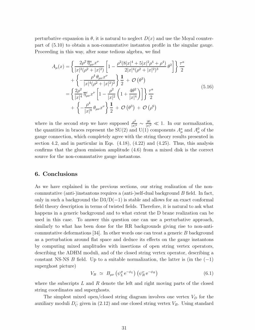
perturbative expansion in θ, it is natural to neglect D(x) and use the Moyal counter-

part of (5.10) to obtain a non-commutative instanton profile in the singular gauge.

Proceeding in this way, after some tedious algebra, we find

Aµ(x) =

{2ρ2 ηa

µνxν

|x|2(ρ2 + |x|2)

[1− ρ2(8|x|4 + 5|x|2ρ4 + ρ4)

2|x|4(ρ2 + |x|2)3θ2

]}τa

2

+

{− ρ4 θµνx

ν

|x|4(ρ2 + |x|2)2

}11

2+ O

(θ3)

=

{2ρ2

|x|4 ηcµνx

ν

[1− ρ2

|x|2(

1 +4θ2

|x|4)]}

τa

2

+

{− ρ4

|x|8 θµνxν

}11

2+ O

(θ3)

+ O(ρ6)

(5.16)

where in the second step we have supposed ρ2

|x|2∼ |θ|

|x|2≪ 1. In our normalization,

the quantities in braces represent the SU(2) and U(1) components Aaµ and A0

µ of the

gauge connection, which completely agree with the string theory results presented in

section 4.2, and in particular in Eqs. (4.18), (4.22) and (4.25). Thus, this analysis

confirms that the gluon emission amplitude (4.6) from a mixed disk is the correct

source for the non-commutative gauge instantons.

6. Conclusions

As we have explained in the previous sections, our string realization of the non-

commutative (anti-)instantons requires a (anti-)self-dual background B field. In fact,

only in such a background the D3/D(−1) is stable and allows for an exact conformal

field theory description in terms of twisted fields. Therefore, it is natural to ask what

happens in a generic background and to what extent the D brane realization can be

used in this case. To answer this question one can use a perturbative approach,

similarly to what has been done for the RR backgrounds giving rise to non-anti-

commutative deformations [34]. In other words one can treat a generic B background

as a perturbation around flat space and deduce its effects on the gauge instantons

by computing mixed amplitudes with insertions of open string vertex operators,

describing the ADHM moduli, and of the closed string vertex operator, describing a

constant NS-NS B field. Up to a suitable normalization, the latter is (in the (−1)

superghost picture)

VB ≃ Bµν

(ψµ

L e−φL) (ψν

R e−φR)

(6.1)

where the subscripts L and R denote the left and right moving parts of the closed

string coordinates and superghosts.

The simplest mixed open/closed string diagram involves one vertex VD for the

auxiliary moduli D−C given in (2.12) and one closed string vertex VB. Using standard

31

conformal field theory methods, one finds that the amplitude under consideration is

〈〈 VDVB 〉〉 ≡ C0

∫dy d2z

dVCKG〈VD(y)VB(z, z)〉

≃ i

g20 (2πα′)

D−c η

cµνB

µν

(6.2)

where we have explicitly exhibited all dimensional constants, but neglected numerical

factors which could be absorbed into the normalization of the vertex VB.

The amplitude (6.2) turns out to be the only one that is relevant in the limit

α′ → 0 with g0 kept fixed, which is the appropriate field theory limit for disk dia-

grams involving open strings with at least one end-point on the D-instantons [21].

Indeed, all other amplitudes with different open string vertex operators or with more

insertions of the closed string vertex VB either vanish or are sub-leading with respect

to (6.2) in the field theory limit. Using (2.9) and (3.10), we can rewrite the above

result as

〈〈 VDVB 〉〉 ≃ iD−c η

cµν (2πα′Bµν) = iD−

c ηcµνθ

µν (6.3)

which shows that the bosonic ADHM constraint (2.13) gets modified by the addition

of a term proportional to ηcµν θ

µν . Of course, if the B background is self-dual this term

vanishes in agreement with what we already found in section 4.1. On the contrary,

in an anti-self-dual background the deformation corresponding to (6.3) is non-trivial

and agrees with the explicit ADHM analysis for non-commutative gauge theories.

In conclusion we have shown that the D3/D(−1) system in a NS-NS B field

correctly describes the instantons of non-commutative gauge theories. When the

background and the gauge field strengths have the same duality, the brane system is

stable and the non-commutative deformation can be treated exactly by means of a

twisted conformal field theory; in the other cases only a perturbative string approach

is available, but in the field theory limit this always agrees with the non-commutative

ADHM construction. Finally, it would be interesting to explore, both in string and in

field theory, the meaning of the non-perturbative corrections in |θ|/x2 to the matrix

U(x) of the non-commutative ADHM construction that are needed to satisfy exactly

the completeness relation in the singular gauge.

Acknowledgments

We thank Francesco Fucito and Igor Pesando for many useful discussions.

A. Notation and Conventions

32

Spinor notation in Euclidean R4: We consider the Euclidean space R

4 with

coordinates xµ, µ = 1, · · ·4. The Clifford algebra {γµ, γν} = 2δµν is satisfied by

γµ = (γµ)† =

(0 σµ

σµ 0

)(A.1)

where σµ = (i~τ , 11), σµ = (σµ)† = (−i~τ , 11), with ~τ being the Pauli matrices.

The matrices σµ and σµ, which satisfy the algebra

σµσν + σν σµ = σµσν + σνσµ = 2δµν 11 , (A.2)

are the Weyl matrices acting, respectively, on chiral and anti-chiral spinors ψα and

ψα.

In our basis, the charge conjugation matrix C is block diagonal and is given by

C = −(ǫαβ 0

0 ǫαβ

). (A.3)

where ǫ12 = ǫ12 = −ǫ12 = −ǫ12 = 1. We use the convention that the dotted indices

are contracted in theր direction, while undotted ones contracted in theց direction:

ψα = ǫαβψβ , ψα = ǫαβψβ . (A.4)

Out of the γ matrices we may construct the generators of the so(4) algebra

Σµν =1

4[γµ, γν ] =

(12σµν 0

0 12σµν

)(A.5)

where

σµν =1

2

(σµσν − σν σµ

), σµν =

1

2

(σµσν − σνσµ

)(A.6)

which are respectively self-dual and anti-self-dual. They act on the irreducible spinor

representations corresponding, respectively, to chiral and anti-chiral spinor, as follows

δωψα =1

4ωµν (σµν) β

α ψβ , δωψα =

1

4ωµν (σµν)α

βψβ . (A.7)

Furthermore, using the symmetry properties of the matrices σµν and σµν , one can

check that also ψβ and ψβ transform as chiral and anti-chiral spinors:

δωψα = −1

4ωµν ψ

β(σµν) αβ , δωψα = −1

4ωµν ψβ(σµν)β

α . (A.8)

The anti-hermiticity of the σµν matrices: [(σµν) βα ]

∗= −(σµν) α

β implies instead

that (ψα)∗ transform like ψα. Then, consistently with the conjugation property of

σµ, we define the complex conjugation as

(ψα)∗ = ψα , (ψα)∗ = −ψα

(ψα)∗ = −ψα, (ψα)∗ = ψα .

(A.9)

33

’t Hooft symbols: The Spin(4) group is isomorphic to SU(2)+ × SU(2)−. The

isomorphism is described at the level of generators using the ’t Hooft symbols:

Jµν = ηcµνJ

+c + ηc

µνJ−c , (A.10)

where Jµν (µ, ν = 1, . . . , 4) are the Spin(4) generators and J±c (c = 1, 2, 3) are the

SU(2)± generators. Explicitly, the ’t Hooft symbols are defined as follows:

ηcµν = −ηc

νµ , ηcµν = −ηc

νµ , (A.11a)

ηcab = ηc

ab = ǫcab , a, b, c ∈ {1, 2, 3} , (A.11b)

ηc4a = ηc

a4 = δca (A.11c)

so that η is self-dual and η is anti-self-dual.

Applied to the irreducible spinor representations, (A.10) states that chiral and

anti-chiral spinors belong respectively to the fundamental representation of SU(2)+

and SU(2)−:

(σµν)β

α = iηcµν(τ

c) βα , (σµν)

αβ

= iηcµν(τ

c)αβ. (A.12)

Let us collect here some useful formulae for manipulating the ’t Hooft symbols:

ηcµνη

dµν = ηc

µν ηdµν = 4δcd (A.13)

ηcµνη

cρσ = δµρδνσ − δνρδµσ + ǫµνρσ (A.14)

ηcµν η

cρσ = δµρδνσ − δνρδµσ − ǫµνρσ (A.15)

We also have

ǫabcηbνση

cρτ = ηa

στδνρ + ηaνρδστ − ηa

ντδσρ − ηaσρδντ , (A.16)

and similarly for the ηbνσ symbols.

References

[1] A. Connes, M. R. Douglas and A. Schwarz, JHEP 9802 (1998) 003 [arXiv:hep-

th/9711162].

[2] A. Abouelsaood, C. G. Callan, C. R. Nappi and S. A. Yost, Nucl. Phys. B 280 (1987)

599.

[3] M. M. Sheikh-Jabbari, Phys. Lett. B 425 (1998) 48 [arXiv:hep-th/9712199].

[4] C. S. Chu and P. M. Ho, Nucl. Phys. B 550 (1999) 151 [arXiv:hep-th/9812219].

[5] V. Schomerus, JHEP 9906 (1999) 030 [arXiv:hep-th/9903205].

[6] F. Ardalan, H. Arfaei, H. and M. M. Sheikh-Jabbari, Nucl. Phys. B576 (2000) 578

[arXiv:hep-th/9906161]

34

[7] C. S. Chu and P. M. Ho, Nucl. Phys. B 568 (2000) 447 [arXiv:hep-th/9906192].

[8] N. Seiberg and E. Witten, JHEP 9909 (1999) 032 [arXiv:hep-th/9908142].

[9] C. S. Chu, “Noncommutative open string: Neutral and charged” [arXiv:hep-

th/0001144].

[10] P. Haggi-Mani, U. Lindstrom and M. Zabzine, Phys. Lett. B 483 (2000) 443

[arXiv:hep-th/0004061].

[11] M. Mihailescu, I. Y. Park and T. A. Tran, Phys. Rev. D 64 (2001) 046006 [arXiv:hep-

th/0011079].

[12] C. S. Chu, R. Russo and S. Sciuto Nuc. Phys. B 585 (2000) 193 [arXiv:hep-th/0004183]

[13] C. S. Chu and R. Russo, Mod. Phys. Lett. A 16 (2001) 211 [Fortsch. Phys. 49 (2001)

633] [arXiv:hep-th/0102164].

[14] J. de Boer, P. A. Grassi and P. van Nieuwenhuizen, Phys. Lett. B 574 (2003) 98

[arXiv:hep-th/0302078].

[15] H. Ooguri and C. Vafa, Adv. Theor. Math. Phys. 7 (2003) 53 [arXiv:hep-th/0302109];

Adv. Theor. Math. Phys. 7 (2004) 405 [arXiv:hep-th/0303063].

[16] N. Seiberg, JHEP 0306 (2003) 010 [arXiv:hep-th/0305248].

[17] E. Witten, Nucl. Phys. B 460 (1996) 335 [arXiv:hep-th/9510135].

[18] M. R. Douglas, J. Geom. Phys. 28, 255 (1998) [arXiv:hep-th/9604198]; “Branes within

branes” [arXiv:hep-th/9512077].

[19] M. F. Atiyah, N. J. Hitchin, V. G. Drinfeld and Y. I. Manin, Phys. Lett. A 65 (1978)

185.

[20] N. Dorey, T. J. Hollowood, V. V. Khoze and M. P. Mattis, Phys. Rept. 371 (2002)

231 [arXiv:hep-th/0206063].

[21] M. Billo, M. Frau, I. Pesando, F. Fucito, A. Lerda and A. Liccardo, JHEP 0302 (2003)

045 [arXiv:hep-th/0211250].

[22] M. B. Green and M. Gutperle, JHEP 0002 (2000) 014 [arXiv:hep-th/0002011].

[23] E. Witten, Nucl. Phys. B 460, 541 (1996) [arXiv:hep-th/9511030].

[24] N. Nekrasov and A. Schwarz Commun. Math. Phys 198 (1998) 689 [arXiv:hep-

th/9802068].

[25] K. Furuuchi, Prog. Theor. Phys. 103 (2000) 1043 [arXiv:hep-th/9912047].

[26] K. Furuuchi, “Topological charge of U(1) instantons on noncommutative R4”,

[arXiv:hep-th/0010006].

35

[27] N. A. Nekrasov, Commun. Math. Phys., 241 (2003) 143-160 [arXiv:hep-th/0010017].

[28] K. Furuuchi, JHEP 0103 (2001) 033 [arXiv:hep-th/0010119].

[29] M. R. Douglas and N. A. Nekrasov, “Noncommutative field theory” [arXiv:hep-

th/0106048].

[30] C. S. Chu, V. V. Khoze and G. Travaglini, Nucl. Phys. B 621 (2002) 101 [arXiv:hep-

th/0108007].

[31] O. Lechtenfeld and A. D. Popov, JHEP 0203 (2002) 040 [arXiv:hep-th/0109209].

[32] Y. Tian and C. J. Zhu, Phys. Rev. D 67 (2003) 045016 [arXiv:hep-th/0210163].

[33] R. Wimmer, JHEP 0505 (2005) 022 [arXiv:hep-th/0502158].

[34] M. Billo, M. Frau, I. Pesando and A. Lerda JHEP 0405 (2004) 023 [arXiv:hep-

th/0402160].

[35] M. Billo, M. Frau, F. Lonegro and A. Lerda JHEP 0505 (2005) 047 [arXiv:hep-

th/0502084].

[36] L. J. Dixon, J. A. Harvey, C. Vafa and E. Witten, Nucl. Phys. B 261 (1985) 678;

S. Hamidi and C. Vafa, Nucl. Phys. B 279 (1987) 465.

[37] A. A. Belavin, A. M. Polyakov, A. S. Schwarz and Y. S. Tyupkin, Phys. Lett. B 59, 85

(1975); G. ’t Hooft, Phys. Rev. D 14, 3432 (1976) [Erratum-ibid. D 18, 2199 (1978)].

[38] A. Armoni, Nucl. Phys. B 593 (2001) 229 [arXiv:hep-th/0005208].

[39] L. Bonora and M. Salizzoni, Phys. Lett. B 504 (2001) 80 [arXiv:hep-th/0011088].

36