Embed Size (px)
Citation preview

HAL Id: tel-01771476https://tel.archives-ouvertes.fr/tel-01771476v1
Submitted on 19 Apr 2018 (v1), last revised 7 Dec 2017 (v2)
HAL is a multi-disciplinary open accessarchive for the deposit and dissemination of sci-entific research documents, whether they are pub-lished or not. The documents may come fromteaching and research institutions in France orabroad, or from public or private research centers.
L’archive ouverte pluridisciplinaire HAL, estdestinée au dépôt et à la diffusion de documentsscientifiques de niveau recherche, publiés ou non,émanant des établissements d’enseignement et derecherche français ou étrangers, des laboratoirespublics ou privés.
Non-invasive personalisation of cardiacelectrophysiological models from surface electrograms
Sophie Giffard-Roisin
To cite this version:Sophie Giffard-Roisin. Non-invasive personalisation of cardiac electrophysiological models from sur-face electrograms. Other. Université Côte d’Azur, 2017. English. �NNT : 2017AZUR4092�. �tel-01771476v1�

UNIVERSITE COTE D’AZUR
ECOLE DOCTORALE STIC
THESE DE DOCTORATPrésentée en vue de l’obtention du grade de
Docteur en Science
Automatique, Traitement du Signal et de l’Image
Défendue par
Sophie Giffard-Roisin
Personnalisation Non-invasive deModèles Electrophysiologiques
Cardiaques à Partird’Electrogrammes Surfaciques
Dirigée par:
Maxime Sermesant, Nicholas Ayache, Hervé Delingette
preparée à Inria Sophia Antipolis, Equipe Asclepios
Defendue le 11 Décembre 2017
Jury :
Président : Reza Razavi - KCL (Londres)Rapporteurs : Rémi Dubois - IHU LIRYC (Bordeaux)
Olaf Doessel - KIT (Karlsruhe)Directeur : Nicholas Ayache - Inria (Sophia-Antipolis)Co-directeur : Hervé Delingette - Inria (Sophia-Antipolis)Co-superviseur : Maxime Sermesant - Inria (Sophia-Antipolis)

UNIVERSITE COTE D’AZUR
DOCTORAL SCHOOL STICSCIENCES ET TECHNOLOGIES DE L’INFORMATION
ET DE LA COMMUNICATION
P H D T H E S I Sto obtain the title of
PhD of Science
Specialty : Automatic, Signal and Image Processing
Defended by
Sophie Giffard-Roisin
Non-invasive Personalisation ofCardiac Electrophysiological
Models from Surface Electrograms
Thesis Advisors:
Maxime Sermesant, Nicholas Ayache, Hervé Delingette
prepared at Inria Sophia Antipolis, Asclepios Team
Defended on 11 December 2017
Jury :
President : Reza Razavi - KCL (London)Reviewers : Rémi Dubois - IHU LIRYC (Bordeaux)
Olaf Doessel - KIT (Karlsruhe)Advisor : Nicholas Ayache - Inria (Sophia-Antipolis)Co-advisor : Hervé Delingette - Inria (Sophia-Antipolis)Co-supervisor : Maxime Sermesant - Inria (Sophia-Antipolis)

Personnalisation Non-invasive de Modèles ElectrophysiologiquesCardiaques à Partir d’Electrogrammes Surfaciques.
Résumé:L’objectif de cette thèse est d’utiliser des données non-invasives (electrocardio-
grammes, ECG) pour personnaliser les principaux paramètres d’un modèle élec-trophysiologique (EP) cardiaque pour prédire la réponse à la thérapie de resyn-chronisation cardiaque. La TRC est un traitement utilisé en routine clinique pourcertaines insuffisances cardiaques mais reste inefficace chez 30% des patients traitésimpliquant une morbidité et un coût importants. Une compréhension précise de lafonction cardiaque propre au patient peut aider à prédire la réponse à la thérapie.Les méthodes actuelles se basent sur un examen invasif au moyen d’un cathéter quipeut être dangereux pour le patient.
Nous avons développé une personnalisation non-invasive du modèle EP fondéesur une base de données simulée et un apprentissage automatique. Nous avons es-timé l’emplacement de l’activation initiale et un paramètre de conduction global.Nous avons étendu cette approche à plusieurs activations initiales et aux ischémiesau moyen d’une régression bayésienne parcimonieuse. De plus, nous avons développéune anatomie de référence afin d’effectuer une régression hors ligne unique et nousavons prédit la réponse à différentes stimulations à partir du modèle personnal-isé. Dans une seconde partie, nous avons étudié l’adaptation aux données ECG à12 dérivations et l’intégration dans un modèle électromécanique à usage clinique.L’évaluation de notre travail a été réalisée sur un ensemble de données important(25 patients, 150 cycles cardiaques). En plus d’avoir des résultats comparables avecles dernières méthodes d’imagerie ECG, les signaux ECG prédits présentent unebonne corrélation avec les signaux réels.
Mots-clés: Imagerie ECG, Personnalisation, Modèle electrophysiologiquecardique, Apprentissage machine, Base de données simulée, Problème inverse.

Non-invasive Personalisation of Cardiac ElectrophysiologicalModels from Surface Electrograms
Abstract:The objective of this thesis is to use non-invasive data (body surface potential
mapping, BSPM) to personalise the main parameters of a cardiac electrophysio-logical (EP) model for predicting the response to cardiac resynchronization ther-apy (CRT). CRT is a clinically proven treatment option for some heart failures.However, these therapies are ineffective in 30% of the treated patients and involvesignificant morbidity and substantial cost. The precise understanding of the patient-specific cardiac function can help to predict the response to therapy. Until now, suchmethods required to measure intra-cardiac electrical potentials through an invasiveendovascular procedure which can be at risk for the patient.
We developed a non-invasive EP model personalisation based on a patient-specific simulated database and machine learning regressions. First, we estimatedthe onset activation location and a global conduction parameter. We extended thisapproach to multiple onsets and to ischemic patients by means of a sparse Bayesianregression. Moreover, we developed a reference ventricle-torso anatomy in order toperform an common offline regression and we predicted the response to differentpacing conditions from the personalised model. In a second part, we studied theadaptation of the proposed method to the input of 12-lead electrocardiograms (ECG)and the integration in an electro-mechanical model for a clinical use. The evalua-tion of our work was performed on an important dataset (more than 25 patients and150 cardiac cycles). Besides having comparable results with state-of-the-art ECGimaging methods, the predicted BSPMs show good correlation coefficients with thereal BSPMs.
Keywords: ECG Imaging, Personalisation, Cardiac Electrophysiology Model,Machine learning, Simulated database, Inverse problem.

iii
Remerciements
Je tiens tout d’abord à remercier chaleureusement Maxime Sermesant, Nicholas Ay-ache et Hervé Delingette pour m’avoir encadrée tout au long de cette aventure. Troissuperviseurs complémentaires qui m’ont permis de garder une vision d’ensemble dela thèse (merci Nicholas!), de me questionner pour m’améliorer (merci Hervé!) etsurtout de me motiver et de proposer sans cesse des idées nouvelles (merci Maxime!).
Je tiens à remercier les membres de mon jury de thèse, et particulièrement mesrapporteurs Rémi Dubois et Olaf Doessel qui ont eu la gentillesse de prendre letemps de lire ce manuscrit.
Je remercie bien sûr toute l’équipe du projet européen VP2HF avec qui j’ai eule plaisir de travailler tout au long de la thèse, lors de réunions toujours convivialesaux quatre coins du continent. J’ai ainsi pu collaborer directement avec le mondemédical, améliorer ma compréhension téléphonique de l’anglais ’british’, et surtoutdécouvrir le ’shuffleboard’ des pubs norvégiens, espèce de curling de table sur sable.Je remercie Reza Razavi, grand coordinateur du projet, mais aussi Tom Jackson etJessica Webb, les cardiologues les plus disponibles de tous les temps et à qui je doistout. Je ne remercierai jamais assez l’équipe de modélisation cardiaque de King’sCollege (Jack Lee, Simone Rivolo et surtout Lauren Fovargue) avec qui nous avonstravaillé pendant plusieurs années à cette étude prospective clinique, dans un esprittoujours agréable malgré les délais parfois très courts!
Ensuite, un grand merci à cette équipe Asclepios (ou devrais-je dire Epionemaintenant!) qui, comme le disait justement un ancien -Loic pour ne pas le nommer-"les doctorants changent, mais l’esprit de colonie de vacances reste"! Tout d’abord,merci aux anciens de la "vieille génération" de m’avoir tout appris: l’installation deSofa, la course à pied, l’utilisation du cluster, les conférences, auron... Je remercieaussi fortement ceux de ma génération et des suivantes pour tous ces moments dedétente passés à jouer au ping-pong, au beach volley, à randonner ou à skier. J’ai unepensée particulière pour mes co-bureaux Rocio et Nicolas. Merci Rocio de m’avoirsi bien accueillie lorsque je n’étais qu’une petite stagiaire, et surtout merci d’êtrerestée si longtemps! Enfin, je n’oublie pas Isabelle pour son travail sans failles maisaussi pour sa bonne humeur au déjeuner!
Je voudrais bien sûr remercier ces amis devenus des frères et des soeurs avec quij’ai partagé ma vie à la villa Ondine et qui ont su me faire sentir si bien à Antibes.Si bien que je ne pourrais faire autrement que d’y revenir de temps en temps!
Enfin, merci aux Giffard, aux Roisin et surtout aux Giffard-Roisin pour lesdéménagements, les réparations de vélo et le soutient moral. Un énorme merci àVincent qui est arrivé dans ma vie au début de cette thèse et qui a réussi à la rendresi agréable et ambitieuse à la fois.


Contents
Introduction (Français) . . . . . . . . . . . . . . . . . . . . . . . . . . . . 1Motivation . . . . . . . . . . . . . . . . . . . . . . . . . . . . . . . . . 1Contributions Principales . . . . . . . . . . . . . . . . . . . . . . . . 2Organisation du Manuscrit . . . . . . . . . . . . . . . . . . . . . . . . 3
1 Context and State-of-the-Art 7
1.1 Introduction . . . . . . . . . . . . . . . . . . . . . . . . . . . . . . . . 71.1.1 Motivation . . . . . . . . . . . . . . . . . . . . . . . . . . . . 71.1.2 Main Contributions . . . . . . . . . . . . . . . . . . . . . . . 81.1.3 Manuscript Organization . . . . . . . . . . . . . . . . . . . . . 9
1.2 Clinical context . . . . . . . . . . . . . . . . . . . . . . . . . . . . . . 121.2.1 Generalities on the Heart . . . . . . . . . . . . . . . . . . . . 121.2.2 Heart Failure and Cardiac Resynchronization Therapy . . . . 141.2.3 Cardiac Electrical Measures . . . . . . . . . . . . . . . . . . . 16
1.3 State-of-the-art . . . . . . . . . . . . . . . . . . . . . . . . . . . . . . 191.3.1 Electrophysiological Cardiac Modelling . . . . . . . . . . . . . 191.3.2 ECG Imaging and Inverse Problem . . . . . . . . . . . . . . . 211.3.3 Cardiac EP Personalisation . . . . . . . . . . . . . . . . . . . 231.3.4 Reference Ventricle-Torso Anatomy in ECGI . . . . . . . . . 231.3.5 Data Driven and Machine Learning for Cardiac EP Personal-
isation . . . . . . . . . . . . . . . . . . . . . . . . . . . . . . . 241.4 Conclusion . . . . . . . . . . . . . . . . . . . . . . . . . . . . . . . . . 28
I Personalisation of a Cardiac Model from Body Surface Poten-tial Mapping (BSPM) 29
2 Activation Onset Location and Global Conductivity Estimation
from BSPM 31
2.1 Introduction . . . . . . . . . . . . . . . . . . . . . . . . . . . . . . . . 322.1.1 Cardiac EP Model Personalisation . . . . . . . . . . . . . . . 322.1.2 The Forward Problem of Electrocardiography . . . . . . . . . 332.1.3 The Inverse Problem of Electrocardiography . . . . . . . . . . 332.1.4 Proposed Approach . . . . . . . . . . . . . . . . . . . . . . . . 342.1.5 Outline of the Chapter . . . . . . . . . . . . . . . . . . . . . . 35
2.2 Materials and Methods . . . . . . . . . . . . . . . . . . . . . . . . . . 352.2.1 Clinical Data . . . . . . . . . . . . . . . . . . . . . . . . . . . 352.2.2 Simulating BSPM data: EP Forward Model . . . . . . . . . . 362.2.3 Personalising a Cardiac EP Model from BSPM . . . . . . . . 38
2.3 Personalisation Experiments and Results . . . . . . . . . . . . . . . . 422.3.1 Evaluation on PVC Benchmark Clinical Dataset . . . . . . . 42

vi Contents
2.3.2 Evaluation on Five Implanted CRT Patients . . . . . . . . . . 432.3.3 Prediction of Stimulation Results from Personalised Model . . 49
2.4 Discussion . . . . . . . . . . . . . . . . . . . . . . . . . . . . . . . . . 492.4.1 Quantifying the Impact of a Precise Myocardial Geometry . . 492.4.2 Modelling Scar Tissue: Its Impact on our Personalisation . . 512.4.3 Future Works . . . . . . . . . . . . . . . . . . . . . . . . . . . 51
2.5 Conclusion . . . . . . . . . . . . . . . . . . . . . . . . . . . . . . . . . 52
3 Sparse Bayesian Non-linear Regression for Multiple Onsets Esti-
mation in Non-invasive Cardiac Electrophysiology 53
3.1 Introduction . . . . . . . . . . . . . . . . . . . . . . . . . . . . . . . . 543.2 Materials and Methods . . . . . . . . . . . . . . . . . . . . . . . . . . 55
3.2.1 Clinical Data . . . . . . . . . . . . . . . . . . . . . . . . . . . 553.2.2 Non-invasive Personalisation of a Cardiac EP Model . . . . . 553.2.3 Dimensionality Reduction of the Myocardial Shape . . . . . . 553.2.4 Parameter Estimation using Relevance Vector Regression . . 57
3.3 Application to the Personalisation of a Simultaneous BiventricularPacing . . . . . . . . . . . . . . . . . . . . . . . . . . . . . . . . . . . 573.3.1 Simultaneous Biventricular Pacing Personalisation . . . . . . 573.3.2 Results . . . . . . . . . . . . . . . . . . . . . . . . . . . . . . 593.3.3 Evaluation on 3 Other Patients . . . . . . . . . . . . . . . . . 61
3.4 Discussion . . . . . . . . . . . . . . . . . . . . . . . . . . . . . . . . . 613.5 Conclusion . . . . . . . . . . . . . . . . . . . . . . . . . . . . . . . . . 62
4 Learning Relevant ECGI Simulations on a Reference Anatomy for
Personalised Predictions of CRT 63
4.1 Introduction . . . . . . . . . . . . . . . . . . . . . . . . . . . . . . . . 644.1.1 EP Model-based Inverse Problem of Electrocardiography . . . 644.1.2 Reference Anatomy in ECGI . . . . . . . . . . . . . . . . . . 654.1.3 Contributions . . . . . . . . . . . . . . . . . . . . . . . . . . . 654.1.4 Outline of the Chapter . . . . . . . . . . . . . . . . . . . . . . 66
4.2 Materials and Methods . . . . . . . . . . . . . . . . . . . . . . . . . . 664.2.1 Clinical Data . . . . . . . . . . . . . . . . . . . . . . . . . . . 664.2.2 BSPM Reference Anatomy . . . . . . . . . . . . . . . . . . . 684.2.3 Offline Simulated Common Database . . . . . . . . . . . . . . 694.2.4 Relevance Vector Regression for SR Sequence Personalisation 71
4.3 Personalisation Results and Pacing Predictions . . . . . . . . . . . . 754.3.1 Projections on the Reduced Shape Space . . . . . . . . . . . . 754.3.2 Estimated Sinus Rhythm Activation Maps . . . . . . . . . . . 754.3.3 Pacing Predictions Results . . . . . . . . . . . . . . . . . . . . 77
4.4 Discussion . . . . . . . . . . . . . . . . . . . . . . . . . . . . . . . . . 804.4.1 Reference Anatomy . . . . . . . . . . . . . . . . . . . . . . . . 804.4.2 Estimating conduction velocity from activation times . . . . . 814.4.3 Estimating the uncertainty . . . . . . . . . . . . . . . . . . . 81

Contents vii
4.4.4 AV node Activation . . . . . . . . . . . . . . . . . . . . . . . 824.5 Conclusion . . . . . . . . . . . . . . . . . . . . . . . . . . . . . . . . . 82
II Applications and Translation to Clinics 83
5 From BSPM to 12-lead ECG : Personalisation Using Routinely
Available Data 85
5.1 Introduction . . . . . . . . . . . . . . . . . . . . . . . . . . . . . . . . 865.2 Estimation of Purkinje Activation from 12-lead ECG . . . . . . . . . 86
5.2.1 Purkinje System and General Context . . . . . . . . . . . . . 865.2.2 Materials and Methods . . . . . . . . . . . . . . . . . . . . . . 875.2.3 Intermittent Left Bundle Branch Block Study . . . . . . . . . 895.2.4 Cardiac Resynchronization Therapy Study . . . . . . . . . . . 915.2.5 Electrode Location Perturbation . . . . . . . . . . . . . . . . 925.2.6 Conclusion of the Purkinje Estimation . . . . . . . . . . . . . 92
5.3 Activation Onset Localisation from 12-lead ECG . . . . . . . . . . . 945.3.1 Clinical Data . . . . . . . . . . . . . . . . . . . . . . . . . . . 945.3.2 Results on Activation Onset Localisation . . . . . . . . . . . . 945.3.3 Conclusion of the Activation Onset Localisation . . . . . . . . 94
5.4 Conclusion . . . . . . . . . . . . . . . . . . . . . . . . . . . . . . . . . 95
6 Personalisation in a CRT Clinical Prospective Study 97
6.1 Introduction . . . . . . . . . . . . . . . . . . . . . . . . . . . . . . . . 986.2 VP2HF Project . . . . . . . . . . . . . . . . . . . . . . . . . . . . . . 98
6.2.1 Motivation . . . . . . . . . . . . . . . . . . . . . . . . . . . . 986.2.2 Goals . . . . . . . . . . . . . . . . . . . . . . . . . . . . . . . 986.2.3 European Partners Involved . . . . . . . . . . . . . . . . . . . 98
6.3 CRT Clinical Prospective Study and Modelling Pipeline . . . . . . . 996.3.1 CRT Clinical Prospective . . . . . . . . . . . . . . . . . . . . 996.3.2 Modelling Pipeline . . . . . . . . . . . . . . . . . . . . . . . . 99
6.4 Electrophysiological Personalisation as part of a Modelling Pipeline . 1006.5 First Results and Patients Modelling Reports . . . . . . . . . . . . . 1026.6 Discussion . . . . . . . . . . . . . . . . . . . . . . . . . . . . . . . . . 1036.7 Conclusion . . . . . . . . . . . . . . . . . . . . . . . . . . . . . . . . . 103
7 Pre-clinical Electro-mechanical Model Personalisation on Canine
Data 109
7.1 Introduction . . . . . . . . . . . . . . . . . . . . . . . . . . . . . . . . 1107.2 Models and Methods . . . . . . . . . . . . . . . . . . . . . . . . . . . 110
7.2.1 Geometry Processing . . . . . . . . . . . . . . . . . . . . . . . 1117.2.2 Electro-Mechanical Modelling: SOFA Software . . . . . . . . 112
7.3 Parameter Estimation . . . . . . . . . . . . . . . . . . . . . . . . . . 1137.3.1 Sensitivity Study . . . . . . . . . . . . . . . . . . . . . . . . . 113

viii Contents
7.3.2 Mechanical Parameters Calibration: Unscented Transform Al-gorithm . . . . . . . . . . . . . . . . . . . . . . . . . . . . . . 114
7.4 Results . . . . . . . . . . . . . . . . . . . . . . . . . . . . . . . . . . . 1147.4.1 Clinical Data . . . . . . . . . . . . . . . . . . . . . . . . . . . 1147.4.2 Current Results . . . . . . . . . . . . . . . . . . . . . . . . . . 1157.4.3 Discussion and Improvements . . . . . . . . . . . . . . . . . . 115
7.5 Conclusion . . . . . . . . . . . . . . . . . . . . . . . . . . . . . . . . . 117
8 Conclusion 119
8.1 Contributions Summary . . . . . . . . . . . . . . . . . . . . . . . . . 1198.2 Publications and Awards . . . . . . . . . . . . . . . . . . . . . . . . . 120
8.2.1 Publications . . . . . . . . . . . . . . . . . . . . . . . . . . . . 1208.2.2 Awards . . . . . . . . . . . . . . . . . . . . . . . . . . . . . . 122
8.3 Perspectives . . . . . . . . . . . . . . . . . . . . . . . . . . . . . . . . 1228.3.1 Clinical Perspectives . . . . . . . . . . . . . . . . . . . . . . . 1228.3.2 Methodological Perspectives . . . . . . . . . . . . . . . . . . . 123
9 Conclusion (français) 127
9.1 Résumé des contributions . . . . . . . . . . . . . . . . . . . . . . . . 1279.2 Publications et Récompenses . . . . . . . . . . . . . . . . . . . . . . 129
9.2.1 Publications . . . . . . . . . . . . . . . . . . . . . . . . . . . . 1299.2.2 Récompenses . . . . . . . . . . . . . . . . . . . . . . . . . . . 130
9.3 Perspectives . . . . . . . . . . . . . . . . . . . . . . . . . . . . . . . . 1319.3.1 Perspectives Cliniques . . . . . . . . . . . . . . . . . . . . . . 1319.3.2 Perspectives Méthodologiques . . . . . . . . . . . . . . . . . . 132
A Electro-Mechanical Personalisation for Image Simulations 135
A.1 A Pipeline for the Generation of Realistic 3D Synthetic Echocardio-graphic Sequences: Methodology and Open-Access Database . . . . . 136
A.2 Generation of Ultra-realistic Synthetic Echocardiographic SequencesTo Facilitate Standardization Of Deformation Imaging . . . . . . . . 137
A.3 A Framework for the Generation of Realistic Synthetic Cardiac USand MRI Sequences from the same Virtual Patients . . . . . . . . . . 138
B Applications of the Mitchell-Schaeffer Electrical Cardiac Model 141
B.1 Smoothed Particle Hydrodynamics for Electrocardiography Model-ing: an Alternative to Finite Element Methods . . . . . . . . . . . . 142
B.2 A Rule-Based Method to Model Myocardial Fiber Orientation forSimulating Ventricular Outflow Tract Arrhythmias . . . . . . . . . . 143
Bibliography 145

Introduction (Français) 1
Introduction (Français)
Motivation
L’insuffisance cardiaque est un problème de santé majeur en Europe, affectant 6millions de patients et grandissant considérablement en raison du vieillissementde la population et de l’amélioration de la survie après un infarctus du myocarde.Le mauvais pronostic à court et à moyen terme de ces patients signifie que destraitements tels que la thérapie de resynchronisation cardiaque peuvent avoir unimpact important [Sutton 2003]. Cependant, ces thérapies sont inefficaces chez30% des patients traités et impliquent une morbidité et un coût importants.
Pour cela, la compréhension précise de la fonction cardiaque propre au patientpeut aider à prédire la réponse à la thérapie et donc sélectionner les candidatspotentiels et optimiser la thérapie. Les fonctions anatomiques, mécaniques etélectrophysiologiques (EP) peuvent être évaluées par des images cliniques etdes enregistrements de signaux. Nous les appelons données invasives lorsque laprocédure conduit à des dommages pour la santé, par exemple par des mesuresélectriques intra-cardiaques par voie endovasculaire. Lors d’une étape de diagnosticou de sélection des patients, les données non invasives constituent une alternativepréférable. L’imagerie par résonance magnétique (IRM), la tomodensitométrie(TDM) et l’échocardiographie sont des techniques d’imagerie non invasives capa-bles de saisir les fonctions anatomiques, mécaniques et physiologiques du cœur.L’électrocardiogramme (ECG) et la cartographie du potentiel de surface corporelle(ou BSPM) sont en mesure de capturer de manière non invasive l’activationélectrique à partir de la surface du torse.
Afin d’aider les cardiologues, la communauté scientifique développe des outilspour identifier automatiquement l’anatomie du patient, la physiologie mais aussila fonction électromécanique (EM). A partir des données électriques BSPM, lechamp d’imagerie ECG vise à reconstruire les schémas électriques cardiaques soità la surface du coeur, soit sur le muscle cardiaque transmural [Pullan 2010]. Ceproblème inverse mal posé est habituellement résolu par des techniques régulariséespour la stabilité des solutions. Cependant, c’est souvent au prix d’une faibleprécision et de propagations électriques non physiologiques.
L’intégration de données médicales dans certains modèles électromécaniquescardiaques (pour de tels modèles, voir [Strumpf 1990, Bestel 2001, Pollard 2003]) aégalement conduit à une modélisation spécifique capable de mieux comprendre lafonction cardiaque personnalisée. L’objectif est d’estimer les principaux paramètresdu modèle afin de les adapter aux données spécifiques au patient. La personnal-isation du modèle est également capable de fournir des informations prédictives.[Sermesant 2012] a proposé de personnaliser un modèle électromécanique du coeurpour prédire la réponse à la thérapie de resynchronisation cardiaque (CRT). La
2 Contents
Understand pathologies
and predict therapies
(ex. CRT)
a) Usinginvasive measurements
+ precise
- risk
- long procedure
- X-ray radiations
Personaliseparameters
b) Usingnon-invasive measures
low-risk +
shorter procedure +
Ill-posed problem -
BSPM
EP Cardiac Model
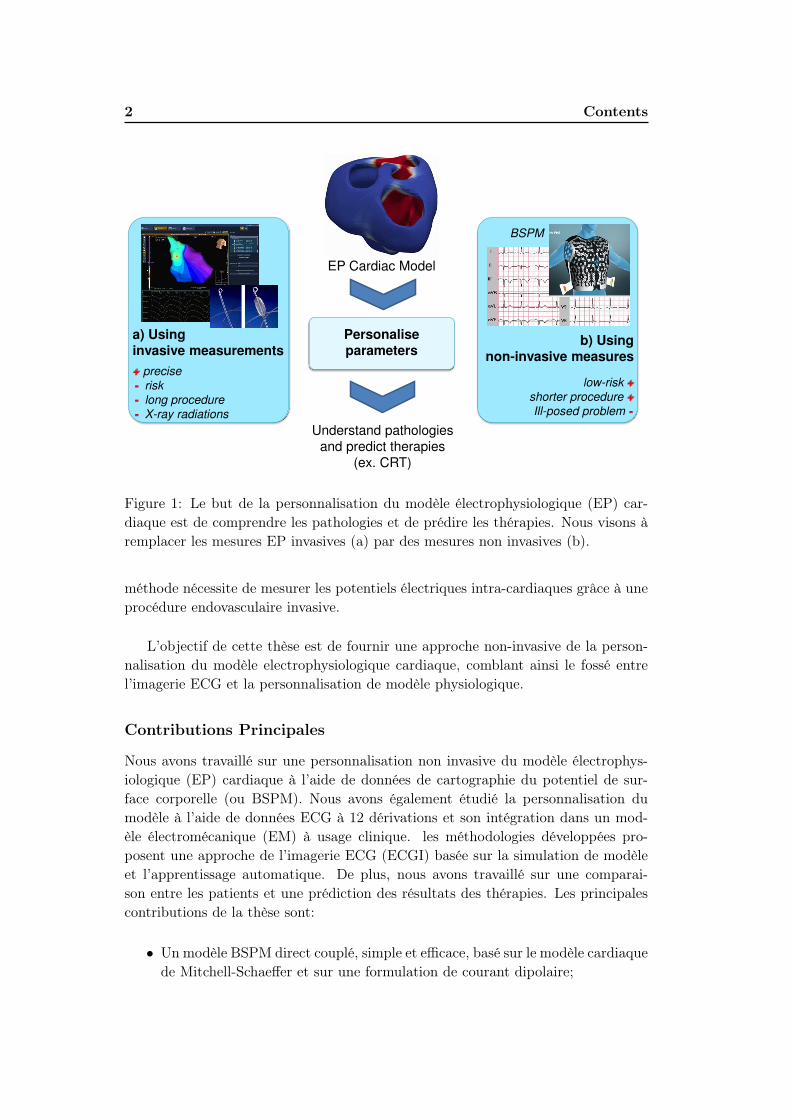
Figure 1: Le but de la personnalisation du modèle électrophysiologique (EP) car-diaque est de comprendre les pathologies et de prédire les thérapies. Nous visons àremplacer les mesures EP invasives (a) par des mesures non invasives (b).
méthode nécessite de mesurer les potentiels électriques intra-cardiaques grâce à uneprocédure endovasculaire invasive.
L’objectif de cette thèse est de fournir une approche non-invasive de la person-nalisation du modèle electrophysiologique cardiaque, comblant ainsi le fossé entrel’imagerie ECG et la personnalisation de modèle physiologique.
Contributions Principales
Nous avons travaillé sur une personnalisation non invasive du modèle électrophys-iologique (EP) cardiaque à l’aide de données de cartographie du potentiel de sur-face corporelle (ou BSPM). Nous avons également étudié la personnalisation dumodèle à l’aide de données ECG à 12 dérivations et son intégration dans un mod-èle électromécanique (EM) à usage clinique. les méthodologies développées pro-posent une approche de l’imagerie ECG (ECGI) basée sur la simulation de modèleet l’apprentissage automatique. De plus, nous avons travaillé sur une comparai-son entre les patients et une prédiction des résultats des thérapies. Les principalescontributions de la thèse sont:
• Un modèle BSPM direct couplé, simple et efficace, basé sur le modèle cardiaquede Mitchell-Schaeffer et sur une formulation de courant dipolaire;

Introduction (Français) 3
Chapter 2 Chapter 3 Chapter 4
Non-invasive cardiac electro-physiological model personalisation
BSPM data 12-lead ECG data Simple data for
E/M integration
CRT clinical
study
Pre-clinical
canine study
Estimated
parameters
1 onset
+ global CV
2 onset
locations
local CV
with scar
Regression
Method
Kernel
Ridge
Relevance
Vector
Relevance
Vector
Study scalepatient-
specific
patient-
specificinterpatient
Pacing
predictionsX X
Chapter 5 Chapter 6 Chapter 7
Part 1 Part 2
Figure 2: Organisation des 6 chapitres principaux. BSPM: cartographie potientiellede la surface du corps; E/M: électromécanique; CV: vitesse de conduction; CRT:thérapie de resynchronisation cardiaque.
• Le développement d’une personnalisation basée sur l’apprentissage automa-tique des principaux paramètres EP cardiaques à partir des BSPM acquiscliniquement, tels que les emplacements d’activation initiale et la vitesse deconduction locale. Pour cela, nous avous utilisé une grande base de donnéessimulée.
• Le développement d’une anatomie de référence permettant d’effectuer unerégression commune et hors ligne et de fournir une analyse inter-patients.
• Une prédiction de la réponse spécifique du patient à différentes configurationsde stimulation.
• Une évaluation sur un ensemble de données important et varié (plus de 25patients et 150 battements cardiaques), incluant différents types de donnéesd’imagerie (IRM, tomodensitométrie), différents types de données électriques(BSPM, ECG 12 dérivations, QRS), différentes pathologies (dyssynchronie, is-chémie, complexe ventriculaire primaire) et différentes stimulations électriques(rythme sinusal, stimulateurs cardiaques).
• Une adaptation aux données d’ECG à 12 dérivations et intégration de méth-odes de personnalisation simples dans des études électromécaniques préclin-iques et cliniques.
Organisation du Manuscrit
Après un examen du contexte clinique de l’eletrophysiologie cardiaque et del’état de l’art de la personnalisation non invasive du modèle EP, le manuscrit est
4 Contents
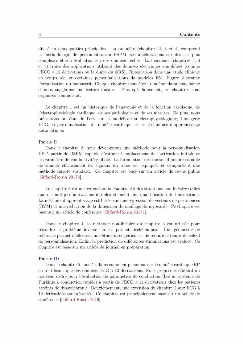
divisé en deux parties principales. La première (chapitres 2, 3 et 4) comprendla méthodologie de personnalisation BSPM, ses améliorations sur des cas pluscomplexes et son évaluation sur des données réelles. La deuxième (chapitres 5, 6et 7) traite des applications utilisant des données électriques simplifiées (commel’ECG à 12 dérivations ou la durée du QRS), l’intégration dans une étude cliniqueen temps réel et certaines personnalisations de modèles EM. Figure 2 résumel’organisation du manuscrit. Chaque chapitre peut être lu indépendamment, mêmesi nous suggérons une lecture linéaire. Plus spécifiquement, les chapitres sontorganisés comme suit:
Le chapitre 1 est un historique de l’anatomie et de la fonction cardiaque, del’électrophysiologie cardiaque, de ses pathologies et de ses mesures. De plus, nousprésentons un état de l’art sur la modélisation eletrophysiologique, l’imagerieECG, la personnalisation du modèle cardiaque et les techniques d’apprentissageautomatique.
Partie I:
Dans le chapitre 2, nous développons une méthode pour la personnalisationEP à partir de BSPM capable d’estimer l’emplacement de l’activation initiale etle paramètre de conductivité globale. La formulation de courant dipolaire capablede simuler efficacement les signaux du torse est expliquée et comparée à uneméthode directe standard. Ce chapitre est basé sur un article de revue publié[Giffard-Roisin 2017b].
Le chapitre 3 est une extension du chapitre 2 à des situations non linéaires tellesque de multiples activations initiales et inclut une quantification de l’incertitude.La méthode d’apprentissage est basée sur une régression de vecteurs de pertinences(RVM) et une réduction de la dimension du maillage du myocarde. Ce chapitre estbasé sur un article de conférence [Giffard-Roisin 2017a].
Dans le chapitre 4, la méthode non-linéaire du chapitre 3 est utilisée pourrésoudre le problème inverse sur les patients ischémiques. Une géométrie deréférence permet d’effectuer une étude inter-patient et de réduire le temps de calculde personnalisation. Enfin, la prédiction de différentes stimulations est évaluée. Cechapitre est basé sur un article de journal en préparation.
Partie II:
Dans le chapitre 5 nous étudions comment personnaliser le modèle cardiaque EPen n’utilisant que des données ECG à 12 dérivations. Nous proposons d’abord unnouveau cadre pour l’évaluation de paramètres de conduction (liés au système dePurkinje à conduction rapide) à partir de l’ECG à 12 dérivations chez les patientsatteints de dyssynchronie. Deuxièmement, une extension du chapitre 2 aux ECG à12 dérivations est présentée. Ce chapitre est principalement basé sur un article deconférence [Giffard-Roisin 2016].

Introduction (Français) 5
Le chapitre 6 est dédié à l’intégration d’une version simplifiée de la person-nalisation electrophysiologique dans une étude prospective clinique non invasiveoù la modélisation électro-mécanique (EM) aide les cliniciens à sélectionnerdes candidats à la CRT. Cette étude a fait partie du projet européen VP2HF(http://www.vp2hf.eu/).
Dans le chapitre Chapter 7, nous avons évalué un modèle cardiaque EM en com-parant le mouvement ventriculaire simulé avec le vrai mouvement du coeur imagépar l’IRM marquée (taguée). Même si certaines données invasives étaient néces-saires, des études précliniques avec des données très précises sont essentielles pourconstruire des méthodes correctes. Dans le cadre d’un challenge électromécanique,ce chapitre est basé sur un article de conférence publié [Giffard-Roisin 2014].
Enfin, le chapitre 8 propose une conclusion générale et des perspectives sur lesaspects cliniques et méthodologiques.
Annexes A et B:
Ce doctorat a également mené à d’autres collaborations liées en partie au sujetde la thèse. Deux annexes rassemblent d’abord les applications de la personnal-isation EM aux simulations d’images dans l’annexe A (échocardiographie 2D et3D, [Alessandrini 2015b, Alessandrini 2015a], IRM [Zhou 2017]) et des applicationsdu modèle cardiaque en annexe B (pour une comparaison avec un modèle sansmaillage [Lluch Alvarez 2017] et pour une étude d’orientation des fibres cardiaques[Doste 2017]).


Chapter 1
Context and State-of-the-Art
Contents
1.1 Introduction . . . . . . . . . . . . . . . . . . . . . . . . . . . . 7
1.1.1 Motivation . . . . . . . . . . . . . . . . . . . . . . . . . . . . 7
1.1.2 Main Contributions . . . . . . . . . . . . . . . . . . . . . . . 8
1.1.3 Manuscript Organization . . . . . . . . . . . . . . . . . . . . 9
1.2 Clinical context . . . . . . . . . . . . . . . . . . . . . . . . . . . 12
1.2.1 Generalities on the Heart . . . . . . . . . . . . . . . . . . . . 12
1.2.2 Heart Failure and Cardiac Resynchronization Therapy . . . . 14
1.2.3 Cardiac Electrical Measures . . . . . . . . . . . . . . . . . . . 16
1.3 State-of-the-art . . . . . . . . . . . . . . . . . . . . . . . . . . . 19
1.3.1 Electrophysiological Cardiac Modelling . . . . . . . . . . . . . 19
1.3.2 ECG Imaging and Inverse Problem . . . . . . . . . . . . . . . 21
1.3.3 Cardiac EP Personalisation . . . . . . . . . . . . . . . . . . . 23
1.3.4 Reference Ventricle-Torso Anatomy in ECGI . . . . . . . . . 23
1.3.5 Data Driven and Machine Learning for Cardiac EP Personal-
isation . . . . . . . . . . . . . . . . . . . . . . . . . . . . . . . 24
1.4 Conclusion . . . . . . . . . . . . . . . . . . . . . . . . . . . . . 28
1.1 Introduction
1.1.1 Motivation
Heart Failure (HF) is a major health issue in Europe affecting 6 million patientsand growing substantially because of the ageing population and improving survivalfollowing myocardial infarction. The poor short to medium term prognosis ofthese patients means that treatments such as cardiac resynchronisation therapycan have substantial impact [Sutton 2003]. However, these therapies are ineffectivein 30% of the treated patients and involve significant morbidity and substantial cost.
To this end, the precise understanding of the patient-specific cardiac func-tion can help predict the response to therapy and therefore select the potentialcandidates and optimise the therapy. The anatomical, mechanical and electrophys-iological (EP) functions can be evaluated by clinical images and signal recordings.

8 Chapter 1. Context and State-of-the-Art
We call them invasive data when the procedure lead to some health damage forexample by intra-cardiac electrical measures through endovascular procedure.At a diagnostic or patient-selection stage the non-invasive data are a preferablealternative. Magnetic resonance (MR) imaging, computed tomography (CT)and echocardiography are non-invasive imaging procedures able to capture theanatomical, mechanical and physiological cardiac functions. The electrocardiogram(ECG) and the body surface potential mapping (BSPM) are meanwhile able tonon-invasively capture the electrical activation from the surface of the torso.
In order to assist cardiologists, the scientific community is developing tools forautomatically identifying the patient anatomy, physiology but also the electro-mechanical (EM) function. From BSPM electrical data, the ECG imaging fieldaims at reconstructing the local cardiac electrical patterns either on the heartsurface or on the transmural cardiac muscle [Pullan 2010]. This ill-posed inverseproblem is usually solved by regularized techniques for the stability of the solutions.However, it is often at the cost of a reduced accuracy and non-physiologicallyplausible electrical propagations.
The integration of medical data into some cardiac physiological electro-mechanical models (for such models see [Strumpf 1990, Bestel 2001, Pollard 2003])has also lead to patient-specific modelling able to better understand the person-alised cardiac function. The goal is to estimate the main model parameters inorder to fit to the patient-specific data. The model personalisation is also ableto provide some predictive information. [Sermesant 2012] proposed to personalizean electro-mechanical model of the heart to predict the response to CRT. Themethod requires to measure intra-cardiac electrical potentials through an invasiveendovascular procedure.
The aim of this thesis is to provide a non-invasive approach to cardiac EP modelpersonalisation, thus bridging the gap between ECG imaging and model personali-sation.
1.1.2 Main Contributions
We worked on a non-invasive cardiac electrophysiological (EP) model personalisa-tion using body surface potential mapping (BSPM) data. We also studied the modelpersonalisation using 12-lead ECG data and its integration in an electromechani-cal (EM) model for a clinical use. Our developed methodologies propose an ECGimaging (ECGI) inverse approach based on model simulation and machine learning.Moreover, we provided some inter-patient comparison and an outcome prediction oftherapies. The main contributions of the thesis are:
• A straightforward and efficient coupled forward BSPM model based on thecardiac Mitchell-Schaeffer model and on a current dipole formulation;

1.1. Introduction 9
Understand pathologies
and predict therapies
(ex. CRT)
a) Usinginvasive measurements
+ precise
- risk
- long procedure
- X-ray radiations
Personaliseparameters
b) Usingnon-invasive measures
low-risk +
shorter procedure +
Ill-posed problem -
BSPM
EP Cardiac Model
Figure 1.1: The goal of electrophysiological (EP) cardiac model personalisation isto understand pathologies and predict therapies. We aim at replacing invasive EPmeasures (a) by non-invasive ones (b).
• The development of a machine learning-based personalisation of the maincardiac EP parameters from BSPM acquired clinically, such as onset activa-tion locations and heterogeneous conduction velocity, from a large simulateddatabase.
• The development of a reference ventricle-torso anatomy able to perform acommon and offline regression and to provide an interpatient analysis.
• A prediction of the patient-specific response to different pacing configurations.
• An evaluation on an important and diverse dataset (more than 25 patientsand 150 heart beats), including different types of imaging data (MRI, CTscan), different types of electrical data (BSPM, 12-lead ECG, QRS duration),different pathologies (dyssynchrony, ischemy, primature ventricular complex)and different electrical stimulations (sinus rhythm, pacemakers).
• An adaptation to 12-lead ECG data and an integration of simple personalisa-tion methods into pre-clinical and clinical electromechanical studies.
1.1.3 Manuscript Organization
After a survey of the clinical context of cardiac EP and of the state-of-the-art ofnon-invasive EP model personalisation, the manuscript is divided into two main

10 Chapter 1. Context and State-of-the-Art
Chapter 2 Chapter 3 Chapter 4
Non-invasive cardiac electro-physiological model personalisation
BSPM data 12-lead ECG data Simple data for
E/M integration
CRT clinical
study
Pre-clinical
canine study
Estimated
parameters
1 onset
+ global CV
2 onset
locations
local CV
with scar
Regression
Method
Kernel
Ridge
Relevance
Vector
Relevance
Vector
Study scalepatient-
specific
patient-
specificinterpatient
Pacing
predictionsX X
Chapter 5 Chapter 6 Chapter 7
Part 1 Part 2
Figure 1.2: Manuscript organization of the 6 main chapters. BSPM: body surfacepotiential mapping; E/M: electro-mechanical; CV: conduction velocity; CRT: cardiacresynchronization therapy.
parts. The former (chapters 2, 3 and 4) includes the BSPM personalisation method-ology, its improvements on more complex cases and its evaluation on real data.The latter (chapters 5, 6 and 7) deals with the applications using some simplifiedelectrical data (as the 12-lead ECG or the QRS duration) and the integration intoa real-time clinical study and some EM model personalisations. Figure 1.2 summa-rizes the manuscript organization. Each chapter can be read independently, even ifwe suggest a linear reading. More specifically, the chapters are organized as followed:
Chapter 1 is a background on the cardiac anatomy and function, on the cardiacelectrophysiology, its pathologies and its measures. Moreover, a state-of-the-arton EP modelling, ECGI, cardiac model personalisation and machine learningtechniques is presented.
Part I:
In Chapter 2, we develop a method for the EP personalisation from BSPM ableto estimate the activation onset location and the global conductivity parameter.The current dipole formulation able to simulate the torso signals efficiently isexplained and compared to a standard forward method. This chapter is based on apublished TBME journal paper [Giffard-Roisin 2017b].
Chapter 3 is an extension of Chapter 2 to non-linear situations such asmultiple onsets and includes uncertainty quantification. The learning methodis based on a relevance vector regression and a myocardial shape dimensionreduction. This chapter is based on a published FIMH conference proceedings

1.1. Introduction 11
paper [Giffard-Roisin 2017a].
In Chapter 4, the non-linear method of Chapter 3 is used for solving the inverseproblem on ischemic patients. A reference ventricle-torso geometry enables toperform an inter-patient study and to reduce the personalisation computation time.Finally, the prediction of different pacings is evaluated. This chapter is based on ajournal paper in preparation.
Part II:
In Chapter 5 we investigate how to personalise the EP cardiac model usingonly 12-lead ECG data. First, we propose a new framework for the evaluationof conduction parameters (linked to the fast conduction Purkinje system) from12-lead ECG in the case of dyssynchroneous patients. Secondly, an extensionof Chapter 2 to 12-lead ECG is presented. This chapter is mostly based on apublished STACOM workshop (held in conjunction with the MICCAI conference)proceedings paper [Giffard-Roisin 2016].
Chapter 6 is dedicated to the integration of a simpler version of EP person-alisation into a non-invasive clinical prospective study, where the EM modellinghelps the clinicians to select CRT candidates. This study was part of the Europeanproject VP2HF (http://www.vp2hf.eu/).
In Chapter 7, we evaluated an EM cardiac model by comparing the simulatedventricular motion with the true motion of hearts imaged by tagged MRI. Even ifsome invasive data were needed, pre-clinical studies with very accurate data areessential for building correct methods. As part of an EM challenge, this chapter isbased on a published STACOM workshop (held in conjunction with the MICCAIconference) proceedings paper [Giffard-Roisin 2014].
Finally, Chapter 8 proposes a general conclusion and perspectives on clinicaland methodological aspects.
Appendices A and B:
This PhD has also led to other collaborations that are partly linked to thethesis subject. Two appendices are gathering first the applications of the EMpersonalisation to image simulations in Appendix A (2D and 3D echocardiogra-phy [Alessandrini 2015b, Alessandrini 2015a], MRI [Zhou 2017]) and second someapplications of our electrical cardiac model in Appendix B (for a comparison toa mesh-free model [Lluch Alvarez 2017] and for a cardiac fiber orientation study[Doste 2017]).

12 Chapter 1. Context and State-of-the-Art
1.2 Clinical context
1.2.1 Generalities on the Heart
1.2.1.1 Anatomy
The heart is the pump providing oxygenated blood to the organs and in parallelsending de-oxygenated blood to the lungs. It is composed of four chambers; twoatria and two ventricles, see Figure 1.3a. The right atrium and ventricle provideblood to the lungs while the left side, with a stronger muscle, is providing blood tothe organs. The left ventricle (LV) and the right ventricle (RV) are separated by anintraventricular muscle, called septum. The inferior part of the heart is called theapex. The ventricles cavities are closed by valves separating the ventricles from theatria. Finally, the pulmonic and aortic valves allow blood to leave the ventricles viathe arteries.
An entire cardiac cycle lasts approximately one second and is divided into twostages: the systole during which the ventricles are contracting, and the diastoleduring which the ventricles relax.
The ventricular muscular wall is called myocardium and has an inner surface(endocardium) and an outer surface (epicardium), see Figure 1.3b. The surroundingmembrane is called the pericardium. The myocardium is composed of myocyte cellsor muscle fibers whose direction varies across the myocardium (Figure 1.3c). Themean elevation angle (obliquity with respect to the plane of the section) variesapproximately from −70◦ in the epicardium to +70◦ in the endocardium. Thisorganization optimizes the contraction.
1.2.1.2 Cardiac Electrical Conduction System
The cardiac contraction is driven by an electrical wave spreading through the my-ocardium and depolarizing each cell; first the atria and then the ventricles. Theventricular depolarization is fast (less than 100ms) and synchronous between theleft and the right side. Because of the particular fiber organization of the myocar-dial cells, the electrical propagation is anisotropic.
The resting polarized state of a myocyte consists in a difference of approximately90mV between the intracellular and extracelluar medium. When a stimulus occurs,the transmembrane potential is modified with respect to the gradient of ionic con-centrations. The concentrations of different ions (sodium, calcium and potassium)and their flow through the membrane are responsible of particular cell state changes.The evolution of the transmembrane potential called action potential is composed of3 phases: the depolarization phase, the plateau phase and the repolarization phase(see Figure 1.4a).
The cardiac rhythm is driven by the sinoatrial node capable of spontaneouslygenerating electrical signals. In a normal sinus rhythm, the stimulus reaches theventricles from the atrioventricular node through the His bundle where the networksplits into two branches, the left bundle and the right bundle (see Figure 1.4b). The

1.2. Clinical context 13
(a) (b)
(c)
Figure 1.3: (a) The 4 chambers of the human heart (b) Membranes and layers of theheart wall (c) Cardiac cells organized in fibers. From www.commons.wikimedia.org

14 Chapter 1. Context and State-of-the-Art
(a) (b)
Figure 1.4: (a) Action potential response of a cardiac cell in mV (from Talbot, Inter-ative Patient-specific Simulation of Cardiac Electrophysiology, 2014). (b) Electricalconduction system of the heart (from hopkinsmedicine.org)
bundle branches are connected to a fast conduction system called Purkinje fibers,composed of specialised heart muscle cells. The Purkinje fibers are located justbeneath the endocardium and are able to conduct quickly and efficiently: typicalconduction velocity ranges from 2 to 3m/s while it ranges from 0.3 to 0.4m/s formyocardial cells [Durrer 1970].
1.2.2 Heart Failure and Cardiac Resynchronization Therapy
1.2.2.1 Heart Failure
Heart failure (HF) includes all pathologies leading an insufficient amount of bloodbeeing pumped for the body’s needs. The two main types are the systolic HF (lackof contraction) and the diastolic HF (lack of relaxation of the ventricles). It can bebrought on by many conditions, including:
• Coronary artery disease or ischemic heart disease occurs when the arteriesthat supply blood to the myocardium become hardened and narrowed.
• Cardiomyopathy is more generally a damage on the myocardium that canbe caused by artery or blood flow problems, infections, alcohol or drug abuse.
• Heart attack occurs when a coronary artery is suddenly blocked, stoppingthe blood flow in the myocardium.
• Overwork of the heart includes high blood pressure, heart valve disease,diabetes or heart defects.
Coronary artery disease or other cardiomyopathies can lead to myocardial in-farction, i.e. myocardial cell death. The necrotic zone called infarct or scar doesnot contract nor conduct anymore, leading to abnormal heart beating patterns.

1.2. Clinical context 15
(a) LBBB (b) RBBB
Figure 1.5: (a) Left bundle branch block (b) Right bundle branch block. A defectin a major bundle causes a dysfunction of the underlying fast conduction system.
1.2.2.2 Ventricular Dyssynchrony
Heart failure is also correlated to electrical conduction pathologies, such as ventric-ular dyssynchrony. Ventricular dyssynchrony consists in a difference of contractiontimings of the ventricles. A large difference can considerably reduce the heart effi-ciency. We distinguish three types of ventricular dyssynchrony: the atrioventriculardyssynchrony, the interventricular dyssynchrony and the intraventricular dyssyn-chrony. The interventricular dyssynchrony occurs when there is a delay between theright and the left ventricular depolarizations. The intraventricular dyssynchronyresults in a discoordinated contraction between the left ventricular segments.
One of the main causes are dysfunctions in the conduction system, for examplebundle branch blocks. Left (LBBB) and right (RBBB) bundle branch blocks are in-terventricular dyssynchronies caused by a defect in one of the main bundle branches(Figure 1.5). Since the electrical impulse no longer uses the fast system, it maypropagate through the muscle in a slower way and with a different direction.
1.2.2.3 Cardiac Resynchronization Therapy
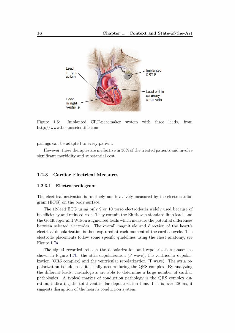
An important treatment to ventricular dyssynchrony is the cardiac resynchroniza-tion therapy (CRT). It consists in the implantation of a cardiac device that sendsan electrical and periodic impulse to the myocardium in order to resynchronize thecontraction. Depending on the pathology and on the device, one or more leadsare placed in contact to the myocardium in different locations. A standard CRTpacemaker is composed of three leads: one in the right atrium, one in the rightventricle and one on the left ventricle (Figure 1.6). The last one is usually insertedin the coronary sinus vein and will pace from the outside (or epicardum) of themyocardium. This lead placement is often the most delicate part of the procedure.It is controlled by radiography and electrocardiogram. Delays and timings between
16 Chapter 1. Context and State-of-the-Art
Figure 1.6: Implanted CRT-pacemaker system with three leads, fromhttp://www.bostonscientific.com.
pacings can be adapted to every patient.
However, these therapies are ineffective in 30% of the treated patients and involvesignificant morbidity and substantial cost.
1.2.3 Cardiac Electrical Measures
1.2.3.1 Electrocardiogram
The electrical activation is routinely non-invasively measured by the electrocardio-gram (ECG) on the body surface.
The 12-lead ECG using only 9 or 10 torso electrodes is widely used because ofits efficiency and reduced cost. They contain the Einthoven standard limb leads andthe Goldberger and Wilson augmented leads which measure the potential differencesbetween selected electrodes. The overall magnitude and direction of the heart’selectrical depolarization is then captured at each moment of the cardiac cycle. Theelectrode placements follow some specific guidelines using the chest anatomy, seeFigure 1.7a.
The signal recorded reflects the depolarization and repolarization phases asshown in Figure 1.7b: the atria depolarization (P wave), the ventricular depolar-ization (QRS complex) and the ventricular repolarization (T wave). The atria re-polarization is hidden as it usually occurs during the QRS complex. By analyzingthe different leads, cardiologists are able to determine a large number of cardiacpathologies. A typical marker of conduction pathology is the QRS complex du-ration, indicating the total ventricular depolarization time. If it is over 120ms, itsuggests disruption of the heart’s conduction system.

1.2. Clinical context 17
(a) (b)
Figure 1.7: (a) Precordial electrode placement in ECG. They are complementedwith an electrode on each arm and one or two electrodes on the legs. (b) Standardsinus rhythm electrocardiogram, composed of the atria depolarization (P wave),the ventricular depolarization (QRS complex) and the ventricular repolarization (Twave). From www.commons.wikimedia.org
Figure 1.8: EnSite navigation system: with (left) fluoroscopic images, (middle) thedeflated and inflated ballon, (right) and the electroanatomical mapping (Imagesfrom KCL, London)
18 Chapter 1. Context and State-of-the-Art
Figure 1.9: CardioInsight device for body surface potential mapping. (ECVUE,CardioInsight Technologies Inc., Cleveland, Ohio)
1.2.3.2 Intra-cardiac Electrical Mapping
In order to have a better insight of the depolarization wave, an invasive procedurecan provide an electrical mapping of the LV endocardial or epicardial potentials.The signals are recorded using two different mapping approaches: a contact map-ping (consisting in moving a catheter along the wall to capture electrical signals) ora non-contact mapping (using a balloon floating inside the chamber and measuringremotely the surrounding electrical activity). An example using the Ensite naviga-tion system is presented in Figure 1.8. EnSite NavX technology displays activationtiming and voltage data to help the physician identify arrhythmias, to create cham-ber models and to guide catheter navigation. The uncertainty in the acquisitionarises mainly from registration issues.
The optical mapping method consists in perfusing the heart with a fluid con-taining voltage-sensitive dye. The change in transmembrane potential is recordedby fluorescence spectra. Optical mapping is very precise but is only dedicated to exvivo experiments.
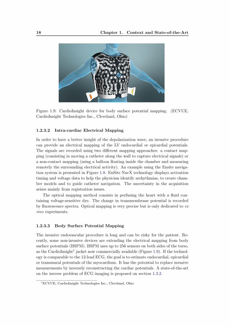
1.2.3.3 Body Surface Potential Mapping
The invasive endovascular procedure is long and can be risky for the patient. Re-cently, some non-invasive devices are extending the electrical mapping from bodysurface potentials (BSPM). BSPM uses up to 256 sensors on both sides of the torso,as the CardioInsight1 jacket now commercially available (Figure 1.9). If the technol-ogy is comparable to the 12-lead ECG, the goal is to estimate endocardial, epicardialor transmural potentials of the myocardium. It has the potential to replace invasivemeasurements by inversely reconstructing the cardiac potentials. A state-of-the-arton the inverse problem of ECG imaging is proposed on section 1.3.2.
1ECVUE, CardioInsight Technologies Inc., Cleveland, Ohio

1.3. State-of-the-art 19
1.3 State-of-the-art
1.3.1 Electrophysiological Cardiac Modelling
1.3.1.1 Categories of Electrophysiological Models
The electrophysiology (EP) of the heart (see section 1.2.1.2) can be modelled inorder to reproduce its behaviour, to understand the mechanisms and pathologiesor to predict the response to treatments. There are several types of EP modelsdescribing the action potential:
• biophysical models [Ten Tusscher 2004]: These complex models includes thedifferent ionic concentrations at the cellular scale. They are able to reproduceand simulate very precisely the cardiac cell behavior, but can be computation-ally demanding.
• Eikonal models developed by [Keener 1991]: they are simplistic models cor-responding to non-linear partial differential equations of the activation time.Their efficiency has been proven, however these models cannot accurately ac-count for complex physiological states.
• phenomenological models as [Aliev 1996, FitzHugh 1961, Mitchell 2003]: theyhave an intermediate complexity and are derived from the biophysical models.They involve less parameters but still capture the action potential shape andits propagation at the organ scale.
Cardiac EP models can be classified as bidomain or monodomain depending onthe considered electrical potentials.
1.3.1.2 Mitchell-Schaeffer Model
The Mitchell-Schaeffer model [Mitchell 2003] is a phenomenological model with 2variables and 6 parameters. A bi-domain and a monodomain version have both beendeveloped. In our work, we used a monodomain version of the Mitchell-Schaeffermodel as implemented in [Talbot 2013].
The Mitchell-Schaeffer model has two variables, the transmembrane potential vand z a secondary variable controlling the repolarization phase. Their evolution isgoverned by:
∂tv = div(D∇v) + zv2(1−v)τin
− vτout
+ Jstim
∂tz =
{
1−zτopen
if v < vgate−z
τcloseif v > vgate
(1.1)
The parameters τopen and τclose define the gate opening and closing depending on thechange-over voltage vgate, and the parameters τin and τout control the depolarisationupstroke and repolarization downstroke. Jstim(t) is the stimulation current applied

20 Chapter 1. Context and State-of-the-Art
Figure 1.10: Transmembrane potential as described in [Mitchell 2003] with the fol-lowing phases: (1) depolarization (2) plateau phase (3) repolarisation (4) rest po-tential.
in the pacing area. The diffusion term is defined by a 3x3 anisotropic diffusiontensor:
D = d · diag(1, r, r) (1.2)
where d is the tissue electrical diffusivity. The anisotropy ratio r enables conductionvelocity in the fibre direction to be larger than in the transverse plane (typicallyr = (1/2.5)2).
The diffusivity d (in m2s−1) can be expressed as a conductivity σ (in S/m) from:
σ = Cmβ d (1.3)
with Cm the membrane capacitance and β the surface-to-volume ratio. The localconductivity σ can be written in terms of intracellular and extracellular conductiv-ities:
σ =σiσe
σi + σe(1.4)
The reduction of the monodomain model implies σi = λσe for some scalar λ resultingin a linear relationship between σ and σi. Finally, the diffusion d is linked to theconduction velocity c in m/s by c = k
√d.
From an onset activation location, the evolution of the transmembrane potentialis computed at each node of a tetrahedral mesh of the myocardium using the finiteelement method. In Figure 1.10 is represented the transmembrane potential asdescribed in [Mitchell 2003], where we can see a good agreement with the actionpotential of a cardiac cell as in Figure 1.4a.
1.3.1.3 Cardiac Electro-mechanical Modelling
The electrical depolarisation wave activates the mechanical contraction at a micro-scopic scale, while the repolarization drives the relaxation. That is why the cardiac

1.3. State-of-the-art 21
Figure 1.11: Inverse and forward problems in ECG imaging, From Danila Potya-gaylo, https://www.ibt.kit.edu/english/1026.php
EP model is often inserted in a 3D electro-mechanical (EM) model, either as apre-processing step or as coupled mechanisms. This way, it is possible to evalu-ate the resulting cardiac motion and the volume of ejected blood. The mechanicalmodels are mainly dependent on the contraction and stiffness parameters of themyocardium tissue. In 2006, the electrical model from [FitzHugh 1961] was coupledwith a simple constitutive contraction law in [Sermesant 2006]. In [Talbot 2013],the Mitchell-Schaeffer model is a pre-processing step to the Bestel-Clement-Sorine(BCS) mechanical modelling [Chapelle 2012]. The latter ensures to take into ac-count the microscopic scale phenomena of the contraction as well as laws of ther-modynamics. In [Sermesant 2012, Marchesseau 2013], the Eikonal EP model wasalso weakly coupled to the same BCS model. A strong EM coupling, where the EPpropagation at time t depends on the current contracted shape, was experimentedin [Giffard-Roisin 2014] with Eikonal and BCS models.
1.3.2 ECG Imaging and Inverse Problem
1.3.2.1 Forward Problem of Cardiac Electrocardiography
The estimation of the ECG data from the cardiac potentials is usually called the for-ward problem of electrocardiography (in opposition to the inverse problem, see Fig-ure 1.11). The two classical numerical approaches are based either on the BoundaryElement Method (BEM) or the Finite Element Method (FEM). They both prop-agate the epicardial heart action potentials to the surface of the body by takinginto account the distance, the null current across the body surface, and the differentproperties of the tissues in between.
Forward models differ also by their incorporation of heterogeneous conductivityregions associated with various organs within the torso. By taking into account thephysical properties of the different tissues, the computed ECG account for more
22 Chapter 1. Context and State-of-the-Art
complex current pathways. In [Keller 2010], Keller et al. demonstrate the impor-tance of the torso inhomogeneity by ranking the influence of the different tissueconductivities on forward-calculated ECGs. Ramanathan et al. [Ramanathan 2001]showed, however, that at a first order approximation the torso inhomogeneities arenot necessary for non-invasive reconstructions. Some techniques rely neither onBEM nor on FEM and assume a homogeneous and infinite torso domain using adipole formulation [Chávez 2015]. While neglecting the null current flow constraintat the body surface, it has been shown to be efficient on simulated experiments.
1.3.2.2 Inverse Problem of Cardiac Electrocardiography
BSPM data has been widely used in the last decades to directly compute the car-diac action potentials by solving an ill-posed inverse problem: finding the transfermatrix linking the torso potentials to the cardiac potential sources [Dössel 2000,Pullan 2010]. If most of the methods are only estimating the potential on the surfaceof the heart (e.g. [Huiskamp 1988, Ghosh 2009]), transmural-based methods havebeen investigated in the last few years but are computationally more demanding[Messnarz 2004, Jiang 2009]. Rather than estimating directly the transmembranepotentials, the 3DCEI technique [Liu 2006, Han 2011, Han 2013, Han 2015] solvesthe inverse problem by estimating the equivalent current density.
Aside from standard regularization techniques, some inverse problem stud-ies have been investigated imposing constraints in temporal and spatial domains[Messnarz 2004, Yu 2015] or trying to take advantage of the space/time couplingof the electrical wave propagation [Oster 1992, Chávez 2015]. Some methods arealso looking into integrating physiological and model-based priors in a Bayesianframework [Rahimi 2016, Wang 2011]. The work by Li and He [Li 2001] solves theinverse problem by means of heart-model parameters (onset activation location) andwas further extended [He 2002] and validated on rabbits [Zhang 2005] and swines[Liu 2008, Liu 2012]. A preliminary step is based on prior knowledge using artifi-cial neural network and an optimization algorithm refining the parameters. Lastly,the fastest route algorithm [Van Dam 2009, van Dam 2013] is used for a preliminarexhaustive ECGI estimation from a simplified EP modelling.
ECG imaging is already commercially available for some clinical applications, asthe CardioInsight Technologies software [Ramanathan 2003] which was also used inrecent ECGI studies [Dubois 2015]. Moreover, a consortium on ECG imaging wasrecently developed, leading to some shared databases, shared methodological toolsand shared publications [Aras 2015, Coll-Font 2016b].
ECG imaging can help in understanding dyssynchony and selecting CRT candi-dates : [Varma 2007] and [Ghosh 2011] worked on characterizing the EP substrateand electrical dyssynchony on HF patients undergoing CRT while [Dawoud 2016]investigated regional electromechanical uncoupling in patients referred for CRT.

1.3. State-of-the-art 23
1.3.3 Cardiac EP Personalisation
The estimation of patient-specific parameters of a cardiac EP model is crucial forunderstanding the pathologies and predicting the response to therapies. The modelpersonalisation usually deals with local parameters, such as conductivities or onsetactivation locations.
1.3.3.1 Cardiac EP Personalisation from Invasive Data
The first EP model personalisations were using invasive data measures such as pre-sented in section 1.2.3.2. [Relan 2011b] used optical mapping in an ex vivo studyto personalize local diffusivity parameters. Personalisation using intra-cardiac po-tential mapping was investigated by [Relan 2011a, Wallman 2014, Konukoglu 2011],also including epicardial recordings. In [Konukoglu 2011], the integration of uncer-tainty estimation was also studied.
1.3.3.2 Cardiac EP Personalisation from Non-invasive Data
Calibration using non-invasive data was recently studied: [Zettinig 2014] used twofeatures from the 12-lead ECG to recover 3 electrical diffusivity parameters usinga polynomial regression. The method is novel and efficient, but it suffers from thefact that the earliest activation site was fixed but actually unknown, and only twofeatures (QRS complex duration and electrical axis) may not be sufficient to describethe cardiac activation. The estimation of heterogeneous myocardial conductionusing a Bayesian framework has been explored by [Dhamala 2017a], but the otherparameters such as the onset are supposed to be known. The problem of uncertaintyin the field of non-invasive cardiac EP model parameter estimations is has also raisedinterests [Dhamala 2017b].
Finally, the estimation of cardiac activation patterns from motion imag-ing data was investigated with the use of a database of synthetic image se-quences [Prakosa 2014]. Using also imaging data (delayed enhanced MRI),[Cabrera-Lozoya 2017] worked on locating cardiac ablation targets to guide radiofre-quency ablation by simulating patient-specific intracardiac electrograms.
1.3.4 Reference Ventricle-Torso Anatomy in ECGI
The personalisations of EP cardiac model parameters from BSPM data rely on time-consuming patient-specific computation. Moreover, the patient-specificity is at theexpense of an inter-patient study where information from different patients could becompared. Because of the natural similarity of the anatomical structures betweenpatients, a common framework could be exploited.
One study showed the importance of the interindividual variability (aver-aged standard deviation) of electrocardiograms (ECG) on 25 healthy subjects[Hoekema 1999]. A large part of this variability is due to the heart position andorientation relative to electrodes. In terms of geometry, the larger variations are

24 Chapter 1. Context and State-of-the-Art
found for the heart long axis angle. Another study showed that ECG imaging issensitive to global anatomical parameters such as the heart orientation and locationwith regard to the lead positions [Huiskamp 1989]. The use of a reference anatomymodel, able to represent every patient, is thus a difficult task. Hoekema et al.[Hoekema 1999] showed that by only moving the electrodes in a frontal plane to acommon reference, the interindividual variability is not reduced because the heartorientation is not preserved. Another study created a patient-specific adapted torsomodel by stretching and squeezing a standard torso model according to the measures[Lenkova 2012]. They concluded that it was crucial to adapt both the outer shape ofthe torso model and the position of electrodes according to reality. Yet, it has beenalso shown that some adapted ventricle-torso standard model were able to get goodECGI results while excluding local geometrical details [Wang 2010, Rahimi 2015].To the best of our knowledge, the goals of these geometrical models were only tosimplify the anatomical modelling process. Yet, a study has recently tackled theinterindividual variability by separating the factors of variation throughout a deepnetwork using a denoising autoencoder on a large ECG dataset [Chen 2017b] forlearning the ventricular tachycardia origin. Inter-subject variations coming fromcardiac EP differences and geometry differences are however not separable, so apersonalised EP model could not be estimated.
1.3.5 Data Driven and Machine Learning for Cardiac EP Person-alisation
In order to tackle model personalisation, several approaches of data-driven algo-rithms exists. On the one hand, sequential algorithms are estimating the errorbetween the simulation results and the real data at each time step to correct thevalues of the parameters. On the other hand, variational techniques are minimizinga functional in order to approximate the extreme function that makes the functionalattain the minimum value. Machine learning techniques are handling problems witha similar criterion as variational approaches, but without estimating the gradientof the criterion. As no large patient-specific database exists, they can only rely onsimulated patient-specific samples covering the parameter space.
1.3.5.1 Sequential Data Assimilation
The Unscented Kalman filter (UKF) [Julier 1997] ia a sequential data assimilationalgorithm. The algorithm, derived from the Unscented Transform and the Kalmanfilter, is used to linearize a function of a random variable through a linear regressionbetween n points drawn from the prior distribution of the random variable. TheUKF consists of the iteration of the following three steps: selection of some sigmapoints where the function is evaluated, model forecast and data assimilation.
For the EP personalisation problem, sequential methods suffers from the factthat the state of the system at time t highly depends on the state at time t − 1
so correcting the parameter values during the simulation might be inefficient, while

1.3. State-of-the-art 25
identifying the initial activation site is nearly impossible. As a solution,[Wang 2011]and [Talbot 2015] used static versions of the UKF where the algorithm iteratesthrough a complete cardiac cycle and thus acting more like the variational ap-proaches.
A recent study has also developed a new sequential estimation method for makingan atrial EP model patient-specific from simulated invasive measures [Collin 2015].They have tackled the problem of complex EP wave shapes such as fibrillation byincorporating a correction term based on topological gradients. This way, it ispossible to act only in active regions on the propagation front.
1.3.5.2 Variational Data Assimilation
The large variety of variational or optimization methods has been used in all prob-lems that can be described by a functional f to minimize (or maximize), correspond-ing to some criterion or error, and a set of available parameter values. Variationaltechniques impose to have the whole sequence of data before trying to optimize theparameters. The minimum of a function can be found by taking steps proportionalto the negative of the gradient (procedure known as the gradient descent), howevermany problems are described with non-differentiable functionals. We will describein the following sections some derivative-free optimization techniques.
1.3.5.3 Evolution Strategy
In this scope, the evolution strategy optimization technique uses natural problem-dependent representations, where mutation and selection are the search operators.These operators are applied in a loop (each iteration is called generation) untila criterion is met. At each generation, new individuals (candidate solutions x)are generated by variation, usually in a stochastic way, of the current parentalindividuals. They are sampled according to a multivariate normal distribution, andpairwise dependencies between the variables in the distribution are represented bya covariance matrix. The covariance matrix adaptation (CMA) is a method toupdate the covariance matrix of this distribution. The CMA evolution strategy(CMA-ES) [Hansen 2006] has been used in cardiac mechanical personalisation by[Molléro 2016] because it is derivative-free and suited for non-convex continuousoptimization problems. The concept of directional optimization in the CMA-ES ona 2D problem is shown in Figure 1.12.
1.3.5.4 Regression Analysis
The multivariate regression analysis is an intuitive machine learning continuous pro-cess for estimating relationships between variables. Regression analysis estimatesthe conditional expectation of the dependent variable given the independent vari-ables. The estimated target is a function of the independent variables called theregression function. Many regression techniques have been developed, among thefamiliar ones are the linear regression and the ordinary least square regression. In

26 Chapter 1. Context and State-of-the-Art
Figure 1.12: Concept of directional optimization in the covariance matrix adaptationevolution strategy (CMA-ES). The spherical optimization landscape is depicted withsolid lines of equal f -values. The population (dots) shows how the distribution of thepopulation (dotted line) changes during the optimization. On this simple problem,the population concentrates over the global optimum within a few generations. Fromwww.commons.wikimedia.org
the polynomial regression the relationship between the independent variable x andthe dependent variable y is modelled as an nth degree polynomial in x. It was usedin [Zettinig 2014] for parameter estimation from two features of the 12-lead ECG.
The ridge regression is a regularized least square method which is suited for areasonable number of training examples. In the kernel ridge regression, we considera non linear mapping x → Φ(x) into a higher-dimensional but linear feature space.The kernel trick consists in only calculating the equivalent kernel K(xi, xj) = Φ(xi)·Φ(xj) without computing Φ(x). It is suited for complex non-linear relationshipsbetween variables. The predicted target y for a new test point x is then estimatedusing:
y = y(K +1
γIn)
−1κ(x)
where y is the matrix of the sampled targets yi, γ is the coefficient balancing thesmoothness and the adherence to the data and the i-th coordinate of the vector κ(x)is defined as (κ(x))i = K(xi, x).
1.3.5.5 Bayesian Inference
In machine learning, many methods are employing statistical inference which con-sists in deducing properties of the underlying probability distribution by analysisof the data. Particularly, Bayesian inference proposes to update the probabilityas more information becomes available. It derives the posterior probability fromthe prior probability and the likelihood function using a statistical model for the
1.3. State-of-the-art 27
observed data. This is done by application of the Bayes’s theorem:
P (H|E) =P (E|H) · P (H)
P (E)
where P (H) the prior probability is the estimate of the probability of the hypothesisH before the data E is observed; P (H|E) is the posterior probability of H givenE; P (E|H) the likelihood is the probability of observing E given H and P (E) isthe marginal likelihood. Graphical models are a way of depicting how random vari-ables relate to one another, such as Markov Random Fields [Clifford 1990]. Thesetechniques enable to take into account every piece of data information, includinguncertainty or probability distributions. The solution is also given as a probabilitywhich interprets a confidence in the result. Because many complex models can-not be processed in closed form by Bayesian analysis, some connections are madewith simulation-based Monte-Carlo techniques [Robert 2004] or Polynomial chaos[Wiener 1938].
In the EP model personalisation, [Konukoglu 2011] is based on an infer-ence method combining polynomial chaos and compressed sensing, [Zettinig 2014]employs polynomial regression into a statistical framework and [Wallman 2014,Dhamala 2017a] rely on a Bayesian inference model. The uncertainty on the resultswas estimated by [Dhamala 2017b] using Gaussian Process-Based Markov ChainMonte Carlo.
1.3.5.6 Relevance Vector Machine
The relevance vector machine (RVM) method [Tipping 2003] performs sparse kernelregression or classification based on a sparsity inducing prior on the weight pa-rameters within a Bayesian framework. Unlike the commonly used Elastic-Net orLasso approaches (based on L1 Norm a.k.a Laplace prior), the RVM method doesnot require to set any regularization parameters through cross-validation. Instead,it automatically estimates the noise level in the input data and performs a trade-off between the number of basis (complexity of the representation) and the abilityto represent the signal. Furthermore, unlike support vector machine regression orElastic-Net, it provides a posterior probability of each estimated quantity which isreasonably meaningful if that quantity is similar to the training set.
The RVR estimates the weights w so that we can predict y for an unknown inputx ∈ RL if we suppose a non-linear relationship between x and y as y = wTΦ(x)
where Φ is a non-linear mapping. We consider our dataset of input-target pairs{xk, tk}Kk=1 where we assume that each target ti represents the true model yi withan addition of noise εi ∼ P (0, σ2):
ti = wTΦ(xi) + εi (1.5)
The complexity of the learned relationship between x and y is constrained by limitingthe growth of the weights w. This is done by imposing a zero-mean Gaussian prior

28 Chapter 1. Context and State-of-the-Art
Figure 1.13: Relevance vector regression: 1D example (sinc function). Fromgithub.com/AmazaspShumik/sklearn-bayes
over the wi′s:
P (wi) = N (0, α−1i ) (1.6)
where the αi are hyperparameters modifying the strength of each weight prior. α =
{αi}Ki=1 and σ are estimated from a marginal likelihood maximisation [Bishop 2000]via an efficient sequential addition and deletion of candidate basis functions (orrelevant vectors). Because the optimal values of many αi are infinite, the RVR onlyselects the BSPM input set that can best explain the activation map in the trainingset, thus limiting the risk of overfitting. RVM regression only performs multivariateregression of a single output scalar value but not of a vector value (unlike kernelridge regression for instance). However, multivalued versions have been recentlyproposed [Le Folgoc 2017].
We can see in Figure 1.13 the result of the relevance vector regression on a 1Dexample of the sinc function with 5000 Gaussian noisy data points. The relevantvectors retained for the regression are in light blue: only 10 are needed. Moreover,we can see the standard deviation of the predictive distribution, which gives anestimation of the uncertainty on the result.
1.4 Conclusion
In this chapter, we presented a background on the cardiac anatomy and function, thecardiac electrophysiology, its pathologies and its measures. We also summarized theresearch on cardiac EP modelling, on ECGI and on cardiac EP model personalisationwith their machine learning techniques.

Part I
Personalisation of a Cardiac
Model from Body Surface
Potential Mapping (BSPM)


Chapter 2
Activation Onset Location and
Global Conductivity Estimation
from BSPM
Contents
2.1 Introduction . . . . . . . . . . . . . . . . . . . . . . . . . . . . 32
2.1.1 Cardiac EP Model Personalisation . . . . . . . . . . . . . . . 32
2.1.2 The Forward Problem of Electrocardiography . . . . . . . . . 33
2.1.3 The Inverse Problem of Electrocardiography . . . . . . . . . . 33
2.1.4 Proposed Approach . . . . . . . . . . . . . . . . . . . . . . . 34
2.1.5 Outline of the Chapter . . . . . . . . . . . . . . . . . . . . . . 35
2.2 Materials and Methods . . . . . . . . . . . . . . . . . . . . . . 35
2.2.1 Clinical Data . . . . . . . . . . . . . . . . . . . . . . . . . . . 35
2.2.2 Simulating BSPM data: EP Forward Model . . . . . . . . . . 36
2.2.3 Personalising a Cardiac EP Model from BSPM . . . . . . . . 38
2.3 Personalisation Experiments and Results . . . . . . . . . . . 42
2.3.1 Evaluation on PVC Benchmark Clinical Dataset . . . . . . . 42
2.3.2 Evaluation on Five Implanted CRT Patients . . . . . . . . . . 43
2.3.3 Prediction of Stimulation Results from Personalised Model . 49
2.4 Discussion . . . . . . . . . . . . . . . . . . . . . . . . . . . . . . 49
2.4.1 Quantifying the Impact of a Precise Myocardial Geometry . . 49
2.4.2 Modelling Scar Tissue: Its Impact on our Personalisation . . 51
2.4.3 Future Works . . . . . . . . . . . . . . . . . . . . . . . . . . . 51
2.5 Conclusion . . . . . . . . . . . . . . . . . . . . . . . . . . . . . 52
This chapter is based on the following paper:Non-Invasive Personalisation of a Cardiac Electrophysiology Model from
Body Surface Potential Mapping, Sophie Giffard-Roisin, Thomas Jackson,Lauren Fovargue, Jack Lee, Hervé Delingette, Reza Razavi, Nicholas Ayache andMaxime Sermesant. IEEE Transactions on Biomedical Engineering, 2017.

32Chapter 2. Activation Onset Location and Global Conductivity
Estimation from BSPM
2.1 Introduction
Heart Failure (HF) is a major health issue in Europe affecting 6 million patientsand growing substantially because of the ageing population and improving survivalfollowing myocardial infarction. The poor short to medium term prognosis of thesepatients means that treatments such as cardiac resynchronisation therapy can havesubstantial impact [Sutton 2003]. However, these therapies are ineffective in 30%of the treated patients and involve significant morbidity and substantial cost. Tothis end, the precise understanding of the patient-specific cardiac function can helppredict the response to therapy and therefore select the potential candidates andoptimise the therapy.
In [Sermesant 2012], Sermesant et al. proposed to personalize an electro-mechanical model of the heart to predict the response to CRT. The method requiresto measure intra-cardiac electrical potentials through an invasive endovascular pro-cedure which can be risky for the patient, and which is not suitable at a patientselection stage. The aim of this article is to extend this approach to non-invasivebody surface potential mapping (BSPM), which uses up to 256 sensors on bothsides of the torso, as the CardioInsight1 jacket now commercially available. Thishas the potential to replace invasive measurements however the ability to estimateparameters and predict activation from such data still needs to be evaluated.
2.1.1 Cardiac EP Model Personalisation
Restricting our study to the ventricles, there are several types of EP models describ-ing the action potential [Pollard 2003]; from complex ones (biophysical models) tovery simplistic ones (Eikonal models). In this study we used the Mitchell-Schaeffermodel [Mitchell 2003] which is a phenomenological model of intermediate complexitywith 2 variables and 6 parameters with a biophysical interpretation. From an onsetactivation location, the evolution of the transmembrane potential is computed ateach node of a tetrahedral mesh of the myocardium using the finite element method.
The estimation of patient-specific parameters of a cardiac EP model is cru-cial for understanding of pathologies and predicting the response to therapies.The model personalisation usually deals with local parameters. [Relan 2011b]used optical mapping in an ex-vivo study to evaluate such algorithms. Person-alisation using intra-cardiac potential mapping was investigated by [Relan 2011a,Wallman 2014, Konukoglu 2011], also including epicardial recordings. Calibrationusing non-invasive data was recently studied: [Dössel 2011] adjusted two param-eters of an atrial EP model using BSPM data. [Zettinig 2014] used two featuresfrom the 12-lead ECG to recover 3 electrical diffusivity parameters using a poly-nomial regression. The method is novel and efficient, but it suffers from the factthat the earliest activation site was fixed but actually unknown, and only two fea-tures (QRS complex duration and electrical axis) may not be sufficient to describethe cardiac activation. Such approaches have explored the use of machine learn-
1ECVUE, CardioInsight Technologies Inc., Cleveland, Ohio

2.1. Introduction 33
ing for EP personalisation, but as no patient-specific database exists, they canonly rely on simulated patient-specific samples covering the parameter space. Interms of personalisation methodology, [Konukoglu 2011] is based on an inferencemethod combining polynomial chaos and compressed sensing, [Zettinig 2014] em-ploys polynomial regression into a statistical framework and [Wallman 2014] relieson a Bayesian inference model.
2.1.2 The Forward Problem of Electrocardiography
The two classical numerical approaches are based either on the Boundary ElementMethod (BEM) or the Finite Element Method (FEM). They both propagate theepicardial heart action potentials to the surface of the body by taking into accountthe distance, the null current across the body surface, and the different propertiesof the tissues in between. Forward models differ also by their incorporation ofheterogeneous conductivity regions associated with various organs within the torso.By taking into account the physical properties of the different tissues, the computedECG account for more complex current pathways. In [Keller 2010], Keller et al.demonstrates the importance of the torso inhomogeneity by ranking the influence ofthe different tissue conductivities on forward-calculated ECGs. Ramanathan et al.[Ramanathan 2001] showed, however, that at a first order approximation the torsoinhomogeneities are not necessary for non-invasive reconstructions. Some techniquesrely neither on BEM nor on FEM and assume a homogeneous and infinite torsodomain using a dipole formulation [Chávez 2015]. While neglecting some the nullcurrent flow constraint at the body surface, it has been shown to be efficient onin-silico experiments.
2.1.3 The Inverse Problem of Electrocardiography
BSPM data has been widely used in the last decades to directly compute thecardiac action potentials by solving an ill-posed inverse problem: finding thetransfer matrix linking the torso potentials to the cardiac potential sources[Dössel 2000, Pullan 2010]. If most of the methods are only estimating the po-tential on the surface of the heart (e.g. [Huiskamp 1988, Ghosh 2009]), transmural-based methods have been investigated in the last few years but are computationallymore demanding [Messnarz 2004, Jiang 2009]. Rather than estimating directly thetransmembrane potentials, the 3DCEI technique [Liu 2006, Han 2011, Han 2013,Han 2015] solves the inverse problem by estimating the equivalent current den-sity. Aside from standard regularization techniques, some inverse problem stud-ies have been investigated imposing constraints in temporal and spatial domains[Messnarz 2004, Yu 2015] or trying to take advantage of the space/time couplingof the electrical wave propagation [Oster 1992, Chávez 2015]. Some methods arealso looking into integrating physiological and model-based priors in a Bayesianframework [Rahimi 2016, Wang 2011]. The work by Li and He [Li 2001] solves theinverse problem by means of heart-model parameters (onset activation location) and

34Chapter 2. Activation Onset Location and Global Conductivity
Estimation from BSPM
was further extended [He 2002] and validated on rabbits [Zhang 2005] and swines[Liu 2008, Liu 2012]. A preliminary step is based on a priori knowledge using arti-ficial neural network and an optimization algorithm refines the parameters. ECGI(Electrographic imaging) is already is commercially available, as the CardioInsightTechnologies software [Ramanathan 2003] which was also used in recent ECGI stud-ies [Dubois 2015]. ECGI can help in understanding dyssynchony and selecting CRTcandidates : Varma et al. [Varma 2007] and Ghosh et al. [Ghosh 2011] worked oncharacterizing the EP substrate and electrical dyssynchony on HF patients undergo-ing CRT while Dawoud et al. [Dawoud 2016] investigated regional electromechanicaluncoupling in patients referred for CRT.
2.1.4 Proposed Approach
Our method is based on adjusting a forward model to measured BSPM in order toestimate patient-specific parameters and activation maps. Our personalisation in-volves identifying the parameters to predict new patient-specific pacing conditions.In order to avoid local minima we used a machine learning approach with the gener-ation of a large patient-specific database of simulated BSPM. Some relevant shapedescriptors were extracted from the simulated BSPM and used as patient-specifictraining set. We first learned the onset activation location using a Kernel RidgeRegression on activation maps, then use a second regression to calibrate the globalventricular conduction velocity. Because the onset activation is a local parameter,this method can be associated with a model personalisation. The contributions ofthis chapter are:
• A two-step algorithm that learns the parameters of the simulation by esti-mating the onset activation location and the global conduction velocity. Thealgorithm relies on machine learning approaches based on a few QRS shape-related features extracted from each BSPM sensor.
• A straightforward and efficient coupled forward model based on the Mitchell-Schaeffer model and on a current dipole formulation, allowing to simulta-neously calculate transmural cardiac potentials and BSPMs. The Mitchell-Schaeffer model previously showed good predictive power in intra-cardiac stud-ies [Chen 2016].
• An evaluation (onset localisation and errors on the BSPM signals) on 52 differ-ent cardiac beats from 6 patients with 2 different types of pathologies: dyssyn-chrony and premature ventricular contraction. All the results were comparedwith standard inverse problem methods commercially available or other state-of-the-art methods, outperforming in a large majority of beats.
• A prediction of biventricular pacing activation maps and BSPM from person-alised EP model parameters on 14 settings from 5 patients. Predicted BSPMare compared with measured BSPM.
• A quantification on the impact of myocardial geometry quality and scar tissue.

2.2. Materials and Methods 35
0
Mitchell-
Schaeffer Model
Dipole
Formulation
FORWARD
EP MODEL
PERSONALISATION
STEP 1:PERSONALISATION
STEP 2:
EVALUATION
Final simulation
PREDICTION
Biventricular pacing
CLINICAL
DATA
PIPELINE
Kernel Ridge
regression2-term exponential
regression
Patient-specific
training set
BSPM recording from
biventricular pacingBSPM recording Pacing
lead
location
Estimated
activation map
Estimated BSPM
Predicted
activation map
Predicted BSPM
PREPROCESSING
Segmentation
+ Meshing
Torso sensor
locations
Imaging
Cardiac mesh
Personalisation data Evaluation data
Fibers
generation
Onset activation
locationGlobal Conduction
velocity
UNTIL CONVERGENCE
Figure 2.1: Personalisation framework of Chapter 2. Patient-specific geometricaldata (section 2.2.1) are used to build the coupled forward model (section 2.2.2). Us-ing Patient-specific training sets, the two-step personalisation (section 2.2.3) basedon machine learning techinques estimates the earliest activation location and theglobal conduction velocity from univentricular pacings or ectopic foci. The truelocation of the pacing lead is used for evaluation. A prediction of biventricularpacings (section 2.3.3) is performed using estimated parameters from sinus rhythmpersonalisation.
2.1.5 Outline of the Chapter
In the following section 2.2 we will present our personalisation framework (Figure2.1): clinical data, forward EP model and machine learning algorithm. Section 2.3 isdedicated to two evaluations on different datasets and to predictions of biventricularpacing. Finally, section 2.4 discusses different aspects of the method, related inparticular to the robustness and to the influence of the myocardial geometry andscar tissue.
2.2 Materials and Methods
2.2.1 Clinical Data
In this study, two datasets with different devices were used. The pacing lead is eitherat the tip of a moving catheter on the LV cavity or from a pacemaker device. TheBSPM potentials were acquired during the procedure at a sampling rate of 1kHz,with different number of torso sensors depending on the device. The anatomy as wellas the location of the torso sensors and the pacing leads were extracted either withimaging (MRI or CT scanner) or through the EP mapping system using magneticsensors. Fibre orientations were estimated with a rule-based method (elevation anglebetween −60◦ to 60◦). More details on the data will be provided in sections 2.3.1.1and 2.3.2.1.

36Chapter 2. Activation Onset Location and Global Conductivity
Estimation from BSPM
2.2.2 Simulating BSPM data: EP Forward Model
2.2.2.1 Mitchell-Schaeffer Cardiac Model
We simulated the electrical activation of the heart using the monodomain versionof the Mitchell-Schaeffer’s EP model [Mitchell 2003] as presented in section 1.3.1.2.It has two variables, the transmembrane potential v and z a secondary variablecontrolling the repolarization phase. The diffusion term is defined by an anisotropicdiffusion tensor D = d · diag(1, r, r) where d is the tissue electrical diffusivity. Theanisotropy ratio r enables conduction velocity in the fibre direction to be larger thanin the transverse plane (we used r = (1/2.5)2).
The diffusivity d (in m2s−1) can be expressed as a conductivity σ (in S/m)by using σ = Cmβ d with Cm the membrane capacitance and β the surface-to-volume ratio. From [Potse 2006], we took Cm = 10−2 F/m2 and β = 105m−1.The local conductivity σ can be written in terms of intracellular and extracellularconductivities: σ = σiσe
σi+σe
The reduction of the monodomain model implies σi = λσe for some scalar λ
resulting in a linear relationship between σ and σi. Finally, the diffusion d is linkedto the conduction velocity c in m/s by c = k
√d, where the constant k was estimated
numerically in our simulations as 0.35 s−1/2.
2.2.2.2 From Cardiac Simulations to BSPM, Current Dipole Formula-
tion
We can compute simultaneously the cardiac electrical sources simulated in section2.2.2.1 and the BSPM. As in [Chávez 2015], we modelled every myocardium volumeelement (tetrahedron) as a spatially fixed but time varying current dipole. We definethe equivalent current density jeq as:
jeq = −σi∇v (2.1)
jeq is a current dipole moment per unit of volume and the local dipole moment p inthe volume V writes as p =
∫
V jeqdV .The torso is composed of different organs that behave as different volume con-
ductors. In a rough approximation, we consider an homogeneous, infinite volumeof conductivity σT , and we took σT = 0.2S/m. According to the volume conductortheory [Malmivuo 1995], the electric potential at a distance R in a homogeneousvolume conductor of conductivity σT is:
Ψ(R) =1
4πσT
∫
Vjeq · ∇(
1
R)dV (2.2)
We model the moving propagation front as a dipole field. The infinitesimal dipolemoment of the volume dVX located at position X is defined as pX = jeq,X dVX =
−σiX ∇vXdVX . As we use linear tetrahedra in the FEM discretization of the my-
ocardium, the potential v is linear and ∇v is constant over the tetrahedron. We get

2.2. Materials and Methods 37
the following formulation of the dipole moment of the charge in the volume VH oftetrahedron H of the myocardial mesh: pH = −σi
H∇vHVH
The gradient of the electric potential ∇vH for a tetrahedron H is estimated
using the node positions XkH and the shape vectors
−−→Dk
H of the tetrahedron H
[Delingette 2004]:
−−→Dk
H =s
VH((Xk⊕2
H −Xk⊕1H )× (Xk⊕3
H −Xk⊕1H ) (2.3)
where s = 1 for k = 2, 4, s = −1 for k = 1, 3, and k ⊕ l = (k − 1 + l) mod 3 + 1.The gradient of the electric potential in the tetrahedron H is then computed fromthe potentials v(Xk
H) at the nodes XkH as:
∇vH =4
∑
k=1
v(XkH)
−−→Dk
H (2.4)
From Equation 2.2, the contribution ΨH of the tetrahedron H to the potential fieldcalculated at position XT is:
ΨH(XT ) =1
4πσT
σiHVH (∇vH · −−→HT )
‖−−→HT‖3(2.5)
with−−→HT the vector from the center of the tetrahedron H to the torso electrode
location T . Finally, we sum over the whole mesh to get the potential field at XT .The implementation was done using the SOFA platform2, with a direct coupling
to the Mitchell-Schaeffer model. For a generic volumetric mesh of 65 000 vertices,every coupled simulation (cardiac model and dipole formulation) of 300 ms runs inless than 6 minutes, with a time step of 0.01 ms (using a dual-Xeon X5670 with12 cores at 2.93GHz). With GPU version of the implementation [Talbot 2012], thesimulation was performed in 2 minutes (using a dual-Xeon X5650 and a Tesla C2050with 112 cores at 1.147 GHz).
2.2.2.3 Comparison of the Current Dipole Results with BEM
While being straightforward and efficient, this method includes some simplificationsas the absence of a null current flow constraint at the body surface. To validate andestimate the errors of our forward model, we compared our results with a classicalBEM forward formulation. We used the symmetric BEM from the OpenMEEGsoftware3 because it was shown to provide an excellent accuracy [Kybic 2005]. Asinput, the isolated dipole source were set at the center of each tetrahedra on themyocardium and calculated the vector sources of each tetrahedron at each time usingEquation 2.1. We defined 3 domains: the myocardium, the torso and the air outside
2SOFA is an Open Source medical simulation software available at http://www.sofa-
framework.org3OpenMEEG is an Open Source software that solves problems related to EEG and MEG,
available at http://openmeeg.github.io.

38Chapter 2. Activation Onset Location and Global Conductivity
Estimation from BSPM
(a) (b)
Figure 2.2: (a) Body surface potentials over one cardiac cycle (4 examples): Open-MEEG (blue), dipole formulation (red). (b) positions of the 4 sensors on the torso,the sensor a is on the back.
the torso (null conductivity). Their interfaces were defined using closed surfacemeshes. The linear operator L which associates dipolar sources to the resultingsensor measurements is calculated by solving L = S G−1D, where D is the dipolematrix, S is the sensor matrix and G is the geometry matrix. With a torso surfacemesh of 4K vertices, a heart surface mesh of 7K, 75K dipolar sources and 52 sensors,the L matrix is computed in 7 hours. As an example, the potentials at 4 randomsensor locations simulated with OpenMEEG (blue) and our dipole formulation (red)are shown in Figure 2.2. In some surface potentials the OpenMEEG ECG has largeramplitude as on b and c, whereas on some other the amplitude is lower as on a andd. The difference is due to the absence of boundary conditions in our formulation.A key point to notice is that the signal shape and sign are similar, while reducingthe computation time from 7 hours to a few minutes.
2.2.3 Personalising a Cardiac EP Model from BSPM
2.2.3.1 A Two-step Machine Learning-based Personalisation
The two machine learning algorithms are two different regressions, both using simu-lated patient-specific data as training sets.For the first step, a Kernel Ridge Regres-sion is estimating the onset activation location. From 250 random onset activationlocations, their respective activation maps are simulated together with their simu-lated BSPM. After a feature extraction on both the measured and the simulatedBSPM, the Kernel Ridge Regression estimates the cardiac activation time corre-sponding to the measured BSPM on each node of the cardiac mesh from the cardiacactivation times of the simulated BSPM with the closest features. The onset loca-tion is identified as the node with the smallest activation time. During the secondstep, 100 conduction velocity values and their simulated BSPMs are used as a train-

2.2. Materials and Methods 39
ing set for a two-term exponential regression. Once the unknowns of the regressionfunction are estimated, the conduction velocity of the true signal is estimated (seeFigure 2.1).
2.2.3.2 BSPM Feature Description
Important aspects of the torso electrical signal are the shape, the timing and the signof the QRS complex. Because the reference electrode is often not localized, eachsignal (measured and simulated) was first subtracted by the mean BSPM signal(measured or simulated). Then each signal (measured or simulated) was normalizedand smoothed with a local Gaussian filter. We then defined 7 × ns descriptors (ns
being the number of sensors in the jacket) of the QRS window as (see Figure 2.3):(1) timing of the global extremum, (2) absolute potential of the global extremum,(3) sign the global extremum, (4) number of zero crossings, (5) number of localextrema, (6) relative algebraic area, (7) sign of the first extremum. This choice wasinspired by previous works on ECG analysis, e.g. [Tereshchenko 2011].
ms0 100 200
mV
1
2 3 4
5
67
Figure 2.3: Example of BSPM for one sensor. The extracted features are the positionof the global extremum (1: red arrow),the absolute potential of the global extremum(2: red bar), the sign of the global extremum (3: red sign), the number of zerocrossings (4: blue lines), the number of local extrema (5: green dots), the algebraicarea (6: blue), the sign of the first extremum (7: green sign).
2.2.3.3 First Step, Locate the Activation Onset with Kernel Ridge Re-
gression
The shape of the measured torso signals strongly depends on the position of the onsetactivation. The first step of the non-invasive cardiac model personalisation is anautomatic estimation of the onset activation site on the cardiac mesh. From a list of250 random nodes on the surface of the cardiac mesh (epicardium and endocardium),we simulated a set of activation maps and corresponding BSPM. We fixed the globalventricular conduction velocity to a nominal value of 0.5m.s−1 and we only used the6 features that are invariant to a small change of the global conduction velocity (i.e.we excluded the timing of the global extremum). The training feature database was

40Chapter 2. Activation Onset Location and Global Conductivity
Estimation from BSPM
normalized along each feature. We used a Kernel Ridge Regression between featuresextracted from the BSPM to predict the activation time on each node of the cardiacmesh. A Ridge Regression is a regularized least square method which is suited fora reasonable number of training examples. The kernel trick is useful here becausethe number of features (roughly 1500) is larger than the number of samples (250).We simulated a database composed of 250 couples (xi, yi) of feature vectors xi andcorresponding depolarization time vectors yi. The predicted target y for a new testpoint x was estimated using:
y = y(K +1
γIn)
−1κ(x)
where y is the matrix of the sampled targets yi, K(xi, xj) = exp(−(xi − xj)2/σ2)
is a Gaussian kernel of bandwidth σ, and the i-th coordinate of the vector κ(x) isdefined as (κ(x))i = K(xi, x). γ is the coefficient balancing the smoothness andthe adherence to the data. The tuning of σ and γ was performed by a ten foldcross-validation. The same values were used for other patients. For each coupleof parameters (σ, γ) the mean distance to the synthetic onset location is plotted inFigure 2.4a. It represents the error, since a perfect initial position estimate wouldresult in a null distance. The estimated prediction error is 5.7mm for the couple(σ = 103.5, γ = 10) . We notice that the value of σ is of the same order of magnitudeas the size of the feature vector xi. This is coherent, because each component of xibelongs to a distribution with unitary standard deviation, so the distance betweenxi and xj is also of the order of their size. Figure 2.4b shows the distance error to thetrue pacing location for a clinical case when varying dataset size (result unchangedafter 200 samples).
log(gamma)
-2 -1 0 1 2
log
(sig
ma
)
1.5
2
2.5
3
3.5
4
4.5
5
10 20 30 40 50
Mean distance error (mm)
(a)
30 50 100 150 200 250 500
6
8
10
12
14
16
18
20
Dis
tanc
e er
ror (m
m)
Number of samples
(b)
Figure 2.4: First Step. (a) Cross-validation: error in terms of mean distance tothe synthetic true initial activation when varying the two parameters of the KernelRidge Regressor. (b) Distance error to the true onset for one clinical case withrespect to the size of the database (retained size is 250 samples).

2.2. Materials and Methods 41
2.2.3.4 Second Step, Estimate the Ventricular Cardiac Conduction Ve-
locity with Two-term Exponential Regression
The previous estimation of the onset location allowed us to further calibrate theEP model. We modelled the ventricles as an homogeneous tissue with a uniformconduction velocity (CV) that we want to estimate. We randomly sample 100 CVin the range [0.2, 1.5]m.s−1. We generated the corresponding personalised BSPMdatabase with fixed onset location. We extracted from the simulated BSPM one typeof feature directly related to the CV: the position of the global extremum. The sizeof one feature vector is thus 1× ns, and the database was composed of 100 couples(xi, yi) of feature vectors xi and corresponding CV parameters yi. The predictedtarget y for a new test point x was estimated by a regression between the first modeof the PCA of the training feature vectors X1,i and the conduction velocities yi. Theestimated function f(X1) = y was fitted using a two-term exponential regression:
f(x) = aebx + cedx (2.6)
In some cases, a too small conductivity can make the extremum of the signalexceed the QRS time frame; so the corresponding samples were automatically ex-cluded. Finally, the measured BSPM can be projected into the PCA space and theCV is estimated from the regression (Figure 2.5).
PC1
Conducti
on v
elo
cit
y (
m/s
)
Measured BSPM
Training sample (one simulation)
Fitted curve
Figure 2.5: Second Step. Example for one patient and one pacing. 2-term expo-nential regression using the first principal component with automatic exclusion ofoutliers (small conductivities). The red star is the measured BSPM projection.
2.2.3.5 Iterating and Final Simulation Using Estimated Parameters
Step 1 and 2 are then iterated until convergence (∆c < 0.05m/s). The final stepconsists in re-running the EP model during one cardiac cycle using the estimatedonset location and the estimated global CV. The final result consists in a transmuralactivation map, where the depolarisation times are computed at each node of themesh. In addition we simulate the corresponding BSPM. An estimation of theresult confidence is given by the averaged correlation coefficient (CC) between thesimulated and measured BSPM.

42Chapter 2. Activation Onset Location and Global Conductivity
Estimation from BSPM
2.3 Personalisation Experiments and Results
2.3.1 Evaluation on PVC Benchmark Clinical Dataset
2.3.1.1 BSPM and Intracardiac Acquisitions
We tested our method on a benchmark study of the ECGI community which providesclinical data from 63 BSPM electrodes on one non-ischemic patient recorded duringan Premature Ventricular Contraction (PVC) ablation procedure. Ventricularlypaced beats from a catheter were also recorded. The dataset4 includes the geometryof the myocardium, the location of the 63 torso electrodes and the 7 pacing sites, aswell as an estimation of the PVC site, see Figure 2.6. For the PVC ground truth,both the earliest measured local activation time measured by intracardiac CARTOsystem and the latest successful ablation site were recorded: they do not match butthey both give an indication about the real PVC location. The BSPMs consist inseveral QRS time windows at a sampling rate of 1kHz. The QRS without pacing(marked as ’PVC’) was recorded 10 times (10 runs), while for the 7 pacing sites thenumber of runs varies from 1 to 14. A volumetric myocardial mesh of roughly 10Kelements was created from the provided surface mesh using the CGAL5 meshingsoftware, and fibre directions were estimated (see Section 2.2.1).
(a) (b)
Figure 2.6: PVC data geometry. (a) myocardial mesh with measured pacing loca-tions (red) and PVC location as the earliest activation time measured (green). (b)64 BSPM electrodes (black), myocardial mesh (pink).
2.3.1.2 Results for PVC and Pacing Sites Localisation
Our personalisation pipeline was launched for every run, and we compared the lo-calization errors with those of the inverse method of [Schulze 2015]. Figure 2.7a
4This dataset was provided by the Institute of Biomedical Engineering, Karlsruhe Institute
of Technology (KIT), Germany and the First Department of Medicine (Cardiology), University
Medical Centre Mannheim, Germany.5CGAL is a Computational Geometry Algorithms Library, available at www.cgal.org

2.3. Personalisation Experiments and Results 43
PVC (9)
Pace1 (14)
Pace2 (10)
Pace3 (1)
Pace4 (1)
Pace5 (1)
Pace6 (1)
Pace7 (1)
0
10
20
30
40
50
err
or
(mm
)
KIT ResultPers. ResultMin. dist. valid
(a) (b) PVC (c) PVC
Figure 2.7: PVC results. (a) Error distances (mm) of estimated onset location to themeasured location by the CARTO system for the PVC (9 runs) and to the catheterpacings for the 7 pacing sites of Figure 2.6 (29 runs in total). Comparison betweenour personalisation and the KIT inverse method. ’Minimal distance valid’: distanceof the measured excitation origin to the closest point in the mesh. Mean valuesare represented by the lines. (b) Personalised PVC transmural activation map. (c)Long and short axis zooms showing the estimated 9 PVC activation onset locationsfrom KIT (black) and from our personalisation (red). Ground truth is taken as theearliest measured local activation time (brown). The latest successful ablation site(dark brown) was found in the aorta.
presents the error distances for the PVC (mean distance error or MDE = 20.3mm)and for 7 catheter pacing locations (MDE = 21.69mm among all pacings). Theerror distances have to be compared to the distance of the measured excitationonset point to the closest point of the mesh (11.8mm for the PVC, pink dottedline), showing that the registration between the intra catheter localisation and thepre-operative imaging is not very accurate. From Figure 2.7a, our personalisationmethod provides results comparable to other state-of-the art inverse problem meth-ods like [Schulze 2015], with better results for a majority of pacing sites locations.Global CV for all PVC runs was found in the range [0.33, 0.38]m/s. Looking at Fig-ures 2.7b and 2.7c, the estimated PVC location is found to be close to the locationof the earliest activation time measured and the latest successful ablation site lyingin the aorta. The former was measured by catheter, while the latter is the locationwhere the ablation procedure succeeded.
2.3.2 Evaluation on Five Implanted CRT Patients
2.3.2.1 BSPM Acquisitions with CardioInsight Jackets
The second dataset was acquired at St Thomas’ Hospital, London. The CardioIn-sight jacket is able to acquire simultaneously 256 signals on the torso surface. Thedataset consists of 5 patients, all being implanted CRT patients and non ischemic.

44Chapter 2. Activation Onset Location and Global Conductivity
Estimation from BSPM
Figure 2.8: CRT patients geometry. CardioInsight geometries from hand segmen-tation of CT image: Torso sensors (black dots), left and right pacing sites (red),epicardial surface (pink).
Table 2.1: CRT patients. Baseline information of the 5 patients treated.
Id Age Gender Sinus rhythm MRI Presence of scar
1 82 M X2 49 F X3 87 M4 69 F5 49 M X X X
In the optimisation procedure, the cardiologists performs several recordings corre-sponding to different pacing combinations and delays between the right ventricle(RV pacing, endocardial) and the left ventricle (LV pacing, epicardial) pacing leads.In total, 114 different settings were recorded. For all patients, an LV pacing and anRV pacing were performed, together with several biventricular pacings where thetwo stimulations are either simultaneous or separated by a delay. A sinus rhythmsequence is also recorded on patients that do not have complete heart blocks, seeTable 2.1. The QRS time window was recorded at a sampling rate of 1kHz. Fromthe information given on the state of every sensor (good, disconnected, missing, bad),the non reliable sensors of each recording was removed. The number of sensors usedin our personalisation varied between 175 and 220.
The relative position of electrodes and pacing sites with respect to an epicar-dial geometry were hand-extracted from a CT scanner performed the day of theintervention (Figure 2.8). Important artifacts on the CT scanner coming from the

2.3. Personalisation Experiments and Results 45
pacemaker prevents creating a better segmentation. The CardioInsight Technologiessoftware is solving the inverse problem on this epicardial surface. The method esti-mates the epicardial potentials based on the standard formulation using a Tikhonovregularization and the generalized minimal residual algorithm [Ramanathan 2003].Clinicians can use the activation maps from the CardioInsight software for diagnosisor therapy planning. In this work, we used these activation maps to evaluate ourpersonalisation algorithm.
For patient 5 the precise geometry of the heart was extracted using MagneticResonance Imaging (MRI), allowing us to segment properly the myocardium. Inaddition, delayed contrast enhancement MRI (DCE-MRI) was also acquired and ascar region was segmented (patient 5 has a non-ischemic cardiomyopathy, NICM).The other patients with recorded BSPM did not undergo MRI as they were alreadyimplanted (Table 2.1). We used this patient to evaluate the effects of the precisemyocardium geometry and the presence of scar tissue.
2.3.2.2 Pre-processing
For Patient 5, the myocardial mesh was generated using the VP2HF 6 platformand the VP2HF meshing pipeline [Groth 2012] creating a tetrahedral mesh withroughly 150K elements. The scar was semi-automatically segmented by a clinicianand registered to the myocardial mesh. We imposed the scar tissue to have noreaction term in the Mitchell-Schaeffer model by setting much higher values of τinand τout (cf. Eq. 1.1) and a small conduction velocity of 0.2m/s. We manuallyrigidly registered this volumetric mesh to the epicardial surface extracted from theCT scanner. For other patients, as no precise geometry was available a genericvolumetric myocardial mesh of roughly 65K tetrahedra was manually registered tothe CT image. Even if the shape of the myocardium is generic, its orientation, itsposition and its size is patient-specific.
2.3.2.3 Error on Onset Activation Location
Figure 2.9 shows for the 5 patients the Euclidean distance between the onset ac-tivation location and the true pacing lead. For all patients, 3 iterations were nec-essary and the mean improvement in terms of localization error was 2mm. TheCardioInsight onset location is constrained to lie on the CardioInsight epicardialmesh whereas our method constrain it to lie on the volumetric mesh (but oftengeneric), so both models include geometry uncertainties. The MDE for both LVand RV pacings were found at 24.6(std = 11.9)mm for our personalisation results,and 39.3(std = 15.8)mm for the CardioInsight inverse solution. Patient 2 has verypoor data quality (obese person with 20% of torso sensors disconnected and locatedin the sensitive zone) explaining the poor result in terms of localization by the per-sonalisation (43mm for RV/LV) as well as by CardioInsight (RV:62mm, LV:52mm).
6VP2HF is a European Seventh Framework Program, http://www.vp2hf.eu
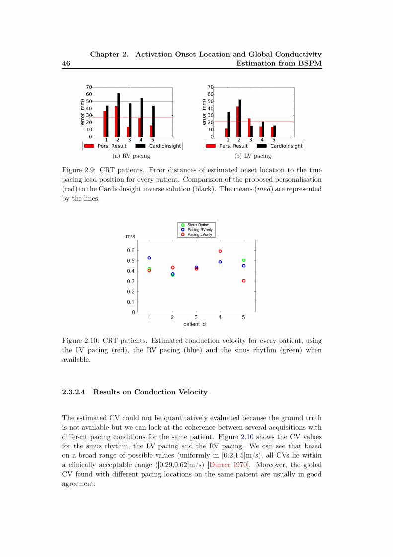
46Chapter 2. Activation Onset Location and Global Conductivity
Estimation from BSPM
1 2 3 4 50
10
20
30
40
50
60
70err
or
(mm
)
Pers. Result CardioInsight
(a) RV pacing
1 2 3 4 50
10
20
30
40
50
60
70
err
or
(mm
)
Pers. Result CardioInsight
(b) LV pacing
Figure 2.9: CRT patients. Error distances of estimated onset location to the truepacing lead position for every patient. Comparision of the proposed personalisation(red) to the CardioInsight inverse solution (black). The means (med) are representedby the lines.
patient Id
1 2 3 4 50
0.1
0.2
0.3
0.4
0.5
0.6
m/s
Sinus Rythm
Pacing RVonly
Pacing LVonly
Figure 2.10: CRT patients. Estimated conduction velocity for every patient, usingthe LV pacing (red), the RV pacing (blue) and the sinus rhythm (green) whenavailable.
2.3.2.4 Results on Conduction Velocity
The estimated CV could not be quantitatively evaluated because the ground truthis not available but we can look at the coherence between several acquisitions withdifferent pacing conditions for the same patient. Figure 2.10 shows the CV valuesfor the sinus rhythm, the LV pacing and the RV pacing. We can see that basedon a broad range of possible values (uniformly in [0.2,1.5]m/s), all CVs lie withina clinically acceptable range ([0.29,0.62]m/s) [Durrer 1970]. Moreover, the globalCV found with different pacing locations on the same patient are usually in goodagreement.

2.3. Personalisation Experiments and Results 47
(a) Sinus rhythm (b) Sinus rhythm (CardioInsight)
(c) RV pacing (d) RV pacing (CardioInsight)
(e) LV pacing (f) LV pacing (CardioInsight)
Figure 2.11: CRT Patient 5 activation maps, the red dot corresponds to the truepacing lead position. (a)(c)(e) Our personalisation result (transmural), (b)(d)(f)CardioInsight solutions (epicardial). (a)(b) Sinus rhythm, (c)(d) RV pacing and(e)(f) LV pacing.
2.3.2.5 Comparison of the Estimated Activation Maps
Figures 2.11a, 2.11c, 2.11e show for Patient 5 the estimated transmural activationmaps obtained after our personalisation for the sinus rhythm, the RV pacing and theLV pacing. The red dot indicates the true pacing lead position as segmented fromthe CT scanner. The early activation zones were found near the true pacing lead.We are also showing the CardioInsight epicardial solution (Figures 2.11b, 2.11d,2.11f). If the comparison shows a good agreement, on this case our personalisationgives a more precise solution. For example, we can see that the sinus rhythm onsetwas found on the septum, which is not visible in the CardioInsight solution.

48Chapter 2. Activation Onset Location and Global Conductivity
Estimation from BSPMm
V
-2
-1
0
1
2n.2 n.45
mV
-2
-1
0
1
2n.82 n.126
ms
0 50 100 150
mV
-2
-1
0
1
2n.170
ms
0 50 100 150
n.207
(a) Sinus rhythm
(CC = 0.32)
mV
-2
-1
0
1
2n.2 n.45
mV
-2
-1
0
1
2n.82 n.126
ms
0 100 200
mV
-2
-1
0
1
2n.170
ms
0 100 200
n.207
(b) RV pacing (CC =
0.83)
mV
-2
-1
0
1
2n.2 n.45
mV
-2
-1
0
1
2n.82 n.126
ms
0 100 200
mV
-2
-1
0
1
2n.170
ms
0 100 200
n.207
(c) LV pacing (CC =
0.48)
(d)
Figure 2.12: CRT Patient 5. Example of 6 BSPM sensors of the QRS measured(black) and personalised (red) in mV per ms. (a) Sinus rhythm (b) RV pacing only(c) LV pacing only. The averaged correlation coefficient are indicated below. (d)Locations of the 6 chosen BSPM sensors, the blue ones are on the back.
mV
-2
-1
0
1
2n.2 n.45
mV
-2
-1
0
1
2n.82 n.126
ms
0 100 200
mV
-2
-1
0
1
2n.170
ms
0 100 200
n.207
(a) Measured
mV
-2
-1
0
1
2n.2 n.45
mV
-2
-1
0
1
2n.82 n.126
ms
0 100 200
mV
-2
-1
0
1
2n.170
ms
0 100 200
n.207
(b) After
preprocess(CC =
−0.15)
mV
-2
-1
0
1
2n.2 n.45
mV
-2
-1
0
1
2n.82 n.126
ms
0 100 200
mV
-2
-1
0
1
2n.170
ms
0 100 200
n.207
(c) After step 1 (CC =
0.65)
mV
-2
-1
0
1
2n.2 n.45
mV
-2
-1
0
1
2n.82 n.126
ms
0 100 200
mV
-2
-1
0
1
2n.170
ms
0 100 200
n.207
(d) After step 2
(CC = 0.83)
Figure 2.13: CRT Patient 5. Example of 6 BSPM sensors for the RV pacing inmV per ms. (black) QRS measured. (green) Pre-processing: simulated QRS usingpatient-specific geometry with random onset location. (orange) Step 1: simulatedQRS after activation onset location estimation. (red) Step 2: simulated QRS afterCV estimation. The averaged correlation coefficient are indicated below.

2.4. Discussion 49
2.3.2.6 Results in terms of BSPM signals
The simulated and the measured BSPMs of patient 5 are represented in Figure 2.12for 6 sensors uniformly chosen. The simulated BSPM has been scaled by its totalnorm and multiplied by the measured BSPM total norm. We calculated for eachrecording the averaged CC between measured and estimated BSPM. We can see agood agreement for the RV pacing and the LV pacing, while the signals of the sinusrhythm are more difficult to reproduce for this patient (CC = 0.32). It may be dueto the fact that this sinus rhythm sequence is complex (presence of scar, possiblymultiple onsets). For the two other sinus rhythm personalisations (patients 1 and2) we found a better agreement with a CC of 0.58 and 0.62. Figure 2.13 depicts theevolution of the estimated signal during the different steps of our personalisation forthe RV pacing. The averaged CC is improved after each step (from -0.15 to 0.83).
2.3.3 Prediction of Stimulation Results from Personalised Model
While our approach does provide an activation map of the myocardium, the mainaim of this personalisation is to benefit from the predictive power of the underlyingforward model. We therefore tested in this section how well the personalised modelscould predict different pacing conditions. To this end, we used the CV results ofour personalisation from the sinus rhythm (estimated in section 2.3.2.4) to simu-late biventricular pacing (when the sinus rhythm was not available, we took themean of the LV pacing and RV pacing). In the clinical procedure several types ofbiventricular pacings were tested by changing the timing between the two stimuli.The 3 classical combinations are: simultaneous pacings; LV stimuli ahead by 40 ms(LV40); RV stimuli ahead by 40 ms (RV40). Results are shown on Figure 2.14 forthe RV40 of Patient 5 and for the LV40 of Patient 4, indicating a reasonably correctprediction in terms of BSPM shape, timings and averaged CC.
2.4 Discussion
2.4.1 Quantifying the Impact of a Precise Myocardial Geometry
Only the data from Patient 5 of the CRT database included MRI and thus allow-ing a precise myocardial segmentation. For other patients, a generic heart meshwas rigidly registered and scaled to the myocardial shape from a CT scanner withimportant artifacts. In this section we want to quantify the impact of a precisemyocardial geometry to our personalisation results in terms of onset location anderrors on BSPM. The results of patient 5 using the MRI segmentation were com-pared to the results using the generic heart manually rigidly registered and scaledto the same location. Since Patient 5 has a scar segmentation available (see Section2.3.2.2), the scar region was also mapped to the generic heart mesh. From Figure2.16, the onset location was found to be less accurate with the generic mesh for theLV pacing (error is 43.4mm for the generic heart, 13.7mm for the MRI segmenta-tion) as well as for the RV pacing (24.3mm for the generic heart, 16.0mm for the

50Chapter 2. Activation Onset Location and Global Conductivity
Estimation from BSPMm
V
-1
-0.5
0
0.5
1n.3 n.43
mV
-1
-0.5
0
0.5
1n.85 n.127
ms
0 50 100 150
mV
-1
-0.5
0
0.5
1n.177
ms
0 50 100 150
n.219
(a) CC = 0.70 (b)
mV
-2
-1
0
1
2n.2 n.45
mV
-2
-1
0
1
2n.82 n.126
ms
0 50 100 150
mV
-2
-1
0
1
2n.170
ms
0 50 100 150
n.207
(c) CC = 0.61 (d)
Figure 2.14: CRT Patients 4 and 5: predictions. (a)(b) Patient 4: biventricularpacing with LV lead ahead by 40ms, using the parameters estimated by our person-alisation of the LV only and RV only. (a) example of 6 BSPM sensors of the QRSmeasured (black) and estimated (red). (b) activation map (generic mesh). (c)(d)Patient 5: biventricular pacing with RV lead ahead by 40ms, using the parametersestimated by our personalisation of the sinus rhythm. (c) example of 6 BSPM sen-sors of the QRS measured (black) and estimated (red). (d) activation map. Thered dots corresponds to the true pacing lead positions.
(a) LV pacing (b) LV pacing (generic mesh) (c) LV pacing (no scar)
Figure 2.15: CRT Patient 5 estimated activation maps for LV pacing, the red dotcorresponds to the true pacing lead position. (a) Result with a personalized geom-etry and scar (same as Figure 2.11e), (b) result with a generic geometry and scar,(c) result with a personalized geometry but no scar.
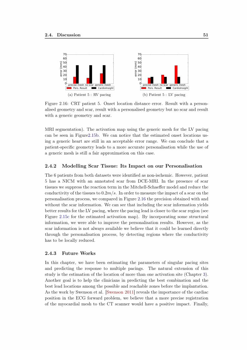
2.4. Discussion 51
precise mesh no scar generic mesh0
10
20
30
40
50
60
70
err
or
(mm
)
Pers. Result CardioInsight
(a) Patient 5 : RV pacing
precise mesh no scar generic mesh0
10
20
30
40
50
60
70
err
or
(mm
)
Pers. Result CardioInsight
(b) Patient 5 : LV pacing
Figure 2.16: CRT patient 5. Onset location distance error. Result with a person-alised geometry and scar, result with a personalised geometry but no scar and resultwith a generic geometry and scar.
MRI segmentation). The activation map using the generic mesh for the LV pacingcan be seen in Figure2.15b. We can notice that the estimated onset locations us-ing a generic heart are still in an acceptable error range. We can conclude that apatient-specific geometry leads to a more accurate personalisation while the use ofa generic mesh is still a fair approximation on this case.
2.4.2 Modelling Scar Tissue: Its Impact on our Personalisation
The 6 patients from both datasets were identified as non-ischemic. However, patient5 has a NICM with an annotated scar from DCE-MRI. In the presence of scartissues we suppress the reaction term in the Mitchell-Schaeffer model and reduce theconductivity of the tissues to 0.2m/s. In order to measure the impact of a scar on thepersonalisation process, we compared in Figure 2.16 the precision obtained with andwithout the scar information. We can see that including the scar information yieldsbetter results for the LV pacing, where the pacing lead is closer to the scar region (seeFigure 2.15c for the estimated activation map). By incorporating some structuralinformation, we were able to improve the personalisation results. However, as thescar information is not always available we believe that it could be learned directlythrough the personalisation process, by detecting regions where the conductivityhas to be locally reduced.
2.4.3 Future Works
In this chapter, we have been estimating the parameters of singular pacing sitesand predicting the response to multiple pacings. The natural extension of thisstudy is the estimation of the location of more than one activation site (Chapter 3).Another goal is to help the clinicians in predicting the best combination and thebest lead locations among the possible and reachable zones before the implantation.As the work by Swenson et al. [Swenson 2011] reveals the importance of the cardiacposition in the ECG forward problem, we believe that a more precise registrationof the myocardial mesh to the CT scanner would have a positive impact. Finally,

52Chapter 2. Activation Onset Location and Global Conductivity
Estimation from BSPM
in this chapter we did not include a Purkinje system model as most of the patientshave bundle branch blocks, but we believe it to be also interesting (see Chapter5). To account for more drastic variations of onset and conductivities, it is neededto use advanced non-linear dimensionality reduction techniques (see Chapter 3 andChapter 4). Even if the current difficulty of the personalisation is to understandand model to complex pathologies, we do think that it could help the analysis ofECGI because the problem is more physiologically constrained.
2.5 Conclusion
From non-invasive measures including BSPM signals, we were able to personalisethe location of the onset activation location and the global conduction velocity ofthe myocardium with a two-step algorithm. We built a large database of simulatedBSPM in order to train a machine learning algorithm based on a few QRS shape-related features from each BSPM sensor. The simulated BSPM relies on a trans-mural forward model based on the Mitchell-Schaeffer model and a current dipoleformulation. We validated our approach on a PVC localisation (MDE = 20.3mm),on 29 runs from 7 pacing sites by catheter (MDE = 21.6mm) and on 10 differentpacing sequences from 5 CRT patients (MDE = 24.6mm). A comparison with twostandard inverse methods revealed that our personalisation provides comparable re-sults. We also showed that we were able to predict the response to biventricularpacings based on our personalised models with concordance in the BSPM signals.Finally, we showed on limited cases that personalised scar and myocardial geometryimproved the results. This is an encouraging first step towards a pre-operative pre-diction of different pacing conditions in order to assist clinicians for CRT decisionand procedure.
The adaptation of this work to 12-lead ECG data was tested and reported inSection 5.3.

Chapter 3
Sparse Bayesian Non-linear
Regression for Multiple Onsets
Estimation in Non-invasive
Cardiac Electrophysiology
Contents
3.1 Introduction . . . . . . . . . . . . . . . . . . . . . . . . . . . . 54
3.2 Materials and Methods . . . . . . . . . . . . . . . . . . . . . . 55
3.2.1 Clinical Data . . . . . . . . . . . . . . . . . . . . . . . . . . . 55
3.2.2 Non-invasive Personalisation of a Cardiac EP Model . . . . . 55
3.2.3 Dimensionality Reduction of the Myocardial Shape . . . . . . 55
3.2.4 Parameter Estimation using Relevance Vector Regression . . 57
3.3 Application to the Personalisation of a Simultaneous
Biventricular Pacing . . . . . . . . . . . . . . . . . . . . . . . . 57
3.3.1 Simultaneous Biventricular Pacing Personalisation . . . . . . 57
3.3.2 Results . . . . . . . . . . . . . . . . . . . . . . . . . . . . . . 59
3.3.3 Evaluation on 3 Other Patients . . . . . . . . . . . . . . . . . 61
3.4 Discussion . . . . . . . . . . . . . . . . . . . . . . . . . . . . . . 61
3.5 Conclusion . . . . . . . . . . . . . . . . . . . . . . . . . . . . . 62
This chapter is based on the following paper:Sparse Bayesian Non-linear Regression for Multiple Onsets Estimation
in Non-invasive Cardiac Electrophysiology, Sophie Giffard-Roisin, HervéDelingette, Thomas Jackson, Lauren Fovargue, Jack Lee, Aldo Rinaldi, NicholasAyache, Reza Razavi, and Maxime Sermesant. In Functional imaging and mod-elling of the heart (FIMH) 2017 Proceedings, Toronto, Canada, June 2017.

54Chapter 3. Sparse Bayesian Non-linear Regression for Multiple Onsets
Estimation in Non-invasive Cardiac Electrophysiology
ECG signals Activation maps
NEW SAMPLE(REAL)
REGRESSION
Feature spaceReduced
shape space
SIMULATEDTRAININGSET (1000)
SIMULATEDTRAINING
SET (1000)
NEW SAMPLE(ESTIMATION) ?
?205 electrodes
RVM:
Relevance
Vector Machine
Figure 3.1: Chapter 4 pipeline: The RVM (relevance vector machine) regression isperformed between BSPM features and a reduced shape space where the patient-specific training activation maps were projected. For a new sample (BSPM data)we estimated its activation map and the regression error. In this paper, the onsetlocations were further extracted from this estimated activation map.
3.1 Introduction
We personalised in Chapter 2 the cardiac EP model from body surface potentialmappings (BSPM). The onset activation location and the global conduction veloc-ity were estimated in different pacing locations from several patients. However,personalisation may often be needed in more complex situations, such as multipleactivation onsets, heterogeneous myocardial tissue (scar) or a particular pathology.Estimation of heterogeneous myocardial conduction using a Bayesian framework hasbeen explored by [Dhamala 2017a], but the other parameters such as the onset aresupposed to be known, and the uncertainty on the result is not estimated. Theproblem of uncertainty in the field of cardiac EP model parameter estimations isvery recently raising interests, for example using Gaussian Process-Based MarkovChain Monte Carlo [Dhamala 2017b].
The contributions of this chapter are the extension of a cardiac EP person-alisation in order to handle non-linear situations (from single to multiple on-sets) and to acquire information relative to the confidence on the results. Themethodology, based on a relevance vector regression and on a myocardial shapedimension reduction, is tested and compared with the method from Chapter 2([Giffard-Roisin 2017b]) on four real biventricular pacing datasets. The method-ology is summarized in Figure 3.1.
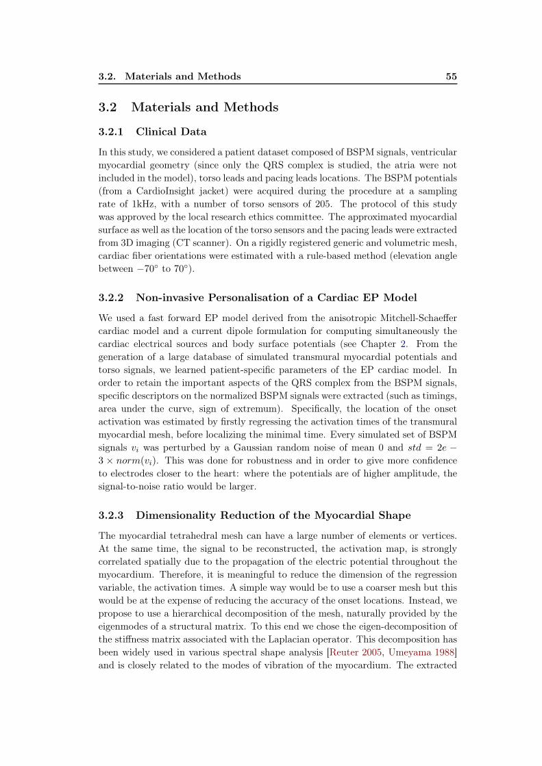
3.2. Materials and Methods 55
3.2 Materials and Methods
3.2.1 Clinical Data
In this study, we considered a patient dataset composed of BSPM signals, ventricularmyocardial geometry (since only the QRS complex is studied, the atria were notincluded in the model), torso leads and pacing leads locations. The BSPM potentials(from a CardioInsight jacket) were acquired during the procedure at a samplingrate of 1kHz, with a number of torso sensors of 205. The protocol of this studywas approved by the local research ethics committee. The approximated myocardialsurface as well as the location of the torso sensors and the pacing leads were extractedfrom 3D imaging (CT scanner). On a rigidly registered generic and volumetric mesh,cardiac fiber orientations were estimated with a rule-based method (elevation anglebetween −70◦ to 70◦).
3.2.2 Non-invasive Personalisation of a Cardiac EP Model
We used a fast forward EP model derived from the anisotropic Mitchell-Schaeffercardiac model and a current dipole formulation for computing simultaneously thecardiac electrical sources and body surface potentials (see Chapter 2. From thegeneration of a large database of simulated transmural myocardial potentials andtorso signals, we learned patient-specific parameters of the EP cardiac model. Inorder to retain the important aspects of the QRS complex from the BSPM signals,specific descriptors on the normalized BSPM signals were extracted (such as timings,area under the curve, sign of extremum). Specifically, the location of the onsetactivation was estimated by firstly regressing the activation times of the transmuralmyocardial mesh, before localizing the minimal time. Every simulated set of BSPMsignals vi was perturbed by a Gaussian random noise of mean 0 and std = 2e −3 × norm(vi). This was done for robustness and in order to give more confidenceto electrodes closer to the heart: where the potentials are of higher amplitude, thesignal-to-noise ratio would be larger.
3.2.3 Dimensionality Reduction of the Myocardial Shape
The myocardial tetrahedral mesh can have a large number of elements or vertices.At the same time, the signal to be reconstructed, the activation map, is stronglycorrelated spatially due to the propagation of the electric potential throughout themyocardium. Therefore, it is meaningful to reduce the dimension of the regressionvariable, the activation times. A simple way would be to use a coarser mesh but thiswould be at the expense of reducing the accuracy of the onset locations. Instead, wepropose to use a hierarchical decomposition of the mesh, naturally provided by theeigenmodes of a structural matrix. To this end we chose the eigen-decomposition ofthe stiffness matrix associated with the Laplacian operator. This decomposition hasbeen widely used in various spectral shape analysis [Reuter 2005, Umeyama 1988]and is closely related to the modes of vibration of the myocardium. The extracted
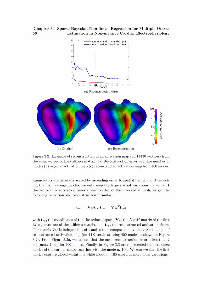
56Chapter 3. Sparse Bayesian Non-linear Regression for Multiple Onsets
Estimation in Non-invasive Cardiac Electrophysiology
(a) Reconstruction error
(b) Original (c) Reconstruction
Figure 3.2: Example of reconstruction of an activation map (on 14430 vertices) fromthe eigenvectors of the stiffness matrix: (a) Reconstruction error wrt. the number ofmodes (b) original activation map (c) reconstructed activation map from 400 modes.
eigenvectors are naturally sorted by ascending order to spatial frequency. By select-ing the first few eigenmodes, we only keep the large spatial variations. If we call tthe vector of N activation times at each vertex of the myocardial mesh, we get thefollowing reduction and reconstruction formulas:
tred = VMt ; trec = VMT tred
with tred the coordinates of t in the reduced space, VM the N×M matrix of the firstM eigenvectors of the stiffness matrix, and trec the reconstructed activation times.The matrix VM is independent of t and is thus computed only once. An example ofreconstructed activation map (on 14K vertices) using 400 modes is shown in Figure3.2c. From Figure 3.2a, we can see that the mean reconstruction error is less than 2ms (max: 7 ms) for 400 modes. Finally, in Figure 3.3 are represented the first threemodes of the cardiac shape together with the mode n. 100. We can see that the firstmodes capture global variations while mode n. 100 captures more local variations.

3.3. Application to the Personalisation of a Simultaneous BiventricularPacing 57
Figure 3.3: Shape modes 1, 2, 3 and 100. We can see that the first modes captureglobal variations while mode n. 100 captures more local variations.
3.2.4 Parameter Estimation using Relevance Vector Regression
In order to regress the myocardial activation times from the BSPM features, weuse the Relevance Vector Machine (RVM) regression method [Tipping 2003]. Thisapproach performs sparse kernel regression based on a sparsity inducing prior on theweight parameters within a Bayesian framework. Unlike the commonly used Elastic-Net or Lasso approaches (based on L1 Norm a.k.a Laplace prior), the RVM methoddoes not require to set any regularization parameters through cross-validation. In-stead, it automatically estimates the noise level in the input data and performs atrade-off between the number of basis (complexity of the representation) and theability to represent the signal. Furthermore, unlike SVM regression or Elastic-Net,it provides a posterior probability of each estimated quantity which is reasonablymeaningful if that quantity is similar to the training set. In our setting, we usedGaussian kernels for the non-linear regression whose variance of the kernel parame-ters need to be defined. The RVM regression only selects the input BSPM featureset that can best explain the activation map in the training set, thus limiting therisk of overfitting. For more details on the relevance vector regression, please referto Section 1.3.5.6. RVM is a multivariate but single-valued approach and thereforethe regression was directly performed on the reduced space of section 3.2.3: only 400regressions are needed to perform an estimation of the 14K activation times. Weused a Gaussian radial basis function with a kernel bandwidth of 1e4 (from cross-validation). On an EliteBook Intel Core i7, a regression of 1000 training samplesand 1235 features runs in 40 sec.
3.3 Application to the Personalisation of a Simultaneous
Biventricular Pacing
3.3.1 Simultaneous Biventricular Pacing Personalisation
We consider here a non-ischemic implanted CRT patient that underwent a pacinglead optimization procedure with a BSPM device. In particular, the 205 workingtorso electrodes recorded a biventricular simultaneous pacing. The anatomy aswell as the location of the torso sensors and the pacing leads were extracted from

58Chapter 3. Sparse Bayesian Non-linear Regression for Multiple Onsets
Estimation in Non-invasive Cardiac Electrophysiology
(a) CardioInsight (b) KRR (c) RVM (d) RVM reduced
Figure 3.4: Results for locating both onsets: ground truth lead locations are the reddots. (a) CardioInsight inverse solution (b) kernel ridge regression activation mapresult (c) relevance vector regression separately for the 14K vertices (d) relevancevector regression on 400 modes of the reduced space. The color maps are showingshort activation times (red) to large ones (purple). On top: flattened representationof the left endocardium in the conventional orientation (i.e. anterior on top).
CT images. Because of important artifacts coming from the pacemaker, only acoarse epicardial geometry of the myocardium is visible. That is why a genericvolumetric myocardial mesh of roughly 65K tetrahedra was manually registeredand scaled to the epicardial geometry. The CardioInsight Technologies softwarealso solves the inverse problem on this epicardial surface (based on the standardformulation using a Tikhonov regularization and the generalized minimal residualalgorithm), see Figure 3.4a. In this work, we used this activation map as part of theevaluation of our method. From this simultaneous pacing, we want to retrieve thetwo onset locations. Locating both activation onset locations by means of an EPmodel parameter estimation has first been studied by He et al. [He 2002], but onlyon synthetic data. For this particular goal, our simulated training set was composedof 1000 simulations with fixed conduction velocity (0.5m/s) and with two onsetlocations randomly selected on the surface of the myocardial mesh (endocardiumand epicardium).

3.3. Application to the Personalisation of a Simultaneous BiventricularPacing 59
3.3.2 Results
We compare here the results of the activation map regression of (i) the Kernel RidgeRegression from Chapter 2, (ii) the RVM regression independently on each pointof the cardiac mesh and (iii) the RVM regression using the reduced shape space(Figure 3.4). The two ground truth onset locations (pacing sites) are the red dots.On top is the flattened representation of the left ventricular endocardium, wherethe apex is at the center [Soto-Iglesias 2016]. The activation map provided by theCardioInsight system on the coarse surface mesh is shown in Figure 3.4a. Althoughthis map is not precise and cannot be used as a ground truth, it gives an idea of thewave shape. We can see that the kernel ridge regression acts as a blurry mixtureof both initializations, not able to separate them. The RVM regression performedon each vertex captures the two onset zones, but the resulting activation maps arenoisy and the two minimal values are not easy to capture. The error distances tothe true pacing leads are 31.7 mm (left lead) and 41.2 mm (right lead). On the otherhand, the RVM performed on the reduced space captures two onset locations withan error distance of less than 23mm for both leads, while having a smooth solution.The mean number of relevance vectors retained was 213 (out of 1000 samples).
The RVM provides the result as a Gaussian probability distribution, where theretained solution of each regression was the mean. By looking at the estimatedvariance across each mode, we can estimate the confidence on our result. On Figure3.5 are plotted the projections on the first spectral modes of the simulated activationmaps (training set) as well as the estimated solution. We have also represented theconfidence interval (+/- standard deviation, std). First, we can see that the retainedsample lies inside the training set point cloud, which is important for RVM toperform well. We have projected the point-wise estimated std onto the myocardialmesh (Figure 3.6a) where we can see that all the vertices from the left ventriclehave an estimated std below 17ms (and below 14 ms for the septum). Althoughhigher values (max: 28.9 ms) are found in the right ventricle, we can notice that theestimated activation times from this region were greater than 100 ms.
However, the confidence on the activation times is not sufficient to quantify theonset location error. This is why we additionally randomly sampled 10K coordinatesfrom the estimated Gaussian distribution in the reduced space (see red ellipsoid fromFigure 3.5). We then reconstructed the activation maps for each one of them andretrieved their minima as estimations of left and the right onsets (see Figure 3.6b forthe right onset). For the most probable location, the distance error to the groundtruth location was 12.3mm for the left lead and 24.5mm for the right lead. Thestandard deviation of the error was 18mm for the left onset and 11.4mm for theright onset. We can notice that the left onset was located more accurately, howeverwith less confidence.

60Chapter 3. Sparse Bayesian Non-linear Regression for Multiple Onsets
Estimation in Non-invasive Cardiac Electrophysiology
(a) (b)
Figure 3.5: Confidence interval in the reduced space (+/- std): (a) projection onmodes 1 and 2 (b) projection on modes 2 and 3. blue dots: projection of the 1000simulated activation maps used for training. Red dot: estimated activation map.
(a) (b)
Figure 3.6: (a) Standard deviation (std) of the estimated activation time, in mil-liseconds. All the points in the left ventricle have an estimated std below 17 ms.(b) Locations of the right onset when randomly sampling the estimated Gaussiandistribution of the reduced space (10K samples).

3.4. Discussion 61
(a) Patient n.2 (b) Patient n.3 (c) Patient n.4 (d) Patient n.4 Car-
dioInsight
Figure 3.7: (a)(b)(c) Results for locating both onsets on 3 other patients: groundtruth lead locations are the red dots. (d) CardioInsight inverse solution for patientn.4 where late activated zones are visible near the LV pacing lead (probably scar).The color maps are showing short activation times (red) to large ones (purple).
3.3.3 Evaluation on 3 Other Patients
We have evaluated our onset estimations on 3 other patients with the same clinicaland same processing protocols. The generic cardiac geometry was also used forthese patients. We can see in Figure 3.7 the mean estimation of the RVM for the3 patients. All activation onsets seem to be captured, with a clear exception forthe patient n.4, where only one onset was captured (the RV onset, on the left). Bylooking at the CardioInsight inverse solution for patient n.4 in Figure 3.7d, we cannotice that the LV pacing site seem to be surrounded by very late activated zones,probably damaged or scar tissue.
3.4 Discussion
The presented method holds several limitations. One current limitation of the RVMregression is the fact that it only performs multivariate regression of a single outputscalar value but not of a vector value (unlike KRR for instance) although multivaluedversions have been recently proposed [Le Folgoc 2017]. Concerning the reconstruc-tion from the reduced space, we also tested it with sharp edges in the activationmap, like scar tissue blocking the activation wave. Despite higher errors of acti-vation times in the scar, the boundaries of the scar were well captured so we canextend our method to ischemic patients. As seen in Figure 3.7c and Figure 3.7d,this extension is necessary for scarred patients.
The estimations of the covariance matrix of the activation map are provided asa by-product of the RVM regression, giving an estimation of the regression error.
62Chapter 3. Sparse Bayesian Non-linear Regression for Multiple Onsets
Estimation in Non-invasive Cardiac Electrophysiology
However, other sources of error may be taken into account in order to have a fullapprehension on the confidence of the result. We think it is the reason why the cloudof possible onsets of Figure 3.6b did not exactly include the true lead. If the torsosensors were well localized by the CT scan, we had to use a generic mesh becauseno precise myocardial shape was available. We would like to test our method onpatient-specific myocardial meshes which will also help in modelling the error sourcewhen using generic meshes. Regarding the errors coming from the BSPM data,they were considerably reduced by the fact that the disconnected or bad leads wereautomatically excluded, and that we added some Gaussian noise to our simulatedBSPM for robustness. Finally, we should also evaluate the EP modelling errors,for instance by analyzing the discrepancy between the true and simulated BSPMsignals.
This new method has been tested on only 4 patients so more experiments areneeded for its validation. As a future work, we want to exploit the generic propertiesof this approach to robustly estimate additional cardiac parameters, like the (local)conduction velocity for instance (see Chapter 4).
3.5 Conclusion
In this chapter, we presented a new methodology for multiple onset estimationfrom BSPM and applied it to 4 clinical datasets. This was integrated in a novelframework for the personalisation of cardiac EP parameters from BSPM data. Thismethod relies on the generation of a simulated patient-specific database on which arelevance vector regression estimates the activation map from a new set of BSPMsignals. As input, specific shape-related features were extracted from the BSPM.As output, the activation map was projected onto a reduced space defined frommyocardial shape oscillations. This pipeline enables the estimation of parametersin more complex situations, as the example presented here with the location of twoonsets from a real biventricular pacing BSPM sequence. This method could be usefulfor a generalization of cardiac EP personalisation, one of the advantages being theconfidence on the regression provided by the RVM.

Chapter 4
Learning Relevant ECGI
Simulations on a Reference
Anatomy for Personalised
Predictions of CRT
Contents
4.1 Introduction . . . . . . . . . . . . . . . . . . . . . . . . . . . . 64
4.1.1 EP Model-based Inverse Problem of Electrocardiography . . 64
4.1.2 Reference Anatomy in ECGI . . . . . . . . . . . . . . . . . . 65
4.1.3 Contributions . . . . . . . . . . . . . . . . . . . . . . . . . . . 65
4.1.4 Outline of the Chapter . . . . . . . . . . . . . . . . . . . . . . 66
4.2 Materials and Methods . . . . . . . . . . . . . . . . . . . . . . 66
4.2.1 Clinical Data . . . . . . . . . . . . . . . . . . . . . . . . . . . 66
4.2.2 BSPM Reference Anatomy . . . . . . . . . . . . . . . . . . . 68
4.2.3 Offline Simulated Common Database . . . . . . . . . . . . . . 69
4.2.4 Relevance Vector Regression for SR Sequence Personalisation 71
4.3 Personalisation Results and Pacing Predictions . . . . . . . 75
4.3.1 Projections on the Reduced Shape Space . . . . . . . . . . . 75
4.3.2 Estimated Sinus Rhythm Activation Maps . . . . . . . . . . . 75
4.3.3 Pacing Predictions Results . . . . . . . . . . . . . . . . . . . 77
4.4 Discussion . . . . . . . . . . . . . . . . . . . . . . . . . . . . . . 80
4.4.1 Reference Anatomy . . . . . . . . . . . . . . . . . . . . . . . 80
4.4.2 Estimating conduction velocity from activation times . . . . . 81
4.4.3 Estimating the uncertainty . . . . . . . . . . . . . . . . . . . 81
4.4.4 AV node Activation . . . . . . . . . . . . . . . . . . . . . . . 82
4.5 Conclusion . . . . . . . . . . . . . . . . . . . . . . . . . . . . . 82
This chapter is based on the following paper:Learning Relevant ECGI Simulations on a Reference Anatomy for
Personalised Predictions of Cardiac Resynchronisation Therapy, SophieGiffard-Roisin, Hervé Delingette, Thomas Jackson, Jessica Webb, Lauren Fovar-gue, Jack Lee, Christopher A. Rinaldi, Reza Razavi, Nicholas Ayache and MaximeSermesant. To be published.

64Chapter 4. Learning Relevant ECGI Simulations on a Reference
Anatomy for Personalised Predictions of CRT
4.1 Introduction
As we have seen in Chapter 1, estimating accurately electrophysiological (EP)patient-specific model parameters is crucial for treatments such as cardiac resyn-chronization therapy, and it often involves invasive measurements [Sermesant 2012].In order to replace these invasive measurements -at risk for the patient-, somestudies proposed to personalise the cardiac EP model from body surface poten-tial mappings (BSPM) [Li 2001, Giffard-Roisin 2017b, Dhamala 2017a]. In one ofthem [Giffard-Roisin 2017b], the onset activation location and the global conduc-tion velocity were estimated in different pacing locations for several patients usinga patient-specific simulated training set. However, personalisation may often beneeded in more complex situations, such as multiple activation onsets or hetero-geneous myocardial tissue (scar). Besides, such patient-specific methods are timeconsuming because a large number of model simulations are needed: the total com-putational time of one model personalisation of Chapter 2 was more than 5 hourson our cluster using parallel computing.
The aim of this article is to develop a reference anatomy model allowing us to per-form a common and offline learning. While reducing considerably the computationaltime of online inference, it also allows to multiply the pathological configurationsin the simulated training set as it is built only once. We have thus extended thecardiac EP model personalisation to infarct situations and applied it to a 20 patientdatabase where the BSPM were recorded using the CardioInsight1 jacket now com-mercially available. The personalised model was then used to predict the electricalresponse to CRT.
4.1.1 EP Model-based Inverse Problem of Electrocardiography
BSPM data has been widely used in the last decades to directly compute the cardiacaction potentials by solving an ill-posed inverse problem: finding the transfer matrixlinking the torso potentials to the cardiac potential sources [Pullan 2010]. Some elec-trocardiographic imaging (ECGI) methods are integrating physiological and model-based priors in a Bayesian framework [Rahimi 2016, Wang 2011]. The work by Liand He [Li 2001] solves the inverse problem by means of heart-model parameters(onset activation location) and was validated with in vivo studies [Liu 2008]. Witha known onset activation location, the estimation of heterogeneous myocardial con-duction using a Bayesian framework has been recently studied by Dhamala et al.[Dhamala 2017a]. The use of non-invasive personalised cardiac parameters for theprediction of new situations (such as pacing procedures) has been tackled on a fewcases only and with a global conductivity parameter in Chapter 2.
1ECVUE, CardioInsight Technologies Inc., Cleveland, Ohio

4.1. Introduction 65
4.1.2 Reference Anatomy in ECGI
These personalisations of EP cardiac model parameters from BSPM data rely ontime-consuming patient-specific computations. Because of the natural similarity ofthe anatomical structures between patients, a reference anatomy can be used.
One study showed the importance of the interindividual variability (aver-aged standard deviation) of electrocardiograms (ECG) on 25 healthy subjects[Hoekema 1999]. A large part of this variability is due to the heart position andorientation relative to electrodes. In terms of geometry, the larger variations arefound for the heart long axis angle. Swenson et al. [Swenson 2011] also revealedthe importance of cardiac angulation in the ECG forward problem. Another studyshowed that ECG imaging is sensitive to global anatomical parameters such as theheart orientation and location with regard to the lead positions [Huiskamp 1989].The use of a reference anatomy model, able to represent every patient, is thus adifficult task. Hoekema et al. [Hoekema 1999] showed that by only moving theelectrodes in a frontal plane to a common reference, the interindividual variability isnot reduced because the heart orientation is not preserved. Another study createda patient-specific adapted torso model by stretching and squeezing a standard torsomodel according to the measures [Lenkova 2012]. They concluded that it was cru-cial to adapt both the outer shape of the torso model and the position of electrodesaccording to reality. Yet, it has been also shown that some adapted ventricle-torsostandard model were able to get good ECGI results while excluding local geomet-rical details [Wang 2010, Rahimi 2015]. To the best of our knowledge, the goals ofthese geometrical models were only to simplify the anatomical modelling process.However, a study has recently tackled the interindividual variability by separatingthe factors of variation throughout a deep network using a denoising autoencoder ona large ECG dataset [Chen 2017b] for learning the ventricular tachycardia origin.Inter-subject variations coming from cardiac EP differences and geometry differ-ences are however not separable, so a personalised EP model could not be estimatedwith this approach.
4.1.3 Contributions
The different contributions of this chapter are:
• A novel reference anatomy approach able to easily represent every patient withpreserved heart orientation and position with respect to the lead positions. Itreduces considerably the computational cost of the personalisation.
• A simulated common database composed of 5 000 heart-torso EP simulationshaving random parameter values in terms of onsets, global conduction valueand scar localisation.
• An EP model-based ECGI technique able to personalise an EP cardiac modelfrom a sinus rhythm BSPM sequence. It is based on a dimensionality reductionof the myocardial shape and a sparse relevance vector regression.

66Chapter 4. Learning Relevant ECGI Simulations on a Reference
Anatomy for Personalised Predictions of CRT
Reference
geometry
Simulated database
(5000 ≠ samples)
Relevance vector regression
(fitting)
Real BSPM signal (QRS)
BSPM matching
to reference geometry
Estimated sinus rhythm activation
Personalised local CV parameters
Prediction of
≠ pacing activations
Mitchell-
Schaeffer Model
Dipole
Formulation
Relevance vector
regression (estimation)
OF
FLI
NE
PA
TIE
NT
-SP
EC
IFIC
Figure 4.1: Fast model-based prediction pipeline: the database composed of 5000EP simulations and the activation map regression fitting are common for the 20patients
• An evaluation on an important database of clinical data composed of 20 pa-tients with a CRT device, and with a comparison to a commercially availableECGI method.
• The simulated predictions of 100 different pacing QRS compared with themeasured BSPM and the commercially available ECGI mapping.
4.1.4 Outline of the Chapter
In the following section 2.2 we will present our prediction framework (Figure 4.1):the clinical data, our reference anatomy model, the simulated EP database and thepersonalisation of the sinus rhythm sequence. Section 4.3 is dedicated to the resultsand the pacing predictions. Finally, section 4.4 discusses the different aspects of themethod.
4.2 Materials and Methods
4.2.1 Clinical Data
Our 20 patients dataset is composed of BSPM signals, ventricular myocardial geom-etry, torso leads and pacing leads locations. All patients have dyssynchrony (eitherleft or right bundle branch block) and were implanted with a biventricular pace-maker (see Table 2.1). The BSPM potentials (from a CardioInsight jacket) wereacquired at a sampling rate of 1kHz during one QRS complex by 200 to 250 torsosensors. The protocol of this study was approved by the local research ethics com-mittee. The approximated myocardial surface, the location of the torso sensors andthe pacing leads were extracted from the 3D CT scanner image. In the stimulation

4.2. Materials and Methods 67
Table 4.1: CRT patients. Baseline information of the 20 patientstreated. NA = information not available; SR = sinus rhythm sequence avail-able; LBBB/RBBB = Left/Right bundle branch block; ICM/NICM/HCM =ischemic/non-ischemic/hypertrophic cardiomyopathy; *: patient #2 was acquired2 times with a 6-months follow-up.
Id Age Gen. Block type Aetiology SR
1 67 M LBBB ICM X2 72 M LBBB HCM
2 6M* 72 M LBBB HCM X3 82 M LBBB NA X4 49 F LBBB NICM X5 79 M RBBB ICM X6 87 M LBBB NICM7 62 M LBBB ICM X8 87 M LBBB ICM X9 77 M LBBB NA X10 69 F LBBB NICM11 49 M LBBB NICM X12 62 F LBBB NA X13 59 M LBBB ICM X14 82 F LBBB NA15 76 M RBBB NICM X16 55 M LBBB NA X18 49 M LBBB NA X19 78 M LBBB NA X20 73 M LBBB NA X22 71 M LBBB NA X
optimisation procedure, cardiologists performed several recordings corresponding todifferent pacing combinations and delays between a right ventricular (RV) endocar-dial and a left ventricular (LV) epicardial pacing leads. For almost all patients, a LVpacing alone and a RV pacing alone were performed, together with the 3 followingbiventricular pacings: simultaneous, LV 40ms (LV lead ahead by 40ms) and RV40ms (RV lead ahead by 40ms). An atrial pacing was active 200ms to 100ms beforethe ventricular pacings. A sinus rhythm sequence was also recorded on patients thatdo not have complete heart blocks. In total, 120 different settings were studied.

68Chapter 4. Learning Relevant ECGI Simulations on a Reference
Anatomy for Personalised Predictions of CRT
4.2.2 BSPM Reference Anatomy
4.2.2.1 Transformation to the Reference Anatomy
In this work, every patient p has a geometry data composed of the 3D biventricularcardiac geometry noted cp and sp = {sjp}j=1:N the locations of the N torso sensors.We define a cardiac and BSPM reference anatomy template {cT ; sT } with sT =
{siT }i=1:M onto which every patient data will be transformed.The current dipole approach formulated in the volume conductor
theory [Malmivuo 1995] has proven its efficiency in BSPM calculation[Giffard-Roisin 2017b]. The electric potential Ψv(sjp) generated by the vol-ume element v and measured at the torso electrode sjp is based on the scalarproduct (jveq, vs
jp) between the equivalent current density jveq of every cardiac
volume element v and the vector directed from v to the torso electrode sjp.Consequently, the shape of the jth BSPM signal Ψv(sjp) is closely linked to thedirection of vsjp. This result is echoing the conclusions of the ECGI sensitivitystudies (see section 4.1.2) showing how the ECG signal is sensitive to the heartorientation and location with respect to the lead positions [Huiskamp 1989].
First, we propose to rigidly register the cardiac geometry cp to the template cT(it is done interactively, as cp is only a coarse epicardial surface and cT a completebiventricular tetrahedral mesh). We define H as the center of mass of the templatecardiac geometry, and HsiT as the half-line from H towards the template torso sensorsiT . We propose the following matching between the template electrodes and theelectrodes of a new patient p:
∀i ≤ M, Ψ(siT ) = Ψ(sjp)
with j = argmink
(
dist(
skp, HsiT
))
This matching between electrodes is not bijective. However, the advantages of thisapproach are that measured BSPM signals are not modified and the direction ofvsjp is best approximated (see Figure 4.2). This projection, allowing the use of areference simulated database, can also be seen as a transfer learning method betweenthe reference domain and the patient-specific domain.
4.2.2.2 Choice of the template
The choice of the template reference anatomy {cT ; sT } is important as cT has torepresent the general shape of the myocardium, and the torso sensors sT should belocated in relevant positions so that every patient would not be too far from it. Inthis study, we used a healthy cardiac mesh of 4K vertices and the 251 torso sensorssT from one of our patients having median torso width and rotation (patient #22).One could estimate a mean shape, but for simplicity and consistency reasons weused real geometries. In Figure 4.3 is shown an example of the matching betweenan original BSPM signal and its translation to the torso geometry.

4.2. Materials and Methods 69
(a) Schematic simple minimal distance matching
(b) Proposed matching of minimal distance to the half straight line
Figure 4.2: Reference anatomy: matching between one template torso electrode siTand the patient electrodes sP . (a) By using a minimal distance between electrodes,the matched electrode would be s3P . (b) With the proposed method, the minimaldistance to the half-line HsiT indicates a matching to the electrode s1P . The resultingangle α corresponding to the difference in heart orientation is thus minimized.
4.2.3 Offline Simulated Common Database
4.2.3.1 Simulated Database
As we do not have ground-truth intra-cardiac measurements on the 20 patients, itis difficult to learn inter-patient information in order to personalise the EP cardiacmodel. In order to generate a common large database with detailed cardiac data,we used EP simulations on the reference anatomy to generate 5 000 virtual caseswith different parameter values. One simulation runs in approximately 2 minuteson our cluster (CPU core Xeon 2.6GHz). This offline database was used as thetraining set for all the personalisations of the cardiac EP model, reducing its onlinecomputational cost.
4.2.3.2 Forward Electrophysiological Model
On the reference myocardial mesh, the cardiac fiber orientations were estimatedwith a rule-based method (elevation angle between −70◦ to 70◦). We simulated

70Chapter 4. Learning Relevant ECGI Simulations on a Reference
Anatomy for Personalised Predictions of CRT
(a) BSPM on Patient #1
(b) Projection of the BSPM on the template torso
Figure 4.3: Example of real BSPM signal matching between the torso of patient#1 and the template, the color represents the voltage at one time point from blue(minimal) to red (maximal). (a) original BSPM signal on the torso of patient #1. (b)projected signal using the proposed matching method on the template, in wireframeare the original torso contours.
the anisotropic electrical activation of the heart using the monodomain version ofthe Mitchell-Schaeffer EP model [Mitchell 2003]. Our forward method is based ona simplified framework composed of sources and sensors in an infinite and homoge-neous domain. We modelled every myocardium volume element (tetrahedron) as aspatially fixed but time varying current dipole. We computed simultaneously thecardiac electrical sources and body surface potentials (see Chapter 2).
4.2.3.3 Variety of Simulations and Parameter Ranges
In order to simulate a large variability of activation maps and their related BSPMsignals, 3 groups of cardiac EP parameters were randomly modified. First, theactivation onset location was randomly selected among all the surface vertices of

4.2. Materials and Methods 71
the cardiac mesh. In order to simulate some more complex and realistic situations,an additional second onset location was selected for every simulation (see Chapter3). Secondly, the global myocardial conduction velocity c was randomly picked in aclinically acceptable range [0.3, 0.7]m/s. Third, in order to capture the conductivityheterogeneity we modelled scar tissue as having no reaction term in the Mitchell-Schaeffer model and a diffusivity reduction of 80%. A varying scar location on theLV with a random and realistic shape [Duchateau 2016] was added in 50% of thesimulations.
4.2.4 Relevance Vector Regression for SR Sequence Personalisa-tion
4.2.4.1 Sinus Rhythm Activation Map Estimation
Using the reference simulated database, we wanted to personalise each patient’s EPbehaviour from the cardiac at-rest recordings, i.e. the sinus rhythm sequence. Forthe patients where the sinus rhythm was not available because of complete heartblocks (see Table 4.1), we used the RV pacing sequence. The different parameters(activation onset locations, conductivity, presence of scar tissue) are linked togetherand their contributions in the resulting BSPM signals are hardly separable. Wetherefore estimated them at the same time, by regressing the cardiac activation map(the myocardial depolarisation times) from the BSPM signals. We first describedthe BSPM signals as a feature vector and we used a dimensionality reduction of therepresentation of the spatial domain given by the myocardial shape. A relevancevector regression was performed between the BSPM features and the reduced acti-vation maps. The first part of the regression (the fitting, taking 6 hours to computeon average on our cluster) is common to every patient and was performed offline,while only the second step is patient-specific (the inference, taking 2 minutes tocompute on average).
4.2.4.2 BSPM Feature Description
For every patient, the torso sensors were matched with the transformation describedin Section 4.2.2.1 to the 251 leads of the template torso. Because the referenceelectrode was not localized, the mean BSPM signal was first subtracted to eachsignal. Then each signal was normalized and smoothed with a local Gaussian filter.We defined specific features from the QRS sequence of every torso leads. Specifically,7 features were extracted from each of the 251 QRS signals (figure 2.3). One BSPMsequence was then represented as the feature vector xi of size L=7x251.
4.2.4.3 Dimensionality Reduction of the Myocardial Shape
As seen in Chapter 3, the myocardial tetrahedral mesh can have a large number ofelements or vertices. At the same time, the signal to be reconstructed, the activationmap, is strongly correlated spatially due to the propagation of the electric potential

72Chapter 4. Learning Relevant ECGI Simulations on a Reference
Anatomy for Personalised Predictions of CRT
ms0 100 200
mV
1
2 3 4
5
67Extracted features:
(1: red arrow) position of the global extremum,(2: red bar) abs. potential of the global extremum, (3: red sign) sign of the global extremum, (4: blue lines)number of zero crossings, (5: green dots) number of local extrema, (6: blue) algebraic area, (7: green sign) sign of the first extremum.
Figure 4.4: Example of BSPM for one torso sensor with the extracted features.
throughout the myocardium. Therefore, it is meaningful to reduce the dimensionof the regression variable, the activation times. A simple way would be to use acoarser mesh but this would be at the expense of reducing the accuracy of theonset locations. Instead, we proposed to use a hierarchical decomposition of themesh, naturally provided by the eigenmodes of a structural matrix. To this end wechose the eigen-decomposition of the stiffness matrix associated with the Laplacianoperator of the tetrahedral shape.
This decomposition has been widely used in various spectral shape analysis[Reuter 2005, Umeyama 1988] and is closely related to the modes of vibration ofthe myocardium. The extracted eigenvectors are naturally sorted by ascending or-der of spatial frequency. By selecting the first eigenmodes, we only kept the modeswith the lowest frequencies corresponding to the largest spatial variations. If we callt the vector of N activation times at each vertex of the myocardial mesh, we get thefollowing reduction and reconstruction formulas:
tred = VMt ; trec = VMT tred
with tred the coordinates of t in the reduced space, VM the N ×M matrix of thefirst M eigenvectors of the stiffness matrix, and trec the reconstructed activationtimes. The matrix VM is independent of t and is thus computed only once. Anexample of reconstructed activation map (on 4K vertices) using M = 400 modes isshown in Figure 3.2c. From Figure 3.2a, we can see that the mean reconstructionerror was less than 1.5 ms (max: 8 ms) for 400 modes.
4.2.4.4 Relevance Vector Regression
In order to regress the myocardial activation times from the BSPM features, we usedthe relevance vector regression (RVR) method [Tipping 2003]. As seen in Chapter3, this approach performs sparse kernel regression based on a sparsity inducing prioron the weight parameters within a Bayesian framework. Unlike the commonly usedElastic-Net or Lasso approaches (based on L1 Norm a.k.a Laplacian prior), theRVR method does not require to set any regularization parameters through cross-validation. Instead, it automatically estimates the noise level in the input data andperforms a trade-off between the number of basis (complexity of the representation)and the ability to represent the signal. Furthermore, unlike SVM regression or

4.2. Materials and Methods 73
(a) Reconstruction error
(b) Original (c) Reconstruction
Figure 4.5: Example of reconstruction of an activation map (on 4312 vertices) fromthe eigenvectors of the stiffness matrix: (a) Reconstruction error wrt. the number ofmodes (b) original activation map (c) reconstructed activation map from 400 modes.
Elastic-Net, it provides a posterior probability of each estimated quantity which isreasonably meaningful if that quantity is similar to the training set.
The RVR estimates the weights w so that we can predict y ∈ RM (here anactivation map in the reduced space) from an input x ∈ RL (here a BSPM featurevector) with a non-linear relationship between x and y as y = wTΦ(x) where Φ isthe non-linear mapping. We consider our dataset of input-target pairs {xi, ti}Ki=1
where we assume that each target ti represents the true model yi with an additionof a Gaussian noise εi = N (0, σ2):
ti = wTΦ(xi) + εi (4.1)
The complexity of the learned relationship between x and y is constrained by limitingthe growth of the weights w. This is done by imposing a zero-mean Gaussian prior

74Chapter 4. Learning Relevant ECGI Simulations on a Reference
Anatomy for Personalised Predictions of CRT
on wi:
P (wi) = N (0, α−1i ) (4.2)
where the αi are hyperparameters modifying the strength of each weight’s prior. α =
{αi}Ki=1 and σ are estimated from a marginal likelihood maximisation [Bishop 2000]via an efficient sequential addition and deletion of candidate basis functions (orrelevant vectors). Because the optimal values of many αi are infinite, the RVR onlyselects the BSPM input set that can best explain the activation map in the trainingset, thus limiting the risk of overfitting.
0 1000 2000 3000 4000 5000 60000.0
0.5
1.0
1.5
2.0
Log-likelihood
(a) Log-likelihood evolution
0 1000 2000 3000 4000 5000 60000
100
200
300
400
500
Number of relevant vectors
(b) Nb of relevant vectors evolution
Figure 4.6: Evolution of the relevance vector regression fitting on the first mode.
RVR is a multivariate but single-valued approach and therefore the regressionwas directly performed on the reduced space of section 4.2.4.3: only 400 regressionsare needed to perform an estimation of more than 4K activation times. In oursetting, a training input-target pair corresponds to a BSPM feature vector xi andits related activation map projected on one mode of the reduced space tmred,i. Weused Gaussian kernels for the non-linear mapping Φ with a kernel bandwidth of1e4. The algorithm2 evolution on the first shape mode (Figure 4.6) shows a rapidconvergence even if small changes in the number of relevant vectors are still visibleafter 3000 iterations. The mean number of retained relevant vectors during thefitting phase was 178 (over 5000 training vectors). As a separate additional step, weregressed from every true BSPM feature vector x its activation map estimation t.
4.2.4.5 Local Conduction Velocity Parameter Estimation
The estimated cardiac activation maps obtained from the sinus rhythm sequencewere used to retrieve patient-specific conduction velocity (CV) parameters. Becausethe regression was performed on simulated activation maps, the resulting solution
2we used a python implementation available at https://github.com/AmazaspShumik/sklearn-
bayes

4.3. Personalisation Results and Pacing Predictions 75
is smooth and physiologically relevant. If we consider that a normal heart QRS isless than 120ms, we make the following hypothesis : regions that are late activatedcorrespond to regions of slow conduction. Specifically, we threshold the estimatedactivation times ta and defined 3 zones: healthy tissue (ta < 120ms, CV = 0.5m/s),damaged tissue (120 < ta < 170ms, CV = 0.3m/s), and scar tissue (170 < ta, noreaction term and diffusion reduced by 80%). We used a single value for the healthytissue based on Chapter 2 where the personalised global CV were all found close to0.5m/s.
4.2.4.6 Pacing Prediction and AV node Activation
For every patient, the true ventricular pacing locations were segmented from theCT scanner image, however the image artefacts due to the device only allow anapproximate lead location. The personalised parameters from sinus rhythm BSPMswere used to predict the activation maps of different pacing situations. On somepatients we found that the RV was activated without ventricular pacing, probablyfrom the atrial pacing (100 to 200ms before) via the AV node. For these patients(#1, #2 6M, #4, #7, #9, #12, #13) we modelled an AV node activation afterthe ventricular pacings. We triggered the earliest activated zones estimated in thesinus rhythm result. Because no recording of atrial stimulation and AV delay wereavailable, the triggering time was arbitrarily set to 40ms.
4.3 Personalisation Results and Pacing Predictions
4.3.1 Projections on the Reduced Shape Space
In Figure 4.7 we showed the RVR results of each real BSPM sequence on the reducedshape space. Because the modes of this space are related to modes of vibration, theresults projected on the larger modes allow us to easily compare the BSPM se-quences. Each grey point represents one simulated activation map used for training.The real sequences of the 20 patients are shown with colours representing the typeof sequence. All the results from the real BSPM data lie inside the training set pointcloud, which is important for the RVR to perform well. We can also see that the 3different pacing sequences are separated in clusters, with the simultaneous betweenthe RV pacing and the LV pacing. The sinus rhythm results in green are almostall situated near the RV pacing cluster, which is to be expected for LBBB patients.Interestingly, we can notice that the two sinus rhythm exceptions that are closer tothe LV pacing group in blue correspond to the two RBBB patients of the cohort(patients #5 and #15).
4.3.2 Estimated Sinus Rhythm Activation Maps
The RVR results of the sinus rhythm sequences in terms of activation map wereused to estimate the local conduction velocity parameter of each patient. In Figure4.8 is represented the mean solution as a transmural activation map (4.8a) that
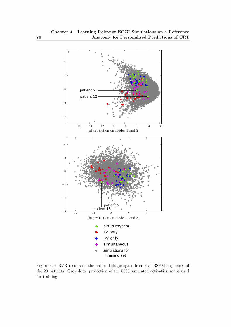
76Chapter 4. Learning Relevant ECGI Simulations on a Reference
Anatomy for Personalised Predictions of CRT
− 16 − 14 − 12 − 10 − 8 − 6 − 4 − 2
− 4
− 2
0
2
4
patient 5
patient 15
(a) projection on modes 1 and 2
− 4 − 2 0 2 4
− 6
− 4
− 2
0
2
4
patient 5patient 15
(b) projection on modes 2 and 3
LV only
RV only
sim ultaneous
sinus rhythm
simulations for
training set
Figure 4.7: RVR results on the reduced shape space from real BSPM sequences ofthe 20 patients. Grey dots: projection of the 5000 simulated activation maps usedfor training.

4.3. Personalisation Results and Pacing Predictions 77
(a) (b)
0.2 0.3 0.5
(c)
Figure 4.8: Sinus rhythm of patient #9 (a) estimated activation map from RVRmethod. up: flattening view of the epicardial surface. (b) CardioInsight epicar-dial inverse solution. (c) Personalised conduction velocity from thresholding theestimated activation map.
was compared with the CardioInsight epicardial inverse solution [Ramanathan 2003](4.8b). The CardioInsight solution is interesting for comparison even if it is only anepicardial surface reconstruction. On top are flat representations of the epicardialsurface [Soto-Iglesias 2016]. The wave shape are similar, with a large late activatedzone on the lateral LV wall with probable scar tissue. In Figure 4.8c are shown theretained zones for healthy, diseased and scar tissues from thresholding of Figure 4.8a.Finally, because the RVR regression provided the result as a Gaussian probabilitydistribution in the reduced shape space, the estimated standard deviation acrosseach mode were projected on the myocardial mesh. The zones with a high estimatedstandard deviation were found near the valves where the mesh is thin, and themedian standard deviation was 0.037s.
4.3.3 Pacing Predictions Results
4.3.3.1 Predicted Activation Maps
From the CV parameters estimated using the RVR solution of the sinus rhythmBSPMs, we ran again our cardiac Mitchell-Schaeffer model with known pacing con-ditions and locations (RV only, LV only, simultaneous, LV 40ms, RV 40ms) andcompared its output to the actual pacing recordings. We recall that in our predic-tions the pacing BSPMs were not used. In Figure 4.9 is represented the predicted

78Chapter 4. Learning Relevant ECGI Simulations on a Reference
Anatomy for Personalised Predictions of CRT
LV 40ms activation map for patient #9 (Figure 4.9a), the prediction if we useda model with a homogeneous myocardial CV (Figure 4.9a) and the CardioInsightsolution (Figure 4.9b). The flat representation allows for a better comparison evenif the projection of the epicardium may differ between two cardiac geometries. Wecan see that the homogeneous CV prediction missed the scar while with the person-alised CV the wave shape and timings globally correspond to CardioInsight. Thedamaged tissue zone on the LV lateral wall (on the left) was well estimated as alsovisible on the CardioInsight map.
(a) homogeneous CV (b) estimated CV (c) CardioInsight
Figure 4.9: LV 40ms pacing prediction of patient #9, flattening epicardial represen-tations of the activation maps (a) pacing prediction using homogeneous conductionvelocity ;(b) using the personalised parameters from sinus rhythm; (c) CardioInsightinverse solution of the actual pacing.
The prediction of LV only pacing of patient 9 is shown on Figure 4.10a. Thepredicted propagation was completely blocked by the scar zone, while an RV acti-vation is visible on the CardioInsight solution Figure 4.10c. With the AV activationmodel (see section 4.2.4.6), the resulting activation map (Figure 4.10b) is closer tothe CardioInsight solution. In Figure 4.7, we could see some LV only projections(red) inside the RV only point cloud: they correspond to patients 1, 9 and 12 allshowing a separate RV activation and also an important LV late activated near theLV pacing lead.
As a quantitative comparison, Figure 4.11 shows the activation times differenceson the flat epicardium, between our predictions and the CardioInsight inverse so-lutions on 20 patients. The total median difference is 23.8ms. It indicates somesimilar activation patterns even if few points have an important difference (higherthan 50ms). A perfect match is difficult because of the epicardial projections differ-ence, the piece-wise constant CardioInsight solution and the approximation in thepacing electrodes locations. We can notice that the LV only seems to be the moredifficult to predict.
4.3.3.2 BSPM predictions
We also predicted the corresponding pacing BSPM signals and compared them withthe true signals. Some signal examples of pacing predictions from patient #3 (Figure

4.3. Personalisation Results and Pacing Predictions 79
(a) estimated CV (b) AV node active (c) CardioInsight
Figure 4.10: LV only pacing prediction of patient #9, flattening epicardial represen-tations. (a) using the personalised parameters from sinus rhythm; (b) adding themodelled activation of the AV node after 40ms; (c) CardioInsight inverse solutionfrom actual recordings of the pacing.
LV only RV only LV 40ms RV 40ms s im.0
20
40
60
80
100
120
140
Acti
va
tio
n t
ime
dif
fere
nce
(m
s)
Figure 4.11: Prediction of pacing activation maps (20 patients): activation timesdifferences on the flattened epicardial points, between our prediction and the Car-dioInsight inverse solution. Median difference (red line): 23.8ms.
4.12) showed a clear improvement when using the personalised CV for the LV only,while the homogeneous CV shows already a good agreement for the RV only. InFigure 4.13 we can see the averaged correlation coefficients (CC) between measuredand predicted BSPM signals. Because the cardiac geometry was generic and thepacing locations not accurate, we cannot expect a perfect match between BSPMs.However, we can see that the mean CC of every pacing type increases when the localCV was personalised from sinus rhythm. In particular, the effects on the LV onlyprediction are highest because the LV damaged tissues can have higher impactson the wave propagation. We can still see some outliers having low CC values.The lowest one (from patient #16) corresponds to the LV only outlier (red) in theprojected modes of Figure 4.7a, in a zone where the training simulations are sparse.
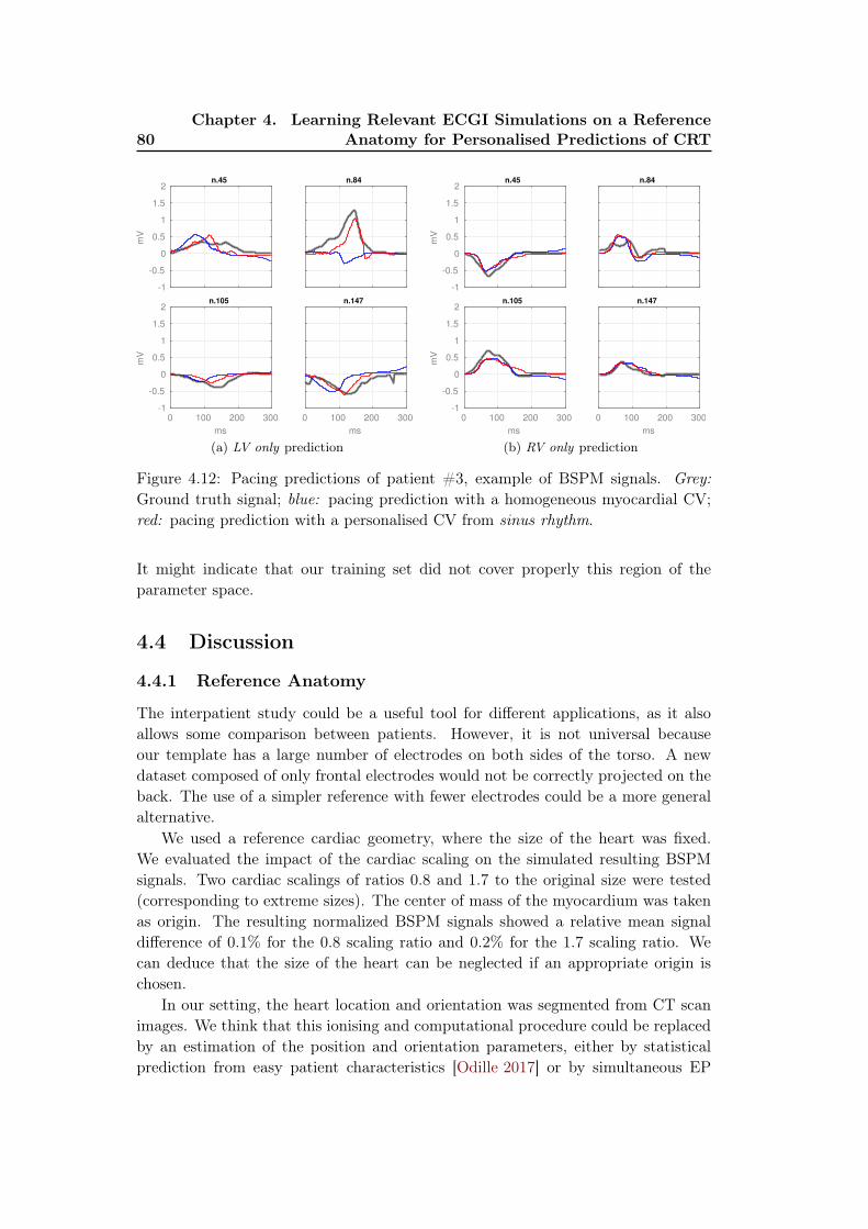
80Chapter 4. Learning Relevant ECGI Simulations on a Reference
Anatomy for Personalised Predictions of CRTm
V
-1
-0.5
0
0.5
1
1.5
2n.45 n.84
ms
0 100 200 300
mV
-1
-0.5
0
0.5
1
1.5
2n.105
ms
0 100 200 300
n.147
(a) LV only predictionm
V
-1
-0.5
0
0.5
1
1.5
2n.45 n.84
ms
0 100 200 300
mV
-1
-0.5
0
0.5
1
1.5
2n.105
ms
0 100 200 300
n.147
(b) RV only prediction
Figure 4.12: Pacing predictions of patient #3, example of BSPM signals. Grey:Ground truth signal; blue: pacing prediction with a homogeneous myocardial CV;red: pacing prediction with a personalised CV from sinus rhythm.
It might indicate that our training set did not cover properly this region of theparameter space.
4.4 Discussion
4.4.1 Reference Anatomy
The interpatient study could be a useful tool for different applications, as it alsoallows some comparison between patients. However, it is not universal becauseour template has a large number of electrodes on both sides of the torso. A newdataset composed of only frontal electrodes would not be correctly projected on theback. The use of a simpler reference with fewer electrodes could be a more generalalternative.
We used a reference cardiac geometry, where the size of the heart was fixed.We evaluated the impact of the cardiac scaling on the simulated resulting BSPMsignals. Two cardiac scalings of ratios 0.8 and 1.7 to the original size were tested(corresponding to extreme sizes). The center of mass of the myocardium was takenas origin. The resulting normalized BSPM signals showed a relative mean signaldifference of 0.1% for the 0.8 scaling ratio and 0.2% for the 1.7 scaling ratio. Wecan deduce that the size of the heart can be neglected if an appropriate origin ischosen.
In our setting, the heart location and orientation was segmented from CT scanimages. We think that this ionising and computational procedure could be replacedby an estimation of the position and orientation parameters, either by statisticalprediction from easy patient characteristics [Odille 2017] or by simultaneous EP
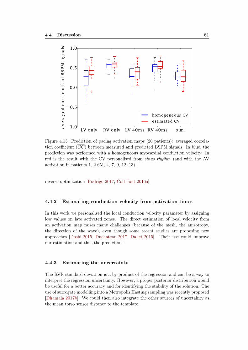
4.4. Discussion 81
LV only RV only LV 40ms RV 40ms s im.1.0
0.5
0.0
0.5
1.0
av
era
ge
d c
orr
. co
ef.
of
BS
PM
sig
na
ls
homogeneous CV
es timated CV
Figure 4.13: Prediction of pacing activation maps (20 patients): averaged correla-tion coefficient (CC) between measured and predicted BSPM signals. In blue, theprediction was performed with a homogeneous myocardial conduction velocity. Inred is the result with the CV personalised from sinus rhythm (and with the AVactivation in patients 1, 2 6M, 4, 7, 9, 12, 13).
inverse optimization [Rodrigo 2017, Coll-Font 2016a].
4.4.2 Estimating conduction velocity from activation times
In this work we personalised the local conduction velocity parameter by assigninglow values on late activated zones. The direct estimation of local velocity froman activation map raises many challenges (because of the mesh, the anisotropy,the direction of the wave), even though some recent studies are proposing newapproaches [Doshi 2015, Duchateau 2017, Dallet 2015]. Their use could improveour estimation and thus the predictions.
4.4.3 Estimating the uncertainty
The RVR standard deviation is a by-product of the regression and can be a way tointerpret the regression uncertainty. However, a proper posterior distribution wouldbe useful for a better accuracy and for identifying the stability of the solution. Theuse of surrogate modelling into a Metropolis Hasting sampling was recently proposed[Dhamala 2017b]. We could then also integrate the other sources of uncertainty asthe mean torso sensor distance to the template..

82Chapter 4. Learning Relevant ECGI Simulations on a Reference
Anatomy for Personalised Predictions of CRT
4.4.4 AV node Activation
We have seen that some patients were activated also from an atrial pacing viathe AV node. We have modelled it with an arbitrary time delay, but we think itwould be possible to integrate it with more complete data (if the atrial stimulationwas recorded). Moreover, the integration of the atria in the ventricular model (forexample as a thin layer [Schenone 2014]) and a study of the whole heart beat ECGcould be beneficial for a precise and global personalisation.
4.5 Conclusion
In this chapter we have developed a methodology for solving the ECG inverseproblem and estimating local cardiac conductivity parameters using a physiologicalmodel-based regression on a reference anatomy. The data matching to the templateanatomy allowed us to use a large offline simulated database of EP forward modelsfor the regression of the BSPM signals from 20 patients with a CRT indication.We used a sparse Bayesian kernel-based regression for the estimation of cardiacactivation maps with the use of specific BSPM descriptors and a reduced spacefor the myocardial geometry. From the CV parameters estimated with the sinusrhythm BSPM sequence, we predicted the responses to different pacing conditions.We compared them with the true pacing BSPMs and with a commercially avail-able epicardial inverse solution (median activation time difference: 24ms). While avalidation with intracardiac recordings is still necessary, we believe that the smallpatient-specific computational time (less than 2 minutes) can be crucial for a clinicaluse.

Part II
Applications and Translation to
Clinics


Chapter 5
From BSPM to 12-lead ECG :
Personalisation Using Routinely
Available Data
Contents
5.1 Introduction . . . . . . . . . . . . . . . . . . . . . . . . . . . . 86
5.2 Estimation of Purkinje Activation from 12-lead ECG . . . . 86
5.2.1 Purkinje System and General Context . . . . . . . . . . . . . 86
5.2.2 Materials and Methods . . . . . . . . . . . . . . . . . . . . . 87
5.2.3 Intermittent Left Bundle Branch Block Study . . . . . . . . . 89
5.2.4 Cardiac Resynchronization Therapy Study . . . . . . . . . . . 91
5.2.5 Electrode Location Perturbation . . . . . . . . . . . . . . . . 92
5.2.6 Conclusion of the Purkinje Estimation . . . . . . . . . . . . . 92
5.3 Activation Onset Localisation from 12-lead ECG . . . . . . 94
5.3.1 Clinical Data . . . . . . . . . . . . . . . . . . . . . . . . . . . 94
5.3.2 Results on Activation Onset Localisation . . . . . . . . . . . 94
5.3.3 Conclusion of the Activation Onset Localisation . . . . . . . . 94
5.4 Conclusion . . . . . . . . . . . . . . . . . . . . . . . . . . . . . 95
This chapter is based on different contributions.Section 5.2 is based on the following paper (except the unpublished CRT ap-plication, part 5.2.4): Estimation of Purkinje Activation from ECG: an
Intermittent Left Bundle Branch Block Study, Sophie Giffard-Roisin,Lauren Fovargue, Jessica Webb, Roch Molléro, Jack Lee, Hervé Delingette, NicholasAyache, Reza Razavi, and Maxime Sermesant. In 7th International StatisticalAtlases and Computational Modeling of the Heart (STACOM) Workshop, Held inConjunction with MICCAI, Lecture Notes in Computer Science, Athens, Greece,October 2016.
Section 5.3 is based on the following paper (thus completing Chapter 2): Non-
Invasive Personalisation of a Cardiac Electrophysiology Model from Body
Surface Potential Mapping, Sophie Giffard-Roisin, Thomas Jackson, LaurenFovargue, Jack Lee, Hervé Delingette, Reza Razavi, Nicholas Ayache, and MaximeSermesant. IEEE Transactions on Biomedical Engineering, 2016.

86Chapter 5. From BSPM to 12-lead ECG : Personalisation Using
Routinely Available Data
5.1 Introduction
In Part I we presented some methodologies to estimate cardiac electrophysiological(EP) parameters from body surface potential mapping (BSPM) data, using between170 to 250 torso electrodes. However, the ECG vest is not routinely used in clinicalpractice. For the analysis of the cardiac electrical activation, the 12-lead ECG (usingonly 9 torso electrodes) is widely used because of its efficiency and reduced cost.The 12 standard Einthoven, Goldberger and Wilson leads (12-lead ECG) measurethe potential differences between selected electrodes (see Figure 5.5).
In this chapter, we will investigate how to personalise the EP cardiac modelusing only 12-lead ECG data. First, we propose a framework for the evaluation of3 conduction parameters (linked to the fast conduction or Purkinje system) fromthe 12-lead ECG in the case of bundle branch block patients. Second, we show anadaptation of the method presented in Chapter 2 for the onset activation estimationusing only the 12-lead ECG. Both studies were evaluated on real datasets.
5.2 Estimation of Purkinje Activation from 12-lead ECG
5.2.1 Purkinje System and General Context
Modelling the cardiac electrophysiology (EP) can help understanding pathologiesand predicting the response to therapies such as cardiac resynchronization therapies(CRT). To this end, estimating patient-specific model parameters is crucial. Inthe case of patients with bundle branch blocks (BBB), part of the Purkinje systemis often affected. The Purkinje fibers are located just beneath the endocardiumand are able to conduct cardiac action potentials quickly and efficiently: typicalconduction velocity (CV) ranges from 2 to 3m/s while it ranges from 0.3 to 0.4m/s
for myocardial cells [Durrer 1970]. Stimulus arrives from the atrioventricular nodethrough the His bundle which separates the network in two branches, the left bundleand the right bundle. When a block occurs in a bundle (LBBB for left, RBBB forright), the Purkinje system is not as efficient and the contraction of the ventriclesisn’t synchronized.
Some studies have been focusing on the understanding of LBBB patterns bysimulating ECGs with different parameters from precise cardiac and torso models[Lorange 1993, Potse 2012]. Because of their complexity, we defined a simpler modelfor the estimation of patient-specific parameters. A study has also recently proposedan EP parameters estimation from ECG data [Zettinig 2014]. It uses two featuresfrom the 12-lead ECG to recover 3 electrical diffusivity parameters using a boundaryelement method forward model and a polynomial regression. As it is difficult todifferentiate the contribution of the Purkinje system, our work was evaluated ontwo particular datasets. The first is an intermittent LBBB case where both LBBBand absence of LBBB (ALBBB) are recorded on 12-lead ECGs. The second is aCRT candidate, where both pre- and post-CRT 12-lead ECGs were recorded. First,an efficient forward EP model is proposed by coupling a 3-parameter cardiac EP
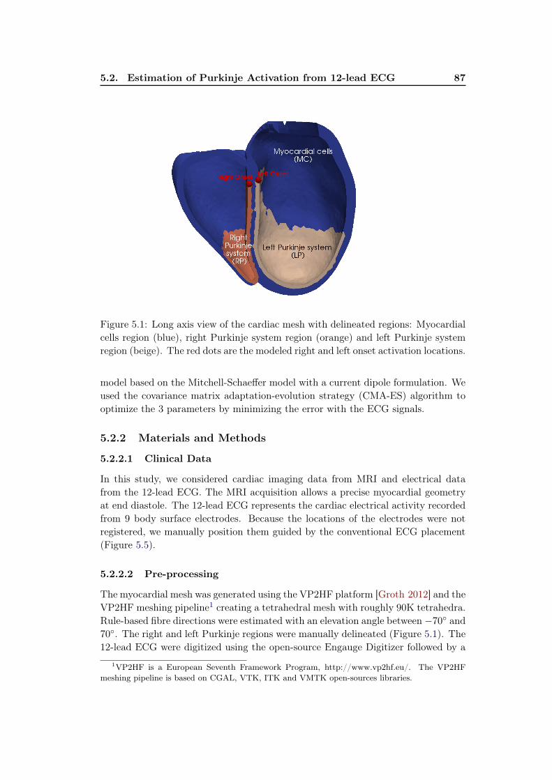
5.2. Estimation of Purkinje Activation from 12-lead ECG 87
Figure 5.1: Long axis view of the cardiac mesh with delineated regions: Myocardialcells region (blue), right Purkinje system region (orange) and left Purkinje systemregion (beige). The red dots are the modeled right and left onset activation locations.
model based on the Mitchell-Schaeffer model with a current dipole formulation. Weused the covariance matrix adaptation-evolution strategy (CMA-ES) algorithm tooptimize the 3 parameters by minimizing the error with the ECG signals.
5.2.2 Materials and Methods
5.2.2.1 Clinical Data
In this study, we considered cardiac imaging data from MRI and electrical datafrom the 12-lead ECG. The MRI acquisition allows a precise myocardial geometryat end diastole. The 12-lead ECG represents the cardiac electrical activity recordedfrom 9 body surface electrodes. Because the locations of the electrodes were notregistered, we manually position them guided by the conventional ECG placement(Figure 5.5).
5.2.2.2 Pre-processing
The myocardial mesh was generated using the VP2HF platform [Groth 2012] and theVP2HF meshing pipeline1 creating a tetrahedral mesh with roughly 90K tetrahedra.Rule-based fibre directions were estimated with an elevation angle between −70◦ and70◦. The right and left Purkinje regions were manually delineated (Figure 5.1). The12-lead ECG were digitized using the open-source Engauge Digitizer followed by a
1VP2HF is a European Seventh Framework Program, http://www.vp2hf.eu/. The VP2HF
meshing pipeline is based on CGAL, VTK, ITK and VMTK open-sources libraries.

88Chapter 5. From BSPM to 12-lead ECG : Personalisation Using
Routinely Available Data
resampling at a rate of 1kHz. Only the 200ms following the Q wave were used (QRSwindow).
5.2.2.3 Forward EP Model
Mitchell-Schaeffer Cardiac Model: We simulated the electrical activation ofthe heart using the monodomain version of the Mitchell-Schaeffer’s EP model[Mitchell 2003], see section 1.3.1.2.
In this work, we considered 3 different domains with uniform conduction ve-locities: the myocardial cells (MC), the left Purkinje system (LP) and the rightPurkinje system (RP). The MC was modelled as one single domain for simplifica-tion reasons. We modelled the LP and RP as a thin layer covering the endocardialsurfaces. By considering that the Purkinje geometry is unknown, this simplificationto a layer allows also a rapid computation. Concretely, the layer is composed of allthe tetrahedra connected to the endocardial surface.
We manually selected the onset activation locations on the septum near thevalves, see Figure 5.1. This was driven by the fact that the electrical wave arrivesfrom the His bundle to the left and right bundles located on the septum.
From Cardiac Simulations to ECG: We computed simultaneously the car-diac electrical sources and body surface potentials. Our forward method is based ona simplified framework composed of sources and sensors in an infinite and homoge-neous domain. As in [Chávez 2015], we modelled every myocardium volume element(tetrahedron) as a spatially fixed but time varying current dipole, see Chapter 2 forfurther details.
5.2.2.4 Parameters Estimation using CMA-ES Algorithm
We estimated the 3 conduction parameters using a Covariance Matrix AdaptationEvolution Strategy (CMA-ES) [Hansen 2006]. It is a derivative-free and stochasticalgorithm that is suited for non-convex continuous optimization problems. At eachiteration, new candidate solutions are sampled from a multivariate normal distri-bution whose covariance matrix is adapted according to the ranking between thecandidate solutions of the previous iteration. We define the score of a simulation S
as its error to the ground truth 12-lead ECGs ΨGT :
f(S) =
∫ T
t=0
1
N
N∑
i=1
|ΨGT (i, t)−‖ΨGT ‖‖ΨS‖
ΨS(i, t)| (5.1)
with N the number of leads (N = 12), T the final time (T = 200ms), ΨGT (i, t)
the ground truth difference of potential of the lead i at time t and ΨS(i, t) thesimulated difference of potential of the lead i at time t. We used a population of100 simulations per generation and optimized over 20 generations. We initializedthe algorithm by a multivariate distribution of mean x0 = (0.6, 0.6, 0.6)m/s andstandard deviation std = 0.1m/s in each direction. We fix the parameter searchingrange at [0.05, 2.5]m/s to avoid non-physical solutions. The best score vs. thenumber of iterations for a parameters estimation is plotted on Figure 5.2.

5.2. Estimation of Purkinje Activation from 12-lead ECG 89
Iteration
5 10 15 20
Be
st
sco
re (
mV
)
0.2
0.22
0.24
0.26
0.28
0.3
Figure 5.2: Best score versus the number of iterations of the CMA-ES algorithm.The score is identified as the mean error between the simulated and real 12-leadECG, in mV.
5.2.3 Intermittent Left Bundle Branch Block Study
5.2.3.1 Intermittent LBBB Patient Data
As a first evaluation of the proposed method, a patient with intermittent LBBBwas selected. The data has been acquired at St Thomas Hospital (London) as partof the VP2HF project. Both LBBB pattern and absence of LBBB (ALBBB) weredocumented on two 12-lead ECG, the ALBBB being recorded after the LBBB. Theparameters were estimated separately for the LBBB and ALBBB. Only the rightonset location was activated for the LBBB whereas both right and left were activatedfor ALBBB because in an LBBB the left bundle is not active.
5.2.3.2 Intermittent LBBB Results
Table 5.1 shows the CV before the parameters estimation, after the LBBB param-eters estimation and after the ALBBB parameters estimation. First, all PurkinjeCV are higher than myocardial CV which is to be expected. We can see that themyocardial cells CV and the right Purkinje CV are very similar between the LBBBand the ALBBB estimations. For the left Purkinje, we found 0.49m/s for LBBBand 1.32m/s for ALBBB, indicating that the model seems to identify the LBBBpathology (affected LP system). Moreover, the MC CV values lie in the myocardialCV range found in the literature [Durrer 1970]. The RP CV (as well as the LP CVfor the ALBBB) is close to the Purkinje CV range found in the literature.
Figure 5.3 shows the simulation results after parameters estimation. Figure 5.3arepresents the true (black) and simulated (blue) 12-lead ECG for the LBBB case andFigure 5.3b the corresponding cardiac activation map. We can see that the shapeof the ECG is coherent with the ground truth and especially the clear notched Rwave on leads V5 and V6, indicator of an LBBB pathology. Figures 5.3c and 5.3ddepict the results for the ALBBB, where both QRS on ECG and activation times are

90Chapter 5. From BSPM to 12-lead ECG : Personalisation Using
Routinely Available Data
100ms
I
II
III
aVR
aVL
aVF
V1
V2
V3
V4
V5
V6
(a) LBBB (b) LBBB
100ms
I
II
III
aVR
aVL
aVF
V1
V2
V3
V4
V5
V6
(c) ALBBB (d) ALBBB
Figure 5.3: Simulation results after parameters estimation. LBBB: (a) Real 12-leadECG (black) and estimated (blue) during the 200 ms after onset activation. (b)Estimated activation map. ALBBB: (c) Real 12-lead ECG (black) and estimated(blue) during the 200 ms after onset activation. (d) Estimated activation map.

5.2. Estimation of Purkinje Activation from 12-lead ECG 91
Table 5.1: Estimated conduction velocities (CV) for LBBB and ALBBB.
CV (m/s) myocardium left Purkinje right Purkinje
Initially 0.6 0.6 0.6LBBB 0.39 0.49 0.95
Absence of LBBB 0.40 1.32 1.22
shorter than for the LBBB. The real and simulated ECG for ALBBB have similarshapes even though we can notice the notched V2 and V3 R waves (so RV and LVare not perfectly synchronous). It may indicate that our Purkinje zone delimitationcould be improved.
The fact that the RP and LP conductions are smaller than the literature rangemay be because we model the Purkinje system as a layer and not a small fibernetwork. For consistency reasons, we initialized the LBBB with only the right onset.However, it leads to different initial settings between ALBBB and LBBB parametersestimation. That is why we also ran the ALBBB using only the right onset: we founda similar myocardial CV (0.39m/s), a higher left Purkinje CV (2m/s) and a smallerright Purkinje (0.17m/s). It seems that the model is compensating the absence ofleft onset, while still showing a clear left Purkinje activation.
5.2.4 Cardiac Resynchronization Therapy Study
5.2.4.1 CRT Candidate Patient Data
We propose in this section to evaluate the Purkinje estimation on another LBBBpatient being a CRT candidate, where both pre- and post-CRT 12-lead ECGs wererecorded. The data has been acquired at St Thomas Hospital (London). For thepost-CRT recording, the patient was under biventricular simultaneous pacing withan RV apex lead and an epicardial LV postero-lateral lead. The exact pacing loca-tions were not recorded so they were manually placed on the cardiac mesh. Thispatient showed presence of scar tissue which was segmented from delayed contrastenhancement MRI. The conduction velocity in the myocardial scar regions was set toa low value (0.2m/s) and the Mitchell-Schaeffer reaction term was set to 0 in theseregions. For this case, we want to evaluate the predictive power of the method: weestimated the 3 conduction parameters from the pre-CRT 12-lead ECG, and usedthem to simulate the post-CRT 12-lead ECG (with pacing). We could finally com-pare the predicted ECG signals under pacing with the real post-CRT ECG signals.
5.2.4.2 CRT Candidate Results
The fitting of the 3 Purkinje parameters from the CMA-ES algorithm on the pre-CRT ECG signals gave the parameters of table 5.2. We can see that the myocardialand left Purkinje values are in the range of the LBBB values found for the inter-

92Chapter 5. From BSPM to 12-lead ECG : Personalisation Using
Routinely Available Data
Table 5.2: Estimated conduction velocities (CV) for the Pre-CRT data.
CV (m/s) myocardium left Purkinje right Purkinje
Initially 0.6 0.6 0.6Pre-CRT 0.36 0.40 0.68
mittent LBBB patient (see table 5.1). On this case the right Purkinje value issmaller even if it remains the higher CV. In Figure 5.4a are shown the simulationresults after parameters estimation using the pre-CRT ECG signals. We can seethat the shape, signs and QRS duration are globally well reproduced, even if somediscrepancies are visible on V5 and V6.
On Figure 5.4c is shown the predicted 12-lead ECG with simulatenous pacing.We recall that the ground truth post-CRT 12-lead ECG is only used as validationand it was not used for the parameters estimation. We can see that here the shapesand timings are well reproduced. Particularly, the changes between pre- and post-signals are visible, such as the sign of II, III, aVL and aVF, the global reduction ofQRS durations but also the time shift of the QRS extremum in V3 (from 100ms to50ms). Again, some discrepancies between ground truth and prediction signals canbe particularly visible on V5 and V6. Because the 9 ECG electrodes were manuallyplaced, we think leads 5 and 6 might be misplaced. A better validation would consistin a dataset where the 9 electrodes are localized.
5.2.5 Electrode Location Perturbation
We have tested the sensitivity of our method to the locations of the 9 torso electrodeby adding Gaussian noise on the intermittent LBBB estimation. After 5 tests witha perturbation mean of 7.5mm in a random direction for each electrode, the relativedifferences to the estimated CVs have a mean of 3% (max = 10%). We can concludethat our method seems to be stable to small perturbations. However, as noted insection 5.2.4.2, some errors on the signals could be avoided by using a dataset wherethe 9 electrodes were localized.
5.2.6 Conclusion of the Purkinje Estimation
In this section, we showed a promising non-invasive parameters estimation for theidentification of the Purkinje system activation using the CMA-ES algorithm. Themethod estimates 3 conduction parameters of the EP cardiac model based on the12-lead ECG and was evaluated on 2 different applications.
For the intermittent LBBB patient, we identified the activation of the Purkinjesystem by independently estimating the parameters of the same patient with andwithout the LBBB pathology. The estimation of CV parameters for LBBB andabsence of LBBB shows a good agreement for the myocardium CV (0.39m/s for
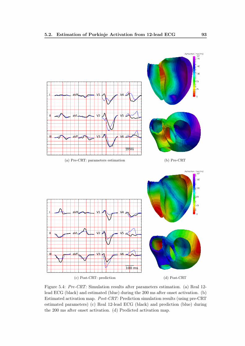
5.2. Estimation of Purkinje Activation from 12-lead ECG 93
(a) Pre-CRT: parameters estimation (b) Pre-CRT
(c) Post-CRT: prediction (d) Post-CRT
Figure 5.4: Pre-CRT: Simulation results after parameters estimation. (a) Real 12-lead ECG (black) and estimated (blue) during the 200 ms after onset activation. (b)Estimated activation map. Post-CRT: Prediction simulation results (using pre-CRTestimated parameters) (c) Real 12-lead ECG (black) and prediction (blue) duringthe 200 ms after onset activation. (d) Predicted activation map.

94Chapter 5. From BSPM to 12-lead ECG : Personalisation Using
Routinely Available Data
ABBB, 0.40m/s for LBBB), while the estimation of the left Purkinje CV seems toidentify the pathology (1.32m/s for ALBBB, 0.49m/s for LBBB).
On the second dataset, we evaluated the predictive power of the method on aCRT candidate. We estimated the personalised parameters on a pre-CRT recordingand showed that we were able to correctly predict the response to pacing.
In both studies, the plots of the simulated 12-lead ECGs and the real ECGsindicate similar shapes. We believe this work to be an interesting first step forunderstanding BBB pathology and selecting the CRT responders based on 12-leadECG.
5.3 Activation Onset Localisation from 12-lead ECG
5.3.1 Clinical Data
The use of 12-lead ECG for onset location has been explored using ECGI methods,and in particular using the fastest route algorithm [van Dam 2013]. We want tostudy here the difference of the personalisation presented on Chapter 2 with BSPMdata to standard 12-lead ECG data. The goal is to estimate the activation onsetlocation from a simulated patient-specific database. As input we provide QRS shape-related descriptors and as output we provide an estimated cardiac activation map.We used a kernel ridge regression (see Chapter 2 for further details).
From the BSPM electrodes of the CRT dataset (5 patients), we extracted foreach patient 9 electrodes roughly located at conventional ECG placements in orderto derive the 12-lead ECG (Figure 5.5). The derivations were performed on thesimulated and on the ground truth signals.
5.3.2 Results on Activation Onset Localisation
We applied our personalisation for the 12-lead ECG data to the 5 CRT patients.The MDE (mean distance error) between true and estimated activation onset was29.8mm, which is slightly higher than the BSPM personalisation (24.6mm). How-ever by looking closely at the results, the errors were particularly important onpatient 2 (RV lead: 57mm, LV lead: 64mm), while small errors were obtained onpatient 5 (RV lead: 10mm, LV lead: 12mm). Knowing that the data from patient2 was of very poor quality and that patient 5 is the only one having a personalisedgeometry (see Chapter 2), the 12-lead ECG may be less robust than BSPM person-alisation. The fact that the onset activation was well located on cases with correctdata quality seems to show that our method is sufficiently constrained such as towork with few signals.
5.3.3 Conclusion of the Activation Onset Localisation
The extension of the BSPM personalisation to standard 12-lead ECG data seem toindicate that for correct quality data, the onset activation can be localized with only12-lead ECG data. This would reduce considerably the complexity and the cost of

5.4. Conclusion 95
Figure 5.5: The 9 electrode locations used for the derivation of the 12-lead ECGand the cardiac mesh.
the procedure. However, for this study the electrodes used were selected from theBSPM vest and thus were precisely localized, which is not the case for the standardECG routine. Moreover, a more refined study (for example by looking at errors interms of epi/endo localisation) would be needed to fully compare the BSPM andthe 12-lead ECG personalisations.
5.4 Conclusion
In this chapter, we investigated the personalisation of a cardiac EP model usingonly data from a 12-lead ECG. We first developed a specific methodology that isable to identify the Purkinje activation and we tested the predictive power of theapproach on a CRT dataset. Then we showed in section 5.3 that using a satisfyingdata quality our personalisation method for onset activation localization is able towork with the 12-lead ECG with similar results. Because the 12-lead ECG is widelyused and of small cost, we think this chapter to be of particular interest, showinghow the cardiac EP personalisation is not restricted to particular and expensiveresearch data.


Chapter 6
Personalisation in a CRT Clinical
Prospective Study
Contents
6.1 Introduction . . . . . . . . . . . . . . . . . . . . . . . . . . . . 98
6.2 VP2HF Project . . . . . . . . . . . . . . . . . . . . . . . . . . 98
6.2.1 Motivation . . . . . . . . . . . . . . . . . . . . . . . . . . . . 98
6.2.2 Goals . . . . . . . . . . . . . . . . . . . . . . . . . . . . . . . 98
6.2.3 European Partners Involved . . . . . . . . . . . . . . . . . . . 98
6.3 CRT Clinical Prospective Study and Modelling Pipeline . . 99
6.3.1 CRT Clinical Prospective . . . . . . . . . . . . . . . . . . . . 99
6.3.2 Modelling Pipeline . . . . . . . . . . . . . . . . . . . . . . . . 99
6.4 Electrophysiological Personalisation as part of a Modelling
Pipeline . . . . . . . . . . . . . . . . . . . . . . . . . . . . . . . 100
6.5 First Results and Patients Modelling Reports . . . . . . . . 102
6.6 Discussion . . . . . . . . . . . . . . . . . . . . . . . . . . . . . . 103
6.7 Conclusion . . . . . . . . . . . . . . . . . . . . . . . . . . . . . 103
This chapter is partly based on the VP2HF deliverables and reports (freely avail-able at http://www.vp2hf.eu/) and on the following VPH 2016 conference abstract:
Personalised Cardiac Electromechanical Modelling in Clinical Time-
frame, Jack Lee, Lauren Fovargue, David Nordsletten, Liya Asner, Myria Had-jicharalambous, Sophie Giffard-Roisin, Maxime Sermesant, Jessica Webb, NicolasSmith, Reza Razavi. Virtual Physiological Human Conference, Amsterdam, TheNetherlands, September 2016.

98 Chapter 6. Personalisation in a CRT Clinical Prospective Study
6.1 Introduction
This PhD thesis is part of the European project entitled VP2HF and we mostlyworked within the work-package entitled ’Non-invasive personalised electrophysio-logical modelling’. Moreover, we contributed to a clinical prospective study wheremechanical and EP models were used to personalise and evaluate the chances ofCRT response of new patients in a clinical time frame. Because BSPM data was notacquired in the prospective study, the personalisation was performed using simplerEP markers and a specific automatic pipeline was developed.
6.2 VP2HF Project
6.2.1 Motivation
Heart failure (HF) is a major health issue in Europe, currently affecting six millionpatients and growing substantially, but the poor short to medium term prognosisof these patients means that treatments such as cardiac re-synchronisation therapy(CRT) and mitral valve (MV) repair can have substantial impact. However, HFtherapies are ineffective in up to 50% of treated patients and involve significantmorbidity and substantial cost.
6.2.2 Goals
The European project VP2HF aims to bring together image and data processingtools, with statistical and integrated biophysical models, into a single clinical work-flow to improve therapy selection and treatment optimisation in HF. This field was,and still is, an emerging field, in which few integrated products are available on themarket. New tools were developed, and existing tools improved, to integrate into asingle clinical HF software platform for intuitive, straightforward use by clinicians;and a prospective clinical study was run to demonstrate the successful translationof the platform into the clinical environment. By using a decision tree stratificationapproach, only the appropriate parts of the tool chain that would add maximumvalue to the predictions were used in individual patients, meaning that the moreresource intensive parts were only used when they provided real value.
6.2.3 European Partners Involved
This 3-year project was funded by the European Union Seventh Framework Programfor research, technological development and demonstration under grant agreementno 611823. It involves 9 European partners: 3 clinical centers (St-Thomas HospitalLondon, CHU Caen, Louvain Hospital), 5 public research teams (King s CollegeLondon, Universtat Pompeu Fabra Barcelona, Inria Sophia-Antipolis, Inria Saclay,Simula Research Laboratory Oslo) and 2 industrial partners (Philips Research, Cen-tron Diasgnostics).

6.3. CRT Clinical Prospective Study and Modelling Pipeline 99
Figure 6.1: Overview of the clinical assessment process, beginning with the patientconsenting to the research, then the clinical assessment and finally the statisticalassessment.
6.3 CRT Clinical Prospective Study and Modelling
Pipeline
6.3.1 CRT Clinical Prospective
A personalised patient selection requires the integration of multidimensional clini-cal data with a suitable decision support system. In the VP2HF project, we havetackled these challenges by combining image and data processing tools with statis-tical and biophysical modelling into a single hierarchical clinical work flow. In 2016,the project has entered a prospective observational trial phase, in which patientsscheduled for CRT implantation were diagnosed using the pipeline in real clinicaltime. The principal goal is to use the non-invasive pre-assessment data to makepatient-specifics therapy outcome predictions. Figure 6.1 represents the overview ofthe clinical assessment process. After the non-invasive acquisitions and the calcu-lation of the clinical biomarkers needed, the decision trees were used to propose apossible outcome after only one day.
6.3.2 Modelling Pipeline
Personalised electromechanical modelling represents the farthermost stage in ourassessment hierarchy, involving the highest level of complexity and data require-ments, and is applied only for those patients regarded as borderline, by other clin-ical biomarkers. If the decision trees indicated modelling after day 1 (Figure 6.1),then the different partners involved in the modelling pipeline worked within a two-week window in order to provide a modelling report with a CRT indication (Figure6.2). The modelling pipeline spans from combined image data processing, to in-verse model parameterisation, finally leading to predictive simulation sweeps. Thetool chain is largely automated, but is designed to be inspected by the operator at

100 Chapter 6. Personalisation in a CRT Clinical Prospective Study
Figure 6.2: Overview of the patient assessment process (Top) and personalised mod-elling pipeline (Bottom). EP: electrophysiology, VM: Ventricular mechanics
pre-defined check points, allowing any necessary interventions and to optimise themodelling trajectory given the available data. The ventricular mechanics part wasperformed at KCL research by Lauren Fovargue, Jack Lee and Simone Rivolo.
6.4 Electrophysiological Personalisation as part of a
Modelling Pipeline
The EP part of the modelling pipeline (Figure 6.2) was included in the PhD work.The EP personalisation is based on the patient-specific geometry, scar morphology,the presence of left or right bundle branch block and the ECG. As a more specificelectrophysiological information is difficult to acquire non-invasively, the optimal ac-tivation pattern for the patient is estimated by incorporating the above informationinto a model to match the QRS duration, from a set of pre-selected pacing locationswith additional clinical guidance.
For the EP simulations, a finite element discretisation of the monodomainequation is solved in conjunction with the Mitchell-Schaeffer model (see section2.2.2.1) providing a spatially dependent depolarisation time map throughout themyocardium. Regional variation of tissue conduction was accounted for by creatingdistinction between healthy tissue, scar, and Purkinje fibres, as shown in Figure 6.3.To simulate LBBB, only right Purkinje fibres were given an accelerated conduc-tion of 1.3m/s (for RBBB patients, only left Purkinje) The scar regions (segmentedfrom late enhancement MRI) were fixed to a minimal value of 0.2m/s. The ini-tial activation site, simulating the sinus rhythm, was taken from literature on the

6.4. Electrophysiological Personalisation as part of a ModellingPipeline 101
Figure 6.3: Regions defined in the electrophysiology (EP) model. Active Purkinjefibres, with fast conduction, are highlighted in gold. Deactivated Purkinje fibresare the basis of left and right bundle branch block, common forms of dyssynchrony.Here, these are modelled by using the same conduction velocity as the healthymyocardium
septum (Figure 6.4).
Fitting the healthy conduction velocity (CV) was achieved through a person-alised training set of 100 simulations with random CV value between 0.15 and 0.8m/s and nearest neighbor regression of the ECG QRS duration. Using the fittedsinus rhythm activation map, some mechanical parameters (passive stiffness andcontractility of the myocardium) were also fitted from 2D echo, tagged MRI dataand left ventricular end systolic pressure (for more details on the mechanical part,see the deliverable 6.4.1 freely available at http://www.vp2hf.eu/).
CRT pacing was induced by fixing the regional personalised conduction and mov-ing initial activation points to the RV apex and LV lead for each pacing location(Figure 6.4). Two stimulating predictions were automatically performed using theMitchell-Schaeffer cardiac model, corresponding to the most used in clinics: simu-latneous pacing and left pacing ahead by 30 ms on the right pacing. On both, theQRS duration was estimated from the activation maps. The pacing activation mapswere also used to predict the mechanical response to CRT by looking at the max-imum LV pressure derivative dP
dt maxand the acute hemodynamic response (AHR,
calculated by the percent increase in dPdt max
). A sensitivity analysis was performedon key parameters arising from susceptible data (such as the peak pressure estimate)giving an uncertainty quantification for the AHR.

102 Chapter 6. Personalisation in a CRT Clinical Prospective Study
Figure 6.4: Onset activation locations manually selected. The sinus rhythm is on theseptum (from literature). The left and right pacing sites correspond to the standardlocations for the biventricular pacing device used in St Thomas Hospital, London.
6.5 First Results and Patients Modelling Reports
The HF platform and the decision trees have been used in all patients who haveconsented to VP2HF in the prospective study. At the time being, more than 50patients were recruited and six entered into the biophysical modelling pipeline andobtaining results within a two-week window (see table 6.1). The final results arestill being compiled since follow-up data from several patients is not available yet.Nevertheless we can already observe than 50% of the patients responded volumet-rically to CRT at 6 months, in line with published literature. Also, more than 50%of the non-responders were identified by the decision trees, which could have hada large impact in the management of these patients if this information would havebeen used for clinician decisions.
The decision trees outcomes of the 6 modelled patients are visible in table 6.1.We can see that the different guidelines are not agreeing, which implied a modellingpipeline. After the whole electromechanical personalisation (2 weeks), a modellingreport was delivered to the clinicians. The first 5 reports are reported in figures6.5,6.6, 6.7, 6.8, and 6.9. They include EP and mechanical responses to pacings.The first 4 patients were estimated to be CRT responders (even if patient n.3 wasfound limited responder), and the patient n.5 was estimated non-responder.
In the name of objectivity, the precise comparison with the true 6-months out-comes are not possible yet. However, we already know that for the modelled patientsn.1, 2, 4 and 5 the outcome prediction of three out of four was correct.

6.6. Discussion 103
Table 6.1: The six patients modelled in the prospective study (LVEF - left ven-tricular ejection fraction, LBBB - left bundle branch block). Reference publishedliterature guidelines : European Society Cardiology (ESC) and National InstituteClinical Excellence (NICE). For every patient, the 3 guidelines are disagreeing.
Patient Etiology LVEF QRSd, LBBB ESC guidelines NICE guidelines Echo dyssynchony
1 Ischaemic 31% 166 ms, LBBB CRT indicated CRT indicated CRT not indicated:no septal flash, abnor-mal ventricular filling,long AV delay
2 Nonischaemic
30% 154 ms, LBBB CRT indicated CRT indicated CRT not indicated:no septal flash, AF, nopassive septal move-ment
3 Nonischaemic
36% Intermittent(84 ms, LBBB)
CRT not indicated Consider CRT CRT indicated: noseptal flash, abnormalventricular filling, nolong AV delay
4 Ischaemic 36% 168 ms, RBBB CRT not indicated Consider CRT CRT not indicated:no septal flash, abnor-mal ventricular filling,long AV delay
5 Nonischaemic
31% 154 ms, LBBB CRT not indicated Consider CRT Consider CRT: septalflash
6 Nonischaemic
40% 168 ms, LBBB CRT not indicated Consider CRT Consider CRT: septalflash
6.6 Discussion
To our knowledge, this is the first time that an electromechanical cardiac modellingwas performed in a non-invasive clinical study and in a reasonable time frame. Onlythe borderline cases were modelled (because of time demand) and we think that itwould be interesting to include some other patients in order to properly validatethe modelling. Moreover, the EP personalisation is only based on the geometry,the scar, the LBBB/RBBB pattern and the QRS duration matching. The complete12-lead ECG was not used because the method presented in section 5.2 was notavailable at the beginning of the prospective study. We believe that it would be animportant step forward. Finally, such a pipeline still needs an important number ofnon-automatic steps and was using the resources of 2 different centers. In the scopeof an integration into a software for clinicians, some important efforts must still bedone.
6.7 Conclusion
In this chapter, we used our EP personalisation into a CRT prospective study in aclinical time frame. Because less data and time was available, BSPM was not usedand a simpler and automatic EP personalisation pipeline was performed to predictthe activation maps under pacing from MRI imaging and sinus rhythm QRS durationand shape. The EP model was integrated in an electro-mechanical personalisationon 6 borderline patients, providing a modelling prediction of the CRT response tothe clinicians.
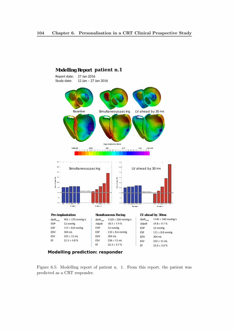
104 Chapter 6. Personalisation in a CRT Clinical Prospective Study
Modelling Report VP2HF_P001
Report date: 27 Jan 2016
Study date: 12 Jan – 27 Jan 2016
Baseline Simultaneous pacing LV ahead by 30 ms
dpdtmax 901 ± 170 mmHg/s
EDP 12 mmHg
ESP 112 ± 8.8 mmHg
EDV 304 mL
ESV 235 ± 11 mL
EF 21.5 ± 4.8 %
Pre-implantation Simultaneous Pacing
dpdtmax 1120 ± 320 mmHg/s
Δdpdt 18.5 ± 7.9 %
EDP 12 mmHg
ESP 110 ± 8.6 mmHg
EDV 304 mL
ESV 236 ± 11 mL
EF 22.3 ± 3.7 %
Simultaneous pacing LV ahead by 30 ms
LV ahead by 30ms
dpdtmax 1140 ± 340 mmHg/s
Δdpdt 19.8 ± 9.7 %
EDP 12 mmHg
ESP 111 ± 8.8 mmHg
EDV 304 mL
ESV 232 ± 11 mL
EF 23.6 ± 3.6 %
Modelling prediction: responder
patient n.1
Figure 6.5: Modelling report of patient n. 1. From this report, the patient waspredicted as a CRT responder.

6.7. Conclusion 105
Modelling Report
Report date: 23 Feb 2016
Study date: 9 Feb – 23 Feb 2016
dpdtmax
948 ± 130 mmHg/s
EDP 11 mmHg
ESP 126 ± 5.5 mmHg
EDV 331 mL
ESV 253 ± 7.3 mL
EF 23.7 ± 1.7 %
Pre-implantation Simultaneous Pacing
dpdtmax
1120 ± 200 mmHg/s
Δdpdt 19.4 ± 3 %
EDP 9 mmHg
ESP 124 ± 5.4 mmHg
EDV 331 mL
ESV 253 ± 7.8 mL
EF 23.5 ± 2 %
Simultaneous pacing LV ahead by 30 ms
LV ahead by 30ms
dpdtmax
1210 ± 260 mmHg/s
Δdpdt 29.9 ± 7.6 %
EDP 9.5 mmHg
ESP 125 ± 5.6 mmHg
EDV 331 mL
ESV 249 ± 7.8 mL
EF 24.8 ± 2 %
QRS = 154 ms QRS = 116 ms QRS = 135 ms
Modelling Prediction : Responder
Responder
Threshold
Responder
Threshold
Baseline Simultaneous pacing LV ahead by 30 ms
Depolarization Time
patient n.2
Figure 6.6: Modelling report of patient n. 2. From this report, the patient waspredicted as a CRT responder.
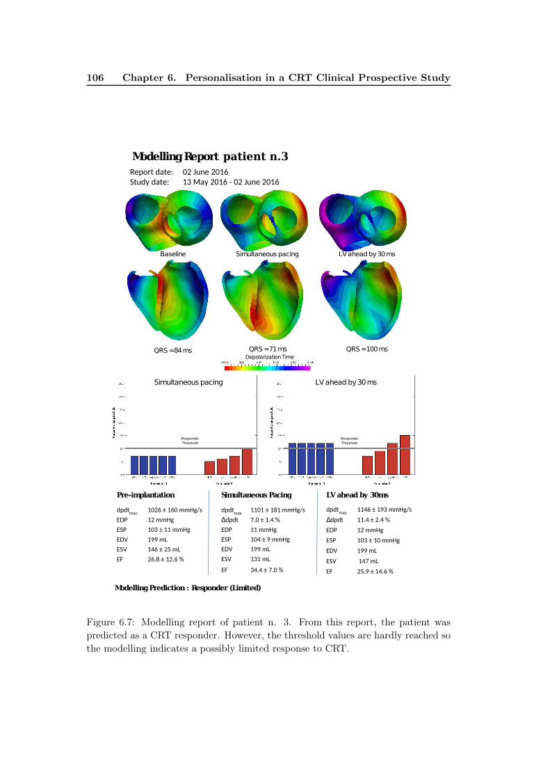
106 Chapter 6. Personalisation in a CRT Clinical Prospective Study
Modelling Report
Report date: 02 June 2016
Study date: 13 May 2016 - 02 June 2016
dpdtmax
1026 ± 160 mmHg/s
EDP 12 mmHg
ESP 103 ± 11 mmHg
EDV 199 mL
ESV 146 ± 25 mL
EF 26.8 ± 12.6 %
Pre-implantation Simultaneous Pacing
dpdtmax
1101 ± 181 mmHg/s
Δdpdt 7.0 ± 1.4 %
EDP 11 mmHg
ESP 104 ± 9 mmHg
EDV 199 mL
ESV 131 mL
EF 34.4 ± 7.0 %
Simultaneous pacing LV ahead by 30 ms
LV ahead by 30ms
dpdtmax
1146 ± 193 mmHg/s
Δdpdt 11.4 ± 2.4 %
EDP 12 mmHg
ESP 103 ± 10 mmHg
EDV 199 mL
ESV 147 mL
EF 25.9 ± 14.6 %
QRS = 84ms QRS = 71 ms QRS = 100 ms
Modelling Prediction : Responder (Limited)
Responder
Threshold
Responder
Threshold
Baseline Simultaneous pacing LV ahead by 30 ms
Depolarization Time
patient n.3
Figure 6.7: Modelling report of patient n. 3. From this report, the patient waspredicted as a CRT responder. However, the threshold values are hardly reached sothe modelling indicates a possibly limited response to CRT.

6.7. Conclusion 107
Modelling Report
Pre-implantation Simultaneous Pacing
Δ
Simultaneous pacing LV ahead by 30 ms
LV ahead by 30ms
Δ
QRS = 169 ms QRS = 172ms QRS = 142 ms
Modelling Prediction : Responder
Responder
Threshold
Responder
Threshold
Baseline Simultaneous pacing LV ahead by 30 ms
Depolarization Time
patient n.4
Figure 6.8: Modelling report of patient n. 4. From this report, the patient waspredicted as a CRT responder.

108 Chapter 6. Personalisation in a CRT Clinical Prospective Study
Modelling Report
Report date: 30 November 2016
Study date: 12 Sept - 30 November 2016
dpdtmax
659 ± 37 mmHg/s
EDP 5 mmHg
ESP 118 ± 4 mmHg
EDV 246 mL
ESV 206 mL
EF 17 %
Pre-implantation Simultaneous Pacing
dpdtmax
601 ± 32 mmHg/s
Δdpdt -8.9 ± 1 %
EDP 5 mmHg
ESP 116 ± 4 mmHg
EDV 246 mL
ESV 211 mL
EF 14 %
Simultaneous pacing LV ahead by 30 ms
LV ahead by 30ms
dpdtmax
623 ± 32 mmHg/s
Δdpdt -5 ± 1 %
EDP 12 mmHg
ESP 115 ± 4 mmHg
EDV 246 mL
ESV 210 mL
EF 15 %
QRS = ms QRS = ms QRS = ms
Modelling Prediction : Non-Responder
Responder
Threshold
Responder
Threshold
Baseline Simultaneous pacing LV ahead by 30 ms
Depolarization Time
134 143123
patient n.5
Figure 6.9: Modelling report of patient n. 5. From this report, the patient waspredicted as a non-responder.

Chapter 7
Pre-clinical Electro-mechanical
Model Personalisation on Canine
Data
Contents
7.1 Introduction . . . . . . . . . . . . . . . . . . . . . . . . . . . . 110
7.2 Models and Methods . . . . . . . . . . . . . . . . . . . . . . . 110
7.2.1 Geometry Processing . . . . . . . . . . . . . . . . . . . . . . . 111
7.2.2 Electro-Mechanical Modelling: SOFA Software . . . . . . . . 112
7.3 Parameter Estimation . . . . . . . . . . . . . . . . . . . . . . . 113
7.3.1 Sensitivity Study . . . . . . . . . . . . . . . . . . . . . . . . . 113
7.3.2 Mechanical Parameters Calibration: Unscented Transform Al-
gorithm . . . . . . . . . . . . . . . . . . . . . . . . . . . . . . 114
7.4 Results . . . . . . . . . . . . . . . . . . . . . . . . . . . . . . . . 114
7.4.1 Clinical Data . . . . . . . . . . . . . . . . . . . . . . . . . . . 114
7.4.2 Current Results . . . . . . . . . . . . . . . . . . . . . . . . . . 115
7.4.3 Discussion and Improvements . . . . . . . . . . . . . . . . . . 115
7.5 Conclusion . . . . . . . . . . . . . . . . . . . . . . . . . . . . . 117
This chapter is based on the following paper:Evaluation of Personalised Canine Electromechanical Models, SophieGiffard-Roisin, Stéphanie Marchesseau, Loic Le Folgoc, Hervé Delingette, andMaxime Sermesant. In Proceedings of the 5th international STACOM workshop(Boston, September 18, 2014), held in Conjunction with MICCAI 2014. LectureNotes in Computer Science, Boston, September 2014.

110Chapter 7. Pre-clinical Electro-mechanical Model Personalisation on
Canine Data
7.1 Introduction
This work is part of a 2014 challenge on cardiac electromechanical (EM) modelling,where cardiac simulations were evaluated by comparing with the true cardiac move-ments recorded by tagged MRI. Several EM methods were finally compared in orderto accelerate progress in the use of such models for clinical use.
Cardiac modelling aims at understanding cardiac diseases (such as heart failure,desynchronization or tachycardia) and predicting cardiac responses to treatment ortherapies (as cardiac resynchronization therapy or radiofrequency ablation). Thegoal is to help cardiologists in detecting anomalies, planning interventions, andselecting suitable patients for a given therapy. Cardiac modelling is driven by theassumption that the electromechanical response of the heart can be simulated fromanatomical and physiological data.
Heartbeat is initiated by an electrical wave that propagates through the my-ocardium, activating mechanical contraction at a microscopic scale. A suitablemodel needs to take into account the anatomical structure, the electrical propaga-tion, as well as the mechanical function of the heart.
For an efficient EM modelling, this work is based on an Eikonal model[Sermesant 2007] for the simulation of the electrophysiological system. The activeand passive mechanical behavior is defined by the Bestel-Clement-Sorine modellingas formulated in [Chapelle 2012]. The latter ensures to take into account the micro-scopic scale phenomena of the contraction as well as laws of thermodynamics.
The coupled electro-mechanical simulation of the cardiac system is implementedwithin the SOFA platform1. The simulations were performed on healthy canineclinical data, provided by the STACOM’2014 challenge. They include left ventricular(LV) geometry, LV volume and LV pressure curves, as well as myocardial fibredirections.
7.2 Models and Methods
Canine and human hearts have close anatomical structures, that is why the canineheart is often used in pre-clinical studies. Both anatomies are composed of twoventricles, left (LV) and right (RV), and two atria. The heart function is mainlydriven by the LV, acting like a pump to send the blood to the body. The systemstudied here is composed of a healthy canine left ventricle. In order to run theelectrical and the mechanical cardiac models, input such as anatomical meshes andfibre directions have been processed.
1SOFA is an Open Source medical simulation software available at http://www.sofa-
framework.org

7.2. Models and Methods 111
(a) (b) (c)
Figure 7.1: Geometry and fibres processing: Identification of the surface zones of theLV myocardium mesh (a), pericardium surface membrane (b) and fibre directionsfrom DTI imaging (c).
7.2.1 Geometry Processing
7.2.1.1 Myocardial Mesh Generation.
The myocardium mesh is generated using CGAL2 meshing software, to create atetrahedral mesh from medical image segmentations. The geometry is computed atend diastole (ED). The number of elements is roughly 50K, so that the average edgelength is close to 1.5mm. This refinement ensures to have enough elements in thethickness of the muscle to describe the anisotropy (at least 5 layers transmurally)while limiting computation time.
In addition to the volumetric mesh segmentation, endocardial (inner lining) andepicardial (outer layer) surface zones are manually delineated, as illustrated in Fig.7.1a. These surface zones are useful for the electrical as well as for the mechanicalsimulations (Sec. 7.2.2).
For a single left ventricular model we consider that the contraction of the leftventricle does not depend on that of the RV as a first approximation. We departfrom classic anatomical terminology in identifying the epicardium with the outerlayer of the left ventricle segmentation.
7.2.1.2 Pericardium Surface Generation.
Our model incorporates boundary conditions that faithfully replicate anatomicalconstraints on the motion of the heart. Specifically, the pericardial membrane ismodelled as a fixed surface around the epicardium as in [Marchesseau 2013], andwas obtained by dilating the segmentation from the diastasis phase of 1.5 mm, seeFig. 7.1b). The SOFA simulation platform allows for realistic collision constraintsbetween the myocardium and the surrounding pericardium, which limits radial mo-
2CGAL is a Computational Geometry Algorithms Library, available at www.cgal.org.

112Chapter 7. Pre-clinical Electro-mechanical Model Personalisation on
Canine Data
Figure 7.2: Complete electromechanical pipeline. A single simulation computessimultaneously the electrical and the mechanical modellings.
tion but also global translations. We model the presence of the RV as part of apericardium membrane surrounding the LV. This is motivated by the fact that thepressure applied by the RV on the external wall of the LV could be approximatedby a rigid constraint.
7.2.1.3 Fibre Directions.
The myocardium is organized in muscle fibres which govern the electric propagationas well as the anisotropic contraction. The anisotropic tensor at each position canbe measured via DTI imaging, and the principal directions (from eigen value de-composition) generate an approximation of the fibre directions. They are displayedin Fig. 7.1c.
7.2.2 Electro-Mechanical Modelling: SOFA Software
The pipeline efficiently couples the simulation of the electrophysiology and mechan-ics of the heart in the SOFA platform. The electrical wave propagation is simulatedin the ED configuration, during the first step of the cardiac cycle. The mechanicalcontraction and relaxation of the myocardium are simultaneously computed fromthe depolarization times output by the electrical simulation, taking into account thedifferent forces and boundary conditions. The pipeline is summarized in Fig. 7.2.
7.2.2.1 Electrophysiological Simulation: Eikonal Model.
The electrophysiological pattern of activity is simulated using an Eikonal model, de-scribing the depolarization front propagation. The depolarization times Td at each
node of the mesh are estimated by solving the Eikonal equation v√
∇T tdD∇Td = 1
using a Multi-Front Fast Marching Method [Sermesant 2007]. v is the local conduc-tion velocity, set here uniformly to 500 mm/s. D is the anisotropic tensor, with ananisotropic ratio of 0.1 between the fibre direction and the perpendicular directions,and with local fibre directions estimated according to section 7.2.1.3.

7.3. Parameter Estimation 113
The initialization of the electric wave is set on the LV endocardial surface (seeFig. 7.1a), to simulate a simultaneous activation pattern of the endocardium fromthe extremities of the Purkinje network.
7.2.2.2 Mechanical Simulation: Bestel-Clement-Sorine Model.
Our study is based on Bestel-Clement-Sorine (BCS) mechanical modelling as for-mulated by [Chapelle 2012], improved and implemented on the SOFA platform by[Marchesseau 2013]. The BCS model is compatible with the laws of thermodynamicsand it is based on the microscopic scale phenomena.
It is composed of a passive hyperelastic part described as a Mooney Rivlin ma-terial, that accounts for the elasticity. The stress along the cardiac fibres is decom-posed into two parts. An active part models the contraction (binding/unbindingof actin-myosin filaments) together with an energy dissipation due to friction, anda parallel passive part corresponds to the elastic bound. The model is further im-proved by taking into account the circulation model representing the 4 phases of thecardiac cycle. Especially, the aortic pressure is modelled following a 2-parameterWinkessel model.
The BCS model is in particular able to capture the Starling effect (adaptation ofthe contraction enabling the stroke volume to compensate the end-diastolic volume)and the unbinding due to a too high relative speed between actin and myosin, witha constant α related to the cross-bridge release. For more details on the mechanicalmodel, refer to [Marchesseau 2013].
7.3 Parameter Estimation
We use the approach described in [Marchesseau 2013] to estimate the parameterson canine hearts. Note that [Marchesseau 2013] was used to estimate parameters onhuman data and therefore cannot be applied as it is since the geometry, the cardiacperiod and the mechanical materials are different. A complete sensitivity study anda personalized calibration of the most relevant parameters have been performed.
7.3.1 Sensitivity Study
The parameters of the model are summarized in Tab. 7.1. The electrophysiologicalmodel is governed by a simple law, and has therefore mainly three parameters (oncefibre directions and initial conditions are set), the local conduction velocity v, theanisotropic ratio A and the action potential duration (APDs). For the mechanicalpart, the parameters can be separated in 3 groups: parameters related to the activecontraction, parameters related to the passive material, and parameters related tothe heamodynamic model.
Starting from the results of [Marchesseau 2013], a quantitative study has beenperformed in order to estimate the range of possible values of each parameter of Tab.7.1. We used pressure and volume observations to control the simulation. Some

114Chapter 7. Pre-clinical Electro-mechanical Model Personalisation on
Canine Data
Parameter Name Unit case 1 case 2 case 3 case 4
EPA (Anisotropic Ratio) 0.1 0.1 0.1 0.1
v (Local Cond. Velocity) mm.s−1 500 500 500 500
APD (Action Pot. Dur.) s 0.18 0.18 0.20 0.24
Contraction
σ0 (Max Contraction) MPa 30 29 20 21
k0 (Max Stiffness) MPa 6 6 6 6
kATP (Contraction Rate) s−1 40 40 40 40
kRS (Relaxation Rate) s−1 90 90 90 90
E (Linear Modulus) MPa 5 5 5 5
α (Cross-bridges Rate) 0.8 0.8 0.8 0.8
µ (Viscosity) MPa.s 0.32 0.32 0.5 0.49
n0 (Red. factor, Starling) 0.5 0.5 0.5 0.5
Passive Mat.c1, c2 (Mooney-R. Mod.) kPa 50 50 50 50
K (Bulk Modulus) MPa 1.7 1.7 2 1.9
WindkesselRp (Wind. Resistance) MPa.m−3s 179 250 310 430
τ (Wind. Charact. Time) s 0.22 0.16 0.23 0.56
Table 7.1: Parameters of the electro-mechanical model for the 4 cases.
parameters do not impact significantly the simulation, as the maximum stiffness k0.Others are easily calibrated, because they are visually perceptible, as the APD.
7.3.2 Mechanical Parameters Calibration: Unscented TransformAlgorithm
The most influential and independent parameters identified as [σ, µ, K]have been calibrated for each heart using the Unscented Transform Algorithm[Julier 1997]. The algorithm, derived from the Unscented Transform according to[Marchesseau 2013], calculates a set of n parameters of a nonlinear transformationthat minimizes the difference between the measured observations and the predictedobservations. Once having performed 2n+1 simulations using some specific param-eter values, the algorithm runs in one iteration. In our case, the observations arethe minimal LV outgoing blood flow and the ejection fraction. LV outgoing flow iscalculated as −dV/dt, with V the LV volume.
Independently, the Unscented Transform algorithm was used to calibrate the2-parameter Windkessel model using the ground truth pressure curves.
7.4 Results
7.4.1 Clinical Data
The STACOM 2014 challenge revolves on data acquired on 4 healthy canine hearts.They include LV geometry and fibre directions. The 4 dogs were paced at 500ms

7.4. Results 115
(a) case 1 (b) case 2 (c) case 3 (d) case 4
Figure 7.3: Comparison between LV pressure volume diagrams computed from sim-ulations (red) and ground truth measures (blue).
Figure 7.4: Simulated end-systolic geometry (red) of the LV of the 4 cases andground truth (blue). The dark blue line represents the initial position (ED).
basic cycle length. The tetrahedral mesh is constructed from binary images of theLV at ED.
7.4.2 Current Results
We give the results of the 4 canine simulations in terms of LV pressure volumediagrams (Fig. 7.3), LV volume, LV outgoing flow curves (Fig. 7.5) and ejectionfractions (Tab.7.2). Comparison is made with the ground truth data, as LV volumeand LV pressure curves were provided by the STACOM’2014 challenge for a completecycle. We are displaying here the second cycle of the simulation, in order to avoidthe wrong initial conditions.
The simulated geometry of the 4 cases at ES is shown in Fig. 7.4. The groundtruth end-systolic position is shown in blue while red is the simulation. The darkblue line represents the initial position (ED).
7.4.3 Discussion and Improvements
This first study shows promising results: the LV pressure volume diagrams and vol-ume variations comparison indicate a realistic response of the model. Furthermore,the large variability of ejection fraction is reproduced in our results. We can alsosee from the slices of Fig. 7.4 that the modelled ventricle has a realistic movement

116Chapter 7. Pre-clinical Electro-mechanical Model Personalisation on
Canine Data
(a) case 1
(b) case 2
(c) case 3
(d) case 4
Figure 7.5: Comparison between LV volume and outgoing flow (as −dV/dt) vari-ations over one cardiac cycle computed from simulations (red) and ground truthmeasures (blue).

7.5. Conclusion 117
Ejection fraction case 1 case 2 case 3 case 4
Measured (%) 53 49 30 34
Estimated (%) 43 42 33 36
Table 7.2: Comparison between ejection fractions computed from the simulationsand the ground truth measures.
(note the correct apico-basal shortening). However, the myocardium wall thicknessvariation is not completely reproduced, corresponding to a simulated muscle notincompressible enough.
The calibration of a model of a standard case is the first step towards the pre-diction of its response to treatments and therapies. Since our model is driven byfaithful anatomical constraints and mechanical laws, we are confident in the factthat such a model will be able to realistically simulate pathology cases and predicttheir responses to treatments.
7.5 Conclusion
In this chapter we have adapted an electro-mechanical cardiac modelling to caninehearts. From the geometry of the left ventricle in end diastole and the heart periodand the fibre directions, we are able to simulate heart movement over the wholecardiac cycle. The quantitative validation (results of the STACOM’2014 challenge)is comforting the tendency of the global indicators: the displacement fields obtainedwith the simulations and the displacement fields obtained by tagged MRI providedby the STACOM’2014 challenge are in good agreement.
In the scope of electrophysiological models, it is essential to also evaluate theresulting cardiac movement. These pre-clinical studies with very precise data areessential for building accurate methods. We can see that for this study on healthycanine hearts, a simple Eikonal electrical model was able to capture the EP dy-namics. However, more complex pathologies might need a more physiological EPmodel.


Chapter 8
Conclusion
Contents
8.1 Contributions Summary . . . . . . . . . . . . . . . . . . . . . 119
8.2 Publications and Awards . . . . . . . . . . . . . . . . . . . . . 120
8.2.1 Publications . . . . . . . . . . . . . . . . . . . . . . . . . . . . 120
8.2.2 Awards . . . . . . . . . . . . . . . . . . . . . . . . . . . . . . 122
8.3 Perspectives . . . . . . . . . . . . . . . . . . . . . . . . . . . . . 122
8.3.1 Clinical Perspectives . . . . . . . . . . . . . . . . . . . . . . . 122
8.3.2 Methodological Perspectives . . . . . . . . . . . . . . . . . . . 123
In this thesis, we explored the non-invasive EP cardiac model personalisation.We will now summarize the main contributions and propose some perspectives ofthe work.
8.1 Contributions Summary
We developed non-invasive methods for the personalisation of some parameters ofthe cardiac EP model, filling the gap between ECG imaging and model personalisa-tion. Even if these new techniques are still exploratory approaches we focused ourwork to their clinical relevance by a constant evaluation on real data. Moreover,we concretely worked on specific methods using routinely available data and on anintegration in a clinical time-frame.
We summarize here the main achievements of this PhD work.
• We proposed a fast physiological simulation of the cardiac EP propagation to-gether with BSPM signals on the torso using the SOFA platform. The efficientforward model is based on the cardiac Mitchell-Schaeffer model and a currentdipole formulation on an infinite domain, allowing to simultaneously calcu-late transmural cardiac potentials and BSPMs. We compared our results witha boundary element method simulation showing only small signal amplitudedifferences.
• We proposed a non-invasive estimation of patient-specific ventricular EP pa-rameters from a large simulated training set, including multiple onset localisa-tion and inhomogeneous ventricular conduction velocity. We developed a QRS

120 Chapter 8. Conclusion
shape-related feature description of the BSPMs and we used machine learn-ing and variational approaches to estimate parameters and cardiac activationmaps. Different algorithms were used depending on the type of parameters toestimate: kernel ridge regression, relevance vector regression, covariance ma-trix adaptation and k-nearest neighbor regression. The evaluation on variousclinical datasets (composed of CRT candidates and a premature ventricularcontraction patient) showed a good estimation of onset activation locationstogether with realistic transmural cardiac activation maps. Moreover, the sim-ulated torso signals using the estimated parameters were in good agreementwith the real signals.
• We proposed a reference ventricle-torso anatomy able to easily represent everypatient with preserved heart orientation and position. We were thus able toperform a model EP personalisation on clinial data with poor cardiac imagequality. Moreover, we showed that a reference anatomy can be applied tomany patients leading to a substantially reduced computational time (thanksto the common simulated dataset and common regression fitting) and to aneasier classification and comparison of EP patterns between patients.
• We proposed a simulated prediction of different pacing configurations for theCRT candidates. We estimated the cardiac response to particular pacing con-figurations from the personalised model. We showed that the inclusion ofpatient-specific parameters lowers the torso signal difference with respect tothe real paced signals. To our knowledge, this is the first non-invasive patient-specific prediction of pacing configurations.
• We proposed some applications using simplified and routinely available datasuch as 12-lead ECG and QRS duration. We showed that for CRT selectionand CRT planning the cardiac EP model personalisation was not restricted toBSPM data. As part of an electro-mechanical modelling pipeline, we experi-enced in a clinical time-frame the prediction of CRT candidates outcomes.
8.2 Publications and Awards
8.2.1 Publications
This thesis has lead to several publications in international peer-reviewed journalsand conferences.
Journal publications
• Non-Invasive Personalisation of a Cardiac Electrophysiology Model from BodySurface Potential Mapping.Sophie Giffard-Roisin, Thomas Jackson, Lauren Fovargue, Jack Lee, HervéDelingette, Reza Razavi, Nicholas Ayache, and Maxime Sermesant. IEEETransactions on Biomedical Engineering, 2017.

8.2. Publications and Awards 121
• Learning Relevant ECGI Simulations on a Reference Anatomy for PersonalisedPredictions of Cardiac Resynchronisation Therapy.Sophie Giffard-Roisin, Hervé Delingette, Thomas Jackson, Jessica Webb,Lauren Fovargue, Jack Lee, Christopher A. Rinaldi, Reza Razavi, NicholasAyache, Maxime Sermesant. To be published.
Conference publications
• Evaluation of Personalised Canine Electromechanical Models.Sophie Giffard-Roisin, Stéphanie Marchesseau, Loic Le Folgoc, HervéDelingette, and Maxime Sermesant. In Proceedings of the 5th internationalSTACOM workshop (Boston, September 18, 2014), held in Conjunction withMICCAI 2014. Lecture Notes in Computer Science, Boston, September 2014.
• Estimation of Purkinje Activation from ECG: an Intermittent Left BundleBranch Block Study.Sophie Giffard-Roisin, Lauren Fovargue, Jessica Webb, Roch Molléro, JackLee, Hervé Delingette, Nicholas Ayache, Reza Razavi, and Maxime Sermesant.In 7th International Statistical Atlases and Computational Modeling of theHeart (STACOM) Workshop, Held in Conjunction with MICCAI, LectureNotes in Computer Science, Athens, Greece, October 2016.
• Sparse Bayesian Non-linear Regression for Multiple Onsets Estimation in Non-invasive Cardiac Electrophysiology.Sophie Giffard-Roisin, Hervé Delingette, Thomas Jackson, Lauren Fovar-gue, Jack Lee, Aldo Rinaldi, Nicholas Ayache, Reza Razavi, and Maxime Ser-mesant. In Functional imaging and modelling of the heart (FIMH) 2017 Pro-ceedings, Toronto, Canada, June 2017.
Co-author Publications
Some other collaborations during the thesis also lead to the following publications ininternational journals and conferences. We invite the reader to read the appendicesA and B for more details on these collaborative works.
• A Pipeline for the Generation of Realistic 3D Synthetic EchocardiographicSequences: Methodology and Open-Access Database.Martino Alessandrini, Mathieu De Craene, Olivier Bernard, Sophie Giffard-
Roisin, Pascal Allain, Irina Waechter-Stehle, Jürgen Weese, Eric Saloux,Hervé Delingette, Maxime Sermesant and Jan D’Hooge IEEE Transactions onMedical Imaging, 2015.
• A Framework for the Generation of Realistic Synthetic Cardiac Ultrasoundand Magnetic Resonance Imaging Sequences from the same Virtual Patients.Yitian Zhou, Sophie Giffard-Roisin, Mathieu De Craene, Jan D’hooge,Martino Alessandrini, Denis Friboulet, Maxime Sermesant and OlivierBernard, IEEE Transactions on Medical Imaging, 2017.

122 Chapter 8. Conclusion
• Generation of Ultra-realistic Synthetic Echocardiographic Sequences to Facil-itate Standardization of Deformation Imaging.Martino Alessandrini, and Brecht Heyde, Sophie Giffard-Roisin, HervéDelingette, Maxime Sermesant, Pascal Allain, Olivier Bernard, Mathieu DeCraene, Jan D’hooge, 12th International Symposium on Biomedical Imaging(ISBI), 2015.
• Smoothed Particle Hydrodynamics for Electrophysiological Modeling: an Al-ternative to Finite Element Methods.Èric Lluch Alvarez, Rubén Doste, Sophie Giffard-Roisin, Alexandre This,Maxime Sermesant, Oscar Camara, Mathieu De Craene and Hernán G.Morales, Functional imaging and modelling of the heart (FIMH) conference,2017.
• A Rule-Based Method to Model Myocardial Fiber Orientation for SimulatingVentricular Outflow Tract Arrhythmias.Rubén Doste, David Soto-Iglesias, Gabriel Bernardino, Rafael Sebastian, So-
phie Giffard-Roisin, Rocio Cabrera-Lozoya, Maxime Sermesant, AntonioBerruezo, Damián Sánchez-Quintana and Oscar Camara, Functional imagingand modelling of the heart (FIMH) conference, 2017.
8.2.2 Awards
The oral presentation of the paper [Giffard-Roisin 2017a] received a Best PaperAward in the electrophysiology category at the 2017 FIMH conference in Toronto.Finally, the journal paper [Giffard-Roisin 2017b] was selected for the TBME High-lights of the TBME journal in September 2017.
8.3 Perspectives
8.3.1 Clinical Perspectives
8.3.1.1 CRT Patient Selection
Because we were part of the VP2HF European project, our work was mainly focusedon dyssynchrony patients and CRT patient selection. We hope that the developedtools could in the future help clinicians for understanding and also for predictingthe patient CRT response. Because we rely on non-invasive data, the gain for thepatient is maximized. Moreover, we believe that the predicted activation maps couldbe very helpful in pre-operatively identifying the best pacing locations. The CRTprospective study in the VP2HF project also showed that a cardiac EM modellingcan fit in a clinical time-frame. However we were not able to test our methods relyingon BSPM data during this study, and we think it would increase the modellingaccuracy needed for a precise outcome prediction.
8.3. Perspectives 123
8.3.1.2 Atrio-Ventricular Personalisation
We have seen that an atrial pacing also activate the ventricles, however we en-counter difficulties in modelling the atrio-ventricular coupling in our biventricularmodel. Moreover, some very recent studies have proposed to use a similar ma-chine learning model-based personalisation for localizing the atrial ectopic beats[Ferrer-Albero 2017]. The integration of the atria in the ventricular model (for ex-ample as a thin layer [Schenone 2014]) and a study of the whole ECG heart beatcould be beneficial for a precise and global personalisation.
8.3.1.3 Non-invasive Personalisation of Cardiac Arrythmias
Cardiac electrophysiology is also an important tool for arrhythmia diagnostic andtreatments. Some machine learning and model-based tools are for example lo-cating local abnormal ventricular abnormalities (LAVA) from invasive procedures[Cabrera-Lozoya 2015]. A non-invasive personalisation for cardiac arrhythmia wouldbe very useful because of the time gain and the smaller risk for the patient. However,such complex pathologies (involving very local changes of tissue properties and anabnormal wave propagation) may be more difficult to apprehend from non-invasivemeasures. One way could be to gather invasive and non-invasive data in order tointegrate precise information into our framework.
8.3.1.4 Personalisation from 12-lead ECG Data
Finally, we have also explored the effectiveness of the methods relying only on 12-leadECGs. Recently, [Potyagaylo 2016] showed that the ECGI results from 12-lead and99-lead ECGs were comparable in many of the tested settings, while [Loewe 2011]was even able to detect ischemia from only 3 electrodes in optimal positions. Wethink that the major issue in using the common 12 leads for ECG imaging is not thenumber of leads but the lack of 3D localization. However, this localization could berecorded [Alioui 2011] or estimated from a learned distribution of previous recordeddatasets. Because the 12-lead ECG is widely used and of small cost, we think itis of particular interest as cardiac EP personalisation should not be restricted toparticular and expensive research data.
8.3.2 Methodological Perspectives
8.3.2.1 Variational vs. Sequential Approaches
We have used machine learning or variational data assimilation methods for ourpersonalisations. As discussed in section 1.3.5, the sequential data assimilation isanother possible approach. We have tested at the beginning of the PhD a sequentialapproach for the personalisation of local conductivity parameters. We coupled ourforward model with a Reduced Order Unscented Kalman Filter (ROUKF), a dataassimilation technique derived from the Kalman Filter and adapted to non-linearmodels with a large number of state variables. To achieve this, the simulation

124 Chapter 8. Conclusion
software SOFA was driven by the Open Source generic library for data assimilationcalled Verdandi. The conductivity parameters were modified at each time step ofthe simulation. While being time efficient, in this case this method suffered fromthe too large number of state variables (the transmembrane potentials of all thenodes) and the high dependence on the previous states, which would have requiredthe development of a more detailed reduction technique. Moreover, parameterssuch as onset activation locations cannot be re-adjusted once the EP simulationhas began. As already mentioned, [Collin 2015] has developed a new sequentialestimation method for making an atrial EP model patient-specific from simulatedinvasive measures. They have tackled the problem of complex EP wave shapes suchas fibrillation by incorporating a correction term based on topological gradients.This way, it is possible to act only in active regions on the propagation front. Thismethod could be applied for ventricular fibrillation patterns, and also maybe improvemethods based on non-invasive data.
8.3.2.2 Cardiac Reduced Shape Space
In Chapter 3 and Chapter 4 we have used a dimensionality reduction of the my-ocardial shape based on the eigenmodes of a structural matrix, linked to modes ofvibration of the tetrahedral mesh. We showed that the reconstruction errors wassmall for 400 modes and we also showed that the first modes were useful for visualiz-ing the spread of simulated and real activation maps. However the small variations,contained in the last modes, are not spatially localized. For some applications suchas the local CV estimation, it could be useful to work with a spatial reduced shapespace, such as wavelet transform. Identifying the CV of simulated neighbors is eachdimension could help in providing a direct local parameter estimation.
8.3.2.3 Transfer Learning
The use of a simulated database was driven by the fact that too few real dataexists and by the fact that the simulated data can be large and patient-specific atthe same time. However, simulated data and real data do not belong to the samedomain (due to noise, geometrical errors or model simplifications). The correctframework would consist in transferring the knowledge between the source domain(large database with labeled data) to the target domain (smaller database, here realdata) where the 2 domains are different but related. The transfer learning methodsare solving these types of problems, and it has been applied for example in anultrasound transducer localization in fluoroscopy images [Heimann 2014]. Becauseonly unlabeled real images were available, they generated a simulated training datawith an automatic labeling. The transfer learning was useful in order to adaptthe simulated learning system to the real data by correcting the sample selectionbias. In our case, the problem is harder as in the real data domain we usuallyhave only one or very few samples. In fact in a patient-specific personalisation theonly available data are the BSPM sequences from the patient itself, where only

8.3. Perspectives 125
few pacings are available. Moreover, the CV parameters are identical in all thesequences, so the transfer learning could not be applied to this task. By the useof a common heart/torso model, we can have more real data samples so we mightconsider it. A recent study on porcine MRI LV segmentation proposes to use transferlearning by fine tuning a deep learning network previously trained on a public humancine MRI dataset [Chen 2017a]. This could be a way to use a reference anatomicaltraining and efficiently refine our learning to a specific patient.
8.3.2.4 Unsupervised Interpatient Study
In Chapter 4 we have seen that a common heart-torso model was useful for theuse of an offline and common simulated database. We also believe that it couldbe way to characterize a new patient by looking at its similarity with the patientspreviously recorded in the database. With a large real database of BSPM signalsfrom different patients, we could determine clusters as groups of patients usingunsupervised machine learning tools. A recent study proposes a similar approachfor the characterization of myocardial motion patterns and identified some measuresto differentiate healthy, breathless and heart failure with preserved ejection fraction(HFPEF) patients [Sanchez-Martinez 2017].
8.3.2.5 Non-invasive Electro-mechanical Personalisation
Chapter 6 and Chapter 7 are dealing with electro-mechanical personalisations.These coupled E/M studies are essential for revealing the final cardiac outcomeby the evaluation the resulting cardiac movement. However Chapter 7 is not usingany EP data and Chapter 6 is only using simpler EP markers. We encounter difficul-ties in gathering good quality data both in non-invasive EP measures and in cardiacmotion images. This coupling would be a necessary validation to non-invasive EPpersonalisations. Moreover, it can also be a very promising pacing prediction per-spective, improving the method of the Chapter 6 by using BSPM data.


Chapter 9
Conclusion (français)
Contents
9.1 Résumé des contributions . . . . . . . . . . . . . . . . . . . . 127
9.2 Publications et Récompenses . . . . . . . . . . . . . . . . . . 129
9.2.1 Publications . . . . . . . . . . . . . . . . . . . . . . . . . . . . 129
9.2.2 Récompenses . . . . . . . . . . . . . . . . . . . . . . . . . . . 130
9.3 Perspectives . . . . . . . . . . . . . . . . . . . . . . . . . . . . . 131
9.3.1 Perspectives Cliniques . . . . . . . . . . . . . . . . . . . . . . 131
9.3.2 Perspectives Méthodologiques . . . . . . . . . . . . . . . . . . 132
Dans cette thèse, nous avons exploré la personnalisation non invasive du mod-èle electrophysiologique cardiaque. Nous allons maintenant résumer les principalescontributions et proposer quelques perspectives de travail.
9.1 Résumé des contributions
Nous avons développé des méthodes non-invasives pour la personnalisation decertains paramètres du modèle EP cardiaque, comblant l’écart entre l’imagerieECG et la personnalisation du modèle. Même si ces nouvelles techniques sontencore des approches exploratoires, nous avons concentré notre travail sur leurpertinence clinique par une évaluation constante sur des données réelles. Deplus, nous avons travaillé concrètement sur des méthodes spécifiques utilisant desdonnées couramment disponibles et sur une intégration dans un délai clinique.
Nous résumons ici les principales réalisations de ce travail de thèse.
• We proposed a fast physiological simulation of the cardiac EP propagation to-gether with BSPM signals on the torso using the SOFA platform. The efficientforward model is based on the cardiac Mitchell-Schaeffer model and a currentdipole formulation on an infinite domain, allowing to simultaneously calcu-late transmural cardiac potentials and BSPMs. We compared our results witha boundary element method simulation showing only small signal amplitudedifferences.
• Nous avons proposé une simulation physiologique rapide de la propagationEP cardiaque avec des signaux BSPM sur le torse en utilisant la plateforme

128 Chapter 9. Conclusion (français)
SOFA. Le modèle direct efficace est basé sur le modèle cardiaque de Mitchell-Schaeffer et sur une formulation de courant dipolaire dans un domaine infini,permettant de calculer simultanément les potentiels cardiaques transmurauxet les BSPM. Nous avons comparé nos résultats avec une simulation de laméthode des éléments aux frontières montrant seulement de petites différencesd’amplitude du signal.
• Nous avons proposé une estimation non-invasive des paramètres ventriculairesspécifiques du patient à partir d’un grand ensemble d’entraînement simulé,incluant plusieurs emplacements d’activation initiale et la vitesse locale deconduction ventriculaire. Nous avons développé des descripteurs des BSPMet nous avons utilisé l’apprentissage automatique et des approches variation-nelles pour estimer les paramètres et les cartes d’activation cardiaque. Dif-férents algorithmes ont été utilisés en fonction du type de paramètres à es-timer: la régression d’arête à noyau, la régression du vecteur de pertinence,l’adaptation de la matrice de covariance et la méthode des k plus prochesvoisins. L’évaluation de divers ensembles de données cliniques (composée decandidats à la CRT et d’un patient contraction ventriculaire prématurée) amontré une bonne estimation des sites initiaux d’activation avec des cartesréalistes d’activation cardiaque transmurale. De plus, les signaux simulés dutorse utilisant les paramètres estimés étaient en bon accord avec les signauxréels.
• Nous avons proposé une anatomie de référence capable de représenter facile-ment chaque patient tout en préservant l’orientation et la position du coeur.Nous avons ainsi pu réaliser une personnalisation EP modélisée sur des don-nées cliniques avec une pauvre qualité d’image cardiaque. De plus, nous avonsmontré qu’une anatomie de référence peut être appliquée à de nombreux pa-tients, ce qui réduit considérablement le temps de calcul (grâce au jeu dedonnées simulé commun et à l’ajustement de régression commun) et facilite laclassification et la comparaison des profils EP entre patients.
• Nous avons proposé une prédiction simulée de différentes configurations destimulation pour les candidats à la CRT. Nous avons estimé la réponse car-diaque à des configurations de stimulation particulières à partir du modèlepersonnalisé. Nous avons montré que la prise en compte des paramètres spé-cifiques du patient abaisse la différence de signal du torse par rapport auxsignaux réels. À notre connaissance, il s’agit de la première prédiction noninvasive personnalisée des configurations de stimulation.
• Nous avons proposé certaines applications en utilisant des données simplifiéeset disponibles de manière routinière, telles que l’ECG 12 dérivations et ladurée du QRS. Nous avons montré que pour la sélection et la planification àla thérapie de resynchronisation, la personnalisation du modèle EP cardiaquen’était pas limitée aux données BSPM. Dans le cadre d’un pipeline de mod-

9.2. Publications et Récompenses 129
élisation électromécanique, nous avons expérimenté dans un laps de tempsclinique la prévision des résultats des candidats à la CRT.
9.2 Publications et Récompenses
9.2.1 Publications
Cette thèse a conduit à plusieurs publications dans des conférences et des revuesinternationales.
Publications dans des Revues
• Non-Invasive Personalisation of a Cardiac Electrophysiology Model from BodySurface Potential Mapping.Sophie Giffard-Roisin, Thomas Jackson, Lauren Fovargue, Jack Lee, HervéDelingette, Reza Razavi, Nicholas Ayache, and Maxime Sermesant. IEEETransactions on Biomedical Engineering, 2017.
• Learning Relevant ECGI Simulations on a Reference Anatomy for PersonalisedPredictions of Cardiac Resynchronisation Therapy.Sophie Giffard-Roisin, Hervé Delingette, Thomas Jackson, Jessica Webb,Lauren Fovargue, Jack Lee, Christopher A. Rinaldi, Reza Razavi, NicholasAyache, Maxime Sermesant. To be published.
Publications à des Conférences
• Evaluation of Personalised Canine Electromechanical Models.Sophie Giffard-Roisin, Stéphanie Marchesseau, Loic Le Folgoc, HervéDelingette, and Maxime Sermesant. In Proceedings of the 5th internationalSTACOM workshop (Boston, September 18, 2014), held in Conjunction withMICCAI 2014. Lecture Notes in Computer Science, Boston, September 2014.
• Estimation of Purkinje Activation from ECG: an Intermittent Left BundleBranch Block Study.Sophie Giffard-Roisin, Lauren Fovargue, Jessica Webb, Roch Molléro, JackLee, Hervé Delingette, Nicholas Ayache, Reza Razavi, and Maxime Sermesant.In 7th International Statistical Atlases and Computational Modeling of theHeart (STACOM) Workshop, Held in Conjunction with MICCAI, LectureNotes in Computer Science, Athens, Greece, October 2016.
• Sparse Bayesian Non-linear Regression for Multiple Onsets Estimation in Non-invasive Cardiac Electrophysiology.Sophie Giffard-Roisin, Hervé Delingette, Thomas Jackson, Lauren Fovar-gue, Jack Lee, Aldo Rinaldi, Nicholas Ayache, Reza Razavi, and Maxime Ser-mesant. In Functional imaging and modelling of the heart (FIMH) 2017 Pro-ceedings, Toronto, Canada, June 2017.

130 Chapter 9. Conclusion (français)
Publications en tant que Co-auteur
D’autres collaborations au cours de la thèse ont aussi mené aux publications suiv-antes dans des revues et des conférences internationales. Nous invitons le lecteur àlire les annexes A et B pour plus de détails sur ces travaux collaboratifs.
• A Pipeline for the Generation of Realistic 3D Synthetic EchocardiographicSequences: Methodology and Open-Access Database.Martino Alessandrini, Mathieu De Craene, Olivier Bernard, Sophie Giffard-
Roisin, Pascal Allain, Irina Waechter-Stehle, Jürgen Weese, Eric Saloux,Hervé Delingette, Maxime Sermesant and Jan D’Hooge IEEE Transactions onMedical Imaging, 2015.
• A Framework for the Generation of Realistic Synthetic Cardiac Ultrasoundand Magnetic Resonance Imaging Sequences from the same Virtual Patients.Yitian Zhou, Sophie Giffard-Roisin, Mathieu De Craene, Jan D’hooge,Martino Alessandrini, Denis Friboulet, Maxime Sermesant and OlivierBernard, IEEE Transactions on Medical Imaging, 2017.
• Generation of Ultra-realistic Synthetic Echocardiographic Sequences to Facil-itate Standardization of Deformation Imaging.Martino Alessandrini, and Brecht Heyde, Sophie Giffard-Roisin, HervéDelingette, Maxime Sermesant, Pascal Allain, Olivier Bernard, Mathieu DeCraene, Jan D’hooge, 12th International Symposium on Biomedical Imaging(ISBI), 2015.
• Smoothed Particle Hydrodynamics for Electrophysiological Modeling: an Al-ternative to Finite Element Methods.Èric Lluch Alvarez, Rubén Doste, Sophie Giffard-Roisin, Alexandre This,Maxime Sermesant, Oscar Camara, Mathieu De Craene and Hernán G.Morales, Functional imaging and modelling of the heart (FIMH) conference,2017.
• A Rule-Based Method to Model Myocardial Fiber Orientation for SimulatingVentricular Outflow Tract Arrhythmias.Rubén Doste, David Soto-Iglesias, Gabriel Bernardino, Rafael Sebastian, So-
phie Giffard-Roisin, Rocio Cabrera-Lozoya, Maxime Sermesant, AntonioBerruezo, Damián Sánchez-Quintana and Oscar Camara, Functional imagingand modelling of the heart (FIMH) conference, 2017.
9.2.2 Récompenses
La présentation orale de l’article [Giffard-Roisin 2017a] a reçu un Prix du meilleurarticle dans la catégorie électrophysiologie lors de la conférence FIMH de 2017 àToronto. Enfin, l’article de revue [Giffard-Roisin 2017b] a été sélectionné pour lesTBME Highlights de la revue TBME en septembre 2017.
9.3. Perspectives 131
9.3 Perspectives
9.3.1 Perspectives Cliniques
9.3.1.1 Sélection de Patients pour la Resynchronisation Cardiaque
Parce que nous faisions partie du projet européen VP2HF, notre travail était prin-cipalement axé sur les patients dyssynchrones et la sélection des patients pour laCRT. Nous espérons que les outils développés pourront à l’avenir aider les clini-ciens à comprendre et aussi à prédire la réponse du patient à la CRT. Parce quenous nous appuyons sur des données non invasives, le gain pour le patient est max-imisé. De plus, nous croyons que les cartes d’activation prédites pourraient être trèsutiles dans l’identification préopératoire des meilleurs emplacements de stimulation.L’étude prospective de CRT dans le projet VP2HF a également montré qu’une mod-élisation EM cardiaque peut tenir dans un délai clinique. Cependant, nous n’avonspas pu tester nos méthodes en s’appuyant sur les données BSPM au cours de cetteétude, et nous pensons que cela augmenterait la précision de modélisation nécessairepour une prédiction précise des résultats.
9.3.1.2 Personalisation Auriculo-Ventriculaire
Nous avons vu qu’une stimulation atriale active également les ventricules, maisnous rencontrons des difficultés pour modéliser le couplage auriculo-ventriculairedans notre modèle biventriculaire. De plus, certaines études très récentes ont pro-posé d’utiliser une personnalisation similaire basée sur un modèle d’apprentissageautomatique pour localiser les battements ectopiques atriaux [Ferrer-Albero 2017].L’intégration des oreillettes dans le modèle ventriculaire (par exemple en couchemince [Schenone 2014]) et une étude de l’ensemble du rythme cardiaque de l’ECGpourraient être bénéfiques pour une personnalisation précise et globale.
9.3.1.3 Personnalisation Non-invasive des Arythmies Cardiaques
L’électrophysiologie cardiaque est également un outil important pour le diagnosticet les traitements d’arythmie. Certains outils d’apprentissage automatique baséssur des modèles ont par exemple localisé des anomalies ventriculaires anormaleslocales (LAVA) par des procédures invasives [Cabrera-Lozoya 2015]. Une person-nalisation non invasive de l’arythmie cardiaque serait très utile en raison du gainde temps et du moindre risque pour le patient. Cependant, de telles pathologiescomplexes (impliquant des changements très locaux des propriétés tissulaires et unepropagation anormale des ondes) peuvent être plus difficiles à appréhender à partirde mesures non invasives. Un moyen pourrait être de recueillir des données inva-sives et non invasives afin d’intégrer des informations précises dans notre méthoded’apprentissage.

132 Chapter 9. Conclusion (français)
9.3.1.4 Personnalisation à partir de Données ECG à 12 dérivations
Enfin, nous avons également exploré l’efficacité des méthodes reposant uniquementsur des ECG à 12 dérivations. Récemment, [Potyagaylo 2016] a montré que les résul-tats d’imagerie ECG reposant sur 12 dérivations et sur 99 dérivations étaient com-parables dans de nombreux paramètres testés, alors que [Loewe 2011] était mêmecapable de détecter l’ischémie à partir de seulement 3 électrodes dans des positionsoptimales. Nous pensons que le principal problème dans l’utilisation des 12 déri-vations pour l’imagerie ECG n’est pas le nombre d’électrodes mais le manque delocalisation 3D. Cependant, cette localisation pourrait être enregistrée [Alioui 2011]ou estimée à partir d’une distribution apprise sur une base de données préalable-ment enregistrée. Étant donné que l’ECG à 12 dérivations est largement utilisé et defaible coût, nous pensons qu’il présente un intérêt particulier, car la personnalisationelectrophysiologique cardiaque ne devrait pas se limiter à des données de rechercheparticulières et coûteuses.
9.3.2 Perspectives Méthodologiques
9.3.2.1 Approches Variationnelles vs. Approches Séquentielles
Nous avons utilisé des méthodes d’apprentissage automatique ou d’assimilation dedonnées variationnelles pour nos personnalisations. Comme discuté dans la section1.3.5, l’assimilation séquentielle des données est une autre approche possible. Nousavons testé au début du doctorat une approche séquentielle pour la personnalisationdes paramètres de conductivité locale. Nous avons couplé notre modèle direct avecune méthode appelée Reduced Order Unscented Kalman Filter (ROUKF), une tech-nique d’assimilation de données dérivée du filtre de Kalman et adaptée aux modèlesnon linéaires avec un grand nombre de variables d’état. Pour y parvenir, le logicielde simulation SOFA a été dirigé par la bibliothèque libre pour l’assimilation desdonnées appelé Verdandi. Les paramètres de conductivité ont été modifiés à chaquepas de temps de la simulation. Tout en étant efficace dans le temps, dans ce cas,cette méthode a souffert du trop grand nombre de variables d’état (les potentielstransmembranaires de tous les noeuds) et la forte dépendance vis-à-vis des étatsprécédents, ce qui aurait nécessité le développement d’un technique de réductiondétaillée. De plus, les paramètres tels que les emplacements d’activation ne peu-vent pas être réajustés une fois que la simulation EP a commencé. Comme nousl’avons déjà mentionné, [Collin 2015] a développé une nouvelle méthode d’estimationséquentielle pour la réalisation d’un modèle EP auriculaire spécifique au patient àpartir de mesures invasives simulées. Ils ont abordé le problème des formes d’ondesEP complexes telles que la fibrillation en incorporant un terme de correction basésur des gradients topologiques. De cette façon, il est possible d’agir uniquementdans les régions actives sur le front de propagation. Cette méthode pourrait êtreappliquée pour les modèles de fibrillation ventriculaire, et peut-être améliorer lesméthodes basées sur des données non invasives.

9.3. Perspectives 133
9.3.2.2 Espace de Forme Cardiaque Réduit
Nous avons utilisé une réduction dimensionnelle de la forme myocardique baséesur les modes propres d’une matrice structurale liée aux modes de vibration dumaillage tétraédrique. Nous avons montré que les erreurs de reconstruction étaientfaibles en utilisant 400 modes et nous avons également montré que les premiersmodes étaient utiles pour visualiser la propagation des cartes d’activation simuléeset réelles. Cependant les petites variations, contenues dans les derniers modes, nesont pas spatialement localisées. Pour certaines applications telles que l’estimationde vitesse de conduction locale, il pourrait être utile de travailler avec un espacede forme réduit spatial, comme la transformée en ondelettes. L’identification de lavitesse de conduction des simulations voisines permettraient dans chaque dimensionde fournir une estimation directe des paramètres locaux.
9.3.2.3 Apprentissage par Transfert
L’utilisation d’une base de données simulée a été motivée par le fait que trop peude données réelles existent et que les données simulées peuvent être nombreuseset en même temps spécifiques au patient. Cependant, les données simulées et lesdonnées réelles n’appartiennent pas au même domaine (à cause du bruit, des er-reurs géométriques ou des simplifications du modèle). Le cadre correct consisteraità transférer les connaissances entre le domaine source (grande base de donnéesavec données étiquetées) au domaine cible (base de données plus petite, ici donnéesréelles) où les 2 domaines sont différents mais liés. Les méthodes d’apprentissagepar transfert résolvent ces types de problèmes, et elles ont été appliquées par ex-emple dans une localisation par transducteur ultrasonore dans les images de fluo-roscopie [Heimann 2014]. Comme seules des images réelles non étiquetées étaientdisponibles, ils ont générer des données d’apprentissage simulées avec un étique-tage automatique. L’apprentissage par transfert était utile pour adapter le systèmed’apprentissage simulé aux données réelles en corrigeant le biais de sélection del’échantillon. Dans notre cas, le problème est plus difficile car dans le domaine desdonnées réelles, nous n’avons généralement qu’un ou très peu d’échantillons. Enfait, dans une personnalisation spécifique au patient, les seules données disponiblessont les séquences BSPM du patient lui-même où seules quelques stimulations sontdisponibles. De plus, les paramètres CV sont identiques dans toutes les séquences, desorte que l’apprentissage par transfert ne peut être appliqué à cette tâche. En util-isant un modèle commun de coeur et de torse, nous pouvons avoir plus d’échantillonsde données réelles, ce qui pourrait permettre un apprentissage par transfert. Uneétude récente sur la segmentation de l’IRM porcine propose d’utiliser l’apprentissagepar transfert en mettant au point un réseau d’apprentissage profond préalablementformé sur un ensemble de données d’IRM ciné humaine [Chen 2017a]. Cela pourraitêtre un moyen d’utiliser une référence anatomique et d’affiner efficacement notreapprentissage pour un patient spécifique.

134 Chapter 9. Conclusion (français)
9.3.2.4 Etude Inter-patient Non Supervisée
Dans le chapitre 4, nous avons vu qu’un modèle de référence coeur-torse était utilepour l’utilisation d’une base de données simulée hors ligne et commune. Nouscroyons également que cela pourrait être la façon de caractériser un nouveau patienten regardant sa similarité avec les patients précédemment enregistrés dans la basede données. Avec une grande base de données réelle comportant des signaux BSPMprovenant de différents patients, nous avons pu déterminer un partitionnement desdonnées par rapport aux groupes de patients, en utilisant des outils d’apprentissageautomatique non supervisés. Une étude récente propose une approche similaire pourla caractérisation des mouvements du myocarde et a identifié des mesures pour dif-férencier l’insuffisance cardiaque saine et l’insuffisance cardiaque avec des patientsà fraction d’éjection préservée (HFPEF) [Sanchez-Martinez 2017].
9.3.2.5 Personnalisation Electromécanique Non-invasive
Les chapitres 6 et 7 traitent de personnalisations électromécaniques. Ces étudescouplées EM sont essentielles pour estimer le résultat cardiaque par l’évaluation dumouvement cardiaque résultant. Cependant, le chapitre 7 n’utilise aucune donnéeEP et le chapitre 6 n’utilise que des marqueurs EP simples. Nous avons rencontrédes difficultés à collecter de données de bonne qualité à la fois dans les mesuresEP invasives et dans les images du mouvement cardiaque. Ce couplage serait unevalidation nécessaire pour les personnalisations EM non invasives. En outre, il peutégalement être une perspective de prédiction de stimulation très prometteuse, enaméliorant la méthode du chapitre 6 par l’utilisation des données BSPM.

Appendix A
Electro-Mechanical
Personalisation for Image
Simulations
Contents
A.1 A Pipeline for the Generation of Realistic 3D Synthetic
Echocardiographic Sequences: Methodology and Open-
Access Database . . . . . . . . . . . . . . . . . . . . . . . . . . 136
A.2 Generation of Ultra-realistic Synthetic Echocardiographic
Sequences To Facilitate Standardization Of Deformation
Imaging . . . . . . . . . . . . . . . . . . . . . . . . . . . . . . . 137
A.3 A Framework for the Generation of Realistic Synthetic
Cardiac US and MRI Sequences from the same Virtual
Patients . . . . . . . . . . . . . . . . . . . . . . . . . . . . . . . 138
This PhD has also lead to other collaborations that are partly linked to thethesis subject. This first appendix collects the electro-mechanical personalisationapplications to image simulations, leading to 3 papers. We are showing in thefollowing sections the papers summaries and our contributions.

136Appendix A. Electro-Mechanical Personalisation for Image Simulations
A.1 A Pipeline for the Generation of Realistic 3D Syn-
thetic Echocardiographic Sequences: Methodology
and Open-Access Database
Based on a collaboration with Martino Alessandrini, we contributed to the followingwork leading to a paper accepted to the Transactions on Medical Imaging journal.
A Pipeline for the Generation of Realistic 3D Synthetic Echocardio-
graphic Sequences: Methodology and Open-Access Database, MartinoAlessandrini, Mathieu De Craene, Olivier Bernard, Sophie Giffard-Roisin, Pas-cal Allain, Irina Waechter-Stehle, Jürgen Weese, Eric Saloux, Hervé Delingette,Maxime Sermesant and Jan D’Hooge IEEE Transactions on Medical Imaging, 2015.10.1109/TMI.2015.2396632
Figure A.1: Proposed pipeline for the simulation of ultra realistic cardiac ultrasoundsequences: (A) a clinical recording works as a template for speckle texture andanatomy definition; (B) an electromechanical model controls the synthetic heartmotion; (C) an ultrasound simulation environment merging information from thetemplate image sequence and the electromechanical model accounts for the imageformation process. In the simulated sequence the cardiac motion is fully controlledby the electromechanical model while the visual appearance is very similar to theone of a real acquisition.
Abstract. Quantification of cardiac deformation and strain with 3D ultra-sound takes considerable research efforts. Nevertheless, a widespread use of thesetechniques in clinical practice is still held back due to the lack of a solid verificationprocess to quantify and compare performance. In this context, the use of fullysynthetic sequences has become an established tool for initial in silico evaluation.Nevertheless, the realism of existing simulation techniques is still too limited torepresent reliable benchmarking data. Moreover, the fact that different centers typ-ically make use of in-house developed simulation pipelines makes a fair comparisondifficult. In this context, this paper introduces a novel pipeline for the generationof synthetic 3D cardiac ultrasound image sequences. State-of-the art solutions inthe fields of electromechanical modeling and ultrasound simulation are combinedwithin an original framework that exploits a real ultrasound recording to learn andsimulate realistic speckle textures. The simulated images show typical artifacts thatmake motion tracking in ultrasound challenging. The ground-truth displacement

A.2. Generation of Ultra-realistic Synthetic EchocardiographicSequences To Facilitate Standardization Of Deformation Imaging 137
field is available voxelwise and is fully controlled by the electromechanical model.By progressively modifying mechanical and ultrasound parameters, the sensitivityof 3D strain algorithms to pathology and image properties can be evaluated. Theproposed pipeline is used to generate an initial library of 8 sequences includinghealthy and pathological cases, which is made freely accessible to the researchcommunity via our project web-page.
Personal contributions. We collaborated with Martino Alssandrini in orderto personalise human cardiac motions from real data imaging and then simulateddifferent pathological conditions. We used the EM model presented in Chapter 7.
A.2 Generation of Ultra-realistic Synthetic Echocardio-
graphic Sequences To Facilitate Standardization Of
Deformation Imaging
Based on a second collaboration with Martino Alessandrini, we contributed to thefollowing work leading to a paper accepted to the International Symposium onBiomedical Imaging.
Generation of Ultra-realistic Synthetic Echocardiographic Sequences
to Facilitate Standardization of Deformation Imaging, Martino Alessandrini,and Brecht Heyde, Sophie Giffard-Roisin, Hervé Delingette, Maxime Sermesant,Pascal Allain, Olivier Bernard, Mathieu De Craene, Jan D’hooge, 12th Interna-tional Symposium on Biomedical Imaging (ISBI), 2015. 10.1109/ISBI.2015.7163982
Figure A.2: Proposed simulation pipeline.
Abstract. Despite the overwhelming availability of techniques for computationof cardiac deformation and strain with 2D echocardiography, their widespreaddissemination in clinical practice is still held back by the reported low repro-ducibility between different solutions. This can in part be attributed to the lackof a solid and open quality assurance framework to assess and compare their

138Appendix A. Electro-Mechanical Personalisation for Image Simulations
performance. Building upon our previous work, we present here a new pipelinefor the benchmarking of such algorithms making use of realistic 2D syntheticsequences. While the synthetic motion is fully controlled by a computational heartmodel, the visual appearance is extremely similar to a real ultrasound recording.The pipeline is used to generate an initial library of four sequences.
Personal contributions. As in section A.1, we collaborated with MartinoAlssandrini in order to personalise human cardiac motions from real data imagingand then simulated different pathological conditions.
A.3 A Framework for the Generation of Realistic Syn-
thetic Cardiac US and MRI Sequences from the
same Virtual Patients
Based on a collaboration with Yitian Zhou, we contributed to the following workleading to a paper accepted to the Transactions on Medical Imaging journal.
A Framework for the Generation of Realistic Synthetic Cardiac
Ultrasound and Magnetic Resonance Imaging Sequences from the same
Virtual Patients, Yitian Zhou, Sophie Giffard-Roisin, Mathieu De Craene, JanD’hooge, Martino Alessandrini, Denis Friboulet, Maxime Sermesant and OlivierBernard, IEEE Transactions on Medical Imaging, 2017. 10.1109/TMI.2017.2708159
Figure A.3: Proposed pipeline for the simulation of realistic cardiac cine and taggedMR sequences.
Abstract. The use of synthetic sequences is one of the most promising tools foradvanced in silico evaluation of the quantification of cardiac deformation and strainthrough 3D ultrasound (US) and magnetic resonance (MR) imaging. In this paper,we propose the first simulation framework which allows the generation of realistic3D synthetic cardiac US and MR (both cine and tagging) image sequences fromthe same virtual patient. A state-of-the-art electromechanical (E/M) model wasexploited for simulating groundtruth cardiac motion fields ranging from healthy tovarious pathological cases including both ventricular dyssynchrony and myocardialischemia. The E/M groundtruth along with template MR/US images and physical

A.3. A Framework for the Generation of Realistic Synthetic CardiacUS and MRI Sequences from the same Virtual Patients 139
simulators were combined in a unified framework for generating synthetic data.We efficiently merged several warping strategies to keep full control of myocardialdeformations while preserving realistic image texture. In total, we generated 18 vir-tual patients, each with synthetic 3D US, cine MR and tagged MR sequences. Thesimulated images were evaluated both qualitatively by showing realistic texturesand quantitatively by observing myocardial intensity distributions similar to realdata. In particular, the US simulation showed a smoother myocardium/backgroundinterface than the state-of-the-art. We also assessed the mechanical properties.The pathological subjects were discriminated from the healthy ones by both globalindexes (ejection fraction and the global circumferential strain) and regional straincurves. The synthetic database is comprehensive in terms of both pathology andmodality, and has a level of realism sufficient for validation purposes. All the 90sequences are made publicly available to the research community via an open-accessdatabase.
Personal contributions. We worked with Yitian Zhou on the generation ofa synthetic database composed of ultrasound and MRI sequences from the samevirtual patients. In this work too we first personalise the EM cardiac model to somereal cardiac images and then simulated realistic pathological motions.

Appendix B
Applications of the
Mitchell-Schaeffer Electrical
Cardiac Model
Contents
B.1 Smoothed Particle Hydrodynamics for Electrocardiogra-
phy Modeling: an Alternative to Finite Element Methods . 142
B.2 A Rule-Based Method to Model Myocardial Fiber Orien-
tation for Simulating Ventricular Outflow Tract Arrhythmias143
This second appendix collects some applications of our Mitchell-Schaeffer elec-trical cardiac model. We are showing in the following sections the papers summariesand our contributions.

142Appendix B. Applications of the Mitchell-Schaeffer Electrical Cardiac
Model
B.1 Smoothed Particle Hydrodynamics for Electrocar-
diography Modeling: an Alternative to Finite Ele-
ment Methods
Based on a collaboration with Èric Lluch Alvarez, we contributed to this workleading to a paper accepted to the functional imaging and modelling of the heart(FIMH) conference.
Smoothed Particle Hydrodynamics for Electrophysiological Model-
ing: an Alternative to Finite Element Methods, Èric Lluch Alvarez, RubénDoste, Sophie Giffard-Roisin, Alexandre This, Maxime Sermesant, Oscar Camara,Mathieu De Craene and Hernán G. Morales, Functional imaging and modelling ofthe heart (FIMH) conference, 2017. 10.1007/978-3-319-59448-4_32
Figure B.1: Left: Contour color map of depolarization times for the left ventriclemodel. Middle: a longitudinal cross section of the ventricle. Right: projectedendocardium onto a disk for both SPH and FEM simulations.
Abstract. Finite element methods (FEM) are generally used in cardiac3D-electromechanical modeling. For FEM modeling, a step of a suitable meshconstruction is required, which is non-trivial and time-consuming for complexgeometries. A meshless method is proposed to avoid meshing. The smoothedparticle hydrodynamics (SPH) method was used to solve an electrophysiologicalmodel on a left ventricle extracted from medical imaging straightforwardly, withoutany need of a complex mesh. The proposed method was compared against FEMin the same left-ventricular model. Both FEM and SPH methods provide similarsolutions of the models in terms of depolarization times. Main differences were upto 10.9% at the apex. Finally, a pathological application of SPH is shown on thesame ventricular geometry with an added scar on the heart wall.
Personal contributions. We collaborated here for a comparison of our finite

B.2. A Rule-Based Method to Model Myocardial Fiber Orientation forSimulating Ventricular Outflow Tract Arrhythmias 143
element method of the Mitchell-Schaeffer model to a new mesh-free model. Aftera pre-processing of the data, we simulated the electrical propagation for differentconditions, where the depolarization times were compared to the proposed mesh-freecomputation.
B.2 A Rule-Based Method to Model Myocardial Fiber
Orientation for Simulating Ventricular Outflow
Tract Arrhythmias
Based on a collaboration with Rubén Doste, we contributed to this work leadingto a paper accepted to the functional imaging and modelling of the heart (FIMH)conference.
A Rule-Based Method to Model Myocardial Fiber Orientation for
Simulating Ventricular Outflow Tract Arrhythmias, Rubén Doste, DavidSoto-Iglesias, Gabriel Bernardino, Rafael Sebastian, Sophie Giffard-Roisin, RocioCabrera-Lozoya, Maxime Sermesant, Antonio Berruezo, Damián Sánchez-Quintanaand Oscar Camara, Functional imaging and modelling of the heart (FIMH)conference, 2017. 10.1007/978-3-319-59448-4_33
Figure B.2: Upper row:(a) Fiber orientation provided by the proposed RBM witha continuous septum; (b) angle differences (in radians) with fibers in a discontin-uous septum; (c) and with Bayer RBM method. Lower row: Electrical activationisochrones (in seconds) provided by different models: the proposed RBM with acontinuous (d) and discontinuous (e) septum; f) Bayer RBM. White arrows pointtowards the main differences found in the septal activation pattern.

144Appendix B. Applications of the Mitchell-Schaeffer Electrical Cardiac
Model
Abstract. Myocardial fiber orientation determines the propagation of electricalwaves in the heart and the contraction of cardiac tissue. One common approach forassigning fiber orientation to cardiac anatomical models are Rule-Based Methods(RBM). However, RBM have been developed to assimilate data mostly from theLeft Ventricle. In consequence, fiber information from RBM does not matchwith histological data in other areas of the heart, having a negative impact incardiac simulations beyond the LV. In this work, we present a RBM where fiberorientation is separately modeled in each ventricle following observations fromhistology. This allows to create detailed fiber orientation in specific regions suchas the right ventricle endocardium, the interventricular septum and the outflowtracts. Electrophysiological simulations including these anatomical structures werethen performed, with patient-specific data of outflow tract ventricular arrhythmias(OTVA) cases. A comparison between the obtained simulations and electro-anatomical data of these patients confirm the potential for in silico identification ofthe site of origin in OTVAs before the intervention.
Personal contributions. In this study, we provided the Mitchell-Schaeffermodel and expertise in a cardiac fiber orientation study.

Bibliography
[Alessandrini 2015a] Martino Alessandrini, Mathieu De Craene, Olivier Bernard,Sophie Giffard-Roisin, Pascal Allain, Irina Waechter-Stehle, Jürgen Weese,Eric Saloux, Hervé Delingette, Maxime Sermesant and Jan D’hooge. Apipeline for the generation of realistic 3D synthetic echocardiographic se-quences: methodology and open-access database. IEEE transactions on medi-cal imaging, vol. 34, no. 7, pages 1436–1451, 2015. (Cited on pages 5 and 11.)
[Alessandrini 2015b] Martino Alessandrini, Brecht Heyde, Sophie Giffard-Roisin,Hervé Delingette, Maxime Sermesant, Pascal Allain, Olivier Bernard,Mathieu De Craene and Jan D’hooge. Generation of ultra-realistic syn-thetic echocardiographic sequences to facilitate standardization of deforma-tion imaging. In Biomedical Imaging (ISBI), 2015 IEEE 12th InternationalSymposium on, pages 756–759. IEEE, 2015. (Cited on pages 5 and 11.)
[Aliev 1996] Rubin R Aliev and Alexander V Panfilov. A simple two-variable modelof cardiac excitation. Chaos, Solitons & Fractals, vol. 7, no. 3, pages 293–301,1996. (Cited on page 19.)
[Alioui 2011] Samir Alioui, Martim Kastelein, Eelco van Dam and Peter van Dam.Automatic Registration of 3D Camera Recording to Model for Leads Localiza-tion. In Computing in Cardiology, 2011, pages 741–744. IEEE, 2011. (Citedon pages 123 and 132.)
[Aras 2015] Kedar Aras, Wilson Good, Jess Tate, Brett Burton, Dana Brooks,Jaume Coll-Font, Olaf Doessel, Walther Schulze, Danila Potyagaylo, LinweiWanget al. Experimental Data and Geometric Analysis Repository EDGAR.Journal of electrocardiology, vol. 48, no. 6, pages 975–981, 2015. (Cited onpage 22.)
[Bestel 2001] Julie Bestel, Frédérique Clément and Michel Sorine. A biomechanicalmodel of muscle contraction. In International Conference on Medical ImageComputing and Computer-Assisted Intervention, pages 1159–1161. Springer,2001. (Cited on pages 1 and 8.)
[Bishop 2000] Christopher M Bishop and Michael E Tipping. Variational relevancevector machines. In Proceedings of the Sixteenth conference on Uncertaintyin artificial intelligence, pages 46–53. Morgan Kaufmann Publishers Inc.,2000. (Cited on pages 28 and 74.)
[Cabrera-Lozoya 2015] Rocío Cabrera-Lozoya. Radiofrequency ablation planningfor cardiac arrhythmia treatment using modeling and machine learning ap-proaches. PhD thesis, Université Nice Sophia Antipolis, 2015. (Cited onpages 123 and 131.)

146 Bibliography
[Cabrera-Lozoya 2017] Rocío Cabrera-Lozoya, Benjamin Berte, Hubert Cochet,Pierre Jaïs, Nicholas Ayache and Maxime Sermesant. Image-based Biophys-ical Simulation of Intracardiac Abnormal Ventricular Electrograms. IEEETransactions on Biomedical Engineering, vol. 64, no. 7, pages 1446–1454,2017. (Cited on page 23.)
[Chapelle 2012] Dominique Chapelle, Patrick Le Tallec, Philippe Moireau andMichel Sorine. Energy-preserving muscle tissue model: formulation and com-patible discretizations. International Journal for Multiscale ComputationalEngineering, vol. 10, no. 2, 2012. (Cited on pages 21, 110 and 113.)
[Chávez 2015] Carlos Eduardo Chávez, Nejib Zemzemi, Yves Coudière, FelipeAlonso-Atienza and Diegó Alvarez. Inverse problem of electrocardiography:Estimating the location of cardiac ischemia in a 3d realistic geometry. InInternational Conference on Functional Imaging and Modeling of the Heart,pages 393–401. Springer, 2015. (Cited on pages 22, 33, 36 and 88.)
[Chen 2016] Zhong Chen, Rocio Cabrera-Lozoya, Jatin Relan, Manav Sohal, AnoopShetty, Rashed Karim, Hervé Delingette, Jaswinder Gill, Kawal Rhode,Nicholas Ayache, Maxime Sermesant and Reza Razavi. Biophysical mod-eling predicts ventricular tachycardia inducibility and circuit morphology: acombined clinical validation and computer modeling approach. Journal ofcardiovascular electrophysiology, vol. 27, no. 7, pages 851–860, 2016. (Citedon page 34.)
[Chen 2017a] Antong Chen, Tian Zhou, Sarayu Parimal, Belma Dogdas, JosephForbes, Smita Sampath, Ansuman Bagchi and Chih-Liang Chin. Transferlearning for the fully automatic segmentation of left ventricle myocardiumin porcine cardiac cine MR images. In International Workshop on Statis-tical Atlases and Computational Models of the Heart (STACOM), held incondjuction with MICCAI. Springer, 2017. (Cited on pages 125 and 133.)
[Chen 2017b] Shuhang Chen, Prashnna K Gyawali, Huafeng Liu, B Milan Horacek,John L Sapp and Linwei Wang. Disentangling inter-subject variations: Au-tomatic localization of ventricular tachycardia origin from 12-lead electrocar-diograms. In ISBI Conference, pages 616–619, 2017. (Cited on pages 24and 65.)
[Clifford 1990] Peter Clifford. Markov random fields in statistics. Disorder in physi-cal systems: A volume in honour of John M. Hammersley, pages 19–32, 1990.(Cited on page 27.)
[Coll-Font 2016a] Jaume Coll-Font. Model Based Approaches to Incorporate Record-ings of Multiple Heartbeats into the Inverse Problem of Electrocardiography.PhD thesis, Northeastern University, 2016. (Cited on page 81.)

Bibliography 147
[Coll-Font 2016b] Jaume Coll-Font, Jwala Dhamala, Danila Potyagaylo,Walther HW Schulze, Jess D Tate, Maria S Guillem, Peter Van Dam,Olaf Dossel, Dana H Brooks and Rob S Macleod. The consortium forelectrocardiographic imaging. In Computing in Cardiology Conference(CinC), 2016, pages 325–328. IEEE, 2016. (Cited on page 22.)
[Collin 2015] Annabelle Collin, Dominique Chapelle and Philippe Moireau. Se-quential State Estimation for Electrophysiology Models with Front Level-SetData Using Topological Gradient Derivations. In International Conferenceon Functional Imaging and Modeling of the Heart, pages 402–411. Springer,2015. (Cited on pages 25, 124 and 132.)
[Dallet 2015] Corentin Dallet, Laura Bear, Josselin Duchateau, Mark Potse, NejibZemzemi, Valentin Meillet, Yves Coudière and Rémi Dubois. Local con-duction velocity mapping for electrocardiographic imaging. In Computing inCardiology Conference (CinC), 2015, pages 225–228. IEEE, 2015. (Cited onpage 81.)
[Dawoud 2016] Fady Dawoud, David D Spragg, Ronald D Berger, Alan Cheng,B Milan Horáček, Henry R Halperin and Albert C Lardo. Non-invasive elec-tromechanical activation imaging as a tool to study left ventricular dyssyn-chronous patients: implication for CRT therapy. Journal of electrocardiology,vol. 49, no. 3, pages 375–382, 2016. (Cited on pages 22 and 34.)
[Delingette 2004] Hervé Delingette and Nicholas Ayache. Soft tissue modeling forsurgery simulation. Handbook of Numerical Analysis, vol. 12, pages 453–550,2004. (Cited on page 37.)
[Dhamala 2017a] Jwala Dhamala, Hermenegild Arevalo, John Sapp, Milan Horacek,Katherine Wu, Natalia Trayanova and Linwei Wang. Spatially-AdaptiveMulti-Scale Optimization for Local Parameter Estimation in Cardiac Electro-physiology. IEEE Transactions on Medical Imaging, 2017. (Cited on pages 23,27, 54 and 64.)
[Dhamala 2017b] Jwala Dhamala, John L Sapp, Milan Horacek and Linwei Wang.Quantifying the Uncertainty in Model Parameters Using Gaussian Process-Based Markov Chain Monte Carlo: An Application to Cardiac Electrophys-iological Models. In International Conference on Information Processing inMedical Imaging, pages 223–235. Springer, 2017. (Cited on pages 23, 27, 54and 81.)
[Doshi 2015] Ashish N Doshi, Richard D Walton, Sébastien P Krul, Joris Rde Groot, Olivier Bernus, Igor R Efimov, Bastiaan J Boukens and RubenCoronel. Feasibility of a semi-automated method for cardiac conduction ve-locity analysis of high-resolution activation maps. Computers in biology andmedicine, vol. 65, pages 177–183, 2015. (Cited on page 81.)

148 Bibliography
[Dössel 2000] O Dössel. Inverse problem of electro-and magnetocardiography: Re-view and recent progress. International Journal of Bioelectromagnetism,vol. 2, no. 2, 2000. (Cited on pages 22 and 33.)
[Dössel 2011] Olaf Dössel, Martin W Krueger, Frank M Weber, ChristopherSchilling, Walther HW Schulze and Gunnar Seemann. A framework for per-sonalization of computational models of the human atria. In Engineering inMedicine and Biology Society, EMBC, 2011 Annual International Conferenceof the IEEE, pages 4324–4328. IEEE, 2011. (Cited on page 32.)
[Doste 2017] Rubén Doste, David Soto-Iglesias, Gabriel Bernardino, Rafael Sebas-tian, Sophie Giffard-Roisin, Rocio Cabrera-Lozoya, Maxime Sermesant, An-tonio Berruezo, Damián Sánchez-Quintana and Oscar Camara. A Rule-BasedMethod to Model Myocardial Fiber Orientation for Simulating VentricularOutflow Tract Arrhythmias. Functional Imaging and Modelling of the Heart,page 344, 2017. (Cited on pages 5 and 11.)
[Dubois 2015] Rémi Dubois, Ashok J Shah, Mélèze Hocini, Arnaud Denis, NicolasDerval, Hubert Cochet, Frédéric Sacher, Laura Bear, Josselin Duchateau,Pierre Jais and Michel Haissaguerre. Non-invasive cardiac mapping in clin-ical practice: Application to the ablation of cardiac arrhythmias. Journal ofelectrocardiology, vol. 48, no. 6, pages 966–974, 2015. (Cited on pages 22and 34.)
[Duchateau 2016] Nicolas Duchateau, Mathieu De Craene, Pascal Allain, Eric Sa-loux and Maxime Sermesant. Infarct localization from myocardial defor-mation: prediction and uncertainty quantification by regression from a low-dimensional space. IEEE Transactions on Medical Imaging, vol. 35, no. 10,pages 2340–2352, 2016. (Cited on page 71.)
[Duchateau 2017] Josselin Duchateau, Mark Potse and Remi Dubois. Spatially co-herent activation maps for electrocardiographic imaging. IEEE Transactionson Biomedical Engineering, vol. 64, no. 5, pages 1149–1156, 2017. (Cited onpage 81.)
[Durrer 1970] Dirk Durrer, R Th Van Dam, GE Freud, MJ Janse, FL Meijler andRC Arzbaecher. Total excitation of the isolated human heart. Circulation,vol. 41, no. 6, pages 899–912, 1970. (Cited on pages 14, 46, 86 and 89.)
[Ferrer-Albero 2017] Ana Ferrer-Albero, Eduardo J Godoy, Miguel Lozano, LauraMartínez-Mateu, Felipe Atienza, Javier Saiz and Rafael Sebastian. Non-invasive localization of atrial ectopic beats by using simulated body surfaceP-wave integral maps. PloS one, vol. 12, no. 7, page e0181263, 2017. (Citedon pages 123 and 131.)
[FitzHugh 1961] Richard FitzHugh. Impulses and physiological states in theoreticalmodels of nerve membrane. Biophysical journal, vol. 1, no. 6, pages 445–466,1961. (Cited on pages 19 and 21.)

Bibliography 149
[Ghosh 2009] Subham Ghosh and Yoram Rudy. Application of L1-norm regulariza-tion to epicardial potential solution of the inverse electrocardiography prob-lem. Annals of Biomedical Engineering, vol. 37, no. 5, pages 902–912, 2009.(Cited on pages 22 and 33.)
[Ghosh 2011] Subham Ghosh, Jennifer NA Silva, Russell M Canham, Tammy MBowman, Junjie Zhang, Edward K Rhee, Pamela K Woodard and YoramRudy. Electrophysiologic substrate and intraventricular left ventriculardyssynchrony in nonischemic heart failure patients undergoing cardiac resyn-chronization therapy. Heart Rhythm, vol. 8, no. 5, pages 692–699, 2011.(Cited on pages 22 and 34.)
[Giffard-Roisin 2014] Sophie Giffard-Roisin, Stéphanie Marchesseau, Loic Le Fol-goc, Hervé Delingette and Maxime Sermesant. Evaluation of PersonalisedCanine Electromechanical Models. In International Workshop on Statisti-cal Atlases and Computational Models of the Heart, pages 74–82. Springer,2014. (Cited on pages 5, 11 and 21.)
[Giffard-Roisin 2016] Sophie Giffard-Roisin, Lauren Fovargue, Jessica Webb, RochMolléro, Jack Lee, Hervé Delingette, Nicholas Ayache, Reza Razavi andMaxime Sermesant. Estimation of Purkinje Activation from ECG: an In-termittent Left Bundle Branch Block Study. In International Workshop onStatistical Atlases and Computational Models of the Heart, pages 135–142.Springer, 2016. (Cited on pages 4 and 11.)
[Giffard-Roisin 2017a] Sophie Giffard-Roisin, Hervé Delingette, Thomas Jackson,Lauren Fovargue, Jack Lee, Aldo Rinaldi, Nicholas Ayache, Reza Razaviand Maxime Sermesant. Sparse Bayesian Non-linear Regression for MultipleOnsets Estimation in Non-invasive Cardiac Electrophysiology. In Interna-tional Conference on Functional Imaging and Modeling of the Heart, pages230–238. Springer, 2017. (Cited on pages 4, 11, 122 and 130.)
[Giffard-Roisin 2017b] Sophie Giffard-Roisin, Thomas Jackson, Lauren Fovargue,Jack Lee, Hervé Delingette, Reza Razavi, Nicholas Ayache and Maxime Ser-mesant. Noninvasive Personalization of a Cardiac Electrophysiology ModelFrom Body Surface Potential Mapping. IEEE Transactions on BiomedicalEngineering, vol. 64, no. 9, pages 2206–2218, 2017. (Cited on pages 4, 10,54, 64, 68, 122 and 130.)
[Groth 2012] A Groth, J Weese and H Lehmann. Robust left ventricular myocardiumsegmentation for multi-protocol MR. In SPIE Medical Imaging, page 83142S.International Society for Optics and Photonics, 2012. (Cited on pages 45and 87.)
[Han 2011] Chengzong Han, Steven M Pogwizd, Cheryl R Killingsworth and BinHe. Noninvasive imaging of three-dimensional cardiac activation sequence

150 Bibliography
during pacing and ventricular tachycardia. Heart Rhythm, vol. 8, no. 8,pages 1266–1272, 2011. (Cited on pages 22 and 33.)
[Han 2013] Chengzong Han, Steven M Pogwizd, Cheryl R Killingsworth, ZhaoyeZhou and Bin He. Noninvasive cardiac activation imaging of ventriculararrhythmias during drug-induced QT prolongation in the rabbit heart. HeartRhythm, vol. 10, no. 10, pages 1509–1515, 2013. (Cited on pages 22 and 33.)
[Han 2015] Chengzong Han, Steven M Pogwizd, Long Yu, Zhaoye Zhou, Cheryl RKillingsworth and Bin He. Imaging cardiac activation sequence during ven-tricular tachycardia in a canine model of nonischemic heart failure. Ameri-can Journal of Physiology-Heart and Circulatory Physiology, vol. 308, no. 2,pages H108–H114, 2015. (Cited on pages 22 and 33.)
[Hansen 2006] Nikolaus Hansen. The CMA evolution strategy: a comparing review.Towards a new evolutionary computation, pages 75–102, 2006. (Cited onpages 25 and 88.)
[He 2002] Bin He, Guanglin Li and Xin Zhang. Noninvasive three-dimensional acti-vation time imaging of ventricular excitation by means of a heart-excitationmodel. Physics in medicine and biology, vol. 47, no. 22, page 4063, 2002.(Cited on pages 22, 34 and 58.)
[Heimann 2014] Tobias Heimann, Peter Mountney, Matthias John and RazvanIonasec. Real-time ultrasound transducer localization in fluoroscopy imagesby transfer learning from synthetic training data. Medical image analysis,vol. 18, no. 8, pages 1320–1328, 2014. (Cited on pages 124 and 133.)
[Hoekema 1999] R Hoekema, GJH Uijen, L Van Erning and A Van Oosterom. In-terindividual variability of multilead electrocardiographic recordings: influ-ence of heart position. Journal of electrocardiology, vol. 32, no. 2, pages137–148, 1999. (Cited on pages 23, 24 and 65.)
[Huiskamp 1988] Geertjan Huiskamp and Adriaan Van Oosterom. The depolar-ization sequence of the human heart surface computed from measured bodysurface potentials. Biomedical Engineering, IEEE Transactions on, vol. 35,no. 12, pages 1047–1058, 1988. (Cited on pages 22 and 33.)
[Huiskamp 1989] Geertjan Huiskamp and Adriaan van Oosterom. Tailored ver-sus realistic geometry in the inverse problem of electrocardiography. IEEETransactions on Biomedical Engineering, vol. 36, no. 8, pages 827–835, 1989.(Cited on pages 24, 65 and 68.)
[Jiang 2009] Yuan Jiang, D Farina and Olaf Dössel. Localization of the originof ventricular premature beats by reconstruction of electrical sources usingspatio-temporal MAP-based regularization. In 4th European Conference ofthe International Federation for Medical and Biological Engineering, pages2511–2514. Springer, 2009. (Cited on pages 22 and 33.)

Bibliography 151
[Julier 1997] Simon J Julier and Jeffrey K Uhlmann. A new extension of the Kalmanfilter to nonlinear systems. In Int. symp. aerospace/defense sensing, simul.and controls, volume 3, pages 182–193. Orlando, FL, 1997. (Cited on pages 24and 114.)
[Keener 1991] James P Keener. The effects of discrete gap junction coupling onpropagation in myocardium. Journal of theoretical biology, vol. 148, no. 1,pages 49–82, 1991. (Cited on page 19.)
[Keller 2010] David UJ Keller, Frank M Weber, Gunnar Seemann and Olaf Dössel.Ranking the influence of tissue conductivities on forward-calculated ECGs.IEEE Transactions on Biomedical Engineering, vol. 57, no. 7, pages 1568–1576, 2010. (Cited on pages 22 and 33.)
[Konukoglu 2011] Ender Konukoglu, Jatin Relan, Ulas Cilingir, Bjoern H Menze,Phani Chinchapatnam, Amir Jadidi, Hubert Cochet, Meleze Hocini, HervéDelingette, Pierre Jaïs, Michel Haissaguerre, Nicholas Ayache and MaximeSermesant. Efficient probabilistic model personalization integrating uncer-tainty on data and parameters: Application to eikonal-diffusion models incardiac electrophysiology. Progress in biophysics and molecular biology,vol. 107, no. 1, pages 134–146, 2011. (Cited on pages 23, 27, 32 and 33.)
[Kybic 2005] Jan Kybic, Maureen Clerc, Touffic Abboud, Olivier Faugeras, RenaudKeriven and Théodore Papadopoulo. A common formalism for the integralformulations of the forward EEG problem. IEEE transactions on medicalimaging, vol. 24, no. 1, pages 12–28, 2005. (Cited on page 37.)
[Le Folgoc 2017] Loïc Le Folgoc, Hervé Delingette, Antonio Criminisi and NicholasAyache. Sparse Bayesian registration of medical images for self-tuning ofparameters and spatially adaptive parametrization of displacements. Medicalimage analysis, vol. 36, pages 79–97, 2017. (Cited on pages 28 and 61.)
[Lenkova 2012] Jana Lenkova, Jana Svehlikova and Milan Tysler. Individualizedmodel of torso surface for the inverse problem of electrocardiology. Journalof electrocardiology, vol. 45, no. 3, pages 231–236, 2012. (Cited on pages 24and 65.)
[Li 2001] Guanglin Li and Bin He. Localization of the site of origin of cardiac activa-tion by means of a heart-model-based electrocardiographic imaging approach.IEEE transactions on biomedical engineering, vol. 48, no. 6, pages 660–669,2001. (Cited on pages 22, 33 and 64.)
[Liu 2006] Zhongming Liu, Chenguang Liu and Bin He. Noninvasive reconstructionof 3D ventricular activation sequence from the inverse solution of distributedequivalent current density. IEEE transactions on medical imaging, vol. 25,no. 10, pages 1307–1318, 2006. (Cited on pages 22 and 33.)

152 Bibliography
[Liu 2008] Chenguang Liu, Nicholas D Skadsberg, Sarah E Ahlberg, Cory M Swin-gen, Paul A Iaizzo and Bin He. Estimation of Global Ventricular ActivationSequences by Noninvasive Three-Dimensional Electrical Imaging: ValidationStudies in a Swine Model During Pacing. Journal of cardiovascular elec-trophysiology, vol. 19, no. 5, pages 535–540, 2008. (Cited on pages 22, 34and 64.)
[Liu 2012] Chenguang Liu, Michael D Eggen, Cory M Swingen, Paul A Iaizzo andBin He. Noninvasive mapping of transmural potentials during activation inswine hearts from body surface electrocardiograms. IEEE transactions onmedical imaging, vol. 31, no. 9, pages 1777–1785, 2012. (Cited on pages 22and 34.)
[Lluch Alvarez 2017] Èric Lluch Alvarez, Rubén Doste, Sophie Giffard-Roisin,Alexandre This, Maxime Sermesant, Oscar Camara, Mathieu De Craene andHernán G Morales. Smoothed particle hydrodynamics for electrophysiologicalmodeling: an alternative to finite element methods. In Pop M, Wright GA,editors. Functional imaging and modelling of the heart. 9th InternationalConference, FIMH 2017; 2017 Jun 11-13; Toronto, Canada.[place unknown]:Springer; 2017. p. 333-43. Springer, 2017. (Cited on pages 5 and 11.)
[Loewe 2011] Axel Loewe, Walther HW Schulze, Yuan Jiang, Mathias Wilhelms andOlaf Dössel. Determination of optimal electrode positions of a wearable ECGmonitoring system for detection of myocardial ischemia: a simulation study.In Computing in Cardiology, 2011, pages 741–744. IEEE, 2011. (Cited onpages 123 and 132.)
[Lorange 1993] Michel Lorange and Ramesh M Gulrajani. A computer heart modelincorporating anisotropic propagation: I. Model construction and simulationof normal activation. Journal of electrocardiology, vol. 26, no. 4, pages 245–261, 1993. (Cited on page 86.)
[Malmivuo 1995] Jaakko Malmivuo and Robert Plonsey. Bioelectromagnetism:principles and applications of bioelectric and biomagnetic fields. Oxforduniversity press, 1995. (Cited on pages 36 and 68.)
[Marchesseau 2013] Stéphanie Marchesseau, Hervé Delingette, Maxime Sermesantand Nicholas Ayache. Fast parameter calibration of a cardiac electromechani-cal model from medical images based on the unscented transform. Biomechan-ics and modeling in mechanobiology, pages 1–17, 2013. (Cited on pages 21,111, 113 and 114.)
[Messnarz 2004] Bernd Messnarz, Bernhard Tilg, Robert Modre, Gerald Fischerand Friedrich Hanser. A new spatiotemporal regularization approach for re-construction of cardiac transmembrane potential patterns. IEEE transactionson Biomedical Engineering, vol. 51, no. 2, pages 273–281, 2004. (Cited onpages 22 and 33.)

Bibliography 153
[Mitchell 2003] Colleen C Mitchell and David G Schaeffer. A two-current model forthe dynamics of cardiac membrane. Bulletin of mathematical biology, vol. 65,no. 5, pages 767–793, 2003. (Cited on pages 19, 20, 32, 36, 70 and 88.)
[Molléro 2016] Roch Molléro, Xavier Pennec, Hervé Delingette, Nicholas Ayacheand Maxime Sermesant. A multiscale cardiac model for fast personalisationand exploitation. In International Conference on Medical Image Computingand Computer-Assisted Intervention, pages 174–182. Springer, 2016. (Citedon page 25.)
[Odille 2017] Freddy Odille, Shufang Liu, Peter van Dam and Jacques Felblinger.Statistical Variations of Heart Orientation in Healthy Adults. In Computingin Cardiology Conference, Rennes. IEEE, 2017. (Cited on page 80.)
[Oster 1992] Howard S Oster and Yoram Rudy. The use of temporal information inthe regularization of the inverse problem of electrocardiography. BiomedicalEngineering, IEEE Transactions on, vol. 39, no. 1, pages 65–75, 1992. (Citedon pages 22 and 33.)
[Pollard 2003] Andrew E Pollard. From myocardial cell models to action potentialpropagation. Journal of electrocardiology, vol. 36, pages 43–49, 2003. (Citedon pages 1, 8 and 32.)
[Potse 2006] Mark Potse, Bruno Dubé, Jacques Richer, Alain Vinet and Ramesh MGulrajani. A comparison of monodomain and bidomain reaction-diffusionmodels for action potential propagation in the human heart. IEEE Trans-actions on Biomedical Engineering, vol. 53, no. 12, pages 2425–2435, 2006.(Cited on page 36.)
[Potse 2012] Mark Potse, Dorian Krause, Ljuba Bacharova, Rolf Krause, Frits WPrinzen and Angelo Auricchio. Similarities and differences between electro-cardiogram signs of left bundle-branch block and left-ventricular uncoupling.Europace, vol. 14, no. suppl_5, pages v33–v39, 2012. (Cited on page 86.)
[Potyagaylo 2016] Danila Potyagaylo, Olaf Dössel and Peter van Dam. Influence ofmodeling errors on the initial estimate for nonlinear myocardial activationtimes imaging calculated with fastest route algorithm. IEEE Transactions onBiomedical Engineering, vol. 63, no. 12, pages 2576–2584, 2016. (Cited onpages 123 and 132.)
[Prakosa 2014] Adityo Prakosa, Maxime Sermesant, Pascal Allain, Nicolas Villain,C Aldo Rinaldi, Kawal Rhode, Reza Razavi, Hervé Delingette and NicholasAyache. Cardiac electrophysiological activation pattern estimation from im-ages using a patient-specific database of synthetic image sequences. IEEETransactions on Biomedical Engineering, vol. 61, no. 2, pages 235–245, 2014.(Cited on page 23.)

154 Bibliography
[Pullan 2010] Andrew J Pullan. The inverse problem of electrocardiography. InComprehensive Electrocardiology, pages 299–344. Springer London, 2010.(Cited on pages 1, 8, 22, 33 and 64.)
[Rahimi 2015] Azar Rahimi and Linwei Wang. Sensitivity of noninvasive cardiacelectrophysiological imaging to variations in personalized anatomical model-ing. IEEE Transactions on Biomedical Engineering, vol. 62, no. 6, pages1563–1575, 2015. (Cited on pages 24 and 65.)
[Rahimi 2016] Azar Rahimi, John Sapp, Jingjia Xu, Peter Bajorski, Milan Horacekand Linwei Wang. Examining the impact of prior models in transmural elec-trophysiological imaging: A hierarchical multiple-model bayesian approach.IEEE transactions on medical imaging, vol. 35, no. 1, pages 229–243, 2016.(Cited on pages 22, 33 and 64.)
[Ramanathan 2001] Charulatha Ramanathan and Yoram Rudy. Electrocardio-graphic imaging: Effect of torso inhomogeneities on noninvasive reconstruc-tion of epicardial potentials, electrograms, and isochrones. Journal of cardio-vascular electrophysiology, vol. 12, no. 2, pages 241–252, 2001. (Cited onpages 22 and 33.)
[Ramanathan 2003] Charulatha Ramanathan, Ping Jia, Raja Ghanem, Daniela Cal-vetti and Yoram Rudy. Noninvasive electrocardiographic imaging (ECGI):application of the generalized minimal residual (GMRes) method. Annalsof biomedical engineering, vol. 31, no. 8, pages 981–994, 2003. (Cited onpages 22, 34, 45 and 77.)
[Relan 2011a] Jatin Relan, Phani Chinchapatnam, Maxime Sermesant, KawalRhode, Matt Ginks, Hervé Delingette, C Aldo Rinaldi, Reza Razavi andNicholas Ayache. Coupled personalization of cardiac electrophysiology mod-els for prediction of ischaemic ventricular tachycardia. Interface Focus, vol. 1,no. 3, pages 396–407, 2011. (Cited on pages 23 and 32.)
[Relan 2011b] Jatin Relan, Mihaela Pop, Hervé Delingette, Graham A Wright,Nicholas Ayache and Maxime Sermesant. Personalization of a cardiac elec-trophysiology model using optical mapping and MRI for prediction of changeswith pacing. IEEE Transactions on Biomedical Engineering, vol. 58, no. 12,pages 3339–3349, 2011. (Cited on pages 23 and 32.)
[Reuter 2005] Martin Reuter, Franz-Erich Wolter and Niklas Peinecke. Laplace-spectra as fingerprints for shape matching. In Proceedings of the 2005 ACMsymposium on Solid and physical modeling, pages 101–106. ACM, 2005.(Cited on pages 55 and 72.)
[Robert 2004] Christian P Robert. Monte carlo methods. Wiley Online Library,2004. (Cited on page 27.)

Bibliography 155
[Rodrigo 2017] Miguel Rodrigo, Andreu M Climent, Alejandro Liberos, IsmaelHernandez-Romero, Angel Arenal, Javier Bermejo, Francisco Fernandez-Aviles, Felipe Atienza and Maria S Guillem. Solving inaccuracies in theheart position and orientation for inverse solution by using electric informa-tion. In Computing in Cardiology Conference, Rennes. IEEE, 2017. (Citedon page 81.)
[Sanchez-Martinez 2017] Sergio Sanchez-Martinez, Nicolas Duchateau, TamasErdei, Alan G Fraser, Bart H Bijnens and Gemma Piella. Characteriza-tion of myocardial motion patterns by unsupervised multiple kernel learning.Medical image analysis, vol. 35, pages 70–82, 2017. (Cited on pages 125and 134.)
[Schenone 2014] Elisa Schenone. Reduced order models, forward and inverse prob-lems in cardiac electrophysiology. PhD thesis, Université Pierre et MarieCurie-Paris VI, 2014. (Cited on pages 82, 123 and 131.)
[Schulze 2015] W. H. W. Schulze. ECG imaging of ventricular activity in clinicalapplications. PhD thesis, Karlsruhe, 2015. (Cited on pages 42 and 43.)
[Sermesant 2006] Maxime Sermesant, Hervé Delingette and Nicholas Ayache. Anelectromechanical model of the heart for image analysis and simulation. IEEEtransactions on medical imaging, vol. 25, no. 5, pages 612–625, 2006. (Citedon page 21.)
[Sermesant 2007] Maxime Sermesant, Ender Konukoglu, Hervé Delingette, YvesCoudière, Phani Chinchapatnam, Kawal S Rhode, Reza Razavi and NicholasAyache. An anisotropic multi-front fast marching method for real-time simu-lation of cardiac electrophysiology. In International Conference on FunctionalImaging and Modeling of the Heart, pages 160–169. Springer, 2007. (Citedon pages 110 and 112.)
[Sermesant 2012] Maxime Sermesant, Radomir Chabiniok, Phani Chinchapatnam,Tommaso Mansi, Florence Billet, Philippe Moireau, Jean-Marc Peyrat,K Wong, Jatin Relan, Kawal Rhode, M. Ginks, P. Lambiase, H. Delingette,M. Sorine, C.A. Rinaldi, D. Chapelle, R. Razavi and N. Ayache. Patient-specific electromechanical models of the heart for the prediction of pacingacute effects in CRT: a preliminary clinical validation. Medical image analy-sis, vol. 16, no. 1, pages 201–215, 2012. (Cited on pages 1, 8, 21, 32 and 64.)
[Soto-Iglesias 2016] David Soto-Iglesias, Constantine Butakoff, David Andreu, JuanFernández-Armenta, Antonio Berruezo and Oscar Camara. Integration ofelectro-anatomical and imaging data of the left ventricle: an evaluationframework. Medical image analysis, vol. 32, pages 131–144, 2016. (Citedon pages 59 and 77.)

156 Bibliography
[Strumpf 1990] RK Strumpf, FCP Yin and JD Humphrey. Determination of aconstitutive relation for passive myocardium:! E. A new functional form.Journal of biomechanical engineering, vol. 112, page 333, 1990. (Cited onpages 1 and 8.)
[Sutton 2003] Martin G St John Sutton, Ted Plappert, William T Abraham, An-drew L Smith, David B DeLurgio, Angel R Leon, Evan Loh, Dusan Z Ko-covic, Westby G Fisher, Myrvin Ellestadet al. Effect of cardiac resynchro-nization therapy on left ventricular size and function in chronic heart failure.Circulation, vol. 107, no. 15, pages 1985–1990, 2003. (Cited on pages 1, 7and 32.)
[Swenson 2011] Darrell J Swenson, Sarah E Geneser, Jeroen G Stinstra, Robert MKirby and Rob S MacLeod. Cardiac position sensitivity study in the elec-trocardiographic forward problem using stochastic collocation and boundaryelement methods. Annals of biomedical engineering, vol. 39, no. 12, page2900, 2011. (Cited on pages 51 and 65.)
[Talbot 2012] Hugo Talbot, Christian Duriez, Hadrien Courtecuisse, Jatin Relan,Maxime Sermesant, Stéphane Cotin and Hervé Delingette. Towards real-time computation of cardiac electrophysiology for training simulator. In In-ternational Workshop on Statistical Atlases and Computational Models ofthe Heart, pages 298–306. Springer, 2012. (Cited on page 37.)
[Talbot 2013] Hugo Talbot, Stéphanie Marchesseau, Christian Duriez, Maxime Ser-mesant, Stéphane Cotin and Hervé Delingette. Towards an interactive elec-tromechanical model of the heart. Interface focus, vol. 3, no. 2, page 20120091,2013. (Cited on pages 19 and 21.)
[Talbot 2015] Hugo Talbot, Stephane Cotin, Reza Razavi, Christopher Rinaldi andHervé Delingette. Personalization of cardiac electrophysiology model usingthe unscented Kalman filtering. In Computer Assisted Radiology and Surgery(CARS 2015), 2015. (Cited on page 25.)
[Ten Tusscher 2004] KHWJ Ten Tusscher, D Noble, PJ Noble and Alexander VPanfilov. A model for human ventricular tissue. American Journal ofPhysiology-Heart and Circulatory Physiology, vol. 286, no. 4, pages H1573–H1589, 2004. (Cited on page 19.)
[Tereshchenko 2011] Larisa G Tereshchenko, Alan Cheng, Barry J Fetics, BarbaraButcher, Joseph E Marine, David D Spragg, Sunil Sinha, Darshan Dalal,Hugh Calkins, Gordon F Tomaselli and Ronald D Berger. A new electrocar-diogram marker to identify patients at low risk for ventricular tachyarrhyth-mias: sum magnitude of the absolute QRST integral. Journal of electrocar-diology, vol. 44, no. 2, pages 208–216, 2011. (Cited on page 39.)

Bibliography 157
[Tipping 2003] Michael E Tipping, Anita C Faulet al. Fast marginal likelihood max-imisation for sparse Bayesian models. In AISTATS, 2003. (Cited on pages 27,57 and 72.)
[Umeyama 1988] Shinji Umeyama. An eigendecomposition approach to weightedgraph matching problems. IEEE transactions on pattern analysis and machineintelligence, vol. 10, no. 5, pages 695–703, 1988. (Cited on pages 55 and 72.)
[Van Dam 2009] Peter M Van Dam, Thom F Oostendorp, André C Linnenbankand Adriaan Van Oosterom. Non-invasive imaging of cardiac activation andrecovery. Annals of biomedical engineering, vol. 37, no. 9, pages 1739–1756,2009. (Cited on page 22.)
[van Dam 2013] Peter M van Dam, Roderick Tung, Kalyanam Shivkumar andMichael Laks. Quantitative localization of premature ventricular contrac-tions using myocardial activation ECGI from the standard 12-lead electrocar-diogram. Journal of electrocardiology, vol. 46, no. 6, pages 574–579, 2013.(Cited on pages 22 and 94.)
[Varma 2007] Niraj Varma, Ping Jia and Yoram Rudy. Electrocardiographic imagingof patients with heart failure with left bundle branch block and response tocardiac resynchronization therapy. Journal of electrocardiology, vol. 40, no. 6,pages S174–S178, 2007. (Cited on pages 22 and 34.)
[Wallman 2014] Mikael Wallman, Nicolas P Smith and Blanca Rodriguez. Computa-tional methods to reduce uncertainty in the estimation of cardiac conductionproperties from electroanatomical recordings. Medical image analysis, vol. 18,no. 1, pages 228–240, 2014. (Cited on pages 23, 27, 32 and 33.)
[Wang 2010] Linwei Wang, Ken C. L. Wong, Heye Zhang, Huafeng Liu andPengcheng Shi. How Much Geometrical Detail Do We Need in Cardiac Elec-trophysiological Imaging? A Generic Heart-Torso Representation for FastSubject-Specific Customization. In STACOM Workshop, held in Conjunc-tion with MICCAI Conference, pages 232–241, 2010. (Cited on pages 24and 65.)
[Wang 2011] Linwei Wang, Ken CL Wong, Heye Zhang, Huafeng Liu and PengchengShi. Noninvasive computational imaging of cardiac electrophysiology for 3-Dinfarct. IEEE Transactions on Biomedical Engineering, vol. 58, no. 4, pages1033–1043, 2011. (Cited on pages 22, 25, 33 and 64.)
[Wiener 1938] Norbert Wiener. The homogeneous chaos. American Journal ofMathematics, vol. 60, no. 4, pages 897–936, 1938. (Cited on page 27.)
[Yu 2015] Long Yu, Zhaoye Zhou and Bin He. Temporal sparse promoting threedimensional imaging of cardiac activation. IEEE transactions on medicalimaging, vol. 34, no. 11, pages 2309–2319, 2015. (Cited on pages 22 and 33.)

158 Bibliography
[Zettinig 2014] Oliver Zettinig, Tommaso Mansi, Dominik Neumann, BogdanGeorgescu, Saikiran Rapaka, Philipp Seegerer, Elham Kayvanpour, FarbodSedaghat-Hamedani, Ali Amr, Jan Haas, Henning Steen, Hugo Katus, Ben-jamin Meder, Nassir Navab, Ali Kamen and Dorin Comaniciu. Data-drivenestimation of cardiac electrical diffusivity from 12-lead ECG signals. Medicalimage analysis, vol. 18, no. 8, pages 1361–1376, 2014. (Cited on pages 23,26, 27, 32, 33 and 86.)
[Zhang 2005] Xin Zhang, Indiresha Ramachandra, Zhongming Liu, BasharatMuneer, Steven M Pogwizd and Bin He. Noninvasive three-dimensional elec-trocardiographic imaging of ventricular activation sequence. American Jour-nal of Physiology-Heart and Circulatory Physiology, vol. 289, no. 6, pagesH2724–H2732, 2005. (Cited on pages 22 and 34.)
[Zhou 2017] Yitian Zhou, Sophie Giffard-Roisin, Mathieu De Craene, Jan D’hooge,Martino Alessandrini, Denis Friboulet, Maxime Sermesant and OlivierBernard. A Framework for the Generation of Realistic Synthetic Cardiac Ul-trasound and Magnetic Resonance Imaging Sequences from the same VirtualPatients. IEEE Transactions on Medical Imaging, 2017. (Cited on pages 5and 11.)

Non-invasive Personalisation of Cardiac ElectrophysiologicalModels from Surface Electrograms
Abstract:The objective of this thesis is to use non-invasive data (body surface potential
mapping, BSPM) to personalise the main parameters of a cardiac electrophysio-logical (EP) model for predicting the response to cardiac resynchronization ther-apy (CRT). CRT is a clinically proven treatment option for some heart failures.However, these therapies are ineffective in 30% of the treated patients and involvesignificant morbidity and substantial cost. The precise understanding of the patient-specific cardiac function can help to predict the response to therapy. Until now, suchmethods required to measure intra-cardiac electrical potentials through an invasiveendovascular procedure which can be at risk for the patient.
We developed a non-invasive EP model personalisation based on a patient-specific simulated database and machine learning regressions. First, we estimatedthe onset activation location and a global conduction parameter. We extended thisapproach to multiple onsets and to ischemic patients by means of a sparse Bayesianregression. Moreover, we developed a reference ventricle-torso anatomy in order toperform an common offline regression and we predicted the response to differentpacing conditions from the personalised model. In a second part, we studied theadaptation of the proposed method to the input of 12-lead electrocardiograms (ECG)and the integration in an electro-mechanical model for a clinical use. The evalua-tion of our work was performed on an important dataset (more than 25 patients and150 cardiac cycles). Besides having comparable results with state-of-the-art ECGimaging methods, the predicted BSPMs show good correlation coefficients with thereal BSPMs.
Keywords: ECG Imaging, Personalisation, Cardiac Electrophysiology Model,Machine learning, Simulated database, Inverse problem.


