:30�������23���������� � � ����

������������� ������������� ������������������

R. Alex Speers1,4, Peter Rogers2 and Bruce Smith3

%&786%'8�

J. Inst. Brew. 109(3), 229–235, 2003

This work reports on the non-linear regression modelling of brewing fermentations. Evaluation of the decline in Plato with time from commercial datasets found a sigmoidal-shaped logistic function best described the data. Four fermentation parameters, the initial and final gravities as well as the slope and midpoint at the inflection point of the curve were derived from a simplex search technique to minimize the residual sum of squares.

The number of times the yeast was repitched had no effect (p > 0.05) on the fermentation. The starting temperature increased the fermentation rate (p < 0.01) while decreasing (p < 0.001) the time to the fermentation midpoint. Final gravities were also posi-tively influenced by initial fermentation temperature (p < 0.001).

This paper also illustrates the construction of prediction inter-vals about the predicted function and for the first time, allows the prediction of process deviations in the fermentation. Predic-tion intervals such as these can be used in a similar fashion to control charts.

The statistical techniques reported in this paper can be used to make informed decisions (Evidence Based Practice) regarding fermentation procedures. For example, one could determine the number of yeast croppings possible before a significant change is observed in any of the fermentation parameters. These tech-niques can be used to examine the effect of process changes (e.g., temperature, yeast strain or starting gravity) on the fermen-tation process by statistically examining for changes in the four fermentation parameters (i.e., the initial and final gravities as well as the slope and midpoint at the inflection point of the fer-mentation curve). These techniques can also be used to evaluate various fermentation treatments or when developing a new strain or higher gravity wort.

Key words: Evidence Based Practice fermentation modelling, non-linear regression.

������������The sigmoidal shape of graphs of the change of fermen-

tation variables versus time (i.e., the decline in gravity, the

increase in ethanol content or total cell count) is one of the first facts learned by students of brewing science. How-ever, few reports on the statistical modelling of industrial fermentation data exist in the literature. Breweries rou-tinely monitor only a few fermentation variables through-out the entire fermentation. While variables such as initial pitching rate, pH, diacetyl and bitterness units are deter-mined at the beginning of the fermentation, density is one of the few parameters routinely and repeatedly measured throughout the complete fermentation.

Current comparison of fermentation variables is often done visually or (at best) by an Analysis of Variance (ANOVA) type test of data at a fixed time during the fer-mentation. Use of either of these techniques is not desir-able. The drawing of conclusions from visual examination of fermentation changes suffers from bias and variability. A general complaint of data presented in most brewing papers is the lack of reporting of error inherent in the ex-periment. Often data from a limited number of experi-ments is presented and error is often simply not reported! Use of ANOVA type analysis on fermentation data at fixed times, while accounting for error, usually ignores the majority of the dataset. General agreement and application of a non-linear regression model to predict fermentation behaviour would allow a more accurate comparison of both industrial and experimental fermentations.

Previous fermentation modelling research has tended to fall into two categories; first, the application of semi-empirical Monod type models such as those of Gee and Ramirez4 and Willaert16 recently reviewed by Remedios-Martin12 and second, the application of neural network and related techniques which are often proposed for use in conjunction with fermentation control strategies1,3,7 avail-able from commercial software companies5 (e.g., Gen-sym’s “Fermentation expert,” http://www.gensym.com). While both approaches have merit, their brewing appli-cations are currently restricted to pilot plants or large brewing concerns. In case of most Monod models, de-tailed information on the consumption of various individ-ual sugars and/or amino acids, yeast biomass levels and production of fermentation products is required, a daunt-ing challenge in an online situation. Neural network-type applications have shown promise and can use less so-phisticated information (i.e., continuous density, CO2 evo-lution and temperature readings) but require knowledge-able research staff during the system launch. Such trained staffs are normally only available in large brewing groups. Neither approach can be efficiently used to analyze data (manually) collected on brewing fermentations (i.e., the abundant, but limited, data available).

1 Department of Food Science and Technology, Dalhousie Univer-sity, P.O. Box 1000, Halifax, NS, Canada B3J 2X4. Telephone: (902) 494-3146. Facsimile: (902) 420-0219. E-mail: Alex.Speers@Dal.Ca

2 National Operations, Carlton and United Breweries, 2–4 South-ampton Crescent, Abbottsford, Victoria 3067, AUS.

3 Department of Mathematics and Statistics, Dalhousie University, Halifax, NS, Canada B3H 4R2.

4 Corresponding author. E-mail: Alex.Speers@Dal.Ca

4YFPMGEXMSR�RS��+���������������

�������8LI�-RWXMXYXI��+YMPH�SJ�&VI[MRK�

���� � � .3962%0�3*�8,)�-278-898)�3*�&6);-2+�

During the last 10 to 15 years, there has been an in-crease in both the field of predictive microbiology8 as well as the use of non-linear modeling techniques10. A number of discussions of this relatively new and powerful statisti-cal technique are available on line11. In the predictive mi-crobiology field, sigmoidal shaped growth models have been used to forecast cell growth rates. The first model was apparently devised by Gompertz6:

Nt = N� * exp{–exp[B * (t – M)]} (1)

where Nt is the population density at any time t, or infinity �, B is the growth rate at M, the time where the absolute growth rate is maximal (i.e., the inflection point of the curve). A modification of this model (not surprisingly termed) the modified Gompertz model is:

Log (Nt) = N0 + D exp{1 + exp[–B * (t – M)]} (2)

where N0 is the population density at any time zero, D is the number of log cycles between N0 and N� and B is the growth rate at M the time where the exponential growth rate is maximal. Finally, a third model commonly em-ployed in microbial population modeling is the logistic model:

Nt = N0 + D/{1 + exp[–B * (t – M)]} (3)

The fit of the above models can be directly tested on total yeast counts and can be modified to semi-empirically model the change in density during fermentation:

Pt = P� * exp{–exp[B * (t – M)]} (4)

Log(Pt) = P� + PDexp{1 + exp[–B * (t – M)]} (5)

Pt = PD/{1 + exp[–B * (t – M)]} + P� (6)

where PD represents the change in the Plato value during the fermentation (i.e., P0 – P�) and Pt and P� are the Plato values at time t and at equilibrium respectively.

As pointed out by McMeekin et al.8 the logistic or auto-catalytic models are based on changes in the growth rate or density change as a function of population or density respectively. Thus, when selecting the ‘best’ model one based on theory is preferred over empirical models such as the modified Gompertz model given equivalent “goodness of fit”. It should also be noted that non-linear curve fitting is like brewing. Both procedures are based on science, but are somewhat of an ‘art’. The application of all statistics, used incorrectly, allows erroneous conclusions to be drawn. To quote Wilkinson et al.15 when discussing nonlinear esti-mation, “There are numerous booby traps (dependencies, discontinuities, local minima etc.) that can ruin your day.” Good discussions of the pitfalls of this non-linear curve fitting technique are available8,10,11. Like linear regression, non-linear regression attempts to minimize the residual sum of squares. However, unlike linear regression, an ex-act, unique solution is not possible. Non-linear regression techniques make a best estimate of the equation parame-ters using one of a number of iterative search techniques that aim to reduce the residual sum of squares. The itera-tive search process continues until the search algorithm is unable to reduce the sum of squares by an appreciable amount. Most, but not all, statistical software packages allow non-linear regression analysis. Recently, the authors

have noted that the solver function in Excel (Microsoft Corp., Redman, WA) can be employed for non-linear re-gression analysis2.

In this paper we will first report on our attempts to model density changes during the fermentation and the relationship of model parameters to other fermentation indices. We will also report on the use of these models as quality assurance tools. It is hoped that this investigation will aid our understanding and encourage future studies into the ‘black box’ of fermentation.

�������� ������!�� Industrial fermentation records of seven brands were

analyzed over six weeks. The records available consisted of initial Plato values, the time and volume of wort and yeast additions to the fermenter, details as to the number of the ‘pitchings’ of each yeast crop as well as tempera-tures and Plato values which were recorded taken manu-ally at 3:00 and 15:00 hours of each day during the fer-mentation. While the different brands examined had dif-ferent start original gravities, all fermentations were started at various specified temperatures and allowed to free rise to set temperatures. Fermentations were con-cluded once diacetyl levels declined to specified values. Miscellaneous analytical details of each batch of wort and beer were also examined.

Data analyses were carried out with two packages. Ver-sion 5.2,1 of the Systat® software analysis package (Systat Software Inc., Richmond, CA) was employed to examine the fit of the three nonlinear models discussed above to the fermentation records. The regression sections of the Sy-stat® package were also employed to relate the estimated fermentation parameters (P0 , P� , D and M) to analytical characteristics of the fermentation.

To illustrate the use of these non-linear models for qual-ity assurance purposes, a second statistical package S-Plus (Version 6.0, Insightful Corporation, Seattle, WA) was used. The logistic model was fit to model the decline in Plato with time using the largest data set (brand VII) and 95% prediction intervals, similar to confidence intervals, were calculated. While readers may be familiar with the confidence intervals on linear models the construction of prediction intervals are substantially more involved. A short explanation of this technique that we have developed is presented in Appendix I. Prediction intervals allow one to examine a fermentation to see if it is or has trended outside an expected range thus alerting staff to potential problems.

�� ��� ����� �� ���

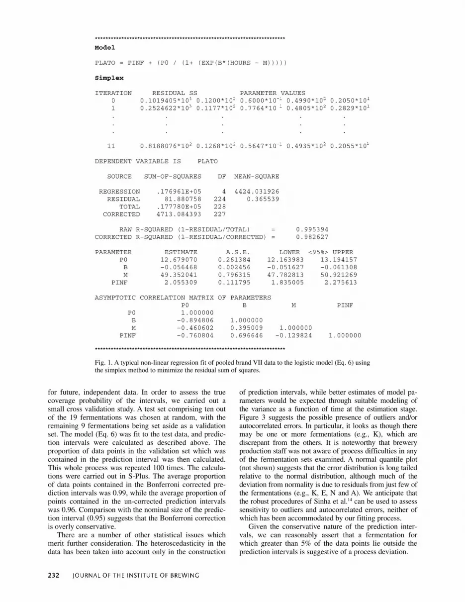
An examination of the fit of the three functions dis-cussed revealed that the logistic model (Eq. 6) best de-scribed the decline in fermentation gravities with time. Using the Systat program, one can select either the sim-plex or quasi-Newton search technique to minimize the re-sidual sum of squares. Both techniques gave similar re-sults, however the simplex fit tended to give slightly better fits as evidenced by examination of the residual sum of squares and plots of the expected and residual values.

:30�������23���������� � � ����

Table I displays the variation of the logistic model pa-rameters for all seven brands. Average values and standard deviations of parameter estimates taken over the different fermentations within a batch indicate the rather large co-efficients of variation for the model parameters. This find-ing is not surprising given the small number of data col-lected (10–15) during each fermentation. After statistical examination of the fermentation parameters (P� , B, M, P0) and other fermentation data such as the number of repitch-ings of each yeast crop, the initial temperature and the initial temperature increase, a few observations could be made.

The effect of yeast repitching was examined by sepa-rate regression analysis of the number of yeast pitchings on P� , B and M. The number of times the yeast was repitched (up to 10 ×’s) had no effect (p > 0.05) on the maximum fermentation rate, B, fermentation midpoint, M or the final gravity. Not surprisingly, (as evidenced by regression analysis) the starting temperature affected the fermentation velocity as evidenced by a significant (p < 0.01) increase in maximum fermentation rate and the ini-tial rate of temperature increase and a significant decrease (p < 0.001) in the time to the fermentation midpoint. Final gravities were also positively influenced by initial fermen-tation temperature (p < 0.001).

It is apparent that these observations, while relatively simple, can be used to make processing decisions on more than an ad hoc basis. For instance, the technique (some-times termed ‘Evidence Based Practice’) could be used to determine the number of yeast croppings possible (before a statistical change in P� , B, M or P0 is observed) during the introduction of a new brand or higher gravity wort.

This technique could (and probably should) be used when evaluating the tendency of malt to cause premature yeast flocculation. Currently, pilot fermentations of sus-pect malts are undertaken and the fermentation curves visually evaluated resulting in an inaccurate assay. Model-ling of the decline in Plato values with time and compari-son of the fermentation parameters would allow a much more accurate assessment of the tendency of test malts to cause premature yeast flocculation.

It has also not escaped our attention that this modeling technique could be employed to as a benchmark or “Gold Standard” when measuring yeast vitality. The ultimate test of yeast vitality is its ability to ferment wort. As our mod-elling technique allows one to accurately describe and measure any change in fermentation behaviour, it can be used to measure any decline in yeast vitality. We plan to

examine the feasibility of this technique as a standard vi-tality test against which other rapid vitality assays could be evaluated.

As the number of yeast repitchings had no effect on the fermentations and the starting temperature was brand de-pendent, the data for each brand was pooled for further analysis. Figure 1 displays a typical result of a logistic fit (Eq. 6) to a pooled data set using the Systat program. As is evident the program searches for a ‘best fit’ which reduces the residual sum of squares by an iterative technique and produces parameter estimates and asymptotic standard er-rors (A.S.E.). Reflecting the much larger sample size ob-tained through pooling all fermentations within a brand, these standard errors are much smaller than the standard deviations reported in Table I. The parameter estimates and asymptotic standard errors are combined as indicated in the appendix (Eq. A.4) to form the 95% confidence in-tervals in Figure 1.

Figure 2 shows the apparent extract versus time for each of the 19 fermentations using brand VII (labeled A, B, . . . , S), together with the estimated mean extract, and 95% prediction intervals, both with (outer intervals) and without (inner intervals) a Bonferroni correction. Figure 3 shows a plot of residuals (apparent extract – estimated mean) versus time for each fermentation of brand VII. It is apparent from Figures 2 and 3 that the variation of the apparent extract about the mean is very small at the begin-ning of the fermentation, then increases, and subsequently decreases. This has implications for the construction of confidence and prediction intervals. Theoretical details concerning the construction of prediction intervals are presented in Appendix I. The principle assumption under-lying this construction is that the errors about the mean line are independent and identically distributed Gaussian variables, having mean 0, and common standard deviation �. It is clear from Figure 3 that the standard deviation of the errors changes with time, and in Figure 2, the predic-tion intervals have been calculated by replacing �̂2 by �̂2

t . The estimate used for �̂2

t was a running variance, using a window spanning 10 hours of data. The two intervals pre-sented in Figure 2 are the associated prediction intervals, with (inner intervals) and without (outer intervals) using a Bonferroni correction.

It appears that the prediction intervals are excessively wide, even without the Bonferroni correction, as few of the observed data points lie outside the intervals. This is, to a certain extent, due to the nature of the plot, in which current data points are overlain with prediction intervals

TABLE I. Variation of logistic model parameters.

Brand

n

PD (°P)

B (°P/h)

M (h)

P`

(°P)

I 5 12.5 (0.6) –0.084 (0.017) 33.7 (2.7) 5.27 (0.4) II 6 8.1 (0.3) –0.091 (0.015) 37.2 (10.1) 2.80 (0.2) III 9 13.1 (1.0) –0.057 (0.010) 47.5 (5.4) 1.59 (0.5) IV 6 12.7 (0.4) –0.083 (0.012) 32.4 (3.4) 5.27 (0.4) V 5 12.5 (1.0) –0.063 (0.008) 46.3 (10.0) 1.98 (0.4) VI 8 13.5 (0.6) –0.070 (0.011) 35.3 (2.1) 5.64 (0.3) VII 19 13.0 (1.5) –0.057 (0.012) 49.5 (5.5) 1.84 (0.8)

N.B. Values in brackets denote the standard deviation of the estimated parameters using the simplex fit. The second column ‘n’ represents the number individual fermentations modelled. As data from each fer-mentation consisted of 10 to 15 data, the total number of points of each fit represents a minimum of 50.

���� � � .3962%0�3*�8,)�-278-898)�3*�&6);-2+�

for future, independent data. In order to assess the true coverage probability of the intervals, we carried out a small cross validation study. A test set comprising ten out of the 19 fermentations was chosen at random, with the remaining 9 fermentations being set aside as a validation set. The model (Eq. 6) was fit to the test data, and predic-tion intervals were calculated as described above. The proportion of data points in the validation set which was contained in the prediction interval was then calculated. This whole process was repeated 100 times. The calcula-tions were carried out in S-Plus. The average proportion of data points contained in the Bonferroni corrected pre-diction intervals was 0.99, while the average proportion of points contained in the un-corrected prediction intervals was 0.96. Comparison with the nominal size of the predic-tion interval (0.95) suggests that the Bonferroni correction is overly conservative.

There are a number of other statistical issues which merit further consideration. The heteroscedasticity in the data has been taken into account only in the construction

of prediction intervals, while better estimates of model pa-rameters would be expected through suitable modeling of the variance as a function of time at the estimation stage. Figure 3 suggests the possible presence of outliers and/or autocorrelated errors. In particular, it looks as though there may be one or more fermentations (e.g., K), which are discrepant from the others. It is noteworthy that brewery production staff was not aware of process difficulties in any of the fermentation sets examined. A normal quantile plot (not shown) suggests that the error distribution is long tailed relative to the normal distribution, although much of the deviation from normality is due to residuals from just few of the fermentations (e.g., K, E, N and A). We anticipate that the robust procedures of Sinha et al.14 can be used to assess sensitivity to outliers and autocorrelated errors, neither of which has been accommodated by our fitting process.

Given the conservative nature of the prediction inter-vals, we can reasonably assert that a fermentation for which greater than 5% of the data points lie outside the prediction intervals is suggestive of a process deviation.

************************************************************************ ����������������������� ����������������������������������������������������������������������������������������������� ������ �� ��� �� �� ��! �� �� �" �� r�� ���� �� �� �! �� ������������� �! !�"!!�� �� ���##�� �� �##"��� r�� ��$ �� �� �!$!��� �������������������������������������������������������������������������������������������������������������������������������������������������������������������������������������������������������������� �$�$$ #"�� �� ��!"$�� �� � "�#�� r�� ���% �� �� �! �� ����������������������������������������&�������'�'�(���������������'�(���������)������������#"�"��� ����������!�� %��!"������������������$��$$ # $���!!������ �%" %�������������������###$ �� ���!!$���&����&��������#�%� $�%�%���!!#����������*��'�(����������������������������������� ��� %���&����&�����'�(������������������&����&����������� ��$!"!#�������������������������������������������������*����+� ,-�������������� ���������!�"#� # ����� �!"�%$������!��"%�$%�����%����� #������������������ � "�"$����� � !� "����� � �"!#����� � "�% $��������������������% ! ������� �#�"%� �����#�#$!$�%���� ��!�!"�����������������!� % ������ ����#� �������$% �����!�!# "�%����.������&�&���������������������������������������������������� ������������������������������������������������ ������������� ���������������������� �$��$ "������ ���������������������� ��" " !���� �%� ������� �������������������� �#" $ ����� �"�""�"���� ��!�$!������� ��************************************************************************

Fig. 1. A typical non-linear regression fit of pooled brand VII data to the logistic model (Eq. 6) usingthe simplex method to minimize the residual sum of squares.

:30�������23���������� � � ����

Fig. 3. A residual plot (apparent extract – estimated mean) versus time for each fermentation of brand VII.

Fig. 2. Change in apparent extract versus time for each of the 19 fermentations using brand VII (labeled A, B, . . . , S), together with the estimated mean extract and 95% prediction intervals, both with (outer intervals) and without (inner intervals) a Bonferroni correction. (See text for a detailed explanation of interval construction.)

���� � � .3962%0�3*�8,)�-278-898)�3*�&6);-2+�

In general, both the prediction intervals and the asymp-totic standard errors will be useful to accurately assess different aspects of fermentation process error.

The result of this calculation is shown in Figure 2, which shows apparent extract versus time for each fer-mentation. Construction of these intervals allows, for the first time, one to predict when a fermentation is “stuck” or “hung” on a statistical basis. For instance, in cases where a fermentation appears to be slow or lagging and the Plato values trend outside the prediction intervals one can de-clare the fermentation “stuck”. When a fermentation trends out of the prediction intervals one can assume that some factor, be it the wort, yeast temperature or oxygen level has caused a process deviation. Thus, the intervals can be used in similar fashion to control charts.

Based on the underlying statistical theory it is expected that roughly 5% of the data points will lie outside the pre-diction intervals, while in this case only one of the 228 data points (fermentation K, at approximately 85 hours) lies close to the prediction interval boundary. This discrep-ancy could be due to the conservative nature of the inter-vals – the Bonferroni technique described in the appendix to construct simultaneous intervals assures only that at most 5% of data points will lie outside the prediction in-terval when there are no process deviations. Furthermore, there may be discrepancies between the assumed and ac-tual models underlying the fermentation process that lead to overly conservative intervals. For example, the variabil-ity of the data about the model has been assumed constant over time (homoscedastic errors), while the data actually appear to be less variable near the beginning and end, than in the middle, of the fermentation process (heteroscedastic errors). Incorporation of a more realistic error structure would be challenging, but might lead to empirical cover-age rates (proportions of points within the prediction inter-vals) closer to the nominal rate (95%). Given the conser-vative nature of the prediction intervals, we can reason-ably assert that a fermentation for which greater than 5% of the data points lie outside the prediction intervals is suggestive of a process deviation.

In general, both the prediction intervals and the asymp-totic standard errors will be useful to accurately assess different aspects of fermentation process error.

������ ��� The changes in fermentation gravities have been shown

to be well modelled by a four parameter logistic model. This non-linear regression modelling technique can be employed to compare fermentations parameters with other fermentation indicators such as the number of yeast repitchings and initial temperature. Statistical comparisons of this type allow fermentation managers to reconsider previous decisions made on an ad hoc basis. It is the au-thors’ hope this ‘evidenced based practice’ technique will be used to examine the influence of various fermentation processes on various fermentation parameters such as di-acetyl, VDK or DMS concentrations. The model could also be applied when evaluating fermentation data from premature yeast flocculation assays.

This non-linear modeling technique also allows re-searchers to compare fermentation treatments on a statisti-

cal basis. As mentioned earlier, comparison of fermenta-tion variables is often done visually or by an ANOVA type analysis of data at fixed times. Use of either of these tech-niques is not desirable. Non-linear regression modeling allows the fermentation dataset to be reduced to a small number of parameters (which represent the entire fermen-tation) which can then be used to evaluate different fer-mentation treatments.

Aside from the use of evidence based practice tech-niques, the development of non-linear prediction intervals has merit in the monitoring of fermentation gravities. Use of these intervals will allow fermentation managers to take action once the fermentation shows evidence of a serious process deviation. It is expected that similar models may be applied to monitor changes in other fermentation in-dices such as alcohol levels, pH etc. It is also hoped that the application of the (non-linear) regression model to predict fermentation behaviour presented in this paper, will allow a more accurate comparison of both industrial and experimental fermentations.

%'/23;0)(+)1)287�

The authors gratefully acknowledge funding by individual grants from Natural Sciences and Engineering Research Council of Canada (to R.A.S. and B.S.) and support from Carlton United Breweries Limited (Melbourne, Vic. AUS).

0-8)6%896)�'-8)(�

1. Boulton, C.A., Developments in real-time monitoring and fer-mentation control. The Brewer, 1999, 85(11), 551–557.

2. Brown, A.M., Non-linear regression analysis of data using a spreadsheet. Am. Lab., 2001, 32(10), 58, 60.

3. Corrieu, G. Treiea, I.C. and Perret, B., On-line estimation and prediction of density and ethanol evolution in the brewery. Tech. Q,. Master Brew. Assoc. Am., 2000, 37(2), 173–181.

4. Gee, D. and Ramirez, W.F., A flavor model for beer fermenta-tion. J. Instit. Brew., 1994, 100(5), 321–329.

5. Gensym Corporation Home Page. http://www.gensym.com/, Gensym Corp., Burlington, MA, (accessed Mar 30. 2002), 2001.

6. Gompertz, B., On the nature of the function expressiveness of the law of human mortality, and a new mode of determining the value of life contingencies. Phil. Trans. Royal Soc., 1825, 115, 513–585.

7. Kurz, T. Fellner, M., Becker, T. and Delgado, A., Observation and control of beer fermentation using cognitive methods. J. In-stit. Brew., 2001, 107(4), 241–252.

8. McMeekin, T.A., Olley, J.N., Ross, T. and Ratkowsky, D.A., Predictive Microbiology: Theory and Applications John Wiley and Sons: New York, NY., 1993, pp. 41–49.

9. Miller, R.G., Simultaneous Statistical Inferences. Springer-Verlag: New York, NY., 1981, pp. 115–116.

10. Motulsky, H.J. and Ransnas, L.A., Fitting curves to data using nonlinear regression: a practical and nonmathematical review. FASEB J., 1987, 1(5), 365–374.

11. Motulsky, H.J., Curvefit.com. The complete guide to nonlinear regression. http://www.curvefit.com, Graph Pad Software: San Diego, CA, (accessed Mar. 30, 2002), 1999.

12. Remedios-Marin, M., Alcoholic Fermentation Modelling: Cur-rent state and perspectives. Am. J. Enol. Viticult., 1999, 50(2), 166–178.

13. Seber, G.A.F. and Wild, C.J., Nonlinear Regression. Wiley: New York, NY, 1989, pp. 191–196.

14. Sinha, S.K., Field, C.A. and Smith, B., Robust estimation of nonlinear regression with autoregressive errors. Stat. Prob. Lett., 2003, 63, 49–59.

:30�������23���������� � � ����

15. Wilkinson, L., Hill, M. and Vang, E., Systat: The System for Statistics. Systat Inc: Evanston, IL, 1992, p. 415.

16. Willaert, R., Sugar consumption kinetics by brewers yeast dur-ing the primarily beer fermentation. Cerevisa, Bel. J. Brew. Bio-technol., 2001, 26(1), 43–49.

(Manuscript accepted for publication September 2003)

%44)2(-<�-�

������"���������������#���"��������$� �

Suppose that observations y1, . . . yn are available which arise from the model

iii tfy ε+θ= ),( (A.1)

where f is a function of time ti and parameters �, and �i represents the deviation of the ith observation from the regression function f. In the context of this paper, f could be the Gompertz, modified Gompertz, or logistic function. For illustrative purposes, suppose that f is the logistic func-tion, in which case

� = {�1, �2, �3, �4}

where �1 = P0, �2 = P�, �3 = B, �4 = M.

The nonlinear least squares estimator �̂ minimizes the sum of squares

( )∑=

θ−n

iii tfy

1

2),( (A.2)

When the errors �i , . . . , �n are independent normal vari-ables with mean 0 and variance �2, it can be shown that the distribution of �̂ is multivariate normal, with mean � and covariance matrix �, where � = �2C–1, C = FT F, and F is an n by 4 matrix whose ij th element is the partial de-rivative of f(ti ,�) with respect to parameter �j . Here C–1 denotes the inverse of C, and FT denotes the transpose of F. That is

jiij tfF θ∂θ∂= /)( (A.3)

For example, in the logistic function, the partial derivative of f(ti ,�) with respect to �1 = P0 is 1, the partial derivative with respect to �2 = P� is 1/{1 + exp[�3(t – �4)]} = 1/{1 + exp[B(t – M)]}, and so on.

It follows from the distribution of �̂ that an approximate 100(1 – �)% confidence interval for the j th parameter �j is given by:

jjkj t σ±θ α ˆˆ2/, (A.4)

where k is the number of error degrees of freedom, tk,� /2 is the � /2th percentile of the t distribution with k degrees of freedom, and �̂jj is the jj th element of �̂, the latter being obtained from � by replacing all unknown regression pa-rameters by their least squares estimates, and replacing �2 by �̂2, the error mean square of the regression.

A 100(1 – �)% confidence interval for f(ti ,�), the re-gression function at time ti is given by

2/12/, )ˆˆˆ()ˆ,( ffttf T

ki ′Σ′±θ α (A.5)

where f̂ � is the vector of partial derivatives of f(ti ,�̂) with respect to the components of �, evaluated at �̂.

The confidence interval on f(ti ,�) is an interval in which the true regression function is expected to lie with probability (1 – �). If interest lies in constructing an inter-val in which we expect a future Plato value y to lie at time ti , then a prediction interval is called for. The predicted Plato value is f(ti ,�̂). The variation of Plato value about this predicted value is normally distributed with mean 0 and variance �2 + f�T� f�, which reflects the two sources of variation in the prediction; the variation of y about the true regression line f(ti ,�), and the variation of the esti-mated regression line f(ti ,�̂) about the true regression line. It follows that a 100(1 – �)% prediction interval for a fu-ture Plato value is given by

2/122/, )ˆˆˆˆ()ˆ,( ffttf T

ki ′Σ′+σ±θ α (A.6)

Such an interval will be expected to contain the Plato value about 100(1 – �)% of the time.

Typically, we would like to make prediction intervals at a number of times t1 , . . . , tN . Although each prediction interval will contain the Plato value with high probability, the probability that one or more of the prediction intervals will not contain the Plato value increases with N (the num-ber of intervals constructed) and will eventually approach 1 as the number of intervals N gets very large. The Bon-ferroni procedure can be used to construct a set of simulta-neous prediction intervals for which the chance of one or more Plato values not being contained in their associated intervals is at most 1 – �. This is effected by replacing � in (A.6) by � /N, where N is the number of constructed intervals. Details concerning the Bonferroni procedure are provided in Miller9. An excellent source for further infor-mation on nonlinear regression and the construction of associated confidence and prediction intervals is Seber and Wild13.