arX

iv:h

ep-t

h/00

1206

1v2

30

Jan

2001

Preprint typeset in JHEP style. - PAPER VERSION NBI-HE-00-43

Noncommutative String Worldsheets from

Matrix Models

K.N. Anagnostopoulos

Department of Physics, University of Crete,

P.O.Box 2208, GR-710 03 Heraklion, Crete, Greece

Email: konstant@physics.uoc.gr

J. Nishimura∗

The Niels Bohr Institute,

Blegdamsvej 17, DK-2100 Copenhagen Ø, Denmark

E-mail: nisimura@nbi.dk

P. Olesen

The Niels Bohr Institute,

Blegdamsvej 17, DK-2100 Copenhagen Ø, Denmark

E-mail: polesen@nbi.dk

Abstract: We study dynamical effects of introducing noncommutativity on string

worldsheets by using a matrix model obtained from the zero-volume limit of

four-dimensional SU(N) Yang-Mills theory. Although the dimensionless noncom-

mutativity parameter is of order 1/N , its effect is found to be non-negligible even

in the large N limit due to the existence of higher Fourier modes. We find that the

Poisson bracket grows much faster than the Moyal bracket as we increase N , which

means in particular that the two quantities do not coincide in the large N limit. The

well-known instability of bosonic worldsheets due to long spikes is shown to be cured

by the noncommutativity. The extrinsic geometry of the worldsheet is described by

a crumpled surface with a large Hausdorff dimension.

Keywords: Matrix Models, Non-Commutative Geometry, Bosonic Strings.

∗On leave of absence from Department of Physics, Nagoya University, Furo-cho, Chikusa-ku,

Nagoya 464-8602, Japan.

Contents

1. Introduction 1

2. From matrices to noncommutative fields 3

3. Matrix model as noncommutative worldsheet theory 7

4. Results 9

5. Conclusions 16

A. Derivation of the roughness functional 17

B. Star-unitary invariance and area-preserving diffeomorphisms 18

1. Introduction

It is well known that the traditional bosonic worldsheet theories described for exam-

ple by the Nambu-Goto action, the Polyakov action and the Schild action are not

well-defined non-perturbatively, as was first observed in the large dimension limit by

Alvarez [1]. This conclusion has been confirmed more directly by the dynamical tri-

angulation approach [2, 3], where the discretized worldsheet embedded in the target

space degenerates to long spikes, and hence one cannot view it as a proper approxi-

mation of a continuous worldsheet. It is therefore of interest to inquire whether it is

possible to have different types of string models, where the worldsheet is well-defined

in the sense that it does not degenerate into long spikes. Some attempts have been

made to make the string more “stiff” by the introduction of extrinsic curvature [4],

but it is not clear whether this will work non-perturbatively [5].

In the present paper we have investigated whether the introduction of noncom-

mutativity on the worldsheet changes the situation. We study such a system by using

a matrix model with N×N hermitian matrices Aµ with µ = 1, 2, 3, 4. Corresponding

to each matrix one can construct a field Xµ(σ) by the Weyl transformation. Here

σ stands for the two discrete variables σ1 and σ2, representing the worldsheet coor-

dinates. Then there exists the following relation between the partition functions in

the matrix model and in the corresponding Weyl-transformed model,∫

dAµ exp

(

1

4g2Tr[Aµ, Aν ]

2

)

=

∫

DXµ(σ) e−S , (1.1)

1

where the action S for the latter is given by

S = − 1

4g2N

∑

σ

(

Xµ(σ) ⋆ Xν(σ)−Xν(σ) ⋆ Xµ(σ))2

. (1.2)

Here ⋆ denotes the star product with the dimensionless noncommutative parameter

being of order 1/N . The partition function on the left hand side of eq. (1.1) was

shown to be finite for N = 3, 4, 5 numerically by Ref. [6]. Monte Carlo simulations

up to N = 256 [7] further suggests that the statement extends 1 to N = ∞. This

means that the corresponding Weyl-transformed model is also well-defined in the

large N limit.

The partition function on the right hand side of eq. (1.1) defines a noncommu-

tative two-dimensional field theory, which is invariant under the star-unitary trans-

formation,

Xµ(σ)→ g∗(σ) ⋆ Xµ(σ) ⋆ g(σ) , with g∗(σ) ⋆ g(σ) = g(σ) ⋆ g∗(σ) = 1 . (1.3)

The action (1.2) resembles the Schild action

SSchild =1

g2N

∫

d2σ

(

∂Xµ

∂σ1

∂Xν

∂σ2− ∂Xν

∂σ1

∂Xµ

∂σ2

)2

, (1.4)

the difference being that the Poisson bracket has been replaced by the Moyal bracket

in the noncommutative case. It has been pointed out long time ago [9] that if the

higher modes in the mode expansion of Xµ(σ) can be neglected, the star-Schild

action in (1.2) reduces to the Schild action (1.4) in the large N limit. The issue is

also relevant when one considers matrix models as a nonperturbative definition of

M-theory and type IIB superstring theory [10, 11]. Of course, whether the higher

modes can really be neglected or not is a non-trivial dynamical question. One of the

main results of this paper is that for the bosonic model we consider, the Poisson and

the Moyal brackets are very different due to the effect of the higher modes, and that

this effect increases with increasing N . To our knowledge, this is the first time that

the agreement (or disagreement) of the two actions in the large N limit is discussed

in a dynamical context.

Recently the Schild action has been investigated non-perturbatively from the

point of view of dynamical triangulation [3]. The result is similar to the one ob-

tained for the Nambu-Goto action, namely that it is dynamically favorable to have

a “surface” which degenerates to long spikes, and hence the notion of a worldsheet

looses its meaning2.

1This has been proved rigorously in a preprint [8], which appeared while our paper was being

revised.2A similar result is not valid in the supersymmetric case, where the worldsheet exists if the

fermions are coupled to a bosonic Schild action [3]. However, in the present paper we shall discuss

the bosonic case only.

2

We shall take a different approach and ask whether the star-Schild action in

(1.2) provides a bosonic string theory with a well-defined worldsheet. The effects of

noncommutativity are found to be drastic. The average link length is finite and it is

observed to be considerably smaller than the average extent of the surface, which is in

sharp contrast [1, 3] to the conclusion for the Schild action (1.4) that the worldsheet

becomes completely unstable due to long spikes. This is not a contradiction since

the Poisson and Moyal brackets are indeed found to be quite different for the theory

under consideration. On the other hand, the extrinsic geometry of the worldsheet

for the star-Schild action is described by a crumpled surface with a large Hausdorff

dimension.

The matrix model on the left hand side of eq. (1.1) can be regarded as the

hermitian matrix version of the Eguchi-Kawai model [12]. (See Refs. [13] and [14]

for the hermitian matrix version of the Eguchi-Kawai model with quenching [15] or

twists [16], respectively.) Large N scaling of SU(N) invariant correlation functions

was obtained analytically to all orders of the 1/D expansion [7], and the results were

reproduced by Monte Carlo simulations [7, 17]. In particular, the one-point function

of a Wilson loop was observed to obey the area law, which suggested that the model

is actually equivalent to large N gauge theory for a finite region of scale even without

quenching [15] or twists [16]. The noncommutative worldsheet theory studied in the

present paper is therefore related to the large N QCD string (For a recent review,

see [18].).

The organization of this paper is as follows. In Section 2 we briefly review the

map from matrices to noncommutative fields. In Section 3 we interpret the matrix

model as noncommutative worldsheet theory. We then discuss the star-unitary in-

variance and the important question of gauge fixing. In Section 4 the results are

presented. Section 5 contains the summary and discussions. In an Appendix we

make some comments on the relationship between the star-unitary invariance and

the area-preserving diffeomorphisms.

2. From matrices to noncommutative fields

In order to derive the equivalence (1.1) between the matrix model and the noncom-

mutative worldsheet theory, we briefly review the one-to-one correspondence between

matrices and noncommutative fields. Most of the results in this Section are known

in the literature (see e.g., [19, 20]), but are given in order to fix the notation.

Throughout this paper, we assume that N is odd3. We first introduce the ’t

3We expect that the large N dynamics of the matrix model on the l.h.s. of (1.1) is independent

of whether N is even or odd. This has been also checked numerically for various SU(N) invariant

quantities. However, the one-to-one correspondence between the matrices and noncommutative

fields works rigorously only for odd N .

3

Hooft-Weyl algebra

Γ1Γ2 = ω Γ2Γ1 , (2.1)

where ω = e4πi/N . It is known that the representation of Γi using N × N unitary

matrices is unique up to unitary transformation Γi → UΓiU†, where U ∈ SU(N).

An explicit representation can be given by

Γ1 =

0 1 0

0 1. . .

. . .

. . . 1

1 0

, Γ2 =

1

ω

ω2

. . .

ω(N−1)

. (2.2)

Then we construct N ×N unitary matrices

Jkdef= (Γ1)

k1(Γ2)k2 e−2πik1k2/N , (2.3)

where k is a 2d integer vector and the phase factor e−2πik1k2/N is included so that

J−k = (Jk)† . (2.4)

Since (Γi)N = 1, the matrix Jk is periodic with respect to ki with period N ,

Jk1+N,k2= Jk1,k2+N = Jk1,k2

. (2.5)

We then define the N ×N matrices

∆(σ)def=∑

ki∈ZN

Jk e2πik·σ/N , (2.6)

labelled by a 2d integer vector σ. Note that ∆(σ) is hermitian due to the property

(2.4). It is periodic with respect to σi with period N ,

∆(σ1 + N, σ2) = ∆(σ1, σ2 + N) = ∆(σ1, σ2) . (2.7)

It is easy to check that ∆(σ) possesses the following properties.

tr∆(σ) = N (2.8)∑

σi∈ZN

∆(σ) = N21N (2.9)

1

Ntr(

∆(σ)∆(σ′))

= N2δσ,σ′(mod N) . (2.10)

Now let us consider gl(N ,C), the linear space of N ×N complex matrices. The

inner product can be defined by tr(M †1M2), where M1,M2∈ gl(N ,C). Eq. (2.10)

implies that ∆(σ) are mutually orthogonal and hence linearly independent. Since

the dimension of the linear space gl(N ,C) is N2 and there are N2 ∆(σ)’s that are

4

linearly independent, ∆(σ) actually forms an orthogonal basis of gl(N, C). Namely,

any N ×N complex matrix M can be written as

M =1

N2

∑

σi∈ZN

f(σ)∆(σ) , (2.11)

where f(σ) is a complex-valued function on the 2d discretized torus obeying periodic

boundary conditions. Using orthogonality (2.10), one can invert (2.11) as

f(σ) =1

Ntr(

M ∆(σ))

. (2.12)

The fact that (2.11) and (2.12) hold for an arbitrary N × N complex matrix M

implies that ∆(σ) satisfies

1

N2

∑

σi∈ZN

∆ij(σ)∆kl(σ) = Nδilδjk . (2.13)

Note also that using (2.8) with (2.11) or using (2.9) with (2.12), one obtains

1

NtrM =

1

N2

∑

σi∈ZN

f(σ) . (2.14)

We define the “star-product” of two functions f1(σ) and f2(σ) by

f1(σ) ⋆ f2(σ)def=

1

Ntr(M1M2∆(σ)) , (2.15)

where

Mα =1

N2

∑

σi∈ZN

fα(σ)∆(σ) α = 1, 2 . (2.16)

The star-product can be written explicitly in terms of fα(σ) as

f1(σ) ⋆ f2(σ) =1

N2

∑

ξi∈ZN

∑

ηi∈ZN

f1(ξ)f2(η)e−2πiǫjk(ξj−σj)(ηk−σk)/N , (2.17)

where ǫij is an antisymmetric tensor with ǫ12 = 1. This formula can be derived in

the following way. Substituting (2.16) into (2.15) and using the definition (2.6) of

∆(σ), one obtains

f1(σ) ⋆ f2(σ) =

(

1

N2

)2∑

ξη

∑

kpq

f1(ξ)f2(η)e2πi(p·ξ+q·η+k·σ) 1

Ntr(JpJqJk) . (2.18)

From the definition of Jk, one easily finds that

1

Ntr(JpJqJk) = e2πiǫijpiqj/Nδk+p+q,0(mod N) . (2.19)

5

Integration over k, p and q in (2.18) yields eq. (2.17).

In order to confirm that the star-product (2.17) is a proper discretized version

of the usual star-product in the continuum, we rewrite it in terms of Fourier modes.

We make a Fourier mode expansion of fα(σ) as

fα(σ) =∑

ki∈ZN

fα(k) e2πik·σ/N (2.20)

fα(k) =1

N2

∑

σi∈ZN

fα(σ) e−2πik·σ/N . (2.21)

Integrating (2.18) over k, ξ and η, one obtains

f1(σ) ⋆ f2(σ) =∑

pi∈ZN

∑

qi∈ZN

f1(p)f2(q) e2πiǫjkpjqk/Ne2πi(p+q)·σ/N , (2.22)

which can be compared to the usual definition of the star-product in the continuum

f1(σ) ⋆ f2(σ) = f1(σ) exp(

i1

2θǫij←−∂i−→∂j

)

f2(σ) . (2.23)

In the present case, the noncommutativity parameter θ is of order 1/N , and therefore

the star-product reduces to the ordinary product in the large N limit if fα(σ) contains

only lower Fourier modes (pj, qj ≪√

N).

It is obvious from the definition (2.15) that the algebraic properties of the star-

product are exactly those of the matrix product. Namely, it is associative but not

commutative. Note also that due to (2.14), summing a function f(σ) over σ corre-

sponds to taking the trace of the corresponding matrix M . Therefore,

∑

σi∈ZN

f1(σ) ⋆ f2(σ) ⋆ · · · ⋆ fn(σ) (2.24)

is invariant under cyclic permutations of fα(σ). What is not obvious solely from the

algebraic properties is that

∑

σi∈ZN

f1(σ) ⋆ f2(σ) =∑

σi∈ZN

f1(σ)f2(σ) , (2.25)

which can be shown by using the definition (2.15) with eq. (2.9).

For later convenience, let us define the Moyal bracket by

{{f1(σ), f2(σ)}} def= i

N

4π

(

f1(σ) ⋆ f2(σ)− f2(σ) ⋆ f1(σ))

= −N

2π

∑

pq

f1(p)f2(q) sin

(

2πǫjkpjqk

N

)

e2πi(p+q)·σ/N . (2.26)

6

We also define the Poisson bracket on a discretized worldsheet. Namely when we

define the Poisson bracket

{f1(σ), f2(σ)} def= ǫij

∂f1(σ)

∂σi

∂f2(σ)

∂σj, (2.27)

we assume that the derivatives are given by the lattice derivatives

∂f(σ)

∂σi=

1

2a

(

f(σ + i)− f(σ − i))

, (2.28)

where a = 2π/N is the lattice spacing. The Poisson bracket thus defined can be

written in terms of Fourier modes as

{f1(σ), f2(σ)} = −(

N

2π

)2∑

pq

f1(p)f2(q)ǫjk sin

(

2πpj

N

)

sin

(

2πqk

N

)

e2πi(p+q)·σ/N .

(2.29)

Note that the appearance of sines is due to discretization of the worldsheet. The

Moyal bracket (2.26) and the Poisson bracket (2.29) agree in the large N limit if

nonvanishing Fourier modes are those with pj , qj ≪√

N .

3. Matrix model as noncommutative worldsheet theory

Let us proceed to the derivation of the equivalence (1.1) between the matrix model

and the noncommutative worldsheet theory. We start from the matrix model with

the action

S = − 1

4g2tr([Aµ, Aν ]

2) , (3.1)

which can be obtained from the zero-volume limit of D-dimensional SU(N) Yang-

Mills theory4. The indices µ run from 1 to D.

As we have done in (2.11), we write the N × N hermitian matrices Aµ in (3.1)

as

Aµ =1

N2

∑

σi∈ZN

Xµ(σ)∆(σ) , (3.2)

where Xµ(σ) is a field on the discretized 2d torus obeying periodic boundary condi-

tions. Since Aµ is hermitian, Xµ(σ) is real, due to the hermiticity of ∆(σ). Eq. (3.2)

can be inverted as

Xµ(σ) =1

Ntr(

Aµ ∆(σ))

. (3.3)

We regard σ as (discretized) worldsheet coordinates and Xµ(σ) as the embedding

function of the worldsheet into the target space.

4For D = 10, the action (3.1) is just the bosonic part of the IIB matrix model [11]. The

dynamical aspects of this kind of matrix models for various D with or without supersymmetry have

been studied by many authors [6, 7, 17, 21] both numerically and analytically.

7

Using the map discussed in the previous section we can rewrite the action (3.1)

in terms of Xµ(σ) as5

S = − 1

4g2N

∑

σi∈ZN

(

Xµ(σ) ⋆ Xν(σ)−Xν(σ) ⋆ Xµ(σ))2

=1

g2N

(

2π

N

)2∑

σi∈ZN

{{Xµ(σ), Xν(σ)}}2 . (3.4)

If Xµ(σ) are sufficiently smooth functions of σ, the Moyal bracket can be replaced

by the Poisson bracket, and therefore we obtain the Schild action

SSchild =1

g2N

(

2π

N

)2∑

σi∈ZN

{Xµ(σ), Xν(σ)}2 . (3.5)

Let us discuss the symmetry of the theory (3.4), which shall be important in

our analysis. For that we recall that the model (3.1) is invariant under the SU(N)

transformation

Aµ → g Aµ g† . (3.6)

From the matrix-field correspondence described in the previous section, one easily

finds that the field Xµ(σ) defined through (3.3) transforms as

Xµ(σ)→ g(σ) ⋆ Xµ(σ) ⋆ g(σ)∗ , (3.7)

where g(σ) is defined by

g(σ) =1

Ntr(

g ∆(σ))

. (3.8)

The fact that g ∈ SU(N) implies that g(σ) is star-unitary;

g(σ)∗ ⋆ g(σ) = g(σ) ⋆ g(σ)∗ = 1 . (3.9)

The action (3.4) is invariant under the star-unitary transformation (3.7) as it should.

We shall refer to this invariance as ‘gauge’ degrees of freedom in what follows.

Even if Xµ(σ) is a smooth function of σ for a particular choice of gauge, it can

be made rough by making a rough star-unitary transformation. Let us quote an

analogous situation in lattice gauge theory. In the weak coupling limit, the configu-

rations can be made very smooth by a proper choice of the gauge. However, without

gauge fixing, they are as rough as could be due to the unconstrained gauge degrees

of freedom. Similarly when we discuss the smoothness of Xµ(σ), we should subtract

the roughness due to the gauge degrees of freedom appropriately. Therefore, a natu-

ral question one should ask is whether there exists at all a gauge choice that makes

Xµ(σ) relatively smooth functions of σ.

5While this work was being completed, we received a preprint [22] where the worldsheet theory

(3.4) is discussed from a different point of view.

8

Figure 1: A typical N = 35 Xµ(σ) (µ = 1) configuration after the gauge fixing.

In order to address this question, we specify a gauge-fixing condition by first

defining the roughness of the worldsheet configuration Xµ(σ) and then choosing a

gauge so that the roughness is minimized. A natural definition of roughness is

I =1

2N2

∑

σi∈ZN

2∑

j=1

(

Xµ(σ + j)−Xµ(σ))2

, (3.10)

which is Lorentz invariant. The gauge fixing is analogous to the Landau gauge in

gauge theories. The roughness functional (3.10) can be written conveniently in terms

of Aµ as (See Appendix A for the derivation.)

I =1

2N

∑

IJ

[

4 sin2 π(I − J)

N|(Aµ)IJ |2 +

∣

∣

∣(Aµ)IJ − (Aµ)I+ N−1

2,J+ N−1

2

∣

∣

∣

2]

. (3.11)

4. Results

Our numerical calculation starts with generating configurations of the model (3.1)

for D = 4 and N = 15, 25, 35 using the method described in Ref. [7]. For each config-

uration we minimize the roughness functional I defined by eq. (3.11) with respect to

the SU(N) transformation (3.6). We perform 2000 sweeps per configuration, where a

sweep is the minimization of I with respect to all SU(2) subgroups of SU(N) [7, 17].

From the configuration Aµ obtained after the SU(N) transformation that minimizes

I, we calculate through (3.3) the worldsheet configuration Xµ(σ). When we define

an ensemble average 〈 · 〉 in what follows, we assume that it is taken with respect

9

Figure 2: The effect of cutting off Fourier modes higher than kc on the worldsheet of

Fig. 1. On the left kc = 1, on the right kc = 3 and on the bottom kc = 5.

to Xµ(σ) after the gauge fixing. The number of configurations used for an ensemble

average is 658, 100 and 320 for N = 15, 25, 35 respectively. We note that in the

present model, finite N effects is known [7] to appear as a 1/N2 expansion. Also, the

large N factorization is clearly observed for N = 16, 32 [7]. (We have checked that

it occurs for N = 15, 25, 35 as well.) We therefore consider that the N we use in the

present work is sufficiently large to discuss the large N asymptotics.

We also note that the parameter g, which appears in the action (3.4), can be

absorbed by the field redefinition X ′µ(σ) = 1√

gXµ(σ). Therefore, g is merely a scale

parameter, and one can determine the g dependence of all the observables on dimen-

sional grounds. The results will be stated in such a way that they do not depend on

the choice of g.

In Fig. 1 we show a typical worldsheet configuration for N = 35 after the gauge

fixing. We observe that the worldsheet has no spikes. We compute the Fourier modes

Xµ(k) of Xµ(σ) through

Xµ(k)def=

1

N2

∑

σi∈ZN

Xµ(σ)e−2πik·σ/N =1

Ntr(AµJk) , (4.1)

where the range of k1 and k2 are chosen to be −(N − 1)/2 to (N − 1)/2. Fig. 2

describes how the same worldsheet configuration shown in Fig. 1 looks like if we cut

off6 the Fourier modes higher than kc. We find that the configuration obtained by

6More precisely, we keep the modes Xµ(k) with k1 ≤ kc and k2 ≤ kc and set the other modes to

10

10

20

30

40

50

15 25 35

N

g-1<R2>g-1<I>

Figure 3: The fluctuation of the surface R2 and the roughness functional I, which repre-

sents the average link length in the target space, are plotted against N with the normaliza-

tion factor g−1. The solid straight line is a fit to the power-law behavior 〈R2〉 ∝ gN0.493(3).

The dotted line is drawn to guide the eye.

keeping only a few lower Fourier modes already captures the characteristic behavior

of the original configuration. We have checked that this is not the case if we do not

fix the gauge.

We measure the fluctuation of the surface, which is given by7

R2 def=

1

N4

∑

σi,σ′

i∈ZN

{

Xµ(σ)−Xµ(σ′)}2

=2

N2

∑

σi∈ZN

Xµ(σ)2 =2

Ntr(A2

µ) . (4.2)

The average of the fluctuation is finite for finite N , and it is plotted in Fig. 3. The

power-law fit to the large N behavior 〈R2〉 ∼ gNp yields p = 0.493(3), which is

consistent with the result p = 1/2 obtained in Ref. [7]. Although the finiteness of

the fluctuation already implies a certain stability of the worldsheet, we note that the

fluctuation defined by the l.h.s. of (4.2) is actually invariant under the star-unitary

transformation (3.7). In particular, the fluctuation is finite even before the gauge

zero by hand.7We note that the action (3.1) is invariant under Aµ 7→ Aµ + αµ11N . Therefore, the trace part

of Aµ is completely decoupled from the dynamics. We fix these degrees of freedom by imposing

the matrices Aµ to be traceless. In the language of the worldsheet theory (3.4), the symmetry

corresponds to the translational invariance Xµ(σ) 7→ Xµ(σ) + const.. The tracelessness condition

for Aµ maps to∑

σi∈ZNXµ(σ) = 0.

11

0

0.01

0.02

0.03

0.04

0.05

0.06

0.07

0 2 4 6 8 10 12 14 16 18

<X∼ µ(

k)X∼ µ(

-k)>

/(g

N1/

2 )

k1

N=15N=25N=35

Figure 4: The Fourier mode amplitudes⟨

Xµ(k)Xµ(−k)⟩

/(gN1/2) are plotted against k1

(k2 = k1) for N = 15, 25, 35.

fixing. Therefore, the smoothness of Xµ(σ) (which appears only after the gauge

fixing) is a notion which is stronger than the finiteness of the fluctuation.

Let us point out also that the roughness functional I actually represents the

average link length in the target space. We therefore plot 〈I〉 in Fig. 3 and compare

it with the fluctuation (4.2). The former is observed to be smaller than the latter8

which is consistent with the observed smoothness of Xµ(σ). The ratio 〈I〉 / 〈R2〉 is

0.364(1), 0.338(2), 0.3290(5) for N = 15, 25, 35, respectively, which may be fitted

to a power-law behavior 〈I〉 / 〈R2〉 ∼ N−0.120(4). This indicates a tendency that the

worldsheet is getting smoother as N increases.

In order to quantify the smoothness of Xµ(σ) further, let us examine the Fourier

mode amplitudes. We first note that there is a relation

∑

ki∈ZN

⟨

Xµ(k)Xµ(−k)⟩

=

⟨

1

N2

∑

σi∈ZN

Xµ(σ)2

⟩

∼ O(gN1/2) . (4.3)

This motivates us to plot⟨

Xµ(k)Xµ(−k)⟩

/(gN1/2) with this particular normaliza-

tion. The results are shown in Fig. 4 and Fig. 5. We find a good scaling in N ;

data points for different N fall on top of each other. The discrepancy in the large k

region can be understood as a finite N effect. The k dependence of the Fourier mode

8If we do not fix the gauge, we observe that the two quantities 〈R2〉 and 〈I〉 coincide, meaning

that the Xµ(σ) is completely rough.

12

1e-05

0.0001

0.001

0.01

0.1

1 10

<X∼ µ(

k)X∼ µ(

-k)>

/(g

N1/

2 )

k1

N=15N=25N=35

Figure 5: The Fourier mode amplitudes⟨

Xµ(k)Xµ(−k)⟩

/(gN1/2) in Fig. 4 are now

plotted in the log-log scale in order to visualize the power-law behavior. The straight line

is a fit to C|k|−q with q = 1.96(5) for the N = 35 data.

amplitudes suggests that the higher modes are indeed suppressed. Moreover we find

that there exist a power-law behavior9

1

gN1/2

⟨

Xµ(k)Xµ(−k)⟩

∼ const. · |k|−q , (4.4)

where |k| =√

(k1)2 + (k2)2. Assuming that the constant coefficient on the r.h.s. of

(4.4) is independent of N , as suggested by the observed scaling in N , the power q

must be q > 2 in order that the sum on the l.h.s. of (4.3) may be convergent in

the large N limit. The power q extracted from N = 35 data is q = 1.96(5), which

may imply that we have not reached sufficiently large k (due to the finite N effect

mentioned above) to extract the correct power. Although we have seen that the

amplitudes of the higher Fourier modes are suppressed, we should remember that

their number for fixed |k| grows linearly with |k|. Therefore, the higher modes can

still be non-negligible.

Let us turn to the question whether the action S in (3.4) approaches the Schild

action SSchild in (3.5) in the large N limit. In terms of Fourier modes, the two actions

9If we do not fix the gauge, we observe that the r.h.s. of (4.4) is replaced by a constant indepen-

dent of k, which means that the worldsheet behaves like a white noise. The constant is proportional

to 1/N2, as expected from the relation (4.3), which is gauge independent. Note, in particular, that

the scaling behavior observed in Fig. 5 emerges only after the gauge fixing.

13

100

1000

10000

100000

15 25 35

N

<S><SSchild>

Figure 6: Plot of 〈S〉 and 〈SSchild〉 as a function of N . The solid line represents the exact

result 〈S〉 = (N2 − 1). The dotted line is drawn to guide the eye.

read

S = −N

g2

∑

klp

Xµ(k)Xν(l)Xµ(p)Xν(−k − l − p)

× sin

(

2π

Nǫnmknlm

)

sin

(

2π

Nǫrspr(k + l)s

)

, (4.5)

SSchild = −N

g2

(

N

2π

)2∑

klp

Xµ(k)Xν(l)Xµ(p)Xν(−k − l − p)

×ǫij sin

(

2π

Nki

)

sin

(

2π

Nlj

)

ǫrs sin

(

2π

Npr

)

sin

(

2π

N(k + l + p)s

)

.(4.6)

If the higher Fourier modes can be neglected one can see from eqs. (4.5) and (4.6) that

S = SSchild in the large N limit. We measure both quantities and plot the results in

Fig. 6. The average of the action (3.4) is known [7] analytically 〈S〉 = N2− 1, which

is clearly reproduced from our data. On the other hand, 〈SSchild〉 is much larger, and

moreover it grows much faster, the growth being close to O(N4). Therefore we can

safely conclude that the two quantities do not coincide in the large N limit.

The disagreement of the two actions (3.4) and (3.5) in the large N limit implies

that the higher modes play a crucial role. In order to see their effects explicitly,

we cut off the Fourier modes higher than kc. In Fig. 7, we plot the average of the

actions thus calculated against kc for N = 35. The two actions with the cutoff at

14

10

100

1000

10000

100000

2 4 6 8 10 12 14 16kc

<S> <SSchild>

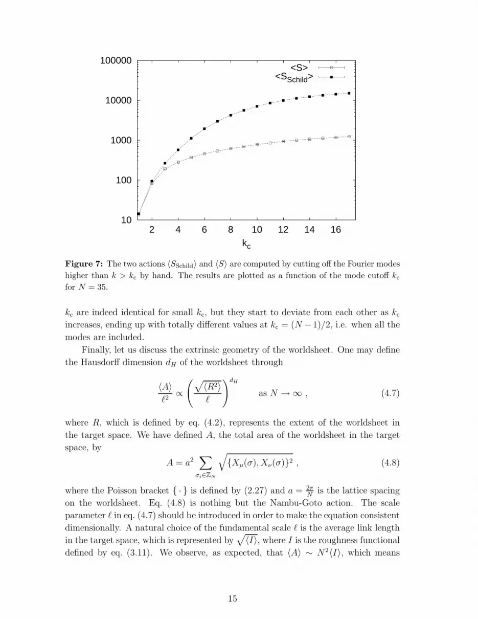
Figure 7: The two actions 〈SSchild〉 and 〈S〉 are computed by cutting off the Fourier modes

higher than k > kc by hand. The results are plotted as a function of the mode cutoff kc

for N = 35.

kc are indeed identical for small kc, but they start to deviate from each other as kc

increases, ending up with totally different values at kc = (N −1)/2, i.e. when all the

modes are included.

Finally, let us discuss the extrinsic geometry of the worldsheet. One may define

the Hausdorff dimension dH of the worldsheet through

〈A〉ℓ2∝(

√

〈R2〉ℓ

)dH

as N →∞ , (4.7)

where R, which is defined by eq. (4.2), represents the extent of the worldsheet in

the target space. We have defined A, the total area of the worldsheet in the target

space, by

A = a2∑

σi∈ZN

√

{Xµ(σ), Xν(σ)}2 , (4.8)

where the Poisson bracket { · } is defined by (2.27) and a = 2πN

is the lattice spacing

on the worldsheet. Eq. (4.8) is nothing but the Nambu-Goto action. The scale

parameter ℓ in eq. (4.7) should be introduced in order to make the equation consistent

dimensionally. A natural choice of the fundamental scale ℓ is the average link length

in the target space, which is represented by√

〈I〉, where I is the roughness functional

defined by eq. (3.11). We observe, as expected, that 〈A〉 ∼ N2〈I〉, which means

15

that the l.h.s. of (4.7) is of O(N2). As we have seen in Fig. 3, we observe that

〈I〉 / 〈R2〉 ∼ N−0.120(4). This means that the Hausdorff dimension dH defined by

(4.7) with the choice ℓ =√

〈I〉 is dH ∼ 33, which might suggest that actually

dH =∞. Therefore, the extrinsic geometry of the embedded worldsheet is described

by a crumpled surface.

5. Conclusions

In this paper we have studied the star-Schild action (1.2) resulting from the zero-

volume limit of SU(N) Yang-Mills theory. We find that the star-Schild action does

not approach the Schild action (1.4) due to the important role played by the ever-

increasing number of higher modes. This has some implications to the ideas presented

long ago [9] that it might be that the Schild action represents the large N QCD

action. From our results the two actions differ more and more with increasing N .

The Poisson bracket increases much faster with N than the corresponding Moyal

bracket. Our conclusion is therefore that QCD strings would be described by a

noncommutative string theory defined by the star-Schild action, rather than the

standard Schild action.

As we have seen, it is possible to find a star-unitary transformation g(σ) such

that the surfaces defined by the star-Schild action are regular (i.e., do not have long

spikes), and this action therefore defines a new type of string theory. The theory

is invariant under star-unitary transformations, which generalize the area-preserving

diffeomorphisms, the invariance of the usual Schild action. As we discuss in the

Appendix B, the reparametrization invariance of the worldsheet fields Xµ(σ) is re-

stricted to linear transformations of the σ’s in the case of the star-Schild action.

(Note, however, that the reparametrization invariance of the usual Schild action is

also much reduced relative to the Nambu-Goto action.) The star-unitary transforma-

tions transform the worldsheet configuration in such a way that the changes cannot

be absorbed by a reparametrization. In obtaining a regular surface we have chosen

a particular “gauge”. The regularity will not be changed drastically under smooth

star-unitary transformations. However, if we do not fix the gauge, we obtain spiky

surfaces, which is connected to a regular surface by a rough star-unitary transforma-

tion g(σ). The main point is that it is at all possible to obtain a regular surface by

fixing the gauge properly.

A possible intuitive understanding of the regularity of the worldsheet in the

noncommutative string is that the action contains higher derivatives in the star-

product. Let us recall that one of the motivations for introducing extrinsic curvature

(which also contains higher derivatives in a different combination) was [4] that this

extra term in the action makes the worldsheet more stiff. One would also expect

a similar effect from the introduction of higher derivatives, because an extremely

rough worldsheet with long spikes would have at least some derivatives rather large.

16

Although the star-product contains these derivatives in a special combination, it is

difficult for all these large derivatives to cancel, and hence a surface dominated by

long spikes would not be preferred. This is confirmed by the observation that the

average link length is much smaller than the average extent. The extrinsic geometry

of the embedded surface, on the other hand, is described by a crumpled surface with

a large Hausdorff dimension.

It would be of interest to address the issues studied in this paper in the su-

persymmetric case using the numerical method developed in Ref. [17]. We hope to

report on it in a future publication.

Acknowledgments

We thank Jan Ambjørn for interesting discussions on instabilities in bosonic strings.

We are also grateful to Z. Burda for helpful comments. K.N.A. acknowledges inter-

esting discussions with E. Floratos, E. Kiritsis and G. Savvidy. K.N.A.’s research was

partially supported by the RTN grants HPRN-CT-2000-00122 and HPRN-CT-2000-

00131 and a National Fellowship Foundation of Greece (IKY) postdoctoral fellowship.

A. Derivation of the roughness functional

In this appendix, we rewrite the roughness functional (3.10) in terms of the matrices

Aµ and derive (3.11). For that purpose, we introduce N ×N unitary matrices

D1 = (Γ†2)

N−12 (A.1)

D2 = (Γ1)N−1

2 , (A.2)

which satisfy

DjΓiD†j = e−2πiδij/NΓi . (A.3)

One can check that

Dj∆(σ)D†j = ∆(σ − j) , (A.4)

which implies

Xµ(σ + j) =1

Ntr(

DjAµD†j∆(σ)

)

. (A.5)

Thus the matrix Dj plays the role of a shift operator in the j-direction. Now we can

rewrite the roughness functional I in terms of the matrices Aµ as

I =1

2N

∑

j

tr(DjAµD†j −Aµ)2

=1

2N

∑

IJ

∑

j

∣

∣

∣(DjAµD

†j)IJ − (Aµ)IJ

∣

∣

∣

2

. (A.6)

17

Using the explicit form of Γµ given by eq. (2.2), we obtain

(D1AµD†1)IJ = (Aµ)IJe2πi(I−J)/N (A.7)

(D2AµD†2)IJ = (Aµ)I+ N−1

2,J+ N−1

2, (A.8)

which yields (3.11).

B. Star-unitary invariance and area-preserving diffeomorphisms

In this appendix, we discuss the relationship between the symmetry of the Schild

action and that of the star-Schild action. Here only we consider that the worldsheet

is given by an infinite two-dimensional flat space parametrized by the continuous

variables σ1 and σ2. Let us define the Schild and star-Schild actions

I1 =

∫

d2σ {φ1(σ), φ2(σ)}2 (B.1)

I2 =

∫

d2σ {{φ1(σ), φ2(σ)}}2θ , (B.2)

where the Poisson and Moyal brackets are defined by

{φ1(σ), φ2(σ)} = ǫij∂φ1

∂σi

∂φ2

∂σj(B.3)

{{φ1(σ), φ2(σ)}}θ =1

θφ1(σ) sin(θǫij

←−∂i−→∂j )φ2(σ) . (B.4)

The Schild action I1 is invariant under the area-preserving diffeomorphism

σi 7→ σi + ǫij∂jf(σ) , (B.5)

where f(σ) is some infinitesimal real function of σ. Under the infinitesimal area-

preserving diffeomorphism, the fields transform as a scalar φα(σ) = φ′α(σ′), so that

one can state the invariance as the one under the field transformation

φα(σ) 7→ φα(σ) + {f(σ), φα(σ)} . (B.6)

On the other hand, the star-Schild action I2 is invariant under the star-unitary

transformation

φα(σ) 7→ φα(σ) + {{f(σ), φα(σ)}}θ . (B.7)

Obviously, this transformation (B.7) reduces to (B.6) if φα(σ) and f(σ) do not contain

higher Fourier modes compared with θ−1/2.

In general the two transformations (B.6) and (B.7) differ. However, we note that

they become identical if f(σ) contains terms only up to quadratic in σ as

f(σ) = aiσi + bijσiσj , (B.8)

18

where bij is a real symmetric tensor. From (B.5), one finds that the corresponding

coordinate transformation is

σi 7→ σi + (vi + λijσj) , (B.9)

where vi = ǫilal and λij = ǫilblj , which is traceless. This transformation includes

the Euclidean group, namely translation and rotation. Thus we find that the linear

(finite) transformation of the coordinates σ′i = Λijσj + vi, where det Λ = 1, can be

expressed as a star-unitary transformation. In other words, the reparametrization

invariance of the star-Schild action is restricted to such linear transformations.

References

[1] O. Alvarez, Phys. Rev. D 24 (1981) 440; M.E. Cates, Europhys. Lett. 8 (1988) 656.

[2] J. Ambjørn, B. Durhuus, and J. Frohlich, Nucl. Phys. B 257 (1985) 433; J. Ambjørn,

B. Durhuus, J. Frohlich, and P. Orland, Nucl. Phys. B 270 (1986) 457.

For a recent review, see J. Ambjørn, B. Durhuus and T. Jonsson, “Quantum Geome-

try”, Cambridge Monographs, 1997.

[3] S. Oda and T. Yukawa, Prog. Theor. Phys. 102 (1999) 215 [hep-th/9903216]; P.

Bialas, Z. Burda, B. Petersson and J. Tabaczek, Nucl. Phys. B 592 (2000) 391,

[hep-lat/0007013].

[4] W. Helfrich, J. Phys. 46 (1985) 1263; L. Peliti and S. Leibler, Phys. Rev. Lett. 54

(1985) 1690; D. Forster, Phys. Lett. A 114 (1986) 115; A. Polyakov, Nucl. Phys. B

268 (1986) 406.

[5] J. Ambjørn, A. Irback, J. Jurkiewicz, and B. Petersson, Nucl. Phys. B 393 (1993) 571,

[hep-lat/9207008]; K.N. Anagnostopoulos, M. Bowick, P. Coddington, M. Falcioni,

L. Han, G. Harris, E. Marinari, Phys. Lett. B 317 (1993) 102, [hep-th/9308091]; J.

Ambjørn, Z. Burda, J. Jurkiewicz, and B. Petersson, Phys. Lett. B 341 (1995) 286,

[hep-th/9408118];

[6] W. Krauth and M. Staudacher, Phys. Lett. B 435 (1998) 350, [hep-th/9804199].

[7] T. Hotta, J. Nishimura and A. Tsuchiya, Nucl. Phys. B 545 (1999) 543,

[hep-th/9811220].

[8] P. Austing and J. F. Wheater, hep-th/0101071.

[9] J. Hoppe, Int. J. Mod. Phys. A 4 (1989) 5235; E.G. Floratos and J. Iliopoulos, Phys.

Lett. B 201 (1988) 237; E.G. Floratos, J. Iliopoulos, and G. Tiktopoulos, Phys. Lett.

217 (1989) 217; D. Fairlie, P. Fletcher, and C. Zachos, Phys. Lett. B 218 (1989) 203;

D. Fairlie and C. Zachos, Phys. Lett. B 224 (1989) 101; D. Fairlie, P. Fletcher, and

C. Zachos, J. Math. Phys. 31 (1990) 1088; I. Bars, Phys. Lett. B 245 (1990) 35; E.G.

Floratos and G.K. Leontaris, Phys. Lett. B 464 (1999) 30, [hep-th/9908106].

19

[10] T. Banks, W. Fischler, S.H. Shenker and L. Susskind, Phys. Rev. D 55 (1997) 5112,

[hep-th/9610043].

[11] N. Ishibashi, H. Kawai, Y. Kitazawa and A. Tsuchiya, Nucl. Phys. B 498 (1997) 467,

[hep-th/9612115]

[12] T. Eguchi and H. Kawai, Phys. Rev. Lett. 48 (1982) 1063.

[13] D. Gross and Y. Kitazawa, Nucl. Phys. B206 (1982) 440.

[14] A. Gonzalez-Arroyo and C.P. Korthals Altes, Phys. Lett. B 131B (1983) 396.

[15] G. Bhanot, U. Heller and H. Neuberger, Phys. Lett. 113B (1982) 47.

[16] A. Gonzalez-Arroyo and M. Okawa, Phys. Rev. D27 (1983) 2397.

[17] J. Ambjørn, K.N. Anagnostopoulos, W. Bietenholz, T. Hotta and J. Nishimura, J.

High Energy Phys. 0007 (2000) 013, [hep-th/0003208].

[18] G. ’t Hooft, “Monopoles, Instantons and Confinement”, notes written by F. Bruck-

mann, [hep-th/0010225].

[19] I. Bars and D. Minic, hep-th/9910091.

[20] J. Ambjørn, Y.M. Makeenko, J. Nishimura and R.J. Szabo, J. High Energy Phys. 9911

(1999) 029, [hep-th/9911041]; Phys. Lett. B 480 (2000) 399, [hep-th/0002158]; J.

High Energy Phys. 0005 (2000) 023, [hep-th/0004147].

[21] J. Nishimura, Mod. Phys. Lett. A 11 (1996) 3049, [hep-lat/9608119]; T. Suyama

and A. Tsuchiya, Prog. Theor. Phys. 99 (1998) 321, [hep-th/9711073]; T. Nakajima

and J. Nishimura, Nucl. Phys. B 528 (1998) 355, [hep-th/9802082]; W. Krauth,

H. Nicolai and M. Staudacher, Phys. Lett. B 431 (1998) 31, [hep-th/9803117];

Phys. Lett. B 453 (1999) 253, [hep-th/9902113]; J. Ambjørn, K.N. Anagnostopou-

los, W. Bietenholz, T. Hotta and J. Nishimura, J. High Energy Phys. 0007 (2000)

011, [hep-th/0005147]; J. Nishimura and G. Vernizzi, J. High Energy Phys. 0004

(2000) 015, [hep-th/0003223]; Phys. Rev. Lett. 85 (2000) 4664, [hep-th/0007022]; S.

Horata and H.S. Egawa, hep-th/0005157; S. Oda and F. Sugino, hep-th/0011175;

Z. Burda, B. Petersson and J. Tabaczek, hep-lat/0012001.

[22] N. Kitsunezaki and S. Uehara, hep-th/0010038.

20