arX

iv:1

103.

2849

v1 [

mat

h-ph

] 1

5 M

ar 2

011

Nonlocal, noncommutative diagrammatics and

the linked cluster Theorems

Christian Brouder ∗, Frederic Patras †

March 16, 2011

Abstract

Recent developments in quantum chemistry, perturbative quantumfield theory, statistical physics or stochastic differential equations requirethe introduction of new families of Feynman-type diagrams. These newfamilies arise in various ways. In some generalizations of the classicaldiagrams, the notion of Feynman propagator is extended to generalizedpropagators connecting more than two vertices of the graphs. In someothers (introduced in the present article), the diagrams, associated tononcommuting product of operators inherit from the noncommutativityof the products extra graphical properties.

The purpose of the present article is to introduce a general way ofdealing with such diagrams. We prove in particular a “universal” linkedcluster theorem and introduce, in the process, a Feynman-type “diagram-matics” that allows to handle simultaneously nonlocal (Coulomb-type)interactions, the generalized diagrams arising from the study of interact-ing systems (such as the ones where the ground state is not the vacuumbut e.g. a vacuum perturbed by a magnetic or electric field, by impu-rities...) or Wightman fields (that is, expectation values of products ofinteracting fields). Our diagrammatics seems to be the first attempt toencode in a unified algebraic framework such a wide variety of situations.

In the process, we promote two ideas. First, Feynman-type diagram-matics belong mathematically to the theory of linear forms on combina-torial Hopf algebras. Second, linked cluster-type theorems rely ultimatelyon Mobius inversion on the partition lattice. The two theories shouldtherefore be introduced and presented accordingly.

Among others, our theorems encompass the usual versions of the the-orem (although very different in nature, from Goldstone diagrams in solidstate physics to Feynman diagrams in QFT or probabilistic Wick theo-rems).

∗Institut de Mineralogie et de Physique des Milieux Condenses, CNRS UMR 7590, Uni-

versites Paris 6 et 7, IPGP, 140 rue de Lourmel, 75015 Paris, France.†Laboratoire J.-A. Dieudonne, CNRS UMR 6621, Universite de Nice, Parc Valrose, 06108

Nice Cedex 02, France.

1

1 Introduction

The attempts to clarify the mathematical framework underlying quantum chem-istry, solid state physics, quantum field theories (QFT) and connected topicssuch as -for example, the grounds for the functional approaches, the principlesunderlying renormalization- as well as attempts to deepen our current under-standing of widely used techniques (effective Hamiltonians, adiabatic limits...)are often hindered by very basic questions regarding the underlying mathemat-ical methods. This is particularly obvious when it comes to developing newtools, see e.g. our studies of enhanced algorithms and formulas for the com-putation of eigenstates of Hamiltonians when the (unperturbed) ground stateis degenerate [1, 2, 3], or of the combinatorics of one-particle-irreducibility forinteracting systems [4].

The present article focusses on diagrammatics. We argue that Feynman-typediagrammatics belong mathematically to the theory of linear forms on combi-natorial Hopf algebras, which allows to generalize the theory to a much widersetting than the classical one. We cover the usual examples corresponding tovacuum expectations over commutative products of fields where the propagatorsare represented by edges -this includes for example the various Goldstone-typediagrams and the perturbative expansions parametrized by Feynman diagramsin quantum field theories. However we go beyond and cover the case of ex-pectations over general states, which requires the introduction of generalizeddiagrams [5, 4]. The same combinatorics happens to provide a pictorial descrip-tion of cumulants in probability. The Hopf algebraic approach also allows tostudy expectations of products of free fields (Wightman fields) and derive newFeynman diagram expansions in this setting.

In a second part, we prove general linked cluster theorems, covering all thesecases and making as explicit as possible the link between the elementary algebraunderlying the theorems and the graphical content (that relies on connected-ness in the graph-theoretical sense). Notice that we avoid deliberately functionalmethods (see e.g.[6]): although very efficient to derive the classical QFT linkedcluster theorem (using a generating function in terms of an external source),they lack the generality and simplicity of the combinatorial proof. Moreover,they cannot deal with noncommutative Feynman diagrams because functionalderivatives commute. In the process, we promote another idea. Namely, linkedcluster-type theorems rely ultimately on Mobius inversion on the partition lat-tice.

Acknowledgements

We are particularly grateful to R. Stora. Many letters and documents (amongwhich [7]) he sent us were the initial incentive for the present article -that wasconceived to bridge the computations in [4] with other approaches to quan-tum field computations and find some suitable mathematical framework forthe (much more advanced) problems these documents suggest. In particular,

2

we aimed at developping a mathematical framework to deal with products ofWightman fields and their average values over general states, one of the prob-lems this article addresses.

Notation

We use the following convention: since various products will be defined alongthe article (such as ∗ or ⊙), when we want to emphasize what product is used inan exponential, a logarithm or any other operation, we put the product symbolin exponent, so that log∗ emans that we compute the logarithm using the ∗product, x⊙n means that we compute the n-th power of x using the ⊙-product,and so on.

2 Free combinatorial Hopf algebras

The objects we will be interested in are combinatorial Hopf algebras in the senseof Joni and Rota [8], that is, bialgebras which coproduct is of combinatorialnature (obtained by “splitting” generating symbols according to combinatorialrules encoded by remarkable “section coefficients” –in high-energy physics, thesecoefficients correspond roughly to the symmetry factors of Feynman graphs).More specifically, we will be interested in families of Hopf algebras correspondingphysically to bosonic or fermionic systems, to the usual algebraic structure ofquantum fields (equipped with a commutative product such as the normal ortime-ordered product) and to Wightman fields.

Since our results are more general than what would be required by applica-tions to quantum systems, we state them in full generality and will show laterhow they specialize to particular physical systems or mathematical problems.Let X be a fixed ordered set, X = {x1, ..., xn, ...}. In most applications, Xwill be infinite and countable, so that the reader may think to X as the set ofnatural numbers.

The notion of combinatorial Hopf algebra, goes back to [8]. The generalnotion is ill-defined in the litterature (there are many natural candidates, butat the moment no convincing general definition). We choose here a simple andrelatively straightforward definition suited for our purposes that reflects some ofthe natural properties one expects from the notion when the underlying algebrais free commutative or free associative.

Definition 1 We call free commutative (resp. free) combinatorial Hopf algebraany connected graded commutative (resp. associative) and cocommutative Hopfalgebra H such that:

• (Freeness) As an algebra,H is the algebra of polynomials (resp. of tensors)over a doubly indexed (finite or countable) set of formal, commuting (resp.noncommuting), variables φi(xS) where S runs over finite subsets ofX andi = 1...nk, where k = |S| and where the sequence of the nk, i ∈ N is afixed sequence of integers.

3

• (Equivariance) The structure maps are equivariant with respect to mapsinduced by substitutions in X . In other terms, any substitution (thatis, any set automorphism) σ induces a Hopf algebra automorphism of Hwhich action on the generators is defined by σ(φi(xS)) := φi(xσ(S)).

The φi(xS) are called the generators of H , the (commutative or associative)monomials in the φi(xS) form a linear basis of H and are therefore called thebasis elements.

We do not look for the outmost generality, and many of our constructionsand definitions can be extended in a fairly straightforward way to more gen-eral systems. For example, one might consider free partially commutative Hopfalgebras which generators φi(xS) would satisfy partial commutation rules (e.g.all the φj(xi) would commute for a fixed i, but without φj(xi) and φk(xl) com-muting for i 6= l, and so on). The so-constructed Hopf algebras can make sensein various applications and inherit all the properties of free commutative or freecombinatorial Hopf algebras that are required for the forthcoming reasonings,we refer e.g. to [9] for details on the subject.

Some further remarks are in order. Recall first that, by the Leray theorem(see e.g. Prop 4 in [10]), any connected graded commutative Hopf algebra His free commutative, so that the assumption that H is freely generated as acommutative algebra comes for free when one assumes that H is connectedgraded commutative.

The key point that makes the Hopf algebra combinatorial (and, as we shallsee, suited to Feynman-type graphical reasonings) is that we assume that a set ofpolynomial generators is fixed and behaves nicely with respect to substitutionsin X .

The particular case where nk = 0 for k > 1 corresponds to the classicalsituation where the only propagators showing up in diagrams are the ones thatdescribe the free propagation of a particle.

Let us mention at last that a more pedantical definition of combinatorialHopf algebras could be given in terms of vector species, following the approachto combinatorial Hopf algebraic structures in [11, 12, 13].

A very important consequence of the equivariance condition is the following.

Lemma 2 For any subset S of X, let us write HS for the subalgebra of Hgenerated by the φi(xT ), T ⊂ S. Then, HS is a Hopf subalgebra of H. Moreover,any automorphism σ of X induces an isomorphism of Hopf algebras from HS

to HT , where T := σ(S).

The second property is a direct consequence of the first one since σ (bydefinition of the induced map) induces an isomorphism of algebras from HS toHT . The proof of the first assertion follows immediately from the equivariancecondition. Indeed, notice that an element of H or of H ⊗ H is invariant byany substitution that acts as the identity on a finite subset S of X if and onlyif it is a polynomial in the φi(xT ), T ⊂ S (or, in H ⊗ H , a sum of tensorproducts of such polynomials). Now, since, for T ⊂ S, φi(xT ) is invariant by

4

any substitution that acts as the identity on S, the same property holds alsotrue of ∆(φi(xT )), from which the Lemma follows.

3 Some remarkable Hopf algebras

Our favorite examples in view of applications to quantum chemistry, QFT andsolid state physics are simple ones. However the generality chosen (allowingfor example n2 6= 0) is natural to handle nonlocal interaction terms in the La-grangians (think for example of the quantum chemistry approach with Coulombinteraction). Our general approach also paves the way to a unification of QFTtechniques (Feynman-type diagrammatics), umbral calculus (duality and lin-ear forms on polynomial algebras) and combinatorics of (possibly ordered) setpartitions.

For notational simplicity, we treat only commutative algebras in the usualsense, that is we do not treat explicitly the fermionic case (Grassmann or exterioralgebras/ Fermi statistics). However, as it is well known, there are no difficultiesin switching from a bosonic to a fermionic framework -it just requires addingthe right signs in the formulas, see [14, 15], but handling simultaneously thecommutative and anticommutative case would have required introducing con-sistently signs in all our formulas. For notational simplicity, we decided to stickto the bosonic, commutative, case, and to let the interested reader adapt ourresults to the anticommutative setting. We use the langage of particle physicsand quantum chemistry (so that the bosonic algebra coincides with the algebraof polynomials).

Definition 3 (Bosonic algebra) We write BXk for the algebra of polynomials

over the set of (formal, commuting) variables

φ1(x1), ..., φ1(xn), ...; ...;φk(x1), ..., φk(xn), ...

where xi ∈ X. These algebras are naturally equipped with a coproduct ∆ : B 7−→B ⊗ B that makes them Hopf algebras (that is, ∆ is a map of algebras). Thecoproduct is defined on the generators φl(xi) by requiring them to be primitive,that is:

∆(φl(xi)) := φl(xi)⊗ 1 + 1⊗ φl(xi)

and extended multiplicatively to P (∆(xy) = ∆(x)∆(y)).

The lower index k should be thought of as the number of quantum fieldsshowing up (in a very broad sense), whereas the xi should be thought of aspoints, momenta or more generally dummy integration variables. For later use,we allow k = ∞ (to encode the countable set of eigenstates of a given many-bodyHamiltonian) and will write simply B for BX

k when no confusion can arise.

Definition 4 (Coulomb algebra) We write PXk for the algebra of polynomi-

als over the set of (formal, commuting) variables φl(xi), l ≤ k, φ(xi,j), wherei 6= j ∈ X. The coproduct is defined by requiring the generators to be primitive.

5

This algebra is used in non-relativistic many-body physics and quantum chem-istry. The Coulomb interaction desribes the force between a charge at point xiand a charge at point xj . These two points are linked by the interaction, and aspecific variable φ(xi,j) is used to describe this connection.

Definition 5 (Tensor algebra) We write FXk for the algebra of noncommu-

tative polynomials over the set of variables

ψ1(x1), ..., ψ1(xn), ...; ...;ψk(x1), ..., ψk(xn), ...

xi ∈ X. The coproduct is defined by requiring the generators to be primitive.

Various other free combinatorial Hopf algebras possibly noncommutativebut fitting in the general framework of the present article are described (orfollow from the results) in [12, 16]. Let us quote the Malvenuto-ReuntenauerHopf algebra and various Hopf algebras of tree-like structures. Although thedecorated version of the Connes-Kreimer Hopf algebra of trees in [12] may havea use for QFT, a more promissing path in that direction is certainly provided by[17], the belief of which we do share : “ultimately we think that combinatoricsis the right approach to QFT and that a QFT should be thought of as thegenerating functional of a certain weighted species in the sense of [18]”. Werestrict however the examples in the present article to well-established domainsof QFT and leave further extensions to future work.

4 Graphication

Let us start by recalling the construction underlying diagrammatic expansionsand show how it can be extended naturally in a noncommutative/nonlocal set-ting. We call this process “graphication”, by analogy with the “arborification”process underlying tree expansions in analysis and dynamical systems [19, 20].In all the article, as a tribute to the physical motivations the ground field is thefield of complex numbers (although the results hold over an arbitrary field ofcharacteristic zero).

The reduced coproduct ∆ : H 7−→ H ⊗ H is defined by ∀x ∈ H,∆(x) :=∆(x) − x⊗ 1 − 1 ⊗ x. The coproduct and reduced coproduct are coassociativein the sense that (∆ ⊗ H) ◦ ∆ = (H ⊗ ∆) ◦ ∆ (and similarly for ∆). Theiterated coproduct and reduced coproduct maps from H to H⊗i are therefore

well-defined and written ∆[i], resp. ∆[i].

We assumed in the definition of combinatorial Hopf algebras that the co-product is cocommutative: with Sweedler’s notation ∆(x) = x(1) ⊗ x(2), thismeans that x(1) ⊗ x(2) = x(2) ⊗ x(1). Many of our forthcoming results could beadapted to the noncocommutative setting. However, this hypothesis is particu-larly usefulf when it comes to graphical encodings.

Definition 6 The graphication map G is the map from H to⊕n

(H⊗n)sym ⊂

6

⊕n

(H⊗n) defined by:

G :=∑

n

∆[n]

n!.

Here, the superscript sym in⊕n

(H⊗n)sym means that the elements in the

image of G are sums of symmetric tensor powers of elements of H . We will usethe canonical isomorphism from covariants

⊕n

(H⊗n)sym :=⊕n

H⊗n/Sn (where

Sn stands for the symmetric group of order n) to invariants

[x1|...|xn] 7−→1

n!

∑

σ∈Sn

xσ(1) ⊗ ...⊗ xσ(n)

to represent invariants using the bar notation (that is, y1 ⊗ ... ⊗ yn in H⊗nsym is

written [y1|...|yn]). Notice that, by definition (since we deal with covariants),for any permutation σ, [y1|...|yn] = [yσ(1)|...|yσ(n)].

For example, in the bosonic algebra, abbreviating φ1 to φ (a notation wewill use without further comments from now on):

G(φ(x1)φ(x2)...φ(xn)) =∑

I

[∏

i∈I1

φ(xi)|...|∏

i∈Ik

φ(xi)]

where I runs over all partitions I1∐...∐Ik, k = 1...n of [n] := {1, ..., n}, with

inf{i ∈ Ij} < inf{i ∈ Ij+1}. Or (isolating some components in the expansion):

G(φ(x1)4φ(x2)

4) = [φ(x1)4φ(x2)

4] + 4[φ(x1)|φ(x1)3φ(x2)

4] + ...

+18[φ(x1)2φ(x2)

2|φ(x1)2φ(x2)

2] + ...

G(φ1(x1)φ2(x1)φ3(x2)2) = [φ1(x1)φ2(x1)φ3(x2)

2] + ...

+[φ1(x1)|φ2(x1)φ3(x2)2] + 2[φ1(x1)φ3(x2)|φ2(x1)φ3(x1)] + ...

The same formulas hold in the tensor algebra and in the Coulomb algebras.Notice however that, in the tensor algebra, products are noncommutative, sothat the order of the products in the monomials does matter. For example, withself-explanatory notation:

[ψ1(x1)|ψ2(x1)ψ3(x2)2] 6= [ψ1(x1)|ψ3(x2)ψ2(x1)ψ3(x2)].

We call brackettings the terms such as [φ(x1)2φ(x2)

2|φ(x1)2φ(x2)

2]. Thelength of a bracketting is the number of vertical bars | plus 1. The support of abracketting Γ is the set of the xi showing up in Γ. For example,

sup([φ3(x1)φ4(x2)2|φ1(x1)

2φ2(x8)2]) = {x1, x2, x8}.

7

For each xi ∈ sup(Γ), we write di for the total degree of the φj(xi)s in Γ (sothat for Γ as above, d1 = 3, d2 = 2, d8 = 2). For later use, we also introducethe product of two brackettings, which is simply the concatenation product:

[u1|...|un] · [v1|...|vn] := [u1|...|un|v1|...|vn].

These ideas and notation extend in a self-explanatory way to arbitrary com-binatorial Hopf algebras. The only change regards the definition of the supportand degree: xi is included in the support of a bracketting whenever there existsa pair (j, S) such that i ∈ S and φj(xS) shows up in Γ so that, for example,

sup([φ3(x1)φ4(x2)2|φ1(x1)

2φ2(x8)2|φ5(x1,5,8,10)]) = {x1, x2, x5, x8, x10}.

Similarly, the degree d8 of x8 in this bracketting accounts for the φ5(x1,5,8,10)term and is therefore d8 = 3.

The coefficients in the right hand side of the equation defining the graphi-cation will be referred to as symmetry factors. They are closely related to thestructure coefficients for the coproduct (in the basis provided by monomials inthe chosen family of generators, e.g. the φi(xj) for the bosonic algebra -thesecoefficients were called section coefficients by Joni and Rota [8]) but encode alsothe symmetries showing up in the coproducts. Whereas, for the bosonic andCoulomb algebras, symmetry factors are defined without ambiguity, for otheralgebras (the tensor algebra or general free combinatorial Hopf algebras) a givenbracketting may appear in the expansion of G(M) for various monomials M inthe generators (for example, in the tensor algebra, [ψ(x1)|ψ(x2)] appears in theexpansion of G(ψ(x1)ψ(x2)) and of G(ψ(x2)ψ(x1))). In general, we will there-fore write sMΓ for the symmetry factor of a bracketting Γ in the expansion ofG(M) and will write simply sΓ in the particular case of the bosonic and Coulombalgebras (where a unique M exists giving rise to such a factor).

5 Graphical representation

Perturbative expansions in particle and solid-state physics are conveniently rep-resented by various families of diagrams. Feynman diagrams are the most pop-ular ones, but there are plenty of other families with construction rules oftenslightly different from the one underlying Feynman diagrams. Just to men-tion one interesting feature, Feynman diagrams are usually independent of thetime-coordinate of the vertices (this is because of the definition of the so-calledFeynman propagators), whereas other families showing up in solid-state physicstake into account causality systematically to construct their diagrams. Theseideas are particularly well-explained in [21], to which we refer, also for a com-prehensive treatment of the zoology of diagrammatic expansions.

Defining a graphical representation associated to a free combinatorial Hopfalgebra depends highly on the structure and particular features of the algebra.We define various such representations, by increasing order of complexity, fo-cussing only on the algebras (tensor, bosonic, Coulomb) we have chosen to inves-tigate in depth. The reader who needs to construct other taylor-made graphical

8

x2

x1 x3Figure 1: Graph of the bracketting [φ1(x1)φ1(x2)

2|φ2(x1)2φ1(x2)2φ2(x3)|φ3(x1)φ3(x2)φ3(x3)].

representations will be able to do so easily using our recipes (for notational sim-plicity and to avoid pointless pedantry, we omit to introduce the most generalpossible definitions since the process of designing them is straightforward oncethe leading principles are understood on some examples).

Let us mention that, when two brackettings U = [u1|...|un] and V = [v1|...|vn]have disjoint supports, their product corresponds to the disjoint union of thecorresponding graphs (this is the usual product on Hopf algebras of Feynmangraphs in QFT, see e.g. [22]).

5.1 Commutative local case: bipartite graphs

We focus in this section on the bosonic algebra. Each Feynman bracket (sayΓ = [φ1(x1)φ1(x2)

2|φ2(x1)2φ1(x2)2φ2(x3)|φ3(x1)φ3(x2)φ3(x3)], see fig. 1) canbe represented uniquely by a bipartite (non planar) graph with unoriented col-ored edges (i.e. by a graph with 2-coloured vertices and colored edges) accordingto the following rule:

1. For each xi ∈ sup(Γ), recall that we write di for the total degree of theφj(xi)s in Γ. Draw a xi-labelled black vertex with di outgoing colorededges (the colors being attributed according to the indices j of the φj(xi),

9

e.g. a 4-edge black vertex for x1 with one 1-colored edge (solid line), two2-colored edges (dotted line) and a 3-colored edge (dashed line).

2. Running recursively from the left to the right of Γ, for each term insidebrackets and bars (e.g. φ1(x1)φ1(x2)

2, then φ2(x1)2φ1(x2)

2φ2(x3), thenφ3(x1)φ3(x2)φ3(x3)), select randomly according to the colors and powersshowing up in the monomials outgoing edges of the corresponding vertices(e.g. select one 1-colored edge from the x1 vertex and two 1-colored edgesfrom the x2 vertex). Connect these edges to a new white vertex (e.g. anew white vertex with 3 outgoing colored edges).

These edge-colored bipartite graphs will be called from now interactiongraphs. See [5, 4] for applications.

Some simplifications are possible in many cases of interest. For example,when the xis are dummy integration variables and can be exchanged freelyin any computation (e.g. of scattering amplitudes), the labelling of the blackvertices can be omitted.

Another classical situation (encountered with scalar quantum field theoriessuch as φ3 or φ4 and in statistical physics) is the one where k = 1. In thatcase, there is just one possible color for the edges, so that the coloring of theedges can safely be omitted in the definition of the graphs. In QFT, whenseveral fields coexist (e.g. in QED, where k = 2), instead of using colors,practitioners use often different representations for the edges that depend on thefields involved (typically, in QED, edges associated to electrons are plain lines,whereas edges associated to photon propagation are represented by a successionof small waves). Of course, the use of colors or the use of different shapes forthe edges are strictly equivalent and a matter of taste and habits.

Another classical simplification occurs when the only brackettings of interestfor practical applications are the ones where the only monomials showing up inthe brackettings are products of degree 2 of the form φi(xj)φi(xk). In thecorresponding graphs, the white vertices always have two outgoing edges withthe same color, so that these vertices can be erased -what remains is a graph withonly black vertices and colored edges (that correspond, physically, to particletypes). These are the celebrated Feynman graphs that one encounters in QFTtextbooks.

From now on we will identify systematically brackettings and the correspond-ing interaction graphs.

5.2 Commutative non local case: tripartite graphs

By nonlocal case, we mean that some ni, i > 1 may be different from zero.The canonical example we have in mind is the one of QED in the solid statepicture, that is with instantaneous Coulombian interactions (in the particlephysics picture the interactions are local and encoded by products of fields inthe Lagrangian; this corresponds to the commutative local case).

For simplicity (and in view of the most natural applications), we assumethat the only brackettings of interest are those in which the monomials showing

10

x2

x1 x33

Figure 2: Graph of the bracketting [φ1(x1)φ1(x2)2|φ2(x1)2φ1(x2)2φ2(x3)|φ3(x1,2,3)].

up are either monomials in the φi(xj), either a φi(xS), |S| > 1 (in other terms,no nontrivial products involving a φi(xS) should appear in the bracketting).

Each Feynman bracket (say for example

Γ = [φ1(x1)φ1(x2)2|φ2(x1)

2φ1(x2)2φ2(x3)|φ3(x1,2,3)])

can be represented uniquely by a tripartite (non planar) graph with two kindsof unoriented edges according to the following rule (see Figure 2):

1. We distinguish between the two kind of edges in the following way: thefirst type of edge is drawn as colored lines (the color is an index i withdi 6= 0); the second type has no color and is drawn as a sequence of waves(as the photon propagators in QED). We call these edges respectively plainand wavy edges.

2. For each xi ∈ sup(Γ), draw a xi-labelled black vertex with di outgoingedges. Colors are attributed to the plain edges according to the indices jof the φj(xi), the other edges correspond to φj(xS)s and are wavy edges.For example, we draw a 4-edges black vertex for x1 with one 1-colorededge (represented by a solid line in Fig. 2), two 2-colored edges (dottedlines) and a wavy edge.

11

3. Running recursively from the left to the right of Γ, for each term in-side brackets and bars (e.g. φ1(x1)φ1(x2)

2, then φ2(x1)2φ1(x2)

2, thenφ3(x1,2,3)),

• If encountering a monomial involving φi(xj)s, proceed as in the com-mutative local case: select randomly according to the colors andpowers showing up in the monomials outgoing edges of the corre-sponding vertices (e.g. select one 1-colored edge from the x1 vertexand two 1-colored edges from the x2 vertex). Connect these edges toa new white vertex (e.g. a new white vertex with 3 outgoing colorededges).

• If encountering a φj(xS), select randomly a wavy edge outgoing fromthe xi, ı ∈ S black vertex, connect all these edges to new j-labelledgrey vertex.

These tripartite graphs will be called from now nonlocal interaction graphs.The particular case of solid state physics QED enters in this framework. More-over, the general case we consider seems new and of interest, since it shouldallow to treat QED computations in a complex background (e.g. with non triv-ial vacua). These concrete applications (that originated this work, together withquestions and remarks by R. Stora) are left for future work.

Great simplifications occur in many simpler cases of interest. The first sit-uation encountered in pratice is the one where n1 = n2 = 1. This correspondsroughly to the case where one class of particles is present (say electrons, up to achange from the bosonic to the fermionic statistics) and where interactions areencoded by nonlocal terms (Coulomb interaction lines). In that case, there isjust one possible color for the edges, so that the coloring of the plain edges can beomitted in the definition of the graphs. Besides, since n2 = 1, the grey verticescan also be erased, so that one ends up with bipartite graphs with two types ofedges (plain and wavy). If one assumes further that the only graphs of interestare those with two outgoing edges, these edges can be also erased. One ends upwith the familiar Feynman diagrams with black vertices only and two types ofedges corresponding to electron propagators and Coulombian interactions.

5.3 Noncommutative local case

We focus in this section on the tensor algebra. Each Feynman bracket (say Γ =[ψ1(x2)ψ1(x1)ψ1(x2)|ψ2(x1)ψ1(x2)ψ2(x3)ψ1(x2)ψ2(x1)|ψ3(x3)ψ3(x1)ψ3(x2)]) canbe represented uniquely by a bipartite (non planar) graph with unoriented col-ored and locally ordered edges (i.e. by a graph with 2-coloured vertices andcolored, locally ordered edges) according to the following rule (the rule willmake clear the meaning of “local order” that corresponds to an order on theedges reaching a white vertex) (see fig. 3):

1. Proceed first as in the commutative case: for each xi ∈ sup(Γ), recall thatwe write di for the total degree of the φj(xi)s in Γ. Draw a xi-labelled

12

x2

x1 x3

a

a

a

b

b

b

c

c

c

ed

Figure 3: Graph of the bracketting [ψ1(x2)ψ1(x1)ψ1(x2)|ψ2(x1)ψ1(x2)ψ2(x3)ψ1(x2)ψ2(x1)|ψ3(x3)ψ3(x1)ψ3(x2)].

13

black vertex with di outgoing colored edges (the colors being attributedaccording to the indices j of the φj(xi), e.g. a 4-edges black vertex forx1 with one 1-colored edge (solid line), two 2-colored edges (dotted lines)and a 3-colored edge (dashed line).

2. Running recursively from the left to the right of Γ, for each term insidebrackets and bars (e.g. ψ1(x2)ψ1(x1)ψ1(x2), then ψ2(x1)ψ1(x2)ψ2(x3)ψ1(x2)ψ2(x1)...),select randomly according to the colors and powers showing up in themonomials outgoing edges of the corresponding vertices and order themaccording to the order of the appearance of the colors in the (noncommu-tative !) monomial (e.g. select a 2-colored edge from the x2 vertex, labelit a; a 1-colored edge from the x1 vertex, label it b; a 2-colored edge fromthe x2 vertex, label it c). Connect these edges to a new white vertex (e.g.a new white vertex with 3 outgoing colored and ordered edges, where theorder is defined by the labels).

These edge-colored and locally ordered bipartite graphs will be called fromnow free interaction graphs.

The usual simplifications are possible in many cases of interest, we do notdetail them and simply mention that, when the only monomials showing up inbrackettings are of the form ψi(xm)ψi(xl), the graphical rule amounts to con-sider “classical” Feynman graphs with labelled vertices and colored and directedpropagators.

The noncommutative nonlocal case could be treated similarly by mixing theconventions for the noncommutative local and commutative local cases. Theexercice is left to the reader.

6 Symmetry factors and connectedness

This section is devoted to a technical but fundamental Lemma that connects thesymmetry factors of graphs with the topological notion of connectedness. Thelemma is the ground for the proof of linked cluster theorems and is particularlymeaningful in the noncommutative case (Wightman fields). We assume in thissection that the Hopf algebra is an arbitrary free or free commutative combi-natorial Hopf algebra which generators are primitive elements (this condition issatisfied by all the combinatorial Hopf algebras we have considered so far).

Let us introduce first a further notation. Let x be a basis element (a commu-tative or noncommutative monomial in the generators) of a combinatorial Hopfalgebra which support S decomposes into a disjoint union T

∐V (the support

is defined as for brackettings). We write xT and xV and call respectively Tand V -components of x the two basis elements (possibly equal to zero) definedby xT ⊗ xV := (PT ⊗ PV ) ◦ ∆(x), where PV stands for the projection on HV

orthogonally to all the basis elements that do not belong to HV .The reader can check that this definition amounts to the following: to get

xT , replace, in the expansion of x as a monomial, all the φi(xK),K ⊂ V by a 1and all the φi(xK),K ∩ V 6= ∅,K ∩ T 6= ∅ by a zero (and similarly for xV ).

14

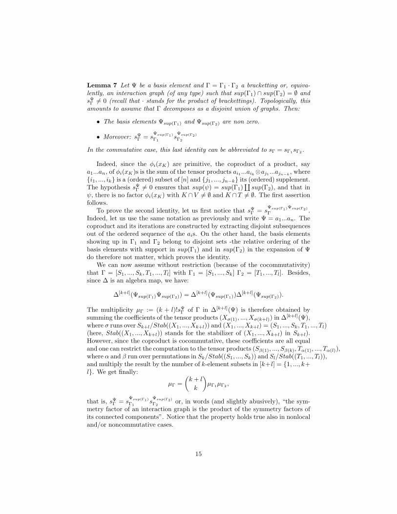
Lemma 7 Let Ψ be a basis element and Γ = Γ1 · Γ2 a bracketting or, equiva-lently, an interaction graph (of any type) such that sup(Γ1) ∩ sup(Γ2) = ∅ andsΨΓ 6= 0 (recall that · stands for the product of brackettings). Topologically, thisamounts to assume that Γ decomposes as a disjoint union of graphs. Then:

• The basis elements Ψsup(Γ1) and Ψsup(Γ2) are non zero.

• Moreover: sΨΓ = sΨsup(Γ1)

Γ1sΨsup(Γ2)

Γ2

In the commutative case, this last identity can be abbreviated to sΓ = sΓ1sΓ2 .

Indeed, since the φi(xK) are primitive, the coproduct of a product, saya1...an, of φi(xK)s is the sum of the tensor products ai1 ...aik ⊗aj1 ...ajn−k

, where{i1, ..., ik} is a (ordered) subset of [n] and {j1, ..., jn−k} its (ordered) supplement.The hypothesis sΨΓ 6= 0 ensures that sup(ψ) = sup(Γ1)

∐sup(Γ2), and that in

ψ, there is no factor φi(xK) with K ∩ V 6= ∅ and K ∩T 6= ∅. The first assertionfollows.

To prove the second identity, let us first notice that sΨΓ = sΨsup(Γ1)Ψsup(Γ2)

Γ .Indeed, let us use the same notation as previously and write Ψ = a1...an. Thecoproduct and its iterations are constructed by extracting disjoint subsequencesout of the ordered sequence of the ais. On the other hand, the basis elementsshowing up in Γ1 and Γ2 belong to disjoint sets -the relative ordering of thebasis elements with support in sup(Γ1) and in sup(Γ2) in the expansion of Ψdo therefore not matter, which proves the identity.

We can now assume without restriction (because of the cocommutativity)that Γ = [S1, ..., Sk, T1, ..., Tl] with Γ1 = [S1, ..., Sk] Γ2 = [T1, ..., Tl]. Besides,since ∆ is an algebra map, we have:

∆[k+l](Ψsup(Γ1)Ψsup(Γ2)) = ∆[k+l](Ψsup(Γ1))∆[k+l](Ψsup(Γ2)).

The multiplicity µΓ := (k + l)!sΨΓ of Γ in ∆[k+l](Ψ) is therefore obtained bysumming the coefficients of the tensor products (Xσ(1), ..., Xσ(k+l)) in ∆[k+l](Ψ),where σ runs over Sk+l/Stab((X1, ..., Xk+l)) and (X1, ..., Xk+l) = (S1, ..., Sk, T1, ..., Tl)(here, Stab((X1, ..., Xk+l)) stands for the stabilizer of (X1, ..., Xk+l) in Sk+l).However, since the coproduct is cocommutative, these coefficients are all equaland one can restrict the computation to the tensor products (Sβ(1), ..., Sβ(k), Tα(1), ..., Tα(l)),where α and β run over permutations in Sk/Stab((S1, ..., Sk)) and Sl/Stab((T1, ..., Tl)),and multiply the result by the number of k-element subsets in [k+l] = {1, ..., k+l}. We get finally:

µΓ =

(k + l

k

)µΓ1µΓ2 ,

that is, sΨΓ = sΨsup(Γ1)

Γ1sΨsup(Γ2)

Γ2or, in words (and slightly abusively), “the sym-

metry factor of an interaction graph is the product of the symmetry factors ofits connected components”. Notice that the property holds true also in nonlocaland/or noncommutative cases.

15

7 Amplitudes and Feynman rules

A linear form on a combinatorial Hopf algebra is unital if ρ(1) = 1 and infinites-imal if ρ(1) = 0.

Let us recall, for example, how linear forms on BXk , X = {x1, ..., xn, ...}, are

usually constructed. Let T be an arbitrary finite sequence of integers. For anypolynomial in k variables, say P (y1, ..., yk) =

∑1≤i1+...+ik≤n

pi1,...,ikyi11 ...y

ikk , we

write P (T ) for the polynomial∏t∈T

P (φ1(xt), ..., φk(xt)) ∈ BXk . One can think of

P as the interacting part of a Lagrangian. Natural forms should then be thought

of as related physical amplitudes. For example, for k = 1, a typical P is λy4

4! ,corresponding to the φ4 theory (see [23] for details). The Green functions ofthis theory are computed via the formula

G(x1, . . . , xn) :=ρ(φ(x1)...φ(xk)e

i∫φ4(x)dx

)

ρ(ei

∫φ4(x)dx

) ,

where ρ denotes the vacuum expectation value of the time-ordered product offields (see section 10.1).

Let us treat now a radically different example to show the ubiquity of theapproach. Let here the role of P be taken by HI(t), the interacting Hamil-tonian of time-dependent perturbation theory (see e.g. our [1, 2]): HI(t) :=eiH0tV e−iH0te−ǫ|t|. Let e1, ..., en, ... be the eigenvectors of H0 with eigenval-ues λ1 < λ2 ≤ ... ≤ λn ≤ .... We assume for simplicity that the groundstate is non degenerate (λ1 6= λ2), although the following reasoning holds infull generality due to [1, 2]. The computation of the ground state of the per-turbed Hamiltonian H0 + V relies on the computation of the quantities suchas: Y =< e1|HI(t1)...H(tp)|e1 >, where t ≥ t1 > ... > tp > −∞. We setk = ∞ and φ2p(tj) := e−iλptj−

ǫ2 |tj | < ep|, φ2p+1(tj) := e+iλptj−

ǫ2 |tj ||ep >.

Then, HI(t) =∑

i,j Vi,jφ2j+1(t)φ2i(t), where Vi,j :=< ej|V |ei >. The unitalform corresponding to the computation of Y is given simply by the form on

F]−∞,t]∞ :

ρ(φi0 (t0)...φi2k+1(t2k+1)) :=

∏

0≤j≤k

Vi2j+1,i2j (φi2j (t2j)|φi2j+1 (t2j+1)),

where (φi2j (t2j)|φi2j+1 (t2j+1)) := φi2j (t2j)φi2j+1 (t2j+1) if i2j is even and i2j+1

odd and zero else. The value of the form ρ on odd products is 0. Of course, thisexample is purely didactical and for such a computation the use of the formalismdevelopped in the present article is largely pointless. It becomes useful whenthe situation gets more involved. Actually, the simple requirement of takingefficiently into account the divergences arising from the adiabatic expansionmay involve advanced combinatorial techniques, see, besides the articles alreadyquoted, our [3].

It is well-known that, in many situations, Green functions such as the ones ofthe φ4 theory split into components parametrized by Feynman diagrams. This

16

property also holds for more complex theories and is best explained throughHopf algebraic computations. Recall first that, since H is a Hopf algebra, theset H∗ of linear forms on H is equipped with an (associative; commutative if His cocommutative) “convolution” product:

∀ρ, µ ∈ H∗, ρ ∗ µ(x) := ρ(x(1))µ(x(2)),

where we used the Sweedler notation ∆(x) = x(1) ⊗ x(2). Notice that, if ρ andµ are infinitesimal forms, ρ ∗ µ(x) := ρ(x{1})µ(x{2}), where we use the nota-

tion ∆(x) = x{1} ⊗ x{2}. By standard graduation arguments, the convolutionlogarithm of a unital form ρ is a well-defined infinitesimal form τ on P . Weextend such a τ to a linear form (still written τ) on P⊗n (resp. P⊗n

sym) by:τ(x1 ⊗ ...⊗ xn) := τ(x1)...τ(xn) or τ [x1|...|xn] := τ(x1)...τ(xn).

Summing up, we get, for X an arbitrary monomial (basis element) in H ,and since τ is an infinitesimal form:

Proposition 8 (Feynman diagrams/rules expansion) For an arbitrary uni-tal form on H, we have:

ρ(X) = exp∗τ (X) = τ ◦ G(X),

or:ρ(X) =

∑

Γ

sXΓ τ(Γ),

where Γ runs over all the brackettings (or interaction graphs) in the image ofX by the graphication map.

The map τ acting on the Γs is called a Feynman rule. Applying Lemma 7, withH as in Sect. 6 we get immediately (with self-explanatory notations):

Lemma 9 Assume that Γ = Γ1 · Γ2, then:

sXΓ τ(Γ) = sX1

Γ1τ(Γ1)s

X2

Γ2τ(Γ2).

8 The combinatorial linked cluster theorem

The combinatorial linked cluster theorem expands a linear form on a combinato-rial Hopf algebra into “connected” parts closely related to the topological notionof connectedness. In this section, we show that this expansion is a very generalphenomenon related to Mobius inversion in the partition lattice. Notations andconventions are in Sect. 6.

We first recall some general facts on the partition lattice and Mobius inver-sion that are familiar in combinatorics but probably not well-known by practi-tioners of Feynman-type diagrammatics and linked cluster theorems (the par-ticular case of Mobius inversion for the partition lattice we are interested in hereseems due to Schutzenberger, we refer to [24] for further details and referenceson the subject).

17

For an arbitrary set S, partitions t := {T1, ..., Tk} of S (that is: T1∐...∐Tk =

S, where∐

stands for the disjoint union) are organized into a poset (partiallyordered set, this poset is actually a lattice -two elements have a max and a min,this follows easily from the definition of the order). We write |t| for the lengthof the partition (so that |t| = k) and abbreviate the partitions of minimal andmaximal length, respectively {S} and {{s}, s ∈ S} to 1 and 0. The subsets Tiare called the blocks, and the order is defined by refinement: for any partitionst and u, t ≤ u if and only if each block of t is contained in a block of u.

The functions f(x, y) on the partition lattice such that f(x, y) 6= 0 only ifx ≤ y form the incidence algebra of the lattice. The (associative) product isdefined by convolution: (f ∗ g)(x, y) :=

∑x≤z≤y

f(x, z)g(z, y). The identity of the

algebra is Kronecker delta function: δ(x, y) := 1 if x = y and := 0 else. Thezeta function ζ(x, y) of the lattice is defined to be equal to 1 if x ≤ y and 0otherwise. The Mobius function µ(x, y) is defined to be the inverse of the zetafunction for the convolution product. It can be computed explicitly: for x ≤ t,where t = {T1, ..., Tk}, we have:

µ(x, t) = (−1)|x|+|t|(n1 − 1)!...(nk − 1)!,

where ni is the number of blocks of x contained in Ti. Using the identitiesµ ∗ ζ(0, 1) = ζ ∗ µ(0, 1) = δ(0, 1) = 0, we recover in particular the useful combi-natorial formulas:

∑

0≤k≤|S|

∑

t

(−1)|t|+|S|(t1 − 1)!...(tk − 1)! = 0

where t runs over the partitions of length k of S and ti stands for the numberof elements in the i-th block Ti of t and, with the same conventions on t,

∑

0≤k≤|S|

∑

t

(−1)|t|+1(|t| − 1)! = 0 (1)

The key application of these notions is to inclusion/exclusion computationsin the partition lattice. Namely, for an arbitrary function h(x) on the lattice, let

us set: h(y) =∑x≤y

h(x). This formula defines uniquely h and, in the convolution

algebra:(h = h ∗ ζ) ⇔ (h = h ∗ µ)

so that h(y) =∑x≤y

h(x)µ(x, y).

Let now x be a basis element of H with support written S, where H is asin Sect. 6. Let ρ be a unital form on H . Recall the notation xT denoting the“T-component” of x for an arbitrary T ⊂ S. For an arbitrary set partitiont = {T1, ..., Tk} of S, we extend ρ to a function ρx on partitions of S and set:

ρx(t) := ρ(xT1)...ρ(xTk).

18

Recall also the decomposition ρ(x) =∑

Γ sxΓτ(Γ). The Γs are represented by

diagrams, among which some are connected. We set ρconn(x) :=∑

ΓcsxΓc

τ(Γc),where the Γc run over connected diagrams. We can then apply the machineryof inclusion/exclusion to ρx and define ρx. The combinatorial linked clustertheorem relates ρconn and ρx:

Theorem 10 (Combinatorial linked cluster theorem) We have, for an ar-bitrary basis element in a free or free commutative combinatorial Hopf algebrawhich generators are primitive elements:

ρconn(x) = ρx(1).

We have indeed:ρx(1) =

∑

t

ρx(t)µ(t, 1)

where t runs over the partitions of S and (with the usual notations) µ(t, 1) =(−1)|t|+1(|t| − 1)!. On the other hand, ρx(t) = ρ(xT1)...ρ(xTk

) and ρ(xTi) =∑

Γi

sxTi

Γiτ(Γi). Lemma 9 ensures that sxΓ1·...·Γk

= sxT1

Γ1...s

xTk

Γk, and we get finally:

ρx(1) =∑

T1∐

...∐

Tk=S

(−1)k+1(k − 1)!∑

Γ1,...,Γk

sxΓ1·...·Γkτ(Γ1) · ... · τ(Γk),

where Γi is a graph showing up in the expansion of ρ(xT1 ).Let now Ψ be an arbitrary graph with sxΨ 6= 0. The graph decomposes

uniquely as a union of topologically disjoint graphs Ψ1

∐...∐

Ψn, where n isthe number of connected components of Ψ. We write Si for sup(Ψi) and SΨ ={S1, ..., Sn}. We have to show that the coefficient of τ(Ψ) in the right hand sideof the previous equation is equal to sxΓ if n = 1 and to 0 else. The first propertyis immediate, since if Γ is connected it appears only in the term associated tothe trivial partition 1 of S and therefore with the coefficient (−1)20!sxΓ = sxΓ.

The second property is slightly less immediate, but follows from the princi-ples of Mobius inversion together with Lemma 9. Notice first that Γ appears inthe right hand side of the equation in association to all partitions of which SΨ

is a refinement. The coefficient of Γ is therefore:

[∑

sΨ≤t≤1

(−1)|t|+1(|t| − 1)!]sxΓ

which is zero as a consequence of the identity ζ ∗µ(SΨ, 1) = δ(SΨ, 1) = 0 in thepartition lattice.

9 The functional linked cluster theorem

A linear form ρ on a free or free commutative combinatorial Hopf algebra H iscalled symmetric if it is invariant by a bijective relabelling of the variables xi -so

19

that ρ(φ1(x2)8φ3(x5)

2φ2(x9)3) = ρ(φ1(x4)

8φ3(x2)2φ2(x1)

3), and so on. WhenX is ordered, the form is called quasi-symmetric if it is invariant by a (strictly)increasing relabelling of the variables, so that e.g. ρ(φ1(x2)

8φ3(x5)2φ2(x9)

3) =ρ(φ1(x4)

8φ3(x5)2φ2(x8)

3), but is not necessarily equal to ρ(φ1(x4)8φ3(x2)

2φ2(x1)3).

Let us consider now a symmetric or quasi-symmetric unital form ρ on H ,where H is as in Sect. 6 with an infinite ordered index set X . For notationalsimplicity, we will assume that X = N. That is, H is an algebra of polynomials(resp. of tensors) over a doubly indexed set of formal, commuting (resp. non-commuting), and primitive variables φi(xS) where S runs over finite subsets ofX and i = 1...nk, where k = |S| and where the sequence of the nk, k ∈ N is afixed sequence of integers.

We first generalize the construction of the “interaction term” P in Sect. 7as follows. We let P = P (T )T⊂X be a family of elements of H such that P (T )is a polynomial (resp. a tensor) in the φi(xS), S ⊂ T .

Definition 11 We say that P is admissible if and only if

1. For any order-preserving bijection φ from T to R, φ(P (T )) = P (R).

2. For any T and any partition U∐V = T (where U and V inherit the

natural order on T ), we have:

∑

b

µb(Pb)U ⊗ (Pb)V = P (U)⊗ P (V ),

where P (T ) =∑

b µbPb is the unique decomposition of P (T ) as a linearcombination of basis elements.

We let the reader check that the map P constructed in Sect. 7 satisfies thisrequirement.

The composition of ρ with P is a “scalar species”: the value ρ(S) := ρ◦P (S)depends only on the number of elements in S (in the quasi-symmetric case,an increasing bijection induces the identity ρ(S) = ρ(T )) so that if we set

ρ(|S|) := ρ(S)|S|! , the scalar species ρ is entirely characterized by the formal power

seriesρ(x) :=

∑

n

ρ(n)xn.

This straightforward remark connects QFT and many-body theory with thevarious algebraic structures existing on the algebra of formal power series. Al-though apparently uselessly pedantical, it is actually useful to understand howthese structures connect to the ones existing on scalar species.

There exists a Hopf-like structure on linear combinations of finite sets (seee.g. [12, 16] for various developments of these ideas and the related notion oftwisted algebras). The coproduct is defined by:

δ(S) :=∑

U∐

T=S

U ⊗ T

20

where∐

stands for the disjoint union, whereas the product is simply inducedby the disjoint union of sets (the product of two overlapping sets is not defined).These maps induce a convolution product written ⊙ (to distinguish it from theconvolution product of forms on H) on scalar species: for α, β two scalar specieswe get:

α⊙ β(S) :=∑

U∐

T=S

α(U)β(T ),

or: α⊙ β(x) = α(x)β(x).

Theorem 12 (General functional linked cluster theorem) We have, forany unital natural form ρ on H and admissible P:

log(ρ(x)) =∑

n

∑

Γcn

snΓcn

n!τ(Γc

n)xn,

where τ := log∗(ρ), Γcn runs over the connected Feynman diagrams with vertex

set [n] and snΓcn

:=∑b

λbsbΓcn, where P ([n]) =

∑b

λbb is the decomposition of

P ([n]) as a linear combination of basis elements.

Proof. We have:

log(ρ(x)) = (log⊙ ρ)(x) =∑

n

(log⊙ ρ)([n])

n!xn

=∑

n

xn

n!

∑

I1∐

...∐

Ik=[n]

(−1)k+1

kρ(I1)...ρ(Ik)

=∑

n

1

n!

∑

k

(−1)k+1

k

∑

I1∐

...∐

Ik=[n]

∑

ΓI1 ,...,ΓIk

si1ΓI1...sikΓIk

τ(ΓI1 )...τ(ΓIk )

=∑

n

1

n!

∑

k

(−1)k+1

k

∑

I1∐

...∐

Ik=[n]

∑

ΓI1 ,...,ΓIk

si1ΓI1...sikΓIk

τ(ΓI1 ...ΓIk)

where ΓIi runs over the Feynman brackets in the expansion of ρ(Ii), i1 := |Ii|and ΓiΓj denotes the concatenation of two brackets (so that e.g. [φ(x1)|φ(x5)2φ(x8)][φ(x2)3|φ(x1)] =[φ(x1)|φ(x5)2φ(x8)|φ(x2)3|φ(x1)]).

Now, let Γ = Γ1

∐...∐

Γp be the (unique) decomposition of a Feynmandiagram showing up in the expansion of ρ([n]) into a product of connected (nonempty) diagrams. According to Lemma 7 and since P is admissible, for anypartition A1

∐...∐Al of [p], we have sa1

ΓA1...san

ΓAl

= snΓ, where ΓAi:=

∐j∈Ai

Γj

and ai is the number of vertices of ΓAi.

The Theorem amounts then to the following properties: the coefficient of

τ(Γ) in log(ρ(x)) issnΓn! x

n if p = 1 (that is if the graph is connected) and zeroelse. The first property (the connected case) is obvious from the expansion.Let us assume therefore that p > 1. The property follows once again from thegeneral properties of the partition posets: the equation (1) concludes the proof.

21

10 Examples

10.1 Quantum Field Theory

In the quantum theory of the scalar field, the underlying Hopf algebra is thebosonic algebra BX

k , where k is the number of fields and the elements of X standfor dummy position or momentum variables.

A typical example is the φ4 (scalar) theory with k = 1 (we write simply φfor φ1). The form ρ computes expectation values of time ordered products offree fields over the vacuum:

ρ(φ(x1)...φ(xk)) :=< 0|T (φ(x1)...φ(xk))|0 > .

Problems arise when some of the xis coincide; these problems are the subjectof the renormalization theory, we do not address them here. The physicallyinteresting quantities are the interacting Green functions

G(x1, . . . , xn) :=ρ(φ(x1)...φ(xk)e

i∫φ4(x)dx

)

ρ(ei

∫φ4(x)dx

) . (2)

The key point is that ρ = exp∗ τ , where τ is zero if its argument has de-gree different from two and τ

(φ(x)φ(y)

):=< 0|T (φ(x)φ(y))|0 > is the Feynman

propagator. The convolution logarithm can then be written as a sum of Feyn-man diagrams, where the lines represent Feynman propagators and the verticesrepresent spacetime points xi. It can be checked that the standard Feynmanrules of quantum field theory [6] are exactly recovered by the convolution ex-ponential [25]. The linked-cluster expansion provides a simple way to deal withthe denominator of eq. (2) [26].

10.2 Cumulants

Let X1, ..., Xn, ... be a sequence of random variables. The underlying Hopfalgebra for this example is once again the bosonic algebra BN

1 . The form ρ isdefined by:

ρ(φ(xi1 )...φ(xik )) := E[Xi1 ...Xik ].

This example enters the general commutative local case.When all the xis are distinct, ρ(φ(xi1 )...φ(xik )) can be expanded as a sum

parametrized by Feynman graphs which are disjoint unions of elementary graphsmade of distinct black vertices, each joigned to a unique white vertex. The con-nected Feynman graphs appearing in the expansion correspond to the cumulantsEc[Xi1 ...Xik ]. The combinatorial linked cluster actually shows that this graph-ical expansion is equivalent to the classical identity:

E[X1...Xn] = Ec[X1...Xn] +∑

A1∪...∪Ak

k∏

i=1

Ec[Xai1...Xai

ji

],

22

where A1 ∪ ...∪Ak runs over the proper partitions of [n] and Ai = {ai1, ..., aiji}.

When the Xi are copies of a given random variable X and setting P ([n]) :=E[X1...Xn] (which is admissible), we recover, using the functional linked clustertheorem:

< eX >c −1 = log(E(eX)),

with the convention < 1 >c= 1 and < Xn >c:= Ec[X1...Xn].

10.3 Quantum field theory with initial correlation

In solid state physics and quantum chemistry, the initial state is generally dif-ferent from the vacuum. The physically relevant form becomes (with the samenotation as in the first example)

ρ(φ(x1)...φ(xk)) :=< Φ|T (φ(x1)...φ(xk))|Φ >,

where |Φ > is a general state. It is also possible to consider a mixed state insteadof the pure state |Φ〉. Except for very special cases (quasi-free states for bosonicfields and Slater determinants for fermionic fields) the convolution logarithm τof ρ is then more complicated than in the first example. In particular, τ canbe nonzero if its argument have degree different from two. In quantum optics,expansions in terms of τ are known as cluster expansions and they lead to muchbetter convergence properties [27]. For the fermionic fields, the convolutionlogarithms τ are equivalent to the cumulants of the reduced density matrices,that are strongly advocated by Kutzelnigg and Mukherjee [28, 29, 30, 31].

The diagrammatic expansions can then not be done anymore using Feynmandiagrams constructed out of Feynman propagators: see e.g. our [4] and requirethe full apparatus of generalized Feynman diagrams for commutative local case.

10.4 Non-Gaussian measures

Perturbative expansions in statistical physics for measures of Gaussian type canbe performed using the usual Feynman graphs of Sect. 10.1. This is becausethe Wick theorem applies. When dealing with arbitrary functional measuresthis is not the case any more: higher cumulants (i.e. higher truncated momentsor truncated Schwinger functions) have to be taken into account.

Feynman graphs and linked-cluster theorems have been developed by Djahand coll. [5] in this framework. They were extensively used in several problemsof probability theory [32, 33, 34]. These Feynman diagrams are equivalent tothose of a quantum field theory with initial correlation.

10.5 Free probabilities

Free probabilities deal with the noncommutative local case and study linearforms on the tensor algebra FN

1 . In general, the graphs required to study suchforms are free interaction graphs.

23

In practice, the theory of free probabilities focus often on linear forms withparticular properties. This allows for various simplifications and typical prop-erties as far as the corresponding cumulant expansions and their diagrammaticexpansions are concerned. In particular, the Speicher’s notion of free (or non-crossing) cumulant is obtained from the moment generating function by Mobiusinversion with respect to the lattice of noncrossing partitions (and not with re-spect to the lattice of partitions), see e.g. [35] for further details and referenceson the subject.

10.6 Truncated Wightman distributions

In axiomatic quantum field theory, the form used in section 10.1 are replacedby

W (x1, ..., xn) :=< Φ|φH(x1)...φH(xk)|Φ >,

where the operator product is used instead of the time-ordered product, thefields are written in the Heisenberg picture and |Φ〉 is the ground state of theinteracting system. Such functions are called Wightman distributions or correla-tion functions. The main difference with the standard case is that the Wightmandistributions are not symmetric, the order of the arguments is fixed. Still, thereis a perturbation theory of Wightman functions that leads to non-commutativeFeynman diagrams [36]. Their combinatorics is the same as for the standardcase [37]. Thus, the corresponding convolution logarithm τ is again zero if its ar-gument is not of degree two, but now τ

(φ(x), φ(y)

)= 〈0|φ(x)φ(y)|0〉 is different

from τ(φ(y), φ(x)

).

However, it is also possible to work at the non-perturbative level and todefine the form ρ

(φ(x1) . . . φ(xn)

):=W (x1, . . . , xn). In that case, the convolu-

tion logarithm τ is generally not zero if its argument is not of degree two andτ(φ(x1) . . . φ(xn)

)is now called a truncated Wightman distribution.

The definition of truncated Wightman distributions was first given by RudolfHaag in 1958 [38]. We follow (up to the order of the variables) the definition ofSandars’ paper [39]: “For n ≥ 1 we let Pn denote the set of all partitions of theset {1, . . . , n} into pairwise disjoint subsets, which are ordered from low to high.If r is an ordered set in the partition P ∈ Pn we write r ∈ P and we denotethe elements of r by r(1) < · · · < r(|r|), where |r| is the number of elementsof r. The truncated n-point distributions ωT

n , n ≥ 1 of a state ω are definedimplicitly in terms of the n-point distributions

ω(ϕ(x1), . . . , ϕ(xn)

)=

∑

P∈Pn

∏

r∈P

ωT|r|(xr(1), . . . , xr(|r|)).

This is exactly the relation between ρ = exp∗ τ and τ for non-commuting vari-ables.

From the physical point of view, the truncation procedure eliminates thecontribution of the vacuum state as an intermediate state [40, p. 271]. Truncateddistributions have many desirable properties. For instance, they decrease muchfaster than Wightman distributions at large space-like separation [41].

24

10.7 Nonrelativistic systems with Coulomb interaction

Let us neglect here the problem of dealing with the Fermi statistics (whichamounts essentially to introducing the correct signs in the definition of theHopf algebra structures, see e.g. [14, 15]).

Let us consider n electrons in a quantum system of non-relativistic electronswith a Coulomb interaction in the external field generated by nuclei. This isthe standard approach of quantum chemistry and solid-state physics.

We assume that the non-interacting state can be described by a Slater deter-minant and that the particle-hole transformation was used to deal with occupiedstates. The form is defined as in section 10.1 and the Green functions are now

G(x1, . . . , xn, y1, . . . , yn) :=ρ(ψ(x1) . . . ψ(xn)ψ

†(y1) . . . ψ†(yn)e

−iI)

ρ(e−iI),

where

I = e2∫dtdrdr′

ψ†(r, t)ψ†(r′, t)ψ(r′, t)ψ(r, t)

8πǫ0|r− r′|.

The main difference with quantum field theory is that the interaction is notlocal. Still, in the linked-cluster expansion, we want to consider that the pointsr and r′ in I are connected. In diagrammatic terms, r and r′ are connected bya wavy line. We introduced the tripartite graphs to deal with this importantcase.

References

[1] Ch. Brouder and F. Patras. Hyperoctahedral Chen calculus for effectiveHamiltonians. J. Algebra, 322:4105–20, 2009.

[2] Ch. Brouder, A. Mestre, and F. Patras. Tree expansions in time-dependentperturbation theory. J. Math. Phys., 51:072104, 2010.

[3] Ch. Brouder, G. Duchamp, F. Patras, and G. Z. Toth. The Rayleigh-Schrodinger perturbation series of quasi-degenerate systems. 2010.arXiv:1011.1751v1 [quant-ph].

[4] Ch. Brouder and F. Patras. Decomposition into one-particle irreducibleGreen functions in many-body physics. proceedings of the conference oncombinatorics and physics, bonn, 2007. Contemp. Math. arXiv:0803.3747,pages ???–??, (to appear).

[5] S.H. Djah, H. Gottschalk, and H. Ouerdiane. Feynman graph representa-tion of the perturbation series for general functional measures. J. Funct.Anal., 227:153–187, 2005.

[6] C. Itzykson and J.-B. Zuber. Quantum Field Theory. McGraw-Hill, NewYork, 1980.

25

[7] R. Stora. Renormalized perturbation theory: a missing chapter. Inter-national Journal of Geometric Methods in Modern Physics, 5, No 8:1345–1360, 2008.

[8] S. A. Joni and G.-C. Rota. Coalgebras and bialgebras in combinatorics.Stud. Appl. Math., 61:93–139, 1979.

[9] F. Patras and C. Reutenauer. On Dynkin and Klyachko idempotents ingraded bialgebras. Adv. Appl. Math., 28:560–79, 2002.

[10] F. Patras. La decomposition en poids des algebres de hopf. Ann. Inst.Fourier, 43 (4):1067–87, 1993.

[11] F. Patras and C. Reutenauer. On descent algebras and twisted bialgebras.Moscow Math. J., 4, n1:199–216, 2004.

[12] F. Patras and M. Schocker. Twisted descent algebras and the Solomon-Titsalgebra. Adv. Math., 199:151–84, 2006.

[13] M. Aguiar and S. Mahajan. Monoidal functors, species and Hopf algebras.CRM Monograph Series, Vol. 29, Montreal, 2010.

[14] P. Cassam-Chenai and F. Patras. The Hopf algebra of identical, fermionicparticle systems. Fundamental concepts and properties. J. Math. Phys.,44:4484–906, 2003.

[15] Ch. Brouder, B. Fauser, A. Frabetti, and R. Oeckl. Quantum field theoryand Hopf algebra cohomology. J. Phys. A: Math. Gen., 37:5895–927, 2004.

[16] F. Patras and M. Schocker. Trees, set compositions and the twisted descentalgebra. J. Algebr. Comb., 28:3–23, 2008.

[17] R. Gurau, J. Magnen, and V. Rivasseau. Tree quantum field theory. Ann.Henri Poincare, 10:867–91, 2009.

[18] P. Leroux, F. Bergeron, and G. Labelle. Combinatorial Species and Tree-like Structures, volume 67 of Encyclopedia of Mathematics and its Applica-tions. Cambridge University Press, Cambridge, 1998.

[19] J. Ecalle. Singularites non abordables par la geometrie. Ann. Inst. Fourier,42:73–143, 1992.

[20] F. Menous. On the stability of some groups of formal diffeomorphisms bythe birkhoff decomposition. Adv. in Math., 216:1–28, 2007.

[21] R.D. Mattuck. A Guide to Feynman Diagrams in the Many-Body Problem(2nd edition). McGraw-Hill, New York, 1976.

[22] A. Connes and D. Kreimer. Renormalization in quantum field theory andthe Riemann-Hilbert problem I: the Hopf algebra structure of graphs andthe main theorem. Commun. Math. Phys., 210:249–73, 2000.

26

[23] H. Kleinert and V. Schulte-Frohlinde. Critical Properties of φ4 Theories.World Scientific, Singapore, 2001.

[24] L. Comtet. Advanced Combinatorics. Reidel, Dordrecht, 1974.

[25] Ch. Brouder. Quantum field theory meets Hopf algebra. Math. Nachr.,282:1664–90, 2009.

[26] E. K. U. Gross, E. Runge, and O. Heinonen. Many-Particle Theory. AdamHilger, Bristol, 1991.

[27] M. Kira and S. W. Koch. Cluster-expansion representation in quantumoptics. Phys. Rev. A, 78:022102, 2008.

[28] W. Kutzelnigg and D. Mukherjee. Normal order and extended Wick the-orem for a multiconfiguration reference wave function. J. Chem. Phys.,107:432–49, 1997.

[29] W. Kutzelnigg and D. Mukherjee. Cumulant expansion of the reduceddensity matrices. J. Chem. Phys., 110:2800–9, 1999.

[30] W. Kutzelnigg and D. Mukherjee. Direct determination of the cumulantsof the reduced density matrices. Chem. Phys. Lett., 317:567–74, 2000.

[31] Liguo Kong, M. Nooijen, and D. Mukherjee. An algebraic proof of gener-alized Wick theorem. J. Chem. Phys., 132:234107, 2010.

[32] S. H. Djah, H. Gottschalk, and H. Ouerdiane. Feynman graphs for non-Gaussian measures. In P. Biane, J. Faraut, and H. Ouerbiane, editors,Analyse et Probabilite, volume 16 of Seminaires et Congres, pages 35–54,Paris, 2008. Soc. Math. France.

[33] H. Gottschalk, H. Ouerdiane, and B. Smii. Convolution calculus on whitenoise spaces and Feynman diagrams representation of generalized renor-malization flows. In A. B. Cruzeiro, H. Ouerbiane, and N. Obata, editors,Mathematical Analysis of Random Phenomena, pages 101–10, Singapore,2007. World Scientific.

[34] H. Gottschalk, B. Smii, and H. Thaler. The Feynman graph representationof convolution semigroups and its applications to Levy statistics. Bernoulli,14:322–51, 2008.

[35] F. Lehner S. Belinschi, M. Bozejko and R. Speicher. The normal distribu-tion is ⊞-infinitely divisible. Adv. Math., 226:3677–3698, 2011.

[36] A. Ostendorf. Feynman rules for Wightman functions. Commun. Math.Phys., 40:273–90, 1984.

[37] R. Brunetti, K. Fredenhagen, and M. Kohler. The microlocal spectrum con-dition and Wick polynomials of free fields on curved spacetimes. Commun.Math. Phys., 180:633–52, 1996.

27

[38] R. Haag. Quantum field theories with composite particles and asymptoticconditions. Phys. Rev., 112:669–73, 1958.

[39] K. Sanders. Equivalence of the (generalised) Hadamard and microlocalspectrum condition for (generalised) free fields in curved spacetime. Com-mun. Math. Phys., 295:485–501, 2010.

[40] H. Epstein and V. Glaser. The role of locality in perturbation theory. Ann.Inst. Henri Poincare, 19:211–95, 1973.

[41] H. Araki. On asymptotic behavior of vacuum expectation values at largespace-like separation. Ann. Phys., 11:260–74, 1960.

28