Nonconvex Piecewise Linear Knapsack Problems

S. Kameshwaran and Y. NarahariElectronic Commerce Laboratory

Department of Computer Science and AutomationIndian Institute of Science

Bangalore - India{ kameshn,hari }@csa.iisc.ernet.in

Abstract

This paper considers the minimization version of a class of nonconvex knapsack problemswith piecewise linear cost structure. The items to be included in the knapsack have a divisiblequantity and a cost function. An item can be included partially in a given quantity range andthe cost is a nonconvex piecewise linear function of quantity. Given a demand, the optimizationproblem is to choose an optimal quantity for each item such that the demand is satisfied and thetotal cost is minimized. This problem is encountered in many situations in manufacturing, logis-tics, and supply chain design. In particular, we are motivated by winner determination in volumediscount procurement auctions in electronic commerce. The piecewise linearity of the cost func-tion gives the problem two different knapsack structures related to precedence constrained andmultiple choice knapsack problems. Two mixed integer linear programming formulations areproposed based on the above structures. Motivated by the unique nature of the varying de-mands on the problem in different scenarios, the following algorithms are developed: (1) a fastpolynomial time, near optimal heuristic using convex envelopes; (2) two exact, pseudo polyno-mial time dynamic programming algorithms; (3) a polynomial time 2-approximation algorithm;and (4) a fully polynomial time approximation scheme. A test suite was developed to generaterepresentative problem instances with different characteristics. Extensive computational experi-ments conducted on these problem instances show that the proposed formulation and algorithmsare faster than the existing techniques.

Keywords

Combinatorial optimization, piecewise linear knapsack problems, precedence constrained knap-sack model, multiple choice knapsack model, LP relaxation, dynamic programming, convexenvelopes, approximation algorithms, fully polynomial time approximation schemes.

All correspondence is to be addressed to: Y. Narahari, Department of Computer Science and Automation,

Indian Institute of Science, Bangalore - 560 012, India. Email: hari@csa.iisc.ernet.in.

1

Acronyms

LP Linear ProgrammingDP Dynamic ProgrammingIP Integer ProgramMILP Mixed Integer Linear ProgramNKP Nonlinear Knapsack ProblemPLKP Piecewise Linear Knapsack ProblemIM Incremental ModelMCM Multiple Choice ModelCCM Convex Combination ModelPCKM Precedence Constrained Knapsack ModelLP:PCKM LP relaxation of PCKMCE:PCKM PCKM with Convex Envelope of original cost functionMCKM Multiple Choice Knapsack ModelMKP Multiple Choice Knapsack ProblemFPTAS Fully Polynomial Time Approximation Scheme

1 Introduction

Knapsack problems are among the the most intensively studied combinatorial optimization prob-lems [31, 28, 22]. The knapsack problem considers a set of items, each having an associated costand a weight. The problem (minimization version) is then to choose a subset of the given itemssuch that the corresponding total cost is minimized while the total weight satisfies the specifieddemand. Well studied variants of the knapsack problems [31, 28] include: bounded/unbounded knap-sack problems, subset-sum problems, change-making problems, multiple knapsack problems, multiplechoice knapsack problems, and bin packing problems. The applications of these problems vary fromindustrial applications and financial management to personal health-care.

1.1 Nonlinear Knapsack Problems

A generic nonlinear knapsack problem (also called nonlinear resource allocation problem) has ademand B and a set J of N items. Each item j ∈ J has a nonlinear cost function Qj(b) definedover the quantity b ∈ [aj , aj ]. The optimization problem is to choose quantity qj ∈ {0, [aj , aj ]}for each item j to meet the demand B (

∑j∈J qj ≥ B) such that the total cost

∑j∈J Qj(qj) of

accumulated demand is minimized. The problem can be formulated as the following nonlinearinteger programming problem:

(NKP) : min∑j∈J

Qj(qj) (1)

subject to ∑j∈J

qj ≥ B

ajxj ≤ qj ≤ ajxj ∀j ∈ J

2

xj ∈ {0, 1}, qj ≥ 0, integer ∀j ∈ J

The decision variable qj can take either zero value or an integer value in the range [aj , aj ].This is implemented as linear inequalities using binary decision variables xj . There are severalvariations to the above problem: the objective function is an arbitrary function Q(q1, . . . , q|J |); eachitem has a weight wj and the demand constraint is

∑j∈J wjqj ≥ B; a generic demand constraint∑

j∈J gj(qj) ≥ B; and the variables qj are continuous. The problem considered in this paper is asin NKP above, with Qj as a nonconvex piecewise linear cost function.

The NKP and its variants are encountered either directly, or as a subproblem, in a variety ofapplications, including production planning, financial modeling, stratified sampling, and in capacityplanning in manufacturing, health-care, and computer networks [5]. Different available algorithmsfor the problem were developed with varying assumptions on the cost function Qj and the demandconstraint. The book by Ibaraki and Katoh [17] provides an excellent collection of algorithms fordemand constraint

∑j∈J qj = B. The paper by Bretthauer and Shetty [5] reviews the algorithms

and applications for NKP with generic demand constraint∑

j∈J gj(qj) ≥ B.The objective functions considered in most of the literature for convex knapsack problems are

separable like in NKP. If the decision variables are continuous, the differentiability and optimalityproperty of the convex functions are used in designing algorithms [34, 2]. For problems withmore general separable nonlinear convex constraint of the form

∑j∈J gj(qj) ≥ B, multiplier search

methods [3] and variable pegging methods [23, 4] are the general techniques. The algorithmsfor problems with discrete variables are based on Lagrangian and linear relaxations. For convexdemand constraints, the solution methodologies include branch-and-bound [3], linearization, anddynamic programming [29, 14].

Unlike convex knapsack problems, very little work has been done on nonconvex knapsack prob-lems. Dynamic programming (DP) is the predominant solution technique for this problem. Apseudo-polynomial time DP algorithm was developed in [17]. Approximation algorithms based ondynamic programming were proposed in [26] (the problem was called as capacitated plant alloca-tion problem). Concave cost functions were considered in [30], but the solution technique usedlocal minimizers for obtaining a local optimal solution. Use of branch-and-bound algorithm wasproposed as a promising technique in [5].

1.2 Contributions and Outline

In this paper, we consider a nonlinear knapsack problem called as nonconvex piecewise linearknapsack problem (PLKP). As the name suggests, the cost function Qj is a nonconvex piecewiselinear cost function. The demand constraints are the same as in NKP. The problem is motivateddue to its application in the winner determination of volume discount procurement auctions inelectronic commerce. The cost function and the associated knapsack problem are introduced inSection 2. We study the problem from different perspectives owing to its diverse demands in varyingscenarios.

3

• First as an optimization problem, Section 3 investigates various mathematical programmingformulations. Two new formulations are proposed based on the precedence constraint andmultiple choice structure of the problem. Computational experiments that compare the solu-tion time of the proposed formulations with that of the existing textbook formulations, whensolved with a commercial optimization solver, are presented. This is useful for practitionersto choose the formulation that best suits their needs.

• For applications that demand a good solution in relatively short time, a fast linear program-ming based heuristic is developed in Section 4. The approach uses the convex envelopes of thecost function to solve the relaxation. Computational experiments were performed on probleminstances with different features to study the trade-off in savings in computational time withthe optimality gap of heuristic solution.

• Two exact algorithms based on dynamic programming are developed in Section 5. Thepurpose of these algorithms is two fold: one of the algorithms is useful in solving PLKPswhich appear as subproblems in multi-attribute procurement and the other algorithm is usedto develop a fully polynomial time approximation scheme.

• The PLKP is NP-hard and it is of theoretical interest to investigate the possibilities ofapproximation. Section 6 presents a 2-approximation algorithm and a fully polynomial timeapproximation scheme. Section 7 concludes the paper.

2 The Nonconvex Piecewise Linear Knapsack Problem

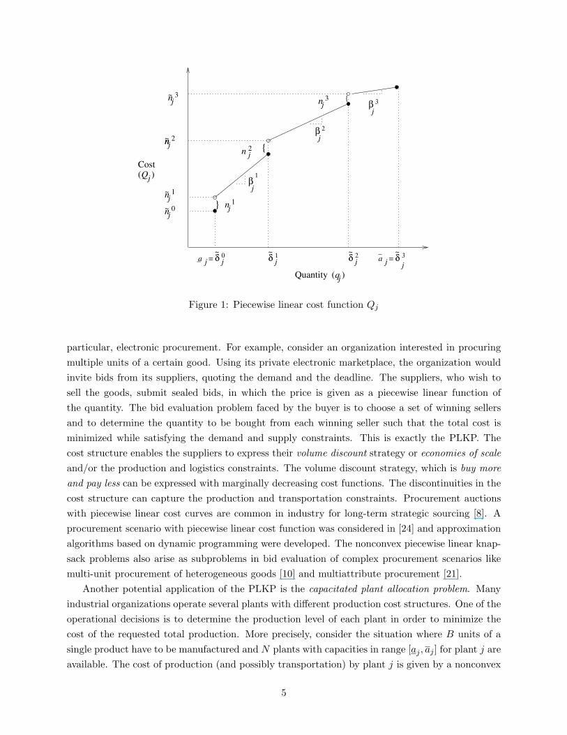
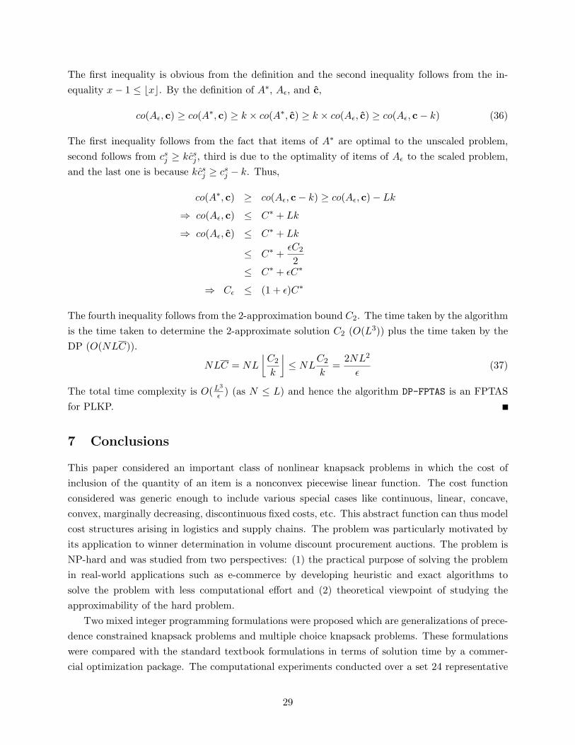
The nonconvex piecewise linear knapsack problem (PLKP) considered in this paper is the same asNKP above, with the cost function Qj as a piecewise linear function. The piecewise linear costfunction Qj defined over the quantity range [aj , aj ] is shown in Figure 1. Table 1 provides thenotation.

The cost function Qj can be represented by tuples of break points, slopes, and costs at breakpoints: Qj ≡ ((aj = δ0

j , . . . , aj = δljj ), (β1

j , . . . , βljj ), (n0

j , . . . , nljj )). For notational convenience,

define δsj ≡ δs

j − δs−1j and ns

j as the fixed cost associated with segment s. Note that, by thisdefinition, n0

j = n0j . The function is assumed to be strictly increasing, but it need not be marginally

decreasing as shown in the figure. The assumed cost structure is generic enough to include variousspecial cases: concave, convex, continuous, and aj = 0. The PLKP with the generic cost structurewas shown to be NP-hard upon reduction from the knapsack problem in [20].

2.1 Motivation for PLKP

The discontinuous piecewise linear cost structure is common in telecommunication and electric-ity pricing, and in manufacturing and logistics. This cost structure for network flow problemswith application is supply chain management was studied in [6]. Our motivation for consideringthis cost structure for knapsack problems is driven by its applications in electronic commerce, in

4

0 1 2! ! !

"1

" 2

~ ~ ~

} n

{

{

n

n

1

2

3" 3

Quantity

!~ 3

n 0

n

nn

n

1

3

2

~

~

~

~

j j j j

j

j

j

j

j

j

jj

j

j

a =jj

qj

a = _

Qj( )

( )

Cost

Figure 1: Piecewise linear cost function Qj

particular, electronic procurement. For example, consider an organization interested in procuringmultiple units of a certain good. Using its private electronic marketplace, the organization wouldinvite bids from its suppliers, quoting the demand and the deadline. The suppliers, who wish tosell the goods, submit sealed bids, in which the price is given as a piecewise linear function ofthe quantity. The bid evaluation problem faced by the buyer is to choose a set of winning sellersand to determine the quantity to be bought from each winning seller such that the total cost isminimized while satisfying the demand and supply constraints. This is exactly the PLKP. Thecost structure enables the suppliers to express their volume discount strategy or economies of scaleand/or the production and logistics constraints. The volume discount strategy, which is buy moreand pay less can be expressed with marginally decreasing cost functions. The discontinuities in thecost structure can capture the production and transportation constraints. Procurement auctionswith piecewise linear cost curves are common in industry for long-term strategic sourcing [8]. Aprocurement scenario with piecewise linear cost function was considered in [24] and approximationalgorithms based on dynamic programming were developed. The nonconvex piecewise linear knap-sack problems also arise as subproblems in bid evaluation of complex procurement scenarios likemulti-unit procurement of heterogeneous goods [10] and multiattribute procurement [21].

Another potential application of the PLKP is the capacitated plant allocation problem. Manyindustrial organizations operate several plants with different production cost structures. One of theoperational decisions is to determine the production level of each plant in order to minimize thecost of the requested total production. More precisely, consider the situation where B units of asingle product have to be manufactured and N plants with capacities in range [aj , aj ] for plant j areavailable. The cost of production (and possibly transportation) by plant j is given by a nonconvex

5

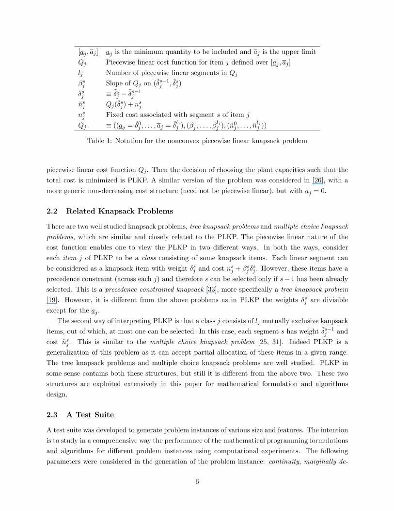
[aj , aj ] aj is the minimum quantity to be included and aj is the upper limitQj Piecewise linear cost function for item j defined over [aj , aj ]lj Number of piecewise linear segments in Qj

βsj Slope of Qj on (δs−1

j , δsj )

δsj ≡ δs

j − δs−1j

nsj Qj(δs

j ) + nsj

nsj Fixed cost associated with segment s of item j

Qj ≡ ((aj = δ0j , . . . , aj = δ

ljj ), (β1

j , . . . , βljj ), (n0

j , . . . , nljj ))

Table 1: Notation for the nonconvex piecewise linear knapsack problem

piecewise linear cost function Qj . Then the decision of choosing the plant capacities such that thetotal cost is minimized is PLKP. A similar version of the problem was considered in [26], with amore generic non-decreasing cost structure (need not be piecewise linear), but with aj = 0.

2.2 Related Knapsack Problems

There are two well studied knapsack problems, tree knapsack problems and multiple choice knapsackproblems, which are similar and closely related to the PLKP. The piecewise linear nature of thecost function enables one to view the PLKP in two different ways. In both the ways, considereach item j of PLKP to be a class consisting of some knapsack items. Each linear segment canbe considered as a knapsack item with weight δs

j and cost nsj + βs

j δsj . However, these items have a

precedence constraint (across each j) and therefore s can be selected only if s− 1 has been alreadyselected. This is a precedence constrained knapsack [33], more specifically a tree knapsack problem[19]. However, it is different from the above problems as in PLKP the weights δs

j are divisibleexcept for the aj .

The second way of interpreting PLKP is that a class j consists of lj mutually exclusive kanpsackitems, out of which, at most one can be selected. In this case, each segment s has weight δs−1

j andcost ns

j . This is similar to the multiple choice knapsack problem [25, 31]. Indeed PLKP is ageneralization of this problem as it can accept partial allocation of these items in a given range.The tree knapsack problems and multiple choice knapsack problems are well studied. PLKP insome sense contains both these structures, but still it is different from the above two. These twostructures are exploited extensively in this paper for mathematical formulation and algorithmsdesign.

2.3 A Test Suite

A test suite was developed to generate problem instances of various size and features. The intentionis to study in a comprehensive way the performance of the mathematical programming formulationsand algorithms for different problem instances using computational experiments. The followingparameters were considered in the generation of the problem instance: continuity, marginally de-

6

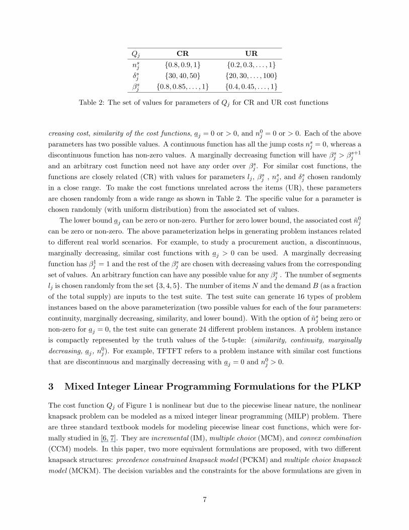
Qj CR UR

nsj {0.8, 0.9, 1} {0.2, 0.3, . . . , 1}

δsj {30, 40, 50} {20, 30, . . . , 100}

βsj {0.8, 0.85, . . . , 1} {0.4, 0.45, . . . , 1}

Table 2: The set of values for parameters of Qj for CR and UR cost functions

creasing cost, similarity of the cost functions, aj = 0 or > 0, and n0j = 0 or > 0. Each of the above

parameters has two possible values. A continuous function has all the jump costs nsj = 0, whereas a

discontinuous function has non-zero values. A marginally decreasing function will have βsj > βs+1

j

and an arbitrary cost function need not have any order over βsj . For similar cost functions, the

functions are closely related (CR) with values for parameters lj , βsj , ns

j , and δsj chosen randomly

in a close range. To make the cost functions unrelated across the items (UR), these parametersare chosen randomly from a wide range as shown in Table 2. The specific value for a parameter ischosen randomly (with uniform distribution) from the associated set of values.

The lower bound aj can be zero or non-zero. Further for zero lower bound, the associated cost n0j

can be zero or non-zero. The above parameterization helps in generating problem instances relatedto different real world scenarios. For example, to study a procurement auction, a discontinuous,marginally decreasing, similar cost functions with aj > 0 can be used. A marginally decreasingfunction has β1

j = 1 and the rest of the βsj are chosen with decreasing values from the corresponding

set of values. An arbitrary function can have any possible value for any βsj . The number of segments

lj is chosen randomly from the set {3, 4, 5}. The number of items N and the demand B (as a fractionof the total supply) are inputs to the test suite. The test suite can generate 16 types of probleminstances based on the above parameterization (two possible values for each of the four parameters:continuity, marginally decreasing, similarity, and lower bound). With the option of ns

j being zero ornon-zero for aj = 0, the test suite can generate 24 different problem instances. A problem instanceis compactly represented by the truth values of the 5-tuple: (similarity, continuity, marginallydecreasing, aj, n0

j ). For example, TFTFT refers to a problem instance with similar cost functionsthat are discontinuous and marginally decreasing with aj = 0 and n0

j > 0.

3 Mixed Integer Linear Programming Formulations for the PLKP

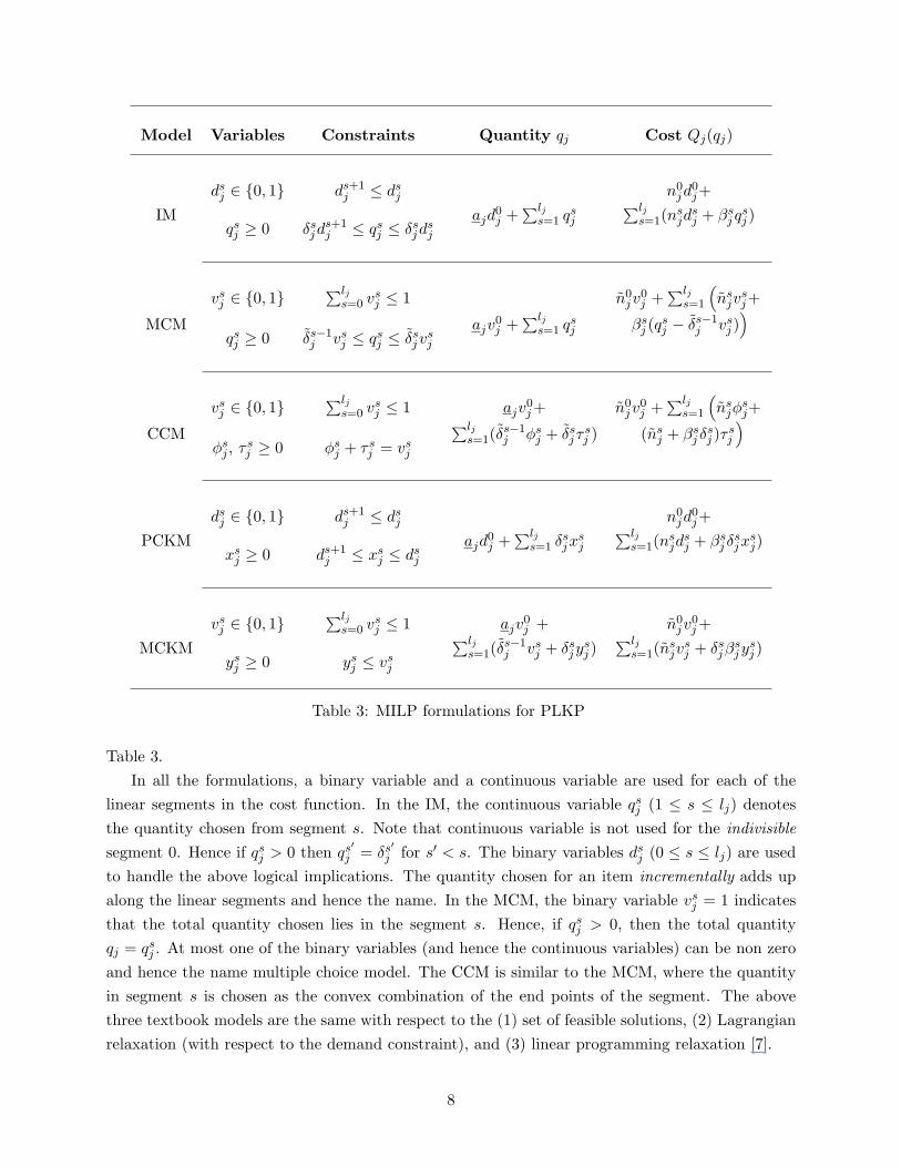
The cost function Qj of Figure 1 is nonlinear but due to the piecewise linear nature, the nonlinearknapsack problem can be modeled as a mixed integer linear programming (MILP) problem. Thereare three standard textbook models for modeling piecewise linear cost functions, which were for-mally studied in [6, 7]. They are incremental (IM), multiple choice (MCM), and convex combination(CCM) models. In this paper, two more equivalent formulations are proposed, with two differentknapsack structures: precedence constrained knapsack model (PCKM) and multiple choice knapsackmodel (MCKM). The decision variables and the constraints for the above formulations are given in

7

Model Variables Constraints Quantity qj Cost Qj(qj)

dsj ∈ {0, 1} ds+1

j ≤ dsj n0

jd0j+

IMqsj ≥ 0 δs

jds+1j ≤ qs

j ≤ δsjd

sj

ajd0j +

∑ljs=1 qs

j

∑ljs=1(n

sjd

sj + βs

j qsj )

vsj ∈ {0, 1}

∑ljs=0 vs

j ≤ 1 n0jv

0j +

∑ljs=1

(ns

jvsj+

MCMqsj ≥ 0 δs−1

j vsj ≤ qs

j ≤ δsjv

sj

ajv0j +

∑ljs=1 qs

j βsj (q

sj − δs−1

j vsj )

)

vsj ∈ {0, 1}

∑ljs=0 vs

j ≤ 1 ajv0j + n0

jv0j +

∑ljs=1

(ns

jφsj+

CCMφs

j , τ sj ≥ 0 φs

j + τ sj = vs

j

∑ljs=1(δ

s−1j φs

j + δsjτ

sj ) (ns

j + βsj δ

sj )τ

sj

)

dsj ∈ {0, 1} ds+1

j ≤ dsj n0

jd0j+

PCKMxs

j ≥ 0 ds+1j ≤ xs

j ≤ dsj

ajd0j +

∑ljs=1 δs

jxsj

∑ljs=1(n

sjd

sj + βs

j δsjx

sj)

vsj ∈ {0, 1}

∑ljs=0 vs

j ≤ 1 ajv0j + n0

jv0j +

MCKMys

j ≥ 0 ysj ≤ vs

j

∑ljs=1(δ

s−1j vs

j + δsjy

sj )

∑ljs=1(n

sjv

sj + δs

jβsjy

sj )

Table 3: MILP formulations for PLKP

Table 3.In all the formulations, a binary variable and a continuous variable are used for each of the

linear segments in the cost function. In the IM, the continuous variable qsj (1 ≤ s ≤ lj) denotes

the quantity chosen from segment s. Note that continuous variable is not used for the indivisiblesegment 0. Hence if qs

j > 0 then qs′j = δs′

j for s′ < s. The binary variables dsj (0 ≤ s ≤ lj) are used

to handle the above logical implications. The quantity chosen for an item incrementally adds upalong the linear segments and hence the name. In the MCM, the binary variable vs

j = 1 indicatesthat the total quantity chosen lies in the segment s. Hence, if qs

j > 0, then the total quantityqj = qs

j . At most one of the binary variables (and hence the continuous variables) can be non zeroand hence the name multiple choice model. The CCM is similar to the MCM, where the quantityin segment s is chosen as the convex combination of the end points of the segment. The abovethree textbook models are the same with respect to the (1) set of feasible solutions, (2) Lagrangianrelaxation (with respect to the demand constraint), and (3) linear programming relaxation [7].

8

The proposed new formulations PCKM and MCKM are similar to the IM and the MCM,respectively. The continuous variables in the proposed models are normalized to vary between 0and 1. These two models, however, reveal the hidden knapsack structures discussed in Section2.2. The proposed formulations are useful in developing different algorithms due their knapsackstructures. The heuristic algorithm based on LP relaxation (Section 4) and the 2-approximationalgorithm (Section 6) are developed using the PCKM formulation while the dynamic programmingbased algorithms (Section 5) and the fully polynomial time approximation scheme (Section 6) aredeveloped using the MCKM formulation.

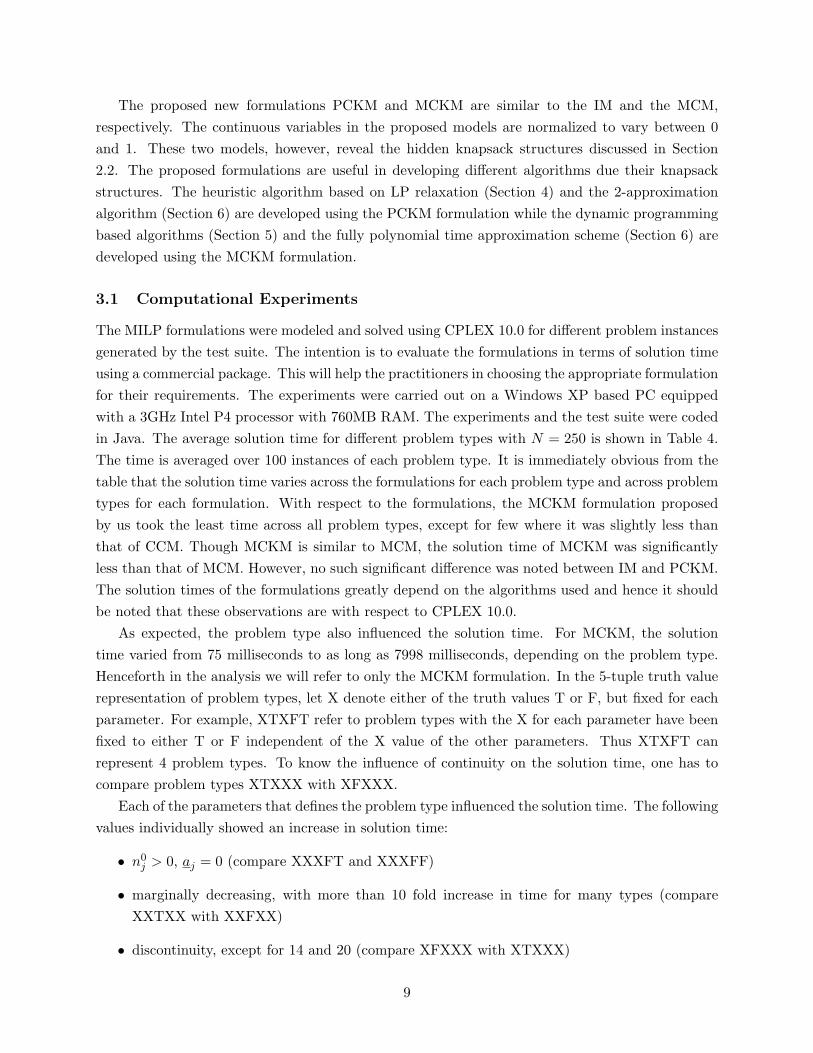
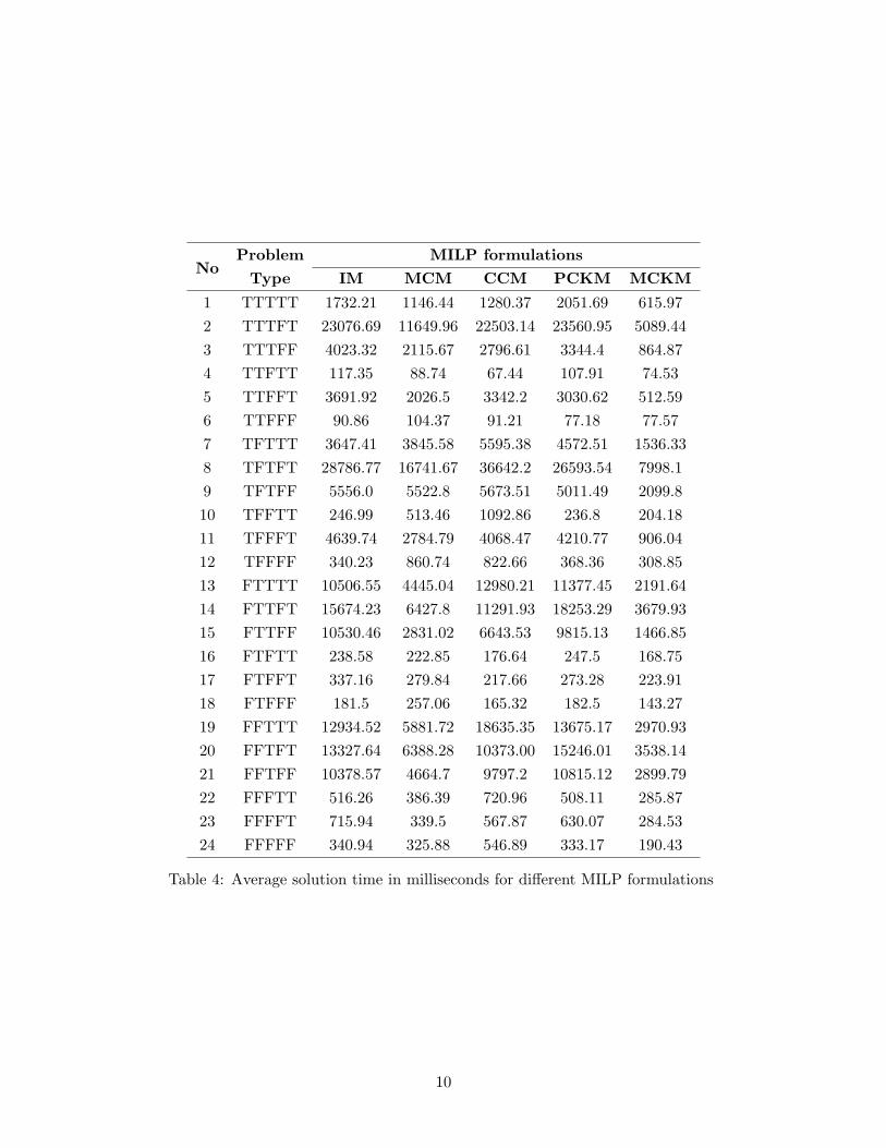
3.1 Computational Experiments

The MILP formulations were modeled and solved using CPLEX 10.0 for different problem instancesgenerated by the test suite. The intention is to evaluate the formulations in terms of solution timeusing a commercial package. This will help the practitioners in choosing the appropriate formulationfor their requirements. The experiments were carried out on a Windows XP based PC equippedwith a 3GHz Intel P4 processor with 760MB RAM. The experiments and the test suite were codedin Java. The average solution time for different problem types with N = 250 is shown in Table 4.The time is averaged over 100 instances of each problem type. It is immediately obvious from thetable that the solution time varies across the formulations for each problem type and across problemtypes for each formulation. With respect to the formulations, the MCKM formulation proposedby us took the least time across all problem types, except for few where it was slightly less thanthat of CCM. Though MCKM is similar to MCM, the solution time of MCKM was significantlyless than that of MCM. However, no such significant difference was noted between IM and PCKM.The solution times of the formulations greatly depend on the algorithms used and hence it shouldbe noted that these observations are with respect to CPLEX 10.0.

As expected, the problem type also influenced the solution time. For MCKM, the solutiontime varied from 75 milliseconds to as long as 7998 milliseconds, depending on the problem type.Henceforth in the analysis we will refer to only the MCKM formulation. In the 5-tuple truth valuerepresentation of problem types, let X denote either of the truth values T or F, but fixed for eachparameter. For example, XTXFT refer to problem types with the X for each parameter have beenfixed to either T or F independent of the X value of the other parameters. Thus XTXFT canrepresent 4 problem types. To know the influence of continuity on the solution time, one has tocompare problem types XTXXX with XFXXX.

Each of the parameters that defines the problem type influenced the solution time. The followingvalues individually showed an increase in solution time:

• n0j > 0, aj = 0 (compare XXXFT and XXXFF)

• marginally decreasing, with more than 10 fold increase in time for many types (compareXXTXX with XXFXX)

• discontinuity, except for 14 and 20 (compare XFXXX with XTXXX)

9

Problem MILP formulationsNo

Type IM MCM CCM PCKM MCKM

1 TTTTT 1732.21 1146.44 1280.37 2051.69 615.972 TTTFT 23076.69 11649.96 22503.14 23560.95 5089.443 TTTFF 4023.32 2115.67 2796.61 3344.4 864.874 TTFTT 117.35 88.74 67.44 107.91 74.535 TTFFT 3691.92 2026.5 3342.2 3030.62 512.596 TTFFF 90.86 104.37 91.21 77.18 77.577 TFTTT 3647.41 3845.58 5595.38 4572.51 1536.338 TFTFT 28786.77 16741.67 36642.2 26593.54 7998.19 TFTFF 5556.0 5522.8 5673.51 5011.49 2099.810 TFFTT 246.99 513.46 1092.86 236.8 204.1811 TFFFT 4639.74 2784.79 4068.47 4210.77 906.0412 TFFFF 340.23 860.74 822.66 368.36 308.8513 FTTTT 10506.55 4445.04 12980.21 11377.45 2191.6414 FTTFT 15674.23 6427.8 11291.93 18253.29 3679.9315 FTTFF 10530.46 2831.02 6643.53 9815.13 1466.8516 FTFTT 238.58 222.85 176.64 247.5 168.7517 FTFFT 337.16 279.84 217.66 273.28 223.9118 FTFFF 181.5 257.06 165.32 182.5 143.2719 FFTTT 12934.52 5881.72 18635.35 13675.17 2970.9320 FFTFT 13327.64 6388.28 10373.00 15246.01 3538.1421 FFTFF 10378.57 4664.7 9797.2 10815.12 2899.7922 FFFTT 516.26 386.39 720.96 508.11 285.8723 FFFFT 715.94 339.5 567.87 630.07 284.5324 FFFFF 340.94 325.88 546.89 333.17 190.43

Table 4: Average solution time in milliseconds for different MILP formulations

10

However, the similarity parameter did not reveal any coherent pattern (compare TXXXX withFXXXX). Six problem types (2, 5, 7, 8, 10, and 12) with CR property had solution times greaterthan that of with UR (14, 17, 19, 20, 22, and 24, respectively) and vice versa for six other problemtypes (1, 3, 4, 6, 9, and 11 took less time than that of 13, 15, 16, 21, and 23, respectively) . Fromthe above individual influences, one is tempted to believe that either of TFTFT or FFTFT shouldhave taken the longest time and indeed TFTFT (number 8) took the longest time.

4 A Heuristic Algorithm based on LP Relaxation and Convex

Envelopes

Certain applications demand a good quality solution in a relatively short time. For example, initerative or multi-round procurement auctions, the winner determination problem has to be solvedin each round. With automated agents participating in the auctions, several hundreds of suchrounds will not be uncommon. In such scenarios it may be advantageous to solve optimally thewinner determination problem only in the later rounds, where less number of bidders will be leftin the auctions. In the initial rounds with more number of bidders, solving the problem fast usinga heuristic which provides a good feasible solution will help in earlier termination of the auction.In certain cases like spot purchase markets and exchanges, even the single round auctions need tobe cleared in very less time. In this section, we develop a fast heuristic that finds a near-optimalsolution to the PLKP. The heuristic is based on LP relaxation of PCKM using the convex envelopeof the cost function.

In LP relaxation based heuristics, the integral variables are relaxed to take on continuousvalues and the resulting linear program is solved. If the optimal solution to the relaxed problem isintegral, then it is also the optimal solution to the original problem. If not, the continuous solutionobtained should be converted into integral solutions using some heuristic rounding techniques sothat it is feasible to the original problem. Often, the integral solutions obtained this way are closeto optimality, depending on the structure of the problem. We first propose a polynomial timealgorithm for solving the LP relaxation of PCKM, followed by a rounding heuristic to construct amixed integer feasible solution from the continuous solution.

4.1 Convex Envelopes and LP Relaxation

The LP relaxation of PCKM can be solved using the convex envelope of the cost function Qj . Itwas shown in [6] that the LP relaxation of the incremental model approximates the cost functionQj with its convex envelope. Since the LP relaxations of PCKM and the incremental model areequivalent (qs

j = δsjx

sj), the LP relaxation of PCKM approximates the function Qj with its convex

envelope. This means that solving the LP relaxation is equivalent to solving the PCKM with theconvex envelope of Qj as its cost function. The notion of convex envelope is introduced first andthen an algorithm is proposed to construct the convex envelope for a nonconvex piecewise linearfunction.

11

! j ! j ! j ! j ! j ! j ! j! j

1

2

3

j1"

1

2

3

j

j

1

2

"

"

0 0

Cost Cost

Quantity Quantity

1 2 3 0 1 2 30~ ~ ~ ~ ~ ~ ~ ~

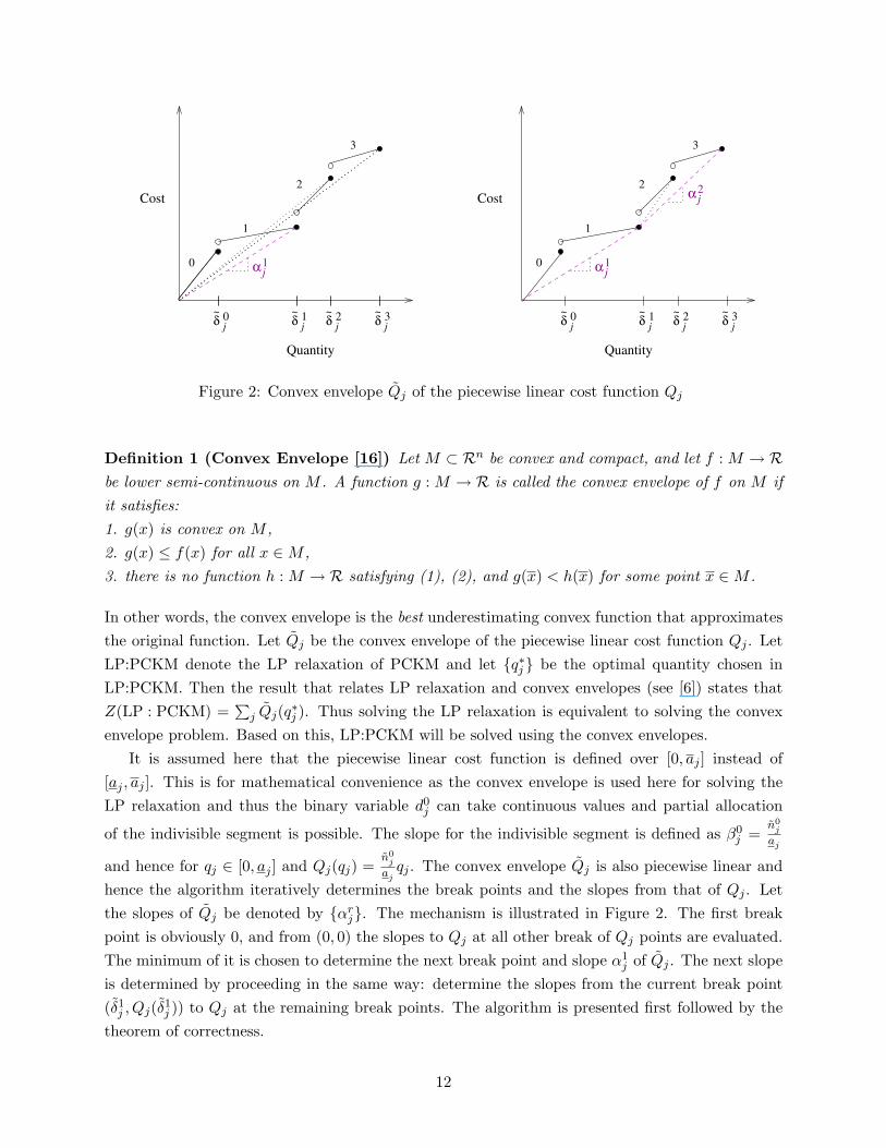
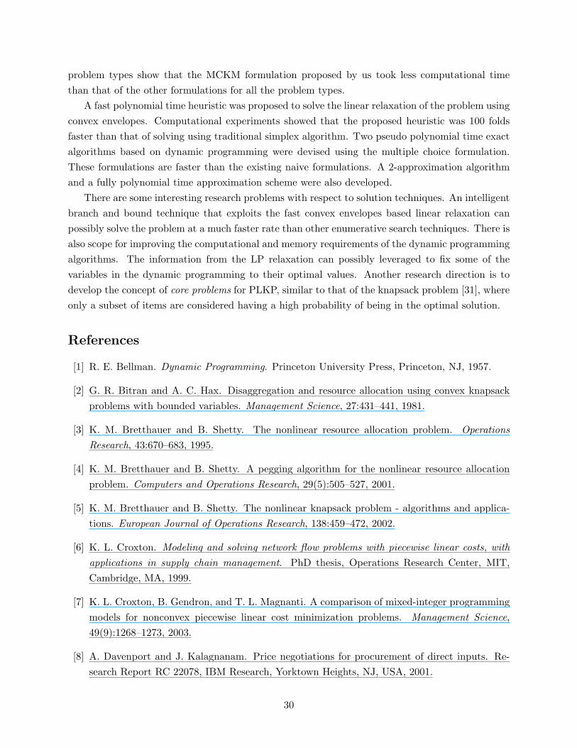
Figure 2: Convex envelope Qj of the piecewise linear cost function Qj

Definition 1 (Convex Envelope [16]) Let M ⊂ Rn be convex and compact, and let f : M → Rbe lower semi-continuous on M . A function g : M → R is called the convex envelope of f on M ifit satisfies:1. g(x) is convex on M ,2. g(x) ≤ f(x) for all x ∈M ,3. there is no function h : M → R satisfying (1), (2), and g(x) < h(x) for some point x ∈M .

In other words, the convex envelope is the best underestimating convex function that approximatesthe original function. Let Qj be the convex envelope of the piecewise linear cost function Qj . LetLP:PCKM denote the LP relaxation of PCKM and let {q∗j } be the optimal quantity chosen inLP:PCKM. Then the result that relates LP relaxation and convex envelopes (see [6]) states thatZ(LP : PCKM) =

∑j Qj(q∗j ). Thus solving the LP relaxation is equivalent to solving the convex

envelope problem. Based on this, LP:PCKM will be solved using the convex envelopes.It is assumed here that the piecewise linear cost function is defined over [0, aj ] instead of

[aj , aj ]. This is for mathematical convenience as the convex envelope is used here for solving theLP relaxation and thus the binary variable d0

j can take continuous values and partial allocation

of the indivisible segment is possible. The slope for the indivisible segment is defined as β0j =

n0j

aj

and hence for qj ∈ [0, aj ] and Qj(qj) =n0

j

ajqj . The convex envelope Qj is also piecewise linear and

hence the algorithm iteratively determines the break points and the slopes from that of Qj . Letthe slopes of Qj be denoted by {αr

j}. The mechanism is illustrated in Figure 2. The first breakpoint is obviously 0, and from (0, 0) the slopes to Qj at all other break of Qj points are evaluated.The minimum of it is chosen to determine the next break point and slope α1

j of Qj . The next slopeis determined by proceeding in the same way: determine the slopes from the current break point(δ1

j , Qj(δ1j )) to Qj at the remaining break points. The algorithm is presented first followed by the

theorem of correctness.

12

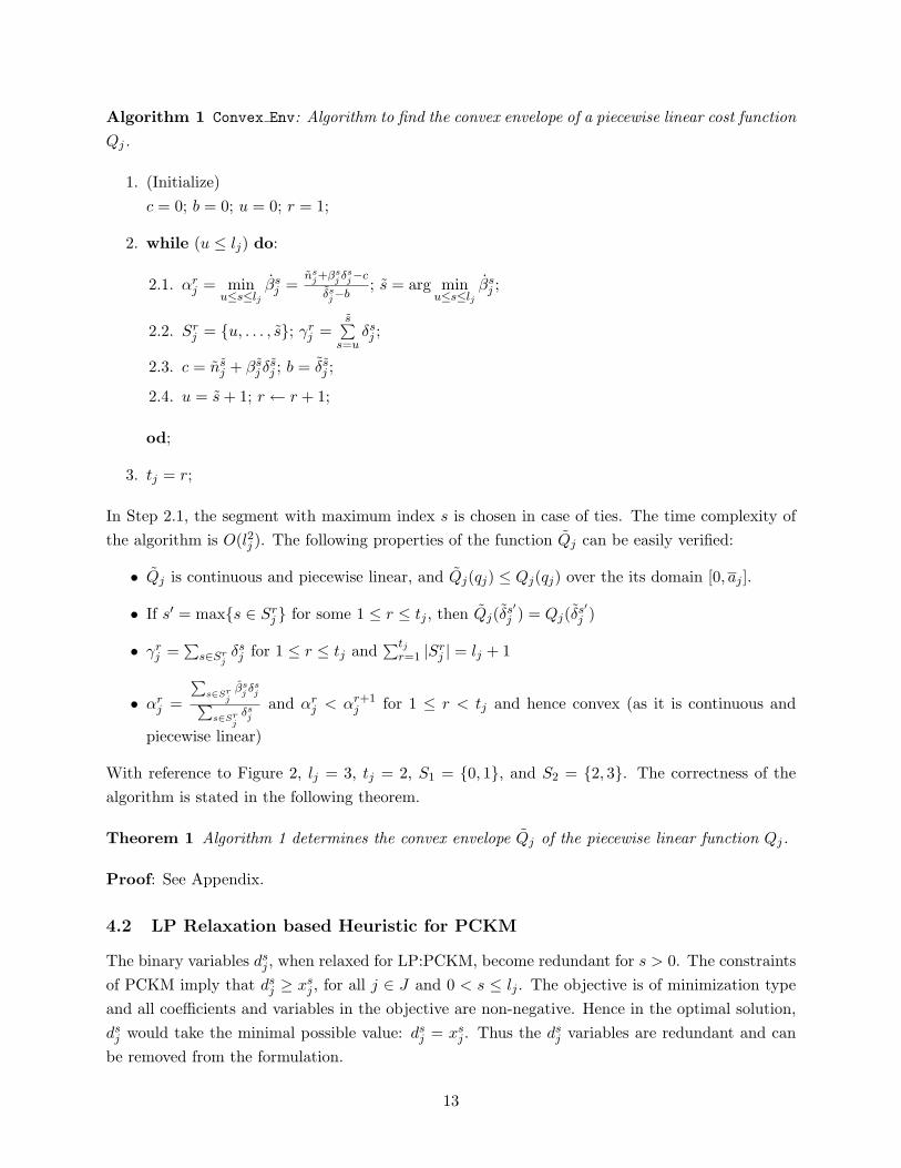
Algorithm 1 Convex Env: Algorithm to find the convex envelope of a piecewise linear cost functionQj.

1. (Initialize)c = 0; b = 0; u = 0; r = 1;

2. while (u ≤ lj) do:

2.1. αrj = min

u≤s≤ljβs

j =ns

j+βsj δs

j−c

δsj−b

; s = arg minu≤s≤lj

βsj ;

2.2. Srj = {u, . . . , s}; γr

j =s∑

s=uδsj ;

2.3. c = nsj + βs

j δsj ; b = δs

j ;

2.4. u = s + 1; r ← r + 1;

od;

3. tj = r;

In Step 2.1, the segment with maximum index s is chosen in case of ties. The time complexity ofthe algorithm is O(l2j ). The following properties of the function Qj can be easily verified:

• Qj is continuous and piecewise linear, and Qj(qj) ≤ Qj(qj) over the its domain [0, aj ].

• If s′ = max{s ∈ Srj } for some 1 ≤ r ≤ tj , then Qj(δs′

j ) = Qj(δs′j )

• γrj =

∑s∈Sr

jδsj for 1 ≤ r ≤ tj and

∑tjr=1 |Sr

j | = lj + 1

• αrj =

∑s∈Sr

jβs

j δsj∑

s∈Srj

δsj

and αrj < αr+1

j for 1 ≤ r < tj and hence convex (as it is continuous and

piecewise linear)

With reference to Figure 2, lj = 3, tj = 2, S1 = {0, 1}, and S2 = {2, 3}. The correctness of thealgorithm is stated in the following theorem.

Theorem 1 Algorithm 1 determines the convex envelope Qj of the piecewise linear function Qj.

Proof: See Appendix.

4.2 LP Relaxation based Heuristic for PCKM

The binary variables dsj , when relaxed for LP:PCKM, become redundant for s > 0. The constraints

of PCKM imply that dsj ≥ xs

j , for all j ∈ J and 0 < s ≤ lj . The objective is of minimization typeand all coefficients and variables in the objective are non-negative. Hence in the optimal solution,ds

j would take the minimal possible value: dsj = xs

j . Thus the dsj variables are redundant and can

be removed from the formulation.

13

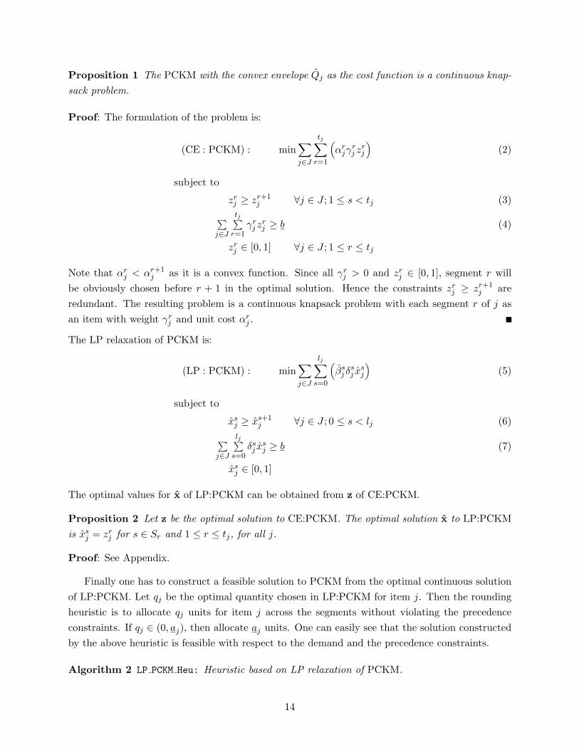
Proposition 1 The PCKM with the convex envelope Qj as the cost function is a continuous knap-sack problem.

Proof: The formulation of the problem is:

(CE : PCKM) : min∑j∈J

tj∑r=1

(αr

jγrj z

rj

)(2)

subject to

zrj ≥ zr+1

j ∀j ∈ J ; 1 ≤ s < tj (3)∑j∈J

tj∑r=1

γrj z

rj ≥ b (4)

zrj ∈ [0, 1] ∀j ∈ J ; 1 ≤ r ≤ tj

Note that αrj < αr+1

j as it is a convex function. Since all γrj > 0 and zr

j ∈ [0, 1], segment r willbe obviously chosen before r + 1 in the optimal solution. Hence the constraints zr

j ≥ zr+1j are

redundant. The resulting problem is a continuous knapsack problem with each segment r of j asan item with weight γr

j and unit cost αrj .

The LP relaxation of PCKM is:

(LP : PCKM) : min∑j∈J

lj∑s=0

(βs

j δsj x

sj

)(5)

subject to

xsj ≥ xs+1

j ∀j ∈ J ; 0 ≤ s < lj (6)

∑j∈J

lj∑s=0

δsj x

sj ≥ b (7)

xsj ∈ [0, 1]

The optimal values for x of LP:PCKM can be obtained from z of CE:PCKM.

Proposition 2 Let z be the optimal solution to CE:PCKM. The optimal solution x to LP:PCKMis xs

j = zrj for s ∈ Sr and 1 ≤ r ≤ tj, for all j.

Proof: See Appendix.

Finally one has to construct a feasible solution to PCKM from the optimal continuous solutionof LP:PCKM. Let qj be the optimal quantity chosen in LP:PCKM for item j. Then the roundingheuristic is to allocate qj units for item j across the segments without violating the precedenceconstraints. If qj ∈ (0, aj), then allocate aj units. One can easily see that the solution constructedby the above heuristic is feasible with respect to the demand and the precedence constraints.

Algorithm 2 LP PCKM Heu: Heuristic based on LP relaxation of PCKM.

14

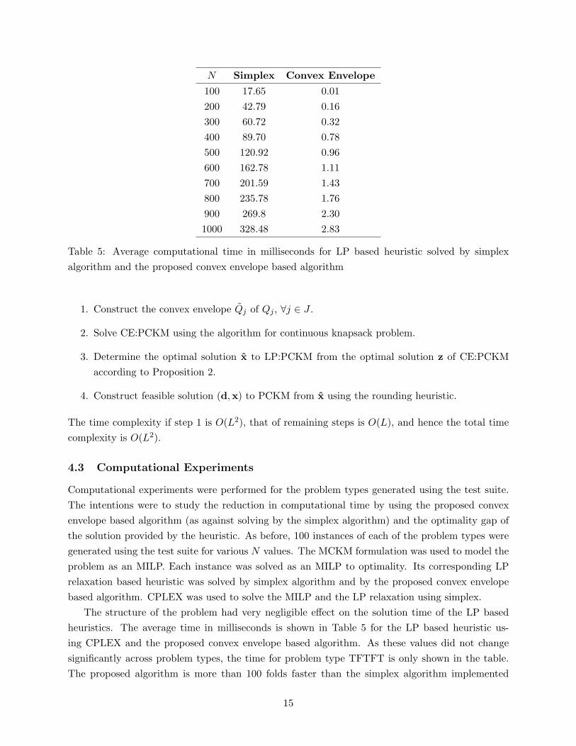
N Simplex Convex Envelope

100 17.65 0.01200 42.79 0.16300 60.72 0.32400 89.70 0.78500 120.92 0.96600 162.78 1.11700 201.59 1.43800 235.78 1.76900 269.8 2.301000 328.48 2.83

Table 5: Average computational time in milliseconds for LP based heuristic solved by simplexalgorithm and the proposed convex envelope based algorithm

1. Construct the convex envelope Qj of Qj , ∀j ∈ J .

2. Solve CE:PCKM using the algorithm for continuous knapsack problem.

3. Determine the optimal solution x to LP:PCKM from the optimal solution z of CE:PCKMaccording to Proposition 2.

4. Construct feasible solution (d,x) to PCKM from x using the rounding heuristic.

The time complexity if step 1 is O(L2), that of remaining steps is O(L), and hence the total timecomplexity is O(L2).

4.3 Computational Experiments

Computational experiments were performed for the problem types generated using the test suite.The intentions were to study the reduction in computational time by using the proposed convexenvelope based algorithm (as against solving by the simplex algorithm) and the optimality gap ofthe solution provided by the heuristic. As before, 100 instances of each of the problem types weregenerated using the test suite for various N values. The MCKM formulation was used to model theproblem as an MILP. Each instance was solved as an MILP to optimality. Its corresponding LPrelaxation based heuristic was solved by simplex algorithm and by the proposed convex envelopebased algorithm. CPLEX was used to solve the MILP and the LP relaxation using simplex.

The structure of the problem had very negligible effect on the solution time of the LP basedheuristics. The average time in milliseconds is shown in Table 5 for the LP based heuristic us-ing CPLEX and the proposed convex envelope based algorithm. As these values did not changesignificantly across problem types, the time for problem type TFTFT is only shown in the table.The proposed algorithm is more than 100 folds faster than the simplex algorithm implemented

15

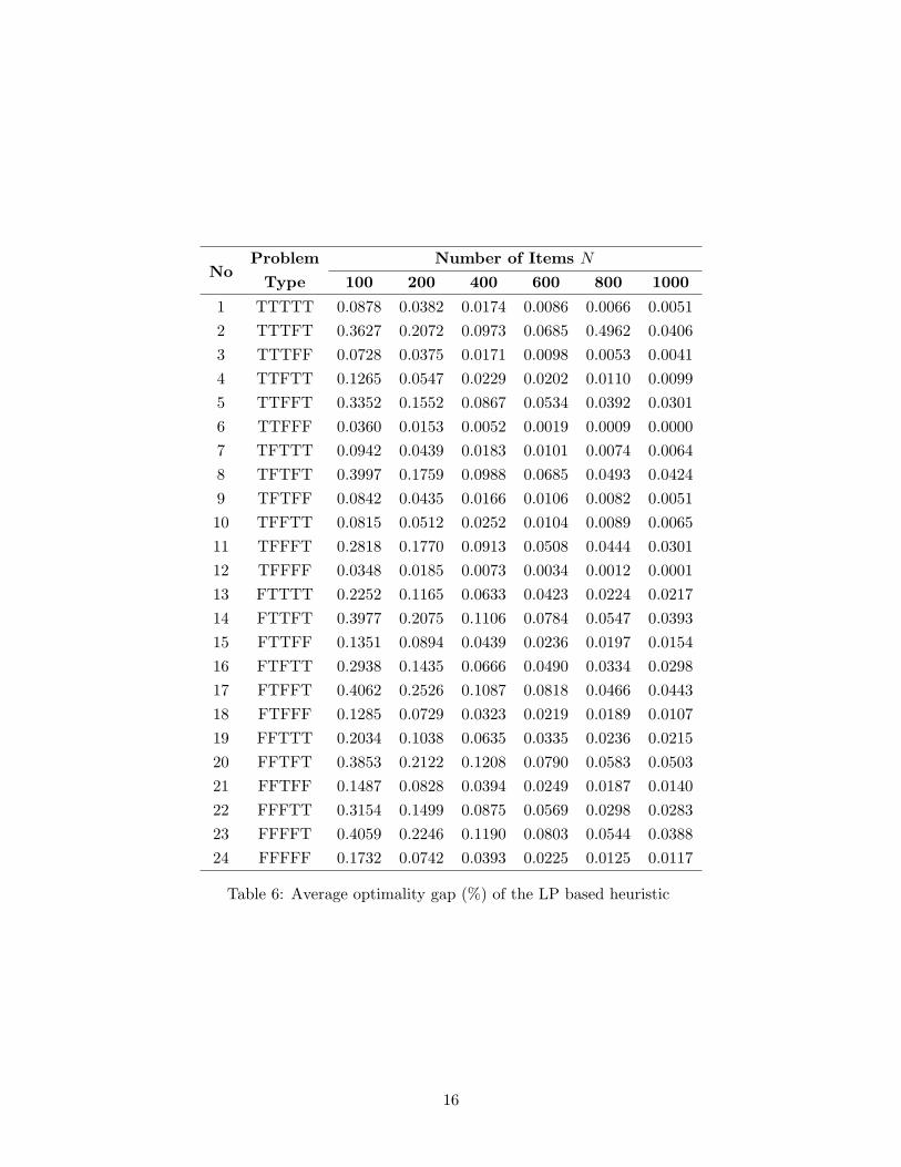
Problem Number of Items NNo

Type 100 200 400 600 800 1000

1 TTTTT 0.0878 0.0382 0.0174 0.0086 0.0066 0.00512 TTTFT 0.3627 0.2072 0.0973 0.0685 0.4962 0.04063 TTTFF 0.0728 0.0375 0.0171 0.0098 0.0053 0.00414 TTFTT 0.1265 0.0547 0.0229 0.0202 0.0110 0.00995 TTFFT 0.3352 0.1552 0.0867 0.0534 0.0392 0.03016 TTFFF 0.0360 0.0153 0.0052 0.0019 0.0009 0.00007 TFTTT 0.0942 0.0439 0.0183 0.0101 0.0074 0.00648 TFTFT 0.3997 0.1759 0.0988 0.0685 0.0493 0.04249 TFTFF 0.0842 0.0435 0.0166 0.0106 0.0082 0.005110 TFFTT 0.0815 0.0512 0.0252 0.0104 0.0089 0.006511 TFFFT 0.2818 0.1770 0.0913 0.0508 0.0444 0.030112 TFFFF 0.0348 0.0185 0.0073 0.0034 0.0012 0.000113 FTTTT 0.2252 0.1165 0.0633 0.0423 0.0224 0.021714 FTTFT 0.3977 0.2075 0.1106 0.0784 0.0547 0.039315 FTTFF 0.1351 0.0894 0.0439 0.0236 0.0197 0.015416 FTFTT 0.2938 0.1435 0.0666 0.0490 0.0334 0.029817 FTFFT 0.4062 0.2526 0.1087 0.0818 0.0466 0.044318 FTFFF 0.1285 0.0729 0.0323 0.0219 0.0189 0.010719 FFTTT 0.2034 0.1038 0.0635 0.0335 0.0236 0.021520 FFTFT 0.3853 0.2122 0.1208 0.0790 0.0583 0.050321 FFTFF 0.1487 0.0828 0.0394 0.0249 0.0187 0.014022 FFFTT 0.3154 0.1499 0.0875 0.0569 0.0298 0.028323 FFFFT 0.4059 0.2246 0.1190 0.0803 0.0544 0.038824 FFFFF 0.1732 0.0742 0.0393 0.0225 0.0125 0.0117

Table 6: Average optimality gap (%) of the LP based heuristic

16

by CPLEX. Thus, it is clearly preferable in time constrained applications than the commercialoptimizers.

The quality of the solution given by the heuristic was measured using the optimality gap,calculated against the optimal solution provided by the MCKM formulation. It is obvious thatthe problem structure will influence the optimality gap, unlike the solution time. The results areshown in Table 6. One can easily verify from the Table 6 that problem types with n0

j > 0 havemore optimality gap than with n0

j = 0 for aj = 0 (by comparing problems XXXFT and XXXFF).With respect to similarity parameter (TXXXX versus FXXXX), UR functions had more gap thanthat of the CR functions. However, there were no significant differences in gap with respect tocontinuity (XTXXX versus XFXXX) and marginally decreasing (XXTXX versus XXFXX).

5 Exact Algorithms based on Dynamic Programming

Dynamic programming (DP) is the earliest exact solution technique to the knapsack problem [1] andhence been successfully applied to its variants. With the knapsack problems having two parameters,cost and demand, DP formulations based on each of the parameters are commonly developed. Theidea is to make on of these parameters as independent variable and determine the other recursively.In the DP based on demand, the minimum cost for a given demand is determined recursively.For the DP based on cost, the maximum demand that can be accommodated for a given cost isdetermined recursively.

5.1 Motivation

The DP algorithms for knapsack problems are pseudo polynomial time algorithms, which workrelatively fast for small problem instances. However, with larger problem instances, they tend tobe inefficient in time and memory. Our purpose of developing DP algorithms for PLKP is mainlytwofold: the DP algorithm based on cost is used to develop fully polynomial time approximationscheme in Section 6 and the DP algorithm based on demand is useful for multi-attribute procure-ment with configurable bids. The DP based on demand does not only provide the optimal solutionfor demand B, but for any demand b ∈ [0, B]. The DP is basically a recursion and hence with asingle run, one can get the optimal solutions for any demand b. This redundancy is useful in certaindecision making scenarios and in particular for PLKP, it is useful auctions with configurable bids.

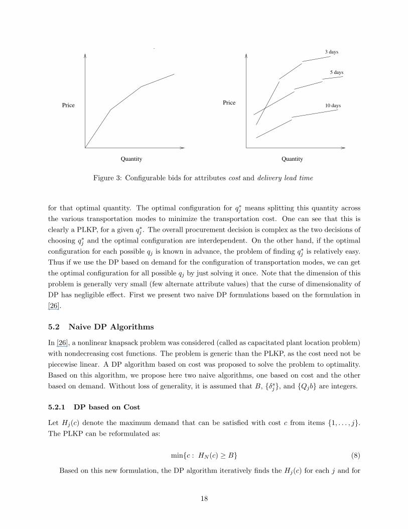
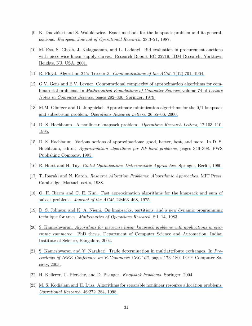
In multi-attribute auctions, there are multiple attributes to be negotiated, in addition to price.Configurable bids allows the suppliers to communicate all of their capabilities and gives the pro-vision for the buyer to configure the bid based on the requirements. For example, consider a steelprocurement scenario, with just two attributes: cost and delivery lead time. With large quantitiesof steel being traded, the suppliers submit configurable bids, as shown in Figure 3. In the figure, theattribute delivery lead time has three possible attribute values, due to the different transportationmodes. Further the cost of delivery depends on the quantity. The buyer has to make two decisions:choose the optimal quantity q∗j from each bid j and an optimal configuration of the delivery modes

17

5 days

10 days

Quantity

Price

Quantity

Price

3 days

Figure 3: Configurable bids for attributes cost and delivery lead time

for that optimal quantity. The optimal configuration for q∗j means splitting this quantity acrossthe various transportation modes to minimize the transportation cost. One can see that this isclearly a PLKP, for a given q∗j . The overall procurement decision is complex as the two decisions ofchoosing q∗j and the optimal configuration are interdependent. On the other hand, if the optimalconfiguration for each possible qj is known in advance, the problem of finding q∗j is relatively easy.Thus if we use the DP based on demand for the configuration of transportation modes, we can getthe optimal configuration for all possible qj by just solving it once. Note that the dimension of thisproblem is generally very small (few alternate attribute values) that the curse of dimensionality ofDP has negligible effect. First we present two naive DP formulations based on the formulation in[26].

5.2 Naive DP Algorithms

In [26], a nonlinear knapsack problem was considered (called as capacitated plant location problem)with nondecreasing cost functions. The problem is generic than the PLKP, as the cost need not bepiecewise linear. A DP algorithm based on cost was proposed to solve the problem to optimality.Based on this algorithm, we propose here two naive algorithms, one based on cost and the otherbased on demand. Without loss of generality, it is assumed that B, {δs

j}, and {Qjb} are integers.

5.2.1 DP based on Cost

Let Hj(c) denote the maximum demand that can be satisfied with cost c from items {1, . . . , j}.The PLKP can be reformulated as:

min{c : HN (c) ≥ B} (8)

Based on this new formulation, the DP algorithm iteratively finds the Hj(c) for each j and for

18

each possible cost c = 0, . . . , C, where C is an upper bound on the optimal cost. Let Q−1j (c) denote

the inverse price function over the domain [Qj(aj), Qj(aj)]:

Q−1j (c) = arg max

b{Qj(b) ≤ c}, c ∈ [Qj(aj), Qj(aj)] (9)

The boundary conditions for Hj(c) are:

H1(c) =

Q−1

1 (c) c ∈ [Q1(a1), Q1(a1)]0 c < Q1(a1)a1 c > Q1(a1)

(10)

Hj(0) = 0 ∀j ∈ J (11)

Hj(c) = Hj−1(c) ∀j > 1, c < Qj(aj) (12)

Hj(c) = Hj(∑i≤j

ai), c >∑i≤j

Qi(ai) (13)

The other values of Hj(c) can be recursively found using the follow relation:

Hj(c) = max

{max

c′∈[Qj(aj),Qj(aj)]∩[0,c]

{Hj−1(c− c′) + Q−1

j (c′)}

,Hj−1(c)

}(14)

The optimality of the above recursion can be verified as follows. The possible contribution fromj in terms of cost is from the set {0 ∪ [Qj(aj), Qj(aj)]}. The first term of 14 chooses the optimalpositive contribution c′ that maximizes the accumulated demand for cost c. The second term is forzero contribution from j (Hj(c) = Hj−1(c)). For each item j, the time complexity is O(C2) andthe optimal solution can be found in O(NC

2) steps. The size of the DP table, which stores all thevalues of H is NC. The C can be any upper bound on the optimal cost. A simple heuristic todetermine C is to select items in the order of the increasing unit costs Qj(aj)/aj , till the demandB is satisfied. The heuristic runs in O(N log N) time.

5.2.2 DP based on Demand

In the similar way, the DP algorithm based on demand can be developed. Let Gj(b) denote theminimum cost at which the demand b can be met using the items 1, . . . , j. The PLKP can restatedas:

minb∈[B,B]

GN (b) (15)

The B is an upper bound on the accumulated demand of the optimal solution. The demand of theoptimal solution can be greater than B, if the allocation from each of the items (in the optimalsolution) consists only of the indivisible segment aj . Hence, the natural choice for the upper boundis B = B + maxj{aj}. If

∑j aj < B, then B = B. The boundary conditions are:

G1(b) =

Q1(b) b ∈ [a1, a1]0 b = 0∞ otherwise

(16)

19

Gj(0) = 0 ∀j ∈ J (17)

Gj(b) = Gj−1(b) ∀j > 1, b < aj (18)

Gj(b) = ∞ if b >∑i≤j

ai (19)

Given the above conditions, the Gj(b) can be determined from the following recursive equation:

Gj(b) = min

{min

b′∈[aj ,aj ]∩[0,b]

{Gj−1(b− b′) + Qj(b′)

}, Gj−1(b)

}(20)

The optimality of the recursion can be easily verified. The possible contribution from j in terms ofdemand is from the set {0∪ [aj , aj ]} and the recursion searches for the minimum cost from this set.For each j, the time complexity is O(B2) and hence the total time complexity is O(NB

2). The sizeof the DP table to store all the G values is NB. Next, we present DP formulations with improvedtime complexity, which exploit the multiple choice knapsack structure of PLKP.

5.3 Improved DP Algorithms

The multiple choice knapsack problem (MKP) [25, 31] has N classes, where each class j has lj

knapsack items, each with a cost and a weight. The problem is to choose at most one item fromeach class such that the demand constraint is met and the overall cost is minimized. As observedearlier, the PLKP is a generalization of MKP, as it allows partial or fractional allocation of anitem. Let item i be called as fractionally allocated if the allocation qi /∈ {0, ai, δ

1i , . . . , ai}. Let

B∗ =∑

j qj denote the total allocation accumulated from the optimal solution. Clearly, B∗ ≥ B

and the following properties are straightforward.

Proposition 3 Let {qj} be an optimal allocation, with B∗ =∑

j qj.

1. If B∗ > B, then qj ∈ {0, aj}, ∀j ∈ J .

2. If B∗ = B, there exists an optimal solution with at most one fractionally allocated item.

3. If item i is fractionally allocated with quantity qi, then the optimal allocation from items J\{i}is equivalent to the optimal allocation of MKP with classes J \ {i} and demand B − qi.

Exploiting the above properties, we propose DP algorithms, which have better time complexitythan the naive formulations. The outline of the algorithms is as follows. The fractional item i couldbe any item in the set J with qi ∈ [ai, ai]. Hence, we first solve N MKP problems, each withoutan item i. For this we use the DP formulations of MKP. Then with each of the above MKP, wecombine the corresponding fractional item i to determine the optimal allocation for PLKP.

For DP formulations of MKP, define csj = Qj(δs

j ), for all j ∈ J and 0 ≤ s ≤ lj . Note that eachitem of PLKP is a class in its corresponding MKP. The DP formulations for MKP were proposedin [9]. The idea is to consider one class of MKP at a time and the problem is solved sequentially.Therefore for a MKP with N classes, the solution is found in N stages.

20

5.3.1 DP based on Cost

First we present the DP algorithm for MKP. Let Vj(c) denote the maximum demand that can besatisfied for a cost c with MKP classes 1, . . . , j. The MKP can then be reformulated as:

Z(MKP ) = min{c : VN (c) ≥ B} (21)

The Vj(c) can be recursively defined as:

Vj(c) = max{max

s{Vj−1(c− cs

j) + δsj}, Vj−1(c)

}(22)

where c = 0, . . . , C for an upper bound C on optimal cost of MKP. It is easy to verify the optimalityof the recursion. At stage j, there are two possibilities: either include or not to include one of theMKP items from class j. The boundary conditions to the recursion are Vj(0) = 0 and Vj(c) = −∞if one cannot accumulate any demand for cost c with classes 0, . . . , j.

The heuristic to determine C for MKP is similar to that of the PLKP. The total time complexityto evaluate the DP table is O(LC) and the size of the DP table is NC. It is worth noting that theabove optimal value is an upper bound to that of PLKP. Using the above formulation, we solvethe PLKP as follows. Any item i could have fractional allocation in PLKP. So, we solve the MKPN additional times, each time without an item i. Let MKP−i denote the MKP without i. Witha slight abuse of notation, we use V −i

j (c) to denote the accumulated demand for the MKP−i. Itclearly follows that for all i ∈ J :

V −ij (c) = Vj(c) ∀j < i, ∀c (23)

Hence MKP−i requires additional N − i evaluations of V . The total space to store all the V valuesof all the MKPs is N2C and the time complexity is O(NLC). If i has the fractional allocationb ∈ [ai, ai] in the optimal solution, then the optimal cost of PLKP is Qi(b)+c, where V −i

N (c) = B−b.Let Zi denote optimal cost such that i has fractional allocation.

Zi = minb∈[ai,ai]

{Qi(b) + min{c : V −i

N (c) = B − b}}

(24)

The minimum is taken over all possible allocations b from i in [ai, ai], with contribution Qi(b).The demand B − b is exactly satisfied from MKP−i (if possible). The V determines the maximumdemand for a given cost and hence many different costs can be achieved for the same demand B−b.The minimum of such costs is chosen as the contribution from MKP−i. For the ease of establishingthe time complexity, we use the following technique to determine the Zi.

Zi = minc∈[0,C]

{c + Qi(b) : b =

(B − V −i

N (c))∈ [ai, ai]

}(25)

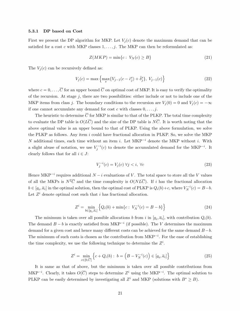
It is same as that of above, but the minimum is taken over all possible contributions fromMKP−i. Clearly, it takes O(C) steps to determine Zi using the MKP−i. The optimal solution toPLKP can be easily determined by investigating all Zi and MKP (solutions with B∗ ≥ B).

21

Z(PLKP) = min

{mini∈J

Zi, minc∈[0,C]

{c : VN (c) ≥ B}}

(26)

The first term takes O(NC) steps and the second term takes O(LC) steps. Hence, the overalltime complexity including the MKP−i, is O(NLC).

5.3.2 DP based on Demand

The DP based on demand exploiting the MKP can be developed in the similar way as above. LetUj(b) be the minimum cost at which the demand b can be met with MKP from classes 1, . . . , j.Then the optimal cost of the MKP is:

Z(MKP) = min{UN (b) : b ≥ B} (27)

The Uj(b) can be recursively defined as:

Uj(b) = min{min

s{Uj−1(b− δs

j ) + csj}, Uj−1(b)

}(28)

where b = 0, . . . , B and B is an upper bound on the accumulated demand from the optimal solutionto MKP. The B = B + maxj{aj} is an upper bound on the accumulated demand. The boundaryconditions are Uj(0) = 0 and Uj(b) =∞ if b units cannot be exactly met from classes 1, . . . , j. Thespace required to maintain all the values is NB and time complexity is O(LB).

Let U−ij (b) denote the corresponding recursion of MKP−i. Similar to that of the previous

algorithm, one can easily see that the total time complexity for evaluating all MKP−i is O(NLB)and the total space required is in O(N2B). If item i has fractional allocation in the optimal solutionof PLKP, then the optimal cost is given by

Zi = minb∈[ai,ai]

{Qi(b) + U−i

N (B − b)}

(29)

The optimal solution to PLKP is then the minimum of all Zi and MKP with no items with fractionalallocation.

Z(PLKP) = min{

mini∈J

Zi,minb≥B{UN (b)}

}(30)

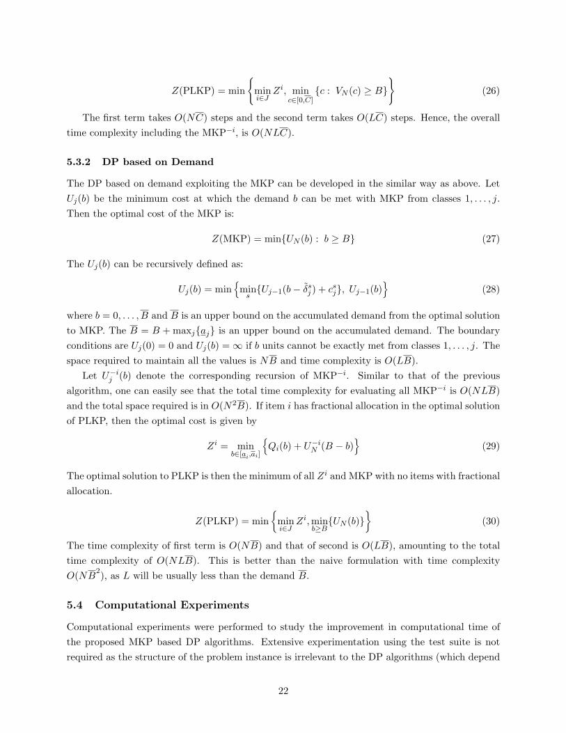
The time complexity of first term is O(NB) and that of second is O(LB), amounting to the totaltime complexity of O(NLB). This is better than the naive formulation with time complexityO(NB

2), as L will be usually less than the demand B.

5.4 Computational Experiments

Computational experiments were performed to study the improvement in computational time ofthe proposed MKP based DP algorithms. Extensive experimentation using the test suite is notrequired as the structure of the problem instance is irrelevant to the DP algorithms (which depend

22

Problem DP-Cost DP-DemandType

N CNaive Improved

BNaive Improved

5 603.5 6.91 0.79 286.94 2.0 0.7710 1105.5 47.8 6.42 517.85 5.91 3.78

DP1 15 1606.4 113.95 22.35 753.68 16.68 8.5920 2168.0 219.35 53.58 995.93 31.43 20.9625 2723.5 354.96 105.93 1228.31 51.74 41.09

5 3694.0 323.24 7.08 2482.6 80.77 3.1210 6909.3 2038.31 46.93 4588.1 507.95 24.03

DP2 15 10407.4 5440.15 159.69 6656.0 1275.11 84.8720 13191.5 9583.26 359.89 8653.4 2321.41 209.5125 16333.5 15298.69 651.19 10577.9 3651.48 389.56

Table 7: Average computational time in milliseconds for DP algorithms

only on N , L, C, and B). Two types of problems were considered with the following characteristics:(DP1) δs

j ∈ {20, 30, 40, 50} and (DP2) δsj ∈ {100, 200, . . . , 500}. The values of other parameters for

both problem types were: lj ∈ {2, 3, 4, 5}, βsj ∈ {1, 2, . . . , 5}, and ns

j ∈ {20, 30, 40, 50}. The twotypes differ only by the values of {δs

j}, which results in varying values for B and C. The experimentswere conducted for small values of N and results are shown in Table 7. The computational timeis averaged over 100 instances of each problem type. The upper bounds B and C shown in thetable are average values. The approximate average values of L for N = 5, 10, 15, 20, and 25 were17, 35, 52, 70, and 87, respectively. There is significant reduction in the computational time ofimproved DP algorithms based on cost. For the DP algorithms based on demand, the reduction intime is more for problems with larger B.

6 Approximation Algorithms

The PLKP is NP-hard and therefore it is of immediate interest to investigate the possibility ofapproximation algorithms. An approximation algorithm is necessarily polynomial, and is evaluatedby the worst or average case possible relative error over all possible instances of the problem. Inthis section, a 2-approximation algorithm is proposed for PLKP, which will be subsequently usedto design a fully polynomial time approximation scheme.

6.1 A 2-Approximation Algorithm for PLKP

For a minimization problem, an ε-approximation (ε ≥ 1) algorithm is a polynomial time algo-rithm that yields a solution with a value that is at most ε times the optimum solution value.A 2-approximation algorithm is proposed here for the PLKP. The approximation algorithms formaximization version of the knapsack problems are well studied [32, 18, 27, 28]. However, these

23

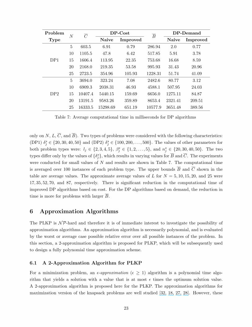
algorithms do not give the same approximation ratio for the minimization version and in somecases it is not even possible to characterize the ratio (though the exact algorithms for maximiza-tion problems can solve the minimization problems). On the contrary, very few papers [12, 26, 13]consider the minimization problem. The general idea for the algorithm is outlined in [12]. Itis a multi-run greedy algorithm that identifies a critical item at each run and the final solutionguarantees a 2-approximation ratio. In the same lines, we design our algorithm by using the LPrelaxation to identify a segment of an item, which we call as the break segment. The break segmentcan be either in or not in the optimal solution and if it is in the optimal solution it can eitherbe partially or fully allocated. Considering all these possibilities, we construct a 2-approximationsolution. If it cannot be guaranteed, the segment is removed and the LP relaxation is again applied.The algorithm stops when a 2-approximation is guaranteed or when it is impossible to remove anymore segments. In the following, we use the decision variables d,x, x consistent with the notationof LP based heuristic of Section4. The x denote the solution of LP:PCKM and d,x denote theconstructed feasible solution of PCKM.

Proposition 4 The feasible solution to PCKM, constructed using the LP rounding heuristic, hasat most one xs

j such that 0 < xsj < 1. If all xs

j are either 1 or 0, then either the solution is optimalor there is exactly one 0 ≤ x0

j < 1 in the LP solution that was rounded to obtain d0j = 1.

Proof: See appendix.

The above proposition identifies an unique segment of a feasible PCKM solution that wasconstructed from the LP solution. The variable corresponding to this segment is an xs

j ∈ (0, 1)or d0

j , whose corresponding LP variable x0j had a fractional value. This segment will hereafter be

referred to as the break segment. Let I denote a set of segments {(j, s)} that preserve the precedenceconstraints and lp pckm(I, A, F , j, s, b) denote the LP relaxation procedure on the set I. Theother arguments in the procedure are outputs: A is the set of segments with LP solution xs

j = 1,F is the set of segments with fractional values 0 < xs

j < 1, j and s define the break segment (j, s),and b = xs

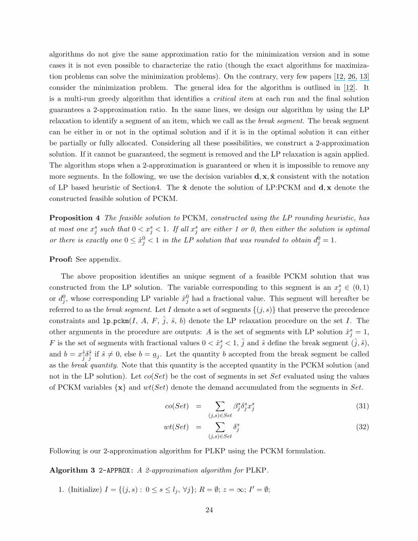
jδsj

if s 6= 0, else b = aj . Let the quantity b accepted from the break segment be calledas the break quantity. Note that this quantity is the accepted quantity in the PCKM solution (andnot in the LP solution). Let co(Set) be the cost of segments in set Set evaluated using the valuesof PCKM variables {x} and wt(Set) denote the demand accumulated from the segments in Set.

co(Set) =∑

(j,s)∈Set

βsj δ

sjx

sj (31)

wt(Set) =∑

(j,s)∈Set

δsj (32)

Following is our 2-approximation algorithm for PLKP using the PCKM formulation.

Algorithm 3 2-APPROX: A 2-approximation algorithm for PLKP.

1. (Initialize) I = {(j, s) : 0 ≤ s ≤ lj , ∀j}; R = ∅; z =∞; I ′ = ∅;

24

2. while wt(I) ≥ B do:

2.1. lp pckm(I, A, F , j, s, b);

2.2. z ← min(z, co(A) + co(F ));

2.3. if F = ∅ then stop fi;

2.4. if co(F ) ≤ co(A) then stop fi;

2.5. I ← I \ {∪s≥s(j, s)}; R← R ∪ {∪s≥s(j, s)};

2.6. if s 6= 0:

2.6.1. δsj← b− 1; I ′ ← I ∪ (j, s) \ {∪s<s(j, s)};

2.6.2. c′′ =∑

s<s δsjβs

j; b′′ =

∑s<s δs

j;

2.6.3. while wt(I ′) ≥ (B − b′′) do:

(a) lp pckm(I ′, A′, F ′, j′, s′, b′);

(b) z ← min(z, c′′ + co(A′) + co(F ′));

(c) if F ′ = ∅ then break fi;

(d) if j′ = j then break fi;

(e) if co(F ′) ≤ (c′′ + co(A′)) then break fi;

(f) I ′ ← I ′ \ {∪s≥s′(j′, s)};od;

fi;

od;

The 2-approximation solution value is stored in z. The set F in lp pckm(·) is the set of segmentswith fractional LP solutions xs

j . All the segments in F would belong to the same item j and they willall be contiguous in s. This is because there will be only one segment of the convex envelope withfractional value in CE:PCKM (as it is equivalent to solving continuous knapsack problem) and thisfractional value results in PLKP segments (of that convex segment) with fractional values. Notethat though the F is determined using LP variables x, in Steps 2.2 and 2.4, the co(F ) is evaluatedusing the PCKM variables x. This gives the contribution (in terms of cost) of the segments from F

to the original problem. To prove the correctness of 2-approximation of the algorithm, the followingobservations are made first:

• If F = ∅, then the break segment (j, s) is null and A has the optimal segments to I.

• If F 6= ∅, then wt(A) < B and A is the set of optimal segments to I for demand wt(A). Thenit follows that co(A) < Z(PCKM).

Theorem 2 Algorithm 2-APPROX is a 2-approximation algorithm to PLKP.

25

Proof: It is required to prove that Z(PCKM) ≤ z ≤ 2 × Z(PCKM). The first inequality can bevalidated easily as z always stores the value of a feasible solution. Consider the first iteration. IfF = ∅, then the solution is optimal and thus the theorem is true. If F 6= ∅, and if co(F ) ≤ co(A)then,

z ≤ (co(A) + co(F )) ≤ 2× co(A) ≤ 2× Z(PCKM) (33)

Thus if the algorithm terminates at Steps 2.3 or 2.4, the theorem is proved. If co(F ) > co(A), thenthere are four possibilities:

1. The break segment (j, s), with quantity greater than or equal to b, is in the optimal solution.

2. The break segment (j, s), with quantity greater than or equal to b, is not in the optimalsolution.

3. The break segment (j, s), with quantity less than b, is in the optimal solution.

4. The break segment (j, s), with quantity less than b, is not in the optimal solution.

The above four exhaust all the possibilities and at least one of them is true. If (1) is true thenco(F ) ≤ Z(PCKM) and hence

z ≤ (co(A) + co(F )) ≤ 2× Z(PCKM) (34)

If (2) or (4) is true then the break segment can be removed from I as it will not alter the optimalsolution. The algorithm can be stopped if (1) is known to be true, but since it is not known which ofthe possibilities is true the algorithm is continued further. Thus if (1) is true, the 2-approximationis guaranteed. If not, remove the break item from I (Step 2.5). Due to the precedence constraints,removal of break segment leads to the removal of the subsequent segments in j from I. Ignoringthe Steps 2.6 to 2.8, z is a 2-approximation value if either of the possibilities (1), (2), and (4) istrue. This is because, at every run of lp pckm(·) at least one of the segments is removed fromI and the set R has the removed items. The algorithm terminates at 2.3 or 2.4 guaranteeing a2-approximation solution, otherwise it terminates when wt(I) < B. At this stage, at least one ofthe segments from R should be in the optimal solution, otherwise it leads to infeasibility. Sincethe possibility of the segments in the optimal solution is taken care of, the 2-approximation isguaranteed.

The possibility (3) is true only if the break segment is not the indivisible segment. This is takencare of in Step 2.6. If break segment is in the optimal solution with quantity less than b, then allsegments preceding s in j belong to the optimal solution. A new PLKP is created with segmentsI ′ and demand b′′. The I ′, however, has the break segment with quantity b − 1, as the optimalquantity is less than b. The Step 2.6.3 is similar to Step 2, except that the problem consideredat 2.6.3 assumes that the break item is in the optimal solution with quantity less than b. Thusthe solution obtained in 2.6.3 guarantees a 2-approximation for I ′. The algorithm, hence, yields a2-approximation solution for all the above four possibilities.

26

The Step 2.1 takes O(L2) time and Step 2.6.3 takes O(L3) time. The Step 2 has to repeatedO(L) times and hence the total time complexity is O(L4). The algorithm could be implemented ina more efficient way by implementing Step 2.6 independently from Step 2. The efficiency is achievedby avoiding the calling the LP relaxation routine repeatedly. Note that in every run of Step 2, thesegments in set A are preserved, that is A is a non-decreasing set, only including new segmentsin the consecutive runs. Thus, in every run, only the new segments to be added to A are to beidentified. This can be implemented in the following way. First evaluate the convex segments of allthe cost functions in O(L2) time. Next, create a min-binary heap of the convex segments in O(L)time [11]. The CE:PCKM can be solved by choosing the convex segments in increasing slopes tillthe demand is satisfied. This is equivalent to removing the root (minimum element) of the binaryheap, till the demand is satisfied. The break segment and the break quantity can be found fromthe last convex segment removed. Note that F contains the linear segments corresponding to thislast convex segment and A contains all the segments removed, but the last segment. According toStep 2.5, segments that follow the break segment should be removed from I. This is equivalent toremoving the remaining convex segments of j from the heap. However, linear segments precedings in F , should be added in I. Find the convex envelopes just for these segments and add to theheap. The I is now the segments in A, plus the segments in the binary heap. Now the new demandis B −wt(A). Remove the root elements from the heap till this new demand is satisfied. Thus theStep 2 (without 2.6) can be implemented by maintaining a single binary heap and a set A. The timecomplexity of deletion of the root in the heap is O(log L). At worst L segments need to be removedand hence the complexity is O(L log L). At every run, convex envelope needs to be evaluated forthe segments s < s, which are in F . In the worst case, it has to be done for all the segments andhence the time complexity is O(L2). The new convex segments then need to be inserted into theheap. Each insertion has O(log L) complexity and hence the total complexity is O(L log L). Thusthe total time complexity of Step 2, excluding 2.6, is O(L2). The Step 2.6 is similar to the above,except that the demand and certain segments are changed. Hence, Step 2.6 also takes O(L2) time.However, it may be required to do this for every segment and hence the total complexity is O(L3).Thus we have the total time complexity of the 2-approximation algorithm as O(L3).

6.2 A Fully Polynomial Time Approximation Scheme

The 2-approximation algorithm developed above is a constant ratio approximation. The approxi-mation schemes are superior to the constant ratio approximations as their performance does notlimit the ratio on the error. A fully polynomial time approximation scheme (FPTAS) is proposedhere for the PLKP.

Definition 2 (FPTAS) An algorithm is called an FPTAS if for a given error parameter ε, itprovides a solution with value z such that z ≤ (1 + ε)z∗ for a problem instance with optimalobjective value z∗, in a running time that is polynomial in the size of the problem and 1

ε .

The ε in 2-approximation is 1 but in FPTAS it can be made as close to 0 as desired with a runningtime as a function of 1

ε , N , and L. FPTAS generally exist for problems with knapsack structure

27

due to the pseudo-polynomial time dynamic programming algorithm. The DP based on cost isthe essential building block for the FPTAS [15]. Recall that the running time of DP based oncost is O(NLC) where C is some upper bound on the objective value. The idea of the FPTAS isto exploit this DP algorithm and the 2-approximation algorithm. The cost cs

j = δsjβ

sj are scaled,

thus reducing the running time of the algorithm to depend on the new scaled value. However,the optimal solution for the scaled problem need not be optimal to the original. With a judiciousselection of the scaling factor, the optimal solution of the scaled problem can be made close to thatof the original problem. Following is the FPTAS for the PLKP. Let C2 be the objective value ofthe 2-approximation algorithm and ε the required approximation ratio.

Algorithm 4 DP-FPTAS: FPTAS for PLKP

1. k = εC22L

2. if k > 1then cs

j =⌊

csj

k

⌋; C =

⌊Ck

⌋;

else csj = cs

j ; C = C2;fi;

3. Cε ← DP Cost(c, C)

The algorithm first determines the scaling factor k based on the desired error parameter ε (if k ≤ 1,scaling is not required). The DP Cost(c, C) is the DP algorithm developed in Section 5.3.1, appliedto the scaled problem with cost c and upper bound C. Let Cost(Set, ct) denote the total cost ofitems in set Set evaluated with cost ct.

Proposition 5 The value C is the upper bound to the scaled problem.

Proof: See appendix.

The above proposition is necessary for the DP-FPTAS algorithm, since without that, one cannotguarantee an optimal solution to the scaled problem.

Theorem 3 Algorithm DP-FPTAS is an FPTAS for the PLKP.

Proof: Let ε be the given error parameter and Cε the optimal objective value of the scaled problemobtained by DP-FPTAS. Then according to the definition of FPTAS, one has to prove Cε ≤ (1+ε)C∗

and running time of DP-FPTAS is polynomial in N , L, and 1ε . First consider the case where k > 1.

Let A∗ be the set of items with optimal quantities to the PLKP and Aε the set of items withoptimal quantities to the scaled problem. Then, co(A∗, c) = C∗ and co(Aε, c) = Cε. As cs

j =⌊

csj

k

⌋,

csj ≥ kcs

j ≥ csj − k (35)

28

The first inequality is obvious from the definition and the second inequality follows from the in-equality x− 1 ≤ bxc. By the definition of A∗, Aε, and c,

co(Aε, c) ≥ co(A∗, c) ≥ k × co(A∗, c) ≥ k × co(Aε, c) ≥ co(Aε, c− k) (36)

The first inequality follows from the fact that items of A∗ are optimal to the unscaled problem,second follows from cs

j ≥ kcsj , third is due to the optimality of items of Aε to the scaled problem,

and the last one is because kcsj ≥ cs

j − k. Thus,

co(A∗, c) ≥ co(Aε, c− k) ≥ co(Aε, c)− Lk

⇒ co(Aε, c) ≤ C∗ + Lk

⇒ co(Aε, c) ≤ C∗ + Lk

≤ C∗ +εC2

2≤ C∗ + εC∗

⇒ Cε ≤ (1 + ε)C∗

The fourth inequality follows from the 2-approximation bound C2. The time taken by the algorithmis the time taken to determine the 2-approximate solution C2 (O(L3)) plus the time taken by theDP (O(NLC)).

NLC = NL

⌊C2

k

⌋≤ NL

C2

k=

2NL2

ε(37)

The total time complexity is O(L3

ε ) (as N ≤ L) and hence the algorithm DP-FPTAS is an FPTASfor PLKP.

7 Conclusions

This paper considered an important class of nonlinear knapsack problems in which the cost ofinclusion of the quantity of an item is a nonconvex piecewise linear function. The cost functionconsidered was generic enough to include various special cases like continuous, linear, concave,convex, marginally decreasing, discontinuous fixed costs, etc. This abstract function can thus modelcost structures arising in logistics and supply chains. The problem was particularly motivated byits application to winner determination in volume discount procurement auctions. The problem isNP-hard and was studied from two perspectives: (1) the practical purpose of solving the problemin real-world applications such as e-commerce by developing heuristic and exact algorithms tosolve the problem with less computational effort and (2) theoretical viewpoint of studying theapproximability of the hard problem.

Two mixed integer programming formulations were proposed which are generalizations of prece-dence constrained knapsack problems and multiple choice knapsack problems. These formulationswere compared with the standard textbook formulations in terms of solution time by a commer-cial optimization package. The computational experiments conducted over a set 24 representative

29

problem types show that the MCKM formulation proposed by us took less computational timethan that of the other formulations for all the problem types.

A fast polynomial time heuristic was proposed to solve the linear relaxation of the problem usingconvex envelopes. Computational experiments showed that the proposed heuristic was 100 foldsfaster than that of solving using traditional simplex algorithm. Two pseudo polynomial time exactalgorithms based on dynamic programming were devised using the multiple choice formulation.These formulations are faster than the existing naive formulations. A 2-approximation algorithmand a fully polynomial time approximation scheme were also developed.

There are some interesting research problems with respect to solution techniques. An intelligentbranch and bound technique that exploits the fast convex envelopes based linear relaxation canpossibly solve the problem at a much faster rate than other enumerative search techniques. There isalso scope for improving the computational and memory requirements of the dynamic programmingalgorithms. The information from the LP relaxation can possibly leveraged to fix some of thevariables in the dynamic programming to their optimal values. Another research direction is todevelop the concept of core problems for PLKP, similar to that of the knapsack problem [31], whereonly a subset of items are considered having a high probability of being in the optimal solution.

References

[1] R. E. Bellman. Dynamic Programming. Princeton University Press, Princeton, NJ, 1957.

[2] G. R. Bitran and A. C. Hax. Disaggregation and resource allocation using convex knapsackproblems with bounded variables. Management Science, 27:431–441, 1981.

[3] K. M. Bretthauer and B. Shetty. The nonlinear resource allocation problem. OperationsResearch, 43:670–683, 1995.

[4] K. M. Bretthauer and B. Shetty. A pegging algorithm for the nonlinear resource allocationproblem. Computers and Operations Research, 29(5):505–527, 2001.

[5] K. M. Bretthauer and B. Shetty. The nonlinear knapsack problem - algorithms and applica-tions. European Journal of Operations Research, 138:459–472, 2002.

[6] K. L. Croxton. Modeling and solving network flow problems with piecewise linear costs, withapplications in supply chain management. PhD thesis, Operations Research Center, MIT,Cambridge, MA, 1999.

[7] K. L. Croxton, B. Gendron, and T. L. Magnanti. A comparison of mixed-integer programmingmodels for nonconvex piecewise linear cost minimization problems. Management Science,49(9):1268–1273, 2003.

[8] A. Davenport and J. Kalagnanam. Price negotiations for procurement of direct inputs. Re-search Report RC 22078, IBM Research, Yorktown Heights, NJ, USA, 2001.

30

[9] K. Dudzinski and S. Walukiewicz. Exact methods for the knapsack problem and its general-izations. European Journal of Operational Research, 28:3–21, 1987.

[10] M. Eso, S. Ghosh, J. Kalagnanam, and L. Ladanyi. Bid evaluation in procurement auctionswith piece-wise linear supply curves. Research Report RC 22219, IBM Research, YorktownHeights, NJ, USA, 2001.

[11] R. Floyd. Algorithm 245: Treesort3. Communications of the ACM, 7(12):701, 1964.

[12] G.V. Gens and E.V. Levner. Computational complexity of approximation algorithms for com-binatorial problems. In Mathematical Foundations of Computer Science, volume 74 of LectureNotes in Computer Science, pages 292–300. Springer, 1979.

[13] M.M. Guntzer and D. Jungnickel. Approximate minimization algorithms for the 0/1 knapsackand subset-sum problem. Operations Research Letters, 26:55–66, 2000.

[14] D. S. Hochbaum. A nonlinear knapsack problem. Operations Research Letters, 17:103–110,1995.

[15] D. S. Hochbaum. Various notions of approximations: good, better, best, and more. In D. S.Hochbaum, editor, Approximation algorithms for NP-hard problems, pages 346–398. PWSPublishing Company, 1995.

[16] R. Horst and H. Tuy. Global Optimization: Deterministic Approaches. Springer, Berlin, 1990.

[17] T. Ibaraki and N. Katoh. Resource Allocation Problems: Algorithmic Approaches. MIT Press,Cambridge, Massachusetts, 1988.

[18] O. H. Ibarra and C. E. Kim. Fast approximation algorithms for the knapsack and sum ofsubset problems. Journal of the ACM, 22:463–468, 1975.

[19] D. S. Johnson and K. A. Niemi. On knapsacks, partitions, and a new dynamic programmingtechnique for trees. Mathematics of Operations Research, 8:1–14, 1983.

[20] S. Kameshwaran. Algorithms for piecewise linear knapsack problems with applications in elec-tronic commerce. PhD thesis, Department of Computer Science and Automation, IndianInstitute of Science, Bangalore, 2004.

[21] S. Kameshwaran and Y. Narahari. Trade determination in multiattribute exchanges. In Pro-ceedings of IEEE Conference on E-Commerce CEC’ 03, pages 173–180. IEEE Computer So-ciety, 2003.

[22] H. Kellerer, U. Pferschy, and D. Pisinger. Knapsack Problems. Springer, 2004.

[23] M. S. Kodialam and H. Luss. Algorithms for separable nonlinear resource allocation problems.Operational Research, 46:272–284, 1998.

31

[24] A. Kothari, D. Parkes, and S. Suri. Approximately strategy proof and tractable multi-unitauctions. In Proceedings of ACM Conference on Electronic Commerce (EC-03), 2003.

[25] D. S. Kung. The multiple choice knapsack problem: Algorithms and applications. PhD thesis,University of Texas, Austin, 1982.

[26] M. Labbe, E. F. Schmeichel, and S. L. Hakimi. Approximation algorithms for the capacitatedplant allocation problem. Operations Research Letters, 15:115–126, 1994.

[27] E. L. Lawler. Fast approximation algorithms for knapsack problems. Mathematics of Opera-tions Research, 4:339–356, 1979.

[28] S. Martello and P. Toth. Knapsack Problems: Algorithms and Computer Implementation. JohnWiley and Sons, 1990.

[29] K. Mathur, H. M. Salkin, and B. B. Mohanty. A note on a general non-linear knapsackproblems. Operations Research Letters, 5:79–81, 1986.

[30] J. J. More and S. A. Vavasis. On the solution of concave knapsack problems. MathematicalProgramming, 49:397–411, 1991.

[31] D. Pisinger and P. Toth. Knapsack problems. In Ding-Zhu Du and P. M. Pardalos, editors,Handbook of Combinatorial Optimization, pages 299–428. Kluwer Academic Publications, 1998.

[32] S. Sahni. Approximate algorithms for the 0-1 knapsack problem. Journal of the ACM, 22:115–124, 1975.

[33] N. Samphaiboon and T. Yamada. Heuristic and exact algorithms for the precedence con-strained knapsack problem. Journal of Optimization Theory and Applications, 105:659–676,2000.

[34] P. H. Zipkin. Simple ranking methods for allocation of one resource. Management Science,26:34–43, 1980.

Appendix

Proof of Theorem 1

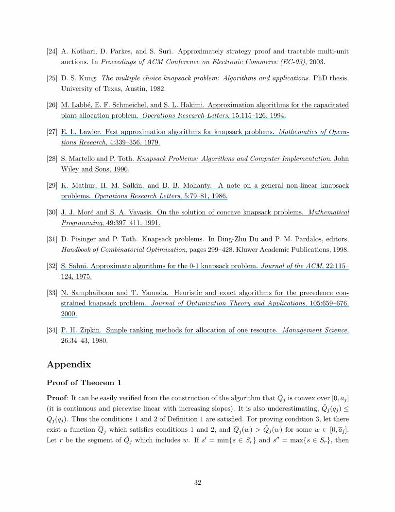
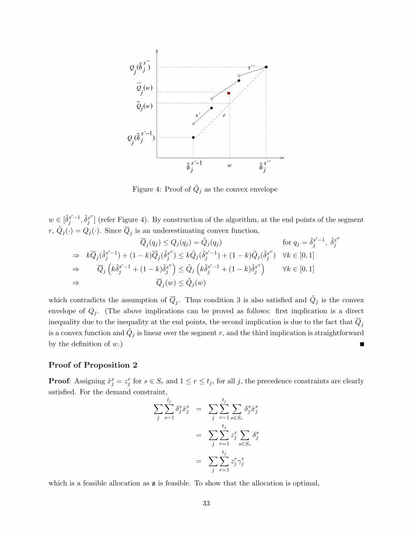
Proof: It can be easily verified from the construction of the algorithm that Qj is convex over [0, aj ](it is continuous and piecewise linear with increasing slopes). It is also underestimating, Qj(qj) ≤Qj(qj). Thus the conditions 1 and 2 of Definition 1 are satisfied. For proving condition 3, let thereexist a function Qj which satisfies conditions 1 and 2, and Qj(w) > Qj(w) for some w ∈ [0, aj ].Let r be the segment of Qj which includes w. If s′ = min{s ∈ Sr} and s′′ = max{s ∈ Sr}, then

32

!~

js’’

~! j

s’!1!~

js’’

Qj~ (w)

~! j

s’!1( )Qj

w

Qj( )

s’

s’’

r

(w)Qj

Figure 4: Proof of Qj as the convex envelope

w ∈ [δs′−1j , δs′′

j ] (refer Figure 4). By construction of the algorithm, at the end points of the segmentr, Qj(·) = Qj(·). Since Qj is an underestimating convex function,

Qj(qj) ≤ Qj(qj) = Qj(qj) for qj = δs′−1j , δs′′

j

⇒ kQj(δs′−1j ) + (1− k)Qj(δs′′

j ) ≤ kQj(δs′−1j ) + (1− k)Qj(δs′′

j ) ∀k ∈ [0, 1]

⇒ Qj

(kδs′−1

j + (1− k)δs′′j

)≤ Qj

(kδs′−1

j + (1− k)δs′′j

)∀k ∈ [0, 1]

⇒ Qj(w) ≤ Qj(w)

which contradicts the assumption of Qj . Thus condition 3 is also satisfied and Qj is the convexenvelope of Qj . (The above implications can be proved as follows: first implication is a directinequality due to the inequality at the end points, the second implication is due to the fact that Qj

is a convex function and Qj is linear over the segment r, and the third implication is straightforwardby the definition of w.)

Proof of Proposition 2

Proof: Assigning xsj = zr

j for s ∈ Sr and 1 ≤ r ≤ tj , for all j, the precedence constraints are clearlysatisfied. For the demand constraint,∑

j

lj∑s=1

δsj x

sj =

∑j

tj∑r=1

∑s∈Sr

δsj x

sj

=∑j

tj∑r=1

zrj

∑s∈Sr

δsj

=∑j

tj∑r=1

zrj γ

rj

which is a feasible allocation as z is feasible. To show that the allocation is optimal,

33

∑j

∑ljs=0 βs

j δsj x

sj =

∑j

tj∑r=1

∑s∈Sr

βsj δ

sj x

sj

=∑j

tj∑r=1

zrj

∑s∈Sr

βsj δ

sj

=∑j

tj∑r=0

αrjγ

rj z

rj

⇒ Z(LP : PCKM) = Z(CE : PCKM)

Proof of Proposition 4

Proof: The CE:PCKM is a continuous knapsack problem (refer Proposition 1) and therefore theoptimal solution will have at most one fractional variable. The convex segment of this fractionalvariable gives rise to fractional variables in the LP solution. If the variable of the convex segmentis not fractional, so are the corresponding variables of the LP solution (by Proposition 1). Hencethe fractional variables in the optimal LP solution are contiguous and belong to the same item j.When converted into a feasible PCKM solution, there will be at most one fractional xs

j . If there areno fractional variables, then either the solution is optimal or the fractional convex segment was thefirst segment which made the corresponding x0

j in the LP solution fractional, and finally roundedthe d0

j = 1.

Proof of Proposition 5

Proof: If k ≤ 1 then the proposition is obvious. For k > 1, let the proposition be false. Then,⌊C2k

⌋< Cε, where Cε is the optimal objective value of the scaled problem. Let A2 be the set of items

with quantities for the 2-approximate solution for the unscaled problem. Then, co(A2, c) = C2.

co(A2, c) ≤⌊C2

k

⌋< Cε (38)

The first inequality follows from the fact that bx1c + . . . + bxnc ≤ b(x1 + . . . + xn)c for any realnumbers x1, . . . , xn. Note that the set of items in A2 are feasible to PLKP (irrespective of the coststructure) and therefore co(A2, c) ≥ Cε. This contradicts the above relation and hence Cε ≤ C.

34