arX

iv:c

ond-

mat

/020

4017

v1 [

cond

-mat

.sta

t-m

ech]

31

Mar

200

2

Nonequilibrium generalization of Forster-Dexter theory for excitation energy transfer∗

Seogjoo Jang, YounJoon Jung, and Robert J. SilbeyDepartment of Chemistry, Massachusetts Institute of Technology, Cambridge, Massachusetts 02139

(February 1, 2008)

Forster-Dexter theory for excitation energy transfer is generalized for the account of short timenonequilibrium kinetics due to the nonstationary bath relaxation. The final rate expression ispresented as a spectral overlap between the time dependent stimulated emission and the stationaryabsorption profiles, which allows experimental determination of the time dependent rate. For aharmonic oscillator bath model, an explicit rate expression is derived and model calculations areperformed in order to examine the dependence of the nonequilibrium kinetics on the excitation-bathcoupling strength and the temperature. Relevance of the present theory with recent experimentalfindings and possible future theoretical directions are discussed.

I. INTRODUCTION

Excitation energy transfer (EET) [1–4] is ubiquitous inphoto sensitive materials [5–12] and is one of the key stepsin photosynthesis [7,13–15]. Since the seminal works ofForster [1,2] and Dexter (FD) [3], their rate expressionshave been confirmed by numerous experiments and haveplayed fundamental roles in understanding various lu-minescence phenomena [4–12]. In these advances, thespectral overlap expression of Forster [1,2], which allowsidentification of the reaction rate without any resort toa model Hamiltonian, has been essential.

The rate expressions of FD are applications of theFermi’s golden rule (FGR), which rely on the smallnessof the resonance interactions. The spectral overlap ex-pression of Forster derives from the additional simplifi-cation that bath modes coupled to the energy donor andacceptor are independent of each other. If there are com-

mon bath modes [16], such a simple expression is not ingeneral valid. However, within the harmonic oscillatorbath model, rigorous extensions of the FD theory canbe made [16–19] with the use of small polaron transfor-mation, and can be further generalized for the study oflong-time dynamics based on the Redfield-type equation[17] and for the understanding of exciton transport inmolecular crystals [19–21]. In recent years, theoreticaladvances to cope with new experiments have been made,such as microscopic consideration of the medium effect[22,23], generalization of the FD rate expression for dis-ordered multichromorphic systems [24–30], and unifiedtheories covering up to the intermediate and strong cou-pling regimes [31–34].

Although often not noticed, the assumption of station-arity is implicit in the FD theory. The FGR is valid onlywhen the initial density operator commutes with the ze-roth order Hamiltonian and the bath time scale is muchshorter than that of the electronic transition. For EETprocesses occurring in nanosecond or longer time scale,

one may safely assume that the bath modes have alreadyrelaxed and become equilibrated with the excited donorbefore the energy transfer takes place, unless there areultra-slow modes or spin interactions with comparabletime scales. Application of the FGR, thus the FD theory,can be justified for this case. However, EET in general isa nonstationary process where nonequilibrium relaxationof the nuclear degrees of freedom occurs during and afterthe electronic excitation. For fast EET processes occur-ring in a time scale comparable to the bath relaxationtime, the reaction kinetics predicted by the FD theorymay not be accurate enough.

The importance of the nonequilibrium effects for fastEET was in fact recognized long time ago, and was namedas hot transfer [35–38]. Due to experimental limita-tions, however, the earlier experiments and relevant theo-ries were concerned with the frequency domain situationwhere the reaction rate at issue is the stationary longtime limit in the presence of an excitation field tuned forthe hot transfer [35,36]. Time dependent pump-probesituation was considered later by Sumi [37,38], who for-mulated a time dependent generalization of the FD the-ory based on a nonequilibrium golden rule approximation[37].

With the advance of ultrafast spectroscopy, it hasbecome possible to induce the electronic excitation inthe femtosecond scale. Experiments [8,11,14,39–41] per-formed in this manner reveal systems where the EETrate is comparable to the vibrational relaxation rate ofsome modes. A typical example for this is the EETfrom B800 to B850 in the light harvesting complex 2(LH2) [14], which is known to occur in about 1 ps. Ev-idences for fast EET were found in other systems alsosuch as the conjugated polymer [8], dendrimers [11], andthe photosynthetic reaction center [41]. In general, themicroscopic mechanisms of the EET in these systems arequite complicated, and considerations of multipolar tran-sitions, multichromorphic effects, and disorder may be

∗published in Chemical Physics, 275, pp. 319–332 (2002)

1

important. However, simple comparison of time scalesindicates that examination of the nonequilibrium effectscannot be overlooked. The theory of Sumi [37,38] and re-cent theories [32–34] on intermediate and strong couplingseem suitable for these considerations. However, the na-ture of the approximation involved in the bath relaxationdynamics, upon which the nonequilibrium kinetics is sen-sitive, is not clear in these approaches.

In the present work, we provide a straightforward andrigorous nonequilibrium generalization of the FD theory.The procedure is to go through the same perturbationtheory as in deriving the FGR, but starting from thenonstationary initial states and considering full time de-pendences. Our analysis is limited to the usual pertur-bation regime of the FD theory. We assume that theresonance interaction is small enough to validate secondorder perturbation theory and that the reaction is virtu-ally irreversible due to either energetic or entropic reason.However, the excitation bath coupling is treated rigor-ously. The present theory is analogous to the nonequilib-rium generalization of the electron transfer [42], but animportant distinction is that we provide a spectral over-lap expression valid for arbitrary bath without commonmodes, a typical situation for the EET.

Our theory can be considered as the pump-probe ver-sion of the hot transfer rate theories [35,36]. More im-portantly, our spectral overlap expression brings a con-nection between the time dependent reaction rate andthe modern ultrafast spectroscopy experiment, which al-lows direct determination of the reaction rate or enablesexperimental confirmation whether the usual assumptionof the EET kinetics is valid. In addition, we provide cal-culations of the time dependent rate for the model of theharmonic oscillator bath, which illustrate some featuresof the nonequilibrium EET kinetics.

The sections are organized as follows. In Sec. IIA, wepresent the main formalism and provide the spectral over-lap expression valid for general bath Hamiltonian withoutcommon modes. Section IIB provides a complementaryresult of an explicit rate expression for the harmonic os-cillator bath. In Sec. III, model calculations are made.Sec. IV concludes with summaries and the relevance ofthe present theory with recent experiments.

II. THEORY

A. General bath without common modes

The system consists of two distinctive chromophores,donor (D) and acceptor (A). The state where both Dand A are in their ground electronic states is denoted as|g〉. The state where D is excited while A remains in theground state is denoted as |D〉 = a†

D|g〉, where a†

Dis the

corresponding creation operator, and |A〉 = a†A|g〉 is de-

fined similarly. We assume that both chromophores are

excited to singlet states and do not consider multiexci-ton states. Therefore, the three electronic states |g〉, |D〉,and |A〉 form a complete set of electronic states. All therest of the dynamic degrees of freedom such as molecularvibrations and solvation coordinates are included in thebath. The bath Hamiltonian is defined as that in theground state |g〉 and is assumed to be Hb = HbD

+ HbA,

where the subscripts of D and A denote the componentscoupled to chromophores D and A, respectively. That is,in the present work, the effect of common modes is disre-garded. For EET processes in a medium where phononsand vibrations are localized, this assumption seems rea-sonable.

Since we consider the excitation dynamics during atime much shorter than the lifetime of the excited state,we neglect the spontaneous decay channels of the excitedstates. Adopting a second quantization notation where|g〉 is treated as if the vacuum state, the zeroth orderHamiltonian describing the interaction-free dynamics canbe written as

H0 = ǫDa†

Da

D+ ǫ

Aa†

Aa

A+ Hb , (2.1)

where ǫD

and ǫA

are excitation energies of D and A.The resonance interaction between |D〉 and |A〉 is rep-

resented by

HDA = J(a†D

aA

+ a†Aa

D) , (2.2)

where J is a function of the position vectors and thetransition dipoles of D and A. The functional form ofJ depends on the mechanism of EET. For dipole-dipoleinteraction, it varies as the inverse third power of thedistance between D and A. For exchange interaction, itis an exponential function of the distance. Here we donot specify the detailed mechanism, but simply assumethat it is small enough to warrant a perturbation analysisand does not have any dependence on the bath operators(vibrational degrees of freedom), so called Condon ap-proximation.

The excitation bath coupling is assumed to be as fol-lows:

Heb = BD

a†D

aD

+ BAa†

Aa

A, (2.3)

where BD

and BA

are bath operators coupled to |D〉 and|A〉 respectively. These operators and the bath Hamilto-nian can be arbitrary except for the following condition:

[HbD, HbA

] = [HbD, B

A] = [HbA

, BD] = 0 , (2.4)

which implies that the bath modes coupled to |D〉 and|A〉 are independent of each other. This assumption canbe justified if the chromophores D and A are far enoughapart from each other and the major nuclear modes cou-pled to excitations are localized to either D or A, whichcan be consistent with the assumption of smallness of J .

2

Summing up Eqs. (2.1)-(2.3), the total Hamiltoniandescribing the dynamics of the chromophores, in the sin-gle excitation manifold, and the bath is given by

H = H0 + HDA + Heb . (2.5)

For t < 0, the chromophores are assumed to be in thestate |g〉 and thus the total Hamiltonian is equal to Hb.The bath is assumed to be in the canonical equilibriumof Hb during this period. At time zero, an impulsivepulse selectively excites D. Here we approximate this asa delta pulse in time. Then, the density operator at timezero, right after the irradiation, is given by

ρ(0) = |D〉〈D|e−βHb/Zb , (2.6)

where β = 1/kBT and Zb = Trb{e

−βHb}.The probability at time t for the excitation to be found

at A is given by

PA(t) = Trb

{

〈A|e−iHt/hρ(0)eiHt/h|A〉}

. (2.7)

For short enough time compared to h/J , a perturbationexpansion of this with respect to HDA can be made. In-serting the first order approximation of the time evolu-tion operator e−iHt/h and the complex conjugate into Eq.(2.7), we obtain the following expression valid up to thesecond order of J :

PA(t) ≈J2

h2

∫ t

0

dt′∫ t

0

dt′′ei(ǫA−ǫD)(t′−t′′)/h

×1

ZbTrb

{

ei(Hb+BA

)(t′−t′′)/he−i(Hb+BD

)t′/h

× e−βHbei(Hb+BD

)t′′/h}

. (2.8)

The time dependent EET rate is then defined as thederivative of this acceptor probability as follows:

k(t) ≡d

dtPA(t)

≈2J2

h2 Re

[∫ t

0

dt′ei(ǫD−ǫ

A)t′/h 1

ZbTrb

{

ei(Hb+BD

)t/h

× e−i(Hb+BA

)t′/he−i(Hb+BD

)(t−t′)e−βHb

}]

.

(2.9)

Under the assumption of Eq. (2.4), the trace over thebath degrees of freedom comprising HbD

and HbAcan be

decoupled from each other in the following way:

k(t) =2J2

h2 Re

[∫ t

0

dt′ei(ǫD−ǫ

A)t′/h

×1

ZbA

TrbA

{

eiHbAt′/he−i(HbA

+BA

)t′/he−βHbA

}

×1

ZbD

TrbD

{

ei(HbD+B

D)t/he−iHbD

t′/h

× e−i(HbD+B

D)(t−t′)/he−βHbD

}]

, (2.10)

where ZbA= TrbA

{e−βHbA} and ZbD= TrbD

{e−βHbD }.Equation (2.10) is the nonequilibrium generalization ofthe FD rate, but expressed in the time domain. As hasbeen outlined in the introduction, this result has been ob-tained by applying second order perturbation theory tothe time dependent density operator with the nonstation-ary initial condition of Eq. (2.6). The decoupled form ofEq. (2.10) makes it possible to express the reaction rateas an overlap of frequency domain spectral profiles of in-dependent donor and acceptor, as will be shown later.Before going through this procedure, it is meaningful toclarify the difference between the present result and theFD rate expression. Two additional approximations arenecessary.

The first is the assumption of stationarity, equivalentto the following replacement:

e−i(HbD+B

D)(t−t′)/he−βHbD ei(HbD

+BD

)(t−t′)/h

→ZbD

Z ′bD

e−β(HbD+B

D) , (2.11)

where Z ′bD

= TrbD{e−β(HbD

+BD

)}. This approximationimplies that the nuclear dynamics on the excited donorpotential energy surface is ergodic in a time scale shorterthan that of the EET transfer kinetics. We define thereaction rate based on this fully relaxed density operatoras

kr(t) =2J2

h2 Re

[∫ t

0

dt′ei(ǫD−ǫ

A)t′/h

×1

ZbATrbA

{

eiHbAt′/he−i(HbA+BA

)t′/he−βHbA

}

×1

Z ′bD

TrbD

{

ei(HbD+BD

)t′/he−iHbDt′/h

× e−β(HbD+BD)}]

. (2.12)

The derivation of this expression can be madeby rewriting ei(HbD+BD)t/h in Eq. (2.10) asei(HbD+BD)(t−t′)/hei(HbD+BD)t′/h, using the cyclic sym-metry of the trace operation for the first term, and thenfinally imposing the replacement of Eq. (2.11).

The second is the infinite time approximation. Thatis, the FD rate corresponds to the following limit:

kF D

= kr(∞) . (2.13)

This approximation is valid if there is time scale separa-tion between the bath dynamics and the EET kinetics.

For practical purposes of evaluating the reaction ratefor real systems, it is important to find the explicit ex-pression for Eq. (2.10) in the frequency domain as anoverlap of independent spectral profiles of the donor andof the acceptor. Considering the fact that the term in-volving the acceptor is identical in Eqs. (2.10) and (2.12),

3

one can expect that the nonequilibrium EET rate also in-volves the stationary absorption profile of the acceptor.For this purpose, we define the absorption profile of theacceptor as

IA(ω) = |µA · e|2∫ ∞

−∞

dt eiωt−iǫA

t/h 1

ZbATrbA

{

eiHbAt/h

× e−i(HbA+BA

)t/he−βHbA

}

, (2.14)

where µA is the transition dipole of the acceptor and e

is the polarization vector of the radiation. Inserting theinverse transform of this into Eq. (2.10),

k(t) =J2

πh2|µA · e|2

∫ ∞

−∞

dω IA(ω)

× Re

[∫ t

0

dt′e−iωt′+iǫD

t′/h 1

ZbDTrbD

{

ei(HbD+BD

)t/h

× e−iHbDt′/he−i(HbD+BD

)(t−t′)/he−βHbD

}]

. (2.15)

The time dependent part involving the donor can be ex-pressed as the stimulated emission profile in a pump-probe experiment. In Appendix A, we derive a time de-pendent stimulated emission profile of the donor which issubject to a stationary field after being excited by a deltapulse. Inserting Eq. (A5) into Eq. (2.15), the frequencydomain expression of the EET rate is given by

k(t) =J2

2πh2|µA · e|2|µD · e|2

∫ ∞

−∞

dωIA(ω)ED(t, ω) .

(2.16)

In the limit where t → ∞, this expression becomes equiv-alent to the Forster’s spectral overlap expression as longas ED(∞, ω) is equal to the spontaneous emission pro-file of the excited donor except for a normalization factorand the universal frequency dependent scaling function.

Equation (2.16) is the central result of the present pa-per. It is the pump-probe version of the hot transferrate [35,36] and generalizes the spectral overlap expres-sion of Forster for fast EET processes. With the moderndevelopment of ultrafast spectroscopy, determination ofk(t) and ED(t, ω) can be made even in femtosecond scale.With the advances in experimental techniques of alteringchromophores by chemical or biological manipulations,independent determinations of IA(ω) and ED(t, ω) canbe done at the same condition as that of k(t) for a broadrange of systems. If these practical issues are settled andif the system satisfies the requirements for applying theperturbation theory, Eq. (2.16) should hold as long asthe effect of common modes is insignificant.

In Eq. (2.9), we have defined the reaction rate as thetime derivative of PA(t). Due to the use of perturba-tion theory, such a definition gives a valid result only for∫ t

0 dt′k(t′) << 1. In the longer time limit when the pop-ulation transfer has occurred significantly, instead, the

reaction rate should be understood as the exponentialdecay rate of 1 − PA(t). The justification for this comesfrom the Redfield-type equation [17] and the assumptionthat the bath relaxation has been completed. A reason-able way of combining these two limits is to exponentiatethe time integration of k(t) as follows:

PA(t) ≈ 1 − exp

(

−

∫ t

0

dt′ k(t′)

)

, (2.17)

where it has been assumed that the transfer from D to Ais irreversible due to either energetic or entropic reason.Equation (2.17) is not based on a rigorous derivation,and conditions when such approximation is valid need tobe clarified based on a more rigorous approach, whichwill be done elsewhere. However, for the purpose of un-derstanding the qualitative aspect of EET kinetics in thenonequilibrium situation, which is the main purpose ofthe present paper, the expression of Eq. (2.17) is useful.

B. Linearly coupled harmonic oscillator bath

For the simple case where the bath consists of inde-pendent harmonic oscillators, an explicit expression canbe found for k(t). Assume that the bath Hamiltonian isgiven by

Hb =∑

n

hωn

(

b†nbn +1

2

)

, (2.18)

and the chromophore-bath interaction is linear in thebath coordinate as follows:

Heb =∑

n

hωn(bn + b†n)(gnDa†D

aD

+ gnAa†Aa

A) , (2.19)

where gnDgnA = 0 and thus the condition of Eq. (2.4)is satisfied. For an explicit calculation, it is convenientto start from Eq. (2.10). The integrand of the reactionrate involves trace of the product of the propagators fordisplaced harmonic oscillators. Each trace over the ac-ceptor bath and the donor bath can be done explicitly,and the resulting expression for the reaction rate can bewritten as

k(t) =2J2

h2 Re

[∫ t

0

dt′ ei(ǫD−ǫ

A)t′/h−i

∑

n(g2

nD+g2nA) sin(ωnt′)

× e2i∑

ng2

nD(sin(ωnt)−sin(ωn(t−t′))

×e−2∑

n(g2

nD+g2nA) coth(βhωn/2) sin2(ωnt′/2)

]

, (2.20)

where

ǫD(A) = ǫD(A) −∑

n

hωng2nD(A)

≡ ǫD(A) − λD(A) , (2.21)

4

where λD and λA are reorganization energies of the donorand acceptor baths. For the harmonic oscillator bathmodel, in fact, the reaction rate can be calculated ex-plicitly even for more general situation where there arecommon modes coupling both the donor and acceptor.In Appendix B, we derive the general expression employ-ing the small polaron transformation. Equation (2.20)can alternatively be obtained from Eq. (B10) by lettinggnDgnA = 0.

Define the following spectral densities:

ηD(ω) ≡∑

n

g2nDω2

nδ(ω − ωn) , (2.22)

ηA(ω) ≡∑

n

g2nAω2

nδ(ω − ωn) . (2.23)

Inserting these definitions into Eq. (2.20), the nonequi-librium EET rate can be expressed as

k(t)=2J2

h2 Re

[∫ t

0

dt′ ei(ǫD−ǫ

A)t′/h

×e−i

∫

∞

0dω(ηD(ω)+ηA(ω)) sin(ωt′)/ω2

×e2i

∫

∞

0dωηD(ω)(sin(ωt)−sin(ω(t−t′)))/ω2

×e−2

∫

∞

0dω(ηD(ω)+ηA(ω)) coth(βhω/2) sin2(ωt′/2)/ω2

]

.

(2.24)

This is the main result of the present subsection. Theexpression for kr(t), which can be calculated from Eq.(2.12) through a similar procedure is given by

kr(t) =2J2

h2 Re

[∫ t

0

dt′ ei(ǫD−ǫ

A)t′/h

×e−i

∫

∞

0dω(ηD(ω)+ηA(ω)) sin(ωt′)/ω2

×e−2

∫

∞

0dω(ηD(ω)+ηA(ω)) coth(βω/2) sin2(ωt′/2)/ω2

]

.

(2.25)

Due to the nonstationary initial condition, the integrandin Eq. (2.24) has an additional dependence on t, whichbecomes clear when we compare the expression with thatof kr(t). In general, further simplifications of the rateexpressions given by Eqs. (2.24) and (2.25) cannot bemade. However, this does not pose a practical difficultyin calculating the reaction rate because direct numericalintegrations of these expressions can be done quite easily.In the next section, we implement these calculations fora simple model spectral density.

Before concluding this section, we examine one impor-tant limit where the stationary phase approximation ispossible. In the strong excitation-bath coupling or hightemperature limit, the dominant contribution of the in-tegration comes from small t′ region. Expanding all thefunctions of t′ in the exponent up to the second order,Eq. (2.24) can be approximated as

ks(t) =2J2

h2 Re

[∫ t

0

dt′ei(δǫ−λT +2C(t))t′/h−(D(β)/2−iS(t))t′2]

= 2J2Re[

e−(δǫ−λT +2C(t))2/(2h2(D(β)−2iS(t)))

×

∫ t

0

dt′e−(D(β)/2−iS(t))

(

t′−i(δǫ−λT +2C(t))

h(D(β)−2iS(t))

)2]

,

(2.26)

where

λT ≡ h

∫ ∞

0

dωηD(ω) + ηA(ω)

ω= λD + λA , (2.27)

S(t) ≡

∫ ∞

0

dωηD(ω) sin(ωt) , (2.28)

C(t) ≡ h

∫ ∞

0

dωηD(ω)

ωcos(ωt) , (2.29)

D(β) ≡

∫ ∞

0

dω(ηD(ω) + ηA(ω)) coth(βhω

2) . (2.30)

Although Eq. (2.26) involves a simpler integration thanEq. (2.24), the complex Gaussian integration for finitet does not convey a clear physical picture. If |S(t)| <<D(β) and in the long enough time limit, one can disregardthe imaginary term S(t) and approximate the integrationin Eq. (2.26) as that from 0 to ∞. The rate expressionunder this situation can be simplified as

ksg(t) =J2

h2

√

2π

D(β)e−(δǫ−λT +2C(t))2/2h2D(β) . (2.31)

This approximation is valid only for long time regimeand for strong enough excitation-bath coupling. Themaximum rate based on this expression is obtained forδǫ = λT − 2C(t). Since C(∞) = 0 for most realisticspectral densities (cf. sub-Ohmic, C(∞) 6= 0), this re-lation implies that the optimum energy difference in thelong time limit is given by δǫ = λT . However, the aboveexpression suggests that the reaction rate for a nonop-timum δǫ can also be substantial during the transientperiod when C(t) changes. If J is not small comparedto the bath relaxation rate, the contribution of this tran-sient term cannot be neglected. A similar observationwas made in the theory of nonequilibrium electron trans-fer reaction [42].

III. MODEL CALCULATIONS

Assume that the bath modes coupled to D and A havethe same spectral profile, while their magnitudes of cou-pling can be different. We consider a model where thenumber of modes increases linearly for small ω and hasan exponential tail for large ω. The corresponding spec-tral densities, defined by Eqs. (2.22) and (2.23), thushave the following form:

5

ηD(A)

(ω) = αD(A)

ω3

ω2c

e−ω/ωc , (3.1)

where αD

and αA

determine the coupling strengths of|D〉 and |A〉 to their respective bath modes. ωc is thecutoff frequency which determines the spectral range ofthe bath. Due to the common value of this cutoff fre-quency, the bath relaxation dynamics has a single timescale and the reaction rate exhibits a simple scaling be-havior. In Appendix C, we provide a detailed form of thereaction rate in the units where h = 1. As can be seenfrom Eq. (C1), all the EET kinetics for different ωc canbe deduced from the following dimensionless rate:

κ(τ) =ωc

J2k(t) , τ = ωct (3.2)

For the case where the reaction rate is time dependent,the instantaneous value of the reaction rate cannot be aclear indication of the efficiency of the energy transfer.For this reason, we also provide the following dimension-less quantity:

p(τ) =

∫ τ

0

dτ ′κ(τ ′) . (3.3)

According to Eq. (2.17), PA(t) ≈ 1−exp{−(J/ωc)2p(τ)},

the population of |A〉 at time t = τ/ωc.For the reaction rate kr(t) given by Eq. (2.25), sim-

ilar quantities can be defined and these are denoted asκr(τ) and pr(τ). The expression for κr(τ) can be ob-tained from that of κ(τ) simply disregarding the thirdterm in Eq. (C2). Equations (C5)-(C7) in combinationwith Eqs. (2.26) and (2.31) provide explicit expressionsfor ks(t) and ksg(t). The dimensionless versions of theserates are denoted as κs(τ) and κsg(τ), and their cumula-tive integrations are represented by ps(τ) and psg(τ).

A. Zero temperature limit

We first performed calculations for αD = αA = 10,a strong coupling limit. The values of the renormalizedenergy difference δǫ were chosen to be λT − λD, λT , andλT +λD, which were motivated by the form of Eq. (2.31).These three cases are analogues of the normal, activation-less, and inverted regimes in the electron transfer kinet-ics. Figure 1 shows the rates. The nonequilibrium effectis shown to be important until about τ ≈ 2. This is incontrast to the behavior of κr(τ), which approaches thelong time limit in about τ ≈ 0.2. During the nonsta-tionary period, κ(τ) goes through a maximum before ap-proaching the long time limit in a smooth fashion. Themaximum value appears earlier for smaller value of δǫ,for which it takes shorter for the bath to relax into theresonance condition. In the classical limit, this can be un-derstood in terms of the average time for the wavepacketin the excited state to go through the crossing point.

The two approximations of κs(τ) and κsg(τ) repro-duce the long time limit quite well for the present case ofstrong coupling limit. In the nonstationary regime, theyexhibit a qualitative behavior similar to that of κ(τ), butthe quantitative agreement is not satisfactory in the re-gion of 1 < τ < 2. This indicates that, in this interme-diate time regime, the coherence of the bath still plays asubstantial role and cannot be well approximated by thestationary phase integration.

In Fig. 2, p(τ) given by Eq. (3.3) and analogousquantities for other approximations are provided. Forδǫ = λT − λD, the nonequilibrium contribution resultsin larger population transfer during the short initial pe-riod, but not in the longer time period. For δǫ = λT , thenonequilibrium effect always leads to smaller populationtransfer. For δǫ = λT + λD, the nonequilibrium popula-tion transfer is smaller than the fully relaxed one untilabout τ ≈ 1, but it becomes larger during the longer timeas the delayed response of the bath brings a resonancecondition. The different kinetics during the nonstation-ary period is seen to result in finite differences in the netpopulation transfer in the long time regime. The valuesof ps(τ) and psg(τ) are seen to overestimate p(τ) whenδǫ = λT − λD and underestimates it for δǫ = λT + λD.The stationary phase approximation seems to work rela-tively well for the case of δǫ = λT .

Some of the patterns observed from the above calcula-tions may be specific for the model of the bath and thetemperature. However, the features that the nonequilib-rium effect is substantial until about up to τ ≈ 2 andthat the maximum peak of the reaction rate appears ear-lier for smaller δǫ are expected to hold quite generally.Due to the assumption of strong coupling, the approx-imate expressions of κs(τ) and κsg(τ) agree quite wellwith κ(τ), although there is still a difference in the netpopulation. Such agreement cannot be seen for the weakcoupling case considered next, an expected result consid-ering the assumptions involved in κs(τ) and κsg(τ).

Calculations were performed for αD = 1 and αA = 1,a weak coupling limit. Figure 3 shows the dimensionlessreaction rates and Fig. 4 their cumulative integrations.Unlike the case of strong coupling, the difference betweenκ(τ) and κr(τ) is not appreciable except for some phasedifference in their oscillations. The resulting time inte-grations, p(τ) and pr(τ), are quite close as can be seenfrom Fig. 4. Especially for the two cases of δǫ = λT

and δǫ = λT + λD, the two curves almost overlap witheach other. The approximations of κs(τ) and κsg(τ) arenot expected to work well for the present weak couplingregime, but it is meaningful to examine their qualitativenature. In Fig. 3 , it is shown that κs(τ) and κsg(τ) donot reproduce the oscillatory behavior and deviate fromκ(τ) systematically, except for the case of δǫ = λT . Theresulting values of ps(τ) and psg(τ) underestimate p(τ)for δǫ = λT − λD and overestimate it for δǫ = λT + λD.

6

These are opposite to the trends observed for strong cou-pling limit. In conclusion, for the present case of weakcoupling, the nonequilibrium effect is unimportant, andboth κ(τ) and κr(τ) rise to their steady state limit in asimilar fashion. The oscillations persistent in both κ(τ)

and κr(τ) in Fig. 3 originate from ei(ǫD−ǫ

A)t′/h in Eqs.

(2.24) and (2.25), which remains significant even in thelong time limit due to the weak excitation-bath coupling.However, even though all the assumptions of the presentsection hold, actual observation of these oscillations ina real system is unlikely due to the energy uncertaintyrelated dephasing.

B. Temperature effect

As the temperature increases, the phonon side bandbecomes broader in the spectral overlap expression ofEq. (2.16). The relaxation and dephasing of the bathbecome faster also. It is interesting to examine how thesechanges affect the nonequilibrium kinetics. For this pur-pose, we compare only κ(τ) and κr(τ). The temperaturedependence was accounted for by using an approximateexpression for γ(τ), in Eq. (C1), as follows:

γ(τ) ≈ (αD + αA)

(

τ2

1 + τ2+

2τ2

(1 + τ2)2

+16τ2

βωc(βωc + 2)((βωc + 2)2 + 4τ2)

)

. (3.4)

This is based on the approximation of coth(x/2) ≈1 + (2/x)e−x/2, which reproduces the proper low andhigh temperature limits. Although the approximationis rather crude in the region of βωc ∼ 1, the overall per-formance is good enough to produce a correct qualitativetrend.

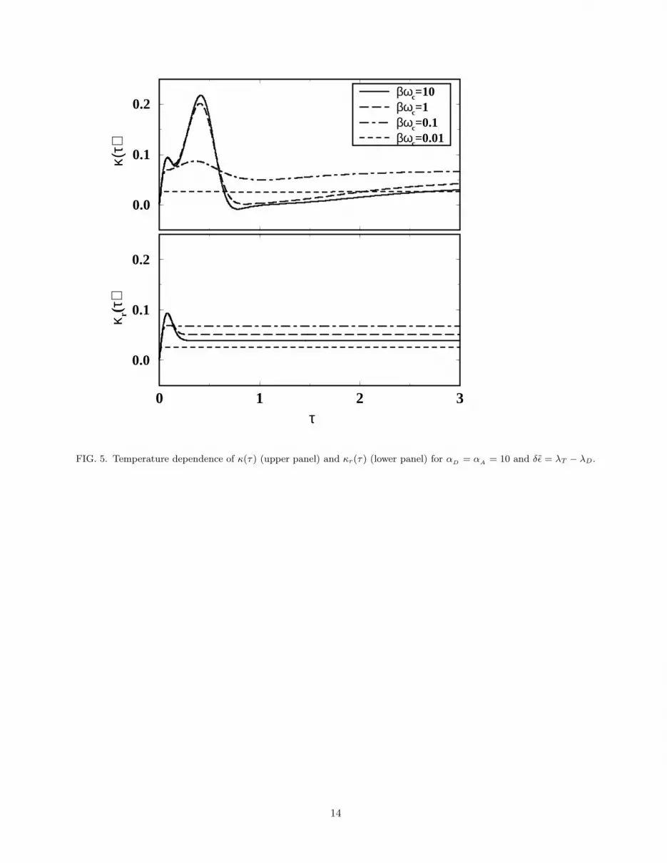
In Fig. 5, we provide results for αD = αA = 10,the strong coupling limit, and for δǫ = λT − λD. Thezero temperature result is shown in the top panel of Fig.1. As the temperature increases, the nonequilibrium ef-fects diminish. However, even for very high tempera-ture limit of βωc = 0.1, there is a noticeable differencebetween κ(τ) and κr(τ). Only in the highest tempera-ture limit of βωc = 0.01, κ(τ) and κr(τ) show an agree-ment. This indicates that for strongly coupled systems,the nonequilibrium effects persist even up to very hightemperature. Next, we considered the weak coupling caseof αD = αA = 1 with the same choice of δǫ = λT − λD.The results are shown in Fig. 6. In the zero temperaturelimit, the nonequilibrium effect was not so significant forthis weak coupling case. This fact remains the same evenfor the higher temperature.

IV. DISCUSSION

The main focus of the present paper was the nonequi-librium bath relaxation effect. For this reason, we con-sidered only the simplest case where donor and acceptoreach have one excited state. However, as recent stud-ies on various systems indicate [7,13–15], the existence ofmultiple chromophores is a general situation rather thanan exception. Therefore, one in general must considerthe case where the donor and the acceptor respectivelyconsist of multiple exciton states. Given that the inter-excitonic relaxation can be disregarded or approximatedin a self consistent way, the generalization of the presenttheory can be done straightforwardly as are those of theFD theory [24–30]. In many cases, this type of simple ex-tension may indeed capture the main aspect of the EETbetween multichromorphic donor and acceptor. However,if some of the excitonic levels are closely spaced or if thereis degeneracy due to symmetry, more careful theoreticalanalysis is necessary.

In a heterogeneous environment or a complex system,disorder plays an important role and its explicit consid-eration becomes necessary for a proper understanding ofthe system. Due to the averaging over the static disor-der involved in this case, our spectral overlap expressioncannot be used directly for the observables of an ensem-ble experiment. However, given that the distribution ofthe static disorder is well characterized by other means,Monte Carlo simulation can provide an indirect way ofdetermining the nonequilibrium population transfer. Thestudy of the interplay between the heterogeneity and thenonequilibrium effect in this way can bring new insightsinto the fast EET kinetics of complex systems.

In the LH2 of purple bacteria, the EET from B800 toB850 occurs in about 1ps and the rate is not so sensi-tive to temperature [14]. This rate is much faster thanthat obtained by the FD theory, but it has recently beenshown that consideration of the multichromorphic natureof the B850 and the disorder account for much of the dis-crepancy [24–27]. However, the theoretical value is stillsomewhat smaller than the experimental one [27]. Manyexplanations are possible for this, and the nonequilibriumeffect is one such possibility.

According to our model calculations, the nonequilib-rium short time kinetics shows complicated time depen-dent behavior and the reaction rate in this regime is lessdependent on the spectral overlap between the stationaryemission and absorption profiles. Some of these featurescan be seen in recent sub-picosecond pump-probe exper-iments [8,11,41]. For example, the reaction rate is shownto be relatively insensitive to the change of the spectralprofile for the EET in the photosynthetic reaction center[41].

Before applying the present theory to a given system,it is always important to examine whether the nature

7

of the system is consistent with the assumption of irre-versibility and the use of second order approximation. Itis expected that our results can be applied as long as δǫ issufficiently large and the bath relaxation of the acceptoris fast enough. However, in order to address these issuesmore systematically, it is necessary to formulate a the-ory that can account for electronic coherence. For thispurpose, one may adopt the formalism of the generalizedmaster equation [43] or consider in the framework of theRedfield-type equation [17].

ACKNOWLEDGMENTS

SJ thanks Prof. R. M. Hochstrasser for discussions onthe EET and pump-probe experiments.

APPENDIX A: TIME DEPENDENT

STIMULATED EMISSION PROFILE OF THE

DONOR

Consider a system consisting of the donor and its ownbath. The relevant Hamiltonian in the single excitationmanifold is given by

HD = ǫD

a†D

aD

+ BD

a†Da

D+ HbD

. (A1)

Assume that the donor is excited at time zero by a deltapulse. Then, the initial density operator at t = 0 is givenby

ρ(0) = |D〉〈D|1

ZbD

e−βHbD . (A2)

Right after the pulse excitation, a stationary field witha fixed frequency ω is turned on. The time dependentHamiltonian governing the dynamics for t > 0, assumingunit field strength, is given by

H(t) = HD + |µD · e|(e−iωt|D〉〈g| + eiωt|g〉〈D|) , (A3)

where rotating wave approximation was used. The prob-ability for the donor to emit a photon and go to theground state, induced by the stationary field, is given by

Pg(t) = |µD · e|2∫ t

0

dt′∫ t

0

dt′′ eiω(t′−t′′)−iǫD

(t′−t′′)/h

×1

ZbD

TrbD

{

e−iHbD(t−t′)/he−i(BD+HbD

)t′/h

× e−βHbD ei(BD+HbD)t′′/heiHbD

(t−t′′)/h}

, (A4)

where weak field approximation was used. The time de-pendent stimulated emission profile is defined as the timederivative of this probability as follows:

ED(t, ω) ≡d

dtPg(t)

= 2|µD · e|2Re

[∫ t

0

dt′e−iωt′+iǫD

t′/h

×1

ZbD

TrbD

{

ei(HbD+BD)t/he−iHbD

t′/h

× e−i(HbD+BD)(t−t′)/he−βHbD

}]

. (A5)

APPENDIX B: RATE EXPRESSION FOR A

GENERAL HARMONIC OSCILLATOR BATH

For a general harmonic oscillator bath model, we de-rive the expression of the nonequilibrium reaction rategiven by Eq. (2.9) based on the small polaron transfor-mation. For this purpose, first we introduce the followinggenerator of small polaron transformation:

S = −∑

n

(bn − b†n)(gnDa†Da

D+ gnAa†

Aa

A) . (B1)

Then, it is straightforward to show that

H = eSHe−S = ǫDa†

Da

D+ ǫ

Aa†

Aa

A+ Hb + HDA

= H0 + HDA , (B2)

where

HDA = JeS(a†D

aA

+ a†Aa

D)e−S

= J(θ†DθAa†D

aA

+ θ†AθDa†Aa

D) , (B3)

where

θ†D(A) = e−∑

ngnD(A)(bn−b†n) . (B4)

Inserting 1 = e−SeS between every two operators in Eq.(2.9), one can show that

k(t) =2J2

h2 Re

[∫ t

0

dt′ei(ǫD−ǫ

A)t′/h

×1

ZbTrb

{

eiHbt′/hΘ†e−iHbt′/hΘρd(t − t′)}

]

, (B5)

where Θ† = θ†DθA,

ρd(t) ≡ e−iHbt/hθ†De−βHbθDeiHbt/h

= e−β∑

nhωn(b†

nD(t)bnD(t)+ 1

2 ) , (B6)

with

bnD(t) ≡ bn − gnDe−iωnt . (B7)

In Eq. (B5),

eiHbt/hΘ†e−iHbt/h

= exp

{

−∑

n

gn∆(bne−iωnt − b†neiωnt)

}

, (B8)

8

where gn∆ ≡ gnD − gnA. Inserting Eqs. (B6)-(B8) intoEq. (B5),

k(t) =2J2

h2 Re

[∫ t

0

dt′ei(ǫD−ǫ

A)t′/he−i

∑

ngn∆ sin(ωnt′)

× e2i∑

ngn∆gnD(sin(ωnt)−sin(ωn(t−t′)))

×1

ZbTrb

{

e−∑

ngn∆((e−iωnt′−1)bnD−(eiωnt′−1)b†

nD)

× e−β∑

nhωn(b†

nDbnD+ 1

2 )}]

, (B9)

where the time dependences of bnD(t− t′) and b†nD(t− t′)have been omitted, but this does not make any differencein the result because of the trace operation. Disentan-gling the summation in the exponent and then evaluatingthe trace over the bath, one can reduce Eq. (B9) into thefollowing integral expression:

k(t) =2J2

h2 Re

[

e2i∑

ngn∆gnD sin(ωnt)

∫ t

0

dt′ ei(ǫD−ǫ

A)t′/h

× e−i∑

ng2

n∆ sin(ωnt′)−2i∑

ngn∆gnD sin(ωn(t−t′))

×e−2∑

ng2

n∆ coth(βhωn/2) sin2(ωnt′/2)]

. (B10)

For the case where there is no common mode,gn∆gnD = g2

nD and g2n∆ = g2

nD + g2nA and the expres-

sion of Eq. (2.20) is reproduced.

APPENDIX C: RATE EXPRESSIONS FOR THE

MODEL SPECTRAL DENSITIES OF SEC. III

For the spectral densities given by Eq. (3.1), the in-tegrations within the exponents of Eq. (2.24) can beperformed explicitly. Adopting the units where h = 1,the reaction rate of Eq. (2.24) can be expressed as

k(t) =2J2

ωcRe

[∫ τ

0

dτ ′ eiφ(τ,τ ′)−γ(τ ′)

]

, (C1)

where τ = ωct, τ′ = ωct

′, and

φ(τ, τ ′) =

(

ǫD− ǫ

A

ωc− 2(α

D− α

A)

)

τ ′ −2(α

D+ α

A)τ ′

(1 + τ ′2)2

−4αD

(

τ − τ ′

(1 + (τ − τ ′)2)2−

τ

(1 + τ2)2

)

. (C2)

In Eq. (C1), the function γ(τ ′) comes from the integra-tion involving coth(βωh/2) in Eq. (2.24). Simple ap-proximation for this function is possible in the limits oflow and high temperature. Using these approximations,

γ(τ)=

(αD

+ αA)(

τ2

1+τ2 + 2τ2

(1+τ2)2

)

, βωc >> 1 ,2(α

D+α

A)

ωcβτ2

1+τ2 , βωc << 1 .(C3)

In the main text, we consider the zero temperature limitfirst and study the finite temperature effect using a sim-ple interpolation formula. Similarly, the quantities enter-ing the approximate rate expressions of Eqs. (2.26) and(2.31) can be calculated. These are

λT = 2(αD

+ αA)ωc , (C4)

S(t) = 24αDω2

c

τ − τ3

(1 + τ2)4, τ = ωct , (C5)

C(t) = 2αDωc

1 − τ2

(1 + τ2)3, τ = ωct , (C6)

D(β) =

{

6(αD

+ αA)ω2

c , βωc >> 1 ,4(α

D+ α

A)ωc/β , βωc << 1 .

(C7)

[1] Th. Forster, Discuss. Faraday Soc. 27, 7 (1953).[2] Th. Forster , in Modern Quantum Chemistry, Part III

, edited by O. Sinanoglu (Academic Press, New York,1965).

[3] D. L. Dexter, J. Chem. Phys. 21, 836 (1953).[4] V. M. Agranovich and M. D. Galanin, Electronic excita-

tion energy transfer in condensed matter, North-Holland,Amsterdam, 1982.

[5] P. Reineker, H. Haken, and H. C. Wolf, Ed., Organic

Molecular Aggregates, Springer-Verlag, Berlin, 1983.[6] E. J. B. Birks, Excited States of Biological Molecules,

John Wiley & Sons, London, 1976.[7] D. L. Andrews and A. A. Demidov, Resonance Energy

Transfer, John Wiley & Sons, Chichester, 1999.[8] G. Cerullo, S. Stagira, M. Zavelani-Rossi, S. De Silvestri,

T. Virgili, D. G. Lidzey, and D. D. C. Bradley, Chem.Phys. Lett. 335, 27 (2001).

[9] S. C. J. Meskers, J. Hubner, M. Oestreich, and H. Bassler,Chem. Phys. Lett. 339, 223 (2001).

[10] A. R. Buckley, M. D. Rahn, J. Hill, J. Cabanillas-Gonzalez, A. M. Fox, and D. D. C. Bradley, Chem. Phys.Lett. 339, 331 (2001).

[11] F. V. R. Neuwahl, R. Righini, A. Adronov, P. R. L.Malenfant, and J. M. J. Frechrt, J. Phys. Chem. B 105,1307 (2001).

[12] J. Morgado, F. Cacialli, R. Iqbal, S. C. Moratti, A. B.Holmes, G. Yahioglu, L. R. Milgrom, and R. H. Friend,J. Mater. Chem. 11, 278 (2001).

[13] X. Hu and K. Schulten, Phys. Today August, 28 (1997).[14] V. Sundstrom, T. Pullerits, and R. van Grondelle, J.

Phys. Chem. B 103, 2327 (1999).[15] T. Renger, V. May, and O. Kuhn, Phys. Rep. 343, 137

(2001).[16] T. F. Soules and C. B. Duke, Phys. Rev. B 3, 262 (1971).[17] S. Rackovsky and R. Silbey, Mol. Phys. 25, 61 (1973).[18] B. Jackson and R. Silbey, J. Chem. Phys. 78, 4193

(1983).[19] R. Silbey, Annu. Rev. Phys. Chem. 27, 203 (1976).[20] M. Grover and R. Silbey, J. Chem. Phys. 54, 4843 (1971).

9

[21] R. W. Munn and R. Silbey, J. Chem. Phys. 68, 2439(1978).

[22] G. Juzeliunas and D. L. Andrews in Ref. 7.[23] C.-P. Hsu, G. R. Fleming, M. Head-Gordon, and T.

Head-Gordon, J. Chem. Phys. 114, 3065 (2001).[24] H. Sumi, J. Phys. Chem. B 103, 252 (1999).[25] K. Mukai, S. Abe, and H. Sumi, J. Phys. Chem. B 103,

6096 (1999).[26] K. Mukai, S. Abe, and H. Sumi, J. Lumin. 87-89, 818

(2000).[27] G. D. Scholes and G. R. Fleming, J. Phys. Chem. B 104,

1854 (2000).[28] G. D. Scholes, X. J. Jordanides, and G. R. Fleming, J.

Phys. Chem. B 105, 1640 (2001).[29] A. Damjanovic, T. Ritz, and K. Schulten, Phys. Rev. E

59, 3293 (1999).[30] E. K. L. Yeow and K. P. Ghiggino, J. Phys. Chem. B

104, 5825 (2000).[31] S. H. Lin, W. Z. Xiao, and W. Dietz, Phys. Rev. E. 47,

3698 (1993).

[32] T. Kakitani, A. Kimura, and H. Sumi, J. Phys. Chem. B103, 3720 (1999).

[33] A. Kimura, T. Kakitani, and T. Yamato, J. Lumin. 87-

89, 815 (2000).[34] A. Kimura, T. Kakitani, and T. Yamato, J. Phys. Chem.

B 104, 9276 (2000).[35] I. Y. Tekhver and V. V. Khizhnyakov, Sov. Phys.-JETP

42, 305 (1976).[36] See pages 149-150 of Ref. 4 for a comprehensive list of

references.[37] H. Sumi, J. Phys. Soc. Japan 51, 1745 (1982).[38] H. Sumi, Phys. Rev. Lett. 50, 1709 (1983).[39] S. Gnanakaran, G. Haran, R. Kumble, and R. M.

Hochstrasser in Ref. 7.[40] R. van Grondelle and O. J. G. Somsen in Ref. 7.[41] B. A. King, A. de Winter, T. B. McAnaney, and S. G.

Boxer, J. Phys. Chem. B 105, 1856 (2001).[42] M. Cho and R. J. Silbey, J. Chem. Phys. 103, 595 (1995).[43] W. M. Zhang, T. Meier, V. Chernyak, and S. Mukamel,

J. Chem. Phys. 108, 7763 (1998).

0 1 2 3τ

0.0

0.1

0.2

0.0

0.1

0.2

κ(τ)

κ(τ)κr(τ)κs(τ)κsg(τ)

0.0

0.1

0.2

FIG. 1. Dimensionless nonequilibrium reaction rate κ(τ ), Eq. (3.2), and analogous quantities for kr(t), ks(t), and ksg(t).α

D= α

A= 10 and temperature is zero. The top panel corresponds to δǫ = λT − λD, the middle panel to δǫ = λT , and the

bottom panel to δǫ = λT + λD.

10

0 1 2 3τ

0.0

0.1

0.2

p(τ)pr(τ)ps(τ)psg(τ)

0.0

0.2

0.4

0.6

p(τ)

0.0

0.1

0.2

FIG. 2. Scaled population p(τ ), Eq. (3.3), and analogous quantities for kr(t), ks(t), and ksg(t). αD

= αA

= 10 andtemperature is zero. The top panel corresponds to δǫ = λT − λD, the middle panel to δǫ = λT , and the bottom panel toδǫ = λT + λD.

11

0 2 4τ

0.0

0.4

0.8

0.0

0.4

0.8

κ(τ) κ(τ)

κr(τ)κs(τ)κsg(τ)

0.0

0.4

0.8

FIG. 3. Dimensionless nonequilibrium reaction rate κ(τ ), Eq. (3.2), and analogous quantities for kr(t), ks(t), and ksg(t).α

D= α

A= 1 and temperature is zero. The top panel corresponds to δǫ = λT − λD, the middle panel to δǫ = λT , and the

bottom panel to δǫ = λT + λD.

12

0 2 4τ

0

1

2

3

p(τ)pr(τ)ps(τ)psg(τ)

0

1

2

3

p(τ)

0

1

2

3

FIG. 4. Scaled population p(τ ), Eq. (3.3), and analogous quantities for kr(t), ks(t), and ksg(t). αD

= αA

= 1 andtemperature is zero. The top panel corresponds to δǫ = λT − λD, the middle panel to δǫ = λT , and the bottom panel toδǫ = λT + λD.

13

0 1 2 3 τ

0.0

0.1

0.2

κ r(τ)

0.0

0.1

0.2κ(

τ)

βωc=10βωc=1βωc=0.1βωc=0.01

FIG. 5. Temperature dependence of κ(τ ) (upper panel) and κr(τ ) (lower panel) for αD

= αA

= 10 and δǫ = λT − λD.

14

0.0 2.0 4.0 τ

0.0

0.4

0.8

κ r(τ)

0.0

0.4

0.8κ(

τ) βωc=10βωc=1βωc=0.1βωc=0.01

FIG. 6. Temperature dependence of κ(τ ) (upper panel) and κr (lower panel) for αD

= αA

= 1 and δǫ = λT − λD.

15