Nonlinear softening as a predictive precursor toclimate tipping

B Y JAN SIEBER1 AND J. MICHAEL T. THOMPSON2

1Department of Mathematics, University of Portsmouth, UK2School of Engineering, University of Aberdeen, UK, and Department of Applied

Mathematics and Theoretical Physics, University of Cambridge, UK

Approaching a dangerous bifurcation, from which a dynamical system such as the Earth’sclimate will jump (tip) to a different state, the current stable state lies within a shrinkingbasin of attraction. Persistence of the state becomes increasingly precarious in the presenceof noisy disturbances. We consider an underlying potential, as defined theoretically for asaddle-node fold and (via averaging) for a Hopf bifurcation. Close to a stable state, thispotential has a parabolic form; but approaching a jump it becomes increasingly dominatedby softening nonlinearities. If we have already detected a decrease in the linear decay rate,nonlinear information allows us to estimate the propensity for early tipping due to noise.If there is no discernable trend in the linear analysis, nonlinear softening is even moreimportant in showing the proximity to tipping.

After extensive normal form calibration studies, we apply our technique to two geolog-ical time series from paleo-climate tipping events. For the ending of the last ice age, wherewe find is no convincing linear precursor, we identify a statistically significant nonlinearsoftening towards increasing temperature. The analysis has thus successfully detected awarning of the imminent tipping event.

Keywords: time series analysis, bifurcation prediction, climate tipping

1. IntroductionThe on-going work by the United Nations, following the major report of the IPCC [1] in2007 and the Climate Change Conferences in Copenhagen and Cancun (Mexico), centreson the prediction of future climate change, a key feature of which would be any suggestionof a sudden and (possibly) irreversible abrupt change called a tipping point (Lenton et al.[2], Scheffer [3]). Many tipping points, such as the switching on and off of ice-ages, arewell documented in paleo-climate studies over millions of years of the Earth’s history.

Predicting such tippings in advance using time-series data derived from preceding be-haviour is now seen as a major challenge, impinging, for example on the possible use ofgeo-engineering (Launder and Thompson [4]). Techniques introduced by Held and Kleinen[5] and Livina and Lenton [6] draw on the assumption that the tipping events are governedby a bifurcation in an underlying nonlinear dissipative dynamical system. Specifically, re-searchers search for a slowing down of intrinsic transient responses within the data, whichis predicted to occur before most bifurcational instabilities. This is done by determininga so-called propagator, estimated from the correlation between successive elements of awindow sliding along the time series. This propagator, such as the ARC(1) mapping co-efficient, is a measure of the linear decay rate and should increase to unity at a tippinginstability (corresponding to a decrease of the linear decay rate to zero).

Article submitted to Phil. Trans. of the Royal Society TEX Paper

arX

iv:1

103.

3064

v1 [

mat

h.D

S] 1

5 M

ar 2

011

2 J. Sieber and J. M.T. Thompson

Prediction techniques can be tested on climatic computer models, but more challeng-ing is to try to predict real ancient climate tippings, using their preceding geological dataprovided by ice cores, sediments, etc. Using this preceding data alone, the aim would be tosee to what extent the actual tipping could have been predicted in advance.

One such study by Livina and Lenton [6] looks at the end of the most recent ice ageand the associated Younger Dryas event, about 11,500 years ago, when the Arctic warmedby 7◦C in 50 years. This pioneering study used a time series derived from Greenland ice-core paleo-temperature data. A second such study (one of eight made by Dakos et al.[7]), using data from tropical Pacific sediments, gives a good prediction for the end of‘greenhouse’ Earth about 34 million years ago when the climate tipped from a tropical stateinto an icehouse state. Lenton et al. [8] gives a complete overview of current techniques forextracting early-warning signals from time series and compares them on realistic modelsand a range of paleo-climate time series.

A caveat that is made during the analysis of Lenton et al. [8] is that the absolute valuesof the extracted quantities have no direct bearing on the tipping probability over time unlessone knows also the size of the basin of attraction. This basin is determined in the simplestcases by the dominant nonlinear term in the underlying equations of motion, which is thesubject of this paper.

2. Concepts from Nonlinear Dynamics

The core techniques for analysis of time series of climate data aim to extract the linear de-cay rate toward (a possibly drifting) noise-perturbed equilibrium [5, 6]. These techniquescan be directed at the Earth’s climate as a whole, or at the relevant climate sub-systemsdescribed by Lenton et al. [2] as tipping elements. Our aim here is to augment this linearinformation with information about nonlinear features of the underlying dynamics, by ex-amining to what extent we can identify nonlinear softening and include it into the list ofearly-warning signs for climate tipping.

(a) Shrinking basins around dangerous bifurcations

As we approach a dangerous bifurcation, from which a nonlinear dissipative dynamicalsystem will experience a finite jump to a remote alternative state, the current attractor islocated within a shrinking basin of attraction. Correspondingly, the maintenance of thestate will become increasingly precarious in the presence of noisy disturbances.

Thinking in terms of an underlying potential energy function (the existence of which istheoretically well-defined for a saddle-node fold and some other bifurcations) the parabolicshape of its graph will become increasingly contaminated by softening nonlinear features.

The relevant bifurcations are the so-called codimension-one events (Thompson et al.[9], Thompson and Stewart [10]), namely those that can be typically encountered un-der a gradual change of a single control parameter. The complete list of the dangerouscodimension-one bifurcations is given in Table 1, where we give a brief description ofthe nature of the shrinking basin. More details can be found in Thompson and Sieber[11]. Focusing first on the local bifurcations (headings (a) and (b) of Table 1) the shrinkingboundaries are illustrated schematically in Figure 1, with the control parameter plotted hor-izontally and the response plotted vertically. In the first picture, Figure 1(a), we illustrateboth types of the saddle-node fold bifurcation: the static fold involving a path of equi-librium fixed-points, and the cyclic fold involving a trace of periodic orbits. For these the

Article submitted to Phil. Trans. of the Royal Society

Nonlinear softening as a predictive precursor to climate tipping 3

(a) Local Saddle-Node BifurcationsStatic Fold (saddle-node of fixed point) one-sided basin shrinkageCyclic Fold (saddle-node of cycle) one-sided basin shrinkage

(b) Local Subcritical BifurcationsSubcritical Hopf complete basin shrinkageSubcritical Neimark-Sacker (secondary Hopf) complete basin shrinkageSubcritical Flip (period-doubling) complete basin shrinkage

(c) Global BifurcationsSaddle Connection (homoclinic connection) outside shrinkage around cycleRegular-Saddle Catastrophe (boundary crisis) fractal basin shrinkageChaotic-Saddle Catastrophe (boundary crisis) fractal basin shrinkage

Table 1: Dangerous Bifurcations and the behaviour of the basin of attraction

Figure 1: Basin boundary transformations at dangerous bifurcations. (a) the fold bifurcations and (b) the subcrit-ical bifurcations. Solid curves denote stable paths while broken curves denote unstable paths. The basin is shownin grey.

basin shrinkage is one-sided. The basin is bounded by the unstable side of the parabolicallyfolding path.

Next, in Figure 1(b), we illustrate the local subcritical bifurcations of which the Hopf,flip and Neimark are codimension-one (we remember that the more familiar static pitchforkbifurcations are codimension-two, being structurally unstable against a symmetry-breakingperturbation). Here we see an unstable solution, which controls the basin boundary, shrink-ing parabolically around the stable solution, from which the (noise-free) system jumps outof our field of view as the control parameter, µ , reaches its critical value of µC.

The static fold and the Hopf bifurcation have a theoretically well-defined potential en-ergy surface that neatly summarizes the shrinking basin as illustrated in Figure 2. Note thatFigure 2(a) will be discussed more fully in section 2(b). For other dangerous bifurcations,where the existence of an underlying potential surface lacks any theoretical backing (andindeed may be technically impossible because of fractal features in the dynamics) there arenevertheless occasions when it is useful and practical to consider such a surface for escapepredictions in the presence of significant noise as we shall demonstrate in section 6.

(b) A closer look at the fold

The fold is the simplest and most common way in which an equilibrium of a nonlineardissipative dynamical system can lose its stability. Having only a single active degree offreedom (x) and being observable under the variation of a single control parameter (µ)it can be illustrated on a graph of x against µ as a smooth curve that simply reaches anextreme value (a maximum, say) of the control µ , as shown in Figure 1(a). So although it is

Article submitted to Phil. Trans. of the Royal Society

4 J. Sieber and J. M.T. Thompson

Figure 2: Total potential energy transformations in (a) the saddle-node fold and (b) the Hopf bifurcation (viaaveraging). Black balls denote stable equilibrium states while white balls denote unstable states.

traditionally called a saddle-node bifurcation, it does not exhibit any obvious ‘bifurcation’of a path, but rather just a smooth folding of an existing path. In the case of a static fold (towhich we shall largely restrict our attention) the path is a trace of equilibrium fixed points,while for a cyclic fold the path would be a trace of periodic solutions.

Assuming, that we are close to a fold the intrinsic damping of the system will have be-come super-critical so the system will have the non-oscillatory response of an over-dampedparticle sliding (in thick oil, as we might imagine) on a notional potential energy surfaceU(x,µ). This is illustrated for the fold in Figure 2(a), where we show the potential en-ergy surface erected over the (x,µ) base plane. Here the solid part of the equilibrium path,corresponding to energy minima, is a stable node, while the dashed part, corresponding toenergy maxima (more generally a geometrical saddle in higher dimensions) is an unstabledynamical saddle.

We see that as the control µ is slowly increased towards its critical value, µC, the stableequilibrium solution gets closer and closer to the hill-top potential barrier, and so getsprogressively more precarious in the presence of noisy disturbances. With µ increasing atan infinitesimal rate, noise will ensure escape over the hill-top before µ reaches µC. If,however, µ increases rapidly, this early escape may be delayed or supressed as we haveexamined quantitatively elsewhere (Thompson and Sieber [12]).

To give a greater perspective to our view of the fold it is useful to introduce another con-trol parameter µ2 such that our parameter space is now represented jointly by the (µ1,µ2)-plane. We can now erect an equilibrium surface, of height x, over the two-dimensional con-trol plane as illustrated in Figure 3. Here we see two fold lines whose projections dividethe control plane into regimes exhibiting either one or three co-existing solutions. Thesefold lines coalesce and vanish at the cusp. This cusp is a codimension-two phenomenon,which is only typically observed when we have independent control of both parameters(µ1 and µ2). This is made transparent by the fact that a typical path in control space cannotbe expected to pass precisely under the cusp point; by contrast, if a parameter path passesthrough a fold line all near-by paths also cross this fold line, which is what ‘the fold hascodimension-one’ means. For an appropriate choice of path in the (µ1,µ2)-plane throughthe cusp one sees a pitchfork bifurcation (Thompson and Stewart [10]).

We will consider the case in which the main equilibrium sheet (in grey) is stable whilethe narrow inverted sheet (white) is unstable.

Article submitted to Phil. Trans. of the Royal Society

Nonlinear softening as a predictive precursor to climate tipping 5

Figure 3: The cusp catastrophe and its associated pattern of folds. The notional axes show how such a cusp mightarise in a climate tipping scenario.

A climate system will have a large number of possible control parameters, but in tryingto predict a tipping point we will be studying a particular evolution which corresponds toa particular route in control space; this is precisely why we are only likely to encounter afold, and not a cusp in Figure 3. To explore possible scenarios that might underlie a tippingstudy, it is now useful to examine some possible routes in our two-parameter model ofFigure 3.

Consider, first, the simple scenario in which the system parameters take path BB leadingtransversally through a fold line. This is the classical encounter with a fold that is implicitlyenvisaged in earlier work. In the presence of noise a premature tip from N occurs witha certain probability depending on the noise level and the speed with which the path istraversed, as analysed by Thompson and Sieber [11]. If the noise level were particularlyhigh, a jump from N could easily be perceived as a purely noise-induced jump with nobifurcation, even though it is actually caused by the proximity to the fold: this could holdeven if there were no movement in the control space at all, the system having rested atN throughout (Ashwin et al. [13] call this N-tipping). Another scenario, not specificallyillustrated in the figure, could arise if the route in control space approached the fold line,but then turned back away from it. Analysis would then show a temporary decrease of thestrength of the attraction (with ARC(1) moving towards unity) which might be discountedas a false alarm, even though the system did approach a fold and a noise-induced escapewas temporarily probable. In this context, see Biggs et al. [14].

Finally, in the scenario of path AA, one would observe a temporary increase of ARC(1),even though no bifurcation is apparent but rather a rapid shift of the steady state. This showsthat a rapid transition can be related to a nearby fold that was just barely missed. Similarly,the R-tipping scenario studied by Ashwin et al. [13] occurs if one changes the other controlparameter in Figure 3 sufficiently rapidly from the path AA to N (avoiding the folds).

Article submitted to Phil. Trans. of the Royal Society

6 J. Sieber and J. M.T. Thompson

3. Time series analysis for leading order terms — qualitative overview

The extraction of the underlying dynamics from time series is divided into subtasks ofincreasing difficulty. Assume that we have a time series coming from a process that iseither stationary or has a slowly drifting underlying parameter µ as suggested by the pathsin Figure 3. In order to predict (or identify) the dynamics one attempts to extract the leadingorders of the dominant components of the underlying equations of motion. We illustrate the

−2

0

2

−2

0

2

0 100 200 3000

2

4

−2

−1

0

1

2

−1

0

1

0 20 400

2

4

N = 805N = 28, 803

x

x

time t time t

moving window

(a–2) de-trended and cut off: (tk, xk)

(a–3) estimate of linear decay rate

(b–2) de-trended and cut off: (tk, xk)

(b–3) estimate of linear decay rate

(a–1) time series (b–1) time series

theoreticalvalue 2

pµ

potential barrier x = −pµ

κUκACF

LDR

,κU,κ

AC

F

true equilibrium x =pµ

(a) Long times series, dense data

ǫ = 0.01, σ = 1, µ(0) = 2, ∆t = 0.01(b) Short time series, sparse data

ǫ = 0, σ = 1, µ= 1.252, ∆t = 0.05

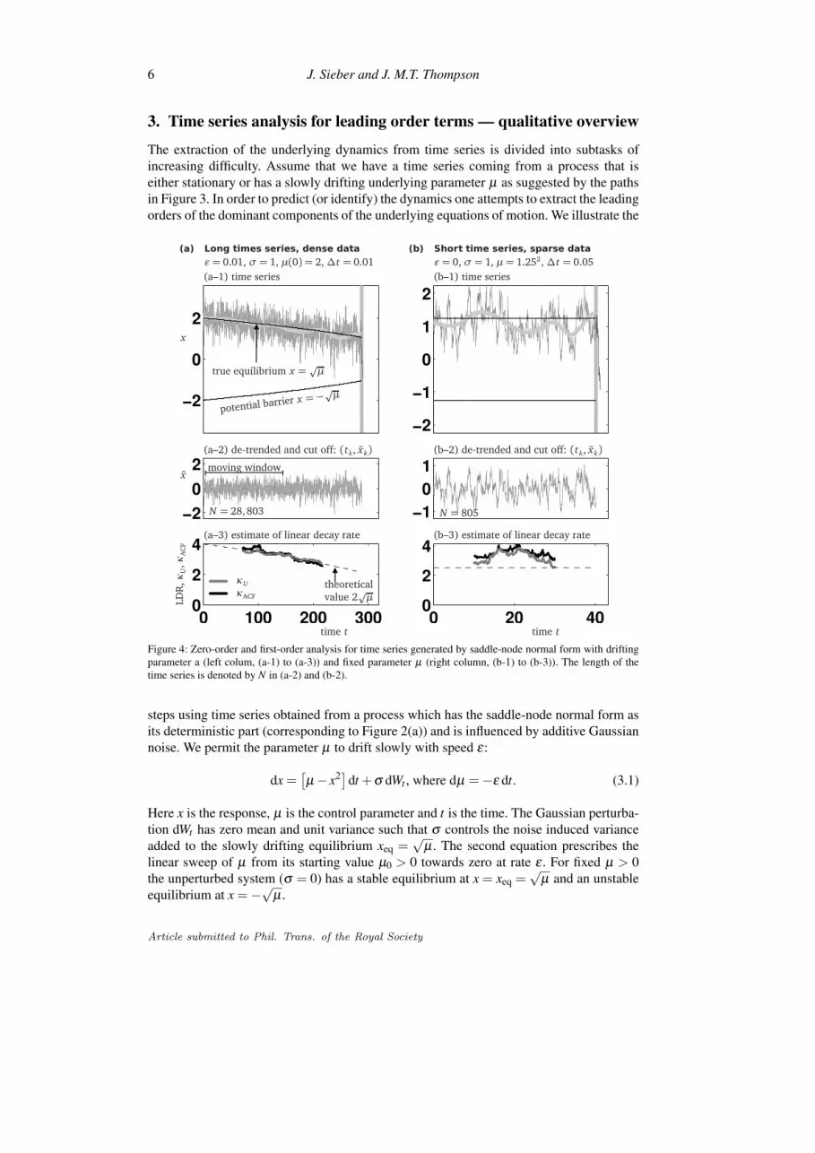
Figure 4: Zero-order and first-order analysis for time series generated by saddle-node normal form with driftingparameter a (left colum, (a-1) to (a-3)) and fixed parameter µ (right column, (b-1) to (b-3)). The length of thetime series is denoted by N in (a-2) and (b-2).

steps using time series obtained from a process which has the saddle-node normal form asits deterministic part (corresponding to Figure 2(a)) and is influenced by additive Gaussiannoise. We permit the parameter µ to drift slowly with speed ε:

dx =[µ− x2]dt +σ dWt , where dµ =−ε dt. (3.1)

Here x is the response, µ is the control parameter and t is the time. The Gaussian perturba-tion dWt has zero mean and unit variance such that σ controls the noise induced varianceadded to the slowly drifting equilibrium xeq =

õ . The second equation prescribes the

linear sweep of µ from its starting value µ0 > 0 towards zero at rate ε . For fixed µ > 0the unperturbed system (σ = 0) has a stable equilibrium at x = xeq =

õ and an unstable

equilibrium at x =−√

µ .

Article submitted to Phil. Trans. of the Royal Society

Nonlinear softening as a predictive precursor to climate tipping 7

We will use the saddle-node normal form (3.1) to test the robustness and reliabilityof a range of estimators. Example time series and the analysis of zero- and first-orderterms are shown in Figure 4, the softening of the full (estimated) nonlinear potential well(corresponding to the illustration in Figure 2(a)) is displayed in Figure 5.

The left column of Figure 4 shows a long time series generated by (3.1) with denselytaken measurements (length of time series N = 28,803, time step ∆t = 0.01, drift speedε = 0.01 for system parameter µ). The right column shows the results for a short timeseries (also generated by (3.1)) with sparser measurements.

(a) Equilibrium — zero order

The location of the slowly drifting equilibrium and its trend is estimated first. Lenton et al.[8] call this step detrending and propose either piecewise linear fitting or filtering witha Gaussian kernel. The result of filtering with a Gaussian kernel is shown as a thick greycurve in the row 1 of Figure 4. Every method for detrending requires a bandwidth parameter(for example the width of the Gaussian kernel). For Figure 4 we chose the bandwidth whichthe kernel density estimation routine (Matlab’s kde by Botev et al. [15]) offered. The thinblack curve in Figure 4(a-1) shows the true value of the equilibrium (for ε = 0). It gives avisual estimate of how the reliability of the zero-order estimates depends on the quality ofthe data. The oscillatory deviations of the extracted equilibrium (thick grey curve) from itstrue value (thin black curve) shows that the automatically chosen bandwidth was slightlysmaller than the theoretical optimum.

(b) Linear decay rate — first order

Assuming that the deterministic part of the underlying process has a stable equilibrium xeq(which is possibly slowly drifting), and that the zero-order estimate is an approximationfor xeq, the next step is to estimate the linear decay rate κ toward xeq and the trend of κ

over time. Generally, if the underlying deterministic process is high-dimensional then theseestimates capture the dominant (that is, smallest) decay rate. They are typically applied tothe detrended time series, that is, x = x−xeq, which is shown in the second row of Figure 4.

• ACF The k-step (usually one-step) autocorrelation function (ACF) α is fitted directlyto the detrended time series: xk+1 = α xk. This was introduced by Held and Kleinen[5] as degenerate finger-printing for the analysis of climate time series. The ACF α

is related to κ viaα = exp(−κACF ∆t).

The estimate for κACF is shown in Figure 4(a-3) and (b-3).

• DFA Detrended fluctuation analysis has been introduced by Livina and Lenton [6]for climate time series, see also Lenton et al. [8] for a short description of how oneextracts κ from this analysis.

• Quasi-stationary density If one assumes that the deterministic dynamics of thedetrended time series x is essentially that of an overdamped particle moving in apotential well U(x), that is,

dx =−∂xU(x)dt +σ dWt , (3.2)

Article submitted to Phil. Trans. of the Royal Society

8 J. Sieber and J. M.T. Thompson

then the linear decay rate equals the second derivative ∂xxU(0) of U at the bottom ofthe well, x = 0. Moreover, the stationary density p(x) is related to the shape of thepotential well U via the stationary Fokker-Planck equation

12

∂xx p(x) = ∂x[−σ

−2∂xU(x) p(x)

], which gives integrated once

12

∂x p(x) =−σ−2

∂xU(x) p(x)+σ−2c, (3.3)

where c is the constant of integration. This constant satisfies c= limx→±∞ ∂xU(x)p(x),and can be interpreted as the flow rate (c < 0 indicates flow toward−∞). Remember-ing that the drift speed ε of the system parameter µ is small, the true time-dependentprobability density p still satisfies (3.3) approximately at each µ:

12

∂x p(x,µ) =−σ−2

∂xU(x,µ) p(x,µ)+σ−2c(µ)+O(ε). (3.4)

In (3.4) we included the dependence of all quantities on µ expressly and rememberthat µ(t) is of order ε . Assuming quasi-stationarity, we neglect the order-ε termsand determine the coefficients, −σ−2∂xU and σ−2c, by fitting the empirical densitypemp(x) from a time window [t−w/2, t +w/2] to the Equation (3.4). Specifically,cemp = σ−2c is a scalar and ∂xU(0) is equal to 0 after detrending such that one hasto fit two coefficients, κU and cemp using (3.4) if one truncates ∂xU after first order:

12

∂x pemp(x) =−κU x pemp(x)+ cemp. (3.5)

In problems where no escape is possible one can drop the term c in (3.3) (and, thus,in (3.4) and (3.5)), and simplify (3.3) to

U =−σ2

2log p. (3.6)

Livina et al. [16] used relation (3.6) (fitting of U with higher-order polynomials) todetect potential wells in time series that included rapid transitions. Fitting U with aparabola (where U(0) is irrelevant and ∂xU(0) = 0) is equivalent to using the vari-ance σ2

emp of pemp(x) if the density pemp is Gaussian. Ditlevsen and Johnsen [17]state that monitoring the empirical variance σ2

emp helps to avoid erroneous detectionof false trends.

Lenton et al. [8] compare these three estimates in detail using time series arising in climatemodels and in paleoclimate records. Methods based on properties of the spectrum of thetime series were proposed and investigated by Kleinen et al. [18], Biggs et al. [14] butare not discussed here. Figure 4 shows how the estimates of κU from the quasi-stationarydensity compare to the ACF estimates κACF. For the long time series the estimates arequantitatively close to the theoretical value of κ (µ = κ2/4, see Figure 4(a-3)). Figure 4(b-3) shows that even for sparse and short time series the estimates for the linear decay rateare qualitatively correct but that discerning trends such as in Figure 4(a-3) is possible onlyfor longer time series. We also observe that in Figure 4(b-3) the local trends of κACF fromthe AR(1) estimate and of κU based on the quasi-stationary density are strongly correlated.As the underlying decay rate has no downward trend one might call the local downward

Article submitted to Phil. Trans. of the Royal Society

Nonlinear softening as a predictive precursor to climate tipping 9

trend of the estimates a ‘false alarm’. However, the parameters of the system make a noise-induced escape (or N-tipping in the notation of Ashwin et al. [13]) likely. Escape occursindeed at time t = 40 in Figure 4(b-1).

There is one notable difference between the AR(1) and the DFA estimate on one handand the distribution-based estimate κU on the other hand: the estimate for κU based on thequasi-stationary density only looks at the distribution of the values xk in the window ofinterest but does not care about the order in which they appear. This is in contrast to, forexample, the AR(1) estimate which determines the correlation between each value xk andits predecessor.

Estimate of the input noise amplitude

If the AR analysis shows the presence of a single positive dominant coefficient (which givesevidence that the underlying dynamics has really one distinct direction in which the decayis slowest) then one can combine both estimates of the decay rate to obtain an estimate ofthe amplitude σ of the additive noise: σ2 = κACF/κU where κACF is the estimate of thelinear decay rate obtained from the autocorrelation and κU is the estimate obtained fromthe quasi-stationary density pemp.

(c) Nonlinearity — basin boundary

One problem left open by the linear analysis is that the quantitative value of the estimatedLDR and the estimated noise-level do not give any indication for the probability of tipping.What the linear methods estimate is the α and the σ of a discrete process

xk+1 = α xk +σηk (3.7)

(where the ηk are assumed to be independent and normally distributed random numbers).The discrete process (3.7) is the linearisation of the time-∆t map of the continuous process(3.2). An estimate for α less than but close to unity does not necessarily indicate that weare close to a stability boundary for the nonlinear problem (3.2). Rather, it implies thatthe time step ∆t between successive measurements has been small compared to the meandecay time to half, log2/κ , of the process:

α(tk) = exp(−κ(tk)∆t) = 1−κ(tk)∆t +O((∆t)2) .

The trend of the estimated α is an indicator for incipient tipping because (if extrapolated inany way) it gives an estimate for the time to tipping if one ignores the possibility of earlyescape. However, the trend of α is less certain even in the artificial time series of Figure 4.Similarly, the estimated noise amplitude σ has to be compared to the coefficient in frontof the leading nonlinear term of the right-hand side (which equals −1 in (3.1)). The ratiobetween σ and nonlinear term enters the estimates for the probability of tipping if there isno discernible upward trend in α (N-tipping), or for the probability of early escape if α

points upwards (see Thompson and Sieber [12]). So without at least an order-of-magnitudeestimate of the leading nonlinear term the linear methods only provide an estimate for thetipping time if there is a clearly discernible trend in α , and even then this estimate discountsearly escape.

The approaches presented in the following all generalise the estimate for κU , basedon the quasi-stationary density, by looking at the full nonlinear potential well Uemp(x)

Article submitted to Phil. Trans. of the Royal Society

10 J. Sieber and J. M.T. Thompson

Figure 5: Nonlinear potential energy surfaces extracted from noisy time series using sliding windows for thesaddle node fold where at either end of the surface we have plotted the known function U(x, t) = x3/3− µ(t)x(σ = 1, ε = 0.01 and µ0 = 2). Red denotes a positive deviation, blue a negative deviation from the parabola givenby linear theory.

associated to the quasi-stationary density pemp(x) via the Fokker-Planck equation (3.4).Figure 5 illustrates how Uemp looks like for the time series shown in Figure 4 column (a).The realisation of the noisy, evolving time series is shown in the base plane together withthe equilibrium path µ = x2, and the estimated (empirical) potential, Uemp is shown as thecoloured surface. The estimate for the potential well is taken in a sliding window, whichexplains why the surface can only be determined in the central region of the time serieswith half the length of the window unrepresented at either end. The numerically estimatedequilibrium trend xeq is displayed as a black curve at the bottom of the valley of Uemp. Forcomparison with this Uemp we display at either end the real (nonlinear) potential U(x, t)corresponding to (3.1), which at the later time is already showing the hill-top to the left.The colour in Figure 5 shows the deviation of the empirical potential from the linear-theoryparabola, which is not itself displayed. The softening, highlighted by the blue colouration,is seen on the left hand side which is approaching the hill-top. Transparency of the colour isused to show the number of data points that support a particular part of the surface Uemp(x)(as given by the empirical quasi-stationary density pemp(x)).

Several methods have been proposed to detect nonlinearity in the potential well in theform of this type of softening (or tilting).

• Skewness Guttal and Jayaprakash [19, 20] studied how the closeness of a bifurcationinfluences the skewness γ of the empirical quasi-stationary density from time series.As this approach is also based on the empirical quasi-stationary density pemp, itgeneralises the estimate κU to non-parabolic features of the well U and non-Gaussianfeatures of the stationary density. Guttal and Jayaprakash [19, 20] proposed to lookat the trend of the skewness γ over time to detect incipient bifurcations.

• Quasi-stationary density Livina et al. [16] generalised the potential well analysisfor the quasi-stationary density beyond the estimate κU for the linear decay rate,fitting the potential well to higher-order polynomials of even degree using rela-tion (3.6). This analysis was not used to attempt prediction of transition probabilitiesfrom time series but it was applied to time series that already included all transitionsto count the number of wells of U depending on time t (which corresponds to thenumber of modes (peaks) of the empirical quasi-stationary density pemp). See alsoBeaulieu et al. [21] for methods that detect change points in time series.

Article submitted to Phil. Trans. of the Royal Society

Nonlinear softening as a predictive precursor to climate tipping 11

• Drift ratio If one assumes that the underlying system parameter is approaching afold more or less linearly (µ(t) = ε > 0) and one is sufficiently close to the foldalready then the ratio between the drift ∆xeq of the equilibrium estimate and theincrease of the estimated linear decay rate ∆κ estimates the quadratic term in thenormal form [12].

4. Quantitative estimates of the nonlinear coefficients

The colour shading of Figure 5 suggests that the nonlinear term in the underlying deter-ministic system shows up in the quasi-stationary density pemp. This raises two questions.First, can the level of deviation from linear theory be distinguished with confidence fromrandom chance? That is, can one state, when looking at a time series, that a significantquadratic term is present? Second, is it possible to quantify the size of the nonlinear termwith reasonable level of certainty?

Finding a significant nonlinearity is far easier than estimating its precise value becausebiases introduced during the zero- and first-order analysis may distort the value of the non-linear estimate but may still keep it significantly different from zero. We will demonstratethis in Section 5 for two paleo-climate time series.

0

0.1

0

2

4

0 1 2 3 4

−2

0

2

4

κ

(a)

(b)

mean

linear decay rate κ =2pµ

pµ

µ

Relation between skewness and system parameter µ

γ

escaperate

c

esca

pera

tec

1

var p

Figure 6: Dependence of mean, variance var p and skewness γ of the empirical stationary density for the saddle-node normal form with additive Gaussian noise (3.1).

Figure 6 shows the dependence of the mean, the variance var p, and the skewness γ

of the empirical stationary density pemp on the system parameter µ for (3.1) as computedusing the stationary Fokker-Planck equation (3.3). Note that this is the stationary densityfor the process where the density is re-scaled to have a unit integral whenever a particleescapes to −∞. Thus, the results shown in Figure 6 refer to the density of realisations thathave not escaped to −∞. We observe that the dependence of γ is strongly nonlinear for thesaddle-node normal form with noise (µ(t) = ε = 0, σ = 1 in Equation (3.1)). This meansthat trends of the skewness are likely to be difficult to ascertain when approaching a fold.

Article submitted to Phil. Trans. of the Royal Society

12 J. Sieber and J. M.T. Thompson

However, the presence of skewness is an indicator for the nonlinearity uniformly for allparameters µ , and its sign indicates the direction of escape.

Note also how the nonlinearity affects the empirical mean and the variance var p, whichis no longer inversely proportional to the linear decay rate κ . This shift of the mean andthe additional variance is in part due to the fraction of trajectories that escape, in part dueto the non-parabolic shape of the well at some distance from its local minimum.

µ

25%–75%

2pµ

(a)

(b)

(c)

(d)

(e)

N2 for linear surrogateN2 for saddle-node normal form

mean75%

25%

length of time series

50%

cemp for linear surrogatecemp for saddle-node normal form

skewness γ for linear surrogateskewness γ for saddle-node normal form

2pµ

κACF (25%, 50%, 75%)κU (25%, 50%, 75%)

Figure 7: Quartiles of lengths (d), and estimates cemp (a), N2 (b), skewness γ (c), κACF, and κU (both (e)) fortime series generated by the saddle-node normal form (3.1) with noise (ε = 0, µ = 1) and for linear time seriesgenerated by (4.2).

We can estimate the nonlinearity directly as the deviation of the empirical potential wellU from a parabola as suggested by figure 5 (we are only interested in ∂xU). The simplestapproach (apart from looking at skewness γ) is to fit κU and cemp to the empirical densitypemp using Equation (3.5). If ∂xU(x) is indeed linear then cemp would be zero such thatcemp is as a signed scalar measure for the deviation of ∂xU(x) from linearity, serving as aproxy for the present nonlinearity. A second alternative is to expand −∂xU(x) to secondorder, incorporating a quadratic nonlinearity directly into ∂xU with an unknown coefficientN2. This leads to

−σ−2

∂xU(x) =−κU x+N2x2, such that we fit12

∂x pemp(x) =[−κU x+N2x2] pemp(x)+ cemp,2. (4.1)

Article submitted to Phil. Trans. of the Royal Society

Nonlinear softening as a predictive precursor to climate tipping 13

Both quantities, cemp and N2, measure the deviation of−σ−2∂xU(x) from its linear approx-imation κU x. The main difference between them is the weighting (x2 for N2, uniform forcemp). Figure 7 shows how the estimates for nonlinearity behave for the saddle-node nor-mal form with noise, Equation (3.1) with ε = 0 and σ = 1. Each panel shows the quartilesof the distribution of the estimate for 100 realisatons of time series generated by (3.1). Eachrealisation was run until it reached 2000 data points or x = −1 (indicating escape). Panel(a) shows the estimate cemp obtained by linear-least-squares fitting of the approximate sta-tionary Fokker-Planck equation (3.5) to the empirical stationary density pemp, panel (b)shows the quadratic coefficient N2 obtained from (4.1), and panel (c) shows the skewnessγ of pemp. For comparison, we generate also 100 linear time series using

dt =−2√

µxdt +dWt (4.2)

and then fit cemp, N2 and γ for these time series, too. Figure 7 compares the distributions fortime series generated by the saddle-node normal form (3.1) and the linear equation (4.2).If there is small overlap in the distribution then the quantity is a good indicator for thepresence of a quadratic nonlinear term. We observe that this is the case for all quanititesas long as the time series has a length of 2000 (see Figure 7(d) for the distribution of timeseries lengths). Naturally, the uncertainty, and, hence, the overlap, increases when the timeseries is shorter due to escape from the potential well to −∞ . This is the case for smallerµ in Figure 7 (see Thompson and Sieber [12] for a quantitative study of escape proba-bilities for small µ). We also notice that all quantities have a systematic deviation fromthe theoretical value of the quantity they supposedly estimate: N2 should be equal to −1according to (3.1), the real escape rate c has a much smaller modulus than cemp (compareFigure 6(a)), and the skewness γ has theoretically a much larger modulus (compare Fig-ure 6(b)). The deviation for N2 is relatively small, and is likely caused by the kernel densityestimate for pemp. The large modulus of cemp shows that the linear term −κU x is a poor fitfor −∂xU(x), which makes cemp a measure of how much the odd symmetry is broken by−∂xU(x), rather than an estimate for the escape rate. We note that cemp,2 as fitted in (4.1)has a realistic modulus (close to zero, not shown in Figure 7). The bias of the skewness γ

is mainly due to our restriction to time series that stay inside the potential well. However,the characteristic dip of γ seen in Figure 6(b) is still visible in Figure 7(c).

The summative conclusion from Figure 7 is that one can detect the underlying nonlin-earity of the deterministic part of Equation (3.1) by observing cemp, N2 or the skewness γ

if the time series is moderately long. One can expect this to be true in the more generalcase of a time series generated by a system with deterministic dynamics close to a fold andadditive noise. While one can in principle recover the underlying parameter µ from the es-timates for κU , N2 and σ (see Thompson and Sieber [12]), the uncertainty in N2 propagatesdramatically into uncertainty for µ (one has to divide by N2).

5. Studies of Geological Time Series

We now apply our nonlinear investigations to two ancient climate tippings. The first is themajor transition marking the end of the latest ice age which occurred about 17,000 yearsbefore the present (yrs BP). The data used for this is a temperature reconstruction fromthe Vostok ice core deuterium record (Petit et al. [22]). The second more recent tipping isthe ending of the Younger Dryas using the grayscale from the Cariaco basin sediments inVenezuela (Hughen [23]). This Younger Dryas event was a curious cooling, about 11,500

Article submitted to Phil. Trans. of the Royal Society

14 J. Sieber and J. M.T. Thompson

years ago, just as the Earth was warming up after the last ice age. It ended in a dramatictipping point, when the Arctic warmed by 7◦C in 50 years. This sudden ending has beenrelated (Houghton [24]) to a switching-on of the global oceanic thermohaline circulation(THC). This switch-on is known from extensive theoretical studies (Dijkstra and Weijer[25]) to be at a saddle-node fold arising as a perturbation of a sub-critical pitchfork (see,for example, Rahmstorf [26] and Thompson and Sieber [12]).

Under linear time-series analysis of the directly preceding data, neither of these twoevents shows a strong trend in the stability propagator (see Figure 9). Meanwhile sampleestimates of the underlying potential functions are shown in Figure 8. In Figure 8(a), for

Figure 8: Two predicted potential energy surfaces for (a) the end of the last glaciation using the Vostok ice-core record and (b) the end of the Younger Dryas event when the Arctic warmed by 7◦C in 50 years, usingthe grey-scale of basin sediment in Cariaco, Venezuela. The colour shows the deviation from a (time-dependent)parabola fitted to Uemp(x, t), three of which are illustrated above. Red signifies a positive deviation, blue a negativedeviation. Time is given in years before the present (BP).

the end of the last glaciation, we see clearly that the well is softening (falling beneaththe parabolic fit) on the high-temperature end while hardening (rising above the parabola)on the low-temperature end. So there is a strong nonlinear signal that a jump to highertemperatures may be pending (as indeed it was). We show that this signal is statisticallysignificant in our full analysis in Figure 9. By comparison, the study of the Younger Dryas,illustrated in Figure 8(b), provided no significant nonlinear conclusions.

For Figure 9 we detrended both time series using Gaussian filtering (see Figures 9(c)and (d)) and estimated the linear indicators κACF and κU , getting results consistent withLenton et al. [8]: weak to non-existent trends, leaving the evidence inconclusive at thelinear level (grey and black curves Figure 9(e) and (f)). The ratio between κACF and κU inFigure 9(e) and (f) gives an estimate of the variance σ2 of the noise input.

However, the time series for the end of the last glaciation has a strong quadratic nonlin-earity in ∂xU(x) where the potential well U is presumed to govern the deterministic part ofthe dynamics (Figure 9(g)). The indicators cemp, N2 and the skewness γ in Figure 9(g) areall far removed from what can be expected by chance in a linear time series. The histogramin the background of Figure 9(g,h) has been sampled from 500 random linear time seriesgenerated by the linear process given in Equation (4.2) with µ = κACF. The percentages atthe top of Figure 9(g,h) express how far in the tail of the histogram the quantity extractedfrom the geological time series is: 50% corresponds to the median of the histogram, a per-

Article submitted to Phil. Trans. of the Royal Society

Nonlinear softening as a predictive precursor to climate tipping 15

2.8% 4.4% 10.8% 18% 22.8% 41%

detr

ende

d−8

−6

−4

−2

0

2

−2

0

2

−4 −2 0

x 104

0

170

180

190

200

−10

0

10

−1.3 −1.25 −1.2 −1.15

x 104

0

time time

End of last glaciation End of Younger Dryas

Tem

pera

ture

(°C

)

Gre

ysc

ale

(0–2

55)

(a) (b)

(c) (d)

(e) (f)

cemp cemp γγ

κACFκACF

κUκU

κU,κ

AC

Fno

nlin

eari

ty

N2 N2

(g) (h)

Figure 9: Linear and nonlinear coefficients for two paleo-climate time series. (a,c,e,g): End of last glaciation(snapshot of data from Petit et al. [22]); (b,d,f,h): End of Younger Dryas (snapshot of data from Hughen [23]).Only the black part of the data in panels (a) and (b) was used in the analysis. Panel (c) and (d) show the time seriesafter detrending. Panel (e) and (f) show the linear indicators κACF and κU . Panel (g) and (h) show the means of theestimates cemp, N2 and the skewness γ , compared to zero (thin vertical black line) and a histogram of estimatessampled from 500 random linear time series generated by the linear process (4.2) with −2

√µ = κACF.

centage smaller than 50% gives the percentage of linear realisations that were further awayfrom the median than the geologocal data.

Visual inspection of the well shape in Figure 8 confirms that the well is softening(bending downward) on the high-temperature end and hardening (bending upward) on thelow-temperature end. So, at the nonlinear level the time series data close to the bottom ofthe well gives already evidence for a propensity to escape toward larger temperatures. Thetime series for the end of the Younger Dryas does not show evidence for strong nonlinearityof the underlying dynamics at the second-order level (Figure 9(h)). The values for cemp, N2and the skewness γ can all be explained by randomness as the histograms of estimates forthe 500 linear time series (as the histograms in Figure 9(h) show). Note that we did notinclude the previous transition (visible at the left end in Figure 9(b)) into our analysis asour aim was to infer the nonlinearity exclusively from the data near the tipping equilibrium.

6. Spirals and Fractals

In the presence of noise, more complex bifurcations and basins are also amenable to thepresent techniques because the noise serves to smear out fine detail and effectively sim-plifies the overall dynamics. See Pavliotis and Stuart [27] for general rigorous results on

Article submitted to Phil. Trans. of the Royal Society

16 J. Sieber and J. M.T. Thompson

Figure 10: A 2D projection of the 3D phase space of the Lorenz system close to a Hopf bifurcation at the parametervalues of our time-series analysis. In the centre, we see a spiralling transient motion approaching a weak attractoralong its slow manifold. Around this is its basin of attraction, separated from the complementary basin by a fractalzone. The right panel shows the stationary distribution of radii if one adds noise to the system.

slow-fast systems subject to noise, which encompass the case of a slowly drifting systemparameter.

To illustrate this message, we look at the Lorenz system (Lorenz [28]) which models asingle convection cell of a fluid heated from below. We write the model as

x =−a(x− y)

y = Rx− y− xz

z = xy−bz.(6.1)

Here x(t), y(t), and z(t) are the dependent variables, and the dot denotes differentiationwith respect to the time, t. We hold constant the parameters as follows: Prandtl number,a = 10; aspect parameter, b = 8/3; Rayleigh number, R = 21.

With these parameters we are close to the sub-critical Hopf bifurcation having moved(under increase of the dimensionless Rayleigh number, R) along one of the stable super-critical equilibrium paths emerging from the symmetry-breaking pitchfork which signalsthe first convective instability.

In our study, at R = 21, the stable solution in the three dimensional phase space has arapid attraction along one real eigenvector, and a slow attraction (signalling the proximityto the Hopf bifurcation) along an inwards spiralling disc governed by complex conjugateeigenvalues, as illustrated in Figure 10.

The only other attractor at R = 21 is the identical complementary state on the otherbranch of the pitchfork, and the two basins of attraction are separated by the fractal basinboundary (McDonald et al. [29]) displayed in Figure 10.

If one applies naively the same technique for recovering a potential well as for thesaddle-node (ignoring the deterministic component of the oscillations) one obtains a sym-metric well that also shows a width that is increasing as R approaches the Hopf bifurcation,making the width of Uemp a valid early-warning indicator for oscillatory systems. More-over, the softening of the valley is also present as indicated by the blue shading in thesurface in Figure 11. Thus, the fractal basins that are present in the deterministic system

Article submitted to Phil. Trans. of the Royal Society

Nonlinear softening as a predictive precursor to climate tipping 17

Figure 11: Potential valley Uemp for a time series of y-values in the Lorenz system (6.1) with uniform noise ofamplitude σ = 1 added. The colour of the surface indicates the deviation of this surface from a fitted parabola,the latter being plotted at either end of the surface in (b).

manifest themselves only as a gradual fattening of the tails in the quasi-stationary densitywhen the system is perturbed by noise.

The result of the AR analysis for oscillatory systems depends strongly on the spacingof the time series relative to the oscillation period. If the spacing of the time series points issufficiently small to resolve the oscillations then the 2-step autocorrelation has one negativevalue.

A more accurate analysis (assuming that the spacing of the time series is small enoughto show the deterministic oscillations) reveals the two-dimensional nature of underlyingdynamics (for example, via Hilbert transform of the one-dimensional time series to geta complex conjugate, or via Takens embedding). The right panel of Figure 10 shows thedistribution of the radii

ri =

√(yi− y)2 +

(yH

i

)2

of the time series values yi where yHi is the imaginary part of the underlying oscillatory sys-

tem written in complex notation (as obtained, for example, by the Hilbert transform), andy is the mean of (yi). The empirical radii ri show that there is a noise-induced oscillation:the empirical density of r2 is that of a χ2(2)-distribution such that the peak of the densityp(r) is non-zero.

7. Conclusion

The main message of the paper is that the linear analysis investigated by Lenton et al. [8]on its own does not give an indication for the probability of tipping over time. The resultof the linear analysis is an estimate of the decay rate κ relative to the time spacing of themeasurements. Even if this decay rate has an identifiable trend to zero the probability oftipping over time is determined by the dominant nonlinear coefficient N2 in conjunctionwith κ and the noise level.

We found that the dominant nonlinear coefficient N2 is much harder to estimate ac-curately, so we also looked at proxies that indicate nonlinearity such as the skewness γ

(as proposed by Guttal and Jayaprakash [19]) or the coefficient cemp from Equation (3.5)(which is also a scalar signed measure for deviation from linear theory). Our study of the

Article submitted to Phil. Trans. of the Royal Society

18 J. Sieber and J. M.T. Thompson

saddle-node normal form suggests that both proxies, γ and cemp, give values that are easierto distinguish from random chance than the estimate for N2 itself. A significantly non-zerovalue of either of these proxies indicates that a quadratic nonlinear term is present andgives its sign.

However, we found the uncertainty for moderately long time series (N = 2000) toolarge to translate the proxy back into a quantitatively reliable estimate for the normal formparameter (this would be necessary to read off the probability for tipping from the tablesin Thompson and Sieber [12]). We also found that the nonlinear proxies do not have dis-cernible trends when one approaches tipping, so it makes sense only to extract their overallmean from the time series but not the trend.

References

[1] IPCC. Climate Change 2007, Contribution of Working Groups I-III to the FourthAssessment Report of the Intergovernmental Panel on Climate Change, I The PhysicalScience Basis, II Impacts, Adaptation and Vulnerability, III Mitigation of ClimateChange. Cambridge University Press, Cambridge, UK, 2007.

[2] Timothy M. Lenton, Hermann Held, Elmar Kriegler, Jim W. Hall, Wolfgang Lucht,Stefan Rahmstorf, and Hans Joachim Schellnhuber. Tipping elements in theEarth’s climate system. Proceedings of the National Academy of Sciences ofthe United States of America, 105(6):1786–1793, 2008. ISSN 1091-6490. doi:10.1073/pnas.0705414105.

[3] Marten Scheffer. Critical Transitions in Nature and Society. Princeton UniversityPress, Princeton, USA, 2009.

[4] B. Launder and J. M. T. Thompson, editors. Geo-Engineering Climate Change: En-vironmental necessity or Pandora’s Box? Cambridge University Press, Cambridge,UK, 2010.

[5] Hermann Held and Thomas Kleinen. Detection of climate system bifurcations by de-generate fingerprinting. Geophysical Research Letters, 31(23):L23207, 2004. ISSN0094-8276. doi: 10.1029/2004GL020972.

[6] Valerie N. Livina and Timothy M. Lenton. A modified method for detecting incipientbifurcations in a dynamical system. Geophysical Research Letters, 34(3):L03712,2007. ISSN 0094-8276. doi: 10.1029/2006GL028672.

[7] Vasilis Dakos, Marten Scheffer, Egbert H. van Nes, Victor Brovkin, VladimirPetoukhov, and Hermann Held. Slowing down as an early warning signal forabrupt climate change. Proceedings of the National Academy of Sciences of theUnited States of America, 105(38):14308–14312, 2008. ISSN 1091-6490. doi:10.1073/pnas.0802430105.

[8] Timothy M. Lenton, Valerie N. Livina, Vasilis Dakos, E H Van Nes, and MartenScheffer. Early warning of climate tipping points : comparing methods to limit falsealarms. Phil. Trans. Roy. Soc. A, submitted, 2011.

Article submitted to Phil. Trans. of the Royal Society

Nonlinear softening as a predictive precursor to climate tipping 19

[9] J. Michael T. Thompson, H. B. Stewart, and Y. Ueda. Safe, explosive, and dangerousbifurcations in dissipative dynamical systems. Physical Review E, 49(2):1019–1027,February 1994. ISSN 1063-651X. doi: 10.1103/PhysRevE.49.1019.

[10] J. Michael T. Thompson and H. B. Stewart. Nonlinear dynamics and chaos. Wiley,Chichester, UK, 2 edition, 2002.

[11] J. Michael T. Thompson and J. Sieber. Predicting Climate Tipping Points, chapter 3,pages 50–83. Cambridge University Press, Cambridge, UK, 2010.

[12] J. Michael T. Thompson and J. Sieber. Climate tipping as a noisy bifurcation: apredictive technique. IMA Journal of Applied Mathematics, 76(1):27–46, 2011. doi:10.1093/imamat/hxq060.

[13] Peter Ashwin, Sebastian Wieczorek, Renato Vitolo, and Peter Cox. Tipping points inopen systems: bifurcation, noise-induced and rate-dependent examples in the climatesystem. Phil. Trans. Roy. Soc. A, submitted:20, March 2011.

[14] Reinette Biggs, Stephen R Carpenter, and William A Brock. Turning back fromthe brink: detecting an impending regime shift in time to avert it. Proceedings ofthe National Academy of Sciences of the United States of America, 106(3):826–831,2009. ISSN 1091-6490. doi: 10.1073/pnas.0811729106.

[15] Z. I. Botev, J. F. Grotowski, and D. P. Kroese. Kernel density estimation via diffusion.The Annals of Statistics, 38(5):2916–2957, October 2010. ISSN 0090-5364.

[16] Valerie N. Livina, F. Kwasniok, and Timothy M. Lenton. Potential analysis revealschanging number of climate states during the last 60 kyr. Climate of the Past, 6(1):77–82, September 2010. ISSN 1814-9359. doi: 10.5194/cpd-5-2223-2009.

[17] Peter D. Ditlevsen and Sigfus J. Johnsen. Tipping points: Early warning and wishfulthinking. Geophysical Research Letters, 37(19):L19703, October 2010. ISSN 0094-8276.

[18] Thomas Kleinen, Hermann Held, and Gerhard Petschel-Held. The potential role ofspectral properties in detecting thresholds in the Earth system: application to the ther-mohaline circulation. Ocean Dynamics, 53(2):53–63, June 2003. ISSN 1616-7341.doi: 10.1007/s10236-002-0023-6.

[19] Vishwesha Guttal and Ciriyam Jayaprakash. Changing skewness: an early warningsignal of regime shifts in ecosystems. Ecology Letters, 11(5):450–60, 2008. ISSN1461-0248. doi: 10.1111/j.1461-0248.2008.01160.x.

[20] Vishwesha Guttal and Ciriyam Jayaprakash. Spatial variance and spatial skewness:leading indicators of regime shifts in spatial ecological systems. Theoretical Ecology,2(1):3–12, March 2008. ISSN 1874-1738. doi: 10.1007/s12080-008-0033-1.

[21] Claudie Beaulieu, Jie Chen, and Jorge L Sarmiento. Change point analysis as a toolto describe past climate variations. Phil. Trans. Roy. Soc. A, submitted, 2011.

Article submitted to Phil. Trans. of the Royal Society

20 J. Sieber and J. M.T. Thompson

[22] J. R. Petit, Jean Jouzel, D. Raynaud, N. I. Barkov, J.-M. Barnola, I. Basile, M. Bender,J. Chappellaz, M. Davis, G. Delaygue, M. Delmotte, V. M. Kotlyakov, M. Legrand,V. Y. Lipenkov, C. Lorius, L. Pepin, C. Ritz, E. Saltzman, and M. Stievenard. Cli-mate and atmospheric history of the past 420,000 years from the Vostok ice core,Antarctica. Nature, 399(6735):429–436, 1999. doi: 10.1038/20859.

[23] K. A. Hughen. Synchronous Radiocarbon and Climate Shifts During the LastDeglaciation. Science, 290(5498):1951–1954, December 2000. ISSN 00368075.

[24] John Theodore Houghton. Global warming: the complete briefing. Cambridge Uni-versity Press, Cambridge, UK, 2004.

[25] Henk A. Dijkstra and Wilbert Weijer. Stability of the global ocean circulation : Basicbifurcation diagrams. Journal of physical oceanography, 35(6):933–948, 2005. ISSN0022-3670.

[26] Stefan Rahmstorf. The Thermohaline Ocean Circulation: A System with Dan-gerous Thresholds? Climatic Change, 46(3):247–256, August 2000. doi:10.1023/A:1005648404783.

[27] Grigoris Pavliotis and Andrew Stuart. Averaging for ODEs and SDEs, chapter 6,pages 145–156. Texts in Applied Mathematics. Springer Verlag, New York, Heidel-berg, Berlin, 2008. ISBN 978-0-387-73828-4.

[28] Edward N. Lorenz. Deterministic nonperiodic flow. Journal of Atmospheric Sciences,20(2):130–141, 1963. doi: 10.1175/1520-0469(1963)020.

[29] Steven W. McDonald, Celso Grebogi, Edward Ott, and James A. Yorke. Fractalbasin boundaries. Physica D: Nonlinear Phenomena, 17(2):125–153, 1985. ISSN01672789. doi: 10.1016/0167-2789(85)90001-6.

Article submitted to Phil. Trans. of the Royal Society